design of effective buffer control policies for atm networks

ELSEVIER Performance Evaluation 26 (1996) 95-114

Design of effective buffer control policies for ATM networks

Sridhar Seshadri a,*, Vijay Srinivasan b,l a Department of Statistics and Operations Research, Leonard N. Stem School of Business, New York University,

New York, NY 10012-1118, USA

b IBM Corporation, PO. Box 12195, Research Triangle Park, NC 27709, USA

Received 28 August 1994; revised 16 May 1995

Abstract

Due to limited buffers and highly unpredictable traffic loads, the design of effective buffer management policies that minimize cell loss is critical to ATM networks. We outline the important characteristics of optimal buffer control policies for a single node, and using a dynamic programming formulation for a simple two-node network, gain insights into the much harder general multi-node problem. The key result we present is that simple non-work- conserving policies which use limited feedback from adjacent nodes can reduce cell loss significantly. We construct a feedback-based control that uses simple “stop-and-go” rules. This control is then enhanced to react to rapidly changing network conditions. This new control is called the Adaptive HILO policy. Simulation studies of complex networks with large delay-bandwidth product show that the Adaptive HILO policy performs impressively under diverse conditions. Using intuitive arguments, we demonstrate that this policy effectively utilizes unused buffer capacity in upstream buffers during periods of heavy load in downstream buffers.

Keywords: Loss systems: Dynamic programming; Telecommunications; ATM networks; Adaptive control; Buffer control; Scheduling

1. Introduction

This paper considers the problem of minimizing the impact of cell loss in high speed integrated services networks based on the Asynchronous Transfer Mode (ATM). These networks are intended to support a diverse set of applications such as voice, interactive video, image and bulk data transfers, and other real- time communications. Although these applications are transported over a common network, they have very different service requirements and traffic characteristics [ 1,191. The parameters of Quality-of-Service (QoS) are usually specified in terms of cell loss, end-to-end delay and delay jitter (the maximum variation in delay experienced by cells from a single application). The values of these parameters can vary from

* Corresponding author. E-mail: [email protected]. I E-mail: [email protected].

0166-5316/96/$15.00 0 1996 Elsevier Science B.V. All rights reserved SSDI 0166-53 16(95)00020-8

96 S. Seshadri, V Srinivasan/Petformance Evaluation 26 (1996) 95-114

application to application. For example, certain voice applications can tolerate some number of lost cells, while transfer of medical images may have zero loss tolerance. Cells from some real-time applications have to reach their destination within a specified delay bound in order for them to meet their “playback” deadline, whereas cells from certain file transfer applications can tolerate significant delays as long as they eventually reach their destination. The characteristics of cell arrivals can also differ widely from application to application; for example, a voice source is often adequately characterized by an ON-OFF process such as the Markov Modulated Poisson Process (MMPP) [20], whereas a video source may generate very bursty traffic, requiring a much more complex model. Providing an acceptable grade of service to applications with such widely differing QoS requirements is a key network management issue and has attracted much attention recently from researchers.

We focus our attention on cell loss in this paper. Since ATM-based networks use statistical multiplexing, the bandwidth allocated to an application may be insufficient to support its peak rate. This makes cell loss a more important issue in ATM-based networks than in circuit-switched networks. When several cells are destined for the same transmission link in an ATM switch, it is possible that more cells than a finite buffer in the switch can accomodate will compete for the limited space in the queue. Thus, cells will have to be dropped (rejected from entry into the queue). Another cause of cell loss in ATM networks is due to cell insertion within an ATM switch. This occurs when a cell is incorrectly routed to a different logical connection by the internal switch hardware. However, this happens relatively infrequently in comparison to cell losses due to buffer overflow.

Methods for regulating the traffic in ATM networks can broadly be classified into schemes designed to control the input to the network and those that specify cells to be discarded and select cells for transmission at each node in the network (see [ 16-181 for examples). Schemes that control the admission of calls to the network and those that regulate the rate of entry of cells to the network such as the leaky bucket mechanism [ 151 fall into the category of input control (controls in this category are usually referred to in the literature as “call-level” and “burst-level” controls). The second category of schemes commonly referred to as “cell- level” controls act on a per cell basis. Any robust network management scheme must exercise control at all these levels. In this paper we only address the scheduling and rejection control decisions at the cell-level, together called the buffer control problem. The scheduling rule determines the order of transmission of cells from the buffer. The rejection rule is used to decide whether to block the admission of a cell to the buffer in the event of congestion.

We address the following questions related to the buffer control problem: (i) given the pattern of cell arrivals from different classes of traffic, can buffer control significantly influence the effect of cell loss, (ii) given a performance measure in terms of cell loss, how to describe some or all of the characteristics of an optimal buffer control policy, and (iii) would an end-to-end buffer control policy (that is, a policy that is exercised over the entire network) be significantly different from one meant for controlling a single node. Our basic approach to answering these questions is to impute a cost of losing cells which may vary between classes of applications and to minimize this cost.

We briefly review the literature related to our work in Section 2. Section 3 defines the problem that we address in this paper. In Section 4 we present important characteristics of optimal buffer control for a single node and extend the single node results to a series of ATM switches in the absence of any interfering cross traffic streams. Optimal policies for the general end-to-end buffer control problem are partially characterized in Section 5. The single node and multiple node results are used in solving a dynamic programming formulation of a simple two-node network with cross traffic at both nodes. Numerical solutions of the dynamic program for a few examples are provided. The results indicate that buffer control can indeed

S. Seshadri, V Srinivasan/Perfomance Evaluation 26 (1996) 95-114 97

yield large reductions in the impact and magnitude of cell loss. We also observe that the optimal policy for the two-node problem is quite different from that for the single node case. Using insights gained from solving the dynamic program, we develop a heuristic that uses a minimal amount of feedback information from neighboring nodes. This policy exercises control over cell transmission and rejection using simple “stop-and-go” rules. We demonstrate via simulation and analysis that this heuristic performs well under different traffic loads and buffer sizes for complex five and six node networks. The reduction in total cell loss obtained from employing this heuristic compared to using the optimal single node policy in each node is significant, both for Poisson traffic and correlated traffic modeled using the Markov Modulated Poisson Process (MMPP). We also design an adaptive version of this heuristic that performs well even in the presence of large delay-bandwidth products such as those seen in ATM networks. Some intuition into the mechanics of these heuristics is provided in Section 7. The main contributions from this work are that limited feedback from adjacent nodes in an ATM network coupled with the use of a non work-conserving scheduling policy can significantly reduce cell loss in an ATM environment. Conclusions and suggestions for future work are given in Section 8.

2. Related work

The problem of minimizing cell loss for the single node case has been widely addressed in the literature. For a detailed survey of these papers, please refer to [ 141.

The end-to-end buffer control problem is very complex and to the best of our knowledge the design of buffer control schemes for this problem as yet remains unaddressed [21]. The main complications in solving this problem are twofold: (i) by delaying transmission of a “valuable” cell, we may be able to prevent its loss in subsequent nodes and (ii) it is difficult, if not impossible, to know the exact instantaneous state of other nodes due to propagation delays. These complications can be addressed by providing some form of limited feedback about the network status to each node. We solve a simple two-node example for the optimal buffer control policy using dynamic programming. Based on insights gained from the numerical results, we propose a heuristic that we call the HILO heuristic which uses minimal feedback from the neighboring nodes in the network, and also captures what, in our opinion, are the key differences in optimal policies for the single node and multiple node cases.

Control mechanisms such as the HILO heuristic that depend on information propagated back from neighboring nodes are loosely referred to in the literature as “hop-by-hop” control methods (see for example [7]). In the past, due to the large bandwidth-delay product present in high-speed networks, feedback methods such as the the adaptive window mechanisms proposed in [5,1 l] were considered infeasible. Recently, there has been a revision of this viewpoint, and results show that such schemes can be implemented [8-lo]. The resurgence of interest in feedback-based mechanisms is seen in works such as a threshold-based feedback control scheme in the presence of non-negligible propagation delays in [22]. Hop-by-hop flow control schemes that incorporate prediction of the states of other nodes have been shown to be very effective in [6,12] and other significant papers such as [2,3].

3. Problem formulation

We model a buffer in an ATM multiplexer (switch) as a finite queue with a single server. The queue has waiting room for K cells and is serviced by a channel of capacity C. Cells arrive to the multiplexer from M

98 S. Seshadri, V Srinivasan/Peflomtance Evaluation 26 (1996) 95-114

different traffic classes (voice, video, data, etc.), and we denote by at < a2 < . . . the successive cell arrival times. We make the assumption that the cell arrival process is independent of the state of the network. We denote the service or transmission times of cells as {Sl , S2, . . .}. If a cell arrives to a full buffer, i.e., with K cells awaiting transmission, either the newly arriving cells or one of the K cells in the buffer is dropped (lost to the system).

The buffer management or control policies that we consider exercise control over the queue through two main actions: the scheduling rule determines the order of transmission of cells from the buffer, and the rejection rule is used to decide which cell(s) to discard from the buffer in the event of congestion. A buffer control policy is considered admissible if it is non-preemptive and non-anticipative - i.e., it does not use information about the future. Specifically it is assumed not to use any information about the service times of the cells waiting for transmission or about when cells from different types or classes of traffic arrive to the buffer (but it may use information about the number and type of cells that have already been serviced/discarded or are awaiting service). The class of all admissible policies will be denoted as A. The elements of A will be denoted as u = (s, r) where s is a scheduling rule and r is a rejection rule. The cell loss process is described by { Lr (t), i = 1,2, . . . , M} where L:(t) is the number of cells discarded from class i until time t under control u E A, starting from time t = 0.

The objective is to find policies u which minimize:

(1) i=l

where fi (.) can be any increasing function for all time instants t c co. In this formulation, each class of traffic has a costfinction representation of its sensitivity to cell loss. A solution to this problem is said to be pathwise least cost (for a discussion of pathwise solutions, see [23]) if the objective function is minimum at each point of time on every sample path under the optimal control. It is indeed rare to be able to obtain a pathwise least cost solution and the single node case is such a special case. Such solutions need not exist in the general end-to-end control case, and in Section 5, we instead consider the objective of minimizing the average number of cells lost in one time slot (where a slot is the time required to transmit a single cell from the buffer).

The single node problem treats one buffer in an ATM network, and the objective is to search for policies that are optimal in the path-wise least cost sense. We summarize the results for the single node problem in Section 4. The multi-node or end-to-end buffer control problem, as we consider it, addresses a route R in an ATM network consisting of a sequence of ATM switches, each represented by the queue model previously described. Traffic from the main stream passes through each of these switches and exits the network at the last switch. Cells from routes that intersect with route R constitute the cross trafJic. These cells compete for buffer space with cells from the main traffic stream. The search for optimal policies for the multi-node problem is very complex due to the presence of cross traffic. We address this problem in Section 5.

4. Theoretical results: Single node case

In this section, we present some of the important characteristics of optimal buffer control policies for a single node. We then extend these results to a series of ATM switches in the absence of any interfering cross traffic streams. Most of the results are based on [4] and we omit their proofs. We make the assumptions

S. Seshadri, V Srinivasan/Pelformance Evaluation 26 (1996) 95-114 99

that the cell arrival process is independent of the state of the network, and that the service time of a cell is independent of the traffic class from which it originates.

Rl: Assume that the objective to be minimized is of form

M

m;ln~ciL~(t), u E A, i=l

(2)

and assume that cl > c2 > . . . > CM > 0. Then, n achieves the objective for every instance t, where n is the scheduling and rejection rule that gives the highest priority to cells from class 1, the next highest priority to cells from class 2 and so on. This means that the next cell to be selected for transmission from the pool of waiting cells will be from the class with the smallest index. Similarly, when a cell has to be discarded because the buffer is full, it will be chosen from the class with the largest index. A policy such as n which assigns absolute priorities to traffic classes is called a static policy.

R2: If the objective is to minimize the number of lost cells or the sum of increasing functions of the losses at a single node (see Eq. (l)), then we may restrict our attention to work-conserving (non-idling) policies.

R3: For the single node case and the same objective as in R2, we may restrict our attention to policies that do not reject a cell when the buffer is not full. Such policies are said to be non-expelling.

R4: Consider a series system of R nodes with finite buffers. The nodes are numbered 1,2, . . . , R. Cells from A4 different classes are multiplexed at the first node. This can be viewed as a route in a communication network R hops in length. The cells from the M classes proceed from node 1 to the finite buffer at node 2, receive service at node 2 and proceed on to node 3, and so on. We assume that no cross traffic interferes with the cells at nodes 2, . . . , R. We will further make the assumption that all cells have the same length (and hence deterministic, identical service times at nodes 1, 2, . . . , R) as in an ATM environment. We then consider the discrete-time version of the system where time is slotted, with the length of a slot equal to the service time for a cell. For the series system described above and the same objective as in R2, if work conserving policies are used at nodes 1, . . . , R, then all the losses in the system will be incurred at node 1. Therefore it is optimal to control only the first node in the series, and all the results for the single node case apply to this system, too.

Further characterizations of optimal control policies when the performance measure is a concave or convex cost function are given in [4].

5. Multi-node control for the general case

The multi-node control problem is much more complex due to the presence of cross traffic. Consider the discrete-time version of the problem where time is slotted, with the length of a slot equal to the service time for a fixed-length cell. We also assume that the cell arrival process is independent of the state of the network. Then, the following facts can be inferred through sample path proof techniques. We omit the details of these proofs here, and they may be found in [ 141.

R5: For the multi-node control problem it can be shown that it is still optimal to restrict the choice of control policies that reject cells only when the buffer is full.

R6: If the objective is to minimize linear loss functions, and if there is a choice between rejecting one of two cells that travel on the same route through the network, it is always better to reject the cheaper cell.

100 S. Seshadri, V Srinivasan / Pelformance Evaluation 26 (1996) 95-l 14

l/l 1 I l/3,1/4) 211

I “1 RI t/i n5

k> 3

B, % I l/1,1/2

n3 rb l/2 II6 2/l, 212)

Fig. 1. Model for two-node control problem.

The above facts give some idea of the type of control to employ for the general case, but our real interest is in knowing how to schedule cells for transmission and how to choose cells for rejection. There is also the possibility that static control policies that are optimal for a single node could perform as well as optimal control policies for multiple nodes (for example, see result R4 in Section 4). To answer these questions we formulate and solve the simplest and still interesting model of an end-to-end control problem involving two nodes, see Fig. 1.

We assume that the cell loss functions are linear. We also assume that global information about the exact instantaneous state of each node is available to a central controller (the interesting case when only partial information is available to each node was found to be extremely complex to model as a dynamic program).

In Fig. 1, there are four classes of external traffic at node 1 and two classes of external traffic at node 2. We denote the external traffic as i/j, where i is the node and j is the class of traffic. l/ 1 is “end-to-end” traffic, and cells from this class pass through nodes 1 and 2 before exiting the system. Traffic class l/2 is identical to l/l but it is more costly to lose a cell of l/2 compared to l/l. l/3 and l/4 are traffic streams that use only node 1 and then exit the system, with l/3 being cheaper than l/4 to lose. Thus, l/3 and l/4 constitute the “cross” traffic at node 1. 2/ 1 and 2/2 are streams that use only node 2 and then exit the system. There are shared finite buffers at nodes 1 and 2, and the buffer sizes are denoted as Br and B2, respectively. The arrival processes are all assumed to be Poisson and the arrival rate of stream i/j will be denoted as hii. The cost of losing a cell of type i/j will be denoted Cij . An important assumption that we make is that the propagation delay for a cell to travel from node 1 to node 2 is negligible. This assumption is somewhat unrealistic in most ATM networks where the propagation delay could constitute a large portion of the delay experienced by a cell while traversing the network. We remove this assumption later on in our numerical investigations in Section 6.

The dynamic program will be set in discrete time, t = 0, 1, 2, . . . The time to transmit a cell will be one unit of time. The time instants 0, 1,2, . . . will correspond to the time at which a decision has to be made on which cells to reject and which to schedule next. These time instants correspond to the start of transmission. Rejection decisions are made prior to scheduling decisions. The transmission is assumed to have been completed at time instants O- , 1 - , . . . Cells that arrive during [t, t + 1) all arrive at time (t + l)-. We assume that there is a temporary bu$%er available for these cells. This is consistent with the model considered in [21], which is motivated by an actual switch architecture. We assume that Cl1 = Cl3 = C21 and that Cl2 = Cl4 = C22. Because of the cost structure we can simplify the state space for this system as given below:

S. Seshadri, V Srinivasan/Peflormance Evaluation 26 (1996) 95-114 101

6

{nl,n?,n),nl,ng,ngj,~ni I Bl,Cni 5 B2,ni =0,1,2,..., , i=l i=5

where Hi, i = 1,. . . (4 correspond to the number of cells at node 1 from class l/ 1, l/2, l/3 and l/4, respectively; ng corresponds to the total number of class 1 / 1 and 2/ 1 cells at node 2; and ng to the total number of cells of class l/2 and 2/2 at node 2.

The transition probabilities in this controlled Markov Chain will depend on the controls allowed for cell scheduling and rejection, which we describe next. We make another simplifying assumption that Cl2 = C22 = Cl4 > Cl1 = C21 = Ct3. This assumption implies that there are two kinds of traffic in the network - a “costly” kind and a “cheap” kind. By the assumption that cells of one kind are much more expensive compared to the other, we simplify the rejection decision as follows. It is clear that cells from class l/4 will be preferred to cells from l/2 because l/4 has a shorter route and is just as costly to lose. Similarly, l/3 will be preferred over l/l. Cells from l/2 will be preferred over cells from l/3 because Cl2 >> C13. So we have a complete ordering at node 1 as far as rejection is concerned: l/4 > l/2 > l/3 > l/ 1.

We assume by R5 that only non-expelling policies will be used at node 1. For node 2, the optimal single node policy discussed in Rl, R2 and R3 in Section 4 will be used.

The dynamic program is difficult to solve even with all these simplifications. The control is merely to decide which cell to schedule for transmission next at node 1, but node 1 is permitted not to transmit any cell, even when there are cells waiting in the buffer. The transition probabilities will involve this control, the static control at node 2, and the arrival rates as well as the rejection rule.

We denote the decisions of the control policy as:

I

0 if node 1 is idle, 1 if node 1 begins the transmission of a cell of type l/l,

d = 2 if node 1 begins the transmission of a cell of type l/2, 3 if node 1 begins the transmission of a cell of type l/3, 4 if node 1 begins the transmission of a cell of type l/4.

Let p(at , ~2, a-3, aq, ~5, Ug) be the probability that at cells of l/l, a2 cells of l/2, a3 cells of type l/3, a4 cells of l/4, a5 cells of type 2/l and U6 cells of type 2/2 arrive in one slot (which is equal to the time to transmit a cell). Based on our assumptions,

= (al +a2 +a3 +a4)!

al !@!uj!u4! ~~I+a:!+ag+a4

x (“:5:;f)! (27 (2)“” (u, :ia, + u3 + u4)! (u;y;;)! e-(hl+k:2)9 where, At = htl +A12 +A13 +hr4, and A2 = A21 +h22. To facilitate writing out the dynamic programming equations, we shall denote the state as s and the outcome of using decision d in state s as the state s(ut, ~2, ~3, aq, ~5, a& d) withprobabilityp(u1, ~2, a3, aq, a5, ug).Foracontrolpolicyu thatusesdecision d as specified above, the state transition can be written as follows. From state s = {nl , n2,123,n4, n5, n6]

to the state s(ut , . . , afj; d) given by:

{min(nr + al - Z[d = 11,

max(bl + Z[d = 2,3, or 41 - n2 - n3 - n4 - a:! - a3 - u4,0)),

102 S. Seshadri, V Srinivasan/Petiormance Evaluation 26 (1996) 95-114

min(n2 + a2 - Z[d = 21, max(bt + Z[d = 41 - n4 - aq, 0)),

min(n3 + a3 - Z[d = 31, max(bl + Z[d = 2 or 41 - n2 - n4 - a2 - a4,0)),

min(n4 + a4 - Z[d = 41, bl),

r&(ns •k Ug - z[n(j = 0,125 > o] + z[d = 11, b2 - z[d = 21 + I[& > o] - ng - Ug),

min(ng + Ufj •k z[d = 21 - z[nfj > 01, b2)}

with probability p (a 1, a2, ~3, ~4, a5, 4).

The one step cost of control u using decision d in state s can be written as

Z?(s; d) = Ctt max[nt + al - Z[d = l] - max(bl + Z[d = 2,3, or 41

- 122 - n3 - 124 - a2 - a3 - a4, O), O]

+ Cl2 max [n2 + a2 - Z[d = 21 - max(bt + Z[d = 41 - 124 - a4,0), 0]

+ Cl3 max [123 + a3 - Z[d = 31 - max(bt + Z[d = 2 or 41 - 122 - n4 - a2 - a4,0), 0]

+ Cl4 max [nq + a4 - Z[d = 41 - bl, 0]

•k c21 m&n5 + U5 - z[n6 = 0, n5 > o] + z[d = 11

- (b2 - z[d = 21 + z[n6 > o] - 126 - U6), o]

+ c22 ITMX [n6 + U6 + z[d = 21 - Z[ng > 0] - b2, 01.

The objective is to minimize the average cost of lost cells over the infinite time horizon. Define V(s)

as the optimal value function. Then the optimal value function should satisfy the following (for example, refer to [ 131):

z + V(s) = min d=0,1,2,3,4

~~~~~~~~~~~~~~~~~~~~~~~~~~~~~~~~~~~~~~~~~~~~~~~~~~~~~ , ai I

where z is the optimal average cost. The recursive computation of the value function is carried out by initializing V’(s) = 0 and setting:

@l(S) = mdn [

R(s, d) + c P(al, a21 a3, a4, a5, a6)(vn(s(al, U2, U3, U4, U5, U6; d)) ai

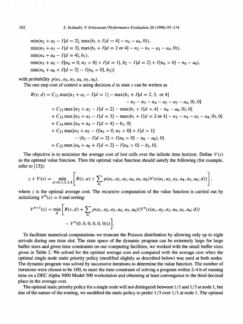
- Vn(O, 0, 0, 0, 0, 0))) - 1 To facilitate numerical computations we truncate the Poisson distribution by allowing only up to eight

arrivals during one time slot. The state space of the dynamic program can be extremely large for large buffer sizes and given time constraints on our computing facilities, we worked with the small buffer sizes given in Table 2. We solved for the optimal average cost and compared with the average cost when the optimal single node static priority policy (modified slightly as described below) was used at both nodes. The dynamic program was solved by successive iterations to determine the value function. The number of iterations were chosen to be 100, to meet the time constraint of solving a program within 24 h of running time on a DEC Alpha 3000 Model 500 workstation and obtaining at least convergence to the third decimal place in the average cost.

The optimal static priority policy for a single node will not distinguish between l/ 1 and l/3 at node 1, but due of the nature of the routing, we modified the static policy to prefer l/3 over l/ 1 at node 1. The optimal

S. Seshadri, K Srinivasan / Performance Evaluation 26 (1996) 95-1 I4 103

Table 1

Parameters for the dynamic program

Traffic type i/j

l/l

l/2 113 114 211 212

COSt Cij Arrival rate &;

1 0.08

2 0.16 1 0.32 2 0.24 1 0.32 2 0.48

-

Table 2 Comparison of static policy to optimal policy from dynamic program

Buffer sizes (bl, b2) Static cost Optimal cost Percent improvement Deviations

c&2) 0.390 0.377 3.4 11.11% (5>5) 0.133 0.114 6.7 24.34%

(7,7) 0.095 0.077 23.4 23.25% -

static policy was used for node 2. We set the parameters for the dynamic program as in Table 1. With the arrival rates shown in Table 1 the load will be 80% at node 1 and 104% at node 2. The buffer sizes were varied by setting (B1 , B2) = (2,2), (5,5) and (7,7), and the results from solving the dynamic program are shown in Table 2. The column under optimal cost gives the average cost estimate after 100 iterations, the costs under the static policy were also obtained similarly using dynamic programming. The column labeled deviations gives the percentage of the total possible states in which the optimal policy deviated from the static policy.

The two interesting points to note from this example are: (1) The improvement from using the optimal policy over the static policy increases with the buffer size. (2) The percentage of the cases in which the optimal policy deviates from the static policy is not too large

(< 25%). The first point is really noteworthy because it implies that when losses are very small then using the

optimal control could be very beneficial. The practical case is exactly when losses are small, say a cell loss probability of 10ee7. The second point is worth noting because it implies that we can cleverly modify the static policy by adding some information about the state of node 2 to the information already available to node 1 and possibly obtain improvements. Variations in the problem parameters other than the buffer size gave very similar results to those shown in Table 2. Based on these findings we were led to ask two questions:

(1) What differentiates the optimal policy from the static policy? (2) How does the optimal policy minimize losses and in what sense?

Apart from some nuances that seem to be applicable only to networks with small buffers, the optimal policy changes the scheduling rule at node 1 by using information about node 2’s overall load. The rule changes as follows: l when the buffer at node 2 is relatively empty, say only 15-20% of the buffer is occupied, then the optimal

policy schedules l/2 in preference to l/4 and l/ 1 in preference to l/3, and the overall scheduling priority at node 1 canbedescribedby l/2 > l/4 > l/l > l/3;

104 S. Seshadri, V Srinivasan/Pelformance Evaluation 26 (1996) 95-114

l when the buffer at node 2 is relatively full, say 60-70% occupied, then the optimal policy does not schedule l/l or l/2 and schedules only l/3 and l/4, with l/4 preferred to l/3;

l when the buffer in both nodes are close to full, and there are only cells of type l/l and l/2 in the buffer at node 1, then the policy transmits cells preferring l/l to l/2. The rules above refer to instantaneous levels of buffer occupancy rather than long-term average values.

The first rule allows the control to take advantage of light load in the downstream node, thus making it “opportunistic” in nature in the transmission of expensive of cells. The second rule implies that the scheduling policy at node 1 is no longer work conserving. The third rule suggests that if the buffer is nearly full at the first node, it is advantageous to transmit cells from the first node and risk their loss at the second node. In the Section 6, we present extensive evaluations of the performance of these rules under different network configurations.

6. Numerical investigations

We use the control policy determined by the rules specified in Section 5 to measure the improvements possible when the buffer sizes are large and losses very small, as may be typical in a real ATM network. The modification of the static policy using these rules is called the HILO heuristic. Comparisons are made via simulation. Prior to running the simulations, we were not sure whether the optimal policy was simply trading off the losses of costly cells against those of cheap cells. The simulations results clarify this issue.

6. I. Poisson arrivals

We first simulate the same two-node example as in Section 5 using the Poisson process to model arrivals for the different traffic classes. The run lengths of the simulations are 10 00 000 time units. We compare three policies: (i) The HILO heuristic, (ii) the Static policy described earlier and (iii) the FIFO rule. For the HILO heuristic, when the number of cells in the buffer at node 2 is above a preset level, called HI, the scheduling rule is l/4 > l/3 and never to schedule l/l or l/2; when the level is below a preset limit, called LO, the rule is to schedule according to l/2 > l/4 > 1 / 1 > l/3, and when it is in between these limits the rule is to use the static priorities l/4 > l/2 > l/3 > l/l. When the buffer occupancy at node 2 is above HI, the only cells in buffer at node 1 are of type l/l and l/2, and the number of cells in the buffer at node 1 are above a level denoted as FULL, cells of type l/l are transmitted in preference to cells of type l/2. Denote the buffer sizes as Bt and B2, respectively. In our simulations, we set LO to 20% of B2, HI as 70% of B2, and FULL as 90% of Bl. The static rule has been discussed in Section 4. The FIFO rule rejects the last arriving cell and schedules the cell that arrived earliest.

We simulate the two-node system with Poisson traffic for two examples. The parameters used in the simulations for the two examples and the results are presented in Tables 3 and 4. Although the offered traffic load on nodes 1 and 2 in both the examples is identical, in the second example cells from 2/l and 2/2 constitute a smaller fraction of the load on node 2 than in the first example. From these results, we can conclude that the Static rule saves expensive cells but does not reduce overall cell loss when compared to FIFO, whereas the HILO heuristic reduces overall cell loss by one order of magnitude. In the sequel, we extend our investigations to more complex arrival processes and network configurations.

S. Seshadri, V Srinivasan /Pedormance Evaluation 26 (I 996) 95-l I4 105

6.2. Correlated arrivals

Encouraged by the results from the simulation of the two-node example using Poisson arrivals, we extend the simulation using arrivals from a two-state Markov Modulated Poisson Process (MMPP). The MMPP process has been shown to capture some of the correlations characteristic of traffic in high speed networks. A 2-state MMPP is described by the parameters hi and pi, i = 1, 2. When the process is in state i = 1, 2, arrivals occur according to a Poisson process of rate hi. The distribution of the time spent in state i = 1. 2 is exponential with parameter pi. The two-state MMPP is commonly referred to as an ON-OFF process, since it has two levels of traffic, “high” and “low”, depending on which state the process is in. We refer to the time spent in the “high” state as the Ontime and in the “low” state as the Offtime. Correspondingly, we refer to the cell arrival rate in each state as Onrate and Offrate, respectively.

Traffic from each class is modeled using an MMPP. We report results from four examples that show that the HILO heuristic is very effective even for correlated arrival processes with widely varying process parameters. The parameters used in the four examples and the distribution of cell losses between the different traffic classes are given in Tables 5-8. In the first two examples, results are presented based on average cell losses over 20 replications of the simulation, each of length lo6 ticks. In the other two examples with large buffers, we increase the length of each run to 5 x lo6 ticks. The parameters of the MMPP processes and the buffer sizes at the two nodes were chosen to reflect a wide range of traffic characteristics and network configurations. From the tables, it is evident that the HILO heuristic is very effective in controlling the cell loss. Once again, the Static rule merely trades off losses of costly cells for cheaper cells, but does not reduce the overall cell loss when compared to the FIFO rule. We now describe how to make the HILO heuristic adaptive to changes in network conditions, and evaluate the performance of the adaptive policy under more complex configurations.

Table 3 Results for a two-node system with Poisson traffic. Simulation duration is IO6 slots, and the results are for a single replication. The buffer sizes are 30 cells at both nodes. The traffic load at node 1 is 70%, and 9 1% at node 2

Policy Losses of traffic type

l/l l/2 l/3 l/4 2/l 212 Total

HILO 0 0 0 0 16 0 16 STATIC 0 0 0 0 278 0 278 FIFO 0 0 0 0 151 101 252 Traffic 0.07 0.14 0.28 0.21 0.28 0.42

Table 4 Results for a two-node system with Poisson traffic. Simulation duration is lo6 slots, and the results are for a single replication. The buffer sizes are 30 cells at both nodes. The traffic load at node 1 is 70%, and 92% at node 2


l/l 112 l/3 l/4 2/l 212 Total

HILO 11 0 0 0 0 0 I1 STATIC 0 0 0 0 433 0 433 FIFO 0 0 0 0 193 201 394 Traffic 0.21 0.21 0.14 0.14 0.2 0.3

106 S. Seshadri, V Srinivasan/Performance Evaluation 26 (1996) 95-l 14

Table 5 Results for a two-node system with MMPP traffic. Simulation duration is lo6 slots, and the results are for 20 replications


l/l 112 l/3 l/4 2/l 212 Total

HILO 239.8 STATIC 0 FIFO 0

MMPP traffic parameters Onrate 0.25 Ontime 0.001 Offrate 0.1 Offtime 0.002

0 0 0 0 0 239.8 0 0 0 1330 0 1330 0 0 0 733.9 602.5 1336.4

0.35 0.2 0.2 0.25 0.25 0.001 0.001 0.001 0.001 0.001 0.1 0.1 0.1 0.1 0.1 0.002 0.002 0.002 0.002 0.002

Table 6 Results for a two-node system with MMPP traffic. Simulation duration is lo6 slots, and the results are for 20 replications. The buffer sizes are 1000 cells at each node. The traffic load is 65.6% at node 1 and 100% at node 2


l/l 112 l/3 l/4 2/l 212 Total

HILO 1133 STATIC 0 FIFO 0

MMPP traffic parameters Onrate 0.32 Ontime 0.01 Offrate 0.1 Offtime 0.02

0 0 0 0 0 1133 0 0 0 2300.6 0 2300.6 0 0 0 1077.3 1222.6 2299.9

0.4 0.15 0.15 0.4 0.45 0.02 0.1 0.1 0.03 0.02 0.1 0.1 0.1 0.1 0.1 0.01 0.01 0.01 0.02 0.04

Table 7 Results for a two-node system with MMPP traffic. Simulation duration is 5 x lo6 slots, and the results are for 20 replications. The buffer sizes are 1100 cells at each node. The traffic load is 65.6% at node 1 and 99.67% at node 2


111 112 113 114 211 212 Total

HILO 927 STATIC 0 FIFO 0

MMPP traflic parameters Onrate 0.315 Ontime 0.01 Offrate 0.1 Offtime 0.02

0 0 0 0 0 927 0 0 0 4072.6 0 4076.6 0 0 0 1913.6 2155.6 4069.2

0.4 0.15 0.15 0.4 0.45 0.02 0.1 0.1 0.03 0.02 0.1 0.1 0.1 0.1 0.1 0.01 0.01 0.01 0.02 0.04

6.3. Making HILO adaptive

The results from the previous examples indicate that there is great scope for minimizing losses using some form of limited feedback and that much of the savings are obtained by turning off the traffic into the

S. Seshadri, V Srinivasan/Peformance Evaluation 26 (1996) 95-114 107

Table 8

Results for a two-node system with MMPP traffic. Simulation duration is 5 x lo6 slots, and the results are for 20 replications. The buffer sizes are 1100 cells at each node. The traffic load is 65.6% at node 1 and 99.47% at node 2


l/l l/2

HILO 235.9 0 STATIC 0 0 FIFO 0 0

MMPP traffic parameters

Onrate 0.312 0.4 Ontime 0.01 0.02 Offrate 0.1 0.1 Offtime 0.02 0.01

l/3 l/4 2/l 212

0 0 0 0 0 0 2175.7 0 0 0 1030.8 1142.2

0.15 0.15 0.4 0.45 0.1 0.1 0.03 0.02 0.1 0.1 0.1 0.1 0.01 0.01 0.02 0.04

Total __-

235.9 2175.7 2172.9

-

Cross Traffic

to Node 2

Cross Tmffic to Node 3

Cross Tr&ic to Node 4

Cross Traffic to Node 5

BIJE:[l] ntJW1 BLF[3] BW41 BWSI

Fig. 2. A five-node system

downstream node when that node’s buffer is almost full. However, due to the random nature of the cell arrival processes, and more specifically of the cross traffic streams, it is desireable that the HILO heuristic be able to react to increases and decreases in cell losses in downstream nodes. For instance, increased cell loss in a downstream node would advocate an increase in the HI value used by an upstream node thus holding back traffic from the congested node. Similarly, a long period without cell loss at a node would indicate that the node is congestion-free, thus warranting a decrease in the HI value at an upstream node. Such adjustments can be made to help the HILO heuristic fine tune the control parameters at each node to achieve the best performance. However, care should be taken to ensure that such adjustments do not result in oscillatory behavior of cell losses.

We studied a simple two node model via simulation as well as Markov Chain analysis to understand the loss behavior of cells. In the two-node model, we had only two types of traffic, one arriving to the first node and proceeding to the second; and the other arriving to the second node (the cross traffic). The HILO rule is implemented by choosing a blocking value b and another value FULL. The rule is to block the transmission at the first node if the downstream buffer has b or more cells and to always transmit when the first node’s buffer is above the level FULL. In these experiments, we observed that the total number of lost cells was a convex function of the blocking value b chosen for the HILO rule. This led to the conjecture that the total number of lost cells is jointly convex in the blocking parameters for any network configuration. We are unable to prove this even for the two-node case. However, based on this assumption the HILO heuristic can be made adaptive.

Consider, for example, the five-node serial system shown in Fig. 2. The buffer size at node i is denoted by BUF[1’], the number of cells lost at node i is Li, the service time is 1 unit of time (deterministic) at all nodes, and all the traffic flow is unidirectional. We designate the controls for this system as (bi , i = 1, 2, . . . , 5).

108 S. Seshadri, V Srinivasan/Performance Evaluation 26 (1996) 95-114

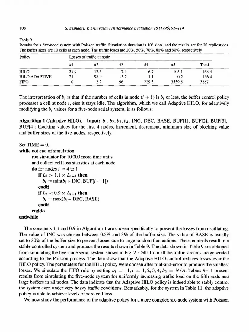
Table 9 Results for a five-node system with Poisson traffic. Simulation duration is lo6 slots, and the results are for 20 replications. The buffer sizes are 10 cells at each node. The traffic loads are 20%, 50%, 70%, 80% and 90%, respectively

Policy Losses of traffic at node

#l #2 #3 #4 #5 Total

HILO 31.9 17.3 7.4 6.7 105.1 168.4 HILO ADAPTIVE 21 98.9 15.2 1.1 0.2 136.4 FIFO 0 2.2 96 229.3 3559.5 3887

The interpretation of bi is that if the number of cells in node (i + 1) is bi or less, the buffer control policy processes a cell at node i, else it stays idle. The algorithm, which we call Adaptive HILO, for adaptively modifying the bi values for a five-node serial system, is as follows:

Algorithm 1 (Adaptive HILO). Input: bl, b2, b3, bq, INC, DEC, BASE, BUF[l], BUF[2], BUF[3], BUF[4]: blocking values for the first 4 nodes, increment, decrement, minimum size of blocking value and buffer sizes of the five-nodes, respectively.

Set TIME = 0. while not end of simulation

run simulator for 10 000 more time units and collect cell loss statistics at each node do for nodes i = 4 to 1

if Li > 1.1 x Li+l then bi = min(bi+ INC, BUF[i + 11)

endif if Li < 0.9 x Li+l then

bi = max(bi - DEC, BASE) endif

enddo endwhile

The constants 1.1 and 0.9 in Algorithm 1 are chosen specifically to prevent the losses from oscillating. The value of INC was chosen between 0.5% and 3% of the buffer size. The value of BASE is usually set to 30% of the buffer size to prevent losses due to large random fluctuations. These controls result in a stable controlled system and produce the results shown in Table 9. The data shown in Table 9 are obtained from simulating the five-node serial system shown in Fig. 2. Cells from all the traffic streams are generated according to the Poisson process. The data show that the Adaptive HILO control reduces losses over the HILO policy. The parameters for the HILO policy were chosen after trial-and-error to produce the smallest losses. We simulate the FIFO rule by setting bi = 11, i = 1,2, 3,4; b5 = N/A. Tables 9-l 1 present results from simulating the five-node system for uniformly increasing traffic load on the fifth node and large buffers in all nodes. The data indicate that the Adaptive HILO policy is indeed able to stably control the system even under very heavy traffic conditions. Remarkably, for the system in Table 11, the adaptive policy is able to achieve levels of zero cell loss.

We now study the performance of the adaptive policy for a more complex six-node system with Poisson

S. Seshadri, V Srinivasan/Perjormance Evaluation 26 (1996) 95-114 109

Cross Tnffii Cross Traffic Cross Traffic Cross Traffic toNode toNode toNode toNode

Fig. 3. A six-node system.

Table 10 Results for a five-node system with Poisson traffic. Simulation duration is lo6 slots, and the results are for 20 replications.

The buffer sizes are 10 cells at each node. The traffic loads are 40%, 41%, 5 l%, 91% and 92%, respectively


#l #2 #3 #4 #5 Total

HILO ADAPTIVE 303.9 0 20.1 701.1 0 1025.1 FIFO 0 0 0 14301.9 0.3 14302.2

Table I1 Results for a five-node system with Poisson traffic. Simulation duration is 5 x lo6 slots, and the results are for 20 replications. The buffer sizes are 100 cells at each node. The traffic loads are 30%, 40%, 41%, 8 1% and 97%, respectively


#l #2 #3 #4 #5 Total

HILO ADAPTIVE 0 0 0 0 0 0 FIFO 0 0 0 0 245.2 245.2

Table 12 Results for a five-node system with Poisson traffic. Simulation duration is 5 x lo6 slots, and the results are for 20 replications. The buffer sizes are 100,50, 100,50 and 100 cells, respectively, at each node. The traffic loads are lo%, 50%, 60%, 89% and 99%, respectively


#l #2 #3 #4 #5 Total

HILO ADAPTIVE 276 6.1 0 0 0 282.1 FIFO 0 0 0 0 22909.7 22909.7

and MMPP traffic streams. In Fig. 3, we show a six node example which is quite similar to the system in Fig. 2, except that from the third node traffic can bifurcate to a sixth node. The splitting probability is 50%, i.e., with probability 0.5 an arriving cell is meant for transmission to the sixth node, else it goes to the fourth node. Note that the route of the arriving cell is known at the instant of arrival. We assume that if the buffer is full at node 3, and a cell has to be dropped, then the cell meant for node 6 gets dropped first. The Adaptive HILO policy for this system is similar to the one in Algorithm 1.

110 S. Seshadri, V Srinivasan/Pe$ormance Evaluation 26 (1996) 95-114

Table 13 Results for a six-node system with Poisson traflic. Simulation duration is lo6 slots, and the results are for 20 replications. The buffer sizes are 10 cells at each node. The traffic loads are 20%, 50%, 70%, 70%, 80% and 70%, respectively


#l #2 #3 #4 #5 #6 Total

HILO 0.4 0.6 18.7 2.3 9.4 13 44.4 HILO ADAPTIVE 0.3 0.1 39.6 10.6 8.8 28.4 87.8 FIFO 0 1.3 110.5 10.4 249.5 38 409.7

Table 14 Results for a six-node system with MMPP traffic. Simulation duration is lo6 slots, and the results are for 20 replications. The buffer sizes are 100 cells at each node. The traffic loads are 24.1%, 44.1%, 72.1%, 65.0%, 87.0% and 50.8%, respectively


l/l 112 l/3 l/4 2/l 212 Total

HILO ADAPTIVE 0 0 0 0 0 0 0 FIFO

Traffic parameters Onrate Ontime Offrate Offtime

0 0 0 0 56.5 0 56.5

(3-+4,3-+6) 0.312 0.4 (0.15,0.25) 0.15 0.4 0.45 0.01 0.02 (0.1,0.02) 0.1 0.03 0.02 0.1 0.1 (0.1,O.l) 0.1 0.1 0.1 0.02 0.01 (0.01,0.02) 0.01 0.02 0.04

Table 15 Results for a six-node system with MMPP traffic. Simulation duration is lo6 slots, and the results are for 20 replications. The buffer sizes are 100 cells at each node. The traffic loads are 24.1%, 44.1%, 72.1%, 74.6%, 96.6% and 50.8%, respectively


l/l l/2 l/3 l/4 2/l 212 Total

HILO ADAPTIVE FIFO

Traffic parameters: Onrate Ontime Offrate Offtime

56.6 0 0 0 0 0 56.6 0 0 0 0 5092.8 0 5092.8

(3-+4,3+6) 0.312 0.4 (0.15,0.25) 0.25 0.4 0.45 0.01 0.02 (0.1,0.02) 0.1 0.03 0.02 0.1 0.1 (0.1,O.l) 0.15 0.1 0.1 0.02 0.01 (0.01,0.02) 0.01 0.02 0.04

The HILO policy, Adaptive HILO policy and the FIFO rule are compared with Poisson traffic in Table 13. The effectiveness of the Adaptive HILO policy in controlling the six node system with bursty traffic is demonstrated in Tables 14 and 15. The parameters for the MMPP processes in these examples were chosen to reflect increasing traffic loads and varying levels of burstiness. The data once again indicate the adaptive policy is robust under varying traffic conditions.

From the studies of the various systems presented in the preceding discussions, it is evident the HILO and the Adaptive HILO policies hold much promise for cell loss control in ATM networks. However, it is a well-known fact that in ATM networks propagation delays will be large in comparison to queueing and transmission delays. This results in a large delay-bandwidth product, implying that a large number of cells could be in transit between nodes at any instant of time. This could cause severe oscillatory behavior

S. Seshadri, K Srinivasan/Perjormance Evaluation 26 (1996) 95-114 111

Table 16 Results for a five-node system with Poisson traffic. Simulation duration is lo6 slots, and the results are@ 20 replications. The buffer sizes are 1000 cells at each node. The traffic loads are 21%, 53%, 75%, 84.999% and 99.999%, respectively. The propagation delay between nodes is 100 times the cell transmission time


#l #2 #3 #4 #5 Total

HILO ADAPTIVE 0 0 0 0 0 0 FIFO 0 0 0 0 271.3 271.3

in controls that are dependent on information propagated back from adjacent nodes. In the sequel, we demonstrate that the Adaptive HILO policy does not suffer from this drawback.

6.4. Incorporating propagation delays

In all the experiments considered thus far, we have neglected the propagation delay for a cell to transit from one node to another. This delay could be several times larger than the transmission time for a single cell in an ATM network. Now we incorporate this component of the total delay into our experiments.

Once again, we consider the five-node system in Fig. 2. The propagation delay between successive nodes is now 100 times the transmission time for a single cell. For links of capacity 150Mbps and ATM cells of size 53 bytes, this corresponds to a physical distance of approximately 1OOkm between nodes. When there are such propagation delays, the delay should not be too large so as to make the feedback information completely useless. Based on our experiments, the following guidelines are useful in constructing controls

for networks with large propagation delays: l the propagation delay multiplied by the time to transmit a cell (i.e, the service rate of the ATM switch)

should be less than a fifth of the size of the downstream buffer, and l the HILO rule needs to account for the cells in transit. We do this by adding the number of cells in transit

to the next node to the buffer content of that node. Note though that the value of the buffer content known to the upstream node is “old” due to the propagation delay. This procedure in some sense attempts to predict the buffer content of the downstream node (for a detailed predictive scheme, see [ 121). We first simulate the five-node system with Poisson traffic and large buffers. The load on the fifth node in

the system is very high (99.999%). From Table 16, we see that the Adaptive HILO policy is very effective in controlling cell losses. Now, we make the buffers smaller and change the traffic streams to the bursty MMPP process. Once again, cell losses are contained (see Table 17).

These preliminary experiments indicate that the Adaptive HILO policy can indeed be useful in real ATM networks with large delay-bandwidth products. We are currently evaluating the policy under various realistic network configurations. In the next section, we provide some intuition into the reasons for the effectiveness of the HILO and Adaptive HILO policies.

7. Discussion

We have shown via a number of examples that the HILO and Adaptive HILO policies do reduce cell loss significantly. Intuitively, these policies hold back traffic from congested nodes in buffers that are relatively lightly utilized until such time that the congestion abates. We hypothesize that these policies are able to

112 S. Seshadri, V Srinivasan/Pelformance Evaluation 26 (1996) 95-114

Table 17 Results for a five-node system with MMPP traffic. Simulation duration is 5 x lo6 slots, and the results are for 16 replications. The buffer sizes are 600 cells at each node. The traffic loads are 24.1%, 44.1%, 54.6%, 75.05% and 97.05%, respectively. The propagation delay between nodes is 100 times the cell transmission time


HILO ADAPTIVE PIP0

Traffic parameters Onrate Ontime Offrate Offtime

#1 #2 #3 #4 #5

0 0 0 0.44 0 0 0 0 0 3602.75

0.32 0.4 0.15 0.38 0.4 0.01 0.02 0.1 0.01 0.03 0.1 0.1 0.1 0.03 0.1 0.02 0.01 0.01 0.01 0.01

Total

0.44 3602.75

Table 18 Single server equivalence

Example Traffic combined and fed into

Total buffer in Buffer(K) in series in the ./D/I/K

Total cell loss

1 2 3 4 5 6 7 8 9

10 11 12 13 14 15

/D/I/Kqueue original example queue HILO Adaptive .lDl1lK

l/l, 1/z 211,212 60 45 16 20 l/l, l/2,2/1,2/2 60 45 11 43 1/1,1/z 2/1,2/2 1000 600 239.8 635.2 1/1,1/z 211,212 2000 1800 1133 849.4 1/1,1/2,2/1,2/2 2200 1980 927 770.4 1/1,1/2,2/1,2/2 2200 1980 235.9 178.3 All 50 30 168.4 187.2 All 50 30 1025.1 530.7 All 500 INF 0 0 All 350 220 282.1 475.3 All Traffic to node #5 50 20 87.8 33.3 All Traffic to node #5 500 INF 0 0 All Traffic to node #5 500 350 56.6 88.4 All 5000 INF 0 0 All 5000 INF 0.4 0

control cell loss due to the effective manner in which they utilize unused buffer capacity in upstream nodes during periods of heavy load in downstream buffers. To test this hypothesis, we conduct a final test of the efficiency of these controls. For each of the fifteen examples previously discussed in this chapter, we pose the following problem:

Assume that all the trafic art-&&g to most heavily loaded node in the system is directed to a single server queue withjnite buffer K. We>all this system a ./D/l/K queue. Find the value of K for this system which gives roughly the same cell loss as the Adaptive HILO rule for the original system.

Comparisons of the ./D/l/K system with the original multi-node system controlled by the Adaptive HILO policy are shown in Table 18. We observe that the value of K for the ./D/l/K system that yields roughly the same losses as the Adaptive HILO controlled system ranges about 40%-90% of the total buffer capacity in the entire original system. The value of K is closer to 90% for bursty MMPP traffic (for example see Examples 4-6). This confirms that the HILO rule makes congestion at downstream nodes visible to upstream nodes well in time - thus filling up empty buffers upstream as the downstream buffers get filled up.

S. Seshadri, K Srinivasan/Pe$ormance Evaluation 26 (1996) 95-114 113

8. Conclusions

We have considered buffer control policies for connections sharing finite buffers in ATM networks. We presented important characteristics of the optimal policy for a single node. For the general multi-node problem, we have presented insights into the nature of optimal policies. Then, using a dynamic programming formulation for a two-node network, we were able to construct a simple heuristic, the HILO policy, that significantly outperformed the static priority rule. We then modified the HILO policy to react to changing network conditions. This new control is called the Adaptive HILO policy. Simulations studies of more complicated networks show that the heuristic is indeed effective under diverse conditions. The key idea we have discovered are that simple ON-OFF type of non work-conserving policies which use limited feedback from adjacent nodes can be effective in controlling cell loss.

We have tested the Adaptive HILO policy for ATM networks with large delay-bandwidth products. Pre- liminary results indicate that cell loss can be effectively contained even in the presence of large propagation delays, and that the policy does not suffer from oscillatory behavior. Future work in this area includes testing of the Adaptive HILO policy under realistic traffic conditions in complex networks.

Acknowledgements

We thank the anonymous reviewers for their detailed feedback and suggestions which have helped strengthen the presentation of this paper.

References

[l] B. Amin-Salehi, G.D. Flinchbaugh and L.R. Pate. Implications of new network services on BISDN capabilities, Proc. of IEEE INFOCOM, 1990, pp. 1038-1045.

[2] L. Benmohamed and SM. Meerkov, Feedback control of congestion in packet switching networks: The case of a single congested node, IEEE/ACM Trans. on Networking 1 ( 1993) 1038-l 045.

[3] K.W. Fendick, M.A. Rodrigues and A. Weiss, Analysis of rate-based feedback control strategy for long haul data transport, Performance Evaluation 16 (1992) 67-84.

[4] E. Gelenbe, S. Seshadri and V. Srinivasan, Pathwise optimum policies for ATM cell scheduling and rejection, Technical Report, Duke University, Department of Computer Science, 1994,94-24.

[5] V, Jacobson, Congestion avoidance and control, Proc. of ACM SIGCOMM, Stanford, California, August 1988, pp. 3 14-329.

[6] K.-T. Ko, P. Mishra and S.K. Tripathi, Interaction among virtual circuits using predictive congestion control, Computer Networks and ISDN Systems 25 (1993) 68 1699.

[7] P. Mishra and H. Kanakia, A hop-by-hop rate-based congestion control scheme, Proc. of ACM SIGCOMM, Baltimore, Maryland, August 1992, pp. 112-123.

[8] D. Mitra, Asymptotically optimal design of congestion control for high speed data networks, IEEE Trans. on Comm. 40 (2) (1992) 301-311.

[9] D. Mitra and J.B. Seery, Dynamic adaptive windows for high speed data networks: Theory and simulations, Proc. of ACM SIGCOMM, September 1990, pp. 30-37.

[lo] D. Mitra and J.B. Seery, Dynamic adaptive windows for high speed data networks with multiple paths and propagation delays, Proc. of IEEE INFOCOM, (2B.l), Bal Harbour, Florida, April 1991, pp. 39-48.

[ 1 l] K.K. Ramakrishnan and R. Jain, A binary feedback scheme for congestion avoidance in computer networks with a connectionless network layer, Proc. of ACM SIGCOMM, Stanford, California, August 1988, pp. 303-3 13.

[ 121 G. Ramamurthy and B. Sengupta, A predictive hop-by-hop congestion control policy for high speed networks, Proc. of IEEE INFOCOM, Vol. 3, San Francisco, California, August 1993, pp. 1033-1041.

114 S. Seshadri, K Srinivasan/Performance Evaluation 26 (1996) 95-l 14

[ 131 S. Ross, Introduction to Dynamic Programming, Academic Press, New York (1983). [ 141 S. Seshadri and V. Srinivasan, On characterizing optimal buffer control policies in ATM nodes, Technical Report, Duke

University, Department of Computer Science, 1994,94-25. [15] M. Sidi, W.-Z. Liu, I. Cidon and I. Gopal, Congestion control through input rate regulation, Proc. of GLOBECOM,

Dallas, Texas, November 1989, pp. 1764-1768. [ 161 Special issue on B-ISDN: High performance transport, IEEE Communications Magazine, September 1991. [ 171 Special issue on congestion control in high speed networks, IEEE Communications Magazine, October 1991. [ 181 Special issue on ATM - The asynchronous transfer mode, Computer Networks and ISDN Systems 24 (4) (1992). [ 191 K. Sriram, Methodologies for bandwidth allocation, transmission scheduling, and congestion avoidance in broadband

ATM networks, Computer Networks and ISDN Systems 26 (1993) 43-59. [20] K. Sriram and W. Whitt, Characterizing superposition arrival processes and the performance of multiplexers for voice

and data, IEEE J. Selected Areas in Comm. SAC-4 (6) (1986). [21] L. Tassiulas, Y. Hung and S.S. Panwar, Optimal buffer control during congestion in an ATM network node, IEEE/ACM

Trans. on Networking 2(4) ( 1994). [22] Y.-T. Wang and B. Sengupta, Performance of a feedback congestion control policy under non-negligible propagation

delay, Proc. of ACM SIGCOMM, Zurich, Switzerland, September 1991, pp. 149-157. [23] P. Yang, Pathwise solutions for a class of linear stochastic systems, Doctoral Dissertation, Stanford University, 1988.

Sridhar Seshadri received the degree of Bachelor of Technology from the Indian Institute of Technology, Madras, India, in 1978, the Post Graduate Diploma in Management from the Indian Institute of Management, Ahmedabad, India, in 1980 and the Ph.D. degree in Management Science from the University of California at Berkeley in 1993. He is currently an Assistant Professor in the Department of Statistics and Operations Research, at the Leonard N. Stem School of Business, New York University. His research interests are in the area of stochastic modeling and optimization, with applications to manufacturing, distribution, telecommunications, database design and finance.

Vijay Srinivasan received a B.S. degree in computer science from North Carolina State University in 1992, and a Ph.D. degree in computer science from Duke University in 1995. Since May 1995, he has been with IBM’s Networking Architecture group in the Research Triangle Park of North Carolina. His research interests include development of algorithms for the control and management of network services, evaluation of these algorithms using analytical, numerical and simulation techniques, and in intelligent networking.

design of effective buffer control policies for atm networks

Documents