Design and Performance of a Scalable ParallelCommunity Climate ModelJohn Drake�, Ian Fostery, John Michalakesy,Brian Tooneny, Patrick Worley�AbstractWe describe the design of a parallel global atmospheric circulation model,PCCM2. This parallel model is functionally equivalent to the National Centerfor Atmospheric Research's Community Climate Model, CCM2, but is struc-tured to exploit distributed memory multicomputers. PCCM2 incorporatesparallel spectral transform, semi-Lagrangian transport, and load balancing al-gorithms. We present detailed performance results on the IBM SP2 and IntelParagon. These results provide insights into the scalability of the individualparallel algorithms and of the parallel model as a whole.1 IntroductionComputer models of the atmospheric circulation are used both to predict tomor-row's weather and to study the mechanisms of global climate change. Over the lastseveral years, we have studied the numerical methods, algorithms, and program-ming techniques required to implement these models on so-called massively parallelprocessing (MPP) computers: that is, computers with hundreds or thousands ofprocessors. In the course of this study, we have developed new parallel algorithmsfor numerical methods used in atmospheric circulation models, and evaluated theseand other parallel algorithms using both testbed codes and analytic performancemodels [8, 10, 11, 29, 32]. We have also incorporated some of the more promisingalgorithms into a production parallel climate model called PCCM2 [6]. The latterdevelopment has allowed us to validate performance results obtained using simplertestbed codes, and to investigate issues such as load balancing and parallel I/O. Ithas also made the computational capabilities of MPP computers available to sci-entists for global change studies, providing the opportunity for increases in spatialresolution, incorporation of improved process models, and longer simulations.In this paper, we provide a comprehensive description of the design of PCCM2and a detailed evaluation of its performance on two di�erent parallel computers, theIBM SP2 and Intel Paragon. We also touch upon aspects of the experimental studies�Oak Ridge National Laboratory, P.O. Box 2008, Bldg. 6012, Oak Ridge, TN 37831-6367.yMathematics and Computer Science Division, Argonne National Laboratory, Argonne, IL60439. 1

used to select the parallel algorithms used in PCCM2. However, these studies arenot the primary focus of the paper.PCCM2 is a scalable parallel implementation of the National Center for Atmo-spheric Research (NCAR)'s Community Climate Model version 2 (CCM2). CCM2is a comprehensive, three-dimensional global atmospheric general circulation modelfor use in the analysis and prediction of global climate [15, 16]. It uses two di�erentnumerical methods to simulate the uid dynamics of the atmosphere. The sphericalharmonic (spectral) transform method [7, 22] is used for the horizontal discretiza-tion of vorticity, divergence, temperature, and surface pressure; this method featuresregular, static, global data dependencies. A semi-Lagrangian transport scheme [31]is used for highly accurate advection of water vapor and an arbitrary number ofother scalar �elds, such as sulfate aerosols and chemical constituents; this schemefeatures irregular, dynamic, mostly local data dependencies. Neither method isstraightforward to implement e�ciently on a parallel computer.CCM2, like other weather and climate models, also performs numerous calcu-lations to simulate a wide range of atmospheric processes relating to clouds andradiation absorption, moist convection, the planetary boundary layer, and the landsurface. These processes share the common feature that they are coupled horizon-tally only through the dynamics. These processes, collectively termed \physics,"have the important property of being independent for each vertical column of gridcells in the model. However, they also introduce signi�cant spatial and temporalvariations in computational load, and it proves useful to incorporate load balancingalgorithms that compensate for these variations.PCCM2 was the �rst spectral, semi-Lagrangian model developed for distributed-memory multicomputers [6]. However, we are not the only group to have examinedparallel formulations of such models. At the European Center for Medium-rangeWeather Forecasts (ECMWF), Dent [4] and his colleagues have developed the In-tegrated Forecast System for both vector multiprocessors and distributed memorymultiprocessors. Sela [25] has adapted the National Meteorological Center's spec-tral model for use on the CM5. Hammond et al. [17] have developed a data-parallelimplementation of CCM2, and Hack et al. [16] have adapted a vector multiproces-sor version of CCM2 to execute on small multicomputers. All these developmentsbuild on previous work on parallel algorithms for atmospheric circulation models,as described in the papers referenced above and in [1, 3, 14, 18, 19, 24].Space does not permit a description of the primitive equations used to model the uid dynamics of the atmosphere [30] or of CCM2. Instead, we proceed directly inSections 2 and 3 to a description of the spectral transform method and the techniquesused to parallelize it in PCCM2. In Sections 4 and 5, we describe the parallel semi-Lagrangian transport and load balancing algorithms used in PCCM2. In Sections 6and 7, we present our performance results and our conclusions, respectively.2 The Spectral Transform AlgorithmThe spectral transform method is based on a dual representation of the scalar �eldson a given vertical level in terms of a truncated series of spherical harmonic func-tions and the values on a rectangular grid whose axes, in a climate model, represent2

longitude and latitude. State variables in spectral space are represented by the co-e�cients of an expansion in terms of complex exponentials and associated Legendrefunctions, �(�; �) = MXm=�M N(m)Xn=jmj �mn Pmn (�)ei�m�; (1)where Pmn (�) is the (normalized) associated Legendre function, i = p�1, � is thelongitude, and � = sin �, where � is the latitude. The spectral coe�cients are thendetermined by the equation�mn = Z 1�1 � 12� Z 2�0 �(�; �)e�i�m�d��Pmn (�)d� � Z 1�1 �m(�)Pmn (�)d� (2)since the spherical harmonics Pmn (�)ei�m� form an orthonormal basis for square in-tegrable functions on the sphere. In the truncated expansion, M is the highestFourier mode and N(m) is the highest degree of the associated Legendre functionin the north-south representation. Since the physical quantities are real, ��mn is thecomplex conjugate of �mn and only spectral coe�cients for nonnegative modes needto be calculated.To evaluate the spectral coe�cients numerically, a fast Fourier transform (FFT)is used to �nd �m(�) for any given �. The Legendre transform (LT) is approximatedusing a Gaussian quadrature rule. Denoting the Gauss points in [�1; 1] by �j andthe Gauss weights by wj, �mn = JXj=1 �m(�j)Pmn (�j)wj: (3)Here J is the number of Gauss points. (For simplicity, we will henceforth refer to(3) as the forward Legendre transform.) The point values are recovered from thespectral coe�cients by computing�m(�) = N(m)Xn=jmj �mn Pmn (�) (4)for each m (which we will refer to as the inverse Legendre transform), followed byFFTs to calculate �(�; �).The physical space grid is rectangular with I grid lines evenly spaced alongthe longitude axis and J grid lines along the latitude axis placed at the Gaussianquadrature points used in the forward LT. In this paper, we assume a triangularspectral truncation: N(m) = M and the (m;n) indices of the spectral coe�cients fora single vertical layer form a triangular grid. To allow exact, unaliased transforms ofquadratic terms, we select I to be the minimummultiple of two such that I � 3M+1,and set J = I=2 [22]. The value ofM can then be used to characterize the horizontalgrid resolution, and we use the term \TM" to denote a particular discretization.Thus with M = 42, we choose I = 128 and J = 64 for T42 resolution.In summary, the spectral transform as used in climate models proceeds in twostages. First, the FFT is used to integrate information along each west-east line ofa latitude/longitude grid, transforming physical space data to Fourier space. This3

stage entails a data dependency in the west-east dimension. Second, a LT is appliedto each wavenumber of the resulting latitude/wavenumber grid to integrate theresults of the FFT in the north-south, or latitudinal, direction, transforming Fourierspace data to spectral space [2]. This stage entails a data dependency in the north-south dimension. In the inverse transform, the order of these operations is reversed.3 PCCM2 Parallel AlgorithmsWe now introduce the parallel algorithms used in PCCM2. This model is designedto execute on distributed memory multicomputers, in which processors, each witha local memory, work independently and exchange data via an interconnection net-work. Hence, our parallel algorithms must specify data distribution, computationdistribution, and the communication required to move data from where it is locatedto where it is required. An important characteristic of the parallel algorithms in-corporated in PCCM2 is that they compute bit-for-bit identical results regardlessof the number of processors applied to a problem. This uniformity is not straight-forward to achieve, because of the lack of associativity in oating-point addition,but was obtained by modifying the sequential implementation of various summationoperations to use the same tree-based summation algorithm as the parallel code.We start our description of PCCM2 by examining the spectral transform, as thisdetermines in large part the data distributions used in other program components.3.1 Algorithmic AlternativesThe spectral transform is a composition of FFT and LT phases, and parallel FFTand LT algorithms are well understood (e.g., see [12, 23, 26, 27]). Nevertheless,the design of parallel spectral transform algorithms is a nontrivial problem, bothbecause the matrices involved are typically much smaller than in other situations(e.g., 64{1024 in each dimension, rather than tens of thousands) and because theFFT and LT phases interact in interesting ways on certain architectures.Spectral models such as CCM2 operate on data structures representing physical,Fourier, and spectral space variables. Each of these data structures can be thoughtof as a three-dimensional grid, with the vertical dimension being the third coordi-nate in each case. The other two coordinates are, in physical space, latitude andlongitude; in Fourier space, Fourier wavenumber and latitude; and in spectral space,wavenumber and degree of associated Legendre polynomial (n). For maximum scal-ability, each of these three spaces must be decomposed over available processors. Inprinciple, data structures can be decomposed in all three dimensions. However, werestrict our attention to two dimensional decompositions, as these provide adequateparallelism on hundreds or thousands of processors and simplify code development.A variety of di�erent decompositions, and hence parallel algorithms, are possiblein spectral atmosphericmodels [10, 11]. Physical space is best partitioned by latitudeand longitude, as a decomposition in the vertical dimension requires considerablecommunication in the physics component. However, Fourier and spectral spacecan be partitioned in several di�erent ways. A latitude/wavenumber decompositionof Fourier space requires communication within the FFT [8, 29]. Alternatively, a4

latitude/vertical decomposition of Fourier space allows FFTs to proceed withoutcommunication, if a transpose operation is �rst used to transform physical spacefrom a latitude/longitude to a latitude/vertical decomposition. Similar alternativesexist for spectral space, with one decomposition requiring communication within theLT, and another avoiding this communication by �rst performing a transpose of thespectral coe�cients. Another possibility, described below, is to decompose spectralspace in just one dimension, replicating it in the other. This reduces communicationcosts at the expense of a modest increase in storage requirements.The di�erent FFT and LT algorithms just described can be combined in di�erentways, leading to a large number of possible parallel algorithms. Performance is alsoin uenced by the number of processors allocated to each decomposed dimension(that is, the aspect ratio of the abstract processor mesh) and the protocols usedto implement the communication algorithms. We have obtained a detailed under-standing of the relative performance of these di�erent algorithms by incorporatingthem in a sophisticated testbed code called PSTSWM [10, 11, 33]. Extensive stud-ies with this code have allowed us to identify optimal algorithm choices, processormesh aspect ratios, and communication protocols for di�erent problem sizes, com-puters, and numbers of processors. As much as possible, these optimal choices areincorporated in PCCM2.Scaling arguments show that for large problem sizes and large numbers of proces-sors, transpose algorithms are the most e�cient, as they communicate the least data.(These algorithms are used in the ECMWF's Integrated Forecast System model,which is designed to operate at T213 resolution using 31 vertical levels [4].) How-ever, both experimental and analytic studies indicate that for the smaller problemsizes considered in climate modeling, nontranspose algorithms are often competitive,particularly for the LT.3.2 PCCM2 Data DecompositionsPCCM2 uses a latitude/longitude decomposition of physical space, a latitude/wave-number decomposition of Fourier space, and a one-dimensional decomposition ofspectral space. These choices are in uenced by both performance and softwareengineering concerns. Performance considerations determine the spectral space de-composition: the one-dimensional decomposition permits the use of a nontransposealgorithm that is known to be more e�cient than a transpose-based LT for manyproblem sizes of interest. Software engineering concerns determine the choice ofFourier space decomposition. While a latitude/vertical decomposition would al-low the use of more e�cient algorithms in some situations, it would signi�cantlycomplicate the conversion of CCM2 into a distributed-memory parallel code, andis subject to signi�cant load balance problems when the number of vertical layersin the model is small compared to the number of processors used to decomposethe vertical dimension. Hence, we use a latitude/wavenumber decomposition, andsupport both a parallel FFT that requires communication within the FFT, and adouble-transpose FFT that avoids communication within the FFT at the cost oftwo transpose operations.We now provide a more detailed description of the PCCM2 domain decompo-sitions. We view the multicomputer as a logical P � Q two-dimensional processor5

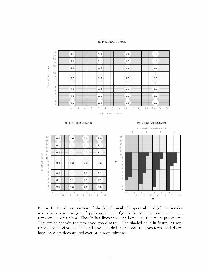
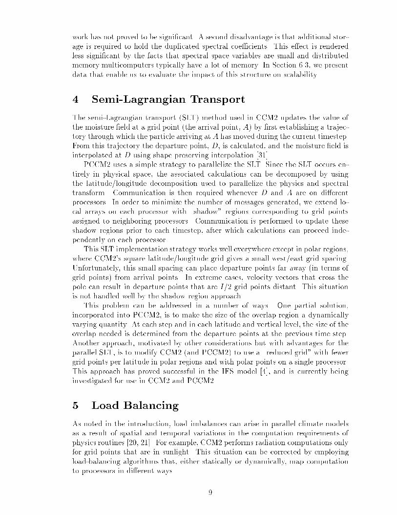
grid. In physical space, the latitudinal dimension is partitioned into 2Q intervals,each containing J=2Q consecutive latitudes (Gauss points) along the latitude axis.Each processor row is assigned two of these intervals, one from the northern hemi-sphere, and the re ected latitudes in the southern hemisphere. This assignmentallows symmetry of the associated Legendre polynomials to be exploited in the LT.The assignment also restricts Q, the number of processor rows, to be no largerthan J=2. The longitudinal dimension is partitioned into P equal intervals, witheach interval being assigned to a di�erent processor column. The resulting \block"decomposition of the physical domain is illustrated in Figure 1 for a small example.The latitude-wavenumber decomposition used for Fourier space in PCCM2 whenusing the double transpose parallel FFT is illustrated in Figure 1. (A di�erent de-composition in used in the other parallel FFT [11].) The latitude dimension is par-titioned as in the physical domain, while the wavenumber dimension is partitionedinto P sets of wavenumbers, with each set being assigned to a di�erent processorcolumn. As illustrated in Figure 1, the ordering for the Fourier coe�cients di�ersfrom the ordering of the longitude dimension in physical space. As described below,this serves to balance the distribution of spectral coe�cients.PCCM2 partitions spectral space in one dimension only (wavenumber), replicat-ing it in the other. The wavenumber dimension is distributed as in Fourier space:wavenumbers are reordered, partitioned into consecutive blocks, and assigned to pro-cessor columns. The spectral coe�cients associated with a given wavenumber arereplicated across all processors in the processor column to which that wavenumberwas assigned. This replication reduces communication costs. Again, see Figure 1for an example decomposition.Note that in a triangular truncation, the number of spectral coe�cients asso-ciated with a given Fourier wavenumber decreases as the wavenumber increases.Without the reordering of the wavenumbers generated by the parallel FFT, a no-ticeable load imbalance would occur, as those processor columns associated withlarger wavenumbers would have very few spectral coe�cients. The particular or-dering used, which was �rst proposed by Barros and Kauranne [1], minimizes thisimbalance.3.3 Parallel Fast Fourier TransformThe data decompositions used in PCCM2 allow \physics" computations to proceedwithout communication within each vertical column. However, communication isrequired for the FFT and LT. As noted above, communication for the FFT can beachieved in two di�erent ways. One approach is to use a conventional parallel FFT;we do not describe this here as the basic techniques are described in [11].An alternative approach that is more e�cient in many cases uses matrix trans-pose operations to transform the physical space data passed to the FFT from alatitude/longitude decomposition to a latitude/vertical+�eld decomposition, parti-tioning the �elds being transformed as well as the vertical layers. A second trans-pose is then used to remap the Fourier coe�cients produced by the FFT froma latitude/vertical+�eld decomposition to the latitude/wavenumber decompositionemployed in Fourier space. This alternative approach avoids the need for communi-cation during the FFT itself, at the cost of two transpose operations, but tends to6

0,0 1,0 2,0 3,0

0,1 1,1 2,1 3,1

0,2 1,2 2,2 3,2

0,3 1,3 2,3 3,3

0,2 1,2 2,2 3,2

0,1 1,1 2,1 3,1

0,0 1,0 2,0 3,0

(a) PHYSICAL DOMAIN

1

2

3

4

5

6

7

8

9

10

11

12

13

14

15

16

2 4 6 8 10 12 14 16 18 20 22 24 26 28 30 32

longitudinal index

latitudinal index

1

2

3

4

5

6

7

8

9

10

11

12

13

14

15

04

15

37

26

812 14

1015

1113

9

0

(c) SPECTRAL DOMAIN

Processor Column Number

0 1 2 3

0,0 1,0 2,0 3,0

0,1

0,2

0,3

0,2

0,1

0,0

1,1 2,1 3,1

1,2 2,2 3,2

1,3 2,3 3,3

1,2 2,2 3,2

1,1 2,1 3,1

1,0 2,0 3,0

(b) FOURIER DOMAIN

1

2

3

4

5

6

7

8

9

10

11

12

13

14

15

16

latitude index

04

15

37

26

812 14

1015

1113

9

n

mmFigure 1: The decomposition of the (a) physical, (b) spectral, and (c) Fourier do-mains over a 4 � 4 grid of processors. For �gures (a) and (b), each small cellrepresents a data item. The thicker lines show the boundaries between processors.The circles contain the processor coordinates. The shaded cells in �gure (c) rep-resent the spectral coe�cients to be included in the spectral transform, and showshow these are decomposed over processor columns7

avoid load balance problems that can arise in a latitude/vertical decomposition.In both cases, FFTs from di�erent latitudes are grouped to reduce the numberof communications. Hence, in the conventional parallel FFT each node sends logQmessages containing a total of D logQ data, where D is the amount of data tobe transformed, while in the double-transpose approach each node sends about 2Qmessages containing a total of about 2D data. Clearly the choice of algorithmdepends on the values of D and Q and on the communication parameters of aparticular computer.3.4 Parallel Legendre TransformCommunication is also required for the Legendre transform used to move betweenFourier and spectral space. In PCCM2, this operation is achieved using a parallelvector sum algorithm; other algorithms are slightly more e�cient in some cases [11,32], but are harder to integrate into PCCM2.The forward and inverse Legendre transforms are�mn = JXj=1 �m(�j)Pmn (�j)wjand �m(�j) = N(m)Xn=jmj �mn Pmn (�j)respectively. For the forward Legendre transform, each �mn depends only on dataassociated with the same wavenumberm, and so depends only on data assigned to asingle processor column. Each processor in that column can calculate independentlyits contribution to �mn , using data associated with the latitudes assigned to thatprocessor. To �nish the calculation, these P contributions need to be summed, andthe result needs to be broadcast to all P processors, since spectral coe�cients areduplicated within the processor column. To minimize communication costs, localcontributions to all spectral coe�cients are calculated �rst. A distributed vector sumalgorithm, which adds the local contributions from each of the P processors, is thenused to accumulate the spectral coe�cients and broadcast the results within eachprocessor column. This sum can be computed in a number of ways; we support botha variant of the recursive halving algorithm [28], and a ring algorithm [11]. For theinverse transform, calculation of �m(�j) requires only spectral coe�cients associatedwith wavenumber m, all of which are local to every processor in the correspondingprocessor column. Thus, no interprocessor communication is required in the inversetransform.This parallel LT algorithm proves to be e�cient for moderate numbers of proces-sors. It also leaves the vertical dimension undecomposed, which avoids the need forcommunication in the vertical coupling in spectral space that is required by the semi-implicit timestepping algorithm. Finally, it is easily integrated into CCM2. (Othermethods, such as the interleaved ring and transpose algorithms, require substantialrestructuring [11, 32].) A disadvantage is that all computations within the spectraldomain must be calculated redundantly within each processor column. However,since CCM2 performs relatively little work in the spectral domain, the redundant8

work has not proved to be signi�cant. A second disadvantage is that additional stor-age is required to hold the duplicated spectral coe�cients. This e�ect is renderedless signi�cant by the facts that spectral space variables are small and distributedmemory multicomputers typically have a lot of memory. In Section 6.3, we presentdata that enable us to evaluate the impact of this structure on scalability.4 Semi-Lagrangian TransportThe semi-Lagrangian transport (SLT) method used in CCM2 updates the value ofthe moisture �eld at a grid point (the arrival point, A) by �rst establishing a trajec-tory through which the particle arriving at A has moved during the current timestep.From this trajectory the departure point, D, is calculated, and the moisture �eld isinterpolated at D using shape preserving interpolation [31].PCCM2 uses a simple strategy to parallelize the SLT. Since the SLT occurs en-tirely in physical space, the associated calculations can be decomposed by usingthe latitude/longitude decomposition used to parallelize the physics and spectraltransform. Communication is then required whenever D and A are on di�erentprocessors. In order to minimize the number of messages generated, we extend lo-cal arrays on each processor with \shadow" regions corresponding to grid pointsassigned to neighboring processors. Communication is performed to update theseshadow regions prior to each timestep, after which calculations can proceed inde-pendently on each processor.This SLT implementation strategy works well everywhere except in polar regions,where CCM2's square latitude/longitude grid gives a small west/east grid spacing.Unfortunately, this small spacing can place departure points far away (in terms ofgrid points) from arrival points. In extreme cases, velocity vectors that cross thepole can result in departure points that are I=2 grid points distant. This situationis not handled well by the shadow region approach.This problem can be addressed in a number of ways. One partial solution,incorporated into PCCM2, is to make the size of the overlap region a dynamicallyvarying quantity. At each step and in each latitude and vertical level, the size of theoverlap needed is determined from the departure points at the previous time step.Another approach, motivated by other considerations but with advantages for theparallel SLT, is to modify CCM2 (and PCCM2) to use a \reduced grid" with fewergrid points per latitude in polar regions and with polar points on a single processor.This approach has proved successful in the IFS model [4], and is currently beinginvestigated for use in CCM2 and PCCM2.5 Load BalancingAs noted in the introduction, load imbalances can arise in parallel climate modelsas a result of spatial and temporal variations in the computation requirements ofphysics routines [20, 21]. For example, CCM2 performs radiation computations onlyfor grid points that are in sunlight. This situation can be corrected by employingload-balancing algorithms that, either statically or dynamically, map computationto processors in di�erent ways. 9

1

1.05

1.1

1.15

1.2

1.25

1.3

1.35

0 100 200 300 400 500

Spee

dup

Processors

Average Speedup on Delta

PhysicsTotal

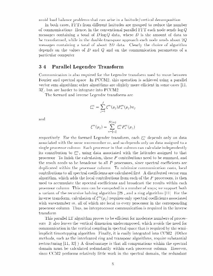
Figure 2: Factor of improvement from load balancing on the Intel DELTA, as afunction of number of processors. Improvements are relative to a version of PCCM2that does not incorporate load balancing, and are given for all of PCCM2 (\Total")and for just the physics component.A exible load-balancing library has been developed as part of the PCCM2e�ort, suitable for use in PCCM2 and other similar climate models. This libraryhas been incorporated into PCCM2 and used to experiment with alternative load-balancing strategies [9]. One simple strategy swaps every second grid point withits partner 180 degrees apart in longitude during radiation calculations. This doesa good job of balancing the diurnal cycle: because CCM2 pairs N/S latitudes, itensures that each processor always has approximately equal numbers of day andnight points. However, it generates a large volume of communication. Anotherstrategy uses a dynamic data-distribution strategy that performs less communicationbut requires periodic reorganizations of model state data. Currently, the formerscheme gives better performance in most cases, and succeeds in eliminating about75 per cent of the ine�ciency attributable to load imbalances when PCCM2 runson 512 processors [9]. This scheme is incorporated in the production PCCM2, andis used in the performance studies reported in the next section. Figure 2 illustratesthe impacts of load balancing. 10

6 Performance StudiesWe performed a wide variety of experiments to measure and characterize PCCM2performance. As noted above, performance of spectral and semi-Lagrangian trans-port codes depends signi�cantly on the parallel algorithms, domain decomposition,and communication protocols used. The results presented here use the double trans-pose parallel FFT, distributed LT, and load balancing algorithms described in pre-ceding sections. A square or almost square processor mesh was used in most cases,as experiments indicated that these generally gave the best performance. Commu-nication protocols are for the most part those identi�ed as e�cient in studies withPSTSWM [10, 11, 33].6.1 ComputersTable 1 describes the two parallel computer systems on which experiments wereperformed: the Intel Paragon XP/S MP 150 and the IBM SP2. These systems havesimilar architectures and programming models, but vary considerably in their com-munication and computational capabilities. Our values for message startup time(ts) and per-byte transfer time (tb) are based on the minimum observed times forswapping data between two nodes using our communication routines, which incor-porate extra subroutine call overhead and communication logic relative to low-levellibraries. Hence, they represent achievable, although not necessarily typical, values.The linear (ts; tb) parameterization of communication costs is a good �t to observeddata for the Paragon but not for the SP2. The MBytes/second measure is bidirec-tional bandwidth: approximately twice 1=tb. The computational rate (M op/sec)is the maximum observed by running the PSTSWM testbed code [33] on a singleprocessor for a variety of problem resolutions, and so is an achieved peak rate ratherthan a theoretical peak rate.N in Table 1 and the X axis for all �gures refer to the number of nodes, not thenumber of processors. This distinction is important because the Paragon used inthese studies has three processors per node. In our experiments, one processor pernode was always used as a dedicated message coprocessor, a second processor wasused for computation, and the third processor was idle. (Some modi�cations to thesource code are required in order to exploit the additional compute processor on theParagon. These modi�cations are currently ongoing.) The Paragon measurementsused the SUNMOS operating system developed at Sandia National Laboratories andthe University of New Mexico, which currently provides better communication per-formance than the standard Intel OSF operating system. Interprocessor communi-cation on the Paragon was performed by using the SUNMOS native communicationcommands, and on the SP2 by using the MPL communication library.Table 1 gives single processor performance data at both single-precision (32-bit oating point values) and double precision (64-bit) arithmetic. Double precision issigni�cantly slower on the 32-bit i860 processor and faster on the 64-bit Power 2processor. Below, we give multiprocessor performance results for both single anddouble precision. We shall see that the SP2 generally performs better at single pre-cision on multiple processors, no doubt because of reduced communication volumewhen sending 32-bit values. 11

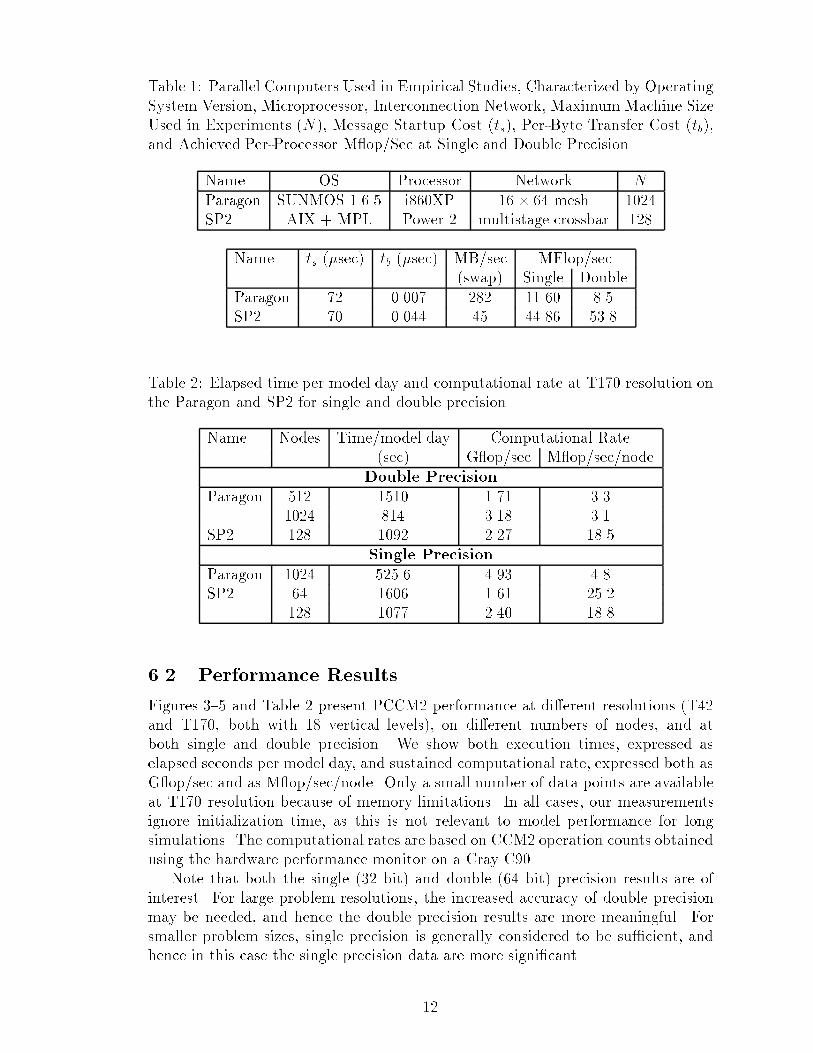
Table 1: Parallel Computers Used in Empirical Studies, Characterized by OperatingSystem Version, Microprocessor, Interconnection Network, Maximum Machine SizeUsed in Experiments (N), Message Startup Cost (ts), Per-Byte Transfer Cost (tb),and Achieved Per-Processor M op/Sec at Single and Double PrecisionName OS Processor Network NParagon SUNMOS 1.6.5 i860XP 16 � 64 mesh 1024SP2 AIX + MPL Power 2 multistage crossbar 128Name ts (�sec) tb (�sec) MB/sec MFlop/sec(swap) Single DoubleParagon 72 0.007 282 11.60 8.5SP2 70 0.044 45 44.86 53.8Table 2: Elapsed time per model day and computational rate at T170 resolution onthe Paragon and SP2 for single and double precisionName Nodes Time/model day Computational Rate(sec) G op/sec M op/sec/nodeDouble PrecisionParagon 512 1510 1.71 3.31024 814 3.18 3.1SP2 128 1092 2.27 18.5Single PrecisionParagon 1024 525.6 4.93 4.8SP2 64 1606 1.61 25.2128 1077 2.40 18.86.2 Performance ResultsFigures 3{5 and Table 2 present PCCM2 performance at di�erent resolutions (T42and T170, both with 18 vertical levels), on di�erent numbers of nodes, and atboth single and double precision. We show both execution times, expressed aselapsed seconds per model day, and sustained computational rate, expressed both asG op/sec and as M op/sec/node. Only a small number of data points are availableat T170 resolution because of memory limitations. In all cases, our measurementsignore initialization time, as this is not relevant to model performance for longsimulations. The computational rates are based on CCM2 operation counts obtainedusing the hardware performance monitor on a Cray C90.Note that both the single (32 bit) and double (64 bit) precision results are ofinterest. For large problem resolutions, the increased accuracy of double precisionmay be needed, and hence the double precision results are more meaningful. Forsmaller problem sizes, single precision is generally considered to be su�cient, andhence in this case the single precision data are more signi�cant.12

10

100

1000

4 8 16 32 64 128 256 512 1024

Tim

e (s

ec)

Nodes

SP2 (Single) (Double)

Paragon (Single) (Double)

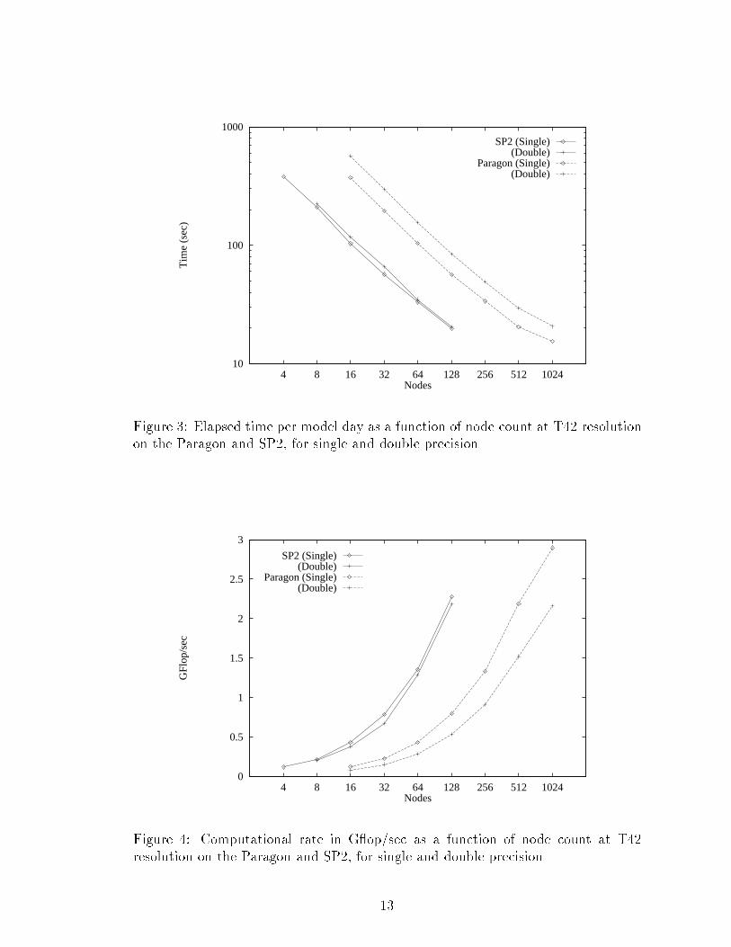
Figure 3: Elapsed time per model day as a function of node count at T42 resolutionon the Paragon and SP2, for single and double precision.0

0.5

1

1.5

2

2.5

3

4 8 16 32 64 128 256 512 1024

GFl

op/s

ec

Nodes

SP2 (Single) (Double)

Paragon (Single) (Double)

Figure 4: Computational rate in G op/sec as a function of node count at T42resolution on the Paragon and SP2, for single and double precision.13

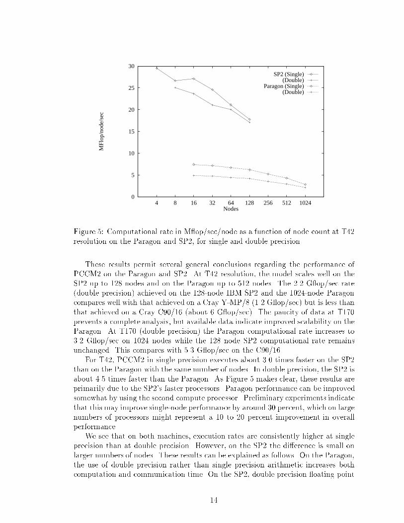
0

5

10

15

20

25

30

4 8 16 32 64 128 256 512 1024

MFl

op/n

ode/

sec

Nodes

SP2 (Single) (Double)

Paragon (Single) (Double)

Figure 5: Computational rate in M op/sec/node as a function of node count at T42resolution on the Paragon and SP2, for single and double precision.These results permit several general conclusions regarding the performance ofPCCM2 on the Paragon and SP2. At T42 resolution, the model scales well on theSP2 up to 128 nodes and on the Paragon up to 512 nodes. The 2.2 G op/sec rate(double precision) achieved on the 128-node IBM SP2 and the 1024-node Paragoncompares well with that achieved on a Cray Y-MP/8 (1.2 G op/sec) but is less thanthat achieved on a Cray C90/16 (about 6 G op/sec). The paucity of data at T170prevents a complete analysis, but available data indicate improved scalability on theParagon. At T170 (double precision) the Paragon computational rate increases to3.2 G op/sec on 1024 nodes while the 128 node SP2 computational rate remainsunchanged. This compares with 5.3 G op/sec on the C90/16.For T42, PCCM2 in single precision executes about 3.0 times faster on the SP2than on the Paragon with the same number of nodes. In double precision, the SP2 isabout 4.5 times faster than the Paragon. As Figure 5 makes clear, these results areprimarily due to the SP2's faster processors. Paragon performance can be improvedsomewhat by using the second compute processor. Preliminary experiments indicatethat this may improve single-node performance by around 30 percent, which on largenumbers of processors might represent a 10 to 20 percent improvement in overallperformance.We see that on both machines, execution rates are consistently higher at singleprecision than at double precision. However, on the SP2 the di�erence is small onlarger numbers of nodes. These results can be explained as follows. On the Paragon,the use of double precision rather than single precision arithmetic increases bothcomputation and communication time. On the SP2, double precision oating point14

computation is faster than single precision since the hardware does all computationsin double and then truncates to a single result. (Preliminary experiments suggestthat PCCM2 single precision performance can be improved by about 10 percent byusing a compiler ag that prevents this truncation for intermediate results; however,the e�ect of this optimization on reproducibility has not yet been determined.) Sofor the SP2, double precision reduces computation costs (as the processor is faster atdouble precision) but increases communication costs (as the data volume increases).The per-node M op/sec data presented in Figure 5 show that neither the i860nor Power 2 microprocessor achieves outstanding performance. (Their peak perfor-mance for double precision computation is 75 and 256 M op/sec, respectively.) Thepercent of peak performance achieved on a single processor depends on the way theprogram utilizes the cache for memory access and on the ability of the compiler tooptimize memory access and computation. The PCCM2 code is structured so thatvector operations can be easily recognized, but e�cient execution for cache basedmachines can require di�erent constructs. The development of program structuringtechniques which are able to better exploit microprocessor-based MPPs must be anurgent topic of future research. The per-node M op/sec data are also in uenced bycommunication costs and load imbalances, both of which tend to increase relativeto computation costs as the number of nodes increases.6.3 Additional ResultsTable 3 shows how much time is spent in di�erent PCCM2 components, while Table 4shows PCCM2 average message sizes. In each case, data is given for a range ofproblem sizes and node counts. For brevity, only results from the SP2 or the Paragonare given in each table, as indicated in the captions. Qualitative results for oneplatform are indicative of results for the other.The time breakdown information (Table 3) provides insights into the scalabilityof di�erent parts of the model. The table indicates how much time was spent indi�erent parts of the model, expressed both as absolute time per time step and as apercentage of total time. These data represent the average across time steps for eachof a number of regions. The table also indicates the aspect ratio chosen in each case:a term P � Q indicates that the latitude dimension is decomposed over P nodesand the longitude dimension is decomposed over Q nodes, or, equivalently, that Pnodes are allocated to each longitude and Q nodes to each latitude. The extremeaspect ratios chosen for some of the T170 runs are due to memory limitations. Anerror in PCCM2 (since corrected) meant that certain aspect ratios had exaggeratedmemory requirements.Indentation in Table 3 indicates subregions within a larger region. Hence, regionMain represents the entire model, and Scan1, SLT, Spectral, and Scan2 representdisjoint subsets of the entire model.Region Scan1 includes physics, the forward FFTs, and part of the transformcalculations into spectral space (the remainder are in region \Spectral"). SubregionPhysics includes all model physics plus the calculation of the non-linear terms indynamics tendencies. Region SLT represents the semi-Lagrangian transport. Sub-region Initialization corresponds to the code that sets up the overlap regions.Region Spectral represents various computations performed in spectral space:15

Gaussian quadrature, completion of the semi-implicit time step, and horizontal dif-fusion calculations. Finally, region Scan2 represents the inverse transform fromspectral space to grid space, and the �nal computation of global integrals of massand moisture integrals for the time step.An examination of how the distribution of time between di�erent regions changeswith the number of nodes (N) provides insights into the scalability of di�erentparallel algorithms. The proportion of time spent in SLT increases signi�cantly withQ, indicating poor scalability. This is due to high communication requirements, aswill be seen below. Spectral also increases when the number of nodes in the N/Sdirection (P ) increases or when the model size increases, again because of increasedcommunication. The proportion of time spent in Physics decreases with N , and theFFT regions increase only slightly, because their communication costs are relativelylow. Notice that a smaller proportion of total time is spent in Physics at doubleprecision than at single precision; this is because of the SP2's better double precisioncompute performance.Further insights in the scaling behavior of PCCM2 is provided by Table 4, whichgives the average message size and number of messages per time step, as a function ofthe number of nodes and problem size. (Note that the forward and backward FFTare included in Scan1 and Scan2, respectively.) These data are for the Paragon;on the SP2 the number of messages increases by 50 percent, because a two-messageprotocol is used that requires that each message exchange be preceded by a synchro-nization message from one of the two nodes involved in the exchange to the other.The use of this two-message protocol is found to improve performance signi�cantlyon the SP2.Table 4 explains some of the trends identi�ed in Table 3, and provides addi-tional information about what happens as the number of nodes increases beyond128. We see that average message size drops rapidly in the FFTs, roughly halvingeach time the number of nodes is doubled. A similar trend is visible in Physics;this corresponds to the communication performed for load balancing. In contrast,message sizes in the SLT stay fairly constant, and eventually completely dominatethe total communication volume. Examining message counts, we see that the num-ber of messages performed in the FFTs increases with the number of nodes, andbecomes a signi�cant contributor to communication costs on large number of nodes.This suggests that there may be advantages to using either a distributed FFT ora O(logP ) transpose FFTs [11] when solving small problems on large number ofnodes.7 SummaryPCCM2 is a production climate model designed to execute on massively parallelcomputer systems. It is functionally equivalent to the shared-memory parallel CCM2model on which it is based, has successfully completed ten year simulations, and isready for use in scienti�c studies.PCCM2 has been developed as part of a research project investigating parallelalgorithms for atmospheric circulation models. The particular algorithms incor-porated in PCCM2 represent pragmatic tradeo�s between choices known from our16

Table 3: Total Time, and Percentage of Time, Spent in Di�erent Parts of PCCM2on the SP2, for Di�erent Problem Sizes and Node Counts, and for both Single andDouble Precision. Times are in Msec, and are for a Single Time StepT42 T170Region N=32 N=64 N=128 N=64 N=128Single Precision 8x4 8x8 16x8 32x2 16x8Main (Time in msec) 788.4 459.0 272.4 5575.8 3740.6Scan1 402.8 214.8 118.5 2206.9 1167.3Physics 361.9 187.6 100.8 1920.3 950.3Forward FFT 24.2 16.6 9.1 155.4 111.4SLT 261.0 175.4 101.7 1337.2 1323.3Initialization 150.3 107.2 66.5 302.2 740.7Spectral 44.3 24.3 27.1 1186.7 738.4Scan2 79.5 44.1 25.0 827.6 501.7Backward FFT 28.2 18.8 10.6 183.2 134.6Main (Percent of total) 100.0 100.0 100.0 100.0 100.0Scan1 51.1 46.8 43.5 39.6 31.2Physics 45.9 40.9 37.0 34.4 25.4Forward FFT 3.1 3.6 3.3 2.8 3.0SLT 33.1 38.2 37.3 24.0 35.4Initialization 19.1 23.4 24.4 5.4 19.8Spectral 5.6 5.3 9.9 21.3 19.7Scan2 10.1 9.6 9.2 14.8 13.4Backward FFT 3.6 4.1 3.9 3.3 3.6Double Precision 8x4 8x8 16x8 N/A 64x2Main (Time in msec) 920.1 482.5 283.3 4033.4Scan1 469.0 221.1 119.6 1085.6Physics 412.3 183.5 98.0 855.4Forward FFT 35.1 23.7 12.9 112.2SLT 307.1 178.5 103.6 1277.3Initialization 178.8 110.4 68.7 741.3Spectral 53.2 27.0 31.4 1139.3Scan2 90.1 55.6 28.4 511.2Backward FFT 42.6 27.8 14.5 129.9Main (Percent of total) 100.0 100.0 100.0 100.0Scan1 51.0 45.8 42.2 26.9Physics 44.8 38.0 34.6 21.2Forward FFT 3.8 4.9 4.6 2.8SLT 33.4 37.0 36.6 31.7Initialization 19.4 22.9 24.2 18.4Spectral 5.8 5.6 11.1 28.2Scan2 9.8 11.5 10.0 12.7Backward FFT 4.6 5.8 5.1 3.217

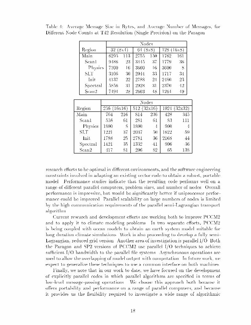
Table 4: Average Message Size in Bytes, and Average Number of Messages, forDi�erent Node Counts at T42 Resolution (Single Precision) on the ParagonNodesRegion 32 (8x4) 64 (8x8) 128 (16x8)Main 6295 113 2755 150 1762 161Scan1 9486 23 3445 37 1779 36Physics 7200 16 3600 16 3600 8SLT 3106 30 2044 33 1717 34Init 4137 22 2788 24 2480 23Spectral 5856 31 2928 31 2370 42Scan2 7494 28 2603 48 1264 49NodesRegion 256 (16x16) 512 (32x16) 1024 (32x32)Main 764 216 814 236 428 345Scan1 558 61 281 61 83 111Physics 1800 8 1800 4 900 4SLT 1221 37 2037 50 1622 59Init 1788 25 2781 36 2168 44Spectral 1421 35 1332 41 906 36Scan2 417 81 206 82 65 138research e�orts to be optimal in di�erent environments, and the software engineeringconstraints involved in adapting an existing vector code to obtain a robust, portablemodel. Performance studies indicate that the resulting code performs well on arange of di�erent parallel computers, problem sizes, and number of nodes. Overallperformance is impressive, but would be signi�cantly better if uniprocessor perfor-mance could be improved. Parallel scalability on large numbers of nodes is limitedby the high communication requirements of the parallel semi-Lagrangian transportalgorithm.Current research and development e�orts are working both to improve PCCM2and to apply it to climate modeling problems. In two separate e�orts, PCCM2is being coupled with ocean models to obtain an earth system model suitable forlong duration climate simulations. Work is also proceeding to develop a fully semi-Lagrangian, reduced grid version. Another area of investigation is parallel I/O. Boththe Paragon and SP2 versions of PCCM2 use parallel I/O techniques to achievesu�cient I/O bandwidth to the parallel �le systems. Asynchronous operations areused to allow the overlapping of model output with computation. In future work, weexpect to generalize these techniques to use a common interface on both machines.Finally, we note that in our work to date, we have focused on the developmentof explicitly parallel codes in which parallel algorithms are speci�ed in terms oflow-level message-passing operations. We choose this approach both because ito�ers portability and performance on a range of parallel computers, and becauseit provides us the exibility required to investigate a wide range of algorithmic18

alternatives. Ultimately, we expect that the more e�cient algorithms identi�ed inthis project may be speci�ed by using more convenient notations.AcknowledgmentsThis work was supported by the CHAMMP program of the O�ce of Health andEnvironmental Research, Environmental Sciences Division, of the U.S. Departmentof Energy under Contract W-31-109-Eng-38 with the University of Chicago and un-der Contract DE-AC05-84OR21400 with Lockheed-Martin Energy Systems. We aregrateful to Ray Flanery, Jace Mogill, Ravi Nanjundiah, Dave Semeraro, Tim Shee-han, and David Walker for their work on various aspects of the parallel model. Wealso acknowledge our colleagues at NCAR for sharing codes and results throughoutthis project. We are grateful to Wu-Sun Cheng and David Soll for their help withperformance tuning on the IBM SP2.This research used the Intel Paragon multiprocessor system of the Oak Ridge Na-tional Laboratory Center for Computational Sciences (CCS), funded by the Depart-ment of Energy's Mathematical, Information, and Computational Sciences (MICS)Division of the O�ce of Computational and Technology Research; the Intel Paragonmultiprocessor system at Sandia National Laboratories; the Intel Touchstone DELTASystem operated by Caltech on behalf of the Concurrent Supercomputing Consor-tium; the IBM SP2 at Argonne National Laboratory; and the IBM SP2 of the NASProgram at the NASA Ames Research Center.References[1] S. Barros and T. Kauranne, On the parallelization of global spectral Eule-rian shallow-water models, in Parallel Supercomputing in Atmospheric Science:Proceedings of the Fifth ECMWF Workshop on Use of Parallel Processors inMeteorology, G.-R. Ho�man and T. Kauranne, eds., World Scienti�c PublishingCo. Pte. Ltd., Singapore, 1993, pp. 36{43.[2] W. Bourke, An e�cient, one-level, primitive-equation spectral model, Mon.Wea. Rev., 102 (1972), pp. 687{701.[3] D. Dent, The ECMWF model on the Cray Y-MP8, in The Dawn of MassivelyParallel Processing in Meteorology, G.-R. Ho�man and D. K. Maretis, eds.,Springer-Verlag, Berlin, 1990.[4] D. Dent, The IFS Model: A Parallel Production Weather Code, submitted toParallel Computing, 1995.[5] U.S. Department of Energy, Building an advanced climate model: Progress planfor the CHAMMP climate modeling program, DOE Tech. Report DOE/ER-0479T, U.S. Department of Energy, Washington, D.C., December, 1990.[6] J. B. Drake, R. E. Flanery, I. T. Foster, J. J. Hack, J. G. Michalakes, R. L.Stevens, D. W. Walker, D. L. Williamson, and P. H. Worley, The message-passing version of the parallel community climate model, in Parallel Supercom-19

puting in Atmospheric Science, World Scienti�c Publishing, Singapore, 1993,pp. 500{513.[7] E. Eliasen, B. Machenhauer, and E. Rasmussen, On a numerical method for in-tegration of the hydrodynamical equations with a spectral representation of thehorizontal �elds, Report No. 2, Institut for Teoretisk Meteorologi, KobenhavnsUniversitet, Denmark, 1970.[8] I. T. Foster, W. Gropp, and R. Stevens, The parallel scalability of the spectraltransform method, Mon. Wea. Rev., 120 (1992), pp. 835{850.[9] I. T. Foster and B. Toonen, Load balancing in climate models, Proc. 1994Scalable High-Performance Computing Conf., IEEE Computer Society Press,Los Alamitos, CA, 1994.[10] I. T. Foster and P. H. Worley, Parallelizing the spectral transform method: Acomparison of alternative parallel algorithms, in Parallel Processing for Scien-ti�c Computing, R. F. Sincovec, D. E. Keyes, M. R. Leuze, L. R. Petzold, andD. A. Reed, eds., Society for Industrial and Applied Mathematics, Philadelphia,PA, 1993, pp. 100{107.[11] I. T. Foster and P. H. Worley, Parallel algorithms for the spectral transformmethod, submitted for publication. Also available as Tech. Report ORNL/TM{12507, Oak Ridge National Laboratory, Oak Ridge, TN, May 1994.[12] G. C. Fox, M. A. Johnson, G. A. Lyzenga, S. W. Otto, J. K. Salmon, andD. W. Walker, Solving Problems on Concurrent Processors, vol. 1, Prentice-Hall, Englewood Cli�s, NJ, 1988.[13] H. Franke, P. Hochschild, P. Pattnaik, J.-P. Prost, and M. Snir, MPI-F: Cur-rent status and future directions, Proc. Scalable Parallel Libraries Conference,Mississippi State, October, IEEE Computer Society Press, 1994.[14] U. G�artel, W. Joppich, and A. Sch�uller, Parallelizing the ECMWF's weatherforecast program: The 2D case, Parallel Computing, 19 (1993), pp. 1413{1426.[15] J. J. Hack, B. A. Boville, B. P. Briegleb, J. T. Kiehl, P. J. Rasch, andD. L. Williamson, Description of the NCAR Community Climate Model(CCM2), NCAR Technical Note TN-382+STR, National Center for Atmo-spheric Research, Boulder, Colo., 1992.[16] J. J. Hack, J. M. Rosinski, D. L. Williamson, B. A. Boville, and J. E. Truesdale,Computational design of the NCAR Community Climate Model, to appear inthis issue of Parallel Computing, 1995.[17] S. Hammond, R. Loft, J. Dennis, and R. Sato, Implementation and performanceissues of a massively parallel atmospheric model, Parallel Computing, this issue.[18] T. Kauranne and S. Barros, Scalability estimates of parallel spectral atmo-spheric models, in Parallel Supercomputing in Atmospheric Science, G.-R. Ho�-man and T. Kauranne, eds., World Scienti�c Publishing Co. Pte. Ltd., Singa-pore, 1993, pp. 312{328. 20

[19] R. D. Loft and R. K. Sato, Implementation of the NCAR CCM2 on the Con-nection Machine, in Parallel Supercomputing in Atmospheric Science, G.-R.Ho�man and T. Kauranne, eds., World Scienti�c Publishing Co. Pte. Ltd.,Singapore, 1993, pp. 371{393.[20] J. Michalakes, Analysis of workload and load balancing issues in NCAR Com-munity Climate Model, Technical Report ANL/MCS-TM-144, Argonne Na-tional Laboratory, Argonne, Ill., 1991.[21] J. Michalakes and R. Nanjundiah, Computational load in model physics of theparallel NCAR Community Climate Model, Technical Report ANL/MCS-TM-186, Argonne National Laboratory, Argonne, Ill., 1994.[22] S. A. Orszag, Transform method for calculation of vector-coupled sums: Ap-plication to the spectral form of the vorticity equation, J. Atmos. Sci., 27,890{895, 1970.[23] M. Pease, An adaptation of the fast Fourier transform for parallel processing,J. Assoc. Comput. Mach., 15 (1968), pp. 252{264.[24] R. B. Pelz and W. F. Stern, A balanced parallel algorithm for spectral globalclimate models, in Parallel Processing for Scienti�c Computing, R. F. Sincovec,D. E. Keyes, M. R. Leuze, L. R. Petzold, and D. A. Reed, eds., Society forIndustrial and Applied Mathematics, Philadelphia, PA, 1993, pp. 126{128.[25] J.G. Sela, Weather forecasting on parallel architectures, to appear in this issueof Parallel Computing, 1995.[26] P. N. Swarztrauber, Multiprocessor FFTs, Parallel Computing, 5 (1987),pp. 197{210.[27] P. N. Swarztrauber, W. L. Briggs, R. A. Sweet, V. E. Henson, and J. Otto,Bluestein's FFT for arbitrary n on the hypercube, Parallel Computing, 17(1991), pp. 607{618.[28] R. A. van de Geijn, On Global Combine Operations, LAPACK Working Note29, CS-91-129, April 1991, Computer Science Department, University of Ten-nessee.[29] D. W. Walker, P. H. Worley, and J. B. Drake, Parallelizing the spectral trans-formmethod. Part II,Concurrency: Practice and Experience, 4 (1992), pp. 509{531.[30] W. Washington and C. Parkinson, An Introduction to Three-Dimensional Cli-mate Modeling, University Science Books, Mill Valley, Calif., 1986.[31] D. L. Williamson and P. J. Rasch, Two-dimensional semi-Lagrangian transportwith shape-preserving interpolation, Mon. Wea. Rev., 117, 102{129, 1989.[32] P. H. Worley and J. B. Drake, Parallelizing the spectral transform method,Concurrency: Practice and Experience, 4 (1992), pp. 269{291.21

[33] P. H. Worley and I. Foster, 1994. Parallel spectral transform shallow watermodel: A runtime-tunable parallel benchmark code, in Proc. Scalable HighPerformance Computing Conf., IEEE Computer Society Press, Los Alamitos,Calif., pp. 207{214.

22