Dependability Modeling & Evaluation

of Multiple-Phased Systems using DEEM∗

Andrea Bondavalli1, Silvano Chiaradonna2,Felicita Di Giandomenico2, Ivan Mura3

1: DSI, Universita di Firenze, Via Lombroso 6/17, 50134 Firenze, Italy,a.bondavalli@dsi.unifi.it

2: ISTI-CNR, Via G. Moruzzi 1, 56124 Pisa, Italy,(s.chiaradonna, f.digiandomenico)@isti.cnr.it

3: Motorola Electronics SpA, Global Software Group Italy, Via C. Massaia 83, 10147, Torino, Italy,Ivan.Mura@motorola.com

Keywords: Phased mission systems, dependability modeling and evaluation, deterministicstochastic Petri nets, Markov regenerative processes, transient analysis, analytical tool.Summary & Conclusions Multiple-Phased Systems (MPS), i.e., systems whose operationallife can be partitioned in a set of disjoint periods, called “phases”, include several classes ofsystems such as Phased Mission Systems and Scheduled Maintenance Systems. Because oftheir deployment in critical applications, the dependability modeling and analysis of Multiple-Phased Systems is a task of primary relevance. The phased behavior makes the analysis ofMultiple-Phased Systems extremely complex. This paper describes the modeling methodologyand the solution procedure implemented in DEEM, a dependability modeling and evaluationtool specifically tailored for Multiple Phased Systems. It also describes its use for the solutionof representative MPS problems. DEEM relies upon Deterministic and Stochastic Petri Nets asthe modeling formalism, and on Markov Regenerative Processes for the model solution. Whencompared to existing general-purpose tools based on similar formalisms, DEEM offers advantageson both the modeling side (sub-models neatly model the phase-dependent behaviors of MPS),and on the evaluation side (a specialized algorithm allows a considerable reduction of the solutioncost and time). Thus, DEEM is able to deal with all the scenarios of MPS which have beenanalytically treated in the literature, at a cost which is comparable with that of the cheapestones, completely solving the issues posed by the phased-behavior of MPS.

ACRONYMS1

MPS multiple-phased systemPMS phased mission systemSMS scheduled maintenance systemDEEM dependability evaluation of multiple-phased systemsDSPN deterministic and stochastic Petri netMRGP Markov regenerative processCTMC continuous-time Markov chainGUI graphical user interface

∗ c©20xx IEEE. Personal use of this material is permitted. However, permission to reprint/republish thismaterial for advertising or promotional purposes or for creating new collective works for resale or redistributionto servers or lists, or to reuse any copyrighted component of this work in other works must be obtained from theIEEE. This material is presented to ensure timely dissemination of scholarly and technical work. Copyright andall rights therein are retained by authors or by other copyright holders. All persons copying this information areexpected to adhere to the terms and constraints invoked by each author’s copyright. In most cases, these worksmay not be reposted without the explicit permission of the copyright holder.

1The singular and plural of an acronym are always spelled the same.

1

SN system netPhN phase netRGP reachability graph of the PhNSRGG sequential reachability graph generation

NOTATION

V (t) transient probability matrix of the MRGP process at time t

~m, ~m′

markings of the DSPNn number of phases that an MPS performsτi duration of phase i

S state space of the MRGP processMi(t) state at time t of the stochastic process defined as the restriction

of the MRGP within the execution of phase i

Si state space of {Mi(t), t ≥ 0}Sn+1 absorbing markings reached by the DSPN at the end of the missionQi transition rate matrix of {Mi(t), t ≥ 0}Vi,j(t) block of the matrix V (t) from phase i to phase j, at time t

p(i, j) unique path linking phase i to phase j

r number of phases of the path p(i, j)ph h-th phase of the path p(i, j)∆i,j branching probability matrix

∆i,j

~m,~m′ entry of ∆i,j

P (t) probability vector of each marking in SN at time t

P0 initial probability vector of the DSPN~mi stable marking of the RGP graph for the phase i

~mji j-th stable marking of the i-th phase

P initi initial state probability vector of the phase i

tiniti initial global time of the phase i

Pi transient state probability vector at the end of the phase i

RGS(~mi) reachability graph of the whole DSPN model when marking ~mi

is the only one permitted for the PhNtDeti deterministic transition which models the time the PMS

spends in phase i

next(~mi) markings reachable from ~mi through the firing of some immediatetransition next to the firing of tDet

i

RGS(~mi, next(~mi)) reachability graph of the whole DSPN model, when the initialmarking of the PhN is ~mi, and transition tDet

i is the onlydeterministic one allowed to fire

Ci cardinality of the state space of the phase i

mmax maximum number of phases reachable directly from a phaseqi maximum absolute diagonal entry of Qi

α number of pairs of missions between partial checks

1 Introduction

Many embedded systems devoted to the control and management of critical activities performa series of tasks which must be accomplished in sequence. Their operational life consists ofa sequence of non-overlapping periods, called phases. These systems are often called Phased

2

Mission Systems (PMS). However, the concept of phased execution of system tasks is applicableto a much wider variety of applications and domains, for which the word “mission” may berestrictive or inadequate. For this reason, we will use in this paper the wording Multiple-PhasedSystems (MPS).

Indeed, MPS are very general, because their phases can be charaterized along a wide varietyof differentiating features:

(1) Tasks executed in a phase may differ from those performed within other phases.

(2) Performance and dependability requirements can differ from one phase to another.

(3) During some phases, the system may be subject to a particularly stressing environment,thus experiencing dramatic increases in the failure rate of its components.

(4) The configuration may change over time, in accordance with performance and dependabil-ity requirements of the phase being currently executed.

(5) The successful completion of a phase may bring a different benefit to the MPS with respectto that obtained with other phases.

Examples of MPS can be found in various application domains, such as nuclear, aerospace,telecommunications, transportation, electronics, and many other industrial fields. Because oftheir deployment in several critical application domains, the dependability modeling and analysisof MPS have been considered tasks of primary relevance, and many different approaches haveappeared in the literature, e.g. [1, 2, 3, 4, 5, 6]. However, modeling an MPS can be a complextask even inside one single phase; when a multiplicity of phases and the dependencies amongthem are to be taken into account, additional difficulties are encountered.

The objective of this paper is to present DEEM (DEpendability Evaluation of Multiple-phased systems) [7], a dependability modeling and evaluation tool specifically tailored for thetime-dependent analysis of MPS. DEEM is currently being developed at the University of Flo-rence, and ISTI-CNR. DEEM supports a methodology proposed in [3, 4] for the dependabilitymodeling and evaluation of MPS. This methodology relies upon Deterministic and StochasticPetri Nets (DSPN) as a modeling formalism, and on Markov Regenerative Processes (MRGP)for the model solution. DEEM is equipped with many modeling features which improve theexpressive power of Petri net models, the same modeling features as those already available inseveral general purpose tools such as SPNP [8], Mobius [9], TimeNET [10], PANDA [11], andSURF-2 [12].

This paper is organized as follows. Section 2 reviews the literature, and provides the motiva-tion underlying the decision of developing a new Petri net modeling & analysis tool specificallytailored for the purposes of MPS dependability evaluation. Then, in Section 3 we summarize theDSPN approach to the modeling of MPS, also showing how it is supported through the DEEMtool. Moreover, the analytical solution technique adopted in DEEM is presented, together witha step-by-step numerical example, and its efficiency discussed. The actual description of thecapabilities of DEEM is rendered through the presentation of the modeling and solution of twoexamples of MPS in Section 4.

2 The rationale for DEEM development

As already mentioned, MPS have been widely investigated, and their dependability analysishas been the object of several research studies. We first recall what the results available in theliterature offer for the dependability analysis of real applications of MPS, then pin point someweak areas DEEM development wanted to improve.

3

2.1 Approaches to MPS modeling and evaluation

Because of various early industrial and military applications, research on MPS dependabilitywas initially oriented towards well established, and commonly accepted modeling formalismsavailable to the safety-critical systems development community. Combinatorial models such asFault Trees, and Reliability Block Diagrams, were widely used to analyze MPS dependability [13,14, 6]. More recently, a new family of approaches based on Fault Trees has been proposed [15, 16],which exploit the gain in computational complexity achievable with the use of model solutionsbased on Binary Decision Diagrams. [17] applies Fault Tree methodology to the dependabilityanalysis of MPS systems with non-repairable, and repairable components. State-based modelingapproaches based on Markov chains and Petri nets were also applied because of their ability torepresent complex dependencies among system components [18, 1, 5, 2, 4, 3].

Today, combinatorial and state-space modeling formalisms still represent the two dominantapproaches to MPS dependability analysis. Each approach has its own advantages and weak-nesses; and the choice of the best one is largely dependent on the specific characteristics of thesystem at hand, and on the goals of the analysis.

Combinatorial models provide simpler formalisms which permit an intuitive mapping be-tween modeling elements, and system failures. Moreover, it is quite immediate to exploit resultsof classical qualitative analysis, such as those made available by the FMEA to build quantitativedependability Fault Tree, and Reliability Block Diagram models. On the other hand, such mod-els show severe limitations with respect to the representation of dependencies among differentsystem components, imperfect coverage of fault containment mechanisms, and repair actions forfailed units & sub-systems.

State-space models exhibit a higher flexibility with respect to the representation capabilities.However, such generality does not come for free; rather it is paid by a higher complexity of boththe modeling formalism itself, and of the modeling process.

The considerations above on tradeoffs between flexibility and expressiveness generally applyto any modeling formalism. In the specific case of MPS, additional increased complexities areto be handled by the dependability modelers because of the phased behavior of the systems tobe analyzed. In particular, the following aspects of MPS pose relevant challenges to the systemmodelers (no matter which formalism is adopted):

(a) The operational configuration of the system is not fixed, but rather may vary from phaseto phase, in accordance with the criticality of the specific phase.

(b) The failure/repair history of one component inside one phase affects system behavior insubsequent phases. Therefore, the state of a component at the beginning of a phase isdependent upon the state it had at the previous phase completion time.

(c) The criteria defining the level of fulfillment of dependability and performance requirementsinside a phase may differ from those valid for a subsequent phase.

The aspects listed above have been tackled in different ways by the various modeling ap-proaches in the literature. An important choice which affects the way all such aspects can bedealt with is represented by the single or separate modeling of the various phases.

Representing all the phases of an MPS with a single model [18, 19, 2, 5] offers some advantageswith respect to the possibility of exploiting the similarities among phases to obtain a compactmodel in which all the phases are properly embedded. Building such a single model may notbe easy/convenient in those cases where the phase specific aspects listed at points (a) and (c)above prevail over the similarities along different phases.

On the other hand, a separate modeling of each phase [13, 20, 16] allows an immediatecharacterization of the differences among phases, in terms of different failure rates and differentconfiguration requirements. Each phase can be separately solved, and its solution outcomesthen aggregated with those of the other phases to obtain the overall result for the MPS, thusexhibiting a better performance at solution time. The major weakness of the separate modeling

4

approach (not shown by the single model one) is the treatment of the dependencies amongphases, which are to be taken into consideration because of the sharing of components amongphases. This approach requires explicitly performing the mapping of the state of a componentat the end of a phase to the state of the component at the beginning of the next phase. Thisjob is conceptually simple, but can be cumbersome and for sure becomes a potential source oferrors for large models.

In the literature, there are examples of separate, and single modeling studies for both com-binatorial, and state-space based approaches. Recently, some hierarchical approaches [21, 4, 3]tried to grab the best aspects while alleviating the limitations of each of the two choices. Theyallow for the definition of a high level single model of the MPS, which has only the purpose ofdefining the sequence of phases; and a second, lower level modeling layer, which focuses on MPSintra-phase behavior.

2.2 Improvement opportunities for MPS modeling

The major objective of DEEM development has been that of providing the dependability com-munity with the first tool specifically oriented to support the automated analysis of MPS. Indeed,no other automated tools specifically developed for MPS currently exist; the results presentedin the literature have been only partially included into general purpose dependability analysistools. More precisely, the methodology in [6] is the only one which has been included into ageneral purpose automated modeling tool (HARP). The resulting tool, called EHARP, is basedon a separate Markov chain modeling the SMS inside the various phases, an approach which stillrequires a considerable amount of user-assistance to correctly model the dependencies amongsuccessive phases.

Now, we shall identify directions for improvement with respect to the current state of theart in MPS dependability modeling and evaluation, which have been taken into considerationwhen defining the requirements of DEEM.

Modeling of phase dependent behaviors. A general, user-friendly methodology and toolfor MPS modeling should offer the possibility of expressing the constraints and conditions whichdefine the phase-dependent behaviors in a concise and unambiguous way. Considering the variousstudies, it appears that most of them focused on ad-hoc modeling approaches without providing agenerally applicable solution. Both proposals based on the separate, and on the single modelingapproaches are actually very similar from the point of view of their ability to represent thephased behavior of MPS.

The conditions defining how an MPS changes from phase to phase can be easily captured byexpressions of a simple logic, such as the following:

If(phasea)then(unitfailurerate = x) (1)

If(phaseb)thenIf(availableunits < n)then(systemfailure = TRUE) (2)

DEEM adopts a modeling process which captures the phased-behavior of MPS through thedefinition of logic clauses, such as those listed in (1), (2). The user will then be allowed to builda compact model of an MPS which represents the particular behavior of each phase as describedby the associated logic clauses.

Modeling phase execution order. The explicit modeling of the sequence of phases traversedby the system to accomplish its goals is one MPS aspect that has been neglected in most ofthe studies, probably due to the implicit assumption that the sequence of phases is alwaysconstituted by a single path from the first phase to the last one. There are indeed examplesof MPS for which the sequence of phases is better represented by a more generic direct acyclicgraph. In this scenario, at the end of a phase, the MPS may select the next phase according toa probability distribution, or depending on its current internal state (as, for example, in [4]).

5

DEEM offers to the modeler the possibility of explicitly capturing the sequence of phases ofwhich the MPS execution is composed.

Modeling of intra-phase behaviors. The capabilities of the existing approaches to modelthe intra-phase behavior of MPS are largely determined by the modeling formalisms adopted.Combinatorial models, such as Fault Trees and Reliability Block Diagrams, are able to representthe failure behavior of system components. They can handle even general failure occurrenceprobability distributions (such as the Weibull distribution). However, approaches based onFault-Trees can only partially cope with other aspects, such as repair processes, coverage of faultdetection mechanisms, and reconfiguration actions of the system. The generality of state-spacemodeling approaches is definitely necessary in such cases. The limits of intra-phase behaviormodeling of these last approaches are only determined by the actual possibility of numericallyhandling the stochastic process underlying the MPS model, for the sake of dependability metricscomputation.

DEEM follows the state-based modeling approach.

Evaluation of generic performability measures. The definition of the metrics of interestagainst which a system is evaluated is a crucial part of every dependability study. Traditionally,MPS have been evaluated in terms of their reliability, based on the assumption that a successfulexecution of the system is one which performs all the planned phases while never reaching afailure condition. This is quite restrictive for systems which have phases of different levels ofcriticality, or which measure their performances on the amount of useful work they conductacross the various phases.

Recently, more general MPS evaluation metrics have been proposed in combinatorial mod-eling studies, such as [16], where the concept of multi-level performance is introduced to definebroader measures, which combine performance and dependability aspects.

This idea of a metric which captures both dependability and performance (performability)was formalized by Meyer in the well-known paper [22]. This powerful concept finds an idealimplementation in a state-based modeling tool called reward structure. Markov reward modelsindeed allow assigning arbitrary reward values to states, and to events of a system. The totalaccumulated reward of the system (at a given point in time or averaged over a period) is ameasure which subsumes most of the classical dependability and performance measures whichhave been considered in modeling.

DEEM provides the modeler with the possibility of defining general measures of MPS per-formability. It supports the definition of reward structures, which allow characterizing therelevance each activity within a phase has for the system overall execution.

3 The DSPN methodology to model MPS adopted in DEEM

Deterministic and Stochastic Petri Nets (DSPN) [23] have been chosen as the modeling formal-ism for DEEM, whereas the solution technique finds its ground in the efficient time-dependentanalysis of Markov Regenerative Processes (MRGP) presented in [24]. Precisely, DEEM is basedon the methodology proposed in [3, 4]. The main advance of that methodology is found in theadoption of a highly expressive modeling formalism for concisely representing MPS dynamicbehavior, coupled with a powerful analytical solution method of the stochastic processes under-lying the models. In its present version, DEEM does not yet fully exploit the potentialities ofthe referred methodology, but the following restrictions are applied:

1) The duration of the phases is deterministic.

2) Each intra-phase process is a time-homogeneous Markov chain (the phase model is re-stricted to contain only exponential and immediate transitions).

DEEM is freely available to academics (see http://dcl.isti.cnr.it/DEEM).

6

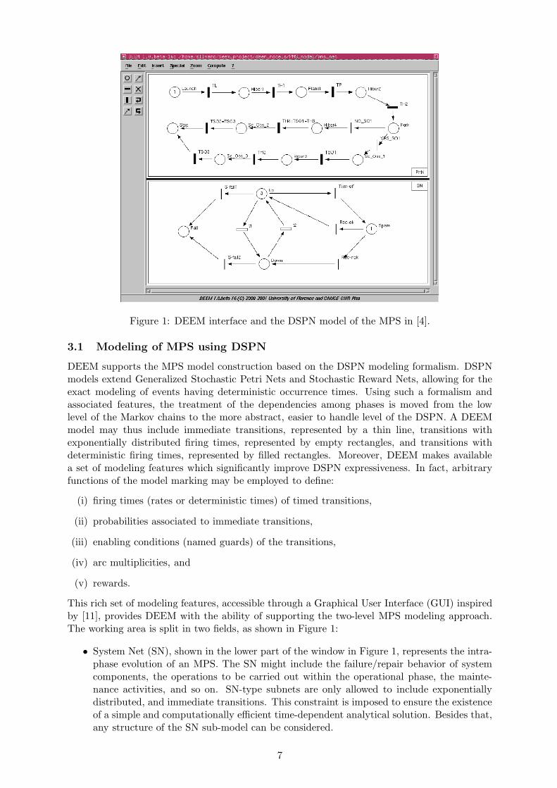
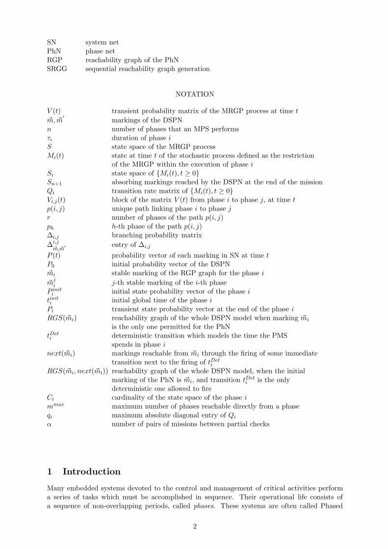
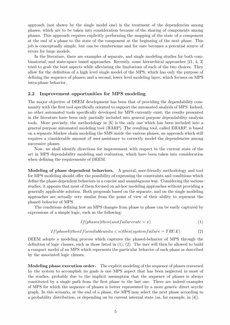
Figure 1: DEEM interface and the DSPN model of the MPS in [4].

3.1 Modeling of MPS using DSPN

DEEM supports the MPS model construction based on the DSPN modeling formalism. DSPNmodels extend Generalized Stochastic Petri Nets and Stochastic Reward Nets, allowing for theexact modeling of events having deterministic occurrence times. Using such a formalism andassociated features, the treatment of the dependencies among phases is moved from the lowlevel of the Markov chains to the more abstract, easier to handle level of the DSPN. A DEEMmodel may thus include immediate transitions, represented by a thin line, transitions withexponentially distributed firing times, represented by empty rectangles, and transitions withdeterministic firing times, represented by filled rectangles. Moreover, DEEM makes availablea set of modeling features which significantly improve DSPN expressiveness. In fact, arbitraryfunctions of the model marking may be employed to define:

(i) firing times (rates or deterministic times) of timed transitions,

(ii) probabilities associated to immediate transitions,

(iii) enabling conditions (named guards) of the transitions,

(iv) arc multiplicities, and

(v) rewards.

This rich set of modeling features, accessible through a Graphical User Interface (GUI) inspiredby [11], provides DEEM with the ability of supporting the two-level MPS modeling approach.The working area is split in two fields, as shown in Figure 1:

• System Net (SN), shown in the lower part of the window in Figure 1, represents the intra-phase evolution of an MPS. The SN might include the failure/repair behavior of systemcomponents, the operations to be carried out within the operational phase, the mainte-nance activities, and so on. SN-type subnets are only allowed to include exponentiallydistributed, and immediate transitions. This constraint is imposed to ensure the existenceof a simple and computationally efficient time-dependent analytical solution. Besides that,any structure of the SN sub-model can be considered.

7

• Phase Net (PhN), shown in the upper part of Figure 1, represents the execution of thevarious phases. PhN contains all the deterministic transitions of the overall DSPN model,and may as well contain immediate transitions. A token in a place of the PhN modelrepresents a phase being executed, and the firing of a deterministic transition models aphase change. The DSPN of the PhN must possess distinct markings corresponding todifferent phases. Notice that the PhN is not limited to have a linear structure, but it maybe a quite general one, such as a tree or cyclic structure [1, 3, 4].

Each net is made dependent on the other one by marking-dependent predicates which modifytransition rates, enabling conditions, transition probabilities, multiplicity functions, etc., tomodel the specific MPS features. The only restriction is that the firing times of the deterministictransitions of the PhN are not allowed to be dependent on the marking of the SN. Notice thatthe predicates expressing enabling conditions are not intended to substitute the classic enablingrules of Petri net model transitions, rather they represent additional constraints a transitionmust fulfill to be eligible for firing.

Several advantages are offered by the DSPN approach over previous proposals, as cited in[3, 4]. First, the modeling features of DSPN allow a very concise, easy to understand & tomodify, representation of MPS, compared with a Markov chain which results in huge models,which readily become sources of errors in modeling. The two parts of the DSPN model representtwo different abstraction levels of the same MPS. The mission profile is explicitly modeled in thePhN, and can be very easily modified to represent different MPS. Moreover, the whole modelingprocedure limits in itself the possibility of introducing errors inside the models. In fact, toincrease the confidence that can be put in the modeling, the separate Petri nets sub-modelscan be checked individually against various structural properties. Further, the links among thevarious sub-models are expressed through predicates of the marking, in a clear and unambiguousway. Phase-triggered reconfigurations, which add a significant complexity to the treatment ofdependencies among phases, are easily handled through the implicit mapping which is embeddedin the model (as in [18, 19, 2, 5]). Indeed, the mapping between successive phases is completelyspecified at the level of the DSPN modeling, thus dramatically reducing the amount of user-assistance needed to define the MPS models with respect to Markov chain-based techniques.

3.2 Dependability measures for MPS

As already mentioned, dependability evaluation process demands for the definition of rewardmodels. In DEEM, very general dependability measures for the MPS evaluation can be definedby a reward function for instantaneous, cumulated, and timed-averaged analysis. Composedmeasures can be also defined, as a function of the evaluated reward-based measures. Among themeasures assessable through such approach are the probability of successful mission completion,the relative impact of each single phase on the overall dependability figures, the impact on MPSreliability of a given maintenance schedule, and the amount of useful work that can be carriedout within the mission. In Section 4, examples of evaluated measures will be shown.

3.3 The specialized analytical technique to solve MPS

We summarize in this section the transient solution technique used by DEEM to evaluatedependability-related measures of MPS at specific time instants. The specialized solution findsits ground by observing that the only deterministic transitions in a DSPN model of a MPS arethe phase durations, and that these transitions are enabled one at a time. Thus, the markingprocess {M(t), t ≥ 0} of the DSPN is a Markov Regenerative Process (MRGP) [24] for whichthe firing times of the deterministic transitions are indeed regeneration points. Moreover, thefollowing property holds for the DSPN model of a MPS: in every non-absorbing marking of theDSPN there is always one deterministic transition enabled, which corresponds to the phase beingcurrently executed.

8

The general solution method for MRGP processes considers the computing of matrix V (t),whose entry ~m, ~m

′

is the occupation probability of marking ~m′

at time t ≥ 0, given the initialmarking ~m. Matrix V (t) is the solution to the generalized Markov renewal equation V (t) =E(t) + K(t) ∗ V (t), where K(t), and E(t) are the global, and local kernel matrices [24]; and “*”is the convolution operator. Instead of directly attacking the solution of the generalized Markovrenewal equation by numerical algorithms or Laplace-Stiltjes transform, DEEM computes V (t)according to the following analytical method. Let S denote the state space of the MRGP process,let 1, 2, ..., n be the set of phases the MPS can perform, and finally let τi denote the duration ofphase i, i = 1, 2, ..., n. Consider the following subsets of S:

Si ≡ {~m ∈ S | phase i is being performed}, i = 1, 2, ..., nSn+1 ≡ {~m ∈ S | no phase is being performed}

Owing to the above recalled property, and because different phases correspond to distinctmarkings of the DSPN model, sets Si, i = 1, 2, ...n + 1, are a partition of the marking spaceS. The stochastic process {Mi(t), t ≥ 0}, i = 1, 2, ...n, defined as the restriction of the MRGPwithin the execution of phase i, is a continuous-time Markov chain (CTMC) with state space Si,and transition rate matrix Qi. The transient analysis of the MRGP is carried out by separatelyconsidering the evolution of the processes {Mi(t), t ≥ 0}. Consider the block structure inducedon matrix V (t) as a result of the marking space partitioning. Each block Vi,j(t) is separatelycomputed as follows. Consider the unique path p(i, j) which links phase i to phase j accordingto the structure of the PhN. This path is a set of phases p(i, j) ≡ {p1, p2, ..., pr}, with p1 = i,and pr = j. Block Vi,j(t) is given by:

Vi,j(t) =

(

r−1∏

h=1

eQphτph ∆ph, ph+1

)

eQj(t−Pr−1

h=1τph) (3)

Where ∆ph, ph+1, h = 1, 2, ..., r−1 is the branching probability matrix, whose entry ∆ph,ph+1

~m,~m′

is defined as the probability that ~m′

is the initial marking of phase ph+1, given that ~m is themarking at the end of phase ph. A more complete description is in [3].

3.4 The solution algorithm

The solution algorithm implemented in DEEM is first described, then its application is providedon a simple example, and finally a discussion on its efficiency follows.

3.4.1 Algorithm description

To asses the defined dependability figures, DEEM computes the probability vector P (t) of eachmarking in SN at time t. P (t) is obtained from the transient probability matrix V (t), throughthe equation P (t) = P0 · V (t), where P0 is the initial probability vector of the DSPN. Equation(3) allows one to evaluate V (t) through the separate analysis of the various alternative pathscomposing the mission; and only requires the computation of the matrix exponentials eQiτ , andthe branching probability matrices ∆i,j, i, j = 1, 2, ..., n, which can be automatically obtainedonce the reachability graph is generated. To compute P (t), the solution engine of DEEM startstaking as input the DSPN model & its initial probability vector P0, and performs the followingsteps:

I. Construction of the reachability graph (RGP) of the PhN sub-model. This graph hasexactly one stable marking ~mi for each phase i = 1, 2, ..., n the MPS may perform.

II. Build the reachability graph RGS(~m1) of the whole DSPN model to obtain P0.

III. Calling deem solver(1, P0, 0).

9

deem solver(i, P initi , tinit

i ) implements a recursive algorithm, whose steps are:

1. Build the reachability graph RGS(~mi) of the whole DSPN model when marking ~mi isthe only one permitted for the PhN. From RGS(~mi) the transition rate matrix Qi of thecontinuous-time Markov chain describing the evolution of the DSPN during the executionof phase i is obtained.

2. If phase i is the last one, or t ≤ tiniti + τi then compute the transient state probability

vector Pi(t) = P initi eQi(t−tinit

i ), and return; else continue at step 3.

3. Compute the transient state probability vector Pi = P initi eQiτi .

4. Build the reachability graph RGS(~mi, next(~mi)), where next(~mi) = {~mj1 , ..., ~mjm}, of thewhole DSPN model, when the initial marking of the PhN is ~mi, and transition tDet

i is theonly deterministic one allowed to fire. Each marking ~mjh

is reachable from ~mi throughthe firing of some immediate transition next to the firing of tDet

i .

5. For each stable marking ~mjh(phase jh), perform the following steps:

5.1 Obtain the branching probability matrix ∆i,jhfor the transition from phase i to phase

jh from RGS(~mi, next(~mi)).

5.2 Compute the initial state probability vector of the phase jh: P initjh

= Pi∆i,jh.

5.3 Call deem solver(jh, P initjh

, tiniti + τi).

To evaluate dependability measures based on reward structures, DEEM operates on Pi ac-cording to the standard computation algorithms [25]. It is worthwhile observing that:

i) the state space of the MRGP process does not need to be generated and handled as awhole;

ii) transition rate matrices Qi can be generated separately one from another;

iii) to build matrices ∆i,jh, the generation of the reachability graph for consecutive phases is

required.

All the steps described above only require well-known algorithms [26, 27]; in fact they havebeen already implemented in most of the tools for the automated evaluation of dependability.The generation of the reachability graphs, and their reduction to CTMC, are obtained usingthe sequential version of the algorithm SRGG proposed in [28], by eliminating on-the-fly allvanishing states (all states with zero sojourn time). This way, CTMC is built directly fromthe SPN without permanently storing all the vanishing states. Before feeding SRGG with theDSPN model, the transitions of the PhN are modified to have exponentially distributed firingtimes. In particular, to generate the RGP in step I, SRGG takes as input the DSPN modelmodified so that the enabling predicates of the transitions of the SN are set to FALSE. To buildthe RGS(~mi) in step 1, SRGG takes as input the DSPN model modified so that the enablingpredicates of the transitions of the PhN are set to FALSE, and the initial marking of the PhNis the one corresponding to phase i. Finally, to generate the RGS(~mi, next(~mi)) in step 4, theSRGG takes as input the DSPN model modified as follows:

• the initial marking of the PhN is that of the phase i;

• the enabling predicate of all the other transitions of PhN is FALSE; and

• rate 1 is assigned to the transition enabled in phase i.

Assuming rate 1, the entries of matrix ∆i,jhin step 5.1 may be obtained directly from the

corresponding values in RGS(~mi, next(~mi)), without normalization. To compute the matrixexponential in steps 2 & 3, the version of the uniformization (or randomization) algorithm in[27] is used.

10

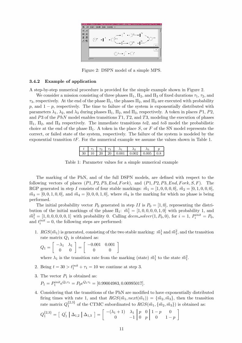
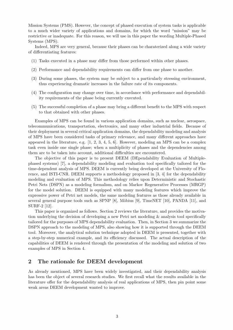
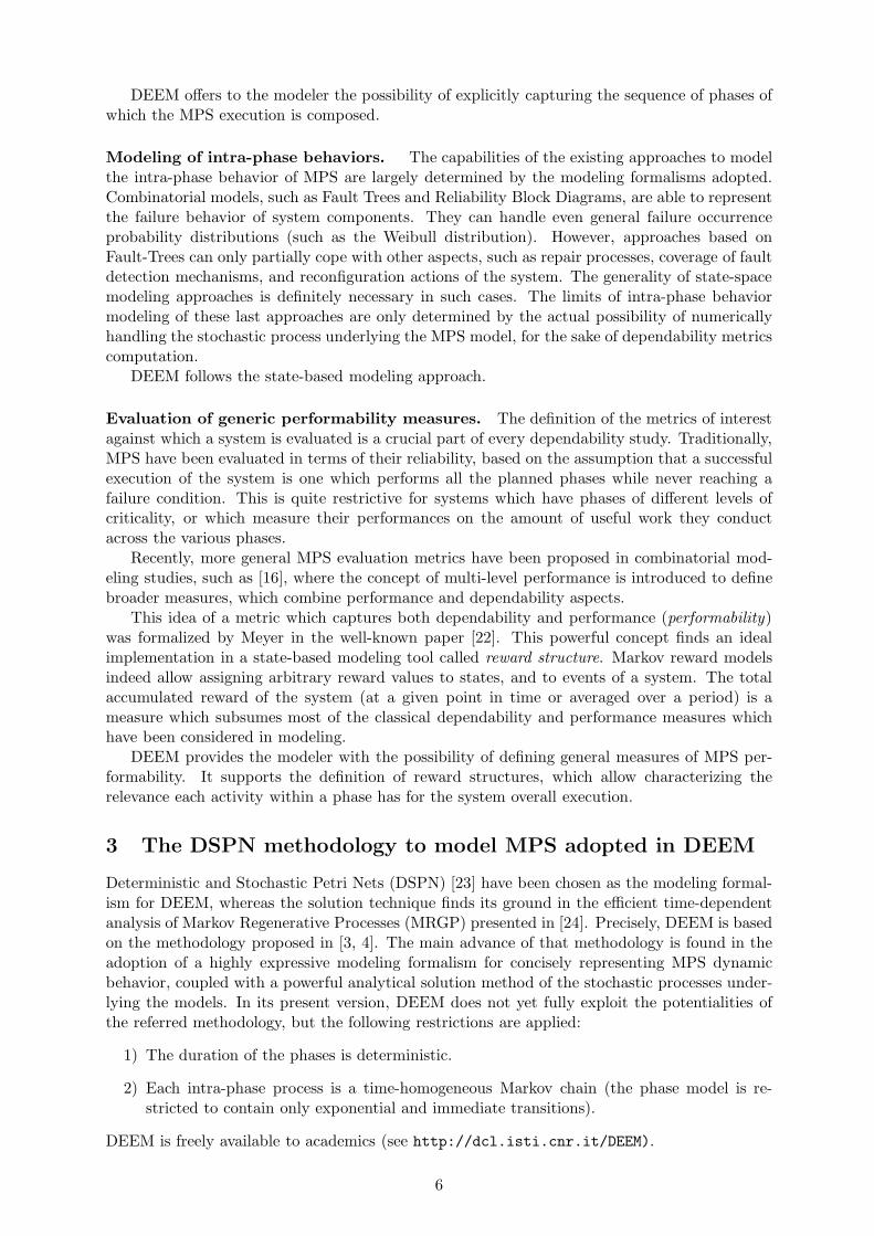
Figure 2: DSPN model of a simple MPS.

3.4.2 Example of application

A step-by-step numerical procedure is provided for the simple example shown in Figure 2.We consider a mission consisting of three phases Π1, Π2, and Π3 of fixed durations τ1, τ2, and

τ3, respectively. At the end of the phase Π1, the phases Π2, and Π3 are executed with probabilityp, and 1 − p, respectively. The time to failure of the system is exponentially distributed withparameters λ1, λ2, and λ3 during phases Π1, Π2, and Π3, respectively. A token in places P1, P2,and P3 of the PhN model enables transitions T1, T2, and T3, modeling the execution of phasesΠ1, Π2, and Π3 respectively. The immediate transitions to2, and to3 model the probabilisticchoice at the end of the phase Π1. A token in the place S, or F of the SN model represents thecorrect, or failed state of the system, respectively. The failure of the system is modeled by theexponential transition tF . For the numerical example we assume the values shown in Table 1.

t τ1 τ2 τ3 λ1 λ2 λ3 p

30 10 20 20 0.001 0.002 0.005 0.8

Table 1: Parameter values for a simple numerical example

The marking of the PhN, and of the full DSPN models, are defined with respect to thefollowing vectors of places (P1, P2, P3, End, Fork), and (P1, P2, P3, End, Fork, S, F ). TheRGP generated in step I consists of four stable markings: ~m1 = [1, 0, 0, 0, 0], ~m2 = [0, 1, 0, 0, 0],~m3 = [0, 0, 1, 0, 0], and ~m4 = [0, 0, 0, 1, 0], where ~m4 is the marking for which no phase is beingperformed.

The initial probability vector P0 generated in step II is P0 = [1, 0], representing the distri-bution of the initial markings of the phase Π1: ~m1

1 = [1, 0, 0, 0, 0, 1, 0] with probability 1, and~m2

1 = [1, 0, 0, 0, 0, 0, 1] with probability 0. Calling deem solver(1, P0, 0), for i = 1, P initi = P0,

and tiniti = 0, the following steps are performed:

1. RGS(~m1) is generated, consisting of the two stable marking: ~m11 and ~m2

1, and the transitionrate matrix Q1 is obtained as:

Q1 =

[

−λ1 λ1

0 0

]

=

[

−0.001 0.0010 0

]

where λ1 is the transition rate from the marking (state) ~m11 to the state ~m2

1.

2. Being t = 30 > tinit1 + τ1 = 10 we continue at step 3.

3. The vector P1 is obtained as:

P1 = P init1 eQ1τ1 = P0e

Q1τ1 = [0.99004983, 0.00995017].

4. Considering that the transitions of the PhN are modified to have exponentially distributedfiring times with rate 1, and that RGS(~m1, next(~m1)) = {~m2, ~m3}, then the transition

rate matrix Q{2,3}1 of the CTMC subordinated to RGS(~m1, {~m2, ~m3}) is obtained as:

Q{2,3}1 =

[

Q′

1 ∆1,2 ∆1,3

]

=

[

−(λ1 + 1) λ1 p 0 1 − p 00 −1 0 p 0 1 − p

]

11

5. For the stable markings ~m2, and ~m3, we obtain:

5.1 ∆1,2 =

[

p 00 p

]

=

[

0.8 00 0.8

]

, and

∆1,3 =

[

1 − p 00 1 − p

]

=

[

0.2 00 0.2

]

5.2 P init2 = P1∆1,2 = [0.79203987, 0.00796013], and

P init3 = P1∆1,3 = [0.19800997, 0.00199003]

5.3 Calling deem solver(2, P init2 , tinit

1 +τ1), for i = 2, P initi = P init

2 , and tiniti = tinit

1 +τ1 =10, the following steps are performed:

i. RGS(~m2) is generated, consisting of the two stable marking: ~m12 and ~m2

2, andthe transition rate matrix Q2 is obtained as:

Q2 =

[

−λ2 λ2

0 0

]

=

[

−0.002 0.0020 0

]

ii. Being t = 30 ≤ tinit2 + τ2 = 10 + 20 = 30, the vector P2(t) is obtained as:

P2(t) = P initi eQi(t−tinit

i ) = P init2 eQ2(t−τ init

2) = [0.76098354, 0.03901646].

Calling deem solver(3, P init3 , tinit

1 +τ1), for i = 3, P initi = P init

3 , and tiniti = tinit

1 +τ1 =10, following results are obtained:

i. Q3 =

[

−λ3 λ3

0 0

]

=

[

−0.005 0.0050 0

]

ii. P3(t) = P initi eQi(t−tinit

i ) = P init3 eQ3(t−τ init

3) = [0.17916683, 0.02083317].

Then, the distribution at time t of the success and failure states of the system can be derivedas P (t) = P2(t) + P3(t) = [0.94015037, 0.05984963].

3.4.3 Evaluation of the algorithm efficiency

For generating the reachability graphs at steps I, II, 1, and 4 (see Section 3.4.1), the asymp-

totic computational complexity is given by O(

(∑mmax

h=0 Cjh)2log(

∑mmax

h=0 Cjh))

, where Ci =|

Si |, j0 = i and mmax ≥ 1 is the maximum number of phases reachable directly from aphase (n − 1 in the worst case), and the asymptotical memory requirements are given by

O(

(∑mmax

h=0 Cjh)2)

. These costs, dominated by the operations at step 4, can be reduced to

O(

∑mmax

h=1 (Ci + Cjh)2log(Ci + Cjh

))

(time complexity), and O(

(Ci + Cjh)2)

(space complex-

ity) by generating the reachability graph only for the two consecutive phases i & jh, for eachphase jh reachable from the current phase i. Note that the same memory space can be reusedto store the reachability graph relative to different consecutive phases. For the transient so-lutions at steps 2 & 3, the computational complexity is O

(

C2i qiτi

)

, where qi is the maximumabsolute diagonal entry of Qi, and the memory requirements are O

(

C2i

)

. For the multiplicationoperations at steps 2, 3, and 5.2 (repeated at most mmax times), the computational complexity

is O(

C2i + Ci

∑mmax

h=1 Cjh

)

; and the memory requirements are O(

C2i + CiCjh

)

. For obtaining

the branching probability matrix at step 5.1 (repeated at most mmax times), the computational

complexity is O(

Ci

∑mmax

h=1 Cjh(Ci + Cjh

))

, and the memory requirement O(

(∑mmax

h=0 Cjh)2)

.

The overall asymptotic computational cost is dominated by the operations at steps 2 & 3,and is given by

O(∑n

i=1 C2i qiτi

)

The overall asymptotic memory requirement is dominated by the costs at step 4, and is given

by O(

(∑mmax

h=0 Cjh)2)

, but can be reduced to O(

(Ci + Cjh)2)

.

12

The complexity orders, for time and space, shown by our algorithm, are very good, beingcomparable to those of the cheapest algorithms in the literature to deal with PMS scenarios[4]. Therefore, the issues posed by the phased-behavior of PMS are completely, and efficiently,solved by our method.

4 Using DEEM to model MPS

The main features the DEEM and its GUI support are:

1) MPS model construction.

2) Definition & management of evaluation scenarios (studies), and setting of the parametervalues for multiple evaluations.

3) Definition of dependability measures of interest, through the general & flexible mechanismof marking-dependent reward functions.

4) Transient analysis to evaluate the dependability measures.

5) Saving (in a file) the state distribution of the model at the end of the transient analysis,and loading (from a file) of the initial state distribution used for the transient analysis.

6) Documentation of the MPS model, producing a LaTeX file.

Other features which the GUI of DEEM supports are those typical of many similar tools, suchas file and editing utilities, help-on-line, etc.

In this section, we illustrate the use of DEEM in the solution of two representative problemswhich have been already studied in the literature, but without the support of any automatedtool. The purpose of the re-examination here is to show the usage of DEEM in interestingcase studies, to better illustrate the advantages the tool offers. The first problem, studied in[4], consists in the modeling and evaluation of a Phased Mission System for space applications.The other, previously dealt with in [1], consists in the optimization of a Scheduled MaintenanceSystem from dependability and cost viewpoints. With respect to PMS, SMS add a furtherdegree of complexity in that the long lifetime of a SMS can be partitioned into a set of missions,each of them composed by several phases.

4.1 The case of a Phased Mission System

Consider a space application whose mission alternates operational phases (as launch, scientificobservations) with hibernation phases (typically entered to maintain a low level of activityduring the navigation). To ensure adequate dependability levels, the system employs N identicalprocessors. The main characteristics of such PMS are the following.

Phase-Triggered Reconfigurations of the SN. The system uses in each phase the numberof processors needed to meet the dependability requirements of the current phase, andkeeps the others as cold spares. Specifically, hibernation phases employ two active pro-cessors, being also able to survive with just one active processor, while operational phasesalways require three active processors. At the start of each hibernation phase, a reconfig-uration takes place, and one of the active processors is turned off. Similarly, when a newoperational phase starts, one spare must be turned on. A standby processor is fault-free;however, a failure may occur when activating a cold spare with probability 1−ca (ca beingthe coverage of the activation procedure).

Phase-Dependent Behavior of the SN. Active processors fail with phase-dependent rates:the failure rate during hibernation phases is lower than the failure rate during operationalphases. Repair actions are applied to faulty components. We assume that active proces-sors fail and are repaired independently from each other. As already discussed, differentsuccess/failure criteria are specified for each phase.

13

Mission Profile Dependent on SN Marking. The choice of the next phase to execute maybe dictated by how the preceding phase ends. Such a dynamic choice of the mission profilemay be useful to skip phases which would endanger the execution of more importantactivities.

4.1.1 The DEEM model

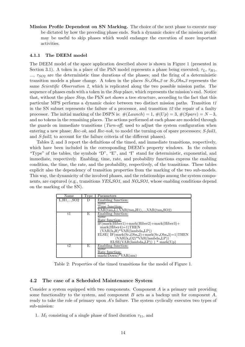
The DEEM model of the space application described above is shown in Figure 1 (presented inSection 3.1). A token in a place of the PhN model represents a phase being executed; τL, τH1,..., τSO2 are the deterministic time durations of the phases; and the firing of a deterministictransition models a phase change. A token in the places Sc Obs 2 or Sc Obs 3 represents thesame Scientific Observation 2, which is replicated along the two possible mission paths. Thesequence of phases ends with a token in the Stop place, which represents the mission’s end. Noticethat, without the place Stop, the PhN net shows a tree structure, according to the fact that thisparticular MPS performs a dynamic choice between two distinct mission paths. Transition t1in the SN subnet represents the failure of a processor, and transition t2 the repair of a faultyprocessor. The initial marking of the DSPN is: #(Launch) = 1, #(Up) = 3, #(Spare) = N −3,and no tokens in the remaining places. The actions performed at each phase are modeled throughthe guards on immediate transitions (Turn-off, used to adjust the system configuration whenentering a new phase; Rec-ok, and Rec-nok, to model the turning-on of spare processors; S-fail1,and S-fail2, to account for the failure criteria of the different phases).

Tables 2, and 3 report the definitions of the timed, and immediate transitions, respectively,which have been included in the corresponding DEEM’s property windows. In the column“Type” of the tables, the symbols “D”, “E”, and “I” stand for deterministic, exponential, andimmediate, respectively. Enabling, time, rate, and probability functions express the enablingcondition, the time, the rate, and the probability, respectively, of the transitions. These tablesexplicit also the dependency of transition properties from the marking of the two sub-models.This way, the dynamicity of the involved phases, and the relationships among the system compo-nents, are captured (e.g., transitions YES SO1, and NO SO1, whose enabling conditions dependon the marking of the SN).

Name Type ParametersL,H1,...,SO2 D Enabling function:

none

Time function:VAR(tau L),VAR(tau H1),...,VAR(tau SO2)

t1 E Enabling function:none

Rate function:IF(mark(Hiber1)+mark(Hiber2)+mark(Hiber3)+mark(Hiber4)=1)THEN(VAR(k H)*VAR(lambda LP))

ELSE( IF(mark(Sc Obs 2)+mark(Sc Obs 3)=1)THEN(VAR(k O2)*VAR(lambda LP))

ELSE(VAR(lambda LP)) ) * mark(Up)t2 E Enabling function:

none

Rate function:mark(Down)*VAR(mu)

Table 2: Properties of the timed transitions for the model of Figure 1.

4.2 The case of a Scheduled Maintenance System

Consider a system equipped with two components. Component A is a primary unit providingsome functionality to the system, and component B acts as a backup unit for component A,ready to take the role of primary upon A’s failure. The system cyclically executes two types ofsub-mission:

1. M1 consisting of a single phase of fixed duration τ11, and

14

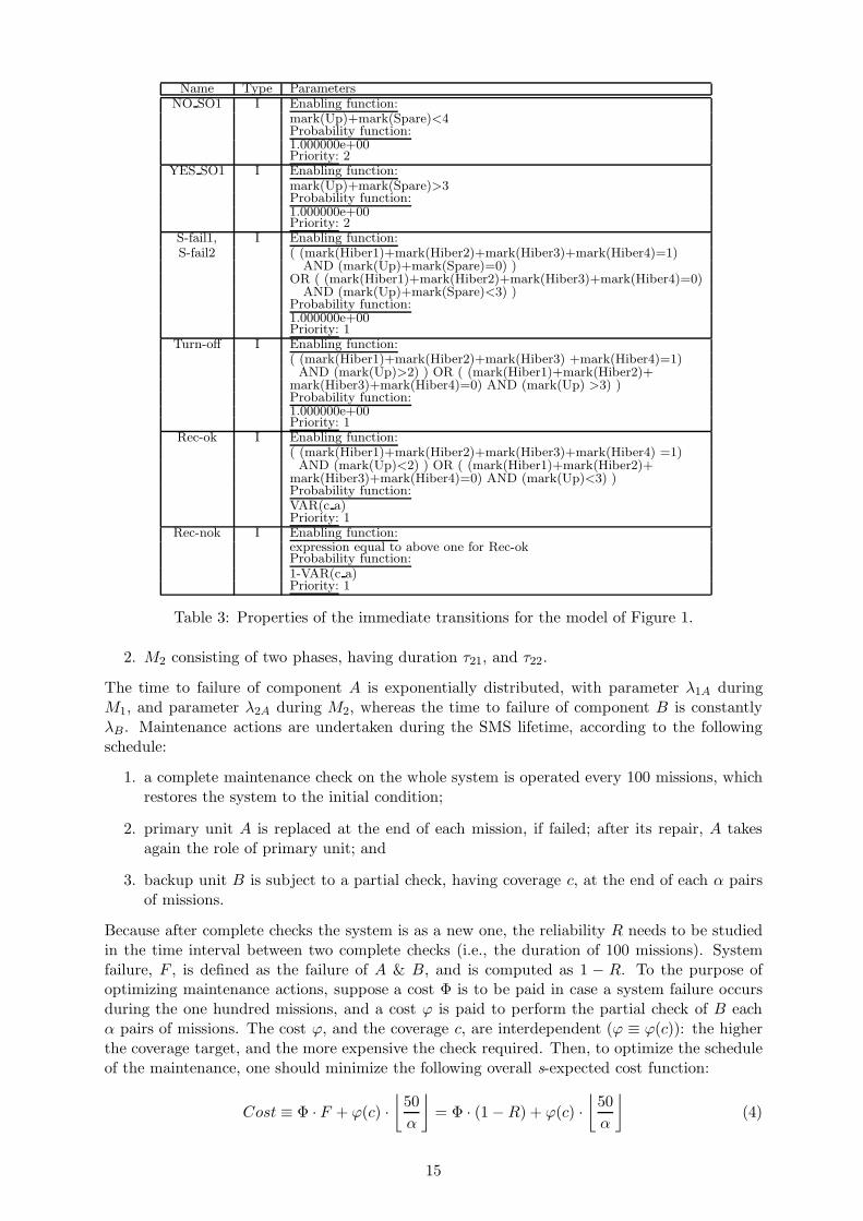
Name Type ParametersNO SO1 I Enabling function:

mark(Up)+mark(Spare)<4Probability function:1.000000e+00Priority: 2

YES SO1 I Enabling function:mark(Up)+mark(Spare)>3Probability function:1.000000e+00Priority: 2

S-fail1, I Enabling function:S-fail2 ( (mark(Hiber1)+mark(Hiber2)+mark(Hiber3)+mark(Hiber4)=1)

AND (mark(Up)+mark(Spare)=0) )OR ( (mark(Hiber1)+mark(Hiber2)+mark(Hiber3)+mark(Hiber4)=0)

AND (mark(Up)+mark(Spare)<3) )Probability function:1.000000e+00Priority: 1

Turn-off I Enabling function:( (mark(Hiber1)+mark(Hiber2)+mark(Hiber3) +mark(Hiber4)=1)AND (mark(Up)>2) ) OR ( (mark(Hiber1)+mark(Hiber2)+

mark(Hiber3)+mark(Hiber4)=0) AND (mark(Up) >3) )Probability function:1.000000e+00Priority: 1

Rec-ok I Enabling function:( (mark(Hiber1)+mark(Hiber2)+mark(Hiber3)+mark(Hiber4) =1)AND (mark(Up)<2) ) OR ( (mark(Hiber1)+mark(Hiber2)+

mark(Hiber3)+mark(Hiber4)=0) AND (mark(Up)<3) )Probability function:VAR(c a)Priority: 1

Rec-nok I Enabling function:expression equal to above one for Rec-okProbability function:1-VAR(c a)Priority: 1

Table 3: Properties of the immediate transitions for the model of Figure 1.

2. M2 consisting of two phases, having duration τ21, and τ22.

The time to failure of component A is exponentially distributed, with parameter λ1A duringM1, and parameter λ2A during M2, whereas the time to failure of component B is constantlyλB . Maintenance actions are undertaken during the SMS lifetime, according to the followingschedule:

1. a complete maintenance check on the whole system is operated every 100 missions, whichrestores the system to the initial condition;

2. primary unit A is replaced at the end of each mission, if failed; after its repair, A takesagain the role of primary unit; and

3. backup unit B is subject to a partial check, having coverage c, at the end of each α pairsof missions.

Because after complete checks the system is as a new one, the reliability R needs to be studiedin the time interval between two complete checks (i.e., the duration of 100 missions). Systemfailure, F , is defined as the failure of A & B, and is computed as 1 − R. To the purpose ofoptimizing maintenance actions, suppose a cost Φ is to be paid in case a system failure occursduring the one hundred missions, and a cost ϕ is paid to perform the partial check of B eachα pairs of missions. The cost ϕ, and the coverage c, are interdependent (ϕ ≡ ϕ(c)): the higherthe coverage target, and the more expensive the check required. Then, to optimize the scheduleof the maintenance, one should minimize the following overall s-expected cost function:

Cost ≡ Φ · F + ϕ(c) ·

⌊

50

α

⌋

= Φ · (1 − R) + ϕ(c) ·

⌊

50

α

⌋

(4)

15

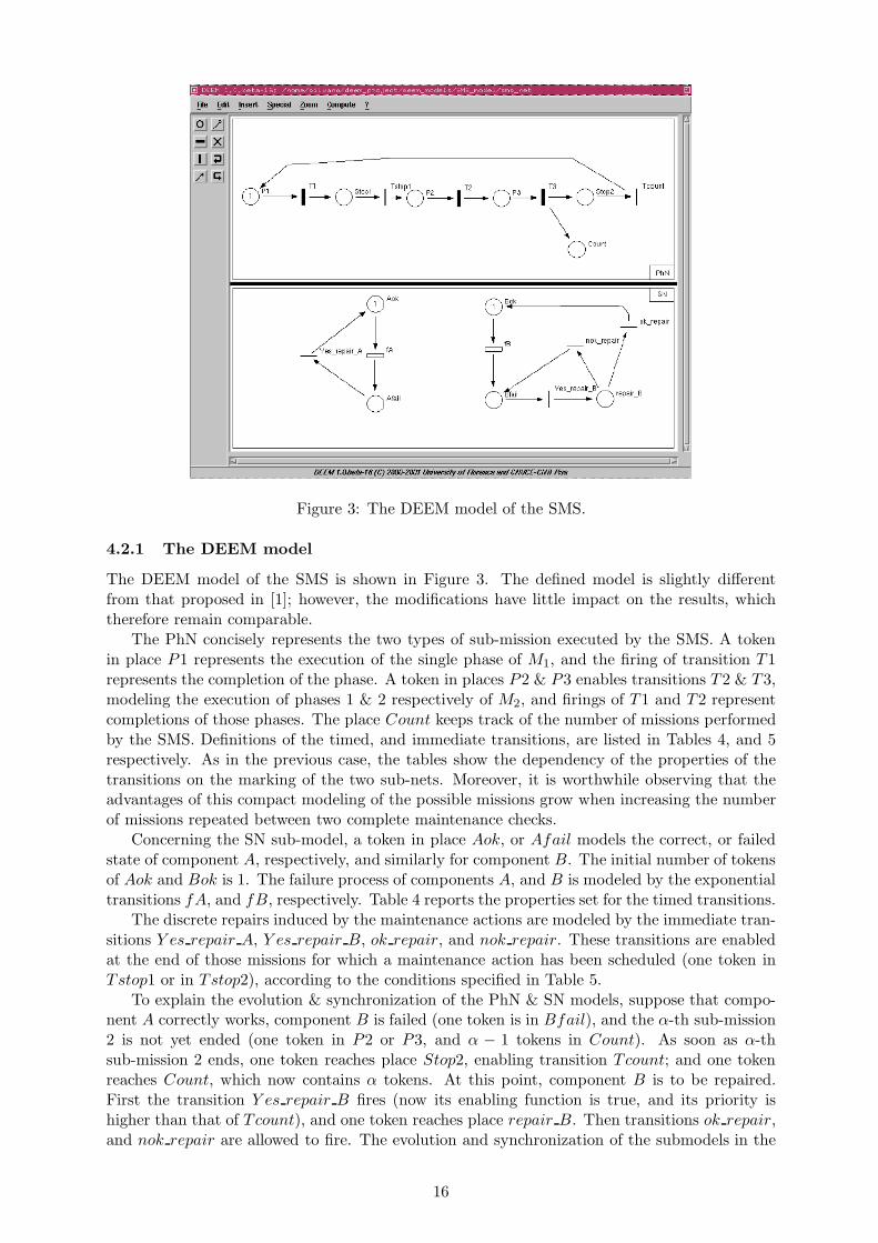
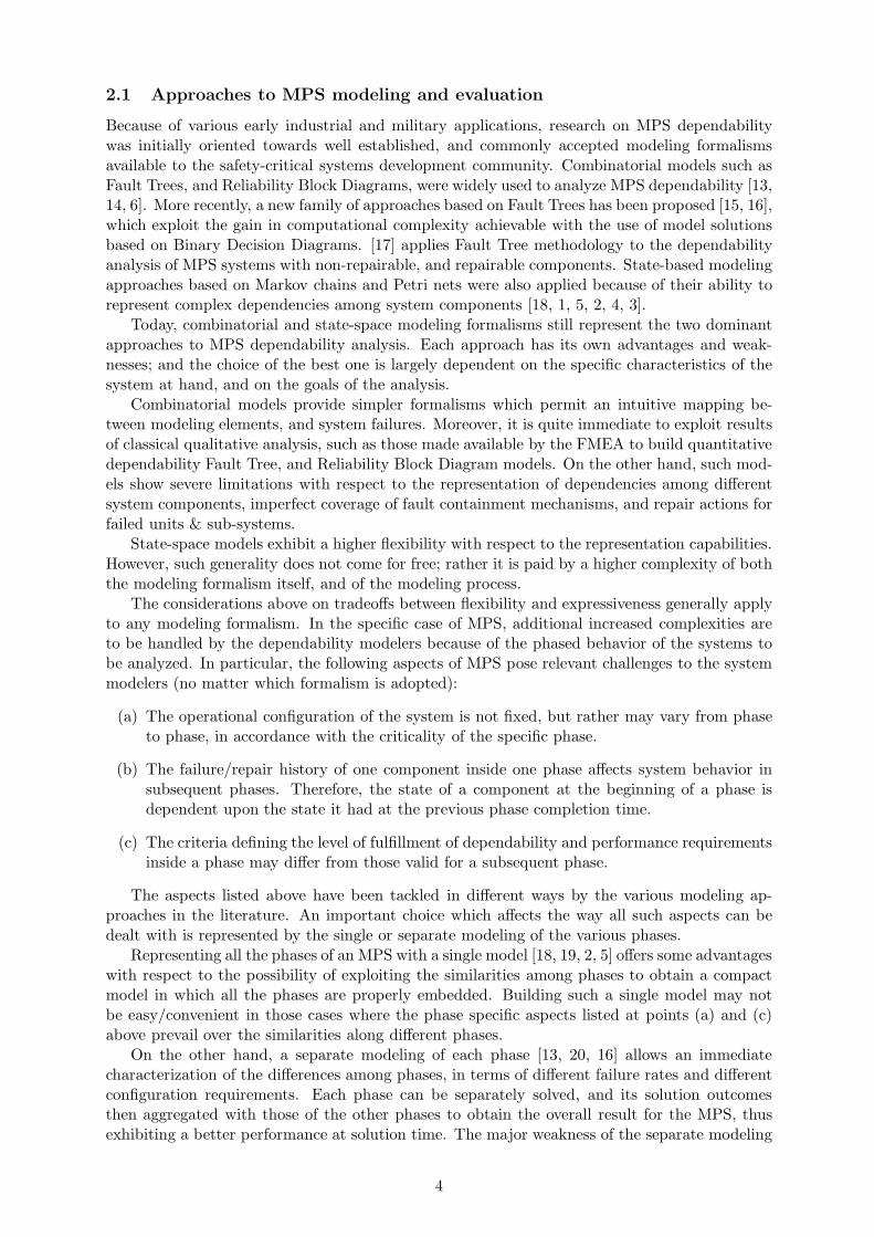
Figure 3: The DEEM model of the SMS.

4.2.1 The DEEM model

The DEEM model of the SMS is shown in Figure 3. The defined model is slightly differentfrom that proposed in [1]; however, the modifications have little impact on the results, whichtherefore remain comparable.

The PhN concisely represents the two types of sub-mission executed by the SMS. A tokenin place P1 represents the execution of the single phase of M1, and the firing of transition T1represents the completion of the phase. A token in places P2 & P3 enables transitions T2 & T3,modeling the execution of phases 1 & 2 respectively of M2, and firings of T1 and T2 representcompletions of those phases. The place Count keeps track of the number of missions performedby the SMS. Definitions of the timed, and immediate transitions, are listed in Tables 4, and 5respectively. As in the previous case, the tables show the dependency of the properties of thetransitions on the marking of the two sub-nets. Moreover, it is worthwhile observing that theadvantages of this compact modeling of the possible missions grow when increasing the numberof missions repeated between two complete maintenance checks.

Concerning the SN sub-model, a token in place Aok, or Afail models the correct, or failedstate of component A, respectively, and similarly for component B. The initial number of tokensof Aok and Bok is 1. The failure process of components A, and B is modeled by the exponentialtransitions fA, and fB, respectively. Table 4 reports the properties set for the timed transitions.

The discrete repairs induced by the maintenance actions are modeled by the immediate tran-sitions Y es repair A, Y es repair B, ok repair, and nok repair. These transitions are enabledat the end of those missions for which a maintenance action has been scheduled (one token inTstop1 or in Tstop2), according to the conditions specified in Table 5.

To explain the evolution & synchronization of the PhN & SN models, suppose that compo-nent A correctly works, component B is failed (one token is in Bfail), and the α-th sub-mission2 is not yet ended (one token in P2 or P3, and α − 1 tokens in Count). As soon as α-thsub-mission 2 ends, one token reaches place Stop2, enabling transition Tcount; and one tokenreaches Count, which now contains α tokens. At this point, component B is to be repaired.First the transition Y es repair B fires (now its enabling function is true, and its priority ishigher than that of Tcount), and one token reaches place repair B. Then transitions ok repair,and nok repair are allowed to fire. The evolution and synchronization of the submodels in the

16

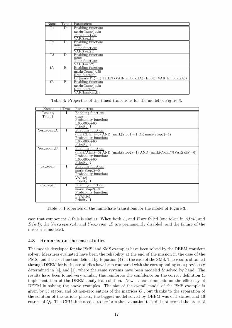
Name Type ParametersT1 D Enabling function:

mark(Count)<50Time function:VAR(tau 11)

T2 D Enabling function:none

Time function:VAR(tau 21)

T3 D Enabling function:none

Time function:VAR(tau 22)

fA E Enabling function:mark(Count)<50Rate function:IF (mark(P1)=1) THEN (VAR(lambda 1A)) ELSE (VAR(lambda 2A))

fB E Enabling function:mark(Count)<50Rate function:VAR(lambda B)

Table 4: Properties of the timed transitions for the model of Figure 3.

Name Type ParametersTcount, I Enabling function:Tstop1 none

Probability function:1.000000e+00Priority: 1

Yes repair A I Enabling function:(mark(Bfail)=0) AND (mark(Stop1)=1 OR mark(Stop2)=1)Probability function:1.000000e+00Priority: 2

Yes repair B I Enabling function:(mark(Afail)=0) AND (mark(Stop2)=1) AND (mark(Count)%VAR(alfa)=0)Probability function:1.000000e+00Priority: 2

ok repair I Enabling function:mark(Stop2)=0Probability function:VAR(c)Priority: 1

nok repair I Enabling function:mark(Stop2)=0Probability function:1-VAR(c)Priority: 1

Table 5: Properties of the immediate transitions for the model of Figure 3.

case that component A fails is similar. When both A, and B are failed (one token in Afail, andBfail), the Y es repair A, and Y es repair B are permanently disabled; and the failure of themission is modeled.

4.3 Remarks on the case studies

The models developed for the PMS, and SMS examples have been solved by the DEEM transientsolver. Measures evaluated have been the reliability at the end of the mission in the case of thePMS, and the cost function defined by Equation (4) in the case of the SMS. The results obtainedthrough DEEM for both case studies have been compared with the corresponding ones previouslydetermined in [4], and [1], where the same systems have been modeled & solved by hand. Theresults have been found very similar; this reinforces the confidence on the correct definition &implementation of the DEEM analytical solution. Now, a few comments on the efficiency ofDEEM in solving the above examples. The size of the overall model of the PMS example isgiven by 35 states, and 60 non-zero entries of the matrices Qi, but thanks to the separation ofthe solution of the various phases, the biggest model solved by DEEM was of 5 states, and 10entries of Qi. The CPU time needed to perform the evaluation task did not exceed the order of

17

a few seconds, and the total amount of physical memory used did not exceed 2100 Kilobytes, ona Pentium II 350 MHz, 192Mb RAM PC. In the SMS case, the overall model size is given by 600states, and 600 non-zero entries of the matrices Qi; but again, thanks to the separation of thesolution of the various phases operated by DEEM, the biggest model solved was of 4 states, and4 entries of Qi. The CPU time needed to perform the evaluation of the study was 100 seconds,and the total amount of physical memory used did not exceed 2100 Kilobytes, on a Pentium II350 MHz, 192Mb RAM PC. From these data, the efficiency of the DEEM’s solution algorithm,with respect to non specialized solutions, can be appreciated.

The DSPN models developed for the considered examples could be solved using differentapproaches, algorithms, and tools, e.g. [24, 10, 29]. A general-purpose transient solver forDSPN, such as TimeNET, can be used for this purpose [10]. TimeNET provides many of themodeling features available under the Stochastic Reward Network paradigm, and is able tosupport our modeling methodology. Actually, this tool implements three different transientsolution techniques: a general solution, and two variants which optimize on time & memoryconsumption, but are restricted to specific DSPN structures. Only PMS models in which asequence of deterministic transitions fire at previously known instants of time are solvable byTimeNET, with a method having the same computational complexity & memory requirementsas DEEM. Instead, the PMS models of our examples belong to the class for which TimeNETneeds to apply the general transient solution algorithm. The asymptotic computational cost ishigher than that of DEEM, being O

(∑n

i=1 C2i qiτij

imax

)

, where jimax denotes the number of steps

required for the discretization of the cumulative distribution function of the firing time of thenon-exponential transitions.

Of course, DEEM’s benefits grow with the growing dimension of the analyzed problem, forwhich the usage of a general-purpose evaluation tool may be easily defeated by the well-knownproblem of state explosion. Among the others, a problem we have dealt with, and where theefficiency of DEEM has been fundamental in allowing the target evaluation activities, has beenthat of the Reactor Protection System in use at Westinghouse nuclear plants [30]. For this verycritical system, we have modeled and analyzed scheduled maintenance actions, which have tobe executed on-line without service interruption. The entire model contains on the order of onemillion states. However, the biggest model solved by DEEM was of 4096 states, and the time toperform a single study did not exceed, on average, the order of few tens of minutes on a PentiumIII 500 MHz, 128 Mb RAM PC.

References

[1] A. Bondavalli, I. Mura, and K. S. Trivedi, “Dependability modelling and sensitivity analysisof scheduled maintenance systems,” in EDCC-3 European Dependable Computing Confer-ence. Prague, Czech Republic: (Also Lecture Notes in Computer Science N. 1667), SpringerVerlag, September 1999, pp. 7–23.

[2] J. B. Dugan, “Automated analysis of phased-mission reliability,” IEEE Transactions onReliability, vol. 40, no. 1, pp. 45–52, 1991.

[3] I. Mura and A. Bondavalli, “Markov regenerative stochastic Petri nets to model and evaluatephased mission systems dependability,” IEEE Transactions on Computers, vol. 50, no. 12,pp. 1337–1351, 2001.

[4] I. Mura, A. Bondavalli, X. Zang, and K. S. Trivedi, “Dependability modelling and evaluationof phased mission systems: a DSPN approach,” in IEEE DCCA-7 - 7th IFIP Int. Conferenceon Dependable Computing for Critical Applications, San Jose, CA, USA, 1999, pp. 299–318.

[5] M. Smotherman and K. Zemoudeh, “A non-homogeneous Markov model for phased-missionreliability analysis,” IEEE Transactions on Reliability, vol. 38, no. 5, pp. 585–590, 1989.

18

[6] A. K. Somani, J. A. Ritcey, and S. H. L. Au, “Computationally-efficent phased-mission reli-ability analysis for systems with variable configurations,” IEEE Transactions on Reliability,vol. 41, no. 4, pp. 504–511, 1992.

[7] A. Bondavalli, I. Mura, S. Chiaradonna, R. Filippini, S. Poli, and F. Sandrini, “DEEM: atool for the dependability modeling and evaluation of multiple phased systems,” in DSN2000IEEE Int. Conference on Dependable Systems and Networks (FTCS-30 and DCCA-8), NewYork, USA, 2000, pp. 23–236.

[8] G. Ciardo, J. Muppala, and K. S. Trivedi, “SPNP: Stochastic Petri net package,” in ThirdIEEE International Workshop On Petri Nets and Performance Models (PNPM89), Kyoto,Japan, 1989, pp. 142–151.

[9] G. Clark, T. Courtney, D. Daly, D. Deavours, S. Derisavi, J. M. Doyle, W. H. Sanders, andP. G. Webster, “The Mobius modeling tool,” in 9th IEEE Int. Workshop on Petri Nets andPerformance Models, Aachen, Germany, September 2001, pp. 241–250.

[10] A. Zimmermann, J. Freiheit, R. German, and G. Hommel, “Petri net modelling and per-formability evaluation with TimeNET 3.0,” in 11th Int. Conf. on Modelling Techniques andTools for Computer Performance Evaluation (TOOLS’2000), LNCS 1786. Schaumburg,Illinois, USA: Springer-Verlag, 2000, pp. 188–202.

[11] S. Allmaier and S. Dalibor, “PANDA - Petri net analysis and design assistant,” inTOOLS’97, 9th Int. Conference on Modelling Techniques and Tools for Computer Per-formance Evaluation, Saint Malo, France, 1997.

[12] C. Beounes, M. Aguera, J. Arlat, C. Bourdeau, J.-E. Doucet, K. Kanoun, J.-C. Laprie,S. Metge, J. Moreira de Souza, D. Powell, and P. Spiesser, “SURF-2: a program fordependability evaluation of complex hardware and software systems,” in 23th IEEE Int.Fault-Tolerant Computing Symposium (FTCS-23), Toulouse, France, 1993, pp. 668–673.

[13] J. D. Esary and H. Ziehms, “Reliability analysis of phased missions,” in Reliability andFault Tree Analysis. SIAM Philadelphia, 1975, pp. 213–236.

[14] A. Pedar and V. V. S. Sarma, “Phased mission analysis for evaluating the effectivenessof aerospace computing systems,” IEEE Transactions on Reliability, vol. 30, no. 5, pp.429–437, 1981.

[15] X. Zang, H. Sun, and K. S. Trivedi, “A BDD-based algorithm for reliability evaluation ofphased mission systems,” IEEE Transactions on Reliability, vol. 48, no. 1, pp. 50–60, 1999.

[16] L. Xing and J. B. Dugan, “Analysis of generalized phased mission system reliability, per-formance and sensitivity,” IEEE Transactions on Reliability, vol. 51, no. 2, pp. 199–211,June 2002.

[17] J. K. Vaurio, “Fault tree analysis of phased mission systems with repairable and non-repairable components,” Reliability Engineering and Systems Safety, Elsevier, vol. 74, no. 2,pp. 169–180, 2001.

[18] M. Alam and U. M. Al-Saggaf, “Quantitative reliability evaluation of reparaible phased-mission systems using Markov approach,” IEEE Transactions on Reliability, vol. R-35,no. 5, pp. 498–503, 1986.

[19] B. E. Aupperle, J. F. Meyer, and L. Wei, “Evaluation of fault-tolerant systems with non-homogeneous workloads,” in 19th IEEE Int. Fault Tolerant Computing Symposium (FTCS-19), 1989, pp. 159–166.

19

[20] J. F. Meyer, D. G. Furchgott, and L. T. Wu, “Performability evaluation of the SIFTcomputer,” in 9th IEEE Int. Fault-Tolerant Computing Symposium (FTCS-9), Madison,Wisconsin, USA, June 1979, pp. 43–50.

[21] I. Mura and A. Bondavalli, “Hierarchical modelling and evaluation of phased-mission sys-tems,” IEEE Transactions on Reliability, vol. 48, no. 4, pp. 360–368, 1999.

[22] J. F. Meyer, “On evaluating the performability of degradable computing systems,” IEEETransactions on Computers, vol. 29, no. 8, pp. 720–731, 1980.

[23] M. Ajmone Marsan and G. Chiola, “On Petri nets with deterministic and exponentiallydistributed firing times,” in Lecture Notes in Computer Science 266. Springer-Verlag,1987, pp. 132–145.

[24] H. Choi, V. G. Kulkarni, and K. S. Trivedi, “Transient analysis of deterministic and stochas-tic Petri nets,” in 14th International Conference on Application and Theory of Petri Nets,Chicago Illinois, USA, 1993, pp. 166–185.

[25] G. Ciardo, J. Muppala, and K. S. Trivedi, “On the solution of GSPN reward models,”Performance Evaluation, vol. 12, pp. 237–254, 1991.

[26] G. Chiola, “Compiling techniques for the analysis of stochastic Petri nets,” in Fourth Inter-national Conference on Modeling Techniques and Tools for Computer Performance Evalu-ation, Palma de Mallorca, Spain, 1988, pp. 11–24.

[27] A. Reibman and K. S. Trivedi, “Numerical transient analysis of Markov models,” Computersand Operations Research, vol. 15, no. 1, pp. 9–36, 1988.

[28] S. C. Allmaier, M. Kowarschik, and G. Horton, “State space construction and steady-statesolution of GSPNs on a shared-memory multiprocessor,” in Seventh IEEE InternationalWorkshop on Petri Nets and Performance Models, Saint Malo, France, 1997, pp. 112–121.

[29] C. Lindemann and A. Thummler, “Transient analysis of deterministic and stochastic Petrinets with concurrent deterministic transitions,” Performance Evaluation, vol. 36–37, no.1–4, pp. 35–54, 1999.

[30] R. Filippini and A. Bondavalli, “Modeling and analysis of a scheduled maintenance system:a DSPN approach,” The Computer Journal, BCS, vol. 47, no. 6, 2004, to appear.

Andrea Bondavalli. Prof. Andrea Bondavalli, DSI, Universita di Firenze, Via Lombroso 6/17,50134 Firenze, Italy, email: a.bondavalli@dsi.unifi.it

Andrea Bondavalli is a Professor in Computer Science at the University of Firenze. Previ-ously he was a researcher of the Italian National Research Council, working at the CNUCEInstitute in Pisa. His research activity is focused on Dependability. In particular he hasbeen working on the design of real-time, fault tolerant systems and their mechanisms andon the quantitative evaluation of dependability attributes such as reliability, availabilityand performability. Andrea Bondavalli participated to several Projects funded by the Eu-ropean Community including PDCS, PDCS-2, HIDE, GUARDS and Caution++. He hasauthored or co-authored more than 100 papers appeared in International Journals andproceedings of International Conferences. He served as reviewer for many Conferencesand Journals and as pc member in several International Conferences. He also served asprogram co-chair of IEEE SRDS-19, IEEE HASE-2001, EDCC-4, IEEE ISADS-2003; asGeneral Chair of IEEE SRDS-22 and vice general Chair for IEEE DSN 2004, and as co-guest editor of a special issue of IEEE Trans. on Computers on “Reliable DistributedSystems”. Currently he is serving as Program Chair of the DCCS Track at DSN 2005.Andrea Bondavalli is a member of the IEEE, the IFIP W.G. 10.4 Working Group on “De-pendable Computing and Fault-Tolerance”, ENCRESS Club Italy and the AICA WorkingGroup on “Dependability in Computer Systems”.

20

Silvano Chiaradonna. Dr. Silvano Chiaradonna, ISTI-CNR, Via G. Moruzzi 1, 56124 Pisa,Italy, email: s.chiaradonna@isti.cnr.it

Silvano Chiaradonna graduated in Computer Science at the University of Pisa in 1992,working on a thesis in cooperation with CNUCE-CNR. Since 1992 he has been workingon dependable computing and participated in European ESPRIT BRA PDCS2 and ES-PRIT 20718 GUARDS projects. S. Chiaradonna was a fellow student at IEI-CNR andhas also been serving as a reviewer for International Conferences. His current researchinterests include the design of dependable computing systems, software and system faulttolerance and the modeling and evaluation of dependability attributes like reliability andperformability.

Felicita Di Giandomenico. Dr. Felicita Di Giandomenico, ISTI-CNR, Via G. Moruzzi 1,56124 Pisa, Italy, email: f.digiandomenico@isti.cnr.it

Felicita Di Giandomenico graduated in Computer Science at the University of Pisa, in1986. Since February 1989, she is a researcher at the Institute ISTI of the Italian NationalResearch Council, where she is currently leading the Dependable Computing research lab-oratory. During these years, she has been involved in numerous European and nationalprojects in the area of dependable computing systems. She has spent nine months (fromAugust 1991 to April 1992) visiting the Computing Laboratory of the University of New-castle upon Tyne (UK) as Guest Member of Staff. Felicita Di Giandomenico has served asa Program Committee Member for several international conferences, and as a reviewer forConferences and Journals. Her current research activities include the design of dependablereal-time computing systems, software implemented fault tolerance and the modeling andevaluation of dependability attributes, mainly reliability, availability and performability.Felicita Di Giandomenico is a member of the IEEE computer Society.

Ivan Mura. Dr. Ivan Mura, Motorola Electronics SpA, Global Software Group Italy, Via C.Massaia 83, 10147, Torino, Italy, email: Ivan.Mura@motorola.com

Dr. Ivan Mura received a Laurea degree in Computer Science and a Ph.D. in ComputerScience Engineering from the University of Pisa, Italy, in 1994 and 1999, respectively.His research interests include the modeling of processing and telecommunications systemsfor performance, dependability, and performability evaluation. During 1995 he was afellowship holder at the IEI, an institute of the Italian National Research Council, carryingon a research on performability optimization in fault-tolerant real-time systems. In 1998,as a partial fulfillment of his Ph.D. course requirements, he was a visiting student at DukeUniversity, NC, under the supervision of Prof. Kishor Trivedi. In 1999 he was appointedthe position of researcher at the CNUCE institute of the Italian National Research Council.That same year, he joined the Motorola Global Software Group in Torino, Italy, where heholds a Project Lead position in the Modeling and Simulation technical area.

21