WIRELESS POWER TRANSFER: EFFICIENCY, FAR FIELD,DIRECTIVITY, AND PHASED ARRAY ANTENNAS

by

Abigail Jubilee Kragt Finnell

A Thesis

Submitted to the Faculty of Purdue University

In Partial Fulfillment of the Requirements for the degree of

Master of Science

Department of Electrical and Computer Engineering

Indianapolis, Indiana

August 2021

THE PURDUE UNIVERSITY GRADUATE SCHOOLSTATEMENT OF COMMITTEE APPROVAL

Dr. Peter Schubert, Chair

Department of Electrical and Computer Engineering

Dr. Maher Rizkalla

Department of Electrical and Computer Engineering

Dr. Lauren Christopher

Department of Electrical and Computer Engineering

Approved by:

Dr. Brian King

2

TABLE OF CONTENTS

LIST OF TABLES . . . . . . . . . . . . . . . . . . . . . . . . . . . . . . . . . . . . . 5

LIST OF FIGURES . . . . . . . . . . . . . . . . . . . . . . . . . . . . . . . . . . . . 6

ABSTRACT . . . . . . . . . . . . . . . . . . . . . . . . . . . . . . . . . . . . . . . . 7

1 INTRODUCTION . . . . . . . . . . . . . . . . . . . . . . . . . . . . . . . . . . . 8

2 FUNDAMENTALS . . . . . . . . . . . . . . . . . . . . . . . . . . . . . . . . . . . 10

2.1 Propagation of Signals and Power . . . . . . . . . . . . . . . . . . . . . . . . 10

2.1.1 The Friis Equation . . . . . . . . . . . . . . . . . . . . . . . . . . . . 11

2.1.2 The Goubau Equation . . . . . . . . . . . . . . . . . . . . . . . . . . 11

2.1.3 The Far Field Equation . . . . . . . . . . . . . . . . . . . . . . . . . 12

2.2 Wireless Power Beaming . . . . . . . . . . . . . . . . . . . . . . . . . . . . . 14

2.3 Gain and Directivity . . . . . . . . . . . . . . . . . . . . . . . . . . . . . . . 15

2.3.1 Example: Transmit Antenna Trade-off Study . . . . . . . . . . . . . 17

2.4 Sidelobe Levels . . . . . . . . . . . . . . . . . . . . . . . . . . . . . . . . . . 18

2.5 Non-Traditional Phased Array Antenna Architecture . . . . . . . . . . . . . 21

2.6 Other Components of Wireless Power Transfer . . . . . . . . . . . . . . . . . 22

3 FAR FIELD DISTANCE STUDY . . . . . . . . . . . . . . . . . . . . . . . . . . . 25

3.1 Far Field Model . . . . . . . . . . . . . . . . . . . . . . . . . . . . . . . . . . 26

3.2 MATLAB Model . . . . . . . . . . . . . . . . . . . . . . . . . . . . . . . . . 27

3.3 Laboratory Work at IUPUI . . . . . . . . . . . . . . . . . . . . . . . . . . . 33

4 FREE SPACE TRANSMISSION EFFICIENCY STUDY . . . . . . . . . . . . . . 40

4.1 Efficiency Equations . . . . . . . . . . . . . . . . . . . . . . . . . . . . . . . 41

Assuming a Constant D(φ) . . . . . . . . . . . . . . . . . . . . . . . 42

Assuming D(φ) is Parabolic on a Logarithmic Scale . . . . . . . . . . 43

Using Numeric Integration . . . . . . . . . . . . . . . . . . . . . . . . 44

4.2 Analysis of a Uniform PAA . . . . . . . . . . . . . . . . . . . . . . . . . . . 45

4.3 Past WPT Experiments . . . . . . . . . . . . . . . . . . . . . . . . . . . . . 47

4.3.1 The Microwave Powered Helicopter . . . . . . . . . . . . . . . . . . . 47

4.3.2 The JPL Experiment . . . . . . . . . . . . . . . . . . . . . . . . . . . 49

3

4.3.3 The Goldstone Experiment . . . . . . . . . . . . . . . . . . . . . . . 50

4.3.4 Equation Comparison . . . . . . . . . . . . . . . . . . . . . . . . . . 51

5 DISCUSSIONS AND ANALYSIS . . . . . . . . . . . . . . . . . . . . . . . . . . . 53

6 CONCLUSIONS AND FUTURE WORK . . . . . . . . . . . . . . . . . . . . . . . 55

6.1 Future Work . . . . . . . . . . . . . . . . . . . . . . . . . . . . . . . . . . . 57

REFERENCES . . . . . . . . . . . . . . . . . . . . . . . . . . . . . . . . . . . . . . . 59

A MATLAB Code . . . . . . . . . . . . . . . . . . . . . . . . . . . . . . . . . . . . . 62

B Laboratory Data . . . . . . . . . . . . . . . . . . . . . . . . . . . . . . . . . . . . 73

4

LIST OF TABLES

B.1 Lab Data: 1.45 m Distance . . . . . . . . . . . . . . . . . . . . . . . . . . . . . 73

B.2 Lab Data: 1.2 m Distance . . . . . . . . . . . . . . . . . . . . . . . . . . . . . . 77

B.3 Lab Data: 0.84 m Distance . . . . . . . . . . . . . . . . . . . . . . . . . . . . . 81

5

LIST OF FIGURES

2.1 Transmit Antenna Costs [ 14 ] . . . . . . . . . . . . . . . . . . . . . . . . . . . 18

2.2 Grating Lobes for 1.5 λ Spacing, Zero Element Phase Shift . . . . . . . . . . 20

2.3 Linear Phased Array Antenna, θ = π/4 . . . . . . . . . . . . . . . . . . . . . 23

3.1 Far Field Square Rectenna Size vs. Distance . . . . . . . . . . . . . . . . . . 28

3.2 Comparison of Singleton and 2x2 Array Phase at 125 mm . . . . . . . . . . 29

3.3 Comparison of Singleton and 2x2 Array Phase at 154 mm . . . . . . . . . . 29

3.4 Comparison of Singleton and 2x2 Array Phase at 600 mm . . . . . . . . . . 30

3.5 Comparison of Singleton and 2x2 Array Phase at 1000 mm . . . . . . . . . . 30

3.6 4x4 Antenna Array: 125 mm . . . . . . . . . . . . . . . . . . . . . . . . . . . 31

3.7 4x4 Antenna Array: 160 mm . . . . . . . . . . . . . . . . . . . . . . . . . . . 31

3.8 4x4 Antenna Array: 200 mm . . . . . . . . . . . . . . . . . . . . . . . . . . . 31

3.9 4x4 Antenna Array: 350 mm . . . . . . . . . . . . . . . . . . . . . . . . . . . 31

3.10 4x4 Antenna Array: 850 mm . . . . . . . . . . . . . . . . . . . . . . . . . . . 32

3.11 4x4 Antenna Array: 2 m . . . . . . . . . . . . . . . . . . . . . . . . . . . . . 32

3.12 Far Field Circular Rectenna Size vs. Distance . . . . . . . . . . . . . . . . . 33

3.13 Comparison of Traditional and Modeled Far Field for PAAs . . . . . . . . . 34

3.14 Laboratory Setup at IUPUI . . . . . . . . . . . . . . . . . . . . . . . . . . . 35

3.15 Laboratory Setup . . . . . . . . . . . . . . . . . . . . . . . . . . . . . . . . . 36

3.16 Comparison of Laboratory Results with MATLAB Data . . . . . . . . . . . 37

3.17 Far Field Model Comparison . . . . . . . . . . . . . . . . . . . . . . . . . . . 39

4.1 Power Beaming Block Diagram . . . . . . . . . . . . . . . . . . . . . . . . . 40

4.2 Layout Used for Efficiency Calculations . . . . . . . . . . . . . . . . . . . . . 41

4.3 Maximum Directivity vs. Lambda Spacing . . . . . . . . . . . . . . . . . . . 46

4.4 Maximum Directivity vs. Number of Antennas . . . . . . . . . . . . . . . . 47

4.5 Microwave Powered Helicopter Experiment [ 31 ] . . . . . . . . . . . . . . . . 48

4.6 The JPL Experiment [ 33 ] . . . . . . . . . . . . . . . . . . . . . . . . . . . . 50

4.7 Goldstone Experiment [ 35 ] . . . . . . . . . . . . . . . . . . . . . . . . . . . . 51

4.8 Free Space Efficiency Equation Comparison . . . . . . . . . . . . . . . . . . 52

6

ABSTRACT

This thesis is an examination of one of the main technologies to be developed on the

path to Space Solar Power (SSP): Wireless Power Transfer (WPT), specifically power beam-

ing. While SSP has been the main motivation for this body of work, other applications

of power beaming include ground-to-ground energy transfer, ground to low-flying satellite

wireless power transfer, mother-daughter satellite configurations, and even ground-to-car or

ground-to-flying-car power transfer. More broadly, Wireless Power Transfer falls under the

category of radio and microwave signals; with that in mind, some of the topics contained

within can even be applied to 5G or other RF applications. The main components of WPT

are signal transmission, propagation, and reception. This thesis focuses on the transmission

and propagation of wireless power signals, including beamforming with Phased Array An-

tennas (PAAs) and evaluations of transmission and propagation efficiency. Signals used to

transmit power long distances must be extremely directive in order to deliver the power at an

acceptable efficiency and to prevent excess power from interfering with other RF technology.

Phased array antennas offer one method of increasing the directivity of a transmitted beam

through off-axis cancellation from the multi-antenna source. Besides beamforming, another

focus of this work is on the equations used to describe the efficiency and far field distance

of transmitting antennas. Most previously used equations, including the Friis equation and

the Goubau equation, are formed by examining singleton antennas, and do not account for

the unique properties of antenna arrays. Updated equations and evaluation methods are

presented both for the far field and the efficiency of phased array antennas. Experimental

results corroborate the far field model and efficiency equation presented, and the implications

of these results regarding space solar power and other applications are discussed. The results

of this thesis are important to the applications of WPT previously mentioned, and can also

be used as a starting point for further WPT and SSP research, especially when looking at

the foundations of PAA technology.

7

1. INTRODUCTION

The number of papers regarding power beaming has increased significantly even as recently

as in the year 2020. The reasons for this are numerous. Power beaming is seen as a field

with increased potential at a time when transmitting and receiving antenna technologies are

beginning to mature and WPT demonstrations are becoming more common. Additionally,

international interest in SSP has increased; Japan, China, and the UK have all invested

in SSP research. While the first inquiries into SSP were conducted in the 1970s, revived

interest into this technology is unsurprising as alternate energy sources continue to be in

high demand, and SSP has the unique capability of constant power, night and day, almost

year-round. That being said, there are still many areas of SSP to be explored; much work

on this subject is necessary before space solar power will be ready for wide-scale use.

As mentioned above, much of the exploration into SSP (and consequently WPT) started

in the early 1970s with interest from NASA. At the time, worldwide tensions about oil and

energy garnered increased attention to renewable energy resources, and the idea of space

solar power—while not original at the time—was considered as a potentially promising tech-

nology. Some of the first experiments into power beaming were conducted in 1975 and

developed with the help of William C. Brown at Raytheon, NASA, and JPL. In one ex-

periment at Raytheon, an end-to-end efficiency of 54.18% was achieved at a distance of 1.7

m. In another experiment at the JPL Goldstone facility later that year, Brown transferred

270 W over 1.54 km with a record-setting rectenna efficiency of over 80%. While this was

a huge achievement, the large distance paired with the relatively small transmitting and

receiving antenna resulted in a path loss of approximately 89%. As these experiments show,

the main components and largest challenges of wireless power transfer have all been present

from the beginning: incredibly high directivities are required to increase transmission effi-

ciencies over long distances; safety, control, and careful evaluation are needed in all steps

of the process; careful rectenna configurations are required for maximum energy harvesting;

and beam steering is necessary for careful transmission. In addition to this, other compo-

nents of WPT become relevant at high power densities: low sidelobe levels are required to

8

prevent the power level accessible to bystanders and external equipment from causing harm

or interference, as well as pin-point accuracy and complete beam control.

The following work details and develops aspects of these key WPT components, specifi-

cally power beaming via phased array antennas or unconventional antenna configurations re-

garding directivity, SLL reduction, and free space path efficiency. Although the overall thrust

of the work is towards Space Solar Power, there are many applications in which power beam-

ing would be beneficial, and much of this work can be expanded to other RF applications.

Additionally, smaller-scale applications that include power beaming will allow for increased

funding and demonstrations of WPT, forming stepping stones to SSP. These applications

may include ground-to-ground WPT, ground-to-low-orbit-satellite WPT, ground-to-car or

ground-to-flying-car WPT, and others. Any situation in which the transfer of power would

be helpful, but the implementation of cables would be unreasonable or impossible, power

beaming can be a solution.

Other peripheral applications can include any radio or RF communications, especially

5G, which relies heavily on PAAs for signal steering. Although this type of application

can be seen as largely different from WPT, as the goal is to transmit signals embedded with

information rather than power, some principles (including efficiency estimations and far-field

specifications) can be seen to overlap.

The remainder of this thesis will be organized as follows. Chapter 2 will form a complete

introduction to wireless power transfer, including all of the assumptions and information

that form the background for the remaining sections. Chapter 3 will detail all of the models,

experiments, and results discussing far field analysis including experimental designs and

results from the lab at IUPUI. Chapter 4 will contain all of the models and results discussing

the free space transmission efficiency, including a comparison of equations with regard to past

wireless power transfer experiments. Chapter 5 will include the discussion and analysis of

experimental results, including the potential impact this work has in the realm of SSP and

power beaming in general. Finally, Chapter 6 will include conclusions and recommendations

for future work.

9

2. FUNDAMENTALS

The fundamentals of wireless power transfer are extremely important to the discussions in

this work. This chapter will discuss WPT fundamentals, including widely used equations

such as the Friis and Goubau equations, the far-field equation and background behind the

associated division into near-field and far-field distances, the history behind the current re-

search in WPT, and other WPT subjects. Beyond allowing for a comprehensive background

for the subject at hand, this section should serve as a starting point and overview for students

who are interested in studying wireless power transfer. Although there are many sources for

students to use, resources such as textbooks often lag behind the state of the art. This

is especially true in the area of WPT, which is currently experiencing rapid development.

Additionally, textbooks can be too specific and detailed for a big picture view, and resources

easily found online are too vague to give an accurate background of current RF technol-

ogy with enough detail to provide the stepping stones to further research. This chapter is

an attempt to bridge that gap by providing an overview with enough specific background

information to allow for further study, as well.

2.1 Propagation of Signals and Power

When initially delving in to the topic of antennas and RF technology, some of the first

equations one might encounter are the Friis equation, the Goubau equation, and the far field

equation. These equations give an overview of the technology at hand: the Friis and Goubau

equations give an estimation of propagation efficiency, and the far field equation, as titled,

provides a baseline distance required for a system to operate in the far field. Unfortunately,

without care, these equations can be misused by applying them in situations that are not

applicable and were not intended upon their formation. This is especially true with the Friis

and Goubou equations, which were formulated with singleton antennas in mind. It is also

true in that many methods of antenna evaluation have been designed for signal transmission,

in which the power delivered only matters in terms of appropriate signal-to-noise ratios, and

not in applications of power delivery itself.

10

2.1.1 The Friis Equation

The Friis equation was first introduced by Harald T. Friis in May of 1946 in a paper that

has been cited over 900 times [1 ]. It was given as a formula for the transmission of RF power

in free space, as follows:Pr

Pt

= ArAt

d2λ2 (2.1)

Where Pt is the power delivered to the transmitting antenna, Pr is the power recovered from

the receiving antenna, Ar is the effective area of the receiving antenna, At is the effective area

of the transmitting antenna, d is the distance between the antennas, and λ is the wavelength.

One of the biggest challenges for this equation is the evaluation of the effective area

of the antenna. In the original document, equations are given for effective areas of many

different antenna types, including dipole antennas, isotropic antennas, parabolic reflectors,

and horns. This is necessary because, while dependent on the physical area, the effective

area is actually defined as the area at which the incident power per unit area multiplied by

the effective area is the total power. This definition, while relatively straightforward, can

be difficult to easily measure, especially for antenna arrays and antennas with very large

antenna gains. These limitations make this equation less useful for cases involving large

scale wireless power transfer or unusual antenna geometry.

2.1.2 The Goubau Equation

Another commonly used efficiency equation is the Goubau equation, as shown:

η = 1 − e−τ2 (2.2)

τ =√

AtAr

dλ(2.3)

This equation was first developed by Georg Goubau and Felix Schwering, and has been

widely used: “On the Guided Propagation of Electromagnetic Wave Beams” has been cited

over 250 times [2 ]. This equation is based on the examination and evaluation of reiterative

11

wave beams, in which the resulting power distributions in the Fresnel zone (as explained

in Section 2.1.3 ) repeat themselves without expansion of energy through the use of phase

transformers to guide the beam [3 ]. In another publication, Goubau’s work is explicitly

dependent on the Fresnel-Kirchhoff theory that excludes super-gain antennas [4 ].

These overlooked requirements result in an equation that can easily be misinterpreted

to produce very large efficiencies. The requirement to exclude super-gain antennas and the

requirement for phase transformations, in the form of dielectric lenses, are often ignored; the

resulting efficiencies are overstated. For this reason and reasons mentioned in Section 2.1.1 ,

the free space efficiency will be studied later in this thesis.

2.1.3 The Far Field Equation

The far field is defined as the region in which the directivity pattern of the propagated

beam is a function only of the angle, not of the distance from the transmitter. In other

words, it is the region in which the transmitter can be viewed as a point source producing a

spherical wave or a plane wave.

Other regions of note are the near field and the Fresnel region. The near field is the region

before a coherent wave is formed; it includes the effects of imperfections of the transmitting

antenna and evanescent waves. The Fresnel region is in between the near field and the

far field; the effects of evanescent waves are no longer present, but the propagated beam

does not yet act as a point source [5 ], [6 ]. The Fresnel region, unlike the near field, can

sometimes be used to advantage in wireless power transfer, either by design or by necessity.

Because the antenna dimensions of the currently used SSP concept are very large to ensure

transmission efficiency, the link would be considered to be in the Fresnel region, not the

far field region. The Fresnel region can also facilitate transmission as a plane wave from

phased array antennas, rather than as a spherical wave. As a note: the Fresnel zone has

a different definition than the Fresnel region. The Fresnel zone is an ellipsoidal region in

space surrounding both the transmitting and receiving antennas, and is defined in order to

examine how obstructions near the antennas will affect transmission.

12

In order to capture the idea of the far field without intense analysis determining if a given

antenna setup fits the above definition, the far field equation is used. This equation, while

widely applied, is rarely explained. The full derivation is included here for easier access by

future students, because I have not been able to find it anywhere else.

The typical equation used to determine the far field is derived through the phase difference

caused by the difference in the distance from one edge of the transmitting antenna to the

receiving point (Redge) and the distance between the transmitting antenna center and the

receiving point (Rcenter). The allowable phase difference typically used is π

8 . The phase

difference can be converted into a physical distance; the corresponding physical distance is

the wavelength divided by sixteen. So, the distances from one edge and the center of the

transmitter to the observation point must be different by no more than λ

16 :

|Redge − Rcenter| ≤ λ

16 (2.4)

For an observation point directly in front of the transmitter, the difference between the

two distances can also be written in terms of their geometrical components, with D being

the diameter of the transmitting antenna, using the Pythagorean theorem:

∣∣∣√D2/4 + R2edge − Redge

∣∣∣ ≤ λ

16 (2.5)

This equation can be simplified:

D2

4 + R2edge ≤ R2

edge + Redgeλ

8 + λ2

162 (2.6)

D2

4 ≤ Redgeλ

8 + λ2

162 (2.7)

Considering the distance will be much larger than the wavelength, this simplifies as:

D2

4 ≤ Redgeλ

8 (2.8)

13

When solving for Redge and labeling it R, this becomes

R ≥ 2D2

λ(2.9)

Which completes the derivation. It is important to note that this is the far field equation

for electromagnetically long antennas; that is, antennas which are larger in diameter than

the wavelength they emit. For electromagnetically short antennas, such as patch antennas,

the far field distance is typically considered to be 2λ. This differentiation is the basis for the

examination of the far field specifically for phased array antennas, which will be discussed

at a later point.

2.2 Wireless Power Beaming

With the acknowledgement that the analysis and origins of this work are rooted in RF

technology used for communications and/or short distance wireless power charging, and thus

many of the results contained within could therefore be retroactively used in those fields, the

remainder of this work will be primarily focused on wireless power beaming, especially with

regards to phased array antennas. For clarity, although the term “Wireless Power Transfer”

can also refer to short distance wireless power charging, in the context of this paper, it refers

to long distance (longer than a few wavelengths) power beaming.

The topic of WPT has increased in popularity as a subject of research significantly in the

past decade. The main objectives of power beaming, as opposed to other technologies using

propagated microwaves, is reliable and cost-effective power transfer, rather than information

transfer, among other objectives such as control, simplicity, efficiency, and feasibility.

The use of phased array antennas for WPT is significantly different for transmitting

and receiving antennas. For receiving antennas, phased array antennas are used to collect

RF energy; for simplicity and robustness, many receiving antennas (named rectennas) are

designed to collect incoming RF waves on an individual or sub-array basis, which allows

for conversion to DC power on a large scale without the added complication of directional

focusing.

14

On the other hand, the directional and beam-forming aspect of the transmitting phased

array antenna is one of the most important aspects of long-distance WPT. The efficiency of

a WPT system is based in part on the capability of the phased array antenna to deliver the

most power possible to the receiving antenna surface. For space solar power, this requires

large arrays, a narrow beam, and considerable control.

2.3 Gain and Directivity

One of the most important metrics when considering a transmitting system is the gain

or directivity of the antenna array. The directivity is a measurement that can be thought

of as the amount of power propagated in any given direction. It is formally defined as the

radiant intensity (U(θ, φ), measured in Watts per steradian) divided by the average power

(the total power output of the antenna array divided by 4π steradians):

D(θ, φ) = U(θ, φ)P/4π

(2.10)

This equation gives a ratio value for each angle of propagation; however, the directivity

of an antenna or antenna array is often given as the maximum directivity of the entire

antenna pattern, listed in dB. Gain, then, is the directivity multiplied by the efficiency of

the transmitting antenna, η:

G(θ, φ) = ηD(θ, φ) (2.11)

Typical directivities of patch antennas are around 5-7 dB, whereas an isotropic antenna

would have a directivity of 1 (or 0 dB); in that case, all directions receive equal radiation.

Many antennas, including horn antennas, parabolic antennas, and others, have com-

monly used equations that estimate the directivity. Often, the main way to increase the

directivity of an antenna is to increase the size. For patch antennas, antenna gain is typ-

ically increased by the formation of an antenna array, with specific tapering methods and

antenna arrangements being an area of considerable interest [7 ]–[10 ].

15

Another metric used to evaluate antenna arrays is the beam form. The beam form, like

the directivity and gain, gives an idea of how much energy is propagated in each direction,

however, it does not follow the same definition. The most commonly used way to find the

beam form of an antenna array is through an array factor. In this case, the beam form

E(θ, φ) is a product of the antenna gain D(θ, φ) and the array factor A(θ, φ):

E(θ, φ) = D(θ, φ)A(θ, φ) (2.12)

Where the array factor is dependent on the antenna configuration. For example, if the array

is a linear, uniformly spaced array with N antenna elements, the array factor is:

A(θ, φ) =N∑

n=1anejφn (2.13)

Where an is the amplitude of the nth antenna element and φn is the phase [11 ]. The

phase can be described in terms of element location:

φn = kdn cos θ + δn (2.14)

Where k is the wave number (1/λ), dn is the nth element spacing, and δn is any additional

phase shift from a phase shifter or other components.

Although this is a fine way to calculate the sidelobe level reduction or to get a general idea

of the directivity pattern, the beam form should not be confused with directivity. Because

it is a multiplication of a ratio and a scaling factor, it no longer follows that the integral of

the total directivity (in ratio form) is constant (4π), as would be the case if the directivity

followed the original defining equation: the directivity, when taken as an integral over the

whole transmitted sphere, should be the total power divided by the average of the total

power, i.e., 4π. This disconnect between the typically used method of describing a phased

array antenna and the directivity equation will be discussed again later.

Another effect often disregarded by directivity calculations is mutual coupling. Because

antennas in phased arrays are within the near field of each other, each antenna’s radiation

pattern will be affected by the presence of other antennas. This causes a minor decrease

16

in total gain that should be considered when developing a practical array but is commonly

disregarded in most phased array antenna discussions. For this reason, in this work, the

mutual coupling between antennas will be considered to be negligible, although it is an area

of research that has considerable interest and should be considered in the future [12 ], [13 ].

The previously mentioned equations for different types of antennas are a basic way to

estimate the gain of a given antenna. For a more detailed evaluation of the antenna gain,

RF solvers and finite element analysis can be used to find the directivity of a given antenna

configuration. This is especially helpful to include the effects of mutual coupling in a phased

array.

In practice, the directivity of an array can be found experimentally by recording the

power received at a given distance while rotating the transmitting antenna to give a full

view of the antenna power distribution. Unfortunately, this method of finding the gain

is often impractical; the area of testing must be completely isolated from any external RF

signals, and the size of antennas in question are often prohibitively large. A mix of small-scale

testing and antenna modeling is often preferred.

2.3.1 Example: Transmit Antenna Trade-off Study

To emphasize the usefulness of the directivity as a metric for system design, an example

of directivity evaluation is presented, including work done for the company Van Wyn and

results included in WISEE papers in 2019 and 2020 [14 ]–[17 ]. This study was a cost analysis

for the transmitting antenna of a Sitallite Stratospheric Platform (a sitting satellite).

In this example, the size of the transmitter was considered the primary variable; with a

larger transmitter comes higher initial cost but also higher directivity, efficiency, and long-

term electricity costs. Also considered in this study was the size of the receiving antenna.

A larger receiving antenna would require a larger system overall to compensate for weight,

and require more energy, but would also encompass more area to receive energy and would

therefore be more efficient.

Figure 2.1 shows a cost analysis of the transmitting setup. As the transmitter becomes

larger, the directivity of the transmitter increases, which allows more of the energy beamed

17

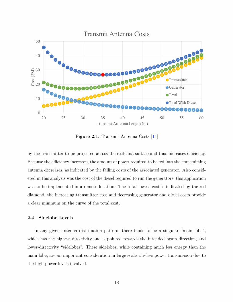
Figure 2.1. Transmit Antenna Costs [14 ]

by the transmitter to be projected across the rectenna surface and thus increases efficiency.

Because the efficiency increases, the amount of power required to be fed into the transmitting

antenna decreases, as indicated by the falling costs of the associated generator. Also consid-

ered in this analysis was the cost of the diesel required to run the generators; this application

was to be implemented in a remote location. The total lowest cost is indicated by the red

diamond; the increasing transmitter cost and decreasing generator and diesel costs provide

a clear minimum on the curve of the total cost.

2.4 Sidelobe Levels

In any given antenna distribution pattern, there tends to be a singular “main lobe”,

which has the highest directivity and is pointed towards the intended beam direction, and

lower-directivity “sidelobes”. These sidelobes, while containing much less energy than the

main lobe, are an important consideration in large scale wireless power transmission due to

the high power levels involved.

18

Sidelobe levels are one of the main showstoppers of SSP for the time being. If sidelobe

levels are not appropriately contained, the excess energy could cause significant problems for

RF signal communications outside of the transmission area. Maximum incident RF energy

for bystanders in areas adjacent to the receiver is also a serious consideration, but is less

likely to be an issue.

There are many methods previously explored in the subject of sidelobe level reduction,

and additionally, many methods of forming RF transmission beams include the sidelobe level

as a limiting parameter [18 ], [19 ]

One method of sidelobe level reduction is tapering of the phased array. In this method,

the antenna elements forming the array are supplied with different power levels; typically,

the antenna elements in the center are supplied with higher power levels than elements on

the edge. This allows for the resulting beam to have a higher power distribution in the

intended beam direction and less power directed elsewhere. Commonly used tapers are a

Gaussian taper, a step-wise taper, and a Dolph-Chebychev taper, although there are many

others.

Another method of sidelobe level reduction is the placement of the antennas within the

phased array. There are many antenna configurations, including in a line, in a circle, square

placement, triangular placement, and others. The distance between antennas can be changed

as well, although the spacing is generally dependent on the grating lobes.

Grating lobes are features of a phased array antenna distribution that can appear when

the intended beam direction and the antenna element distribution cause spatial aliasing [20 ].

These lobes tend to be much higher than sidelobes, and are the result of coherence of the

beam in undesirable directions. As mentioned in Section 2.3 , the array factor and resulting

antenna directivity pattern are a function of the amplitudes and phases of the individual

elements. For example, when considering a uniformly spaced linear array, propagating in the

direction θ, the individual antenna element phases can be calculated (similarly to Equation

2.14 ) as follows:

φn = dn2π

λsin θ (2.15)

19

Where λ is the wavelength and dn is the nth element spacing.

This results in an array with the direction of maximum propagation being as follows:

θ = sin−1(

λφ

d2π

)(2.16)

As this gives the direction in terms of a sine wave, there could be multiple different

solutions if the antenna spacing and primary angle of propagation are not properly considered

(the individual antenna element phases can be considered as φ + 2πm where m is a whole

number). These different solutions are the grating lobes.

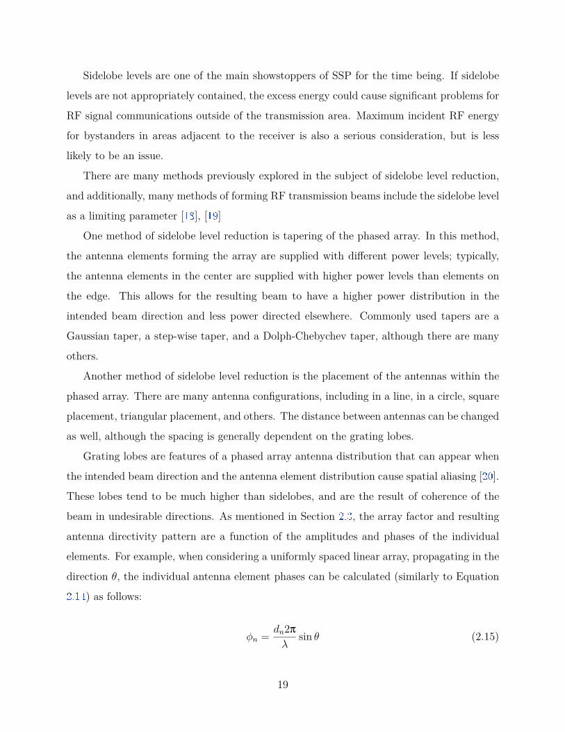
Figure 2.2. Grating Lobes for 1.5 λ Spacing, Zero Element Phase Shift

As an example, if a linear antenna array with an antenna spacing of 1.5λ is propagating

straight forward, then the phase delay of each antenna is zero, and an alternate solution to

Equation 2.16 when m is 1 is 41.8°. This is shown in Figure 2.2 ; four antennas marked with

blue triangles are shown with their associated radiation patterns. The coherence of the beam

in the broadside direction is shown with the horizontal line; clearly, the zero-phase-difference

antenna array propagates in that direction. The grating lobes are also present, shown as the

20

line slanted 41.8°to the right; although this is not the goal of this phase configuration, the

phase becomes coherent in that direction anyway.

With sidelobes and grating lobes in mind, the antenna placement and directions of propa-

gation must be evaluated for directivity and associated efficiency, sidelobe levels, and possible

grating lobes as well. All in all, the large number of variables involved and variations al-

lowed make sidelobe level reduction one of the most complicated and interesting problems

on the pathway to space solar power. Currently, the highest SLL reduction reported is -

120dB [21 ]. This configuration is dependent on an extremely large phased array setup with

a Dolph-Chebychev taper and minimal antenna failures.

2.5 Non-Traditional Phased Array Antenna Architecture

One of the main concerns of wireless power beaming is the cost of the total system.

This cost includes not only the cost of the system components, but the cost of system

transportation and setup, especially in the case of space solar power. With this in mind,

systems with fewer components or lighter components can be seen as advantageous. Two

potential methods for obtaining high results (as described above in terms of high directivity

and low sidelobe levels) with fewer components are heterogeneous arrays, which use multiple

different types of antennas in an attempt to increase directivity, and sparse arrays, which

have selectively less antenna elements in different locations around the array.

The idea of a heterogeneous array was conceived as a solution to issues presented by

preliminary results of antenna array power distributions for very low sidelobe levels, as de-

scribed by Schubert in 2016 [21 ]. In this paper, an extremely low sidelobe level (-120dB)

is the result of an extremely large phased antenna array with a Dolph-Chebychev taper.

Because of the large dimensions of the array and the specificity of the taper, the elements

at the center of the array require power levels that are several orders of magnitude larger

than the elements at the edges. To attempt to alleviate the issues this causes with power

distribution in a large array, antenna elements with a higher natural directivity were con-

sidered for the central elements of the array, and elements with lower directivities for the

edges. Unfortunately, initial results in the examination of this method were not favorable.

21

Because the elements had different radiation patterns from one another, they did not act as

a cohesive phased array, and produced distribution patterns with lower directivity patterns

than either element in a homogeneous array.

Sparse arrays, on the other hand, are a widely examined method to reduce antenna

mass, volume, and costs [22 ], [23 ]. There are many different methods for implementing

sparse arrays. Some methods involve removing antennas from the array randomly; others

involve specific densities based on geometry or distance from the antenna center. Although

the results of these arrays are more promising than heterogeneous arrays, they still produce

less directive antenna patterns with higher sidelobe levels. Because of this, sparse arrays

may be more practical for smaller scale applications in which sidelobe levels are not of such

high importance.

One method adjacent to sparse arrays is the idea of using unpowered antenna elements.

Although this method does not help reduce the number of antennas used, it may reduce

the cost of the supporting electronic equipment with less severe results than sparse antennas

themselves. In models of this method, arrays with selected antennas remaining unpowered

cause less disruption from full antenna results than arrays with the elements removed alto-

gether. This may be because of mutual coupling effects; unpowered antennas provide the

same electronic environment for their powered peers as powered antennas do, which, as in

the case of the heterogeneous array versus the homogeneous array, could allow for higher

beam coherence of the antenna as a whole.

2.6 Other Components of Wireless Power Transfer

There are many other components of Wireless Power Transfer that are discussed in detail

in current publications. Some of these components will be briefly discussed here, including

beam steering, link communications, and retrodirective antennas.

One of the main advantages of Phased Array Antennas is their beam steering capability.

As discussed in Section 2.4 and shown in Figure 2.3 , the direction of the propagated wave

is controlled by the phase delivered to individual antenna elements. This allows for steering

even in situations where physical maneuvering of the antenna itself is not feasible, for ex-

22

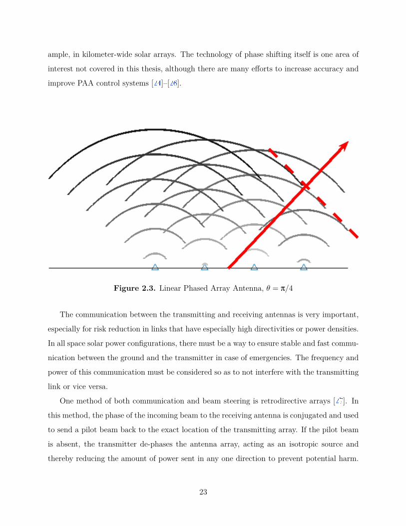
ample, in kilometer-wide solar arrays. The technology of phase shifting itself is one area of

interest not covered in this thesis, although there are many efforts to increase accuracy and

improve PAA control systems [24 ]–[26 ].

Figure 2.3. Linear Phased Array Antenna, θ = π/4

The communication between the transmitting and receiving antennas is very important,

especially for risk reduction in links that have especially high directivities or power densities.

In all space solar power configurations, there must be a way to ensure stable and fast commu-

nication between the ground and the transmitter in case of emergencies. The frequency and

power of this communication must be considered so as to not interfere with the transmitting

link or vice versa.

One method of both communication and beam steering is retrodirective arrays [27 ]. In

this method, the phase of the incoming beam to the receiving antenna is conjugated and used

to send a pilot beam back to the exact location of the transmitting array. If the pilot beam

is absent, the transmitter de-phases the antenna array, acting as an isotropic source and

thereby reducing the amount of power sent in any one direction to prevent potential harm.

23

This method is the prevalent form of beam steering currently considered for space solar

power, but there are still many questions to be answered about its specific implementation.

24

3. FAR FIELD DISTANCE STUDY

This chapter will discuss work examining the far field, specifically in regard to phased array

antennas. A new model for the far field is presented, along with modeling done in MATLAB

and experimental results, with the goal of understanding the transmission of an antenna

array.

The far field, as discussed in Chapter 2 , is an important concept for ensuring coherence

of phase across a receiving array. Although the impact of this phase difference depends on

the configuration of the receiving antenna itself, it is an important consideration to take

into account when looking at the transmission efficiency. Lack of phase coherence can cause

decreases in efficiency due to the cancellation of power as it is collected by the receiving

antenna.

With this in mind, a fresh look at the far field of phased array antennas is required.

While each individual element is electrically small, and so the far field for a single element

would be 2λ, it does not make sense to adapt this as the far field for a phased array antenna.

It also does not make sense to adapt the entire size of the array as the size to be used in a

far field calculation, because the phase result at each point is not only determined from the

distance from one side versus the other; it is also determined from the phase of the individual

elements. For this reason, the far field distance of phased array antennas is discussed.

One application for an examination of the far field distance is to reduce the necessary

distance required for antenna testing [28 ]. If a phased array antenna is used, as in the

following discussion and in 5G applications, the traditional far field equation can be unnec-

essarily limiting and examining the reasons behind it can produce smaller testing distances

and consequently lower costs.

Another reason to examine the far field is to glean more information about the power

density at any given point between the transmitter and receiver. The maximum power

density in a transmission setup is an important parameter to be aware of in order to ensure

safety measures are followed.

25

3.1 Far Field Model

As discussed in Section 2.1.1 , the far field is neatly described in terms of the phase

difference at a receiving point for electronically large antennas and as 2λ for electrically small

antennas. This definition is somewhat lacking in terms of phased array antennas; the entire

array is electrically large, but the individual elements are electrically small. Additionally,

one of the main benefits of phased array antennas is the electronic steering implemented by

adjusting the phase of individual elements. Because of this, the far field definition is lacking;

since the phase can be changed from one edge of the antenna array to the other, allowing

for the phase along a receiving plane to be manipulated, it no longer makes sense to define

the far field in that way.

The far field itself, separate from its typically used equation, is defined as the distance at

which all variation in directivity is a function of azimuth and elevation, not distance. The

near-field is the region at which strong inductive or capacitive effects exist. Neither of these

definitions allow for an examination of mid-range phased array antennas, at which power

could be transferred but before the phase pattern acts as if it is from a point source. Instead,

for this evaluation, this transition zone is examined as a function not only of distance, but of

receiver size as well. As opposed to looking at the far field as caused by the phase difference

due to the transmitting antenna size at a singular receiving point, the receiving antenna field

is considered as the area of coherent phase over a plane produced by the resulting beam of

a transmitting antenna. The limit for the coherence of phase will be π/2 radians, or λ/4.

In other words, at a given distance from the transmitter, all points that have a resulting

phase within π/2 radians of each other will be considered to be in the receiving antenna field.

This value was chosen to ensure minimal interference of phase at the receiving antenna to

maximize power received. This is a divergence from the traditional far field model; however,

because this coherence of phase is needed to ensure efficiency of collection at the rectenna

rather than to ensure each point at the far field has a coherent phase, it is more acceptable.

26

3.2 MATLAB Model

This evaluation of the receiving plane was modeled in MATLAB. Select code from MAT-

LAB is shown in Appendix A . The goal of the MATLAB model was to be able to provide

an antenna array setup and a distance and evaluate all possible points that resulted in a

phase that would allow coherence across a rectenna. There are many different starting points

possible for this analysis; although any antenna configuration and individual antenna beam

pattern would be allowed, for simplicity and coherence with lab work discussed later in this

chapter, a patch antenna beam pattern was used along with a square, uniform array. The

resulting beam pattern along a receiving plane was calculated by summing the resulting

electromagnetic field of each antenna, as described by Shinohara [11 ].

For ease of modeling, the transmitting antenna was assumed to be a uniform antenna

array, with a square arrangement of patch antennas with 0.8λ spacing. The points in the far

field were found by determining which points arranged in a square were within π/2 radians

of phase with each other. The rectenna could be any shape; for this test, a square was chosen

to match the shape of the transmitting antenna and because a square rectenna is easy to

design and visualize. Additionally, the frequency was chosen to be 2.4 GHz to match the

frequency of the laboratory experiments and because 2.4 GHz and 5.8 GHz are the most

used frequencies for wireless power transfer analysis due to the atmospheric losses at those

frequencies. A series of different antenna sizes were tested for maximum far field rectenna

size across various distances, as shown in Figure 3.1 .

Initially, the far field rectenna sizes shown in Figure 3.1 can seem somewhat chaotic,

but they are, in fact, completely dependent on the size and shape of the antenna arrays

in question. Figures 3.2 through 3.5 , for example, compare the phase plane produced by a

singular antenna vs. a 2x2 antenna array for various distances, labeled as 1 through 4 in red

on Figure 3.1 . In these figures, the placement of the antennas is marked by a black asterisk,

and a square surrounding all possible points on a rectenna at that distance is marked in

black. The color map of the figures is a color wheel, so that there isn’t a large difference in

color for the phases 0 and 2π.

27

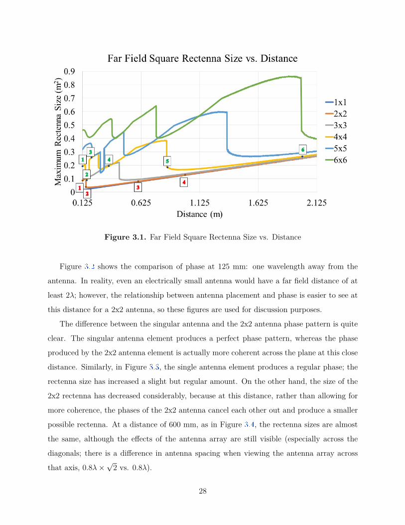
Figure 3.1. Far Field Square Rectenna Size vs. Distance

Figure 3.2 shows the comparison of phase at 125 mm: one wavelength away from the

antenna. In reality, even an electrically small antenna would have a far field distance of at

least 2λ; however, the relationship between antenna placement and phase is easier to see at

this distance for a 2x2 antenna, so these figures are used for discussion purposes.

The difference between the singular antenna and the 2x2 antenna phase pattern is quite

clear. The singular antenna element produces a perfect phase pattern, whereas the phase

produced by the 2x2 antenna element is actually more coherent across the plane at this close

distance. Similarly, in Figure 3.3 , the single antenna element produces a regular phase; the

rectenna size has increased a slight but regular amount. On the other hand, the size of the

2x2 rectenna has decreased considerably, because at this distance, rather than allowing for

more coherence, the phases of the 2x2 antenna cancel each other out and produce a smaller

possible rectenna. At a distance of 600 mm, as in Figure 3.4 , the rectenna sizes are almost

the same, although the effects of the antenna array are still visible (especially across the

diagonals; there is a difference in antenna spacing when viewing the antenna array across

that axis, 0.8λ ×√

2 vs. 0.8λ).

28

Figure 3.2. Comparison of Singleton and 2x2 Array Phase at 125 mm

Figure 3.3. Comparison of Singleton and 2x2 Array Phase at 154 mm

While the effects of the antenna placement are easiest to see for a 2x2 antenna, the trends

continue for larger sizes. Figures 3.6 through 3.11 show the results of the same analysis for

a 4x4 antenna array, shown at the distances marked in green in Figure 3.1 , as well as the

circular rectenna results, which are shown in total in Figure 3.12 .

Similarly to the 2x2 antenna, the resulting maximum square rectenna for a 4x4 antenna

increases and decreases in size, depending on the coherence of the antenna array at that point.

29

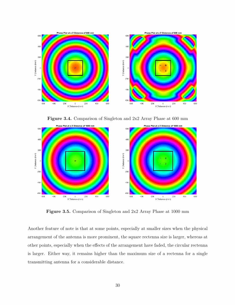
Figure 3.4. Comparison of Singleton and 2x2 Array Phase at 600 mm

Figure 3.5. Comparison of Singleton and 2x2 Array Phase at 1000 mm

Another feature of note is that at some points, especially at smaller sizes when the physical

arrangement of the antenna is more prominent, the square rectenna size is larger, whereas at

other points, especially when the effects of the arrangement have faded, the circular rectenna

is larger. Either way, it remains higher than the maximum size of a rectenna for a single

transmitting antenna for a considerable distance.

30

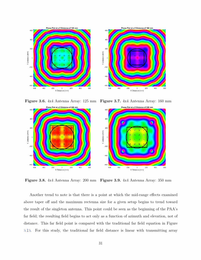
Figure 3.6. 4x4 Antenna Array: 125 mm Figure 3.7. 4x4 Antenna Array: 160 mm

Figure 3.8. 4x4 Antenna Array: 200 mm Figure 3.9. 4x4 Antenna Array: 350 mm

Another trend to note is that there is a point at which the mid-range effects examined

above taper off and the maximum rectenna size for a given setup begins to trend toward

the result of the singleton antenna. This point could be seen as the beginning of the PAA’s

far field; the resulting field begins to act only as a function of azimuth and elevation, not of

distance. This far field point is compared with the traditional far field equation in Figure

3.13 . For this study, the traditional far field distance is linear with transmitting array

31

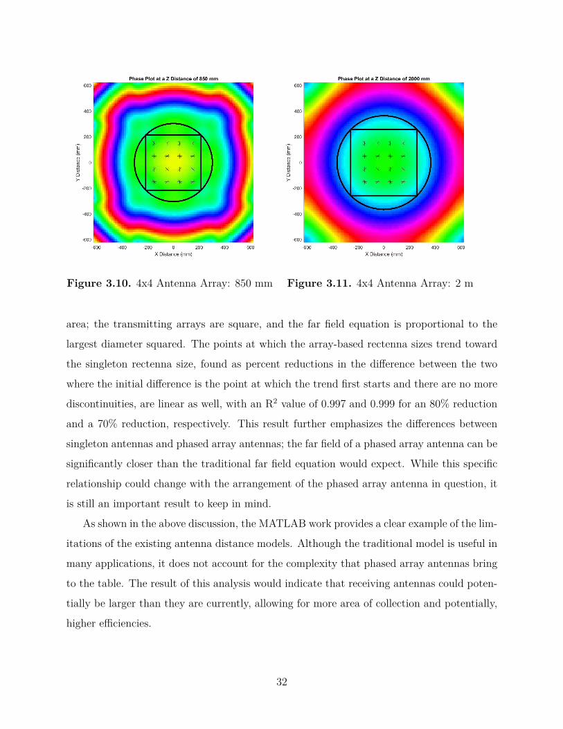
Figure 3.10. 4x4 Antenna Array: 850 mm Figure 3.11. 4x4 Antenna Array: 2 m

area; the transmitting arrays are square, and the far field equation is proportional to the

largest diameter squared. The points at which the array-based rectenna sizes trend toward

the singleton rectenna size, found as percent reductions in the difference between the two

where the initial difference is the point at which the trend first starts and there are no more

discontinuities, are linear as well, with an R2 value of 0.997 and 0.999 for an 80% reduction

and a 70% reduction, respectively. This result further emphasizes the differences between

singleton antennas and phased array antennas; the far field of a phased array antenna can be

significantly closer than the traditional far field equation would expect. While this specific

relationship could change with the arrangement of the phased array antenna in question, it

is still an important result to keep in mind.

As shown in the above discussion, the MATLAB work provides a clear example of the lim-

itations of the existing antenna distance models. Although the traditional model is useful in

many applications, it does not account for the complexity that phased array antennas bring

to the table. The result of this analysis would indicate that receiving antennas could poten-

tially be larger than they are currently, allowing for more area of collection and potentially,

higher efficiencies.

32

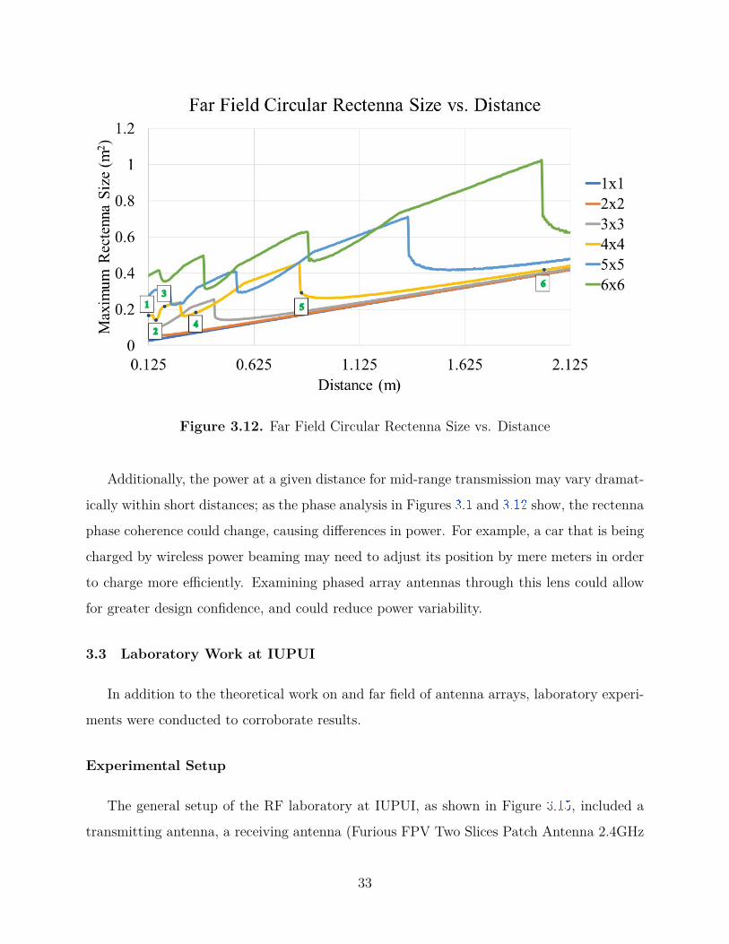
Figure 3.12. Far Field Circular Rectenna Size vs. Distance

Additionally, the power at a given distance for mid-range transmission may vary dramat-

ically within short distances; as the phase analysis in Figures 3.1 and 3.12 show, the rectenna

phase coherence could change, causing differences in power. For example, a car that is being

charged by wireless power beaming may need to adjust its position by mere meters in order

to charge more efficiently. Examining phased array antennas through this lens could allow

for greater design confidence, and could reduce power variability.

3.3 Laboratory Work at IUPUI

In addition to the theoretical work on and far field of antenna arrays, laboratory experi-

ments were conducted to corroborate results.

Experimental Setup

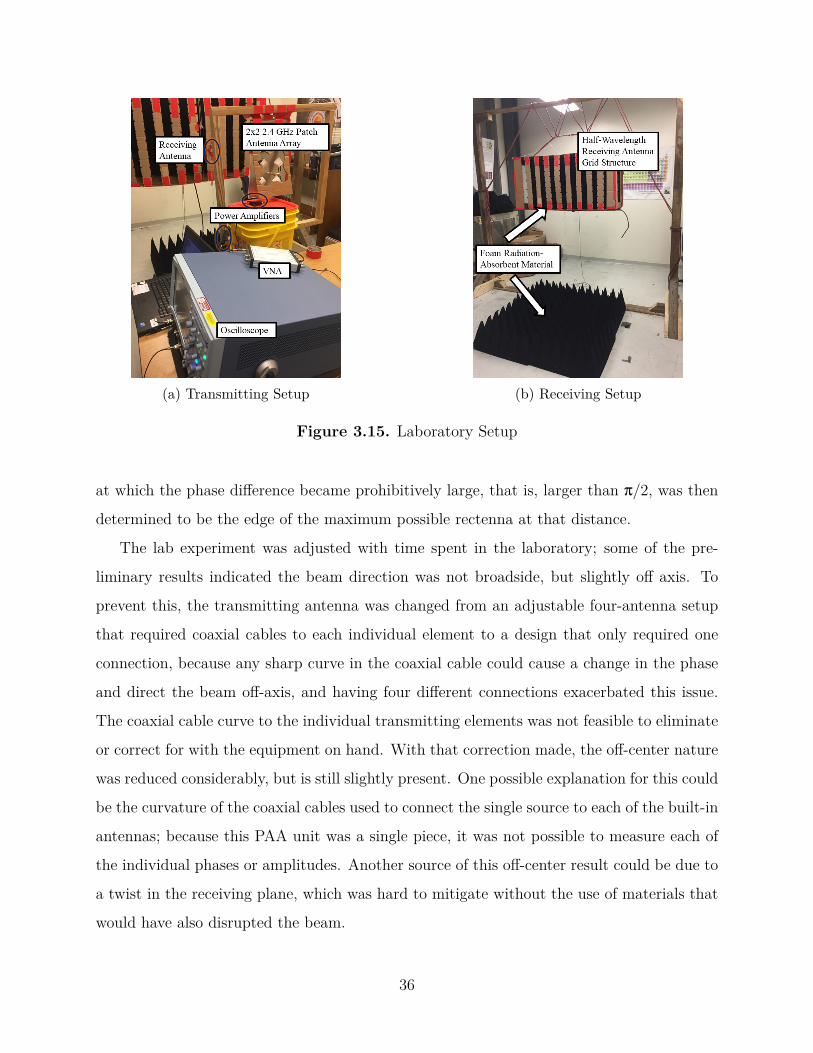
The general setup of the RF laboratory at IUPUI, as shown in Figure 3.15 , included a

transmitting antenna, a receiving antenna (Furious FPV Two Slices Patch Antenna 2.4GHz

33

Figure 3.13. Comparison of Traditional and Modeled Far Field for PAAs

RHCP), and the associated testing equipment; VNA RF signal generator (TPI Synthesizer,

Model No. TPI-1001-B, Serial No. 0184), coaxial cables and connectors, oscilloscope (LeCroy

Wavepro 7300A 3 GHz Oscilloscope), power amplifiers (WiFi Signal Booster 3000mW 2.4GHz

35dBm), and isolating foam, among others.

To ensure accurate readings, the peripheral equipment in the RF lab was as out of the

way as possible; in particular, anything including metal or RF waves was out of the line of

sight from the transmitter to the receiver. Additionally, all metal equipment was separated

from the testing equipment with isolating foam, if possible. All WiFi devices in the lab were

placed on airplane mode to reduce interference. Any material that could potentially interfere

with the RF transmission was out of the way, including personnel.

Measures were taken to prevent potential harm, including staying out of the way of

the transmitted beam and ensuring that persons with pacemakers or other similar health

equipment stayed well away from any excess radiation.

The VNA was connected to the laptop through a USB. The power amplifiers were con-

nected in series with the RF transmission and connected to the power source. Wooden

34

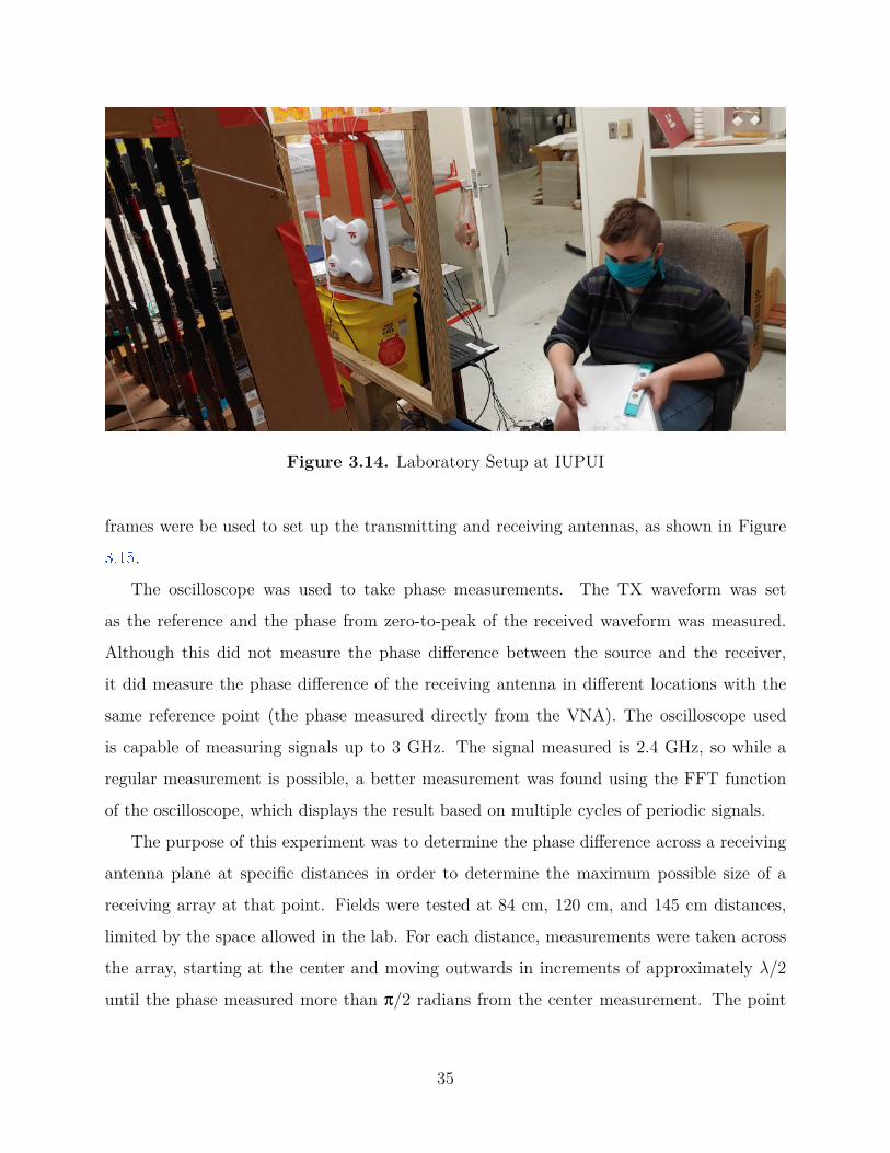
Figure 3.14. Laboratory Setup at IUPUI

frames were be used to set up the transmitting and receiving antennas, as shown in Figure

3.15 .

The oscilloscope was used to take phase measurements. The TX waveform was set

as the reference and the phase from zero-to-peak of the received waveform was measured.

Although this did not measure the phase difference between the source and the receiver,

it did measure the phase difference of the receiving antenna in different locations with the

same reference point (the phase measured directly from the VNA). The oscilloscope used

is capable of measuring signals up to 3 GHz. The signal measured is 2.4 GHz, so while a

regular measurement is possible, a better measurement was found using the FFT function

of the oscilloscope, which displays the result based on multiple cycles of periodic signals.

The purpose of this experiment was to determine the phase difference across a receiving

antenna plane at specific distances in order to determine the maximum possible size of a

receiving array at that point. Fields were tested at 84 cm, 120 cm, and 145 cm distances,

limited by the space allowed in the lab. For each distance, measurements were taken across

the array, starting at the center and moving outwards in increments of approximately λ/2

until the phase measured more than π/2 radians from the center measurement. The point

35

(a) Transmitting Setup (b) Receiving Setup

Figure 3.15. Laboratory Setup

at which the phase difference became prohibitively large, that is, larger than π/2, was then

determined to be the edge of the maximum possible rectenna at that distance.

The lab experiment was adjusted with time spent in the laboratory; some of the pre-

liminary results indicated the beam direction was not broadside, but slightly off axis. To

prevent this, the transmitting antenna was changed from an adjustable four-antenna setup

that required coaxial cables to each individual element to a design that only required one

connection, because any sharp curve in the coaxial cable could cause a change in the phase

and direct the beam off-axis, and having four different connections exacerbated this issue.

The coaxial cable curve to the individual transmitting elements was not feasible to eliminate

or correct for with the equipment on hand. With that correction made, the off-center nature

was reduced considerably, but is still slightly present. One possible explanation for this could

be the curvature of the coaxial cables used to connect the single source to each of the built-in

antennas; because this PAA unit was a single piece, it was not possible to measure each of

the individual phases or amplitudes. Another source of this off-center result could be due to

a twist in the receiving plane, which was hard to mitigate without the use of materials that

would have also disrupted the beam.

36

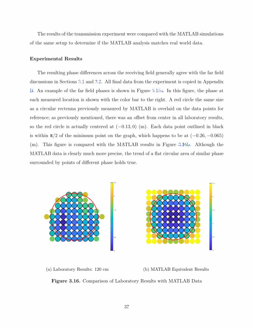
The results of the transmission experiment were compared with the MATLAB simulations

of the same setup to determine if the MATLAB analysis matches real world data.

Experimental Results

The resulting phase differences across the receiving field generally agree with the far field

discussions in Sections 3.1 and 3.2 . All final data from the experiment is copied in Appendix

B . An example of the far field phases is shown in Figure 3.16a . In this figure, the phase at

each measured location is shown with the color bar to the right. A red circle the same size

as a circular rectenna previously measured by MATLAB is overlaid on the data points for

reference; as previously mentioned, there was an offset from center in all laboratory results,

so the red circle is actually centered at (−0.13, 0) (m). Each data point outlined in black

is within π/2 of the minimum point on the graph, which happens to be at (−0.26, −0.065)

(m). This figure is compared with the MATLAB results in Figure 3.16b . Although the

MATLAB data is clearly much more precise, the trend of a flat circular area of similar phase

surrounded by points of different phase holds true.

(a) Laboratory Results: 120 cm (b) MATLAB Equivalent Results

Figure 3.16. Comparison of Laboratory Results with MATLAB Data

37

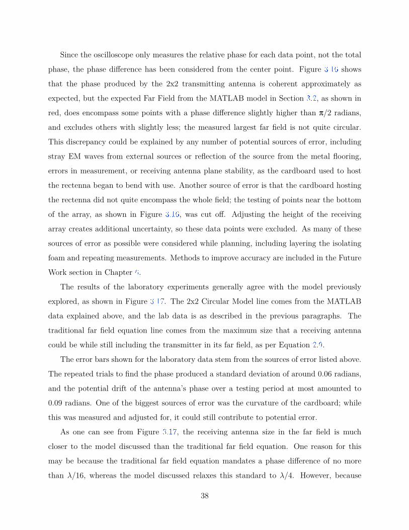
Since the oscilloscope only measures the relative phase for each data point, not the total

phase, the phase difference has been considered from the center point. Figure 3.16 shows

that the phase produced by the 2x2 transmitting antenna is coherent approximately as

expected, but the expected Far Field from the MATLAB model in Section 3.2 , as shown in

red, does encompass some points with a phase difference slightly higher than π/2 radians,

and excludes others with slightly less; the measured largest far field is not quite circular.

This discrepancy could be explained by any number of potential sources of error, including

stray EM waves from external sources or reflection of the source from the metal flooring,

errors in measurement, or receiving antenna plane stability, as the cardboard used to host

the rectenna began to bend with use. Another source of error is that the cardboard hosting

the rectenna did not quite encompass the whole field; the testing of points near the bottom

of the array, as shown in Figure 3.16 , was cut off. Adjusting the height of the receiving

array creates additional uncertainty, so these data points were excluded. As many of these

sources of error as possible were considered while planning, including layering the isolating

foam and repeating measurements. Methods to improve accuracy are included in the Future

Work section in Chapter 6 .

The results of the laboratory experiments generally agree with the model previously

explored, as shown in Figure 3.17 . The 2x2 Circular Model line comes from the MATLAB

data explained above, and the lab data is as described in the previous paragraphs. The

traditional far field equation line comes from the maximum size that a receiving antenna

could be while still including the transmitter in its far field, as per Equation 2.9 .

The error bars shown for the laboratory data stem from the sources of error listed above.

The repeated trials to find the phase produced a standard deviation of around 0.06 radians,

and the potential drift of the antenna’s phase over a testing period at most amounted to

0.09 radians. One of the biggest sources of error was the curvature of the cardboard; while

this was measured and adjusted for, it could still contribute to potential error.

As one can see from Figure 3.17 , the receiving antenna size in the far field is much

closer to the model discussed than the traditional far field equation. One reason for this

may be because the traditional far field equation mandates a phase difference of no more

than λ/16, whereas the model discussed relaxes this standard to λ/4. However, because

38

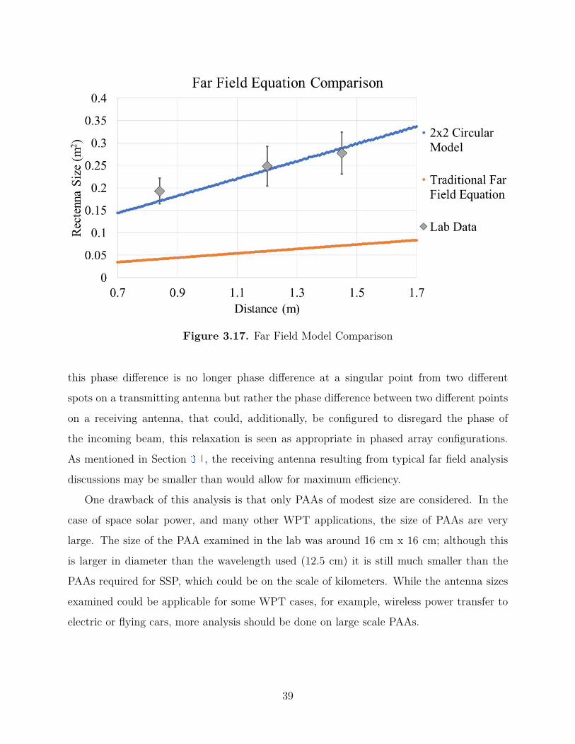
Figure 3.17. Far Field Model Comparison

this phase difference is no longer phase difference at a singular point from two different

spots on a transmitting antenna but rather the phase difference between two different points

on a receiving antenna, that could, additionally, be configured to disregard the phase of

the incoming beam, this relaxation is seen as appropriate in phased array configurations.

As mentioned in Section 3.1 , the receiving antenna resulting from typical far field analysis

discussions may be smaller than would allow for maximum efficiency.

One drawback of this analysis is that only PAAs of modest size are considered. In the

case of space solar power, and many other WPT applications, the size of PAAs are very

large. The size of the PAA examined in the lab was around 16 cm x 16 cm; although this

is larger in diameter than the wavelength used (12.5 cm) it is still much smaller than the

PAAs required for SSP, which could be on the scale of kilometers. While the antenna sizes

examined could be applicable for some WPT cases, for example, wireless power transfer to

electric or flying cars, more analysis should be done on large scale PAAs.

39

4. FREE SPACE TRANSMISSION EFFICIENCY STUDY

This chapter will examine the free space efficiency of phased array antenna systems. As men-

tioned in Section 2.1 , the previously used equations are not entirely applicable to wireless

power beaming; the purpose of this study is to remedy this and provide a useful, compre-

hensive efficiency analysis starting point. There have been comparisons of the typically used

efficiency equations in the past; however, the most common method of evaluation beyond the

equations mentioned is numerical analysis of the system in question [29 ]. This study goes

beyond that to create easy to understand, easy to use equations that predict the efficiency

of a system efficiently and realistically.

Figure 4.1. Power Beaming Block Diagram

The overall efficiency of WPT systems has many components, related to the blocks in

Figure 4.1 ; there is the efficiency of the DC-to-RF system, the efficiency of the transmit-

ting antennas, the free space transmission efficiency, the efficiency of the receiving antennas,

and the efficiency of the RF-to-DC system. This chapter specifically examines free space

efficiency: the power available for capture at the receiving antenna divided by the power

transmitted across the surface of the transmitting antenna. This definition of the free space

efficiency and the definition of directivity are used to provide a simple, comprehensive method

that can be used for any type of WPT system and is not based on specific antenna configu-

rations or previous efficiency approximations.

40

4.1 Efficiency Equations

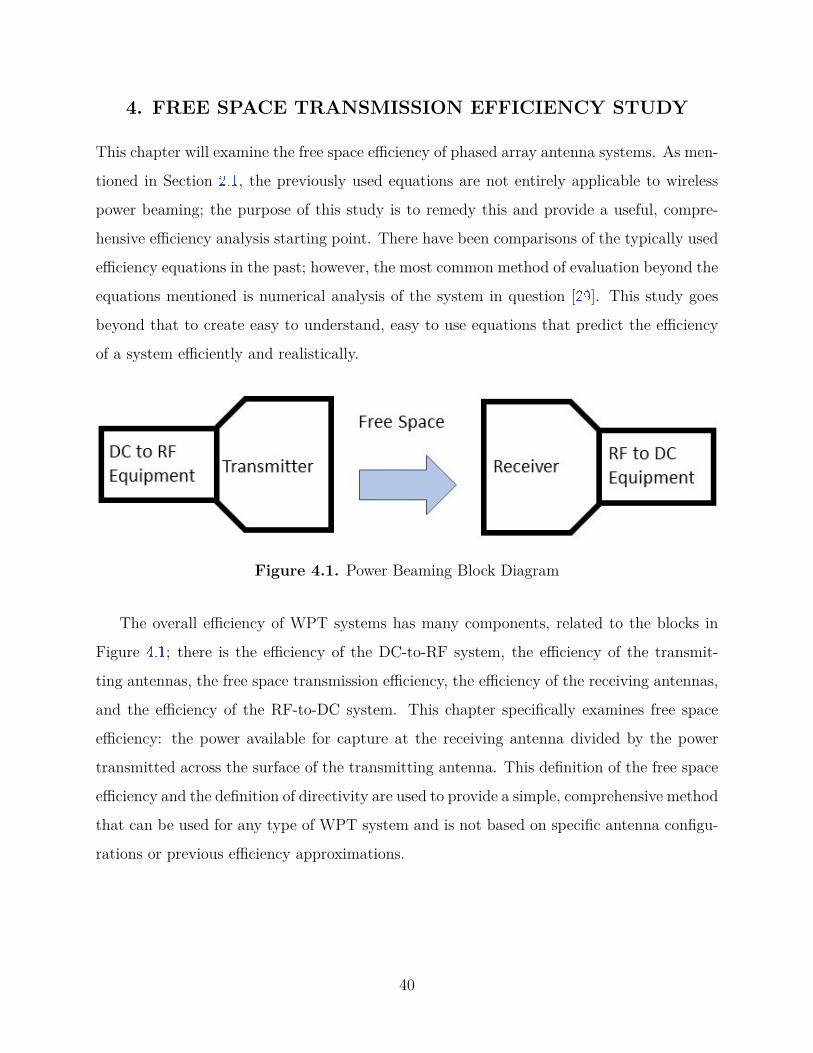
The following equation formulation will be based on the directivity of the transmitting

antenna and the geometry of the transmission setup, as shown in Figure 4.2 . The directivity

is defined as in Equation 2.10 : the radiant intensity divided by the average power. The angle

Φ indicating the area of reception can be found using the dimensions of the transmission:

Φ = tan−1(

d/2R

)(4.1)

Figure 4.2. Layout Used for Efficiency Calculations

where d is the diameter of the receiving antenna and R is the distance between receiving

and transmitting antennas. Although an azimuth angle of this kind would typically be

represented by θ, in the case of power beaming, θ is used for the steering direction of the

beam, so Φ is chosen for clarity. The total power can be calculated as the radiant intensity

over all angles:

Ptotal =∫ 2π

0

∫π

0U(θ, φ) sin θ dθ dφ (4.2)

And so the power at the receiving antenna can be calculated as

PR =∫ 2π

0

∫ Φ

0Ptotal

D(θ, φ)4π

sin θ dθ dφ (4.3)

41

If we assume radial symmetry, this equation simplifies to:

PR = Ptotal

2

∫ Φ

0D(φ) sin φ dφ (4.4)

Assuming a Constant D(φ)

If D(φ) is constant, integral is quite simple:

PR = Ptotal

2

∫ Φ

0D sin φ dφ (4.5)

PR = PtotalD

2 [− cos φ]Φ0 (4.6)

PR = PtotalD

2 [1 − cos Φ] (4.7)

PR = PtotalD

2

[1 − cos

(tan−1

(Di/2

R

))](4.8)

PR = PtotalD

2

1 − R√R2 + D2

i /4

(4.9)

This derivation gives a simple, easy to use equation, but has limited accuracy; care must

be taken to only apply this equation across receiving antennas in which the constant D(φ)

assumption is reasonable. This condition is what prevents efficiencies higher than unity; only

a couple dB decrease in directivity can be allowed from center to edge, which limits the size

of the receiving area.

Another necessary condition of this equation is that the receiving antenna be in the far

field of the transmitter as a whole. Typically used antenna elements in a PAA would no

doubt be in the far field of the receiver individually, but the receiver must also be far enough

away for the transmitting antenna to form a single coherent beam.

42

Assuming D(φ) is Parabolic on a Logarithmic Scale

Typically, antenna directivity is displayed on a dB scale, and is shown to have a roughly

parabolic curve. If this were a perfect assumption, the curve would be in the form

D(φ) = De−φ2/β (4.10)

where D is the maximum directivity and β is some shaping constant. This is equivalent

to a Gaussian distribution with µ = 0 and the standard deviation found from the maximum

directivity and half-power beam width. Additionally, this can be found by approximating

the dB curve with a second-order Taylor series. If b is one half of the half power beam

width (HPBW) found from a pre-existing directivity pattern of the transmitting antenna,

approximated from known configurations or calculated with AWR or other antenna analysis

tools, then β can be found:

D(b) = 12D = De−b2/β (4.11)

− ln(2) = −b2/β (4.12)

β = b2/ ln(2) (4.13)

This allows for the directivity to be written:

D(φ) = De−φ2ln(2)/b2 (4.14)

The total power can then be found as:

PR = Ptotal

2

∫ Φ

0De−φ2ln(2)/b2 sin φ dφ (4.15)

43

The sin φ component can be approximated by φ on a small enough scale, so this equation

simplifies as:

PR = Ptotal

2

∫ Φ

0De−φ2ln(2)/b2

φ dφ (4.16)

With a u-substitution of u = −φ2 ln(2)/b2, this becomes

PR = −PtotalDb2

4 ln(2)

∫ −Φ2 ln(2)/b2

0eu du (4.17)

PR = PtotalDb2

4 ln(2)[1 − e−φ2 ln(2)/b2] (4.18)

Again, this equation should only be used in cases when the assumption of a Gaussian

distribution and approximation of sin φ as φ hold true. Both φ and b should be in units of

radians.

Using Numeric Integration

The integral form of the efficiency can be found numerically as well. This method, while

not allowing for a simple, concise equation, does allow for a better approximation of efficiency

for any pattern of directivity that is not easily approximated by the previous sections, and

has been used before [30 ].

It is important to note that the total efficiency (if taking the angle from zero to 180

degrees) should be unity. Any pattern of directivity used should be scaled accordingly; if

the integral from zero to 180 is not one, the integral over the desired area should be divided

by this “total” efficiency.

It is very helpful in system design to have a baseline equation that can estimate the

expected gain. The following section discusses some of the relationships between antenna

array designs and directivity, and the formation of a design equation for a uniform antenna

array that can be used in conjunction with the efficiency equations presented.

44

4.2 Analysis of a Uniform PAA

As mentioned above, it was desired to have an easy-to-use equation for the directivity

of a phased array antenna in order to predict the efficiency of a given transmission setup.

Although there are many factors that can change antenna efficiency, a simple PAA setup

was chosen for this evaluation. This allows for an estimation of directivity and efficiency for

an antenna array that is simple to arrange and easy to replicate.

The design chosen was a square array of uniformly spaced, uniformly powered patch

antennas, with uniform phase. This design was modeled in MATLAB and AWR to find the

directivity for differing transmit antenna sizes and antenna spacings.

The MATLAB code for this evaluation is found in Appendix A . The results found from

MATLAB and AWR were very similar, besides a shift in directivity in AWR that resulted

in all antenna arrangements with the same number of elements producing the same amount

of directivity, regardless of the change in half power beam width. This is an indication that

the AWR phased array wizard uses the antenna factor to find the gain, which as discussed

in Section 2.3 , is incorrect. AWR has been contacted about this issue. Their response, in

part, is as follows:

[...the Phased Array Wizard] is considered to be a part of our Visual SystemsSimulator (VSS), not Microwave Office (MWO). That means that it is part ofa high-level behavioral approach to a complete system simulation rather thana precise/complete solution. At the practical level, this means that our “gain”is measured as signal power gain since it uses generic VSS measurements andit is not customized to phased array definitions. We take into account thearray factor and element radiation patterns to calculate the signal gain at theoutput of the array. Since phased arrays are used in VSS as part of largercommunications systems, we need to be able to track the signal power whenthey are present.[...] you would likely want to use AXIEM to do the actual design of yourphased array.

In short, there is agreement about the fact that the antenna factor is used, but it is

determined to be acceptable for that tool because it is primarily used for large scale com-

munication system analysis; for more exacting power analysis, a different tool should be

used. This is one example of the fact that most antenna tools are used for communications,

45

not power transfer; it is important to evaluate tools that are used to ensure accuracy for

alternate applications.

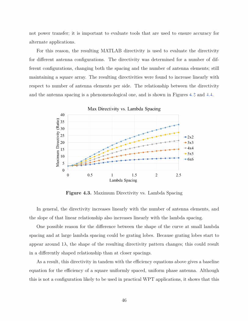
For this reason, the resulting MATLAB directivity is used to evaluate the directivity

for different antenna configurations. The directivity was determined for a number of dif-

ferent configurations, changing both the spacing and the number of antenna elements; still

maintaining a square array. The resulting directivities were found to increase linearly with

respect to number of antenna elements per side. The relationship between the directivity

and the antenna spacing is a phenomenological one, and is shown in Figures 4.3 and 4.4 .

Figure 4.3. Maximum Directivity vs. Lambda Spacing

In general, the directivity increases linearly with the number of antenna elements, and

the slope of that linear relationship also increases linearly with the lambda spacing.

One possible reason for the difference between the shape of the curve at small lambda

spacing and at large lambda spacing could be grating lobes. Because grating lobes start to

appear around 1λ, the shape of the resulting directivity pattern changes; this could result

in a differently shaped relationship than at closer spacings.

As a result, this directivity in tandem with the efficiency equations above gives a baseline

equation for the efficiency of a square uniformly spaced, uniform phase antenna. Although

this is not a configuration likely to be used in practical WPT applications, it shows that this

46

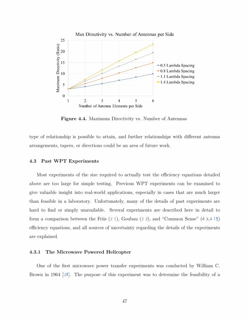
Figure 4.4. Maximum Directivity vs. Number of Antennas

type of relationship is possible to attain, and further relationships with different antenna

arrangements, tapers, or directions could be an area of future work.

4.3 Past WPT Experiments

Most experiments of the size required to actually test the efficiency equations detailed

above are too large for simple testing. Previous WPT experiments can be examined to

give valuable insight into real-world applications, especially in cases that are much larger

than feasible in a laboratory. Unfortunately, many of the details of past experiments are

hard to find or simply unavailable. Several experiments are described here in detail to

form a comparison between the Friis (2.1 ), Goubau (2.2 ), and “Common Sense” (4.9 ,4.18 )

efficiency equations, and all sources of uncertainty regarding the details of the experiments

are explained.

4.3.1 The Microwave Powered Helicopter

One of the first microwave power transfer experiments was conducted by William C.

Brown in 1964 [31 ]. The purpose of this experiment was to determine the feasibility of a

47

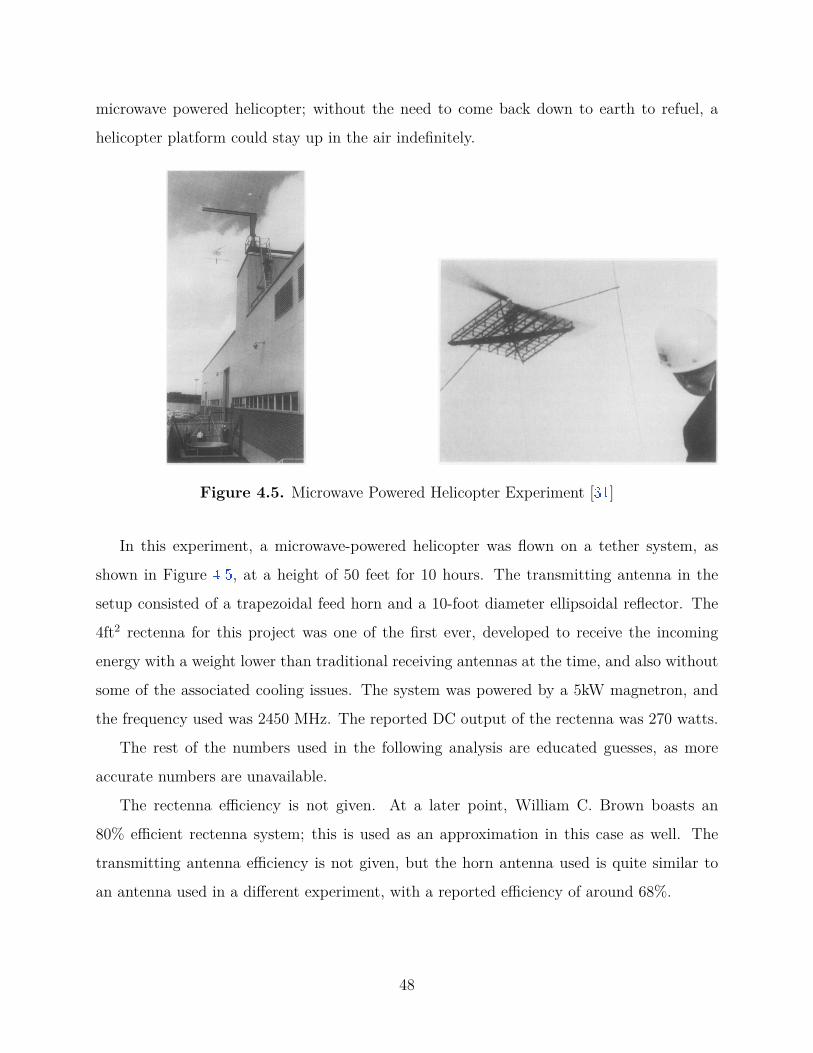
microwave powered helicopter; without the need to come back down to earth to refuel, a

helicopter platform could stay up in the air indefinitely.

Figure 4.5. Microwave Powered Helicopter Experiment [31 ]

In this experiment, a microwave-powered helicopter was flown on a tether system, as

shown in Figure 4.5 , at a height of 50 feet for 10 hours. The transmitting antenna in the

setup consisted of a trapezoidal feed horn and a 10-foot diameter ellipsoidal reflector. The

4ft2 rectenna for this project was one of the first ever, developed to receive the incoming

energy with a weight lower than traditional receiving antennas at the time, and also without

some of the associated cooling issues. The system was powered by a 5kW magnetron, and

the frequency used was 2450 MHz. The reported DC output of the rectenna was 270 watts.

The rest of the numbers used in the following analysis are educated guesses, as more

accurate numbers are unavailable.

The rectenna efficiency is not given. At a later point, William C. Brown boasts an

80% efficient rectenna system; this is used as an approximation in this case as well. The

transmitting antenna efficiency is not given, but the horn antenna used is quite similar to

an antenna used in a different experiment, with a reported efficiency of around 68%.

48

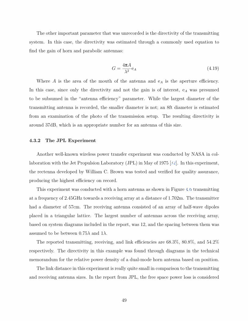
The other important parameter that was unrecorded is the directivity of the transmitting

system. In this case, the directivity was estimated through a commonly used equation to

find the gain of horn and parabolic antennas:

G = 4πA

λ2 eA (4.19)

Where A is the area of the mouth of the antenna and eA is the aperture efficiency.

In this case, since only the directivity and not the gain is of interest, eA was presumed

to be subsumed in the “antenna efficiency” parameter. While the largest diameter of the

transmitting antenna is recorded, the smaller diameter is not; an 8ft diameter is estimated

from an examination of the photo of the transmission setup. The resulting directivity is

around 37dB, which is an appropriate number for an antenna of this size.

4.3.2 The JPL Experiment

Another well-known wireless power transfer experiment was conducted by NASA in col-

laboration with the Jet Propulsion Laboratory (JPL) in May of 1975 [32 ]. In this experiment,

the rectenna developed by William C. Brown was tested and verified for quality assurance,

producing the highest efficiency on record.

This experiment was conducted with a horn antenna as shown in Figure 4.6 transmitting

at a frequency of 2.45GHz towards a receiving array at a distance of 1.702m. The transmitter

had a diameter of 57cm. The receiving antenna consisted of an array of half-wave dipoles

placed in a triangular lattice. The largest number of antennas across the receiving array,

based on system diagrams included in the report, was 12, and the spacing between them was

assumed to be between 0.75λ and 1λ.

The reported transmitting, receiving, and link efficiencies are 68.3%, 80.8%, and 54.2%

respectively. The directivity in this example was found through diagrams in the technical

memorandum for the relative power density of a dual-mode horn antenna based on position.

The link distance in this experiment is really quite small in comparison to the transmitting

and receiving antenna sizes. In the report from JPL, the free space power loss is considered

49

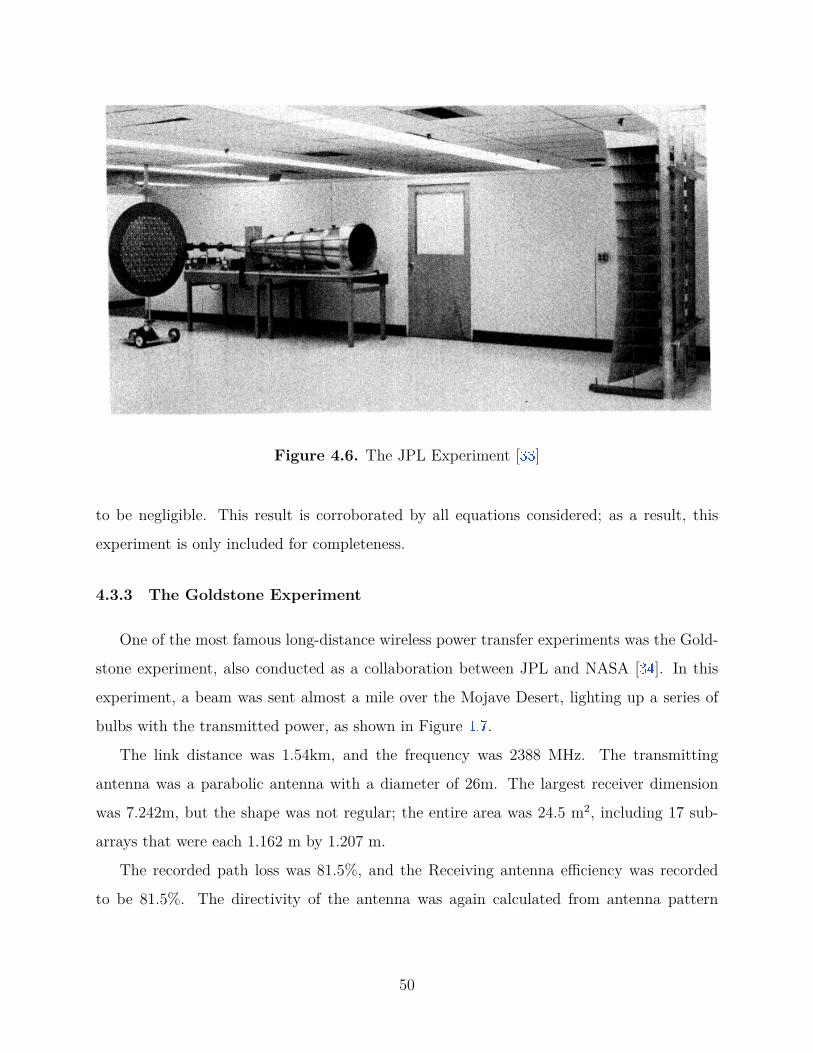
Figure 4.6. The JPL Experiment [33 ]

to be negligible. This result is corroborated by all equations considered; as a result, this

experiment is only included for completeness.

4.3.3 The Goldstone Experiment

One of the most famous long-distance wireless power transfer experiments was the Gold-

stone experiment, also conducted as a collaboration between JPL and NASA [34 ]. In this

experiment, a beam was sent almost a mile over the Mojave Desert, lighting up a series of

bulbs with the transmitted power, as shown in Figure 4.7 .

The link distance was 1.54km, and the frequency was 2388 MHz. The transmitting

antenna was a parabolic antenna with a diameter of 26m. The largest receiver dimension

was 7.242m, but the shape was not regular; the entire area was 24.5 m2, including 17 sub-

arrays that were each 1.162 m by 1.207 m.

The recorded path loss was 81.5%, and the Receiving antenna efficiency was recorded

to be 81.5%. The directivity of the antenna was again calculated from antenna pattern

50

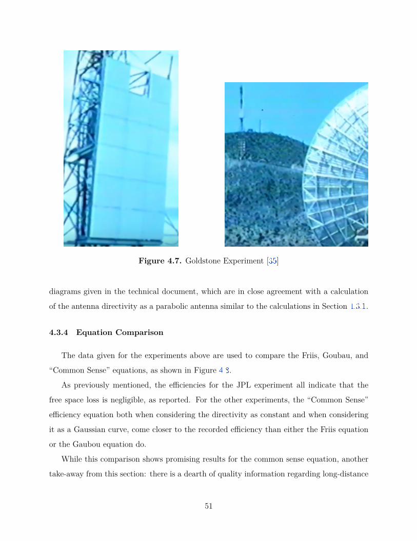
Figure 4.7. Goldstone Experiment [35 ]

diagrams given in the technical document, which are in close agreement with a calculation

of the antenna directivity as a parabolic antenna similar to the calculations in Section 4.3.1 .

4.3.4 Equation Comparison

The data given for the experiments above are used to compare the Friis, Goubau, and

“Common Sense” equations, as shown in Figure 4.8 .

As previously mentioned, the efficiencies for the JPL experiment all indicate that the

free space loss is negligible, as reported. For the other experiments, the “Common Sense”

efficiency equation both when considering the directivity as constant and when considering

it as a Gaussian curve, come closer to the recorded efficiency than either the Friis equation

or the Gaubou equation do.

While this comparison shows promising results for the common sense equation, another

take-away from this section: there is a dearth of quality information regarding long-distance

51

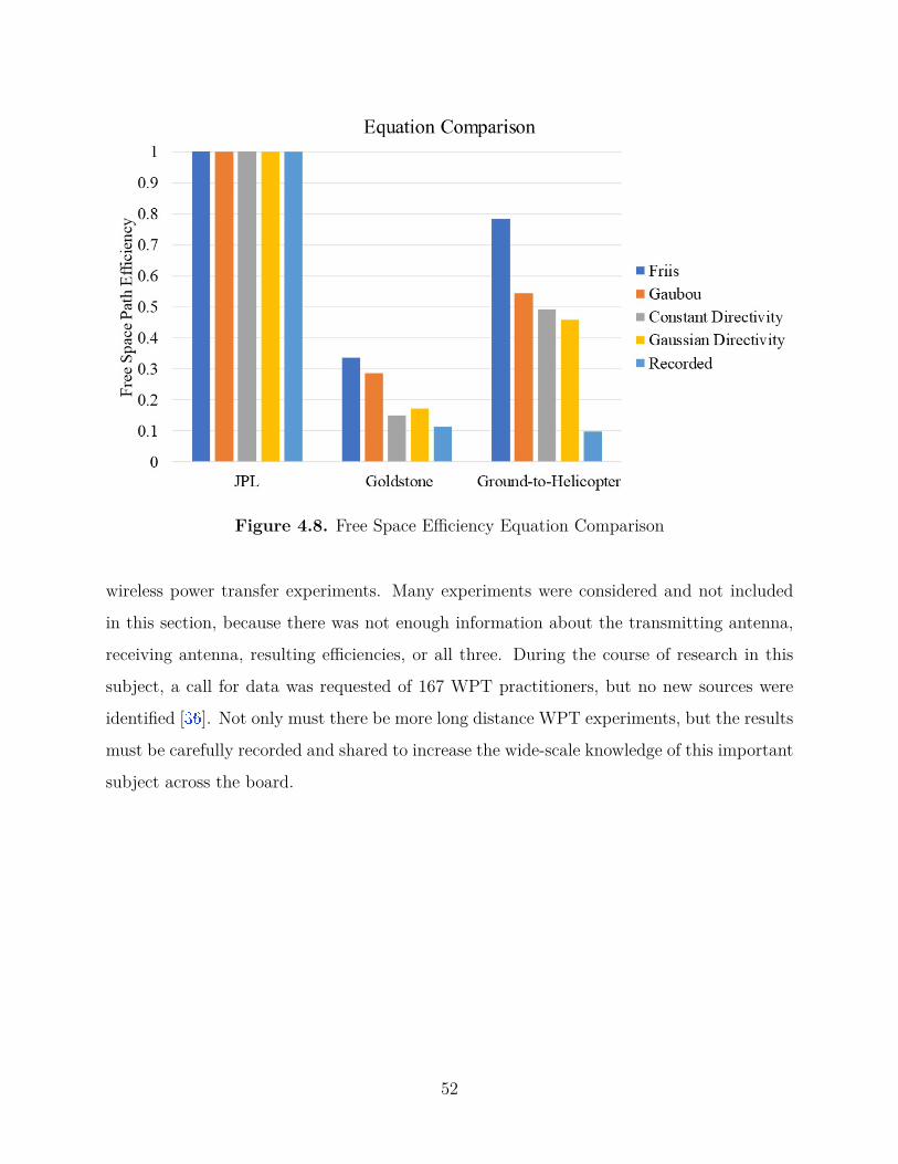
Figure 4.8. Free Space Efficiency Equation Comparison

wireless power transfer experiments. Many experiments were considered and not included

in this section, because there was not enough information about the transmitting antenna,

receiving antenna, resulting efficiencies, or all three. During the course of research in this

subject, a call for data was requested of 167 WPT practitioners, but no new sources were

identified [36 ]. Not only must there be more long distance WPT experiments, but the results

must be carefully recorded and shared to increase the wide-scale knowledge of this important

subject across the board.

52

5. DISCUSSIONS AND ANALYSIS

The results presented in this thesis are relevant in a wide variety of applications.

As mentioned in Chapter 3 , the result that the far field is unnecessarily restrictive for

phased array antennas could result in smaller testing areas for the PAAs used in 5G ap-

plications. Also, the examination of the phase distributions produced by PAAs could have

potential applications for mid-distance wireless power beaming. It also provides a stepping

point for the examination of the power distribution surrounding a phased array antenna,

which could have applications in many areas.

Another potential application for this work, as discussed in the introduction, is Space

Solar Power. Although there has been much discussion about this technology since it was

first introduced in the late 1970s, the basic setup is not much changed [37 ]–[41 ]. In the most

common design, a 1 km diameter transmitting antenna with a geosynchronous equatorial

orbit (GEO) at around 35 thousand km transmits power to an elongated receiving antenna

with a collection area with a 10 km diameter [37 ].

The free space efficiency from the economic analysis of the SSP concept was considered

to be almost negligible; the ionospheric and atmospheric transfer efficiency was considered to

be 90% at worst [40 ]. In a different document written by William C. Brown on the efficiency

of the rectenna, the free space efficiency of the beam was considered to be over 90% [41 ]. In

actuality, when considering a transmission of that distance to a rectenna of that size, the

transmission efficiency is not negligible.

In order to achieve an efficiency of 90%, a directivity of around 89 dB must be achieved

(as implicated by the analysis of Chapter 4 . If a 60dB directivity was used instead, the

efficiency would only be around 0.122%.

When considering the size of the transmitting antenna, the requirement of an 89 dB beam

is a high order. If considering the transmitting antenna to be a square, uniformly powered

phased array antenna with a 0.8λ spacing at 5.8 GHz, then the directivity would be only

around 47.63 dB (from the analysis presented in Section 4.2 ). For an 89 dB beam, the size

of the transmitting antenna would need to be around 950% larger.

53

As this analysis shows, the free space efficiency is not a negligible parameter when con-

sidering space solar power. Although directivities of this magnitude aren’t impossible with

the transmitter size given, it is important to recognize this as a limiting parameter; the

technology is not there yet, and cannot be assumed to be there for system designs going

forward. This area requires work, and should not be ignored.

Along the same vein, this work also impacts many other technologies, including any tech-

nology requiring long distance wireless power transfer; examples include mother-daughter

satellite configurations, high altitude stratospheric pseudo-satellites (HAPS), and power

transfer to remote areas including disaster recovery and Forward Operating Bases (FOBs). If

care is not taken to ensure accurate analysis of the efficiencies involved, the resulting designs

will be estimated as smaller than actually required, and progress of wireless power transfer

will be stalled. Accurate design equations are necessary for progressing this technology, and

should be shared as much as possible.

54

6. CONCLUSIONS AND FUTURE WORK

As discussed in the previous chapters of this work, the differences between phased array an-

tennas and singleton antennas and the differences between power transfer and signal transfer

should not be neglected.

In Chapter 2 , the fundamentals of wireless power transfer were discussed. In many

ways, the differences between WPT and radio-wave based signals are small; both rely on

fundamental properties of energy transfer and phase based signals. However, assuming that

there are no differences, especially in the case of the far field and efficiency equations, is an

oversimplification that can lead to uninformed design.

As discussed in Chapter 3 , the far field of an antenna is based almost entirely on the

phase at given receiving points. In the traditionally used equation, the far field is determined

to be the distance at which the phase difference caused by different distances between the

edges of the transmitter and the receiving point became negligible. This can be an important

metric, because it ensures that other governing equations for WPT still apply.

However, as examined in Chapter 3 , the phase plane of a phased array antenna acts

differently. It does not make sense to label the far field as the point where each individual

antenna’s far field begins, because the phased array has not yet formed a coherent beam.

It also does not make sense to label the far field as the point at which the phase from each

individual element is within a certain phase difference, because that would create a definition

that is unnecessarily restrictive, especially since the nature of a phased array antenna is to

change the phase of individual elements based on design needs.

Instead, as discussed, a far field model can be produced that encompasses the unique

nature of a phased array antenna; the resulting phase at each point can be determined over

a receiving plane to determine the maximum possible receiving antenna size at that distance.

Examining the far field in this way has the potential to produce more flexible transmitting

and receiving antenna designs, and provides a clearer picture of the resulting phased array

antenna beam.

Also discussed is the evaluation of the free space efficiency of wireless power transfer.

As discussed in Chapter 2 , previously used equations such as the Friis equation and the

55

Goubau equation have fundamental limitations that, while not vitally important in most

applications, make their use in WPT applications limited.

The Friis equation is defined through the effective area of an antenna. In the same way

that the size of a phased array antenna does not effectively convey information about the far

field the same way the size of a singleton antenna does, the size of a phased array antenna

does not convey information about the effective area the same way a singleton antenna does.

This causes a fundamental limitation when applying the Friis equation to WPT.

The Goubau equation, similarly, was designed through the evaluation of reiterative wave

beams. Although it can be applicable in some situations, it does not make sense for most

applications of long-distance wireless power transfer, because there is no mechanism for

the reiteration of the phase profile. It also does not include super-gain antennas; this is a

potential limitation, as there is no theoretical limit to the gain of a phased array antenna.

With these limitations of efficiency equations in mind, the equation formulation in Chap-

ter 4 is presented. The efficiency of any WPT setup can be evaluated with this method.

Although the most accurate evaluations would require additional information, including the

directivity of the transmitting antenna, the simplified equations can give a general idea for

the efficiency of a layout, as well. These equations could help the design of long-distance wire-

less power transfer by providing realistic, easy-to-use equations that estimate the efficiency

of a given system.

One important note from this work is the result of a comparison of the beam profiles from

AWR and individual analysis. As mentioned in Section 4.2 , the “Phased Array Wizard” in

the AWR tool uses an antenna factor to find the beam form and labels it the gain. Although

this is perfectly acceptable as a method to find the general profile for directivity for a given

array, it is not perfect; it does not actually determine the gain as can be used per the

definition as in Chapter 4 . This should serve as a reminder that while most microwave tools

used for system analysis should be able to be converted from use on signal transfer systems

to power transfer systems, not all parameters are the same or have the same importance.

While the general approach of antenna engineers seems to be rather lax, it’s important

to remember that all equations, even the Friis and Goubau equations which together have

56

been cited over a thousand times, are formed through a series of assumptions which may or

may not hold when the application is far enough removed from the source.

6.1 Future Work

Given the complex nature of wireless power transfer and phased array antennas in par-

ticular, there are many more studies that could be conducted in this area in the future.

Additional experiments regarding long-distance wireless power transfer are absolutely

necessary. As mentioned in Chapter 4 , there is a lack of WPT experiments in general with

enough information available to draw reasonable conclusions. Additionally, experiments that

can mitigate sources of error as mentioned in Chapter 3 , such as potential reflections of the

transmitted beam and instability in receiving antenna equipment, should be pursued. This

could include testing within an anechoic chamber, or potentially testing in locations of future

use, such as the tops of buildings or out-of-doors.

One large potential area of study is the expansion of the phased array antenna models

presented in this work to include other directions, layouts, and tapering. All of the phased

array antennas evaluated in this work were designed to transmit power straight forward

(broadside direction). Additionally, most of the antennas were designed in a square forma-

tion, with regular spacing (usually 0.8λ). Also, all of the arrays considered were uniform.

One of the largest benefits of phased array antennas, aside from their directional capabil-

ities, is the benefit of increased gain with only changes to layout or tapering. For example,

the evaluation of the directivity of phased array antennas, as provided in Section 4.2 , could

be completed with a Dolph-Chebychev taper and a triangular spacing, which would increase

the directivity considerably for the same number of antenna elements. Many studies about

the best possible configurations for phased array antennas to form the incredibly narrow

beams required for SSP are already underway; inclusion of those methods for this type of

analysis could be helpful as well.

Another hugely important area of study is the mutual coupling between antenna elements

and their effect on the antenna directivity and phase. Although the mutual coupling is

57

ignored in many cases, it could have a significant impact on the overall directivity of an

antenna system.

One possible method of mutual coupling analysis is as follows. An element would be

studied in multiple different electronic environments; its electrical field would be determined

as it is by itself as well as in various antenna configurations. The difference in the resulting

electrical field for that singular element would be the result of mutual coupling. This dif-

ference in resulting field could then be applied to an entire array through the array factor

and resulting beam form, and that beam form could be compared to the array without the

mutual coupling factor and to the array profile as determined through finite element analysis,

which would include the effects of mutual coupling as well.

Other considerations for mutual coupling could include the effect that mutual coupling

has on sparse arrays, and if the effect of unpowered elements rather than removed elements

is, in fact, the result of mutual coupling, as is hypothesized in Section 2.5 . Mutual coupling

is possibly one of the most important areas of future study, as it directly relates to many of

the issues discussed in this thesis.

All in all, this area of research has many avenues to pursue, and will require much work

before the goal of reliable, clean, constant Space Solar Power is possible.

58

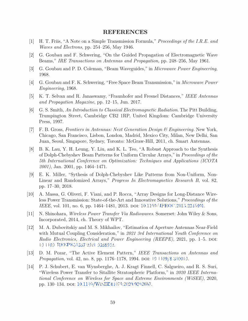
REFERENCES[1] H. T. Friis, “A Note on a Simple Transmission Formula,” Proceedings of the I.R.E. and

Waves and Electrons, pp. 254–256, May 1946.[2] G. Goubau and F. Schwering, “On the Guided Propagation of Electromagnetic Wave

Beams,” IRE Transactions on Antennas and Propagation, pp. 248–256, May 1961.[3] G. Goubau and P. D. Coleman, “Beam Waveguides,” in Microwave Power Engineering,

1968.[4] G. Goubau and F. K. Schwering, “Free Space Beam Transmission,” in Microwave Power

Engineering, 1968.[5] K. T. Selvan and R. Janaswamy, “Fraunhofer and Fresnel Distances,” IEEE Antennas

and Propagation Magazine, pp. 12–15, Jun. 2017.[6] G. S. Smith, An Introduction to Classical Electromagnetic Radiation. The Pitt Building,

Trumpington Street, Cambridge CB2 1RP, United Kingdom: Cambridge UniversityPress, 1997.

[7] F. B. Gross, Frontiers in Antennas: Next Generation Design & Engineering. New York,Chicago, San Francisco, Lisbon, London, Madrid, Mexico City, Milan, New Delhi, SanJuan, Seoul, Singapore, Sydney, Toronto: McGraw-Hill, 2011, ch. Smart Antennas.

[8] B. K. Lau, Y. H. Leung, Y. Liu, and K. L. Teo, “A Robust Approach to the Synthesisof Dolph-Chebyshev Beam Patterns for Uniform Circular Arrays,” in Proceedings of the5th International Conference on Optimization: Techniques and Applications (ICOTA2001), Jan. 2001, pp. 1464–1471.

[9] E. K. Miller, “Sythesis of Dolph-Chebyshev Like Patterns from Non-Uniform, Non-Linear and Randomized Arrays,” Progress In Electromagnetics Research B, vol. 82,pp. 17–30, 2018.

[10] A. Massa, G. Oliveri, F. Viani, and P. Rocca, “Array Designs for Long-Distance Wire-less Power Transmission: State-of-the-Art and Innovative Solutions,” Proceedings of theIEEE, vol. 101, no. 6, pp. 1464–1481, 2013. doi: 10.1109/JPROC.2013.2245491 .

[11] N. Shinohara, Wireless Power Transfer Via Radiowaves. Somerset: John Wiley & Sons,Incorporated, 2014, ch. Theory of WPT.

[12] M. A. Dubovitskiy and M. S. Mikhailov, “Estimation of Aperture Antennas Near-Fieldwith Mutual Coupling Consideration,” in 2021 3rd International Youth Conference onRadio Electronics, Electrical and Power Engineering (REEPE), 2021, pp. 1–5. doi:10.1109/REEPE51337.2021.9388032 .

[13] D. M. Pozar, “The Active Element Pattern,” IEEE Transactions on Antennas andPropagation, vol. 42, no. 8, pp. 1176–1178, 1994. doi: 10.1109/8.310010 .

[14] P. J. Schubert, E. van Wynsberghe, A. J. Kragt Finnell, C. Salgueiro, and R. S. Suri,“Wireless Power Transfer to Sitallite Stratospheric Platform,” in 2020 IEEE Interna-tional Conference on Wireless for Space and Extreme Environments (WiSEE), 2020,pp. 130–134. doi: 10.1109/WiSEE44079.2020.9262657 .

59

[15] A. J. Kragt Finnell and P. J. Schubert, “Antenna Arrangement Verification for LowSidelobe Levels,” in 2019 IEEE International Conference on Wireless for Space andExtreme Environments (WiSEE), 2019, pp. 54–58. doi: 10.1109/WiSEE.2019.8920353 .

[16] A. J. Kragt Finnell, S. H. Powell, P. Heng, and P. J. Schubert, “Spacetenna Flatness andError Correction,” in 2019 IEEE International Conference on Wireless for Space andExtreme Environments (WiSEE), 2019, pp. 48–53. doi: 10.1109/WiSEE.2019.8920300 .

[17] P. J. Schubert, E. van Wynsberghe, A. J. K. Finnell, C. Salgueiro, and R. S. Suri,“Performance Estimates for a Fuel-Free Stationary Platform in the Stratosphere,” IEEERFID, 2021. doi: 10.1109/JRFID.2021.3080509 .

[18] P. Delos, B. Broughton, and J. Kraft, “Phased-Array Antenna Patterns (Part 6)- Side-lobes and Tapering,” Microwaves&RF, 2020.

[19] T. Uno and S. Adachi, “Optimization of Aperture Illumination for Radio Wave PowerTransmission,” IEEE Transactions on Antennas and Propagation, vol. 32, no. 6, pp. 628–632, 1984. doi: 10.1109/TAP.1984.1143372 .

[20] P. Delos, B. Broughton, and J. Kraft, “Phased-Array Antenna Patterns (Part 4)- Grat-ing Lobes,” Microwaves&RF, 2020.

[21] P. Schubert, “Sidelobe Reduction for Geo to Earth Wireless Power Transfer,” in 67thInternational Astronautical Congress (IAC 2016), 2016.

[22] J.-F. Hopperstad and S. Holm, “The Coarray of Sparse Arrays with Minimum SidelobeLevel,” Feb. 1970.

[23] C. I. Coman, I. E. Lager, and L. P. Ligthart, “Design Considerations in Sparse Ar-ray Antennas,” in 2006 European Radar Conference, 2006, pp. 72–75. doi: 10.1109/EURAD.2006.280276 .

[24] S. I. M. Sheikh, A. A. P. Gibson, M. Basorrah, G. Alhulwah, K. Alanizi, M. Alfarsi,and J. Zafar, “Analog/Digital Ferrite Phase Shifter for Phased Array Antennas,” IEEEAntennas and Wireless Propagation Letters, vol. 9, pp. 319–321, 2010.

[25] T. F. Chun, A. Zamora, B. J. Lei, R. T. Iwami, and W. A. Shiroma, “An Interleaved,Interelement Phase-Detecting/ Phase-Shifting Retrodirective Antenna Array for Inter-ference Reduction,” IEEE Antennas and Wireless Propagation Letters, vol. 10, pp. 919–922, 2011.

[26] Q. Zhang, C. Yuan, and L. Liu, “Studies on Mechanical Tunable Waveguide PhaseShifters for Phased-Array Antenna Applications,” in 2016 IEEE International Sympo-sium on Phased Array Systems and Technology, 2016.

[27] Y. C. Guo, X. W. Schi, and L. Chen, “Retrodirective Array Technology,” Progress InElectromagnetics Research B, vol. 5, pp. 153–167, 2008.

[28] B. Derat, “5G Antenna Characterization in the Far-Field: How Close can Far-Field Be?”In 2018 IEEE International Symposium on Electromagnetic Compatibility and 2018IEEE Asia-Pacific Symposium on Electromagnetic Compatibility (EMC/APEMC), May2018, pp. 959–962.

60

[29] Q. Chen, X. Chen, and P. Feng, “A Comparative Study of Space Transmission Efficiencyfor the Microwave Wireless Power Transmission,” in 2015 Asia-Pacific Microwave Con-ference (APMC), Dec. 2016.

[30] R. C. Hansen, J. McSpadden, and J. N. Benford, “A Universal Power Transfer Curve,”IEEE Microwave and Wireless Components Letters, vol. 15, no. 5, pp. 369–371, 2005.doi: 10.1109/LMWC.2005.847718 .

[31] W. C. Brown, “Experiments Involving a Microwave Beam to Power and Position aHelicopter,” IEEE Transactions on Aerospace and Electronic Systems, vol. AES-5,no. 5, pp. 692–702, 1969. doi: 10.1109/TAES.1969.309867 .

[32] R. M. Dickinson and W. C. Brown, “Radiated Microwave Power Transmission SystemEfficiency Measurements,” Jet Propulsion Laboratory, NASA, Pasadena, California,Technical Memorandum 33-727, May 1975.

[33] W. Brown, “Adapting Microwave Techniques to Help Solve Future Energy Problems,”in 1973 IEEE G-MTT International Microwave Symposium, 1973, pp. 189–191. doi:10.1109/GMTT.1973.1123144 .

[34] R. M. Dickinson, “Evaluation of a Microwave High-Power Reception-Conversion Ar-ray for Wireless Power Transmission,” Jet Propulsion Laboratory, NASA, Pasadena,California, Technical Memorandum 33-741, Sep. 1975.

[35] W. Brown. (2017). Dr. William Brown Wireless Power Beaming Tests, Youtube, SSI:Space Studies Institute, [Online]. Available: https://www.youtube.com/watch?v=9angvpwHOy8 (visited on 05/06/2021).

[36] A. J. K. Finnell and P. J. Schubert, “Efficiency Equations for Long-Distance WirelessPower Transfer using Phased Array Antennas,” in C3. IAF Space Power Symposium,Oct. 2020. doi: IAC-20,C3,2,3,x58197 .

[37] J. Mankins, “A Fresh Look at Space Solar Power: New Architectures, Concepts, andTechnologies,” in IAF-97-R.2.03, 38th International Astronautical Federation, 1997,pp. 6–17.

[38] J. Mankins, “A Fresh Look at Space Solar Power,” in IECEC 96. Proceedings of the 31stIntersociety Energy Conversion Engineering Conference, vol. 1, 1996, 451–456 vol.1.doi: 10.1109/IECEC.1996.552925 .

[39] J. A. Vedda and K. L. Jones, “Space-Based Solar Power: A Near-Term InvestmentDecision,” in Center for Space Policy and Strategy, Oct. 2020, pp. 1–12.

[40] G. A. Hazelrigg, “Space-Based Solar Power Conversion and Delivery Systems Study.Volume 3: Economic Analysis of Space-Based Solar Power Systems,” NASA, George C.Marshall Space Flight Center, Princeton, N.J., Technical Memorandum 76-145-2, Jun.1976.

[41] W. C. Brown, “Electronic and Mechanical Improvement of the Receiving Terminal of aFree-Space Microwave Power Transmission System,” NASA, Wayland, Mass., TechnicalMemorandum NASA CR-135194, Aug. 1977.

61

A. MATLAB Code

Attached is some of the MATLAB code used at various points in this work.

The main file is as follows.

1 %THIS IS TO PLOT THE PHASE AT A GIVEN DISTANCE ACROSS AN

ENTIRE FIELD

2 %Functions used in this code: pondProp3D , farFieldSizeCirc ,

farFieldSizeSq

3 %AJ Finnell , 2021

4

5 %constants

6 c = 299792458; %m/s

7 freq = 2.4*10^9; %Hz

8 lambda = c/freq; %m

9 spacing = 800*c/freq; %space between antennas: 0.8*lambda (in

mm)

10

11 %calculation of time required to encompass an entire wave , in

ps

12 maxTime = ceil(10^12/freq) + 10;

13

14 %recieving field setup

15 sizeField = 90; %90x90 tested grid

16 sqSize = 14; %size of each edge; aprox 1/9th lambda spacing

17 hand = figure('position' ,[100,100,600,570]); %handle for

resulting MATLAB figure

18 edgeForPlot = 0:14:14*(sizeField -1); %x and y vector for

plotting

19 edgeForPlot = edgeForPlot - mean(edgeForPlot);

20

62

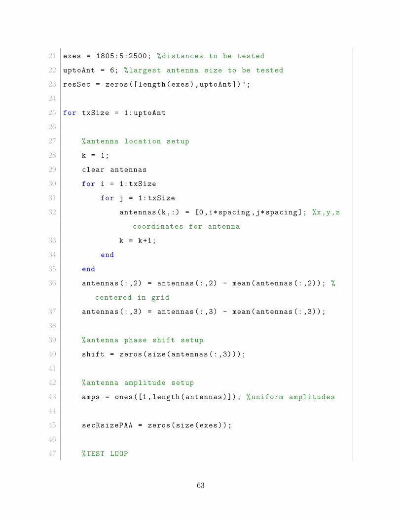
21 exes = 1805:5:2500; %distances to be tested

22 uptoAnt = 6; %largest antenna size to be tested

23 resSec = zeros([length(exes),uptoAnt])';

24

25 for txSize = 1:uptoAnt

26

27 %antenna location setup

28 k = 1;

29 clear antennas

30 for i = 1:txSize

31 for j = 1:txSize

32 antennas(k,:) = [0,i*spacing ,j*spacing]; %x,y,z

coordinates for antenna

33 k = k+1;

34 end

35 end

36 antennas(:,2) = antennas(:,2) - mean(antennas(:,2)); %

centered in grid

37 antennas(:,3) = antennas(:,3) - mean(antennas(:,3));

38

39 %antenna phase shift setup

40 shift = zeros(size(antennas(:,3)));

41

42 %antenna amplitude setup

43 amps = ones([1,length(antennas)]); %uniform amplitudes

44

45 secRsizePAA = zeros(size(exes));

46

47 %TEST LOOP

63

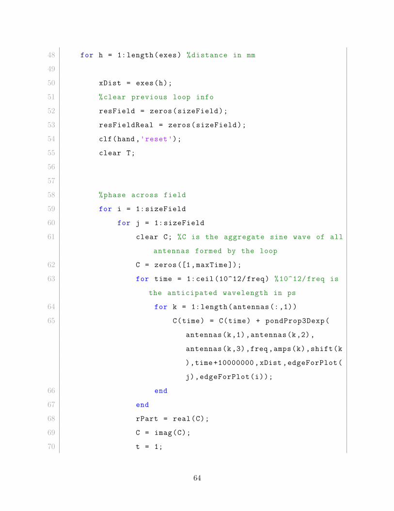
48 for h = 1:length(exes) %distance in mm

49

50 xDist = exes(h);

51 %clear previous loop info

52 resField = zeros(sizeField);

53 resFieldReal = zeros(sizeField);

54 clf(hand ,'reset');

55 clear T;

56

57

58 %phase across field

59 for i = 1:sizeField

60 for j = 1:sizeField

61 clear C; %C is the aggregate sine wave of all

antennas formed by the loop

62 C = zeros([1,maxTime]);

63 for time = 1:ceil(10^12/freq) %10^12/freq is

the anticipated wavelength in ps

64 for k = 1:length(antennas(:,1))

65 C(time) = C(time) + pondProp3Dexp(

antennas(k,1),antennas(k,2),

antennas(k,3),freq ,amps(k),shift(k

),time+10000000,xDist ,edgeForPlot(

j),edgeForPlot(i));

66 end

67 end

68 rPart = real(C);

69 C = imag(C);

70 t = 1;

64

71 while(abs(C(t)-max(C)) > 0.0000001)

72 t = t+1; %find when the max is: phase

shifted to that pt

73 end

74 resField(j,i) = t*freq*2*pi/10^12; %time

shift to radians

75 t = 1;

76 while(abs(rPart(t)-max(rPart)) > 0.0000001)

77 t = t+1; %find when the max is: phase

shifted to that pt

78 end

79 resFieldReal(j,i) = t*freq*2*pi/10^12; %time

shift to radians

80 end

81 end

82

83 %far field points across field

84 T = farFieldSizeCirc(edgeForPlot ,resField);

85 rad = max(T(length(T),1),T(length(T),2));

86 secRsizePAA(hmm) = pi*(rad)^2;

87

88 %to plot circle around FF

89 ang = linspace(0,360)*pi/180;

90 xf = rad.*cos(ang);

91 yf = rad.*sin(ang);

92 zf = 4.5*ones(size(ang));

93

94 %plot results and save figure as jpg

95 %plot phases

65

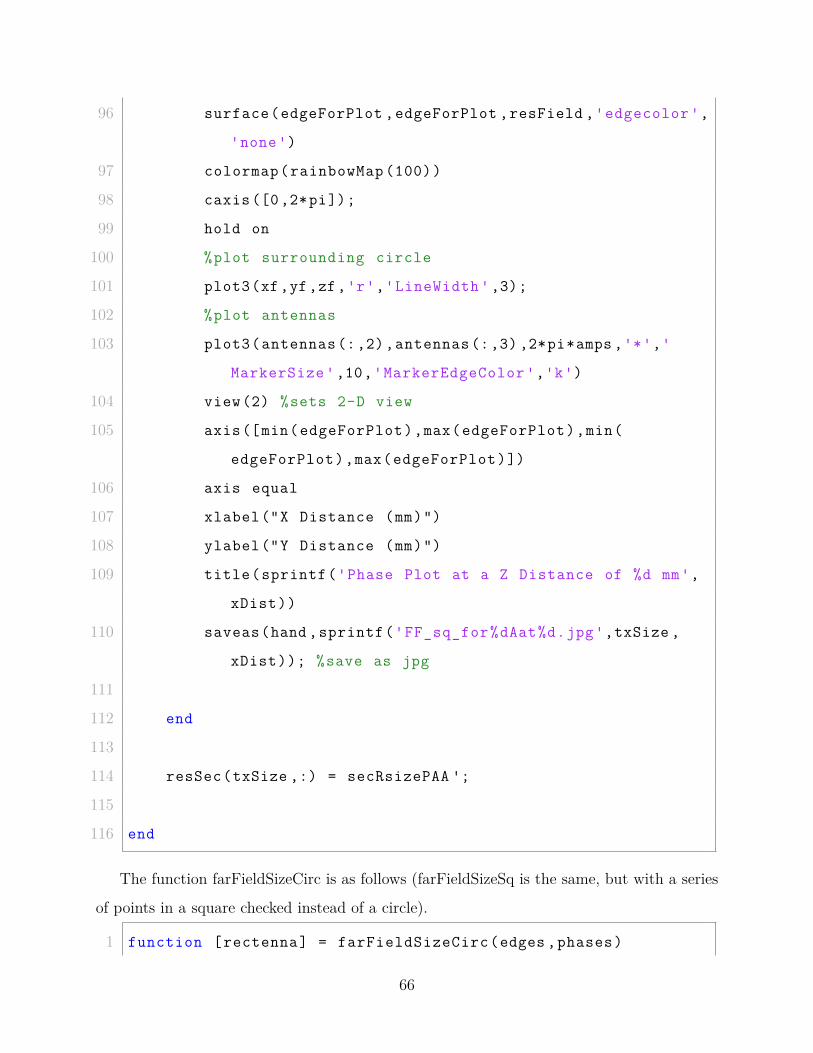
96 surface(edgeForPlot ,edgeForPlot ,resField ,'edgecolor',

'none')

97 colormap(rainbowMap(100))

98 caxis([0,2*pi]);

99 hold on

100 %plot surrounding circle

101 plot3(xf,yf,zf,'r','LineWidth',3);

102 %plot antennas

103 plot3(antennas(:,2),antennas(:,3) ,2*pi*amps ,'*','

MarkerSize',10,'MarkerEdgeColor','k')

104 view(2) %sets 2-D view

105 axis([min(edgeForPlot),max(edgeForPlot),min(

edgeForPlot),max(edgeForPlot)])

106 axis equal

107 xlabel("X Distance (mm)")

108 ylabel("Y Distance (mm)")

109 title(sprintf('Phase Plot at a Z Distance of %d mm',

xDist))

110 saveas(hand ,sprintf('FF_sq_for%dAat%d.jpg',txSize ,

xDist)); %save as jpg

111

112 end

113

114 resSec(txSize ,:) = secRsizePAA ';

115

116 end

The function farFieldSizeCirc is as follows (farFieldSizeSq is the same, but with a series

of points in a square checked instead of a circle).

1 function [rectenna] = farFieldSizeCirc(edges ,phases)

66

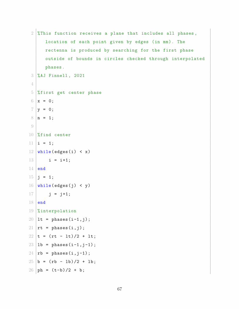
2 %This function receives a plane that includes all phases ,

location of each point given by edges (in mm). The

rectenna is produced by searching for the first phase

outside of bounds in circles checked through interpolated

phases.

3 %AJ Finnell , 2021

4

5 %first get center phase

6 x = 0;

7 y = 0;

8 n = 1;

9

10 %find center

11 i = 1;

12 while(edges(i) < x)

13 i = i+1;

14 end

15 j = 1;

16 while(edges(j) < y)

17 j = j+1;

18 end

19 %interpolation

20 lt = phases(i-1,j);

21 rt = phases(i,j);

22 t = (rt - lt)/2 + lt;

23 lb = phases(i-1,j-1);

24 rb = phases(i,j-1);

25 b = (rb - lb)/2 + lb;

26 ph = (t-b)/2 + b;

67

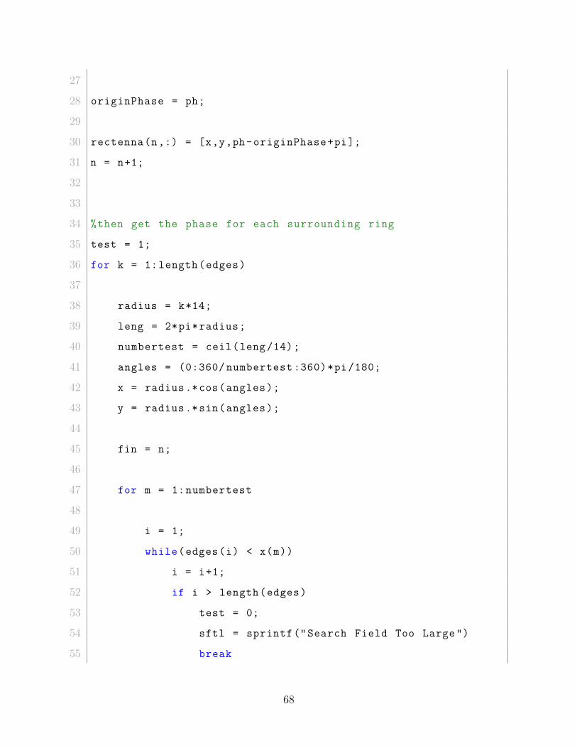
27

28 originPhase = ph;

29

30 rectenna(n,:) = [x,y,ph-originPhase+pi];

31 n = n+1;

32

33

34 %then get the phase for each surrounding ring

35 test = 1;

36 for k = 1:length(edges)

37

38 radius = k*14;

39 leng = 2*pi*radius;

40 numbertest = ceil(leng/14);

41 angles = (0:360/numbertest:360)*pi/180;

42 x = radius.*cos(angles);

43 y = radius.*sin(angles);

44

45 fin = n;

46

47 for m = 1:numbertest

48

49 i = 1;

50 while(edges(i) < x(m))

51 i = i+1;

52 if i > length(edges)

53 test = 0;

54 sftl = sprintf("Search Field Too Large")

55 break

68

56 end

57 end

58

59 j = 1;

60 while(edges(j) < y(m))

61 j = j+1;

62 if j > length(edges)

63 test = 0;

64 sftl = sprintf("Search Field Too Large")

65 break

66 end

67 end

68

69 if test == 0

70 break

71 end

72

73 %interpolation

74 lt = phases(i-1,j);

75 rt = phases(i,j);

76 if lt-rt > pi/2

77 lt = lt - 2*pi;

78 elseif rt-lt > pi/2

79 rt = rt - 2*pi;

80 end

81 t = (rt - lt)*(x(m) - edges(i-1))/(edges(i) - edges(i

-1)) + lt;

82 lb = phases(i-1,j-1);

83 rb = phases(i,j-1);

69

84 if lb-rb > pi/2

85 lb = lb - 2*pi;

86 elseif rb-lb > pi/2

87 rb = rb - 2*pi;

88 end

89 b = (rb - lb)*(x(m) - edges(i-1))/(edges(i) - edges(i

-1)) + lb;

90 if b - t > pi/2

91 b = b - 2*pi;

92 elseif t - b > pi/2

93 t = t - 2*pi;

94 end

95 ph = (t-b)*(y(m) - edges(j-1))/(edges(j) - edges(j-1)

) + b;

96 ph = ph - originPhase+pi;

97 ph = mod(ph,2*pi);

98

99 rectenna(n,:) = [x(m),y(m),ph];

100 n = n+1;

101 end

102

103 %making sure rectenna is in FF

104 if (max(rectenna(:,3)) - min(rectenna(:,3)) > pi/2)

105 rectenna(fin:n-1,:) = [];

106 n = length(rectenna) + 1;

107 test = 0;

108 break

109 end

110

70

111 end

112

113 end

The function pondProp3Dexp is as follows. The 1D and 2D versions were conceptualized

through the ripples propagating in a still pond after stones are dropped in; thus the name

“pondProp”.

1 function [propVals] = pondProp3Dexp(xLoc , yLoc , zLoc , freq ,

amp, phase , time , x0, y0, z0)

2 %This function takes the input values of one patch antenna

source and outputs the propagation , using angleLookup for

the patch antenna distribution.

3 % xLoc: x value of the source origin (mm)

4 % yLoc: y value of the source origin (mm)

5 % zLoc: z value of the source origin (mm)

6 % freq: frequency of the source (hZ)

7 % amp: amplitude of the source

8 % phase: phase shift of the source (rad)

9 % time: time that the source has propagated (ps)

10 % x0: initial x-axis value (mm)

11 % y0: initial y-axis value (mm)

12 % z0: initial z-axis value (mm)

13 %AJ Finnell , 2021

14

15 c = 299792458; %speed of light (m/s)

16

17 %FOR A POINT

18 dist = sqrt((y0-yLoc)^2+(x0-xLoc)^2+(z0-zLoc)^2); %distance

from antenna (x,y,z) to point in question (x0,y0,z0)

71

19 if (dist/(1000*c) > time/10^12) %if it hasn 't reached that

point yet, it's zero

20 propVals = 0;

21 else

22 %find angles for angleLookup

23 if abs(z0) < 0.0000000001

24 phi = 0;

25 else

26 phi = atan(y0/z0)*180/pi;

27 end

28 theta = atan(sqrt(y0^2+z0^2)/x0)*180/pi;

29 mag = angleLookup(phi,theta);

30

31 %propagation calculation

32 propVals = mag*(1000*amp/dist^2)*exp(sqrt(-1)*((2*pi*freq

)*(time/10^12-dist/(1000*c))-phase)); %if it has

reached that point , it's at this amplitude in the

cycle , divided by r^2.

33 end

34

35 end

72

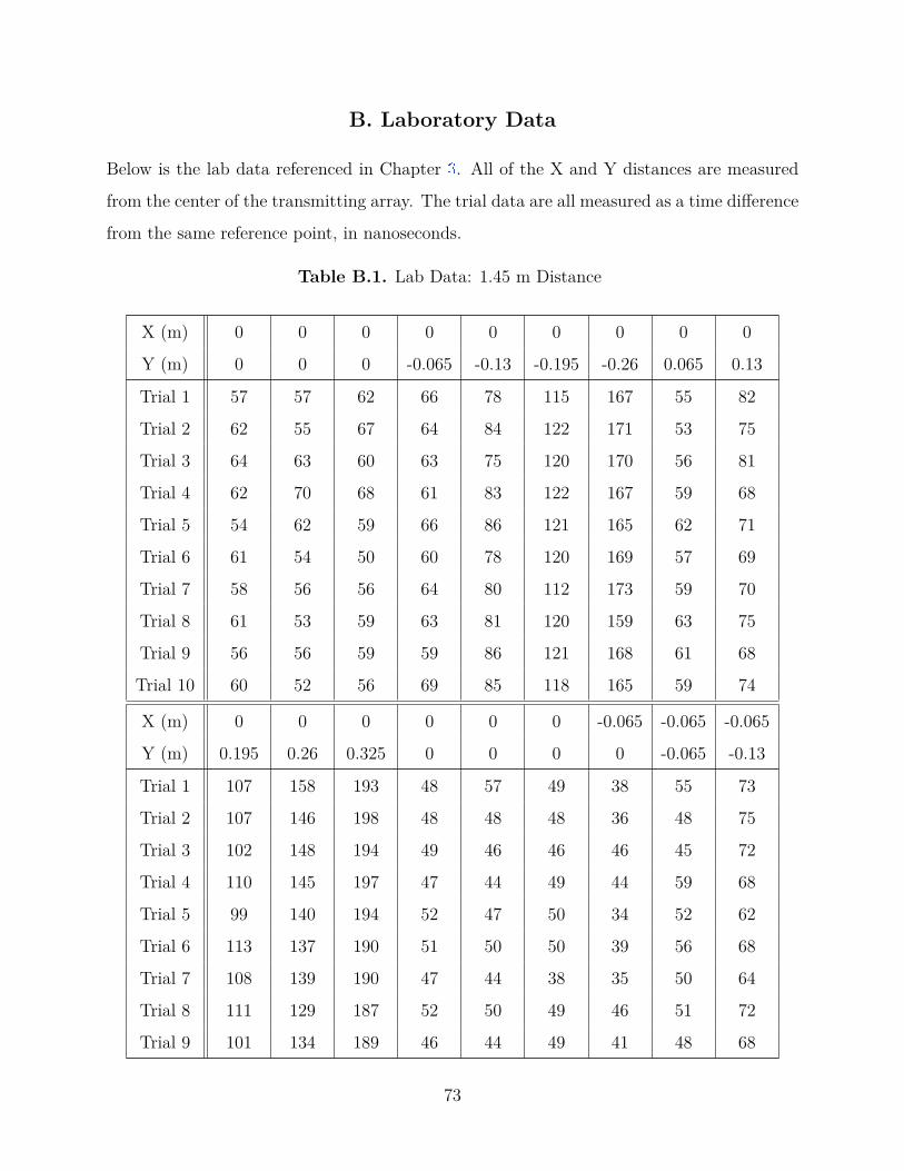
B. Laboratory Data

Below is the lab data referenced in Chapter 3 . All of the X and Y distances are measured

from the center of the transmitting array. The trial data are all measured as a time difference

from the same reference point, in nanoseconds.

Table B.1. Lab Data: 1.45 m Distance

X (m) 0 0 0 0 0 0 0 0 0

Y (m) 0 0 0 -0.065 -0.13 -0.195 -0.26 0.065 0.13

Trial 1 57 57 62 66 78 115 167 55 82

Trial 2 62 55 67 64 84 122 171 53 75

Trial 3 64 63 60 63 75 120 170 56 81

Trial 4 62 70 68 61 83 122 167 59 68

Trial 5 54 62 59 66 86 121 165 62 71

Trial 6 61 54 50 60 78 120 169 57 69

Trial 7 58 56 56 64 80 112 173 59 70

Trial 8 61 53 59 63 81 120 159 63 75

Trial 9 56 56 59 59 86 121 168 61 68

Trial 10 60 52 56 69 85 118 165 59 74

X (m) 0 0 0 0 0 0 -0.065 -0.065 -0.065

Y (m) 0.195 0.26 0.325 0 0 0 0 -0.065 -0.13

Trial 1 107 158 193 48 57 49 38 55 73

Trial 2 107 146 198 48 48 48 36 48 75

Trial 3 102 148 194 49 46 46 46 45 72

Trial 4 110 145 197 47 44 49 44 59 68

Trial 5 99 140 194 52 47 50 34 52 62

Trial 6 113 137 190 51 50 50 39 56 68

Trial 7 108 139 190 47 44 38 35 50 64

Trial 8 111 129 187 52 50 49 46 51 72

Trial 9 101 134 189 46 44 49 41 48 68

73

Table B.1. Lab Data: 1.45 m Distance (Continued)

Trial 10 100 131 194 51 50 47 46 48 68

X (m) -0.065 -0.065 -0.065 -0.065 -0.065 -0.065 -0.065 0 0

Y (m) -0.195 -0.26 0.065 0.13 0.195 0.26 0.325 0 0

Trial 1 113 157 47 68 91 131 190 37 36

Trial 2 120 147 50 62 96 126 195 43 36

Trial 3 117 161 44 65 85 123 191 37 42

Trial 4 109 153 50 68 92 120 193 37 45

Trial 5 111 160 49 62 99 133 191 41 40

Trial 6 110 151 53 60 90 124 192 38 41

Trial 7 117 143 45 66 94 134 188 36 36

Trial 8 114 153 46 67 88 127 187 41 36

Trial 9 113 152 46 65 87 134 193 45 41

Trial 10 113 155 42 59 92 129 191 40 41

X (m) 0 -0.13 -0.13 -0.13 -0.13 -0.13 -0.13 -0.13 -0.13

Y (m) 0 0 -0.065 -0.13 -0.195 -0.26 0.065 0.13 0.195

Trial 1 40 14 12 38 91 134 38 61 97

Trial 2 45 19 23 38 82 128 29 61 92

Trial 3 42 14 20 36 92 131 32 58 83

Trial 4 40 17 26 47 82 130 27 61 84

Trial 5 46 23 20 38 86 139 34 52 88

Trial 6 38 21 36 43 77 130 34 63 95

Trial 7 38 17 18 41 87 137 36 53 90

Trial 8 40 19 25 49 80 130 40 50 85

Trial 9 34 26 19 40 86 132 39 61 97

Trial 10 31 15 25 44 79 139 30 53 89

X (m) -0.13 -0.13 0 0 0 -0.195 -0.195 -0.195 -0.195

Y (m) 0.26 0.325 0 0 0 0 -0.065 -0.13 -0.195

74

Table B.1. Lab Data: 1.45 m Distance (Continued)

Trial 1 150 188 50 47 51 23 32 42 75

Trial 2 141 192 45 45 41 28 41 38 80

Trial 3 151 202 47 47 48 26 26 41 80

Trial 4 146 195 48 44 44 28 27 35 76

Trial 5 137 188 45 43 47 34 34 34 68

Trial 6 143 200 46 39 43 28 31 41 79

Trial 7 134 197 52 51 52 25 28 36 73

Trial 8 146 193 51 45 48 29 35 42 85

Trial 9 145 194 46 45 50 29 34 38 76

Trial 10 150 186 49 47 49 28 31 39 86

X (m) -0.195 -0.195 -0.195 -0.195 -0.195 -0.195 0 0 0

Y (m) -0.26 0.065 0.13 0.195 0.26 0.325 0 0 0

Trial 1 142 37 66 104 152 203 37 38 45

Trial 2 140 47 58 104 153 201 46 43 41

Trial 3 141 37 59 107 152 211 48 39 38

Trial 4 140 39 64 108 148 203 39 50 43

Trial 5 145 38 65 108 155 203 42 50 45

Trial 6 136 38 60 102 148 202 40 45 42

Trial 7 140 39 61 105 154 201 40 45 44

Trial 8 139 45 63 104 154 198 40 44 46

Trial 9 142 39 52 103 152 202 43 42 46

Trial 10 137 42 58 100 147 200 46 49 35

X (m) -0.26 -0.26 -0.26 -0.26 -0.26 -0.26 -0.26 0 0

Y (m) 0 -0.065 -0.13 -0.195 0.065 0.13 0.195 0 0

Trial 1 112 126 125 169 117 138 138 38 44

Trial 2 107 122 132 165 112 137 174 49 47

Trial 3 117 125 138 171 114 133 164 37 51

75

Table B.1. Lab Data: 1.45 m Distance (Continued)

Trial 4 114 121 125 159 125 139 169 45 49

Trial 5 114 128 131 164 121 145 166 40 40

Trial 6 109 127 132 173 116 140 167 38 50

Trial 7 110 126 140 170 120 143 163 39 43

Trial 8 114 127 133 160 111 135 157 39 51

Trial 9 114 127 132 167 111 123 171 41 39

Trial 10 114 119 132 162 119 141 164 40 53

X (m) 0 -0.325 -0.325 -0.325 -0.325 -0.325 -0.39 0.065 0.065

Y (m) 0 0 -0.065 -0.13 0.065 0.13 0 0 -0.065

Trial 1 50 136 136 163 143 161 197 119 128

Trial 2 46 141 145 164 151 164 205 119 136

Trial 3 39 142 135 168 147 162 200 116 135

Trial 4 43 138 140 154 153 156 203 123 131

Trial 5 48 133 136 155 138 153 203 122 136

Trial 6 48 148 143 167 146 159 208 119 131

Trial 7 43 131 138 167 154 161 202 112 128

Trial 8 45 132 135 162 151 156 201 117 133

Trial 9 41 145 138 158 145 157 207 117 127

Trial 10 41 137 142 159 142 157 199 120 140

X (m) 0.065 0.065 0.065 0.065 0.065 0 0 0 0.13

Y (m) -0.13 -0.195 0.065 0.13 0.195 0 0 0 0

Trial 1 138 168 126 147 168 34 36 42 150

Trial 2 140 161 123 142 171 43 45 45 157

Trial 3 133 166 128 143 168 42 46 45 152

Trial 4 134 154 122 145 176 42 37 42 159

Trial 5 142 163 129 157 172 46 42 45 163

Trial 6 132 167 127 142 169 50 50 43 148

76

Table B.1. Lab Data: 1.45 m Distance (Continued)

Trial 7 136 160 139 145 174 43 42 33 154

Trial 8 132 153 123 145 169 42 45 31 146

Trial 9 142 161 125 146 172 44 44 33 161

Trial 10 135 165 127 137 168 41 36 41 147

X (m) 0

Y (m) 0

Trial 1 42

Trial 2 34

Trial 3 50

Trial 4 54

Trial 5 39

Trial 6 37

Trial 7 48

Trial 8 53

Trial 9 47

Trial 10 50

Table B.2. Lab Data: 1.2 m Distance

X (m) 0 0 0 0 0 0 0 0 0

Y (m) 0 -0.065 -0.13 -0.195 -0.26 0.065 0.13 0.195 0.26

Trial 1 11 -4 4 14 46 26 42 85 144

Trial 2 1 -11 3 16 49 22 41 89 148

Trial 3 7 -10 4 17 59 26 43 87 147

Trial 4 -2 -2 3 21 37 30 39 90 141

Trial 5 4 0 3 28 36 28 40 87 148

Trial 6 5 -1 4 26 43 26 44 93 140

Trial 7 2 -12 1 16 50 27 36 84 145

77

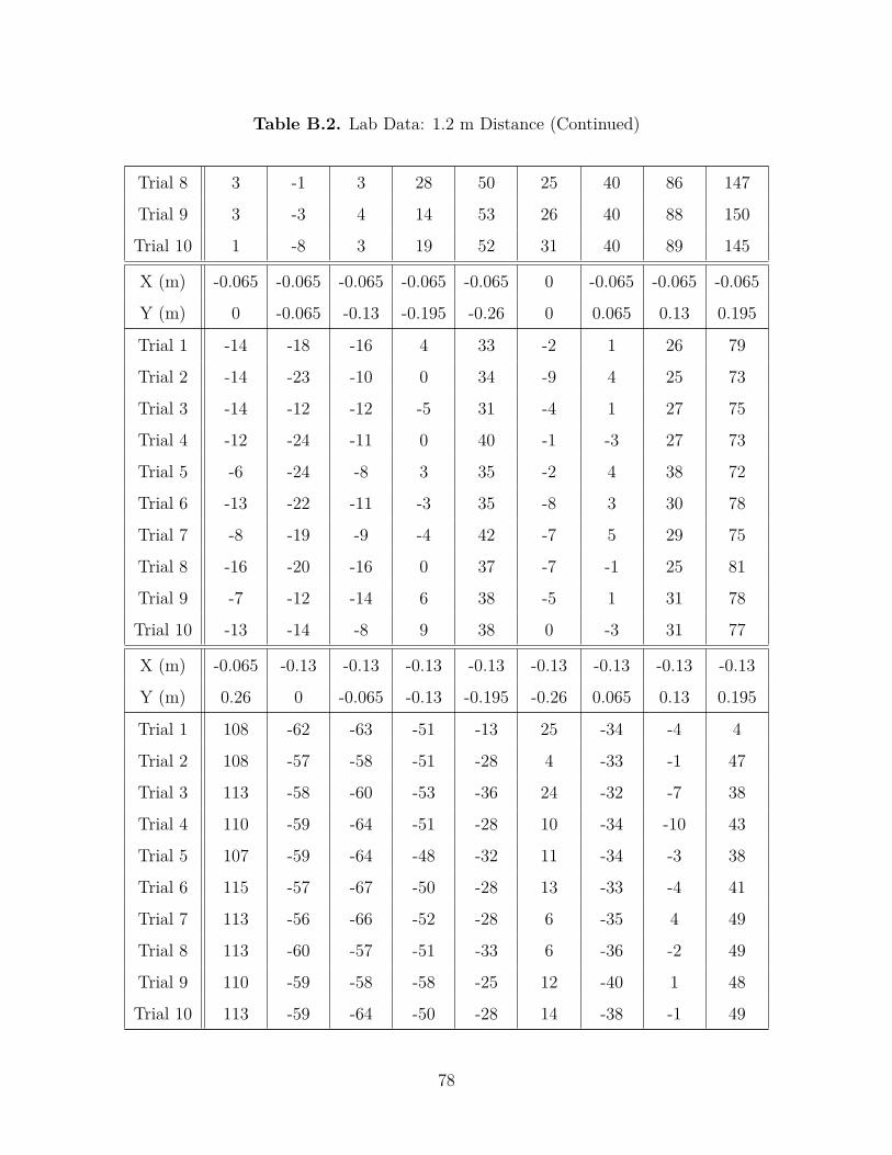
Table B.2. Lab Data: 1.2 m Distance (Continued)

Trial 8 3 -1 3 28 50 25 40 86 147

Trial 9 3 -3 4 14 53 26 40 88 150

Trial 10 1 -8 3 19 52 31 40 89 145

X (m) -0.065 -0.065 -0.065 -0.065 -0.065 0 -0.065 -0.065 -0.065

Y (m) 0 -0.065 -0.13 -0.195 -0.26 0 0.065 0.13 0.195

Trial 1 -14 -18 -16 4 33 -2 1 26 79

Trial 2 -14 -23 -10 0 34 -9 4 25 73

Trial 3 -14 -12 -12 -5 31 -4 1 27 75

Trial 4 -12 -24 -11 0 40 -1 -3 27 73

Trial 5 -6 -24 -8 3 35 -2 4 38 72

Trial 6 -13 -22 -11 -3 35 -8 3 30 78

Trial 7 -8 -19 -9 -4 42 -7 5 29 75

Trial 8 -16 -20 -16 0 37 -7 -1 25 81

Trial 9 -7 -12 -14 6 38 -5 1 31 78

Trial 10 -13 -14 -8 9 38 0 -3 31 77

X (m) -0.065 -0.13 -0.13 -0.13 -0.13 -0.13 -0.13 -0.13 -0.13

Y (m) 0.26 0 -0.065 -0.13 -0.195 -0.26 0.065 0.13 0.195

Trial 1 108 -62 -63 -51 -13 25 -34 -4 4

Trial 2 108 -57 -58 -51 -28 4 -33 -1 47

Trial 3 113 -58 -60 -53 -36 24 -32 -7 38

Trial 4 110 -59 -64 -51 -28 10 -34 -10 43

Trial 5 107 -59 -64 -48 -32 11 -34 -3 38

Trial 6 115 -57 -67 -50 -28 13 -33 -4 41

Trial 7 113 -56 -66 -52 -28 6 -35 4 49

Trial 8 113 -60 -57 -51 -33 6 -36 -2 49

Trial 9 110 -59 -58 -58 -25 12 -40 1 48

Trial 10 113 -59 -64 -50 -28 14 -38 -1 49

78

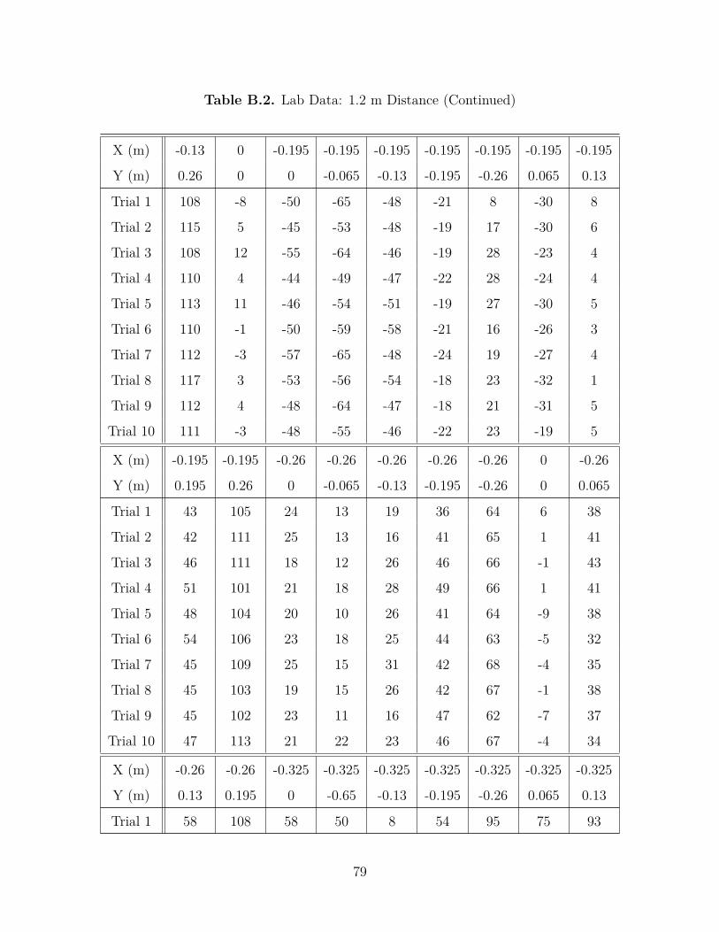
Table B.2. Lab Data: 1.2 m Distance (Continued)

X (m) -0.13 0 -0.195 -0.195 -0.195 -0.195 -0.195 -0.195 -0.195

Y (m) 0.26 0 0 -0.065 -0.13 -0.195 -0.26 0.065 0.13

Trial 1 108 -8 -50 -65 -48 -21 8 -30 8

Trial 2 115 5 -45 -53 -48 -19 17 -30 6

Trial 3 108 12 -55 -64 -46 -19 28 -23 4

Trial 4 110 4 -44 -49 -47 -22 28 -24 4

Trial 5 113 11 -46 -54 -51 -19 27 -30 5

Trial 6 110 -1 -50 -59 -58 -21 16 -26 3

Trial 7 112 -3 -57 -65 -48 -24 19 -27 4

Trial 8 117 3 -53 -56 -54 -18 23 -32 1

Trial 9 112 4 -48 -64 -47 -18 21 -31 5

Trial 10 111 -3 -48 -55 -46 -22 23 -19 5

X (m) -0.195 -0.195 -0.26 -0.26 -0.26 -0.26 -0.26 0 -0.26

Y (m) 0.195 0.26 0 -0.065 -0.13 -0.195 -0.26 0 0.065

Trial 1 43 105 24 13 19 36 64 6 38

Trial 2 42 111 25 13 16 41 65 1 41

Trial 3 46 111 18 12 26 46 66 -1 43

Trial 4 51 101 21 18 28 49 66 1 41

Trial 5 48 104 20 10 26 41 64 -9 38

Trial 6 54 106 23 18 25 44 63 -5 32

Trial 7 45 109 25 15 31 42 68 -4 35

Trial 8 45 103 19 15 26 42 67 -1 38

Trial 9 45 102 23 11 16 47 62 -7 37

Trial 10 47 113 21 22 23 46 67 -4 34

X (m) -0.26 -0.26 -0.325 -0.325 -0.325 -0.325 -0.325 -0.325 -0.325

Y (m) 0.13 0.195 0 -0.65 -0.13 -0.195 -0.26 0.065 0.13

Trial 1 58 108 58 50 8 54 95 75 93

79

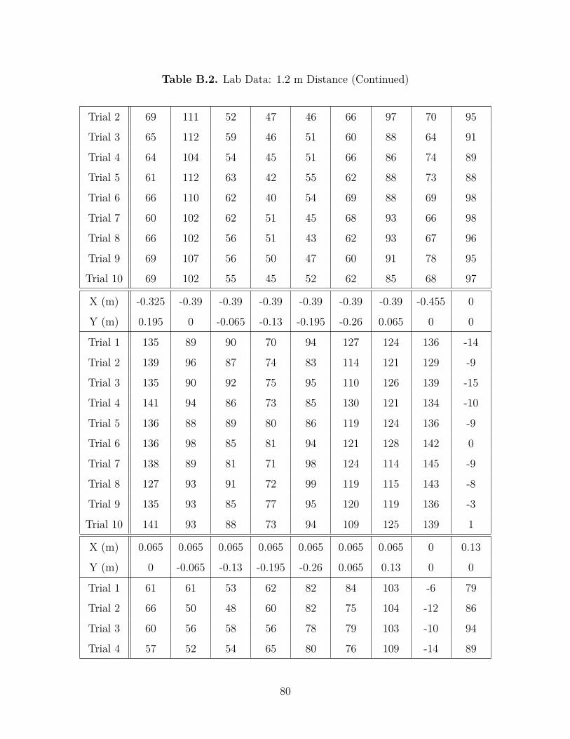
Table B.2. Lab Data: 1.2 m Distance (Continued)

Trial 2 69 111 52 47 46 66 97 70 95

Trial 3 65 112 59 46 51 60 88 64 91

Trial 4 64 104 54 45 51 66 86 74 89

Trial 5 61 112 63 42 55 62 88 73 88

Trial 6 66 110 62 40 54 69 88 69 98

Trial 7 60 102 62 51 45 68 93 66 98

Trial 8 66 102 56 51 43 62 93 67 96

Trial 9 69 107 56 50 47 60 91 78 95

Trial 10 69 102 55 45 52 62 85 68 97

X (m) -0.325 -0.39 -0.39 -0.39 -0.39 -0.39 -0.39 -0.455 0

Y (m) 0.195 0 -0.065 -0.13 -0.195 -0.26 0.065 0 0

Trial 1 135 89 90 70 94 127 124 136 -14

Trial 2 139 96 87 74 83 114 121 129 -9

Trial 3 135 90 92 75 95 110 126 139 -15

Trial 4 141 94 86 73 85 130 121 134 -10

Trial 5 136 88 89 80 86 119 124 136 -9

Trial 6 136 98 85 81 94 121 128 142 0

Trial 7 138 89 81 71 98 124 114 145 -9

Trial 8 127 93 91 72 99 119 115 143 -8

Trial 9 135 93 85 77 95 120 119 136 -3

Trial 10 141 93 88 73 94 109 125 139 1

X (m) 0.065 0.065 0.065 0.065 0.065 0.065 0.065 0 0.13

Y (m) 0 -0.065 -0.13 -0.195 -0.26 0.065 0.13 0 0

Trial 1 61 61 53 62 82 84 103 -6 79

Trial 2 66 50 48 60 82 75 104 -12 86

Trial 3 60 56 58 56 78 79 103 -10 94

Trial 4 57 52 54 65 80 76 109 -14 89

80

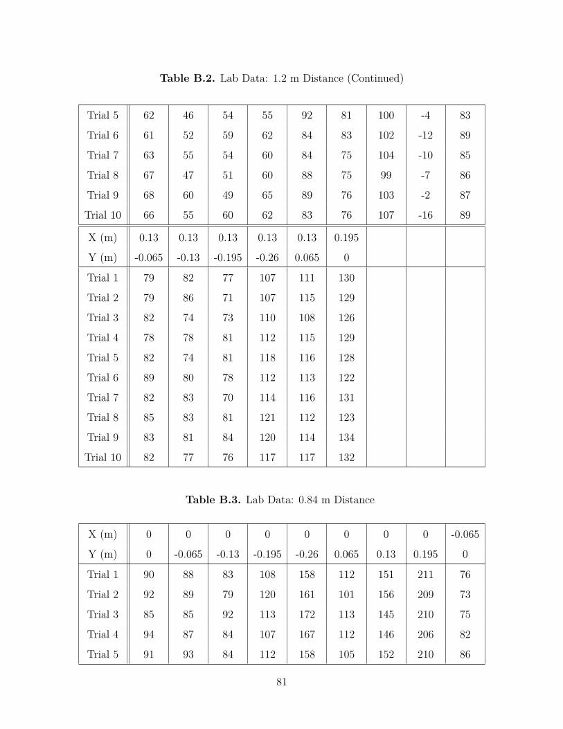
Table B.2. Lab Data: 1.2 m Distance (Continued)

Trial 5 62 46 54 55 92 81 100 -4 83

Trial 6 61 52 59 62 84 83 102 -12 89

Trial 7 63 55 54 60 84 75 104 -10 85

Trial 8 67 47 51 60 88 75 99 -7 86

Trial 9 68 60 49 65 89 76 103 -2 87

Trial 10 66 55 60 62 83 76 107 -16 89

X (m) 0.13 0.13 0.13 0.13 0.13 0.195

Y (m) -0.065 -0.13 -0.195 -0.26 0.065 0

Trial 1 79 82 77 107 111 130

Trial 2 79 86 71 107 115 129

Trial 3 82 74 73 110 108 126

Trial 4 78 78 81 112 115 129

Trial 5 82 74 81 118 116 128

Trial 6 89 80 78 112 113 122

Trial 7 82 83 70 114 116 131

Trial 8 85 83 81 121 112 123

Trial 9 83 81 84 120 114 134

Trial 10 82 77 76 117 117 132

Table B.3. Lab Data: 0.84 m Distance

X (m) 0 0 0 0 0 0 0 0 -0.065

Y (m) 0 -0.065 -0.13 -0.195 -0.26 0.065 0.13 0.195 0

Trial 1 90 88 83 108 158 112 151 211 76

Trial 2 92 89 79 120 161 101 156 209 73

Trial 3 85 85 92 113 172 113 145 210 75

Trial 4 94 87 84 107 167 112 146 206 82

Trial 5 91 93 84 112 158 105 152 210 86

81

Table B.3. Lab Data: 0.84 m Distance (Continued)

Trial 6 91 93 77 114 170 111 152 202 87

Trial 7 88 88 90 109 173 109 149 212 78

Trial 8 88 89 86 110 165 104 146 210 79

Trial 9 95 98 92 113 163 109 153 213 81

Trial 10 89 83 90 118 164 113 146 204 80

X (m) -0.065 -0.065 -0.065 -0.065 -0.065 -0.065 -0.065 0 -0.13

Y (m) -0.065 -0.13 -0.195 -0.26 0.065 0.13 0.195 0 0

Trial 1 79 82 108 159 112 143 214 80 61

Trial 2 91 80 107 159 104 142 206 75 55

Trial 3 91 81 109 160 113 151 209 88 64

Trial 4 86 84 103 156 108 141 208 89 65

Trial 5 85 79 106 164 105 140 214 93 67

Trial 6 81 82 105 167 108 147 212 77 61

Trial 7 84 82 110 156 112 151 221 79 62

Trial 8 83 85 106 165 106 143 212 84 55

Trial 9 81 80 112 162 117 146 212 83 57

Trial 10 90 82 103 158 108 138 205 84 58

X (m) -0.13 -0.13 -0.13 -0.13 -0.13 -0.13 -0.13 -0.13 -0.195

Y (m) -0.065 -0.13 -0.195 -0.26 0.065 0.13 0.195 0.26 0

Trial 1 56 52 83 139 88 137 179 278 87

Trial 2 46 56 80 144 94 130 172 277 74

Trial 3 51 55 101 141 93 133 173 286 74

Trial 4 55 58 87 139 86 125 170 288 87

Trial 5 55 61 83 136 91 127 174 283 80

Trial 6 52 56 91 145 89 131 178 282 79

Trial 7 56 56 92 138 90 133 184 288 76

Trial 8 55 53 91 137 94 126 175 290 80

82

Table B.3. Lab Data: 0.84 m Distance (Continued)

Trial 9 54 51 88 138 90 131 177 281 82

Trial 10 50 49 85 145 88 132 186 277 71

X (m) -0.195 -0.195 -0.195 -0.195 -0.195 -0.195 -0.195 0 -0.26

Y (m) -0.065 -0.13 -0.195 -0.26 0.065 0.13 0.195 0 0

Trial 1 74 77 107 174 108 141 214 83 169

Trial 2 72 70 109 181 106 146 208 71 168

Trial 3 69 71 103 172 110 143 215 81 168

Trial 4 70 70 108 177 105 137 215 80 168

Trial 5 69 69 98 173 108 145 219 81 172

Trial 6 68 79 97 174 102 149 211 86 180

Trial 7 60 80 100 173 102 142 216 90 179

Trial 8 65 72 98 175 107 145 212 80 173

Trial 9 66 76 105 170 106 148 214 82 175

Trial 10 60 78 95 177 103 147 221 82 170

X (m) -0.26 -0.26 -0.26 -0.26 -0.325 0 0.065 0.065 0.065

Y (m) -0.065 -0.13 -0.195 0.065 0 0 0 -0.065 -0.13

Trial 1 171 172 206 195 252 89 145 141 140

Trial 2 164 170 190 193 265 85 149 136 137

Trial 3 162 163 190 196 259 82 148 129 134

Trial 4 173 163 192 199 260 86 141 132 135

Trial 5 167 169 199 194 256 80 148 129 133

Trial 6 167 167 201 198 255 84 144 140 141

Trial 7 163 169 199 195 257 95 147 143 137

Trial 8 165 169 192 192 261 86 148 136 130

Trial 9 168 173 196 188 259 84 148 139 140

Trial 10 164 174 195 198 264 85 152 130 130

X (m) 0.065 0.065 0.065 0.065 0 0.13 0.13 0.13 0.13

83

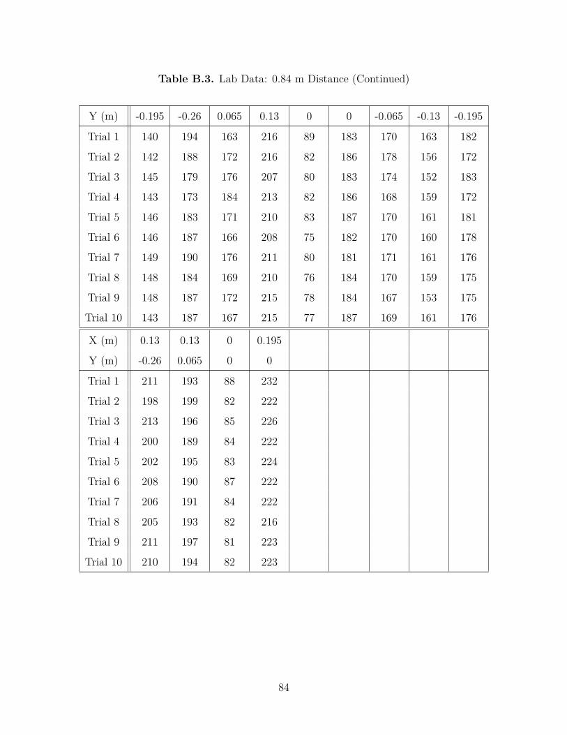
Table B.3. Lab Data: 0.84 m Distance (Continued)

Y (m) -0.195 -0.26 0.065 0.13 0 0 -0.065 -0.13 -0.195

Trial 1 140 194 163 216 89 183 170 163 182

Trial 2 142 188 172 216 82 186 178 156 172

Trial 3 145 179 176 207 80 183 174 152 183

Trial 4 143 173 184 213 82 186 168 159 172

Trial 5 146 183 171 210 83 187 170 161 181

Trial 6 146 187 166 208 75 182 170 160 178

Trial 7 149 190 176 211 80 181 171 161 176

Trial 8 148 184 169 210 76 184 170 159 175

Trial 9 148 187 172 215 78 184 167 153 175

Trial 10 143 187 167 215 77 187 169 161 176

X (m) 0.13 0.13 0 0.195

Y (m) -0.26 0.065 0 0

Trial 1 211 193 88 232

Trial 2 198 199 82 222

Trial 3 213 196 85 226

Trial 4 200 189 84 222

Trial 5 202 195 83 224

Trial 6 208 190 87 222

Trial 7 206 191 84 222

Trial 8 205 193 82 216

Trial 9 211 197 81 223

Trial 10 210 194 82 223

84