UNCORRECTEDPROOF

JrnlID 10950_ArtID 9217_Proof# 1 - 11/11/10

J SeismolDOI 10.1007/s10950-010-9217-4

ORIGINAL ARTICLE

Rapid directivity detection by azimuthal amplitudespectra inversion

Simone Cesca · Sebastian Heimann ·Torsten Dahm

Received: 24 February 2010 / Accepted: 4 November 2010© Springer Science+Business Media B.V. 2010

Abstract An early detection of the presence of1

rupture directivity plays a major role in the correct2

estimation of ground motions and risks associated3

to the earthquake occurrence. We present here4

a simple method for a fast detection of rupture5

directivity, which may be additionally used to6

discriminate fault and auxiliary planes and have7

first estimations of important kinematic source8

parameters, such as rupture length and rupture9

time. Our method is based on the inversion of10

amplitude spectra from P-wave seismograms to11

derive the apparent duration at each station and12

on the successive modelling of its azimuthal be-13

haviour. Synthetic waveforms are built assuming a14

spatial point source approximation, and the finite15

apparent duration of the spatial point source is16

interpreted in terms of rupture directivity. Since17

synthetic seismograms for a point source are cal-18

culated very quickly, the presence of directivity19

may be detected within few seconds, once a focal20

mechanism has been derived. The method is here21

first tested using synthetic datasets, both for lin-22

ear and planar sources, and then successfully ap-23

plied to recent Mw 6.2–6.8 shallow earthquakes in24

Peloponnese, Greece. The method is suitable for25

S. Cesca (B) · S. Heimann · T. DahmInstitut für Geophysik, Universität Hamburg,Bundesstrasse 55, 20146 Hamburg, Germanye-mail: simone.cesca@zmaw.de

automated application and may be used to im- 26

prove kinematic waveform modelling approaches. 27

28

Keywords Directivity · Earthquake source · 29

Kinematic model · Amplitude spectra 30

1 Introduction 31

Tectonically driven shallow earthquake sources 32

are generally explained by means of shear cracks 33

occurring along a limited, almost planar region, 34

we refer as the focal region. A point source repre- 35

sentation is a common first approximation, which 36

is valid when treating far-field low frequency seis- 37

mic waveform, using wavelengths larger than the 38

rupture size. Higher frequencies seismograms and 39

spectra contain information which can be related 40

to the finiteness of the rupture process and thus 41

can be used to determine parameters describing 42

the finite source. Size and shape of the rupture 43

area, rupture velocity and preferential rupture 44

directions, an effect known as rupture directivity, 45

are some of the parameters which can be retrieved 46

by the analysis of high-frequency waveforms. In 47

particular, we are interested here in discussing the 48

problem of early detection of rupture directiv- 49

ity, distinguishing between a prominent or partial 50

unilateral rupture (a case which will be further 51

referred as asymmetric bilateral rupture), and a 52

UNCORRECTEDPROOF

JrnlID 10950_ArtID 9217_Proof# 1 - 11/11/10

J Seismol

bilateral one, with rupture nucleating at the centre53

of the rupture area and propagating toward its54

edges. The azimuthal dependency of amplitudes55

and durations of different seismic phases is a first56

indicator of directivity effects and is consequence57

of the characteristics of the finite rupture process58

along the fault plane, specifically the main di-59

rection and speed of the rupture front propaga-60

tion. Directivity has been often observed and has61

been modelled for several earthquakes in the past,62

with several studies treating specific earthquakes63

or limited datasets (e. g., McGuire et al. 2002;64

Warren and Shearer 2006; Caldeira et al. 2009). A65

quick detection of directivity effects is important66

towards a correct estimation of ground motions,67

stress field perturbations and tsunamogenic risks68

and consequently to mitigate earthquake effects.69

These considerations provide important reasons70

to further investigate and develop specific tools71

for stable, rapid and automated directivity de-72

tection, which can be used within early warning73

systems.74

Several methods have been applied in the past75

to detect and classify earthquake source direc-76

tivity. A common approach is the identification77

of predominant unilateral ruptures from the time78

duration and spectral analysis of body wave pulses79

(e.g. Boore and Joyner 1978; Beck et al. 1995;80

Warren and Shearer 2006; Caldeira et al. 2009).81

Pulse lengths at different stations are interpreted82

in terms of the apparent duration of the source83

time function (STF), and their variation in depen-84

dence on azimuth and incidence angle is inter-85

preted to detect directivity: similarly to a Doppler86

effect in classical physics, shorter STFs would in-87

dicate a rupture propagating towards the consid-88

ered station, while longer pulses indicate a rupture89

propagation in the opposite direction. Directiv-90

ity effects may also be revealed based on the91

analysis of surface waves at different azimuths92

(Ben-Menahem 1961; Pro et al. 2007). Whereas93

time domain methods remain more common, a94

significant contribution within this type of inver-95

sion methods was provided by the spectral ap-96

proach discussed in Warren and Shearer (2006).97

This method is based on the spectral estimation98

of the pulse broadening and accounts for the az-99

imuthal and incidence angle dependencies; it is100

well suited for the analysis of intermediate and101

deep focus earthquakes and was successfully ap- 102

plied to several events. The main limits of this 103

class of methods are related to the fact that wave 104

propagation and the superposition of different 105

seismic phases are not accounted, since wave 106

propagation effects between source and receiver 107

(Green’s functions) are limited to the estimation 108

of the incidence angle of given seismic phases. 109

Another possible limitation is the requirement of 110

several stations with good azimuthal coverage in 111

order to ensure reliable results. A second range 112

of applications, which on the contrary accounts 113

precisely for the effects of the earth’s model on 114

the observed waveforms, is based on empirical 115

Green’s functions technique (Hartzell 1978; Li 116

and Toksöz 1993; Velasco et al. 1994; Cassidy 117

1995; Müller 1985; Velasco et al. 2004; Vallée 118

2007). In this case, an aftershock with common 119

hypocenter and focal mechanism of the studied 120

event can be used to remove path effects, and iso- 121

late finite source apparent durations at different 122

stations. Evidently, the application of these tech- 123

niques is strongly limited by the availability of 124

a proper aftershock. Brüstle and Müller (1987), 125

and Imanishi and Takeo (2002) have investigated 126

the adoption of master-event techniques to detect 127

directivity: the identification of stopping phases 128

(Madariaga 1977, 1983; Bernard and Madariaga 129

1984; Spudich and Frazer 1984) at different sta- 130

tions was used there to determine the main di- 131

rection of rupture propagation, besides other 132

source properties. Stopping phases identification 133

(Imanishi and Takeo 1998, 2002) typically re- 134

quires a careful waveform analysis, which may be 135

hardly implemented within automated routines. 136

A third group of techniques are based on com- 137

plete kinematic waveform inversion, with the aim 138

of retrieving a most detailed image of the finite 139

rupture process, not limited to the identification 140

of directivity. The range of methods and appli- 141

cations is very wide, including higher order mo- 142

ment tensor analysis (Dahm and Krüger 1999; 143

McGuire et al. 2001, 2002), detailed slip map 144

approaches (e.g. Olson and Apsel 1982; Hartzell 145

and Helmberger 1982; Hartzell and Heaton 1983; 146

Beroza and Spudich 1988), and inversion meth- 147

ods adopting constrained and simplified kinematic 148

models (Dreger and Kaverina 2000; Vallée and 149

Bouchon 2004; Gallovic et al. 2009; Cesca et al. 150

UNCORRECTEDPROOF

JrnlID 10950_ArtID 9217_Proof# 1 - 11/11/10

J Seismol

2010). All these methods have a significant poten-151

tial for a stable determination of directivity but152

their adoption towards its very fast detection is153

limited, often requiring time consuming computa-154

tion of synthetic seismograms for several extended155

source models. Methods developed by Dreger and156

Kaverina (2000) and following Cesca et al. (2010)157

have shown a good performance and have been158

tested for near real-time applications, but they are159

still based on extended source representations and160

thus require heavier computations with respect to161

our method. Finally, recent results by Zahradnik162

et al. (2008) showed the possibility of discrimi-163

nating the true fault plane on the base of spatial164

offsets between epicentre and centroid locations.165

However, the method has been currently applied166

only to a limited number of earthquakes, with167

variable results, and the determination of directiv-168

ity may be beyond its possibilities, for example for169

symmetric bilateral ruptures.170

We present here a simple alternative method to171

quickly detect directivity for shallow earthquakes172

and discuss it with the aid of a set of applica-173

tions, including both synthetic datasets and obser-174

vations from recent earthquakes in Greece. Our175

method is based on a point source representation,176

which drastically reduces computational require-177

ments and makes it feasible for early detection.178

Directivity is detected on the basis of a frequency179

domain inversion of the apparent duration at180

each station and the further interpretation of its181

azimuthal variation. Main strength points of the182

proposed method include the adoption of a com-183

mon dataset and modelling tools for focal mech-184

anism and directivity determination, the inclusion185

of Green’s functions accounting for wave propa-186

gation through the chosen earth models without187

needing specific aftershocks, and the simplicity188

and quickness of the inversion process.189

2 Directivity and amplitude spectra inversion190

We make here use of the recently developed191

Kiwi tools (Heimann 2010; Cesca et al. 2010;192

http://kinherd.org), which provide a flexible in-193

strument to generate synthetic seismograms for194

point and extended sources and to invert different195

earthquake source parameters, allowing the se-196

lection of different waveform tapers, frequency 197

filters, inversion domains and misfit functions. 198

Cesca et al. (2010) showed successful applications 199

to shallow earthquake at regional distances, and 200

was able to derive both point source (best double 201

couple, DC, model, scalar moment and centroid 202

depth) and extended source (fault plane discrim- 203

ination, rupture size, rupture time, rupture nucle- 204

ation) parameters. 205

The first inversion step follows the approach 206

described in Cesca et al. (2010), to obtain the focal 207

mechanism, scalar moment and centroid depth: 208

1. Focal mechanism. We invert amplitude spec- 209

tra of full waveforms, according to Cesca et al. 210

(2010), to derive a point source focal mech- 211

anism (DC, depth and scalar moment); the 212

source epicentral location is assumed to be 213

originally known. 214

2. Polarities. The focal mechanism presents a 215

polarity ambiguity, which can be solved by 216

comparing observed displacements and syn- 217

thetic seismograms for the two possible polar- 218

ity configurations; however, the detection of 219

the true polarity is here not strictly required, 220

as the whole inversion process is carried out 221

in the frequency domain, and only amplitude 222

spectra are involved in the fitting procedure. 223

The source representation through the Kiwi tools 224

allows the adoption of different rise times. For a 225

spatially extended source model, where the rup- 226

ture region is discretised into a number of spatial 227

point sources, the rise time represent the time 228

during which each point source radiates seismic 229

energy. The duration of the whole rupture process 230

is related to rise and rupture times. If we adopt 231

a point source representation, the rise time will 232

represent the duration of the source time function. 233

This parameter was used in Cesca et al. (2010) 234

to have a first, rough, estimate of rupture times 235

and to choose a proper rise time during kinematic 236

source modelling. We proceed here differently: in- 237

stead of determining true duration of the rupture 238

process, we investigate apparent durations as seen 239

by individual stations. 240

In detail, during the second inversion step, we 241

proceed as follows (Fig. 1 illustrates an example 242

of the main steps, relative to selected seismic 243

UNCORRECTEDPROOF

JrnlID 10950_ArtID 9217_Proof# 1 - 11/11/10

J Seismol

DIVS, Serbia, Epic. distance: 699km, Azimuth: -11°

MATE, Italy, Epic. distance: 521km, Azimuth: -53°

WDD, Malta, Epic. distance 674km, Azimuth: -108°

E

N

Z

E

N

Z

E

N

Z

Time [s]30 150 Freq [Hz]0.0 0.5 App.Duration [s]

Mis

fit (

L2 )

0.3

1.0

0 12

Time [s]30 150 Freq [Hz]0.0 0.5 App.Duration [s]

Mis

fit (

L2 )

0.3

1.0

0 12

Time [s]30 60 90 120 150

Freq [Hz]0.0 0.1 0.2 0.3 0.4 0.5

App.Duration [s]0 2 4 6 8 10 12

Mis

fit (

L2 )0.3

1.0

Dis

plac

emen

ts, A

max

1.5

8mm

Dis

plac

emen

ts, A

max

3.2

3mm

Dis

plac

emen

ts, A

max

1.4

3mm

Am

pl.S

pec.

, Am

ax 4

.97m

m/H

zA

mpl

.Spe

c., A

max

4.0

2mm

/Hz

Am

pl.S

pec.

, Am

ax 4

.80m

m/H

z

1.5s

4.0s

8.5s

Fig. 1 Example of the procedure followed to derive theapparent source duration at different stations. Selectedwaveforms, spectra and amplitude spectra inversion re-sults refer to an application to the Andravida earthquake,Greece, which is further extensively discussed in this study.Left: filtered displacements (black lines) and synthetic seis-mograms (red lines) for the chosen point source model are

tapered to select P waves time windows (grey intervals).Centre: amplitude spectra comparison (red lines corre-spond to the best fitting synthetic spectra, after comparingseveral source durations). Right: comparison of amplitudespectra misfit values for different source durations (bestsolutions for each station are identified by red circles)

waveforms from the Andravida earthquake,244

which is later discussed in the text):245

1. Waveform selection. We use all available spa-246

tial components, preferably using North, East247

and vertical orientations, rather than rotated 248

traces, in order to have P wave energy on all 249

traces (which is theoretically null on transver- 250

sal components); the presence of more traces 251

for each station has a smoothing effect; after 252

UNCORRECTEDPROOF

JrnlID 10950_ArtID 9217_Proof# 1 - 11/11/10

J Seismol

testing with different datasets, we found that253

more components provide more stability. We254

perform a deconvolution of the instrumental255

response from the data, and conversion to256

displacements.257

2. Tapering. We limit the inversion process to P-258

wave time windows, which are automatically259

selected on the base of the source-receiver260

geometry and theoretical arrival time for the261

earth model used during the inversion (an ar-262

rival time database is calculated in advance, to263

reduce computational effort at the time of the264

inversion); for the case studies here described265

we use 60 s length time windows, starting 15 s266

before theoretical first P arrival, and apply267

a bandpass filter in the range 0.01–0.5 Hz268

(these parameters may be modified depending269

on the earthquake size, the source depth, the270

average duration, and the range of epicen-271

tral distances where waveforms are inverted).272

Tapers should be chosen in order to resolve273

directivity effects. A minimum length should274

account at least for two times the average rup-275

ture duration and for different periods at the276

frequency range used for the inversion. For277

stations located at small epicentral distances,278

with minor delay between S and P phases,279

tapers may be modified to avoid S waves.280

3. Scalar moment inversion. Since the estima-281

tion of the scalar moment may slightly vary282

depending on the inversion approach (e.g.,283

full waveform or body waves, time domain or284

amplitude spectra inversion, etc.), we mention285

here the possibility to perform a specific in-286

version using an approach consistent with the287

following directivity inversion. Traces from288

all seismic stations would be used to invert289

the scalar moment (e.g. by amplitude spectra290

inversion, using a Levenberg–Marquardt ap-291

proach and an L2 norm misfit function). In292

the following applications this step is not per-293

formed, as we count with stable estimations of294

the scalar moments, provided by the fit of low295

frequency amplitude spectra from the whole296

waveforms.297

4. Apparent duration inversion. For each of the298

stations, we perform an amplitude spectra in-299

version to derive the apparent source duration300

at that station; the frequency domain inver-301

sion approach is less sensitive to unmodelled 302

structural heterogeneities; we perform here 303

a grid search for possible durations (for the 304

following case studies, tested durations varies 305

up to 30 s, with an increment of 0.5 s); in 306

general we observe smooth single-minimum 307

curves of misfit versus apparent durations, 308

and tests with different inversion approaches 309

(e.g. gradient methods) have shown very con- 310

sistent results with respect to the grid walk 311

procedure. 312

The apparent source time function durations can 313

be then quickly interpreted in term of simplified 314

laws for finite rupture models. With the aid of 315

synthetic tests and application to selected earth- 316

quake datasets, we will show that, often, it is not 317

necessary to have a complex rupture model to 318

fit the azimuthal distribution of apparent dura- 319

tions. For simple extended source model, such as 320

a one-dimensional linear source or a Haskell bi- 321

dimensional rupture model (Haskell 1964), the 322

effects of directivity can be treated analytically. A 323

unilateral rupture along a horizontal linear source 324

will produce theoretical P-wave pulses of shorter 325

duration for stations located toward the rupture 326

propagation, and larger duration for stations in 327

the opposite direction. Bilateral ruptures result 328

in a minor azimuthal variation of the apparent 329

source time function. A range of asymmetrically 330

bilateral rupture models exists in between. Effects 331

of oblique and vertical rupture propagations may 332

also be modelled but are more difficult to reveal 333

(Beck et al. 1995) and have been more rarely 334

observed (e.g. Eshghi and Zare 2003; Nadim et al. 335

2004). 336

We originally focus on the two-dimensional 337

problem, with source and observer laying on the 338

same plane. Let us assume a horizontal linear 339

source model of length L, with the rupture starting 340

at one edge (A) and propagating unilaterally till 341

the other edge (B). The rupture time tR is the time 342

required for the rupture front to propagate along 343

the entire rupture length, from A to B, at a rupture 344

velocity vR, which is assumed to be constant. The 345

rise time tr, defined as the duration of seismic 346

source emission from a point along the source, is 347

here assumed to be constant, according to healing 348

front theory (Nielsen and Madariaga 2003) and 349

UNCORRECTEDPROOF

JrnlID 10950_ArtID 9217_Proof# 1 - 11/11/10

J Seismol

will be further considered negligible with respect350

to the rupture time. Finally, vP is the average P351

wave velocity at the focal region. Typically, rup-352

ture propagates with a velocity slightly below the353

shear wave velocity at the focal region, which also354

shows a common scale with compressional wave355

velocity in seismogenic regions. Then, according356

to Ben-Menahem and Singh (1981), and including357

the rise time, for a receiver located at azimuth ϕ358

(defined with respect to the direction of rupture359

propagation) the apparent source duration Δt(ϕ)360

will be given by:361

�t (ϕ) = tr + LvR

− LvP

cos (ϕ) . (1a)

In view of a more general formulation, also ac-362

counting for asymmetric and pure bilateral rup-363

ture, the rupture length L is divided into two364

segments L1 and L2, with the following expression365

for the apparent source duration Δt(ϕ):366

�t (ϕ) = Max[tr+L1

/vR− (

L1/vP

)cos (ϕ) ,

tr+L2/vR+ (

L2/vP

)cos (ϕ)

](1b)

We can then introduce the following non-367

dimensional variables: τ (ϕ) is the ratio between368

the apparent source duration Δt(ϕ) and the rup-369

ture time tR, tr/R is the ratio between rise and370

rupture time, vR/P is the ratio between rupture371

velocity and P wave velocity at the source; L1 and372

L2 (L1 ≥ L2) are expressed as (1-χ)L and χL,373

respectively, χ being the ratio between the short-374

est segment and the entire rupture length (χ may375

range from 0, for a pure unilateral rupture, to 0.5,376

for a pure bilateral one). The azimuthal depen-377

dency of τ (ϕ), making use of the non-dimensional378

notation is the following (tr/R can be in general379

neglected):380

τ (ϕ) = Max[tr/R + 1 − vR/P cos (ϕ) ,

tr/R + L2/

L1 + L2/

L1 cos(ϕ)]. (2)

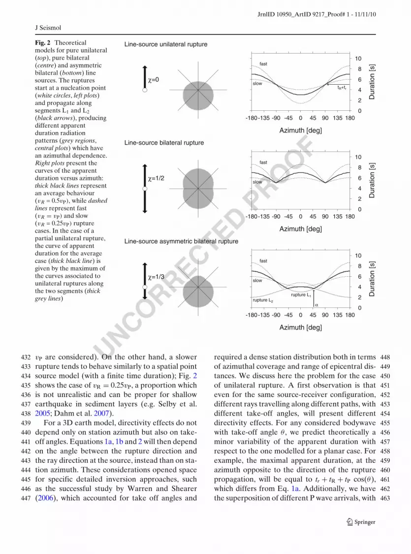
The radiation pattern for three significant cases381

(pure unilateral, pure bilateral and asymmetric382

bilateral) is shown in Fig. 2, where we have chosen383

vR/P = 0.5 (vR/P equal to 0.25 and 1.0 for the slow384

and fast cases respectively), χ is equal to 0, 1/3385

and 1/2 for the three considered cases. We choose386

different rupture lengths L, in order to have a387

constant length of the largest rupture segment.388

Symmetries of apparent duration radiation pat- 389

terns can be observed, with a one lobe shape for 390

a pure unilateral rupture and a two lobe shape for 391

a pure bilateral one. The theoretical curve of the 392

apparent rupture duration (Fig. 2, right) for the 393

unilateral case range from tr + tR − tP (azimuth of 394

rupture direction) to tr + tR + tP (opposite direc- 395

tion); its average value is equal to tr + tR (for a 396

unilateral rupture model tR and tP are the rupture 397

time and P wave travel time along the entire 398

rupture length). For the pure bilateral rupture, the 399

apparent duration varies between tr + tR (perpen- 400

dicular to rupture direction) to tr + tR + tP (paral- 401

lel to rupture direction), with tR and tP referring 402

here to half of the rupture length. The larger vari- 403

ation of the apparent duration for the unilateral 404

case, with respect to the bilateral, explains the 405

major difficulties in observing directivity for the 406

second case. Less known is the behaviour of asym- 407

metric bilateral ruptures, although this model is 408

the most general. In this case the radiation pat- 409

tern (Fig. 2, bottom) present a deformed one- 410

lobe shape, with the minimum observed apparent 411

rupture duration at about 45◦ from the rupture di- 412

rection of the largest rupture length. The azimuth 413

α, where a cusp-like minimum in the apparent 414

duration may be observed, can be obtained by 415

equalizing the two right terms in Eq. 2: 416

α = a cos[(1 − 2χ)

vR/P

]. (3)

Since vR pertains to [0, vP], it follows that for a 417

pure unilateral rupture (χ = 0) we have a sin- 418

gle minimum in direction of rupture propagation, 419

while cusp-like minima are not observed. For a 420

pure bilateral rupture (χ = 0.5), α = ±π/2 always. 421

For the intermediate case of asymmetric bilateral 422

ruptures (0 < χ < 0.5), two cusp-like minima are 423

observed if the following condition is met: 424

χ >

(1/vR/P

)

2. (4)

This means that the observation of two minima in 425

the apparent duration curve indicate a dominant 426

bilateral rupture processes. 427

Figure 2 additionally shows how larger vari- 428

ations in the apparent duration estimations are 429

found, when increasing the rupture velocity (in 430

the figure, effects for an extreme case of vR = 431

UNCORRECTEDPROOF

JrnlID 10950_ArtID 9217_Proof# 1 - 11/11/10

J Seismol

Fig. 2 Theoreticalmodels for pure unilateral(top), pure bilateral(centre) and asymmetricbilateral (bottom) linesources. The rupturesstart at a nucleation point(white circles, left plots)and propagate alongsegments L1 and L2(black arrows), producingdifferent apparentduration radiationpatterns (grey regions,central plots) which havean azimuthal dependence.Right plots present thecurves of the apparentduration versus azimuth:thick black lines representan average behaviour(vR = 0.5vP), while dashedlines represent fast(vR = vP) and slow(vR = 0.25vP) rupturecases. In the case of apartial unilateral rupture,the curve of apparentduration for the averagecase (thick black line) isgiven by the maximum ofthe curves associated tounilateral ruptures alongthe two segments (thickgrey lines)

Line-source unilateral rupture

Line-source bilateral rupture

Line-source asymmetric bilateral rupture

χ=0

χ=1/2

χ=1/3

0

2

4

6

8

10

Dur

atio

n [s

]

-180-135 -90 -45 0 45 90 135 180

Azimuth [deg]

fast

slow tR+tr

0

2

4

6

8

10

Dur

atio

n [s

]

-180-135 -90 -45 0 45 90 135 180

Azimuth [deg]

fast

slow

0

2

4

6

8

10

Dur

atio

n [s

]

-180-135 -90 -45 0 45 90 135 180

Azimuth [deg]

fast

slow

rupture L2

rupture L1

α

vP are considered). On the other hand, a slower432

rupture tends to behave similarly to a spatial point433

source model (with a finite time duration); Fig. 2434

shows the case of vR = 0.25vP, a proportion which435

is not unrealistic and can be proper for shallow436

earthquake in sediment layers (e.g. Selby et al.437

2005; Dahm et al. 2007).438

For a 3D earth model, directivity effects do not439

depend only on station azimuth but also on take-440

off angles. Equations 1a, 1b and 2 will then depend441

on the angle between the rupture direction and442

the ray direction at the source, instead than on sta-443

tion azimuth. These considerations opened space444

for specific detailed inversion approaches, such445

as the successful study by Warren and Shearer446

(2006), which accounted for take off angles and447

required a dense station distribution both in terms 448

of azimuthal coverage and range of epicentral dis- 449

tances. We discuss here the problem for the case 450

of unilateral rupture. A first observation is that 451

even for the same source-receiver configuration, 452

different rays travelling along different paths, with 453

different take-off angles, will present different 454

directivity effects. For any considered bodywave 455

with take-off angle θ , we predict theoretically a 456

minor variability of the apparent duration with 457

respect to the one modelled for a planar case. For 458

example, the maximal apparent duration, at the 459

azimuth opposite to the direction of the rupture 460

propagation, will be equal to tr + tR + tP cos(θ), 461

which differs from Eq. 1a. Additionally, we have 462

the superposition of different P wave arrivals, with 463

UNCORRECTEDPROOF

JrnlID 10950_ArtID 9217_Proof# 1 - 11/11/10

J Seismol

different take-off angles. In any case, the interpre-464

tation of the maximal apparent duration following465

Eq. 1a and neglecting take-off angles and rise time466

effects will lead to an overestimation of the terms467

tR and tP and consequently an overestimation of468

the rupture length. The value derived in such ap-469

proximation can be safely considered as an upper470

bound to the real rupture length.471

Our approach here is to model only the az-472

imuthal variation of directivity effects. The ap-473

proximation is limited by different conditions.474

First, we will focus on shallow earthquakes and475

use only regional distances seismograms (epicen-476

tral distances in the range 200–1,000 km), basing477

our inversion on the fit of time windows centred at478

the first P wave arrivals. Additionally, we will con-479

sider only the case of horizontal to sub-horizontal480

ruptures (rupture propagating along direction dip-481

ping at most 20◦). In these circumstances, we will482

show that the main rupture propagation can be483

detected even with the approximated approach484

here described. The interpretation of additional485

rupture parameters is strongly limited by neglect-486

ing take-off angles and rise time effects, and the487

derived rupture length should be considered as an488

upper bound to its real value.489

On the base of the previous discussion, we can490

now explain the last step of the inversion ap-491

proach, where the distribution of apparent source492

time durations is interpreted in terms of simplified493

rupture models:494

1. Point source model. If we assume a spatial495

point source model, with a given source time496

function of duration tr, the curve of appar-497

ent duration will be a straight line, with no498

azimuthal dependence. This is the particular499

case, which can also be described by the pre-500

vious equations, with L = 0, which leads to501

tR = tP = 0. The model has a unique unknown,502

tr (by definition, rise time), which represents503

the apparent rupture time everywhere.504

2. Pure/predominant unilateral rupture. In this505

case, the azimuthal distribution of apparent506

durations is expected to follow a sinusoidal be-507

haviour. The fit is expected to be larger in case508

of a pure unilateral rupture, but the model can509

still well reproduce data also for asymmetric510

bilateral ruptures. In both cases, the minimum511

of the curve will indicate the main rupture 512

direction (ϕ0). The model is represented by 513

the curve of the apparent duration Δt(ϕ): 514

�t (ϕ) = −A cos (ϕ − ϕ0) + B (5)

with A and B positive, describing in first approx- 515

imation the travel time of P waves along the rup- 516

ture length (tP) and the sum of rise and rupture 517

times (tr + tR). 518

3. Pure bilateral rupture. In case of a pure bilat- 519

eral rupture, we will use the following curve, 520

instead: 521

�t (ϕ) = A |cos (ϕ − ϕ0)| + B. (6)

4. Comparison of directivity models. Since 522

Eqs. 5 and 6 are dependent on three unknown 523

parameters, while the standard average rup- 524

ture time has only one (the average earth- 525

quake duration or duration of the common 526

source time function), they will always pro- 527

vide a better fit with respect to the common 528

rupture duration model. An F test can than 529

be used to evaluate the misfit improvement 530

versus the increase of degrees of freedom. F 531

values above 0.5 will be used here to prefer 532

unilateral or bilateral models with respect to 533

the point source solution. The modelling of 534

asymmetric bilateral rupture requires more 535

free parameters, being the superposition of 536

two functions as in Eq. 5. Chances for the im- 537

plementation of such a model are highly lim- 538

ited by several factors, including data quality, 539

focal mechanism, epicentral azimuthal cover- 540

age and local structural heterogeneities. We 541

suggest here the adoption of this model only 542

for specific cases rather than its implementa- 543

tion within the automated processing. 544

The major advantages of the presented approach 545

are that only point source synthetic seismograms 546

are used, so that forward modelling and inversion 547

are fast. A second advantage lies in the intrinsic 548

simplicity of this approach, which provides simple 549

plots of easy interpretation and suggest its imple- 550

mentation for automated routines. In the worse 551

case, if no clear pattern is detected, the retrieved 552

information can still be used to better focus a 553

more detailed full waveform kinematic inversion 554

UNCORRECTEDPROOF

JrnlID 10950_ArtID 9217_Proof# 1 - 11/11/10

J Seismol

(e.g., as in Cesca et al. 2010), by limiting the555

range of rupture times and/or spatial extension556

to be tested. A last important advantage resides557

in the coherency of the inversion approach: we558

use the same tools and the same data to derive559

first the focal mechanism (or moment tensor) and560

to detect directivity effects, instead of relying on561

an externally calculated focal mechanism solution,562

which may be biased by a specific selection of563

stations, earth model, and processing routines. An564

important limitation of the method applicability565

is represented by a specific range of earthquake566

magnitudes. For small earthquakes, with the rup-567

ture process occurring in less than 2 s, the vari-568

ation of the apparent rupture duration could be569

only detected by fitting high frequency spectra (up570

to 0.5 Hz or above), which requires a detailed571

knowledge of the crustal structure, and possibly572

the adoption of 3D earth models. On the opposite573

side, large earthquakes may present more com-574

plex rupture processes, with different slip patches575

or asperities, breaking at different times. Large576

earthquakes also present significant discrepancies577

between hypocentral and centroid locations. Both578

effects are not considered in our model and can579

then lead to erroneous interpretations. As a rule580

of thumb, we believe that earthquakes with mag-581

nitudes in a range Mw 5.5–7.0 may be the best582

suited for a successful application.583

3 Synthetic tests for linear and planar sources584

Before applying the method to real data, and in585

order to assess the method performance, we carry586

out a set of inversions using synthetic datasets.587

We generate synthetic seismograms first for lin-588

ear sources and consequently to planar ones.589

Considered source models present different sig-590

nificant focal mechanisms and directions of rup-591

ture propagation. Both synthetics for linear and592

planar sources are generated using the Kiwi tools593

(http://kinherd.org; Heimann 2010), assuming the594

PREM model (Dziewonski and Anderson 1981).595

The inversion is then carried out as described in596

the previous paragraph, assuming a spatial point597

source. Focal mechanisms, scalar moment and598

depth are retrieved at a first stage, by using the599

method described in Cesca et al. (2010), which has600

been here specifically modified in order to include 601

the retrieval of the apparent rupture time at each 602

station. In the synthetic tests, a dense grid of 154 603

stations is considered, in order to plot apparent 604

duration contours. Stations location accomplish 605

to the chosen conditions in terms of epicentral 606

distances. 607

Three line source mechanisms (strike-slip (SS) 608

strike ϕ = 30, dip δ = 90, rake λ = 0; normal fault 609

(NF) ϕ = 30, δ = 45, λ = 90; thrust fault (TF) ϕ = 610

30, δ = 20, λ = −90) and three rupturing mod- 611

els (pure unilateral, asymmetric bilateral, pure 612

bilateral) are considered at first, thus providing 613

a set of nine source models. Ruptures propagate 614

horizontally for the strike-slip and normal fault, in 615

direction NNE–SSW, and toward ESE along the 616

low-angle dipping plane, for the thrust fault. The 617

source model centroid is always located at a depth 618

of 20 km, the source length is 30 km, rupture ve- 619

locity is 3.5 km/s. Pure unilateral ruptures start at 620

the southern (SS, NF) or western (TF) edge. The 621

same main rupture direction is used for asymmet- 622

ric bilateral ruptures, the two ruptured segments 623

having lengths L1 = 22.5 and L2 = 7.5 km. Rise 624

time is fixed to 2 s in all cases. The inversion 625

is carried out using 40 s time windows, starting 626

10 s before the theoretical arrival of P phases. A 627

frequency bandpass, between 0.01 and 0.5 Hz, is 628

used to filter Green’s functions and data. Inver- 629

sion results are shown in Fig. 3. Coloured surface, 630

representing the inverted apparent source dura- 631

tion, highlight the radiation patterns of apparent 632

duration. The azimuthal distribution of apparent 633

duration clearly shows directivity effect and its 634

minor dependence on epicentral distance using 635

our approach and proof that a good quality fit 636

can be achieved using the simplified azimuthal de- 637

pendent curves. In particular, the fit of the cosine 638

curve described by Eq. 5 can be used to detect uni- 639

lateral or asymmetric bilateral ruptures, while the 640

curve from Eq. 6 to detect pure bilateral ruptures. 641

Rupture directivity is correctly detected in all 642

cases, with the exception of the bilateral rupture 643

along the low-dipping angle plane of the thrust 644

mechanism (Fig. 3, bottom right), where unilateral 645

rupture is incorrectly estimated. The reason for 646

this discrepancy can be described as follows. Since 647

the extended source is not horizontal, the seg- 648

ment toward ESE and WNW are located below 649

UNCORRECTEDPROOF

JrnlID 10950_ArtID 9217_Proof# 1 - 11/11/10

J Seismol

Unilateral Asymmetric bilateral Bilateral

Nor

mal

faul

t T

hrus

t fau

lt S

trik

e-sl

ip

Apparentduration [s]

Azimuth [deg] Azimuth [deg] Azimuth [deg]

Lat [

deg]

A

ppar

ent

dura

tion

[s]

App

aren

t du

ratio

n [s

]

20 25 30 20 25 30 20 25 30

36

40

44

36

40

44

36

40

44

0

5

10

15

0

5

10

15

-120 0 120 -120 0 1200

5

10

15

-120 0 120

0123456789

10111213141516

Fig. 3 Inversion results for linear sources. We considerthree focal mechanisms (strike-slip, top; normal fault,centre; thrust fault, bottom) and three rupture processes(pure unilateral, left; asymmetric bilateral, centre; purebilateral, right). For each case, we show colour plots rep-resenting the inverted apparent duration at a dense gridof station around the epicentre (red to blue scale repre-sents increasingly longer apparent durations). The focalmechanisms are shown at the epicentral location, togetherwith white arrows describing rupture directions (arrow

sizes are proportional to rupture lengths). Graphics beloweach colour plot represent the apparent duration versusazimuth (dots) and the best fitting model (red curves).Upper triangles represent the correct solution (a singleblack triangle is plotted at the proper azimuth for unilateraland asymmetric bilateral ruptures; two white trianglesindicate rupture directions for pure bilateral rupturecases). Inverted triangles represent inversion results(single red triangle for unilateral and asymmetric bilateralruptures, two white triangles for pure bilateral ruptures)

UNCORRECTEDPROOF

JrnlID 10950_ArtID 9217_Proof# 1 - 11/11/10

J Seismol

and above the centroid depth, respectively. Since650

we use a layered model, the frequency content651

of synthetic seismogram varies from shallower to652

deeper sources, as well as take off angles. These653

effects, which cannot be reproduced by a point654

source located at the centroid depth, results larger655

than those related to the bilateral rupture, thus656

explaining the detection of an apparent directivity657

towards dip direction.658

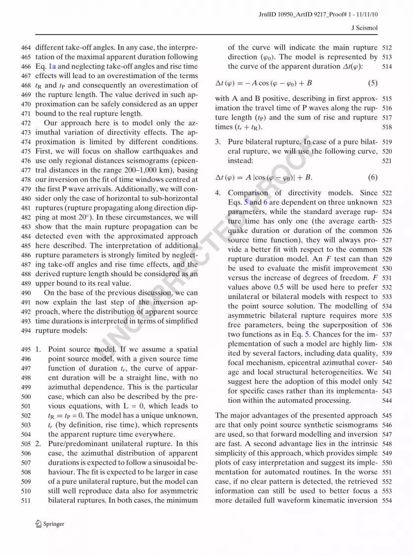
Given the successful application to line sources, 659

we simulate now more realistic rupture processes, 660

generating synthetic seismograms for the eikonal 661

source model (Heimann 2010; Cesca et al. 2010). 662

We use here circular faults, with rupture propagat- 663

ing with a variable velocity, scaling by a coefficient 664

0.9 with shear wave velocity in the crustal model. 665

Given the adoption of the PREM model, the 666

source depth and its extension, rupture velocity 667

Fig. 4 Inversion resultsfor circular eikonalsources. For each of thenine considered sourcemodels, we show colourplots representing theinverted apparentduration around theepicentre (red to bluescale representsincreasingly longerapparent durations).Graphics below eachcoloured plot representthe apparent durationversus azimuth (dots) andthe best fitting model (redcurves). We use the samesymbol convention as inFig. 3

Unilateral Asymmetric bilateral Bilateral

Nor

mal

faul

t T

hrus

t fau

lt S

trik

e-sl

ip

Apparentduration [s]

Azimuth [deg] Azimuth [deg] Azimuth [deg]

Lat [

deg]

A

ppar

ent

dura

tion

[s]

App

aren

t du

ratio

n [s

]

20 25 30 20 25 30 20 25 30

36

40

44

36

40

44

36

40

44

0

5

10

15

0

5

10

15

-120 0 120 -120 0 1200

5

10

15

-120 0 120

0123456789

10111213141516

UNCORRECTEDPROOF

JrnlID 10950_ArtID 9217_Proof# 1 - 11/11/10

J Seismol

range between 2.9 and 4.0 km/s. Inversion is car-668

ried out using the same approach and parameters669

as for the previous test and results summarized in670

Fig. 4. The main characteristics of the azimuthal671

patterns of the apparent rupture duration are pre-672

served. Directivity effects can be detected and673

modelled for all pure unilateral and asymmetric674

bilateral ruptures, although the fit quality results675

in some cases significantly poorer than for line676

source cases. The adoption of bi-dimensional rup-677

tures, and specifically the inclusion of sources at678

different depths, slightly modifies the apparent679

duration pattern, as can be seen by the compari-680

son of plots in Figs. 3 and 4 relative to normal fault681

mechanism. The modification of the apparent682

rupture radiation pattern has similar causes than683

those described for linear sources. Additionally,684

it is here also depending on the variable rupture685

velocity (which, according to the crustal model,686

is faster for deeper sources than for shallower687

ones). These effects result critical for the inversion688

of a bilateral rupture for the case of a thrust689

fault mechanism, which is erroneously interpreted690

as unilateral (with a rupture propagation in dip691

direction). On the other hand, the discrimination692

between pure and asymmetric bilateral rupture is693

not always possible; the observation of the charac-694

teristic lobe associated to the asymmetric bilateral695

rupture may indicate such a rupture process, but696

could not be sufficient, alone, to distinguish this697

case to a pure unilateral rupture.698

A variation of the scalar moment will lead to a699

scaling of synthetic seismograms and modify their700

amplitude spectra. As a consequence, the inver-701

sion of apparent durations may lead to slightly702

different results. In order to investigate these703

effects, we have perturbed the scalar moments704

used for synthetic tests, and analyse inversion705

results. While the uni- or bilateral mode of the706

rupture and the main rupture direction are not707

influenced by a variation of the scalar moment and708

are always correctly retrieved, the rupture time709

and the following estimation of rupture lengths710

suffer slight changes. A perturbation of 10% of711

the correct scalar moment always led to uncer-712

tainties below 5% in terms of rupture time and713

rupture length. Synthetic tests suggest the imple-714

mentation of the method here proposed towards a715

rapid detection of directivity effects. Additionally,716

these tests point out specific cases, where the in- 717

version approach results more critical, and where 718

a careful discussion of results is suggested. In gen- 719

eral, horizontal ruptures and pure or partially uni- 720

lateral ruptures are more easily detected, whereas 721

pure bilateral sources and rupture propagating 722

along dipping directions may be more problematic 723

to resolve. 724

4 The Andravida 8.6.2008 earthquake 725

On June 8th, 2008, a magnitude Mw 6.4 726

earthquake struck NW Peloponnese, Greece. 727

The earthquake, here further referred as the 728

Andravida earthquake, produced two casual- 729

ties, about 100 injuries and several damages 730

(Chouliaras 2009). A wide number of studies cov- 731

ered the earthquake source and its effects. A pure 732

strike-slip focal mechanisms was unanimously 733

provided by several institutions and catalogues 734

surveying regional and global seismicity, includ- 735

ing National Observatory in Athens (NOA), 736

Aristotle University of Thessaloniki (AUTH), 737

INGV European-Mediterranean RCMT Cata- 738

logue (INGV-RCMT), Swiss Federal Institute 739

of Technology, United States Geological Sur- 740

vey (USGS) and Global CMT Catalogue (CMT). 741

According to these models, fault planes are al- 742

most vertical and oriented NNE–SSW and WNW– 743

ESE. Source depth estimations showed some 744

variability, ranging between 10 and 38 km, and 745

magnitudes Mw ranged between 6.3 and 6.5. 746

The epicentral locations of the earthquake after- 747

shocks (Ganas et al. 2009; Gallovic et al. 2009; 748

Kostantinou et al. 2009), which are distributed 749

within a narrow strip extending NNE–SSW, pro- 750

vide a convincing image of the rupture orienta- 751

tion. The cloud of aftershocks elongates for about 752

30–35 km, providing a first rough estimation of 753

rupture size. The aftershock distribution is denser 754

towards the Northern edge. To the south, epi- 755

central locations may indicate a minor bending 756

of the rupture area to a slightly larger strike. 757

All published source models are consistent with 758

the identification of the NNE–SSW striking fault 759

plane. Sokos et al. (2008), using hypocentral- 760

centroid relative location method, identified the 761

same plane; since centroids locations are generally 762

UNCORRECTEDPROOF

JrnlID 10950_ArtID 9217_Proof# 1 - 11/11/10

J Seismol

located North of hypocentral locations, some indi-763

cation for a dominant propagation towards North764

may arise from this study. Even more convincing,765

with respect to the detection of directivity, are766

the studies of Kostantinou et al. (2009), Gallovic767

et al. (2009) and Cesca et al. (2010). The first768

authors derived a finite source model, also con-769

sistent with their aftershock relocations, finding770

a rupture length of 22.4 km and an asymmetric771

bilateral rupture, with a major rupture along the772

NE branch. Gallovic et al. (2009) used a conjugate773

gradient method to detect the spatio-temporal774

evolution of the rupture process. Results indicate775

a predominantly unilateral rupture, propagating776

along a main slip patch, with a rupture length777

of about 20 km and a rupture velocity of about778

3 km/s. Cesca et al. (2010), based on amplitude779

spectra inversion of full waveform and assuming780

an eikonal source model, detected an asymmet- 781

ric rupture propagation, with a predominance of 782

rupture propagation towards NNE; the rupture 783

length was estimated 40 km, while the average 784

rupture velocity was fixed to about 3.2 km/s. The 785

consistency of these results (see Fig. 5 bottom), 786

obtained with different methods and datasets, 787

offer a serious reference to our study in terms of 788

fault plane identification and rupture directivity. 789

In our inversion, we assume the epicentral lo- 790

cation provided on the EMSC-CSEM webpage 791

and the focal mechanism determined by Cesca 792

et al. (2010), which is based on the fit of full 793

waveform amplitude spectra. We observed that 794

a new estimation of the scalar moment, based 795

on the fit of P wave spectra only, would present 796

minor variation with respect to the assumed value 797

(5.97e18 instead of 6.07e18 Nm). Then, we invert 798

Longitude E

Latit

ude

N

Apparent duration [s]

App

aren

t dur

atio

n [s

]

Aftershocks Sokos et al. 2008 Gallovic et al. 2009 Cesca et al. 2009 This study

15 20 25 30

35

40

45

0

5

10

15Pure unilateral model

0

5

10

15

-180 -90 0 90 180

Asymmetric bilateral model

0 1 2 3 4 5 6 7 8 9

21.2 21.6 22 37.6

38

38.4

21.2 21.6 22 21.2 21.6 22 21.2 21.6 22 21.2 21.6 22

Fig. 5 Inversion results for the Mw 6.4 Andravida (NWPeloponnese) earthquake (top) and comparison with pub-lished source models (bottom). Top: coloured dots repre-sent the inverted apparent duration at the stations used,according to the given colour scale; the azimuthal dis-tribution of apparent durations may be fitted (top right)assuming a pure unilateral or, better, a partially unilateralrupture (thick lines). Bottom: the comparison of after-shocks distribution (after Gallovic et al. 2009) identifies

the NNE–SSW rupture plane in agreement with centroid-hypocentral technique (Sokos et al. 2008), adjoint method(Gallovic et al. 2009), full waveform kinematic inversion(Cesca et al. 2010) and our results; the last four methodsconsistently detect a partially unilateral rupture towardsNNE. Stars and blue circles represent here nucleationpoints and centroids respectively; the rupture area is plot-ted in red

UNCORRECTEDPROOF

JrnlID 10950_ArtID 9217_Proof# 1 - 11/11/10

J Seismol

for the apparent duration at each station sep-799

arately and plot resulting values in function of800

station azimuth (Fig. 5), according to the discussed801

methodology. As a first approximation, we try to802

fit apparent durations by means of pure unilateral803

and pure bilateral rupture models, assuming both804

fault planes. Since fault planes are almost vertical,805

only horizontal directions of the rupture velocity806

along these planes are considered. The unilateral807

rupture model with rupture propagation towards808

NNE provide a very good fit to the apparent du-809

ration data, and is preferred to remaining models810

on the base of the F test. This result provides a811

clear indication for a rupture propagating towards812

NNE, and thus can be used to discriminate the813

true fault plane (NNE–SSW) from the auxiliary814

one (WNW–ESE). Based on the good fit, we try815

to refine our solution by investigating asymmetric816

bilateral ruptures. Results provide an even more817

convincing fit (Fig. 5, bottom right), when an818

asymmetric bilateral source model with rupture819

propagating mostly Northward is assumed, as the820

curve account for the two symmetric minima at821

about −21.5 and 82.5◦ and the internal charac-822

teristic lobe of asymmetric rupture (see Fig. 2,823

bottom). On the other side, this result is in very824

good agreement with published models discussed825

before. According to the previous discussion for826

a simplified bidimensional case, the maxima of827

the two cosine curves associated to the rupturing828

of two segments of the fault are equal to tP +829

tR + tr, where these terms refer to the P wave830

propagation, rupture and rise time related to each831

segment. The maxima of the apparent duration832

curve are equal to 8.9 s (segment L1 toward NNE)833

and 2.7 s (segment L2 toward SSW). Assuming834

an average P wave velocity of 8 km/s (consistent835

with the used velocity model at the hypocentral836

depth), a rupture velocity of 3 km/s (consistent837

with Gallovic et al. 2009), and considering the rise838

time negligible with respect to rupture time, we839

obtain rupture lengths of about 19 and 6 km. The840

total length of about 25 km for the main patch841

is in general agreement with most of published842

results. We observe a discrepancy with the rupture843

size of about 40 km determined in Cesca et al.844

(2010). This last value might be overestimated,845

as the adopted full waveform kinematic inversion846

may in some cases be affected by a trade-off be-847

tween different source parameters. The observed 848

discrepancy may also indicate a different response 849

of the two approaches to the rupture process and 850

energy emission, with the full waveform inver- 851

sion detecting the largest rupture length, and the 852

directivity inversion identifying the main rupture 853

patch. The upper limit value we found here is 854

slightly larger than the length estimated by stan- 855

dard empirical relations (according to Wells and 856

Coppersmith 1994, the average rupture length for 857

a Mw 6.4 is about 14 km). We remark that the 858

interpretation of inversion results to this extent 859

should be carried out only in best conditions, 860

where the fitting of the apparent duration curve 861

is good enough to further interpret it. 862

5 The SW Peloponnese 14–20.2.2008 seismic 863

sequence 864

A seismic sequence struck the region offshore 865

SW Peloponnese, Greece, in the days following 866

February 14th, 2008, with three major earth- 867

quakes occurring within a week. On February 868

14th, a first Mw 6.8 (magnitude estimated by 869

EMSC-CSEM and Cesca et al. 2010) event struck 870

the region at 10:09 UTC. Two hours later, at 871

12:08, UTC, a Mw 6.2 aftershock occurred. Fi- 872

nally, on February 20th (18:27 UTC), a Mw 6.2 873

event took place. Focal mechanisms (EMSC- 874

CSEM webpage) indicate thrust faulting for the 875

first two events, while the last one has a different, 876

strike-slip mechanism, with fault planes striking 877

ENE and NNW. Source depths, according to 878

EMSC-CSEM catalogue, were 30, 20 and 25 km, 879

respectively, for the three earthquakes. Whereas 880

different institutions (e.g. NOA, AUTH, Uni- 881

versity of Patras UPSL, INGV-RCMT, USGS, 882

CMT) provided point source solutions for these 883

events, few trials has been carried out so far to 884

interpret rupture kinematics (Roumelioti et al. 885

2009; Cesca et al. 2010). A strongly uneven sta- 886

tion distribution and large epicentral gaps toward 887

SW have possibly limited source modelling until 888

now. Based on full waveform inversion, Cesca 889

et al. (2010) identified the ENE–WSW plane for 890

the strike-slip earthquake of February 20th, and 891

a partial unilateral rupture towards the coast was 892

found. For the first two earthquakes, the low angle 893

UNCORRECTEDPROOF

JrnlID 10950_ArtID 9217_Proof# 1 - 11/11/10

J Seismol

planes dipping toward NW were preferred, but the894

inversion results were not completely satisfacto-895

rily. Roumelioti et al. (2009) adopted an empirical896

Green’s functions approach, using the Mw 6.2897

aftershock to model the finite fault of the largest898

earthquake; their results support the identification899

of the low angle dipping plane as well as directivity900

towards SSW. Finally, the identification of low901

dip angle rupture planes in this region for thrust902

earthquakes would agree with local tectonics, as-903

sociating the earthquake occurrence to oceanic904

subduction (Underhill 1999).905

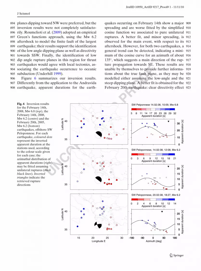
Figure 6 summarizes our inversion results.906

Differently from the application to the Andravida907

earthquake, apparent durations for the earth-908

quakes occurring on February 14th show a major 909

spreading and are worse fitted by the simplified 910

cosine function we associated to pure unilateral 911

ruptures. A better fit, and minor spreading, is 912

observed for the main event, with respect to its 913

aftershock. However, for both two earthquakes, a 914

general trend can be detected, indicating a mini- 915

mum of the cosine curve for an azimuth of about 916

135◦, which suggests a main direction of the rup- 917

ture propagation towards SE. These results are 918

unable by themselves to provide further informa- 919

tions about the true fault plane, as they may be 920

modelled either assuming the low-angle and the 921

steep dipping plane. A better fit is obtained for the 922

February 20th earthquake: clear directivity effect 923

Fig. 6 Inversion resultsfor the February 14th,2008, Mw 6.8 (top), theFebruary 14th, 2008,Mw 6.2 (centre) and theFebruary 20th, 2005,Mw 6.2 (bottom)earthquakes, offshore SWPeloponnese. For eachearthquake, coloured dotsrepresent the invertedapparent duration at thestations used, accordingto the colour scale givenfor each case; theazimuthal distribution ofapparent durations (right)may be fitted assumingunilateral ruptures (thickblack lines). Invertedtriangles indicate theretrieved rupturedirections

SW Pelponnese 14.02.08, 10:09, Mw 6.8

Latit

ude

N

SW Peloponnese, 14.02.08, 12:08, Mw 6.2

Latit

ude

N

SW Peloponnese, 20.02.08, 18:27, Mw 6.2

Latit

ude

N

Longitude E Azimuth [deg]

App

aren

t dur

atio

n [s

]A

ppar

ent d

urat

ion

[s]

App

aren

t dur

atio

n [s

]

Apparent duration [s]

Apparent duration [s]

Apparent duration [s]

35

40

0

10

20

30

0

10

20

30

0

10

20

30

35

40

0

5

10

15

20

0

5

10

15

20

0

5

10

15

20

15 20 25 30

35

40

0

5

10

15

20

-180 -90 0 90 180

0

5

10

15

20

-180 -90 0 90 180

0

5

10

15

20

-180 -90 0 90 180

0 2 4 6 8 10 12 14

0 3 6 9 12 15 18 21

5 8 11 14 17 20 23 26 29 32

UNCORRECTEDPROOF

JrnlID 10950_ArtID 9217_Proof# 1 - 11/11/10

J Seismol

is here retrieved, indicating a rupture mostly prop-924

agating towards ENE, thus along the WSW–ENE925

fault plane. The differentiation between pure or926

partial unilateral rupture may be here rewarded927

as beneath the limit of a safe data interpretation,928

but we observed how the general result is in well929

agreement with previous results by Cesca et al.930

(2010), where the source model was derived by931

the fit of high-frequency (up to 0.1 Hz) amplitude932

spectra from the whole waveforms.933

Finally, we investigate effects of the assumption934

of imprecise point source parameters on the esti-935

mation of rupture directivity. The effects of anom-936

alous source depth estimation are studied for the937

February 20th aftershock, as different Institutions938

have provided a range of different values ranging939

from 8 to 25 km. We repeated the inversion using940

a different point source solution (strike 249◦, dip941

88◦, rake −12◦, depth 12 km), as provided by the942

INGV European-Mediterranean RCMT Catalog;943

this focal mechanism is similar to our solution and944

major differences concern centroid depth, which is945

now shallower. Directivity inversion remains very946

stable, showing a consistent identification of uni-947

lateral rupture direction toward SE, and indicates948

that a source depth variation of about 10km does949

not result in any significant variation in the radia-950

tion pattern of apparent duration. In a similar way,951

we tested slightly different focal mechanisms for952

both earthquakes of February 14th: even if our fo-953

cal mechanisms are in relatively good agreement954

with other published solutions, some difference955

can be observed. For example, the INGV-RCMT956

catalogue indicates strike angles of 333◦ and 298◦,957

for these earthquakes, which differ from our so-958

lution (347◦ and 341◦ respectively). Even in this959

case, after adopting the source parameters pro-960

vided by INGV-RCMT, the inversion results are961

stable, with the detection of main rupture direc-962

tions pointing towards SE–ESE.963

6 Conclusions964

We propose here a new method for a quick detec-965

tion of directivity effects for shallow earthquakes966

at regional distances. Among the most important967

features of the method, we highlight here the 968

following ones: 969

• Rapid inversion 970

The assumption of spatial point source allows 971

an extremely rapid generation of synthetic seis- 972

mograms and point source parameters inversion, 973

thus offering a tool to early detect directivity; to 974

quantify such improvement, on a standard single 975

processor PC the inversion of directivity is here 976

carried out within a minute, about 20 times faster 977

than the full kinematic inversion for the same 978

event, using the approach described in Cesca et al. 979

(2010). 980

• Coherent inversion 981

The use of the Kiwi tools for data processing 982

and inversions improves significantly the consis- 983

tency of our methodology: for example, the same 984

dataset and the same inversion tools can be used 985

to first derive the focal mechanism, then the scalar 986

moment and finally the apparent duration; we 987

believe this consistency between data used for 988

different inversions significantly improve the co- 989

herency of the inversion approach. 990

• Accounting for wave propagation 991

The method is based on amplitude spectra inver- 992

sion, using theoretical Green’s functions for the 993

chosen earth model. In this way, we account for 994

wave propagation effect, an improvement with 995

respect to standard methods based on pulse length 996

estimations. 997

• No requirements of specific aftershocks 998

Avoiding the use of empirical Green’s function, 999

the method is not limited by the existence of 1000

a proper aftershock, nor need to wait for its 1001

occurrence. 1002

• Automation 1003

The adoption of the Kiwi tools and the simplicity 1004

of the inversion approach made possible the im- 1005

plementation of the method as automated routine. 1006

In this manuscript we have demonstrated the 1007

method performance, both with a range of syn- 1008

thetic tests and with observed data for different 1009

UNCORRECTEDPROOF

JrnlID 10950_ArtID 9217_Proof# 1 - 11/11/10

J Seismol

shallow earthquakes recently occurred. These ap-1010

plications offer indications about the quality and1011

extent of inversion results. The retrieval of pure1012

unilateral and pure bilateral ruptures is in gen-1013

eral better resolved than asymmetric ruptures,1014

although the application to the June 8th, 2008,1015

Andravida earthquake showed that this case can1016

also be detected, in favourable conditions. In1017

general, directivity effects are better resolved for1018

strike slip earthquakes, with respect to normal or1019

thrust faulting. Directivity detection offers often a1020

chance to identify the rupture plane, discriminat-1021

ing it from the auxiliary one. The determination1022

of rupture time, rise time and rupture velocity on1023

the base of the proposed method is beyond its1024

purposes and should require a careful supervision.1025

We have here focused to earthquake with magni-1026

tudes of Mw 6 to 7 and shallow hypocentres. The1027

extension of this inversion approach for the study1028

of other range of magnitudes or deeper sources1029

may be investigated in future.1030

Acknowledgements We thank Prof. J. Zahradnik and1031two anonymous reviewers for useful comments and sug-1032gestions. The facilities of GEOFON and IRIS Data1033Management System, and specifically the IRIS Data Man-1034agement Center, were used for access part of the waveform1035and metadata required in this study. We acknowledge all1036institutions providing seismic data used in this research:1037GEOFON, MEDNET Project, Greek National Seismic1038Network and Aristotle University Thessaloniki Network.1039Maps and focal mechanisms have been plotted with GMT1040(Wessel and Smith 1998). This work has been funded by the1041German DFG project KINHERD (DA478/14–1/2) and the1042German BMBF/DFG “Geotechnologien” project RAPID1043(BMBF07/343).1044

References1045

Beck SL, Silver P, Wallace TC, James D (1995) Directivity1046analysis of the deep Bolivian earthquake of June 9,10471994. Geophys Res Lett 22:2257–22601048

Ben-Menahem A (1961) Radiation of seismic surface1049waves from finite moving sources. Bull Seismol Soc1050Am 51:401–4531051

Ben-Menahem A, Singh SJ (1981) Seismic waves and1052sources. Springer, New York1053

Bernard P, Madariaga R (1984) A new asymptotic method1054for the modelling of near-field accelerograms. Bull1055Seismol Soc Am 74:539–5571056

Beroza GC, Spudich P (1988) Linearized inversion for fault 1057rupture behaviour: application to the 1984 Morgan 1058Hill, California, earthquake. J Geophys Res 93:6275– 10596296 1060

Boore D, Joyner W (1978) The influence of rupture inco- 1061herence on seismic directivity. Bull Seismol Soc Am 106268:283–300 1063

Brüstle W, Müller G (1987) Stopping phases in seismo- 1064grams and the spatiotemporal extent of earthquakes. 1065Bull Seismol Soc Am 1:47–68 1066

Caldeira B, Bezzeghoud M, Borges JF (2009) DIRDOP: 1067a directivity approach to determining the seismic rup- 1068ture velocity vector. J Seismol 14:565–600. doi:10.1007/ 1069s10950-009-9183-x 1070

Cassidy JF (1995) Rupture directivity and slip distrib- 1071ution for the Ms 6.8 earthquake of 6 April 1992, 1072Offshore British Columbia: an application of the em- 1073pirical Green’s function method using surface waves. 1074Bull Seismol Soc Am 85:736–746 1075

Cesca S, Heimann S, Stammler K, Dahm T (2010) Auto- 1076mated procedure for point and kinematic source inver- 1077sion at regional distances. J Geophys Res 115:B06304. 1078doi:10.1029/2009JB006450 1079

Chouliaras G (2009) Seismicity anomalies prior to 8 June 10802008, Mw 6.4 earthquake in Western Greece. Nat 1081Hazards Earth Syst Sci 9:327–335 1082

Dahm T, Krüger F (1999) Higher-degree moment ten- 1083sor inversion using far-field broad-band recordings: 1084theory and evaluation of the method with application 1085to the 1994 Bolivia deep earthquake. Geophys J Int 1086137:35–50 1087

Dahm T, Kruger F, Stammler K, Klinge K, Kind R, 1088Wylegalla K, Grasso JR (2007) The 2004 Mw 4.4 1089Rotenburg, Northern Germany, Earthquake and its 1090possible relationship with Gas Recovery. Bull Seismol 1091Soc Am 97:691–704 1092

Dreger D, Kaverina A (2000) Seismic remote sensing 1093for the earthquake source process and near-source 1094strong shaking: a case study of the October 16, 1999 1095Hector mine earthquake. Geophys Res Lett 27:1941– 10961944 1097

Dziewonski AM, Anderson DL (1981) Preliminary refer- 1098ence earth model. Phys Earth Planet Int 25:297–356 1099

Eshghi S, Zare M (2003) Reconnaisance report on 26 1100December 2003 Bam earthquake. International Insti- 1101tute of Earthquake Engineering (IIEES) 1102

Gallovic F, Zahradnik J, Krizova D, Plicka V, Sokos 1103E, Serpetsidaki A, Tselentis GA (2009) From earth- 1104quake centroid to spatial-temporal rupture evolution: 1105Mw 6.3 Movri Mountain earthquake, June 8, 2008, 1106Greece. Geophys Res Lett 36:L21310. doi:10.1029/ 11072009GL040283 1108

Ganas A, Serpelloni E, Drakatos G, Kolligri M, Adamis I, 1109Tsimi C, Batsi E (2009) The Mw 6.4 SW-Achaia (west- 1110ern Greece) earthquake of 8 June 2008: seismological, 1111field, GPS, observations and stress modeling. J Earthq 1112Eng 8:1101–1124 1113

Hartzell SH (1978) Earthquake aftershocks as Green’s 1114functions. Geophys Res Lett 5:1–4 1115

UNCORRECTEDPROOF

JrnlID 10950_ArtID 9217_Proof# 1 - 11/11/10

J Seismol

Hartzell S, Heaton DV (1983) Inversion of strong ground1116motion and teleseismic waveform data for the fault1117rupture history of the 1979 Imperial Valley, California,1118earthquake. Bull Seismol Soc Am 83:1553–15831119

Hartzell S, Helmberger DV (1982) Strong-motion mod-1120elling of the Imperial Valley earthquake of 1979. Bull1121Seismol Soc Am 72:571–5961122

Haskell NA (1964) Total energy and energy spectral den-1123sity of elastic wave radiation from propagating faults.1124Bull Seismol Soc Am 54:1811–18411125

Heimann S (2010) A robust method to estimate kinematic1126earthquake source parameters. PhD Thesis, Univer-1127sity of Hamburg, Germany, pp 1451128

Imanishi K, Takeo M (1998) Estimates of fault dimensions1129for small earthquakes using stopping phases. Geophys1130Res Lett 25:2897–29001131

Imanishi K, Takeo M (2002) An inversion method to1132analyze rupture process of small earthquakes using1133stopping phases. J Geophys Res 107:ESE2.1–ESE2.16.1134doi:10.1029/2001JB0002011135

Kostantinou KI, Melis NS, Lee SJ, Evangelidis CP,1136Boukouras K (2009) Rupture process and aftershock1137relocation of the 8 June 2008 Mw 6.4 earthquake1138in Northwest Peloponnese, Western Greece. Bull1139Seismol Soc Am 99:3374–33891140

Li Y, Toksöz MN (1993) Study of the source process of1141the 1992 Columbia Ms = 7.3 earthquake with the em-1142pirical Green’s function method. Geophys Res Lett114320:1087–10901144

Madariaga R (1977) High-frequency radiation from crack1145(stress drop) models of earthquake faulting. Geophys1146J R Astron Soc 51:625–6511147

Madariaga R (1983) High-frequency radiation from dy-1148namic earthquake fault models. Ann Geophys 1:17–231149

McGuire JJ, Zhao L, Jordan TH (2001) Teleseismic in-1150version for the second-degree moments of earthquake1151space-time distributions. Geophys J Int 145:661–11526781153

McGuire JJ, Zhao L, Jordan TH (2002) Predominance of1154unilateral rupture for a global catalog of large earth-1155quakes. Bull Seismol Soc Am 92:3309–33171156

Müller CS (1985) Source pulse enhancement by deconvolu-1157tion of empirical Green’s functions. Geophys Res Lett115812:33–361159

Nadim F, Moghtaderi-Zadeh M, Lindholm C, Andresen1160A, Remseth S, Bolourchi MJ, Mokhtari M, Tvedt T1161(2004) The Bam earthquake of 26 December 2003.1162Bull Earthquake Eng 2:119–1531163

Nielsen S, Madariaga R (2003) On the self-healing fracture1164mode. Bull Seismol Soc Am 93:2375–23881165

Olson AJ, Apsel RJ (1982) Finite faults and inverse theory1166with applications to the 1979 Imperial Valley earth-1167quake. Bull Seismol Soc Am 72:1969–20011168

Pro C, Buforn E, Udías A (2007) Rupture length and 1169velocity for earthquakes in the Mid-Atlantic Ridge 1170from directivity effects in body and surface waves. 1171Tectonophysics 433:65–79 1172

Roumelioti Z, Benetatos C, Kiratzi A (2009) the 14 1173February 2008 earthquake (M6.7) sequence offshore 1174south Peloponnese (Greece): source models of the 1175three strongest events. Tectonophysics 471:272–284 1176

Selby N, Eshun E, Patton H, Douglas A (2005) Un- 1177usual long-period Rayleigh wave from a vertical dip- 1178slip source: the 7 May 2001, North Sea earthquake. 1179J Geophys Res 110:B10304. doi:10.1029/2005JB003721 1180

Sokos E, Serpetsidaki A, Tselentis GA, Zahradnik J (2008) 1181Quick assessment of the fault plane, for the recent 1182strike-slip event in the North-Western Peloponnese, 1183Greece, (8 June 2008, Mw 6.3). EMSC-CSEM Report 1184

Spudich P, Frazer LN (1984) Use of ray theory to calcu- 1185late high-frequency radiation from earthquake sources 1186having spatially variable rupture velocity and stress 1187drop. Bull Seismol Soc Am 74:2061–2082 1188

Underhill JR (1999) Late Cenozoic deformation of the 1189Hellenide forelands, Western Greece. Geol Soc Am 1190Bull 101:613–634 1191

Vallée M (2007) Rupture properties of the giant suma- 1192tra earthquake imaged by empirical Green’s function 1193analysis. Bull Seismol Soc Am 97:103–114 1194

Vallée M, Bouchon M (2004) Imaging coseismic rupture in 1195the far field by slip patches. Geophys J Int 156:615–630 1196

Velasco AA, Ammon CJ, Lay T (1994) Empirical green 1197function deconvolution of broadband surface waves: 1198Rupture directivity of the 1992 Landers, California 1199(Mw = 7.3), earthquake. Bull Seismol Soc Am 84:735– 1200750 1201

Velasco AA, Ammon CJ, Farrell J, Pankow K (2004) 1202Rupture directivity of the 3 November 2002 denali 1203fault earthquake determined from surface waves. Bull 1204Seismol Soc Am 94:293–299 1205

Warren LM, Shearer PM (2006) Systematic determination 1206of earthquake rupture directivity and fault planes from 1207analysis of long-period P-wave spectra. Geophys J Int 1208164:46–62 1209

Wells DL, Coppersmith KJ (1994) New empirical relations 1210among magnitude, rupture length, rupture width, rup- 1211ture area and surface displacements. Bull Seismol Soc 1212Am 84:974–1002 1213

Wessel P, Smith WHF (1998) New improved version of 1214the generic mapping tools released. Eos Trans AGU 121579:579 1216

Zahradnik J, Gallovic F, Sokos E, Serpetsidaki A, 1217Tselentis GA (2008) Quick fault-plane identification 1218by geometrical method: application to Mw 6.2 Leoni- 1219dio earthquake, January 6, 2008, Greece. Seismol Res 1220Lett 79:653–662 1221

UNCORRECTEDPROOF

JrnlID 10950_ArtID 9217_Proof# 1 - 11/11/10

AUTHOR QUERY

NO QUERY