This article was downloaded by: [National Forest Service Library]On: 01 July 2014, At: 08:54Publisher: Taylor & FrancisInforma Ltd Registered in England and Wales Registered Number: 1072954 Registeredoffice: Mortimer House, 37-41 Mortimer Street, London W1T 3JH, UK

International Journal of GeographicalInformation SciencePublication details, including instructions for authors andsubscription information:http://www.tandfonline.com/loi/tgis20

Delineating generalized speciesboundaries from species distributiondata and a species distribution modelMatthew P. Petersa, Stephen N. Matthewsab, Louis R. Iversona &Anantha M. Prasada

a Northern Research Station, USDA Forest Service, Delaware, OH,USAb Terrestrial Wildlife Ecology Lab, School of Environment andNatural Resources, The Ohio State University, Columbus, OH, USAPublished online: 01 Nov 2013.

To cite this article: Matthew P. Peters, Stephen N. Matthews, Louis R. Iverson & Anantha M. Prasad(2014) Delineating generalized species boundaries from species distribution data and a speciesdistribution model, International Journal of Geographical Information Science, 28:8, 1547-1560,DOI: 10.1080/13658816.2013.840381

To link to this article: http://dx.doi.org/10.1080/13658816.2013.840381

PLEASE SCROLL DOWN FOR ARTICLE

Taylor & Francis makes every effort to ensure the accuracy of all the information (the“Content”) contained in the publications on our platform. However, Taylor & Francis,our agents, and our licensors make no representations or warranties whatsoever as tothe accuracy, completeness, or suitability for any purpose of the Content. Any opinionsand views expressed in this publication are the opinions and views of the authors,and are not the views of or endorsed by Taylor & Francis. The accuracy of the Contentshould not be relied upon and should be independently verified with primary sourcesof information. Taylor and Francis shall not be liable for any losses, actions, claims,proceedings, demands, costs, expenses, damages, and other liabilities whatsoever orhowsoever caused arising directly or indirectly in connection with, in relation to or arisingout of the use of the Content.

This article may be used for research, teaching, and private study purposes. Anysubstantial or systematic reproduction, redistribution, reselling, loan, sub-licensing,systematic supply, or distribution in any form to anyone is expressly forbidden. Terms &

Conditions of access and use can be found at http://www.tandfonline.com/page/terms-and-conditions

Dow

nloa

ded

by [

Nat

iona

l For

est S

ervi

ce L

ibra

ry]

at 0

8:54

01

July

201

4

International Journal of Geographical Information Science, 2014Vol. 28, No. 8, 1547–1560, http://dx.doi.org/10.1080/13658816.2013.840381

Delineating generalized species boundaries from species distributiondata and a species distribution model

Matthew P. Petersa*, Stephen N. Matthewsa,b , Louis R. Iversona and Anantha M. Prasada

aNorthern Research Station, USDA Forest Service, Delaware, OH, USA; bTerrestrial WildlifeEcology Lab, School of Environment and Natural Resources, The Ohio State University, Columbus,

OH, USA

(Received 3 May 2013; accepted 27 August 2013)

Species distribution models (SDM) are commonly used to provide information aboutspecies ranges or extents, and often are intended to represent the entire area of poten-tial occupancy or suitable habitat in which individuals occur. While SDMs can provideresults over various geographic extents, they normally operate within a grid and cannotdelimit distinct, smooth boundaries. Additionally, there are instances where a zone ofprimary occupancy (i.e., a mostly continuous region where species exists, excludingoutliers) is better suited for particular analyses, such as when examining source/sinkpopulation dynamics or modeling movement into new habitats. We present a semi-au-tomated method to delineate a generalized species boundary (GSB) from SDM output,which provides a practical alternative to digitizing. This preliminary boundary is thenmanually updated based on inventory data and historical ranges. We used the methodto generate contemporary boundaries for 132 tree species of the eastern United States,which are complementary to the ranges generated by Elbert Little for North Americaduring the 1970s, but are not replacements. The methods we present can broadly beapplied to other grid-based SDM to generate GSBs.

Keywords: eastern United States; forest inventory and analysis; geoprocessing;R statistical language; tree ranges

Introduction

Current ranges and distributions of many tree species have long been delineated (Munns1938, Little 1971), or more recently, modeled (Moore et al. 1991, Skyes et al. 1996,Harrison et al. 2006, Rehfeldt et al. 2006, McKenney et al. 2007, Iverson et al. 2008).However, species ranges delineated from large-scale field and herbarium surveys areusually now being superseded by process-based or statistical species distribution mod-els (SDM) to map the potential extent of suitable habitat for a species. SDMs mayuse environmental data obtained from remote sensing along with field survey recordsto develop empirical relationships to predict species abundance or occurrence over alandscape (Franklin and Miller 2009). These correlative relationships provide needed

*Corresponding author. Email: matthewpeters@fs.fed.us

The work of Matthew P. Peters, Stephen N. Matthews, Louis R. Iverson and Anantha M. Prasad is published by permission ofthe USDA Forest Service. The U.S. Government retains for itself, and others acting on its behalf, a paid-up, non-exclusive, andirrevocable worldwide license in said article to reproduce, prepare derivative works, distribute copies to the public, and performpublicly and display publicly, by or on behalf of the Government.

The work of Matthew P. Peters, Stephen N. Matthews, Louis R. Iverson and Anantha M. Prasad was authored as part of theirofficial duties as Employees of the United States Government and is therefore a work of the United States Government. Inaccordance with 17 U.S.C. 105, no copyright protection is available for such works under U.S. Law.

Dow

nloa

ded

by [

Nat

iona

l For

est S

ervi

ce L

ibra

ry]

at 0

8:54

01

July

201

4

1548 M.P. Peters et al.

information about the ways in which species distributions are shaped by their surround-ing environment and can then be applied to unsampled locations in a predictive mannerto map presence/absence or abundance/importance of a species. While the model out-put is continuous and highly informative, the resulting maps make it difficult to estimatedistinct boundaries associated with the species (MacArthur 1972, Kirkpatrick and Barton1997). Many processes (e.g., climate, land use, site quality, etc.) govern the area occupiedby a species, which result in ranges with unique patterns, especially near range bound-aries where conditions often are less than optimal and thresholds of habitat suitabilityebb and flow. This dynamic along the range boundaries results from competition amongspecies and disturbance events. Because these interactions vary over time and space, thereare numerous ways to define the range boundary, including the use of clustering andedge detection algorithms (Fortin and Drapeau 1995), fuzzy set algorithms (Leung 1987,Burrough and Frank 1996), or Mahalanobis distance algorithms (Sangermano and Eastman2012). Regardless of the method, species ranges are often generalized to represent the like-lihood of the species being present near the edge of the range (Brown et al. 1996, Gaston2009).

In this paper, we define a ‘generalized species boundary’ (hereafter GSB) as a highlyconnected region ranging from high to low density of potential suitable habitat. We havegenerated these boundaries for 132 of the 134 tree species previously modeled for theeastern United States with DISTRIB (Iverson et al. 2008). These models are based onspecies-level data, and as such, they ignore genetic variation within species ranges, suchan extensive data set does not exist for most species. We realize that genetic variation playsan important role in determining the successful establishment and survival of a species in aparticular place, and recognize the need for further research and data acquisition of geneticspatial variation for many species.

The use of a GSB, or the primary zone of occupancy for a particular species, hasthe benefit of excluding potential outlier populations when exploring species migrationpotentials (Ordonez and Williams 2013, Prasad et al. 2013), or when defining range limits(Purves 2009). Analyses that utilize the full species’ range as defined by an unmodifiedSDM are susceptible to introducing potential errors, or at least numerous outlier ‘islands’,at or near the edge of the range boundary where greater uncertainty exists at the tail of adistribution (Jiménez-Valverde and Lobo 2007). This error is particularly problematic forbinary range boundaries (e.g., Little’s range boundaries, Little 1971), where no abundancedata are available, or when small sample sizes are used. To further reduce error propagationalong the boundary edges, as described by Brown et al. (1996), for tree species using ourDISTRIB models, we set out to define the zone of primary occupancy of suitable habitatfor each species to generate GSBs.

Range boundaries occur naturally as a result of various interacting phenomena, andthere are several ways to define a species range (Gaston 1991, Brown et al. 1996). However,there is little literature on how to create a boundary via digital processes (Purves 2009).This deficit may be due to the fact that in recent decades, most researchers are usinggrid-based SDMs to identify potential suitable habitat (Graham and Hijmans 2006), thusreplacing the need for maps and vector boundaries digitized from survey data. However,each SDM has its own set of caveats [e.g., environmental equilibrium, inclusion of habitatcharacteristics, and relevant scale (spatial and temporal), Franklin and Miller 2009], and itmight be undesirable to include the entire extent of suitable habitat from a SDM for certainanalyses (e.g., those considering the core or primary region of a species). In this paper, wedescribe and present a new method for creating a boundary of primary occupancy from agrid-based SDM output of potential species abundance.

Dow

nloa

ded

by [

Nat

iona

l For

est S

ervi

ce L

ibra

ry]

at 0

8:54

01

July

201

4

International Journal of Geographical Information Science 1549

Methodology

Data

During the 1970s, Elbert Little published a five-volume atlas of tree species ranges inNorth America delineated from published tree distributions, herbarium records, and fieldsurveys. In general, Little’s boundaries define a generous extent for the species, with linesdrawn around the greatest extent of the species, and thus there are often large areas withinthe boundaries that have sparse occupancy. The final ranges were reviewed by botanists,foresters, and other experts (Little 1971), and today digital copies of the range boundariesare available from the US Geological Survey (http://esp.cr.usgs.gov/data/atlas/little/) for679 tree and shrub species. Little’s ranges are widely used, including by us for this paper,to define a historical extent for a species’ distribution throughout the United States. It isimportant to emphasize that the work we present in this paper is not intended to replaceLittle’s boundaries, but to complement them in that we focus on the ‘zone of primaryoccupancy’, rather than the extent of the species. Thus, we would expect that for mostspecies, Little’s ranges would be larger than the GSBs.

The US Forest Service’s Forest Inventory and Analysis (FIA) program is a long-termeffort mandated by the US Congress with the principal purpose to survey the extent,condition, volume, growth, and depletions of timber on US-forested lands (Smith 2006).Plot-level data were used to indicate the presence or absence of species as a visual checkwhile editing the GSBs. Plot locations with truncated coordinates (Lister et al. 2005) fromperiodic inventories during 1980–1993 (hereafter ‘old’, Smith 2006) provided informationrelated to the distribution of tree species of the current model. Additionally, newer annu-alized inventories during 1999–2010 (Woudenberg et al. 2010) were combined with theearlier periodic records (1980–2010, hereafter ‘newer’) to help with the delineation of coreboundaries. At each FIA plot, the most recent inventory records were used to calculateimportance values for 132 modeled tree species (Iverson et al. 1998).

Predicted importance values (IV, i.e., relative abundance) from the DISTRIB model(Iverson and Prasad 2008) use 38 environmental predictor variables and FIA data to sta-tistically model potential suitable habitat for tree species. An ensemble technique usingRandomForest, bagging, and regression tree analysis (Prasad et al. 2006) is employed torelate IVs at plot locations with environmental predictors. Output from DISTRIB (http://www.nrs.fs.fed.us/atlas/) has a 20 × 20 km resolution across the eastern United Statesand predicts importance values representing suitable habitat, even where few forested FIAplots existed, under both current (1961–1990) and future (2071–2100) climate scenarios.Each species model has a potential value of 0–100 for each grid and is rated for reliabilitybased on a series of statistical procedures, so that users know how to evaluate the pre-dicted IVs (Iverson et al. 2008). The models thus range from high to low reliability, withless reliability where FIA data for the species are sparse or wide-ranging. DISTRIB differsfrom many other SDMs in that it produces a grid of predicted IVs (i.e., potential abun-dance), rather than a probability of presence/absence, thus low values indicate areas wherea species’ habitat is potentially suitable but where individuals would be found only in lownumbers.

Procedures

A digital processing method, using R statistical language (R Development Core Team2010), and custom geoprocessing tools, was used to delineate a representation of the

Dow

nloa

ded

by [

Nat

iona

l For

est S

ervi

ce L

ibra

ry]

at 0

8:54

01

July

201

4

1550 M.P. Peters et al.

SDMoutput

Delineationalgorithm

Manualinspection

/editing

Selectboundaryfeatures

Convertto raster

Convert topolyline

Manualinspection

/editing

Convert topolygon

Smooth

Clip toregion

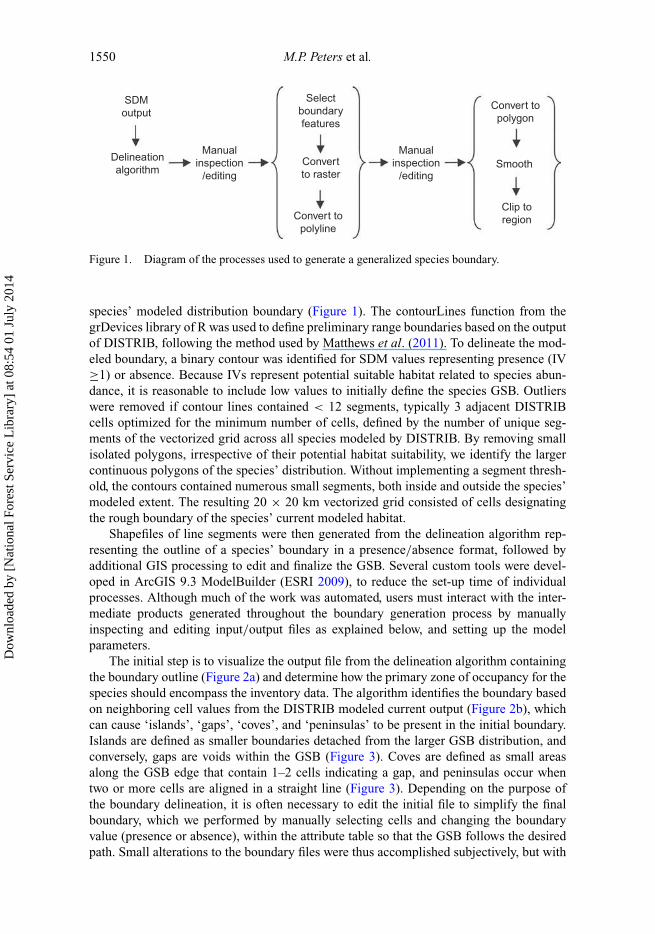
Figure 1. Diagram of the processes used to generate a generalized species boundary.

species’ modeled distribution boundary (Figure 1). The contourLines function from thegrDevices library of R was used to define preliminary range boundaries based on the outputof DISTRIB, following the method used by Matthews et al. (2011). To delineate the mod-eled boundary, a binary contour was identified for SDM values representing presence (IV≥1) or absence. Because IVs represent potential suitable habitat related to species abun-dance, it is reasonable to include low values to initially define the species GSB. Outlierswere removed if contour lines contained < 12 segments, typically 3 adjacent DISTRIBcells optimized for the minimum number of cells, defined by the number of unique seg-ments of the vectorized grid across all species modeled by DISTRIB. By removing smallisolated polygons, irrespective of their potential habitat suitability, we identify the largercontinuous polygons of the species’ distribution. Without implementing a segment thresh-old, the contours contained numerous small segments, both inside and outside the species’modeled extent. The resulting 20 × 20 km vectorized grid consisted of cells designatingthe rough boundary of the species’ current modeled habitat.

Shapefiles of line segments were then generated from the delineation algorithm rep-resenting the outline of a species’ boundary in a presence/absence format, followed byadditional GIS processing to edit and finalize the GSB. Several custom tools were devel-oped in ArcGIS 9.3 ModelBuilder (ESRI 2009), to reduce the set-up time of individualprocesses. Although much of the work was automated, users must interact with the inter-mediate products generated throughout the boundary generation process by manuallyinspecting and editing input/output files as explained below, and setting up the modelparameters.

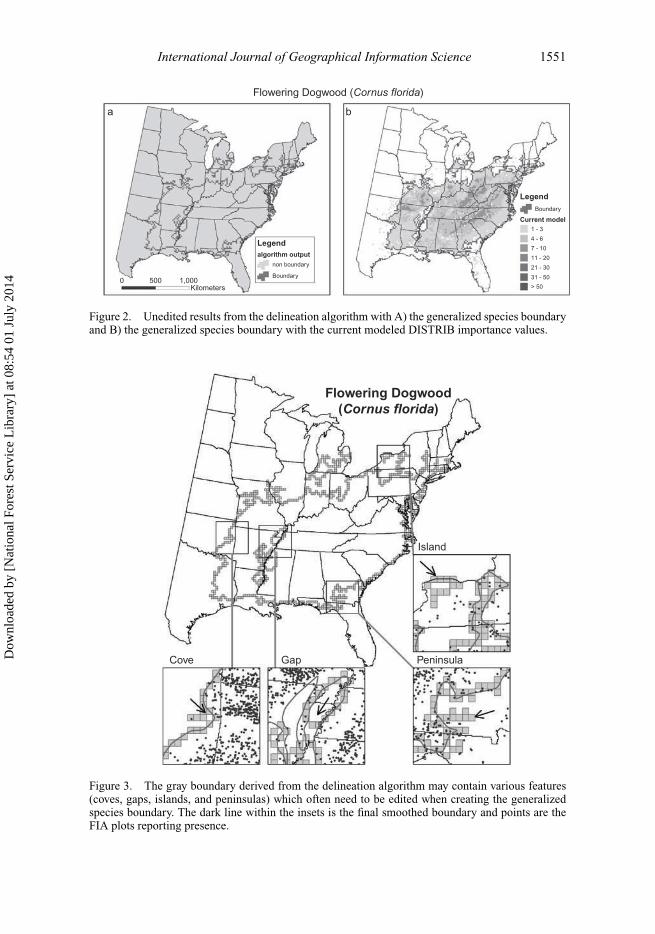
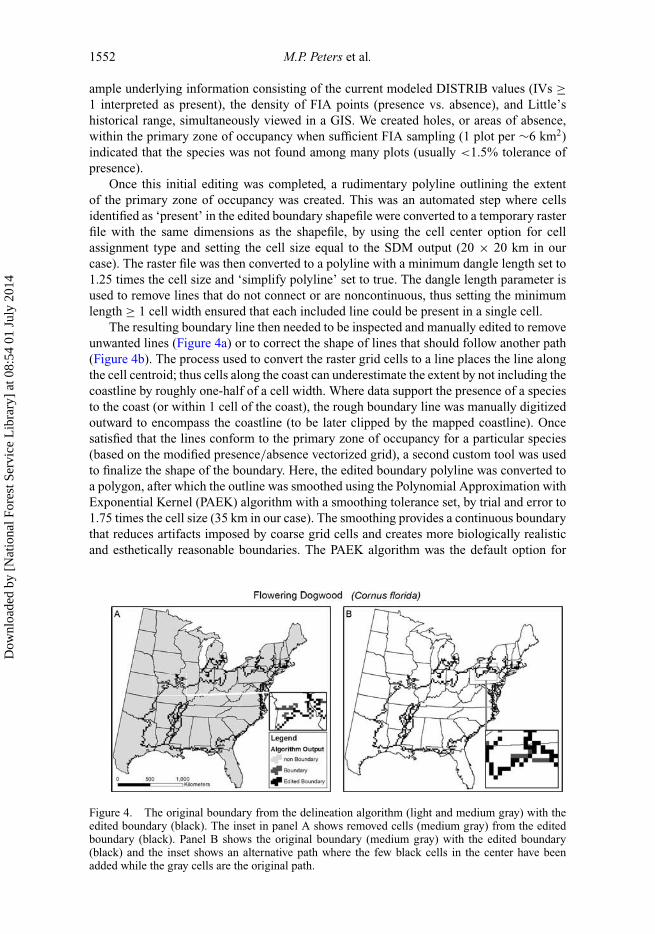
The initial step is to visualize the output file from the delineation algorithm containingthe boundary outline (Figure 2a) and determine how the primary zone of occupancy for thespecies should encompass the inventory data. The algorithm identifies the boundary basedon neighboring cell values from the DISTRIB modeled current output (Figure 2b), whichcan cause ‘islands’, ‘gaps’, ‘coves’, and ‘peninsulas’ to be present in the initial boundary.Islands are defined as smaller boundaries detached from the larger GSB distribution, andconversely, gaps are voids within the GSB (Figure 3). Coves are defined as small areasalong the GSB edge that contain 1–2 cells indicating a gap, and peninsulas occur whentwo or more cells are aligned in a straight line (Figure 3). Depending on the purpose ofthe boundary delineation, it is often necessary to edit the initial file to simplify the finalboundary, which we performed by manually selecting cells and changing the boundaryvalue (presence or absence), within the attribute table so that the GSB follows the desiredpath. Small alterations to the boundary files were thus accomplished subjectively, but with

Dow

nloa

ded

by [

Nat

iona

l For

est S

ervi

ce L

ibra

ry]

at 0

8:54

01

July

201

4

International Journal of Geographical Information Science 1551

Legend

Legend

a b

Flowering Dogwood (Cornus florida)

algorithm output

Current model

0 500 1,000Kilometers

non boundary

Boundary

1 - 3

4 - 6

7 - 10

11 - 20

21 - 30

31 - 50

> 50

Boundary

Figure 2. Unedited results from the delineation algorithm with A) the generalized species boundaryand B) the generalized species boundary with the current modeled DISTRIB importance values.

Cove Gap Peninsula

Island

Flowering Dogwood(Cornus florida)

Figure 3. The gray boundary derived from the delineation algorithm may contain various features(coves, gaps, islands, and peninsulas) which often need to be edited when creating the generalizedspecies boundary. The dark line within the insets is the final smoothed boundary and points are theFIA plots reporting presence.

Dow

nloa

ded

by [

Nat

iona

l For

est S

ervi

ce L

ibra

ry]

at 0

8:54

01

July

201

4

1552 M.P. Peters et al.

ample underlying information consisting of the current modeled DISTRIB values (IVs ≥1 interpreted as present), the density of FIA points (presence vs. absence), and Little’shistorical range, simultaneously viewed in a GIS. We created holes, or areas of absence,within the primary zone of occupancy when sufficient FIA sampling (1 plot per ∼6 km2)indicated that the species was not found among many plots (usually <1.5% tolerance ofpresence).

Once this initial editing was completed, a rudimentary polyline outlining the extentof the primary zone of occupancy was created. This was an automated step where cellsidentified as ‘present’ in the edited boundary shapefile were converted to a temporary rasterfile with the same dimensions as the shapefile, by using the cell center option for cellassignment type and setting the cell size equal to the SDM output (20 × 20 km in ourcase). The raster file was then converted to a polyline with a minimum dangle length set to1.25 times the cell size and ‘simplify polyline’ set to true. The dangle length parameter isused to remove lines that do not connect or are noncontinuous, thus setting the minimumlength ≥ 1 cell width ensured that each included line could be present in a single cell.

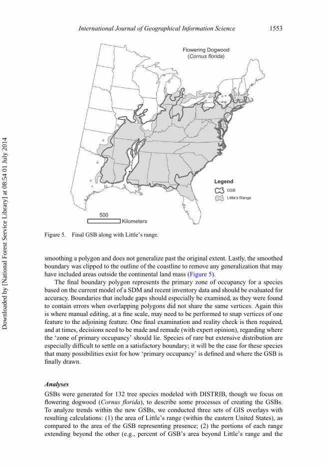
The resulting boundary line then needed to be inspected and manually edited to removeunwanted lines (Figure 4a) or to correct the shape of lines that should follow another path(Figure 4b). The process used to convert the raster grid cells to a line places the line alongthe cell centroid; thus cells along the coast can underestimate the extent by not including thecoastline by roughly one-half of a cell width. Where data support the presence of a speciesto the coast (or within 1 cell of the coast), the rough boundary line was manually digitizedoutward to encompass the coastline (to be later clipped by the mapped coastline). Oncesatisfied that the lines conform to the primary zone of occupancy for a particular species(based on the modified presence/absence vectorized grid), a second custom tool was usedto finalize the shape of the boundary. Here, the edited boundary polyline was converted toa polygon, after which the outline was smoothed using the Polynomial Approximation withExponential Kernel (PAEK) algorithm with a smoothing tolerance set, by trial and error to1.75 times the cell size (35 km in our case). The smoothing provides a continuous boundarythat reduces artifacts imposed by coarse grid cells and creates more biologically realisticand esthetically reasonable boundaries. The PAEK algorithm was the default option for

Figure 4. The original boundary from the delineation algorithm (light and medium gray) with theedited boundary (black). The inset in panel A shows removed cells (medium gray) from the editedboundary (black). Panel B shows the original boundary (medium gray) with the edited boundary(black) and the inset shows an alternative path where the few black cells in the center have beenadded while the gray cells are the original path.

Dow

nloa

ded

by [

Nat

iona

l For

est S

ervi

ce L

ibra

ry]

at 0

8:54

01

July

201

4

International Journal of Geographical Information Science 1553

Flowering Dogwood(Cornus florida)

Legend

GSB

500Kilometers

Little's Range

Figure 5. Final GSB along with Little’s range.

smoothing a polygon and does not generalize past the original extent. Lastly, the smoothedboundary was clipped to the outline of the coastline to remove any generalization that mayhave included areas outside the continental land mass (Figure 5).

The final boundary polygon represents the primary zone of occupancy for a speciesbased on the current model of a SDM and recent inventory data and should be evaluated foraccuracy. Boundaries that include gaps should especially be examined, as they were foundto contain errors when overlapping polygons did not share the same vertices. Again thisis where manual editing, at a fine scale, may need to be performed to snap vertices of onefeature to the adjoining feature. One final examination and reality check is then required,and at times, decisions need to be made and remade (with expert opinion), regarding wherethe ‘zone of primary occupancy’ should lie. Species of rare but extensive distribution areespecially difficult to settle on a satisfactory boundary; it will be the case for these speciesthat many possibilities exist for how ‘primary occupancy’ is defined and where the GSB isfinally drawn.

Analyses

GSBs were generated for 132 tree species modeled with DISTRIB, though we focus onflowering dogwood (Cornus florida), to describe some processes of creating the GSBs.To analyze trends within the new GSBs, we conducted three sets of GIS overlays withresulting calculations: (1) the area of Little’s range (within the eastern United States), ascompared to the area of the GSB representing presence; (2) the portions of each rangeextending beyond the other (e.g., percent of GSB’s area beyond Little’s range and the

Dow

nloa

ded

by [

Nat

iona

l For

est S

ervi

ce L

ibra

ry]

at 0

8:54

01

July

201

4

1554 M.P. Peters et al.

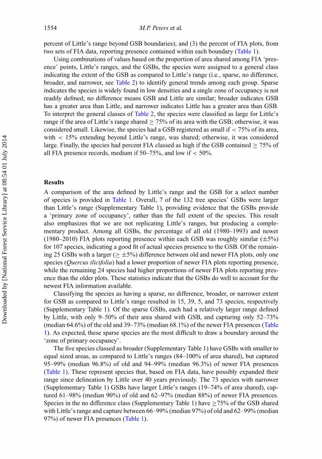
percent of Little’s range beyond GSB boundaries); and (3) the percent of FIA plots, fromtwo sets of FIA data, reporting presence contained within each boundary (Table 1).

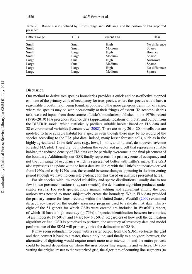
Using combinations of values based on the proportion of area shared among FIA ‘pres-ence’ points, Little’s ranges, and the GSBs, the species were assigned to a general classindicating the extent of the GSB as compared to Little’s range (i.e., sparse, no difference,broader, and narrower, see Table 2) to identify general trends among each group. Sparseindicates the species is widely found in low densities and a single zone of occupancy is notreadily defined; no difference means GSB and Little are similar; broader indicates GSBhas a greater area than Little, and narrower indicates Little has a greater area than GSB.To interpret the general classes of Table 2, the species were classified as large for Little’srange if the area of Little’s range shared ≥ 75% of its area with the GSB; otherwise, it wasconsidered small. Likewise, the species had a GSB registered as small if < 75% of its area,with < 15% extending beyond Little’s range, was shared; otherwise, it was consideredlarge. Finally, the species had percent FIA classed as high if the GSB contained ≥ 75% ofall FIA presence records, medium if 50–75%, and low if < 50%.

Results

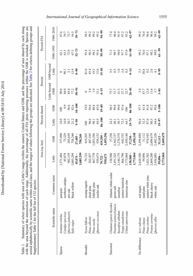
A comparison of the area defined by Little’s range and the GSB for a select numberof species is provided in Table 1. Overall, 7 of the 132 tree species’ GSBs were largerthan Little’s range (Supplementary Table 1), providing evidence that the GSBs providea ‘primary zone of occupancy’, rather than the full extent of the species. This resultalso emphasizes that we are not replicating Little’s ranges, but producing a comple-mentary product. Among all GSBs, the percentage of all old (1980–1993) and newer(1980–2010) FIA plots reporting presence within each GSB was roughly similar (±5%)for 107 species, indicating a good fit of actual species presence to the GSB. Of the remain-ing 25 GSBs with a larger (≥ ±5%) difference between old and newer FIA plots, only onespecies (Quercus ilicifolia) had a lower proportion of newer FIA plots reporting presence,while the remaining 24 species had higher proportions of newer FIA plots reporting pres-ence than the older plots. These statistics indicate that the GSBs do well to account for thenewest FIA information available.

Classifying the species as having a sparse, no difference, broader, or narrower extentfor GSB as compared to Little’s range resulted in 15, 39, 5, and 73 species, respectively(Supplementary Table 1). Of the sparse GSBs, each had a relatively larger range definedby Little, with only 9–50% of their area shared with GSB, and capturing only 52–73%(median 64.6%) of the old and 39–73% (median 68.1%) of the newer FIA presences (Table1). As expected, these sparse species are the most difficult to draw a boundary around the‘zone of primary occupancy’.

The five species classed as broader (Supplementary Table 1) have GSBs with smaller toequal sized areas, as compared to Little’s ranges (84–100% of area shared), but captured95–99% (median 96.8%) of old and 94–99% (median 96.3%) of newer FIA presences(Table 1). These represent species that, based on FIA data, have possibly expanded theirrange since delineation by Little over 40 years previously. The 73 species with narrower(Supplementary Table 1) GSBs have larger Little’s ranges (19–74% of area shared), cap-tured 61–98% (median 90%) of old and 62–97% (median 88%) of newer FIA presences.Species in the no difference class (Supplementary Table 1) have ≥75% of the GSB sharedwith Little’s range and capture between 66–99% (median 97%) of old and 62–99% (median97%) of newer FIA presences (Table 1).

Dow

nloa

ded

by [

Nat

iona

l For

est S

ervi

ce L

ibra

ry]

at 0

8:54

01

July

201

4

International Journal of Geographical Information Science 1555

Tabl

e1.

Sum

mar

yof

sele

ctsp

ecie

sw

ith

area

ofL

ittl

e’s

rang

e(w

ithi

nth

eea

ster

nU

nite

dS

tate

s)an

dG

SB

,an

dth

epe

rcen

tage

ofar

eash

ared

byea

chal

ong

wit

hth

ear

eabe

yond

the

inte

rsec

tion

ofea

chra

nge.

Add

itio

nally

,th

epe

rcen

tage

ofal

lF

IApl

ots

repo

rtin

gpr

esen

cew

ithi

nth

eG

SB

isin

clud

ed.

Spe

cies

are

sort

edal

phab

etic

ally

bysc

ient

ific

nam

ew

ithi

nea

chcl

ass,

and

the

rang

esof

valu

esfo

llow

ing

the

grou

psar

ein

dica

ted.

See

Tabl

e2

for

crit

eria

defi

ning

grou

psan

dS

uppl

emen

tary

Tabl

e1

for

the

full

list

of13

2sp

ecie

s.

Are

a(s

q.km

)Pe

rcen

tsha

red

Perc

ent

Perc

entF

IA

Sci

enti

fic

nam

eC

omm

onna

me

Lit

tle

GS

BL

ittl

eG

SB

Lit

tle

beyo

ndG

SB

GS

Bbe

yond

Lit

tle

1980

–199

319

80–2

010

Spa

rse

Asi

min

atr

ilob

apa

wpa

w1,

571,

484

157,

490

10.0

100

90.0

062

.147

.6C

atal

pasp

ecio

sano

rthe

rnca

talp

a45

,074

73,2

2916

.09.

984

.090

.163

.339

.7Q

uerc

uspa

lust

ris

pin

oak

902,

159

285,

630

30.7

96.6

69.4

3.1

72.0

72.7

Sali

xni

gra

blac

kw

illo

w3,

085,

299

758,

240

21.2

92.6

77.2

13.9

67.5

54.5

45,0

74–

3,08

5,29

927

,405

–75

8,24

09–

5010

–100

50–9

10–

9052

–73

39–7

3

Bro

ader

Nys

sabi

flora

swam

ptu

pelo

79,7

2241

9,20

510

019

.00

81.0

95.4

94.5

Pin

usel

liot

tii

slas

hpi

ne26

2,45

744

7,54

596

.656

.63.

443

.498

.598

.2P

inus

taed

alo

blol

lypi

ne86

7,77

01,

053,

296

98.1

80.8

1.9

19.2

99.2

99.2

Que

rcus

cocc

inea

scar

leto

ak93

0,67

393

0,15

284

.985

.015

.115

.095

.495

.279

,722

–93

0,67

341

9,20

5–

1,05

3,29

684

–100

19–8

50–

1515

–81

95–9

994

–99

Nar

row

erC

ham

aecy

pari

sth

yoid

esA

tlan

tic

whi

te-c

edar

138,

500

37,2

3024

.390

.575

.79.

571

.377

.4F

raxi

nus

penn

sylv

anic

agr

een

ash

3,45

1,32

52,

362,

137

68.1

99.8

31.7

0.5

90.7

90.4

Sass

afra

sal

bidu

msa

ssaf

ras

2,14

4,17

91,

270,

379

58.7

99.0

41.3

1.0

94.0

91.9

Tsu

gaca

nade

nsis

east

ern

hem

lock

866,

790

642,

535

72.3

97.6

27.7

2.4

97.7

97.2

Ulm

usam

eric

ana

Am

eric

anel

m3,

773,

064

2,45

0,14

864

.710

032

.70.

397

.095

.213

8,50

0–

3,77

3,06

437

,230

–2,

450,

148

19–7

486

–100

26–8

10–

1461

–98

62–9

7

No

diff

eren

ceA

cer

rubr

umre

dm

aple

2,62

8,58

82,

599,

880

96.6

97.7

3.4

2.3

99.2

99.2

Pin

uscl

ausa

sand

pine

59,0

9631

,112

32.3

61.4

67.7

38.6

76.6

76.4

Pin

usst

robu

sea

ster

nw

hite

pine

1,02

1,38

297

4,54

387

.691

.812

.48.

297

.196

.6P

runu

sse

roti

nabl

ack

cher

ry2,

869,

200

2,60

9,67

988

.597

.211

.62.

698

.298

.4Q

uerc

usal

baw

hite

oak

2,43

6,08

52,

402,

320

94.6

95.6

5.7

4.1

99.0

99.2

59,0

96–

3,77

3,06

431

,112

–2,

609,

679

19–9

75–

100

3–81

0–95

61–

9962

–99

Dow

nloa

ded

by [

Nat

iona

l For

est S

ervi

ce L

ibra

ry]

at 0

8:54

01

July

201

4

1556 M.P. Peters et al.

Table 2. Range classes defined by Little’s range and GSB area, and the portion of FIA. reportedpresence.

Little’s range GSB Percent FIA Class

Small Small High No differenceSmall Small Medium SparseSmall Large High BroaderSmall Large Medium SparseLarge Small High NarrowerLarge Small Medium SparseLarge Large High No differenceLarge Large Medium Sparse

Discussion

Our method to derive tree species boundaries provides a quick and cost-effective mappedestimate of the primary zone of occupancy for tree species, where the species would have areasonable probability of being found, as opposed to the more generous definition of range,where the species may be seen occasionally at their fringes of extent. To accomplish thistask, we used inputs from three sources: Little’s boundaries published in the 1970s, recent(1980–2010) FIA presence/absence data (approximate locations of plots), and output fromthe DISTRIB model which statistically predicts suitable habitat based on FIA data and38 environmental variables (Iverson et al. 2008). There are many 20 × 20 km cells that aremodeled to have suitable habitat for a species even though there may be no record of thespecies according to the FIA plot data; indeed, many lesser forested cells, such as in thehighly agricultural ‘Corn Belt’ zone (e.g., Iowa, Illinois, and Indiana), do not even have oneforested FIA plot. Therefore, by including the vectorized grid cell that represents suitablehabitat, the reduced density of FIA data can be partially overcome in the final placement ofthe boundary. Additionally, our GSB finally represents the primary zone of occupancy andnot the full range of occupancy which is represented better with Little’s maps. The GSBalso represents an update with the latest data available; with the Little’s boundaries derivedfrom 1960s and early 1970s data, there could be some changes appearing in the interveningperiod (though we have no concrete evidence for this based on analyses presented here).

For six species with low model reliability and sparse distributions, usually due to toofew known presence locations (i.e., rare species), the delineation algorithm produced unde-sirable results. For such species, more manual editing and agreement among the fourauthors was needed to more subjectively create the boundary. While FIA data providedthe primary source for forest records within the United States, Westfall (2009) examinedits accuracy based on the quality assurance program used to validate FIA data. Thirty-eight of the 51 genera for which GSBs were created are included in Westfall’s report,of which 10 have a high accuracy (≥ 75%) of species identification between inventories,14 are moderate (≥ 50%), and 14 are low (< 50%). Regardless of how well the delineationalgorithm or final GSB is perceived to perform, the accuracy of inventory data and modelperformance of the SDM will primarily drive the delineation of GSBs.

It may seem redundant to begin with a raster output from the SDM, vectorize the gridand then convert it back to a raster, then a polyline, and finally to a polygon; however, thealternative of digitizing would require much more user interaction and the entire processcould be biased depending on where the user places line segments and vertices. By con-verting the original raster to the vectorized grid, the algorithm of counting line segments (to

Dow

nloa

ded

by [

Nat

iona

l For

est S

ervi

ce L

ibra

ry]

at 0

8:54

01

July

201

4

International Journal of Geographical Information Science 1557

thin out outliers) can be performed. Then with the conversion to a raster, we can define theplacement of vertices globally as the centroids of each raster cell, which are then convertedinto a set of polylines, and which are then manually edited before cleaning up into thefinal boundary polygon files. Thus, we use some automation where traditional digitizingwould require a large amount of user interaction. An advantage of creating polygon bound-aries over the line files that were created during the process is the ability to calculate areastatistics or perform overlay analyses with other files based on the polygons’ geometry andspatial configuration.

While the entire process can usually be completed for one species in under an hourby someone familiar with the data (and with the data all in place), there are disadvantageswith this process. These include the manual inspections and editing between automatedprocedures, generalization along the outer edges where inventory data may be sparse,and determining general rules for defining the primary zone of occupancy versus gaps orislands. Such rules should consider the purpose of the resulting boundary to deal withundesirable artifacts from the delineation algorithm. Additionally, our method requiresextensive information (e.g., an extensive inventory data set plus historic boundaries) aboutthe spatial distribution of species. Thus, for other applications, our approach may not pro-duce reliable results; but for locations with adequate inventory data and SDMs (dependenton scale and scope of application), the delineation algorithm and custom tools could beapplied to generate a GSB.

Alternative methods could have been used to delineate a polygon boundary fromthe output of a SDM (e.g., minimum bounding geometry, threshold classification, etc.).However, creating a boundary from the minimum bounding geometry of vertices alongthe outline of the SDM would need to deal with outliers and uncertainty near the edge.Additionally, classifying the SDM based on a threshold has issues, as discussed byJiménez-Valverde and Lobo (2007), and, thus, applying a threshold ≥1 to DISTRIB’s out-put could have introduced gaps within the range boundary. While outliers and some or mostof the uncertainty near the edge may be removed, the threshold method has the potential toallow small outlying areas of presence to remain during the delineation process. Similarly,if FIA data were used to place vertices around the majority of records via clustering, theresulting boundary would be more subjective and similarly weak where FIA plots are fewor missing.

With respect to Little’s (1971) ranges, we believe that for many applications (e.g.,examining source/sink population dynamics or modeling movement into new habitats),these GSBs might better define the species’ range since they exclude outlier populationsthat may differ from the core distribution, and are based on large amounts of data col-lected since the time of Little. The work of Little attempts to create a well-establishedrange extent for species based on many sources of data, however, since many herbariumrecords contain only coarse-level county locations and the resulting distributions were cre-ated prior to major advances in GPS and GIS technologies, one can assume that somelevel of generalization is present in the ranges. Additionally, Little’s range maps are agingsuch that significant changes in presence/absence and actual distributions are possiblein the time that has passed (Woodall et al. 2009). Little (1971) also used communitytype boundaries to define edges for individual species, which has the potential to haveoverestimated the full extent of the range. Furthermore, when recent FIA data is over-laid with Little’s range for most of the 132 species, many locations near the edge of theboundary contain few or no survey plots reporting presence. Thus, Little’s range mapsrepresent a more broad distribution as compared to the generalized species boundaries

Dow

nloa

ded

by [

Nat

iona

l For

est S

ervi

ce L

ibra

ry]

at 0

8:54

01

July

201

4

1558 M.P. Peters et al.

presented here. Range maps created by Little represent the distribution of tree speciesin North America, and still have highly significant scientific values. However, there areinstances where the broadening assumptions (e.g., including an entire county based ona single herbarium record) encompassing Little’s boundaries are a limiting factor. Suchchallenges arise predominantly when the distinction between zones of realized occupancyare needed, e.g., for purposes of assessing a species’ colonization potential, where a bound-ary derived from plot level data and modeling results provide a closer link to the SDMinference.

The classification of each GSB into the four categories, albeit subjective, provided away to describe general trends among species, even though changing any of the thresholdsused could place species in another class. Thus, for sparse species, GSBs were generatedover an area with FIA plots generally more sparsely dispersed than for other species. Thefive broader species have GSBs more broadly defined than Little’s boundary, and couldrepresent species that have expanded their range since defined by Little or, more likely,presence is now found in places previously thought to be absent due to additional or moreextensive sampling. Species with a narrower GSB represent the bulk of the species andhave ranges smaller than those defined by Little; these GSBs captured a high percentage ofFIA plots, suggesting that the core area can be defined by a smaller area than the full extentas defined by Little. This does not indicate that the species has lost habitat, but rather thatthe GSB is defining a primary zone of occupancy with a higher density of FIA samplingsites. The no difference GSBs typically share an area similar to that defined by Little’srange and also contained a high portion of FIA presence.

Conclusions

In an age when computer-based technologies dominate many aspects of the scientificprocess, more and more species ranges and distributions are being generated fromcomputer-based models. Though widely needed to assess trends in global biodiversity,large-scale efforts to survey vast tracks of land to delineate species’ ranges are not com-mon, and some key efforts are aging (e.g., Little (1971) for North America and Jalas andSuominen (1972) for European vascular plants). In keeping pace with the current practicesof using a SDM to define ranges, we offer one way to create a polygon boundary froma grid-based estimate of suitable habitat. Because the resulting boundary maps were cre-ated from a combination of FIA presence/absence data, Little’s maps, and model outputsof suitable habitat, they provide a reasonable estimate of the primary zone of occupancywithin a species’ distribution. We believe that the combination of the best characteristics ofeach of the three input sources provides an overall better product that represents the recentrange. It should be noted, however, that these GSBs are based on data and models that arelikely to change over time, with additional FIA data and with newer suitable habitat modelsrun at finer resolutions or with different data sets (The latter is underway by the authors.).We believe the GSBs are appropriate for many purposes, among them to provide a basisfrom which to model migration or assisted migration under climate change. The methodspresented here can also be used with other SDM output to delineate ranges of suitablehabitat for both animal and plant species. To do so will require recent inventory data forthe species and knowledge of its habitat environment.

The generalized species boundaries we describe should not be viewed as replacementsfor Little’s maps or FIA plot data, but rather as supplemental products aimed at the pri-mary zone of a species’ distribution, potentially useful to others for various applications.

Dow

nloa

ded

by [

Nat

iona

l For

est S

ervi

ce L

ibra

ry]

at 0

8:54

01

July

201

4

International Journal of Geographical Information Science 1559

Our intention is to provide these boundaries for 132 tree species online along with our cli-mate change atlas (http://www.nrs.fs.fed.us/atlas). We also provide details on the methodsused to create the GSBs should others wish to generate specific boundaries for their work.Specifics on the protocol are available from the corresponding author.

AcknowledgmentsWe thank those who have reviewed this manuscript and offered comments. We are greatly indebtedto those who have collected FIA data over the years, without which this work would not be possible.We are also grateful for the gigantean effort of Elbert Little as the Chief Dendrologist for the USForest Service for at least four decades. One of us (Louis R. Iverson) counts a field trip with Dr.Little as a highlight of his career.

ReferencesBrown, J.H., Stevens, G.C., and Kaufman, D.M., 1996. The geographic range: size, shape, bound-

aries, and internal structures. Annual Review of Ecological Systems, 27, 597–623.Burrough, P.A., and Frank, A.U., eds., 1996. Geographic objects with indeterminate boundaries.

London: Taylor & Francis.ESRI (Environmental Systems Resource Institute) 2009.‘ArcMap 9.3’ ESRI: Redlands, CAFortin, M.-J., and Drapeau, P., 1995. Delineation of ecological boundaries: comparison of approaches

and significance tests. OIKOS, 72 (3), 323–332.Franklin, J. and Miller, J.A., 2009. Mapping species distributions: spatial inference and prediction,

Vol. 338. Cambridge: Cambridge University Press.Gaston, K.J., 1991. How large is a species’ geographic range? OIKOS, 61 (3), 434–438.Gaston, K.J., 2009. Geographic range limits: achieving synthesis. Proceedings of the Royal Society B,

276, 1395–1406.Graham, C.H., and Hijmans, R.J., 2006. A comparison of methods for mapping species ranges and

species richness. Global Ecology and Biogeography, 15, 578–587.Harrison, P.A., et al., 2006. Modelling climate change impacts on species’ distributions at the

European scale: implications for conservation policy. Environmental Science & Policy, 9,116–128.

Iverson, L.R., and Prasad, A.M., 1998. Predicting abundance of 80 tree species following climatechange in the eastern United States. Ecological Monographs, 68, 465–485.

Iverson, L.R., et al., 2008. Estimating potential habitat for 134 eastern US tree species under sixclimate scenarios. Forest Ecology and Management, 254, 390–406.

Jalas, J. and Suominen, J., 1972. Atlas Florae Europaeae. Distribution of Vascular Plants in Europe.1. Pteridophyta (Psilotaceae to Azollaceae). —The Committee for Mapping the Flora of Europe& Societas Biologica Fennica Vanamo, Helsinki. 121 pp.

Jiménez-Valverde, A., and Lobo, J.M., 2007. Threshold criteria for conversion of probability ofspecies presence to either–or presence–absence. Acta Oecologica, 31 (3). 361–369.

Kirkpatrick, M., and Barton, N.H., 1997. Evolution of a species’ range. The American Naturalist,150 (1). 1–23.

Leung, Y., 1987. On the imprecision of boundaries. Geographical Analysis, 19 (2), 125–151.Lister, A., et al., 2005. Strategies for preserving owner privacy in the national information manage-

ment system of the USDA forest service’s forest inventory and analysis unit. In: R.E. McRoberts,et al., eds. Proceedings of the fourth annual Forest Inventory and Analysis symposium; 2002November 19–21; New Orleans, LA. Gen. Tech. Rep. NC-252. St. Paul, MN: U.S. Departmentof Agriculture, Forest Service, North Central Research Station. 257 p.

Little, E.L., Jr., 1971. Atlas of United States trees, volume 1, Conifers and important hardwoods:U.S. Department of Agriculture Miscellaneous Publication 1146, 9 p., 200 maps.

MacArthur, R.H., 1972. Geographical ecology: patterns in the distributions of species. New York:Harper and Row.

Matthews, S.N., et al., 2011. Modifying climate change habitat models using tree species-specificassessments of model uncertainty and life history-factors. Forest Ecology and Management, 262,1460–1472.

Dow

nloa

ded

by [

Nat

iona

l For

est S

ervi

ce L

ibra

ry]

at 0

8:54

01

July

201

4

1560 M.P. Peters et al.

McKenney, D.W., et al., 2007. Potential impacts of climate change on the distribution of NorthAmerican Trees. BioScience, 57 (11). 939–948.

Moore, D.M., Lees, B.G., and Davey, S.M., 1991. A new method for predicting vegetation dis-tributions using decision tree analysis in a geographic information system. EnvironmentalManagement, 15 (1), 59–71.

Munns, E.N., 1938. The distribution of important forest trees of the United States. U.S. Departmentof Agriculture, Misc. Pub. 287. 176 p.

Ordonez, A. and Williams, J.W., 2013. Climatic and biotic velocities for woody taxa distributionsover the last 16 000 years in eastern North America. Ecology Letters, 16 (6). 773–781.

Prasad, A.M., et al., 2013. Exploring tree species colonization potentials using a spatially explicitsimulation model: implications for four oaks under climate change. Global Change Biology, 19(7), 2196–2208.

Prasad, A.M. , Iverson, L.R., and Liaw, A., 2006. Newer classification and regression tree techniques:Bagging and Random Forests for ecological prediction. Ecosystems, 9 (2), 181–199.

Purves, D.W., 2009. The demography of range boundaries versus range cores in eastern US treespecies. Proceedings of the Royal Society B, 276, 1477–1484.

R Development Core Team (2010). R: a language and environment for statistical computing. RFoundation for Statistical Computing, Vienna, Austria. ISBN 3-900051-07-0, URL, http://www.R-project.org

Rehfeldt, G.E., et al., 2006. Empirical analysis of plant-climate relationships for the western UnitedStates. International Journal of Plant Sciences, 167 (6), 1123–1150.

Sangermano, F., and Eastman, J.R., 2012. A GIS framework for the refinement of species geographicranges. International Journal of Geographical Information Science, 26 (1), 39–55.

Smith, W.B. 2006. An overview of inventory and monitoring and the Role of FIA in NationalAssessments. In: C. Aguirre-Bravo et al., eds. 2006. Monitoring Science and TechnologySymposium: Unifying Knowledge for Sustainability in the Western Hemisphere. 2004September 20–24; Denver, CO. Proceedings RMRS-P-42CD. Fort Collins, CO: U.S. Departmentof Agriculture, Forest Service, Rocky Mountain Research Station. p. 223–229.

Sykes, M.T., Prentice, I.C., and Cramer, W., 1996. A bioclimatic model for the potential distributionsof North European Tree Species under present and future climates. Journal of Biogeography,23 (2), 203–233.

Westfall, J.A., 2009. FIA national assessment of data quality for forest health indicators. Gen.Tech. Rep. NRS-53. Newtown Square, PA: U.S. Department of Agriculture, Forest Service,Northeastern Research Service, 80.

Woodall, C.W., et al., 2009. An indicator of tree migration in forests of the eastern United States.Forest Ecology and Management, 257, 1434–1444.

Woudenberg, S.W., et al., 2010. The Forest Inventory and Analysis Database: Database descriptionand users manual version 4.0 for Phase 2. Gen. Tech. Rep. RMRSGTR-245. Fort Collins, CO:U.S. Department of Agriculture, Forest Service, Rocky Mountain Research Station, 336.

Dow

nloa

ded

by [

Nat

iona

l For

est S

ervi

ce L

ibra

ry]

at 0

8:54

01

July

201

4