delafuente-river modelling in belgium
TRANSCRIPT
RIVER MODELLING
River modeling and floodplainimplementation for one section of
Scheppelijke River – Molse Nete catchment
Students: Juan Pablo De la FuenteCusicanqui
Camilo Pico Rodríguez
Professor: Patrick Willems
Date of presentation: 28/01/2013

Table of Contents
1. Introduction................................................1
2. Objectives..................................................23. Case Study..................................................2
3.1. Study Area..............................................23.2. Data Source.............................................3
4. Exercise 1: River branch implementation.....................44.1. Introduction............................................4
4.2. Objectives..............................................44.3. Methodology.............................................5
4.3.1. Network file...........................................54.3.2. Cross section file.....................................7
4.3.3. Boundary condition file................................94.3.4. Hydrodynamic parameters (HD Parameter file)...........12
4.3.5. Simulation settings...................................124.4. Results................................................13
4.4.1. Longitudinal profile and cross section output.........134.4.2. Water level and discharge series......................15
4.5. Conclusion.............................................175. Floodplain modelling.......................................18
5.1. Introduction...........................................185.2. Objectives.............................................18
5.3. Methodology............................................195.3.1. MIKE-GIS tool.........................................19
5.3.2. Network file for floodplain implementation............19
5.3.3. Flood branch cross sections...........................205.3.4. River branch and flood branch connection..............21
5.3.5. Boundary conditions for flood branch..................225.3.6. Hydrodinamic parameters...............................22
5.4. Results................................................245.4.1. Hydrodynamic simulation results.......................24
5.4.2. Floodplain map........................................265.5. Conclusions............................................26
6. Composite hydrograph calculation...........................286.1. Introduction...........................................28
6.2. Objectives.............................................286.3. Methodology............................................29
6.4. Results................................................316.4.1. Selection of independent peak flows...................31
6.4.2. Extreme value analysis................................336.4.3. Discharge-Duration-Frequency (QDF) relationship.......33
6.4.4. Composite hydrograph..................................346.4.5. Flood modelling.......................................35
6.5. Conclusions............................................367. References.................................................37
List of Figures
Figure 1: Molse Nete catchment.................................2Figure 2: Section (red circle) chosen for branch implementation in Scheppelijke River..........................................3Figure 3: Network file view (river branch) for selected section of Scheppelijke River..........................................5Figure 4: Raw cross section profile for chainage 49.86 m in selected section of Scheppelijke River.........................7Figure 5: Processed cross section (Area vs. H) for chainage 49.86 m in selected section of Scheppelijke River..............8Figure 6: Processed cross section (Conveyance vs. H) for chainage 49.86 m in selected section of Scheppelijke River.....8Figure 7: Cross section profile for chainage 1082.28 m (Downstream BC) in selected section of Scheppelijke River......9Figure 8: Discharge series used as upstream BC in selected section of Scheppelijke River.................................10Figure 9: Discharge series used as lateral BC (rainfall-runoff) in selected section of Scheppelijke River.....................11Figure 10: Watershed delineation made by SWAT for obtaining corresponding areas for lateral and upstream BC for the selectedsection of the Scheppelijke river.............................11Figure 11: Longitudinal profile from the simulation for the selected section of the Scheppelijke river....................14Figure 12: Cross section outputs from the simulation for the selected section of the Scheppelijke river....................15Figure 13: Water level time series upstream (black), middle (blue) and downstream (green) for the selected section of the Scheppelijke river............................................16Figure 14: Discharge time series upstream (black), middle (blue)and downstream (green) for the selected section of the Scheppelijke river............................................16Figure 15: MIKE GIS flood branch implementation for selected section of Scheppelijke River.................................20Figure 16: Floodplain cross sections profile..................21Figure 17: River branch and flood branch network (link channels as connection)................................................22Figure 18: Characteristics of river branch, flood branch and link channels (tabular view of network file)..................22
Figure 19: Hd Parameter file – Maps tab window (for flood map generation)...................................................23Figure 20: Longitudinal profile of river branch after flood branch implementation.........................................24Figure 21: Longitudinal profile of flood branch...............25Figure 22: Cross sections of river branch at link channel positions.....................................................25Figure 23: Flood map generated for the historical event for the selected section of Scheppelijke River........................26Figure 24: Discharge-duration-frequency relationships for different aggregation levels..................................34Figure 25: Composite hydrograph for a return period of 100 years..............................................................35Figure 26: Flood map generated for the synthetic event (100 years return period) for the selected section of Scheppelijke River.........................................................36
List of Tables
Table 1: Hydraulic structures implemented in the selected section of Scheppelijke River..................................6Table 2: Recession constant and w-parameter filter for differentaggregation levels............................................32Table 3: Highest peak for different aggregation levels........32Table 4: POT results for different aggregation levels.........32Table 5: Extreme value analysis parameters....................33Table 6: Design discharges for different return periods.......33Table 7: Distributed discharges for the composite hydrograph. .34
River modeling and floodplainimplementation for one section of
Scheppelijke River – Molse Nete catchment
1.Introduction
For any investigation, analysis, study or project involved withriver management, such as predicting the response of riversafter changes on their configuration, setting up flood controlstrategies, identifying of potential flooding zones, planning ofhydraulic structures along rivers, and many more; river modelingis a necessary and highly important tool since it allows waterengineers and designers to understand the behavior of rivers andtheir impact to the mentioned possible projects. Therefore, inthe present report, a one dimensional hydrodynamic model forriver modelling analysis will be implemented.
This project aims to get the basic knowledge about theprinciples, techniques and applications of river modelling. Toaccomplish this task, a river model will be built for a riverstretch situated in the Molse Nete catchment, this isScheppelijke River. Additionally, flooding will be simulated andflood maps will be created along this river reach for floodinganalysis, this will be done in the second exercise. In this way,flood simulation will be conducted for historical events, butalso for synthetic events in the last exercise.
The river model applied in the project is MIKE 11, a onedimensional fully hydrodynamic model. MIKE 11 is a commercialsoftware developed by DHI, which stands for Danish HydraulicInstitute. It is an industry standard for simulating flow andwater level, water quality and sediment transport in rivers,flood plains, irrigation canals, reservoirs and other inlandwater bodies. It requires input such as cross sectionsperpendicular to the flow and stream bed resistance factors
1
which are essential factor for the discharge and water levelcalculations, and also time series of the flow dischargesincluding the boundary conditions. For each grid cell, theaverage water depth and velocity is calculated using a finitedifference approximation to solve the Saint Venant equations.This way, the first exercise in this project is theimplementation of a river branch using a determined time seriesfor the simulation of MIKE 11.
The flooding analysis is done also using MIKE 11; bur using aswell its extension with ARCGIS which is the MIKE GIS which makespossible the flooding extraction and generation, and it isdirectly linked with MIKE 11. An intermediate solution between1D and 2D known as quasi 2D modelling was implemented in thisexercise. In quasi 2D, the river and flood branch are separatelymodelled in 1D and linked using link channels. These representthe dikes or embankment elevations between the river bed and thefloodplains. The quasi 2D approach has an advantage over the 2Dapproach because the computational load and time is shorter.But, more detail is given in the corresponding section of thisexercise.
2.Objectives
The general objective of this project is to apply the differentknowledge and techniques learned during the theoretical sessionsthrough the demonstrations and practical exercises on a givendata set as implemented in MIKE 11 model. The specificobjectives included:
River Branch Implementation for one section ofScheppelijke River.
Flood plain modelling using historical data, in this casefor the year 2001.
2
Development of a flood map using synthetic time seriesfrom a composite hydrograph for a 100 year return period.
3.Case Study
3.1. Study Area
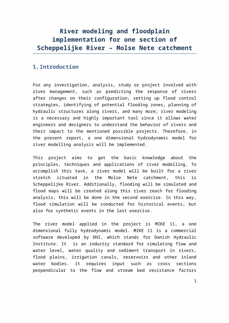
For the present analysis, the MIKE 11 model was applied in onesection of the Scheppelijke River which is part of the MolseNete catchment. This catchment is one of the 13 subbasins of theNete basin, in the North-east of Belgium. The Molse Nete catchment islocated in the eastern part of the Nete basin and stretches over themunicipalities of Mol, Geel, Balen and Lommel; as it can be observedin Figure 1:
Figure 1: Molse Nete catchment
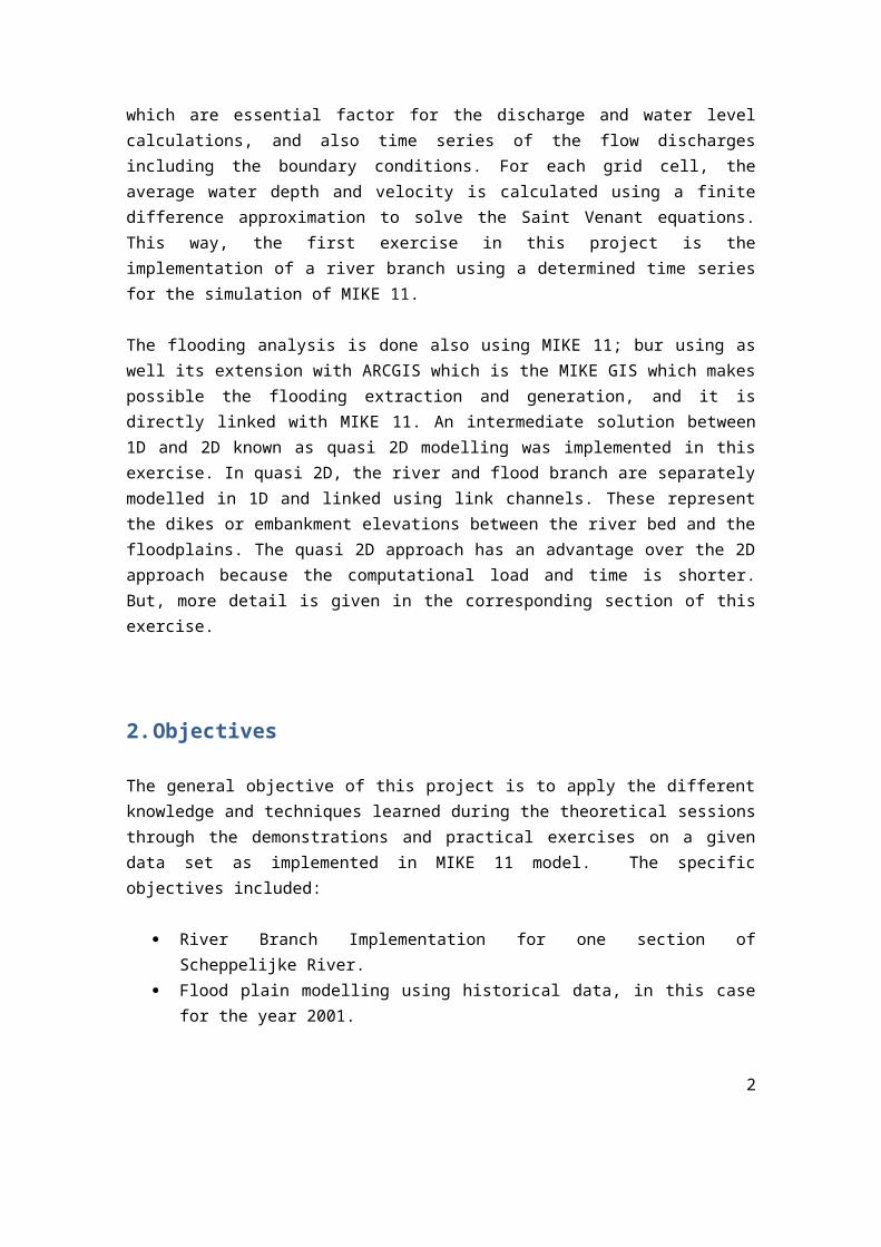
The river branch for this exercise will be implemented in theScheppelijke River which is in the northern part of the MolseNete catchment. This river is subdivided in different sections,and one of them, the second from the most upstream part of the
3
river, will be part of the present project, this section can beobserved enclosed in the red circle in Figure 2:
Figure 2: Section (red circle) chosen for branch implementation inScheppelijke River
3.2. Data Source
In this project, data was collected from the www.hydronet.bewebsite which the website in which all measured data formeteorological parameters is stored; in this case data of riverdischarge was needed for the corresponding boundary conditionsin the MIKE 11 model, then flow representative of theSchppelijke River was obtained from this source. Nevertheless,the only available data which was found was from Geel stationwhich is not close to the river, it is in fact, much moredownstream; but flow form the river also converge to thisstation, thus using data from this station is possible; however,the whole area representative of this stations must be used forthe boundary conditions in the project; this is explained inmuch more detailed in the corresponding section of the presentreport. The collected time series data is for 4 years between1998 and 2001; which will be used for the third exercise. Forthe first two exercises, only one event is picked from the wholetime series due to the fact that this exercise is for academicpurpose, thus for the introduction and understanding of the
4

basics of the model only, and one event simulation is fairlygood for this purpose.
5
4.Exercise 1: River branch implementation
4.1. Introduction
Regarding to the model, the river branch implementation in MIKE11 requires several files for its corresponding river flowsimulation. These are indeed the input (editors) files given tothe model, where different types of data can be implemented andedited. The different editors include: network files (*.nwk11),cross section file (*.xns11), the boundary file (*.bnd11),Hydrodynamic parameter file (*.hd11), Time series file (*.dsf0)and rainfall runoff files (*.dfs2) among others; but thementioned ones are the ones created for this exercise. Theindividual files have no linkage except with the MIKE 11simulator editor (*.sim) which provides the link between thegraphical views of all the other editor files. It also containsthe simulation and control parameters used to start asimulation.
In the present project, one section in the upper part of theSchppelijke River will be modelled using MIKE 11. This exercisefocuses in the implementation of a one dimensional hydrodynamicmodel for this river branch using one historical event, as itwas mentioned, for academic purpose only one event is chosen. Inthis case the event is chose from the time series obtained, andit is chosen the event with the highest peak from the hydrographobserved In the year 2001 from the available data. Thiscorrespond with the time between July 2nd and Augustst 30th whichmeans that the simulation is made for two months historicalevent, with an hourly time step which must be used for riverdischarges.
In a hydrodynamic model, flow routing is calculated by the deSaint Venant equations. Solving these equations can be done bynumerical solution; in this finite difference approximation is
6

used to solve these equations. The MIKE 11 software enables thuslocal calculations of discharges and water levels. Forcalculating these parameters, Mike 11 also needs correspondinggeometrical and friction information; hence cross section andmanning coefficient “n” are needed as input in the model, so themodel can calculated the water level at every point where across section and manning coefficient are known based ongeometrical information and friction information respectively.
4.2. Objectives
The main objective for this part of the exercise is to implementa river branch in MIKE 11. The specific objectives included:
Setting up of a network file, a cross-section file, aboundary conditions file, and a model parameter file.
Delineating the Sub catchment using GIS based on DEM ofthe catchment.
Simulating the discharge for selected time period. Determining the optimal time step while evaluating the
stability of the model. Visualisation of the results as time series of discharges
and water levels at specific calculation nodes along therivers, and as longitudinal profiles of water levels alongthe river, this by using the MIKE VIEW tool of MIKE 11.
4.3. Methodology
For the build-up of the MIKE 11 model, all input files (editors)mentioned in the previous sections must be created individually,then through the simulation file the will be linked and then thesimulation can start. Therefore, the build-up of these files isdone individually and it is explained in the next sections.
7
4.3.1. Network file
This file is the first one to be implemented since the riverbranch is created here, and then all parameters necessary in thedifferent point along the branch are added to this file throughthe tabular view of this file.
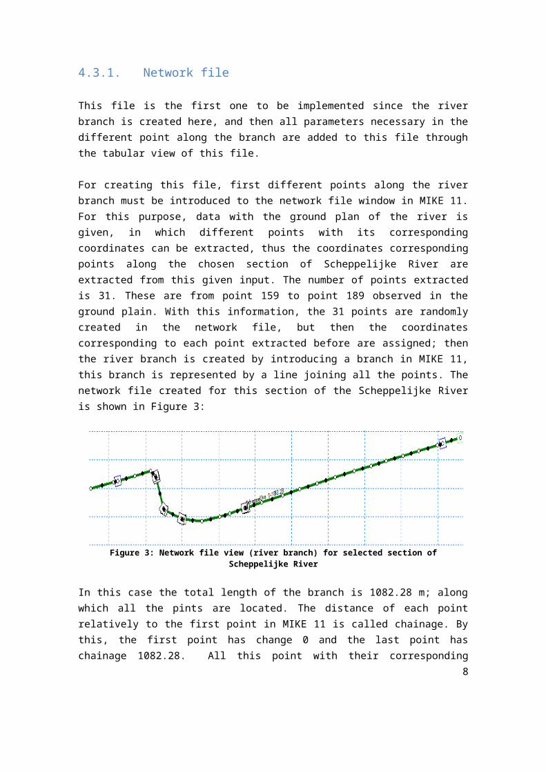
For creating this file, first different points along the riverbranch must be introduced to the network file window in MIKE 11.For this purpose, data with the ground plan of the river isgiven, in which different points with its correspondingcoordinates can be extracted, thus the coordinates correspondingpoints along the chosen section of Scheppelijke River areextracted from this given input. The number of points extractedis 31. These are from point 159 to point 189 observed in theground plain. With this information, the 31 points are randomlycreated in the network file, but then the coordinatescorresponding to each point extracted before are assigned; thenthe river branch is created by introducing a branch in MIKE 11,this branch is represented by a line joining all the points. Thenetwork file created for this section of the Scheppelijke Riveris shown in Figure 3:
Figure 3: Network file view (river branch) for selected section ofScheppelijke River
In this case the total length of the branch is 1082.28 m; alongwhich all the pints are located. The distance of each pointrelatively to the first point in MIKE 11 is called chainage. Bythis, the first point has change 0 and the last point haschainage 1082.28. All this point with their corresponding
8
coordinates and chainage are then defined and can be observed inthe tabular view of the network file; these chainages are all bydefault defined as “system defined” determined by thecoordinates; but if the user wants to change the chainage of anypoint, this can be change by changing this option to “userdefined”.
In the tabular view, the branch and its characteristics can bealso observed; when the branch was created, it was supposed tobe introduced following the flow direction, this means fromupstream to downstream, this means that the flow is “positive”and this is defined in this table, if it was not introduced fromupstream to downstream, then this can be put as “negative”, butin this case it was introduced following the flow direction, sono change is necessary. In this window it the first and lastchainage, which in this case are, as mentioned, 0 and 1082.28respectively. The “maximum dx” is also defined and this willdefined the minimum distance ate which the water level “H” willbe calculated, this means that if no cross section is defined ina distance equal or shorter than this dx, then the model willcalculate H at the position of dx by interpolation. In this casethe dx is defined as 100 m. Finally, the branch type is defined;since in this case this is a river branch, the default type“Regular” is left.
Then, the hydraulic structures must be also introduced sincethey are also very important in the river implementation sincethey are in charge of regulating the flow at those points, andtherefore at these points the river discharges “Q” arecalculated by the model. In this section four weirs and twoculverts are located and must be introduced in the model; theyare implemented also in the tabular view where theircharacteristics are introduced and based on these, the modelcalculates the Q-h relations. These characteristics are alsogiven as data for the Scheppelijke River, they are taken fromthe artwork file given as data. The summary of the estructresimplemented in the models is presented in Table 1. In this table
9
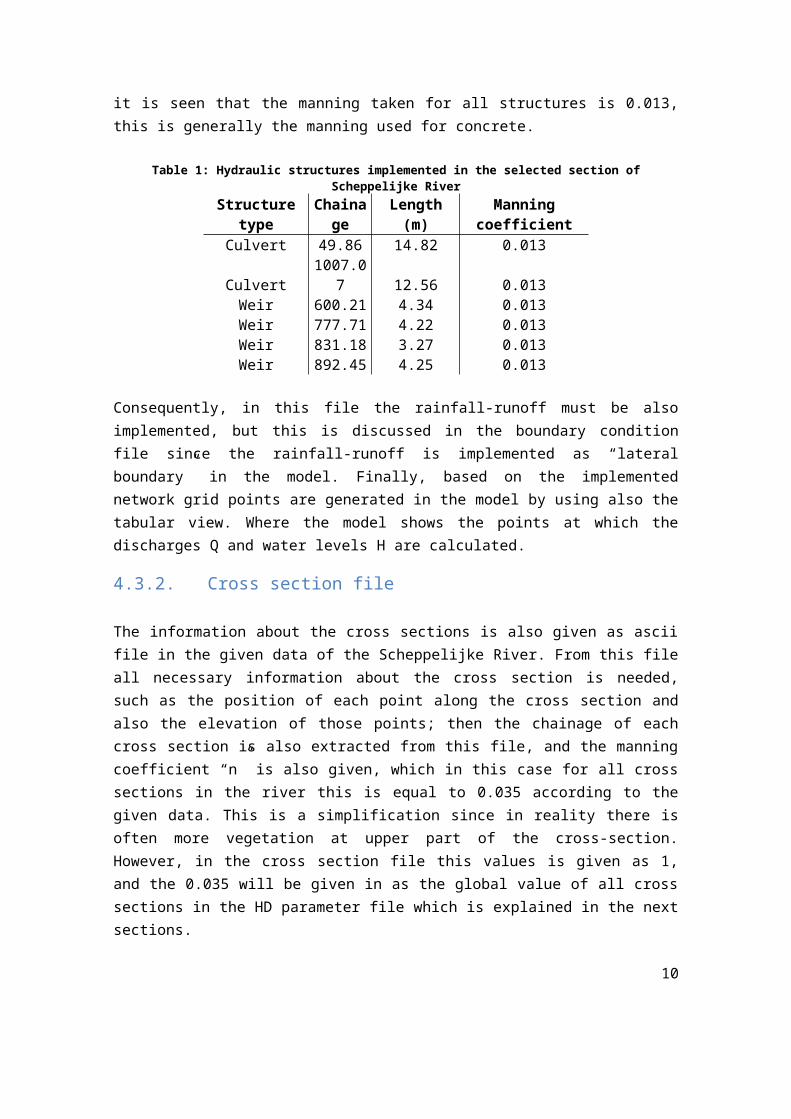
it is seen that the manning taken for all structures is 0.013,this is generally the manning used for concrete.
Table 1: Hydraulic structures implemented in the selected section ofScheppelijke River
Structuretype
Chainage
Length(m)
Manningcoefficient
Culvert 49.86 14.82 0.013
Culvert1007.0
7 12.56 0.013Weir 600.21 4.34 0.013Weir 777.71 4.22 0.013Weir 831.18 3.27 0.013Weir 892.45 4.25 0.013
Consequently, in this file the rainfall-runoff must be alsoimplemented, but this is discussed in the boundary conditionfile since the rainfall-runoff is implemented as “lateralboundary” in the model. Finally, based on the implementednetwork grid points are generated in the model by using also thetabular view. Where the model shows the points at which thedischarges Q and water levels H are calculated.
4.3.2. Cross section file
The information about the cross sections is also given as asciifile in the given data of the Scheppelijke River. From this fileall necessary information about the cross section is needed,such as the position of each point along the cross section andalso the elevation of those points; then the chainage of eachcross section is also extracted from this file, and the manningcoefficient “n” is also given, which in this case for all crosssections in the river this is equal to 0.035 according to thegiven data. This is a simplification since in reality there isoften more vegetation at upper part of the cross-section.However, in the cross section file this values is given as 1,and the 0.035 will be given in as the global value of all crosssections in the HD parameter file which is explained in the nextsections.
10
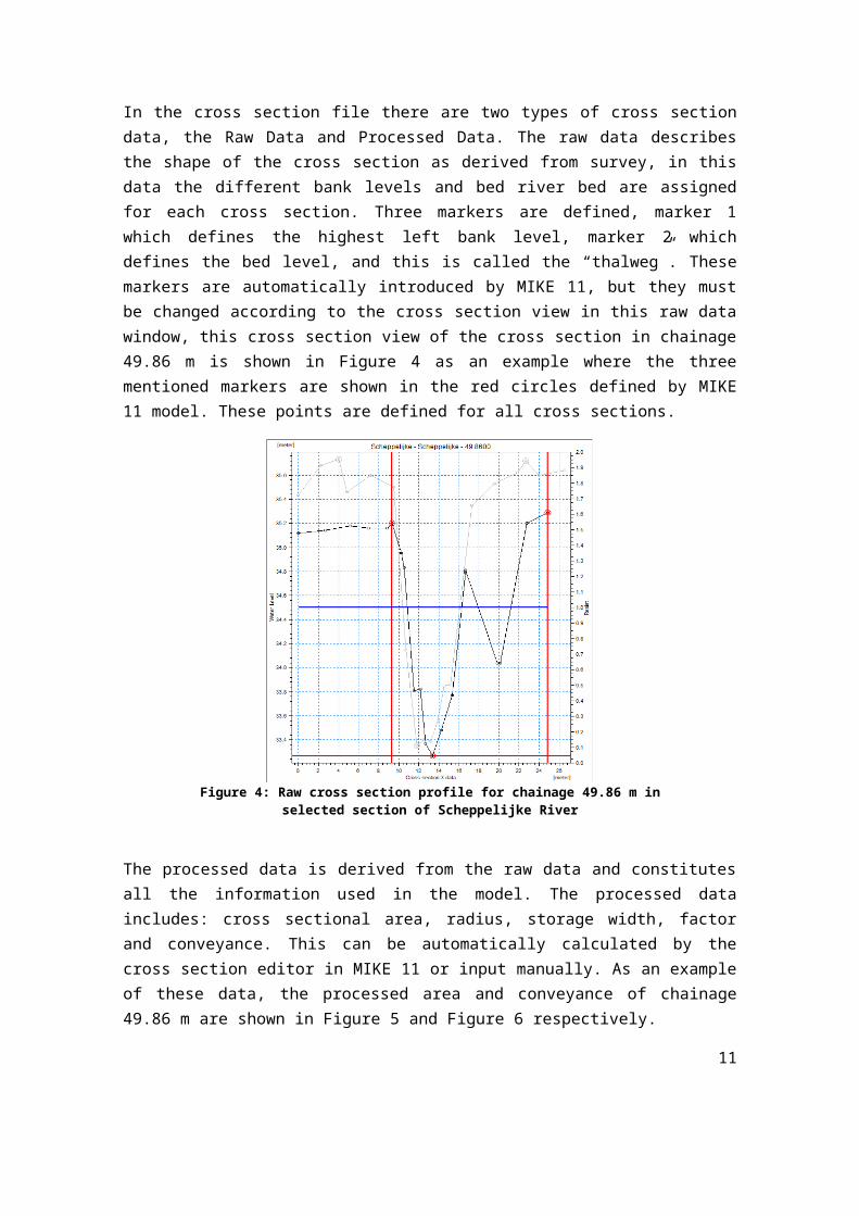
In the cross section file there are two types of cross sectiondata, the Raw Data and Processed Data. The raw data describesthe shape of the cross section as derived from survey, in thisdata the different bank levels and bed river bed are assignedfor each cross section. Three markers are defined, marker 1which defines the highest left bank level, marker 2 whichdefines the bed level, and this is called the “thalweg”. Thesemarkers are automatically introduced by MIKE 11, but they mustbe changed according to the cross section view in this raw datawindow, this cross section view of the cross section in chainage49.86 m is shown in Figure 4 as an example where the threementioned markers are shown in the red circles defined by MIKE11 model. These points are defined for all cross sections.
Figure 4: Raw cross section profile for chainage 49.86 m inselected section of Scheppelijke River
The processed data is derived from the raw data and constitutesall the information used in the model. The processed dataincludes: cross sectional area, radius, storage width, factorand conveyance. This can be automatically calculated by thecross section editor in MIKE 11 or input manually. As an exampleof these data, the processed area and conveyance of chainage49.86 m are shown in Figure 5 and Figure 6 respectively.
11
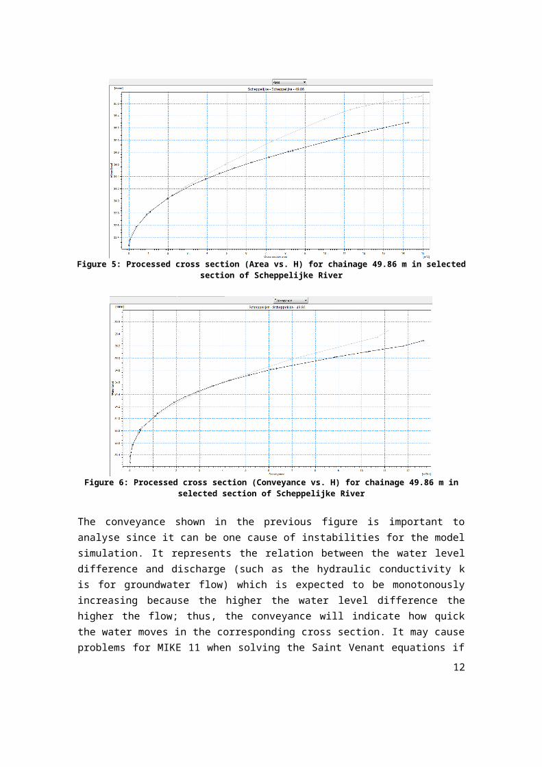
Figure 5: Processed cross section (Area vs. H) for chainage 49.86 m in selectedsection of Scheppelijke River
Figure 6: Processed cross section (Conveyance vs. H) for chainage 49.86 m inselected section of Scheppelijke River
The conveyance shown in the previous figure is important toanalyse since it can be one cause of instabilities for the modelsimulation. It represents the relation between the water leveldifference and discharge (such as the hydraulic conductivity kis for groundwater flow) which is expected to be monotonouslyincreasing because the higher the water level difference thehigher the flow; thus, the conveyance will indicate how quickthe water moves in the corresponding cross section. It may causeproblems for MIKE 11 when solving the Saint Venant equations if
12
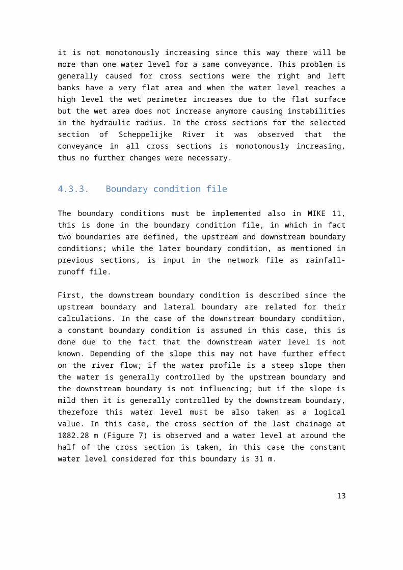
it is not monotonously increasing since this way there will bemore than one water level for a same conveyance. This problem isgenerally caused for cross sections were the right and leftbanks have a very flat area and when the water level reaches ahigh level the wet perimeter increases due to the flat surfacebut the wet area does not increase anymore causing instabilitiesin the hydraulic radius. In the cross sections for the selectedsection of Scheppelijke River it was observed that theconveyance in all cross sections is monotonously increasing,thus no further changes were necessary.
4.3.3. Boundary condition file
The boundary conditions must be implemented also in MIKE 11,this is done in the boundary condition file, in which in facttwo boundaries are defined, the upstream and downstream boundaryconditions; while the later boundary condition, as mentioned inprevious sections, is input in the network file as rainfall-runoff file.
First, the downstream boundary condition is described since theupstream boundary and lateral boundary are related for theircalculations. In the case of the downstream boundary condition,a constant boundary condition is assumed in this case, this isdone due to the fact that the downstream water level is notknown. Depending of the slope this may not have further effecton the river flow; if the water profile is a steep slope thenthe water is generally controlled by the upstream boundary andthe downstream boundary is not influencing; but if the slope ismild then it is generally controlled by the downstream boundary,therefore this water level must be also taken as a logicalvalue. In this case, the cross section of the last chainage at1082.28 m (Figure 7) is observed and a water level at around thehalf of the cross section is taken, in this case the constantwater level considered for this boundary is 31 m.
13
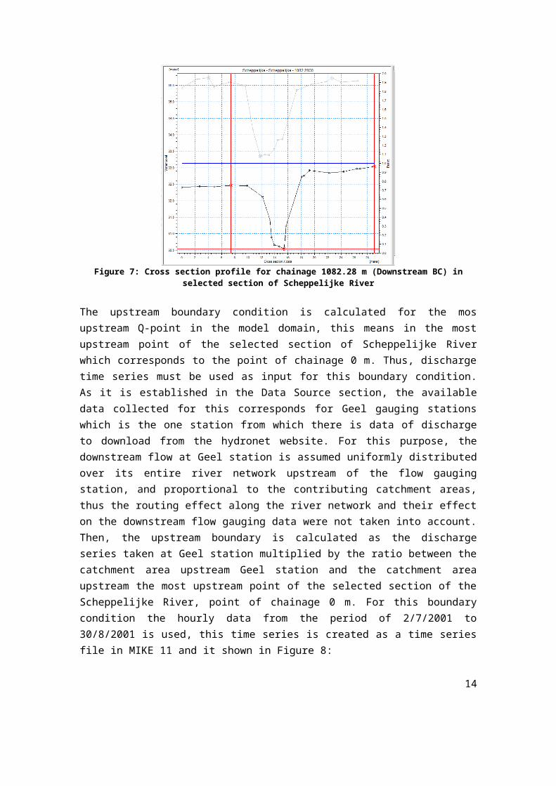
Figure 7: Cross section profile for chainage 1082.28 m (Downstream BC) inselected section of Scheppelijke River
The upstream boundary condition is calculated for the mosupstream Q-point in the model domain, this means in the mostupstream point of the selected section of Scheppelijke Riverwhich corresponds to the point of chainage 0 m. Thus, dischargetime series must be used as input for this boundary condition.As it is established in the Data Source section, the availabledata collected for this corresponds for Geel gauging stationswhich is the one station from which there is data of dischargeto download from the hydronet website. For this purpose, thedownstream flow at Geel station is assumed uniformly distributedover its entire river network upstream of the flow gaugingstation, and proportional to the contributing catchment areas,thus the routing effect along the river network and their effecton the downstream flow gauging data were not taken into account.Then, the upstream boundary is calculated as the dischargeseries taken at Geel station multiplied by the ratio between thecatchment area upstream Geel station and the catchment areaupstream the most upstream point of the selected section of theScheppelijke River, point of chainage 0 m. For this boundarycondition the hourly data from the period of 2/7/2001 to30/8/2001 is used, this time series is created as a time seriesfile in MIKE 11 and it shown in Figure 8:
14
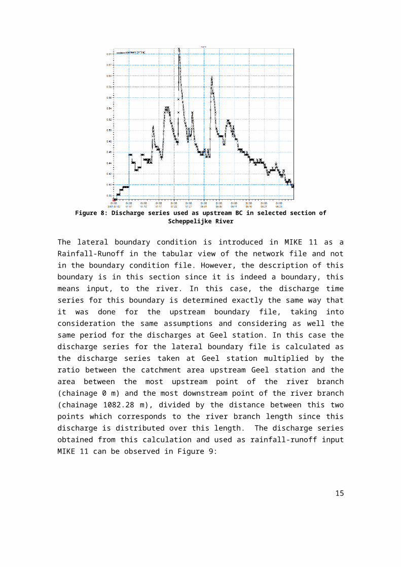
Figure 8: Discharge series used as upstream BC in selected section ofScheppelijke River
The lateral boundary condition is introduced in MIKE 11 as aRainfall-Runoff in the tabular view of the network file and notin the boundary condition file. However, the description of thisboundary is in this section since it is indeed a boundary, thismeans input, to the river. In this case, the discharge timeseries for this boundary is determined exactly the same way thatit was done for the upstream boundary file, taking intoconsideration the same assumptions and considering as well thesame period for the discharges at Geel station. In this case thedischarge series for the lateral boundary file is calculated asthe discharge series taken at Geel station multiplied by theratio between the catchment area upstream Geel station and thearea between the most upstream point of the river branch(chainage 0 m) and the most downstream point of the river branch(chainage 1082.28 m), divided by the distance between this twopoints which corresponds to the river branch length since thisdischarge is distributed over this length. The discharge seriesobtained from this calculation and used as rainfall-runoff inputMIKE 11 can be observed in Figure 9:
15
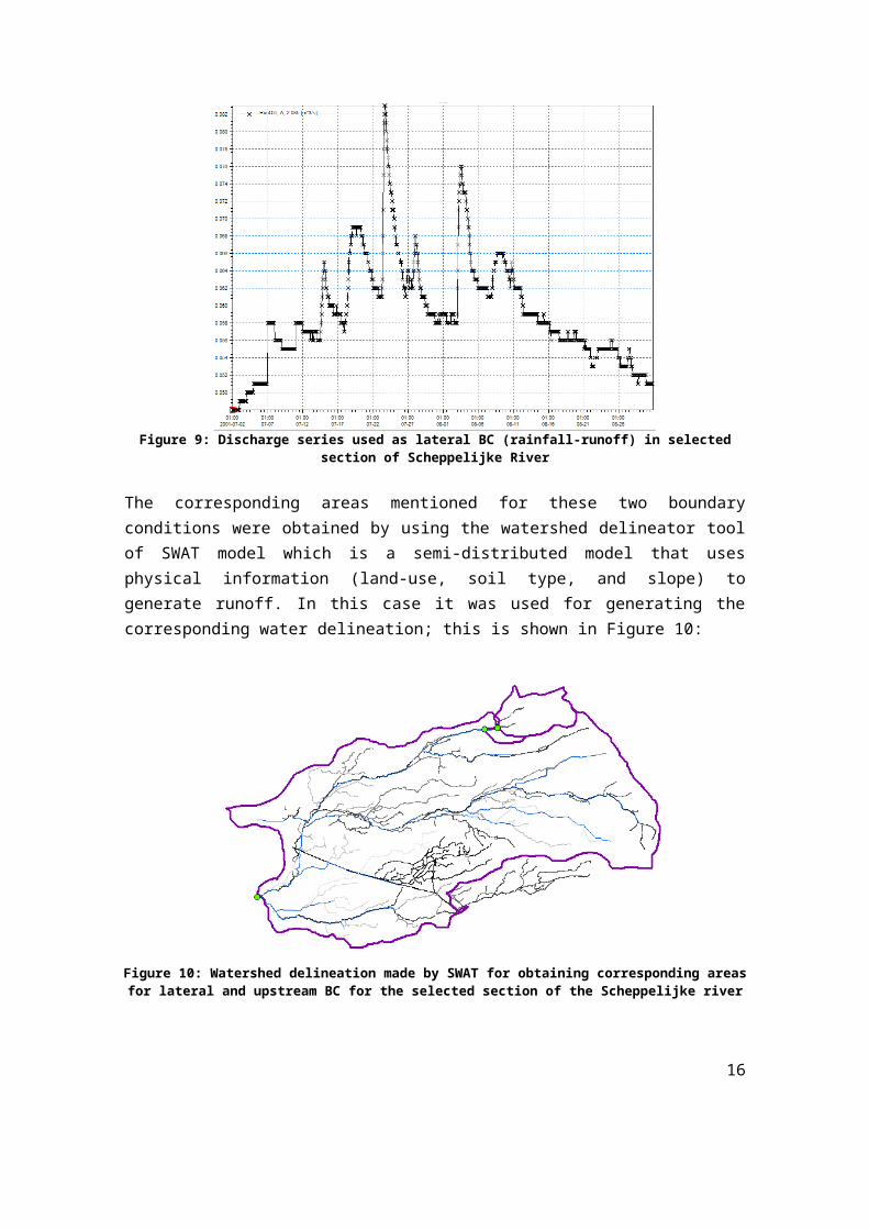
Figure 9: Discharge series used as lateral BC (rainfall-runoff) in selectedsection of Scheppelijke River
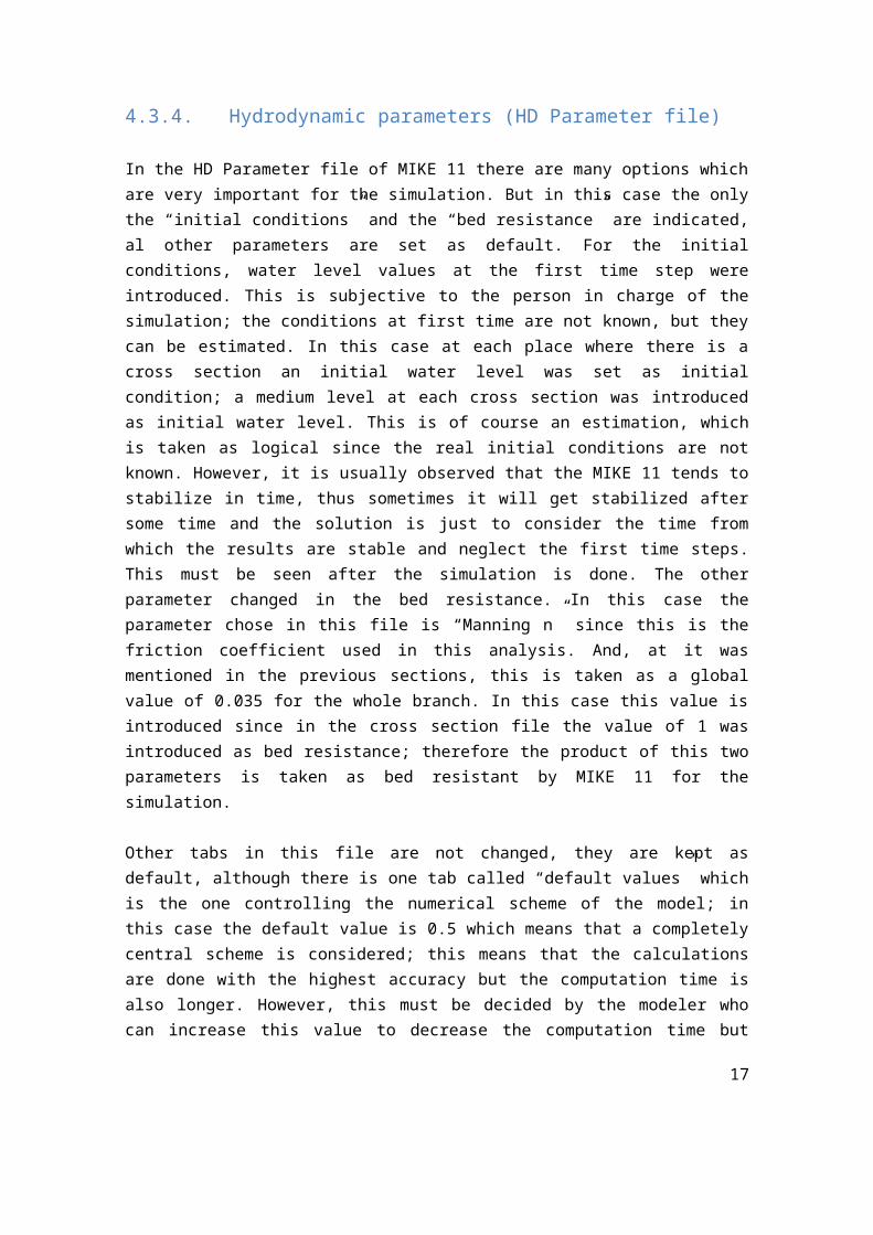
The corresponding areas mentioned for these two boundaryconditions were obtained by using the watershed delineator toolof SWAT model which is a semi-distributed model that usesphysical information (land-use, soil type, and slope) togenerate runoff. In this case it was used for generating thecorresponding water delineation; this is shown in Figure 10:
Figure 10: Watershed delineation made by SWAT for obtaining corresponding areasfor lateral and upstream BC for the selected section of the Scheppelijke river
16
4.3.4. Hydrodynamic parameters (HD Parameter file)
In the HD Parameter file of MIKE 11 there are many options whichare very important for the simulation. But in this case the onlythe “initial conditions” and the “bed resistance” are indicated,al other parameters are set as default. For the initialconditions, water level values at the first time step wereintroduced. This is subjective to the person in charge of thesimulation; the conditions at first time are not known, but theycan be estimated. In this case at each place where there is across section an initial water level was set as initialcondition; a medium level at each cross section was introducedas initial water level. This is of course an estimation, whichis taken as logical since the real initial conditions are notknown. However, it is usually observed that the MIKE 11 tends tostabilize in time, thus sometimes it will get stabilized aftersome time and the solution is just to consider the time fromwhich the results are stable and neglect the first time steps.This must be seen after the simulation is done. The otherparameter changed in the bed resistance. In this case theparameter chose in this file is “Manning n” since this is thefriction coefficient used in this analysis. And, at it wasmentioned in the previous sections, this is taken as a globalvalue of 0.035 for the whole branch. In this case this value isintroduced since in the cross section file the value of 1 wasintroduced as bed resistance; therefore the product of this twoparameters is taken as bed resistant by MIKE 11 for thesimulation.
Other tabs in this file are not changed, they are kept asdefault, although there is one tab called “default values” whichis the one controlling the numerical scheme of the model; inthis case the default value is 0.5 which means that a completelycentral scheme is considered; this means that the calculationsare done with the highest accuracy but the computation time isalso longer. However, this must be decided by the modeler whocan increase this value to decrease the computation time but
17
lose some accuracy. In the present case this was kept as defaultsince the computation time was not a problem for the simulation.
4.3.5. Simulation settings
After all the previous files are already made, they areintroduced in a “simulation file” were they are linked. In thisfile all previous files are loaded for the simulation. Then, inthis simulation file, the simulation settings must beestablished. It is possible to use a fixed time step for thewhole simulation, but it is important to choose one time that ishigh enough for not having a very large computation time, butalso sufficiently low for avoiding problems with instabilityduring the simulation. This Instability in the numerical schemeresults due to a small courant number. Courant number refers tothe ratio between time step, ∆t and space step, ∆x as shown inequation below:
∆t≪ ∆xU+c
Where: U = stream velocity, c = wave velocity, ∆t = time step,∆x = space step.If a large time step is used for simulation, information is lostand the simulation becomes unstable. This can be solved by usinga very small time step, but at it was mentioned, the smaller thetime step, the longer the calculation time is. Hence, the spacestep in this case must be also checked since it should not betoo short because that leads to instabilities.
Generally cross sections are measured just some meters after andsome meters before hydraulic structures, that is why thedistance between cross sections between structures in the fileis very short. In this case the distance between some crosssections were increase, and in two cases the cross sections weredeleted since the distance was too short and it was leading toinstabilities in the simulation.
18

Then, an “adaptive time step” was chosen for the simulation, inthis case Mike 11 looks for the optimal time step in eachcalculation, but the range of time should be given, for thisanalysis the range given was between 10 second and 2 minutes.
Next step was to choose the initial condition that the modelwill take for the simulation. It was possible to choose “steadystate” condition, so this way the initial conditions would becalculated automatically by MIKE 11 taking into account thestated boundary conditions and looking for analytical solutionssimplifying the Saint Venant equations (replace the equations byequations that can be solved in steady state conditions);however, the possibility of the model to use the steady statecondition depends also in the characteristics of the riversystem because if the system is very complex, it is not possibleto find the analytical solutions for the model. This was thecase for this river branch. Therefore, the initial conditionstaken were the ones from the “Parameter file” which are actuallythe ones introduced before in the HD Parameter file.
Finally, the time period for which the simulation is run isselected. In this case, the period is the same as the one givenfor the boundary condition time series, this means from 2/7/2001to 30/8/2001. It was chosen to see the results hourly, and thesimulation was run.
4.4. Results
The results are observed using the MIKE VIEW tool from MIKE 11.The results are save in *.res11 file which MIKE VIEW opens toobserve the results of the simulation done for the selectedsection of the Scheppelijke River. These results are presentedin this section.
19
4.4.1. Longitudinal profile and cross section output
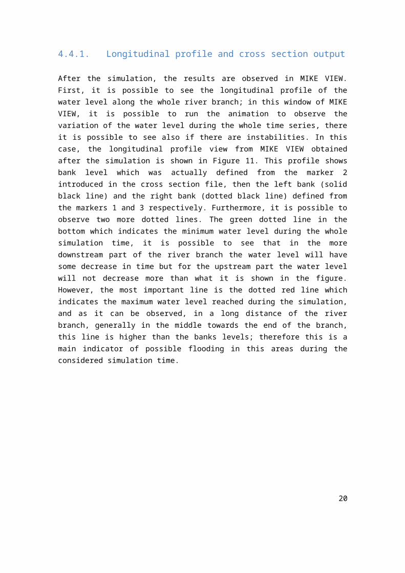
After the simulation, the results are observed in MIKE VIEW.First, it is possible to see the longitudinal profile of thewater level along the whole river branch; in this window of MIKEVIEW, it is possible to run the animation to observe thevariation of the water level during the whole time series, thereit is possible to see also if there are instabilities. In thiscase, the longitudinal profile view from MIKE VIEW obtainedafter the simulation is shown in Figure 11. This profile showsbank level which was actually defined from the marker 2introduced in the cross section file, then the left bank (solidblack line) and the right bank (dotted black line) defined fromthe markers 1 and 3 respectively. Furthermore, it is possible toobserve two more dotted lines. The green dotted line in thebottom which indicates the minimum water level during the wholesimulation time, it is possible to see that in the moredownstream part of the river branch the water level will havesome decrease in time but for the upstream part the water levelwill not decrease more than what it is shown in the figure.However, the most important line is the dotted red line whichindicates the maximum water level reached during the simulation,and as it can be observed, in a long distance of the riverbranch, generally in the middle towards the end of the branch,this line is higher than the banks levels; therefore this is amain indicator of possible flooding in this areas during theconsidered simulation time.
20
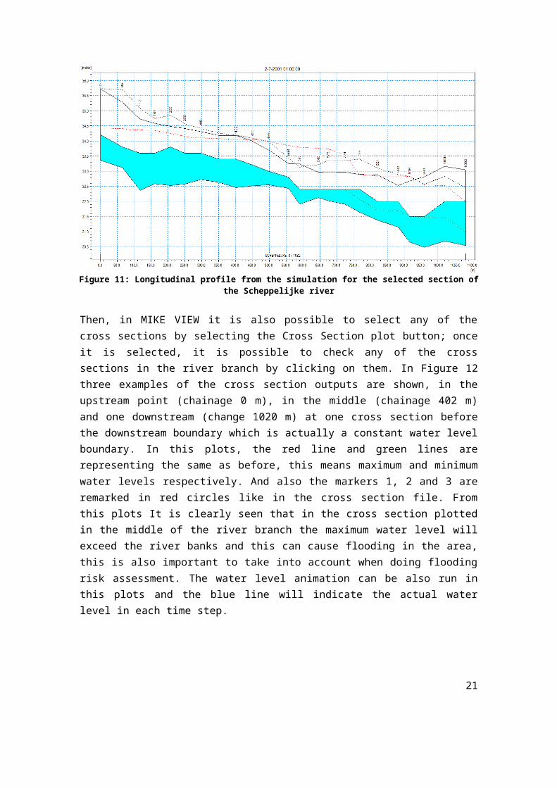
Figure 11: Longitudinal profile from the simulation for the selected section ofthe Scheppelijke river
Then, in MIKE VIEW it is also possible to select any of thecross sections by selecting the Cross Section plot button; onceit is selected, it is possible to check any of the crosssections in the river branch by clicking on them. In Figure 12three examples of the cross section outputs are shown, in theupstream point (chainage 0 m), in the middle (chainage 402 m)and one downstream (change 1020 m) at one cross section beforethe downstream boundary which is actually a constant water levelboundary. In this plots, the red line and green lines arerepresenting the same as before, this means maximum and minimumwater levels respectively. And also the markers 1, 2 and 3 areremarked in red circles like in the cross section file. Fromthis plots It is clearly seen that in the cross section plottedin the middle of the river branch the maximum water level willexceed the river banks and this can cause flooding in the area,this is also important to take into account when doing floodingrisk assessment. The water level animation can be also run inthis plots and the blue line will indicate the actual waterlevel in each time step.
21

Figure 12: Cross section outputs from the simulation for the selected sectionof the Scheppelijke river
4.4.2. Water level and discharge series
In MIKE VIEW, it is also possible to see the time series foreach point at which water level and discharge was calculated bythe model. For the water level simulation, in Figure 13 a plotof water level time series in the upstream (chainage 0 m),middle (chainage 498 m) and downstream (change 1020 m) points isshown by the black, blue and green lines respectively. First, itis important to remark that for every simulation results thefirst peiod of time is for the model to stabilize since theintial conditions may not be as precise as desired. For theseresults, the first period may not be included in the analysissince it is accomodating the low initial conditions set. Then,in this plot it is possible to observe that the differencebetween the water levels is due to the elevation of the crosssections, since upstream is more elevated than downstream, butthe water level high and low differences in between thesimulation period is slightly different. For upstream, in sometimes during the period a change in water level is higher than
22
the change in the water level downstream; thus it is importantto analyze how the river routing changes certain characteristicsof the time series. The water level fluctuations present on theupstream water level is attenuated by the river and thedownstream water level fluctuates less.
Figure 13: Water level time series upstream (black), middle (blue) anddownstream (green) for the selected section of the Scheppelijke river
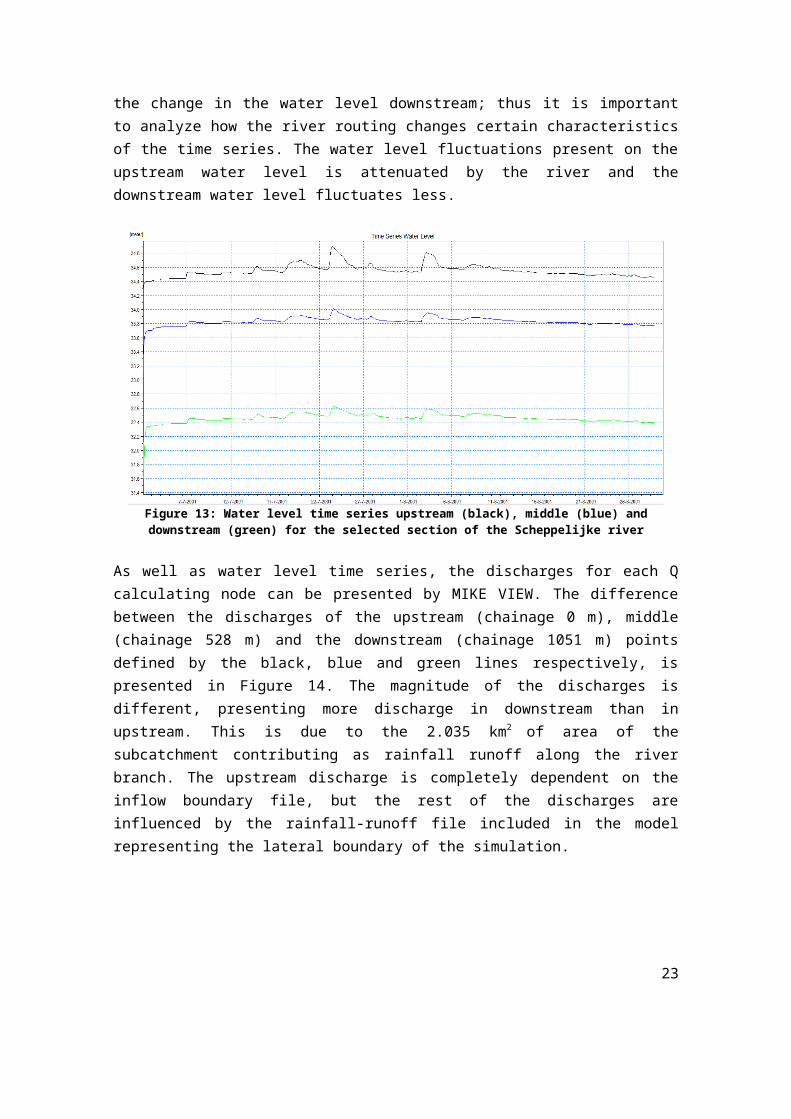
As well as water level time series, the discharges for each Qcalculating node can be presented by MIKE VIEW. The differencebetween the discharges of the upstream (chainage 0 m), middle(chainage 528 m) and the downstream (chainage 1051 m) pointsdefined by the black, blue and green lines respectively, ispresented in Figure 14. The magnitude of the discharges isdifferent, presenting more discharge in downstream than inupstream. This is due to the 2.035 km2 of area of thesubcatchment contributing as rainfall runoff along the riverbranch. The upstream discharge is completely dependent on theinflow boundary file, but the rest of the discharges areinfluenced by the rainfall-runoff file included in the modelrepresenting the lateral boundary of the simulation.
23
Figure 14: Discharge time series upstream (black), middle (blue) and downstream(green) for the selected section of the Scheppelijke river
4.5. Conclusion
In this section of the report, a river branch implementation waspresented, using the MIKE 11 model it is seen that it ispossible to make this implementation using the appropriate andnecessary data. In this case it is important, besides having thegeographical characteristics of the river (coordinates of thedifferent points to delineate the branch), to have the values ofthe different cross sections and manning coefficient along theriver since these are the most important parameters that themodel will use to solve the Saint Venant equations by which itcalculated the different variables along the river. In thiscase, all necessary data was given to make the correspondingimplementation and run the simulation.
The time discharges chosen as input for the upstream boundaryand the lateral boundary are from 2/7/2001 to 30/8/2001, theywere chosen from Geel station which is much downstream of theScheppelijke River but it is the closest station where data wasavailable. Then, catchment delineation was applied using SWATmodel to represent the corresponding discharges upstream theriver branch and along the river as runoff from the catchment.
24

The cross sections and hydraulic structures were implemented,and the manning coefficient was introduced as a global value(the same value for the whole branch) of 0.035 since in thegiven data for all cross sections this is the same. Thedifferent instabilities were analyzed, so for cross sectionsvery close to each other some were separated for a reasonabledistance, and other were extracted from the branch since theycould cause instabilities. Also an adaptive time step was chosenwith a range between 10 seconds and two minutes. The initialconditions were included following the water level at differentcross section. Following the mentioned cautions, the simulationwas run without any instability, obtaining results very hour.
The results are visualized using MIKE VIEW, from these; it ispossible to observe the longitudinal profile of the branchduring the simulation time, but also the cross section outputs,and the water level and discharges time series; where it ispossible to see that the model stabilizes the simulation after alittle time from the initial condition. Also it is possible tosee the effect of the runoff caused in the discharges along theriver branch. In these results it is possible to see that thereis risk of flooding during the simulation time in many placesalong the river branch, therefore the corresponding analysis isdone in the next exercises.
5.Floodplain modelling
25

5.1. Introduction
A simple definition of floods is that they are natural processeswhere tidal waters inundate dry land. Numerical modelling offlood events often requires a description of the flooding acrosscertain plains that are part of the river hydrodynamics.
Flood mapping could best be achieved by 2-dimentionalhydrodynamic modelling. These 2-D models solve the Saint Venantequation in two dimensions applying finite difference or finiteelement. However because of the complexity and high datarequirement involved, its applicability is heavily restricted.The effective alternative to the 2-D flood mapping is the Quasi-2D modelling. In a Quasi 2D model, the flood plains areconnected to the main river by link channels and the dischargethrough these links is calculated using the equation of a weir.
In this exercise, a simulation of a flood model is done by theimplementation of a fictitious flood branch, extraction of crosssections along the floodplain from the Digital Elevation ModelDEM of the Molse Nete catchment. And implementation of Linkchannels describing the embankment overflow process will bedescribed.
After implementation of the flood branch, the MIKE11 modelincluding the flood branch can be simulated for an historicalflood period, in the actual case, will be for the same periodused as for the previous exercise. Afterwards, flood mappingwill be done based on the results of flooding simulationresults, using the MIKE-GIS interfacing software.
5.2. Objectives
The main objective of this report is to implement through MIKEGIS and MIKE 11 a Quasi-2 dimensional hydrodynamic model for thefloodplain along the branch representing the Scheppelijke Rivermade in the previous exercise. The main objective is achieved bythe following actions:
26
Implementation of a fictitious floodbranch in MIKE GISextracting the cross sections along the floodplain fromthe DEM.
Set up of the hydrodynamic model in MIKE 11 by theimplementation to the river model the floodbranch, spillsor link channels, by describing the embankment overflowprocess, and the specification of the floodplainroughness.
Simulating the water level and discharge for a selectedhistorical flood period.
Creating a floodmap using MIKE GIS interfacing with thesimulation results, visualizing the maximal spatial extentof the simulated flood.
5.3. Methodology
In this exercise, the implementation of the floodplain to theriver model already described in the previous exercise is done.The characteristics of the river model already set will not bechanged. This exercise must be applied using both, MIKE 11 forthe hydrodynamic model and MIKE GIS for the spatial analysis.
5.3.1. MIKE-GIS tool
For the floodplain implementation, it is required the use ofMIKE GIS which is an extension for ArcGIS which is linkeddirectly with MIKE 11; therefore, some introduction to this toolis important. MIKE GIS integrates ArcGIS and MIKE 11, by mergingthe technologies of numerical river modelling and GeographicInformation Systems. It is an advanced tool for the spatialpresentation and analysis of 1D flood model results.
From the MIKE 11 manual, it is possible to say that the floodmaps produced by MIKE 11 GIS are generated applying an automaticand highly efficient interpolation routine. The interface
27
requires as essential information a MIKE 11 river network, aMIKE 11 simulation and a Digital Elevation Model (DEM). Forfurther analysis, information such as maps/themes of rivers,infrastructure, land use, satellite images and other spatialdata can be included. The river network of a MIKE 11 model isgeo-referenced in MIKE 11 GIS through the Branch Route System.Linking a MIKE 11 Result file to the BRS, MIKE 11 GIS producesthree types of flood maps. These are depth/area inundation,duration and comparison/impact flood maps.
5.3.2. Network file for floodplain implementation
In this exercise, the floodplain is identified as a separatereach called the “flood branch” in the model network, placedadjacent to the “river branch” made in the previous exerciserepresenting the selected section of the Schppelijke River. Forthe implementation of the flood branch, a pre-processing processmust be done using the MIKE GIS in the ArcGIS interface. Forthis, the provided DEM of the Molse Nete catchment previouslygeoreferenced is loaded to the MIKE GIS. Then river branch isloaded into MIKE GIS as well, giving the network a spatialreference.
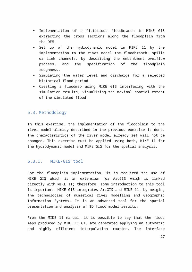
Firstly, the seperate flood branch was digitilized in accordanceto the DEM loaded into the workspace. The DEM of the area showsthat the elevations comes from higher in upstream to lower indownstream. The flood branch is digitilized in an area adjacentto the river with lower altitudes, where water may be retainedand the river is overflowing, but also in the section of theriver branch where possible flooding was defined from theprevious exercies. Therefore, these two factors are the onesdefining the place where the flood branch is implemented. InFigure 15 the river branch (down) and the flood branch (up) arepresented in light blue. It is possible to observe that theflood branch is placed in an area of lower altituda an the itslenght covers from the place where the possible inundationobtained from the previous exercise (Figure 11) at about
28
chainage 450 m to the end of the river branch. The flood branchhas a length of 559.79 m and its flow direction is from upstreamto downstream following the direction of the main river branch.
Figure 15: MIKE GIS flood branch implementation for selected section ofScheppelijke River
This DEM was then clipped since in MIKE 11 for generating theflood map in next steps the size of the file should not be solarge for facilitating the model to generate the map. Then, thisDEM was saved as *.dfs2 file to use it in MIKE 11.
5.3.3. Flood branch cross sections
The flood branch cross sections are then created, they can bealso observed in Figure 15 shown above. The cross sections aredelimited in accordance to the elevation of the area, startingwhere the low elevation ends up to the river, thus they aredefined so that they started at the river dike and extendeduntil elevation increased again. It is important to create thecross sections since they are the indicators of how much volumecan be stored in the floodplain, and also they will give an ideaabout the volume-level relation since from the topographicinformation in the cross section it is possible to know thewater level of a volume of water that is coming from the riverto the flood plain. The cross sections are created in this caseat about 50 m from each other; in between two cross sections thecross sections are linearly interpolated. The distances are then
29
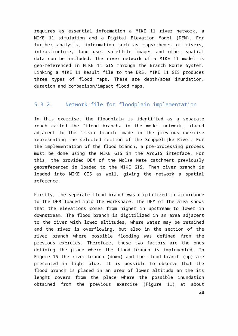
good since no strong variation in topography in the flood plain,and also it is good to put a fairly long distance due to theinstabilities explained in the previous exercises. Then, MIKEGIS facilitates the automatic extraction of flood plaintopography (flood plain cross-sections and area elevationrelations) from the DEM. The extracted flood plain topographycan readily be imported into a MIKE 11 cross section database.In MIKE 11 the roughness of the flood plain cross sections mustbe specified. Since the floodplain is vegetated the manningcoefficient is expected to be higher, for this exercise all ofthem were set with 0.045. For these cross sections also marker1, 2, and 3 represent the left bank, lowest point, and rightbank of the cross sections, respectively; and the are introducedthe same way it was done for the cross section of the riverbranch in the previous exercise. The flood plain cross sectionsprofiles are shown in Figure 16:
Figure 16: Floodplain cross sections profile
5.3.4. River branch and flood branch connection
The connection between the flood branch and the river branch wasdone using another branch; in this case this branch is specifiedin MIKE 11 as a “link channel”. Link channels are simplifiedbranches in which flow through the branch is calculated as flow
30
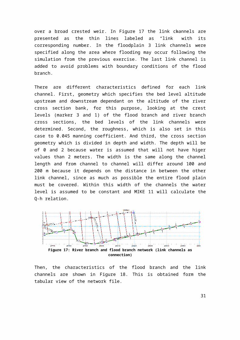
over a broad crested weir. In Figure 17 the link channels arepresented as the thin lines labeled as “link” with itscorresponding number. In the floodplain 3 link channels werespecified along the area where flooding may occur following thesimulation from the previous exercise. The last link channel isadded to avoid problems with boundary conditions of the floodbranch.
There are different characteristics defined for each linkchannel. First, geometry which specifies the bed level altitudeupstream and downstream dependant on the altitude of the rivercross section bank, for this purpose, looking at the crestlevels (marker 3 and 1) of the flood branch and river branchcross sections, the bed levels of the link channels weredetermined. Second, the roughness, which is also set in thiscase to 0.045 manning coefficient. And third, the cross sectiongeometry which is divided in depth and width. The depth will beof 0 and 2 because water is assumed that will not have higervalues than 2 meters. The width is the same along the channellength and from channel to channel will differ around 100 and200 m because it depends on the distance in between the otherlink channel, since as much as possible the entire flood plainmust be covered. Within this width of the channels the waterlevel is assumed to be constant and MIKE 11 will calculate theQ-h relation.
Figure 17: River branch and flood branch network (link channels asconnection)
Then, the characteristics of the flood branch and the linkchannels are shown in Figure 18. This is obtained form thetabular view of the network file.
31
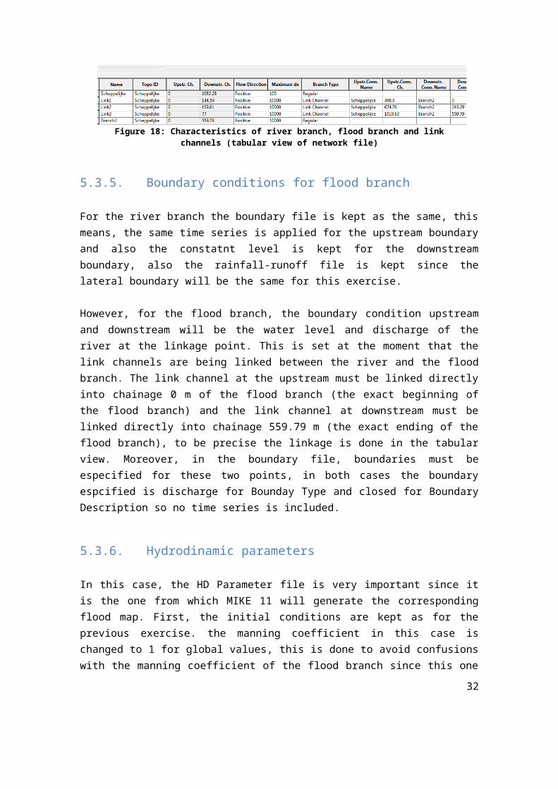
Figure 18: Characteristics of river branch, flood branch and linkchannels (tabular view of network file)
5.3.5. Boundary conditions for flood branch
For the river branch the boundary file is kept as the same, thismeans, the same time series is applied for the upstream boundaryand also the constatnt level is kept for the downstreamboundary, also the rainfall-runoff file is kept since thelateral boundary will be the same for this exercise.
However, for the flood branch, the boundary condition upstreamand downstream will be the water level and discharge of theriver at the linkage point. This is set at the moment that thelink channels are being linked between the river and the floodbranch. The link channel at the upstream must be linked directlyinto chainage 0 m of the flood branch (the exact beginning ofthe flood branch) and the link channel at downstream must belinked directly into chainage 559.79 m (the exact ending of theflood branch), to be precise the linkage is done in the tabularview. Moreover, in the boundary file, boundaries must beespecified for these two points, in both cases the boundaryespcified is discharge for Bounday Type and closed for BoundaryDescription so no time series is included.
5.3.6. Hydrodinamic parameters
In this case, the HD Parameter file is very important since itis the one from which MIKE 11 will generate the correspondingflood map. First, the initial conditions are kept as for theprevious exercise. the manning coefficient in this case ischanged to 1 for global values, this is done to avoid confusionswith the manning coefficient of the flood branch since this one
32
is different from the one of the river branch. However, thischange obligates to change the manning coefficient of each crosssection of the river branch to 0.035, this was done.
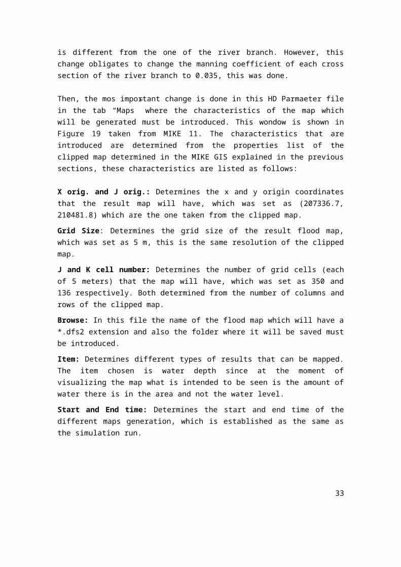
Then, the mos important change is done in this HD Parmaeter filein the tab “Maps” where the characteristics of the map whichwill be generated must be introduced. This wondow is shown inFigure 19 taken from MIKE 11. The characteristics that areintroduced are determined from the properties list of theclipped map determined in the MIKE GIS explained in the previoussections, these characteristics are listed as follows:
X orig. and J orig.: Determines the x and y origin coordinatesthat the result map will have, which was set as (207336.7,210481.8) which are the one taken from the clipped map.
Grid Size: Determines the grid size of the result flood map,which was set as 5 m, this is the same resolution of the clippedmap.
J and K cell number: Determines the number of grid cells (eachof 5 meters) that the map will have, which was set as 350 and136 respectively. Both determined from the number of columns androws of the clipped map.
Browse: In this file the name of the flood map which will have a*.dfs2 extension and also the folder where it will be saved mustbe introduced.
Item: Determines different types of results that can be mapped.The item chosen is water depth since at the moment ofvisualizing the map what is intended to be seen is the amount ofwater there is in the area and not the water level.
Start and End time: Determines the start and end time of thedifferent maps generation, which is established as the same asthe simulation run.
33
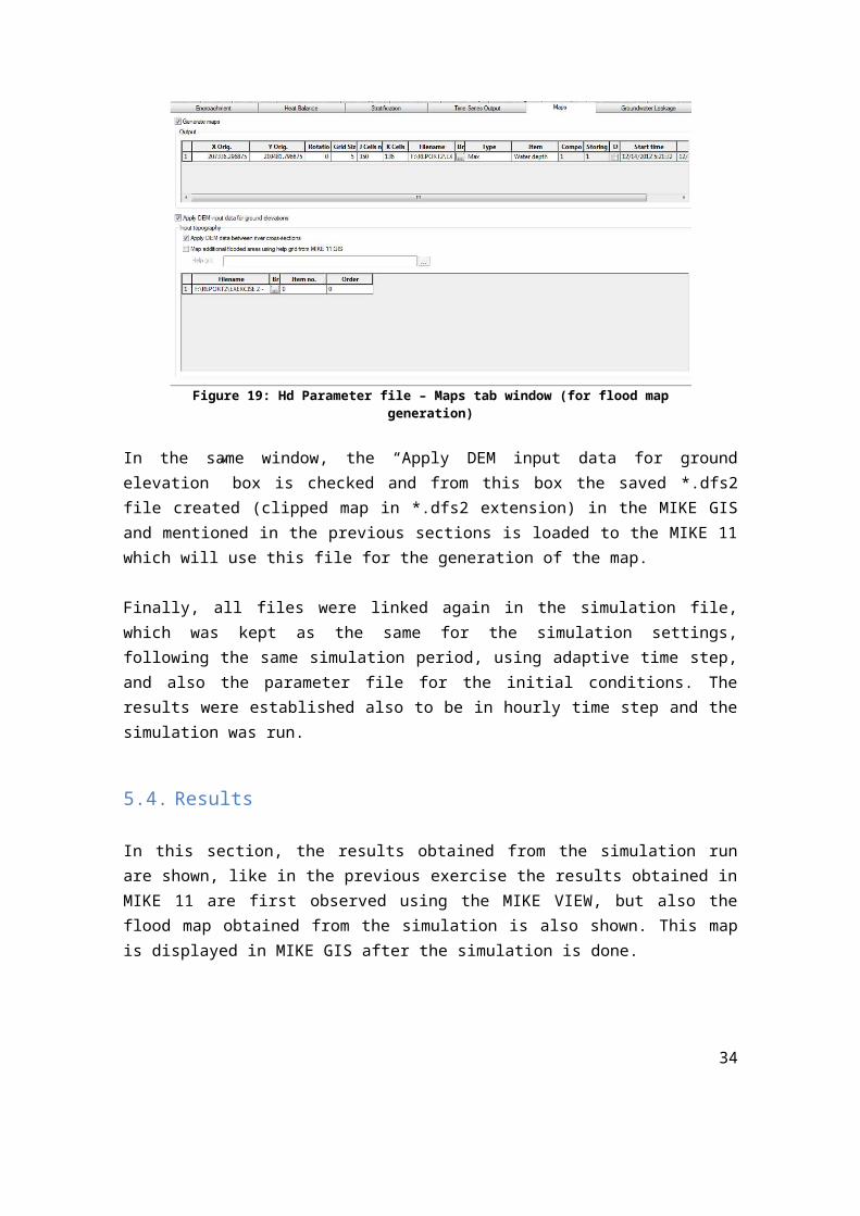
Figure 19: Hd Parameter file – Maps tab window (for flood mapgeneration)
In the same window, the “Apply DEM input data for groundelevation” box is checked and from this box the saved *.dfs2file created (clipped map in *.dfs2 extension) in the MIKE GISand mentioned in the previous sections is loaded to the MIKE 11which will use this file for the generation of the map.
Finally, all files were linked again in the simulation file,which was kept as the same for the simulation settings,following the same simulation period, using adaptive time step,and also the parameter file for the initial conditions. Theresults were established also to be in hourly time step and thesimulation was run.
5.4. Results
In this section, the results obtained from the simulation runare shown, like in the previous exercise the results obtained inMIKE 11 are first observed using the MIKE VIEW, but also theflood map obtained from the simulation is also shown. This mapis displayed in MIKE GIS after the simulation is done.
34
5.4.1. Hydrodynamic simulation results
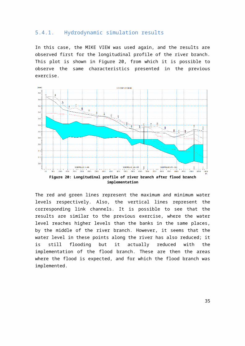
In this case, the MIKE VIEW was used again, and the results areobserved first for the longitudinal profile of the river branch.This plot is shown in Figure 20, from which it is possible toobserve the same characteristics presented in the previousexercise.
Figure 20: Longitudinal profile of river branch after flood branchimplementation
The red and green lines represent the maximum and minimum waterlevels respectively. Also, the vertical lines represent thecorresponding link channels. It is possible to see that theresults are similar to the previous exercise, where the waterlevel reaches higher levels than the banks in the same places,by the middle of the river branch. However, it seems that thewater level in these points along the river has also reduced; itis still flooding but it actually reduced with theimplementation of the flood branch. These are then the areaswhere the flood is expected, and for which the flood branch wasimplemented.
35
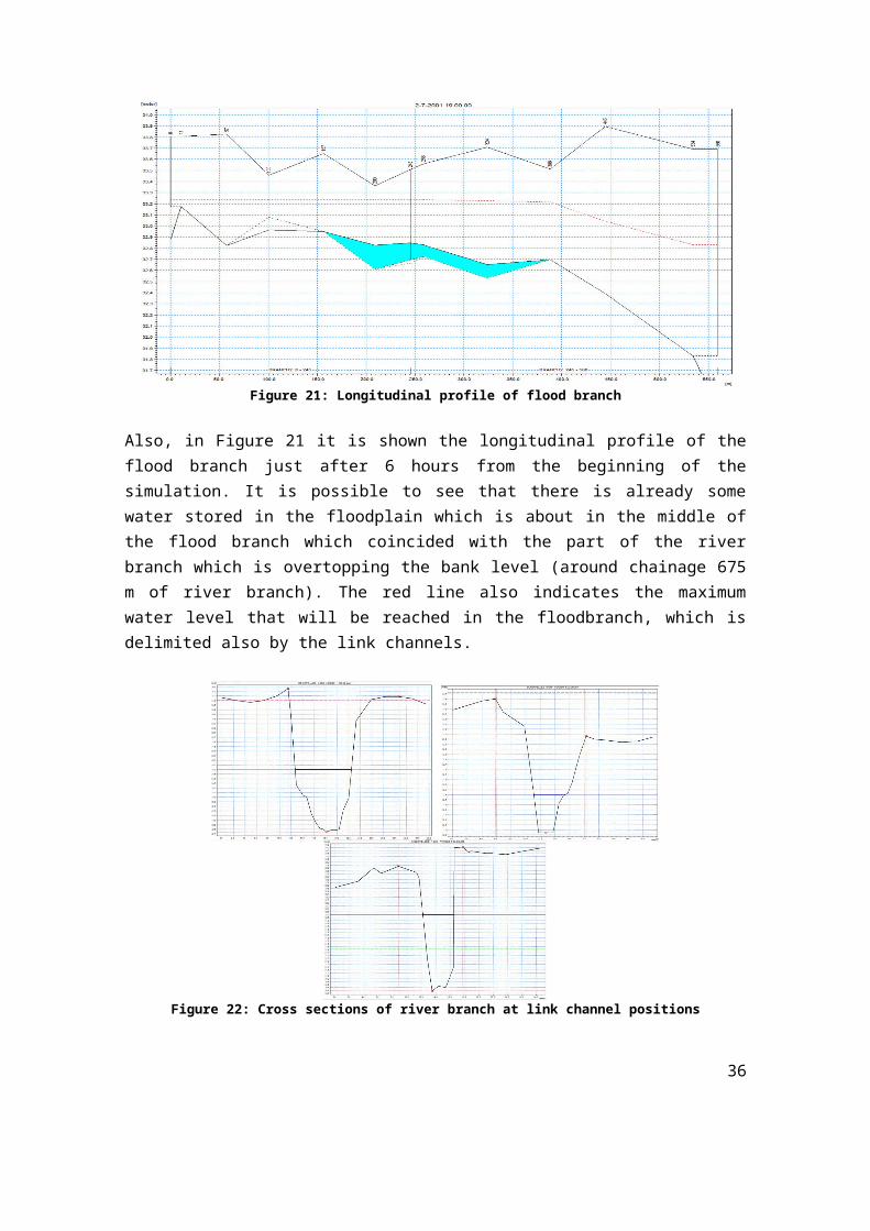
Figure 21: Longitudinal profile of flood branch
Also, in Figure 21 it is shown the longitudinal profile of theflood branch just after 6 hours from the beginning of thesimulation. It is possible to see that there is already somewater stored in the floodplain which is about in the middle ofthe flood branch which coincided with the part of the riverbranch which is overtopping the bank level (around chainage 675m of river branch). The red line also indicates the maximumwater level that will be reached in the floodbranch, which isdelimited also by the link channels.
Figure 22: Cross sections of river branch at link channel positions
36
Furthermore, the cross sections of the river branch where thelink channels where introduced are also plotted, and they areshown in Figure 22. It is possible to see that in the firstcross section some water will cross the left bank where thefloodplain is implemented, in the second cross section theflooding is also very clear marked by the red line in the wholecross section, and in the last cross section there is noflooding. This coincides with the longitudinal profile obtainedin Figure 20 where the link channels are also observed.
5.4.2. Floodplain map
The floodplain map is generated by MIKE 11 after the simulationis done. It is stored as a *.dfs2 file in the folder where wasestablished in the HD Parameter file. Then, it is plotted in theMIKE GIS interface since it can read the *.dfs2 file and it isconverted to a grid format by applying some raster tooloperations in ArcGIS.
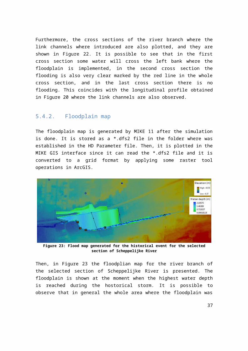
Figure 23: Flood map generated for the historical event for the selectedsection of Scheppelijke River
Then, in Figure 23 the floodplian map for the river branch ofthe selected section of Scheppelijke River is presented. Thefloodplain is shown at the moment when the highest water depthis reached during the hostorical storm. It is possible toobserve that in general the whole area where the floodplain was
37
implemented is flooded according to this map. Water depth tendsto be higher in the downstream area of the floodplain getting upto about 1.3 m, in the central area water depth vary betweenabout 0.8 to 1.1 m approximately, and in the more upstream partthe water depth is lower varying between about 0.2 to 0.7 m. Ingeneral the water depth is relatively high in this floodplain.As it was mentioned, this map was generated with MIKE GIS andMIKE 11 using the historical event chosen for the two firstexercises.
5.5. Conclusions
In general, from this exercise it is possible to affirm that forapplications to support decision makers, a map would explainbetter the magnitude of the spatial extent and the distributionof the flood. The maps generated in MIKE 11 use format of dfs2file which can be converted into a grid file to be read in a GISpackage. The application of flood maps is wide at the time ofrisk assessment in a certain area for a territorial planning anddisaster prevention especially in wet periods when flooding ispossible to occur.
In this exercise, for the flooding analysis, a pre-processingand post-processing use of GIS had to be applied. This meansthat the use of the DEM was indispensable since all topographiccharacteristics were extracted from the DEM. Also, thefloodbranch and cross sections were created according to thetopography obtained from the DEM. This means as well that theresults may be better if DEM with more resolution were used.
The simulation was achieved by the connection between thecreated flood branch and the previous implemented river branch,which was represented by the link channels; this way the quasi-2D approach was applied by MIKE 11. Probably more accuracy inthe flood map would have been accomplished if more link channelshad been implemented, especially in the middle part of thefloodbranch where the water level is constantly higher than the
38
bank level and flooding is generated. However, the map wasgenerated after the simulation showing different water depthareas with more water depth in the downstream areas.
The Flood plain modeling is an important tool for decisionsupport at water management and engineering level, it allowspredicting the spatial extent and the distribution of the floodunder different scenarios, which helps for risk assessment,territorial planning and disaster prevention especially in wetperiods.
39
6.Composite hydrograph calculation
6.1. Introduction
Nowadays, it is very important to carry out flood models inorder estimate and analyze a possible situation that may occur.Therefore, it is necessary to build composite hydrographs usinghistorical data series in order to calculate and visualize acorresponding flood map using suitable software for waterengineering. Likewise, the composite hydrograph can be simulatedin the river and floodplain model in order to analyze the riskof flooding on a specific location across the river.
When there is the case of flood simulations, the use ofhistorical data series will help in order to obtain thecorresponding POTs and get the highest peaks in the same way. Inaddition, an extreme value analysis has to be carried out inorder to make a calibration of the extreme value distributionand obtain the discharges, water levels or flood maps for agiven return period. However, it is not necessary to use thesame return period for all the locations of the river. Incontrast, you may use several scenarios for flooding mapping.Finally, we will use the composite hydrograph in order tosimulate and build the floodmap.
Besides, composite hydrographs are composed by Discharge-Duration-Frequency (QDF) relationships using several returnperiods and several durations for the estimation of designdischarges. As a result, QDF curves synthesize the floodhydrological regime of a catchment from a statistical point ofview as they contain data from several rain storms. For ourcase, we have to use 4 different aggregation levels ascorresponding durations: 1 hour, 6 hours, 24 hours (1 day) and168 hours (7 days).
40
For this exercise, the composite hydrograph and the Discharge-duration-frequency relationships are built using an hourly 4years data series from 01/01/1998 1:00 to 31/12/2011 23:00. Thisdata is also obtained from the same source of the firstexercise, Geel station.
6.2. Objectives
The aim of this exercise is to calculate a composite hydrograph for the selected return period of 100 years in order to use it as input in the river hydrodynamic and floodplain model (constructed previous exercises).
The specific objectives are given by:
Each aggregation level has to be aggregated using the moving window approach.
Peak over threshold (POT) selection for each aggregation level.
Extreme value analysis. Calibration of extreme value distribution. Derivation of the flow value for the selected return
period. Build-up of the composite hydrograph for a return period
of 100 years. Generation the corresponding floodmap for 100 return
period.
6.3. Methodology
First of all, we have to make the aggregation using the movingwindow approach for the different aggregation levels: 1 hour, 6hours, 24 hours (1 day) and 168 hours (7 days). In addition, forthis step we have to calculate the central average in order toget the discharges for each aggregation level.
41
After the aggregation process, we have to make the selection ofthe POTs, the extreme value analysis and the calibration of thedistribution for each aggregation level. To sum up, theprocedure is given by:
Peak over threshold (POT) selection
Independent peak flow (POT) values are extracted from thedischarge series using the WETSPRO program. Two successivedischarge peaks can be considered independent when: theindependence period between two peaks is longer than therecession constant k, the minimum discharge in between those twopeaks is smaller than a fraction f of the peak discharge, andone more additional criterion can be applied to avoid smallpeaks heights.
Extreme value analysis
Extreme value analysis is performed to the POT values selectedpreviously using the hydrological extreme value analysis tool:ECQ (Willems, 2004). The proper type of distribution is selectedand the distribution parameters are calibrated for that range ofaggregation level. To calibrate the extreme value distributionof rainfall-runoff discharges, non-flooded points have to beidentified and they must be discriminated using modelingsoftware.
Calibration of the extreme values
The relationships between the model parameters and theaggregation levels are analyzed. The model parameter values canbe eventually modified (while still being acceptable), to derivesmooth mathematical relationships between these parametersversus the aggregation level. Then, for consecutive aggregationlevels, the optimal threshold ranks should be selected as closeas possible (Willems, 2005).
42
The Exponential distribution is used to calculate the returnperiod of the peak discharges, using the following formulas:
T=nt∙ 11−G (x) (3.1)
Where:T = return period (years)n = total number of yearst = number of exceedences of the threshold level xt
1 – G(x) = extreme value distribution
G (x)=1−e−(x−xt
β ) (3.2)
Equation (3.1) is used to determine the return period for eachaggregation level depending to the return period. Then, the QDF-curves for different return periods (10, 25, 50 and 100 years)and different aggregation levels (1h, 6h, 24h and 168h) areobtained.
Composite hydrograph
The composite hydrograph, for a return period of 100 years, isconstructed using the previously obtained QDF relationships insuch a way that the design discharge for each aggregation levelis the mean discharge for that duration time. The resultinghydrograph is centered and symmetric around the peak dischargefor an aggregation time of 1 hour.
In addition, to calculate the distribution of the discharges onthe composite hydrograph for the four aggregation levels, we canuse the following expressions that depend on the values obtainedfor a return period of 100 years:
Q6h∙6∙Δt=2.5∙Q6h∙Δt+Q1h∙Δt+2.5∙Q6∙Δt (3.3)
43
Q24h∙24∙Δt=9∙Q24h∙Δt+5∙Q6h∙Δt+Q1h∙Δt+9∙Q24h∙Δt(3.4)
Q168h∙24∙Δt=144∙Q168h∙Δt+18∙Q24h∙Δt+2.5∙Q6h∙Δt+Q1h∙Δt(3.5)
Where:Δt = 3600s of time intervalQ6h = Average discharge for an aggregation level of 6 hours
from the QDF plot (Known)Q6h = Discharge for an aggregation level of 6 hours on thecomposite hydrograph (Unknown)Q24h = Average discharge for an aggregation level of 24hours from the QDF plot (Known)Q24h = Discharge for an aggregation level of 24 hours on thecomposite hydrograph (Unknown)Q168h = Average discharge for an aggregation level of 168hours from the QDF plot (Known)Q168h = Discharge for an aggregation level of 168 hours onthe composite hydrograph (Unknown)
This equation can be solved using some algebraic manipulation.As a result, we can get the real values for the compositehydrograph.
Floodmap
The obtained composite hydrograph is introduced as input and isused to model the flooded area expected with a return period of100 years. . In this case case, the input (upstream boundary)and runoff (lateral boundary) must be found with area factors asit was done before in exercise 1, but since the station is thesame, the same factors are used. The final output is thefloodmap for the corresponding return period. This map isobtained using MIKE11.
44
6.4. Results
According to the methodology described previously, the compositehydrograph for Geel station and 100 years of return period iscalculated and then is used to map the extension of the floodedarea simulated by the model developed in exercise 2.
6.4.1. Selection of independent peak flows
After making the aggregation for each aggregation level usingthe moving window approach, independent peak flow (POT) valuesare extracted from the discharge series of Geel station usingthe WETSPRO software for each aggregation level: 1 hour, 6hours, 24 hours (1 day) and 168 hours (7 days).
In order to select the independent peaks we have to take intoaccount that two successive discharge peaks are consideredindependent when: the independence period (IP) between two peaksis longer than the recession constant k, the minimum dischargein between those two peaks is smaller than a fraction f of thepeak discharge, and if the discharge is bigger than the selectedminimum peak height (MP).
Using the different aggregation levels (1h, 6h, 1 day and 7days) we got some changes specially on the a decrease on thepeak values. As a result, for the POT extraction there is adecrease on the amount of POT values, there is a potentialchange of independency especially for high aggregation levels,there is an increase of Maximum Ratio difference between quickflow and subflow and there is reduction on the minimum peak highfor quick flow and slow flow. However, the recession constant and the w-parameter filter arekept constant in order to keep the same filtering results.
To sum up, different results are given by the following:
45
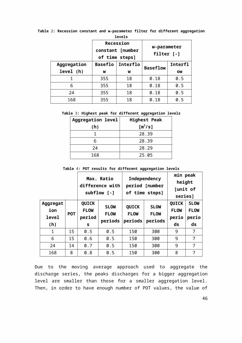
Table 2: Recession constant and w-parameter filter for different aggregationlevels
Recessionconstant [numberof time steps]
w-parameterfilter [-]
Aggregationlevel (h)
Baseflow
Interflow Baseflow Interfl
ow1 355 18 0.18 0.56 355 18 0.18 0.524 355 18 0.18 0.5168 355 18 0.18 0.5
Table 3: Highest peak for different aggregation levelsAggregation level
(h)Highest Peak
[m3/s]1 28.396 28.3924 28.29168 25.05
Table 4: POT results for different aggregation levels
Max. Ratiodifference withsubflow [-]
Independencyperiod [numberof time steps]
min peakheight
[unit ofseries]
Aggregationlevel(h)
POT
QUICKFLOWperiod
s
SLOWFLOW
periods
QUICKFLOW
periods
SLOWFLOW
periods
QUICKFLOWperiods
SLOWFLOWperiods
1 15 0.5 0.5 150 300 9 76 15 0.6 0.5 150 300 9 724 14 0.7 0.5 150 300 9 7168 8 0.8 0.5 150 300 8 7
Due to the moving average approach used to aggregate thedischarge series, the peaks discharges for a bigger aggregationlevel are smaller than those for a smaller aggregation level.Then, in order to have enough number of POT values, the value of
46
the minimum peak height, MP is reduced for increasingaggregation levels; also the max. Ratio difference value isincreased for increasing aggregation levels (Table 3).
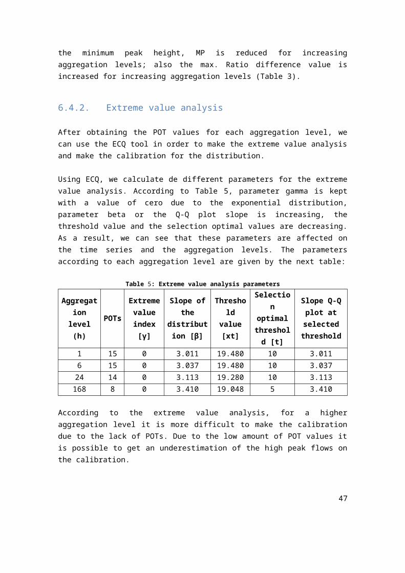
6.4.2. Extreme value analysis
After obtaining the POT values for each aggregation level, wecan use the ECQ tool in order to make the extreme value analysisand make the calibration for the distribution.
Using ECQ, we calculate de different parameters for the extremevalue analysis. According to Table 5, parameter gamma is keptwith a value of cero due to the exponential distribution,parameter beta or the Q-Q plot slope is increasing, thethreshold value and the selection optimal values are decreasing.As a result, we can see that these parameters are affected onthe time series and the aggregation levels. The parametersaccording to each aggregation level are given by the next table:
Table 5: Extreme value analysis parameters
Aggregation
level(h)
POTs
Extremevalueindex[γ]
Slope ofthe
distribution [β]
Threshold
value[xt]
Selection
optimalthreshold [t]
Slope Q-Qplot atselectedthreshold
1 15 0 3.011 19.480 10 3.0116 15 0 3.037 19.480 10 3.03724 14 0 3.113 19.280 10 3.113168 8 0 3.410 19.048 5 3.410
According to the extreme value analysis, for a higheraggregation level it is more difficult to make the calibrationdue to the lack of POTs. Due to the low amount of POT values itis possible to get an underestimation of the high peak flows onthe calibration.
47
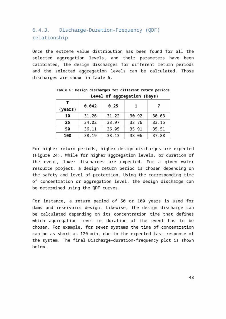
6.4.3. Discharge-Duration-Frequency (QDF) relationship
Once the extreme value distribution has been found for all theselected aggregation levels, and their parameters have beencalibrated, the design discharges for different return periodsand the selected aggregation levels can be calculated. Thosedischarges are shown in Table 6.
Table 6: Design discharges for different return periodsLevel of aggregation (Days)
T(years) 0.042 0.25 1 7
10 31.26 31.22 30.92 30.0325 34.02 33.97 33.76 33.1550 36.11 36.05 35.91 35.51100 38.19 38.13 38.06 37.88
For higher return periods, higher design discharges are expected(Figure 24). While for higher aggregation levels, or duration ofthe event, lower discharges are expected. For a given waterresource project, a design return period is chosen depending onthe safety and level of protection. Using the corresponding timeof concentration or aggregation level, the design discharge canbe determined using the QDF curves.
For instance, a return period of 50 or 100 years is used fordams and reservoirs design. Likewise, the design discharge canbe calculated depending on its concentration time that defineswhich aggregation level or duration of the event has to bechosen. For example, for sewer systems the time of concentrationcan be as short as 120 min, due to the expected fast response ofthe system. The final Discharge-duration-frequency plot is shownbelow.
48
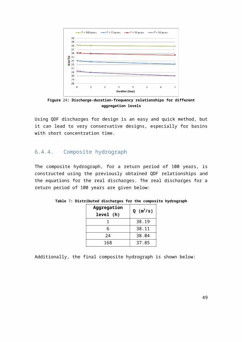
Figure 24: Discharge-duration-frequency relationships for differentaggregation levels
Using QDF discharges for design is an easy and quick method, butit can lead to very conservative designs, especially for basinswith short concentration time.
6.4.4. Composite hydrograph
The composite hydrograph, for a return period of 100 years, isconstructed using the previously obtained QDF relationships andthe equations for the real discharges. The real discharges for areturn period of 100 years are given below:
Table 7: Distributed discharges for the composite hydrographAggregationlevel (h) Q (m3/s)
1 38.196 38.1124 38.04168 37.85
Additionally, the final composite hydrograph is shown below:
49
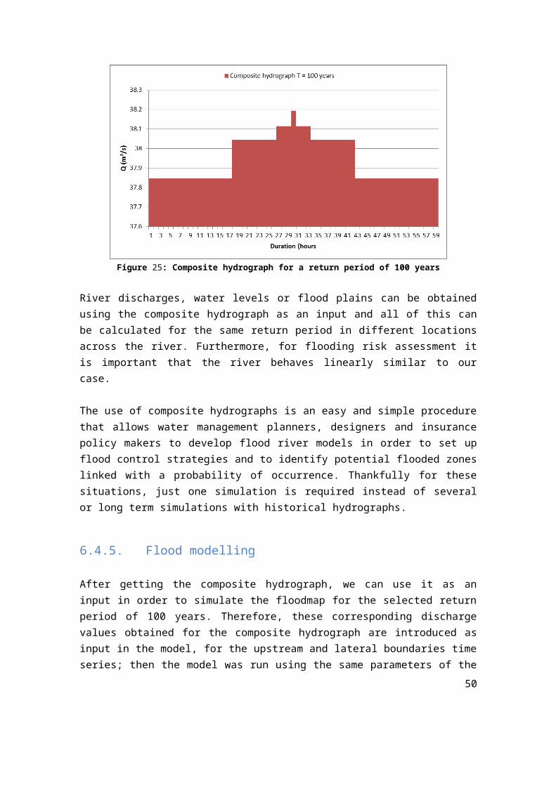
Figure 25: Composite hydrograph for a return period of 100 years
River discharges, water levels or flood plains can be obtainedusing the composite hydrograph as an input and all of this canbe calculated for the same return period in different locationsacross the river. Furthermore, for flooding risk assessment itis important that the river behaves linearly similar to ourcase.
The use of composite hydrographs is an easy and simple procedurethat allows water management planners, designers and insurancepolicy makers to develop flood river models in order to set upflood control strategies and to identify potential flooded zoneslinked with a probability of occurrence. Thankfully for thesesituations, just one simulation is required instead of severalor long term simulations with historical hydrographs.
6.4.5. Flood modelling
After getting the composite hydrograph, we can use it as aninput in order to simulate the floodmap for the selected returnperiod of 100 years. Therefore, these corresponding dischargevalues obtained for the composite hydrograph are introduced asinput in the model, for the upstream and lateral boundaries timeseries; then the model was run using the same parameters of the
50

previous exercise. From this simulation, Figure 26 shows themap of the flooding area according to the composite hydrographthat corresponds to a return period of 100 years. Comparing withthe previous flooding map, the water depth increased as well asthe area flooded. However, the difference is not much in theextension of the flooded area, also the water depth hasincreased but not considerably compared to the previousexercise, and the wate depth is also higher in the same areas asin the previous exercise, but the depth has increased getting toabout 2 m as the higghest level. Thus, his type of analysis isof great importance for flood risk assessment.
Figure 26: Flood map generated for the synthetic event (100 years returnperiod) for the selected section of Scheppelijke River
6.5. Conclusions
The conclusions reached form the developed exercise, are listedas follows:
According to the aggregation level, for a higher valuethere is a decrease on the amount of POTs and the highestpeak value.
According to an increase of each aggregation level, thereis a slight change of dependency for the extraction ofnearly independent extremes and hydrograph separation.
According to the POT selection, there is an increase ofMaximum Ratio difference between quick flow and subflow
51
and there is reduction on the minimum peak high for quickflow and slow flow.
According to the Extreme value analysis, for an increaseon the aggregation level , the value of beta or the Q-Qplot slope is increasing, the threshold value and theselection optimal values are decreasing.
Using the QDF relationships, we can estimate a dischargedepending on the return period and the duration.
For higher return periods, higher design discharges areexpected. While for higher aggregation levels, or durationof the event, lower discharges are expected.
Depending on the safety and level of protection, requiredfor a water resource project, a given return period ischosen for design. Using the corresponding time ofconcentration, the design discharge can be determinedusing the QDF relationships.
Using QDF discharges for design is an easy and quickmethod, but it can lead to very conservative designs,especially for basins with short concentration time.
The use of composite hydrographs in river flood modelingwill lead to modeling results (discharges, water levels,or even flood plains) with the same return period at allplaces in the river which is ideal for flooding riskassessment.
The flood map obtained for a synthetic event of for 100year return period is similar to the previous one, but theextension of the flood as well as the depth has increased,but not considerably.
A big advantage on the application of this method is thatwhen a composite hydrograph is used as input into ahydrodynamic model, the river states both discharge andwater level with the same return period will be simulatedfor all locations along the river in a single run (Willemset al., 2000). Such information can be utilised in designof flood protection facilities.
The use of composite hydrograph in river flood modellingis essential in Water Engineering since the the spatialextent of a flood for a given return period is equivalent
52
to an estimation of damage that can be caused due tooccurrence of such a flood.
7.References
DHI (2004) – MIKE 11. A modelling system for Rivers and Channels- User guide.
Bauwens, W. Text notes for the subject: “Surface waterhydrology”. Chapter 3: Precipitation and Chapter 5: Surfacerunoff.
Vaes G., P. Willems & J. Berlamont (2000). 'Selection andcomposition of representativehydrographs for river designcalculations’, ERB 2000, Int. Conference on ‘Monitoring andmodelling catchment water quantity and quality’ (ERB), Gent, 27-29 september 2000, 53-55
Willems, P. Text notes for the subject: “River modeling”.Chapter 3: Selection and composition of representativehydrographs for river design calculations.
Willems, P. 2004, Water Engineering Time Series processing toolWETSPRO Version 2.0, Reference Manual, K.U.Leuven – HydraulicsLaboratory.
Willems, P. Text notes for the subject: “Statistics for WaterEngineering”. Chapter 4: Extreme value analysis.
53