at SciVerse ScienceDirect

Environmental Modelling & Software 47 (2013) 1e14

Contents lists available

Environmental Modelling & Software

journal homepage: www.elsevier .com/locate/envsoft

OpenMI-based integrated sediment transport modelling of the riverZenne, Belgium

Narayan Kumar Shrestha a,*, Olkeba Tolessa Leta a, Bruno De Fraine b,Ann van Griensven a,c, Willy Bauwens a

aDepartment of Hydrology and Hydraulic Engineering, Vrije Universiteit Brussel, Pleinlaan 2, 1050 Brussels, BelgiumbDepartment of Computer Science, Vrije Universiteit Brussel, Pleinlaan 2, 1050 Brussels, BelgiumcUNESCO-IHE Institute for Water Education, Core of Hydrology and Water Resources, The Netherlands

a r t i c l e i n f o

Article history:Received 17 September 2012Received in revised form25 April 2013Accepted 7 May 2013Available online xxx

Keywords:OpenMIIntegrated modellingSediment transportThe Zenne river

* Corresponding author. Tel.: þ32 26 293 027; fax:E-mail address: nashrest@vub.ac.be (N.K. Shrestha

1364-8152/$ e see front matter � 2013 Elsevier Ltd.http://dx.doi.org/10.1016/j.envsoft.2013.05.004

a b s t r a c t

Recent observations show that the river Zenne (Belgium) remains well below the water quality goalsstated by the European Union Water Framework Directive. An interuniversity, multidisciplinary researchproject was therefore launched to evaluate the effects of wastewater management plans on theecological functioning of the river. To this end, different water quantity and quality processes had to beconsidered and modelled, e.g., the hydrology in the river basin, hydraulics in the river and sewers,erosion and sediment transport, faecal bacteria transport and decay. This paper considers the develop-ment of an Open Modelling Interface (OpenMI) based integrated model for the purpose of simulating theriver’s sediment dynamics. We used the Soil and Water Assessment Tool (SWAT) to model water andsediment fluxes from rural areas. The Storm Water Management Model (SWMM) was used to simulatethe hydraulics of the river, canal, and sewer systems in urban catchments. Newmodel codes for sedimenttransport and stream water temperature were developed to complement SWMM. The results show thatthe integrated sediment transport model reproduced the sediment concentrations in the river Zennewith ‘good’ to ‘satisfactory’ accuracy. We may therefore conclude that the OpenMI has been successfullyimplemented to integrate water quality models into a hydraulic one. While the OpenMI run-time datacommunication inflicted calculation time overhead, we found that the overhead was not significant withrespect to the total run-time of the integrated model.

� 2013 Elsevier Ltd. All rights reserved.

1. Introduction

The river Zenne is situated in Belgium’s Scheldt river basin, andtraverses the city of Brussels. Parallel to the river is a canal thatinteracts with it. During dry weather flow (DWF) periods, at least50% of the river (flowing downstream from Brussels) comprisestreated sewer discharges mainly originating from Brussels’ twowastewater treatment plants (WWTPs) (Garnier et al., 2012). Thedownstream part of the river is subjected to the tidal influence ofthe river Scheldt. During stormy conditions, the combined seweroverflows within Brussels have a major impact on the Zenne’s flowregime and water quality. Considering all these components andinteractions, the system can be quite complex.

In 2000, the European Union launched the Water FrameworkDirective (EU-WFD) (EU, 2000), formulating the need for all inland

þ32 32 052 437.).

All rights reserved.

and coastal waters of member countries to attain quality ecologicalstatus by 2015. Despite huge investments in the management ofBrussels’ sewer systems, the river Zenne still receives highpollutant loads, and that in spite of the small size of this receivingwater. In terms of the EU-WFD specifications for a good ecologicalstatus, the river Zenne leaves much to be desired. An interuniver-sity, multidisciplinary research project called ‘Good EcologicalStatus of the river Zenne (GESZ)’ was therefore launched to eval-uate the effects of wastewater management plans for the basin.

The GESZ project considered different water quantity andquality processes: the hydrology of the river basin, hydraulics in theriver and sewers, erosion and sediment transport, faecal bacteriatransport, fate of trace metals, and carbonenitrogenephosphorus(CeNeP) cycle. Modelling the transport and deposition of sus-pended solids is often essential in such analysis (Verbanck, 1990) asthe sedimentation of suspended solids is a pathway for the transferof nutrients from the water column to the river bed and vice-versa.Suspended solids also provide a surface area for the adsorption ofnumerous hydrophobic substances such as trace metals, organisms

N.K. Shrestha et al. / Environmental Modelling & Software 47 (2013) 1e142

and other contaminants (see e.g., Crabill et al., 1999; Garcia-Armisen and Servais, 2009; Ouattara et al., 2011).

While the need for an integrated modelling in order to gaininsight into complex and interrelated systems (like the Zenne) isgenerally recognised (Argent et al., 2006; Bulatewicz et al., 2013;Candela et al., 2012; Gaddis et al., 2007; Knapen et al., 2013; Laniaket al., 2013; Parker et al., 2002), the problem is how to integrate allthe needed models to represent the different processes. Integratingmodels is a rather difficult task because the simulators: (a) arecoded in different programming languages and often ill-documented, (b) have different dimensionalities, (c) use differentgrids, and (d) use different time steps (Bulatewicz et al., 2010;Peckham, 2010).

Constructing a single model that would include all these pro-cesses is an option. Voinov and Shugart (2013) named such simu-lators ‘Integrals’. Integrals, however, lack flexibility (Betrie et al.,2011) as the modules in such tight coupling are interrelated andoften depend on each other (Sui and Maggio, 1999). Changing onemodule could trigger a so-called ‘ripple effect’ in other dependentmodules (Black, 2001).

Another option would be to use a loosely coupled scheme byutilising the ‘most suitable’ model for each of the processes and bymaking the different simulators use each other’s outputs. The mostfundamental way to achieve such coupling is a file-based manuallinking. However, such a linkage is a time-consuming and error-prone procedure (Brandmeyer and Karimi, 2000; Reußer et al.,2009). Pre-processing of the output is often needed here, as theoutputs of the provider-model are e in most cases e not directlycompatible with the inputs required by the accepter-model.Moreover, it might not provide a feasible solution in cases wherethe interaction can be two-way, such as for a sewer that can beflooded or influenced by backwater from the receiving water.However, a major advantage of a loosely coupled scheme in modelintegration is the models’ re-usability, thereby preserving the in-vestments made on those models. Such model re-usability isimportant in the sense that most of the environmental models,developed to meet different goals (Voinov et al., 2004), are usedonly once (Rizzoli and Davis, 1999).

Although the tight coupling of environmental simulators hasbeen the more prevalent practice up to now, the interest in loosecoupling is growing mainly due to the development of variousframeworks that support loose coupling schemes (Castronova andGoodall, 2010, 2013). These developments might be seen as aresponse to Parker et al. (2002) who stressed that new, open andtransparent tools are needed to achieve easy and feasible integra-tion of environmental models. Laniak et al. (2013) envisioned asimilar approach and developed a roadmap for the future of inte-grated environmental modelling. They stressed that the modellingcommunity should accept and use globally recognized standardsand interfaces when designing and implementing software-basedproducts. Similar conclusions were also reached by the OpenMI-Life project (OpenMI, 2009). The project recommended practi-tioners to follow an ‘open source route’ and create a functionalcollaborative community.

The Open Modelling Interface (OpenMI) (Gregersen et al., 2007;Moore and Tindall, 2005) is an example of a loosely coupled schemeinspired by the component-based software engineering philosophy(Argent, 2004), where complex systems are decomposed into a setof components (Argent et al., 2006). The decomposition aims at amore flexible representation of the specific process and allows foran analysis of the impact of specific components on the integratedsystem (Castronova et al., 2012; Rizzoli et al., 2008). Additionally,the identification of the individual components’ robustness isfacilitated by inspecting their outputs. It allows the modeller todecide whether to replace or modify the least accurate component

in order to achieve the integrated system’s desired level of accuracy.The OpenMI interface allows the models to exchange data as theyrun. It eliminates therefore the cumbersome and error-prone tasksof (manually) transforming the outputs of onemodel into inputs foranother model (Reußer et al., 2009) while allowing for bi-directional interactions between the model components. Obvi-ously, the benefits of a standard like OpenMI increases with thenumber of compliant models (Gregersen et al., 2007). Once a largepool of OpenMI-compliant models becomes available, the user cansimply pick and plug the most suitable ones to form an integratedmodel using the OpenMI platform. For this, existing models can bemoved to the OpenMI platform while new simulators can bedeveloped in such a way that they become OpenMI-compliantdirectly (Moore and Tindall, 2005). While the OpenMI can beapplied in different scientific domains, very few applications aremade outside the water and environmental disciplines (Knapenet al., 2013).

We believe that the growing use of the OpenMI standard maysignificantly contribute to the development of integrated environ-mental modelling. For the integrated modelling of the river Zenne’swater quality, we thus opted for the use and/or development ofdifferent model components and linking them to the OpenMIplatform. This paper focuses on modelling sediment transport, inview of coupling it with other water quality models. The mainobjective is to demonstrate the feasibility of using OpenMI forlinking the different model components as well as investigating theadvantages and disadvantages of OpenMI as a component-basedintegration scheme.

The OpenMI-based integrated sediment transport model for theZenne system includes a hydrological model e the Soil and WaterAssessment Tool (SWAT) (Arnold et al., 1998), a hydraulic model ethe Storm Water Management Model (SWMM) (Rossman, 2009), anew model for sediment transport, and another new one forsimulating the stream water temperature. Such combination wasneeded to overcome the shortcomings of the individual models,and to accurately represent the river basin under study. Forexample, as SWAT includes hydrologic river routingmodules, basedon the variable storage coefficient (Williams, 1969) or Muskingummethod (Chow, 1959), it is unable to account for the backwatereffects (Betrie et al., 2011) that are important in view of the tidaleffects in the lower reaches of the river, and is incapable of dealingwith the sewer systems. Additionally, SWAT cannot incorporatehydraulic structures (such as weirs, pumping stations, etc.) used inthe canal and sewer systems. Hence, SWAT had to be com-plemented by a hydraulic model that is able to deal with thebackwater and with the flow in closed conduits. Thus, SWMM wasselected. On the other hand, the SWMM hydrological module ismuch too simplified and not apt to deal with diffuse pollutionsources originating from rural areas. To overcome such deficienciesand to make use of the strengths of each of these models, we usedSWAT to model the hydrology and diffuse pollution sources fromrural areas, while we used SWMM for the (urbanized) downstreamreach of the river, canal and sewer systems. SWAT then essentiallyforms the upstream boundary condition for the SWMM model. Asto the sediment, SWAT includes an erosion module and a simplifiedin-stream sediment transport module. It has been successfully usedfor sediment modelling at the watershed scale (e.g., Benaman andShoemaker, 2005; Betrie et al., 2011; Easton et al., 2010;Srinivasan et al., 1998). The sediment routine in SWMM is based onpollution build-up and wash-off concepts and specifically targetedthe sewer systems (Rossman, 2009). As SWMM sediment transportroutines are not adequate for river systems, we opted to develop anew and separate OpenMI-compliant sediment model to comple-ment the SWMM model. In addition, we also developed anOpenMI-compliant in-stream temperature simulator that is needed

N.K. Shrestha et al. / Environmental Modelling & Software 47 (2013) 1e14 3

to compensate temperature dependency in kinematic viscosity, aninput parameter in the sediment model. While an OpenMI-compliant version of SWAT was available (Betrie et al., 2011), wealso had to make SWMM OpenMI-compliant. We hope that ourcontribution will be incorporated by practitioners as ‘buildingblocks’ for modelling complex environmental systems.

2. Materials and methods

2.1. The study area

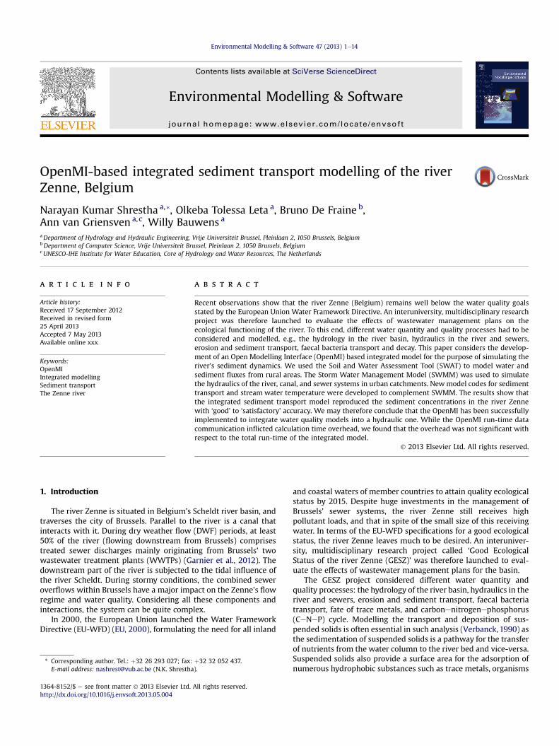
The river Zenne is a part of the international Scheldt basin. The basin has anarea of 1162 km2. The main river has a total length of 103 km and runs through theWalloon, the Brussels-Capital and the Flemish Region of Belgium (Fig. 1). The rivermeets the river Dijle in Mechelen. Upstream from Brussels, the river follows anatural meandering course, while in the Brussels-Capital region, the river has beenvaulted over a distance of approximately 8.3 km. Downstream from Brussels, theriver bed level has been re-profiled. In the downstream part, the river experiences atidal effect. The river basin is crossed by the canal Brussels-Charleroi and the SeaCanal Brussels-Scheldt. In theWalloon Region, the canal is fed by former tributariesof the river. In the reach between the borders of the Walloon and the BrusselsRegion, different tributaries discharge into the river namely; Molenbeek, Zuun-beek, and Groebengracht (Fig. 1). The canal also receives water from the riverthrough several overflows to prevent flooding in the Brussels-Capital Region.Excess water in the canal can be discharged back into the river in Vilvoorde,downstream of Brussels.

The total population within the river basin is approximately 1.5 million. Morethan 1 million people live in the Brussels-Capital Region. The population density inthe basin is about 1259 inhabitants/km2, whichmakes it themost densely populatedbasin of the Scheldt watershed (van Griensven, 2002). The land-use in the catch-ment is dominated by agriculture (51%), mostly in upstream part, and by urbanregions (19%) in the downstream part. Several medium-sized Waste Water Treat-ment Plants (WWTPs) exist in the basin (Fig. 1). With a capacity of 1.1 millioninhabitant equivalent, the WWTP of Brussels North is the largest treatment plant inthe basin.

2.2. The models

In what follows, the different model components are briefly described, with anemphasis on the sediment model.

2.2.1. The hydrologic model: SWATSWAT is a physically-based, semi-distributed, hydrologic simulator that can

operate on different time steps at basin scale, developed by United States Depart-ment of Agriculture (USDA). It has the capability to perform continuous simulationsfor the major groups of processes (hydrology, nutrients, pesticides, soil erosion and

Fig. 1. The Zenne basin with the sub-basins simulated with SWAT, the SWMM networkmeteorological, stream temperature, sediment measurement stations, the GESZ sampling s

sediment transport) in large, complex watersheds (Jha et al., 2007; Lam et al., 2010;Santhi et al., 2001; White and Chaubey, 2005). Additionally, SWAT can integratecomplex watersheds with varying landuse, weather, soil, topography, and man-agement conditions over a long period of time. Hence, the model is interfaced with aGeographic Information System (GIS) to integrate the various spatial and hydro-meteorological data (Winchell et al., 2010). For modelling purposes, a watershedis divided into sub-basins that are homogeneous in terms of climatic conditions (VanLiew et al., 2005). Sub-basins are further subdivided into Hydrological ResponseUnits (HRUs), whereby each HRU has a unique combination of land-use, soiltype andslope (Arnold et al., 2011).

The hydrological module of SWAT accounts for precipitation, evapotranspira-tion, surface runoff, lateral flow, return flow, and deep groundwater losses (Neitschet al., 2011). The model uses a modification of the Soil Conservation Service CurveNumber (SCS-CN) method (USDA-SCS, 1986) or the Green and Ampt method asmodified by Mein and Larson (1973) to compute the runoff volume and the infil-tration for each HRU. Percolation through each soil layer is estimated using a storagerouting technique (Arnold et al., 1995). The generated stream flows can be routedusing the variable storage method (Williams, 1969) or the Muskingum routingmethod (Chow, 1959).

Soil erosion in SWAT is a hydrologically driven process. The soil erosion andsediment yield from each HRU are modelled by the Modified Universal Soil LossEquation (MUSLE) (Lal, 2001; Williams and Berndt, 1977), as given by:

SedYld ¼ 11:8�Qsurf*qpeak*areahru

�0:56*Kusle*Cusle*Pusle*LSusle*CFRG (1)

where SedYld is the sediment yield on a given day (metric tons), Qsurf is the surfacerunoff volume (mm/ha), qpeak is the peak runoff rate (m3/s), areahru is the area of theHRU (ha), Kusle is the soil erodibility factor (0.013 metric ton m2 h/(m3-metric ton cm)), Cusle is the USLE cover and management factor, Pusle is the USLEsupport practice factor, LSusle is the USLE topographic factor and CFRG is the coarsesediment fragment factor.

The right side variables of Eq. (1), which are outside the bracket, are user-defined parameters, subjected to calibration. A detailed explanation of the param-eters is given by Neitsch et al. (2011). Sediment transport in the channel is controlledby two simultaneous processes: deposition and degradation (Srinivasan et al., 1998;Williams and Berndt, 1977). The channel sediment routing module uses the modi-fied Bagnold’s sediment transport method (Bagnold, 1977), which determines thesediment transport capacity as a function of stream flow velocity. The maximumconcentration of sediment (Concsed,mx) that can be transported from a reach iscalculated as:

Concsed;mx ¼ SPCON*VSPEXPpk (2)

where Vpk is the peak channel velocity (m/s) and SPCON & SPEXP are modelparameters. If the actual sediment concentration is larger than the maximum con-centration, deposition will be the dominant process; otherwise degradation willprevail.

for the river, the canal, the sewer systems and the major WWTPs (left); the hydro-tations and combined sewer overflow (CSO) points (right).

N.K. Shrestha et al. / Environmental Modelling & Software 47 (2013) 1e144

2.2.2. The hydraulic model: SWMMDeveloped by the United States Environmental Protection Agency (US EPA),

SWMM is a dynamic rainfall runoff simulationmodel computing runoff quantity andquality (primarily) from urban areas. It can be used for both continuous and singleevent modelling. A drainage system in SWMM is modelled as a series of water andmaterial flows between four major subunits: the atmosphere, the land surfacecompartment, the groundwater, and the transport or conveyance compartment(Gironás et al., 2009; Rossman, 2009). SWMM adopts a distributed non-linearreservoir concept to simulate the runoff from a specific sub-catchment afterdepression loss, infiltration and evaporation are satisfied. While doing so, the sub-catchment is divided into impervious and pervious zones, the infiltration phe-nomena being considered only from the latter zone. The one dimensional flowrouting in the transport compartment is based on the full set of equations of Barré deSaint-Venant (Lai, 1987).

SWMM has provisions to build up any pollutant on the sub-catchment surfaceand for their subsequent wash-off. However, once the pollutant is in suspension,there is no provision to allow for sedimentation or resuspension. This is importantsince some pollutants can be adsorbed to sediment particles and then start behavingas the sediments while being transported.

2.2.3. The sediment transport simulatorModelling of sediment transport is by no doubt one of the most challenging

issues in hydraulics. Many models have been proposed in literature, each with itsown merits and limitations. When evaluating the simulator that we developed, oneshould keep the broad objective of the project in mind, which is the evaluation ofalternative water quality management plans. Hereto, there is a need for an evalua-tion of such plans considering different conditions of the system and thus for themodelling of continuous, long term time series (Demuynck et al., 1997). Hence, aneed for a robust and computationally fast sediment transport module that does notnecessarily have to reproduce each individual event with high precision, but thatrepresents the processes in a coherent way.

The new sediment simulator is based on the concept of the critical shear stressand the related critical particle diameter (dcr) for the initiation of motion of non-cohesive bed particles. Hence, it assumes a critical diameter that divides the sedi-ment between a fraction in motion, and a fraction without motion. A limitation onthe transport capacity is imposed by using Velikanov’s energy equation (Velikanov,1954), an implementation proposed and tested by Zug et al. (1998). The followingsections elaborate on the determination of the critical diameter and of the limitationof the transport capacity.

2.2.3.1. Determination of critical diameter. Awell-knownmethod for the calculationof the initial motion is the method proposed by Shields (1936). It is based on anempirical relationship between two dimensionless quantities. The first quantity isthe ratio of the force exerted by the bed shear-stress (s) to move a grain on the bed,to the submerged weight of the grain counteracting this. This ratio is the dimen-sionless shear stress (q).

q ¼ sðrs � rÞgd ¼ u2*r

ðrs � rÞgd (3)

where s is the bed shear stress (N/m2), rs and r are the sediment grain density andthe water density (kg/m3), g is the gravity constant (m/s2), d is the diameter of thegrains (m), and u* is the critical shear velocity (m/s).

The second quantity is the particle Reynolds number (R*).

R* ¼ u*n

¼ffiffiffiffiffiffiffiffigRS

pn

(4)

where n is the kinematic viscosity of water (m2/s), R is the hydraulic radius (m), and Sis the friction slope.

The temperature dependence on the kinematic viscosity is assessed by anequation proposed by US Bureau of Reclamation (USDI-BR, 2006):

n ¼ 1:792� 10�6

1:0þ 0:033Ts þ 0:000221T2s(5)

where Ts is the stream water temperature (�C).More recently, Soulsby and Whithouse (1997) proposed an algebraic expression

that fits Shields’ curve closely and passes reasonably well through an extended set ofdata. For the ordinate, the dimensionless shear stress (q) is still employed. For theabscissa, the dimensionless grain size (D*) is used. The proposed relationship be-tween q and D* is as follows:

q ¼ 0:24D*

þ 0:055�1� e�0:02D*

�with D* ¼

ffiffiffiffiffiffiffiffiffiffiffiffiffiffiffiðs� 1Þ

n23

rd (6)

where D* is the dimensionless grain size, and s is the specific grain gravity.The Soulsby and Whitehouse equation (Eq. (6)) is advantageous for program-

ming purposes as it provides a direct means to obtain the dimensionless criticalshear stress and the critical shear velocity that corresponds to a given particle

diameter. Hence, it is used to determine the critical diameter. Re-arranging Eqs. (3)e(6), leads to the following equation:

u*�d� ¼

ffiffiffiffiffiffiffiffiffiffiffiffiffiffiffiffiffiffiffiffiffiffiffiffiffiffiffiffiffiffiffiqðdÞ ðs� 1Þ gd

q(7)

For the inverse operation, i.e. to compute the critical diameter corresponding toa given shear velocity u*, the equation u*(d) ¼ u* must be solved for d. Since nostraightforward algebraic inverse of u*(d) is available, a numerical root finding isemployed. The NewtoneRhapson iteration complemented with a bisection processis used to ensure a fast convergence.

Once the critical diameter is determined, the fate of the sediment particles isdetermined. For this, the sediment is divided into a number of classes, according tothe diameter of the particles, in order to account for the Particles Size Distribution(PSD). Each single class is treated individually and behaves uniformlywith respect toerosion and deposition (i.e. a class erodes or deposits in its entirety). The resolutionof the PSD should thus be high enough, such that the particle size distribution is wellrepresented. The upper and lower bound of a class is compared with the calculatedcritical diameter, to determine the deposition or the scour. The lower bound of theparticle diameters of fraction i is written di. The upper bound is di þ 1, which issimultaneously the lower bound for fraction i þ 1. A class may be in one of threesituations, depending on the relation of its bounds to the critical diameter:

� If dcr � di, the class i in suspension is deposited to the bed.� If di þ 1 � dcr, the class i on the bed is eroded and enters into suspension.� If di < dcr < di þ 1, the state of the class i is not modified.

2.2.3.2. Determination of carrying capacity. Determining the state of deposition andresuspension based only on the critical diameter may pose problems as the carryingcapacity of the flow e and thus the resuspension capacity e is considered as un-limited. This may result into unrealistically high sediment concentrations duringhigh flow conditions. To take this into account, the Velikanov’s energy equation(Velikanov, 1954) is used in a similar way as done by Zug et al. (1998). The methodallows defining themaximum/minimum sediment concentration that can/should beconveyed, based on energy considerations. The approach has a simple mathematicalformulation, requires only a limited number of parameters and is fairly robust (Zuget al., 1998). The maximum and minimum sediment concentrations are given as:

CTmin ¼ h1srw

ðs� 1Þuws

S (8)

CTmax ¼ h2srw

ðs� 1Þuws

S (9)

where CTmax is the critical erosion transport capacity (kg/m3), CTmin is the criticalsedimentation transport capacity (kg/m3), h1 is the critical sedimentation efficiencycoefficient, h2 is the critical erosion efficiency coefficient,ws is the settling velocity ofgrains (m/s), and u is the velocity of the water (m/s)

The settling velocity of grains (ws) is determined using the equation of Rubey(1933) as:

ws ¼ffiffiffiffiffiffiffiffiffiffiffiffiffiffiffiffiffiffiffiffigdðs� 1Þ

q 24

ffiffiffiffiffiffiffiffiffiffiffiffiffiffiffiffiffiffiffiffiffiffiffiffiffiffiffiffiffiffiffi23þ 36n2

gd3�s� 1

�s

�ffiffiffiffiffiffiffiffiffiffiffiffiffiffiffiffiffiffiffiffiffiffiffi

36n2

gd3�s� 1

�s 3

5 (10)

2.2.4. The temperature simulatorTo determine stream water temperature, a regression model between air and

stream water temperature is used. Such regression models have become thesimplest means to predict stream temperature especially driven by the fact that dataon the air temperature is readily available (Webb et al., 2003). These models havelesser calculation overhead and proved to be quite accurate as well. A non-linear fit(Eq. (11)) is used, as suggested by Mohseni et al. (1998):

Ts ¼ mþ a� m

1þ egðb�TaÞ (11)

where Ta and Ts are the air and the streamwater temperature respectively (�C), m isthe minimum stream temperature (�C); a is the maximum stream temperature (�C),g is the steepest slope at the inflection point of the Ts function plotted against Ta, andb is the air temperature at the inflection point of the Ts function plotted againstTa (�C).

Studies have shown that stream temperatures tend to follow the air tempera-tures but with some time lag (Grant, 1977; Stefan and Preud’homme, 1993). Stefanand Preud’homme (1993) observed time lags to be related to stream depth andobserved the lag ranging from hours to days, in accordance with increasing streamdepth. Grant (1977) suggested predicting stream temperature with a time lag of 1day (using air temperature of the same and preceding day). The temperature modeldeveloped for this study involves a time lag of 2 days (using temperature of the sameday and two previous days). Besides, thermal discharges from e.g., WWTPs can alsobe considered. As already depicted, at least 50% of the river flow downstream of

N.K. Shrestha et al. / Environmental Modelling & Software 47 (2013) 1e14 5

Brussels consists of treated sewer discharges, mainly originating from the twoWWTPs of Brussels (Garnier et al., 2012), their effect on thermal regime of the rivercould be significant because the effluents are discharged rather at a constant tem-perature throughout the year. Hence, consideration of such thermal discharge fromthe WWTPs is needed in the temperature model.

2.3. The adaptation of the simulators to the OpenMI platform

Only OpenMI linkable components can be linked together to form an integratedmodel in OpenMI platform. In general, a simulator can be integrated into theOpenMI platform, while new simulators can be developed in such a way that theydirectly become OpenMI-compliant (Moore and Tindall, 2005). The following sec-tions elaborate on how this was achieved. We used OpenMI version 1.4. AlthoughOpenMI 2.0 is recently launched, it needs to be tested in different case studies whileversion 1.4 has already been tested in several case studies successfully.

2.3.1. The migration of existing simulators to the OpenMI platform2.3.1.1. The SWMM OpenMI model. The recommended practice for migrating anexisting model engine to OpenMI, is to construct a ‘wrapper’, i.e. an intermediatesoftware component that makes the engine addressable on the platform used byOpenMI (namely Microsoft .NET), according to the interface prescribed by theOpenMI standard. The solution consists of three steps: (a) the existing engine code iscompiled as a Windows Dynamic Link Library (DLL), (b) a basic .NET componentemploys the interoperability functionality of the .NET platform to make this DLLaccessible, and (c) another .NET component implements the OpenMI interface byinterpreting the requests from OpenMI and translating them to the native functionsof the model engine. As such, the execution of a simulation by the original modelengine is triggered by the ‘request-reply’ mechanism of OpenMI. The OpenMI as-sociation provides a software development toolkit that contains auxiliary code to aidwith step (c) of this process.

The standard ‘wrapping’ approach has been adopted for the SWMM OpenMImodel, with one important modification to step (b). The standard SWMM 5 code-base already makes the basic functionality of the model engine available as a DLL forthe benefit of the SWMM graphical user interface. We extended this provision in theSWMM codebase with a functionality to access the network elements (nodes andlinks) of a SWMM project and to inspect their basic hydraulic properties (such asflow, volume, depth,.) during simulation. Our modifications to the SWMM 5codebase were limited and localized in just a few source code files. By tracking thesemodifications using the Subversion source code version control system (Collins-Sussman et al., 2011), we gained the ability to ‘upgrade’ to a new version of theSWMM codebase with minimal effort.

2.3.1.2. The SWAT OpenMI model. The SWAT OpenMI model is also a migration of anexisting codebase to OpenMI using the standard ‘wrapper’ approach. More infor-mation on SWAT OpenMI migration was provided by Betrie et al. (2011).

2.3.2. Conceiving new simulators for the OpenMI platformAs we explained above, the sediment transport and temperature simulators

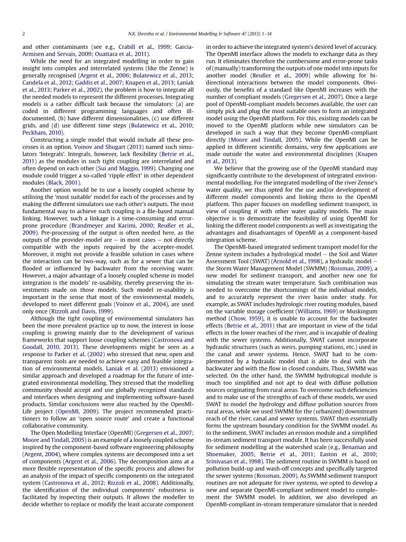
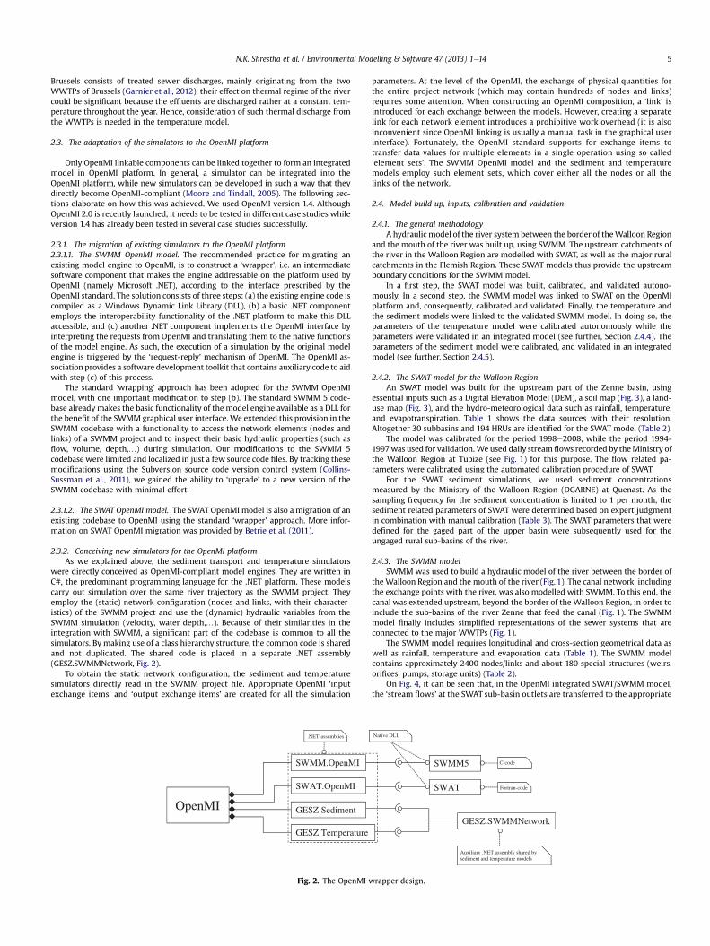
were directly conceived as OpenMI-compliant model engines. They are written inC#, the predominant programming language for the .NET platform. These modelscarry out simulation over the same river trajectory as the SWMM project. Theyemploy the (static) network configuration (nodes and links, with their character-istics) of the SWMM project and use the (dynamic) hydraulic variables from theSWMM simulation (velocity, water depth,.). Because of their similarities in theintegration with SWMM, a significant part of the codebase is common to all thesimulators. By making use of a class hierarchy structure, the common code is sharedand not duplicated. The shared code is placed in a separate .NET assembly(GESZ.SWMMNetwork, Fig. 2).

To obtain the static network configuration, the sediment and temperaturesimulators directly read in the SWMM project file. Appropriate OpenMI ‘inputexchange items’ and ‘output exchange items’ are created for all the simulation

OpenMI GESZ.Sediment

GESZ.Temperature

SWMM.OpenMI

SWAT.OpenMI

.NET-assemblies

Fig. 2. The OpenMI w

parameters. At the level of the OpenMI, the exchange of physical quantities forthe entire project network (which may contain hundreds of nodes and links)requires some attention. When constructing an OpenMI composition, a ‘link’ isintroduced for each exchange between the models. However, creating a separatelink for each network element introduces a prohibitive work overhead (it is alsoinconvenient since OpenMI linking is usually a manual task in the graphical userinterface). Fortunately, the OpenMI standard supports for exchange items totransfer data values for multiple elements in a single operation using so called‘element sets’. The SWMM OpenMI model and the sediment and temperaturemodels employ such element sets, which cover either all the nodes or all thelinks of the network.

2.4. Model build up, inputs, calibration and validation

2.4.1. The general methodologyA hydraulic model of the river system between the border of theWalloon Region

and the mouth of the river was built up, using SWMM. The upstream catchments ofthe river in the Walloon Region are modelled with SWAT, as well as the major ruralcatchments in the Flemish Region. These SWAT models thus provide the upstreamboundary conditions for the SWMM model.

In a first step, the SWAT model was built, calibrated, and validated autono-mously. In a second step, the SWMM model was linked to SWAT on the OpenMIplatform and, consequently, calibrated and validated. Finally, the temperature andthe sediment models were linked to the validated SWMM model. In doing so, theparameters of the temperature model were calibrated autonomously while theparameters were validated in an integrated model (see further, Section 2.4.4). Theparameters of the sediment model were calibrated, and validated in an integratedmodel (see further, Section 2.4.5).

2.4.2. The SWAT model for the Walloon RegionAn SWAT model was built for the upstream part of the Zenne basin, using

essential inputs such as a Digital Elevation Model (DEM), a soil map (Fig. 3), a land-use map (Fig. 3), and the hydro-meteorological data such as rainfall, temperature,and evapotranspiration. Table 1 shows the data sources with their resolution.Altogether 30 subbasins and 194 HRUs are identified for the SWAT model (Table 2).

The model was calibrated for the period 1998e2008, while the period 1994-1997was used for validation.We used daily stream flows recorded by theMinistry ofthe Walloon Region at Tubize (see Fig. 1) for this purpose. The flow related pa-rameters were calibrated using the automated calibration procedure of SWAT.

For the SWAT sediment simulations, we used sediment concentrationsmeasured by the Ministry of the Walloon Region (DGARNE) at Quenast. As thesampling frequency for the sediment concentration is limited to 1 per month, thesediment related parameters of SWAT were determined based on expert judgmentin combination with manual calibration (Table 3). The SWAT parameters that weredefined for the gaged part of the upper basin were subsequently used for theungaged rural sub-basins of the river.

2.4.3. The SWMM modelSWMM was used to build a hydraulic model of the river between the border of

theWalloon Region and the mouth of the river (Fig. 1). The canal network, includingthe exchange points with the river, was also modelled with SWMM. To this end, thecanal was extended upstream, beyond the border of the Walloon Region, in order toinclude the sub-basins of the river Zenne that feed the canal (Fig. 1). The SWMMmodel finally includes simplified representations of the sewer systems that areconnected to the major WWTPs (Fig. 1).

The SWMM model requires longitudinal and cross-section geometrical data aswell as rainfall, temperature and evaporation data (Table 1). The SWMM modelcontains approximately 2400 nodes/links and about 180 special structures (weirs,orifices, pumps, storage units) (Table 2).

On Fig. 4, it can be seen that, in the OpenMI integrated SWAT/SWMM model,the ‘stream flows’ at the SWAT sub-basin outlets are transferred to the appropriate

Native DLL

Fortran-code

C-code

GESZ.SWMMNetwork

SWAT

SWMM5

Auxiliary .NET assembly shared by sediment and temperature models

rapper design.

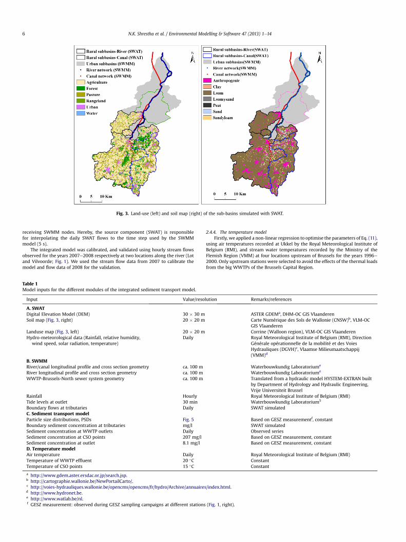
Fig. 3. Land-use (left) and soil map (right) of the sub-basins simulated with SWAT.

N.K. Shrestha et al. / Environmental Modelling & Software 47 (2013) 1e146

receiving SWMM nodes. Hereby, the source component (SWAT) is responsiblefor interpolating the daily SWAT flows to the time step used by the SWMMmodel (5 s).

The integrated model was calibrated, and validated using hourly stream flowsobserved for the years 2007e2008 respectively at two locations along the river (Lotand Vilvoorde; Fig. 1). We used the stream flow data from 2007 to calibrate themodel and flow data of 2008 for the validation.

Table 1Model inputs for the different modules of the integrated sediment transport model.

Input Value/reso

A. SWATDigital Elevation Model (DEM) 30 � 30 mSoil map (Fig. 3, right) 20 � 20 m

Landuse map (Fig. 3, left) 20 � 20 mHydro-meteorological data (Rainfall, relative humidity,

wind speed, solar radiation, temperature)Daily

B. SWMMRiver/canal longitudinal profile and cross section geometry ca. 100 mRiver longitudinal profile and cross section geometry ca. 100 mWWTP-Brussels-North sewer system geometry ca. 100 m

Rainfall HourlyTide levels at outlet 30 minBoundary flows at tributaries DailyC. Sediment transport modelParticle size distributions, PSDs Fig. 5Boundary sediment concentration at tributaries mg/lSediment concentration at WWTP outlets DailySediment concentration at CSO points 207 mg/lSediment concentration at outlet 8.1 mg/lD. Temperature modelAir temperature DailyTemperature of WWTP effluent 20 �CTemperature of CSO points 15 �C

a http://www.gdem.aster.ersdac.or.jp/search.jsp.b http://cartographie.wallonie.be/NewPortailCarto/.c http://voies-hydrauliques.wallonie.be/opencms/opencms/fr/hydro/Archive/annuaired http://www.hydronet.be.e http://www.watlab.be/nl.f GESZ measurement: observed during GESZ sampling campaigns at different stations

2.4.4. The temperature modelFirstly, we applied a non-linear regression to optimise the parameters of Eq. (11),

using air temperatures recorded at Ukkel by the Royal Meteorological Institute ofBelgium (RMI), and stream water temperatures recorded by the Ministry of theFlemish Region (VMM) at four locations upstream of Brussels for the years 1996e2000. Only upstream stations were selected to avoid the effects of the thermal loadsfrom the big WWTPs of the Brussels Capital Region.

lution Remarks/references

ASTER GDEMa, DHM-OC GIS VlaanderenCarte Numérique des Sols de Wallonie (CNSW)b, VLM-OCGIS VlaanderenCorrine (Walloon region), VLM-OC GIS VlaanderenRoyal Meteorological Institute of Belgium (RMI), DirectionGénérale opérationnelle de la mobilité et des VoiesHydrauliques (DGVH)c, Vlaamse Milieumaatschappij(VMM)d

Waterbouwkundig Laboratoriume

Waterbouwkundig Laboratoriume

Translated from a hydraulic model HYSTEM-EXTRAN builtby Department of Hydrology and Hydraulic Engineering,Vrije Universiteit BrusselRoyal Meteorological Institute of Belgium (RMI)Waterbouwkundig Laboratorium5

SWAT simulated

Based on GESZ measurementf, constantSWAT simulatedObserved seriesBased on GESZ measurement, constantBased on GESZ measurement, constant

Royal Meteorological Institute of Belgium (RMI)ConstantConstant

s/index.html.

(Fig. 1, right).

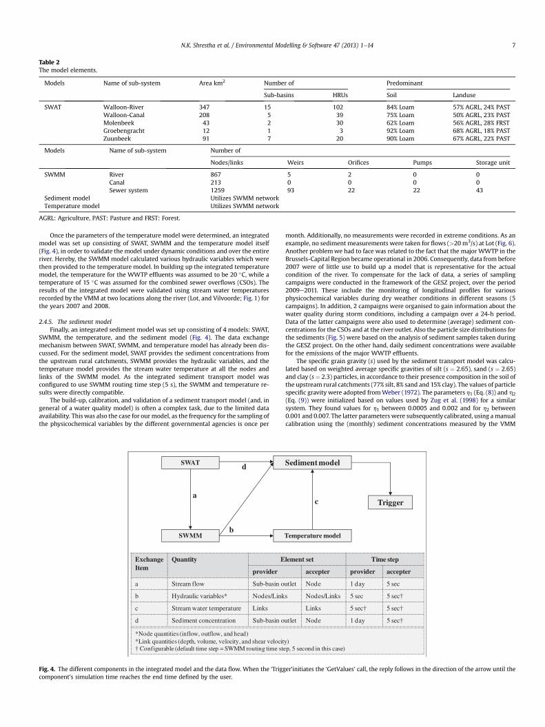
Table 2The model elements.

Models Name of sub-system Area km2 Number of Predominant

Sub-basins HRUs Soil Landuse

SWAT Walloon-River 347 15 102 84% Loam 57% AGRL, 24% PASTWalloon-Canal 208 5 39 75% Loam 50% AGRL, 23% PASTMolenbeek 43 2 30 62% Loam 56% AGRL, 28% FRSTGroebengracht 12 1 3 92% Loam 68% AGRL, 18% PASTZuunbeek 91 7 20 90% Loam 67% AGRL, 22% PAST

Models Name of sub-system Number of

Nodes/links Weirs Orifices Pumps Storage unit

SWMM River 867 5 2 0 0Canal 213 0 0 0 0Sewer system 1259 93 22 22 43

Sediment model Utilizes SWMM networkTemperature model Utilizes SWMM network

AGRL: Agriculture, PAST: Pasture and FRST: Forest.

N.K. Shrestha et al. / Environmental Modelling & Software 47 (2013) 1e14 7

Once the parameters of the temperature model were determined, an integratedmodel was set up consisting of SWAT, SWMM and the temperature model itself(Fig. 4), in order to validate the model under dynamic conditions and over the entireriver. Hereby, the SWMM model calculated various hydraulic variables which werethen provided to the temperature model. In building up the integrated temperaturemodel, the temperature for the WWTP effluents was assumed to be 20 �C, while atemperature of 15 �C was assumed for the combined sewer overflows (CSOs). Theresults of the integrated model were validated using stream water temperaturesrecorded by the VMM at two locations along the river (Lot, and Vilvoorde; Fig. 1) forthe years 2007 and 2008.

2.4.5. The sediment modelFinally, an integrated sediment model was set up consisting of 4 models: SWAT,

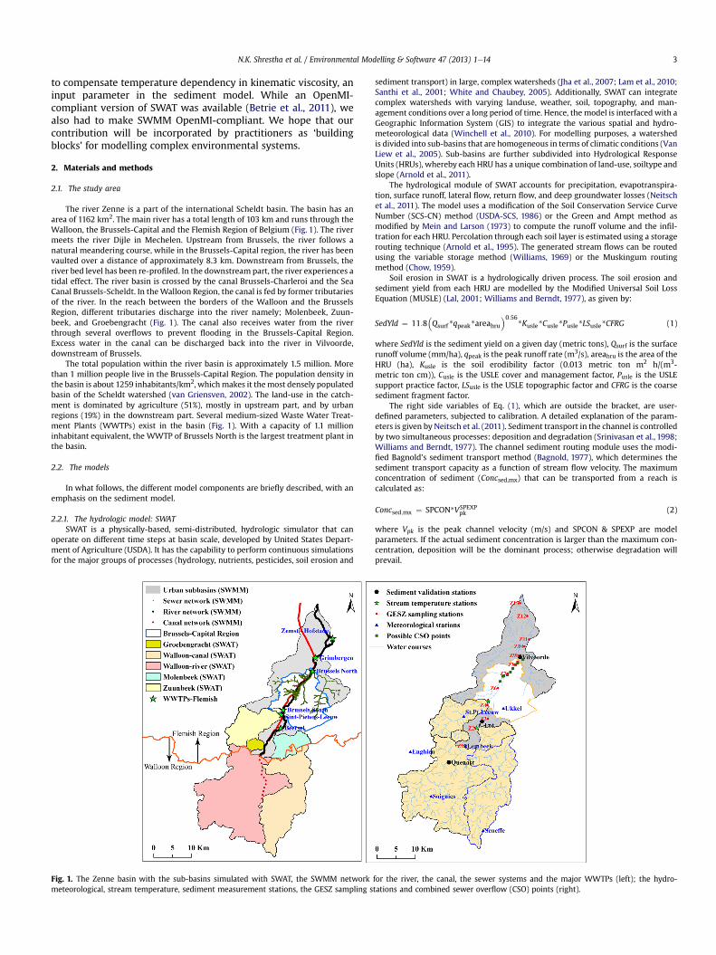
SWMM, the temperature, and the sediment model (Fig. 4). The data exchangemechanism between SWAT, SWMM, and temperature model has already been dis-cussed. For the sediment model, SWAT provides the sediment concentrations fromthe upstream rural catchments, SWMM provides the hydraulic variables, and thetemperature model provides the stream water temperature at all the nodes andlinks of the SWMM model. As the integrated sediment transport model wasconfigured to use SWMM routing time step (5 s), the SWMM and temperature re-sults were directly compatible.

The build-up, calibration, and validation of a sediment transport model (and, ingeneral of a water quality model) is often a complex task, due to the limited dataavailability. This was also the case for ourmodel, as the frequency for the sampling ofthe physicochemical variables by the different governmental agencies is once per

SWAT

SWMM

a

b

d

ExchangeItem

EytitnauQ

provider

a Stream flow Sub-basin o

b Hydraulic variables* Nodes/Link

c Stream water temperature Links

d Sediment concentration Sub-basin o

*Node quantities (inflow, outflow, and head)*Link quantities (depth, volume, velocity, and shear velocit† Configurable (default time step = SWMM routing time ste

Fig. 4. The different components in the integrated model and the data flow. When the ‘Triggcomponent’s simulation time reaches the end time defined by the user.

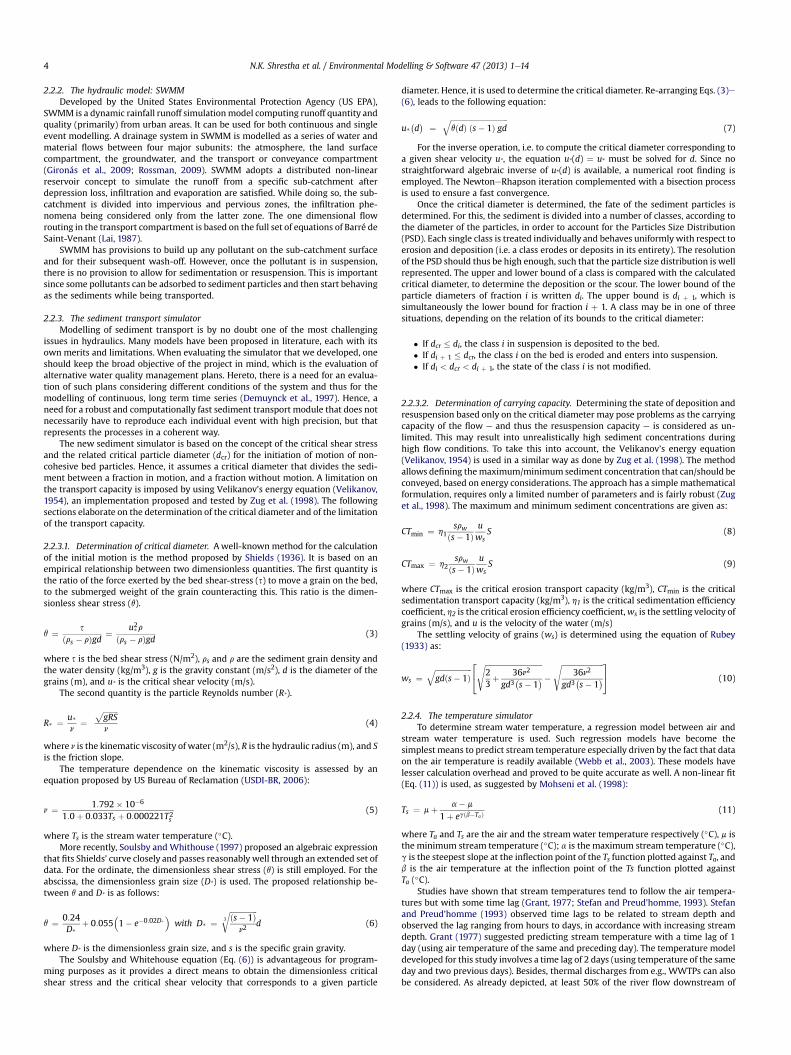
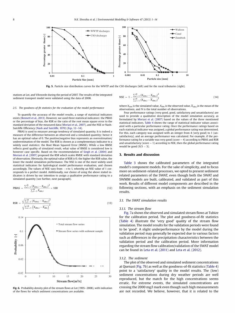
month. Additionally, no measurements were recorded in extreme conditions. As anexample, no sediment measurements were taken for flows (>20 m3/s) at Lot (Fig. 6).Another problemwe had to face was related to the fact that the major WWTP in theBrussels-Capital Region became operational in 2006. Consequently, data from before2007 were of little use to build up a model that is representative for the actualcondition of the river. To compensate for the lack of data, a series of samplingcampaigns were conducted in the framework of the GESZ project, over the period2009e2011. These include the monitoring of longitudinal profiles for variousphysicochemical variables during dry weather conditions in different seasons (5campaigns). In addition, 2 campaigns were organised to gain information about thewater quality during storm conditions, including a campaign over a 24-h period.Data of the latter campaigns were also used to determine (average) sediment con-centrations for the CSOs and at the river outlet. Also the particle size distributions forthe sediments (Fig. 5) were based on the analysis of sediment samples taken duringthe GESZ project. On the other hand, daily sediment concentrations were availablefor the emissions of the major WWTP effluents.

The specific grain gravity (s) used by the sediment transport model was calcu-lated based on weighted average specific gravities of silt (s ¼ 2.65), sand (s ¼ 2.65)and clay (s¼ 2.3) particles, in accordance to their presence composition in the soil ofthe upstream rural catchments (77% silt, 8% sand and 15% clay). The values of particlespecific gravity were adopted fromWeber (1972). The parameters h1 (Eq. (8)) and h2

(Eq. (9)) were initialized based on values used by Zug et al. (1998) for a similarsystem. They found values for h1 between 0.0005 and 0.002 and for h2 between0.001 and 0.007. The latter parameters were subsequently calibrated, using amanualcalibration using the (monthly) sediment concentrations measured by the VMM

c

Sediment model

Temperature model

petsemiTtestnemel

accepter provider accepter

utlet Node 1 day 5 sec

s Nodes/Links 5 sec 5 sec†

Links 5 sec† 5 sec†

utlet Node 1 day 5 sec†

y)p, 5 second in this case)

Trigger

er’initiates the ‘GetValues’ call, the reply follows in the direction of the arrow until the

0

20

40

60

80

100

0.001 0.01 0.1 1 10

Per

cent

age

grea

ter

than

s [-

]

Particle size [mm]

Walloon

Canal

Zuunbeek

0

20

40

60

80

100

11.010.0

Per

cent

age

grea

ter

tha

ns [

-]

Particle Size [mm]

WWTP discharges

CSO discharges

Fig. 5. Particle size distribution curves for the WWTP and the CSO discharges (left) and for the rural tributaries (right).

N.K. Shrestha et al. / Environmental Modelling & Software 47 (2013) 1e148

stations at Lot, and Vilvoorde during the period of 2007. The results of the integratedsediment transport model were validated using the data of 2008.

2.5. The goodness-of-fit statistics for the evaluation of the model performance

To quantify the accuracy of the model results, a range of statistical indicatorsexists (Bennett et al., 2013). However, we used three statistical indicators: the PBIASor the percentage of bias, the RSR or the ratio of the root mean square error to thestandard deviation of the measured data (Moriasi et al., 2007), and the NSE or Nash-Sutcliffe Efficiency (Nash and Sutcliffe, 1970) (Eqs. 12e14).

PBIAS is used to measure average tendency of simulated quantity. It is indeed ameasure of the difference between an observed and a simulated quantity; hence ithas an optimal value of 0. The positive/negative bias represents an overestimation/underestimation of the model. The RSR is chosen as a complementary indicator to awidely used statistics: the Root Mean Squared Error (RMSE). While a low RMSEreflects good quality of simulated result, what value of RMSE is considered low ishowever case specific. Based on the recommendation of Singh et al. (2004) andMoriasi et al. (2007) proposed the RSR which scales RMSE with standard deviationof observation. Obviously, the optimal value of RSR is 0; the higher the RSR value, thelower the model simulation performance. The NSE is one of the most widely usedstatistical indicators for hydrological model performance evaluation, and chosenaccordingly. The values of NSE vary from �Nto 1, whereby an NSE value of 1 cor-responds to a perfect model. Additionally, our choice of using the above stated in-dicators is driven by our intention to assign a qualitative performance rating to asimulated quantity (see further, next paragraph).

PBIAS ¼PN

i¼1�Xsim;i � Xobs;i

�2PNi¼ 1 Xobs;i

� 100 (12)

RSR ¼ffiffiffiffiffiffiffiffiffiffiffiffiffiffiffiffiffiffiffiffiffiffiffiffiffiffiffiffiffiffiffiffiffiffiffiffiffiffiffiffiffiffiffiffiffiffiffiffiPN

i¼1�Xsim;i � Xobs;i

�2qffiffiffiffiffiffiffiffiffiffiffiffiffiffiffiffiffiffiffiffiffiffiffiffiffiffiffiffiffiffiffiffiffiffiffiffiffiffiffiffiffiffiffiffiffiffiffiffiPN

i¼1

�Xobs;i � Xobs

�2r (13)

-0.02

0.02

0.06

0.1

0.14

0 5 10 15 20 25 30

Pro

babi

lity

[-]

Stream flow[m3/s]

Total stream flow series

Stream flow series with sediment sample

Fig. 6. Probability density plot of the stream flows at Lot (1995e2008), with indicationof the flows for which sediment concentrations are available.

NSE ¼ 1�PN

i¼1 Xsim;i � Xobs;i2

PN �X � X

�2 (14)

� �i¼1 obs;i obs;i

where Xsim is the simulated value, Xobs is the observed value, Xobs;iis the mean of theobservations, and N is the total number of observations.

Four performance ratings (very good, good, satisfactory and unsatisfactory) areused to provide a qualitative description of the model simulation accuracy, asformulated by Moriasi et al. (2007) based on the values of the three mentionedstatistical indicators. Table 4 shows the range of statistical indicator values associ-ated with a particular performance rating. Once the performance ratings based oneach statistical indicator was assigned, a global performance rating was determined.For this, each category was assigned with an integer from 4 (very good) to 1 (un-satisfactory), and an average performance was calculated. For example, if the per-formance rating for a variable was very good (score ¼ 4) according to PBIAS and RSRand unsatisfactory (score ¼ 1) according to NSE, then the global performance ratingwould be good (9/3 ¼ 3).

3. Results and discussion

Table 3 shows the calibrated parameters of the integratedmodel’s component models. For the sake of simplicity, and to focusmore on sediment-related processes, we opted to present sedimentrelated parameters of the SWAT, even though both the SWAT andSWMM models are built, calibrated, and validated as part of thiswork. Results of different model components are described in thefollowing sections, with an emphasis on the sediment simulationresults.

3.1. The SWAT simulation results

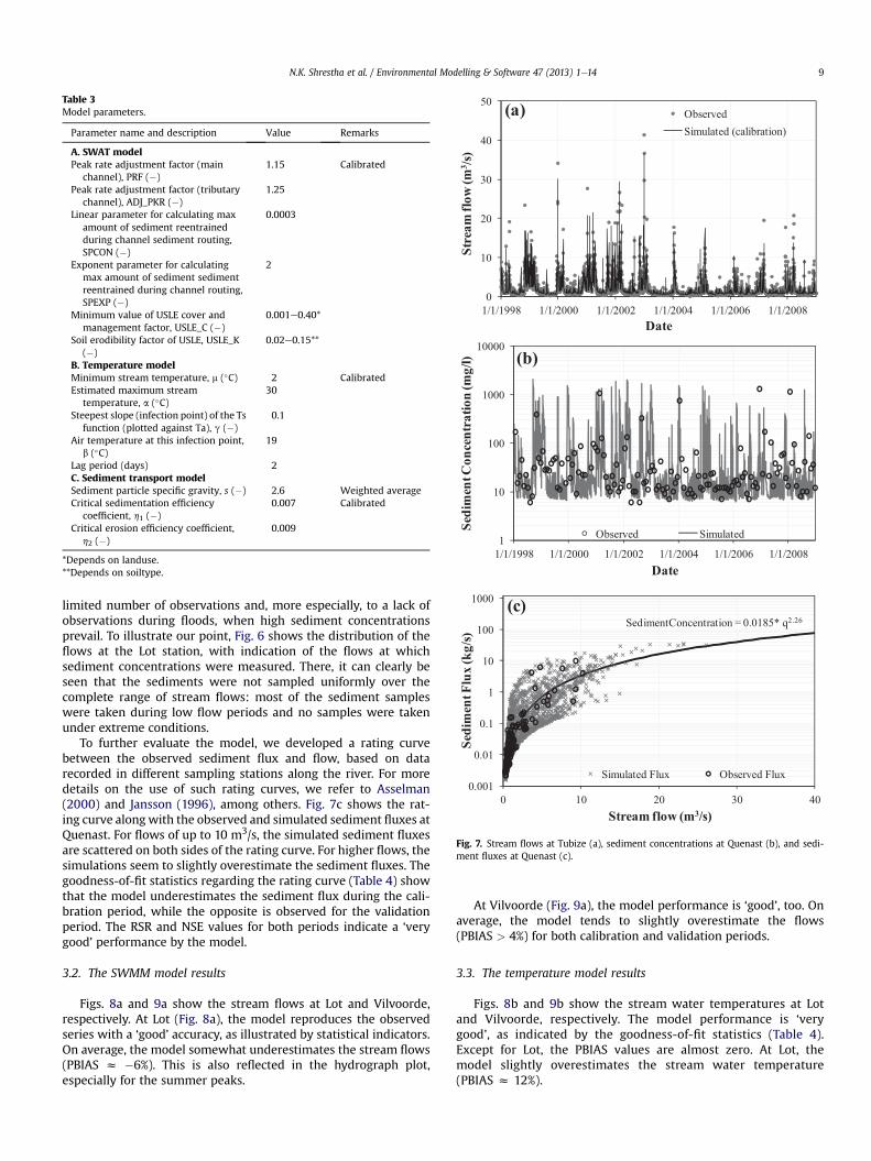
3.1.1. The stream flowFig. 7a shows the observed and simulated stream flows at Tubize

for the calibration period. The plot and goodness-of-fit statistics(Table 4) illustrate the ‘very good’ quality of the stream flowsimulation. The model results for the validation periods were foundto be ‘good’. A slight underperformance by the model during thevalidation period may generally be expected due to various factorssuch as differences in the precipitation characteristics between thevalidation period and the calibration period. More informationregarding the stream flow calibration/validation of the SWATmodelcan be found in Leta et al. (2011) and Leta et al. (2012).

3.1.2. The sedimentThe plot of the observed and simulated sediment concentrations

at Quenast (Fig. 7b) as well as the goodness-of-fit statistics (Table 4)point to a ‘satisfactory’ quality in the model results. The (low)sediment concentrations during dry weather periods are wellreproduced, but the match for the high concentrations seemserratic. For extreme events, the simulated concentrations arecrossing the 2000mg/l mark even though such highmeasurementsare not recorded. We believe, however, that it is related to the

1

10

100

1000

10000

1/1/1998 1/1/2000 1/1/2002 1/1/2004 1/1/2006 1/1/2008

Sedi

men

t Con

cent

ratio

n (m

g/l)

Date

(b)

Observed Simulated

SedimentConcentration = 0.0185* q2.26

0.001

0.01

0.1

1

10

100

1000

0 10 20 30 40

Sedi

men

t Flu

x (k

g/s)

Stream flow (m3/s)

(c)

Simulated Flux Observed Flux

0

10

20

30

40

50

1/1/1998 1/1/2000 1/1/2002 1/1/2004 1/1/2006 1/1/2008

Stre

am fl

ow (m

3 /s)

Date

(a) ObservedSimulated (calibration)

Fig. 7. Stream flows at Tubize (a), sediment concentrations at Quenast (b), and sedi-ment fluxes at Quenast (c).

Table 3Model parameters.

Parameter name and description Value Remarks

A. SWAT modelPeak rate adjustment factor (main

channel), PRF (�)1.15 Calibrated

Peak rate adjustment factor (tributarychannel), ADJ_PKR (�)

1.25

Linear parameter for calculating maxamount of sediment reentrainedduring channel sediment routing,SPCON (�)

0.0003

Exponent parameter for calculatingmax amount of sediment sedimentreentrained during channel routing,SPEXP (�)

2

Minimum value of USLE cover andmanagement factor, USLE_C (�)

0.001e0.40*

Soil erodibility factor of USLE, USLE_K(�)

0.02e0.15**

B. Temperature modelMinimum stream temperature, m (�C) 2 CalibratedEstimated maximum stream

temperature, a (�C)30

Steepest slope (infection point) of the Tsfunction (plotted against Ta), g (�)

0.1

Air temperature at this infection point,b (�C)

19

Lag period (days) 2C. Sediment transport modelSediment particle specific gravity, s (�) 2.6 Weighted averageCritical sedimentation efficiency

coefficient, h1 (�)0.007 Calibrated

Critical erosion efficiency coefficient,h2 (�)

0.009

*Depends on landuse.**Depends on soiltype.

N.K. Shrestha et al. / Environmental Modelling & Software 47 (2013) 1e14 9

limited number of observations and, more especially, to a lack ofobservations during floods, when high sediment concentrationsprevail. To illustrate our point, Fig. 6 shows the distribution of theflows at the Lot station, with indication of the flows at whichsediment concentrations were measured. There, it can clearly beseen that the sediments were not sampled uniformly over thecomplete range of stream flows: most of the sediment sampleswere taken during low flow periods and no samples were takenunder extreme conditions.

To further evaluate the model, we developed a rating curvebetween the observed sediment flux and flow, based on datarecorded in different sampling stations along the river. For moredetails on the use of such rating curves, we refer to Asselman(2000) and Jansson (1996), among others. Fig. 7c shows the rat-ing curve alongwith the observed and simulated sediment fluxes atQuenast. For flows of up to 10 m3/s, the simulated sediment fluxesare scattered on both sides of the rating curve. For higher flows, thesimulations seem to slightly overestimate the sediment fluxes. Thegoodness-of-fit statistics regarding the rating curve (Table 4) showthat the model underestimates the sediment flux during the cali-bration period, while the opposite is observed for the validationperiod. The RSR and NSE values for both periods indicate a ‘verygood’ performance by the model.

3.2. The SWMM model results

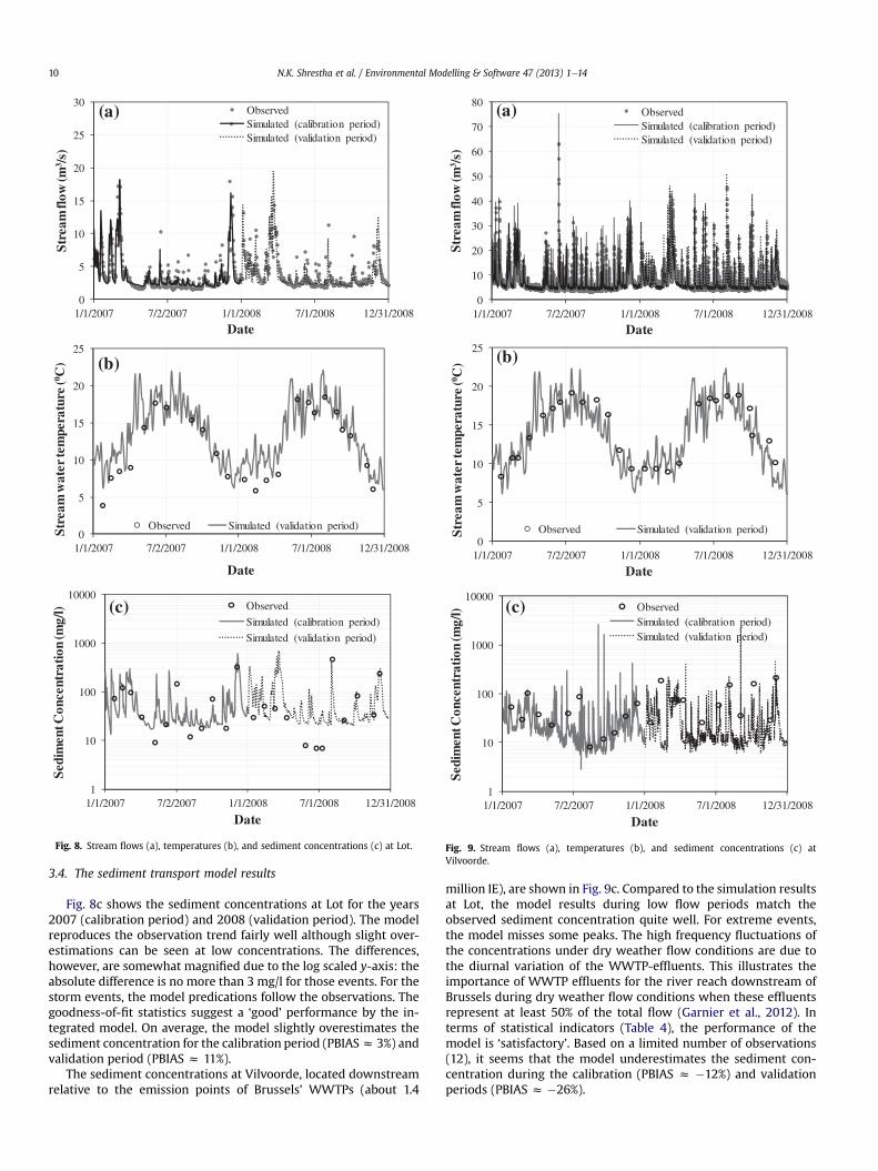
Figs. 8a and 9a show the stream flows at Lot and Vilvoorde,respectively. At Lot (Fig. 8a), the model reproduces the observedseries with a ‘good’ accuracy, as illustrated by statistical indicators.On average, the model somewhat underestimates the stream flows(PBIAS z �6%). This is also reflected in the hydrograph plot,especially for the summer peaks.

At Vilvoorde (Fig. 9a), the model performance is ‘good’, too. Onaverage, the model tends to slightly overestimate the flows(PBIAS > 4%) for both calibration and validation periods.

3.3. The temperature model results

Figs. 8b and 9b show the stream water temperatures at Lotand Vilvoorde, respectively. The model performance is ‘verygood’, as indicated by the goodness-of-fit statistics (Table 4).Except for Lot, the PBIAS values are almost zero. At Lot, themodel slightly overestimates the stream water temperature(PBIAS z 12%).

0

5

10

15

20

25

30

1/1/2007 7/2/2007 1/1/2008 7/1/2008 12/31/2008

Str

eam

flow

(m3 /

s)

Date

(a) ObservedSimulated (calibration period)Simulated (validation period)

1/1/2007 7/2/2007 1/1/2008 7/1/2008 12/31/20080

5

10

15

20

25

Date

Stre

am w

ater

tem

pera

ture

(0 C) (b)

Observed Simulated (validation period)

1

10

100

1000

10000

1/1/2007 7/2/2007 1/1/2008 7/1/2008 12/31/2008

Sedi

men

t Con

cent

rati

on (m

g/l)

Date

(c) Observed

Simulated (calibration period)

Simulated (validation period)

Fig. 8. Stream flows (a), temperatures (b), and sediment concentrations (c) at Lot.

0

10

20

30

40

50

60

70

80

1/1/2007 7/2/2007 1/1/2008 7/1/2008 12/31/2008

Stre

am fl

ow (m

3 /s)

Date

(a) ObservedSimulated (calibration period)Simulated (validation period)

1/1/2007 7/2/2007 1/1/2008 7/1/2008 12/31/20080

5

10

15

20

25

Date

Stre

am w

ater

tem

pera

ture

(0 C) (b)

Observed Simulated (validation period)

1

10

100

1000

10000

1/1/2007 7/2/2007 1/1/2008 7/1/2008 12/31/2008

Sedi

men

t Con

cent

rati

on (m

g/l)

Date

(c) ObservedSimulated (calibration period)Simulated (validation period)

Fig. 9. Stream flows (a), temperatures (b), and sediment concentrations (c) atVilvoorde.

N.K. Shrestha et al. / Environmental Modelling & Software 47 (2013) 1e1410

3.4. The sediment transport model results

Fig. 8c shows the sediment concentrations at Lot for the years2007 (calibration period) and 2008 (validation period). The modelreproduces the observation trend fairly well although slight over-estimations can be seen at low concentrations. The differences,however, are somewhat magnified due to the log scaled y-axis: theabsolute difference is no more than 3 mg/l for those events. For thestorm events, the model predications follow the observations. Thegoodness-of-fit statistics suggest a ‘good’ performance by the in-tegrated model. On average, the model slightly overestimates thesediment concentration for the calibration period (PBIASz 3%) andvalidation period (PBIAS z 11%).

The sediment concentrations at Vilvoorde, located downstreamrelative to the emission points of Brussels’ WWTPs (about 1.4

million IE), are shown in Fig. 9c. Compared to the simulation resultsat Lot, the model results during low flow periods match theobserved sediment concentration quite well. For extreme events,the model misses some peaks. The high frequency fluctuations ofthe concentrations under dry weather flow conditions are due tothe diurnal variation of the WWTP-effluents. This illustrates theimportance of WWTP effluents for the river reach downstream ofBrussels during dry weather flow conditions when these effluentsrepresent at least 50% of the total flow (Garnier et al., 2012). Interms of statistical indicators (Table 4), the performance of themodel is ‘satisfactory’. Based on a limited number of observations(12), it seems that the model underestimates the sediment con-centration during the calibration (PBIAS z �12%) and validationperiods (PBIAS z �26%).

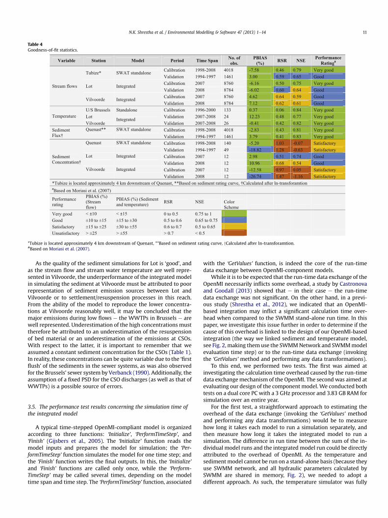
Table 4Goodness-of-fit statistics.

*Tubize is located approximately 4 km downstream of Quenast, **Based on sediment rating curve, yCalculated after ln-transforamtion.#Based on Moriasi et al. (2007).

N.K. Shrestha et al. / Environmental Modelling & Software 47 (2013) 1e14 11

As the quality of the sediment simulations for Lot is ‘good’, andas the stream flow and stream water temperature are well repre-sented in Vilvoorde, the underperformance of the integrated modelin simulating the sediment at Vilvoorde must be attributed to poorrepresentation of sediment emission sources between Lot andVilvoorde or to settlement/resuspension processes in this reach.From the ability of the model to reproduce the lower concentra-tions at Vilvoorde reasonably well, it may be concluded that themajor emissions during low flows e the WWTPs in Brussels e arewell represented. Underestimation of the high concentrations musttherefore be attributed to an underestimation of the resuspensionof bed material or an underestimation of the emissions at CSOs.With respect to the latter, it is important to remember that weassumed a constant sediment concentration for the CSOs (Table 1).In reality, these concentrations can be quite variable due to the ‘firstflush’ of the sediments in the sewer systems, as was also observedfor the Brussels’ sewer system by Verbanck (1990). Additionally, theassumption of a fixed PSD for the CSO discharges (as well as that ofWWTPs) is a possible source of errors.

3.5. The performance test results concerning the simulation time ofthe integrated model

A typical time-stepped OpenMI-compliant model is organizedaccording to three functions: ‘Initialize’, ‘PerformTimeStep’, and‘Finish’ (Gijsbers et al., 2005). The ‘Initialize’ function reads themodel inputs and prepares the model for simulation; the ‘Per-formTimeStep’ function simulates the model for one time step; andthe ‘Finish’ function writes the final outputs. In this, the ‘Initialize’and ‘Finish’ functions are called only once, while the ‘Perform-TimeStep’ may be called several times, depending on the modeltime span and time step. The ‘PerformTimeStep’ function, associated

with the ‘GetValues’ function, is indeed the core of the run-timedata exchange between OpenMI-component models.

While it is to be expected that the run-time data exchange of theOpenMI necessarily inflicts some overhead, a study by Castronovaand Goodall (2013) showed that e in their case e the run-timedata exchange was not significant. On the other hand, in a previ-ous study (Shrestha et al., 2012), we indicated that an OpenMI-based integration may inflict a significant calculation time over-head when compared to the SWMM stand-alone run time. In thispaper, we investigate this issue further in order to determine if thecause of this overhead is linked to the design of our OpenMI-basedintegration (the way we linked sediment and temperature model,see Fig. 2, making them use the SWMMNetwork and SWMMmodelevaluation time step) or to the run-time data exchange (invokingthe ‘GetValues’ method and performing any data transformations).

To this end, we performed two tests. The first was aimed atinvestigating the calculation time overhead caused by the run-timedata exchange mechanism of the OpenMI. The second was aimed atevaluating our design of the component model. We conducted bothtests on a dual core PC with a 3 GHz processor and 3.83 GB RAM forsimulation over an entire year.

For the first test, a straightforward approach to estimating theoverhead of the data exchange (invoking the ‘GetValues’ methodand performing any data transformations) would be to measurehow long it takes each model to run a simulation separately, andthen measure how long it takes the integrated model to run asimulation. The difference in run time between the sum of the in-dividual model runs and the integrated model run could be directlyattributed to the overhead of OpenMI. As the temperature andsedimentmodel cannot be run on a stand-alone basis (because theyuse SWMM network, and all hydraulic parameters calculated bySWMM are shared in memory, Fig. 2), we needed to adopt adifferent approach. As such, the temperature simulator was fully

N.K. Shrestha et al. / Environmental Modelling & Software 47 (2013) 1e1412

integrated within the sediment simulator. By doing so, we elimi-nated two external links with respect to the original componentmodel (Fig. 4): the link between SWMM and the temperaturemodel (link ‘b’ in Fig. 4); and the link between the sediment and thetemperature models (link ‘c’ in Fig. 4). A reduction in simulationtime is to be expected with this new model, as the ‘GetValues’ callsrelated to these links are eliminated. For the sake of completeness,it should be mentioned that the simulation time will also bereduced by the fact that the ‘Initialize’ and ‘Finish’ functions of thetemperaturemodel need not be invoked. The impact of the latter onthe global simulation time can however be neglected.

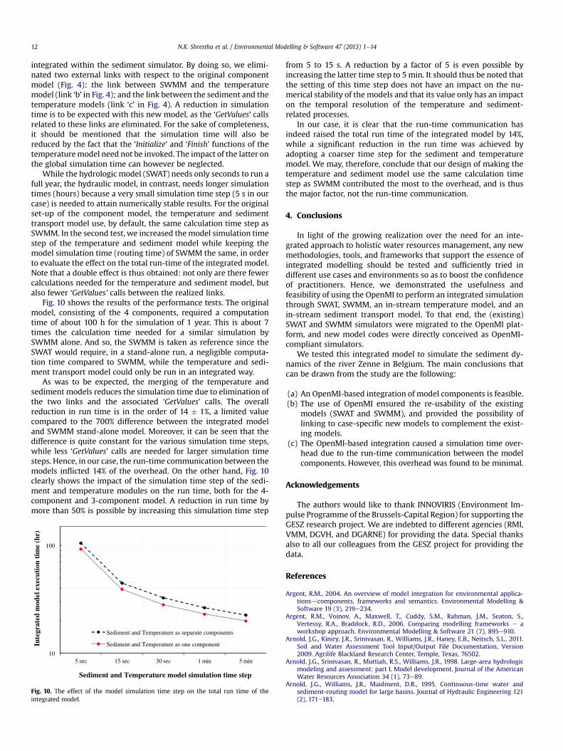
While the hydrologic model (SWAT) needs only seconds to run afull year, the hydraulic model, in contrast, needs longer simulationtimes (hours) because a very small simulation time step (5 s in ourcase) is needed to attain numerically stable results. For the originalset-up of the component model, the temperature and sedimenttransport model use, by default, the same calculation time step asSWMM. In the second test, we increased themodel simulation timestep of the temperature and sediment model while keeping themodel simulation time (routing time) of SWMM the same, in orderto evaluate the effect on the total run-time of the integrated model.Note that a double effect is thus obtained: not only are there fewercalculations needed for the temperature and sediment model, butalso fewer ‘GetValues’ calls between the realized links.

Fig. 10 shows the results of the performance tests. The originalmodel, consisting of the 4 components, required a computationtime of about 100 h for the simulation of 1 year. This is about 7times the calculation time needed for a similar simulation bySWMM alone. And so, the SWMM is taken as reference since theSWAT would require, in a stand-alone run, a negligible computa-tion time compared to SWMM, while the temperature and sedi-ment transport model could only be run in an integrated way.

As was to be expected, the merging of the temperature andsediment models reduces the simulation time due to elimination ofthe two links and the associated ‘GetValues’ calls. The overallreduction in run time is in the order of 14 � 1%, a limited valuecompared to the 700% difference between the integrated modeland SWMM stand-alone model. Moreover, it can be seen that thedifference is quite constant for the various simulation time steps,while less ‘GetValues’ calls are needed for larger simulation timesteps. Hence, in our case, the run-time communication between themodels inflicted 14% of the overhead. On the other hand, Fig. 10clearly shows the impact of the simulation time step of the sedi-ment and temperature modules on the run time, both for the 4-component and 3-component model. A reduction in run time bymore than 50% is possible by increasing this simulation time step

10

100

5 sec 15 sec 30 sec 1 min 5 min

Inte

grat

ed m

odel

exe

cuti

on t

ime

(hr)

Sediment and Temperature model simulation time step

Sediment and Temperature as separate components

Sediment and Temperature as one component

Fig. 10. The effect of the model simulation time step on the total run time of theintegrated model.

from 5 to 15 s. A reduction by a factor of 5 is even possible byincreasing the latter time step to 5 min. It should thus be noted thatthe setting of this time step does not have an impact on the nu-merical stability of the models and that its value only has an impacton the temporal resolution of the temperature and sediment-related processes.

In our case, it is clear that the run-time communication hasindeed raised the total run time of the integrated model by 14%,while a significant reduction in the run time was achieved byadopting a coarser time step for the sediment and temperaturemodel. We may, therefore, conclude that our design of making thetemperature and sediment model use the same calculation timestep as SWMM contributed the most to the overhead, and is thusthe major factor, not the run-time communication.

4. Conclusions

In light of the growing realization over the need for an inte-grated approach to holistic water resources management, any newmethodologies, tools, and frameworks that support the essence ofintegrated modelling should be tested and sufficiently tried indifferent use cases and environments so as to boost the confidenceof practitioners. Hence, we demonstrated the usefulness andfeasibility of using the OpenMI to perform an integrated simulationthrough SWAT, SWMM, an in-stream temperature model, and anin-stream sediment transport model. To that end, the (existing)SWAT and SWMM simulators were migrated to the OpenMI plat-form, and new model codes were directly conceived as OpenMI-compliant simulators.

We tested this integrated model to simulate the sediment dy-namics of the river Zenne in Belgium. The main conclusions thatcan be drawn from the study are the following:

(a) An OpenMI-based integration of model components is feasible.(b) The use of OpenMI ensured the re-usability of the existing

models (SWAT and SWMM), and provided the possibility oflinking to case-specific new models to complement the exist-ing models.

(c) The OpenMI-based integration caused a simulation time over-head due to the run-time communication between the modelcomponents. However, this overhead was found to be minimal.

Acknowledgements

The authors would like to thank INNOVIRIS (Environment Im-pulse Programme of the Brussels-Capital Region) for supporting theGESZ research project. We are indebted to different agencies (RMI,VMM, DGVH, and DGARNE) for providing the data. Special thanksalso to all our colleagues from the GESZ project for providing thedata.

References

Argent, R.M., 2004. An overview of model integration for environmental applica-tionsdcomponents, frameworks and semantics. Environmental Modelling &Software 19 (3), 219e234.

Argent, R.M., Voinov, A., Maxwell, T., Cuddy, S.M., Rahman, J.M., Seaton, S.,Vertessy, R.A., Braddock, R.D., 2006. Comparing modelling frameworks e aworkshop approach. Environmental Modelling & Software 21 (7), 895e910.

Arnold, J.G., Kiniry, J.R., Srinivasan, R., Williams, J.R., Haney, E.B., Neitsch, S.L., 2011.Soil and Water Assessment Tool Input/Output File Documentation, Version2009. Agrilife Blackland Research Center, Temple, Texas, 76502.

Arnold, J.G., Srinivasan, R., Muttiah, R.S., Williams, J.R., 1998. Large-area hydrologicmodeling and assessment: part I. Model development. Journal of the AmericanWater Resources Association 34 (1), 73e89.

Arnold, J.G., Williams, J.R., Maidment, D.R., 1995. Continuous-time water andsediment-routing model for large basins. Journal of Hydraulic Engineering 121(2), 171e183.

N.K. Shrestha et al. / Environmental Modelling & Software 47 (2013) 1e14 13

Asselman, N.E.M., 2000. Fitting and interpretation of sediment rating curves.Journal of Hydrology 234 (3e4), 228e248.

Bagnold, R.A., 1977. Bed load transport by natural rivers. Water Resources Research13 (2), 303e312.

Benaman, J., Shoemaker, C.A., 2005. An analysis of high-flow sediment eventdata for evaluating model performance. Hydrological Processes 19 (3), 605e620.

Bennett, N.D., Croke, B.F.W., Guariso, G., Guillaume, J.H.A., Hamilton, S.H.,Jakeman, A.J., Marsili-Libelli, S., Newham, L.T.H., Norton, J.P., Perrin, C.,Pierce, S.A., Robson, B., Seppelt, R., Voinov, A.A., Fath, B.D., Andreassian, V., 2013.Characterising performance of environmental models. Environmental Model-ling & Software 40 (0), 1e20.

Betrie, G.D., van Griensven, A., Mohamed, Y.A., Popescu, I., Mynett, A.E., Hummel, S.,2011. Linking SWAT and SOBEK using open modelling interface (OpenMI) forsediment transport simulation in the Blue Nile river basin. American Society ofAgricultural and Biological Engineers 54 (5), 1749e1757.

Black, S., 2001. Computing ripple effect for software maintenance. Journalof Software Maintenance and Evolution: Research and Practice 13 (4), 263e279.

Brandmeyer, J.E., Karimi, H.A., 2000. Coupling methodologies for environmentalmodels. Environmental Modelling & Software 15 (5), 479e488.

Bulatewicz, T., Yang, X., Peterson, J.M., Staggenborg, S., Welch, S.M., Steward, D.R.,2010. Accessible integration of agriculture, groundwater, and economic modelsusing the open modeling interface (OpenMI): methodology and initial results.Hydrology and Earth Systems Sciences 14 (3), 521e534.

Bulatewicz, T., Allen, A., Peterson, J.M., Staggenborg, S., Welch, S.M., Steward, D.R.,2013. The simple script wrapper for OpenMI: enabling interdisciplinarymodeling studies. Environmental Modelling & Software 39 (0), 283e294.

Candela, A., Freni, G., Mannina, G., Viviani, G., 2012. Receiving water body qualityassessment: an integrated mathematical approach applied to an Italian casestudy. Journal of Hydroinformatics 14 (1), 30e47.

Castronova, A.M., Goodall, J.L., 2010. A generic approach for developing process-level hydrologic modeling components. Environmental Modelling & Software25 (7), 819e825.

Castronova, A.M., Goodall, J.L., 2013. Simulating watersheds using loosely integratedmodel components: evaluation of computational scaling using OpenMI. Envi-ronmental Modelling & Software 39 (0), 304e313.

Castronova, A.M., Goodall, J.L., Ercan, M.B., 2012. Integrated modeling within ahydrologic information system: an OpenMI based approach. EnvironmentalModelling & Software. http://dx.doi.org/10.1016/j.envsoft.2012.02.011.

Chow, V.T., 1959. Open Channel Hydraulics. McGraw-Hill Book Company, New York.Collins-Sussman, B., Fitzpatrick, B.W., Pilato, C.M., 2011. Version Control with Sub-

version: for Subversion 1.7: (Compiled from r4288). Creative Commons, 559Nathan Abbott Way, Stanford, California 94305, USA.

Crabill, C., Donald, R., Snelling, J., Foust, R., Southam, G., 1999. The impact of sedi-ment fecal coliform reservoirs on seasonal water quality in Oak Creek, Arizona.Water Research 33 (9), 2163e2171.

Demuynck, C., Bauwens, W., De Pauw, N., Dobbelaere, I., Poelman, E., 1997. Evalu-ation of pollutant reduction scenarios in a river basin: application of long termwater quality simulations. Water Science & Technology 35 (9), 65e75.

Easton, Z.M., Fuka, D.R., White, E.D., Collick, A.S., Biruk Ashagre, B., McCartney, M.,Awulachew, S.B., Ahmed, A.A., Steenhuis, T.S., 2010. A multi basin SWAT modelanalysis of runoff and sedimentation in the Blue Nile, Ethiopia. Hydrology andEarth System Sciences 14 (10), 1827e1841.

EU, 2000. Directive 2000/60/EC of the European Parliament and of the council of 23October 2000 establishing a framework for community action in the field ofwater policy. Official Journal of the European Communities L327, 1e72.

Gaddis, E.J.B., Vladich, H., Voinov, A., 2007. Participatory modeling and the dilemmaof diffuse nitrogen management in a residential watershed. EnvironmentalModelling & Software 22 (5), 619e629.

Garcia-Armisen, T., Servais, P., 2009. Partitioning and fate of particle-associated E.coli in river waters. Water Environment Research 81 (1), 21e28.

Garnier, J., Brion, N., Callens, J., Passy, P., Deligne, C., Billen, G., Servais, P., Billen, C.,2012. Modeling historical changes in nutrient delivery and water quality of theZenne River (1790se2010): the role of land use, waterscape and urban waste-water management. Journal of Marine Systems (in press).

Gijsbers, P., Brinkman, R., Gregersen, J., Hummel, S., Westen, S., 2005. OpenMI: OpenModeling Interface. In: The OpenMI Document Series: Part C the Org.OpenMI.Standard Interface Specification (Version 1.0). Available at: http://www.OpenMI.org.

Gironás, J., Roesner, L.A., Davis, J., 2009. Storm Water Management Model Appli-cation Manual. US EPA.

Grant, P.J., 1977. Water temperatures of the Ngaruroro River at three stations.Journal of Hydrology (New Zealand) 16 (2), 148e157.

Gregersen, J.B., Gijsbers, P.J.A., Westen, S.J.P., 2007. OpenMI: open modelling inter-face. Journal of Hydroinformatics 9 (3), 175e191.

Jansson, M.B., 1996. Estimating a sediment rating curve of the Reventazón river atPalomo using logged mean loads within discharge classes. Journal of Hydrology183 (3e4), 227e241.

Jha, M.K., Gassman, P.W., Arnold, J.G., 2007. Water quality modeling for the Raccoonriver watershed using SWAT. Transactions of the American Society of Agricul-tural and Biological Engineers 50 (2), 479e493.

Knapen, R., Janssen, S., Roosenschoon, O., Verweij, P., de Winter, W., Uiterwijk, M.,Wien, J.-E., 2013. Evaluating OpenMI as a model integration platform acrossdisciplines. Environmental Modelling & Software 39 (0), 274e282.

Lai, C., 1987. Numerical modeling of unsteady open-channel flow. In: Yen, B.C. (Ed.),Advances in Hydroscience. Academic Press, New York, pp. 161e333.

Lal, R., 2001. Soil degradation by erosion. Land Degradation & Development 12 (6),519e539.

Lam, Q.D., Schmalz, B., Fohrer, N., 2010. Modelling point and diffuse source pollutionof nitrate in a rural lowland catchment using the SWAT model. AgriculturalWater Management 97 (2), 317e325.

Laniak, G.F., Olchin, G., Goodall, J., Voinov, A., Hill, M., Glynn, P., Whelan, G.,Geller, G., Quinn, N., Blind, M., Peckham, S., Reaney, S., Gaber, N., Kennedy, R.,Hughes, A., 2013. Integrated environmental modeling: a vision and roadmap forthe future. Environmental Modelling & Software 39 (0), 3e23.

Leta, O.T., Shrestha, N.K., De Fraine, B., Bauwens, W., 2011. Accessible Linking ofHydrological and Hydraulic Models Through OpenMI for Integrated River BasinManagement, Water 2011: Integrated Water Resources Management in Tropicaland Subtropical Drylands: Mekelle, Ethiopia.

Leta, O.T., Shrestha, N.K., De Fraine, B., van Griensven, A., Bauwens, W., 2012.OpenMI based flow and water quality modelling of the river Zenne. In:(SHF), S.H.d.F (Ed.), Proceedings of the SimHydro 2012, 2nd InternationalConference, 12the14th September. Nice-Sophia Antipolis, France: Nice,France.

Mein, R.G., Larson, C.L., 1973. Modeling infiltration during a steady rain. WaterResources Research 9 (2), 384e394.

Mohseni, O., Stefan, H.G., Erickson, T.R., 1998. A nonlinear regression model forweekly stream temperatures. Water Resources Research 34 (10), 2685e2692.

Moore, R.V., Tindall, C.I., 2005. An overview of the open modelling interfaceand environment (the OpenMI). Environmental Science & Policy 8 (3),279e286.

Moriasi, D.N., Arnold, J.G., Van Liew, M.W., Binger, R.L., Harmel, R.D., Veith, T., 2007.Model evaluation guidelines for systematic quantification of accuracy inwatershed simulations. Transactions of the ASABE 50 (3), 885e900.

Nash, J.E., Sutcliffe, J.V., 1970. River flow forecasting through conceptual models partI e a discussion of principles. Journal of Hydrology 10 (3), 282e290.

Neitsch, S.L., Arnold, J.G., Kiniry, J.R., Williams, J.R., 2011. Soil & Water AssessmentTool Theoretical Documentation, Version 2009. Grassland, Soil and WaterResearch Laboratory-Agricultural Research Service Blackland Research Center-tTexas AgriLife Research.

OpenMI, 2009. OpenMI Life Project Website. http://www.openmi-life.org/.Ouattara, N., Passerat, J., Servais, P., 2011. Faecal contamination of water and sedi-

ment in the rivers of the Scheldt drainage network. Environmental Monitoringand Assessment, 1e15.

Parker, P., Letcher, R., Jakeman, A., Beck, M.B., Harris, G., Argent, R.M., Hare, M., Pahl-Wostl, C., Voinov, A., Janssen, M., Sullivan, P., Scoccimarro, M., Friend, A.,Sonnenshein, M., Barker, D., Matejicek, L., Odulaja, D., Deadman, P., Lim, K.,Larocque, G., Tarikhi, P., Fletcher, C., Put, A., Maxwell, T., Charles, A., Breeze, H.,Nakatani, N., Mudgal, S., Naito, W., Osidele, O., Eriksson, I., Kautsky, U., Kautsky, E.,Naeslund, B., Kumblad, L., Park, R., Maltagliati, S., Girardin, P., Rizzoli, A.,Mauriello, D., Hoch, R., Pelletier, D., Reilly, J., Olafsdottir, R., Bin, S., 2002. Progress inintegrated assessment andmodelling. EnvironmentalModelling & Software 17 (3),209e217.

Peckham, S., 2010. CSDMS Handbook of Concepts and Protocols: A Guide for CodeContributors. Available at: http://csdms.colorado.edu/wiki/Help:Tools_CSDMS_Handbook.

Reußner, F., Alex, J., Bach, M., Schutze, M., Muschalla, D., 2009. Basin-wide inte-grated modelling via OpenMI considering multiple urban catchments. WaterScience & Technology 60 (5), 1241e1248.

Rizzoli, A.E., Davis, J.R., 1999. Integration and re-use of environmental models.Environmental Modelling & Software 14 (6), 493e494.

Rizzoli, A.E., Donatelli, M., Athanasiadis, I.N., Villa, F., Huber, D., 2008. Semantic linksin integrated modelling frameworks. Mathematics and Computers in Simula-tion 78 (2e3), 412e423.

Rossman, L.A., 2009. Storm water management model user’s manual, version 5.0.Rubey, W.W., 1933. Settling velocities of gravel sand and silt particles. American

Journal of Science 25 (148), 325e338.Santhi, C., Arnold, J.G., Williams, J.R., Dugas, W.A., Srinivasan, R., Hauck, L.M., 2001.

Validation of the SWAT model on a large river basin with point and nonpointsources. JAWRA Journal of the American Water Resources Association 37 (5),1169e1188.

Shields, A., 1936. Anwendung der ahnlichkeits-mechanik und der turbulenzfor-schung auf die geschiebebewegung. Preus Versuchsanstalt Wasserbau Schiff-fahrt Berlin Mitteil 2b.

Singh, J., Knapp, H.V., Demissie, M., 2004. Hydrologic Modeling of the Iroquois RiverWatershed Using HSPF and SWAT. Available at: http://www.isws.illinois.edu/pubdoc/CR/ISWSCR2004-08.pdf (accessed 20.02.13.).

Shrestha, N.K., Leta, O.T., de Fraine, B., van Griensven, A., Garcia-Armisen, T.,Ouattara, N.K., Servais, P., Bauwens, W., 2012. Integrated modelling of riverZenne using OpenMI. In: Hinkelmann, R., Nasermoaddeli, M.H., Liong, S.Y.,Savic, D., Fröhle, P., Daemrich, K.F. (Eds.), Proceedings of the 10th InternationalConference on Hydroinformatics HIC 2012, 14the18th July, Hamburg, Germany.

Soulsby, R.L., Whithouse, R., 1997. Threshold of sediment motion in coastal envi-ronments. In: Proceedings Pacific Coasts and Ports ’97 Conference, Christ-church, vol. 1. University of Canterbury, New Zeland, pp. 149e154.

Srinivasan, R., Ramanarayanan, T.S., Arnold, J.G., Bednarz, S.T., 1998. Large areahydrologic modelling and assessment. Part II: model application. Journal of theAmerican Water Resources Association 34 (1), 91e101.

N.K. Shrestha et al. / Environmental Modelling & Software 47 (2013) 1e1414

Stefan, H.G., Preud’homme, E.B., 1993. Stream temperature estimation from airtemperature. Water Resources Bulletin 29 (1), 27e45.

Sui, D.Z., Maggio, R.C., 1999. Integrating GIS with hydrological modeling: practices,problems, and prospects. Computers, Environment and Urban Systems 23 (1),33e51.

USDA-SCS, 1986. US Department of Agriculture-Soil Conservation Service (USDA-SCS): Urban Hydrology for Small Watersheds. USDA, Washington, DC.

USDI-BR, 2006. Erosion and Sedimentation Manual. U.S. Department of the Interior,Bureau of Reclamation, Technical Service Center, Colorado.

van Griensven, A., 2002. Developments towards Integrated Water Quality Model-ling for River Basins. Department of Hydrology and Hydraulic Engineering. VrijeUniversiteit Brussel, Brussels.

Van Liew, M.W., Arnold, J.G., Bosch, D.D., 2005. Problems and potential of autoca-librating a hydrologic model. Transactions of the American Society of Agricul-tural and Biological Engineers 48 (3), 1025e1040.

Velikanov, M.A., 1954. Gravitational theory for sediment transport. Journal of Sci-ence of the Soviet Union. Geophysics (in Russian) 4.

Verbanck, M., 1990. Sewer sediment and its relation with the quality characteristicsof combined sewer flows. Water Science & Technology 22 (10/11), 247e257.

Voinov, A., Fitz, C., Boumans, R., Costanza, R., 2004. Modular ecosystem modeling.Environmental Modelling & Software 19 (3), 285e304.

Voinov, A., Shugart, H.H., 2013. ‘Integronsters’, integral and integrated modeling.Environmental Modelling & Software 39 (0), 149e158.

Webb, B.W., Clack, P.D., Walling, D.E., 2003. Watereair temperature relationships in aDevonriver systemand the roleofflow.Hydrological Processes17 (15), 3069e3084.

Weber, W.J., 1972. Physicochemical Processes for Water Quality Control. Wiley, NewYork.

White, K.L., Chaubey, I., 2005. Sensitivity analysis, calibration, and validations for amultisite and multivariable SWAT model. JAWRA Journal of the American WaterResources Association 41 (5), 1077e1089.

Williams, J.R., 1969. Flood routing with variable travel time or variable storagecoefficients. Transactions of the American Society of Agricultural and BiologicalEngineers 12, 100e103.

Williams, J.R., Berndt, H.D., 1977. Sediment yield prediction based on watershedhydrology. Transactions of the American Society of Agricultural Engineers 20(6), 1100e1104.

Winchell, M., Srinivasan, R., Luzio, M.D., 2010. ArcSWAT Interface for SWAT2009User’s Guide. Soil and Water Research Laboratory-Agricultural Research Service,Blackland, Texas.

Zug, M., Bellefleur, D., Phan, L., Scrivener, O., 1998. Sediment transport model insewer networks e a new utilization of the Velikanov model. Water Science &Technology 37 (1), 187e196.