Dear Editor, dear Referee,

Thank you very much for handling our paper once again. We have improved the paper according to

the very constructive and helpful comments by yourself and the reviewer.

Following your suggestions, we have seen that values of the D50 are indeed nearly constant along the

entire western Peruvian margin and range between 2 and 3 cm. The largest D50 with values up to 6

cm have been measured in streams that are either sourced in the Cordillera Negra where mean basin

slope angles are larger than 20°, or in the Rio Ocoña and Rio Camaña rivers located at 16°-17°S,

which have the largest mean annual discharge as they capture their waters from a broad area on the

Altiplano. We thus suggest that the generally uniform grain size pattern has been perturbed where

either mean basin slopes, or water fluxes exceed threshold conditions.

The major changes include the improvement of the discussion part with a focus on the comparison

between the particularly larger D50 and the basins where hillslope gradients are steeper than 0.4 on

the average (i.e., 20-22°), or where mean annual stream flows exceed the average values of the

western Peruvian streams (10-40 m3/s) by a factor of 2. In addition, we have updated the Figures with

more information about earthquake occurrence, and we have corrected the text following the

Referee’s recommendations. Finally, we have tuned down most of the inferences and interpretations,

which were based on weak correlations only. We have thus re-structured the discussion part

accordingly.

Please find below a point-by-point response of how we have handled the suggestions and comments.

Thank you very much for your hard work.

On behalf of the co-authors

Camille Litty

[1] Comments by section:

Editor’s comments

Abstract:

We have tuned down the interferences and removed the statements, which lack a significant

correlation. We have also removed the linkage to the earthquake occurrence, as this appears to

be weakly introduced, as noted by the Editor.

Introduction:

We have improved the presentation of the past efforts in exploring the controls on the grain size

pattern in streams. We made an effort to frame this section in a more global perspective, as

required.

Results:

We have mentioned that the morphometric variables and related to this, information about

sediment fluxes and water discharge are inter-related, as required.

We have removed the section, which discusses streams that have no gravel bars, since we have

no information about where the gravel front is situated. We thus follow the recommendation by

the editor not to spend too much space on an issue which lacks any data.

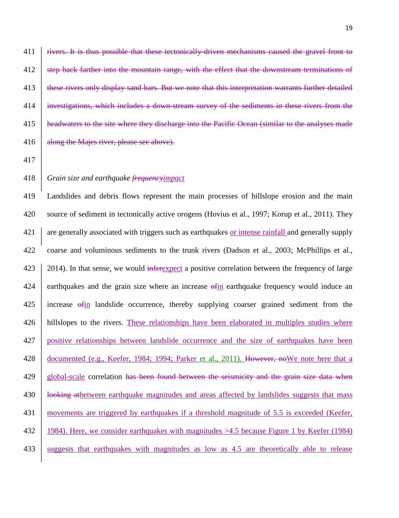
We indeed consider earthquake intensity as an important variable, and magnitude thresholds >

5.5 might need to be exceeded for the release of large volumes of landslides, as noted by the

Editor. However, Figure 1 by Keefer (1984) suggests that earthquakes with magnitudes 4.5 are

are theoretically able to release landslides over an area >10 km2, which is substantial.

Therefore, we have decided to keep our threshold where we considered earthquakes with a

magnitude M>4.5.

We have completely rewritten the remaining part of the discussion following the

recommendations by the Referee, thereby focusing on the pattern of the D50 as recommended.

Referee’s comments

Tectonics and geological setting:

Section 1.1 provides some good information about the geological context, but more is needed. Firstly,

I am confused about the boundaries of the tectonic domains. The authors describe a change in the

degree of interseismic coupling between north and south, specifically with high coupling and high

seismicity south of 13-16 °S, and low coupling and low seismicity to the north. The authors cite a

paper by Nocquet et al. (2014), but this paper does not contain data as far south as 13-16 °S, and

instead appears to place the gap in seismicity at 3-10 °S. Almost all of the catchments in this study

area are south of 10 °S, so it needs to be clarified where this boundary is. I’m struggling to reconcile

the data in Nocquet et al. (2014) with the statements in this section. This needs to be cleared up.

Indeed, this paper by Nocquet does not contain data as far south as 13-16 °S. We have

corrected this point and modified the tectonic section, plus we have expanded the figures

showing the depth of the Nazca plate beneath the South American plate plus the frequency of

earthquake occurrence over a broader scale.

Second, Fig. 3 shows a long-wavelength feature in the slope data (panel G), from 7 to 14 °S; what is

this? It has quite a significant amplitude, with slopes almost doubling in the centre, but it isn’t

discussed. This could be significant – see my later suggestions.

We have discussed this large wavelength pattern of mean basin slopes. Please see the revised

version where we wrote: The pattern of mean slopes per drainage basin reveals a distinct N-S

trend (Table 1). The corresponding values increase from 20° to 25° going from 6°S to 10°S

latitude (where they reach maximum values between 0.4 to 0.45 m/m) after which they decrease

by nearly 50% to values ranging between 10° and 15°. These relationships have not been

explored yet, but most likely reflect the extent to which streams have crossed the western

escarpment and sourced their waters in the relatively flat plateau of the Puna region. Indeed,

most of the western Peruvian streams have their water sources on this flat area and then cross

the western escarpment, which yields relatively low mean basin slopes particularly for basins

south of 12°S. Contrariwise, the basins around 11°-12°S latitudes (which are characterized by

the steep slopes) have their sources in the relatively steep Cordillera Negra (Figure 1A), which

is a relatively dry mountain range situated on the steep escarpment. Along these latitudes, the

high Andes are constituted by the high and heavily glaciated Cordillera Blanca situated farther

to the east (Figure 1A). This mountain range is drained by the Rio Santa, which flows parallel

to the Andes strike within the valley of the Rio Santa, and then crosses the Cordillera Negra at

a right angle (Figure 1A).

In this context: We agree that exceptionally larger D50 values of 4-6 cm were measured for

basins situated between 11-12°S and 16-17°S where hillslope gradients are steeper than 0.4 on

the average (i.e., 20-22°), or where mean annual stream flows exceed the average values of the

western Peruvian streams (10-40 m3/s) by a factor of 2. We have changed the discussion part

quite significantly based on the Referee’s comment the reviewer have made.

Finally, what timescale do the historical earthquake records average over? Is this sufficient to

compare with grain size data?

The historical earthquakes that have been listed on the Figure 3 records earthquakes for at least

the last century. In Peru, the older earthquakes that have been recorded by the USGS survey

catalogue dates to the 28th of Sept. 1906, located in northern Peru. When it is know that

sediments are evacuated on the basis of several years (one year in the Alps for example), more

than a century should be a sufficiently long timescale.

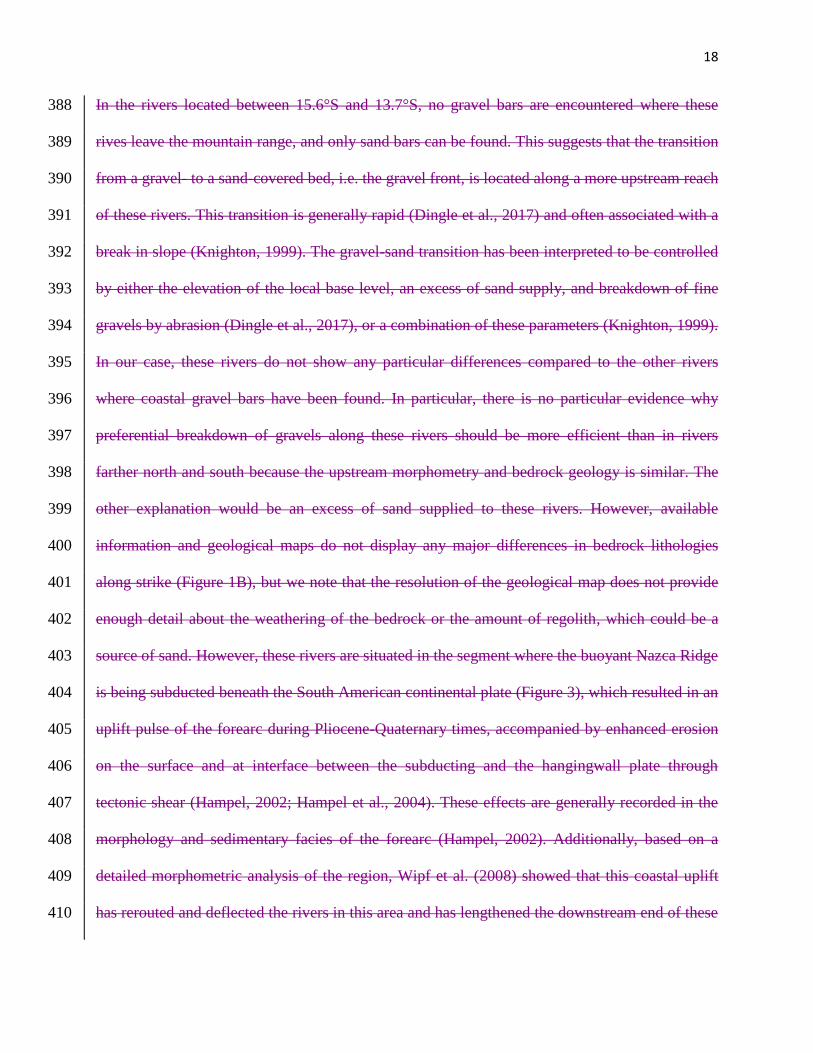
Section 4.1.2. “Absence of gravels in rivers between 15.6 °S and 13.7 °S:

I’m not convinced by the arguments in this section. The authors propose that this sub-group of

catchments lack gravel bars potentially because they have been lengthened by tectonic deformation,

which resulted in a pulse of uplift and enhanced erosion, and the gravel-sand transition simultaneously

migrated upstream into the catchments. Do the authors expect the gravel-sand transition to migrate

upstream in response to enhanced erosion? This seems counterintuitive to me, and also contradicts the

interpretations they make about grain size correlating (weakly) with sediment flux (e.g., Fig. 5a).

Also, Fig. 4 shows the fining rates are fairly low in this landscape, with D50 only decreasing by a few

mm over >100 km. How far upstream do the authors propose the gravel-sand transition has migrated

in order to supply only sand at their sampling location? How much have these catchments supposedly

been lengthened? As it stands, this section raises more questions than it answers.

I recommend the authors take a look at Lamb, M.P. and Venditti, J.V., 2016, The grain size gap and

abrupt gravel-sand transitions in rivers due to suspension fallout, Geophysical Research Letters, 43,

doi: 10.1002/2016GL068713. This paper discusses gravel-sand transitions and suggests they arise

because of changes in bed shear velocity (the wash load hypothesis). Are there any reasons why these

catchments might have different bed shear velocities? Perhaps the framework in this paper can help

the authors develop a more robust argument, if they do want to invoke gravel-sand transitions here. At

the moment this section seems contradictory and unintuitive.

A more minor point: this argument is repeated all over again in section 4.1.3 from lines 318-323, and

this repetition is not needed.

We removed this aspect of our analysis as this section was raising more questions than it

answered and since the discussion about the lack of gravels was not the focus of the paper.

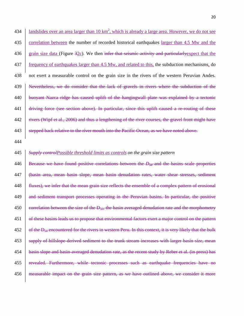
Section 4.1.4. “Supply control on the grain size pattern”.

This section overstates some of the results. Lines 329-331: “the positive correlation between the size

of the D50 and the morphometry of these basins” – there is no correlation between D50 and slope, so

do the authors mean with catchment area? This is still a weak correlation, so I think this statement is

over-selling the relationship. Especially given the authors then claim “environmental factors exert a

major control on the pattern of the D50 encountered for the rivers in western Peru”. These are weak

correlations, not evidence for “major control”.

Yes, indeed, correlations are weak and our previous statements were a tentative effort to

explain our dataset, but we have probably over-interpreted these weak correlations. Please see

the revised manuscript where we wrote: We consider the correlations between the grain size

data (e.g., D50) and the basins scale properties (basin area, mean basin denudation rates, water

shear stresses, sediment fluxes) as not strong and convincing enough for the identification of

potential controls of these variables on the grain size caliber.

Instead, we follow the recommendation by the Referee and focused on the pattern of the D50

only.

Also lines 332-335: “it is very likely that the bulk supply of hillslope-derived sediment to the trunk

stream increases with larger basin size, mean basin slope and basin-averaged denudation rate” – there

seems to be no correlation between D50 and mean slope, so how can this explain the grain size

patterns? The relationships that can be drawn from the data are being overstated.

Yes, these correlations are weak and relationships were overstated. Instead, we focus on the

sections where the D50 were larger than on average. We have thus completely changed the

discussion as recommended by the Referee.

Next, the sentence from lines 341-344 needs to be clearer. Are the authors suggesting that the

catchments with coarser grain sizes experience El Niños and extreme rainfall events with a greater

sensitivity than the catchments with finer grain sizes? I find this to be very unlikely, not to mention

the lack of correlation between sediment flux, water discharge and any of the grain size percentiles.

With a lack of correlation between sediment flux, water discharge and grain size distribution,

this part was overselling our data. We have refocused our analysis on the pattern of the D50.

Please see also our responses above.

Finally, the paragraph from lines 345-364 isn’t very clear either. My understanding is that the authors

propose the coarser-grained catchments are experiencing a downstream shift in the position of gravel

fronts, due to greater sediment supply from hillslope sources. However Fig. 5a shows that catchments

can have a large D50 with either a very low sediment flux or a very high sediment flux (the full

range), and Table 3 shows that no grain size percentiles correlate with catchment slopes. The authors

imply that denudation rates act as a proxy for the amount of hillslope-derived sediment, but this isn’t

necessarily the case.

As this section was raising more questions than it answered and that it was not the focus of the paper,

we removed this part.

We have removed this entire section since it has opened more questions than it has offered

answers. Please see also our response above.

Furthermore, it might be that slopes act to perturb sediment flux (and grain size) above thresholds,

e.g., some threshold angle for landslides and debris flows. In this case a simple correlation (like Table

3) might not reveal whether there is a threshold-controlled grain size response to hillslope processes,

because below the threshold you wouldn’t even expect a correlation.

Yes this is what we state in this new version. This is summarized in the abstract: Exceptionally

large D50 values of 4-6 cm were measured for basins situated between 11-12°S and 16-17°S

where hillslope gradients are steeper than 0.4 on the average (i.e., 20-22°), or where mean

annual stream flows exceed the average values of the western Peruvian streams (10-40 m3/s)

by a factor of 2. We suggest that the generally uniform grain size pattern has been perturbed

where either mean basin slopes, or water fluxes exceed threshold conditions.

Section 4.1.5. “Hydrological control on the grain size distribution”

Line 373-374. “grain sizes correlate with the shear stress values”. The relationships in Fig. 5b-c look

quite tenuous to me.

Yes indeed, correlations are week. The mechanisms by which grain size can be mediated

through a threshold effect upon transport are less well understood, but it has been known at

least since the engineering work by Shields (1936), and particularly by Peter Meyer Müller

(1948) that threshold conditions have to be exceeded upon the transport of grains in fluvial

streams. As a consequence, at transport-limited conditions, sediment flux, and most likely also

the caliber of the transported material, depends on the frequency and the magnitudes at which

these thresholds are exceeded rather than on a mean value of water discharge (Dadson et al.,

2003). This might be the reason why values of water shear stresses, that are calculated based

on the annual mean of water flux, are not sufficiently strongly correlated with the D50 values to

invoke a strong controls thereof.

If you took away the one point with very large grain size the correlations might even become

negative?

Yes, we note that these correlations are weak and some might even break apart if the largest

values (for e.g., shear stresses) are removed.

I think the text is overselling the data here, and this section is unsatisfying because [1] the plots in Fig.

5 are not conclusive, and [2] because the previous section suggested that grain size is limited by

hillslope sediment supply. It’s difficult to explain the data as both supply-limited and transport-limited

at the same time. Also, the average particle size apparently isn’t correlated with either water discharge

or shear stress, so I’m really not convinced at all that it’s possible to infer “a hydraulic control on

grain size distribution of the Peruvian rivers” as the authors claim.

We interpret the data to point towards transport limited conditions, where sediment flux, and

most likely also the caliber of the transport material, depends on the frequency and the

magnitudes at which thresholds upon transport are exceeded rather than on a mean value of

water discharge (Dadson et al., 2003). This might be the reason why values of water shear

stresses, that are calculated based on the annual mean of water flux, are not sufficiently strongly

correlated with the D50 values to invoke a strong controls thereof. The hydraulic forcing has a

control only when a threshold is exceeded. We have outlined these relationships and a possible

interpretation.

Section 4.2. “Transport distance and slope angle controls on sphericity”

Lines 394-398. Recycling particles from a terrace surely won’t make them more spherical, because

while the particles are being stored they aren’t being abraded. Lines 405-406. The authors propose

that in catchments with steeper slopes, denudation rates will be faster and transport distances will be

shorter. Table 3 shows no correlation between slope and denudation rate (or sediment flux). This may

be because slopes influence denudation rates non-linearly (see my earlier comment about the potential

role of thresholds in this landscape), but either way this section seems to contradict the author’s use of

correlations and their data. Furthermore, it is unclear to me how steeper slopes will reduce the

transport distance of material. Residence time yes, but not distance.

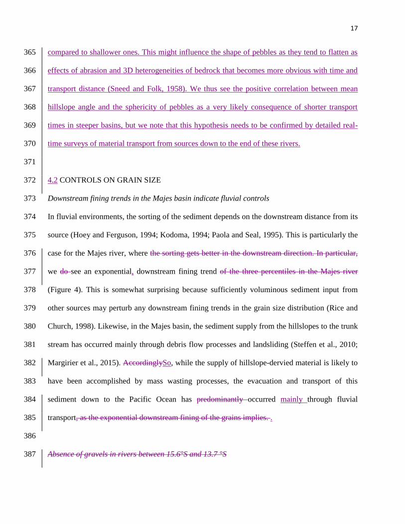
See ‘Slope angle controls on sphericity’: The relative poor positive correlation between the

sphericity of the pebbles and distance from the escarpment edge prevents us from inferring a

distinct control of this variable. We have thus corrected this point. Contrariwise, the positive

Pearson correlation between the sphericity of the pebbles and the mean basin slope is quite

high, thus pointing towards a significant control. This suggests that basins with steeper slopes,

as is the case for the Cordillera Negra, produce rounder pebbles. We tentatively infer that time

scales of transport and evacuation of material is likely to be shorter in steeper basins compared

to shallower ones. This might influence the shape of pebbles as they tend to flatten in response

to effects of abrasion and 3D heterogeneities of bedrock that becomes more obvious with time

and transport distance (Sneed and Folk, 1958). We thus see the positive correlation between

mean hillslope angle and the sphericity of pebbles as a very likely consequence of shorter

transport times in steeper basins, but we note that this hypothesis needs to be confirmed by

detailed real-time surveys of material transport from sources down to the end of these rivers.

[2] Minor comments:

Lines 75-81. This sentence is very long and needs to be broken up. It also sounds like the authors

expect grain size to be limited by all different factors at once. If “grain size… reflects the ensemble of

mechanisms at work”, then all of those mechanisms are limiting grain size together, e.g. the grain size

characteristics are both supply-limited and transport-limited at the same time. The authors should

think about whether this is really what they mean.

Line 92. Trujillo isn’t marked on the map. As was suggested in the first round of review, it would be

helpful to refer to towns that are marked on the map.

Trujillo has been added on the Figure 1.

Line 93. “…up to 100 km broad coastal forearc plain”. Is this 100 km wide? Long?

It is a 100 km wide broad coastal forearc plain, this has been added.

Line 120. “Andean” should be changed to “Andes”.

Done.

Line 140. As was pointed out in the first round of review, “strong precipitation rates” implies a high

intensity of rainfall, which isn’t the same as a greater overall amount. Consider “high precipitation

rates” instead.

We have used high precipitation rates.

Line 144. “to reach” should be “from reaching”.

Done

Line 148-149. Again, like in the first round of review, please be careful about equating El Niño with

ENSO. El Niño is one state of the ENSO, but they’re not the same thing.

We have carefully changed this.

Line 161. “We will use” – I recommend sticking to one tense here, present is probably best. See also

line 163, “sampling sites were situated” – use the present tense, because the sites are still there.

The sentences have been checked to stick to only one tense.

Lines 164-166. Again, see my point for lines 75-81, which also applies here. Do the authors expect

grain size to record all environmental “conditions and forces” at the same time? Put another way, is

grain size simultaneously supply-limited and transport-limited?

We have changed that in the introduction

Line 187. Percentiles should be plural.

Done

Line 204. The authors refer to a paper by Reber et al. (in press) – I still think it would be good to

briefly say how much time the discharge records cover (1 year, 100 years? Which years, i.e. are they

biased by El Niño?), and in general terms where the stations are (e.g., near the catchment mouths or

higher up in the catchments, are they are in similar places in each catchment?). It doesn’t need to be a

detailed account of every station, but very briefly the reader needs to know, in this paper, whether the

data record a meaningful period of time and can be fairly compared between catchments. This only

needs 1 or 2 sentences.

An explanation has been added to the text in the methods part: The mean annual water fluxes

were obtained by combining hydrological data reported by the Sistema Nacional de

Informacion de Recursos Hidricos (2 to c. 20 years of record) and the TRMM-V6.3B43.2

precipitation database (Huffman et al., 2007).

Lines 208-211. This sentence is really unclear. Sediment flux can indeed affect grain size fining rates,

but why does this principle mean denudation rates are variable in this study area?

We have considered the 10Be-based basin mean denudation rates (Reber et al., 2017; Table 1)

as variable because in the supply-limited case, higher denudation rates could be associated with

the supply of more coarse-grained material to the trunk stream, which in turn could result in

larger clasts in these streams.

Line 232. “at 106 km river upstream” – this wording can be improved.

The wording has been improved: The D50 percentile of the b-axis decreases from 6.2 cm to a

value of 5.2 cm c. 80 km farther downstream.

Line 233. “for the Pacific coast” should be “from the Pacific coast”.

Done.

Line 312. “Infer” means to deduce something, but here the authors are speculating. I would change to

“expect” or something similar.

Done.

Line 313. “Increase *in* earthquake frequency”.

Done.

Line 399. The 2016-2017 winter was not really an El Niño. There were restricted temperature

anomalies that are sometimes called a “coastal El Niño”, but this is not the same as an actual El Niño,

e.g., the Niño 3.4 box showed neutral anomalies. The warm water only pooled around southern

Ecuador and northern Peru.

We have changed our discussion part.

Lines 421-427. This really isn’t “unravelled” in this paper. Wouldn’t flattening the fabric of a clast

reduce the c-axis, which isn’t measured here? Either way, there’s no explanation for the lack of

correlation between slope and sediment flux or denudation rate, which seems counterintuitive given

that sediment flux should relate to the residence time of clasts. This is more a hypothesis than a

conclusion.

Indeed. We have changed the interpretation: The relative poor positive correlation between the

sphericity of the pebbles and distance from the escarpment edge prevents us from inferring a

distinct control of this variable. Contrariwise, the positive Pearson correlation between the

sphericity of the pebbles and the mean basin slope is quite high, thus pointing towards a

significant control. This suggests that basins with steeper slopes, as is the case for the

Cordillera Negra, produce rounder pebbles. We tentatively infer that time scales of transport

and evacuation of material is likely to be shorter in steeper basins compared to shallower ones.

This might influence the shape of pebbles as they tend to flatten as effects of abrasion and 3D

heterogeneities of bedrock that becomes more obvious with time and transport distance

(Sneed and Folk, 1958). We thus see the positive correlation between mean hillslope angle and

the sphericity of pebbles as a very likely consequence of shorter transport times in steeper

basins, but we note that this hypothesis needs to be confirmed by detailed real-time surveys of

material transport from sources down to the end of these rivers. Please see also our response

above.

Line 427-428. “the ensemble of erosional and sediment transport processes have reached an

equilibrium at the scale of individual clasts”. It’s not clear what this actually means.

Yes, this was unclear and has been removed.

Lines 429-430. “the clast fabric of the channel fill has dynamically adjusted to water and sediment

flux and their specific timescales”. This is also unclear. What timescales are being referred to here?

What does it mean to say a “clast fabric has dynamically adjusted”?

We have removed this part.

Fig. 1. The latitude ticks are horizontal while the maps are actually rotated with respect to north, and

I’m struggling to identify the latitudes of the catchments. The northernmost catchment looks to be

around 9 °S on these maps, but plots at about 7 °S in Fig. 3. The coordinate system of the map could

be clearer.

This has been shown in a clearer way on the figure 1

Fig. 1C. Around line 132 the authors describe a major N-S gradient in rainfall rates of ~1000 mm/yr. I

can’t see evidence for this on the map, and the rainfall rates in the catchments look very uniform. If

there is a major N-S gradient it’s hidden in the colour scale – consider using a different colour scheme

that shows more variation between 0-1000 mm/yr. Also, the caption misspells “extent”.

There is a clear E-W trend but no clear N-S trend. The caption has been corrected

Fig. 2. The figure caption has an open bracket.

This has been corrected

Fig. 3. It’s unhelpful that the town names don’t match Fig. 1.

We have add the name of the city Camana in the figure 1

[3] General suggestions:

Here I am making some general suggestions to the authors, which they can take or leave as they like. I

think a better way to interpret the grain size data would be to start with the D50 record in Fig. 3h and

look at the spatial patterns. Most of the catchments have a uniform D50 of 2-3mm, and there are two

places where there are peaks above this baseline. One is around 11-12 °S, and these catchments are

the smaller ones between Lima and Huaraz that don’t seem to cross the western escarpment, while the

others do. I suggested looking at this in my original review, and it still seems to me that this particular

peak in grain size could be related to the catchments being shorter and steeper and not crossing the

escarpment, but I’m not familiar enough with the area to develop this further. The authors should

think about it, also because these catchments lie right in the centre of the long-wavelength feature

visible in the slopes (Fig. 3g). If slopes are mediating grain size via a threshold effect, this could

explain why the grain size peak is quite narrow and restricted to only the zone with the highest slopes

and these shorter catchments in exactly this location.

The second peak is around 16-17 °S and coincides with a big spike in the mean annual water

discharge. It could be that the correlation coefficients don’t show a relationship between grain size

and water discharge because the authors are plotting loads of noise against itself (most of the

catchments have a baseline discharge of 10-20 m3/s), but if they look across latitudes there seems to

be an obvious response here. Where discharge jumps up to ~80 m3/s, D50 jumps up to ~6 mm.

Examining these two features in the grain size data would be a better way forward. They are similar in

amplitude (D50 increasing by a factor of 2x to 3x, which is significant), but presumably result from

different triggers – one to do with discharge (the zone where discharge spikes is where the rivers

move coarser material), and the other potentially due to the catchments shortening, not crossing the

escarpment, and having the greatest slopes. Both of these responses (to discharge and slopes) could be

non-linear and involve thresholds, so the authors need to think about whether simple correlation

coefficients are suitable for exploring this (I think not), and whether the relationships get obscured by

just doing bulk correlations between all the other catchments as well, when actually the grain size

responses are limited to just a few catchments.

If this is correct, then you have two cases where grain size is similarly perturbed (perhaps by

thresholds), but as a result of very different perturbations. That’s important, because many studies use

grain size perturbations to infer climatic/tectonic forcings, but this would suggest both can have

similar effects in the sedimentary record that might be difficult to tell apart. Furthermore, the positions

of these grain size peaks make sense, suggesting that this is a robust data set that has been measured

with great care in the field. The authors have done a great job putting the data set together, now they

need to write a paper that does all their hard work justice.

We are very grateful for this comment and have changed the paper accordingly, thereby

following closely these recommendations. Our previous version was indeed an overstating of

the relationships between week correlations.

We have proceeded carefully with the acquisition of the grain size data and we are happy to

read that the Referee considers the data as valuable contribution for the community.

We hope this new version of the manuscript will indeed give justice to the work, which has

been done.

1

EnvironmentalPossible threshold controls on sediment grain 1

properties of Peruvian coastal river basins 2

3

Camille Litty1, Fritz Schlunegger

1, Willem Viveen

2 4

5

1 Institute of Geological Sciences, University of Bern, Baltzerstrasse 1+3, CH- 3012 Bern. 6

2 Area de Geología, Sección de Ingeniería de Minas, Departamento de Ingeniería, Pontificia 7

Universidad Católica del Perú, Av. Universitaria 1801, San Miguel, Lima, Perú. 8

9

ABSTRACT 10

Twenty-one coastal rivers located onalong the entire western Peruvian margin were analyzed to 11

determine the relationships between fluvial and tectonic processes and possible controls on 12

sediment grain properties. This represents one of the largest grain size dataset that has been 13

collected over a large area. Modern gravel beds were sampled along a north-south transect on the 14

western side of the Peruvian Andes where the rivers cross the tip of the mountain range, and at 15

each site the long a-axis and the intermediate b-axis of about 500 pebbles were measured. 16

Morphometric properties of each drainage basin, sediment and water discharge together with 17

flow shear stresses were determined and compared against measured grain properties. Grain size 18

data show a large scatter in the D50, D84, D96 values and in the ratiothat the values for the D50 are 19

nearly constant and range between 2-3 cm, while the values of the D96 range between 6 and 12 20

cm. The ratios between the intermediate and the long axis. We have not found any range from 21

0.67 to 0.74. Linear correlations between the frequency of earthquakes and the grain size pattern, 22

which suggests that the current seismic, and likewise tectonic, regime has no major controls on 23

2

the supply of material on the hillslopes and the grain size pattern in the trunk stream. However, 24

positive correlations betweenall grain size percentiles and water shear stresses, mean basin 25

denudation rates, mean basin slopes and basin sizes on nearly all grain size percentiles suggest a 26

geomorphic control where larger denudation rates operating in largerare small to non-existent. 27

However exceptionally large D50 values of 4-6 cm were measured for basins, situated between 28

11-12°S and 16-17°S latitude where hillslope gradients are steeper basins, paired with larger 29

flow shear stresses, are capablethan on the average or where mean annual stream flows exceed 30

the average values of transporting more and coarser grained material. Furthermore, we use 31

correlations between the clasts’ sphericities and transport distances to infer a transport time 32

control on the shapethe western Peruvian streams by a factor of the clasts2. We thus suggest that 33

the generally uniform grain size distribution of gravel bars and the fabric of individual 34

clastspattern has dynamically adjusted tobeen perturbed where either mean basin slopes, or water 35

and sediment flux and their specific time scalesfluxes exceed threshold conditions. 36

37

1. INTRODUCTION 38

The size and shape of gravels bear crucial information about (i) the transport dynamics of 39

mountain rivers (Hjulström, 1935; Shields, 1936; Blissenbach, 1952; Koiter et al., 2013; 40

Whittaker et al., 2007; Duller et al., 2012; Attal et al., 2015), (ii) the mechanisms of sediment 41

supply and provenance (Parker, 1991; Paola et al., 1992a, b; Attal and Lavé, 2006), and (iii) 42

environmental conditions such as uplift and precipitation (Heller and Paola, 1992; Robinson and 43

Slingerland, 1998; Foreman et al., 2012; Allen et al., 2013; Foreman, 2014). The mechanisms by 44

which grain size and shape change from source to sink have often been studied with flume 45

experiments (e.g. McLaren and Bowles, 1985; Lisle et al., 1993) and numerical models (Hoey 46

3

and Ferguson, 1994). These studies have mainly been directed towards exploring the controls on 47

the downstream reduction in grain size of gravel beds (Schumm and Stevens, 1973; Hoey and 48

Fergusson, 1994; Surian, 2002; Fedele and Paola, 2007; Allen et al., 2016). In addition, it has 49

been proposed that the grain size distribution particularly of mountainous rivers reflect the 50

erosional processes at work on the bordering hillslopes. This has recently been illustrated based 51

on a study encompassing all major rivers in the Swiss Alps with sources in various litho-teconic 52

units of the Central European Alps (Litty and Schlunegger, 2017). Among the various processes, 53

the supply of material through landsliding (van den Berg and Schlunegger, 2012) and torrential 54

floods in tributary rivers (Bekaddour et al., 2013) were proposed to have the greatest influence 55

on the grain size distribution in these rivers (Allen et al., 2013), where tributary pulses of 56

sediment supply alter the caliber of the trunk stream material. Accordingly, the nature of 57

erosional processes on valley flanks are likely to have a measurable impact on the supply of 58

material to the valleys’ trunk rivers, and thus on the sediment caliber in these streams. 59

Among the various conditions, hillslope erosion and the supply of material to the trunk stream 60

has been shown to mainly dependmainly depends on: (i) tectonic uplift resulting in steepening of 61

the entire landscape (Dadson et al., 2003; Wittmann et al., 2007; Ouimet et al., 2009), (ii) 62

earthquakes and seismicity causing the release of large volumes of landslides (Dadson et al., 63

2003; McPhillips et al., 2014),); (iii) precipitation rates and patterns, controlling the streams’ 64

runoffriver discharge and shear stresses (D’Arcy et al., 2017; Litty et al., 2017),); and (iv) 65

bedrock lithology where low erodibilty lithologies are sources of larger volumes of material 66

(Korup and Schlunegger, 2009). , Allen et al., 2015). Accordingly, the sediment caliber in these 67

rivers could either reflect the nature of erosional processes in the headwaters and conditions 68

thereof (such as lithology, slope angles, seismicity releasing landslides), which then corresponds 69

4

to supply-limited conditions. Alternatively, if enough material is supplied to the streams, then the 70

grain size pattern mainly depends on the runoff and related shear stresses in these rivers, which 71

in turn corresponds to transport-limited conditions. 72

The western margin of the Peruvian Andes represents a prime example where these mechanisms 73

and related controls on the grain size distribution of river sediments can be explored. In 74

particular, this mountain belt experiences intense and frequent earthquakes (Nocquet et al., 2014) 75

in response to subduction of the oceanic Nazca plate beneath the continental South American 76

plate at least since late Jurassic times (Isacks, 1988). Therefore, it is not surprising that erosion 77

and the transfer of material from the hillslopes to the rivers has been considered to strongly 78

depend on the occurrence of earthquakes, as measured 10

Be concentrations in pebbles suggest 79

(McPhilipps et al., 2014). On the other hand, it has also been proposed that denudation in this 80

part of the Andes is controlled by the distinct N-S and E-W precipitation rate gradients. These 81

inferences have been made based on concentrations of in-situ cosmogenic 10

Be measured in 82

river-born quartz (Abbühl et al., 2011; Carretier et al., 2015; Reber et al.,in press 2017), and on 83

morphometric analyses of the western Andean landscape (Montgomery et al., 2001). 84

BecauseAccordingly, erosion along the western Peruvian Andes has been related to either the 85

occurrence of earthquakes and thus to tectonic processes (McPhillips et al., 2014) or rainfall rates 86

(Abbühl et al., 2011; Carretier et al., 2015) and thus to the stream’s mean annual runoff (Reber et 87

al., in press), and since 2017). Therefore, we hypothesize that hillslope erosion andpaired with 88

the supply of material to trunk streams isrunoff are likely to influence, or at least to perturb, the 89

caliber of the bedload material in mountainous streams (Bekaddour et al., 2013), it is possible 90

that have a measurable impact on the grain size pattern in the Peruvian trunk rivers reflects the 91

ensemble of these mechanisms at workstreams. 92

5

Here we present data on sediment grain properties from rivers situated on the western margin of 93

the Peruvian Andes (Figure 1A) in order to elucidate the possible effects of intrinsic factors such 94

as morphometric properties of the drainage basins, (mean slope, drainage area, stream lengths), 95

and extrinsic properties (runoff and seismic activity) on sediment grain properties. To this extent, 96

we collected grain size data from gravel bars of each stream along the entire western Andean 97

margin of Peru that are derived from 21, over 700-km2-large basins. Sampling sites were situated 98

at the outlets of valleys close to the Pacific Coast. This represents one of the largest grain size 99

datasets that have ever been collected over areas which have experienced different tectonic and 100

climatic conditions. 101

102

1.1 Geologic and tectonic setting 103

The study area is located at the transition from the Peruvian Andes to the coastal lowlands along 104

a transect from the cities of Trujillo in the north (8°S) to Tacna in the south (18°S). In northern 105

and central Peru, a flat, up-to 100 km wide, broad coastal forearc plain with Paleogene-Neogene 106

and Quaternary sediments connects to the western Cordillera. This part of the western Cordillera 107

consists of Cretaceous to late Miocene plutons of various compositions (diorite, but also tonalite, 108

granite and granodiorite) that crop out over an almost continuous, 1600-km long arc that is 109

referred to as the Coastal Batholith (e.g. Atherton, 1984; Mukasa, 1986; Haederle and Atherton, 110

2002; Figure 1B). In southern Peru, the coastal plain gives way to the Coastal Cordillera that 111

extends far into Chile. The western Cordillera comprises the central volcanic arc region of the 112

Peruvian Andes with altitudes of up to 6768 m.asl,a.s.l., where currently active volcanoes south 113

of 14°S of latitude are related to a steep slab subduction. On the other hand, Cenozoic volcanoes 114

6

in the central and northern Peruvian arc have been extinct since c. 11 Ma due to a flat slab 115

subduction, which inhibited magma upwelling from the asthenosphere (Ramos, 2010). 116

The bedrock of the Western Cordillera is dominated by Paleogene, Neogene and Quaternary 117

volcanic rocks (mainly andesitic or dacitic tuffs, and ignimbrites) originating from distinct 118

phases of Cenozoic volcanic activity (Vidal, 1993). These rocks rest on Mesozoic and Early 119

TertiaryPaleogene sedimentary rocks (Figure 1B). 120

The tectonic conditions of the western Andes are characterized by strong N-S gradients in 121

Quaternary uplift, seismicity and long-term subduction processes, which in turn seem controlled 122

by a plethora of tectonic processes. The northern segment of the coastal Peruvian margin (i.e. to 123

the north of 13°S latitude), hosts a coastal plain that shows little evidence for uplift, and the 124

Nazca plate subducts at a low angle. Also in this region, the occurrence of large historical 125

earthquakes at least along the coastal segment has been much less (Figure 2c). Only in 126

northernmost Peru (4° to 6° S latitude) uplift of the coastal area is associated with subduction 127

earthquakes (Bourgois et al., 2007). Further south, in the Cordillera Blanca area (around 12° S 128

latitude) may have been uplifted due to upwelling of magma (McNulty and Farber, 2002). In 129

particular, the coastal segment south of 13°S hosts raised Quaternary marine terraces (Regard et 130

al., 2010), suggesting the occurrence of surface uplift at least during Quaternary times. Since the 131

number and altitude of the terraces increases closer to the area where currently the Nazca ridge 132

subducts, uplift of the coastal area in a radius of approximately 200 km around the ridge (roughly 133

12° to 14° S latitude) is attributed to ridge subduction (Sébrier et al., 1988; Macharé and Ortlieb, 134

1992). Between 15° and 18° S latitude, uplift is associated with bending of the Bolivian orocline 135

(Noury et al., 2016). The area south of 12° S latitude is also the segment of the Andes where the 136

number of earthquakes with magnitudes > 4 has been large relative to the segment farther north 137

7

(Figures 1 and 2c). In contrast, the northern segment of the coastal Peruvian margin (i.e., to the 138

north of 13°S latitude), hosts a coastal plain that has been subsiding and the Nazca plate subducts 139

at a low angle. Also in this region, the frequency of large historical earthquakes at least along the 140

coastal segment has been much less (Figure 2c) 141

142

1.2 Morphology 143

The local relief along the western Cordillera has been formed by deeply incising rivers that flow 144

perpendicular to the strike of the Andes (Schildgen et al., 2007). The morphology of the 145

longitudinal stream profiles is characterized by two segments separated by a distinct knickzone 146

(Trauerstein et al., 2013). These geomorphic features have formed through headward retreat in 147

response to a phase of enhanced surface uplift during the late Miocene (e.g., Schildgen et al., 148

2007). Upstream of these knickzones, the streams are mainly underlain by TertiaryCenozoic 149

volcanoclastic rocks, while farther downstream incision has disclosed the Coastal Batholith and 150

older meta-sedimentary units (Trauerstein et al. 2013). The upstream edges of these knickzones 151

also delineate the upper boundaries of the major sediment sources (Litty et al., 2017). In contrast, 152

littleLittle to nearly zero clastic material has been derived from the headwater reaches inon the 153

Altiplano, where the flat landscape has experienced nearly zero erosion, as 10Be-based 154

denudation rate estimates (Abbühl et al., 2011) and provenance tracing have shown (Litty et al., 155

2017). 156

The tectonic conditions of the western Andean are characterized by strong N-S gradients in 157

Quaternary uplift, seismicity and long-term subduction processes. In particular, the coastal 158

segment south of 13°S and particularly south of 16°S hosts raised Quaternary marine terraces 159

(Regard et al., 2010), suggesting the occurrence of surface uplift at least during Quaternary 160

8

times. This is also the segment of the Andes where the Nazca plate subducts at a steep angle and 161

where the current seismicity implies a relatively high degree of interseismic coupling, resulting 162

in a high frequency of earthquakes with magnitudes M>4 (Nocquet et al., 2014). In contrast, the 163

northern segment of the coastal Peruvian margin hosts a coastal plain that has been subsiding 164

(Hampel, 2002). Also in this region, the interseismic coupling along the plate interface is low, as 165

revealed by the relatively low frequency of earthquake occurrence (Nocquet et al., 2014). 166

167

The pattern of mean slopes per drainage basin reveals a distinct N-S trend (Table 1). The 168

corresponding values increase from 20° to 25° going from 6°S to 10°S latitude (where they reach 169

maximum values between 0.4 to 0.45 m/m) after which they decrease by nearly 50% to values 170

ranging between 10° and 15°. These relationships have not been explored yet, but most likely 171

reflect the extent to which streams have crossed the western escarpment and sourced their waters 172

in the relatively flat plateau of the Puna region. Indeed, most of the western Peruvian streams 173

have their water sources on this flat area and then cross the western escarpment, which yields 174

relatively low mean basin slopes particularly for basins south of 12°S. Contrariwise, the basins 175

around 11°-12°S latitudes (which are characterized by the steep slopes) have their sources in the 176

relatively steep Cordillera Negra (Figure 1A), which is a relatively dry mountain range situated 177

on the steep escarpment. Along these latitudes, the high Andes are constituted by the high and 178

heavily glaciated Cordillera Blanca situated farther to the east (Figure 1A). This mountain range 179

is drained by the Rio Santa, which flows parallel to the Andes strike within the valley of the Rio 180

Santa , and then crosses the Cordillera Negra at a right angle (Figure 1A). 181

182

1.2 Climatic setting and runoff of streams 183

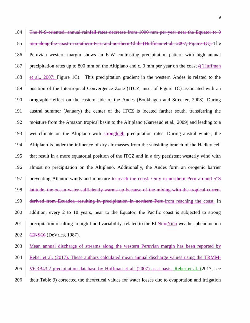
9

The N-S-oriented, annual rainfall rates decrease from 1000 mm per year near the Equator to 0 184

mm along the coast in southern Peru and northern Chile (Huffman et al., 2007; Figure 1C). The 185

Peruvian western margin shows an E-W contrasting precipitation pattern with high annual 186

precipitation rates up to 800 mm on the Altiplano and c. 0 mm per year on the coast (((Huffman 187

et al., 2007; Figure 1C). This precipitation gradient in the western Andes is related to the 188

position of the Intertropical Convergence Zone (ITCZ, inset of Figure 1C) associated with an 189

orographic effect on the eastern side of the Andes (Bookhagen and Strecker, 2008). During 190

austral summer (January) the center of the ITCZ is located farther south, transferring the 191

moisture from the Amazon tropical basin to the Altiplano (Garreaud et al., 2009) and leading to a 192

wet climate on the Altiplano with stronghigh precipitation rates. During austral winter, the 193

Altiplano is under the influence of dry air masses from the subsiding branch of the Hadley cell 194

that result in a more equatorial position of the ITCZ and in a dry persistent westerly wind with 195

almost no precipitation on the Altiplano. Additionally, the Andes form an orogenic barrier 196

preventing Atlantic winds and moisture to reach the coast. Only in northern Peru around 5°S 197

latitude, the ocean water sufficiently warms up because of the mixing with the tropical current 198

derived from Ecuador, resulting in precipitation in northern Peru.from reaching the coast. In 199

addition, every 2 to 10 years, near to the Equator, the Pacific coast is subjected to strong 200

precipitation resulting in high flood variability, related to the El NinoNiño weather phenomenon 201

(ENSO) (DeVries, 1987). 202

Mean annual discharge of streams along the western Peruvian margin has been reported by 203

Reber et al. (2017). These authors calculated mean annual discharge values using the TRMM-204

V6.3B43.2 precipitation database by Huffman et al. (2007) as a basis. Reber et al. (2017, see 205

their Table 3) corrected the theoretical values for water losses due to evaporation and irrigation 206

10

using the gauging record of a minimum of 12 basins situated close to the Pacific ocean. For these 207

areas hydrological data has been reported by the Sistema Nacional de Información de Recursos 208

Hídricos (SNIRH). The hydrological data thus cover a time span of c. 12 years. The results show 209

a pattern where mean annual ruonff of these streams ranges between c. 10-40 m3/s. Rivers where 210

mean annual runoff values are nearly 80 m3/s comprise the Rio Santa at c. 9°S latitude (Figure 211

1A), which derives its water from glaciers in the Cordillera Blanca. Two other streams with high 212

discharge values are situated at 16°-17°S (Rio Ocoña and Rio Camaña, Figure 1A) where the 213

corresponding headwaters spread over a relatively large area across the Altiplano, thereby 214

collecting more rain than the other basins. 215

216

2. SITE SELECTION AND METHODS 217

We selected river basins between 8°S and 18°S latitude situated on the western margin of the 218

Peruvian Andes, because of the presence of marked N-S contrasts in precipitation rates and the 219

presence of strong seismic activity due to the subduction of the Nazca plate (Table 1). Only the 220

main river basins were selected, which were generally larger than 700 km2. These basins have 221

recently been analyzed for 10

Be-based catchment averaged denudation rates and mean annual 222

water fluxes (Reber et al., in press). This allows us to explore whether sediment flux, which 223

equals the product between 10

Be-based denudation rates and basin size, has a measurable 224

impact on the grain size pattern. In addition, also for these streams, Reber et al. (in press) 225

presented data on mean annual water discharge using the records of gauging stations and the 226

TRMM-V6.3B43.2 precipitation dataset as basis (Huffman et al., 2007). We will use this 227

information to explore the controls of water shear stresses on the caliber of the bedload material 228

(see below). 229

11

Sampling sites wereare situated in the main river valleys in the western Cordillera between 8°S 230

and 18°S latitude just before it gives way to the coastal margin. Only the 21 main river basins 231

were selected, which were generally larger than 700 km2. We selected the downstream end of 232

these rivers because the grain size pattern at these sites is likely to record the ensemble of the 233

mainfor simplicity because this yields comparable conditions and forces controlling the supply of 234

material to the trunk stream farther upstream. We randomly selected c. five longitudinal bars 235

where we collected our grain size datasetas the base level is the same for all streams. Sampling 236

sites are all accessible along the Pan-American Highway (see Table 1 for the coordinates of the 237

sampling sites). Additionally, the Majes basin (marked with red color on Figure 1A), which is 238

part of the 21 studied basins,) has been sampled at five sites from upstream to downstream to 239

explore the effects related to the sediment transport processes for a section across the mountain 240

belt, but along the stream (Figure 23; Table 2). The Majes basin has been chosen because of its 241

easy accessibility in the upstream direction and because the morphology of this basin has been 242

analyzed in a previous study (Steffen et al., 2010). 243

We randomly selected five longitudinal bars where we collected our grain size dataset. It has 244

been shown that using a standard frame with fixed dimensions to assist gravel sampling reduces 245

user-biased selections of gravels (Marcus et al., 1995; Bunte and Abt, 2001a). In order to reduce 246

this bias, we substituted the frame by shooting an equal number of photos at a fixed distance (c. 1 247

m) from the ground surface at each longitudinal bar. Ten photos were taken from an 248

approximately 10 m2-large area to take potential spatial variabilities among the gravel bars into 249

account. From those photos, the intermediate b-axes and the ratio of the b-axes and the long a-250

axis of around 500 randomly chosen pebbles were manually measured (Bunte and Abt, 2001b) 251

and processed using the software program ImageJ (Rasband, 1997). Our sample population 252

12

exceeds the minimum number of samples needed for statistically reliable estimations of grain 253

size distributions in gravel bars (Howard, 1993; Rice and Church, 1998). 254

The pebbles were characterized on the basis of their median (D50), the D84 and the coarse (D96) 255

fractions. This means that 50%, 84% and 96% of the sampled fraction is finer grained than the 256

50th

, 84th

and 96th

percentilepercentiles of the samples. On a gravel bar, pebbles tend to lie with 257

their short axis perpendicular to the surface, thus exposing their section that contains the a- and 258

b-axes (Bunte and Abt, 2001b). However, the principal limitation is the inability to accurately 259

measure the fine particles < 3 mm (see also Whittaker et al., 2010). While we cannot resolve this 260

problem with the techniques available, we do not expect that this adds a substantial bias in the 261

grain size distributions reported here as their relative contributions to the point- count results are 262

minor (i.e. < 5%, based on visual inspection of the digital images). 263

Catchment-scale morphometric parameters and characteristics, including drainage area, mean 264

slope angle and for each catchment, slope angle of the stream channel at the sampling site (Table 265

1), and distances from the sample sites to the upper edge of the Western Escarpment were 266

extracted from the 90-m-resolution digital elevation model (DEM) Shuttle Radar Topography 267

Mission (SRTM; Reuter et al., 2007). The distances from the sample sites to the upper edge of 268

the Western Escarpment (Trauerstein et al., 2013) have been measured. 269

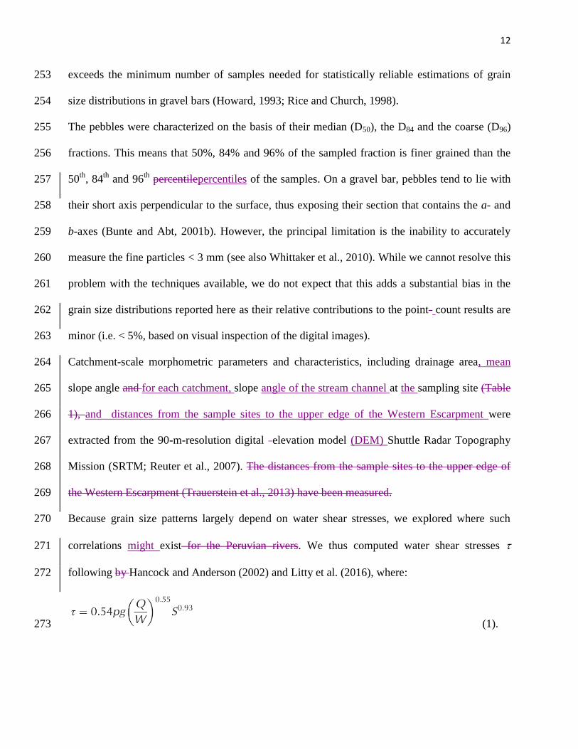
Because grain size patterns largely depend on water shear stresses, we explored where such 270

correlations might exist for the Peruvian rivers. We thus computed water shear stresses 271

following by Hancock and Anderson (2002) and Litty et al. (2016), where: 272

(1). 273

13

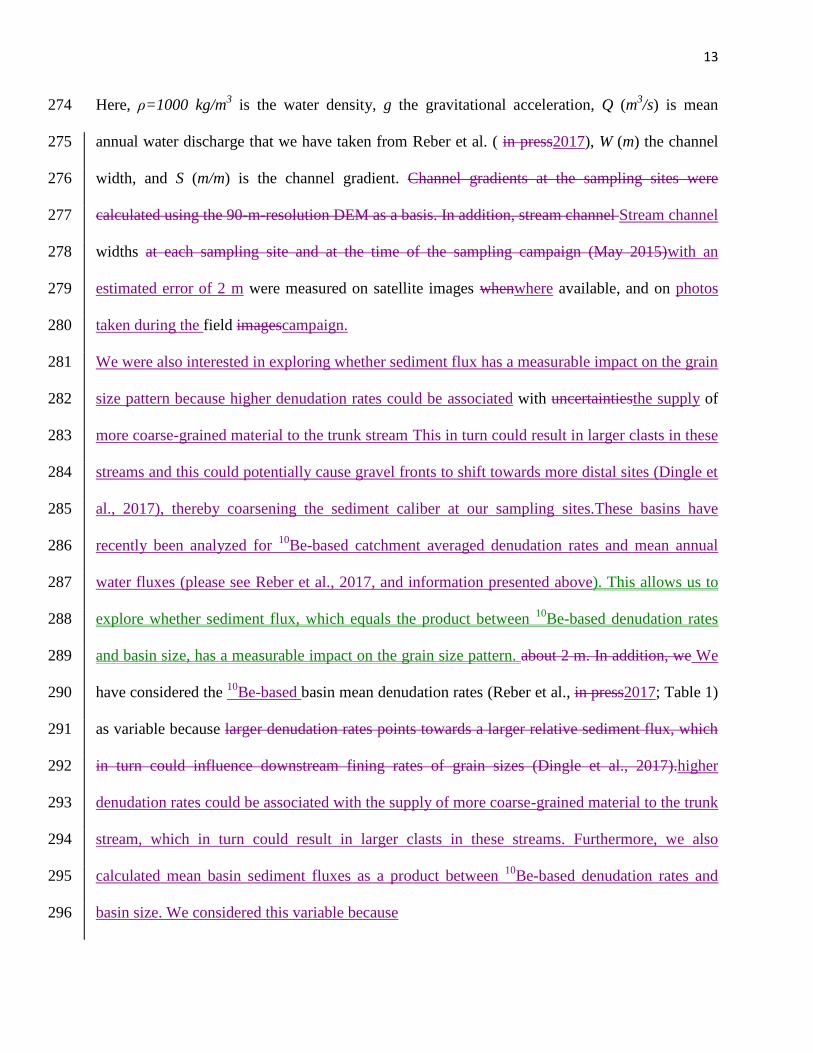
Here, ρ=1000 kg/m3 is the water density, g the gravitational acceleration, Q (m

3/s) is mean 274

annual water discharge that we have taken from Reber et al. ( in press2017), W (m) the channel 275

width, and S (m/m) is the channel gradient. Channel gradients at the sampling sites were 276

calculated using the 90-m-resolution DEM as a basis. In addition, stream channel Stream channel 277

widths at each sampling site and at the time of the sampling campaign (May 2015)with an 278

estimated error of 2 m were measured on satellite images whenwhere available, and on photos 279

taken during the field imagescampaign. 280

We were also interested in exploring whether sediment flux has a measurable impact on the grain 281

size pattern because higher denudation rates could be associated with uncertaintiesthe supply of 282

more coarse-grained material to the trunk stream This in turn could result in larger clasts in these 283

streams and this could potentially cause gravel fronts to shift towards more distal sites (Dingle et 284

al., 2017), thereby coarsening the sediment caliber at our sampling sites.These basins have 285

recently been analyzed for 10

Be-based catchment averaged denudation rates and mean annual 286

water fluxes (please see Reber et al., 2017, and information presented above). This allows us to 287

explore whether sediment flux, which equals the product between 10

Be-based denudation rates 288

and basin size, has a measurable impact on the grain size pattern. about 2 m. In addition, we We 289

have considered the 10

Be-based basin mean denudation rates (Reber et al., in press2017; Table 1) 290

as variable because larger denudation rates points towards a larger relative sediment flux, which 291

in turn could influence downstream fining rates of grain sizes (Dingle et al., 2017).higher 292

denudation rates could be associated with the supply of more coarse-grained material to the trunk 293

stream, which in turn could result in larger clasts in these streams. Furthermore, we also 294

calculated mean basin sediment fluxes as a product between 10

Be-based denudation rates and 295

basin size. We considered this variable because 296

14

Possible covariations and correlations between grain size and/or morphometric parameters and 297

basin characteristics were evaluated using Pearson correlation coefficients;, thus providing 298

corresponding r-values (Table 3) and p-values with a significance level alpha < 0.1 (Table 4). 299

The r-values measure the linear correlations between variables. The values range between +1 and 300

−1, where +1 reflects a 100% positive linear correlation, 0 reflects no linear correlation, and −1 301

indicates a 100% negative linear correlation (Pearson, 1895). Threshold values of > + 0.30 and < 302

- 0.30 were selected to assign positive and negative correlations, respectively. 303

304

3. RESULTS 305

3.1 Grain size 306

The results of the grain size measurements reveal a large variation for the b-axis where the 307

values of the D50 range from 1.3 cm to 5.5 cm for rivers along the entire western Peruvian 308

margin (Figure 3h2h; Table 1). Likewise, D84 values vary between 3 cm and 10.5 cm. The sizes 309

for the D96 reveal the largest spread, ranging from 6 cm to 31 cm. In addition, theThe ratio 310

between the lengths of the b-axis and a-axis (sphericity ratio) is nearly constant and varies 311

between 0.67 and 0.74 (Figure 3i2i). Note that between 15.6°S and 13.7°S, no gravel bars are 312

encountered in the rivers where they leave the mountain range, and only sand bars can be found. 313

Therefore no results are exhibited for these latitudes (Figure 3h2h and 3i2i). 314

315

3.2 The Majes basin 316

The D50 percentile of the b-axis decreases from 6.2 cm at 106 km river upstream to a value of 5.2 317

cm at 20 km upstream for the Pacific coastc. 80 km farther downstream (Figures 23 and 4 and 318

Table 2). Likewise, the D84 decreases from 19 cm to 8.7 cm, and the D96 decreases from 31 cm to 319

15

11.6 cm (Figure 4). Geomorphologists widely accept the notion that the downstream hydraulic 320

geometry of alluvial channels reflects the decrease of particle size within an equilibrated system 321

involving stream flow, channel gradient, sediment supply and transport (e.g. Hoey and Ferguson, 322

1994; Fedele and Paola, 2007; Attal and Lavé, 2009). Sternberg (1875) formalized these 323

relations and predicted an exponential decline in particle size in gravel -bed rivers as a 324

consequence of abrasion and selective transport where the gravel is transported downstream. The 325

relation follows the form: Dx = D0 e –αx (Sternberg, 1875). Here, the exponent α decreases from 326

0.3 for the largest percentile (i.e., the D96) to c. 0.1 for the D50 (Figure 4). 327

328

3.3 Correlations between grain sizes and morphometric properties 329

Table 3 shows the Pearson correlation coefficients (r-value) between the grain sizes, the 330

morphometric parameters and the characteristics of the basins. As was expected, the D50, D84 and 331

D96 all strongly correlate with each other (0.73 < r-value < 0.93), but the b/a ratios do not 332

correlate with any of the 3three percentiles (-0.1 < r-value < 0.1). Likewise, inter-correlation 333

relationships also exist among other variables such as catchment area, distance from the western 334

escarpment, sediment flux and water discharge (Table 3). The D50 values positively (but weakly) 335

correlate with the sizes of the catchment area (r-value = 0.31), the distances from the Western 336

Escarpment (r-value = 0.35), the mean annual shear stress at the sampling site (r-value = 0.23), 337

the denudation rates (r-value = 0.34) and the sediment fluxes (r-value = 0.42; Figure 5A).The 338

sediment fluxes show the highest significance level; p-value = 0.05 (Table 4). 3). The D84 and 339

the D96 values correlate positively with the mean annual shear stress exerted by the water on an 340

mean annual basisflux with a r-value =of 0.33 and 0.39 (Table 3). However, we note that these 341

16

correlations are weak, and p-value = 0.14some might break apart if the largest values for e.g. 342

shear stresses (Table 3) are removed. 343

At a broader scale, values of the D50 are nearly constant between 2 and 0.08 respectively (Figure 344

5B3 cm (Table 3). The largest D50 with values of up to 6 cm are encountered in streams that are 345

either sourced in the Cordillera Negra where mean basin slope angles are larger than 20°, or in 346

the Rio Ocoña and C).Rio Camaña rivers located at 16°-17°S, which have the largest mean 347

annual discharge as they capture their waters from a broad area on the Altiplano. 348

The ratio of the intermediate axis over the long axis negatively correlates with the distance from 349

the Western Escarpment (r-value = -0.33), albeit with a poor correlation, but a strong and 350

positive correlation is found with the mean slope angles of the basins (r-value = 0.63; p-value = 351

0.01; Figure 5DTable 3). 352

353

4. DISCUSSION 354

4.1 355

4.1 SLOPE ANGLE CONTROLS ON SPHERICITY 356

The poor negative correlation of -0.33 between the sphericity of the pebbles and distance from 357

the escarpment edge (Table 3) prevents us from inferring a distinct control of this variable. On 358

the other hand, the positive Pearson correlation of 0.63 between the sphericity of the pebbles and 359

the mean basin slope is quite high (Table 3), thus pointing towards a significant control. This 360

suggests that basins with steeper slopes produce rounder pebbles. We do not consider that this 361

pattern is due to differences in exposed bedrock in the hinterland because the litho-tectonic 362

architecture is fairly constant along the entire Peruvian margin (Figure 1). We tentatively infer 363

that time scales of transport and evacuation of material are likely to be shorter in steeper basins 364

17

compared to shallower ones. This might influence the shape of pebbles as they tend to flatten as 365

effects of abrasion and 3D heterogeneities of bedrock that becomes more obvious with time and 366

transport distance (Sneed and Folk, 1958). We thus see the positive correlation between mean 367

hillslope angle and the sphericity of pebbles as a very likely consequence of shorter transport 368

times in steeper basins, but we note that this hypothesis needs to be confirmed by detailed real-369

time surveys of material transport from sources down to the end of these rivers. 370

371

4.2 CONTROLS ON GRAIN SIZE 372

Downstream fining trends in the Majes basin indicate fluvial controls 373

In fluvial environments, the sorting of the sediment depends on the downstream distance from its 374

source (Hoey and Ferguson, 1994; Kodoma, 1994; Paola and Seal, 1995). This is particularly the 375

case for the Majes river, where the sorting gets better in the downstream direction. In particular, 376

we do see an exponential, downstream fining trend of the three percentiles in the Majes river 377

(Figure 4). This is somewhat surprising because sufficiently voluminous sediment input from 378

other sources may perturb any downstream fining trends in the grain size distribution (Rice and 379

Church, 1998). Likewise, in the Majes basin, the sediment supply from the hillslopes to the trunk 380

stream has occurred mainly through debris flow processes and landsliding (Steffen et al., 2010; 381

Margirier et al., 2015). AccordinglySo, while the supply of hillslope-dervied material is likely to 382

have been accomplished by mass wasting processes, the evacuation and transport of this 383

sediment down to the Pacific Ocean has predominantly occurred mainly through fluvial 384

transport, as the exponential downstream fining of the grains implies. . 385

386

Absence of gravels in rivers between 15.6°S and 13.7 °S 387

18

In the rivers located between 15.6°S and 13.7°S, no gravel bars are encountered where these 388

rives leave the mountain range, and only sand bars can be found. This suggests that the transition 389

from a gravel- to a sand-covered bed, i.e. the gravel front, is located along a more upstream reach 390

of these rivers. This transition is generally rapid (Dingle et al., 2017) and often associated with a 391

break in slope (Knighton, 1999). The gravel-sand transition has been interpreted to be controlled 392

by either the elevation of the local base level, an excess of sand supply, and breakdown of fine 393

gravels by abrasion (Dingle et al., 2017), or a combination of these parameters (Knighton, 1999). 394

In our case, these rivers do not show any particular differences compared to the other rivers 395

where coastal gravel bars have been found. In particular, there is no particular evidence why 396

preferential breakdown of gravels along these rivers should be more efficient than in rivers 397

farther north and south because the upstream morphometry and bedrock geology is similar. The 398

other explanation would be an excess of sand supplied to these rivers. However, available 399

information and geological maps do not display any major differences in bedrock lithologies 400

along strike (Figure 1B), but we note that the resolution of the geological map does not provide 401

enough detail about the weathering of the bedrock or the amount of regolith, which could be a 402

source of sand. However, these rivers are situated in the segment where the buoyant Nazca Ridge 403

is being subducted beneath the South American continental plate (Figure 3), which resulted in an 404

uplift pulse of the forearc during Pliocene-Quaternary times, accompanied by enhanced erosion 405

on the surface and at interface between the subducting and the hangingwall plate through 406

tectonic shear (Hampel, 2002; Hampel et al., 2004). These effects are generally recorded in the 407

morphology and sedimentary facies of the forearc (Hampel, 2002). Additionally, based on a 408

detailed morphometric analysis of the region, Wipf et al. (2008) showed that this coastal uplift 409

has rerouted and deflected the rivers in this area and has lengthened the downstream end of these 410

19

rivers. It is thus possible that these tectonically-driven mechanisms caused the gravel front to 411

step back farther into the mountain range, with the effect that the downstream terminations of 412

these rivers only display sand bars. But we note that this interpretation warrants further detailed 413

investigations, which includes a down-stream survey of the sediments in these rivers from the 414

headwaters to the site where they discharge into the Pacific Ocean (similar to the analyses made 415

along the Majes river, please see above). 416

417

Grain size and earthquake frequencyimpact 418

Landslides and debris flows represent the main processes of hillslope erosion and the main 419

source of sediment in tectonically active orogens (Hovius et al., 1997; Korup et al., 2011). They 420

are generally associated with triggers such as earthquakes or intense rainfall and generally supply 421

coarse and voluminous sediments to the trunk rivers (Dadson et al., 2003; McPhillips et al., 422

2014). In that sense, we would inferexpect a positive correlation between the frequency of large 423

earthquakes and the grain size where an increase ofin earthquake frequency would induce an 424

increase ofin landslide occurrence, thereby supplying coarser grained sediment from the 425

hillslopes to the rivers. These relationships have been elaborated in multiples studies where 426

positive relationships between landslide occurrence and the size of earthquakes have been 427

documented (e.g., Keefer, 1984; 1994; Parker et al., 2011). However, noWe note here that a 428

global-scale correlation has been found between the seismicity and the grain size data when 429

looking atbetween earthquake magnitudes and areas affected by landslides suggests that mass 430

movements are triggered by earthquakes if a threshold magnitude of 5.5 is exceeded (Keefer, 431

1984). Here, we consider earthquakes with magnitudes >4.5 because Figure 1 by Keefer (1984) 432

suggests that earthquakes with magnitudes as low as 4.5 are theoretically able to release 433

20

landslides over an area larger than 10 km2, which is already a large area. However, we do not see 434

correlation between the number of recorded historical earthquakes larger than 4.5 Mw and the 435

grain size data (Figure 32c). We then infer that seismic activity and particularlyexpect that the 436

frequency of earthquakes larger than 4.5 Mw, and related to this, the subduction mechanisms, do 437

not exert a measurable control on the grain size in the rivers of the western Peruvian Andes. 438

Nevertheless, we do consider that the lack of gravels in rivers where the subduction of the 439

buoyant Nazca ridge has caused uplift of the hangingwall plate was explained by a tectonic 440

driving force (see section above). In particular, since this uplift caused a re-routing of these 441

rivers (Wipf et al., 2006) and thus a lengthening of the river courses, the gravel front might have 442

stepped back relative to the river mouth into the Pacific Ocean, as we have noted above. 443

444

Supply controlPossible threshold limits as controls on the grain size pattern 445

Because we have found positive correlations between the D50 and the basins scale properties 446

(basin area, mean basin slope, mean basin denudation rates, water shear stresses, sediment 447

fluxes), we infer that the mean grain size reflects the ensemble of a complex pattern of erosional 448

and sediment transport processes operating in the Peruvian basins. In particular, the positive 449

correlation between the size of the D50, the basin averaged denudation rate and the morphometry 450

of these basins leads us to propose that environmental factors exert a major control on the pattern 451

of the D50 encountered for the rivers in western Peru. In this context, it is very likely that the bulk 452

supply of hillslope-derived sediment to the trunk stream increases with larger basin size, mean 453

basin slope and basin-averaged denudation rate, as the recent study by Reber et al. (in press) has 454

revealed. Furthermore, while tectonic processes such as earthquake frequencies have no 455

measurable impact on the grain size pattern, as we have outlined above, we consider it more 456

21

likely that hillslope processes occurred in response to strong precipitation events, as suggested 457

Bekaddour et al. (2014) and as recently shown by the devastating mudflows and floods in coastal 458

Peru (March 2017) due to an El Niño event. The consequence is that higher denudation rates, and 459

larger basins, result in a larger sediment flux in the trunk stream, which in turn yields an increase 460

in the scale at which transport and deposition of material occurs (Armitage et al., 2011). Related 461

mechanisms are likely to shift gravel fronts in rivers towards more distal sites, which could 462

positively influence the mean grain size percentile of the trunk rivers in the sense that the 463

material will coarsen. 464

We note that following the results from the Majes basin, we would expect a decrease in the size 465

of the D50 for larger basins and larger distances from the uppermost edge of the Western 466

Escarpment, because of larger transport distances and thus a higher impact related to any 467

downstream fining trends. While these mechanisms, i.e, fining trends of all percentiles, are likely 468

to be observed at the scale of individual basins, we do not consider that transport distance alone 469

is capable of explaining the D50 pattern in rivers at the scale of the entire western Andean margin 470

of Peru. In particular, the fining rate not only depends on the abrasion (Dingle et al., 2017) and 471

the selective entrainment processes upon transport (Ashword and Ferguson, 1989), but also on 472

the rate at which sediment is supplied to the rivers (e.g. McLaren, 1981; McLaren and Bowles, 473

1985). Particularly, in basins where the rate of hillslope-derived supply of sediment from the 474

hillslopes to the trunk stream is large, the overall downstream fining rate of the material is 475

expected to be less, because lateral sediment pulses are likely to cause the grain size fraction to 476

increase. This has been exemplified for modern examples in the Swiss Alps (Bekaddour et al., 477

2013) and for the Pisco river in Peru (Litty et al., 2016), where fining rates of modern stream 478

sediment, which record low denudation rates (Bekaddour et al., 2014), are greater than those of 479

22

Pleistocene fluvial terraces, which record fast paleo-denudation rates (Bekaddour et al., 2014). 480

Support for this interpretation is also provided by the positive correlation between the D50 and 481

the mean basin denudation rate, where larger hillslope-derived material is likely to increase the 482

overall sediment flux within the rivers. The consequence is a downstream shift of the gravel front 483

and thus of the larger size fraction of the material, as we have interpreted above. 484

485

Hydrological control on the grain size distribution 486

Hydrodynamic conditions of rivers influence the grain size upon entrainment, transport, and 487

deposition (Hjulström, 1935; Komar and Miller 1973; Surian, 2002). In this sense, rivers with 488

larger shear stresses are capable of transporting larger clasts. Accordingly, at equilibrium 489

conditions, we expect a correlation between the grain-size distributions and the shear stresses 490

exerted by the water at our surveying sites, because greater flow strengths are required to entrain 491

the coarser fractions of the material that make up the river beds (e.g., Ferguson et al. 1989; 492

Komar and Shih 1992). This is the case in our study where the grain sizes correlate with the 493

shear stress values. Interestingly, the correlation coefficients between the shear stress and the 494

grain size percentiles increase from 0.23 for the D50 to 0.33 for the D84 and to 0.39 for the D96. 495

This suggests that the shear stress exerted by mean annual water flows has a greater impact on 496

the coarse fractions than on the fine fractions of the stream sediments. While we cannot fully 497

explain why the larger percentiles reveal a better correlation with shear stresses of mean annual 498

flow conditions with the available dataset, we do infer a hydraulic control on grain size 499

distribution of the Peruvian rivers. 500

501

4.2 TRANSPORT DISTANCE AND SLOPE ANGLE CONTROLS ON SPHERICITY 502

23

We consider a control of the transport distance on the sphericity of the pebbles. We indeed see a 503

negative correlation between the sphericity and the distance from the Western Escarpment where 504

the major sediment sources are situated, as provenance tracing investigations have shown (Litty 505

et al., 2017). This suggests a decrease of the sphericity with a larger transport distance. As 506

particles are transported over longer distances, we actually would expect abrasion (Dingle et al., 507

2017) to equalize the length of the three axes, thus making a particle more spherical. While this 508

concept is likely to be valid for pebbles with a homogenous fabric, it likely fails to describe the 509

abrasion and break-down of material with an inherited planar geologic fabric (such as gneisses 510

and sediments). Indeed, pebbles flatten as effects of abrasion and 3D heterogeneities of bedrock 511

that becomes more obvious with time and transport distance (Sneed and Folk, 1958). We note 512

that this is only valid if we assume a linear correlation between river length and transport time. 513

The reincorporation of previously abraded gravels from earlier erosion and multiple transport 514

cycles of clasts that were temporarily stored in cut-and-fill terrace sequences, as e.g., put forward 515

by Bekaddour et al. (2014) in their study about cut-and-fill terraces in the Pisco valley at c. 516

13.7°S latitude, would positively contribute to this effect upon increasing the time scale of 517

sediment evacuation. 518

Additionally, we consider a control of the mean catchment slope on the sphericity of the pebbles, 519

where correlations are positive, i.e. the steeper a basin the rounder the pebbles (Figure 5). We do 520

not consider that this pattern is due to differences in exposed bedrock in the hinterland because 521

the litho-tectonic architecture is fairly constant along the entire Peruvian margin (Figure 1). 522

Instead, the observations point toward the same control mechanisms on the pebble sphericity as 523

noted above. Steeper slope angles are most likely associated with faster denudation rates as the 524

Peruvian study by Reber et al. (in press) has shown. Accordingly, we infer a shorter transport 525

24

distance of the material and thus a shorter time scale of transport compared to the evacuation 526

time in long and less steep rivers. Similar to what we have noted above, we see the positive 527

correlation between mean hillslope angle and the sphericity of pebbles as a very likely 528

consequence of shorter transport times in steeper basins, but we note that this hypothesis needs to 529

be confirmed by detailed real-time surveys of material transport from sources down to the end of 530

these rivers. 531

We consider the correlations between the grain size data and the basins scale properties (basin 532

area, mean basin denudation rates, water shear stresses, sediment fluxes) as weak and 533

unconvincing (Table 3). However, we recall that the D50 records a nearly uniform pattern with 534

values that range between 2-3 cm along the studied western Peruvian margin. However, higher 535

values of up to 6 cm are either measured in streams where mean slope angles of the bordering 536

hillslopes in the upstream basin exceed 20° (between 11° and 12°S) or where water runoff values 537

are nearly twice as large as the mean of all Peruvian streams (ranging between 10-40 m3/s 538

between 16° and 17°S; see Figure 3 and Table 3). Based on these observations, we tentatively 539

interpret a supply control on the median grain size for the Cordillera Negra streams where slopes 540

are mediating grain size through a threshold effect. In this case, these thresholds on the hillslopes 541

are likely to be conditioned by the at-yield mechanical states of bedrock (Montgomery, 2001; 542

Ouimet et al., 2009), where hillslopes with dip angles up to 20-25° can be sustained. Under these 543

conditions, mass failure processes are likely to dominate the supply of material to the trunk 544

stream, thereby increasing the caliber of the supplied material and causing the bedload material 545

to coarsen. In the same sense, a threshold response to steeper slopes has been interpreted for the 546

pattern of 10

Be-based denudation rates in the Andes (Reber et al., 2017) and in the Himalayas 547

(Ouimet et al., 2009). In both cases, the relationships between denudation rates and mean basin 548

25

slopes was considered to follow a non-linear diffusive mass transport model where denudation 549

rates are proportional to mean basin slopes for low gradients, while these relationships become 550

non-linear for slopes approaching a critical value. Reber et al. (2017) set this critical value to 551

27.5°, but the linear relationship of their dataset breaks apart for gradients larger than 0.4, which 552

corresponds to an angle of c. 21°. At these conditions, hillslopes approach a threshold where 553

slope angles are limited by the mechanical strength of bedrock (Montgomery, 2001; Schlunegger 554

et al., 2013). Hillslope erosion is then mainly accomplished through mass failure processes, 555

which in turn, is likely to supply more coarse-grained material to the trunk stream (see above), as 556

modern examples have shown (Bekaddour et al., 2013). We note, however, that a confirmation 557

of this hypothesis requires data about the spatial density and frequency of landslide occurrence 558

along the western Peruvian Andes. This dataset, however, is not available yet, and its 559

establishment warrants further investigations. 560

In basins situated between 16°-17°S, mean basin slopes are clearly below threshold conditions, 561

but the D50 is twice as large as in neighboring rivers. Interestingly, these streams have mean 562

annual discharge values that are twice as large as the western Peruvian streams on the average. 563

Similar to the Cordillera Negra, we relate the relationships at 16°-17°S to threshold controls. In 564

this case, however, they are likely to be conditioned by transport. The mechanisms by which 565

grain size can be mediated through a threshold effect upon transport are less well understood, but 566

it has been known at least since the engineering work by Shields (1936), and particularly by 567

Peter Meyer Müller (1948) that threshold conditions have to be exceeded and have a control on 568

transport of grains in fluvial streams. As a consequence, at transport-limited conditions, sediment 569

flux, and most likely also the caliber of the transported material, depends on the frequency and 570

the magnitudes at which these thresholds are exceeded rather than on a mean value of water 571

26

discharge (Dadson et al., 2003). This might be the reason why values of water shear stresses, that 572

are calculated based on the annual mean of water flux, are not sufficiently strongly correlated 573

with the D50 values to invoke a strong controls thereof (Table 3). However, the lack of 574

information about discharge patterns prevents us from calculating the magnitude-frequency 575

distribution of runoff. Nevertheless, we consider the occurrence of larger peak floods for streams 576

that capture a large portion of their waters on the Altiplano Plateau. This might indeed be the 577

case for the Rio Ocoña and Rio Camaña. We thus tentatively assign large peak floods for these 578

streams, which might explain the larger D50 values encountered in their gravel bars. Although 579

highly speculative, we support our statement by the highly seasonal character of preciptation 580

occurrence particularly on the eastern Andean margin and the Altiplano Plateau, which is largely 581

conditioned by the monsoonal Andean jet (see above). We note, however, that this statement 582

warrants a high resolution hydrological dataset for the western Peruvian sreams, which is not 583

available. 584

An exception from these relationships is presented by the Rio Santa (Figure 1A) where mean 585

annual water discharge reaches a value of almost 80 m3/s, but where the size of the D50 is low. 586

We relate this to the possible supply-limited state of this stream, conditioned by the orogen-587

parallel valley of the Rio Santa between the Cordillera Blanca and the Cordillera Negra, which 588

has acted as a subsiding graben since the past 5.4 Ma (Giovanni et al., 2010; Margirier et al., 589

2015) and which might thus have operated as a sediment trap. This interpretation is also 590

consistent with the low 10

Be-based catchment averaged denudation rates measured for the Rio 591

Santa basin, as noted by Reber et al. (2017). 592

Note that our inferences are largely based on the pattern of the D50, and that the consideration of 593

the larger percentiles might add alternative views on our interpretations. However, since all 594

27

percentiles are inter-correlated, as the pattern of the Pearson correlation coefficients suggests 595

(Table 3), we think that our general conclusions about the occurrence of thresholds upon the 596

supply and transport of sediment will not change. Note also that either transport or supply control 597

and related thresholds were identified by Reber et al. (2017) for their explanation of the 10Be-598

based datasets on basin-averaged denudation rates on the western Peruvian Andes. We 599

tentatively interpret that the grain size pattern of the Peruvian streams follows these lines. 600

601

Conclusion 602

We have conductedpresent a complete dataset about grain size analysis of gravel bars insizes for 603

all major rivers that are situated on the western Andean margin of Peru where they leave the 604

mountain belt.. We havedid not foundfind any correlations to the current seismic regimes, where 605

a larger seismicityoccurrence of earthquakes with magnitudes larger than 4.5 Mw is expected to 606

increase the supply of coarse-grained material. InsteadHowever, we found positive 607

correlationsthat the values for the D50 are nearly constant and range between water shears 608

stresses, 2 and 3 cm. Exceptionally larger D50 values of 4-6 cm were measured for basins situated 609

between 11-12°S and 16-17°S where hillslope gradients are steeper than average (i.e., 20-22°), 610

and where mean basin denudation rates,annual stream flows exceed the average values of the 611

western Peruvian streams (10-40 m3/s) by a factor of 2. We suggest that the generally uniform 612

grain size pattern has been perturbed where either mean basin slopes and basin sizes on nearly all 613

grain size percentiles. We interpret these results as the combined effect of various geomorphic, 614

or water fluxes exceed threshold conditions where larger denudation rates operating in larger 615

basins, and steeper slopes, paired with larger flow shear stresses, are capable of transporting 616

more and coarser-grained material. Furthermore, we unravel a upon the supply and the transport 617

28

time control on the shape of the clasts where steeper slopes and smaller basins (i.e., shorter 618

distances to the edge of the Western Escarpment) are anticipated to shorten the residence timeof 619

material. This might have implications for our understanding of the clasts in the system, thereby 620

yielding more spherical clasts. In particular, longer residence times would allow abrasion to be 621

more selective because of a planar lithologic fabric of most of the clasts, which in turn, would 622

cause clasts to flatten upon longer exposure towards abrasion. This suggest that the ensemble of 623

erosional and sediment transport processes have reached an equilibrium at the scale of individual 624

clasts, but also at the reach scale of rivers where the sedimentary architecture and the clast fabric 625

of the channel fill has dynamically adjusted to water and sediment flux and their specific time 626

scales. Accordingly, we see the western Peruvian margin as ideal laboratory to analyze the 627

relationships between sediment supply and water runoffcontrols on the grain size pattern of the 628

bedload, and we propose that the bedload caliber of these streams has reached an equilibrium to 629

environmental conditions including water discharge, sediment flux and channel 630

geometriesdistribution of gravelly-based streams. 631

632

ACKNOWLEDGMENTS 633

This project is funded by the Swiss National Science Foundation (project Number 137516). 634

635

REFERENCES CITED 636

Abbühl, L.M., Norton, K.P., Jansen, J.D., Schlunegger, F., Aldahan, A., and Possnert, G., 2011, 637

Erosion rates and mechanisms of knickzone retreat inferred from 10Be measured across 638

strong climate gradients on the northern and central Andes Western Escarpment: Earth 639

Surface Processes and Landforms, v. 36, p. 1464–1473. 640

29

Allen, G. H., Barnes, J. B., Pavelsky, T. M. and Kirby, E., 2013, Lithologic and tectonic controls 641

on bedrock channel form at the northwest Himalayan front: Journal of Geophysical 642

Research: Earth Surface, v. 118, no. 3, p. 1806-1825. 643

Allen, P.A., Armitage, J.J., Whittaker, A.C., Michael, N.A., Roda-Boluda, D. and D’Arcy, M., 644

2015, Fragmentation model of the grain size mix of sediment supplied to basins: The 645

Journal of Geology, v. 123, p. 405-427. 646

Allen, P. A., Michael, N. A., D’Arcy, M., Roda‐Boluda, D. C., Whittaker, A. C., Duller, R. A., 647

and Armitage, J. J., 2016. Fractionation of grain size in terrestrial sediment routing 648

systems. Basin Research. v. 29(2), p. 180-202 649

Armitage, J. J., Duller, R. A., Whittaker, A. C., and Allen, P. A., 2011. Transformation of 650

tectonic and climatic signals from source to sedimentary archive. Nature Geoscience, 651

4(4), 231-235. 652

Ashworth, P. J. and Ferguson, R. I., 1989. Size‐selective entrainment of bed load in gravel bed 653

streams. Water Resources Research, v. 25(4), p. 627-634. 654

Atherton, M. P., 1984. The coastal batholith of Peru. In Andean Magmatism (pp. 168-179). 655

Birkhäuser Boston. 656

Attal, M. and Lavé, J., 2006, Changes of bedload characteristics along the Marsyandi River 657

(central Nepal): Implications for understanding hillslope sediment supply, sediment load 658

evolution along fluvial networks, and denudation in active orogenic belts: Geological 659

Society of America Special Papers, v. 398, p.143-171. 660

Attal, M. and Lavé, J., 2009. Pebble abrasion during fluvial transport: experimental results and 661

implications for the evolution of the sediment load along rivers. J. Geophys. Res. 662

114:F04023. doi:10.1029/2009JF001328. 663

Attal, M., Mudd, S. M., Hurst, M. D., Weinman, B., Yoo, K. and Naylor, M., 2015, Impact of 664

change in erosion rate and landscape steepness on hillslope and fluvial sediments grain 665

size in the Feather River basin (Sierra Nevada, California): Earth Surface Dynamics, v. 3, 666

p. 201-222. 667

Bekaddour, T., Schlunegger, F., Attal, M. and Norton, K. P., 2013. Lateral sediment sources and 668

knickzones as controls on spatio‐temporal variations of sediment transport in an Alpine 669

river. Sedimentology, v. 60(1), p. 342-357. 670

30

Bekaddour, T., Schlunegger, F., Vogel, H., Delunel, R., Norton, K. P., Akçar, N., and Kubik, P., 671

2014. Paleo erosion rates and climate shifts recorded by Quaternary cut-and-fill 672

sequences in the Pisco valley, central Peru. Earth and planetary science letters, v. 390, p. 673

103-115. 674

Blissenbach, E., 1952. Relation of surface angle distribution to particle size distribution on 675

alluvial fans: J. Sediment. Petrol., v. 22, p. 25–28. 676

Bookhagen, B. and Strecker, M. R., 2008, Orographic barriers, high-resolution TRMM rainfall, 677

and relief variations along the eastern Andes, Geophysical Research Letters, v. 35, p. 678

L06403. 679

Bourgois, J., Bigot‐Cormier, F., Bourles, D., Braucher, R., Dauteuil, O., Witt, C., & Michaud, F., 680

2007. Tectonic record of strain buildup and abrupt coseismic stress release across the 681

northwestern Peru coastal plain, shelf, and continental slope during the past 200 kyr. 682

Journal of Geophysical Research: Solid Earth, 112(B4). 683

Bunte, K., Abt, S.R., 2001a. Sampling frame for improving pebble count accuracy in coarse 684

gravel-bed rivers. Journal of the American Water Resources Association, v. 37 (4), p. 685

1001- 1014. 686

Bunte, K., Abt, S.R., 2001b. Sampling surface and subsurface particle-size distributions in 687

wadable gravel- and cobble-bed rivers for analyses in sediment transport, hydraulics, 688

and streambed monitoring. General Technical Report RMRS-GTR-74. United States 689

Department of Agriculture; Forest Service; Rocky Mountain Research Station. Fort 690

Collings, USA, p. 428. 691

Carretier, S., Tolorza, V., Rodríguez, M. P., Pepin, E., Aguilar, G., Regard, V. and Hérail, G., 692

2015. Erosion in the Chilean Andes between 27° S and 39° S: tectonic, climatic and 693

geomorphic control. Geological Society, London, Special Publications, v. 399(1), p. 401-694

418. 695

Dadson, S. J., Hovius, N., Chen, H., Dade, W. B., Hsieh, M. L., Willett, S. D. and Lague, D., 696

2003. Links between erosion, runoff variability and seismicity in the Taiwan orogen. 697

Nature, v. 426(6967), p. 648-651. 698

D'arcy, M., Whittaker, A. C., and Roda‐Boluda, D. C., 2017. Measuring alluvial fan sensitivity 699

to past climate changes using a self‐similarity approach to grain‐size fining, Death 700

Valley, California. Sedimentology, v. 64(2), p. 388-424. 701

31

DeVries, T. J., 1987, A review of geological evidence for ancient El Nino activity in Peru. J. 702

Geophys. Res, v. 92, no. 14, p. 471–14. 703

Dingle, E. H., Attal, M., and Sinclair, H. D., 2017. Abrasion-set limits on Himalayan gravel flux. 704

Nature, v. 544(7651), p. 471-474. 705

Duller, R. A., Whittaker, A. C., Swinehart, J. B., Armitage, J. J., Sinclair, H. D., Bair, A. and 706

Allen, P. A., 2012, Abrupt landscape change post-6 Ma on the central Great Plains, 707

USA: Geology, v. 40, p. 871-874. 708

Fedele, J. J. and Paola C., 2007, Similarity solutions for fluvial sediment fining by selective 709

deposition: Journal of Geophysical Research: Earth Surface (2003–2012), v. 112. 710

Ferguson, R. I., Prestegaard, K. L. and Ashworth, P. J., 1989. Influence of sand on hydraulics 711

and gravel transport in a braided gravel bed river. Water Resources Research, v. 25(4), p. 712

635-643. 713

Foreman, B. Z., Heller, P. L. and Clementz, M. T., 2012, Fluvial response to abrupt global 714

warming at the Palaeocene/Eocene boundary: Nature, v. 491, no. 7422, p. 92-95 715

Foreman, B. Z., 2014, Climate‐driven generation of a fluvial sheet sand body at the Paleocene–716

Eocene boundary in north‐west Wyoming (USA): Basin Research, v. 26, no. 2, p. 225-717

241. 718

Garreaud, R. D., Vuille, M., Compagnucci, R., and Marengo, J., 2009, Present-day South 719

American climate. Palaeogeography, Palaeoclimatology, Palaeoecology, v. 281, no. 3, p. 720

180-195. 721

Haederle, M. and Atherton, M. P., 2002. Shape and intrusion style of the Coastal Batholith, Peru. 722

Tectonophysics, v. 345(1), p. 17-28. 723

Hampel, A., 2002. The migration history of the Nazca Ridge along the Peruvian active margin: a 724

re-evaluation. Earth and Planetary Science Letters, v. 203(2), p.665-679. 725

Hampel, A., Adam, J., and Kukowski, N., 2004. Response of the tectonically erosive south 726

Peruvian forearc to subduction of the Nazca Ridge: Analysis of three‐dimensional 727

analogue experiments. Tectonics, 23(5). 728

Hancock, G. S. and Anderson, R. S., 2002. Numerical modeling of fluvial strath-terrace 729

formation in response to oscillating climate. Geological Society of America Bulletin, v. 730

114(9), p. 1131-1142. 731

32

Heller, P. L. and Paola, C., 1992, The large-scale dynamics of grain-size variation in alluvial 732

basins, 2: Application to syntectonic conglomerate: Basin Research, v. 4, no. 2, p. 91-733

102. 734

Hjulström, F., 1935, Studies in the morphological activity of rivers as illustrated by the river 735

Fyris: Bulletin of the Geological Institution of the University of Uppsala, v 25, p. 221-736

528. 737

Hoey, T. B. and Ferguson, R., 1994, Numerical simulation of downstream fining by selective 738

transport in gravel bed rivers: Model development and illustration: Water resources 739

research, v.30, p. 2251-2260. 740

Hovius, N., Stark, C. P. and Allen, P. A., 1997. Sediment flux from a mountain belt derived by 741

landslide mapping. Geology, v. 25(3), p. 231-234. 742

Howard, J.L., 1993. The statistics of counting clasts in rudites: a review with examples from the 743

upper Paleogene of southern California, USA. Sedimentology 40, 157-174. 744

Huffman, G. J., Bolvin, D. T., Nelkin, E. J., Wolff, D. B., Adler, R. F., Gu, G. and Stocker, E. F., 745

2007, The TRMM multisatellite precipitation analysis (TMPA): Quasi-global, multiyear, 746

combined-sensor precipitation estimates at fine scales. Journal of Hydrometeorology, v. 747

8, no. 1, p. 38-55. 748

Isacks, B. L., 1988. Uplift of the central Andean plateau and bending of the Bolivian orocline. 749

Journal of Geophysical Research: Solid Earth, v. 93(B4), p. 3211-3231. 750

Knighton, A. D., 1999. The gravel–sand transition in a disturbed catchment. Geomorphology, v. 751

27(3), p. 325-341. 752

Keefer, D. K., 1984. Landslides caused by earthquakes. Geological Society of America Bulletin, 753

v. 95(4), p. 406-421. 754

Kodoma, Y., 1994, Downstream changes in the lithology and grain size of fluvial gravels, the 755

Watarase River, Japan: Evidence of the role of abrasion in downstream fining: Journal of 756

Sedimentary Research, Section A: Sedimentary Petrology and Processes, v. 64A, p. 68-757

75. 758

Koiter, A. J., Owens, P. N., Petticrew, E. L. and Lobb, D. A., 2013, The behaviour characteristics 759

of sediment properties and their implications for sediment fingerprinting as an approach 760

for identifying sediment source sin river basins: Earth Science Reviews, v. 125, p. 24-42. 761

33

Komar, P. D. and Miller, M. C., 1973. The threshold of sediment movement under oscillatory 762

water waves. Journal of Sedimentary Research, v. 43(4). 763

Komar, P. D. and Shih, S. M., 1992. Equal mobility versus changing bedload grain sizes in 764

gravel-bed streams. Dynamics of gravel-bed rivers, p. 73-106. 765

Korup, O. and Schlunegger, F., 2009. Rock-type control on erosion-induced uplift, eastern Swiss 766

Alps. Earth and Planetary Science Letters, v. 278(3), p. 278-285. 767

Korup, O. and Weidinger, J. T., 2011. Rock type, precipitation, and the steepness of 768

Himalayan threshold hillslopes. Geological Society, London, Special Publications, v. 769

353(1), p. 235-249. 770

Lisle, T.E., Iseya, F. and Ikeda, H., 1993, Response of a channel with alternate bars to a 771

decrease in supply of mixed‐size bed load: A flume experiment: Water resources 772

research, v. 29, p. 3623–3629. 773

Litty, C., Duller, R., and Schlunegger, F., 2016. Paleohydraulic reconstruction of a 40 ka‐old 774

terrace sequence implies that water discharge was larger than today. Earth surface 775

processes and landforms. 776

Litty and Schlunegger, 2017. Controls on Pebbles’ Size and Shape in Rivers of the Swiss Alps. 777

The Journal of Geology., v. 125, p. 101–112. 778

Litty, C., Lanari, P., Burn, M., and Schlunegger, F., 2017, Climate-controlled shifts in sediment 779

provenance inferred from detrital zircon ages, Western Peruvian Andes. Geology. v. 45; 780

no. 1; p. 59–62. 781

Macharé, J., & Ortlieb, L., 1992. Plio-Quaternary vertical motions and the subduction of the 782

Nazca Ridge, central coast of Peru. Tectonophysics, v. 205(1-3), p. 97-108. 783

Marcus, W.A., Ladd, S.C., Stoughton, J.A., Stock, J.W., 1995. Pebble counts and the role of 784

user-dependent bias in documenting sediment size distributions. Water Resources 785

Research, v. 31 (10), p. 2625-2631. 786

Margirier, A., Robert, X., Audin, L., Carcaillet, J., SchwartzGautheron, C., Bernet, M., Hall, S., 787

Simon-Labric, T., 2015. Slab flattening, magmatism, and Benavente, surface uplift inC., 788

2015, Tectonic and climatic controls on the Chuquibamba landslide (western Andes, 789

southernCordillera Occidental (northern Peru). Earth Surface Dynamics, 3(2), 281-790

289Geology, v. 43, p. 1031-1034. 791

34

McLaren, P., 1981. An interpretation of trends in grain size measures. Journal of Sedimentary 792

Research, 51(2). 793

McLaren, P. and Bowles, D., 1985, The Effects of Sediment Transport on Grain-Size 794

Distributions: Journal of Sedimentary Petrology, v. 55, p. 457-470. 795

McNulty, B., & Farber, D., 2002. Active detachment faulting above the Peruvian flat slab. 796

Geology, v. 30(6), p. 567-570. 797

McPhillips, D., Bierman, P. R., & Rood, D. H., 2014. Millennial-scale record of landslides in the 798

Andes consistent with earthquake trigger. Nature Geoscience, v. 7(12), p. 925-930. 799

Meyer-Peter, E., & Müller, R., 1948. Formulas for bed-load transport. In IAHSR 2nd meeting, 800

Stockholm, appendix 2. IAHR. 801

Montgomery, D., 2001. Slope distributions, threshold hillslopes, and steady-state topography. 802

American Journal of Science, v. 301, p. 432-454. 803

Montgomery, D. R., Balco, G. and Willett, S. D., 2001. Climate, tectonics, and the morphology 804

of the Andes. Geology, v. 29(7), p. 579-582. 805

Mukasa, S. B., 1986. Zircon U-Pb ages of super-units in the Coastal batholith, Peru: Implications 806

for magmatic and tectonic processes. Geological Society of America Bulletin, v. 97(2), p. 807

241-254. 808

Nocquet, J. M., Villegas-Lanza, J. C., Chlieh, M., Mothes, P. A., Rolandone, F., Jarrin, P. and 809

Martin, X., 2014. Motion of continental slivers and creeping subduction in the northern 810

Andes. Nature Geoscience, v. 7(4), p. 287-291. 811

Noury, M., Bernet, M., Schildgen, T. F., Simon‐Labric, T., Philippon, M., & Sempere, T., 2016. 812

Crustal‐scale block tilting during Andean trench‐parallel extension: Structural and geo‐813

thermochronological insights. Tectonics, v. 35(9), p. 2052-2069. 814

Ouimet, W. B., Whipple, K. X., & Granger, D. E., 2009. Beyond threshold hillslopes: Channel 815

adjustment to base-level fall in tectonically active mountain ranges. Geology, v. 37(7), p. 816

579-582. 817

Paola, C., Heller, P. L. and Angevinet, C. L., 1992a, The large-scale dynamics of grain-size 818

variation in alluvial basins, 1: Theory: Basin Research, v. 4, p. 73-90. 819

Paola, C. and Seal, R., 1995, Grain size patchiness as a cause of selective deposition and 820

downstream fining: Water Resources Research, v. 31, p. 1395-1407. 821

35

Parker, G., 1991, Selective sorting and abrasion of river gravel. 1: Theory: Journal of 822

Hydraulic Engineering, v. 117, no. 2, p. 131-147. 823

Parker, R. N., Densmore, A. L., Rosser, N. J., De Michele, M., Li, Y., Huang, R. & Petley, D. 824

N., 2011. Mass wasting triggered by the 2008 Wenchuan earthquake is greater than 825

orogenic growth. nature geoscience, v. 4(7), p. 449-452. 826

Pearson, K., 1895, Notes on regression and inheritance in the case of two parents, Proceedings of 827

the Royal Society of London, v. 58, p. 240–242. 828

Ramos, V. A., 2010. The tectonic regime along the Andes: Present‐day and Mesozoic regimes. 829

Geological Journal, v. 45(1), p. 2-25. 830

Rasband, W.S., ImageJ, U. S. National Institutes of Health, Bethesda, Maryland, USA, 831

http://imagej.nih.gov/ij/, 1997-2016. 832

Reber, R., Delunel, R., Schlunegger, F., Litty, C., Madella, A., Akçar, N., Christl, M. In press in 833

Terra Nova. Environmental controls on 10Be-based catchment averaged denudation 834

rates along the western margin of the Peruvian Andes. Terra Nova. 835

Regard, V., Saillard, M., Martinod, J., Audin, L., Carretier, S., Pedoja, K. and Hérail, G., 2010. 836

Renewed uplift of the Central Andes Forearc revealed by coastal evolution during the 837

Quaternary. Earth and Planetary Science Letters, v. 297(1), p. 199-210. 838

Reuter, H. I., Nelson, A. and Jarvis, A., 2007. An evaluation of void‐filling interpolation 839

methods for SRTM data. International Journal of Geographical Information Science, v. 840

21(9), p. 983-1008. 841

Rice, S. and Church, M., 1998, Grain size along two gravel-bed rivers: Statistical variation, 842

spatial pattern and sedimentary links: Earth Surface Processes and Landforms, v. 23, p. 843

345-363. 844

Robinson, R. A. and Slingerland, R. L., 1998, Origin of fluvial grain-size trends in a foreland 845

basin: the Pocono Formation on the central Appalachian basin: Journal of Sedimentary 846

Research, v. 68, no. 3. 847

Schildgen, T. F., Hodges, K. V., Whipple, K. X., Reiners, P. W. and Pringle, M. S., 2007, Uplift 848

of the western margin of the Andean plateau revealed from canyon incision history, 849

southern Peru. Geology 35, 523–526. 850

36

Schlunegger, F., Norton, K.P., Caduff, R., 2013. Hillslope processes in temperate environments. 851

In: John F. Shorder (ed.): Treatise on Geomorphology, v. 7: p. 337-345, San Diego: 852

Academic Press. 853

Schumm, S. A. and Stevens, M. A., 1973, Abrasion in place: a mechanism for rounding and size 854

reduction of coarse sediments in rivers: Geology, v. 1, p. 37-40. 855

Sébrier, M., Mercier, J. L., Macharé, J., Bonnot, D., Cabrera, J., & Blanc, J. L., 1988. The state 856

of stress in an overriding plate situated above a flat slab: The Andes of central Peru. 857

Tectonics, v. 7(4), p. 895-928. 858

Shields, A., 1936, Anwendung der Ahnlichkeitsmekanik und der Turbulenzforschung auf die 859

Geschiebebewegung, Mittelung der preussischen Versuchsanstalt für Wasserbau und 860

Schiffbau, 26. (Berlin). 861

Sneed, E.D., and Folk, R.L., 1958. Pebbles in the lower Colorado River, Texas a study in particle 862

morphogenesis. The Journal of Geology, 114-150. 863

SNIRH; Sistema Nacional de Informacion de Recursos Hidricos. http://snirh.ana.gob. 864

pe/consultasSnirh/ConsHidrom2.aspx 865

Steffen, D., Schlunegger, F., and Preusser, F., 2010, Late Pleistocene fans and terraces in the 866

Majes valley, southern Peru, and their relation to climatic variations. International 867

Journal of Earth Sciences, v. 99(8), p. 1975-1989. 868

Sternberg, H., 1875, Untersuchungen über längen-und Querprofil geschiebeführender Flüsse, Z. 869

Bauwes., 25, 486–506. 870

Surian, N., 2002, Downstream variation in grain size along an Alpine river: analysis of 871

controls and processes: Geomorphology, v. 43, p. 137-149. 872

Trauerstein, M., Norton, K. P., Preusser, F., and Schlunegger, F., 2013, Climatic imprint on 873

landscape morphology in the western escarpment of the Andes. Geomorphology, v. 194, 874

p. 76-83. 875

Van den Berg, F., and Schlunegger, F., 2012. Alluvial cover dynamics in response to floods of 876

various magnitudes: The effect of the release of glaciogenic material in a Swiss Alpine 877

catchment. Geomorphology, v. 141, p. 121-133. 878

Vidal, J. C., 1993, Geologia de los cuadrangulos de Huambo y Orcopampa, v 46. Instituto 879

Geologico Minero y Metalurgico, Lima. 880

37

Whittaker, A. C., Cowie, P. A., Attal, M., Tucker, G. E. and Roberts, G. P., 2007, Bedrock 881

channel adjustment to tectonic forcing: Implications for predicting river incision rates: 882

Geology, v. 35, no. 2, p.103-106. 883

Whittaker, A. C., Attal, M. and Allen, P.A., 2010, Characterising the origin, nature and fate of 884

sediment exported from catchment perturbed by active tectonics. Basin Research. v. 22. p. 885

809-828. 886

Wittmann, H., von Blanckenburg, F., Kruesmann, T., Norton, K. P., and Kubik, P. W., 2007. 887

Relation between rock uplift and denudation from cosmogenic nuclides in river sediment 888

in the Central Alps of Switzerland. Journal of Geophysical Research: Earth Surface, 889

112(F4). 890

Wipf, M., Zeilinger, G., Seward, D., and Schlunegger, F., 2008. Focused subaerial erosion 891

during ridge subduction: impact on the geomorphology in south‐central Peru. Terra Nova, 892

v. 20(1), p. 1-10. 893

894

FIGURES AND TABLES CAPTIONS 895

896

Table 1: Location of the sampling sites with the altitude in meters above sea level. The table also 897

displays grain size results together with the rivers’ and basins’ properties and hydrological 898

properties. 899

900

Table 2: Location of the sampling sites in the Majes basin and grain size results in the Majes 901

basin. 902

903

Table 3: Results of the statistical investigations, illustrated here as correlation matrix of the r-904

values. The valuess in bold show significant correlation between the grain size data and the 905

different catchment scale properties. 906

907

38

Table 4: Results of the statistical investigations, illustrated here as correlation matrix of the p-908

values. The values in bold have a significance level alpha < 0.1 909

910

Figure 1: A: Map of the studied basins showing the sampling sites and the western escarpment 911

(western escarpment modified after Trauerstein et al., 2013). The southern and northern group of 912

basins represent catchments displaying differences in terms of their sizes and relationships with 913

grain sizes (see Results) The purple strip east of the trench axis corresponds to the swath over 914

which the historical earthquake data, presented in Figure 3, The map also illustrates the location 915

of the buoyant Nazca ridge, depth of the slab in dashed line, plus patterns of earthquake 916

occurrence. B: Geological map of the western Peruvian Andes. C: Map of the precipitation rates 917

showing the spatial extendextent of the ITCZ, modified after Huffman et al., 2007. 918

919

Figure 2: Geological map of the Majes basin overlain by the precipitation pattern (Precipitation 920

data from Steffen et al., 2010., where the black dashed lines show precipitation rates (mm/yr). 921

GS1 to GS5 represent sites where grain size data has been collected. The right corner shows the 922

Majes river long profile. 923

924

925

Figure 32: Topography of subducting Nazca plate, where slab depth data has been extracted 926

from earthquake.usgs.gov/data/slab/./ modified form Reber et al., 2017. This N-S projection also 927

illustrates: a) tectonic lineaments such as submarine ridges and MFZ: Mendaña Fracture Zone; 928

NFZ: Nazca Fracture Zone; b) Holocene Volcanoes; c) Earthquake data, taken from 929

earthquake.usgs.gov/earthquakes/search/; number of earthquakes M>4 within 30 km radius 930

39

window. d) Coastal elevation. The data has been extracted from a 20 km-wide swath prole along 931

the coast. The three lines represent maximum, mean and minimum elevations within the selected 932

swath; e) Catchment averaged denudation rates have been corrected for quartz contents (Reber et 933

al. in press2017); f) Mean annual precipitation rates (Reber et al., in press2017); g) Mean annual 934

water discharge (Reber et al., in press2017); h) Grain size results for the intermediate (b)-axis of 935

the pebbles in the rivers from north to south at the sampling sites presented in Figure 1; i) Ratio 936

between the intermediate axis and the long (a)-axis (modied after Reber et al., in press).2017). 937

Exceptionally larger D50 values of 4-6 cm were measured for basins situated between 11-12°S 938

and 16-17°S where hillslope gradients are steeper than 0.4 on the average (i.e., 20-22°), or where 939

mean annual stream flows exceed the average values of the western Peruvian streams (10-40 940

m3/s) by a factor of 2. 941

942

Figure 3: Geological map of the Majes basin overlain by the precipitation pattern (Precipitation 943

data from Steffen et al., 2010), where the black dashed lines show precipitation rates (mm/yr). 944

GS1 to GS5 represent sites where grain size data has been collected. The right corner shows the 945

Majes river long profile. 946

947

Figure 4: Grain size results along the Majes River. 948

949

Figure 5: Correlations between the grain size data and the river parameters. A: D50 versus 950

sediment fluxes. B: D84 versus shear stress exerted by the water. C: D96 versus shear stress 951

exerted by the water. D: Ratio b/a versus mean catchment slope. 952