czech technical university in prague faculty of electrical
TRANSCRIPT
Czech Technical University in PragueFaculty of Electrical Engineering
Department of Measurement
AC ARC FAULT DETECTIONDETEKCE OBLOUKU VE STRIDAVYCH OBVODECH
by
KAZIM YIGIT BASER
Master’s ThesisSupervisor: doc. Ing. Radislav Smıd, Ph.D.Field of Study: Cybernetics and Robotics
Prague, May 2019

Supervisor:doc. Ing. Radislav Smıd, Ph.D.Department of MeasurementFaculty of Electrical EngineeringCzech Technical University in PragueTechnicka 1902/2166 27 Prague 6Czech Republic
Copyright c© 2019 KAZIM YIGIT BASER
ii


I, KAZIM YIGIT BASER declare that I carried out the research, complete the assignedthesis,’AC Arc Fault Detection’ by myself and I referenced materials I used.
Date:
Signature:
iv
Abstract
This thesis aims to propose a detection algorithm for AC Arc Fault Detection Devices(AFDD)using direct digitization and supervised machine learning algorithms.
The price of high frequency, direct digitization devices have been steadily decreasing inrecent years and it is expected that this trend will continue in the future. Therefore, dataprocessing using direct digitization is becoming a feasible method to use in AC arc faultdetection devices.
The main purpose of this thesis is to analyze arc faults in suitable domains and topropose a method for detection based on supervised machine learning algorithms. In orderto analyze arc faults, measurements were gathered according to IEC62606 standards. Aftersuitable analysis, this data was then used to design supervised machine learning algorithmsto achieve successful detection performance.
In particular, the main contributions of the thesis to arc fault detection research are asfollows:
1. An optimized algorithm for detection that can be utilized both in existing solutionsand in the proposed solution in this thesis
2. An automated feature selection tool from current waveforms that is done heuristicallyin existing solutions.
Keywords:Supervised Machine Learning, AC Arc Fault Detection, Arc Fault Detection Device(AFDD)
Support Vector machine, Feature extraction, Fourier transform.
v
Abstract
Cılem teto prace je vyvinout detekcnı algoritmus pro detekci strıdaveho oblouku v zarızenıchAFDD s vyuitım prıme digitalizace a strojoveho uceni.
Cena obvodu pro rychlou prımou digitalizaci stale v poslednıch letech klesa a ocekavase pokracovanı tohoto trendu. Proto bude mone pouitı prıme digitalizace v zarızenıch prodetekci oblouku AFDD.
Hlavnım cılem prace je analyza oblouku ve vhodnych oblastech a navrh metody de-tekce zaloene na strojovem ucenı s ucitelem. Pro analyzu byla provedena merenı podlestandardu IEC62606. Po analyze byla tato data pouita pro navrh algoritmu strojovehoucenı s ucitelem k dosaenı spesne detekcnı schopnosti. Hlavnım prınosem prace k vyzkumu
detekce oblouku je:
1. optimalizovany algoritmus pro detekci, ktery mue byt pouit v existujıcıch resenıch av resenı navrenem v teto praci
2. nastroj pro automatizovany vyber prıznaku, ktery je v existujıcıch resenıch provadenheuristicky
Klıcova slova:Strojove ucenı s ucitelem, detekce str ıdaveho oblouku, zarızenı pro detekci strıdaveho
oblouku, SVM, extrakce prıznaku, Fourierova transformace
vi

Acknowledgements
I would like to express my appreciation to my supervisor doc. Ing. Radislav Smıd, Ph.D. forbeing a constant source of support and leading me whenever I needed assitance throughoutmy thesis. Without his guidance throughout the duration of research, this thesis could nothave been written.
I would like to thank Dr.Ozlem Sen for helping me whenever I needed support. Togetherwith her guidance, she inspired me with her virtues that I will keep as a guide in my life.
I am grateful to my colleagues at Eaton EEIC with whom it was a pleasure to work. Iexpress my special thanks to Adam Gabriel for trying to show his support when needed.
Additionally, I would like express my gratitude to the proof readers who helped me editthis thesis, namely Sara Loucille Steil, Deepak Koranga, Jeremy Kramer, Arturo Montesde Oca Zapiain, Nicola Zaru and, Anna West.
I need to thank my friends Mert Daloglu and Ulas Ozipek for being there for me.The author thanks the International Electrotechnical Commission (IEC) for permission
to reproduce Information from its International Standards. All such extracts are copyrightof IEC, Geneva, Switzerland. All rights reserved. Further information on the IEC isavailable from www.iec.ch. IEC has no responsibility for the placement and context inwhich the extracts and contents are reproduced by the author, nor is IEC in any wayresponsible for the other content or accuracy therein.
Last, but not least, I deeply appreciate the efforts of my family, my father Adnan andmy mother Ayten. Without their constant support, infinite patience, understanding, careand love, I would not have accomplished to write this thesis.
vii
Contents
Abbreviations xiii
1 Introduction 11.1 Motivation . . . . . . . . . . . . . . . . . . . . . . . . . . . . . . . . . . . . 21.2 Goals of the Thesis . . . . . . . . . . . . . . . . . . . . . . . . . . . . . . . 31.3 Structure of the Thesis . . . . . . . . . . . . . . . . . . . . . . . . . . . . . 3
2 AC Arc fault detection 52.1 AC Arc Faults . . . . . . . . . . . . . . . . . . . . . . . . . . . . . . . . . . 5
2.1.1 Parallel Arc Fault . . . . . . . . . . . . . . . . . . . . . . . . . . . . 72.1.2 Ground Arc Fault . . . . . . . . . . . . . . . . . . . . . . . . . . . . 72.1.3 Series Arc Fault . . . . . . . . . . . . . . . . . . . . . . . . . . . . . 8
2.2 Arc Fault Characteristics . . . . . . . . . . . . . . . . . . . . . . . . . . . . 92.3 Protection Devices . . . . . . . . . . . . . . . . . . . . . . . . . . . . . . . 9
2.3.1 Miniature Circuit Breaker(MCB) and Moulded Case Circuit Breaker(MCCB) . . . . . . . . . . . . . . . . . . . . . . . . . . . . . . . . . 10
2.3.2 Residual Current Device(RCD) or Residual Current Circuit Breaker(RCCB) . . . . . . . . . . . . . . . . . . . . . . . . . . . . . . . . . 10
2.3.3 Arc Fault Detection Device (AFDD) . . . . . . . . . . . . . . . . . 122.4 Residential Loads and Characteristics . . . . . . . . . . . . . . . . . . . . . 13
2.4.1 Resistive Loads . . . . . . . . . . . . . . . . . . . . . . . . . . . . . 142.4.2 Power Electronics/Switched Mode Power Supply . . . . . . . . . . . 142.4.3 Energy Efficient Lighting . . . . . . . . . . . . . . . . . . . . . . . . 152.4.4 Single Phase Induction Motor . . . . . . . . . . . . . . . . . . . . . 162.4.5 Universal Motor . . . . . . . . . . . . . . . . . . . . . . . . . . . . . 17
3 AFDD Tests and Measurements 183.1 European Standards Test Procedure . . . . . . . . . . . . . . . . . . . . . . 18
3.1.1 Cable Specimen . . . . . . . . . . . . . . . . . . . . . . . . . . . . . 19
viii
Contents
3.1.2 Arc generator . . . . . . . . . . . . . . . . . . . . . . . . . . . . . . 203.1.3 Experiments Described in Standards . . . . . . . . . . . . . . . . . 21
3.2 Measurement Setup . . . . . . . . . . . . . . . . . . . . . . . . . . . . . . . 253.3 Measured Loads and Analysis . . . . . . . . . . . . . . . . . . . . . . . . . 26
3.3.1 Heaters . . . . . . . . . . . . . . . . . . . . . . . . . . . . . . . . . 273.3.2 Switched Mode Power Supply(SMPS) . . . . . . . . . . . . . . . . . 293.3.3 Universal Motor . . . . . . . . . . . . . . . . . . . . . . . . . . . . . 303.3.4 Light Emitting Diode(LED) . . . . . . . . . . . . . . . . . . . . . . 323.3.5 Fluorescent Lamps . . . . . . . . . . . . . . . . . . . . . . . . . . . 343.3.6 Dimmer . . . . . . . . . . . . . . . . . . . . . . . . . . . . . . . . . 34
4 Direct Digitization Approach 374.1 Fundamentals of SVM . . . . . . . . . . . . . . . . . . . . . . . . . . . . . 404.2 Feature Extraction . . . . . . . . . . . . . . . . . . . . . . . . . . . . . . . 43
4.2.1 Feature Selection . . . . . . . . . . . . . . . . . . . . . . . . . . . . 474.3 SVM Training . . . . . . . . . . . . . . . . . . . . . . . . . . . . . . . . . . 504.4 Performance Evaluation . . . . . . . . . . . . . . . . . . . . . . . . . . . . 51
4.4.1 Performance Metrics . . . . . . . . . . . . . . . . . . . . . . . . . . 524.4.2 Cross-validation . . . . . . . . . . . . . . . . . . . . . . . . . . . . . 54
5 Results 555.1 Feature Selection . . . . . . . . . . . . . . . . . . . . . . . . . . . . . . . . 62
5.1.1 Neighborhood Component Analysis . . . . . . . . . . . . . . . . . . 635.1.2 Sequential Feature Selection . . . . . . . . . . . . . . . . . . . . . . 665.1.3 Classification Performance Using Selected Features . . . . . . . . . 68
6 Conclusions 716.1 Future Work . . . . . . . . . . . . . . . . . . . . . . . . . . . . . . . . . . . 73
References 74
ix
List of Figures
2.1 Illustration of fault causes[63] . . . . . . . . . . . . . . . . . . . . . . . . . . . 6
2.2 Parallel Arc[10] . . . . . . . . . . . . . . . . . . . . . . . . . . . . . . . . . . . 7
2.3 Ground Arc[10] . . . . . . . . . . . . . . . . . . . . . . . . . . . . . . . . . . . 8
2.4 Series Arc[10] . . . . . . . . . . . . . . . . . . . . . . . . . . . . . . . . . . . . 8
2.5 Miniature Circuit Breaker[17] . . . . . . . . . . . . . . . . . . . . . . . . . . . 10
2.6 RCD Working Principle[16] . . . . . . . . . . . . . . . . . . . . . . . . . . . . 11
2.7 Arc fault detection device[19] . . . . . . . . . . . . . . . . . . . . . . . . . . . 12
2.8 Residential Load Types . . . . . . . . . . . . . . . . . . . . . . . . . . . . . . 14
2.9 North America Industrial and Commercial LED Lighting Market Share, 2012-2022 (USD millions)[27] . . . . . . . . . . . . . . . . . . . . . . . . . . . . . . 16
2.10 Single Phase Induction Motor[28] . . . . . . . . . . . . . . . . . . . . . . . . . 16
2.11 Universal Motor . . . . . . . . . . . . . . . . . . . . . . . . . . . . . . . . . . . 17
3.1 Cable Specimen[6] . . . . . . . . . . . . . . . . . . . . . . . . . . . . . . . . . 19
3.2 Prepared Cable Specimen . . . . . . . . . . . . . . . . . . . . . . . . . . . . . 20
3.3 Arc generator[6] . . . . . . . . . . . . . . . . . . . . . . . . . . . . . . . . . . . 21
3.4 Test circuit for series arc fault test[6] . . . . . . . . . . . . . . . . . . . . . . . 21
3.5 Test circuit for parallel arc fault test[6] . . . . . . . . . . . . . . . . . . . . . . 23
3.6 Test circuit for parallel arc cable cutting test[6] . . . . . . . . . . . . . . . . . 24
3.7 Test Apparatus[6] . . . . . . . . . . . . . . . . . . . . . . . . . . . . . . . . . . 24
3.8 Test Circuit . . . . . . . . . . . . . . . . . . . . . . . . . . . . . . . . . . . . . 25
3.9 High voltage power source and safety equipment . . . . . . . . . . . . . . . . . 25
3.10 Current waveform of electrical heater(400W)(Red: Arcing, Blue: Non-arcing) . 28
3.11 Current waveform of electrical heaters(3350W)(Red: Arcing, Blue: Non-arcing) 29
3.12 Current waveform of SMPS(Cooler Master) with A-pfc(600W) (Red: Arcing,Blue: Non-arcing) . . . . . . . . . . . . . . . . . . . . . . . . . . . . . . . . . . 30
3.13 Current waveform of SMPSs(Cooler Master+Platimax) with A-pfc(1200W)(Red: Arcing, Blue: Non-arcing) . . . . . . . . . . . . . . . . . . . . . . . . . 30
x
List of Figures
3.14 Current waveform of Universal Motor(Cultivator)(1400W)(Red: Arcing, Blue:Non-arcing) . . . . . . . . . . . . . . . . . . . . . . . . . . . . . . . . . . . . . 31
3.15 Current waveform of Universal Motor(Cultivator+Vacuum Cleaner)(2600W)(Red:Arcing, Blue: Non-arcing) . . . . . . . . . . . . . . . . . . . . . . . . . . . . . 32
3.16 Current waveform of LED(44W)(Red: Arcing, Blue: Non-arcing) . . . . . . . 333.17 Current waveform of 10 LEDs+Tristar(1240W)(Red: Arcing, Blue: Non-arcing) 333.18 Current waveform of 10 Fluorescent Lamps(360W in total)(Red: Arcing, Blue:
Non-arcing) . . . . . . . . . . . . . . . . . . . . . . . . . . . . . . . . . . . . . 343.19 Current waveform of Dimmer(Minimum setting(0 degree)) with 400W resistive
load(Heater) . . . . . . . . . . . . . . . . . . . . . . . . . . . . . . . . . . . . . 353.20 Current waveform of Dimmer(Maximum setting(180 degree)) with 400W res-
istive load(Heater) . . . . . . . . . . . . . . . . . . . . . . . . . . . . . . . . . 35
4.1 General System Diagram of Designed Method . . . . . . . . . . . . . . . . . . 384.2 Optimal separating hyperplane, support vectors and decision boundary(Separable
case) . . . . . . . . . . . . . . . . . . . . . . . . . . . . . . . . . . . . . . . . . 414.3 General Diagram of Signal Processing Chain . . . . . . . . . . . . . . . . . . . 444.4 Single-sided spectrum of current waveform of heater without harmonics under
normal working conditions (0-400Hz) . . . . . . . . . . . . . . . . . . . . . . . 454.5 Feature vector in 2D for one load(heater) from 3MHz to 30 MHz, Feature
Index: 98-1000 . . . . . . . . . . . . . . . . . . . . . . . . . . . . . . . . . . . 464.6 Normalized feature vector in 2D for one load(heater) from 3MHz to 30 MHz,
Feature Index: 98-1000 . . . . . . . . . . . . . . . . . . . . . . . . . . . . . . . 464.7 Feature Selection Approaches: a) Filter Approach, b) Wrapper Approach . . . 484.8 Sequential Feature Selection General Procedure . . . . . . . . . . . . . . . . . 504.9 Classifier Training Process . . . . . . . . . . . . . . . . . . . . . . . . . . . . . 514.10 Testing and training error as a function of model complexity[56] . . . . . . . . 52
5.1 Feature selection using NCA in 4.5MHz-5.5Mhz . . . . . . . . . . . . . . . . . 635.2 Feature selection using NCA in 16.5MHz-17.5Mhz . . . . . . . . . . . . . . . . 645.3 Feature selection using NCA in 15MHz-23Mhz . . . . . . . . . . . . . . . . . . 655.4 Feature selection using NCA in 7MHz-30Mhz . . . . . . . . . . . . . . . . . . 655.5 Illustration of 2 features(X Axis:Total energy in 0-30kHz, Y Axis:Total energy
in 120-150kHz)(Red:Non-arcing, Blue:Arcing) . . . . . . . . . . . . . . . . . . 665.6 Frequency band that most of the features are selected-LEDs while arcing(16Mhz
to 18MHz) . . . . . . . . . . . . . . . . . . . . . . . . . . . . . . . . . . . . . . 685.7 Receiver Operating Characteristics of Support Vector Machine with RBF ker-
nel using selected data . . . . . . . . . . . . . . . . . . . . . . . . . . . . . . . 70
xi
List of Tables
2.1 Limit values of break time for Un = 230 V AFDDs . . . . . . . . . . . . . . . 13
3.1 Limit values of break time for Un = 230 V AFDDs if arc generator is used . . 183.2 Maximum allowed number of arcing half-cycles within 0.5 s for AFDDs . . . . 233.3 Equipment list used in measurements . . . . . . . . . . . . . . . . . . . . . . . 263.4 Measurements for first dataset . . . . . . . . . . . . . . . . . . . . . . . . . . . 273.5 Measured Loads by Group . . . . . . . . . . . . . . . . . . . . . . . . . . . . . 273.6 Resistive Loads used in measurements in details(Heaters) . . . . . . . . . . . . 283.7 Energy efficient lighting loads used in measurements in details(LEDs) . . . . . 32
4.1 Confusion Matrix . . . . . . . . . . . . . . . . . . . . . . . . . . . . . . . . . . 52
5.1 Confusion Matrix-SVM(Linear Kernel) . . . . . . . . . . . . . . . . . . . . . . 555.2 Confusion Matrix-SVM(Polynomial Kernel(degree 2)) . . . . . . . . . . . . . . 565.3 Confusion Matrix-SVM(Polynomial Kernel(degree 3)) . . . . . . . . . . . . . . 565.4 Confusion Matrix-SVM(RBF Kernel) . . . . . . . . . . . . . . . . . . . . . . . 575.5 Confusion Matrix-k-nearest neighbors(k=2) . . . . . . . . . . . . . . . . . . . 585.6 Confusion Matrix-k-nearest neighbors(k=3) . . . . . . . . . . . . . . . . . . . 585.7 Confusion Matrix-k-nearest neighbors(k=5) . . . . . . . . . . . . . . . . . . . 585.8 Confusion Matrix-Decision Tree . . . . . . . . . . . . . . . . . . . . . . . . . . 595.9 Confusion Matrix-Decision Tree-7 Splits . . . . . . . . . . . . . . . . . . . . . 595.10 Confusion Matrix-Decision Tree-11 Splits . . . . . . . . . . . . . . . . . . . . . 595.11 Confusion Matrix-Adaboost . . . . . . . . . . . . . . . . . . . . . . . . . . . . 605.12 Performance Metrics of Different Classifiers Using All Bandwidth . . . . . . . 615.13 Confusion Matrix-SVM(Linear Kernel)-Selected Features . . . . . . . . . . . . 685.14 Confusion Matrix-SVM(Polynomial Kernel (degree 2))-Selected Features . . . 695.15 Confusion Matrix-SVM(Polynomial Kernel (degree 3))-Selected Features . . . 695.16 Confusion Matrix-SVM(RBF kernel)-Selected Features . . . . . . . . . . . . . 695.17 Performance Metrics of Classifiers Using Selected Features . . . . . . . . . . . 69
xii

Abbreviations
AFDD Arc Fault Detection DeviceALCI Appliance Leakage Current Interruptera-PFC Active Power Factor CorrelationANN Artificial Neural NetworkCFL Compact Fluorescent LampDFT Discrete Fourier TransformGFCI Ground Fault Circuit InterrupterGFI Ground Fault InterrupterGIL General Incandescent BulbKtoe Thousand Tonnes of Oil EquivalentLED Light Emitting DiodeMCB Miniature Circuit BreakerMCCB Moulded Case Circuit BreakerNCA Neighborhood Component Analysisn-PFC No Power Factor Correlationp-PFC Passive Power Factor CorrelationRBF Radial Basis FunctionRCBO Residual Current Circuit Breaker with Overcurrent ProtectionRCCB Residual Current Circuit BreakerRCD Residual Current DeviceSMPS Switched Mode Power SupplySPIM Single Phase Induction MotorSVM Support Vector Machine
xiii

Chapter 1
Introduction
In this chapter, the motivation for thesis subject ” AC arc fault detection” is specified,challenges in design of arc fault detection devices are addressed and outcomes and structureof thesis are stated.
Electrical fires are one of deadliest and common hazards of the 21stcentury. Accordingto Fire Safe Europe which is an European association for fire safety in buildings, 200000fires are reported in Europe each year and 90% of fires in the European Union happen inbuildings. 4000 people are killed by fire in Europe every year which is 11 deaths per day.7000 people are hospitalized in Europe each year due to severe injuries caused by fire. 126billion Euro which is equivalent to 1% of European GDP is eaten up by fire damage eachyear. [1] From 2014 to 2016, an estimated 24,000 residential building electrical fires werereported to United States fire departments each year and these fires caused an estimated310 deaths, 850 injuries and $871 million in property loss. [3][4]
According to the Geneva Association, 25% of fires are ignited by electrical failure inEurope.[2]. In only 17% of residential building electrical fires, the fire spread was limitedto the object where the fire started.[3] Residential building electrical fires occurred mostoften in the winter month of January (12%) which is considered because of an increase indemand of heating.[3]
Together with deaths and injuries, there are also economical losses caused by fires. Inthe U.S, residential building electrical fires cost $27.500 loss per fire.[3]
Different protective devices are used to prevent deaths, injuries, and economic loss.Most widely used devices are circuit breakers, introduced in more detail in Section 2.3.1.Circuit breakers provide protection against overloads and short circuits. Residual currentdevices explained in Section 2.3.2 are used to detect the imbalance between live and neutralwires, namely, leakages. However, these devices cannot provide protection against arcfaults. Arc fault detection devices, introduced in more detail in Section 2.3.3, are necessaryto employ in order to provide more protection.
Since unspecified short-circuit arc (23%), and short-circuit arc from defective, worninsulation (11%) are a big portion of the factors that contribute to the ignition of residentialelectrical fires, together with the malfunction (43%) and other electrical failure[3], arc
1
1. Introduction
fault detection devices are important with respect to saving lives, preventing injuries andeconomical loss.
Lastly, according to Transparency Market Research (TMR), the arc fault detectiondevice market revenue has reached the $3.769 billion in 2017 and it is expected to growwith a solid 5.3% compound annual growth rate until 2025 where revenue is projectedto increase 5.596$ billion by 2025. [5] This presents a promising opportunity for thistechnology to be adopted by the market.
1.1 Motivation
Arcing is defined as ”luminous discharge of electricity across an insulating medium, usuallyaccompanied by the partial volatilization of the electrodes”[6]
When arc fault occurs, it generates broadband noise up to 1GHz. Arc fault detectionis a challenging task because of the complexity of phenomena explained in Section 2.2.However, introduction of new loads with different noise characteristics, power line com-munication devices, or different type of distribution systems such as ring circuitry, makedetection even more challenging for existing detection methods. In light of this inform-ation, it is needed to investigate advancements in arc fault detection technology and topropose more robust solutions.
A number of parameters make it difficult to identify arc fault events. These include widespectrum noise, complex cause-effect relationships, and load dependant signal properties.As such, it is important to employ a variety of signal processing approaches, including:
1. Time domain signal processing
2. Frequency domain signal processing
3. Time-frequency domain signal processing
Generally, the approaches above are combined in many products on the market toincrease robustness and minimize nuisance tripping. Robustness issues decrease the protec-tion level while nuisance tripping has economical impacts due to unnecessary de-energizationof circuitry. As an answer to this, there are numerous algorithms being developed to in-crease robustness of arc fault detection.
Arc fault detection is a binary classification task, a task of classifying the elementsof a given set into two groups (predicting which group each one belongs to) on the basisof a classification rule.[24] Considering the advancements in data acquisition devices andclassification algorithms rapidly developed in recent past, it becomes feasible to proposea new detection algorithm using direct digitization for data acquisition and supervisedmachine learning algorithms for detection.
2
1.2. Goals of the Thesis
1.2 Goals of the Thesis
This thesis is intended to analyze arc faults that occur in low voltage level residential areasusing suitable signal processing techniques and to propose a novel detection algorithm forarc fault detection using supervised machine learning algorithms.
In order to investigate arc faults in detail, measurements in compliance with theIEC:62606 standard [6] that contains general requirements for arc fault detection devicesare used because using real measurements is more reliable and the result is guaranteedcompared to other methods such as modelling arc faults.
To design an arc fault detection algorithm, data acquired by measurements need tobe analyzed in suitable domains. In this thesis, main goal is to achieve best detectionperformance by applying suitable signal processing techniques.
Another goal of the thesis is to design supervised machine learning algorithms for arcfault detection and then to design an algorithm to achieve successful and robust detectionperformance.
In particular, the main contributions of the thesis to arc fault detection research are asfollows:
1. A successful detection algorithm that is suitable to use with a proposed data ac-quisition method, namely, direct digitization. The algorithm can also be utilized byexisting detection solutions to increase efficiency and robustness.
2. An automated feature selection tool, for analyzing current waveforms, that is usedfor pinpointing the frequency bands that provide sufficiently enough data to classifyan arc fault event successfully. This is done heuristically in existing solutions.
1.3 Structure of the Thesis
The thesis is organized into six chapters as follows:
1. Introduction: Describes the motivation behind arc fault detection and gives statisticaldata. Main contributions of the thesis are introduced.
2. AC Arc Fault Detection: Introduces AC arc fault types, arc characteristics and pro-tection devices. Load types and characteristics are introduced.
3. AFDD Tests and Measurements : Tests and measurements according to IEC:62606 areintroduced. Measurement results and test setups used in measurements are explained.
4. Direct Digitization Approach: Proposed algorithm for arc fault detection is explainedin detail. Basics of support vector machine are introduced. Designed feature extrac-tion algorithms are presented. Proposed detection algorithm from signal processingto detection are explained in detail. Performance metrics and criteria are introduced.
5. Main Results : Results of research are summarized according to decided metrics.
3

1. Introduction
6. Conclusion: Findings are discussed and possible topics for further research is presen-ted.
4
Chapter 2
AC Arc fault detection
In this chapter, AC arc fault types and corresponding protection devices with a focus onarc fault detection device is explained.
2.1 AC Arc Faults
According to IEC62606:2013 which is the international standard published by InternationalElectrotechnical Commission for general requirements for arc fault detection devices, anarc is defined as a luminous discharge of electricity across an insulating medium, whichusually results in the partial volatilisation of the electrodes. The definition of an arc fault isgiven as a hazardous unintentional arc between two conductors.[6] An AFDD is describedas a device able to detect and mitigate the effects of arc faults by disconnecting the circuitwhen such a fault is detected.[7]
Although arcing or sparks may occur under normal operation in loads such as electricaldrills or air compressors, these are not classified as hazardous. As such the standard for aharmful arc, in arc fault detection research is much higher. Since an AFDD is intended tode-energize the circuit when a hazardous arc occurs, these devices must be able to ignorenon-hazardous arcing. When distinguishing between hazardous arc faults and arcing dueto normal operation, some loads can still present a large challenge in arc fault detectionresearch
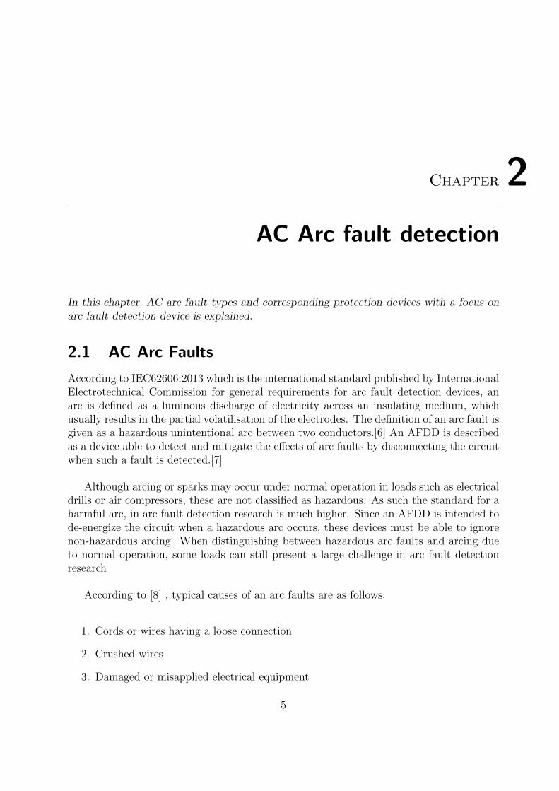
According to [8] , typical causes of an arc faults are as follows:
1. Cords or wires having a loose connection
2. Crushed wires
3. Damaged or misapplied electrical equipment
5
2. AC Arc fault detection
4. Ageing installations
5. Pets and rodent bites
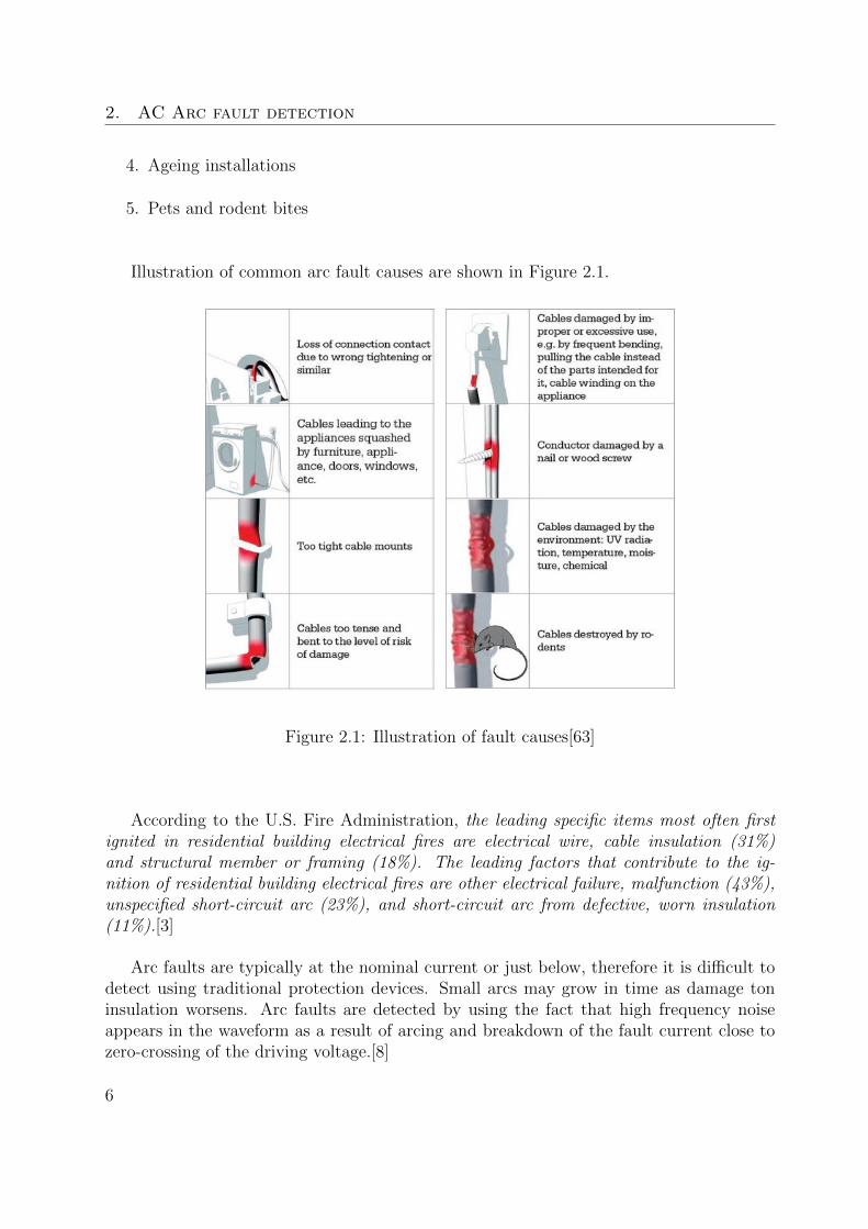
Illustration of common arc fault causes are shown in Figure 2.1.
Figure 2.1: Illustration of fault causes[63]
According to the U.S. Fire Administration, the leading specific items most often firstignited in residential building electrical fires are electrical wire, cable insulation (31%)and structural member or framing (18%). The leading factors that contribute to the ig-nition of residential building electrical fires are other electrical failure, malfunction (43%),unspecified short-circuit arc (23%), and short-circuit arc from defective, worn insulation(11%).[3]
Arc faults are typically at the nominal current or just below, therefore it is difficult todetect using traditional protection devices. Small arcs may grow in time as damage toninsulation worsens. Arc faults are detected by using the fact that high frequency noiseappears in the waveform as a result of arcing and breakdown of the fault current close tozero-crossing of the driving voltage.[8]
6
2.1. AC Arc Faults
According to IEC62606, there are three types of arc faults which are earth arc faults,parallel arc faults and series arc faults. These are introduced in more detail in the followingsections.
2.1.1 Parallel Arc Fault
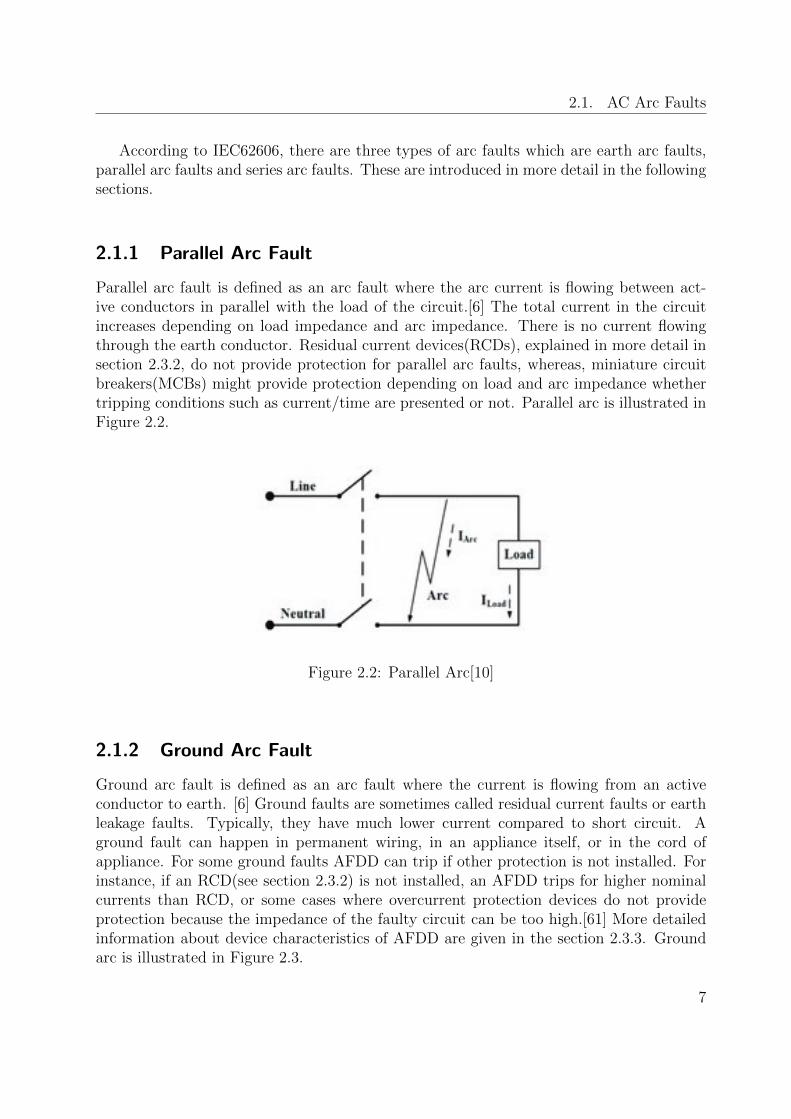
Parallel arc fault is defined as an arc fault where the arc current is flowing between act-ive conductors in parallel with the load of the circuit.[6] The total current in the circuitincreases depending on load impedance and arc impedance. There is no current flowingthrough the earth conductor. Residual current devices(RCDs), explained in more detail insection 2.3.2, do not provide protection for parallel arc faults, whereas, miniature circuitbreakers(MCBs) might provide protection depending on load and arc impedance whethertripping conditions such as current/time are presented or not. Parallel arc is illustrated inFigure 2.2.
Figure 2.2: Parallel Arc[10]
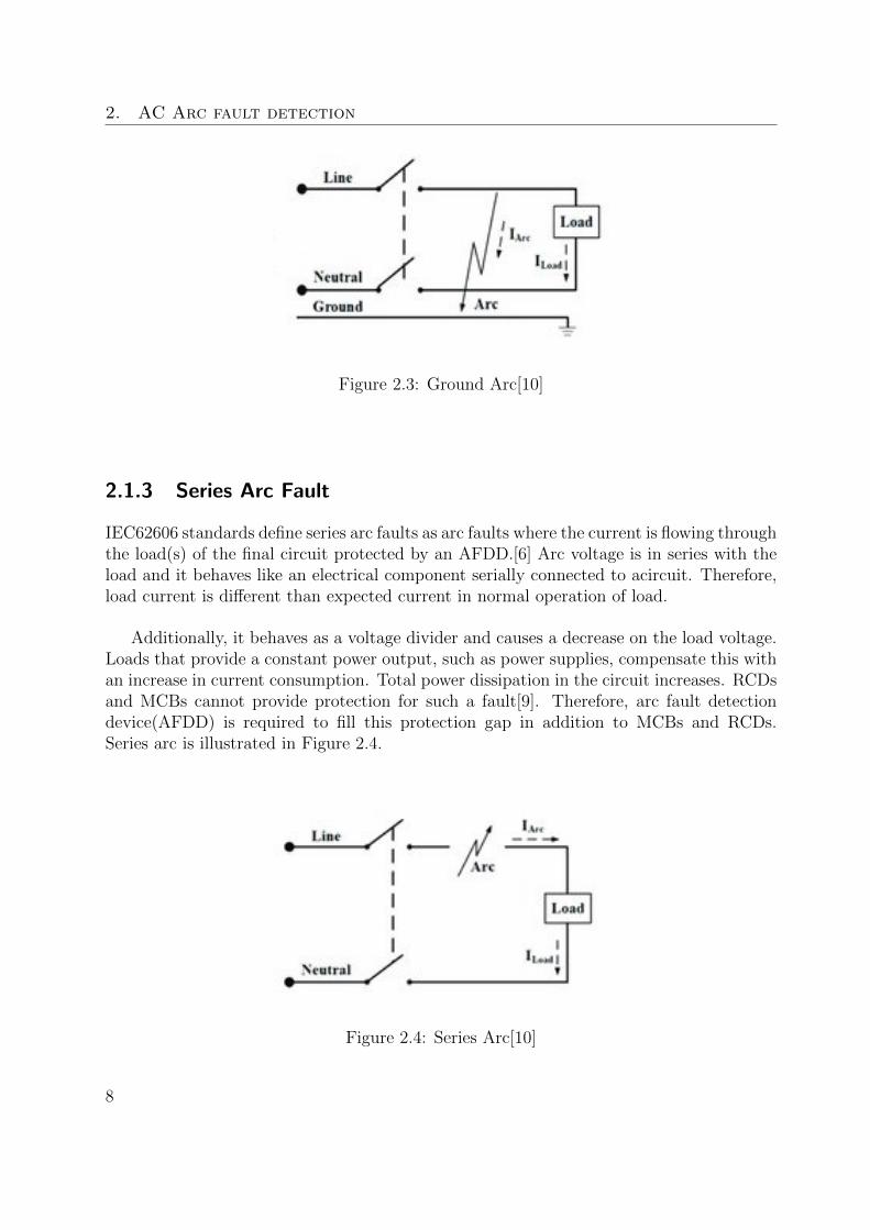
2.1.2 Ground Arc Fault
Ground arc fault is defined as an arc fault where the current is flowing from an activeconductor to earth. [6] Ground faults are sometimes called residual current faults or earthleakage faults. Typically, they have much lower current compared to short circuit. Aground fault can happen in permanent wiring, in an appliance itself, or in the cord ofappliance. For some ground faults AFDD can trip if other protection is not installed. Forinstance, if an RCD(see section 2.3.2) is not installed, an AFDD trips for higher nominalcurrents than RCD, or some cases where overcurrent protection devices do not provideprotection because the impedance of the faulty circuit can be too high.[61] More detailedinformation about device characteristics of AFDD are given in the section 2.3.3. Groundarc is illustrated in Figure 2.3.
7
2. AC Arc fault detection
Figure 2.3: Ground Arc[10]
2.1.3 Series Arc Fault
IEC62606 standards define series arc faults as arc faults where the current is flowing throughthe load(s) of the final circuit protected by an AFDD.[6] Arc voltage is in series with theload and it behaves like an electrical component serially connected to acircuit. Therefore,load current is different than expected current in normal operation of load.
Additionally, it behaves as a voltage divider and causes a decrease on the load voltage.Loads that provide a constant power output, such as power supplies, compensate this withan increase in current consumption. Total power dissipation in the circuit increases. RCDsand MCBs cannot provide protection for such a fault[9]. Therefore, arc fault detectiondevice(AFDD) is required to fill this protection gap in addition to MCBs and RCDs.Series arc is illustrated in Figure 2.4.
Figure 2.4: Series Arc[10]
8
2.2. Arc Fault Characteristics
2.2 Arc Fault Characteristics
According to a US patent filed by Siemens[12], during the time that the arc is conductingcurrent, it produces wide-band, high-frequency noise ranging from about 10kHz to 1GHz.The inventor of [12], also stated that the resulting characteristic pattern of high-frequencynoise with synchronous gaps is unique to arcing and therefore an algorithm for analyzingrepetitive patterns in the amplitude of the noise can be used to detect arcing.
Beacuse the noise generated by arcing is wide-band and reaches frequencies up to 1GHz,any informative combination of frequency spectrum can be used to detect arcing. However,there are some advantages of using a bandwidth of 1 to 50MHz, which are clearly statedin [12] and the advantages are listed as follows:
1. Household appliances are intentionally designed to minimize the noise above 1MHzsince it can interfere with radio broadcasts. Therefore, noise generated by load itselfis minimal above 1MHz so that it is suitable to use in the detection of an arc fault.[12]
2. Loading effects of devices connected to the line can be presented. Therefore arc noisesignal is attenuated. Power distribution lines behaves as transmission lines at highfrequencies. Other devices that are supplied by the same power distribution line areinductively isolated from the power distribution line by their main cords and internalwires, which limits the amount of attenuation they can produce. Using a frequencyband of 1 to 50MHz will eliminate the possible effects of these loading effects.[12]
Noise generated by the arc fault appears on both the line voltage and load currentsolely when arcing conducts. Amplitude of the noise is exactly 0 as the arc extinguishesand reignites at zero-cross section of line voltage,i.e every half-cycle of the line frequency.This is the reason that synchronous gaps are observed on the noise generated by an arcing.For resistive loads, arc voltage is in phase with the line voltage. Therefore, these gapsoccurs simultaneously with the zero-crossing of line voltage. For reactive loads, arc voltageand the gaps may shift in phase up to plus or minus 90◦ depending on the line voltage.[12]Reactance of the load in series with the arc is determinative if the gaps occur simultaneouslywith the zero-crossings of line voltage. However, regardless of phase shifts, gaps in the noisegenerated by arcing are equal in to half of the line frequency cycle.
2.3 Protection Devices
Protection devices in residential power systems are introduced in following sections. Thereare three different subcategories. Devices with same functionality have different naming indifferent places and they are often combined.
9
2. AC Arc fault detection
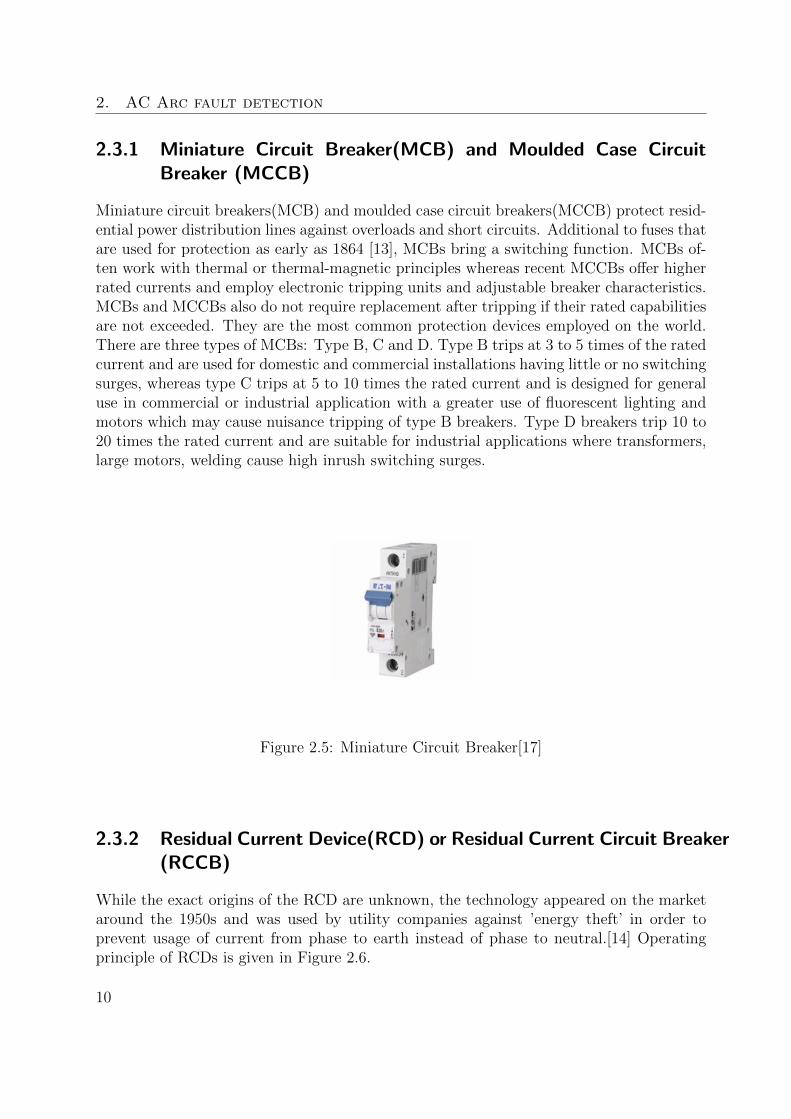
2.3.1 Miniature Circuit Breaker(MCB) and Moulded Case CircuitBreaker (MCCB)
Miniature circuit breakers(MCB) and moulded case circuit breakers(MCCB) protect resid-ential power distribution lines against overloads and short circuits. Additional to fuses thatare used for protection as early as 1864 [13], MCBs bring a switching function. MCBs of-ten work with thermal or thermal-magnetic principles whereas recent MCCBs offer higherrated currents and employ electronic tripping units and adjustable breaker characteristics.MCBs and MCCBs also do not require replacement after tripping if their rated capabilitiesare not exceeded. They are the most common protection devices employed on the world.There are three types of MCBs: Type B, C and D. Type B trips at 3 to 5 times of the ratedcurrent and are used for domestic and commercial installations having little or no switchingsurges, whereas type C trips at 5 to 10 times the rated current and is designed for generaluse in commercial or industrial application with a greater use of fluorescent lighting andmotors which may cause nuisance tripping of type B breakers. Type D breakers trip 10 to20 times the rated current and are suitable for industrial applications where transformers,large motors, welding cause high inrush switching surges.
Figure 2.5: Miniature Circuit Breaker[17]
2.3.2 Residual Current Device(RCD) or Residual Current Circuit Breaker(RCCB)
While the exact origins of the RCD are unknown, the technology appeared on the marketaround the 1950s and was used by utility companies against ’energy theft’ in order toprevent usage of current from phase to earth instead of phase to neutral.[14] Operatingprinciple of RCDs is given in Figure 2.6.
10
2.3. Protection Devices
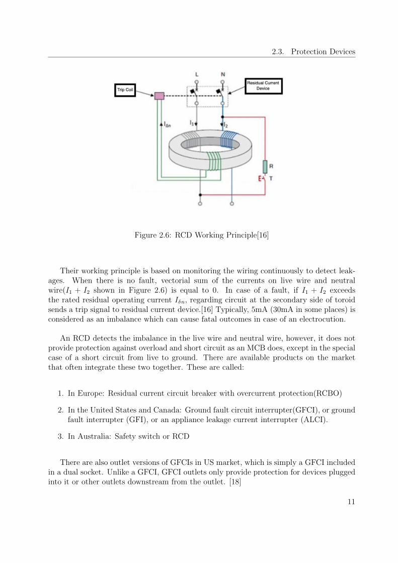
Figure 2.6: RCD Working Principle[16]
Their working principle is based on monitoring the wiring continuously to detect leak-ages. When there is no fault, vectorial sum of the currents on live wire and neutralwire(I1 + I2 shown in Figure 2.6) is equal to 0. In case of a fault, if I1 + I2 exceedsthe rated residual operating current Iδn, regarding circuit at the secondary side of toroidsends a trip signal to residual current device.[16] Typically, 5mA (30mA in some places) isconsidered as an imbalance which can cause fatal outcomes in case of an electrocution.
An RCD detects the imbalance in the live wire and neutral wire, however, it does notprovide protection against overload and short circuit as an MCB does, except in the specialcase of a short circuit from live to ground. There are available products on the marketthat often integrate these two together. These are called:
1. In Europe: Residual current circuit breaker with overcurrent protection(RCBO)
2. In the United States and Canada: Ground fault circuit interrupter(GFCI), or groundfault interrupter (GFI), or an appliance leakage current interrupter (ALCI).
3. In Australia: Safety switch or RCD
There are also outlet versions of GFCIs in US market, which is simply a GFCI includedin a dual socket. Unlike a GFCI, GFCI outlets only provide protection for devices pluggedinto it or other outlets downstream from the outlet. [18]
11
2. AC Arc fault detection
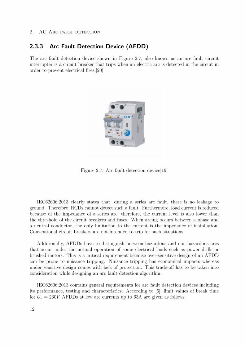
2.3.3 Arc Fault Detection Device (AFDD)
The arc fault detection device shown in Figure 2.7, also known as an arc fault circuitinterrupter is a circuit breaker that trips when an electric arc is detected in the circuit inorder to prevent electrical fires.[20]
Figure 2.7: Arc fault detection device[19]
IEC62606:2013 clearly states that, during a series arc fault, there is no leakage toground. Therefore, RCDs cannot detect such a fault. Furthermore, load current is reducedbecause of the impedance of a series arc; therefore, the current level is also lower thanthe threshold of the circuit breakers and fuses. When arcing occurs between a phase anda neutral conductor, the only limitation to the current is the impedance of installation.Conventional circuit breakers are not intended to trip for such situations.
Additionally, AFDDs have to distinguish between hazardous and non-hazardous arcsthat occur under the normal operation of some electrical loads such as power drills orbrushed motors. This is a critical requirement because over-sensitive design of an AFDDcan be prone to nuisance tripping. Nuisance tripping has economical impacts whereasunder sensitive design comes with lack of protection. This trade-off has to be taken intoconsideration while designing an arc fault detection algorithm.
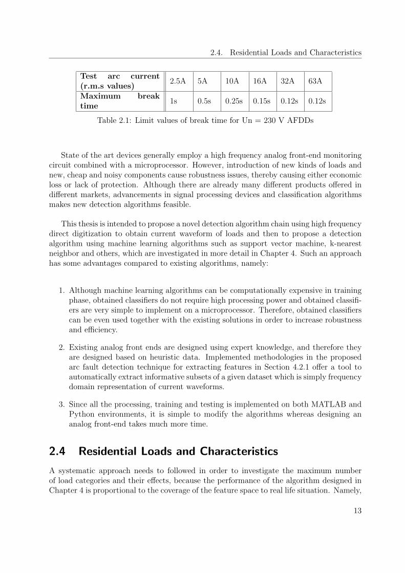
IEC62606:2013 contains general requirements for arc fault detection devices includingits performance, testing and characteristics. According to [6], limit values of break timefor Un = 230V AFDDs at low arc currents up to 63A are given as follows.
12
2.4. Residential Loads and Characteristics
Test arc current(r.m.s values)
2.5A 5A 10A 16A 32A 63A
Maximum breaktime
1s 0.5s 0.25s 0.15s 0.12s 0.12s
Table 2.1: Limit values of break time for Un = 230 V AFDDs
State of the art devices generally employ a high frequency analog front-end monitoringcircuit combined with a microprocessor. However, introduction of new kinds of loads andnew, cheap and noisy components cause robustness issues, thereby causing either economicloss or lack of protection. Although there are already many different products offered indifferent markets, advancements in signal processing devices and classification algorithmsmakes new detection algorithms feasible.
This thesis is intended to propose a novel detection algorithm chain using high frequencydirect digitization to obtain current waveform of loads and then to propose a detectionalgorithm using machine learning algorithms such as support vector machine, k-nearestneighbor and others, which are investigated in more detail in Chapter 4. Such an approachhas some advantages compared to existing algorithms, namely:
1. Although machine learning algorithms can be computationally expensive in trainingphase, obtained classifiers do not require high processing power and obtained classifi-ers are very simple to implement on a microprocessor. Therefore, obtained classifierscan be even used together with the existing solutions in order to increase robustnessand efficiency.
2. Existing analog front ends are designed using expert knowledge, and therefore theyare designed based on heuristic data. Implemented methodologies in the proposedarc fault detection technique for extracting features in Section 4.2.1 offer a tool toautomatically extract informative subsets of a given dataset which is simply frequencydomain representation of current waveforms.
3. Since all the processing, training and testing is implemented on both MATLAB andPython environments, it is simple to modify the algorithms whereas designing ananalog front-end takes much more time.
2.4 Residential Loads and Characteristics
A systematic approach needs to followed in order to investigate the maximum numberof load categories and their effects, because the performance of the algorithm designed inChapter 4 is proportional to the coverage of the feature space to real life situation. Namely,
13
2. AC Arc fault detection
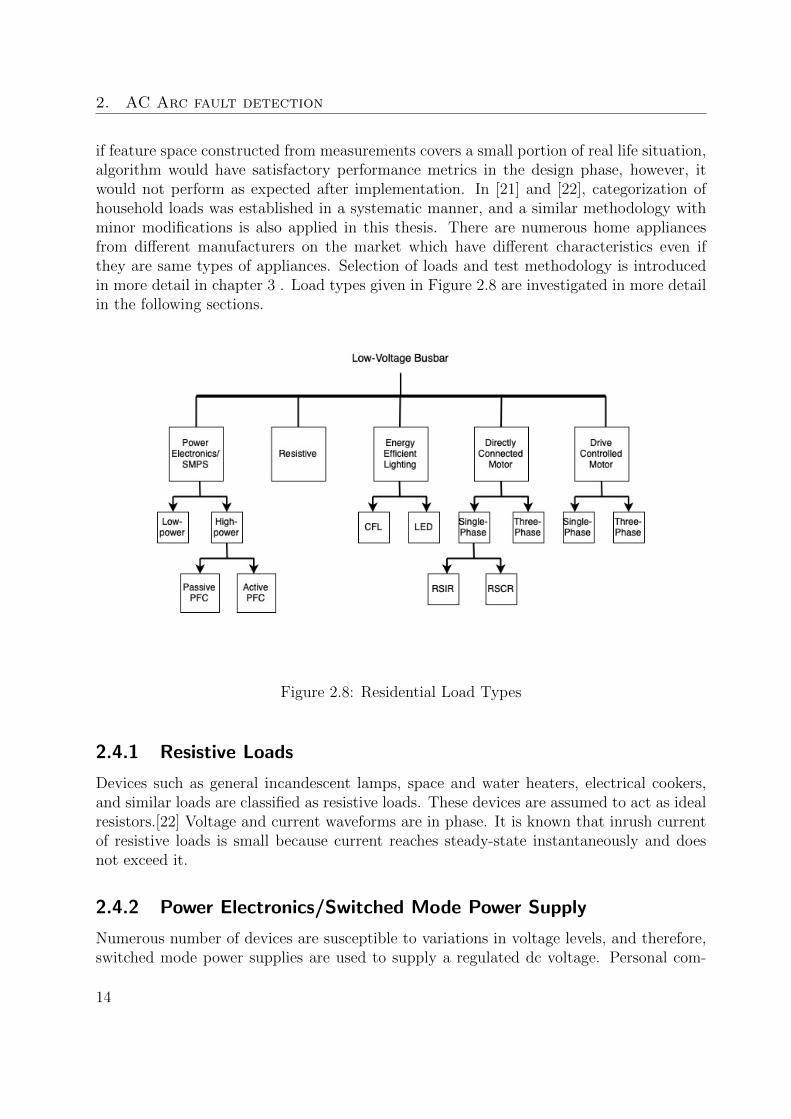
if feature space constructed from measurements covers a small portion of real life situation,algorithm would have satisfactory performance metrics in the design phase, however, itwould not perform as expected after implementation. In [21] and [22], categorization ofhousehold loads was established in a systematic manner, and a similar methodology withminor modifications is also applied in this thesis. There are numerous home appliancesfrom different manufacturers on the market which have different characteristics even ifthey are same types of appliances. Selection of loads and test methodology is introducedin more detail in chapter 3 . Load types given in Figure 2.8 are investigated in more detailin the following sections.
Figure 2.8: Residential Load Types
2.4.1 Resistive Loads
Devices such as general incandescent lamps, space and water heaters, electrical cookers,and similar loads are classified as resistive loads. These devices are assumed to act as idealresistors.[22] Voltage and current waveforms are in phase. It is known that inrush currentof resistive loads is small because current reaches steady-state instantaneously and doesnot exceed it.
2.4.2 Power Electronics/Switched Mode Power Supply
Numerous number of devices are susceptible to variations in voltage levels, and therefore,switched mode power supplies are used to supply a regulated dc voltage. Personal com-
14
2.4. Residential Loads and Characteristics
puters, televisions and monitors are widely used examples that utilize SMPSs. Accordingto [25], the total energy consumption by household appliances grew 1.7% every year onaverage from 1970 to 2013 in the United Kingdom and consumer electronics that generallyutilize SMPSs have the biggest residential consumption with an estimation of 1868 ktoe.
According to related standards[23], switched mode power supplies are divided into threesubcategories, as follows:
1. No Power Factor Correlation(n-PFC): SMPS with a rated power smaller than 75 Wdo not have to meet harmonic legislation. Therefore, they do not need to include apower factor correlation circuit.
2. Active Power Factor Correlation(a-PFC): Some SMPS with rated power larger than75 W include an additional dc-dc converter circuit in order to shape the input currentto have appropriate sinusoidal waveform in-phase with the supply voltage. [22]
3. Passive Power Factor Correlation(p-PFC): p-PFC utilizes a large inductor in the pathof current transmission since inductors resist change in current, therefore resulting awaveform that is smoother and has less harmonic content.
P-PFC has a wider usage than a-PFC because of its easier implementation and signi-ficantly lower cost. However, usage of a-PFC increases as the cost of components decreasessteadily.
2.4.3 Energy Efficient Lighting
Light emitting diodes(LEDs) and compact fluorescent lamps (CFLs) are the most widelyused loads that falls into this category. Due to the economic benefits of LEDs comparedto general incandescent bulbs(GILs), energy efficient lighting has been constantly gainingpopularity.
According to the International Energy Agency, LED lighting sales expeienced terrificgrowth in recent years. In 2011, LEDs and fluorescent lamps were formed 40% of total saleswith 1% and 39% of the market share respectively. However, in 2018, these two formed82% of total sales, with LEDs at 40% and fluorescent lamps at 42% of total sales. It isexpected that this trend will continue and LEDs will capture the 80% of total sales andfluorescent lighting will capture 20% of total sales by the end of 2030. [26]
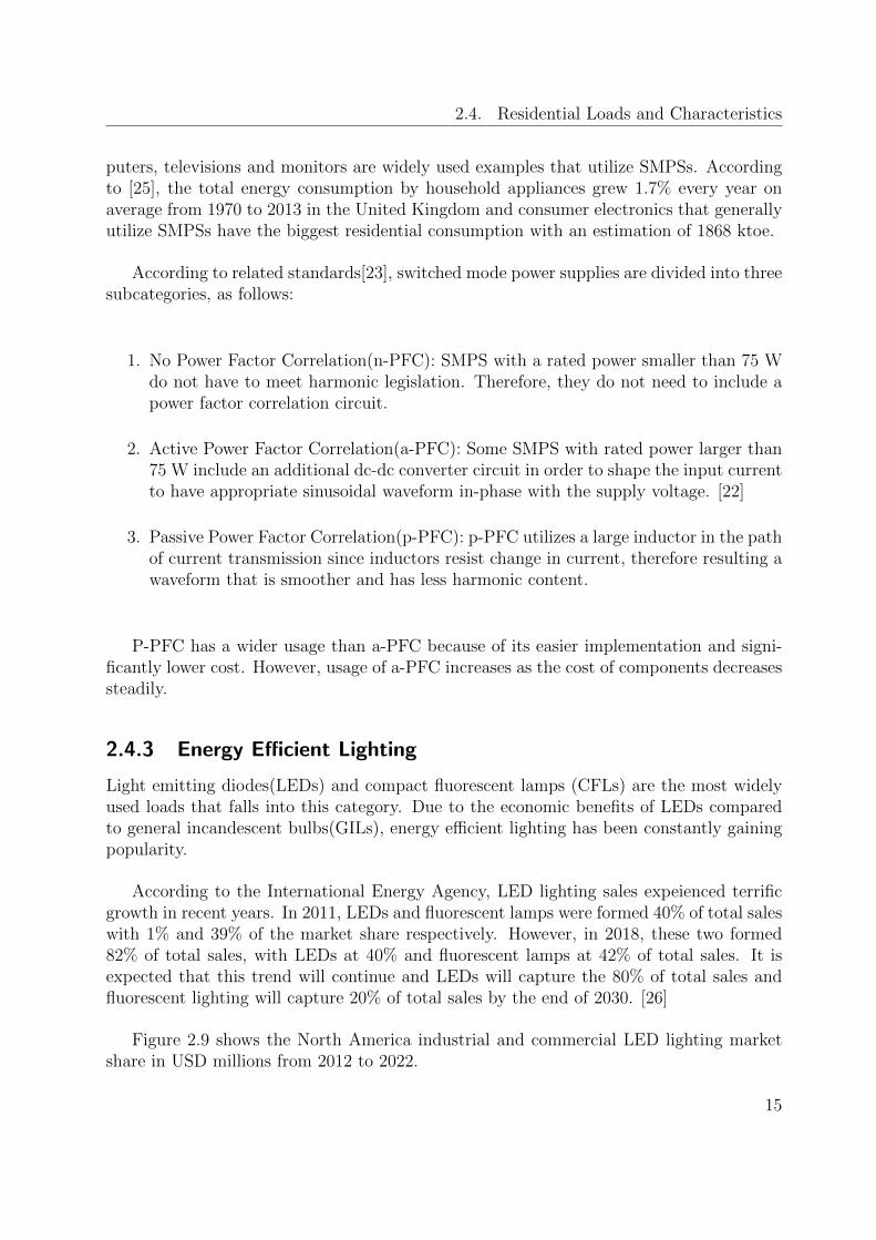
Figure 2.9 shows the North America industrial and commercial LED lighting marketshare in USD millions from 2012 to 2022.
15
2. AC Arc fault detection
Figure 2.9: North America Industrial and Commercial LED Lighting Market Share, 2012-2022 (USD millions)[27]
CFLs of 8, 11 and 18 W are widely replaced with 40, 60 , 100 W GILs accordinglybecause of similar output lumens together with much less power consumption.[22] Becauseof nonlinearity, harmonics are introduced to the supply system by CFLs.
2.4.4 Single Phase Induction Motor
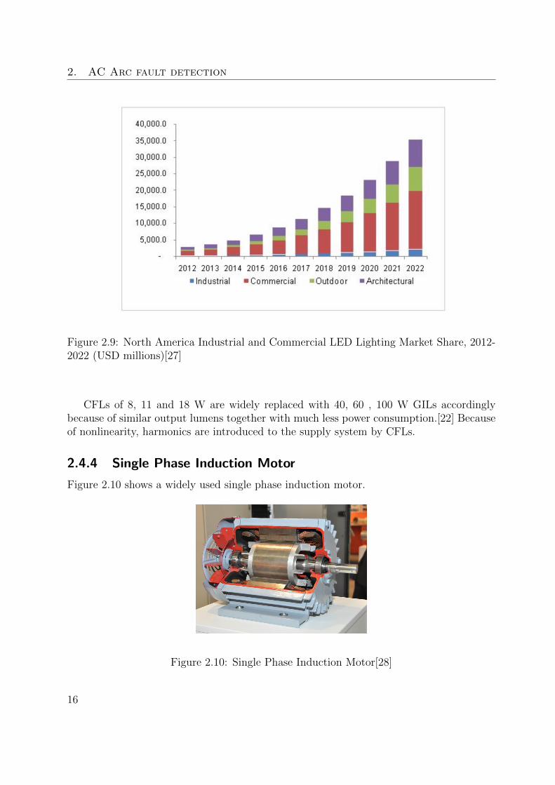
Figure 2.10 shows a widely used single phase induction motor.
Figure 2.10: Single Phase Induction Motor[28]
16

2.4. Residential Loads and Characteristics
Single phase induction motors are one the most common types of loads found in devicessuch as refrigerators, dishwashers, freezers, and air conditioners, which all contains SPIMs.The reason they are called ’single phase’ is because they work with single phase residentialAC supply. Three phase motors are not included in this thesis since they are outside thescope of this research. Single phase induction motors are used when a fixed speed is needed.SPIM has a simple design.
2.4.5 Universal Motor
The universal motor is one of the most widely used components found in numerous appli-ances, such as blenders, vacuum cleaners, hair dryers, drill machine, sanders, and others.Another use is for applications that require speed control. Universal motors can operatewith AC and DC. The size of universal motors is relatively small compared to AC motorsthat operate on the same frequency. The main features of universal motors are its cap-ability of working at high speeds, its relatively high start torque, and its small size andcompact design.[21] The disadvantages posed by the universal motors is the acoustic andelectromagnetic noise generated by them.
Figure 2.11: Universal Motor
17
Chapter 3
AFDD Tests and Measurements
In this chapter, European test procedure and equipment used in the measurements arepresented. Tested residential loads are introduced. Measured loads are analyzed in timedomain and frequency domain. In order to analyze the arc fault events, different approachescan be employed. In this thesis, real measurements are employed because of the reliabilityof measurement procedures and guaranteed results.
3.1 European Standards Test Procedure
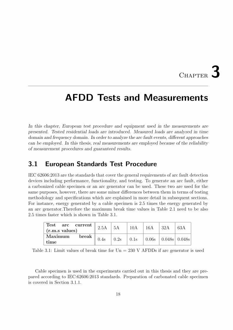
IEC 62606:2013 are the standards that cover the general requirements of arc fault detectiondevices including performance, functionality, and testing. To generate an arc fault, eithera carbonized cable specimen or an arc generator can be used. These two are used for thesame purposes, however, there are some minor differences between them in terms of testingmethodology and specifications which are explained in more detail in subsequent sections.For instance, energy generated by a cable specimen is 2.5 times the energy generated byan arc generator.Therefore the maximum break time values in Table 2.1 need to be also2.5 times faster which is shown in Table 3.1.
Test arc current(r.m.s values)
2.5A 5A 10A 16A 32A 63A
Maximum breaktime
0.4s 0.2s 0.1s 0.06s 0.048s 0.048s
Table 3.1: Limit values of break time for Un = 230 V AFDDs if arc generator is used
Cable specimen is used in the experiments carried out in this thesis and they are pre-pared according to IEC:62606:2013 standards. Preparation of carbonated cable specimenis covered in Section 3.1.1.
18
3.1. European Standards Test Procedure
3.1.1 Cable Specimen
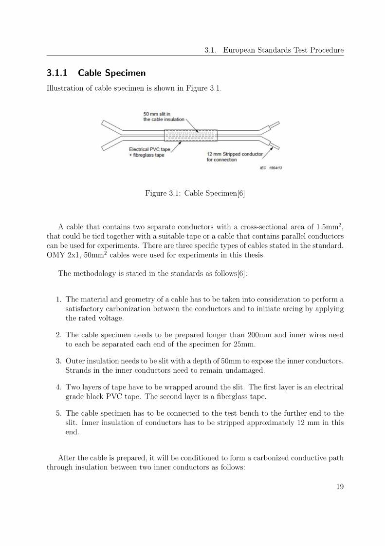
Illustration of cable specimen is shown in Figure 3.1.
Figure 3.1: Cable Specimen[6]
A cable that contains two separate conductors with a cross-sectional area of 1.5mm2,that could be tied together with a suitable tape or a cable that contains parallel conductorscan be used for experiments. There are three specific types of cables stated in the standard.OMY 2x1, 50mm2 cables were used for experiments in this thesis.
The methodology is stated in the standards as follows[6]:
1. The material and geometry of a cable has to be taken into consideration to perform asatisfactory carbonization between the conductors and to initiate arcing by applyingthe rated voltage.
2. The cable specimen needs to be prepared longer than 200mm and inner wires needto each be separated each end of the specimen for 25mm.
3. Outer insulation needs to be slit with a depth of 50mm to expose the inner conductors.Strands in the inner conductors need to remain undamaged.
4. Two layers of tape have to be wrapped around the slit. The first layer is an electricalgrade black PVC tape. The second layer is a fiberglass tape.
5. The cable specimen has to be connected to the test bench to the further end to theslit. Inner insulation of conductors has to be stripped approximately 12 mm in thisend.
After the cable is prepared, it will be conditioned to form a carbonized conductive paththrough insulation between two inner conductors as follows:
19
3. AFDD Tests and Measurements
1. The cable specimen needs to be connected to a circuit that provides 30mA shortcircuit current and an open circuit voltage at least 7kV. This connection needs to besustained either for 10 seconds or until the smoking stops.
2. As the last step, it is needed to connect the cable specimen to a circuit that provides300mA short circuit current at a voltage of at least 2 kV or adequate to current flowsthrough it. This step needs to be applied at least one minute or until the smokestops.
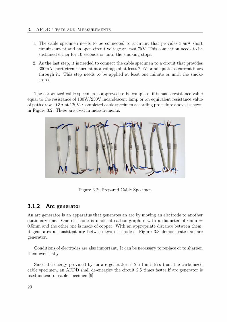
The carbonized cable specimen is approved to be complete, if it has a resistance valueequal to the resistance of 100W/230V incandescent lamp or an equivalent resistance valueof path draws 0.3A at 120V. Completed cable specimen according procedure above is shownin Figure 3.2. These are used in measurements.
Figure 3.2: Prepared Cable Specimen
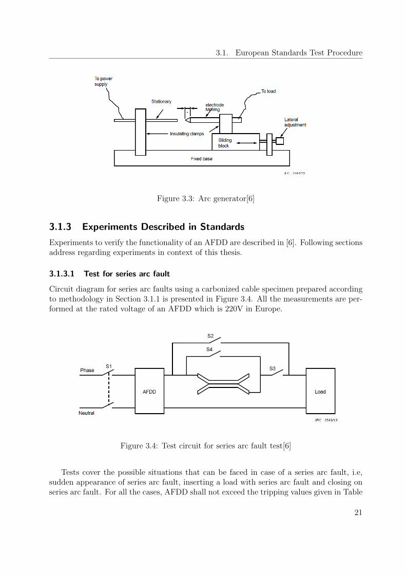
3.1.2 Arc generator
An arc generator is an apparatus that generates an arc by moving an electrode to anotherstationary one. One electrode is made of carbon-graphite with a diameter of 6mm ±0.5mm and the other one is made of copper. With an appropriate distance between them,it generates a consistent arc between two electrodes. Figure 3.3 demonstrates an arcgenerator.
Conditions of electrodes are also important. It can be necessary to replace or to sharpenthem eventually.
Since the energy provided by an arc generator is 2.5 times less than the carbonizedcable specimen, an AFDD shall de-energize the circuit 2.5 times faster if arc generator isused instead of cable specimen.[6]
20
3.1. European Standards Test Procedure
Figure 3.3: Arc generator[6]
3.1.3 Experiments Described in Standards
Experiments to verify the functionality of an AFDD are described in [6]. Following sectionsaddress regarding experiments in context of this thesis.
3.1.3.1 Test for series arc fault
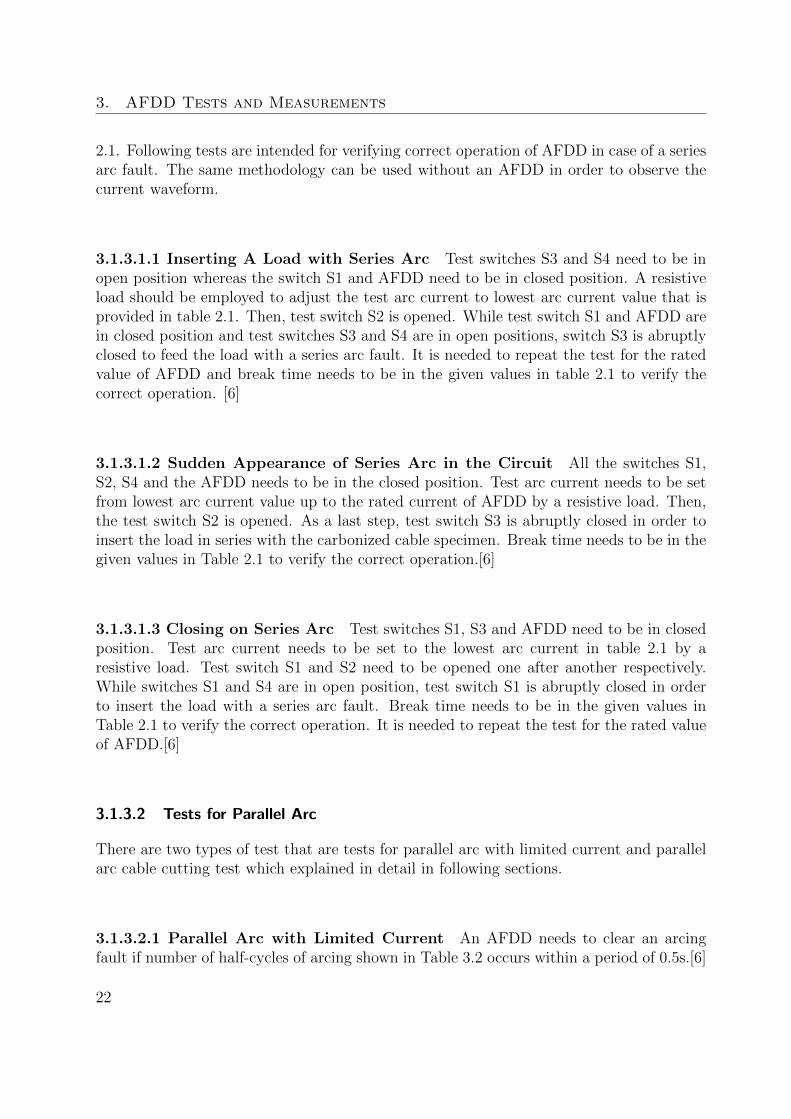
Circuit diagram for series arc faults using a carbonized cable specimen prepared accordingto methodology in Section 3.1.1 is presented in Figure 3.4. All the measurements are per-formed at the rated voltage of an AFDD which is 220V in Europe.
Figure 3.4: Test circuit for series arc fault test[6]
Tests cover the possible situations that can be faced in case of a series arc fault, i.e,sudden appearance of series arc fault, inserting a load with series arc fault and closing onseries arc fault. For all the cases, AFDD shall not exceed the tripping values given in Table
21
3. AFDD Tests and Measurements
2.1. Following tests are intended for verifying correct operation of AFDD in case of a seriesarc fault. The same methodology can be used without an AFDD in order to observe thecurrent waveform.
3.1.3.1.1 Inserting A Load with Series Arc Test switches S3 and S4 need to be inopen position whereas the switch S1 and AFDD need to be in closed position. A resistiveload should be employed to adjust the test arc current to lowest arc current value that isprovided in table 2.1. Then, test switch S2 is opened. While test switch S1 and AFDD arein closed position and test switches S3 and S4 are in open positions, switch S3 is abruptlyclosed to feed the load with a series arc fault. It is needed to repeat the test for the ratedvalue of AFDD and break time needs to be in the given values in table 2.1 to verify thecorrect operation. [6]
3.1.3.1.2 Sudden Appearance of Series Arc in the Circuit All the switches S1,S2, S4 and the AFDD needs to be in the closed position. Test arc current needs to be setfrom lowest arc current value up to the rated current of AFDD by a resistive load. Then,the test switch S2 is opened. As a last step, test switch S3 is abruptly closed in order toinsert the load in series with the carbonized cable specimen. Break time needs to be in thegiven values in Table 2.1 to verify the correct operation.[6]
3.1.3.1.3 Closing on Series Arc Test switches S1, S3 and AFDD need to be in closedposition. Test arc current needs to be set to the lowest arc current in table 2.1 by aresistive load. Test switch S1 and S2 need to be opened one after another respectively.While switches S1 and S4 are in open position, test switch S1 is abruptly closed in orderto insert the load with a series arc fault. Break time needs to be in the given values inTable 2.1 to verify the correct operation. It is needed to repeat the test for the rated valueof AFDD.[6]
3.1.3.2 Tests for Parallel Arc
There are two types of test that are tests for parallel arc with limited current and parallelarc cable cutting test which explained in detail in following sections.
3.1.3.2.1 Parallel Arc with Limited Current An AFDD needs to clear an arcingfault if number of half-cycles of arcing shown in Table 3.2 occurs within a period of 0.5s.[6]
22
3.1. European Standards Test Procedure
Test arc current (r.m.s values) 75A 100A 150A 200A 300A 500A
N 12 10 8 8 8 8
Notes: 1) Test arc current values are prospective currents before arcing in the circuit
2) N is the number of half cycles at the rated frequency.
Table 3.2: Maximum allowed number of arcing half-cycles within 0.5 s for AFDDs
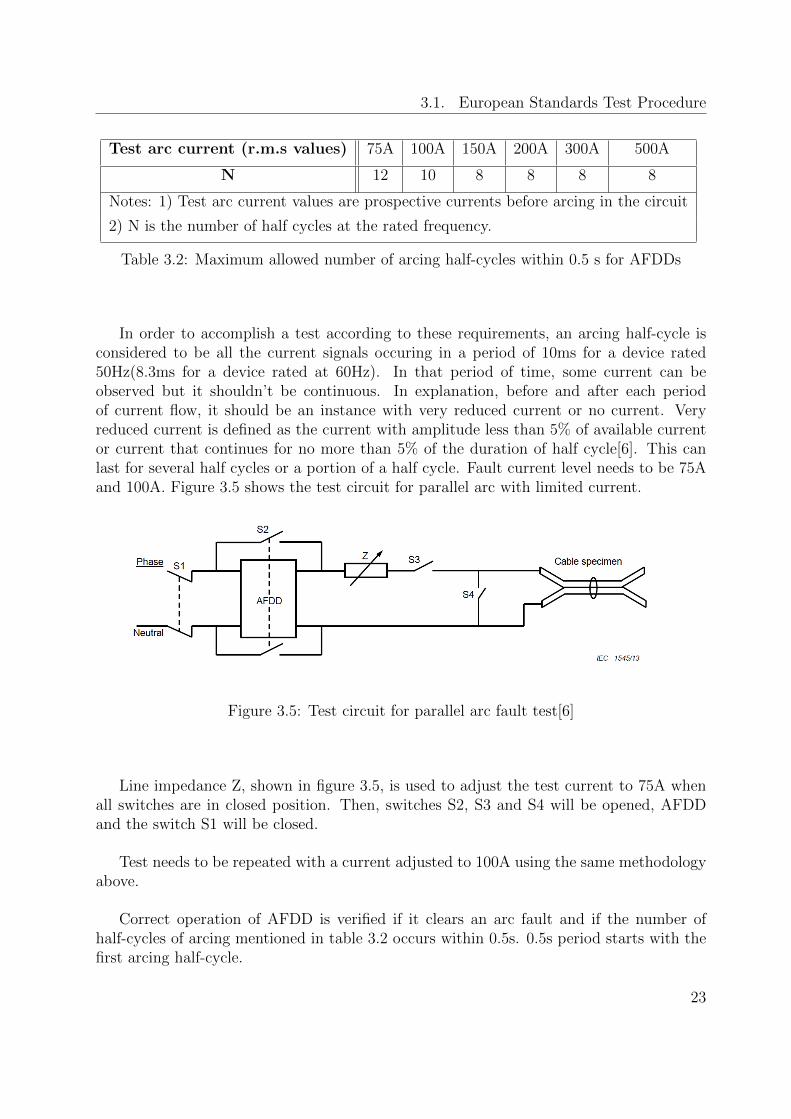
In order to accomplish a test according to these requirements, an arcing half-cycle isconsidered to be all the current signals occuring in a period of 10ms for a device rated50Hz(8.3ms for a device rated at 60Hz). In that period of time, some current can beobserved but it shouldn’t be continuous. In explanation, before and after each periodof current flow, it should be an instance with very reduced current or no current. Veryreduced current is defined as the current with amplitude less than 5% of available currentor current that continues for no more than 5% of the duration of half cycle[6]. This canlast for several half cycles or a portion of a half cycle. Fault current level needs to be 75Aand 100A. Figure 3.5 shows the test circuit for parallel arc with limited current.
Figure 3.5: Test circuit for parallel arc fault test[6]
Line impedance Z, shown in figure 3.5, is used to adjust the test current to 75A whenall switches are in closed position. Then, switches S2, S3 and S4 will be opened, AFDDand the switch S1 will be closed.
Test needs to be repeated with a current adjusted to 100A using the same methodologyabove.
Correct operation of AFDD is verified if it clears an arc fault and if the number ofhalf-cycles of arcing mentioned in table 3.2 occurs within 0.5s. 0.5s period starts with thefirst arcing half-cycle.
23
3. AFDD Tests and Measurements
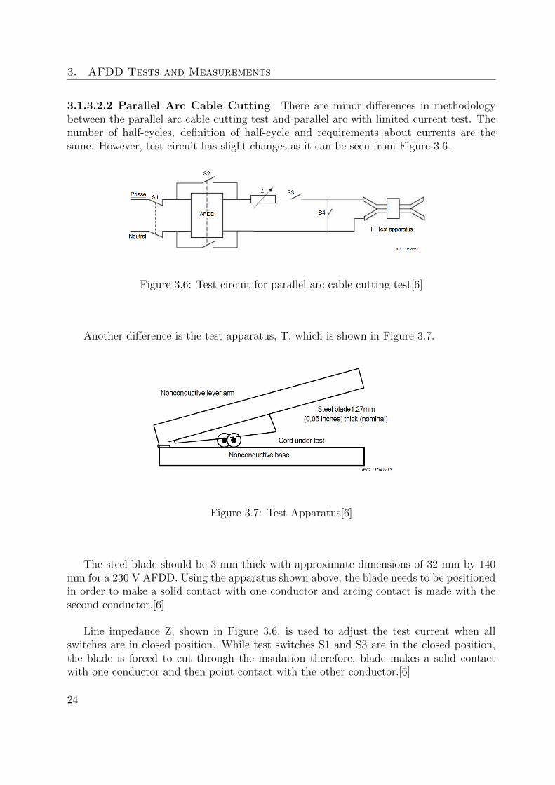
3.1.3.2.2 Parallel Arc Cable Cutting There are minor differences in methodologybetween the parallel arc cable cutting test and parallel arc with limited current test. Thenumber of half-cycles, definition of half-cycle and requirements about currents are thesame. However, test circuit has slight changes as it can be seen from Figure 3.6.
Figure 3.6: Test circuit for parallel arc cable cutting test[6]
Another difference is the test apparatus, T, which is shown in Figure 3.7.
Figure 3.7: Test Apparatus[6]
The steel blade should be 3 mm thick with approximate dimensions of 32 mm by 140mm for a 230 V AFDD. Using the apparatus shown above, the blade needs to be positionedin order to make a solid contact with one conductor and arcing contact is made with thesecond conductor.[6]
Line impedance Z, shown in Figure 3.6, is used to adjust the test current when allswitches are in closed position. While test switches S1 and S3 are in the closed position,the blade is forced to cut through the insulation therefore, blade makes a solid contactwith one conductor and then point contact with the other conductor.[6]
24
3.2. Measurement Setup
AFDD needs to clear an arc fault according to values given in Table 3.2 which occurin a period of 0.5s.
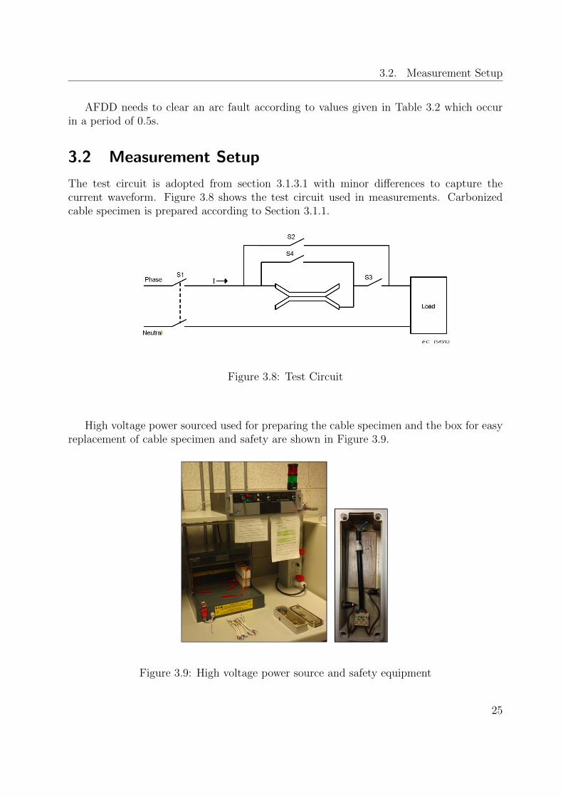
3.2 Measurement Setup
The test circuit is adopted from section 3.1.3.1 with minor differences to capture thecurrent waveform. Figure 3.8 shows the test circuit used in measurements. Carbonizedcable specimen is prepared according to Section 3.1.1.
Figure 3.8: Test Circuit
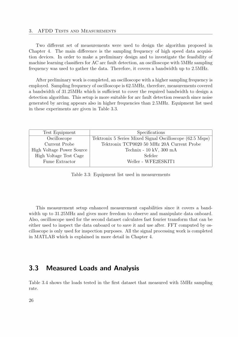
High voltage power sourced used for preparing the cable specimen and the box for easyreplacement of cable specimen and safety are shown in Figure 3.9.
Figure 3.9: High voltage power source and safety equipment
25
3. AFDD Tests and Measurements
Two different set of measurements were used to design the algorithm proposed inChapter 4. The main difference is the sampling frequency of high speed data acquisi-tion devices. In order to make a preliminary design and to investigate the feasibility ofmachine learning classifiers for AC arc fault detection, an oscilloscope with 5MHz samplingfrequency was used to gather the data. Therefore, it covers a bandwidth up to 2.5MHz.
After preliminary work is completed, an oscilloscope with a higher sampling frequency isemployed. Sampling frequency of oscilloscope is 62.5MHz, therefore, measurements covereda bandwidth of 31.25MHz which is sufficient to cover the required bandwidth to design adetection algorithm. This setup is more suitable for arc fault detection research since noisegenerated by arcing appears also in higher frequencies than 2.5MHz. Equipment list usedin these experiments are given in Table 3.3.
Test Equipment SpecificationsOscilloscope Tektronix 5 Series Mixed Signal Oscilloscope (62.5 Msps)
Current Probe Tektronix TCP0020 50 MHz 20A Current ProbeHigh Voltage Power Source Technix - 10 kV, 300 mA
High Voltage Test Cage SefelecFume Extractor Weller - WFE2ESKIT1
Table 3.3: Equipment list used in measurements
This measurement setup enhanced measurement capabilities since it covers a band-width up to 31.25MHz and gives more freedom to observe and manipulate data onboard.Also, oscilloscope used for the second dataset calculates fast fourier transform that can beeither used to inspect the data onboard or to save it and use after. FFT computed by os-cilloscope is only used for inspection purposes. All the signal processing work is completedin MATLAB which is explained in more detail in Chapter 4.
3.3 Measured Loads and Analysis
Table 3.4 shows the loads tested in the first dataset that measured with 5MHz samplingrate.
26
3.3. Measured Loads and Analysis
Measured Load Type Load NameSMPS(p-pfc) Power Drill
SPIM(Directly Desk FanConnected Motor)
Resistive HeaterLighting FleurescentResistive General Incandescent Lamp
Table 3.4: Measurements for first dataset
Since the measurements for first dataset were only used for preliminary work and invest-igation of feasibility, they are not explained in the following sections. Only measurementsin the second dataset which are shown in Table 3.5 are explained.
Due to time and resource limitations, it was not possible to measure all different cat-egories stated in Figure 2.8. However, most challenging loads in terms of arc fault detectionwere used in experiments. Loads are selected according to their usage statistics. Most soldloads in Czech market were chosen. Measured loads that are used in design of detectionalgorithm are given in Table 3.5.
Measured Load Load Type
Heaters Resistive Load
LED Energy Efficient Lighting
Fluorescent Lamp Energy Efficient Lighting
Cultivator Universal Motor
Power Supply Switched Mode PowerSupply with a-PFC
Heaters with Dimmer Resistive Load
Table 3.5: Measured Loads by Group
The same number of measurements were planned to be taken for arcing and normalworking conditions of different loads. However, it is simpler to capture normal operationof a load since there is no need for preparation of the cable specimen. Therefore for someloads, number of measurements with an arc fault are less than normal operation.
3.3.1 Heaters
Resistive loads are the easiest load types for arc fault detection because of their consistentand unique characteristics. Additionally, they do not contribute to nuisance tripping. In
27
3. AFDD Tests and Measurements
the following table, measured resistive loads(heaters) and their combinations are given.
Measured Load Power Current Number of(by name) (W) (A) Measurements
Sahara 400 1.739 42
Sahara+Eurom 900(400+500) 3,913 42
Sahara+Concept 1150(400+750) 5 42Sahara+Tristar 1600(400+1200) 6.957 42
Tristar+Concept 2050(1200+850) 8.913 42Eurom+Tristar+Concept 2550(500+800+1250) 11.087 42Eurom+Sahara+Tristar 3350(500+400 14.565 42
+Concept +1200+1250)
Table 3.6: Resistive Loads used in measurements in details(Heaters)
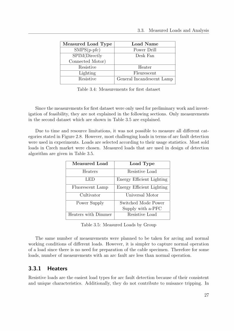
Two different types of measurements are done for every combination of heaters. One isto observe current waveform in normal working condition and the other is to observe currentwaveform of the load with a series arc. Figure 3.10 and Figure 3.11 show the regardingwaveforms of heater with the lowest power consumption(400W) and the combination ofheaters with the highest power consumption(3350W). For the case with series arc fault,shoulders at the zero crossings are visible without further analysis. Also, it is observedthat characteristics of a resistive load for arcing and non-arcing do not show remarkablechanges based on the power consumption.
Figure 3.10: Current waveform of electrical heater(400W)(Red: Arcing, Blue: Non-arcing)
28
3.3. Measured Loads and Analysis
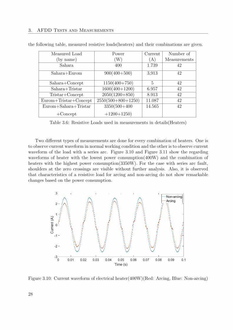
Figure 3.10 is the measurements of the heater with lowest power consumption, 400W.Figure 3.11 shows the measurement of combination of heaters with a power consumptionof 3350W in total.
Figure 3.11: Current waveform of electrical heaters(3350W)(Red: Arcing, Blue: Non-arcing)
As it can be seen from Figure 3.10 and 3.11, when arc distinguishes and re-ignitesaround zero-crossings, it causes shoulders to appear in the waveform and these are visibleby eye inspection without a need of further analysis.
3.3.2 Switched Mode Power Supply(SMPS)
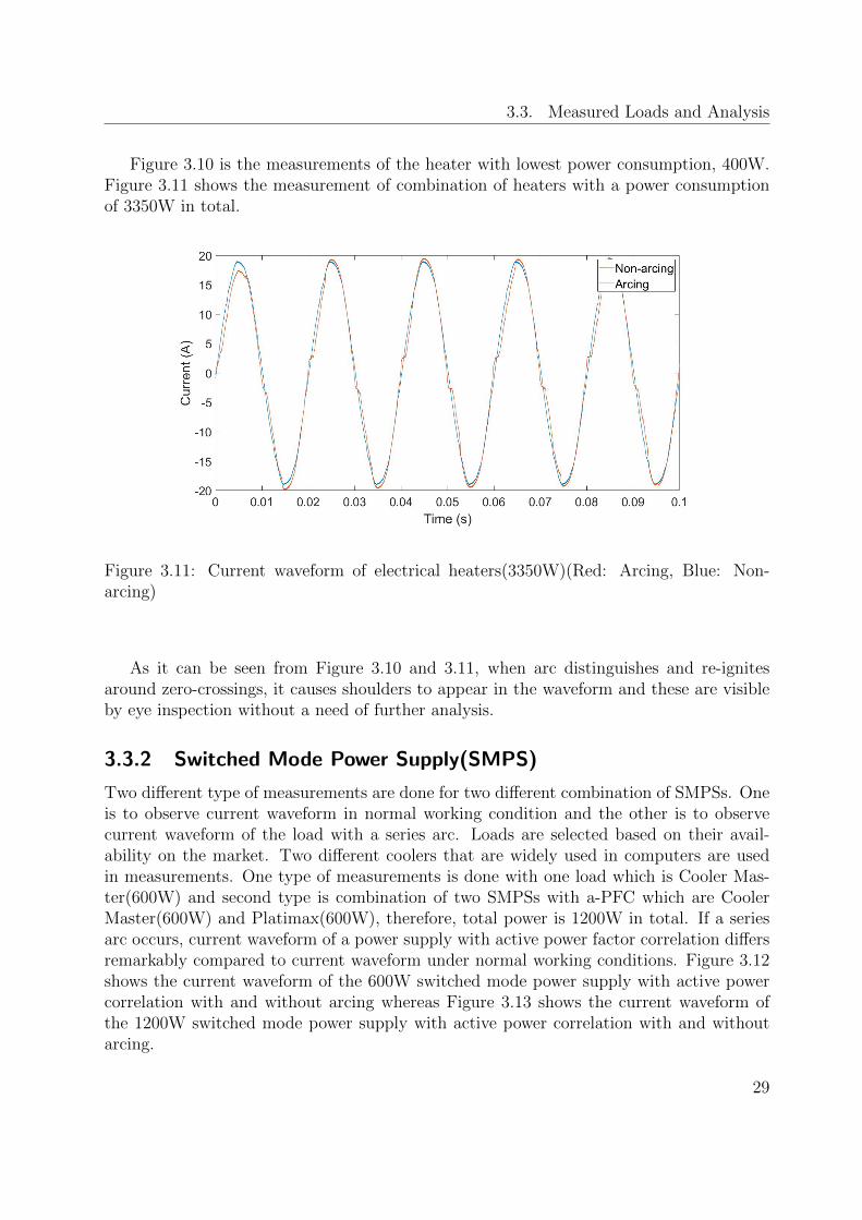
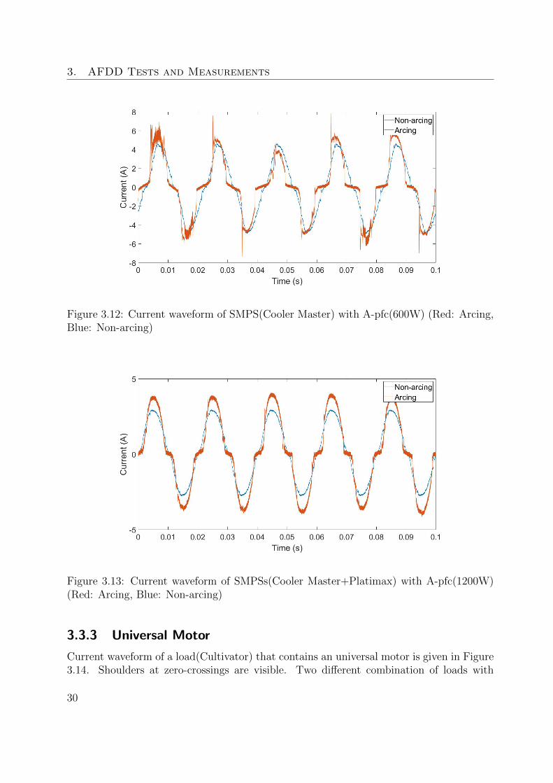
Two different type of measurements are done for two different combination of SMPSs. Oneis to observe current waveform in normal working condition and the other is to observecurrent waveform of the load with a series arc. Loads are selected based on their avail-ability on the market. Two different coolers that are widely used in computers are usedin measurements. One type of measurements is done with one load which is Cooler Mas-ter(600W) and second type is combination of two SMPSs with a-PFC which are CoolerMaster(600W) and Platimax(600W), therefore, total power is 1200W in total. If a seriesarc occurs, current waveform of a power supply with active power factor correlation differsremarkably compared to current waveform under normal working conditions. Figure 3.12shows the current waveform of the 600W switched mode power supply with active powercorrelation with and without arcing whereas Figure 3.13 shows the current waveform ofthe 1200W switched mode power supply with active power correlation with and withoutarcing.
29
3. AFDD Tests and Measurements
Figure 3.12: Current waveform of SMPS(Cooler Master) with A-pfc(600W) (Red: Arcing,Blue: Non-arcing)
Figure 3.13: Current waveform of SMPSs(Cooler Master+Platimax) with A-pfc(1200W)(Red: Arcing, Blue: Non-arcing)
3.3.3 Universal Motor
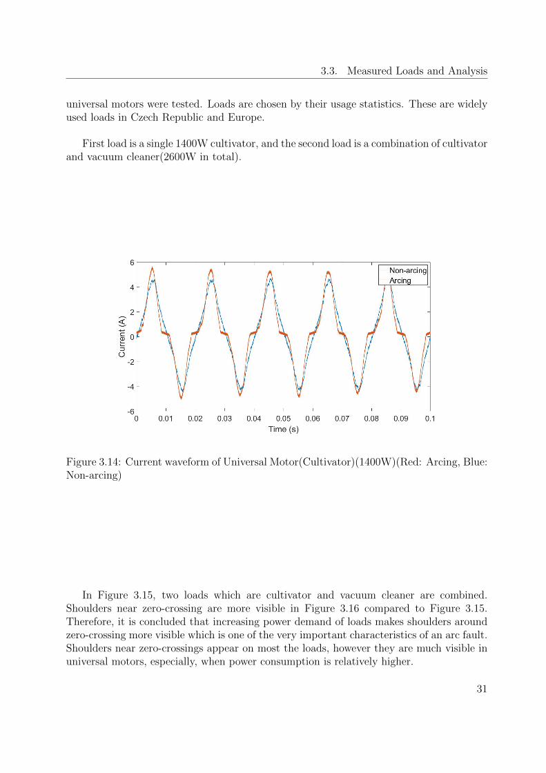
Current waveform of a load(Cultivator) that contains an universal motor is given in Figure3.14. Shoulders at zero-crossings are visible. Two different combination of loads with
30
3.3. Measured Loads and Analysis
universal motors were tested. Loads are chosen by their usage statistics. These are widelyused loads in Czech Republic and Europe.
First load is a single 1400W cultivator, and the second load is a combination of cultivatorand vacuum cleaner(2600W in total).
Figure 3.14: Current waveform of Universal Motor(Cultivator)(1400W)(Red: Arcing, Blue:Non-arcing)
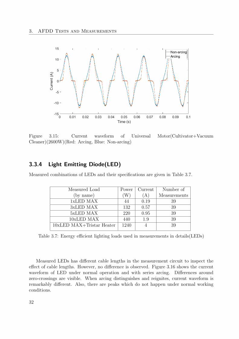
In Figure 3.15, two loads which are cultivator and vacuum cleaner are combined.Shoulders near zero-crossing are more visible in Figure 3.16 compared to Figure 3.15.Therefore, it is concluded that increasing power demand of loads makes shoulders aroundzero-crossing more visible which is one of the very important characteristics of an arc fault.Shoulders near zero-crossings appear on most the loads, however they are much visible inuniversal motors, especially, when power consumption is relatively higher.
31
3. AFDD Tests and Measurements
Figure 3.15: Current waveform of Universal Motor(Cultivator+VacuumCleaner)(2600W)(Red: Arcing, Blue: Non-arcing)
3.3.4 Light Emitting Diode(LED)
Measured combinations of LEDs and their specifications are given in Table 3.7.
Measured Load Power Current Number of(by name) (W) (A) Measurements
1xLED MAX 44 0.19 393xLED MAX 132 0.57 395xLED MAX 220 0.95 3910xLED MAX 440 1.9 39
10xLED MAX+Tristar Heater 1240 4 39
Table 3.7: Energy efficient lighting loads used in measurements in details(LEDs)
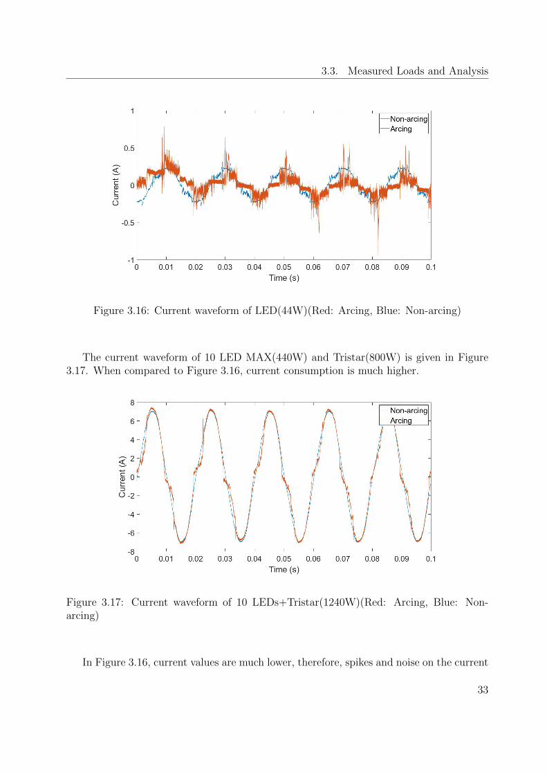
Measured LEDs has different cable lengths in the measurement circuit to inspect theeffect of cable lengths. However, no difference is observed. Figure 3.16 shows the currentwaveform of LED under normal operation and with series arcing. Differences aroundzero-crossings are visible. When arcing distinguishes and reignites, current waveform isremarkably different. Also, there are peaks which do not happen under normal workingconditions.
32
3.3. Measured Loads and Analysis
Figure 3.16: Current waveform of LED(44W)(Red: Arcing, Blue: Non-arcing)
The current waveform of 10 LED MAX(440W) and Tristar(800W) is given in Figure3.17. When compared to Figure 3.16, current consumption is much higher.
Figure 3.17: Current waveform of 10 LEDs+Tristar(1240W)(Red: Arcing, Blue: Non-arcing)
In Figure 3.16, current values are much lower, therefore, spikes and noise on the current
33
3. AFDD Tests and Measurements
waveform is more visible. It is concluded that arcing causes remarkable changes in currentwaveforms. That is also why LEDs have good classification rates that explained in Section5 in detail.
3.3.5 Fluorescent Lamps
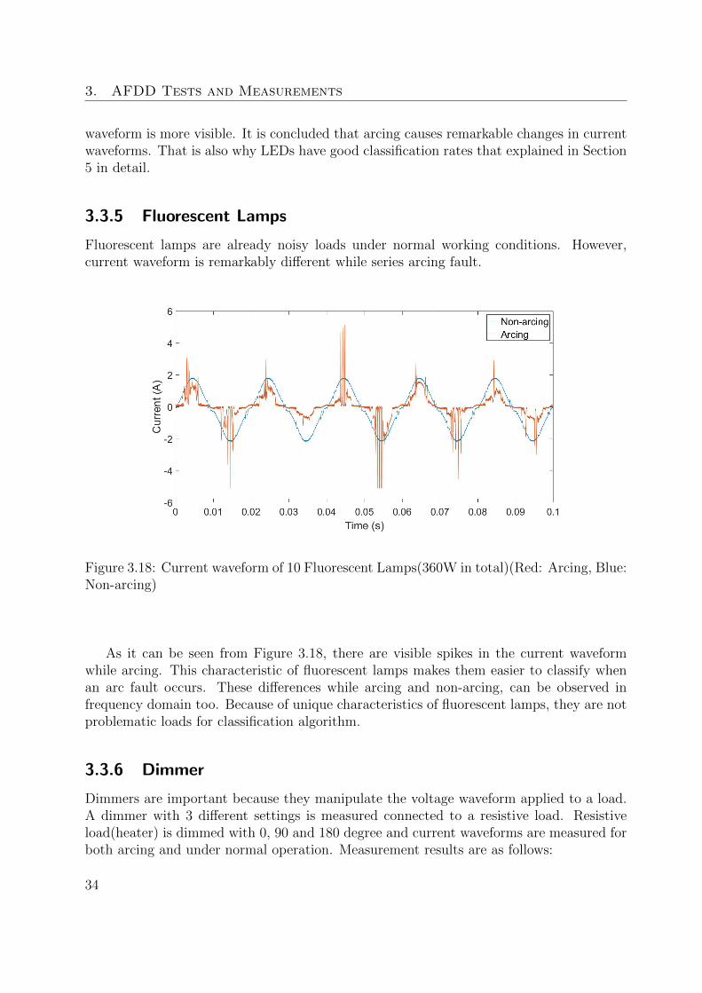
Fluorescent lamps are already noisy loads under normal working conditions. However,current waveform is remarkably different while series arcing fault.
Figure 3.18: Current waveform of 10 Fluorescent Lamps(360W in total)(Red: Arcing, Blue:Non-arcing)
As it can be seen from Figure 3.18, there are visible spikes in the current waveformwhile arcing. This characteristic of fluorescent lamps makes them easier to classify whenan arc fault occurs. These differences while arcing and non-arcing, can be observed infrequency domain too. Because of unique characteristics of fluorescent lamps, they are notproblematic loads for classification algorithm.
3.3.6 Dimmer
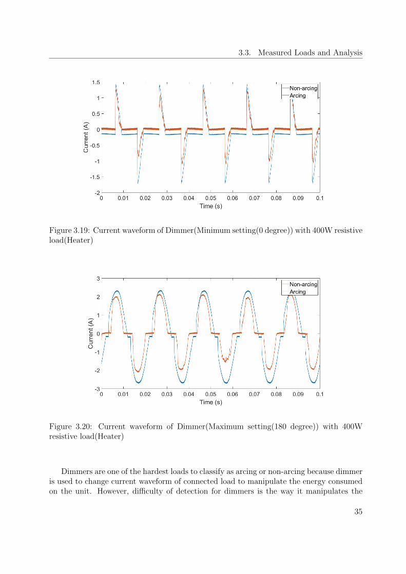
Dimmers are important because they manipulate the voltage waveform applied to a load.A dimmer with 3 different settings is measured connected to a resistive load. Resistiveload(heater) is dimmed with 0, 90 and 180 degree and current waveforms are measured forboth arcing and under normal operation. Measurement results are as follows:
34
3.3. Measured Loads and Analysis
Figure 3.19: Current waveform of Dimmer(Minimum setting(0 degree)) with 400W resistiveload(Heater)
Figure 3.20: Current waveform of Dimmer(Maximum setting(180 degree)) with 400Wresistive load(Heater)
Dimmers are one of the hardest loads to classify as arcing or non-arcing because dimmeris used to change current waveform of connected load to manipulate the energy consumedon the unit. However, difficulty of detection for dimmers is the way it manipulates the
35

3. AFDD Tests and Measurements
current waveform. Dimmed resistive load’s current waveform and current waveform undernormal operation of resistive loads are very similar as it can be seen from Figure 3.19 andFigure 3.20. Although there are differences while arcing and normal operation, generalcharacteristics are similar and it is another reason that makes dimmers hard to classifywhile arcing.
36
Chapter 4
Direct Digitization Approach
In this chapter, novel detection methodology that consists of direct digitization and super-vised machine learning algorithms is introduced. Fundamentals of support vector machineis presented. Generation of feature space and feature selection algorithms are explained.Performance metrics are specified.
Existing arc fault detection methods are based on high frequency analog front endmonitoring/conditioning circuit combined with a microprocessor. Analog front end is de-signed to monitor and to detect specific noise characteristics in different bands in frequencyspectrum. The information used in analog front end is heuristically found and then imple-mented on the analog circuit.
Existing algorithms used in detection are well established and are optimized to detectmost of the arc faults successfully. Also, they are designed in a way to distinguish betweenhazardous and non-hazardous sparks in the circuit. However, introduction of new kinds ofloads, cheap and noisy components or power line communication devices cause robustnessissues. Robustness issues result in either nuisance tripping that causes economical lossbecause the circuit is de-energized unnecessarily, whereas not tripping when it is necessarycauses lack of protection.
Price of high speed acquisition devices are decreasing constantly in recent years andthey are expected to be cheaper in the future. In the light of this knowledge, it becomesfeasible to employ direct digitization instead of analog front end since the same informationused in analog circuits is also achievable by direct digitization. Using direct digitizationhas advantages compared to analog front end. It is easier to modify detection algorithmsand it gives more freedom on signal processing. Since more types of information can begathered using direct digitization, it allows a various number of algorithms to implement fordetection. However, analog circuit based solutions are much cheaper to produce therefore,analog front end is more feasible as of today for industrial usage.
37
4. Direct Digitization Approach
To analyze and to design an algorithm for arc fault detection, arc faults needs to beinvestigated in detail. There are two possible ways to achieve deep understanding of arcingphenomena. The first way is to construct an arc model which requires deep understandingof arc phenomena, therefore, highly skilled human resource and time. The second way is touse real measurements explained in chapter 3. Using real measurements is more suitablemethodology for the context of this thesis because arc model is already a complex taskitself to complete in limited time whereas using measurements are easier, much faster andmore accurate for the measured load types.
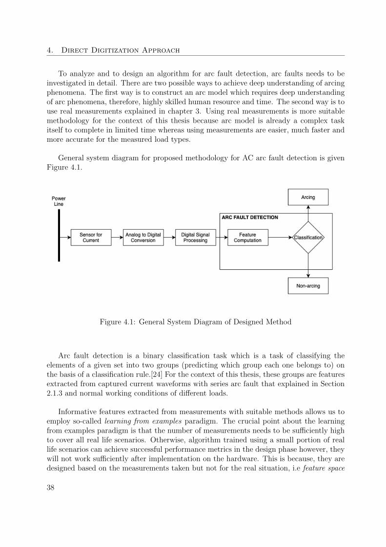
General system diagram for proposed methodology for AC arc fault detection is givenFigure 4.1.
Figure 4.1: General System Diagram of Designed Method
Arc fault detection is a binary classification task which is a task of classifying theelements of a given set into two groups (predicting which group each one belongs to) onthe basis of a classification rule.[24] For the context of this thesis, these groups are featuresextracted from captured current waveforms with series arc fault that explained in Section2.1.3 and normal working conditions of different loads.
Informative features extracted from measurements with suitable methods allows us toemploy so-called learning from examples paradigm. The crucial point about the learningfrom examples paradigm is that the number of measurements needs to be sufficiently highto cover all real life scenarios. Otherwise, algorithm trained using a small portion of reallife scenarios can achieve successful performance metrics in the design phase however, theywill not work sufficiently after implementation on the hardware. This is because, they aredesigned based on the measurements taken but not for the real situation, i.e feature space
38
is not sufficiently rich. Therefore, quality and number of measurements have a crucialimportance for success rates of designed algorithms for the implementation phase.
Feature extraction is another crucial task to design a successful classifier. It is alsocrucial in the phase of implementation on hardware . It is because if suitable features arenot selected from feature space, namely all the bandwidth used for detection, detectionalgorithm works with both informative and uninformative data, therefore it is needed toprocess more data then necessary. It is not feasible in terms of computational complexityand it has other drawbacks such as:
1. It decreases accuracy of machine learning algorithm
2. It increases training time
3. It can cause overfitting
These drawbacks and benefits are investigated in more detail in section 4.2.1.
For the context of arc fault detection algorithm, selection of features simply meansselection of proper bands that can be informative enough for classification. This is one ofthe main purposes of this thesis because an algorithm that is capable of choosing informat-ive bands automatically for classification will ease the design of future algorithms, whereascurrent designs are based on expert knowledge and heuristic data. Proposed metaheuristicsare investigated in section 4.2.1.1 and 4.2.1.2.
The goal of binary classification task is to learn a function F (x) that minimizes themisclassification probability P{yF (x) < 0}, where y is the class label with + 1 for positiveand 1 for negative. [29] There are numerous effectual binary classification algorithms suchas kernel methods[30] , ensemble methods[31] , and deep learning methods[32] . Supportvector machine, SVM,[33] is a powerful kernel method. Boosting, [34],[35] and randomforest (RF) [36] fall into ensemble methods. Deep learning methods are based on artificialneural networks (ANNs) [37].
According to [65], k-nearest neighbors algorithm (k-NN) is a non-parametric methodused for classification and regression. [64]. The input consists of the k closest trainingexamples in the feature space. The output is a class membership. An object is classifiedby a plurality vote of its neighbors, with the object being assigned to the class most commonamong its k nearest neighbors where k is a positive integer.[65]
All classification techniques mentioned above have advantages and disadvantages. Theseadvantages and disadvantages have been taken into consideration according to the analyzeddata. SVM, which is introduced in more detail in section 4.1, performed well for a wide
39
4. Direct Digitization Approach
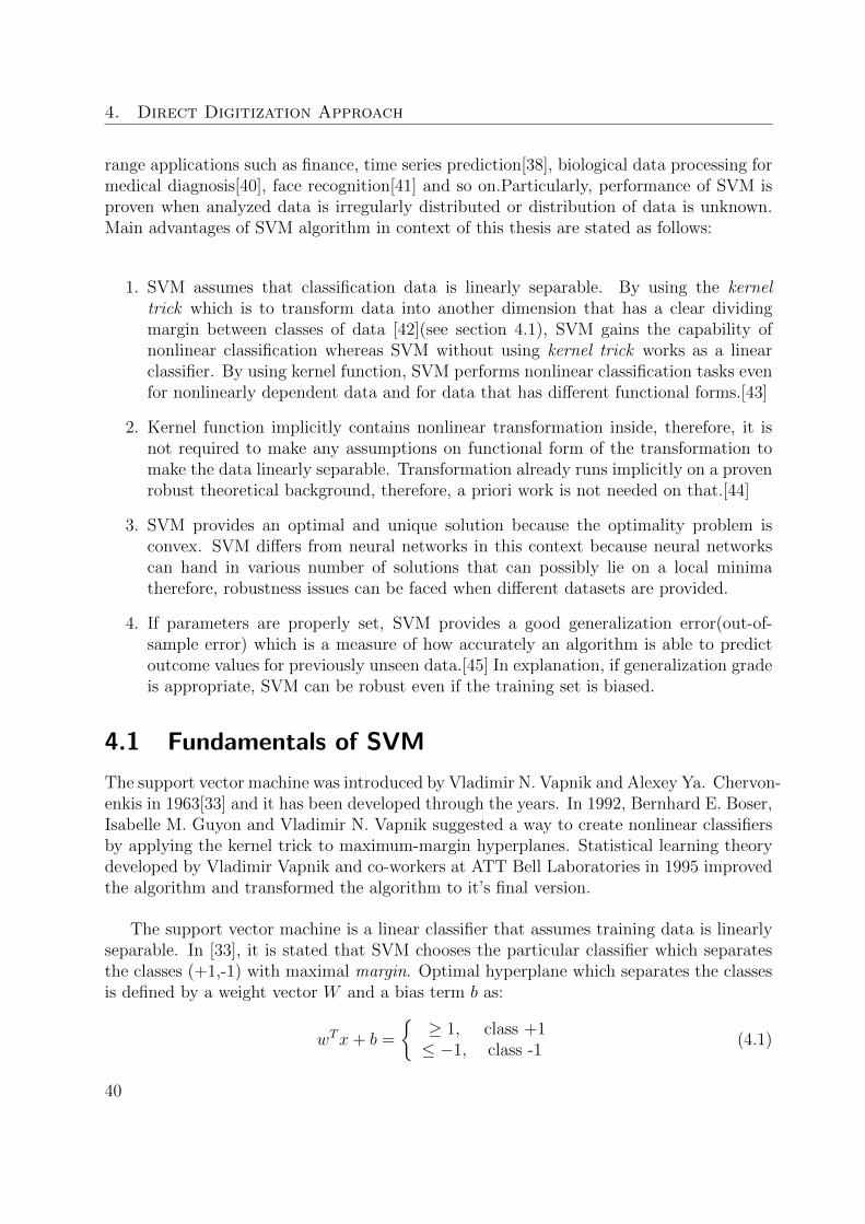
range applications such as finance, time series prediction[38], biological data processing formedical diagnosis[40], face recognition[41] and so on.Particularly, performance of SVM isproven when analyzed data is irregularly distributed or distribution of data is unknown.Main advantages of SVM algorithm in context of this thesis are stated as follows:
1. SVM assumes that classification data is linearly separable. By using the kerneltrick which is to transform data into another dimension that has a clear dividingmargin between classes of data [42](see section 4.1), SVM gains the capability ofnonlinear classification whereas SVM without using kernel trick works as a linearclassifier. By using kernel function, SVM performs nonlinear classification tasks evenfor nonlinearly dependent data and for data that has different functional forms.[43]
2. Kernel function implicitly contains nonlinear transformation inside, therefore, it isnot required to make any assumptions on functional form of the transformation tomake the data linearly separable. Transformation already runs implicitly on a provenrobust theoretical background, therefore, a priori work is not needed on that.[44]
3. SVM provides an optimal and unique solution because the optimality problem isconvex. SVM differs from neural networks in this context because neural networkscan hand in various number of solutions that can possibly lie on a local minimatherefore, robustness issues can be faced when different datasets are provided.
4. If parameters are properly set, SVM provides a good generalization error(out-of-sample error) which is a measure of how accurately an algorithm is able to predictoutcome values for previously unseen data.[45] In explanation, if generalization gradeis appropriate, SVM can be robust even if the training set is biased.
4.1 Fundamentals of SVM
The support vector machine was introduced by Vladimir N. Vapnik and Alexey Ya. Chervon-enkis in 1963[33] and it has been developed through the years. In 1992, Bernhard E. Boser,Isabelle M. Guyon and Vladimir N. Vapnik suggested a way to create nonlinear classifiersby applying the kernel trick to maximum-margin hyperplanes. Statistical learning theorydeveloped by Vladimir Vapnik and co-workers at ATT Bell Laboratories in 1995 improvedthe algorithm and transformed the algorithm to it’s final version.
The support vector machine is a linear classifier that assumes training data is linearlyseparable. In [33], it is stated that SVM chooses the particular classifier which separatesthe classes (+1,-1) with maximal margin. Optimal hyperplane which separates the classesis defined by a weight vector W and a bias term b as:
wTx+ b =
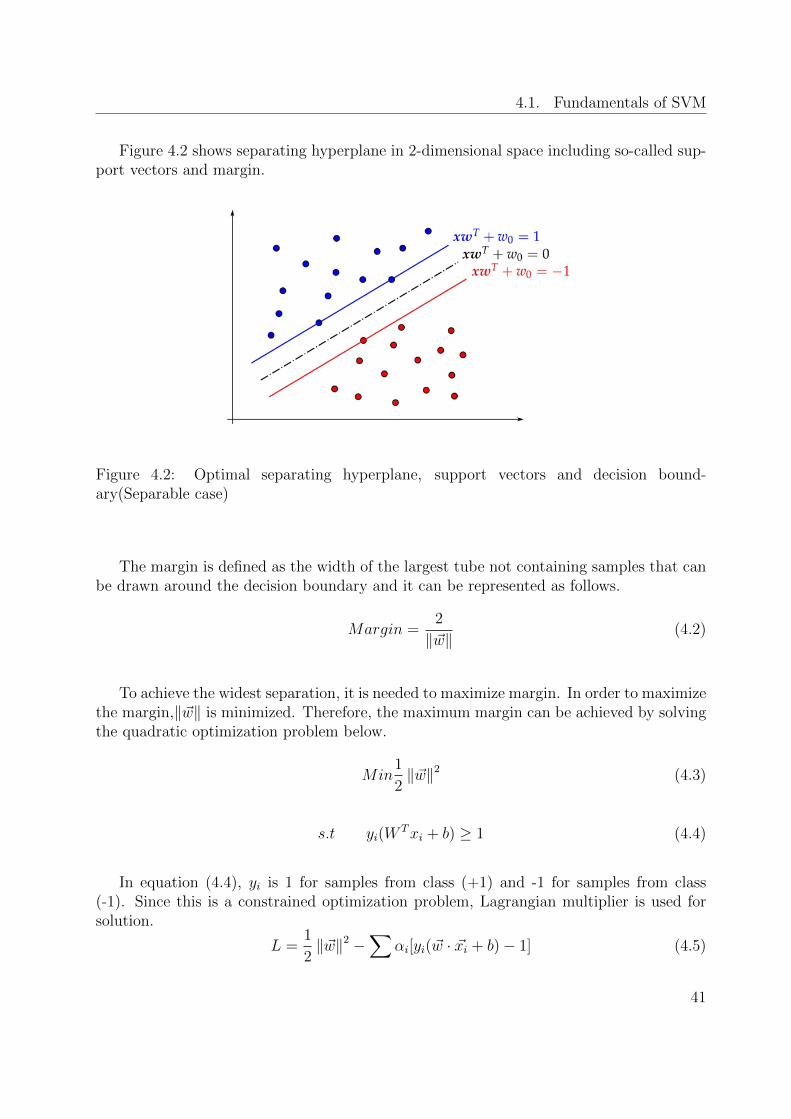
{≥ 1, class +1≤ −1, class -1
(4.1)
40
4.1. Fundamentals of SVM
Figure 4.2 shows separating hyperplane in 2-dimensional space including so-called sup-port vectors and margin.
Figure 4.2: Optimal separating hyperplane, support vectors and decision bound-ary(Separable case)
The margin is defined as the width of the largest tube not containing samples that canbe drawn around the decision boundary and it can be represented as follows.
Margin =2
‖~w‖(4.2)
To achieve the widest separation, it is needed to maximize margin. In order to maximizethe margin,‖~w‖ is minimized. Therefore, the maximum margin can be achieved by solvingthe quadratic optimization problem below.
Min1
2‖~w‖2 (4.3)
s.t yi(WTxi + b) ≥ 1 (4.4)
In equation (4.4), yi is 1 for samples from class (+1) and -1 for samples from class(-1). Since this is a constrained optimization problem, Lagrangian multiplier is used forsolution.
L =1
2‖~w‖2 −
∑αi[yi(~w · ~xi + b)− 1] (4.5)
41
4. Direct Digitization Approach
∂L
∂ ~w= ~w −
∑αiyixi = 0 =⇒ ~w =
∑i
αiyixi (4.6)
∂L
∂b= −
∑αiyi = 0 =⇒
∑i
αiyi = 0 (4.7)
If equation (4.6) and (4.7) are inserted into (4.5). L is as follows where αi is Lagrangianmultiplier.
L =∑i
αi −1
2
∑∑αiαjyiyjxixj where αi ≥ 0 (4.8)
Equation (4.9) shows that optimization depends on only dot product of pairs of samplesxixj because the other terms in the equation are constant. By inserting the findings in(4.6) and (4.7) into decision rule (4.1), following decision rule is obtained where every termexcept ~xi~u are constant.
∑αiyi~xi~ui + b =
{≥ 1, class +1≤ −1, class -1
(4.9)
When optimization problem is solved, training points with α∗i > 0 are the supportvectors(SVs), and w∗ is calculated as follows:
w∗ =∑i
α∗i yixi (4.10)
Kernel function is used to add the ability of making nonlinear classification to SVMs.Kernels are used to map the input data to a new multidimensional space. Feature vectorsare mapped into the new image space by using mapping K. SVM performs linear clas-sification task in the newly mapped image space, however, this corresponds to nonlinearclassification in the original space. Widely used kernel functions are given as follows:
1. Polynomial Kernel: K(xi, xj) = (xi · xj + 1)p
2. Radial Basis Function Kernel: K(xi, xj) = e−γ‖xi−xj‖2
where γ > 0
3. Sigmoid Kernel: K(xi, xj) = tanh(ηxi · xj + v)
42
4.2. Feature Extraction
4.2 Feature Extraction
In order to process the data and to investigate the noise characteristics of different loadsin normal working condition and with an arc fault; as well as to construct a suitablefeature space to train machine learning algorithms, it is needed to process the data whichis current waveforms of loads. Domain of analysis is important since the quality, namelyinformativeness of feature space is important. Following domains can be employed to createthe feature space for the machine learning algorithms.
1. Time-domain
2. Frequency Domain
3. Time-frequency Domain
There are numerous papers in literature that propose a detection algorithm using eachof the three domains above. [47], [48], [49] [50] propose frequency domain based approachesfor different applications. [47], uses FFT to obtain signal energy and calculates the changein it for arc faults in photo-voltaic systems. This approach is similar to the approach appliedin this thesis with a difference in analysis of band selection and detection methodology.In this thesis, given approach to determine the frequency bands are done using featureselection algorithms in section 4.2.1.
[48], proposes a method for arc fault detection using FFT and wavelet packet decom-position. The drawback of using FFT is stated as an inherent trade-off between time andfrequency resolution. Using FFT also gives global frequency components of a signal withouttime information.[48] In order to have a better resolution of frequency, the time windowneeds to be extended while the sampling frequency is fixed. The most crucial finding ofthis paper is the duration of the time window for FFT, which is stated as 200 ms basedon extensive analysis. Therefore, it has to be taken into consideration while designing thedetection algorithm because longer time used for signal processing means there is less timeavailable for the detection algorithm to run. This trade off has be taken into considera-tion in the design process of general detection methodology. Machine learning classifiers,especially SVM, are advantageous from this point of view because although SVM can becomputationally expensive in the training phase, it does not require high computationalpower as a classifier, therefore it is fast compared to most other algorithms proposed inliterature. Therefore, analysis done in [48] contributes to prove feasibility of SVM classifierto use for AC arc fault detection based on frequency domain analysis.
[49] and [50] also uses frequency domain analysis but for DC arc fault detection. Thearc characteristics observed in AC and DC applications has differences however, they alsouse information extracted from current waveforms by applying frequency domain analysis.
43
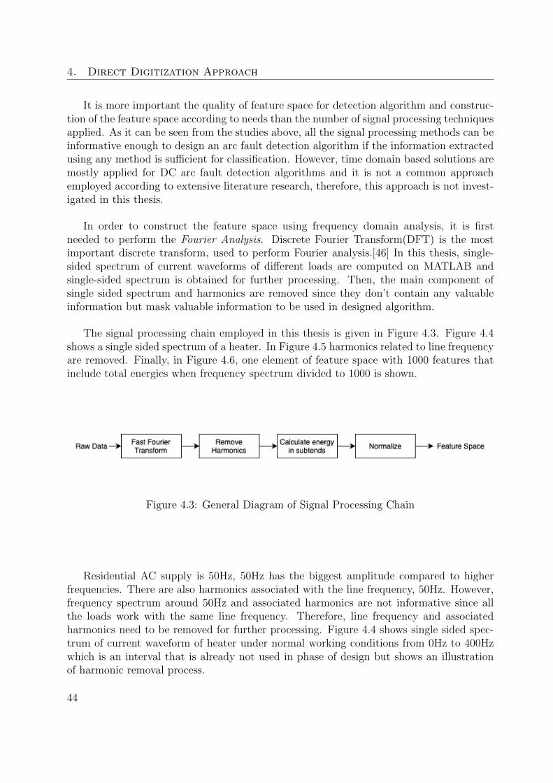
4. Direct Digitization Approach
It is more important the quality of feature space for detection algorithm and construc-tion of the feature space according to needs than the number of signal processing techniquesapplied. As it can be seen from the studies above, all the signal processing methods can beinformative enough to design an arc fault detection algorithm if the information extractedusing any method is sufficient for classification. However, time domain based solutions aremostly applied for DC arc fault detection algorithms and it is not a common approachemployed according to extensive literature research, therefore, this approach is not invest-igated in this thesis.
In order to construct the feature space using frequency domain analysis, it is firstneeded to perform the Fourier Analysis. Discrete Fourier Transform(DFT) is the mostimportant discrete transform, used to perform Fourier analysis.[46] In this thesis, single-sided spectrum of current waveforms of different loads are computed on MATLAB andsingle-sided spectrum is obtained for further processing. Then, the main component ofsingle sided spectrum and harmonics are removed since they don’t contain any valuableinformation but mask valuable information to be used in designed algorithm.
The signal processing chain employed in this thesis is given in Figure 4.3. Figure 4.4shows a single sided spectrum of a heater. In Figure 4.5 harmonics related to line frequencyare removed. Finally, in Figure 4.6, one element of feature space with 1000 features thatinclude total energies when frequency spectrum divided to 1000 is shown.
Figure 4.3: General Diagram of Signal Processing Chain
Residential AC supply is 50Hz, 50Hz has the biggest amplitude compared to higherfrequencies. There are also harmonics associated with the line frequency, 50Hz. However,frequency spectrum around 50Hz and associated harmonics are not informative since allthe loads work with the same line frequency. Therefore, line frequency and associatedharmonics need to be removed for further processing. Figure 4.4 shows single sided spec-trum of current waveform of heater under normal working conditions from 0Hz to 400Hzwhich is an interval that is already not used in phase of design but shows an illustrationof harmonic removal process.
44
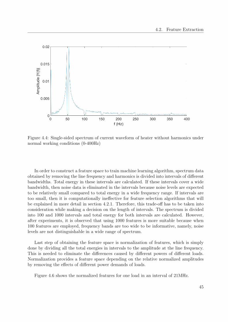
4.2. Feature Extraction
Figure 4.4: Single-sided spectrum of current waveform of heater without harmonics undernormal working conditions (0-400Hz)
In order to construct a feature space to train machine learning algorithm, spectrum dataobtained by removing the line frequency and harmonics is divided into intervals of differentbandwidths. Total energy in these intervals are calculated. If these intervals cover a widebandwidth, then noise data is eliminated in the intervals because noise levels are expectedto be relatively small compared to total energy in a wide frequency range. If intervals aretoo small, then it is computationally ineffective for feature selection algorithms that willbe explained in more detail in section 4.2.1. Therefore, this trade-off has to be taken intoconsideration while making a decision on the length of intervals. The spectrum is dividedinto 100 and 1000 intervals and total energy for both intervals are calculated. However,after experiments, it is observed that using 1000 features is more suitable because when100 features are employed, frequency bands are too wide to be informative, namely, noiselevels are not distinguishable in a wide range of spectrum.
Last step of obtaining the feature space is normalization of features, which is simplydone by dividing all the total energies in intervals to the amplitude at the line frequency.This is needed to eliminate the differences caused by different powers of different loads.Normalization provides a feature space depending on the relative normalized amplitudesby removing the effects of different power demands of loads.
Figure 4.6 shows the normalized features for one load in an interval of 21MHz.
45
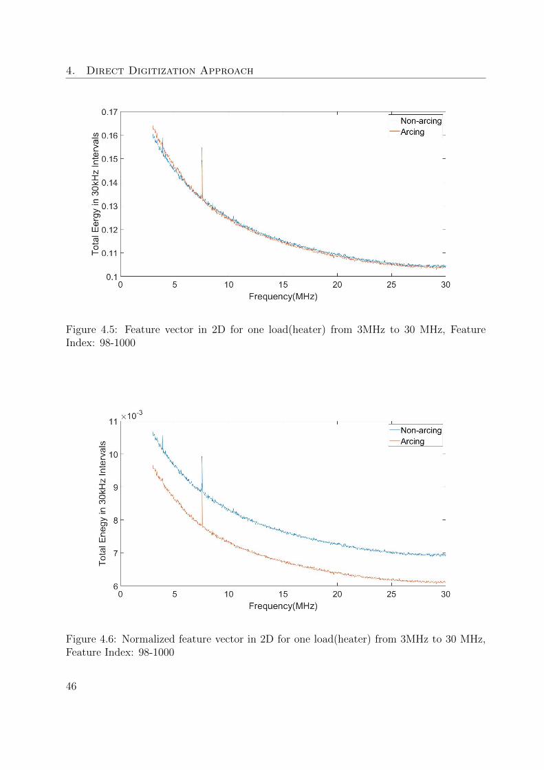
4. Direct Digitization Approach
Figure 4.5: Feature vector in 2D for one load(heater) from 3MHz to 30 MHz, FeatureIndex: 98-1000
Figure 4.6: Normalized feature vector in 2D for one load(heater) from 3MHz to 30 MHz,Feature Index: 98-1000
46
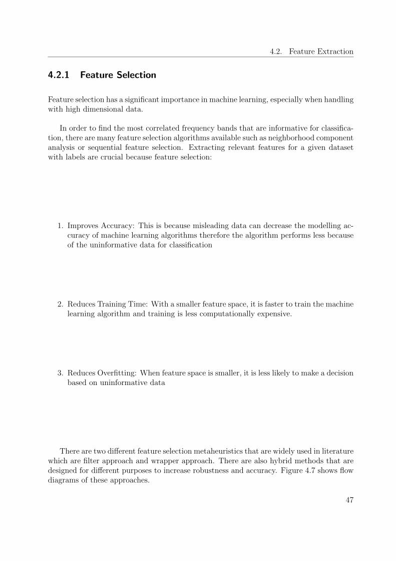
4.2. Feature Extraction
4.2.1 Feature Selection
Feature selection has a significant importance in machine learning, especially when handlingwith high dimensional data.
In order to find the most correlated frequency bands that are informative for classifica-tion, there are many feature selection algorithms available such as neighborhood componentanalysis or sequential feature selection. Extracting relevant features for a given datasetwith labels are crucial because feature selection:
1. Improves Accuracy: This is because misleading data can decrease the modelling ac-curacy of machine learning algorithms therefore the algorithm performs less becauseof the uninformative data for classification
2. Reduces Training Time: With a smaller feature space, it is faster to train the machinelearning algorithm and training is less computationally expensive.
3. Reduces Overfitting: When feature space is smaller, it is less likely to make a decisionbased on uninformative data
There are two different feature selection metaheuristics that are widely used in literaturewhich are filter approach and wrapper approach. There are also hybrid methods that aredesigned for different purposes to increase robustness and accuracy. Figure 4.7 shows flowdiagrams of these approaches.
47
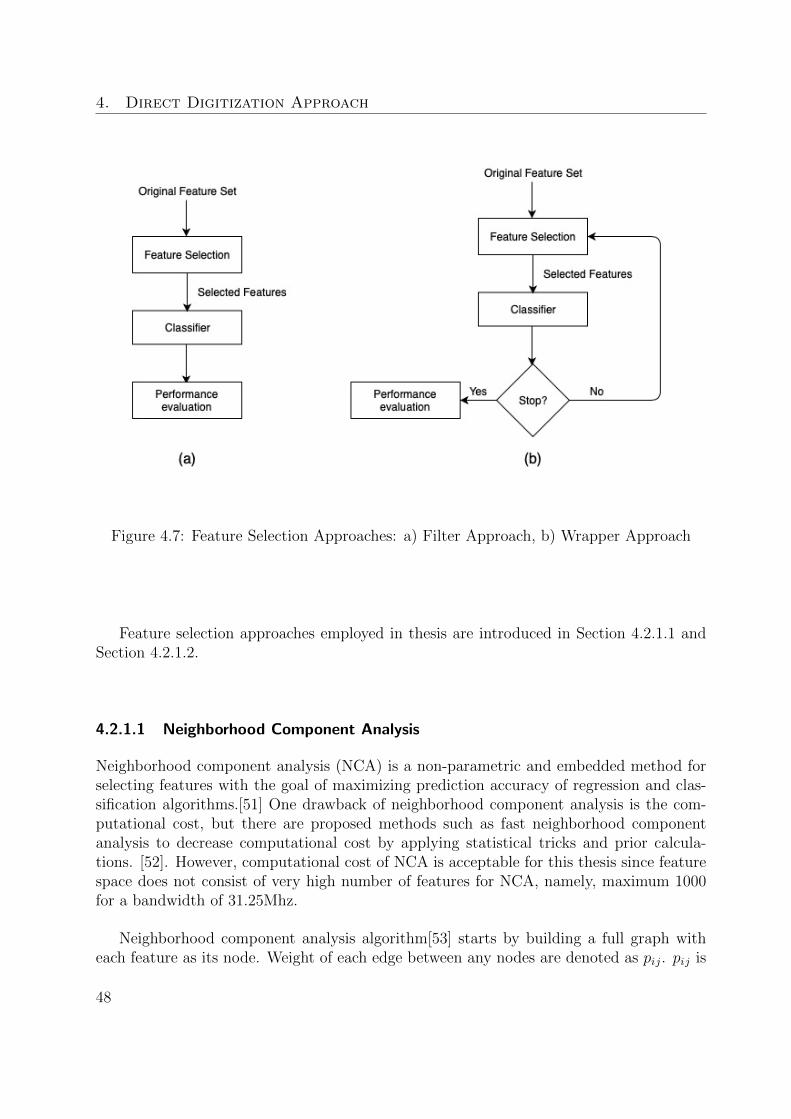
4. Direct Digitization Approach
Figure 4.7: Feature Selection Approaches: a) Filter Approach, b) Wrapper Approach
Feature selection approaches employed in thesis are introduced in Section 4.2.1.1 andSection 4.2.1.2.
4.2.1.1 Neighborhood Component Analysis
Neighborhood component analysis (NCA) is a non-parametric and embedded method forselecting features with the goal of maximizing prediction accuracy of regression and clas-sification algorithms.[51] One drawback of neighborhood component analysis is the com-putational cost, but there are proposed methods such as fast neighborhood componentanalysis to decrease computational cost by applying statistical tricks and prior calcula-tions. [52]. However, computational cost of NCA is acceptable for this thesis since featurespace does not consist of very high number of features for NCA, namely, maximum 1000for a bandwidth of 31.25Mhz.
Neighborhood component analysis algorithm[53] starts by building a full graph witheach feature as its node. Weight of each edge between any nodes are denoted as pij. pij is
48
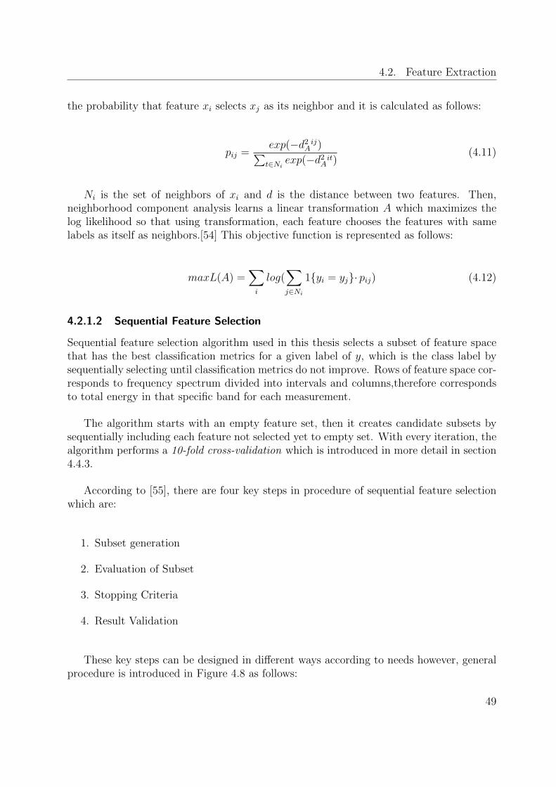
4.2. Feature Extraction
the probability that feature xi selects xj as its neighbor and it is calculated as follows:
pij =exp(−d2Aij)∑t∈Ni
exp(−d2Ait)(4.11)
Ni is the set of neighbors of xi and d is the distance between two features. Then,neighborhood component analysis learns a linear transformation A which maximizes thelog likelihood so that using transformation, each feature chooses the features with samelabels as itself as neighbors.[54] This objective function is represented as follows:
maxL(A) =∑i
log(∑j∈Ni
1{yi = yj}· pij) (4.12)
4.2.1.2 Sequential Feature Selection
Sequential feature selection algorithm used in this thesis selects a subset of feature spacethat has the best classification metrics for a given label of y, which is the class label bysequentially selecting until classification metrics do not improve. Rows of feature space cor-responds to frequency spectrum divided into intervals and columns,therefore correspondsto total energy in that specific band for each measurement.
The algorithm starts with an empty feature set, then it creates candidate subsets bysequentially including each feature not selected yet to empty set. With every iteration, thealgorithm performs a 10-fold cross-validation which is introduced in more detail in section4.4.3.
According to [55], there are four key steps in procedure of sequential feature selectionwhich are:
1. Subset generation
2. Evaluation of Subset
3. Stopping Criteria
4. Result Validation
These key steps can be designed in different ways according to needs however, generalprocedure is introduced in Figure 4.8 as follows:
49
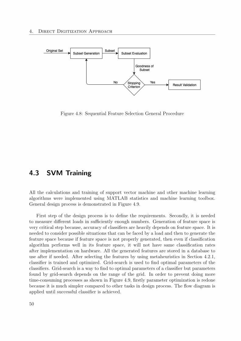
4. Direct Digitization Approach
Figure 4.8: Sequential Feature Selection General Procedure
4.3 SVM Training
All the calculations and training of support vector machine and other machine learningalgorithms were implemented using MATLAB statistics and machine learning toolbox.General design process is demonstrated in Figure 4.9.
First step of the design process is to define the requirements. Secondly, it is neededto measure different loads in sufficiently enough numbers. Generation of feature space isvery critical step because, accuracy of classifiers are heavily depends on feature space. It isneeded to consider possible situations that can be faced by a load and then to generate thefeature space because if feature space is not properly generated, then even if classificationalgorithm performs well in its feature space, it will not have same classification ratesafter implementation on hardware. All the generated features are stored in a database touse after if needed. After selecting the features by using metaheuristics in Section 4.2.1,classifier is trained and optimized. Grid-search is used to find optimal parameters of theclassifiers. Grid-search is a way to find to optimal parameters of a classifier but parametersfound by grid-search depends on the range of the grid. In order to prevent doing moretime-consuming processes as shown in Figure 4.9, firstly parameter optimization is redonebecause it is much simpler compared to other tasks in design process. The flow diagram isapplied until successful classifier is achieved.
50
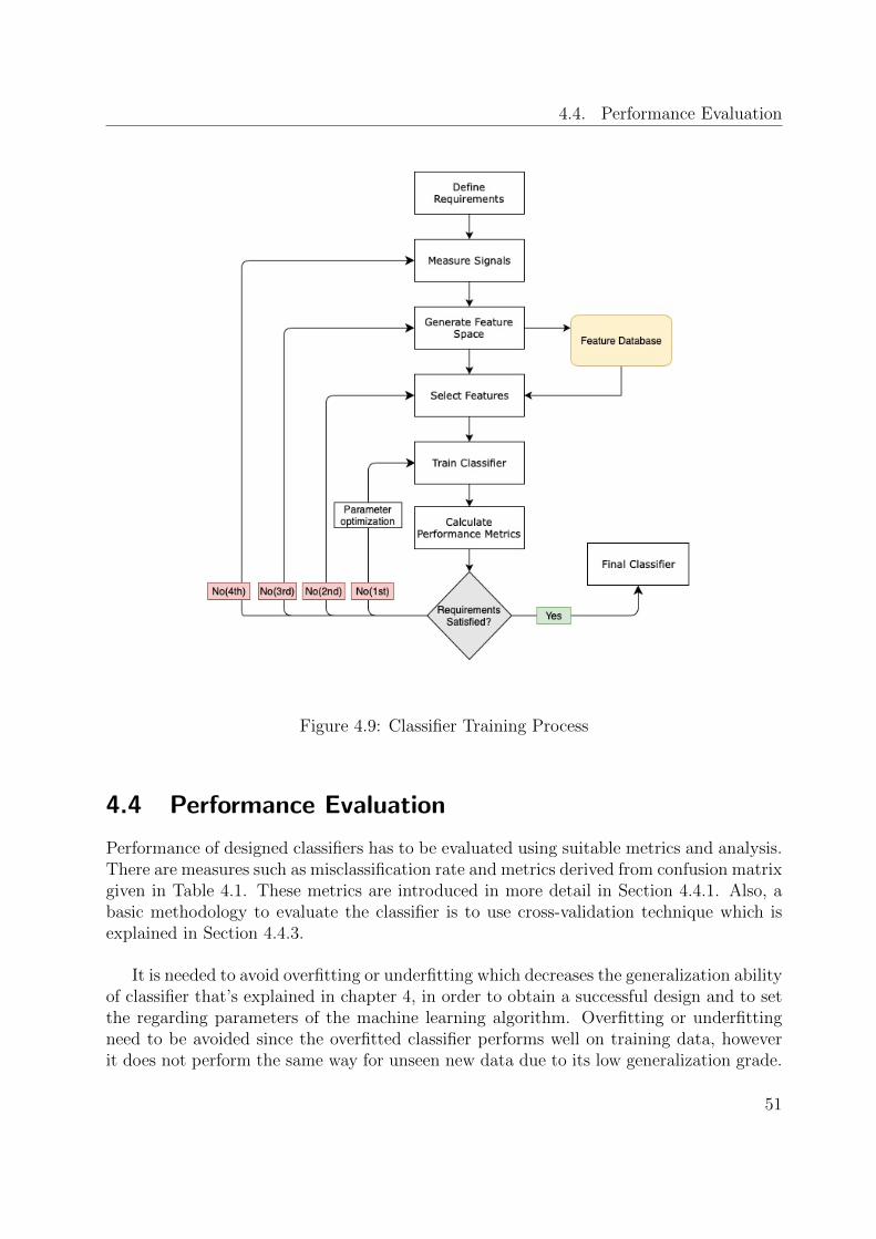
4.4. Performance Evaluation
Figure 4.9: Classifier Training Process
4.4 Performance Evaluation
Performance of designed classifiers has to be evaluated using suitable metrics and analysis.There are measures such as misclassification rate and metrics derived from confusion matrixgiven in Table 4.1. These metrics are introduced in more detail in Section 4.4.1. Also, abasic methodology to evaluate the classifier is to use cross-validation technique which isexplained in Section 4.4.3.
It is needed to avoid overfitting or underfitting which decreases the generalization abilityof classifier that’s explained in chapter 4, in order to obtain a successful design and to setthe regarding parameters of the machine learning algorithm. Overfitting or underfittingneed to be avoided since the overfitted classifier performs well on training data, howeverit does not perform the same way for unseen new data due to its low generalization grade.
51
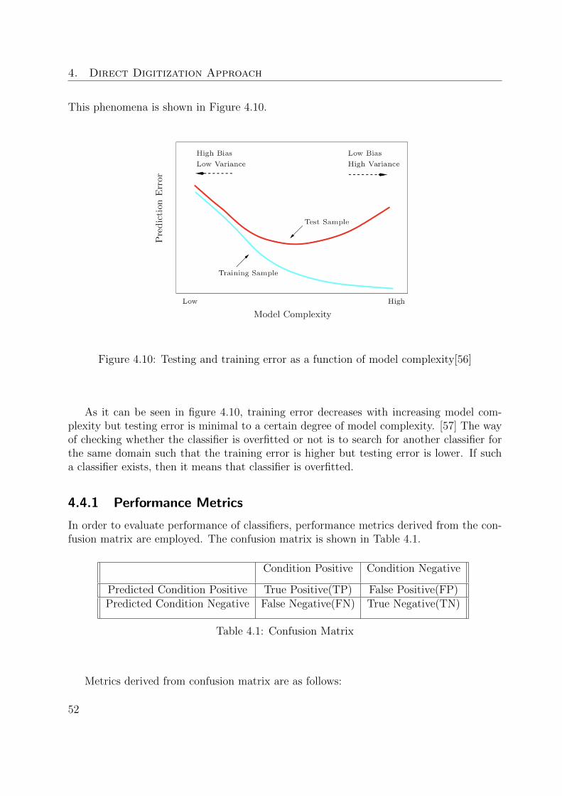
4. Direct Digitization Approach
This phenomena is shown in Figure 4.10.
Figure 4.10: Testing and training error as a function of model complexity[56]
As it can be seen in figure 4.10, training error decreases with increasing model com-plexity but testing error is minimal to a certain degree of model complexity. [57] The wayof checking whether the classifier is overfitted or not is to search for another classifier forthe same domain such that the training error is higher but testing error is lower. If sucha classifier exists, then it means that classifier is overfitted.
4.4.1 Performance Metrics
In order to evaluate performance of classifiers, performance metrics derived from the con-fusion matrix are employed. The confusion matrix is shown in Table 4.1.
Condition Positive Condition Negative
Predicted Condition Positive True Positive(TP) False Positive(FP)Predicted Condition Negative False Negative(FN) True Negative(TN)
Table 4.1: Confusion Matrix
Metrics derived from confusion matrix are as follows:
52
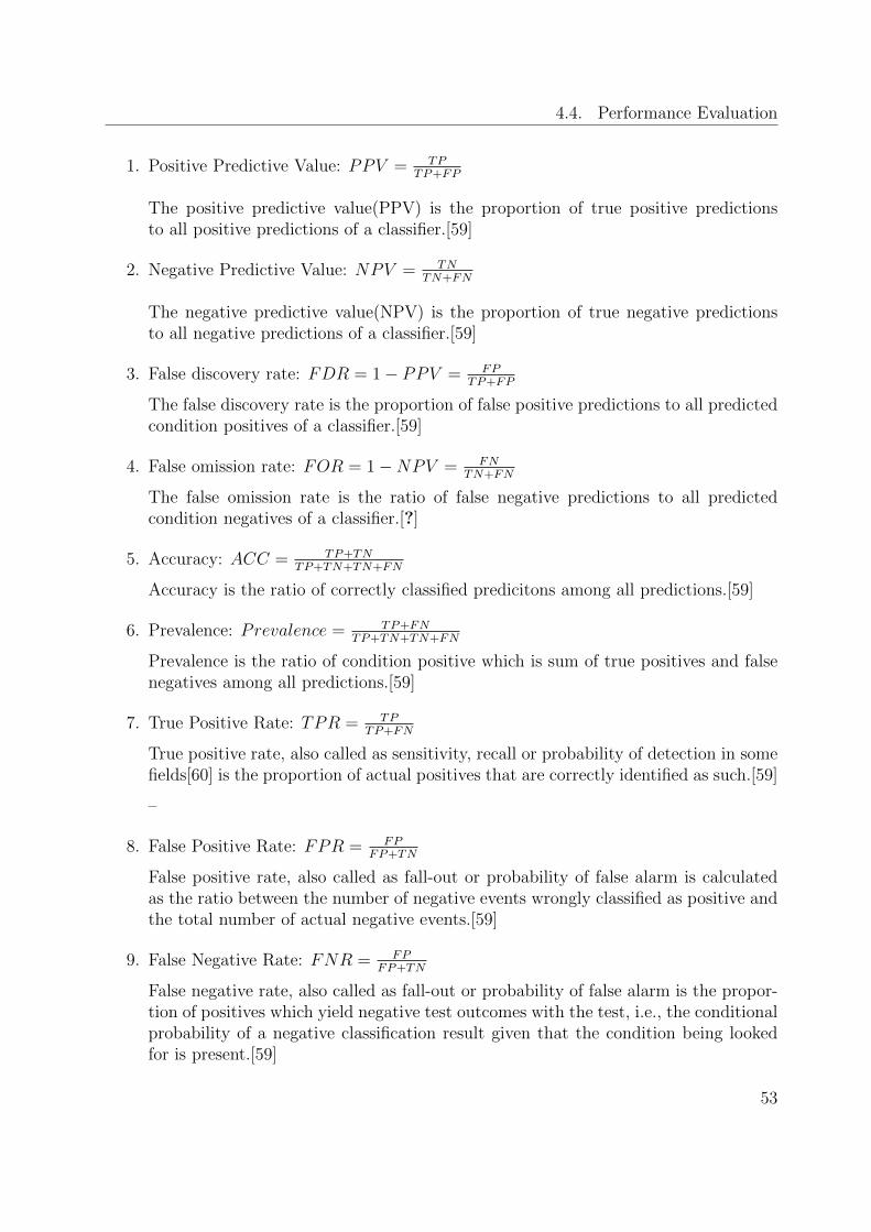
4.4. Performance Evaluation
1. Positive Predictive Value: PPV = TPTP+FP
The positive predictive value(PPV) is the proportion of true positive predictionsto all positive predictions of a classifier.[59]
2. Negative Predictive Value: NPV = TNTN+FN
The negative predictive value(NPV) is the proportion of true negative predictionsto all negative predictions of a classifier.[59]
3. False discovery rate: FDR = 1− PPV = FPTP+FP
The false discovery rate is the proportion of false positive predictions to all predictedcondition positives of a classifier.[59]
4. False omission rate: FOR = 1−NPV = FNTN+FN
The false omission rate is the ratio of false negative predictions to all predictedcondition negatives of a classifier.[?]
5. Accuracy: ACC = TP+TNTP+TN+TN+FN
Accuracy is the ratio of correctly classified predicitons among all predictions.[59]
6. Prevalence: Prevalence = TP+FNTP+TN+TN+FN
Prevalence is the ratio of condition positive which is sum of true positives and falsenegatives among all predictions.[59]
7. True Positive Rate: TPR = TPTP+FN
True positive rate, also called as sensitivity, recall or probability of detection in somefields[60] is the proportion of actual positives that are correctly identified as such.[59]
–
8. False Positive Rate: FPR = FPFP+TN
False positive rate, also called as fall-out or probability of false alarm is calculatedas the ratio between the number of negative events wrongly classified as positive andthe total number of actual negative events.[59]
9. False Negative Rate: FNR = FPFP+TN
False negative rate, also called as fall-out or probability of false alarm is the propor-tion of positives which yield negative test outcomes with the test, i.e., the conditionalprobability of a negative classification result given that the condition being lookedfor is present.[59]
53
4. Direct Digitization Approach
10. True Negative Rate: TNR = FPFP+TN
True negative rate also called as specificity measures the proportion of actual negat-ives that are correctly classified as such (e.g., the percentage of non-arcing waveformsthat are correctly classified as non-arcing).[59]
4.4.2 Cross-validation
According to [11], cross-validation, also called rotation estimation is one of numerous modelvalidation methodologies used to identify how a classifier will generalize to an independentdataset. It is employed in the design process of machine learning algorithms to investigatethe ability of the classifier on unseen data. The way it works is to use a limited subset ofdataset for training, and to test the performance of it on the data reserved for test.
Cross-validation has a single parameter, k, that is the number of folds that a dataset isto be separated into. It is a very popular methodology because it is very simple to employand it gives a better understanding of the classifiers performance compared to simplermethods such as train/test split. [66]
Procedure is as follows:
1. Seperate dataset into k random subsets with same amount of data
2. For each group, take one out as a hold to use as a test set, then use all others as atraining set
3. Train a model using the training set and test it with the test set
4. Record the classifier performance
5. Repeat this procedure from 2nd step for each fold
6. Calculate average loss by averaging k different performance metrics
Each data in the dataset should be assigned to only one group and the group thatparticular data point belongs to should not change through the procedure. This meansthat each data point is used once in testing and k-1 times for training the classifier.
In this thesis, separation of groups are done in a way that all different load types havean equal number of data in the test and training sets. Namely, data is randomly separatedinto groups but subgroups are also taken into consideration.
54
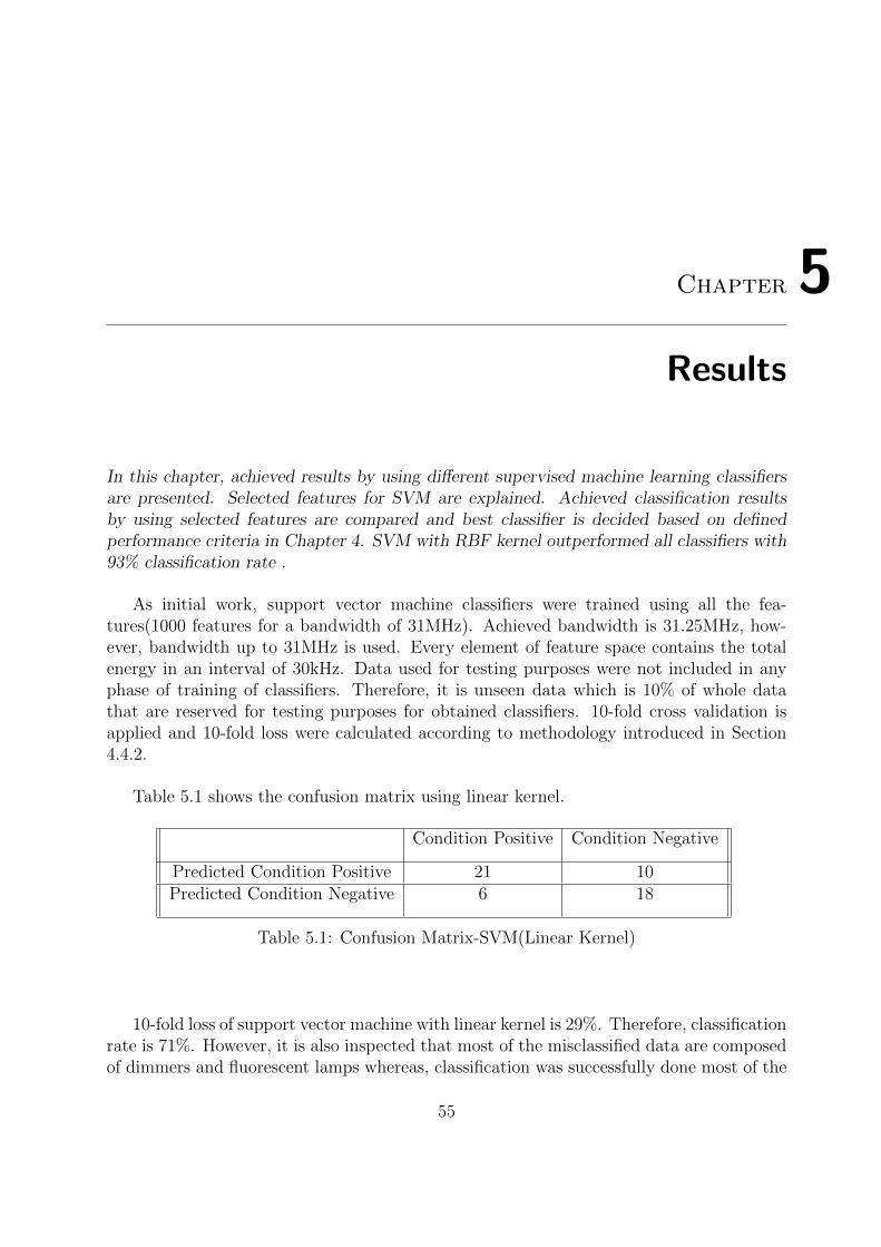
Chapter 5
Results
In this chapter, achieved results by using different supervised machine learning classifiersare presented. Selected features for SVM are explained. Achieved classification resultsby using selected features are compared and best classifier is decided based on definedperformance criteria in Chapter 4. SVM with RBF kernel outperformed all classifiers with93% classification rate .
As initial work, support vector machine classifiers were trained using all the fea-tures(1000 features for a bandwidth of 31MHz). Achieved bandwidth is 31.25MHz, how-ever, bandwidth up to 31MHz is used. Every element of feature space contains the totalenergy in an interval of 30kHz. Data used for testing purposes were not included in anyphase of training of classifiers. Therefore, it is unseen data which is 10% of whole datathat are reserved for testing purposes for obtained classifiers. 10-fold cross validation isapplied and 10-fold loss were calculated according to methodology introduced in Section4.4.2.
Table 5.1 shows the confusion matrix using linear kernel.
Condition Positive Condition Negative
Predicted Condition Positive 21 10Predicted Condition Negative 6 18
Table 5.1: Confusion Matrix-SVM(Linear Kernel)
10-fold loss of support vector machine with linear kernel is 29%. Therefore, classificationrate is 71%. However, it is also inspected that most of the misclassified data are composedof dimmers and fluorescent lamps whereas, classification was successfully done most of the
55
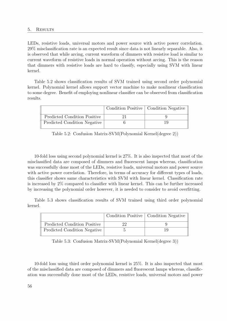
5. Results
LEDs, resistive loads, universal motors and power source with active power correlation.29% misclassification rate is an expected result since data is not linearly separable. Also, itis observed that while arcing, current waveform of dimmers with resistive load is similar tocurrent waveform of resistive loads in normal operation without arcing. This is the reasonthat dimmers with resistive loads are hard to classify, especially using SVM with linearkernel.
Table 5.2 shows classification results of SVM trained using second order polynomialkernel. Polynomial kernel allows support vector machine to make nonlinear classificationto some degree. Benefit of employing nonlinear classifier can be observed from classificationresults.
Condition Positive Condition Negative
Predicted Condition Positive 21 9Predicted Condition Negative 6 19
Table 5.2: Confusion Matrix-SVM(Polynomial Kernel(degree 2))
10-fold loss using second polynomial kernel is 27%. It is also inspected that most of themisclassified data are composed of dimmers and fluorescent lamps whereas, classificationwas successfully done most of the LEDs, resistive loads, universal motors and power sourcewith active power correlation. Therefore, in terms of accuracy for different types of loads,this classifier shows same characteristics with SVM with linear kernel. Classification rateis increased by 2% compared to classifier with linear kernel. This can be further increasedby increasing the polynomial order however, it is needed to consider to avoid overfitting.
Table 5.3 shows classification results of SVM trained using third order polynomialkernel.
Condition Positive Condition Negative
Predicted Condition Positive 22 9Predicted Condition Negative 5 19
Table 5.3: Confusion Matrix-SVM(Polynomial Kernel(degree 3))
10-fold loss using third order polynomial kernel is 25%. It is also inspected that mostof the misclassified data are composed of dimmers and fluorescent lamps whereas, classific-ation was successfully done most of the LEDs, resistive loads, universal motors and power
56
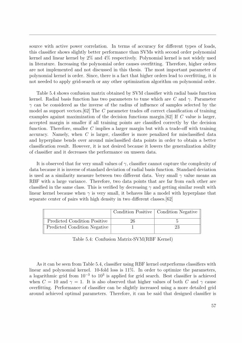
source with active power correlation. In terms of accuracy for different types of loads,this classifier shows slightly better performance than SVMs with second order polynomialkernel and linear kernel by 2% and 4% respectively. Polynomial kernel is not widely usedin literature. Increasing the polynomial order causes overfitting. Therefore, higher ordersare not implemented and not discussed in this thesis. The most important parameter ofpolynomial kernel is order. Since, there is a fact that higher orders lead to overfitting, it isnot needed to apply grid-search or any other optimization algorithm on polynomial order.
Table 5.4 shows confusion matrix obtained by SVM classifier with radial basis functionkernel. Radial basis function has two parameters to tune which are C and γ. Parameterγ can be considered as the inverse of the radius of influence of samples selected by themodel as support vectors.[62] The C parameter trades off correct classification of trainingexamples against maximization of the decision functions margin.[62] If C value is larger,accepted margin is smaller if all training points are classified correctly by the decisionfunction. Therefore, smaller C implies a larger margin but with a trade-off with trainingaccuracy. Namely, when C is larger, classifier is more penalized for misclassified dataand hyperplane bends over around misclassified data points in order to obtain a betterclassification result. However, it is not desired because it lowers the generalization abilityof classifier and it decreases the performance on unseen data.
It is observed that for very small values of γ, classifier cannot capture the complexity ofdata because it is inverse of standard deviation of radial basis function. Standard deviationis used as a similarity measure between two different data. Very small γ value means anRBF with a large variance. Therefore, two data points that are far from each other areclassified in the same class. This is verified by decreasing γ and getting similar result withlinear kernel because when γ is very small, it behaves like a model with hyperplane thatseparate center of pairs with high density in two different classes.[62]
Condition Positive Condition Negative
Predicted Condition Positive 26 5Predicted Condition Negative 1 23
Table 5.4: Confusion Matrix-SVM(RBF Kernel)
As it can be seen from Table 5.4, classifier using RBF kernel outperforms classifiers withlinear and polynomial kernel. 10-fold loss is 11%. In order to optimize the parameters,a logarithmic grid from 10−3 to 103 is applied for grid search. Best classifier is achievedwhen C = 10 and γ = 1. It is also observed that higher values of both C and γ causeoverfitting. Performance of classifier can be slightly increased using a more detailed gridaround achieved optimal parameters. Therefore, it can be said that designed classifier is
57
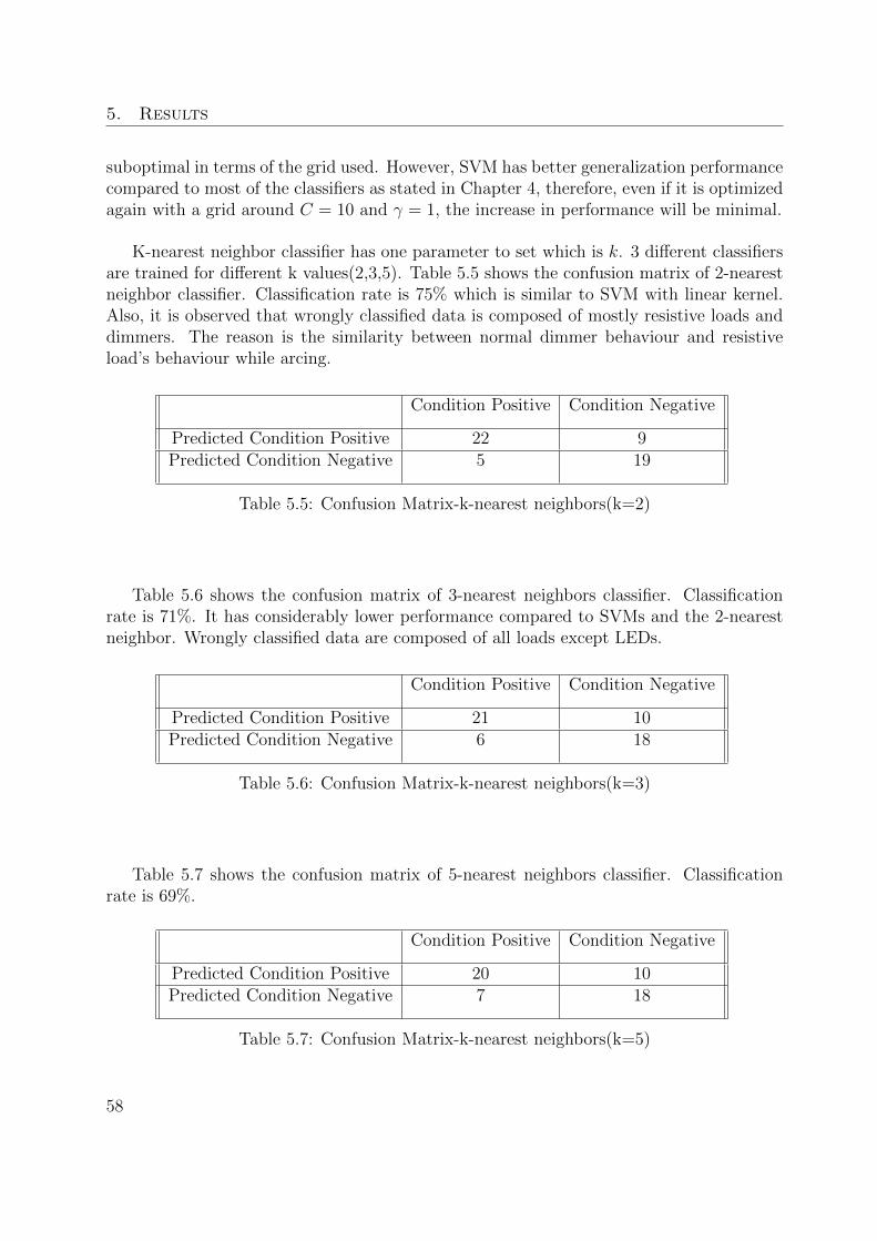
5. Results
suboptimal in terms of the grid used. However, SVM has better generalization performancecompared to most of the classifiers as stated in Chapter 4, therefore, even if it is optimizedagain with a grid around C = 10 and γ = 1, the increase in performance will be minimal.
K-nearest neighbor classifier has one parameter to set which is k. 3 different classifiersare trained for different k values(2,3,5). Table 5.5 shows the confusion matrix of 2-nearestneighbor classifier. Classification rate is 75% which is similar to SVM with linear kernel.Also, it is observed that wrongly classified data is composed of mostly resistive loads anddimmers. The reason is the similarity between normal dimmer behaviour and resistiveload’s behaviour while arcing.
Condition Positive Condition Negative
Predicted Condition Positive 22 9Predicted Condition Negative 5 19
Table 5.5: Confusion Matrix-k-nearest neighbors(k=2)
Table 5.6 shows the confusion matrix of 3-nearest neighbors classifier. Classificationrate is 71%. It has considerably lower performance compared to SVMs and the 2-nearestneighbor. Wrongly classified data are composed of all loads except LEDs.
Condition Positive Condition Negative
Predicted Condition Positive 21 10Predicted Condition Negative 6 18
Table 5.6: Confusion Matrix-k-nearest neighbors(k=3)
Table 5.7 shows the confusion matrix of 5-nearest neighbors classifier. Classificationrate is 69%.
Condition Positive Condition Negative
Predicted Condition Positive 20 10Predicted Condition Negative 7 18
Table 5.7: Confusion Matrix-k-nearest neighbors(k=5)
58
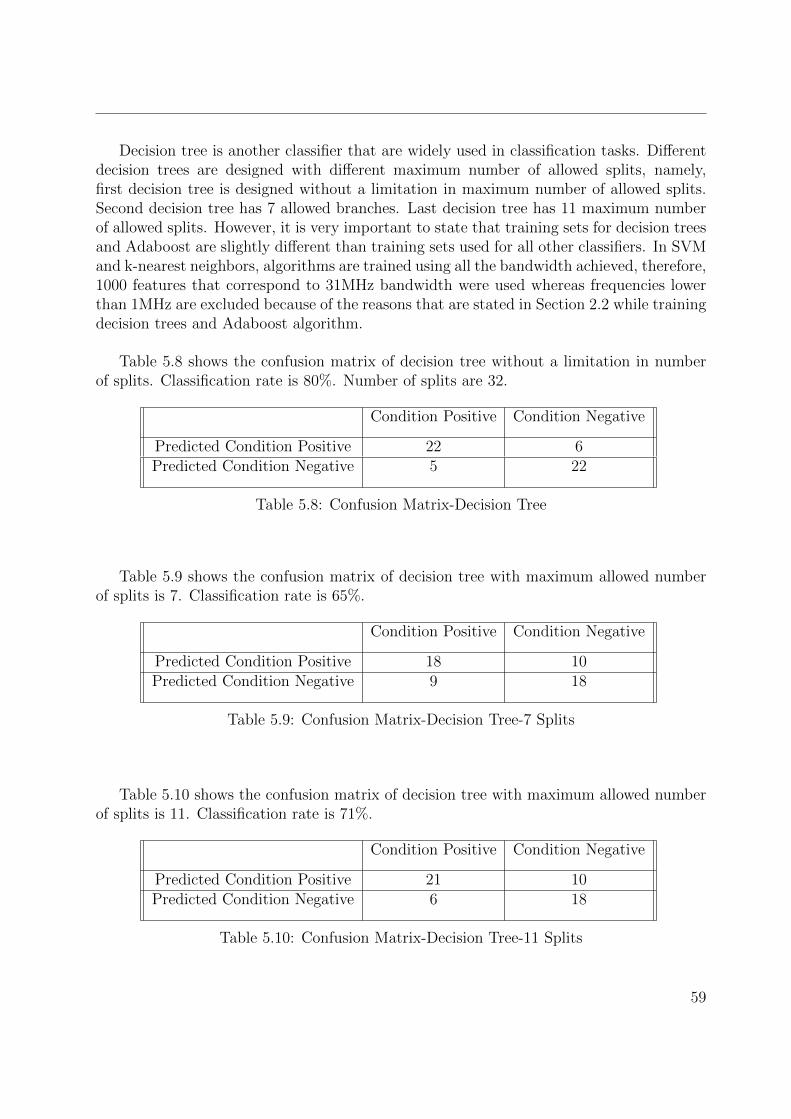
Decision tree is another classifier that are widely used in classification tasks. Differentdecision trees are designed with different maximum number of allowed splits, namely,first decision tree is designed without a limitation in maximum number of allowed splits.Second decision tree has 7 allowed branches. Last decision tree has 11 maximum numberof allowed splits. However, it is very important to state that training sets for decision treesand Adaboost are slightly different than training sets used for all other classifiers. In SVMand k-nearest neighbors, algorithms are trained using all the bandwidth achieved, therefore,1000 features that correspond to 31MHz bandwidth were used whereas frequencies lowerthan 1MHz are excluded because of the reasons that are stated in Section 2.2 while trainingdecision trees and Adaboost algorithm.
Table 5.8 shows the confusion matrix of decision tree without a limitation in numberof splits. Classification rate is 80%. Number of splits are 32.
Condition Positive Condition Negative
Predicted Condition Positive 22 6Predicted Condition Negative 5 22
Table 5.8: Confusion Matrix-Decision Tree
Table 5.9 shows the confusion matrix of decision tree with maximum allowed numberof splits is 7. Classification rate is 65%.
Condition Positive Condition Negative
Predicted Condition Positive 18 10Predicted Condition Negative 9 18
Table 5.9: Confusion Matrix-Decision Tree-7 Splits
Table 5.10 shows the confusion matrix of decision tree with maximum allowed numberof splits is 11. Classification rate is 71%.
Condition Positive Condition Negative
Predicted Condition Positive 21 10Predicted Condition Negative 6 18
Table 5.10: Confusion Matrix-Decision Tree-11 Splits
59
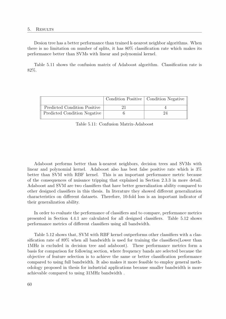
5. Results
Desion tree has a better performance than trained k-nearest neighbor algorithms. Whenthere is no limitation on number of splits, it has 80% classification rate which makes itsperformance better than SVMs with linear and polynomial kernel.
Table 5.11 shows the confusion matrix of Adaboost algorithm. Classification rate is82%.
Condition Positive Condition Negative
Predicted Condition Positive 21 4Predicted Condition Negative 6 24
Table 5.11: Confusion Matrix-Adaboost
Adaboost performs better than k-nearest neighbors, decision trees and SVMs withlinear and polynomial kernel. Adaboost also has best false positive rate which is 3%better than SVM with RBF kernel. This is an important performance metric becauseof the consequences of nuisance tripping that explained in Section 2.3.3 in more detail.Adaboost and SVM are two classifiers that have better generalization ability compared toother designed classifiers in this thesis. In literature they showed different generalizationcharacteristics on different datasets. Therefore, 10-fold loss is an important indicator oftheir generalization ability.
In order to evaluate the performance of classifiers and to compare, performance metricspresented in Section 4.4.1 are calculated for all designed classifiers. Table 5.12 showsperformance metrics of different classifiers using all bandwidth.
Table 5.12 shows that, SVM with RBF kernel outperforms other classifiers with a clas-sification rate of 89% when all bandwidth is used for training the classifiers(Lower than1MHz is excluded in decision tree and adaboost). These performance metrics form abasis for comparison for following section, where frequency bands are selected because theobjective of feature selection is to achieve the same or better classification performancecompared to using full bandwidth. It also makes it more feasible to employ general meth-odology proposed in thesis for industrial applications because smaller bandwidth is moreachievable compared to using 31MHz bandwidth .
60
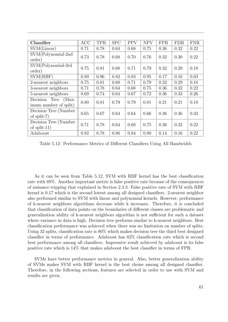
Classifier ACC TPR SPC PPV NPV FPR FDR FNRSVM(Linear) 0.71 0.78 0.64 0.68 0.75 0.36 0.32 0.22SVM(Polynomial-2ndorder)
0.73 0.78 0.68 0.70 0.76 0.32 0.30 0.22
SVM(Polynomial-3rdorder)
0.75 0.81 0.68 0.71 0.79 0.32 0.29 0.18
SVM(RBF) 0.89 0.96 0.82 0.83 0.95 0.17 0.16 0.032-nearest neighbors 0.75 0.81 0.68 0.71 0.79 0.32 0.29 0.183-nearest neighbors 0.71 0.78 0.64 0.68 0.75 0.36 0.32 0.225-nearest neighbors 0.69 0.74 0.64 0.67 0.72 0.36 0.33 0.26Decision Tree (Max-imum number of split)
0.80 0.81 0.79 0.79 0.81 0.21 0.21 0.18
Decision Tree (Numberof split:7)
0.65 0.67 0.64 0.64 0.66 0.36 0.36 0.33
Decision Tree (Numberof split:11)
0.71 0.78 0.64 0.68 0.75 0.36 0.32 0.22
Adaboost 0.82 0.78 0.86 0.84 0.80 0.14 0.16 0.22
Table 5.12: Performance Metrics of Different Classifiers Using All Bandwidth
As it can be seen from Table 5.12, SVM with RBF kernel has the best classificationrate with 89%. Another important metric is false positive rate because of the consequencesof nuisance tripping that explained in Section 2.3.3. False positive rate of SVM with RBFkernel is 0.17 which is the second lowest among all designed classifiers. 2-nearest neighboralso performed similar to SVM with linear and polynomial kernels. However, performanceof k-nearest neighbors algorithms decrease while k increases. Therefore, it is concludedthat classification of data points on the boundaries of different classes are problematic andgeneralization ability of k-nearest neighbors algorithm is not sufficient for such a datasetwhere variance in data is high. Decision tree performs similar to k-nearest neighbors. Bestclassification performance was achieved when there was no limitation on number of splits.Using 32 splits, classification rate is 80% which makes decision tree the third best designedclassifier in terms of performance. Adaboost has 82% classification rate which is secondbest performance among all classifiers. Impressive result achieved by adaboost is its falsepositive rate which is 14% that makes adaboost the best classifier in terms of FPR.
SVMs have better performance metrics in general. Also, better generalization abilityof SVMs makes SVM with RBF kernel is the best choise among all designed classifier.Therefore, in the following sections, features are selected in order to use with SVM andresults are given.
61
5. Results
5.1 Feature Selection
Different frequency bands are selected according to methodologies presented in Section4.2.1. Combinations of these bands are used to train the classifiers. Quality of selectedbands is evaluated according to the performance of classifiers. Filter approach that intro-duced in Section 4.2.1 employs a methodology that features are selected based on decisionrules in feature selection methodology. Therefore, performance of classifier is not a para-meter for filter approach in the phase of feature selection whereas wrapper approach alreadytakes performance into account while selecting the features and it gives more robust andguaranteed results in terms of resulting classifier’s performance.
In this thesis, forward sequential feature selection is applied. In forward sequentialfeature selection, selected data is an empty matrix in the beginning. While algorithmruns, it checks every combination of features by adding one by one and it selects thefeatures that give the biggest increase in performance until performance converges or untilall combinations are tried. Therefore, it does not lie on a local minima. Algorithm trainsa classifier for every combination of features, therefore, it is computationally expensive.Backward sequential feature selection is another sequential feature selection method whereselected features set includes all features in the beginning, then they are removed oneby one for every iteration of algorithm. Therefore, it is less computationally expensive.Backward sequential feature selection is not employed in this thesis but it stays a futurework to do.
Selected frequency bands by different algorithms(neighborhood component analysis andsequential feature selection) for best classification performance, methodology of selectionand performance metrics of trained classifiers are given in the following sections.
62
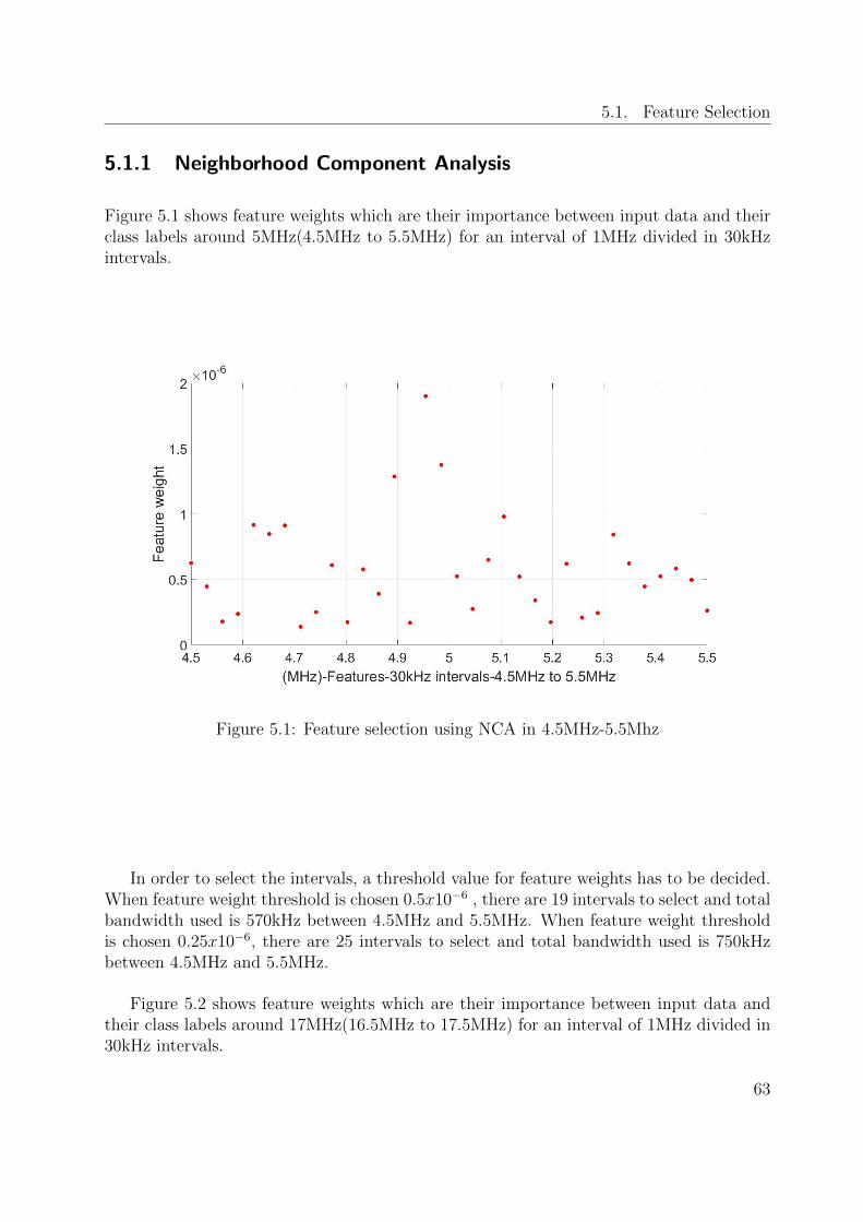
5.1. Feature Selection
5.1.1 Neighborhood Component Analysis
Figure 5.1 shows feature weights which are their importance between input data and theirclass labels around 5MHz(4.5MHz to 5.5MHz) for an interval of 1MHz divided in 30kHzintervals.
Figure 5.1: Feature selection using NCA in 4.5MHz-5.5Mhz
In order to select the intervals, a threshold value for feature weights has to be decided.When feature weight threshold is chosen 0.5x10⁻⁶ , there are 19 intervals to select and totalbandwidth used is 570kHz between 4.5MHz and 5.5MHz. When feature weight thresholdis chosen 0.25x10⁻⁶, there are 25 intervals to select and total bandwidth used is 750kHzbetween 4.5MHz and 5.5MHz.
Figure 5.2 shows feature weights which are their importance between input data andtheir class labels around 17MHz(16.5MHz to 17.5MHz) for an interval of 1MHz divided in30kHz intervals.
63
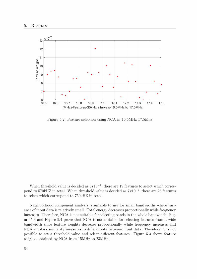
5. Results
Figure 5.2: Feature selection using NCA in 16.5MHz-17.5Mhz
When threshold value is decided as 8x10⁻⁷, there are 19 features to select which corres-pond to 570kHZ in total. When threshold value is decided as 7x10⁻⁷, there are 25 featuresto select which correspond to 750kHZ in total.
Neighborhood component analysis is suitable to use for small bandwidths where vari-ance of input data is relatively small. Total energy decreases proportionally while frequencyincreases. Therefore, NCA is not suitable for selecting bands in the whole bandwidth. Fig-ure 5.3 and Figure 5.4 prove that NCA is not suitable for selecting features from a widebandwidth since feature weights decrease proportionally while frequency increases andNCA employs similarity measures to differentiate between input data. Therefore, it is notpossible to set a threshold value and select different features. Figure 5.3 shows featureweights obtained by NCA from 15MHz to 23MHz.
64
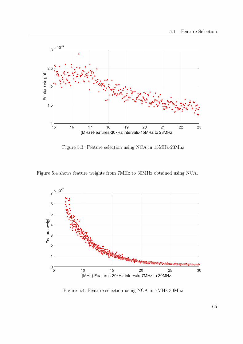
5.1. Feature Selection
Figure 5.3: Feature selection using NCA in 15MHz-23Mhz
Figure 5.4 shows feature weights from 7MHz to 30MHz obtained using NCA.
Figure 5.4: Feature selection using NCA in 7MHz-30Mhz
65
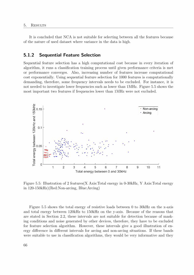
5. Results
It is concluded that NCA is not suitable for selecting between all the features becauseof the nature of used dataset where variance in the data is high.
5.1.2 Sequential Feature Selection
Sequential feature selection has a high computational cost because in every iteration ofalgorithm, it runs a classification training process until given performance criteria is metor performance converges. Also, increasing number of features increase computationalcost exponentially. Using sequential feature selection for 1000 features is computationallydemanding, therefore, some frequency intervals needs to be excluded. For instance, it isnot needed to investigate lower frequencies such as lower than 1MHz. Figure 5.5 shows themost important two features if frequencies lower than 1MHz were not excluded.
Figure 5.5: Illustration of 2 features(X Axis:Total energy in 0-30kHz, Y Axis:Total energyin 120-150kHz)(Red:Non-arcing, Blue:Arcing)
Figure 5.5 shows the total energy of resistive loads between 0 to 30kHz on the x-axisand total energy between 120kHz to 150kHz on the y-axis. Because of the reasons thatare stated in Section 2.2, these intervals are not suitable for detection because of mask-ing conditions and noise generated by other devices, therefore, they have to be excludedfor feature selection algorithm. However, these intervals give a good illustration of en-ergy difference in different intervals for arcing and non-arcing situations. If these bandswere suitable to use in classification algorithms, they would be very informative and they
66
5.1. Feature Selection
would be classified with very high classification rates by SVM or other algorithms becausedifference in energies are even visible by eye inspection in 2D graph.
In order to narrow the scope of bandwidth that feature selection selects the featuresfrom, frequency intervals used in literature and know-how from existing devices are helpfulto decide initial subsets. In total of 12.4MHz bandwidth was covered using sequentialfeature selection. 12.4MHz bandwidth corresponds to 413 features in feature space. 5MHzand 17MHz are main frequencies that form the biggest single portions of initial bandwidthwith 2.5MHz of bandwidth each(5MHz in total). Other 7.4MHz bandwidth was randomlychosen from 1MHz to 30MHz. When 36 features are selected which correspond to 1.08MHzbandwidth, performance converges with better classification rate than using all bandwidth.Using 26 selected features which correspond to 690kHz, performance is similar to using allbandwidth.
Performance metrics for classifiers that are trained using all bandwidth showed thatSVM outperforms all other classifiers. Therefore, sequential feature selection was appliedonly for support vector machine classifiers with different kernels.
Figure 5.6 shows the frequency interval that most of features are selected using sequen-tial feature selection. There are 66 features shown in Figure 5.6 from 16Mhz to 18MHz. 14features are selected by sequential feature selection among shown features. All the showndata in Figure 5.6 are the measurements of LEDs while arcing occurs. However, it is im-portant to state that selected features in these interval together with the other selectedfeatures in different bands give the best classification results.
67
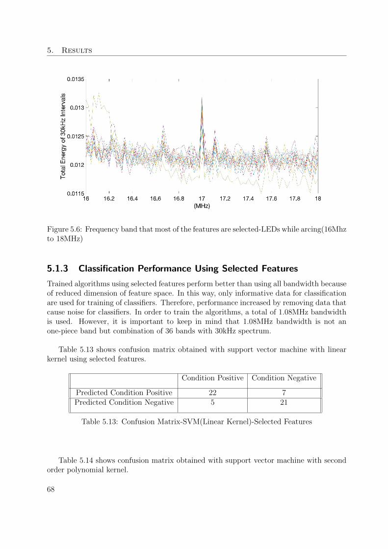
5. Results
Figure 5.6: Frequency band that most of the features are selected-LEDs while arcing(16Mhzto 18MHz)
5.1.3 Classification Performance Using Selected Features
Trained algorithms using selected features perform better than using all bandwidth becauseof reduced dimension of feature space. In this way, only informative data for classificationare used for training of classifiers. Therefore, performance increased by removing data thatcause noise for classifiers. In order to train the algorithms, a total of 1.08MHz bandwidthis used. However, it is important to keep in mind that 1.08MHz bandwidth is not anone-piece band but combination of 36 bands with 30kHz spectrum.
Table 5.13 shows confusion matrix obtained with support vector machine with linearkernel using selected features.
Condition Positive Condition Negative
Predicted Condition Positive 22 7Predicted Condition Negative 5 21
Table 5.13: Confusion Matrix-SVM(Linear Kernel)-Selected Features
Table 5.14 shows confusion matrix obtained with support vector machine with secondorder polynomial kernel.
68
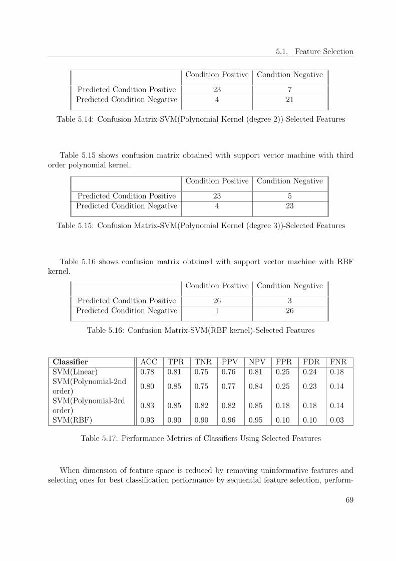
5.1. Feature Selection
Condition Positive Condition Negative
Predicted Condition Positive 23 7Predicted Condition Negative 4 21
Table 5.14: Confusion Matrix-SVM(Polynomial Kernel (degree 2))-Selected Features
Table 5.15 shows confusion matrix obtained with support vector machine with thirdorder polynomial kernel.
Condition Positive Condition Negative
Predicted Condition Positive 23 5Predicted Condition Negative 4 23
Table 5.15: Confusion Matrix-SVM(Polynomial Kernel (degree 3))-Selected Features
Table 5.16 shows confusion matrix obtained with support vector machine with RBFkernel.
Condition Positive Condition Negative
Predicted Condition Positive 26 3Predicted Condition Negative 1 26
Table 5.16: Confusion Matrix-SVM(RBF kernel)-Selected Features
Classifier ACC TPR TNR PPV NPV FPR FDR FNRSVM(Linear) 0.78 0.81 0.75 0.76 0.81 0.25 0.24 0.18SVM(Polynomial-2ndorder)
0.80 0.85 0.75 0.77 0.84 0.25 0.23 0.14
SVM(Polynomial-3rdorder)
0.83 0.85 0.82 0.82 0.85 0.18 0.18 0.14
SVM(RBF) 0.93 0.90 0.90 0.96 0.95 0.10 0.10 0.03
Table 5.17: Performance Metrics of Classifiers Using Selected Features
When dimension of feature space is reduced by removing uninformative features andselecting ones for best classification performance by sequential feature selection, perform-
69
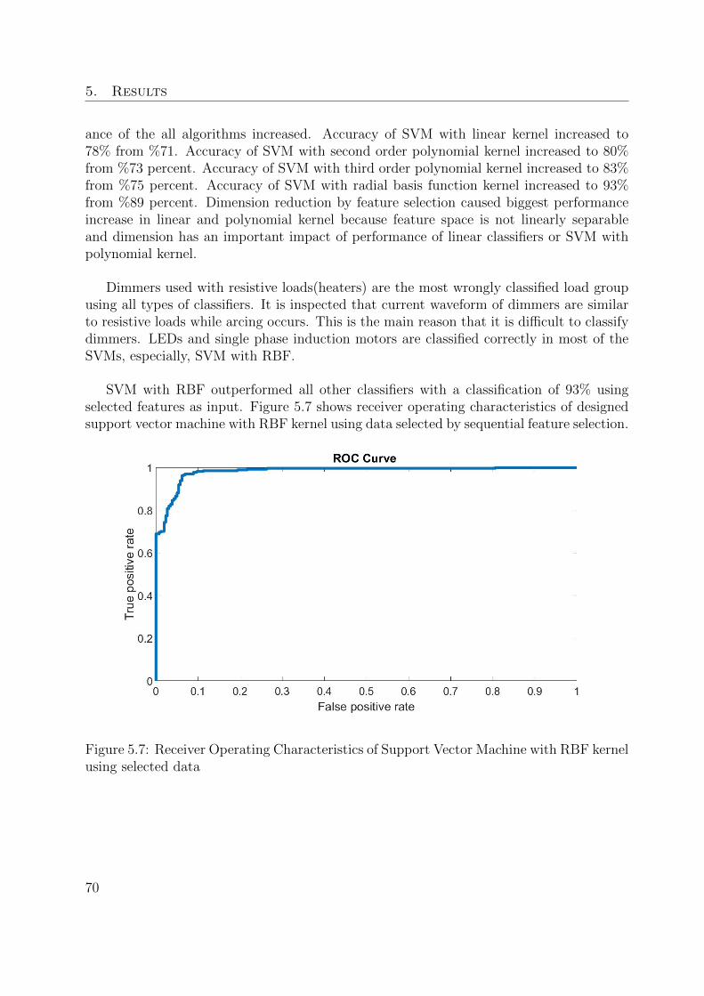
5. Results
ance of the all algorithms increased. Accuracy of SVM with linear kernel increased to78% from %71. Accuracy of SVM with second order polynomial kernel increased to 80%from %73 percent. Accuracy of SVM with third order polynomial kernel increased to 83%from %75 percent. Accuracy of SVM with radial basis function kernel increased to 93%from %89 percent. Dimension reduction by feature selection caused biggest performanceincrease in linear and polynomial kernel because feature space is not linearly separableand dimension has an important impact of performance of linear classifiers or SVM withpolynomial kernel.
Dimmers used with resistive loads(heaters) are the most wrongly classified load groupusing all types of classifiers. It is inspected that current waveform of dimmers are similarto resistive loads while arcing occurs. This is the main reason that it is difficult to classifydimmers. LEDs and single phase induction motors are classified correctly in most of theSVMs, especially, SVM with RBF.
SVM with RBF outperformed all other classifiers with a classification of 93% usingselected features as input. Figure 5.7 shows receiver operating characteristics of designedsupport vector machine with RBF kernel using data selected by sequential feature selection.
Figure 5.7: Receiver Operating Characteristics of Support Vector Machine with RBF kernelusing selected data
70
Chapter 6
Conclusions
Direct digitization as data acquisition method combined with supervised machine learningalgorithms based on features extracted in frequency domain is suitable technique for ACarc fault detection. 5MHz and 17MHz are the best main frequencies to use for detectionpurposes. Support vector machine with RBF kernel has a classification rate of 93%. Usingselected bands to train the algorithms improves classification accuracy considerably. SVMwith RBF kernel outperformed SVM with linear kernel by 7%. Classification rates ofSVMs with polynomial kernel, for both second order and third order, were 7% and 8% lessrespectively when RBF kernel was used.
Arc fault detection by using direct digitization was realized in this thesis and feasibilityof method is proved by classification rates. Direct digitization is more flexible compared toexisting detection methods in terms of possibilities and freedom of signal processing oppor-tunities. Bandwidth is divided into sub-bands of 30kHz and feature selection algorithmswere applied. In existing solutions, bandwidths of 30kHz are not feasible to design an ana-log front end, however, using direct digitization and properly selected 36 features whichmeans a total of 1.08MHz bandwidth, are able to classify arc faults with 93% accuracy.
The advantage of direct digitization is the ability of using relatively small intervals(suchas 30kHz). Using such small bands are advantageous because for wider bands, noise char-acteristics can be masked by another signal and if there is a stochastic or deterministicsignal that causes masking, all the information gathered through that wide band becomesunavailable. However, direct digitization prevents this because even if there is a maskingsituation, it only affects a single band but others still remain informative.
Two different feature selection metaheuristics were applied to select suitable features.It was seen that neighborhood component analysis is not effective when input data hashigh variance. Since, high frequency components of frequency spectrum are much smallerthan lower frequencies, NCA is not able provide effective selection of features for wide
71
6. Conclusions
bandwidths. However, when variance of input is not high, namely, smaller band is givenas input, NCA was able to perform feature selection more efficiently.
Sequential feature selection is effective for choosing suitable bands because algorithmitself takes classifier performance into account in selection process. 1.08MHz of band-width(36 features of 30kHz) was chosen by sequential feature selection. By using thesefeatures, best classifier’s(SVM with RBF) performance was increased to 93%.
Dimmers have the lowest classification rates in the tested loads. It is inspected thatcurrent waveforms of dimmers under normal operation are similar to current waveforms ofresistive loads while arcing fault occurs. This is the main reason that dimmers has lowerclassification rates compared to other loads.
LEDs and power sources with active power correlation has the best classification ratesand they are classified correctly using SVM with RBF kernel as classification algorithm.
SVM classifiers with different kernels(linear, second order polynomial, radial basis func-tion), k-nearest neighbors classifiers with different k values(2,3,5), decision tree with differ-ent limits of splits(maximum, 7,11) and Adaboost algorithm are trained and their perform-ance are compared. Feature space is generated using frequency domain analysis and allfeature space was used to train algorithms for comparison purposes. SVM with RBF kerneloutperformed all other classifiers with its classification rate(89%) before feature selection.Adaboost also has successful performance metrics, especially, false positive rate. However,accuracy and other performance metrics of SVM with RBF kernel are better than Ada-boost. These metrics and generalization ability of SVM make it the most suitable classifierto employ in AC arc fault detection. Therefore, best features are selected to train SVMs bysequential feature selection. In total 1.08MHz that corresponds to 36 features are selectedand SVM with RBF kernel has 93% classification rate when it is trained with these selectedfeatures.
This thesis proves that using direct digitization as data acquisition method and fre-quency domain analysis is increasingly feasible method for AC arc fault detection.
Main purposes of this thesis are to design a successful detection algorithm by employingdirect digitization and supervised machine learning classifiers. Objective is achieved witha 93% classification rate.
Designed feature selection algorithms form a basis to select features for both designedalgorithm in this thesis and for existing analog frontend solutions. However, some modi-fications are necessary to make for analog frontend solutions. For instance, it would notbe feasible to design an analog circuit that has 36 or more band-pass filters whereas it isvery simple in direct digitization. Therefore, feature selection algorithm can be modifiedto choose consecutive bands so that they are usable with analog frontend solutions.
72
6.1. Future Work
6.1 Future Work
Future work can be summarized as follows:
◦ Performance of supervised machine learning algorithms is heavily dependant on con-struction and informativeness of feature space. It can be further increased by increas-ing the number of measurements, load scenarios, and combinations of loads namely,expanding the feature space with different data.
◦ Although most of the achieved bandwidth and widely used bands in literature areinvestigated with sequential feature selection algorithm, covering all the achievedbandwidth can increase the performance of designed algorithm.
◦ Obtained classifier(SVM with RBF kernel) is optimal by the grid used in grid-searchto tune the regarding parameters of algorithm. Therefore, performance can be slightlyincreased by fine tuning around the achieved parameters.
◦ Modified accuracy score can be implemented to penalize false positive classifications.Therefore, nuisance tripping can be avoided better by training the algorithms toavoid false positives.
◦ Feature space for SVM does not have be constructed by the analysis in frequencydomain. Analysis and features extracted from other domains such as time-frequencydomain(STFT), or wavelet transformation can be used to increase performance androbustness of the designed detection method.
◦ In order to use the feature selection methodologies offered with existing solutions,it is needed to modify the feature selection algorithm to choose consecutive bandsin feature space because approach implemented in this thesis freely chooses differentbands without considering their positions. However, such selection of bands wouldnot be feasible for existing solutions.
◦ Recurrent neural networks, especially long short term memory units which is a specialkind of RNN explicitly designed to be capable of learning long-term dependencies[57],are very interesting algorithms to employ for AC arc fault detection. Using deeplearning instead of supervised machine learning ease the process of feature selectiontogether with other advantages. Therefore, it should be further investigated to useLSTM networks for AC arc fault detection.
73
References
[1] Fire Safe Europe, FSEU publications, 2019, https://firesafeeurope.eu/fseu-publications/, online , accessed: 11.05.2019
[2] The Geneva Association World Fire Statistics Bulletin No. 29 Newsletter April 2014
[3] United States Fire Administration Residential Building Electrical Fires (2014-2016),2018, Topical Fire Report Volume 19 Issue 8 Newsletter April 2014
[4] United States Fire Administration, National Estimates Methodologyfor Building Fires and Losses, August 2012, https://www.usfa.fema.gov/downloads/pdf/statistics/res bldg fire estimates.pdf
[5] Transparency Market Research, Global Arc Fault Circuit Interrupter Market:Booming Construction Industry in Middle East, Asia Pacific to Drive Growth,2017, https://www.transparencymarketresearch.com/pressrelease/arc-fault-circuit-interrupter-market.htm
[6] International Electrotechnical Commission IEC:62606 General requirements for arcfault detection devices: Edition 1.0. Copyright 2017 IEC Geneva, Switzerland.www.iec.ch Switzerland, 2013-07
[7] Wikipedia, Arc-fault circuit interrupter https://en.wikipedia.org/wiki/Arc-fault circuit interrupter. accessed: 20.04.2019.
[8] Electrical circuit protection for low voltage residential and light commercial installa-tions http://promotions.eaton.com/content/dam/beacon/residential/UK/home/for-installers/fire-safety-season/circuit-protection/brochure/AFDD+-range-brochure.pdf. accessed: 16.02.2019.
[9] Jean-Mary Martel, Series arc faults in low-voltage AC electrical installations, Uni-versittsverlag Ilmenau 2018
74
References
[10] Hong-Keun Ji, Guoming Wang, Woo-Hyun Kim, Gyung-Suk Kil, Optimal Designof a Band Pass Filter and an Algorithm for Series Arc Detection,2018, Energies11(4):992 DOI: 10.3390/en11040992, licence by: CC BY 4.0
[11] Wikipedia, Cross-validation (statistics), https://en.wikipedia.org/wiki/Cross-validation (statistics), online, accessed:10.01.2019
[12] F. Blades, ”Method and apparatus for detecting arcing in AC power systems bymonitoring high frequency noise”, United States of America Patent US 5729145 A17 March 1998.
[13] Wikipedia, Fuse(electrical) https://en.wikipedia.org/wiki/Fuse(electrical. accessed :12.04.2019.
[14] Low Voltage Protection-RCD https://electrical-engineering-portal.com/residual-current-device-rcd. accessed: 26.04.2019.
[15] Wikipedia, Residual-Current Device, https://en.wikipedia.org/wiki/Residual-current device accessed: 27.04.2019.
[16] Bob Dean, Residual-current device https://www.electricalengineeringtoolbox.com/2016/01/how-residual-current-device-rcd-works.html. accessed: 27.04.2019.
[17] Eaton UK, Miniature Circuit Breaker http://www.eaton.uk.com/EatonUK/ProductsSolutions /Electrical/ProductsServices/ResidentialLight-Commercial /CircuitProtec-tion/EatonResidentialRange6A/index.htm. accessed: 09.04.2019.
[18] Martin M, Understanding the differences between ground fault and arc fault cir-cuit interrupters http://www.maximumspaces.com/understanding-the-differences-between-ground-fault-and-arc-fault-circuit-interrupters.html. 12.02.2018 accessed:12.04.2019.
[19] Eaton s.r.o, Arc fault detection device brochure,http://www.eatonelektrotechnika.cz/cz/obloukova-ochrana-afdd.html. February2018
[20] Jean-Francois Rey, Do you know an Arc Fault Detection Device (AFDD) canprevent from an electrical fire? http://https://blog.schneider-electric.com/power-management-metering-monitoring-power-quality/2013/07/03/do-you-know-an-arc-fault-detection-device-afdd-can-prevent-from-an-electrical-fire/. 03.07.2013 accessed:11.05.2019.
[21] Amna Farooq Husain, Series Arc Fault Detection in the Presence of Household Elec-trical Loads 2017 Czech Technical University
75
References
[22] A. Collin, J. Acosta, B. Hayes and S. Djokic, Component-based Aggregate LoadModels for Combined Power Flow and Harmonic Analysis 7th Mediterranean Con-ference and Exhibition on Power Generation, Transmission, Distribution and EnergyConversion 2010
[23] IEC 61000-3-2:2014, Electromagnetic compatibility (EMC) - part 3-2: Limits forharmonic current emissions (equipment input current :s 16 A per phase),” 2007.
[24] Wikipedia, Binary Classification, https://en.wikipedia.org/wiki/Binary classification, online, accessed: 01.02.2019
[25] UK Department of Energy and Climate Change, Energy Consumption in the UK(2013), Domestic energy consumption in the UK between 1970 and 2012 25.07.2013
[26] International Energy Agency, Tracking Clean Energy Progress-Lighting, ht-tps://www.iea.org/tcep/buildings/lighting/ 13.03.2019
[27] Viribright, Comparing LED vs CFL vs Incandescent Light Bulbs, 2016,https://www.viribright.com/lumen-output-comparing-led-vs-cfl-vs-incandescent-wattage/, online, accessed: 17.05.2019
[28] Gabriel Brindusescu, Better Electric Motors to Arrive? Scientists Discovered NewMagnetic Properties in Iron, 2014, https://www.autoevolution.com/news/better-electric-motors-to-arrive-scientists-discovered-new-magnetic-properties-in-iron-80619.html
[29] Science Direct https://www.sciencedirect.com/topics/computer-science/binary-classification accessed: 11.05.2019.
[30] Hoffmann, R.; Fabian,T.; Dr, F., 2008. Comparison of yields and nutritive value ofdifferent spring green forage mixtures. Acta Agric. Slov., 92 (suppl 2): 143-148
[31] Polikar, R.: Ensemble based systems in decision making. IEEE Circuit Syst. Mag. 6,21-45,DOI: 10.1109/MCAS.2006.1688199, October 2006
[32] Yoshua Bengio, Learning Deep Architectures for AI,Foundations and Trends in Ma-chine Learning, 2009, ISBN: 978-1-60198-294-0
[33] Drucker, H., D. Wu and V.N. Vapnik, 1999. Support Vector Machines for SpamCategorization. IEEE Transaction on Neural Networks
[34] Yoav Freund and Robert E. Schapire, A Decision-Theoretic Generalization of On-Line Learning and an Application to Boosting, Journal of computer and systemsciences 55, 119-139 (1997)
[35] Friedman N, Linial M, Nachman I, Pe’er D, Friedman N, et al. (2000) Using Bayesiannetworks to analyze expression data. J Comput Biol 7(3-4):601-20
76
References
[36] Breiman, L., Random Forests, Machine Learning (2001) 45: 5. ht-tps://doi.org/10.1023/A:1010933404324
[37] Bishop DV, North T, Donlan C.,Genetic basis of specific language impairment: evid-ence from a twin study. Dev Med Child Neurol. 1995 Jan;37(1):56-71.
[38] F Fernndez-Rodrguez, S Sosvilla-Rivero, Testing nonlinear forecastability in timeseries: theory and evidence from the EMS,1999 Economics Letters 59, 49-63
[39] Van Gestel, Tony, et al., 2001. Financial Time Series Prediction Using Least SquaresSupport Vector Machines Within the Evidence Framework, IEEE Transactions onNeural Networks, Volume 12, Number 4, July 2001, Pages 809-821
[40] K. Veropoulos, N. Cristianini and C. Campbell, The Application of Support VectorMachines to Medical Decision Support: A Case Study, 2009
[41] Azriel Rosenfeld, Harry Wechsler, Pattern Recognition: Historical Perspective andFuture Directions, 2000
[42] Wikipedia, Kernel method, https://en.wikipedia.org/wiki/Kernel method, online,accessed: 12.01.2019
[43] Li H., Qi F., Wang S. (2005) A Comparison of Model Selection Methods for Multi-class Support Vector Machines. In: Gervasi O. et al. (eds) Computational Scienceand Its Applications ICCSA 2005. ICCSA 2005. Lecture Notes in Computer Science,vol 3483. Springer, Berlin, Heidelberg
[44] Laura Auria, Rouslan A. Moro, Support Vector Machines (SVM) as a Technique forSolvency Analysis, 2008, German Institute for Economic Research Discussion Papers
[45] Wikipedia, Generalization error, https://en.wikipedia.org/wiki/Generalization error,accessed: 21.03.2019
[46] Wikipedia, Fourier Transform,https://en.wikipedia.org/wiki/Discrete Fouriertransform, accessed: 01.05.2019
[47] Grichting, B.; Goette, J.; Jacomet, M.: Cascaded fuzzy logic based arc fault detectionin photovoltaic applications. 2015 International Conference on Clean Electrical Power(ICCEP), 2015, (178183), doi:10.1109/ICCEP.2015.7177620.
[48] Cao, Y.; Li, J.; Sumner, M.; aj.: Arc fault generation and detection in DC systems. In2013 IEEE PES Asia-Pacific Power and Energy Engineering Conference (APPEEC),IEEE, 2013, s. 15, doi:10.1109/APPEEC.2013.6837123.
[49] Yuan Gao ; Junjun Zhang ; Yandan Lin ; Yaojie Sun, An Innovative Photovoltaic DCArc Fault Detection Method through Multiple Criteria Algorithm Based on a NewArc Initiation Method, 2014, IEEE 40th Photovoltaic Specialist Conference (PVSC),IEEE, doi: 10.1109/PVSC.2014.6925613
77
References
[50] Gab-Su Seo, Katherine A. Kim, Kyu-Chan Lee, Kyung-Jun Lee, Bo-Hyung Cho, ANew DC Arc Fault Detection Method Using DC System Component Modeling andAnalysis in Low Frequency Range, 2015,IEEE Applied Power Electronics Conferenceand Exposition (APEC), doi: 10.1109/APEC.2015.7104690
[51] Mathworks, https://www.mathworks.com/help/stats/neighborhood-component-analysis.html, online, accessed: 04.05.2019
[52] Wei Yang, Kuanquan Wang, Wangmeng Zuo, Fast neighborhoodcomponent analysis, 2012 Neurocomputing Volume 83,(31-37), ht-tps://www.sciencedirect.com/science/article/pii/S0925231211007120
[53] J. Goldberger, G. E. Hinton, S. T. Roweis,R. Salakhutdinov, Neighbourhood com-ponents analysis, in Advances in neural information processing systems, 2004, pp.513520.
[54] Dong Wang, Xiaoyang Tan, Bayesian Neighbourhood Component Analysis, 2017,IEEE Transactions on Neural Networks and Learning Systems(Volume: 29 , Issue:7),pp. 3140 - 3151 doi:10.1109/TNNLS.2017.2712823
[55] Vipin Kumar, Sonajharia Minz, Feature Selection: A literature Review, 2014, SmartComputing Review, vol. 4, no. 3, June 2014,pp. 211-229
[56] Trevor Hastie, Robert Tibshirani, Jerome Friedman, The Elements of StatisticalLearning Data Mining, Inference, and Prediction, 2001, pp. 38
[57] Petr Pok, BE3M33UI Artificial Intelligence Lecture Slides Non-linear models, Basisexpansion, Overfitting, Regularization, 2019, Czech Technical University in PragueFaculty of Electrical Engineering Dept. of Cybernetics
[58] Fletcher, Robert H. Fletcher ; Suzanne W. (2005). Clinical epidemiology : the essen-tials (4th ed.). Baltimore, Md.: Lippincott Williams Wilkins. p. 45. ISBN: 0-7817-5215-9.
[59] Wikipedia, Confusion Matrix, https://en.wikipedia.org/wiki/Confusion matrix, on-line, accessed:10.05.2019
[60] Mathworks, ”Detector Performance Analysis Using ROC Curves MATLAB Sim-ulink Example”, www.mathworks.com, 2016, online, accessed: 14.05.2019
[61] Siemens , ”5SM6 AFD Units - Technology Primer,” Siemens AG , 2016.
[62] Scikit-learn, RBF SVM parameters, https://scikit-learn.org/stable/auto examples/svm/plot rbf parameters.html, online, accessed:19.05.2019
78
References
[63] Siemens, Sentron 5SM6 AFD units Technology Primer, ht-tps://assets.new.siemens.com/siemens/assets/public.1492678703.d8eedd48f65bce75615cabcc29ccfa5b19b85cfc.technikfibel-brandschutz-en.pdf, online, accessed:15.05.2019
[64] Altman, N. S. (1992). ”An introduction to kernel and nearest-neighbornonparametric regression”. The American Statistician. 46 (3): 175185.doi:10.1080/00031305.1992.10475879. hdl:1813/31637.
[65] Wikipedia, k-nearest neighbors algorithm, https://en.wikipedia.org/wiki/K-nearest neighbors algorithm, online, accessed: 21.05.2019
[66] Jason Brownlee, A Gentle Introduction to k-fold Cross-Validation, 2018, StatisticalMethods, online, accessed: 11.04.2019
79