customization of adaptive optical systems
TRANSCRIPT
QUALIFYING PhD EXAM
CUSTOMIZATION OF ADAPTIVE
OPTICAL SYSTEMS
Otávio Gomes de Oliveira
Supervisor
Davies W. de Lima Monteiro
PPGEE – UFMG
2010
P a g e | 2
1. ABSTRACT
Adaptive optics (AO) is a promising field either for scientific or commercial investments,
especially in areas such as medicine and industry. Adaptive optics systems are found in
applications in many different areas, such as: astronomy, military defense, ophthalmology,
laser industry, laser-based materials processing, free-space communication and biomedicine.
AO systems are used to improve the quality and the capabilities of optical systems, generally
by compensating for distortions (wavefront aberrations) that affect light waves. These image
distortions can represent a serious problem in many different applications where high-quality
images are demanded. Basically, AO systems are composed of three subsystems: wavefront
sensor (WFS), wavefront modulator (WFM) and control system. The WFS is used to measure
the distortions present in the light waves. The control system is responsible for analyzing the
measurement and actuating the WFM, which corrects for the light wave distortions.
The main objective of this work is to design and assemble an adaptive optics system and
propose a suitable and optimized configuration for a specific application. To accomplish this
task, three main activities have been carried out.
a. Optimization of a lenslet array, an element of the WFS, for ophthalmological purposes.
b. Development of a DSP-based embedded system to control the AO system.
c. Optical design and assemble of an AO system.
This text describes the so far accomplished results in each of the three activities and indicates
the next steps to be performed in order to achieve the main project goal.
P a g e | 3
2. RESUMO
Óptica adaptativa (OA) é um campo muito promissor para investimentos tanto científicos
quanto comerciais, principalmente em áreas como a medicina e a indústria. Sistemas ópticos
adaptativos são encontrados em muitas e diferentes áreas, tais como: astronomia, defesa
militar, oftalmologia, indústria de lasers, processamento de materiais usando lasers,
comunicação de espaço livre e biomedicina.
Sistemas OA são usados para aumentar qualidade e potencial de sistemas ópticos, geralmente
através da compensação de distorções (aberrações de frente de onda) que afetam os feixes de
luz. Estas distorções podem representar um sério problema em várias aplicações em que
imagens de alta qualidade são necessárias. Basicamente, sistemas ópticos adaptativos são
compostos de três subsistemas: sensor de frente de onda, modulador de frente de onda e
sistema de controle. O sensor de frente de onda é usado para medir as distorções presentes
no feixe de luz. O sistema de controle é responsável por analisar o resultado dessas medições e
operar o modulador de frente de onda, que atua na correção das distorções.
O principal objetivo deste trabalho é projetar e montar um sistema óptico adaptativo e propor
uma configuração conveniente e otimizada para uma aplicação específica. Para cumprir estas
metas, três atividades estão sendo desenvolvidas.
a. Otimização de uma matriz de microlentes, um elemento do sensor de frente de onda,
para aplicação em oftalmologia.
b. Desenvolvimento de um sistema embarcado, baseado em DSP, para controlar o
sistema óptico adaptativo.
c. Projeto óptico e montagem do sistema óptico adaptativo.
Este texto descreve os avanços obtidos até o momento em cada uma dessas três atividades,
além das tarefas a serem desenvolvidas para que se possa atingir o objetivo principal aqui
proposto.

P a g e | 4
3. SUMMARY
1. ABSTRACT .............................................................................................................................. 2
2. RESUMO ................................................................................................................................ 3
3. SUMMARY ............................................................................................................................. 4
4. FIGURES ................................................................................................................................. 5
5. INTRODUCTION ..................................................................................................................... 7
6. ADAPTIVE OPTICS ................................................................................................................ 10
6.1. CONCEPTS AND DEFINITIONS ...................................................................................... 10
6.2. OPTICAL ABERRATIONS ............................................................................................... 10
7. ADAPTIVE OPTICS SYSTEM .................................................................................................. 20
7.1. WAVEFRONT SENSOR .................................................................................................. 21
7.2. WAVEFRONT MODULATOR ......................................................................................... 23
7.3. CONTROL SYSTEM ....................................................................................................... 24
8. METHODS, RESULTS AND DISCUSSIONS ............................................................................. 26
8.1. LENSLET ARRAY OPTIMIZATION FOR APPLICATION IN OPHTHALMOLOGY ................ 26
8.1.1. NUMERICAL MODEL OF THE HARTMANN-SHACK METHOD ............................... 29
8.1.2. MATHEMATICAL MODEL OF LENSES ................................................................... 32
8.1.3. WAVEFRONT ABERRATIONS GENERATOR ........................................................... 34
8.1.4. OPTIMIZATION ALGORITHM ............................................................................... 35
8.1.5. METHODOLOGY................................................................................................... 37
8.1.6. RESULTS AND DISCUSSION .................................................................................. 39
8.2. EMBEDDED SYSTEM FOR ADAPTIVE OPTICS SYSTEM CONTROL ................................ 44
8.2.1. DIGITAL SIGNAL PROCESSOR (DSP) ..................................................................... 44
8.2.2. IMAGE ANALYSIS ALGORITHM ............................................................................ 45
8.2.3. WAVEFRONT RECONSTRUCTION ALGORITHM ................................................... 51
8.3. ADAPTIVE OPTICS SYSTEM DESIGN ............................................................................. 52
9. FUTURE WORK .................................................................................................................... 56
10. SCHEDULE ........................................................................................................................ 56
11. FINAL REMARKS ............................................................................................................... 57
12. ACKNOWLEDGEMENTS ................................................................................................... 58
13. REFERENCES .................................................................................................................... 59

P a g e | 5
4. FIGURES
Figure 1 – Illustration of the effect of turbulent atmosphere on astronomical images. .............. 8
Figure 2 – Wavefronts (dashed line) for parallel and spherically divergent light beams. .......... 10
Figure 3 – Wavefront aberration................................................................................................. 11
Figure 4 – Wavefront aberration introduced by a non-isotropic medium. ................................ 11
Figure 5 – Aberration introduced through refraction. ................................................................ 12
Figure 6 – Aberration introduced through reflection. ................................................................ 12
Figure 7 –Aberrated wavefronts after reaching optical components. ........................................ 13
Figure 8 – Image formation of a point source for a diffraction-limited system.......................... 13
Figure 9 – Point spread function (PSF) for a perfect eye. ........................................................... 14
Figure 10 – Point spread function for a typical eye. ................................................................... 14
Figure 11 – Spherical aberration. ................................................................................................ 15
Figure 12 – Comma. .................................................................................................................... 15
Figure 13 – Astigmatism. ............................................................................................................. 15
Figure 14 – Image formation by an aberrated optical system. (a: PSF, b: object and c: result) . 16
Figure 15 – Comparison of images formed in human eyes with different PSFs. ........................ 16
Figure 16 – Polar system coordinates. ........................................................................................ 17
Figure 17 – 3D representation of Zernike terms. ........................................................................ 18
Figure 18 – Point Spread function for each Zernike term. .......................................................... 19
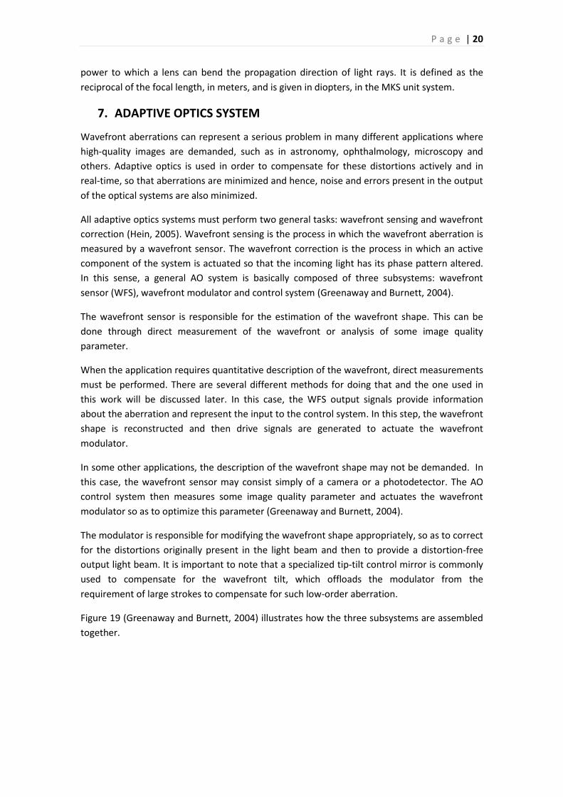
Figure 19 – AO system. ................................................................................................................ 21
Figure 20 – 1D schematics of the Hartmann-Shack principle (a: plane wavefront, b: arbitrary
wavefront). .................................................................................................................................. 22
Figure 21 – Relation between the local wavefront (WF) aberration 𝑊 and the ray deviation. . 22
Figure 22 – Micromachined membrane deformable mirror. ...................................................... 24
Figure 23 – Membrane deformable mirror correcting for an wavefront (WF) aberration. ........ 24
Figure 24 – Objective function for the lenslet array optimization. ............................................. 28
Figure 25 – Schematics of the optimization function operation................................................. 29
Figure 26 – Block-diagram of the Hartmann-Shack numerical model. ....................................... 30
Figure 27 – Geometrical representation of the optical system. ................................................. 33
Figure 28 – Steps for calculating the light beam deviation after passing through a plano-convex
lens. ............................................................................................................................................. 33
Figure 29 – Zernike coefficients generated by the algorithm. .................................................... 35
Figure 30 – The three types of children in a new generation. .................................................... 37
Figure 31 – Performance of the optimized 16-lenslet arrays. .................................................... 40
Figure 32 – Orthogonal (a) and optimized (b) 16-lenslet arrays. ................................................ 40
Figure 33 – Performance of the optimized 25-lenslet array. ...................................................... 41
Figure 34 – Orthogonal (a) and optimized (b) 25-lenslet arrays. ................................................ 41
Figure 35 – Performance of the optimized 36-lenslet array. ...................................................... 41
Figure 36 – Orthogonal (a) and optimized (b) 36-lenslet arrays. ................................................ 42
Figure 37 – Maximum number of Zernike terms (or modes) that can be reliably reconstructed
for a given number of lenslets in the array. ................................................................................ 43
Figure 38 – An example of an output image of the Hartmann-Shack method. .......................... 46
Figure 39 – Block-diagram of the image processing algorithm. .................................................. 47
Figure 40 – Graph of the offset function. .................................................................................... 48

P a g e | 6
Figure 41 – Binary image generated by step 4. ........................................................................... 49
Figure 42 – Detection of light spots. The lateral size of the mask used in the picture on the right
is 20 times bigger than the one on the left. ................................................................................ 49
Figure 43 – Example of white regions that do not represent light spots. The acquired image is
shown in (a) and the binary image, in (b). .................................................................................. 50
Figure 44 –(a) Acquired image. (b) Image with light-spots centroids detected (marked with a
small black cross in the middle of a white box). ......................................................................... 51
Figure 45 – Lenses configuration for optical phase conjugation. ............................................... 52
Figure 46 – AO system design. .................................................................................................... 53
Figure 47 – AO system assembled. ............................................................................................. 55
Figure 48 – (a) Far-field and (b) interferogram images without the beam splitter. ................... 55
Figure 49 – (a) Far-field and (b) interferogram images generated with the beam splitter. ....... 55
P a g e | 7
5. INTRODUCTION
“If the Theory of making Telescopes could at length be fully brought into Practice, yet there
would be certain Bounds beyond which Telescopes could not perform. For the Air through
which we look upon the Stars, is in a perpetual Tremor; as may be seen by the tremulous
Motion of Shadows cast from high Towers, and by the twinkling of the fix’d Stars. But these
Stars do not twinkle when viewed through Telescopes which have large apertures. For the Rays
of Light which pass through divers parts of the aperture, tremble each of them apart, and by
means of their various and sometimes contrary Tremors, fall at one and the same time upon
different points in the bottom of the Eye, and their trembling Motions are too quick and
confused to be perceived severally. And all these illuminated Points constitute one broad lucid
Point, composed of those many trembling Points confusedly and insensibly mixed with one
another by very short and swift Tremors, and thereby cause the Star to appear broader than it
is, and without any trembling of the whole. Long Telescopes may cause Objects to appear
brighter and larger than short ones can do, but they cannot be so formed as to take away that
confusion of the Rays which arises from the Tremors of the Atmosphere. The only Remedy is a
most serene and quiet Air, such as may perhaps be found on the tops of the highest Mountains
above the grosser Clouds.” (Newton, 2007).
When trying to observe fainter astronomical objects (such as other galaxies), using large
telescopes, astronomers faced a limitation: images appeared blurred and the objects could not
be distinguished. The reason was that light coming from the astronomical object passed
through turbulent atmosphere before reaching the telescope lenses (Hein, 2005). As claimed
by Sir Isaac Newton in his Opticks, the “quiet air” of high mountains contributes to better
observations. However, even such a “serene air” is prone to contain turbulences, and
therefore, to decrease the quality of the observed image by introducing aberrations in the light
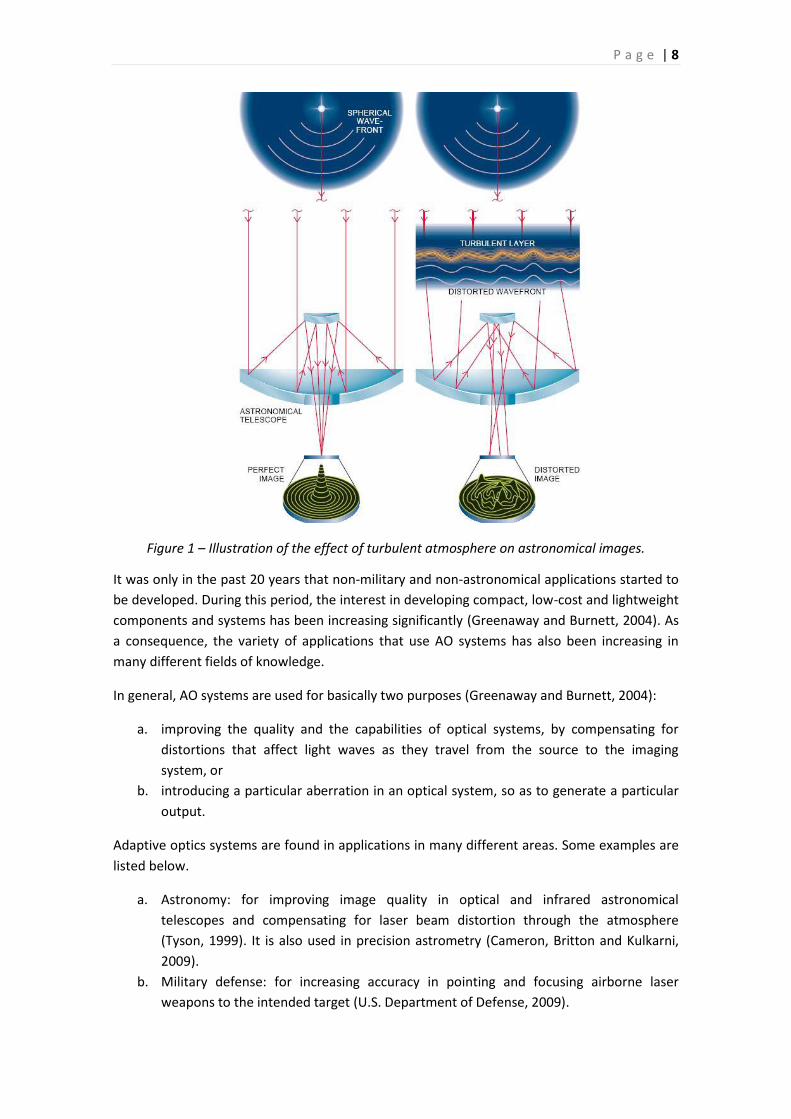
beam that passes through it. Figure 1 (Hein, 2005) illustrates the comparison of the observed
images from an astronomical object generated by a telescope in two cases: when light passes
through turbulent air and when there is no turbulence at all (hypothetical).
Despite representing a great problem, it was only in the second half of the 20th century that
astronomers and militaries started to develop ways of overcoming turbulent effects of the
atmosphere. Although it is impossible to avoid the introduction of aberrations in the images
when light passes through the atmosphere, it is feasible to compensate for these aberrations,
using a deformable element in the optical system. Basically, in practice, the system must be
capable of detecting the deformation present in the image, quantifying it and converting the
results into information useful to actuate the deformable element. A requirement is that all
this has to be continually performed in a loop and in real-time. Hence, an optical system like
this would constantly adapt itself to the atmospheric turbulence, therefore compensating for
the deformations present in the observed images.
The first adaptive optics (AO) systems were initially developed specifically for applications in
defense and astronomy, where the focus was more on performance than on cost or size. These
systems started to be developed only after enough technology was available to build the
necessary components, what happened about twenty years after the first alternative of an
adaptive optics system was proposed (Tyson, 1999).
P a g e | 8
Figure 1 – Illustration of the effect of turbulent atmosphere on astronomical images.
It was only in the past 20 years that non-military and non-astronomical applications started to
be developed. During this period, the interest in developing compact, low-cost and lightweight
components and systems has been increasing significantly (Greenaway and Burnett, 2004). As
a consequence, the variety of applications that use AO systems has also been increasing in
many different fields of knowledge.
In general, AO systems are used for basically two purposes (Greenaway and Burnett, 2004):
a. improving the quality and the capabilities of optical systems, by compensating for
distortions that affect light waves as they travel from the source to the imaging
system, or
b. introducing a particular aberration in an optical system, so as to generate a particular
output.
Adaptive optics systems are found in applications in many different areas. Some examples are
listed below.
a. Astronomy: for improving image quality in optical and infrared astronomical
telescopes and compensating for laser beam distortion through the atmosphere
(Tyson, 1999). It is also used in precision astrometry (Cameron, Britton and Kulkarni,
2009).
b. Military defense: for increasing accuracy in pointing and focusing airborne laser
weapons to the intended target (U.S. Department of Defense, 2009).
P a g e | 9
c. Ophthalmology: for improving image quality in ophthalmoscopy, through measuring
and correcting the high order aberrations of the human eye (Roorda, Romero-Borja, et
al., 2002; Zhang, Poonja and Roorda, 2006; Carroll, Gray, et al., 2005).
d. Laser industry: for improving beam quality through compensating for the optical
aberrations introduced during the amplification step in high-power lasers (Oughstun,
1981; Welp, Heuck and Wittrock, 2007).
e. Laser-based materials processing: for increasing reliability in processes such as
welding, cutting, laser forward-transfer and other, through precise control of the
shape of the intensity profile of the laser beam (Arnold and McLeod, 2007; Jesacher,
Marshall, et al., 2010).
f. Free-space communication: for increasing reliability through compensation of the
optical aberrations introduced in the laser beam by the propagating medium (Arnon
and Kopeika, 1997; Arnold and McLeod, 2007).
g. Biomedical applications: for improving signal intensity and image quality in optical
microscopy for medical imaging of tissues (Wright, Poland, et al., 2007; Girkin, Poland
and Wright, 2009).
The examples just listed illustrate how adaptive optics can be applied to many different areas.
The increasing interest in a broad range of applications is confirmed by the papers recently
published, which focus more on low-cost, robust, compact and lightweight complete systems
and components, rather than on complex and expensive systems (Vdovin, De Lima Monteiro,
et al., 2004). Such technological advances are crucial to expand the range of applications of
adaptive optics.
Moreover, the growing interest in applications using adaptive optics is also confirmed by the
volume of scientific literature on the field. The number of papers published referencing AO has
increased from about 50 per year during the 1980s to about 500 in 2003 (Greenaway and
Burnett, 2004).
However, the interest in the development of AO applications is not only scientific. The
evolution of the number of patents referring AO in the last decades reveals a growing
commercial interest in the area. From the beginning of the 1980s to 2003, the number of
granted patents per year referring AO has risen by a factor of four. Ophthalmology is the area
with the largest number of patents referring AO (Greenaway and Burnett, 2004).
All these aspects suggest that AO is a promising field for scientific and commercial
investments, especially in medical and industrial areas. To ensure the feasibility of commercial
applications, it is important to focus on the development of low-cost, compact and reliable
systems and also of components that can be easily integrated, so as to guarantee the
standardization and the possibility of series production.
In this sense, this work aims to contribute to the development of the field not only by adding
significant scientific results, but also by training human resources with expertise in the area,
which is especially important in a country as Brazil, where scientific activity in the area is still
limited. The main objective of this work is to design and assemble an adaptive optics system
and propose a suitable and optimized configuration for a specific application.
P a g e | 10
6. ADAPTIVE OPTICS
6.1. CONCEPTS AND DEFINITIONS
Adaptive optics systems are real-time distortion-compensating systems (Tyson, 1999). All
adaptive optics systems must perform two general tasks: wavefront sensing and wavefront
correction (Hein, 2005). This section discusses some concepts which are essential to
understand how an optical system accomplishes these tasks.
6.2. OPTICAL ABERRATIONS
An optical aberration can be understood as a distortion in an image or in a wavefront
introduced by optical components or by the propagating medium. To define more precisely
and to understand how it can affect the image quality, it is important to first introduce the
concept of a wavefront.
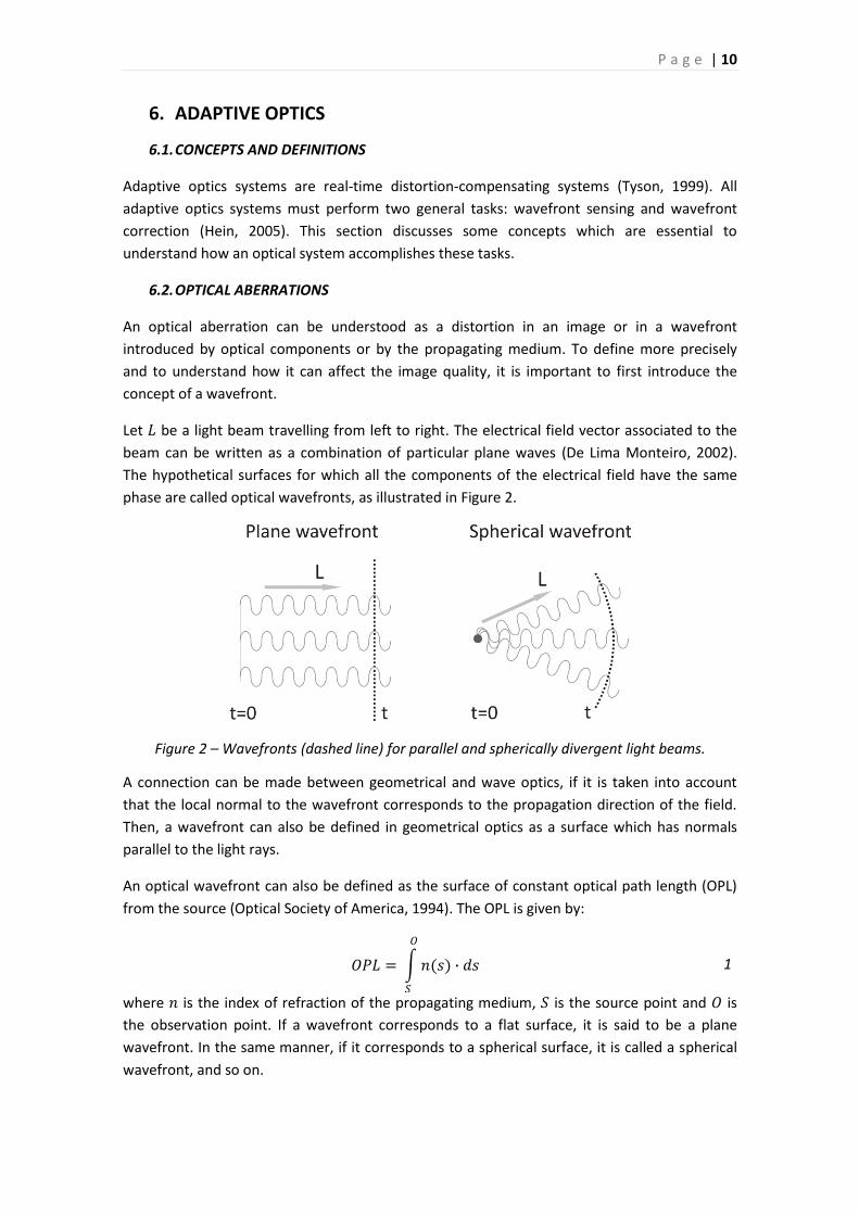
Let 𝐿 be a light beam travelling from left to right. The electrical field vector associated to the
beam can be written as a combination of particular plane waves (De Lima Monteiro, 2002).
The hypothetical surfaces for which all the components of the electrical field have the same
phase are called optical wavefronts, as illustrated in Figure 2.
Figure 2 – Wavefronts (dashed line) for parallel and spherically divergent light beams.
A connection can be made between geometrical and wave optics, if it is taken into account
that the local normal to the wavefront corresponds to the propagation direction of the field.
Then, a wavefront can also be defined in geometrical optics as a surface which has normals
parallel to the light rays.
An optical wavefront can also be defined as the surface of constant optical path length (OPL)
from the source (Optical Society of America, 1994). The OPL is given by:
𝑂𝑃𝐿 = 𝑛(𝑠) ∙ 𝑑𝑠
𝑂
𝑆
1
where 𝑛 is the index of refraction of the propagating medium, 𝑆 is the source point and 𝑂 is
the observation point. If a wavefront corresponds to a flat surface, it is said to be a plane
wavefront. In the same manner, if it corresponds to a spherical surface, it is called a spherical
wavefront, and so on.
P a g e | 11
When the phase pattern of the electrical field of a light beam becomes distorted, the
wavefront changes its shape. The distortions introduced in the wavefront may correspond to
the errors or noise measured when the information it carries is read.
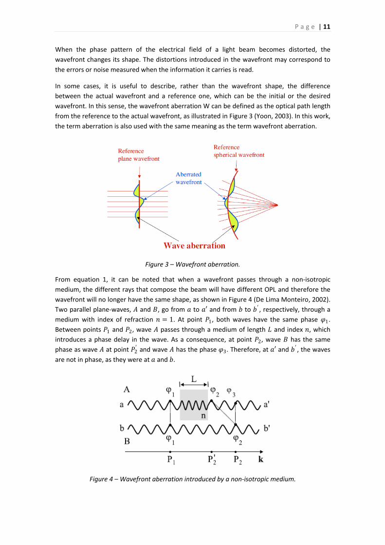
In some cases, it is useful to describe, rather than the wavefront shape, the difference
between the actual wavefront and a reference one, which can be the initial or the desired
wavefront. In this sense, the wavefront aberration W can be defined as the optical path length
from the reference to the actual wavefront, as illustrated in Figure 3 (Yoon, 2003). In this work,
the term aberration is also used with the same meaning as the term wavefront aberration.
Figure 3 – Wavefront aberration.
From equation 1, it can be noted that when a wavefront passes through a non-isotropic
medium, the different rays that compose the beam will have different OPL and therefore the
wavefront will no longer have the same shape, as shown in Figure 4 (De Lima Monteiro, 2002).
Two parallel plane-waves, 𝐴 and 𝐵, go from 𝑎 to 𝑎′ and from 𝑏 to 𝑏′ , respectively, through a
medium with index of refraction 𝑛 = 1. At point 𝑃1, both waves have the same phase 𝜑1.
Between points 𝑃1 and 𝑃2, wave 𝐴 passes through a medium of length 𝐿 and index 𝑛, which
introduces a phase delay in the wave. As a consequence, at point 𝑃2, wave 𝐵 has the same
phase as wave 𝐴 at point 𝑃2′ and wave 𝐴 has the phase 𝜑3. Therefore, at 𝑎′ and 𝑏′ , the waves
are not in phase, as they were at 𝑎 and 𝑏.
Figure 4 – Wavefront aberration introduced by a non-isotropic medium.
P a g e | 12
The fluctuations in the index of refraction through an optical path may occur for many
different reasons: thermal fluctuations, gases, fog and turbulence in general.
Another situation in which the shape of a wavefront may be altered is when a light beam
reaches a non-flat optical surface. It can be a surface separating two different transparent
media or a reflective surface. In the former case, the aberration is introduced through
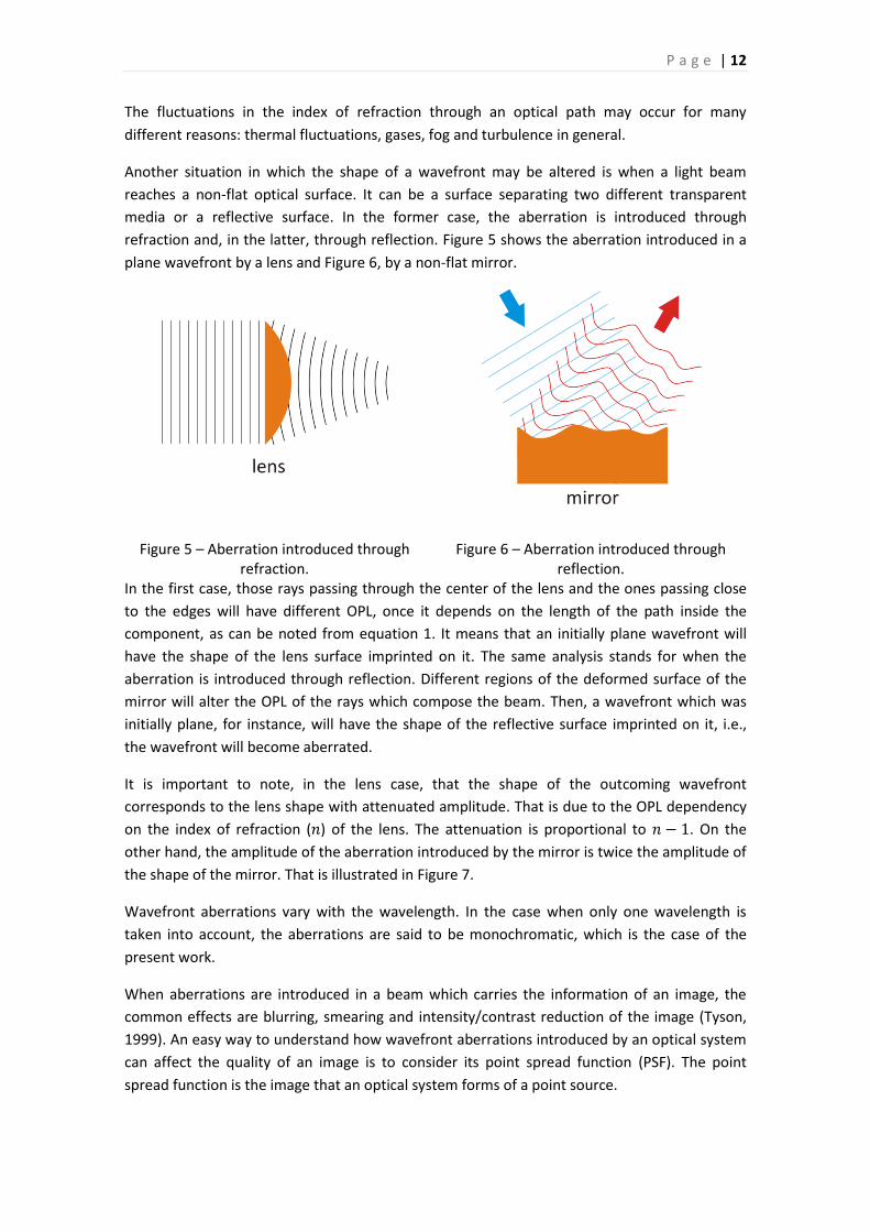
refraction and, in the latter, through reflection. Figure 5 shows the aberration introduced in a
plane wavefront by a lens and Figure 6, by a non-flat mirror.
Figure 5 – Aberration introduced through refraction.
Figure 6 – Aberration introduced through reflection.
In the first case, those rays passing through the center of the lens and the ones passing close
to the edges will have different OPL, once it depends on the length of the path inside the
component, as can be noted from equation 1. It means that an initially plane wavefront will
have the shape of the lens surface imprinted on it. The same analysis stands for when the
aberration is introduced through reflection. Different regions of the deformed surface of the
mirror will alter the OPL of the rays which compose the beam. Then, a wavefront which was
initially plane, for instance, will have the shape of the reflective surface imprinted on it, i.e.,
the wavefront will become aberrated.
It is important to note, in the lens case, that the shape of the outcoming wavefront
corresponds to the lens shape with attenuated amplitude. That is due to the OPL dependency
on the index of refraction (𝑛) of the lens. The attenuation is proportional to 𝑛 − 1. On the
other hand, the amplitude of the aberration introduced by the mirror is twice the amplitude of
the shape of the mirror. That is illustrated in Figure 7.
Wavefront aberrations vary with the wavelength. In the case when only one wavelength is
taken into account, the aberrations are said to be monochromatic, which is the case of the
present work.
When aberrations are introduced in a beam which carries the information of an image, the
common effects are blurring, smearing and intensity/contrast reduction of the image (Tyson,
1999). An easy way to understand how wavefront aberrations introduced by an optical system
can affect the quality of an image is to consider its point spread function (PSF). The point
spread function is the image that an optical system forms of a point source.
P a g e | 13
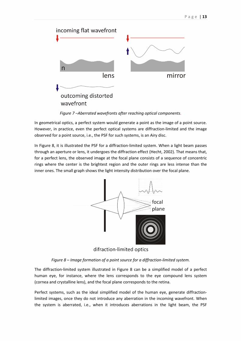
Figure 7 –Aberrated wavefronts after reaching optical components.
In geometrical optics, a perfect system would generate a point as the image of a point source.
However, in practice, even the perfect optical systems are diffraction-limited and the image
observed for a point source, i.e., the PSF for such systems, is an Airy disc.
In Figure 8, it is illustrated the PSF for a diffraction-limited system. When a light beam passes
through an aperture or lens, it undergoes the diffraction effect (Hecht, 2002). That means that,
for a perfect lens, the observed image at the focal plane consists of a sequence of concentric
rings where the center is the brightest region and the outer rings are less intense than the
inner ones. The small graph shows the light intensity distribution over the focal plane.
Figure 8 – Image formation of a point source for a diffraction-limited system.
The diffraction-limited system illustrated in Figure 8 can be a simplified model of a perfect
human eye, for instance, where the lens corresponds to the eye compound lens system
(cornea and crystalline lens), and the focal plane corresponds to the retina.
Perfect systems, such as the ideal simplified model of the human eye, generate diffraction-
limited images, once they do not introduce any aberration in the incoming wavefront. When
the system is aberrated, i.e., when it introduces aberrations in the light beam, the PSF
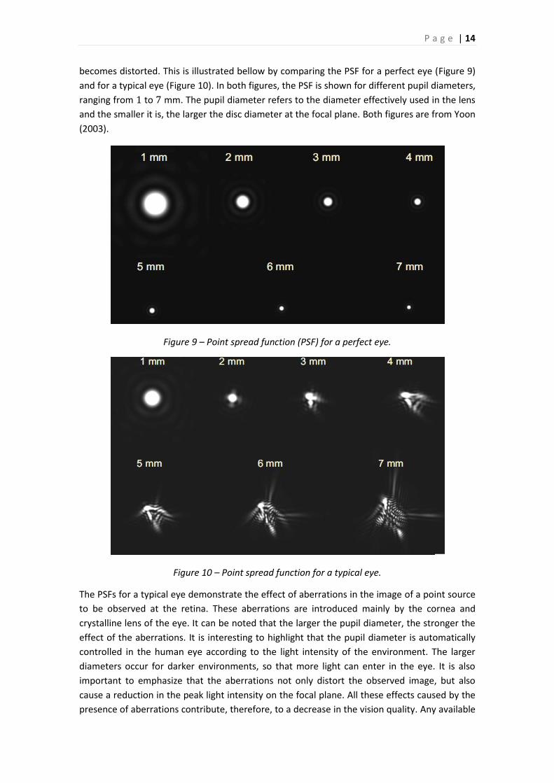
P a g e | 14
becomes distorted. This is illustrated bellow by comparing the PSF for a perfect eye (Figure 9)
and for a typical eye (Figure 10). In both figures, the PSF is shown for different pupil diameters,
ranging from 1 to 7 mm. The pupil diameter refers to the diameter effectively used in the lens
and the smaller it is, the larger the disc diameter at the focal plane. Both figures are from Yoon
(2003).
Figure 9 – Point spread function (PSF) for a perfect eye.
Figure 10 – Point spread function for a typical eye.
The PSFs for a typical eye demonstrate the effect of aberrations in the image of a point source
to be observed at the retina. These aberrations are introduced mainly by the cornea and
crystalline lens of the eye. It can be noted that the larger the pupil diameter, the stronger the
effect of the aberrations. It is interesting to highlight that the pupil diameter is automatically
controlled in the human eye according to the light intensity of the environment. The larger
diameters occur for darker environments, so that more light can enter in the eye. It is also
important to emphasize that the aberrations not only distort the observed image, but also
cause a reduction in the peak light intensity on the focal plane. All these effects caused by the
presence of aberrations contribute, therefore, to a decrease in the vision quality. Any available
P a g e | 15
ways of correcting or compensating for these effects would bring benefits to vision acuity. As
an example, Sabesan et. al. (2007) demonstrated the effectiveness of customized soft contact
lenses to reduce significantly the high-order aberrations in keratoconic eyes, guaranteeing
therefore a normal quality of vision to those abnormal corneal patients.
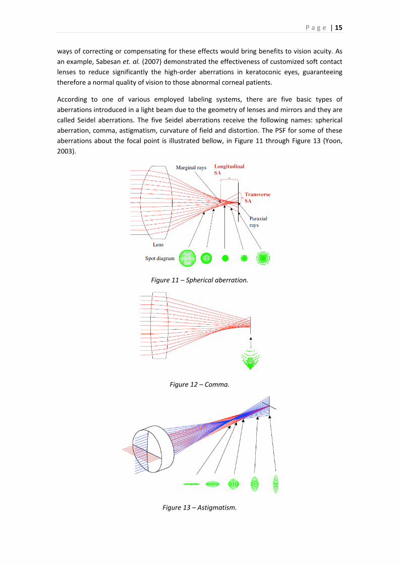
According to one of various employed labeling systems, there are five basic types of
aberrations introduced in a light beam due to the geometry of lenses and mirrors and they are
called Seidel aberrations. The five Seidel aberrations receive the following names: spherical
aberration, comma, astigmatism, curvature of field and distortion. The PSF for some of these
aberrations about the focal point is illustrated bellow, in Figure 11 through Figure 13 (Yoon,
2003).
Figure 11 – Spherical aberration.
Figure 12 – Comma.
Figure 13 – Astigmatism.
P a g e | 16
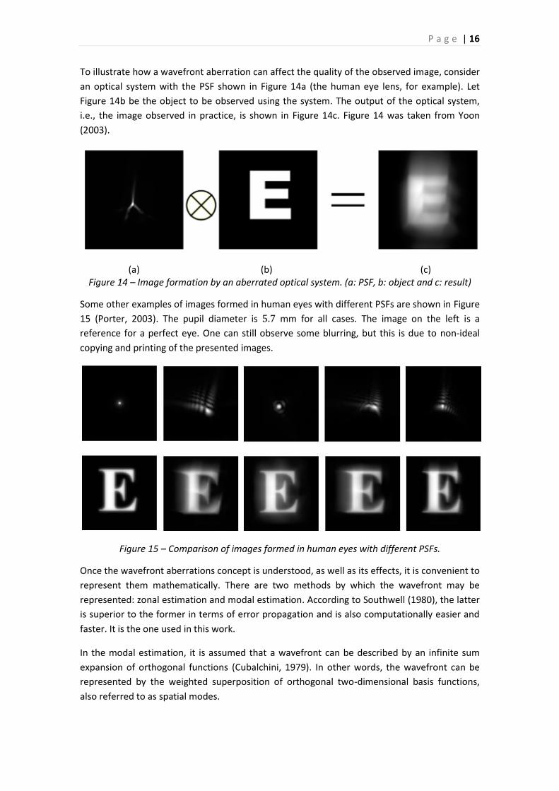
To illustrate how a wavefront aberration can affect the quality of the observed image, consider
an optical system with the PSF shown in Figure 14a (the human eye lens, for example). Let
Figure 14b be the object to be observed using the system. The output of the optical system,
i.e., the image observed in practice, is shown in Figure 14c. Figure 14 was taken from Yoon
(2003).
(a) (b) (c) Figure 14 – Image formation by an aberrated optical system. (a: PSF, b: object and c: result)
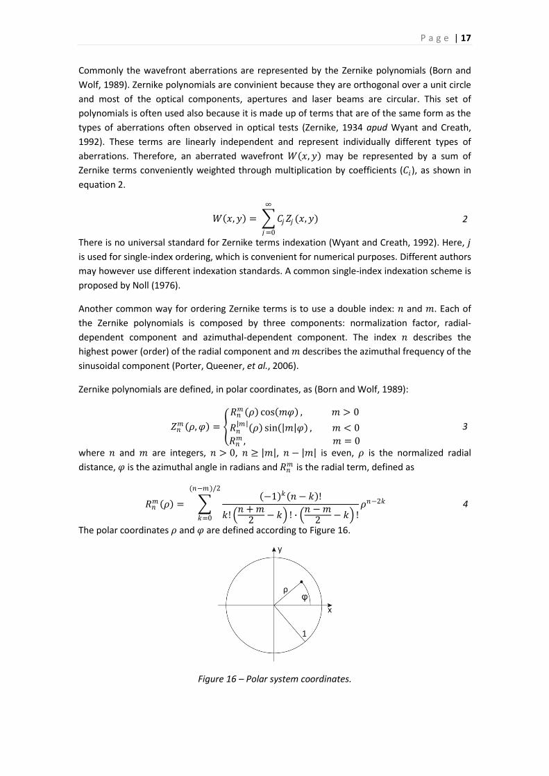
Some other examples of images formed in human eyes with different PSFs are shown in Figure
15 (Porter, 2003). The pupil diameter is 5.7 mm for all cases. The image on the left is a
reference for a perfect eye. One can still observe some blurring, but this is due to non-ideal
copying and printing of the presented images.
Figure 15 – Comparison of images formed in human eyes with different PSFs.
Once the wavefront aberrations concept is understood, as well as its effects, it is convenient to
represent them mathematically. There are two methods by which the wavefront may be
represented: zonal estimation and modal estimation. According to Southwell (1980), the latter
is superior to the former in terms of error propagation and is also computationally easier and
faster. It is the one used in this work.
In the modal estimation, it is assumed that a wavefront can be described by an infinite sum
expansion of orthogonal functions (Cubalchini, 1979). In other words, the wavefront can be
represented by the weighted superposition of orthogonal two-dimensional basis functions,
also referred to as spatial modes.
P a g e | 17
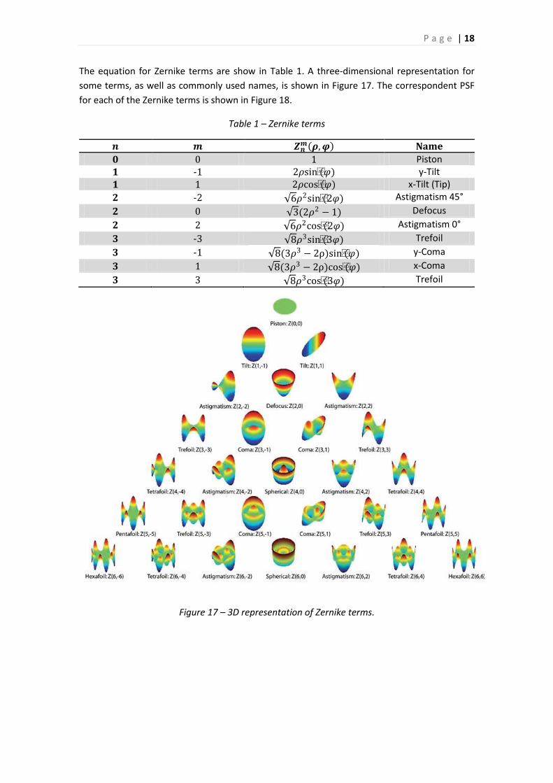
Commonly the wavefront aberrations are represented by the Zernike polynomials (Born and
Wolf, 1989). Zernike polynomials are convinient because they are orthogonal over a unit circle
and most of the optical components, apertures and laser beams are circular. This set of
polynomials is often used also because it is made up of terms that are of the same form as the
types of aberrations often observed in optical tests (Zernike, 1934 apud Wyant and Creath,
1992). These terms are linearly independent and represent individually different types of
aberrations. Therefore, an aberrated wavefront 𝑊 𝑥, 𝑦 may be represented by a sum of
Zernike terms conveniently weighted through multiplication by coefficients (𝐶𝑖), as shown in
equation 2.
𝑊 𝑥, 𝑦 = 𝐶𝑗𝑍𝑗 (𝑥, 𝑦)
∞
𝑗 =0
2
There is no universal standard for Zernike terms indexation (Wyant and Creath, 1992). Here, 𝑗
is used for single-index ordering, which is convenient for numerical purposes. Different authors
may however use different indexation standards. A common single-index indexation scheme is
proposed by Noll (1976).
Another common way for ordering Zernike terms is to use a double index: 𝑛 and 𝑚. Each of
the Zernike polynomials is composed by three components: normalization factor, radial-
dependent component and azimuthal-dependent component. The index 𝑛 describes the
highest power (order) of the radial component and 𝑚 describes the azimuthal frequency of the
sinusoidal component (Porter, Queener, et al., 2006).
Zernike polynomials are defined, in polar coordinates, as (Born and Wolf, 1989):
𝑍𝑛𝑚 𝜌, 𝜑 =
𝑅𝑛𝑚 𝜌 cos 𝑚𝜑 , 𝑚 > 0
𝑅𝑛 𝑚 𝜌 sin 𝑚 𝜑 , 𝑚 < 0
𝑅𝑛𝑚 , 𝑚 = 0
3
where 𝑛 and 𝑚 are integers, 𝑛 > 0, 𝑛 ≥ 𝑚 , 𝑛 − 𝑚 is even, 𝜌 is the normalized radial
distance, 𝜑 is the azimuthal angle in radians and 𝑅𝑛𝑚 is the radial term, defined as
𝑅𝑛𝑚 𝜌 =
−1 𝑘 𝑛 − 𝑘 !
𝑘! 𝑛 + 𝑚
2 − 𝑘 ! ∙ 𝑛 − 𝑚
2 − 𝑘 !
(𝑛−𝑚)/2
𝑘=0
𝜌𝑛−2𝑘 4
The polar coordinates 𝜌 and 𝜑 are defined according to Figure 16.
Figure 16 – Polar system coordinates.
P a g e | 18
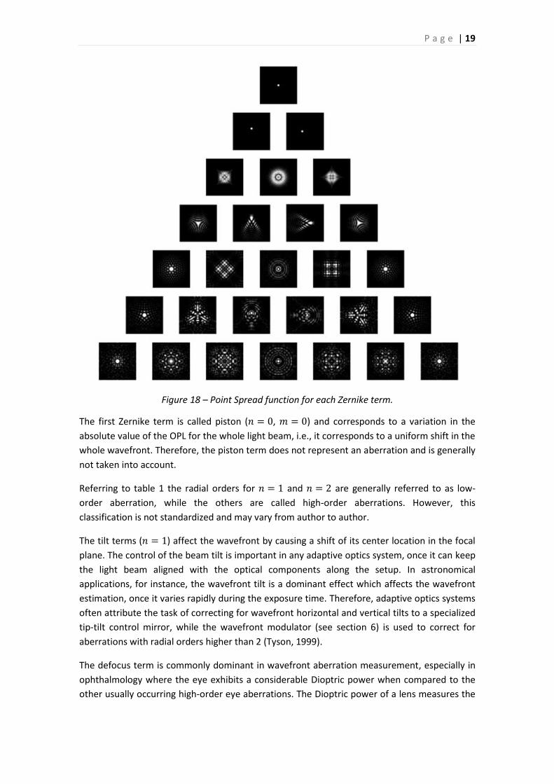
The equation for Zernike terms are show in Table 1. A three-dimensional representation for
some terms, as well as commonly used names, is shown in Figure 17. The correspondent PSF
for each of the Zernike terms is shown in Figure 18.
Table 1 – Zernike terms
𝒏 𝒎 𝒁𝒏𝒎 𝝆, 𝝋 Name
0 0 1 Piston 1 -1 2𝜌sin(𝜑) y-Tilt 1 1 2𝜌cos(𝜑) x-Tilt (Tip)
2 -2 6𝜌2sin(2𝜑) Astigmatism 45°
2 0 3(2𝜌2 − 1) Defocus
2 2 6𝜌2cos(2𝜑) Astigmatism 0°
3 -3 8𝜌3sin(3𝜑) Trefoil
3 -1 8(3𝜌3 − 2ρ)sin(𝜑) y-Coma
3 1 8(3𝜌3 − 2ρ)cos(𝜑) x-Coma
3 3 8𝜌3cos(3𝜑) Trefoil
Figure 17 – 3D representation of Zernike terms.
P a g e | 19
Figure 18 – Point Spread function for each Zernike term.
The first Zernike term is called piston (𝑛 = 0, 𝑚 = 0) and corresponds to a variation in the
absolute value of the OPL for the whole light beam, i.e., it corresponds to a uniform shift in the
whole wavefront. Therefore, the piston term does not represent an aberration and is generally
not taken into account.
Referring to table 1 the radial orders for 𝑛 = 1 and 𝑛 = 2 are generally referred to as low-
order aberration, while the others are called high-order aberrations. However, this
classification is not standardized and may vary from author to author.
The tilt terms (𝑛 = 1) affect the wavefront by causing a shift of its center location in the focal
plane. The control of the beam tilt is important in any adaptive optics system, once it can keep
the light beam aligned with the optical components along the setup. In astronomical
applications, for instance, the wavefront tilt is a dominant effect which affects the wavefront
estimation, once it varies rapidly during the exposure time. Therefore, adaptive optics systems
often attribute the task of correcting for wavefront horizontal and vertical tilts to a specialized
tip-tilt control mirror, while the wavefront modulator (see section 6) is used to correct for
aberrations with radial orders higher than 2 (Tyson, 1999).
The defocus term is commonly dominant in wavefront aberration measurement, especially in
ophthalmology where the eye exhibits a considerable Dioptric power when compared to the
other usually occurring high-order eye aberrations. The Dioptric power of a lens measures the
P a g e | 20
power to which a lens can bend the propagation direction of light rays. It is defined as the
reciprocal of the focal length, in meters, and is given in diopters, in the MKS unit system.
7. ADAPTIVE OPTICS SYSTEM
Wavefront aberrations can represent a serious problem in many different applications where
high-quality images are demanded, such as in astronomy, ophthalmology, microscopy and
others. Adaptive optics is used in order to compensate for these distortions actively and in
real-time, so that aberrations are minimized and hence, noise and errors present in the output
of the optical systems are also minimized.
All adaptive optics systems must perform two general tasks: wavefront sensing and wavefront
correction (Hein, 2005). Wavefront sensing is the process in which the wavefront aberration is
measured by a wavefront sensor. The wavefront correction is the process in which an active
component of the system is actuated so that the incoming light has its phase pattern altered.
In this sense, a general AO system is basically composed of three subsystems: wavefront
sensor (WFS), wavefront modulator and control system (Greenaway and Burnett, 2004).
The wavefront sensor is responsible for the estimation of the wavefront shape. This can be
done through direct measurement of the wavefront or analysis of some image quality
parameter.
When the application requires quantitative description of the wavefront, direct measurements
must be performed. There are several different methods for doing that and the one used in
this work will be discussed later. In this case, the WFS output signals provide information
about the aberration and represent the input to the control system. In this step, the wavefront
shape is reconstructed and then drive signals are generated to actuate the wavefront
modulator.
In some other applications, the description of the wavefront shape may not be demanded. In
this case, the wavefront sensor may consist simply of a camera or a photodetector. The AO
control system then measures some image quality parameter and actuates the wavefront
modulator so as to optimize this parameter (Greenaway and Burnett, 2004).
The modulator is responsible for modifying the wavefront shape appropriately, so as to correct
for the distortions originally present in the light beam and then to provide a distortion-free
output light beam. It is important to note that a specialized tip-tilt control mirror is commonly
used to compensate for the wavefront tilt, which offloads the modulator from the
requirement of large strokes to compensate for such low-order aberration.
Figure 19 (Greenaway and Burnett, 2004) illustrates how the three subsystems are assembled
together.
P a g e | 21
Figure 19 – AO system.
For a better understanding of how the adaptive optics system works, each of its three
subsystems will be treated separately in more detail in the following sections.
7.1. WAVEFRONT SENSOR
The wavefront sensor detects the wavefront shape. There are many different methods
available to measure wavefront aberrations, such as: pyramidal sensor, laser ray tracing
technique, Hartmann test, interferometric methods, and others (De Lima Monteiro, 2002).
However, the most popular wavefront sensor in the world is the Hartmann-Shack sensor (Platt
and Shack, 2001).
The principle of the Hartmann-Shack wavefront sensor is based on geometrical optics. It is
composed of a lenslet array and a 2D detector, which can be a camera, such as a CCD, or an
array of optical position-sensitive detectors (PSDs). The lenslets that compose the array have
all the same focal length, and are assembled in the system so that the detector plane coincides
with the focal plane.
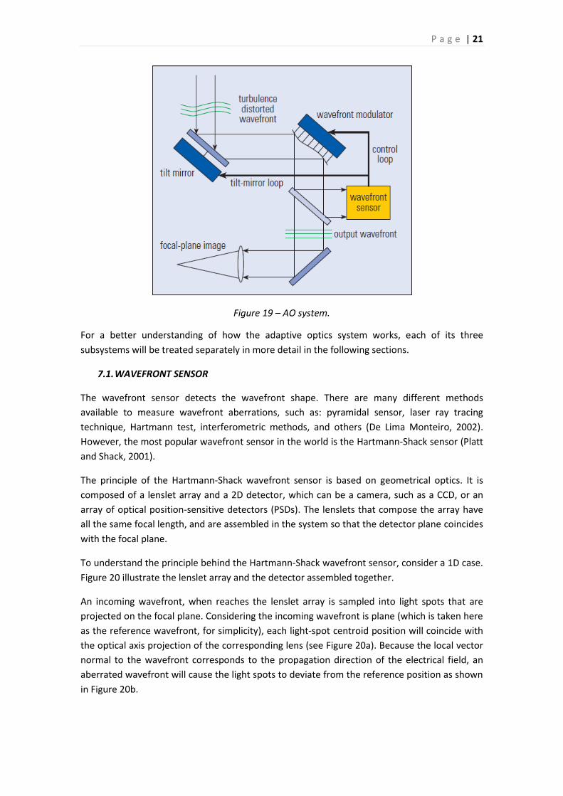
To understand the principle behind the Hartmann-Shack wavefront sensor, consider a 1D case.
Figure 20 illustrate the lenslet array and the detector assembled together.
An incoming wavefront, when reaches the lenslet array is sampled into light spots that are
projected on the focal plane. Considering the incoming wavefront is plane (which is taken here
as the reference wavefront, for simplicity), each light-spot centroid position will coincide with
the optical axis projection of the corresponding lens (see Figure 20a). Because the local vector
normal to the wavefront corresponds to the propagation direction of the electrical field, an
aberrated wavefront will cause the light spots to deviate from the reference position as shown
in Figure 20b.
P a g e | 22
(a) (b)
Figure 20 – 1D schematics of the Hartmann-Shack principle (a: plane wavefront, b: arbitrary wavefront).
For each light spot, the deviation from the reference position is proportional to the mean
wavefront tilt in the respective lens. This relation between deviation and mean wavefront local
tilt is shown graphically in Figure 21 and is written in equation 5.
Figure 21 – Relation between the local wavefront (WF) aberration 𝑊 and the ray deviation.
𝑆𝑥 = tan 𝜃𝑥𝑖= 𝑑𝑊𝑥
𝑑𝑥
(𝑥𝑖 ,𝑦𝑖)≅
∆𝑥
𝐷; 𝑆𝑦 = tan 𝜃𝑦𝑖
= 𝑑𝑊𝑦
𝑑𝑦
(𝑥𝑖 ,𝑦𝑖)
≅∆𝑦
𝐷 5
The approximation in equation 5 is because the change in the propagation direction caused by
the lens is not being taken into account in the equation, for simplicity. In practice, a corrector
factor which depends both on 𝜃 and 𝑛 appears multiplying ∆𝑥 and ∆𝑦. See section 8.1.2 for a
rigorous treatment of the lens influence on the deviation measurement.
The set of light-spot deviations enables the reconstruction of the wavefront aberration
through a mathematical model, which will be explained in the control system section (7.3).
When the 2D detector is a CCD camera, the output of the sensor is an image of the light spots,
which has to be processed by the control system in order to determine the centroid positions;
then the deviation of each light spot needs to be estimated before reconstructing the
wavefront aberration.
P a g e | 23
Another possibility is when the focal plane comprises an array of position-sensitive detectors,
which can measure the x and y coordinates of light-spot centroids. In this case, each optical
detector is associated to a lenslet and therefore is responsible for measuring the position of
the correspondent light spot. The output of each optical position detector is an analog signal
proportional to the light spot deviation. These signals are then converted to digital signals
which are read and interpreted by the control system, before reconstructing the wavefront.
Once the Hartmann-Shack method is based on spatially sampling the wavefront, it is likely that
errors related to the sampling process will be present. In general, these errors are closely
related to the lenslet array geometric parameters, such as the grid pitch, lens diameter and
array geometric shape. The error also depends on the number of spatial modes, namely
Zernike terms, necessary to describe the wavefront aberration.
7.2. WAVEFRONT MODULATOR
The wavefront modulator is an active element responsible for modifying the wavefront shape.
There are different types of wavefront modulators, which can actuate either through
refraction or reflection. Some examples are: liquid-crystal phase modulators, continuous or
segmented mirrors and bimorph mirrors (Greenaway and Burnett, 2004).
The most widely used wavefront modulators for adaptive optics are the deformable mirrors. A
deformable mirror can change its surface shape to match the phase distortions measured by
the wavefront sensor (Tyson, 1999).
There are basically three types of deformable mirrors: segmented, bimorph and membrane.
The segmented mirror surface is composed of small reflective parts, which can be individually
actuated through mechanical mechanisms. The bimorph mirror makes use of PZT material,
which deforms when voltage is applied to it. The membrane deformable mirror exploits
electrostatic forces, electromagnetic coils (Hamelinck, Rosielle, et al., 2007), piezoelectric rod
extension or thermal expansion (Vdovin and Loktev, 2002; Vdovin, Loktev and Soloviev, 2007)
to deform a flexible reflective surface. The electrostatic actuated membrane mirror is used in
this work. More details about it will be given bellow. A detailed description of other mirrors
types is given by Greenaway and Burnett (2004).
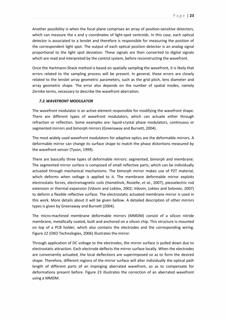
The micro-machined membrane deformable mirrors (MMDM) consist of a silicon nitride
membrane, metallically coated, built and anchored on a silicon chip. This structure is mounted
on top of a PCB holder, which also contains the electrodes and the corresponding wiring.
Figure 22 (OKO Technologies, 2006) illustrates the mirror.
Through application of DC voltage to the electrodes, the mirror surface is pulled down due to
electrostatic attraction. Each electrode deflects the mirror surface locally. When the electrodes
are conveniently actuated, the local deflections are superimposed so as to form the desired
shape. Therefore, different regions of the mirror surface will alter individually the optical path
length of different parts of an impinging aberrated wavefront, so as to compensate for
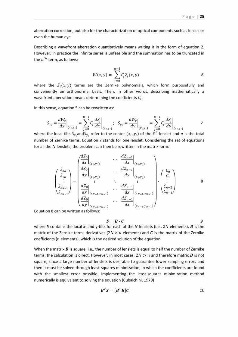
deformations present before. Figure 23 illustrates the correction of an aberrated wavefront
using a MMDM.
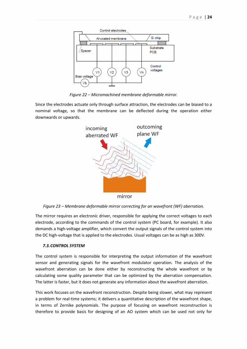
P a g e | 24
Figure 22 – Micromachined membrane deformable mirror.
Since the electrodes actuate only through surface attraction, the electrodes can be biased to a
nominal voltage, so that the membrane can be deflected during the operation either
downwards or upwards.
Figure 23 – Membrane deformable mirror correcting for an wavefront (WF) aberration.
The mirror requires an electronic driver, responsible for applying the correct voltages to each
electrode, according to the commands of the control system (PC board, for example). It also
demands a high-voltage amplifier, which convert the output signals of the control system into
the DC high-voltage that is applied to the electrodes. Usual voltages can be as high as 300V.
7.3. CONTROL SYSTEM
The control system is responsible for interpreting the output information of the wavefront
sensor and generating signals for the wavefront modulator operation. The analysis of the
wavefront aberration can be done either by reconstructing the whole wavefront or by
calculating some quality parameter that can be optimized by the aberration compensation.
The latter is faster, but it does not generate any information about the wavefront aberration.
This work focuses on the wavefront reconstruction. Despite being slower, what may represent
a problem for real-time systems; it delivers a quantitative description of the wavefront shape,
in terms of Zernike polynomials. The purpose of focusing on wavefront reconstruction is
therefore to provide basis for designing of an AO system which can be used not only for
P a g e | 25
aberration correction, but also for the characterization of optical components such as lenses or
even the human eye.
Describing a wavefront aberration quantitatively means writing it in the form of equation 2.
However, in practice the infinite series is unfeasible and the summation has to be truncated in
the 𝑛𝑡ℎ term, as follows:
𝑊 𝑥, 𝑦 = 𝐶𝑗𝑍𝑗 (𝑥, 𝑦)
𝑛−1
𝑗 =0
6
where the 𝑍𝑖(𝑥, 𝑦) terms are the Zernike polynomials, which form purposefully and
conveniently an orthonormal basis. Then, in other words, describing mathematically a
wavefront aberration means determining the coefficients 𝐶𝑖 .
In this sense, equation 5 can be rewritten as:
𝑆𝑥𝑖= 𝑑𝑊𝑥
𝑑𝑥
(𝑥𝑖 ,𝑦𝑖)= 𝐶𝑗
𝑑𝑍𝑗
𝑑𝑥
(𝑥𝑖 ,𝑦𝑖)
𝑛−1
𝑗 =0
; 𝑆𝑦𝑖=
𝑑𝑊𝑦
𝑑𝑦
(𝑥𝑖 ,𝑦𝑖)
= 𝐶𝑗 𝑑𝑍𝑗
𝑑𝑦
(𝑥𝑖 ,𝑦𝑖)
𝑛−1
𝑗 =0
7
where the local tilts 𝑆𝑥𝑖and𝑆𝑦𝑖
refer to the center (𝑥𝑖 , 𝑦𝑖) of the 𝑖𝑡ℎ lenslet and 𝑛 is the total
number of Zernike terms. Equation 7 stands for one lenslet. Considering the set of equations
for all the 𝑁 lenslets, the problem can then be rewritten in the matrix form:
𝑆𝑥0
𝑆𝑦0
⋮𝑆𝑥𝑁−1
𝑆𝑦𝑁−1
=
𝑑𝑍0
𝑑𝑥
(𝑥0 ,𝑦0) ⋯ 𝑑𝑍𝑛−1
𝑑𝑥 (𝑥0 ,𝑦0)
𝑑𝑍0
𝑑𝑦
(𝑥0 ,𝑦0)
⋯ 𝑑𝑍𝑛−1
𝑑𝑦 (𝑥0 ,𝑦0)
⋮ ⋱ ⋮
𝑑𝑍0
𝑑𝑥
(𝑥𝑁−1 ,𝑦𝑁−1)⋯ 𝑑𝑍𝑛−1
𝑑𝑥 (𝑥𝑁−1 ,𝑦𝑁−1)
𝑑𝑍0
𝑑𝑦
(𝑥𝑁−1 ,𝑦𝑁−1)
⋯ 𝑑𝑍𝑛−1
𝑑𝑥 (𝑥𝑁−1 ,𝑦𝑁−1)
∙
𝐶0
𝐶1
⋮𝐶𝑛−2
𝐶𝑛−1
8
Equation 8 can be written as follows:
𝑺 = 𝑩 ∙ 𝑪 9 where 𝑺 contains the local x- and y-tilts for each of the 𝑁 lenslets (i.e., 2𝑁 elements), 𝑩 is the
matrix of the Zernike terms derivatives (2𝑁 × 𝑛 elements) and 𝑪 is the matrix of the Zernike
coefficients (𝑛 elements), which is the desired solution of the equation.
When the matrix 𝑩 is square, i.e., the number of lenslets is equal to half the number of Zernike
terms, the calculation is direct. However, in most cases, 2𝑁 > 𝑛 and therefore matrix 𝑩 is not
square, since a large number of lenslets is desirable to guarantee lower sampling errors and
then it must be solved through least-squares minimization, in which the coefficients are found
with the smallest error possible. Implementing the least-squares minimization method
numerically is equivalent to solving the equation (Cubalchini, 1979)
𝑩𝑇𝑺 = 𝑩𝑇𝑩 𝑪 10
P a g e | 26
where 𝑩𝑇 is the transpose of 𝑩. Once the wavefront is reconstructed, the control system is
able to operate the deformable mirror. Different techniques for controlling the mirror can be
used, depending on the hardware built for the application.
In general, the control systems comprise a computer and peripherals, such as analog/digital
converters and voltage amplifiers. The control task reduces then to writing algorithms capable
of generating output signals to drive the mirror in order to compensate for the wavefront
aberration.
A great deal in generating the output signals for driving the mirror refers to converting the
wavefront aberration information into voltage signals. It depends on mirror characteristics,
such as possible modes that can be reproduced and the influence functions Influence functions
describe how the operation of each electrode alters the mirror surface. All these specific
demands of the designed adaptive optics system suggest that the control systems are
generally customized to match the application requirements and the AO system
characteristics.
When using a micro-machined membrane deformable mirror, the algorithm must be capable
of determining what will be the voltages to be applied to each electrode. The procedure
consists in relating the light-spot deviations to the voltages applied to the mirror. In this case,
the wavefront aberration is not described in terms of Zernike polynomials. Instead, the basis
used consists of the influence functions of the mirror. Therefore, the Zernike derivatives in
matrix 𝑩 of equation 10 are replaced with the measured spot deviations obtained by
sequentially actuating each of the electrodes at a time. The result of equation 10 is matrix 𝑪
which, in this case, contains the square of the voltages to be applied to the mirror, rather than
the Zernike coefficients (De Lima Monteiro, 2002). The voltage information is then sent to the
hardware interface, which will actually apply, according to the control commands, the
specified voltages to each of the actuators.
8. METHODS, RESULTS AND DISCUSSIONS
8.1. LENSLET ARRAY OPTIMIZATION FOR APPLICATION IN OPHTHALMOLOGY
In ophthalmology, the Hartmann-Shack wavefront sensor is included in a class of equipments
commonly referred to as aberrometers. It is a useful tool for assessment of the image quality
of the eye, with applications to both research and clinical evaluation (Llorente, Marcos, et al.,
2007).
An important element in the Hartmann-Shack wavefront sensor is the lenslet array,
responsible for sampling the incoming wavefront into light-spots on the focal plane. The
position of each light-spot provides information about the wavefront averaged local tilts over
the respective lenslet. The lenslet array is characterized by its grid/gridless pattern, lens
contour, number of lenslets and fill factor1. Typically, the used grid patterns consist in either a
fixed rectangular or hexagonal configuration. The number of lenslets range from tens to more
than 15,000 (Llorente, Marcos, et al., 2007).
1 Fill factor: ratio of the area occupied by lenses to the total array area.
P a g e | 27
It is important to emphasize here that the aberrations introduced in a light beam depend on
characteristics of the medium (see section 6.2). This set of characteristics that describe the
medium impose that the aberrations it introduces in a light beam will contain similarities. In
other words, typical aberrations are associated to each medium. To each of these contexts, i.e.
set of characteristics that describe a medium, an appropriate statistical model can be
associated to describe the typical aberrations it introduces in a light beam. For example,
aberrations introduced by the atmosphere are generally described by the Kolmogoroff model
(Noll, 1976). Aberrations introduced by the human eye can be described by models based on
the measurement of aberrations in a large population (Porter, Guirao, et al., 2001). Another
context refers to the aberrations introduced by underwater environments, due to water
turbulence, temperature and salinity variations, what can affect significantly the quality of
underwater imaging (Yura, 1973; Holohan and Dainty, 1997).
Soloviev and Vdovin (2005) have discussed about the influence of the geometry of a
Hartmann-Shack lenslet array on the wavefront reconstruction error, which indicates the
accuracy with which the reconstructed wavefront matches the exact shape of the original one.
They propose the use of a randomized array geometry, which doubles the number of correctly
reconstructed modes, adding no additional computation time and providing a smaller
reconstruction error. That was verified in the article for up to 40 modes.
In their paper, Soloviev and Vdovin (2005) propose a general mathematical model to describe
the modal wavefront reconstruction, depending neither on the choice of the basis functions
nor on the statistics used for describing the wavefront. This model demonstrates the
dependency of the reconstruction error on the array geometry. They have carried out tests
with lenslet array of different geometries and compared the reconstruction error in each case,
using Zernike polynomials with coefficients generated by a statistics for the description of the
atmospheric turbulence (Noll, 1976). Arrays with randomly distributed lenslet centers
generated better results than the regular ones, especially when the number of Zernike terms
increased to more than 40, situation in which the regular arrays experience a catastrophic
growth of the aliasing error.
They have also demonstrated that the optimal number of Zernike terms that can be correctly
reconstructed by the Hartmann-Shack method is always less or of the same order than the
number of lenslets. Moreover, they have shown that it is possible to increase the number of
Zernike terms, maintaining the same reconstruction error, just by randomizing the lenslets
positions.
Since it has been demonstrated that random arrays can generate smaller reconstruction errors
than regular ones, one interesting question can be formulated: given a certain statistics
describing the wavefront aberrations in some context, is it possible to specify the best lenslet
array geometry, i.e., the one that will generate the smallest reconstruction errors?
In order to try to answer this question, a methodology is proposed in this work to find the
lenslets distribution pattern in the array that minimizes the reconstruction error in a
Hartmann-Shack sensor.
P a g e | 28
Here, the wavefront aberrations used were generated by the statistical model for ocular
aberrations, described in section 8.1.3. Therefore, the lenslet array will be optimized for
ophthalmological purposes, although the proposed methodology can be carried out with any
other wavefront-aberration statistics.
The importance of specifying an optimal array for ophthalmology is expressed in the words2 of
Llorente et al (2007):
The determination of a sampling pattern with the minimum sampling density that provides
accurate results is of practical importance for sequential aberrometers, since it would decrease
measurement time, and of general interest to better understand the trade-offs between
aberrometers. It is also useful to determine whether there are sampling patterns that are
better adapted to typical ocular aberrations, or particular sampling patterns optimized for
measurement under specific conditions.
Note that, besides determining an optimal lenslet array for a specified number of lenslets, it is
also desirable to determine arrays with a smaller number of lenslets, preserving the
reconstruction error magnitude. Both aspects are exploited in this work.
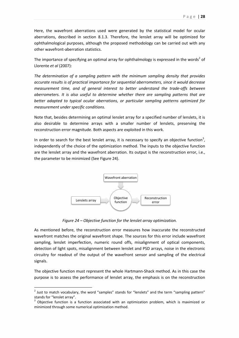
In order to search for the best lenslet array, it is necessary to specify an objective function3,
independently of the choice of the optimization method. The inputs to the objective function
are the lenslet array and the wavefront aberration. Its output is the reconstruction error, i.e.,
the parameter to be minimized (See Figure 24).
Figure 24 – Objective function for the lenslet array optimization.
As mentioned before, the reconstruction error measures how inaccurate the reconstructed
wavefront matches the original wavefront shape. The sources for this error include wavefront
sampling, lenslet imperfection, numeric round offs, misalignment of optical components,
detection of light spots, misalignment between lenslet and PSD arrays, noise in the electronic
circuitry for readout of the output of the wavefront sensor and sampling of the electrical
signals.
The objective function must represent the whole Hartmann-Shack method. As in this case the
purpose is to assess the performance of lenslet array, the emphasis is on the reconstruction
2 Just to match vocabulary, the word “samples” stands for “lenslets” and the term “sampling pattern”
stands for “lenslet array”. 3 Objective function is a function associated with an optimization problem, which is maximized or
minimized through some numerical optimization method.
Objective function
Wavefront aberration
Lenslets arrayReconstruction
error

P a g e | 29
error due to the wavefront sampling process. Therefore, an algorithm was used to simulate
the Hartmann-Shack method, including the steps of generation of an incoming wavefront,
input to a specified lenslet array, wavefront sampling, calculation of light-spots deviation,
wavefront reconstruction and calculation of the reconstruction error. The detection step is not
taken into account and is, in practice, performed by a CCD camera or a 2D array of position-
sensitive detectors.
Once the objective function is defined, one must specify an optimization method, which will be
responsible for trying to find the lenslet array that minimizes the reconstruction error.
Therefore, the input to the optimization method will be the reconstruction error and its output
will be the lenslet array.
Figure 25 – Schematics of the optimization function operation.
To provide the wavefront aberration input to the objective function, an algorithm must be
built for generating the aberrations according the desired statistics.
The next sections will treat in detail the algorithm to simulate the Hartmann-Shack method
and the chosen optimization method.
8.1.1. NUMERICAL MODEL OF THE HARTMANN-SHACK METHOD
An algorithm built in C++ language was adapted from a source code initially developed at the
Electronic Instrumentation Lab/TU-Delft/The Netherlands by G. Vdovin, D. W. de Lima
Monteiro and S. Sakarya to simulate a Hartmann-Shack system. As previously stated, the
detection of the light-spots positions is not taken into account here, since the focus is on the
reconstruction error generated by different lenslet arrays.
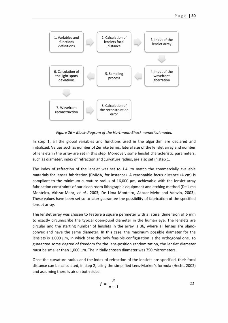
Figure 26 bellow shows a block-diagram of the algorithm. Steps 1 and 2 are used to initialize
the algorithm by setting the values of all global parameters needed in the calculations. Steps 3
and 4 comprise the input of two externally generated variables: lenslet array and incoming
wavefront aberration. In step 5, the aberration is sampled by the lenslet array. Steps 6 and 7
are for the reconstruction of the wavefront aberration from the information generated by the
sampling process. Finally, in step 8, the reconstruction error is calculated. More detailed
comments on each step are given below.
Objective function
Wavefront aberration
Lenslets arrayReconstruction
error
Optimization method
P a g e | 30
Figure 26 – Block-diagram of the Hartmann-Shack numerical model.
In step 1, all the global variables and functions used in the algorithm are declared and
initialized. Values such as number of Zernike terms, lateral size of the lenslet array and number
of lenslets in the array are set in this step. Moreover, some lenslet characteristic parameters,
such as diameter, index of refraction and curvature radius, are also set in step 1.
The index of refraction of the lenslet was set to 1.4, to match the commercially available
materials for lenses fabrication (PMMA, for instance). A reasonable focus distance (4 cm) is
compliant to the minimum curvature radius of 16,000 μm, achievable with the lenslet-array
fabrication constraints of our clean room lithographic equipment and etching method (De Lima
Monteiro, Akhzar-Mehr, et al., 2003; De Lima Monteiro, Akhzar-Mehr and Vdovin, 2003).
These values have been set so to later guarantee the possibility of fabrication of the specified
lenslet array.
The lenslet array was chosen to feature a square perimeter with a lateral dimension of 6 mm
to exactly circumscribe the typical open-pupil diameter in the human eye. The lenslets are
circular and the starting number of lenslets in the array is 36, where all lenses are plano-
convex and have the same diameter. In this case, the maximum possible diameter for the
lenslets is 1,000 μm, in which case the only feasible configuration is the orthogonal one. To
guarantee some degree of freedom for the lens-position randomization, the lenslet diameter
must be smaller than 1,000 μm. The initially chosen diameter was 750 micrometers.
Once the curvature radius and the index of refraction of the lenslets are specified, their focal
distance can be calculated, in step 2, using the simplified Lens-Marker’s formula (Hecht, 2002)
and assuming there is air on both sides:
𝑓 = 𝑅
𝑛 − 1 11
1. Variables and functions
definitions
2. Calculation of lenslets focal
distance
3. Input of the lenslet array
4. Input of the wavefront aberration
5. Sampling process
6. Calculation of the light-spots
deviations
7. Wavefront reconstruction
8. Calculation of the reconstruction
error
P a g e | 31
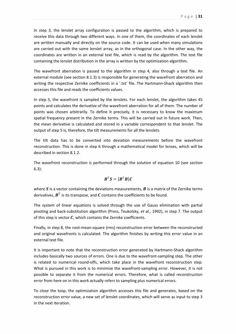
In step 3, the lenslet array configuration is passed to the algorithm, which is prepared to
receive this data through two different ways. In one of them, the coordinates of each lenslet
are written manually and directly on the source code. It can be used when many simulations
are carried out with the same lenslet array, as in the orthogonal case. In the other way, the
coordinates are written in an external text file, which is read by the algorithm. The text file
containing the lenslet distribution in the array is written by the optimization algorithm.
The wavefront aberration is passed to the algorithm in step 4, also through a text file. An
external module (see section 8.1.3) is responsible for generating the wavefront aberration and
writing the respective Zernike coefficients in a ‘.txt’ file. The Hartmann-Shack algorithm then
accesses this file and reads the coefficients values.
In step 5, the wavefront is sampled by the lenslets. For each lenslet, the algorithm takes 45
points and calculates the derivative of the wavefront aberration for all of them. The number of
points was chosen arbitrarily. To define it precisely, it is necessary to know the maximum
spatial frequency present in the Zernike terms. This will be carried out in future work. Then,
the mean derivative is calculated and stored in a variable correspondent to that lenslet. The
output of step 5 is, therefore, the tilt measurements for all the lenslets.
The tilt data has to be converted into deviation measurements before the wavefront
reconstruction. This is done in step 6 through a mathematical model for lenses, which will be
described in section 8.1.2.
The wavefront reconstruction is performed through the solution of equation 10 (see section
6.3):
𝑩𝑇𝑺 = 𝑩𝑇𝑩 𝑪
where 𝑺 is a vector containing the deviations measurements, 𝑩 is a matrix of the Zernike terms
derivatives, 𝑩𝑇 is its transpose, and 𝑪 contains the coefficients to be found.
The system of linear equations is solved through the use of Gauss elimination with partial
pivoting and back-substitution algorithm (Press, Teukolsky, et al., 1992), in step 7. The output
of this step is vector 𝑪, which contains the Zernike coefficients.
Finally, in step 8, the root-mean-square (rms) reconstruction error between the reconstructed
and original wavefronts is calculated. The algorithm finishes by writing this error value in an
external text file.
It is important to note that the reconstruction error generated by Hartmann-Shack algorithm
includes basically two sources of errors. One is due to the wavefront-sampling step. The other
is related to numerical round-offs, which take place in the wavefront reconstruction step.
What is pursued in this work is to minimize the wavefront-sampling error. However, it is not
possible to separate it from the numerical errors. Therefore, what is called reconstruction
error from here on in this work actually refers to sampling plus numerical errors.
To close the loop, the optimization algorithm accesses this file and generates, based on the
reconstruction error value, a new set of lenslet coordinates, which will serve as input to step 3
in the next iteration.

P a g e | 32
8.1.2. MATHEMATICAL MODEL OF LENSES
To convert the wavefront local tilts onto each lenslet into deviation measurements on the
focal plane, a model describing how plano-convex lenses influence the propagation direction
of light should be used. The model developed here is quite rigorous, so as to be sufficiently
general for cases in which the lens sagitta cannot be disregarded. To describe the model,
consider the following definitions on Table 2.
Table 2- Definition of variables for describing the lens model.
Symbol Name
C Curvature center R Curvature radius n Index of refraction of the lens material n’ Index of refraction of the external medium d Sagitta D Lens diameter A Output point of the light beam m Distance between point A and the focal plane V Lens vertex and input point of the light beam l Distance from the lens to the focal plane f Focal distance Δx Deviation of the light beam from the optical axis measured on the focal plane r Distance between the input and output points δ Distance between the optical axis and the exit point A θ Input incident angle ω, γ, β, α Angles
Figure 27 illustrates a light beam reaching a lens. From the geometrical representation of the
system, relations can be built between various angles and distances, so as to find the beam
deviation from the optical axis ∆𝑥.
The equations derived from the geometrical representation of Figure 27 are the following:
1. Snell’s Law
𝑠𝑖𝑛 𝜃 = 𝑛 ∙ 𝑠𝑖𝑛 𝛼 12 𝑛 ∙ 𝑠𝑖𝑛 𝛽 = 𝑠𝑖𝑛 𝛾 13
2. Sine’s Law (triangle CÂV)
𝑅
𝑠𝑖𝑛(180 − 𝛼)=
𝑅 − 𝑑
𝑠𝑖𝑛 𝛽=
𝑟
𝑠𝑖𝑛 𝜔 14
𝑅 ∙ 𝑠𝑖𝑛 𝛽 = 𝑅 − 𝑑 ∙ 𝑠𝑖𝑛 𝛼 𝑠𝑖𝑛 𝛽 =𝑅 − 𝑑
𝑅∙ 𝑠𝑖𝑛 𝛼 15
3. Geometrical description of the system
𝜔 = 𝛼 − 𝛽 16
𝑟 ∙ 𝑠𝑖𝑛 𝛼 = 𝑅 ∙ 𝑠𝑖𝑛 𝜔 = 𝛿 17
𝑚 = 𝑙 + 𝑑 − 𝑟 ∙ 𝑐𝑜𝑠 𝛼 𝑚 = 𝑓 −𝑅 ∙ 𝑠𝑖𝑛 𝜔
𝑠𝑖𝑛 𝛼∙ 𝑐𝑜𝑠 𝜔 18
∆𝑥 = 𝑚 ∙ 𝑡𝑎𝑛 𝛾 + 𝜔 + 𝛿 19
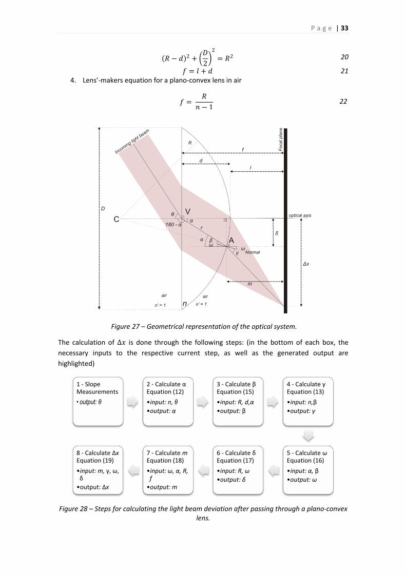
P a g e | 33
𝑅 − 𝑑 2 + 𝐷
2
2
= 𝑅2 20
𝑓 = 𝑙 + 𝑑 21 4. Lens’-makers equation for a plano-convex lens in air
𝑓 = 𝑅
𝑛 − 1 22
Figure 27 – Geometrical representation of the optical system.
The calculation of ∆𝑥 is done through the following steps: (in the bottom of each box, the
necessary inputs to the respective current step, as well as the generated output are
highlighted)
Figure 28 – Steps for calculating the light beam deviation after passing through a plano-convex lens.
1 - Slope Measurements
• output: θ
2 - Calculate αEquation (12)
•input: n, θ
•output: α
3 - Calculate βEquation (15)
•input: R, d,α
•output: β
4 - Calculate γEquation (13)
•input: n,β
•output: γ
5 - Calculate ωEquation (16)
•input: α, β
•output: ω
6 - Calculate δEquation (17)
•input: R, ω
•output: δ
7 - Calculate mEquation (18)
•input: ω, α, R, f
•output: m
8 - Calculate ΔxEquation (19)
•input: m, γ, ω, δ
•output: Δx

P a g e | 34
8.1.3. WAVEFRONT ABERRATIONS GENERATOR
The algorithm to generate wavefront aberrations was developed based on statistics of ocular
aberrations according to Porter et. al. (2001) who listed the typical amplitudes and mean
values of the Zernike coefficients for a mean pupil diameter of 5.7 mm. They have measured
the wavefront aberrations of both eyes of 109 normal human subjects and analyzed the
aberration distribution in the population, describing it in terms of 18 Zernike coefficients
(piston and tilt are not considered).
Porter et. al. (2001) have then computed and plotted the mean values and corresponding
standard deviation of all Zernike coefficients. They present their result through a graph of
error-bars centered in their mean values.
This data was used in this work as a basis for writing the wavefront-aberration generator
algorithm. The idea is to generate wavefront aberrations that belong to a statistical description
based on real measurements, so as to simulate a real application. To do that, Gaussian
probability distributions (equation 23) were associated to each of the Zernike coefficients.
𝑓 𝑥 = 1
2𝜋𝜍2𝑒
−(𝑥−𝜇)2
2𝜍2 23
In equation 23, 𝜇 stands for the mean value of each coefficient and 𝜍, for the standard
deviation. The values of 𝜇 and 𝜍 for each Zernike coefficient are taken from the data reported
by Porter et. al. (2001). As the results are reported in the article only through a graph, the
mean values and corresponding standard deviations were assessed visually from the graph
scale.
To demonstrate accordance between the results generated by the simulation algorithm and
the ones actually measured by Porter et. al. (2001), 10,000 wavefront aberrations were
generated. The mean value and the standard deviation for each Zernike coefficients were
computed and plotted. The result is shown in Figure 29. This graph reproduces exactly the
result found by Porter et. al. (2001, p. 1796), which is based on the real measurement of
wavefront aberrations of 218 human eyes.
P a g e | 35
Figure 29 – Zernike coefficients generated by the algorithm.
8.1.4. OPTIMIZATION ALGORITHM
The optimization problem treated in this work consists in minimizing the reconstruction error
of a Hartmann-Shack sensor by means of an optimal distribution pattern to the lenslet array.
A requirement of the present problem, that affects the choice of the optimization method, is
that the objective function that describes the problem cannot be written in an analytical form.
That is because the simulation of the Hartmann-Shack method includes several recursive
independent operations on the input variables, which cannot be translated together into an
analytical function. Therefore, the optimization method to be used should access only the
input variables to the Hartmann-Shack simulation and its output result, independently of how
the simulation operates the input to generate the reconstruction error as an output.
Considering this aspect, the optimization method chosen was the Genetic Algorithm (GA) –
refer to (Mitchell, 1999) for a detailed study about GA. The GA is a method to solve both
constrained and unconstrained optimization problems and is based on natural selection, the
process that drives biological evolution. The genetic algorithm repeatedly modifies a
population of individual solutions. At each step, the genetic algorithm selects individuals at
random from the current population to be parents and uses them to produce the children for
the next generation. Over successive generations, the population "evolves" towards an
optimal solution. GA can be applied to solve a variety of optimization problems that are not
well suited for standard optimization algorithms, including problems in which the objective
function is discontinuous, non-differentiable, stochastic, or highly nonlinear (The MathWorks,
Inc., 2010).
Z2
0Z
2
-2Z
2
2Z
3
-1Z
3
1Z
3
-3Z
3
3Z
4
0Z
4
2Z
4
-2Z
4
4Z
4
-4Z
5
1Z
5
-1Z
5
3Z
5
-3Z
5
5Z
5
-5
-2
0
2
4
6
8
Mic
rom
ete
rs o
f A
be
rra
tio
n
Zernike coefficient
Z3
-1Z
3
1Z
3
-3Z
3
3Z
4
0Z
4
2Z
4
-2Z
4
4Z
4
-4Z
5
1Z
5
-1Z
5
3Z
5
-3Z
5
5Z
5
-5
-0,3
-0,2
-0,1
0,0
0,1
0,2
0,3

P a g e | 36
The software MatLab© (R2008a) contains a toolbox (OPTIMTOOL – Optimization Toolbox 4.0)
for optimization problems using several different methods, including GA.
The following steps summarize how GA works (The MathWorks, Inc., 2010):
a. Initially, the algorithm creates a random initial population. The population comprises
individuals, which correspond to the coordinates of different lenslet arrays. The
toolbox can generate this initial population by itself; however, if restrictions are
present a function has to be written to generate the individuals. In the present
problem, the arrays have a restriction: the minimum distance between two lenslets
cannot be less than the lenslet diameter; otherwise adjacent lenses will be
superimposed. Therefore, a numerical function had to be written to generate the
initial random population.
b. The algorithm then creates a sequence of new populations. At each step, the
algorithm uses the individuals in the current generation to create the next population,
through the following steps:
i. Scores each individual of the current population by computing its fitness value
(the wavefront reconstruction error in this case), i.e., the output of the
objective function.
ii. Order the individuals of the current population according to a specified
criterion. The rules for ordering the individuals can be specified in the
algorithm. A standard procedure consists in organizing them according to an
ascending order of their fitness values.
iii. Selects individuals, called parents, to generate new individuals, called children.
Here, the selection is based on the fitness value. Therefore, parents and
children are also sets of lenslets coordinates.
iv. Some of the individuals in the current population that have lower fitness
values, i.e. smaller reconstruction error, are chosen as elite. The elite
individuals are passed to the next population.
v. Produces children from the parents. Children are produced either by making
random changes to a single parent (mutation) or by combining the vector
entries of a pair of parents (crossover). More details about the children
generation are given bellow.
vi. Replaces the current population with the children and elite individuals to form
the next generation.
c. The algorithm stops when one of the stopping criteria is reached. The criterion can be
a minimum difference in the fitness value among the individuals of the population, or
a maximum number of generations, or a specified minimum value for the fitness
function, etc.
The new generation is then composed of three types of children: elite, crossover and
mutation. Figure 30 illustrates how each type is created from the correspondent parent.
P a g e | 37
Figure 30 – The three types of children in a new generation.
The elite children are passed to the next generation without any changes. They correspond to
the individuals of lower fitness value in the present generation. The number 𝑒 of elite
individuals in each generation has to be set in the algorithm. Once this number is defined, the
other individuals will be generated either through crossover or mutation. In this work, the elite
operation means that the 𝑒 lenslet arrays that have generated the smallest reconstruction
errors are simply repeated in the next generation, without any changes.
The fraction of the population which will be generated through crossover has to be set in the
algorithm. The others are therefore generated by mutation.
The mutation operation consists in making small random changes in the individuals of the
population. Mutation guarantees genetic diversity to the algorithm. That means that the
search for the optimal solution will occur in a broader space of possible solutions. In the
present context, the mutation consists in causing small changes to the lenslets coordinates of
an array.
The crossover children are generated by a combination of a pair of parents. There are different
functions to control the combination. One of them consists in taking a randomly weighted
average of the pair of parents. In the present problem, the crossover operation means mixing
two different lenslet arrays: 𝐴 and 𝐵. The combination may consist, for instance, in selecting
some lenslets from 𝐴 and some others from 𝐵 and then putting them together to form the
new array. It may also consist in averaging, for each lenslet, the coordinates given by both
arrays, so as to build the new children. The way the pair of parents is combined is specified in
the algorithm.
8.1.5. METHODOLOGY
This section discusses how to approach the lenslet randomization problem using the
optimization tools available.
Before discussing the methodology itself, it is very important to emphasize one aspect: the
objective function has many local minima. This makes the problem very difficult to solve, in
terms of finding a global minimum and also proving it is actually the global one.
P a g e | 38
An important fact to consider is that the optimized, supposedly random, array has to yield an
error lower than that of the regular lens array at least for the majority of incident wavefront
aberrations. The number of possible wavefront aberrations, according to the ocular
aberrations statistics, is infinite. Therefore, a possible approach to the problem would be to
select some wavefront aberrations and then find the optimal array for each of these
aberrations. The arrays found would then be averaged so that one single array could be
specified as the optimized array (mean array, in this case).
However, that approach would not lead to significant results, because the mean array is very
similar to the regular one. The problem is that the arrays can be very different from one
optimization process to the other, due to not only the different input aberrations, but also the
undetermined number of local minima. Therefore, in the average, the lenslet coordinates tend
to be those of the regular array. Moreover, trying to find the best array through some kind of
mathematical manipulation of the arrays previously found can lead to catastrophic results,
once the objective function is very sensitive to small changes in the lenslet positions and
because there is a restriction that two lenslet centers cannot be closer than one lenslet
diameter.
The methodology developed for optimizing the lenslet array is summarized in the following
outline:
1. For each Zernike coefficient, the mean value shown in Figure 29 was taken and then a
typical wavefront aberration could be specified. This typical wavefront aberration
represents the whole universe of possible aberrations for the considered statistics.
2. The optimization process is carried out 10 times for this typical wavefront aberration.
Then, the result consists of 10 different lenslet arrays.
3. Each of these arrays is subjected to a comparison test with the orthogonal array. The
test consists in calculating the reconstruction error both for the optimized and regular
arrays for a fixed set of 2,000 different wavefront aberrations under the same
statistics. This number was chosen arbitrarily, but it is assumed to represent the whole
population. It may be important to emphasize that the original paper, which generated
the statistical data for ocular aberrations, analyzed 109 human cases (Porter, Guirao,
et al., 2001), what is considered a large population in ophthalmological studies. The
optimized arrays are then compared to regular arrays in terms of:
a. how smaller the reconstruction errors they produce are and
b. the percentage of wavefront aberrations for which the optimized array
produces a smaller reconstruction error.
4. The array which generates the best results, according to the criteria above, is
considered as the best array found.
There are no means of guaranteeing that this is the best array that can ever be found. But it
can be surely stated that it is better than the regular one and also better than at least other
nine non-regular arrays.
The genetic algorithm configuration used to solve the problem is:
a. Number of elite individuals: 2 out of 250.
P a g e | 39
b. Crossover fraction, i.e., the fraction of the total population (minus the elite individuals)
which will be generated by the crossover operation: 50%.
c. Crossover function: intermediate, which creates children by a random weighted
average of the parents.
d. Mutation function: adaptive feasible, which starts with a large mutation possibility in
the beginning of the optimization and then sets it smaller as the process converges to
the final solution.
e. Stopping criterion: objective function tolerance, which means that the GA will stop
when the fitness value does not change more than 5 × 10⁻⁵ from one generation to
another. This value was chosen arbitrarily.
As an additional goal, more than just finding the array geometry that produces smaller
reconstruction errors, the work also aimed at searching for arrays with smaller number of
lenslets that can still generate reasonably small reconstruction errors. Therefore, the whole
optimization process just described was carried out for arrays with 36, 25 and 16 lenslets, all
with the same diameter and building characteristics.
One may find interesting to know about the computation times. The optimization process
takes about 6 hours in a computer with an Intel Core2Quad Q6600 processor and with 3GB of
RAM Memory. The test step for comparison with the regular array takes approximately 1.5
hour. There are many possibilities for improving this time, including code and methodology
optimization and the use of C-language GA packages, which are considerably faster than the
used toolbox from MatLab©. Those alternatives were not exploited for a matter of focus of
the work. That means that the large computation time has not been a big problem in itself
until the present moment. In practice, the computation time is not relevant, since the
optimized lenslet array for each application or wavefront aberrations statistics can be found
after running the methodology just once.
8.1.6. RESULTS AND DISCUSSION
The optimization methodology just described was applied to three cases: arrays with 16, 25
and 36 lenslets. In each case, the output is a group of ten arrays, which are compared to the
orthogonal one. The choice of the best lenslet array among the ones obtained for each
optimization process was based on two parameters:
a. The average (over 2,000 wavefront aberrations) percent difference in wavefront
reconstruction errors generated by optimized and the orthogonal arrays.
b. The percentage of the tested wavefront aberrations for which the optimized array
generated a lower reconstruction error than the orthogonal.
For each of the three cases, a graph was built to confront the number of wavefront aberrations
(among 2000), for which the optimized array generated lower reconstruction errors than the
orthogonal one, and the average percent difference in the reconstruction error generated by
the orthogonal and optimized arrays.
The average percent difference %𝑥 is calculated as follows:
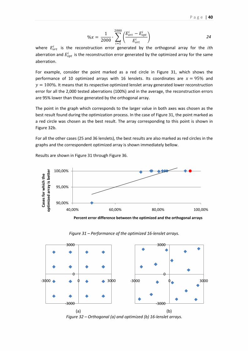
P a g e | 40
%𝑥 = 1
2000∙
𝐸𝑜𝑟𝑡𝑖 − 𝐸𝑜𝑝𝑡
𝑖
𝐸𝑜𝑟𝑡𝑖
2000
𝑖=1
24
where 𝐸𝑜𝑟𝑡𝑖 is the reconstruction error generated by the orthogonal array for the 𝑖th
aberration and 𝐸𝑜𝑝𝑡𝑖 is the reconstruction error generated by the optimized array for the same
aberration.
For example, consider the point marked as a red circle in Figure 31, which shows the
performance of 10 optimized arrays with 16 lenslets. Its coordinates are 𝑥 = 95% and
𝑦 = 100%. It means that its respective optimized lenslet array generated lower reconstruction
error for all the 2,000 tested aberrations (100%) and in the average, the reconstruction errors
are 95% lower than those generated by the orthogonal array.
The point in the graph which corresponds to the larger value in both axes was chosen as the
best result found during the optimization process. In the case of Figure 31, the point marked as
a red circle was chosen as the best result. The array corresponding to this point is shown in
Figure 32b.
For all the other cases (25 and 36 lenslets), the best results are also marked as red circles in the
graphs and the correspondent optimized array is shown immediately bellow.
Results are shown in Figure 31 through Figure 36.
Figure 31 – Performance of the optimized 16-lenslet arrays.
(a) (b)
Figure 32 – Orthogonal (a) and optimized (b) 16-lenslet arrays.
90,00%
95,00%
100,00%
40,00% 60,00% 80,00% 100,00%
Cas
es
for
wh
ich
th
e
op
tim
ize
d a
rray
is b
ett
er
Percent error difference between the optimized and the orthogonal arrays
-3000
0
3000
-3000 0 3000
-3000
0
3000
-3000 0 3000
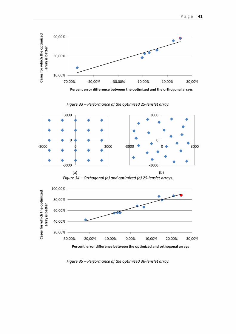
P a g e | 41
Figure 33 – Performance of the optimized 25-lenslet array.
(a) (b)
Figure 34 – Orthogonal (a) and optimized (b) 25-lenslet arrays.
Figure 35 – Performance of the optimized 36-lenslet array.
10,00%
50,00%
90,00%
-70,00% -50,00% -30,00% -10,00% 10,00% 30,00%Cas
es
for
wh
ich
th
e o
pti
miz
ed
ar
ray
is b
ett
er
Percent error difference between the optimized and the orthogonal arrays
-3000
0
3000
-3000 0 3000
-3000
0
3000
-3000 0 3000
20,00%
40,00%
60,00%
80,00%
100,00%
-30,00% -20,00% -10,00% 0,00% 10,00% 20,00% 30,00%Cas
es
for
wh
ich
th
e o
pti
miz
ed
ar
ray
is b
ett
er
Percent error difference between the optimized and orthogonal arrays
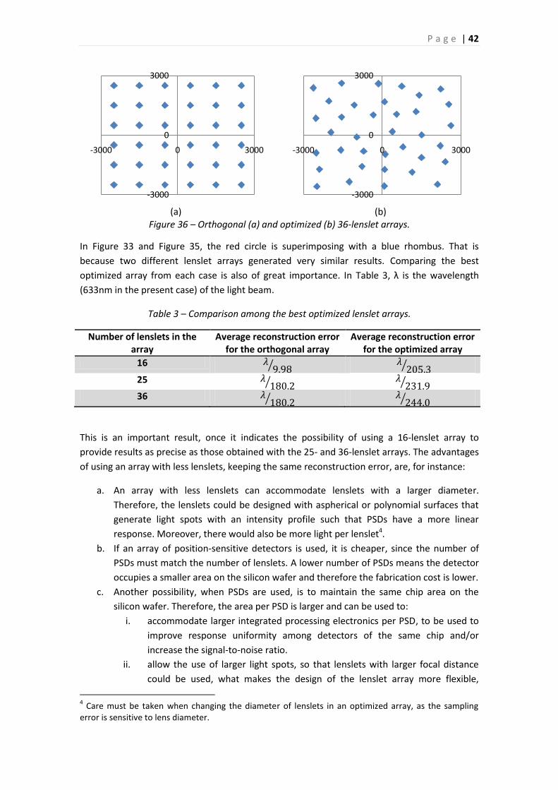
P a g e | 42
(a) (b)
Figure 36 – Orthogonal (a) and optimized (b) 36-lenslet arrays.
In Figure 33 and Figure 35, the red circle is superimposing with a blue rhombus. That is
because two different lenslet arrays generated very similar results. Comparing the best
optimized array from each case is also of great importance. In Table 3, λ is the wavelength
(633nm in the present case) of the light beam.
Table 3 – Comparison among the best optimized lenslet arrays.
Number of lenslets in the array
Average reconstruction error for the orthogonal array
Average reconstruction error for the optimized array
16 𝜆9.98 𝜆 205.3
25 𝜆180.2 𝜆
231.9
36 𝜆180.2 𝜆
244.0
This is an important result, once it indicates the possibility of using a 16-lenslet array to
provide results as precise as those obtained with the 25- and 36-lenslet arrays. The advantages
of using an array with less lenslets, keeping the same reconstruction error, are, for instance:
a. An array with less lenslets can accommodate lenslets with a larger diameter.
Therefore, the lenslets could be designed with aspherical or polynomial surfaces that
generate light spots with an intensity profile such that PSDs have a more linear
response. Moreover, there would also be more light per lenslet4.
b. If an array of position-sensitive detectors is used, it is cheaper, since the number of
PSDs must match the number of lenslets. A lower number of PSDs means the detector
occupies a smaller area on the silicon wafer and therefore the fabrication cost is lower.
c. Another possibility, when PSDs are used, is to maintain the same chip area on the
silicon wafer. Therefore, the area per PSD is larger and can be used to:
i. accommodate larger integrated processing electronics per PSD, to be used to
improve response uniformity among detectors of the same chip and/or
increase the signal-to-noise ratio.
ii. allow the use of larger light spots, so that lenslets with larger focal distance
could be used, what makes the design of the lenslet array more flexible,
4 Care must be taken when changing the diameter of lenslets in an optimized array, as the sampling
error is sensitive to lens diameter.
-3000
0
3000
-3000 0 3000
-3000
0
3000
-3000 0 3000
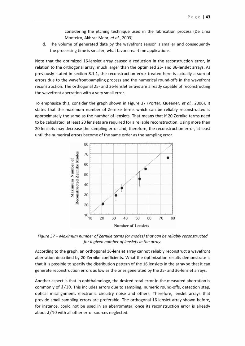
P a g e | 43
considering the etching technique used in the fabrication process (De Lima
Monteiro, Akhzar-Mehr, et al., 2003).
d. The volume of generated data by the wavefront sensor is smaller and consequently
the processing time is smaller, what favors real-time applications.
Note that the optimized 16-lenslet array caused a reduction in the reconstruction error, in
relation to the orthogonal array, much larger than the optimized 25- and 36-lenslet arrays. As
previously stated in section 8.1.1, the reconstruction error treated here is actually a sum of
errors due to the wavefront-sampling process and the numerical round-offs in the wavefront
reconstruction. The orthogonal 25- and 36-lenslet arrays are already capable of reconstructing
the wavefront aberration with a very small error.
To emphasize this, consider the graph shown in Figure 37 (Porter, Queener, et al., 2006). It
states that the maximum number of Zernike terms which can be reliably reconstructed is
approximately the same as the number of lenslets. That means that if 20 Zernike terms need
to be calculated, at least 20 lenslets are required for a reliable reconstruction. Using more than
20 lenslets may decrease the sampling error and, therefore, the reconstruction error, at least
until the numerical errors become of the same order as the sampling error.
Figure 37 – Maximum number of Zernike terms (or modes) that can be reliably reconstructed for a given number of lenslets in the array.
According to the graph, an orthogonal 16-lenslet array cannot reliably reconstruct a wavefront
aberration described by 20 Zernike coefficients. What the optimization results demonstrate is
that it is possible to specify the distribution pattern of the 16 lenslets in the array so that it can
generate reconstruction errors as low as the ones generated by the 25- and 36-lenslet arrays.
Another aspect is that in ophthalmology, the desired total error in the measured aberration is
commonly of 𝜆 10 . This includes errors due to sampling, numeric round-offs, detection step,
optical misalignment, electronic circuitry noise and others. Therefore, lenslet arrays that
provide small sampling errors are preferable. The orthogonal 16-lenslet array shown before,
for instance, could not be used in an aberrometer, once its reconstruction error is already
about 𝜆 10 with all other error sources neglected.
P a g e | 44
8.2. EMBEDDED SYSTEM FOR ADAPTIVE OPTICS SYSTEM CONTROL
Greenaway and Burnett (2004) emphasize that the first generation of adaptive optics systems
has yielded impressive results, but are not still in routine use in the world. Therefore, there is a
growing interest in low-cost, robust, compact and “plug-and-play” systems and components.
In this sense, this work aims at developing a dedicated embedded system for controlling the
adaptive optics system. To accomplish to this task, the system must be able to perform the
following tasks:
a. Receive as input either the image generated by an off-the-shelf camera or the signals
generated by an array of position-sensitive detectors. In this work, a CCD camera is
used.
b. Analyze the input so as to extract the deviations of each light spot, which were
generated by the Hartmann-Shack method.
c. Reconstruct the wavefront aberration.
d. Actuate the wavefront modulator: a deformable mirror, in the present case.
Hitherto this system has not been completed yet. Then, this section will describe the used
technology and the parts that have already been concluded.
8.2.1. DIGITAL SIGNAL PROCESSOR (DSP)
The control task in an adaptive optics system is generally accomplished by a computer. The
substitution by an embedded control system is motivated by the possibility of building more
compact and portable AO systems. Although cost reduction is also likely to occur with the
substitution, it is not sufficiently significant (in comparison with the cost of the entire AO
system) to motivate the whole task by itself. Portable and compact AO systems may contribute
to increasing its range of applications to include the possibility of using it in airplanes and
submarines, for instance. Moreover, such systems could be designed to offer mobility, in the
sense that the same system could be transported to perform diagnostics in different places of,
for example, a production line in industry.
The first step in designing the control system for AO consists in selecting the appropriate
development hardware, which depends on the application requirements. When a CCD camera
is used to capture the image of the light spots generated in the Hartmann-Shack method, the
input to the control system is an image. That means that the development hardware must be
capable of decoding video. Moreover, the hardware must feature large enough memory space
to allow embedded processing of image data and reconstruction of the wavefront aberration.
These requirements guided the choice of the development hardware.
A DSP-based (Digital Signal Processor) hardware was chosen to be used in the control system.
A development kit from Analog Devices, Inc. was chosen, the ADSP-BF533 EZ-KIT Lite®, which
already contains decoder and encoder chips for video processing onboard (Analog Devices,
Inc., 2007). The kit uses the DSP BF533 of the BlackFin® series of Analog Devices, Inc.
Besides the system requirements mentioned above, the choice was also guided by
convenience in aspects such as availability of personal contacts with experience in
P a g e | 45
programming processors from this family, availability of a development kit featuring enough
memory size and video interface, familiar development environment and familiar
programming language.
The use of a development kit, rather than the processor and specific electronics for running
the control system, is purely due to convenience. As the name suggests, it is easier to use it
during the development step, once there is no need to worry about electronic-circuit design.
Moreover, the low cost of a development kit (compared to the entire AO system cost),
together with characteristics such as portability, compactness and reliability, suggest that the
development of a specific electronics for the AO control system can be postponed to future
work, as the market is still a niche one and the focus of this development is currently on
academic research. Designing such electronic circuits, including video decoder, access to
external memories and interfaces for communication with the development environment
would demand additional effort, which could be as for now more usefully in the firmware5
development.
The development kit is designed to be used in conjunction with the Visual DSP++®
development environment, which is a management system that provides a suite of tools for
developing processor applications and projects with a C/C++ compiler. Besides the project
manager facility, it also includes debugging features, such as plotting values from memory and
using breakpoints to view registers and memory (Analog Devices, Inc., 2007).
The ADSP-BF533 EZ-KIT Lite® features (Analog Devices, Inc., 2007): ADSP-BF533 BlackFin®
processor; 64MB of synchronous dynamic random access memory (SDRAM); 2MB of flash
memories; analog audio interface with 96KHz audio codec, with 4 input and 6 output RCA
jacks; analog video interface through video decoder and encoder chips with 3 input and 3
output RCA jacks; universal asynchronous receive/transmitter (UART); LEDS and push buttons.
Some characteristics of the BF533 processor are (Analog Devices, Inc., 2008): performance of
600MHz, 148KB of RAM memory, external memory controller, parallel peripheral interface
(PPI), DMA (direct memory access), SPI-compatible port, real-time clock and universal
asynchronous receiver/transmitter (UART).
8.2.2. IMAGE ANALYSIS ALGORITHM
The first two tasks the embedded system has to perform are receiving an image as an input
and processing the image in order to determine the light-spot deviations. Figure 38 shows an
example of a Hartmann-Shack image that must be processed by the image analysis algorithm.
5 A firmware is an algorithm that is programmed and runs directly on the hardware.
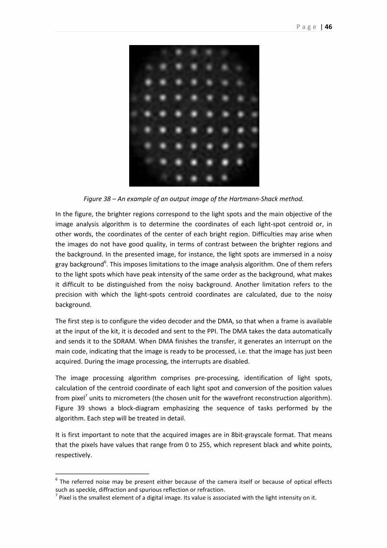
P a g e | 46
Figure 38 – An example of an output image of the Hartmann-Shack method.
In the figure, the brighter regions correspond to the light spots and the main objective of the
image analysis algorithm is to determine the coordinates of each light-spot centroid or, in
other words, the coordinates of the center of each bright region. Difficulties may arise when
the images do not have good quality, in terms of contrast between the brighter regions and
the background. In the presented image, for instance, the light spots are immersed in a noisy
gray background6. This imposes limitations to the image analysis algorithm. One of them refers
to the light spots which have peak intensity of the same order as the background, what makes
it difficult to be distinguished from the noisy background. Another limitation refers to the
precision with which the light-spots centroid coordinates are calculated, due to the noisy
background.
The first step is to configure the video decoder and the DMA, so that when a frame is available
at the input of the kit, it is decoded and sent to the PPI. The DMA takes the data automatically
and sends it to the SDRAM. When DMA finishes the transfer, it generates an interrupt on the
main code, indicating that the image is ready to be processed, i.e. that the image has just been
acquired. During the image processing, the interrupts are disabled.
The image processing algorithm comprises pre-processing, identification of light spots,
calculation of the centroid coordinate of each light spot and conversion of the position values
from pixel7 units to micrometers (the chosen unit for the wavefront reconstruction algorithm).
Figure 39 shows a block-diagram emphasizing the sequence of tasks performed by the
algorithm. Each step will be treated in detail.
It is first important to note that the acquired images are in 8bit-grayscale format. That means
that the pixels have values that range from 0 to 255, which represent black and white points,
respectively.
6 The referred noise may be present either because of the camera itself or because of optical effects
such as speckle, diffraction and spurious reflection or refraction. 7 Pixel is the smallest element of a digital image. Its value is associated with the light intensity on it.
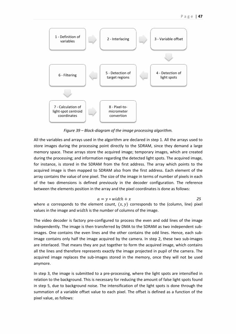
P a g e | 47
Figure 39 – Block-diagram of the image processing algorithm.
All the variables and arrays used in the algorithm are declared in step 1. All the arrays used to
store images during the processing point directly to the SDRAM, since they demand a large
memory space. These arrays store the acquired image; temporary images, which are created
during the processing; and information regarding the detected light spots. The acquired image,
for instance, is stored in the SDRAM from the first address. The array which points to the
acquired image is then mapped to SDRAM also from the first address. Each element of the
array contains the value of one pixel. The size of the image in terms of number of pixels in each
of the two dimensions is defined previously in the decoder configuration. The reference
between the elements position in the array and the pixel coordinates is done as follows:
𝑎 = 𝑦 ∗ 𝑤𝑖𝑑𝑡ℎ + 𝑥 25 where 𝑎 corresponds to the element count, (𝑥, 𝑦) corresponds to the (column, line) pixel
values in the image and 𝑤𝑖𝑑𝑡ℎ is the number of columns of the image.
The video decoder is factory pre-configured to process the even and odd lines of the image
independently. The image is then transferred by DMA to the SDRAM as two independent sub-
images. One contains the even lines and the other contains the odd lines. Hence, each sub-
image contains only half the image acquired by the camera. In step 2, these two sub-images
are interlaced. That means they are put together to form the acquired image, which contains
all the lines and therefore represents exactly the image projected in pupil of the camera. The
acquired image replaces the sub-images stored in the memory, once they will not be used
anymore.
In step 3, the image is submitted to a pre-processing, where the light spots are intensified in
relation to the background. This is necessary for reducing the amount of false light spots found
in step 5, due to background noise. The intensification of the light spots is done through the
summation of a variable offset value to each pixel. The offset is defined as a function of the
pixel value, as follows:
1 - Definition of variables
2 - Interlacing 3 - Variable offset
4 - Detection of light spots
5 - Detection of target regions
6 - Filtering
7 - Calculation of light-spot centroid
coordinates
8 - Pixel-to-micrometer convertion
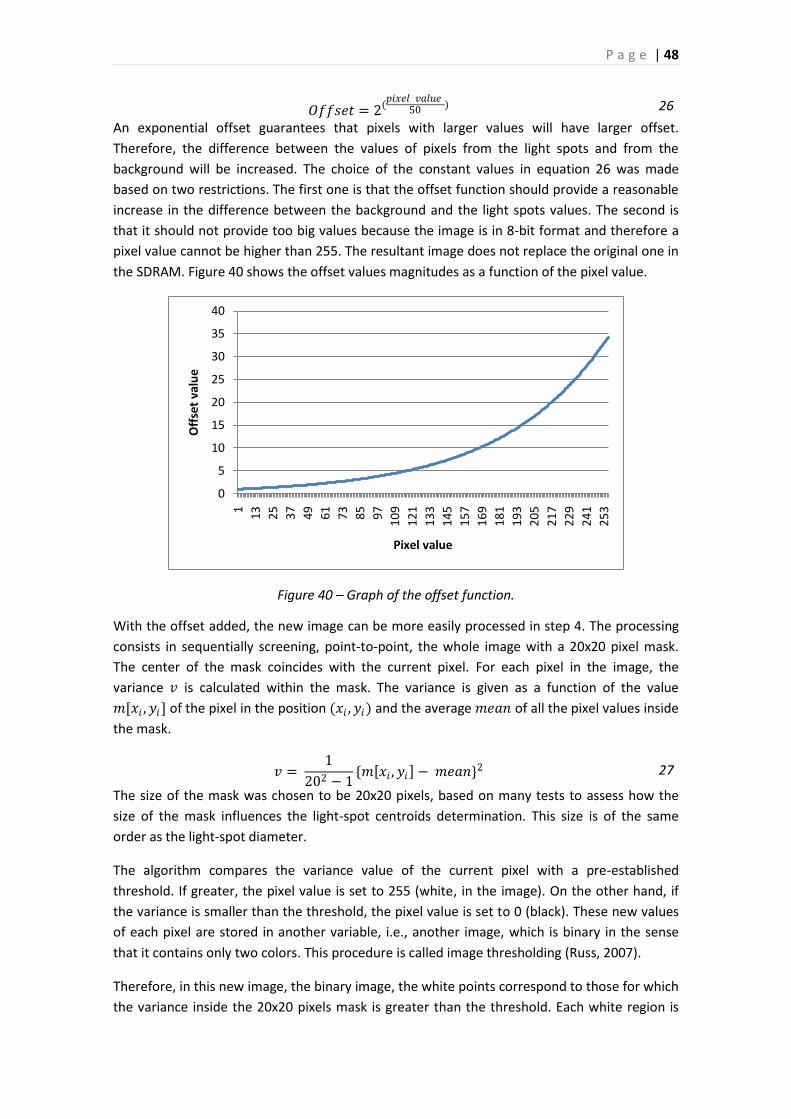
P a g e | 48
𝑂𝑓𝑓𝑠𝑒𝑡 = 2(𝑝𝑖𝑥𝑒𝑙 𝑣𝑎𝑙𝑢𝑒
50) 26
An exponential offset guarantees that pixels with larger values will have larger offset.
Therefore, the difference between the values of pixels from the light spots and from the
background will be increased. The choice of the constant values in equation 26 was made
based on two restrictions. The first one is that the offset function should provide a reasonable
increase in the difference between the background and the light spots values. The second is
that it should not provide too big values because the image is in 8-bit format and therefore a
pixel value cannot be higher than 255. The resultant image does not replace the original one in
the SDRAM. Figure 40 shows the offset values magnitudes as a function of the pixel value.
Figure 40 – Graph of the offset function.
With the offset added, the new image can be more easily processed in step 4. The processing
consists in sequentially screening, point-to-point, the whole image with a 20x20 pixel mask.
The center of the mask coincides with the current pixel. For each pixel in the image, the
variance 𝑣 is calculated within the mask. The variance is given as a function of the value
𝑚[𝑥𝑖 , 𝑦𝑖] of the pixel in the position (𝑥𝑖 , 𝑦𝑖) and the average 𝑚𝑒𝑎𝑛 of all the pixel values inside
the mask.
𝑣 = 1
202 − 1{𝑚 𝑥𝑖 , 𝑦𝑖 − 𝑚𝑒𝑎𝑛}2 27
The size of the mask was chosen to be 20x20 pixels, based on many tests to assess how the
size of the mask influences the light-spot centroids determination. This size is of the same
order as the light-spot diameter.
The algorithm compares the variance value of the current pixel with a pre-established
threshold. If greater, the pixel value is set to 255 (white, in the image). On the other hand, if
the variance is smaller than the threshold, the pixel value is set to 0 (black). These new values
of each pixel are stored in another variable, i.e., another image, which is binary in the sense
that it contains only two colors. This procedure is called image thresholding (Russ, 2007).
Therefore, in this new image, the binary image, the white points correspond to those for which
the variance inside the 20x20 pixels mask is greater than the threshold. Each white region is
0
5
10
15
20
25
30
35
40
1
13
25
37
49
61
73
85
97
10
9
12
1
13
3
14
5
15
7
16
9
18
1
19
3
20
5
21
7
22
9
24
1
25
3
Off
set
valu
e
Pixel value
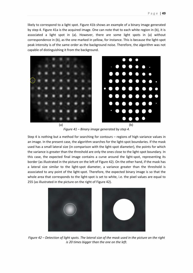
P a g e | 49
likely to correspond to a light spot. Figure 41b shows an example of a binary image generated
by step 4. Figure 41a is the acquired image. One can note that to each white region in (b), it is
associated a light spot in (a). However, there are some light spots in (a) without
correspondence in (b), as the one marked in yellow, for instance. This is because the light-spot
peak intensity is of the same order as the background noise. Therefore, the algorithm was not
capable of distinguishing it from the background.
(a) (b)
Figure 41 – Binary image generated by step 4.
Step 4 is nothing but a method for searching for contours – regions of high variance values in
an image. In the present case, the algorithm searches for the light-spot boundaries. If the mask
used has a small lateral size (in comparison with the light-spot diameter), the points for which
the variance is greater than the threshold are only the ones close to the light-spot boundary. In
this case, the expected final image contains a curve around the light-spot, representing its
border (as illustrated in the picture on the left of Figure 42). On the other hand, if the mask has
a lateral size similar to the light-spot diameter, a variance greater than the threshold is
associated to any point of the light-spot. Therefore, the expected binary image is so that the
whole area that corresponds to the light-spot is set to white, i.e. the pixel values are equal to
255 (as illustrated in the picture on the right of Figure 42).
Figure 42 – Detection of light spots. The lateral size of the mask used in the picture on the right is 20 times bigger than the one on the left.
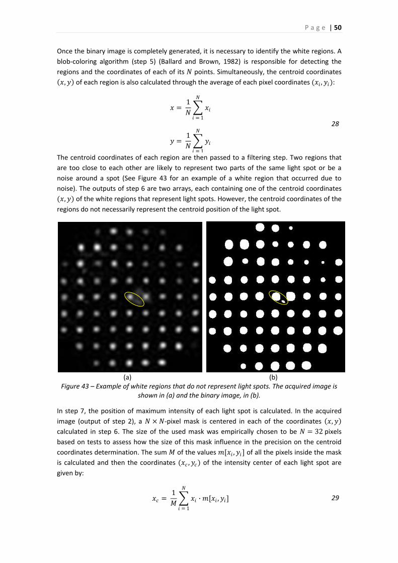
P a g e | 50
Once the binary image is completely generated, it is necessary to identify the white regions. A
blob-coloring algorithm (step 5) (Ballard and Brown, 1982) is responsible for detecting the
regions and the coordinates of each of its 𝑁 points. Simultaneously, the centroid coordinates
𝑥, 𝑦 of each region is also calculated through the average of each pixel coordinates (𝑥𝑖 , 𝑦𝑖):
𝑥 = 1
𝑁 𝑥𝑖
𝑁
𝑖 = 1
𝑦 = 1
𝑁 𝑦𝑖
𝑁
𝑖 = 1
28
The centroid coordinates of each region are then passed to a filtering step. Two regions that
are too close to each other are likely to represent two parts of the same light spot or be a
noise around a spot (See Figure 43 for an example of a white region that occurred due to
noise). The outputs of step 6 are two arrays, each containing one of the centroid coordinates
(𝑥, 𝑦) of the white regions that represent light spots. However, the centroid coordinates of the
regions do not necessarily represent the centroid position of the light spot.
(a) (b)
Figure 43 – Example of white regions that do not represent light spots. The acquired image is shown in (a) and the binary image, in (b).
In step 7, the position of maximum intensity of each light spot is calculated. In the acquired
image (output of step 2), a 𝑁 × 𝑁-pixel mask is centered in each of the coordinates 𝑥, 𝑦
calculated in step 6. The size of the used mask was empirically chosen to be 𝑁 = 32 pixels
based on tests to assess how the size of this mask influence in the precision on the centroid
coordinates determination. The sum 𝑀 of the values 𝑚[𝑥𝑖 , 𝑦𝑖] of all the pixels inside the mask
is calculated and then the coordinates (𝑥𝑐 , 𝑦𝑐) of the intensity center of each light spot are
given by:
𝑥𝑐 = 1
𝑀 𝑥𝑖 ∙ 𝑚[𝑥𝑖 , 𝑦𝑖]
𝑁
𝑖 = 1
29
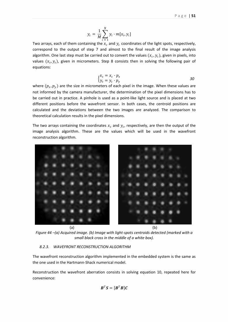
P a g e | 51
𝑦𝑐 = 1
𝑀 𝑦𝑖 ∙ 𝑚[𝑥𝑖 , 𝑦𝑖]
𝑁
𝑖 = 1
Two arrays, each of them containing the 𝑥𝑐 and 𝑦𝑐 coordinates of the light spots, respectively,
correspond to the output of step 7 and almost to the final result of the image analysis
algorithm. One last step must be carried out to convert the values (𝑥𝑐 , 𝑦𝑐), given in pixels, into
values (𝑥𝑠 , 𝑦𝑠), given in micrometers. Step 8 consists then in solving the following pair of
equations:
𝑥𝑠 = 𝑥𝑐 ∙ 𝑝𝑥
𝑦𝑠 = 𝑦𝑐 ∙ 𝑝𝑦 30
where (𝑝𝑥 , 𝑝𝑦) are the size in micrometers of each pixel in the image. When these values are
not informed by the camera manufacturer, the determination of the pixel dimensions has to
be carried out in practice. A pinhole is used as a point-like light source and is placed at two
different positions before the wavefront sensor. In both cases, the centroid positions are
calculated and the deviations between the two images are analyzed. The comparison to
theoretical calculation results in the pixel dimensions.
The two arrays containing the coordinates 𝑥𝑠 and 𝑦𝑠 , respectively, are then the output of the
image analysis algorithm. These are the values which will be used in the wavefront
reconstruction algorithm.
(a) (b)
Figure 44 –(a) Acquired image. (b) Image with light-spots centroids detected (marked with a small black cross in the middle of a white box).
8.2.3. WAVEFRONT RECONSTRUCTION ALGORITHM
The wavefront reconstruction algorithm implemented in the embedded system is the same as
the one used in the Hartmann-Shack numerical model.
Reconstruction the wavefront aberration consists in solving equation 10, repeated here for
convenience:
𝑩𝑇𝑺 = 𝑩𝑇𝑩 𝑪
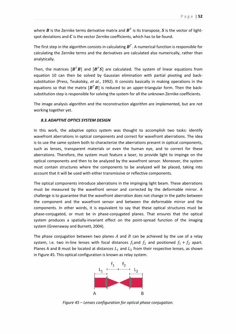
P a g e | 52
where 𝑩 is the Zernike terms derivative matrix and 𝑩𝑇 is its transpose, 𝑺 is the vector of light-
spot deviations and 𝑪 is the vector Zernike coefficients, which has to be found.
The first step in the algorithm consists in calculating 𝑩𝑇. A numerical function is responsible for
calculating the Zernike terms and the derivatives are calculated also numerically, rather than
analytically.
Then, the matrices [𝑩𝑇𝑩] and [𝑩𝑇𝑺] are calculated. The system of linear equations from
equation 10 can then be solved by Gaussian elimination with partial pivoting and back-
substitution (Press, Teukolsky, et al., 1992). It consists basically in making operations in the
equations so that the matrix [𝑩𝑇𝑩] is reduced to an upper-triangular form. Then the back-
substitution step is responsible for solving the system for all the unknown Zernike coefficients.
The image analysis algorithm and the reconstruction algorithm are implemented, but are not
working together yet.
8.3. ADAPTIVE OPTICS SYSTEM DESIGN
In this work, the adaptive optics system was thought to accomplish two tasks: identify
wavefront aberrations in optical components and correct for wavefront aberrations. The idea
is to use the same system both to characterize the aberrations present in optical components,
such as lenses, transparent materials or even the human eye, and to correct for these
aberrations. Therefore, the system must feature a laser, to provide light to impinge on the
optical components and then to be analyzed by the wavefront sensor. Moreover, the system
must contain structures where the components to be analyzed will be placed, taking into
account that it will be used with either transmissive or reflective components.
The optical components introduce aberrations in the impinging light beam. These aberrations
must be measured by the wavefront sensor and corrected by the deformable mirror. A
challenge is to guarantee that the wavefront aberration does not change in the paths between
the component and the wavefront sensor and between the deformable mirror and the
components. In other words, it is equivalent to say that these optical structures must be
phase-conjugated, or must be in phase-conjugated planes. That ensures that the optical
system produces a spatially-invariant effect on the point-spread function of the imaging
system (Greenaway and Burnett, 2004).
The phase conjugation between two planes 𝐴 and 𝐵 can be achieved by the use of a relay
system, i.e. two in-line lenses with focal distances 𝑓1and 𝑓2 and positioned 𝑓1 + 𝑓2 apart.
Planes A and B must be located at distances 𝐿1 and 𝐿2 from their respective lenses, as shown
in Figure 45. This optical configuration is known as relay system.
Figure 45 – Lenses configuration for optical phase conjugation.
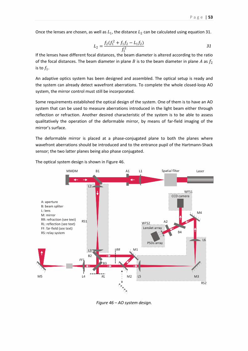
P a g e | 53
Once the lenses are chosen, as well as 𝐿1, the distance 𝐿2 can be calculated using equation 31.
𝐿2 =𝑓2(𝑓1
2 + 𝑓1𝑓2 − 𝐿1𝑓2)
𝑓12 31
If the lenses have different focal distances, the beam diameter is altered according to the ratio
of the focal distances. The beam diameter in plane 𝐵 is to the beam diameter in plane 𝐴 as 𝑓2
is to 𝑓1.
An adaptive optics system has been designed and assembled. The optical setup is ready and
the system can already detect wavefront aberrations. To complete the whole closed-loop AO
system, the mirror control must still be incorporated.
Some requirements established the optical design of the system. One of them is to have an AO
system that can be used to measure aberrations introduced in the light beam either through
reflection or refraction. Another desired characteristic of the system is to be able to assess
qualitatively the operation of the deformable mirror, by means of far-field imaging of the
mirror’s surface.
The deformable mirror is placed at a phase-conjugated plane to both the planes where
wavefront aberrations should be introduced and to the entrance pupil of the Hartmann-Shack
sensor; the two latter planes being also phase conjugated.
The optical system design is shown in Figure 46.
Figure 46 – AO system design.

P a g e | 54
The light beam is emitted by the laser and passes through a spatial filter, emerging divergently
from it. After passing through the lens L1, the beam becomes parallel, i.e. collimated. In
aperture A1, the beam diameter is set to 12mm, to match the reliable reflective area of the
deformable mirror. The deformable mirror diameter is 15mm. It is advisable to avoid the
boundaries of the deformable surface, since the electrodes are concentrated in the center and
the border is anchored on a frame that limits its deflection and might affect its correction
capabilities. Therefore, the beam diameter impinging on the mirror is 12mm.
Then the beam passes through the beam splitter B1 and reaches the deformable mirror
perpendicularly. In its way backwards, the beam is reflected by the beam splitter B1 and enters
in the relay system RS1. This relay system is used to phase-conjugate the deformable mirror
and three planes: the ones to introduce aberration (aberration planes) through reflection (RL)
and refraction (RR) and the plane (FF) to generate the far-field image. The same relay system is
also used to reduce the beam diameter to 6 mm, to match the entrance pupil of many optical
components for which the wavefront aberration is to be measured, including the eyes, and
also the entrance pupil of the Hartmann-Shack wavefront sensors deployed here.
In beam splitter B2, part of the beam is reflected to impinge on the optical component through
refraction. The other part of the beam reaches beam splitter B3 and is divided to impinge on
the lens L4 and the plane RL. The light that reaches the lens L4 is focused on a micro-objective
to generate the far-field image, which is projected on the wall by mirror M5.
The mirror M2 is used to choose between the aberration planes to be analyzed: reflection or
refraction. It can be moved in order to prevent that one of the beams coming from either RL or
RR reaches the relay system RS2. This relay system is used to phase-conjugate the aberration
planes to the entrance pupil of the wavefront sensor.
Two Hartmann-Shack wavefront sensors are being used. One (WFS1) uses a CCD camera to
detect the image of light-spots. The other (WFS2) uses a 2D array of position-sensitive
detectors. The purpose of using two wavefront sensors is to compare the results from both
methods. When the light beam reaches beam splitter B4, it is divided to reach both wavefront
sensors. The lenslet array used in WFS1 is coupled to the camera, whereas the one in WFS2 is
placed before the PSDs array, as indicated in the figure. The WFS2 is not yet couped to the
system.
The assembled system is shown in Figure 47.
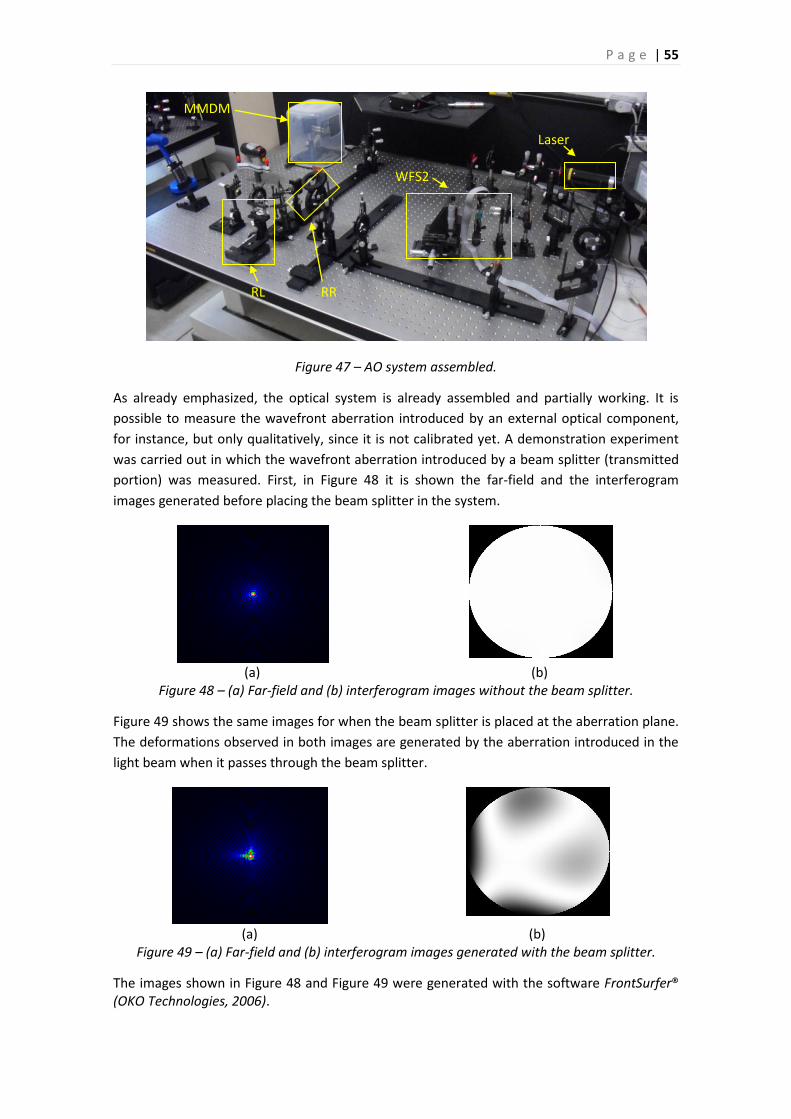
P a g e | 55
Figure 47 – AO system assembled.
As already emphasized, the optical system is already assembled and partially working. It is
possible to measure the wavefront aberration introduced by an external optical component,
for instance, but only qualitatively, since it is not calibrated yet. A demonstration experiment
was carried out in which the wavefront aberration introduced by a beam splitter (transmitted
portion) was measured. First, in Figure 48 it is shown the far-field and the interferogram
images generated before placing the beam splitter in the system.
(a) (b) Figure 48 – (a) Far-field and (b) interferogram images without the beam splitter.
Figure 49 shows the same images for when the beam splitter is placed at the aberration plane.
The deformations observed in both images are generated by the aberration introduced in the
light beam when it passes through the beam splitter.
(a) (b) Figure 49 – (a) Far-field and (b) interferogram images generated with the beam splitter.
The images shown in Figure 48 and Figure 49 were generated with the software FrontSurfer® (OKO Technologies, 2006).
MMDM
WFS2
RL RR
Laser

P a g e | 56
9. FUTURE WORK
1. Calculation of spatial frequencies of wavefront aberrations, described by Zernike
polynomials, that impinge the lenslet array.
2. Calibration of the AO system. (Through measurement of known aberrations)
3. Validation of the embedded system to measure wavefront aberrations.
4. Implementation of the mirror control on the embedded system.
5. Fabrication of the optimized lenslet array and empirical tests for comparison with
regular array.
6. Characterization of the AO system.
10. SCHEDULE
The activities listed in section 9 will be performed according to the following schedule,
separated into semesters.
Activity
1/2
01
0
2/2
01
0
1/2
01
1
2/2
01
1
Calculation of spatial frequencies of Zernike terms. Calibration of AO system Validation of the embedded system Implementation of mirror control Fabrication of optimized lenslet array Characterization of the AO system
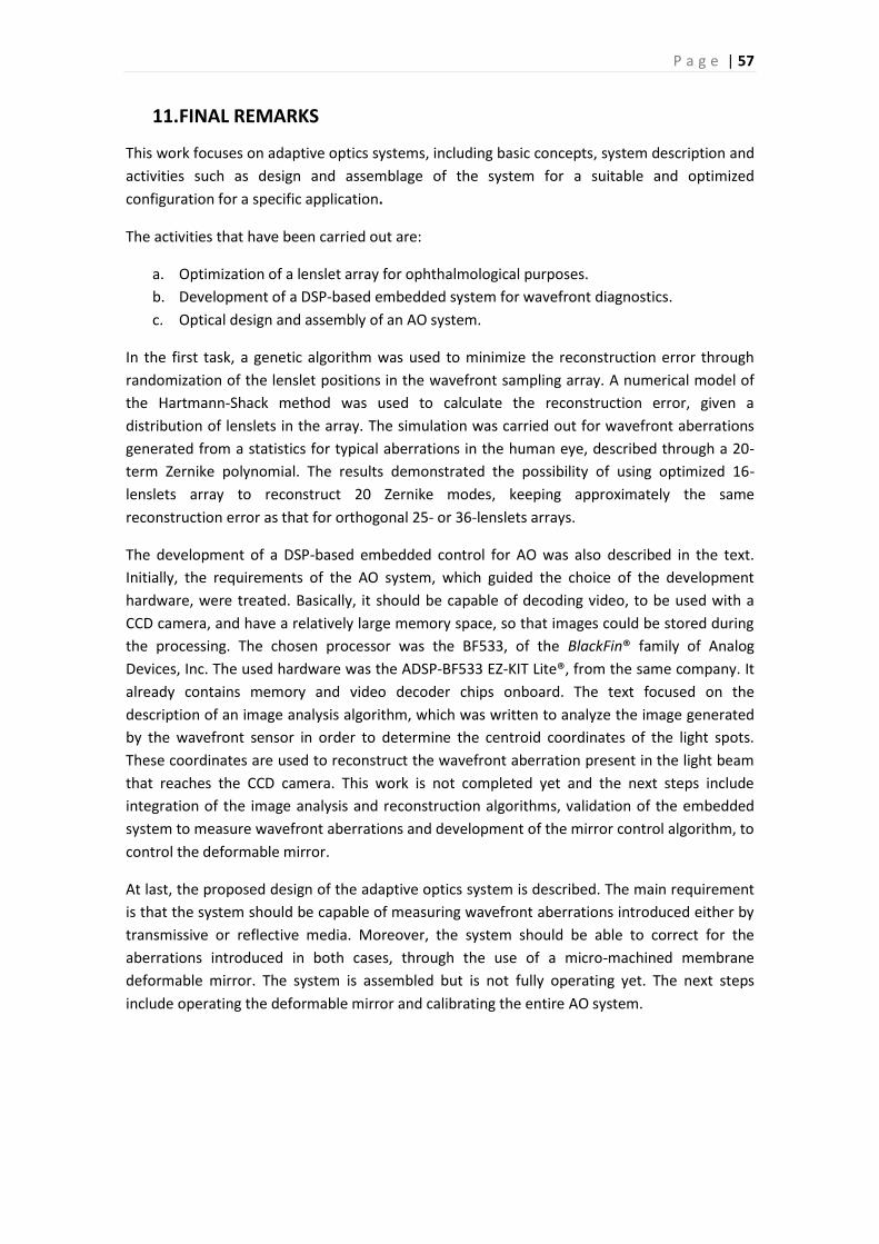
P a g e | 57
11. FINAL REMARKS
This work focuses on adaptive optics systems, including basic concepts, system description and
activities such as design and assemblage of the system for a suitable and optimized
configuration for a specific application.
The activities that have been carried out are:
a. Optimization of a lenslet array for ophthalmological purposes.
b. Development of a DSP-based embedded system for wavefront diagnostics.
c. Optical design and assembly of an AO system.
In the first task, a genetic algorithm was used to minimize the reconstruction error through
randomization of the lenslet positions in the wavefront sampling array. A numerical model of
the Hartmann-Shack method was used to calculate the reconstruction error, given a
distribution of lenslets in the array. The simulation was carried out for wavefront aberrations
generated from a statistics for typical aberrations in the human eye, described through a 20-
term Zernike polynomial. The results demonstrated the possibility of using optimized 16-
lenslets array to reconstruct 20 Zernike modes, keeping approximately the same
reconstruction error as that for orthogonal 25- or 36-lenslets arrays.
The development of a DSP-based embedded control for AO was also described in the text.
Initially, the requirements of the AO system, which guided the choice of the development
hardware, were treated. Basically, it should be capable of decoding video, to be used with a
CCD camera, and have a relatively large memory space, so that images could be stored during
the processing. The chosen processor was the BF533, of the BlackFin® family of Analog
Devices, Inc. The used hardware was the ADSP-BF533 EZ-KIT Lite®, from the same company. It
already contains memory and video decoder chips onboard. The text focused on the
description of an image analysis algorithm, which was written to analyze the image generated
by the wavefront sensor in order to determine the centroid coordinates of the light spots.
These coordinates are used to reconstruct the wavefront aberration present in the light beam
that reaches the CCD camera. This work is not completed yet and the next steps include
integration of the image analysis and reconstruction algorithms, validation of the embedded
system to measure wavefront aberrations and development of the mirror control algorithm, to
control the deformable mirror.
At last, the proposed design of the adaptive optics system is described. The main requirement
is that the system should be capable of measuring wavefront aberrations introduced either by
transmissive or reflective media. Moreover, the system should be able to correct for the
aberrations introduced in both cases, through the use of a micro-machined membrane
deformable mirror. The system is assembled but is not fully operating yet. The next steps
include operating the deformable mirror and calibrating the entire AO system.

P a g e | 58
12. ACKNOWLEDGEMENTS
I would like to thank:
a. CNPq and FAPEMIG, for financial support;
b. Jens Verstraet, for significant help in the optical system assembly;
c. Marcos Carvalho, also for helping in the optical system assembly and providing
information about the ophthalmology context of optical aberrations, and
d. Luciana P. Salles, for working together on the Hartmann-Shack numerical model.
P a g e | 59
13. REFERENCES
ANALOG DEVICES, INC. ADSP-BF533 EZ-KIT Lite: Evaluation system manual. Norwood, p. 89.
2007. (3.1).
ANALOG DEVICES, INC. Visual DSP++ 5.0 user's guide. Norwood, p. 442. 2007. (3.0).
ANALOG DEVICES, INC. BlackFin embedded processor: ADSP-BF531/ADSP-BF532/ADSP-
BF533. Norwood, p. 64. 2008.
ARNOLD, C. B.; MCLEOD, E. A new approach to adaptive optics for materials processing.
Photonics Spectra, p. 78-84, November 2007.
ARNON, S.; KOPEIKA, N. S. Adaptive optical transmitter and receiver for space communication
through thin clouds. Applied Optics, v. 36, n. 9, p. 1987-1993, 20 March 1997.
BALLARD, D. H.; BROWN, C. M. Computer vision. Englewood Cliffs: Prentice-Hall, Inc., 1982.
BORN, M.; WOLF, E. Principles of optics: eletromagnetic theory of propagation, interference,
and diffraction of light. 6th. ed. New York: Pergamon Press, 1989.
CAMERON, P. B.; BRITTON, M. C.; KULKARNI, S. R. Precision astromety with adaptive optics.
The Astronomical Journal, v. 137, p. 83-93, January 2009.
CARROLL, J. C. et al. Recent advances in retinal imaging with adaptive optics. Optics and
Photonics News, p. 36-42, January 2005.
CUBALCHINI, R. Modal wave-front estimation from phase derivative measurements. Journal of
the Optical Society of America, v. 69, n. 7, p. 972-977, July 1979.
DE LIMA MONTEIRO, D. W. CMOS-based integrated wavefront sensor. Delft: Delft University
Press, 2002.
DE LIMA MONTEIRO, D. W. et al. Single-mask microfabrication of aspherical optics using KOH
anisotropic etching of Si. Optics Express, v. 11, n. 18, p. 2244-2252, September 2003.
DE LIMA MONTEIRO, D. W.; AKHZAR-MEHR, O.; VDOVIN, G. Prime microlens arrays for
Hartmann-Shack sensors - an economical fabrication technology. 4th Adaptive Optics
Conference for Industry and Medicine. Münster: Springer. 2003. p. 197-205.
FERREIRA JR., A. I.; DE LIMA MONTEIRO, D. W.; PATARO, C. D. M. Diagnóstico de aberrações
ópticas e controle de sistema óptico adaptativo com o método Adaline. Universidade Federal
de Minas Gerais. Belo Horizonte, p. 75. 2006.
FLEXIBLE OPTICAL BV. Flexible Optical. Available in: <www.okotech.com>. Access: 25 January
2010.
GIRKIN, J. M.; POLAND, S.; WRIGHT, A. J. Adaptive optics for deeper imaging of biological
samples. Current Opinion in Biotechnology, v. 20, p. 106-110, March 2009.
P a g e | 60
GREENAWAY, A.; BURNETT, J. Industrial and medical applications of adaptive optics. [S.l.].
2004.
HAMELINCK, R. et al. Deformable membrane mirror with high actuator density and
distributed control. Proceedings of the Sixth International Workshop on Adaptive Optics for
Industry and Medicine. London, UK: Imperial College Press. 2007. p. 35-40.
HARDY, J. W. Adaptive Optics: Technology developed during the cold war is giving new
capabilities to ground-based astronomical telescopes. Scientific American, p. 40-45, 1994.
HECHT, E. Optics. 4th Edition. ed. San Francisco: Addison and Wesley, 2002.
HEIN, M. Adaptive optics: an introduction and overview. Portland State University. Portland.
2005.
HOLOHAN, M. L.; DAINTY, J. C. Low-order adaptive optics: a possible use in underwater
imaging? Optics and Laser Technology, v. 29, n. 1, p. 51-55, 1997.
JESACHER, A. et al. Adaptive optics for direct laser writing with plasma emission aberration
sensing. OPTICS EXPRESS, v. 18, n. 2, p. 657-661, January 2010.
LLORENTE, L. et al. Effect of sampling on real ocular aberrations measurements. Journal of the
Optical Society of America A: Opt Image, v. 24, n. 9, p. 2783-2796, September 2007.
MITCHELL, M. An introduction to genetic algorithms. Cambridge, MA: The Mit Press, 1999.
NEWTON, S. I. Opticks: or a treatise of the reflections and refractions, inflections & colours of
light. New York: Cosimo Classics, 2007. 110-111 p. Prop. VIII. Prob. II. "To shorten Telescopes."
NOLL, R. J. Zernike polynomials and atmospheric turbulence. Journal of the Optical Society of
America, v. 66, n. 3, p. 207-211, March 1976.
OKO TECHNOLOGIES. Technical documents: Typical passports. Flexible Optical, 2006. Available
in: <http://www.okotech.com/passports>. Access: 14 January 2010.
OPTICAL SOCIETY OF AMERICA. Handbook of optics: Fundamentals, techniques and design.
2nd Edition. ed. New York: McGraw-Hill, Inc, v. 1, 1994.
OUGHSTUN, K. E. Intracavity adaptive optic compensation of phase aberrations. I: Analysis. J.
Opt. Soc. Am., v. 71, p. 862-872, 1981.
PLATT, B. C.; SHACK, R. History and principles of Shack-Hartmann wavefront sensing. Journal of
Refractive Surgery, v. 17, p. 573-577, September/October 2001.
PORTER, J. Principals of eye design. Center for Adaptive Optics, 2003. Available in:
<http://cfao.ucolick.org/pubs/presentations/eyedesign/06_Aberrations_JP.pdf>. Access: 10
January 2010.
PORTER, J. et al. Monochromatic aberrations of the human eye in a large population. Journal
of the Optical Society of America, v. 18, n. 8, p. 1793-1803, August 2001.
P a g e | 61
PORTER, J. et al. Adaptive optics for vision science: principles, practices, design and
applications. Jersey City: John Wiley & Sons, 2006. 640 p. ISBN ISBN 978-0-471-67941-7.
PRESS, W. H. et al. Numerical recipes in C: The art of scientific computing. Second Edition. ed.
New York: Cambridge University Press, 1992.
ROORDA, A. et al. Adaptive optics scanning laser ophthalmoscopy. Optics Express, v. 10, n. 9,
p. 405-412, 6 May 2002. ISSN 405-412.
RUSS, J. C. The image processing handbook. Fifth Edition. ed. New York: CRC Press, 2007.
SABESAN, R. et al. Vision improvement by correcting high-order aberrations with customized
soft contact lenses in keratoconic eyes. Optics Letters, v. 32, n. 8, p. 1000-1002, April 2007.
SOLOVIEV, O.; VDOVIN, G. Hartmann-Shack test with random masks for modal wavefront
reconstruction. Optics Express, 13, 14 November 2005.
SOUTHWELL, W. H. Wave-front estimation from wave-front slope measurements. Journal of
the Optical Society of America, v. 70, n. 8, p. 998-1006, August 1980.
THE MATHWORKS, INC. The MathWorks: accelerating the pace of engineering and science.
Documentation: Genetic Algorithm and Direct Search Toolbox, 2010. Available in:
<http://www.mathworks.com/access/helpdesk/help/toolbox/gads/f6187.html>. Access: 31
January 2010.
TYSON, R. K. Principles of adaptive optics. 2nd Edition. ed. San Diego: Academic Press, 1997.
TYSON, R. K. Adaptive optics engineering handbook. 1ª Edição. ed. New York: Marcell Dekker
Inc, 1999. 339 p. ISBN ISBN 0824782755.
U.S. DEPARTMENT OF DEFENSE. Airborne laser fact sheet. The Missile Defense Agency, 16
September 2009. Available in: <http://www.mda.mil/global/documents/pdf/laser.pdf>.
Access: 9 January 2010.
VDOVIN, G. et al. Silicon micro-optics for smart light control. Photonics West - SPIE - MOEMS,
Displays and Imaging Systems II. San Jose, CA: Bellingham: SPIE Press. February 2004. p. 135-
149.
VDOVIN, G.; LOKTEV, M. Deformable mirror with thermal actuators. Optics Letters, v. 27, n. 9,
p. 677-679, May 2002.
VDOVIN, G.; LOKTEV, M.; SOLOVIEV, O. Deformable mirrors based on transversal piezoeffect.
Proceedings of the Sixth International Workshop on Adaptive Optics for Industry and
Medicine. London, UK: Imperial College Press. 2007. p. 83-88.
WELP, P.; HEUCK, H.-M.; WITTROCK, U. Intracavity adaptive optics optimization of an end-
pumped Nd: YVO4 laser. Conference on Lasers and Electro-Optics Europe, 2007 and the
International Quantum Electronics Conference. CLEOE-IQEC 2007. Munich: [s.n.]. 2007. p. 1.

P a g e | 62
WEYRAUCH, T. et al. Fiber coupling with adaptive optics for free-space optical
communication. Proc. SPIE. San Diego, CA, USA: [s.n.]. 2003. p. 177-184.
WRIGHT, A. J. et al. Adaptive optics for enhanced signal in CARS microscopy. Optics Express, v.
15, n. 26, p. 18209-18219, 24 December 2007.
WYANT, J. C.; CREATH, K. Basic wavefront aberration theory for optical metrology. In:
SHANNON, R. R.; WYANT, J. C. Applied Optics and Optical Engineering. Boston: Academic
Press, v. XI, 1992. Cap. 1.
YOON, G. Center for adaptive optics. Principles of Eye Design, 2003. Available in:
<http://cfao.ucolick.org/pubs/presentations/eyedesign/05_aberrations_GY.pdf>. Access: 10
January 2010.
YURA, H. T. Imaging in clear ocean water. Applied Optics, v. 12, n. 5, p. 1061-1066, May 1973.
ZERNIKE, F. Beugungstheorie des Schneidensverfahrens und seiner verbesserten Form, der
Phasenkontrastmethode. Physica, v. 1, p. 689-704, 1934.
ZHANG, Y.; POONJA, S.; ROORDA, A. MEMS-based adaptive optics scanning laser
ophthalmoscopy. Optics Letters, v. 31, n. 9, p. 1268-1270, 1 May 2006.