Cross-Border Banking Flows Spillovers in theEurozone: Evidence from an Estimated DSGE Model

Jean-Christophe Poutineau∗ Gauthier Vermandel†

This version: July 16, 2014

Abstract

This paper seeks to evaluate quantitatively how interbank and corporate cross-border flows shape business cycles in a monetary union. Using Bayesian tech-niques, we estimate a two-country DSGE model that distinguishes between Euro-zone core and peripheral countries and accounts for national heterogeneities and aset of real, nominal and financial frictions. We find evidence of the key role of thiscross-border channel as an amplifying mechanism in the diffusion of asymmetricshocks. Our model also reveals that under banking globalization, most nationalvariables and the central bank interest rate are less sensitive to financial shockswhile investment and current account imbalances are more sensitive to financialshocks. Finally, a counterfactual analysis shows that cross-border lending hasaffected the transmission of the recent financial crisis between the two groups ofcountries.

JEL classification: E32; E44; E52; F36; F41;

Keywords: Banking Globalization; Monetary Policy; Financial Accelerator; Inter-

bank Market; Eurozone; Cross-border Lending

∗CREM, UMR CNRS 6211, Universite de Rennes I, Rennes, France. E-mail: jean-christophe.poutineau@univ-rennes1.fr†CREM, UMR CNRS 6211, Universite de Rennes I, Rennes, France. E-mail: gauthier@vermandel.frWe are grateful to Miguel Casares and Dimitris Korobilis for helpful comments on Bayesian esti-

mations. We benefited from discussions with Luca Fornaro, Robert Kollmann, Samuel Maveyraud, Do-minik M. Rosch, Katheryn Russ and Marc-Alexandre Senegas as well as seminar participants at CEPRWorkshop on the Economic of Cross-Border Banking, Association Francaise de Sciences Economiques(AFSE), Universidad Publica de Navarra, 30th International Symposium on Money, Banking and Fi-nance (GDRE), Universite Rennes 1. The revised paper was written while Gauthier Vermandel wasworking for European Central Bank, DG-Macro-Prudential Policy and Financial Stability, Macro-Financial Linkages Division in 2014. We remain responsible for any errors and omissions

1

1 Introduction

By eliminating currency risk, the adoption of the euro in 1999 generated forces for a

greater economic and financial integration. The single currency reshaped financial mar-

kets and international investment patterns by enhancing cross-border banking activity

between the members of the European Monetary Union (EMU). This phenomenon can

be measured along various complementary dimensions such as the increase of FDI in

bank activities, the diversification of bank assets and liabilities between countries, the

access of local banks to international financial sources or through the increase of banks’

lending via foreign branches and direct cross-border lending.

This paper focuses more specifically on the consequences of the rise in cross-border

loan flows observed since the adoption of the Euro in 1999. Cross-border lending is a

distinguishing feature of financial integration in the Eurozone:1 it has been multiplied

by 3 in 9 years, before experiencing a 25% decrease after the recent financial crisis.

The critical role of cross-border lending in the EMU must be assessed by taking into

account the key role of banks in providing the main funding source for households and

firms in the euro area: in 2012 the banking sector in the European Union was 4.5 times

larger than its US counterpart (respectively 347% of EU GDP and 74% of US GDP).

At its peak value in 2008, total cross-border lending represented around 120% of GDP

for Eurozone countries, while the corresponding figure was 40% for the US and 20% for

Japan. Taking a closer look at the data, this cross-border phenomenon is heterogenous

as it affects mainly interbank lending and corporate lending, while cross-border lending

to households is negligible2

We develop a two-country DSGE model to document how the transmission of asym-

metric shocks in the Eurozone has been affected with a banking system that provides

cross-border interbank and corporate lending facilities. This solution is original with

respect to the existing literature of monetary policy issues in a monetary union. In-

deed, most papers related to this topic can roughly be separated in two strands. On

the one hand, one-country models such as Gerali et al. (2010), Paries et al. (2011) and

Christiano et al. (2010), assume complete banking integration so that all countries are

impacted in the same way by the ECB monetary policy. On the other hand, two-country

models such Kollmann et al. (2011) ignore the possibility of cross-border funds. In the

meanwhile, the fewer models that adopt a middle of the road solution by assuming an

imperfect integration of the loan market (Faia (2007); Dedola and Lombardo (2012);

Ueda (2012); Dedola et al. (2013)) do not account for the above mentioned heterogeneity

1See Fig. 1 in the text below.2As underlined by Fig. 2, European banks mainly finance foreign banks on the interbank market

and foreign firms on the corporate credit market while mortgage and deposit markets remain stronglysegmented in the Eurosystem.

2

in Eurozone cross-border loan flows.

Our paper brings theoretical and empirical contributions. To keep the model tractable,

we analyze cross-border loans through home bias in the borrowing decisions concerning

interbank and corporate loans using CES function aggregates3. Cross-border banking

flows are introduced analogously to standard trade channel assuming CES function ag-

gregates. This modelling strategy is flexible as it allows to treat in a more compact

way two levels of cross-border lending related to interbank loans and corporate loans.

The heterogeneity between national financial systems is accounted for through different

interest rate set by financial intermediaries. In our setting, bonds are mainly used, as in

the intertemporal macroeconomics literature, to allow households to smooth intertem-

porally consumption and countries to finance current account deficits. Thus, our model

does not truly introduce banking but rather reinterpret the financial accelerator from a

banking perspective4.

To enhance the empirical relevance of the model we introduce a set of nominal,

financial and real rigidities. We estimate the model on quarterly data using Bayesian

techniques over a sample time period running from 1999Q1 to 2013Q3. The estimation

procedure is implemented by splitting the Eurozone in two groups of countries, the core

and the periphery. According to our estimates, we find that accounting for cross-border

loans strongly improves the fit of the model.

In this setting, we find evidence of the role of cross-border lending channel as an

amplifying mechanism for the transmission of asymmetric shocks. First, using Bayesian

impulse response functions, we get two main results. In all cases, cross-border lend-

ing leads to more diverging investment cycles following either real or financial shocks

and, as a consequence, clearly affects the dynamics of the current account with respect

to the segmentation of the loan market. Furthermore, cross-border loans amplify the

transmission of a negative financial shock on aggregate activity in the Eurozone. Sec-

ond, an analysis of the historical variance decomposition shows that for most variables

cross-border lending has reduced the impact of national financial shocks on national

variables while it has increased the effect of financial shocks on the bilateral current

3Home bias in the borrowing decisions catches up some extra costs involved by cross-border activi-ties, such as increasing monitoring costs due to the distance, differences in legal systems and payments,etc. These iceberg costs are closely related to home biais as underlined by Obstfeld and Rogoff (2001).

4As a first modelling choice, we do not attempt to model explicitly the balance sheet of the bankingsystem but we try to capture the key elements relevant to our analysis, namely the way the acceleratoris affected by cross-border lending. We thus depart from some recent papers where the balance sheetof the banking system lies at the heart of the analysis such as Angeloni and Faia (2013) (that pro-vide an integrated framework to investigate how bank regulation and monetary policy interact whenthe banking system is fragile and may be subject to runs depending on their degree of leverage) orGertler and Karadi (2012) (where financial intermediaries face endogenously determined balance sheetconstraints to evaluate the effects of unconventional monetary policy decisions to dampen the effect ofthe financial crisis).

3

account between core and peripheral countries. Third, we perform a counterfactual ex-

ercise to evaluate the effect of cross-border banking in the transmission of the financial

crisis between the two groups of countries. We find that peripheral countries have been

much more affected by the crisis through a deeper impact on interbank loan shortage

and that the degree of cross-border banking affects the time path of the main national

macroeconomic indicators.

The rest of the paper is organized as follows: Section 2 presents some stylized facts

and a quick summary of the related literature. Section 3 describes the financial compo-

nent of model. Section 4 presents the real component of the model. Section 5 presents

the data and the econometric method. Section 6 uses Bayesian IRFs to evaluate the

consequences of cross-border bank lending on the transmission of asymmetric real and

financial shocks. Section 7 provides a quantitative evaluation of the consequences of

cross-border flows on the volatility of representative aggregates. Section 8 concludes.

2 Stylized Facts and Related Literature

2.1 Cross-border lending in the Eurozone

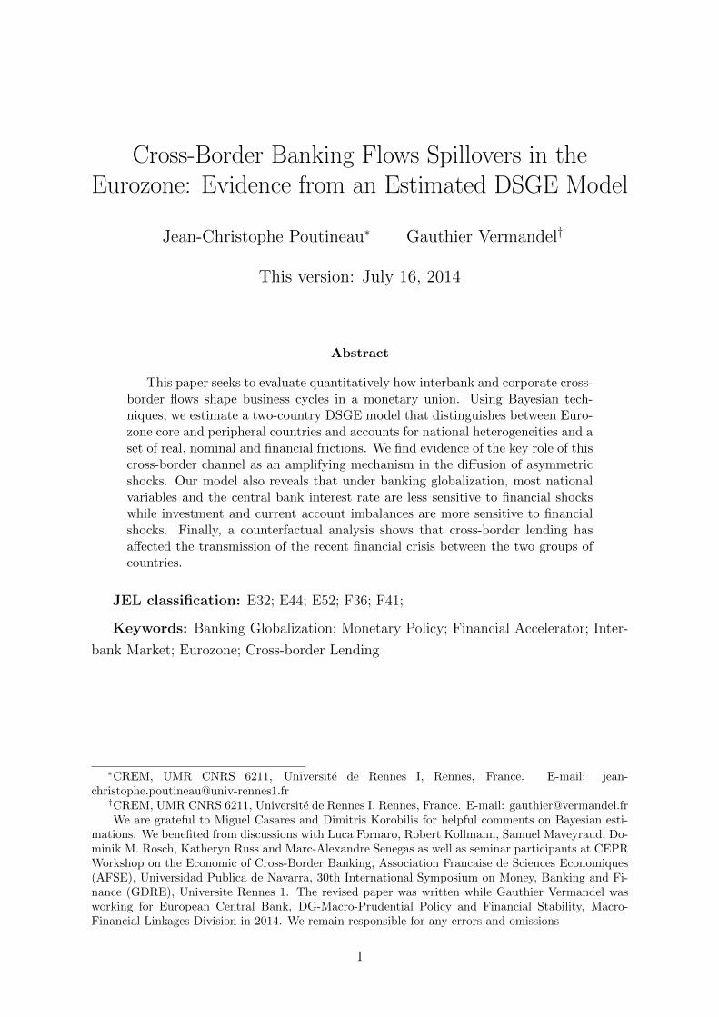
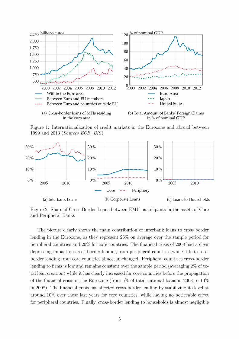
Cross-border lending is a distinguishing feature of financial integration in the Eurozone.

As reported in panel (a) of Fig. 1, between 1999Q1-2012Q1, cross-border loans have

increased much more between participating counties than between the Eurozone and

the European Union, and even much more than with countries outside Europe. The

rise in cross-border loans is peaking in 2008, where cross-border loans represented 300%

of the value initially observed in 1999. The financial crisis is characterized by a 25%

drop in cross-border lending between Euro partners. As underlined in panel (b), in

2008, cross-border lending represented around 120% of GDP for Eurozone countries at

its peak value, while the corresponding figures were 40% for the US and 20% for Japan.

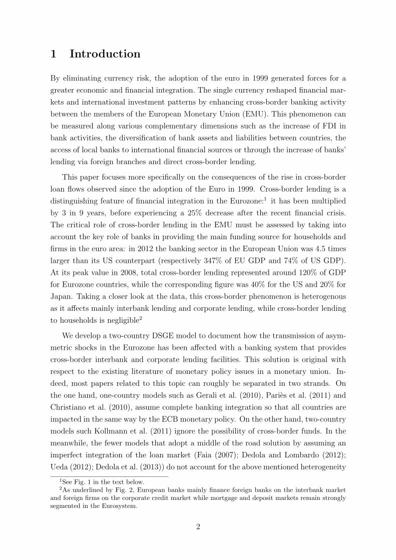
However, a closer view at the data underlines the heterogeneity of bilateral flows within

the Eurozone. In Fig. 2, we split the Eurozone in two groups: core countries and

peripheral countries. In the first group we aggregate data for Germany and France,

while in the second group, we aggregate data for Spain, Greece, Ireland, Italy and

Portugal. We summarize the main stylized fact by contrasting interbank loans (in panel

(a)), Corporate loans (in panel (b)) and loans to households (in panel (c)). Cross border

loans are reported as the percentage of loans exported to the other economies either

by core countries (plain lines) or peripheral countries (dotted lines). Thus, each curve

represents the percentage points of loans exported by the relevant group of countries

towards the rest of the Monetary Union.

4

2000 2002 2004 2006 2008 2010 2012

500

750

1,000

1,250

1,500

1,750

2,000

2,250 billions euros

(a) Cross-border loans of MFIs residingin the euro area

Within the Euro areaBetween Euro and EU membersBetween Euro and countries outside EU

2000 2002 2004 2006 2008 2010 20120

20

40

60

80

100

120 % of nominal GDP

(b) Total Amount of Banks’ Foreign Claimsin % of nominal GDP

Euro AreaJapanUnited States

Figure 1: Internationalization of credit markets in the Eurozone and abroad between1999 and 2013 (Sources ECB, BIS )

2005 20100 %

10 %

20 %

30 %

(a) Interbank Loans

2005 20100 %

10 %

20 %

30 %

(b) Corporate Loans

Core Periphery

2005 20100 %

10 %

20 %

30 %

(c) Loans to Households

Figure 2: Share of Cross-Border Loans between EMU participants in the assets of Coreand Peripheral Banks

The picture clearly shows the main contribution of interbank loans to cross border

lending in the Eurozone, as they represent 25% on average over the sample period for

peripheral countries and 20% for core countries. The financial crisis of 2008 had a clear

depressing impact on cross-border lending from peripheral countries while it left cross-

border lending from core countries almost unchanged. Peripheral countries cross-border

lending to firms is low and remains constant over the sample period (averaging 2% of to-

tal loan creation) while it has clearly increased for core countries before the propagation

of the financial crisis in the Eurozone (from 5% of total national loans in 2003 to 10%

in 2008). The financial crisis has affected cross-border lending by stabilizing its level at

around 10% over these last years for core countries, while having no noticeable effect

for peripheral countries. Finally, cross-border lending to households is almost negligible

5

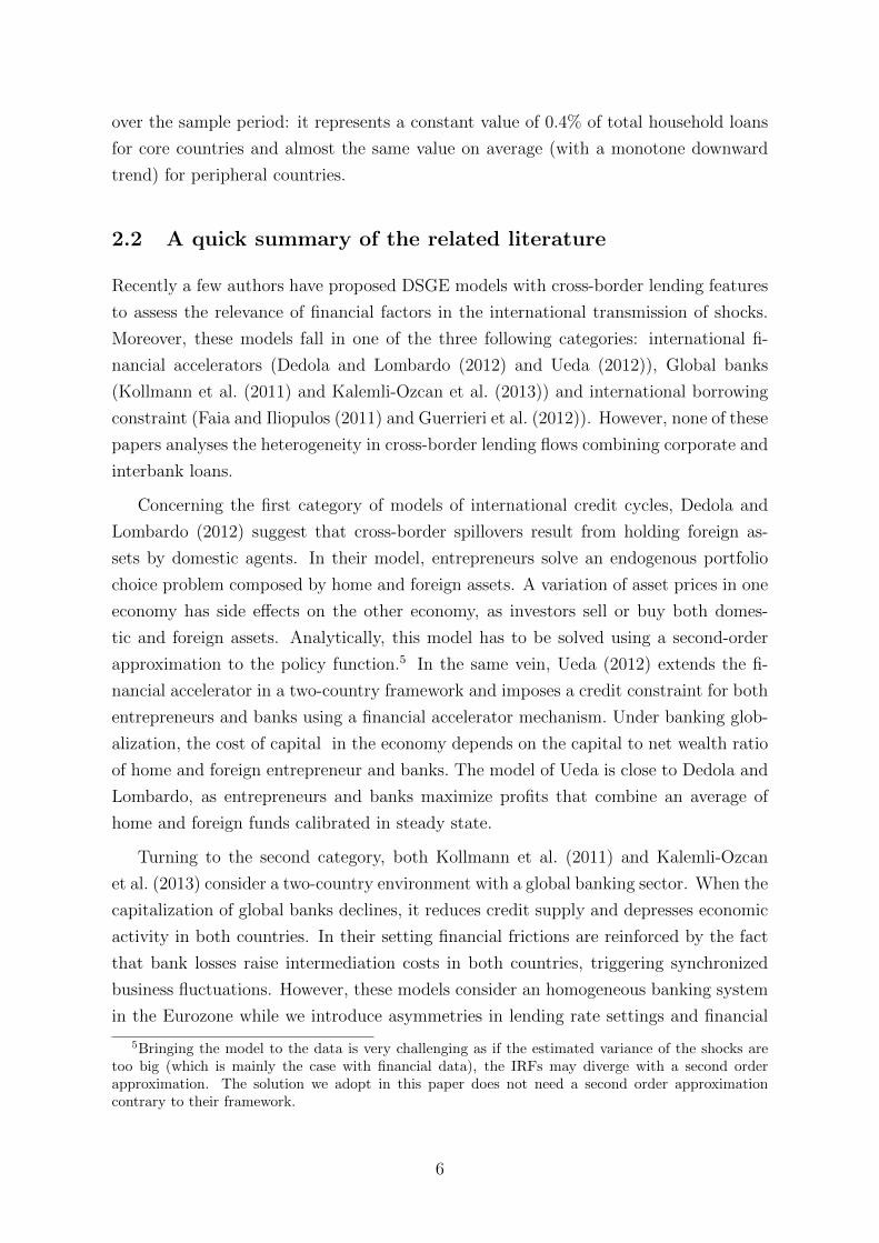
over the sample period: it represents a constant value of 0.4% of total household loans

for core countries and almost the same value on average (with a monotone downward

trend) for peripheral countries.

2.2 A quick summary of the related literature

Recently a few authors have proposed DSGE models with cross-border lending features

to assess the relevance of financial factors in the international transmission of shocks.

Moreover, these models fall in one of the three following categories: international fi-

nancial accelerators (Dedola and Lombardo (2012) and Ueda (2012)), Global banks

(Kollmann et al. (2011) and Kalemli-Ozcan et al. (2013)) and international borrowing

constraint (Faia and Iliopulos (2011) and Guerrieri et al. (2012)). However, none of these

papers analyses the heterogeneity in cross-border lending flows combining corporate and

interbank loans.

Concerning the first category of models of international credit cycles, Dedola and

Lombardo (2012) suggest that cross-border spillovers result from holding foreign as-

sets by domestic agents. In their model, entrepreneurs solve an endogenous portfolio

choice problem composed by home and foreign assets. A variation of asset prices in one

economy has side effects on the other economy, as investors sell or buy both domes-

tic and foreign assets. Analytically, this model has to be solved using a second-order

approximation to the policy function.5 In the same vein, Ueda (2012) extends the fi-

nancial accelerator in a two-country framework and imposes a credit constraint for both

entrepreneurs and banks using a financial accelerator mechanism. Under banking glob-

alization, the cost of capital in the economy depends on the capital to net wealth ratio

of home and foreign entrepreneur and banks. The model of Ueda is close to Dedola and

Lombardo, as entrepreneurs and banks maximize profits that combine an average of

home and foreign funds calibrated in steady state.

Turning to the second category, both Kollmann et al. (2011) and Kalemli-Ozcan

et al. (2013) consider a two-country environment with a global banking sector. When the

capitalization of global banks declines, it reduces credit supply and depresses economic

activity in both countries. In their setting financial frictions are reinforced by the fact

that bank losses raise intermediation costs in both countries, triggering synchronized

business fluctuations. However, these models consider an homogeneous banking system

in the Eurozone while we introduce asymmetries in lending rate settings and financial

5Bringing the model to the data is very challenging as if the estimated variance of the shocks aretoo big (which is mainly the case with financial data), the IRFs may diverge with a second orderapproximation. The solution we adopt in this paper does not need a second order approximationcontrary to their framework.

6

shocks between the core and the periphery to account for financial heterogeneity in the

Eurozone.

Faia and Iliopulos (2011) develop a small open economy DSGE model with durable

and non durable goods sectors where households face a collateral constraint on the

foreign level of debt. The model offers a reduced form of the banking system and

concentrates on housing that is financed through foreign lending. We do not use this

model for our purposes given the marginal flows of cross-border loans for house purchases

encountered in Eurozone data as showed in Fig. 2. Furthermore, as a small open country

model, it can not be kept for our analysis that requires a two-country model. Finally,

in the model developed by Guerrieri et al. (2012), banks grant loans to firms and invest

in bonds issued by home and foreign government. The model is calibrated on the

Euro area. In a two-country set-up, there are core and peripheral countries where large

contractionary shocks trigger sovereign default. This model is well suited to analyze the

diffusion of sovereign default risk in the Eurozone as shock to the value of peripheral

bonds have side effects on the core economy. The model is also very rich in terms of

financial frictions. However, the model is aimed at evaluating the diffusion of a sovereign

debt crisis, a topic not covered in this paper.

One of the novelty of our analysis is to provide a simple way to model cross-border

lending activity to account for the previous stylized facts. To take our two-country

model to the data easily, we assume that the banking system determines the loan inter-

est rate while the quantity of loans that is contracted is determined by loan demand.

Thus, in this paper, rather than assuming that loans result of optimal portfolio choices

from the supply side of the credit market, we suppose that the cross-border decisions

arise from the demand side of credit market. International financial linkages are analo-

gous to the external trade channels, assuming that a CES function aggregates domestic

and international lending. This choice - that borrows from the New Open Economy

Macroeconomics (NOEM) - remains quite simplistic but offers an interesting feature

when going to the empirical estimation of the model and a simple reinterpretation of

the financial accelerator from a banking perspective.

3 A Monetary Union with Cross-border Loans

We describe a two-country world. The two countries are equal in size and share a

common currency. Each country i ∈ {h, f} (where h is for home and f for foreign) is

populated by consumers, labor unions, intermediate and final producers, entrepreneurs,

capital suppliers and a banking system. Regarding the conduct of macroeconomic policy,

we assume national fiscal authorities and a common central bank. As in Christiano

7

et al. (2005) and Smets and Wouters (2003, 2007), we account for several sources of

rigidities to enhance the empirical relevance of the model. The set of real rigidities

encompasses consumption habits, investment adjustment costs, loan demand habits.

Regarding nominal rigidities, we account for stickiness in final goods prices, wages and

loan interest rates.

Central Bank

Bank

Bank

Production

Production

Household

Household

Ch,t

Cf,t

Lsh,t

Lsf,t

InvestmentFlows

BondsFlows

ConsumptionFlows

Cross-BordersLoans

RefinancingRate Rt

RefinancingRate Rt

InterbankFlows

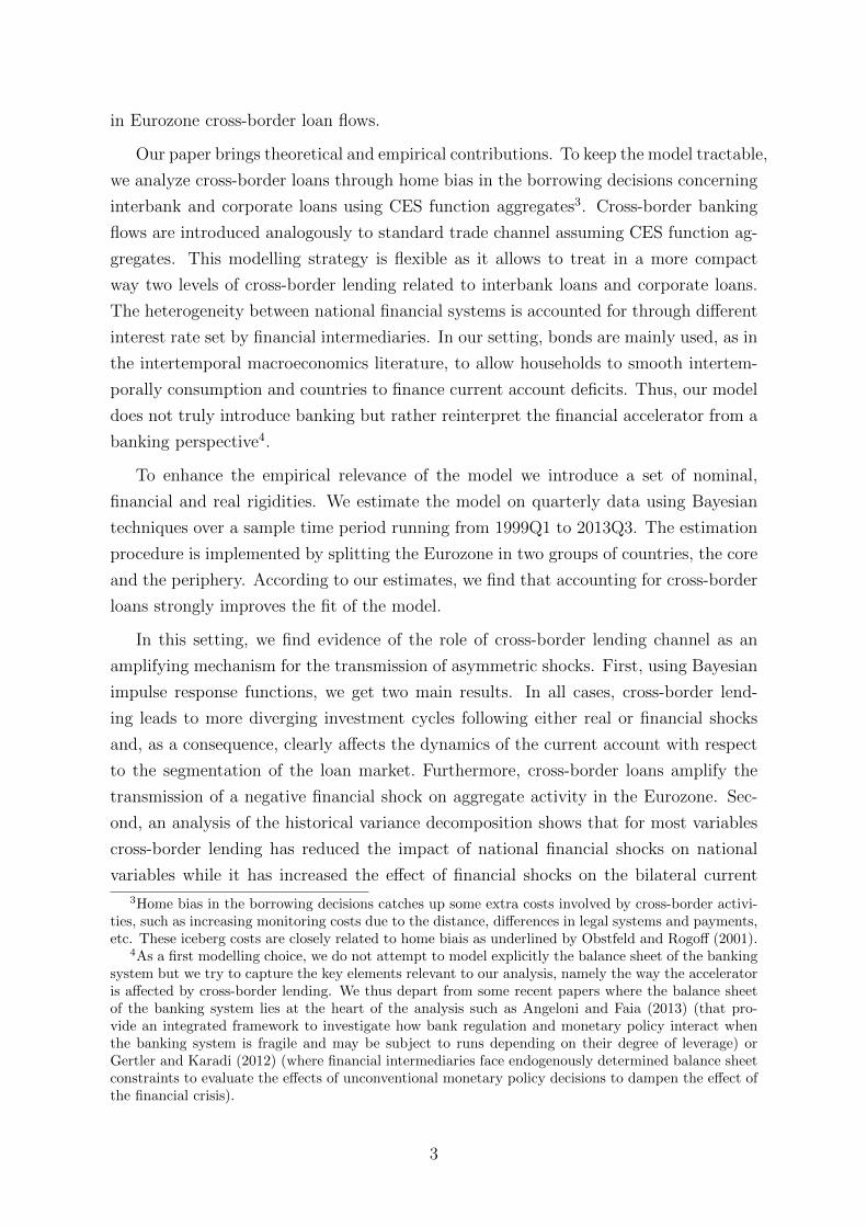
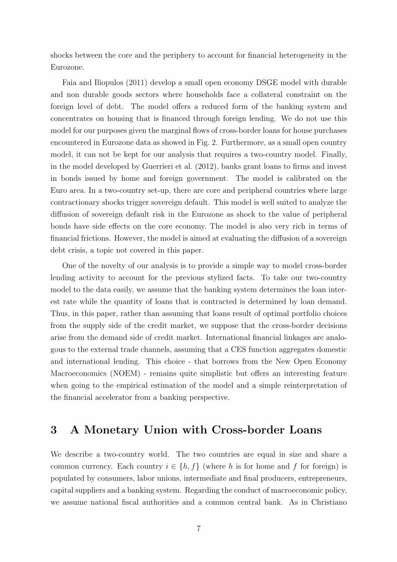
Figure 3: The model of a two-country monetary union with international bank loanflows

The general structure of the model is summarized in Fig. 3. For expository pur-

poses, this section describes the financial component of the model. We first outline the

structure of the banking system that gives rise to cross-border interbank loan, then we

describe the origin of cross-border corporate loans. The standard new Keynesian and

RBC components of the model are presented afterward in Section 4.

3.1 An Heterogenous Banking System

In each country, the banking sector finances investment projects to home and foreign

entrepreneurs by supplying one period loans. The banking system is heterogenous with

regard to liquidity, and banks engage in interbank lending at the national and interna-

tional levels. Thus, cross-border loans are made of corporate loans (between banks and

entrepreneurs) and interbank loans.

To introduce an interbank market, we suppose that the banking system combines

liquid and illiquid banks. Normalizing the total number of banks in each economy to

1, we assume that banks distributed over [0, λ] are illiquid (i.e. credit constrained),

while the remaining banks distributed over share [λ, 1] are liquid and supply loans to

entrepreneurs and to illiquid banks. We assume that a liquid bank is characterized by

her direct accessibility to the ECB fundings. Conversely, an illiquid bank does not have

access to the ECB fundings. This assumption is empirically motivated: in the Eurosys-

tem, only a fraction of the 2500 banks participates regularly to the bidding process in

8

main refinancing operations of the ECB while the others rely on interbank funding, as

underlined by Gray et al. (2008). Extending this assumption in an international per-

spective, illiquid banks can borrow from both domestic and foreign liquid banks, which

gives rise to cross-border interbank lending flows.

Illiquid Banks: The representative illiquid bank b ∈ [0, λ] in country i operates

under monopolistic competition to provide a quantity of loans Lsi,t+1 (b) to entrepreneurs

that is financed by interbank loans IBi,t+1 (b) from the interbank market (with a one

period maturity) at a rate P IBi,t . The balance sheet of the bank writes,

Lsi,t+1 (b) = IBHi,t+1 (b) +BKi,t+1 (b) + liabi,t, (1)

where Lsi,t+1 (b) is the loan supply of borrowing banks, IBHi,t+1 (b) is the interbank loans

supplied by liquid banks subject to external habits, BKi,t+1 (b) is the bank capital and

liabi,t are other liabilities in the balance sheet of the bank that are not considered in the

model6. We suppose that the demand for interbank funds are subject to external habits

at a degree hibi where, IBHi,t+1 (b) = IBdi,t+1 (b) − hibi

(IBd

i,t+1 − IBdi

). These habits are

deemed necessary to catch up the high autocorrelation observed in the supply of loans7.

This bank engages in corporate loans. In this setting, we assume that there is

no discrimination between borrowers, so that the representative and risk-neutral bank

serves both domestic and foreign entrepreneurs without taking into account specificities

regarding the national viability of projects. Bank default expectation regarding en-

trepreneurs’ projects is defined as, ηi,t+1 ≡(1− αLi

)ηEh,t+1 + αLi η

Ef,t+1, where ηEi,t+1is the

default rate in country i ∈ {h, f} of entrepreneurs and(1− αLi

)measures the home bias

in corporate loan distribution. Thus, the marginal cost of one unit of corporate loan

MCilli,t (b) provided by the illiquid bank is the solution of the expected profit EtΠB

i,t+1 (b)

optimization problem,

maxLsi,t+1(b)

Etηi,t+1MCilli,t (b)Lsi,t+1 (b)− P IB

i,t

(Lsi,t+1 (b)−BKi,t+1 (b)− liabt (b)

). (2)

The marginal cost of one unit of loan, denoted MCilli,t (b), is the same across illiquid

banks,

MCilli,t (b) = MCill

i,t =P IBi,t

Etηi,t+1

, (3)

6We suppose that they follow an exogenous AR(1) shock process εBi,t such that, liabi,t = eεBi,t liabi,

this shock captures some aggregate movements in the capital constraint of banks.7In the fit exercise, DSGE models with banking are estimated on the outstanding amount of loans

contracted in the economy. Since DSGE models only include one-period maturity loans, externalhabits are a tractable way to catch up the high persistence in the loan contracts without modifying thesteady state. Guerrieri et al. (2012) develops a similar financial friction in the borrowing constraint ofentrepreneurs.

9

so that each bank decides the size of the spread depending on the expected failure rate

of its customers Etηi,t+1.The bank has access to domestic and foreign interbank loans to

meet its balance sheet. The total amount borrowed by the representative bank writes,

IBdi,t+1 (b) =

((1− αIBi

)1/ξIBd

h,i,t+1 (b)(ξ−1)/ξ +(αIBi

)1/ξIBd

f,i,t+1 (b)(ξ−1)/ξ)ξ/(ξ−1)

, (4)

where parameter ξ is the elasticity of substitution between domestic and foreign in-

terbank funds, αIBi represents the percentage of cross-border interbank loan flows in

the monetary union and IBdh,i,t+1 (b) (resp. IBd

f,i,t+1 (b)) the amount of domestic (resp.

foreign) loans demanded by borrowing bank b in country i. The total cost incurred by

illiquid banks to finance interbank loans, P IBi,t , is thus defined according to the CES

aggregator,

P IBi,t =

((1− αIBi

) (RIBh,t

)1−ξ+ αIBi

(RIBf,t

)1−ξ)1/(1−ξ), (5)

where RIBh,t (resp. RIB

f,t ) is the cost of loans obtained from home (resp. foreign) banks in

country i. The decision to borrow from a particular bank is undertaken on the basis of

relative interbank national interest rates,

IBdh,i,t+1 (b) =

(1− αIBi

) [RIBh,t

P IBi,t

]−ξIBd

i,t+1 (b) , and IBdf,i,t+1 (b) = αIBi

[RIBf,t

P IBi,t

]−ξIBd

i,t+1 (b) .

Here, cross-border lending is measured through the values undertaken by IBdh,f,t+1 (b) ,

(i.e., interbank loans contracted by liquid foreign banks from domestic overliquid banks)

and symmetrically by IBdf,h,t+1 (b) (i.e., interbank loans contracted by liquid domestic

banks from foreign overliquid banks). Finally following Hirakata et al. (2009), the bank

capital accumulation process of illiquid banks (BKi,t+1 (b)) is determined by,

BKi,t+1 (b) =(1− τBK

)ΠBi,t (b) , (6)

where τBK is a proportional tax on the profits of the bank.

Liquid Banks: The representative liquid bank b ∈ [λ; 1] in country i operates under

monopolistic competition to provide a quantity of loans Lsi,t+1 (b) to entrepreneurs. It

also provides a quantity of interbank loans IBsi,t+1 (b) to illiquid banks. We suppose that

the intermediation process between liquid and illiquid banks is costly: we introduce a

convex monitoring technology a la Curdia and Woodford (2010) and Dib (2010) with

a functional form ACIBi,t+1 (b) =

χIBi2

(IBs

i,t+1 (b)− IBs

i (b))2

where parameter χIBi is the

level of financial frictions between liquid banks in country i and home and foreign illiquid

banks8. Loans created by the liquid bank are financed by one-period maturity loans

8Contrary to Curdia and Woodford (2010) but in the same vein of Dib (2010), the monitoringtechnology does not alter the steady state of the model to keep the estimation of χIBi as simple as

10

from the central bank (LECBi,t+1 (b)) at the refinancing interest rate Rt. Finally, the bank’s

balance sheet is defined by,

Lsi,t+1 (b) + IBsi,t+1 (b) = LECBi,t+1 (b) +BKi,t+1 (b) + liabt (b) .

According to the behavior of illiquid banks, we assume that there is no discrimination

between borrowers. The marginal cost of one unit of loan MC liqi,t (b) solves the profit

(ΠBi,t (b)) maximization problem,

maxLsi,t+1(b),IBi,t+1(b)

Etηi,t+1MC liqi,t (b)Lsi,t+1 (b)+RIB

i,t (b) IBsi,t+1 (b)−RtL

ECBi,t+1 (b)−ACIB

i,t+1 (b) .

(7)

The marginal cost of one unit of loan is the same for all liquid banks,

MC liqi,t (b) = MC liq

i,t =Rt

Etηi,t+1

. (8)

Similarly to the illiquid bank, bank capital evolves according to Eq. (6)9.

Loan interest rates: There are two interest rates to be determined: the interest

rate on the interbank market and the interest rate on corporate loans. First, on a

perfectly competitive market, the interbank rate in country i is determined from the

problem (7),

RIBi,t (b) = χIBi

(IBi,t+1 (b)− IBs

i (b))

+Rt, (9)

where, χIBi is a cost parameter, IBsi,t+1 (b) is the amount of interbank loans contracted

in period t with a one period maturity and IBs

i (b) is the steady state value of interbank

loans.

Second, the interest rate charged by banks of country i on corporate loans accounts

for the liquidity of the national banking system. Anticipating over symmetric issues

at the equilibrium to improve the tractability of the model, we assume that all banks

belonging to a national banking system share the same marginal cost of production,

reflecting the average liquidity degree of national banks. Thus, aggregating over each

group of banks, we get,∫ λ

0MCill

i,t (b)db = MCL,illi,t , and

∫ 1

λMC liq

i,t (b)db = MC liqi,t . Aggre-

gate marginal cost MCLi,t combines outputs from liquid and illiquid banks of country i

possible. Several papers refer to monitoring technology functions in the intermediation process ofbanks, see for example Goodfriend and McCallum (2007) or Casares and Poutineau (2011).

9The accumulation of bank capital is necessary to close the model but it is not binding for liquidbanks as they are not credit constrained.

11

according to10,

MCLi,t =

(MC ill

i,t

)λ (MC liq

i,t

)(1−λ)

=

(P IBi,t

)λ(Rt)

(1−λ)

Etηi,t+1

. (10)

Thus, the representative bank b ∈ [0; 1] of country i operates under monopolistic com-

petition to provide a quantity of loans Lsi,t+1 (b) incurring a marginal cost MCLi,t. The

marginal cost is the same for all banks b and depends on the expected failure rate

of borrowers’ projects and the central bank refinancing rate. Eq. (10) taken in logs

becomes,

mcLi,t =1(

1− N/K) [(1− αLi ) (1− κi) levi,t + αLi (1− κj) levj,t

]+ (1− λ) rt + λpIBi,t ,

∀i 6= j ∈ {h, f}, where, levi,t is the leverage ratio of entrepreneurs and N/K is

the steady state net worth to capital ratio. Under Calvo pricing with partial index-

ation, banks set the interest rate on loans contracted by entrepreneurs on a stag-

gered basis as in Paries et al. (2011). A fraction θLi of banks is not allowed to opti-

mally set the credit rate11 and index it by ξLi percent of the past credit rate growth,

RLi,t (b) =

(RLi,t−1/R

Li,t−2

)ξLi RLi,t−1 (b). Assuming that it is able to modify its loan interest

rate with a constant probability 1−θLi , it chooses RL∗i,t (b) to maximize its expected sum

of profits,

max{RL∗

i,t (b)}Et{∑∞

τ=0

(θLi β

)τ λci,t+τλci,t

ηi,t+1+τ

[(1− τL

)RL∗i,t (b) ΞL

i,t,τ −MCLi,t+τ

]Li,t+1+τ (b)

},

subject to, Li,t+1+τ (b) =(ΞLi,t,τR

L∗i,t (b) /RL

i,t+τ

)−µLi,t+τ/(µLi,t+τ−1)Li,t+1+τ , ∀τ > 0, where

ΞLi,t,τ =

∏τk=1

(RLi,t+k−1/R

Li,t+k−2

)ξLi is the sum of past credit rate growth and Li,t (b)

denotes the quantity of differentiated banking loans b that is used by the retail banks12.

The time-varying markup is defined by, µLi,t = µL + εLi,t, so that an increase in εLi,t can

be interpreted as a cost-push shock to the credit rate equation13. As Benigno and

Woodford (2005), we introduce a proportional tax τL on profits that restores the first-

best allocation in the steady state. Allowing for a partial indexation of credit interest

rates on their previous levels (where ξLi ∈ [0; 1] is the level of indexation that catches

some imperfect interest rate pass-though with θLi ), and imposing symmetry, the log

10We borrow this aggregation procedure from the solution introduced by Gerali et al. (2010), toaggregate borrowing and saving households labor supply.

11This parameter, once estimated in the next section, will serve as a measure to measure the flexibilityof national banking systems in the transmission of interest rate decisions.

12Retail banks are perfectly competitive loan packers, they buy the differentiated loans and aggregatethem through a CES technology into one loan and sell them to entrepreneurs.

13Differentiated loans are imperfect substitutes, with elasticitity of substitution denoted by µL

(µL−1) .

12

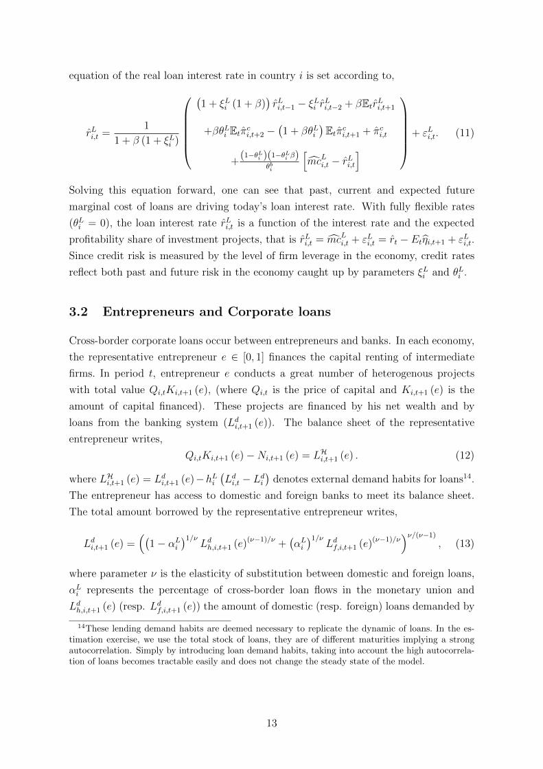
equation of the real loan interest rate in country i is set according to,

rLi,t =1

1 + β (1 + ξLi )

(1 + ξLi (1 + β)

)rLi,t−1 − ξLi rLi,t−2 + βEtrLi,t+1

+βθLi Etπci,t+2 −(1 + βθLi

)Etπci,t+1 + πci,t

+(1−θLi )(1−θLi β)

θbi

[mcLi,t − rLi,t

]

+ εLi,t. (11)

Solving this equation forward, one can see that past, current and expected future

marginal cost of loans are driving today’s loan interest rate. With fully flexible rates

(θLi = 0), the loan interest rate rLi,t is a function of the interest rate and the expected

profitability share of investment projects, that is rLi,t = mcLi,t + εLi,t = rt − Etηi,t+1 + εLi,t.

Since credit risk is measured by the level of firm leverage in the economy, credit rates

reflect both past and future risk in the economy caught up by parameters ξLi and θLi .

3.2 Entrepreneurs and Corporate loans

Cross-border corporate loans occur between entrepreneurs and banks. In each economy,

the representative entrepreneur e ∈ [0, 1] finances the capital renting of intermediate

firms. In period t, entrepreneur e conducts a great number of heterogenous projects

with total value Qi,tKi,t+1 (e), (where Qi,t is the price of capital and Ki,t+1 (e) is the

amount of capital financed). These projects are financed by his net wealth and by

loans from the banking system (Ldi,t+1 (e)). The balance sheet of the representative

entrepreneur writes,

Qi,tKi,t+1 (e)−Ni,t+1 (e) = LHi,t+1 (e) . (12)

where LHi,t+1 (e) = Ldi,t+1 (e)−hLi(Ldi,t − Ldi

)denotes external demand habits for loans14.

The entrepreneur has access to domestic and foreign banks to meet its balance sheet.

The total amount borrowed by the representative entrepreneur writes,

Ldi,t+1 (e) =((

1− αLi)1/ν

Ldh,i,t+1 (e)(ν−1)/ν +(αLi)1/ν

Ldf,i,t+1 (e)(ν−1)/ν)ν/(ν−1)

, (13)

where parameter ν is the elasticity of substitution between domestic and foreign loans,

αLi represents the percentage of cross-border loan flows in the monetary union and

Ldh,i,t+1 (e) (resp. Ldf,i,t+1 (e)) the amount of domestic (resp. foreign) loans demanded by

14These lending demand habits are deemed necessary to replicate the dynamic of loans. In the es-timation exercise, we use the total stock of loans, they are of different maturities implying a strongautocorrelation. Simply by introducing loan demand habits, taking into account the high autocorrela-tion of loans becomes tractable easily and does not change the steady state of the model.

13

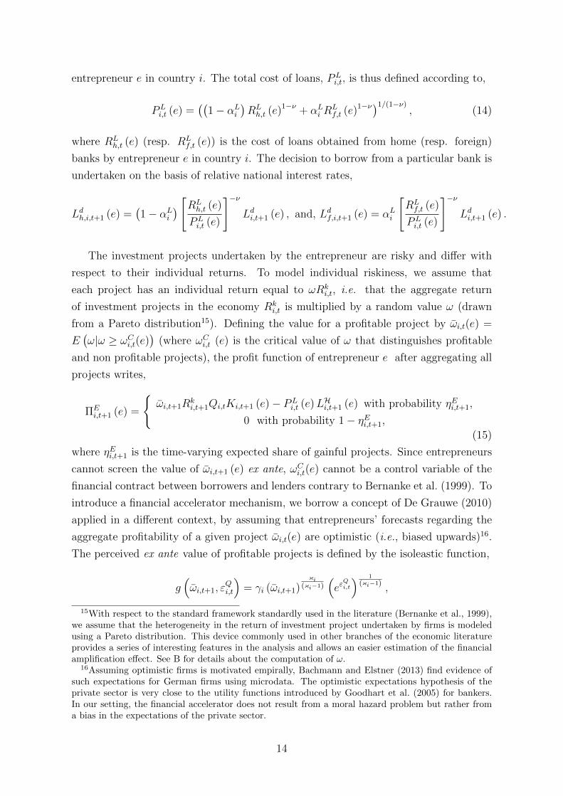
entrepreneur e in country i. The total cost of loans, PLi,t, is thus defined according to,

PLi,t (e) =

((1− αLi

)RLh,t (e)1−ν + αLi R

Lf,t (e)1−ν)1/(1−ν)

, (14)

where RLh,t (e) (resp. RL

f,t (e)) is the cost of loans obtained from home (resp. foreign)

banks by entrepreneur e in country i. The decision to borrow from a particular bank is

undertaken on the basis of relative national interest rates,

Ldh,i,t+1 (e) =(1− αLi

) [RLh,t (e)

PLi,t (e)

]−νLdi,t+1 (e) , and, Ldf,i,t+1 (e) = αLi

[RLf,t (e)

PLi,t (e)

]−νLdi,t+1 (e) .

The investment projects undertaken by the entrepreneur are risky and differ with

respect to their individual returns. To model individual riskiness, we assume that

each project has an individual return equal to ωRki,t, i.e. that the aggregate return

of investment projects in the economy Rki,t is multiplied by a random value ω (drawn

from a Pareto distribution15). Defining the value for a profitable project by ωi,t(e) =

E(ω|ω ≥ ωCi,t(e)

)(where ωCi,t (e) is the critical value of ω that distinguishes profitable

and non profitable projects), the profit function of entrepreneur e after aggregating all

projects writes,

ΠEi,t+1 (e) =

{ωi,t+1R

ki,t+1Qi,tKi,t+1 (e)− PL

i,t (e)LHi,t+1 (e) with probability ηEi,t+1,

0 with probability 1− ηEi,t+1,

(15)

where ηEi,t+1 is the time-varying expected share of gainful projects. Since entrepreneurs

cannot screen the value of ωi,t+1 (e) ex ante, ωCi,t(e) cannot be a control variable of the

financial contract between borrowers and lenders contrary to Bernanke et al. (1999). To

introduce a financial accelerator mechanism, we borrow a concept of De Grauwe (2010)

applied in a different context, by assuming that entrepreneurs’ forecasts regarding the

aggregate profitability of a given project ωi,t(e) are optimistic (i.e., biased upwards)16.

The perceived ex ante value of profitable projects is defined by the isoleastic function,

g(ωi,t+1, ε

Qi,t

)= γi (ωi,t+1)

κi(κi−1)

(eεQi,t

) 1

(κi−1),

15With respect to the standard framework standardly used in the literature (Bernanke et al., 1999),we assume that the heterogeneity in the return of investment project undertaken by firms is modeledusing a Pareto distribution. This device commonly used in other branches of the economic literatureprovides a series of interesting features in the analysis and allows an easier estimation of the financialamplification effect. See B for details about the computation of ω.

16Assuming optimistic firms is motivated empirally, Bachmann and Elstner (2013) find evidence ofsuch expectations for German firms using microdata. The optimistic expectations hypothesis of theprivate sector is very close to the utility functions introduced by Goodhart et al. (2005) for bankers.In our setting, the financial accelerator does not result from a moral hazard problem but rather froma bias in the expectations of the private sector.

14

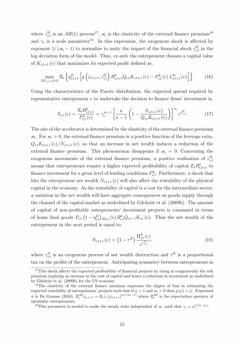
where εQi,t is an AR(1) process17, κi is the elasticity of the external finance premium18

and γi is a scale parameter19. In this expression, the exogenous shock is affected by

exponent 1/ (κi − 1) to normalize to unity the impact of the financial shock εQi,t in the

log deviation form of the model. Thus, ex-ante the entrepreneur chooses a capital value

of Ki,t+1 (e) that maximizes its expected profit defined as,

max{Ki,t+1(e)}

Et{ηEi,t+1

[g(ωi,t+1, ε

Qi,t

)Rki,t+1Qi,tKi,t+1 (e)− PL

i,t (e)LHi,t+1 (e)]}

. (16)

Using the characteristics of the Pareto distribution, the expected spread required by

representative entrepreneur e to undertake the decision to finance firms’ investment is,

Si,t (e) =EtRk

i,t+1

PLi,t (e)

= γκi−1i

[κ

κ− 1

(1− Ni,t+1 (e)

Qi,tKi,t+1 (e)

)]κieεQi,t . (17)

The size of the accelerator is determined by the elasticity of the external finance premium

κi. For κi > 0, the external finance premium is a positive function of the leverage ratio,

Qi,tKi,t+1 (e) /Ni,t+1 (e), so that an increase in net wealth induces a reduction of the

external finance premium. This phenomenon disappears if κi = 0. Concerning the

exogenous movements of the external finance premium, a positive realization of εQi,tmeans that entrepreneurs require a higher expected profitability of capital EtR

ki,t+1 to

finance investment for a given level of lending conditions PLi,t. Furthermore, a shock that

hits the entrepreneur net wealth Ni,t+1 (e) will also affect the rentability of the physical

capital in the economy. As the rentability of capital is a cost for the intermediate sector,

a variation in the net wealth will have aggregate consequences on goods supply through

the channel of the capital market as underlined by Gilchrist et al. (2009b). The amount

of capital of non-profitable entrepreneurs’ investment projects is consumed in terms

of home final goods Pi,t(1− ηEi,t

)ωi,t (e)Rk

i,tQi,t−1Ki,t (e). Thus the net wealth of the

entrepreneur in the next period is equal to,

Ni,t+1 (e) =(1− τE

) ΠEi,t (e)

eεNi,t

, (18)

where εNi,t is an exogenous process of net wealth destruction and τE is a proportional

tax on the profits of the entrepreneur. Anticipating symmetry between entrepreneurs in

17This shock affects the expected profitability of financial projects by rising in exogeneously the riskpremium implying an increase in the cost of capital and hence a reduction in investment as underlinedby Gilchrist et al. (2009b) for the US economy.

18The elasticity of the external finance premium expresses the degree of bias in estimating theexpected rentability of entrepreneurs’ projects such that if ω > 1 and κi > 0 then g (ω) > ω. Expressed

a la De Grauwe (2010), Eoptt ωi,t+1 = Etγi (ωi,t+1)κi/(κi−1)

where Eoptt is the expectation operator ofoptimistic entrepreneurs.

19This parameter is needed to make the steady state independent of κi ,such that γi = ω1/(1−κi).

15

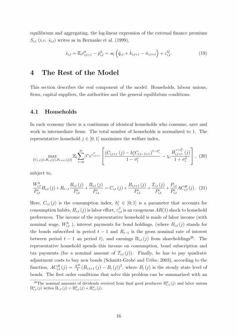
equilibrium and aggregating, the log-linear expression of the external finance premium

Si,t (i.e. si,t) writes as in Bernanke et al. (1999),

si,t = Etrki,t+1 − pLi,t = κi(qi,t + ki,t+1 − ni,t+1

)+ εQi,t. (19)

4 The Rest of the Model

This section describes the real component of the model: Households, labour unions,

firms, capital suppliers, the authorities and the general equilibrium conditions.

4.1 Households

In each economy there is a continuum of identical households who consume, save and

work in intermediate firms. The total number of households is normalized to 1. The

representative household j ∈ [0, 1] maximizes the welfare index,

max{Ci,t(j),Hi,t(j),Bi,t+1(j)}

Et∞∑τ=0

βτeεβi,t+τ

(Ci,t+τ (j)− hciCi,t−1+τ )1−σci

1− σci− χi

H1+σLi

i,t+τ (j)

1 + σLi

, (20)

subject to,

W hi,t

P ci,t

Hi,t (j)+Rt−1Bi,t (j)

P ci,t

+Πi,t (j)

P ci,t

= Ci,t (j)+Bi,t+1 (j)

P ci,t

+Ti,t (j)

P ci,t

+Pi,tP ci,t

ACBi,t (j) . (21)

Here, Ci,t (j) is the consumption index, hci ∈ [0; 1] is a parameter that accounts for

consumption habits, Hi,t (j) is labor effort, εβi,t is an exogenous AR(1) shock to household

preferences. The income of the representative household is made of labor income (with

nominal wage, W hi,t ), interest payments for bond holdings, (where Bi,t (j) stands for

the bonds subscribed in period t − 1 and Rt−1 is the gross nominal rate of interest

between period t − 1 an period t), and earnings Πi,t (j) from shareholdings20. The

representative household spends this income on consumption, bond subscription and

tax payments (for a nominal amount of Ti,t (j)). Finally, he has to pay quadratic

adjustment costs to buy new bonds (Schmitt-Grohe and Uribe, 2003), according to the

function, ACBi,t (j) = XB

2(Bi,t+1 (j)−Bi (j))

2, where Bi (j) is the steady state level of

bonds. The first order conditions that solve this problem can be summarized with an

20The nominal amounts of dividends received from final good producers Πyi,t (j) and labor unions

Πwi,t (j) writes Πi,t (j) = Πy

i,t (j) + Πwi,t (j).

16

Euler bond condition,

βRt

1 + Pi,tXB (Bi,t+1 (j)−Bi (j))= Et

{eεβi,t

eεβi,t+1

P ci,t+1

P ci,t

((Ci,t+1 (j)− hciCi,t)(Ci,t (j)− hciCi,t−1)

)σci}, (22)

and a labor supply function,

W hi,t

P ci,t

= χiHi,t (j)σLi (Ci,t (j)− hciCi,t−1)σ

ci . (23)

The consumption basket of the representative household and the consumption price in-

dex of country i are, Ci,t(j) =((

1− αCi)1/µ

Ch,i,t(j)(µ−1)/µ +

(αCi)1/µ

Cf,i,t (j)(µ−1)/µ

)µ/(µ−1)

and P ci,t =

((1− αCi

)P 1−µh,t + αCi P

1−µf,t

)1/(1−µ)where µ is the elasticity of substitution be-

tween the consumption of home (Ch,i,t(j)) and foreign (Cf,i,t (j)) goods and αCi is the

degree of openness of the economy. In this model, we assume home bias in consumption,

so that αCi <12.

4.2 Labor Unions

Households provide differentiated labor types, sold by labor unions to perfectly competi-

tive labor packers who assemble them in a CES aggregator and sell the homogenous labor

to intermediate firms. Each representative union is related to an household j ∈ [0; 1].

Assuming that the trade union is able to modify its wage with a probability 1− θwi , it

chooses the optimal wage W ∗i,t (j) to maximize its expected sum of profits,

max{W ∗

i,t(j)}Et

{∑∞

τ=0(θwi β)τ

λci,t+τλci,t

[(1− τw)

W ∗i,t (j)

P ci,t+τ

τ∏k=1

(πci,t+k−1

)ξwi − W hi,t+τ (j)

P ci,t+τ

]Hi,t+τ (j)

},

subject to the downgrade sloping demand constraint from labor packers, Hi,t+τ (j) =(W ∗i,t (j) /Wi,t+τ

∏τk=1

(πci,t+k−1

)ξwi )−µwi,t+τ/(µwi,t+τ−1)Hi,t+τ , ∀τ > 0, where Hi,t (j) denotes

the quantity of differentiated labor types j that is used in the labor packer production

with time-varying substitutability µwi,t/(µwi,t − 1

)between different labor varieties. The

first order condition results in the following equation for the re-optimized real wage,

W ∗i,t (j)

P ci,t

=µwi,t+τ

(1− τw)

Et∑∞

τ=0

(θwi β)τ

(µwi,t+τ−1)λci,t+τλci,t

Whi,t+τ (j)

P ci,t+τHi,t+τ (j)

Et∑∞

τ=0

(θwi β)τ

(µwi,t+τ−1)λci,t+τλci,t

τ∏k=1

(πci,t+k−1)ξwi

πci,t+kHi,t+τ (j)

(24)

The markup of the aggregate wage over the wage received by the households is taxed

by national governments (at rate τwi that cancels the markup in steady state (Benigno

17

and Woodford, 2005)).

4.3 Firms

This sector is populated by two groups of agents: intermediate firms and final firms.

Intermediate firms produce differentiated goods i, choose labor and capital inputs, and

set prices according to the Calvo model. Final goods producers act as a consumption

bundler by combining national intermediate goods to produce the homogenous final

good21.

Concerning the representative intermediate firm i ∈ [0, 1], it has the following tech-

nology, Yi,t (i) = eεAi,tKu

i,t (i)αHdi,t (i)1−α, where Yi,t (i) is the production function of the

intermediate good that combines (an effective quantity of) capital Kui,t (i), labor Hd

i,t (i)

and technology eεAi,t (an AR(1) productivity shock)22. Intermediate goods producers

solve a two-stage problem. In the first stage, taking the input prices Wi,t and Zi,t as

given, firms rent inputs Hdi,t (i) and Ku

i,t (i) in a perfectly competitive factor markets in

order to minimize costs subject to the production constraint. The first order condition

leads to the marginal cost expression,

MCi,t(i) = MCi,t =1

eεAi,t

(Zi,tα

)α(Wi,t

(1− α)

)(1−α)

. (25)

From the cost minimization problem, inputs also satisfy, αHdi,t (i)Wi,t = Zi,tK

ui,t (i) (1− α).

In the second-stage, firm i sets the price according to a Calvo mechanism. Each

period, firm i is not allowed to reoptimize its price with probability θpi but price increases

of ξpi ∈ [0; 1] at last period’s rate of price inflation, Pi,t (i) = πξpii,t−1Pi,t−1 (i). The firm

allowed to modify its selling price with a probability 1−θpi chooses{P ∗i,t(i)

}to maximize

its expected sum of profits,

max{P ∗

i,t(i)}Et{∑∞

τ=0(θpi β)τ

λci,t+τλci,t

[(1− τ y)P ∗i,t (i)

τ∏k=1

πξpii,t+k−1 −MCi,t+k

]Yi,t+τ (i)

},

under the demand constraint, Yi,t+τ (i) =(∏τ

k=1πξpii,t+k−1P

∗i,t (i) /Pi,t+τ

)−εpY di,t+τ , ∀ τ >

0, where Y di,t represents the quantity of the goods produced in country i, τ y is a pro-

21Final good producers are perfectly competitive and maximize profits, Pi,tYdi,t−

∫ 1

0Pi,t (i)Yi,t (i)di,

subject to the production function Y di,t = (∫ 1

0Yi,t (i)

(εp−1)/εpdi)εp/(εp−1). We find the intermediate

demand functions associated with this problem are, Yi,t (i) = (Pi,t(i)/Pi,t)−εp Y di,t, ∀i. where Y di,t is the

aggregate demand.22As in Smets and Wouters (2003, 2007), we assume that capital requires one period to be settled so

that, Kui,t (i) = ui,tKi,t−1 (i) given a (variable) level of capital utilization of capital ui,t, and a quantity

of capital Ki,t (i) provided to the intermediate firm in the previous period. Both the level of ui,t andthe quantity Ki,t (i) are determined below by capital suppliers.

18

portional tax income on final goods producers’ profits which removes the steady state

price distortion caused by monopolistic competition (Benigno and Woodford, 2005), λci,t

is the household marginal utility of consumption. The first order condition that defines

the price of the representative firm i is,

P ∗i,t(i) =εp

(εp − 1) (1− τ y)

Et

{ ∞∑τ=0

(θpi β)τλci,t+τλci,t

MCi,t+kYi,t+τ (i)

}

Et

{ ∞∑τ=0

(θpi β)τλci,t+τλci,t

τ∏k=1

πξpii,t+k−1Yi,t+τ (i)

} . (26)

4.4 Capital Suppliers

Capital suppliers are homogeneous and distributed over a continuum normalized to one.

The representative capital supplier k ∈ [0; 1] acts competitively to supply a quantity

Ki,t+1 (k) of capital. Investment is costly, i.e. the capital supplier pays an adjustment

cost ACIi,t (k) on investment, such that ACI

i,t (k) =X Ii2

(Ii,t (k) /Ii,t−1 (k)− 1)2. The cap-

ital stock of the representative capital supplier thus evolves according to, Ki,t+1 (k) =(1− ACI

i,t (k))Ii,t (k) + (1− δ)Ki,t (k). The capital supplier produces the new capi-

tal stock Qi,tKi,t+1 (k) by buying the depreciated capital (1− δ)Ki,t (k) and investment

goods Ii,t (k), where Ii,t (k) =((

1− αIi)1/µ

Ihi,t (k)(µ−1)/µ +(αIi)1/µ

Ifi,t (k)(µ−1)/µ)µ/(µ−1)

.

In this expression, parameter µ is the elasticity of substitution between domestic and

foreign goods in investment and αIi measures the degree of investment diversifica-

tion in the monetary union between home and foreign countries. We assume a na-

tional bias in investment choices so that, αIi < 0.5. The price index of investment

is, P Ii,t =

((1− αIi

)(Ph,t)

1−µ + αIi (Pf,t)1−µ)1/(1−µ)

. The representative capital supplier

chooses Ii,t (k) to maximize profits,

max{Ii,t(k)}

Et{∑∞

τ=0βτλci,t+τλci,t

[Qi,t

(1− ACI

i,t (k))− P I

i,t

]Ii,t (k)

}, (27)

where βτλci,t+τλci,t

is the household stochastic discount factor. The price of capital renting

thus solves,

Qi,t = P Ii,t +Qi,t

∂(Ii,t (k)ACI

i,t (k))

∂Ii,t (k)+ βEt

λci,t+1

λci,tQi,t+1

∂(Ii,t+1 (k)ACI

i,t+1 (k))

∂Ii,t (k). (28)

As in Smets and Wouters (2003, 2007), capital requires one period to be settled so that,

Kui,t = ui,tKi,t−1 given a level of capital utilization of capital ui,t. Thus, the return from

19

holding one unit of capital from t to t+ 1 is determined by,

EtRki,t+1

1 + Pi,tXB (Bi,t+1 (j)−Bi (j))= Et

[Zi,t+1ui,t+1 − Pi,t+1Φ (ui,t+1) + (1− δ)Qi,t+1

Qi,t

](29)

where Φ (ui,t+1) is the capital utilization cost function. Thus, the optimal capital utiliza-

tion determines the relationship between capital utilization and the marginal production

of capital is defined in logs by, ψi1−ψi ui,t = zi,t , where ψi ∈ [0; 1] is the elasticity of uti-

lization costs with respect to capital inputs23.

4.5 Authorities

National governments finance public spending by charging proportional taxes on profits

arising from imperfect competition to compensate price distortions in the steady state

and from entrepreneurs net wealth accumulation. Governments also receive a total value

of taxes from households. The total amount of public spending, Pi,tGi,t, is entirely home

biased in the ith economy24 and evolves according to an AR(1) exogenous shock process

Pi,tGεGi,t. The balance sheet of governments writes,

Pi,tGεGi,t =

∫ 1

0

Ti,t (j) dj + τ y∫ 1

0

Pi,t (i)Yi,t (i) di+ τw∫ 1

0

Wi,t (j)Hi,t (j) dj

+ τL∫ 1

0

Lsi,t+1 (b)RLi,t (b) db+ τE

∫ 1

0

NEi,t (e) de+ τBK

∫ 1

0

BKi,t (b) db

Gi,t is the total amount of public spending in the ith economy that follows and AR(1)

shock process, τ y = (1− εp)−1, τw = (1− µw) and τL =(1− µL

)are taxes that mitigate

the negative effects of monopolistic competition in steady states.

The central banks reacts to fluctuations in union wide measures of price and activity

growths. The general expression of the interest rule implemented by the monetary union

central bank writes,

Rt

R=

(Rt−1

R

)ρ [(πch,tπ

cf,t

)φπ ( Yh,tYf,tYh,t−1Yf,t−1

)φ∆y] 1

2(1−ρ)

eεRt (30)

where εRt is a AR(1) monetary policy shock process, φπ is the inflation target parameter

23When households do not take capital supply decisions, the optimal capital utilization is determinedby solving, maxui,t

(Zi,tui,t − Φ (ui,t))Ki,t. The utilization choice is defined by the first order condition,

Φ′ (ui,t) = Zi,t, up to a first-order approximation in deviation from steady states, Φ′′(u)uΦ′(u) ui,t = zi,t.

24National public spending are entirely home biased and consists of home varieties, i.e., Pi,tGi,t =

Pi,t(∫ 1

0Gi,t (i)

(εp−1)/εpdi)εp/(εp−1). The governement demand for home goods writes, Gi,t (i) =(Pi,t(i)Pi,t

)−εpGi,t.

20

and φ∆y is the GDP growth target.

4.6 Equilibrium conditions

In this model, there are in total 8 country specific structural shocks and one common

shock in the Taylor rule. For i ∈ {h, f}, exogenous disturbances follow a first-order

autoregressive process, εsi,t = ρsiεsi,t−1 + ηsi,t for ∀s = {β,A,Q,N, L,B} and one common

shock in the Taylor rule, εRt = ρRεRt−1 + ηRt . For the spending shock process, it is af-

fected by the productivity shock as follows, εGi,t = ρGi εGi,t−1 +ηGi,t+ρagi η

Ai,t; this assumption

is empirically motivated as spending also includes net exports, which may be affected

by domestic productivity developments (Smets and Wouters, 2007). The wage mark-up

disturbance is assumed to follow an ARMA(1,1) process, εWi,t = ρWi εWi,t−1 +ηWi,t −uWi ηWi,t−1,

where the MA term uWi is designed to capture the high-frequency fluctuations in wages.

Finally, to catch up the co-moment in financial time series, we add common financial

shocks ηst for ∀s = {Q,N,L,B}. We denote by ρβi , ρAi , ρGi , ρQi , ρNi , ρLi , ρWi , ρBi and ρR the

autoregressive terms of the exogenous variables, ηβi,t, ηAi,t, η

Gi,t, η

Qi,t, η

Ni,t, η

Li,t, η

Wi,t , η

Bi,t and

ηQt , ηNt , ηLt , ηBt , ηRt are standard errors that are mutually independent, serially uncorre-

lated and normally distributed with zero mean and variances σ2i,β, σ2

i,A, σ2i,G, σ2

i,Q, σ2i,N ,

σ2i,L,σ2

i,W , σ2i,B and , σ2

Q, σ2N , σ2

L, σ2B, σ

2R respectively. A general equilibrium is defined

as a sequence of quantities {Qt}∞t=0 and prices {Pt}∞t=0 such that for a given sequence

of quantities {Qt}∞t=0 and the realization of shocks {St}∞t=0, the sequence {Pt}∞t=0, guar-

antees the equilibrium on the capital, labor, loan, intermediate goods and final goods

markets.

After (i) aggregating all agents and varieties in the economy, (ii) imposing market

clearing for all markets, (iii) assuming that countries are mirror images of one another

in terms of market openness25, (iv) substituting the relevant demand functions, the

resource constraint for the home country reads as follows,

Yh,t∆ph,t

=(1− αC

)(Ph,tP ch,t

)−µCh,t + αC

(Ph,tP cf,t

)−µCf,t (31)

+(1− αI

)(Ph,tP Ih,t

)−µ (1 + ACI

h,t

)Ih,t + αI

(Ph,tP If,t

)−µ (1 + ACI

f,t

)If,t

+ GεGh,t + ACBh,t +

(1− ηEh,t

)ωh,tQh,tKh,t + Φ (uh,t)Kh,t−1,

where ∆pi,t =

∫ 1

0(Pi,t(i)/Pi,t)

−εpdi is the price dispersion term26. The aggregation of

25i.e, αsh = αs ⇔ αsf = (1− αs) for markets s = C, I, L, IB and the two countries are of equal size.26To close the model, additional costs are entirely home biased, i.e. adjustment costs on bonds

ACBi,t =(∫ 1

0ACBi,t (i)

(εp−1)/εp di)εp/(εp−1)

, insolvent investment projects of entrepreneurs and capital

21

prices of the final goods sector leads to the expression,

P1−εpi,t = θpi

(Pi,t−1π

ξpii,t−1

)1−εp+ (1− θpi )

(P ∗i,t)1−εp

. (32)

Concerning unions, the aggregation of unions allowed and not allowed to reoptimize

leads to the following expression of the aggregate wage index,

W1

1−µwi,t

i,t = θwi

[Wi,t−1

(πCi,t−1

)ξwi ] 11−µw

i,t + (1− θwi )(W ∗i,t

) 11−µw

i,t , (33)

and the equilibrium on this market reads,∫ 1

0Hi,t (j)dj = ∆w

i,t

∫ 1

0Hdi,t (i)di, where ∆w

i,t =∫ 1

0

(Wi,t(j)

Wi,t

)−µwi,t/(µwi,t−1)dj is the wage dispersion term between different labor types.

The equilibrium on the home loan market reads,

Lsh,t+1 =

((1− αL

) [RLh,t

PLh,t

]−νLdh,t+1 + αL

[RLh,t

PLf,t

]−νLdf,t+1

)∆Lh,t,

where ∆Li,t =

∫ 1

0

(RLi,t(b)

RLi,t

)−µLi,t/(µLi,t−1)db is the dispersion term of credit rates in the econ-

omy. The aggregation of loan prices writes,

(RLi,t

) 1

1−µLi,t = θLi

RLi,t−1

(RLi,t−1

RLi,t−2

)ξLi 1

1−µLi,t

+(1− θLi

) (RLi,t

) 1

1−µLi,t .

On the perfectly competitive interbank market, the market clears when the following

condition holds,

IBsh,t+1 =

λ

1− λ

(1− αIB) [RIBh,t

P IBh,t

]−ξIBd

h,t+1 + αIB

[RIBh,t

P IBf,t

]−ξIBd

f,t+1

Asset market equilibrium implies that the world net supply of bonds is zero, the same

applies to current accounts excess and deficits, Bh,t+1+Bf,t+1 = 0 and CAh,t+CAf,t = 0,

where home current account dynamic reads as follow,

CAh,t = (Bh,t+1 −Bh,t) + [(Lh,f,t+1 − Lh,f,t)− (Lf,h,t+1 − Lf,h,t)]+ [(IBh,f,t+1 − IBh,f,t)− (IBf,h,t+1 − IBf,h,t)] .

utilization costs from capital suppliers Ki,t =(∫ 1

0Ki,t (i)

(εp−1)/εp di)εp/(εp−1)

. The demands associated

with the previous costs are, ACBi,t (i) = (Pi,t (i) /Pi,t)−εp ACBi,t, Ki,t (i) = (Pi,t (i) /Pi,t)

−εp Ki,t.

22

5 Estimation

5.1 Data

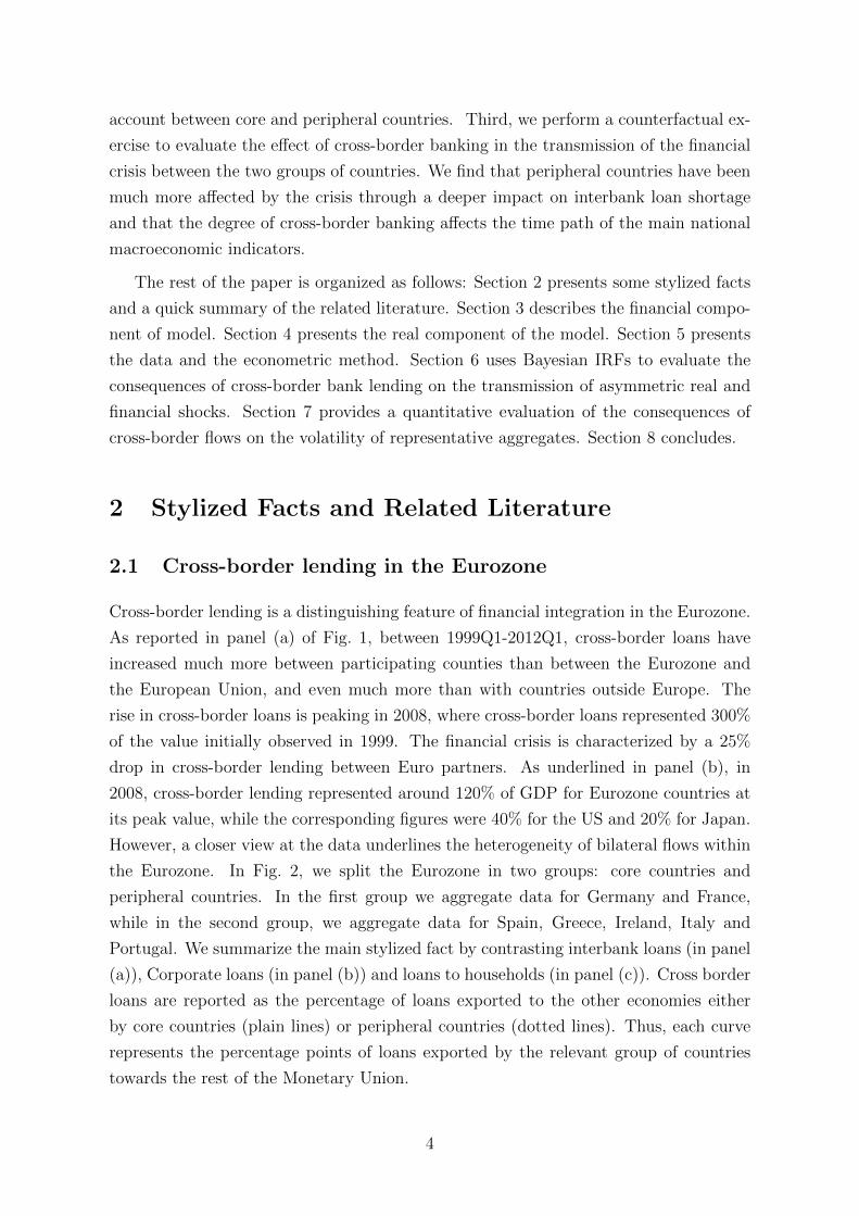
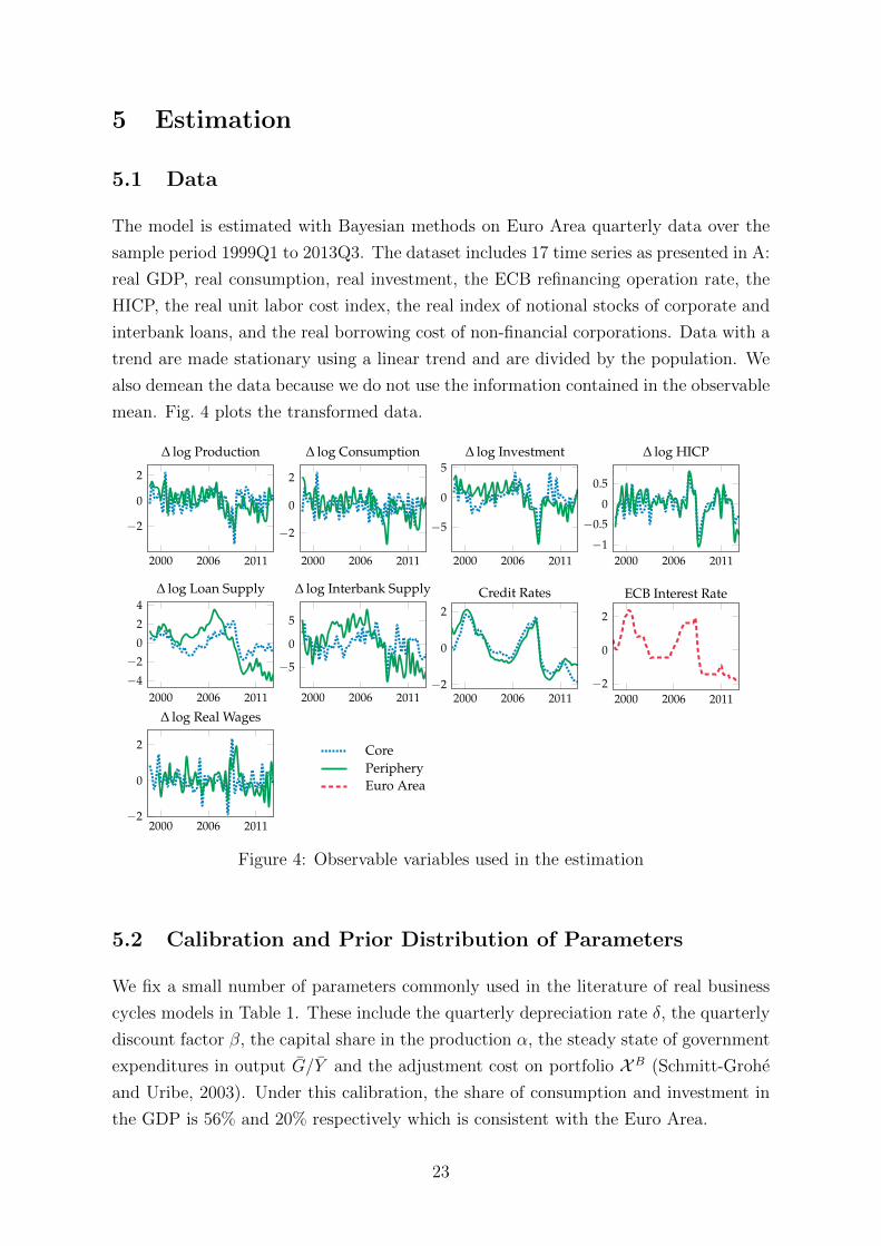
The model is estimated with Bayesian methods on Euro Area quarterly data over the

sample period 1999Q1 to 2013Q3. The dataset includes 17 time series as presented in A:

real GDP, real consumption, real investment, the ECB refinancing operation rate, the

HICP, the real unit labor cost index, the real index of notional stocks of corporate and

interbank loans, and the real borrowing cost of non-financial corporations. Data with a

trend are made stationary using a linear trend and are divided by the population. We

also demean the data because we do not use the information contained in the observable

mean. Fig. 4 plots the transformed data.

2000 2006 2011

−2

0

2

∆ log Production

2000 2006 2011

−2

0

2

∆ log Consumption

2000 2006 2011

−5

0

5∆ log Investment

2000 2006 2011−1

−0.5

0

0.5

∆ log HICP

2000 2006 2011−4

−2

0

2

4∆ log Loan Supply

2000 2006 2011

−5

0

5

∆ log Interbank Supply

2000 2006 2011−2

0

2

Credit Rates

2000 2006 2011−2

0

2

ECB Interest Rate

2000 2006 2011−2

0

2

∆ log Real Wages

CorePeripheryEuro Area

Figure 4: Observable variables used in the estimation

5.2 Calibration and Prior Distribution of Parameters

We fix a small number of parameters commonly used in the literature of real business

cycles models in Table 1. These include the quarterly depreciation rate δ, the quarterly

discount factor β, the capital share in the production α, the steady state of government

expenditures in output G/Y and the adjustment cost on portfolio XB (Schmitt-Grohe

and Uribe, 2003). Under this calibration, the share of consumption and investment in

the GDP is 56% and 20% respectively which is consistent with the Euro Area.

23

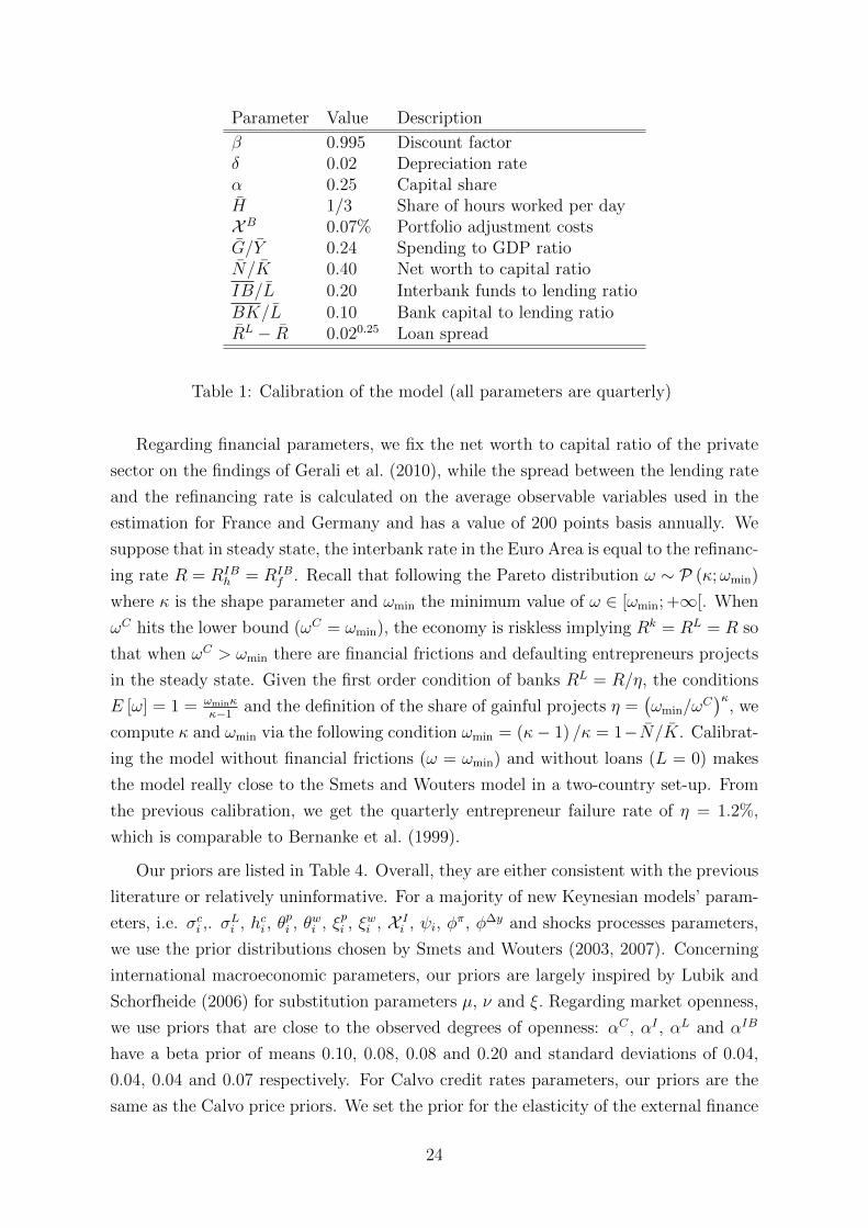
Parameter Value Description

β 0.995 Discount factorδ 0.02 Depreciation rateα 0.25 Capital shareH 1/3 Share of hours worked per dayXB 0.07% Portfolio adjustment costsG/Y 0.24 Spending to GDP ratioN/K 0.40 Net worth to capital ratioIB/L 0.20 Interbank funds to lending ratioBK/L 0.10 Bank capital to lending ratioRL − R 0.020.25 Loan spread

Table 1: Calibration of the model (all parameters are quarterly)

Regarding financial parameters, we fix the net worth to capital ratio of the private

sector on the findings of Gerali et al. (2010), while the spread between the lending rate

and the refinancing rate is calculated on the average observable variables used in the

estimation for France and Germany and has a value of 200 points basis annually. We

suppose that in steady state, the interbank rate in the Euro Area is equal to the refinanc-

ing rate R = RIBh = RIB

f . Recall that following the Pareto distribution ω ∼ P (κ;ωmin)

where κ is the shape parameter and ωmin the minimum value of ω ∈ [ωmin; +∞[. When

ωC hits the lower bound (ωC = ωmin), the economy is riskless implying Rk = RL = R so

that when ωC > ωmin there are financial frictions and defaulting entrepreneurs projects

in the steady state. Given the first order condition of banks RL = R/η, the conditions

E [ω] = 1 = ωminκκ−1

and the definition of the share of gainful projects η =(ωmin/ω

C)κ

, we

compute κ and ωmin via the following condition ωmin = (κ− 1) /κ = 1−N/K. Calibrat-

ing the model without financial frictions (ω = ωmin) and without loans (L = 0) makes

the model really close to the Smets and Wouters model in a two-country set-up. From

the previous calibration, we get the quarterly entrepreneur failure rate of η = 1.2%,

which is comparable to Bernanke et al. (1999).

Our priors are listed in Table 4. Overall, they are either consistent with the previous

literature or relatively uninformative. For a majority of new Keynesian models’ param-

eters, i.e. σci ,. σLi , hci , θ

pi , θ

wi , ξpi , ξ

wi , X I

i , ψi, φπ, φ∆y and shocks processes parameters,

we use the prior distributions chosen by Smets and Wouters (2003, 2007). Concerning

international macroeconomic parameters, our priors are largely inspired by Lubik and

Schorfheide (2006) for substitution parameters µ, ν and ξ. Regarding market openness,

we use priors that are close to the observed degrees of openness: αC , αI , αL and αIB

have a beta prior of means 0.10, 0.08, 0.08 and 0.20 and standard deviations of 0.04,

0.04, 0.04 and 0.07 respectively. For Calvo credit rates parameters, our priors are the

same as the Calvo price priors. We set the prior for the elasticity of the external finance

24

premium κi to a normal distribution with prior mean equal to 0.10 and standard devi-

ation 0.05 consistent with previous financial accelerator estimations (De Graeve, 2008;

Gilchrist et al., 2009a). For loan demand habits for firms and banks, we chose a very

uninformative prior of mean 0.50 and standard deviation 0.20 with a beta distribution.

Finally, the monitoring cost is set to a normal distribution with mean 0.50 and variance

0.20 which is consistent with Curdia and Woodford (2010).

5.3 Posterior Estimates

The methodology is standard to the Bayesian estimation of DSGE models27. Fig. 5

reports the prior and posterior marginal densities of the parameters of the model, ex-

cluding the standard deviation of the shocks and the parameters driving the shocks

processes. In Fig. 5, the data were relatively informative except for a small numbers

of parameters for which the posterior distribution stay very close to the chosen priors.

These parameters are the risk consumption parameter σci , the elasticity of the external

premium for peripheral countries κf , the inflation and GDP growth penalization degrees

in the Taylor rule φπ and φ∆y, the elasticity for loans ξ, ν and the financial openness

αL for the corporate sector28. We investigate the sources of non identification for these

parameters using methods developed by Saltelli et al. (2008), Andrle (2010) and Iskrev

(2010). We find that the low identification of parameters driving the risk aversion co-

efficient σci and the substitutions of loans ν and ξ is due to their small impacts on the

likelihood. As An and Schorfheide (2007), we find that the the Taylor rule smoothing

ρ is the best identified parameter, and that it strongly interacts with other parameters

in the Taylor rule φπ and φ∆y. Indeed, using the brute force search a la Iskrev (2010),

we note a correlation link that involves φπ, φ∆y with ρ29. We also find a partial con-

27Interest rates data are associated with one-year maturity loans, we take into ac-count this maturity by multiplying by 4 the rates in the measurement equation.The number of shocks is higher (or equal) to observable variables to avoid stochas-tic singularity issue. Recalling that i ∈ {h, f}, the vectors of observables Yobst =[∆ log Yi,t,∆ log Ci,t,∆ log Ii,t, Rt,∆ logHICPi,t,∆Wt,∆L

si,t, R

Li,t,∆IB

s

i,t

]′and measurement equa-

tions Yt =[yi,t − yi,t−1, ci,t − ci,t−1, ıi,t − ıi,t−1, 4× rt, πci,t, wt − wt−1, l

si,t − lsi,t−1, 4× rLi,t, ib

s

i,t − ibs

i,t−1

]′,

where ∆ denotes the temporal difference operator, Xt is per capita variable of Xt. The model matchesthe data setting Yobst = Y + Yt where Y is the vector of the mean parameters, we suppose this is avector of all 0. The posterior distribution combines the likelihood function with prior information. Tocalculate the posterior distribution to evaluate the marginal likelihood of the model, the Metropolis-Hastings algorithm is employed. To do this, a sample of 400, 000 draws was generated, neglecting thefirst 50, 000. The scale factor was set in order to deliver acceptance rates of between 20 and 30 percent.Convergence was assessed by means of the multivariate convergence statistics taken from Brooks andGelman (1998).

28The elasticity of intertemporal substitution, inflation weight and output growth in the monetarypolicy rule are parameters that are frequently not well identified, see for exemple An and Schorfheide(2007) or Kolasa (2008).

29See An and Schorfheide (2007) for further explanations on this correlation link.

25

w/ common financial shocks w/o common financial shocksM1 (θ)autarky

M2 (θ)globalization

M1 (θ)autarky

M2 (θ)globalization

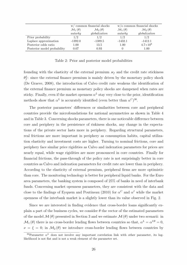
Prior probability 1/2 1/2 1/2 1/2Laplace approximation -1392.0 -1389.5 -1432.1 -1412.1Posterior odds ratio 1.00 13.5 1.00 4.7×108

Posterior model probability 0.07 0.93 0 1.00

Table 2: Prior and posterior model probabilities

founding with the elasticity of the external premium κf and the credit rate stickiness

θLf : since the external finance premium is mainly driven by the monetary policy shock

(De Graeve, 2008), the introduction of Calvo credit rate weakens the identification of

the external finance premium as monetary policy shocks are dampened when rates are

sticky. Finally, even if the market openness αL stay very close to the prior, identification

methods show that αL is accurately identified (even better than αC)30.

The posterior parameters’ differences or similarities between core and peripheral

countries provide the microfoundations for national asymmetries as shown in Table 4

and in Table 3. Concerning shocks parameters, there is one noticeable difference between

core and periphery in the persistence of riskiness shocks, any change in the expecta-

tions of the private sector lasts more in periphery. Regarding structural parameters,

real frictions are more important in periphery as consumption habits, capital utiliza-

tion elasticity and investment costs are higher. Turning to nominal frictions, core and

periphery face similar price rigidities as Calvo and indexation parameters for prices are

nearly equal, while wage rigidities are more pronounced in core countries. Finally for

financial frictions, the pass-through of the policy rate is not surprisingly better in core

countries as Calvo and indexation parameters for credit rate are lower than in periphery.

According to the elasticity of external premium, peripheral firms are more optimistic

than core. The monitoring technology is better for peripheral liquid banks. For the Euro

area parameters, the banking system is composed of 25% of banks in need of interbank

funds. Concerning market openness parameters, they are consistent with the data and

close to the findings of Eyquem and Poutineau (2010) for αC and αI while the market

openness of the interbank market is a slightly lower than its value observed in Fig. 2.

Since we are interested in finding evidence that cross-border loans significantly ex-

plain a part of the business cycles, we consider θ the vector of the estimated parameters

of the modelM (θ) presented in Section 3 and we estimateM (θ) under two scenarii: in

M1 (θ) there is no cross-border lending flows between countries so that, αL = αIB = 0,

ν = ξ = 0; in M2 (θ) we introduce cross-border lending flows between countries by

30Parameter αL does not involve any important correlation link with other parameter, its log-likelihood is not flat and is not a weak element of the parameter set.

26

estimating αL, αIB ∈ [0; 1], ν, ξ ≥ 0. At last, we are interested in finding evidence that

cross-border loans significantly explain a part of the business cycles of the Eurozone.

Put differently, we examine the hypothesis H0: αL = αIB = 0, ν = ξ = 0 against the

hypothesis H1: αL, αIB ∈ [0; 1), ν, ξ > 0, to do this we evaluate the posterior odds

ratio of M2 (θ) on M1 (θ) using Laplace-approximated marginal data densities. The

posterior odds of the null hypothesis of no significance of banking flows is 13.5:1 which

leads us to strongly reject the null, i.e. cross-border lending flows do matter in ex-

plaining the business cycles of the Euro Area. This result is confirmed in terms of log

marginal likelihood. When the models are estimated without common financial shocks,

then cross-border flows have an even more important role in explaining the business

cycles as the posterior odds ratio becomes 4.7×108:1.

6 The Consequences of Cross-border Loans

Once the model has been estimated, we evaluate the consequences of cross-border lend-

ing on the national and international transmission of asymmetric shocks. We report the

Bayesian IRFs obtained from linearized models M1 and M2. We concentrate on three

main shocks that affect the core countries: an asymmetric productivity shock affecting

firms, an asymmetric financial shock that reduces the net worth of entrepreneurs and a

positive shock affecting the liquidity situation of the banking system.

6.1 A Positive Shock on Total Factor Productivity

Fig. 6 reports the simulated responses of the main macroeconomic and financial variables

following a positive shock to εAh,t equal in size to the standard deviation of total factor

productivity estimated in Table 4.

In the benchmark situation (dotted line), loan markets are segmented. As standardly

documented in the literature, this productivity shock increases production, consumption

and investment while decreasing the inflation rate in the core countries (Smets and

Wouters, 2003). This shock is transmitted to peripheral economies through the terms

of trade, the current account and the reaction of the central bank interest rate. The

deterioration of the core countries’ terms of trade increases the relative competitiveness

and the exports of core countries goods towards peripheral economies. The decrease of

the relative price of core countries goods depresses peripheral activity and investment.

The average union wide rate of consumption price inflation decreases, which leads the

central bank to reduce the interbank interest rate (Eyquem and Poutineau, 2010). As

observed, corporate loans increase in both countries. In core countries, entrepreneurs

27

contract more loans to finance new investment flows after the positive supply shock.

Central bank reaction affects the banking system through the decrease of the interest

rate. This, in turn, lowers the interest rate on loans and increases corporate loan

demand. As observed, interbank lending also rises to allow illiquid banks to meet the

increased corporate loan demand. This increase in corporate loan demand dampens the

decrease in investment as all the new loans remain in the periphery. However the rise in

firm leverage increases the failure rate of investment projects in both countries and by

so, the interest rate served by banks increases after 5 quarters. Thus, the segmentation

of the loan market has a clear dampening effect in the periphery with regards to the

transmission of core countries’ productivity shocks.

The possibility of banks to engage in cross-border lending (plain lines) acts as a

mechanism that mainly increases the dispersion of investment cycles in the monetary

union. As cross-border lending improves the international allocation of financial re-

sources in the monetary union, it amplifies the positive impact on investment in core

countries and the negative impact in the peripheral economies, while leaving unaffected

the dynamics of consumption and activity in both part of the monetary union. As a

consequence, the current account adjustment (that reflects net savings) is significantly

affected by the assumption regarding the degree of cross-border banking. Part of the in-

crease in domestic investment is fuelled by foreign loans: the increase in foreign lending

increases (partly financed by an increase in interbank lending in the peripheral coun-

tries). This implies a net increase in foreign loan supply after 5 quarters with regard

to the segmented situation. By lending to more productive domestic firms, the foreign

banking system has access to more reliable borrowers. Cross-border lending clearly im-

pacts negatively the foreign macroeconomic performance, as more lending resources are

diverted towards the domestic economy. This is clearly shown by the increased slump in

peripheral countries’ investment. With cross-border relations, the increase in interbank

lending is reflected by a decrease in core countries’ loan supply. Part of the liquidity of

domestic banks comes from peripheral banks, through cross-border interbank lending.

Cross-border lending significantly affects the dynamics of the current account. Ig-

noring cross-border banking, the adjustment of the current account is standard, as the

domestic economy experiences a surplus of net exports, that depicts the intertemporal

allocation of the increase in national resources over a sample time period of thirty quar-

ters. Cross-border loans clearly deteriorate core countries’ current account with respect

to the benchmark situation (dotted lines). As activity and consumption remain unaf-

fected by the integration of the loan market, and as the increase of investment is higher

in the core countries (while the decrease in investment is higher in peripheral coun-

tries), the current account of core countries deteriorates with respect to the segmented

situation, to reflect the increased dispersion of investment cycles. Finally, the IRFs of

28

the terms of trade and of the central bank interest rate are unaffected by cross-border

lending.

6.2 A Negative Shock on Firms Net Worth

The second set of IRFs, reported in Fig. 7, describes the consequences of a negative

shock on core countries’ firm net worth εNh,t. This negative shock can be thought of as

an overnight decrease in the value of investor capital (following, for example a stock

exchange collapse).

Without cross-border loans (dotted lines), a reduction in firms’ net worth depresses

investment and production and is deflationary in core countries. The reduction of

activity is driven by the decrease in investment decisions. The central bank reacts to

deflation by decreasing the interbank interest rate. This, in turn, increases consumption

and dampens the negative impact on core countries’ investment after 4 periods. As

investment decreases more than activity, consumption increases and, as core countries’

inflation rate decreases more than peripheral inflation rate, the domestic terms of trade

deteriorates. As a consequence, more domestic goods are exported and consumed by

peripheral households. The production of foreign goods decreases which, in turn, implies

a decrease in investment decisions. In the meanwhile, following the decrease in the

ECB central bank interest rate, peripheral consumption increases (this increase falls

on imported goods). Initially, the negative wealth shock increases the probability of

insolvent projects, and leads to higher interest rates on loans, despite the reduction of the

central bank interest rate. This, in turn depresses investment. As observed, since banks

engage in less corporate loans, their liquidity situation improves and interbank lending

decreases. The improvement in core countries’ current account reflects the increase in

net savings coming from the decrease of investment in this part of the monetary union.

Finally, interbank loans remain almost unaffected in peripheral countries.

Cross-border bank activity (plain lines) acts as a mechanism that amplifies the neg-

ative financial shock in core countries while it improves the situation of the periphery.

The positive impact observed on peripheral investment comes from the fact that part of

core countries’s loans are diverted towards the periphery. This net inflow of loans in the

periphery fuels firm investment. The second phenomenon is the drop in interbank loans:

now part of corporate loans is directly distributed by core countries’ banks to peripheral

entrepreneurs. This phenomenon is reinforced by the fact that the borrowing cost of

corporate loans is cheaper in the periphery with cross border loans, with respect to the

segmented situation. Thus, as banks engage in cross-border loans towards peripheral

firms, they lend less to core countries’ firms, which furthermore depresses investment

and activity in this part of the monetary union.

29

Taken globally, the macroeconomic performance of the currency union worsens with

cross-border bank lending, as activity slightly decreases with respect to the segmented

situation. The combination of a higher deterioration of the core countries terms of trade

and decrease in domestic investment improves the current account of core countries.

Thus cross-border lending clearly amplifies the diffusion of a negative net worth shock

in the monetary union. It also increases the heterogeneity of investment cycles and

the dispersion of current account positions. Negative consequences of net worth shocks

have already been studied in the literature with financial globalization (Ueda, 2012) and

without (Hirakata et al., 2011). Our results are in line with this literature.

6.3 A Positive Shock on Bank Resources

The third set of IRFs, reported in Fig. 8, describes the consequences of a positive shock

on bank resources εliabh,t . This positive shock represents an increase in the resources of the

core countries’ banking system. It improves the liquidity situation of the core countries’

banking system which in turn implies the creation of more corporate loans and reduces

the need for interbank loans.

Without cross-border loans (dotted lines), this shock induces an increase in core

countries’ investment, which in turn leads to more activity. However, as it generates

a positive demand shock (the increase in investment is higher than that of activity),

it leads to more inflation and to an initial improvement in the terms of trade of core

countries. This last phenomenon deteriorates the price competitiveness of core countries’

goods while increasing that of peripheral goods. As a consequence, activity increases

in the peripheral economies. In the meanwhile as this shock implies an increase in the

average inflation rate of the monetary union, the central bank reacts by increasing its

interest rate, which in turn depresses consumption and leads to a decrease in activity

and inflation after 5 periods in core countries. Lending decisions in the periphery can be

explained as follows: the increase in the interest rate of the central bank affects positively

the interest rate on loans which in turn depresses loan demand in the periphery. As a

consequence, the increase in peripheral investment is financed by peripheral entrepreneur

net wealth.

Cross-border bank activity (plain lines) acts as a mechanism that amplifies the trans-

mission of the core country shock on peripheral countries’ investment. Now, peripheral

entrepreneurs have access to domestic corporate loans which increases peripheral in-

vestment. With cross-border lending, interbank developments should be understood as

follows: the further decrease in interbank loans and higher increase in peripheral coun-

tries interbank lending clearly fuels investment in the periphery. The increase in the

supply of corporate loans is channelled though the increase in interbank lending and

30

the increase in cross-border bank lending (more decrease in the core countries’ inter-

bank loans). Initially more corporate loans are distributed in the periphery. However,

as it leads to an increase in the leverage ratio of firms, it increases the probability of

unproductive projects and, by so, increases the interest rate on loans after 4 periods.

This, in turn, depresses peripheral investment after 4 periods.

Cross border banking impacts the dynamics of the bilateral current account. As the

dynamics of investment in the periphery is reversed between segmented and integrated

situations, it clearly affects the time path of investment and, by so, the time path of the

current account. This reaction of investment more than compensate the impact of the

terms of trade improvement that leads to the current account deficit in the situation

with segmented loan markets.

7 The Driving Forces of Business and Credit Cycles

7.1 The Historical Variance Decomposition

Table 5 reports the posterior variance decomposition of the main aggregates (rate of

growth of activity, consumption, investment and loan supply), the average interest rate

paid by borrowers, the interest rate of the central bank and the current account. To

evaluate the consequences of cross-border interbank and corporate loans, we contrast

the variance decomposition reported for model M2 with corresponding benchmark fig-

ures reported for M1 under loan market segmentation. To see the role played by the

shocks on these evolutions, we decompose each aggregate variations into the proportions

explained by supply shocks (we aggregate ηAi,t and ηWi,t ), demand shocks (we aggregate ηβi,tand ηGi,t), financial shocks (we aggregate ηNi,t, η

Qi,t, η

Bi,t and ηLi,t) and the monetary policy

shock (ηRt ).

As reported, most of the variance of the growth rate of activity, consumption and

inflation is explained by real supply shocks, while the variance of investment, loan supply

and interest rates are mainly affected by national financial shocks. These results are in

line with the ones reported by Hirakata et al. (2011). Remarkably, the contribution of

financial shocks to the fluctuations in the rate of interbank and corporate loan growth

rate are comparable (respectively around 46% and 48%).

Besides these general features, our model reports national heterogeneities regarding

financial and real supply shocks. On average, financial shocks have a higher impact on

core countries’ variables than on peripheral variables. As an example, the contribution

of the financial shocks accounts respectively for 14.6% and 1.7% of the variance of

activity and consumption in core countries, while it accounts for respectively 10.0% and

31

1.2% in the periphery. As a main noticeable exception core investment is less affected

by financial shock than peripheral investment (50.1% instead of 51.4%). For activity

and consumption, real supply shocks have a stronger impact on peripheral aggregates.

As observed, fluctuations in financial indicators related to lending decisions are

deeply affected by financial shocks. Contrasting the relative contribution of national,

cross-border and common financial shocks, we find that with the noticeable exception

of investment (mainly affected by national shocks), variables are mainly affected by

common shocks. In contrast, cross-border shocks have only a marginal contribution to

the fluctuations of the variables of interest. In most cases, cross-border financial shocks

have a higher contribution than cross-border real supply and demand shocks. The main

impact of cross-border shocks is observed for financial shocks on financial variables.

As an example, peripheral financial shocks account for 7.9% of the fluctuation of core

countries’ corporate loan interest rate. As reported, leaving aside activity, core countries

variables are more altered by cross-border shocks than peripheral variables .

We evaluate how the transmission of shocks is affected by cross-border loans by

contrasting these general findings with the lower part of Table 5. As reported, cross-

border banking has a stabilizing effect on financial shocks for activity and consumption

(this affects all dimensions of the financial shocks) but increases the contribution of the

financial shocks on the fluctuations of the growth rate of investment. Evidence is mixed

for other national variables. However has reported, core countries get a higher profit

from the integration of the loan market in the Eurozone, as we observe more reduction

in the contribution of national financial shocks on national indicators (for 12 variables

instead of 9 for peripheral countries). Thus, cross-border lending has a per-se impact on

the diffusion of financial shocks as it significantly reduces the contribution of national

financial shocks on the fluctuations of national variables.

Finally, contrasting the two models, we find that cross-border lending reduces the

contribution of financial shocks to the fluctuations in the central bank interest rate (it

explains 71.4% of the interest rate fluctuations instead of 77.6% if the loan market is

segmented).

7.2 Understanding the Time Path of the Current Account

The last rows devoted to the modelsM2 andM1in Table 5 present the variance decom-

position of current account fluctuations. As reported, it is clearly affected by the inte-

gration of the loan market: under loan market segmentation, financial shocks contribute

to 57.6% of current account fluctuations, while they account for 91.8% with cross-border

banking. Remarkably, the contribution of both national and common shocks increase.

32

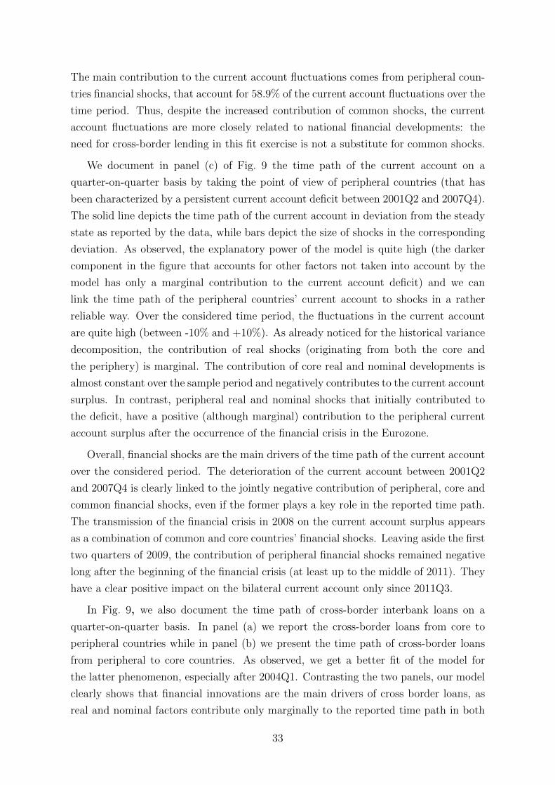
The main contribution to the current account fluctuations comes from peripheral coun-

tries financial shocks, that account for 58.9% of the current account fluctuations over the

time period. Thus, despite the increased contribution of common shocks, the current

account fluctuations are more closely related to national financial developments: the

need for cross-border lending in this fit exercise is not a substitute for common shocks.

We document in panel (c) of Fig. 9 the time path of the current account on a

quarter-on-quarter basis by taking the point of view of peripheral countries (that has

been characterized by a persistent current account deficit between 2001Q2 and 2007Q4).

The solid line depicts the time path of the current account in deviation from the steady

state as reported by the data, while bars depict the size of shocks in the corresponding

deviation. As observed, the explanatory power of the model is quite high (the darker

component in the figure that accounts for other factors not taken into account by the

model has only a marginal contribution to the current account deficit) and we can

link the time path of the peripheral countries’ current account to shocks in a rather

reliable way. Over the considered time period, the fluctuations in the current account

are quite high (between -10% and +10%). As already noticed for the historical variance

decomposition, the contribution of real shocks (originating from both the core and

the periphery) is marginal. The contribution of core real and nominal developments is

almost constant over the sample period and negatively contributes to the current account

surplus. In contrast, peripheral real and nominal shocks that initially contributed to

the deficit, have a positive (although marginal) contribution to the peripheral current

account surplus after the occurrence of the financial crisis in the Eurozone.

Overall, financial shocks are the main drivers of the time path of the current account

over the considered period. The deterioration of the current account between 2001Q2

and 2007Q4 is clearly linked to the jointly negative contribution of peripheral, core and

common financial shocks, even if the former plays a key role in the reported time path.

The transmission of the financial crisis in 2008 on the current account surplus appears

as a combination of common and core countries’ financial shocks. Leaving aside the first

two quarters of 2009, the contribution of peripheral financial shocks remained negative

long after the beginning of the financial crisis (at least up to the middle of 2011). They

have a clear positive impact on the bilateral current account only since 2011Q3.

In Fig. 9, we also document the time path of cross-border interbank loans on a

quarter-on-quarter basis. In panel (a) we report the cross-border loans from core to

peripheral countries while in panel (b) we present the time path of cross-border loans

from peripheral to core countries. As observed, we get a better fit of the model for

the latter phenomenon, especially after 2004Q1. Contrasting the two panels, our model

clearly shows that financial innovations are the main drivers of cross border loans, as

real and nominal factors contribute only marginally to the reported time path in both

33

cases. Common financial factor affecting both regions of the Eurozone have had a

positive impact on cross-border lending in both cross-border directions all over the time

period. In particular they are the main driver of cross-border loans from peripheral

countries. The financial situation of core countries leads to more cross-border loans

towards the periphery (they affect positively the reported time path) while it affects

negatively cross-border loans from the periphery. In contrast, financial shocks in the

periphery contribute positively to cross-border lending from the core and negatively

to the core. Putting pieces altogether clearly shows that peripheral countries have

benefited form cross border lending over the sample time period: they received more

loans than they exported, and this phenomenon has mainly been fuelled by peripheral

financial shocks, as already been noted above for the time path of the bilateral current

account.

7.3 Counterfactual Analysis

We report in Fig. 10 the propagation of the financial crisis of 2009 on the model. We

represent it as the sum of all the shocks that affected each economy in 2009Q1. In this

figure, plain lines represent the adjustment of the corresponding variable estimated by

the model, dotted lines report the IRFs computed with perfect banking integration and

dashed lines report the IRFs computed without cross-border lending between the two

regions of the Eurozone. We get two main findings from this counterfactual exercise:

(i) peripheral countries have been much more affected by the crisis than core countries

and (ii) the degree of cross-border banking affects the time path of the main national

macroeconomic indicators (consumption being the main exception).

First, we find a deeper impact of the financial crisis on interbank loans (reported

figures for the IRFs are almost twice the value of corporate loans for each part of

the Eurozone). There is a sharp reduction in both corporate and interbank loans in

the periphery while, in the core country group, the reduction of interbank loans ’only’

diminishes by up to -10% (instead of -40% for the periphery) and the reduction in

corporate loans reaches ’only’ -3% (instead of -20% for the periphery). The persistency of

the shock is also much higher on peripheral loans. Cross border banking has deteriorated

the evolution of interbank lending in core countries while it has mildly improved the

situation of interbank lending in the periphery. In contrast, the degree of cross-border

banking estimated by the model between the two group of countries did not have a

significant effect on the time path of corporate loans or on the cost of borrowing faced

by firms.

Second, the size of the fluctuations in macroeconomic aggregates are in line with the

behavior of financial variables, as the fluctuations in activity and investment are much

34

more pronounced in the periphery than in the core countries. However, in both parts

of the world, the time path of activity mimics that of investment. In the periphery, the

financial crisis has clearly led to a sharper and more persistent decrease in investment

(reaching a maximum decrease of -12% after 8 quarters instead of -2% after 5 quarters

and going back to equilibrium after 11 periods for the core country group) and activity

(reaching a maximum decrease of -1.5% after 8 quarters instead of -0.4% after 5 quar-

ters and going back to equilibrium after 11 periods for the core country group). The

contribution of cross border banking to the observed dynamics of output and invest-

ment underlines that cross-border lending has reduced the negative consequences of the

financial crisis for core countries, with respect to a segmentation of the loan market,

while it has mildly deteriorated the situation of the periphery.

As a final counterfactual exercise, we find that a perfect banking integration of the

Eurozone (in dotted lines) would have amplified the fluctuations of all core countries’

variables, while dampening that of peripheral countries. This complete integration

would have led to a transfer of volatility between the two components of the Eurozone,

contributing to a better mutualization of the negative consequences of the financial crisis

over the region.

8 Conclusion

In this paper, we have developed and estimated a two-country DSGE model with bank-

ing activity that accounts for interbank and corporate cross-border loan flows. Using

Bayesian econometrics, we have found evidence of the key role of this cross-border chan-

nel as an amplifying mechanism in the diffusion of asymmetric shocks. In particular,

our model reveals that under banking globalization, most national variables are less sen-

sitive to national financial shocks while investment and current account imbalances are

more affected. In a counterfactual analysis, we have analyzed how cross border lending

has affected the transmission of the recent financial crisis between the two groups of

countries.

Our model contributes to the New Open Economy Macroeconomics literature by

finding two new channels of propagation of macroeconomic shocks between countries.

Taken altogether, our results underline the critical contribution of corporate and in-

terbank cross-border loans in the Eurozone to account for both the transmission of

asymmetric shocks and the effect of monetary policy decisions. In particular, they sug-

gest the importance of cross border loans to assess the impact of the financial accelerator

in models of the Eurozone.

Looking forward, our analysis outlines several areas for future research. In particular,

35

our model could be used as a framework to assess alternative way of supervising lending

decisions (based on the home or host principle) and thus contribute to the current

discussion of the best way of implementing macroprudential measures in the European

Monetary Union.

References

An, S., Schorfheide, F., 2007. Bayesian analysis of dsge models. Econometric reviews 26 (2-4), 113–172.

Andrle, M., 2010. A note on identification patterns in dsge models. Tech. rep., European Central Bank

Frankfurt.

Angeloni, I., Faia, E., 2013. Capital regulation and monetary policy with fragile banks. Journal of

Monetary Economics 60 (3), 311–324.

Bachmann, R., Elstner, S., 2013. Firms optimism and pessimism.

Benigno, P., Woodford, M., 2005. Inflation stabilization and welfare: The case of a distorted steady

state. Journal of the European Economic Association 3 (6), 1185–1236.

Bernanke, B., Gertler, M., Gilchrist, S., 1999. The financial accelerator in a quantitative business cycle

framework. Handarticle of macroeconomics 1, 1341–1393.

Brooks, S. P., Gelman, A., 1998. General methods for monitoring convergence of iterative simulations.

Journal of computational and graphical statistics 7 (4), 434–455.

Casares, M., Poutineau, J., 2011. Short-run and long-run effects of banking in a new keynesian model.

The BE Journal of Macroeconomics 11 (1).

Christiano, L., Motto, R., Rostagno, M., 2010. Financial factors in economic fluctuations.

Christiano, L. J., Eichenbaum, M., Evans, C. L., 2005. Nominal rigidities and the dynamic effects of a

shock to monetary policy. Journal of political Economy 113 (1), 1–45.

Curdia, V., Woodford, M., 2010. Credit spreads and monetary policy. Journal of Money, Credit and

Banking 42, 3–35.

De Graeve, F., 2008. The external finance premium and the macroeconomy: Us post-wwii evidence.

Journal of Economic Dynamics and Control 32 (11), 3415–3440.

De Grauwe, P., 2010. The scientific foundation of dynamic stochastic general equilibrium (dsge) models.

Public choice 144 (3-4), 413–443.

Dedola, L., Karadi, P., Lombardo, G., 2013. Global implications of national unconventional policies.

Journal of Monetary Economics 60 (1), 66–85.

Dedola, L., Lombardo, G., 2012. Financial frictions, financial integration and the international propa-

gation of shocks. Economic Policy 27 (70), 319–359.

Dib, A., 2010. Banks, credit market frictions, and business cycles. Tech. rep., Bank of Canada Working

Paper.

36

Eyquem, A., Poutineau, J.-C., 2010. Markets integration and macroeconomic dispersion in a monetary

union. Louvain Economic Review 76 (1), 5–30.

Faia, E., 2007. Finance and international business cycles. Journal of Monetary Economics 54 (4),

1018–1034.

Faia, E., Iliopulos, E., 2011. Financial openness, financial frictions and optimal monetary policy. Journal

of Economic Dynamics and Control 35 (11), 1976–1996.

Gerali, A., Neri, S., Sessa, L., Signoretti, F. M., 2010. Credit and banking in a dsge model of the euro

area. Journal of Money, Credit and Banking 42 (s1), 107–141.

Gertler, M., Karadi, P., 2012. A framework for analyzing large scale asset purchases as a monetary

policy tool*.

Gilchrist, S., Ortiz, A., Zakrajsek, E., 2009a. Credit risk and the macroeconomy: Evidence from an

estimated dsge model. Unpublished manuscript.

Gilchrist, S., Sim, J., Zakrajsek, E., 2009b. Uncertainty, credit spreads, and investment dynamics.

Goodfriend, M., McCallum, B., 2007. Banking and interest rates in monetary policy analysis: A

quantitative exploration. Journal of Monetary Economics 54 (5), 1480–1507.

Goodhart, C. A., Sunirand, P., Tsomocos, D. P., 2005. A risk assessment model for banks. Annals of

Finance 1 (2), 197–224.

Gray, S., Chailloux, A., McCaughrin, R., 2008. Central bank collateral frameworks: Principles and

policies. IMF Working Papers, 1–67.

Guerrieri, L., Iacoviello, M., Minetti, R., 2012. Banks, sovereign debt and the international transmission

of business cycles.

Hirakata, N., Sudo, N., Ueda, K., 2009. Chained credit contracts and financial accelerators.

Hirakata, N., Sudo, N., Ueda, K., 2011. Do banking shocks matter for the us economy? Journal of

Economic Dynamics and Control 35 (12), 2042–2063.

Iskrev, N., 2010. Local identification in dsge models. Journal of Monetary Economics 57 (2), 189–202.

Kalemli-Ozcan, S., Papaioannou, E., Perri, F., 2013. Global banks and crisis transmission. Journal of

International Economics 89 (2), 495–510.

Kolasa, M., 2008. Structural heterogeneity or asymmetric shocks? poland and the euro area through

the lens of a two-country dsge model.

Kollmann, R., Enders, Z., Muller, G. J., 2011. Global banking and international business cycles. Eu-

ropean Economic Review 55 (3), 407–426.

Lubik, T., Schorfheide, F., 2006. A bayesian look at the new open economy macroeconomics, 313–382.

Obstfeld, M., Rogoff, K., 2001. The six major puzzles in international macroeconomics: is there a

common cause?, 339–412.

37

Paries, M. D., Sørensen, C. K., Rodriguez-Palenzuela, D., 2011. Macroeconomic propagation under

different regulatory regimes: Evidence from an estimated dsge model for the euro area. International

Journal of Central Banking 7 (4), 49–113.

Saltelli, A., Ratto, M., Andres, T., Campolongo, F., Cariboni, J., Gatelli, D., Saisana, M., Tarantola,

S., 2008. Global sensitivity analysis: the primer. John Wiley & Sons.

Schmitt-Grohe, S., Uribe, M., 2003. Closing small open economy models. Journal of international

Economics 61 (1), 163–185.

Smets, F., Wouters, R., 2003. An estimated dynamic stochastic general equilibrium model of the euro

area. Journal of the European Economic Association 1 (5), 1123–1175.

Smets, F., Wouters, R., 2007. Shocks and frictions in us business cycles: A bayesian dsge approach.

American Economic Review 97 (3).

Ueda, K., 2012. Banking globalization and international business cycles: Cross-border chained credit

contracts and financial accelerators. Journal of International Economics 86 (1), 1–16.

A Data sources

Gross domestic product: expenditure approach, millions of national currency, cur-

rent prices, quarterly levels, seasonally adjusted - sources Eurostat. Private final

consumption expenditure: millions of national currency, current prices, quarterly

levels, seasonally adjusted - sources Eurostat. Gross fixed capital formation: mil-

lions of national currency, current prices, quarterly levels, seasonally adjusted - sources

Eurostat. HICP: Overall Index excluding food and energy, Deseasonalized using a

multiplicative decomposition - sources ECB. Loans to Non-Financial corporations:

Index of Notional Stocks, Total maturity, Euro area (changing composition) counter-

part, Deseasonalized using a multiplicative decomposition, monthly data (aggregated

to get quarterly data) - sources ECB (internal backcasted series). Loans to MFIs: In-

dex of Notional Stocks, Total maturity, Euro area (changing composition) counterpart,

Deseasonalized using a multiplicative decomposition, monthly data (aggregated to get

quarterly data) - sources ECB (internal backcasted series). Borrowing cost: monthly

(taken in average to get quarterly data), Credit and other institutions (MFI except

MMFs and central banks); Loans up to 1 year; BS counterpart sector: Non-Financial

corporations (S.11); Outstanding amount - sources ECB. For 1999Q1-2003Q1, we ap-

proximated the series by using the interest rate on loans other than revolving loans

and overdrafts, New business. Official refinancing operation rates: central bank

interest rates, one year maturity, quarterly data - sources Eurostat. Wages: Labour

cost index, nominal value - quarterly data (NACE Rev. 2), Seasonally adjusted and

38

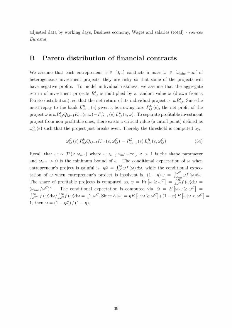
adjusted data by working days, Business economy, Wages and salaries (total) - sources

Eurostat.

B Pareto distribution of financial contracts

We assume that each entrepreneur e ∈ [0, 1] conducts a mass ω ∈ [ωmin,+∞[ of

heterogeneous investment projects, they are risky so that some of the projects will

have negative profits. To model individual riskiness, we assume that the aggregate

return of investment projects Rki,t is multiplied by a random value ω (drawn from a

Pareto distribution), so that the net return of its individual project is, ωRki,t. Since he

must repay to the bank LHi,t+1 (e) given a borrowing rate PLi,t (e), the net profit of the

project ω is ωRki,tQi,t−1Ki,t (e, ω)−PL

i,t−1 (e)LHi,t (e, ω). To separate profitable investment

project from non-profitable ones, there exists a critical value (a cutoff point) defined as

ωCi,t (e) such that the project just breaks even. Thereby the threshold is computed by,

ωCi,t (e)Rki,tQi,t−1Ki,t

(e, ωCi,t

)= PL

i,t−1 (e)LHi,t(e, ωCi,t

)(34)

Recall that ω ∼ P (κ, ωmin) where ω ∈ [ωmin; +∞[, κ > 1 is the shape parameter

and ωmin > 0 is the minimum bound of ω. The conditional expectation of ω when

entrepreneur’s project is gainful is, ηω =∫∞ωCωf (ω) dω, while the conditional expec-

tation of ω when entrepreneur’s project is insolvent is, (1− η)ω =∫ ωCωmin

ωf (ω)dω.

The share of profitable projects is computed as, η = Pr[ω ≥ ωC

]=∫∞ωCf (ω)dω =

(ωmin/ωC)κ . The conditional expectation is computed via, ω = E

[ω|ω ≥ ωC

]=∫∞

ωCωf (ω)dω/

∫∞ωCf (ω)dω = κ

κ−1ωC . Since E [ω] = ηE

[ω|ω ≥ ωC

]+(1− η)E

[ω|ω < ωC

]=

1, then ω = (1− ηω) / (1− η).

39

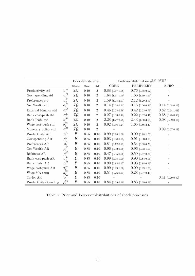
Prior distributions Posterior distribution [5%:95%]Shape Mean Std. CORE PERIPHERY EURO

Productivity std σAi IG 0.10 2 0.88 [0.67:1.08] 0.76 [0.58:0.92] -Gov. spending std σGi IG 0.10 2 1.64 [1.37:1.90] 1.66 [1.39:1.93] -

Preferences std σβi IG 0.10 2 1.59 [1.08:2.07] 2.12 [1.29:2.90] -Net Wealth std σNi IG 0.10 2 0.14 [0.08:0.21] 0.15 [0.06:0.23] 0.14 [0.08:0.19]

External Finance std σQi IG 0.10 2 0.46 [0.03:0.78] 0.42 [0.03:0.79] 0.82 [0.64:1.01]

Bank cost-push std σLi IG 0.10 2 0.27 [0.03:0.48] 0.22 [0.02:0.47] 0.68 [0.45:0.90]

Bank Liab. std σBi IG 0.10 2 2.28 [1.77:2.78] 2.43 [1.80:3.03] 0.08 [0.02:0.16]

Wage cost-push std σWi IG 0.10 2 0.92 [0.56:1.24] 1.65 [0.86:2.47] -Monetary policy std σR IG 0.10 2 - - 0.09 [0.07:0.11]

Productivity AR ρAi B 0.85 0.10 0.99 [0.98:1.00] 0.99 [0.98:1.00] -Gov.spending AR ρGi B 0.85 0.10 0.93 [0.88:0.98] 0.91 [0.83:0.99] -

Preferences AR ρβi B 0.85 0.10 0.81 [0.72:0.91] 0.54 [0.38:0.70] -Net Wealth AR ρNi B 0.85 0.10 0.96 [0.92:0.99] 0.96 [0.93:1.00] -

Riskiness AR ρQi B 0.85 0.10 0.47 [0.35:0.59] 0.59 [0.47:0.71] -Bank cost-push AR σLi B 0.85 0.10 0.99 [0.98:1.00] 0.90 [0.84:0.96] -Bank Liab. AR ρBi B 0.85 0.10 0.90 [0.83:0.97] 0.93 [0.88:0.99] -Wage cost-push AR σWi B 0.85 0.10 0.99 [0.99:1.00] 0.99 [0.99:1.00] -Wage MA term uWi B 0.85 0.10 0.51 [0.26:0.77] 0.28 [0.07:0.49] -Taylor AR ρRi B 0.85 0.10 - - 0.41 [0.29:0.52]

Productivity-Spending ρagi B 0.85 0.10 0.84 [0.69:0.99] 0.83 [0.69:0.99] -

Table 3: Prior and Posterior distributions of shock processes

40

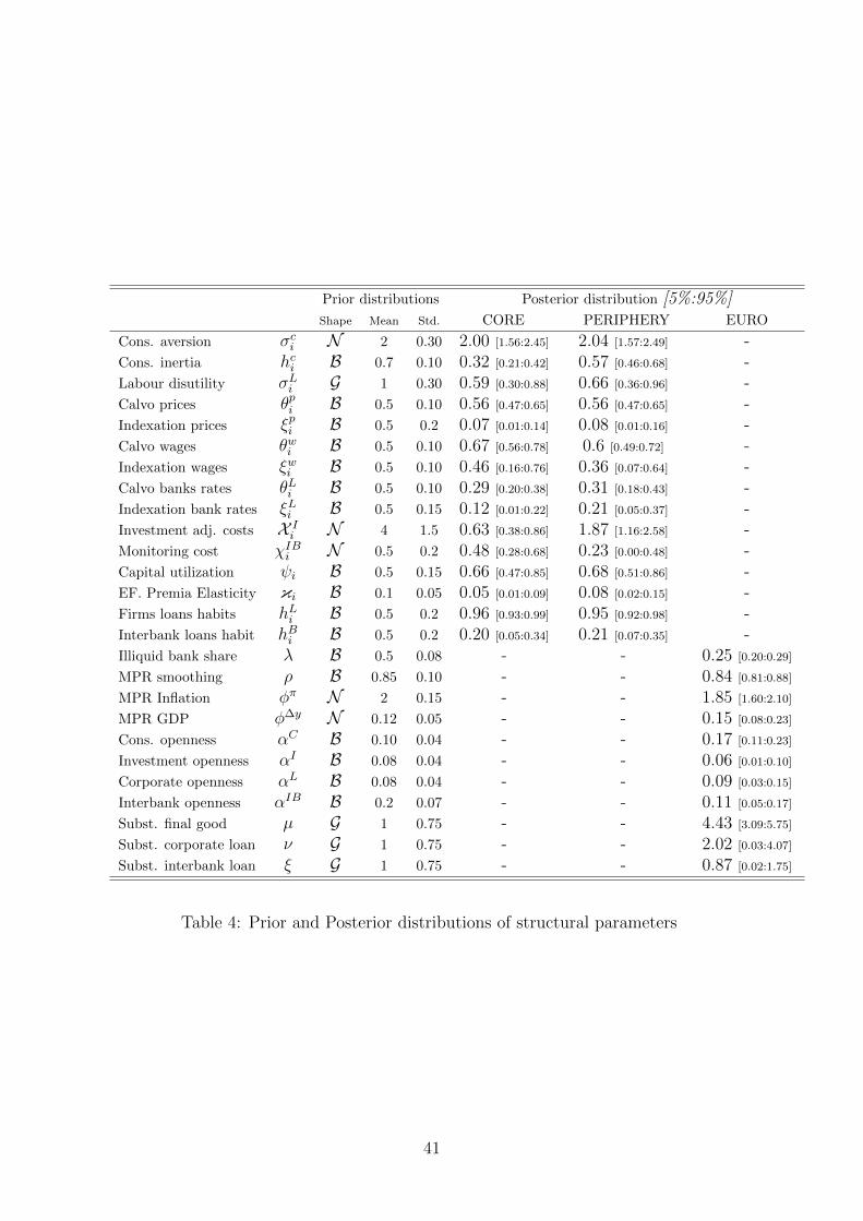
Prior distributions Posterior distribution [5%:95%]Shape Mean Std. CORE PERIPHERY EURO

Cons. aversion σci N 2 0.30 2.00 [1.56:2.45] 2.04 [1.57:2.49] -Cons. inertia hci B 0.7 0.10 0.32 [0.21:0.42] 0.57 [0.46:0.68] -Labour disutility σLi G 1 0.30 0.59 [0.30:0.88] 0.66 [0.36:0.96] -Calvo prices θpi B 0.5 0.10 0.56 [0.47:0.65] 0.56 [0.47:0.65] -Indexation prices ξpi B 0.5 0.2 0.07 [0.01:0.14] 0.08 [0.01:0.16] -Calvo wages θwi B 0.5 0.10 0.67 [0.56:0.78] 0.6 [0.49:0.72] -Indexation wages ξwi B 0.5 0.10 0.46 [0.16:0.76] 0.36 [0.07:0.64] -Calvo banks rates θLi B 0.5 0.10 0.29 [0.20:0.38] 0.31 [0.18:0.43] -Indexation bank rates ξLi B 0.5 0.15 0.12 [0.01:0.22] 0.21 [0.05:0.37] -Investment adj. costs X I

i N 4 1.5 0.63 [0.38:0.86] 1.87 [1.16:2.58] -Monitoring cost χIBi N 0.5 0.2 0.48 [0.28:0.68] 0.23 [0.00:0.48] -Capital utilization ψi B 0.5 0.15 0.66 [0.47:0.85] 0.68 [0.51:0.86] -EF. Premia Elasticity κi B 0.1 0.05 0.05 [0.01:0.09] 0.08 [0.02:0.15] -Firms loans habits hLi B 0.5 0.2 0.96 [0.93:0.99] 0.95 [0.92:0.98] -Interbank loans habit hBi B 0.5 0.2 0.20 [0.05:0.34] 0.21 [0.07:0.35] -Illiquid bank share λ B 0.5 0.08 - - 0.25 [0.20:0.29]

MPR smoothing ρ B 0.85 0.10 - - 0.84 [0.81:0.88]

MPR Inflation φπ N 2 0.15 - - 1.85 [1.60:2.10]

MPR GDP φ∆y N 0.12 0.05 - - 0.15 [0.08:0.23]

Cons. openness αC B 0.10 0.04 - - 0.17 [0.11:0.23]

Investment openness αI B 0.08 0.04 - - 0.06 [0.01:0.10]

Corporate openness αL B 0.08 0.04 - - 0.09 [0.03:0.15]

Interbank openness αIB B 0.2 0.07 - - 0.11 [0.05:0.17]

Subst. final good µ G 1 0.75 - - 4.43 [3.09:5.75]

Subst. corporate loan ν G 1 0.75 - - 2.02 [0.03:4.07]

Subst. interbank loan ξ G 1 0.75 - - 0.87 [0.02:1.75]

Table 4: Prior and Posterior distributions of structural parameters

41

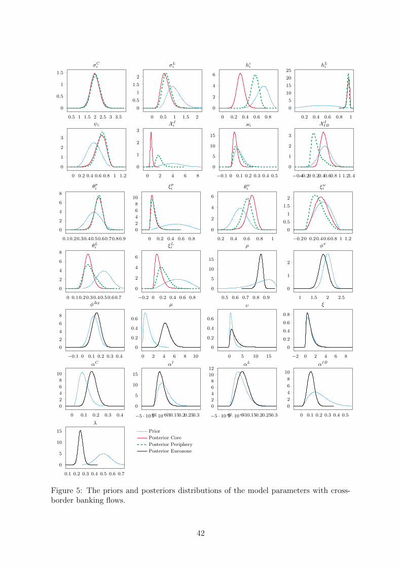
0.5 1 1.5 2 2.5 3 3.5

0

0.5

1

1.5

σCi

0 0.5 1 1.5 2

0

0.5

1

1.5

2

σLi

0 0.2 0.4 0.6 0.8

0

2

4

6

hci

0.2 0.4 0.6 0.8 1

0

5

10

15

20

25hLi

0 0.2 0.4 0.6 0.8 1 1.2

0

1

2

3

ψi

0 2 4 6 8

0

1

2

3

X Ii

−0.1 0 0.1 0.2 0.3 0.4 0.5

0

5

10

15

κi

−0.4−0.20 0.20.40.60.8 1 1.21.4

0

1

2

3

X IIB

0.10.20.30.40.50.60.70.80.9

0

2

4

6

8

θpi

0 0.2 0.4 0.6 0.8

0

2

4

6

8

10

ξpi

0.2 0.4 0.6 0.8 1

0

2

4

6

θwi

−0.20 0.20.40.60.8 1 1.2

0

0.5

1

1.5

2

ξwi

0 0.10.20.30.40.50.60.7

0

2

4

6

8

θLi

−0.2 0 0.2 0.4 0.6 0.8

0

2

4

6

ξLi

0.5 0.6 0.7 0.8 0.9

0

5

10

15

ρ

1 1.5 2 2.5

0

1

2

φπ

−0.1 0 0.1 0.2 0.3 0.4

0

2

4

6

8

φ∆y

0 2 4 6 8 10

0

0.2

0.4

0.6

µ

0 5 10 15

0

0.2

0.4

0.6

υ

−2 0 2 4 6 8

0

0.2

0.4

0.6

0.8

ξ

0 0.1 0.2 0.3 0.4

0

2

4

6

8

10

αC

−5 · 10−205 · 10−20.10.150.20.250.3

0

5

10

15

αI

−5 · 10−205 · 10−20.10.150.20.250.3

0

2

4

6

8

10

12αL

0 0.1 0.2 0.3 0.4 0.5

0

2

4

6

8

10

αIB

0.1 0.2 0.3 0.4 0.5 0.6 0.7

0

5

10

15

λ

Prior

Posterior Core

Posterior Periphery

Posterior Eurozone

Figure 5: The priors and posteriors distributions of the model parameters with cross-border banking flows.

42

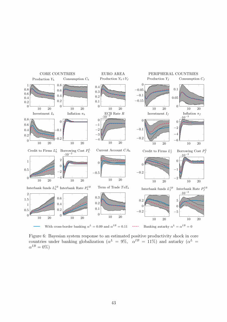
10 200

0.20.40.60.8

1

Production Yh

10 200

0.2

0.4

0.6

0.8

Consumption Ch

10 200

0.1

0.2

0.3

0.4

Production Yh+Yf

10 20

−0.15

−0.1

−0.05

0

Production Yf

10 200

0.05

0.1

Consumption Cf

b

I

10 200

0.2

0.4

0.6

0.8

Investment Ih

10 20

−0.2

−0.1

0

Inflation πh

10 20−4

−3

−2

−1

0·10−2

ECB Rate R

10 20

−0.2

−0.1

0

Investment If

10 20−6

−4

−2

0·10−2

Inflation πf

b

I

10 200

0.5

1

Credit to Firms Lsh

b

I

10 20−4

−2

0

2

·10−2Borrowing Cost PL

h

b

I

10 20

−0.5

0

Current Account CAh

b

I

10 20

−0.2

0

Credit to Firms Lsf

b

I

10 20−2

−1

0

·10−2Borrowing Cost PL

f

b

I

10 200

0.5

1

1.5

2

Interbank funds LIBh

b

I

10 200

0.2

0.4

0.6

Interbank Rate P IBh

b

I

10 200

0.1

0.2

0.3

Term of Trade ToTh

b

I

With cross-border banking αL = 0.09 and αIB = 0.11 Banking autarky αL = αIB = 0

10 20

−0.2

0

0.2

Interbank funds LIBf

b

I

10 20

−5

0

5

·10−2Interbank Rate P IB

f

b

I

CORE COUNTRIES PERIPHERAL COUNTRIESEURO AREA

Figure 6: Bayesian system response to an estimated positive productivity shock in corecountries under banking globalization (αL = 9%, αIB = 11%) and autarky (αL =αIB = 0%)

43

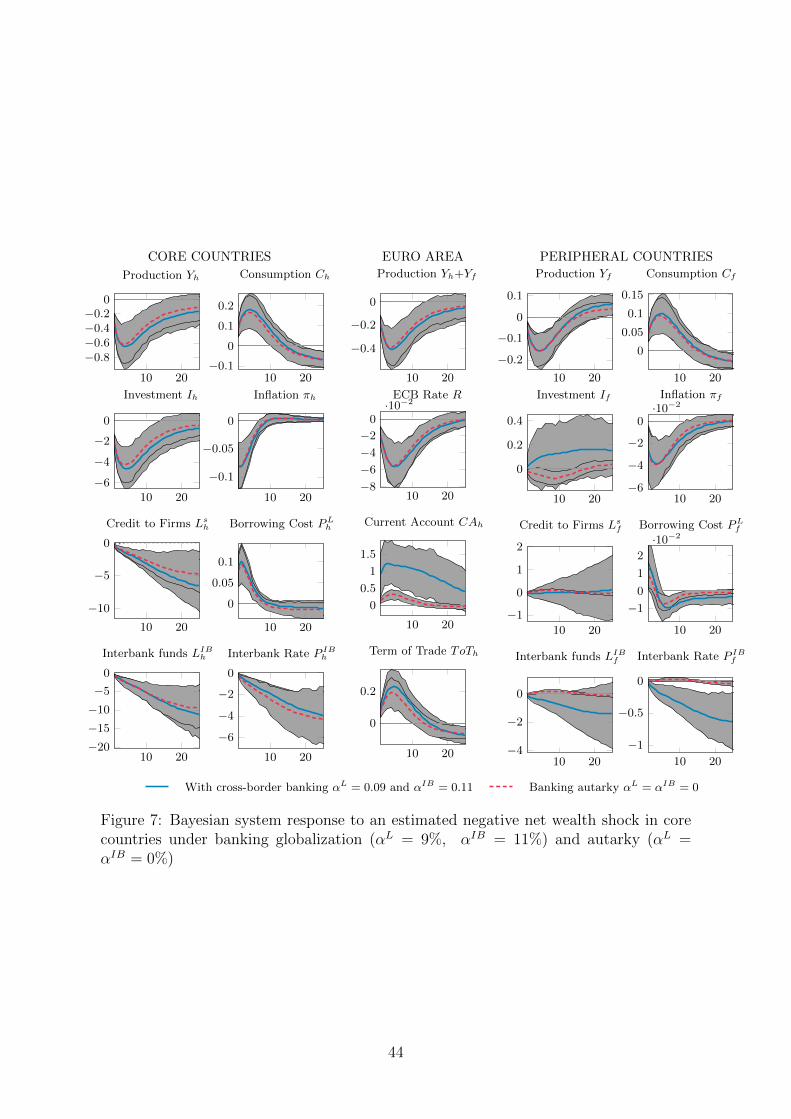
10 20

−0.8−0.6−0.4−0.2

0

Production Yh

10 20−0.1

0

0.1

0.2

Consumption Ch

10 20

−0.4

−0.2

0

Production Yh+Yf

10 20

−0.2

−0.1

0

0.1

Production Yf

10 20

0

0.05

0.1

0.15

Consumption Cf

b

I

10 20−6

−4

−2

0

Investment Ih

10 20

−0.1

−0.05

0

Inflation πh

10 20−8

−6

−4

−2

0·10−2

ECB Rate R

10 20

0

0.2

0.4

Investment If

10 20−6

−4

−2

0·10−2

Inflation πf

b

I

10 20

−10

−5

0

Credit to Firms Lsh

b

I

10 20

0

0.05

0.1

Borrowing Cost PLh

b

I

10 20

0

0.5

1

1.5

Current Account CAh

b

I

10 20

−1

0

1

2

Credit to Firms Lsf

b

I

10 20

−1

0

1

2

·10−2Borrowing Cost PL

f

b

I

10 20−20

−15

−10

−5

0

Interbank funds LIBh

b

I

10 20

−6

−4

−2

0

Interbank Rate P IBh

b

I

10 20

0

0.2

Term of Trade ToTh

b

I

With cross-border banking αL = 0.09 and αIB = 0.11 Banking autarky αL = αIB = 0

10 20−4

−2

0

Interbank funds LIBf

b

I

10 20

−1

−0.5

0

Interbank Rate P IBf

b

I

CORE COUNTRIES PERIPHERAL COUNTRIESEURO AREA

Figure 7: Bayesian system response to an estimated negative net wealth shock in corecountries under banking globalization (αL = 9%, αIB = 11%) and autarky (αL =αIB = 0%)

44

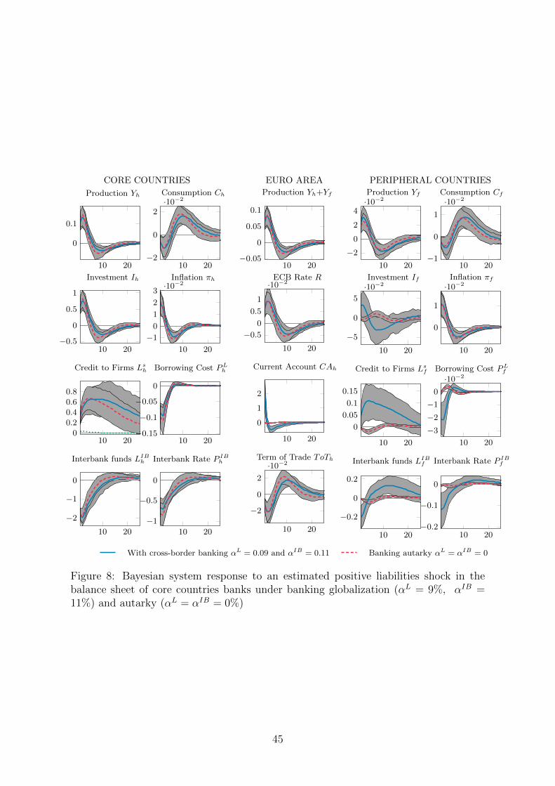
10 20

0

0.1

Production Yh

10 20−2

0

2·10−2Consumption Ch

10 20−0.05

0

0.05

0.1

Production Yh+Yf

10 20

−2

0

2

4·10−2Production Yf

10 20−1

0

1

·10−2Consumption Cf

b

I

10 20−0.5

0

0.5

1

Investment Ih

10 20

−1

0

1

2

3·10−2

Inflation πh

10 20

−0.5

0

0.5

1

·10−2ECB Rate R

10 20

−5

0

5

·10−2Investment If

10 20

0

1

·10−2Inflation πf

b

I

10 200

0.20.40.60.8

Credit to Firms Lsh

b

I

10 20−0.15

−0.1

−0.05

0

Borrowing Cost PLh

b

I

10 20

0

1

2

Current Account CAh

b

I

10 20

0

0.05

0.1

0.15

Credit to Firms Lsf

b

I

10 20

−3

−2

−1

0

·10−2Borrowing Cost PL

f

b

I

10 20

−2

−1

0

Interbank funds LIBh

b

I

10 20

−1

−0.5

0

Interbank Rate P IBh

b

I

10 20

−2

0

2

·10−2Term of Trade ToTh

b

I

With cross-border banking αL = 0.09 and αIB = 0.11 Banking autarky αL = αIB = 0

10 20

−0.2

0

0.2

Interbank funds LIBf

b

I

10 20−0.2

−0.1

0

Interbank Rate P IBf

b

I

CORE COUNTRIES PERIPHERAL COUNTRIESEURO AREA

Figure 8: Bayesian system response to an estimated positive liabilities shock in thebalance sheet of core countries banks under banking globalization (αL = 9%, αIB =11%) and autarky (αL = αIB = 0%)

45

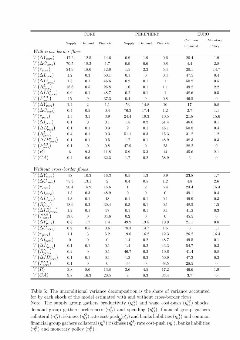
CORE PERIPHERY EURO

Supply Demand Financial Supply Demand FinancialCommon

Financial

Monetary

Policy

With cross-border flowsV (∆Ycore) 47.2 12.5 14.6 0.9 1.9 0.6 20.4 1.9

V (∆Ccore) 70.5 18.2 1.7 0.9 0.6 0.8 4.4 2.8

V (πcore) 24.9 18.6 12.6 1.5 2.2 5.4 20.1 14.7

V (∆Icore) 1.2 0.3 50.1 0.1 0 0.4 47.5 0.4

V (∆Lscore) 1.3 0.1 46.6 0.2 0.1 1 50.2 0.5

V(RLcore

)18.6 0.5 26.8 1.6 0.1 1.1 49.2 2.2

V (∆IBscore) 0.9 0.1 48.7 0.2 0.1 1 48.6 0.5

V(P IBcore

)15 0 37.3 0.4 0 0.8 46.5 0

V (∆Yperi) 1.2 2 1.1 53 14.8 10 17 0.8

V (∆Cperi) 0.4 0.5 0.4 76.3 17.4 1.2 2.7 1.1

V (πperi) 1.5 3.1 3.9 24.4 19.3 10.5 21.8 15.6

V (∆Iperi) 0.1 0 0.1 1.5 0.2 51.4 46.6 0.1

V(∆Lsperi

)0.1 0.1 0.3 2 0.1 46.1 50.8 0.4

V(RLperi

)0.4 0.1 0.3 51.1 0.3 15.3 31.2 1.2

V(∆IBs

peri

)0.1 0.1 0.5 1.7 0.1 48.9 48.3 0.3

V(P IBperi

)0.1 0 0.8 47.9 0 23 28.2 0

V (R) 6 9.3 11.8 5.9 5.3 14 45.6 2.1

V (CA) 0.4 0.6 32.3 1.7 0.2 58.9 6 0

Without cross-border flowsV (∆Ycore) 45 10.3 16.3 0.5 1.3 0.9 23.8 1.7

V (∆Ccore) 75.3 13.1 2 0.4 0.5 1.2 4.8 2.6

V (πcore) 20.4 15.9 15.6 1 2 6.4 23.4 15.3

V (∆Icore) 1.3 0.3 48.9 0 0 0 49.1 0.4

V (∆Lscore) 1.3 0.1 48 0.1 0.1 0.1 49.9 0.3

V(RLcore

)18.9 0.2 30.4 0.3 0.1 0.1 48.5 1.5

V (∆IBscore) 1.2 0.1 57 0.1 0.1 0.1 41.2 0.3

V(P IBcore

)19.6 0 34.6 0.2 0 0 45.5 0

V (∆Yperi) 0.8 1.7 1.4 49.9 13.5 10.9 21.1 0.8

V (∆Cperi) 0.2 0.5 0.6 78.3 14.7 1.5 3 1.1

V (πperi) 1.1 3 5.2 19.6 16.2 12.3 26.2 16.4

V (∆Iperi) 0 0 0 1.4 0.2 48.7 49.5 0.1

V(∆Lsperi

)0.1 0.1 0.1 1.4 0.2 43.3 54.7 0.3

V(RLperi

)0.2 0 0.1 46.7 0.2 10.6 41.4 0.8

V(∆IBs

peri

)0.1 0.1 0.1 1.3 0.2 50.9 47.3 0.2

V(P IBperi

)0.1 0 0 33 0 38.5 28.5 0

V (R) 3.8 8.6 13.8 3.6 4.5 17.2 46.6 1.9

V (CA) 9.8 16.3 20.5 8 8.3 33.4 3.7 0

Table 5: The unconditional variance decomposition is the share of variance accountedfor by each shock of the model estimated with and without cross-border flows.Note: The supply group gathers productivity (ηAi,t) and wage cost-push (ηWi,t ) shocks,

demand group gathers preferences (ηβi,t) and spending (ηGi,t), financial group gathers

collateral (ηNi,t) riskiness (ηQi,t) rate cost-push (ηLi,t) and banks liabilities (ηBi,t) and common

financial group gathers collateral (ηNt ) riskiness (ηQt ) rate cost-push (ηLt ), banks liabilities(ηBt ) and monetary policy (ηRt ).

46

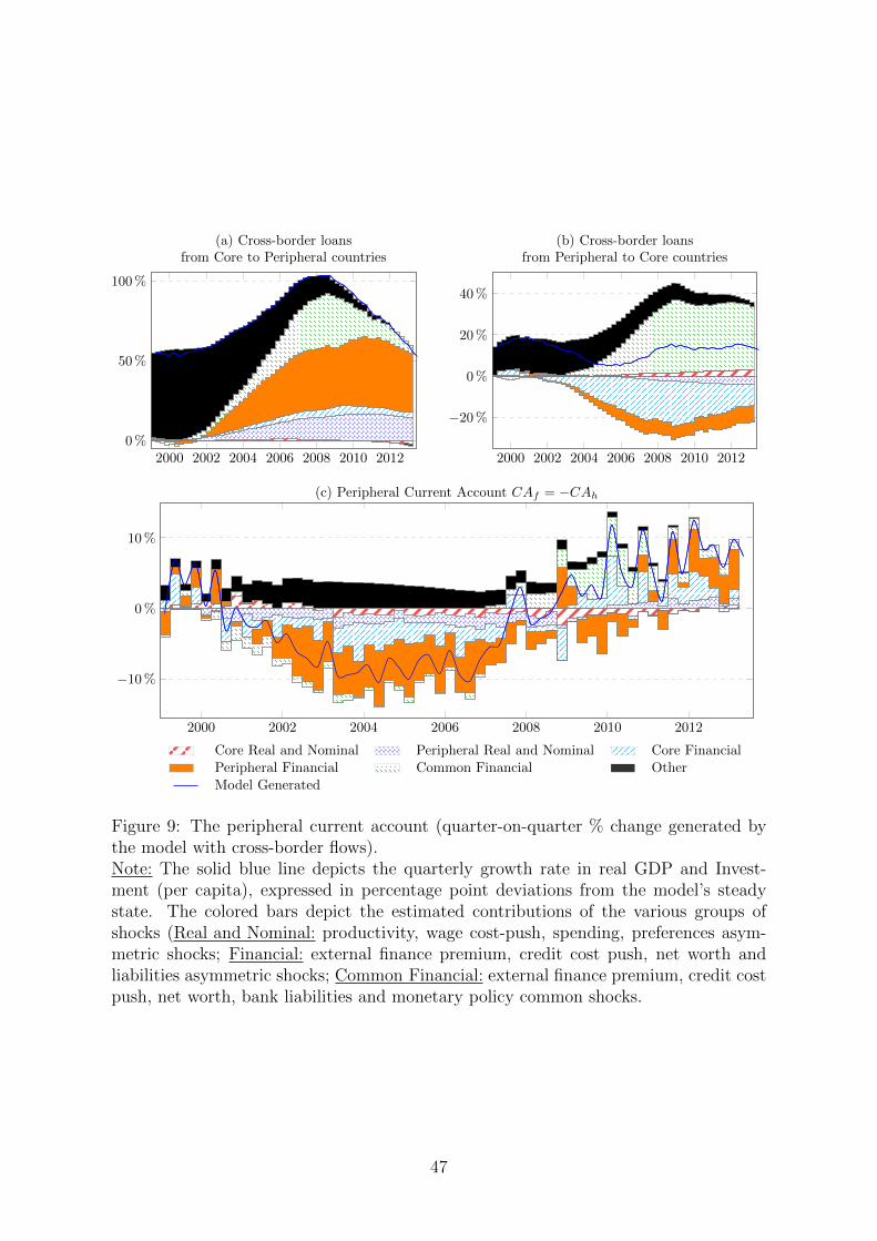
2000 2002 2004 2006 2008 2010 20120%

50%

100%

(a) Cross-border loansfrom Core to Peripheral countries

2000 2002 2004 2006 2008 2010 2012

−20%

0%

20%

40%

(b) Cross-border loansfrom Peripheral to Core countries

2000 2002 2004 2006 2008 2010 2012

−10%

0%

10%

(c) Peripheral Current Account CAf = −CAh

Core Real and Nominal Peripheral Real and Nominal Core FinancialPeripheral Financial Common Financial OtherModel Generated

Figure 9: The peripheral current account (quarter-on-quarter % change generated bythe model with cross-border flows).Note: The solid blue line depicts the quarterly growth rate in real GDP and Invest-ment (per capita), expressed in percentage point deviations from the model’s steadystate. The colored bars depict the estimated contributions of the various groups ofshocks (Real and Nominal: productivity, wage cost-push, spending, preferences asym-metric shocks; Financial: external finance premium, credit cost push, net worth andliabilities asymmetric shocks; Common Financial: external finance premium, credit costpush, net worth, bank liabilities and monetary policy common shocks.

47

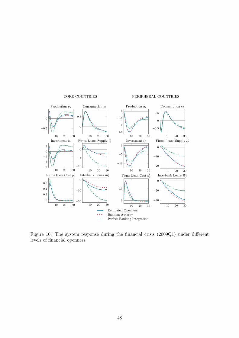
10 20 30

−0.5

0

Production yh

10 20 30

0

0.5

Consumption ch

10 20 30

−1.5

−1

−0.5

0

Production yf

10 20 30

−0.5

0

0.5

Consumption cf

10 20 30−6

−4

−2

0

2

Investment ih

10 20 30

−10

−5

0

Firms Loans Supply lsh

10 20 30

−10

−5

0

Investment if

10 20 30

−20

−10

0

Firms Loans Supply lsf

10 20 30

0

0.2

0.4

0.6

Firms Loan Cost plh

Estimated Openness

Banking Autarky

Perfect Banking Integration

10 20 30−20

−10

0

Interbank Loans ibsh

10 20 30

0

0.5

Firms Loan Cost plf

10 20 30

−40

−20

0

Interbank Loans ibsf

CORE COUNTRIES PERIPHERAL COUNTRIES

Figure 10: The system response during the financial crisis (2009Q1) under differentlevels of financial openness

48