coordinate descent methods for non-differentiable convex

HAL Id: tel-02944077https://hal.archives-ouvertes.fr/tel-02944077

Submitted on 22 Sep 2020

HAL is a multi-disciplinary open accessarchive for the deposit and dissemination of sci-entific research documents, whether they are pub-lished or not. The documents may come fromteaching and research institutions in France orabroad, or from public or private research centers.

L’archive ouverte pluridisciplinaire HAL, estdestinée au dépôt et à la diffusion de documentsscientifiques de niveau recherche, publiés ou non,émanant des établissements d’enseignement et derecherche français ou étrangers, des laboratoirespublics ou privés.

Coordinate descent methods for non-differentiableconvex optimisation problems

Olivier Fercoq

To cite this version:Olivier Fercoq. Coordinate descent methods for non-differentiable convex optimisation problems.Optimization and Control [math.OC]. Sorbonne Université, 2019. tel-02944077

https://hal.archives-ouvertes.fr/tel-02944077

https://hal.archives-ouvertes.fr

Méthodes de descente par coordonnée pour les problèmes

d'optimisation convexes non-dérivables

Coordinate descent methods for non-dierentiable convex

optimisation problems

Mémoire d'Habilitation à Diriger des Recherches

présenté par

Olivier Fercoq

Soutenu le 5 décembre 2019 devant le jury composé de :

Pascal Bianchi LTCI Télécom Paris examinateurAntonin Chambolle CMAP CNRS président du juryJérôme Malick Laboratoire Jean Kuntzmann CNRS rapporteurArkadi Nemirovski ISYE Georgia Tech rapporteurYurii Nesterov CORE Université Catholique de Louvain rapporteurEmmanuel Trélat LJLL Sorbonne Université examinateur

Contents

1 Introduction 5

1.1 Historical motivation for coordinate descent . . . . . . . . . . . . . . . . . . . . . . . . . . 51.2 Why is coordinate descent useful? . . . . . . . . . . . . . . . . . . . . . . . . . . . . . . . 61.3 Two counter-examples . . . . . . . . . . . . . . . . . . . . . . . . . . . . . . . . . . . . . . 81.4 A negative result on universal coordinate descent . . . . . . . . . . . . . . . . . . . . . . . 91.5 Plan of the thesis . . . . . . . . . . . . . . . . . . . . . . . . . . . . . . . . . . . . . . . . . 111.6 Publications related to my PhD thesis . . . . . . . . . . . . . . . . . . . . . . . . . . . . . 12

2 Fast algorithms for composite dierentiable-separable functions 13

2.1 Applications . . . . . . . . . . . . . . . . . . . . . . . . . . . . . . . . . . . . . . . . . . . . 132.1.1 Empirical risk minimization . . . . . . . . . . . . . . . . . . . . . . . . . . . . . . . 132.1.2 Submodular optimization . . . . . . . . . . . . . . . . . . . . . . . . . . . . . . . . 152.1.3 Packing and covering linear programs . . . . . . . . . . . . . . . . . . . . . . . . . 162.1.4 Least squares semi-denite programming . . . . . . . . . . . . . . . . . . . . . . . 16

2.2 APPROX . . . . . . . . . . . . . . . . . . . . . . . . . . . . . . . . . . . . . . . . . . . . . 172.2.1 Description of the algorithm . . . . . . . . . . . . . . . . . . . . . . . . . . . . . . . 172.2.2 Comparison with previous approaches . . . . . . . . . . . . . . . . . . . . . . . . . 18

2.3 Accelerated coordinate descent in a distributed setting . . . . . . . . . . . . . . . . . . . . 192.4 Restart of accelerated gradient methods . . . . . . . . . . . . . . . . . . . . . . . . . . . . 202.5 Using second order information . . . . . . . . . . . . . . . . . . . . . . . . . . . . . . . . . 22

3 Coordinate descent methods for saddle point problems 25

3.1 A coordinate descent version of the Vu Condat method with long step sizes . . . . . . . . 253.1.1 Introduction . . . . . . . . . . . . . . . . . . . . . . . . . . . . . . . . . . . . . . . 253.1.2 Main algorithm and convergence theorem . . . . . . . . . . . . . . . . . . . . . . . 273.1.3 Convergence rate . . . . . . . . . . . . . . . . . . . . . . . . . . . . . . . . . . . . . 28

3.2 Smooth minimization of nonsmooth functions with parallel coordinate descent methods . 303.3 A Smooth Primal-Dual Optimization Framework for Nonsmooth Composite Convex Min-

imization . . . . . . . . . . . . . . . . . . . . . . . . . . . . . . . . . . . . . . . . . . . . . 323.3.1 Introduction . . . . . . . . . . . . . . . . . . . . . . . . . . . . . . . . . . . . . . . 323.3.2 Technical results . . . . . . . . . . . . . . . . . . . . . . . . . . . . . . . . . . . . . 353.3.3 Extensions . . . . . . . . . . . . . . . . . . . . . . . . . . . . . . . . . . . . . . . . 36

3.4 A primal-dual coordinate descent method based on smoothing . . . . . . . . . . . . . . . . 36

4 Applications to statistics 39

4.1 Gap Safe screening rules for sparsity enforcing penalties . . . . . . . . . . . . . . . . . . . 394.1.1 Introduction . . . . . . . . . . . . . . . . . . . . . . . . . . . . . . . . . . . . . . . 394.1.2 Safe Screening rules . . . . . . . . . . . . . . . . . . . . . . . . . . . . . . . . . . . 404.1.3 Experiments . . . . . . . . . . . . . . . . . . . . . . . . . . . . . . . . . . . . . . . 424.1.4 Alternative Strategies: a Brief Survey . . . . . . . . . . . . . . . . . . . . . . . . . 42

4.2 Ecient Smoothed Concomitant Lasso Estimation for High Dimensional Regression . . . 444.3 Safe Grid Search with Optimal Complexity . . . . . . . . . . . . . . . . . . . . . . . . . . 454.4 Joint Quantile regression . . . . . . . . . . . . . . . . . . . . . . . . . . . . . . . . . . . . . 46

5 Perspectives 49

3

Chapter 1

Introduction

1.1 Historical motivation for coordinate descent

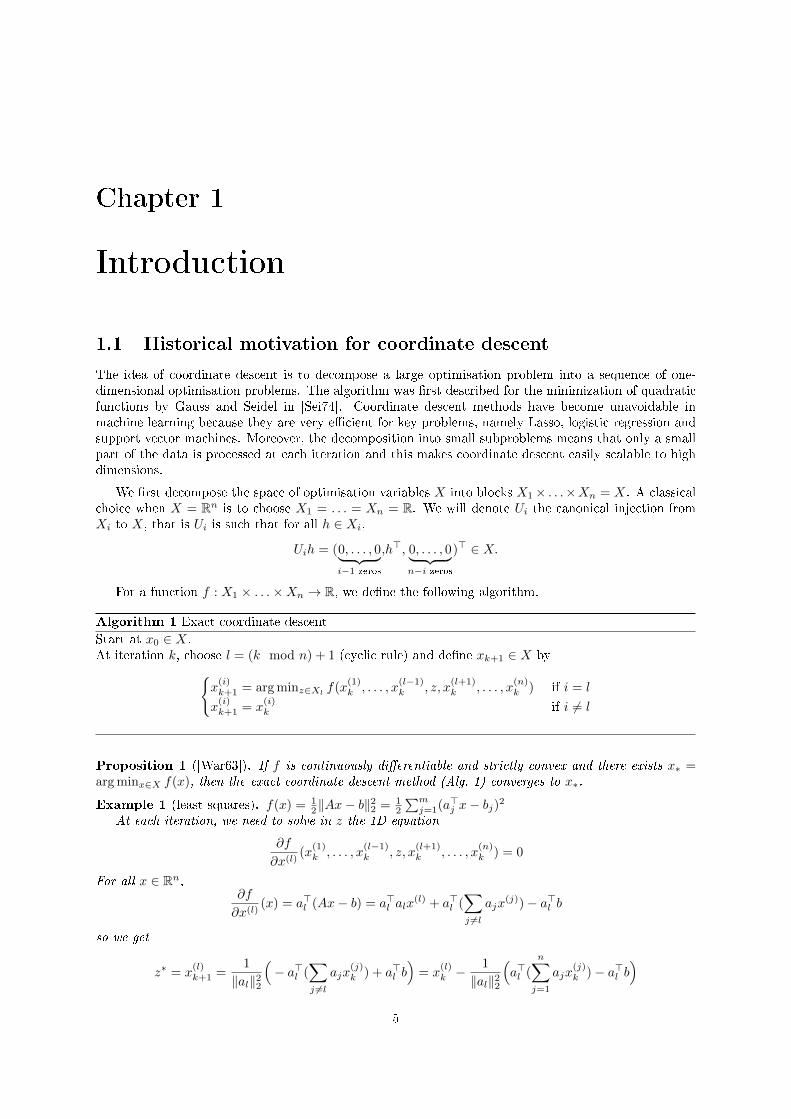
The idea of coordinate descent is to decompose a large optimisation problem into a sequence of one-dimensional optimisation problems. The algorithm was rst described for the minimization of quadraticfunctions by Gauss and Seidel in [Sei74]. Coordinate descent methods have become unavoidable inmachine learning because they are very ecient for key problems, namely Lasso, logistic regression andsupport vector machines. Moreover, the decomposition into small subproblems means that only a smallpart of the data is processed at each iteration and this makes coordinate descent easily scalable to highdimensions.

We rst decompose the space of optimisation variables X into blocks X1× . . .×Xn = X. A classicalchoice when X = Rn is to choose X1 = . . . = Xn = R. We will denote Ui the canonical injection fromXi to X, that is Ui is such that for all h ∈ Xi,

Uih = (0, . . . , 0︸︷︷︸i−1 zeros

,h>, 0, . . . , 0︸︷︷︸n−i zeros

)> ∈ X.

For a function f : X1 × . . .×Xn → R, we dene the following algorithm.

Algorithm 1 Exact coordinate descent

Start at x0 ∈ X.At iteration k, choose l = (k mod n) + 1 (cyclic rule) and dene xk+1 ∈ X by

x(i)k+1 = arg minz∈Xl f(x

(1)k , . . . , x

(l−1)k , z, x

(l+1)k , . . . , x

(n)k ) if i = l

x(i)k+1 = x

(i)k if i 6= l

Proposition 1 ([War63]). If f is continuously dierentiable and strictly convex and there exists x∗ =arg minx∈X f(x), then the exact coordinate descent method (Alg. 1) converges to x∗.

Example 1 (least squares). f(x) = 12‖Ax− b‖

22 = 1

2

∑mj=1(a>j x− bj)2

At each iteration, we need to solve in z the 1D equation

∂f

∂x(l)(x

(1)k , . . . , x

(l−1)k , z, x

(l+1)k , . . . , x

(n)k ) = 0

For all x ∈ Rn,∂f

∂x(l)(x) = a>l (Ax− b) = a>l alx

(l) + a>l (∑j 6=l

ajx(j))− a>l b

so we get

z∗ = x(l)k+1 =

1

‖al‖22

(− a>l (

∑j 6=l

ajx(j)k ) + a>l b

)= x

(l)k −

1

‖al‖22

(a>l (

n∑j=1

ajx(j)k )− a>l b

)5

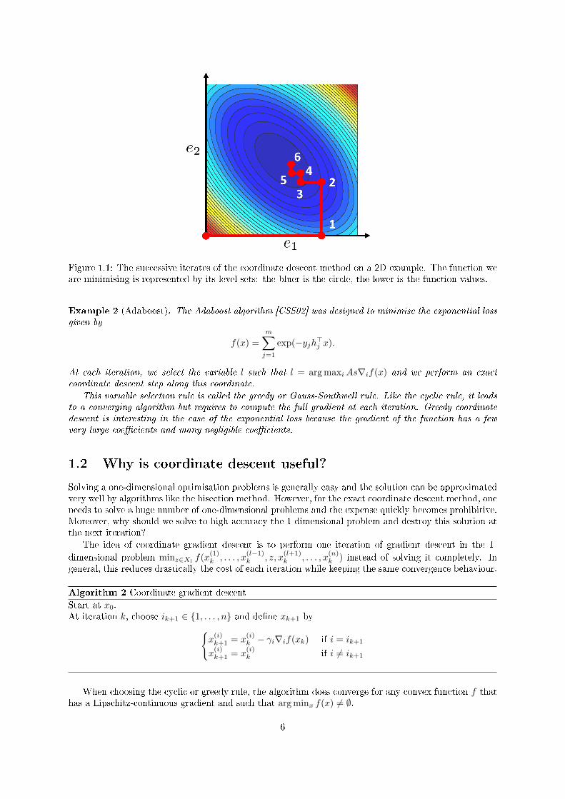
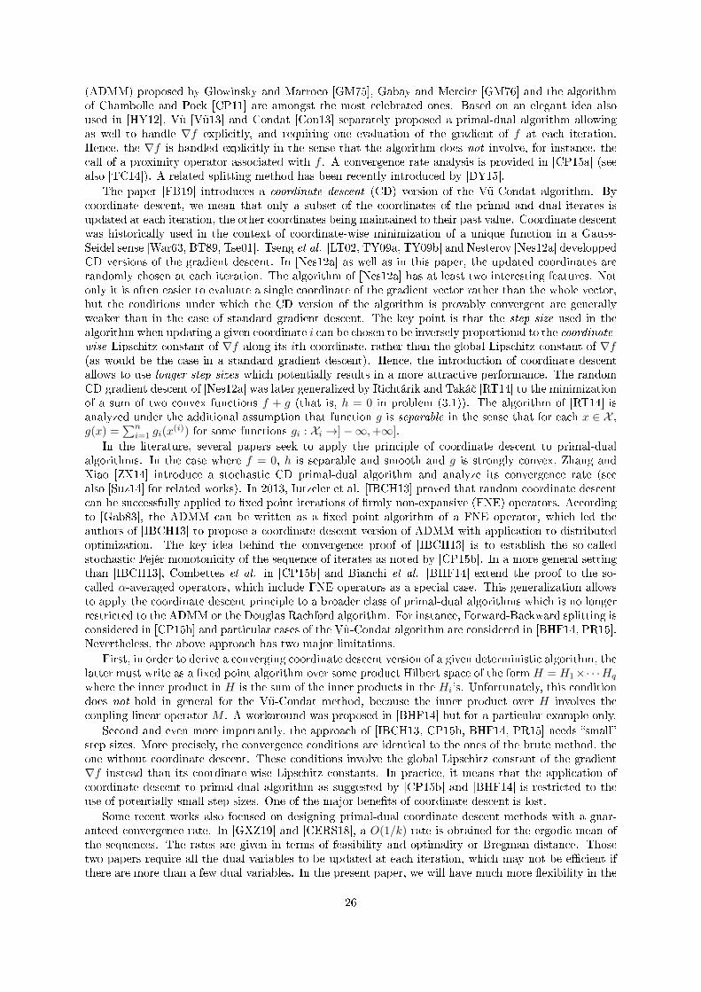
Figure 1.1: The successive iterates of the coordinate descent method on a 2D example. The function weare minimising is represented by its level sets: the bluer is the circle, the lower is the function values.

Example 2 (Adaboost). The Adaboost algorithm [CSS02] was designed to minimise the exponential lossgiven by

f(x) =

m∑j=1

exp(−yjh>j x).

At each iteration, we select the variable l such that l = arg maxiAs∇if(x) and we perform an exactcoordinate descent step along this coordinate.

This variable selection rule is called the greedy or Gauss-Southwell rule. Like the cyclic rule, it leadsto a converging algorithm but requires to compute the full gradient at each iteration. Greedy coordinatedescent is interesting in the case of the exponential loss because the gradient of the function has a fewvery large coecients and many negligible coecients.

1.2 Why is coordinate descent useful?

Solving a one-dimensional optimisation problems is generally easy and the solution can be approximatedvery well by algorithms like the bisection method. However, for the exact coordinate descent method, oneneeds to solve a huge number of one-dimensional problems and the expense quickly becomes prohibitive.Moreover, why should we solve to high accuracy the 1-dimensional problem and destroy this solution atthe next iteration?

The idea of coordinate gradient descent is to perform one iteration of gradient descent in the 1-

dimensional problem minz∈Xl f(x(1)k , . . . , x

(l−1)k , z, x

(l+1)k , . . . , x

(n)k ) instead of solving it completely. In

general, this reduces drastically the cost of each iteration while keeping the same convergence behaviour.

Algorithm 2 Coordinate gradient descent

Start at x0.At iteration k, choose ik+1 ∈ 1, . . . , n and dene xk+1 by

x(i)k+1 = x

(i)k − γi∇if(xk) if i = ik+1

x(i)k+1 = x

(i)k if i 6= ik+1

When choosing the cyclic or greedy rule, the algorithm does converge for any convex function f thathas a Lipschitz-continuous gradient and such that arg minx f(x) 6= ∅.

6

In fact we will assume that we actually know the coordinate-wise Lipschitz constants of the gradientof f , namely the Lipschitz constants of the functions

gi,x : Xi → R

h 7→ f(x+ Uih) = f(x(1), . . . , x(i−1), x(i) + h, x(i+1), . . . , x(n)) (1.1)

We will denote Li = supx L(∇gi,x) this Lipschitz constant. Written in terms of f , this means that

∀x ∈ X,∀i ∈ 1, . . . , n,∀h ∈ Xi, ‖∇f(x+ Uih)−∇f(x)‖2 ≤ Li‖Uih‖2.

Lemma 1. If f has a coordinate-wise Lipschitz gradient with constants L1, . . . , Ln, then ∀x ∈ X,∀i ∈ 1, . . . , n,∀h ∈ Xi,

f(x+ Uih) ≤ f(x) + 〈∇if(x), h〉+Li2‖h‖2

Proposition 2 ([BT13]). Assume that f is convex, ∇f is Lipschitz continuous and arg minx∈X f(x) 6= ∅.If ik+1 is chosen with the cyclic rule ik+1 = (k mod n) + 1 and ∀i, γi = 1

Li, then the coordinate gradient

descent method (Alg. 2) satises

f(xk+1)− f(x∗) ≤ 4Lmax(1 + n3L2max/L

2min)

R2(x0)

k + 8/n

where R2(x0) = maxx,y∈X‖x− y‖ : f(y) ≤ f(x) ≤ f(x0), Lmax = maxi Li and Lmin = mini Li.

The proof of this result is quite technical and in fact the bound is much more pessimistic than whatis observed in practice (n3 is very large if n is large). This is due to the fact that the cyclic rule behavesparticularly bad on some extreme examples. To avoid such traps, it has been suggested to randomisethe coordinate selection process.

Proposition 3 ([Nes12a]). Assume that f is convex, ∇f is Lipschitz continuous and arg minx∈X f(x) 6=∅. If ik+1 is randomly generated, independently of i1, . . . , ik and ∀i ∈ 1, . . . , n, P(ik+1 = i) = 1

n andγi = 1

Li, then the coordinate gradient descent method (Alg. 2) satises for all x∗ ∈ arg minx f(x)

E[f(xk+1)− f(x∗)] ≤n

k + n

((1− 1

n)(f(x0)− f(x∗)) +

1

2‖x∗ − x0‖2L

)where ‖x‖2L =

∑ni=1 Li‖x(i)‖22.

Comparison with gradient descent The iteration complexity of the gradient descent method is

f(xk+1)− f(x∗) ≤L(∇f)

2(k + 1)‖x∗ − x0‖22

This means that to get an ε-solution (i.e. such that f(xk)−f(x∗) ≤ ε), we need at most L(∇f)2ε ‖x∗−x0‖22

iterations. What is most expensive in gradient descent is the evaluation of the gradient ∇f(x) with acost C, so the total cost of the method is

Cgrad = CL(∇f)

2ε‖x∗ − x0‖22

Neglecting the eect of randomisation, we usually have an ε-solution with coordinate descent innε

((1 − 1

n )(f(x0) − f(x∗)) + 12‖x∗ − x0‖2L

)iterations. The cost of one iteration of coordinate descent is

of the order of the cost of evaluation one partial derivative ∇if(x), with a cost c, so the total cost of themethod is

Ccd = cn

ε

((1− 1

n)(f(x0)− f(x∗)) +

1

2‖x∗ − x0‖2L

)How do these two quantities compare?Let us consider the case where f(x) = 1

2‖Ax− b‖22.

• Computing ∇f(x) = A>(Ax− b) amounts to updating the residuals r = Ax− b (one matrix vectorproduct and a sum) and computing one matrix vector product. We thus have C = O(nnz(A)).

7

x0

x1 = x

2

0 0.1 0.2 0.3 0.4 0.5 0.6 0.7 0.8 0.9 10

0.1

0.2

0.3

0.4

0.5

0.6

0.7

0.8

0.9

1

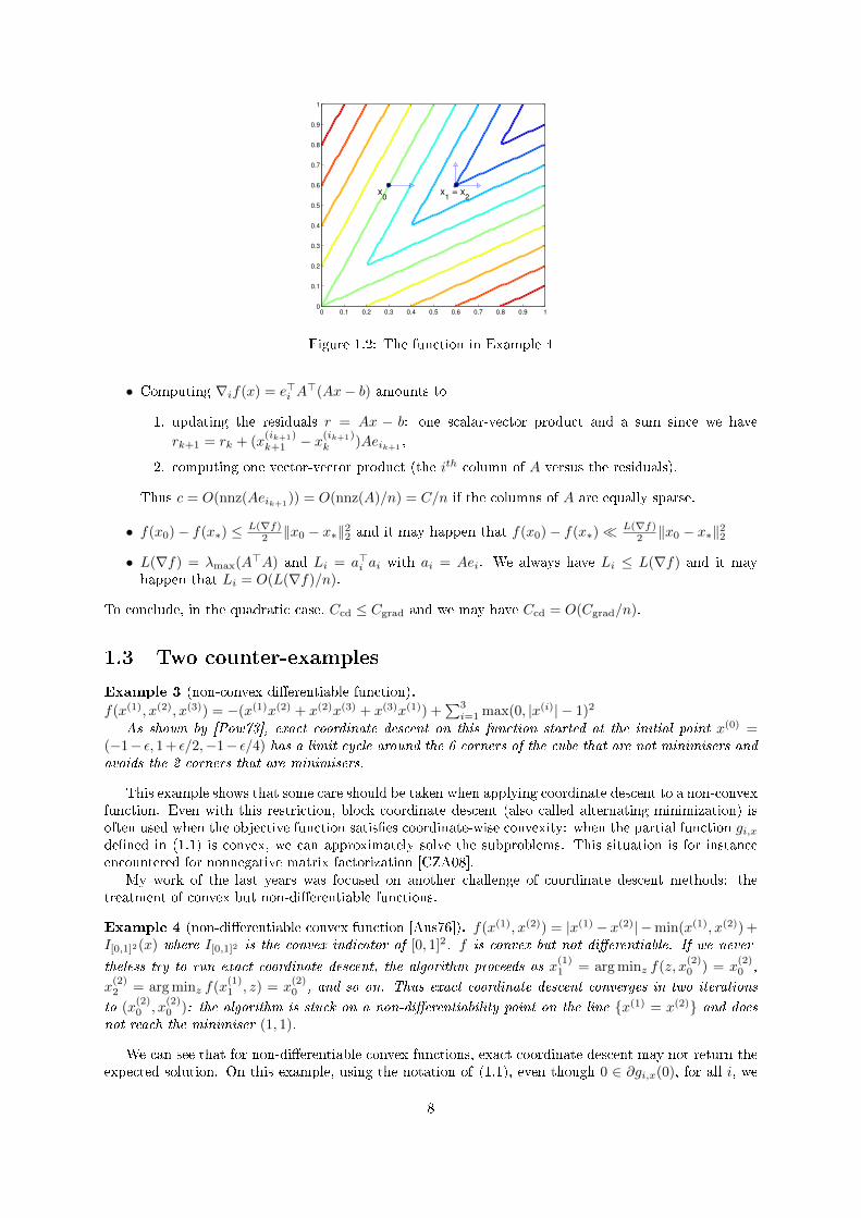
Figure 1.2: The function in Example 4

• Computing ∇if(x) = e>i A>(Ax− b) amounts to

1. updating the residuals r = Ax − b: one scalar-vector product and a sum since we have

rk+1 = rk + (x(ik+1)k+1 − x(ik+1)

k )Aeik+1,

2. computing one vector-vector product (the ith column of A versus the residuals).

Thus c = O(nnz(Aeik+1)) = O(nnz(A)/n) = C/n if the columns of A are equally sparse.

• f(x0)− f(x∗) ≤ L(∇f)2 ‖x0 − x∗‖22 and it may happen that f(x0)− f(x∗) L(∇f)

2 ‖x0 − x∗‖22

• L(∇f) = λmax(A>A) and Li = a>i ai with ai = Aei. We always have Li ≤ L(∇f) and it mayhappen that Li = O(L(∇f)/n).

To conclude, in the quadratic case, Ccd ≤ Cgrad and we may have Ccd = O(Cgrad/n).

1.3 Two counter-examples

Example 3 (non-convex dierentiable function).

f(x(1), x(2), x(3)) = −(x(1)x(2) + x(2)x(3) + x(3)x(1)) +∑3i=1 max(0, |x(i)| − 1)2

As shown by [Pow73], exact coordinate descent on this function started at the initial point x(0) =(−1− ε, 1 + ε/2,−1− ε/4) has a limit cycle around the 6 corners of the cube that are not minimisers andavoids the 2 corners that are minimisers.

This example shows that some care should be taken when applying coordinate descent to a non-convexfunction. Even with this restriction, block coordinate descent (also called alternating minimization) isoften used when the objective function satises coordinate-wise convexity: when the partial function gi,xdened in (1.1) is convex, we can approximately solve the subproblems. This situation is for instanceencountered for nonnegative matrix factorization [CZA08].

My work of the last years was focused on another challenge of coordinate descent methods: thetreatment of convex but non-dierentiable functions.

Example 4 (non-dierentiable convex function [Aus76]). f(x(1), x(2)) = |x(1) − x(2)| −min(x(1), x(2)) +I[0,1]2(x) where I[0,1]2 is the convex indicator of [0, 1]2. f is convex but not dierentiable. If we never-

theless try to run exact coordinate descent, the algorithm proceeds as x(1)1 = arg minz f(z, x

(2)0 ) = x

(2)0 ,

x(2)2 = arg minz f(x

(1)1 , z) = x

(2)0 , and so on. Thus exact coordinate descent converges in two iterations

to (x(2)0 , x

(2)0 ): the algorithm is stuck on a non-dierentiability point on the line x(1) = x(2) and does

not reach the minimiser (1, 1).

We can see that for non-dierentiable convex functions, exact coordinate descent may not return theexpected solution. On this example, using the notation of (1.1), even though 0 ∈ ∂gi,x(0), for all i, we

8

have 0 6∈ ∂f(x). Said otherwise, even when 0 is not in the subdierential of f at x, for all direction ithere may exist a subgradient q ∈ ∂f(x) such q(i) = 0.

A classical workaround is to restrict the attention to composite problems involving the sum of adierentiable function and a separable nonsmooth functions [Tse01].

Denition 1. A function f is said to be separable if it can be written as

f(x) =

n∑i=1

fi(x(i)) .

My contribution includes faster algorithms to deal with non-dierentiable separable functions, smooth-ing techniques for non-dierentiable non-separable functions and primal-dual algorithms. A substantialamount of my research has been driven by the wish to extend successful optimization techniques tocoordinate descent. I also have a great interest in applications of coordinate descent that involve theresolution of optimization problems in large dimensions.

1.4 A negative result on universal coordinate descent

The universal gradient algorithm introduced by Nesterov [Nes13b] is an algorithm that is able to minimizesmooth as well as nonsmooth convex functions without any a priori knowledge on the level of smoothnessof the function. This a particularly desirable feature. First of all, the same algorithm may be used fora large class of problems and, having no parameter to tune, it is very robust. Secondly, the adaptiveprocess that discovers the level of smoothness of the function may take prot of a locally favorablesituation, even though the function is dicult to minimize at the global scope.

Our aim in the paper [FR14] is to design and analyze a universal coordinate descent method for theproblem of minimizing a convex composite function:

minx∈RN

[F (x) ≡ f(x) + Ψ(x)] , (1.2)

where Ψ is convex and has a simple proximal operator. The function f(x) is convex and can be smoothor nonsmooth. It is still interesting to consider the composite framework because we can take prot ofthe proximal operator of Ψ.

Classical coordinate descent algorithm may get stuck at a non-stationary point if applied to a generalnonsmooth convex problem. However, several coordinate-descent-type methods have been proposed fornonsmooth problems. An algorithm based on the averaging of past subgradient coordinates is presentedin [TKCW12] and a successful subgradient-based coordinate descent method for problems with sparsesubgradients is proposed by Nesterov [Nes12b]. An important feature of these algorithms is that at eachpoint x, one subgradient ∇f(x) is selected and then the updates are performed according to the ith

coordinate ∇if(x) of the subgradient. This is dierent to partial subgradients. A coordinate descentalgorithm based on smoothing was proposed in [FR17] for the minimization of nonsmooth functions witha max-structure. However if one tries to use one of these algorithms on a smooth problem, one wouldget a very slow algorithm with iteration complexity in O(1/ε2).

The adaptive procedure of the universal gradient method is based on a line search, the parameterof which estimates either the Lipschitz constant of the function (if it is nonsmooth) or the Lipschitzconstant of the gradient of the function (if it is smooth). We designed such a line search procedurefor universal coordinate descent. On top of being able to deal with nonsmooth functions, it covers thecomposite framework with a nonsmooth regularizer and uses only partial derivatives evaluation.

We extend the theory of parallel coordinate descent developed in [RT15] to the universal coordinatedescent method. In particular, we dene a non-quadratic expected separable overapproximation forpartially separable functions that allows us to run independent line searches on all the coordinates to beminimized at a given iteration. This is a result of independent interest as this is the rst time that aline search procedure is introduced for parallel coordinate descent.

We design a universal accelerated coordinate descent method with optimal rates of convergenceO(1/

√ε) for smooth problems and O(1/ε2) for nonsmooth problems. We recover many previous results.

In particular we recover the universal primal gradient method [Nes13b] when we consider one single block(in our notation, n = 1) and we recover the accelerated coordinate descent method [FR15]. Moreover,the line search procedure allows us not to bother about the coordinatewise Lipschitz constant.

9

Algorithm 3 Universal coordinate descent

Choose (Lj0)j∈[n] and accuracy ε.For k ≥ 0 do:

1. Select a subgradient ∇f(xk)

2. Select block jk at random.

3. Find the smallest sk ∈ N such that for

x+k = arg min

z∈RjΨjk(z) + f(xk) + 〈∇jf(xk), z − x(jk)

k 〉+1

22skLjkk ‖z − x

(jk)k ‖2(jk),

we have1

2

1

2sk−1Ljkk

(‖∇jkf(xk)−∇jkf(x+

k )‖∗(jk)

)2 ≤ 2sk−1Ljkk2

‖x(jk)k − (x+

k )(jk)‖2(jk) +ε

2n.

4. Set xk+1 = x+k and Ljkk+1 = 2skLjkk

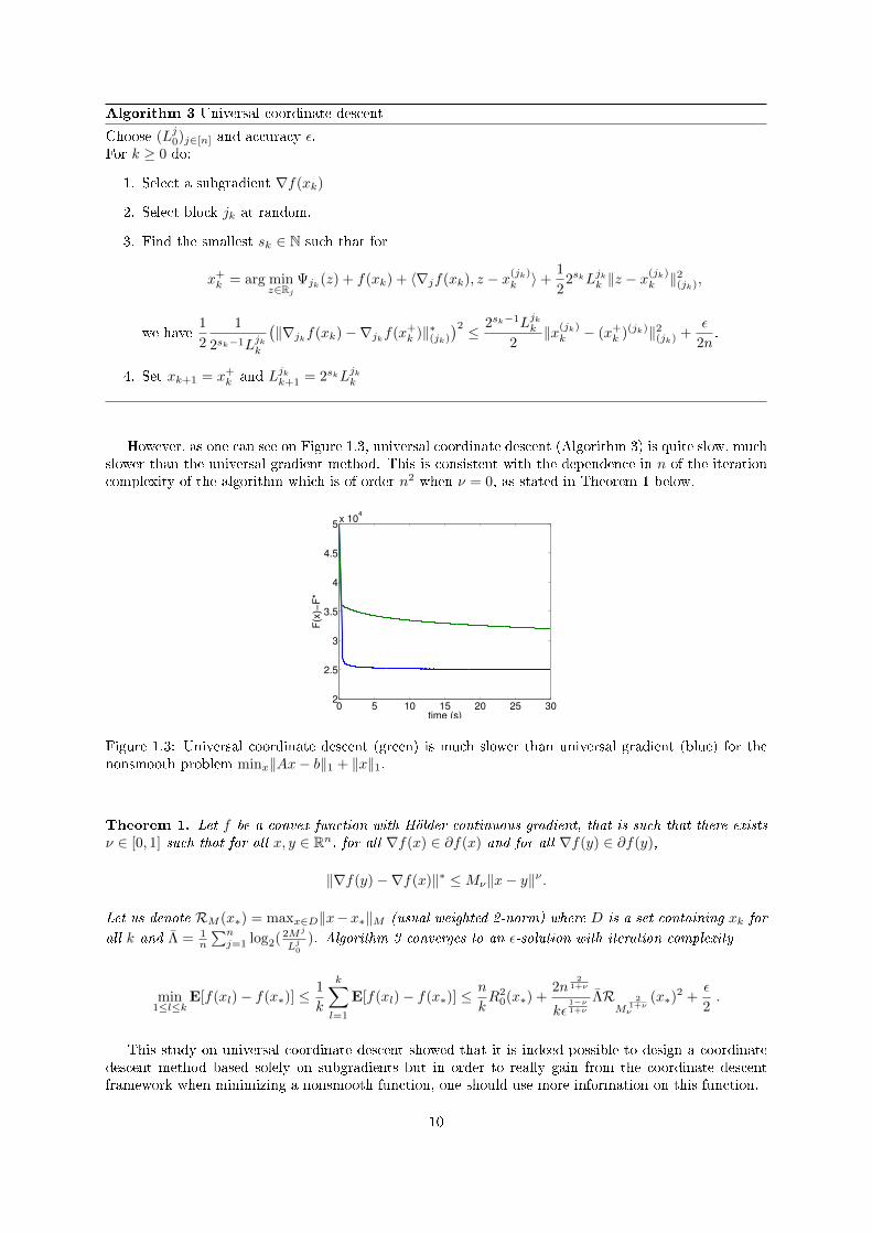
However, as one can see on Figure 1.3, universal coordinate descent (Algorithm 3) is quite slow, muchslower than the universal gradient method. This is consistent with the dependence in n of the iterationcomplexity of the algorithm which is of order n2 when ν = 0, as stated in Theorem 1 below.

0 5 10 15 20 25 302

2.5

3

3.5

4

4.5

5x 10

4

time (s)

F(x

)−F

*

Figure 1.3: Universal coordinate descent (green) is much slower than universal gradient (blue) for thenonsmooth problem minx‖Ax− b‖1 + ‖x‖1.

Theorem 1. Let f be a convex function with Hölder continuous gradient, that is such that there existsν ∈ [0, 1] such that for all x, y ∈ Rn, for all ∇f(x) ∈ ∂f(x) and for all ∇f(y) ∈ ∂f(y),

‖∇f(y)−∇f(x)‖∗ ≤Mν‖x− y‖ν .

Let us denote RM (x∗) = maxx∈D‖x−x∗‖M (usual weighted 2-norm) where D is a set containing xk for

all k and Λ = 1n

∑nj=1 log2( 2Mj

Lj0). Algorithm 3 converges to an ε-solution with iteration complexity

min1≤l≤k

E[f(xl)− f(x∗)] ≤1

k

k∑l=1

E[f(xl)− f(x∗)] ≤n

kR2

0(x∗) +2n

21+ν

kε1−ν1+ν

ΛRM

21+νν

(x∗)2 +

ε

2.

This study on universal coordinate descent showed that it is indeed possible to design a coordinatedescent method based solely on subgradients but in order to really gain from the coordinate descentframework when minimizing a nonsmooth function, one should use more information on this function.

10

1.5 Plan of the thesis

This thesis summarizes my research work between 2012 and 2018 while I was working at the Universityof Edinburgh and at Télécom Paristech. My publications follow three main tracks:

Chapter 2. Fast algorithms for composite dierentiable-separable functions

Coordinate descent methods have shown very ecient for problems of the form minx f(x) +∑i ψi(xi) with f dierentiable. This chapter is based on the following papers.

[FQRT14] Olivier Fercoq, Zheng Qu, Peter Richtárik, and Martin Taká£. Fast distributed coordinate descentfor minimizing non-strongly convex losses. In IEEE International Workshop on Machine Learningfor Signal Processing, 2014.

[FR15] Olivier Fercoq and Peter Richtárik. Accelerated, parallel and proximal coordinate descent. SIAMJournal on Optimization, 25(4):19972023, 2015.

[FR16] Olivier Fercoq and Peter Richtárik. Optimization in high dimensions via accelerated, parallel, andproximal coordinate descent. SIAM Review, 58(4):739771, 2016.

[QRTF16] Zheng Qu, Peter Richtárik, Martin Takác, and Olivier Fercoq. Sdna: stochastic dual newtonascent for empirical risk minimization. In International Conference on Machine Learning, pages18231832, 2016.

[FQ16] Olivier Fercoq and Zheng Qu. Restarting accelerated gradient methods with a rough strongconvexity estimate. arXiv preprint arXiv:1609.07358, 2016.

[FQ17] Olivier Fercoq and Zheng Qu. Adaptive restart of accelerated gradient methods under localquadratic growth condition. arXiv preprint arXiv:1709.02300, 2017.

[FQ18] Olivier Fercoq and Zheng Qu. Restarting the accelerated coordinate descent method with a roughstrong convexity estimate. arXiv preprint arXiv:1803.05771, 2018.

Chapter 3. Coordinate descent methods for saddle point problems

In this line of work, I have been trying to show that coordinate descent methods can be appliedsuccessfully to a much wider class of functions that what was previously thought. I have works onprimal-dual methods, smoothing theory and their relations to coordinate descent.

[FR13] Olivier Fercoq and Peter Richtárik. Smooth Minimization of Nonsmooth Functions by ParallelCoordinate Descent. arXiv:1309.5885, 2013.

[Fer13] Olivier Fercoq, Parallel coordinate descent for the Adaboost problem In International Conferenceon Machine Learning and Applications, 2013.

[FR14] Olivier Fercoq and Peter Richtárik. Universal coordinate descent and line search for parallelcoordinate descent. Technical report, The University of Edinburgh, 2014.

[FB15] Olivier Fercoq and Pascal Bianchi. A Coordinate Descent Primal-Dual Algorithm with Large StepSize and Possibly Non Separable Functions. arXiv preprint arXiv:1508.04625, 2015. Accepted forpublication in SIAM Journal on Optimization.

[BF16] Pascal Bianchi and Olivier Fercoq. Using Big Steps in Coordinate Descent Primal-Dual Algorithms.In Proc. of the Conference on Decision and Control, 2016.

[VNFC17] Quang Van Nguyen, Olivier Fercoq, and Volkan Cevher. Smoothing technique for nonsmoothcomposite minimization with linear operator. arXiv preprint arXiv:1706.05837, 2017.

[ADFC17] Ahmet Alacaoglu, Quoc Tran Dinh, Olivier Fercoq, and Volkan Cevher. Smooth primal-dual coor-dinate descent algorithms for nonsmooth convex optimization. In Advances in Neural InformationProcessing Systems, pages 58525861, 2017.

11

[TDFC18] Quoc Tran-Dinh, Olivier Fercoq, and Volkan Cevher. A smooth primal-dual optimization frame-work for nonsmooth composite convex minimization. SIAM Journal on Optimization, 28(1):96134,2018.

[YFLC18] Alp Yurtsever, Olivier Fercoq, Francesco Locatello, and Volkan Cevher. A conditional gradientframework for composite convex minimization with applications to semidenite programming. InICML, 2018.

Chapter 4. Applications to statistics

Statistical estimators are often dened as the solution of an optimization problem. Moreover,the structure of the functions encountered in statistics and the massive amount of data to dealwith makes it a natural playground for coordinate descent methods. I have contributions in safescreening rules, a concomitant lasso solver, joint quantile regression and ε-insensitive losses.

[FGS15] Olivier Fercoq, Alexandre Gramfort, and Joseph Salmon. Mind the duality gap: safer rules for thelasso. In ICML, pages 333342, 2015.

[NFGS15] Eugène Ndiaye, Olivier Fercoq, Alexandre Gramfort, and Joseph Salmon. GAP safe screeningrules for sparse multi-task and multi-class models. NIPS, pages 811819, 2015.

[NFGS16] Eugène Ndiaye, Olivier Fercoq, Alexandre Gramfort, and Joseph Salmon. GAP safe screeningrules for Sparse-Group Lasso. NIPS, 2016.

[SFdB16] Maxime Sangnier, Olivier Fercoq, and Florence d'Alché Buc. Joint quantile regression in vector-valued rkhss. In Advances in Neural Information Processing Systems, pages 36933701, 2016.

[NFGS17] Eugene Ndiaye, Olivier Fercoq, Alexandre Gramfort, and Joseph Salmon. Gap safe screening rulesfor sparsity enforcing penalties. Journal of Machine Learning Research, 18(1):46714703, 2017.

[MFGS17] Mathurin Massias, Olivier Fercoq, Alexandre Gramfort, and Joseph Salmon. Heteroscedasticconcomitant lasso for sparse multimodal electromagnetic brain imaging. In Proc. of the 21stInternational Conference on Articial Intelligence and Statistics, 1050:27, 2017.

[SFdB17] Maxime Sangnier, Olivier Fercoq, and Florence d'Alché Buc. Data sparse nonparametric regressionwith ε-insensitive losses. In Asian Conference on Machine Learning, pages 192207, 2017.

[NFT+18] Eugène Ndiaye, Olivier Fercoq, Joseph Salmon, Ichiro Takeuchi, and Le Tam. Safe grid searchwith optimal complexity. Technical report, Télécom ParisTech and Nagoya Institute of Technology,2018.

1.6 Publications related to my PhD thesis

[BCF+12] Frédérique Billy, Jean Clairambault, Olivier Fercoq, Stéphane Gaubert, Thomas Lepoutre, ThomasOuillon, and Shoko Saito. Synchronisation and control of proliferation in cycling cell populationmodels with age structure. Mathematics and Computers in Simulation, 2012.

[Fer12a] Olivier Fercoq. Convergence of Tomlin's HOTS algorithm. arXiv:1205.6727, 2012.

[Fer12b] Olivier Fercoq. PageRank optimization applied to spam detection. In 6th International conferenceon NETwork Games, COntrol and OPtimization (Netgcoop), pages 124131, 2012.

[Fer13] Olivier Fercoq. Perron vector optimization applied to search engines. Applied Numerical Mathe-matics, 2013. doi :10.1016/j.apnum.2012.12.006.

[FABG13] Olivier Fercoq, Marianne Akian, Mustapha Bouhtou, and Stéphane Gaubert. Ergodic Control andPolyhedral approaches to PageRank Optimization. IEEE TAC, 58:134148, 2013.

[CF16] Jean Clairambault and Olivier Fercoq. Physiologically structured cell population dynamic modelswith applications to combined drug delivery optimisation in oncology. Mathematical Modelling ofNatural Phenomena, 11(6), 2016.

[FerPhD] Olivier Fercoq. Optimization of Perron eigenvectors: from web ranking to chronotherapeutics.PhD thesis, Ecole Polytechnique, 2012.

12

Chapter 2

Fast algorithms for composite

dierentiable-separable functions

In this line of work we focus on the solution of convex optimization problems with a huge number ofvariables of the form

minx∈RN

f(x) + Ψ(x). (2.1)

Here x = (x(1), . . . , x(n)) ∈ RN is a decision vector composed of n blocks with x(i) ∈ RNi , andN =∑iNi.

We assume that Ψ : RN → R ∪ +∞ is a convex (and lower semicontinous) block separable regularizer(e.g., the L1 norm).

Despite the major limitation on the nonsmooth part of the objective, this setup has had a lot ofapplications. For instance, a breakthrough was made in large scale sparse regression when coordinatedescent was shown to be the most ecient method for the resolution of the Lasso problem [FHHT07].

2.1 Applications

In this section we describe four applications areas for accelerated coordinate descent, all motivated andbuilding on the work [FR15] where we developed the Accelerated, Parallel and Proximal coordinatedescent method APPROX (see Table 2.1). Empirical risk minimization is a natural framework forcoordinate descent methods but acceleration increased its range of applicability to other domains.

2.1.1 Empirical risk minimization

Empirical risk minimization (ERM) is a powerful and immensely popular paradigm for training statistical(machine) learning models [SSBD14]. In statistical learning, one wishes to learn an unknown functionh∗ : X → Y, where X (set of samples) and Y (set of labels) are arbitrary domains. Roughly speaking, thegoal of statistical learning is to nd a function (predictor, hypothesis) h : X → Y from some predenedset (hypothesis class) H of predictors which in some statistical sense is the best approximation of h∗.In particular, we assume that there is an unknown distribution D over ξ ∈ X . Given a loss function` : Y × Y → R, we dene the risk (generalization error) associated with predictor h ∈ H to be

LD(h) = Eξ∼D `(h(ξ), h∗(ξ)). (2.2)

Application Paper Section

Empirical risk minimization [FQRT14, LLX15] 2.1.1Submodular optimization Ene and Nguyen [EN15] 2.1.2

Packing and covering linear programs Allen-Zhu & Orecchia [AZO15] 2.1.3Least-squares semidenite programming Sun, Toh and Yang [STY16] 2.1.4

Table 2.1: Selected applications of APPROX, developed by others after the publication of [FR15].

13

The goal of statistical learning is to nd h ∈ H of minimal risk:

minh∈H

LD(h). (2.3)

A natural albeit in general intractable choice of a loss function in some applications is `(y, y′) = 0 ify = y′ and `(y, y′) = 1 otherwise.

Let X be a collection of images, Y = −1, 1 and let h∗(ξ) be 1 of image ξ contains an image ofa cat, and h∗(ξ) = −1 otherwise. If we are able to learn h∗, we will be able to detect images of cats.Problems where Y consist of two elements are called classication problems. The domain set can insteadrepresent a video collection, a text corporus, a collection of emails or any other collection of objectswhich we can represent mathematically. If Y is a nite set consisting of more than two elements, wespeak of multi-class classication. If Y = R, we speak of regression.

One of the fundamental issues making (2.3) dicult to solve is the fact that the distribution D is notknown. ERM is a paradigm for overcoming this obstacle, assuming that we have access to independentsamples from D. In ERM, we rst collect a training set of i.i.d. samples and their labels; that is,S = (ξj , yj) ∈ X × Y : j = 1, 2, . . . ,m, where yj = h∗(ξj). Subsequently, we replace the expectationin (2.2) dening the risk, by a sample average approximation, which denes the empirical risk:

LS(h) =1

m

m∑j=1

`(h(ξj), yj).

The ERM paradigm is to solve the empirical risk minimization problem

minh∈H

LS(h) (2.4)

instead of the harder risk minimization problem (2.3). In practice, H is often chosen to be a parametricclass of functions described by a parameter x ∈ Rd. For instance, let X ⊆ Rd (d = number of features)and Y = R, and consider the class of linear predictors: H = h : h(ξ) = x>ξ. Clearly, h is uniquelydened by x ∈ Rd. Dening `j : R→ R via `j(t) = 1

m`(t, yj), and setting fj(x) = `j(ξTj x), we have

f(x) =

m∑j=1

fj(x) =

m∑j=1

`j(ξTj x) = LS(h).

Hence, the ERM problem ts our framework (2.1), with ψ ≡ 0. However, in practice one often usesnonzero ψ, which is interpreted as a regularizer, and is included in order to prevent overtting and henceallow the estimator to generalize to future, unobserved samples.

ERM has a tight connection with coordinate descent methods. Indeed, coordinate descent methodsbecame very popular when their eciency was proved for the Lasso problem [FHHT07]. It is a regressionproblem where the goal is to nd sparse solutions. It can be written as

minx∈Rn

1

2‖Ax− b‖22 + λ‖x‖1

where y ∈ Rm is the signal, made out of m observations, A is a matrix of features of size m × n andx is the parameter vector that we seek to estimate so that it has a few nonzero coecients. This is anon-dierentiable problem but it can be decomposed in a smooth part 1

2‖Ax− b‖22 and a separable part

λ‖x‖1 = λ∑ni=1 |xi|. It is thus amenable to coordinate descent methods.

If the number of features is larger than the number of examples (d m), which is typical for Lassoproblems, randomized coordinate descent is an ecient algorithm for solving (2.1) [RT14, RT15, SSZ13].If the training set S is so large that it does not t the memory (or disk space) of a single machine, oneneeds to employ a distributed computing system and solve ERM via a distributed optimization algorithm.One option is the use of distributed coordinate descent [RT16c, MRT15], known as Hydra. APPROXhas been successfully applied in the distributed setting, leading to the Hydra2 method [FQRT14]. Inthis work, the authors solve an ERM problem involving a training set of several terabytes in size, and50 billion features.

If the number of examples in the training set is larger than the number of features (m d), it istypically not ecient to employ randomized coordinate descent, to the ERM problem directly. Instead,the state of the art methods are variants of randomized coordinate descent applied to the dual problem.

14

The (Fenchel) dual of the regularized ERM problem for linear predictors considered above has theform

miny∈Rm

ψ∗

1

m

m∑j=1

yjξj

+1

m

m∑j=1

`∗j (−yj),

where ψ∗ (resp. `∗j ) is the Fenchel conjugate of ψ (resp. `j). The function y 7→ ψ∗( 1m

∑j yjξj) has

Lipschitz gradient if we assume that ψ is strongly convex, and y 7→ 1m

∑mj=1 `

∗j (−yj) is separable. This

also ts the framework (2.1), f corresponding to the rst part of the objective (and consisting of a singlesummand), and ψ corresponding to the second part of the objective (block separability is implied byseparability).

We developed APPROX with ERM as an application in mind and hence our numerical experimentsconsider two key ERM problems: the Lasso problem and the Support Vector Machine (SVM) problem.

Following our paper, Lin, Lu and Xiao [LLX15] proposed a version of APPROX designed for stronglyconvex problems. Their motivation was that practitioners often choose regularizers that are at the sametime separable and strongly convex. This leads to problems for which we have a good lower bound on thestrong convexity parameter. With this additional knowledge, they showed that the rate of convergence ofa properly modied APPROX algorithm, applied to the dual problem, leads to state of the art complexityfor a class of ERM problems.

2.1.2 Submodular optimization

Ene and Nguyen [EN15] showed how the APPROX algorithm leads to a state-of-the-art method forminimizing decomposable submodular functions. Submodular minimization has a vast and growing ar-ray of applications, including image segmentation [RKB04, EN15], graphical model structure learning,experimental design, Bayesian variable selection and minimizing matroid rank functions [Bac13].

We now briey introduce the notion of submodularity. Let V = 1, 2, . . . , d be a nite ground set. Areal-valued set function φ : 2V → R is called modular, if φ(∅) = 0 and there exists a vector w ∈ Rd suchthat φ(A) =

∑i∈A wi for all ∅ 6= A ⊆ V . It is called submodular if φ(A) + φ(B) ≥ φ(A ∩B) + φ(A ∪B)

for any two sets A,B ⊆ V . An equivalent and often more intuitive characterization of submodularityis the following diminishing returns property: φ is submodular if and only if for all A ⊆ B ⊆ V andk ∈ V such that k /∈ B, we have φ(A ∪ k)− φ(A) ≥ φ(B ∪ k)− φ(B).

Ene and Nguyen [EN15] consider the decomposable submodular minimization problem

minA⊆V

n∑i=1

φi(A), (2.5)

where φi : 2V → R are simple submodular functions (simplicity refers to the assumption that it is simpleto minimize φi plus a modular function). Instead of solving (2.5) directly, one can focus on solving theunconstrained convex minimization problem

minz∈Rd

n∑i=1

(φi(z) +

1

2n‖z‖2

), (2.6)

where ‖ · ‖ is the standard Euclidean norm, and φi : Rd → R is the Lovász extension of φi (i.e., thesupport function of the base polytope Pi ⊂ Rd of φi). Given a solution z, one recovers the solution of(2.5) by setting

A = A(z) = k ∈ V : zk ≥ 0. (2.7)

Further, instead of solving (2.6), one focuses on its (Fenchel) dual:

minx(1)∈P1,...,x(n)∈Pn

f(x) =1

2

∥∥∥∥∥n∑i=1

x(i)

∥∥∥∥∥2

. (2.8)

It can be shown that if x = (x(1), . . . , x(n)) ∈ Rnd = RN solves (2.8), then

z = −n∑i=1

x(i) (2.9)

15

solves (2.6). Note that f is a convex quadratic function. If we let Ψ be the indicator function of the setP = P1 × · · · × Pn ⊆ RN , i.e., Ψ(x) = 0 if x ∈ P and Ψ(x) = +∞ otherwise, then (2.8) is of the form(2.1), where Ni = d for all i. It remains to apply the APPROX method to this problem, and transformthe solution back via (2.9) and then (2.7) to obtain solution of the original problem (2.5).

2.1.3 Packing and covering linear programs

Packing and covering problems are a pair of mutually-dual linear programming problems of the form

Packing LP: maxx≥01Tx : Ax ≤ 1

Covering LP: miny≥01T y : AT y ≤ 1,

where A is a real matrix, and 1 denotes the vector of appropriate dimension with all entries equalto 1. These problems become more dicult as the size of A grows since each iteration of interior-point solvers becomes more expensive. Allen-Zhu and Orecchia [AZO15] developed algorithms for theseproblems whose complexity is O(NA log(NA) log(ε−1)/ε) for packing and O(NA log(NA) log(ε−1)ε−1.5)for covering LP, respectively. This complexity is nearly linear in the size of the problem NA = nnz(A)(number of nonzero entries in A), does not depend on the magnitude of the elements of A and has abetter dependence on the accuracy ε than other nearly-linear time approaches. The improvement inthe complexity is due to the use of accelerated proximal coordinate descent techniques such as thosedeveloped in our paper, combined with extra techniques, such as the use of an exponential penalty.

2.1.4 Least squares semi-denite programming

Semidenite programming have a very important role in optimization due to its ability to model andeciently solve a wide array of problems appearing in elds such as control, network science, signalprocessing and computer science [VB96, Tod01, BTN01, WSV10]. In semidenite programming, one aimsto minimize a linear function in a matrix variable, subject to linear equality and inequality constraintsand the additional requirement that the matrix variable be positive semidenite.

Sun, Toh and Yang [STY16] consider the canonical semidenite program (SDP)

minX∈Sn+, s∈RmI

〈C,X〉

subject to AE(X) = bE , AI(X) = s, L ≤ X ≤ U, l ≤ s ≤ u,

where 〈C,X〉 is the trace inner product, Sn+ is the cone of n×n symmetric positive semidenite matrices,AE : Sn+ → RmE and AI : Sn+ → RmI are linear maps, L ≤ U are given positive semidenite matricesand l ≤ u are given vectors in RmI .

The above SDP can be solved by a proximal point algorithm (PPA) of Rockafellar [Roc76a, Roc76b].In each iteration of PPA, one needs to solve a least-squares semidenite program (LS-SDP) of the form

(Xk+1, sk+1) = arg minX∈Sn+,s∈RmI

〈C,X〉+1

2σk(‖X −Xk‖2 + ‖s− sk‖2)

subject to AE(X) = bE , AI(X) = s, L ≤ X ≤ U, l ≤ s ≤ u,

where (Xk, sk) is the previous iterate, and σk > 0 a regularization parameter. Sun, Toh and Yang [STY16]observe that the dual of LS-SDP has block-separable constraints and can hence be written in the form(2.1), with either 2 or 4 blocks (n = 2 or n = 4). They used this observation as a starting point to proposenew algorithms for LS-SDP that combine advanced linear algebra techniques, a ne study of the errorsmade by each inner solver, and coordinate descent ideas. They consider APPROX and block coordi-nate descent as natural competitors to their specialized methods. They implemented the methods using4 blocks, each equipped with a nontrivial norm dened by a well chosen positive semi-denite matrixBi ∈ RNi×Ni and approximate solutions to the proximity operators. Finally, Sun, Toh and Yang con-ducted extensive experiments on 616 SDP instances coming from relaxations of combinatorial problems.It is worth noting that on these instances, APPROX is vastly faster than standard (non-accelerated)block coordinate descent.

16

2.2 APPROX

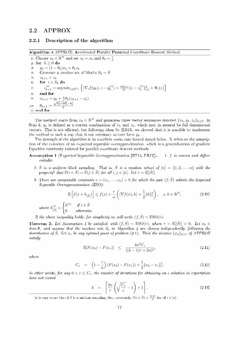
2.2.1 Description of the algorithm

Algorithm 4 APPROX: Accelerated Parallel Proximal Coordinate Descent Method

1: Choose x0 ∈ RN and set z0 = x0 and θ0 = τn

2: for k ≥ 0 do3: yk = (1− θk)xk + θkzk4: Generate a random set of blocks Sk ∼ S5: zk+1 = zk6: for i ∈ Sk do7: z

(i)k+1 = arg minz∈RNi

〈∇if(yk), z − y(i)

k 〉+ nθkvi2τ ‖z − z

(i)k ‖2(i) + Ψi(z)

8: end for

9: xk+1 = yk + nτ θk(zk+1 − zk)

10: θk+1 =

√θ4k+4θ2

k−θ2k

211: end for

The method starts from x0 ∈ RN and generates three vector sequences denoted xk, yk, zkk≥0. InStep 3, yk is dened as a convex combination of xk and zk, which may in general be full dimensionalvectors. This is not ecient; but following ideas by [LS13], we showed that it is possible to implementthe method in such a way that it not necessary to ever form yk.

The strength of the algorithm is its excellent worst case bound stated below. It relies on the assump-tion of the existence of an expected separable overapproximation, which is a generalization of gradientLipschitz continuity tailored for parallel coordinate descent methods.

Assumption 1 (Expected Separable Overapproximation [RT15, FR17]). 1. f is convex and dier-entiable.

2. S is a uniform block sampling. That is, S is a random subset of [n] = 1, 2, . . . , n with theproperty1 that P(i ∈ S) = P(j ∈ S) for all i, j ∈ [n]. Let τ = E[|S|].

3. There are computable constants v = (v1, . . . , vn) > 0 for which the pair (f, S) admits the ExpectedSeparable Overapproximation (ESO):

E[f(x+ h[S])

]≤ f(x) +

τ

n

(〈∇f(x), h〉+

1

2‖h‖2v

), x, h ∈ RN , (2.10)

where h(i)

[S]=

h(i) if i ∈ S0 otherwise

If the above inequality holds, for simplicity we will write (f, S) ∼ ESO(v).

Theorem 2. Let Assumption 1 be satised, with (f, S) ∼ ESO(v), where τ = E[|S|] > 0. Let x0 ∈dom Ψ, and assume that the random sets Sk in Algorithm 4 are chosen independently, following thedistribution of S. Let x∗ be any optimal point of problem (2.1). Then the iterates xkk≥1 of APPROXsatisfy:

E[F (xk)− F (x∗)] ≤4n2C∗

((k − 1)τ + 2n)2, (2.11)

where

C∗ =(

1− τ

n

)(F (x0)− F (x∗)) +

1

2‖x0 − x∗‖2v. (2.12)

In other words, for any 0 < ε ≤ C∗, the number of iterations for obtaining an ε-solution in expectationdoes not exceed

k =

⌈2n

τ

(√C∗ε− 1

)+ 1

⌉. (2.13)

1It is easy to see that if S is a uniform sampling, then necessarily, P(i ∈ S) = E|S|n

for all i ∈ [n].

17

The main novelty in the analysis of APPROX was to show that the iterates remain within theconstraint set, although they are dened as an overrelaxation of admissible points in Step 9.

Lemma 2. Let xk, zkk≥0 be the iterates of Algorithm 4. Then for all k ≥ 0 we have

xk =

k∑l=0

γlkzl, (2.14)

where the constants γ0k, γ

1k, . . . , γ

kk are non-negative and sum to 1. That is, xk is a convex combination of

the vectors z1, . . . , zk. In particular, the constants are dened recursively in k by setting γ00 = 1, γ0

1 = 0,γ1

1 = 1 and for k ≥ 1,

γlk+1 =

(1− θk)γlk, l = 0, . . . , k − 1,

θk(1− nτ θk−1) + n

τ (θk−1 − θk), l = k,nτ θk, l = k + 1.

(2.15)

Moreover, for all k ≥ 0, the following identity holds

γkk+1 +n− ττ

θk = (1− θk)γkk . (2.16)

2.2.2 Comparison with previous approaches

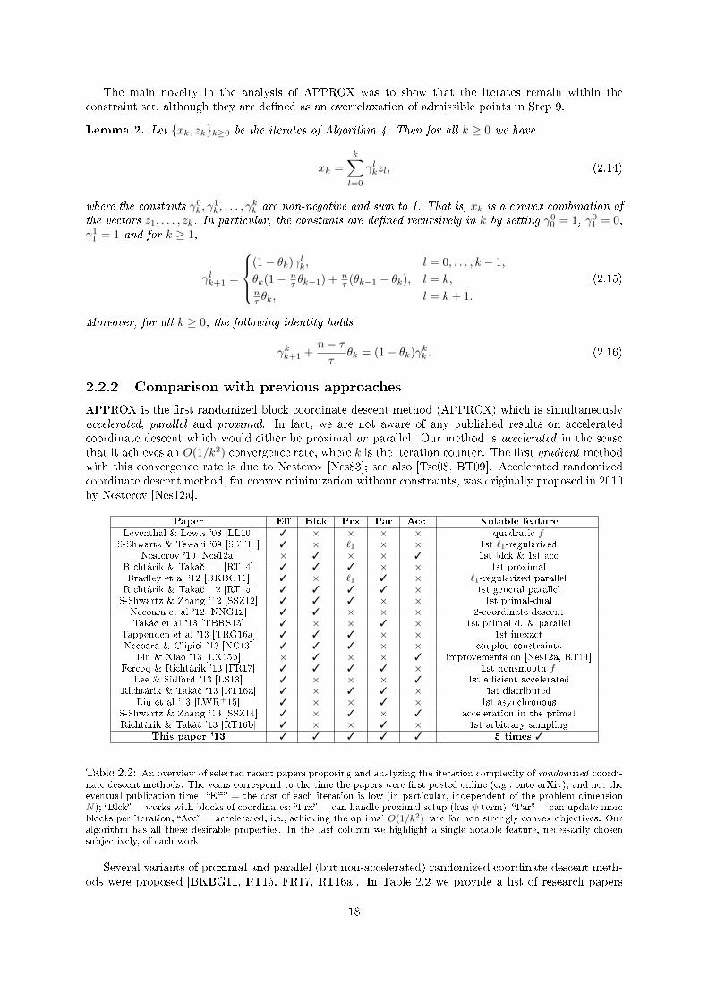
APPROX is the rst randomized block coordinate descent method (APPROX) which is simultaneouslyaccelerated, parallel and proximal. In fact, we are not aware of any published results on acceleratedcoordinate descent which would either be proximal or parallel. Our method is accelerated in the sensethat it achieves an O(1/k2) convergence rate, where k is the iteration counter. The rst gradient methodwith this convergence rate is due to Nesterov [Nes83]; see also [Tse08, BT09]. Accelerated randomizedcoordinate descent method, for convex minimization without constraints, was originally proposed in 2010by Nesterov [Nes12a].

Paper E Blck Prx Par Acc Notable feature

Leventhal & Lewis '08 [LL10] 3 × × × × quadratic fS-Shwartz & Tewari '09 [SST11] 3 × `1 × × 1st `1-regularized

Nesterov '10 [Nes12a] × 3 × × 3 1st blck & 1st accRichtárik & Taká£ '11 [RT14] 3 3 3 × × 1st proximalBradley et al '12 [BKBG11] 3 × `1 3 × `1-regularized parallelRichtárik & Taká£ '12 [RT15] 3 3 3 3 × 1st general parallelS-Shwartz & Zhang '12 [SSZ12] 3 3 3 × × 1st primal-dual

Necoara et al '12 [NNG12] 3 3 × × × 2-coordinate descentTaká£ et al '13 [TBRS13] 3 × × 3 × 1st primal-d. & parallel

Tappenden et al '13 [TRG16a] 3 3 3 × × 1st inexactNecoara & Clipici '13 [NC13] 3 3 3 × × coupled constraints

Lin & Xiao '13 [LX15b] × 3 × × 3 improvements on [Nes12a, RT14]Fercoq & Richtárik '13 [FR17] 3 3 3 3 × 1st nonsmooth f

Lee & Sidford '13 [LS13] 3 × × × 3 1st ecient acceleratedRichtárik & Taká£ '13 [RT16a] 3 × 3 3 × 1st distributed

Liu et al '13 [LWR+15] 3 × × 3 × 1st asynchronousS-Shwartz & Zhang '13 [SSZ14] 3 × 3 × 3 acceleration in the primalRichtárik & Taká£ '13 [RT16b] 3 × × 3 × 1st arbitrary sampling

This paper '13 3 3 3 3 3 5 times 3

Table 2.2: An overview of selected recent papers proposing and analyzing the iteration complexity of randomized coordi-nate descent methods. The years correspond to the time the papers were rst posted online (e.g., onto arXiv), and not theeventual publication time. E = the cost of each iteration is low (in particular, independent of the problem dimensionN); Blck = works with blocks of coordinates; Prx = can handle proximal setup (has ψ term); Par = can update moreblocks per iteration; Acc = accelerated, i.e., achieving the optimal O(1/k2) rate for non-strongly convex objectives. Ouralgorithm has all these desirable properties. In the last column we highlight a single notable feature, necessarily chosensubjectively, of each work.

Several variants of proximal and parallel (but non-accelerated) randomized coordinate descent meth-ods were proposed [BKBG11, RT15, FR17, RT16a]. In Table 2.2 we provide a list of research papers

18

proposing and analyzing randomized coordinate descent methods. The table substantiates our obser-vation that while the block (Blck column) and proximal (Prx column) setup is relatively commonin the literature, parallel methods (Par column) are much less studied, and there is just a handful ofpapers dealing with accelerated variants (Acc column). Moreover, existing accelerated methods are notecient (E column)with the exception of [LS13]

2.3 Accelerated coordinate descent in a distributed setting

More and more often in modern applications, the data describing the problem is so large that it doesnot t into the RAM of a single computer. In such a case, unless the application at hand can tolerateslow performance due to frequent HDD reads/writes, it is often necessary to distribute the data amongthe nodes of a cluster and solve the problem in a distributed manner. With such big data problems it isnecessary to design algorithms able to utilize modern parallel computing architectures. This resulted inan interest in parallel [RT15, FR17, RT16b] and distributed [RT16a] coordinate descent methods.

The core of the paper [FQRT14] forms the development of new stepsizes that improve on previousworks on parallel coordinate descent using the following assumptions on the objective function

f(x) + Ψ(x) =

m∑j=1

φj(e>j Ax) +

n∑i=1

Ψi(x(i)) .

We also assumed that the data is partitioned among c computers dealing with s coordinates each. Weassume that each computer updates τ coordinates in parallel at each iteration. We denote n = cs. Letωj be the number of nonzeros in the jth row of A and ω′j be the number of partitions active at row j,i.e., the number of indexes l ∈ 1, . . . , c for which the set i ∈ Pl : Aji 6= 0 is nonempty. As soon as Adoes not have an empty row or column, we know that 1 ≤ ωj ≤ n and 1 ≤ ω′j ≤ c.

The goal is to show that there exists computable constants v1, . . . , vn such that the ESO inequal-ity (2.10) holds:

E[f(x+ h[S])

]≤ f(x) +

τ

s

(〈∇f(x), h〉+

1

2‖h‖2v

), x, h ∈ RN .

Then the algorithm will consist in Algorithm 4 that uses the Expected Separable Overapproximation(ESO) inequality (2.10) required by Assumption 1. On top of allowing us to prove the convergence ofthe algorithm, the ESO has the following benets:

(i) Since the overapproximation is a convex quadratic in h, it is easy to compute h(x).

(ii) Since the overapproximation is block separable, one can compute the updates h(i)(x) in parallel forall i ∈ 1, 2, . . . , n.

(iii) For the same reason, one can compute the updates or i ∈ Sk only, where Sk is the sample set drawnat iteration k following the law describing S.

Finding smaller constants vi directly transfers into longer step-sizes and thus a potentially better paral-lelization speedup.

The rst proposition corresponds to the shared memory framework.

Proposition 1. Suppose that f(x) =∑mj=1 φj(e

>j Ax) and that S consists in choosing τc coordinates

uniformly at random. Then f satises the Expected Separable Overapproximation (2.10) with parameters

vi =

m∑j=1

(1 +

(ωj − 1)(τc− 1)

sc− 1

)A2ji.

The main conclusion of the study, made precise in the next proposition, is that as long as the numberof processors per computer τ ≥ 2, the eect of partitioning the data (across the nodes) on the iterationcomplexity of the algorithm is negligible, and vanishes as τ increases.

19

Proposition 2. Suppose that f(x) =∑mj=1 φj(e

>j Ax) Suppose that S consists in choosing for each

computer, τ coordinates uniformly at random among the s ones it manages. Then f satises the ExpectedSeparable Overapproximation (2.10) with parameters

vi =

n∑j=1

(1 +

(ωj − 1)(τ − 1)

s− 1+(τs− τ − 1

s− 1

)ω′j − 1

ω′jωj

)A2ji.

In [FQRT14], we gave an extensive comparison of the ESOs available in the literature and showedthat the newly proposed is much better than former ones.

2.4 Restart of accelerated gradient methods

On top of parallel processing, I also studied restarting schemes as a complementary mean of acceleration.For a mild additional computational cost, accelerated gradient methods transform the proximal gra-

dient method, for which the optimality gap F (xk) − F ? decreases as O(1/k), into an algorithm withoptimal O(1/k2) complexity [Nes83]. Accelerated variants include the dual accelerated proximal gra-dient [Nes05b, Nes13a], the accelerated proximal gradient method (APG) [Tse08] and FISTA [BT09].Gradient-type methods, also called rst-order methods, are often used to solve large-scale problems be-cause of their good scalability and easiness of implementation that facilitates parallel and distributedcomputations.

When solving a convex problem whose objective function satises a local quadratic error bound (this isa generalization of strong convexity), classical (non-accelerated) gradient and coordinate descent methodsautomatically have a linear rate of convergence, i.e. F (xk)− F ? ∈ O((1− µ)k) for a problem dependent0 < µ < 1 [NNG12, DL16], whereas one needs to know explicitly the strong convexity parameter inorder to set accelerated gradient and accelerated coordinate descent methods to have a linear rate ofconvergence, see for instance [LS13, LMH15, LLX14, Nes12a, Nes13a]. Setting the algorithm with anincorrect parameter may result in a slower algorithm, sometimes even slower than if we had not triedto set an acceleration scheme [OC12]. This is a major drawback of the method because in general, thestrong convexity parameter is dicult to estimate.

In the context of accelerated gradient method with unknown strong convexity parameter, Nes-terov [Nes13a] proposed a restarting scheme which adaptively approximates the strong convexity param-eter. The same idea was exploited by Lin and Xiao [LX15a] for sparse optimization. Nesterov [Nes13a]also showed that, instead of deriving a new method designed to work better for strongly convex func-tions, one can restart the accelerated gradient method and get a linear convergence rate. However, therestarting frequency he proposed still depends explicitly on the strong convexity of the function andso O'Donoghue and Candes [OC12] introduced some heuristics to adaptively restart the algorithm andobtain good results in practice.

The restarted algorithm is given in Algorithm 5, where APPROX(f, ψ, xr,K) means Algorithm 4run on the function f + ψ with initial point xr and for K iterations.

Algorithm 5 APPROX with restart

Choose x0 ∈ domψ and set x0 = x0.Choose RestartTimes ⊆ N.for r ≥ 0 doK = RestartTimes(r + 1) - RestartTimes(r)xr+1 = APPROX(f, ψ, xr,K)

end for

Gradient method In [FQ17], we showed that, if the objective function is convex and satises a localquadratic error bound, we can restart accelerated gradient methods at any frequency and get a linearlyconvergent algorithm. The rate depends on an estimate of the quadratic error bound and we show thatfor a wide range of this parameter, one obtains a faster rate than without acceleration. In particular, wedo not require this estimate to be smaller than the actual value. In that way, our result supports andexplains the practical success of arbitrary periodic restart for accelerated gradient methods.

20

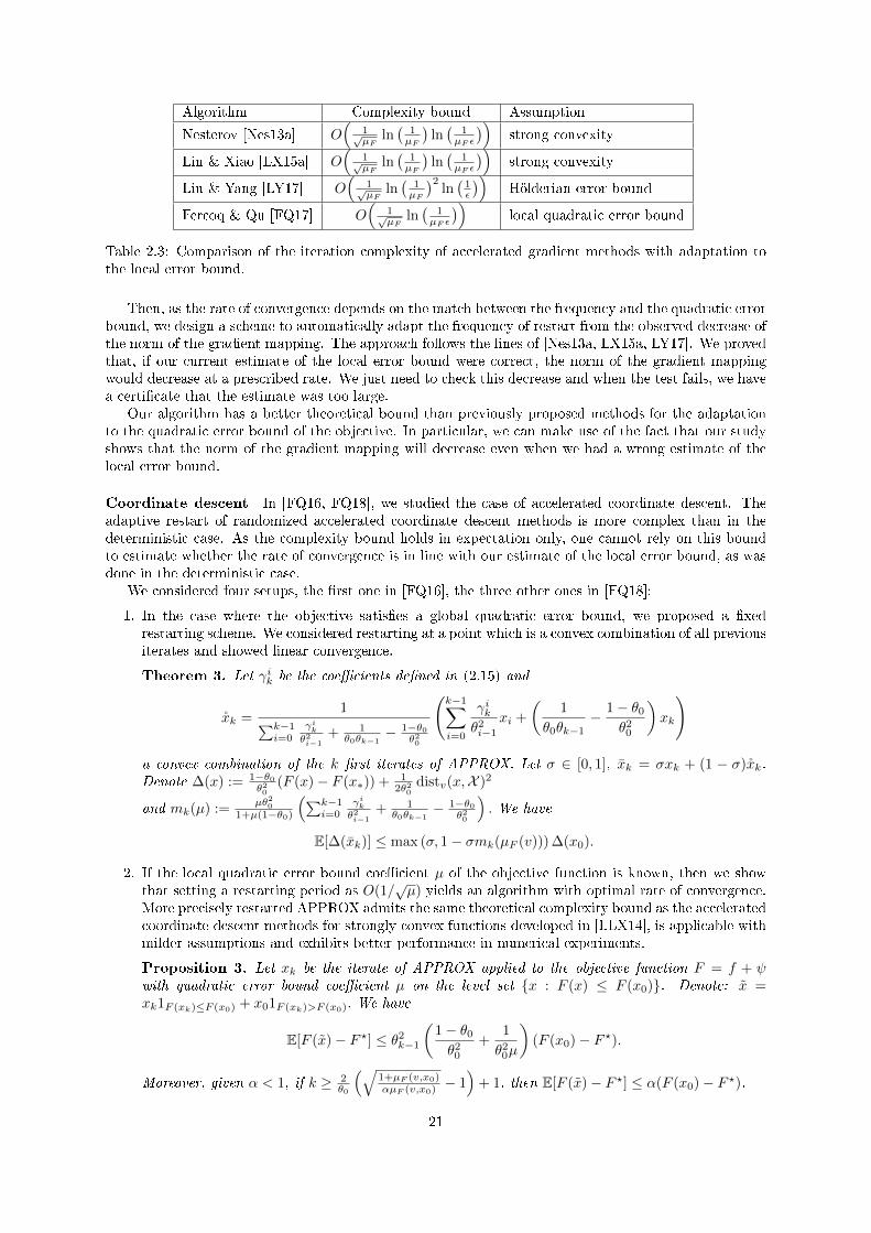
Algorithm Complexity bound Assumption

Nesterov [Nes13a] O(

1√µF

ln(

1µF

)ln(

1µF ε

))strong convexity

Lin & Xiao [LX15a] O(

1√µF

ln(

1µF

)ln(

1µF ε

))strong convexity

Liu & Yang [LY17] O(

1√µF

ln(

1µF

)2ln(

1ε

))Hölderian error bound

Fercoq & Qu [FQ17] O(

1√µF

ln(

1µF ε

))local quadratic error bound

Table 2.3: Comparison of the iteration complexity of accelerated gradient methods with adaptation tothe local error bound.

Then, as the rate of convergence depends on the match between the frequency and the quadratic errorbound, we design a scheme to automatically adapt the frequency of restart from the observed decrease ofthe norm of the gradient mapping. The approach follows the lines of [Nes13a, LX15a, LY17]. We provedthat, if our current estimate of the local error bound were correct, the norm of the gradient mappingwould decrease at a prescribed rate. We just need to check this decrease and when the test fails, we havea certicate that the estimate was too large.

Our algorithm has a better theoretical bound than previously proposed methods for the adaptationto the quadratic error bound of the objective. In particular, we can make use of the fact that our studyshows that the norm of the gradient mapping will decrease even when we had a wrong estimate of thelocal error bound.

Coordinate descent In [FQ16, FQ18], we studied the case of accelerated coordinate descent. Theadaptive restart of randomized accelerated coordinate descent methods is more complex than in thedeterministic case. As the complexity bound holds in expectation only, one cannot rely on this boundto estimate whether the rate of convergence is in line with our estimate of the local error bound, as wasdone in the deterministic case.

We considered four setups, the rst one in [FQ16], the three other ones in [FQ18]:

1. In the case where the objective satises a global quadratic error bound, we proposed a xedrestarting scheme. We considered restarting at a point which is a convex combination of all previousiterates and showed linear convergence.

Theorem 3. Let γik be the coecients dened in (2.15) and

xk =1∑k−1

i=0γikθ2i−1

+ 1θ0θk−1

− 1−θ0θ20

(k−1∑i=0

γikθ2i−1

xi +

(1

θ0θk−1− 1− θ0

θ20

)xk

)

a convex combination of the k rst iterates of APPROX. Let σ ∈ [0, 1], xk = σxk + (1 − σ)xk.Denote ∆(x) := 1−θ0

θ20

(F (x)− F (x∗)) + 12θ2

0distv(x,X )2

and mk(µ) :=µθ2

0

1+µ(1−θ0)

(∑k−1i=0

γikθ2i−1

+ 1θ0θk−1

− 1−θ0θ20

). We have

E[∆(xk)] ≤ max (σ, 1− σmk(µF (v))) ∆(x0).

2. If the local quadratic error bound coecient µ of the objective function is known, then we showthat setting a restarting period as O(1/

√µ) yields an algorithm with optimal rate of convergence.

More precisely restarted APPROX admits the same theoretical complexity bound as the acceleratedcoordinate descent methods for strongly convex functions developed in [LLX14], is applicable withmilder assumptions and exhibits better performance in numerical experiments.

Proposition 3. Let xk be the iterate of APPROX applied to the objective function F = f + ψwith quadratic error bound coecient µ on the level set x : F (x) ≤ F (x0). Denote: x =xk1F (xk)≤F (x0) + x01F (xk)>F (x0). We have

E[F (x)− F ?] ≤ θ2k−1

(1− θ0

θ20

+1

θ20µ

)(F (x0)− F ?).

Moreover, given α < 1, if k ≥ 2θ0

(√1+µF (v,x0)αµF (v,x0) − 1

)+ 1, then E[F (x)− F ?] ≤ α(F (x0)− F ?).

21

3. If the objective function is strongly convex, we show that we can restart the accelerated coordinatedescent method at the last iterate at any frequency and get a linearly convergent algorithm. Therate depends on an estimate of the local quadratic error bound and we show that for a wide range ofthis parameter, one obtains a faster rate than without acceleration. In particular, we do not requirethe estimate of the error bound coecient to be smaller than the actual value. The dierence withrespect to [FQ16] is that in this section, we show that there is no need to restart at a complexcombination of previous iterates.

Theorem 4. Denote ∆(x) = 1−θ0θ20

(F (x) − F ?) + 12θ2

0distv(x,X )2. Assume that F is µF strongly

convex. Then the iterates of APPROX satisfy

E[∆(xK)] ≤ 1 + (1− θ0)µF

1 +θ20

2θ2K−1

µF∆(x0)

4. If the local error bound coecient is not known, we introduce a variable restarting periods andshow that up to a log(log 1/ε) term, the algorithm is as ecient as if we had known the local errorbound coecient.

Theorem 5. We dene the sequence

K0 = K0 K1 = 21K0 K2 = K0 K3 = 22K0 K4 = K0 K5 = 21K0 K6 = K0 K7 = 23K0 . . .

such that K2j−1 = 2jK0, ∀j ∈ N and |l ≤ 2J −1 | Kl = 2jK0| = 2×|l ≤ 2J −1 | Kl = 2j−1K0|for all j ∈ 1, . . . J − 1, J ∈ N.

We denote δ0 = F (x0) − F ∗ and K(µF ) = 2θ0

(√1+µFe−2µF

− 1)

+ 1, where µF is the (unknown)

quadratic error bound coecient µ of F .

Suppose that the restart times are given by the variable restart periods dened above. Then theiterates of restarted APPROX satisfy E(F (xk)− F (x∗)) ≤ ε as soon as

k ≥(

max(

log(K(µF )

K0

), 0)

+ log2

( log( δ0ε )

2

)) log( δ0ε )

2max(K(µF ),K0) .

On Figure 2.1, we can see that restarting the accelerated coordinate descent clearly outperforms bothcoordinate descent and plain accelerated coordinate descent. Moreover, using a version of acceleratedcoordinate descent designed for strongly convex functions [LLX14] is not safe: it may fail to converge orbe very slow depending on the estimate of strong convexity that we are using.

2.5 Using second order information

There have been several attempts at designing methods that combine randomization with the use ofcurvature (second-order) information. For example, methods based on running coordinate ascent in thedual such as [RT15, FR17, FR15, FQRT14, QRZ15] use curvature information contained in the diagonalof a bound on the Hessian matrix. Block coordinate descent methods, when equipped with suitabledata-dependent norms for the blocks, use information contained in the block diagonal of the Hessian[TRG16b]. A more direct route to incorporating curvature information was taken by [SYG07] in theirstochastic L-BFGS method and by [BHNS14] and [SDPG14] in their stochastic quasi-Newton methods.Complexity estimates are not easy to nd. An exception in this regard is the work of [BBG09], who givea O(1/ε) complexity bound for a Quasi-Newton SGD method.

An alternative approach is to consider block coordinate descent methods with overlapping blocks [TY09a,FT15]. While typically ecient in practice, none of the methods mentioned above are equipped withcomplexity bounds (bounds on the number of iterations). Tseng and Yun [TY09a] only showed conver-gence to a stationary point and focus on non-overlapping blocks for the rest of their paper. Numericalevidence that this approach is promising is provided in [FT15] with some mild convergence rate resultsbut no iteration complexity.

The main contribution of the work [QRTF16] is the analysis of stochastic block coordinate descentmethods with overlapping blocks. We then instantiate this to get a new algorithmStochastic Dual

22

0 1000 2000 3000 4000 5000 6000

time

10-8

10-6

10-4

10-2

100

102

104

log

(Prim

al D

ua

l G

ap

)

rcv1 λ1

=10000

COORDINATE DESCENT

APPROX

APCG mu = 1e-3

APCG mu = 1e-5

APCG mu = 1e-7

PROX-NEWTON

Variable restart APPROX mu0 = 1e-2

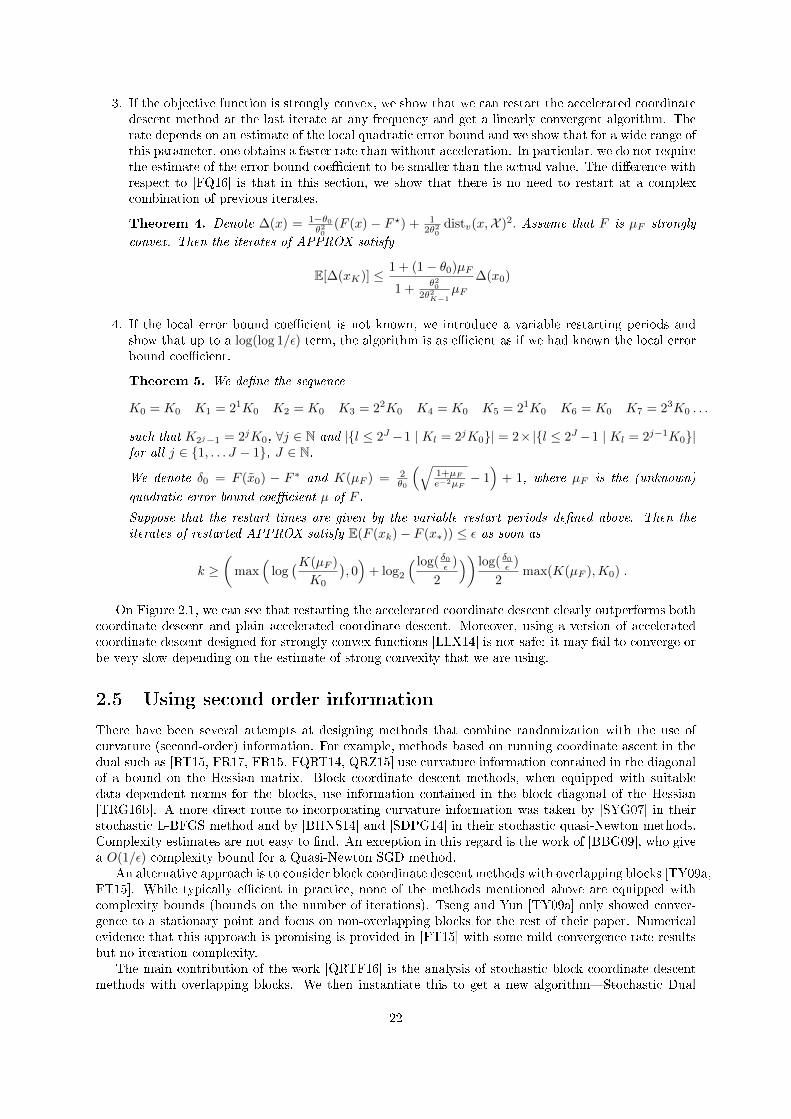
Figure 2.1: Comparison of (accelerated) coordinate descent algorithms for the logistic regression problemon the dataset RCV1: coordinate descent, APPROX, APCG [LLX14] with µ ∈ 10−3, 10−5, 10−7, Prox-Newton [LSS12] and APPROX with variable restart initiated with K0 = K(10−2).

Newton Ascent (SDNA)for solving a regularized Empirical Risk Minimization problem with smoothloss functions and a strongly convex regularizer (primal problem). Our method is stochastic in natureand has the capacity to utilize all curvature information inherent in the data.

SDNA in each iteration picks a random subset of the dual variables (which corresponds to picking aminibatch of examples in the primal problem), following an arbitrary probability law, and maximizes,exactly, the dual objective restricted to the random subspace spanned by the coordinates. Equivalently,this can be seen as the solution of a proximal subproblem involving a random principal submatrix ofthe Hessian of the quadratic function. Hence, SDNA utilizes all curvature information available in therandom subspace in which it operates. Note that this is very dierent from the update strategy of parallel/ minibatch coordinate descent methods. Indeed, while these methods also update a random subset ofvariables in each iteration, they instead only utilize curvature information present in the diagonal of theHessian.

In the case of quadratic loss, and when viewed as a primal method, SDNA can be interpreted as avariant of the Iterative Hessian Sketch algorithm [PW14].

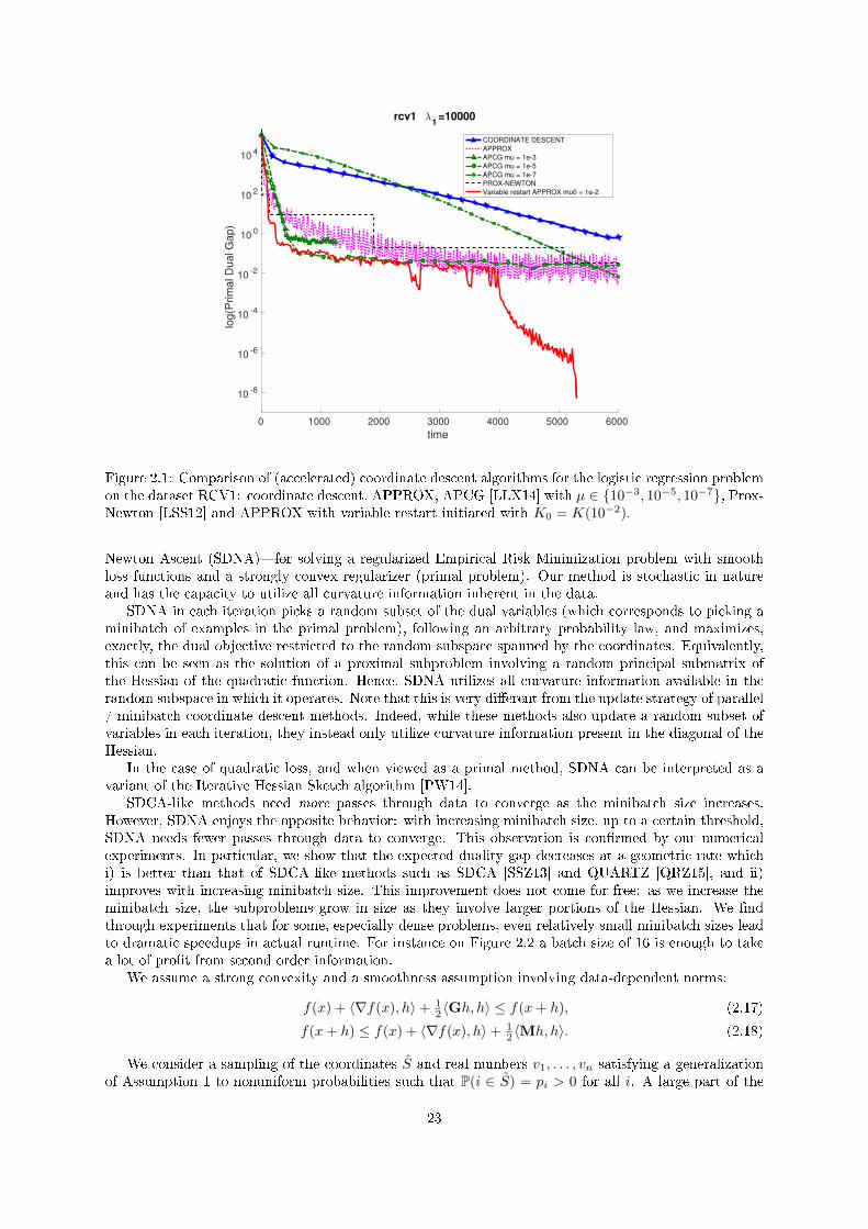
SDCA-like methods need more passes through data to converge as the minibatch size increases.However, SDNA enjoys the opposite behavior: with increasing minibatch size, up to a certain threshold,SDNA needs fewer passes through data to converge. This observation is conrmed by our numericalexperiments. In particular, we show that the expected duality gap decreases at a geometric rate whichi) is better than that of SDCA-like methods such as SDCA [SSZ13] and QUARTZ [QRZ15], and ii)improves with increasing minibatch size. This improvement does not come for free: as we increase theminibatch size, the subproblems grow in size as they involve larger portions of the Hessian. We ndthrough experiments that for some, especially dense problems, even relatively small minibatch sizes leadto dramatic speedups in actual runtime. For instance on Figure 2.2 a batch size of 16 is enough to takea lot of prot from second order information.

We assume a strong convexity and a smoothness assumption involving data-dependent norms:

f(x) + 〈∇f(x), h〉+ 12 〈Gh, h〉 ≤ f(x+ h), (2.17)

f(x+ h) ≤ f(x) + 〈∇f(x), h〉+ 12 〈Mh, h〉. (2.18)

We consider a sampling of the coordinates S and real numbers v1, . . . , vn satisfying a generalizationof Assumption 1 to nonuniform probabilities such that P(i ∈ S) = pi > 0 for all i. A large part of the

23

0 200 400 600 800 1000

10−15

10−10

10−5

100

cov

Elapsed Time [s]

Du

alit

y G

ap

SDNA 1

SDNA 4

SDNA 16

SDNA 32

SDNA 64

Figure 2.2: Runtime of SDNA for minibatch sizes τ = 1, 4, 16, 32, 64 for a L2-regularized least squaresproblem on the cov dataset: d = 54, n = 522, 911).

paper consists in comparing three quantities:

σ1 := λmin

(G1/2E

[(MS

)†]G1/2

), (2.19)

σ2 := λmin

(G1/2D(p)

(E[MS

])−1D(p)G1/2

), (2.20)

σ3 := λmin

(G1/2D(p)D(v−1)G1/2

), (2.21)

where λmin stands for the smallest eigenvalue. We show that SDNA converges linearly as E[f(xk+1) −f(x∗)] ≤ (1 − σ1)E[f(xk) − f(x∗)] while the parallel coordinate descent method (PCDM) converges asE[f(xk+1) − f(x∗)] ≤ (1 − σ3)E[f(xk) − f(x∗)]. Moreover, as σ1 ≥ σ2 ≥ σ3, the worst case complexityindicates that SDNA should be faster than PCDM. We went even further by showing that as the numberof processors τ increases, σ1(τ) ≥ τσ1(1) = τσ3(1) ≥ σ3(τ). In particular, SDNA enjoys superlinearspeedup in τ , to be compared with the sublinear speedup of PCDM.

24

Chapter 3

Coordinate descent methods for saddle

point problems

We now turn to convex optimization problems of the form

minx∈X

f(x) + g(x) + h(Mx), (3.1)

where x = (x(1), . . . , x(n)) ∈ X = X1 × . . . × Xn is a decision vector composed of n blocks f is adierentiable convex function with coordinate-wise Lipschitz gradients, g : X → R∪ +∞ and h : Y →R∪+∞ are convex and lower semicontinous functions andM : X → Y is a continuous linear operator.We also assume that Y = Y1 × . . .× Yp for some integer p.

Under the standard qualication condition 0 ∈ ri(M dom g − domh) (where dom and ri are thedomain and the relative interior), a point x ∈ X is a minimizer of (3.1) if and only if there exists y ∈ Ysuch that (x, y) is a saddle point of the Lagrangian function

L(x, y) = f(x) + g(x) + 〈y,Mx〉 − h?(y)

where h? : y 7→ supz∈Y〈y, z〉 − h(z) is the Fenchel-Legendre transform of h.Problem (3.1) is much more general than Problem (2.1) that we studied in the previous chapter.

It allows us to consider nonsmooth nonseparable objectives, containing for instance linear equality andinequality constraints. Indeed, it provides a unied formulation for a broad set of applications in variousdisciplines, see, e.g., [BT89, BV04, CBS14, CRPW12, MCTD+14, NW06, Wai14]. While problem (3.1)is presented in the unconstrained form, it automatically covers constrained settings by means of indicatorfunctions. For example, (3.1) covers the following prototypical optimization template via h(z) := δb(z)(i.e., the indicator function of the convex set b):

minx∈X

f(x) + g(x) + δb(Ax)

= minx∈X

f(x) + g(x) : Ax = b

, (3.2)

Note that (3.2) is suciently general to cover standard convex optimization subclasses, such as conicprogramming, monotropic programming, and geometric programming, as specic instances [BTN01,Ber96, BPC+11b].

In the rst section of this chapter, we study a primal dual coordinate descent method based on a xedpoint operator. The other sections are devoted to methods based on a smoothing technique. We studyparallel coordinate descent for smoothed nonsmooth functions, a generalization of Nesterov's smoothingtechnique to linear equality constraints and a second primal-dual coordinate descent with a very goodworst case guarantee.

3.1 A coordinate descent version of the Vu Condat method with

long step sizes

3.1.1 Introduction

There is a rich literature on primal-dual algorithms searching for a saddle point of L (see [TC14] andreferences therein). In the special case where f = 0, the alternating direction method of multipliers

25

(ADMM) proposed by Glowinsky and Marroco [GM75], Gabay and Mercier [GM76] and the algorithmof Chambolle and Pock [CP11] are amongst the most celebrated ones. Based on an elegant idea alsoused in [HY12], Vu [Vu13] and Condat [Con13] separately proposed a primal-dual algorithm allowingas well to handle ∇f explicitly, and requiring one evaluation of the gradient of f at each iteration.Hence, the ∇f is handled explicitly in the sense that the algorithm does not involve, for instance, thecall of a proximity operator associated with f . A convergence rate analysis is provided in [CP15a] (seealso [TC14]). A related splitting method has been recently introduced by [DY15].

The paper [FB19] introduces a coordinate descent (CD) version of the Vu-Condat algorithm. Bycoordinate descent, we mean that only a subset of the coordinates of the primal and dual iterates isupdated at each iteration, the other coordinates being maintained to their past value. Coordinate descentwas historically used in the context of coordinate-wise minimization of a unique function in a Gauss-Seidel sense [War63, BT89, Tse01]. Tseng et al. [LT02, TY09a, TY09b] and Nesterov [Nes12a] developpedCD versions of the gradient descent. In [Nes12a] as well as in this paper, the updated coordinates arerandomly chosen at each iteration. The algorithm of [Nes12a] has at least two interesting features. Notonly it is often easier to evaluate a single coordinate of the gradient vector rather than the whole vector,but the conditions under which the CD version of the algorithm is provably convergent are generallyweaker than in the case of standard gradient descent. The key point is that the step size used in thealgorithm when updating a given coordinate i can be chosen to be inversely proportional to the coordinate-wise Lipschitz constant of ∇f along its ith coordinate, rather than the global Lipschitz constant of ∇f(as would be the case in a standard gradient descent). Hence, the introduction of coordinate descentallows to use longer step sizes which potentially results in a more attractive performance. The randomCD gradient descent of [Nes12a] was later generalized by Richtárik and Taká£ [RT14] to the minimizationof a sum of two convex functions f + g (that is, h = 0 in problem (3.1)). The algorithm of [RT14] isanalyzed under the additional assumption that function g is separable in the sense that for each x ∈ X ,g(x) =

∑ni=1 gi(x

(i)) for some functions gi : Xi →]−∞,+∞].

In the literature, several papers seek to apply the principle of coordinate descent to primal-dualalgorithms. In the case where f = 0, h is separable and smooth and g is strongly convex, Zhang andXiao [ZX14] introduce a stochastic CD primal-dual algorithm and analyze its convergence rate (seealso [Suz14] for related works). In 2013, Iutzeler et al. [IBCH13] proved that random coordinate descentcan be successfully applied to xed point iterations of rmly non-expansive (FNE) operators. Accordingto [Gab83], the ADMM can be written as a xed point algorithm of a FNE operator, which led theauthors of [IBCH13] to propose a coordinate descent version of ADMM with application to distributedoptimization. The key idea behind the convergence proof of [IBCH13] is to establish the so-calledstochastic Fejér monotonicity of the sequence of iterates as noted by [CP15b]. In a more general settingthan [IBCH13], Combettes et al. in [CP15b] and Bianchi et al. [BHF14] extend the proof to the so-called α-averaged operators, which include FNE operators as a special case. This generalization allowsto apply the coordinate descent principle to a broader class of primal-dual algorithms which is no longerrestricted to the ADMM or the Douglas Rachford algorithm. For instance, Forward-Backward splitting isconsidered in [CP15b] and particular cases of the Vu-Condat algorithm are considered in [BHF14, PR15].Nevertheless, the above approach has two major limitations.

First, in order to derive a converging coordinate descent version of a given deterministic algorithm, thelatter must write as a xed point algorithm over some product Hilbert space of the form H = H1×· · ·Hq

where the inner product in H is the sum of the inner products in the Hi's. Unfortunately, this conditiondoes not hold in general for the Vu-Condat method, because the inner product over H involves thecoupling linear operator M . A workaround was proposed in [BHF14] but for a particular example only.

Second and even more importantly, the approach of [IBCH13, CP15b, BHF14, PR15] needs smallstep sizes. More precisely, the convergence conditions are identical to the ones of the brute method, theone without coordinate descent. These conditions involve the global Lipschitz constant of the gradient∇f instead than its coordinate-wise Lipschitz constants. In practice, it means that the application ofcoordinate descent to primal-dual algorithm as suggested by [CP15b] and [BHF14] is restricted to theuse of potentially small step sizes. One of the major benets of coordinate descent is lost.

Some recent works also focused on designing primal-dual coordinate descent methods with a guar-anteed convergence rate. In [GXZ19] and [CERS18], a O(1/k) rate is obtained for the ergodic mean ofthe sequences. The rates are given in terms of feasibility and optimality or Bregman distance. Thosetwo papers require all the dual variables to be updated at each iteration, which may not be ecient ifthere are more than a few dual variables. In the present paper, we will have much more exibility in the

26

variables we choose to update at each iteration, while retaining a provable convergence rate.Our main contribution is to provide a CD primal-dual algorithm with a broad range of admissible

step sizes. Our numerical experiments show that remarkable performance gains can be obtained whenusing larger step sizes. We also identify two setups for which the structure of the problem is favorable tocoordinate descent algorithms. Finally, we prove a sublinear rate of convergence in general and a linearrate of convergence if the objective enjoys strong convexity properties.

3.1.2 Main algorithm and convergence theorem

Consider Problem (3.1). We note M = (Mj,i : j ∈ 1, . . . , p, i ∈ 1, . . . , n) where Mj,i : Xi → Yj arethe block components of M . For each j ∈ 1, . . . , p, we introduce the set I(j) :=

i ∈ 1, . . . , n :

Mj,i 6= 0. Otherwise stated, the jth component of vectorMx only depends on x through the coordinates

x(i) such that i ∈ I(j). We denote by mj := card(I(j)) the number of such coordinates. Without loss ofgenerality, we assume that mj 6= 0 for all j. We also denote πj := 1

card(I(j)) .

For all i ∈ 1, . . . , n, we dene J(i) :=j ∈ 1, . . . , p : Mj,i 6= 0

. Note that for every pair (i, j),

the statements i ∈ I(j) and j ∈ J(i) are equivalent.Let σ = (σ1, . . . , σp) and τ = (τ1, . . . , τn) be two tuples of positive real numbers. Consider an

independent and identically distributed sequence (ik : k ∈ N∗) with uniform distribution on 1, . . . , n(the results of this paper easily extend to the selection of several primal coordinates at each iterationwith a uniform samplings of the coordinates, using the techniques introduced in [RT15]). The proposedprimal-dual coordinate descent algorithm consists in updating two sequences xk ∈ X , yk ∈ Y. It isprovided in Algorithm 6 below.

Algorithm 6 Coordinate-descent primal-dual algorithm

Initialization: Choose x0 ∈ X , y0 ∈ Y.Iteration k: Dene:

yk+1 = proxσ,h?(yk +D(σ)Mxk

)xk+1 = proxτ,g

(xk −D(τ)

(∇f(xk) + 2M?yk+1 −M?yk

) ).

For i = ik+1 and for each j ∈ J(ik+1), update:

x(i)k+1 = x

(i)k+1

y(j)k+1 = y

(j)k + πj(y

(j)k+1 − y

(j)k ) .

Otherwise, set x(i′)k+1 = x

(i′)k , and y

(j′)k+1 = y

(j′)k .

Our convergence result holds under the following assumptions.

Assumption 2. 1. The functions f , g, h are closed proper and convex.

2. The function f is dierentiable on X .

3. For every i ∈ 1, . . . , n, there exists βi ≥ 0 such that for any x ∈ X , any u ∈ Xi,

f(x+ Uiu) ≤ f(x) + 〈∇f(x), Uiu〉+βi2‖u‖2Xi .

4. The random sequence (ik)k∈N∗ is independent, uniformly distributed on 1, . . . , n.

5. The step sizes τ = (τ1, . . . , τn) and σ = (σ1, . . . , σp) satisfy for all i ∈ 1, . . . , n,

τi <1

βi + ρ(∑

j∈J(i)(2− πj)mjσjM?j,iMj,i

) .27

We denote by S the set of saddle points of the Lagrangian function L. Otherwise stated, a couple(x∗, y∗) ∈ X × Y lies in S if and only if it satises the following inclusions

0 ∈ ∇f(x∗) + ∂g(x∗) +M?y∗ (3.3)

0 ∈ −Mx∗ + ∂h?(y∗) . (3.4)

We shall also refer to elements of S as primal-dual solutions.

Theorem 6. Let Assumption 2 hold true and suppose that S 6= ∅. Let (xk, yk) be a sequence generatedby Algorithm 6. Almost surely, there exists (x∗, y∗) ∈ S such that

limk→∞

xk = x∗

limk→∞

yk = y∗ .

In order to prove this result, we introduced the concept of duplication of dual variables. Indeed, asnoted in the introduction, the squared norm with which distances are measured in Vu and Condat's proofis not separable. This poses a major diculty in the analysis of coordinate descent, that we circumventedby allowing nonseparable objective functions. When mj > 1, i.e. the dual variable y(j) inuences severalprimal variables x(i), i ∈ I(j), we articially duplicate the dual variable y(j) into a vector of size mj

denoted by (y(j)(i))i∈I(j). In order to get an equivalent problem, we replace h by h that forces the

constraint y(j)(i) = y(j)(i′) for all i, i′ ∈ I(j). In this equivalent problem, mj = 1 for all j and we candene a separable squared norm. This allows us to prove the convergence of the algorithm with theduplicated dual space and then Theorem 6 by showing that both algorithm are in fact the same.

Ecient implementation using problem structure In Algorithm 6, it is worth noting that quan-tities (xk+1, yk+1) do not need to be explicitly calculated. At iteration k, only the coordinates

x(ik+1)k+1 and y

(j)k+1, ∀j ∈ J(ik+1)

are needed to perform the update. From a computational point of view, it is often the case that theevaluation of the above coordinates is less demanding than the computation of the whole vectors xk+1,yk+1. Two situations have been reported in the literature:

• If g is separable, one only needs to compute the quantities ∇ik+1f(xk), (2M?yk+1 −M?yk)(ik+1)

and proxτik+1,gik+1

to perform the kth iteration. A classical example of such smart residual up-

date [Nes12b] can be found in the proximal coordinate descent gradient algorithm (case g separableand h = 0) [RT14]. More generally, if g (resp. h?) is block-separable, we can use this structure inthe algorithm, even if this block structure does not match X1 × . . .×Xn (resp. Y1 × . . .× Yp).We used this idea in Figure 3.1 to deal eciently with the proximal operator of the `2,1 norm.

• If g is the indicator of the consensus constraint x1 = · · · = xn, f is separable and h = 0, werecover MISO [Mai15]. In that case, we can store ∇f(xk) and update its average. Thanks to theseparability of f , only one coordinate of ∇f(xk) needs to be updated at each iteration.

We used similar ideas in Figure 3.2 to deal eciently with the projection onto the subspace or-thogonal to a vector.

To illustrate the importance of these implementation tricks, we give in Table 3.1 a comparison of thenumber of operations to compute the updates of the standard Vu-Condat method against the proposedalgorithm.

3.1.3 Convergence rate

We present below the convergence guarantee for Algorithm 6. It is of the same order as what can beobtained by other primal-dual methods like the ADMM [DY17], i.e. O(1/

√k) in general. Note that the

result holds for the sequence (xk) only, since xk may not be feasible by design.

28

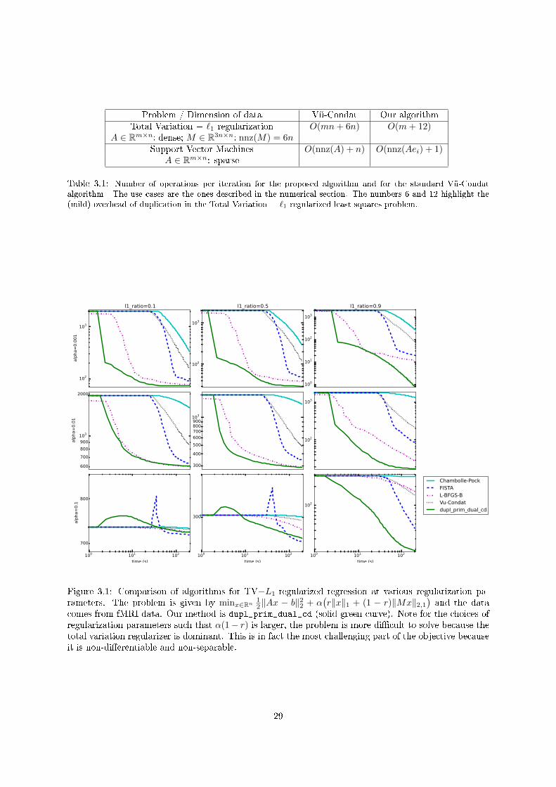
Problem / Dimension of data Vu-Condat Our algorithmTotal Variation + `1 regularization O(mn+ 6n) O(m+ 12)

A ∈ Rm×n: dense; M ∈ R3n×n: nnz(M) = 6nSupport Vector Machines O(nnz(A) + n) O(nnz(Aei) + 1)

A ∈ Rm×n: sparse

Table 3.1: Number of operations per iteration for the proposed algorithm and for the standard Vu-Condatalgorithm - The use cases are the ones described in the numerical section. The numbers 6 and 12 highlight the(mild) overhead of duplication in the Total Variation + `1 regularized least squares problem.

102

103

alpha=0.001

l1_ratio=0.1

102

103

l1_ratio=0.5

100

101

102

103

l1_ratio=0.9

103

600

700

800

900

2000

alpha=0.01 103

300

400

500

600

700800900

102

103

100 101 102

time (s)

700

800

alpha=0.1

100 101 102

time (s)

300

100 101 102

time (s)

102

Chambolle-PockFISTAL-BFGS-BVu-Condatdupl_prim_dual_cd

Figure 3.1: Comparison of algorithms for TV+L1-regularized regression at various regularization pa-rameters. The problem is given by minx∈Rn

12‖Ax − b‖22 + α

(r‖x‖1 + (1 − r)‖Mx‖2,1

)and the data

comes from fMRI data. Our method is dupl_prim_dual_cd (solid green curve). Note for the choices ofregularization parameters such that α(1− r) is larger, the problem is more dicult to solve because thetotal variation regularizer is dominant. This is in fact the most challenging part of the objective becauseit is non-dierentiable and non-separable.

29

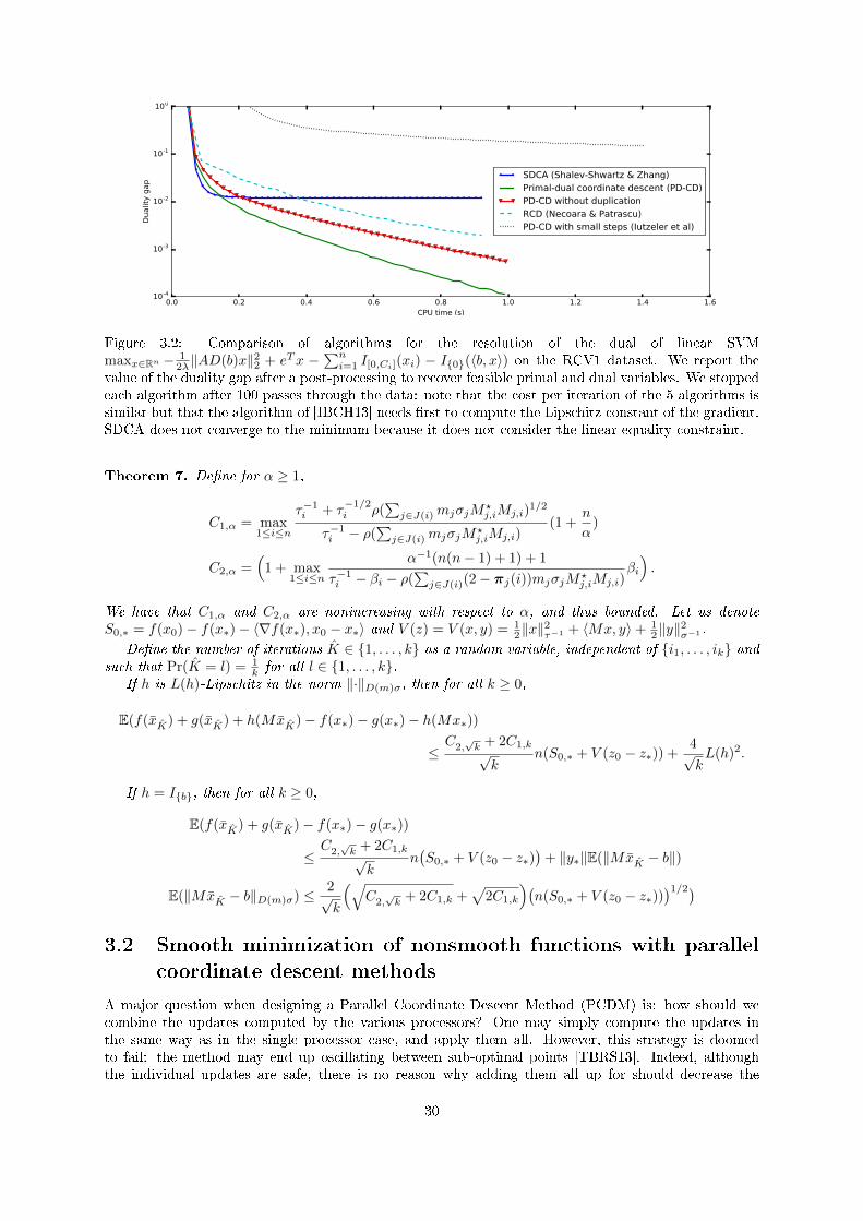
0.0 0.2 0.4 0.6 0.8 1.0 1.2 1.4 1.6CPU time (s)

10-4

10-3

10-2

10-1

100

Dualit

y g

ap

SDCA (Shalev-Shwartz & Zhang)Primal-dual coordinate descent (PD-CD)PD-CD without duplicationRCD (Necoara & Patrascu)PD-CD with small steps (Iutzeler et al)

Figure 3.2: Comparison of algorithms for the resolution of the dual of linear SVMmaxx∈Rn − 1

2λ‖AD(b)x‖22 + eTx −∑ni=1 I[0,Ci](xi) − I0(〈b, x〉) on the RCV1 dataset. We report the

value of the duality gap after a post-processing to recover feasible primal and dual variables. We stoppedeach algorithm after 100 passes through the data: note that the cost per iteration of the 5 algorithms issimilar but that the algorithm of [IBCH13] needs rst to compute the Lipschitz constant of the gradient.SDCA does not converge to the minimum because it does not consider the linear equality constraint.

Theorem 7. Dene for α ≥ 1,

C1,α = max1≤i≤n

τ−1i + τ

−1/2i ρ(

∑j∈J(i)mjσjM

?j,iMj,i)

1/2

τ−1i − ρ(

∑j∈J(i)mjσjM?

j,iMj,i)(1 +

n

α)

C2,α =(

1 + max1≤i≤n

α−1(n(n− 1) + 1) + 1

τ−1i − βi − ρ(

∑j∈J(i)(2− πj(i))mjσjM?

j,iMj,i)βi

).

We have that C1,α and C2,α are nonincreasing with respect to α, and thus bounded. Let us denoteS0,∗ = f(x0)− f(x∗)− 〈∇f(x∗), x0 − x∗〉 and V (z) = V (x, y) = 1

2‖x‖2τ−1 + 〈Mx, y〉+ 1

2‖y‖2σ−1 .

Dene the number of iterations K ∈ 1, . . . , k as a random variable, independent of i1, . . . , ik andsuch that Pr(K = l) = 1

k for all l ∈ 1, . . . , k.If h is L(h)-Lipschitz in the norm ‖·‖D(m)σ, then for all k ≥ 0,

E(f(xK) + g(xK) + h(MxK)− f(x∗)− g(x∗)− h(Mx∗))

≤C2,√k + 2C1,k√k

n(S0,∗ + V (z0 − z∗)) +4√kL(h)2.

If h = Ib, then for all k ≥ 0,

E(f(xK) + g(xK)− f(x∗)− g(x∗))

≤C2,√k + 2C1,k√k

n(S0,∗ + V (z0 − z∗)

)+ ‖y∗‖E(‖MxK − b‖)

E(‖MxK − b‖D(m)σ) ≤ 2√k

(√C2,√k + 2C1,k +

√2C1,k

)(n(S0,∗ + V (z0 − z∗))

)1/2)3.2 Smooth minimization of nonsmooth functions with parallel

coordinate descent methods

A major question when designing a Parallel Coordinate Descent Method (PCDM) is: how should wecombine the updates computed by the various processors? One may simply compute the updates inthe same way as in the single processor case, and apply them all. However, this strategy is doomedto fail: the method may end up oscillating between sub-optimal points [TBRS13]. Indeed, althoughthe individual updates are safe, there is no reason why adding them all up for should decrease the

30

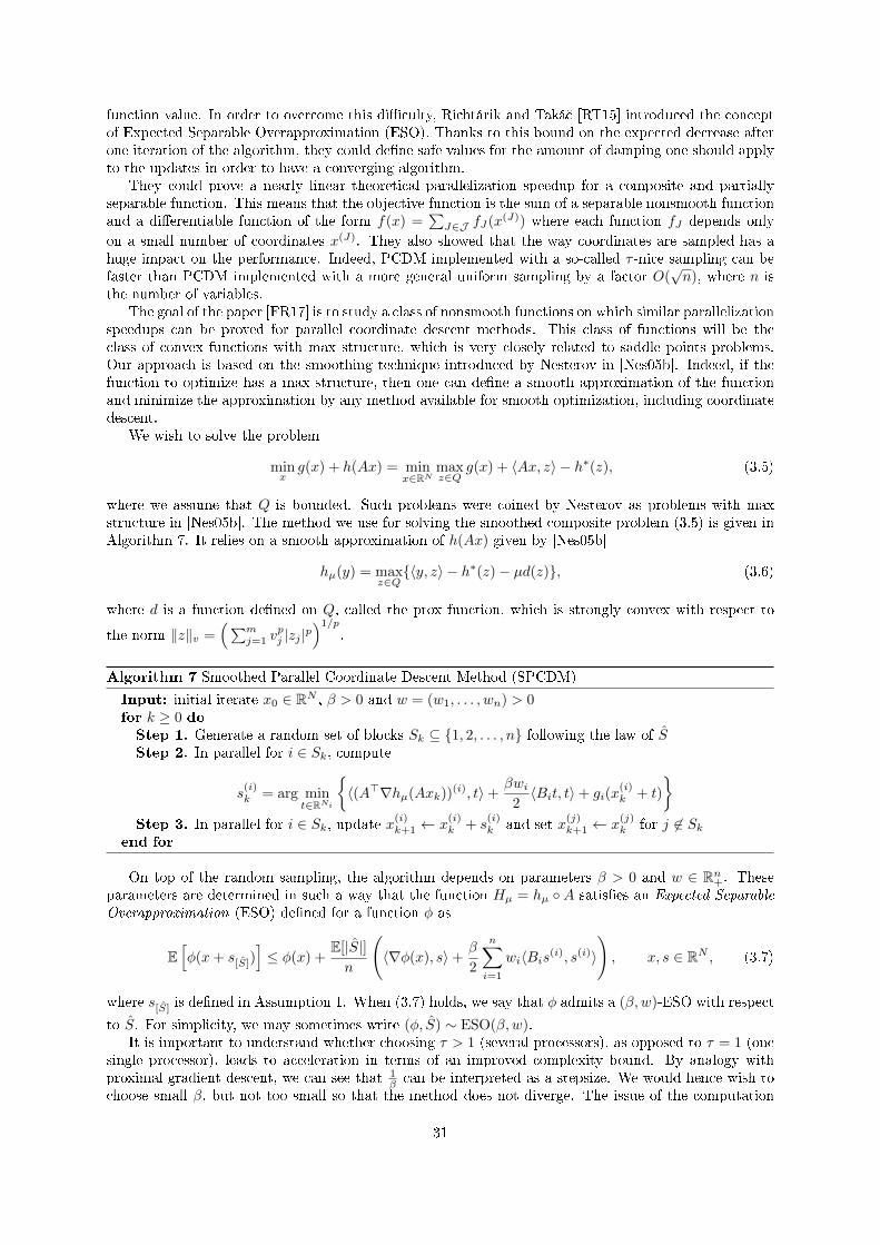
function value. In order to overcome this diculty, Richtárik and Taká£ [RT15] introduced the conceptof Expected Separable Overapproximation (ESO). Thanks to this bound on the expected decrease afterone iteration of the algorithm, they could dene safe values for the amount of damping one should applyto the updates in order to have a converging algorithm.

They could prove a nearly linear theoretical parallelization speedup for a composite and partiallyseparable function. This means that the objective function is the sum of a separable nonsmooth functionand a dierentiable function of the form f(x) =

∑J∈J fJ(x(J)) where each function fJ depends only

on a small number of coordinates x(J). They also showed that the way coordinates are sampled has ahuge impact on the performance. Indeed, PCDM implemented with a so-called τ -nice sampling can befaster than PCDM implemented with a more general uniform sampling by a factor O(

√n), where n is

the number of variables.The goal of the paper [FR17] is to study a class of nonsmooth functions on which similar parallelization

speedups can be proved for parallel coordinate descent methods. This class of functions will be theclass of convex functions with max structure, which is very closely related to saddle points problems.Our approach is based on the smoothing technique introduced by Nesterov in [Nes05b]. Indeed, if thefunction to optimize has a max-structure, then one can dene a smooth approximation of the functionand minimize the approximation by any method available for smooth optimization, including coordinatedescent.

We wish to solve the problem

minxg(x) + h(Ax) = min

x∈RNmaxz∈Q

g(x) + 〈Ax, z〉 − h∗(z), (3.5)

where we assume that Q is bounded. Such problems were coined by Nesterov as problems with maxstructure in [Nes05b]. The method we use for solving the smoothed composite problem (3.5) is given inAlgorithm 7. It relies on a smooth approximation of h(Ax) given by [Nes05b]

hµ(y) = maxz∈Q〈y, z〉 − h∗(z)− µd(z), (3.6)

where d is a function dened on Q, called the prox function, which is strongly convex with respect to

the norm ‖z‖v =(∑m

j=1 vpj |zj |p

)1/p

.

Algorithm 7 Smoothed Parallel Coordinate Descent Method (SPCDM)

Input: initial iterate x0 ∈ RN , β > 0 and w = (w1, . . . , wn) > 0for k ≥ 0 doStep 1. Generate a random set of blocks Sk ⊆ 1, 2, . . . , n following the law of SStep 2. In parallel for i ∈ Sk, compute

s(i)k = arg min

t∈RNi

〈(A>∇hµ(Axk))(i), t〉+

βwi2〈Bit, t〉+ gi(x

(i)k + t)

Step 3. In parallel for i ∈ Sk, update x(i)

k+1 ← x(i)k + s

(i)k and set x

(j)k+1 ← x

(j)k for j 6∈ Sk

end for

On top of the random sampling, the algorithm depends on parameters β > 0 and w ∈ Rn+. Theseparameters are determined in such a way that the function Hµ = hµ A satises an Expected SeparableOverapproximation (ESO) dened for a function φ as

E[φ(x+ s[S])

]≤ φ(x) +

E[|S|]n

(〈∇φ(x), s〉+

β

2

n∑i=1

wi〈Bis(i), s(i)〉

), x, s ∈ RN , (3.7)

where s[S] is dened in Assumption 1. When (3.7) holds, we say that φ admits a (β,w)-ESO with respect

to S. For simplicity, we may sometimes write (φ, S) ∼ ESO(β,w).It is important to understand whether choosing τ > 1 (several processors), as opposed to τ = 1 (one

single processor), leads to acceleration in terms of an improved complexity bound. By analogy withproximal gradient descent, we can see that 1

β can be interpreted as a stepsize. We would hence wish tochoose small β, but not too small so that the method does not diverge. The issue of the computation

31

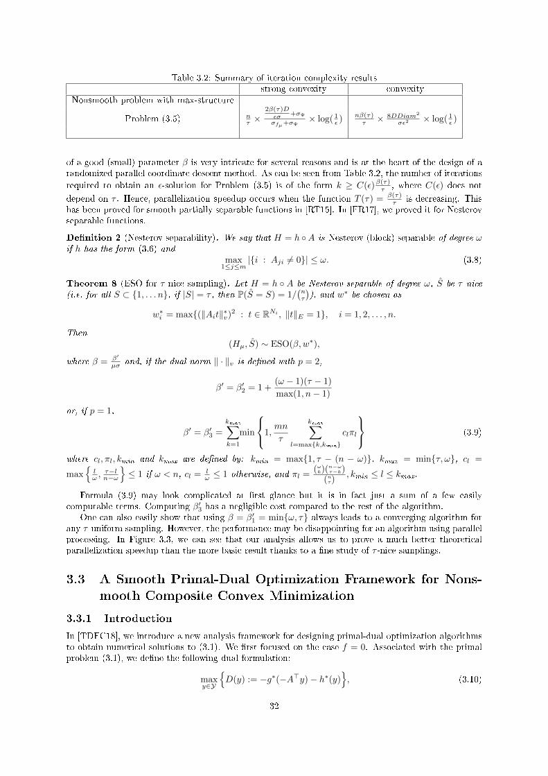
Table 3.2: Summary of iteration complexity resultsstrong convexity convexity

Nonsmooth problem with max-structure

Problem (3.5) nτ ×

2β(τ)Dεσ +σΨ

σfµ+σΨ× log( 1

ε ) nβ(τ)τ × 8DDiam2

σε2 × log( 1ε )

of a good (small) parameter β is very intricate for several reasons and is at the heart of the design of arandomized parallel coordinate descent method. As can be seen from Table 3.2, the number of iterations

required to obtain an ε-solution for Problem (3.5) is of the form k ≥ C(ε)β(τ)τ , where C(ε) does not

depend on τ . Hence, parallelization speedup occurs when the function T (τ) = β(τ)τ is decreasing. This

has been proved for smooth partially separable functions in [RT15]. In [FR17], we proved it for Nesterovseparable functions.

Denition 2 (Nesterov separability). We say that H = h A is Nesterov (block) separable of degree ωif h has the form (3.6) and

max1≤j≤m

|i : Aji 6= 0| ≤ ω. (3.8)

Theorem 8 (ESO for τ -nice sampling). Let H = h A be Nesterov separable of degree ω, S be τ -nice(i.e. for all S ⊂ 1, . . . n, if |S| = τ , then P(S = S) = 1/

(nτ

)), and w∗ be chosen as

w∗i = max(‖Ait‖∗v)2 : t ∈ RNi , ‖t‖E = 1, i = 1, 2, . . . , n.

Then(Hµ, S) ∼ ESO(β,w∗),

where β = β′

µσ and, if the dual norm ‖ · ‖v is dened with p = 2,

β′ = β′2 = 1 +(ω − 1)(τ − 1)

max(1, n− 1)

or, if p = 1,

β′ = β′3 =

kmax∑k=1

min

1,mn

τ

kmax∑l=maxk,kmin

clπl

(3.9)

where cl, πl, kmin and kmax are dened by: kmin = max1, τ − (n − ω), kmax = minτ, ω, cl =

maxlω ,

τ−ln−ω

≤ 1 if ω < n, cl = l

ω ≤ 1 otherwise, and πl =(ωk)(

n−ωτ−k)

(nτ), kmin ≤ l ≤ kmax.

Formula (3.9) may look complicated at rst glance but it is in fact just a sum of a few easilycomputable terms. Computing β′3 has a negligible cost compared to the rest of the algorithm.

One can also easily show that using β = β′1 = minω, τ always leads to a converging algorithm forany τ -uniform sampling. However, the performance may be disappointing for an algorithm using parallelprocessing. In Figure 3.3, we can see that our analysis allows us to prove a much better theoreticalparallelization speedup than the more basic result thanks to a ne study of τ -nice samplings.

3.3 A Smooth Primal-Dual Optimization Framework for Nons-

mooth Composite Convex Minimization

3.3.1 Introduction

In [TDFC18], we introduce a new analysis framework for designing primal-dual optimization algorithmsto obtain numerical solutions to (3.1). We rst focused on the case f = 0. Associated with the primalproblem (3.1), we dene the following dual formulation:

maxy∈Y

D(y) := −g∗(−A>y)− h∗(y)

, (3.10)

32

0 0.5 1 1.5 2 2.5 3x 10^60

50

100

150

200

250

300

350

400

450

τ

β

0 10 20 30 400

5

10

15

20

25

30

35

40

τ

β

Figure 3.3: Comparison of three formulae for β′ as a function of the number of processors τ (smaller β′

is better). Left: Large number of processors. Right: Zoom for smaller number of processors. We haveused matrix A ∈ Rm×n with m = 2, 396, 130, n = 3, 231, 961 and ω = 414. Blue solid line: τ -uniform

sampling, β′1 = minω, τ. Green dashed line: τ -nice sampling and p = 2, β′2 = 1 + (ω−1)(τ−1)max1,n−1

(Theorem 8). Red dash-dotted line: τ -nice sampling and p = 1, β′3 follows (3.9) in Theorem 8. Notethat β′1 reaches its maximal value ω quickly, whereas β′2 increases slowly. When τ is small compared ton, this means that β′2 remains close to 1. Recall that small values of β′ directly translate into bettercomplexity and parallelization speedup.

where g∗ and h∗ are the Fenchel conjugate of g and h, respectively.Among classical convex optimization methods, the primal-dual approach is perhaps one of the best

candidates to solve the primal-dual pair (3.1)-(3.10). Theory and methods along this approach havebeen developed for several decades and have led to a diverse set of algorithms. A comparison betweensome famous primal-dual methods and our approach in this paper is given in Tables 3.3 and 3.4. Thereare several reasons for our emphasis on rst-order primal-dual methods for (3.1)-(3.10), with the mostobvious one being their scalability. Coupled with recent demand for low-to-medium accuracy solutionsin applications, these methods indeed provide important trade-os between the per-iteration complexityand the iteration-convergence rate along with the ability to distribute and decentralize the computation.

Associated with the primal problem (3.1) and the dual one (3.10), we dene

G(w) := P (x)−D(y), (3.11)

as a primal-dual gap function, where w := (x, y) is the concatenated primal-dual variable. The gapfunction G in (3.11) is convex in terms of w. Under strong duality, we have G(w?) = 0 if and only ifw? = (x?, y?) is a primal-dual solution of (3.1) and (3.10).

In stark contrast with the existing literature, our analysis relies on a novel combination of threeclassical concepts in convex optimization applied to the primal-dual gap function: Nesterov's smoothingtechnique, the accelerated proximal gradient descent method and homotopy in a nontrivial manner. Whilesome combinations of these techniques have already been studied in the literature, their full combinationis important for the desiderata and had not been studied before.

Smoothing: We can obtain a smoothed estimate of the gap function within Nesterov's smoothingtechnique applied to g and h [BT12, Nes05b]. In the sequel, we denote the smoothed gap function byGγβ(w) := Pβ(x) −Dγ(y) to approximate the primal-dual gap function G(w), where Pβ is a smoothedapproximation to P depending on the smoothness parameter β > 0, and Dγ is a smoothed approximationto D depending on the smoothness parameter γ > 0. By smoothed approximation, we mean the samemax-form approximation as [Nes05b]. However, it was previously unclear how to properly update thesesmoothness parameters in primal-dual methods.

Acceleration: Using an accelerated scheme, we will design new primal-dual decomposition methodsthat satisfy the following smoothed gap reduction model:

Gγk+1βk+1(wk+1) ≤ (1− τk)Gγkβk(wk) + ψk, (3.12)

where wk and the parameters are generated by the algorithms with τk ∈ [0, 1) and max(ψk, 0) converges

33

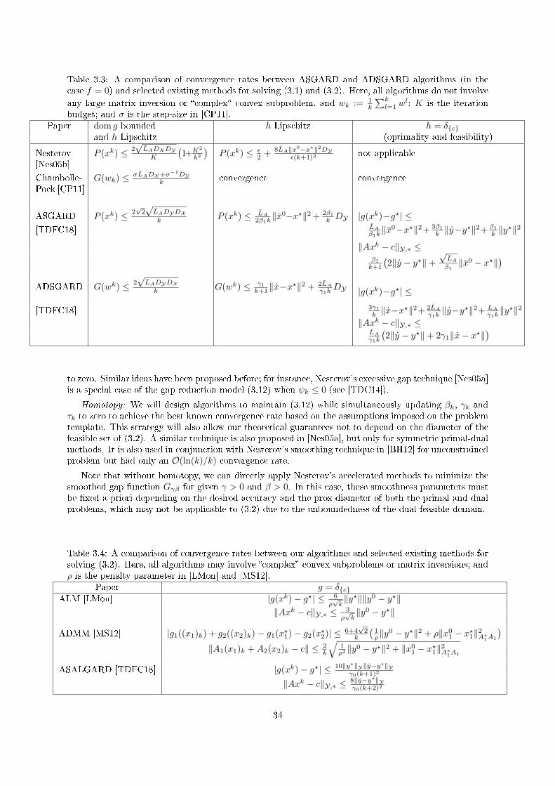
Table 3.3: A comparison of convergence rates between ASGARD and ADSGARD algorithms (in thecase f = 0) and selected existing methods for solving (3.1) and (3.2). Here, all algorithms do not involve

any large matrix inversion or complex convex subproblem, and wk := 1k

∑kl=1 w

l; K is the iterationbudget; and σ is the step-size in [CP11].

Paper dom g boundedand h Lipschitz

h Lipschitz h = δc. (optimality and feasibility)

Nesterov[Nes05b]

P (xk) ≤ 2√LADXDYK

(1+K2

k2

)P (xk) ≤ ε

2 + 8LA‖x0−x?‖2DYε(k+1)2 not applicable

Chambolle-Pock [CP11]

G(wk) ≤ σLADX+σ−1DYk convergence convergence

ASGARD P (xk) ≤ 2√

2√LADYDXk P (xk) ≤ LA

2β1k‖x0−x?‖2 + 2β1

k DY |g(xk)−g?| ≤[TDFC18] LA

β1k‖x0−x?‖2+ 3β1

k ‖y−y?‖2+ β1

k ‖y?‖2

‖Axk − c‖Y,∗ ≤β1

k+1

(2‖y − y?‖+

√LAβ1‖x0 − x?‖

)ADSGARD G(wk) ≤ 2

√LADYDXk G(wk) ≤ γ1

k+1‖x−x?‖2 + 2LA

γ1kDY |g(xk)−g?| ≤

[TDFC18] 3γ1

k ‖x−x?‖2+ 2LA

γ1k‖y−y?‖2+ LA

γ1k‖y?‖2

‖Axk − c‖Y,∗ ≤LAγ1k

(2‖y − y?‖+ 2γ1‖x− x?‖

)

to zero. Similar ideas have been proposed before; for instance, Nesterov's excessive gap technique [Nes05a]is a special case of the gap reduction model (3.12) when ψk ≤ 0 (see [TDC14]).

Homotopy: We will design algorithms to maintain (3.12) while simultaneously updating βk, γk andτk to zero to achieve the best known convergence rate based on the assumptions imposed on the problemtemplate. This strategy will also allow our theoretical guarantees not to depend on the diameter of thefeasible set of (3.2). A similar technique is also proposed in [Nes05a], but only for symmetric primal-dualmethods. It is also used in conjunction with Nesterov's smoothing technique in [BH12] for unconstrainedproblem but had only an O(ln(k)/k) convergence rate.

Note that without homotopy, we can directly apply Nesterov's accelerated methods to minimize thesmoothed gap function Gγβ for given γ > 0 and β > 0. In this case, these smoothness parameters mustbe xed a priori depending on the desired accuracy and the prox-diameter of both the primal and dualproblems, which may not be applicable to (3.2) due to the unboundedness of the dual feasible domain.

Table 3.4: A comparison of convergence rates between our algorithms and selected existing methods forsolving (3.2). Here, all algorithms may involve complex convex subproblems or matrix inversions; andρ is the penalty parameter in [LMon] and [MS12].

Paper g = δcALM [LMon] |g(xk)− g?| ≤ 6

ρ√k‖y?‖‖y0 − y?‖

‖Axk − c‖Y,∗ ≤ 3ρ√k‖y0 − y?‖

ADMM [MS12] |g1((x1)k) + g2((x2)k)− g1(x?1)− g2(x?2)| ≤ 6+4√

2k

(1ρ‖y

0 − y?‖2 + ρ‖x01 − x?1‖2A∗1A1

)‖A1(x1)k +A2(x2)k − c‖ ≤ 2

k

√1ρ2 ‖y0 − y?‖2 + ‖x0

1 − x?1‖2A∗1A1

ASALGARD [TDFC18] |g(xk)− g?| ≤ 10‖y?‖Y‖y−y?‖Yγ0(k+1)2

‖Axk − c‖Y,∗ ≤ 8‖y−y?‖Yγ0(k+2)2

34

3.3.2 Technical results

Lemma 3 is fundamental to our theory since it relates the decrease in the smoothed gap to the objectivevalue and the feasibility gap in the very important case of equality constraints. It shows that when thesmoothed gap and the smoothing parameters are small at the same time, then objective value gap andfeasibility gap are both small.

This question had been open for several years in the area of convergence rates for primal-dual methods.Previous works either made assumptions that forbade equality constraints or proved results in terms ofquantities that are not natural measures of optimality (for instance the restricted duality gap in [CP11]).Concurrently to our work, alternative approaches have been proposed by Y. Drori in [Dro14] and by Y.Xu in [Xu17]. Note that although the rates obtained are the same, our approach using smoothing ismore principled.

Lemma 3. Let Gγβ be the smoothed gap function and Sβ(x; y) := Pβ(x; y)−P (x?) = f(x)+gβ(Ax; y)−P (x?) be the smoothed objective residual. Then, we have

Sβ(x; y) ≤ Gγβ(w; w) + γbX (x?, x) and1

2‖y∗β(Ax; y)− y?‖2Y,∗ ≤ bY(y?, y) +

1

βSβ(x; y). (3.13)

Suppose that g(·) := δc(·). Then, for any y? ∈ y? and x ∈ X , one has

− ‖y?‖Y‖Ax− c‖Y,∗ ≤ f(x)− f(x?) (3.14)

and the following primal objective residual and feasibility gap estimates hold for (3.2):f(x)− f(x?) ≤ Sβ(x; y)− 〈y?, Ax− c〉+ βbY(y?, y),

‖Ax− c‖Y,∗ ≤ βLbY[‖y? − y‖Y +

(‖y? − y‖2Y + 2L−1

bYβ−1Sβ(x; y)

)1/2],

(3.15)

where the quantity in the square root is always nonnegative.

Using the smoothed gap machinery, we dened a new algorithm, that we called the AcceleratedSmoothed GAp ReDuction algorithm (ASGARD). The idea is at each iteration to run one step ofaccelerated gradient on the smoothed gap function and then to decrease the smoothing parameter βk asmuch as our analysis allows us to do while maintaining (3.12).

xk = (1− τk)xk + τkxk,

y∗βk+1(Axk; y) := arg max

y∈Y〈Axk, y〉 − h∗(y)− βk+1bY(y, y),

xk+1 = proxβk+1L−1A g

(xk − βk+1L

−1A A>y∗βk+1

(Axk; y)),

xk+1 = xk − τ−1k (xk − xk+1),

τk+1 ∈ (0, 1) is the unique positive root of τ3/LbY + τ2 + τ2k τ − τ2

k = 0,

βk+2 = βk+1

1+L−1bYτk+1

(ASGARD)

We prove an O(1/k) convergence rate on the objective residual P (xk)−P ? of (3.1) for the algorithm,which is the best known in the literature for the fully nonsmooth setting. For the constrained case (3.2),we also prove the convergence of the algorithm in terms of the primal objective residual and the feasibilityviolation, both achieve an O(1/k) convergence rate, and are independent of the prox-diameters unlikeexisting smoothing techniques [BT12, Nes05a, Nes05b]. As the optimality measure is dierent in eachcase, we state two distinct theorems.

Theorem 9. Suppose that f = 0 and h = δc. Let β1 > 0 and bY be chosen such that LbY = 1. Let

xk be the primal sequence generated by Algorithm ASGARD. Then the following bounds hold for (3.2):g(xk)−g? ≥ −‖y?‖Y‖Axk − c‖Y,∗,

g(xk)−g? ≤ 1kLA2β1‖x0 − x?‖2X + ‖y?‖Y‖Axk − c‖Y,∗ + 2β1

k+1bY(y?, y),

‖Axk − c‖Y,∗ ≤ β1

k+1

[‖y? − y‖Y +

(‖y? − y‖2Y + β−2

1 LA‖x0 − x?‖2X)1/2]

.

(3.16)

35

Clearly, the choice of β1 in Theorem 9 trades o between ‖x0 − x?‖2X and ‖y? − y‖2Y on the primalobjective residual g(xk)− g? and on the feasibility gap ‖Axk − c‖Y,∗.

Theorem 10. Suppose that f = 0 and h is Lipschitz continuous, so that DY = supy∈dom g∗ bY(y, y) <

+∞. Let β1 > 0 and bY be chosen such that LbY = 1. Let xk be the primal sequence generated byAlgorithm ASGARD. Then, the primal objective residual of (3.1) satises

P (xk)− P (x?) ≤ LA2β1k

‖x0 − x?‖2X +2β1

k + 1DY , for all k ≥ 1. (3.17)

3.3.3 Extensions

The exibility of the framework allowed us to develop several variants of ASGARD.

Dual algorithm We developed in [TDFC18] a dual version of ASGARD, called ADSGARD, thatupdates a sequence of primal-dual vectors (xk, yk). Its main feature is that, although it is a dualalgorithm, it has guarantees on the smoothed duality gap, from which we can derive a convergence ratein the primal space.

Moreover, by considering the non-strongly convex smoothing bX (x, x) = 12‖Ax − Ax‖2, we could

dene ASALGARD, a method similar to the Augmented Lagrangian method but with improved worstcase guarantee of the order O(1/k2).

When the objective function g is µ-strongly convex, we showed that it is not necessary to smooth itsFenchel conjugate g∗. Taking γk = 0 in the algorithm yields a faster algorithm with rate O(1/k2).

Heuristic restart Similar to other accelerated gradient algorithms in [GB14, OC12, SBC14, FQ16],restarting ASGARD and ADSGARD may lead to a better performance in practice.

If we consider ASGARD, then, when a restart takes place, we perform the following steps:xk+1 ← xk+1,y ← y∗βk+1

(Axk+1; y),

βk+1 ← β1,τk+1 ← 1.

(3.18)

Extension to Problem 3.1 In [VNFC17], we showed that ASGARD can deal with dierentiablefunctions through their gradient. The step-sizes need to be adapted accordingly. We also proposed anovel line search that adapts the step-sizes and the smoothing parameters together. Thus, if the functionh happened to be smooth near the optimum, the algorithm will automatically switch to acceleratedgradient with O(1/k2) rate.

Going from a purely proximal to a forward-backward type method was a requirement in order todesign a coordinate descent version of ASGARD that would take prot of longer step-sizes.

Conditional gradient with linear constraints In [YFLC18], we showed how to use the smoothingframework with a conditional gradient method. We obtain an algorithm that, using only gradients andlinear minimization oracles, can solve complex problems, like for instance semi-denite programs, andhas a convergence guarantee of order O(1/

√k). This is the rst method with such a rate under the setup

of conditional gradient with linear constraints and the method has very good practical performance.

3.4 A primal-dual coordinate descent method based on smooth-

ing

The paper [ADFC17] develops a random coordinate descent method to solve the composite problem(3.1):

F ? = minx∈RpF (x) = f(x) + g(x) + h(Ax),

36

where f : Rp → R, g : Rp → R ∪ +∞, and h : Rn → R ∪ +∞ are proper, closed and convexfunctions, A ∈ Rn×p is a given matrix. As explained before in this thesis, the optimization template (3.1)covers many important applications including support vector machines, sparse model selection, logisticregression, etc. It is also convenient to formulate generic constrained convex problems by choosing anappropriate h.

Before this work, there was no coordinate descent method for the general three-composite form(3.1) within our structure assumptions studied here that had rigorous convergence speed guarantees. Inparticular, we had not derived the convergence rate of Algorithm 6 yet. For such a theoretical develop-ment, coordinate descent algorithms require specic assumptions on the convex optimization problems[Nes12a, FR15, NC13]. As a result, to rigorously handle the three-composite case, we assume that (i)f is smooth, (ii) g is non-smooth but decomposable (each component has an eciently computableproximal operator), and (iii) h is non-smooth.

We generalize [FR15, QR16] to the three composite case (3.1). For this purpose, we combine sev-eral classical and contemporary ideas: We exploit the smoothing technique in [Nes05b], the ecientimplementation technique in [Nes12a, FR15], the homotopy strategy in [TDC15], and the nonuniformcoordinate selection rule in [QR16] in our algorithm, achieving the best known complexity estimate.

Surprisingly, the combination of these ideas are achieved in a very natural and elementary primal-dual gap-based framework. However, the extension is indeed not trivial since it requires to deal with acomposition of a non-smooth function h and a linear operator A.

We propose a new smooth primal-dual randomized coordinate descent method (Algorithm 8) forsolving (3.1) where f is smooth, g is nonsmooth, separable and has a block-wise proximal operator, andh is a general nonsmooth function. Under such a structure, we show that our algorithm achieves thebest known O(n/k) convergence rate, where k is the iteration count.

We instantiate our algorithm to solve special cases of (3.1) including the case g = 0 and constrainedproblems. We analyze the convergence rate guarantee of these variants individually and discuss the choiceof nonuniform distribution to achieve the best convergence rate. Exploiting the strategy in [FR15], weshow that our algorithm can be implemented in parallel by breaking up the full vector updates. We alsoprovide a restart strategy to enhance practical performance.

Algorithm 8 (SMooth, Accelerate, Randomize The Coordinate Descent (SMART-CD))

Require: Choose β1 > 0 and α ∈ [0, 1] as two input parameters.

1: Set B0i := Li + ‖Ai‖2

β1for i ∈ [n]. Compute Sα :=

∑ni=1(B0

i )α and qi :=(B0i )α

Sαfor all i ∈ [n].

2: Set τ0 := minqi : 1 ≤ i ≤ n ∈ (0, 1] for i ∈ [n].

3: for k ← 0, 1, · · · , kmax do

4: Update xk := (1− τk)xk + τkxk and compute uk := Axk.

5: Compute the dual step y∗βk+1(uk) := proxβ−1

k+1h∗y − β−1

k+1uk.

6: Select a block coordinate ik ∈ [n] according to the probability distribution q.7: Set xk+1 := xk, and compute the primal ik-block coordinate:

xk+1ik

:= argminxik∈R

pik

〈∇ikf(xk) +ATiky

∗βk+1

(uk), xik − xik〉(ik) + gik(xik) +τkB

kik

2τ0‖xik − xkik‖

2(ik)

.

8: Update xk+1 := xk + τkτ0

(xk+1 − xk).

9: Compute τk+1 ∈ (0, 1) as the unique positive root of τ3 + τ2 + τ2k τ − τ2

k = 0.

10: Update βk+2 := βk1+τk+1

and Bk+1i := Li + ‖Ai‖2

βk+2for i ∈ [n].

11: end for

As the proof is using Lemma 3, our convergence result is split into the two important cases of Lipschitzh and linear equality constraint.

Theorem 11. Let x? be an optimal point of (3.1) where h is Dh∗-Lipschitz continuous and let β1 > 0be given. Let τ0 := minqi : i ∈ [n] ∈ (0, 1] and β0 := (1 + τ0)β1 be given parameters. For all k ≥ 1,the sequence xk generated by Algorithm 8 satises:

E[F (xk)− F (x?)] ≤ C?

τ0(k − 1) + 1+β1(1 + τ0)D2

h∗

2(τ0k + 1), (3.19)

37

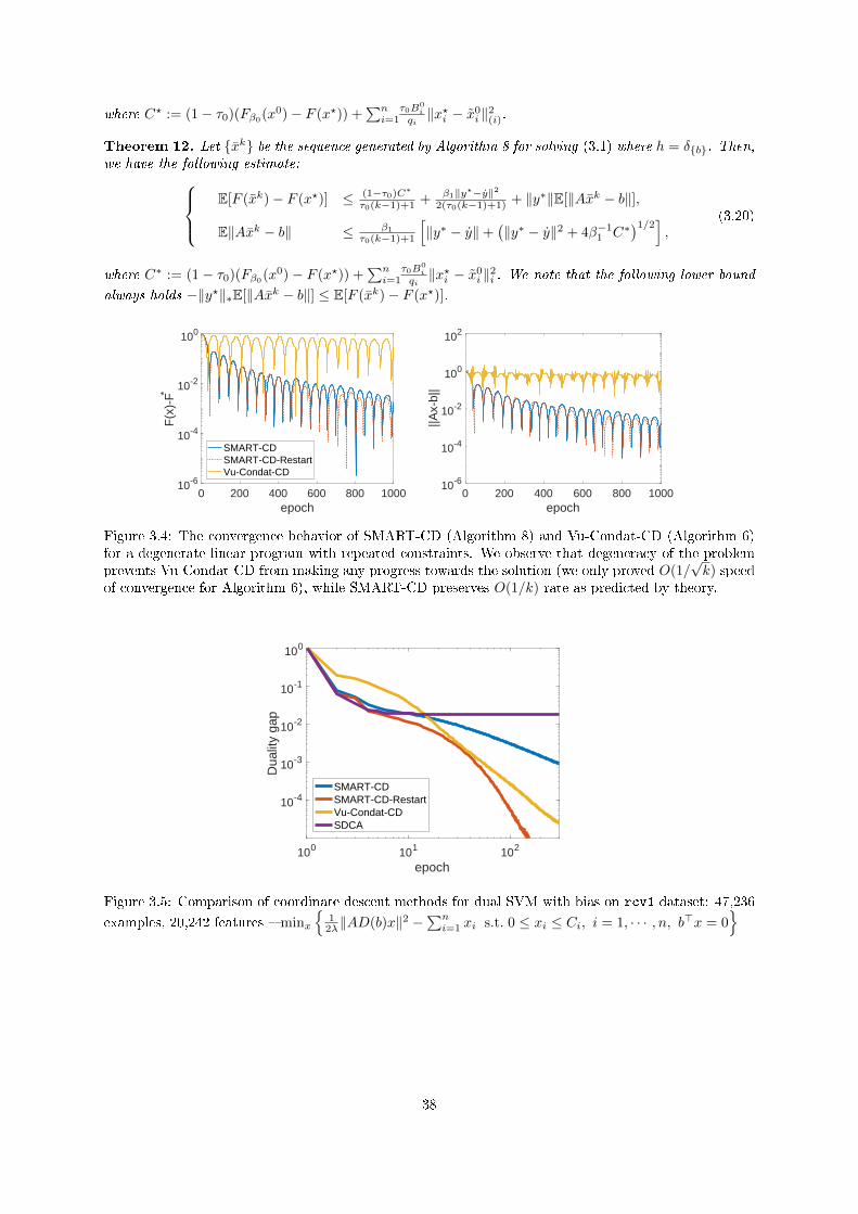
where C? := (1− τ0)(Fβ0(x0)− F (x?)) +∑ni=1

τ0B0i

qi‖x?i − x0

i ‖2(i).

Theorem 12. Let xk be the sequence generated by Algorithm 8 for solving (3.1) where h = δb. Then,we have the following estimate:

E[F (xk)− F (x?)] ≤ (1−τ0)C∗

τ0(k−1)+1 + β1‖y?−y‖22(τ0(k−1)+1) + ‖y∗‖E[‖Axk − b‖],

E‖Axk − b‖ ≤ β1

τ0(k−1)+1

[‖y∗ − y‖+

(‖y∗ − y‖2 + 4β−1

1 C∗)1/2]

,(3.20)

where C∗ := (1− τ0)(Fβ0(x0)− F (x?)) +∑ni=1

τ0B0i

qi‖x?i − x0

i ‖2i . We note that the following lower bound

always holds −‖y?‖∗E[‖Axk − b‖] ≤ E[F (xk)− F (x?)].

0 200 400 600 800 1000epoch

10-6

10-4

10-2

100

F(x

)-F*

SMART-CDSMART-CD-RestartVu-Condat-CD

0 200 400 600 800 1000epoch

10-6

10-4

10-2

100

102

||Ax-

b||

Figure 3.4: The convergence behavior of SMART-CD (Algorithm 8) and Vu-Condat-CD (Algorithm 6)for a degenerate linear program with repeated constraints. We observe that degeneracy of the problemprevents Vu-Condat-CD from making any progress towards the solution (we only proved O(1/

√k) speed

of convergence for Algorithm 6), while SMART-CD preserves O(1/k) rate as predicted by theory.

100 101 102

epoch

10-4

10-3

10-2

10-1

100

Dua

lity

gap

SMART-CDSMART-CD-RestartVu-Condat-CDSDCA

Figure 3.5: Comparison of coordinate descent methods for dual SVM with bias on rcv1 dataset: 47,236

examples, 20,242 features minx

1

2λ‖AD(b)x‖2 −∑ni=1 xi s.t. 0 ≤ xi ≤ Ci, i = 1, · · · , n, b>x = 0

38

Chapter 4

Applications to statistics

4.1 Gap Safe screening rules for sparsity enforcing penalties

4.1.1 Introduction

The computational burden of solving high dimensional regularized regression problem has led to a vastliterature on improving algorithmic solvers in the last two decades. With the increasing popularityof `1-type regularization ranging from the Lasso [Tib96] or group-Lasso [YL06] to regularized logisticregression and multi-task learning, many algorithmic methods have emerged to solve the associatedoptimization problems [KKB07, BJM+12]. Although for the simple `1 regularized least square a specicalgorithm (e.g. the LARS [EHJT04]) can be considered, for more general formulations, penalties, andpossibly larger dimensions, (block) coordinate descent has proved to be an ecient strategy [FHT10].

Our main objective in this work is to propose a technique that can speed-up any iterative solver forsuch learning problems, and that is particularly well suited for (block) coordinate descent method as thistype of method can easily ignore useless coordinates.

The safe rules introduced by [EVR12] for generalized `1 regularized problems, is a set of rules allowingto eliminate features whose associated coecients are guaranteed to be zero at the optimum, even beforestarting any algorithm. Relaxing the safe rule, one can obtain some additional speed-up at the price ofpossible mistakes. Such heuristic strategies, called strong rules by [TBF+12] reduce the computationalcost using an active set strategy, but require dicult post-processing to check for features possiblywrongly discarded.

Another road to speed-up screening method has been pursued following the introduction of sequen-tial safe rules [EVR12, WWY12, XWR14, WZL+14]. The idea is to improve the screening thanks tothe computation done for a previous regularization parameter as in homotopy/continuation methods.This scenario is particularly relevant in machine learning, where one computes solutions over a gridof regularization parameters, so as to select the best one, e.g. by cross-validation. Nevertheless, theaforementioned methods suer from the same problem as strong rules, since relevant features can bewrongly disregarded. Indeed, sequential rules usually rely on the exact knowledge of certain theoreticalquantities that are only known approximately. Especially, for such rules to work one needs the exactdual optimal solution from the previous regularization parameter, a quantity (almost) never available tothe practitioner.

The introduction of dynamic safe rules by [BERG15, BERG14] has opened a promising venue byperforming variable screening, not only before the algorithm starts, but also along the iterations. Thisscreening strategy can be applied for any standard optimization algorithm such as FISTA [BT09],primal-dual [CP11], augmented Lagrangian [BPC+11a]. Yet, it is particularly relevant for strategiesthat can benet from support reduction or active sets[KWGA11, JG15], such as coordinate-descent[Fu98, FHHT07, FHT10].

We shall present the methods introduced rst for the Lasso in [FGS15] and then for `1/`2 norms in[NFGS15] as well as for Sparse Group Lasso in [NFGS16], and summarized in [NFGS17]. Our so-calledGap Safe rules (because the screening rules rely on duality gap computations), improved on dynamicsafe rules for a broad class of learning problems with the following benets:

• Gap Safe rules are easy to insert in existing solvers,

39

• they are proved to be safe and unify sequential and dynamic rules,

• they are more ecient in practice than previously known safe rules,

• they achieve fast variable identications.

Furthermore, it is worth noting that strategies also leveraging dual gap computations have recentlybeen considered to safely discard irrelevant coordinates: [SKHT16] have considered screening rules forlearning tasks with both feature sparsity and sample sparsity, such as for `1-regularized SVM. In thiscase, some interesting developments have been proposed, namely safe keeping strategies, which allow toidentify features and samples that are guaranteed to be active. Constrained convex problems such asminimum enclosing ball can also be included as shown in [ROG+16]. The Blitz algorithm by [JG15] aimsto speed up working set methods using duality gaps computations; signicant gains were also obtainedin limited-memory and distributed settings.

4.1.2 Safe Screening rules

We propose to estimate the vector of parameters β by solving

β(λ) ∈ arg minβ∈Rp

Pλ(β), for Pλ(β) := F (β) + λΩ(β) :=

n∑i=1

fi(x>i β) + λΩ(β) , (4.1)

where all fi : R 7→ R are convex and dierentiable functions with 1/γ-Lipschitz gradient and Ω : Rp 7→ R+

is a norm that is group-decomposable, i.e. Ω(β) =∑g∈G Ωg(βg) where each Ωg is a norm on Rng . The

λ parameter is a non-negative constant controlling the trade-o between the data tting term and theregularization term. We shall denote the dual norm of Ω by ΩD(z) = maxg∈G ΩDg (zg).

A dual formulation of 4.1 is given by

θ(λ) = arg maxθ∈∆X

−n∑i=1

f∗i (−λθi) =: Dλ(θ), (4.2)

where ∆X = θ ∈ Rn : ∀g ∈ G,ΩDg (X>g θ) ≤ 1. Moreover, the Fermat's rule reads:

∀i ∈ [n], θ(λ)i = −∇fi(x>i β(λ))/λ (link equation), (4.3)

∀g ∈ G, X>g θ(λ) ∈ ∂Ωg(β(λ)g ) (sub-dierential inclusion). (4.4)

For any θ ∈ Rn let us introduce G(θ) := [∇f1(θ1), . . . ,∇fn(θn)]> ∈ Rn. Then the primal/dual link

equation can be written θ(λ) = −G(Xβ(λ))/λ .Contrarily to the primal, the dual problem has a unique solution under our assumption on the fi's.

Indeed, the dual function is strongly concave.Screening rules rely on a direct consequence of Fermat's rule. If β(λ)g 6= 0, then ΩDg (X>g θ

(λ)) = 1thanks to the formula for the subdierential of a norm

∂Ω(x) =

z ∈ Rd : ΩD(z) ≤ 1 = BΩD , if x = 0,

z ∈ Rd : ΩD(z) = 1 and z>x = Ω(x), otherwise.(4.5)

Since θ(λ) ∈ ∆X , it implies, by contrapositive, that if ΩDg (X>g θ(λ)) < 1 then β(λ)g = 0. This relation

means that the g-th group can be discarded whenever ΩDg (X>g θ(λ)) < 1. However, since θ(λ) is unknown,

this rule is of limited use. Fortunately, it is often possible to construct a set R ⊂ Rn, called a safe region,that contains θ(λ). This observation leads to the following result.

Proposition 4 (Safe screening rule [EVR12]). If θ(λ) ∈ R, and g ∈ G:

maxθ∈R

ΩDg (X>g θ) < 1 =⇒ ΩDg (X>g θ(λ)) < 1 =⇒ β(λ)g = 0 . (4.6)

The so-called safe screening rule consists in removing the g-th group from the problem whenever theprevious test is satised, since then β(λ)g is guaranteed to be zero. Should R be small enough to screenmany groups, one can observe considerable speed-ups in practice as long as the testing can be performedeciently. A natural goal is to nd safe regions as narrow as possible: smaller safe regions can onlyincrease the number of screened out variables. To have useful screening procedures one needs:

40

• the safe region R to be as small as possible (and to contain θ(λ)),

• the computation of the quantity maxθ∈R

ΩDg (X>g θ) to be cheap.

Various shapes have been considered in practice for the safe region R such as balls [EVR12], domes[FGS15] or more rened sets (see [XWR14] for a survey). Here we consider for simplicity the so-calledsphere regions (following the terminology introduced by [EVR12]) choosing a ball R = B(θc, r) as asafe region. Thanks to the triangle inequality, we have:

maxθ∈B(θc,r)

ΩDg (X>g θ) ≤ ΩDg (X>g θc) + maxθ∈B(θc,r)

ΩDg (X>g (θ − θc)),

and denoting ΩDg (Xg) := supu 6=0ΩDg (X>g u)

‖u‖2 the operator norm of Xg associated to ΩDg (·), we deduce fromProposition 4.6 the screening rule for the g-th group:

Safe sphere test: If ΩDg (X>g θc) + rΩDg (Xg) < 1, then β(λ)g = 0 . (4.7)

Finding a center To create a useful center for a safe sphere, one needs to be able to create dualfeasible points, i.e. points in the dual feasible set ∆X . One such point is θmax := −G(0)/λmax whichleads to the original static safe rules proposed by [EVR12]. Yet, it has a limited interest, being helpfulonly for a range of small regularization parameters λ. A more generic way of creating a dual point thatwill be key for creating our safe rules is to rescale any point z ∈ Rn such that it is in the dual set ∆X .The rescaled point is denoted by Θ(z) and is dened by

Θ(z) :=

z, if ΩD(X>z) ≤ 1,

zΩD(X>z)

, otherwise.(4.8)

This choice guarantees that ∀z ∈ Rn,Θ(z) ∈ ∆X . A candidate often considered for computing a dualpoint consists in starting by the (generalized) residual term z = −G(Xβ)/λ. This choice is motivated

by the primal-dual link equation (4.3) i.e. θ(λ) = −G(Xβ(λ))/λ. We also have the following theoreticalguarantee.

Proposition 5 (Convergence of the dual points). Let βk be the current estimate of β(λ) and θk =

Θ(−G(Xβk)/λ) be the current estimate of θ(λ). Then limk→+∞ βk = β(λ) implies limk→+∞ θk = θ(λ).

Finding a radius Now that we have seen how to create a center candidate for the sphere, we need tond a proper radius, that would allow the associated sphere to be safe. The following theorem proposesa way to obtain a radius using the duality gap:

Theorem 13 (Gap Safe sphere). Assuming that F has 1/γ-Lipschitz gradient, we have

∀β ∈ Rp,∀θ ∈ ∆X , ‖θ(λ)− θ‖2 ≤

√2(Pλ(β)−Dλ(θ))

γλ2=: rλ(β, θ) . (4.9)

Hence R = B(θ, rλ(β, θ)) is a safe region for any β ∈ Rn and θ ∈ ∆X .

Safe Active Set Note that any time a safe rule is performed thanks to a safe region R = B(θ, r), onecan associate a safe active set Aθ,r, consisting of the features that cannot be removed yet by the test in

Equation 4.7. Hence, the safe active set contains the true support of β(λ).When choosing z = −G(Xβ)/λ as proposed in Section 4.1.2 as the current residual, the computation

of θ = Θ(z) in Equation 4.8 involves the computation of ΩD(X>z). A straightforward implementationwould cost O(np) operations. This can be avoided: when using a safe rule one knows that the indexachieving the maximum for this norm is in A(θ, r). Indeed, by construction of the safe active set, itis easy to see that ΩD(X>z) = maxg∈A(θ,r) ΩDg (X>g z). In practice the evaluation of the dual gap istherefore O(nq) where q is the size of A(θ, r). In other words, using a safe screening rule also speeds upthe evaluation of the stopping criterion.

41

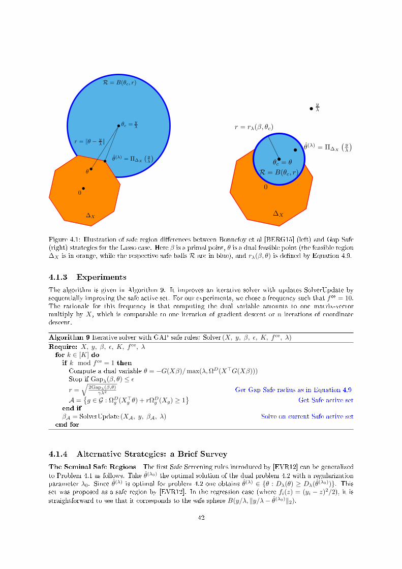
Figure 4.1: Illustration of safe region dierences between Bonnefoy et al [BERG15] (left) and Gap Safe(right) strategies for the Lasso case. Here β is a primal point, θ is a dual feasible point (the feasible region∆X is in orange, while the respective safe balls R are in blue), and rλ(β, θ) is dened by Equation 4.9.

4.1.3 Experiments

The algorithm is given in Algorithm 9. It improves an iterative solver with updates SolverUpdate bysequentially improving the safe active set. For our experiments, we chose a frequency such that f ce = 10.The rationale for this frequency is that computing the dual variable amounts to one matrix-vectormultiply by X, which is comparable to one iteration of gradient descent or n iterations of coordinatedescent.

Algorithm 9 Iterative solver with GAP safe rules: Solver (X, y, β, ε, K, f ce, λ)

Require: X, y, β, ε, K, f ce, λfor k ∈ [K] doif k mod f ce = 1 thenCompute a dual variable θ = −G(Xβ)/max(λ,ΩD(X>G(Xβ)))Stop if Gapλ(β, θ) ≤ εr =

√2Gapλ(β,θ)

γλ2 Get Gap Safe radius as in Equation 4.9

A =g ∈ G : ΩDg (X>g θ) + rΩDg (Xg) ≥ 1

Get Safe active set

end if

βA = SolverUpdate (XA, y, βA, λ) Solve on current Safe active setend for

4.1.4 Alternative Strategies: a Brief Survey

The Seminal Safe Regions The rst Safe Screening rules introduced by [EVR12] can be generalized

to Problem 4.1 as follows. Take θ(λ0) the optimal solution of the dual problem 4.2 with a regularizationparameter λ0. Since θ(λ) is optimal for problem 4.2 one obtains θ(λ) ∈ θ : Dλ(θ) ≥ Dλ(θ(λ0)). Thisset was proposed as a safe region by [EVR12]. In the regression case (where fi(z) = (yi − z)2/2), it is

straightforward to see that it corresponds to the safe sphere B(y/λ, ‖y/λ− θ(λ0)‖2).

42

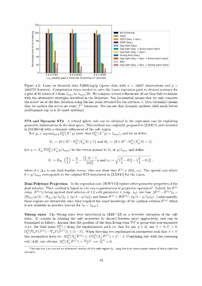
Figure 4.2: Lasso on nancial data E2006-log1p (sparse data with n = 16087 observations and p =1668737 features). Computation times needed to solve the Lasso regression path to desired accuracy fora grid of 10 values of λ from λmax to λmax/20. We compare several renements of our Gap Safe techniquewith the alternative strategies described in the literature. Seq (sequential) means that we only computethe active set at the rst iteration using the last point returned for the previous λ. Dyn (dynamic) meansthat we update the active set every f ce iterations. We can see that dynamic updates yield much betterperformance (up to a 10 times speedup).

ST3 and Dynamic ST3 A rened sphere rule can be obtained in the regression case by exploitinggeometric informations in the dual space. This method was originally proposed in [XXR11] and extendedin [BERG14] with a dynamic renement of the safe region.

Let g? ∈ arg maxg∈G ΩDg (X>y) (note that ΩDg?(X>y) = λmax), and let us dene

V? := θ ∈ Rn : ΩDg?(X>g?θ) ≤ 1 and H? := θ ∈ Rn : ΩDg?(X>g?θ) = 1.

Let η := Xg?∇ΩDg?(X>g?y/λmax) be the vector normal to V? at y/λmax and dene

θc := ΠH?

( yλ

)=y

λ−〈 yλ , η〉 − 1

‖η‖22η and rθ :=

√‖ yλ− θ‖22 − ‖

y

λ− θc‖22 ,

where θ ∈ ∆X is any dual feasible vector. One can show that θ(λ) ∈ B(θc, rθ). The special case whereθ = y/λmax corresponds to the original ST3 introduced in [XXR11] for the Lasso.

Dual Polytope Projection In the regression case, [WWY12] explore other geometric properties of the

dual solution. Their method is based on the non-expansiveness of projection operators1. Indeed, for θ(λ)

(resp. θ(λ0))) being optimal dual solution of 4.2 with parameter λ (resp. λ0), one has: ‖θ(λ) − θ(λ0)‖2 =

‖Π∆X(y/λ)− Π∆X

(y/λ0)‖2 ≤ ‖y/λ− y/λ0‖2 and hence θ(λ) ∈ B(θ(λ0), ‖y/λ− y/λ0‖2). Unfortunately,

those regions are intractable since they required the exact knowledge of the optimal solution θ(λ0) whichis not available in practice (except for λ0 = λmax).

Strong rules The Strong rules were introduced in [TBF+12] as a heuristic extension of the saferules. It consists in relaxing the safe properties to discard features more aggressively, and can beformalized as follows. Assume that the gradient of the data tting term ∇F is group-wise non-expansivew.r.t. the dual norm ΩDg (·) along the regularization path i.e. that for any g ∈ G, any λ > 0, λ′ > 0,

ΩDg(∇gF (β(λ))−∇gF (β(λ′))

)≤ |λ−λ′|. When choosing two regularization parameters such that λ < λ′

this assumption leads to: λΩDg (X>g θ(λ)) ≤ λ′ΩDg (X>g θ

(λ′)) + λ′ − λ. Combining this with the screening

rule (4.6), one obtains: ΩDg (X>g θ(λ′)) < 2λ−λ′

λ′ =⇒ β(λ)g = 0.

1The authors also proved an enhanced version of this safe region by using the rm non-expansiveness of the projectionoperator.

43

The set of variables not eliminated is called the strong active set. Note that Strong rules are un-safebecause the non-expansiveness condition on the (gradient of the) data tting term is usually not satisedwithout stronger assumptions on the design matrix X; see discussion in [TBF+12]. It requires the exact

knowledge of θ(λ′) which is not available in practice. Using such rules, the authors advised to check theKKT condition a posteriori, to avoid removing wrongly some features.

Correlation Based Rule Previous works in statistics have proposed various model-based screeningmethods to select important variables. Those methods discard variables with small correlation betweenthe features and response variables. For instance Sure Independence Screening (SIS) by [FL08] reads:for a chosen critical threshold γ remove the feature if the correlation with the observation is smaller thanγ. It is a marginal oriented variable selection method and it is worth noting that SIS can be recast as astatic sphere test in linear regression scenarios:

If ΩDg (X>g y) < γ = λ(1− rΩDg (Xg)

)then β(λ)

g = 0 (remove Xg).

Other renements can also be found in the literature such as iterative screening (ISIS) [FL08], thatbears some similarities with dynamic sphere safe tests.

4.2 Ecient Smoothed Concomitant Lasso Estimation for High

Dimensional Regression

In the context of high dimensional regression where the number of features is greater than the numberof observations, standard least squares need some regularization to both avoid over-tting and ease theinterpretation of discriminant features. Among the least squares with sparsity inducing regularization,the Lasso [Tib96], using the `1 norm as a regularizer, is the most standard one. It hinges on a reg-ularization parameter governing the trade-o between data tting and sparsity of the estimator, andrequires careful tuning. Though this estimator is well understood theoretically (we refer to [Bv11] for areview), the choice of the tuning parameter remains an open and critical question in practice as well as intheory. For the Lasso, statistical guarantees [BRT09] rely on choosing the tuning parameter proportionalto the noise level, a quantity that is usually unknown to practitioners. We also want to mention thatautomatic tuning (e.g. by cross-validation) would be time consuming for applications like dictionarylearning, where this parameter is often set once and for all [MBPS10]. Besides, the noise level is ofpractical interest since it is required in the computation of model selection criterions such as AIC, BIC,SURE or in the construction of condence sets. As shown in [FGH12], this is a challenging task in highdimension because of the spurious correlation phenomenon.

A convenient way to estimate both the regression coecient and the noise level is to perform ajoint estimation, for instance by performing the penalized maximum likelihood of the joint distribution.Unfortunately, a direct approach leads to a non-convex formulation (though one can recover a jointlyconvex formulation through a change of variable [SBv10]).

Another road for this joint estimation was inspired by the robust theory developed by Huber [Hub81],particularly in the context of location-scale estimation. Indeed, Owen [Owe07] extended it to handlesparsity inducing penalty, leading to the jointly convex optimization formulation

(β(λ), σ(λ)) ∈ arg minβ∈Rp,σ>0

‖y −Xβ‖2

2nσ+σ

2+ λ‖β‖1. (4.10)

Since then, his estimator has appeared under various name, and we coined it the Concomitant Lasso.Indeed, as far as we know Owen was the rst to propose such a formulation.

Later, the same formulation was mentioned in [Ant10], in a response to [SBv10], and was thor-oughly analyzed in [SZ12], under the name Scaled-Lasso. Similar results were independently obtainedin [BCW11] for the same estimator, though with a dierent formulation. While investigating pivotalquantities, Belloni et al. proposed to solve the following convex program: modify the standard Lasso byremoving the square in the data tting term. Thus, they termed their estimator the Square-root Lasso(see also [CD11]). A second approach leading to this very formulation, was proposed by [XCM10] toaccount for noise in the design matrix, in an adversarial scenario. Interestingly their robust constructionled exactly to the Square-root Lasso formulation.

44

Under standard design assumption (see [BRT09]), it is proved that the Scaled/Square-root Lassoreaches optimal rates for sparse regression, with the additional benet that the regularization parameteris independent of the noise level [BCW11, SZ12]. Moreover, a practical study [RTF13] has shown thatthe Concomitant Lasso estimator, or its debiased version (see for instance [BC13, Led13] for a discussionon least-squares retting), is particularly well suited for estimating the noise level in high dimension.

Among the solutions to compute the Concomitant Lasso, two roads have been pursued so far. On theone hand, considering the Scaled-Lasso formulation, Sun and Zhang [SZ12] have proposed an iterativeprocedure that alternates Lasso steps and noise estimation steps, the later leading to rescaling the tuningparameter iteratively. On the other hand, considering the Square-root Lasso formulation, Belloni et al.[BCW11] have leaned on second order cone programming solvers, e.g. TFOCS [BCG11].

Despite the appealing properties listed above, among which the superiority of the theoretical resultsis the most striking, no consensus for an ecient solver has yet emerged for the Concomitant Lasso. Ourcontribution in [NFG+17] aims at providing a more numerically stable formulation, called the SmoothedConcomitant Lasso:

arg minβ∈Rp,σ∈R

‖y −Xβ‖2

2nσ+σ

2+ λ‖β‖1 + ι[σ0,+∞[(σ).

This variant allows to obtain a fast solver: we rst adapt a coordinate descent algorithm to the smoothversion (in the sense given in [Nes05b]) of the original problem (4.10). Then, we apply safe rules strategies,like the ones in Section 4.1 to our estimator. Such rules allow to discard features whose coecientsare certied to be zero, either prior any computation or as the algorithm proceeds. Combined witha coordinate descent, this leads to important acceleration in practice, as illustrated for the Lasso case[FGS15]. We show similar accelerations for the Smoothed Concomitant Lasso, both on real and simulateddata. Overall, our method presents the same computational cost as for the Lasso, but enjoys the nicefeatures mentioned earlier in terms of statistical properties.

In [MFGS17], we studied an extension of the Smoothed Concomitant Lasso estimator to the casewhere we know that the observations can be partitioned into given groups with a dierent noise level.This situation occurs for instance when observations stem from dierent types of sensors like in M/EEG(magnetometers, gradiometers and electrodes). This leads to the following homoscedastic model

arg minB∈Rp×q,

σ1,...,σK∈R+

σk≥σk,∀k∈[K]

K∑k=1

(‖Y k −XkB‖2

2nqσk+nkσk2n

)+ λ‖B‖2,1

that can also be solved using a block coordinate descent method acting on lines of B and (σk)k∈[K].

4.3 Safe Grid Search with Optimal Complexity

Various machine learning problems are formulated as a minimization of an empirical loss function f , reg-ularized by a term Ω whose calibration and complexity is controlled by a non negative hyperparameter λ.The (optimal) choice of regularization parameter λ is crucial since it directly inuences the generalizationperformance of the estimator, i.e. its score on unseen data set. One of the most popular method in suchapproaches is cross-validation (CV), see [AC10] for a detailed review. For simplicity, we investigate herethe simplied holdout version that consists in splitting the data in two parts: on the rst part (trainingset) the method is trained for a pre-dened collection of candidates ΛT := λ0, . . . , λT−1, and on thesecond part (validation set), the best parameter is selected. For a piecewise quadratic loss f and a piece-wise linear regularization Ω, one can show [OPT00, RZ07] that the set of solutions follows a piecewiselinear curve with respect to to the parameter λ. Hence there are several ecient algorithms that cangenerate the full path such as LARS for Lasso [EHJT04], for SVM [HRTZ04] and for the generalizedlinear models [PH07].

Unfortunately, these methods have a worst case complexity, i.e. the number of linear segment, thatis exponential in the dimension of the problem [GJM12] leading to unpractical solutions. To overcomethis issue, an approximation of the solution path up to accuracy ε was proposed and optimal complexitywas proved to be O(1/ε) [GJL10] in a fairly general setting. A noticeable contribution was proposed by[MY12], who rened that bound to O(1/

√ε) in the Lasso case. The later result was then generalized by

[GMLS12] with a lower and upper bound of order O(1/√ε). A generic algorithm was also derived by

45

Algorithm 10 εp-Path on Training Set: Training_path

Input: f,Ω, εp, [λmin, λmax]Initialize t = 0, λ0 = λmax, Λ = λmax.repeat

Solve minβ f(Xβ) + λtΩ(β) up to accuracy εo < εpCompute ρ`t = maxρ s.t. Qt,Vf∗ (ρ) ≤ εpSet λt+1 = λt × (1− ρ`t)Λ← Λ ∪ λt+1 and t← t+ 1

until λt+1 ≤ λmin

Return: β(λt) : λt ∈ Λ

assuming a quadratic lower bound on the objective function. Unfortunately, this assumption does nothold for a large class of problem, in particular for logistic regression.

Following such ideas, [SSKT15] have proposed, for classication problem, to approximate the regu-larization path for the hold-out cross-validation error. Indeed, the later is a more natural criterion tomonitor when one aims at selecting a hyperparameter guaranteed to achieve the best validation errorpossible. The main idea is to construct an upper and lower bound on the validation error as simple func-tions of the regularization parameter. Hence by sequentially varying the parameters, one can estimate arange of parameter for which the validation error is smaller than an accuracy εv.

In [NFS+18], we revisit the approximation and validation path results in a unied framework, undergeneral regularity assumptions on the conjugate of the loss function f that are commonly satised inmachine learning problems:

Uf∗,x(z − x) ≤ f∗(z)− f∗(x)− 〈∇f∗(x), z − x〉 ,Vf∗,x(z − x) ≥ f∗(z)− f∗(x)− 〈∇f∗(x), z − x〉 .

These assumptions are general enough to encompass both classication (logistic loss) and regression(square loss) problems.

Suppose we have at our disposal a primal/dual pair of vector (β(λt), θ(λt)) computed as outputs ofan optimization algorithm at regularization parameter λt, we denote

Gapt := Gapλt(β(λt), θ(λt)),

∆t := f(Xβ(λt))− f(∇f∗(zt)) for zt := −λtθ(λt).

Our analysis is based on bounds on the duality gap for unseen values of the regularization parameter λ.

Lemma 4 (Bounding the Warm Start Error). Assume −λθ(λt) ∈ dom(f∗) and X>θ(λt) ∈ dom(Ω∗).For ρ = 1− λ/λt,

Gapt + ρ · (∆t −Gapt) + Uf∗,zt(ρ · zt) ≤ Gapλ(β(λt), θ(λt)) ≤ Gapt + ρ · (∆t −Gapt) + Vf∗,zt(ρ · zt).

Denoting the upper bound Qt,Vf∗ (ρ) = Gapt + ρ · (∆t − Gapt) + Vf∗,zt(ρ · zt), we can dene an

algorithm (Algorithm 10) that returns an εp-Path, that is, for each λ ∈ [λmin, λmax] a β(λ) such that

f(Xβ(λ)) + λΩ(βλ) ≤ εp + f(Xβ(λ)) + λΩ(βλ).We then provide a complexity analysis along with optimality guarantees. We discuss the relationship

between the regularity of the loss function and the complexity of the approximation path. We provethat its complexity is O(1/ d

√ε) for uniformly convex loss of order d > 0 i.e. uniformly convex with

modulus µ‖·‖d/d (µ > 0) and O(1/√ε) for the logistic loss thanks to a rened measure of its curvature

throughout its Generalized Self-Concordant properties [STD17]. Finally, we provide an algorithm, withglobal convergence property, for selecting a hyperparameter with a validation error εv-close to the bestpossible hyparameter on a given range.

4.4 Joint Quantile regression

Given a couple (X,Y ) of random variables, where Y takes scalar values, a common aim in statisticsand machine learning is to estimate the conditional expectation E[Y | X = x] as a function of x.

46

λ0 = λmaxλ1λ2λ3λ4λ5 = λmin

Regularization parameter λ

εc

ε

Up

per

Bou

nd

ofth

eD

ual

ity

Gap

Duality gap control

Figure 4.3: Illustration of ε-path for the Lasso at accuracy ε = 10−2.

In the previous setting, called regression, one assumes that the main information in Y is a scalar valuecorrupted by a centered noise. However, in some applications such as medicine, economics, social sciencesand ecology, a more complete picture than an average relationship is required to deepen the analysis.Quantiles are natural quantities able to achieve this goal.

Since quantiles of a distribution are closely related, joint quantile regression is subsumed under theeld of multi-task learning [AEP08]. As a consequence, vector-valued kernel methods are appropriatefor such a task. They have already been used for various applications, such as structured classication[DOGP11] and prediction [BSdB16], manifold regularization [MBM16, BdBS11] and functional regression[KDP+15]. Quantile regression is a new opportunity for vector-valued reproducing kernel Hilbert spacesto perform in a multi-task problem, along with a loss that is dierent from the `2 cost predominantlyused in the previous references.

Let Y ⊂ R be a compact set, X be an arbitrary input space and (X,Y ) ∈ X × Y a pair of randomvariables following an unknown joint distribution. For a given probability τ ∈ (0, 1), the conditionalτ -quantile of (X,Y ) is the function µτ : X → R such that µτ (x) = infµ ∈ R : PY ≤ µX = x ≥ τ.Thus, given a training set (xi, yi)ni=1 ∈ (X × Y)n, the quantile regression problem aims at estimatingthis conditional τ -quantile function µτ . Following [Koe05], this can be achieved by minimization of thepinball loss: `τ (r) = max(τr, (τ − 1)r), where r ∈ R is a residual. Using such a loss rst arose from theobservation that the location parameter µ that minimizes the `1-loss

∑ni=1 |yi−µ| is an estimator of the

unconditional median [KB78].Now focusing on the estimation of a conditional quantile, one can show that the target function µτ is

a minimizer of the τ -quantile risk Rτ (h) = E[`τ (Y −h(X))] [LLZ07]. However, since the joint probabilityof (X,Y ) is unknown but we are provided with an i.i.d sample of observations (xi, yi)ni=1, we resortto minimizing the empirical risk, in the same fashion as least squares correspond to the estimation ofconditional expectation. We thus wish to minimize

Rempτ (h) =

1

n

n∑i=1

`τ (yi − h(xi)),

within a class H ⊂ (R)X of functions, calibrated in order to overcome the shift from the true risk tothe empirical one. In particular, when H has the form: H = h = f + b : b ∈ R, f ∈ (R)X , ψ(f) ≤ c,with ψ : (R)X → R being a convex function and c > 0 a constant, [TLSS06] proved that (similarly to

the unconditional case) the quantile property is satised: for any estimator h, obtained by minimizing

Rempτ in H, the ratio of observations lying below h (i.e. yi < h(xi)) equals τ to a small error (the ration

of observations exactly equal to h(xi)). Moreover, under some regularity assumptions, this quantityconverges to τ when the sample grows. Note that these properties are true since the intercept b isunconstrained.

In many real problems (such as medical reference charts), one is not only interested by estimatinga single quantile curve but a few of them. Thus, denoting [p] the range of integers between 1 and p,for several quantile levels τj (j ∈ [p]) and functions hj ∈ H, the empirical loss to be minimized can bewritten as the following separable function: Remp

τ (h1, . . . , hp) = 1n

∑ni=1

∑pj=1 `τj (yi − hj(xi)), where τ

denotes the p dimensional vector of quantile levels.

47

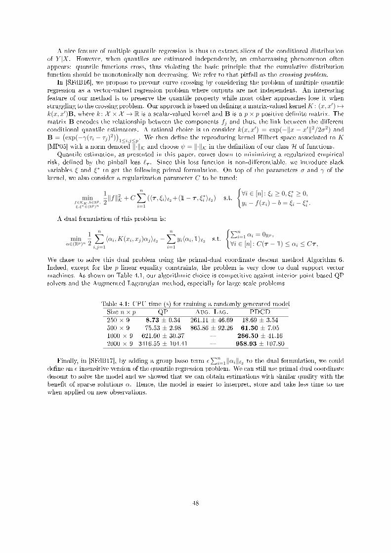
A nice feature of multiple quantile regression is thus to extract slices of the conditional distributionof Y |X. However, when quantiles are estimated independently, an embarrassing phenomenon oftenappears: quantile functions cross, thus violating the basic principle that the cumulative distributionfunction should be monotonically non-decreasing. We refer to that pitfall as the crossing problem.

In [SFdB16], we propose to prevent curve crossing by considering the problem of multiple quantileregression as a vector-valued regression problem where outputs are not independent. An interestingfeature of our method is to preserve the quantile property while most other approaches lose it whenstruggling to the crossing problem. Our approach is based on dening a matrix-valued kernelK : (x, x′) 7→k(x, x′)B, where k : X × X → R is a scalar-valued kernel and B is a p× p positive denite matrix. Thematrix B encodes the relationship between the components fj and thus, the link between the dierentconditional quantile estimators. A rational choice is to consider k(x, x′) = exp(−‖x − x′‖2/2σ2) andB =

(exp(−γ(τi − τj)2)

)1≤i,j≤p. We then dene the reproducing kernel Hilbert space associated to K

[MP05] with a norm denoted ‖·‖K and choose ψ = ‖·‖K in the denition of our class H of functions.Quantile estimation, as presented in this paper, comes down to minimizing a regularized empirical

risk, dened by the pinball loss `τ . Since this loss function is non-dierentiable, we introduce slackvariables ξ and ξ∗ to get the following primal formulation. On top of the parameters σ and γ of thekernel, we also consider a regularization parameter C to be tuned:

minf∈KK,b∈Rp,ξ,ξ∗∈(Rp)n

1

2‖f‖2K + C

n∑i=1

(〈τ , ξi〉`2 +〈1− τ , ξ∗i 〉`2) s.t.

∀i ∈ [n] : ξi ≥ 0, ξ∗i ≥ 0,

yi − f(xi)− b = ξi − ξ∗i .

A dual formulation of this problem is:

minα∈(Rp)n

1

2

n∑i,j=1

〈αi,K(xi, xj)αj〉`2 −n∑i=1

yi〈αi,1〉`2 s.t.

∑ni=1 αi = 0Rp ,

∀i ∈ [n] : C(τ − 1) ≤ αi ≤ Cτ ,

We chose to solve this dual problem using the primal-dual coordinate descent method Algorithm 6.Indeed, except for the p linear equality constraints, the problem is very close to dual support vectormachines. As shown on Table 4.1, our algorithmic choice is competitive against interior point based QPsolvers and the Augmented Lagrangian method, especially for large scale problems

Table 4.1: CPU time (s) for training a randomly generated modelSize n× p QP Aug. Lag. PDCD

250 × 9 8.73 ± 0.34 261.11 ± 46.69 18.69 ± 3.54500 × 9 75.53 ± 2.98 865.86 ± 92.26 61.30 ± 7.051000 × 9 621.60 ± 30.37 266.50 ± 41.162000 × 9 3416.55 ± 104.41 958.93 ± 107.80

Finally, in [SFdB17], by adding a group-lasso term ε∑ni=1‖αi‖`2 to the dual formulation, we could

dene an ε-insensitive version of the quantile regression problem. We can still use primal-dual coordinatedescent to solve the model and we showed that we can obtain estimations with similar quality with thebenet of sparse solutions α. Hence, the model is easier to interpret, store and take less time to usewhen applied on new observations.

48

Chapter 5

Perspectives

According to me, the optimization community has been driven by three main research agendas:

• Write optimization models that describe practical issues. There is a compromise to make betweenthe description power of the models and our ability to solve them.

• Discover new algorithmic paradigms that allow us to solve new, more complex models. We maycite primal-dual methods that avoid projecting onto complex sets, stochastic gradient methods thatcan replace the computation of an integral by the generation of random samples or line search thathelps taking prot of the local smoothness of the objective function.

• Optimize the optimization algorithms available in order to be quicker and be able to solve largerinstances. The tremendous amount of work put for this purpose has made optimization solverssuccessful on a large variety of problems.

There are still major unresolved challenges in nonconvex optimization and for the resolution of prob-lems in large dimension. I would like to add my contribution as follows.

Primal-dual methods with optimal rate of convergence

State-of-the-art primal-dual methods have either a O(1/k) rate for weakly convex functions but are ratherslow in practice or they exhibit a linear rate for well behaved function but have a worst case O(1/

√k)

rate. My goal is to design new methods that would be ecient in both regimes. This may require tocombine techniques from primal-dual algorithms and restart of accelerated methods as well as derivingnew bounds for the purpose of the study.

Stochastic gradient methods for constrained convex optimization

When solving an optimization problem where the objective can be written as an expectation, stochasticgradient methods may be the preferred alternative against coordinate descent. The study of stochasticgradient for saddle point problems has only begun very recently. I plan to base on our smoothingtechnique to design new ecient algorithms in this context.

Stochastic compressed second order methods

Optimization algorithms using Hessians usually require much less iterations than those using gradientonly, but each iteration is much more computationally intensive. We aim at developing ecient stochasticsecond order methods by extracting curvature information through randomized compression. This willalleviate both the cost of calculating the second order derivative matrix and the cost of manipulatingthe resulting matrix since it will be low rank.

49

Generative models for nonconvex optimization

This line of research aims at tackling nonconvex optimization problems using a generative model. Thegoal is design an optimization method that takes prot of a randomness to explore the set of parametersbut is also able to focus on local mimima. The generative model will be trained on a set of optimizationproblems: the choice of training problems is critical to get good performance in practice. There is also alot of freedom on how we parametrize the algorithm. We plan to focus on neural network architecturesthat have a lot of exibility.

Analog-to-feature converter for smart sensors

This interdisciplinary project will put machine learning concerns at the heart of the design of sensors.The goal is to extract the features of the signal before digitizing it. We expect massive computationaland energy gains through the use of a dedicated architecture, that should be optimized for our purpose.

50

Bibliography

[AC10] S. Arlot and A. Celisse. A survey of cross-validation procedures for model selection. Statis-tics surveys, 4:4079, 2010.

[ADFC17] Ahmet Alacaoglu, Quoc Tran Dinh, Olivier Fercoq, and Volkan Cevher. Smooth primal-dual coordinate descent algorithms for nonsmooth convex optimization. In Advances inNeural Information Processing Systems, pages 58525861, 2017.

[AEP08] A. Argyriou, T. Evgeniou, and M. Pontil. Convex multi-task feature learning. MachineLearning, 73(3):243272, 2008.

[Ant10] A. Antoniadis. Comments on: `1-penalization for mixture regression models. TEST,19(2):257258, 2010.

[Aus76] Alfred Auslender. Optimisation: Méthodes Numériques. Masson, Paris, 1976.

[AZO15] Zeyuan Allen-Zhu and Lorenzo Orecchia. Nearly-Linear Time Packing and Covering LPSolver with Faster Convergence Rate Than O(1/ε2). In Proceedings of the Forty-SeventhAnnual ACM on Symposium on Theory of Computing (STOC 2015), 2015.

[Bac13] Francis Bach. Learning with Submodular Functions: A Convex Optimization Perspective.Foundations and Trends R© in Machine Learning, 6(2-3):145373, 2013.

[BBG09] Antoine Bordes, Léon Bottou, and Patrick Gallinari. SGD-QN: Careful quasi-Newtonstochastic gradient descent. JMLR, 10:17371754, 2009.

[BC13] A. Belloni and V. Chernozhukov. Least squares after model selection in high-dimensionalsparse models. Bernoulli, 19(2):521547, 2013.

[BCG11] S. R. Becker, E. J. Candès, and M. C. Grant. Templates for convex cone problems withapplications to sparse signal recovery. Math. Program. Comput., 3(3):165218, 2011.

[BCW11] A. Belloni, V. Chernozhukov, and L. Wang. Square-root Lasso: Pivotal recovery of sparsesignals via conic programming. Biometrika, 98(4):791806, 2011.

[BdBS11] C. Brouard, F. d'Alché Buc, and M. Szafranski. Semi-supervised Penalized Output KernelRegression for Link Prediction. In Proceedings of the 28th International Conference onMachine Learning, 2011.

[Ber96] Dimitri P. Bertsekas. Constrained Optimization and Lagrange Multiplier Methods. AthenaScientic, 1996.

[BERG14] Antoine Bonnefoy, Valentin Emiya, Liva Ralaivola, and Rémi Gribonval. A dynamic screen-ing principle for the lasso. In European Signal Processing Conference EUSIPCO, 2014.

[BERG15] Antoine Bonnefoy, Valentin Emiya, Liva Ralaivola, and Rémi Gribonval. Dynamic Screen-ing: Accelerating First-Order Algorithms for the Lasso and Group-Lasso. IEEE Trans.Signal Process., 63(19):20, 2015.

[BH12] Radu Ioan Boµ and Christopher Hendrich. A variable smoothing algorithm for solvingconvex optimization problems. TOP, 23(1):124150, 2012.

51

[BHF14] Pascal Bianchi, Walid Hachem, and Iutzeler Franck. A stochastic coordinate descent primal-dual algorithm and applications. In 2014 IEEE International Workshop on Machine Learn-ing for Signal Processing (MLSP), pages 16. IEEE, 2014.

[BHNS14] Richard H Byrd, Samantha L Hansen, Jorge Nocedal, and Yoram Singer. A stochasticquasi-Newton method for large-scale optimization. arXiv:1401.7020, 2014.

[BJM+12] Francis Bach, Rodolphe Jenatton, Julien Mairal, Guillaume Obozinski, et al. Convexoptimization with sparsity-inducing norms. Foundations and Trends in Machine Learning,4(1):1106, 2012.

[BKBG11] Joseph K. Bradley, Aapo Kyrola, Danny Bickson, and Carlos Guestrin. Parallel Coordi-nate Descent for L1-Regularized Loss Minimization. In 28th International Conference onMachine Learning, 2011.

[BPC+11a] S. Boyd, N. Parikh, E. Chu, B. Peleato, and J. Eckstein. Distributed optimization andstatistical learning via the alternating direction method of multipliers. Foundations andTrends in Machine Learning, 3(1):1122, 2011.

[BPC+11b] Stephen Boyd, Neal Parikh, Eric Chu, Borja Peleato, and Jonathan Eckstein. Distributedoptimization and statistical learning via the alternating direction method of multipliers.Foundations and Trends in Machine Learning, 3(1):1122, 2011.

[BRT09] P. J. Bickel, Y. Ritov, and A. B. Tsybakov. Simultaneous analysis of Lasso and Dantzigselector. Ann. Statist., 37(4):17051732, 2009.

[BSdB16] C. Brouard, M. Szafranski, and F. d'Alché Buc. Input Output Kernel Regression: Super-vised and Semi-Supervised Structured Output Prediction with Operator-Valued Kernels.Journal of Machine Learning Research, 17(176):148, 2016.

[BT89] Dimitri P Bertsekas and John N Tsitsiklis. Parallel and distributed computation: numericalmethods. Prentice Hall, 1989.

[BT09] Amir Beck and Marc Teboulle. A fast iterative shrinkage-thresholding algorithm for linearinverse problems. SIAM Journal on Imaging Sciences, 2(1):183202, 2009.

[BT12] Amir Beck and Marc Teboulle. Smoothing and First Order Methods: A Unied Framework.SIAM J. Optim., 22(2):557580, 2012.

[BT13] Amir Beck and Luba Tetruashvili. On the convergence of block coordinate descent typemethods. SIAM journal on Optimization, 23(4):20372060, 2013.

[BTN01] Aharon Ben-Tal and Arkadi Nemirovski. Lectures on modern convex optimization: Analysis,algorithms, and engineering applications, volume 3 of MOS-SIAM Series on Optimization.SIAM, 2001.

[BV04] S. Boyd and L. Vandenberghe. Convex Optimization. University Press, Cambridge, 2004.

[Bv11] P. Bühlmann and S. van de Geer. Statistics for high-dimensional data. Springer Series inStatistics. Springer, Heidelberg, 2011. Methods, theory and applications.

[CBS14] Volkan Cevher, Steen Becker, and Martin Schmidt. Convex optimization for big data:Scalable, randomized, and parallel algorithms for big data analytics. IEEE Signal ProcessingMagazine, 31(5):3243, 2014.

[CD11] S. Chrétien and S. Darses. Sparse recovery with unknown variance: a lasso-type approach.IEEE Trans. Inf. Theory, 2011.

[CERS18] Antonin Chambolle, Matthias J Ehrhardt, Peter Richtárik, and Carola-Bibiane Schonlieb.Stochastic primal-dual hybrid gradient algorithm with arbitrary sampling and imagingapplications. SIAM Journal on Optimization, 28(4):27832808, 2018.

52

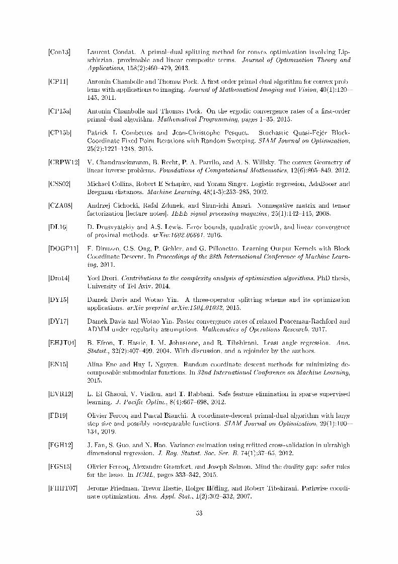
[Con13] Laurent Condat. A primaldual splitting method for convex optimization involving Lip-schitzian, proximable and linear composite terms. Journal of Optimization Theory andApplications, 158(2):460479, 2013.

[CP11] Antonin Chambolle and Thomas Pock. A rst-order primal-dual algorithm for convex prob-lems with applications to imaging. Journal of Mathematical Imaging and Vision, 40(1):120145, 2011.

[CP15a] Antonin Chambolle and Thomas Pock. On the ergodic convergence rates of a rst-orderprimaldual algorithm. Mathematical Programming, pages 135, 2015.

[CP15b] Patrick L Combettes and Jean-Christophe Pesquet. Stochastic Quasi-Fejér Block-Coordinate Fixed Point Iterations with Random Sweeping. SIAM Journal on Optimization,25(2):12211248, 2015.

[CRPW12] V. Chandrasekaranm, B. Recht, P. A. Parrilo, and A. S. Willsky. The convex Geometry oflinear inverse problems. Foundations of Computational Mathematics, 12(6):805849, 2012.

[CSS02] Michael Collins, Robert E Schapire, and Yoram Singer. Logistic regression, AdaBoost andBregman distances. Machine Learning, 48(1-3):253285, 2002.

[CZA08] Andrzej Cichocki, Rafal Zdunek, and Shun-ichi Amari. Nonnegative matrix and tensorfactorization [lecture notes]. IEEE signal processing magazine, 25(1):142145, 2008.

[DL16] D. Drusvyatskiy and A.S. Lewis. Error bounds, quadratic growth, and linear convergenceof proximal methods. arXiv:1602.06661, 2016.

[DOGP11] F. Dinuzzo, C.S. Ong, P. Gehler, and G. Pillonetto. Learning Output Kernels with BlockCoordinate Descent. In Proceedings of the 28th International Conference of Machine Learn-ing, 2011.

[Dro14] Yoel Drori. Contributions to the complexity analysis of optimization algorithms. PhD thesis,University of Tel Aviv, 2014.

[DY15] Damek Davis and Wotao Yin. A three-operator splitting scheme and its optimizationapplications. arXiv preprint arXiv:1504.01032, 2015.

[DY17] Damek Davis and Wotao Yin. Faster convergence rates of relaxed Peaceman-Rachford andADMM under regularity assumptions. Mathematics of Operations Research, 2017.

[EHJT04] B. Efron, T. Hastie, I. M. Johnstone, and R. Tibshirani. Least angle regression. Ann.Statist., 32(2):407499, 2004. With discussion, and a rejoinder by the authors.

[EN15] Alina Ene and Huy L Nguyen. Random coordinate descent methods for minimizing de-composable submodular functions. In 32nd International Conference on Machine Learning,2015.

[EVR12] L. El Ghaoui, V. Viallon, and T. Rabbani. Safe feature elimination in sparse supervisedlearning. J. Pacic Optim., 8(4):667698, 2012.

[FB19] Olivier Fercoq and Pascal Bianchi. A coordinate-descent primal-dual algorithm with largestep size and possibly nonseparable functions. SIAM Journal on Optimization, 29(1):100134, 2019.

[FGH12] J. Fan, S. Guo, and N. Hao. Variance estimation using retted cross-validation in ultrahighdimensional regression. J. Roy. Statist. Soc. Ser. B, 74(1):3765, 2012.

[FGS15] Olivier Fercoq, Alexandre Gramfort, and Joseph Salmon. Mind the duality gap: safer rulesfor the lasso. In ICML, pages 333342, 2015.

[FHHT07] Jerome Friedman, Trevor Hastie, Holger Höing, and Robert Tibshirani. Pathwise coordi-nate optimization. Ann. Appl. Stat., 1(2):302332, 2007.

53

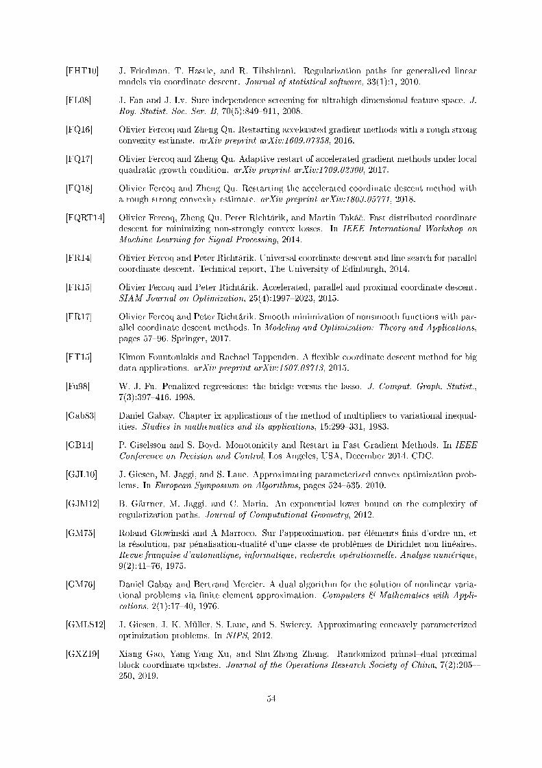
[FHT10] J. Friedman, T. Hastie, and R. Tibshirani. Regularization paths for generalized linearmodels via coordinate descent. Journal of statistical software, 33(1):1, 2010.

[FL08] J. Fan and J. Lv. Sure independence screening for ultrahigh dimensional feature space. J.Roy. Statist. Soc. Ser. B, 70(5):849911, 2008.

[FQ16] Olivier Fercoq and Zheng Qu. Restarting accelerated gradient methods with a rough strongconvexity estimate. arXiv preprint arXiv:1609.07358, 2016.

[FQ17] Olivier Fercoq and Zheng Qu. Adaptive restart of accelerated gradient methods under localquadratic growth condition. arXiv preprint arXiv:1709.02300, 2017.

[FQ18] Olivier Fercoq and Zheng Qu. Restarting the accelerated coordinate descent method witha rough strong convexity estimate. arXiv preprint arXiv:1803.05771, 2018.

[FQRT14] Olivier Fercoq, Zheng Qu, Peter Richtárik, and Martin Taká£. Fast distributed coordinatedescent for minimizing non-strongly convex losses. In IEEE International Workshop onMachine Learning for Signal Processing, 2014.

[FR14] Olivier Fercoq and Peter Richtárik. Universal coordinate descent and line search for parallelcoordinate descent. Technical report, The University of Edinburgh, 2014.

[FR15] Olivier Fercoq and Peter Richtárik. Accelerated, parallel and proximal coordinate descent.SIAM Journal on Optimization, 25(4):19972023, 2015.

[FR17] Olivier Fercoq and Peter Richtárik. Smooth minimization of nonsmooth functions with par-allel coordinate descent methods. In Modeling and Optimization: Theory and Applications,pages 5796. Springer, 2017.

[FT15] Kimon Fountoulakis and Rachael Tappenden. A exible coordinate descent method for bigdata applications. arXiv preprint arXiv:1507.03713, 2015.

[Fu98] W. J. Fu. Penalized regressions: the bridge versus the lasso. J. Comput. Graph. Statist.,7(3):397416, 1998.

[Gab83] Daniel Gabay. Chapter ix applications of the method of multipliers to variational inequal-ities. Studies in mathematics and its applications, 15:299331, 1983.

[GB14] P. Giselsson and S. Boyd. Monotonicity and Restart in Fast Gradient Methods. In IEEEConference on Decision and Control, Los Angeles, USA, December 2014. CDC.

[GJL10] J. Giesen, M. Jaggi, and S. Laue. Approximating parameterized convex optimization prob-lems. In European Symposium on Algorithms, pages 524535, 2010.

[GJM12] B. Gärtner, M. Jaggi, and C. Maria. An exponential lower bound on the complexity ofregularization paths. Journal of Computational Geometry, 2012.

[GM75] Roland Glowinski and A Marroco. Sur l'approximation, par éléments nis d'ordre un, etla résolution, par pénalisation-dualité d'une classe de problèmes de Dirichlet non linéaires.Revue française d'automatique, informatique, recherche opérationnelle. Analyse numérique,9(2):4176, 1975.

[GM76] Daniel Gabay and Bertrand Mercier. A dual algorithm for the solution of nonlinear varia-tional problems via nite element approximation. Computers & Mathematics with Appli-cations, 2(1):1740, 1976.

[GMLS12] J. Giesen, J. K. Müller, S. Laue, and S. Swiercy. Approximating concavely parameterizedoptimization problems. In NIPS, 2012.

[GXZ19] Xiang Gao, Yang-Yang Xu, and Shu-Zhong Zhang. Randomized primaldual proximalblock coordinate updates. Journal of the Operations Research Society of China, 7(2):205250, 2019.

54

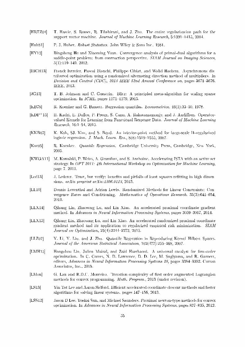
[HRTZ04] T. Hastie, S. Rosset, R. Tibshirani, and J. Zhu. The entire regularization path for thesupport vector machine. Journal of Machine Learning Research, 5:13911415, 2004.

[Hub81] P. J. Huber. Robust Statistics. John Wiley & Sons Inc., 1981.

[HY12] Bingsheng He and Xiaoming Yuan. Convergence analysis of primal-dual algorithms for asaddle-point problem: from contraction perspective. SIAM Journal on Imaging Sciences,5(1):119149, 2012.

[IBCH13] Franck Iutzeler, Pascal Bianchi, Philippe Ciblat, and Walid Hachem. Asynchronous dis-tributed optimization using a randomized alternating direction method of multipliers. InDecision and Control (CDC), 2013 IEEE 52nd Annual Conference on, pages 36713676.IEEE, 2013.

[JG15] T. B. Johnson and C. Guestrin. Blitz: A principled meta-algorithm for scaling sparseoptimization. In ICML, pages 11711179, 2015.

[KB78] R. Koenker and G. Bassett. Regression quantiles. Econometrica, 46(1):3350, 1978.

[KDP+15] H. Kadri, E. Duos, P. Preux, S. Canu, A. Rakotomamonjy, and J. Audiren. Operator-valued Kernels for Learning from Functional Response Data. Journal of Machine LearningResearch, 16:154, 2015.

[KKB07] K. Koh, SJ. Kim, and S. Boyd. An interior-point method for large-scale l1-regularizedlogistic regression. J. Mach. Learn. Res., 8(8):15191555, 2007.

[Koe05] R. Koenker. Quantile Regression. Cambridge University Press, Cambridge, New York,2005.

[KWGA11] M. Kowalski, P. Weiss, A. Gramfort, and S. Anthoine. Accelerating ISTA with an active setstrategy. In OPT 2011: 4th International Workshop on Optimization for Machine Learning,page 7, 2011.

[Led13] J. Lederer. Trust, but verify: benets and pitfalls of least-squares retting in high dimen-sions. arXiv preprint arXiv:1306.0113, 2013.

[LL10] Dennis Leventhal and Adrian Lewis. Randomized Methods for Linear Constraints: Con-vergence Rates and Conditioning. Mathematics of Operations Research, 35(3):641654,2010.

[LLX14] Qihang Lin, Zhaosong Lu, and Lin Xiao. An accelerated proximal coordinate gradientmethod. In Advances in Neural Information Processing Systems, pages 30593067, 2014.

[LLX15] Qihang Lin, Zhaosong Lu, and Lin Xiao. An accelerated randomized proximal coordinategradient method and its application to regularized empirical risk minimization. SIAMJournal on Optimization, 25(4):22442273, 2015.

[LLZ07] Y. Li, Y. Liu, and J. Zhu. Quantile Regression in Reproducing Kernel Hilbert Spaces.Journal of the American Statistical Association, 102(477):255268, 2007.

[LMH15] Hongzhou Lin, Julien Mairal, and Zaid Harchaoui. A universal catalyst for rst-orderoptimization. In C. Cortes, N. D. Lawrence, D. D. Lee, M. Sugiyama, and R. Garnett,editors, Advances in Neural Information Processing Systems 28, pages 33843392. CurranAssociates, Inc., 2015.

[LMon] G. Lan and R.D.C. Monteiro. Iteration-complexity of rst-order augmented Lagrangianmethods for convex programming. Math. Program., 2013 (under revision).

[LS13] Yin Tat Lee and Aaron Sidford. Ecient accelerated coordinate descent methods and fasteralgorithms for solving linear systems. pages 147156, 2013.

[LSS12] Jason D Lee, Yuekai Sun, and Michael Saunders. Proximal newton-type methods for convexoptimization. In Advances in Neural Information Processing Systems, pages 827835, 2012.

55

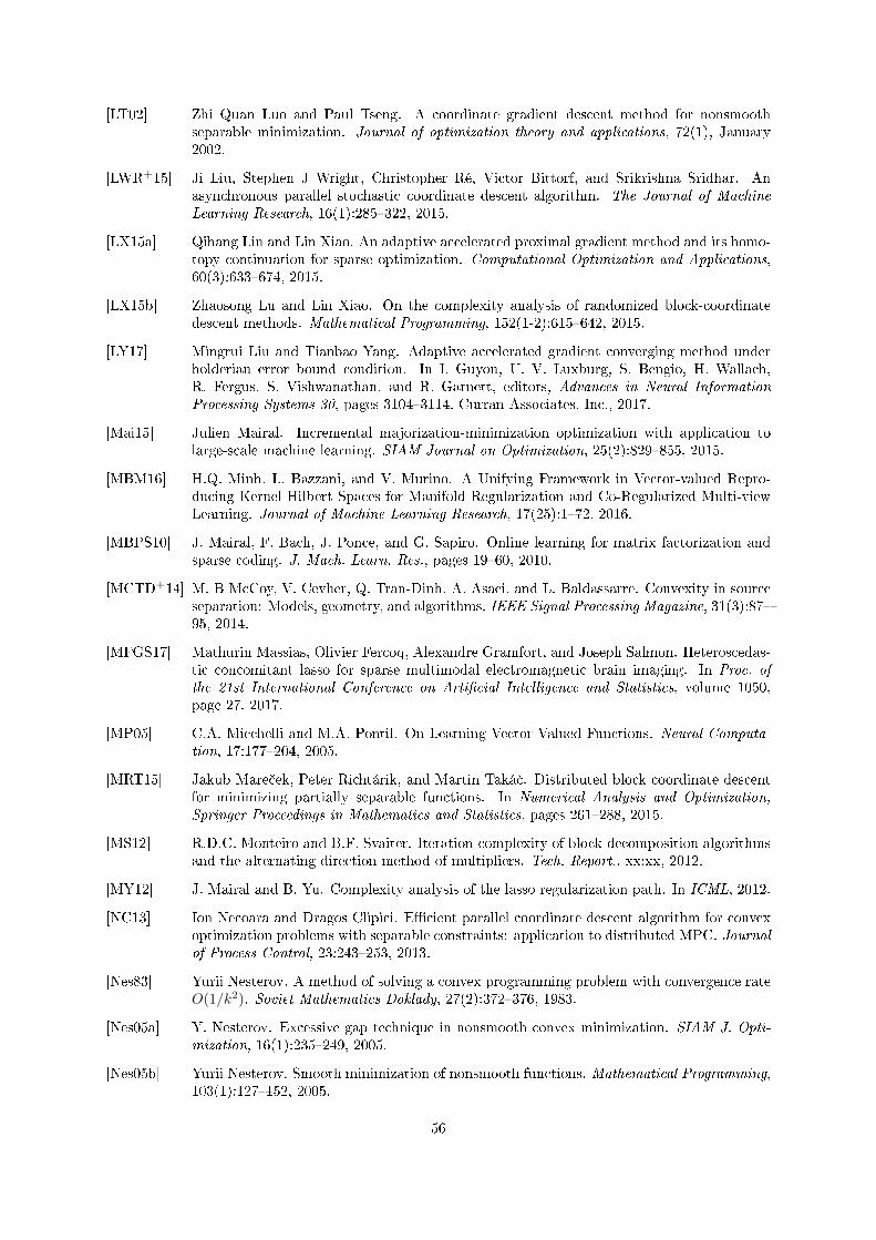
[LT02] Zhi Quan Luo and Paul Tseng. A coordinate gradient descent method for nonsmoothseparable minimization. Journal of optimization theory and applications, 72(1), January2002.

[LWR+15] Ji Liu, Stephen J Wright, Christopher Ré, Victor Bittorf, and Srikrishna Sridhar. Anasynchronous parallel stochastic coordinate descent algorithm. The Journal of MachineLearning Research, 16(1):285322, 2015.

[LX15a] Qihang Lin and Lin Xiao. An adaptive accelerated proximal gradient method and its homo-topy continuation for sparse optimization. Computational Optimization and Applications,60(3):633674, 2015.

[LX15b] Zhaosong Lu and Lin Xiao. On the complexity analysis of randomized block-coordinatedescent methods. Mathematical Programming, 152(1-2):615642, 2015.

[LY17] Mingrui Liu and Tianbao Yang. Adaptive accelerated gradient converging method underholderian error bound condition. In I. Guyon, U. V. Luxburg, S. Bengio, H. Wallach,R. Fergus, S. Vishwanathan, and R. Garnett, editors, Advances in Neural InformationProcessing Systems 30, pages 31043114. Curran Associates, Inc., 2017.

[Mai15] Julien Mairal. Incremental majorization-minimization optimization with application tolarge-scale machine learning. SIAM Journal on Optimization, 25(2):829855, 2015.

[MBM16] H.Q. Minh, L. Bazzani, and V. Murino. A Unifying Framework in Vector-valued Repro-ducing Kernel Hilbert Spaces for Manifold Regularization and Co-Regularized Multi-viewLearning. Journal of Machine Learning Research, 17(25):172, 2016.

[MBPS10] J. Mairal, F. Bach, J. Ponce, and G. Sapiro. Online learning for matrix factorization andsparse coding. J. Mach. Learn. Res., pages 1960, 2010.

[MCTD+14] M. B McCoy, V. Cevher, Q. Tran-Dinh, A. Asaei, and L. Baldassarre. Convexity in sourceseparation: Models, geometry, and algorithms. IEEE Signal Processing Magazine, 31(3):8795, 2014.

[MFGS17] Mathurin Massias, Olivier Fercoq, Alexandre Gramfort, and Joseph Salmon. Heteroscedas-tic concomitant lasso for sparse multimodal electromagnetic brain imaging. In Proc. ofthe 21st International Conference on Articial Intelligence and Statistics, volume 1050,page 27. 2017.

[MP05] C.A. Micchelli and M.A. Pontil. On Learning Vector-Valued Functions. Neural Computa-tion, 17:177204, 2005.

[MRT15] Jakub Mare£ek, Peter Richtárik, and Martin Taká£. Distributed block coordinate descentfor minimizing partially separable functions. In Numerical Analysis and Optimization,Springer Proceedings in Mathematics and Statistics, pages 261288, 2015.

[MS12] R.D.C. Monteiro and B.F. Svaiter. Iteration-complexity of block-decomposition algorithmsand the alternating direction method of multipliers. Tech. Report., xx:xx, 2012.

[MY12] J. Mairal and B. Yu. Complexity analysis of the lasso regularization path. In ICML, 2012.

[NC13] Ion Necoara and Dragos Clipici. Ecient parallel coordinate descent algorithm for convexoptimization problems with separable constraints: application to distributed MPC. Journalof Process Control, 23:243253, 2013.

[Nes83] Yurii Nesterov. A method of solving a convex programming problem with convergence rateO(1/k2). Soviet Mathematics Doklady, 27(2):372376, 1983.

[Nes05a] Y. Nesterov. Excessive gap technique in nonsmooth convex minimization. SIAM J. Opti-mization, 16(1):235249, 2005.

[Nes05b] Yurii Nesterov. Smooth minimization of nonsmooth functions. Mathematical Programming,103(1):127152, 2005.

56

[Nes12a] Yurii Nesterov. Eciency of coordinate descent methods on huge-scale optimization prob-lems. SIAM Journal on Optimization, 22(2):341362, 2012.

[Nes12b] Yurii Nesterov. Subgradient Methods for Huge-Scale Optimization Problems. CORE DIS-CUSSION PAPER 2012/2, 2012.

[Nes13a] Yurii Nesterov. Gradient methods for minimizing composite functions. Mathematical Pro-gramming, 140(1):125161, 2013.

[Nes13b] Yurii Nesterov. Universal Gradient Methods for Convex Optimization Problems. Corediscussion paper, 2013.

[NFG+17] Eugene Ndiaye, Olivier Fercoq, Alexandre Gramfort, Vincent Leclère, and Joseph Salmon.Ecient smoothed concomitant lasso estimation for high dimensional regression. In Journalof Physics: Conference Series, volume 904, page 012006. IOP Publishing, 2017.

[NFGS15] Eugène Ndiaye, Olivier Fercoq, Alexandre Gramfort, and Joseph Salmon. GAP safe screen-ing rules for sparse multi-task and multi-class models. NIPS, pages 811819, 2015.

[NFGS16] Eugène Ndiaye, Olivier Fercoq, Alexandre Gramfort, and Joseph Salmon. GAP safe screen-ing rules for Sparse-Group Lasso. NIPS, 2016.

[NFGS17] Eugene Ndiaye, Olivier Fercoq, Alexandre Gramfort, and Joseph Salmon. Gap safe screen-ing rules for sparsity enforcing penalties. The Journal of Machine Learning Research,18(1):46714703, 2017.

[NFS+18] Eugène Ndiaye, Olivier Fercoq, Joseph Salmon, Ichiro Takeuchi, and Le Tam. Safe gridsearch with optimal complexity. Technical report, Télécom ParisTech and Nagoya Instituteof Technology, 2018.

[NNG12] Ion Necoara, Yurii Nesterov, and Francois Glineur. Eciency of randomized coordinatedescent methods on optimization problems with linearly coupled constraints. Technicalreport, Politehnica University of Bucharest, 2012.

[NW06] J. Nocedal and S.J. Wright. Numerical Optimization. Springer Series in Operations Re-search and Financial Engineering. Springer, 2 edition, 2006.

[OC12] Brendan O'Donoghue and Emmanuel Candes. Adaptive restart for accelerated gradientschemes. Foundations of Computational Mathematics, pages 118, 2012.

[OPT00] M. R. Osborne, B. Presnell, and B. A. Turlach. A new approach to variable selection inleast squares problems. IMA J. Numer. Anal., 20(3):389403, 2000.

[Owe07] A. B. Owen. A robust hybrid of lasso and ridge regression. Contemporary Mathematics,443:5972, 2007.

[PH07] M. Y. Park and T. Hastie. L1-regularization path algorithm for generalized linear models.Journal of the Royal Statistical Society: Series B (Statistical Methodology), 69(4):659677,2007.

[Pow73] Michael JD Powell. On search directions for minimization algorithms. Mathematical pro-gramming, 4(1):193201, 1973.

[PR15] Jean-Christophe Pesquet and Audrey Repetti. A class of randomized primal-dual algo-rithms for distributed optimization. Journal of Nonlinear Convex Analysis, 16(12), 2015.

[PW14] Mert Pilanci and Martin J. Wainwright. Iterative Hessian sketch: fast and accurate solutionapproximation for constrained least-squares. arXiv:1411.0347, 2014.

[QR16] Zheng Qu and Peter Richtárik. Coordinate descent with arbitrary sampling I: algorithmsand complexity. Optimization Methods and Software, 2016.

57

[QRTF16] Zheng Qu, Peter Richtárik, Martin Takác, and Olivier Fercoq. Sdna: stochastic dual newtonascent for empirical risk minimization. In International Conference on Machine Learning,pages 18231832, 2016.

[QRZ15] Zheng Qu, Peter Richtárik, and Tong Zhang. Quartz: Randomized Dual Coordinate Ascentwith Arbitrary Sampling. In NIPS 28, pages 865873. 2015.

[RKB04] Carsten Rother, Vladimir Kolmogorov, and Andrew Blake. Grabcut: Interactive foregroundextraction using iterated graph cuts. ACM Transactions on Graphics (TOG), 23(3):309314, 2004.

[Roc76a] R T Rockafellar. Augmented Lagrangians and applications of the proximal point algorithmin convex programming. Mathematics of Operations Research, 1:97116, 1976.

[Roc76b] R T Rockafellar. Monotone operators and the proximal point algorithm. SIAM Journal onControl and Optimization, 14:877898, 1976.

[ROG+16] A. Raj, J. Olbrich, B. Gärtner, B. Schölkopf, and M. Jaggi. Screening rules for convexproblems. arXiv preprint arXiv:1609.07478, 2016.

[RT14] Peter Richtárik and Martin Taká£. Iteration complexity of randomized block-coordinatedescent methods for minimizing a composite function. Mathematical Programming, Ser. A,144(1-2):138, 2014.

[RT15] Peter Richtárik and Martin Taká£. Parallel coordinate descent methods for big data opti-mization. Mathematical Programming, pages 152, 2015.

[RT16a] Peter Richtárik and Martin Taká£. Distributed coordinate descent method for learningwith big data. The Journal of Machine Learning Research, 17(1):26572681, 2016.

[RT16b] Peter Richtárik and Martin Taká£. On optimal probabilities in stochastic coordinate descentmethods. Optimization Letters, 10(6):12331243, 2016.

[RT16c] Peter Richtárik and Martin Taká£. Distributed coordinate descent method for learningwith big data. The Journal of Machine Learning Research, 17(1):26572681, 2016.

[RTF13] S. Reid, R. Tibshirani, and J. Friedman. A study of error variance estimation in lassoregression. arXiv preprint arXiv:1311.5274, 2013.

[RZ07] S. Rosset and J. Zhu. Piecewise linear regularized solution paths. The Annals of Statistics,pages 10121030, 2007.

[SBC14] W. Su, S. Boyd, and E. Candes. A dierential equation for modeling Nesterov's acceleratedgradient method: Theory and insights. In Advances in Neural Information ProcessingSystems (NIPS), pages 25102518, 2014.

[SBv10] N. Städler, P. Bühlmann, and S. van de Geer. `1-penalization for mixture regression models.TEST, 19(2):209256, 2010.

[SDPG14] Jascha Sohl-Dickstein, Ben Poole, and Surya Ganguli. Fast large-scale optimization byunifying stochastic gradient and quasi-Newton methods. In ICML, 2014.

[Sei74] Ludwig Seidel. Ueber ein Verfahren, die Gleichungen, auf welche die Methode der klein-sten Quadrate führt, sowie lineäre Gleichungen überhaupt, durch successive Annäherungaufzulösen:(Aus den Abhandl. dk bayer. Akademie II. Cl. XI. Bd. III. Abth. Verlag der k.Akademie, 1874.

[SFdB16] Maxime Sangnier, Olivier Fercoq, and Florence d'Alché Buc. Joint quantile regression invector-valued rkhss. In Advances in Neural Information Processing Systems, pages 36933701, 2016.

58

[SFdB17] Maxime Sangnier, Olivier Fercoq, and Florence d'Alché Buc. Data sparse nonparametricregression with ε-insensitive losses. In Asian Conference on Machine Learning, pages 192207, 2017.

[SKHT16] A. Shibagaki, M. Karasuyama, K. Hatano, and I. Takeuchi. Simultaneous safe screening offeatures and samples in doubly sparse modeling. In ICML, pages 15771586, 2016.

[SSBD14] Shai Shalev-Shwartz and Shai Ben-David. Understanding Machine Learning: From Theoryto Algorithms. Cambridge University Press, New York, NY, USA, 2014.

[SSKT15] A. Shibagaki, Y. Suzuki, M. Karasuyama, and I. Takeuchi. Regularization path of cross-validation error lower bounds. In NIPS, 2015.

[SST11] Shai Shalev-Shwartz and Ambuj Tewari. Stochastic methods for `1-regularized loss mini-mization. Journal of Machine Learning Research, 12:18651892, 2011.

[SSZ12] Shai Shalev-Shwartz and Tong Zhang. Proximal Stochastic Dual Coordinate Ascent.arXiv:1211.2717, 2012.

[SSZ13] Shai Shalev-Shwartz and Tong Zhang. Stochastic Dual Coordinate Ascent Methods forRegularized Loss Minimization. Journal of Machine Learning Research, 14(1):567599,2013.

[SSZ14] Shai Shalev-Shwartz and Tong Zhang. Accelerated proximal stochastic dual coordinateascent for regularized loss minimization. In International Conference on Machine Learning,pages 6472, 2014.

[STD17] Tianxiao Sun and Quoc Tran-Dinh. Generalized self-concordant functions: a recipe forNewton-type methods. Mathematical Programming, pages 169, 2017.

[STY16] Defeng Sun, Kim-Chuan Toh, and Liuqin Yang. An ecient inexact ABCD method forleast squares semidenite programming. SIAM Journal on Optimization, 26(2):10721100,2016.

[Suz14] Taiji Suzuki. Stochastic dual coordinate ascent with alternating direction method of multi-pliers. In Proceedings of the 31st International Conference on Machine Learning (ICML-14),pages 736744, 2014.

[SYG07] Nicol N. Schraudolph, Jin Yu, and Simon Günter. A stochastic quasi-Newton method foronline convex optimization. In AISTATS, pages 433440, 2007.

[SZ12] T. Sun and C.-H.. Zhang. Scaled sparse linear regression. Biometrika, 99(4):879898, 2012.

[TBF+12] R. Tibshirani, J. Bien, J. Friedman, T. Hastie, N. Simon, J. Taylor, and R. J. Tibshirani.Strong rules for discarding predictors in lasso-type problems. J. Roy. Statist. Soc. Ser. B,74(2):245266, 2012.

[TBRS13] Martin Taká£, Avleen Bijral, Peter Richtárik, and Nathan Srebro. Mini-batch primal anddual methods for SVMs. In 30th International Conference on Machine Learning, 2013.

[TC14] Quoc Tran-Dinh and Volkan Cevher. A primal-dual algorithmic framework for constrainedconvex minimization. arXiv preprint arXiv:1406.5403, 2014.

[TDC14] Quoc Tran-Dinh and Volkan Cevher. Constrained convex minimization via model-basedexcessive gap. In Proc. the Neural Information Processing Systems Foundation conference(NIPS2014), volume 27, pages 721729, Montreal, Canada, December 2014.

[TDC15] Quoc Tran-Dinh and Volkan Cevher. An optimal rst-order primal-dual gap reductionframework for constrained convex optimization. Tech. Report, LIONS-EPFL, pages 141,2015.

59

[TDFC18] Quoc Tran-Dinh, Olivier Fercoq, and Volkan Cevher. A smooth primal-dual optimizationframework for nonsmooth composite convex minimization. SIAM Journal on Optimization,28(1):96134, 2018.

[Tib96] R. Tibshirani. Regression shrinkage and selection via the lasso. J. Roy. Statist. Soc. Ser.B, 58(1):267288, 1996.

[TKCW12] Qing Tao, Kang Kong, Dejun Chu, and Gaowei Wu. Stochastic Coordinate Descent Meth-ods for Regularized Smooth and Nonsmooth Losses. Machine Learning and KnowledgeDiscovery in Databases, pages 537552, 2012.

[TLSS06] I. Takeuchi, Q.V. Le, T.D. Sears, and A.J. Smola. Nonparametric Quantile Estimation.Journal of Machine Learning Research, 7:12311264, 2006.

[Tod01] Micheal J. Todd. Semidenite optimization. Acta Numerica, 10:515560, 2001.

[TRG16a] Rachael Tappenden, Peter Richtárik, and Jacek Gondzio. Inexact coordinate descent: com-plexity and preconditioning. Journal of Optimization Theory and Applications, pages 133,2016.

[TRG16b] Rachael Tappenden, Peter Richtárik, and Jacek Gondzio. Inexact coordinate descent: com-plexity and preconditioning. Journal of Optimization Theory and Applications, 170(1):144176, 2016.

[Tse01] Paul Tseng. Convergence of a block coordinate descent method for nondierentiable mini-mization. Journal of optimization theory and applications, 109(3):475494, June 2001.

[Tse08] Paul Tseng. On accelerated proximal gradient methods for convex-concave optimization.Submitted to SIAM Journal on Optimization, 2008.

[TY09a] Paul Tseng and Sangwoon Yun. A coordinate gradient descent method for nonsmoothseparable minimization. Mathematical Programming, 117:387423, 2009.

[TY09b] Paul Tseng and Sangwoon Yun. Block-Coordinate Gradient Descent Method for LinearlyConstrained Non Separable Optimization. Journal of Optimization Theory and Applica-tions, 140:513535, 2009.

[VB96] Lieven Vandenberghe and Stephen Boyd. Semidenite Programming. SIAM Review,38(1):4995, 1996.

[VNFC17] Quang Van Nguyen, Olivier Fercoq, and Volkan Cevher. Smoothing technique for non-smooth composite minimization with linear operator. arXiv preprint arXiv:1706.05837,2017.

[Vu13] Bang Công Vu. A splitting algorithm for dual monotone inclusions involving cocoerciveoperators. Advances in Computational Mathematics, 38(3):667681, 2013.

[Wai14] M. J. Wainwright. Structured regularizers for high-dimensional problems: Statistical andcomputational issues. Annu. Rev. Stat. Appl., 1:233253, 2014.

[War63] Jack Warga. Minimizing certain convex functions. Journal of the Society for Industrial &Applied Mathematics, 11(3):588593, 1963.

[WSV10] HenryWolkowicz, Romesh Saigal, and Lieven Vandenberghe, editors. Handbook of Semide-nite Programming, volume 27 of International Series in Operations Research & ManagementScience. Kluwer Academic Publishers, Boston, MA, 2010.

[WWY12] J. Wang, P. Wonka, and J. Ye. Lasso screening rules via dual polytope projection. arXivpreprint arXiv:1211.3966, 2012.

[WZL+14] J. Wang, J. Zhou, J. Liu, P. Wonka, and J. Ye. A safe screening rule for sparse logisticregression. In NIPS, pages 10531061, 2014.

60

[XCM10] H. Xu, C. Caramanis, and S. Mannor. Robust regression and lasso. IEEE Trans. Inf.Theory, 56(7):35613574, 2010.

[Xu17] Yangyang Xu. Accelerated rst-order primal-dual proximal methods for linearly constrainedcomposite convex programming. SIAM Journal on Optimization, 27(3):14591484, 2017.

[XWR14] Z. J. Xiang, Y. Wang, and P. J. Ramadge. Screening tests for lasso problems. arXiv preprintarXiv:1405.4897, 2014.

[XXR11] Z. J. Xiang, H. Xu, and P. J. Ramadge. Learning sparse representations of high dimensionaldata on large scale dictionaries. In NIPS, pages 900908, 2011.

[YFLC18] Alp Yurtsever, Olivier Fercoq, Francesco Locatello, and Volkan Cevher. A conditionalgradient framework for composite convex minimization with applications to semideniteprogramming. In International Conference on Machine Learning, 2018.

[YL06] M. Yuan and Y. Lin. Model selection and estimation in regression with grouped variables.J. Roy. Statist. Soc. Ser. B, 68(1):4967, 2006.

[ZX14] Yuchen Zhang and Lin Xiao. Stochastic primal-dual coordinate method for regularizedempirical risk minimization. arXiv preprint arXiv:1409.3257, 2014.

61

coordinate descent methods for non-differentiable convex

Documents