differentiable electron microscopy simulation - arxiv

DIFFERENTIABLE ELECTRON MICROSCOPY SIMULATION:METHODS AND APPLICATIONS FOR VISUALIZATION

A PREPRINT

Ngan Nguyen1,*, Feng Liang1,*, Dominik Engel2, Ciril Bohak1, Peter Wonka1, Timo Ropinski2, and Ivan Viola1

1King Abdullah University of Science and Technology (KAUST), Saudi Arabia.E-mails: {ngan.nguyen | feng.liang | ciril.bohak | peter.wonka | ivan.viola}@kaust.edu.sa.

2Ulm University, Ulm, Germany.E-mail: {dominik.engel | timo.ropinski}@uni-ulm.de.

*N. Nguyen and F. Liang are co-first authors.

May 27, 2022

Figure 1: Three main contributions of this work are: (1) DiffTEM: a differentiable electron microscopy simulator, (2)a use case for automatic detector parameter estimation, and (3) a use case for denoising the data from real electronmicroscope.

ABSTRACT

We propose a new microscopy simulation system that can depict atomistic models in a micrographvisual style, similar to results of physical electron microscopy imaging. This system is scalable, ableto represent simulation of electron microscopy of tens of viral particles and synthesizes the imagefaster than previous methods. On top of that, the simulator is differentiable, both its deterministic aswell as stochastic stages that form signal and noise representations in the micrograph. This notableproperty has the capability for solving inverse problems by means of optimization and thus allowsfor generation of microscopy simulations using the parameter settings estimated from real data. Wedemonstrate this learning capability through two applications: (1) estimating the parameters of themodulation transfer function defining the detector properties of the simulated and real micrographs,and (2) denoising the real data based on parameters trained from the simulated examples. Whilecurrent simulators do not support any parameter estimation due to their forward design, we show thatthe results obtained using estimated parameters are very similar to the results of real micrographs.Additionally, we evaluate the denoising capabilities of our approach and show that the results showed

arX

iv:2

205.

0446

4v2

[q-

bio.

QM

] 2

6 M

ay 2

022

A PREPRINT - MAY 27, 2022

an improvement over state-of-the-art methods. Denoised micrographs exhibit less noise in thetilt-series tomography reconstructions, ultimately reducing the visual dominance of noise in directvolume rendering of microscopy tomograms.

Keywords Transmission Electron Microscopy Simulation; Data Models; Software Prototype; Life Sciences, Health,Medicine, Biology, Bioinformatics, Genomics; Computer Graphics Techniques; Image and Signal Processing

1 Introduction

With the revolution in the resolution [1] in 2014, the cryogenic electron microscopy (cryo-EM) became an uniquetool to study and visualize the cell and its inner structures at the molecular level [2]. Still, extraction of the valuableinformation from the data obtained using cryo-EM and developing the computational methods for processing, analyzing,and/or visualizing such data are not trivial tasks. The main reason is the fact that the data acquisition process istime-consuming, costly, and is still performed mainly by bio-experts. This situation results in a relatively small amountof data available for developing learning-centric computational methods. Additionally, due to the limitation to only uselow electron beam doses to protect the specimen, the data always suffer from a low signal-to-noise ratio (SNR). Finally,because of the limited specimen tilting during the acquisition process, high-tilt projections are missing, which resultsin the missing wedge problem [3]. All these shortcomings make the usage of such data difficult for visualization. Toovercome these challenges, it is possible to use highly-accurate simulated data, which are similar-to-indistinguishableto the actual acquired data. Such simulation data can be easily used in ground-truth based evaluations, since the inputstructural model is known prior to the microscopy simulation process. It can be used in training structural biologiststo learn interpreting microscopy projections, i. e., micrographs. Such simulation can be also regarded as a distinctrendering style, useful for example in generating animation sequences where a biological structure is transformed into amicrograph and vice versa. Last but not least, such data can be used for developing new Deep Learning (DL) methodsfor interpreting real micrographs, their testing, evaluation, and validation.

In recent years, researchers have developed several Transmission Electron Microscopy (TEM) simulators to supportstudies in biological specimen research, some of which are based on physical principles [4–6] or parallel multi-slicesimulation [7]. The simulator presented by Rullgard et al. [4] uses the multi-slice method [8] for modeling the interactionof electron and biological specimen, which is well suited for a computer simulation [9]. Additionally, the authors havedeveloped a phantom generator for generating a specimen model and the calculation of its scattering potential basedon a physical model. The above-mentioned simulator properties make it a good choice for simulating an acquisitionprocess of biological specimens using cryo-EM. However, the simulator has two major limitations. First, the simulatedmicroscope parameters need to be calibrated manually, which is a tedious and time-consuming process where even theinitial values are not available. Second, the simulator is very slow when simulating structures larger than a few proteins.Some enveloped viral particles are huge macromolecular model (e. g., ZIKA or SARS-CoV-2). It is entirely infeasibleto run a microscopy simulation of many instances of such particles with any of the previous microscopy simulationsystems.

In the field of differentiable rendering, visualization problems are addressed with the use of differentiable pipelines.For example, DiffDVR [10] uses a differentiable direct volume rendering (DVR) pipeline to optimize view points,transfer functions and voxel properties. Therefore, taking inspiration from differentiable rendering, we present a fastdifferentiable simulator, which enables us to optimize for all continuous parameters of a microscope simulator. Wedemonstrate the capabilities of our differentiable simulator with two use cases, which are (1) detector parametersestimation from real data and (2) denoising. We show that using the detector parameters estimated from real data withour differentiable simulator yields accurate results. Additionally, denoising real micrographs using our pipeline iseffective and outperforms state-of-the-art DL-based approaches.

This paper presents several technical contributions that and visualization applications:

• The overall architecture of the first differentiable microscopy simulator that is scalable to render realisticmicroscopy simulations within seconds or minutes.

• Learning detector parameters from real projections, to generate synthetic micrographs with the same detectorcharacteristics that lead to similar visual appearance of the synthetic and the real projection.

• Utilization of deterministic and stochastic differentiation for various stages of the microscopy pipeline.• Generation of large micrographs on par with physical dimensions and complexity of real-world microscopy.• A new denoising method which learns from noisy projections to create a noise-free version of real-world

projections. Subsequent tomographic reconstruction then results in a noise-free volume that can be used for3D visualization.

2


2 Related work

First we give a brief overview of TEM simulators developed in recent years. Next, we discuss differentiable renderingand how it relates to the TEM simulation. Then, we provide background information for gradient estimation indistribution learning. Finally, we discuss related works on DL-based denoising.

TEM Simulators: Several Electron Microscopy (EM) simulators were developed for simulating the specimenacquisition process from different domains as presented in a book by Kirkland [9]. One of the most commonly usedsimulators for non-crystalline biological specimens is TEM simulator presented by Rullgard et al. [4], which is alsothe basis for our differentiable version of the TEM simulator. The presented simulator aims to provide an accuratesimulation based on a well-defined physical model. Still, the implementation of the simulator introduces a set ofuser-adjustable parameters (e. g., detector parameters), which require a time-consuming manual calibration process.The researchers have later presented a new TEM simulator which aims to improve the above one. While the originalTEM simulator calculates the scattering potential of the specimen by estimating the potential of the atoms, InSilicoTEM [5] calculates it more precisely by also including the scattering potential of molecular bonds. It also reduces thenumber of detector parameters and estimates them from experiments. In the recent work of Himes and Grigorieff [6],they considered the TEM simulation of amorphous samples which are sensitive to electron radiations. Additionally,they also slice the simulation in the time domain, which leads to the generation of movie frames of an exposure. Thelatter approaches are more accurate than the original TEM simulator [4] trading in additional physical aspects of thesimulator with much higher computational costs. Nevertheless, all the presented simulators only support the forwardsimulation. To the best of our knowledge, our proposed work is the first to offer a forward and backward approach tosimulation through differentiability, which is crucial in optimization for different visualization tasks.

To solve the reconstruction problem, CryoGAN [11] takes advantage of a Generative Adversarial Network (GAN) [12]and uses an EM simulator based on the ASTRA Toolbox [13] for generating realistic EM projections. During theforward calculation, it utilizes the simulation algorithm from the toolbox, while the back-projection approach fromthe toolbox is used to calculate gradients to enable differentiability. Given a training dataset of noisy micrographs,researchers crop empty patches that contain only background noise from the data. Next, they train a neural volumegenerator, whose generated volumes are fed into the simulator from the toolbox to generate clean micrographs. Theempty patches of background noise are added to the clean micrographs, mocking noisy micrographs. The resultingnoisy micrographs are given to the discriminator network, along with the real noisy micrographs. In contrast to ourapproach, this method does not model noise generation within the simulation and therefore assumes that the noise inmicrographs is signal-independent. However, in the physical model of the TEM simulator [4], this assumption does nothold because the models for shot noise and detector blurring depend on pixel values. Moreover, CryoGAN [11] assumesthat the background noise is similar throughout the specimen, which is not the case due to the change in thickness ofthe specimen from center towards the boundary.

Differentiable Rendering: Together with neural rendering, it has seen dramatic progress mostly in the context ofcomputer vision and photorealistic rendering. For example, in Li et al. [14], rendering parameters (e. g., scene geome-tries, camera intrinsics, and lighting conditions) can be estimated directly from images thanks to its differentiability.Hasselgren et al. [15] use a gradient estimator to optimize for ray tracing rendering parameters (i. e., sample numbers ofpixels). MVTN [16] takes advantage of a differentiable renderer to optimize for the performance of a downstream task(i. e., 3D geometry classification).

If we compare photorealistic rendering with TEM simulation in a general sense, they both share similar pipelinesfrom geometries to rendered artifacts, given a rendering method. Similar to how differentiable rendering has openeda new view on solving well-known problems in a novel way with an explainable approach, can differentiable EMsimulation provide new insight into solving simulation-related problems with an optimization approach. CryoGAN [11]already shows promising results along these lines. The main difference is that it was developed for a single-particlereconstruction and is thus lacking generalizability. In the recent work, Kniesel et al. [17] developed a differentiableScanning Transmission Electron Microscopy (STEM) pipeline and showed promising results for implicit volumereconstruction. With our TEM simulator, we can estimate Modulation Transfer Function (MTF) parameters of thesimulator’s detector part, which is in a way similar to estimating rendering parameters in a differentiable renderingmethod as was shown by Weiss and Westermann [10] for direct volume rendering. Moreover, our approach provides anovel approach for denoising by using images generated with a TEM simulator in a similar way as Noise2Noise [18]and Topaz-Denoise [19] but based on a simulator physics model [4].

Gradient Estimation in Distribution Learning: Distribution learning has been a challenging problem in variousfields of DL. There are many approaches to learning a random distribution. Still, they can be classified into two categories,

3


learning the parameters of distributions (e. g., µ and σ of a normal distribution) and learning the manipulation ofdistributions, (e. g., fθ (x) where θ parameterizes f , and x is sampled from a prescribed distribution).

In some scenarios, the distribution of the learning objectives of a task is not known. For example, in face generation,the distribution of faces is not known nor well-defined, which means random distributions must be prescribed andmanipulated. Therefore, how to manipulate predefined random distributions is the key target of optimization. Formally,such learning can be formulated as

argminθ

E(L( fθ (X),Y )), X ∼ D,

where θ is the set of parameters of f , L a loss function, D a prescribed distribution, and Y a training dataset. GAN [12] isa typical case in which the optimization targets are not the parameters of the prescribed distributions but the parametersof the functions that manipulate the distributions.

When the distribution of the learning objectives is known, the distribution parameters are often the optimization target.For example, in Reinforcement Learning (RL), models can be asked to make stochastic decisions with a discretedistribution (e. g., a categorical distribution). In such settings, the optimization can be described formally as:

argminω

E(L( f (X),Y )), X ∼ R(ω),

where ω is the set of parameters of a distribution R. From the perspective of Calculus, ∂L∂ω

is not defined, so researchersturn to statistical gradient estimators. One of the most widely used gradient estimators is the Monte Carlo (MC) family.The details of MC gradient estimators are beyond the scope of this paper, so we refer the reader to the review on MCgradient estimators [20].

Variational Autoencoder (VAE) [21] is a hybrid case in which distributions’ parameters and functions’ parameters thatmanipulate the distributions are jointly learned. VAE can be formulated as:

argmin{θ0,θ1}

E(L(gθ1(Z),Y )), Z ∼ P( fθ0(X)),

where f and g are functions paremterized by θ0 and θ1 respectively and P a distribution of a prescribed type parameter-ized by fθ0(X).

As new and even more complex probabilistic models than VAE emerge, existing gradient estimators and optimizationtechniques that are designed for specific models are not enough for training new models. Therefore, Schulman et al. [22]seek a general formulation of probabilistic models, which is stochastic compute graphs. Based on stochastic computegraphs, they devised a new way to transform deterministic loss functions into ones whose gradients are general gradientestimators of all parameters, including parameters of distributions. Such loss functions are called surrogate lossfunctions, and the compute graph including surrogate loss functions is called a surrogate loss function computationgraph.

In our work, when estimating detector parameters, we take a GAN-like approach, optimizing for function parameters byprescribing a distribution. In the case of denoising micrographs, we define the surrogate loss function computationgraph for gradient estimation based on the work of Schulman et al. [22].

2.1 Denoising

When denoising cryo-EM micrographs, clean references are not available, so many approaches have been proposed tospecifically denoise cryo-EM micrographs, addressing this problem.

Researchers have proposed various analytical filters for denoising, such as simple averaging, Gaussian filters, and manyfilters in the frequency space that enhance or damp signal responses. Additionally, physics-based techniques wereproposed, such as Nonlinear Anisotropic Diffusion (NAD) [23], which takes advantage of a diffusion model to denoise3D volumes. For a comprehensive review on filters used in cryo-EM, we refer the reader to the review [24].

In the era of DL, many neural networks are proposed to denoise cryo-EM micrographs. Noise2Noise [18] is a generaldenoising approach that does not require clean data and has been adapted in CryoCARE [25] and Topaz-Denoise [19].In CryoCARE [25], a neural network is trained as a denoiser with multiple micrographs that come from multipleconsecutive exposures or multiple aligned micrographs in a tilt series or movie frames captured during a long exposure.In Topaz-Denoise [19], the researchers trained the model with a larger dataset containing thousands of micrographsacquired in different conditions, which enables better generalizability of their neural networks. Besides Noise2Noise-based approaches, Noise-Transfer2Clean (NT2C) [26] trains two neural denoisers and a GAN-based noise synthesizerto decouple noise from micrographs that are generated using a cryo-EM simulator based on real and synthetic data.

4


Scene withatomistic

modelGPU TEM

Diff TEM

Simulatedmicrograph

Real cryo-EMdata

Denoising

Detectorparametersoptimization

Denoisedmicrograph

Similar configuration

Figure 2: Our GPU-TEM (GPU-TEM) simulator receives scene configuration and detector parameters estimated fromreal data by Differentiable TEM (Diff-TEM) simulator for generating simulated micrograph. Our Diff-TEM simulatordenoises the real data, the denoised data can be used for reconstruction and the reconstrution can be visualized by directvolume rendering.

The implicit reconstruction approach by Kniesel et al. [17] also incorporates a normalizing flows neural network tomodel the noise distribution in the STEM data in a signal-dependent manner, allowing them to separate the noise fromthe clean reconstruction.

Our approach is similar to Noise2Noise [18] in the way that our model is required to output similar noisy images (i.e.,noisy EM projections). However, in our simulator, we do not involve neural networks but a physical model.

3 Architecture overview

Our system contains two simulators as shown in Figure 2, GPU-TEM for rendering and Diff-TEM for learning. TheGPU-TEM receives the scene with the same configuration as used for acquisition with the real cryo-EM, and the learnedparameters (e. g., MTF) from the Diff-TEM as inputs. It then simulates the synthetic data that are similar to the realdata. The Diff-TEM receives the real cryo-EM data and performs the learning, e. g., estimating MTF parameters ordenoising the real data. By using this design, our system resolves two limitations of the TEM Simulator [4]: (1) theneed for user-estimated parameters, and (2) a time-consuming simulation process for scenes containing many instancesof macro-molecular structures.

Both the GPU-TEM and the Diff-TEM simulators are based on the TEM simulator [4] and its main purpose is tosimulate the image formation process. The simulator contains components similar to a real microscopy system: electrongun; specimen; optical system – aperture, condenser lens, objective lens, projector lens, and detector. The schema ofthe simulator is shown in Fig. 3, where we specify the parameters with their names in blue boxes, the outputs of a stepin green boxes, and stochastic nodes in circles.

To simulate the image formation process, the simulator performs two tasks. First, assembling a model of the specimenand calculating the scattering potential of the specimen are completed by the phantom generator. Second, simulatingthe image formation process is further split into electron-specimen interaction, electron wave propagation, and intensitydetection by the detectors.

The phantom generator allows to define a specimen, including objects, background, and distribution of objects withinthe background. The background is assumed to be pure cryonized water. The phantom generator receives as inputan atomistic model of objects defined by homologous proteins from Protein Data Bank (PDB) [27], their distributionwithin the specimen (user-defined or random), sample properties (thickness, sample hole diameter), and electron gunvoltage. From the inputs, it calculates the scattering potential of objects by summing the electrostatic potential ofindividual atoms. Next, it calculates the scattering potential of the background. Finally, it fuses background and objectpotentials. The details of the calculation are presented in Appendix B of the TEM simulator paper [4].

5


Propagation

Interact withDetector in

Reciprocal Space

Imaging

Shot noise(Poissonprocess)

Detector Interactions

Noise-free projection without MTF

ElectronGun

CondenserLens

System

ProjectorLens

System

Detector

ObjectiveLens

System Specimen

Electrons

Wave Function

Propagate

Interact withParticles in

Reciprocal Space

Noisy Projection

DetectorParameters

Geometry ErrorsParticle Coordinates

Atom TypesSample Specifications

ElectronBeam SpecificationsOptics Specifications

Figure 3: TEM simulator contains an electron guns, optical system with many lens, a detector and a specimen. Eachelectron is defined by its wave function, it interacts with specimen give the scattered wave function which is recorded atdetectors to form micrographs.

Electron-specimen interaction is modeled using the Helmholtz equation presented in the work of Fanelli and Oktem [28].Electron wave propagation through the specimen is modeled using the multi-slice method [8] that accounts for thethickness of the specimen and multiple scattering. The method divides the specimen into many slices with suitablethickness and describes a single electron with its wave function. For each slice, the electron wave interacts with theatoms of objects (particles) within the slice, followed by the transmission and propagation to the next slice. The processcontinues until the electron wave leaves the specimen.

The optical system is modeled as a convolution operator on the scattered electron wave. After leaving the specimen, theelectron wave is subject to defocus, spherical aberration, and chromatic aberration of electron microscope lens. Theseeffects are modeled through the optics contrast transfer function.

After passing the electron microscope lens, a scattered electron wave is detected by the detector. The detector is definedas a rectangular area of square pixels and characterized by parameters such as gain, MTF, detective quantum efficiency,and noise sources. The primary type of noise is the shot noise [29] due to fluctuations in the number of electrons whichare emitted within a given time from the electron source and detected at each pixel. The electron detection in one pixelis independent with other pixels. Therefore, it is reasonably modeled with the Poisson distribution taking the pixelintensity as the expected value. In this work, we adapted the detector in line with the direct detector so other types ofnoise can be eliminated [30]. The detective quantum efficiency describes the detector response of the signal. The MTFdescribes the resolution of the detector and is defined by the modulus of the Fourier transform of Point spread function(PSF). The PSF specifies the blurring of each electron contribution when detected at a pixel and propagates it into theneighboring pixels. The PSF is a real-valued even function, so MTF is real valued as well. The assumption used in theTEM simulator [4] is that PSF is rotationally symmetric, so we can define MTF as the Fourier transform of PSF.

6


The MTF is commonly parametrized [31] as:

MTF(ω) =a

1+αω2 +b

1+βω2 + c, (1)

where ω is the spatial frequency in unit of 1/pixel. a, b, c, α > 0, and β > 0 are the parameters depending on the typeof detector and independent of the specimen.

4 TEM Implementation

To accelerate the TEM simulator, we developed the GPU-TEM simulator that exploits parallelism of the GPU hardwareusing the CUDA API [32]. A large portion of the simulator pipeline is implemented in CUDA, while there are somestages where we resort to the CPU implementation. We make a parallel version of the phantom generator and a per-sliceparallelized version the electron-particle interaction algorithm.

For the phantom generator, the most time-consuming task is computing the scattering potential of biological structures(particles). The scattering potential of one particle is calculated by the sum of the scattering potential of all atoms thatform the particle. In the original TEM [4] simulator, this task is performed sequentially. To overcome this bottleneck inour GPU-TEM, we make a CUDA kernel for computing scattering potential for one atom, so the scattering potential ofall atoms in the particle is computed in parallel at the atom level.

To calculate the electron-specimen interaction of each slice, we first determine which structures of the specimen arewithin the slice. Then we calculate the scattered electron wave after it interacts with these particles. This task is alsoperformed sequentially in the original TEM [4] simulator. We make another CUDA kernel in our GPU-TEM simulatorto compute the scattered electron wave after it interacts with one structure, so the electron-specimen interaction of eachslice is computed in parallel at the particle level.

To implement our Diff-TEM simulator, we use Pytorch [33] and Taichi [34, 35]. Pytorch is a well-known machinelearning framework for parallel computing with GPU acceleration. With Pytorch, all gradients of each componentin the simulator are calculated automatically and can be used for optimization with gradient descent. However, theTEM simulator uses the multi-slice method for computing the electron-specimen interaction, which is a sequentialalgorithm and hard to be expressed in Pytorch operators. Therefore, to speed up and differentiate this computation, weuse Taichi [34, 35] and implement the calculation using Taichi kernels.

Our Diff-TEM simulator is differentiable, so all continuous parameters of different parts of the simulator can beoptimized or learned from the real data via backpropagation and gradient descent. We demonstrate this capacity throughtwo examples: (1) MTF parameters estimation and (2) denoising. From the pipeline, the final projection is obtained byadding Poisson noise to the noise-free projection and applying MTF afterward. Therefore, to estimate MTF, we performbackpropagation from real projections and use gradient descent for optimization. To denoise the real projections withgradient-based optimizations, we estimate the gradients of Poisson noise by using the method proposed by Schulmanet al. [22] and apply gradient descent.

5 Learning components

The differentiability gives us the capability to estimate parameters along the entire electron microscopy process pipeline.In this paper we focus on detector parameters, which are at the very end of the microscopy simulation.

5.1 MTF Parameters Estimation

Because MTF parameters are independent of the specimen, we can optimize these parameters by using a few cropsof background from the real projections. These crops are M×N pixels in size. They are considered as the labelledprojections Il1 , Il2 , . . . , Iln . The predicted projections Ip1 , Ip2 , . . . , Ipn are created using our simulator with the sameconfiguration for the sample, electron beam and optical system. The specimen of the predicted projection contains onlythe background. The predicted projections have the same size as the labelled projections. Both labelled projections andpredicted projections are normalized to the range [0,1]. Applying MTF is performed in the frequency domain which ismotivation for us to choose a loss function that can capture the differences of the predicted and the labelled projectionin both spatial and frequency domain. In this work, we choose focal frequency loss (FFL) [36] combined with meansquare error (MSE) by summing them into the loss function.

The computational graph for estimating the MTF parameters is shown in Fig. 4.

7


Apply MTF Loss Function(i.e., FFL)

Noisy Training Data

Loss

Detector Parameters:MTF parameters

Poisson

Noise-freeBackground

Projectionwithout MTF

Figure 4: Compute Graph of Detector Parameter Estimation: The Diff-TEM first receives noisy training data, computesthe loss with simulated noisy data, applies the predicted MTF, and performs gradient descent for optimizing MTFparameters.

The optimization can be formally described as:

argminΘD

E(L(MTFΘD(Poisson(I)), ND)),

where ΘD is the set of MTF parameters, I a noise-free projection without MTF, ND is the noisy dataset, and L is theloss function. ND can be the synthetic or real-world data. We conducted experiments for both.

The FFL loss is defined through a weight matrix and a frequency distance matrix. Fl1 ,Fl2 , . . . ,Fln are 2D discreteFourier transforms of labelled projections Il1 , Il2 , . . . , Iln . Fp1 ,Fp2 , . . . ,Fpn are 2D discrete Fourier transforms of predictedprojections Ip1 , Ip2 , . . . , Ipn .

The FFL of labelled projection Ili and predicted projection Ipi is:

FFL(Fli ,Fpi) = mean(w(Fli ,Fpi)∗∣∣Fli −Fpi

∣∣2) (2)

where∣∣Fli −Fpi

∣∣ is frequency distance between the labelled projection Ili and the predicted projection Ipi , w(Fli ,Fpi) =

Normalize(∣∣Fli −Fpi

∣∣α) is weighted matrix, α is the scaling factor for flexibility. The bigger α is, the more focus onoptimization for hard frequencies (frequency components that are hard to synthesize). We conducted an experimentwith different values for α and chose the best one.

The MTF parameters are optimized using the Adam optimizer [37] (β1 = 0.8,β2 = 0.992, lr = 0.1). We also experi-mented with optimization using only MSE loss. The evaluation shows that combining FFL and MSE performs best forthe task.

5.2 Denoising

As shown in Fig. 3, in the forward computation of our simulator, the input of quantization is a noise-free projectionwithout MTF and the output of our simulator is a noisy projection.

Since our simulator is differentiable, we can do inverse computations via gradient descent, which means we canre-formulate the problem of denoising into an inverse problem. That is, given noisy data and a differentiable computepipeline, to recover the noise-free projections without MTF, which are in the upstream of our forward computation. Theoptimization can be formulated as:

argminI

E(SL(MTF(Q(I)), RD)),

where I is the recovered denoised projection without MTF, SL the surrogate loss function devised from the work ofstochastic compute graph [22], RD the real data (e. g., noisy SARS-CoV-2 projections), and L a loss function. To get adenoised projection Id from I, we bypass the quantization and apply MTF directly, which means Id = MTF(I).

8


Algorithm 1 MTF Parameters OptimizationIln ← Noisy Pro jectionsIln ← Normalize(Iln)ΘD← random valuesI← noise- f ree pro jection without MTFα ← Learning RateIT ← iterationsi← 1while i≤ IT do

Ipn ←MTF(Poisson(I))Ipn ←← Normalize(Ipn)loss←MSE(Ipn , Iln)+FFL(Ipn , Iln)

ΘD←ΘD−α∂ loss∂ΘD

i← i+1end whilereturn ΘD

Projection without MTF

Quantization Apply MTF

KnownDetector

Parameters

NoisyProjectionPrediction Surrogate

Loss Function

NoisyProjection

without MTF

LogLikelihood

NoisyTraining

Data

SurrogateLoss

Figure 5: Compute graph of denoising: The projection without MTF is the optimization target. Log likelihood valuesare used in our surrogate loss function along with the comparison loss that computes the difference between noisyprojection predictions and noisy projections in a dataset.

The compute flow of the optimization of denoising is shown in Fig. 5. The I (i. e., Projection without MTF) isinitialized with random values. The quantization models the shot noise of a detector. Given a Poisson distributionand its parameter λ , we can calculate the log likelihood of a sampled value x ∼ Poisson(λ ), which is denoted asLL(x,λ ) = ln(P(x|Poisson,λ )) where ln is the natural logarithm. After sampling with quantization and calculating loglikelihoods, the results with shot noise Iq (i. e.Noisy Projection without MTF in Fig. 5) are applied with MTF,which yields the predicted noisy projections In.

Inspired by the surrogate loss functions by Schulman et al. [22], we take the surrogate loss function as Eq. 3 where llequals LL(Iq, I) and mean(·) is the operator taking the mean value of all values in a tensor.

SL(In,RD, ll) = mean((RD−In)2 ∗ ll). (3)

The whole optimization algorithm is shown in Algorithm 2. The normalization trick in Line 5 ensures consistentand standardized contrast and thus stabilizes our optimization. Note that due to the scarcity of real noisy projections,we perform data augmentations to generate meaningful training data. For one micrograph P in a tilt series, wealign its neighboring micrographs, which are denoted as P− and P+, using perspective-based image alignment inOpenCV [38] because we assume that neighboring micrographs have minor differences compared to P, which is areasonable assumption when the tilt angle increment is small, for example, 2-3 degrees. Therefore, in Algorithm 2,Pn = {P−,P,P+}. Furthermore, we preprocess Pn with Topaz-Denoise [19] to generate training data that are less noisy.The data augmentation is optional in the synthetic setting because we have sufficient amount of noisy training data,

9


Algorithm 2 Denoising Optimization1: Pn← Noisy Aligned Pro jections2: α ← Learning Rate3: IT ← iterations4: Pt ← Topaz-Denoise(Pn)5: P← Normalize(Pn∪Pt)6: I← random values7: i← 18: while i≤ IT do9: Iq← Q(I)

10: ll← LL(Iq, I)11: In←MTF(Iq)12: loss← SL(In,P, ll)13: I← I−α

∂ loss∂ I

14: i← i+115: end while16: Id = MTF(I)

Table 1: Details of experiments for estimating MTF parameters

SUBJECT MTF PARAMTERS NO. OF IMAGES

3 TMV 0.7, 0.2, 0.1, 10, 40 5, 10, 20, 50≈ 10 SARS-CoV-2 0.6, 1.24, -0.84, 0.97, 0.97 48TMV with synthetic MTF -2.86, 2.113, -0.1318, 57.288, 25.429 50

but in the real setting, it is necessary because (1) the available raw data is scarce (i. e., only one), (2) the amount ofinformation from only one projection with a low SNR is limited, and (3) as discussed in Section 2.1, our method isessentially a physical-model-based Noise2Noise [18], which means it cannot be trained with only one projection. In thedenoising optimization, we use Adam [37] as the optimizer with (β1 = 0.8,β2 = 0.992, lr = 1.0).

6 Reverse-Engineering MTF

For estimating MTF parameters, we perform experiments on both synthetic and real-world data. The synthetic datais created from the envelope of SARS-CoV-2 and Tobacco Mosaic virus (TMV) virions. The real-world dataset isprovided by Yao et al. [39] and consists of 20 tilt series containing several SARS-CoV-2 virions each. For the purposeof parameter optimization we only use cropped sub-projections containing background. The real data was acquiredusing a Titan Krios microscope with K3 detector from Gatan, operated at a voltage of 300 kV. The ground truth of MTFparameters for real data was obtained by performing curve-fitting from MTF curve of Gatan K3 detector1. The groundtruth values of MTF parameters for the synthetic data TMV are provided by Rullgard et al. [4] in their simulation andcalibrated with their real data which is the micrograph of TMV virions measured by a Philips CM 200 FEG TEMmicroscope.

We conducted experiments for each loss function (MSE, MSE + FFL) with varying number of background images ofsynthetic data to see the correlation between performance of each loss and the numbers of projections. The numberthat gives the best performance on synthetic data is used for the number of projections we use in experiments with realdata. Furthermore, we conducted experiments with varying FFL loss α values: (0.0,0.5,1.0,2.0). To demonstrate thegeneralization of the estimation method, we also experimented with synthetic data using MTF varying in shape fromthe previous MTF used in synthetic and real data cases.

The effect of MTF is difficult to visually inspect in the noisy cryo-EM projections because of low SNR. Therefore weapplied both ground truth MTF and predicted MTF on the noise-free projection of the synthetic scene for evaluation.The details of the synthetic data, the number of background projections, and ground truth values of MTF parameters(a,b,c,α,β ) are shown in Table 1.

To evaluate the effect of the MTF on the noise-free projection, we calculated the contribution of each frequencyfor the noise-free projection and determined which frequency band yields the largest contribution by summing the

1https://www.gatan.com/K3#resources

10

https://www.gatan.com/K3#resources


SARS-CoV-2

(c) Experiment with FFL alpha parameter values.

(d) Images from experiment with FFL alpha parameter values.

Synthetic MTF TMV

(b) Images from experiment with number of samples.

MSE

(a) Experiment with number of samples.

FFL MSE vs. FFL

5-samples

GT

10-samples 20-samples 50-samples

FFL

mean: 0.825, max: 11.029

mean: 151.185, max: 255

mean: 3.397, max: 35.505 mean: 0.927, max: 28.329 mean: 0.309, max:12.409

MSE

mean: 0.918, max: 10.833 mean: 1.011, max: 5.444 mean: 1.037, max: 9.982 mean: 2.989, max: 51.036

alpha = 0.0 alpha = 0.5 alpha = 1.0 alpha = 2.0

SARS-CoV-2

mean: 1.368, max: 14.594mean: 122.455, max: 255

GT

mean: 0.736, max: 9.457 mean: 2.189, max: 19.124 mean: 1.935, max: 17.559

Synthetic MTF

mean: 7.392, max: 28.759mean: 160.453. max: 255 mean: 8.155, max: 37.831 mean: 3.605, max: 21.076

TMV

mean: 0.34, max: 3.237mean: 151.185, max: 255 mean: 0.309, max: 12.409 mean: 1.589, max: 53.293 mean: 0.078, max: 2.08

mean: 7.002, max: 13.6

Di�erence images (pixel values at interval [0, 255])

Di�erence images (pixel values at interval [0, 255])

Figure 6: MTF parameter estimation experiment results: (a) Predicted MTF curves estimated by using MSE and FFLwith different number of sample; (b) Noise-free projections applied MTFs in (a); (c) Predicted MTF curve for eachscene using different α value for FFL; (d) Noise-free projection of each scene when applying MTFs in (c).

magnitude for each band. The frequency bands (in units 1pixel ) we used are {[0.0,0.02), [0.02,0.04), . . . , [0.48,0.5)}. If

the predicted MTF aligns well with the most contributing frequency bands of the ground truth MTF, their effects onthe noise-free projections are similar. Additionally, from the noise-free projections that applied ground truth MTF andpredicted MTF, we first calculate pixel-wise difference between them, then compute the mean and maximum of thepixel-wise difference. If two MTFs align with the ground truth MTF in the same degree, the better one is the MTFwhich has the smaller mean and maximum difference values.

The correlation between the number of background projections and the performance of each loss function on syntheticdata is shown in Fig. 6 (a, b). The MSE performance decreases when the number of background projections is greaterthan 10, the gap between the predicted MTF and the ground truth MTF increases, the mean and maximum differencesalso increase. With 50 background projections, the projections with applied predicted MTF are blurry, and it is hard tosee the details of individual TMV virions. On the contrary, FFL performance improves when increasing the number ofbackground projections. The predicted MTF with 5 background projections is more aligned with the ground truth MTFthan 10, 20 background projections. However, the estimation from 50 background projections is better. The projectionapplied with the predicted MTF based on 50 projections has the smallest mean and maximum differences values. Thecomparison of the best MSE and FFL results is shown in Fig. 6 (a, b). It is clear that FFL is a better choice than MSE.

We also investigated how the change of FFL α parameter affects the MTF estimation for different setting. The resultsare shown in Fig. 6 (c, d). The best predicted MTF for SARS-CoV-2, TMV, and synthetic setting are obtained byusing α = 0.5, α = 2.0, α = 2.0, for FFL respectively. The best α value for each experiment is different because ofthe settings (electron dose, sample preparation, etc.) of different experiments are not the same, the distribution offrequencies in background projections is different. The results show that our system works effectively for differenttypes of MTF curve. The first type is the real MTF (TMV and SARS-CoV-2), which gives high modulation in themost contributing frequency bands. This results in preservation of virion details. The second type is the syntheticMTF, the modulation decreases in the most contributing frequency band, resulting in blurred images with applied MTF.Our predicted MTF for each case is aligned well with the ground truth in the most contributing frequency band, andproduces similar effect on the noise-free projection.

11


Table 2: Performance evaluation using varying viral models in terms of number of atoms and their rendering timesusing original simulator and GPU-TEM

VIRIONS NO. OF ATOMS TEM [4] GPU-TEM (OURS)

TMV 12505 45s 4sZIKA 21149 1m 51s 1m 46sSARS-CoV-2 ≈ 13 millions 7m 25s 6m 4s

Table 3: Performance on many instances of ZIKA

NO. OF INSTANCES TEM [4] GPU-TEM (OURS)

1 1m 51s 1m 46s5 2m 9s 3m 1s

10 2m 16s 3m 10s50 3m 34s 3m 30s

100 2m 16s 3m 48s500 21m 17s 5m 42s

1000 35m 27s 6m 22s5000 4h11m 18m 9s

7 Scalable TEM Simulation

Once we obtain the MTF parameters we can generate synthetic micrographs with the same detector properties aswere used for a reference real micrograph. For the purpose of fast rendering we use the GPU-TEM implementationwith several stages parallelized using CUDA. We compare the performance of the original TEM simulator and ourGPU-TEM. In the phantom generator we used the model of SARS-CoV-2 virus modelled by Nguyen et al. [40], ZIKAvirus PDBid 5IRE, and TMV PDBid 2OM3. We demonstrate the scalability of our GPU-TEM in two aspects: (1)number of atoms and (2) number of virion instances. The performance of each simulator for a single instance of eachvirus type is shown in Table 2. All performance experiments were done on the same workstation with one processorIntel(R) Xeon(R) CPU E5-2687W v4 3GHz and one GPU NVIDIA GeForece RTX 3090.

From the Table 2, it can be seen that for a single instance of TMV, and a single instance of SARS-CoV-2 our GPU-TEMis faster than the baseline [4]. The performance for a single instance of the ZIKA virus is similar for GPU-TEM andthe baseline. For better understanding of simulator performance, we measure the performance on a varying numberof ZIKA virion instances. The results are shown in Table 3. Our GPU-TEM significantly outperforms the originalimplementation for scenes containing a high number of instances which are close to the realistic numbers of instancesin the real microscopy experiments. Further parallelization of the simulator pipeline stages would result in an evenlarger performance gap.

To illustrate the capability of our GPU-TEM simulator, in Fig. 7 we also show the result of simulating a larger scenewith multiple SARS-CoV-2 virions side-by-side with the real microscope image. The presented specimens are on thesame level of complexity with respect to the number of atoms/particles.

8 Denoising Micrographs

Our differentiable simulator Diff-TEM gives us the capability to predict the noise-free version of our micrographs. Wehave investigated this capability by means of multiple experiments, whereby we compare the denoising capabilities ofour approach in synthetic and real settings qualitatively and quantitatively.

First, we conducted experiments using a synthetic dataset generated with our simulator given TMV virions. In thissetting, we obtain a clean ground truth data that is synthesized by bypassing the quantization.

Note that in simulation and in the real electron microscopy process, the dose, measured in electrons per nm2 perprojection, is a major factor that determines SNR. We tested our denoising method with synthetic datasets with varyingdoses. The higher the dose is, the higher SNR is. For generating a tilt series of 60 projections, 100 electrons/nm2 per

12


Figure 7: Real and simulated tomographs of scene with multiple SARS-CoV-2 virions.

projection is a typical low dose while 2000 is a typical high dose. We tested datasets acquired using doses of {100, 200,300, 500, 700, 1000, 1500, 2000} per nm2 per projection. We used such doses because it is possible to use a very highdose (e. g., 1000) if the number of total projections is low and thus the total dose stays the same. Moreover, the numberof available projections of the same scene (i. e., same tilt angle and specimen) also affects the denoising quality. Wetested our method on the numbers of available projections of {2, 5, 10, 25, 50}. We denote varying data settings withpairs, i. e., (dose, number of available projections).

Moreover, to compare with the original Noise2Noise model [18] and Topaz-Denoise [19], in the synthetic setting, wetrained a Noise2Noise model and a Topaz-Denoise model (denoted as Topaz T) with our synthetic data. The datasetting for training the Noise2Noise model is (100, 5000) while it is (100, 4500) for training the Topaz-Denoise model.We also use the pretrained Topaz-Denoise model (denoted as Topaz P) for comparison. Note that in the syntheticsetting, we do not apply any kind of data augmentation in our method.

Using the synthetic data with ground truth in the setting (100, 2) shown in Fig. 8 (a), we have very limited amountof projections (i. e., only 2) and a low dose which leads to a low SNR. In settings like this where data are scarce andfull of noise, a natural choice is to average the two available projections. Although the denoised result is not closeto the noise-free reference, our method outperforms the simple average of the two available projections in terms ofstructural similarity (SSIM) [41], MSE, peak signal-to-noise ratio (PSNR) and FFL. In the very high dose cases (i. e.,700, 1000, 1500, 2000), we show consistently better results than simple averaging in terms of FFL. For example, thequantitative comparison in Fig. 8 (b) shows that the FFL of our method is roughly 4 times better than simple averaging.The quantitative comparisons of these two figures show that our physically-based Noise2Noise-like model is effective.

To compare with the original Noise2Noise [18] model and Topaz-Denoise [19], we present our results from the setting(100, 50) denoted as Ours-50 in Fig. 9. The figure also shows the results of a trained Noise2Noise model, Topaz Pand Topaz T. The Noise2Noise model does not learn to denoise even if we have a large amount of available data (i. e.,5000). Therefore, we further tested the performance of the Topaz model with our synthetic dataset. The results showthat the pretrained model (i. e., Topaz P) generalizes well by filtering out high-frequency noise and preserves theparticles, but it is worse than our method because the boundaries of particles are blurred. Our trained Topaz model(i. e., Topaz T) filters out most of the noise and recognizes the positions of the particles. However, it does not preservethe shape of the particles, which makes it unusable. On the contrary, our method can work in the setting with lessdata (i. e., (100, 50)), which shows that our method is advantageous over training a Noise2Noise model [18] and aTopaz-Denoise model [19] from scratch.

It is noteworthy that the Noise2Noise model and Topaz T are trained with data settings (100, 5000) and (100, 4500)respectively. It is not realistic nor viable to obtain such large datasets in real-world scenarios, which means these twomodels are not usable. However, Topaz P generalizes well in our setting, so we use it for data augmentation in thereal-world scenario to generate more data for our denoising method.

For more results of our method under synthetic settings, we refer the reader to the supplementary material.

In the experiments using real micrographs, we use the tilt series from Yao et al. [39], which show SARS-CoV-2 virions.The dose in the dataset is 320 electrons per nm2 per projection. Therefore, without data augmentations, the data settingis (320, 1). As discussed in Section 5.2, our method cannot work in a scenario with only single projection, so in ourexperiments, we apply a number of data augmentations. In the setting Ours(T), the data augmentation with Topaz

13


Figure 8: Denoising visual and quantitative comparison of synthetic data: (a) The results of data setting (100, 2). (b) Theresults of data setting (2000, 50). Note that in these two settings our method (Ours) does not apply data augmentation.

P is used, yielding one more projection, which means the data setting is (320, 2). In the setting denoted as Ours(N),neighboring projections of a projection are aligned and used, so the data setting is (320, 3). In the setting Ours(T+N),Topaz P and aligned neighboring projections are used, so the data setting is (320, 6). The case of Ours(T+N) matchesexactly our Algorithm 2 while in the case of Ours(T), Pn = {P}, and in the case of Ours(N), preprocessing withTopaz-Denoise is not used (i. e., Ptrain = Normalize(Pn)). In the real setting, we do not have noise-free ground truthprojections to compare against, so we first present results of the qualitative comparison.

On the top of Fig. 11, we can see Topaz has block-like artifacts and Noisy contains more noise while others haveminor visual difference. However, if we zoom-in the images, as shown in the bottom of Fig. 11, we can see (1) Topazhas more blurring artifacts, (2) Noisy has the most noise, and (3) Ours(T+N) is better than Ours(N) and Ours(T) in

14


Figure 9: Comparison of denoising the synthetic data: images in the top row show original noisy projection (NP) andclean ground truth projection (GT) and our denoising result, in bottom row are denoising results using the trainedNoise2Noise result (Noise2Noise), pretrained Topaz-Denoise (Topaz P), and Topaz-Denoise trained on our noisyprojections (Topaz T).

Table 4: SSIM, PSNR and FFL comparisonSSIM PSNR FFL

Noisy Topaz Ours(T) Ours(N) Ours(T+N) Noisy Topaz Ours(T) Ours(N) Ours(T+N) Noisy Topaz Ours(T) Ours(N) Ours(T+N)

Noisy 1.0000 0.6017 0.4139 0.7395 0.6547 361.200 65.8250 65.8270 70.1500 66.1000 0.0000 0.0096 0.0082 0.0032 0.0095Topaz 0.6017 1.0000 0.6894 0.7184 0.8651 65.8250 361.200 72.2000 68.9700 75.0400 0.0096 0.0000 0.0012 0.0045 0.0008

Ours(T) 0.4139 0.6894 1.0000 0.7797 0.8001 65.8270 72.2000 361.200 71.6200 76.2800 0.0082 0.0012 0.0000 0.0020 0.0001Ours(N) 0.7395 0.7184 0.7797 1.0000 0.9098 70.1500 68.9700 71.6200 361.200 71.6700 0.0032 0.0045 0.0020 0.0000 0.0029

Ours(T+N) 0.6547 0.8651 0.8001 0.9098 1.0000 66.1000 75.0400 76.2800 71.6700 361.200 0.0095 0.0008 0.0001 0.0029 0.0000

that it has less high-frequency noise while preserving clear boundaries. This makes our method Ours(T+N) the bestamong these five because of its good balance between denoising and preserving boundaries from the view of quality.

We also present quantitative results in Table 4. Based on the bottom images from Fig. 11, we can conclude that Topazcontains the least noise while Noisy contains the most noise. With this conclusion, the values in bold in the tableshow that (1) Ours(T+N) is the closest one to Topaz and (2) Ours(T+N) has a moderate amount of noise compared toOurs(T) and Ours(N). This means Ours(T+N) is a good compromise between removing noise and preserving details,echoing with our qualitative comparison.

In addition to the example on the top two rows of Fig. 11, we give another example of denoising real data. From thelast row in Fig. 11, we can draw similar conclusions. Topaz has the least noise, but compromised boundaries whileOurs(T+N) has a moderate amount of noise but also clearer boundaries and more visibility of spikes.

The application of such denoising are also useful for the tomographic reconstruction. In left part of Fig. 10 we show themid-slice from the volumes reconstructed using SIRT reconstruction technique from IMOD [42] from original noisyprojections (left), from denoised projections using Topaz (middle), and from denoised projections using our approachOurs(T+N) (right). One can clearly see that Topaz and our approach are better that reconstruction from the originalnoisy projections. Moreover, our approach retains more details which are smudged out by Topaz.

15


Figure 10: Tomographic reconstructions from the tilt series (left) and DVR renderings (right).

Figure 11: Topaz: the real projection denoised by Topaz P; Noisy: the real noisy projection; Top: Full views; Middle:Zoom-in of the first row. In the bottom row is another example of our denoising method, Ours(T+N) contains lessnoise while preserving boundaries.

Additionally, in the right part of Fig. 10, we show DVR rendering of the same volumes using the same renderingparameters apart from the threshold, which was manually adapted for each case. One can see that Topaz cleans thevolume extensively, but also removes parts of the virions and removes the high frequency details from the structures.This is not the case for results using our approach. While there is more noise present in the volume, the high-frequencydetails are retained. Both approaches are clearly better choice than rendering the original noisy volume.

16


9 Conclusion

With this work, we have presented a system combining GPU-TEM and Diff-TEM simulators that enables renderinglarge micrographs on par with physical dimensions and complexity of real-world microscopy. Nonetheless, our systemnot only performs forward calculation, but also enables backward computation, which gives rise to a new way to solveinverse problems in microscopy imaging. We demonstrate its ability by showcasing two examples, detector parameterestimation, and denoising, which are typical inverse problems.

Our GPU-TEM simulator outperforms the baseline TEM simulator when simulating a scene containing a high numberof complex structures. However, because the calculation for all slices of the specimen is still performed on the CPU, ourGPU-TEM still takes time to transfer the data from GPU to CPU for this calculation. In the future, we plan to performthis calculation in parallel.

Our method for detector parameters estimation learns from the real data, automating the time-consuming manualcalibration. Moreover, users can use this functionality to guess a reasonable set of parameters and fine-tune themmanually if desired. This narrows the search space and speeds up tuning. However, some hyperparameters, such as α

for FFL and the initial values for detector parameters, are selected randomly. In the future, we plan to develop a methodfor determining the distribution of frequencies. We can guess which frequency components are hard to synthesize, andchoose a good α for FFL from the distribution of frequencies. We also plan to apply a DL-based approach to find agood initialization for detector parameters.

Our method of denoising is a physically-based Noise2Noise model, showing better results on our synthetic datasetsthan existing DL-based methods. On a real micrograph, with data augmentation using a state-of-the-art denoiser andneighboring projections, we show improvements compared to the state-of-the-art. For downstream applications, ourdenoised projections can contribute to better tomographic reconstruction and thus improve the quality of visualizations(e. g., DVR). In spite of the improvements, our denoising method shares the same limitation as in the originalNoise2Noise [18]. This means that our method needs multiple projections to denoise one projection while in real-worldscenario the data are limited. To mitigate this limitation, we believe it is possible to use neural networks to learn andtransfer the patterns from various data. With the differentiability of our simulator, future work can be done to embed aneural network into the physics model of our simulator, taking advantage of the generalizability of neural networkswhile preserving physical intuitions.

Acknowledgment

The authors would like to thank Sai Li and his team at School of Life Sciences, Tsinghua University, China for sharingthe SARS-CoV-2 cryo-EM data for this work.

17


References

[1] Werner Kuhlbrandt. The resolution revolution. Science, 343(6178):1443–1444, 2014.

[2] Eva Nogales and Sjors HW Scheres. Cryo-em: a unique tool for the visualization of macromolecular complexity.Molecular cell, 58(4):677–689, 2015.

[3] Martin Turk and Wolfgang Baumeister. The promise and the challenges of cryo-electron tomography. FEBSLetters, 594(20):3243–3261, 2020.

[4] Hans Rullgard, L-G Ofverstedt, Sergey Masich, Bertil Daneholt, and Ozan Oktem. Simulation of transmissionelectron microscope images of biological specimens. Journal of microscopy, 243(3):234–256, 2011.

[5] Milos Vulovic, Raimond BG Ravelli, Lucas J van Vliet, Abraham J Koster, Ivan Lazic, Uwe Lucken, HansRullgard, Ozan Oktem, and Bernd Rieger. Image formation modeling in cryo-electron microscopy. Journal ofstructural biology, 183(1):19–32, 2013.

[6] Benjamin Himes and Nikolaus Grigorieff. Cryo-tem simulations of amorphous radiation-sensitive samples usingmultislice wave propagation. IUCrJ, 8(6), 2021.

[7] I Lobato and D Van Dyck. Multem: A new multislice program to perform accurate and fast electron diffractionand imaging simulations using graphics processing units with cuda. Ultramicroscopy, 156:9–17, 2015.

[8] John M Cowley and A F Moodie. The scattering of electrons by atoms and crystals. i. a new theoretical approach.Acta Crystallographica, 10(10):609–619, 1957.

[9] Earl J Kirkland. Advanced Computing in Electron Microscopy. Springer, 3rd. edition, 2020.

[10] Sebastian Weiss and Rudiger Westermann. Differentiable direct volume rendering. IEEE Transactions onVisualization and Computer Graphics, 28(1):562–572, 2022.

[11] Harshit Gupta, Michael T. McCann, Laurene Donati, and Michael Unser. CryoGAN: A New ReconstructionParadigm for Single-Particle Cryo-EM Via Deep Adversarial Learning. IEEE Transactions on ComputationalImaging, 7:759–774, 2021.

[12] Ian Goodfellow, Jean Pouget-Abadie, Mehdi Mirza, Bing Xu, David Warde-Farley, Sherjil Ozair, Aaron Courville,and Yoshua Bengio. Generative Adversarial Nets. In Z. Ghahramani, M. Welling, C. Cortes, N. Lawrence, andK. Q. Weinberger, editors, Advances in Neural Information Processing Systems, volume 27. Curran Associates,Inc., 2014.

[13] Wim Van Aarle, Willem Jan Palenstijn, Jan De Beenhouwer, Thomas Altantzis, Sara Bals, K Joost Batenburg,and Jan Sijbers. The astra toolbox: A platform for advanced algorithm development in electron tomography.Ultramicroscopy, 157:35–47, 2015.

[14] Tzu-Mao Li, Miika Aittala, Fredo Durand, and Jaakko Lehtinen. Differentiable Monte Carlo Ray Tracing throughEdge Sampling. ACM Trans. Graph. (Proc. SIGGRAPH Asia), 37(6):222:1–222:11, 2018.

[15] Jon Hasselgren, Jacob Munkberg, Marco Salvi, Anjul Patney, and Aaron Lefohn. Neural Temporal AdaptiveSampling and Denoising. Computer Graphics Forum, 2020.

[16] Abdullah Hamdi, Silvio Giancola, and Bernard Ghanem. MVTN: Multi-View Transformation Network for 3DShape Recognition. In Proceedings of the IEEE/CVF International Conference on Computer Vision (ICCV), pages1–11, October 2021.

[17] Hannah Kniesel, Timo Ropinski, Tim Bergner, Kavitha Shaga Devan, Clarissa Read, Paul Walther, Tobias Ritschel,and Pedro Hermosilla. Clean implicit 3d structure from noisy 2d stem images. In Proc. Computer Vision andPattern Recognition (CVPR), IEEE, 2022.

[18] Jaakko Lehtinen, Jacob Munkberg, Jon Hasselgren, Samuli Laine, Tero Karras, Miika Aittala, and Timo Aila.Noise2Noise: Learning Image Restoration without Clean Data. In Jennifer Dy and Andreas Krause, editors,Proceedings of the 35th International Conference on Machine Learning, volume 80 of Proceedings of MachineLearning Research, pages 2965–2974. PMLR, 10–15 Jul 2018.

[19] Tristan Bepler, Kotaro Kelley, Alex J. Noble, and Bonnie Berger. Topaz-Denoise: general deep denoising modelsfor cryoEM and cryoET. Nature Communications, 11(1):5208, Oct 2020.

[20] Shakir Mohamed, Mihaela Rosca, Michael Figurnov, and Andriy Mnih. Monte Carlo Gradient Estimation inMachine Learning. J. Mach. Learn. Res., 21(132):1–62, 2020.

[21] Diederik P Kingma and Max Welling. Auto-Encoding Variational Bayes, 2014.

18


[22] John Schulman, Nicolas Heess, Theophane Weber, and Pieter Abbeel. Gradient Estimation Using StochasticComputation Graphs. In Proceedings of the 28th International Conference on Neural Information ProcessingSystems - Volume 2, NIPS’15, pages 3528–3536, Cambridge, MA, USA, 2015. MIT Press.

[23] Achilleas S. Frangakis and Reiner Hegerl. Noise Reduction in Electron Tomographic Reconstructions UsingNonlinear Anisotropic Diffusion. Journal of Structural Biology, 135(3):239–250, 2001.

[24] XR Huang, S Li, and S Gao. [Progress in filters for denoising cryo-electron microscopy images]. Beijing da xuexue bao. Yi xue ban = Journal of Peking University. Health sciences, 53(2):425–433, March 2021.

[25] Tim-Oliver Buchholz, Mareike Jordan, Gaia Pigino, and Florian Jug. Cryo-care: Content-aware image restorationfor cryo-transmission electron microscopy data. In 2019 IEEE 16th International Symposium on BiomedicalImaging (ISBI 2019), pages 502–506, 2019.

[26] Hongjia Li, Hui Zhang, Xiaohua Wan, Zhidong Yang, Chengmin Li, Jintao Li, Renmin Han, Ping Zhu, andFa Zhang. Noise-Transfer2Clean: denoising cryo-EM images based on noise modeling and transfer. Bioinformat-ics, 02 2022.

[27] Helen Berman, Kim Henrick, and Haruki Nakamura. Announcing the worldwide protein data bank. Naturestructural biology, 10(12):980, 2003.

[28] Duccio Fanelli and Ozan Oktem. Electron tomography: a short overview with an emphasis on the absorptionpotential model for the forward problem. Inverse Problems, 24(1):013001, 2008.

[29] Walter Schottky. Uber spontane stromschwankungen in verschiedenen elektrizitatsleitern. Annalen der physik,362(23):541–567, 1918.

[30] Barnaby DA Levin. Direct detectors and their applications in electron microscopy for materials science. Journalof Physics: Materials, 4(4):042005, 2021.

[31] JM Zuo. Electron detection characteristics of a slow-scan ccd camera, imaging plates and film, and electron imagerestoration. Microscopy research and technique, 49(3):245–268, 2000.

[32] NVIDIA, Peter Vingelmann, and Frank H.P. Fitzek. Cuda, release: 10.2.89, 2020.[33] Adam Paszke, Sam Gross, Francisco Massa, Adam Lerer, James Bradbury, Gregory Chanan, Trevor Killeen,

Zeming Lin, Natalia Gimelshein, Luca Antiga, et al. Pytorch: An imperative style, high-performance deeplearning library. Advances in neural information processing systems, 32, 2019.

[34] Yuanming Hu, Tzu-Mao Li, Luke Anderson, Jonathan Ragan-Kelley, and Fredo Durand. Taichi: a languagefor high-performance computation on spatially sparse data structures. ACM Transactions on Graphics (TOG),38(6):201, 2019.

[35] Yuanming Hu, Luke Anderson, Tzu-Mao Li, Qi Sun, Nathan Carr, Jonathan Ragan-Kelley, and Fredo Durand.DiffTaichi: Differentiable Programming for Physical Simulation. ICLR, 2020.

[36] Liming Jiang, Bo Dai, Wayne Wu, and Chen Change Loy. Focal frequency loss for image reconstruction andsynthesis. In Proceedings of the IEEE/CVF International Conference on Computer Vision, pages 13919–13929,2021.

[37] Diederik P Kingma and Jimmy Ba. Adam: A method for stochastic optimization. arXiv preprint arXiv:1412.6980,2014.

[38] G. Bradski. The OpenCV Library. Dr. Dobb’s Journal of Software Tools, 2000.[39] Hangping Yao, Yutong Song, Yong Chen, Nanping Wu, Jialu Xu, Chujie Sun, Jiaxing Zhang, Tianhao Weng,

Zheyuan Zhang, Zhigang Wu, Linfang Cheng, Danrong Shi, Xiangyun Lu, Jianlin Lei, Max Crispin, Yigong Shi,Lanjuan Li, and Sai Li. Molecular Architecture of the SARS-CoV-2 Virus. Cell, 183(3):730–738, 2020.

[40] Ngan Nguyen, Ondrej Strnad, Tobias Klein, Deng Luo, Ruwayda Alharbi, Peter Wonka, Martina Maritan, PeterMindek, Ludovic Autin, David S Goodsell, et al. Modeling in the time of covid-19: Statistical and rule-basedmesoscale models. IEEE transactions on visualization and computer graphics, 27(2):722, 2021.

[41] Zhou Wang, A.C. Bovik, H.R. Sheikh, and E.P. Simoncelli. Image quality assessment: from error visibility tostructural similarity. IEEE Transactions on Image Processing, 13(4):600–612, 2004.

[42] James R Kremer, David N Mastronarde, and J Richard McIntosh. Computer visualization of three-dimensionalimage data using imod. Journal of structural biology, 116(1):71–76, 1996.

19


Supplementary Material

More Comparisons of Denoising Synthetic Projections

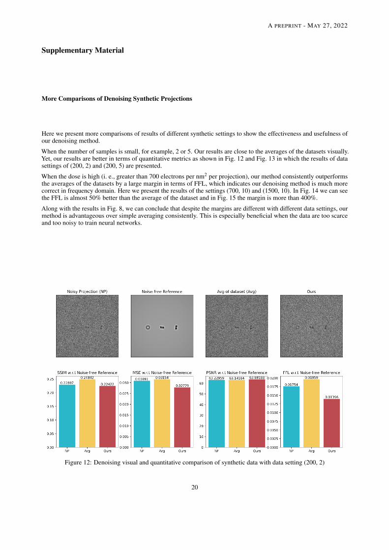
Here we present more comparisons of results of different synthetic settings to show the effectiveness and usefulness ofour denoising method.

When the number of samples is small, for example, 2 or 5. Our results are close to the averages of the datasets visually.Yet, our results are better in terms of quantitative metrics as shown in Fig. 12 and Fig. 13 in which the results of datasettings of (200, 2) and (200, 5) are presented.

When the dose is high (i. e., greater than 700 electrons per nm2 per projection), our method consistently outperformsthe averages of the datasets by a large margin in terms of FFL, which indicates our denoising method is much morecorrect in frequency domain. Here we present the results of the settings (700, 10) and (1500, 10). In Fig. 14 we can seethe FFL is almost 50% better than the average of the dataset and in Fig. 15 the margin is more than 400%.

Along with the results in Fig. 8, we can conclude that despite the margins are different with different data settings, ourmethod is advantageous over simple averaging consistently. This is especially beneficial when the data are too scarceand too noisy to train neural networks.

Figure 12: Denoising visual and quantitative comparison of synthetic data with data setting (200, 2)

20




21



22

differentiable electron microscopy simulation - arxiv

Documents