THE UNIVERSITY OF HERTFORDSHIRE

BUSINESS SCHOOL

WORKING PAPER SERIES

The Working Paper series is intended for rapid dissemination of research results, work-in-progress, innovative teaching methods, etc., at the pre-publication stage. Comments are welcomed and should be addressed to the individual author(s). It should be remembered that papers in this series are often provisional and comments and/or citation should take account of this. For further information about this, and other papers in the series, please contact:

University of Hertfordshire Business School

College Lane

Hatfield

Hertfordshire

AL10 9AB

United Kingdom

2

Consumption, Wealth and Indebtedness in the context of Uncertainty:

The Consumption Function meets Portfolio Theory.

Abstract: The objective of this paper is to provide a sound theoretical framework for the

empirical analysis of consumer indebtedness, by integrating Portfolio theory with the Life-

Cycle hypothesis (LCH) model of consumption. Modern versions of this LCH theory

almost always assume that utility is additive over time, but in this study the multiplicative

‘Cobb-Douglas’ function is used. The new synthesis also explains the stochastic properties

of consumption more fully and clearly than previous studies, in particular the uncertainty

arising from rates of return on risky assets. The new theory will also help to improve the

explanation of the ‘surprise’ changes in consumption because these sources of risk are

incorporated explicitly into the analysis.

By: David Bywaters and D. Gareth Thomas.

Key Words: Consumption function, Life-Cycle, Portfolio.

JEL Classification: D11, E21, G11.

Email address: d.bywaters@herts.ac.uk.

University of Hertfordshire, Business School, De Havilland Campus, Hatfield, Hertfordshire, AL10 9AB. U.K.

3

Introduction1

The plan of the discussion within the paper is, first, to outline the crucial elements of

Modern Portfolio theory and the Capital Asset Pricing Model. The crucial theoretical

contribution of this theory is to categorise all assets as falling into one of only two

categories, ‘risk free’, or ‘risky’. Second, the deterministic Life-Cycle theory is used to

derive consumption clearly from income and real wealth, but initially in the context of

certainty. Third, a synthesis is set out to show unequivocally how individual or household

expenditure depends on the risks associated with these two types of asset. The sources of

uncertainty are then discussed in the framework of the stochastic consumption function

derived. Finally, the theory is applied to consumer indebtednessi and aggregate

consumption.

[2]

Portfolio Theory and the Capital Asset Pricing Modelii

Uncertainty in the standard capital asset pricing model (CAPM) relates to the rate of return

on each risky asset during each ‘period’; investors are taken to be concerned about the

expected values and variances (and covariances) of the rates of return on risky assets. By

assumption, because differing investors have similar expectations and knowledge of the

stochastic properties of the risky assets and borrowings (or holdings of the risk free asset),

there is a ‘capital market line’ in the expected portfolio rate of return and standard deviation

space. This is the same line for all investors in the market, that is

,tttt re σα+=

[1]

1 The writers would like to thank the help and constructive comments made by Dr. Y.C.Yin and the anonymous referee.

4

where te is the expected rate of return earned by the investor in period t;

tr is the (non stochastic) rate of return on the risk free asset in period t;

tR is the expected rate of return on the market portfolio of risky assets in period t;

mtσ is the standard deviation on the market portfolio of risky assets in period t;

tσ is the standard deviation on the investor’s (whole) portfolio in period t.

tα is ./)( mttt rR σ−

Investors have varying preferences with respect to return and risk, because they choose

portfolios on differing points of the capital market line. The power and relevance of the

CAPM, is that, according to the model each investor’s asset holdings can be taken to

consist of only two elements: a share of the market portfolio of risky assets as well as

borrowing or lending of the risk free security. This result requires only that investors are

risk averse to varying degrees.

To illustrate this theory in a form suitable for application, assume the investor wishes to

maximise a ‘certainty equivalent’ return,

,22tttt heE σ−=

subject to equation [1]iii. Ideally, the analysis requires a utility function to be consistent with

earning the risk free rate of return, in the absence of risk, or in conditions of certainty, when

.0=σ The study also requires that the first derivative to be negative with respect to sigma

for risk aversion, and the second derivative to be minus for a maximum. Three possibilities,

therefore, can be considered: ,)/1( hσ where ‘h’ would be some constant; );1( σh− and

).1( 22σh− The first possibility would be undefined in the absence of risk, and has a positive

second order partial derivative. The second one has a second order derivative of zero,

which is not negative. The third, which is adopted in the analysis, is consistent with

conditions of certainty as well as having first and second order partial derivatives that are

minus.

5

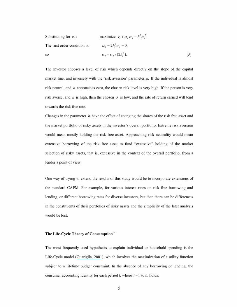
Substituting for :te maximize .22ttttt hr σσα −+

The first order condition is: ,02 2 =− ttt h σα

so ).2(/ 2ttt hασ = [3]

The investor chooses a level of risk which depends directly on the slope of the capital

market line, and inversely with the ‘risk aversion’ parameter, .h If the individual is almost

risk neutral, and h approaches zero, the chosen risk level is very high. If the person is very

risk averse, and h is high, then the chosen σ is low, and the rate of return earned will tend

towards the risk free rate.

Changes in the parameter h have the effect of changing the shares of the risk free asset and

the market portfolio of risky assets in the investor’s overall portfolio. Extreme risk aversion

would mean mostly holding the risk free asset. Approaching risk neutrality would mean

extensive borrowing of the risk free asset to fund “excessive” holding of the market

selection of risky assets, that is, excessive in the context of the overall portfolio, from a

lender’s point of view.

One way of trying to extend the results of this study would be to incorporate extensions of

the standard CAPM. For example, for various interest rates on risk free borrowing and

lending, or different borrowing rates for diverse investors, but then there can be differences

in the constituents of their portfolios of risky assets and the simplicity of the later analysis

would be lost.

The Life-Cycle Theory of Consumptioniv

The most frequently used hypothesis to explain individual or household spending is the

Life-Cycle model (Guariglia, 2001), which involves the maximization of a utility function

subject to a lifetime budget constraint. In the absence of any borrowing or lending, the

consumer accounting identity for each period t, where 1=t to n, holds:

6

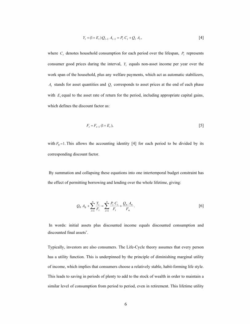
,)1( 11 tttttttt AQCPAQEY +=++ −− [4]

where tC denotes household consumption for each period over the lifespan, tP represents

consumer good prices during the interval, tY equals non-asset income per year over the

work span of the household, plus any welfare payments, which act as automatic stabilizers,

tA stands for asset quantities and tQ corresponds to asset prices at the end of each phase

with tE equal to the asset rate of return for the period, including appropriate capital gains,

which defines the discount factor as:

),1(1 ttt EFF += − [5]

with .10 =F This allows the accounting identity [4] for each period to be divided by its

corresponding discount factor.

By summation and collapsing these equations into one intertemporal budget constraint has

the effect of permitting borrowing and lending over the whole lifetime, giving:

.11

00n

nnn

t t

ttn

t t

t

FAQ

FCP

FY

AQ +=+ ∑∑==

[6]

In words: initial assets plus discounted income equals discounted consumption and

discounted final assetsv.

Typically, investors are also consumers. The Life-Cycle theory assumes that every person

has a utility function. This is underpinned by the principle of diminishing marginal utility

of income, which implies that consumers choose a relatively stable, habit-forming life style.

This leads to saving in periods of plenty to add to the stock of wealth in order to maintain a

similar level of consumption from period to period, even in retirement. This lifetime utility

7

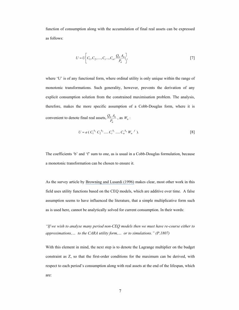
function of consumption along with the accumulation of final real assets can be expressed

as follows:

,,...,....,,, 21

=

n

nnnt P

AQCCCCUU [7]

where ‘U’ is of any functional form, where ordinal utility is only unique within the range of

monotonic transformations. Such generality, however, prevents the derivation of any

explicit consumption solution from the constrained maximisation problem. The analysis,

therefore, makes the more specific assumption of a Cobb-Douglas form, where it is

convenient to denote final real assets,n

nn

PAQ , as :nW

.)..........( 2121

fn

bn

bt

bb WCCCCaU nt= [8]

The coefficients ‘b’ and ‘f’ sum to one, as is usual in a Cobb-Douglas formulation, because

a monotonic transformation can be chosen to ensure it.

As the survey article by Browning and Lusardi (1996) makes clear, most other work in this

field uses utility functions based on the CEQ models, which are additive over time. A false

assumption seems to have influenced the literature, that a simple multiplicative form such

as is used here, cannot be analytically solved for current consumption. In their words:

“If we wish to analyse many period non-CEQ models then we must have re-course either to

approximations,… to the CARA utility form,… or to simulations.” (P.1807)

With this element in mind, the next step is to denote the Lagrange multiplier on the budget

constraint as Z, so that the first-order conditions for the maximum can be derived, with

respect to each period’s consumption along with real assets at the end of the lifespan, which

are:

8

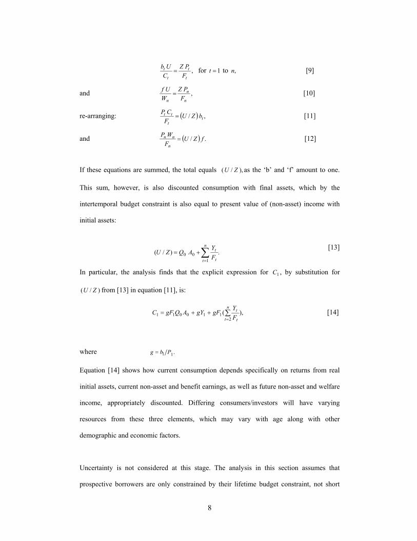
,t

t

t

t

FPZ

CUb

= for 1=t to ,n [9]

and ,n

n

n FPZ

WUf

= [10]

re-arranging: ( ) ,/ tt

tt bZUFCP

= [11]

and ( ) ./ fZUFWP

n

nn = [12]

If these equations are summed, the total equals ),/( ZU as the ‘b’ and ‘f’ amount to one.

This sum, however, is also discounted consumption with final assets, which by the

intertemporal budget constraint is also equal to present value of (non-asset) income with

initial assets:

.)/(1

00 ∑=

+=n

t t

t

FY

AQZU [13]

In particular, the analysis finds that the explicit expression for 1C , by substitution for

)/( ZU from [13] in equation [11], is:

∑=

++=n

t t

t

FY

gFgYAQgFC2

110011 ),( [14]

where .11 Pbg =

Equation [14] shows how current consumption depends specifically on returns from real

initial assets, current non-asset and benefit earnings, as well as future non-asset and welfare

income, appropriately discounted. Differing consumers/investors will have varying

resources from these three elements, which may vary with age along with other

demographic and economic factors.

Uncertainty is not considered at this stage. The analysis in this section assumes that

prospective borrowers are only constrained by their lifetime budget constraint, not short

9

term liquidity constraints. The absence of uncertainty means that actual, expected and

‘certainty equivalent’ rates of return are all the same. The notation, ,tE relates to the

‘certainty equivalent’ rate of return, as in the context of Portfolio theory, for relevance to

the subsequent synthesis.

Portfolio Theory, Life-Cycle Consumption and Sources of Uncertainty in

Consumption

The analysis now incorporates the CAPM results, expressed as equations [1], [2], and [3]

into the Life-Cycle theory, exemplified by the consumption function [14], to bring together

all the channels of uncertainty into one. Thus, the Life-Cycle theory is re-examined,

incorporating the uncertain rates of return into the utility function and the budget constraint,

in the form of ‘certainty equivalent’ rates of return, .tE This entails utilising the CAPM

assumption that investors’ preferences depend on both the expected rates of return on risky

assets and on the standard deviations (for each time period),σ . The results will differ from

those of earlier ‘synthesisers’, such as Fama (1970), because the functional form

assumptions are more specific here.

The overall market value of assets for an investor, where tQ and tA , are defined earlier,

becomes

,2211tttt AQAQ + [15]

where superscript “1” denotes the risk free asset and “2” denotes the market portfolio of all

risky assets at the end of each period t.

There are also rates of return tr and tR on each of these types of asset, which depend on the

interest, dividends or rental yield, and the movement in prices. The return on the risk free

asset, almost by definition, is non-stochastic. An interesting special case is where the risk

10

free asset is a deposit, or short term government bond, in which case 11 =tQ for all ,t and

the return is ‘the’ interest rate.vi The rate of return on the market portfolio of risky assets,

however, is stochastic, and has an expected value, which is the weighted sum of the

component rates. The standard deviation depends on the covariance of these elements. The

‘certainty equivalent’ rate of return is defined from these in equation [2].

Moreover, the Cobb-Douglas assumption, embraced previously, was consistent with respect

to final wealth, with the requirements that the first order partial derivative is positive, and

the second one is negative. In the case of risk, or the standard deviation of the rate of return,

the requests are that the first order be negative (more risk leading to less satisfaction, or

lower preference), and that the second one be negative as well, as discussed in the context

of the CAPM earlier.

The utility function is still given by [8], but in principle the budget constraint could be used

to substitute for real final wealth, nW , and then the ‘certainty equivalent’ rates of return,

tE , would appear directly in the utility function. The problem here is specified as

maximising a Lagrange function formed from expression [8], subject to the overall budget

constraint equation [6], where the rates of return in the discount factors (F) are taken to be

the ‘certainty equivalent’ values, incorporating the capital market lines for each period from

1 to n, equation [1]. This Lagrange is optimised with respect to consumption (C), final

wealth (W) and the standard deviations,σ , after substitution for tE using equation [2].

Re-calling the Lagrange multiplier on the budget constraint was denoted previously by Z,

the conditions for a maximum are still expressions [11] and [12], together with the first

order terms forσ . Denoting the whole Lagrange equation as L, and using the function of a

function rule, initially for ,/ nL σ∂∂ because it occurs in only the one ,nF then

11

.0)/()/()/(/ =∂∂∂∂∂∂=∂∂ nnnnnn EEFFLL σσ [16]

nn EF ∂∂ / is 1−nF , from [5], and not zero. nFL ∂∂ / can be obtained from differentiation of

the budget constraint, [6], because nF does not appear in the utility function. The result has

2nF squared as a denominator, and only some terms from the budget constraint, and

therefore is not zero. 0/ =∂∂ nnE σ , however, is exactly how equation [3] is derived, in the

context of the CAPM. Expression [3] therefore still holds, at this stage for nσ in this new

framework.

In fact, equation [3] holds for all tσ , because the study can work down from n-1 to 1, taking

account of one extra tF each time. tL σ∂∂ / includes a ttE σ∂∂ / term for each relevant F,

which implies a zero for an optimum. This is because tEF ∂∂ / is still not zero, and nor is

FL ∂∂ / for all the relevant Fs. Equation [3], hence, serves to determine the choices of risk

in each period. The expected rates of return ,te can be found by substitution into [1], the

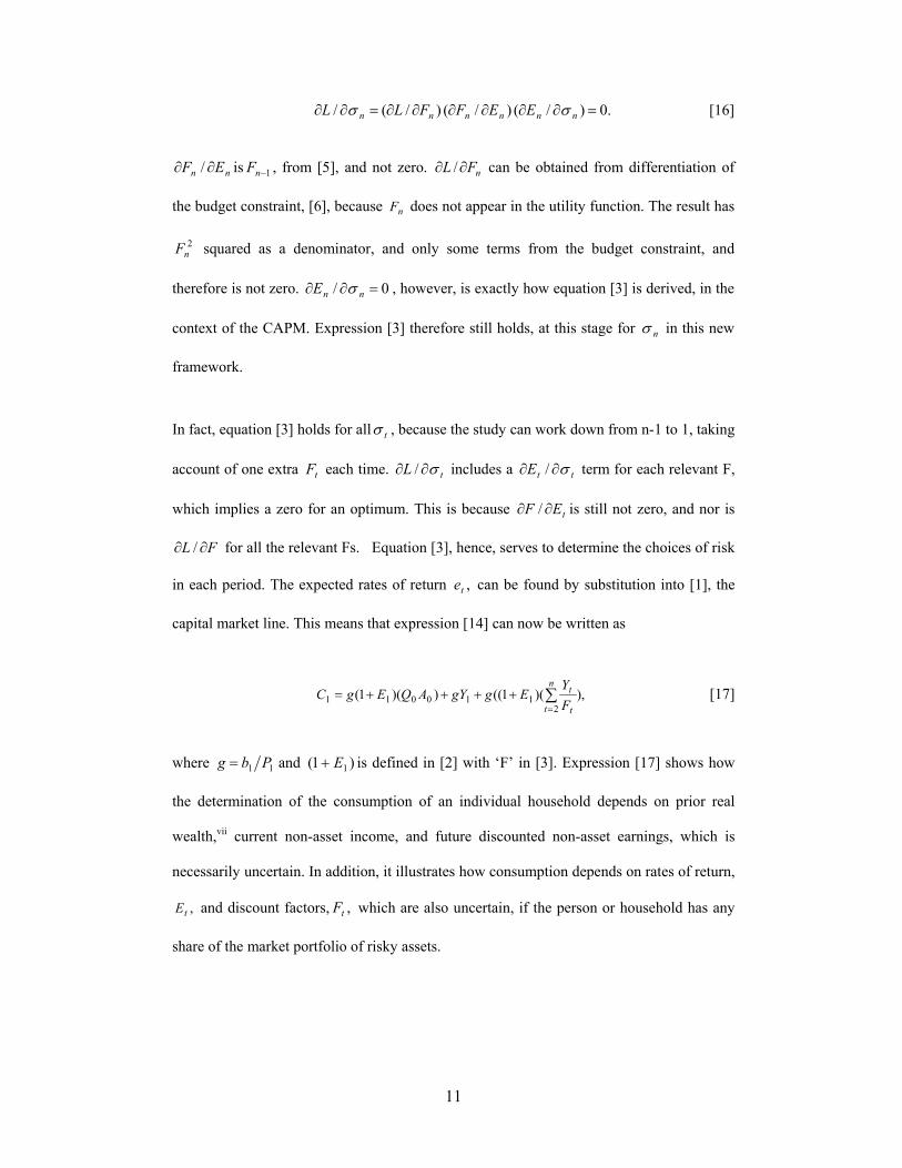
capital market line. This means that expression [14] can now be written as

∑=

++++=n

t t

t

FY

EggYAQEgC2

110011 ),)(1(())(1( [17]

where 11 Pbg = and )1( 1E+ is defined in [2] with ‘F’ in [3]. Expression [17] shows how

the determination of the consumption of an individual household depends on prior real

wealth,vii current non-asset income, and future discounted non-asset earnings, which is

necessarily uncertain. In addition, it illustrates how consumption depends on rates of return,

,tE and discount factors, ,tF which are also uncertain, if the person or household has any

share of the market portfolio of risky assets.

12

From Theory to Practice

There are essentially two sources of uncertainty in the consumption function. There is

insecurity in expected future non-asset income, .tY This has been analysed by Caballero

(1990) as well as Guariglia and Rossi (2002)viii. There is also uncertainty, however, in the

discount factors (or rates of return), which are specific to each consumer or investor. The

source is the uncertainty in the rates of return on the market portfolio of risky assets. This

component is present in the original formulation of the Life-Cycle hypothesis, but only

implicitly. Definitions of rates of return were left vague. This aspect of the analysis is

advanced with the embodiment of the CAPM into the consumption function.

In fact, the factor ),1( tE+ which comes from equation [2], brings risk/uncertainty into the

‘picture’ from the unanticipated innovations (or shocks) that arise from financial markets in

the form of capital gains/losses, or interest and dividends from the holding of a “menu of

assets” (Deaton, 1992). The risk varies in a predictable way from one investor to another; it

is higher for those individuals who have relatively high weightings of the market portfolio

of risky assets in their selection; it is low for those persons who have relatively high

weightings of the risk free asset. This variation in risk between investors explains why

individuals can face higher risks than the aggregate market does, partly because other

people choose less risk, and choose higher weightings of the risk free asset in their

portfolios. Those households who borrow the risk free asset will have higher expected

discount rates than those who hold the risk free asset, or lend it. This is because the

expected rate of return on the market portfolio of risky assets is higher than the (non

stochastic) rate of return on the risk free asset, and has a higher contribution to their

portfolios. The corollary is that the variance, or standard deviation, will be larger too,

because the risky market portfolio has a greater weight for them.

13

To apply this theory, some categorisation of individual or household assets into ‘market

portfolio of risky assets’ and ‘risk free assets’ must be made. Company shares, or equity,

and real estate, housing or property, would presumably be considered ‘risky’. Government

bonds, particularly ones with a short maturity, and perhaps index linked bonds which help

to remove inflation risk, might be ‘risk free’. Some other ‘assets’ raise more difficulty; for

example pension entitlement.

Consumer Indebtedness

Consumer indebtedness can be analysed in the context of the synthesis expressed as

equation [17]. The risk aversion parameters, ,2th may vary predictably over lifetimes.

Older people will have a larger marginal propensity to spend out of wealth because of a

prior accumulation of income and property assets to fund an endowment for their retirement

period.

An ageing population could mean that the number of consumers wanting to hold risky

assets, such as equities for property income growth, may fall relative to safe holdings with a

secure income-earning potential, depending on the degree of risk aversion of older

households.

By contrast, young individuals plan to consume the increase in wealth over a longer

horizon, and therefore will spend a smaller fraction of the increased income from assets in

any year whilst borrowing on expected labour income (Betti and et al., 2003). Obviously,

the individual consumption function, equation [17], depends on the membership and age of

the household, the expected retirement period as well as the presence or absence of social

security payments. Briefly, the variables highlighted by this theory are real current and

14

future non-asset income along with the accumulation of wealth in the form of assets from

saving, which can be converted into uncertain ‘property’ earnings, or the accumulation of

debts and need to pay interest.

Future discounted income, however, is not only dependant on the rate of return, but also is

a function of the make-up of the market portfolio of risky assets, such as real estate or

property, which not only generate additional income to a household for consumption in the

form of mortgage equity, but also determine the degree of liquidity constraint faced by an

individual household, as well as the level of ‘indebtedness’ from borrowing.

The difficulty is that, in reality the prospective lenders have differing expectations of future

non-asset income from prospective borrowers, which should only be constrained by the

life-time budget. Short-term liquidity restrictions can then constrain long-term future

expectations.

These short-run expectations of non-asset income inside the economy, in certain

circumstances, will override those of the individual or household concerned. Then

consumption may depend on the status of individuals within the economy, for example

whether or not they are employed. Similarly, it may be easier for certain groups of

households to borrow risk free assets if a share of the market portfolio of risky assets is

already owned, for example as a house, which is dependant on age and status of

individuals.

The Aggregate Consumption Function and Automatic Stabilisers

This discussion relates equation [17] to the contemporary literature. It may be that the

prevailing belief within this field of study is fallacious; that unequivocal solutions can only

come from utility functions that are quadratic in consumption and additive over time

periods. Equation [17] and its derivation demonstrates that explicit solutions can be

15

obtained by employing a Cobb-Douglas utility function, which shows that the presumptions

of the economic profession in this regard are unfounded.

The implications for the aggregate consumption function in an economy follow from the

summation of equation [17] over all the individual households in the economy. The

additive structure of [17] means that aggregate consumption is related to aggregate wealth,

aggregate current non-asset income and discounted future non-asset income, although the

weighting required involves some complications, because the summation cannot be taken

inside the terms.

It may be helpful to categorise households by a number of states at the economy level

(Deaton, 1992). The consumption of one category may be determined by liquidity

constraints perceived in the short-run, meaning that for a percentage of households, S, their

consumption is ruled by Keynes’ (1936) marginal propensity to consume out of current

disposable income, because they have no assets, and prospective lenders take too poor a

view of their income expectations to lend. They can only spend out of their current income,

which may be replaced or supplemented by government benefits.

The other segment of the population, (1-S), will be able to consume from property as well

as current non-asset income, and can borrow on discounted future expected income without

constraint, although affected by uncertain rates of return. This means that the real cause of

changes in consumption is unexpected changes in the rate of return on risky assets. An

unexpectedly low return will reduce prior asset value in future periods, and may affect

adversely future risk aversion parameters, h, so increasing the ‘certainty equivalent’

discount rates E and reducing future discounted non-asset income.

In fact, it is in this wealthier category of households that the element of uncertainty is

concentrated, because current income is not generally as uncertain as the market portfolio

of risky assets. Changes in consumption can be explained from [17] as:

16

.))(1(())(1((2

10011

++++∆=∆ ∑

=

n

t t

t

FY

EgAQEggYC

[18]

The source of uncertainty in changes in consumption can be captured by relating the

“surprise” element of the modern theory (Hall, 1978) to the variations in the pattern of

consumption from the present trend arising over and above current non-asset income,

which can be denoted by .ε

This can also be expressed in the Campbell and Mankiw (1989) form as

.)1()( 11 εSYgSC −+=∆ [19]

On the one hand, the analysis that underlies expression [19] is reinforced by the empirical

findings of

Betti and et al. (2003) that high income status bestowed on a certain per cent of households,

embodied in ,ε can borrow and accumulate liabilities/assets early in their working life,

although they could face uncertain ‘surprises’ in their undertakings to maintain a smooth

pattern of consumption. According to the analysis here, the uncertainty and the element of

surprise could well arise from the uncertain rates of return embodied in [18].

On the other hand, in the other category, low income groups face limited uncertainty

because they are credit rationed, and so, consume out of current labour and benefit income

to sustain a constant level of consumption.

This is reinforced by the function of automatic stabilizers such as the income-support

system, or the welfare state, with unemployment benefits and credits, in conjunction with

the progressive tax instruments of local and national governments, to insure against

shortfalls in current labour income (Muellbauer, 1994). The end-result for this hypothesis is

that the built-in fiscal flexibility does not dampen the element of uncertainty and risk

17

associated with asset-generating incomes that arise from the portfolio of assets and

indebtedness held to finance the consumption path.

This discussion implies that liquidity constraints together with the welfare system acting as

automatic stabilizers lead to certain consumption configurations for certain groups of

households in the model. The expectations of future discounted income add a degree of

uncertainty because of the varying rates of return. The insecurity of the asset markets is

transmitted into property income along with values. In other words, illiquid assets such as

equities, housing and land appreciate and depreciate according to the health and uncertainty

of the economy as well as depending on the rates of return encapsulated in expression [18].

Summary

The objective of the analysis in this paper is to integrate Modern Portfolio theory with the

Life-Cycle hypothesis of consumption. The latter theory can show how consumption is

maintained over a life time by varying proportions of income and wealth. The former

theory, in particular the Capital Asset Pricing Model, shows how an investor should acquire

wealth (or loans) as a holding of a share of the market portfolio of risky assets, together

with risk free assets or liabilities. The synthesis of the two theories enriches the explanation

of the consumption function, and integrates a risk dimension into the analysis to account

also for asset accumulation, or “indebtedness” via borrowing.

This paper therefore constructs a theoretical framework in which consumption, the holding

of assets, and indebtedness can be analysed under conditions of uncertainty. Individual

households can face greater uncertainty than the personal or household sector in an

economy, so issues requiring an individual focus such as consumer indebtedness, may

benefit more from this approach than issues such as aggregate consumption, although they

should benefit too.

18

Endnotes i See the analysis by Betti and et al. (2003). ii See Elton and et al. (2003) for an overview of portfolio theory. A recent study in the empirical aspect of this field comes from a discussion paper by Tofallis (2004). iii The notion of certainty equivalence solution is also adopted by the empirical investigation by Lyhagen (2001). iv The theory was developed by Modigliani and Brumberg in a series of articles based on Fisher’s model of consumption. The Nobel Prize lecture, which outlines the bulk of the work, is in Modigliani (1986). For a straightforward discussion of the Life-Cycle model see European Commission (2004). For a summary of the other ‘stylized parables’ in the field of modelling consumption see Muellbauer (1994). v The intermediate asset terms all cancel out, and an important ingredient is to define the discount factors correctly, so that this happens. vi At times of low (or absence) inflation, the risk free asset can be identified with government securities, bank and building society deposits, which do not change in monetary terms (Mill, 1848). The return here is entirely attributed to income, and not capital gain or change in the value of wealth. vii Another issue concerns the utility function. Given the definition of ,nn AQ and ‘f’, the analysis has an apparent anomaly that:

.

212211 f

n

nnf

n

nnfn P

AQP

AQW

=

The overall asset value, however, equals the sum of the two asset values, not a product. The solution to this anomaly is set out in Theil (1973). There is a reliable way of calculating weights (in this case the ‘f’s’) from the elements of a sum, so that a product relationship holds to a very high degree of accuracy and He shows that way. viii They introduce uncertainty into their analysis by presuming a stochastic process for employment income based on the AR (1) procedure with drift.

19

References Betti, Gianni.; Dourmashkin, Neil.; Rossi, Mariacristina.; Yin, Ya Ping. “Consumer Over-

Indebtedness and Income Distribution”, University of Hertfordshire, Economic Paper 28,

2003.

Browning, Martin.; Lusardi, Annamaria. “Household Saving: Micro Theories and Micro Facts,”

Journal of Economic Literature, Vol. 34, No.4, Dec., 1996, pp.1797-1855.

Caballero, Ricardo J. “Consumption Puzzles and Precautionary Savings,” Journal of Monetary

Economics Vol. 25, 1990, pp 113 to 136.

Campbell, John.Y.; Mankiw, N.Gregory. “Consumption, Income and Interest Rates: Reinterpreting

the Time Series Evidence,” NBER Macroeconomics Annual, 1989 pp 185-216.

Deaton, Angus. Understanding Consumption, Clarendon Press, Oxford, UK, 1992.

Elton, Edwin J.; Gruber, Martin J.;Brown, Stephen J. Modern Portfolio and Investment Analysis,

Sixth Edition, Wiley, New York, 2003.

Fama, Eugene F. “Multiperiod Consumption-Investment Decisions,” American Economic Review,

,Vol. 60, No. 1, 1970, pp 163-174.

European Commission, Quarterly Report on the Euro Area, Vol. 3, No.1, 2004.

Guariglia, Alessandra. “Saving Behaviour and Earnings Uncertainty: Evidence from the British

Household Panel Survey,” Journal of Population Economics, 14 (4), 2001, pp 617-40.

20

Guariglia, Alessandra; Rossi, Mariacristina. “Consumption, Habit Formation and Precautionary

Saving: Evidence from the British Household Panel Survey,” Oxford Economic Papers,

Vol. 54, 2002, pp 1-19.

Hall, Robert .E. “Stochastic Implications of the Life-Cycle-Permanent Income Hypothesis: Theory

and Evidence,” Journal of Political Economy, 96, Dec.,1978, pp 971-988.

Keynes, John M. ‘The General Theory of Employment, Interest and Money, Macmillan and Co.,

London, UK, 1936.

Lyhagen, Johan. “The Effect of Precautionary Saving on Consumption in Sweden,” Applied

Economics, 33, 2001, pp 673-681.

Mill, John .S. Principles of Political Economy, London, UK, 1848.

Modigliani, Franco. “Life-Cycle, Individual Thrift and the Wealth of Nations,” American Economic

Review, 76, June, 1986, pp 297-313.

Muellbauer, John. “The Assessment: Consumer Expenditure”, Oxford Review of Economic Policy,

Vol. 10, No. 2, June, 1994, pp 1-41

Theil, Henri. “A New Index Number Formula,” Review of Economics and Statistics, Vol. 55, No.4,

November, 1973, pp 498-502.

Tofallis, Christopher. “A Critique of the Standard Beta Estimation and a Simple Way Forward,”

Discussion Paper, University of Hertfordshire, 2004.