KWAME NKRUMAH UNIVERSITY OF SCIENCE AND

TECHNOLOGY, KUMASI

DEPARTMENT OF ECONOMICS

ECON 554: MACROECONOMICS II

TERM PAPER JUNE, 2012

ESTIMATING THE CONSUMPTION FUNCTION UNDER THE

PERMANENT INCOME HYPOTHESIS: EVIDENCE FROM GHANA

NAME: BONUEDI ISAAC INDEX NO: PG 5541711

Abstract

The aim of this paper is to examine Ghana’s consumption function under the permanent income

hypothesis by adopting Cagan’s adaptive expectations principle. The study employs an annual

time series data from 1980-2010 to estimate both the short-run and long-run elasticities of

consumption for Ghana. It is found that there is a very wide difference between the elasticity to

consume out of current income and the elasticity to consume out of permanent income and the

expectation coefficient is very small. Therefore, we conclude that permanent income hypothesis

(PIH) is valid in the case of Ghana. The statistical significance of the coefficient lagged

consumption also provides empirical evidence in support of Duesenberry’s relative-income

hypothesis (RIH) in Ghana. It is found that increases in the interest rates tend to lower

significantly interest-sensitive consumption expenditure in Ghana. The overall conclusion

drawn from the study is that government policies that are aimed at improving the disposable

income of Ghanaian households, in order to stimulate consumption and economic growth must

be permanent or sustained long enough for their full effect to materialize.

1.0 INTRODUCTION AND STATEMENT OF PROBLEM

Consumption consists of the expenditures on goods and services by households

(individuals and non-profit institutions) except new houses (these are counted as

residential investment). Such expenditures can be broken down into three

subcategories, namely nondurable goods, durable goods, and services. Nondurable

goods are tangible goods that are expected to last less than one year, such as food and

clothing. Durable goods are tangible goods that last a long time, such as automobiles,

radios, TVs sets and appliances. Services are intangible items such as recreation,

entertainment, education and medical care (DerLorme and Ekelund, 1983; Abel,

Bernanke and Smith, 1999).

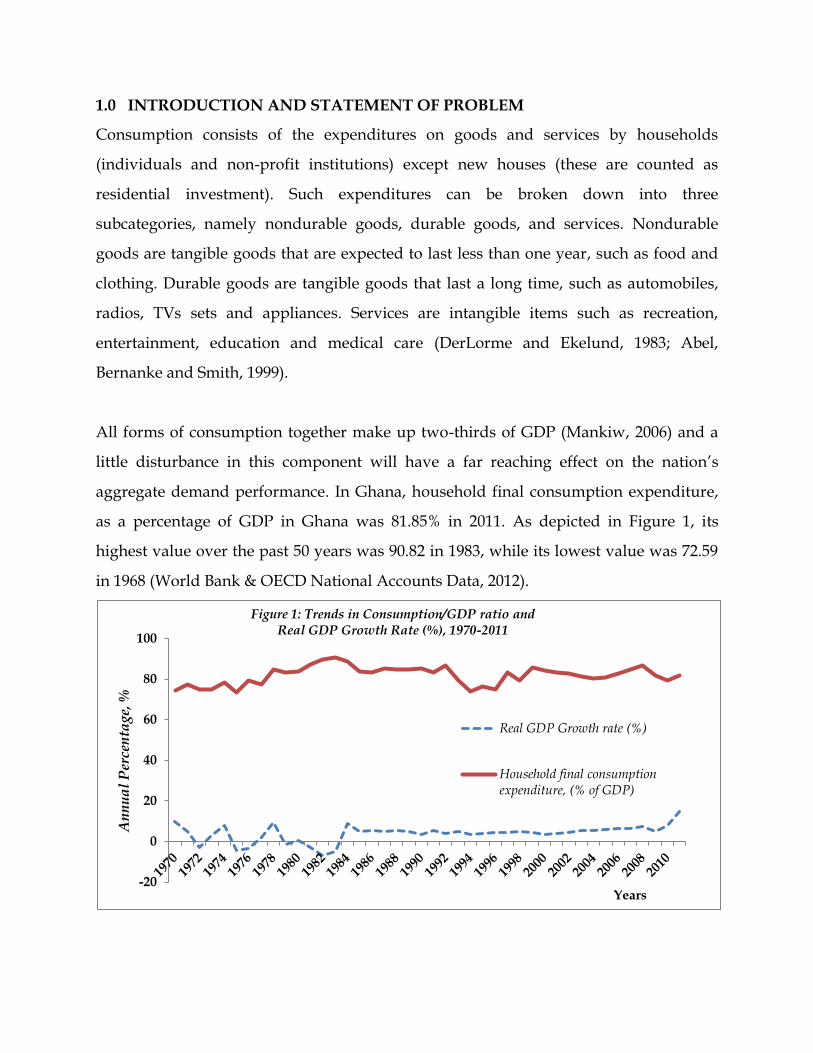
All forms of consumption together make up two-thirds of GDP (Mankiw, 2006) and a

little disturbance in this component will have a far reaching effect on the nation’s

aggregate demand performance. In Ghana, household final consumption expenditure,

as a percentage of GDP in Ghana was 81.85% in 2011. As depicted in Figure 1, its

highest value over the past 50 years was 90.82 in 1983, while its lowest value was 72.59

in 1968 (World Bank & OECD National Accounts Data, 2012).

-20

0

20

40

60

80

100

An

nu

al

Per

cen

tage

, %

Years

Figure 1: Trends in Consumption/GDP ratio and Real GDP Growth Rate (%), 1970-2011

Real GDP Growth rate (%)

Household final consumption expenditure, (% of GDP)

According to the 5th Ghana Living Standard Survey Report (2008), the average annual

household expenditure in Ghana is GH¢1,918.00 whilst the mean annual per capita

consumption expenditure in Ghana is GH¢644.00. Regional differences exist with

Greater Accra Region having the highest per capita expenditure of GH¢1,050.00 whilst

Upper West has the lowest of GH¢166.00. The average annual household expenditure is

about 1.6 times higher in urban localities (GH¢2,449) than in rural localities (GH¢1,514)

even though the household size in rural households tends to be larger than urban

households (GLSS V, 2008).

Because consumption is so large and plays an important role in national welfare and

business cycle fluctuations, macroeconomists have devoted much attention, time and

energy to studying how households decide how much to consume, response to

uncertainty over future incomes, movements in interest rates, and expectations of future

shifts in taxes and wages, which are key determinants of the impact of government

policy. The concept of the consumption function, which was coined from Keynes’

fundamental psychological law, shows the relationship between consumption and

disposable income.

According to the simple Keynesian consumption function, consumption depends solely

on disposable income in the current period. Two implications of this Absolute Income

Hypothesis (AIH) are worth noting. Firstly, household consumption is volatile rather

than smooth, because any change in current income is reflected in a change in

consumption. Secondly, there should no difference between the effect on consumption

of transitory and permanent changes in personal income (Carlin & Sosckice, 2006).

However, these predictions are too extreme and unrealistic because it does not consider

individuals’ expected path of income or time preference for consumption and ability to

borrow, which is captured by the real rate of interest. Therefore, there are contradictions

between the simple Keynesian consumption function and empirical evidence.

Alternative views of consumption taking these factors into account were proposed in

Milton Friedman’s permanent income hypothesis (PIH) in 1957 and in the closely

related Life-Cycle Hypothesis (LCH) by Franco Modigliani and Richard Brumberg in

1954. They suggested consumption was a function not of a measured income as in the

Keynesian consumption function but of average or expected income or value of lifetime

resources.

Since the publication of Friedman's A Theory of Consumption Function (1957), a number

of researchers, including Motaqed (2011), Khan et. al., (2010), Manitsaris (2006); Katsouli

(2011) and Hayashi (1982) have empirically tested the permanent income hypothesis

(PIH) using historical data from European countries, Pakistan, Iran and other countries.

To the best of my knowledge, empirical work on the applicability of the permanent

income hypothesis to Ghana is nonexistent. It is, therefore, the objective of this paper is

to replicate these studies in Ghana, by modeling Ghana’s consumption function under

the PIH and testing the consistency of Ghana’s household final consumption with the

predictions of the PIH. The rest of the paper is organized as follow. Section two presents

a review of theoretical and empirical literature on theories of consumption. Section

three discusses the methodology and data employed in this study. Section four presents

and discusses the empirical results of the study. Section five summarizes the findings of

the study and concludes with the policy implications of the results.

2.0 LITERATURE REVIEW

2.1 A Brief Review Of Consumption Function Under The Life-Cycle Model

And Permanent-Income Hypothesis

There is no topic in macroeconomics that has a longer, deeper, or more prominent

literature than households’ choice of how much of their income to consume and save.

Many economists have written about the theory of consumer behaviour in an attempt to

interpret data on the relationship between income and consumption. For the purposes

of this study, we discuss, in this section, two initially distinct theoretical paths that

eventually merged into one are the lifecycle model developed by Franco Modigliani,

Albert Ando, and Richard Brumberg in the mid-1950s and the permanent-income

hypothesis introduced by Milton Friedman in 1957. Much of the literature in this section

is drawn from Oguz (1996).

Modigliani’s life-cycle hypothesis (LCH) emphasizes that income varies somewhat

predictably over a person’s life and that consumers use saving and borrowing to

smooth their consumption over their lifetimes. According to this hypothesis,

consumption depends on both income and wealth. Friedman’s permanent-income

hypothesis (PIH) emphasizes that individuals experience both permanent and

transitory fluctuations in their income. Because consumers can save and borrow, and

because they want to smooth their consumption, consumption does not respond much

to transitory income. Consumption depends primarily on permanent income.

The basic idea underlying both theories is that the consumer plans his expenditures not

on the basis of the income received during the current period but rather on the basis of

long-run or lifetime income expectation. Friedman points out that a person does not

plan his expenditures for one day according to what income he expects to receive on

that particular day. In terms of theory of consumption function, this means that the

consumer plans his expenditure for a given period, whether it is a day or a year, on the

basis of a longer run view of the resources that will be available to him. In a sense, these

views reflect a return to the pre-Keynesian views of the importance of wealth and

interests. Modigliani and his associates postulate that the typical individual has an

income stream which is relatively low at the beginning and end of his life, when his

productivity is low, and high during the middle of his life. In many respects these

theories are very similar but there are also some key differences. Both theories divide

the current income of the consumer unit into permanent (YP) and transitory (YT)

components, and the same is true for current consumption expenditures (CP and CT,

respectively. The PIH assumes the absence any correlation between YP and YT, between

CP and CT, or between YT and CT. in the LCH also, no correlation is assumed between

YP and YT, but over time YT may add to YP because when it is invested, the yield on the

investment raises permanent income.

In both cases, the key relationship is that permanent consumption, CP, is a linear

multiple, k, of permanent income YP. to Friedman, the multiple depends on the interest

rate, on the ration of nonhuman to total wealth and on a catch-all variable which

includes age and tastes as major components. Modigliani accepts the same determining

variables but allows the multiple to vary with time and stresses the age of consumer

unit. In both formulations permanent income is obtained as the product of the

estimated wealth is discounted. Friedman puts more emphasis on estimating wealth on

the basis of the flow of current and past incomes as a proxy for YP whereas Modigliani

puts more emphasis on current income plus nonhuman net worth for estimating for

estimating household resources. In both approaches consumption is defined to include

the real consumption of goods and services rather than monetary expenditures;

durables are expenditures only to the extent that they are depreciated in a particular

period, not the amount spent for their acquisition. By either formulation, the central

hypothesis is that the proportion of permanent income saved by the consumer unit is

independent of its income in particular period, and that transitory income has no

(Friedman) or little (Modigliani) effect on current consumption. In both models, an

increase in real income may raise the saving ratio, in the PIH because this increases

permanent income, and consumption, relative to their measured components. In the

LCH the effect varies with the age of household, being positive for younger households

and negative for older, and the retired, households. Modigliani specifically allows for a

positive secular relationship because of income growth due to both population increase

and high productivity.

2.2 A Brief Survey Of Empirical Literature On LCPI Hypothesis

While such hypothesis seem simple in theory, testing them gives rise to a great many

empirical problems, primarily because of the difficulty of separating the permanent

from the transitory components of income and consumption. A substantial empirical

work evolved in the attempt to test LCH and PIH. Since both theories are closely

related, in the literature both theories are combined as the Life Cycle-Permanent Income

(LCPI) theory of consumption. In simple terms, LCPI hypothesis suggest that

consumers choose current consumption after considering the state of resources

available to them over their entire lifetime. Consumers behave as if their budget must

be met not on a period by period basis, but on a lifetime basis. Hall (1978) developed

stronger implication of the basic LCPI theory for consumption. Hall showed that, under

rational expectations, consumption must follow a ‘random walk’ or first order

autoregressive process (AR(1)) if the LCPI hypothesis is true. This is the only

information available at time, t-1, useful in predicting consumption at time t is the

consumption at time t-1. No other variable known at t-1 can increase the accuracy of the

prediction.

Hall’s random-walk hypothesis combines the permanent-income hypothesis with the

assumption that consumers have rational expectations about future income. It implies

that changes in consumption are unpredictable, because consumers change their

consumption only when they receive news about their lifetime resources.

Bilson (1980) tested the rational expectations and LCPI model and reached an

ambiguous conclusions; aggregate consumption was demonstrated to be independent

anticipated changes in income in both Germany and the U.K. on the other hand, the

tests suggested that lagged innovations in income influenced consumption in German

and U.S. samples, and the anticipated change in income was significant in predicting

consumption in the U.S.

Flavin (1981) developed a structural econometric model of consumption and showed

that the LCPI hypothesis proposed by Hall (1978) can be thought of as a test based on

the reduced form of this structural model. Using this structural version of Hall’s model

she found that consumption was more sensitive to income changes than predicted by

the LCPI theory.

Blinder and Deaton (1985) reproduced Flavin’s finding that the change in consumption

was predictable from past income. In their empirical work, lagged income and the

forecast of current income based on past lagged information are both significant,

contrary to the implications of LCPI theory.

Mankiw and Campbell (1990) re-examines the consistency of the permanent-income

hypothesis with aggregate postwar U.S. data. The permanent-income hypothesis is

nested within a more general model in which a fraction of income accrues to

individuals who consume their current income rather than their permanent income.

This fraction is estimated to be about 50%, indicating a substantial departure from the

permanent-income hypothesis. Their results cannot be easily explained by time

aggregation or small-sample bias, by changes in the real interest rate, or by

nonseparabilities in the utility function of consumers.

Manitsaris (2006) examined the consumption function under the permanent income

hypothesis using annual data covering the period from 1980 to 2005 for selected 15

European Union member-states. The specifications adopted refer to the combined

partial adjustment and adaptive expectations model, and the adaptive expectations

model. The results show strong support for the hypothesis, supporting thus the

consumption function under the permanent income hypothesis and the adaptive

expectations model.

Khan et. al (2010) estimated the consumption function for Pakistan under the

permanent income hypothesis (PIH) using the annual data from 1970 to 2010. The

consumption function under PIH was estimated through ordinary least square (OLS)

method and instrumental variable (IV) approach. The results of both OLS and IV

approach showed a small difference between marginal propensity to consume (MPC)

out of current income and MPC out of permanent income. Therefore, they concluded

that, these results indicate the invalidity of PIH and validity of Keynesian absolute

income hypothesis in a case of Pakistan.

3.0 METHODOLOGY AND DATA

3.1 Theoretical Framework and Model Specification

According to Milton Friedman’s (1957) permanent income hypothesis actual

consumption expenditure (Ct) is made up of two parts namely, permanent ( ) and

transitory ( ) following two parts:

Similarly, actual income (Yt) is the sum of permanent income, and transitory income,

. That is,

Furthermore, permanent consumption expenditure is assumed to be determined by

permanent income, such that

where α and β are parameters to be estimated.

The purpose of this paper is to estimate a version of the consumption function in (3), or

the so called ‘consumption function under the permanent income hypothesis’ for

Ghana.

Since and

are not directly observable, we need to specify the mechanism that

generates permanent consumption and permanent income. Following Manitsaris (2006),

Gujarati (2004) and Koutsoyiannis (1977) we combine Cagan’s adaptive expectations

hypothesis, we

where is the adaptive expectations coefficient.

Substituting (1) into (3), the following equation is obtained,

which is written in econometric terms as

From (7)

Lagging (8) one period yields

Substituting (8) and (9) in the ‘adaptive expectations’ equation in (4) we obtain

Equation (9) is the short-run consumption function under the permanent income

hypothesis and the adaptive expectations model, and is estimable in the sense that all

the variables involved are expressed in actual and not in observable variables.

From the short-run consumption function in equation (9), is the autonomous

consumption; is the short-run MPC;

measures the long-run MPC and the

adjustment coefficient, is given as .

In order to assess the effects of interest rates (IR) on consumption, we incorporate this

variable into the estimable function in equation (9). This yields

By assuming that equation (10) satisfies all the Classical Linear Regression (CLR)

assumptions, we use the Ordinary Least Squares (OLS) estimation procedure to

estimate the parameters and the coefficients examined on the basis of theoretical and

statistical criterion. As a priori we expect the parameters in (10) to assume the following

theoretical signs: In order to achieve stationarity in the

series and minimize the presence of heteroscedasticity and autocorrelation, we

estimated the log-linear form of the model specified in equation (10). By using the log-

linear form of the equations, the estimated parameters give the elasticities of the

regressand with respect to the regressors (i.e. the percentage change in the dependent

variable due to a percentage change in the respective independent variables).

3.2 Data Source

The data on the variables in this study, household final consumption expenditure, and

income (GDP), are taken from World Development Indicators, published by United

Nations, Department of Economic and Social Affairs, Statistics Division. Data on real

interest rate (IR), which is proxied by the lending rate, is taken from the Bank of Ghana,

and World Bank World Development Indicators database. The data are annual and

spans the time period 1980 to 2010. All the variables are measured in real terms.

4.0 PRESENTATION AND ANALYSIS OF EMPIRICAL RESULTS

4.1 Augment-Dickey Fuller Unit Root Test Results

Before estimating Ghana’s consumption function under the permanent income

hypothesis, we first examined the stationarity of the variables employed this study by

testing for unit root for each variable using the Augmented Dickey-Fuller (ADF).

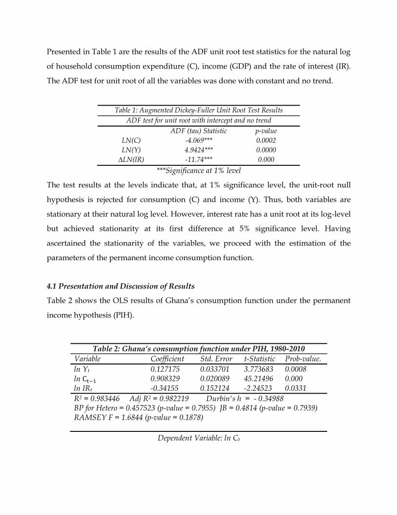
Presented in Table 1 are the results of the ADF unit root test statistics for the natural log

of household consumption expenditure (C), income (GDP) and the rate of interest (IR).

The ADF test for unit root of all the variables was done with constant and no trend.

Table 1: Augmented Dickey-Fuller Unit Root Test Results

ADF test for unit root with intercept and no trend

ADF (tau) Statistic p-value

LN(C) -4.069*** 0.0002

LN(Y) 4.9424*** 0.0000

∆LN(IR) -11.74*** 0.000

***Significance at 1% level

The test results at the levels indicate that, at 1% significance level, the unit-root null

hypothesis is rejected for consumption (C) and income (Y). Thus, both variables are

stationary at their natural log level. However, interest rate has a unit root at its log-level

but achieved stationarity at its first difference at 5% significance level. Having

ascertained the stationarity of the variables, we proceed with the estimation of the

parameters of the permanent income consumption function.

4.1 Presentation and Discussion of Results

Table 2 shows the OLS results of Ghana’s consumption function under the permanent

income hypothesis (PIH).

Dependent Variable: ln Ct

Table 2: Ghana’s consumption function under PIH, 1980-2010

Variable Coefficient Std. Error t-Statistic Prob-value.

ln Yt 0.127175 0.033701 3.773683 0.0008 ln 0.908329 0.020089 45.21496 0.000 ln IRt -0.34155 0.152124 -2.24523 0.0331

R2 = 0.983446 Adj R2 = 0.982219 Durbin's h = - 0.34988 BP for Hetero = 0.457523 (p-value = 0.7955) JB = 0.4814 (p-value = 0.7939) RAMSEY F = 1.6844 (p-value = 0.1878)

The results show that the elasticity of current consumption with respect to current

income is 0.127 percent. This implies that, in the short-run, 1% rise in the current income

of Ghanaian households, as measured by real GDP, would raise the current household

final consumption expenditure by 0.127%. The short-run elasticity to consume out of

current income is highly statistically significant at 5% level and is consistent with prior

expectation. This result suggests that, current consumption is considerably less

responsive to changes in current income in Ghana.

From Table 2, we compute the adjustment coefficient, as

. This suggests that if the increase in income is sustained, the elasticity to consume

out of permanent income will be

. This is highly elastic,

suggesting that if Ghanaian households have had enough time to adjust to 1% change in

their income, they will increase their consumption ultimately by 12.25%.

Given the short-run elasticity as 0.127% and the long-run elasticity as 12.25%, the

adjustment coefficient of 0.092 suggests that in any given time period Ghanaian

households adjusts their consumption by 9.2% towards their desired or long-run level.

In other words, only 9.2% of their expectations are realized in any given period.

Since there is a very wide difference between elasticity to consume out of current

income and the elasticity to consume out of permanent income and the expectation

coefficient is very small, we conclude that permanent income hypothesis (PIH) is valid

in Ghana.

The coefficient of lagged-consumption, although of no direct interest to the present

study, is also highly statistically significant, suggesting that previous level of

consumption is a significant determinant of current consumption in Ghana. This

provides an empirical support for Duesenberry’s relative-income hypothesis (RIH) that

present consumption is not influenced merely by present levels of absolute and relative

income, but also by levels of consumption attained in previous periods (Branson, 1989).

To augment the overall performance or the predictive power of the model understudy,

we introduce real interest rate as one of the regressands. The estimated results suggest

that current consumption and interest rate are negatively related, such that a 1% rise in

the interest rate reduces current consumption by 0.342%. The interest rate elasticity of

consumption is statistically significant at 1% error level. Since we proxied real interest

rate by the lending rate, the implication of this result is an increase in the lending rate

raises the cost of borrowing and therefore reduces interest rate-sensitive consumption

expenditure in Ghana.

4.3 Model Diagnostic Tests

Reported in Table 2 are some diagnostic test statistics for overall significance,

autocorrelation, heteroscedasticity, normality and specification. The adjusted coefficient

of determination, which is a better measure of the overall significance of the model, is as

high as 0.982, suggesting that about 98% of the total variation in Ghana’s consumption

expenditure is explained by thee variation the income level, the rate of interest and the

lagged consumption expenditure. Thus, these variables are jointly important

determinants of consumption behavior in Ghana.

The Durbin’s h statistic of -0.349 sufficiently lies within the critical Z-score of , at

95% confidence level. Thus, the null hypothesis of serial autocorrelation in residuals is

not rejected at 5% error level. Also, the Breusch-Pagan (LM) test statistic for

heteroscedasticity is given as 0.4575. Since it p-value of 0.7955 is greater the assumed 5%

significance level, we do not reject the null hypothesis of homoscedasticity in the

variance of the residuals of the model.

Although the sample size is not large enough, an application of the Jarque–Bera test

shows that the JB statistic is about 0.4814, and the probability of obtaining such a

statistic under the normality assumption is about 79.4 percent. Therefore, we do not

reject the hypothesis that the error terms are normally distributed. Moreover, the model

is correctly specified using the Ramsey’s RESET test for specification, given that the p-

value of the F-statistic is greater than the significance level of 5%.

The structural stability test is conducted by employing the cumulative residuals

(CUSUM) and the cumulative sum of squares of recursive residuals (CUSUMSQ). See

Appendix for the CUSUM and CUSUMSQ plots. It is shown that in both plots, CUSUM

and CUSUMSQ stays within the 5% critical bound and the null hypothesis that all the

coefficients are stable cannot be rejected.

5.0 SUMMARY OF FINDINGS AND CONCLUSION

Drawing on relevant theoretical stipulations and empirical research carried out in most

for developed countries on consumption function, the objective of this paper is to

replicate these studies in the case of Ghana and empirically investigate the validity of

the permanent income hypothesis in Ghana. Following Manitsaris (2006), Gujarati

(2004) and Koutsoyiannis (1977), this study utilizes the ordinary least squares (OLS)

econometric estimation method to estimate Ghana’s consumption function under the

permanent income hypothesis and adaptive expectation model. The study uses annual

time series data on household final consumption expenditure, real GDP and interest

rate for the period 1980-2010 obtained from the World Bank database, and various

Monetary Policy reports of the Bank of Ghana. The following intriguing results are

obtained.

It is found that there is a very wide difference between the elasticity to consume out of

current income and the elasticity to consume out of permanent income and the

expectation coefficient is very small. Therefore, we conclude that permanent income

hypothesis (PIH) is valid in the case of Ghana.

The statistical significance of the coefficient lagged consumption also provides

empirical evidence in support of Duesenberry’s relative-income hypothesis (RIH) in

Ghana.

Interest rate is found to be an important determinant of consumption in Ghana. This is

because it is found that interest rate and consumption are not only negatively related,

but the interest rate elasticity of consumption is also highly statistically significant.

Finally, the estimated parameters of Ghana’s consumption function under the

permanent income hypothesis are found to be structurally stable throughout the entire

period of the study. The diagnostics tests show there stationarity in the variables,

normality, homoscedasticity and no serial autocorrelation in the residuals and that the

model is correctly specified.

The overall conclusion drawn from this paper is that the life-cycle-permanent-income

hypothesis under rational expectations that current consumption is primarily

determined by the average expected life time (permanent) income cannot be rejected in

the case of Ghana. The policy implication of this result is that temporary fiscal policy

changes that affect the income of consumers in Ghana would not have any significant

impact on household final consumption expenditure. Thus, to encourage consumption

in order to stimulate economic growth, government policies that aim at improving the

disposable income and for that matter the purchasing power of Ghanaian households

must be permanent or sustained long enough for their full effect to materialize.

REFERENCES

Bernanke B. S., Abel A. B., and Smith G. W., (1999) Macroeconomics, 2nd Canadian Edition. Adisson Wesley Longman Ltd.

Bilson, J. F. O., (1980) The rational expectations approach to the consumption function” European EconomicReview,

Blinder, A. S., and Deaton, A (1985) Time series consumption revisited. Brookings Papers on Economic Activity

Branson W. H., (1989), Macroeconomic Theory and Policy, Third Edition. Harper & Row Publishers, New York

Carlin W., and Sosckice (2006) Macroeconomic Imperfections, Institutions and Policies. Oxford University Press, 2006

DerLorme C., and Ekelund R. B. Jr., (1983) Macroeconomics, Business Publications Inc., Texas, USA

Flavin M. A., (1981) The adjustment of consumption to changing expectations about future income, Journal of Political Economy

Friedman, M., (1957) A Theory of Consumption Function, Princeton, New Jersey: Princeton University Press.

Ghana Living Standards Survey Report Of The Fifth Round (GLSS 5) published by Ghana Statistical Service September 2008

Gujarati (2004) Basic Econometrics, Fourth Edition The McGraw−Hill Companies, 2004 Hall, Robert E. 1978. Stochastic Implications of the Life Cycle-Permanent Income Hypothesis: Theory and Evidence. Journal of Political Economy 86 (6):971-987. Hayashi F., (1982) The Permanent Income Hypothesis: Estimation and Testing by Instrumental Variables, Journal of Political Economy, Vol. 90, No. 5 (Oct., 1982), pp. 895. Published by: The University of Chicago Press. Available online at “ http://www.jstor.org/stable/1837125 Katsouli, E. (2011) Testing the ‘surprise’ consumption function: A comparative Study between 15 European Union member-states. International Research Journal of Finance and Economics Keynes, John Maynard. 1936. The General Theory of Employment, Interest and Money. New York: Harcourt, Brace.

Khan K., Muhammad A., Mohammed N., (2010) Estimation of Consumption Function under the Permanent Income Hypothesis: Evidence from Pakistan Koutsoyiannis A., (1977) Theory of Econometrics, 2nd Edition Published by Palgrave MacMillan, New York.

Manitsaris A., (2006) “Estimating the European Union Consumption Function under the Permanent Income Hypothesis”, International Research Journal of Finance and Economics

Mankiw N. G., (2006) Macroeconomics, 5th Edition Thomson Southern-western Publishers

Mankiw G. N., and Campell J. Y., (1990) Permanent Income, Current Income and Consumption, American Statistical Association Journal of Business & Economic Statistics, July 1990, Vol. 8, No. 3 Motaqed S., (2011), Estimation the Consumption Function for Urban and Rural Household in Developing Country: A Case Study of Iranian Southern Province., European Journal of Economics, Finance and Administrative Sciences ISSN 1450-2275 Issue 33 (2011) Oguz A., (1994) Alternative theories of Consumption and Application to the Turkish Economy, Central Bank of the Republic of Turkey Discussion Paper No. 9604

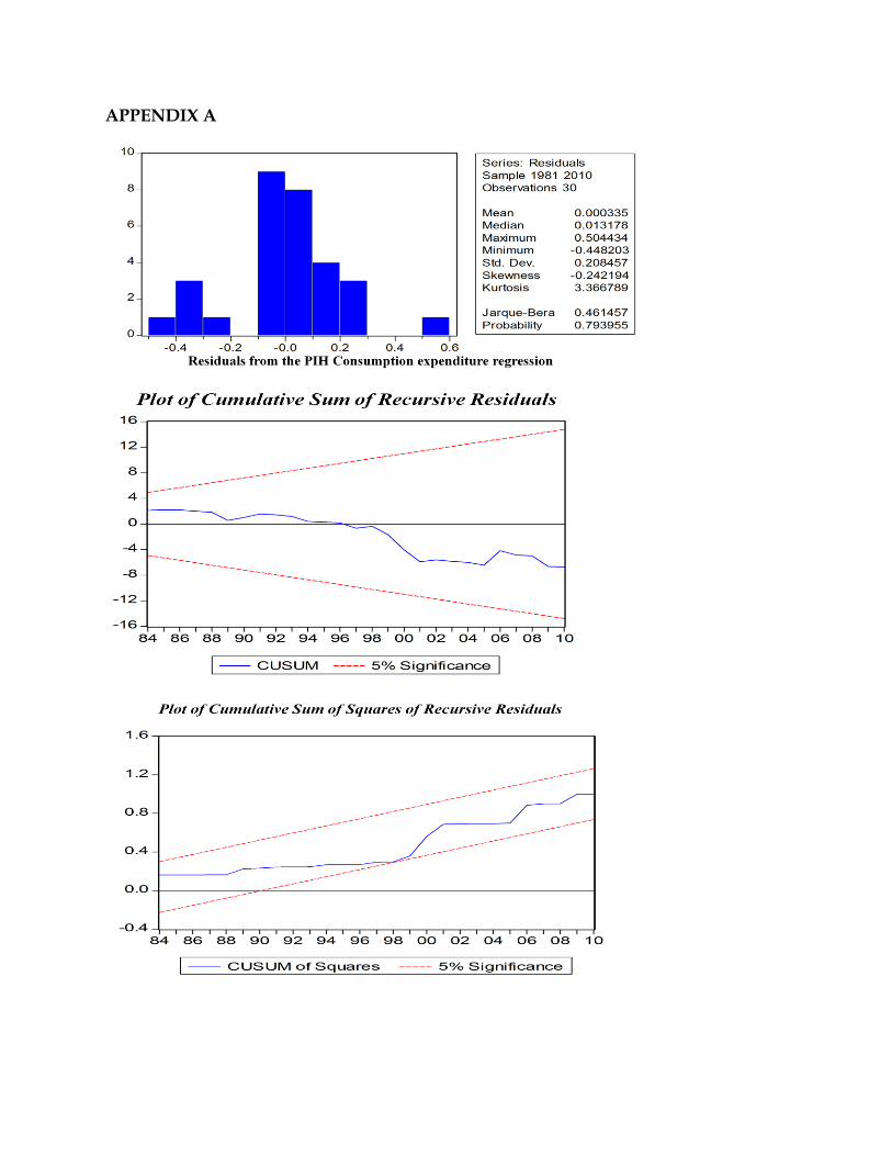
APPENDIX A

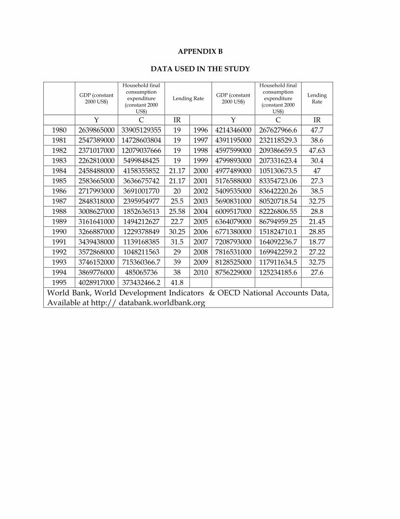
APPENDIX B

DATA USED IN THE STUDY

GDP (constant

2000 US$)

Household final consumption expenditure

(constant 2000 US$)

Lending Rate GDP (constant

2000 US$)

Household final consumption expenditure

(constant 2000 US$)

Lending Rate

Y C IR

Y C IR

1980 2639865000 33905129355 19 1996 4214346000 267627966.6 47.7

1981 2547389000 14728603804 19 1997 4391195000 232118529.3 38.6

1982 2371017000 12079037666 19 1998 4597599000 209386659.5 47.63

1983 2262810000 5499848425 19 1999 4799893000 207331623.4 30.4

1984 2458488000 4158355852 21.17 2000 4977489000 105130673.5 47

1985 2583665000 3636675742 21.17 2001 5176588000 83354723.06 27.3

1986 2717993000 3691001770 20 2002 5409535000 83642220.26 38.5

1987 2848318000 2395954977 25.5 2003 5690831000 80520718.54 32.75

1988 3008627000 1852636513 25.58 2004 6009517000 82226806.55 28.8

1989 3161641000 1494212627 22.7 2005 6364079000 86794959.25 21.45

1990 3266887000 1229378849 30.25 2006 6771380000 151824710.1 28.85

1991 3439438000 1139168385 31.5 2007 7208793000 164092236.7 18.77

1992 3572868000 1048211563 29 2008 7816531000 169942259.2 27.22

1993 3746152000 715360366.7 39 2009 8128525000 117911634.5 32.75

1994 3869776000 485065736 38 2010 8756229000 125234185.6 27.6

1995 4028917000 373432466.2 41.8

World Bank, World Development Indicators & OECD National Accounts Data, Available at http:// databank.worldbank.org