constant and switching gains in semi-active damping of vibrating structures

International Journal of ControlVol. 85, No. 12, December 2012, 1886–1897

Constant and switching gains in semi-active damping of vibrating structures

Franco Blanchinia, Daniele Casagrandeb*, Paolo Gardoniob and Stefano Mianib

aDepartment of Mathematics and Computer Science, University of Udine, Via delle Scienze,208-33100 Udine, Italy; bDepartment of Electrical, Managerial and Mechanical Engineering,

University of Udine, Via delle Scienze, 208-33100 Udine, Italy

(Received 2 April 2012; final version received 7 July 2012)

We consider the problem of optimal control of vibrating structures and we analyse the solution provided bycollocated semiactive decentralised damping devices. We mainly consider the H1 criterion and we first study thecase of constant dampers, showing that in the case of a single damper the performance is a quasi-convex functionof friction so there is a single local minimum which is a global one. The case of multiple dampers does not exhibitthis feature and time-expensive computations may be required. Secondly, we consider the case in which dampersmay be tuned on line, and in particular the case in which they work in a switching on–off mode. We propose astate-switching feedback control strategy, which outperforms the constant damping approach with the optimalstatic gain performance as an upper bound. For large distributed flexible structures, state feedback is unrealisticand so we propose a stochastic strategy based on a Markov-jump criterion for which the transition probabilityare not assigned but designed to optimise average performance, with guaranteed asymptotic stability. Finally, weshow that the same result provided for the H1 case holds for the H2 and the l1 criteria.

Keywords: semi-active control; switching control; optimal control

1. Introduction and preliminaries

The control of vibration and sound radiation ofdistributed flexible structures with active systems is achallenging problem. Complex multichannel feedbackcontrollers are often used; however, they are difficult torealise in practice (Clark, Saunders, and Gibbs 1978;Preumont 2002). During the past decade, research hasshifted to much simpler solutions based on decentra-lised velocity feedback, which generate active dampingon the structure. The interest for this control config-uration is twofold. First, the decentralised controlloops are bound to be unconditionally stable, providedthe sensor and actuator pairs are dual and collocated(Balas 1979). Secondly, when considering broadbandrandom disturbances on plate structures, as the controlgains of the decentralised control units are increasedfrom zero, both the vibrational response and soundradiation tend to decrease up to a certain gain beyondwhich they progressively go back to the valuescorresponding to a feedback gain equal to zero(Elliott, Gardonio, Sors, and Brennan 2002;Gardonio, Miani, Blanchini, Casagrande, andElliott 2012). Simulations indicate that there is anoptimal gain for the velocity feedback such thatboth vibrational response and sound radiation areminimised. Thus decentralised velocity feedbackcontrol offers a stable and simple control strategy to

reduce broad-band random disturbances in distributed

flexible structures.Many structural vibration control applications can

be interpreted as semi-active control scenarios (Spencer

and Nagarajaiah 2003). In particular, among other

techniques, the well-known H1 approach (Yamashita,

Fujimori, Hayakawa, and Kimura 1994; Du, Sze, and

Lam 2005; Karimi, Zapateiro, and Luo 2009;

Prabakar, Sujatha, and Narayanan 2009; Fallah,

Bhat, and Xie 2010; Karimi, Zapateiro, and Luo

2010; Li, Gao, and Liu 2011; Sun, Gao, and Kaynak

2011) and the model predictive control (Canale,

Milanese, and Novara 2006) have been successfully

applied. The reader is referred to Cavallo, De Maria,

and Natale (2010) for a detailed survey. As far as the

practical realisation of the control is concerned, several

configurations have been investigated experimentally,

which employ different types of sensor-actuator pairs

for the implementation of the decentralised velocity

feedback loops, such as piezoelectric transducers

(Hagood and von Flotow 1991; Dosch, Inman, and

Garcia 1992; Cole and Clark 1994; Petitjean and

Legrain 1996; Petitjean, Legrain, Simon, and Pauzin

2002; Bianchi, Gardonio, and Elliott 2004; Gardonio,

Aoki, and Elliott 2010) or electromagnetic transducers

(Paulitsch, Gardonio, and Elliott 2006; Alujevic,

Gardonio, and Frampton 2011; Rohlfing, Gardonio,

*Corresponding author. Email: [email protected]

ISSN 0020–7179 print/ISSN 1366–5820 online

� 2012 Taylor & Francis

http://dx.doi.org/10.1080/00207179.2012.710915

http://www.tandfonline.com

and Thompson 2011). Of particular interest is the ideaof implementing switching controllers, which enhancethe damping action of passive shunts (Ji, Qiu, Xia, andGuyomar 2011). In general, these studies are focusedon two aspects for the given pair of sensor-actuatortransducers: first, how to set the controller in order toget a negative feedback that would produce a dampingeffect on the structure in the audio frequency range ofinterest; second, how to ensure the feedback loops arestable for the control gains that would minimise theflexural vibration and sound radiation of the panelstructure.

In parallel to the work on active control of vibrationand sound radiation by distributed flexible structures,the idea of using decentralised velocity feedback controlunits has also been explored for vibration isolationproblems, i.e. to reduce ground disturbances transmis-sion to delicate equipment (normally measurementsetups or precise fabrication devices) or to vehicles(cars, trains, etc.) and to control the disturbancetransmission by running equipment (reciprocatingengines or compressors, electric motors, flying wheels,etc.) to the supporting structure (Gordon 1995; Fuller,Elliott, and Nelson 1996; Preumont 2002). Normally,both types of problems are tackled by using compliantmounts. However, very soft mounts are required toensure good isolation effects starting from low seismicfrequencies but this requirement cannot be easilysatisfied as the mounts have also to be stiff enough towithstand the static load exerted by the suspendedsystem. With reference to this problem, decentralisedvelocity feedback (Kim, Elliott, and Brennan 2001) and‘sky-hook’ active damping (Karnopp 1995) have beeninvestigated. In both cases, the feedback systems aremounted in parallel with the passive mount. In case ofnarrow band disturbances, inertial actuators thatoperate at resonance frequency have been used(Elliott, Serrand, and Gardonio 2001). Alternatively,semi-active systems have been developed where thedamping of the suspension system is switched from lowto high values in such a way as to synthesise a sky-hookdamping effect, which more efficiently dissipates energyand thus reduces vibration transmission (Karnopp,Crosby, and Harwood 1974; Fischer and Isermann2003). In particular, the use of magneto-rheologicalfluid dampers has been extensively investigated (Jean,Ohayon, Mace, and Gardonio 2006).

In parallel to the practical development of thefeedback loops to which the above-mentioned worksrefer, there has been a lot of theoretical work on theformulation of optimal output feedback control laws.For instance, as summarised in Mkula and Toivonen’s(1987) survey, a number of studies have beenproposed for the optimal tuning of decentralisedvelocity feedback control loops with constant gain

(e.g. Toivonen 1985; Skogestad and Postlethwaite1996). In this article we consider the specific problemof a weakly damped structure controlled by collocateddampers, of which only the friction coefficient can betuned. In particular, we focus on the optimal controlproblem related to the minimisation of the H1 normof a relevant transfer function. The case of constanttunable dampers with the tuning performed off-line isstudied first. Then the case in which the dampingvalues can be switched on line in an on–off mode isanalysed.

A state-switching can introduce a considerableadvantage in semi-active control for two reasons.First, from a technological point of view, switchingstrategies are suitable for easy on-line retuning and canbe implemented at a reasonable cost. Second, as shownbelow, they outperform constant strategies. Third, theimplementation of a constant damper can be doneeither actively (a proportional control) at a high costand with stability problem due to phase lag, orpassively. In this second case, tuning the dampingcoefficient is conceptually simple but practicallydifficult, because friction devices are subject to broadvariations due to external factors such as temperature.Conversely switching allows for a ‘virtually perfect’tuning of the damping factor.

The main results of the paper are detailed below.

. In the case of a SISO system with a singledamper in which either a displacement or avelocity is taken as output, we show that theminimum of theH1 norm is unique. Precisely,given a performance level �, we can providethe interval of all gains which ensure such aperformance level. The global minimum isreadily achieved by bisection. However, in thecase of multiple dampers, non-convex optimi-sation is necessary.

. In the case in which a semi-active approach isallowed, so that the damping coefficient canbe changed on-line, we show that there exists aswitching strategy that outperforms staticones, provided that the state feedback ispossible. The switching strategy is achievedby considering the storage function associatedwith the constant gain.

. If state feedback is not applicable, then weshow how to use a probabilistic approach,with guaranteed stability. The resultingclosed-loop system is a Markov jump linearsystems whose transition properties are opti-mised by means of parametric matrixinequalities.

. We briefly discuss the case of H2-norm andl1-norm, showing that one can obtain

International Journal of Control 1887

analogous results to those that hold in the caseof the H1-norm.

Preliminary results on the problem considered in thispaper are found in Blanchini, Casagrande, Gardonio,and Miani (2011). Furthermore, the problem is relatedto the consistency for which very recent results areprovided in Geromel, Deaecto, and Daafouz (2011).

2. Problem setup

Consider a mechanical vibrating system modelled by

M €qðtÞ ¼ � �KqðtÞ þ �B2uðtÞ þ �E2wðtÞ,

yðtÞ ¼ C2 _qðtÞ,

zðtÞ ¼ H1qðtÞ þH2 _qðtÞ,

8><>: ð1Þ

where y2 IRp is the output velocities vector, M and �Kare the mass and stiffness positive definite matrices,�B2 and �E2 are the control and the primary excitationmatrices, u2 IRp and w are the control and primaryexcitation (i.e. noise) inputs, z is the performanceoutput, H1 and H2 are constant matrices. The statevariable are casted in the Lagrangian coordinate vectorq2 IRm and C2 is the control velocities matrix.

We consider the case of a negative linear feedback,namely the case of a linear damper of the form

uðtÞ ¼ �GyðtÞ, ð2Þ

in which G¼ diag{g} is a p� p diagonal matrixwith positive entries gi2 IR representing the frictioncoefficients of the damper (g ¼ ð g1, . . . , gpÞ

>2 IR

pþ is

the vector of the non-negative diagonal entries).We will work under the following assumption.

Assumption 2.1: Denoting by B2i the ith column of �B2

and by C2i the i-th row of C2 matrix B2iC2i þ C>2iB>2i is

positive semidefinite.

Remark 2.2: The previous assumption implies thatB2i is aligned with C>2i. Note that in most cases, forcollocated dampers we have simply that C2 ¼ �B>2 ,which ensures that Assumption 2.1 is satisfied. In turn,the assumption assures that �B2C2 þ C>2

�B>2 is positivesemidefinite.

Assumption 2.3: The system is reachable from anyinput channel ui and observable from any output yi.

Before dealing with damping optimisation, wepresent a result concerning the stability of the closed-loop system.

Proposition 2.4: Under the previous assumptions,system (2) is asymptotically stable for any choicegi� 0 such that at least one parameter is strictlypositive gi4 0.

Conversely, Assumption 2.3 means that the dam-

pers are not misplaced, for instance in a node of the

vibrating structure.By introducing the variables x1¼ q and x2 ¼ _q and

K ¼ �M�1 �K, E2 ¼ �M�1 �E2 and B2 ¼ �M�1 �B2 we obtain

the state space representation

_x1

_x2

� �¼

0 I

�K 0

� �x1

x2

� �þ

0

E2

� �wþ

0

B2

� �u, ð3Þ

z ¼ H1 H2

� � x1

x2

� �, ð4Þ

y ¼ 0 C2

� � x1

x2

� �: ð5Þ

The closed loop system becomes

_xðtÞ ¼ Að gÞxðtÞ þ EwðtÞ

zðtÞ ¼ HxðtÞð6Þ

where

A¼0 I

�K �B2GC2

� �, E¼

0

E2

� �, H¼ H1 H2ð Þ:

The problem considered in this article is how to

minimise the effect of the input w on the output z by

tuning g. The effect can be measured by using any of

the following performance indices, defined for x(0)¼ 0.

. Energy-to-energy gain:

J1 ¼ supR 10kwk22ðtÞdt�1

Z 10

kzðtÞk22dt:

where kwk2¼wTw, is the Euclidean norm.. Impulse response energy:

J2 ¼

Z 10

kzðtÞDk22dt,

where zD(t) is the impulse response of

system (6).. Peak-to-peak amplification:

J1 ¼ supkwð�Þk1�1

kzðtÞk1, ð7Þ

where k � k1, is the infinity norm:

kwð�Þk1 ¼ supt�0

max jwij:

We develop in particular the first criterion, since

the other two lead essentially to very similar results.

1888 F. Blanchini et al.

3. H1 optimisation

3.1 The SISO case with a single damper

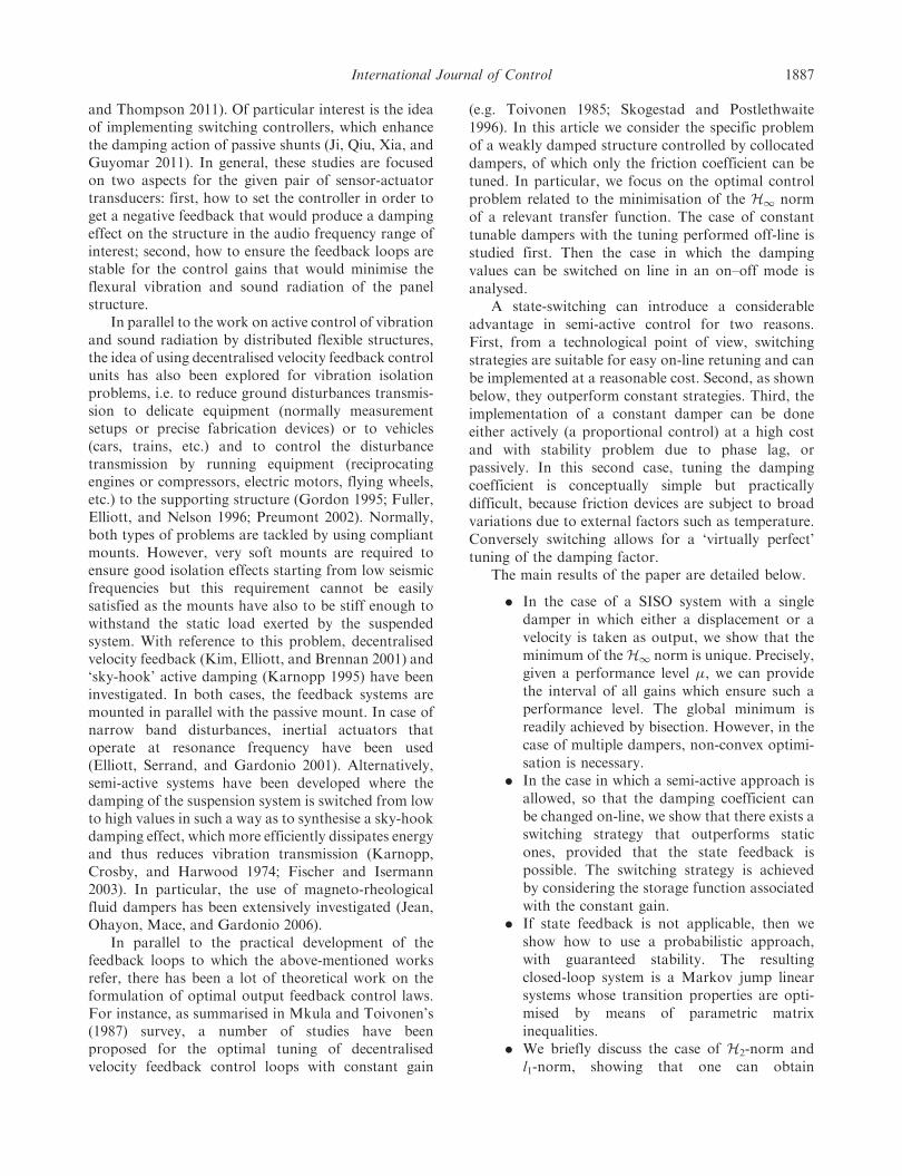
Consider a system of masses and springs and a single

damper as the one depicted in Figure 1 and suppose

that the value of the damping coefficient g has to be

tuned in order to minimise the effect of the motion of

one of the masses on the motion of another mass,

namely the effect of an input w on an output z.

Denoting by F(s, g) the (g-dependent) closed-loop

transfer function from the input w to the output z,

assuming g constant, we can write the performance

index as

J1ð gÞ ¼ sup!�0jFð j!, gÞj: ð8Þ

The next theorem shows that for displacement or

velocity output the function has no multiple local

minima.

Theorem 3.1: If in (1) either H1¼ 0 or H2¼ 0, then J1does not have local minima which are not global. œ

Proof: We prove the theorem in the case H2¼ 0. The

case H1¼ 0 is identical.Assuming that H2¼ 0 the transfer function of

system (3)–(5) is of the form

Fðs, gÞ ¼�ðs2Þ þ gs�ðs2Þ

�ðs2Þ þ gs�ðs2Þ, ð9Þ

where �, �, � and � are even polynomials1 and

�(s)þ gs�(s) is Hurwitz for any positive g. Indeed,

the closed-loop system with u¼� gy in the input–out-

put representation can be written as

zðsÞ ¼ sH1 s2Iþ Kþ sgB2C2

� �1E2wðsÞ, ð10Þ

where z(s) and w(s) are the Laplace transforms of z(t)

and w(t), respectively, and I is the identity matrix.

Assumption 2.3 implies that B2C2 has rank one,

therefore

det s2Iþ Kþ sgB2C2

� is a polynomial function of s2 and an affine function of

�¼ sg. Similarly, the determinant of any sub-matrix of

s2IþKþ �B2C2 is an affine function of �. Then each

entry of

s2Iþ Kþ �B2C2

� �1is a bilinear function (the ratio of two affine functions)

of �¼ sg, precisely it has the form

�ijðs2Þ þ ��ijðs

2Þ

�ðs2Þ þ ��ðs2Þ:

Since all these functions have a common (Hurwitz in

view of Proposition 2.4) denominator,

Fðs, gÞ ¼ H1 s2Iþ Kþ sgB2C2

� �1E2

is of the required form.Now, let �4 0 be an arbitrary value. Setting

�¼ g2, the inequality jF(j!, g)j �� for all ! is

equivalent to

�ð�!2Þ2þ �!2�ð�!2Þ

2� �2 �ð�!2Þ

2þ �!2�ð�!2Þ

2�

,

that can be rewritten as

!2�ð�!2Þ2��2!2�ð�!2Þ

2�

�� 2�ð�!2Þ2��ð�!2Þ

2�

:

ð11Þ

The set of positive values �4 0 which satisfy the

previous inequality is a half-bounded interval. The

admissible set for � is the intersection of all such half-

bounded intervals, which is a (possibly empty) interval:

�ð�Þ ¼ f�j ð11Þ is verified for all ! � 0g

In other words, J1 is a quasi-convex function,2

and there cannot exist local minima which are

not global. œ

The case in which H1 and H2 are both different

from 0 remains open and it is not clear if multiple local

minima are possible.

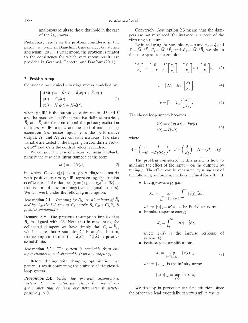
3.2 Multiple dampers cases

We conclude the section analysing the case of multiple

(different) dampers. Since the aim of this article is to

show that a switching damping strategy may outper-

form a constant damping approach, which occurs for

the single damper case described above, we do not

compare the performance of the two approaches in the

case of multiple dampers. However, we show that this

case is associated with a non-convex optimisation

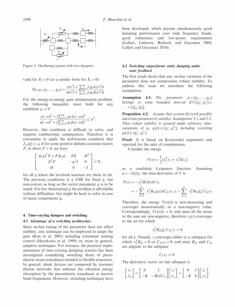
problem.In the case of multiple dampers, as that depicted in

Figure 2, the transfer function takes the extended form

g

z

w

Figure 1. Oscillating system with a feedback made of a singledamper whose coefficient g varies with time. w and z are theexternal input and performance output, respectively.


valid for E2¼ 0 (or a similar form for E1¼ 0)

Fðs, g1, g2, . . . , gmÞ ¼�ðs2Þ þ

Pmk¼1ð gk�kðs

2ÞÞ

�ðs2Þ þPm

k¼1ð gk�kðs2ÞÞ

For the energy-to-energy gain minimisation problem,the following inequality must hold for anycandidate �4 0

�ð�!Þ2 þ ðPm

k¼1 gk�kð�!ÞÞ2

�ð�!Þ2 þ ðPm

k¼1 gk�kð�!ÞÞ2� �2:

However, this condition is difficult to solve, andrequires cumbersome computation. Therefore it isconvenient to apply the well-known condition thatJ1(g)5� if for some positive definite constant matrixP, in short P4 0, we have

Að gÞTPþ PAð gÞ PE HT

ETP ��2I 0

H 0 �I

264

3755 0,

for all g where the involved matrices are those in (6).The previous conditions is a LMI for fixed g, butnon-convex as long as the vector parameter g is to betuned. For low dimensional g the problem is affordablewithout difficulties, but might be hard to solve in caseof many components gi.

4. Time-varying dampers and switching

4.1 Advantage of a switching architecture

Since on-line tuning of the parameter does not affectstability, any technique can be employed to adapt thegain (Kim et al. 2001) including extremum seekingcontrol (Hayakawa et al. 1999) or, more in general,adaptive techniques. For instance, the practical imple-mentation of time-varying damping systems has beeninvestigated considering switching shunt of piezo-electric strain transducers bonded to flexible structures.In general, shunt devices are composed by resonantelectric networks that enhance the vibration energyabsorption by the piezoelectric transducer at narrowband frequencies. However, switching techniques have

been developed, which present simultaneously good

damping performance over wide frequency bands,

good robustness and low-power requirements

(Lallart, Lefeuvre, Richard, and Guyomar 2008;

Lallart and Guyomar 2010).

4.2 Switching outperforms static damping understate feedback

The first result shows that any on-line variation of the

parameter does not compromise robust stability. To

address this issue we introduce the following

assumption.

Assumption 4.1: The parameter g¼ (g1, . . . , gm)

belongs to some bounded interval G¼4½ g�1 , g

þ1 � �

� � � � ½ g�m, gþm�.

Proposition 4.2: Assume that system (6) (with possibly

uncertain parameters) satisfies Assumptions 2.1 and 2.3.

Then robust stability is assured under arbitrary time-

variations of gi, giðtÞ 2 ½ g�i , g

þi �, including switching

giðtÞ 2 fg�i , gþi g.

Proof: It is based on Krasowskii arguments and

reported for the sake of completeness.Consider the energy

VðxÞ ¼1

2½xT2 x2 þ xT1Kx1�

as a candidate Lyapunov function. Assuming

u¼�G(t)y, the time-derivative of V is

_VðxÞ ¼ �xT2B2GðtÞCx2

¼ �Xpk¼1

xT2B2kgkðtÞC2kx2 � �Xpk¼1

xT2B2kg�k C2kx2

Therefore, the energy V(x(t)) is non-increasing and

converges monotonically to a non-negative value.

Correspondingly, _VðxðtÞÞ ! 0, and since all the terms

in the sum are non-negative, therefore x2(t) converges

to the set for which

xT2B2kg�k C2kx2 ¼ 0

for all k. Namely x converges either to a subspace for

which xT2B2k ¼ 0 or C2kx2¼ 0, and since B2k and C2k

are aligned, to the subspace

C2x2 ¼ 0:

The derivative vector on this subspace is

_x1

_x2

� �¼

0 I

�K �B2GC2

� �x1

x2

� �¼

0 I

�K 0

� �x1

x2

� �:

w

z

u1

u2

u3

Figure 2. Oscillating system with two dampers.


Then to preserve the condition C2x2¼ 0, it must be

d

dtðC2x2Þ ¼ C2 _x2 ¼ �C2Kx1 ¼ 0:

In turn this condition has to be preserved, so that

d

dtðC2Kx1Þ ¼ C2K _x1 ¼ C2Kx2 ¼ 0:

Then recursively, one must have C2K _x2 ¼ 0, hence

C2K2x1¼ 0, and then C2K

2x2¼ 0 and so on to get

C2Kix2 ¼ 0:

On the other hand, denoting by O the observability

matrix, we have

O0

x2

� �¼

0 C2

�C2K 0

0 �C2K

C2K2 0

: :

26666664

37777775

0

x2

� �¼ 0,

then if x2 6¼ 0 the observability assumptions would be

violated. Hence, x2 and its derivative must converge to

zero. Since K is positive definite, x1 must converges to 0

as well.

The following theorem shows that the strategy of

switching among different values of g may perform

better than a feedback with a constant g.

Theorem 4.3: Assume that the (possibly optimal)

gain g provides a value J1. Then there exists a

switching strategy which achieves at least the same

performances. œ

Proof: Consider the case of the H1 strategy and

suppose that a constant gain g(t)¼ g is applied. Then

by the standard H1 theory (Zhou, Doyle, and Glower

1996; Sanchez Pena and Sznaier 1998) J15 1 if and

only if3 there exists a positive definite matrix P such

that, for all t� 0,

d

dtxðtÞ>PxðtÞ5 � kzðtÞk2 þ kwðtÞk2: ð12Þ

In fact, by integrating Equation (12) from the current

instant t to infinity, we obtainZ 1t

ðkzðÞk2 � kwðÞk2Þd � xðtÞ>PxðtÞ:

The function xðtÞ>PxðtÞ is the so called storage

function and for the initial condition x(0)¼ 0 we haveZ 10

kzðÞk2d �

Z 10

kwðÞk2d � 1,

which means J15 1. It is known that P must satisfythe Riccati equation

A>ðgÞPþ PAðgÞ þ PEE>Pþ H>H ¼ 0:

Again, denoting by xðtÞ the constant-gain solution fora given current state and for g(t)¼ g, by minimising thederivative of xðtÞ>PxðtÞ we obtain

ming2½ g�,gþ�

d

dtxðtÞ>PxðtÞ

�d

dtxðtÞ>PxðtÞ � �kzðtÞk2 þ kwðtÞk2:

Thus in a right neighbourhood of t, we have

xðtþ Þ>Pxðtþ Þ � xðtþ Þ>Pxðtþ Þ,

which means that the storage function x>Px achievedby the constant gain is always an upper bound for theenergy achieved by the switching strategy. On the otherhand, it is known that (12) is an equality for the worstcase of the input w and therefore the constant gaincannot outperform the switching gain strategy. œ

Therefore the strategy suggested by the previoustheorem is

gðxÞ ¼ arg mingi2fg

�i,gþ

ig

x>PAð gÞx:

4.3 Switching without state feedback

The switching strategy requires the knowledge of thestate of the system, since it is based on the minimisa-tion of the quantity x>PA(g)x, hence an observer isneeded. This requirement is reasonable in simplesystems, but it may be difficult to fulfill for high-orderdistributed flexible structures. In this case the use of anopen-loop switching strategy may be a viable solution.A possibility is to apply a dynamic random processwith transition probabilities suitably chosen.

Denote by Ai, for i¼ 1, 2, . . . , 2m, the matricesachieved by taking all possible values of the parametersat their extrema. The transition probability among thediscrete states can be governed by a Markov matrix Q,the entries of which verifyX

j

qij ¼ 0, qii 5 0:

This is a Markov-jump system whose performance isgiven by the following condition (de Souza, Trofino,and Barbosa 2006).

Proposition 4.4: The index J1 satisfies, J1�� ifand only if there exist symmetric matrices Pj4 0


such that

ATi Pi þ PiAi þ

Pj qijPj PiE HT

ETPi ��2I 0

H 0 �I

264

3755 0 ð13Þ

The Markov chain Q is a design parameter which hasto be optimised rather then assigned as in most of theexisting literature. Unfortunately, the last quadraticcondition is bilinear in the matrices Pi and Q and noconvex characterisation of the set of solutions can beprovided. None the less, the random switching approachappears to be promising, as shown by Example 6.2 inSection 6.

5. The H2 and l1 cases

5.1 H2 performance and switching

The H2 performance in the case of a single transferfunction can be expressed in the frequency domain as:

J2ð gÞ ¼1

�

Z 10

Fð j!, gÞFð�j!, gÞd!: ð14Þ

Adopting the same notations of the previous sections,we obtain

J2ð�Þ ¼1

�

Z 10

�ð�!2Þ2þ �!2�ð�!2Þ

2

�ð�!2Þ2þ �!2�ð�!2Þ

2d!,

where, again, �¼ g2. As observed by As observed byBlanchini et al. (2011), one may take advantage from aconvex–concave decomposition of this functional, butit is not clear if the optimisation problem admitsmultiple local minima.

The performance optimisation can be approachedby means of standard theory (Zhou et al. 1996) bysolving the problem

J2 ¼ ming

trfETPEg,

s:t: Að gÞTPþ PAð gÞ ¼ �HTH,ð15Þ

which is equivalent to minimising the ratio of twopolynomials in g, as shown by the following result.

Theorem 5.1: Problem (15) is equivalent to the mini-misation of the ratio of two polynomials in g. œ

Proof: By introducing the notation ~g ¼ g� g�,A1¼A(g�) and

A2 ¼Að gþÞ � Að g�Þ

gþ � g�,

the Lyapunov equation in (15) can be written as

A1 þ ~gA2ð ÞTPþ P A1 þ ~gA2ð Þ ¼ �HTH, ð16Þ

an equation whose solution can be found via

Kronecker products and sums (Zhou et al. 1996).

By defining4

~A1 ¼ AT1 � I2n þ I2n � AT

1 ,

~A2 ¼ AT2 � I2n þ I2n � AT

2 ,

X ¼ vecfPg,

the optimal H2 index can be found as

J2 ¼ ming

vecfEETgTX,

s:t: ~A1 þ ~g ~A2

�X ¼ �vecfHTHg:

Now, since by Proposition 4.2 A1 is invertible, so is ~A1,

hence the problem can be rewritten as

J2 ¼ ming

vecfEETgTX,

s:t: Iþ ~g ~A�11~A2

�X ¼ � ~A�11 vecfHTHg,

which results in the minimisation problem

J2 ¼ ming�vecfEETgT Iþ ~g ~A�11

~A2

��1~A�11 vecfHTHg:

It is straightforward to see that the term to be

minimised is the ratio of two polynomials in ~g and

hence in g. œ

Once the former problem has been solved, one can

again improve the performance by switching. The

following result holds.5

Theorem 5.2: Assume that the (possibly optimal) gain

g provides the value J2 for the cost function (14). There

exists a state-feedback strategy which assures at least

the same performances.

Proof: Consider the Lyapunov equation

AðgÞ>Pþ PAðgÞ ¼ �H>H: ð17Þ

The integral of the energy from the current instant t to

infinity is

J2,resðtÞ ¼4

Z 1t

zð gðÞ, Þ2d

¼

Z 1t

xð gðÞ, Þ>H>Hxð gðÞ, Þd: ð18Þ

Denote by J2,resðtÞ the value achieved when in (18), a

constant gain g()¼ g is used. In view of (17),

J2,resðtÞ ¼ �

Z 1t

xðg, Þ> AðgÞ>Pþ PAðgÞ �

xðg, Þd

¼ xðtÞ>PxðtÞ:


Now, consider again the index (18), and suppose that

the constant value g()¼ g, not necessarily equal to g,

is applied in the interval [t, tþ ] and the value g from

the instant tþ on, so that the state value at tþ equals eAð g

ÞxðtÞ and the resulting cost J2,res(t) isZ tþ

t

x>ð g, ÞH>Hxð g, Þd

þ xðtÞ>eA>ð gÞPeAð g

ÞxðtÞ

¼ x>ðtÞ

Z

0

eA>ð gÞH>HeAð g

Þd

� �xðtÞ

þ x>ðtÞeA>ð gÞPeAð g

ÞxðtÞ:

The above expression can be written by using theexponential power series expansion, that is, for a

matrix M and a scalar �, the identity

eM� ¼ Iþ �MþOð�2Þ,

with O(�)! 0 when �! 0. We obtain

J2,resðtÞ ¼ x>ðtÞhH>H þ A>ð gÞH>Hþ H>HAð gÞ

��2

2þ Pþ A>ð gÞPþ PAð gÞ

�þOð2Þ

ixðtÞ,

where O(2)! 0 when ! 0. Therefore, with the given

strategy, the integral of the energy from the current

instant t to infinity is

x>ðtÞ Pþ H>Hþ A>ð gÞPþ PAð gÞ � �

xðtÞ

þ x>ðtÞOð2ÞxðtÞ:

A minimisation of the residual energy, up to the

first-order term, is obtained by minimising the above

value with respect to g, namely by adopting the

following strategy

gðtÞ ¼ arg ming2½ g�,gþ�

xðtÞ> PAð gÞ þ A>ð gÞP �

xðtÞ: ð19Þ

Since the above minimisation results in a value of

J2res(t) not greater than J2,resðtÞ, this means that for a

given state x(t) at time t, the residual energy at timetþ , for any 4 0, achieved by the switching strategy

is not greater than the energy achieved by a constant g,

which means that the constant-gain strategy cannot be

better than the switching one. œ

Note that a more general class of controllers can be

designed if one allows an active control, rather than a

semi-active architecture. The reader is referred to

Geromel, Colaneri, and Bolzern (2008) for details

and a survey. However, in the presence of a more

general architecture, the robust stability is a major

issue, while here stability is assured under arbitrary

switching.

5.2 l1 performance and switching

The l1 performances of (6) for given g can be computed

as follows. Denote by F(t, g) the impulse response

matrix corresponding to the gain g. Then, given the

bound suptjwi(t)j5 1 for all i, the performance

index (7) is given by Barabanov and Granichin

(1984) and Dahleh and Pearson (1987)

J1 ¼ maxi

Xj

Z 10

jFijðt, gÞjdt:

Assuming that a certain performance J1 is assured via

static feedback with constant feedback gain g, the

question is if also in this case a switching strategy can

achieve at least the same performance. We can provide

a positive answer to this question (up to an arbitrarily

small tolerance) along with a constructive solution.

Theorem 5.3: Assume that J1(g) is the (optimal)

performance given by the vector gain g. Then given

4 0 there exists a switching strategy which achieves the

performance J1(g)þ .

Proof: The proof is based on the set–theoretic

characterisation of J1 (Blanchini and Miani 2008).

The performance is equivalent to the existence of a

convex and compact set P including the origin in its

interior and included in the set

Sð Þ ¼ fx : kHxk1 � J1ðgÞ þ g

For a small 4 0 we can approximate (Blanchini and

Miani 1999) P by S(0) which is the unit ball in a

smooth norm6 V(x) for which

rVðxÞ½AðgÞxþ Ew� � ��,

for all w such that kw k1� 1, for some �4 0, and for

all x such that V(x)� 1. From this Lyapunov

characterisation, and the fact that A(g) is affine in g,

we have

arg mingi2fg

�i,gþ

igrVðxÞ½Að gÞxþ Ew�

� rVðxÞ½AðgÞxþ Ew� � ��:

which implies that the set S is attractive for the system

governed by the switching rule

gðtÞ ¼ arg mingi2fg

�i,gþ

igrVðxÞ½Að gÞxþ Ew�:

œ


6. Examples

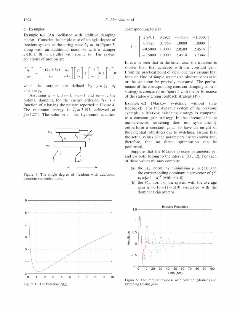
Example 6.1 (An oscillator with additive damping

mass): Consider the simple case of a single degree of

freedom system, as the spring–mass k1–m1 in Figure 3,

along with an additional mass m2 with a damper

g2 [0.1, 10] in parallel with spring k2. The system

equations of motion are

€q1

€q2

" #¼�ðk1 þ k2Þ k2

k2 �k2

" #q1

q2

" #þ

1

�1

" #uþ

1

1

" #w

while the outputs are defined by y ¼ _q2 � _q1and z¼ q1.

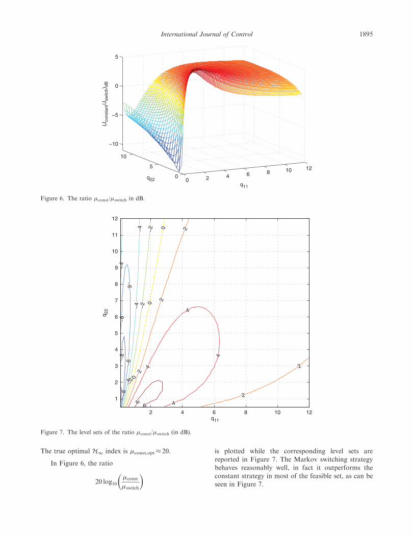
Assuming k1¼ 1, k2¼ 1, m1¼ 1 and m2¼ 1, the

optimal damping for the energy criterion H2 is a

function of g having the pattern reported in Figure 4.

The minimum energy is J2 ¼ 3:193, achieved at

g¼ 1.274. The solution of the Lyapunov equation

corresponding to g is

P ¼

2:9401 0:3925 �0:5000 �1:5000

0:3925 0:7850 1:0000 1:0000

�0:5000 1:0000 2:0589 2:4514

�1:5000 1:0000 2:4514 3:2364

26664

37775:

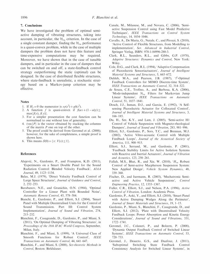
In can be seen that in the latter case, the transient is

shorter than that achieved with the constant gain.

From the practical point of view, one may assume that

for such kind of simple systems an observer does exist

or the state can be precisely measured. The perfor-

mance of the corresponding constant-damping control

strategy is compared in Figure 5 with the performance

of the state-switching feedback strategy (19).

Example 6.2 (Markov switching without state

feedback): For the dynamic system of the previous

example, a Markov switching strategy is compared

to a constant gain strategy. In the absence of state

measurements, switching does not systematically

outperform a constant gain. To have an insight of

the potential robustness due to switching, assume that

the actual values of the parameters are unknown and,

therefore, that no direct optimisation can be

performed.Suppose that the Markov process parameters q11

and q22 both belong to the interval [0.1, 12]. For each

of these values we may compute

(a) the H1 norm, by minimising � in (13) and

the corresponding dominant eigenvector of QT

v0¼ [� 1� �]T (with �4 0);(b) the H1 norm of the system with the average

gain g¼ 0.1�þ (1� �)10 associated with the

dominant eigenvector.

0 1 2 3 4 5 6 7 8 9 103

4

5

6

7

8

9

Figure 4. The function J2(g).

0 10 20 30 40 50 60 70 80 90 100−1

−0.5

0

0.5

1

1.5Impulse Response

Time (sec)

Am

plitu

de

Figure 5. The impulse response with constant (dashed) andswitching (plain) gain.

m2

m1

k2

k1

g

w

z

Figure 3. The single degree of freedom with additionaldamping suspended mass.


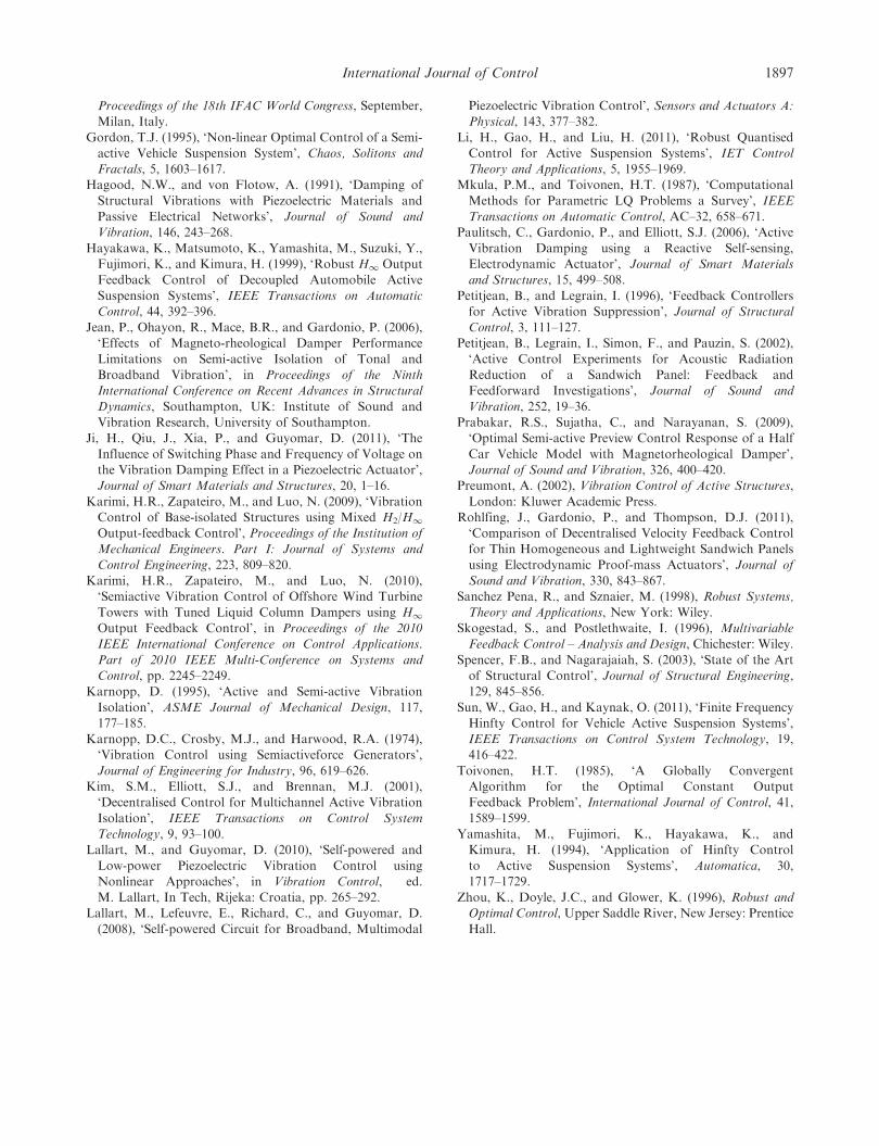
The true optimal H1 index is �const,opt 20.

In Figure 6, the ratio

20 log10�const

�switch

� �is plotted while the corresponding level sets are

reported in Figure 7. The Markov switching strategy

behaves reasonably well, in fact it outperforms the

constant strategy in most of the feasible set, as can be

seen in Figure 7.

−8−

8−

6

−6

−6

−4

−4

−4

−4

−2

−2−

2

0

0

0

2

2

2

2

24

4

4

46

6

q11

q 22

2 4 6 8 10 12

1

2

3

4

5

6

7

8

9

10

11

12

Figure 7. The level sets of the ratio �const/�switch (in dB).

0 2 4 6 8 10 12

0

5

10

−10

−5

0

5

q11

q22

(Jco

nsta

nt/J

switc

h)dB

Figure 6. The ratio �const/�switch in dB.


7. Conclusions

We have investigated the problem of optimal semi-active damping of vibrating structures, taking intoaccount, in particular, the H1 criterion. In the case ofa single constant damper, finding the H1 performanceis a quasi-convex problem, while in the case of multipledampers the problem does not have this feature andtime-expensive computations may be required.Moreover, we have shown that in the case of tunabledampers, and in particular in the case of dampers thatcan be switched on and off, a state-feedback controlstrategy outperforming the static (optimal) can bedesigned. In the case of distributed flexible structures,where state-feedback is unrealistic, a stochastic strat-egy based on a Markov-jump criterion may beeffective.

Notes

1. If H1¼ 0 the numerator is s�(s2)þ g�(s2).2. A function f is quasi-convex if f(�xþ (1��)y)�

max{f(x), f( y)}.3. For a simpler presentation the cost function can be

normalised to one without loss of generality.4. (vec{P} is the vector obtained by stacking the columns

of the matrix P one on top of the other.5. The proof could be derived from Geromel et al. (2008);

however, for the sake of completeness, a simple proof isshown here.

6. This means S(0)¼ {x: V(x)� 1}.

References

Alujevic, N., Gardonio, P., and Frampton, K.D. (2011),

‘Experiments on a Smart Double Panel for the Sound

Radiation Control: Blended Velocity Feedback’, AIAA

Journal, 49, 1123–1134.Balas, M.J. (1979), ‘Direct Velocity Feedback Control of

Large Space Structures’, Journal of Guidance and Control,

2, 252–253.

Barabanov, N.E., and Granichin, O.N. (1984), ‘Optimal

Controller for a Linear Plant with Bounded Noise’,

Automatic Remote Control, 45, 578–584.Bianchi, E., Gardonio, P., and Elliott, S.J. (2004), ‘Smart

Panel with Multiple Decentralised Units for the Control of

Sound Transmission. Part III: Control System

Implementation’, Journal of Sound and Vibration, 274,

215–232.

Blanchini, F., Casagrande, D., Gardonio, P., and Miani, S.

(2011), ‘On Optimal Damping of Vibrating Structures’, in

Proceedings of the 18th IFAC World Congress, September,

Milan, Italy.Blanchini, F., and Miani, S. (1999), ‘A Universal Class of

Smooth Functions for Robust Control’, IEEE

Transactions on Automatic Control, 44, 641–647.Blanchini, F., and Miani, S. (2008), Set-theoretic Methods in

Control, Boston: Birkhauser.

Canale, M., Milanese, M., and Novara, C. (2006), ‘Semi-active Suspension Control using Fast Model Predictive

Techniques’, IEEE Transactions on Control SystemTechnology, 14, 1034–1046.

Cavallo, A., De Maria, G., Natale, C., and Pirozzi, S. (2010),

‘Active Control of Flexible Structures, from Modelling toimplementation’, Ser. Advanced in Industrial Control,Springer Verlag, ISBN: 978-1-84996-280-3.

Clark, R.L., Saunders, R.L., and Gibbs, G.P. (1978),Adaptive Structures: Dynamics and Control, New York:Wiley.

Cole, D.G., and Clark, R.L. (1994), ‘Adaptive Compensationof Piezoelectric Sensoriactuators’, Journal of IntelligentMaterial Systems and Structures, 5, 665–672.

Dahleh, M.A., and Pearson, J.B. (1987), ‘l1-OptimalFeedback Controllers for MIMO Discrete-time System’,IEEE Transactions on Automatic Control, 32, 314–322.

de Souza, C.E., Trofino, A., and Barbosa, K.A. (2006),‘Mode-independent H1 Filters for Markovian JumpLinear Systems’, IEEE Transactions on Automatic

Control, 51, 1837–1841.Dosch, J.J., Inman, D.J., and Garcia, E. (1992), ‘A Self-sensing Piezoelectric Actuator for Collocated Control’,

Journal of Intelligent Material Systems and Structures, 3,166–185.

Du, H., Sze, K.Y., and Lam, J. (2005), ‘Semi-active H1

Control of Vehicle Suspension with Magneto-rheologicalDampers’, Journal of Sound and Vibration, 283, 981–996.

Elliott, S.J., Gardonio, P., Sors, T.C., and Brennan, M.J.(2002), ‘Active Vibro-acoustic Control with Multiple

Feedback Loops’, Journal of the Acoustical Society ofAmerica, 111, 908–915.

Elliott, S.J., Serrand, M., and Gardonio, P. (2001),

‘Feedback Stability Limits for Active Isolation Systemswith Reactive and Inertial Actuators’, Journal of Vibrationand Acoustics, 123, 250–261.

Fallah, M.S., Bhat, R., and Xie, W. (2010), ‘H1 RobustControl of Semi-active Macpherson Suspension System:New Applied Design’, Vehicle System Dynamics, 48,

339–360.Fischer, D., and Isermann, R. (2003), ‘Mechatronic Semi-active and Active Vehicle Suspensions’, Control

Engineering Practice, 12, 1353–1367.Fuller, C.R., Elliott, S.J., and Nelson, P.A. (1996), ActiveControl of Vibration, London: Academic Press.

Gardonio, P., Aoki, Y., and Elliott, S.J. (2010), ‘Smart Panelwith Active Damping Wedges Along the Perimeter’,Journal of Smart Materials and Structures, 19, 1–15.

Gardonio, P., Miani, S., Blanchini, F., Casagrande, D., andElliott, S.J. (2012), ‘Plate with Decentralised VelocityFeedback Loops: Power Absorption and Kinetic Energy

Considerations’, Journal of Sound and Vibrations, 331,1722–1741.

Geromel, J.C., Colaneri, P., and Bolzern, P. (2008),

‘Dynamic Output Feedback Control of Switched LinearSystems’, IEEE Transactions on Automatic Control, 53,720–733.

Geromel, J., Deaecto, G.S., and Daafouz, J. (2011),‘Suboptimal Switching State Feedback ControlConsistency Analysis for Switched Linear Systems’, in


Proceedings of the 18th IFAC World Congress, September,Milan, Italy.

Gordon, T.J. (1995), ‘Non-linear Optimal Control of a Semi-active Vehicle Suspension System’, Chaos, Solitons andFractals, 5, 1603–1617.

Hagood, N.W., and von Flotow, A. (1991), ‘Damping of

Structural Vibrations with Piezoelectric Materials andPassive Electrical Networks’, Journal of Sound andVibration, 146, 243–268.

Hayakawa, K., Matsumoto, K., Yamashita, M., Suzuki, Y.,Fujimori, K., and Kimura, H. (1999), ‘Robust H1 OutputFeedback Control of Decoupled Automobile Active

Suspension Systems’, IEEE Transactions on AutomaticControl, 44, 392–396.

Jean, P., Ohayon, R., Mace, B.R., and Gardonio, P. (2006),‘Effects of Magneto-rheological Damper Performance

Limitations on Semi-active Isolation of Tonal andBroadband Vibration’, in Proceedings of the NinthInternational Conference on Recent Advances in Structural

Dynamics, Southampton, UK: Institute of Sound andVibration Research, University of Southampton.

Ji, H., Qiu, J., Xia, P., and Guyomar, D. (2011), ‘The

Influence of Switching Phase and Frequency of Voltage onthe Vibration Damping Effect in a Piezoelectric Actuator’,Journal of Smart Materials and Structures, 20, 1–16.

Karimi, H.R., Zapateiro, M., and Luo, N. (2009), ‘VibrationControl of Base-isolated Structures using Mixed H2/H1Output-feedback Control’, Proceedings of the Institution ofMechanical Engineers. Part I: Journal of Systems and

Control Engineering, 223, 809–820.Karimi, H.R., Zapateiro, M., and Luo, N. (2010),‘Semiactive Vibration Control of Offshore Wind Turbine

Towers with Tuned Liquid Column Dampers using H1Output Feedback Control’, in Proceedings of the 2010IEEE International Conference on Control Applications.

Part of 2010 IEEE Multi-Conference on Systems andControl, pp. 2245–2249.

Karnopp, D. (1995), ‘Active and Semi-active Vibration

Isolation’, ASME Journal of Mechanical Design, 117,177–185.

Karnopp, D.C., Crosby, M.J., and Harwood, R.A. (1974),‘Vibration Control using Semiactiveforce Generators’,

Journal of Engineering for Industry, 96, 619–626.Kim, S.M., Elliott, S.J., and Brennan, M.J. (2001),‘Decentralised Control for Multichannel Active Vibration

Isolation’, IEEE Transactions on Control SystemTechnology, 9, 93–100.

Lallart, M., and Guyomar, D. (2010), ‘Self-powered and

Low-power Piezoelectric Vibration Control usingNonlinear Approaches’, in Vibration Control, ed.M. Lallart, In Tech, Rijeka: Croatia, pp. 265–292.

Lallart, M., Lefeuvre, E., Richard, C., and Guyomar, D.

(2008), ‘Self-powered Circuit for Broadband, Multimodal

Piezoelectric Vibration Control’, Sensors and Actuators A:Physical, 143, 377–382.

Li, H., Gao, H., and Liu, H. (2011), ‘Robust QuantisedControl for Active Suspension Systems’, IET ControlTheory and Applications, 5, 1955–1969.

Mkula, P.M., and Toivonen, H.T. (1987), ‘Computational

Methods for Parametric LQ Problems a Survey’, IEEETransactions on Automatic Control, AC–32, 658–671.

Paulitsch, C., Gardonio, P., and Elliott, S.J. (2006), ‘Active

Vibration Damping using a Reactive Self-sensing,Electrodynamic Actuator’, Journal of Smart Materialsand Structures, 15, 499–508.

Petitjean, B., and Legrain, I. (1996), ‘Feedback Controllersfor Active Vibration Suppression’, Journal of StructuralControl, 3, 111–127.

Petitjean, B., Legrain, I., Simon, F., and Pauzin, S. (2002),

‘Active Control Experiments for Acoustic RadiationReduction of a Sandwich Panel: Feedback andFeedforward Investigations’, Journal of Sound and

Vibration, 252, 19–36.Prabakar, R.S., Sujatha, C., and Narayanan, S. (2009),‘Optimal Semi-active Preview Control Response of a Half

Car Vehicle Model with Magnetorheological Damper’,Journal of Sound and Vibration, 326, 400–420.

Preumont, A. (2002), Vibration Control of Active Structures,

London: Kluwer Academic Press.Rohlfing, J., Gardonio, P., and Thompson, D.J. (2011),‘Comparison of Decentralised Velocity Feedback Controlfor Thin Homogeneous and Lightweight Sandwich Panels

using Electrodynamic Proof-mass Actuators’, Journal ofSound and Vibration, 330, 843–867.

Sanchez Pena, R., and Sznaier, M. (1998), Robust Systems,

Theory and Applications, New York: Wiley.Skogestad, S., and Postlethwaite, I. (1996), MultivariableFeedback Control – Analysis and Design, Chichester: Wiley.

Spencer, F.B., and Nagarajaiah, S. (2003), ‘State of the Artof Structural Control’, Journal of Structural Engineering,129, 845–856.

Sun, W., Gao, H., and Kaynak, O. (2011), ‘Finite FrequencyHinfty Control for Vehicle Active Suspension Systems’,IEEE Transactions on Control System Technology, 19,416–422.

Toivonen, H.T. (1985), ‘A Globally ConvergentAlgorithm for the Optimal Constant OutputFeedback Problem’, International Journal of Control, 41,

1589–1599.Yamashita, M., Fujimori, K., Hayakawa, K., andKimura, H. (1994), ‘Application of Hinfty Control

to Active Suspension Systems’, Automatica, 30,1717–1729.

Zhou, K., Doyle, J.C., and Glower, K. (1996), Robust andOptimal Control, Upper Saddle River, New Jersey: Prentice

Hall.


constant and switching gains in semi-active damping of vibrating structures

Documents