conditioning in dynamic models
TRANSCRIPT

CONDITIONING IN DYNAMIC MODELS
BY J.-P. FLORENS
G.R.E.Q.E., E.H.E.S.S. and Universite‘ d’Aix-Marseille
A N D
M. MOUCHART
C.O.R.E., Universite‘ Catholique de Louvain
Abstract. A statistical model is generally defined through a probability on some variables conditionally on other variables and refers to some parameters of interest. Therefore, it seems natural to ask under which conditions such a model does not lose information with respect to a model describing more variables and implying more parameters. Admissibility conditions for reductions by conditioning are investigated both in one-shot and in dynamic models. By so doing, concepts of ‘exogeneity’ and of ‘non-causality’ are integrated into a general framework. This paper is essentially a non-technical introduction to the theory of reduction developed more formally in other papers. It also supplies various examples of the concepts introduced in that theory.
Keywords. Reduction of statistical models; exogeneity ; ancillarity ; cut; dynamic models; transitivity; conditional independence.
1. INTRODUCTION
One approach to model building is to start from a ‘large’ model allowing for a large class of interdependences and dynamics and then to look for simplification with a view to better predictions, and for more efficient parametric inferences. Those simplifications may be viewed as ‘reduction’ of the initial model. By ‘reduction’ we mean two types of operation: either marginalization or condition- ing. These operations may be carried out either on the parameter space or on the sample space.
Marginalization or conditioning on the parameter space presupposes a proba- bility on the parameter space, and implicitly, at least, a Bayesian approach. Marginalization on the parameter space is the natural operation when integrating out nuisance parameters, while conditioning allows for a proper treatment of restriction on the parameters.
Similarly, on the sample space, marginalization corresponds to the specification of the data generating process for a part of the variables only while conditioning on some variables corresponds to treat those variables ‘as if’they were not random.
In this paper we focus the attention on reductions obtained by conditioning on the sample space. A conditional model may be viewed as a partly specified model i.e., a model where the data-say x-are split into two components-say
0143-9782/85/01 0015-20 $02.50/0 JOURNAL OF TIME SERIES ANALYSIS Vol. 6, NO. I
15
0 1985 J.-P. Florens and M. Mouchart

16 J.-P. FLORENS AND M. MOUCHART
x = (y, z)-and the data generating process specifies the process generating y given z only, leaving unspecified the process generating z. Such a partial specifica- tion raises two questions: Why would it be useful and, if useful, when is it justified?
The usefulness of conditional models may be empirically answered by remark- ing that a very high proportion of statistical models used in applied work (e.g., almost all in econometrics) are conditional. This may be explained by two factors. When, as often happens, a real world phenomenon is deemed to be statistically ill-behaved (e.g., nonstationary, involving incidental parameters, etc.), one objec- tive of modelling is precisely to try to isolate, in the marginal process generating z, that ill-behaved aspect of the phenomenon with the hope that the conditional model will be amenable to a more powerful statistical analysis. The other factor is robustness: It is to be expected that the analysis of the conditional model alone would be robust to specification error that could affect any specification of the marginal process generating z.
In this paper, we focus the attention on displaying conditions which justify the use of conditional models. In this context, the use of conditional model is justified if such a model does not lose information on the parameters of interest (when compared with a completely specified model). Heuristically a variable is said to be exogenous when it provides a justified conditioning. The object of this paper is to give a precise content to this intuitive idea. Our motivation to pursue this idea is multiple. A precise concept of exogeneity appears to be crucial when extending the asymptotic theory of i.i.d. processes to regression-type process. We shall come back to this issue in the conclusions. Clearly, a good understanding of what exogeneity is, underlies any attempts of testing for exogeneity (see e.g., Wu (1973) or Haussman (1978)). The field of model choice also relies on a clear understanding of exogeneity (see e.g., GouriCroux et al. (1983), Mizon and Richard (1983), Florens and Scotto (1984)) ; this is particularly true for the field of dynamic specification (see e.g., Sims (1980), Palm (198 l ) , Hendry and Richard (1983)).
The concept of ‘not losing information on the parameters of interest’ will be formalized in the framework of the theory of reductions, i.e., the theory of ancillarity and of sufficiency viewed dually on the parameter space and on the sample space. We therefore shall summarize briefly the basic ideas of that theory before presenting the organization of the paper. Finally, although our approach is essentially Bayesian, we want to make precise the role of the prior specification and develop the analysis until obtaining conditions depending very weakly on the prior distribution: This is our strategy to bridge the sampling theory and the Bayesian approach.
Statistical Models
In a sampling theory framework, a statistical model A may be defined as a family of probabilities on a sample space X . Typically such a family is indexed by a parameter a E A.

CONDITIONING IN DYNAMIC MODELS 17
For expository purposes, we shall assume that every probability is representable through a density (w.r.t. some appropriate measure). Let
A = {p(xla) a E A }
where p(xla) is a probability density on X for every a E A. In a Bayesian framework, such a model is also endowed with a so-called ‘prior’
probability p on the parameter space. The Bayesian model, therefore, becomes a (unique) probability T on the product space A xX, viz. ~ ( x , a ) = p(a)p(xla). Bayesian computations usually consist of a dual decomposition of this joint probability into a so-called predictive probability on X , p(x), and into a family of ‘posterior’ probabilities on A, p(a1x). The Bayesian model is therefore written, in terms of densities, as (see e.g., Raiffa and Schlaifer (1961)):
A = M X , a ) = p(a)p(xla) =P(x)P(alx)l.
When ambiguity is possible we write instead of A. The transformation p ( a ) n p(alx) is the cornerstone of Bayesian Inference. Note the following notational convention: .rr, p and p are respectively used to denote probability densities on A xX, A and X .
Reductions
Consider a function of the parameters b = b ( a ) and a function of the observa- tions z = z(x). Marginal models are obtained by integrating ~ ( x , a ) to obtain ~ ( z , a ) or T(X, b ) or ~ ( z , b ) . For instance, if a = (b, c) and x = (y, z), then ~ ( z , a) , ~ ( x , b ) and ~ ( z , 6) are obtained by integrating out respectively y , c or ( y , c) in ~ ( x , a) . In particular:
A b , x = [ d x , b ) = P(b)P(Xlb) =P(x)P(blx)l
where
P(Xlb) = P(xla)P(clb) dc
and p ( b ) and p(blx) are the marginal prior and posterior densities respectively. Conditional models are obtained by conditioning ~ ( x , a ) w.r.t. z, b or (z, b) .
Thus a conditional model is a family of models; for instance:
A’,,, = [..(Y, alz) = I.L(alz)p(yla, z ) =p(ylz)tL(aly, z ) l
represents a family of models indexed by z. Analysing such a family corresponds to an analysis where the sampling process generating z is neglected.
Similarly, models conditioned on the parameter space such as
A2.X = [ d x , clb) = p(clb)p(xlb, c) =p(xlb)p(clx, b)l
are analysed when b is considered as a known parameter. An example is given by models with exact restriction on the parameter. As a matter of notation, a

18 I.-P. FLORENS A N D M. MOUCHART
superscript is used for conditional models and subscript for marginal models. A model may be both marginal and conditional (e.g., A:,z or A;,,).
and the conditional model p:,, (resp. A:,,) are called complementary reductions. For a given function b ( a ) (resp. z ( x ) ) , the marginal model Ath,, (resp.
Admissible Reductions
A model is said to be totally non-informative when its prior and posterior distributions coincide and a reduction is said to be an admissible reduction of a given model when its complementary reduction is totally non-informative : heuristically, in an admissible reduction the transformation ‘prior-to-posterior distribution’ is the same as in the complete model. A function of the parameter or of the observation is said to be suficient if the corresponding marginal reduction is admissible and it is said to be ancillary if the corresponding conditional reduction is admissible.
Parameters of Interest
The admissibility of a reduction therefore appears as relative to a specified complete model but admissibility is not the only ground on which either a given model or a reduction can be justified. If the loss functions depends on b only, the analysis of the marginal model Ah,x may be justified by the fact that b = b ( a ) is the only parameter of interest and that the object of inference becomes the transformation p ( b ) P, p ( b l x ) instead of p ( a ) P, p(a1x) . Thus the Bayesian treatment of so-called ‘nuisance parameters’ consists of concentrating attention on the model marginal on the parameter of interest. This position of principle nevertheless raises, in particular, problems of robustness and computability. In the construction of .Ab,,, p ( x l b ) has the role of a sampling probability but crucially depends on p( c( b) , the prior probability conditional on b ; modifying this condi- tional prior specification would involve analysing another model. This lack of robustness is often undesirable. Moreover the integration involved in the computa- tion of p(x1b) is often cumbersome and leads to a non-standard data density. These two considerations of non-robust and cumbersome integration motivate the search for properties which makes the inference less dependent on such features.
Organization of the Paper
The next section considers the analysis of exogeneity when the inference is based on the complete sample result; this is called ‘one-shot sampling’. Section 3 considers the analysis when the sample result is decomposed into a series of individual observations x = ( x , , . . . , x n ) ; this is called ‘sequential sampling’. The one-shot analysis must be considered as an introduction to dynamic models in which the concepts defined in this paper take all their interest.

CONDITIONING I N DYNAMIC MODELS 19
REMARK. The analysis contained in this paper was presented in May 1978 at the ‘Journtes de 1’Association des Statisticiens Universitaires’ (Paris) where a first draft was circulated. This paper belongs to a series of papers in the field of the theory of reduction. The originality of this paper consists of presenting a synthesis organized on a single theme (conditioning on the sample space) rather than a general theory. This has allowed us to discuss a number of examples and counterexamples generally absent of the other papers. Also in this paper, tech- nicalities and proofs have systematically been avoided. Although the original exposition was in terms of a-fields, this paper is presented in terms of densities. Therefore, families of probabilities are supposed to be dominated, conditional probabilities are supposed to admit a regular version and null sets are left aside.
The analysis of exogeneity in one-shot sampling is drawn from Florens and Mouchart (1977); the corresponding analysis for dynamic models is drpwn from Florens and Mouchart (1980) and Florens, Mouchart and Rolin (1980); this later paper has been published in French with a more cryptic presentation. The particular problem of noncausality has also been considered in Florens and Mouchart ( 1982) which incorporates, in an appendix, some results on conditional independence in terms of a-fields.
In this paper, we have chosen simple examples to illustrate the concepts and to suggest, in particular, the relevance of our analysis for the treatment of dynamic error-in-variables models and of vector-valued autoregressive models. For the i.i.d. case, a more detailed treatment of a general linear model may be found in Florens, Mouchart and Richard (1979). For dynamic models, examples may also be found in Richard (1979, 1980) and in Engle, Hendry and Richard (1983) to be referenced henceforth as EHR.
Conditional models are widely used in econometrics. In this paper we have not made an attempt to compare our analysis with the econometric literature. Indeed EHR have already compiled and compared a number of different concepts of exogeneity (including those presented here) along with their connection with those of ‘predetermines’ and of ‘structural invariance’. They also show the relevance of those concepts for the modelling on economic phenomena. By contrast, this paper embeds this topic in the general theory of reduction and, by so doing, makes use of theorems connecting the different properties being defined. In order to facilitate the comparison we shall systematically connect, when possible, the definitions and the examples of this paper with those of EHX.
2. ONE-SHOT SAMPLING: EXOGENEITY
Heuristically, a statistic z = z (x ) is ‘exogenous’ if for the parameter of interest, the inference based on the complete process (generating x) is the same as the inference based on the conditional process generating (x lz) i.e., if is an admissible reduction of We shall elaborate on this idea through arguments in terms of independence in probability within a Bayesian framework.
If the parameter of interest is the complete parameter a (i.e., b = b ( a ) is bijective), the exogeneity concept coincides with the usual concept of ancillarity,

20 J.-P. FLORENS A N D M. MOUCHART
the Bayesian definition of the latter being:
2.1. DEFINITION. A statistic z = z ( x ) is ancillary if z and a are independent, 0 in which case we write a 1 z.
This concept means that the prior probability p ( a ) is a s . the same as the posterior probability p( a l z ) obtained in the marginal model .&a,z; therefore, the inference in the complete model Ata,, is the same as the inference based on the conditional model Ancillarity also means that the predictive probability on z, p(z), is a s . the same as the sampling probability p(z(a). The corresponding sampling-theory concept says that the sampling probability on z is the same for all parameter value. (As the Bayesian concept involves only the p-almost sure constancy of p ( z l a ) , it differs therefore through the null sets of p only.)
2.2. EXAMPLE. Let xi = ( y i , z i ) be independently distributed according to a central normal distribution i.e., xi - 1. N(0 , Z) where
Z=(: ;), i = l , . . . , n.
Then each of y = ( y l , . . . , y , ) or z = (zI, . . . , z , ) are separately ancillary whatever the prior distribution on a. (For a discussion of this example in a sampling-theory
0 framework, see e.g., Cox and Hinkley (1974), Example 2.30.)
The concept of exogeneity becomes more involved in the presence of so-called ‘nuisance’ parameters (more precisely, when b = b(a) is not injective). In a sampling-theory framework, the treatment of nuisance parameters has often been considered as a controversial matter except in particular structures (see e.g., Barndorff-Nielsen (1978), Basu (1977), Cox and Hinkley (1974) or, more recently Godambe (1976, 1980)). In a Bayesian framework, definition 2.1 is naturally generalized as follows:
2.3. DEFINITION. A statistic z = z ( x ) and a (function of the) parameter b = 0 b(a) are mutually ancillary if z and b are independent: b l z.
This concept is thus essentially the same as that of complete ancillarity, once the complete experiment has been reduced to A,,. Note that if a and z are mutually ancillary, b and z are also mutually ancillary for any b = b(a). When b is not injective, the property of mutual ancillarity is not, in general, a property of the sampling process alone, i.e., of p ( x l a ) , but a property ofp(x1b): it therefore typically depends on the conditional prior distribution p ( a l b). As mentioned in the introduction, this involves both a problem of computation and a problem of robustness; in particular, (b, z ) may be mutually ancillary for a given p( a\ b) but nor for another p’(a1b). These problems may be illustrated by the following example:

CONDITIONING IN DYNAMIC MODELS 21
2.4. EXAMPLE. Let xi = (y,, z , ) - I . N ( 0 , a ) i = 1,. . . , n, the prior distribution on a be Inverted Wishart and b ( u ) = ~ , ~ ( a ~ , ) - ’ . Then it may be checked that z = ( z , , . . . , z , ) and b are mutually ancillary. Note however that this would not be true if the prior distribution on a would not make b and a,, independent.
0
A first step towards a weaker dependence on the prior specification is given by the following concept.
2.5. DEFINITION. A statistic z = z ( x ) and a (function of the) parameter b =
(i) b and z are mutually ancillary ( b l z )
b ( a ) are mutually exogenous iff
(ii) b is sufficient in the conditional model d:,, ( a 1 xlb, z ) . 0
The mutual exogeneity of b and z means that the marginal process p ( z l b ) does not inform on b and that the conditional process characterized by p(x la , z ) informs on b only (i.e., ‘ p ( x l a , z ) depends on b only’) and therefore p(x la , z ) need not be formally integrated w.r.t. p ( a1 b ) in order to obtain p(xl b, z ) . Therefore the prior specification p ( a l b ) is used to check the mutual ancillarity of b and z only (i.e., to check whether the sampling probability in the marginal modei p ( z l b ) depends on b or not) but is not used for the computation of the posterior distribution p ( blx). This leads to looking for conditions on the sampling probabil- ity p ( x l a ) which imply the mutual exogeneity of b and z for a ‘large’ family of prior probabilities. Consider the following example:
2.6. EXAMPLE. Let
a = (b , c ) , b - N(0, l ) and ( c lb ) - N ( b , 1). Then z and b are mutually ancillary (indeed E ( z l b ) =0) and b is a sufficient parameter in A:,, (indeed E(ylz , a ) = z + 2 b ) . 0
Note that in order to check the mutual ancillarity of z and b we formally needed to integrate p ( z l a ) w.r.t. p( a lb ) . This integration was required because we parametrized the model in b and c. Had we parametrized in b and d = b - c then p ( z l a ) would depend on d only and because, in this case, b and d are a priori independent, no integration would be required to check the mutual ancillarity of b and z. This would still be true for any prior probability on a that keeps b and d a priori independent. This motivates the following definition.
2.7. DEFINITION. Let b = b ( a ) , c = c ( a ) and z = z ( x ) . Then [b, ( z , c)] operates a Bayesian cut i f
( i ) b and c are a priori independent ( b l c )

22 J.-P. FLORENS A N D M. MOUCHART
(ii) c is sufficient in A, , ( a 1 z ( c ) (iii) b is sufficient in A:,, ( a l x l b , z ) . cl
2.8. THEOREM. Zf [b, ( z , c ) ] operates a Bayesian cut:
(i) (b , c) is a suficient parameterfor the cemplete model (i.e., a 1 xlb, c ) (ii) b and z are mutually exogenous (i.e., b l z and a y x l b , x)
(iii) b and c are a posteriori independent (i.e., b l clx).
A cut also implies that c and z are mutually sufficient where mutual suficiency means that c is suficient in A,, ( a 1 zI c ) and z is suficient in A,, ( L 1 xlz)-for
0 more details and proof; see Florens and Mouchart (1977).
The last two hypothesis in definition 2.7 implies a factorization of the data density into p ( x l a ) =p( z l c )p (x l z , b) . In the Bayesian cut, the only condition on the prior distribution is the prior independence between b and c (condition (i)): it is therefore the counterpart to the variation-free condition which defines the classical cut (see Barndorff-Nielsen (1978)). A Bayesian cut allows for a total decomposition of the inference: the marginal prior distribution on b is revised in the conditional model A:,, and the marginal prior distribution on c is revised in the marginal model A,,. The classical cut implies that the maximum likelihood of b and c can be computed independently from p(z1c) and from p ( x l z , b ) respectively and that the information matrix is block-diagonal. Note however that a (classical) cut is a stronger condition than the factorization of the likelihood function.
In a Bayesian framework, the concept of a cut is used to allow a treatment of nuisance parameters that depends essentially on a basic structure of the (complete) sampling process and depends on the prior probability only through a rather weak property (the prior independence of b and c ) , while mutual exogeneity or mutual ancillarity depend both on a structure of the sampling process and on the specific form of the conditional prior distribution p(a1b). In the phase of inference on a parameter of interest b = b ( a ) , mutual-ancillarity is the basic concept for reduction of the sampling process by conditioning (i.e., to permit neglect of the specification of the process generating z and to consider z 'as if it were constant') but, in the phase of model-building, the concept of a cut is crucial if we want an analysis reasonably robust w.r.t. the prior specification: furthermore, a cut also provides robustness w.r.t. the process generating the exogenous variable.
The next two examples show two typical constructions of cuts in the context of linear models. The first one does not involve restrictions on the parameter space while the second one does, due to the presence of incidental parameters. The third example clarifies the relationship between the three concepts of mutual ancillarity, mutual exogeneity and cut.
2.9. EXAMPLE. Let xi - 1. N ( 0 , Z), i = 1,. . . , Z, xi = ( y l , z i ) E R", y i E R", zi E R k ( n + k = m ) , b = ( X y z Z ; J , Z y y z ) = ( b l , b,) say, where Z y y , = Z , , ~ - Z , , , Z ~ ~ Z z , , , c =

CONDITIONING IN DYNAMIC MODELS 23
(Ezz), a priori: X - ZW( vo, So). Let us also write Y = (yl, . . . , y , ) , 2 = ( zI, . . . , z I ) . The prior distribution implies that b and c are independent and, therefore, [b, ( z , c ) ] operates a cut. Note that the structure of the cut is kept if the prior distribution is modified while maintaining only the prior independence between b and c. Suppose now that b alone is of interest; the conditional model, (y i lz i ) - I. N ( b l z i , b2) , would then be the only model of interest even if the marginal model, generating z,, was modified, provided that its new parameters, say c*, were independent of b. In this example, the cut places no restriction on the parameter C. The bivariate case is also presented in EHR as example 3.1. 0
2.10. EXAMPLE. In the previous example, the x,’s are i.i.d. Let us now consider the linear model x, - 1. N(&, E) with A,,$, = 0 where A, is a p x m matrix whose elements are identified functions of a parameter 8 and t, are ( m x 1) vectors of incidental parameters. As in example 2.9, x, is partitioned into x, = ( y i , z : ) with y, E R” and z, E Rk ( n + k = m ) ; so is also X. We also partition Z = [tl * 5,]’ into
C,] with Be = p x m and C,: p X k. We now define 7, = E ( y , ( z , ) ( v , : n X 1 ) and H =[vl * - . 77,]’. Even if we decompose the parameter a = (8, E, X) into b = (8, H, 2,, =) and c = (Ez, X z z ) , [b, ( z , c ) ] would operate a cut only through an (exogeneity) assumption on the parameter a, viz.: BOXyZ + COX,, = 0 (or equivalently, z, and A,x, are independent). Under this additional assumption, the conditional model is written as (y, lz ,) - I. N ( v,, X,, z )
and Bg9, + C,z, = 0 a.s. If B, is square ( p = n), this model is equivalent to a simultaneous equation model Boy, + C,z, = u, and u, - IN(0, X,, z ) . In such a case, the incidental parameters 9, are eliminated by the identity 9, = -B;ICgzI; otherwise (i.e., p < n), this model corresponds to a so-called ‘incomplete model’. Note that the incompleteness of the model involves the presence of ( n - p ) incidental parameters. This example has been analyzed with details in Florens,
‘ Ez] and A, into A = [ B , - - ==[c,:
Mouchart and Richard (1979). 0
2.11. EXAMPLE. Againa=(b ,c ) a n d x = ( y , z ) butnow b ~ { b l , b 2 } , c ~ { c I c 2 } , y E { y l , y2} and z E { z I , z2}. The Bayesian model characterized by the joint proba- bility m(a, x) is completely defined by the following 15 numbers (assumed to be different from zero for expository purposes only):
P(bI) = Po
P(cllbi) = Pi i = 1 , 2
P(Zllbi, cj) = P V i , j = 1 , 2
p(YlIzi, bj, c k ) = qijk i,j, k = 1 , 2 .
The mutual ancillarity between b and z is equivalent to p ( z l l b l ) = p ( z l ( b , ) i.e.,
PlPll + ( I -Pl)PI2=PzP2I + ( I -P2)P*2. (R1)
For mutual exogeneity, the supplementary condition ( a 1 X J Z , b ) is equivalent to the four equalities:
qVl = qV2 i, j = 1,2. W )

24 J.-P. FLORENS A N D M. MOUCHART
In order to have a cut, it is necessary to check condition (R2) plus the following two:
PI =P2 (i.e*, b_ll c) (R3)
plj = p 2 j , j = 1,2 (i.e., a_II zlc). (R4)
Mutual ancillarity requires the only restriction R1 and mutual exogeneity requir- ing (Rl ) and (W), may be obtained without cut. Even under prior independence (R3), mutual exogeneity does not imply a cut.
3. SEQUENTIAL ANALYSIS: INITIAL AND SEQUENTIAL EXOGENEITY
In sequential analysis, the observation x is decomposed into a sequence of observations xI, x2, . . . , x, . . . . We shall use the following notation (where m > n ) :
x," = (x, * * * x,+, * * ' x,)
(and similarly for z," or y r with z, and y , being function of x,). Furthermore initial conditions xo are introduced; for example they may be introduced to represent some pre-sample information; more fundamentally economy in specifi- cation is striven for by conditioning on xo. We now have a sequence of models A,,; characterized by the data densities p(x,"la). Such a sequence may be analysed from different points of view. In particular, sequential models are characterized by the data densities p ( x , ( a , x:-'): they are typically introduced when building up a data generating process as they describe the process generating each observa- tion conditionally on past history; they are also useful for characterizing the learning process as they make the revision of the prior distribution after observing a supplementary observation, explicit. On the other hand, initial models are characterized by the data densities p(xYla,x,,) and are based on the process generating a complete sample (xI , . . . , x,) conditionally on initial conditions. Thus, the concepts of mutual ancillarity, of exogeneity and of cut have an initial version by considering x = x," and by conditioning on xo the properties of condi- tional independence used to define these concepts in the previous section. Similarly these concepts have a sequential version by considering x = x, and by conditioning on xg-'. These concepts are summarized in the following table:
TABLE 1 PROPERTIES DEFINING ADMISSIBLE REDUCTIONS
In the Initial Model In the Sequential Model
Mutual Ancillarity bJl4lxo b l z,,lx:-'
Mutual Exogeneity b l l Z Y b O blz,,lx:-' aJl X Y l h z Y , xo alx,lb, z,, xo"-'
c u t
CONDITIONING I N DYNAMIC MODELS 25
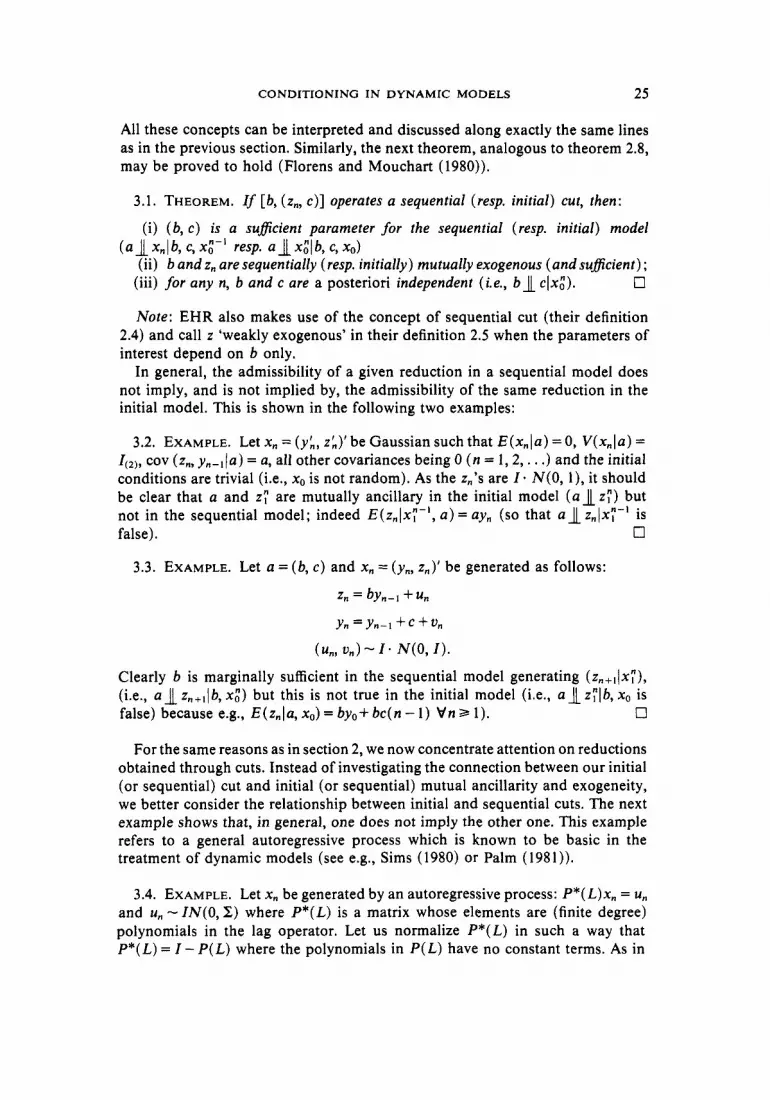
All these concepts can be interpreted and discussed along exactly the same lines as in the previous section. Similarly, the next theorem, analogous to theorem 2.8, may be proved to hold (Florens and Mouchart (1980)).
3.1. THEOREM. If [b, (z,, c ) ] operates a sequential (resp. initial) cut, then:
(i) ( b , c ) is a suficient parameter for the sequential (resp. initial) model
(ii) b and z, are sequentially (resp. initially) mutually exogenous (andsuficient) ; 0
Note: EHR also makes use of the concept of sequential cut (their definition 2.4) and call z 'weakly exogenous' in their definition 2.5 when the parameters of interest depend on b only.
In general, the admissibility of a given reduction in a sequential model does not imply, and is not implied by, the admissibility of the same reduction in the initial model. This is shown in the following two examples:
( a 4 x, I b, c, x:-' resp. a 4 x:l b, c, xo)
(iii) for any n, b and c are a posteriori independent (i.e., b l c l x ; ) .
3.2. EXAMPLE. Let x, = (yk , &)'be Gaussian such that E ( x , J a ) = 0, V(x , la ) = cov (z,, y , - ' ( a ) = a, all other covariances being 0 ( n = 1 ,2 , . . .) and the initial
conditions are trivial (i.e., xo is not random). As the 2,'s are I - N(0 , l) , it should be clear that a and z ; are mutually ancillary in the initial model ( a 1 z ; ) but not in the sequential model; indeed E(z , , Ix ; - I ,a )=ay , , (so that a l z , , I x ; - ' is false). 0
3.3. EXAMPLE. Let a = (b , c ) and x, = (y,,, z,)' be generated as follows:
z , = b ~ , - ~ + ~ ,
Y , =y,-l + C + %
(%, u,) - I * N O , 0. Clearly b is marginally sufficient in the sequential model generating ( Z , + ~ I X ; ) , (i.e., a_II z,+llb, x;) but this is not true in the initial model (Le., a 1 z;lb, xo is
0 false) because e.g., E(z,la, xo) = byo+ bc(n - 1) tln a 1).
For the same reasons as in section 2, we now concentrate attention on reductions obtained through cuts. Instead of investigating the connection between our initial (or sequential) cut and initial (or sequential) mutual ancillarity and exogeneity, we better consider the relationship between initial and sequential cuts. The next example shows that, in general, one does not imply the other one. This example refers to a general autoregressive process which is known to be basic in the treatment of dynamic models (see e.g., Sims (1980) or Palm (1981)).
3.4. EXAMPLE. Let x, be generated by an autoregressive process: P * ( L ) x , = u, and u, - IN(0 , X) where P*(L) is a matrix whose elements are (finite degree) polynomials in the lag operator. Let us normalize P*(L) in such a way that P*(L) = I - P(L) where the polynomials in P ( L ) have no constant terms. As in

26 J.-P. FLORENS A N D M. MOUCHART
example 2.9, we partition x, into xk = (yk , z:) and P ( L ) and S. into:
P ( L ) = [P;(L) ; p:(L)I
We then obtain: (z,Ix:-l, a ) - N(P, (L)x , Xzz) and (y,lz,, x,"-', a ) is also normally distributed with parameters:
E(Ynlzn,xo"-', a ) = n z n +Q(L>xn
V(YnIZn, 4-', a ) =Z.?'.vz
where n = ZyzZ;,'
Therefore, if one defines b = (K Q ( L ) , Zyyz )
and if the prior distribution makes b and c a priori independent, then [b, (z,,, c ) ] would clearly operate a sequential cut but not an initial cut; indeed, it may be checked that, for instance, the marginal expectations E(z,lxo, a ) involve both b and c. Note that the condition of prior independence is satisfied when ( P ( L) , Z) are distributed a priori according to a natural conjugate distribution (i.e., matrix normal Inverted Wishart, see e.g., Drhze and Richard (1983)). A bivariate case of this example is also discussed in example 3.1 of EHR, with another normaliz- ation of P*( L). 0
At the inference phase, i.e. once the data generating process is firmly estab- lished, both initial and sequential cuts allow a factorization of the data density. Indeed, in the case of a sequential cut, one has:
n n
p(x;Ia, xo) = iI P(Z~IG x t ' ) * II p(yrIb, zt, xA-') r = l f = 1
In the case of an initial cut, one has:
n n

CONDITIONING IN DYNAMIC MODELS 27
Both factorizations have considerable practical importance: both ensure the information matrix to be block-diagonal and both allow a separation of the computations involved in inference on b and on c, both in maximum likelihood estimation and in Bayesian inferences.
At the phase of model building, the situation is different. In the case of a sequential cut, the two factors f l (c ) and f 2 ( b ) do not represent the sampling processes generating (z;lxo) and (yrlz;, xo). Therefore, at the phase of model building, a sequential cut is not a sufficient condition to decompose the data generating process into two subprocesses that could be specified separately. In other words, if a statistician only specifies the second factor f 2 ( b ) , he should realize that he does no? specify a data generating process; in particular, integrating A ( b ) over y ; would not give 1 because the y,'s also appear in each x?' ( j 2 0 ) . He therefore specifies part of a statistical model only. Also, a modification of the specification of the marginal process generating (z;lxo, a ) could affect the inference on b while a modification of the specification of the processes generating (z,Ix,"-', a ) would not. In case of an initial cut, the two factors g l ( c ) and g 2 ( b ) do represent two sampling processes generating (z;lxo) and (y;lz;, x i ) . This ensures that the robustness arguments exposited in the case of a cut in one-shot analysis (see Section 2) carry over and may lead to a natural progressiveness in the model building process: one may first decompose the process generating (x;lxo) into two subprocesses generating (z;lxo) and (yylz;, xo) and thereafter, in case of interest in the second one, the (sequential) processes generating (ynly;-l, z;, a ) is specified.
It is therefore interesting to know conditions under which an initial (resp. sequential) cut is also a sequential (resp. initial) cut. Those conditions are in the nature of non-causality conditions and may be written in equivalent forms as given in the following theorem.
3.5. THEOREM. The following conditions are equivalent and define ' y does not cause z given u ' :
(i) Zn+I ~Y, " lZ , " , xo,
(4 .?+I 1 y,"lz,", xo, v
(iii) z?+, l y n I z n , x:-', u.
PROOF. Florens and Mouchart (1982). 0
When u = a, 3.5(i) is Granger's (1969) concept of ' y does not cause z' in terms of conditional independence. Sim's (1972) concept of non-causality may be written as:
z:+ I 1 Y" I z," 9 xo, a.
Clearly, this is implied by, but is not equivalent to, 3S(ii). Note that 3.5(ii) or (iii) may be viewed as modifications of Sims' concept that makes it equivalent to Granger's one. These kinds of concept of non-causality do therefore not claim

28 J.-P. FLORENS A N D M. MOUCHART
any philosophical involvement with the notion of causality. They are basically a particular kind of transitivity as defined earlier in the statistical literature, Bahadur (1954) or Hall, Wijsman and Ghosh (1965); for more details, see Florens and Mouchart (1982).
3.6. EXAMPLE. Let us consider the multivariate autoregressive process of example 3.4. If P J L ) =0, y does not cause z given a (i.e., in the sampling
0 process) as (z,Ix:-l, a ) does not depend on yo"-'.
Examples 3.2, 3.3 and 3.4 pointed out that sequential and initial cuts are not implied by each other. The next theorem shows that non-causality conditions are precisely the supplementary conditions needed to make the two cuts equivalent.
3.7. THEOREM. The following properties are equivalent: (i) [b, (z,, c)] operates a sequential cut and y does not cause z given c.
(ii) [b, (z,, c)] operates an initial cut and y does not cause z given a.
PROOF. See Florens and Mouchart (1980, Proposition 5 ) .
The basic idea of the proof is that the non-causality conditions ensure that the factorizations of the data density implied by the sequential and the initial cut do coincide i.e.,fi(c) = g l ( c ) andfi(b) = g 2 ( b ) . The following corollary may be easily verified.
3.8. COROLLARY. Under any of the properties in theorem 3.7, y does not cause 0 2, i.e. ( Z n + l l x,"lz,", xo).
Let us compare the three non-causality conditions involved in theorem 3.7 and in corollary 3.8:
non-causality given a : z , + ~ 1 x:lz,", xo, a
non-causality given c: z,+~ 1 xo"lz,", xo, c
non-causality : Z,+I 1 Xo"lZ,", xo.
In general, these three non-causality conditions are not equivalent neither does any one of them imply another one; furthermore, non-causality given a is a property of the data density alone, this is precisely Granger's non-causality (in a sampling-theory framework) ; the other two non-causality conditions involve both the data density and the prior distribution (p(a1c) and p ( a ) respectively) because they can be checked only after integrating parameters in the data density. An example may illustrate this point.

CONDITIONING I N DYNAMIC MODELS 29
Clearly y does not cause z given a but this is not any more true in the predictive 0 process, indeed E ( a l x , " ) involves y,".
In theorem 3.7 the supplementary condition that makes a sequential cut also initial is non-causality given c. In this case, however, checking non-causality given c does not require the integration of the data density p ( ~ , + ~ I x , " , a ) w.r.t. p(alc, x , " ) ; indeed the second condition of a sequential cut a 1 z,lc, .,"-I (along with non-causality given c ) are equivalent to z,+~ 1 (a, x,")lz,", x,, c and this condition is a property of the data density alone: it says that p ( z , + , J a , x,") depends on (z,+I, z,", xo, c ) only.
It may also be shown that a sequential cut along with non-causality given a (i.e., Granger's non-causality) does imply an initial cut (and non-causality both given c and in the predictive process) under a supplementary condition of so-called 'measurable separability'. This more technical problem has been analyzed in Florens and Mouchart (1980) and in Florens, Mouchart and Rolin (1980). In those papers, we also show how to initialize other sequential reductions than cuts (such as mutual ancillarity, exogeneity or sufficiency) and why non- causality is necessary to initialize a sequential cut (in the sense that under a condition of so-called 'strong identification', a cut being both initial and sequential implies the three non-causality properties). Note that EHR defines 2, to be 'strongly exogenous' (their definition 2.6) in the case of a sequential cut along with non-causality given a (i.e., in the sampling process). Their assertion that it implies an initial cut (their formulae (21), (22), and (23)) overlooks the necessity of assuming the condition of 'measurable separability'. It may be shown (Mouchart and Rolin (1979)) that such an omission is of the same nature as Basu's error in 1955 and corrected by himself in 1958.
In the next three examples, the above concepts are applied to justify the construction of several standard dynamic models.
3.10. EXAMPLE. Consider again the multivariate auto-regressive process as discussed in examples 3.6 and 3.4. The condition PJL) = O implies that (z , Ix; - l , a ) - N(P, , (L)z , , Xzz): the condition z,+~ 1 (a, x,")lz,", x,, c is therefore satisfied, thus y does not cause z given c and, by theorem 3.7, the cut defined in example 3.4 is both initial and sequential.
3.1 1. EXAMPLE. We now consider a first dynamic version of the example 2.10. We use the notation of examples 2.9, 2.10 and 3.4 and consider the model:
P * ( L ) ( x , - 5,) - w o , X) A&,, = 0.
After normalization of P*(L) as P*(L) = I - P( L) where the polynomials of P( L ) have no constant terms, we also write:
W x , " - ' , a ) - N 5 n + P ( L ) ( x , - & I , X).
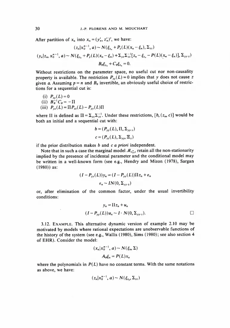
30 J.-P. FLORENS A N D M. MOUCHART
After partition of x, into x, = (y ; , z:)', we have:
(z,Ixon-l, a ) - Ntzn +Pz(L)(x, - 5n), L z )
(y,(z,, xon-I, a ) - Ntyn +P,(L)(x, - 5,) +X&,l[Z, - 52. - P ( L ) ( x n -5n)l, LA Bat," + C,&. = 0.
Without restrictions on the parameter space, no useful cut nor non-causality property is available. The restriction P,(L) = 0 implies that y does not cause z given a. Assuming p = n and B, invertible, an obviously useful choice of restric- tions for a sequential cut is:
(i) P,(L) = o (ii) BilCa = -II
(iii) P,,,(L)=nP,,(L)-P,,(L)n
where n is defined as n = X y z X ; ; . Under these restrictions, [b, (z,,, c)] would be both an initial and a sequential cut with:
b = (F"Y(L), n, & y 2 ) c = (PZZ(L), z,,
if the prior distribution makes b and c a priori independent. Note that in such a case the marginal model A,;,, retain all the non-stationarity
implied by the presence of incidental parameter and the conditional model may be written in a well-known form (see e.g., Hendry and Mizon (1978), Sargan (1980)) as:
(1 - P,,(L))Y, = (1 - p,,(L))nZ, + E ,
En - ", X Y y J
or, after elimination of the common factor, under the usual invertibility conditions:
y, = nz, + u,
3.12. EXAMPLE. This alternative dynamic version of example 2.10 may be motivated by models where rational expectations are unobservable functions of the history of the system (see e.g., Wallis (1980), Sims (1980); see also section 4 of EHR). Consider the model:
(x,Ixon-I, a ) - N ( 5 n , Z)
AaSn = P ( L ) x ,
where the polynomials in P( L ) have no constant terms. With the same notations as above, we have:
(Znlxon-l, a ) - N ( t Z " , X z z )

CONDITIONING IN DYNAMIC MODELS 31
(YnlZn, xgn-l, a ) - "tY" + W z n -t2,), X y y z )
B81yn + c88Z , = p ( L ) x n .
Using the same method as in Florens, Mouchart and Richard (1979), a sequential cut may be obtained through the following restriction:
B,Xyz + COXZZ = 0.
(YfllZn, X F ' , a ) - N(%, X."J>.z)
Indeed, under these restrictions, the conditional model may be written as:
B O T n +c8zn = p(L)xn
and [b, (z,,, c)] would be a sequential cut with
= L H , x y v z , B8, c8, p ( L ) l I
c = [ = z , Z z z l
if the prior distribution makes b and c a priori independent. Note that if the model is complete (i.e., p = n and B, regular), the conditional model have no incidental parameters anymore:
(YfllZn, xgn-l, a ) - N ( m l +BilP(L)xfl, X y y z ) or, alternatively,
B8Yn +c8zn = p(L)xn + E n , E n - N(o, x y y . z )
and the marginal model retains all the non-stationarity implied by the presence of incidental parameters. In this case we only have a sequential cut. An initial cut, and therefore a non-causality given a, should depend on specific assumptions regarding the process generating 5;. ; in particular, if &, is viewed as involving rational expectations, the non-causality condition would be satisfied only if the information used in forming tZn depends on the history of z only. More generally, formalizing exogeneity in the case of incidental parameters raise problems out
0 of the scope of this paper.
4. SOME CONCLUDING REMARKS
Conditioning on the sample space basically means that when modelling the data generating process, the marginal process of some variables is not specified: these variables are treated 'as if ' they were not random. When such a reduction of the sampling process is admissible, the conditioning variables are called 'exogenous'.
When all the parameters are of interest, ancillarity is the technical concept that guarantees the conditioning on such a statistic (or variable) to be admissible. This is not controversial in a sampling theory approach or in a Bayesian approach and both approaches coincide (up to null sets).

32 J.-P. FLORENS A N D M. MOUCHART
When only part of the parameters is of interest (i.e., some other parameters are said to be ‘of nuisance’), a minimal condition is that of ‘mutual ancillarity’ but robustness w.r.t. the prior specification and simplification of the computations lead to successively stronger conditions of ‘mutual exogeneity’ and of ‘cut’. The last (and most specific) concept of cut is essentially a property of the data generating process as it depends only weakly on the prior specification: at this level again the sampling theory and Bayesian approaches practically coincide.
In dynamic models, several levels of model specification are to be distinguished. This motivates the search of exogeneity both in initial and in sequential models and it has been shown that both initial and sequential cuts produce a factorization of the data density. The relationship between these two kinds of cuts has been analyzed in terms of an extension of Granger’s non-causality.
One should stress that the very power of a structure of both an initial and a sequential cut also involves its own danger: it may induce the temptation of venturesome assumptions in an uncontrolled search for simplifying hypotheses. As suggested at the end of example 3.12, dynamic economic reasoning may render some non-causality unplausible. But the theory around non-causality may also be used to explain why some dynamic specification embodying unwarranted non-causality hypothesis leads to unplausible empirical results.
Let us now consider briefly the problem of testing (conditional) independence assumptions defining exogeneity and non-causality. Various tests of independence have already been presented in the statistical literature. Those tests are often robust w.r.t. the model specification but generally their lack of power and the actual availability of economic data make the use of such tests problematical. For this reason, tests based on more specific maintained hypothesis are often preferred. Such is the case of linear models with normality assumptions: (condi- tional) independence then is equivalent to (partial) uncorrelatedness. It is also possible to restrict the above theory to conditional orthogonality in the Hilbert- space of square-integrable random variables (in the spirit of Hosoya (1977)); and this direction has been more systematically pursued in Florens and Mouchart (1981).
The above theory is invariant w.r.t. any bijective transformation of a, b ( a ) , x or z(x). For instance, if b ( a ) and z(x) are mutually exogenous so are b ’ ( a ) and z’(x) where b’ and z‘ are bijective transformations of b and of z. This is the main reason why the original theory has been elaborated in terms of a-fields. This formal aspect should not lead one to forget that the real-world meaning of b ( a ) is evidently not invariant w.r.t. a bijective transformation of b. For instance, a particular description of the parameter of interest ( b ) may induce the components of b to be a priori independent and this independence may be grounded on an assertion of structural stability of those components. For an interesting discussion of such crucial issues in model building the reader should be referred to EHR.
The study of exogeneity has a fundamental role for the asymptotic properties of statistical models. Stationary or ZZD processes are often unsuitable for modelling time series. The search for exogenous variables may be viewed as a decomposition of a joint process into a (possibly non-stationary) marginal process

CONDITIONING IN DYNAMIC MODELS 33
and a ‘conditionally stationary’ conditional process. The modelling of the specific- ity of each individual observation is therefore captured in the model generating the exogenous variables and typically, this model is not the object of inference. The problem is nevertheless to provide minimal conditions on the process generat- ing the exogenous variables that ensures the possibility of consistent inference in the conditional model. This intricate problem has received attention in Burguete, Gallant and Souza (1983), Feigin (1982), Florens and Rolin (1984), Gallant and Holly (1980).
ACKNOWLEDGEMENTS
The authors are grateful to J. H. Dreze, M. Lubrano, J.-F. Richard and an anonymous referee for comments on earlier versions of this paper. They owe a particular debt to D. F. Hendry for penetrating discussions on both the ideas and the presentation of this paper.
REFERENCES
BAHADUR, R. R. (1954) Sufficiency and Statistical Decision Functions. Ann. Math. Statist. 25,423-462. BARNDORFF-NIELSEN, 0. (1978) Information and Exponential Families in Statistical Theory. J. Wiley
BASU, D. (1955) On Statistics Independent of a Complete Sufficient Statistic. Sankhya 15, 377-380. BASU, D. (1958). On Statistics Independent of Sufficient Statistics. Sankhya 20, 223-226. BASU, D. (1977) On the Elimination of Nuisance Parameters, Part I, 6. J. Amer. Statist. Ass. 72 (358),
BURGUETE, J., R. GALLANT, and SOUZA (1983) On Unification of the Asymptotic Theory of
C o x , D. R. and D. V. HINKLEY (1974) Theoretical Statistics. Chapman & Hall: London. DREZE, J. H. and J.-F. RICHARD (1983) Bayesian Analysis of Simultaneous Equations Systems. In
ENGLE, R. F., D. F. HENDRY and J.-F. RICHARD (1983) Exogeneity. Econornetrica 51, 277-304. FEIGIN, PAUL D. (1982) Theory of Conditional Inference for Stochastic Processes. Presented at the
15th European Meeting of Statisticians, Palermo, Sept. 1982. FLORENS, J.-P. and M. MOUCHART (1977) Reduction of Bayesian Experiments. CORE Discussion
Paper 7737, Universitt Catholique de Louvain, Louvain-la-Neuve, Belgium. FLORENS, J.-P. and M. MOUCHART ( 1980) Initial and Sequential Reduction of Bayesian Experiments.
CORE Discussion Paper 801 5, Universit6 Catholique de Louvain, Louvain-la-Neuve, Belgium. FLORENS, J.-P. and M. MOUCHART (1981) A Linear Theory for Non-Causality. Technical Report
No 51, Department of Statistics, Stanford University, to appear in Econometrica 53 (1985). FLORENS, J.-P. and M. MOUCHART (1982) A Note on Non-Causality. Econometrica 50 ( 3 ) . 583-591. FLORENS, J.-P., M. MOUCHART and J.-F. R I C H A R D (1979) Specification and Inference in Linear
Models. CORE Discussion Paper 7943, Universitt Catholique de Louvain, Louvain-la-Neuve, Belgium.
FLORENS, J.-P., M. MoucHARTand J.-M. ROLIN (1980) Rtductions dans les Exptriences Baytsien- nes Sc5quentielles. Cahiers Centre Etudes Rech. Op6rat. 22, No 3-4.
FLORENS, J.-P. and J.-M. ROLIN (1984) Asymptotic Sufficiency and Exact Estimability in Bayesian Experiments. In Alternative Approaches to Time-Series Analysis, Proceedings of the Third Franco- Belgian Meeting of Statisticians, edited by J.-P. Florens, M. Mouchart, J.-P. Raoult and L. Simar, in Rouen, November 25-26, 1982, Publications des Facultts Universitaires Saint-Louis: Brussels.
FLORENS, J.-P. and S. S c o r r o (1984) Information Value and Econometric Modelling. Southern European Economics Discussion Series, D P 17.
GALLANT, R. and A. HOLLY (1980) Statistical Inference in an Implicit Nonlinear Simultaneous Equations Model in the Context of Maximum Likelihood Estimation. Econornetrica 48,697-720.
& Sons: New York.
355-366.
Nonlinear Econometric Models. Econ. Rev. 1 (2) , 151-212.
Handbook of Econometrics, edited by M. Intriligator. North-Holland: Amsterdam.

34 J.-P. FLORENS A N D M. MOUCHART
GODAMBE, V. P. ( 1976) Conditional Likelihood and Unconditional Optimum Estimating Equations. Biometrika 63, 2, 277-284.
GODAMBE, V. P. (1980) O n Sufficiency and Ancillarity in the Presence of a Nuisance Parameter. Biomerrika 67, 1, 155-162.
GOURIEROUX, C., A. MoNFoRTand A. TROGNON (1983) Testing Nested or Non-nested Hypotheses. J. Econometrics 21, 83-1 15.
GRANGER, C. W. J. (1969) Investigating Causal Relations by Econometric Models and Cross-Spectral Methods. Economefrica 37, 424-438.
HALL, W. J. R., A. WIJSMAN and J. K. GHOSH (1965) The Relationships between Sufficiency and Invariance with Applications in Sequential Analysis. Ann. Marh. Sfafist. 36, 575-614.
HAUSMAN, J. A. (1969) Specification Tests in Econometrics. Econometrica 46, 1251-1271. HENDRY, D. F. and G. F. MIZON (1978) Serial Correlation as a Convenient Simplification, not a
Nuisance. A Comment on a Study of the Demand for Money by the Bank of England. Econ. J.
HENDRY, D. F. and J.-F. RICHARD (1983) The Econometric Analysis of Economic Time-Series. In!.
HOSOYA, Y. (1977) On the Granger Condition for Non-Causality. Economefrica 45, 1735-1736. MIZON, G. and J.-F. RICHARD (1983) The Encompassing Principle and Model Selection. CORE
Discussion Paper 8330, UniversitC Catholique de Louvain, Louvain-la-Neuve, Belgium. MOUCHART, M. and J.-M. ROLIN (1979) A Note on Conditional Independence with Statistical
Applications. Rapport No 129, SCminaire de Mathimatique AppliquCe et MCcanique, Institut de MathCmatique Pure et AppliquCe, UniversitC Catholique de Louvain, Louvain-la-Neuve, Belgium, to appear in Stafisfica (1984).
PALM, F. (1981) Structural Econometric Modelling and Time Series Analysis: An Integrated Approach. Research memorandum 198 1-16, Economische Fakulteit, Vrije Universiteit, Rot- terdam.
RAIFFA, H. and R. SCHLAIFER (1961) Applied Statistical Decision Theory. Division of Research, Graduate School of Business Administration, Harvard University, Boston.
RICHARD, J.-F. ( 1979) Exogeneity, Inference and Prediction in So-called Incomplete Dynamic Simultaneous Equation Models. CORE Discussion Paper 7922, UniversitC Catholique de Louvain, Louvain-la-Neuve, Belgium.
RICHARD, J.-F. (1980) Models with Several Regimes and Changes in Exogeneity. Rev. Econ. Stud. 47, 1-20.
88, 549-563.
Sfaf i s f . Rev. 51, 1 1 1-163.
SARGAN, J. D. (1980) Some Tests of Dynamic Specification for a Single Equation. Economefrica 48, 879-897.
SIMS, C. A. (1972) Money, Income and Causality. Amer. Econ. Rev. 62, 540-562. SIMS, C. A. (1980) Macroeconomics and Reality. Econometrica 48 ( I ) , 1-48, WALLIS, K. F. (1980) Econometric Implications of the Rational Expectations Hypothesis.
Wu, D. M. ( 1973) Alternative Tests of Independence between Stochastic Regressors and Disturbances. Economefrica 48 ( I ) , 49-74.
Econometrica 41, 733-750.