Appl. Sci. 2022, 12, 3093. https://doi.org/10.3390/app12063093  www.mdpi.com/journal/applsci 

Article 

Comparisons of Dynamic Landslide Models on GIS Platforms 

Yuming Wu 1, Aohua Tian 1,2,3 and Hengxing Lan 1,* 

1  State Key Laboratory of Resources and Environmental Information System, Institute of Geographic Sciences 

and Natural Resources Research, Chinese Academy of Sciences, Beijing 100101, China;   

wuym@lreis.ac.cn (Y.W.); tian1454565116@163.com (A.T.) 2  College of Geoscience and Surverying Engineering, China University of Mining and Technology‐Beijing, 

Beijing 100083, China 3  College of Resources and Environment, University of Chinese Academy of Sciences, Beijing 100049, China 

*  Correspondence: lanhx@lreis.ac.cn; Tel.: +86‐10‐64888783 

Abstract: Numerical  simulation  is one of  the methods  to  assess  landslide movement processes, 

which is beneficial for engineering design and urban planning. With the development of computer 

technology, GIS has gradually become the mainstream platform for landslide simulation due to data 

availability and algorithm integrability. However, the dynamic processes of landslides are compli‐

cated, which makes integration difficult on GIS platforms. Some assumptions are applied to sim‐

plify these dynamic processes and solve this problem. Generally, there are two main types of nu‐

merical models on GIS platforms: models based on the Eulerian description and models based on 

the Lagrangian description. Case studies show that Eulerian models are suitable for flow‐like move‐

ment, and Lagrangian models are suitable for discrete rigid bodies movement. Different models face 

different problems: the Eulerian‐based models show numerical diffusion and oscillation, and the 

Lagrangian‐based model needs to consider complicated shear and collision processes. In addition, 

the 3‐D model can describe more details  in  the z‐direction, while  the depth‐averaged model can 

obtain a reasonable range of motion, depth, and speed quickly. From the view of numerical simula‐

tion, inappropriate models, assumptions, and numerical schemes will produce errors. The landslide 

type refers to several forms of mass wasting associated with a wide range of ground movements, 

which guides establishing dynamic models and numerical schemes on GIS platforms and helps us 

obtain results accurately. 

Keywords: landslide dynamics; landslide classification; dynamic models; depth‐averaged model; 

GIS 

 

1. Introduction 

Landslides cause a large number of casualties and property losses every year. Quan‐

titative risk analysis (QRA) is essential for reducing property damage and loss of life. Nu‐

merical simulation is one of the methods for assessing the landslide movement process 

and potential hazard levels [1,2], which is part of quantitative risk analysis [3]. Many nu‐

merical models are used to obtain the landslide runout distance, thus providing a basis 

for urban planning [4–7]. 

From dynamics, all landslides follow Newton’s second law [2] and, thus, mass con‐

servation, momentum conservation, and energy conservation are the governing equations 

in numerical simulations. In terms of force, gravity is the primary driving force [8], and 

friction is the major resistance force during motion. However, different shear processes 

and collision processes make landslide dynamics complex. 

There are  two model  types: discrete models and  continuum models. The discrete 

models describe the interactions and shocks well, but the continuum models describe the 

flow well. The Lagrangian functions describe the translation and rotation of each discrete 

element for the discrete models. Eulerian functions are the best to calculate the field for 

Citation: Wu, Y.; Tian, A.; Lan, H. 

Comparisons of Dynamic Landslide 

Models on GIS Platforms. Appl. Sci. 

2022, 12, 3093. https://doi.org/ 

10.3390/app12063093 

Academic Editors: Ricardo Castedo, 

Miguel Llorente Isidro   

and David Moncoulon 

Received: 18 February 2022 

Accepted: 16 March 2022 

Published: 17 March 2022 

Publisher’s Note: MDPI  stays  neu‐

tral  with  regard  to  jurisdictional 

claims in published maps and institu‐

tional affiliations. 

 

Copyright: © 2022 by the authors. Li‐

censee  MDPI,  Basel,  Switzerland. 

This article  is an open access article 

distributed under the terms and con‐

ditions of the Creative Commons At‐

tribution (CC BY) license (https://cre‐

ativecommons.org/licenses/by/4.0/). 

Appl. Sci. 2022, 12, 3093  2  of  16  

the continuum models. With the development of computation, meshless methods such as 

SPH are proposed to solve problems dominated by complex boundary dynamics for the 

continuum models.  In  the SPH method,  finding neighboring nodes  is difficult. Models 

with different accuracies are used  to describe  the processes  [7]. These models  include 

Rockfall Analyst [9], Rocfall [10], and Rockyfor3D [11] for rockfalls, and Massflow [12], 

Flo‐2D [13], r.avaflow [14], and Titan2D [15] for mass flow. 

In some simulations, different software programs yield different trajectories based 

on methods, assumptions, and numerical schemes  [16]. Models may  face various chal‐

lenges. For example, fluid mechanics models may encounter numerical diffusions and os‐

cillations [17]; rigid body models need to consider complicated shear and collision pro‐

cesses [18]. Therefore, a suitable model is a prerequisite for obtaining accurate results, and 

the physical insights provided by models can help us understand the landslide process. 

GIS  provides  some  functions  that  allow  users  to  build  numerical models  [19].  It 

makes programming convenient and easy. There are two types of landslide simulations 

on GIS platforms: add‐in programs and stand‐alone programs. Add‐in programs use the 

GUI and functions on GIS platforms to build a dynamic landslide model. This combina‐

tion  is easy to  implement, but the GIS platform may limit some capacities. Stand‐alone 

programs use open libraries such as GDAL. They are computationally efficient but require 

a lot of development time. The landslide dynamics programs on GIS platforms need to be 

simplified to accommodate the GIS file structure. Therefore, appropriate assumptions and 

suitable models are the keys to simulation on GIS platforms. 

Landslide classification uses simple words to describe the characteristics of landslide 

phenomena, which may guide us to select a suitable model for simulation on GIS plat‐

forms. Several authors, including Heim [20], Zaruba and Mencl [21], and Sharpe [22], pro‐

posed different landslide classification systems. In most of these classifications, the name 

of the landslide is a combination of the material and motion type [23–26]. The most well‐

known classification system  is Varnes’ classification  [27].  In  this classification, material 

types include rock, debris, and earth, and motion types include falling, toppling, sliding, 

spreading flow, and complex. Subsequently, Hungr [23] updated the Varnes’ classifica‐

tion to assess landslide phenomena, and the material types were more detailed than those 

in the original classification. Landslide types are often indicators of the critical movement 

process, and a suitable numerical model must consider the appropriate variables. 

However, the relationship between the landslide movement process and the physical 

mechanism of  landslides  is not very clear.  It  results  in difficulty  in obtaining accurate 

runout zones on GIS platforms.  In  this paper, we compared numerical models on GIS 

platforms and established relationships between landslide types and the selection of nu‐

merical models on GIS platforms. 

2. Models 

2.1. Descriptions 

Landslides contain two main motion processes: rigid body motion and flow‐like mo‐

tion. The rigid body motion assumes that the block does not deform or change shape [28]; 

the  flow‐like motion assumes  that the material  is continuous mass rather than discrete 

particles. The driving force is gravity, and the resistance force is mainly friction during 

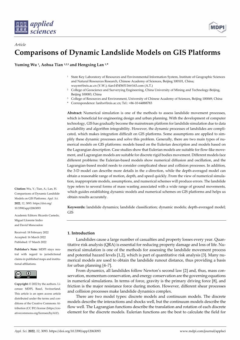
the movement (Figure 1). 

Appl. Sci. 2022, 12, 3093  3  of  16  

 

Figure 1. Two main motion processes: (A) the rigid body motion, and (B) the flow‐like motion. 

In dynamics, there are five major categories in the Varnes’ movement type: falling, 

toppling, sliding, spreading, and  flowing. The movement  type  is related  to  the critical 

processes  that occur during motion. All  the processes  follow Newton’s  laws of motion 

[29,30], which are given by 

dmvf

dt   (1)

where m is the mass, v is the velocity, and f is the resultant force, which depends on the 

movement type. The left‐hand side (LHS) of Equation (1) represents the motion process, 

and the right‐hand side (RHS) is the resultant force. 

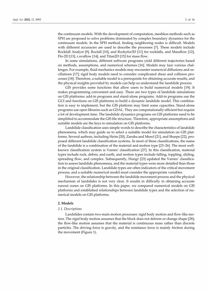
There are two common descriptions of motion in numerical models: the Eulerian de‐

scription and  the Lagrangian description  [31]  (Figure 2).  In  the Eulerian description, a 

model is not concerned about the location or velocity of any particular particle or columns, 

and the focus is on the grid. In the Lagrangian description, individual particles or columns 

are marked, and their positions and velocities are described as a function of time. 

 

Figure 2. Eulerian and Lagrangian descriptions. 

2.1.1. Models Based on the Lagrangian Description 

The rigid body motion includes translation and rotation, which are six‐degrees‐of‐

freedom processes (three components for the translation process and three components 

for the rotation process). Using the center of mass and inertia matrix, the force and torque 

equations take the form: 

, R Rm I I F a T   (2)

where F is the force, T is the torque,  a   is the acceleration, m is the mass,  RI   is the mo‐

ment of inertia matrix,    is the angular velocity, and    is the angular acceleration. The equations of translation and rotation on the Lagrangian description are 

Appl. Sci. 2022, 12, 3093  4  of  16  

21

2t t t t tt t x x v a   (3)

21

2t t t+Δt t t tθ θ ω α (4)

where xt is the location at time t, vt is the velocity at time t, at is the acceleration at t,  tθ   is 

the angle at time t,  tω   is the angular velocity at time t, and  tα   is the angular acceleration 

at time t. 

2.1.2. Models Based on the Eulerian Description 

In the continuum systems, the Eulerian description is best for simulating motion, and 

the Navier–Stokes equations are the basis of modeling [32]: 

t

v 0   (5)

/ t fv v v S   (6)

where ρ is the mass density, t is time,  v   is the velocity,  fS   is the field which includes 

gravity, friction, and other forces. The best way to solve these equations is through nu‐

merical analysis due  to  lacking a smooth analytical solution. Traditional CFDs such as 

Openfoam® use these equations to simulate the landslide dynamics. In these programs, 

the geometric modeling process is complex. 

To describe flowing grain–fluid mixture, Iverson proposed a mixture theory [33], and 

the  fS   is: 

' f s fS T T T g   (7)

in which 

s s v v   (8)

/s s s f f f v v v . (9)

Here, is the mixture mass density,  v   is the mixture velocity,  sv   is the velocity in 

the solid phase and  fv   is the velocity  in the fluid phase,  s   is the volume fraction of 

solid, f is the volume fraction of fluid,  g is the gravitational acceleration,  sT   is the solid 

stress,  fT   is the fluid stress, and  'T   is a contribution to the mixture stress. The stress 

'T   can be avoided by using an approximation suitable for many debris flows. 

To reduce the difficulty of traditional CFDs, Savage and Hutter proposed the depth‐

averaged theory [34]. This model allows the GIS to integrate simulation codes. Depth av‐

eraging  is one of the steps to eliminate the calculation  in the z‐direction. The averaged 

velocities and resultant forces are calculated on the x–y plane [32,34,35]. In this method, 

the assumption is that ρ is constant and the landslide depth is shallow. Thus, the equations 

[32,36] are 

0yxhvhvh

t x y

  (10)

2

0-

hx x y yxx xx zxx

hv hv v Thv T Tg dz

t x y x y z

  (11)

Appl. Sci. 2022, 12, 3093  5  of  16  

2

0-

hyy x y xy yy zyy

hvhv hv v T T Tg dz

t y x x y z

.  (12)

Where 0

1 h

x xv v dzh

, 0

1 h

y yv v dzh

. As shown in the equations, the velocity in the z‐di‐

rection is averaged. Based on the depth‐averaged theory, a depth‐averaged mixture model 

was proposed by Iverson and Denlinger [32]. Subsequently, two‐phase and multi‐phase 

depth‐averaged models were proposed to describe distinct mechanical responses and dy‐

namic behaviors of material [35,37]. 

Some studies considered the erosion process, a mechanical process by which the bed 

material is mobilized by the flow and dominant mechanical processes in geophysical mass 

flows [38]. Erosion determines enhanced or reduced mobility but is not understood thor‐

oughly. In the dynamic model, the erosion rate  /E b t   and erosion velocity bu are 

two important parameters, which change mass and momentum productions  E   and  bu E  

[38],  respectively. Subsequently, Pudashini and Fischer proposed  a  two‐phase  erosion 

model on this basis [39]. The emergence of these models has further developed the con‐

tinuum model on GIS platforms. 

2.2. Forces 

Gravity, friction, collision force, and hydraulic pressure are the major forces during 

motion. Some forces have less influence and can be ignored during the movement. 

2.2.1. Collision Force 

Collision force is one of the factors affecting the process of landslide movement, es‐

pecially during falls and topples. The collision process is complicated, which makes the 

calculation difficult. Traditionally, the spring–dashpot model is widely used to describe 

the nonlinear process, which is 

n el dissF F F   (13)

where  nF   is the collision force,  elF   is the elastic force (spring), and  dissF   is the dissipa‐

tive force (dashpot). The spring obeys Hooke’s law, and the dashpot obeys Newton’s law 

of viscosity [40,41]. To simplify the process, Evans and Hungr used a lumped mass model 

in ROCKFALL programs  in 1993 [42]. The associated assumptions of the  lumped mass 

model are as follows: (1) each rock is a small spherical particle; (2) rocks do not have any 

size, only mass. The lumped mass model uses one or two restitution coefficients to express 

this process to avoid calculating complex collision forces. The restitution coefficients are 

the ratio of the rebound velocity to the incident velocity, the impulse ratio, and the work 

ratio, which involves the square root of work performed. Most models use two restitution 

coefficients: the tangential restitution coefficient Rt and the normal restitution coefficient 

Rn; however, a few models use only one restitution coefficient to quantify dissipation in 

terms of velocity magnitude loss. Hybrid approaches were proposed on GIS platforms to 

simulate rockfall accurately. These models, such as CRSP [43], RocFall [44], and STONE 

[45], consider the influence of shape and nonlinear collision based on the lumped mass 

model. Hybrid approaches have been the mainstream models on GIS platforms. There‐

fore, there are three models for describing the collision force, a fully rigid body model, a 

lumped mass model, and a hybrid approach [46], on GIS platforms. 

2.2.2. Friction Force 

Friction is the force that resists the relative motion of solid surfaces, fluid layers, and 

material elements sliding against each other, which is important for the movement calcu‐

lation. In this process, kinetic energy is converted to thermal energy when motion with 

friction occurs. There are two types of resistance: viscosity and Coulomb’s friction. 

Appl. Sci. 2022, 12, 3093  6  of  16  

For dry granular flow, Coulomb’s friction is adopted, which is 

N   (14)

where τ is the unit base resistance and    is the friction coefficient, and N is the normal 

force. Generally, the basal shear forces, obtained by simple infinite landslide models, are 

calculated by Coulomb’s friction. 

For fluid flow, viscosity is a measure of resistance to deformation at a given rate. It 

can be conceptualized as the internal frictional force that arises between adjacent layers of 

fluid that are in relative motion. There are three viscosity equations: Newtonian, Bingham, 

and quadratic fluids. 

(1) The Newtonian fluid is: 

  (15)

where μ is the shear viscosity of a fluid and    is the derivative of the velocity compo‐

nent. 

(2) The Bingham fluid model is 

0 +   (16)

where  0   is a constant yield strength,    is the shear viscosity of the fluid, and    is the derivative of the velocity component. 

(3) The quadratic fluid model is 

20 + +   (17)

The first two terms are referred to as the Bingham shear stresses. The last term rep‐

resents the dispersive and turbulent shear stresses. Fluid friction can be generalized as: 

+s v tf f f f   (18)

where  vf   is  the viscosity  term,  sf   is  the  constant  term,  and  tf   is  a  turbulent  term. 

Based on the depth‐averaged theory, shear stress is depth‐integrated, and the correspond‐

ing equation is 

1S fdz

h   (19)

where S is depth‐integrated shear stress. Therefore, Equation (18) can be transformed to: 

fx v tdS S S S .  (20)

2.2.3. Other Forces 

Hydraulic pressure in the depth‐averaged model is the force imparted per unit area 

of liquid or flow‐like materials on the surfaces, which can be expressed in the Eulerian 

description as: 

2

2i

hF

x

  (21)

where β can be changed to  xs   and  x

f   based on the form of the phase [37]. For fluid, 

the β is gz. For solids, the force created by collisions among particles is simplified to an 

internal force based on soil mechanics, and the β is:   

1x z fs sKg   (22)

Appl. Sci. 2022, 12, 3093  7  of  16  

2 2 2 1 2/ 2sec 1 (1 cos sec ) 1pas actK   (23)

where    is the internal frictional angle and    is the basal frictional angle. The collisions and frictions among particles are difficult to calculate during the motion. 

There are two methods to describe the form of hydraulic pressure on the Lagrangian 

description. The first method is the particle‐in‐cell (PIC) method [47], which converts par‐

ticles or columns to fields based on the volume in each cell. The other is smoothed‐particle 

hydrodynamics (SPH) approximation [48–50], and they are: 

21

2I IP h   (24)

2 2JI

p J IJJ I J

PPH m gradW

h h

  (25)

where  IP   is an averaged hydraulic pressure term, WIJ is the value of the SPH kernel func‐

tion WIJ centered at node I evaluated at node J. The weighting function or kernel WIJ is a 

symmetric function of xI − xJ. Additionally, mJ has no physical meaning. When the node 

moves, the material contained in a column of base ΩI has entered it or will leave it as the 

column moves with an averaged velocity, which is not the same for all particles or col‐

umns in it [48]. 

In addition, buoyancy and drag forces  in the two‐phase and multi‐phase flow can 

also influence the landslide motion. Buoyancy is an upward force exerted by a fluid that 

opposes the weight of a partially or fully immersed object, and it is a vertical force. Buoy‐

ancy can reduce  the pressure at  the basal surface. Therefore, buoyancy can reduce  the 

resistance, especially in multi‐phase flow. Drag forces are shear forces caused by different 

velocities and accelerations in different phases. In other words, solid particles may accel‐

erate relative to fine solids or fluids [37]. 

3. Software 

With the development of computer technology, GIS has gradually become a main‐

stream system  for engineering design and urban planning. There are a  lot of GIS pro‐

grams, such as GRASS GIS, QGIS, and ArcGIS. GRASS GIS and QGIS are popular in pro‐

gram development due to being  free and open source. ArcGIS  is a mature commercial 

program and  is widely applied  in urban planning and engineering design. These pro‐

grams provide a rich interface such as raster import, vector import, raster statistics, and 

vector analysis, and are convenient for users to call the functions and develop their pro‐

grams. In addition, these programs provide a GUI to display the results calculated by their 

programs. More and more landslide simulation codes support GIS. At present, there are 

two kinds of programs: programs based on the rigid body model and programs based on 

the flow‐like model. 

3.1. Programs Based on the Rigid Body Model 

On GIS platforms, there are several programs to simulate the discrete rigid body mo‐

tions, as shown in Table 1. On GIS platforms, the format of input parameters of GIS data 

needs to be considered, especially DEM data. The choice of parameter expressions deter‐

mines the model. There are three types of DEMs to express on GIS platforms: triangulated 

irregular networks (TINs), grid networks, and vector or contour‐based networks. Relying 

on the algorithm, the selection of the DEM is also different. For example, Rockfall Analyst 

and Rockyfor3D select the grid networks. The lumped mass models are popular in early 

GIS platforms  among  these models. With  the GIS  technique development,  the hybrid 

model is mainstream on GIS platforms. These programs include Hy‐STONE, Rockyfor3D, 

and PICUS Rock’n’Roll. 

   

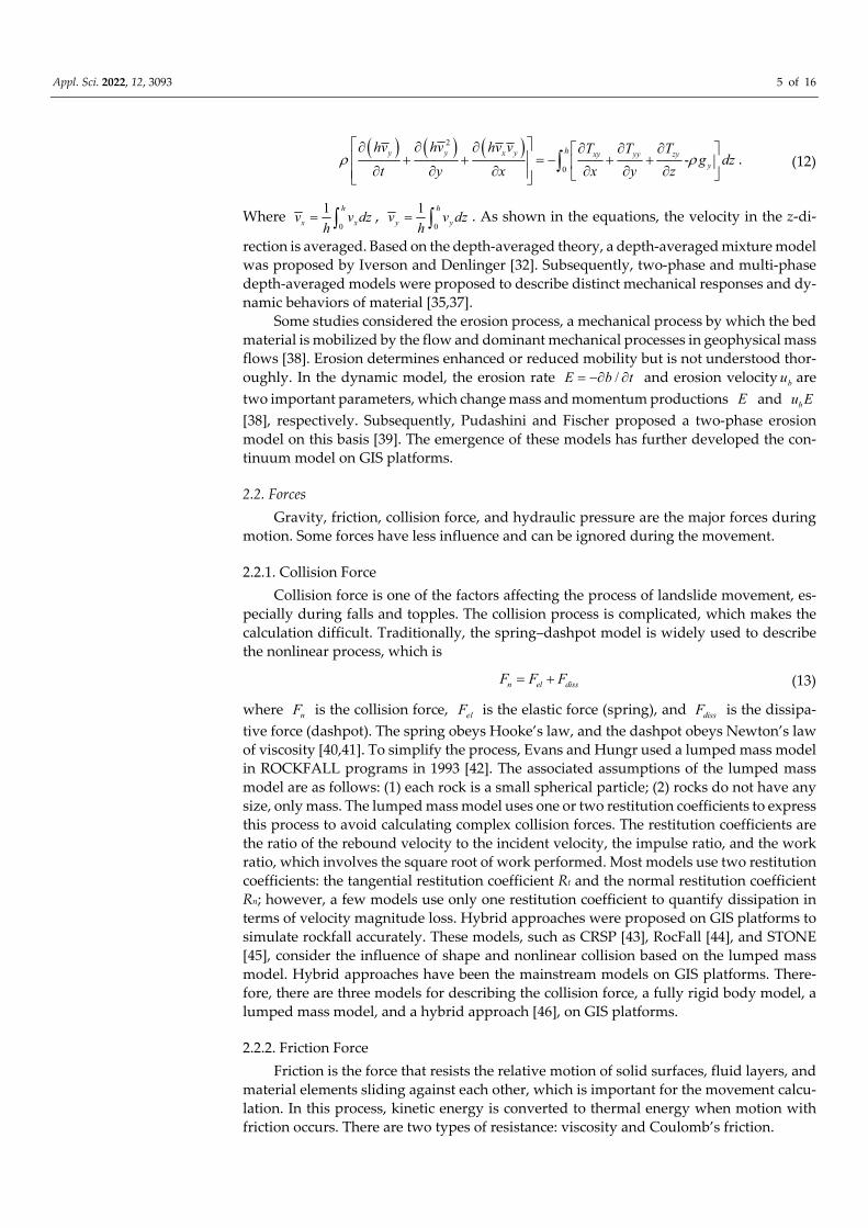
Appl. Sci. 2022, 12, 3093  8  of  16  

Table 1. Rigid body programs on GIS platforms. 

Software  Scheme  Platform  Format 

STONE [45]  Lumped mass    ASCII 

Hy‐STONE [51]  Hybrid    ASCII 

Rockfall Analyst [9]  Lumped mass  ArcGIS  All raster format 

Rockyfor3D [11]  Hybrid    ASCII 

PICUS Rock’n’Roll [52]  Hybrid  PICUS   

RAMMS::ROCKFALL [53]  Rigid body    ASCII 

RockGIS [54]  Lumped mass    ASCII 

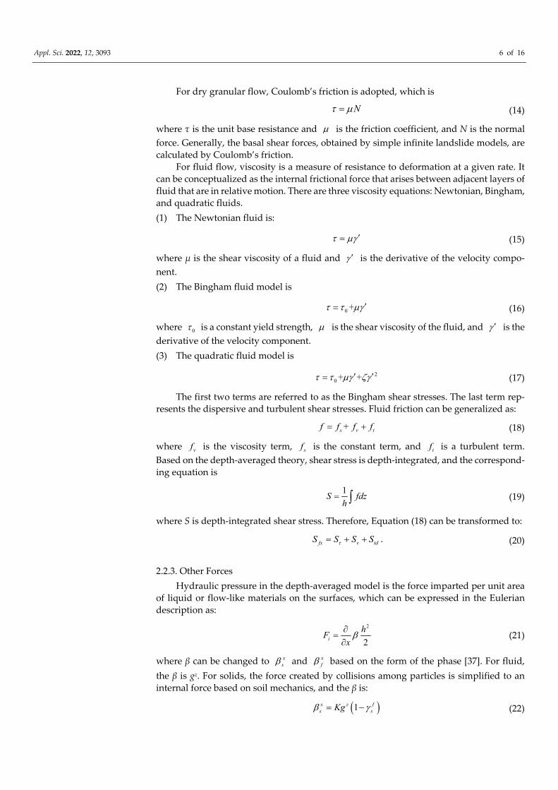
3.2. Programs Based on the Flow‐Like Model 

Based on the description, the grid networks of DEM are best for flow‐like models on 

GIS platforms. The grid networks make the calculation simple and accurate. At present, 

there are a  lot of codes on the GIS platforms, such as r.avaflow, LA, DA, Titan2D, and 

Massflow (Table 2). As for the model, the depth‐averaged theory model is employed to 

obtain the depths and velocities in each cell. The simulation r.avaflow is popular around 

the world. The program has a built‐in multi‐phase flow method based on the depth‐aver‐

aged theory and is applied in GRASS GIS and R. It is a very good cross‐platform program, 

which means that we can use the program on Windows, Linux, and Mac OS [35,37,38]. 

Table 2. Flow‐like programs on GIS platforms. 

Software  Description  Scheme  Format  Platform 

r.avaflow [14]  Eulerian  NOC  All raster format  GRASS 

RAMMS [55]  Eulerian  1st/2nd order  ASCII, Geotiff   

Massflow [12]  Eulerian  TVD–MacCormack  ASCII   

Massmov2D [56]  Eulerian  2‐step scheme  PCRaster  PCRaster 

LA and DA [31,57] Eulerian–Lagran‐

gian PIC‐like  GeoTIFF   

Titan2D [15]  Eulerian  AMR  All raster format  GRASS 

IMEX_SfloW2D [58]  Eulerian Semi‐discrete central 

scheme ASCII   

Geo‐Claw [59]  Eulerian  AMR  ASCII, NetCDF   

FLO‐2D [13]  Eulerian  1st order  All raster format  QGIS 

DAN3D [60]  Lagrangian  SPH  ASCII   

SPHERA [61]  Lagrangian  SPH  All raster format  QGIS 

For flow‐like programs, the numerical scheme is one of the factors affecting results. 

Most codes use 1st or 2nd order finite difference methods to solve the partial differential 

equations. In these programs, the numerical diffusion and numerical oscillation are the 

difficulties for the models in the Eulerian description. Some codes use the TVD method 

and adaptive mesh refinement (AMR) to improve precision. In addition, some methods 

use the Lagrangian or Eulerian–Lagrangian description to solve difficulties such as the 

material point method (MPM) [62], particle‐in‐cell (PIC) [47], and smoothed particle hy‐

drodynamics (SPH) [63]. In these models, the computational cost of simulations per num‐

ber of particles may be higher than the cost of grid‐based simulations per number of cells. 

In some cases, these methods solve the numerical solution problem of differential equa‐

tions to a certain extent. 

4. Results and Discussion 

Many factors affect the simulation results, such as models, algorithms, and descrip‐

tions. In this section, we show cases such as bilateral dam break, a rockfall example in the 

Appl. Sci. 2022, 12, 3093  9  of  16  

RA program, and the Yigong landslide to analyze the effect on models, algorithms, and 

descriptions. 

4.1. Reason for Differences 

4.1.1. Differences Caused by Models 

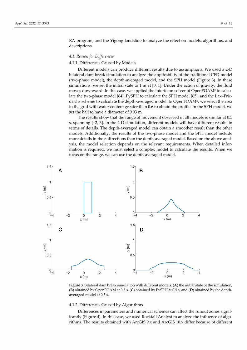
Different models can produce different results due to assumptions. We used a 2‐D 

bilateral dam break simulation to analyze the applicability of the traditional CFD model 

(two‐phase model), the depth‐averaged model, and the SPH model (Figure 3). In these 

simulations, we set the initial state to 1 m at [0, 1]. Under the action of gravity, the fluid 

moves downward. In this case, we applied the interfoam solver of OpenFOAM® to calcu‐

late the two‐phase model [64], PySPH to calculate the SPH model [65], and the Lax–Frie‐

drichs scheme to calculate the depth‐averaged model. In OpenFOAM®, we select the area 

in the grid with water content greater than 0.6 to obtain the profile. In the SPH model, we 

set the ball to have a diameter of 0.03 m. 

The results show that the range of movement observed in all models is similar at 0.5 

s, spanning [−2, 3]. In the 2‐D simulation, different models will have different results in 

terms of details. The depth‐averaged model can obtain a smoother result than the other 

models. Additionally,  the  results of  the  two‐phase model and  the SPH model  include 

more details in the z‐directions than the depth‐averaged model. Based on the above anal‐

ysis,  the model  selection depends on  the  relevant  requirements. When detailed  infor‐

mation  is required, we must select a complex model  to calculate  the results. When we 

focus on the range, we can use the depth‐averaged model. 

 

Figure 3. Bilateral dam break simulation with different models: (A) the initial state of the simulation, 

(B) obtained by OpenFOAM at 0.5 s, (C) obtained by PySPH at 0.5 s, and (D) obtained by the depth‐

averaged model at 0.5 s. 

4.1.2. Differences Caused by Algorithms 

Differences in parameters and numerical schemes can affect the runout zones signif‐

icantly (Figure 4). In this case, we used Rockfall Analyst to analyze the influence of algo‐

rithms. The results obtained with ArcGIS 9.x and ArcGIS 10.x differ because of different 

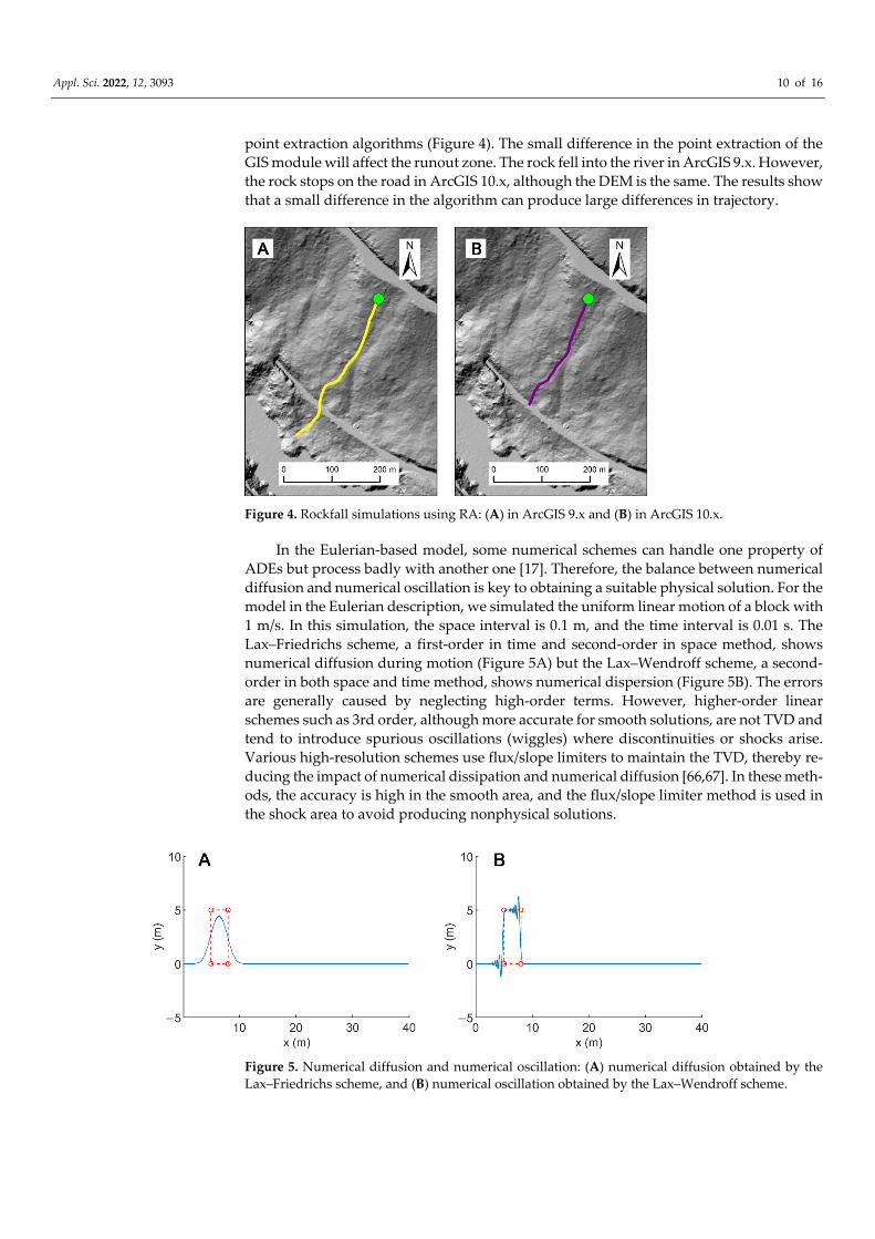
Appl. Sci. 2022, 12, 3093  10  of  16  

point extraction algorithms (Figure 4). The small difference in the point extraction of the 

GIS module will affect the runout zone. The rock fell into the river in ArcGIS 9.x. However, 

the rock stops on the road in ArcGIS 10.x, although the DEM is the same. The results show 

that a small difference in the algorithm can produce large differences in trajectory. 

 

Figure 4. Rockfall simulations using RA: (A) in ArcGIS 9.x and (B) in ArcGIS 10.x. 

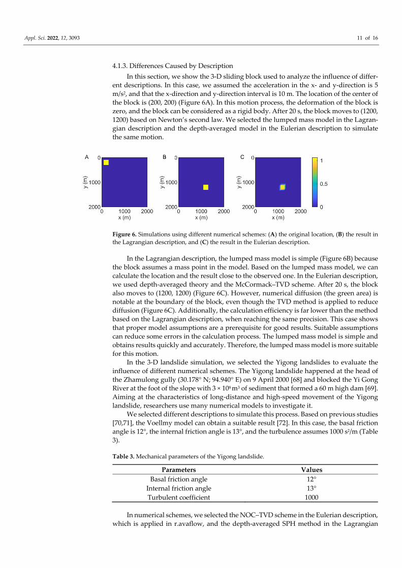
In the Eulerian‐based model, some numerical schemes can handle one property of 

ADEs but process badly with another one [17]. Therefore, the balance between numerical 

diffusion and numerical oscillation is key to obtaining a suitable physical solution. For the 

model in the Eulerian description, we simulated the uniform linear motion of a block with 

1 m/s. In this simulation, the space interval is 0.1 m, and the time interval is 0.01 s. The 

Lax–Friedrichs scheme, a  first‐order  in  time and second‐order  in space method, shows 

numerical diffusion during motion (Figure 5A) but the Lax–Wendroff scheme, a second‐

order in both space and time method, shows numerical dispersion (Figure 5B). The errors 

are  generally  caused  by  neglecting  high‐order  terms.  However,  higher‐order  linear 

schemes such as 3rd order, although more accurate for smooth solutions, are not TVD and 

tend  to  introduce spurious oscillations  (wiggles) where discontinuities or shocks arise. 

Various high‐resolution schemes use flux/slope limiters to maintain the TVD, thereby re‐

ducing the impact of numerical dissipation and numerical diffusion [66,67]. In these meth‐

ods, the accuracy is high in the smooth area, and the flux/slope limiter method is used in 

the shock area to avoid producing nonphysical solutions. 

 

Figure 5. Numerical diffusion and numerical oscillation: (A) numerical diffusion obtained by the 

Lax–Friedrichs scheme, and (B) numerical oscillation obtained by the Lax–Wendroff scheme. 

   

Appl. Sci. 2022, 12, 3093  11  of  16  

4.1.3. Differences Caused by Description 

In this section, we show the 3‐D sliding block used to analyze the influence of differ‐

ent descriptions. In this case, we assumed the acceleration in the x‐ and y‐direction is 5 

m/s2, and that the x‐direction and y‐direction interval is 10 m. The location of the center of 

the block is (200, 200) (Figure 6A). In this motion process, the deformation of the block is 

zero, and the block can be considered as a rigid body. After 20 s, the block moves to (1200, 

1200) based on Newton’s second law. We selected the lumped mass model in the Lagran‐

gian description and the depth‐averaged model  in the Eulerian description to simulate 

the same motion. 

 

Figure 6. Simulations using different numerical schemes: (A) the original location, (B) the result in 

the Lagrangian description, and (C) the result in the Eulerian description. 

In the Lagrangian description, the lumped mass model is simple (Figure 6B) because 

the block assumes a mass point in the model. Based on the lumped mass model, we can 

calculate the location and the result close to the observed one. In the Eulerian description, 

we used depth‐averaged theory and the McCormack–TVD scheme. After 20 s, the block 

also moves to (1200, 1200) (Figure 6C). However, numerical diffusion (the green area) is 

notable at the boundary of the block, even though the TVD method is applied to reduce 

diffusion (Figure 6C). Additionally, the calculation efficiency is far lower than the method 

based on the Lagrangian description, when reaching the same precision. This case shows 

that proper model assumptions are a prerequisite for good results. Suitable assumptions 

can reduce some errors in the calculation process. The lumped mass model is simple and 

obtains results quickly and accurately. Therefore, the lumped mass model is more suitable 

for this motion. 

In  the 3‐D  landslide simulation, we selected the Yigong  landslides  to evaluate the 

influence of different numerical schemes. The Yigong landslide happened at the head of 

the Zhamulong gully (30.178° N; 94.940° E) on 9 April 2000 [68] and blocked the Yi Gong 

River at the foot of the slope with 3 × 108 m3 of sediment that formed a 60 m high dam [69]. 

Aiming at the characteristics of  long‐distance and high‐speed movement of the Yigong 

landslide, researchers use many numerical models to investigate it. 

We selected different descriptions to simulate this process. Based on previous studies 

[70,71], the Voellmy model can obtain a suitable result [72]. In this case, the basal friction 

angle is 12°, the internal friction angle is 13°, and the turbulence assumes 1000 s2/m (Table 

3). 

Table 3. Mechanical parameters of the Yigong landslide.

Parameters  Values 

Basal friction angle  12° 

Internal friction angle  13° 

Turbulent coefficient  1000 

In numerical schemes, we selected the NOC–TVD scheme in the Eulerian description, 

which  is applied  in r.avaflow, and  the depth‐averaged SPH method  in  the Lagrangian 

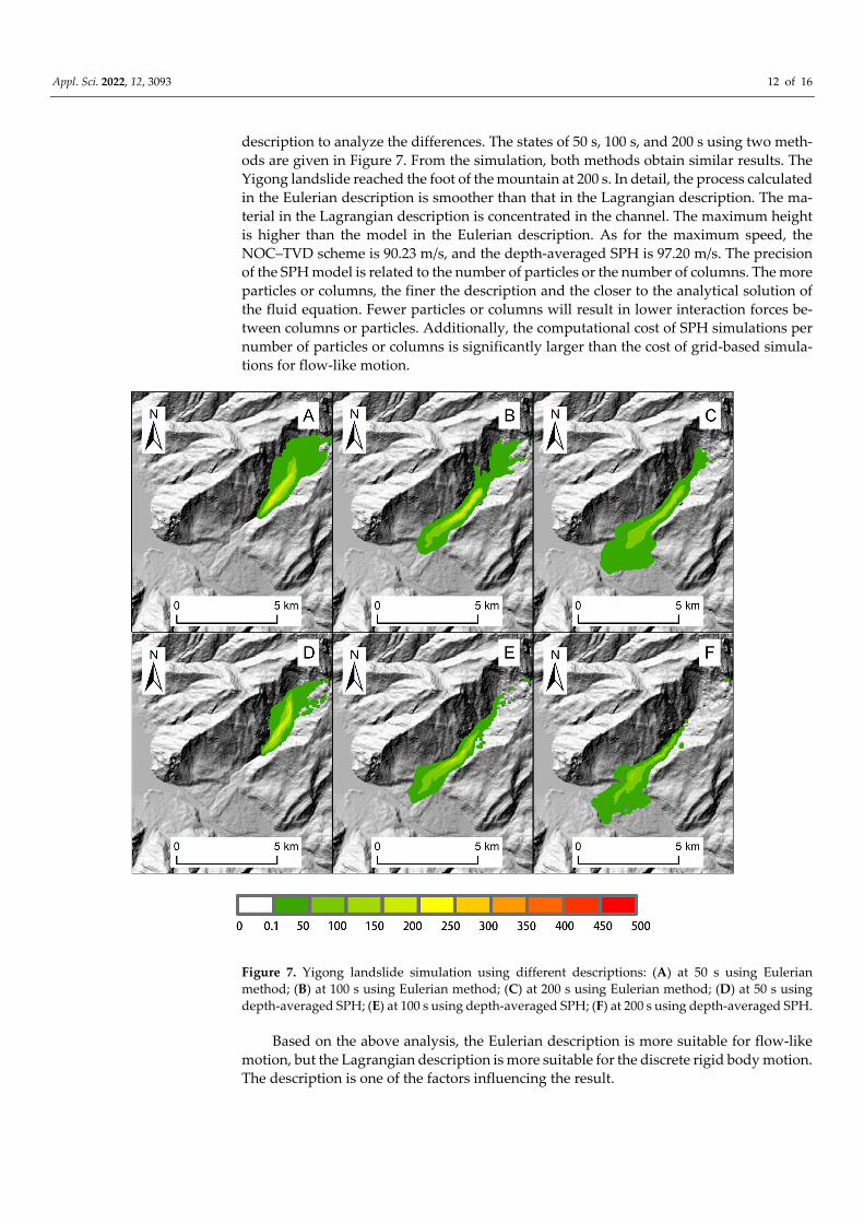
Appl. Sci. 2022, 12, 3093  12  of  16  

description to analyze the differences. The states of 50 s, 100 s, and 200 s using two meth‐

ods are given in Figure 7. From the simulation, both methods obtain similar results. The 

Yigong landslide reached the foot of the mountain at 200 s. In detail, the process calculated 

in the Eulerian description is smoother than that in the Lagrangian description. The ma‐

terial in the Lagrangian description is concentrated in the channel. The maximum height 

is higher  than  the model  in  the Eulerian description. As  for  the maximum  speed,  the 

NOC–TVD scheme is 90.23 m/s, and the depth‐averaged SPH is 97.20 m/s. The precision 

of the SPH model is related to the number of particles or the number of columns. The more 

particles or columns, the finer the description and the closer to the analytical solution of 

the fluid equation. Fewer particles or columns will result in lower interaction forces be‐

tween columns or particles. Additionally, the computational cost of SPH simulations per 

number of particles or columns is significantly larger than the cost of grid‐based simula‐

tions for flow‐like motion. 

 

Figure  7.  Yigong  landslide  simulation  using  different  descriptions:  (A)  at  50  s  using  Eulerian 

method; (B) at 100 s using Eulerian method; (C) at 200 s using Eulerian method; (D) at 50 s using 

depth‐averaged SPH; (E) at 100 s using depth‐averaged SPH; (F) at 200 s using depth‐averaged SPH. 

Based on the above analysis, the Eulerian description is more suitable for flow‐like 

motion, but the Lagrangian description is more suitable for the discrete rigid body motion. 

The description is one of the factors influencing the result. 

   

Appl. Sci. 2022, 12, 3093  13  of  16  

4.2. Model Selection 

Based on Varnes’ classification [27], the materials include rock, debris (coarse soil), 

and earth (fine soil). Rock is a solid mass of geological materials, debris is scattered mate‐

rial (large rock fragments), and earth is a cohesive, plastic, clayey soil. These terms are 

neither geological nor geotechnical [32,34,35,73,74] but are related to the size, shape, quan‐

tity, and properties, which help us select a suitable description. A rock is a solid mass and 

an aggregate of minerals that can be considered a discontinuous rigid body in landslide 

dynamics due to its characteristics. “Earth” is neither a geological term nor a geotechnical 

term, and it describes construction material or agricultural soil [75]. Earth is defined as a 

material in which at least 80% of particles are smaller than 2 mm [27]. Debris is a mixture 

of large and small blocks of rock, and debris motion involves multi‐phase flow (20% to 

80% of particles >2 mm). The properties of debris encompass the characteristics of both 

rigid bodies and fluids. Particle size is one of the critical factors to consider in the descrip‐

tion of motion. When the material volume is small, and the quantity of material is large, 

the Eulerian description including the depth‐averaged model is generally suitable for de‐

scribing these motions. The Lagrangian description is suitable for large‐volume and small‐

quantity discrete rigid body movement. The Eulerian–Lagrangian method may be suita‐

ble for the rock and soil aggregate movement. 

In addition, the motion types include falling, sliding, spreading, and flowing. In fall‐

ing and toppling, collisions and shearing are the major contact processes, and shearing is 

the main contact process in sliding, flowing, and spreading. This indicates that the move‐

ment type determines the force model in a given situation. Collision and friction are criti‐

cal forces to change the movement state for falling and toppling. However, dry friction 

and viscosity need to be considered in sliding, spreading, and flowing. Therefore, land‐

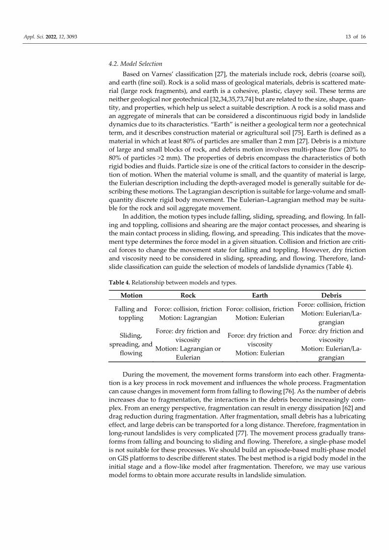
slide classification can guide the selection of models of landslide dynamics (Table 4). 

Table 4. Relationship between models and types. 

Motion  Rock  Earth  Debris 

Falling and 

toppling 

Force: collision, friction 

Motion: Lagrangian 

Force: collision, friction 

Motion: Eulerian 

Force: collision, friction 

Motion: Eulerian/La‐

grangian 

Sliding, 

spreading, and 

flowing 

Force: dry friction and 

viscosity 

Motion: Lagrangian or 

Eulerian 

Force: dry friction and 

viscosity 

Motion: Eulerian 

Force: dry friction and 

viscosity 

Motion: Eulerian/La‐

grangian 

During the movement, the movement forms transform into each other. Fragmenta‐

tion is a key process in rock movement and influences the whole process. Fragmentation 

can cause changes in movement form from falling to flowing [76]. As the number of debris 

increases due to fragmentation, the interactions in the debris become increasingly com‐

plex. From an energy perspective, fragmentation can result in energy dissipation [62] and 

drag reduction during fragmentation. After fragmentation, small debris has a lubricating 

effect, and large debris can be transported for a long distance. Therefore, fragmentation in 

long‐runout landslides is very complicated [77]. The movement process gradually trans‐

forms from falling and bouncing to sliding and flowing. Therefore, a single‐phase model 

is not suitable for these processes. We should build an episode‐based multi‐phase model 

on GIS platforms to describe different states. The best method is a rigid body model in the 

initial stage and a  flow‐like model after  fragmentation. Therefore, we may use various 

model forms to obtain more accurate results in landslide simulation. 

Appl. Sci. 2022, 12, 3093  14  of  16  

5. Conclusions 

Based on the above analysis, we can draw the following conclusions: 

(1) A suitable model with proper assumptions can reduce uncertainties and simplify cal‐

culations. We must select suitable models to simulate different types of landslides. 

The proposed classification can provide some guidance for model selection. Land‐

slide classification helps us understand landslide phenomena and select suitable dy‐

namic models. 

(2) Compared with the two different models, the 3‐D model can describe more details of 

the moving process than the depth‐averaged model. Landslide runout zone, height, 

and speed are critical parameters in engineering design. The depth‐averaged model 

meets the actual needs and provides engineering parameters quickly. Therefore, we 

can use the depth‐averaged model to obtain the runout zones. If we pay more atten‐

tion to the details, such as surge waves, the 3‐D landslide simulation model is better. 

(3) A small difference in algorithms can produce a large difference in the runout zones. 

We should use as many algorithms as possible to obtain the trajectory for engineering 

design. 

(4) The number of elements, property, and material size determine the model selection. 

For discrete rigid body motion, models based on the Lagrangian description are suit‐

able; for flow‐like motion, models based on the Eulerian description are proper; for 

materials with various properties, models based on the Eulerian–Lagrangian descrip‐

tion are best. 

Author Contributions: Conceptualization, H.L. and Y.W.; methodology, Y.W.; software, Y.W. and 

A.T.; validation, H.L. and Y.W.; formal analysis, Y.W.; writing—original draft preparation, Y.W.; 

writing—review and editing, Y.W.; visualization, Y.W.; supervision, Y.W.; funding acquisition, H.L. 

and Y.W. All authors have read and agreed to the published version of the manuscript. 

Funding: This research was supported by the Strategic Priority Research Program of the Chinese 

Academy of Sciences  (CAS)  (Grant No. XDA23090301), National Natural Science Foundation of 

China  (Grant No. 41941019, 42041006), and  the Second Tibetan Plateau Scientific Expedition and 

Research (STEP) program (Grant No. 2019QZKK0904). 

Institutional Review Board Statement: Not applicable. 

Informed Consent Statement: Not applicable. 

Conflicts of Interest: The authors declare no conflict of interest. 

References 

1. McDougall, S. 2014 Canadian Geotechnical Colloquium: Landslide  runout analysis—Current practice and  challenges. Can. 

Geotech. J. 2017, 54, 605–620. 

2. Lo, C.‐M.; Feng, Z.‐Y.; Chang, K.‐T. Landslide hazard zoning based on numerical simulation and hazard assessment. Geomat. 

Nat. Hazards Risk 2018, 9, 368–388. 

3. Pastor, M.; Blanc, T.; Haddad, B.; Petrone, S.; Sanchez Morles, M.; Drempetic, V.; Issler, D.; Crosta, G.; Cascini, L.; Sorbino, G. 

Application of a SPH depth‐integrated model to landslide run‐out analysis. Landslides 2014, 11, 793–812. 

4. Pedrazzini, A.; Froese, C.R.; Jaboyedoff, M.; Hungr, O.; Humair, F. Combining digital elevation model analysis and run‐out 

modeling to characterize hazard posed by a potentially unstable rock slope at Turtle Mountain, Alberta, Canada. Eng. Geol. 

2012, 128, 76–94. https://doi.org/10.1016/j.enggeo.2011.03.015. 

5. Sun,  D.;  Xu,  J.; Wen, H.; Wang,  D.  Assessment  of  landslide  susceptibility mapping  based  on  Bayesian  hyperparameter 

optimization: A comparison between logistic regression and random forest. Eng. Geol. 2021, 281, 105972. 

6. Liu, J.; Wu, Y.; Gao, X.; Zhang, X. A Simple Method of Mapping Landslides Runout Zones Considering Kinematic Uncertainties. 

Remote Sens. 2022, 14, 668. 

7. Fell, R.; Corominas, J.; Bonnard, C.; Cascini, L.; Leroi, E.; Savage, W.Z. Guidelines for landslide susceptibility, hazard and risk 

zoning for land‐use planning. Eng. Geol. 2008, 102, 99–111. 

8. Glade, T.; Crozier, M.J. The nature of landslide hazard impact. In Landslide Hazard Risk; Wiley: Chichester, UK, 2005; pp. 43–74. 

9. Lan, H.; Martin, C.D.; Lim, C.H. RockFall analyst: A GIS extension  for  three‐dimensional and spatially distributed rockfall 

hazard modeling. Comput. Geosci. 2007, 33, 262–279. 

10. Stevens, W.D. RocFall, a Tool for Probabilistic Analysis, Design of Remedial Measures and Prediction of Rockfalls. Ph.D. Thesis, 

University of Toronto, Toronto, ON, Canada, 1998. 

Appl. Sci. 2022, 12, 3093  15  of  16  

11. Dorren, L.K. Rockyfor3D (v5. 2) revealed—Transparent description of the complete 3D rockfall model. ecorisQ Pap. 2015, 32,1‐

33. 

12. Ouyang, C.; He, S.; Xu, Q.; Luo, Y.; Zhang, W. A MacCormack‐TVD  finite difference method  to simulate  the mass  flow  in 

mountainous terrain with variable computational domain. Comput. Geosci. 2013, 52, 1–10. 

13. FLO‐2D. FLO‐2D Reference Manual; FLO‐2D Software Inc.: Nutrioso, AZ, USA, 2017. 

14. Mergili, M.; Fischer, J.‐T.; Krenn, J.; Pudasaini, S.P. R.avaflow v1, an advanced open‐source computational framework for the 

propagation and interaction of two‐phase mass flows. Geosci. Model Dev. 2017, 10, 553–569. 

15. Sheridan, M.F.; Stinton, A.J.; Patra, A.; Pitman, E.; Bauer, A.; Nichita, C. Evaluating Titan2D mass‐flow model using the 1963 

Little Tahoma peak avalanches, Mount Rainier, Washington. J. Volcanol. Geotherm. Res. 2005, 139, 89–102. 

16. Scaringi, G.; Fan, X.; Xu, Q.; Liu, C.; Ouyang, C.; Domènech, G.; Yang, F.; Dai, L. Some considerations on the use of numerical 

methods  to  simulate past  landslides  and possible  new  failures: The  case  of  the  recent Xinmo  landslide  (Sichuan, China). 

Landslides 2018, 15, 1359–1375. 

17. Chang, Y.‐S.; Chang, T.‐J. SPH simulations of solute transport in flows with steep velocity and concentration gradients. Water 

2017, 9, 132. 

18. Mishra, B.; Rajamani, R.K. The discrete element method for the simulation of ball mills. Appl. Math. Model. 1992, 16, 598–604. 

19. Rigaux, P.; Scholl, M.; Voisard, A. Spatial Databases: With Application to GIS; Morgan Kaufmann: Burlington, MA, USA, 2002. 

20. Heim, A. Landslides and Human Lives (Bergsturz und Menchenleben); Bi‐Tech Publishers: Vancouver, BC, USA, 1932; p. 196. 

21. Zaruba, Q.; Mencl, V. Landslides and Their Control; Elsevier: Amsterdam, The Netherlands, 2014. 

22. Sharpe, C. Landslides and Related Phenomena; Columbia University Press: New York, NY, USA, 1938. 

23. Hungr, O.; Leroueil, S.; Picarelli, L. The Varnes classification of landslide types, an update. Landslides 2014, 11, 167–194. 

24. Varnes, D.J. Landslide types and processes. Landslides Eng. Pract. 1958, 24, 20–47. 

25. Cruden, D.; Varnes, D. Landslide  types and processes.  In Landslides‐Investigation and Mitigation; National Research Council 

Transportation  Research  Board  Special  Report  247;  Turner,  K.A.,  Schuster,  R.L,  Eds.;  Transportation  Research  Board: 

Washington, DC, USA, 1996. 

26. WP/WLI. UNESCO Working Party for World Landslide Inventory G 1993; BiTech Publishers Ltd.: Richmond, BC, Canada, 1993. 

27. Varnes, D.J. Slope movement types and processes. Spec. Rep. 1978, 176, 11–33. 

28. Dorren, L.K. A review of rockfall mechanics and modelling approaches. Prog. Phys. Geogr. 2003, 27, 69–87. 

29. Iverson, R.M. Landslide triggering by rain infiltration. Water Resour. Res. 2000, 36, 1897–1910. 

30. Wang, Y.; Xu, G. Back‐Analysis of Water Waves Generated by the Xintan Landslide. In Landslide Disaster Mitigation in Three 

Gorges Reservoir, China; Springer: Berlin/Heidelberg, Germany, 2009; pp. 433–445. 

31. Wu, Y.; Lan, H. Debris flow analyst (DA): A debris flow model considering kinematic uncertainties and using a GIS platform. 

Eng. Geol. 2020, 279, 105877. 

32. Iverson, R.M.; Denlinger, R.P. Flow of variably fluidized granular masses across three‐dimensional terrain: 1. Coulomb mixture 

theory. J. Geophys. Res. Solid Earth 2001, 106, 537–552. 

33. Iverson, R.M. The physics of debris flows. Rev. Geophys. 1997, 35, 245–296. 

34. Savage, S.B.; Hutter, K. The motion of a finite mass of granular material down a rough incline. J. Fluid Mech. 1989, 199, 177–215. 

35. Pudasaini, S.P. A general two‐phase debris flow model. J. Geophys. Res. Earth Surf. 2012, 117, 1‐28. 

36. Denlinger, R.P.; Iverson, R.M. Granular avalanches across irregular three‐dimensional terrain: 1. Theory and computation. J. 

Geophys. Res. Earth Surf. 2004, 109, 1‐16. 

37. Pudasaini, S.P.; Mergili, M. A multi‐phase mass flow model. J. Geophys. Res. Earth Surf. 2019, 124, 2920–2942. 

38. Pudasaini,  S.P.;  Krautblatter,  M.  The  mechanics  of  landslide  mobility  with  erosion.  Nat.  Commun.  2021,  12,  6793. 

https://doi.org/10.1038/s41467‐021‐26959‐5. 

39. Pudasaini, S.P.; Fischer, J.‐T. A mechanical erosion model for two‐phase mass flows. Int. J. Multiph. Flow 2020, 132, 103416. 

40. Worgull, M. Chapter 3—Molding Materials for Hot Embossing. In Hot Embossing; Worgull, M., Ed.; William Andrew Publishing: 

Boston, MA, USA, 2009; pp. 57–112. 

41. Zeng, S.; Migórski, S. A class of  time‐fractional hemivariational  inequalities with application  to  frictional  contact problem. 

Commun. Nonlinear Sci. Numer. Simul. 2018, 56, 34–48. 

42. Evans, S.; Hungr, O. The assessment of rockfall hazard at the base of talus slopes. Can. Geotech. J. 1993, 30, 620–636. 

43. Pfeiffer, T.J. Rockfall Hazard Analysis Using Computer  Simulation  of Rockfalls. Ph.D. Thesis, Colorado  School  of Mines, 

Golden, C, USA, 1989. 

44. Spadari, M.; Kardani, M.; De Carteret, R.; Giacomini, A.; Buzzi, O.; Fityus, S.; Sloan, S. Statistical evaluation of rockfall energy 

ranges for different geological settings of New South Wales, Australia. Eng. Geol. 2013, 158, 57–65. 

45. Guzzetti, F.; Crosta, G.; Detti, R.; Agliardi, F. STONE: A computer program for the three‐dimensional simulation of rock‐falls. 

Comput. Geosci. 2002, 28, 1079–1093. 

46. Li, L.; Lan, H. Probabilistic modeling of rockfall trajectories: A review. Bull. Eng. Geol. Environ. 2015, 74, 1163–1176. 

47. Tskhakaya, D.; Matyash, K.; Schneider, R.; Taccogna, F. The Particle‐In‐Cell Method. Contrib. Plasma Phys. 2007, 47, 563–594. 

48. Pastor, M.; Haddad, B.; Sorbino, G.; Cuomo, S.; Drempetic, V. A depth‐integrated, coupled SPH model for flow‐like landslides 

and related phenomena. Int. J. Numer. Anal. Methods Geomech. 2009, 33, 143–172. 

49. Lin, C.; Pastor, M.; Li, T.; Liu, X.; Qi, H.; Lin, C. A SPH two‐layer depth‐integrated model for  landslide‐generated waves in 

reservoirs: Application to Halaowo in Jinsha River (China). Landslides 2019, 16, 2167–2185. 

Appl. Sci. 2022, 12, 3093  16  of  16  

50. Longo, A.; Pastor, M.; Sanavia, L.; Manzanal, D.; Martin Stickle, M.; Lin, C.; Yague, A.; Tayyebi, S.M. A depth average SPH 

model including μ (I) rheology and crushing for rock avalanches. Int. J. Numer. Anal. Methods Geomech. 2019, 43, 833–857. 

51. Agliardi, F.; Crosta, G.B. High resolution three‐dimensional numerical modelling of rockfalls. Int. J. Rock Mech. Min. Sci. 2003, 

40, 455–471. https://doi.org/10.1016/S1365‐1609(03)00021‐2. 

52. Woltjer, M.; Rammer, W.; Brauner, M.; Seidl, R.; Mohren, G.; Lexer, M. Coupling a 3D patch model and a rockfall module to 

assess rockfall protection in mountain forests. J. Environ. Manag. 2008, 87, 373–388. 

53. Bartelt, P.; Bieler, C.; Bühler, Y.; Christen, M.; Christen, M.; Dreier, L.; Gerber, W.; Glover, J.; Schneider, M.; Glocker, C. RAMMS: 

Rockfall User Manual v1. 6; WSL Institute for Snow and Avalanche Research SLF: Davos, Switzerland, 2016. 

54. Matas, G.; Lantada, N.; Corominas,  J.; Gili,  J.; Ruiz‐Carulla, R.; Prades, A. RockGIS: A GIS‐based model  for  the analysis of 

fragmentation in rockfalls. Landslides 2017, 14, 1565–1578. 

55. Christen, M.; Kowalski, J.; Bartelt, P. RAMMS: Numerical simulation of dense snow avalanches in three‐dimensional terrain. 

Cold Reg. Sci. Technol. 2010, 63, 1–14. 

56. Molinari, M.E.; Cannata, M.; Begueria, S.; Ambrosi, C. GIS‐based Calibration of MassMov2D. Trans. GIS 2012, 16, 215–231. 

57. Wu, Y.; Lan, H. Landslide Analyst—A landslide propagation model considering block size heterogeneity. Landslides 2019, 16, 

1107–1120. 

58. de’Michieli Vitturi, M.; Esposti Ongaro, T.; Lari, G.; Aravena, A. IMEX_SfloW2D 1.0: A depth‐averaged numerical flow model 

for pyroclastic avalanches. Geosci. Model Dev. 2019, 12, 581–595. 

59. Berger, M.J.;  George,  D.L.;  LeVeque,  R.J.; Mandli,  K.T.  The  GeoClaw  software  for  depth‐averaged  flows with  adaptive 

refinement. Adv. Water Resour. 2011, 34, 1195–1206. 

60. Hungr, O.; McDougall, S. Two numerical models for landslide dynamic analysis. Comput. Geosci. 2009, 35, 978–992. 

61. Amicarelli, A.; Manenti, S.; Albano, R.; Agate, G.; Paggi, M.; Longoni, L.; Mirauda, D.; Ziane, L.; Viccione, G.; Todeschini, S. 

SPHERA v. 9.0. 0: A Computational Fluid Dynamics research code, based on the Smoothed Particle Hydrodynamics mesh‐less 

method. Comput. Phys. Commun. 2020, 250, 107157. 

62. Li, X.; Tang, X.; Zhao, S.; Yan, Q.; Wu, Y. MPM evaluation of the dynamic runout process of the giant Daguangbao landslide. 

Landslides 2021, 18, 1509–1518. 

63. Crosta, G.; Imposimato, S.; Roddeman, D. Numerical modelling of entrainment/deposition in rock and debris‐avalanches. Eng. 

Geol. 2009, 109, 135–145. 

64. Jasak,  H.;  Jemcov,  A.;  Tukovic,  Z.  OpenFOAM:  A  C++  library  for  complex  physics  simulations.  In  Proceedings  of  the 

International Workshop on Coupled Methods in Numerical Dynamics, Dubrovnik, Croatia, 19–21 September 2007; pp. 1–20. 

65. Ramachandran,  P.  PySPH:  A  reproducible  and  high‐performance  framework  for  smoothed  particle  hydrodynamics.  In 

Proceedings of the 15th Python in Science Conference, Austin, TX, USA, 11–17 July 2016; pp. 127–135. 

66. Wang, J.‐S.; Ni, H.‐G.; He, Y.‐S. Finite‐difference TVD scheme for computation of dam‐break problems. J. Hydraul. Eng. 2000, 

126, 253–262. 

67. Ming, H.T.; Chu, C.R. Two‐dimensional shallow water flows simulation using TVD‐MacCormack scheme. J. Hydraul. Res. 2000, 

38, 123–131. 

68. Delaney, K.B.; Evans, S.G. The 2000 Yigong landslide (Tibetan Plateau), rockslide‐dammed lake and outburst flood: Review, 

remote sensing analysis, and process modelling. Geomorphology 2015, 246, 377–393. 

69. Guo, C.; Montgomery, D.R.; Zhang, Y.; Zhong, N.; Fan, C.; Wu, R.; Yang, Z.; Ding, Y.; Jin, J.; Yan, Y. Evidence for repeated 

failure of the giant Yigong landslide on the edge of the Tibetan Plateau. Sci. Rep. 2020, 10, 14371. 

70. Kang, C. Modelling Entrainment in Debris Flow Analysis for Dry Granular Material. Int. J. Geomech. 2016, 17, 04017087. 

71. Zhuang,  Y.;  Yin,  Y.;  Xing, A.;  Jin,  K.  Combined  numerical  investigation  of  the  Yigong  rock  slide‐debris  avalanche  and 

subsequent dam‐break flood propagation in Tibet, China. Landslides 2020, 17, 2217–2229. 

72. Voellmy, A. Die Zerstorungs‐Kraft von lawinen, Sonderdruck aus der Schweiz. Bauzeitung 1955, 73, 159–165. 

73. Morgenstern, N.R. The evaluation of slope stability—A 25 year perspective. In Proceedings of the Stability and Performance of 

Slopes and Embankments II, Berkeley, CA, USA, 29 June–1 July 1992; pp. 1–26. 

74. Leroueil, S.; Locat, J.; Vaunat, J.; Picarelli, L.; Lee, H. Geotechnical characterization of slope movements. In Proceedings of the 

Landslides, Trondheim, Norway, 17–21 June 1996; pp. 53–74. 

75. Bates, R.L.; Jackson, J.A. Dictionary of Geological Terms; Anchor Books: New York, NY, USA, 1984; Volume 584. 

76. Ruiz‐Carulla, R.; Corominas, J.; Mavrouli, O. A fractal fragmentation model for rockfalls. Landslides 2017, 14, 875–889. 

77. Davies, T.; McSaveney, M.; Hodgson, K. A fragmentation‐spreading model for  long‐runout rock avalanches. Can. Geotech. J. 

1999, 36, 1096–1110.