composite structures - system design optimization laboratory
TRANSCRIPT

Composite Structures 160 (2017) 964–975
Contents lists available at ScienceDirect
Composite Structures
journal homepage: www.elsevier .com/locate /compstruct
Exploring how optimal composite design is influenced by model fidelityand multiple objectives
http://dx.doi.org/10.1016/j.compstruct.2016.10.0890263-8223/� 2016 Elsevier Ltd. All rights reserved.
⇑ Corresponding author.E-mail addresses: [email protected] (S. Joglekar), [email protected] (K. Von
Hagel), [email protected] (M. Pankow), [email protected] (S. Ferguson).
Shreyas Joglekar, Kayla Von Hagel, Mark Pankow, Scott Ferguson ⇑Department of Mechanical and Aerospace Engineering, North Carolina State University, Raleigh, NC 27695, USA
a r t i c l e i n f o a b s t r a c t
Article history:Received 6 January 2016Revised 19 October 2016Accepted 21 October 2016Available online 22 October 2016
Keywords:Composite panel designMulti-objective optimizationFinite element modelAnalytic modelSolution seeding
This paper explores how optimal configuration of a composite panel is influenced by the choice of anal-ysis model – analytic or computational – and the consideration of multiple objectives. While pastresearch has explored aspects of this problem separately – composite ply orientation, multiple load sce-narios, and multiple performance objectives – there has been limited work addressing the interactionsbetween these factors. Three loading scenarios are considered in this work, and it is demonstrated thatfor certain scenarios an analytical model likely over-predicts composite performance. Further, for com-plex loading scenarios it is impossible to develop an analytical model. However, this work also demon-strates that the use of analytical models can be advantageous. Analytical models can provide similarestimates to computational models for some loading cases at significantly reduced computationalexpense. More importantly, it is also shown how solutions from the analytical model, which can be rel-atively cheap to find computationally, can be used to seed the initial designs of a Finite Element-basedoptimization. Run time reductions as large as 80% are demonstrated when these informed seeded designsare used, even when the designs were created for a different set of loading scenarios.
� 2016 Elsevier Ltd. All rights reserved.
1. Introduction
Composite laminate design problems often involve large designspaces that are discrete or mixed-integer. Engineers control thenumber of layers and tailor the stacking sequence and fiber orien-tation to the load path of a structure [1–3]. Additionally, choiceshave to be made between (1) incorporating time-saving, low-fidelity models or (2) accepting the computational cost and/or riskof missing a deadline by using high-fidelity models. After the prob-lem is formulated and the analysis model is chosen, an optimiza-tion is completed and the solutions are used to guide compositedesign decisions [4–8].
Early researchers formulated single objective optimizationproblems with reduced design spaces and used analytical modelsto diminish computational cost. Improved computationalresources have led to a greater prevalence of computational mod-els that are more complex and the consideration of larger designspaces that require advanced optimization techniques. The pres-ence of multiple loading scenarios further complicates the selec-tion of an optimal configuration. An optimal composite layup for
a single loading scenario is likely to be drastically sub-optimalacross multiple loading scenarios. The need to navigate such trade-offs is common, especially in aerospace engineering applicationswhere composites may experience uniaxial tension and transversecompression, uniaxial tension and biaxial compression, and loadcases with out-of-plane pressure.
Yet little, if any, research exists that explores problems withmultiple load scenarios and competing performance objectives.In light of more complete theoretical [9–11] and computationalmodels [2,12] that have been created from increased understand-ing of composite panel design, a better understanding of the rela-tionship between model selection, computational cost, andquality of solution is needed.
The objective of this paper is to explore the differences in opti-mal composite configuration when a choice is made between usingan analytical model or a computational Finite Element (FE) modelin the presence of multiple performance objectives across threedifferent loading conditions. The research presented in this papercompares where analytical and computational models exhibit sim-ilar and different solution behavior. This outcome is importantbecause it directly addresses the challenge of when each modelcan be used to facilitate exploration (generating new design candi-dates and analyzing them cheaply) versus where exploitation may

S. Joglekar et al. / Composite Structures 160 (2017) 964–975 965
be needed using more computationally expensive models toensure the estimated performance of a design is accurate.
Previous research has considered multiple objectives for a sin-gle load case when continuous angle orientations are used [13–15]. Conversely, computational cost is managed in research thatconsiders multiple load cases by restricting the number of possibleorientation angles (typically to 5 or less) and relying on singleobjective formulations [16]. This paper extends existing effortsby allowing each ply to take on one of 19 possible fiber orientationsand by formulating multi-objective problem formulations for eachof the three loading scenarios considered. Outcomes from eachmodel are then analyzed for differences in terms of estimated sys-tem performance and the design configurations that comprise thefinal solution sets. Computational expense is also considered, andopportunities for leveraging a combination of analytical and com-putational models are discussed.
The layout of this paper is as follows: Section 2 provides rele-vant background information regarding how FE methods (analyti-cal and computational) and optimization approaches (problemformulation, algorithm development) have been applied to com-posite panel design problems. The research approach and problemformulations are introduced in Section 3, and results are presentedin Section 4. These results are discussed in Section 5 while conclu-sions and avenues for future work are presented in Section 6.
2. Brief discussion of theoretical foundations
Advancements made in modeling composite panels and opti-mizing are presented in this section. The goal is not to comprehen-sively cover all possible research associated with the analysis ofcomposite panels, or different approaches taken toward optimizingthem. Rather, prior work advancing the state-of-the-art is high-lighted and current limitations are discussed.
2.1. Modeling of composite materials
Early composite analysis used Classical Laminated Plate Theory(CLPT) which was an analytical formulation [9–11]. CLPT enabledresearchers to explore simple laminates where only a single plylayer was optimized [10,11]. Other researchers extended the workto predict buckling loads and first ply failure [9]; however, onlysimple structures (plates or shells) could be considered and theinclusion of multi-angle structures of complex geometry was notpermitted. Therefore, researchers naturally expanded into FiniteElement analysis, which is capable of predicting the response formuch more complicated loading scenarios.
Initial FE models were implemented using in-house codes. Forexample, initial optimization using these codes centered on platessubjected to transverse pressure and optimized with respect to themass and deflection [8]. Since then, numerous commercial FEcodes have been investigated with different failure theories. Shellelements are often used as the basis of the analysis as they aremore computationally efficient than 3D solid elements and arewell suited for thin laminate analysis. Plate buckling with firstply failure optimization was performed using the commercial FEcode SAMCEF with Hashin failure criteria [13]. Almeida andAwruch consider multiple load case scenarios [16], but the choiceof fiber orientation in these analyses was limited to no more than 5orientation angles. Lee et al. extended the feasible set of fiber ori-entation angles to 12; however, only a single load case was consid-ered [14].
Computational resource improvements have facilitated thetransition from analytical methods of analysis to FE-based compu-tational methods, enabling more complex problems to be explored.Yet, even the computational power offered by a typical desktop
computer can result in run times on the order of 15–30 min persimulation. For thousands of iteration calls this can result in a largecomputational expense. Additionally, optimization algorithmshave seen significant advancements in the form of gradient estima-tion, the creation of new heuristic approaches, and parallelizationassociated with population-based strategies. Overall, theseadvancements improve solution quality while simultaneouslyreducing computational expense, as discussed in the next section.
2.2. Optimization of composite materials
The choice of algorithm used to optimize a composite materialoften depends on the structure of the problem formulation – dis-crete or continuous variables, constraints, number of objectives –and the availability of computational resources needed to solvethe problem in a timely manner. Techniques used in the literatureinclude direct search techniques [3], gradient-based approaches[3,4], applications of heuristics and greedy behavior [3,12,5,6,17],hybridizations of existing methods [3,18,19], and tailored algo-rithms that make specific use of composite properties [7,20,21].Direct search methods eliminate the computational cost associatedwith calculating the derivative [22], but such approaches are gen-erally applied to problem formulations that contain only a fewdesign variables due to decreased convergence rates [3]. For exam-ple, partitioning methods were used in [23] because only a singlevariable problem was considered. Small design spaces also allowfor enumeration strategies [24,25], where the outcomes of the enu-meration can be used to guide design space down-selection [26]and to identify which variables have the greatest impact on perfor-mance measures [27].
Gradient-based methods offer faster convergence than directand heuristic methods, but often lack the ability to escape localminimum and require continuous variables for gradient calcula-tion [28] which limit applicability toward composite panel opti-mization. The limitations of gradient-based approaches for morecomplex problem formulations, and those with multiple minima,have led to increased application of heuristic and greedy algo-rithms [3,29]. For example, Irisarri et al. used an Evolutionary Algo-rithm to maximize the buckling and collapse loads of a compositestiffened panel [13]. The stacking sequences of the skin and stiffen-ers were determined while maintaining a constant panel mass.Genetic algorithms have also seen increased use when consideringobjectives such as strength, buckling loads, weight, and stiffness[3] because of their zero-order nature, the ability to tailor algo-rithm performance, and their ability to find global minimums inmultimodal spaces.
The consideration of multiple objectives when formulating theproblem requires the use of different classes of optimization algo-rithms. Early efforts used fiber orientation and a weighted sumapproach to maximize prebuckling stiffness, initial postbucklingstiffness and the critical buckling load of uniaxially loaded lami-nated plates [10]. Walker et al. used a golden section method todetermine the Pareto optimal value of fiber angle when maximiz-ing the buckling loads associated with torsional and axial buckling[11]. Genetic algorithms and finite element models have beencombined in [8] to simultaneously minimize mass and the deflec-tion of laminated composite structures, and a Pareto-based evolu-tionary algorithm has been used when minimizing the number ofplies while maximizing buckling margins [9].
A challenge of multiobjective problem formulations is that thedesign space associated with them tends to be quite large. Compu-tational efficiency becomes a significant consideration, and inade-quate tuning of heuristic algorithms that lead to poor overallsolution quality may further increase computational expense.While analytic models for composite panel design problems maynot be as accurate as Finite Element models, the design space is

966 S. Joglekar et al. / Composite Structures 160 (2017) 964–975
less computationally expensive to explore when they are used. Amissing contribution is identifying how the advantages offeredby an analytic model can be leveraged. An approach to answeringthis question is introduced in the next section.
3. Research approach
While the application of optimization strategies to compositepanel design is not new, previous work has placed serious restric-tions on the number of layers that could be considered, the orien-tation angles that could be used, the number and complexity ofobjective functions, and whether the problem formulation couldinclude constraints. The study in this paper removes, or relaxes,some of these restrictions by allowing the orientation angle of eachply in an 8-layer composite to be chosen from a set of 19 angle ori-entations. The optimization problem formulation also includes twocompeting objective functions and three different load cases areconsidered. Further, as the computational cost of an optimizationis strongly influenced by the expense associated with each objec-tive function evaluation, two different evaluation methods are con-sidered. Solutions to these different formulations are explored forsimilarities to understand how model fidelity can be leveraged toachieve computational savings or where it leads to different pre-dictions of performance that must be further analyzed.
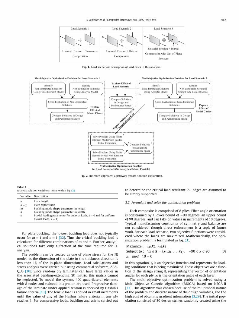
The problem investigated in this work is a pressurized fuselageskin modeled as a two-dimensional plate. The material in this anal-ysis is a square (20-inch by 20-inch) graphite epoxy compositewith a constant thickness of 0.01 in. and simply supported edges.Pressure on the panel induces loads in the axial and hoop direc-tions. Additionally, a compressive load may exist, accounting forfuselage bending. Associated material properties are listed inTable 1. The loading scenarios considered are: (1) uniaxial tensionand transverse compression, (2) uniaxial tension and non-uniformbiaxial compression, and (3) uniaxial tension and non-uniformbiaxial compression with out-of-plane pressure. Load scenariosare depicted in Fig. 1. In all three cases, buckling failure is exam-ined for compressive loads. In load scenarios (2) and (3), the com-pressive load in the direction of tension is 10% of the compressiveload in the transverse direction.
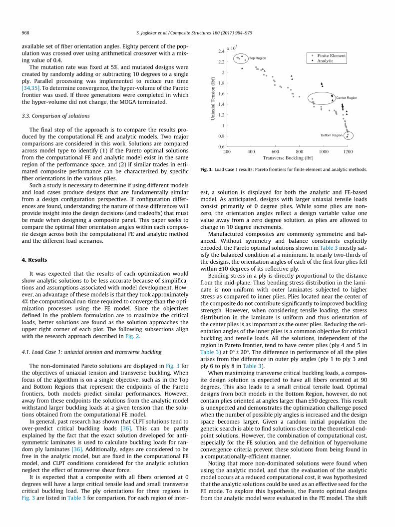
A computational model based on FE allows for complex struc-tures to be considered under a wide variety of loading scenarios.Analytic methods have higher computational efficiency, but accu-racy decreases as composite complexity increases. Further, differ-ent formulations of the analytic model are needed for differentloading scenarios. To explore how the choice of analysis modeland load scenario influences the optimal results, the approach inFig. 2 was developed. For Load Scenarios 1 and 2, non-dominatedpoints associated with a multiobjective optimization problem areidentified using both a Finite Element and analytic model. Thesenon-dominated points are then cross-evaluated to better under-stand how model choice influences predicted composite perfor-
Table 1Material properties: constituent properties ofcomposite.
Material properties Values
E1 30� 106 psiE2 0:75� 106 psiv12 0:25G12 0:375� 106 psiXt 150� 103 psiYt 6� 103 psiS 10� 103
Xc 100� 103 psiYc 17� 103 psi
mance. Non-dominated solutions obtained from the analyticmodel for Load Scenarios 1 and 2 are then cross-evaluated toexplore how changes to load scenario might cause previously opti-mal designs to underperform. An analytic model form is not possi-ble for Load Scenario 3. For this loading case, the focus is onunderstanding how using previously identified optimal solutionsto a different loading scenario (here the non-dominated solutionsassociated with the analytic model for Load Scenario 2) can be usedto reduce computational expense. This is achieved by using thesenon-dominated solutions as an initial starting point for the opti-mization of the composite in Load Scenario 3.
3.1. Selecting an analytical and computational model
Critical loads are calculated by considering the loading scenarioand the analysis model being used. For the analytic models, criticaltensile loads are calculated assuming CLPT and analytic expres-sions for Hashin’s failure criteria [30]:
1. Fiber failure in tension: Ftf ¼ r11
Xt
� �2þ s12
S
� �2.2. Fiber failure in compression: Fc
f ¼ r11Xc
� �2
3. Matrix failure in tension: Ftm ¼ r22
Yt
� �2þ s12
S
� �24. Matrix failure in compression: Fc
m ¼ r222S
� �2 þ s12S
� �2þYc2S
� �2 � 1h i
� r22YC
r11, r22, and s12 indicate stress in the fiber direction, stress inthe transverse direction and shear stress for individual lamina,respectively. For uniaxial tensile loading, only one componentout of stress and moment resultant is non-zero. Using Eq. (1), fail-ure strains for each laminate are calculated. Since Hashin’s criteriais a unidirectional failure criteria, the laminate strains are trans-formed into each individual ply direction and the smallest criticalload value is selected to indicate first ply failure.
NM
� �¼ A B
B D
� �ej
h ið1Þ
Plate edges are assumed to be free. An exact solution for criticalbuckling load is not available and most available solutions assumethe bending-extension matrix to be zero. A solution which consid-ers a non-zero B matrix exists for anti-symmetric angle ply lami-nates (�hn) and is used in this analysis to calculate criticalbuckling loads. However, the terms A16, A26;B11, B12, B22, B66, D16
and D26 are still assumed to be zero. Eq. (2) [31] is used to calculatethe critical buckling load N0. Table 2 gives the variable descriptionsfor Eq. (2).
N0 ¼ p2
R2b2ðm2 þ kn2R2Þ
�D11m4 þ 2m2n2R2ðD12 þ 2D66Þ
þ D22n4R4 � 1J1½mJ2ðB16m2 þ 3B26n2R2Þ
þ nRJ3ð3B16m2 þ B26n2R2Þ�
ð2Þ
where
J1 ¼ ðA11m2 þ A66n2R2ÞðA66m2 þ A22n2R2Þ � ðA12 þ A66Þ2m2n2R2
J2 ¼ ðA11m2 þ A66n2R2ÞðB16m2 þ 3B26n2R2Þ� ðA12 þ A66Þn2R2ð3B16m2 þ 3B26n2R2Þ
J3 ¼ ðA66m2 þ A22n2R2Þð3B16m2 þ B26n2R2Þ� ðA12 þ A66Þn2R2ðB16m2 þ 3B26n2R2Þ
Multiobjective Optimization Problem for Load Scenario 1
IdentifyNon-dominated Solutions
Using Finite Element Model
Compare Solutions in Designand Performance Space
Cross-Evaluation of Non-dominatedSolutions
Compare Solutionsin Design and
Performance Space
Explore Effect ofLoad ScenarioIdentify
Non-dominated SolutionsUsing Analytic Model
Solve Problem Using FiniteElement Model with Seeded
Initial Population Compare Solutionsin Design and
Performance Space
Multiobjective Optimization Problemfor Load Scenario 3 (No Analytical Model Possible)
Solve Problem Using FiniteElement Model with Random
Initial Population
ecudeRotytilibAerolpxE Computational Cost
Multiobjective Optimization Problem for Load Scenario 2
IdentifyNon-dominated Solutions
Using Analytic Model
Compare Solutions in Designand Performance Space
Cross-Evaluation of Non-dominatedSolutions
IdentifyNon-dominated Solutions
Using Finite Element Model
ExploreEffect of
Model Choice
ExploreEffect of
Model Choice
Fig. 2. Research approach: a pathway toward solution exploration.
Load Scenario 1 Load Scenario 2 Load Scenario 3
Uniaxial Tension + Transverse
Compression
Uniaxial Tension + Biaxial
Compression
Uniaxial Tension + Biaxial
Compression with Out-of-Plane
Pressure
Fig. 1. Load scenarios: description of load cases in this analysis.
Table 2Analytic solution variables: terms within Eq. (2).
Variable Description
b Plate lengthR ¼ a
b Plate aspect ratiom Buckling mode shape parameter in lengthn Buckling mode shape parameter in widthk Biaxial loading parameter (for uniaxial loads, k ¼ 0 and for uniform
biaxial loads, k ¼ 1)
S. Joglekar et al. / Composite Structures 160 (2017) 964–975 967
For plate buckling, the lowest buckling load does not typicallyoccur for m ¼ 1 and n ¼ 1 [32]. Thus the critical buckling load iscalculated for different combinations of m and n. Further, analyti-cal solutions take only a fraction of the time required for FEanalysis.
The problem can be treated as one of plane stress for the FEmodel, as the dimension of the plate in the thickness direction isless than 1% of the in-plane dimensions. Load calculations andstress analysis were carried out using commercial software, ABA-QUS [30]. Since random ply laminates can have large values inthe associated bending-extending (B) matrix, this matrix cannotbe neglected. To model the system, 400 quadrilateral elementswith 8 nodes and reduced integration are used. Progressive dam-age of the laminate under applied tension is checked by Hashin’sfailure criteria [13]. The tensile load is applied in small incrementsuntil the value of any of the Hashin failure criteria in any plyreaches 1. For compressive loads, buckling analysis is carried out
to determine the critical load resultant. All edges are assumed tobe simply supported.
3.2. Formulate and solve the optimization problems
Each composite is comprised of 8 plies. Fiber angle orientationis constrained by a lower bound of �90 degrees, an upper boundof 90 degrees, and can take on values in increments of 10 degrees.Typical manufacturing constraints of symmetry and balance arenot considered, though direct enforcement is a topic of futurework. For each load scenario, two objective functions were consid-ered where the loads are maximized. Mathematically, the opti-mization problem is formulated as Eq. (3).
Maximize : k1ðXÞ; k2ðXÞSubject to : 8x 2 X ¼ fx1; x2; . . . ; x8g; �90 6 x 6 90xi mod 10 ¼ 0
ð3Þ
In this equation, ki is an objective function and represents the load-ing conditions that is being maximized. These objectives are a func-tion of the design string X, representing the vector of orientationangles for each ply. xi is the orientation angle of each layer.
The multi-objective optimization problem is solved using aMulti-Objective Genetic Algorithm (MOGA) based on NSGA-II[33]. This algorithm was chosen because of the multimodal natureof the problem, the discrete nature of the design variables, and thehigh cost of obtaining gradient information [3,29]. The initial pop-ulation consisted of 80 design strings randomly created using the
200 400 600 800 1000 12000.6
0.8
1
1.2
1.4
1.6
1.8
2
2.2
2.4 x 10⁵
Transverse Buckling (lbf)
Uni
axia
l Ten
sion
(lbf
)
Finite ElementAnalytic
Bottom Region
Center Region
Top Region
Fig. 3. Load Case 1 results: Pareto frontiers for finite element and analytic methods.
968 S. Joglekar et al. / Composite Structures 160 (2017) 964–975
available set of fiber orientation angles. Eighty percent of the pop-ulation was crossed over using arithmetical crossover with a mix-ing value of 0.4.
The mutation rate was fixed at 5%, and mutated designs werecreated by randomly adding or subtracting 10 degrees to a singleply. Parallel processing was implemented to reduce run time[34,35]. To determine convergence, the hyper-volume of the Paretofrontier was used. If three generations were completed in whichthe hyper-volume did not change, the MOGA terminated.
3.3. Comparison of solutions
The final step of the approach is to compare the results pro-duced by the computational FE and analytic models. Two majorcomparisons are considered in this work. Solutions are comparedacross model type to identify (1) if the Pareto optimal solutionsfrom the computational FE and analytic model exist in the sameregion of the performance space, and (2) if similar trades in esti-mated composite performance can be characterized by specificfiber orientations in the various plies.
Such a study is necessary to determine if using different modelsand load cases produce designs that are fundamentally similarfrom a design configuration perspective. If configuration differ-ences are found, understanding the nature of these differences willprovide insight into the design decisions (and tradeoffs) that mustbe made when designing a composite panel. This paper seeks tocompare the optimal fiber orientation angles within each compos-ite design across both the computational FE and analytic methodand the different load scenarios.
4. Results
It was expected that the results of each optimization wouldshow analytic solutions to be less accurate because of simplifica-tions and assumptions associated with model development. How-ever, an advantage of these models is that they took approximately4% the computational run-time required to converge than the opti-mization processes using the FE model. Since the objectivesdefined in the problem formulation are to maximize the criticalloads, better solutions are found as the solution approaches theupper right corner of each plot. The following subsections alignwith the research approach described in Fig. 2.
4.1. Load Case 1: uniaxial tension and transverse buckling
The non-dominated Pareto solutions are displayed in Fig. 3 forthe objectives of uniaxial tension and transverse buckling. Whenfocus of the algorithm is on a single objective, such as in the Topand Bottom Regions that represent the endpoints of the Paretofrontiers, both models predict similar performances. However,away from these endpoints the solutions from the analytic modelwithstand larger buckling loads at a given tension than the solu-tions obtained from the computational FE model.
In general, past research has shown that CLPT solutions tend toover-predict critical buckling loads [36]. This can be partlyexplained by the fact that the exact solution developed for anti-symmetric laminates is used to calculate buckling loads for ran-dom ply laminates [36]. Additionally, edges are considered to befree in the analytic model, but are fixed in the computational FEmodel, and CLPT conditions considered for the analytic solutionneglect the effect of transverse shear force.
It is expected that a composite with all fibers oriented at 0degrees will have a large critical tensile load and small transversecritical buckling load. The ply orientations for three regions inFig. 3 are listed in Table 3 for comparison. For each region of inter-
est, a solution is displayed for both the analytic and FE-basedmodel. As anticipated, designs with larger uniaxial tensile loadsconsist primarily of 0 degree plies. While some plies are non-zero, the orientation angles reflect a design variable value onevalue away from a zero degree solution, as plies are allowed tochange in 10 degree increments.
Manufactured composites are commonly symmetric and bal-anced. Without symmetry and balance constraints explicitlyencoded, the Pareto optimal solutions shown in Table 3 mostly sat-isfy the balanced condition at a minimum. In nearly two-thirds ofthe designs, the orientation angles of each of the first four plies fellwithin ±10 degrees of its reflective ply.
Bending stress in a ply is directly proportional to the distancefrom the mid-plane. Thus bending stress distribution in the lami-nate is non-uniform with outer laminates subjected to higherstress as compared to inner plies. Plies located near the center ofthe composite do not contribute significantly to improved bucklingstrength. However, when considering tensile loading, the stressdistribution in the laminate is uniform and thus orientation ofthe center plies is as important as the outer plies. Reducing the ori-entation angles of the inner plies is a common objective for criticalbuckling and tensile loads. All the solutions, independent of theregion in Pareto frontier, tend to have center plies (ply 4 and 5 inTable 3) at 0� ± 20�. The difference in performance of all the pliesarises from the difference in outer ply angles (ply 1 to ply 3 andply 6 to ply 8 in Table 3).
When maximizing transverse critical buckling loads, a compos-ite design solution is expected to have all fibers oriented at 90degrees. This also leads to a small critical tensile load. Optimaldesigns from both models in the Bottom Region, however, do notcontain plies oriented at angles larger than ±50 degrees. This resultis unexpected and demonstrates the optimization challenge posedwhen the number of possible ply angles is increased and the designspace becomes larger. Given a random initial population thegenetic search is able to find solutions close to the theoretical end-point solutions. However, the combination of computational cost,especially for the FE solution, and the definition of hypervolumeconvergence criteria prevent these solutions from being found ina computationally-efficient manner.
Noting that more non-dominated solutions were found whenusing the analytic model, and that the evaluation of the analyticmodel occurs at a reduced computational cost, it was hypothesizedthat the analytic solutions could be used as an effective seed for theFE mode. To explore this hypothesis, the Pareto optimal designsfrom the analytic model were evaluated in the FE model. The shift

Table 3Load Case 1 overview: sample Pareto optimal composite designs.
Region Analysis model Transverse buckling (lbf) Uniaxial tension (lbf) Ply (deg.)
1 2 3 4 5 6 7 8
Top FE 285.12 227806 0 10 0 �10 �10 0 0 10Analytic 324.43 230366 �10 0 10 0 0 10 0 �10
Center FE 908.88 144204.4 �30 30 0 10 0 0 �30 30Analytic 1072.7 147392.8 �40 20 �10 �20 �10 0 20 �40
Bottom FE 1199.46 82648 �40 40 40 10 �10 20 �40 40Analytic 1193.69 78272.4 �40 40 �20 �20 �10 30 40 �50
200 400 600 800 1000 1200 1400 16000
0.5
1
1.5
2
2.5 x 10⁵
Biaxial Buckling (lbf)
Uni
axia
l Ten
sion
(lbf
)
TopRegion
CenterRegion
BottomRegion
Fig. 5. Load Case 2 results: Pareto frontiers for finite element and analytic methods.
S. Joglekar et al. / Composite Structures 160 (2017) 964–975 969
in objective function values for the analytic frontier when thedesigns are evaluated using the FE model is shown in Fig. 4(a).Due to the limitations of CLPT, when the analytic solutions areevaluated in the FE model there is a reduction in transverse buck-ling (average percent error of 11%) and minor changes in uniaxialtension (average percent error of 0.91%). The higher error for ana-lytic buckling load comes from the assumptions associated withEq. (2).
Fig. 4(b) shows the comparison of the analytic frontier evalu-ated using the FE model to the non-dominated solution identifiedwhen running the MOGA on the FE model. There is strong compar-ison amongst most of the frontier, indicating that both models con-verge to similar ply angle solutions. More importantly, this resultsupports the hypothesis that analytic solutions can be used toinform the solution of the non-dominated set when an FE modelis used. Non-dominated analytic solutions can be found at a greatlyreduced computational expense, and these solutions can then beevaluated in the FE model and used to seed the MOGA populationfor the remainder of the search.
4.2. Load Case 2: uniaxial tension and biaxial buckling
To further explore the similarities and differences between theanalytic and the FE model a second load case of uniaxial tensionand biaxial buckling is evaluated. The buckling load is 10% of theload in the transverse direction. Fig. 5 depicts the Pareto frontiersgenerated by the FE and analytic method.
For large critical uniaxial tensile loads (the Top Region) the Par-eto frontiers obtained from both models overlap. However, as thecritical biaxial buckling load increases, the analytic model over-predicts the load. The analytic frontier predicts critical biaxialbuckling loads 400 lbf greater (38%) than the largest critical biaxialbuckling load generated by the FE model. Conversely, the FE model
200 400 600 800 1000 12000.6
0.8
1
1.2
1.4
1.6
1.8
2
2.2
2.4 x 10⁵
Buckling (lbf)
Uni
axia
l Ten
sion
(lbf
)
(a) (
Fig. 4. (a) Cross evaluation in Load Case 1: evaluation of analytic Pareto frontier in FE moPareto frontier in FE model with FE solution.
predicts larger (nearly 3000 lbf greater, or 1.3%) critical uniaxialtensile loads. This larger prediction is due to the shear additionalstresses induced by the coupling terms that are better capturedby FE models, resulting in smaller critical load values than the ana-lytic model.
The design solutions corresponding to a single solution from theTop, Center, and Bottom regions of each model are reported inTable 4. As seen in the previous study, designs with the highestcritical uniaxial tensile load have plies with orientations close, orequal, to zero degrees. Again, the solutions from either model donot contain ply solutions with orientation angles larger or smallerthan �50 degrees, even when biaxial buckling is maximized. There
200 400 600 800 1000 12000.8
1
1.2
1.4
1.6
1.8
2
2.2
2.4 x 10⁵
Buckling (lbf)
Uni
axia
l Ten
sion
(lbf
)
b)
del with analytic solution. (b) Cross evaluation in Load Case 1: evaluation of analytic
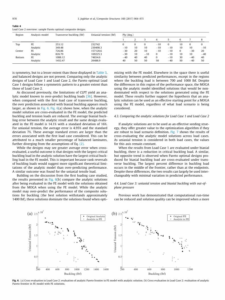
Table 4Load Case 2 overview: sample Pareto optimal composite designs.
Region Analysis model Transverse buckling (lbf) Uniaxial tension (lbf) Ply (deg.)
1 2 3 4 5 6 7 8
Top FE 253.12 232742 0 0 0 �10 0 10 0 0Analytic 349.48 230498.3 �10 10 10 �10 �10 10 10 �10
Center FE 726.06 157120.6 �30 20 10 �10 �10 0 �30 20Analytic 826.79 169225.3 �30 10 �10 0 �10 10 10 �40
Bottom FE 1088.12 74654.6 �40 40 40 0 �10 30 �40 40Analytic 1452.47 26488.9 40 50 50 50 �40 50 �40 50
970 S. Joglekar et al. / Composite Structures 160 (2017) 964–975
is symmetry, but to a lesser extent than those displayed in Table 3,and balanced designs are not present. Comparing only the analyticdesigns of Load Case 1 and Load Case 2, the Pareto optimal LoadCase 1 designs follow a symmetric pattern to a greater extent thanthose of Load Case 2.
As discussed previously, the limitations of CLPT yield an ana-lytic model known to over-predict buckling loads [36]. However,when compared with the first load case of transverse buckling,the over prediction associated with biaxial buckling appears muchlarger, as shown in Fig. 6. Fig. 6(a) shows how, when the analyticmodel solution are cross-evaluated in the FE model, the predictedbuckling and tension loads are reduced. The average biaxial buck-ling error between the analytic result and the same design evalu-ated in the FE model is 14.1% with a standard deviation of 16%.For uniaxial tension, the average error is 4.95% and the standarddeviation 7%. These average standard errors are larger than theerrors associated with the first load case considered. This can beattributed to a much smaller percentage of balanced laminates,further diverging from the assumptions of Eq. (2).
While the designs may see greater average error when cross-evaluated, a useful outcome is that designs with the largest criticalbuckling load in the analytic solution have the largest critical buck-ling load in the FE model. This is important because rank reversalsof buckling loads would suggest more significant theoretical limi-tations of the analytic model than over-predicting performance.A similar outcome was found for the uniaxial tensile load.
Building on the discussion from the first loading case studied,the results presented in Fig. 6(b) compare the analytic solutionsafter being evaluated in the FE model with the solutions obtainedfrom the MOGA when using the FE model. While the analyticmodel may over-predict the performance of the composite solu-tions for buckling (the best solution withstands approximately1400 lbf), these solutions dominate the solutions found when opti-
200 400 600 800 1000 1200 1400 16000
0.5
1
1.5
2
2.5 x 10⁵
Buckling (lbf)
Uni
axia
l Ten
sion
(lbf
)
(a) (
Fig. 6. (a) Cross evaluation in Load Case 2: evaluation of analytic Pareto frontier in FE moPareto frontier in FE model with FE solutions.
mizing with the FE model. Elsewhere in the space there is usefulsimilarity between predicted performances, except in the regionswhere the buckling load is between 700 and 1000 lbf. Despitethe differences in this region of the performance space, the MOGAusing the analytic model identified solutions that would be non-dominated with respect to the solutions generated using the FEmodel. These results further support the hypothesis that an ana-lytic solution can be used as an effective starting point for a MOGAusing the FE model, regardless of what load scenario is beingconsidered.
4.3. Comparing the analytic solutions for Load Case 1 and Load Case 2
If analytic solutions are to be used as an effective seeding strat-egy, they offer greater value to the optimization algorithm if theyare robust to load scenario definition. Fig. 7 shows the results ofcross-evaluating the analytic model solutions across load cases.As uniaxial tension is considered in both load cases, the valuesfor this axis remain constant.
When the results from Load Case 1 are evaluated under biaxialbuckling, there is a reduction in critical buckling load. A similar,but opposite trend is observed when Pareto optimal designs pro-duced for biaxial buckling load are cross-evaluated under trans-verse buckling. The largest percent difference in buckling loadoccurs in the middle of the frontier, rather than at the endpoints.Despite these differences, the two results can largely be used inter-changeably with minimal variation in predicted performance.
4.4. Load Case 3: uniaxial tension and biaxial buckling with out-of-plane pressure
Previous work has demonstrated that computational run-timecan be reduced and solution quality can be improved when a more
200 400 600 800 1000 12000
0.5
1
1.5
2
2.5 x 10⁵
Buckling (lbf)
Uni
axia
l Ten
sion
(lbf
)
b)
del with analytic solution. (b) Cross evaluation in Load Case 2: evaluation of analytic
0 1000 2000 3000 4000 5000 6000 70001
1.2
1.4
1.6
1.8
2
2.2
2.4 x 10⁵
Buckling (lbf)
Uni
axia
l Ten
sion
(lbf
)TopRegion
CenterRegion
BottomRegion
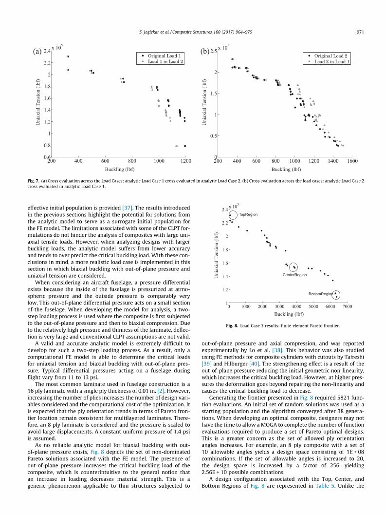
Fig. 8. Load Case 3 results: finite element Pareto frontier.
200 400 600 800 1000 12000.6
0.8
1
1.2
1.4
1.6
1.8
2
2.2
2.4 x 10⁵
Buckling (lbf)
Uni
axia
l Ten
sion
(lbf
)
Original Load 1Load 1 in Load 2
200 400 600 800 1000 1200 1400 16000
0.5
1
1.5
2
2.5 x 10⁵
Buckling (lbf)
Uni
axia
l Ten
sion
(lbf
)
Original Load 2Load 2 in Load 1
(a) (b)
Fig. 7. (a) Cross evaluation across the Load Cases: analytic Load Case 1 cross evaluated in analytic Load Case 2. (b) Cross evaluation across the load cases: analytic Load Case 2cross evaluated in analytic Load Case 1.
S. Joglekar et al. / Composite Structures 160 (2017) 964–975 971
effective initial population is provided [37]. The results introducedin the previous sections highlight the potential for solutions fromthe analytic model to serve as a surrogate initial population forthe FE model. The limitations associated with some of the CLPT for-mulations do not hinder the analysis of composites with large uni-axial tensile loads. However, when analyzing designs with largerbuckling loads, the analytic model suffers from lower accuracyand tends to over predict the critical buckling load. With these con-clusions in mind, a more realistic load case is implemented in thissection in which biaxial buckling with out-of-plane pressure anduniaxial tension are considered.
When considering an aircraft fuselage, a pressure differentialexists because the inside of the fuselage is pressurized at atmo-spheric pressure and the outside pressure is comparably verylow. This out-of-plane differential pressure acts on a small sectionof the fuselage. When developing the model for analysis, a two-step loading process is used where the composite is first subjectedto the out-of-plane pressure and then to biaxial compression. Dueto the relatively high pressure and thinness of the laminate, deflec-tion is very large and conventional CLPT assumptions are not valid.
A valid and accurate analytic model is extremely difficult todevelop for such a two-step loading process. As a result, only acomputational FE model is able to determine the critical loadsfor uniaxial tension and biaxial buckling with out-of-plane pres-sure. Typical differential pressures acting on a fuselage duringflight vary from 11 to 13 psi.
The most common laminate used in fuselage construction is a16 ply laminate with a single ply thickness of 0.01 in. [2]. However,increasing the number of plies increases the number of design vari-ables considered and the computational cost of the optimization. Itis expected that the ply orientation trends in terms of Pareto fron-tier location remain consistent for multilayered laminates. There-fore, an 8 ply laminate is considered and the pressure is scaled toavoid large displacements. A constant uniform pressure of 1.4 psiis assumed.
As no reliable analytic model for biaxial buckling with out-of-plane pressure exists, Fig. 8 depicts the set of non-dominatedPareto solutions associated with the FE model. The presence ofout-of-plane pressure increases the critical buckling load of thecomposite, which is counterintuitive to the general notion thatan increase in loading decreases material strength. This is ageneric phenomenon applicable to thin structures subjected to
out-of-plane pressure and axial compression, and was reportedexperimentally by Lo et al. [38]. This behavior was also studiedusing FE methods for composite cylinders with cutouts by Tafreshi[39] and Hilburger [40]. The strengthening effect is a result of theout-of-plane pressure reducing the initial geometric non-linearity,which increases the critical buckling load. However, at higher pres-sures the deformation goes beyond repairing the non-linearity andcauses the critical buckling load to decrease.
Generating the frontier presented in Fig. 8 required 5821 func-tion evaluations. An initial set of random solutions was used as astarting population and the algorithm converged after 38 genera-tions. When developing an optimal composite, designers may nothave the time to allow a MOGA to complete the number of functionevaluations required to produce a set of Pareto optimal designs.This is a greater concern as the set of allowed ply orientationangles increases. For example, an 8 ply composite with a set of10 allowable angles yields a design space consisting of 1E + 08combinations. If the set of allowable angles is increased to 20,the design space is increased by a factor of 256, yielding2.56E + 10 possible combinations.
A design configuration associated with the Top, Center, andBottom Regions of Fig. 8 are represented in Table 5. Unlike the
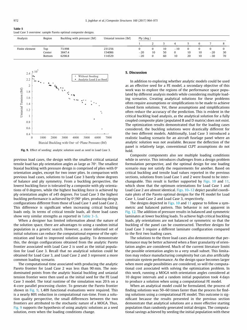
Table 5Load Case 3 overview: sample Pareto optimal composite designs.
Analysis Region Buckling with pressure (lbf) Uniaxial tension (lbf) Ply (deg.)
1 2 3 4 5 6 7 8
Finite element Top 73.998 231256 0 0 10 �10 0 0 0 0Center 3847.4 154086 �20 10 50 0 10 10 �20 30Bottom 6298.8 114529 �20 0 60 10 20 10 �30 70
0 1000 2000 3000 4000 5000 6000 70000.4
0.6
0.8
1
1.2
1.4
1.6
1.8
2
2.2
2.4 x 10⁵
Biaxial Buckling with Out−of−Plane Pressure (lbf)
Uni
axia
l Ten
sion
(lbf
)
Fig. 9. Effect of seeding: analytic solution used as seed in Load Case 3.
972 S. Joglekar et al. / Composite Structures 160 (2017) 964–975
previous load cases, the design with the smallest critical uniaxialtensile load has ply orientation angles as large as 70�. The smallestbiaxial buckling with pressure design is comprised of plies with 0�orientation angles, except for two inner plies. In comparison withprevious load cases, solutions to Load Case 3 barely show degreesof balance and ply symmetry. From a buckling perspective, thelowest buckling force is tolerated by a composite with ply orienta-tions of 0 degrees, while the highest buckling force is achieved byply orientation angles of ±45 degrees. For Load Case 3 the highestbuckling performance is achieved by 0�/90� plies, producing designconfigurations different from those of Load Case 1 and Load Case 2.This difference is significant when increasing critical bucklingloads only. In terms of critical tensile loads, all three load casesshow very similar strengths as reported in Table 3–5.
When a designer has limited information about the nature ofthe solution space, there are advantages to using a random initialpopulation in a genetic search. However, a more informed set ofinitial solutions can reduce the computational expense of the opti-mization and lead to improved solution quality. To demonstratethis, the design configurations obtained from the analytic Paretofrontier associated with Load Case 2 is used as the initial popula-tion for Load Case 3. Recall that no analytical solution could beobtained for Load Case 3, and Load Case 2 and 3 represent a morecommon loading scenario.
The computational time associated with producing the analyticPareto frontier for Load Case 2 was less than 90 min. The non-dominated points from the analytic biaxial buckling and uniaxialtension frontier were then used as the initial seed for the FE LoadCase 3 model. The total runtime of the simulation was 20 h on a4-core parallel processing cluster. To generate the Pareto frontiershown in Fig. 9, 1,409 functional evaluations were required. Thisis a nearly 80% reduction in computational run-time. From a solu-tion quality perspective, the small differences between the twofrontiers are attributed to the stochastic nature of a MOGA. Thus,Fig. 9 supports the hypothesis of using analytic solutions as a seedsolution, even when the loading conditions change.
5. Discussion
In addition to exploring whether analytic models could be usedas an effective seed for a FE model, a secondary objective of thiswork was to explore the regions of the performance space popu-lated by different analysis models while considering multiple load-ing scenarios. Creating analytical solutions for these problemsoften require assumptions or simplifications to be made to achieveclosed form solutions. Yet, these assumptions and simplificationsoften reduce the accuracy of the prediction. This is evident in thecritical buckling load analysis, as the analytical solution for a fullycoupled composite plate (populated B and D matrix) does not exist.The optimization results demonstrated that for the loading casesconsidered, the buckling solutions were drastically different forthe two different models. Additionally, Load Case 3 introduced arealistic loading scenario for an aircraft fuselage panel where ananalytic solution was not available. Because the deflection of thepanel is relatively large, conventional CLPT assumptions do nothold.
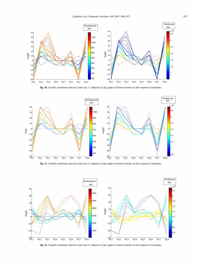
Composite components also see multiple loading conditionswhile in service. This introduces challenges from a design problemformulation perspective, and the optimal design for one loadingscenario may not satisfy the requirements for another. Based oncritical buckling and tensile load values reported in the previoussections, solutions from Load Case 1 and 2 were found to be inter-changeable. This result is further supported by Figs. 10 and 11,which show that the optimum orientations for Load Case 1 andLoad Case 2 are almost identical. Figs. 10–12 depict parallel coordi-nate plots of the Pareto optimal designs for the FE model for LoadCase 1, Load Case 2 and Load Case 3, respectively.
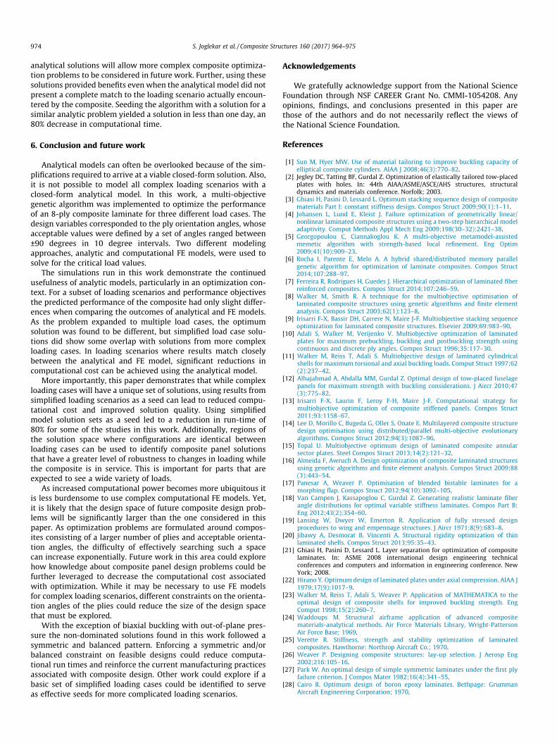
The designs depicted in Figs. 10 and 11 appear to follow a sym-metric and balanced pattern. This behavior is not apparent inFig. 12. The addition of pressure results in balanced and symmetriclaminates at lower buckling loads. To achieve high critical bucklingloads, ply orientations are not balanced or symmetric so that thebuckling of the panel can be counteracted. Therefore designs forLoad Case 3 require a different laminate configuration comparedto the first two loading cases.
The solutions to the three load cases also demonstrate that per-formance may be better achieved when a finer granularity of orien-tation angles are considered. Much of the current literature limitsthe possible orientation angles to a very small subset. This limita-tion may reduce manufacturing complexity but can also artificiallyconstrain system performance. As the design space becomes largerwhen more angle possibilities are considered, so will the computa-tional cost associated with solving the optimization problem. Inthis work, running a MOGA with orientation angles considered at10 degree intervals and a random initial population took 4 daysto produce a solution when using a computational FE model.
When an analytical model could be formulated, the process offinding solutions was 50–60 times faster than the process for find-ing solutions using a computational FE model. This outcome is sig-nificant because the results presented in the previous sectiondemonstrate that analytical solutions are a more effective startingpopulation than randomly generated initial designs. The computa-tional savings achieved by seeding the initial population with these
Ply1 Ply2 Ply3 Ply4 Ply5 Ply6 Ply7 Ply8−40
−30
−20
−10
0
10
20
30
40
50
60
Ang
le
300
400
500
600
700
800
900
1000
1100
BucklingLoad(lbf)
Ply1 Ply2 Ply3 Ply4 Ply5 Ply6 Ply7 Ply8−40
−30
−20
−10
0
10
20
30
40
50
60
Ang
le
1
1.2
1.4
1.6
1.8
2
2.2x 10⁵
TensileLoad(lbf)
Fig. 10. Parallel coordinates plot for Load Case 1: influence of ply angles of Pareto frontier on the response of laminate.
Ply1 Ply2 Ply3 Ply4 Ply5 Ply6 Ply7 Ply8−50
−40
−30
−20
−10
0
10
20
30
40
Ang
le
300
400
500
600
700
800
900
1000
BucklingLoad(lbf)
Ply1 Ply2 Ply3 Ply4 Ply5 Ply6 Ply7 Ply8−50
−40
−30
−20
−10
0
10
20
30
40
Ang
le
0.8
1
1.2
1.4
1.6
1.8
2
2.2
x 105
TensileLoad(lbf)
Fig. 11. Parallel coordinates plot for Load Case 2: influence of ply angles of Pareto frontier on the response of laminate.
Ply1 Ply2 Ply3 Ply4 Ply5 Ply6 Ply7 Ply8−60
−40
−20
0
20
40
60
80
Ang
le
1000
2000
3000
4000
5000
6000
BucklingLoad
(lbf)
Ply1 Ply2 Ply3 Ply4 Ply5 Ply6 Ply7 Ply8−60
−40
−20
0
20
40
60
80
Ang
le
0.6
0.8
1
1.2
1.4
1.6
1.8
2
2.2
x 105
TensileLoad(lbf)
Fig. 12. Parallel coordinates plot for Load Case 3: influence of ply angles of Pareto frontier on the response of laminate.
S. Joglekar et al. / Composite Structures 160 (2017) 964–975 973
974 S. Joglekar et al. / Composite Structures 160 (2017) 964–975
analytical solutions will allow more complex composite optimiza-tion problems to be considered in future work. Further, using thesesolutions provided benefits even when the analytical model did notpresent a complete match to the loading scenario actually encoun-tered by the composite. Seeding the algorithm with a solution for asimilar analytic problem yielded a solution in less than one day, an80% decrease in computational time.
6. Conclusion and future work
Analytical models can often be overlooked because of the sim-plifications required to arrive at a viable closed-form solution. Also,it is not possible to model all complex loading scenarios with aclosed-form analytical model. In this work, a multi-objectivegenetic algorithm was implemented to optimize the performanceof an 8-ply composite laminate for three different load cases. Thedesign variables corresponded to the ply orientation angles, whoseacceptable values were defined by a set of angles ranged between±90 degrees in 10 degree intervals. Two different modelingapproaches, analytic and computational FE models, were used tosolve for the critical load values.
The simulations run in this work demonstrate the continuedusefulness of analytic models, particularly in an optimization con-text. For a subset of loading scenarios and performance objectivesthe predicted performance of the composite had only slight differ-ences when comparing the outcomes of analytical and FE models.As the problem expanded to multiple load cases, the optimumsolution was found to be different, but simplified load case solu-tions did show some overlap with solutions from more complexloading cases. In loading scenarios where results match closelybetween the analytical and FE model, significant reductions incomputational cost can be achieved using the analytical model.
More importantly, this paper demonstrates that while complexloading cases will have a unique set of solutions, using results fromsimplified loading scenarios as a seed can lead to reduced compu-tational cost and improved solution quality. Using simplifiedmodel solution sets as a seed led to a reduction in run-time of80% for some of the studies in this work. Additionally, regions ofthe solution space where configurations are identical betweenloading cases can be used to identify composite panel solutionsthat have a greater level of robustness to changes in loading whilethe composite is in service. This is important for parts that areexpected to see a wide variety of loads.
As increased computational power becomes more ubiquitous itis less burdensome to use complex computational FE models. Yet,it is likely that the design space of future composite design prob-lems will be significantly larger than the one considered in thispaper. As optimization problems are formulated around compos-ites consisting of a larger number of plies and acceptable orienta-tion angles, the difficulty of effectively searching such a spacecan increase exponentially. Future work in this area could explorehow knowledge about composite panel design problems could befurther leveraged to decrease the computational cost associatedwith optimization. While it may be necessary to use FE modelsfor complex loading scenarios, different constraints on the orienta-tion angles of the plies could reduce the size of the design spacethat must be explored.
With the exception of biaxial buckling with out-of-plane pres-sure the non-dominated solutions found in this work followed asymmetric and balanced pattern. Enforcing a symmetric and/orbalanced constraint on feasible designs could reduce computa-tional run times and reinforce the current manufacturing practicesassociated with composite design. Other work could explore if abasic set of simplified loading cases could be identified to serveas effective seeds for more complicated loading scenarios.
Acknowledgements
We gratefully acknowledge support from the National ScienceFoundation through NSF CAREER Grant No. CMMI-1054208. Anyopinions, findings, and conclusions presented in this paper arethose of the authors and do not necessarily reflect the views ofthe National Science Foundation.
References
[1] Sun M, Hyer MW. Use of material tailoring to improve buckling capacity ofelliptical composite cylinders. AIAA J 2008;46(3):770–82.
[2] Jegley DC, Tatting BF, Gurdal Z. Optimization of elastically tailored tow-placedplates with holes. In: 44th AIAA/ASME/ASCE/AHS structures, structuraldynamics and materials conference. Norfolk; 2003.
[3] Ghiasi H, Pasini D, Lessard L. Optimum stacking sequence design of compositematerials Part I: constant stiffness design. Compos Struct 2009;90(1):1–11.
[4] Johansen L, Lund E, Kleist J. Failure optimization of geometrically linear/nonlinear laminated composite structures using a two-step hierarchical modeladaptivity. Comput Methods Appl Mech Eng 2009;198(30–32):2421–38.
[5] Georgopoulou C, Ciannakoglou K. A multi-objective metamodel-assistedmemetic algorithm with strength-based local refinement. Eng Optim2009;41(10):909–23.
[6] Rocha I, Parente E, Melo A. A hybrid shared/distributed memory parallelgenetic algorithm for optimization of laminate composites. Compos Struct2014;107:288–97.
[7] Ferreira R, Rodrigues H, Guedes J. Hierarchical optimization of laminated fiberreinforced composites. Compos Struct 2014;107:246–59.
[8] Walker M, Smith R. A technique for the multiobjective optimisation oflaminated composite structures using genetic algorithms and finite elementanalysis. Compos Struct 2003;62(1):123–8.
[9] Irisarri F-X, Bassir DH, Carrere N, Maire J-F. Multiobjective stacking sequenceoptimization for laminated composite structures. Elsevier 2009;69:983–90.
[10] Adali S, Walker M, Verijenko V. Multiobjective optimization of laminatedplates for maximum prebuckling, buckling and postbuckling strength usingcontinuous and discrete ply angles. Compos Struct 1996;35:117–30.
[11] Walker M, Reiss T, Adali S. Multiobjective design of laminated cylindricalshells for maximum torsional and axial buckling loads. Comput Struct 1997;62(2):237–42.
[12] Alhajahmad A, Abdalla MM, Gurdal Z. Optimal design of tow-placed fuselagepanels for maximum strength with buckling considerations. J Aircr 2010;47(3):775–82.
[13] Irisarri F-X, Laurin F, Leroy F-H, Maire J-F. Computational strategy formultiobjective optimization of composite stiffened panels. Compos Struct2011;93:1158–67.
[14] Lee D, Morillo C, Bugeda G, Oller S, Onate E. Multilayered composite structuredesign optimisation using distributed/parallel multi-objective evolutionaryalgorithms. Compos Struct 2012;94(3):1087–96.
[15] Topal U. Multiobjective optimum design of laminated composite annularsector plates. Steel Compos Struct 2013;14(2):121–32.
[16] Almeida F, Awruch A. Design optimization of composite laminated structuresusing genetic algorithms and finite element analysis. Compos Struct 2009;88(3):443–54.
[17] Panesar A, Weaver P. Optimisation of blended bistable laminates for amorphing flap. Compos Struct 2012;94(10):3092–105.
[18] Van Campen J, Kassapoglou C, Gurdal Z. Generating realistic laminate fiberangle distributions for optimal variable stiffness laminates. Compos Part B:Eng 2012;43(2):354–60.
[19] Lansing W, Dwyer W, Emerton R. Application of fully stressed designprocedures to wing and empennage structures. J Aircr 1971;8(9):683–8.
[20] Jibawy A, Desmorat B, Vincenti A. Structural rigidity optimization of thinlaminated shells. Compos Struct 2013;95:35–43.
[21] Ghiasi H, Pasini D, Lessard L. Layer separation for optimization of compositelaminates. In: ASME 2008 international design engineering technicalconferences and computers and information in engineering conference. NewYork; 2008.
[22] Hirano Y. Optimum design of laminated plates under axial compression. AIAA J1979;17(9):1017–9.
[23] Walker M, Reiss T, Adali S, Weaver P. Application of MATHEMATICA to theoptimal design of composite shells for improved buckling strength. EngComput 1998;15(2):260–7.
[24] Waddoups M. Structural airframe application of advanced compositematerials-analytical methods. Air Force Materials Library, Wright-PattersonAir Force Base; 1969.
[25] Verette R. Stiffness, strength and stability optimization of laminatedcomposites. Hawthorne: Northrop Aircraft Co.; 1970.
[26] Weaver P. Designing composite structures: lay-up selection. J Aerosp Eng2002;216:105–16.
[27] Park W. An optimal design of simple symmetric laminates under the first plyfailure criterion. J Compos Mater 1982;16(4):341–55.
[28] Cairo R. Optimum design of boron epoxy laminates. Bethpage: GrummanAircraft Engineering Corporation; 1970.

S. Joglekar et al. / Composite Structures 160 (2017) 964–975 975
[29] Soremekun G. Genetic algorithm for composite laminate design andoptimization; 1997.
[30] ABAQUS Version 6.12, Providence, RI: Dassault Systems Simulia Corp; 2012.[31] Whitney J. Structural analysis of laminated anisotropic plates. Lancaster,
Pa: Technomic Pub. Co.; 1987.[32] Jones R. Mechanics of composite materials. Philadelphia, PA: Taylor & Francis;
1999.[33] Deb K. A fast and elitist multiobjective genetic algorithm: NSGA-II. IEEE Trans
Evol Comput 2002;6(2):182–97.[34] Henderson J. Laminated plate design using genetic algorithms and parallel
processing. Comput Syst Eng 1994;5(4–6):441–53.[35] Kere P, Lento J. Design optimization of laminated composite structures using
distributed grid resources. Compos Struct 2005;71(3–4):435–8.[36] Kant T, Swaminathan K. Analytic solutions for free vibration of laminated
composite and sandwich plates based on a higher-order refined theory.Compos Struct 2001;53(1):73–85.
[37] Foster G, Ferguson S, Donndelinger J. Creating targeted initial populations forgenetic product searches in heterogeneous markets. Eng Optim 2014;46(12):1729–47.
[38] Lo H, Crate H, Schwartz B. Buckling of thin walled cylinder under axialcompression and internal pressure. National Advisory Committee forAeronautics, Langley Field; 1949.
[39] Tafreshi A. Buckling and post-buckling analysis of composite cylindrical shellswith cutouts subjected to internal pressure and axial compression loads. Int JPress Vessels Pip 2002;79(5):351–9.
[40] Hilburger M, Waas A, Starnes J. Response of composite shells with cutouts tointernal pressure and compression loads. AIAA J 1999;37(2):232–7.