Engineering Structures 87 (2015) 86–104

Contents lists available at ScienceDirect

Engineering Structures

journal homepage: www.elsevier .com/locate /engstruct

Component based design model for composite beam to reinforcedconcrete wall moment-resistant joints

http://dx.doi.org/10.1016/j.engstruct.2014.12.0390141-0296/� 2015 Elsevier Ltd. All rights reserved.

⇑ Corresponding author at: ISISE, Civil Engineering Department, University ofCoimbra, Pólo 2 da Universidade, Rua Luís Reis Santos, Pinhal de Marrocos, 3030-788 Coimbra, Portugal. Tel.: +351 239797254.

E-mail address: filippo.gentili@uc.pt (F. Gentili).

J. Henriques, F. Gentili ⇑, L. Simões da Silva, R. SimõesISISE, Civil Engineering Department, University of Coimbra, Pinhal de Marrocos, 3030 Coimbra, Portugal

a r t i c l e i n f o

Article history:Received 30 July 2014Revised 23 December 2014Accepted 27 December 2014

Keywords:Structural steel-to-concrete jointsBehavior of jointsComponent methodMoment–rotation curveDesign model

a b s t r a c t

The use of the structural systems combining members of different nature, such as reinforced concretewalls with steel/composite beams and columns, presents a competitive solution benefiting from thestructural efficiency of each type of member. This paper investigates the behavior of a composite beamto reinforced concrete wall moment-resistant joint configuration. The proposed joint configuration is asimple solution with structural capacity to connect these types of members in a non-seismic region.An experimental campaign was conducted within the work programme of a RFCS research project thatdemonstrated the structural efficiency of the joint.

An analytical component based design model is proposed. The development of the model wasperformed with the aid of numerical simulations and experimental results. In the present paper, thecalibration and validation of model is first presented for parts of the joint, where only several componentsare activated, and after the global model is assembled and verified against the experimental results. Sub-sequently, a parametric study is presented extending the range of validity of the model. Finally, this studyshows the need to detail the concrete components appropriately (wall) in order to prevent brittle failureof the joint.

� 2015 Elsevier Ltd. All rights reserved.

1. Introduction

In many cases the use of mixed steel–concrete structures is themost competitive solution. The concept of mixed structure is basedon using different materials for different members according totheir best structural performance. Clear examples of this practiceare the use of reinforced concrete (RC) for foundations staircases/lift cores and steel/composite for columns, slabs and beams.Optimized solutions can be obtained in terms of structural perfor-mance, weight of the structure, erection time and therefore cost. Atypical example of the efficiency of this practice is the MillenniumTower in Vienna [1].

Besides the aspects of global analysis, when dealing with thedesign of mixed structures, engineers are faced with two distinctaspects: the design of members and joints and the design of inter-faces between different materials. The Eurocodes [2–4] appropri-ately address the first aspect; however, for the latter, when steel/composite members have to be connected to reinforced concretemembers, a lack of guidance is evident. Current solutions consist

on the development of creative models, defined for particular orexceptional situations, based on methods used for steel and con-crete [5]. However, the complexity of such models requires a highlevel of expertise in three fields: (i) steel connections; (ii) anchor-age in concrete (using fasteners or reinforcement bars); and (iii)concrete.

For the design of steel and composite joints, the componentmethod is nowadays a consensual approach, with provenefficiency, that is able to evaluate the nonlinear response ofsteel/composite joints. This approach, firstly developed for steeljoints and later extended to composite joints, is now commonpractice in Europe. In Eurocode 3 Part 1-8 [6] the method is pre-scribed and several joint configurations may be analyzed accord-ingly. In Eurocode 4 Part 1-1 [4] the extension to compositejoints is made adding the transmission of forces achieved throughthe composite slab and the strengthening of several componentsdue to the embedment of steel components in concrete.

The anchorage in concrete is a key part of a steel-to-concretejoint; however, it is not a mainstream task in the activity of ‘‘steel’’designers. In recent years, considerable research work has beenperformed in this field. The knowledge on this field is wellexpressed in several design guides and standards, such as: CEBDesign Guide [7], ETAG 001 [8], ACI 318 [9], fib Design Guideline[10], CEN Technical Specifications [11], and Eligehausen et al.

J. Henriques et al. / Engineering Structures 87 (2015) 86–104 87

[12]. The underlying design philosophy is based on capacity design,evaluating the resistance of the anchorage and disregarding itsdeformation.

Concerning the reinforced concrete part of the joints in a mixedsteel–concrete structure, discontinuity regions (D-region) are‘‘generated’’ in the reinforced concrete member. In such regions,the strain distribution is significantly nonlinear. Due to the inappli-cability of truss models for such complex regions, a rationalapproach has been developed known as strut-and-tie models(STM). This approach simplifies the design with some loss of accu-racy; however, it is a preferable methodology when compared toan empirical approach based on detailing, experience and goodpractice [13]. The use of strut-and-tie models is currently theapproach prescribed in Eurocode 2 [2] for the design of reinforcedconcrete members where a non-linear strain distribution isexpected, such as supports and near concentrated loads.

Clearly, the lack of background knowledge is not an issue for anefficient analysis of joints in mixed steel–concrete structures. Themain obstacle relies in the absence of unification of the differentapproaches that can be integrated in design standards and thedesign practice of engineers. Even if joints between steel and con-crete members such as column bases [14] have been addressed inthe past, the design approach remained distinct. The concrete partis dealt with independently by the concrete ‘‘side’’, as prescribed bythe steel code [6]. Furthermore, beam to wall joints, in mixedsteel–concrete structures, are completely disregarded.

Recently, an European RFCS (Research Fund for Coal and Steel)research project entitled ‘‘InFaSo – New market chances for steelstructures by innovative fastening solutions’’ [15] was devoted tothe analysis of joints in mixed steel–concrete structures. At theEuropean level, for such type of joints, this was a first step regardingthe development of simplified design models that assemble allactive parts, with special emphasis on the anchorage in concrete.As a complement of this research work, at the University of Coim-bra, a PhD thesis [16] was developed. In this paper, the study ofthe behavior of composite beam to reinforced concrete wall jointis presented. The results of the experimental tests and the proposedanalytical model are exposed. Given the limited number of testsperformed, numerical simulations were performed to complementthe analysis and to further support the analytical proposals. Thevalidation and calibration of these numerical simulations has beenpreviously published [17,18] and therefore no detailed informationabout these simulations is herein provided. Finally, a parametricstudy using the proposed analytical model is presented extendingthe range of the different parameters influencing the joint response.

The studied joint configuration is illustrated in Fig. 1 and maybe divided in two parts: (i) upper part, connection between rein-forced concrete slab and wall; (ii) bottom part, connection betweensteel beam and reinforced concrete wall. In the upper part, the con-nection is achieved by extending and anchoring the longitudinal

a

d

bc e

f

a – Longitudinal reinforcement barsb – Anchor platec – Headed anchorsd – Steel brackete – Steel plate welded to steel bracket f – Steel beam end plateg – Steel contact plate

g

Fig. 1. Composite beam to reinforced concrete wall joint configuration according tothe InFaSo project report [15].

reinforcement bars of the slab (a) into the wall. Slab and wall areexpected to be concreted in separate stages and therefore, thecontinuity between these members is only provided by the longi-tudinal reinforcement bars. In the bottom part, the fastening tech-nology is implemented to connect the steel beam to the reinforcedconcrete wall. Thus, a steel plate (b) is anchored to the reinforcedconcrete wall using headed anchors (c), pre-installation system.The plate is embedded in the concrete wall with aligned externalsurfaces. Then, on the external face of the plate, a steel bracket(d) is welded. A second plate (e) is also welded to this steel bracketbut it is not aligned in order to create a ‘‘nose’’. The steel beam withan extended end plate (f) sits on the steel bracket, and theextended part of the end plate and steel bracket ‘‘nose’’ performan interlock connection avoiding the slip of the steel beam out ofthe steel bracket. A contact plate (g) is welded to the extendedend plate (f), at the level of the beam bottom flange.

Finally, it is noted that this joint configuration was developedfor application in non-seismic regions and therefore the studywas limited to the case of the joint submitted to hogging bendingmoment.

2. Experimental research

2.1. Description of the experimental programme

The test programme comprised six tests. Three were performedat the Institute for Structural Design of the University of Stuttgart(USTUTT) and the other three at the Faculty of Civil Engineering ofthe Czech Technical University in Prague (CTU). The configurationof the reference test specimen consists of a cantilever compositebeam supported by a reinforced concrete wall (Fig. 2). The geome-try of the test specimens varied within each group of three tests.One specimen had the same geometric properties and thereforewas common to both groups. Besides this common test specimen,the variation of geometry differed from one institution to another.In Stuttgart, the variation consisted of the percentage of reinforce-ment in the slab and the disposition of the shear studs in the com-posite beam (a – distance of the first shear stud to the joint face). InPrague, the geometric parameters, thickness of the anchor plateand the steel bracket, were varied. The geometric and materialproperties within the different test specimens are summarized inTables 1 and 2, respectively. The test procedure relied on applyinga concentrated load at the free-end of the cantilever beam with ahydraulic jack up to failure. The tests were static monotonic andwere performed using displacement control. The reinforced con-crete wall was fixed at bottom and top.

In Fig. 3 the test layout is shown. Test results were obtained bymonitoring displacements at beam’s end, along the beam, on thewall and on the anchor plate; load on the hydraulic jack; crackopening on the composite beam; strains on longitudinal reinforce-ment inside the composite beam. The interested reader may findmore detailed information on the tests in the InFaSo project report[15].

2.2. Test results

In all tests, failure occurred by rupture of one of the longitudinalsteel reinforcement bars in tension. Consequently, the longitudinalsteel reinforcement in tension was the component governing thebehavior of the joint. The Prague tests demonstrated that the vari-ations of the anchor plate and steel bracket geometry did not affectsignificantly the results, leading to similar results for all tests. Incontrast, in the Stuttgart tests, the behavior of the joint was com-pletely governed by the longitudinal steel reinforcement. For thisreason, only the tests performed in Stuttgart are used hereafter.

1600

mm

300 mm

1550 mm

460

mm

a 6 x Φ16 or Φ12

Pl 30x200xtcp

Pl 150x200xtsbPl 300x300xtap

4xSD22/200

Φr

Fig. 2. (a) Test specimen’s general configuration; (b) joint detail.

Table 1Geometric properties of the experimental tests on composite beam to reinforcedconcrete wall joint [15].

Stuttgart tests Prague tests

Test ID SP13 SP14 SP15 P15-20 P15-50 P10-50

tap (mm) 15 15 15 15 15 10tsb (mm) 20 20 20 20 50 50Ur (mm) 16 12 16 16 16 16a (mm) 500 270 270 270 270 270

88 J. Henriques et al. / Engineering Structures 87 (2015) 86–104

Fig. 4 presents the moment–rotation curves. Fig. 5 illustrates atest specimen after failure. A ductile failure is confirmed by therotation capacity achieved in all tests. The variation of the percent-age of reinforcement resulted in a significant variation of theresistance, showing an increase between SP14 and SP13/SP15 ofabout 80%. In what concerns the effect of the position of the shearstuds a, as observed in Schäfer [19], there is an influence on thedeformation capacity of the joint. The comparison between testspecimen SP13 and SP15 reveals that higher ultimate rotation isobtained with a higher value of a. This result is consistent withthe experimental observations in Schäfer [19]. For smaller valuesof a, the cracks concentrate near the joint face resulting in a smallerelongation length contributing to the joint rotation. Higher slipwas observed closer to the joint, and with the increase of thedistance to the joint, the slip diminished. Table 3 summarizes thejoint mechanical properties observed in the tests.

3. Background for the design of steel-to-concrete joints

The design of steel-to-concrete joints requires extensiveknowledge on steel and composite joints, reinforced concretejoints and anchorage in concrete. A great deal of background infor-mation exists and a thorough review and discussion may be foundin Henriques [16]. Table 4 summarizes the main approaches

Table 2Mean values of the material properties of the experimental tests on composite beam to re

Test ID Concrete wall(fck,cub) MPa

Concrete slab(fck,cub) MPa

Steel long rebars (fy; fu; ey; eu

MPa; MPa; ‰; ‰

SP13 73.5 71.3 520; 673.11; 2.62; 73.58SP14 71.6 66.1 540; 679.27; 3.14; 81.89SP15 70.3 69.9 Same as SP13P15-50 83.3 73.0 Same as SP13P10-50 83.3 73.0 Same as SP13P15-20 71.4 62.5 Same as SP13

required for the design of steel-to-concrete joints. These form thebasis of the design model proposed in this paper.

4. Design model: component base model

4.1. General considerations

In order to extend the method to steel-to-concrete joints, thejoint components activated in the selected joint configuration(subject to hogging bending moment) are listed in Table 5 andtheir positions are shown in Fig. 6. It is noted that the numberattributed to the joint components does not follow the usual num-bering in Eurocode 3 Part 1-8 [6].

As referred above, this joint configuration was developed fornon-seismic regions. Accordingly, the joint was studied for hoggingbending moment loading conditions only. In Henriques [16] wasshown that the shear load has a residual effect on the jointresponse and consequently, its effects may be analyzed separately.Thus, for hogging bending moment, the joint can be subdivided inthree groups of components, according to their role on the jointbehavior: (i) anchor plate connection in compression (bottom partof the joint); (ii) tension components (upper part of the joint); (iii)concrete panel (equilibrium between tension and compressionintroduced into the wall). In the following sections, the modelsproposed for each of these parts of the joint are presented.Subsequently, the joint global model is described and validated,through comparison with experimental tests and numericalsimulations.

4.2. Anchor plate in compression

4.2.1. IntroductionThe analytical model proposed for the anchor plate was

developed considering this connection as an isolated connectionsubject to similar loading conditions as in the composite beam to

inforced concrete wall joint [15].

) Steel headed anchors(fy, fu) MPa; MPa

Steel plates (fy, fu)MPa; MPa

Steel profile (fy, fu)MPa; MPa

460; 562 427; 553 380; 539Same as SP13 Same as SP13 Same as SP13Same as SP13 Same as SP13 Same as SP13Same as SP13 Same as SP13 Same as SP13Same as SP13 Same as SP13 Same as SP13Same as SP13 Same as SP13 Same as SP13

Fig. 3. Test layout [15].

0

50

100

150

200

250

300

350

0 20 40 60

M[k

N.m

]

Φ [mrad]

SP13

SP14

SP15

Fig. 4. Joint moment–rotation curves [15].

Fig. 5. Test specimen SP14 at failure [15].

Table 3Summary of the joint mechanical properties of all tested specimens.

SP13 SP14 SP15

Sj,ini (kN m/rad) 25076.4 32917.9 37390.6Mj,max (kN m) 319.3 178.9 330.8Uj,u (mrad) 50.2 35.00 42.4

J. Henriques et al. / Engineering Structures 87 (2015) 86–104 89

reinforced concrete wall joint depicted in Fig. 6. Accordingly, theanchor plate connection is subjected to pure compression andthe shear load is neglected, as illustrated in Fig. 7. Analogously tocolumn bases, the problem can be seen as the component platein bending under compression with headed anchors on the non-loaded side of the plate. In Eurocode 8 Part 1-8 [6], the referredcomponent may be represented by a T-stub in compression, whichis a simplified model with practical interest. However, this modelcannot take into consideration the effect of the headed anchorson the non-loaded side. Therefore, a more sophisticated modelingof the anchor plate in compression reproducing their effect is pro-posed, based on the sophisticated model for columns bases pro-posed in Guisse et al. [29]. Finally, for practical use, amodification of the T-stub in compression is proposed that incor-porates the effect of the headed anchors on the non-loaded side.

4.2.2. Sophisticated modelBased on numerical analysis [16,17] and the model for column

bases proposed in Guisse et al. [29], a sophisticated mechanicalmodel for the anchor plate connection subject to pure compressionwas idealized. It is represented in Fig. 8 and considers the followingcomponents (Table 5): (i) extensional springs for the concrete incompression under the plate (component 6); (ii) three rotationalsprings located at the sections of the plate where significant bend-ing of the plate was numerically observed (components 5 and 10);(iii) three extensional springs in the positions of anchor row on thenon-loaded side of the connection (components 7–9). These

springs represent the components activated within the connection.Despite the level of sophistication of the model, it corresponds to a2D model that neglects the 3D behavior of the connection. The 3Deffects in the connection were incorporated in a simplified way inthe components (springs) behavior.

4.2.2.1. Concrete in compression (component 6). The concrete incompression component depends on the plate-to-concrete contact.For this reason the component is represented by a group of springs.The more springs are used the better the approximation for theidentification of the boundary of the no contact section. For thedetermination of the component properties it is necessary todefine the dimension under the plate where stresses are admissi-ble. Fig. 9 illustrates the ‘‘effective’’ dimensions of the plate. Itwas assumed that the whole length (lap) of the plate may be undercompressive stresses. The development of stresses on the farthestedges from the loaded area (lcp � bcp) depends on the flexibilityof the plate, which is taken into consideration in the model usingthe rotational springs. For the width, similarly to the Guisse model[29], two zones are distinguished: (i) within the contact platelength (lcp); (ii) and outside the contact plate length. For the firstzone, the concept of equivalent rigid plate was used, requiringthe determination of the bearing width ‘‘c’’, as defined in Eurocode8 Part 1-8 [6] for the T-stub in compression. In the second zone, allthe plate width is assumed. It is noted that along the width of thetwo zones the contact stresses are assumed constant. Finally, thethick dashed lines in Fig. 9 represent the location of the rotationalsprings.

In order to reproduce the behavior of the concrete in compres-sion the expression proposed by Guisse [29] is used. It is based on aparabolic constitutive stress–strain relation. However, instead ofusing the characteristic cylinder strength of the concrete (fck), anamplified bearing strength (fj) is considered, because of thebeneficial effect of the confinement on the load bearing zone, asin the T-stub in compression model [6]. In this model, the maxi-mum bearing strength of the concrete is achieved at an ultimatestrain ecu and followed by a plateau. Here, the concrete is assumedto fail when the ultimate strain (ecu) is reached. In order to convertthe stress–strain curve into a force–deformation curve, the con-crete-to-plate contact zone was discretized using a set of springs.Each spring represents an equivalent area of contact (Aci) where

Table 4Main background for the design of steel-to-concrete joints.

Type of joint/connection Background knowledge Reference

Steel and composite

Left Connection Right Connection

Web PanelComponent method [4,6,20–23]Evaluation of componentsConstruction of spring modelsAssembly of joint components to determine joint properties

Reinforced concrete joints

T

T

C

C

STM models [2,13,25–28]Evaluation of struts, ties and nodes resistance

Anchorage in concrete (a) (b)

F FDifferent type of anchorage in concrete [7–12]Evaluation of the failure modes associated to specific anchor type

Column bases Column bases models and related components [6,14,15,29,30]Anchor plate connection models and new advances steel-to-concrete joints (InFaSoresearch project)

90 J. Henriques et al. / Engineering Structures 87 (2015) 86–104

the stresses are assumed constant. Then, for the deformation of thesprings, an equivalent concrete height (hc,eq) is determined wherethe strain is assumed constant. The resulting force–deformationrelation is expressed in Eq. (1). According to the numerical studypresented in Henriques [16], the equivalent concrete height (hc,eq),which governs the deformability of the component, may be givenby Eq. (2).

Fi ¼f j � Ececu

e2cu

di

hc;eq

� �2

þ Ecdi

hc;eq

� �" #Aci ð1Þ

hc;eq ¼ 12:13h0:235c t0:485

ap ð2Þ

where Fi is the force in the spring i of equivalent area of concrete–plate contact (Aci), Ec is the Young’s modulus of the concrete, di is theelongation of the spring i, hc is the concrete member thickness andtap is the anchor plate thickness.

4.2.2.2. Anchorage in tension (components 7, 8, 9). The anchorage intension comprises the contribution of three components: (i) tensilefailure of the steel anchors; (ii) concrete cone failure; (iii) pull-outfailure. The analytical characterization of the behavior of thesethree individual components is summarized in Table 6. It includesnew developments from the research project InFaSo [15]. Subse-quently, the behavior of the anchorage in tension is determinedfrom the assembly of the components, described in Table 6. Thebehavior of the individual components and the resulting equiva-lent component is illustrated in Fig. 10 using the mechanical andgeometrical properties of the experimental tests presented above[15].

4.2.2.3. Plate in bending under compression and tension (components5 and 10). The behavior of the plate in bending component isderived from the moment–rotation curve of a rectangular cross-section in bending. The total width of the plate is considered to

Table 5List of components.

ComponentID

Basic joint component Type

1 Longitudinal steel reinforcement bar inthe slab

Tension

2 Slip of composite beam Tension3 Beam web and flange Compression4 Steel contact plate Compression5 Anchor plate in bending under

compressionCompression

6 Concrete in compression Compression7 Headed anchor in tension Tension8 Concrete cone Tension9 Pull-out of anchor Tension

10 Anchor plate in bending under tension Tension11 Concrete panel Tension and

compression12 Hanger reinforcement Tension13 Plate–concrete friction Vertical shear14 Headed anchor in shear Vertical shear15 Concrete pry-out Vertical shear

13,14,15

3,4,5,6

2

1

11

7,8,9,10

12

Fig. 6. Location of the joint components.

Fc

Fig. 7. Anchor plate subject to pure compression.

5 and 10

6 7,8,9

Fig. 8. Spring mechanical model proposed to reproduce the anchor plate connec-tion subject to pure compression.

lap

lcp

bcpbap

c

s0

lsb

Fig. 9. Effective plate dimensions considered in the sophisticated model for theanchor plate connection subject to pure compression.

J. Henriques et al. / Engineering Structures 87 (2015) 86–104 91

contribute to the section resistance. No hardening is assumed andtherefore the maximum resistance is limited to the yield strength(fy) of the steel plate. Accordingly, the maximum bending momentcorresponds to the complete yielding of the cross-section. Theelastic resistance, plastic resistance and cross-section rotation(curvature), before complete yielding, are determined according

to Eqs. (11)–(13), respectively, where x denotes the distancebetween the opposite steel fibers achieving the yield strain (ey).These properties are subsequently assigned to the rotationalsprings representing components 5 and 10.

My ¼f ybapt2

ap

6ð11Þ

Mpl ¼f ybapt2

ap

4ð12Þ

U ¼ ey

xð13Þ

4.2.2.4. Model assembly. The component model for the anchor plateconnection in compression is illustrated in Fig. 11 and the assem-bly procedure follows the formulation proposed in Guisse et al.[29]. The following assumptions apply:

� Forces and displacements are positive downwards while rota-tions are positive in the anticlockwise direction.� Four zones are identified and delimited by the edges of the

anchor plate and the rotational springs.� Four degrees of freedom are considered: u, vertical displace-

ments; a1, rotation of the bar in zone 1; a2, rotation of the barin zone 3; a3, rotation of the bar in zone 4.

Table 6Characterization and assembly of components for the anchorage in concrete.

Component Model Eq.

Steel failure of anchor shaft R Ns;k ¼ Asf yk (3)

Nus;k ¼ Asf uk

D Ks;ini ¼ EsAsla;s

(4)

Concrete cone failure R Nuc;k ¼Ac;N

A0c;N

Ws;NWec;NWm;NWre;NWucr;NN0uc;k

(5)

D dc ¼ 0! N ¼ Nu;c (6)dc > 0! N ¼ Nu;c þ dckc

kc ¼ ac

ffiffiffiffiffiffiffihef

q ffiffiffiffiffiffiffiffiffiffiffiffiffif cc;200

qAc;N

A0c;N

ac ¼ �537

Pull-out failure R Np;k ¼ pkAh (7)D

dp1 ¼ apkakAC1

NAhf cc;200n

� �2 (8)

c1 ¼ 300 for headed studs in un-cracked concretec1 ¼ 600 for headed studs in cracked concreteaa ¼ 0:5ðdh � dÞka ¼

ffiffiffiffiffiffiffiffiffiffi5=aa

pP 1

kA ¼ 0:5ffiffiffiffiffiffiffiffiffiffiffiffiffiffiffiffiffiffiffiffiffiffiffiffiffiffiffiffiffiffiffiffiffiffiffid2 þmðd2

h � d2Þq

� 0:5dh

Assembly R Fa;max ¼ MinðNus;k; Np;k; Nuc;K Þ (9)D da ¼

PdiðFaÞ (10)

R – resistance; D – deformation.

92 J. Henriques et al. / Engineering Structures 87 (2015) 86–104

� Bar in zone 2 is assumed to remain in the horizontal position(assumption of constant deformations in the concrete withinthe contact plate length (lcp) as observed numerically).� The origin of the (x) axis is located at the middle of the contact

plate length (lcp).

The assumed displacement field may be expressed as follows[16].

Zone 1 uðxÞ ¼ uþ a1 xþ lcp

2

� �Zone 2 uðxÞ ¼ u

Zone 3 uðxÞ ¼ u� a2 x� lcp

2

� �

Zone 4 uðxÞ ¼ u� a2ðs0 þ lsbÞ � a3 x� s0 þ lsb þlcp

2

� �� �ð14Þ

where x is the position of each spring, lcp, s0 and lsb are geometricaldimensions of the anchor plate connection as defined in Fig. 9. Eq.(15) describes the resulting vertical and rotational equilibriumequations [16], where Fc and Mi represent the external loading (notethat Mi is zero in the present case). Due to the non-linearity of sev-eral components, as concrete in compression, pull-out failure andplate in bending, the problem needs to be solved using an iterativeprocedure. The Newton–Raphson method was adopted.

k11 k12 k13 k14

k21 k22 0 0k31 0 k33 k34

k41 0 k43 k44

26664

37775

DuDa1

Da2

Da3

26664

37775 ¼

DFc

DM1

DM2

DM3

26664

37775 ð15Þ

with

k11 ¼X

kz1 þX

kz2 þX

kz3 þX

kz4

k12 ¼ k21 ¼X

kz1 xz1 þlcp

2

� �

k13 ¼ k31 ¼ �X

kz3 xz3 �lcp2

� ��X

kz4ðs0 þ lsBÞ

k14 ¼ k41 ¼ �X

kz4 xz4 � s0 þ lsB þlcp

2

� �� �

k22 ¼X

kz1 xz1 þlcp

2

� �2

þ kRS1a1

k23 ¼ k32 ¼ 0

k24 ¼ k42 ¼ 0

k33 ¼X

kz3 xz3 �lcp

2

� �2

þ kRS2a2 þX

kz4ðs0 þ lsBÞ2 þ kRS3a3

k34 ¼ k43 ¼X

kz4 xz4 � s0 þ lsB þlcp

2

� �� �ðs0 þ lsBÞ � kRS3a3

k44 ¼X

kz4 xz4 � s0 þ lsB þlcp

2

� �� �2

þ kRS3a3

where kzi represents the stiffness of the extensional springs, xzi isthe position in relation to the referential defined above and kRSi rep-resents the stiffness of the rotational springs (the tangential stiff-ness is obtained from the component behavior according to therespective load–deformation behavior).

4.2.3. Simplified modelNoting the similarities between the anchor plate in compres-

sion and column bases, specifically in the compression zone, anadaptation of the T-stub in compression Eurocode 3 Part 1-8 [6]is proposed and presented hereafter.

4.2.3.1. Direct modifications. The T-stub in compression resistancemodel was developed regarding its application to column baseswhere the installation conditions may differ from the anchor plate,namely the use of grout that is not expected in the latter. Conse-quently, the foundation joint material coefficient (bj), used todetermine the concrete bearing strength, is set to 1. This coefficientshould be smaller when the use of grout is considered. Thus, anincrease of the concrete bearing strength is obtained and conse-quently of the resistance of the component. This assumption isconsistent with results by Weynand [31] that refers ratios betweenthe experiments and calculations ranging from 1.4 to 2.5.

Similarly, for the initial stiffness, the influence of the grout iscorrected. As described in Steenhuis et al. [32] and Weynand

0

50

100

150

200

250

300

350

400

450

0 1 2 3 4 5 6

F [k

N]

d [mm]

Headed Anchor in TensionConcrete Cone FailurePull-Out FailureAnchorage Equivalent Component

Fig. 10. Force–deformation curve characterizing the behavior of the componentsactivated in anchorage subject to tension.

Fc (+)

Zone 1 Zone 2 Zone 3 Zone 4

α1α2

α3RS1

u

RS3

RS2

Y

X

Fig. 11. Schematic representation of the model for the anchor plate in compression.

J. Henriques et al. / Engineering Structures 87 (2015) 86–104 93

[31], the stiffness coefficient currently specified in Eurocode 3 Part1-8 [6] implicitly includes a reduction factor of 1.5 for the qualityof the concrete surface and the grout layer influence. Neglectingthis reduction factor, the stiffness coefficient is rewritten asfollows.

k0T-stub ¼Ec

ffiffiffiffiffiffiffiffiffiffiffiffiffibeff leff

p0:85E

ð16Þ

where beff and leff are the dimensions of the effective T-stub in com-pression contributing to the initial stiffness and Ec and E are theYoung’s Modulus of concrete and steel, respectively.

4.2.3.2. New proposal for the equivalent rigid plate to determine thecomponent resistance. In the resistance model for the T-stub incompression an equivalent rigid plate dimension under uniformconcrete bearing stresses (fj) is assumed. The key parameter ofthe model is the bearing width of the plate c (Fig. 12a). The latteris obtained calculating a cantilever beam (Fig. 12b) with cross-sec-tion properties equivalent to the anchor plate (h = tap; b = 1). Thevalue of c is then obtained by equating the bending moment of thiscantilever beam to the yielding of the edge fibers (fytap

2/6) at thesupport cross-section. However, the process is iterative, as thebearing strength of the concrete (fj) depends on the bearing widthc. In the anchor plate under study, this model is valid in alldirections except on the non-loaded side (side where anchors areactivated in tension). Thus, a new bearing width c0 (Fig. 12c) is pro-posed, determined according to the structural system illustrated inFig. 12d.

Although the beam in Fig. 12d could be solved by any structuralanalysis method, the non-uniform cross-section and the uncer-tainty in the load application length lead to an excessively complexexpression for practical use.

Based on numerical calibration, Eq. (17) was adopted as a rea-sonable approximation of the new bearing width (c0) [16].

c0 ¼ vca ð17Þ

with

a ¼ �0:0003f j þ 1:0257

v ¼ bcdefg

b ¼ 1:775f 0:053j

c ¼ 0:460f 0:135y

d ¼ 572:12 p1 �lcp

2

� �1:203

e ¼ 0:102l0:470sB

f ¼ 0:377t0:2893sB

g ¼ �0:0002t2ap þ 0:0093tap þ 0:937

where fj is the concrete bearing strength; fy is the steel plate yieldstrength, (p1 � lcp) is the distance of the non-load side anchors tothe contact plate, lsB is the length of the steel bracket, tcB is thethickness of the steel bracket and tap is the thickness of the anchorplate.

4.2.3.3. Correction of the bearing width for the stiffness of thecomponent. The stiffness model of T-stub in compression is alsobased on similar interaction between the concrete and the baseplate, as assumed for the resistance. With this model the initialstiffness of the component is estimated. The numerical models[16] used to validate the modifications on the resistance modelshowed that the initial stiffness of the component is not affectedby the presence of the anchors on the non-loaded side of the plate.Therefore, no specific modification for the stiffness model is pro-posed. However, using the theoretical stiffness model describedin Steenhuis et al. [32] and for the loaded dimensions, lcp and bcp,from 20 mm to 40 mm and 100 mm to 200 mm, respectively, anew approximation for the bearing width (c) was obtained [16],given by Eq. (18).

c ¼ 1:4tap ð18Þ

4.2.4. Validation and calibration of the modelThe process of validation and calibration of the proposed mod-

els was performed by comparison with numerical models [16]. Aparametric study was performed, described in Table 7.

The calibration of the model, described in detail in Henriques[16], comprised the following aspects:

� Application of a factor aSR to the rotational springs of thesophisticated model to account for the 3D behavior of the plate.The values found for the factor aRS1–2 and aRS3 were 0.05 and0.01, respectively.� Correction factor [16] to determine the concrete bearing

strength (fj), which for high concrete grade showed deviations.A factor (afcm) function of the mean concrete strength is thenapplied. This factor is calculated as follows and applied to bothtype of models, sophisticated and simplified.

afcm ¼ 6:83f�0:62cm ð19Þ

(a) Equivalent rigid plate dimensions according to current model

(b) Cantilever beam to determine the bearing width (c)

(c) Proposal for equivalent plate dimension for the anchor plate

(d) Structural system to determine the new bearing width (c’)

≤ c

c

≤ c≤ c

leff

beff

c

fj

I1

x

leff

beff≤ c

c’

≤ c≤ c

fj

c’

ka

I1 I2 I1

x

Fig. 12. Model to determine the concrete in compression resistance using the T-stub model.

Table 7Variables and range of values considered in the parametric study.

tap (mm) lcp (mm) bcp (mm) lsb (mm) fy (N/mm2) fcm (N/mm2)

10 20 100 105 235 2415 30 150 140 355 4520 40 200 175 460 68

94 J. Henriques et al. / Engineering Structures 87 (2015) 86–104

The result of the application of the analytical model is com-pared with the numerical models in Fig. 13. The numerical simula-tions have been previously validated in [17]. Only the resultsconsidering the variation of the concrete strength are presented,as this was the variable that required a calibration of the model.The sophisticated model presents an excellent agreement. Con-cerning the simplified model, good agreement is obtained for thestiffness, while conservative results are noted for resistance.

4.3. Tension components

4.3.1. Longitudinal reinforcement in tensionThe application of the component method to composite joints

assumes each layer of longitudinal reinforcement bars as addi-tional bolt rows. According to Eurocode 4 [4], the longitudinal steelreinforcement bar may be stressed to its design yield strength. It isassumed that all the reinforcement within the effective width ofthe concrete flange is used to transfer forces. Fig. 14 illustratesthe analytical models available [4,24] to determine the force–deformation response of the component. The code approach is con-servative, as it limits the resistance to the yield strength of the steel

reinforcement bars. In addition, it does not provide any procedureto evaluate the ultimate deformation capacity. Though, if rein-forcement bars class C are used, it may be assumed that sufficientdeformation capacity to redistribute the load is available in thecase of more than one layer [33]. Regarding the deformation, bothmodels require the definition of the elongation length. In the caseof the code approach, this value is constant as it only considers theelastic range. Thus, analogously to the code provisions for single-sided composite joints, the dimension h involved in determinationof the components stiffness coefficient (ksr) is assumed, as repre-sented in Fig. 15. Without sufficient experimental data to deriveanother value, the coefficient 3.6 is kept. In the model proposedin ECCS publication, two parts of longitudinal reinforcement aredistinguished in the deformation model: one inside the wall andone inside the slab. The definition of these parts may be found inECCS Publication n�109 [24].

4.3.2. Slip of the composite beamThe slip of the composite beam is not directly related to the

resistance of the joint, although the level of interaction betweenconcrete slab and steel beam defines the maximum load actingon the longitudinal reinforcement bar. In Eurocode 4 [4], the slipof composite beam component is not evaluated in terms of resis-tance. The level of interaction is considered on the resistance ofthe composite beam. Concerning the deformation of the joint, inAnderson and Najafi [34] it is demonstrated that the shear connec-tion flexibility could not be excluded from the connection stiffnessderivation. Non-negligible influence of the slip between concreteslab and the steel beam on the joint rotation was also observednumerically in Aribert [35]. In Eurocode 4 [4], the influence of

Fig. 13. Comparison between numerical and analytical results: influence of the concrete strength (fcm).

F

Δ

Fsru

Fsry

Δsry Δsru

Eurocode 4

ECCS

Fsr1

Fsrn

Fig. 14. Force–deformation behavior of the longitudinal steel reinforcement bar intension.

h Lt

Fig. 15. Definition of dimension h for the elongation length of the joint componentlongitudinal steel reinforcement bar in the wall.

Table 8Results of the application of the deformation model for slip of the composite beamcomponent.

Test 1 Test 3

ksc = 100 kN/mm Dslip = 0.870 mm Dslip = 0.898 mmksc

calc = 106.36 kN/mm ksccalc = 118.97 kN/mm

J. Henriques et al. / Engineering Structures 87 (2015) 86–104 95

the slip of composite beam is taken into account affecting the stiff-ness coefficient of the longitudinal reinforcement (ksr).

According to Aribert [35], the slip resistance may be obtainedfrom the level of interaction determined as prescribed in Eurocode4 [4].

In what concerns the deformation of the component, either theshear load distribution is uniform along the beam and the defor-mation capacity is then limited by the shear stud with lowestdeformation capacity, leading to [36]:

kslip ¼ Nksc ð20Þ

or the shear load distribution is non-uniform along the beam andthe deformation capacity of the component is then limited by thedeformation capacity of the first loaded shear connector [34],yielding:

Dslip ¼Fslip

PRK

� �PRK

ksc

� �¼ Fslip

ksc6 du;1SC ð21Þ

The model expressed in Eq. (20) is stiffer, as all the shearstuds contribute to the stiffness of the shear connection, whilethe latter assumes the stiffness is provided only by one shearstud at the time. In the latter model, a plastic distribution ofthe interaction load can only be obtained if ductile studs areused. As expressed in Eqs. (20) and (21), these are dependentof the stiffness of one shear connector (ksc). The range of varia-tion of this parameter is considerable. According to Ahmed andNethercot [36] it varies between 110 kN/mm and 350 kN/mm.In the code [4] the value of 100 kN/mm is suggested for 19 mmdiameter headed stud.

In the case of the composite beam to reinforced concrete walljoint tested in the InFaSo project Report [15], the appropriate defor-mation model is the one expressed in Eq. (20). The model wasapplied to the test specimens in the InFaSo project [15]. Initially,as no specific tests on the shear connection were performed, theshear stiffness of one stud was assumed equal to 100 kN/mm.Then, a shear stiffness was determined using the slip observed inthe tests. Table 8 presents the results of these calculations. Thestiffness of one shear connector calculated with the slip measuredin the tests shows that the value of 100 kN/mm is acceptable forthis joint.

4.4. Concrete panel

4.4.1. IntroductionThe analytical model for the concrete panel is based on STM and

follows the numerical study detailed in Henriques [16]. Thenumerical study of the concrete panel [16] identified the main flow

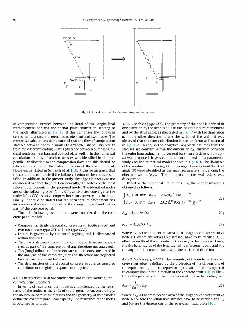
T

T C

C

Strut

Node N1

Node N2

11

θ

Fig. 16. Model proposed for the concrete panel component.

96 J. Henriques et al. / Engineering Structures 87 (2015) 86–104

of compression stresses between the bend of the longitudinalreinforcement bar and the anchor plate connection, leading tothe model illustrated in Fig. 16. It this comprises the followingcomponents: a single diagonal concrete strut and two nodes. Thenumerical calculations demonstrated that the flow of compressionstresses between nodes is similar to a ‘‘bottle’’ shape. This resultsfrom the different loading widths (distance between outer longitu-dinal reinforcement bars and contact plate width). In the numericalcalculations, a flow of tension stresses was identified in the per-pendicular direction to the compression flow, and this should betaken into account in the failure criterion of the concrete strut.However, as stated in Schlaich et al. [13], it can be assumed thatthe concrete strut is safe if the failure criterion of the nodes is sat-isfied. In addition, in the present study, the edge distances are notconsidered to affect the joint. Consequently, the nodes are the mostrelevant components of the proposed model. The identified nodesare of the following type: N1 is CTT, as two ties converge to thenode; N2 is CCC, as only compression struts converge to the node.Finally, it should be stated that the horizontal reinforcement tiesare considered as a component of the complete joint and not aspart of the concrete panel.

Thus, the following assumptions were considered in the con-crete panel model:

� Components: Single diagonal concrete strut (bottle shape) andtwo nodes (one type CTT and one type CCC).� Failure is governed by the nodal regions, and is disregarded

within the strut.� The flow of stresses through the wall to supports are not consid-

ered as part of the concrete panel and therefore not analyzed.� Ties (longitudinal reinforcement) are components considered in

the analysis of the complete joint and therefore are neglectedfor the concrete panel behavior.� The deformation of the diagonal concrete strut is assumed to

contribute to the global response of the joint.

4.4.2. Characterization of the components and determination of theconcrete panel properties

In terms of resistance, the model is characterized by the resis-tance of the nodes at the ends of the diagonal strut. Accordingly,the maximum admissible stresses and the geometry of these nodesdefine the concrete panel load capacity. The resistance of the nodesis obtained as follows.

4.4.2.1. Node N1 (type CTT). The geometry of the node is defined inone direction by the bend radius of the longitudinal reinforcementand by the strut angle, as illustrated in Fig. 17 with the dimensiona. In the other direction (along the width of the wall), it wasobserved that the stress distribution is non-uniform; as illustratedin Fig. 18a. Hence, as the analytical approach assumes that thestresses are constant within the dimension brb (distance betweenthe outer longitudinal reinforcement bars), an effective width (beff,-rb) was proposed. It was calibrated on the basis of a parametricstudy and the numerical model shown in Fig. 18b. The diameterof the reinforcement bar (drb), the spacing of bars (srb) and the strutangle (h) were identified as the main parameters influencing theeffective width (beff,rb). The influence of the wall edges wasdisregarded.

Based on the numerical simulations [16], the node resistance isobtained as follows:

srb P 80 mm : beff ;rb ¼ 2:62d0:96rb ðCos hÞ�1:05

srb < 80 mm : beff ;rb ¼ 2:62d0:96rb Cos hð Þ�1:05 srb

80

0:61

8<: ð22Þ

AN1 ¼ beff ;rb2r CosðhÞ ð23Þ

Fr;N1 ¼ AN10:75mf cd ð24Þ

where AN1 is the cross-section area of the diagonal concrete strut atnode N1 where the admissible stresses have to be verified, beff,rb

effective width of the concrete contributing to the node resistance,r is the bend radius of the longitudinal reinforcement bars and h isthe angle of the concrete strut with the horizontal direction.

4.4.2.2. Node N2 (type CCC). The geometry of the node, on the con-crete strut edge, is defined by the projection of the dimensions ofthe equivalent rigid plate, representing the anchor plate subjectedto compression, in the direction of the concrete strut. Fig. 19 illus-trates the geometry and the dimensions of this node, leading to:

AN2 ¼leff

CosðhÞ beff ð25Þ

where AN2 is the cross-section area of the diagonal concrete strut atnode N2 where the admissible stresses have to be verified and leff

and beff are the dimensions of the equivalent rigid plate [16].

brb

θ

a = 2 r Cos (θ)

brb

θ aa

Fig. 17. Definition of the width of the node N1.

(a) Scheme of stresses “under” the reinforcement bars

(b) Numerical model used in the parametric study

a

beff,rbσ – uniform

σ – non-uniform

σadm

σmin < σadm

σmax > σadma

Numericalapproach

Analytical approach

Target reinforcement bar

Fig. 18. Approach to derive the effective width under each reinforcement bar subjected to constant admissible compression stresses in a CTT node with bent reinforcementbars.

J. Henriques et al. / Engineering Structures 87 (2015) 86–104 97

Considering the admissible stresses and the node dimensions,the resistance of the node is obtained [16].

Fr;N2 ¼ AN23mf cd ð26Þ

fcd is the concrete design strength and t is a factor related to theconcrete characteristic compressive strength (fck).

4.4.2.3. Concrete panel properties. The resistance of the concretepanel is given by the minimum resistance of the two nodes, N1and N2, Eq. (27) [16]. Note that the resistance is projected in thehorizontal direction. It should be noted that for equilibrium innode N1, the vertical component of the load in the diagonal struthas to be equilibrated by the vertical reinforcement in the wall.

The design of this reinforcement is not analyzed in the presentstudy.

FC-T;CP ¼Min Fr;N1; Fr;N2ð ÞCosðhÞ ð27Þ

In terms of deformation, the problem is more complex as thestrain field within the diagonal strut is highly variable. However,as the deformation pattern of the concrete panel is not verysensitive to geometric variations [16], a mathematical expression(Eq. (28)) was fitted to the numerical force–deformation curve.Thus, the horizontal projection of the deformation of the diagonalstrut is obtained as a function of the horizontal component of theload on the strut. In Eq. (28), the load (FC-T,CP) is introduced in kNand the deformation is obtained in mm.

beff

leffbeff

θ

Fig. 19. Definition of the dimensions of node N2.

Table 9Ratio between FCP,An/FCP,Num.

Parameter thicknessof wall

Ratio[FCP,An/FCP,Num]

Parameter heightof composite beam

Ratio[FCP,An/FCP,Num]

Parameter bend radiusof longitudinal reinforcement

Ratio[FCP,An/FCP,Num]

JL-T150 0.588 JL-H226 0.998 JL-R80 0.850JL-T200 0.855 JL-H416 [Ref]a 0.997 JL-R120 0.974JL-T250 0.965 JL-H620 0.826 JL-R160 [Ref]a 0.997JL-T300 [Ref]a 0.997JL-T350 0.977JL-T400 0.951

a Ref – is the reference model which uses the same geometrical properties as in the tests performed in [15].

1,4

98 J. Henriques et al. / Engineering Structures 87 (2015) 86–104

dh;CP ¼ ð6:48E�8F2C-T;CP þ 7:47E�5FC-T;CPÞCos h ð28Þ

0

0,2

0,4

0,6

0,8

1

1,2

30 40 50 60 70 80 90

F anal

ytic

al /

F num

eric

al

θ [º]

Fig. 20. Influence of the strut angle (h) on the analytical prediction.

4.4.3. Application and validation of the modelIn order to assess the quality of the analytical model proposed

for the concrete panel, it was applied and compared to the numer-ical results [16]. Table 9 shows good agreement between theseresults, both in terms of failure mode (upper node in all cases)and resistance, except for thinner walls (150 mm) where the ratiois below 0.6. Plotting the resistance ratio as a function of the angleof the strut (h), as shown in Fig. 20, it can be observed that the ana-lytical model loses accuracy for angles above 70�, becoming tooconservative. For these cases, a different STM model should be con-sidered, e.g. adopting two diagonal springs with height equal tohalf of the lever arm. However, this was not pursued in the presentwork.

4.5. Joint mechanical model and assembly of joint components

4.5.1. Idealized modelThe joint components activated in the composite beam to rein-

forced concrete wall joint, subjected to hogging bending moment,were identified in Table 5. Accordingly, a representative spring andrigid link model was idealized and it is illustrated in Fig. 21a. Twovertical rigid bars separate three groups of springs. The rigid barsavoid the interplay between tension and compression components,simplifying the joint assembly. Another simplification was intro-duced by considering a single horizontal spring to represent theconcrete panel. In what concerns the tension springs, it wasassumed that slip and the longitudinal reinforcement are at thesame level although slip is observed at the steel beam – concreteslab interface. Finally, concerning the anchor plate, an equivalenttranslational spring (5–10)eq was considered, leading to the sim-pler joint model of Fig. 21b.

4.5.2. Joint assembly and determination of the joint propertiesFor the joint under hogging bending moment, the assembly

procedure is based on the mechanical model depicted in Fig. 21b.The determination of the joint properties under bending momentwas performed using two different approaches: ‘‘optimized’’ and‘‘simplified’’. EC4 model [4]). In the first case, the longitudinal steelreinforcement bar in slab follows the ECCS recommendations [24],while the slip of the composite beam and the anchor plate compo-nents consider the ‘‘sophisticated’’ models described before. Forthe second approach, the longitudinal steel reinforcement bar inslab follows the EC4 model [4], while the anchor plate componentsconsider the ‘‘simplified’’ models.

4.5.2.1. ‘‘Optimized’’ model. The mechanical model represented inFig. 21b presents only one row of components in tension andanother in compression. This leads to a simple assembly procedure,as no distribution of load is required amongst rows, as in steel/composite joint with two or more tension rows. Thus, the first step

J. Henriques et al. / Engineering Structures 87 (2015) 86–104 99

is the assembly of the components per row. Equivalent springs aredefined per row, as represented in Fig. 22. The determination oftheir properties takes into consideration the relative position ofthe components: acting in series or in parallel [16], leading toEqs. (29) and (30), for resistance (Feq,t and Feq,c) and deformation(Deq,t and Deq,c), respectively.

Feq ¼Min Fi to Fnf g ð29Þ

Deq ¼Xn

i¼1

Di ð30Þ

where the index i represents all relevant components either in ten-sion or in compression, depending on the row under consideration.

In order to determine the joint properties (Mj, Uj), it is necessaryto define the lever arm hr. According to the joint configuration, itwas assumed that the lever arm is the distance between the cen-troid of the longitudinal steel reinforcement bar and the mid thick-ness of bottom flange of the steel beam. The centroid of steelcontact plate is aligned with this reference point of the steel beam.Accordingly, the joint properties are obtained as follows [16]:

Mj ¼Min Feq;t ; Feq;c; FCP� �

hr ð31Þ

Uj ¼Deq;t þ Deq;c þ DCP

hrð32Þ

where Feq,t and Feq,c are the equivalent resistance of the tension andcompression rows, respectively, determined using Eq. (29); Deq,t

and Deq,c are the equivalent deformation of the tension and com-pression rows, respectively, determined using Eq. (30), FCP is theconcrete panel resistance, (Eq. (27)) and DCP is the deformation ofthe concrete panel (Eq. (28)).

4.5.2.2. ‘‘Simplified’’ model. In what concerns to the model assem-bly, the main difference lies in the deformation model which con-sists in the calculation of the joint initial rotational stiffness. Usingthe stiffness coefficients of the joint components, the joint rota-tional stiffness may be determined as expressed in Eq. (33) as pre-scribed in [6]. For the concrete panel, no stiffness coefficient wasderived though, as the contribution of this component is consider-ably smaller. Thus, as for two of the compression components, thiscomponent may be assumed as infinite rigid.

Sj;ini ¼Eh2

r

1keq;tþ 1

keq;c

� � ð33Þ

keq,t and keq,c are the equivalent stiffness coefficient of the tensionand compression components, respectively.

In the case of structural non-linear analysis, the joint character-ization requires the determination of its ultimate rotation capacity.This property is strongly dependent on the limiting component. Asobserved in the joint tests [15], this component is the longitudinalsteel reinforcement bar. In the code, no estimation of the ultimatedeformation capacity of this component is provided. The ECCS pub-lication [24] proposes a model to evaluate this parameter. Thismodel is suggested for evaluation of the joint rotation capacity.As conservative approach, the joint ultimate rotation capacitymay be determined using only the ultimate deformation capacityof the longitudinal steel reinforcement bar in the slab, and neglect-ing the contribution of the other joint components [16]. Thus, inEq. (34), the component ultimate deformation (Dsru) should beobtained using the appropriate equation given before.

Uj;u ¼Dsru

hrð34Þ

The complete moment–rotation curve is obtained using thesame principles as in Eurocode 3 Part 1-8 [6] for steel joints. The

modified (Sj) stiffness was determined using the appropriate jointstiffness modification coefficient g, as expressed in Eq. (35). Thenon-linear moment–rotation curve was defined using the jointstiffness expression prescribed by Eurocode 3 Part 1-8 [6], asreproduced in Eq. (36). In this expression, the stiffness ratio (l)is constant and equal to 1 up to 2/3 of Mj,Rd, after a non-linear rangeis defined up to Mj,Rd, as expressed in Eq. (37).

Sj ¼sj;ini

gð35Þ

Sj ¼Eh2

r

lP

i1ki

ð36Þ

With

if Mj;Ed 623 Mj;Rd : l ¼ 1

if 23 Mj;Rd < Mj;Ed 6 Mj;Rd : l ¼ 1:5Mj;Ed

Mj;Rd

� �W

8<: ð37Þ

The coefficient W is assumed equal 1.7 as recommend in Eurocode 4[4] for a contact plate joint. Values for the rotational stiffness mod-ification coefficient (g) are provided in Eurocode 3 Part 1-8 [6].These vary according to the joint configuration. In the case ofbeam-to-column joints the value of 2 is proposed. In the case ofcomposite beam to reinforced concrete walls, no information isavailable and therefore the use of the value for steel and compositejoints is suggested.

4.6. Validation of the model

The application of the model is shown in Fig. 23. The joint bend-ing moment to joint rotation curves compare analytical modelsand experimental tests. The quality of the model varies withparameter under analysis and with the type of model, ‘‘optimized’’or code based. For the resistance, the approximation of the ‘‘opti-mized model’’ is excellent. The code model limits the governingcomponent, the longitudinal steel reinforcement bar, to its yieldcapacity therefore, the lower resistance obtained with this modelwas expected. In terms of initial stiffness, the quality of the modelsis reversed. For this parameter, the code model provides a betterapproximation, being very close to the experimental results. Inwhat concerns the ‘‘optimized’’ model, it was seen that the initialstiffness required improvement. A stiffer response was observedwhich may be attributed to the fact that the ‘‘optimized’’ modelneglects discontinuity in the wall–slab interface. Because thesemembers are concreted in different stages, the small bond devel-oped between these members is rapidly exceeded. Consequently,an initial ‘‘crack’’ between wall and slab may be assumed fromthe beginning of loading and therefore the joint is a more flexiblethan if full continuity existed between these members. As the codebase model provided a good approximation for this parameter. Itwas decided to propose a modification to the joint componentmodel described above. In this way, the initial stiffness is deter-mined using same elongation length as used in the code basedmodel: 3.6h. See Fig. 15 for definition of the dimension h. Subse-quently, the model to determine the ultimate deformation was alsomodified introducing the previous consideration. In Table 10 issummarized the modifications proposed in [16] for the ‘‘opti-mized’’ model of the longitudinal steel reinforcement bar in theslab component. Though, it should be noted that if wall and slabare concreted at the same time, the initial proposal for the ‘‘opti-mized’’ model should be more accurate and therefore used insteadof the proposed modification. In what respects to the ultimaterotation, the ‘‘optimized’’ model is conservative though, also theanalytical model to determine the ultimate deformation of thelongitudinal steel reinforcement bar should be affected by the

(a) Complete model (b) Simplified model

1 2

11

34

5

7,8,910

6

1 2

11

34(5-10)eq

Fig. 21. Joint component model for the composite beam to reinforced concrete wall joint.

hr

Feq,t ; Δeq,t

Feq,c; Δeq,c

Fig. 22. Simplified joint model with assembly of components per row.

100 J. Henriques et al. / Engineering Structures 87 (2015) 86–104

wall–slab interface behavior. The code based model is absent inwhat concerns this parameter. The limit of the represented plateauwas assumed equal to the ultimate joint rotation determined withthe ‘‘optimized’’ model.

According to the results presented Fig. 23, both models presenta good approximation of the joint behavior and therefore, aresuitable for application.

5. Design procedure

The design procedure to determine the joint properties is sum-marized here below (Fig. 24). The range of validity of the proposed

(a) SP13

050

100150200250300350

0 10 20 30 40 50 60

Mj[

kN.m

]

Φj [mrad]

Experimental

'Optimized' proposal

Code based model

(c

0

50

100

150

200

250

300

350

0 20

Mj[

kN.m

]

Φ

Ex'OCo

Fig. 23. Joint bending moment to joint rotation curve (Mj–Uj) comparing modification

procedure is limited to joint configurations with only one row oflongitudinal reinforcement in tension. In the case of more thanone row in tension, the distribution of forces amongst tension rowsand the assembly procedure should be similar to that prescribed bythe [6] for steel joints. However, it has not yet been validated.

6. Parametric study

6.1. Introduction

The design methodology presented in the previous sections isable to predict with good level of accuracy the behavior of thesteel–concrete composite beam to reinforced concrete wall jointsubject to hogging moment. It highlights that various distinct fail-ure modes may control its behavior. In particular, depending onthe critical component, either a ductile or a brittle behavior maybe observed. Hence according to the design principles of the Euro-codes, it is important to assess and provide guidance for achievinga ductile behavior, especially if a semi-continuous design approachis to be used.

Table 5 identified the relevant components in the selected joint.Given that the longitudinal steel reinforcement is the componentthat may provide a ductile behavior, while the components that

(b) SP14

0

50

100

150

200

0 20 40 60

Mj[

kN.m

]

Φj [mrad]

Experimental

'Optimized' proposal

Code based model

) SP15

40 60

j [mrad]

perimentalptimized' proposalde based model

on the ‘‘optimized’’ model with experimental tests and code based model results.

Table 10Proposed modifications for the ‘‘optimized’’ model of the longitudinal steel rein-forcement in slab component.

Elongation length 3.6hUltimate

deformationq < 0:8% : Dsru ¼ 3:6hesrmu

q P 0:8% and a < Lt : Dsru ¼ 3:6hesrmu

q P 0:8% and a > Lt : Dsru ¼ 3:6hesrmu þ ða� 3:6hÞsrmy

Determine joint properties (Eq. 31 and Eq. 32)

Or(Eq. 31, Eq. 33 and Eq. 34)

Assembly of joint component per row (see Fig. 22)

Evaluation of the joint components (see Table 11)

Idealization of the joint component model (see Fig. 21)

Identification of joints components activated in the joint

Joint M-φ curve

Fig. 24. Composite beam to reinforced concrete wall joint design procedure.

J. Henriques et al. / Engineering Structures 87 (2015) 86–104 101

depend on the concrete behavior are brittle, a parametric studywas carried out to assess the behavior for a realistic range of geom-etries and material properties. Attention is mainly focused on thesteel reinforcement and the concrete panel. The force in the rein-forcement is a function of the steel grade and of the bars layout.The first aspect concerns the yield strength (fsyk), the ratio betweenultimate and yield strength (k) and ductility (es,u). The number andthe diameter of bars and the number of layers characterize the sec-ond aspect. In the analysis, three values of fsyk, four values of k,three es,u values and four reinforcement layouts are considered.

The possibility of the development of strut and tie mechanismsin the concrete panel depends on the angle h. This geometricalquantity is calculated through the ratio between the sum of thebeam depth and the slab thickness and the thickness of the wall.In the analysis, six beam profiles, four wall thickness twall and threeslab thickness sslab are considered. The concrete properties of thewall, i.e. the characteristic compressive cylinder (fck,cyl) or cubic(fck,cube) strength, and secant modulus of elasticity (Ecm), affect aswell the concrete panel behavior. In the analysis, five concretegrades are considered for the wall. In total, the parametric studycomprised 51,840 combinations. Table 12 summarizes the param-eters considered for the sensitivity study.

To consider the possibility of two concrete grades for wall andslab, a modification of the approach given in ECCS Publication n�109 [24] for longitudinal reinforcement behavior is proposed. Par-tial factors for steel reinforcements (cS = 1.15), for steel (cM = 1.0),for concrete (cC = 1.5) and for design shear resistance of a headed

stud (cm = 1.25) are taken into account. Table 11 synthesizes theused method in the parametric analysis for all components.

6.2. Results and discussion

Considering the simultaneous variation of all parameters, themost common failure type is the concrete panel (65.9%); only in28.0% of the cases slab reinforcement failure occurred; in few cases(6.2%) failure depends on the behavior of beam. Fig. 25 summarizesthese results.

6.2.1. Influence of slab reinforcementFig. 26 illustrates the influence of the slab reinforcement.

Firstly, increasing the reinforcement area, concrete panel failuregrows significantly from 62.4% for Case A to 80.5% for Case C. Con-sidering the reinforcement in two layers (Case D), brittle failuresare 47.0%. Beam failure is only relevant in Case D (19.2%).

As expected, one of the most influential parameter is the steelgrade. Increasing the yield strength, the percentage of concretepanel failure increases from 52.6% to 77.3%. The variation ofductility of the rebars does not lead to changes in failure typedistribution. Finally, increasing the ratio k leads to increasedconcrete panel failure from 57.9% to 72.9%.

6.2.2. Influence of angle hFig. 27 illustrates the influence of the angle h. The main

parameter that affects the development of the failure mecha-nism is the wall thickness. Failure occurs in the concrete panelin 93.4% of cases for a thickness of 160 mm. This percentagedrops to 76.0% for a thickness of 200 mm. Ductile failure onlybecomes the governing type of failure for a thickness of300 mm (62.9%).

For the three values of the slab thickness considered (120 mm,160 mm and 200 mm), failure happens in the concrete panel inmost of the cases (variation between 61.9% and 71.5%). Beam fail-ure does not vary appreciably (from 4.1% to 5.2%).

The depth of the beam determines a clear trend. For a depth of240 mm, failure occurs in the concrete panel in about 50% of thecases, increasing to 78.3% for a beam depth of 400 mm. For lowbeam depths, beam failure is not negligible (22.8%), decreasing sig-nificantly for larger beam depths.

6.2.3. Influence of wall concrete gradeFig. 28 shows the percentage of cases for each failure type. For

concrete grade C20/25, concrete panel failure governs for almostall the cases (97.2%). This percentage drops approximately linearlyto 36.9% for concrete C60/75.

6.2.4. Combined influence of wall thickness and concrete gradeThe combined influence of wall thickness and concrete grade is

illustrated in Fig. 29. For a thickness of 160 mm, concrete panelfailure governs for all types of concrete. This percentage drops from100% (C20/25) to 81.9% (C60/75). The rate of decrease of concretepanel failure increases with increasing thickness, reaching only3.0% for C60/75 and twall = 300 mm.

6.2.5. Summary and pre design charts for ductile behaviorThe sensitivity analysis shows the main parameters that affect

the failure mode:

– yield strength: cases with brittle failure rises from 52.6% (forfsyk = 400 MPa) to 77.3% (for fsyk = 600 MPa);

– wall thickness: the concrete panel failure occurs in 93.4% ofcases for a thickness of 160 mm and in 37.1% for a thicknessof 300 m;

Table 11Summary of the design expressions to determine the joint components behavior.

Component Property Expressions

Longitudinal reinforcement Resistance [16,24] Fsr ¼ rsrAsr

with

rsr1;d;SLAB ¼rsr1;SLAB

cs¼ f ctm;SLAB �kc

cs �q1þ q Es

Ec

h irsr1;d;WALL ¼

rsr1;WALLcs¼ f ctm;WALL �kc

cs �q1þ q Es

Ec

h irsrn;d;SL ¼ 1:3 � rsr1;d;SL

rsrn;d;WA ¼ 1:3 � rsr1;d;WA

Stiffness [16,24] D 6 Dsry : D ¼ eWAhþ eSLLt

esr1;SL ¼rsr1;d;SL

Es� Desr;SL esr1;WA ¼

rsr1;d;WAEs� Desr;WA

esr;SL ¼f ctm;SL �kc

cS �Es �q Desr;WA ¼f ctm;WA �kc

cS �Es �q

esrn;SL ¼ esr1;SL þ esr;SL esrn;WA ¼ esr1;WA þ Desr;WA

esmy;SL ¼f syk;d�rsrn;d;SL

Esþ esr1;SL þ Desr;SL

esmy;WA ¼f syk;d�rsrn;d;WA

Esþ esr1;WA þ Desr;WA

esmu;SL ¼ esy � btDesr;SL þ d 1� rsr1;d;SL

f syk;d

� �ðesu � esyÞ

esmu;WA ¼ esy � btDesr;WA þ d 1� rsr1;d;WA

f syk;d

� �ðesu � esyÞ

q < 0:8% : Dsu ¼ 2 � Lt �minðesmuSL; esmuWAÞq P 0:8% and a < Lt : Dsu ¼ hc

2 � esmu;WA þ Lt � esmu;SL

q P 0:8% and a < Lt : Dsu ¼ hc2 � esmu;WA þ Lt � esmu;SL þ ða� LtÞ � esmy;SL

Slip of beam Resistance [4]Eq. (24) with PRK ¼min 0:8�f u �p�d

2

cV �4;

0:29�a�d2ffiffiffiffiffiffiffiffiffiffif ckEcm

pcV

� �Stiffness Eq. (27)

Beam web and flange Resistance [6] Mc;Rd ¼Wpl �f syk

cM

Fc;fb;Rd ¼Mc;Rd

ðhb�tfbÞ

Stiffness Assumed infinite (rigid component)

Concrete panel Resistance Eq. (34)Stiffness Eq. (35)

T-stub Resistance [16] FC;Rd ¼f jd �Aeff

cC

withAeff ¼minð2c þ bcp; bapÞ � ðc0 þ lcp þminðc; e1;cpÞÞ

Stiffness Eq. (16)

Steel contact plate Resistance [4] Fcp ¼f y;cp �Aeff ;cp

cM

Stiffness Assumed infinite (rigid component)

Table 12Summary of the parametric study.

Element Parameter

Reinforcement Yield strengthfsyk (MPa) 400 500 600Coefficient fu/fsyk

k (–) 1.05 1.15 1.25 1.35Ductilityes,u (‰) 25 50 75Bar layout

Case A Case B Case C Case DN layers (–) 1 1 1 2N bars (–) 6 6 6 6Diameter bars (mm) 12 14 16 16

Slab Thicknesstslab (mm) 120 160 200

Wall Thicknesstwall (mm) 160 200 240 300Concrete gradefck,cyl (MPa) 20 30 40 50 60fck,cube (MPa) 25 37 50 60 75Ecm (GPa) 30 33 35 37 39

Beam ProfileIPE 240 IPE 270 IPE 300 IPE 330 IPE 360 IPE 400

102 J. Henriques et al. / Engineering Structures 87 (2015) 86–104

– total height of the composite beam: for the lowest value(360 mm) a ductile failure happens in 59.3% cases, while forthe highest height, 19.7% of cases show this failure;

– concrete grade: for C20/25, there are 97.2% cases of brittlebehavior, and this percentage drops to 36.9 % for concreteC60/75.

Though, this conclusions have to take into considerationthat the joint model for the concrete panel have a limitedaccuracy related to the angle of the concrete strut. Outside ofthe range concrete strut angles proposed, the model becomesconservative.

6.17

65.87

27.96

Beam Web and Flange

Joint Link

Reinforcement

Fig. 25. Failure type.

62.43

52.6057.87

73.5667.71

62.22

80.4977.31

66.06

47.01

72.92

0.00

20.00

40.00

60.00

80.00

100.00

Case A

Case B

Case C

Case D

400 500 600 1.05 1.15 1.25 1.35

Bar Layout [-] fsyk [MPa] k [-]

Failu

re M

echa

nism

[%

]

Fig. 26. Influence of slab reinforcement on brittle failure.

93.45

61.86

49.34

76.04

66.1758.8556.94

71.5365.14

37.06

69.76

78.29 78.30

0.00

20.00

40.00

60.00

80.00

100.00

Fai

lure

Mec

hani

sm [

%]

160 200 240 300 120 160 200 240 270 300 330

twall [mm] tslab [mm] hbeam [mm]360 400

Fig. 27. Influence of angle h.

1.163.79 6.94

9.00 9.92

97.25 83.97

63.74

47.80

36.86

1.59

12.24

29.31 43.20

53.22

0.00

20.00

40.00

60.00

80.00

100.00

20 29.6 40 50 60

Failu

re M

echa

nism

[%

]

fckcylWall [MPa]

Beam Web and Flange Joint Link Reinforcement

Fig. 28. Influence of wall concrete grade.

99.88

96.0689.35

81.94

100.00

94.9179.17

63.89

44.68

97.92

82.52

55.21

31.48

17.59

91.09

57.75

24.54

14.70

3.010.00

20.00

40.00

60.00

80.00

100.00

20 29.6 40 50 60

twall = 160mm twall = 160mm twall = 240mm twall = 300mm

t wall [mm]

Failu

re M

echa

nism

[%

]

Fig. 29. Influence of wall concrete grade and wall thickness.

160

180

200

220

240

260

280

300

20 30 40 50 60

twall[mm]

fckcylWall [MPa]

fsyk 400 MPa k 1,05 fsyk 500 MPa k 1,05 fsyk 600 MPa k 1,05 fsyk 400 MPa k 1,15fsyk 500 MPa k 1,15 fsyk 600 MPa k 1,15 fsyk 400 MPa k 1,25 fsyk 500 MPa k 1,25fsyk 600 MPa k 1,25 fsyk 400 MPa k 1,35 fsyk 500 MPa k 1,35 fsyk 600 MPa k 1,35

B

D

B

D

B

D

B

D

B

D

B

D

B

D

B

D

B

D

B

D

B

D

B

D

σ12

σ13

σ20

σ12

σ23

σ19

σ9

σ16

σ15

σ16

σ7

σ8

σ17

σ10

σ9

σ21

σ21

σ13

σ10

σ10

σ9

σ12

σ15

σ10

σ22

Fig. 30. Predesign chart for ductile behavior in case of total depth of the compositebeam between 360 and 440 mm.

J. Henriques et al. / Engineering Structures 87 (2015) 86–104 103

A pre design chart (Fig. 30) can be a useful tool in order to leadto a ductile failure. Here, the wall thickness (on the ordinate) isrelated to the concrete grade (on the abscissa). Separation curvesbetween ductile (top-right) and brittle (bottom-left) failure canbe built for nine steel grades (3 fsyk and 3 k). To take into accountthe total height of the composite beam, three charts may be drawn:Fig. 30 represents the pre design chart for a total height between360 mm and 440 mm; similar charts are available for other rangesof total height [37].

In Fig. 30, black lines refer to fsyk = 400 MPa, dark gray tofsyk = 500 MPa and light gray fsyk = 600 MPa; solid lines refer tok = 1.05, dash lines to k = 1.15, long dash lines to k = 1.25, dash–dot–dot lines to k = 1.35. Curves stretches found for regressionare shown dotted.

For example, for a total height of 390 mm, a wall thickness of160 mm and a concrete characteristic compressive cylinder equalto 50 MPa, the steel yield strength that ensure a ductile behavioris equal to 400 MPa with a k = 1.05, according to Fig. 30.

104 J. Henriques et al. / Engineering Structures 87 (2015) 86–104

7. Conclusions

This paper presents a design model for moment resisting com-posite beam to reinforced concrete wall joints. It allows to deter-mine the joint properties in terms of moment–rotation (Mj–Uj)curve. The basis of the presented study is the joint configurationdeveloped within the research project InFaSo [15]. The objectiveto characterize the behavior of steel-to-concrete joints providinganalytical tools, extending the component method, for a simpledesign was accomplished and may be summarized as follows:

� Identification of activated components.� Idealization of component model to reproduce the joint

response.� Characterization of all activated components in terms of force–

deformation curves.� Application and validation of joint model.� Parametric study.

Tools for characterization of all activated components are pre-sented in the paper. Though, the main emphasis has been givenfor those involving the concrete and therefore new componentshave been identified. The proposed models have been successfullyvalidate against numerical and experimental data available. Theintegration of these components in the global joint has been lateraccomplished and the accuracy of the global model verified againstexperimental tests. The application this model to the test speci-mens of the experimental programme of the research project InF-aSo [15] showed that the proposed models can provide an accuratecharacterization of the joint properties. Finally, the parametricstudy presented the application of the proposed model to a consid-erable number of cases exploiting the influence of different param-eters related to material and geometrical properties. According tothis study, as main outcome, the concrete panel appears as thecomponent governing the joint response. Thus, to achieve a ductilebehavior of the joint is essential to detail the concrete reinforce-ment in the concrete panel.

Acknowledgements

Part of the work reported in this paper was granted by theResearch Fund for Coal and Steel by the financed project N�RFSPR-2007-00051. The findings, observations and conclusions inthis paper are, however, those of the writers.

References

[1] Stahlbau Magazine, 68(8). Ernst & Sohn, Berlin; 1999.[2] CEN, European Committee for Standardization (2004). Eurocode 2: design of

concrete structures – part 1-1: general rules and rules for buildings. EN 1992-1-1. Brussels, Belgium; December 2004.

[3] CEN, European Committee for Standardization (2005). Eurocode 3: design ofsteel structures – part 1-1: general rules and rules for buildings. EN 1993-1-1.Brussels, Belgium; May 2005.

[4] CEN, European Committee for Standardization (2004). Eurocode 4: design ofcomposite steel and concrete structures – part 1-1: general rules and rules forbuildings. EN 1994-1-1. Brussels, Belgium; December 2004.

[5] Stark J, Hordijk DA. Where structural steel and concrete meet. In: EligehausenR, editor. International symposium on ‘‘connections between steel andconcrete. University of Stuttgart, Stuttgart; 2001. p. 1–11. ISBN 2-912143-25-X.

[6] CEN, European Committee for Standardization (2005). Eurocode 3: design ofsteel structures - part 1-8: design of joints. EN 1993-1-8. Brussels, Belgium;May 2005.

[7] CEB. CEB design guide: design of fastenings in concrete. Comité Euro-International du Béton, Lausanne, Suisse; 1997.

[8] EOTA. Guideline for European technical approval of anchors (metal anchors)for use in concrete. Part 1, 2 and 3 and annexes A, B, and C. Final draft, EOTA,Brussels; February 1997.

[9] ACI. ACI 318: ACI standard 318. Building code requirements for structuralconcrete. American Concrete Institute; 2001.

[10] fib, Federation International du Beton. fib guide for the design of fastenings inconcrete: part 1: general, part 2: post-installed anchors – mechanical, part 3:post-installed anchors – bonded anchors and rebar systems, part 4: headedanchors, part 5: anchor channels. Lausanne; 2007.

[11] CEN, European Organization for Standardization. CEN technical specification(TS): design of fastenings for use in concrete, part 1: general, part 2: headedfasteners, part 3: anchor channels, part 4: post-installed fasteners –mechanical systems, part 5: post-installed fasteners – chemical systems.Brussels; 2007.

[12] Eligehausen R, Mallée R, Silva JF. Anchorage in concreteconstruction. Berlin: Ernst & Sohn; 2006.

[13] Schlaich J, Schäfer K, Jennewein M. Toward a consistent design of structuralconcrete. PCI J 1987;32(3):74–150.

[14] Wald F, Sokol Z, Steenhuis CM, Jaspart J-P. Component method for steelcolumn bases. Heron 2008;53(1/2):3–20.

[15] Kuhlmann U, Eligehausen R, Wald F, da Silva L, Hofmann J. New marketchances for steel structures by innovative fastening solutions. Final report ofthe RFCS project INFASO, project N� RFSPR-CT-2007-00051; 2014.

[16] Henriques J. Behaviour of joints: simple and efficient steel-to-concrete joints.PhD thesis, University of Coimbra; June 2013.

[17] Henriques J, Simões da Silva L, Valente I. Numerical modeling of compositebeam to reinforced concrete wall joints part I: calibration of joint components.Eng Struct 2013;52:747–61.

[18] Henriques J, Simões da Silva L, Valente I. Numerical modeling of compositebeam to reinforced concrete wall joints part II: global behavior. Eng Struct2013;52:734–46.

[19] Schäfer M. Zum Rotationsnachweis teiltragfähiger Verbundknoten inverschieblichen Verbundrahmen. Doctoral thesis, University of Stuttgart;July 2005 [in German].

[20] Zoetemeijer P. A design method for tension side of statically-loaded boltedbeam-to-column joints. Heron 1974;20(1):1–59.

[21] Jaspart J-P. Étude de la semi-rigidité des nœuds poutre-colonne et soninfluence sur la résistance des ossatures en acier. PhD thesis, University Liège,Liège; 1991 [in French].

[22] Weynand K, Jaspart J-P, Steenhuis M. The stiffness model of revised annex J ofEurocode 3. In: Colson A, Bjorhovde R, Zandonini R, editors. Connections insteel structures III. Oxford and New York: Pergamon; 1996. p. 441–52.

[23] Simões da Silva L, Coelho A. A ductility model for steel connections. J ConstrSteel Res 2002;41(1):31–60.

[24] European Convention for Constructional Steelwork – ECCS. Design ofcomposite joints for buildings. ECCS publication n�109. Technical committee11 – composite structures. Belgium; 1999.

[25] Schlaich J, Schäfer K. Design and detailing of structural concrete using strut-and-tie models. Struct Eng 1991;69(6).

[26] Comité Euro-International du Béton – CEB. CEB-FIP model code 1990: designcode. Lausanne; 1993.

[27] Narayanan RS, Beeby A. Designers’ guide to EN1992-1-1 and EN 1992-1-2.Eurocode 2: design of concrete structures. General rules and rules for buildingsand structural fire design. Series editor Haig Gulvanessian, Thomas Telford,London; 2005.

[28] Federation International du Béton – fib. Practitioners’ guide to finite elementmodelling of reinforced concrete structures. fib – Bulletin 45. Lausanne; 2008.

[29] Guisse S, Vandegans D, Jaspart J-P. Application of the component method tocolumn bases: experimentation and development of a mechanical model forcharacterization. Research Centre of the Belgian Metalworking Industry,MT195, Liège; 1996.

[30] Wald F, Sokol Z, Steenhuis M. Proposal of the stiffness design model of thecolumn bases. In: Connections in steel structures III: behaviour, strength anddesign. Proceedings of the third international workshop, Trento; 1996. p. 237–49.

[31] Weynand K. Column bases in steel building frames. COST C1 – semi-rigidbehaviour of civil engineering structural connections. Luxembourg; 1999.

[32] Steenhuis M, Wald F, Sokol Z, Stark J. Concrete in compression and base platein bending. Heron 2008;53(1/2):51–68 [Delft].

[33] Demonceau J. Steel and composite building frames: sway-response underconventional loading and development of membrane effects in beam furtherto an exceptional actions. PhD thesis, University of Liège, Liège; 2008.

[34] Anderson D, Najafi AA. Performance of composite connections: major axis endplate joints. J Constr Steel Res 1994;31:31–57.

[35] Aribert JM. Influence of slip on joint behaviour. In: Connections in steelstructures III: behaviour, strength and design. Third international workshop,Trento; 1995. p. 29–31.

[36] Ahmed B, Nethercot DA. Prediction of initial stiffness and available rotationcapacity of major axis composite flush endplate connections. J Constr Steel Res1997;41(1):31–60.

[37] Wald F, Hofmann J, Kuhlmann U, Becková S, Gentili F, Gervásio H, et al. Designof steel-to-concrete joints. Design manual II’’, RFCS project valorisation ofknowledge for innovative fastening solution between steel and concrete,project N� RFSPR-CT-2007-00051; 2014.