complexity of normal forms on structures of bounded degree
TRANSCRIPT
Complexity of
Normal Formson Structures of Bounded Degree
Dissertation
zur Erlangung des akademischen Grades
doctor rerum naturalium
(Dr. rer. nat.)
im Fach Informatik
eingereicht an der
Mathematisch-Naturwissenschaftlichen Fakultät
der Humboldt-Universität zu Berlin
von
Dipl.-Inf. Lucas Heimberg
Präsidentin der Humboldt-Universität zu Berlin
Prof. Dr.-Ing. Dr. Sabine Kunst
Dekan der Mathematisch-Naturwissenschaftlichen Fakultät
Prof. Dr. Elmar Kulke
Gutachter/innen:
1. Prof. Dr. Nicole Schweikardt, Humboldt-Universität zu Berlin
2. Prof. Dr. Dietrich Kuske, Technische Universität Ilmenau
3. Prof. Dr. Stephan Kreutzer, Technische Universität Berlin
Tag der mündlichen Prüfung: 18. 12. 2017

iii
Abstract
Normal forms express semantic properties of logics by means of syntacticalrestrictions. Often, normal forms allow algorithms to benefit from restrictions ofthe expressive power of a logic. A typical example is the locality of first-order logic(FO), which implies that, e.g., properties like reachability or connectivity cannotbe defined in FO. This is formalised by Gaifman’s local normal form, which statesthe satisfaction conditions of an FO-formula by a Boolean combination of localstatements. Gaifman normal form serves as a first step in fixed-parameter model-checking algorithms, parameterised by the size of the formula, on a wide range ofsparse graph classes. However, it is known that, even on acyclic graphs, there arenon-elementary lower bounds for the costs involved in transforming a formula intoGaifman normal form. This leads to an enormous parameter-dependency of theaforementioned algorithms. Similar non-elementary lower bounds also hold forFeferman-Vaught decompositions, which are an important tool in model-checkingand satisfiability-checking, and for the preservation theorems by Lyndon, Łoś, andTarski, stating that a formula is preserved under extensions (homomorphisms) ifand only if it is equivalent to an existential (existential-positive) formula.
This thesis investigates the complexity of these normal forms when restrictingattention to classes of structures of bounded degree, for which the non-elementarylower bounds are known to fail. As a matter of fact, the thesis provides algorithmswith elementary and even worst-case optimal running time for the construction ofGaifman normal form and Feferman-Vaught decompositions under this restriction.For the preservation theorems, algorithmic versions with elementary runningtime and non-matching lower bounds are provided.
Crucial for these results is the notion of Hanf normal form, which, on classes ofstructures of bounded degree, is also in its own right an important ingredient foralgorithms. Here, the present thesis provides a characterisation of sets of unarycounting quantifiers in terms of ultimately periodic sets, for which the respectiveextensions of FO allow generalisations of Hanf normal form. In particular, thisincludes modulo-counting quantifiers. For all such extensions, a construction ofHanf normal form with worst-case optimal running time is presented. On classesof structures of bounded degree, this leads to fixed-parameter model-checkingalgorithms for all such extensions and also allows respective generalisations of theconstructions for Feferman-Vaught decompositions and preservation theorems.


v
Zusammenfassung
Normalformen drücken semantische Eigenschaften einer Logik durch syntaktischeRestriktionen aus. Sie ermöglichen es Algorithmen, Grenzen der Ausdrucksstärkeeiner Logik auszunutzen. Ein Beispiel ist die Lokalität der Logik erster Stufe (FO),die impliziert, dass Graph-Eigenschaften wie Erreichbarkeit oder Zusammenhangnicht FO-definierbar sind. Gaifman-Normalformen drücken die Bedeutung einerFO-Formel als Boolesche Kombination lokaler Eigenschaften aus. Sie haben einewichtige Rolle in Model-Checking Algorithmen für eine Vielzahl von Klassen dünnbesetzter („sparse“) Graphen, deren Laufzeit durch die Größe der auszuwerten-den Formel parametrisiert ist. Selbst für Klassen azyklischer Graphen ist jedochbekannt, dass Gaifman-Normalformen nur mit nicht-elementarem Aufwand kon-struiert werden können. Dies führt zu einer enormen Parameterabhängigkeitder genannten Algorithmen. Ähnliche nicht-elementare untere Schranken sindauch für Feferman-Vaught-Zerlegungen bekannt, die ein wichtiges Werkzeug fürModel-Checking und Erfüllbarkeitsalgorithmen sind, und für die Erhaltungssätzevon Lyndon, Łoś und Tarski, laut denen die Gültigkeit einer Formel unter Erwei-terungen (Homomorphismen) genau dann erhalten bleibt, wenn die Formel zueiner existenziellen (existenziell-positiven) Formel äquivalent ist.Diese Arbeit untersucht die Komplexität der genannten Normalformen auf
Klassen von Strukturen beschränkten Grades, für welche die nicht-elementarenunteren Schranken nicht gelten. Für diese Einschränkung werden Algorithmen mitelementarer Laufzeitschranke für die Konstruktion von Gaifman-Normalformen,Feferman-Vaught-Zerlegungen, und für die Erhaltungssätze von Lyndon, Łoś undTarski, vorgestellt, die in den ersten beiden Fällen sogar worst-case optimal sind.
Ein wichtiges Werkzeug hierfür sind Hanf-Normalformen die, auf Klassen vonStrukturen beschränkten Grades, auch Anwendungen in Algorithmen finden. Einweiterer Beitrag dieser Arbeit ist eine Charakterisierung von Mengen unärerZählquantoren, für die die jeweilige Erweiterung von FO Hanf-Normalformenerlaubt. Es stellt sich heraus, dass dies genau die Zählquantoren sind, die durchultimativ-periodische Mengen charakterisiert sind. Dies schließt insbesondereModulo-Zählquantoren ein. Für Erweiterungen von FO durch solche ultimativ-periodische Zählquantoren wird eine worst-case optimale Konstruktion von Hanf-Normalformen beschrieben. Auf Klassen von Strukturen von beschränktem Gradführt dies für solche Erweiterungen von FO zu parametrisierten Model-Checking-Algorithmen und zu Verallgemeinerungen der Algorithmen für Feferman-Vaught-Zerlegungen und die Erhaltungssätze von Lyndon, Łoś und Tarski.

vii
Acknowledgements
This thesis would not have been possible without the help, inspiration, andmotivation I received from my colleagues, family, and friends.
First and foremost, I want to thank my advisor and coauthor Prof. Dr. NicoleSchweikardt. I am very grateful for the opportunity to work and learn in herresearch group. Her deep scientific insights and perseverance were an enormousinspiration for me. I am also thankful for her patience and helpfulness, and thecooperative atmosphere she created in her research group.To Prof. Dr. Dietrich Kuske, I’m indebted for reviewing my thesis, for many
interesting discussions at the Highlights conferences, and for being a greatcoauthor. I also want to thank Prof. Dr. Stephan Kreutzer for being reviewer ofmy thesis and for my research stay at his research group in the summer of 2013.
This thesis would have been much harder to finish without the support of themembers of my current research group “Logic in Computer Science” in Berlin,my former research group in Frankfurt, and also the members of the researchgroup “Computer Science Education”. In particular, I want to thank PetraKämpfer, Jutta Nadland, and Eva Sandig for supplying the infrastructure for agood working environment. I would like to point out Dr. André Frochaux andDr. Berit Grußien for their open ears, their constructive and uplifting support,and their tolerance in times of frustration, as well as for sailing trips and a reliablesupply of cookies. Furthermore, I want to thank my coauthor Frederik Harwathfor so many inspiring discussions about logic. I also thank PD Dr. LouchkaPopova-Zeugmann for motivating me and forcing me to stay focussed.
In particular, I want to thank my parents, Juliane and Andreas Heimberg, andmy brother, Felix Heimberg, for their trust, appreciation, and practical supportduring the last years. For a long time, they endured me being either absent orabsent-minded. I am very lucky to have such a family.Finally, I want to focus on my friends. Thank you, André Frochaux and
Waltraud Wild. You were a rock in troubled waters, and I could not imaginebetter friends than you. In the same way, and without any other orderingthan imposed by the alphabet, I also want to thank Aline von der Assen, BeritGrußien, Christoph Hethey, Frauke Quurck, Frederik Harwath, Irina Ewomba,Jane Katusiime, Katharina Zeh, Maria Tammik, Mariano Zelke, Noemi LaBaume, Sandra Kiefer, Sandra Schulz, Stephan Grötschel, Stephan Liebchen,and Svetlana Kulagina.
In memory of Michael Härtel22. 8. 1980 – 16. 7. 2013

Contents
Abstract iii
Zusammenfassung v
Acknowledgements vii
Contents ix
1 Introduction 1
2 Preliminaries 172.1 Basic Notation . . . . . . . . . . . . . . . . . . . . . . . . . . . . 172.2 Model of Computation . . . . . . . . . . . . . . . . . . . . . . . . 192.3 Signatures and Structures . . . . . . . . . . . . . . . . . . . . . . 202.4 Logics . . . . . . . . . . . . . . . . . . . . . . . . . . . . . . . . . 212.5 Ultimately Periodic Quantifiers . . . . . . . . . . . . . . . . . . . 272.6 Transductions . . . . . . . . . . . . . . . . . . . . . . . . . . . . . 292.7 Graphs . . . . . . . . . . . . . . . . . . . . . . . . . . . . . . . . . 352.8 Locality . . . . . . . . . . . . . . . . . . . . . . . . . . . . . . . . 362.9 A Divide-and-Conquer Scheme for Formulae . . . . . . . . . . . . 42
3 Hanf Normal Form 493.1 Introduction . . . . . . . . . . . . . . . . . . . . . . . . . . . . . . 493.2 Modulo-Counting Quantifiers . . . . . . . . . . . . . . . . . . . . 553.3 An Alternative Proof of Nurmonen’s Locality Theorem . . . . . . 733.4 Model-Checking . . . . . . . . . . . . . . . . . . . . . . . . . . . . 763.5 Conclusion . . . . . . . . . . . . . . . . . . . . . . . . . . . . . . 79
ix

x Contents
4 Gaifman Normal Form 814.1 Introduction . . . . . . . . . . . . . . . . . . . . . . . . . . . . . . 814.2 Gaifman Normal Form for Counting-Sentences . . . . . . . . . . 854.3 The Gaifman Normal Form Algorithm . . . . . . . . . . . . . . . 944.4 Conclusion . . . . . . . . . . . . . . . . . . . . . . . . . . . . . . 95
5 Feferman-Vaught Decompositions 975.1 Introduction . . . . . . . . . . . . . . . . . . . . . . . . . . . . . . 975.2 Constructing Decompositions from Hanf Normal Form . . . . . . 1015.3 Decompositions with respect to Transductions . . . . . . . . . . . 1075.4 Decompositions with respect to Direct Products . . . . . . . . . 1115.5 Conclusion . . . . . . . . . . . . . . . . . . . . . . . . . . . . . . 114
6 Preservation Theorems 1176.1 Introduction . . . . . . . . . . . . . . . . . . . . . . . . . . . . . . 1176.2 Preservation under Extensions . . . . . . . . . . . . . . . . . . . 1246.3 Preservation under Homomorphisms . . . . . . . . . . . . . . . . 1376.4 Closure Properties . . . . . . . . . . . . . . . . . . . . . . . . . . 1456.5 Conclusion . . . . . . . . . . . . . . . . . . . . . . . . . . . . . . 147
7 Tuple-Counting Quantifiers 1497.1 Introduction . . . . . . . . . . . . . . . . . . . . . . . . . . . . . . 1497.2 Resolving Tuple-Counting Quantifiers . . . . . . . . . . . . . . . 1517.3 Hanf Normal Form . . . . . . . . . . . . . . . . . . . . . . . . . . 1587.4 Feferman-Vaught Decompositions . . . . . . . . . . . . . . . . . . 1637.5 Preservation Theorems . . . . . . . . . . . . . . . . . . . . . . . . 1687.6 Conclusion . . . . . . . . . . . . . . . . . . . . . . . . . . . . . . 174
8 Ultimately Periodic Quantifiers 1778.1 Introduction . . . . . . . . . . . . . . . . . . . . . . . . . . . . . . 1778.2 Only Ultimately Periodic Quantifiers are Additive . . . . . . . . 1798.3 Modulo-Counting versus Ultimately-Periodic Quantifiers . . . . . 1828.4 Hanf Normal Form . . . . . . . . . . . . . . . . . . . . . . . . . . 1878.5 Feferman-Vaught Decompositions . . . . . . . . . . . . . . . . . . 1938.6 Preservation Theorems . . . . . . . . . . . . . . . . . . . . . . . . 1998.7 Conclusion . . . . . . . . . . . . . . . . . . . . . . . . . . . . . . 203
Contents xi
9 Lower Bounds 2059.1 Introduction . . . . . . . . . . . . . . . . . . . . . . . . . . . . . . 2059.2 Tree Encodings . . . . . . . . . . . . . . . . . . . . . . . . . . . . 2089.3 Hanf Normal Form . . . . . . . . . . . . . . . . . . . . . . . . . . 2209.4 Gaifman Normal Form . . . . . . . . . . . . . . . . . . . . . . . . 2239.5 Feferman-Vaught Decompositions . . . . . . . . . . . . . . . . . . 2399.6 Preservation Theorems . . . . . . . . . . . . . . . . . . . . . . . . 2469.7 Conclusion . . . . . . . . . . . . . . . . . . . . . . . . . . . . . . 259
10 Conclusion 261
Bibliography 267
Index 274

1 Introduction
Normal forms express semantic properties of a logic by means of syntacticalrestrictions. On the one hand, this can be used for inexpressibility results, thatis, for showing that certain properties are not definable in the logic (cf., e.g.,[Lib97, LN00, EF99, Lib04]). On the other hand, normal forms make limitationsof the expressive power of a logic accessible for algorithmic purposes [See96, FG01,GW04, FG04, Kre11, GKS14, DG07, KS11, DSS14, Seg14, BKS17, KS17].In particular in the latter context, not only the existence of normal forms
is of interest, but also their efficiency, that is, the size of the normal form incomparison to the original formula, and the resources required for its construction[GW04, DGKS07, DG07, Lin08, BK12, HKS13, HKS16, KS17].
A typical example is Gaifman normal form [Gai82] for first-order logic, whichmakes local conditions for the validity of a formula in a structure explicit.On various classes of sparse structures, Gaifman normal form leads to fixed-parameter tractable model-checking algorithms that are parameterised by thesize of the input formula [FG01, GW04, FG04, Kre11, GKS14]. More precisely,the algorithm’s running time only depends linearly or pseudo-linearly on thesize of the structure the input formula is checked against. On the other hand,the running time in terms of the size of the input formula depends on the timeneeded for turning the formula into Gaifman normal form.
However, it was shown that, without further restrictions, this transformationis only possible with non-elementary cost [DGKS07]. Thus, the parameter-dependency of such a model-checking algorithm is not bounded by any k-foldexponential function for any k ∈ N whatsoever.Similar lower bounds were shown for the size of Feferman-Vaught decomposi-
tions [DGKS07] and for the preservation theorems of Lyndon, Łoś, and Tarski.More precisely, there are non-elementary lower bounds on the size of an equivalentexistential sentence for a sentence that is preserved under extensions [DGKS07],and for the size of an equivalent existential-positive sentence for a sentence thatis preserved under homomorphisms [Gur90, Ros08].A closer look at the lower bound proofs shows their failure on classes of
1
2 Chapter 1. Introduction
structures of bounded degree. A structure has degree ≤ d (for some d ∈ N) if foreach of its elements, there are at most d other elements with which it occurstogether in the tuples of the relations of the structure. A class of structureshas bounded degree if there is a d ∈ N such that all structures in the class havedegree ≤ d.This thesis provides an analysis of the efficiency of the mentioned normal
forms when equivalence to the original formulae is only required with respectto a class of structures of bounded degree. Under this relaxation, algorithmswith elementary running time are developed and complemented by – mostly –matching lower bounds [HKS13, HHS14, HHS15].
For classes of structures of bounded degree, crucial tools for the above men-tioned results are Hanf’s locality theorem [Han65, FSV95] for first-order logic andthe corresponding Hanf normal form [EF99, BK12]. Both also found importantapplications in algorithms on classes of structures of bounded degree in theirown right [See96, FG04, DG07, KS11, BKS17, KS17].Hanf’s locality theorem does not only hold for first-order logic but has a
generalisation to the extension of first-order logic by modulo-counting quanti-fiers [Nur00], which also gives rise to a normal form [HKS16]. This motivatesa second line of results of this thesis, examining extensions of first-order logicby unary counting quantifiers. Here, a complete characterisation of all the setsof unary counting quantifiers that have an analogue to Hanf’s theorem andHanf normal form is given in terms of ultimately periodic sets (cf. [Mat94]).Furthermore, it is shown that in all these cases, the corresponding variant ofHanf normal form can be computed in worst-case optimal time [HKS16].The generalisation of Hanf normal form to formulae using ultimately peri-
odic quantifiers also leads to corresponding generalisations of the elementaryalgorithms concerning Feferman-Vaught decompositions and preservation theor-ems.A well-known construction (cf., e.g., [Str94]), which resolves tuple-counting
quantifiers into quantifiers counting only single elements of structures, furthermoreallows to extend these results to ultimately periodic tuple-counting quantifiers.
The results presented in this thesis were largely already published in [HKS13,HHS14, HHS15, HKS16]. In the following pages, an overview over these resultsis given. To this aim, the normal forms of concern are informally introduced andprevious work, in particular with a focus on applications of the normal forms andknown upper and lower bounds for their efficiency, is mentioned. The overviewis in parts based on [HKS13, HHS14, HHS15, HKS16].
3
Normal Forms for Locality
It is known that first-order logic1 (FO) can only express local properties (cf.,e.g., [Han65, Gai82, FSV95, SB99, EF99, Lib04]). In particular, this excludesproperties like connectivity or reachability in graphs, which can only be decided bya global view on the graph (cf., e.g., [FSV95, EF99, Lib04]). There are differentformalisations of this limitation to the expressive power of FO in the shape oftheorems by Hanf, by Gaifman, and by Schwentick and Barthelmann [Han65,Gai82, FSV95, SB99]. All these formalisations of locality give rise to normalforms for FO.
In particular, sentences in Hanf normal form [EF99, BK12] are Boolean com-binations of statements of the form
(H) “there are ≥ k elementswhose r-neighbourhood has isomorphism type τ”,
whereas sentences in Gaifman normal form [Gai82] are Boolean combinations ofstatements of the form
(G) “there are ≥ k elements x of pairwise distance > 2rwhose r-neighbourhood satisfies a formula %(x).”
For formulae with free variables, Hanf normal form additionally allows state-ments that check the isomorphism type of the r-neighbourhood of their freevariables [HKS16]. For the same purpose, Gaifman normal form uses, moregenerally, formulae whose validity only depends on the r-neighbourhood of theirfree variables [Gai82].An important difference between Hanf’s and Gaifman’s theorem is that the
former only applies to classes of structures of bounded degree, while the latterapplies to all relational structures.The theorems of Hanf and Gaifman have found various applications in al-
gorithms and complexity (cf., [See96, LN00, Lib97, FG01, GW04, DGKS06,DG07, Kre11]). In particular, there are very general algorithmic meta-theoremsstating that FO model-checking is fixed-parameter tractable for various classesof sparse structures, ranging from classes of structures of bounded degree to
1In the subsequent chapters of this thesis, threshold-counting quantifiers, stating that thereare ≥ k witnesses for a quantified formula, are often assumed to be built-in. However, theycan easily be expressed in plain first-order logic with a slight increase in quantifier rank andformula size. For the introduction, we can ignore this distinction.
4 Chapter 1. Introduction
classes that are nowhere dense [See96, FG01, GW04, FG04, Kre11, GKS14].Furthermore, it was proven that results of queries defined by formulae of FO (andcertain extensions of it) on classes of structures of bounded degree or low degreecan be enumerated with constant delay after a (pseudo-)linear time preprocessingphase [DG07, KS11, DSS14, Seg14, BKS17, KS17]. Another application arepolynomial time approximation schemes for FO-definable optimisation problemson classes with excluded minors [DGKS06]. In the context of such applica-tions, the efficiency of constructing such normal forms has attracted interest[GW04, DGKS07, DG07, Lin08, BK12, HKS13, HKS16, KS17].
Hanf Normal Form
A direct consequence of Hanf’s locality theorem [Han65, FSV95] is that for eachFO-formula ϕ over a relational signature σ, and for every degree bound d ≥ 0,there exists a d-equivalent Hanf normal form ψ, that is, a Hanf normal formwhich is equivalent to ϕ on all σ-structures of degree ≤ d [EF99, BK12].
A first algorithm for the construction of such Hanf normal form for FO wasdescribed in [See96]. However, this algorithm is not primitive-recursive. The firstprimitive-recursive algorithms for computing Hanf normal form can be foundin [DG07, Lin08]. The algorithm from [DG07], at first sight, seems to be non-elementary, but it actually is 4-fold exponential [Clo12, HKS13]. Finally, a 3-foldexponential algorithm and a matching lower bound were presented in [BK12].
Modulo-Counting Quantifiers
Notions of locality have also been developed for extensions of FO, and theyhave found application in proving inexpressibility results for these logics (cf.,e.g., [Nur96, Lib98, HLN99, Nur00, LN00, Lib04, KS17]). When restrictingattention to classes of finite structures of bounded degree, these locality notionsalso give rise to normal forms for the respective logics.In particular, in [Nur00], Nurmonen extended Hanf’s locality theorem to the
extension of FO by a modulo-counting quantifier Dp of period p ≥ 2, where aformula of the form Dpy ψ(x, y) states that the number of witnesses y for ψ(x, y)is divisible by p. As an easy consequence of Nurmonen’s theorem, one obtainsthat for every sentence ϕ, possibly using the quantifier Dp, and for every degreebound d ≥ 0, there exists a d-equivalent Boolean combination of statements ofthe form (H) and of the form
5
“the number of elements whose r-neighbourhood has isomorphism type τ isdivisible by p with remainder m.”
Again, we say that ψ is in Hanf normal form.For algorithmic applications, an effective procedure for computing ψ on input
of ϕ and the degree bound d would be desirable (cf., e.g., the use of Nurmonen’stheorem in the proof of Theorem 7 in the full version of [NSST15]). Similarly toHanf’s theorem, the proof of [Nur00], however, does not lead to such an effectiveprocedure.
In this direction, the contribution of this thesis is an algorithm which, on inputof a degree bound d and a formula ϕ from FO extended by an arbitrary set ofmodulo-counting quantifiers, computes a d-equivalent Hanf normal form. Thisalgorithm uses 3-fold exponential time for d ≥ 3 and 2-fold exponential time ford = 2 and is worst-case optimal in both cases.As an easy application of this result, we obtain that Seese’s [See96] fixed-
parameter tractability result for the data complexity of FO model-checking onclasses of structures of bounded degree can be generalised to extensions of FOby sets of modulo-counting quantifiers. Moreover, the existence of Hanf normalform for FO with sets of modulo-counting quantifiers also leads to an alternativeproof of Nurmonen’s locality theorem.
Both aforementioned results were published in [HKS16].Recently, the construction of Hanf normal form for FO with modulo-counting
quantifiers found use in [BKS17]. There, it serves as an intermediate step inalgorithms that enumerate the results of queries with constant delay after a lineartime preprocessing phase, even in the presence of updates on the database.
Ultimately Periodic Quantifiers
Generalising on Nurmonen’s locality theorem and the corresponding Hanf normalform, the following questions arise:
(1) Which extensions of FO by a set C of unary counting quantifiers permitHanf normal form?
(2) If such an extension of FO permits Hanf normal form, (how) can theseHanf normal forms be computed?
On finite structures, a unary counting quantifier is a subset Q of the naturalnumbers, and a sentence in Hanf normal form is a Boolean combination ofstatements of the form
6 Chapter 1. Introduction
“there are n+ k elements whose r-neighbourhood has isomorphism type τ ,for some number n ∈ Q”,
where Q is a quantifier from C or the existential quantifier. We say that theextension of FO by the unary counting quantifiers from the set C permits Hanfnormal form if for each relational signature σ and every degree bound d, eachformula over the signature σ has a d-equivalent Hanf normal form.This thesis provides a complete answer to both questions. Concerning Ques-
tion (1), a characterisation is given to the effect that an extension of FO by unarycounting quantifiers permits Hanf normal form if and only if all allowed quantifi-ers are ultimately periodic. Intuitively, ultimately periodic [Mat94] quantifiersare the quantifiers that can be obtained from Boolean combinations of modulo-counting and threshold-counting quantifiers. Answering Question (2) it is shownthat for each such extension of FO, Hanf normal form can also be computed inroughly the same time as for the special case of modulo-counting quantifiers.This way, we also obtain a corresponding generalisation of Seese’s model-checkingalgorithm for ultimately periodic quantifiers. The results presented above werepublished in [HKS16].
Gaifman Normal Form
Already Gaifman’s article [Gai82] provides an algorithm for transforming FO-formulae into Gaifman normal form, which proceeds by an induction over theshape of the input formula. However, this algorithm leads to a non-elementaryblow-up of the size of the Gaifman normal form in terms of the quantifier rankof the input formula. In [DGKS07] it is proven that indeed this transformationis only possible at non-elementary cost, if the algorithm has to handle arbitraryFO-formulae and has to return a Gaifman normal form that is equivalent to theinput formula on all structures (more generally, even on all finite trees). However,this does not rule out more efficient algorithms (in particular, with elementaryrunning time) for cases where restrictions on the form of the input formula areimposed, or where equivalence of the computed Gaifman normal form to theinput formula is only required on a restricted class of structures.Towards restricted formulae, we know from [GW04] that purely existential
formulae can be transformed in 1-fold exponential time into asymmetric Gaifmannormal form, which is a slightly weaker variant of Gaifman normal form. Con-sidering fragments of FO with a fixed number of variables, [GJL12] shows thata non-elementary lower bound already holds for the 3-variable fragment of FO.
7
However, for the 2-variable fragment of FO, [GJL12] describes a transformationinto Gaifman normal form that can be carried out in 2-fold exponential time.
Towards restricted classes of structures, a closer look at the proof of the non-elementary lower bound of [DGKS07] shows that the proof fails when restrictingattention to a class of graphs of bounded degree. Indeed, [DGKS07] observesthat for every FO-formula ϕ and every degree bound d, there exists a formula inGaifman normal form that is d-equivalent to ϕ and whose size is at most 4-foldexponential in the size of ϕ. The corresponding proof, however, adapts the modeltheoretic proof of Gaifman’s theorem presented in [EF99], and does not lead toa primitive-recursive algorithm. The first procedure with elementary (in fact,5-fold exponential) running time is based on the algorithm of [Gai82] and wasdeveloped in the author’s master’s thesis [Hei12].The contribution of this thesis is an algorithm which, on input of a degree
bound d and an FO-formula ϕ, computes a d-equivalent Gaifman normal form.For d ≥ 3, the algorithm takes 3-fold exponential time in the size of ϕ, and ford = 2, it takes 2-fold exponential time. For both cases, the algorithm is shown tobe worst-case optimal (for binary trees, that is, degree bound 3, this was alreadyproven in [Hei12]).
The results presented in this section are published in [HKS13].
Feferman-Vaught Decompositions
The theory of a structure is the set of FO-sentences that hold in this struc-ture [Hod93]. The classical Feferman-Vaught theorem [FV59] states that forcertain forms of compositions of structures, the theory of a structure composedfrom component structures is determined by the theories of the componentstructures. Compositions for which this applies are, for example, disjoint unionsand, more generally, disjoint sums, as well as direct products2 (cf., e.g., [Hod93]).Feferman-Vaught like theorems find application in results concerning the decid-ability of theories, as well as for model-checking and satisfiability-checking (cf.,e.g., [Mak04, GJL12]). Regarding first-order logic, another important applicationlies within the proof of Gaifman’s theorem [Gai82].Another way to express decompositions à la Feferman-Vaught, which is
particularly useful for algorithmic applications, uses so-called reduction se-quences [FV59, Mak04, GJL12]: A given sentence ϕ that shall be evaluated
2also known as cartesian products or as tensor products
8 Chapter 1. Introduction
in the composition A of s structures A1, . . . ,As, can be transformed into asequence ∆1, . . . ,∆s of finite sets of formulae and a propositional formula β
whose propositions are tests of the form
“the i-th structure Ai satisfies the j-th formula in the i-th set ∆i”,
such that A is a model of ϕ if and only if β is true.One way to compute such a decomposition is via quantifier elimination (cf.,
e.g., [Mak04]). Such a quantifier elimination preserves the quantifier rank of theinput formula. That is, if ϕ has quantifier rank q, then also the formulae in thesets ∆1, . . . ,∆s have quantifier rank at most q. On the other hand, a similarcorrespondence does not hold for formula size. In [DGKS07] it was shown that anon-elementary blow-up of the decomposition is unavoidable, even when onlytrees are considered as component structures. However, this does not rule outbetter (in particular, elementary) upper bounds when restricting the shape of theinput formula to be decomposed, or when imposing restrictions to the componentstructures considered.Towards restricted formulae, [GJL12] shows that a non-elementary lower
bound already holds for the 3-variable fragment of FO, whereas for the 2-variablefragment, a 2-fold exponential upper bound can be shown.
Towards restricted classes of component structures, the present thesis contrib-utes an algorithm which, on input of an FO-formula with ultimately periodicquantifiers, and an arity s ≥ 1, computes a decomposition with respect to disjointsums of relational structures of degree at most d. For degree bounds d ≥ 3,the algorithm has 3-fold exponential time complexity and, for d = 2, 2-foldexponential time complexity. For both cases, it is furthermore shown to beworst-case optimal. Note that, as with Hanf normal form, ultimately periodicquantifiers turn out to be the largest class of unary counting quantifiers whereevery formula using these quantifiers is guaranteed to have a decomposition withrespect to disjoint sums.
Regarding other forms of compositions, the algorithm is generalised to decom-positions with respect to compositions obtained by applying transductions todisjoint sums. As a particular example, this leads to an algorithm with roughlythe same time complexity for the construction of decompositions with respect todirect products of d-bounded structures.
For the case of input formulae from FO, the algorithms for decompositions withrespect to disjoint sums, direct products, and transductions over disjoint sums,as well as the corresponding lower bound were published in [HHS14, HHS15].
9
Preservation Theorems
Preservation theorems are classical results of model theory that relate syntacticrestrictions of formulae with structural properties of the classes of structuresdefined by the formulae (cf., e.g., [Lyn59, Hod93]). They are originally provenusing the compactness theorem for first-order logic [Lyn59, Hod93] and thus arestated for the class of all (that is, finite and infinite) structures. In the following,we let σ be a relational signature and denote by C the class of all, finite andinfinite, structures over this signature. Furthermore, we only consider formulaeover the signature σ.
The Łoś-Tarski theorem (cf., e.g., [Hod93]) states the following equivalence foreach FO-sentence ϕ:
ϕ is preserved under extensions on C
iff ϕ is equivalent to an existential sentence on C.
Here, ϕ is said to be preserved under extensions on C if every structure in C thatcontains a model of ϕ from C as an induced substructure is also a model of ϕ.Furthermore, a formula is existential if it is quantifier-free, apart from a prefix ofexistential quantifiers.On the other hand, the homomorphism preservation theorem (also called
Lyndon-Łoś-Tarski theorem, cf., e.g., [Lyn59, Hod93, Ros08]) states that anFO-sentence
ϕ is preserved under homomorphisms on C
iff ϕ is equivalent to an existential-positive sentence on C.
Here, ϕ is said to be preserved under homomorphisms on C if for any twostructures A,B ∈ C, if A is a model of ϕ and there is a homomorphism fromA to B, then also B is a model of ϕ. Furthermore, a formula is existential-positive if it is existential and the quantifier-free subformula is only built fromatomic formulae as well as conjunctions and disjunctions. In the context ofdatabase theory, existential-positive formulae correspond to unions of conjunctivequeries, which are a typical and, in practice, very common class of databasequeries [AHV95].Since, in both preservation theorems, the class C occurs in the hypothesis as
well as in the conclusion of the biimplication, neither the Łoś-Tarski theorem nor
10 Chapter 1. Introduction
the homomorphism preservation theorem relativise straightforwardly to restrictedclasses of structures, e.g., to the class of finite structures.Indeed, it turned out that the Łoś-Tarski Theorem fails when considering
the class of all finite structures instead of the class of all finite and infinitestructures [Tai59, Gur84]. On the other hand, in [ADG08] it was shown to holdfor various classes of structures, including the class of all finite structures ofdegree at most d, the class of all finite structures of treewidth at most k, and allwide classes of structures that are closed under taking substructures and disjointunions.
The homomorphism preservation theorem was shown to hold on the class of allfinite structures [Ros08, Ros16], as well as for the classes of all finite structuresof degree at most d or of treewidth at most k [ADK06], and, in general, forquasi-wide classes of structures that are closed under taking substructures anddisjoint unions [Daw10], which includes classes of bounded expansion and classesthat locally exclude minors.For classes of structures for which a theorem in the style of the Łoś-Tarski
theorem or the homomorphism preservation theorem is known to hold, it is ofinterest to understand the complexity of the construction of an existential orexistential-positive sentence, given a sentence that is preserved under extensionsor homomorphisms on the class, respectively.
Preservation under Extensions
In [DGKS07], a lower bound in respect to a class of finite acyclic structuresis shown, where sentences that are preserved under extensions on this classhave non-elementarily larger existential sentences. For another class of finitestructures, even a non-recursive lower bound is known (Benjamin Rossman,personal communication, 2nd Decembre, 2013). However, the proofs of theselower bounds fail on classes of structures of bounded degree. For this case, a5-fold exponential upper bound on the size of existential sentences for the classof acyclic structures of degree at most d was shown in [DGKS07].
The present thesis generalises this result in the following ways:
(1) It is shown that the 5-fold exponential upper bound of [DGKS07] holds forevery class of structures of degree at most d that is closed under takinginduced substructures and disjoint unions.
11
(2) The existential sentences do not only have at most 5-fold (3-fold) exponentialsize in terms of the size of the input sentence, but can also be computedwithin 5-fold (3-fold) exponential time for degree bounds d ≥ 3 (d = 2).
(3) The algorithm does not only allow input sentences from FO, but formulaewith free variables that may also use ultimately periodic quantifiers.
The main ingredient of the proof is a new upper bound on the size of minimalmodels of formulae that are preserved under extensions on the respective class.This upper bound is based on an iterative construction using Hanf’s theorem.
The 5-fold exponential upper bound is complemented by a non-matching 3-foldexponential lower bound.For the case of input sentences from FO extended by a modulo-counting
quantifier, the algorithm and the lower bound were published in [HHS14, HHS15].
Preservation under Homomorphisms
Similarly to preservation under extensions, it is shown in [Gur90, Ros08] thatthere is a class of finite acyclic structures where the construction of existential-positive sentences for sentences that are preserved under homomorphisms on thisclass leads to a non-elementary blow-up of the formula size.
In contrast, for any class of structures of degree at most d that is closed undertaking induced substructures and disjoint unions, and that is decidable in 1-foldexponential time (this is the case, e.g., for the class of all finite structures ofdegree at most d), the present thesis contributes an algorithmic version of thehomomorphism preservation theorem on this class. As input, the algorithm takesa formula from the extension of first-order logic by ultimately periodic quantifiers,which is preserved under homomorphisms on the respective class, and it outputsan existential-positive FO-formula that is equivalent to the input formula on thisclass. For degree bounds d ≥ 3, this takes 4-fold exponential time, and it takes3-fold exponential time for d = 2.
The 4-fold exponential upper bound is complemented by a non-matching 3-foldexponential lower bound.For the case of input sentences from FO extended by a modulo-counting
quantifier, the algorithm and the lower bound were published in [HHS14, HHS15].
12 Chapter 1. Introduction
About the Thesis
This section gives an overview over the publications this thesis is based on. Thepublications are co-authored with Frederik Harwath, Dietrich Kuske, and NicoleSchweikardt, and presented in chronological order.
[HKS13] Lucas Heimberg, Dietrich Kuske, and Nicole Schweikardt. An optimalGaifman normal form construction for structures of bounded degree.In Proceedings of the 28th Annual ACM/IEEE Symposium on Logic inComputer Science, (LICS 2013), pages 63–72, 2013.
The algorithm for the construction of Gaifman normal form of [HKS13] ispresented in Chapter 4, where it is very slightly extended to FO with threshold-counting quantifiers. The corresponding lower bound of [HKS13] is presented inSection 9.4, where it is strengthened to a sequence of lower bounds for growingdegree bounds.
[HHS14] Frederik Harwath, Lucas Heimberg, and Nicole Schweikardt. Preserva-tion and decomposition theorems for bounded degree structures. InJoint Meeting of the 23rd EACSL Annual Conference on ComputerScience Logic (CSL) and the 29th Annual ACM/IEEE Symposium onLogic in Computer Science (LICS), (CSL-LICS 2014), pages 49:1-49:10.ACM, 2014.
[HHS15] Frederik Harwath, Lucas Heimberg, and Nicole Schweikardt. Preser-vation and decomposition theorems for bounded degree structures.Logical Methods in Computer Science, 11(4), 2015.
The algorithms for preservation theorems of [HHS14, HHS15], as well as thecounterexamples, showing the necessity of closure under disjoint unions andinduced substructures for the underlying classes of structures, are presented inSection 6.2, Section 6.3, and Section 6.4, respectively. There, the algorithmsare generalised to input formulae with free variables and to extensions of FOby threshold-counting quantifiers and arbitrary sets of modulo-counting quanti-fiers. In Section 7.5, both algorithms are extended to FO with threshold- andmodulo-counting quantifiers that may also count tuples. Finally, Section 8.6generalises both algorithms to extensions of FO by ultimately periodic tuple-counting quantifiers. The lower bounds concerning preservation under extensionsand preservation under homomorphisms of [HHS14, HHS15] are presented inSection 9.6.
13
The constructions for Feferman-Vaught decompositions of [HHS14, HHS15]are presented in Chapter 5 and, for the case of disjoint sums, generalised toFO with threshold- and modulo-counting quantifiers. In Section 7.4, the al-gorithms for Feferman-Vaught decompositions with respect to disjoint sums,direct products, and transductions over disjoint sums are lifted to FO withthreshold- and modulo-counting quantifiers over tuples. Finally, Section 8.5generalises all three constructions to FO with ultimately periodic tuple-countingquantifiers. Furthermore, it is shown there, using an idea of [HKS16], that ulti-mately periodic quantifiers are also the largest set of unary counting quantifierspermitting decompositions with respect to disjoint sums. The lower bound of[HHS14, HHS15] concerning Feferman-Vaught decompositions with respect todisjoint sums is presented in Section 9.5 and strengthened to a sequence of lowerbounds for growing degree bounds.
[HKS16] Lucas Heimberg, Dietrich Kuske, and Nicole Schweikardt. Hanf normalform for first-order logic with unary counting quantifiers. In Proceedingsof the 31th Annual ACM/IEEE Symposium on Logic in ComputerScience, (LICS 2016), pages 63–72, 2016.
The construction of Hanf normal form for first-order logic with modulo-countingquantifiers and a corresponding generalisation of Seese’s model-checking al-gorithm [See96] from [HKS16] are presented in Chapter 3. There, also analternative proof of Nurmonen’s locality theorem [Nur00], based on this Hanfnormal form, is presented. In Section 7.3, all these results are generalised totuple-counting quantifiers. Section 8.3 contains the transformations betweenmodulo-counting and ultimately periodic quantifiers, published in [HKS16]. Sec-tion 8.2 and Section 8.4 present the characterisation of sets of unary countingquantifiers that permit Hanf normal form, provided by [HKS16]. Furthermore,Section 8.4 contains the construction of Hanf normal form for ultimately peri-odic quantifiers and the corresponding generalisation of Seese’s model-checkingalgorithm from [HKS16]. In Chapter 8, the transformations between modulo-counting and ultimately periodic quantifiers of [HKS16] are also used to generalisethe algorithms for Feferman-Vaught decompositions and preservation theoremsfrom [HHS14, HHS15] accordingly.
14 Chapter 1. Introduction
Structure of the Thesis
Chapter 2 introduces basic notations and concepts, as well as a divide-and-conquer scheme for the construction of certain formulae, which willbe crucial for the time complexity of the construction of Hanf normalform in Section 3.2, as well as for the construction of existentialformulae in Section 6.2 and the transformation of tuple-countingquantifiers in Section 7.2.
Chapter 3 generalises Hanf normal form to extensions of FO by unary countingquantifiers and shows how Hanf normal form for FO with modulo-counting quantifiers can be computed worst-case optimally. The latterresult is applied in an alternative proof of Nurmonen’s locality the-orem and a generalisation of Seese’s fixed-parameter model-checkingalgorithm. The results of this chapter were published in [HKS16].
Chapter 4 computes Gaifman normal form on classes of structures of boundeddegree in elementary and, moreover, worst-case optimal time. Theresults of this chapter were published in [HKS13]
Chapter 5 constructs Feferman-Vaught decompositions for FO-formulae withmodulo-counting quantifiers with respect to disjoint sums over classesof structures of bounded degree. For FO-formulae, this is general-ised to transductions on disjoint sums and to direct products. Forthe special case of FO, the results of this chapter were publishedin [HHS14, HHS15].
Chapter 6 describes elementary algorithms for the construction of existential(existential-positive) formulae for FO-formulae with modulo-countingquantifiers that are preserved under extensions (homomorphisms) ona class of structures of bounded degree that is closed under disjointunions and induced substructures. It is also shown that these closureproperties are unavoidable. The results of this chapter were publishedin [HHS14, HHS15].
Chapter 7 uses a method from [Str94] to resolve tuple-counting quantifiers intoquantifiers that count only single elements. The transformation isdescribed for threshold-counting and modulo-counting quantifiers andgeneralises the results of Chapter 3, Chapter 5, and Chapter 6.
15
Chapter 8 transforms between modulo-counting and ultimately periodic quan-tifiers, which allows a corresponding generalisation of the resultspresented in Chapter 3, Chapter 5, and Chapter 6 (respectively, theirextensions to tuple-quantifiers of Chapter 7). For Hanf normal formand Feferman-Vaught decompositions, it is shown that ultimatelyperiodic quantifiers are the largest class of unary counting quantifierswhere this is possible. The transformation between modulo-countingand ultimately periodic quantifiers, as well as the characterisationresult for Hanf normal form, are published in [HKS16].
Chapter 9 complements the results of the previous chapters by lower bounds.The lower bounds for Hanf normal form, Gaifman normal form, andFeferman-Vaught decompositions are slight strengthenings of thelower bounds in [BK12, Hei12, HKS13, HHS14, HHS15]. The lowerbounds for preservation theorems were published in [HHS14, HHS15].
Chapter 10 concludes the thesis with a summary of its results and mentions somequestions left open.
Chapter 3Chapter 5 Chapter 6
Chapter 4
Chapter 9
Chapter 7
Chapter 8
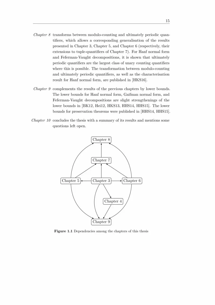
Figure 1.1 Dependencies among the chapters of this thesis

2 Preliminaries
This chapter contains the basic notations and concepts used throughout the thesis.Section 2.1 recalls the essential notation concerning arithmetic and the growth offunctions, as well as for finite and infinite words. Section 2.2 shortly discusses themodel of computation used for the analysis of algorithms. Section 2.3 introducesfinite signatures and finite structures. Section 2.4 defines the logics this thesis isinterested in. To this aim, a succession of extensions of first-order logic by unarycounting quantifiers is described. Ultimately periodic counting quantifiers willbe explained in Section 2.5. Section 2.6 recalls transductions, also called logicalinterpretations, and states a transduction lemma. In Section 2.7, basic notationabout graphs is presented. Section 2.8 recalls the Gaifman graph of structuresand uses this concept to define spheres and types – in particular, for classes ofstructures of bounded degree.The chapter closes with Section 2.9, where a divide-and-conquer scheme for
the construction of formulae will be introduced. This divide-and-conquer schemewill be used later on for a worst-case optimal construction of Hanf normal formin Section 3.2, as well as to improve the time complexity of the constructionof existential formulae in Section 6.2 and the transformation of tuple-countingquantifiers in Section 7.2.
2.1 Basic Notation
We write Z to denote the set of integers and we write N to denote the set ofnon-negative integers. For each number t ∈ N, we let N≥t := n ∈ N : n ≥ t. Ifn,m ∈ N, then [n,m] denotes the set of all i ∈ N with n ≤ i ≤ m. In particular,[n,m] = ∅ if m < n. Furthermore, we let [n,m) := [n,m−1].
For a set M ⊆ N, the least common multiple of the numbers in M is denotedby lcm(M). By convention, the least common multiple of an empty set is 1.For numbers i, j ∈ N, we let bit(j, i) := bi/2jc mod 2 denote the j-th bit in
the binary expansion of i.
17
18 Chapter 2. Preliminaries
Furthermore, we write R to denote the set of real numbers and we let R≥0
denote the set of all non-negative real numbers. For any r ∈ R≥0 with r > 0 wewrite log r to denote the logarithm of r with respect to base 2.
2.1.1 Growth of Functions
We use the standard O-notation as, e.g., summarised in [FG06, Appendix A].For a function f : N → R≥0, we write o(f) to denote the class of all functionsg : N → R≥0 where for all c ∈ N≥1 there is an n0 ∈ N such that for all n ∈ Nwith n > n0 we have g(n) ≤ f(n)
c .Similarly, O(f) is the class of all functions g : N→ R≥0 where there is a c ∈ N≥1
and an n0 ∈ N such that for all n ∈ N with n > n0 we have g(n) ≤ c · f(n).We will sometimes use the fact that if g ∈ O(f) for a function g : N → R≥0
and an increasing function f : N→ (R≥0\0), then there is a number c ∈ N≥1
such that g(n) ≤ c · f(n) for all n ∈ N.Furthermore, we write poly(f) to denote the class of all functions g : N→ R≥0
for which there exists a number c ∈ N≥1 and an n0 ∈ N such that for all n ∈ Nwith n > n0 we have g(n) ≤ (f(n))c.
The function Tower: N× R≥0 → R≥0 is defined by (cf., e.g., [DGKS07])
Tower(0, r) := r and Tower(n, r) := 2Tower(n−1,r)
for each n ≥ 1 and all r ∈ R≥0. That is,
Tower(n, r) = 22···2r
a tower of 2s of height n with r on top.
For n ∈ N, we abbreviate Tower(n) := Tower(n, 1).We say that a function f : N → R≥0 is at most k-fold exponential, for some
k ∈ N, if f(n) ∈ Tower(k, poly(n)). More generally, f is called elementary if it isk-fold exponential for some k ≥ 0.
2.1.2 Words
Let Σ be a set (which we also call alphabet). A finite word over Σ is a sequencew = w0w1 · · ·wn−1 of length n ≥ 0 of elements from Σ. We also write |w| forthe length of w. By ε we denote the (unique) empty word, that is, the word oflength 0. By Σ∗ we denote the set of all finite words over Σ.
An ω-word over Σ (cf., e.g., [Str94]) is a sequence w = w0w1w2 · · · where, foreach n ∈ N, wi ∈ Σ. For each n ∈ N, we write w[n] to denote the letter wn in w
2.3 Model of Computation 19
at position n, and for numbers i, j ∈ N with i ≤ j, we write w[i, j] for the (finite)word wiwi+1 · · ·wj . Similarly, w(i, j] denotes the (finite) word wi+1 · · ·wj . Inparticular, w(i, i] is the empty word ε, and w(j−1, j] = w[j]. By Σω we denotethe set of all ω-words over Σ. We denote the concatenation of a finite word uand a word v (which may be a finite word or an ω-word) by uv. Then, we alsocall u a prefix of uv.Often, we will also call a finite word a tuple. In this context, we write
a = (a1, . . . , an) for the word a1 · · · an of length n ≥ 0 with a1, . . . , an from Σ.For each m ≥ 0 and indices 1 ≤ i1 < · · · < im ≤ n, the tuple (ai1 , . . . , aim) is asubtuple of a.
2.2 Model of Computation
We use Random Access Machines as introduced in [FG06, Appendix A.1]: A Ran-dom Access Machine (ram) consists of a finite control unit, a program counter,and an infinite sequence r0, r1, r2, . . . of registers. Each of these registers stores anatural number. Often, we will also store words over other countable alphabets Σin sequences of registers. In these cases, we assume some bijection between Σ anda subset of the natural numbers. A program for a ram consists of a sequence ofinstructions, indexed by the program counter. Instructions include the arithmeticinstructions addition, subtraction, and division by 2, restricted to the naturalnumbers. Furthermore, there are instructions available for indirect addressingand conditional as well as unconditional jumps.The input and the output of a ram are finite words from Σ∗ stored in an
initial segment of its registers. In order to measure the running time of a ramwe use the uniform cost measure, where the time needed for a run of a ram ismeasured as the number of instructions carried out and thus, in particular, isindependent of the size of the numbers in the registers. A ram program runsin time t : N → N if for every input word w ∈ Σ∗, the length of the run of theprogram on input w is at most t(|w|).
We call an algorithm k-fold exponential for a k ∈ N, if it can be performed by aram program in time t for a k-fold exponential function t : N→ N. More general,we call the algorithm elementary if it is k-fold exponential for some k ∈ N.
20 Chapter 2. Preliminaries
2.3 Signatures and Structures
In this section, we recall notation concerning signatures, structures, and relationsbetween structures, which is based on the standard notation used in, e.g., [EF99,Lib04]. The section also describes encodings for signatures and structures asinput for a ram.
2.3.1 Signatures
By Rel and Const we denote countable sets of relation symbols and constantsymbols, respectively. A function ar : Rel→ N≥1 associates every relation sym-bol R ∈ Rel with its arity. A signature σ is a tuple (R1, . . . , Rk, c1, . . . , c`)of k ≥ 0 distinct relation symbols R1, . . . , Rk ∈ Rel and ` ≥ 0 distinct constantsymbols c1, . . . , c` ∈ Const. The signature σ is called relational if ` = 0, that is,if it only contains relation symbols.We represent σ as a finite word over the alphabet Rel ∪ Const ∪ #. More
precisely, we let
rep(σ) := Rar(R1)1 · · ·Rar(Rk)
k #c1 · · · c`.
The size ||σ|| of a signature σ is the length of rep(σ). Note that, in particular,||σ|| = `+ 1 +
∑ki=1 ar(Ri), that is, the number of its constant symbols plus the
sum of the arities of its relation symbols.
2.3.2 Structures
A σ-structure A is a tuple (A,RA1 , . . . , RAk , cA1 , . . . , cA` ) consisting of a finite non-empty set A, also called the universe of A, a relation RAi ⊆ Aar(Ri) for eachi ∈ [1, k], and an element cAi ∈ A for each i ∈ [1, `].Suppose that A = a1, . . . , an for an n ≥ 1. Furthermore, suppose that the
elements a1, . . . , an are ordered, e.g., by the linear order on the natural numbersif A ⊆ N or an ordering provided by the representation of A as natural numbersstored in the registers of a ram. We represent any relation RA of A by the wordrep(RA) := a1 · · · am, where a1, . . . , am are the m ≥ 0 tuples belonging to theset RA in their lexicographic order. This way, we can represent A as a wordrep(A) over the alphabet A ∪ #, defined by
rep(A) := a1 · · · an# rep(RA1 )# · · · rep(RAk )#cA1 · · · cA` .
2.4 Logics 21
The size ||A|| of a σ-structure A is defined as the size of its representation,and thus
||A|| = |A| +k∑i=1
(1 + |RAi | · ar(Ri)
)+ 1 + `.
In particular, ||A|| ∈ O(||σ||) · |A|||σ||.
2.3.3 Relations between Structures
If τ is a subtuple of σ, then for any σ-structure A we denote by A|τ the τ -reductof A, that is, the τ -structure with universe A where RA|τ := RA for each relationsymbol R in τ , and where cA|τ := cA for each constant symbol c in τ . On theother hand, we call A a σ-expansion of A|τ .To indicate that two σ-structures A and B are isomorphic, we write A ∼= B.In the following, suppose that σ is a relational signature. We say that B is
a substructure of A if B ⊆ A and RB ⊆ RA for each relation symbol R from σ.The structure B is an induced substructure of A if B is a substructure of A andRB = RA ∩ Br for each relation symbol R of arity r ≥ 1 from σ. We then saythat B is the substructure of A induced by the set B.
For every set B such that A∩B 6= ∅, we write A[B] to denote the substructureof A induced by A ∩ B. Furthermore, if A \ B 6= ∅ then A \ B is the inducedsubstructure A[A \B] of A obtained by deleting all elements from B.
Two σ-structures are disjoint, if their universes are disjoint. Let s ≥ 1, and letA1, . . . ,As be (not necessarily disjoint) σ-structures. The union A1 ∪ · · · ∪As ofA1, . . . ,As is the σ-structure C with universe A1∪· · ·∪As where, for each relationsymbol R from σ, the relation RC is the union of the relations RA1 , . . . , RAs .A σ-structure D is called a disjoint union of A1, . . . ,As if it is the union of
pairwise disjoint σ-structures A′1, . . . ,A′s, that is, of σ-structures whose universesare pairwise disjoint, such that A′i ∼= Ai for each i ∈ [1, s].
2.4 Logics
In this section, we define the logics used in this thesis. The notation introducedis based on [EF99]. We commence with the standard notation for propositionallogic, which we need for a definition of so-called reduction sequences in Chapter 5.The main part of this section will provide the syntax and semantics of the logicsin the focus of this thesis, that is, first-order logic and its extensions by unary
22 Chapter 2. Preliminaries
counting quantifiers. For each such logic, we will also define an extension bytuple-counting quantifiers.
2.4.1 Propositional Logic
By PS we denote a countable set of propositional symbols. PL is the set ofpropositional formulae, that is, the smallest set of formulae that is closed underatomic propositional formulae (A) and Boolean connectives (B) as describedbelow:
(A) PS ⊆ PL and 0,1 ∈ PL.
(B) If ϕ,ψ ∈ PL, then also ¬ϕ ∈ PL and (ϕ ∨ ψ) ∈ PL.
We omit parentheses if this does not lead to ambiguity, and we treat the Booleanconnectives ϕ ∧ ψ, ϕ → ψ, and ϕ ↔ ψ, as abbreviations for the formulae¬(¬ϕ ∨ ¬ψ), ¬ϕ ∨ ψ, and (ϕ→ ψ) ∧ (ψ → ϕ), respectively.A propositional formula ϕ is represented by a word rep(ϕ) over the alphabet
PS ∪ ¬,∨, (, ),0,1. The size ||ϕ|| of ϕ is the length of rep(ϕ).A propositional interpretation is a function µ : PS→ 0, 1. For any formula
ϕ ∈ PL we write µ |= ϕ to express that µ is a model of ϕ (and we write µ 6|= ϕ ifthis is not the case). The model relation is defined recursively as follows:
(A) µ |= 1 and µ 6|= 0, and for each X ∈ PS,
µ |= X iff µ(X) = 1.
(B) For ϕ,ψ ∈ PL,
µ |= ¬ϕ iff µ 6|= ϕ
and
µ |= ϕ ∨ ψ iff µ |= ϕ or µ |= ψ.
2.4.2 First-Order Logic and Unary Counting Quantifiers
By Var we denote a countable set of variable symbols, which we will also callvariables for short. Variables will be the only terms allowed in the formulaeintroduced in the sequel. In particular, no constant or function symbols are used.Every logic L considered in this thesis contains all atomic formulae (A) and isclosed under Boolean connectives (B). More precisely, the set of formulae in anylogic L adheres to the following rules:
2.4 Logics 23
(A) If x, y ∈ Var, then x=y ∈ L, andif R ∈ Rel is of arity r ≥ 1 and x1, . . . , xr ∈ Var, then R(x1, . . . , xr) ∈ L.
(B) If ϕ,ψ ∈ L, then also the formulae ¬ϕ and ϕ ∨ ψ belong to L.
We treat the Boolean connectives ϕ∧ψ, ϕ→ ψ, and ϕ↔ ψ as abbreviations forthe formulae ¬(¬ϕ ∨ ¬ψ), ¬(ϕ ∨ ψ), and (ϕ→ ψ) ∧ (ψ → ϕ), respectively.Whenever we speak about a logic L in this thesis, we will mean one of the
logics defined below. For a relational signature σ, we denote by L[σ] the subsetof the logic L that contains all formulae from L that only make use of the relationsymbols occurring in σ.The formulae of all logics defined in the following are built from atomic
formulae and Boolean connectives, as described above, and are distinguished bythe allowed quantifiers.
Unary Counting Quantifiers
As we only consider finite structures, we understand a unary counting quantifier Q(for short: quantifier) as a subset of the natural numbers (cf., e.g., [LN00, Nur00]).Broadly speaking, the numbers in this set represent the cardinalities of the witnesssets accepted by the quantifier. More formal semantics for the logics using suchquantifiers are given further down below. We will also allow derived quantifiers(Q+k) that increment the numbers in the set Q by a constant k ∈ N, that is,
(Q+k) := n+k : n ∈ Q.
Clearly, (Q+0) = Q.
Example 2.4.1. As we only consider finite structures, the existential quantifier ∃can be defined by the set of all natural numbers ≥ 1. For each k ≥ 0, thethreshold-counting quantifier (∃+k) is given by the set of all natural numbers > k.
Other examples for unary counting quantifiers are the set of all prime numbers,and the set of all natural numbers representing (in a suitable encoding) Turingmachines (cf., e.g., [EF99]) that halt on the empty input.
By Call we denote the set of all unary counting quantifiers, that is, the set P(N)of all subsets of the natural numbers. In the following, we define a series of logics,starting with first-order logic and closing with the extension of first-order logicby arbitrary unary counting quantifiers from Call. In another direction, we willextend each of these logics to a logic whose quantifiers can also count tuples of
24 Chapter 2. Preliminaries
elements instead of only single elements. When we talk about some abstractlogic in the sequel, we will always mean one of the logics defined below.
After defining the syntax of the considered logics, we will define some crucialparameters of logic formulae as, e.g., the quantifier rank, and conclude the sectionby providing semantics for these logics.
Plain First-Order Logic
Plain first-order logic (for short: FO) is the smallest set of formulae that is closedunder the rules (A), (B), and the following rule for existential quantification:
(∃) If ϕ ∈ FO and x ∈ Var, then ∃xϕ ∈ FO.
We treat universal quantification ∀xϕ as an abbreviation for the formula ¬∃x¬ϕ.
First-Order Logic with Threshold-Counting
First-order logic with threshold-counting (for short: FO+unT) additionally allowsthreshold-counting. That is, FO+unT is the smallest set of formulae that is closedunder the rules (A), (B), and the following generalisation to the rule (∃):
(T) If ϕ ∈ FO+unT, x ∈ Var, and k ≥ 0, then (∃+k)xϕ ∈ FO+unT.
Clearly, FO ⊂ FO+unT.
First-Order Logic with Modulo-Counting
A modulo-counting quantifier with period p ≥ 2 is a unary counting quantifierthat is defined by the subset
Dp := n ∈ N : n is divisible by p
of the natural numbers (cf., e.g., [Nur00]). By Dall, we denote the set of allmodulo-counting quantifiers for arbitrary periods p ≥ 2.
For every set D ⊆ Dall, first-order logic with modulo-counting quantifiersfrom D (for short: FO+unM(D)) is the smallest set of formulae that is closedunder (A), (B), (T), and the following rule:
(D) If ϕ ∈ FO+unM(D), x ∈ Var, Dp ∈ D, and r ∈ [0, p),then (Dp+r)xϕ ∈ FO+unM(D).
In the following, we also abbreviate FO+unM(Dall) by FO+unM.
2.4 Logics 25
First-Order Logic with Arbitrary Unary Counting Quantifiers
For an arbitrary set C ⊆ Call of unary counting quantifiers, first-order logicwith counting quantifiers from C (for short: FO+unC(C)) is the smallest set offormulae that is closed under (A), (B), (T), and the following rule:
(C) If ϕ ∈ FO+unC(C), x ∈ Var, Q ∈ C, and k ≥ 0,then (Q+k)xϕ ∈ FO+unC(C).
For short, we also write FO+unC for FO+unC(Call).
Logics with Tuple-Counting Quantifiers
For any logic L of the aforementioned ones, we denote by Ltpl the logic whereeach quantifier allowed in L is allowed to count over finite tuples. That is, Ltpl isthe smallest set of formulae that adheres to the rules describing the logic L asdefined above, and the following rule for tuple-counting quantifiers (cf., [Str94]):
(tpl) If Qxϕ ∈ Ltpl for some Q ⊆ N and x ∈ Var, then also Q(x1, . . . , xm)ϕ ∈ Ltpl
for any tuple (x1, . . . , xm) of m ≥ 1 pairwise distinct variables.
Note that L ⊆ Ltpl and that (Ltpl)tpl = Ltpl.
Alternative Notation forThreshold- and Modulo-Counting Quantifiers
For a better readability, we will also use the following abbreviations in the sequel.Let ϕ be a formula from FO+unCtpl and let x be a non-empty tuple of pairwisedistinct variables. Then,
∃>kxϕ := (∃+k)xϕ for each k ≥ 0,∃≥kxϕ := (∃+(k−1))xϕ for each k ≥ 1,∃=kxϕ := ∃≥kxϕ ∧ ¬∃>kxϕ for all k ≥ 1,∃=0xϕ := ¬∃xϕ, and
∃≡ rmod pxϕ := (Dp+r)xϕ for all p ≥ 2 and r ∈ [0, p).
Properties of Formulae
Let L be one of the logics defined above and consider an L-formula ϕ.The quantifier rank qr(ϕ) and the set of free variables free(ϕ) are defined
inductively over the shape of ϕ as follows: If ϕ is an atomic formula, then

26 Chapter 2. Preliminaries
qr(ϕ) := 0 and free(ϕ) is the set of all variables from Var that appear in ϕ. If ϕis of the shape ¬ϕ′, then qr(ϕ) := qr(ϕ′) and free(ϕ) := free(ϕ′); and if ϕ is ofthe shape ϕ′ ∨ ϕ′′, then qr(ϕ) is the maximum of qr(ϕ′) and qr(ϕ′′), and free(ϕ)is the union of free(ϕ′) and free(ϕ′′). Finally, suppose that ϕ is of the shapeQ(x1, . . . , xm)ϕ′ for a tuple (x1, . . . , xm) of m ≥ 1 pairwise distinct variables.Then, qr(ϕ) := m+qr(ϕ′) and free(ϕ) := free(ϕ′)\x1, . . . , xm. In particular, ϕis called quantifier-free if qr(ϕ) = 0.
The dimension of ϕ is 1 if ϕ is quantifier-free, and otherwise it is the maximumlength of all variable tuples x for which ϕ contains a subformula of the shapeQxψ for some unary counting quantifier Q.For formulae ϕ from FO+unMtpl (and thus, in particular, formulae from
FO+unTtpl), we define two additional parameters: The threshold of ϕ is thesmallest K ≥ 0 such that every subformula of the shape (∃+k)xψ has k ≤ K,and the maximum period of ϕ is the smallest P ≥ 0 such that every subformulaof the shape (Dp+r)xψ for some p ≥ 2 and r ∈ [0, p) has p ≤ P .
Semantics
In the following, we fix a relational signature σ. A σ-interpretation is atuple (A, β), consisting of a σ-structure A and a function β : Var → A. Theuniverse of (A, β) is the universe A of A.
For a logic L as defined above and a formula ϕ ∈ L[σ], we write (A, β) |= ϕ toexpress that (A, β) is a model of ϕ (and we write (A, β) 6|= ϕ if this is not thecase). The model relation is defined recursively as follows:
(A) For variables x, y ∈ Var,
(A, β) |= x=y iff β(x) = β(y).
For each relation symbol R from σ with arity r ≥ 1 and all x1, . . . , xr ∈ Var,
(A, β) |= R(x1, . . . , xr) iff (β(x1), . . . , β(xr)) ∈ RA.
(B) For formulae ϕ,ψ from L[σ],
(A, β) |= ¬ϕ iff (A, β) 6|= ϕ
and
(A, β) |= ϕ ∨ ψ iff (A, β) |= ϕ or (A, β) |= ψ.
2.5 Ultimately Periodic Quantifiers 27
(C) For any formula Q(x1, . . . , xm)ϕ that belongs to L[σ], where Q ⊆ N andwhere (x1, . . . , xm) is a tuple of m ≥ 1 pairwise distinct variables,
(A, β) |= Q(x1, . . . , xm)ϕ
iff∣∣∣(a1, . . . , am) ∈ Am :
(A, β a1,...,am
x1,...,xm
)|= ϕ
∣∣∣ ∈ Q.
In the latter equivalence, β a1,...,amx1,...,xm
denotes the function β′ : Var→ A withβ′(xi) := ai for all i ∈ [1,m] and β′(z) := β(z) for all z ∈ Var\x1, . . . , xm.
For a tuple x = (x1, . . . , xn) of pairwise distinct variables and a formula ϕ from L,we write ϕ(x) to express that free(ϕ) ⊆ x1, . . . , xn. Note that this also inducesan order on the free variables of ϕ.For a σ-structure A and a tuple a = (a1, . . . , an) ∈ An, the tuple (A, a)
denotes the interpretation (A, β) for ϕ(x) where β : Var→ A is defined such thatβ(xi) = ai for all i ∈ [1, n] and such that β(y) = a for all y ∈ Var \ x1, . . . , xnand an arbitrary but fixed element a ∈ A. In particular, we write (A, a) |= ϕ
(for short: A |= ϕ[a]) to express that (A, β) is a model of ϕ(x).For a class C of σ-structures, two formulae ϕ(x) and ψ(x) from L[σ] are
C-equivalent, ifA |= ϕ[a] iff A |= ψ[a]
for each structure A ∈ C and every tuple a ∈ An. The formulae ϕ(x) and ψ(x)are called equivalent if they are C-equivalent for the class C of all σ-structures.
2.5 Ultimately Periodic Quantifiers
In this section, we introduce so-called ultimately periodic unary counting quanti-fiers (cf. [Mat94]). Ultimately periodic quantifiers will turn out to be the largestclass of unary counting quantifiers for which most of the results of this thesisare applicable. In contrast to unary counting quantifiers in general, ultimatelyperiodic quantifiers can be represented by suitable finite words and thus allowus to define a finite encoding of formulae that only use ultimately periodicquantifiers.
Intuitively, ultimately periodic quantifiers are unary counting quantifiers thatcan be obtained from threshold-counting and modulo-counting quantifiers bya finite number of applications of the set-theoretic operations complement andunion. However, another characterisation will turn out to be more useful for ourpurposes:
28 Chapter 2. Preliminaries
Definition 2.5.1. A unary counting quantifier Q ⊆ N is ultimately periodic ifthere exist numbers p, n0 ∈ N with p ≥ 1, such that
for all n ≥ n0 we have n ∈ Q iff n+ p ∈ Q .
The period of Q is the minimal p ≥ 1 for which the latter property is true forsome n0. The number n0 is called an offset of Q.
We denote the set of all ultimately periodic unary counting quantifiers by Uall.
Example 2.5.2. The existential quantifier and all quantifiers (Dp+r) with p ≥ 2and r ∈ [0, p) are ultimately periodic with period 1 and offset 1, and with period pand offset r, respectively. More generally, if Q ⊆ N is ultimately periodic withperiod p ≥ 1 and offset n0 ≥ 0, then, for each k ≥ 0, the quantifier (Q+k) isultimately periodic with period p and offset n0 + k.
As a counterexample, the sets of all square numbers or all prime numbers arenot ultimately periodic.
We call a logic L as defined in Section 2.4.2 ultimately periodic if all quantifierspermitted in the logic are ultimately periodic.
Example 2.5.3. All the logics FO, FO+unT, FO+unM(D) for all D ⊆ Dall, andFO+unC(U) for all U ⊆ Uall, as well as their tuple-counting extensions, areultimately periodic.
Until now we have described unary counting quantifiers by sets of naturalnumbers. In the following, we provide an alternative description, which isuseful for encoding ultimately periodic quantifiers, as well as for applying wordcombinatorial reasoning to them (see Chapter 8).
Definition 2.5.4. The characteristic sequence of a quantifier Q ⊆ N is theω-word χQ := w0w1w2 . . . over the alphabet 0, 1 where, for each i ∈ N,
wi = 1 iff i ∈ Q.
A finite word w ∈ 0, 1∗ is primitive (cf., e.g., [Lot84]) if for every wordu ∈ 0, 1∗, w ∈ u∗ implies w = u. Any finite non-empty word π ∈ 0, 1∗ canbe written as wn for some primitive word w ∈ 0, 1∗ and some n ≥ 1. Note thatthis primitive word w is uniquely determined by π and thus called the primitiveroot of π.
The following fact defines an ultimately periodic quantifier in terms of itscharacteristic sequence.
2.6 Transductions 29
Fact 2.5.5. For every Q ⊆ N, the following holds:
• If Q is ultimately periodic with period p ≥ 1 and offset n0 ≥ 0, then thereis a word α ∈ 0, 1∗ of length n0 and a primitive word π ∈ 0, 1+ oflength p such that χQ = απω.
• If χQ = απω for finite words α ∈ 0, 1∗ and π ∈ 0, 1+, then Q isultimately periodic, its period is the length of the primitive root of π,and |α| is an offset.
Thus, we can represent an ultimately periodic quantifier Q by the finite wordrep(Q) := α#π over the alphabet 0, 1,#, where χQ = απω. To make thisdefinition unambiguous, we demand that p := |π| is the period of Q, and n0 := |α|is the smallest offset of Q. The size ||Q|| of Q is the length of rep(Q).In particular, ||Q|| = n0 + p+ 1 ≥ 2 and ||(Q+k)|| = ||Q||+ k for all k ≥ 0.
Example 2.5.6. The existential quantifier is represented by the word rep(∃) = 0#1.On the other hand, for every period p ≥ 2 and each remainder r ∈ [0, p), themodulo-counting quantifier with period p and remainder r is represented by theword rep((Dp+r)) = 0r#10p−1.
Using this representation, any formula ϕ from any ultimately periodic logiccan be represented by a word rep(ϕ) over the alphabet
Var ∪ Rel ∪ , ∪ =,¬,∨, (, ), 0, 1,#,
where each quantifier Q ∈ Uall is represented by the word rep(Q). The size ||ϕ||of ϕ is the length of rep(ϕ).
2.6 Transductions
The following introduction to transductions1 is based on [EF99, Gru16, Gro17].For the following, we let L denote one of the logics defined in the previous sections.In this thesis, we will only consider first-order transductions.Broadly spoken, for relational signatures σ and τ , a transduction Θ from σ
to τ is a tuple of formulae from FO[σ]. The satisfying assignments for the freevariables of these formulae in respect to a σ-structure A define the universe andthe relations of an associated τ -structure Θ[A]. On the other hand, given aformula ϕ from L[τ ], the transduction can be used to transform ϕ into a so-called
1also called logical (or: syntactical) interpretations (cf., e.g., [EF99])
30 Chapter 2. Preliminaries
Θ-reduct ϕ−Θ of ϕ, which is a formula of Ltpl[σ] that, in a σ-structure A, hasthe same meaning as ϕ in the τ -structure Θ[A].The so-called transduction lemma, stated further at the end of Section 2.6,
describes the crucial relationship between the structure Θ[A] and the Θ-reductformally.For the following, we fix two relational signatures σ and τ . In particular,
we suppose that τ = (R1, . . . , R`) for an ` ≥ 0 and a relation symbol Ri ofarity ri ≥ 1 for each i ∈ [1, `].
Definition 2.6.1. Let t ≥ 1, let
• θ(x1, . . . , xt) be an FO[σ]-formula, and let
• θRi(y1, . . . , yri), for each i ∈ [1, `], be a formula from FO[σ] with the variabletuples yj := (yj,1, . . . , yj,t) for all j ∈ [1, ri].
The tuple Θ = (θ, θR1 , . . . , θR`) is called a transduction from σ to τ with arity t.The quantifier rank qr(Θ) and the size ||Θ|| of Θ are the maximum of the
quantifier rank and the size of the formulae θ, θR1 , . . . , θR` , respectively.
Example 2.8.3 further down below provides an example of a transduction thatturns structures over σ into their so-called Gaifman-graph.
The following definition describes the application of a transduction from σ to τto a σ-structure. To avoid ambiguity, we introduce a notation to explicitly denotetuples of tuples. Recall that, for tuples b1, . . . , bn, the expression (b1, . . . , bn)usually denotes the concatenation of these tuples, i.e., a tuple of length |b1|+ · · ·+|bn|. To denote the tuple of length n whose elements are the tuples b1, . . . , bn,we will use the expression (b1; . . . ; bn) from now on.
Definition 2.6.2. Let Θ = (θ, θR1 , . . . , θR`) be a transduction from σ to τ witharity t ≥ 1. Let A be a σ-structure such that the set
B := b ∈ At : A |= θ[b].
is not empty. Then, the application Θ[A] of Θ to A is defined, and given by theτ -structure
B := (B,RB1 , . . . , RB` )
where, for each i ∈ [1, `],
RBi := (b1; . . . ; bri) ∈ Bri : A |= θRi [b1, . . . , bri ].
2.6 Transductions 31
For a transduction Θ from σ to τ , a Θ-reduct of an L[τ ]-sentence ϕ is anL′[σ]-sentence over a logic L′ that is satisfied by a σ-structure A whenever theτ -structure Θ[A] satisfies ϕ. The following definition makes this precise and alsocovers formulae with free variables.
Definition 2.6.3. Let Θ be a transduction from σ to τ with arity t ≥ 1, andlet ϕ(x) be a formula from L[τ ] with free variables from a tuple x = (x1, . . . , xn)of length n ≥ 0. A Θ-reduct of ϕ(x) is a formula ψ(x1, . . . , xn) from L′[σ], forsome logic L′, with free variables from the tuples xi := (xi,1, . . . , xi,t) for alli ∈ [1, n], for which the following holds: If A is a σ-structure for which Θ[A] isdefined and b1, . . . , bn are elements from the universe of Θ[A], then
Θ[A] |= ϕ[b1; . . . ; bn]iff A |= ψ[b1, . . . , bn].
Note that Θ-reducts are not defined uniquely, but just as formulae of somelogic with the semantic property described above. This will be useful later inChapter 5, where we transform Θ-reducts using tuple-counting quantifiers intoequivalent formulae without tuple-counting quantifiers, which we also want totreat as Θ-reducts.
The following transduction lemma shows that for each transduction Θ from σ
to τ and every formula ϕ ∈ L[τ ], a canonically defined Θ-reduct ϕ−Θ of ϕ existsin Ltpl[σ]. Here, tuple-counting quantifiers are only necessary if Θ has arity ≥ 2.I.e., if Θ has arity 1, then ϕ−Θ belongs to L[σ].
The lemma also provides upper bounds on the quantifier rank, number of freevariables, and dimension of the Θ-reduct. For ultimately periodic L, also upperbounds on the size and the time required for the construction of the Θ-reductare given. Furthermore, for the special case of input formulae from FO+unMtpl,also the threshold and the maximum period of Θ-reducts are examined.
Lemma 2.6.4. Let σ and τ be relational signatures, and let Θ be a transductionfrom σ to τ with arity t ≥ 1. Let L be a logic. For every formula ϕ from L[τ ],there is a Θ-reduct ϕ−Θ in Ltpl[σ].
Suppose that q, n ≥ 0 and m ≥ 1 are the quantifier rank, the number of freevariables, and the dimension of ϕ, respectively, and that qΘ ≥ 0 is the quantifierrank of Θ. The formula ϕ−Θ has quantifier rank ≤ t · q + qΘ, t · n free variables,and dimension ≤ t ·m.
32 Chapter 2. Preliminaries
Moreover, if L is ultimately periodic, there is an algorithm which, on inputof Θ and ϕ, computes ϕ−Θ in time
||Θ|| · O(||τ ||) + ||Θ|| · O(||ϕ||)
and of size ||Θ|| · O(||ϕ||).Finally, if ϕ ∈ FO+unMtpl[τ ] then ϕ−Θ ∈ FO+unMtpl[σ] has the same
threshold and maximum period as ϕ.
Proof. Let σ and τ be relational signatures and suppose that τ = (R1, . . . , R`)for an ` ≥ 0 and a relation symbol Ri of arity ri ≥ 1 for each i ∈ [1, `]. LetΘ = (θ, θR1 , . . . , θR`) be a transduction from τ to σ with arity t ≥ 1 and quantifierrank qΘ ≥ 0. Furthermore, let L be a logic and ϕ(x) a formula from L[τ ] witha tuple x = (x1, . . . , xn) of n ≥ 0 free variables, quantifier rank q ≥ 0, anddimension m ≥ 1.
Let v0, v1, v2, . . . be a sequence of variables from Var. Without loss of generalitywe suppose that ϕ(x) only uses variables from the sequence v0, vt, v2t, . . . . Thatis, for any variable x in ϕ, there is an i ≥ 0 such that x = vi·t. This way, thevariable xj := vi·t+j−1, for each j ∈ [1, t], does not occur in ϕ. In particular, welet xi := (xi,1, . . . , xi,t) for each i ∈ [1, n].Recall that ||Θ|| is the maximum of the size of the formulae θ, θR1 , . . . , θR` .
Thus, to read the transduction Θ takes time in ||Θ|| · O(||τ ||). Afterwards, theconstruction of ϕ−Θ(x1, . . . , xn) from ϕ(x1, . . . , xn) proceeds by an inductionover the shape of ϕ(x1, . . . , xn), where we show the following inductive invariantto hold:
Claim 1.
(i) ϕ−Θ(x1, . . . , xn) is a Θ-reduct of ϕ(x1, . . . , xn) that belongs to Ltpl[σ]
(ii) ϕ−Θ(x1, . . . , xn) has dimension ≤ t ·m.
(iii) ϕ−Θ(x1, . . . , xn) has quantifier rank ≤ t · q + qΘ.
(iv) If ϕ ∈ FO+unMtpl[τ ] then ϕ−Θ(x1, . . . , xn) ∈ FO+unMtpl[σ] has the samethreshold and maximum period as ϕ.
(v) For an ultimately periodic logic L, there is an algorithm that takes at most
c · ||Θ|| · ||ϕ||
time steps to compute ϕ−Θ(x1, . . . , xn), for a suitable number c ∈ N≥1.
2.6 Transductions 33
We start by a description of the construction of ϕ−Θ(x1, . . . , xn) and byshowing the validity of the Statements (i) to (iv). Afterwards, we conclude withan analysis of the running time of the algorithm, which, for ultimately periodicL, is implied by the construction.
If ϕ(x1, . . . , xn) is of the shape xi1=xi2 for indices i1, i2 = [1, n], let
ϕ−Θ(x1, . . . , xn) :=n∧i=1
θ(xi) ∧t∧
j=1xi1,j=xi2,j .
Since Θ only uses FO[σ]-formulae, ϕ−Θ(x1, . . . , xn) belongs to FO[σ]. Thus, inparticular, it has dimension 1, threshold 0, maximum period 0, and quantifierrank ≤ qΘ. By definition of Θ[A] for σ-structures A it is straightforward to verifythat ϕ−Θ(x1, . . . , xn) indeed is a Θ-reduct of ϕ(x1, . . . , xn). Hence, Statements (i)to (iv) of Claim 1 are satisfied.
If ϕ is of the shape Ri(xj1 , . . . , xjri ) for i ∈ [1, `] and indices j1, . . . , jri = [1, n],let
ϕ−Θ(x1, . . . , xn) :=n∧i=1
θ(xi) ∧ θRi(xj1 , . . . , xjri ).
Clearly, ϕ−Θ(x1, . . . , xn) belongs to FO[σ]. It follows directly from the definitionof Θ[A] for σ-structures A, that the formula ϕ−Θ(x1, . . . , xn) is a Θ-reductfor ϕ(x1, . . . , xn) and thus, Statement (i) of Claim 1 holds. Furthermore, byconstruction, ϕ−Θ(x1, . . . , xn) has dimension 1, threshold 0, maximum period 0,and quantifier rank ≤ qΘ. Therefore, also Statements (ii) to (iv) hold.
For a Boolean combination ϕ(x), the translation distributes. That is, we let(¬ϕ′)−Θ := ¬(ϕ′)−Θ and (ϕ′ ∨ϕ′′)−Θ := (ϕ′)−Θ ∨ (ϕ′′)−Θ. Clearly, Statements (i)to (iv) of Claim 1 are satisfied in both cases.
Suppose that ϕ(x) = (Q+k)y ψ(x, y) for some quantifier Q ⊆ N permitted in L,a number k ≥ 0, and a tuple y = (y1, . . . , ym′) of m′ ∈ [1,m] pairwise distinctvariables. By Statement (i) of Claim 1 we know that Ltpl[σ] contains a Θ-reductψ−Θ(x1, . . . , xn, y1, . . . , ym′) of ψ(x, y) where yi := (yi,1, . . . , yi,t) for all i ∈ [1,m′].Using this Θ-reduct, we let
ϕ−Θ(x1, . . . , xn) := (Q+k)(y1, . . . , ym′)( m′∧i=1
θ(yi) ∧
ψ−Θ(x1, . . . , xn, y1, . . . , ym′)).

34 Chapter 2. Preliminaries
By construction, ϕ−Θ(x1, . . . , xn) belongs to Ltpl[σ].To see that Statement (i) of Claim 1 is satisfied, consider a σ-structure A
for which Θ[A] is defined. Furthermore, let b1, . . . , bn be elements from theuniverse of Θ[A]. Due to the definition of the universe of Θ[A] and sinceψ−Θ(x1, . . . , xn, y1, . . . , ym′) is a Θ-reduct of ψ(x, y), the following equivalenceholds for all tuples c1, . . . , cm′ from At:
c1, . . . , cm′ are from the universe of Θ[A] andΘ[A] |= ψ[b1; . . . ; bn; c1; . . . ; cm′ ]
iff A |= θ[ci] for all i ∈ [1,m′] and A |= ψ−Θ[b1, . . . , bn, c1, . . . , cm′ ].
Thus, it follows from the construction of ϕ−Θ(x1, . . . , xn) that
Θ[A] |= ϕ[b1; . . . ; bn]iff A |= ϕ−Θ[b1, . . . , bn].
By Statements (ii) to (iv) of Claim 1, the formula ψ−Θ(x1, . . . , xn, y1, . . . , ym′)has quantifier rank ≤ t · (q−m′) + qΘ and dimension ≤ t ·m. Furthermore, ifψ(x, y) is from FO+unMtpl[τ ], then its Θ-reduct has the same threshold andmaximum period.
Thus, it is straightforward to see that ϕ−Θ(x1, . . . , xn) has quantifier rank
≤ t ·m′ + t · (q−m′) + qΘ = t · q + qΘ,
dimension ≤ t ·m, and, if ϕ(x) belongs to FO+unMtpl[τ ], the same thresholdand maximum period as ϕ(x). Therefore, Statements (ii) to (iv) of Claim 1 aresatisfied.
Time complexity. In the following, we show that also Statement (v) of Claim 1holds for the particular case of an ultimately periodic logic L.For an atomic formula ϕ, clearly, there is a number c ∈ N≥1 such that ϕ−Θ
can be constructed in ≤ c · ||Θ|| · ||ϕ|| time steps.In the case of ϕ being a Boolean combination it is also straightforward to see
that ϕ−Θ can be computed in at most c · ||Θ|| · ||ϕ|| time steps by calling thealgorithm recursively on the subformulae.
If ϕ is a quantified formula, that is, of the shape ϕ = (Q+k)y ψ, the algorithmtakes at most c · ||Θ|| · ||ψ|| time steps to compute the Θ-reduct for ψ. By theshape of ϕ−Θ one can verify that it can be constructed in at most
c′ · (||(Q+k)||+m′ · (t+ ||θ||)) + c · ||Θ|| · ||ψ||< 2c′ · (||ϕ|| − ||ψ||) · ||Θ||+ c · ||Θ|| · ||ψ|| ≤ c · ||Θ|| · ||ϕ||
2.7 Graphs 35
time steps, for c ≥ 2c′.
In particular, this implies that ϕ−Θ has size in ||Θ|| · O(||ϕ||). It follows that,altogether, the construction of a Θ-reduct for ϕ from Θ and ϕ takes time in
||Θ|| · O(||τ ||) + ||Θ|| · O(||ϕ||).
This completes the proof of Lemma 2.6.4.
2.7 Graphs
In this section, we recall standard notation on graphs (cf., e.g., [EF99]) anddescribe a sequence of slow-growing first-order formulae that recognise pathsin graphs up to a certain length. From now on, E will always denote a binaryrelation symbol. A graph A is a structure over the signature (E). We also call theelements of the universe of A nodes, and the tuples of the relation EA edges. Thegraph A is undirected if for all (a, b) ∈ EA, also (b, a) ∈ EA, and it is loop-free if(a, a) 6∈ EA for all a ∈ A.2
The degree of a node a ∈ A is the number of distinct b ∈ A for which (a, b) ∈ EA
or (b, a) ∈ EA. The degree of A is the maximum degree of its nodes. We alsosay that A is d-bounded (for a degree bound d ∈ N) if A has degree ≤ d.A path from a node a to a node b of A is a tuple (a1, . . . , an) of n ≥ 1 nodes
from A with a1 = a and an = b, such that (ai, ai+1) ∈ EA for every i ∈ [1, n).The length of the path (a1, . . . , an) is the number of edges on the path andthus n− 1.
The following lemma shows that paths in graphs up to length n can be definedby FO[E]-formulae of size logarithmic in n. The construction is based on [FG04,Lemma 20]. In particular, these formulae will be useful for the proofs of thelower bounds presented in Chapter 9. However, we will also use these formulaein Section 2.8 to speak about distances and local neighbourhoods in relationalstructures
Lemma 2.7.1. There is a sequence (path≤n(x, y))n≥0 of FO[E]-formulae suchthat for every n ≥ 0, the following holds for each graph A and all a, b ∈ A:
A |= path≤n[a, b]
2Note that, by this definition and contrary to, e.g., [EF99], a graph is allowed to containdirected edges and loops if not explicitly described as undirected and loop-free, respectively.
36 Chapter 2. Preliminaries
iff there is a path of length ≤ n from a to b in A.
Furthermore, there is an algorithm which computes the formula path≤n(x, y) oninput of n ≥ 0 in time O(log n) for n ≥ 1.
Proof. For paths of length 0 and 1, let
path≤0(x, y) := x=y and path≤1(x, y) := path≤0(x, y) ∨ E(x, y).
For paths of length at least 2, we proceed recursively: For n ≥ 1, let
path≤2n(x, y) := ∃z∀u∀v((
(u=x ∧ v=z) ∨ (u=z ∧ v=y))
→ path≤n(u, v)).
andpath≤2n+1(x, y) := ∃z
(path≤1(x, z) ∧ path≤2n(z, y)
).
A straightforward induction over the path length n ∈ N leads to the upper boundon the time required for the construction of the formula.
In Section 9.2, further notation concerning forests and trees will be introduced.
2.8 Locality
This section introduces notation concerning local neighbourhoods in structures,as used, e.g., in [EF99, Lib04]. The key concept, which we will explain first,is the Gaifman graph of a structure [Gai82]. The Gaifman graph leads to adistance measure between the elements of a structure, which allows to definelocal neighbourhoods around such elements. Furthermore, it allows to definestructures of bounded degree by generalising the concept of graphs of boundeddegree. In the remainder of the section, we will examine the properties of localneighbourhoods in structures of bounded degree that will be crucial for thealgorithms described in the subsequent chapters.
For the following, we let c1, c2, . . . be a sequence of pairwise distinct constantsymbols and we let σ := (R1, . . . , Rk, c1, . . . , c`) be a signature with k ≥ 0 relationsymbols Ri of arity ri ≥ 1, for i ∈ [1, k], and ` ≥ 0 constant symbols.
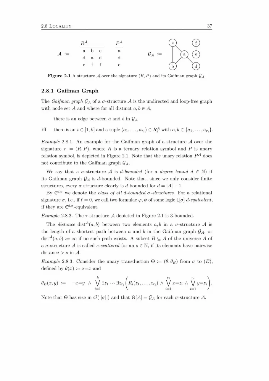
2.8 Locality 37
A :=
RA
a b cd a de f f
PA
ade
GA := a
b
c
d
e
f
Figure 2.1 A structure A over the signature (R,P ) and its Gaifman graph GA.
2.8.1 Gaifman Graph
The Gaifman graph GA of a σ-structure A is the undirected and loop-free graphwith node set A and where for all distinct a, b ∈ A,
there is an edge between a and b in GA
iff there is an i ∈ [1, k] and a tuple (a1, . . . , ari) ∈ RAi with a, b ∈ a1, . . . , ari.
Example 2.8.1. An example for the Gaifman graph of a structure A over thesignature τ := (R,P ), where R is a ternary relation symbol and P is unaryrelation symbol, is depicted in Figure 2.1. Note that the unary relation PA doesnot contribute to the Gaifman graph GA.
We say that a σ-structure A is d-bounded (for a degree bound d ∈ N) ifits Gaifman graph GA is d-bounded. Note that, since we only consider finitestructures, every σ-structure clearly is d-bounded for d = |A| − 1.By Cd,σ we denote the class of all d-bounded σ-structures. For a relational
signature σ, i.e., if ` = 0, we call two formulae ϕ,ψ of some logic L[σ] d-equivalent,if they are Cd,σ-equivalent.
Example 2.8.2. The τ -structure A depicted in Figure 2.1 is 3-bounded.
The distance distA(a, b) between two elements a, b in a σ-structure A isthe length of a shortest path between a and b in the Gaifman graph GA, ordistA(a, b) := ∞ if no such path exists. A subset B ⊆ A of the universe A ofa σ-structure A is called s-scattered for an s ∈ N, if its elements have pairwisedistance > s in A.
Example 2.8.3. Consider the unary transduction Θ := (θ, θE) from σ to (E),defined by θ(x) := x=x and
θE(x, y) := ¬x=y ∧k∨i=1∃z1 · · · ∃zri
(Ri(z1, . . . , zri) ∧
ri∨i=1
x=zi ∧ri∨i=1
y=zi
).
Note that Θ has size in O(||σ||) and that Θ[A] = GA for each σ-structure A.
38 Chapter 2. Preliminaries
By using Lemma 2.6.4 to construct Θ-reducts for the formulae (path≤n(x, y))n≥0
from Lemma 2.7.1, we obtain the following corollary.
Corollary 2.8.4. There is a sequence (dist≤n(x, y))n≥0 of FO[σ]-formulae suchthat for all n ≥ 0 the following holds for each σ-structure A and all a, b ∈ A:
A |= dist≤n[a, b] iff distA(a, b) ≤ n.
Furthermore, there is an algorithm which computes the formula dist≤n(x, y) oninput of σ and n ≥ 0 in time ||σ|| · O(log n) for n ≥ 1.
For a better readability, we will also write dist(x, y) ≤ n for the formuladist≤n(x, y). Moreover, if x is a tuple (x1, . . . , xm) of m ≥ 1 pairwise variables,we write dist(x, y) ≤ n for the formula
∨mi=1 dist(xi, y) ≤ n.
2.8.2 Neighbourhoods
Consider a σ-structure A. For each r ≥ 0 and every a ∈ A, the r-neighbourhoodof a in A is the set
NAr (a) := b ∈ A : distA(a, b) ≤ r.
For a set W ⊆ A we let NAr (W ) :=⋃a∈AN
Ar (a). Furthermore, for a non-empty
tuple a = (a1, . . . , an) of elements from A, we write NAr (a) for NAr (a1, . . . , an).
2.8.3 Types and Spheres
For each r ≥ 0 and every n ≥ 1, a σ-type with n centres and radius r is astructure τ = (B, b1, . . . , bn) over the signature (R1, . . . , Rk, c1, . . . , cn), where Bis a structure of signature (R1, . . . , Rk) and (b1, . . . , bn) ∈ Bn is a tuple with theproperty that all elements in the universe of B have distance ≤ r to at least oneof the elements b1, . . . , bn. In other words, B = NBr (b1, . . . , bn). We also call theelements b1, . . . , bn the centres of τ . If the signature, the radius, and the numberof centres are understood from the context, we will sometimes omit them andjust speak of a type.For each σ-structure A and every tuple (a1, . . . , an) ∈ An, the r-sphere of
(a1, . . . , an) in A is the type
NAr (a1, . . . , an) :=(A|(R1,...,Rk)[NAr (a1, . . . , an)], a1, . . . , an
).
2.8 Locality 39
Example 2.8.5. Reconsider the structure A over the signature (R,P ) from Ex-ample 2.8.1, depicted in Figure 2.1. The 1-sphere of the tuple (b, f) is the(R,P, c1, c2)-structure (B, b, f) where B is the substructure of A induced by theelements a, b, c, e, f , that is, the (R,P )-structure with RB := (a, b, c), (e, f, f)and PB := a, e.
For a σ-type τ with n centres and radius r, we say that the tuple (a1, . . . , an)realises τ if, and only if,
NAr (a1, . . . , an) ∼= τ.
For a σ-type τ with one centre and radius r and a σ-structure A, we furthermoredenote by
τ(A) := a ∈ A : NAr (a) ∼= τ
the set of elements of A that realise τ .
2.8.4 Types in Structures of Bounded Degree
Let d ≥ 0 be a degree bound. The crucial property of d-bounded structures,used along the course of this thesis is that there is an upper bound on the size ofd-bounded types realised in a d-bounded structure, which only depends on thetheir radius, number of centres, and the degree bound, but not on the size of thewhole structure.
To bound the size of a d-bounded σ-type with a single centre in dependencefrom its radius r ≥ 0, let νd : N→ N≥1 be defined by
νd(r) := 1 + d ·r−1∑i=0
(d− 1)i.
Then, for any d-bounded σ-structure A, any element a ∈ A, and any r ≥ 0, wehave
|NAr (a)| ≤ νd(r) .
Observe that for all r ≥ 0, we have ν0(r) = 1 and ν1(r) ≤ 2. On the other hand,
ν2(r) = 2r + 1
and, for degree bounds d ≥ 3,
(d− 1)r ≤ νd(r) ≤ dr+1.
In other words, νd is growing linearly for d ≤ 2 and exponentially for d ≥ 3.
40 Chapter 2. Preliminaries
Two σ-types can be checked for isomorphism by a straightforward brute-forcealgorithm. For d-bounded σ-types, we obtain the following upper bound on thetime complexity of such an algorithm.
Lemma 2.8.6. There is an algorithm which, on input of a signature σ and twoσ-types τ and τ ′ with n ≥ 1 centres decides whether τ ∼= τ ′. The algorithm takestime in
2O(||σ||)·(n·νd(r))2,
where d, r ≥ 0 are upper bounds on the degree bound and the radius of τ and τ ′.
Proof. Let σ be a signature, and let τ and τ ′ be two σ-types with n ≥ 1 centres.Let d, r ≥ 0 such that τ and τ ′ are both d-bounded and of radius ≤ r. LetN := n · νd(r) be an upper bound on the size of the universes of τ and τ ′.For the special case of N = 1, there is only one bijection mapping the single
element of τ to the single element of τ ′, and it takes time in O(||σ||), to checkwhether this bijection is an isomorphism.
If N ≥ 2, then for every bijection between the elements of τ and τ ′, it can bechecked in at most c′ · (n+N ||σ||) ≤ N c′′·||σ|| time steps, for numbers c′, c′′ ∈ N≥1
with c′ < c′′, whether the bijection is indeed an isomorphism. Since there are atmost NN bijections, the test whether τ and τ ′ are isomorphic can be performedin time
NN ·NO(||σ||) ⊆ 2O(||σ||)·N2.
Thus, in any case, the algorithm takes time in 2O(||σ||)·(n·νd(r))2 .
The upper bound n · νd(r) on the number of elements in d-bounded σ-typesof radius r ≥ 0 and with n ≥ 1 centres implies that there is also only a finitenumber of such types that are pairwise non-isomorphic. In fact, this numbergrows 2-fold exponentially with the radius.
In the remainder of this section, we can suppose σ to be relational. For d, r ≥ 0and n ≥ 1, we denote by Td,σr (n) a set of representatives of the isomorphismclasses of all d-bounded σ-types with n centres and radius r. That is, for everyd-bounded type τ with n centres and radius r that may be realised by a tuplea ∈ An in a d-bounded σ-structure A, there is precisely one type τ ′ ∈ Td,σr (n)with τ ∼= τ ′. The following lemma uses the isomorphism test of Lemma 2.8.6 toconstruct such sets Td,σr (n).
2.8 Locality 41
Lemma 2.8.7. There is an algorithm which, on input of a relational signature σ,d, r ≥ 0, and n ≥ 1, computes the set Td,σr (n) in time
2max2,n·νd(r)O(||σ||).
Proof. Let σ be a relational signature, let d, r ≥ 0, and let n ≥ 1. Recall thatthe universe of each type in the set Td,σr (n) has at most N := n · νd(r) elements.
For the case that N = 1, there are at most 2||σ|| types in Td,σ0 (1) which can beeasily constructed in time O(2||σ||) ⊆ 22O(||σ||) .In the following, we suppose that N ≥ 2 and let the universe of each type
in Td,σr (n) be a subset of [1, N ]. Hence, the relations of an arbitrary type inTd,σr (n) can be represented by a word over the alphabet 0, 1 of length atmost N ||σ||. Furthermore, each of its n centres is interpreted by an elementfrom [1, N ]. Hence, there are at most
Nn · 2N ||σ|| ≤ 2N ·logN+N ||σ|| < 2N ||σ||+2
candidates for types in Td,σr (n).For any such candidate, we need at most time NO(||σ||) to decide whether
the candidate is indeed a d-bounded σ-type with radius r. For any two suchcandidates, we use the algorithm from Lemma 2.8.6 for testing whether they areisomorphic. In summary, Td,σr (n) can be constructed in time
2N ||σ||+2 ·NO(||σ||) +(2N ||σ||+2)2
· 2O(||σ||)·N2 ⊆ 2NO(||σ||).
Thus, we can subsume the cases of N = 1 and N ≥ 2 under the upper boundstated in the lemma.
For a d-bounded σ-type τ with radius r and n centres, one can construct [BK12]a sphere-formula sphτ (x) with the free variables x = (x1, . . . , xn) from FO[σ],such that for every σ-structure A and each tuple a ∈ An,
A |= sphτ [a] iff NAr (a) ∼= τ.
The following lemma gives an upper bound on the time needed to construct sucha sphere-formulae.
Lemma 2.8.8. There is an algorithm which, on input of a relational signature σand, for a degree bound d ≥ 0, a d-bounded σ-type τ with radius r ≥ 0 and n ≥ 1centres, computes the formula sphτ (x) in time
max2, n · νd(r)O(||σ||).
42 Chapter 2. Preliminaries
Proof. Suppose that σ = (R1, . . . , Rk) for some k ≥ 0. Let τ = (A, c1, . . . , cn),let M := |A|, and let a1, . . . , aM = A. Choose indices i1, . . . , in ∈ [1,M ] suchthat cj = aij for all i ∈ [1, n]. With this preparation, we can choose
sphτ (x) := ∃z1 · · · ∃zM( ∧ϕ∈Φ
ϕ(z1, . . . , zM ) ∧n∧j=1
xj=zij
∧ ∀y(dist(x, y) ≤ r →
M∨i=1
y=zi))
where Φ is the set of all atomic and negated atomic formulae ϕ(z1, . . . , zM ) overthe signature σ such that A |= ϕ[a1, . . . , aM ].
Let N := n·νd(r). The cardinality of the set Φ is in O(k) if N = 1 and, if N ≥ 2,in NO(||σ||). Hence, the formula sphτ (x) can be constructed in time O(||σ||)if N = 1, and in time NO(||σ||) if N ≥ 2. Altogether, we can bound the timerequired for the construction of sphτ (x) by the expression stated in the lemma.
2.9 A Divide-and-Conquer Scheme for Formulae
Suppose that σ is a signature, thatM is a finite and non-empty set, and that ϕj(y)for j ∈M are formulae with the property that each element in any σ-structuresatisfies at most one of these formulae. To check whether the number of elementsin a σ-structure that satisfy one of these formulae is congruent r modulo p forsome p ≥ 2 and r ∈ [0, p), or exceeds a certain threshold k ≥ 0, we clearly canuse the formulae
∃≡ rmod py∨j∈M
ϕj(y) (2.1)
and∃>ky
∨j∈M
ϕj(y), (2.2)
respectively. A reoccuring task in the following chapters (in particular in Sec-tion 3.2, Section 6.2, and Section 7.2) will be, to decompose formulae similar toSentence (2.1) and Sentence (2.2) into Boolean combinations of formulae thatcount the elements satisfying each of the formulae ϕj(y), j ∈M , separately. Inthe particular case of Sentence (2.1) and Sentence (2.2), a first straightforwardattempt gives us the sentence∨
f∈F
∧j∈M∃≡ f(j) mod py ϕj(y), (2.3)
2.9 A Divide-and-Conquer Scheme for Formulae 43
where F is the set of all functions f : M → [0, p) such that the sum of f(j) forall j ∈M is congruent to r modulo p, and the sentence∨
g∈G
∧j∈M,g(j)≥0
∃>g(j)y ϕj(y),
where G is the set of all functions g : M → [−1, k] such that the sum of g(j) + 1for all j ∈ M equals k + 1. The disadvantage of these latter formulae is thatalready the number of clauses of their corresponding outer disjunction growsexponentially with the cardinality of the set M . In particular, |F | = p|M |−1.
Example 2.9.1. Let σ be a relational signature, let d ≥ 0 be a degree bound, andlet r ≥ 0. Each element of a d-bounded σ-structure A realises precisely one ofthe σ-types in Td,σr (1), that is, it satisfies precisely one of the formulae sphτ (y)for τ ∈ Td,σr (1). Expressing the statement “A has a universe of even cardinality”in the manner of Sentence (2.3) results in a sentence of size > 2|T
d,σr (1)|.
In this section, we describe a divide-and-conquer approach, which leads to anexponentially smaller size of the resulting Boolean combinations in comparisonto the naive brute-force approach just described. More precisely, the size ofthe resulting Boolean combination only grows polynomially with |M | insteadof exponentially. In particular, in Section 3.2, this will help us to obtain analgorithm whose running time meets the corresponding lower bounds, and inSection 6.2 it will reduce the gap between upper and lower bounds. The approachdistills the idea of constructions used in [HHS15, HKS16].The following two lemmas describe the divide-and-conquer procedure for the
cases of modulo-counting and threshold-counting. Both lemmas are stated in avery general way which is necessary to cover the various settings in the subsequentchapters in which they are used. Note that the restriction to ultimately periodiclogics is not necessary for the constructions themselves, but only for theirstatement and analysis as algorithms.
Lemma 2.9.2. Let L be an ultimately periodic logic. There is an algorithmwhich, on input of
• numbers p ≥ 2 and r ∈ [0, p),
• a non-empty and finite set M , and
• L-formulae δij for all i ∈ [0, p) and j ∈M ,
44 Chapter 2. Preliminaries
computes an L-formula⟨δij⟩≡ rmod pM
that is equivalent to the L-formula∨f∈F
∧j∈M
δf(j)j , (2.4)
where F is the set of all functions f : M → [0, p) such that the sum of f(j) forall j ∈M is congruent to r modulo p.
The algorithm takes time in
(2p)dlog |M |e+1 · O(n),
where n ≥ 1 is an upper bound on the size of δij for all i ∈ [0, p) and j ∈M .
Note that Formula (2.4) has size in p|M |−1 ·|M |·O(n), that is, the formula growsexponentially with the size of M . On the other hand, the formula
⟨δij⟩≡ rmod pM
only grows polynomially with the size of M .
Proof. Let L be an ultimately periodic logic. Let p ≥ 2, r ∈ [0, p), let M be anon-empty and finite set, and let δij for all i ∈ [0, p) and j ∈M be an L-formula.
The construction proceeds by a divide-and-conquer approach on the set M .
For each singleton set m ⊆M and each s ∈ [0, p), let⟨δij⟩≡ smod pm := δsm.
For any subset M ′ ⊆M of cardinality |M ′| ≥ 2 and each s ∈ [0, p), we divide M ′
into two sets of almost equal size. More precisely, we choose M1 ⊂ M ′ with|M1| = b|M ′|/2c, let M2 = M ′ \M1, and let the expression⟨
δij⟩≡ smod pM ′
denote the disjunction of all formulae⟨δij⟩≡ s1 mod pM1
∧⟨δij⟩≡ s2 mod pM2
where s1, s2 ∈ [0, p) such that s1 + s2 ≡ s mod p.A straightforward induction shows that the formula
⟨δij⟩≡ rmod pM
is indeedequivalent to Formula (2.4): The induction base for a singleton set m ⊆ M
and a remainder s ∈ [0, p) follows directly from the construction of⟨δij⟩≡ smod pm ,
since, of course, there is only one function f : m → [0, p) such that f(m) ≡ smod p. For a subset M ′ ⊆ M of cardinality ≥ 2, the subsets M1,M2 of M ′
2.9 A Divide-and-Conquer Scheme for Formulae 45
defined above, and a remainder s ∈ [0, p), the formula⟨δij⟩≡ smod pM ′
is equivalentto the disjunction of all formulae∨
f1∈F1
∧j∈M1
δf1(j)j ∨
∨f2∈F2
∧j∈M2
δf2(j)j (1)
for all s1, s2 ∈ [0, p) such that s1+s2 ≡ s mod p and such that, for each k ∈ 1, 2,Fk is the set of all functions f : Mk → [0, p) where the sum of f(j) for all j ∈Mk
is congruent to sk modulo p. In every clause of the disjunction, for all f1 ∈ F1 andf2 ∈ F2, the sum of the values fk(j) for all k ∈ 1, 2 and j ∈Mk is congruentto s modulo p. On the other hand, the range of every function f : M ′ → [0, p)where the sum of f(j) for all j ∈M ′ is congruent to s modulo p can be partitionedinto the sets M1 and M2, leading to functions fk : Mk → [0, p), for k ∈ 1, 2,such that the sum of fk(j) for all j ∈Mk is congruent sk for values s1, s2 ∈ [0, p)with s1 + s2 ≡ s mod p. Thus, Formula (1) is equivalent to the formula∨
f∈F
∧j∈M ′
δf(j)j
where F is the set of all functions f : M ′ → [0, p) for which the sum of f(j) forall j ∈M ′ is congruent to s modulo p.
Time complexity. For an upper bound on the time required to construct theformula
⟨δij⟩≡ rmod pM
, observe that the recursion depth of the construction is atmost dlog |M |e+ 1. Furthermore, each recursive call for the non-singleton setsM ′ ⊆M involves 2p subsequent recursive calls. On the other hand, for singletonsets M ′, the constructed formula has size ≤ n, where n ≥ 1 is an upper boundon the size of the formulae δij for all i ∈ [0, p) and j ∈ M . Thus, the formula⟨ϕij⟩≡ rmod pM
can altogether be constructed within the time bound stated in thelemma.
Example 2.9.3. Continuing with Example 2.9.1, the statement “A has a universeof even cardinality” can now be expressed by the sentence⟨
δiτ⟩≡ 0 mod 2Td,σr (1)
with δiτ := ∃≡ imod 2y sphτ (y) for all i ∈ 0, 1 and τ ∈ Td,σr (1). The size of thissentence only grows polynomially with the cardinality of the set Td,σr (1).
The following lemma is proven in a similar way to Lemma 2.9.2.
46 Chapter 2. Preliminaries
Lemma 2.9.4. Let L be an ultimately periodic logic. There is an algorithmwhich, on input of
• a number k ≥ 0,
• a non-empty and finite set M , and
• L-formulae δij for all i ∈ [0, k] and j ∈M ,
computes an L-formula⟨δij⟩>kM
that is equivalent to the L-formula∨g∈G
∧j∈M,g(j)≥0
δg(j)j , (2.5)
where G is the set of all functions g : M → [−1, k] such that the sum of g(j) + 1for all j ∈M equals k + 1.The algorithm takes time in
(2k+2)dlog |M |e+1 · O(n),
where n ≥ 1 is an upper bound on the size of δij for all i ∈ [0, k] and j ∈M .
Proof. Let L be an ultimately periodic logic. Let k ≥ 0, let M be a non-emptyand finite set, and let δij for all i ∈ [0, p) and j ∈M be an L-formula. Again, theconstruction proceeds by a divide-and-conquer approach on the set M .
For each singleton set m ⊆M and each ` ∈ [0, k], let⟨δij⟩>`m := δ`m.
For any subset M ′ ⊆M of cardinality |M ′| ≥ 2 and each ` ∈ [0, k], we divide M ′
into two sets M1,M2 of almost equal size, and let the expression⟨δij⟩>`M ′
denote the disjunction of the formula⟨δij⟩>`M1∨⟨δij⟩>`M2
with all formulae
⟨δij⟩>`1M1
∧⟨δij⟩>`2M2
where `1, `2 ∈ [0, `) and (`1+1) + (`2+1) = `+ 1.A straightforward induction as in the proof of Lemma 2.9.2 shows that the
formula⟨δij⟩>kM
is equivalent to Formula (2.5).
2.9 A Divide-and-Conquer Scheme for Formulae 47
Time complexity. For an upper bound on the time required to construct theformula
⟨δij⟩>kM
, we proceed in a similar fashion as in the case of modulo-countingquantifiers. The recursion depth of the construction is at most dlog |M |e+ 1 andeach recursive call for the non-singleton sets M ′ ⊆ M involves at most 2k + 2further recursive calls. Thus, the formula
⟨δij⟩>kM
can altogether be constructedwithin the time bound stated in the lemma.

3 Hanf Normal Form
This chapter is based on [HKS16]. It generalises the notion of Hanf normalform [BK12] to extensions of first-order logic by unary counting quantifiers andshows that, for formulae with modulo-counting quantifiers, such Hanf normalforms can be computed within worst-case optimal 3-fold exponential time fordegree bounds d ≥ 3. As an application, Seese’s well-known algorithm formodel-checking with linear data complexity on classes of structures of boundeddegree [See96] will be generalised to formulae with modulo-counting quantifiers.As a second application, we obtain an alternative proof of Nurmonen’s localitytheorem [Nur00].
3.1 Introduction
In this chapter, we focus on Hanf’s theorem [Han65] and the local normal formderived from it, called Hanf normal form [BK12]. Hanf’s theorem was originallystated for finite and infinite structures, and later adapted to the setting of finitestructures [FSV95]. Given a quantifier rank q ≥ 0, Hanf’s theorem providesconditions on the number of realisations of one-centred types of radius r (wherer grows exponentially with q) in two structures that make those structuresindistinguishable for an FO-sentence up to quantifier rank q.
We recapitulate Hanf’s theorem for the particular case of structures of boundeddegree. For the following, let σ denote a relational signature. Furthermore,recall that Td,σr (n) denotes a set of representatives of the isomorphism classesof all σ-types with n ≥ 1 centres and radius r ≥ 0 that may be realised ina d-bounded σ-structure, and that τ(A) is the number of realisations of theone-centred type τ in the structure A.
Theorem 3.1.1 (Hanf’s Theorem (cf., e.g., [EF99])). Let σ be a relationalsignature, let d ≥ 0 be a degree bound, and let n, q ≥ 0. Suppose that A and Bare d-bounded σ-structures and that a ∈ An and b ∈ Bn, such that the followingconditions hold for r := 3q:
49
50 Chapter 3. Hanf Normal Form
(1) NAr (a) ∼= NBr (b).
For every type τ ∈ Td,σr (1),
(2) either |τ(A)| = |τ(B)| or |τ(A)|, |τ(B)| ≥ (n+q) · νd(r).
Then, for each tuple x of n distinct variables and every formula ϕ(x) from FO[σ]with quantifier rank ≤ q,
A |= ϕ[a] iff B |= ϕ[b].
Hanf’s locality theorem implies [BK12] that for every FO[σ]-formula ϕ and forevery degree bound d ≥ 0, there is an FO+unT[σ]-formula ψ that is equivalentto ϕ on all σ-structures of degree ≤ d and that is a Boolean combination ofstatements of the form
“there are at least k elements that realise type τ”,
and
“the interpretation of the free variables realises type %.”
In the following, we will give a formal definition of this normal form – not onlyfor first-order logic, but for the more general case of first-order logic with unarycounting quantifiers. For the beginning, we only consider formulae without freevariables.
Definition 3.1.2. A counting-formula is a formula of the shape
Qy sphτ (x, y),
where Q is a unary counting quantifier, x is a tuple of n ≥ 0 free variables, and τis a σ-type with radius r ≥ 0 and n+ 1 centres. We call r the locality radius ofthe counting-formula. In particular, a counting-sentence is a counting-formulawithout free variables, that is, a counting-formula where τ has one centre and xis the empty tuple. On the other hand, a proper counting-formula has at leastone free variable.
The counting-formula above expresses that the number of interpretations for ysuch that the r-sphere around x, y is isomorphic to τ , belongs to the set Q. Thatis, for every σ-structure A and every tuple a ∈ An, we have
(A, a) |= Qy sphτ (x, y) iff |b ∈ A : NAr (a, b) ∼= τ| ∈ Q.
3.1 Introduction 51
Proper counting-formulae are used in the original definition of Hanf normalform [BK12] (cf., Theorem 3.1.7 and Remark 3.1.8 below), and we also needthem as an intermediate step in later proofs. However, in our definition of Hanfnormal form, only counting-sentences occur.
Definition 3.1.3. A Hanf normal form sentence (for short: a hnf-sentence) isa Boolean combination ψ of counting-sentences. We also say that ψ is in Hanfnormal form. The locality radius of ψ is the maximum of the locality radii of itscounting-sentences.
Observation 3.1.4. A hnf-sentence from FO+unT[σ] is a Boolean combinationof counting-sentences of the shape ∃≥ky sphτ (y) with k ≥ 1. A hnf-sentencefrom FO+unM[σ] can, additionally, also use counting-sentences of the shape∃≡ kmod py sphτ (y) for p ≥ 2 and k ∈ [0, p). Finally, a hnf-sentence fromFO+unC(C)[σ] for some C ⊆ Call is built of counting-sentences of the shape(Q+k)y sphτ (y) with Q ∈ ∃ ∪ C and k ≥ 0. Note that, for every logic L, thetuple-counting logic Ltpl has the same hnf-sentences as L.
Example 3.1.5. Let d ≥ 2 be a degree bound and let T denote the set of all typeswith radius 1 and one centre that may be realised in graphs over the signature (E)of degree ≤ d. Because of the bound d on the degree, this set is clearly finite.Furthermore, let τ be the (E)-type with radius 1 and one centre, consisting of a(directed) path of length 2 with the centre being situated in its middle. Then,∧
T\τ¬∃y sphτ (y)
is a hnf-sentence that states in a graph of degree ≤ d that every node realises τ .Thus, it is satisfied by such a graph if the graph is a disjoint union of circles(that is, paths where the first and the last node are the same) of length ≥ 4.
The following illustrates how to use Hanf’s theorem to obtain d-equivalent hnf-sentences from FO+unT[σ] for sentences from FO[σ]. Note that this constructionis not effective since it requires a decision procedure for satisfiability of FO-sentences on finite structures of bounded degree, which is not decidable [Wil94,BK12] even for graphs.
Proposition 3.1.6 ([BK12]). For every degree bound d ≥ 0, every sentencefrom FO[σ] is d-equivalent to a hnf-sentence from FO+unT[σ].
Proof. Let d ≥ 0 be a degree bound, let ϕ be an FO[σ]-sentence with quantifierrank q ≥ 0, let r := 3q, and let t := q ·νd(r) be the threshold from Hanf’s theorem.
52 Chapter 3. Hanf Normal Form
For every d-bounded σ-structure A, let fA : Td,σr (1)→ [0, t] be the function wherefA(τ) := minτ(A), t for each τ ∈ Td,σr (1). Clearly, the set of all such functionsis finite. For each f : Td,σr (1)→ [0, t], let
ψf :=∧
τ∈Td,σr (1),f(τ)<t
∃=f(τ)y sphτ (y) ∧∧
τ∈Td,σr (1),f(τ)=t
∃≥ty sphτ (y).
Thus, if ϕ is satisfiable in d-bounded σ-structures, it is d-equivalent to thedisjunction over the sentences ψf for all functions f : Td,σr (1)→ [0, t] for whichthere is a d-bounded σ-structure with A |= ϕ and fA = f . Otherwise, ϕ isd-equivalent to an arbitrary unsatisfiable hnf-sentence.
[BK12] provides a 3-fold exponential algorithm and, for degree bounds d ≥ 3, amatching lower bound. In particular, the lower bound, which we will recapitulatein Section 9.3, also shows that our algorithmic results concerning Hanf normalform for extensions of first-order logic are worst-case optimal.
Theorem 3.1.7 ([BK12, HKS13]). There is an algorithm which, on input of adegree bound d ≥ 2, a relational signature σ, and a formula ϕ(x) from FO[σ],computes a Boolean combination ψ(x) of counting-formulae from FO+unT[σ]that is d-equivalent to ϕ.
Furthermore, the algorithm constructs ψ(x) in time
2(||ϕ||·νd(4q))O(||σ||).
Remark 3.1.8. The actual statement of Theorem 3.1.7 in [BK12, HKS13] differsfrom the one given above in that the constructed Boolean combinations areformulae from FO. That is, threshold-counting quantifiers ∃≥kxϕ are not directlyavailable in, but defined by the formula
∃y1 · · · ∃yk
∧i,j∈[1,k],i 6=j
¬yi=yj ∧ ∀y(
k∨i=1
y=yi → ϕ
) .Furthermore, the output of the algorithm of [BK12, HKS13] only fits to ourdefinition of hnf-sentences in the case of input formulae without free variables.For input formulae with free variables, it computes a Boolean combination ofcounting-formulae that may also use free variables.
In our following definition of Hanf normal form for formulae with free variables,we will handle free variables in a different way, which is especially well-suited to
3.1 Introduction 53
algorithmic applications, e.g., for model-checking (see Section 3.4) and for theconstruction of Gaifman normal form and Feferman-Vaught style decompositions(see Chapter 4 and Chapter 5). Another advantage is that the shape of formulaein Hanf normal form parallels the conditions of Hanf’s Theorem even in thepresence of free variables.
In the following, we generalise Definition 3.1.3 for Hanf normal form sentencesfrom sentences to formulae with free variables. Recall that, for a σ-type % withradius r ≥ 0 and n ≥ 1 centres,
A |= sph%[a] iff NAr (a) ∼= %.
The locality radius of a sphere-formula sph%(x) is the radius r of the type %.
Definition 3.1.9. A Hanf normal form formula (for short: a hnf-formula) isa Boolean combination ψ of counting-sentences and sphere-formulae, that is, aBoolean combination of formulae of the shapes
Qy sphτ (y) and sph%(x)
with Q ⊆ N and σ-types τ and % with one and ≥ 1 centres, respectively.We also say that ψ is in Hanf normal form. The locality radius of ψ is the
maximum of the locality radii of its counting-sentences and sphere-formulae.
Extending the proof of Proposition 3.1.6 it can be shown that for eachdegree bound d ≥ 0, every FO[σ]-formula is d-equivalent to a hnf-formulafrom FO+unT[σ].In the following, we look beyond plain first-order logic and examine which
extensions of first-order logic by unary counting quantifiers permit Hanf normalform. For this purpose, suppose that L is one of the logics defined in Section 2.4.2,that is, one of the logics FO+unT, FO+unM(D) with D ⊆ Dall, or FO+unC(C)with C ⊆ Call, or one of the corresponding tuple-counting logics FO+unTtpl,FO+unM(D)tpl, or FO+unC(C)tpl defined in Section 2.4.2.
Definition 3.1.10. L permits Hanf normal form if for each degree bound d ≥ 0,every relational signature σ, and every L[σ]-formula ϕ(x), there is a d-equivalenthnf-formula in L[σ].
In the course of this thesis, we will give a complete answer to the followingtwo questions:
54 Chapter 3. Hanf Normal Form
(1) Which logics L permit Hanf normal form?
(2) If a logic L permits Hanf normal form, (how) can L-formulae be turnedeffectively into hnf-formulae from L?
Towards the first question, we already know from Hanf’s theorem that FO+unTpermits Hanf normal form (recall that, according to Remark 3.1.8, threshold-counting quantifiers can be defined in plain first-order logic with a slight increaseof quantifier rank and formula size). Furthermore, we know that these Hanfnormal forms can, at least in the way they are defined in [BK12], be computedeffectively.For the extension of FO by a single modulo-counting quantifier Dp with
period p ≥ 2, Nurmonen’s locality theorem [Nur00] extends Hanf’s theorem byone additional condition, requesting that
(3) For every type τ ∈ Td,σr (1), |τ(A)| ≡ |τ(B)| mod p.
Extending the proof of Proposition 3.1.6, this leads to the observation that alsoFO+unM(Dp) for a single modulo-counting quantifier Dp with p ≥ 2 permitsHanf normal form.In this chapter, we show that, for arbitrary D ⊆ Dall, the logic FO+unM(D)
permits Hanf normal form. Moreover, we describe an effective procedure thatleads to a worst-case optimal elementary algorithm to transform formulae overrelational signatures from FO+unM(D) into d-equivalent hnf-formulae fromFO+unM(D), which takes 3-fold exponential time in the size of the input formulafor degree bounds d ≥ 3 and 2-fold exponential time for d ≤ 2.The remainder of this chapter points out two consequences of this result: In
Section 3.3, we obtain an alternative proof of Nurmonen’s locality theorem [Nur00]for FO+unM. We will later make use of this locality theorem in Chapter 6.
In Section 3.4, we use our algorithm for the construction of hnf-formulae forFO+unM to generalise Seese’s model-checking algorithm for plain first-orderlogic [See96] on classes of structures of bounded degree to input formulaefrom FO+unM.The algorithm for the construction of hnf-formulae for FO+unM, as well as
the generalisation of Seese’s model-checking algorithm were published in [HKS16],where both results were also extended to ultimately periodic quantifiers (seeChapter 8).
3.2 Modulo-Counting Quantifiers 55
3.2 Modulo-Counting Quantifiers
In this section we show that for every degree bound d ≥ 2, each formula ϕ
from FO+unM over a relational signature has a d-equivalent hnf-formula ψ inFO+unM over the same signature and with the same modulo-counting quantifiers.Furthermore, we show that ψ can be computed effectively from ϕ.
The precise statement of this section’s main result is as follows:
Theorem 3.2.1. There is an algorithm which, on input of
• a degree bound d ≥ 2,
• a relational signature σ, and
• a formula ϕ(x) from FO+unM(D)[σ] with D ⊆ Dall,
computes a hnf-formula ψ(x) from FO+unM(D)[σ] that is d-equivalent to ϕ(x).Let T, P, n, q ≥ 0 be the threshold, the maximum period, the number of free
variables, and the quantifier rank of ϕ(x), respectively. Then, the computedformula ψ(x) has locality radius ≤ 4q and threshold
< T + (n+q) · νd(4q).
Moreover, the algorithm constructs ψ(x) in time
(2 max1, T, P)(||ϕ||·νd(4q))O(||σ||).
Note that every hnf-formula that is d-equivalent to the input formula ϕ isalso d′-equivalent to ϕ for each d′ < d.
Remark 3.2.2. Clearly, T, P, n, q < ||ϕ||. Thus, under the assumption that σcontains only the relation symbols that actually occur in ϕ, that is, ||σ|| < ||ϕ||,we can conclude that for every degree bound d ≥ 3, the algorithm of Theorem 3.2.1takes 3-fold exponential time
2d2O(||ϕ||)
in the size of ϕ, and the threshold of ψ is in d2O(||ϕ||) .Moreover, for degree bound d = 2, the algorithm takes 2-fold exponential time
22poly(||ϕ||)
and ψ has threshold in 2O(||ϕ||).For the special case of input sentences from FO, Theorem 3.2.1 implies the
algorithm for the construction of Hanf normal form from [BK12, HKS13].
56 Chapter 3. Hanf Normal Form
The algorithm of Theorem 3.2.1 proceeds by induction over the shape of theinput formula ϕ. In the base step, we transform quantifier-free formulae intoHanf normal form. In the inductive step, we have to handle formulae of theform ¬ψ′, ψ′ ∨ ψ′′, and (Q+k)xn+1 ψ
′(x, xn+1) where ψ′ and ψ′′ already arehnf-formulae, and where Q is either ∃ or a modulo-counting quantifier. The firsttwo cases of negations and disjunctions do not pose any problems since the setof hnf-formulae is closed under Boolean combinations.The crucial step is to turn a formula ϕ(x) = (Q+k)xn+1 ψ
′(x, xn+1), wherethe quantified formula ψ′(x, xn+1) is already a hnf-formula, into a d-equivalenthnf-formula. In the following Section 3.2.1, this is done in two steps: First, weconstruct a Boolean combination of counting-formulae that is d-equivalent to ϕ(x).Then, we turn each counting-formula that is not already a counting-sentence intoa d-equivalent hnf-formula.
In Section 3.2.2, the construction from Section 3.2.1 is employed in the inductiveproof of Theorem 3.2.1.
In the following, we denote by σ a relational signature and by d ≥ 2 a degreebound. A central observation, used throughout the steps of the proof is thatthere is only a finite number (which grows, in fact, 2-fold exponentially with r)of non-isomorphic d-bounded σ-types with radius r and n centres; and that ther-sphere of any tuple a ∈ An in an arbitrary d-bounded σ-structure A belongsto precisely one of these isomorphism classes.In particular, this allows us to replace formulae by disjunctions of formulae
which are only evaluated in interpretations where the r-sphere around theassignment of the free variables realises a certain fixed type. These formulae canthen be simplified using knowledge about the shape of this type.Recall that for all d, r ≥ 0 and n ≥ 1, we denote by Td,σr (n) a set of rep-
resentatives of the isomorphism classes of all d-bounded σ-types with radius rand n centres. In particular, for each d-bounded σ-structure A and for everytuple a ∈ An, there is exactly one τ ∈ Td,σr (n) such that NAr (a) ∼= τ .
Consider two L[σ]-formulae ϕ(x) and ψ(x) of some logic L (e.g., for this section,FO+unM). Suppose that x is a tuple of n ≥ 1 pairwise distinct variables, andlet τ be a σ-type with radius r ≥ 0 and n centres. We call ϕ and ψ equivalentwith respect to τ if in each σ-structure A,
A |= ϕ[a] iff A |= ψ[a] for all a ∈ An with NAr (a) ∼= τ .
The following observation will be used frequently during this section.
3.2 Modulo-Counting Quantifiers 57
Observation 3.2.3. Let d, r ≥ 0, and let n ≥ 1. Let ϕ(x) be an L[σ]-formulawhose free variables are among the tuple x of length n. For each τ ∈ Td,σr (n),suppose that ϕτ (x) is an L[σ]-formula that is equivalent to ϕ(x) with respect to τ .Then, ϕ(x) is d-equivalent to the formula∨
τ∈Td,σr (n)
(sphτ (x) ∧ ϕτ (x)
).
3.2.1 The Inductive Step for Quantifiers
This section describes how to turn formulae of the shape (Q+k)xn+1 ψ′(x, xn+1),
where the quantified formula ψ′(x, xn+1) is already a hnf-formula, again into ad-equivalent hnf-formula. This forms the crucial part of the inductive construc-tion of hnf-formulae for arbitrary formulae from FO+unM[σ]. The transforma-tion is summarised in Lemma 3.2.4.
The algorithm consists of two main parts: In a first step, the input formula isturned into a Boolean combination of counting-formulae. Here, the divide-and-conquer strategy of Section 2.9 leads to a sufficiently small Boolean combination.In a second step, Lemma 3.2.6 turns proper counting-formulae, that is, counting-formulae with free variables, into hnf-formulae.
Lemma 3.2.4. There is an algorithm which, on input of
• a degree bound d ≥ 2,
• a relational signature σ, and
• a formula ϕ(x) = (Q+k)xn+1 ψ′(x, xn+1) from the logic FO+unM(D)[σ],
where D ⊆ Dall, Q ∈ D ∪ ∃, k ≥ 0, x is a tuple of n ≥ 0 free variables,and ψ′(x, xn+1) is a hnf-formula with threshold T ≥ 0,
computes a hnf-formula ψ(x) from FO+unM(D)[σ] that is d-equivalent to ϕ(x).If r ≥ 1 is an upper bound on the locality radius of ψ′(x, xn+1), then ψ(x) has
locality radius ≤ 4r. Furthermore, ψ(x) has threshold at most
T if Q ∈ D, or maxT, k + n · νd(2r+1) if Q = ∃.
Moreover, the algorithm constructs ψ(x) in time
||ψ′|| · (2 maxk, p)((n+1)·νd(4r))O(||σ||),
where p ≥ 1 is the period of Q (recall that the existential quantifier has period 1).
58 Chapter 3. Hanf Normal Form
For the following proofs, we denote by >σ a tautological hnf-sentence
>σ := ∃y sphτ (y) ∨ ¬∃y sphτ (y),
where τ is an arbitrary σ-type with radius 0 and one centre, and we let ⊥σ
denote the unsatisfiable hnf-sentence ¬>σ.
Proof of Lemma 3.2.4. Let d ≥ 2 be a degree bound and let σ be a relationalsignature. Furthermore, let D ⊆ Dall and let ϕ(x) = (Q+k)xn+1 ψ
′(x, xn+1) bea formula from FO+unM(D)[σ] where Q ∈ D ∪ ∃, k ≥ 0, and ψ′(x, xn+1) is ahnf-formula of locality radius at most r ≥ 1 and with threshold T ≥ 0. Let p ≥ 1be the period of Q. Recall that p = 1 if and only if Q is the existential quantifier.Furthermore, recall that k ∈ [0, p) if otherwise Q is a modulo-counting quantifierfrom D with a period p ≥ 2.
The algorithm proceeds as follows:
(Step 1) Compute the set Td,σr (n+1) of all d-bounded σ-types with radius r andn+ 1 centres.
(Step 2) Recall that ψ′(x, xn+1) is a hnf-formula and therefore a Boolean com-bination of sphere-formulae with free variables among x, xn+1 and ofcounting-sentences. In particular, every sphere-formula in ψ′(x, xn+1)has locality radius ≤ r and thus, its validity in a σ-interpretation(A, a, an+1) only depends on the r-sphere of a, an+1 in A.
Claim 1. For each τ ∈ Td,σr (n+1), there is a hnf-sentence ψ′τ that isequivalent to ψ′(x, xn+1) with respect to τ .
Before we prove Claim 1, note that, by Observation 3.2.3, ψ′(x, xn+1)is d-equivalent to the formula∨
τ∈Td,σr (n+1)
(sphτ (x, xn+1) ∧ ψ′τ
).
Proof of Claim 1. Let τ ∈ Td,σr (n+1). Recall that τ is a σ-typewith n+ 1 centres, that is, a structure (B, b, bn+1) over the signature(σ, c1, . . . , cn, cn+1). Consider a sphere-formula sph%(xi1 , . . . , xim) fromψ′(x, xn+1) with m ∈ [1, n+1] free variables (xi1 , . . . , xim) from x, forsuitable indices 1 ≤ i1 < · · · < im ≤ n + 1. We check whetherB |= sph%[bi1 , . . . , bim ], that is, whether NBs (bi1 , . . . , bim) ∼= %, where
3.2 Modulo-Counting Quantifiers 59
s ≤ r is the radius of %, and replace sph%(xi1 , . . . , xim) by
>σ if NBs (bi1 , . . . , bim) ∼= %, or by⊥σ if NBs (bi1 , . . . , bim) 6∼= %.
This completes the proof of Claim 1.
(Step 3) From Step (2) we obtain that ϕ(x) is d-equivalent to the formula
(Q+k)xn+1∨
τ∈Td,σr (n+1)
(sphτ (x, xn+1) ∧ ψ′τ
). (1)
Observe that for each σ-structure A and each tuple a ∈ An, the setsan+1 ∈ A : (A, a, an+1) |= sphτ (x, xn+1) ∧ ψ′τ
for all types τ ∈ Td,σr (n+1) are pairwise disjoint, and let
δiτ (x) := (Q+i)xn+1(
sphτ (x, xn+1) ∧ ψ′τ
)for all i ≥ 0 and τ ∈ Td,σr (n+1).In the following, we describe how to replace Formula (1) by a
sufficiently small equivalent Boolean combination of formulae δiτ (x)with i ≥ 0 and τ ∈ Td,σr (n+1). To this aim, we make a case distinctionon the shape of the quantifier (Q+k).
(Case 1) If (Q+k) = ∃≡ kmod p for k ∈ [0, p), then Formula (1) isequivalent to the formula∨
f∈F
∧τ∈Td,σr (n+1)
δf(τ)τ (x)
where F is the set of all functions f : Td,σr (n+1) → [0, p)such that the sum of the values f(τ) for all τ ∈ Td,σr (n+1)is congruent to k modulo p. Unfortunately, this formulagrows exponentially with the cardinality of the set Td,σr (n+1)and thus would lead to a 4-fold exponential size of the finalconstructed Hanf normal form in terms of the quantifier rankof the input formula.
However, by Lemma 2.9.2, we know that the latter formulais equivalent to the Boolean combination
δ(x) :=⟨δiτ⟩≡ kmod pTd,σr (n+1)
of formulae δ`τ (x) with ` ∈ [0, p) and τ ∈ Td,σr (n+1).
60 Chapter 3. Hanf Normal Form
(Case 2) If (Q+k) = ∃>k, then Formula (1) is equivalent to the formula∨g∈G
∧τ∈Td,σr (n+1),
g(τ)≥0
δg(τ)τ (x)
where G is the set of all functions g : Td,σr (n+1) → [−1, k]such that the values g(τ)+1 for all τ ∈ Td,σr (n+1) add upto k + 1. By Lemma 2.9.4, we know that this formula isequivalent to the Boolean combination
δ(x) :=⟨δiτ⟩>kTd,σr (n+1)
of formulae δ`τ (x) with ` ∈ [0, k] and τ ∈ Td,σr (n+1).
(Step 4) Any formula δ`τ (x) is of the shape
(Q+`)xn+1(
sphτ (x, xn+1) ∧ ψ′τ
)and thus equivalent to
¬ψ′τ ∨ (Q+`)xn+1 sphτ (x, xn+1) if (Q+`) = ∃≡ 0 mod p, and toψ′τ ∧ (Q+`)xn+1 sphτ (x, xn+1) otherwise.
Carrying out these replacements in the formula δ(x) obtained in Step (3)we obtain a Boolean combination χ(x) of counting-formulae with localityradius ≤ r.In particular, if n = 0, that is, x is the empty tuple, then χ is a
Boolean combination of counting-sentences and thus in Hanf normalform. In this case, the construction is complete and we let ψ := χ.Otherwise, we proceed with the next Step (5).
(Step 5) If n ≥ 1, then χ(x) is a Boolean combination of
(a) counting-sentences with threshold ≤ T and locality radius ≤ r,originating from the hnf-sentences ψ′τ and thus from ψ′(x, xn+1),and
(b) counting-formulae of the shape (Q+`)xn+1 sphτ (x, xn+1) whereeither (Q+`) = ∃>` for an ` ∈ [0, k] or (Q+`) = ∃≡ `mod p for an` ∈ [0, p), and where τ is a type from the set Td,σr (n+1).
To obtain a hnf-formula ψ(x) from χ(x), we employ Lemma 3.2.5, whichis stated below. The lemma allows us to turn each counting-formula of
3.2 Modulo-Counting Quantifiers 61
Shape (b) in χ(x) into a d-equivalent hnf-formula. By Lemma 3.2.5,all of the resulting hnf-formulae have locality radius ≤ 4r and thus,the same holds for the constructed hnf-formula ψ(x).
This completes the construction of the hnf-formula ψ(x). In the following, wecomplete the proof of Lemma 3.2.4 by an analysis of the threshold of ψ(x) andby an analysis of the time required for its construction.
Threshold of ψ(x). For a bound on the threshold of the constructed hnf-formula,recall that the formulae ψ′τ for each τ ∈ Td,σr (n+1) have threshold ≤ T .
(Case 1) If (Q+k) = ∃≡ kmod p, the formulae δ(x), χ(x), and ψ(x) also havethreshold T , irrespective of the number of free variables.
(Case 2) If (Q+k) = ∃>k, the formula δ(x), obtained in Step (3), and thus, alsothe formula χ(x) from Step (4), have threshold maxT, k.If n = 0, also ψ = χ has threshold maxT, k.If n ≥ 1, Step (5) applies Lemma 3.2.6, resulting in a hnf-formula ψ(x)
with threshold ≤ maxT, k + n · νd(2r+1).
We complete the proof of Lemma 3.2.4 by an analysis of the time required bythe described algorithm to carry out Steps (1) to (5).
Time complexity. We number the steps of the computation in the same way asin the description of the algorithm and abbreviate the expression (n+1) · νd(r)by N . Observe that N ≥ 2, since d ≥ 2 and r ≥ 1.
(Step 1) According to Lemma 2.8.7, the set Td,σr (n+1) can be constructed intime
2NO(||σ||).
In particular, this implies that also |Td,σr (n+1)| ∈ 2NO(||σ||) .
(Step 2) The isomorphism test for an arbitrary type τ ∈ Td,σr (n+1) and a sphere-formula sph% from ψ′ takes time in 2O(||σ||)·N2 , according to Lemma 2.8.6(recall that % has at most n+ 1 centres and locality radius ≤ r).
Since |Td,σr (n+1)| ∈ 2NO(||σ||) and ψ′ contains at most ||ψ′|| sphere-formulae, we obtain that the construction of the hnf-sentences ψ′τ forall types τ ∈ Td,σr (n+1) takes time in
||ψ′|| · 2NO(||σ||) · 2O(||σ||)·N2 ⊆ ||ψ′|| · 2NO(||σ||).
Clearly, each hnf-sentence ψ′τ has size ≤ ||ψ′||.
62 Chapter 3. Hanf Normal Form
(Step 3) For the construction of the Boolean combination δ(x), recall fromLemma 2.8.8 that the formulae sphτ (x, xn+1) for all τ ∈ Td,σr (n+1)have size in NO(||σ||) and can be constructed within the same timebound. Thus, each formula δiτ (x) has size in ||(Q+i)||+NO(||σ||) + ||ψ′||.
We know that |Td,σr (n+1)| ∈ 2NO(||σ||) and thus, the recursion depthof the constructions described in Section 2.9 is at most
dlog |Td,σr (n+1)|e+ 1 ∈ NO(||σ||).
We distinguish between the following cases:
(Case 1) If (Q+k) = ∃≡ kmod p, all formulae δiτ (x) that occur in δ(x)have i < p and thus, size in 2p + NO(||σ||) + ||ψ′||. ByLemma 2.9.2, we can conclude that δ(x) can be construc-ted in time
(2p)NO(||σ||) · (2p+NO(||σ||) + ||ψ′||) ⊆ ||ψ′|| · (2p)NO(||σ||).
(Case 2) If (Q+k) = ∃>k, all formulae δiτ (x) that occur in δ(x) havei ≤ k and thus, size in k +NO(||σ||) + ||ψ′||. By Lemma 2.9.4,we can conclude that δ(x) can be constructed in time
(2k+2)NO(||σ||) ·(k+NO(||σ||)+||ψ′||) ⊆ ||ψ′||·(2k+2)NO(||σ||).
In summary, we can conclude that the construction of δ(x) in any casetakes time in
||ψ′|| · (2 maxk, p)NO(||σ||)
(Step 4) The construction of the formula χ(x) from δ(x) can be carried out intime O(||δ||) and thus also takes time in ||ψ′|| · (2 maxk, p)NO(||σ||) .
(Step 5) For each counting-formula of the shape (Q+`)xn+1 sphτ (x, xn+1) in χ(x),the algorithm from Lemma 3.2.5 requires time in
(2 max`, p) · 2(n·νd(4r))O(||σ||).
Clearly, χ(x) contains at most ||χ|| such counting-formulae, and thesize of χ is bounded by the time required for its construction. Further-more, ` ≤ k. Thus, Step (5) can be performed in time
||ψ′|| · (2 maxk, p)NO(||σ||) · (2 maxk, p) · 2(n·νd(4r))O(||σ||)
⊆ ||ψ′|| · (2 maxk, p)((n+1)·νd(4r))O(||σ||).
3.2 Modulo-Counting Quantifiers 63
Summing up the time needed to perform Steps (1) to (5), we obtain that thedescribed algorithm can be carried out in time
||ψ′|| · (2 maxk, p)((n+1)·νd(4r))O(||σ||).
This completes the proof of Lemma 3.2.4.
It remains to show how proper counting-formulae, that is, counting-formulaewith free variables can be turned into d-equivalent hnf-formulae.
Lemma 3.2.5. There is an algorithm which, on input of
• a degree bound d ≥ 2,
• a relational signature σ, and
• a counting-formula α(x) := (Q+`)xn+1 sphτ (x, xn+1) from FO+unM[σ],where x is a tuple of n ≥ 1 free variables and τ is a σ-type with n + 1centres and radius at most r ≥ 1,
computes a hnf-formula β(x) from FO+unM[σ] that is d-equivalent to α(x).In particular, if (Q+`) = ∃≡ `mod p for a period p ≥ 2, then β(x) is a formula
from FO+unM(Dp)[σ] and of threshold 0. Otherwise, that is, if (Q+`) = ∃>`,then β(x) is a formula from FO+unT[σ] and has threshold ≤ `+ n · νd(2r+1).
Furthermore, the algorithm computes β(x) in time
(2 max`, p) · 2(n·νd(4r))O(||σ||),
where p ≥ 1 is the period of Q (recall that the existential quantifier has period 1).
For the proof of Lemma 3.2.5, which can be found further down below, weshow a result about arbitrary unary counting quantifiers from which it is straight-forward to derive the special case of modulo-counting and threshold-countingquantifiers required for the proof of Lemma 3.2.4. For the following, we gener-alise the threshold of formulae from FO+unM to formulae from FO+unC(Q),where Q is an arbitrary unary counting quantifier: The shift of a formula ϕ fromFO+unC(Q) is the smallest K ∈ N, such that ϕ only uses quantifiers (Q+k)with k ≤ K.
Lemma 3.2.6. Let d ≥ 2 be a degree bound, let σ be a relational signature, andlet
α(x) := Qxn+1 sphτ (x, xn+1)
64 Chapter 3. Hanf Normal Form
be a counting-formula with Q ⊆ N, a tuple x of n ≥ 1 free variables, and aσ-type τ with n+ 1 centres and radius at most r ≥ 1.There is a hnf-formula β(x) in FO+unC(Q)[σ] that is d-equivalent to α(x).
Moreover, β(x) has locality radius ≤ 4r and shift ≤ n · νd(2r+1).Furthermore, for ultimately periodic Q, there is an algorithm which com-
putes β(x), on input of d, σ, and α(x), in time
||Q|| · 2(n·νd(4r))O(||σ||).
Proof. Let σ be a relational signature, and let α(x) := Qxn+1 sphτ (x, xn+1) bea counting-formula where Q ⊆ N, x = (x1, . . . , xn) is a tuple of n ≥ 1 freevariables, and where τ is a σ-type with radius at most r ≥ 1 and n+ 1 centresc, cn+1 = (c1, . . . , cn, cn+1).The crucial combinatorial argument lies in the following claim.
Claim 1. For every % ∈ Td,σ4r (n) there is a hnf-sentence β% in FO+unC(Q)[σ]that is equivalent to α(x) with respect to %, and that has locality radius ≤ r andshift ≤ n · νd(2r+1).
Using Claim 1, it follows from Observation 3.2.3 that α(x) is d-equivalent tothe hnf-formula
β(x) :=∨
%∈Td,σ4r (n)
(sph%(x) ∧ β%
), (1)
which also has shift ≤ n · νd(2r+1). The locality radius is determined by thesphere-formulae for the types from Td,σ4r (n) and thus, β(x) has locality radius ≤ 4r.
Proof of Claim 1. Let % ∈ Td,σ4r (n) and let b = (b1, . . . , bn) denote the n centresof %. The construction of the hnf-sentence β% proceeds by the following casedistinction, which is also depicted in Figure 3.1.
(Case 1) If cn+1 ∈ N τ2r+1(c), then N τ
r (c) intersects N τr (cn+1) or some edge of
the Gaifman graph of τ connects some element of the former set tosome element of the latter set.Hence, for each σ-structure A and every a ∈ An, we have
|an+1 ∈ A : NAr (a, an+1) ∼= τ|= |an+1 ∈ NA2r+1(a) : NAr (a, an+1) ∼= τ|.
(2)
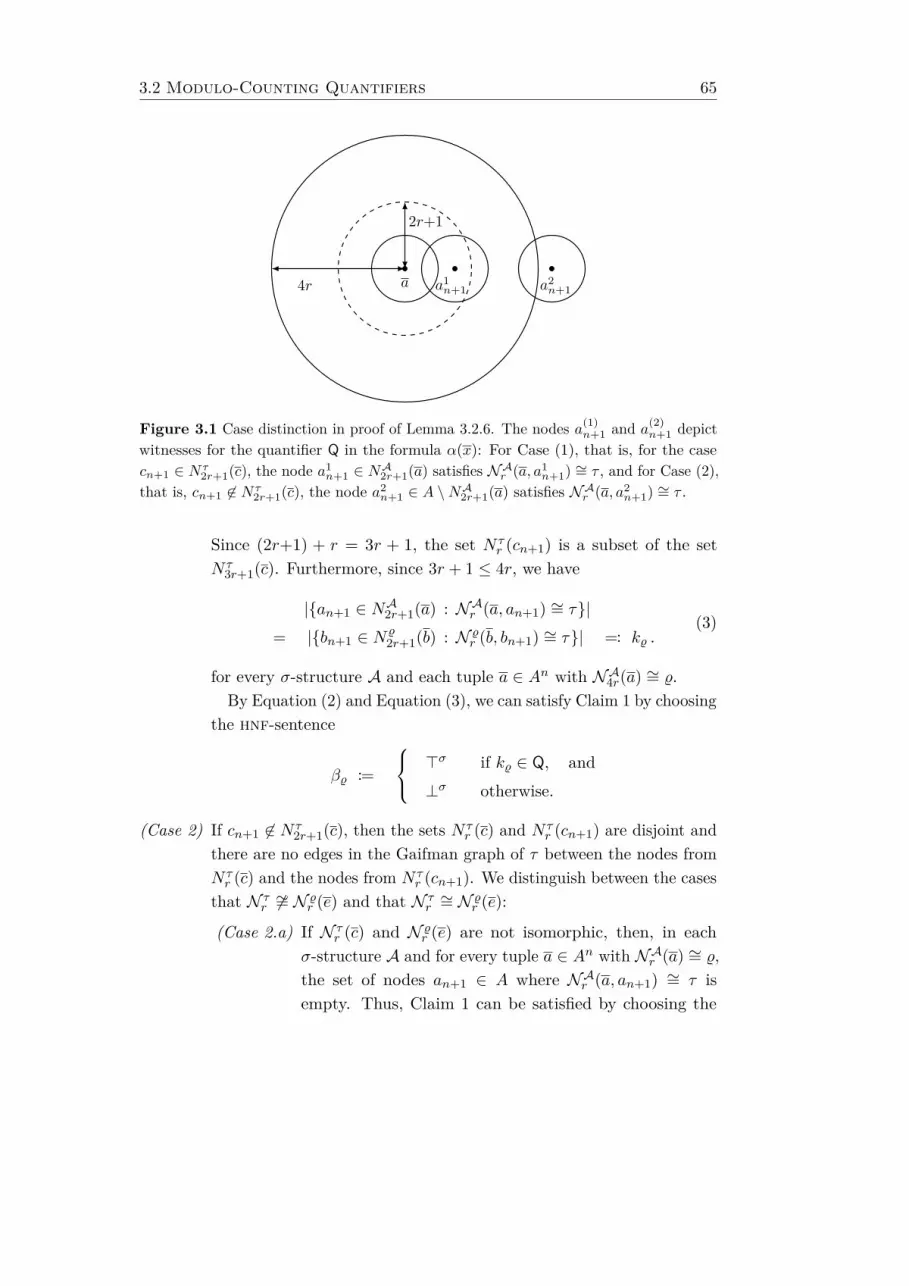
3.2 Modulo-Counting Quantifiers 65
a a1n+1 a2
n+14r
2r+1
Figure 3.1 Case distinction in proof of Lemma 3.2.6. The nodes a(1)n+1 and a(2)
n+1 depictwitnesses for the quantifier Q in the formula α(x): For Case (1), that is, for the casecn+1 ∈ Nτ
2r+1(c), the node a1n+1 ∈ NA2r+1(a) satisfies NAr (a, a1
n+1) ∼= τ , and for Case (2),that is, cn+1 6∈ Nτ
2r+1(c), the node a2n+1 ∈ A \NA2r+1(a) satisfies NAr (a, a2
n+1) ∼= τ .
Since (2r+1) + r = 3r + 1, the set N τr (cn+1) is a subset of the set
N τ3r+1(c). Furthermore, since 3r + 1 ≤ 4r, we have
|an+1 ∈ NA2r+1(a) : NAr (a, an+1) ∼= τ|= |bn+1 ∈ N%
2r+1(b) : N %r (b, bn+1) ∼= τ| =: k% .
(3)
for every σ-structure A and each tuple a ∈ An with NA4r(a) ∼= %.By Equation (2) and Equation (3), we can satisfy Claim 1 by choosing
the hnf-sentence
β% :=
>σ if k% ∈ Q, and⊥σ otherwise.
(Case 2) If cn+1 6∈ N τ2r+1(c), then the sets N τ
r (c) and N τr (cn+1) are disjoint and
there are no edges in the Gaifman graph of τ between the nodes fromN τr (c) and the nodes from N τ
r (cn+1). We distinguish between the casesthat N τ
r 6∼= N %r (e) and that N τ
r∼= N %
r (e):
(Case 2.a) If N τr (c) and N %
r (e) are not isomorphic, then, in eachσ-structure A and for every tuple a ∈ An with NAr (a) ∼= %,the set of nodes an+1 ∈ A where NAr (a, an+1) ∼= τ isempty. Thus, Claim 1 can be satisfied by choosing the
66 Chapter 3. Hanf Normal Form
hnf-sentence
β% :=
>σ if 0 ∈ Q, and⊥σ otherwise.
(Case 2.b) If N τr (c) and N %
r (e) are isomorphic, we have for each tuplea ∈ An in every σ-structure A that
|an+1 ∈ A : NAr (a, an+1) ∼= τ|= |an+1 ∈ A \NA2r+1(a) : NAr (an+1) ∼= N τ
r (cn+1)|.(4)
Furthermore, since (2r+1) + r = 3r + 1 ≤ 4r, we have
|an+1 ∈ NA2r+1(a) : NAr (an+1) ∼= N τr (cn+1)|
= |bn+1 ∈ N%2r+1(b) : N %
r (bn+1) ∼= N τr (cn+1)| := `%
(5)
whenever NA4r(a) ∼= %.Thus, combining Equations (4) and (5), we obtain that
for all σ-structures A and all a ∈ An with NA4r(a) ∼= %,
|an+1 ∈ A : NAr (a, an+1) ∼= τ|= |an+1 ∈ A : NAr (an+1) ∼= N τ
r (cn+1)| − `%.
Hence, we can satisfy Claim 1 by choosing the hnf-sentence
β% := (Q+`%)y sphN τr (cn+1)(y).
Clearly, the size of `% is bounded by the number of elementsthat may exist in a d-bounded type with radius 2r + 1and n centres, and thus, β% has shift ≤ n · νd(2r+1).
Note that, in all cases of the construction, the hnf-sentence β% has localityradius ≤ r and shift ≤ n · νd(2r+1). This completes the proof of Claim 1.For ultimately periodic Q, it can easily be decided for a number m ∈ N
if m ∈ Q. In Case (1) and Case (2.a) in the proof of Claim 1, this is usedfor m = k% and m = 0, respectively, and leads to an algorithm which constructsthe hnf-formula β(x). We complete the proof of Lemma 3.2.6 by an analysis ofthe time complexity of this algorithm.
Time complexity. In the following, we abbreviate N := n · νd(4r). Observethat N ≥ 2, since d ≥ 2 and n, r ≥ 1.
3.2 Modulo-Counting Quantifiers 67
By Lemma 2.8.7, the set Td,σ4r (n) can be constructed in time
2NO(||σ||). (6)
To obtain the hnf-formula β(x), we have to construct the sphere-formula sph%(x)and the hnf-sentence β% for each type % ∈ Td,σ4r (n).
Let % ∈ Td,σ4r (n). By Lemma 2.8.8 it takes time
NO(||σ||) (7)
to construct sph%(x). For the construction of β% according to Claim 1, we haveto make a case distinction depending on whether cn+1 ∈ N τ
2r+1(c).To determine which of the two cases actually applies for the given type τ ,
recall that the universe of τ has size at most (n+1) ·νd(r). Thus, the time neededto decide whether cn+1 ∈ N τ
2r+1(c) is in
NO(||σ||). (8)
(Case 1) If cn+1 ∈ N τ2r+1(c), we compute the number k% defined in Equation (3).
This requires us to check for at most n · νd(2r+1) ≤ N types withradius r and n+ 1 centres whether they are isomorphic to τ . As eachof these types is d-bounded, the number k% can be computed in time
N · 2O(||σ||)·N2 ⊆ 2O(||σ||)·N2
by using the brute-force isomorphism test described in the proof ofLemma 2.8.6.
The representation rep(Q) of the quantifier Q can be used for testingwhether k% ∈ Q. This takes time in O(k%). Since k% ≤ N , the algorithmaltogether constructs β% in Case (1) in time
2O(||σ||)·N2 (9)
(Case 2) If cn+1 6∈ N τ2r+1(c), we have to check whether the two types N τ
r (c)and N %
r (b) are isomorphic. According to Lemma 2.8.6 this takes timein
2O(||σ||)·N2. (10)
(Case 2.a) If N τr (c) and N %
r (b) are not isomorphic, we need constanttime to check whether 0 ∈ Q and to construct β% accord-ingly.
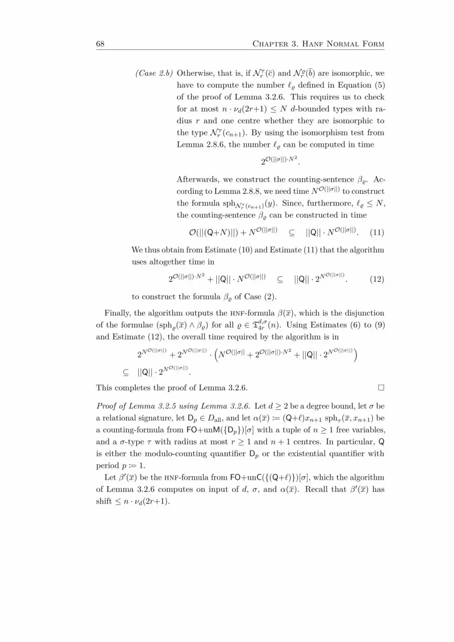
68 Chapter 3. Hanf Normal Form
(Case 2.b) Otherwise, that is, if N τr (c) and N %
r (b) are isomorphic, wehave to compute the number `% defined in Equation (5)of the proof of Lemma 3.2.6. This requires us to checkfor at most n · νd(2r+1) ≤ N d-bounded types with ra-dius r and one centre whether they are isomorphic tothe type N τ
r (cn+1). By using the isomorphism test fromLemma 2.8.6, the number `% can be computed in time
2O(||σ||)·N2.
Afterwards, we construct the counting-sentence β%. Ac-cording to Lemma 2.8.8, we need time NO(||σ||) to constructthe formula sphN τr (cn+1)(y). Since, furthermore, `% ≤ N ,the counting-sentence β% can be constructed in time
O(||(Q+N)||) +NO(||σ||) ⊆ ||Q|| ·NO(||σ||). (11)
We thus obtain from Estimate (10) and Estimate (11) that the algorithmuses altogether time in
2O(||σ||)·N2 + ||Q|| ·NO(||σ||) ⊆ ||Q|| · 2NO(||σ||). (12)
to construct the formula β% of Case (2).
Finally, the algorithm outputs the hnf-formula β(x), which is the disjunctionof the formulae (sph%(x) ∧ β%) for all % ∈ Td,σ4r (n). Using Estimates (6) to (9)and Estimate (12), the overall time required by the algorithm is in
2NO(||σ||) + 2NO(||σ||) ·(NO(||σ|| + 2O(||σ||)·N2 + ||Q|| · 2NO(||σ||))
⊆ ||Q|| · 2NO(||σ||).
This completes the proof of Lemma 3.2.6.
Proof of Lemma 3.2.5 using Lemma 3.2.6. Let d ≥ 2 be a degree bound, let σ bea relational signature, let Dp ∈ Dall, and let α(x) := (Q+`)xn+1 sphτ (x, xn+1) bea counting-formula from FO+unM(Dp)[σ] with a tuple of n ≥ 1 free variables,and a σ-type τ with radius at most r ≥ 1 and n + 1 centres. In particular, Qis either the modulo-counting quantifier Dp or the existential quantifier withperiod p := 1.
Let β′(x) be the hnf-formula from FO+unC((Q+`))[σ], which the algorithmof Lemma 3.2.6 computes on input of d, σ, and α(x). Recall that β′(x) hasshift ≤ n · νd(2r+1).

3.2 Modulo-Counting Quantifiers 69
(Case 1) If Q = ∃, then β′(x) is, in particular, a hnf-formula from FO+unT[σ]with threshold ≤ `+ n · νd(2r+1). Thus, we can choose β(x) := β′(x).
(Case 2) If Q = Dp, then ` ∈ [0, p) and β′(x) is a hnf-formula from the logicFO+unC((Dp+`))[σ]. We replace every counting-sentence of theshape (Dp+k)y sph%(y) and with k ≥ p in β′(x) by the counting-sentence (Dp+k′)y sph%(y), for which k′ ∈ [0, p) is chosen such thatk ≡ k′ mod p. Afterwards, we output the resulting hnf-formula β(x),which, in particular, belongs to FO+unM(Dp)[σ].
Furthermore, β(x) has threshold 0, since already β′(x) only usescounting-sentences (∃+k)y sph%(y) with k = 0.
Time complexity. Recalling the encoding of ultimately periodic quantifiers, weknow that ||(Q+`)|| ≤ max3+`, 2p ≤ 2 max`, p+ 3. Thus, the constructionof β′(x) from α(x) takes time in
(2 max`, p) · 2(n·νd(4r))O(||σ||). (1)
As the construction of β(x) from β′(x) takes time linear in the size of β′(x),Estimate (1) is also an upper bound on the time required to construct β(x)from α(x). This completes the proof of Lemma 3.2.5.
3.2.2 The Hanf Normal Form Algorithm
We are now ready to prove Theorem 3.2.1 – the main result of this chapter.The proof uses the induction step described in Section 3.2.1 to turn arbitraryformulae with modulo-counting quantifiers into Hanf normal form.
Proof of Theorem 3.2.1. We describe the algorithm on input of a degree boundd ≥ 2, a relational signature σ, and a formula ϕ(x) from FO+unM(D)[σ], whereD ⊆ Dall. Let n := |x| be the number of free variables of ϕ and let T, P, q ≥ 0 bethe threshold, the maximum period, and the quantifier rank of ϕ, respectively.
The algorithm proceeds by induction on the shape of ϕ(x). We will show thatthe following inductive invariant holds for the constructed hnf-formula ψ(x):
Claim 1.
(a) ψ(x) is d-equivalent to ϕ(x).
(b) ψ(x) has locality radius ≤ 4q.
(c) ψ(x) has threshold ≤ T + (n+q) · νd(4q).
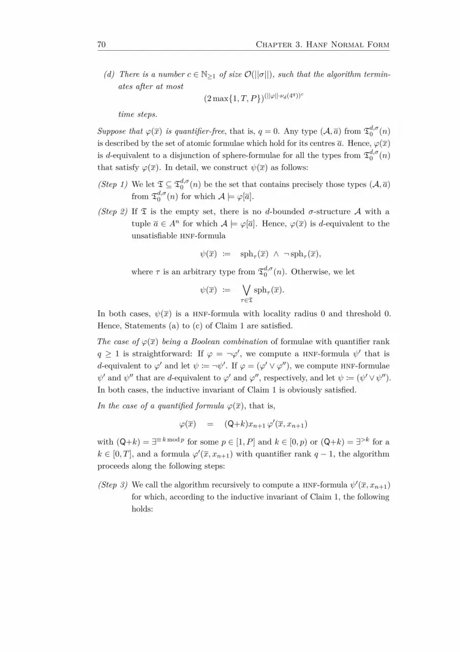
70 Chapter 3. Hanf Normal Form
(d) There is a number c ∈ N≥1 of size O(||σ||), such that the algorithm termin-ates after at most
(2 max1, T, P)(||ϕ||·νd(4q))c
time steps.
Suppose that ϕ(x) is quantifier-free, that is, q = 0. Any type (A, a) from Td,σ0 (n)is described by the set of atomic formulae which hold for its centres a. Hence, ϕ(x)is d-equivalent to a disjunction of sphere-formulae for all the types from Td,σ0 (n)that satisfy ϕ(x). In detail, we construct ψ(x) as follows:
(Step 1) We let T ⊆ Td,σ0 (n) be the set that contains precisely those types (A, a)from Td,σ0 (n) for which A |= ϕ[a].
(Step 2) If T is the empty set, there is no d-bounded σ-structure A with atuple a ∈ An for which A |= ϕ[a]. Hence, ϕ(x) is d-equivalent to theunsatisfiable hnf-formula
ψ(x) := sphτ (x) ∧ ¬ sphτ (x),
where τ is an arbitrary type from Td,σ0 (n). Otherwise, we let
ψ(x) :=∨τ∈T
sphτ (x).
In both cases, ψ(x) is a hnf-formula with locality radius 0 and threshold 0.Hence, Statements (a) to (c) of Claim 1 are satisfied.
The case of ϕ(x) being a Boolean combination of formulae with quantifier rankq ≥ 1 is straightforward: If ϕ = ¬ϕ′, we compute a hnf-formula ψ′ that isd-equivalent to ϕ′ and let ψ := ¬ψ′. If ϕ = (ϕ′ ∨ ϕ′′), we compute hnf-formulaeψ′ and ψ′′ that are d-equivalent to ϕ′ and ϕ′′, respectively, and let ψ := (ψ′ ∨ψ′′).In both cases, the inductive invariant of Claim 1 is obviously satisfied.
In the case of a quantified formula ϕ(x), that is,
ϕ(x) = (Q+k)xn+1 ϕ′(x, xn+1)
with (Q+k) = ∃≡ kmod p for some p ∈ [1, P ] and k ∈ [0, p) or (Q+k) = ∃>k for ak ∈ [0, T ], and a formula ϕ′(x, xn+1) with quantifier rank q − 1, the algorithmproceeds along the following steps:
(Step 3) We call the algorithm recursively to compute a hnf-formula ψ′(x, xn+1)for which, according to the inductive invariant of Claim 1, the followingholds:
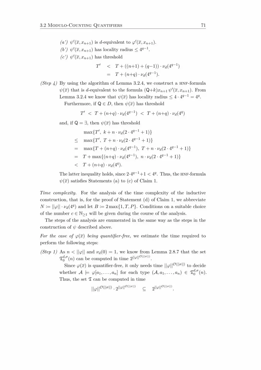
3.2 Modulo-Counting Quantifiers 71
(a’) ψ′(x, xn+1) is d-equivalent to ϕ′(x, xn+1).(b’) ψ′(x, xn+1) has locality radius ≤ 4q−1.(c’) ψ′(x, xn+1) has threshold
T ′ < T + ((n+1) + (q−1)) · νd(4q−1)= T + (n+q) · νd(4q−1).
(Step 4) By using the algorithm of Lemma 3.2.4, we construct a hnf-formulaψ(x) that is d-equivalent to the formula (Q+k)xn+1 ψ
′(x, xn+1). FromLemma 3.2.4 we know that ψ(x) has locality radius ≤ 4 · 4q−1 = 4q.
Furthermore, if Q ∈ D, then ψ(x) has threshold
T ′ < T + (n+q) · νd(4q−1) < T + (n+q) · νd(4q)
and, if Q = ∃, then ψ(x) has threshold
maxT ′, k + n · νd(2 · 4q−1 + 1)≤ maxT ′, T + n · νd(2 · 4q−1 + 1)= maxT + (n+q) · νd(4q−1), T + n · νd(2 · 4q−1 + 1)= T + max(n+q) · νd(4q−1), n · νd(2 · 4q−1 + 1)< T + (n+q) · νd(4q).
The latter inequality holds, since 2·4q−1+1 < 4q. Thus, the hnf-formulaψ(x) satisfies Statements (a) to (c) of Claim 1.
Time complexity. For the analysis of the time complexity of the inductiveconstruction, that is, for the proof of Statement (d) of Claim 1, we abbreviateN := ||ϕ|| · νd(4q) and let B := 2 max1, T, P. Conditions on a suitable choiceof the number c ∈ N≥1 will be given during the course of the analysis.
The steps of the analysis are enumerated in the same way as the steps in theconstruction of ψ described above.
For the case of ϕ(x) being quantifier-free, we estimate the time required toperform the following steps:
(Step 1) As n < ||ϕ|| and νd(0) = 1, we know from Lemma 2.8.7 that the setTd,σ0 (n) can be computed in time 2||ϕ||O(||σ||) .Since ϕ(x) is quantifier-free, it only needs time ||ϕ||O(||σ||) to decide
whether A |= ϕ[a1, . . . , an] for each type (A, a1, . . . , an) ∈ Td,σ0 (n).Thus, the set T can be computed in time
||ϕ||O(||σ||) · 2||ϕ||O(||σ||) ⊆ 2||ϕ||O(||σ||).

72 Chapter 3. Hanf Normal Form
(Step 2) For each type τ ∈ T, the sphere-formula sphτ (x) can be computedin time ||ϕ||O(||σ||), according to Lemma 2.8.8. Hence, the whole for-mula ψ(x) can be computed in time
||ϕ||O(||σ||) · 2||ϕ||O(||σ||) ⊆ 2||ϕ||O(||σ||).
By adding up the time required for both steps, we can conclude that c ∈ N≥1
can be chosen of size O(||σ||) such that the algorithm terminates in at most
2||ϕ||c ≤ BNc
time steps and thus, Statement (d) of Claim 1 is satisfied.
For ϕ(x) being a Boolean combination of formulae with quantifier rank q ≥ 1,Statement (d) of Claim 1 holds trivially.
Suppose that ϕ(x) is a quantified formula of the shape (Q+k)xn+1 ϕ′(x, xn+1),
where Q has period p ≥ 1. Again, we analyse the time required for the steps inthe construction of ψ(x).
(Step 3) According to Statement (d) of Claim 1, the algorithm constructsψ′(x, xn+1) from ϕ′(x, xn+1) in at most
(2 max1,K, P)(||ϕ′||·νd(4q−1))c ≤ B(N−1)c
time steps; and this is also an upper bound on the size of ψ′(x, xn+1).
(Step 4) By Lemma 3.2.4, the hnf-formula ψ(x) can be computed from theformula (Q+k)xn+1 ψ
′(x, xn+1) in time
||ψ′|| · (2 maxk, p)((n+1)·νd(4r))O(||σ||).
Since 2 maxk, p ≤ B and (n+1) · νd(4r) ≤ N , there is a numberc′ ∈ N≥1 of size O(||σ||), such that the algorithm from Lemma 3.2.4takes at most
B(N−1)c ·BNc′ = B(N−1)c+Nc′
time steps.
Summing up the time needed for Step (3) and Step (4), the algorithm needs atmost
B(N−1)c +B(N−1)c+Nc′ ≤ B(N−1)c+Nc′′
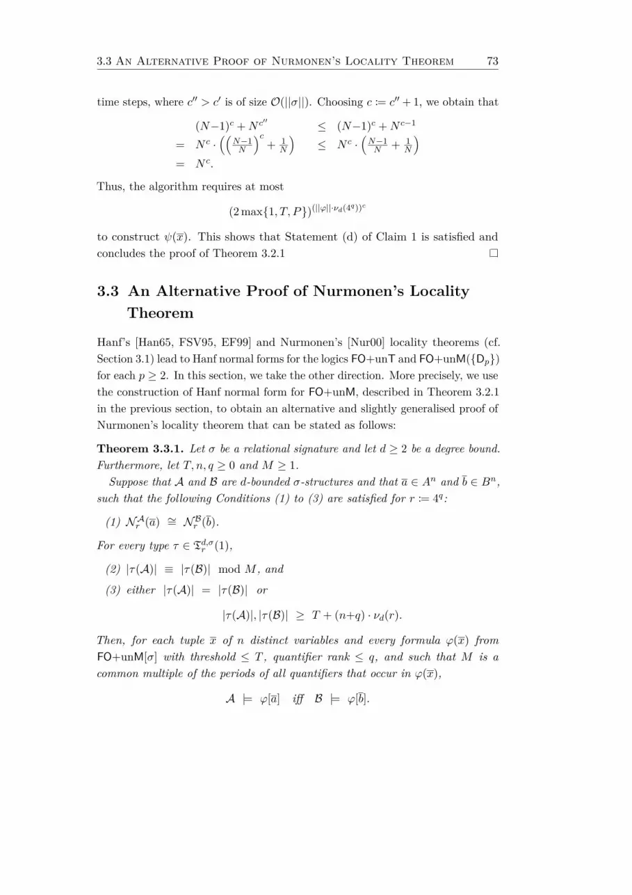
3.3 An Alternative Proof of Nurmonen’s Locality Theorem 73
time steps, where c′′ > c′ is of size O(||σ||). Choosing c := c′′ + 1, we obtain that
(N−1)c +N c′′ ≤ (N−1)c +N c−1
= N c ·((
N−1N
)c+ 1
N
)≤ N c ·
(N−1N + 1
N
)= N c.
Thus, the algorithm requires at most
(2 max1, T, P)(||ϕ||·νd(4q))c
to construct ψ(x). This shows that Statement (d) of Claim 1 is satisfied andconcludes the proof of Theorem 3.2.1
3.3 An Alternative Proof of Nurmonen’s LocalityTheorem
Hanf’s [Han65, FSV95, EF99] and Nurmonen’s [Nur00] locality theorems (cf.Section 3.1) lead to Hanf normal forms for the logics FO+unT and FO+unM(Dp)for each p ≥ 2. In this section, we take the other direction. More precisely, we usethe construction of Hanf normal form for FO+unM, described in Theorem 3.2.1in the previous section, to obtain an alternative and slightly generalised proof ofNurmonen’s locality theorem that can be stated as follows:
Theorem 3.3.1. Let σ be a relational signature and let d ≥ 2 be a degree bound.Furthermore, let T, n, q ≥ 0 and M ≥ 1.
Suppose that A and B are d-bounded σ-structures and that a ∈ An and b ∈ Bn,such that the following Conditions (1) to (3) are satisfied for r := 4q:
(1) NAr (a) ∼= NBr (b).
For every type τ ∈ Td,σr (1),
(2) |τ(A)| ≡ |τ(B)| mod M , and
(3) either |τ(A)| = |τ(B)| or
|τ(A)|, |τ(B)| ≥ T + (n+q) · νd(r).
Then, for each tuple x of n distinct variables and every formula ϕ(x) fromFO+unM[σ] with threshold ≤ T , quantifier rank ≤ q, and such that M is acommon multiple of the periods of all quantifiers that occur in ϕ(x),
A |= ϕ[a] iff B |= ϕ[b].
74 Chapter 3. Hanf Normal Form
For the special case of sentences from FO, Theorem 3.3.1 implies Hanf’s The-orem as stated in, e.g., Theorem 2.4.1 of [EF99]. More generally, for sentenceswith threshold 0 from FO+unM(Dp), for some period p ≥ 2, Theorem 3.3.1implies Nurmonen’s theorem (Theorem 3.4 in [Nur00]). In fact, the game theor-etical condition for elementary equivalence with respect to first-order logic with amodulo-counting quantifier, defined in [Nur00], and the subsequent combinatorialproof of Nurmonen’s theorem there, can be extended to an alternative proof ofTheorem 3.3.1.
Note that, due to the specific construction of Hanf normal form appliedin the proof of Theorem 3.3.1 below, the locality radius r := 4q obtained inTheorem 3.3.1 grows faster with the quantifier rank as in Hanf’s and Nurmonen’stheorems, whose combinatorial proofs lead to locality radius 3q.
Proof of Theorem 3.3.1. Let σ be a relational signature and let d ≥ 2 be a degreebound. Furthermore, let T, n, q ≥ 0, M ≥ 1, and let r := 4q.Suppose that A and B are d-bounded σ-structures and that furthermore
a = (a1, . . . , an) ∈ An and b = (b1, . . . , bn) ∈ Bn, such that Conditions (1) to (3)of Theorem 3.3.1 are satisfied.Let ϕ(x) be a formula from FO+unM[σ]. Let D ⊆ Dall be the set of all
modulo-counting quantifiers that appear in ϕ, and suppose that ϕ has threshold≤ T , quantifier rank ≤ q, at most n free variables from a tuple x = (x1, . . . , xn),and that M is a common multiple of the periods of the quantifiers occurring inϕ.
We want to show that
A |= ϕ[a] iff B |= ϕ[b]. (1)
Let ψ(x) the hnf-formula from FO+unM(D)[σ], computed by Theorem 3.2.1 oninput of d, σ, and ϕ(x). In particular, ψ(x) is d-equivalent to ϕ(x) and, moreover,a Boolean combination of
(a) sphere-formulas sph%(x), where % is a σ-type with radius ≤ r and at most ncentres,
(b) counting-sentences ∃>ky sphτ (y), where
k < T + (n+q) · νd(r)
and τ is a σ-type with radius ≤ r and one centre, and
3.3 An Alternative Proof of Nurmonen’s Locality Theorem 75
(c) counting-sentences ∃≡ kmod py sphτ (y) where p ≥ 2 divides M , k ∈ [0, p),and τ is a σ-type with radius ≤ r and one centre.
Since ϕ(x) and ψ(x) are d-equivalent and A, B are d-bounded, Equivalence (1)follows directly from the following claim.
Claim 1.A |= ψ[a] iff B |= ψ[b].
Proof of Claim 1 We show that for each subformula γ(x) of ψ(x) of Shape (a),Shape (b), or Shape (c),
A |= γ[a] iff B |= γ[b].
(a) Consider a sphere-formula sph%(xi1 , . . . , xim) from ψ(x), where xi1 , . . . , ximare m ∈ [1, n] pairwise distinct variables from x1, . . . , xn for suitable indicesi1, . . . , im ∈ [1, n], and where % is a σ-type of radius s ≤ r and with m
centres. The following equivalences hold:
A |= sph%[ai1 , . . . , aim ]iff NAs (ai1 , . . . , aim) ∼= %
iff NBs (bi1 , . . . , bim) ∼= % (by Condition (1))iff B |= sph%[bi1 , . . . , bim ].
(b) Suppose that ∃>ky sphτ (y) is a counting-sentence occuring in ψ(x) withk < T + (n+q) · νd(r) and a σ-type τ with radius ≤ r and one centre. Thefollowing equivalences hold:
A |= ∃>ky sphτ (y)iff |τ(A)| ≥ k + 1iff |τ(B)| ≥ k + 1 (?)iff B |= ∃>ky sphτ (y).
For Equivalence (?), assume that |τ(A)| 6= |τ(B)|. Then, by Condition (3),
|τ(A)|, |τ(B)| ≥ T + (n+q) · νd(r) ≥ k + 1.
(c) Let ∃≡ kmod py sphτ (y) be a counting-sentence occurring in ψ(x) wherep ≥ 2, k ∈ [0, p), and τ is a σ-type with radius ≤ r and one centre.
76 Chapter 3. Hanf Normal Form
Since M is a multiple of p, the following equivalences hold:
A |= ∃≡ kmod py sphτ (y)iff |τ(A)| ≡ k mod p
iff |τ(B)| ≡ k mod p (by Condition (2))iff B |= ∃≡ kmod py sphτ (y).
This completes the proof of Claim 1 and also the proof of Theorem 3.3.1.
3.4 Model-Checking
In Section 3.2, it was shown that for each degree bound d ≥ 2 and everyrelational signature σ, any formula from FO+unM[σ] can be turned effectivelyinto a d-equivalent hnf-formula from FO+unM[σ].As an immediate application, we obtain that Seese’s fixed-parameter tract-
ability result for model-checking of formulas from FO on structures of boundeddegree [See96] can be generalised to FO+unM. More precisely, we prove thefollowing theorem:
Theorem 3.4.1. There is an algorithm which, on input of
• a formula ϕ(x) from FO+unM where x are the n ≥ 0 free variables of ϕ,
• a finite σ-structure A (where σ consists of precisely the relation symbolsthat occur in ϕ), and a tuple a ∈ An,
decides whether A |= ϕ[a].This algorithm takes time in
(2 max1, T, P)(||ϕ||·νd(4q))O(||σ||) · ||A||
where T, P, q ≥ 0 are the threshold, the maximum period, and the quantifier rankof ϕ(x), respectively, and where d ≥ 2 is a bound on the degree of A.
Remark 3.4.2. Since T, P, q, ||σ|| < ||ϕ||, the algorithm of Theorem 3.4.1 takes3-fold exponential time
2d2O(||ϕ||)· ||A||
in the size of ϕ for every σ-structure A with degree d ≥ 3, and 2-fold exponentialtime
22poly(||ϕ||) · ||A||
in the size of ϕ for every σ-structure A with degree d ≤ 2.
3.4 Model-Checking 77
In [FG04], a different approach to such a fixed-parameter tractable model-checking algorithm for FO on structures of bounded degree is presented. Thisapproach also uses Hanf-locality but not by constructing Hanf normal form. Notethat the corresponding lower bounds, also provided in [FG04], imply that themodel-checking algorithm of Theorem 3.4.1 is basically worst-case optimal (underthe complexity theoretic assumption FPT 6= AW[∗]).
Proof of Theorem 3.4.1. Let ϕ(x) be a formula from FO+unM(D), for a suit-able D ⊆ Dall, and let σ consist of precisely the relation symbols that occur in ϕ.Let n := |x| be the number of free variables of ϕ. Moreover, let A be a finiteσ-structure and let a ∈ An.
For checking whether A |= ϕ[a], the algorithm proceeds as follows:
(Step 1) Compute an upper bound d ≥ 2 on the degree of A.
(Step 2) Employ the algorithm from Theorem 3.2.1 to transform ϕ(x) into ad-equivalent hnf-formula ψ(x) from FO+unM(D)[σ].
(Step 3) For each sphere-formula α that occurs in ψ, check if A |= α[a], andreplace each occurrence of α in ψ with the Boolean constant 1 ifA |= α[a], and with the Boolean constant 0 otherwise.
(Step 4) For each counting-sentence χ that occurs in ψ, check if A |= χ, andreplace each occurrence of χ in ψ with the Boolean constant 1 if A |= χ,and with the Boolean constant 0 otherwise.
(Step 5) After having performed Steps (1) to (4), we have obtained a Booleancombination of the Boolean constants 0 and 1. Evaluate this Booleancombination and output “yes” if the result is 1, and output “no” if theresult is 0.
Obviously, the algorithm’s output is “yes” if, and only if, A |= ϕ[a].
Time complexity. We describe the details of Steps (1) to (5) in a run time analysisof the algorithm sketched above. For the following, let x = (x1, . . . , xn) and leta = (a1, . . . , an). Furthermore, let T, P, q ≥ 0 be the threshold, the maximumperiod, and the quantifier rank of ϕ, respectively.
In the following, we abbreviate N := ||ϕ|| · νd(4q).
(Step 1) To compute d, compute an adjacency list representation of A’s Gaifman-graph GA: For each relation symbol R in σ and each occurrence of an
78 Chapter 3. Hanf Normal Form
element of A in a tuple of RA, we have to add at most ar(R) ≤ ||σ||edges to GA. Since A is d-bounded, each adjacency list has < d entries.In summary, computing GA and d takes time in
O(||σ||) · ||A|| · d. (1)
(Step 2) According to Theorem 3.2.1, the construction of the hnf-formula ψ(x)takes time in
(2 max1, T, P)NO(||σ||). (2)
Recall that ψ(x) is a Boolean combination of
(a) sphere-formulae of the shape sph%(x′), for a tuple of m ∈ [1, n]variables belonging to the tuple x and a d-bounded σ-type % withradius ≤ 4q and m centres, and
(b) counting-sentences of the shape (Q+k)y sphτ (y), with Q ∈ D∪∃,k ≥ 0, and a d-bounded σ-type τ with radius ≤ 4q and one centre.
(Step 3) Consider a sphere-formula α(x′) := sph%(x′) with m ∈ [1, n] free vari-ables x′ = (xi1 , . . . , xim) for suitable indices i1, . . . , im from [1, n], andwhere % is a d-bounded σ-type with radius r ≤ 4q and m centres.
To decide whether A |= α[a′], for a′ = (ai1 , . . . , aim), we have to checkwhether NAr (a′) ∼= %. Since r ≤ 4q and m ≤ n, this can in time
2O(||σ||)·N2 ⊆ 2NO(||σ||) (3)
by using the algorithm of Lemma 2.8.6.
(Step 4) Consider a counting-sentence χ := (Q+k)y sphτ (y) that occurs in ψ.In particular, τ is a d-bounded type with radius r ≤ 4q and one centre.
To decide whether A |= χ, we first compute the number kτ of elementsa ∈ A with NAr (a) ∼= τ . Afterwards, we check if kτ ∈ (Q+k). Thelatter can be done easily using the encoding of (Q+k).
To compute kτ , we consider every a ∈ A, compute the sphere NAr (a),and check whether NAr (a) ∼= τ . From Step (3) we know that foreach a ∈ A this can be done in time 2NO(||σ||) .Since there are at most ||ψ|| counting-sentences in ψ, the entire
Step (4) takes time in
(2 max1, T, P)NO(||σ||) · 2NO(||σ||) · |A|
⊆ (2 max1, T, P)NO(||σ||) · |A|. (4)
3.5 Conclusion 79
(Step 5) Evaluation the resulting variable-free propositional formula takes timepolynomial in the size of ψ, that is, time in
(2 max1, T, P)NO(||σ||). (5)
In summary, we can conclude from Estimates (1) to (5) that the total runningtime of the algorithm is
(2 max1, T, P)NO(||σ||) · ||A|| = (2 max1, T, P)(||ϕ||·νd(4q))O(||σ||) · ||A||.
This completes the proof of Theorem 3.4.1.
3.5 Conclusion
In this chapter, a generalisation of Hanf normal form to extensions of first-orderlogic by unary counting quantifiers was introduced. This motivated the question,which sets of unary counting quantifiers actually permit Hanf normal form. Thatis, for which such extensions of first-order logic by unary counting quantifiers,every formula has a d-equivalent hnf-formula for every degree bound d ≥ 0?
As a partial answer to this question, we have shown that each logic FO+unM(D),for any set D ⊆ Dall, permits Hanf normal form. This extends slightly on Nur-monen’s locality theorem, which only implies that FO+unM(Dp) for singlemodulo-counting quantifiers permits Hanf normal form, and also lead to analternative proof of Nurmonen’s locality theorem [Nur00].Moreover, our corresponding proof does not only show the existence of Hanf
normal forms, but also how to compute them in 3-fold exponential time in thesize of the input formula for degree bounds d ≥ 3, and in 2-fold exponential timefor d = 2. In Section 9.3, we will see that this algorithm is basically worst-caseoptimal for both cases.
As an application, we used our construction of Hanf normal form for a model-checking algorithm which decides whether a d-bounded interpretation (A, a)satisfies a formula ϕ(x) from FO+unM in 3-fold (2-fold) exponential time in thesize of ϕ, for d ≥ 3 (d = 2), and in linear time in the size of A.In Section 7.3 and Section 8.4, we will extend the results of this chapter to
further logics. In particular, in Section 7.3, we consider the extension FO+unMtpl
of FO+unM by tuple-counting quantifiers. In Section 8.4, we look beyondmodulo-counting quantifiers and provide a characterisation of all sets of unarycounting-quantifiers that permit Hanf normal form, answering the question stated
80 Chapter 3. Hanf Normal Form
above. More precisely, we will show that ultimately periodic logics are preciselythe logics that permit Hanf normal form. Moreover, for all ultimately periodiclogics, we also obtain corresponding generalisations for the algorithmic results ofthis chapter.
4 Gaifman Normal Form
This chapter is based on [HKS13]. It is know that the construction of anequivalent Gaifman normal form from an FO-formula involves a non-elementaryblow-up, even on classes of trees of unbounded degree [DGKS07]. In contrast,for cases where only equivalence on a class of structures of degree at most d isrequired, this chapter presents an algorithm which computes Gaifman normalform in worst-case optimal 3-fold exponential time, for d ≥ 3.
4.1 Introduction
In this chapter we turn our attention to Gaifman’s locality theorem [Gai82]and the corresponding local normal form for first-order logic, called Gaifmannormal form. According to [Gai82] every FO-sentence over a relational signatureis equivalent to a Gaifman normal form, that is, a Boolean combination ofexpressions of the form
“there are at least k elements x of pairwise distance > 2r whoser-sphere satisfies a formula %(x)”.
However, this Gaifman normal form may be non-elementarily larger then theoriginal formula, even when equivalence to the original formula is only requiredon the class of trees [DGKS07]. This non-elementary lower bound does not holdwhen imposing restrictions on the degree of the trees in the class.
We present an algorithm that transforms formulae from FO+unT, for degreebounds d ≥ 2, into d-equivalent formulae in Gaifman normal form from FO+unT.For d = 2, the algorithm takes 2-fold exponential time in the size of the inputformula and for d ≥ 3, it takes 3-fold exponential time. The algorithm waspublished in [HKS13]. A lower bound, presented in Section 9.4, shows that it isworst-case optimal.
Our algorithm is carried out in two phases: First, the input formula is turnedinto a d-equivalent Hanf normal form. In a second step, all counting-sentences in
81
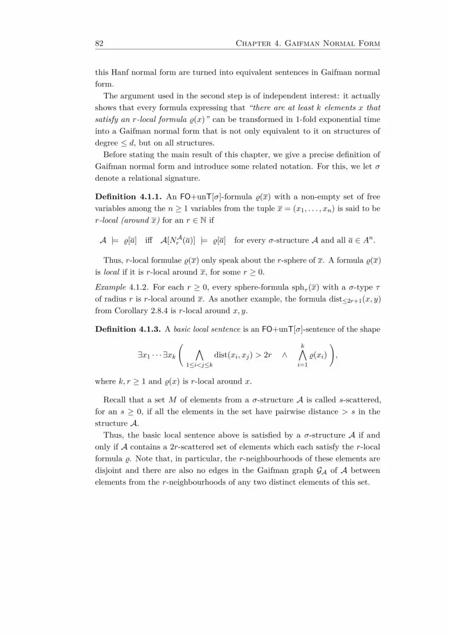
82 Chapter 4. Gaifman Normal Form
this Hanf normal form are turned into equivalent sentences in Gaifman normalform.The argument used in the second step is of independent interest: it actually
shows that every formula expressing that “there are at least k elements x thatsatisfy an r-local formula %(x)” can be transformed in 1-fold exponential timeinto a Gaifman normal form that is not only equivalent to it on structures ofdegree ≤ d, but on all structures.Before stating the main result of this chapter, we give a precise definition of
Gaifman normal form and introduce some related notation. For this, we let σdenote a relational signature.
Definition 4.1.1. An FO+unT[σ]-formula %(x) with a non-empty set of freevariables among the n ≥ 1 variables from the tuple x = (x1, . . . , xn) is said to ber-local (around x) for an r ∈ N if
A |= %[a] iff A[NAr (a)] |= %[a] for every σ-structure A and all a ∈ An.
Thus, r-local formulae %(x) only speak about the r-sphere of x. A formula %(x)is local if it is r-local around x, for some r ≥ 0.
Example 4.1.2. For each r ≥ 0, every sphere-formula sphτ (x) with a σ-type τof radius r is r-local around x. As another example, the formula dist≤2r+1(x, y)from Corollary 2.8.4 is r-local around x, y.
Definition 4.1.3. A basic local sentence is an FO+unT[σ]-sentence of the shape
∃x1 · · · ∃xk
( ∧1≤i<j≤k
dist(xi, xj) > 2r ∧k∧i=1
%(xi)),
where k, r ≥ 1 and %(x) is r-local around x.
Recall that a set M of elements from a σ-structure A is called s-scattered,for an s ≥ 0, if all the elements in the set have pairwise distance > s in thestructure A.Thus, the basic local sentence above is satisfied by a σ-structure A if and
only if A contains a 2r-scattered set of elements which each satisfy the r-localformula %. Note that, in particular, the r-neighbourhoods of these elements aredisjoint and there are also no edges in the Gaifman graph GA of A betweenelements from the r-neighbourhoods of any two distinct elements of this set.
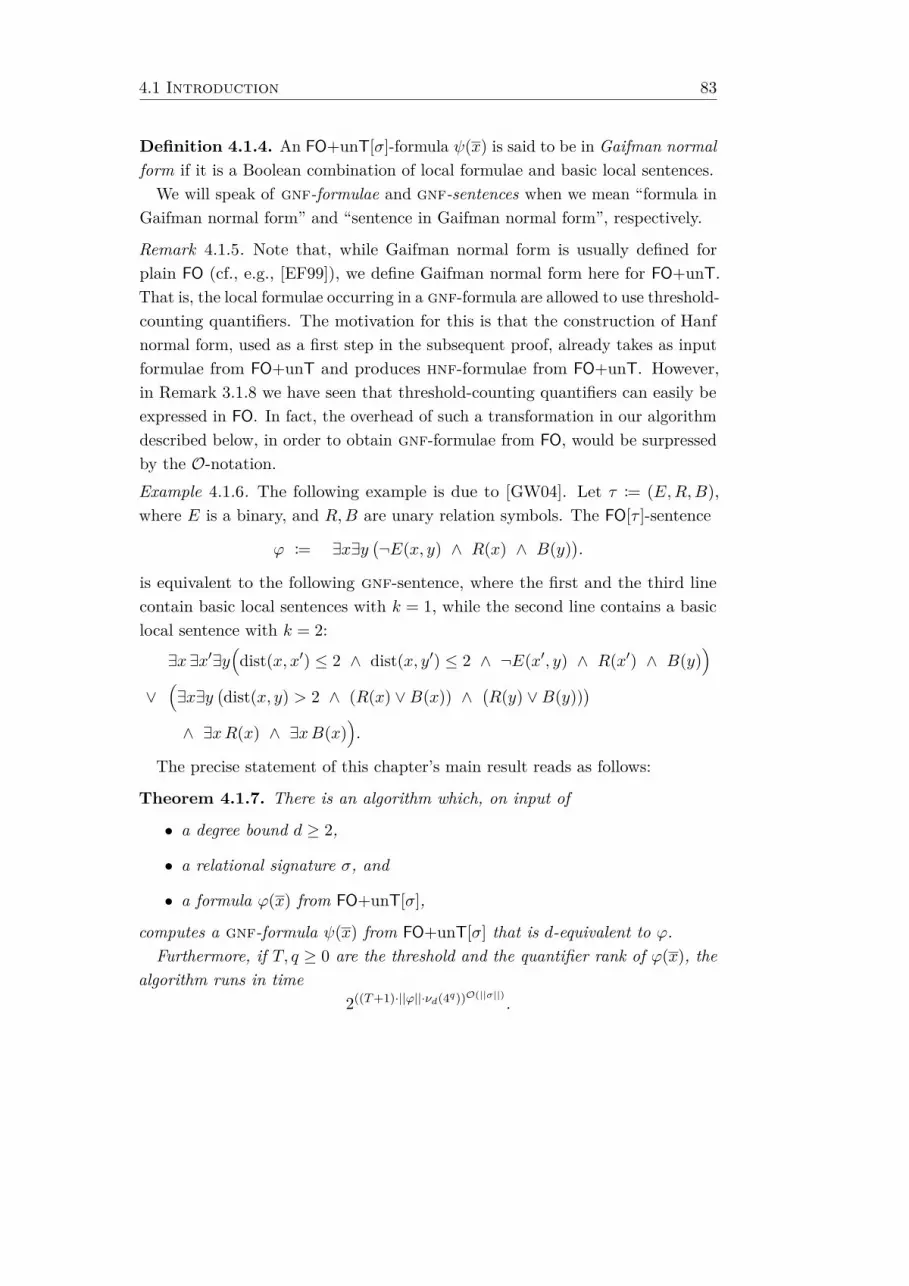
4.1 Introduction 83
Definition 4.1.4. An FO+unT[σ]-formula ψ(x) is said to be in Gaifman normalform if it is a Boolean combination of local formulae and basic local sentences.
We will speak of gnf-formulae and gnf-sentences when we mean “formula inGaifman normal form” and “sentence in Gaifman normal form”, respectively.
Remark 4.1.5. Note that, while Gaifman normal form is usually defined forplain FO (cf., e.g., [EF99]), we define Gaifman normal form here for FO+unT.That is, the local formulae occurring in a gnf-formula are allowed to use threshold-counting quantifiers. The motivation for this is that the construction of Hanfnormal form, used as a first step in the subsequent proof, already takes as inputformulae from FO+unT and produces hnf-formulae from FO+unT. However,in Remark 3.1.8 we have seen that threshold-counting quantifiers can easily beexpressed in FO. In fact, the overhead of such a transformation in our algorithmdescribed below, in order to obtain gnf-formulae from FO, would be surpressedby the O-notation.Example 4.1.6. The following example is due to [GW04]. Let τ := (E,R,B),where E is a binary, and R,B are unary relation symbols. The FO[τ ]-sentence
ϕ := ∃x∃y(¬E(x, y) ∧ R(x) ∧ B(y)
).
is equivalent to the following gnf-sentence, where the first and the third linecontain basic local sentences with k = 1, while the second line contains a basiclocal sentence with k = 2:
∃x ∃x′∃y(dist(x, x′) ≤ 2 ∧ dist(x, y′) ≤ 2 ∧ ¬E(x′, y) ∧ R(x′) ∧ B(y)
)∨(∃x∃y
(dist(x, y) > 2 ∧ (R(x) ∨B(x)) ∧
(R(y) ∨B(y))
)∧ ∃xR(x) ∧ ∃xB(x)
).
The precise statement of this chapter’s main result reads as follows:
Theorem 4.1.7. There is an algorithm which, on input of
• a degree bound d ≥ 2,
• a relational signature σ, and
• a formula ϕ(x) from FO+unT[σ],
computes a gnf-formula ψ(x) from FO+unT[σ] that is d-equivalent to ϕ.Furthermore, if T, q ≥ 0 are the threshold and the quantifier rank of ϕ(x), the
algorithm runs in time2((T+1)·||ϕ||·νd(4q))O(||σ||)
.

84 Chapter 4. Gaifman Normal Form
Remark 4.1.8. Suppose that σ contains only the relation symbols that actuallyoccur in ϕ(x), that is, ||σ|| < ||ϕ|| and recall that also T, q < ||ϕ||. Then, for everydegree bound d ≥ 3, the algorithm of Theorem 4.1.7 takes 3-fold exponentialtime
2d2O(||ϕ||)
in the size of ϕ(x). And for degree bound d = 2, the algorithm takes 2-foldexponential time
22poly(||ϕ||).
The remainder of this chapter is devoted to the proof of Theorem 4.1.7. Thefirst step of the proof is to turn the input formula into Hanf normal form. Forthis, we employ the following special case of Theorem 3.2.1 for an empty set ofmodulo-counting quantifiers.
Corollary 4.1.9. There is an algorithm which, on input of
• a degree bound d ≥ 2,
• a relational signature σ, and
• a formula ϕ(x) from FO+unT[σ],
computes a hnf-formula ψH(x) from FO+unT[σ] that is d-equivalent to ϕ.If T, n, q ≥ 0 are the threshold, the number of free variables, and the quantifier
rank of ϕ(x), then ψH(x) has locality radius ≤ 4q and threshold
< T + (n+q) · νd(4q).
Furthermore, the algorithm constructs ψH(x) in time
(2 max1, T)(||ϕ||·νd(4q))O(||σ||).
Recall from Definition 3.1.9 that a hnf-formula from FO+unT[σ] is a Booleancombination of sphere-formulae sph%(x) and counting-sentences of the shape∃≥ky sphτ (y) with k ≥ 1. On input of a degree bound d ≥ 2, a relationalsignature σ, and a formula ϕ(x) from FO+unT[σ], the algorithm of Theorem 4.1.7proceeds in the following steps:
(Step 1) The algorithm of Corollary 4.1.9 transforms ϕ into a d-equivalent hnf-formula ψH(x) from FO+unT[σ].
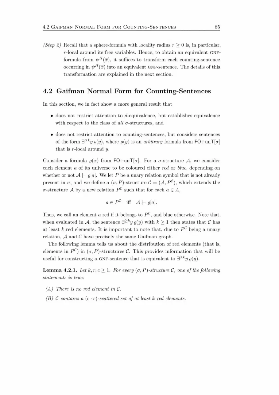
4.2 Gaifman Normal Form for Counting-Sentences 85
(Step 2) Recall that a sphere-formula with locality radius r ≥ 0 is, in particular,r-local around its free variables. Hence, to obtain an equivalent gnf-formula from ψH(x), it suffices to transform each counting-sentenceoccurring in ψH(x) into an equivalent gnf-sentence. The details of thistransformation are explained in the next section.
4.2 Gaifman Normal Form for Counting-Sentences
In this section, we in fact show a more general result that
• does not restrict attention to d-equivalence, but establishes equivalencewith respect to the class of all σ-structures, and
• does not restrict attention to counting-sentences, but considers sentencesof the form ∃≥ky %(y), where %(y) is an arbitrary formula from FO+unT[σ]that is r-local around y.
Consider a formula %(x) from FO+unT[σ]. For a σ-structure A, we considereach element a of its universe to be coloured either red or blue, depending onwhether or not A |= %[a]. We let P be a unary relation symbol that is not alreadypresent in σ, and we define a (σ, P )-structure C = (A, P C), which extends theσ-structure A by a new relation P C such that for each a ∈ A,
a ∈ P C iff A |= %[a].
Thus, we call an element a red if it belongs to P C , and blue otherwise. Note that,when evaluated in A, the sentence ∃≥ky %(y) with k ≥ 1 then states that C hasat least k red elements. It is important to note that, due to P C being a unaryrelation, A and C have precisely the same Gaifman graph.The following lemma tells us about the distribution of red elements (that is,
elements in P C) in (σ, P )-structures C. This provides information that will beuseful for constructing a gnf-sentence that is equivalent to ∃≥ky %(y).
Lemma 4.2.1. Let k, r, c ≥ 1. For every (σ, P )-structure C, one of the followingstatements is true:
(A) There is no red element in C.
(B) C contains a (c · r)-scattered set of at least k red elements.
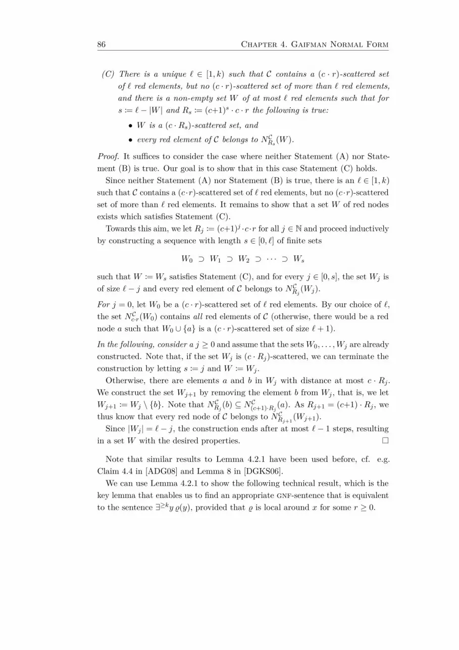
86 Chapter 4. Gaifman Normal Form
(C) There is a unique ` ∈ [1, k) such that C contains a (c · r)-scattered setof ` red elements, but no (c · r)-scattered set of more than ` red elements,and there is a non-empty set W of at most ` red elements such that fors := `− |W | and Rs := (c+1)s · c · r the following is true:
• W is a (c ·Rs)-scattered set, and• every red element of C belongs to NCRs(W ).
Proof. It suffices to consider the case where neither Statement (A) nor State-ment (B) is true. Our goal is to show that in this case Statement (C) holds.Since neither Statement (A) nor Statement (B) is true, there is an ` ∈ [1, k)
such that C contains a (c ·r)-scattered set of ` red elements, but no (c ·r)-scatteredset of more than ` red elements. It remains to show that a set W of red nodesexists which satisfies Statement (C).
Towards this aim, we let Rj := (c+1)j ·c ·r for all j ∈ N and proceed inductivelyby constructing a sequence with length s ∈ [0, `] of finite sets
W0 ⊃ W1 ⊃ W2 ⊃ · · · ⊃ Ws
such that W := Ws satisfies Statement (C), and for every j ∈ [0, s], the set Wj isof size `− j and every red element of C belongs to NCRj (Wj).
For j = 0, let W0 be a (c · r)-scattered set of ` red elements. By our choice of `,the set NCc·r(W0) contains all red elements of C (otherwise, there would be a rednode a such that W0 ∪ a is a (c · r)-scattered set of size `+ 1).
In the following, consider a j ≥ 0 and assume that the setsW0, . . . ,Wj are alreadyconstructed. Note that, if the set Wj is (c ·Rj)-scattered, we can terminate theconstruction by letting s := j and W := Wj .Otherwise, there are elements a and b in Wj with distance at most c · Rj .
We construct the set Wj+1 by removing the element b from Wj , that is, we letWj+1 := Wj \ b. Note that NCRj (b) ⊆ NC(c+1)·Rj (a). As Rj+1 = (c+1) ·Rj , wethus know that every red node of C belongs to NCRj+1
(Wj+1).Since |Wj | = `− j, the construction ends after at most `− 1 steps, resulting
in a set W with the desired properties.
Note that similar results to Lemma 4.2.1 have been used before, cf. e.g.Claim 4.4 in [ADG08] and Lemma 8 in [DGKS06].We can use Lemma 4.2.1 to show the following technical result, which is the
key lemma that enables us to find an appropriate gnf-sentence that is equivalentto the sentence ∃≥ky %(y), provided that % is local around x for some r ≥ 0.
4.2 Gaifman Normal Form for Counting-Sentences 87
Lemma 4.2.2. Let C be a (σ, P )-structure, let r ≥ 1, and let Rs := 9s · 8r forall s ∈ N.
For each k ≥ 1, C contains at least k red elements if and only if one of thefollowing statements is true:
(1) C contains an 8r-scattered set of at least k red elements.
(2) There is a red element in C whose Rk-neighbourhood contains at least k redelements.
(3) Each of the following statements is true:
(i) There is a unique ` ∈ [1, k) such that C contains an 8r-scattered setof ` red elements, but no 8r-scattered set of more than ` red elements.
(ii) There is an s ∈ [0, `) such that C contains an 8Rs-scattered set of `−sred elements and if s ≥ 1, then C does not contain an 8Rs−1-scatteredset of `− (s−1) red elements.
(iii) There is a number t ∈ [1, `−s] and numbers
1 ≤ n1 < · · · < nt < k and m1, . . . ,mt ∈ [1, k]
with
m1 + · · ·+mt = `−s and m1 · n1 + · · ·+mt · nt ≥ k
such that for each j ∈ [1, t] there is a 6Rs-scattered set of mj redelements whose 2Rs-neighbourhoods each contain exactly nj red ele-ments.
Proof. We prove the two directions of Lemma 4.2.2.
For the “only if” direction, suppose that C contains at least k red nodes. Itsuffices to consider the case where neither Statement (1) nor Statement (2) istrue. Our goal is to show that in this case Statement (3), that is, each of theStatements (3.i) to (3.iii), is satisfied.We use Lemma 4.2.1 for the numbers k and r, and we let c := 8. Note that
by assumption, C does not satisfy Statement (A) of Lemma 4.2.1. Moreover, bychoice of the number c = 8, C also does not satisfy Statement (B) of Lemma 4.2.1.Thus, Statement (C) of Lemma 4.2.1 must be true:
• There is an ` ∈ [1, k) such that C contains an 8r-scattered set of ` redelements, but no 8r-scattered set of more than ` red elements, and hence,Statement (3.i) is satisfied.
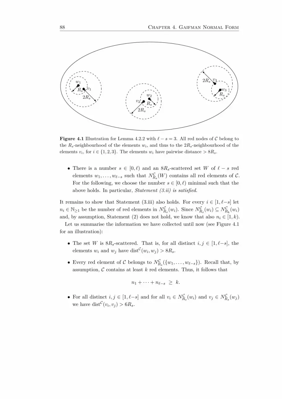
88 Chapter 4. Gaifman Normal Form
w1
v1
w2v2
w3
v3
Rs
Rs
Rs2Rs
2Rs
2Rs
Figure 4.1 Illustration for Lemma 4.2.2 with `− s = 3. All red nodes of C belong tothe Rs-neighbourhood of the elements wi, and thus to the 2Rs-neighbourhood of theelements vi, for i ∈ 1, 2, 3. The elements wi have pairwise distance > 8Rs.
• There is a number s ∈ [0, `) and an 8Rs-scattered set W of ` − s redelements w1, . . . , w`−s such that NCRs(W ) contains all red elements of C.For the following, we choose the number s ∈ [0, `) minimal such that theabove holds. In particular, Statement (3.ii) is satisfied.
It remains to show that Statement (3.iii) also holds. For every i ∈ [1, `−s] letni ∈ N≥1 be the number of red elements in NCRs(wi). Since N
CRs
(wi) ⊆ NCRk(wi)and, by assumption, Statement (2) does not hold, we know that also ni ∈ [1, k).
Let us summarise the information we have collected until now (see Figure 4.1for an illustration):
• The set W is 8Rs-scattered. That is, for all distinct i, j ∈ [1, `−s], theelements wi and wj have distC(wi, wj) > 8Rs.
• Every red element of C belongs to NCRs(w1, . . . , w`−s). Recall that, byassumption, C contains at least k red elements. Thus, it follows that
n1 + · · ·+ n`−s ≥ k.
• For all distinct i, j ∈ [1, `−s] and for all vi ∈ NCRs(wi) and vj ∈ NCRs(wj)we have distC(vi, vj) > 6Rs.
4.2 Gaifman Normal Form for Counting-Sentences 89
• For each i ∈ [1, `−s] and every vi ∈ NCRs(wi), the set NC2Rs(vi) containsexactly the same red elements as NCRs(wi).
Let us now group the numbers n1, . . . , n`−s according to their value. To thisend, let T := n1, . . . , n`−s be the set of distinct values among the numbersn1, . . . , n`−s and let t := |T | be the number of distinct values. For each valuein T , we choose a representative among the numbers n1, . . . , n`−s with this value.That is, we choose indices i1, . . . , it ∈ [1, `−s] such that T = ni1 , . . . , nit. Foreach j ∈ [1, t], we let
mij := |i ∈ [1, `−s] : ni = nij|
be the number of occurrences of the value nij among the numbers n1, . . . , n`−s.Then Statement (3.iii) is satisfied, since
mi1 + · · ·+mit = `−s
andmi1 · ni1 + · · ·+mit · nit = n1 + · · ·+ n`−s ≥ k,
and furthermore, for every j ∈ [1, t], there are is a 6Rs-scattered set of at least mij
red elements whose 2Rs-neighbourhoods each contain exactly nij red elements.This completes the proof of the “only if” direction of Lemma 4.2.2.
For the “if” direction, observe that if Statement (1) or Statement (2) is true,then C obviously contains at least k red elements. Hence, in the following wesuppose that Statement (3) is satisfied. In this case it follows from Statement (3.i)that there is an 8r-scattered set of red elements, but no 8r-scattered set of morethan ` red elements.Moreover, according to Statement (3.ii), there is a number s ∈ [0, `) and an
8Rs-scattered set of red elements w1, . . . , w`−s, for which the following claimsare true:
Claim 1. All red elements of C belong to NCRs(w1, . . . , w`−s).
For a proof of Claim 1, assume towards a contradiction that there is a redelement v 6∈ NRs(w1, . . . , w`−s). If s = 0, then w1, . . . , w`, v is a 8r-scatteredset of `+ 1 red nodes, contradicting Statement (3.i). In case that s > 0 we knowthat distC(v, wi) > Rs = 9Rs−1 > 8Rs−1, for all i ∈ [1, `−s]. Thus, there is an8Rs−1-scattered set of (`−s) + 1 = `− (s−1) red elements. This contradicts thechoice of s according to Statement (3.ii).
90 Chapter 4. Gaifman Normal Form
The following claim holds, since for all distinct i, j ∈ [1, `−s], we havedistC(wi, wj) > 8Rs.
Claim 2. For all distinct i, j ∈ [1, `−s] and for all nodes vi ∈ NCRs(wi) andvj ∈ NCRs(wj), we have distC(vi, vj) > 6Rs.
As an immediate consequence of Claim 1 and Claim 2 we obtain
Claim 3. For each i ∈ [1, `−s] and every vi ∈ NCRs(wi), the 2Rs-neighbourhoodof vi contains exactly the same red elements as the Rs-neighbourhood of wi.
From Statement (3.iii) we know that there is a number t ∈ [1, `−s] and numbers
1 ≤ n1 < · · · < nt < k and m1, . . . ,mt ∈ [1, k]
with
m1 + · · ·+mt = `−s and m1 · n1 + · · ·+mt · nt ≥ k (1)
such that for each j ∈ [1, t] there is a 6Rs-scattered set of mj red elementsuj,1, . . . , uj,mj whose 2Rs-neighbourhoods each contain exactly nj red elements.Due to Claim 1, for each of the red elements uj,i there exists a number
kj,i ∈ [1, `−s] such that uj,i ∈ NCRs(wkj,i). The following claim implies that eachof the nodes uj,i belongs to the Rs-neighbourhood of a different element fromw1, . . . , w`−s.
Claim 4. For all j, j′ ∈ [1, t] and i ∈ [1,mj ], i′ ∈ [1,mj′ ], it holds that
if kj,i = kj′,i′ then j = j′ and i = i′.
We will prove Claim 4 below. Since w1, . . . , w`−s form an 8Rs-scatteredset, Claim 4 in particular implies that the 2Rs-neighbourhoods for each of thenodes uj,i do not intersect. By Property (1), that is, Statement (3.iii), we thusobtain that there are indeed m1 ·n1 + · · ·+mt ·nt ≥ k distinct red elements in C.Thus we have shown that C has at least k red elements. With the proof
of Claim 4 below, the proof of the “if” direction and also the whole proof ofLemma 4.2.2 are complete.
Proof of Claim 4. Let κ := kj,i = kj′,i′ and observe that the nodes uj,i and uj′,i′both belong to the Rs-neighbourhood of wκ. Thus, their distance is at most 2Rs.From Claim 3 we know that the 2Rs-neighbourhood of uj,i contains exactly thesame red elements as the 2Rs-neighbourhood of uj′,i′ . Thus nj = nj′ , and hencej = j′. Consequently i = i′, for otherwise the distance of uj,i and uj,i′ would belarger than 6Rs.
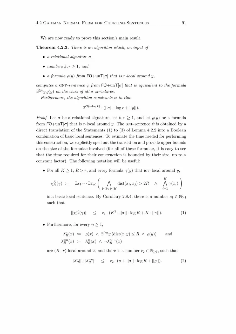
4.2 Gaifman Normal Form for Counting-Sentences 91
We are now ready to prove this section’s main result.
Theorem 4.2.3. There is an algorithm which, on input of
• a relational signature σ,
• numbers k, r ≥ 1, and
• a formula %(y) from FO+unT[σ] that is r-local around y,
computes a gnf-sentence ψ from FO+unT[σ] that is equivalent to the formula∃≥ky %(y) on the class of all σ-structures.Furthermore, the algorithm constructs ψ in time
2O(k·log k) · (||σ|| · log r + ||%||).
Proof. Let σ be a relational signature, let k, r ≥ 1, and let %(y) be a formulafrom FO+unT[σ] that is r-local around y. The gnf-sentence ψ is obtained by adirect translation of the Statements (1) to (3) of Lemma 4.2.2 into a Booleancombination of basic local sentences. To estimate the time needed for performingthis construction, we explicitly spell out the translation and provide upper boundson the size of the formulae involved (for all of these formulae, it is easy to seethat the time required for their construction is bounded by their size, up to aconstant factor). The following notation will be useful:
• For all K ≥ 1, R > r, and every formula γ(y) that is r-local around y,
χKR (γ) := ∃x1 · · · ∃xK
( ∧1≤i<j≤K
dist(xi, xj) > 2R ∧K∧i=1
γ(xi))
is a basic local sentence. By Corollary 2.8.4, there is a number c1 ∈ N≥1
such that
||χKR (γ)|| ≤ c1 · (K2 · ||σ|| · logR+K · ||γ||). (1)
• Furthermore, for every n ≥ 1,
λnR(x) := %(x) ∧ ∃≥ny(dist(x, y) ≤ R ∧ %(y)
)and
λ=nR (x) := λnR(x) ∧ ¬λn+1
R (x)
are (R+r)-local around x, and there is a number c2 ∈ N≥1, such that
||λnR||, ||λ=nR || ≤ c2 · (n+ ||σ|| · logR+ ||%||). (2)
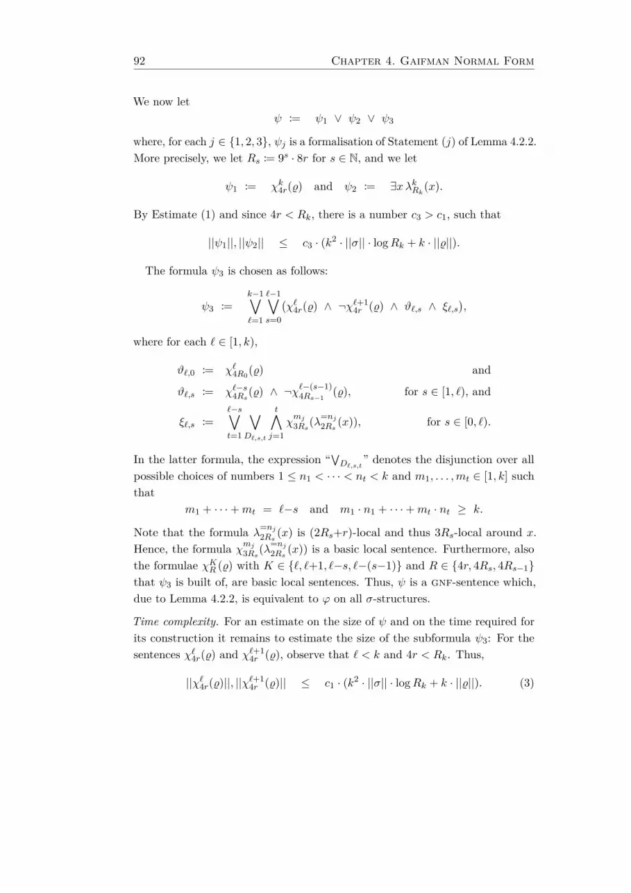
92 Chapter 4. Gaifman Normal Form
We now letψ := ψ1 ∨ ψ2 ∨ ψ3
where, for each j ∈ 1, 2, 3, ψj is a formalisation of Statement (j) of Lemma 4.2.2.More precisely, we let Rs := 9s · 8r for s ∈ N, and we let
ψ1 := χk4r(%) and ψ2 := ∃xλkRk(x).
By Estimate (1) and since 4r < Rk, there is a number c3 > c1, such that
||ψ1||, ||ψ2|| ≤ c3 · (k2 · ||σ|| · logRk + k · ||%||).
The formula ψ3 is chosen as follows:
ψ3 :=k−1∨`=1
`−1∨s=0
(χ`4r(%) ∧ ¬χ`+1
4r (%) ∧ ϑ`,s ∧ ξ`,s),
where for each ` ∈ [1, k),
ϑ`,0 := χ`4R0(%) and
ϑ`,s := χ`−s4Rs(%) ∧ ¬χ`−(s−1)4Rs−1
(%), for s ∈ [1, `), and
ξ`,s :=`−s∨t=1
∨D`,s,t
t∧j=1
χmj3Rs(λ
=nj2Rs (x)), for s ∈ [0, `).
In the latter formula, the expression “∨D`,s,t
” denotes the disjunction over allpossible choices of numbers 1 ≤ n1 < · · · < nt < k and m1, . . . ,mt ∈ [1, k] suchthat
m1 + · · ·+mt = `−s and m1 · n1 + · · ·+mt · nt ≥ k.
Note that the formula λ=nj2Rs (x) is (2Rs+r)-local and thus 3Rs-local around x.
Hence, the formula χmj3Rs(λ=nj2Rs (x)) is a basic local sentence. Furthermore, also
the formulae χKR (%) with K ∈ `, `+1, `−s, `−(s−1) and R ∈ 4r, 4Rs, 4Rs−1that ψ3 is built of, are basic local sentences. Thus, ψ is a gnf-sentence which,due to Lemma 4.2.2, is equivalent to ϕ on all σ-structures.
Time complexity. For an estimate on the size of ψ and on the time required forits construction it remains to estimate the size of the subformula ψ3: For thesentences χ`4r(%) and χ`+1
4r (%), observe that ` < k and 4r < Rk. Thus,
||χ`4r(%)||, ||χ`+14r (%)|| ≤ c1 · (k2 · ||σ|| · logRk + k · ||%||). (3)
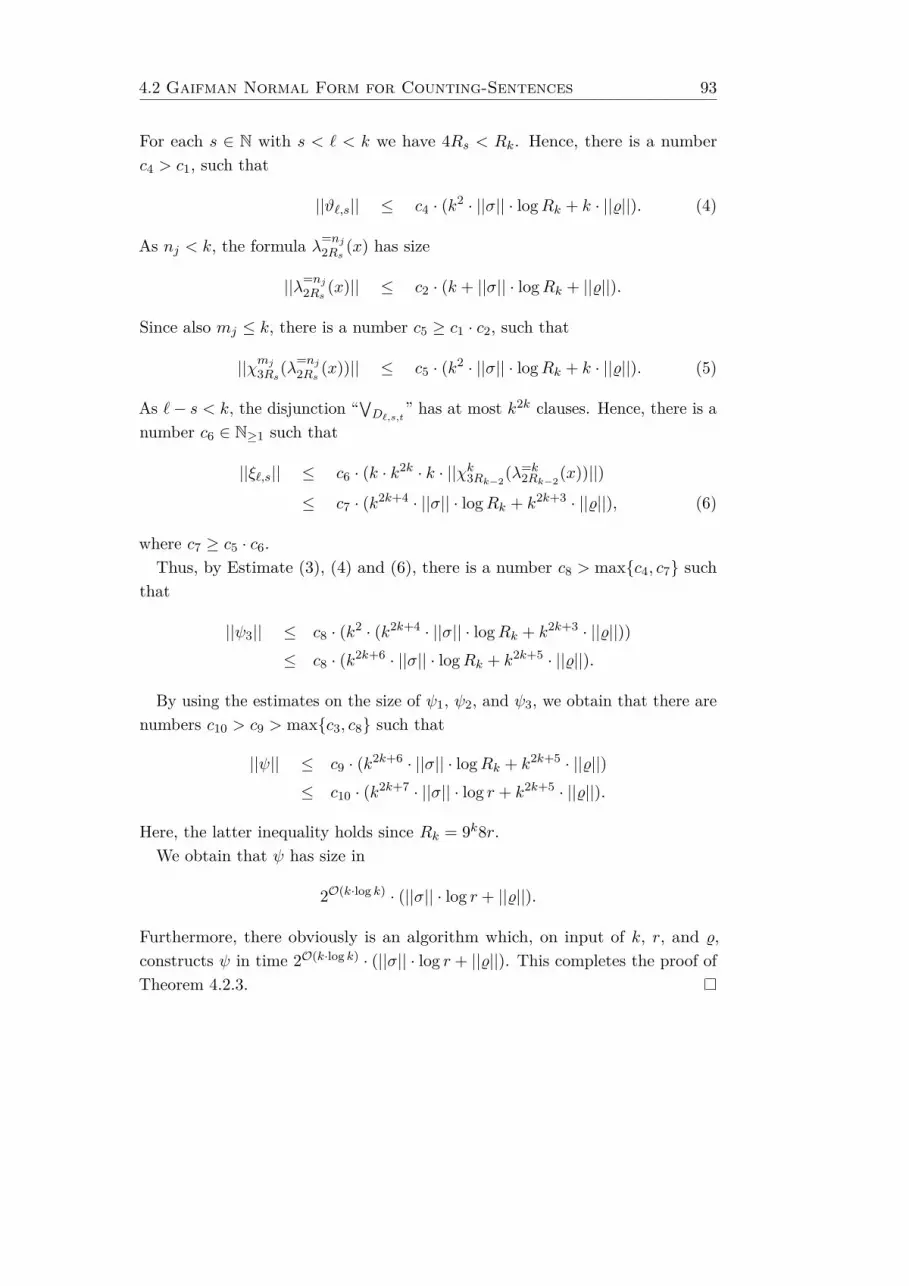
4.2 Gaifman Normal Form for Counting-Sentences 93
For each s ∈ N with s < ` < k we have 4Rs < Rk. Hence, there is a numberc4 > c1, such that
||ϑ`,s|| ≤ c4 · (k2 · ||σ|| · logRk + k · ||%||). (4)
As nj < k, the formula λ=nj2Rs (x) has size
||λ=nj2Rs (x)|| ≤ c2 · (k + ||σ|| · logRk + ||%||).
Since also mj ≤ k, there is a number c5 ≥ c1 · c2, such that
||χmj3Rs(λ=nj2Rs (x))|| ≤ c5 · (k2 · ||σ|| · logRk + k · ||%||). (5)
As `− s < k, the disjunction “∨D`,s,t
” has at most k2k clauses. Hence, there is anumber c6 ∈ N≥1 such that
||ξ`,s|| ≤ c6 · (k · k2k · k · ||χk3Rk−2(λ=k2Rk−2(x))||)
≤ c7 · (k2k+4 · ||σ|| · logRk + k2k+3 · ||%||), (6)
where c7 ≥ c5 · c6.Thus, by Estimate (3), (4) and (6), there is a number c8 > maxc4, c7 such
that
||ψ3|| ≤ c8 · (k2 · (k2k+4 · ||σ|| · logRk + k2k+3 · ||%||))≤ c8 · (k2k+6 · ||σ|| · logRk + k2k+5 · ||%||).
By using the estimates on the size of ψ1, ψ2, and ψ3, we obtain that there arenumbers c10 > c9 > maxc3, c8 such that
||ψ|| ≤ c9 · (k2k+6 · ||σ|| · logRk + k2k+5 · ||%||)≤ c10 · (k2k+7 · ||σ|| · log r + k2k+5 · ||%||).
Here, the latter inequality holds since Rk = 9k8r.We obtain that ψ has size in
2O(k·log k) · (||σ|| · log r + ||%||).
Furthermore, there obviously is an algorithm which, on input of k, r, and %,constructs ψ in time 2O(k·log k) · (||σ|| · log r + ||%||). This completes the proof ofTheorem 4.2.3.
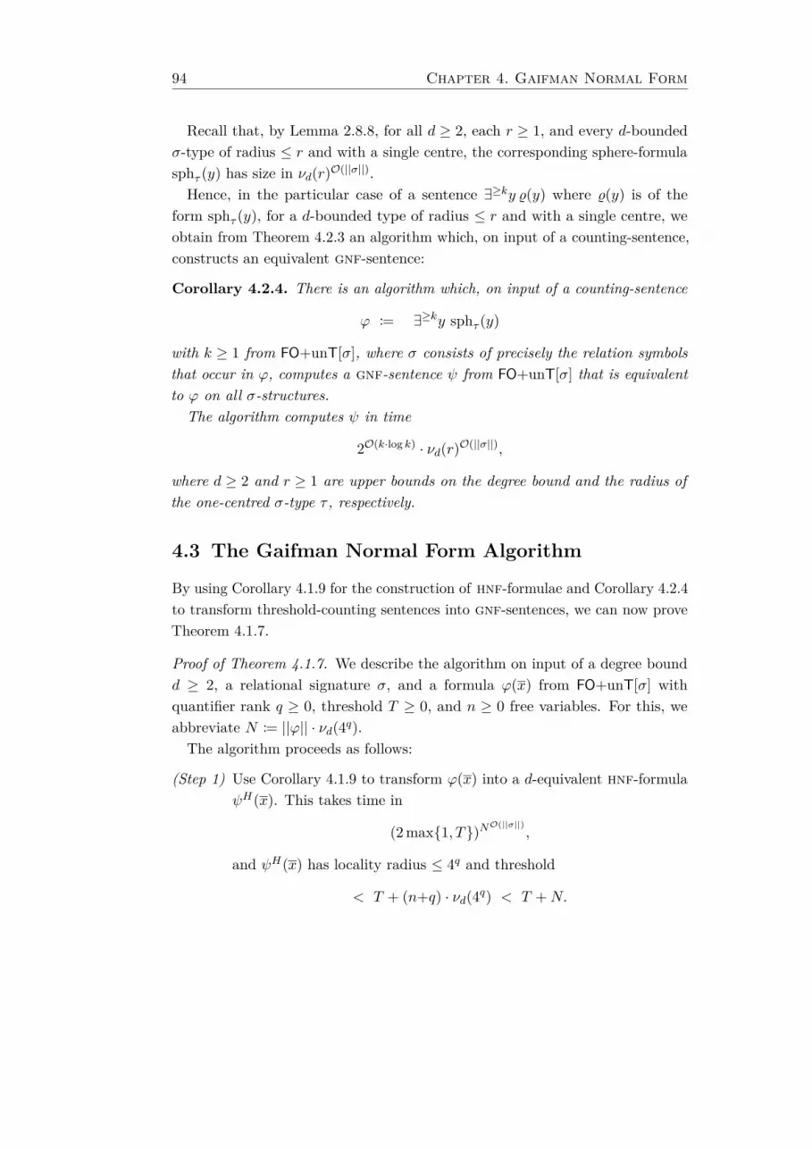
94 Chapter 4. Gaifman Normal Form
Recall that, by Lemma 2.8.8, for all d ≥ 2, each r ≥ 1, and every d-boundedσ-type of radius ≤ r and with a single centre, the corresponding sphere-formulasphτ (y) has size in νd(r)O(||σ||).Hence, in the particular case of a sentence ∃≥ky %(y) where %(y) is of the
form sphτ (y), for a d-bounded type of radius ≤ r and with a single centre, weobtain from Theorem 4.2.3 an algorithm which, on input of a counting-sentence,constructs an equivalent gnf-sentence:
Corollary 4.2.4. There is an algorithm which, on input of a counting-sentence
ϕ := ∃≥ky sphτ (y)
with k ≥ 1 from FO+unT[σ], where σ consists of precisely the relation symbolsthat occur in ϕ, computes a gnf-sentence ψ from FO+unT[σ] that is equivalentto ϕ on all σ-structures.
The algorithm computes ψ in time
2O(k·log k) · νd(r)O(||σ||),
where d ≥ 2 and r ≥ 1 are upper bounds on the degree bound and the radius ofthe one-centred σ-type τ , respectively.
4.3 The Gaifman Normal Form Algorithm
By using Corollary 4.1.9 for the construction of hnf-formulae and Corollary 4.2.4to transform threshold-counting sentences into gnf-sentences, we can now proveTheorem 4.1.7.
Proof of Theorem 4.1.7. We describe the algorithm on input of a degree boundd ≥ 2, a relational signature σ, and a formula ϕ(x) from FO+unT[σ] withquantifier rank q ≥ 0, threshold T ≥ 0, and n ≥ 0 free variables. For this, weabbreviate N := ||ϕ|| · νd(4q).
The algorithm proceeds as follows:
(Step 1) Use Corollary 4.1.9 to transform ϕ(x) into a d-equivalent hnf-formulaψH(x). This takes time in
(2 max1, T)NO(||σ||),
and ψH(x) has locality radius ≤ 4q and threshold
< T + (n+q) · νd(4q) < T +N.
4.4 Conclusion 95
(Step 2) Use Corollary 4.2.4 to transform each counting-sentence in ψH(x) intoan equivalent gnf-sentence.
Consider a counting-sentence ∃≥ky sphτ (y). For k = 1, the counting-sentence is also a basic local sentence. Thus, we only have to considerthe case of k ≥ 2. Recall that τ has locality radius ≤ 4q and thatk < T +N . From Corollary 4.2.4 we know that the construction of anequivalent gnf-sentence takes time in
2O((T+N)·log(T+N)) · νd(4q)O(||σ||) ⊆ 2O((T+N)2) ·NO(||σ||)
⊆ 2(T+N)O(||σ||).
Since every sphere-formula occurring in ψH(x) is already a local formula, thiscompletes the construction of the gnf-formula ψ(x). As also the size of ψH(x)is bounded by (2 max1, T)NO(||σ||) , the algorithm takes altogether time in
(2 max1, T)NO(||σ||) · 2(T+N)O(||σ||) ⊆ 2((T+1)·N)O(||σ||).
By replacing N with ||ϕ|| · νd(4q) again, we obtain a running time in
2((T+1)·||ϕ||·νd(4q))O(||σ||)
This completes the proof of Theorem 4.1.7.
4.4 Conclusion
In this chapter, we have presented an algorithm that turns a formula fromFO+unT into a d-equivalent Gaifman normal form. For d ≥ 3, the algorithmhas 3-fold exponential time complexity with respect to the size of the inputformula, and for d = 2, its time complexity is 2-fold exponential. For both cases,a matching lower bound in Section 9.4 will show that the algorithm is basicallyworst-case optimal.
The algorithm relies on the construction of Hanf normal form, presented inChapter 3. The crucial step of the algorithm is the construction of Gaifmannormal form for counting-sentences. Towards this aim, we have shown that, moregenerally, for each FO+unT-formula ϕ of the shape ∃≥ky %(y) where % is localaround y, a sentence in Gaifman normal form, which is equivalent to ϕ on allstructures of the respective signature, can be computed in 1-fold exponentialtime.

5 Feferman-Vaught Decompositions
It is known that that the construction of Feferman-Vaught decompositions forfirst-order formulae involves a non-elementary blow-up, even on classes of treesof unbounded degree [DGKS07]. In contrast, in this chapter, we present analgorithm that computes such decompositions with respect to disjoint sums ofd-bounded structures in worst-case optimal 3-fold exponential time, for degreebounds d ≥ 3. The algorithm also allows input formulae with modulo-countingquantifiers. For FO-formulae, we furthermore generalise the algorithm to decom-positions with respect to transductions and, in particular, direct products. Thischapter is based on [HHS14, HHS15].
5.1 Introduction
Algorithmic versions of decompositions à la Feferman-Vaught are typically of thefollowing form (cf., [Mak04, GJL12]): A given sentence ϕ that shall be evaluatedin the composition A of s structures A1, . . . ,As, can be transformed into asequence ∆1, . . . ,∆s of finite sets of formulae and a propositional formula β
whose propositions are tests of the form
“the i-th structure Ai satisfies the j-th formula in ∆i”,
such that A is a model of ϕ if and only if β is true. Further down below, we willgive a formal description of such decompositions in terms of so-called reductionsequences (cf.,e.g., [Mak04]).
In this chapter, we first focus on compositions given by disjoint sums1 (cf., e.g.,[Hod93, KM14]) of structures. Informally, a disjoint sum is a disjoint unionof structures extended by additional unary relation symbols that represent theuniverses of the disjoint component structures, and a ⊕-decomposition is adecomposition with respect to such disjoint sums.
The main result of this chapter is an algorithm which computes ⊕-decompositionsfor formulae from the logic FO+unM on classes of structures of bounded degree.
1also called “rich disjoint sums” (cf., e.g., [KM14])
97
98 Chapter 5. Feferman-Vaught Decompositions
The algorithm takes 3-fold exponential time in the size of the input formula fordegree bounds d ≥ 3, and 2-fold exponential time for degree bound d = 2. Forboth cases, a matching lower bound (see Section 9.5) shows that the algorithmis worst-case optimal. The lower bounds for d = 2 and d = 3, as well as thealgorithm for the special case of input formulae from FO, were published in[HHS14, HHS15].In the remainder of the chapter, we consider other forms of compositions of
structures apart from disjoint sums. Section 5.3 defines compositions that areobtained by applying transductions to disjoint sums, and shows how to computecorresponding decompositions in elementary time on classes of structures ofbounded degree. As an example, we use this result in Section 5.4 to compute⊗-decompositions, that is, decompositions with respect to direct products ofstructures. Note that in Section 5.3 and Section 5.4, we have to restrict ourselfsto input formulae from FO. For this case, both algorithms were already publishedin [HHS14, HHS15]. We will get rid of the restriction to FO later in Section 7.4.Before turning to the proof of Theorem 5.2.1, we give formal definitions of
disjoint sums of structures, reduction sequences, and ⊕-decompositions.
5.1.1 Disjoint Sums
Throughout the remainder of this chapter, we let σ denote a relational signatureand we let P1, P2, . . . be a sequence of unary relation symbols that are not alreadypresent in σ. For every s ≥ 1, we let σs := (σ, P1, . . . , Ps) denote the extensionof σ by the relation symbols P1, . . . , Ps.
Disjoint sums extend disjoint unions of structures by labelling the elements ofthe universe according to the component structure they originate from.
Definition 5.1.1. Let s ≥ 1, and let A1, . . . ,As be σ-structures. A disjoint sumof A1, . . . ,As is a σs-structure S with the following properties:
• The σ-reduct of S is a disjoint union of A1, . . . ,As and thus, in particular,a union of structures A′1, . . . ,A′s with pairwise disjoint universes and suchthat there is an isomorphism πi : A′i → Ai from A′i to Ai for each i ∈ [1, s].
• For each i ∈ [1, s], the unary relation PSi contains precisely the elements ofthe universe A′i of A′i.
We call π−11 , . . . , π−1
s references of A1, . . . ,As in S. On the other hand, the unionπ : S → A1 ∪ · · · ∪ As of the functions π1, . . . , πs (that is, the function π whereπ(a) := πi(a) for all i ∈ [1, s] and a ∈ A′i) is a back reference of S in A1, . . . ,As.

5.1 Introduction 99
Note that, e.g., a disjoint sum of a structure with itself shows that (back)references are not uniquely determined.
Observe that the sets PS1 , . . . , P Ss in S form a partition of the universe S, andfor all distinct i, j ∈ [1, s] there is no edge in the Gaifman graph of S betweenany a ∈ PSi and b ∈ PSj .
5.1.2 Reduction Sequences
For the following definitions, let L denote a logic as defined in Section 2.4.2..
Definition 5.1.2. For each i ∈ [1, s], let ∆i be a finite set of formulae δ from L[σ]and let β be a propositional formula that only uses the propositional symbols Xi,δ
for all i ∈ [1, s] and δ ∈ ∆i. The tuple
∆ = (β,∆1, . . . ,∆s)
is called an s-ary reduction sequence over L[σ] (for short: reduction sequence).If the size of the formulae in the sets ∆1, . . . ,∆s is defined (e. g., if the logic L
is ultimately periodic), then the size ||∆|| of ∆ can be defined as
||β|| +s∑i=1
∑δ∈∆i
||δ||.
The reduction sequence ∆ represents a Boolean combination of statements,expressed by formulae from the sets ∆1, . . . ,∆s, about the individual structuresof sequences A1, . . . ,As of σ-structures.
In the following, we define models of such reduction sequences.
Definition 5.1.3. Let s ≥ 1 and let ∆ = (β,∆1, . . . ,∆s) be an s-ary reductionsequence over L[σ], where the free variables of each formula in the sets ∆1, . . . ,∆s
belong to a tuple (x1, . . . , xn) of length n ≥ 0.If A1, . . . ,As are σ-structures and a1, . . . , an are elements from A1 ∪ · · · ∪ As,
then the tuple (A1, . . . ,As, (a1, . . . , an)) is a model of ∆, for short
A1, . . . ,As |= ∆[a1, . . . , an],
if, and only if, µ |= β, where µ : PS → 0, 1 is a propositional interpretationsuch that for each i ∈ [1, s] and every formula δ(x1, . . . , xn) ∈ ∆i, it holds that
µ(Xi,δ) = 1 iff aj ∈ Ai for every xj ∈ free(δ), andAi |= δ[a1, . . . , an].
Note that not all of the variables x1, . . . , xn have to be free in each formula δ.
100 Chapter 5. Feferman-Vaught Decompositions
5.1.3 Decompositions with respect to Disjoint Sums
We are now ready to define ⊕-decompositions as a special case of reductionsequences. For this, let L′ denote a logic. Typically, in this chapter, L′ and Lwill be the same logic FO+unM or FO, respectively. In later chapters, we willconsider cases where L = L′tpl.
Definition 5.1.4. Let C be a class of σ-structures and let ϕ(x) be a formulafrom L′[σs], whose n ≥ 0 free variables are given by the tuple x.An s-ary ⊕-decomposition for ϕ(x) (on C) over L[σ] is an s-ary reduction
sequence ∆ = (β,∆1, . . . ,∆s) over L[σ], where the free variables of the formulaein the sets ∆1, . . . ,∆s belong to the tuple x, and for which the following holds:
If S is a disjoint sum of σ-structures A1, . . . ,As (from C) with back reference π,and a1, . . . , an ∈ S, then
S |= ϕ[a1, . . . , an]iff A1, . . . ,As |= ∆[π(a1), . . . , π(an)].
Intuitively, an ⊕-decomposition for a formula ϕ(x) from L′[σ] on C is a Booleancombination β of formulae from L[σ] which is equivalent to ϕ(x) on any disjointsum S of structures from C when every formula in β is evaluated in one ofthe components of the disjoint sum. The sets ∆1, . . . ,∆s determine in whichcomponent every formulae of β is evaluated in.
Example 5.1.5. In a graph, the FO[E]-formula
ϕ(x) := ∃y∃z(¬y=z ∧ ¬E(y, x) ∧ ¬E(z, x)
)is satisfied if and only if there are at least two nodes that do not have an edgeto x. Since every component of a disjoint sum has to be non-empty and thereare no edges between nodes from different components, the reduction sequence(
X1,ψ ∨ X2,ψ ∨ (X1,χ ∧X2,δ) ∨ (X2,χ ∧X1,δ), ψ, χ, δ, ψ, χ, δ)
with
ψ := ∃y¬E(y, x), χ(x) := x=x, and δ := ∃y∃z¬y=z
is a binary ⊕-decomposition for ϕ over FO[E] on the class of graphs.
5.2 Constructing Decompositions from Hanf Normal Form 101
5.2 Constructing Decompositions from Hanf NormalForm
Recall that Cd,σ, for d ≥ 0, denotes the class of all d-bounded σ-structures.In this section, we present a worst-case optimal algorithm that computes, oninput of a degree bound d ≥ 2, a relational signature σ, an arity s ≥ 1, and aformula from FO+unM[σs], an s-ary ⊕-decomposition over FO+unM[σ] on Cd,σ.The algorithm uses the construction of Hanf normal form from Theorem 3.2.1in Chapter 3 and adds a second step which computes ⊕-decompositions forthe sphere-formulae and counting-sentences of hnf-formulae on the class of allσ-structures.
Theorem 5.2.1. There is an algorithm which, on input of
• a degree bound d ≥ 2,
• a relational signature σ,
• an arity s ≥ 1,
• and a formula ϕ(x) from FO+unM(D)[σs] with D ⊆ Dall, n := |x| freevariables, quantifier rank q ≥ 0, and threshold T ≥ 0,
computes an s-ary ⊕-decomposition (β,∆1, . . . ,∆s) for ϕ(x) over FO+unM(D)[σ]on Cd,σ, where the sets ∆1, . . . ,∆s only contain hnf-formulae with threshold< T + (n+q) · νd(4q).Furthermore, the algorithm computes ∆ in time
(2 max1, T, P)(||ϕ||·νd(4q))O(||σs||),
where P ≥ 0 is the maximum period of ϕ(x).
Remark 5.2.2. Recall that T, P, q < ||ϕ||. If furthermore σ only contains therelation symbols that occur in ϕ(x), also ||σ|| < ||ϕ||. Under these assumptions,the algorithm takes 3-fold exponential time
2ds·2O(||ϕ||)
for d = 3, and, for d = 2, it takes 2-fold exponential time
22s·poly(||ϕ||).
102 Chapter 5. Feferman-Vaught Decompositions
For a degree bound d ≥ 2, a relational signature σ, an arity s ≥ 1, and aformula ϕ(x) from FO+unM(D)[σs], where D ⊆ Dall, the proof of Theorem 5.2.1proceeds in two main steps:
(Step 1) The algorithm of Theorem 3.2.1 turns the input formula ϕ(x) into ad-equivalent hnf-formula ψ(x) from FO+unM(D)[σs].
(Step 2) Lemma 5.2.3 below replaces each counting-sentence and each sphere-formula in ψ(x) by an s-ary ⊕-decomposition over FO+unM(D)[σ] onthe class of all σ-structures.
Altogether, this yields an s-ary ⊕-decomposition for ψ(x), and thus an s-ary⊕-decomposition for ϕ(x) on Cd,σ.
The following Lemma 5.2.3 provides the transformation of hnf-formulae into⊕-decompositions. Note that the lemma is more general than actually neededfor the proof of Theorem 5.2.1.
• The lemma constructs a ⊕-decomposition on the class of all σ-structuresinstead of just σ-structures of degree at most d.
• The lemma shows that for every hnf-formula from any logic L[σs] as definedin Section 2.4.2, there is a corresponding ⊕-decomposition over L[σ] on theclass of all σ-structures. For an ultimately periodic logic L, the constructionof Lemma 5.2.3 allows to be read as an algorithm. In particular, this holdsfor FO+unM.
Lemma 5.2.3. Let L be a logic, let σ be a relational signature, let s ≥ 1,and let ψ(x) be a hnf-formula from L[σs]. There is an s-ary ⊕-decomposition∆ = (β,∆1, . . . ,∆s) for ψ(x) over L[σ] on the class of all σ-structures, where allformulae in the sets ∆1, . . . ,∆s are hnf-formulae.Furthermore, if L is ultimately periodic, there is an algorithm which, on input
of s and ψ(x), computes ∆ in time
s · O(||ψ||).
In particular, if ψ(x) is from FO+unM(D)[σs] for some D ⊆ Dall and ofthreshold T ≥ 0, then ∆ is also over FO+unM(D)[σ], and all formulae inthe sets ∆1, . . . ,∆s have threshold ≤ T .
For the construction of s-ary ⊕-decompositions for counting-sentences and sphere-formulae, the following notation will be useful. We call a σs-structure A mono-chrome (with colour i) if there is an i ∈ [1, s] such that A = PAi and PAj = ∅
5.2 Constructing Decompositions from Hanf Normal Form 103
for all j ∈ [1, s] with j 6= i. The crucial point in the proof of Lemma 5.2.3 isthat in every σs-type (B, b) which can be realised by a tuple in a disjoint sum ofof σ-structures A1, . . . ,As, the underlying σs-structure B is a union of pairwisedisjoint monochrome σs-structures. This follows directly from the definition ofdisjoint sums.
Proof of Lemma 5.2.3. Let L be a logic, let σ be a relational signature, let s ≥ 1,and let ψ(x) be a hnf-formula from L[σs] with free variables from the tuple x oflength n ≥ 0.
The algorithm proceeds in the following steps:
(Step 1) Consider a counting-sentence χ = Qy sphτ (y) that occurs in ψ(x) andrecall that τ is a σs-type (B, b) with one centre.
(Case 1.a) If B is monochrome with colour i ∈ [1, s], we replace χin ψ(x) by the propositional symbol βχ := Xi,χ and let
χ := Qy sphτ (y),
where τ := (B|σ, b). Furthermore, we let ∆χi := χ and
∆χj := ∅ for all j ∈ [1, s] with j 6= i.
(Case 1.b) If this is not the case, we replace χ in ψ by the Booleanconstant
βχ :=
1 if 0 ∈ Q, or0 if 0 6∈ Q,
and let ∆χj := ∅ for all j ∈ [1, s].
We prove the following claim after completing the construction.
Claim 1. (βχ,∆χ1 , . . . ,∆χ
s ) is a ⊕-decomposition for χ.
(Step 2) Consider a sphere-formula α(x′) = sph%(x′) that occurs in ψ(x). Inparticular, the tuple x′ is of length m ∈ [1, |x|] and % is a σs-type (B, b)with the m centres b = (b1, . . . , bm) and radius r ≥ 0. We proceed asfollows:
Choose k ≥ 1 as the number of connected components which consti-tute the σs-structure B, that is, the unique number k such that thereare pairwise disjoint σs-structures B1, . . . ,Bk, each with a connectedGaifman graph, whose union is B.
104 Chapter 5. Feferman-Vaught Decompositions
(Case 2.a) Suppose that each of the structures B1, . . . ,Bk is mono-chrome. Let J ⊆ [1, s] such that for each j ∈ J , there is atleast one structure from B1, . . . ,Bk with colour j. For eachj ∈ J , let jm ∈ [1,m] and let ij,1, . . . , ij,jm ∈ [1,m] withij1 < · · · < ij,jm be the indices of all the elements fromb1, . . . , bm that belong to PBj .
Moreover, let bj := (bij,1 , . . . , bij,jm ) be the subtuple of bconsisting of all these elements. Then, for each j ∈ J , theinduced substructure B[NBr (bj)] of B is the union of allstructures Bi with i ∈ [1, k] that are monochrome withcolour j.
For each j ∈ J , we let %j := (B[NBr (bj)|σ, bj) and replaceα(x′) by the propositional formula
βα :=∧j∈J
Xj,αj(x′j)
where for each j ∈ J we let x′j := (xij,1 , . . . , xij,jm ) andαj(x′j) := sph%j (x
′j). Furthermore, we let ∆α
j := αj ifj ∈ J and, otherwise, ∆α
j := ∅ for all j ∈ [1, s].(Case 2.b) Otherwise, that is, if at least one of the structures B1, . . . ,Bk
is not monochrome, we replace α(x′) with the Boolean con-stant βα := 0 and let ∆α
j := ∅ for all j ∈ [1, s].
We prove the following claim below.
Claim 2. (βα,∆α1 , . . . ,∆α
s ) is a ⊕-decomposition for α(x′).
(Step 3) By β we denote the propositional formula obtained by replacing eachcounting-sentence χ and each sphere-formulae α(x) in ψ(x) by thepropositional formulae βχ and βα, respectively. . For each i ∈ [1, s], welet ∆i the union of the sets ∆χ
i and ∆αi for all counting-sentences χ
and all sphere-formulae α of ψ(x).Then, the s-ary reduction sequence (β,∆1, . . . ,∆s) is, according to
Claim 1 and Claim 2, a ⊕-decomposition for ψ(x).
By the construction just described it is clear that if ψ(x) is from L[σs], then∆1, . . . ,∆s ⊆ L[σ]. In particular, if ψ(x) is from FO+unM[σs] and of thresholdT ≥ 0, all formulae in the sets ∆1, . . . ,∆s are from FO+unM[σ] and havethreshold ≤ T .

5.2 Constructing Decompositions from Hanf Normal Form 105
The proofs of Claim 1 and Claim 2 below are straightforward and use thenotation introduced in the corresponding cases of the construction above. Forboth proofs, we let S be a disjoint sum of some arbitrary σ-structures A1, . . . ,Aswith a back reference π. In particular, we suppose that the σ-reduct of S is theunion of the pairwise disjoint σ-structures A′1, . . . ,A′s with A′i ∼= Ai and PSi = A′ifor each i ∈ [1, s].
Proof of Claim 1. We distinguish between Case (1.a) and Case (1.b) above.
If B is monochrome with a colour i ∈ [1, s], the following equivalences hold:
S |= χ
iff |τ(S)| ∈ Qiff |τ(A′i)| ∈ Q (since A′i is the σ-reduct of S[PSi ])iff |τ(Ai)| ∈ Q (since A′i ∼= Ai)iff Ai |= χ
iff A1, . . . ,As |= ∆χ.
If B is not monochrome, then |τ(S)| = 0. Thus, the following equivalences hold:
S |= χ iff 0 ∈ Q iff A1, . . . ,As |= ∆χ.
This completes the proof of Claim 1.
Proof of Claim 2. Let a1, . . . , am ∈ S. We distinguish between Case (2.a) andCase (2.b) above.
Suppose that each of the structures B1, . . . ,Bk is monochrome. Furthermore,let c1, . . . , ck ∈ [1, s] be the colours of the structures B1, . . . ,Bk. The followingequivalences hold:
S |= sph%[a1, . . . , am]iff N Sr (aij,1 , . . . , aij,jm ) ∼= (B[NBr (bj)], bj) for all j ∈ J
iff NA′cjr (aij,1 , . . . , aij,jm ) ∼= %j for all j ∈ J
iff NAcjr (π(aij,1), . . . , π(aij,jm )) ∼= %j for all j ∈ J
iff Acj |= αj [π(aij,1), . . . , π(aij,jm )] for all j ∈ Jiff A1, . . . ,As |= ∆α[π(a1), . . . , π(am)].
If one of the structures B1, . . . ,Bk is not monochrome, then S 6|= sph%[a1, . . . , am]and, by construction, also A1, . . . ,As 6|= ∆α[π(a1), . . . , π(am)].
106 Chapter 5. Feferman-Vaught Decompositions
This completes the proof of Claim 2.
Time complexity. In the following, we analyse the time required by the steps ofthe algorithm described above for the case of a hnf-formula from an ultimatelyperiodic logic L.
(Step 1) Consider a counting-sentence χ = Qy sphτ (y) from ψ(x) with a typeτ = (B, b). Recall that the sphere-formula sphτ contains a conjunctionof all (negated) atomic σs-formulae that hold for the elements of τ .Hence, by an examination of the sphere-formula sphτ , it takes time inO(χ) to decide whether B is monochrome and, if yes, to construct thecounting-sentence χ.
Since the sum of the length of the counting-sentences is bounded bythe size of ψ(x), Step (1) altogether needs time in O(||ψ||).
(Step 2) Consider a sphere-formula α(x′) = sph%(x′) from ψ(x) where % = (B, b).Similar to the procedure in Step (1), it requires time in O(α) to decidewhether B is a union of pairwise disjoint monochrome σs-structures.
If this is the case, then for each j ∈ J , the same time is required to con-struct the sphere-formula αj(x′j). For this, recall that the correspondingtype %j contains precisely the j-coloured elements of %.Since |J | ≤ s, the algorithm needs time in s · O(α) to compute the
propositional formula for the sphere-formula α(x′).As the sum of the lengths of the sphere-formulae is bounded by the
size of ψ(x), Step (2) altogether needs time in s · O(||ψ||).
(Step 3) The size of the propositional formula β is in s · O(||ψ||), which alsobounds the time required to compute the sets ∆1, . . . ,∆s.
In summary, the construction of the reduction sequence (β,∆1, . . . ,∆s) on inputof ψ(x) takes time in s · O(||ψ||). This completes the proof of Lemma 5.2.3.
We are now ready to complete the proof of Theorem 5.2.1.
Proof of Theorem 5.2.1. We describe the algorithm on input of a degree boundd ≥ 2, a relational signature σ, a number s ≥ 1, and a formula ϕ(x) fromFO+unM(D)[σs], for a set D ⊆ Dall. Let T, P, q ≥ 0 be the threshold, themaximum period, and the quantifier rank of ϕ(x), respectively. Furthermore, letn := |x| denote the number of free variables of ϕ(x).The algorithm proceeds as follows:
5.3 Decompositions with respect to Transductions 107
(Step 1) The algorithm of Theorem 3.2.1 constructs, on input of d, σs, and ϕ(x),a hnf-formula ψ(x) from FO+unM(D)[σs] that is d-equivalent to ϕ(x)and that has threshold < T + (n+q) · νd(4q). This takes time in
(2 max1, T, P)(||ϕ||·νd(4q))O(||σs||). (1)
(Step 2) The algorithm of Lemma 5.2.3 computes, on input of the arity s and thehnf-formula ψ(x), an s-ary ⊕-decomposition ∆ = (β,∆1, . . . ,∆s) forψ(x) over FO+unM(D)[σ] on the class of all σ-structures. This requirestime in s · O(||ψ||). Since the size of ψ(x) is bounded by the timerequired for its construction, this can also be bounded by Estimate (1).Furthermore, by Lemma 5.2.3, all formulae in the sets ∆1, . . . ,∆s
are hnf-formulae with threshold ≤ T .
Since ϕ(x) and ψ(x) are d-equivalent, ∆ is also an s-ary ⊕-decompositionfor ϕ(x) on Cd,σ. The overall time required by the algorithm to construct ∆ canbe bounded by Estimate (1). This completes the proof of Theorem 5.2.1.
5.3 Decompositions with respect to Transductions
In this section, we turn our attention from ⊕-decompositions to decompositionsspeaking about other forms of compositions of structures. More precisely, we showhow to transfer the algorithm of Theorem 5.2.1 to an algorithm that producesdecompositions on composite structures obtained by applying transductions todisjoint sums of structures. Note that, in [Mak04], transductions are used ina similar way to obtain the classical Feferman-Vaught theorem for so-calledgeneralised products [FV59] from its special cases for disjoint unions and directproducts of structures.
The following definition of such decompositions is more general than actuallyused in this section, but will be used in this general form later on in Section 7.4.Suppose that L and L′ are logics.
Definition 5.3.1. Let σ and τ be relational signatures, and let C be a class ofσ-structures. Let s ≥ 1 and let Θ be a transduction from σs to τ with arity t ≥ 1.Let ϕ(x) be a formula from L′[τ ], whose n ≥ 0 free variables are given by thetuple x = (x1, . . . , xn). For all i ∈ [1, n], let furthermore xi = (xi,1, . . . , xi,t).A Θ-decomposition for ϕ(x) (on C) over L[σ] is an s-ary reduction sequence
∆ = (β,∆1, . . . ,∆s) over L[σ], where the free variables of all formulae in the sets∆1, . . . ,∆s all belong to the tuple (x1, . . . , xn), and for which the following holds:
108 Chapter 5. Feferman-Vaught Decompositions
If S is a disjoint sum of σ-structures A1, . . . ,As (from C) with back reference π,for which Θ[S] is defined, and if ai = (ai,1, . . . , ai,t) for each i ∈ [1, n] belongs tothe universe of Θ[S], then
Θ[S] |= ϕ[a1; . . . ; an]iff A1, . . . ,As |= ∆[(π(a1,1), . . . , π(a1,t)), . . . , (π(an,1), . . . , π(an,t))].
The following lemma shows that a Θ-decomposition of an L′-formula ϕ can beobtained from a ⊕-decomposition of a Θ-reduct of ϕ from some logic L′′.
Lemma 5.3.2. Let L, L′, L′′ be logics. Let σ and τ be relational signatures, andlet C be a class of σ-structures. Let s ≥ 1 and let Θ be a transduction from σs
to τ with arity t ≥ 1.Suppose that ϕ is a formula from L′[τ ], that ψ is a Θ-reduct for ϕ from L′′[σs],
and that ∆ is a t-ary ⊕-decomposition for ψ over L[σ] on C.Then, ∆ is a Θ-decomposition for ϕ over L[σ] on C.
Proof. The proof follows directly from the definitions. Let L, L′, L′′ be logics. Letσ and τ be relational signatures, and let C be a class of σ-structures. Let s ≥ 1and let Θ be a transduction from σs to τ with arity t ≥ 1. Let ϕ(x) be a formulafrom L′[τ ] with the n ≥ 0 free variables x = (x1, . . . , xn). For all i ∈ [1, n], letfurthermore xi = (xi,1, . . . , xi,t).
Suppose that ψ(x1, . . . , xn) is a Θ-reduct for ϕ(x) from L′′[σs]. Then, for everyσs-structure A for which Θ[A] is defined, and for all elements a1, . . . , an fromthe universe of Θ[A],
Θ[A] |= ϕ[a1; . . . ; an]iff A |= ψ[a1, . . . , an].
(1)
Let ∆ be a t-ary ⊕-decomposition for ψ(x1, . . . , xn) over L[σ] on C. If S isa disjoint sum with back reference π of σ-structures A1, . . . ,As ∈ C and iffurthermore ai = (ai,1, . . . , ai,t) ∈ St for each i ∈ [1, n], then
S |= ψ[a1, . . . , an]iff A1, . . . ,As |= ∆[(π(a1,1), . . . , π(a1,t)), . . . , (π(an,1), . . . , π(an,t))].
(2)
Hence, putting Equivalence (1) and Equivalence (2) together, we know thatif S is a disjoint sum of σ-structures A1, . . . ,As ∈ C with back reference π, forwhich Θ[S] is defined, and if ai = (ai,1, . . . , ai,t) ∈ St for each i ∈ [1, n], then
Θ[S] |= ϕ[a1; . . . ; an]iff A1, . . . ,As |= ∆[(π(a1,1), . . . , π(a1,t)), . . . , (π(an,1), . . . , π(an,t))].
5.3 Decompositions with respect to Transductions 109
Thus, we can conclude that ∆ is a Θ-decomposition for ϕ(x) over L[σ] on C.
To actually compute Θ-decompositions on classes of structures of boundeddegree, an algorithm first uses Lemma 2.6.4 to compute a reduct ϕ−Θ of theinput formula ϕ with respect to the transduction Θ, which is also given as aninput to the algorithm. Afterwards, the algorithm of Theorem 5.2.1 is invokedon the reduct ϕ−Θ.However, there is a catch. Suppose that Θ has arity t ≥ 2, which is needed,
e. g., for the construction of decompositions with respect to direct productsof structures in the next Section 5.4. In this case, the construction of ϕ−Θ
may introduce tuple-counting quantifiers and thus, cannot serve as an input forTheorem 5.2.1 in general.
Therefore, in this and the next section, we restrict attention to input formulaefrom FO. Since a formula of the shape ∃(y1, . . . , yt)ψ can be replaced by theequivalent formula ∃y1 · · · ∃yt ψ, Lemma 2.6.4 guarantees that, in this case, thereis also a Θ-reduct for ϕ in FO.
In Chapter 7, we will see how to turn arbitrary formulae from FO+unMtpl intoequivalent formulae from FO+unM. This will allow us to extend the results ofthis section and the next to such formulae.
The main result of this section can now be stated as follows:
Theorem 5.3.3. There is an algorithm which, on input of
• a degree bound d ≥ 2,
• relational signatures σ and τ ,
• an arity s ≥ 1,
• a transduction Θ from σs to τ with arity t ≥ 1 and quantifier rank qΘ ≥ 0,and
• a formula ϕ(x) from FO[τ ] with n := |x| free variables and quantifierrank q ≥ 0,
computes a Θ-decomposition ∆ = (β,∆1, . . . ,∆s) over FO+unT[σ] for ϕ(x)on Cd,σ, where all formulae in the sets ∆1, . . . ,∆s are hnf-formulae with threshold< (t · (n+ q) + qΘ) · νd(4t·q+qΘ).
110 Chapter 5. Feferman-Vaught Decompositions
Furthermore, the algorithm computes ∆ in time
||Θ|| · O(||τ ||) + 2(||Θ||·||ϕ||·νd(4t·q+qΘ )
)O(||σs||)
and of size
2(||Θ||·||ϕ||·νd(4t·q+qΘ )
)O(||σs||)
.
Proof. Let d ≥ 2 be a degree bound, let σ and τ be relational signatures, andlet s ≥ 1. Furthermore, let Θ be a transduction from σs to τ with arity t ≥ 1and quantifier rank qΘ ≥ 0. Moreover, let ϕ(x) be a formula from FO[τ ] withquantifier rank q ≥ 0, and the n ≥ 0 free variables x = (x1, . . . , xn). For alli ∈ [1, n], let furthermore xi = (xi,1, . . . , xi,t).The algorithm proceeds in the two following steps:
(Step 1) The algorithm of Lemma 2.6.4 computes a Θ-reduct ϕ−Θ(x1, . . . , xn)for ϕ(x) from FOtpl[σs] with quantifier rank ≤ t · q+ qΘ, dimension ≤ t,and n·t free variables. In particular, every quantified subformula of ϕ−Θ
is either of the shape ∃y ϕ′ or of the shape ∃(y1, . . . , yt)ϕ′, where thelatter can be replaced by a formula ∃y1 · · · ∃yt ϕ′ to obtain a Θ-reductψ(x1, . . . , xn) for ϕ(x) from FO[σs] which, in particular, has the samequantifier rank as ϕ−Θ(ϕ)(x1, . . . , xn).
(Step 2) Recall that each formula in FO[σs] has threshold 0. The algorithm ofTheorem 5.2.1 is called on input of d, σ, s, and ψ(x1, . . . , xn), resultingin an s-ary ⊕-decomposition ∆ = (β,∆1, . . . ,∆s) for ψ(x1, . . . , xn)over FO+unT[σ] on Cd,σ where, in particular, all formulae in the sets∆1, . . . ,∆s are hnf-formulae with threshold
< (t · n+ t · q + qΘ) · νd(4t·q+qΘ) = (t · (n+ q) + qΘ) · νd(4t·q+qΘ).
By Lemma 5.3.2, we know that ∆ is also a Θ-decomposition for ϕ(x) overFO+unT[σ] on the class of d-bounded σ-structures.
Size and time complexity. We follow the steps of the algorithm.
(Step 1) The call of Lemma 2.6.4 on input of Θ and ϕ(x) takes time in
||Θ|| · O(||τ ||) + ||Θ|| · O(||ϕ||),
and yields a Θ-reduct ϕ−Θ(x1, . . . , xn) of size ||Θ|| · O(||ϕ||). Theconstruction of the FO[σs]-formula ψ(x1, . . . , xn) from ϕ−Θ(x1, . . . , xn)takes time in O(||ϕ−Θ||).
5.4 Decompositions with respect to Direct Products 111
(Step 2) By the upper bounds on the size and the quantifier rank of ψ(x1, . . . , xn),the algorithm of Theorem 5.2.1 takes time in
2(||Θ||·||ϕ||·νd(4t·q+qΘ )
)O(||σs||)
to compute the Θ-decomposition ∆ on input of d, σ, s, and ψ(x1, . . . , xn).In particular, the latter estimate is also an upper bound on the sizeof ∆.
Altogether, the algorithm takes time in
||Θ|| · O(||τ ||) + 2(||Θ||·||ϕ||·νd(4t·q+qΘ )
)O(||σs||)
for the construction of ∆. This completes the proof of Theorem 5.3.3.
5.4 Decompositions with respect to Direct Products
We conclude Chapter 5 with an exemplary application of Theorem 5.3.3 to directproducts2 (cf., e.g., [Hod93]). In the following, suppose that σ = (R1, . . . , R`) isa relational signature with ` ≥ 0 relation symbols and let s ≥ 1.A σ-structure P = (P,RP1 , . . . , RP` ) is the direct product of σ-structures
A1, . . . ,As if P = A1 × · · · × As, and for each relation symbol R of arity r ≥ 1in σ, we have
RP :=
((a1,1, . . . , a1,s), . . . , (ar,1, . . . , ar,s)) : (a1,i, . . . , ar,i) ∈ RAifor all i ∈ [1, s]
.
We also denote the direct product of A1, . . . ,As by A1⊗ · · ·⊗As. See Figure 5.1for an example of a direct product. Analogous to ⊕-decompositions we define⊗-decompositions. To this aim, we let L and L′ be (not necessarily distinct)logics.
Definition 5.4.1. Let σ be a relational signature, let C be a class of σ-structures,let s ≥ 1, and let ϕ(x) be a formula from L′[σs], whose n ≥ 0 free variablesare given by the tuple x = (x1, . . . , xn). For all i ∈ [1, n] let furthermorexi := (xi,1, . . . , xi,s).An s-ary ⊗-decomposition for ϕ(x) (on C) over L[σ] is an s-ary reduction
sequence ∆ = (β,∆1, . . . ,∆s) over L[σ], where the free variables of the formulae2also called tensor products or cartesian products

112 Chapter 5. Feferman-Vaught Decompositions
1 2
a
b
⊗ =1, a
1, b
2, a
2, b
Figure 5.1 Example for the direct product of two (E)-structures with universe 1, 2and universe a, b, respectively.
in the sets ∆1, . . . ,∆s belong to the tuple (x1, . . . , xn), and for which the followingholds:
If P is the direct product of σ-structures A1, . . . ,As (from C) and if furthermorea1, . . . , an ∈ P , then
P |= ϕ[a1; . . . ; an]iff A1, . . . ,As |= ∆[a1, . . . , an].
Direct products can be obtained from disjoint sums of σ-structures by trans-ductions from σs to σ, which correspond to the definition of the universe andthe relations of direct products [Mak04]. More precisely, we define for each s ≥ 1an s-ary transduction Θσ
s := (θ, θR1 , . . . , θR`) with
θ(x1, . . . , xs) :=s∧i=1
Pi(xi)
and, for each relation symbol R of arity r ≥ 1 from σ,
θR(x1, . . . , xr) :=s∧i=1
R(x1,i, . . . , xr,i),
where xj := (xj,1, . . . , xj,s) for each j ∈ [1, r].It is straightforward to verify that if S is a disjoint sum of σ-structures
A1, . . . ,As with back reference π, and P is the direct product of A1, . . . ,As, then
Θσs [S] ∼= P
by the isomorphism % from Θσs [S] to P defined by
%(a1, . . . , as) = (π(a1), . . . , π(as)) (5.1)
for all elements (a1, . . . , as) in the universe of Θσs [S].
The following lemma shows that the transductions just defined can indeed beused to obtain ⊗-decompositions.
5.4 Decompositions with respect to Direct Products 113
Lemma 5.4.2. Let L and L′ be logics. Let σ be a relational signature and let Cbe a class of σ-structures. Let s ≥ 1, let ϕ be a formula from L′[σs] and supposethat ∆ is a Θσ
s -decomposition for ϕ over L[σ] on C.Then, ∆ is also an s-ary ⊗-decomposition for ϕ over L[σ] on C.
Proof. Let L and L′ be logics. Let σ be a relational signature and let C be a classof σ-structures. Let s ≥ 1 and let ϕ(x) be a formula from L′[σs] with the n ≥ 0free variables x = (x1, . . . , xn). Moreover, for all i ∈ [1, n], let xi = (xi,1, . . . , xi,s).
Furthermore, let ∆ = (β,∆1, . . . ,∆s) be a Θσs -decomposition for ϕ(x) over L[σ]
on C. Recall that the free variables of all formulae in the sets ∆1, . . . ,∆s belongto the tuple (x1, . . . , xn).
If S is a disjoint sum with back reference π of σ-structures A1, . . . ,As from C,% is the isomorphism from Θσ
s [S] to the direct product P of A1, . . . ,As given byEquation (5.1), and ai = (ai,1, . . . , ai,s) ∈ P for all i ∈ [1, n], then the followingequivalences hold:
P |= ϕ[a1; . . . ; an]iff Θσ
s [S] |= ϕ[%−1(a1); . . . ; %−1(an)]iff Θσ
s [S] |= ϕ[(π−1(a1,1), . . . , π−1(a1,s)); . . . ; (π−1(an,1), . . . , π−1(an,s))]iff A1, . . . ,As |= ∆[(π(π−1(a1,1)), . . . , π(π−1(a1,s))), . . .
(π(π−1(an,1)), . . . , π(π−1(an,s)))]iff A1, . . . ,As |= ∆[a1, . . . , an].
Hence, we can conclude that ∆ is an s-ary ⊗-decomposition for ϕ(x) over L[σ]on C.
This leads to the following application of Theorem 5.3.3.
Theorem 5.4.3. There is an algorithm which, on input of
• a degree bound d ≥ 2,
• a relational signature σ,
• an arity s ≥ 1, and
• a formula ϕ(x) from FO[σs] with n := |x| free variables and quantifierrank q ≥ 0,
114 Chapter 5. Feferman-Vaught Decompositions
computes an s-ary ⊗-decomposition (β,∆1, . . . ,∆s) for ϕ(x) over FO+unT[σ]on the class of d-bounded σ-structures, where all formulae in the sets ∆1, . . . ,∆s
are hnf-formulae with threshold < s · (n+ q) · νd(4s·q).Furthermore, the algorithm computes ∆ in time
2(||ϕ||·νd(4s·q)
)O(||σs||·log ||σs||)
.
Proof of Theorem 5.4.3. Let d ≥ 2 be a degree bound, let σ be a relationalsignature, let s ≥ 1, and let ϕ(x) be a formula from FO[σ] with n := |x| freevariables and quantifier rank q ≥ 0.
On input of d, the signatures σs and σ, the transduction Θσs defined above, and
the formula ϕ(x), the algorithm of Theorem 5.3.3 computes a Θσs -decomposition
∆ = (β,∆1, . . . ,∆s) over FO+unT[σ] for ϕ(x) on the class of all d-boundedσ-structures where, in particular, all formulae in the sets ∆1, . . . ,∆s are hnf-formulae with threshold < s · (n+ q) · νd(4s·q).By Lemma 5.4.2, we know that ∆ is also a ⊗-decomposition for ϕ(x) over
FO+unT[σ] on the class of d-bounded σ-structures.
Time complexity. Clearly, the transduction Θσs is of quantifier rank 0 and can be
computed in time s·O(||σ||). Therefore, the call of the algorithm of Theorem 5.3.3needs time in
s · O(||σ||)2 + 2(s·O(||σ||)·||ϕ||·νd(4s·q)
)O(||σs||)
⊆ 2(||ϕ||·νd(4s·q)
)O(||σs||·log ||σs||)
.
This completes the proof of Theorem 5.4.3.
5.5 Conclusion
In this chapter, we have shown how to compute ⊕-decompositions for formulaefrom FO+unM on classes of d-bounded structures. For d ≥ 3, the correspondingalgorithm has 3-fold exponential running time in the size of the formula to bedecomposed. For d = 2, its running time is 2-fold exponential. In Section 9.5, wewill provide matching lower bounds, showing that, for both cases, this algorithmis worst-case optimal.In a first step, the algorithm relies on the construction of Hanf normal form,
presented in Chapter 3. Its second step is a construction of ⊕-decompositions forthe individual counting-sentences and sphere-formulae of the Hanf normal form.The restriction to degree-bounded structures is only required for the constructionof Hanf normal form, while the second step is irrespective of the degree bound.
5.5 Conclusion 115
In the remainder of the chapter, we have extended this algorithm to decom-positions defined by transductions on disjoint sums. In particular, this includesdirect products. Due to the fact that the construction of reducts with respect to atransduction of arity ≥ 2 may introduce tuple-counting quantifiers, we restrictedourselves here to the case of input formulae from FO, where tuple-quantifiers caneasily be resolved. The obtained algorithms have roughly the same running timeas the algorithm for ⊕-decompositions.
In Section 7.4, the handling of tuple-counting quantifiers, described there, willallow us to extend all the above mentioned algorithms to input formulae fromthe logic FO+unMtpl. Finally, Section 8.5 generalises these algorithms further toall ultimately periodic logics. There, we will also show that only for ultimatelyperiodic logics ⊕-decompositions for the formulae of the logic are guaranteed toexist.

6 Preservation Theorems
It is known that, for FO-sentences that are preserved under extensions on acertain class of acyclic structures of unbounded degree, equivalent existentialsentences can grow non-elementarily [DGKS07]. Similar non-elementary lowerbounds also hold in respect to existential-positive sentences for FO-sentencesthat are preserved under homomorphisms [Ros08].This chapter investigates algorithmic versions of preservation theorems on
classes of structures of bounded degree. The results of this chapter are based on[HHS14, HHS15]. Its first result is an elementary algorithm which, on input of anFO+unM-formula that is preserved under extensions on the class of d-boundedstructures, computes a d-equivalent existential formula. For d ≥ 3, the algorithmtakes 5-fold exponential time in the size of the input formula.
A second result is an elementary algorithm which, on input of a formula fromFO+unM that is preserved under homomorphisms on the class of d-boundedstructures, computes a d-equivalent existential-positive formula. For d ≥ 3, thisalgorithm takes 4-fold exponential time.
6.1 Introduction
Before stating the two main results of this chapter, we explain what it means fora formulae to be preserved under extensions or preserved under homomorphismson a class of structures. Furthermore, we introduce the corresponding normalforms, called existential and existential-positive formulae (cf., e.g, [Hod93, Lyn59,Ros08]).
Throughout this chapter, σ will always denote a relational signature. Further-more, in the following definitions, we let C denote a class of σ-structures, and welet L denote one of the logics defined in Section 2.4.2
A σ-structure B is an extension of a σ-structure A if A is an induced substruc-ture of B.
117
118 Chapter 6. Preservation Theorems
Definition 6.1.1. A formula ϕ(x) from L[σ] is preserved under extensions on C
if the following holds for each interpretation (A, a) for ϕ(x) with A ∈ C:
if A |= ϕ[a] then B |= ϕ[a] for each extension B ∈ C of A.
Definition 6.1.2. A formula from FO[σ] is existential if it has the shape
∃x1 · · · ∃xn ϕ(x1, . . . , xn)
where ϕ is quantifier-free.
It is straightforward to see that every existential FO[σ]-formula is preservedunder extensions on arbitrary classes of σ-structures.
Example 6.1.3. The FO[E]-sentence
ϕ := ∃x∃y∃z(¬x=y ∧ ¬y=z ∧ ¬z=x ∧ E(x, y) ∧ E(y, z) ∧ E(z, x)
)states in a graph that there are three distinct nodes which form a triangle. Asthe sentence is existential, we know that it is preserved under extensions on allgraphs.
Recall that a homomorphism from a σ-structure A to a σ-structure B is amapping h : A→ B such that for each relation symbol R of arity r ≥ 1 from σ andall tuples (a1, . . . , ar) ∈ Ar, if (a1, . . . , ar) ∈ RA then (h(a1), . . . , h(ar)) ∈ RB. Ifa = (a1, . . . , an) ∈ An for an n ≥ 0, we also write in the following h(a) for thetuple (h(a1), . . . , h(an)), that is, we apply the homomorphism h component-wiseto the tuple a.
Definition 6.1.4. A formula ϕ(x) from L[σ] with a tuple x of n ≥ 0 variables ispreserved under homomorphisms on C if the following holds for each interpretation(A, a) for ϕ(x) with A ∈ C and a ∈ An:
if A |= ϕ[a]then B |= ϕ[h(a)] for every σ-structure B ∈ C for which
there is a homomorphism h from A to B.
Definition 6.1.5. An existential-positive formula from FO[σ] is an existential for-mula that does not contain the symbol ¬ (and thus, also not the abbreviations →and ↔). Furthermore, also the symbol ⊥ is understood as an existential-positiveformula that is not satisfied by any σ-structure.
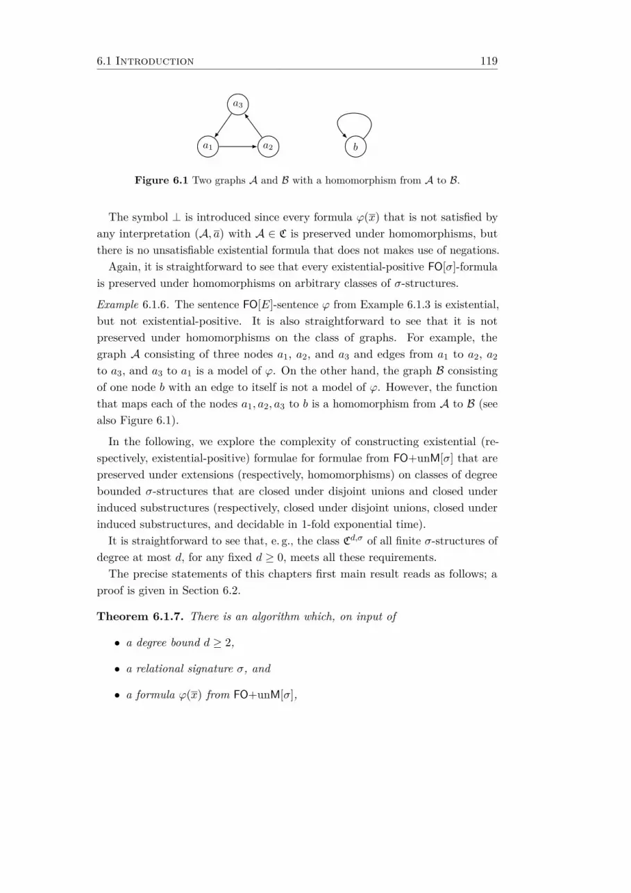
6.1 Introduction 119
a1 a2
a3
b
Figure 6.1 Two graphs A and B with a homomorphism from A to B.
The symbol ⊥ is introduced since every formula ϕ(x) that is not satisfied byany interpretation (A, a) with A ∈ C is preserved under homomorphisms, butthere is no unsatisfiable existential formula that does not makes use of negations.
Again, it is straightforward to see that every existential-positive FO[σ]-formulais preserved under homomorphisms on arbitrary classes of σ-structures.
Example 6.1.6. The sentence FO[E]-sentence ϕ from Example 6.1.3 is existential,but not existential-positive. It is also straightforward to see that it is notpreserved under homomorphisms on the class of graphs. For example, thegraph A consisting of three nodes a1, a2, and a3 and edges from a1 to a2, a2
to a3, and a3 to a1 is a model of ϕ. On the other hand, the graph B consistingof one node b with an edge to itself is not a model of ϕ. However, the functionthat maps each of the nodes a1, a2, a3 to b is a homomorphism from A to B (seealso Figure 6.1).
In the following, we explore the complexity of constructing existential (re-spectively, existential-positive) formulae for formulae from FO+unM[σ] that arepreserved under extensions (respectively, homomorphisms) on classes of degreebounded σ-structures that are closed under disjoint unions and closed underinduced substructures (respectively, closed under disjoint unions, closed underinduced substructures, and decidable in 1-fold exponential time).
It is straightforward to see that, e. g., the class Cd,σ of all finite σ-structures ofdegree at most d, for any fixed d ≥ 0, meets all these requirements.The precise statements of this chapters first main result reads as follows; a
proof is given in Section 6.2.
Theorem 6.1.7. There is an algorithm which, on input of
• a degree bound d ≥ 2,
• a relational signature σ, and
• a formula ϕ(x) from FO+unM[σ],
120 Chapter 6. Preservation Theorems
constructs an existential formula ψ(x) from FO[σ] such that the following holdsfor any class D of d-bounded σ-structures that is closed under disjoint unionsand induced substructures: If ϕ(x) is preserved under extensions on D, then ϕ(x)and ψ(x) are D-equivalent.
Furthermore, the algorithm computes ψ(x) in time
||ϕ|| ·(2νd(2νd(4q)O(||σ||) ) · (T+n+q) · L
)(n+q)·O(log max1,T,P),
where T, P, n, q ≥ 0 and L ≥ 1 are the threshold, the maximum period, thenumber of free variables, the quantifier rank, and the least common multiple ofthe periods of all modulo-counting quantifiers in ϕ(x), respectively. In particular,the constants suppressed by the O-notation do not depend on the signature σ.
For the case of input sentences from FO+unM(Dp) with threshold 0, where Dp
is a single modulo-counting quantifier with period p ≥ 2, Theorem 6.1.7 wasalready proven in [HHS14, HHS15].
Remark 6.1.8. Suppose that σ only contains relation symbols that actually occurin ϕ(x) and thus, ||σ|| < ||ϕ||. We know that T, P, n, q < ||ϕ||. Moreover, L = 1if there are no modulo-counting quantifiers in ϕ, and otherwise
L ≤ P ! ≤ 2P ·logP .
Thus, for every degree bound d ≥ 3, the algorithm of Theorem 6.1.7 takes 5-foldexponential time in the size of the input formula ϕ(x), that is, time in
2d2d2O(||ϕ||)
,
and for d = 2, the algorithm takes 3-fold exponential time, that is, time in
222poly(||ϕ||).
In Section 9.6, this is complemented by a 3-fold exponential lower bound.
Remark 6.1.9. Moreover, for input sentences ϕ from FO, that is, for formulaewhere T = P = n = 0 and L = 1, the running time of the algorithm ofTheorem 6.1.7 can be bounded by the simpler expression
||ϕ|| · 2νd(2νd(4q)O(||σ||) ).
6.1 Introduction 121
This chapters second main result reads as follows; a proof is given in Section 6.3below. Here, we say that a class C′ of structures is decidable in time t(n) forsome function t : N≥1 → N≥1 if there is an algorithm which decides on input ofa signature σ and a σ-structure A in time t(||σ||+ ||A||) whether A ∈ C′. Notethat here, the class C′ is not restricted to structures over a specific signature(which is provided as input to the algorithm).
Theorem 6.1.10. Let C′ a class of structures that is decidable in time t(n) forsome function t : N≥1 → N≥1 and that is closed under disjoint unions and inducedsubstructures.
There is an algorithm which, on input of
• a degree bound d ≥ 2,
• a relational signature σ, and
• a formula ϕ(x) from FO+unM[σ],
constructs an existential-positive formula ψ(x) from FO[σ] such that the followingholds for the class D of d-bounded σ-structures from C′: If ϕ(x) is preservedunder homomorphisms on D, then ϕ(x) and ψ(x) are D-equivalent.
Furthermore, the algorithm computes ψ(x) in time
2||ϕ||·(n+1)O(||σ||)·2νd(2·4q)O(||σ||)· t((n+1)O(||σ||) · 2νd(2·4q)O(||σ||))
where n, q ≥ 0 are the number of free variables and the quantifier rank of ϕ(x),respectively. Moreover, the formula ψ(x) is of size
2(n+1)O(||σ||)·2νd(2·4q)O(||σ||).
For the case of input sentences from FO+unM(Dp) with threshold 0, where Dp
is a single modulo-counting quantifier with period p ≥ 2, Theorem 6.1.10 wasalready proven in [HHS14, HHS15].
Remark 6.1.11. Note that, in contrast to Theorem 6.1.7, the running timeof the algorithm neither depends on the threshold nor on the periods of themodulo-counting quantifiers in the input formula.
Suppose that the function t : N≥1 → N≥1 is at most 1-fold exponential (this isclearly the case if, e.g., C′ is the class of all structures). Recall that n, q < ||ϕ||.If we suppose that σ contains only the relation symbols that actually occurin ϕ(x), that is, ||σ|| < ||ϕ|| then, for every degree bound d ≥ 3, the algorithm of
122 Chapter 6. Preservation Theorems
Theorem 6.1.10 takes 4-fold exponential time in the size of the input formula ϕ(x),that is, time in
22d2O(||ϕ||)
and the size of ψ(x) is bounded by the same expression.For degree bound d = 2, the algorithm takes 3-fold exponential time
222poly(||ϕ||
and the size of ψ(x) is again bounded by the same expression.
In Section 9.6, this is complemented by a 3-fold exponential lower bound.
Remark 6.1.12. For input sentences ϕ from FO, that is, for formulae where n = 0,the running time of the algorithm of Theorem 6.1.10 can be bounded by
2||ϕ||·2νd(2·4q)O(||σ||)· t(2νd(2·4q)O(||σ||)),
and the size of the computed existential-positive sentence ψ by
22νd(2·4q)O(||σ||).
In Section 6.4, we present two examples of classes of structures, which showthat the closure properties required in Theorem 6.1.7 and Theorem 6.1.10 areindeed necessary, and not just an artifact of the specific proofs.
A key concept in the proofs of Theorem 6.1.7 and Theorem 6.1.10 are minimalmodels of formulae. Again, we denote by C a class of σ-structures.
Definition 6.1.13. Let ϕ(x) be a formula from L[σ]. An interpretation (A, a)for ϕ(x) with A ∈ C is called a C-minimal model of ϕ if A |= ϕ[a], but B 6|= ϕ[a]for every proper induced substructure B of A that belongs to C and that containsall the elements from the tuple a.
Let d ≥ 0 and let D be a class of d-bounded σ-structures that is closed underdisjoint unions and closed under induced substructures. The main combinatorialparts (Theorem 6.2.1 and Theorem 6.3.1) of the proofs of Theorem 6.1.7 and The-orem 6.1.10 provide upper bounds on the size of the universe of D-minimal modelsfor formulae from FO+unM[σ] that are preserved under extensions (respectively,homomorphisms) on D.The proofs of both upper bounds on the size of the universe of D-minimal
models proceed as follows: Suppose that ϕ(x) is a formula from FO+unM[σ]
6.1 Introduction 123
that is preserved under extensions (homomorphisms) on D. For a contradiction,we assume that there is a D-minimal model (A, a) of ϕ(x) where the cardinalityof A exceeds the upper bound. Then, a proper induced substructure A′ ∈ D
of A can be constructed such that (A′, a) is also a model of ϕ(x). This is acontradiction to the minimality of (A, a).
In both cases, we use the variant of Nurmonen’s theorem [Nur00], stated in The-orem 3.3.1, which provides us with local conditions that make two interpretationsindistinguishable for ϕ(x).The proof of Theorem 6.1.7 employs a novel inductive construction that
constructs a sequence (Ci)i≥0 of structures from D that alternates betweenproper induced substructures and disjoint extensions of A and finally stopswith two consecutive structures Ci and Ci+1 for some i ≥ 0 such that theinterpretations (Ci, a) and (Ci+1, a) can not be distinguished by ϕ(x).
The proof of Theorem 6.1.10 is an adaptation of a result by Ajtai and Gurevich(Lemma 7.1 in [AG94]) where we use Theorem 3.3.1 instead of Gaifman’s theorem.
Recall that an r-scattered set of elements in a structure A, for some r ≥ 0, isa set of elements of pairwise distance > r in A. Both proofs for lower bounds onthe size of D-minimal models make use of the following easy fact.
Lemma 6.1.14 (cf., e.g., [ADG08]). Let d ≥ 0 be a degree bound and let A be ad-bounded σ-structure. For all m, r ≥ 0, the following holds: If
|A| > (m−1) · νd(2r),
then there exists an r-scattered subset of A with cardinality m.
Proof. Let d ≥ 0 be a degree bound and let A be a d-bounded σ-structure.Form, r ≥ 0, we show that if there is no r-scattered subset of A with cardinalitym,then |A| ≤ (m−1) · νd(2r).Choose a number n < m such that there is an r-scattered set B ⊆ A with
cardinality n in A, but no r-scattered subset of cardinality greater than n.Every element a of A has to be contained in the 2r-neighbourhood of B (forotherwise, B ∪ a would be an r-scattered subset of A with cardinality n+ 1).Therefore,
|A| = |NA2r(B)| ≤ (m−1) · νd(2r).
Finally, the upper bounds on the size of the universe of D-minimal modelsare used as an input to algorithms that compute a D-equivalent existential(existential-positive) FO[σ]-formula for the input formula ϕ(x).
124 Chapter 6. Preservation Theorems
The construction for existential formulae for formulae from FO+unM[σ] gener-alises Lemma 8.4 in [DGKS07]. Here, the handling of modulo-counting quantifiersuses the divide-and-conquer approach described in Section 2.9 to ensure thedesired time complexity.
The construction for existential-positive sentences uses an algorithmic versionof the Chandra-Merlin theorem ([CM77], cf., e.g., [AHV95]), which requires anadditional assumption on the decidability of D.
Recall that for all d ≥ 0 and r ≥ 0, Td,σr (1) is the set of all (up to isomorphism)one-centred types with radius r that may be realised in a d-bounded σ-structure.For the rest of this chapter, we abbreviate
Sd,s(r) := 2νd(r)O(s).
That is, S·,·(·) is the set of all functions f : N× N× N≥1 → N where there is anumber c ∈ N≥1 such that
f(d, r, s) ≤ 2νd(r)c·s
for all d, r ≥ 0 and s ≥ 1. Note that, in particular, there is a function f ∈ Ssuch that for all d ≥ 2 and r ≥ 1 we have |Td,σr (1)| ≤ f(d, r, ||σ||).
6.2 Preservation under Extensions
This section is devoted to the proof of Theorem 6.1.7. In the following, welet d ≥ 2 a degree bound and denote by D a class of d-bounded σ-structures thatis closed under disjoint unions and induced substructures.The main combinatorial contribution of this section is an upper bound on
the size of D-minimal models for formulae from FO+unM[σ] that are preservedunder extensions on D, which is provided by Theorem 6.2.1 below. Afterwards,Lemma 6.2.2 uses this upper bound to construct existential formulae. Thesection concludes with the actual proof of Theorem 6.1.7, which combines theaforementioned steps.
Theorem 6.2.1. There is a function N : N6 → N with
Nd,||σ||(T, n, q, L) ∈ Sd,||σ||(Sd,||σ||(4q)) · (T+n+q) · L,
such that the following holds for every relational signature σ, every degreebound d ≥ 2, every class D of d-bounded σ-structures that is closed under disjointunions and induced substructures, and every formula ϕ(x) from FO+unM[σ]:
6.2 Preservation under Extensions 125
If ϕ(x) is preserved under extensions on D, then every D-minimal modelof ϕ(x) has a universe of size at most Nd,||σ||(T, n, q, L), where T, n, q ≥ 0 arethe threshold, the number of free variables, and the quantifier rank of ϕ(x), andwhere L ≥ 1 is the least common multiple of the periods of all modulo-countingquantifiers that appear in ϕ(x).
Proof. Let σ be a relational signature, let d ≥ 2, and let D be a class of d-boundedσ-structures that is closed under disjoint unions and induced substructures.
Furthermore, let ϕ(x) be a formula from FO+unM[σ] that is preserved underextensions on D. Let T , q ≥ 0 be the threshold and the quantifier rank of ϕ,let n := |x| be the number of free variables of ϕ(x), and let L ≥ 1 be the leastcommon multiple of the periods of all modulo-counting quantifiers that appearin ϕ(x).
Choose r := 4q and the threshold
t := T + (n+q) · νd(r) (1)
from Condition (3) of Theorem 3.3.1 for the numbers T , n, q, and r.Furthermore, let
s ∈ Sd,||σ||(r)
be the number of non-isomorphic σ-types with radius r and one centre that maybe realised in structures from D and let
R := 2s · r, and S ∈ Sd,||σ||(R)
be the number of non-isomorphic σ-types with radius R and one centre that maybe realised in σ-structures from D.
Towards a contradiction, assume that ϕ(x) has a D-minimal model (A, a) witha universe of size
|A| > (2S · t · L+ n− 1) · νd(2R).
By Lemma 6.1.14, there exists an R-scattered subset Z of A of cardinality2S · t · L+ n. Suppose that a = (a1, . . . , an) and observe that
• each of the elements ai with i ∈ [1, n] only belongs to the R-neighbourhoodof at most one element of Z, and that
• there are at most S pairwise non-isomorphic σ-type with radius R and onecentre realised in A.
126 Chapter 6. Preservation Theorems
Then, there is an R-scattered set Y ⊆ Z with cardinality 2t · L, whose elementsall realise the same type from Td,σr (1) and such that none of the elements aiwith i ∈ [1, n] belong to the R-neighbourhood of Y .
In the following, we call a type τ ∈ Td,σr (1) frequent in a structure A if|τ(A)| ≥ t. Otherwise, it is rare in A. Note that each type τ ∈ Td,σr (1) thatis realised by an element from the (R−r)-neighbourhood of Y is frequent in A,because it occurs at least 2t · L ≥ t times in A.
Let X be a subset of Y with cardinality t · L. Since
NAR (a) ∼= NAR (b) for each a ∈ X and each b ∈ Y \X, (2)
the following holds for each type τ ∈ Td,σr (1):
If |τ(A) ∩NAR−r(X)| ≥ t, also |τ(A−NAR−r(X))| ≥ t.
That is, every type τ ∈ Td,σr (1) that is realised by at least t elements from the(R−r)-neighbourhood of the set X in A is still frequent in the substructure of Ainduced by deleting the (R−r)-neighbourhood of X.
In the following, a disjoint extension C of A (by a structure D) is an extensionof A where there is no edge between any element from A and any element fromC \A in the Gaifman graph GC of C (and where C −A is isomorphic to D).
Consider the following sequences (Ci)i≥0 and (D2i)i≥1 of σ-structures from D.Let C0 := A and C1 := A−X. For i ≥ 2, we proceed inductively and distinguishbetween even and odd numbers i:
(Even i) Here, Di := Ci−1[NA2(i−1)r(X)] and Ci is a disjoint extension of A by Di.
(Odd i) For odd i, the structure Di is neither defined nor required. On theother hand, Ci is the union of the disjoint structures A−NA2(i−1)r(X)and Di−1.
For a visualisation of the sequence (Ci)i≥0, see Figure 6.2. In particular, for alleven i ≥ 0, the structure Ci is a disjoint extension of A, and for all odd i, thestructure Ci is a proper induced substructure of A. Furthermore, for all i ∈ [1, s],every element aj with j ∈ [1, n] is still present in Ci and, in particular,
N Cir (a) ∼= NAr (a). (3)
Consider a type τ ∈ Td,σr (1). Recall that |X| = t · L and that the R-spheres
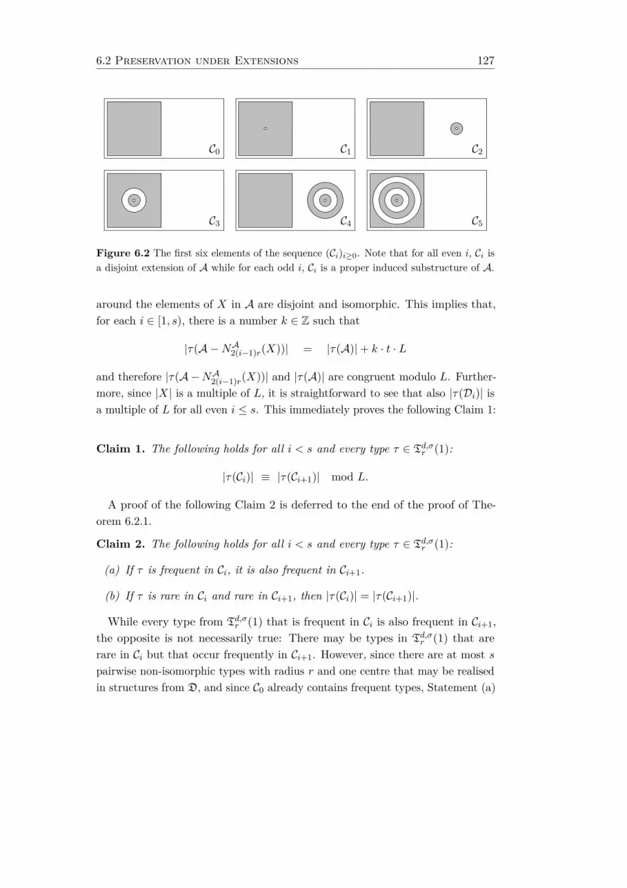
6.2 Preservation under Extensions 127
C0 C1 C2
C3 C4 C5
Figure 6.2 The first six elements of the sequence (Ci)i≥0. Note that for all even i, Ci isa disjoint extension of A while for each odd i, Ci is a proper induced substructure of A.
around the elements of X in A are disjoint and isomorphic. This implies that,for each i ∈ [1, s), there is a number k ∈ Z such that
|τ(A−NA2(i−1)r(X))| = |τ(A)|+ k · t · L
and therefore |τ(A−NA2(i−1)r(X))| and |τ(A)| are congruent modulo L. Further-more, since |X| is a multiple of L, it is straightforward to see that also |τ(Di)| isa multiple of L for all even i ≤ s. This immediately proves the following Claim 1:
Claim 1. The following holds for all i < s and every type τ ∈ Td,σr (1):
|τ(Ci)| ≡ |τ(Ci+1)| mod L.
A proof of the following Claim 2 is deferred to the end of the proof of The-orem 6.2.1.
Claim 2. The following holds for all i < s and every type τ ∈ Td,σr (1):
(a) If τ is frequent in Ci, it is also frequent in Ci+1.
(b) If τ is rare in Ci and rare in Ci+1, then |τ(Ci)| = |τ(Ci+1)|.
While every type from Td,σr (1) that is frequent in Ci is also frequent in Ci+1,the opposite is not necessarily true: There may be types in Td,σr (1) that arerare in Ci but that occur frequently in Ci+1. However, since there are at most spairwise non-isomorphic types with radius r and one centre that may be realisedin structures from D, and since C0 already contains frequent types, Statement (a)
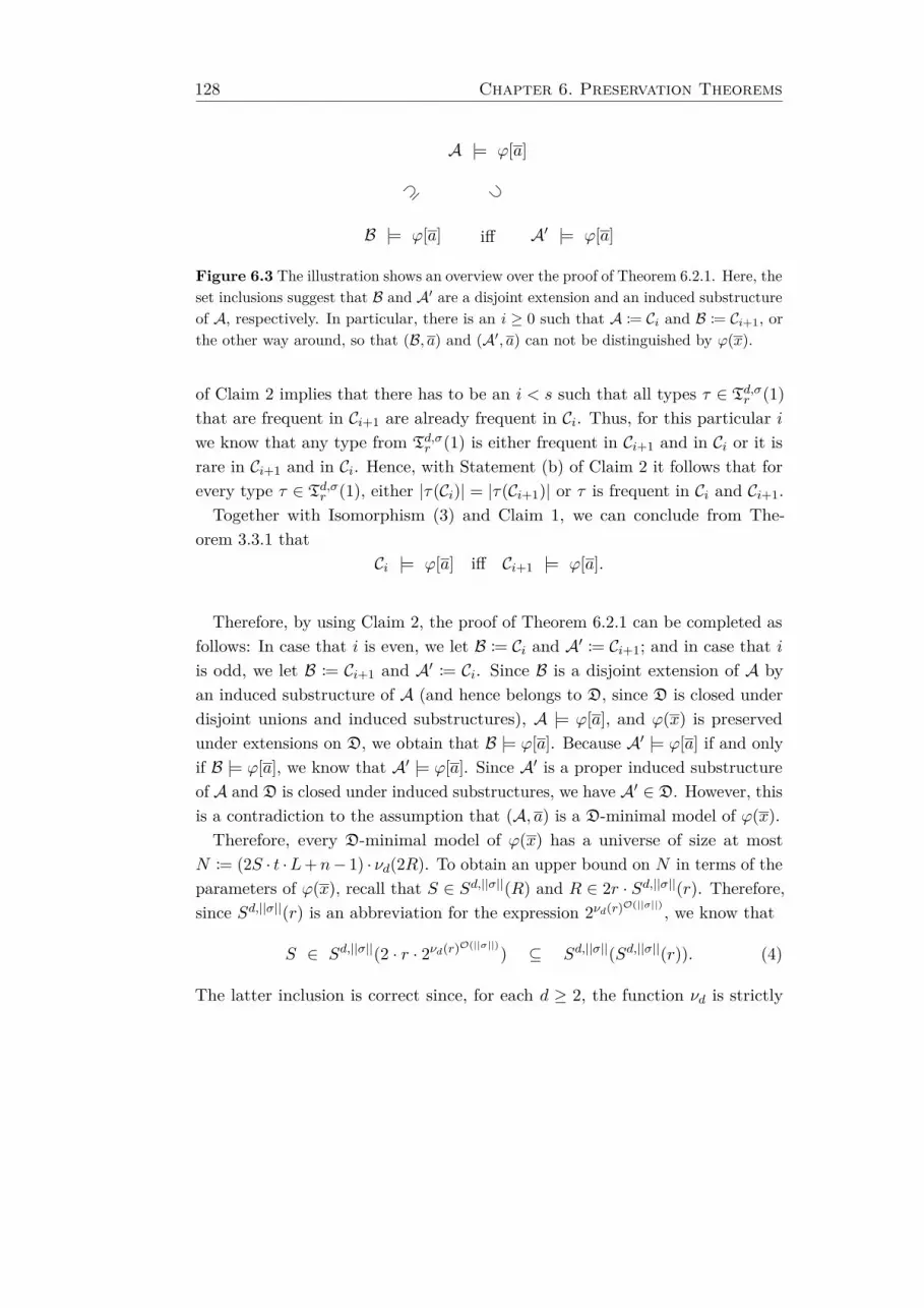
128 Chapter 6. Preservation Theorems
A |= ϕ[a]
B |= ϕ[a] A′ |= ϕ[a]iff
⊇ ⊃
Figure 6.3 The illustration shows an overview over the proof of Theorem 6.2.1. Here, theset inclusions suggest that B and A′ are a disjoint extension and an induced substructureof A, respectively. In particular, there is an i ≥ 0 such that A := Ci and B := Ci+1, orthe other way around, so that (B, a) and (A′, a) can not be distinguished by ϕ(x).
of Claim 2 implies that there has to be an i < s such that all types τ ∈ Td,σr (1)that are frequent in Ci+1 are already frequent in Ci. Thus, for this particular iwe know that any type from Td,σr (1) is either frequent in Ci+1 and in Ci or it israre in Ci+1 and in Ci. Hence, with Statement (b) of Claim 2 it follows that forevery type τ ∈ Td,σr (1), either |τ(Ci)| = |τ(Ci+1)| or τ is frequent in Ci and Ci+1.Together with Isomorphism (3) and Claim 1, we can conclude from The-
orem 3.3.1 thatCi |= ϕ[a] iff Ci+1 |= ϕ[a].
Therefore, by using Claim 2, the proof of Theorem 6.2.1 can be completed asfollows: In case that i is even, we let B := Ci and A′ := Ci+1; and in case that iis odd, we let B := Ci+1 and A′ := Ci. Since B is a disjoint extension of A byan induced substructure of A (and hence belongs to D, since D is closed underdisjoint unions and induced substructures), A |= ϕ[a], and ϕ(x) is preservedunder extensions on D, we obtain that B |= ϕ[a]. Because A′ |= ϕ[a] if and onlyif B |= ϕ[a], we know that A′ |= ϕ[a]. Since A′ is a proper induced substructureof A and D is closed under induced substructures, we have A′ ∈ D. However, thisis a contradiction to the assumption that (A, a) is a D-minimal model of ϕ(x).Therefore, every D-minimal model of ϕ(x) has a universe of size at most
N := (2S · t ·L+n− 1) · νd(2R). To obtain an upper bound on N in terms of theparameters of ϕ(x), recall that S ∈ Sd,||σ||(R) and R ∈ 2r · Sd,||σ||(r). Therefore,since Sd,||σ||(r) is an abbreviation for the expression 2νd(r)O(||σ||) , we know that
S ∈ Sd,||σ||(2 · r · 2νd(r)O(||σ||)) ⊆ Sd,||σ||(Sd,||σ||(r)). (4)
The latter inclusion is correct since, for each d ≥ 2, the function νd is strictly
6.2 Preservation under Extensions 129
increasing. Similarly, we have that
νd(2R) = νd(2 · 2 · r · 2νd(r)O(||σ||)) ⊆ νd(Sd,||σ||(r)). (5)
Thus, using Estimate (4) and Definition 1, the expression 2S · t · L+ n− 1 canbe bounded from above by
2Sd,||σ||(Sd,||σ||(r)) · (T + (n+q) · νd(r)) · L+ n− 1⊆ Sd,||σ||(Sd,||σ||(r)) · (T + (n+q) · νd(r)) · L⊆ Sd,||σ||(Sd,||σ||(r)) · (T+n+q) · L (6)
By putting Estimate (5) and Estimate (6) together, and recalling that r = 4q,we obtain that N ≤ Nd,||σ||(T, P, n, q, L) for
Nd,||σ||(T, P, n, q, L) ∈ Sd,||σ||(Sd,||σ||(4q)) · (T+n+q) · L · νd(Sd,||σ||(4q))⊆ Sd,||σ||(Sd,||σ||(4q)) · (T+n+q) · L.
All that remains to be done to finish the proof of Theorem 6.2.1 is to proveClaim 2.
Proof of Claim 2. Observe that for all i, j ≤ s,
Ci[A \NAR−2r(X)] ∼= Cj [A \NAR−2r(X)]. (7)
Let i < s. For the proof of Statement (b) of Claim 2, let τ ∈ Td,σr (1) be atype that is rare in Ci and Ci+1. Since X is an R-scattered set of size ≥ t, therareness of τ implies that τ(Ci) and τ(Ci+1) are subsets of A \NAR−r(X). Hence,Isomorphism (7) implies that |τ(Ci)| = |τ(Ci+1)|. This proves Statement (b) ofClaim 2.For the proof of Statement (a) of Claim 2, we distinguish between even and
odd i.
(Even i) Recall that C0 = A and that for each even i ≥ 2, the structure Ci is adisjoint extension of A by Di, that is, the union of A with a structure D′ithat is isomorphic to Di and has an universe disjoint from A. Let τ bea type from Td,σr (1) that is frequent in Ci. In the following, we make acase distinction on the elements of Ci which realise τ .
(Case 1) Suppose that τ is realised in Ci by an element in the setNAR−r(X). Then, τ is realised by at least t elements fromNAR−r(X), since X is R-scattered and |X| ≥ t. Furthermore,
130 Chapter 6. Preservation Theorems
we obtain from Isomorphism (2) that τ is also realised by atleast t elements in the set NAR−r(X ′ X). Since X ⊆ X ′, theset X ′ is R-scattered, and 2i · r < R, we can conclude that τis frequent in the structure A − NA2i·r(X). Thus, τ is alsofrequent in Ci+1.
(Case 2) Suppose that i ≥ 2 and τ is realised by an element of D′i.Since D′i ∼= Di, the type τ is also realised by an element fromDi ⊆ NAR−r(X) in Ci+1. Thus, τ is also frequent in Ci+1.
(Case 3) Otherwise, we know that τ is already realised by at least telements from A that do not belong to NAR−r(X). Then, itfollows from Isomorphism (7) that τ is also frequent in Ci+1.
(Odd i) Recall that C1 = A−X and that, for each odd i ≥ 3, the structure Ci isthe union of A−NA2(i−1)·r(X) and Di−1. Let τ be a type from Td,σr (1)that is frequent in Ci. Again, we make a case distinction on the elementsof Ci which realise τ .
(Case 1) Suppose that τ is in Ci realised by an element from the setNA2(i−1)·r+r(X). Since X is R-scattered and |X| ≥ t, at least telements from NA2(i−1)·r+r(X) realise τ in Ci. As Di+1 isthe structure Ci[NA2(i−1)·r+2r(X)], we can conclude that τ isfrequent in Di+1. Then, τ is also frequent in Ci+1, since Ci+1
is the disjoint extension of A by Di+1.(Case 2) Otherwise, we know that in Ci, the type τ is realised by
at least t elements from A \NA2(i−1)·r+r(X). However, sincethe r-sphere of each element a ∈ A \ NA2(i−1)·r+r(X) in thestructure A−NA2(i−1)·r(X) is isomorphic to its r-sphere in A,and Ci+1 is a disjoint extension of A by Di+1, the type τ isalso frequent in Ci+1.
This concludes the proof of Claim 2 and Theorem 6.2.1.
For proving Theorem 6.1.7, it remains to do the following: for a given for-mula ϕ(x) from FO+unM[σ] that is preserved under extensions on D and for anupper bound on the size of its D-minimal models, obtained from Theorem 6.2.1,construct an existential formula from FO[σ] that is D-equivalent to ϕ(x). Thisis done by using the following lemma, which is a generalisation of Lemma 8.4in [DGKS07] to formulae (possibly with free variables) with modulo-countingquantifiers.
6.2 Preservation under Extensions 131
Lemma 6.2.2. There is an algorithm which, on input of
• a number N ≥ 1 and
• a formula ϕ(x) from FO+unM[σ] over a relational signature σ,
constructs an existential formula ψ(x) from FO[σ] such that the following holdsfor every class C of σ-structures that is closed under induced substructures:If ϕ(x) is preserved under extensions on C and every C-minimal model of ϕ(x)
has a universe of size ≤ N , then ψ(x) is C-equivalent to ϕ(x).Furthermore, the algorithm constructs ψ(x) in time
||ϕ|| · (2 max1, T, P)(n+q)·O(logN),
where T, P, q ≥ 0 are the threshold, the maximum period, and the quantifier rankof ϕ(x). The constant suppressed by the O-notation does not depend on thesignature σ.
The key ingredient for the proof of Lemma 6.2.2 is contained in the followinglemma. Here, an enumeration of a set A is a tuple (e1, . . . , eM ) ∈ AM of lengthM = |A| that contains each element of A exactly once, that is, A = e1, . . . , eM.
Lemma 6.2.3. Let σ be a relational signature, let m ≥ 0, and let ϕ(x1, . . . , xm)be a formula from FO+unM[σ] where all variables occurring in ϕ are amongx1, . . . , xm.For each M ≥ 1 and every function s : [1,m]→ [1,M ], there is a quantifier-free
formula (ϕ)M,s(y1, . . . , yM ) from FO[σ] such that for each σ-structure A withexactly M elements and every enumeration (e1, . . . , eM ) of A,
A |= ϕ[es(1), . . . , es(m)]iff A |= (ϕ)M,s[e1, . . . , eM ].
Furthermore, there is an algorithm which, on input of ϕ(x), M , and s, con-structs (ϕ)M,s in time
O(||ϕ||) · (2 maxT, P)q·O(logM),
where T, P, q ≥ 0 are the threshold, the maximum period, and the quantifierrank of ϕ(x). The constants suppressed by the O-notation do not depend on thesignature σ.
Before presenting the proof of Lemma 6.2.3, we first show how to use Lemma 6.2.3for proving Lemma 6.2.2.
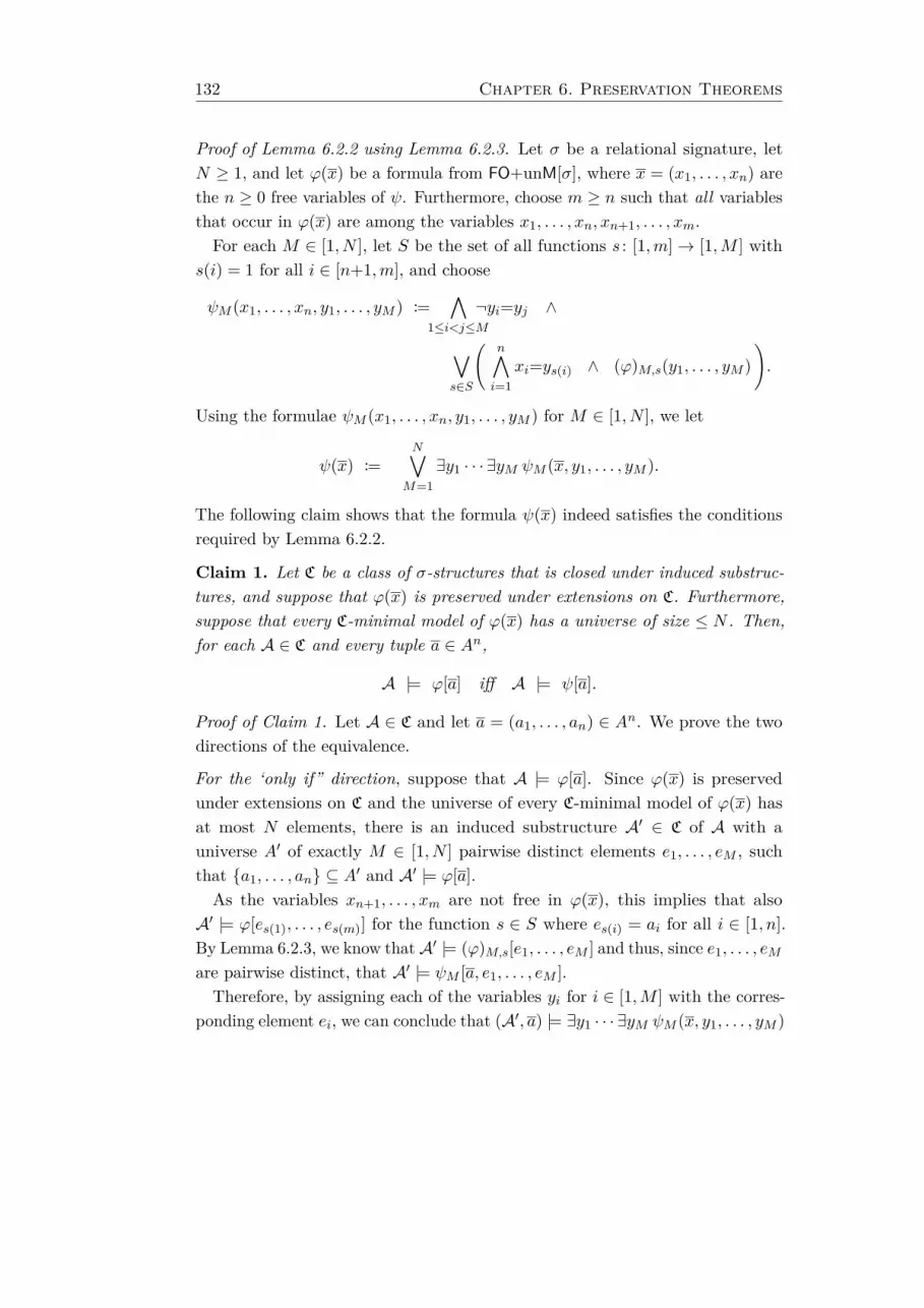
132 Chapter 6. Preservation Theorems
Proof of Lemma 6.2.2 using Lemma 6.2.3. Let σ be a relational signature, letN ≥ 1, and let ϕ(x) be a formula from FO+unM[σ], where x = (x1, . . . , xn) arethe n ≥ 0 free variables of ψ. Furthermore, choose m ≥ n such that all variablesthat occur in ϕ(x) are among the variables x1, . . . , xn, xn+1, . . . , xm.For each M ∈ [1, N ], let S be the set of all functions s : [1,m]→ [1,M ] with
s(i) = 1 for all i ∈ [n+1,m], and choose
ψM (x1, . . . , xn, y1, . . . , yM ) :=∧
1≤i<j≤M¬yi=yj ∧
∨s∈S
(n∧i=1
xi=ys(i) ∧ (ϕ)M,s(y1, . . . , yM )).
Using the formulae ψM (x1, . . . , xn, y1, . . . , yM ) for M ∈ [1, N ], we let
ψ(x) :=N∨
M=1∃y1 · · · ∃yM ψM (x, y1, . . . , yM ).
The following claim shows that the formula ψ(x) indeed satisfies the conditionsrequired by Lemma 6.2.2.
Claim 1. Let C be a class of σ-structures that is closed under induced substruc-tures, and suppose that ϕ(x) is preserved under extensions on C. Furthermore,suppose that every C-minimal model of ϕ(x) has a universe of size ≤ N . Then,for each A ∈ C and every tuple a ∈ An,
A |= ϕ[a] iff A |= ψ[a].
Proof of Claim 1. Let A ∈ C and let a = (a1, . . . , an) ∈ An. We prove the twodirections of the equivalence.
For the ‘only if” direction, suppose that A |= ϕ[a]. Since ϕ(x) is preservedunder extensions on C and the universe of every C-minimal model of ϕ(x) hasat most N elements, there is an induced substructure A′ ∈ C of A with auniverse A′ of exactly M ∈ [1, N ] pairwise distinct elements e1, . . . , eM , suchthat a1, . . . , an ⊆ A′ and A′ |= ϕ[a].As the variables xn+1, . . . , xm are not free in ϕ(x), this implies that also
A′ |= ϕ[es(1), . . . , es(m)] for the function s ∈ S where es(i) = ai for all i ∈ [1, n].By Lemma 6.2.3, we know thatA′ |= (ϕ)M,s[e1, . . . , eM ] and thus, since e1, . . . , eM
are pairwise distinct, that A′ |= ψM [a, e1, . . . , eM ].Therefore, by assigning each of the variables yi for i ∈ [1,M ] with the corres-
ponding element ei, we can conclude that (A′, a) |= ∃y1 · · · ∃yM ψM (x, y1, . . . , yM )
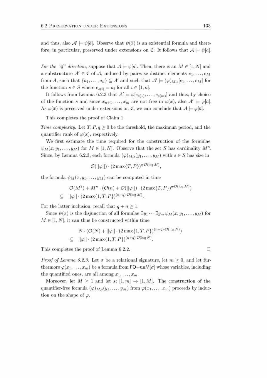
6.2 Preservation under Extensions 133
and thus, also A′ |= ψ[a]. Observe that ψ(x) is an existential formula and there-fore, in particular, preserved under extensions on C. It follows that A |= ψ[a].
For the “if” direction, suppose that A |= ψ[a]. Then, there is an M ∈ [1, N ] anda substructure A′ ∈ C of A, induced by pairwise distinct elements e1, . . . , eM
from A, such that a1, . . . , an ⊆ A′ and such that A′ |= (ϕ)M,s[e1, . . . , eM ] forthe function s ∈ S where es(i) = ai for all i ∈ [1, n].It follows from Lemma 6.2.3 that A′ |= ϕ[es(1), . . . , es(m)] and thus, by choice
of the function s and since xn+1, . . . , xm are not free in ϕ(x), also A′ |= ϕ[a].As ϕ(x) is preserved under extensions on C, we can conclude that A |= ϕ[a].
This completes the proof of Claim 1.
Time complexity. Let T, P, q ≥ 0 be the threshold, the maximum period, and thequantifier rank of ϕ(x), respectively.We first estimate the time required for the construction of the formulae
ψM (x, y1, . . . , yM ) for M ∈ [1, N ]. Observe that the set S has cardinality Mn.Since, by Lemma 6.2.3, each formula (ϕ)M,s(y1, . . . , yM ) with s ∈ S has size in
O(||ϕ||) · (2 maxT, P)q·O(logM),
the formula ψM (x, y1, . . . , yM ) can be computed in time
O(M2) +Mn ·(O(n) +O(||ϕ||) · (2 maxT, P)q·O(logM))
⊆ ||ϕ|| · (2 max1, T, P)(n+q)·O(logM).
For the latter inclusion, recall that q + n ≥ 1.Since ψ(x) is the disjunction of all formulae ∃y1 · · · ∃ym ψM (x, y1, . . . , yM ) for
M ∈ [1, N ], it can thus be constructed within time
N · (O(N) + ||ϕ|| · (2 max1, T, P)(n+q)·O(logN))⊆ ||ϕ|| · (2 max1, T, P)(n+q)·O(logN).
This completes the proof of Lemma 6.2.2.
Proof of Lemma 6.2.3. Let σ be a relational signature, let m ≥ 0, and let fur-thermore ϕ(x1, . . . , xm) be a formula from FO+unM[σ] whose variables, includingthe quantified ones, are all among x1, . . . , xm.Moreover, let M ≥ 1 and let s : [1,m] → [1,M ]. The construction of the
quantifier-free formula (ϕ)M,s(y1, . . . , yM ) from ϕ(x1, . . . , xm) proceeds by induc-tion on the shape of ϕ.
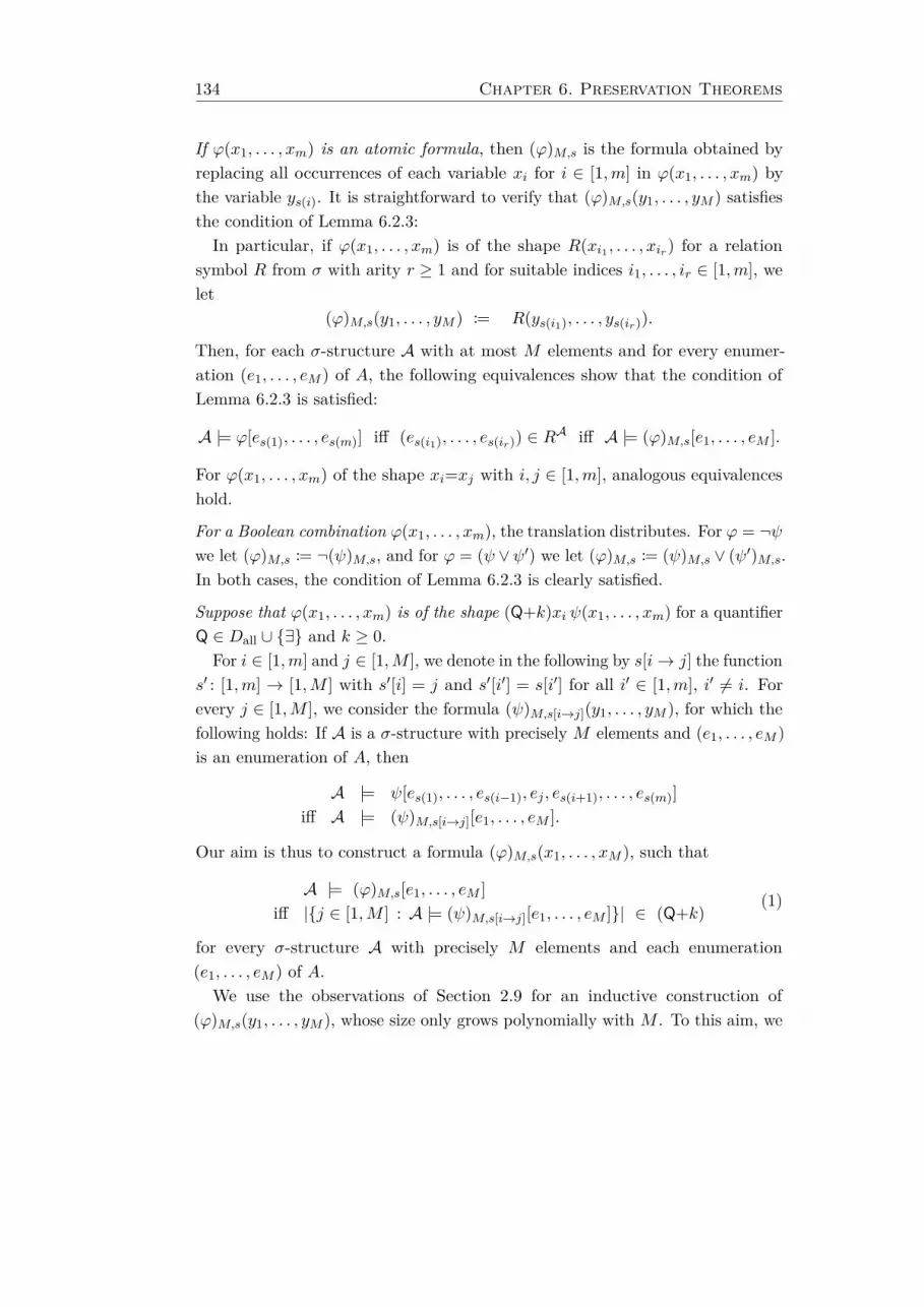
134 Chapter 6. Preservation Theorems
If ϕ(x1, . . . , xm) is an atomic formula, then (ϕ)M,s is the formula obtained byreplacing all occurrences of each variable xi for i ∈ [1,m] in ϕ(x1, . . . , xm) bythe variable ys(i). It is straightforward to verify that (ϕ)M,s(y1, . . . , yM ) satisfiesthe condition of Lemma 6.2.3:In particular, if ϕ(x1, . . . , xm) is of the shape R(xi1 , . . . , xir) for a relation
symbol R from σ with arity r ≥ 1 and for suitable indices i1, . . . , ir ∈ [1,m], welet
(ϕ)M,s(y1, . . . , yM ) := R(ys(i1), . . . , ys(ir)).
Then, for each σ-structure A with at most M elements and for every enumer-ation (e1, . . . , eM ) of A, the following equivalences show that the condition ofLemma 6.2.3 is satisfied:
A |= ϕ[es(1), . . . , es(m)] iff (es(i1), . . . , es(ir)) ∈ RA iff A |= (ϕ)M,s[e1, . . . , eM ].
For ϕ(x1, . . . , xm) of the shape xi=xj with i, j ∈ [1,m], analogous equivalenceshold.
For a Boolean combination ϕ(x1, . . . , xm), the translation distributes. For ϕ = ¬ψwe let (ϕ)M,s := ¬(ψ)M,s, and for ϕ = (ψ ∨ψ′) we let (ϕ)M,s := (ψ)M,s ∨ (ψ′)M,s.In both cases, the condition of Lemma 6.2.3 is clearly satisfied.
Suppose that ϕ(x1, . . . , xm) is of the shape (Q+k)xi ψ(x1, . . . , xm) for a quantifierQ ∈ Dall ∪ ∃ and k ≥ 0.
For i ∈ [1,m] and j ∈ [1,M ], we denote in the following by s[i→ j] the functions′ : [1,m] → [1,M ] with s′[i] = j and s′[i′] = s[i′] for all i′ ∈ [1,m], i′ 6= i. Forevery j ∈ [1,M ], we consider the formula (ψ)M,s[i→j](y1, . . . , yM ), for which thefollowing holds: If A is a σ-structure with precisely M elements and (e1, . . . , eM )is an enumeration of A, then
A |= ψ[es(1), . . . , es(i−1), ej , es(i+1), . . . , es(m)]iff A |= (ψ)M,s[i→j][e1, . . . , eM ].
Our aim is thus to construct a formula (ϕ)M,s(x1, . . . , xM ), such that
A |= (ϕ)M,s[e1, . . . , eM ]iff |j ∈ [1,M ] : A |= (ψ)M,s[i→j][e1, . . . , eM ]| ∈ (Q+k)
(1)
for every σ-structure A with precisely M elements and each enumeration(e1, . . . , eM ) of A.
We use the observations of Section 2.9 for an inductive construction of(ϕ)M,s(y1, . . . , yM ), whose size only grows polynomially with M . To this aim, we
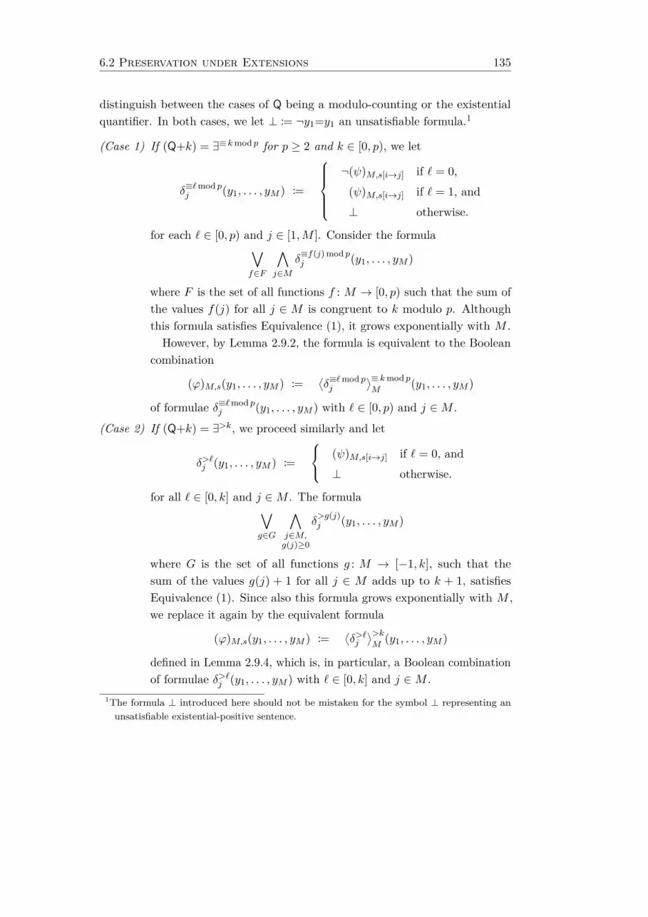
6.2 Preservation under Extensions 135
distinguish between the cases of Q being a modulo-counting or the existentialquantifier. In both cases, we let ⊥ := ¬y1=y1 an unsatisfiable formula.1
(Case 1) If (Q+k) = ∃≡ kmod p for p ≥ 2 and k ∈ [0, p), we let
δ≡`mod pj (y1, . . . , yM ) :=
¬(ψ)M,s[i→j] if ` = 0,
(ψ)M,s[i→j] if ` = 1, and⊥ otherwise.
for each ` ∈ [0, p) and j ∈ [1,M ]. Consider the formula∨f∈F
∧j∈M
δ≡f(j) mod pj (y1, . . . , yM )
where F is the set of all functions f : M → [0, p) such that the sum ofthe values f(j) for all j ∈ M is congruent to k modulo p. Althoughthis formula satisfies Equivalence (1), it grows exponentially with M .
However, by Lemma 2.9.2, the formula is equivalent to the Booleancombination
(ϕ)M,s(y1, . . . , yM ) :=⟨δ≡`mod pj
⟩≡ kmod pM
(y1, . . . , yM )
of formulae δ≡`mod pj (y1, . . . , yM ) with ` ∈ [0, p) and j ∈M .
(Case 2) If (Q+k) = ∃>k, we proceed similarly and let
δ>`j (y1, . . . , yM ) :=
(ψ)M,s[i→j] if ` = 0, and⊥ otherwise.
for all ` ∈ [0, k] and j ∈M . The formula∨g∈G
∧j∈M,g(j)≥0
δ>g(j)j (y1, . . . , yM )
where G is the set of all functions g : M → [−1, k], such that thesum of the values g(j) + 1 for all j ∈ M adds up to k + 1, satisfiesEquivalence (1). Since also this formula grows exponentially with M ,we replace it again by the equivalent formula
(ϕ)M,s(y1, . . . , yM ) :=⟨δ>`j
⟩>kM
(y1, . . . , yM )
defined in Lemma 2.9.4, which is, in particular, a Boolean combinationof formulae δ>`j (y1, . . . , yM ) with ` ∈ [0, k] and j ∈M .
1The formula ⊥ introduced here should not be mistaken for the symbol ⊥ representing anunsatisfiable existential-positive sentence.
136 Chapter 6. Preservation Theorems
We complete the proof of Lemma 6.2.3 by providing an analysis of the timerequired for constructing the formula (ϕ)M,s(y1, . . . , yM ).
Time complexity. In the following, we let T, P, q ≥ 0 the threshold, the maximumperiod, and the quantifier rank of ϕ.The only size increasing steps in the inductive translation are the ones for
quantifiers, that is, subformulae of the shape (Q+k)xi ψ. Summing up the timeneeded for the case of (Q+k) = ∃≡ kmod p for p ∈ [2, P ] and k ∈ [0, p), and forthe case of (Q+k) = ∃>k with k ∈ [0, T ], this increases the size of the formula bya factor of (2 maxT, P)O(logM), according to Lemma 2.9.2 and Lemma 2.9.4,respectively. Thus,
||(ϕ)M,s|| ∈ O(||ϕ||) · (2 maxT, P)q·O(logM).
It is easy to see that the time required for the construction of (ϕ)M,s(y1, . . . , yM )can be bounded by the same expression. This completes the proof of Lemma 6.2.3.
Theorem 6.1.7 is now obtained by a straightforward combination of The-orem 6.2.1 and Lemma 6.2.2.
Proof of Theorem 6.1.7. Let d ≥ 2 be a degree bound, let σ be a relationalsignature, and let ϕ(x) be a formula from FO+unM[σ] with n := |x| free variables,threshold T ≥ 0, maximum period P ≥ 0, and quantifier rank q ≥ 0. Furthermore,let L ≥ 1 be the least common multiple of the periods of all modulo-countingquantifiers occurring in ϕ(x).
Let D be a class of d-bounded σ-structures that is closed under disjoint unionsand induced substructures and suppose that ϕ(x) is preserved under extensionson D.
The algorithm proceeds in the following two steps:
(Step 1) Compute the upper bound
N := Nd,||σ||(T, n, q, L)∈ Sd,||σ||(Sd,||σ||(4q)) · (T+n+q) · L (1)
on the size of D-minimal models of ϕ(x), obtained from Theorem 6.2.1.In particular, we can assume that N ≥ 2.
6.3 Preservation under Homomorphisms 137
(Step 2) The algorithm of Lemma 6.2.2 constructs an existential formula ψ(x)from FO[σ] that is D-equivalent to ϕ(x). This takes time in
O(||ϕ||) · (2 max1, T, P)(n+q)·O(logN)
⊆ ||ϕ|| ·N (n+q)·O(log max1,T,P)
Thus, by replacing N in the latter estimate with Estimate (1) and recalling thedefinition of S·,·(·), we obtain that ψ(x) can altogether be computed in time
||ϕ|| ·(2νd(2νd(4q)O(||σ||) ) · (T+n+q) · L
)(n+q)·O(log max1,T,P).
This completes the proof of Theorem 6.1.7.
6.3 Preservation under Homomorphisms
This section is devoted to the proof of Theorem 6.1.10, whose combinator-ial essence is contained in the following Theorem 6.3.1. Further down below,Lemma 6.3.2 uses this upper bound on the size of minimal models of formulaethat are preserved under homomorphisms, to construct existential-positive for-mulae. The section concludes with the actual proof of Theorem 6.1.10, whichcombines the aforementioned steps.
Theorem 6.3.1. There is a function N : N4 → N with
Nd,||σ||(n, q) ∈ (n+1) · Sd,||σ||(2 · 4q)
such that the following holds for every relational signature σ, every degree boundd ≥ 2, every class D of d-bounded σ-structures that is closed under disjointunions and induced substructures, and every formula ϕ(x) from FO+unM[σ]:
If ϕ(x) is preserved under homomorphisms on D, then every D-minimal modelof ϕ(x) has a universe of size at most Nd,||σ||(n, q), where n, q ≥ 0 are the numberof free variables and the quantifier rank of ϕ(x), respectively.
Note that, in contrast to Theorem 6.2.1, the upper bound on the size ofthe universe of D-minimal models for a formula ϕ that is preserved underhomomorphisms on D neither depends on the threshold nor on the periods ofthe quantifiers in ϕ.
Proof of Theorem 6.3.1. The proof is similar to the proof of Lemma 7.1 in [AG94].However, it does not rely on Gaifman’s theorem but uses the generalisation ofNurmonen’s theorem to FO+unM, stated in Theorem 3.3.1.
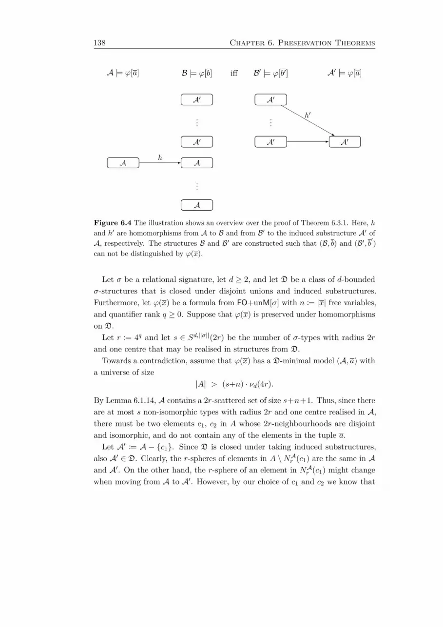
138 Chapter 6. Preservation Theorems
A |= ϕ[a] B |= ϕ[b] iff B′ |= ϕ[b′] A′ |= ϕ[a]
A
A
...
A
A′
...
A′
A′
...
A′
A′
h
h′
Figure 6.4 The illustration shows an overview over the proof of Theorem 6.3.1. Here, hand h′ are homomorphisms from A to B and from B′ to the induced substructure A′ ofA, respectively. The structures B and B′ are constructed such that (B, b) and (B′, b′)can not be distinguished by ϕ(x).
Let σ be a relational signature, let d ≥ 2, and let D be a class of d-boundedσ-structures that is closed under disjoint unions and induced substructures.Furthermore, let ϕ(x) be a formula from FO+unM[σ] with n := |x| free variables,and quantifier rank q ≥ 0. Suppose that ϕ(x) is preserved under homomorphismson D.Let r := 4q and let s ∈ Sd,||σ||(2r) be the number of σ-types with radius 2r
and one centre that may be realised in structures from D.Towards a contradiction, assume that ϕ(x) has a D-minimal model (A, a) with
a universe of size|A| > (s+n) · νd(4r).
By Lemma 6.1.14, A contains a 2r-scattered set of size s+n+1. Thus, since thereare at most s non-isomorphic types with radius 2r and one centre realised in A,there must be two elements c1, c2 in A whose 2r-neighbourhoods are disjointand isomorphic, and do not contain any of the elements in the tuple a.Let A′ := A − c1. Since D is closed under taking induced substructures,
also A′ ∈ D. Clearly, the r-spheres of elements in A \NAr (c1) are the same in Aand A′. On the other hand, the r-sphere of an element in NAr (c1) might changewhen moving from A to A′. However, by our choice of c1 and c2 we know that
6.3 Preservation under Homomorphisms 139
every r-sphere that is realised in A is also realised in A′: For elements outsidethe r-neighbourhood of c1 this is obvious; and for elements c′1 ∈ NAr (c1), ther-sphere of c′1 in A is realised in A′ by the corresponding element c′2 ∈ NA
′r (c2).
In the following, we will use Theorem 3.3.1 to show that also A′ |= ϕ[a]. Theargumentation is sketched in Figure 6.4. Let L ≥ 1 denote the least commonmultiple of the periods of all modulo-counting quantifiers that occur in ϕ(x), andlet t := T + (n+q) · νd(r), where T ≥ 0 is the threshold of ϕ, denote the numberchosen in Condition (3) of Theorem 3.3.1 for the degree bound d.
Let B be a disjoint union of t · L copies of A and t · L copies of A′. Since D isclosed under taking disjoint unions, we know that B ∈ D. Obviously, there is aninjective homomorphism h that maps A to one of the copies of A in B. SinceA |= ϕ[a] and ϕ(x) is preserved under homomorphisms on D, we thus obtainthat B |= ϕ[b] for b = h(a). Furthermore, NAr (a) ∼= NBr (b).Now let B′ be a disjoint union of t · L copies of A′. Since D is closed under
taking disjoint unions, also B′ ∈ D. By construction of B and B′, every one-centred σ-type τ with radius r is realised in B if it is realised in B′, and vice versa.Furthermore, the number of realisations of τ in B or B′ is a multiple of t · L.Consider an arbitrary disjoint copy of A′ in B′, and let b′ be the tuple of elementsof this copy corresponding to the tuple a in A. In particular, NBr (b) ∼= NB′r (b′).Thus, the interpretations (B, b) and (B′, b′) for ϕ(x) satisfy the assumptions ofTheorem 3.3.1, and, since B |= ϕ[b], in particular also B′ |= ϕ[b′].
By mapping each element of each disjoint copy of A′ in B′ to the correspondingelement in A′, we obtain an injective homomorphism h′ from B′ to A′ suchthat, in particular, h′(b′) = a. Since B′ |= ϕ[b′] and ϕ(x) is preserved underhomomorphisms on D, we obtain that also A′ |= ϕ[a].This, however, contradicts our assumption that (A, a) is a D-minimal model
of ϕ(x). Therefore, every D-minimal model of ϕ(x) has a universe of sizeN ≤ (s+n) · νd(4r). Recalling that r = 4q, we obtain that N ≤ Nd,||σ||(n, q) for
Nd,||σ||(n, q) ∈ (Sd,||σ||(2 · 4q) + n) · νd(4 · 4q)⊆ (n+1) · Sd,||σ||(2 · 4q).
This concludes the proof of Theorem 6.3.1.
In the following Lemma 6.3.2, we construct existential-positive FO[σ]-formulaefor formulae from an arbitrary ultimately periodic logic L[σ] that are preserved un-der homomorphisms on an arbitrary decidable class of σ-structures. In particular,this includes the logic FO+unM[σ].
140 Chapter 6. Preservation Theorems
Note that the lemma is stated in a more general way than actually needed forthe proof of Theorem 6.1.10, where we only have to consider decidable classesof σ-structures of bounded degree that are closed under disjoint unions andinduced substructures and only input formulae from FO+unM[σ]. However, thegeneralisation to formulae from arbitrary ultimately periodic logics L[σ] will beused later in Section 7.5 and Section 8.6.
The proof of Lemma 6.3.2 is an algorithmic version of the proof of Theorem 3.1in [ADK06].
Lemma 6.3.2. Let L be an ultimately periodic logic and let C′ be a class ofstructures that is decidable in time t(n) for some function t : N≥1 → N≥1.
There is an algorithm which, on input of
• a relational signature σ,
• a number N ≥ 2, and
• a formula ϕ(x) from L[σ] with n := |x| free variables,
constructs an existential-positive formula ψ(x) from FO[σ], such that the followingholds for the class D of all σ-structures from C′:
If ϕ(x) is preserved under homomorphisms on D and every D-minimal modelof ϕ(x) has a universe of size at most N , then ψ(x) is D-equivalent to ϕ(x).
Furthermore, the algorithm constructs ψ(x) in time
2||ϕ||·NO(||σ||) · t(NO(||σ||))
and ψ(x) has size in2(n+1)·NO(||σ||)
.
The following theorem, well-known as the Chandra-Merlin theorem [CM77](cf., [AHV95]) is crucial for the construction of existential-positive formulae inLemma 6.3.2. For its statement, we require some more notation:
Let A be a σ-structure. Without loss of generality, we assume that the universeof A is a subset of the natural numbers of cardinalityM ≥ 1. That is, the universeof A consists of M elements e1, . . . , eM ∈ N with e1 < · · · < eM . Furthermore,let a = (ej1 , . . . , ejn) ∈ An for indices j1, . . . , jn ∈ [1,M ] be a tuple of n ≥ 0elements from A. The canonical conjunctive query associated with (A, a) is theFO[σ]-formula
γ(A,a)(x1, . . . , xn) := ∃y1 · · · ∃yM
(n∧i=1
xi=yji ∧ δA(y1, . . . , yM )),
6.3 Preservation under Homomorphisms 141
where δA(y1, . . . , yM ) is the conjunction of all atomic formulae of the formR(yi1 , . . . , yir) with a relation symbol R from σ of arity r ≥ 1 and indicesi1, . . . , ir ∈ [1,M ], for which (ei1 , . . . , eir) ∈ RA.
Theorem 6.3.3 ([CM77, AHV95]). Let σ be a relational signature, let A andB be σ-structures, and let a ∈ An and b ∈ Bn be tuples of length n ≥ 0. Thefollowing equivalence holds:
B |= γ(A,a)[b]
iff there is a homomorphism h from A to B where b = h(a).
Before giving a proof of Theorem 6.3.3, we first show how Theorem 6.3.3 isused for the proof of Lemma 6.3.2.
Proof of Lemma 6.3.2 using Theorem 6.3.3. Let L be an ultimately periodic lo-gic and let C′ be a class of structures that is decidable in time t(n) for somefunction t : N≥1 → N≥1. Let σ be a relational signature and let D be the classof all σ-structures from C′. Furthermore, let N ≥ 2 and let ϕ(x) be a formulafrom L[σ] with n := |x| free variables.
The algorithm proceeds along the following steps:
(Step 1) Compute the set K that consists of all tuples (A, a) with A ∈ D
and a ∈ An, such that A = [1,M ] for an M ≤ N and A |= ϕ[a].
(Step 2) If K = ∅, output ψ := ⊥. Otherwise, that is, if K 6= ∅, output theformula
ψ(x) :=∨
(A,a)∈Kγ(A,a)(x)
Obviously, ψ(x) is an existential-positive formula from FO[σ].Before giving details on the algorithm’s Step (1) and its running time, let us
first show that ψ(x) is D-equivalent to ϕ(x), provided that ϕ(x) is preservedunder homomorphisms on D and that every D-minimal model of ϕ(x) has auniverse of at most N elements. To this end, let B be an arbitrary σ-structurefrom D and let b ∈ Bn.
If B |= ψ[b], then there is a tuple (A, a) ∈ K such that B |= γ(A,a)[b]. Dueto the Chandra-Merlin theorem (that is, Theorem 6.3.3 above), there is ahomomorphism h from A to B with b = h(a). As A ∈ D and A |= ϕ[a] byconstruction of K, and since ϕ(x) is preserved under homomorphisms on D, weobtain that B |= ϕ[b].
142 Chapter 6. Preservation Theorems
Now suppose that B |= ϕ[b]. As ϕ(x) is preserved under homomorphisms on D
it is, in particular, also preserved under extensions on D. Thus, B is eitheran extension of a structure A ∈ D such that (A, b) is a D-minimal modelof ϕ(x) or (B, b) itself is a D-minimal model of ϕ(x). In the latter case, welet A := B. By assumption, N is an upper bound on the size of the universe of A.Thus, by choice of K, the set K contains a tuple (A′, a′) for which there is anisomorphism h : A′ → A from A′ to A with b = h(a′). Since, more general, h is ahomomorphism from A′ to B, we obtain from Theorem 6.3.3 that B |= γ(A′,a′)[b]and thus, since (A′, a′) ∈ K, also B |= ψ[b].
In summary, this shows that ψ(x) is D-equivalent to ϕ(x).
Size and time complexity. The cardinality of the set K is bounded by the numberof all tuples (A, a) where A is a σ-structure with universe [1,M ] for an M ≤ Nand where a ∈ An, and thus by
N∑M=1
Mn · 2max2,M||σ|| ≤ Nn+1 · 2N ||σ|| ∈ 2(n+1)·NO(||σ||). (1)
Furthermore, for each tuple (A, a) ∈ K, the canonical conjunctive query γ(A,a)(x)can be constructed in time
O(n) +NO(||σ||). (2)
Hence, using Estimate (1) and Estimate (2), the size of ψ(x) is also in
2(n+1)·NO(||σ||).
Let us now turn to the algorithm’s Step (1) and the analysis of its timecomplexity. To compute the set K, the algorithm enumerates all σ-structures Awhose universe is the set [1,M ] for some M ∈ [1, N ] and checks whether A ∈ C′.If this is the case, the algorithm enumerates all tuples a ∈ An and decides whetheralso A |= ϕ[a].By assumption, it can be decided in time t(||σ|| + ||A||), respectively in
time t(NO(||σ||)), whether A ∈ C′. For an ultimately periodic logic L, a naivemodel-checking algorithm can proceed in the same fashion as for the case ofFO, that is, by recursion over the shape of ϕ and, for each ultimately periodicquantifier, interpreting the tuple of quantified variables by all possible tuples ofelements of A with the same length. Thus, it takes time in N ||ϕ||·O(||σ||) to decidewhether A |= ϕ[a].
6.3 Preservation under Homomorphisms 143
Using Estimate (1) on the cardinality of K and recalling that n+ 1 < ||ϕ||, theentire computation of K and ψ takes time in
2(n+1)·NO(||σ||) ·(t(NO(||σ||)) +NO(||σ||)·||ϕ||
)⊆ 2||ϕ||·NO(||σ||) · t(NO(||σ||)).
This completes the proof of Lemma 6.3.2.
Before combining Theorem 6.3.1 and Lemma 6.3.2 into a proof of The-orem 6.1.10, we recapitulate a proof of the Chandra-Merlin theorem, as statedin Theorem 6.3.3.
Proof of Theorem 6.3.3. Let σ be a relational signature, let A,B be σ-structures,and let a = (a1, . . . , an) ∈ An and b = (b1, . . . , bn) ∈ Bn be tuples of length n ≥ 0.We assume that the universe of A is a subset of the natural numbers. LetM := |A|and let e1, . . . , eM with e1 < · · · < eM denote the elements of A. Furthermore,choose indices j1, . . . , jn ∈ [1,M ] such that (a1, . . . , an) = (ej1 , . . . , ejn).We prove the two directions of the equivalence of Theorem 6.3.3.
For the “only if” direction, suppose that B |= γ(A,a)[b]. Then, there are (notnecessarily distinct) elements c1, . . . , cM in B such that B |= δA[c1, . . . , cM ].
Claim 1. The function h : A → B with h(ei) = ci for all i ∈ [1,M ] is ahomomorphism from A to B such that b = h(a).
Proof of Claim 1. By construction of the canonical conjunctive query γ(A,a)(x),bi = cji = h(eji) = h(ai) for all i ∈ [1, n]. To show that h is indeed a homo-morphism from A to B, let R be a relation symbol from σ with arity r ≥ 1, andsuppose that, for indices i1, . . . , ir from [1,M ], the tuple (ei1 , . . . , eir) belongsto the relation RA. Thus, the atomic formula R(yi1 , . . . , yir) occurs in the con-junction δA(y1, . . . , yM ). Since B |= δA[c1, . . . , cM ] it follows that, in particular,(ci1 , . . . , cir) = (h(ei1), . . . , h(eir)) belongs to the relation RB.
This completes the proof of Claim 1 and the “only if” direction of Theorem 6.3.3.
For the “if” direction, suppose that there is a homomorphism h from A to B whereb = h(a). For each i ∈ [1,M ], let ci := h(ei). Let R(yi1 , . . . , yir), for a relationsymbol R from σ with arity r ≥ 1 and indices i1, . . . , ir ∈ [1,M ], be an atomicformula from the conjunction δA(y1, . . . , yM ). By construction of δA(y1, . . . , ym),we know that the tuple (ei1 , . . . , eir) belongs to the relation RA. Since h is
144 Chapter 6. Preservation Theorems
a homomorphism from A to B, it follows that the tuple (h(ei1), . . . , h(eir)) =(ci1 , . . . , cir) belongs to the relation RB. Hence, B |= δA[c1, . . . , cM ]. Furthermore,by choice of c1, . . . , cM and the assumption on the homomorphism h, we havethat bi = h(ai) = h(eji) = cji for each i ∈ [1, n]. Altogether, we can conclude thatB |= γ(A,a)[b] when interpreting the quantified variables y1, . . . , yM in γ(A,a)(x)by the elements c1, . . . , cM from B.This completes the proof of Theorem 6.3.3.
Theorem 6.1.10 is now obtained by a straightforward combination of The-orem 6.3.1 and Lemma 6.3.2.
Proof of Theorem 6.1.10. Let C′ be a class of structures (of arbitrary relationalsignatures) that is closed under disjoint unions and induced substructures anddecidable in time t(n) for some function t : N≥1 → N≥1. Furthermore, let d ≥ 2a degree bound and denote by C′d the class of all d-bounded structures in C′.For a structure A of some relational signature, it can be decided in time
d · O(||A||2) whether A has degree ≤ d: For this, an adjacency list representationof A’s Gaifman-graph GA is computed. For each tuple of length r ≥ 1 in everyrelation of A, less than r2 edges have to be added to GA. Since the adjacencylist for each element of A only has to be computed for ≤ d entries, each edgecan be added in time O(d).Thus, whether a structure A belongs to C′d can be decided in time
t′d(||A||) := t(||A||) + d · O(||A||2).
Clearly, the algorithm of Lemma 6.3.2 is uniform in the degree bound d, whenchoosing C′d as the underlying class of structures. That is, we can consider d asan input to the algorithm.Let σ be a relational signature and let D denote the class of all σ-structures
from C′d. Furthermore, let ϕ(x) be a formula from FO+unM[σ] with quantifierrank q ≥ 0 and n ≥ 0 free variables that is preserved under homomorphismson D.
The algorithm proceeds in the following steps:
(Step 1) Compute the upper bound
N := Nd,||σ||(n, q) ∈ (n+1) · Sd,||σ||(2 · 4q)
on the size of D-minimal models of ϕ(x), obtained from Theorem 6.3.1.Observe that N ≥ 2.
6.4 Closure Properties 145
(Step 2) Using this upper bound, the algorithm of Lemma 6.3.2 constructsan existential-positive formula ψ(x) from FO[σ] that is D-equivalentto ϕ(x). This takes time in
2||ϕ||·((n+1)·Sd,||σ||(2·4q))O(||σ||) · t(((n+1) · Sd,||σ||(2 · 4q))O(||σ||))
⊆ 2||ϕ||·(n+1)O(||σ||)·Sd,||σ||(2·4q) · t((n+1)O(||σ||) · Sd,||σ||(2 · 4q))
⊆ 2||ϕ||·(n+1)O(||σ||)·2νd(2·4q)O(||σ||)· t((n+1)O(||σ||) · 2νd(2·4q)O(||σ||))
Furthermore, the constructed existential-positive formula ψ(x) has sizein
2(n+1)·((n+1)·Sd,||σ||(2·4q))O(||σ||) ⊆ 2(n+1)O(||σ||)·2νd(2·4q)O(||σ||).
This completes the proof of Theorem 6.1.10.
6.4 Closure Properties
Theorem 6.1.7 and Theorem 6.1.10 require that the considered classes be closedunder disjoint unions and induced substructures. This section provides exampleswhich show that these closure properties are indeed necessary.
Both examples use graphs that are directed paths where some endpointsare coloured green. More precisely, these are structures P over the signatureσ := (E,G), where G is an additional unary relation symbol, whose (E)-reductis a graph which solely consists of nodes on a directed path. The nodes in therelation GP are called “green nodes”. Moreover, a node is a left endpoint or aright endpoint if it has no ingoing or no outgoing edge, respectively. An endpointis either a left or a right endpoint. For n ≥ 1, a directed path on n nodes whereexactly the endpoints are coloured green will be denoted by Pn and a directedpath on 2n+1 nodes where just the central node is coloured green will be denotedby Cn.
Theorem 6.4.1. There is a class C′ of σ-structures of degree at most 2 that isclosed under substructures but not under disjoint unions, and there is a sentence ϕin FO[σ] that is preserved under extensions and homomorphisms on C′, but thathas no C′-equivalent existential sentence in FO[σ].
Proof. Let C′ be the class that contains precisely the σ-structures for which thereis an n ≥ 1 such that the structure is isomorphic to a substructure of Pn. By

146 Chapter 6. Preservation Theorems
construction, C′ is closed under substructures. It is not closed under disjointunions, since e. g., the disjoint union of two copies of Pn, for some n ≥ 1, is nota substructure of Pm for any m ≥ 1.
There is an obvious sentence ϕ in FO[σ] that is satisfied by a σ-structure A ifand only if |A| ≥ 3 and all endpoints of A are green. The models of ϕ that belongto C′ are exactly the structures that are isomorphic to Pn for some n ≥ 3, becauseeach structure A with |A| ≥ 3 that is isomorphic to a proper substructure ofsome Pn contains an endpoint that is not green. The sentence ϕ is preservedunder homomorphisms (and hence also under extensions) on C′ for the reasonthat the only structure in C′ to which there is a homomorphism from Pn is Pnitself.
It remains to show that on C′ the formula ϕ is not equivalent to an existentialsentence. Assume towards a contradiction that ϕ is C′-equivalent to an existentialsentence ψ := ∃x1 · · · ∃xk γ(x1, . . . , xk), where k ≥ 1 and where γ is quantifier-free. In particular, Pk+3 |= ψ so that there are nodes a1, . . . , ak in Pk+3 for whichPk+3 |= γ[a1, . . . , ak]. Let P be the substructure of Pk+3 induced by a1, . . . , ak.Clearly, P |= γ[a1, . . . , ak] and so P |= ψ. On the other hand, P contains at leastone endpoint that is not coloured green. Therefore, P 6|= ϕ. This contradicts ourassumption that ϕ and ψ are equivalent.
Theorem 6.4.2. There is a class C′′ of σ-structures of degree at most 2 that isclosed under disjoint unions but not under induced substructures, and there isa sentence ϕ in FO[σ] that is preserved under extensions and homomorphismson C′′, but that has no C′′-equivalent existential sentence in FO[σ].
Proof. Let C′′ be the class of all σ-structures that are disjoint unions of structuresthat are isomorphic to Pn or Cm, for n,m ≥ 1. By construction, C′′ is closedunder disjoint unions. It is not closed under induced substructures, since, e. g., P3
has an isolated node that is not coloured green as an induced substructure, butsuch graphs do not belong to C′′.There is an obvious sentence ϕ in FO[σ] that is satisfied by a σ-structure A
if and only if |A| ≥ 2 and A contains a green endpoint. A structure belongingto C′′ satisfies ϕ if and only if it contains a copy of Pn for some n ≥ 2, sinceno Cn for any n ≥ 1 contains a green endpoint. The sentence ϕ is preservedunder homomorphisms (and hence also under extensions) on C′′ because there isno homomorphism from Pn with n ≥ 2 to Cm for any m ≥ 1 whatsoever, due tothe two green endpoints.

6.5 Conclusion 147
It remains to show that ϕ is not C′′-equivalent to an existential sentence.Assume to the contrary that ϕ is C′′-equivalent to an existential sentence ψ ofthe shape ∃x1 · · · ∃xk γ(x1, . . . , xk), where k ≥ 1 and where γ is quantifier-free.Then Pk+1 |= ψ, which implies that there are nodes a1, . . . , ak in Pk+1 for whichPk+1 |= γ[a1, . . . , ak]. Let M := a1, . . . , ak. We partition M into sets L, R,where L is the (possibly empty) set of all nodes nodes from M that belong tothe connected component, in Pk+1[M ], of the left endpoint of Pk+1, and letR := M \ L. Clearly, L and R are disconnected in Pk+1[M ] and, in particular,the set L can not contain the right endpoint of Pk+1.
Suppose that L is empty and thus, R = M . There is a set M ′ ⊆ Ck of nodes “leftof” the central green node in Ck such that Ck[M ′] ∼= Pk+1[M ]. Hence, Ck |= ψ.But clearly Ck[M ′] 6|= ϕ. This is a contradiction.
In the case that L is not empty, the path Ck contains induced substructuresthat are isomorphic to Pk+1[L] and Pk+1[R], respectively (“right of” and “left of”the central green node). Let A be the disjoint union of two copies A1 and A2
of Ck. We map the nodes in L and R to the corresponding nodes of A1 and A2,respectively. Now let M ′ be the image of M under this mapping. It is easy toverify that A[M ′] ∼= Pk+1[M ]. Hence, A |= ψ. But clearly A 6|= ϕ. This is acontradiction.
6.5 Conclusion
In this chapter, we have developed elementary algorithms that construct, oninput of a formula from FO+unM[σ], for some relational signature σ, that ispreserved under extensions (homomorphisms) on the class Cd,σ of d-boundedσ-structures, a d-equivalent existential (existential-positive) FO[σ]-formula.For preservation under extensions, the algorithm has actually 5-fold (3-fold)
exponential time complexity in the size of the input formula for degree boundsd ≥ 3 (d = 2). For preservation under homomorphisms, its time complexityis 4-fold (3-fold) exponential.Note that both results do not only hold for the class Cd,σ of all d-bounded
σ-structures but, more generally, for classes of d-bounded σ-structures that areclosed under disjoint unions and induced substructures (and, for preservationunder homomorphisms, decidable in 1-fold exponential time). In this direction, wehave also shown that the mentioned closure properties are not just required by our
148 Chapter 6. Preservation Theorems
specific proofs but are indeed necessary to ensure the existence of correspondingexistential, and thus, existential-positive sentences.Both proofs consisted of two basic steps: In the first step, an upper bound
on the size of Cd,σ-minimal models for the input formula was found. For thecase of preservation under extensions, we applied a novel iterative constructionusing the locality theorem for FO+unM, stated in Section 3.3. For the case ofpreservation under homomorphisms, a construction of Ajtai and Gurevich [AG94]was adapted to this locality theorem. In the second step, the upper bound on thesize of Cd,σ-minimal models is used for the construction of the actual existentialor existential-positive sentence. For preservation under extensions, we extendeda method from [DGKS07], while for preservation under homomorphisms, theconstruction is based on the Chandra-Merlin theorem [CM77].For both algorithms, Section 9.6 provides non-matching 3-fold exponential
lower bounds for degree bound d = 3.In Section 7.5, we will extend the above mentioned algorithms to formulae from
FO+unMtpl and, in Section 8.6, finally to formulae from arbitrary ultimatelyperiodic logics.
7 Tuple-Counting Quantifiers
This chapter extends the results of the previous chapters concerning Hanf normalform, Feferman-Vaught decompositions, and preservation theorems, to formulaewith modulo-counting and threshold-counting quantifiers that may not only countsingle elements, but tuples of elements. Towards this aim it is shown, using awell-known construction (see [Str94]), how formulae from FO+unMtpl can beturned into equivalent formulae from FO+unM with the same quantifier rank,threshold, and maximum period.This transformation is then used in algorithms that compute, on classes of
structures of bounded degree and for formulae from FO+unMtpl, Hanf normalform and existential or existential-positive formulae (in the latter two cases,provided that the input formula is preserved under extensions or homomorphismson the corresponding class, respectively).
For Feferman-Vaught decompositions, we obtain analogous results. In partic-ular, tuple-counting quantifiers allow here the construction of decompositionsobtained from transductions on disjoint sums and, in particular, decompositionswith respect to direct products of structures for formulae from FO+unM and,moreover, from FO+unMtpl. In Chapter 5, this was only possible for FO.
7.1 Introduction
Recall that a formula of the shape
Q(y1, . . . , ym)ϕ(y),
with Q ⊆ N and a tuple y = (y1, . . . , ym) of m ≥ 1 pairwise distinct variables, issatisfied by a structure A of suitable signature if and only if
|a ∈ An : A |= ϕ[a]| ∈ Q.
In this chapter we want to express such formulae by formulae which only makeuse of counting quantifiers that count single elements, that is, where only m = 1
149
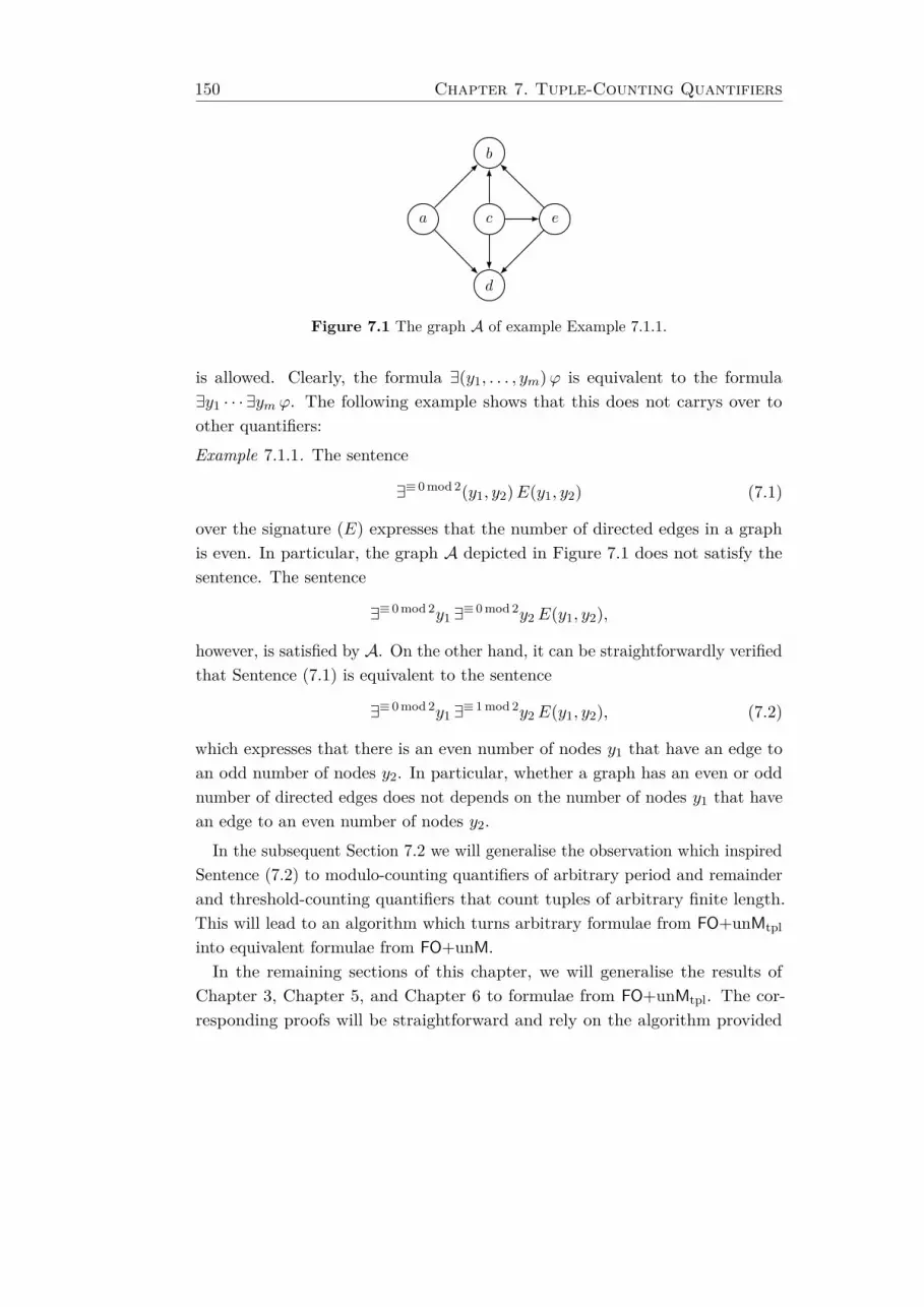
150 Chapter 7. Tuple-Counting Quantifiers
ca e
d
b
Figure 7.1 The graph A of example Example 7.1.1.
is allowed. Clearly, the formula ∃(y1, . . . , ym)ϕ is equivalent to the formula∃y1 · · · ∃ym ϕ. The following example shows that this does not carrys over toother quantifiers:
Example 7.1.1. The sentence
∃≡ 0 mod 2(y1, y2)E(y1, y2) (7.1)
over the signature (E) expresses that the number of directed edges in a graphis even. In particular, the graph A depicted in Figure 7.1 does not satisfy thesentence. The sentence
∃≡ 0 mod 2y1 ∃≡ 0 mod 2y2E(y1, y2),
however, is satisfied by A. On the other hand, it can be straightforwardly verifiedthat Sentence (7.1) is equivalent to the sentence
∃≡ 0 mod 2y1 ∃≡ 1 mod 2y2E(y1, y2), (7.2)
which expresses that there is an even number of nodes y1 that have an edge toan odd number of nodes y2. In particular, whether a graph has an even or oddnumber of directed edges does not depends on the number of nodes y1 that havean edge to an even number of nodes y2.
In the subsequent Section 7.2 we will generalise the observation which inspiredSentence (7.2) to modulo-counting quantifiers of arbitrary period and remainderand threshold-counting quantifiers that count tuples of arbitrary finite length.This will lead to an algorithm which turns arbitrary formulae from FO+unMtpl
into equivalent formulae from FO+unM.In the remaining sections of this chapter, we will generalise the results of
Chapter 3, Chapter 5, and Chapter 6 to formulae from FO+unMtpl. The cor-responding proofs will be straightforward and rely on the algorithm provided
7.2 Resolving Tuple-Counting Quantifiers 151
in Section 7.2 and the observation, that the transformation performed by thisalgorithm does not change the threshold or the periods of the quantifiers in thetransformed formula.
7.2 Resolving Tuple-Counting Quantifiers
In this section, it is shown how formulae from FO+unMtpl can be turned intoequivalent formulae from FO+unM, that is, into formulae whose quantifiers onlycount single elements of structures.
The main result of this section is stated in the following theorem. Its proof isbased on a construction described in [Str94, p. 164], which generalises the ideaused in Sentence (7.2).
Theorem 7.2.1. There is an algorithm which, on input of a formula ϕ(x) fromFO+unM(D)tpl[σ] with D ⊆ Dall and σ being a relational signature, computes aformula ψ(x) from FO+unM(D)[σ] that is equivalent to ϕ(x) and that has thesame threshold and quantifier rank as ϕ(x).
Furthermore, the algorithm computes ψ(x) in time
O(||ϕ||) · 2O(q)·(log maxT+1,P)2,
where T, P, q ≥ 0 are the threshold, the maximum period, and the quantifier rankof ϕ(x), respectively. In particular, the constants suppressed by the O-notationdo not depend on the signature σ.
The proof of Theorem 7.2.1 proceeds by an induction on the shape of the inputformula, which can be found at the end of this section. The crucial part of thisinduction is the handling of tuple-counting quantifiers, which is provided by thefollowing Lemma 7.2.2 and Lemma 7.2.3.
Lemma 7.2.2 describes the handling of modulo-counting quantifiers.
Lemma 7.2.2. Let σ be a relational signature, let D ⊆ Dall, and let m ≥ 2. Forevery formula
ϕ(x) := ∃≡ kmod py γ(x, y)
from FO+unM(D)tpl[σ], where p ≥ 2, k ∈ [0, p), y is a tuple of m pairwisedistinct variables, and γ(x, y) is a formula from FO+unM(D)[σ], there is aformula ψ(x) in FO+unM(D)tpl[σ] of dimension m−1 that is equivalent to ϕ(x).
152 Chapter 7. Tuple-Counting Quantifiers
The formula ψ(x) has the same threshold and the same quantifier rank as ϕ(x)and, moreover, ψ(x) is a Boolean combination of formulae of the shape
∃≡ jmod p(y1, . . . , ym−1) γ′(x, y1, . . . , ym−1) (7.3)
with j ∈ [0, p) and where γ′(x, y1, . . . , ym−1) is some formula from FO+unM(D)[σ].Furthermore, there is an algorithm that computes ψ(x) on input of ϕ(x) in
time||ϕ|| · 2O((log p)2),
where the constant suppressed by the O-notation does not depend on the signa-ture σ.
Lemma 7.2.2 describes the handling of threshold-counting quantifiers.
Lemma 7.2.3. Let σ be a relational signature, let D ⊆ Dall, and let m ≥ 2. Forevery formula
ϕ(x) := ∃>ky γ(x, y),
where k ≥ 1, y is a tuple of m pairwise distinct variables, and γ(x, y) is a formulafrom FO+unM(D)[σ], there is a formula ψ(x) in FO+unM(D)tpl[σ] of dimensionm− 1 that is equivalent to ϕ(x)The formula ψ(x) has the same threshold and the same quantifier rank as ϕ(x)
and, moreover, ψ(x) is a Boolean combination of formulae from FO+unM(D)[σ]and formulae of the shape
∃>j(y1, . . . , ym) γ′(x, y1, . . . , ym−1) (7.4)
with j ∈ [0, k] and γ′(x, y1, . . . , ym−1) a formula from FO+unM(D)[σ].Furthermore, there is an algorithm that computes ψ(x) on input of ϕ(x) in
time||ϕ|| · 2O((log(k+1))2),
where the constant suppressed by the O-notation does not depend on the signa-ture σ.
In the proofs of both lemmas, we generalise the idea of Sentence (7.2) inExample 7.1.1 to turn a formula of the shape
ϕ(x) := Qy γ(x, y),
where Q is either a modulo-counting quantifier ∃≡ kmod p or a threshold-countingquantifier ∃>k, where x, y are tuples of n ≥ 0 and m ≥ 2 pairwise distinct
7.2 Resolving Tuple-Counting Quantifiers 153
variables, respectively, and where γ(x, y) is a formula from FO+unM(D)[σ] for aset D ⊆ Dall, into an equivalent formula from FO+unM(D)tpl[σ] of dimensionm− 1. For each σ-structure A and every tuple a ∈ An, we let
Wϕ[A, a] := b ∈ Am : A |= γ[a, b],
denote the set of witnesses of the quantifier Q in respect to the interpretation(A, a) for ϕ(x). For each tuple b ∈ Am−1, we furthermore let
Wϕ[A, a, b] := b ∈ A : A |= γ[a, b, b].
Example 7.2.4. For the sentence ϕ from (7.1), we have n = 0. Thus, for thegraph A of Figure 7.1, we have Wϕ[A, (), c] = b, d, e.
Proof of Lemma 7.2.2. Let σ be a relational signature, let D ⊆ Dall, andlet m ≥ 2. Furthermore, let ϕ(x) := ∃≡ kmod py γ(x, y) be a formula fromFO+unM(D)tpl[σ] where p ≥ 2, k ∈ [0, p), |y| = m, and γ(x, y) is a formula fromFO+unM(D)[σ].
For each σ-structure A and every tuple a ∈ An, let
Wϕj [A, a] :=
b ∈ Am−1 : |Wϕ[A, a, b]| ≡ j mod p
for all j ∈ [1, p). Clearly, the sets Wϕ
j [A, a] for all j ∈ [1, p) are pairwise disjointand, moreover,
p−1∑j=1|Wϕ
j [A, a]| · j ≡ |Wϕ[A, a]| mod p. (1)
Example 7.2.5. Continuing Example 7.2.4, we have Wϕ0 [A, ()] = a, b, d, e and
Wϕ1 [A, ()] = c for the sentence ϕ from (7.1) and the graph A of Figure 7.1.In the following, we define for each i ∈ [0, p) and j ∈ [1, p) a formula δ≡imod p
j (x),such that for each σ-structure A and every a ∈ An,
A |= δ≡imod pj [a] iff |Wϕ
j [A, a]| · j ≡ i mod p. (2)
For each ` ∈ [0, p), we let
ε≡`mod pj (x) := ∃≡ `mod p(y1, . . . , ym−1) ∃≡ jmod pym γ(x, y).
154 Chapter 7. Tuple-Counting Quantifiers
Note that ε≡`mod pj (x) is of Shape (7.3) and of size O(||ϕ||).
We now let L be the set of all ` ∈ [0, p) such that ` ·j is congruent to i modulo p.If L is non-empty, we choose δ≡imod p
j (x) as the formula∨`∈L
ε≡`mod pj (x)
Note that in this case, δ≡imod pj (x) is a disjunction of formulae of Shape (7.3) of
size p · O(||ϕ||). Otherwise, that is, if L is the empty set, we let δ≡imod pj (x) be
the unsatisfiable formula
ε≡0 mod pj (x) ∧ ¬ε≡0 mod p
j (x)
which is a Boolean combination of formulae of Shape (7.3) of size O(||ϕ||).Now, ψ(x) could be chosen as the formula
∨f∈F
p−1∧j=1
δ≡f(j) mod pj (x) (3)
where F is the set of all functions f : [1, p)→ [0, p) such that
p−1∑j=1
f(j) ≡ k mod p.
To see this, consider a σ-structure A and a tuple a ∈ An. Suppose first thatA |= ϕ[a], that is, |Wϕ[A, a]| is congruent k modulo p. Thus, by Congruence (1),there is a function f ∈ F such that |Wϕ
j [A, a]| · j is congruent to f(j) foreach j ∈ [1, p). Hence, it follows from Equivalence (2) that (A, a) satisfiesFormula (3).
For the other direction, suppose that (A, a) satisfies Formula (3). Then, thereis a function f ∈ F such that |Wϕ
j [A, a]| · j is congruent to f(j) for each j ∈ [1, p)and thus, by definition of f and Congruence (1), |Wϕ[A, a]| is congruent kmodulo p. It follows, that A |= ϕ[a].
However, Formula (3) has size in pp−1 ·p ·O(||ϕ||) and thus grows exponentiallywith the period p. To obtain an equivalent formula that only grows polynomiallywith p, we use Lemma 2.9.2 and let
ψ(x) :=⟨δ≡imod pj
⟩≡ kmod p[1,p) (x).
Note that, in particular, ψ(x) is a Boolean combination of formulae δ≡imod pj (x)
with i ∈ [0, p) and j ∈ [1, p).
7.2 Resolving Tuple-Counting Quantifiers 155
Time complexity. For each i ∈ [0, p) and j ∈ [1, p), the formula δ≡imod pj (x) has
size in p · O(||ϕ||). Thus, by Lemma 2.9.2, the construction of ψ(x) takes time in
p · O(||ϕ||) · (2p)dlog pe+1 ⊆ ||ϕ|| · 2O((log p)2).
This completes the proof of Lemma 7.2.2.
Proof of Lemma 7.2.3. Let σ be a relational signature and let D ⊆ Dall. Letk ≥ 1, let y be a tuple of pairwise distinct variables of length m ≥ 2, and letϕ(x) := ∃>ky γ(x, y) with a formula γ(x, y) from FO+unM(D)[σ].We proceed in a similar fashion as in the proof of Lemma 7.2.2. For each
σ-structure A and every tuple a ∈ An, let
V ϕj [A, a] :=
b ∈ Am−1 : |Wϕ[A, a, b]| = j
for all j ∈ [1, k]. Clearly, the sets V ϕ
j [A, a] for all j ∈ [1, k] are pairwise disjointand |Wϕ[A, a] > k if and only if one of the two following conditions holds:
(I) there is a b ∈ Am−1 such that |Wϕ[A, a, b]| > k
(II)k∑j=1|V ϕj [A, a]| · j > k
Condition (I) can be expressed by the formula
ψI(x) := ∃y1 · · · ∃ym−1 ∃>kym γ(x, y).
In the following, we construct a formula ψII(x) that expresses Condition (II). Foreach i ∈ [0, k] and j ∈ [1, k], we let
δ>ij (x) := ∃>`(y1, . . . , ym−1) ∃=jym γ(x, y)
where ` ∈ [0, k] is chosen minimal such that (`+1) · j > i. Then, for eachσ-structure A and every a ∈ An,
A |= δ>ij [a] iff |V ϕj [A, a]| · j > i.
In a similar manner as in the proof of Lemma 7.2.2, one can verify that Condi-tion (II) is expressed by the formula∨
g∈G
∧j∈[1,k],g(j)≥0
δ>ij (x)
156 Chapter 7. Tuple-Counting Quantifiers
where G is the set of all functions g : [1, k]→ [−1, k] such that the sum of g(j)+1for all j ∈ [1, k] equals k+ 1. By Lemma 2.9.4, we can replace the latter formulaeby the equivalent formula
ψII(x) :=⟨δ>ij⟩>k
[1,k](x),
where⟨δ>ij⟩>k
[1,k](x) is a Boolean combination of formulae δ>ij (x) with i ∈ [0, k]and j ∈ [1, k].Altogether, we can choose
ψ(x) := ψI(x) ∨ ψII(x).
Time complexity. The formula ψI(x) as well as each formula δ>ij (x) for i ∈ [0, k]and j ∈ [1, k] has size in O(||ϕ||). Thus, by Lemma 2.9.4, the construction ofψ(x) takes time in
O(||ϕ||) +O(||ϕ||) · (2k+2)dlog ke+1 ⊆ ||ϕ|| · 2O((log(k+1))2).
This completes the proof of Lemma 7.2.3.
We are now ready to prove Theorem 7.2.1 by using Lemma 7.2.2 and Lemma 7.2.3.
Proof of Theorem 7.2.1. Let σ be a relational signature, let D ⊆ Dall, andlet ϕ(x) a formula from FO+unM(D)tpl[σ]. Furthermore, let T, P, q ≥ 0 denotethe threshold, the maximum period, and the quantifier rank of ϕ, respectively.
In the special case of a formula ϕ(x) from FOtpl[σ], we replace each subformulaof the shape ∃(y1, . . . , ym)ϕ′ with m ≥ 2 by the formula ∃y1 · · · ∃ym ϕ′. Thistakes altogether time in O(||ϕ||).
Observe that otherwise, T ≥ 1 or P ≥ 2. In this case, the algorithm proceedsby an induction over the shape of ϕ(x), where we show the following inductiveinvariant to hold for the constructed formula ψ(x) from FO+unM(D)[σ]:
Claim 1.
(a) ψ(x) is equivalent to ϕ(x).
(b) ψ(x) has the same threshold and quantifier rank as ϕ(x).
(c) There are numbers c, d ∈ N≥1 (whose size is independent of ||σ||), suchthat the algorithm terminates after at most
c · ||ϕ|| · 2d·q·(log maxT+1,P)2
time steps.
7.2 Resolving Tuple-Counting Quantifiers 157
If ϕ is a formula from FO+unM(D)[σ], there is nothing to do and we let ψ := ϕ.Clearly, Claim 1 is satisfied.
Suppose that ϕ(x) is a Boolean combination of formulae from FO+unM(D)tpl[σ].If ϕ = ¬ϕ′, the algorithm computes a suitable formula ψ′ from FO+unM(D)[σ]for ϕ′ and outputs ψ := ¬ψ′. If ϕ = (ϕ′∨ϕ′′), the algorithm computes formulae ψ′
and ψ′′ from FO+unM(D)[σ] for ϕ′ and ϕ′′, respectively, and outputs the formulaψ := (ψ′ ∨ ψ′′). It is straightforward to verify that Claim 1 is satisfied.
Suppose that ϕ(x) has the shape Qy ϕ′(x, y). Let m := |y| and recall that ϕ′ hasquantifier rank q −m.
In a first step, the algorithm computes a formula ψ′(x, y) from FO+unM(D)[σ]for ϕ′(x, y), such that the following holds:
(a’) ψ′(x) is equivalent to ϕ′(x).
(b’) ψ′(x) has the same threshold and quantifier rank as ϕ′(x).
(c’) The algorithm took at most
c · ||ϕ′|| · 2d·(q−m)·(log maxT+1,P)2 (1)
time steps to construct ψ′(x) from ϕ′(x).
If m = 1, that is, y is a single variable y, then ψ(y) can be chosen as Qy ψ′(x, y).For the following, we suppose that m ≥ 2 and perform a case distinction by theshape of the quantifier Q.
(Case 1) If Q = ∃≡ kmod p for a period p ∈ [2, P ] and k ∈ [0, p), the formula ψ(x)is constructed by applying the algorithm of Lemma 7.2.2 to the formula∃≡ kmod py ψ′(x, y) and then to all subformulae of the resulting formulaof Shape (7.3). This process has to be repeated m − 1 times, untila formula ψ(x) from FO+unM(D)[σ] is reached that is equivalent toϕ(x) and has the same threshold and quantifier rank.
Thus, it follows from Lemma 7.2.2, that a constant d ∈ N≥1 can bechosen such that this process takes at most
||ψ′|| · 2d·(m−1)·(log p)2 ≤ ||ψ′|| · 2d·(m−1)·(logP )2
time steps.
(Case 2) If Q = ∃>0 = ∃, the algorithm outputs ψ(x) := ∃y1 · · · ∃ym ψ′(x, y),where (y1, . . . , ym) = y.
158 Chapter 7. Tuple-Counting Quantifiers
(Case 3) If Q = ∃>k for some k ∈ [1, T ], the formula ψ(x) is constructed byapplying the algorithm of Lemma 7.2.3 to the formula ∃>ky ψ′ andthen to all subformulae of the resulting formula of Shape (7.4). Thisprocess has to be repeated m − 1 times, until a formula ψ(x) fromFO+unM(D)[σ] is reached that is equivalent to ϕ(x) and has the samethreshold and quantifier rank.
By Lemma 7.2.3, the constant d ∈ N≥1 can be chosen such that thistakes at most
||ψ′|| · 2d·(m−1)·(log(k+1))2 ≤ ||ψ′|| · 2d·(m−1)·(log(T+1))2
time steps.
We have already seen that the constructed formula ψ(x) satisfies Statement (a)and Statement (b) of Claim 1.
For Statement (c), note that Estimate (1) is also an upper bound on the sizeof ψ′(x). Thus, ψ(x) can be constructed in time
2d·(m−1)·(log maxT+1,P)2 · c · ||ϕ′|| · 2d·(q−m)·(log maxT+1,P)2
≤ c · ||ϕ|| · 2d·q·(log maxT+1,P)2.
This completes the inductive construction of ψ(x) which, by Statement (c) ofClaim 1, altogether takes time in
O(||ϕ||) · 2O(q)·(log maxT+1,P)2.
Thus, the proof of Theorem 7.2.1 is completed.
7.3 Hanf Normal Form
In this section, we use the construction of the previous section to extend theresults of Chapter 3 from the logic FO+unM to FO+unMtpl. The proofs arestraightforward combinations of Theorem 7.2.1 and the corresponding theoremin Chapter 3.
7.3.1 Constructing Hanf Normal Form
This section generalises Theorem 3.2.1 to input formulae from FO+unMtpl, whichcan be stated as follows.
7.3 Hanf Normal Form 159
Theorem 7.3.1. There is an algorithm which, on input of
• a degree bound d ≥ 2,
• a relational signature σ, and
• a formula ϕ(x) from FO+unM(D)tpl[σ], for a set D ⊆ Dall,
computes a hnf-formula ψ(x) from FO+unM(D)[σ] that is d-equivalent to ϕ(x).Let T, P, n, q ≥ 0 be the threshold, the maximum period, the number of free
variables, and the quantifier rank of ϕ(x), respectively.Then, the computed formula ψ(x) has locality radius ≤ 4q and threshold
< T + (n+q) · νd(4q).
Moreover, the algorithm constructs ψ(x) in time
2(||ϕ||·2q·(log maxT+1,P)2 ·νd(4q)
)O(||σ||)
.
Remark 7.3.2. In particular, the upper bounds on the locality radius and thethreshold of the computed hnf-formula do not change in the generalisation ofTheorem 3.2.1 from FO+unM to FO+unMtpl.
Furthermore, under the assumption that ||σ|| < ||ϕ||, the algorithm also takes3-fold exponential time in the size of ϕ(x) for d ≥ 3, and 2-fold exponential timein the size of ϕ(x) for d = 2, since T, P, q < ||ϕ||.
Proof of Theorem 7.3.1. Let σ be a relational signature, let D ⊆ Dall, and letϕ(x) be a formula from FO+unM(D)tpl[σ]. Furthermore, let d ≥ 2 be a degreebound.
The algorithm proceeds in the following two steps:
(Step 1) The algorithm described in the proof of Theorem 7.2.1 constructs aformula ϕ(x) from FO+unM(D)[σ] that is equivalent to ϕ(x). Thistakes time in
O(||ϕ||) · 2O(q)·(log maxT+1,P)2, (1)
where T, P, q ≥ 0 are the threshold, the maximum period, and thequantifier rank of ϕ(x) and, by Theorem 7.2.1, in particular also thethreshold, maximum period, and quantifier rank of ϕ(x).
160 Chapter 7. Tuple-Counting Quantifiers
(Step 2) The algorithm of Theorem 3.2.1 computes, on input of d, σ, and ϕ(x),a hnf-formula ψ(x) from FO+unM(D)[σ] that is d-equivalent to ϕ(x)and thus also to ϕ(x). By Theorem 3.2.1, ψ(x) has locality radius ≤ 4q
and threshold < T + (n+q) · νd(4q), where n ≥ 0 is the number of freevariables of ϕ(x).
The construction of ψ(x) from ϕ(x) takes time in
(2 max1, T, P)(||ϕ||·νd(4q))O(||σ||). (2)
Combining Estimate (1), which also serves as an upper bound on the size of ϕ(x),with Estimate (2), we obtain that the algorithm can altogether runs in time
(2 max1, T, P)(O(||ϕ||)·2O(q)·(log maxT+1,P)2 ·νd(4q)
)O(||σ||)
⊆ 2(||ϕ||·2q·(log maxT+1,P)2 ·νd(4q)
)O(||σ||)
.
This completes the proof of Theorem 7.3.1.
7.3.2 Nurmonen’s Theorem for Tuple-Counting Quantifiers
In the following, we show that the locality theorem for FO+unM, that is, The-orem 3.3.1, also holds for formulae from FO+unMtpl. In particular, no modific-ations to the preconditions are required. The proof follows directly from theobservation that when transforming from FO+unMtpl to FO+unM, the quantifierrank, the threshold, and the period of the modulo-counting quantifiers in theformulae do not change.
Theorem 7.3.3. Let σ be a relational signature and let d ≥ 2 be a degree bound.Furthermore, let T, n, q ≥ 0, and M ≥ 1.
Suppose that A and B are d-bounded σ-structures and a ∈ An, b ∈ Bn, suchthat the following Conditions (1) to (3) are satisfied for r := 4q:
(1) NAr (a) ∼= NBr (b).
For every type τ ∈ Td,σr (1),
(2) |τ(A)| ≡ |τ(B)| mod M , and
(3) either |τ(A)| = |τ(B)| or
|τ(A)|, |τ(B)| ≥ T + (n+q) · νd(r).

7.3 Hanf Normal Form 161
Then, for every formula ϕ(x) from FO+unMtpl[σ] with threshold ≤ T , quantifierrank ≤ q, at most n free variables x, and such that M is a common multiple ofthe periods of all modulo-counting quantifiers that occur in ϕ(x),
A |= ϕ[a] iff B |= ϕ[b].
Proof. Let σ be a relational signature and let d ≥ 2 be a degree bound. Fur-thermore, let T, n, q ≥ 0, and M ≥ 1. Suppose that A and B are d-boundedσ-structures and a ∈ An, b ∈ Bn, such that Conditions (1) to (3) of Theorem 7.3.3are satisfied.Consider a formula ϕ(x) from FO+unMtpl[σ] with threshold ≤ T , quantifier
rank ≤ q, and a tuple x of at most n free variables, and such that M is a commonmultiple of the periods of all modulo-counting quantifiers occurring in ϕ(x).By Theorem 7.2.1, ϕ(x) is equivalent to a formula ϕ(x) from FO+unM[σ],
which also has threshold ≤ T , quantifier rank ≤ q, at most n free variables,and where M is also a common multiple of the periods of all modulo-countingquantifiers occurring in the formula. In particular, we know by Theorem 3.3.1that
A |= ϕ[a] iff B |= ϕ[b].
Thus, since ϕ(x) and ϕ(x) are equivalent, also
A |= ϕ[a] iff B |= ϕ[b].
This completes the proof of Theorem 7.3.3.
7.3.3 Model-Checking
We conclude the section with a generalisation of the model-checking algorithmfor FO+unM from Theorem 3.4.1 to formulae from FO+unMtpl.
Theorem 7.3.4. There is an algorithm which, on input of
• a formula ϕ(x) from FO+unMtpl, where the tuple x consists of the n ≥ 0free variables of ϕ,
• a finite σ-structure A (where σ consists of precisely the relation symbolsthat occur in ϕ), and a tuple a ∈ An,
decides whether A |= ϕ[a].
162 Chapter 7. Tuple-Counting Quantifiers
This algorithm takes time in
2(||ϕ||·2q·(log maxT+1,P)2 ·νd(4q)
)O(||σ||)
· ||A||
where T, P, q ≥ 0 are the threshold, the maximum period, and the quantifier rankof ϕ(x), respectively, and where d ≥ 2 is a bound on the degree of A.
Remark 7.3.5. Since T, P, q, ||σ|| < ||ϕ||, the algorithm of Theorem 3.4.1 takes 3-fold exponential time in the size of ϕ(x) for every σ-structure A with degree d ≥ 3,and 2-fold exponential time for every σ-structure A with degree d ≤ 2 (andindependent of that, linear time in the size of A).
Proof of Theorem 7.3.4. Let ϕ(x) be a formula from FO+unMtpl[σ] whose n ≥ 0free variables are described by the tuple x and where σ consists of preciselythe relation symbols that occur in ϕ(x). Furthermore, let A be a σ-structureand a ∈ An.
The algorithm proceeds in the following two steps:
(Step 1) The algorithm of Theorem 7.2.1 constructs for ϕ(x) an equivalentformula ϕ(x) from FO+unM[σ]. This takes time in
O(||ϕ||) · 2O(q)·(log maxT+1,P)2, (1)
where T, P, q ≥ 0 are the threshold, the maximum period, and thequantifier rank of ϕ(x) and, by Theorem 7.2.1, also the threshold, themaximum period, and the quantifier rank of ϕ(x).
(Step 2) The algorithm of Theorem 3.4.1 decides, on input of ϕ(x), A, and a,whether A |= ϕ[a]. This takes time in
(2 max1, T, P)(||ϕ||·νd(4q))O(||σ||) · ||A||, (2)
where d ≥ 2 is an upper bound on the degree of A.
Since Estimate (1) is also an upper bound on the size of ϕ(x), we obtain togetherwith Estimate (2), that to decide whether A |= ϕ[a] takes time in
(2 max1, T, P)(O(||ϕ||)·2O(q)·(log maxT+1,P)2 ·νd(4q)
)O(||σ||)
· ||A||
⊆ 2(||ϕ||·2q·(log maxT+1,P)2 ·νd(4q)
)O(||σ||)
· ||A||.
This completes the proof of Theorem 7.3.4.

7.4 Feferman-Vaught Decompositions 163
7.4 Feferman-Vaught Decompositions
In this section, we apply the transformation of formulae from FO+unMtpl intoequivalent formulae from FO+unM, described in Section 7.2, to Feferman-Vaughtdecompositions.
The construction of Hanf normal form for FO+unMtpl, described in the previoussection, leads to an algorithm to compute ⊕-decompositions for FO+unMtpl onclasses of structures of bounded degree.Recall that, in Chapter 5, we could construct decompositions with respect
to transductions and direct products only for plain FO-formulae. This wasdue to the tuple-counting quantifiers introduced by computing reducts for suit-able transductions. In the present section, we can get rid of this restrictionand finally compute such decompositions for arbitrary formulae from FO+unMand FO+unMtpl.
7.4.1 Decompositions with respect to Disjoint Sums
In this section, we generalise the algorithm of Theorem 5.2.1 to formulae fromFO+unMtpl. More precisely, we show the following result:
Theorem 7.4.1. There is an algorithm which, on input of
• a degree bound d ≥ 2,
• a relational signature σ,
• an arity s ≥ 1, and
• a formula ϕ(x) from FO+unMtpl(D)[σs] with D ⊆ Dall, n := |x| freevariables, threshold T ≥ 0, and quantifier rank q ≥ 0,
computes an s-ary ⊕-decomposition (β,∆1, . . . ,∆s) for ϕ(x) over FO+unM(D)[σ]on Cd,σ, where all formulae in the sets ∆1, . . . ,∆s are hnf-formulae with threshold< T + (n+q) · νd(4q).Furthermore, the algorithm computes ∆ in time
2(||ϕ||·2q·(log maxT+1,P)2 ·νd(4q)
)O(||σs||)
where P ≥ 0 is the maximum period of ϕ(x).
164 Chapter 7. Tuple-Counting Quantifiers
Remark 7.4.2. Suppose that σ only contains relation symbols that actuallyoccur in ϕ(x) and recall that T, P, q < ||ϕ||. Then, the algorithm takes 3-foldexponential time
2ds·2O(||ϕ||)
in the size of the input formula for d = 3, and, for d = 2, 2-fold exponential time
22s·poly(||ϕ||).
Recall that the algorithm of Theorem 5.2.1 first transformed the input formulainto a d-equivalent hnf-formula from FO+unM, whose counting-sentences andsphere-formulae subsequently got decomposed separately. For the proof ofTheorem 7.4.1, we just have to replace the first step for the construction ofhnf-formulae by the corresponding algorithm of Theorem 7.3.1 for formulae fromFO+unMtpl.
Proof of Theorem 7.4.1. We describe the algorithm on input of a degree boundd ≥ 2, a relational signature σ, a number s ≥ 1, and a formula ϕ(x) fromFO+unM(D)tpl[σs] with D ⊆ Dall. Let T, P, q ≥ 0 be the threshold, the max-imum period, and the quantifier rank of ϕ(x), respectively, and let n := |x| bethe number of free variables of ϕ(x).
(Step 1) The algorithm of Theorem 7.3.1 constructs, on input of d, σs, and ϕ(x),a hnf-formula ψ(x) from FO+unM(D)[σs] that is d-equivalent to ϕ(x)and that has threshold < T + (n+q) · νd(4q). This takes time in
2(||ϕ||·2q·(log maxT+1,P)2 ·νd(4q)
)O(||σs||)
. (1)
(Step 2) On input of s and ψ(x), the algorithm of Lemma 5.2.3 computes an s-ary⊕-decomposition ∆ = (β,∆1, . . . ,∆s) for ψ(x) over FO+unM(D)[σ] onthe class of all σ-structures where all formulae in the sets ∆1, . . . ,∆s
are hnf-formulae with threshold < T + (n+q) · νd(4q).This takes time in s · O(||ψ||). Since the size of ψ(x) is bounded
by the time required for its construction, this can also be bounded byEstimate (1).
Clearly, ∆ is also an s-ary ⊕-decomposition for ϕ(x) on Cd,σ, and the timerequired by the algorithm to construct ∆ can be bounded by Estimate (1). Thiscompletes the proof of Theorem 7.4.1.

7.4 Feferman-Vaught Decompositions 165
Note that an alternative proof of Theorem 7.4.1 that uses the algorithms ofTheorem 7.2.1 and Theorem 5.2.1 as intermediate steps leads to the same timecomplexity.
7.4.2 Decompositions with respect to Transductions
The result of this section enables us to compute decompositions defined bytransductions on disjoint sums for formulae from FO+unMtpl, thus extendingthe corresponding results for the special case of FO from Chapter 5. It can bestated as follows:
Theorem 7.4.3. There is an algorithm which, on input of
• a degree bound d ≥ 2,
• relational signatures σ and τ ,
• an arity s ≥ 1,
• a transduction Θ from σs to τ with arity t ≥ 1 and quantifier rank qΘ ≥ 0,and
• a formula ϕ(x) from FO+unM(D)tpl[τ ] with D ⊆ Dall, n := |x| free vari-ables, threshold T ≥ 0, and quantifier rank q ≥ 0,
computes a Θ-decomposition ∆ = (β,∆1, . . . ,∆s) over FO+unM(D)[σ] for ϕ(x)on Cd,σ, where all the formulae in the sets ∆1, . . . ,∆s are hnf-formulae withthreshold < T + (t · (n+ q) + qΘ) · νd(4t·q+qΘ)
Furthermore, the algorithm computes ∆ in time
||Θ|| · O(||τ ||) + 2(||Θ||·||ϕ||·2(t·q+qΘ)·(log maxT+1,P)2 ·νd(4t·q+qΘ )
)O(||σs||)
and of size
2(||Θ||·||ϕ||·2(t·q+qΘ)·(log maxT+1,P)2 ·νd(4t·q+qΘ )
)O(||σs||)
where P ≥ 0 is the maximum period of ϕ(x).
Remark 7.4.4. Clearly, T, P, q < ||ϕ|| and qΘ < ||Θ||. Under the assumption thatfurthermore ||σ|| ≤ ||ϕ|| and t < ||Θ||, we can conclude that for every degreebound d ≥ 3, the algorithm of Theorem 7.4.3 takes time in
||Θ|| · O(||τ ||) + 2ds·2||Θ||·O(||ϕ||)
.
166 Chapter 7. Tuple-Counting Quantifiers
Moreover, for degree bound d = 2, the algorithm takes time in
||Θ|| · O(||τ ||) + 22s·||Θ||·poly(||ϕ||).
Proof. Let d ≥ 2 be a degree bound, let σ and τ be relational signatures, and lets ≥ 1. Furthermore, let Θ be a transduction from σs to τ with arity t ≥ 1 andquantifier rank qΘ ≥ 0. Moreover, let ϕ(x) be a formula from FO+unM(D)tpl[σ]with D ⊆ Dall, the n ≥ 0 free variables x = (x1, . . . , xn), threshold T ≥ 0, andquantifier rank q ≥ 0. For all i ∈ [1, n], let xi = (xi,1, . . . , xi,t).The algorithm proceeds in the two following steps:
(Step 1) The algorithm of Lemma 2.6.4 computes a Θ-reduct ϕ−Θ(x1, . . . , xt) forϕ(x) from FO+unM(D)tpl[σs] that has quantifier rank ≤ t · q+ qΘ, n · tfree variables, and the same threshold and maximum period as ϕ(x).This takes time in
||Θ|| · O(||τ ||) + ||Θ|| · O(||ϕ||),
and Θ−1(ϕ)(x1, . . . , xt) has size in ||Θ|| · O(||ϕ||).
(Step 2) The algorithm of Theorem 7.4.1 computes, on input of d, σ, s, andϕ−Θ(x1, . . . , xt), an s-ary ⊕-decomposition ∆ = (β,∆1, . . . ,∆s) forϕ−Θ(x1, . . . , xt) over FO+unM(D)[σ] on Cd,σ, where the sets ∆1, . . . ,∆s
only contain hnf-formulae with threshold less than T + (t · (n+ q) +qΘ) · νd(4t·q+qΘ). This takes time in
2(||Θ||·||ϕ||·2(t·q+qΘ)·(log maxT+1,P)2 ·νd(4t·q+qΘ )
)O(||σs||)
,
where P ≥ 0 is the maximum period of ϕ(x). Note that the latterestimate also bounds the size of ∆.
By Lemma 5.3.2, we know that ∆ is also a Θ-decomposition for ϕ(x) overFO+unM(D)[σ] on the class of d-bounded σ-structures.
Altogether, the algorithm takes time in
||Θ|| · O(||τ ||) + 2(||Θ||·||ϕ||·2(t·q+qΘ)·(log maxT+1,P)2 ·νd(4t·q+qΘ )
)O(||σs||)
to compute ∆. This completes the proof of Theorem 7.4.3.
7.4 Feferman-Vaught Decompositions 167
7.4.3 Decompositions with respect to Direct Products
We conclude Section 7.4 by an application of Theorem 7.4.3, which provides uswith an algorithm to compute ⊗-decompositions for FO+unMtpl on classes ofstructures of bounded degree. More precisely, we show the following:
Theorem 7.4.5. There is an algorithm which, on input of
• a degree bound d ≥ 2,
• a relational signature σ,
• an arity s ≥ 1, and
• a formula ϕ(x) from FO+unM(D)tpl[σs] with D ⊆ Dall, n := |x| freevariables, threshold T ≥ 0, and quantifier rank q ≥ 0,
computes an s-ary ⊗-decomposition (β,∆1, . . . ,∆s) for ϕ(x) over FO+unM(D)[σ]on Cd,σ, where all formulae in the sets ∆1, . . . ,∆s are hnf-formulae with threshold< T + s · (n+q) · νd(4s·q).Furthermore, the algorithm computes ∆ in time
2(||ϕ||·2q·(log maxT+1,P)2 ·νd(4s·q)
)O(||σs||·log ||σs||)
where P ≥ 0 is the maximum period of ϕ.
Remark 7.4.6. Clearly, T, P, q < ||ϕ||. Under the assumption that furthermore||σ|| < ||ϕ||, we can conclude that for every degree bound d ≥ 3, the algorithmof Theorem 7.4.5 takes time in
2d2s·O(||ϕ||).
Moreover, for degree bound d = 2, the algorithm takes time in
22s·poly(||ϕ||).
Proof. Let d ≥ 2, let σ be a relational signature, and let s ≥ 1. Furthermore,let ϕ(x) be a formula from FO+unM(D)tpl[σs] with D ⊆ Dall, threshold T ≥ 0,and quantifier rank q ≥ 0.On input of d, the signatures σs and σ, the transduction Θδ
s, defined inSection 5.4, and the formula ϕ(x), the algorithm of Theorem 7.4.3 computesa Θσ
s -decomposition ∆ = (β,∆1, . . . ,∆s) over FO+unM(D)[σ] for ϕ(x) on Cd,σ
168 Chapter 7. Tuple-Counting Quantifiers
where all formulae in the sets ∆1, . . . ,∆s are hnf-formulae with threshold< T + s · (n+ q) · νd(4s·q).By Lemma 5.4.2, we know that ∆ is also ⊗-decomposition for ϕ(x) over
FO+unM(D)[σ] on Cd,σ.
Time complexity. The transduction Θσs is of quantifier rank 0 and can be computed
in time s · O(||σ||). Therefore, the call of the algorithm of Theorem 7.4.3 needstime in
s · O(||σ||)2 + 2(s·||σ||·||ϕ||·2s·q·(log maxT+1,P)2 ·νd(4s·q)
)O(||σs||)
⊆ 2(||ϕ||·2q·(log maxT+1,P)2 ·νd(4s·q)
)O(||σs||·log ||σs||)
,
where P ≥ 0 is the maximum period of ϕ. This completes the proof of The-orem 7.4.5.
7.5 Preservation Theorems
In Chapter 6, we have shown how formulae from FO+unM that are preservedunder extensions (homomorphisms) on a class of structures of bounded degree thatis closed under disjoint unions and induced substructures (and, for preservationunder homomorphisms, decidable in 1-fold exponential time) can be turned intoexistential (existential-positive) formulae in elementary time.
In this section, we generalise these results from the logic FO+unM to FO+unMtpl.
7.5.1 Preservation under Extensions
In this section, we show the following generalisation of Theorem 6.1.7:
Theorem 7.5.1. There is an algorithm which, on input of
• a degree bound d ≥ 2,
• a relational signature σ, and
• a formula ϕ(x) from FO+unMtpl[σ],
constructs an existential formula ψ(x) from FO[σ] such that the following holdsfor any class D of d-bounded σ-structures that is closed under disjoint unionsand induced substructures: If ϕ(x) is preserved under extensions on D, then ϕ(x)and ψ(x) are D-equivalent.

7.5 Preservation Theorems 169
Furthermore, the algorithm computes ψ(x) in time
||ϕ|| ·(2νd(2νd(4q)O(||σ||) ) · (T+n+q) · L
)(n+q)·O((log max1,T,P)2),
where T, P, n, q ≥ 0 and L ≥ 1 are the threshold, the maximum period, thenumber of free variables, the quantifier rank, and the least common multiple ofthe periods of all modulo-counting quantifiers in ϕ(x), respectively. In particular,the constants suppressed by the O-notation do not depend on the signature σ.
Remark 7.5.2. In particular, if we assume that σ only contains relation symbolsthat actually occur in ϕ(x), then the algorithm of Theorem 7.5.1 takes 5-fold ex-ponential time in the size of ϕ(x) for degree bounds d ≥ 3, and 3-fold exponentialtime for d = 2.
The main tasks of the proof of Theorem 7.5.1 are, analogous to the proof ofTheorem 6.1.7, an upper bound on the size of minimal models for the inputformula, and the construction of an existential formula using this upper bound.We first focus on these tasks and prove Theorem 7.5.1 afterwards.
For the first task, it turns out that the upper bound on the size of minimalmodels, stated in Theorem 6.2.1 for formulae from FO+unM, also holds forformulae from FO+unMtpl. This is due to the fact that, by Theorem 7.2.1, eachformula from FO+unMtpl is equivalent to a formula from FO+unM over the samesignature, with the same threshold and quantifier rank, and with modulo-countingquantifiers of the same periods. Another way to see this is to just replace theuse of Theorem 3.3.1 in the proof of Theorem 6.2.1 by Theorem 7.3.3.
In the following corresponding corollary to Theorem 6.2.1, we use the expressionSd,s(r) := 2νd(r)O(s) as introduced in Chapter 6.
Corollary 7.5.3. There is a function
Nd,||σ||(T, n, q, L) ∈ Sd,||σ||(Sd,||σ||(4q)) · (T+n+q) · L,
such that the following holds for every relational signature σ, every degree boundd ≥ 2, every class D of d-bounded σ-structures that is closed under disjointunions and induced substructures, and every formula ϕ(x) from FO+unMtpl[σ]:
If ϕ(x) is preserved under extensions on D, then every D-minimal model ofϕ(x) has a universe of size at most Nd,||σ||(T, n, q, L), where T, n, q ≥ 0 are thethreshold, the number of free variables, and the quantifier rank of ϕ(x), andwhere L ≥ 1 is the least common multiple of the periods of all modulo-countingquantifiers that appear in ϕ(x).
170 Chapter 7. Tuple-Counting Quantifiers
Proof. Let σ be a relational signature, let d ≥ 2, and let D be a class of d-boundedσ-structures that is closed under disjoint unions and induced substructures.
Furthermore, let ϕ(x) be a formula from FO+unMtpl[σ] that is preserved underextensions on D. Let D ⊆ Dall be the set of all modulo-counting quantifiers thatoccur in ϕ, let T, q ≥ 0 be the threshold and the quantifier rank of ϕ, let n := |x|be the number of free variables of ϕ(x), and let L ≥ 1 be the least commonmultiple of the periods of all modulo-counting quantifiers in the set D.
By Theorem 7.2.1, there is a formula ϕ(x), equivalent to ϕ(x), in FO+unM(D)[σ]that has the same threshold T , the same quantifier rank q, and the same numberof free variables as ϕ(x), and where L is also the least common multiple of theperiods of all modulo-counting quantifiers appearing in ϕ(x).
LetN := Nd,||σ||(T, n, q, L) be the upper bound on the size ofD-minimal modelsof ϕ(x), provided by Theorem 6.2.1. Since ϕ(x) and ϕ(x) are equivalent, N isalso an upper bound on the size of the D-minimal models of ϕ(x).
This completes the proof of Corollary 7.5.3.
The following corollary extends Lemma 6.2.2 from FO+unM to FO+unMtpl.
Corollary 7.5.4. There is an algorithm which, on input of
• a number N ≥ 1 and
• a formula ϕ(x) from FO+unMtpl[σ] over a relational signature σ whosen ≥ 0 free variables are the variables of the tuple x,
constructs an existential formula ψ(x) from FO[σ] such that the following holdsfor every class C of σ-structures that is closed under induced substructures:If ϕ(x) is preserved under extensions on C and every C-minimal model of ϕ(x)
has a universe of size ≤ N , then ψ(x) is C-equivalent to ϕ(x).Furthermore, the algorithm constructs ψ(x) in time
O(||ϕ||) · 2(n+q)·(log maxT+1,P)2·O(logN),
where T, P, q ≥ 0 are the threshold, the maximum period, and the quantifier rankof ϕ(x), respectively. The constant suppressed by the O-notation does not dependon the signature σ.
Proof. Let σ be a relational signature, let N ≥ 1, and let ϕ(x) be a formulafrom FO+unMtpl[σ] with n := |x| free variables. Let D ⊆ Dall be the set of allmodulo-counting quantifiers in ϕ(x), and let T, P, q ≥ 0 be the threshold, themaximum period, and the quantifier rank of ϕ(x), respectively.
7.5 Preservation Theorems 171
(Step 1) By Theorem 7.2.1, a formula ϕ(x) from FO+unM(D)[σ] that is equi-valent to ϕ(x) and that has the same threshold and quantifier rankas ϕ(x) can be computed in time
O(||ϕ||) · 2O(q)·(log maxT+1,P)2. (1)
and of size bounded by the same expression.
(Step 2) The algorithm of Lemma 6.2.2 computes, on input of N and ϕ(x), anexistential formula ϕN (x) from FO[σ] such that the following holds forevery class C of σ-structures that is closed under induced substructures:
If ϕ(x) (and thus, ϕ(x)) is preserved under extensions on C and everyC-minimal model of ϕ(x) (and thus, of ϕ(x)) has a universe of size ≤ N ,then ϕN (x) is C-equivalent to ϕ(x) and ϕ(x).This takes time in
||ϕ|| · (2 max1, T, P)(n+q)·O(logN). (2)
Putting Estimate (1) and Estimate (2) together, we obtain that the constructionof ϕN (x) altogether takes time in
O(||ϕ||) · 2(n+q)·(log maxT+1,P)2·O(logN).
This completes the proof of Corollary 7.5.4.
We are now ready to prove Theorem 7.5.1 by using Corollary 7.5.3 and Corol-lary 7.5.4. The proof has the same overall shape as the proof of Theorem 6.1.7.
Proof of Theorem 7.5.1. Let d ≥ 2 be a degree bound, let σ be a relationalsignature, and let ϕ(x) be an FO+unMtpl[σ]-formula with n := |x| free variables,threshold T ≥ 0, maximum period P ≥ 0, and quantifier rank q ≥ 0. Furthermore,let L ≥ 1 be the least common multiple of the periods of all modulo-countingquantifiers occurring in ϕ(x).
Let D be a class of d-bounded σ-structures that is closed under disjoint unionsand induced substructures and suppose that ϕ(x) is preserved under extensionson D.The algorithm proceeds in the following two steps:
(Step 1) Compute the upper bound
N := Nd,||σ||(T, n, q, L)∈ Sd,||σ||(Sd,||σ||(4q)) · (T+n+q) · L (1)
172 Chapter 7. Tuple-Counting Quantifiers
on the size of D-minimal models of ϕ(x), obtained from Corollary 7.5.3.In particular, we can assume that N ≥ 2.
(Step 2) The algorithm of Corollary 7.5.4 constructs an existential formula ψ(x)from FO[σ] that is D-equivalent to ϕ(x). This takes time in
O(||ϕ||) · 2(n+q)·(log maxT+1,P)2·O(logN)
⊆ ||ϕ|| ·N (n+q)·O((log max1,T,P)2).
Thus, by replacing N in the latter estimate with Estimate (1) and recalling thedefinition of S·,·(·), we obtain that ψ(x) can altogether be computed in time
||ϕ|| ·(2νd(2νd(4q)O(||σ||) ) · (T+n+q) · L
)(n+q)·O((log max1,T,P)2).
This completes the proof of Theorem 6.1.7.
7.5.2 Preservation under Homomorphisms
In this section, we show the following generalisation of Theorem 6.1.10:
Theorem 7.5.5. Let C′ a class of structures that is decidable in time t(n) forsome function t : N≥1 → N≥1 and that is closed under disjoint unions and inducedsubstructures.
There is an algorithm which, on input of
• a degree bound d ≥ 2,
• a relational signature σ, and
• a formula ϕ(x) from FO+unMtpl[σ],
constructs an existential-positive formula ψ(x) from FO[σ] such that the followingholds for the class D of d-bounded σ-structures from C′: If ϕ(x) is preservedunder homomorphisms on D, then ϕ(x) and ψ(x) are D-equivalent.
Furthermore, the algorithm computes ψ(x) in time
2||ϕ||·(n+1)O(||σ||)·2νd(2·4q)O(||σ||)· t((n+1)O(||σ||) · 2νd(2·4q)O(||σ||)),
where n, q ≥ 0 are the number of free variables and the quantifier rank of ϕ(x),respectively; and the formula ψ(x) is of size
2(n+1)O(||σ||)·2νd(2·4q)O(||σ||).
7.5 Preservation Theorems 173
Remark 7.5.6. In particular, if t : N≥1 → N≥1 is at most 1-fold exponential and ifwe assume that σ only contains relation symbols that actually occur in the inputformula ϕ, then the algorithm of Theorem 7.5.5 takes 4-fold exponential time inthe size of ϕ(x) for degree bounds d ≥ 3, and 3-fold exponential time for d = 2.
The proof of Theorem 7.5.5 has the same structure as the one of Theorem 6.1.10.In the first step, we find upper bounds on the size of the minimal models offormulae from FO+unMtpl. It turns out that these upper bounds are preciselythe same as the ones for formulae from FO+unM stated in Theorem 6.3.1. In thesecond step, we use Lemma 6.3.2 again to construct existential-positive formulaeusing this upper bound.
Corollary 7.5.7. There is a function
Nd,||σ||(n, q) ∈ (n+1) · Sd,||σ||(2 · 4q)
such that the following holds for every relational signature σ, every degree boundd ≥ 2, every class D of d-bounded σ-structures that is closed under disjointunions and induced substructures, and every formula ϕ(x) from FO+unMtpl[σ]:
If ϕ(x) is preserved under homomorphisms on D, then every D-minimal modelof ϕ(x) has a universe of size at most Nd,||σ||(n, q), where n, q ≥ 0 are the numberof free variables and the quantifier rank of ϕ, respectively.
Proof. Let σ be a relational signature, let d ≥ 2 be a degree bound, and let Dbe a class of d-bounded σ-structures that is closed under disjoint unions andinduced substructures.Let ϕ(x) be a formula from FO+unMtpl[σ] with n ≥ 0 free variables and
quantifier rank q ≥ 0. By Theorem 7.2.1 there is a formula ϕ(x) in FO+unM[σ]with the same number of free variables and the same quantifier rank as ϕ(x) andthat is equivalent to ϕ(x).Suppose that ϕ(x) and ϕ(x) are preserved under homomorphisms on D. By
Theorem 6.3.1, every D-minimal model of ϕ(x) has a universe of size at mostNd,||σ||(n, q) for the function provided by Theorem 6.3.1. Since ϕ(x) and ϕ(x)are equivalent, the same holds also for ϕ(x). Thus, the proof of Corollary 7.5.7is completed, since we can choose the same function as in Theorem 6.3.1 for anupper bound on the size of minimal models.
With this, we are ready to prove Theorem 7.5.5.
Proof sketch of Theorem 7.5.5. The proof of Theorem 7.5.5 proceeds in exactlythe same fashion and with the same estimates as the proof of Theorem 6.1.10.
174 Chapter 7. Tuple-Counting Quantifiers
The only difference is the use of Corollary 7.5.7 instead of Theorem 6.3.1 for theupper bound on the size of minimal models.
7.6 Conclusion
In this chapter, we have extended our results from the previous chapters to thelogic FO+unMtpl, that is, the extension of first-order logic by threshold- andmodulo-counting quantifiers over tuples.To this aim, we have used a construction (described in, e.g., [Str94]) that
turns formulae from FO+unMtpl into equivalent formulae from FO+unM. Thistransformation takes linear time in the size of the input formula and exponentialtime in its quantifier rank, and yields formulae with the same threshold and withthe same modulo-counting quantifiers.
Using this construction, the extensions of our algorithmic results from Chapter 3,Chapter 5, and Chapter 6 have roughly the same running time as for the specialcase of FO+unM.
For the following summary, we focus on degree bounds d ≥ 3. In particular, wehave shown that formulae from FO+unMtpl can be turned into d-equivalent hnf-formulae from FO+unM in 3-fold exponential time. Using these hnf-formulae,we can perform model-checking for formulae ϕ from FO+unMtpl and structures Aof degree at most d in 3-fold exponential time in the size of ϕ and linear time inthe size of A. Furthermore, the existence of hnf-formulae for FO+unMtpl leadsto a locality theorem in the manner of Nurmonen’s theorem for FO+unMtpl.Concerning Feferman-Vaught decompositions, we have shown that formulae
from FO+unMtpl can, on classes of structures of bounded degree, be decomposedin respect to disjoint sums, transductions on disjoint sums, and in particular,direct products. Each of the corresponding algorithms takes 3-fold exponentialtime. For decompositions with respect to disjoint sums, this just generalised ourresult for FO+unM from Section 5.2 to FO+unMtpl. On the other hand, only thetransformation from FO+unMtpl to FO+unM, obtained in the present chapter,allowed us to also efficiently construct decompositions for FO+unM with respectto transductions of arity ≥ 2 and, in particular, direct products.
Finally, our algorithmic versions of preservation theorems, described in Chapter 6,could be extended from input formulae of FO+unM to input formulae fromFO+unMtpl.
After generalising from quantifiers that count single elements to tuple-counting
7.6 Conclusion 175
quantifiers in this chapter, the next chapter aims to extend our results frommodulo-counting quantifiers to other unary counting quantifiers.

8 Ultimately Periodic Quantifiers
In this chapter, we show that all results of the previous chapters (apart fromGaifman normal form) can be generalised to extensions of first-order logic by so-called ultimately periodic counting quantifiers. We will also show that ultimatelyperiodic counting quantifiers are actually the largest class of unary countingquantifiers for which, in particular, Hanf normal form and Feferman-Vaught styledecompositions with respect to disjoint sums are possible at all. This chapter isbased on [HKS16].
8.1 Introduction
The main technical difficulties in the constructions described in the earlierchapters of this thesis already lie in the handling of formulae with only threshold-counting and modulo-counting quantifiers. There, we implicitly used that sets Cof threshold-counting and modulo-counting quantifiers are additive. Intuitively,this means that statements about the sum n+m of two summands n andm using aquantifier from C can be expressed by statements about the individual summandsn and m that also only use the quantifiers from C. More precisely, statements ofthe shape “n+m ∈ (Q+k)” for quantifiers Q ∈ C can be expressed by Booleancombinations of statements of the shape “n ∈ (R+`)” and “m ∈ (R+`)” usingquantifiers R which are either from the set C or the existential quantifier. Inthis chapter, we show that our results actually hold for all additive sets of unarycounting quantifiers.
Ultimately periodic quantifiers (cf., e.g., [Mat94]) were introduced in Section 2.5.We will see that sets of unary counting quantifiers are additive if and only if allits quantifiers are ultimately periodic. In particular, the transformations involvedin showing that sets of ultimately periodic counting quantifiers are additivewill allow us to generalise the results of Chapter 3, Chapter 5, Chapter 6, andChapter 7 to all ultimately periodic logics. The transformation as well as theresulting construction of Hanf normal form for ultimately periodic logics and a
177
178 Chapter 8. Ultimately Periodic Quantifiers
corresponding generalisation of Seese’s model-checking algorithm [See96] werealready published in [HKS16].
On the other hand, our argument to show that only sets of ultimately periodiccounting quantifiers are additive will be used to show that ultimately periodiclogics are also the only logics that permit Hanf normal form and decompositionswith respect to disjoint sums. This is based on a proof in [HKS16].
For a precise definition of additivity, we let P be a unary relation symbol.
Definition 8.1.1. A set C ⊆ Call is additive if for each Q ∈ C∪∃ and all k ≥ 0,there is a Boolean combination1 δ(Q+k) of FO+unC(C)[P ]-sentences of the shape
(R+`)y P (y) or (R+`)y ¬P (y),
with R ∈ C ∪ ∃ and ` ≥ 0, such that for every (P )-structure A,
|A| ∈ (Q+k) iff A |= δ(Q+k).
Example 8.1.2. The following observations were already used in Section 2.9.Every set D ⊆ Dall is additive: For each modulo-counting quantifier Dp ∈ D
and for every k ≥ 0, the Boolean combination δ(Q+k) can be chosen as thedisjunction over all formulae
(Dp+`1)y P (y) ∧ (Dp+`2)y ¬P (y)
where 0 ≤ `1, `2 ≤ maxk, p such that `1 + `2 ≥ k and `1 + `2 ≡ k mod p.Moreover, for each k ≥ 0, δ(∃+k) can be chosen as the disjunction of the
formulae ∃>ky P (y) and ∃>ky ¬P (y), as well as all formulae
∃>`1y P (y) ∧ ∃>`2y ¬P (y)
where `1, `2 ∈ [0, k) and (`1+1) + (`2+1) = k+1.
In Section 8.2, we will prove that only sets of ultimately periodic quantifiersare additive (see Lemma 8.2.1). For the other direction of the characterisation,Lemma 8.3.1 in Section 8.3 transforms formulae from a logic FO+unC(U)tplwith U ⊆ Uall into equivalent formulae from the logic FO+unMtpl over thesame signature and with the same dimension, which only use modulo-countingquantifiers from the set
DU := Dp : U contains a quantifier with period p ≥ 2.1Recall that we only consider finite Boolean combinations
8.2 Only Ultimately Periodic Quantifiers are Additive 179
Section 8.3 also provides the means to transform formulae from FO+unM(DU )tplback into equivalent formulae from FO+unC(U)tpl (see Lemma 8.3.5).Together with Example 8.1.2, this already shows the following observation:
Observation 8.1.3. The following characterisation holds for any set C ⊆ Call:
C is additive iff C only contains ultimately periodic quantifiers.
Since the transformations between formulae from FO+unM(U)tpl and formulaefrom FO+unM(DU )tpl, described in Section 8.3, are algorithmic, we can usethem in the subsequent sections of this chapter to extend our algorithm for theconstruction of Hanf normal form (see Section 8.4) to ultimately periodic logics.This result was already published in [HKS16].
In the same way, we can generalise the algorithms for Feferman-Vaught styledecompositions (see Section 8.5) and existential (existential-positive) formulaefor formulae that are preserved under extensions (homomorphisms) on classesof structures of bounded degree (see Section 8.6) to formulae with ultimatelyperiodic quantifiers.
For formulae ϕ from ultimately periodic logics, we introduce a parameter which,in a sense, generalises the threshold and the maximum period of FO+unMtpl-formulae. The quantifier weight is the maximum of 2 and the size ||Q|| of allquantifiers Q that occur in ϕ. Note that the quantifier weight is defined to be atleast 2 in order to avoid special cases for quantifier-free formulae in the estimatesmade in the sequel.
8.2 Only Ultimately Periodic Quantifiers areAdditive
In this section, we show that only sets of ultimately periodic quantifiers areadditive. Actually, we prove the following stronger result, saying that, for a non-ultimately periodic counting quantifier S, the statement “|A| ∈ S” for structures Awith a single unary relation PA cannot be expressed by an equivalent Booleancombination of sentences of the shape Qy P (y) and Qy ¬P (y) for arbitrary unarycounting quantifiers Q ∈ Call.In Section 8.4 and Section 8.5, we will use Lemma 8.2.1 below to show that
logics that allow quantifiers that are not ultimately periodic neither permit Hanfnormal form nor Feferman-Vaught decompositions with respect to disjoint sums.

180 Chapter 8. Ultimately Periodic Quantifiers
Lemma 8.2.1. Let P be a unary relation symbol, and let S ⊆ N be a unarycounting quantifier that is not ultimately periodic.
Then, there is no Boolean combination ψ of sentences of the shape
Qy P (y) and Qy ¬P (y)
with Q ∈ Call, such that
A |= ψ iff |A| ∈ S
for all (P )-structures A.
Proof. Let S ⊆ N be a unary counting quantifier that is not ultimately periodic.Let ψ be a Boolean combination of sentences of the shape
Qy P (y) and Qy ¬P (y) (1)
with Q ∈ Call. We will show that ψ does not expresses “|A| ∈ S”.Since ψ is finite, there is a finite set Cψ ⊂ Call such that Q ∈ Cψ in each of
the sentences of Shape (1) that ψ is built of.Let n ∈ N≥1 and let Q1,Q2, . . . ,Qn be an enumeration of all Q ∈ Cψ. For
each j ∈ N consider the bit string wj of length n, defined as
wj := w1,jw2,j · · · wn,j ,
where, for each i ∈ [1, n],
wi,j :=
1 if j ∈ Qi, and0 if j 6∈ Qi.
Since there is only a finite number of bit strings of length n, the following claimholds:
Claim 1. There are natural numbers b > a ≥ 1 such that wa = wb, that is, forall i ∈ [1, n],
a ∈ Qi iff b ∈ Qi.
If, for all c ∈ N, we have a+ c ∈ S if and only if b+ c ∈ S, then S is ultimatelyperiodic (with period dividing b− a and offset a). Since this is not the case, thefollowing claim holds:
Claim 2. There is a number c ∈ N such that
a+ c ∈ S iff b+ c 6∈ S.
8.3 Only Ultimately Periodic Quantifiers are Additive 181
Now consider (P )-structures A and B with |A| = a + c, |B| = b + c, and|PA| = |PB| = c. By Claim 2, we have
|A| ∈ S iff |B| 6∈ S. (2)
Nevertheless, we can show that A and B cannot be distinguished by any of thesentences of Shape (1) that occur in ψ. To this end, consider a quantifier Qi ∈ Cψfor an i ∈ [1, n].
(Case 1) For the sentence Qiy P (y), we have
A |= Qiy P (y)iff |PA| ∈ Qi
iff |PB| ∈ Qi (since |PA| = |PB|)iff B |= Qiy P (y).
(Case 2) For the sentence Qiy ¬P (y), we have
A |= Qiy ¬P (y)iff |A \ PA| ∈ Qi
iff a ∈ Qi (since |A \ PA| = a)iff b ∈ Qi (by Claim 1)iff |B \ PB| ∈ Qi (since |B \ PB| = b)iff B |= Qiy ¬P (y).
In summary, the structures A and B satisfy the same counting-sentences thatoccur in ψ. As ψ is a Boolean combination of these counting-sentences, we obtainthat
A |= ψ iff B |= ψ.
Thus, it follows from Equivalence (2) that ψ does not expresses “|A| ∈ S”.
We can conclude that any set C ⊆ Call that contains a quantifier S that isnot ultimately periodic is not additive, as the Boolean combination δS fromDefinition 8.1.1 would be a contradiction to Lemma 8.2.1.
182 Chapter 8. Ultimately Periodic Quantifiers
8.3 Modulo-Counting versus Ultimately-PeriodicQuantifiers
Let U ⊆ Uall be a set of ultimately periodic quantifiers. In this section, we showhow formulae from FO+unC(U)tpl can be turned into equivalent formulas fromFO+unM(DU )tpl (see Section 8.3.1), and, for a special case, the other way round(see Section 8.3.2).
Note that, although we state the result of Section 8.3.1 for formulae withdimension ≥ 1, this does not add any difficulty to the corresponding proofs, thatis, the proofs are identical to the ones for the restriction to dimension 1.
8.3.1 From Ultimately Periodic to Modulo-Counting Quantifiers
This section shows how a formula from FO+unC(U)tpl can be turned into anequivalent formula from FO+unM(DU )tpl with the same dimension and quantifierrank. The following Lemma 8.3.1 is the main result of this section and describesthis transformation.
Lemma 8.3.1. There is an algorithm which, on input of a formula ϕ fromFO+unC(U)tpl, for a set U ⊆ Uall, computes an equivalent formula ϕ fromFO+unM(DU )tpl.The constructed formula ϕ has the same signature, the same quantifier rank,
the same free variables, and the same dimension as ϕ, and it has threshold < w,where w ≥ 2 is the quantifier weight of ϕ.
Furthermore, the algorithm constructs ϕ from ϕ in time
O(||ϕ||) · O(w)q,
where q ≥ 0 is the quantifier rank of ϕ.
The proof of Lemma 8.3.1 is a straightforward induction on the shape of theinput formula and can be found below. It relies on the following Lemma 8.3.2that shows how to turn a formula of the shape (Q+k)y ψ, where Q is ultimatelyperiodic with period p ≥ 1, into an equivalent Boolean combination of formulasusing only threshold-counting (and modulo-counting with period p if p ≥ 2).
The idea is to consider the characteristic sequence χQ = απω of Q, in which α,π are suitable words over the alphabet 0, 1. The non-periodic part α can beexpressed with threshold-counting using the existential quantifier. The periodicpart π can be expressed by formulae using modulo-counting quantifiers withperiod p, each speaking about one position of π.
8.3 Modulo-Counting versus Ultimately-Periodic Quantifiers 183
Lemma 8.3.2. Let U ⊆ Uall, let Q ∈ U be ultimately periodic with period p ≥ 1,and let
ϕ := (Q+k)y ψ
be a formula, where Q ∈ U is ultimately periodic with period p ≥ 1, k ≥ 0, yis a non-empty tuple of pairwise distinct variables, and ψ is a formula fromFO+unT(DU )tpl with threshold T ≥ 0.There is an algorithm which computes, on input of ϕ, a formula from the logic
FO+unM(DU )tpl that is equivalent to ϕ, that has the same quantifier rank anddimension as ϕ, and that has threshold ≤ max||(Q+k)||−2, T.
The algorithm takes time in
||ϕ|| · O(||(Q+k)||).
Proof. Let U ⊆ Uall, let Q ∈ U be ultimately periodic with period p ≥ 1, letϕ ∈ FO+unT(DU )tpl, let y be a tuple of m ≥ 1 distinct variables, and let k ≥ 0.Recall that (Q+k) is also ultimately periodic with period p and represented
by a word α#π, where n0 := |α| is the smallest offset and |π| = p, such thatχ(Q+k) = απω.In the following construction, we distinguish on whether p = 1 or p ≥ 2. In
both cases, a disjunction over an empty set will stand for the unsatisfiable formula∃y ψ ∧ ¬∃y ψ, and ∃≥0y ψ will represent the tautological formula ∃y ψ ∨ ¬∃y ψ.
(Case 1) If p = 1, we only need threshold-counting quantifiers to express thequantifier (Q+k). We let S0 the set of all n ∈ (Q+k) with n < n0, andchoose the formula∨
n∈S0
∃=ny ψ if π = 0, or∨n∈S0
∃=ny ψ ∨ ∃≥n0y ψ if π = 1.
(Case 2) If p ≥ 2, we let n1 ∈ N be the (unique) number in [n0, n0 + p) that isdivisible by p. Clearly, (Q+k) is also ultimately periodic with period pand offset n1. Let
R := r ∈ [0, p) : n1 + r ∈ (Q+k).
It is now straightforward to verify that (Q+k)y ψ is equivalent to theformula ∨
n∈S1
∃=ny ψ ∨(∃≥n1y ψ ∧
∨r∈R∃≡ rmod py ψ
),
184 Chapter 8. Ultimately Periodic Quantifiers
where S1 is the set of all n ∈ (Q+k) with n < n1.
In both cases, the resulting formula belongs to the logic FO+unM(DU )tpl, hasthe same quantifier rank and the same dimension as (Q+k)y ψ and, by theinequalities n0, n1 < n0 + p < ||(Q+k)||, threshold ≤ max||(Q+k)||−2, T.
Time complexity. By construction, |S0|, |S1| ≤ n1 < ||(Q+k)||. Furthermore,also |R| ≤ p < ||(Q+k)||. Observe that all the quantified subformulae in theconstructed formula have size linear in ||ϕ||. Thus, the algorithm takes time in
||ϕ|| · O(||(Q+k)||).
This completes the proof of Lemma 8.3.2.
Proof of Lemma 8.3.1 using Lemma 8.3.2. Let U ⊆ Uall and let ϕ a formulafrom FO+unC(U)tpl with quantifier weight w ≥ 2. The algorithm proceeds byan induction over the shape of ϕ, where the only size increasing step is the onefor quantified subformulae of the shape (Q+k)y ϕ′ with Q ∈ U , which, accordingto Lemma 8.3.2, increases the resulting formula by a factor in O(w). Thus thesize of the formula ϕ, which the algorithm computes, and the time needed for itsconstruction is in
O(||ϕ||) · O(w)q.
Since each threshold-counting quantifier (∃+k) already present in ϕ has k < w,it can be shown straightforwardly along the course of the induction that ϕ hasthreshold < w. This completes the proof of Lemma 8.3.1.
8.3.2 From Modulo-Counting to Ultimately Periodic Quantifiers
In the following, it is shown how to turn a formula of the shape (Dp+k)y ϕwith period p ≥ 2 into a Boolean combination of formulae using only threshold-counting and arbitrary ultimately periodic counting quantifiers with the sameperiod p.Before doing this, we prove the following lemma that will turn out to be
central in this translation. Intuitively, it tells us the following: Suppose that thequantifier Q is ultimately periodic with period p ≥ 1 and offset n0 ≥ 0. Then, forany number n ≥ n0 we can decide whether n is congruent n0 modulo p just bylooking at the p positions in the characteristic sequence of Q that follow on n.
8.3 Modulo-Counting versus Ultimately-Periodic Quantifiers 185
Lemma 8.3.3. Let α, β, π ∈ 0, 1∗ such that π is primitive of length p ≥ 1 andβ is a prefix of απω of length at least |α|. Then,
|α| ≡ |β| mod p iff βπ is a prefix of απω .
Proof. We prove the two directions of the equivalence.
“Only if” direction. Suppose |β| − |α| is a multiple of p = |π|, that is, there isan i ≥ 0 such that |β|−|α| = ip. Since β is a prefix of απω, in particular β = απi.Hence, also βπ = απi+1 is a prefix of απω.
“If” direction. Suppose now that βπ is a prefix of απω. Let i ∈ N be maximalsuch that απi is a prefix of βπ. Such an i ≥ 0 exists since α = απ0 is a prefixof β.The following claim shows that |β| − |α| is a multiple of p and, this way,
completes the proof of Lemma 8.3.3.
Claim 1. απi = βπ.
Proof of Claim 1. Towards a contradiction, assume that απi is a proper prefixof βπ, that is, there exists a non-empty word u ∈ 0, 1∗ of length < p suchthat απiu = β.Since βπ and απi+1 both are prefixes of απω and since |βπ| < |απi+1|, there
exists v ∈ 0, 1∗ with βπv = απi+1. Hence απi+1 = βπv = απiuv, whichimplies that uv = π.
Moreover, βπvu = απi+1u is a prefix of απω. Note that (απω)[n] = (απω)[n+p]for all n ≥ |α| and therefore in particular for all n ≥ |β|. Since βπ is a prefixof απω, this implies απω = βπω, that is, βπvu is a prefix of βπω. Hence vu is aprefix of πω of length |vu| = |uv| = |π|, that is, vu = π.Thus, we have uv = π = vu. We use the following proposition, adapted from
[Lot84, Proposition 1.3.2]:
Proposition 8.3.4. For all non-empty words u, v ∈ 0, 1∗, it holds that
uv = vu iff there is a word w ∈ 0, 1∗ such that u, v ∈ w∗.
Let w ∈ 0, 1∗ such that u, v ∈ w∗ and therefore π ∈ w∗. Since π is primitive,this implies w = π. Since |u| < |π| and u ∈ π∗, we obtain u = ε. This is acontradiction to the assumption that u is non-empty, and completes the proof ofClaim 1 and Lemma 8.3.3.
186 Chapter 8. Ultimately Periodic Quantifiers
We now turn the observation of Lemma 8.3.3 into a construction for the desiredformula.
Lemma 8.3.5. Let U ⊆ Uall, let Q ∈ U be ultimately periodic with period p ≥ 2,and let
ϕ := ∃≡ rmod py ψ
for r ∈ [0, p) and a formula ψ from FO+unC(U)tpl.There is an algorithm which, on input of ϕ and Q, computes a Boolean
combination of formulae from FO+unC(U)tpl of the shape
(Q+`)y ψ and ∃>`y ψ
with ||(Q+`)||, ||∃>`|| < ||Q||+ p that is equivalent to ϕ.Furthermore, the algorithm takes time in
O(||ϕ||) · (||Q||+ p)2.
Proof. Let U ⊆ Uall and let Q ∈ U be ultimately periodic with period p ≥ 2.Furthermore, let ϕ := ∃≡ rmod py ψ for an r ∈ [0, p) and a formula ψ fromFO+unC(U)tpl.Let n0 ≥ 0 be the minimal offset of Q and let furthermore α be the shortest
prefix of χQ of length n1 ≥ maxn0, r with |α| ≡ r mod p. Then there exists aprimitive word π of length p with χQ = απω.Let π1, π2, . . . , πp ∈ 0, 1 such that π = πp · · ·π2π1. It is straightforward to
see that for all n ∈ N with n ≥ |απ|,
χQ[n−p, n) = π
iff n−i ∈ Q for each i ∈ [1, p] with πi = 1, andn−i 6∈ Q for each i ∈ [1, p] with πi = 0
iff n ∈ Q+i for each i ∈ [1, p] with πi = 1, andn 6∈ Q+i for each i ∈ [1, p] with πi = 0.
By Lemma 8.3.3, the formula ∃≡ rmod py ϕ is equivalent to the formula∨n∈S
∃=ny ψ
∨(∃≥n1+p−1y ψ ∧
∧i∈[1,p] :πi=1
(Q+i)y ψ ∧∧
j∈[1,p] :πj=0
¬ (Q+j)y ψ),
(1)
8.4 Hanf Normal Form 187
where S is the set of all n ∈ ∃≡ rmod p with n < |απ|.Observe that n1 < n0 +p and thus, απ has length less than n0 + 2p. Therefore,
each of the quantifiers that explicitly occur in Formula (1) has size less than
||Q||+ p.
Using this, it is straightforward to see that Formula (1) can be computed in time
O(||ϕ||) · (||Q||+ p)2.
This completes the proof of Lemma 8.3.5.
8.4 Hanf Normal Form
In Chapter 3 and Section 7.3 we have seen that the logics FO+unM(D) andFO+unM(D)tpl, for all D ⊆ Dall, permit Hanf normal form, and that the corres-ponding hnf-formulae can also be computed effectively and, in particular, inworst-case optimal 3-fold exponential time (for degree bounds ≥ 3).
In this section, we build on these results to provide complete answers toQuestion (1) and Question (2) from Section 3.1. More precisely, we show thefollowing characterisation of all logics FO+unC(C)tpl with C ⊆ Call that permitHanf normal form. Note that the same characterisation also holds for the logicsFO+unC(C) with C ⊆ Call, since hnf-formulae only have dimension one.
Theorem 8.4.1. For every set C ⊆ Call, the following equivalence holds:
FO+unC(C)tpl permit Hanf normal form
iff every quantifier in C is ultimately periodic.
Proof. Let C ⊆ Call.
For the “if” direction, suppose that all quantifiers in C are ultimately peri-odic. We have to show that for each relational signature σ and each formula ϕfrom FO+unC(C)tpl[σ], there is a d-equivalent hnf-formulae for every degreebound d ≥ 0.
To this aim, Theorem 8.4.2 further down below actually provides an elementaryalgorithm for the construction of such hnf-formulae.2
2Observe that for any formula ϕ, every d-equivalent hnf-formula is also d′-equivalent to ϕ forevery degree bound d′ < d.
188 Chapter 8. Ultimately Periodic Quantifiers
For the “only if” direction, suppose that C contains a quantifier S that is notultimately periodic. Let P be a unary relation symbol. We will show thatthere is a sentence from FO+unC(C)[P ] (and thus, from FO+unC(C)tpl[P ]), forwhich there is no d-equivalent hnf-formula in FO+unC(C)[P ] for any degreebound d ≥ 0.Observe that, since P is unary, every (P )-structure has degree 0. In every
structure A over the signature (P ), the FO+unC(C)[P ]-sentence Sy y=y expressesthat |A| ∈ S. Towards a contradiction, assume that there is a hnf-sentence ψ inFO+unC(C)[P ] that is equivalent to Sy y=y.Since P is unary, any σP -type of any radius with one centre consists of its
centre, only. Consequently, every sphere-formula sphτ (y), where τ is a (P )-typewith one centre, is either equivalent to the formula P (y) or to the formula ¬P (y).In particular, this means that the hnf-sentence ψ is equivalent to a Booleancombination of sentences of the shape
(Q+`)y P (y) or (Q+`)y ¬P (y)
with Q ∈ C ∪ ∃ and ` ≥ 0. However, this is a contradiction to Lemma 8.2.1.
In the following section, we show how hnf-formulae for formulae from logicsFO+unC(U)tpl with U ⊆ Uall can be computed effectively. Afterwards, a localitytheorem for FO+unC(U)tpl in the manner of Nurmonen’s theorem [Nur00] willbe presented. The section is concluded by a model-checking algorithm forFO+unC(U)tpl.
8.4.1 Constructing Hanf Normal Form
In this subsection, we prove the following result:
Theorem 8.4.2. There is an algorithm which, on input of
• a degree bound d ≥ 2,
• a relational signature σ, and
• a formula ϕ(x) from FO+unC(U)tpl[σ] with U ⊆ Uall,
computes a hnf-formula ψ(x) from FO+unC(U)[σ] that is d-equivalent to ϕ(x).Let w ≥ 2 and n, q ≥ 0 be the quantifier weight, the number of free variables,
and the quantifier rank of ϕ(x), respectively.
8.4 Hanf Normal Form 189
The computed formula ψ(x) has locality radius ≤ 4q and quantifier weight
< 2w + (n+q) · νd(4q).
Moreover, the algorithm constructs ψ(x) in time
2(||ϕ||·2q·(logw)2 ·νd(4q)
)O(||σ||)
.
Remark 8.4.3. Clearly, w, n, q < ||ϕ||. Furthermore, suppose that σ only containsrelation symbols that actually occur in ϕ(x) and thus, ||σ|| < ||ϕ||. Then, thealgorithm of Theorem 8.4.2 takes 3-fold exponential time
2d2O(||ϕ||)
in the size of the input formula for degree bounds d ≥ 3, and, for d = 2, 2-foldexponential time
22poly(||ϕ||).
Proof. Let d ≥ 2 be a degree bound, let σ be a relational signature, and letU ⊆ Uall. Furthermore, let ϕ(x) be a formula from FO+unC(U)tpl[σ] with n ≥ 0free variables.
The algorithm proceeds in the following three steps:
(Step 1) The algorithm of Lemma 8.3.1 constructs a formula ϕ(x) from the logicFO+unM(DU )tpl[σ] that is equivalent to ϕ(x). The size of ϕ(x) andthe time to construct the formula are bounded by
O(||ϕ||) · O(w)q, (1)
where w ≥ 2 and q ≥ 0 are the quantifier weight and the quantifierrank of ϕ(x). Furthermore, the threshold and the maximum period ofϕ(x) are < w, and ϕ has the same quantifier rank as ϕ(x).
(Step 2) On input of d, σ, and ϕ(x), the algorithm of Theorem 7.3.1 computesa hnf-formula ψ(x) from FO+unM(DU )[σ] that is d-equivalent to ϕ(x)and thus, also d-equivalent to ϕ(x). Using the upper bounds on thesize, the threshold, and the maximum period of ϕ(x), this takes time in
2(O(||ϕ||)·O(w)q ·2q·(logw)2 ·νd(4q)
)O(||σ||)
⊆ 2(||ϕ||·2q·(logw)2 ·νd(4q)
)O(||σ||)
. (2)
Furthermore, by Theorem 7.3.1, ψ(x) has threshold < w+(n+q) ·νd(4q)and locality radius ≤ 4q.
190 Chapter 8. Ultimately Periodic Quantifiers
(Step 3) We apply the algorithm of Lemma 8.3.5 to each counting-sentence of theshape χ := ∃≡ rmod py sphτ (y) in ψ(x) and the corresponding quantifierQ ∈ U of period p. By the transformations in the previous steps, wecan assume that Q already occurs in ϕ(x) and thus, ||Q|| ≤ w and,in particular, ||Q|| + p < 2w. For each such counting-sentence, thealgorithm of Lemma 8.3.5 takes time in
O(||χ||) · (2w)2
and results in an equivalent hnf-formula from FO+unC(U)[σ] withquantifier weight < 2w.
Since the number and size of such counting-sentences is bounded bythe size of ψ(x), it takes time in
O(w)2 ·(2(||ϕ||·2q·(logw)2 ·νd(4q)
)O(||σ||))2
⊆ 2(||ϕ||·2q·(logw)2 ·νd(4q)
)O(||σ||)
(3)
to obtain a hnf-formula ψ(x) from FO+unC(U)[σ] that is equivalentto ψ(x) and thus, d-equivalent to ϕ(x). Furthermore, by taking thethreshold of the hnf-formula ψ(x) into account, we know that ψ(x) hasquantifier weight
< max2w,w + (n+q) · νd(4q) + 2 < 2w + (n+q) · νd(4q).
Adding up Estimates (1) to (3), we can conclude that the algorithm takes time in
2(||ϕ||·2q·(logw)2 ·νd(4q)
)O(||σ||)
to compute ψ(x) from ϕ(x). This completes the proof of Theorem 8.4.2.
8.4.2 A Locality Theorem for Ultimately Periodic Quantifiers
In this section, we generalise the locality theorem of Section 7.3 from the logicFO+unMtpl to the logic FO+unC(Uall)tpl. More precisely, we prove the following:
Theorem 8.4.4. Let σ be a relational signature and let d ≥ 2 be a degree bound.Furthermore, let w ≥ 2, n, q ≥ 0, and M ≥ 1.
Suppose that A and B are d-bounded σ-structures and a ∈ An, b ∈ Bn, suchthat the following Conditions (1) to (3) are satisfied for r := 4q:
8.4 Hanf Normal Form 191
(1) NAr (a) ∼= NBr (b).
For every type τ ∈ Td,σr (1),
(2) |τ(A)| ≡ |τ(B)| mod M , and
(3) either |τ(A)| = |τ(B)| or
|τ(A)|, |τ(B)| ≥ w + (n+q) · νd(r).
Then, for every tuple x of n pairwise distinct variables, for every formula ϕ(x)from FO+unC(Uall)tpl[σ] with quantifier weight ≤ w, quantifier rank ≤ q, andsuch thatM is a common multiple of the periods of all ultimately periodic countingquantifiers that occur in ϕ(x),
A |= ϕ[a] iff B |= ϕ[b].
Proof. Let σ be a relational signature and let d ≥ 2 be a degree bound. Further-more, let w ≥ 2, n, q ≥ 0, and M ≥ 1. Suppose that A and B are d-boundedσ-structures and a ∈ An, b ∈ Bn, such that Conditions (1) to (3) of Theorem 8.4.4are satisfied.Consider a tuple x of n pairwise distinct variables, and a formula ϕ(x) from
FO+unC(Uall)tpl[σ] with quantifier weight ≤ w, quantifier rank ≤ q, where M isa common multiple of the periods of all ultimately periodic counting quantifiersoccurring in ϕ(x). Let U ⊆ Uall consist of precisely the ultimately periodiccounting quantifiers that occur in ϕ.
By Lemma 8.3.1, ϕ(x) is equivalent to a formula ϕ(x) from FO+unM(DU )tpl[σ]with the same dimension and quantifier rank, and with threshold < w. Fur-thermore, M is also a common multiple of the periods of all modulo-countingquantifiers occurring in ϕ(x). In particular, we know by Theorem 7.3.3 that
A |= ϕ[a] iff B |= ϕ[b].
Thus, since ϕ(x) and ϕ(x) are equivalent, also
A |= ϕ[a] iff B |= ϕ[b].
This completes the proof of Theorem 8.4.4.
192 Chapter 8. Ultimately Periodic Quantifiers
8.4.3 Model-Checking
In this section, we generalise the model-checking algorithm of Section 7.3 fromFO+unMtpl to FO+unC(Uall)tpl. That is, we prove the following:
Theorem 8.4.5. There is an algorithm which, on input of
• a formula ϕ(x) from FO+unC(Uall)tpl where the tuple x consists of then ≥ 0 free variables of ϕ(x),
• a finite σ-structure A (where σ consists of precisely the relation symbolsthat occur in ϕ), and a tuple a ∈ An,
decides whether A |= ϕ[a].This algorithm takes time in
2(||ϕ||·2q·(logw)2 ·νd(4q)
)O(||σ||)
· ||A||
where w ≥ 2 and q ≥ 0 are the quantifier weight and the quantifier rank of ϕ(x).
Remark 8.4.6. Since w, q, ||σ|| < ||ϕ||, the algorithm of Theorem 8.4.5 takes 3-foldexponential time in the size of ϕ(x) for every σ-structure A with degree ≥ 3, and2-fold exponential time for every σ-structure A with degree ≤ 2 (and linear timein the size of A).
Proof of Theorem 8.4.5. Let ϕ(x) be a formula from FO+unC(U)tpl[σ] with U ⊆Uall, where x are the n ≥ 0 free variables of ϕ and where σ consists of preciselythe relation symbols that occur in ϕ(x). Furthermore, let A be a σ-structureand a ∈ An.
The algorithm proceeds in the following two steps:
(Step 1) The algorithm of Lemma 8.3.1 constructs a formula ϕ(x) from the logicFO+unM(DU )tpl[σ] that is equivalent to ϕ(x). This takes time in
O(||ϕ||) · O(w)q, (1)
where w ≥ 2 and q ≥ 0 are the quantifier weight and the quantifierrank of ϕ(x). By Lemma 8.3.1, the threshold and the maximum periodof ϕ(x) are < w, and ϕ(x) has the same quantifier rank as ϕ(x).
8.5 Feferman-Vaught Decompositions 193
(Step 2) On input of ϕ(x), A, and a, the algorithm of Theorem 7.3.4 decideswhether A |= ϕ[a] and thus, whether A |= ϕ[a]. Using the upper boundsof Step (1), this takes time in
2(O(||ϕ||)·O(w)q ·2q·(logw)2 ·νd(4q)
)O(||σ||)
· ||A||
⊆ 2(||ϕ||·2q·(logw)2 ·νd(4q)
)O(||σ||)
· ||A||. (2)
Altogether we obtain from Estimate (1) and Estimate (2) that the algorithmterminates in time
2(||ϕ||·2q·(logw)2 ·νd(4q)
)O(||σ||)
· ||A||.
This completes the proof of Theorem 8.4.5.
8.5 Feferman-Vaught Decompositions
In this section, we use the construction of hnf-formulae for formulae fromFO+unC(Uall)tpl, provided by Section 8.4, to obtain Feferman-Vaught decompos-itions for this logic. The algorithms for the construction of ⊕-decompositions,decompositions defined by transductions and ⊗-decompositions, described below,rely on the corresponding algorithms in Section 7.4.
Furthermore, we show, similarly to the case of Hanf normal form in Section 8.4,that only logics with only ultimately periodic counting quantifiers allow theconstruction of ⊕-decompositions. Thus, the algorithms presented in this sectioncan not be further extended in terms of the allowed unary counting quantifiersof the input formulae.For a more precise statement, suppose that L is one of the logics FO+unT,
FO+unM(D) with D ⊆ Dall, or FO+unC(C) with C ⊆ Call, or one of the cor-responding tuple-counting logics FO+unTtpl, FO+unM(D)tpl, or FO+unC(C)tpl,defined in Section 2.4.2. We say:
Definition 8.5.1. L permits ⊕-decompositions if for each degree bound d ≥ 0,every relational signature σ, each s ≥ 1 and every L[σs]-formula ϕ(x), there isan s-ary ⊕-decomposition for ϕ(x) over L[σ] on Cd,σ.
By Chapter 5 and Section 7.4, we already know that the logics FO+unT andFO+unM(D) for all D ⊆ Dall permit ⊕-decompositions and that the same holdsfor FO+unTtpl and FO+unMtpl(D). Here, we provide the following characterisa-tion:
194 Chapter 8. Ultimately Periodic Quantifiers
Theorem 8.5.2. For every set C ⊆ Call, the following equivalence holds:
FO+unC(C)tpl permits ⊕-decompositions
iff every quantifier in C is ultimately periodic.
Proof. Let C ⊆ Call.
For the “if” direction, suppose that all quantifiers in C are ultimately periodic.For each degree bound d ≥ 0 and every relational signature σ, each s ≥ 1,and every formula ϕ(x) from FO+unC(C)tpl[σs], the algorithm of Theorem 8.5.3further down below computes an s-ary ⊕-decomposition over FO+unC(C)[σ] onthe class of d-bounded σ-structures.3
For the “only if” direction, suppose that C contains a quantifier S that is notultimately periodic. We proceed in a similar fashion as in the proof of the “onlyif” direction of Theorem 8.4.1.In the following, we denote by C the class of all finite structures over the
empty signature ∅. All structures in C are sets of isolated elements and thushave degree 0.Note that, in any structure A ∈ C, the FO+unC(C)[∅]-sentence ϕ := Sy y=y
expresses that |A| ∈ S. Towards a contradiction, assume that there is a 2-ary⊕-decomposition ∆ = (β,∆1,∆2) for ϕ over FO+unC(C)tpl[∅] on C. In thefollowing, we show that such a ⊕-decomposition leads to a contradiction toLemma 8.2.1.All formulae in ∆1 and ∆2 are sentences from FO+unC(C)tpl[∅]. For every
i ∈ 1, 2 and each propositional symbol Xi,δ with δ ∈ ∆i that occurs in β, wedefine a unary counting quantifier Qi,δ ⊆ N such that
Qi,δ := |A| : A ∈ C and A |= δ.
Let P be a unary relation symbol. We replace each propositional symbol Xi,δ
in β with the sentence
Qi,δ y P (y) if i = 1, andQi,δ y ¬P (y) if i = 2.
and call the resulting FO+unC[P ]-sentence ψ. On almost all σP -structures, ψ isequivalent to ϕ:
3Note that the algorithm of Theorem 8.5.3 only takes degree bounds d ≥ 2 as an input. Thisdoes not pose any problem here, since every ⊕-decomposition on 2-bounded σ-structures isalso a ⊕-decomposition on d-bounded σ-structures for d < 2.
8.5 Feferman-Vaught Decompositions 195
Claim 1. For every (P )-structure A where neither PA = A nor PA = ∅,
A |= ψ iff A |= ϕ.
Proof of Claim 1. Let A be a (P )-structure with ∅ ⊂ PA ⊂ A, and let A1,A2 ∈ C
be the ∅-structures with universes A1 = PA and A2 = A \PA, respectively (notethat we had to make the restriction on the set PA to be able to define thesestructures properly).
Since ∆ is a 2-ary ⊕-decomposition for ϕ on C, we know that
A1 ⊕A2 |= ϕ iff A1,A2 |= ∆.
In order to show that
A1,A2 |= ∆ iff A |= ψ,
we show that for every propositional symbol Xi,δ that occurs in β,
A1 |= δ iff A |= Q1,δ y P (y) if i = 1, andA2 |= δ iff A |= Q2,δ y ¬P (y) if i = 2.
We only prove the case of i = 1. The argumentation for i = 2 is analogous.Let X1,δ be a propositional symbol with δ ∈ ∆1 that occurs in β. Then, thefollowing equivalences holds:
A1 |= δ
iff |A1| ∈ Q1,δ (by definition of Q1,δ)iff |PA| ∈ Q1,δ (by construction of A1)iff A |= Q1,δ y P (y).
This completes the proof of Claim 1.
We now use the sentence ψ to construct a sentence that is equivalent to ϕon all σP -structures A. To this aim, we have to handle the special cases thatPA = A and that PA = ∅. Clearly, we can choose(∃y P (y) ∧ ∃y ¬P (y) ∧ ψ
)∨(¬∃y ¬P (y) ∧ Sy P (y)
)∨(¬∃y P (y) ∧ Sy ¬P (y)
).
However, we know by Lemma 8.2.1 that, since S is not ultimately periodic, such asentence can not exist. This leads to the desired contradiction and thus completesthe proof of Theorem 8.5.2.
196 Chapter 8. Ultimately Periodic Quantifiers
8.5.1 Decompositions with respect to Disjoint Sums
In this section, we generalise the algorithm of Theorem 7.4.1 to formulae fromFO+unC(Uall)tpl. More precisely, we show the following result:
Theorem 8.5.3. There is an algorithm which, on input of
• a degree bound d ≥ 2,
• a relational signature σ,
• an arity s ≥ 1, and
• a formula ϕ(x) from FO+unC(U)tpl[σs] with U ⊆ Uall, n := |x| free vari-ables, quantifier weight w ≥ 2, and quantifier rank q ≥ 0,
computes an s-ary ⊕-decomposition (β,∆1, . . . ,∆s) for ϕ(x) over FO+unC(U)[σ]on the class of d-bounded σ-structures, where all formulae in the sets ∆1, . . . ,∆s
are hnf-formulae with quantifier weight < 2w + (n+q) · νd(4q).Furthermore, the algorithm computes ∆ in time
2(||ϕ||·2q·(logw)2 ·νd(4q)
)O(||σs||)
.
Remark 8.5.4. Suppose that σ only contains relation symbols that actually occurin ϕ(x). Recall that w, q < ||ϕ||. Then, the algorithm takes 3-fold exponentialtime
2ds·2O(||ϕ||)
in the size of ϕ for d = 3, and, for d = 2, 2-fold exponential time
22s·poly(||ϕ||).
Proof. Let d ≥ 2 be a degree bound, let σ be a relational signature, and let s ≥ 1.Furthermore, let U ⊆ Uall and let ϕ(x) be a formula from FO+unC(U)tpl[σs]with n := |x| free variables, quantifier weight w ≥ 2, and quantifier rank q ≥ 0.The algorithm proceeds as follows:
(Step 1) The algorithm of Lemma 8.3.1 constructs a formula ϕ(x) from the logicFO+unM(DU )tpl[σs] that is equivalent to ϕ(x). The size of ϕ(x) andthe time to construct the formula are bounded by
O(||ϕ||) · O(w)q (1)
Furthermore, the threshold and the maximum period of ϕ(x) are < w,and ϕ(x) has the same quantifier rank as ϕ(x).
8.5 Feferman-Vaught Decompositions 197
(Step 2) On input of d, σ, s, and ϕ(x), the algorithm of Theorem 7.4.1 computesan s-ary ⊕-decomposition ∆ = (β, ∆1, . . . , ∆s) for ϕ(x) (and thus, forϕ(x)) over FO+unM(DU )[σ] on the class of d-bounded σ-structures. Inparticular, all formulae in the sets ∆1, . . . , ∆s are hnf-formulae withthreshold < w + (n+q) · νd(4q).
Since ϕ(x) has threshold and maximum period < w, this takes timein
2(O(||ϕ||)·O(w)q ·2q·(logw)2 ·νd(4q)
)O(||σs||)
⊆ 2(||ϕ||·2q·(logw)2 ·νd(4q)
)O(||σs||)
. (2)
(Step 3) We apply the algorithm of Lemma 8.3.5 to each counting-sentence ofthe shape χ := ∃≡ rmod py sphτ (y) in each of the formulae of the sets∆1, . . . , ∆s and the corresponding quantifier Q ∈ U of period p. By thetransformations in the previous steps, we can assume that Q alreadyoccurs in ϕ(x) and thus, ||Q|| ≤ w and, in particular, ||Q|| + p < 2w.For each such counting-sentence, the algorithm of Lemma 8.3.5 takestime in O(||χ||) · (2w)2 and results in an equivalent hnf-formula fromFO+unC(U)[σ] with quantifier weight < 2w.
Since the number and size of such counting-sentences is bounded bythe size of ∆, it takes time in
O(w)2 ·(2(||ϕ||·2q·(logw)2 ·νd(4q)
)O(||σs||))2
⊆ 2(||ϕ||·2q·(logw)2 ·νd(4q)
)O(||σs||)
(3)
to obtain an s-ary ⊕-decomposition ∆ = (β,∆1, . . . ,∆s) for ϕ(x) overFO+unC(U)[σ] on the class of d-bounded σ-structures, where all for-mulae in the sets ∆1, . . . ,∆s are hnf-formulae with quantifier weightless than 2w + (n+q) · νd(4q).
Adding up Estimates (1) to (3), we see that altogether, the time required for theconstruction of ∆ is in
2(||ϕ||·2q·(logw)2 ·νd(4q)
)O(||σs||)
.
This completes the proof of Theorem 8.5.3.

198 Chapter 8. Ultimately Periodic Quantifiers
8.5.2 Decompositions with respect to Transductions and DirectProducts
The following two results, which extend the algorithms of Theorem 7.4.3 andTheorem 7.4.5 to formulae from FO+unC(Uall)tpl, can be proven in a completelyanalogous way to Theorem 8.5.3, just by replacing the application of The-orem 7.4.1 in the proof of Theorem 8.5.3 by an application of Theorem 7.4.3 orTheorem 7.4.5. Therefore, we do not write out the proofs but only state theresults.
The first result describes an algorithm for the construction of decompositionswith respect to transductions for formulae from FO+unC(Uall)tpl on classes ofstructures of bounded degree.
Theorem 8.5.5. There is an algorithm which, on input of
• a degree bound d ≥ 2,
• relational signatures σ and τ ,
• an arity s ≥ 1,
• a transduction Θ from σs to τ with arity t ≥ 1 and quantifier rank qΘ ≥ 0,and
• a formula ϕ(x) from FO+unC(U)tpl[τ ] with U ⊆ Uall, n := |x| free variables,quantifier weight w ≥ 2, and quantifier rank q ≥ 0,
computes a Θ-decomposition ∆ = (β,∆1, . . . ,∆s) over FO+unC(U)[σ] for ϕ(x)on Cd,σ, where all the formulae in the sets ∆1, . . . ,∆s are hnf-formulae withquantifier weight < 2w + (t · (n+q) + qΘ) · νd(4t·q+qΘ).
Furthermore, the algorithm computes ∆ in time
||Θ|| · O(||τ ||) + 2(||Θ||·||ϕ||·2(t·q+qΘ)·(logw)2 ·νd(4q)
)O(||σs||)
.
and with size in2(||Θ||·||ϕ||·2(t·q+qΘ)·(logw)2 ·νd(4q)
)O(||σs||)
.
The second result describes an algorithm for the construction of ⊗-decompositionsfor formulae from FO+unC(Uall)tpl on classes of structures of bounded degree.
Theorem 8.5.6. There is an algorithm which, on input of
8.6 Preservation Theorems 199
• a degree bound d ≥ 2,
• a relational signature σ,
• an arity s ≥ 1, and
• a formula ϕ(x) from FO+unC(U)tpl[σs] with U ⊆ Uall, n := |x| free vari-ables, quantifier weight w ≥ 2, and quantifier rank q ≥ 0,
computes an s-ary ⊗-decomposition (β,∆1, . . . ,∆s) for ϕ(x) over FO+unC(U)[σ]on Cd,σ, where all formulae in the sets ∆1, . . . ,∆s are hnf-formulae with threshold< 2w + s · (n+q) · νd(4s·q).Furthermore, the algorithm computes ∆ in time
2(||ϕ||·2q·(logw)2 ·νd(4s·q)
)O(||σs||·log ||σs||)
.
8.6 Preservation Theorems
In this section, we generalise the algorithms of Section 7.5 further to formulaefrom logics FO+unC(U)tpl with U ⊆ Uall.More precisely, we show how to construct existential formulae for formulae
from FO+unC(U)tpl that are preserved under extensions on a class of boundeddegree structures that is closed under disjoint unions and induced substructures.For formulae from FO+unC(U)tpl that are preserved under homomorphismson this class (provided that the class is decidable), we show how to constructexistential-positive formulae.
8.6.1 Preservation under Extensions
In this section, we prove the following generalisation of Theorem 7.5.1:
Theorem 8.6.1. There is an algorithm which, on input of
• a degree bound d ≥ 2,
• a relational signature σ, and
• a formula ϕ(x) from FO+unC(Uall)tpl[σ],
constructs an existential formula ψ(x) from FO[σ] such that the following holdsfor any class D of d-bounded σ-structures that is closed under disjoint unions
200 Chapter 8. Ultimately Periodic Quantifiers
and induced substructures: If ϕ(x) is preserved under extensions on D, then ϕ(x)and ψ(x) are D-equivalent.
Furthermore, the algorithm computes ψ(x) in time
||ϕ|| ·(2νd(2νd(4q)O(||σ||) ) · (w+n+q) · L
)(n+q)·O((logw)2)
where w ≥ 2 and n, q ≥ 0 are the quantifier weight, the number of free variables,and the quantifier rank of ϕ(x), respectively, and where L ≥ 1 is the least commonmultiple of the periods of all ultimately periodic counting quantifiers in ϕ(x).
In particular, the constants suppressed by the O-notation do not depend onthe signature σ.
Remark 8.6.2. Under the assumption that ||σ|| < ||ϕ||, and since w, n, q < ||ϕ||and L ≤ 2||ϕ||2 , the algorithm of Theorem 8.6.1 takes 5-fold exponential time inthe size of ϕ(x) for degree bounds d ≥ 3, and 3-fold exponential time for d = 2.
Proof. Let d ≥ 2 be a degree bound, let σ be a relational signature, and let ϕ(x)be a formula from FO+unC(Uall)tpl[σ] with quantifier weight w ≥ 2, n ≥ 0 freevariables, quantifier rank q ≥ 0. Let U ⊆ Uall be the set of all ultimately periodiccounting quantifiers that occur in ϕ(x), and let L ≥ 1 be the least commonmultiple of the periods of the quantifiers in U .The algorithm proceeds in the following two steps:
(Step 1) The algorithm of Lemma 8.3.1 constructs a formula ϕ(x) from the logicFO+unM(DU )tpl[σ] that is equivalent to ϕ(x), has the same quantifierrank as ϕ(x), and threshold and maximum period < w. This takes timein
O(||ϕ||) · O(w)q. (1)
Note that, in particular, L is also the least common multiple of theperiods of all modulo-counting quantifiers in DU .
(Step 2) The algorithm of Theorem 7.5.1 constructs, on input of d, σ, and ϕ(x),an existential formula ψ(x) from FO[σ] such that for each class D ofd-bounded σ-structures that is closed under disjoint unions and inducedsubstructures, if ϕ(x) (respectively, ϕ(x)) is closed under extensions onD, then ϕ(x) and ψ(x) are D-equivalent. This takes time in
O(||ϕ||) · O(w)q ·(2νd(2νd(4q)O(||σ||) ) · (w+n+q) · L
)(n+q)·O((logw)2)
⊆ ||ϕ|| ·(2νd(2νd(4q)O(||σ||) ) · (w+n+q) · L
)(n+q)·O((logw)2). (2)
8.6 Preservation Theorems 201
Adding up Estimate (1) and Estimate (2), we obtain that Estimate (2) is also anupper bound on the running time of the algorithm. This completes the proof ofTheorem 8.6.1.
8.6.2 Preservation under Homomorphisms
In this section, we show the following generalisation of Theorem 7.5.5. Its proofis particularly straightforward, since already the upper bounds on the size ofminimal models for formulae from FO+unM and FO+unMtpl did not depend onthe threshold or maximum period of the formulae, and since Lemma 6.3.2 forthe construction of existential-positive formulae was already stated for arbitraryultimately periodic logics.
Theorem 8.6.3. Let C′ a class of structures that is decidable in time t(n) forsome function t : N≥1 → N≥1 and that is closed under disjoint unions and inducedsubstructures.
There is an algorithm which, on input of
• a degree bound d ≥ 2,
• a relational signature σ, and
• a formula ϕ(x) from FO+unC(Uall)tpl[σ],
constructs an existential-positive formula ψ(x) from FO[σ] such that the followingholds for the class D of d-bounded σ-structures from C′: If ϕ(x) is preservedunder homomorphisms on D, then ϕ(x) and ψ(x) are D-equivalent.
Furthermore, the algorithm computes ψ(x) in time
2||ϕ||·(n+1)O(||σ||)·2νd(2·4q)O(||σ||)· t((n+1)O(||σ||) · 2νd(2·4q)O(||σ||))
where n, q ≥ 0 are the number of free variables and the quantifier rank of ϕ(x),respectively, and the formula ψ(x) is of size
2(n+1)||ϕ||·O(||σ||)·2νd(2·4q)O(||σ||).
Remark 8.6.4. Note that the upper bounds on the size of the computed existential-positive sentence and the time required for its construction are the same as inTheorem 8.6.3 and Theorem 6.1.10.
In particular, if t : N≥1 → N≥1 is at most 1-fold exponential and if we as-sume that σ only contains relation symbols that actually occur in the input
202 Chapter 8. Ultimately Periodic Quantifiers
formula ϕ(x), then the algorithm of Theorem 8.6.3 takes 4-fold exponential timein the size of ϕ(x) for degree bounds d ≥ 3, and 3-fold exponential time for d = 2.The proof of Theorem 8.6.3 has the same structure as the ones for The-
orem 6.1.10 and Theorem 7.5.5. In the first step, we find upper bounds onthe size of the minimal models of formulae from FO+unC(Uall)tpl. As alreadythe corresponding upper bound for FO+unM and FO+unMtpl only depends onthe number of free variables and the quantifier rank of the formulae (apartfrom the degree bound and the signature), we get the same upper bound forFO+unC(Uall)tpl.
Corollary 8.6.5. There is a function
Nd,||σ||(n, q) ∈ (n+1) · Sd,||σ||(2 · 4q)
such that the following holds for every relational signature σ, each degree boundd ≥ 2, every class D of d-bounded σ-structures that is closed under disjoint unionsand induced substructures, and every formula ϕ(x) from FO+unC(Uall)tpl[σ]:
If ϕ(x) is preserved under homomorphisms on D, then every D-minimal modelof ϕ(x) has a universe of size at most Nd,||σ||(n, q), where n, q ≥ 0 are the numberof free variables and the quantifier rank of ϕ(x), respectively.
Proof. Let σ be a relational signature, let d ≥ 2 be a degree bound, and let Dbe a class of d-bounded σ-structures that is closed under disjoint unions andinduced substructures.
Let ϕ(x) be a formula from FO+unC(Uall)tpl[σ] with n ≥ 0 free variables andquantifier rank q ≥ 0. By Lemma 8.3.1 there is a formula ϕ(x) in FO+unMtpl[σ]with the same number of free variables and the same quantifier rank as ϕ(x) andthat is equivalent to ϕ(x).Suppose that ϕ(x) and ϕ(x) are preserved under homomorphisms on D. By
Corollary 7.5.7, every D-minimal model of ϕ(x) has a universe of size at mostNd,||σ||(n, q) for the function already provided by Theorem 6.3.1. This completesthe proof of Corollary 8.6.5.
With this, we are ready to prove Theorem 8.6.3.
Proof sketch of Theorem 8.6.3. The proof of Theorem 8.6.3 proceeds in exactlythe same fashion and with the same estimates as the proof of Theorem 6.1.10and Theorem 7.5.5. The only difference is the use of Corollary 8.6.5 instead ofTheorem 6.3.1 and Corollary 7.5.7, respectively, for the upper bound on the sizeof minimal models.
8.7 Conclusion 203
8.7 Conclusion
In this chapter, we have finally generalised our main algorithmic results of theprevious chapters to all ultimately periodic logics.Let us focus on the case of degree bounds d ≥ 3. Concerning Hanf normal
form, we have shown that for each formula from FO+unC(Uall)tpl, a d-equivalenthnf-formula can be computed in 3-fold exponential time in the size of the inputformula. This also led us to a locality theorem for FO+unC(Uall)tpl in the mannerof Nurmonen’s theorem [Nur00] and to a model-checking algorithm for formulaefrom FO+unC(Uall)tpl and d-bounded structures that requires linear time in thesize of the input structure and 3-fold exponential time in the size of the inputformulae.
Furthermore, we have shown that the logic FO+unC(Uall)tpl is also, in a sense,the largest logic for which hnf-formulae exist. More precisely, even for thesimple sentence Sy y=y where S ⊆ N is not ultimately periodic, no d-equivalenthnf-formulae exists for any degree bound d ≥ 0 over the signature (P ).Regarding Feferman-Vaught decompositions, we have shown that for each
formula from FO+unC(Uall)tpl, decompositions with respect to disjoint sums,transductions over disjoint sums, and direct products on classes of d-boundedσ-structures can be computed in 3-fold exponential time.Similarly to the case of Hanf normal form, we have furthermore seen that
formulae with quantifiers that are not ultimately periodic do not necessarily havedecompositions with respect to disjoint sums.Finally, we have extended our algorithms for the construction of existential
(existential-positive) formulae to formulae from FO+unC(Uall)tpl that are pre-served under extensions (homomorphisms) on a class of d-bounded structures withcertain closure properties. For preservation under extensions, our algorithm needs5-fold exponential time in the size of the input formulae, and for preservationunder homomorphisms, the algorithm requires 4-fold exponential time.In the next chapter we will see that, in particular, our algorithms for Hanf
normal form, Gaifman normal form, and decompositions with respect to disjointsums have worst-case optimal time complexity. For our upper bounds concern-ing preservation under extensions and homomorphisms, we will provide 3-foldexponential lower bounds.

9 Lower Bounds
In this chapter, we provide lower bounds for the construction of Hanf normalform, Gaifman normal form, and Feferman-Vaught decompositions on classes ofstructures of bounded degree, showing that our respective algorithms presentedin the previous chapters are basically worst-case optimal. The lower boundfor Hanf normal form is based on [BK12], while the lower bounds for Gaifmannormal form and Feferman-Vaught decompositions are based on [Hei12, HKS13]and [HHS14, HHS15], respectively.
For the construction of existential or existential-positive formulae for formulaethat are preserved under extensions or homomorphisms on classes of structuresof bounded degree we present 3-fold exponential lower bounds from [HHS14,HHS15].
9.1 Introduction
In the previous chapters, we have presented algorithms for the constructionof various normal forms on classes of structures of bounded degree which, inparticular, provided us with elementary upper bounds on the time required tocompute these normal forms. The aim of this chapter is to find correspondinglower bounds.
For Hanf normal form, we have proven in Section 8.4 (see Remark 8.4.3) that,even for formulae ϕ from FO+unC(Uall)tpl, d-equivalent hnf-formulae can becomputed in time
22poly(||ϕ||) for d = 2, and in time 2d2O(||ϕ||)for d ≥ 3.
In Section 9.3, we show that this cannot be improved substantially. Even forsentences ϕ from FO, there are no algorithms for the construction of d-equivalenthnf-formulae that terminate in time
22o(||ϕ||) for d = 2, or in time 2d2o(||ϕ||) for d ≥ 3.
This generalises the lower bound of [BK12] to degree bounds d = 2 and d > 3.
205
206 Chapter 9. Lower Bounds
For the construction of d-equivalent gnf-sentences for formulae ϕ from FO+unT,the upper bounds in terms of the size of the input formula implied by our al-gorithm in Chapter 4 (see Remark 4.1.8) and the lower bounds presented inSection 9.4 below are the same as for Hanf normal form and show that also thisalgorithm is basically worst-case optimal. The lower bounds for Gaifman normalform on structures of bounded degree extend the proofs of [Hei12, HKS13] todegree bounds > 3. The combinatorial essence of the proofs is distilled in a gamecharacterisation.
According to Section 8.5, the construction of ⊕-decompositions with arity s ≥ 1for formulae ϕ from FO+unC(Uall)tpl and with respect to classes of d-boundedstructures can be performed in time
22s·poly(||ϕ||) for d = 2, and in time 2ds·2O(||ϕ||)
for d ≥ 3.
In Section 9.5, we will show that even for the construction of ⊕-decompositionsof arity 2 for FO-sentences, there are no algorithms that terminate in time
22o(||ϕ||) for d = 2, or in time 2d2o(||ϕ||) for d ≥ 3.
This lower bound is based on [HHS14, HHS15] and here generalised to degreebounds > 3.
In Section 8.6, we have shown that for formulae ϕ from FO+unC(Uall)tpl thatare preserved under extensions (homomorphisms) on a class C of structures ofbounded degree that is closed under disjoint unions and induced substructures(and, for preservation under homomorphisms, decidable in 1-fold exponentialtime), a C-equivalent existential (existential-positive) sentence can be computedin 5-fold (4-fold) exponential time in the size of ϕ. In Section 9.6, we prove 3-foldexponential lower bounds for both cases that already hold for FO-sentences (see[HHS14, HHS15]).The basic approach to the lower bounds presented in this chapter will be to
find slow-growing sequences of formulae over a suitable signature for which wecan find lower bounds on the size of corresponding normal forms in respect to aclass of structures of bounded degree.The following lemma shows how this leads to lower bounds on the running
time of algorithms constructing the respective normal form.
Lemma 9.1.1. Let Σ be a countable alphabet and let L ⊆ Σ∗. For each wordw ∈ L, let Lw ⊆ Σ∗ be non-empty. Suppose that there is a number h0 ∈ N≥1, a
9.1 Introduction 207
sequence (wh)h≥h0 of words from L, a number c ∈ N≥1, and strictly increasingfunctions f, g : N≥h0 → N≥1, such that for each h ≥ h0,
(1) |wh| ≤ c · g(h), and
(2) every v ∈ Lwh has size |v| ≥ f(g(h)).
Then, there is no algorithm which computes, on input of a word w ∈ L, intime f(o(|w|)) an element of Lw.
Note that, in the lemma, we speak about the input and the desired output ofalgorithms in terms of sets of words over some alphabet. Although we will onlyuse the lemma with (representations) of FO-sentences over some signature as theset L of inputs, the lemma is phrased in this general way so that it can be fittedto the various normal forms like Hanf normal form, Gaifman normal form, and⊕-decompositions we wish to compute.
Proof of Lemma 9.1.1. Let Σ be a countable alphabet and let L ⊆ Σ∗. For eachw ∈ L, let Lw ⊆ Σ∗ be a non-empty set. Let h ∈ N≥1, let (wh)h≥h0 be a sequenceof words from L, let c ∈ N≥1, and let f, g : N≥h0 → N≥1 be strictly increasingsuch that for all h ≥ h0, |wh| ≤ c · g(h) and every v ∈ Lwh has size |v| ≥ f(g(h)).Towards a contradiction, assume that there is a function t(n) ∈ o(n) and an
algorithm, which on input of a word w ∈ L, computes a word v ∈ Lw in timef(t(|w|)). Then, in particular, |v| ≤ f(t(|w|)).
For each h ≥ h0, the word vh, computed by the algorithm on input of wh, hassize
f(g(h)) ≤ |vh| ≤ f(t(|wh|)) ≤ f(t(c · g(h))).
Hence, we haveg(h) ≤ t(c · g(h)) for each h ≥ h0. (1)
Consider the function T (n) := nt(n) . Since t(n) ∈ o(n), there is an H0 ≥ h0
such that T (c · g(h)) > c for all h ≥ H0. Therefore, for each h ≥ H0, we obtain
t(c · g(h)) = c · g(h)T (c · g(h)) < g(h) ≤ t(c · g(h)). (2)
With this contradiction, the proof of Lemma 9.1.1 is complete.
A key ingredient to obtain “small” sentences with “large” normal forms will beencodings of large initial segments of the natural numbers by trees of bounded
208 Chapter 9. Lower Bounds
degree that can be compared by small FO-formulae. We will introduce these treeencodings and some basic notation about trees in the subsequent Section 9.2.Note that similar methods as used here go back to [SM73] and were also
applied in [FG04, PV06] for lower bounds in parameterised complexity theory,and in [GS04, GS05] for lower bounds on the succinctness of logics. Furthermore,[DGKS07] obtained non-elementary lower bounds on the size of Gaifman normalform, Feferman-Vaught decompositions, and existential sentences on acyclicstructures of arbitrary degree.
9.2 Tree Encodings
In this section, we introduce encodings of initial segments of the natural numbersby tree-like structures over various signatures. We will also show that “large”numbers in these encodings can be compared by “small” FO-formulae over therespective signature. This section can be optionally skipped and read later, whena specific encoding is used for the statement and proof of the lower bounds inthe subsequent sections.
Trees and Forests
We commence with some general notation about directed trees. Recall that Eis a binary relation symbol. A tree is a finite (E)-structure T which contains anode a ∈ T such that for every node b ∈ T there is precisely one path from a
to b in T . The node a is also called the root of T .A forest F is a finite disjoint union of trees. The height of a node b ∈ F is
the length of the unique path from the root node of its connected componentto b, and the height of the forest F is the maximum height of all its nodes. Theparent of a non-root node b ∈ F is the unique node c ∈ F such that (c, b) ∈ EF .A node c ∈ F is a successor (or, child) of b if (b, c) ∈ EF . A leaf is a node thatdoes not has any successors.For each node a ∈ F and every ` ≥ 0, the set SF` (a) denotes the set of all
nodes in F that can be reached from a by a directed path of length at most `,and SF` (a) denotes the subtree of F with root a induced by the set SF` (a).1
1Note that this is similar to the notion of `-neighbourhoods NF` (a) and `-spheres NF` (a),which, however, are defined by the distance measure provided by the Gaifman graph, andnot by the length of directed paths in the forest.
9.2 Tree Encodings 209
Similarly, SF (a) is the union of SF` (a) for all ` ≥ 0, and SF (a) is the subtreeof F with root a induced by the set SF (a).
By T we denote the class of all trees, and by F the class of all forests.
Tree-like and Forest-like Structures
In the following, we extend the notation just introduced to structures oversignatures σ that, in a sense, look like forests. In particular, the Gaifman graphof such structures is the same as the Gaifman graph of a forest. Mostly, we willuse this generalisation to talk about labelled and ordered forests.
Consider a signature σ that only contains binary relation symbols S0, . . . , Sn forsome n ≥ 1 and possibly further unary relation symbols. We call a σ-structure Aforest-like, if the following conditions hold:
• The relations SA0 , . . . , SAn are pairwise disjoint and for each a ∈ A andevery i ∈ [0, n], there is at most one b ∈ A such that (a, b) ∈ SAi .
• The structure F over the signature (E) with the same universe A, andwhere EF is the disjoint union of the relations SA0 , . . . , SAn , is a forest.
In particular, if F is a tree, then A is called tree-like. In a forest-like structure A,the leaves of A are the leafs of F , the height of a node from A is the height ofthe same node in F , and the height of A is the height of F . In the same way, wegeneralise the notions of parents and successors of nodes, and of reachable nodesets and induced subtrees. Moreover, if A is tree-like, then the root of F is alsothe root of A.
Sometimes we will also call forest-like and tree-like structures forests and trees,respectively, if this does not lead to ambiguity.
9.2.1 Labelled and Ordered Trees of Bounded Arity
In the following, we let L denote a unary relation symbol and we let S0, S1, . . .
denote binary relation symbols. Using these relation symbols we define, foreach d ≥ 2, a signature τd := (L, S0, . . . , Sd−2).2
Let d ≥ 2. A labelled and ordered tree T of arity d−1 is a tree-like structure overthe signature τd where the binary relation symbols S0, . . . , Sd−2 are interpretedas the j-th successor for j ∈ [0, d−2], respectively. In particular, this means that
2Note that is not the same as the signatures σs = (σ, P1, . . . , Ps) for relational signatures σand s ≥ 1 used in Chapter 5.
210 Chapter 9. Lower Bounds
for each node a ∈ T and every j ∈ [0, d−2], there is at most one j-th successor,that is, at most one node b ∈ T with (a, b) ∈ STj . Clearly, T has degree ≤ d.By Td we denote the class of all labelled and ordered trees of arity d − 1,
and by Fd the class of all finite disjoint unions of labelled and ordered trees ofarity d− 1.
We call a node a ∈ T full if it has an Sj-successor for each j ∈ [0, d−2].Furthermore, T is said to be complete with height ` ≥ 0 if each of its nodes iseither full or a leaf, and all leaves have height `. For each ` ≥ 0, we let Td,`
denote the set of all (up to isomorphism) labelled and ordered trees of arity d− 1that are complete with height `.
Note that we can understand the structures in a set Td,` as encodings ofnatural numbers whose binary expansion is given by the labelling of the nodes ofthe structures. However, we will not speak about these numbers explicitly butjust use that the structures in Td,` can be discriminated by small formulae. Inparticular for the case of d = 3, the corresponding labelled and ordered binarytrees were also used in, e.g., [FG04, BK12] for proofs of lower bounds.
Observe that the structures in T2,`, for each ` ≥ 1, are labelled paths of length `and thus, each have `+ 1 nodes. On the other hand, for degree bounds d ≥ 3and ` ≥ 1, any structure in Td,` has
∑i=0
(d−1)i = (d−1)`+1 − 1d− 2 > (d−1)` ≥ d
`2
nodes. The latter inequality holds since (d− 1)2 ≥ d for all d ≥ 3. This leads usto the following observation.
Observation 9.2.1. There are function fd : N → N≥1 with d ≥ 2, for eachh ≥ 0 defined by
f2(h) := 22h if d = 2, and fd(h) := 2d2h−1if d ≥ 3,
such that for each d ≥ 2 and every h ≥ 0,
|Td,2h | > fd(h).
Observation 9.2.1 leads to the following corollary to Lemma 9.1.1, which wewill use frequently in the subsequent sections of this chapter.
Corollary 9.2.2. Let d ≥ 2, let Σ be a countable alphabet, and let L ⊆ Σ∗. Foreach word w ∈ L, let Lw ⊆ Σ∗ be non-empty. Suppose that there is a sequence(wh)h≥1 of words from L and a number c ∈ N≥1, such that for each h ≥ 1,
9.2 Tree Encodings 211
(1) |wh| ≤ c · h, and
(2) every v ∈ Lwh has size |v| ≥ |Td,2h |.
Then, there is no algorithm which computes, on input of a w ∈ L, in time
22o(|w|) if d = 2, and in time 2d2o(|w|) if d ≥ 3,
an element of Lw.
Proof. Let d ≥ 2, let Σ be a countable alphabet, and let L ⊆ Σ∗. For each w ∈ L,let Lw ⊆ Σ∗ be a non-empty set. Suppose that there is a sequence (wh)h≥1 ofwords from L and a number c ∈ N≥1 such that for each h ≥ 1, |wh| ≤ c · h andevery v ∈ Lwh has size |v| ≥ |Td,2h | ≥ fd(h), where fd : N→ N≥1 is the functiondefined in Observation 9.2.1.
For applying Lemma 9.1.1, we let h0 = 1, f := fd and g the identity function.With this, it follows, that there is no algorithm which computes, on input of aword w ∈ L, in time
22o(|w|) = f2(o(|w|))
a word v ∈ Lw.For d ≥ 3, Lemma 9.1.1 shows that there is no algorithm which computes, on
input of a word w ∈ L, in time
2d2o(|w|) ⊆ 2d2o(|w|)−1= fd(o(|w|))
a word v ∈ Lw.This completes the proof of Corollary 9.2.2.
The formulae provided by the following lemma, which generalises [FG04,Lemma 25], show that the structures from the sets Td,2h for d ≥ 2 and h ≥ 1 canbe compared and recognised by comparatively “small” formulae. This will becrucial for the application of Corollary 9.2.2 in our proofs of lower bounds forstructures of bounded degree.
Lemma 9.2.3 (cf. [FG04, Lemma 25]). For each d ≥ 2, there is a numbercd ∈ N≥1 and sequences (isod,h(x, x′))h≥1 and (completed,h(x))h≥1 of FO[τd]-formulae of size ≤ cd · h, such that for each h ≥ 1, the following holds:
(a) For each F ∈ Fd and all a, a′ ∈ F where SF2h(a) and SF2h(a′) are completewith height 2h,
F |= isod,h[a, a′] iff SF2h(a) ∼= SF2h(a′).
212 Chapter 9. Lower Bounds
(b) For each F ∈ Fd and all a ∈ A,
F |= completed,h[a] iff SF (a) is complete with height 2h.
For the proof of Lemma 9.2.3, some notation will be convenient. Let d ≥ 2and let ` ≥ 0. Consider a structure F ∈ Fd, and let a, b, a′, b′ ∈ F . We call b, b′
co-reachable with distance ≤ ` from a, a′ if and only if the following holds: Thereis a number n ≤ ` and sequences a = c0, . . . , cn = b and a′ = c′0, . . . , c
′n = b′
of nodes of F such that for every i ∈ [0, n), there is a j ∈ [0, d−2] such that(ci, ci+1) and (c′i, c′i+1) belong to the j-th successor relation SFj . Intuitively, thismeans that b and b′ can be reached from a and a′, respectively, by paths usingthe same successor relations in the same order.
Proof of Lemma 9.2.3. Let d ≥ 2. Before constructing the formulae isod,h(x, x′)and completed,h(x) for h ≥ 1, we define formulae that recognise co-reachablepairs of nodes up to a certain distance, and which only grow logarithmically withthis distance.
Claim 1. For each ` ≥ 0, there is an FO[τd]-formula co-reachd,`(x, y, x′, y′) suchthat for every F ∈ Fd and all a, b, a′, b′ ∈ F ,
F |= co-reachd,`[a, b, a′, b′]
iff b, b′ are co-reachable from a, a′ with distance ≤ `.
Proof of Claim 1. We construct the formulae by an induction on ` ≥ 0, followingLemma 25 in [FG04]. For ` = 0, we let
co-reachd,0(x, y, x′, y′) := x=y ∧ x′=y′,
and for ` = 1, we let
co-reachd,1(x, y, x′, y′) := co-reachd,0(x, y, x′, y′)
∨d−2∨j=0
(Sj(x, y) ∧ Sj(x′, y′)
).
For all ` ≥ 1, we let
co-reachd,2`(x, y, x′, y′) := ∃z∃z′∀u∀v∀u′∀v′((
(u=x ∧ u′=x′ ∧ v=z ∧ v′=z′) ∨
(u=z ∧ u′=z′ ∧ v=y ∧ v′=y′))
→ co-reachd,`(u, v, u′, v′))
9.2 Tree Encodings 213
and
co-reachd,2`+1(x, y, x′, y′) := ∃z∃z′(co-reachd,1(x, z, x′, z′)∧ co-reachd,2`(z, y, z′, y′)
).
After proving Claim 1, we now turn to the construction of the formulae isod,h(x, x′)and completed,h(x). Let h ≥ 1.
(a) The formula
isod,h(x, x′) := ∀y∀y′(co-reachd,2h(x, y, x′, y′) →
(L(y)↔ L(y′)
))states that, up to distance 2h, each two nodes y and y′ that are in the sameposition in the tree below x and x′, respectively, are labelled in the sameway. This suffices, since we suppose that the subtrees below x and x′ arecomplete with height 2h.
(b) For each ` ≥ 0, we let
reachd,`(x, y) := co-reachd,`(x, y, x, y),
which is satisfied if there is any path of length ≤ ` from x to y. With this,we let
completed,h(x) := ∃y(reachd,2h(x, y) ∧ ¬ reachd,2h−1(x, y)
)∧ ∀y
((reachd,2h(x, y) ∧ ¬ reachd,2h−1(x, y)
)→ ¬
d−2∨j=0∃z Sj(y, z)
)
∧ ∀y(reachd,2h−1(x, y) →
d−2∧j=0∃z Sj(y, z)
).
Here, the first, second, and third line together state that the subtree below x
has height precisely 2h, and the fourth line states that every node of heightless than 2h−1 is full.
By induction on the inductive definition of the formulae co-reachd,`(x, y, x′, y′) itcan be shown straightforwardly that there is a number cd ∈ N≥1 such that forall h ≥ 1, the formulae isod,h(x, x′) and completed,h(x) have size ≤ cd · h. Thiscompletes the proof of Lemma 9.2.3.
In the next section, we introduce some notation about the special case oflabelled and ordered trees with arity 1, which we call labelled chains.
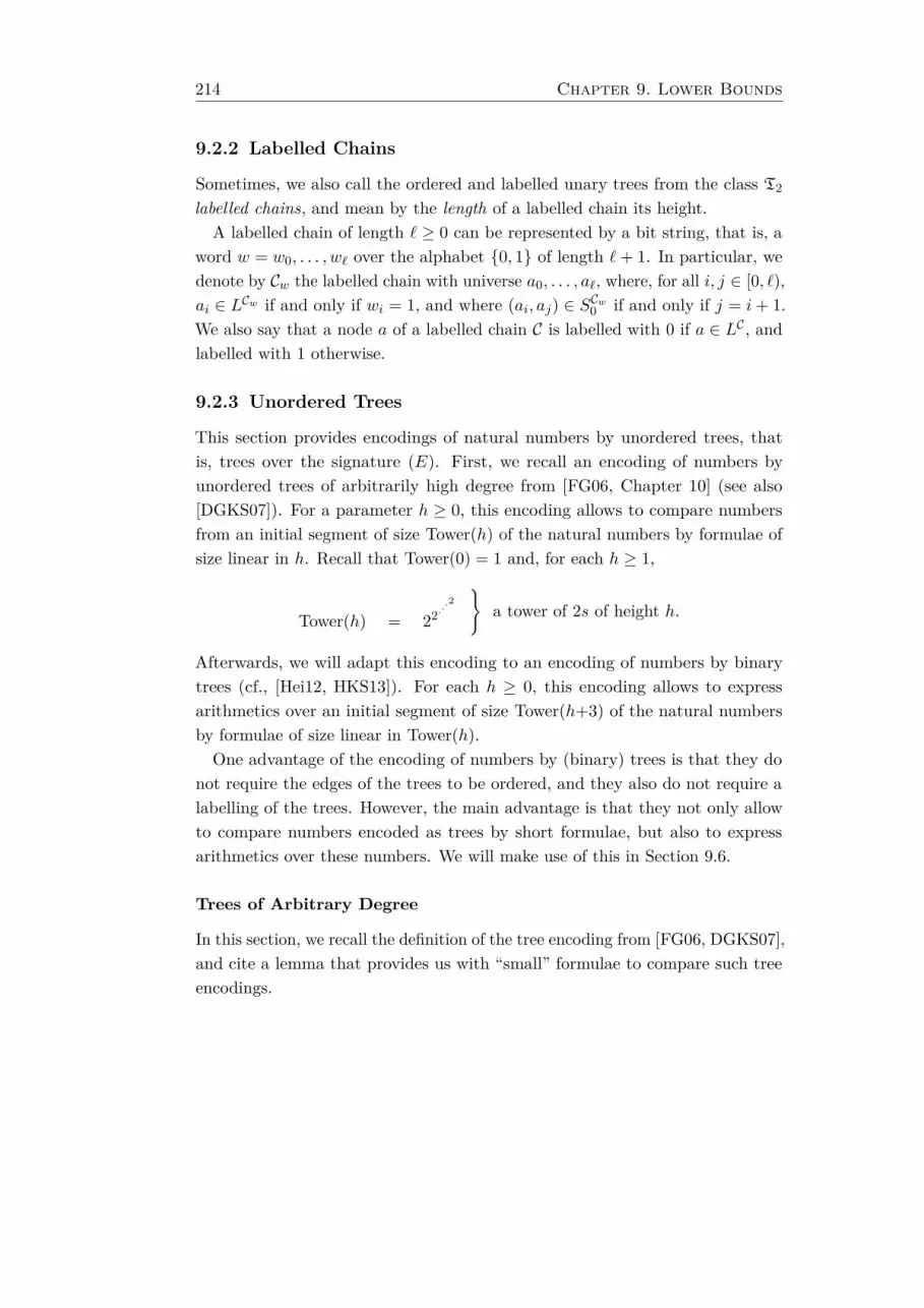
214 Chapter 9. Lower Bounds
9.2.2 Labelled Chains
Sometimes, we also call the ordered and labelled unary trees from the class T2
labelled chains, and mean by the length of a labelled chain its height.A labelled chain of length ` ≥ 0 can be represented by a bit string, that is, a
word w = w0, . . . , w` over the alphabet 0, 1 of length `+ 1. In particular, wedenote by Cw the labelled chain with universe a0, . . . , a`, where, for all i, j ∈ [0, `),ai ∈ LCw if and only if wi = 1, and where (ai, aj) ∈ SCw0 if and only if j = i+ 1.We also say that a node a of a labelled chain C is labelled with 0 if a ∈ LC , andlabelled with 1 otherwise.
9.2.3 Unordered Trees
This section provides encodings of natural numbers by unordered trees, thatis, trees over the signature (E). First, we recall an encoding of numbers byunordered trees of arbitrarily high degree from [FG06, Chapter 10] (see also[DGKS07]). For a parameter h ≥ 0, this encoding allows to compare numbersfrom an initial segment of size Tower(h) of the natural numbers by formulae ofsize linear in h. Recall that Tower(0) = 1 and, for each h ≥ 1,
Tower(h) = 22···2
a tower of 2s of height h.
Afterwards, we will adapt this encoding to an encoding of numbers by binarytrees (cf., [Hei12, HKS13]). For each h ≥ 0, this encoding allows to expressarithmetics over an initial segment of size Tower(h+3) of the natural numbersby formulae of size linear in Tower(h).One advantage of the encoding of numbers by (binary) trees is that they do
not require the edges of the trees to be ordered, and they also do not require alabelling of the trees. However, the main advantage is that they not only allowto compare numbers encoded as trees by short formulae, but also to expressarithmetics over these numbers. We will make use of this in Section 9.6.
Trees of Arbitrary Degree
In this section, we recall the definition of the tree encoding from [FG06, DGKS07],and cite a lemma that provides us with “small” formulae to compare such treeencodings.
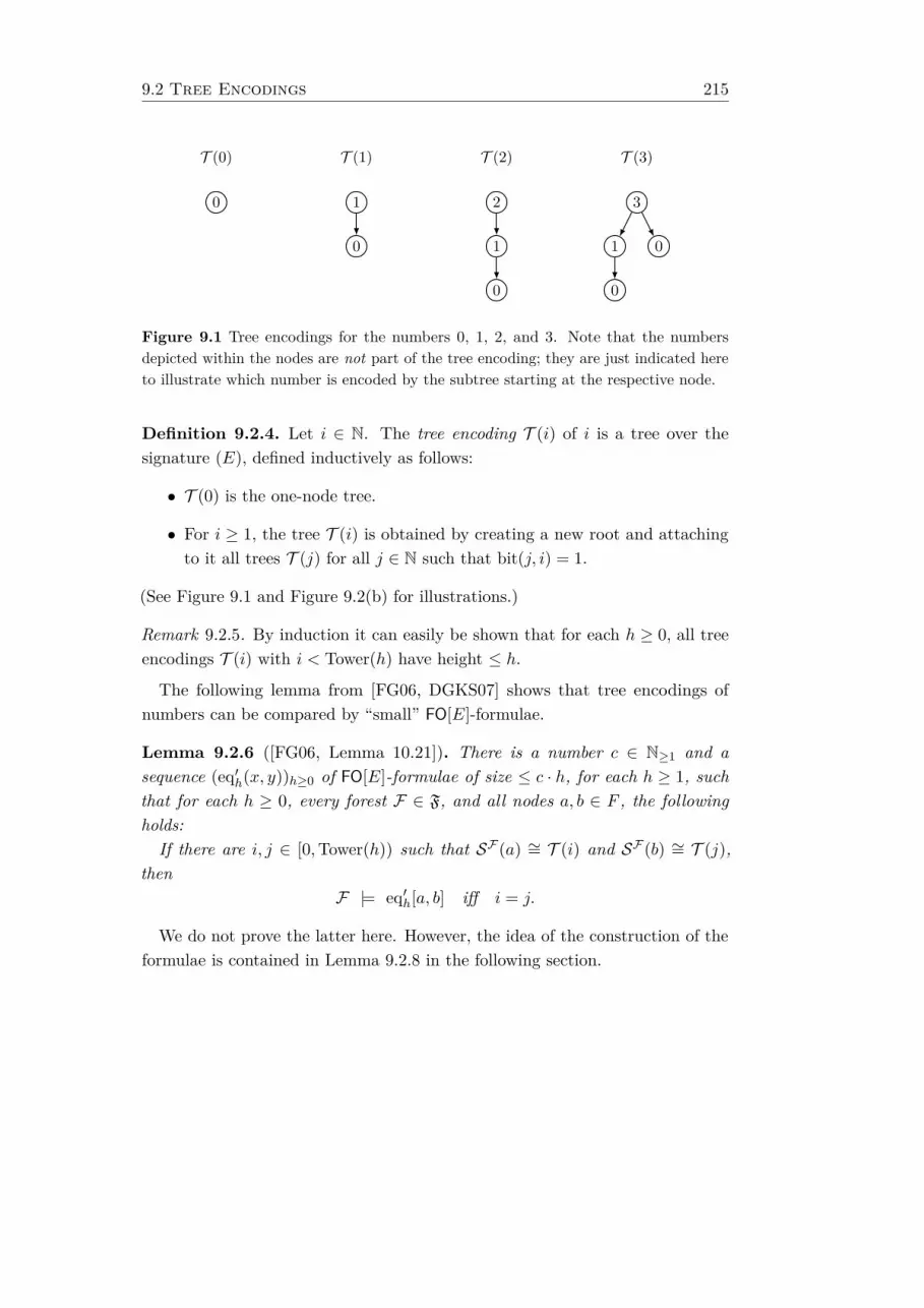
9.2 Tree Encodings 215
T (0)
0
T (1)
1
0
T (2)
2
1
0
T (3)
3
1
0
0
Figure 9.1 Tree encodings for the numbers 0, 1, 2, and 3. Note that the numbersdepicted within the nodes are not part of the tree encoding; they are just indicated hereto illustrate which number is encoded by the subtree starting at the respective node.
Definition 9.2.4. Let i ∈ N. The tree encoding T (i) of i is a tree over thesignature (E), defined inductively as follows:
• T (0) is the one-node tree.
• For i ≥ 1, the tree T (i) is obtained by creating a new root and attachingto it all trees T (j) for all j ∈ N such that bit(j, i) = 1.
(See Figure 9.1 and Figure 9.2(b) for illustrations.)
Remark 9.2.5. By induction it can easily be shown that for each h ≥ 0, all treeencodings T (i) with i < Tower(h) have height ≤ h.
The following lemma from [FG06, DGKS07] shows that tree encodings ofnumbers can be compared by “small” FO[E]-formulae.
Lemma 9.2.6 ([FG06, Lemma 10.21]). There is a number c ∈ N≥1 and asequence (eq′h(x, y))h≥0 of FO[E]-formulae of size ≤ c · h, for each h ≥ 1, suchthat for each h ≥ 0, every forest F ∈ F, and all nodes a, b ∈ F , the followingholds:
If there are i, j ∈ [0,Tower(h)) such that SF (a) ∼= T (i) and SF (b) ∼= T (j),then
F |= eq′h[a, b] iff i = j.
We do not prove the latter here. However, the idea of the construction of theformulae is contained in Lemma 9.2.8 in the following section.
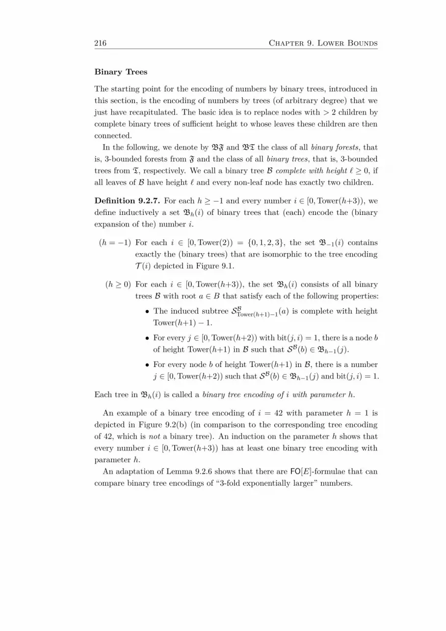
216 Chapter 9. Lower Bounds
Binary Trees
The starting point for the encoding of numbers by binary trees, introduced inthis section, is the encoding of numbers by trees (of arbitrary degree) that wejust have recapitulated. The basic idea is to replace nodes with > 2 children bycomplete binary trees of sufficient height to whose leaves these children are thenconnected.
In the following, we denote by BF and BT the class of all binary forests, thatis, 3-bounded forests from F and the class of all binary trees, that is, 3-boundedtrees from T, respectively. We call a binary tree B complete with height ` ≥ 0, ifall leaves of B have height ` and every non-leaf node has exactly two children.
Definition 9.2.7. For each h ≥ −1 and every number i ∈ [0,Tower(h+3)), wedefine inductively a set Bh(i) of binary trees that (each) encode the (binaryexpansion of the) number i.
(h = −1) For each i ∈ [0,Tower(2)) = 0, 1, 2, 3, the set B−1(i) containsexactly the (binary trees) that are isomorphic to the tree encodingT (i) depicted in Figure 9.1.
(h ≥ 0) For each i ∈ [0,Tower(h+3)), the set Bh(i) consists of all binarytrees B with root a ∈ B that satisfy each of the following properties:
• The induced subtree SBTower(h+1)−1(a) is complete with heightTower(h+1)− 1.
• For every j ∈ [0,Tower(h+2)) with bit(j, i) = 1, there is a node bof height Tower(h+1) in B such that SB(b) ∈ Bh−1(j).
• For every node b of height Tower(h+1) in B, there is a numberj ∈ [0,Tower(h+2)) such that SB(b) ∈ Bh−1(j) and bit(j, i) = 1.
Each tree in Bh(i) is called a binary tree encoding of i with parameter h.
An example of a binary tree encoding of i = 42 with parameter h = 1 isdepicted in Figure 9.2(b) (in comparison to the corresponding tree encodingof 42, which is not a binary tree). An induction on the parameter h shows thatevery number i ∈ [0,Tower(h+3)) has at least one binary tree encoding withparameter h.
An adaptation of Lemma 9.2.6 shows that there are FO[E]-formulae that cancompare binary tree encodings of “3-fold exponentially larger” numbers.
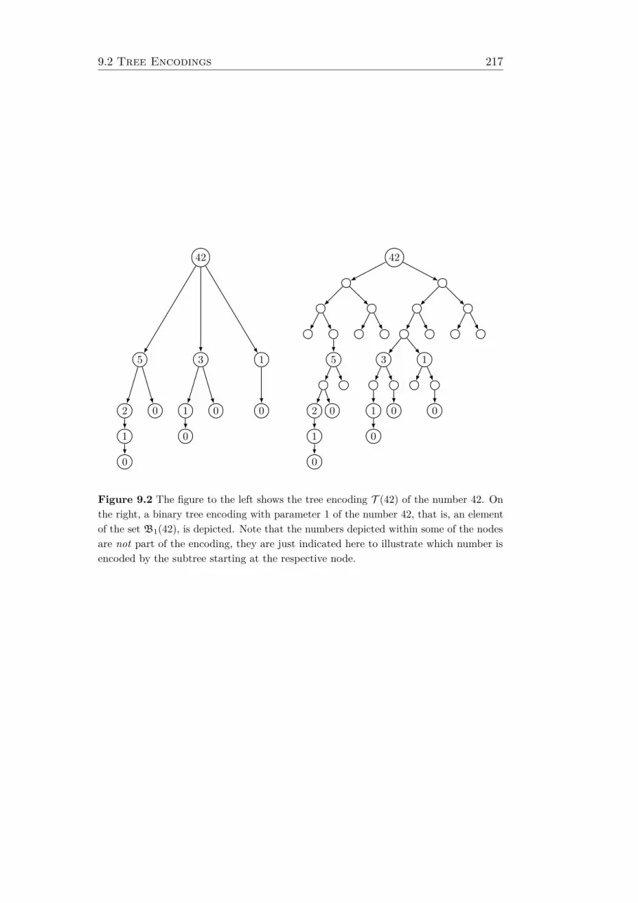
9.2 Tree Encodings 217
42
5
2
1
0
0
3
1
0
0
1
0
42
5
2
1
0
0
3
1
0
0
1
0
Figure 9.2 The figure to the left shows the tree encoding T (42) of the number 42. Onthe right, a binary tree encoding with parameter 1 of the number 42, that is, an elementof the set B1(42), is depicted. Note that the numbers depicted within some of the nodesare not part of the encoding, they are just indicated here to illustrate which number isencoded by the subtree starting at the respective node.
218 Chapter 9. Lower Bounds
Lemma 9.2.8. There is a number c ∈ N≥1 and a sequence (eqh(x, y))h≥−1 ofFO[E]-formulae of size ≤ c ·Tower(h), for h ≥ 0, such that for each h ≥ 0, everyF ∈ BF, and all nodes a, b ∈ F , the following holds:If there are numbers i, j ∈ [0,Tower(h+3)) such that SF (a) ∈ Bh(i) and
SF (b) ∈ Bh(j), thenF |= eqh[a, b] iff i = j.
A straightforward induction shows the following observation, which will turnout useful for finding the upper bound on the size of the formulae of Lemma 9.2.8.
Observation 9.2.9. For all h ≥ 0,
h∑i=0
Tower(i) < 2 · Tower(h).
Proof of Lemma 9.2.8. For h = −1, a formula eq−1(x, y) that is satisfied by twonodes a, b in a binary forest F , if and only if SF (a) and SF (b) are isomorphic tothe same tree T (i) for an i ∈ 0, 1, 2, 3 can be straightforwardly defined.
For h ≥ 0, the construction of the formula eqh(x, y) is best understood by keepingthe binary expansions of the numbers encoded by binary trees in mind. That is,the formula expresses that every bit set in the binary expansion of the number iencoded by the subtree below x, the same bit is also set in the binary expansionof the number j encoded by the subtree below y, and vice versa.
To traverse the complete binary trees connecting the root node with the nodesrepresenting the bits of the binary expansion of the encoded numbers, recallthe formulae provided by Lemma 2.7.1. There is a sequence of FO[E]-formulae(path≤n(x, y))n≥1 of size O(log n), such that for each graph A and all a, b ∈ A,
A |= path≤n[a, b] iff there is a path of length ≤ n from a to b in A.
In the following, we let
πh(x, y) := path≤Tower(h+1)(x, y) ∧ ¬ path≤Tower(h+1)−1(x, y)
be the formula expressing that there is a path of length precisely Tower(h+1)
9.2 Tree Encodings 219
between x and y. Clearly, πh(x, y) is of size O(Tower(h)). With this, we let
eqh(x, y) :=(∃x′πh(x, x′) ↔ ∃y′πh(y, y′)
)∧
∀x′(πh(x, x′) →
∃y′(πh(y, y′) ∧
∀y′′(πh(y, y′′) →
∃x′′(πh(x, x′′) ∧
∀u∀v(
( (u=x′ ∧ v=y′) ∨ (u=x′′ ∧ v=y′′) )
→ eqh−1(u, v))))))
For the size of eqh(x, y), it follows from Observation 9.2.9 that there is a numberc ∈ N≥1 such that || eqh || ≤ c · Tower(h) for all h ≥ 0. This completes the proofof Lemma 9.2.8.
In the following sections, the latter construction is used together with the follow-ing corollary to Lemma 9.1.1 for lower bounds on the complexity of constructingnormal forms on the class BF.
Corollary 9.2.10. Let Σ be a countable alphabet and L ⊆ Σ∗. For each wordw ∈ L, let Lw ⊆ Σ∗ be non-empty. Suppose that there is a number h0 ∈ N≥1,a sequence (wh)h≥h0 of words from L, and a number c ∈ N≥1, such that foreach h ≥ h0:
(1) |wh| ≤ c · Tower(h), and
(2) every v ∈ Lwh has size |v| ≥ Tower(h+3).
Then, there is no algorithm which computes, on input of a word w ∈ L, in time
222o(|w|)
an element of Lw.
Proof. Let Σ be a countable alphabet and let L ⊆ Σ∗. For each word w ∈ L,let Lw ⊆ Σ∗ be a non-empty set. Suppose that there is a number h0 ∈ N≥1, asequence (wh)h≥1 of words from L and a number c ∈ N≥1, such that for eachh ≥ h0, |wh| ≤ c · Tower(h) and every v ∈ Lwh has size
|v| ≥ Tower(h+3) = 222Tower(h)
220 Chapter 9. Lower Bounds
For an application of Lemma 9.1.1, we let f, g : N≥h0 → N≥1 be defined suchthat f(h) := 222h and g(h) := Tower(h) for each h ≥ h0. Then, it follows thatthere is no algorithm which computes, on input of a word w ∈ L, in time
222o(|w|) = f(o(|w|))
a word v ∈ Lw. This completes the proof of Corollary 9.2.10.
9.3 Hanf Normal Form
In this section, we show that the algorithm of Theorem 3.2.1 and thus also thealgorithms of Theorem 7.3.1 and Theorem 8.4.2 for the construction of Hanfnormal are basically worst-case optimal. The lower bounds already hold forthe special case of input formulae from FO. For every degree bound d ≥ 2,recall that Fd is the class of labelled and ordered forests of arity d − 1 overthe signature τd, defined in Section 9.2.1. In particular, all structures in Fd
are d-bounded.
Theorem 9.3.1. Let d ≥ 2. There is no algorithm that computes, on input of asentence ϕ from FO[τd], in time
22o(||ϕ||) for d = 2, and in time 2d2o(||ϕ||) for d ≥ 3
a hnf-sentence from FO+unT[τd] that is equivalent to ϕ on Fd.
Theorem 9.3.1 follows directly from Corollary 9.2.2 and the following lemma,where we construct suitable sequences of “small” formulae for which we show lowerbounds on the size of d-equivalent hnf-sentences. The proof of Lemma 9.3.2 isprovided in Section 9.3.2. It follows the basic idea of the lower bound from [BK12].Its key combinatorial argument is stated and proven in Section 9.3.1 below.
Lemma 9.3.2. Let d ≥ 2 be a degree bound. There is a number cd ∈ N≥1 and asequence (ϕd,h)h≥1 of FO[τd]-sentences such that for every h ≥ 1,
(1) ||ϕd,h|| ≤ cd · h, and
(2) every hnf-sentence in FO+unT[τd] that is Fd-equivalent to ϕd,h has size≥ |Td,2h |.
9.3 Hanf Normal Form 221
9.3.1 The Combinatorial Argument
In the following, we call a set D of structures substructure-free if no properinduced substructure of a structure in D is also contained in D. Observe that, inparticular, the sets Td,h for degree bounds d ≥ 2 and h ≥ 0 are substructure-free.
Lemma 9.3.3. Let σ be a relational signature and let C be a class of σ-structuresthat is closed under disjoint unions and induced substructures. Let D be a finitesubstructure-free subset of C such that each structure in D has at least twoelements and a connected Gaifman graph, and such that all structures in D arepairwise non-isomorphic.Suppose that there is a sentence ϕ in FO[σ] such that for every A ∈ C,
A |= ϕ
iff A contains at most one disjoint copy of each structure from D.
Then, every hnf-sentence ψ in FO+unT[σ] that is equivalent to ϕ on C containsat least |D| counting-sentences and thus, ||ψ|| > |D|.
Proof. Let σ be a relational signature and let C be a class of σ-structures thatis closed under disjoint unions and induced substructures. Let D be a finitesubstructure-free subset of C such that each structure in D has at least twoelements and a connected Gaifman graph, and such that all structures in D arepairwise non-isomorphic.For a contradiction, assume that ψ ∈ FO+unT[σ] is a hnf-sentence that is
equivalent to ϕ on C and that contains less than |D| counting-sentences.Then, there has to be a structure C ∈ D, such that for every counting-sentence
∃≥k y sphτ (y) that occurs in ψ,
τ 6∼= (C, c) for every c ∈ C. (1)
In the following, we choose K ≥ 1 and R ≥ 0, such that each counting-sentence∃≥k y sphτ (y) in ψ has k ≤ K and a type τ of radius r ≤ R.
Let A ∈ C be the disjoint union of K copies of all proper induced substructuresC[NCr (c)] of C with c ∈ C and r ≤ R (such structures exist since C has atleast two elements). Since D is substructure-free and all structures in D havea connected Gaifman graph, A does not contain any structure from D as aninduced substructure.
222 Chapter 9. Lower Bounds
Furthermore, let B ∈ C be the disjoint union of A with two copies of thestructure C. By choice of ϕ, we have that
A |= ϕ and B 6|= ϕ .
Since ψ is equivalent to ϕ on C, we furthermore have
A |= ψ and B 6|= ψ . (2)
We complete the proof of Lemma 9.3.3 by showing that
A |= ψ iff B |= ψ , (3)
which, obviously, is a contradiction to Statement (2).Consider an arbitrary counting-sentence χ := ∃≥k y sphτ (y) from ψ. Note that
k ∈ [1,K] and τ is a type of radius r ≤ R. We will show that
A |= χ iff B |= χ . (4)
Since B is a disjoint extension of A, the “only if” direction of Equivalence (4) isobvious. For the “if” direction, assume towards a contradiction that
A 6|= χ and B |= χ .
Since, by definition of χ, this implies that
|a ∈ A : NAr (a) ∼= τ| < k and |b ∈ B : NBr (b) ∼= τ| ≥ k , (5)
we can conclude that there is a c ∈ C such that τ ∼= N Cr (c). Recall that, byStatement (1), τ 6∼= (C, c). But then, by construction of A, the structure Acontains at least K copies of C[NCr (c)] as disjoint substructures. This is acontradiction to the left side of Statement (5). Thus, A |= χ.We can conclude that Equivalence (3) holds, which is a contradiction to
Statement (2). This completes the proof of Lemma 9.3.3.
9.3.2 Small Sentences with Large Hanf Normal Form Sentences
In this section, we prove Lemma 9.3.2. To this aim, recall that for each de-gree bound d ≥ 2, the class Fd is closed under disjoint unions and inducedsubstructures. Furthermore, for each h ≥ 1, the set Td,2h is substructure-free, allstructures in the set are pairwise non-isomorphic, and each structure in Td,2h
has more than two elements and a connected Gaifman graph.
9.4 Gaifman Normal Form 223
Proof of Lemma 9.3.2 using Lemma 9.3.3. Let d ≥ 2 be a degree bound. Usingthe formulae provided by Lemma 9.2.3, we let, for each h ≥ 1,
ϕd,h := ∀x∀y((
rootd,h(x) ∧ rootd,h(y) ∧ ¬x=y)→ ¬ isod,h(x, y)
)with the subformula
rootd,h(x) := ¬∃yd−2∨j=0
Sj(x, y) ∧ completed,h(x).
By this definition, it holds for every A ∈ Fd that
A |= ϕd,h
iff A contains at most one disjoint copy of each structure from Td,2h .
By Lemma 9.2.3, there is a number cd ∈ N≥1 such that for all h ≥ 1, thesentence ϕd,h has size ≤ cd · h. Therefore, it follows from Lemma 9.3.3 that eachhnf-sentence in FO+unT[τd] that is Fd-equivalent to ϕd,h has size at least |Td,2h |.This completes the proof of Lemma 9.3.2.
9.4 Gaifman Normal Form
In this section, we show that the algorithm of Theorem 4.1.7 for the constructionof Gaifman normal form on classes of structures of bounded degree is basicallyworst-case optimal.
For the statement of the first main result of this section, recall that Td, ford ≥ 3, is the class of labelled and ordered trees of arity d− 1 (cf. Section 9.2.1).
Theorem 9.4.1. Let d ≥ 3 be a degree bound. There is no algorithm thatcomputes, on input of a sentence ϕ from FO[τd], in time
2d2o(||ϕ||)
a gnf-sentence from FO+unT[τd] that is Td-equivalent to ϕ.
For the specific case of degree bound 3, we can show the following lower boundon the class BT of binary trees (cf. Section 9.2.3) over the signature (E).
Theorem 9.4.2. There is no algorithm that computes, on input of a sentence ϕfrom FO[E], in time
222o(||ϕ||)
a gnf-sentence from FO+unT[E] that is BT-equivalent to ϕ.
224 Chapter 9. Lower Bounds
For degree bound 2, recall from Section 9.2.2 that T2 is the class of all labelledchains.
Theorem 9.4.3. There is no algorithm that computes, on input of a sentence ϕfrom FO[τ2], in time
22o(||ϕ||)
a gnf-sentence from FO+unT[τ2] that is T2-equivalent to ϕ.
The proofs for the lower bounds stated in Theorem 9.4.1, Theorem 9.4.2, andTheorem 9.4.3 are based on the proof of Theorem 4.2 in [DGKS07], where thetree encoding recalled in Section 9.2.3 is used for a non-elementary lower boundon the size of Gaifman normal forms on the class T of trees.In Section 9.4.1, a game is presented that distills the basic idea of the latter
lower bound of [DGKS07] in the shape of a game. Section 9.4.2 presents as The-orem 9.4.5 a straightforward application of the game for lower bounds on classesof structures that are closed under disjoint unions (e.g., forest-like structures).There, we also show a slight improvement of the non-elementary lower bound of[DGKS07] with respect to the class of forests of arbitrary degree, which can begeneralised to the class of trees.The following sections are devoted to the proofs of Theorem 9.4.1, The-
orem 9.4.2, and Theorem 9.4.3. Although similar to the proof of Theorem 9.4.5,considerably more care is needed in the construction of the lower bounds onclasses of connected structures.
9.4.1 A Game Characterisation
Let σ be a relational signature, let C be a class of σ-structures, and let ϕ be anFO+unT[σ]-sentence.
For each H ≥ 1, the H-game for ϕ on C has three rounds and is played betweentwo players, called Spoiler and Duplicator. The idea behind the game is thatfor any gnf-sentence ψ of size < H , Duplicator tries to find structures A,B ∈ C
which can be distinguished by ϕ, but not by ψ.In particular, Duplicator can choose A an B depending on the locality radius
of the local formulae in the basic local sentences of ψ. This will be useful if C isa class of structures that is not closed under disjoint unions as, e.g., the class ofbinary trees.
9.4 Gaifman Normal Form 225
(Round 1) Spoiler chooses a number r ≥ 0.
Duplicator chooses a structure A ∈ C.
If A |= ϕ, the game continues. Otherwise, Spoiler wins.
(Round 2) Spoiler chooses a tuple a ∈ An of length n ∈ [1, H).
Duplicator chooses a structure B ∈ C and a tuple b ∈ Bn.
If B 6|= ϕ and NAr (a) ∼= NBr (b), the game continues.Otherwise, Spoiler wins.
(Round 3) Spoiler chooses a number s ≤ r anda 2s-scattered tuple b ∈ Bn of length n ∈ [1, H).
Duplicator chooses a tuple a ∈ An.
If NAs (a) ∼= NBs (b), Duplicator wins. Otherwise, Spoiler wins.
In the description of the game, a tuple (b1, . . . , bn) ∈ Bn of length n ≥ 0 ofelements from the universe of a σ-structure B is called s-scattered, for an s ≥ 0,if the nodes b1, . . . , bn are pairwise distinct and, furthermore, have pairwisedistance > s in the Gaifman graph GB of B.Duplicator has a winning strategy in the H-game for ϕ on C, if he can win
the game for all possible choices of Spoiler in Rounds (1) to (3). The followinglemma shows that this implies a lower bound on the size of Gaifman normalforms on C.
Lemma 9.4.4. For every relational signature σ, each class C of σ-structures,every FO+unT[σ]-sentence ϕ, and each H ≥ 1, the following holds: If Duplicatorhas a winning strategy in the H-game for ϕ on C, then every gnf-sentencefrom FO+unT[σ] that is C-equivalent to ϕ has size ≥ H.
Proof. Let σ be a relational signature and let C be a class of σ-structures. Let ϕbe an FO+unT[σ]-sentence and let H ≥ 1 such that Duplicator has a winningstrategy in the H-game for ϕ on C.
For a contradiction, assume that there is a gnf-sentence ψ in FO+unT[σ] withsize < H that is C-equivalent to ϕ. That is, for each A ∈ C, we have
A |= ϕ iff A |= ψ. (1)
226 Chapter 9. Lower Bounds
Being a gnf-sentence, ψ is a Boolean combination of basic local sentencesχ1, . . . , χL, for an L ≥ 1, where each basic local sentence χ` is of the shape
∃x1 · · · ∃k`
( ∧1≤i<j≤k`
dist(xi, xj) > 2r` ∧k∧i=1
%`(xi)︸ ︷︷ ︸δ`(x1,...,xk` )
)
for numbers k`, r` ≥ 1 and a formula %`(x) that is r`-local around x. Foreach ` ∈ [1, L], we denote by δ`(x1, . . . , xk`) the subformula of χ` without thequantifier prefix ∃x1 · · · ∃xk` .
In the rest of the proof, we will use the winning strategy for Duplicator in theH-game for ϕ on C to obtain structures A,B ∈ C which can be distinguished by ϕbut not by ψ — which immediately leads to a contradiction to the assumptionstated in Equivalence (1).
In Round (1), let Spoiler choose the number r := maxr1, . . . , r`, that is, themaximum of the radii of the local formulae in the basic local sentences of ψ.Duplicator’s winning strategy provides a structure A ∈ C such that A |= ϕ.Since ϕ and ψ are, by assumption, C-equivalent, also A |= ψ.The following claim implies that there is a structure B ∈ C such that B 6|= ϕ
but B |= ψ, completing the proof of Lemma 9.4.4.
Claim 1. There is a structure B ∈ C such that B 6|= ϕ and for each ` ∈ [1, L],
A |= χ` iff B |= χ`.
For the proof of Claim 1, we make use of Duplicator’s winning strategy forRound (2) and Round (3).
Proof of Claim 1. Without loss of generality, there is an L ∈ [0, L] such that
A |= χ` for all ` ≤ L, and A 6|= χ` for all ` > L. (2)
For all ` ∈ [1, L], we know by Statement (2) that A |= χ`. Hence, for each` ∈ [1, L], there is a tuple a ∈ Ak` such that A |= δ`[a]. Let a := (a1, . . . , aL) theconcatenation of all these tuples. Clearly, the length n := k1 + · · ·+ kL of a isless than ||ψ|| and thus less than H.
In Round (2), let Spoiler choose the tuple a just defined. Duplicator’s winningstrategy provides us with a structure B ∈ C with B 6|= ϕ and a tuple b ∈ Bn suchthat NAr (a) ∼= NBr (b). For every ` ∈ [1, L], let b` ∈ Bk` such that b = (b1, . . . , bL).
9.4 Gaifman Normal Form 227
In particular, we have NAr (a`) ∼= NBr (b`) for each ` ∈ [1, L]. Since r` ≤ r, itfollows, that B |= δ`[b`] and hence, B |= χ` for all ` ∈ [1, L].
For each ` ∈ [L+1, L], we know that A 6|= χ`, and we want to show that alsoB 6|= χ`. Towards a contradiction, assume that B |= χ`. That is, assume thatthere is a tuple b ∈ Bk` such that B |= δ`[b]. Of course, k` < H. Furthermore,by construction of δ`(x1, . . . , xk`), the tuple b is 2r`-scattered for r` ≤ r.
In Round (3), let Spoiler choose the number r` and the 2r`-scattered tuple bjust defined. Duplicator’s winning strategy provides a tuple a ∈ Ak` withNAr` (a) ∼= NBr`(b). Therefore, A |= δ`[a] and hence, A |= χ`. This, however, is acontradiction to the assumption that A 6|= χ`. It follows that B 6|= χ`.
This completes the proof of Claim 1 and also the proof of Lemma 9.4.4.
The following section presents a straightforward application of Lemma 9.4.4 toprove lower bounds on the size of Gaifman normal forms with respect to classesof structures that are closed under disjoint unions.
9.4.2 Lower Bounds for Classes Closed Under Disjoint Unions
As an easy example for the application of Lemma 9.4.4, we consider classes ofstructures that are closed under disjoint unions in this section. Precisely, weshow the following variation of Theorem 9.4.1, which is a weaker statement in thesense that the stated lower bounds are not over classes of tree-like but forest-likestructures. On the other hand, it also includes a lower bound for degree bound 2.
For the first result of this section, recall from Section 9.2.1 that Fd is the classof all labelled and ordered forests of degree d− 1.
Theorem 9.4.5. Let d ≥ 2 be a degree bound. There is no algorithm thatcomputes, on input of a sentence ϕ from FO[τd], in time
22o(||ϕ||) for d = 2, and in time 2d2o(||ϕ||) for d ≥ 3
a gnf-sentence from FO+unT[τd] that is Fd-equivalent to ϕ.
In the same manner as Theorem 9.4.5, we can also improve the lower boundof Theorem 4.3 in [DGKS07] for classes of forests of bounded height (withoutany restriction to the degree). For each h ≥ 0, we denote by F≤h the class of allforests of height ≤ h from F.
228 Chapter 9. Lower Bounds
Theorem 9.4.6. There is a sequence (ϕh)h≥1 of FO[E]-sentences of size O(h)such that, for each h ≥ 1, every gnf-sentence from FO+unT[E] that is equivalentto ϕ on F≤h has size ≥ Tower(h).
For comparison, the sequence of FO[E]-sentences provided by Theorem 4.3of [DGKS07] has the same lower bound on the size of F≤h-equivalent gnf-sentences for each h ≥ 1 but its sentences have size in Ω(h4). The reason for thisis that the sentences make use of sub-formulae expressing arithmetic over treeencodings.
The following application of Lemma 9.4.4 shows that there are simpler sentences,which do not use arithmetic over tree encodings, that have large equivalent gnf-sentences (with respect to a class of structures). The lemma will be used in theproofs of Theorem 9.4.5 and Theorem 9.4.6.
Lemma 9.4.7. Let σ be a relational signature and let C be a class of structuresover the signature σ that is closed under disjoint unions. Let D be a non-emptyfinite set pairwise non-isomorphic structures from C.Suppose that ϕ is a sentence from FO+unT[σ] such that for every A ∈ C,
A |= ϕ
iff no structure D ∈ D has precisely one disjoint copy in A.
Then, each gnf-sentence in FO+unT[σ] that is C-equivalent to ϕ has size ≥ |D|.
Proof. Let σ be a relational signature, let C be a class of σ-structures that isclosed under disjoint unions, and let D be a non-empty finite set of pairwisenon-isomorphic structures from C. Furthermore, suppose that ϕ is a sentencefrom FO+unT[σ] such that any structure A ∈ C is a model of ϕ if and only if nostructure D ∈ D has precisely one disjoint copy in A. Let H := |D|.In the following, we will show that Duplicator has a winning strategy in the
H-game for ϕ on C, and thus, by Lemma 9.4.4, each gnf-sentence in FO+unT[σ]that is C-equivalent to ϕ has size ≥ H.Let A be the disjoint union of two copies of each structure from D. By
assumption on ϕ, A |= ϕ. For each D ∈ D, we let A−D be the inducedsubstructure of A obtained by removing one disjoint copy of the structure Dfrom A. Clearly, A−D 6|= ϕ.Duplicator wins the H-game for ϕ on C by the following winning strategy.
Round (1). Independent of Spoiler’s choice of r ≥ 0, Duplicator replies with thestructure A defined above.
9.4 Gaifman Normal Form 229
Round (2). Let a ∈ An with n ∈ [1, H) be the tuple chosen by Spoiler. As |D| > n,there is a structure D ∈ D such that none of the elements of a belongs to one ofthe copies of D in A. Duplicator replies with the structure A−D and with thesame tuple a. Clearly, NAr (a) ∼= NA−Dr (a). Furthermore, by construction of ϕ,A−D 6|= ϕ.
Round (3). Suppose that Spoiler chooses s ≤ r and a 2s-scattered tuple b fromA−D of length n ∈ [1, H). Recall that A−D is an induced substructure of A andthat each disjoint substructure of A−D is, without any modifications, also presentin A. Thus, we have NAs (b) ∼= NADs (b). Duplicator replies with the same tuple b.This completes the proof of Lemma 9.4.7.
Theorem 9.4.5 is a direct consequence of Corollary 9.2.2 and the followinglemma, which, for each d ≥ 2, uses Lemma 9.4.7 to provide lower bounds on thesize of Fd-equivalent gnf-sentences for a sequence of sentences from FO[τd].
Lemma 9.4.8. Let d ≥ 2 be a degree bound. There is a number cd ∈ N≥1 and asequence (ϕd,h)h≥1 of FO[τd]-sentences such that for every h ≥ 1,
(1) ||ϕd,h|| ≤ cd · h, and
(2) every gnf-sentence in FO+unT[τd] that is Fd-equivalent to ϕd,h has size≥ |Td,2h |.
Proof. Let d ≥ 2 be a degree bound. For each h ≥ 1, let
ϕd,h := ∀x(root(x) → ∃y
(root(y) ∧ isod,h(x, y) ∧ ¬x=y
))with root(x) := ¬∃y E(y, x). By construction of ϕd,h, it holds that for everydisjoint union A of structures from the set Td,2h ,
A |= ϕd,h
iff no T ∈ Td,2h has precisely one disjoint copy in A.
Since all disjoint unions of structures from Td,2h belong to Fd, it follows fromLemma 9.4.7 that every gnf-sentence in FO+unT[τd] that is Fd-equivalent toϕd,h has size ≥ |Td,2h |. This completes the proof of Lemma 9.4.8.
We conclude the section with the proof of Theorem 9.4.6.
230 Chapter 9. Lower Bounds
Proof. The proof is very similar to the one of Lemma 9.4.8 but uses the encodingof numbers by trees over the signature (E), introduced in the first part ofSection 9.2.3. For each h ≥ 1, let
ϕh := ∀x(root(x) → ∃y
(root(y) ∧ eqh(x, y) ∧ ¬x=y
))with root(x) := ¬∃y E(y, x) and the formula eqh(x, y) provided by Lemma 9.2.6.Clearly, there is a number c ∈ N≥1 such that ||ϕh|| ≤ c · h for each h ≥ 1.Let h ≥ 1 and let T(h) denote the set of all tree encodings T (i) for all
numbers i ∈ [0,Tower(h)). For every disjoint union A of trees from T(h) it isstraightforward to verify that
A |= ϕh
iff no tree from T(h) has precisely one disjoint copy in A.
Since all disjoint unions of trees from T(h) belong to F≤h, it follows fromLemma 9.4.7 that every gnf-sentence in FO+unT[E] which is equivalent to ϕhon F≤h has size ≥ |T(h)| = Tower(h).
9.4.3 Ordered and Labelled Trees of Bounded Degree
This section is devoted to the proof of Theorem 9.4.1, which is implied byCorollary 9.2.2 and the following lemma. The lemma uses the idea of the proofof Theorem 4.2 in [DGKS07].
Lemma 9.4.9. Let d ≥ 3 be a degree bound. There is a number cd ∈ N≥1 and asequence (ϕd,h)h≥1 of FO[τd]-sentences such that for every h ≥ 1,
(1) ||ϕd,h|| ≤ cd · h, and
(2) every gnf-sentence in FO+unT[τd] that is Td-equivalent to ϕd,h has size≥ |Td,2h |.
Proof. Let d ≥ 3 be a degree bound. Let h ≥ 1 and let H := |Td,2h |. Foreach R ≥ 6, we define the following τd-structures:
• Ch,R is a path of S0-edges along nodes a0, . . . , a(2H+1)R, that is, theτd-structure with universe a0, . . . , a(2H+1)R and where for all i, j ∈[0, (2H+1)R], the tuple (ai, aj) belongs to SCh,R0 if and only if j = i + 1.The other successor relations SCh,Rj for j ∈ [1, d−2] are empty.
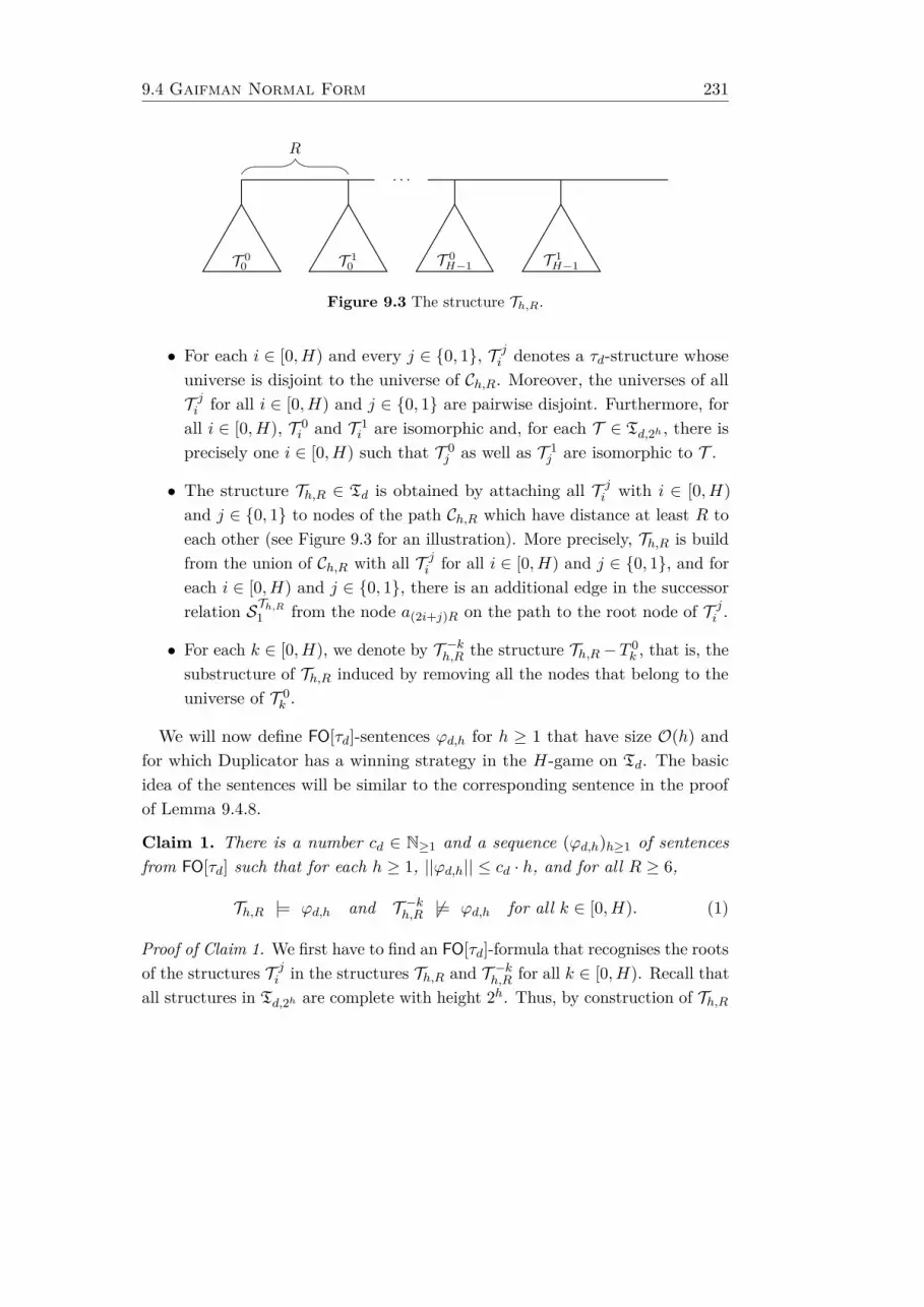
9.4 Gaifman Normal Form 231
. . .
T 00 T 1
0 T 0H−1 T 1
H−1
R
Figure 9.3 The structure Th,R.
• For each i ∈ [0, H) and every j ∈ 0, 1, T ji denotes a τd-structure whoseuniverse is disjoint to the universe of Ch,R. Moreover, the universes of allT ji for all i ∈ [0, H) and j ∈ 0, 1 are pairwise disjoint. Furthermore, forall i ∈ [0, H), T 0
i and T 1i are isomorphic and, for each T ∈ Td,2h , there is
precisely one i ∈ [0, H) such that T 0j as well as T 1
j are isomorphic to T .
• The structure Th,R ∈ Td is obtained by attaching all T ji with i ∈ [0, H)and j ∈ 0, 1 to nodes of the path Ch,R which have distance at least R toeach other (see Figure 9.3 for an illustration). More precisely, Th,R is buildfrom the union of Ch,R with all T ji for all i ∈ [0, H) and j ∈ 0, 1, and foreach i ∈ [0, H) and j ∈ 0, 1, there is an additional edge in the successorrelation STh,R1 from the node a(2i+j)R on the path to the root node of T ji .
• For each k ∈ [0, H), we denote by T −kh,R the structure Th,R−T 0k , that is, the
substructure of Th,R induced by removing all the nodes that belong to theuniverse of T 0
k .
We will now define FO[τd]-sentences ϕd,h for h ≥ 1 that have size O(h) andfor which Duplicator has a winning strategy in the H-game on Td. The basicidea of the sentences will be similar to the corresponding sentence in the proofof Lemma 9.4.8.
Claim 1. There is a number cd ∈ N≥1 and a sequence (ϕd,h)h≥1 of sentencesfrom FO[τd] such that for each h ≥ 1, ||ϕd,h|| ≤ cd · h, and for all R ≥ 6,
Th,R |= ϕd,h and T −kh,R 6|= ϕd,h for all k ∈ [0, H). (1)
Proof of Claim 1. We first have to find an FO[τd]-formula that recognises the rootsof the structures T ji in the structures Th,R and T −kh,R for all k ∈ [0, H). Recall thatall structures in Td,2h are complete with height 2h. Thus, by construction of Th,R
232 Chapter 9. Lower Bounds
and T −kh,R, the roots of the T ji are precisely the nodes satisfying the formulacompleted,h(x) provided by Lemma 9.2.3.
With this, it is straightforward to verify that, for each h ≥ 1, the sentence
ϕd,h := ∀x(completed,h(x) → ∃y
(completed,h ∧ isod,h(x, y) ∧ ¬x=y
)).
satisfies Statement (1). Furthermore, by Lemma 9.2.3, there is a number cd ∈ N≥1
such that ||ϕd,h|| ≤ cd · h for all h ≥ 1. This completes the proof of Claim 1.
By Lemma 9.4.4, it suffices to prove the following claim to complete the proofof Lemma 9.4.9.
Claim 2. For each h ≥ 1, Duplicator has a winning strategy in the H-gamefor ϕd,h on Td.
Proof of Claim 2. Let h ≥ 1. We describe a winning strategy for Duplicator inthe H-game for ϕd,h on Td.
Round (1). Suppose that Spoiler chooses the radius r ≥ 0. For the following, let
R := 4 + max2, 4r.
By Statement (1), Duplicator can reply with the tree Th,R to win this round.
Round (2). Let a be the tuple of elements from Th,R which Spoiler chooses inthis round, and let n ∈ [1, H) be the length of this tuple.
By construction, Th,R contains all the trees T 0i for all i ∈ [0, H). Furthermore,
for all i, j ∈ [0, H), each node a from T 0i and each node b from T 0
j have pairwisedistance ≥ R + 2. Thus, there has to be a number k ∈ [0, H) such that noneof the elements of a belongs to the subtree T 0
k of Th,R, and also not to the(R/2)-neighbourhood of the nodes of T 0
k in Th,R.Duplicator replies with the structure T −kh,R and with the same tuple a. Recall
that, by Statement (1), T −kh,R 6|= ϕd,h. Furthermore, since R/2 > 2r, also
N Th,Rr (a) ∼= NT −kh,R
r (a).
Thus, Duplicator wins the round.
Round (3). Let s ≤ r be the radius chosen by Spoiler, let b be the 2s-scatteredtuple of nodes from T −kh,R chosen by Spoiler, and let n ∈ [1, H) be the length of b.Recall that Duplicator has to reply with a tuple a of the same length n of nodesfrom Th,R such that
N Th,Rs (a) ∼= NT −kh,R
s (b). (2)
9.4 Gaifman Normal Form 233
Of course, each of the nodes in b also occurs in Th,R and the pairwise distance ofthese nodes is the same as in T −kh,R and thus > 2s. If furthermore the s-spheres ofall nodes in b are the same in Th,R and T −kh,R, Duplicator satisfies Isomorphism (2)by replying with the same tuple a := b.In the following, we suppose that this is not the case. That is, we suppose
that the s-sphere of some of the nodes from b are different in T −kh,R and Th,R.Observe that all nodes of b whose s-sphere is different in T −kh,R and Th,R have tobelong to the (s−1)-neighbourhood of the node to which T 0
k is attached in Th,Rbut not in T −kh,R, that is, the node a2kR. Since the (s−1)-sphere of a2kR is just apath of S0-successors of length 2(s−1) with the centre a2kR in the middle and,moreover, the nodes of b have pairwise distance > 2s, there is only one suchnode bm, for a suitable m ∈ [1, n]. Note that the s-sphere of bm in T −kh,R is a pathof S0-successors of length 2s with the centre bm in the middle, whereas in Th,R,the s-neighbourhood of bm also contains nodes from the substructure T 0
k .To find a valid reply for Duplicator, that is, a tuple a of length n of nodes
from Th,R for which Isomorphism (2) holds, it suffices to find a node am ∈ Th,Rthat has distance > 2s to each of the nodes b1, . . . , bm−1, bm+1, . . . , bn and forwhich
N Th,Rs (am) ∼= NT −kh,R
s (bm), (3)
that is, the s-sphere of the node am in Th,R is also a path of S0-successors oflength 2s with the centre am in the middle.Since n− 1 < H − 1 and R/2 > 2r > 2s, we can find an ` ∈ [0, H) such that
none of the nodes b1, . . . , bm−1, bm+1, . . . , bn belongs to the 2s-neighbourhoodof the node a2`R+(R/2). Furthermore, by construction of Th,R, the s-sphereof a2`R+(R/2) is a path of S0-successors of length 2s with the centre a2`R+(R/2) inthe middle. Hence, Isomorphism (3) holds if Duplicator chooses am := a2`R+(R/2).Thus, Duplicator can reply with the tuple b1, . . . , bm−1, am, bm+1, . . . , bn satisfyingIsomorphism (2).
This completes the proof of Claim 2. In particular, Lemma 9.4.4 implies that,for each h ≥ 1, every gnf-sentence from FO+unT[τd] that is Td-equivalent toϕd,h, has size ≥ |Td,2h |. This concludes the proof of Lemma 9.4.9.
9.4.4 Binary Trees
This section is devoted to the proof of Theorem 9.4.2, which is implied byCorollary 9.2.10 and the following lemma.
234 Chapter 9. Lower Bounds
Lemma 9.4.10. There is a number c ∈ N≥1 and a sequence (ϕh)h≥1 of sentencesfrom FO[E] such that for every h ≥ 1,
(1) ||ϕh|| ≤ c · Tower(h), and
(2) every gnf-sentence in FO+unT[E] that is BT-equivalent to ϕh has size≥ Tower(h+3).
The proof of Lemma 9.4.10 is very similar to the proof of Lemma 9.4.9 in theprevious section. The major difference is that we use the encoding of numbers bybinary trees over the signature (E), introduced in the second part of Section 9.2.3,instead of ordered and labelled trees of arity 2 over the signature τ3.
Thus, we define the sentences ϕh, h ≥ 1, and the structures these sentences aretalking about in a different way. The argumentation for showing that Duplicatorhas a winning strategy in the Tower(h+3)-game for ϕh on BT can be takenalmost verbatim from the proof of Lemma 9.4.9. In the following, we will thereforeuse mostly the same notation as in the proof of Lemma 9.4.9.
Proof of Lemma 9.4.10. Let h ≥ 1 and let H := Tower(h+3). For each R ≥ 6,we define the following binary trees from BT:
• Ch,R is a path along nodes a0, . . . , a2(H+1)R, that is, the (E)-structure withuniverse a0, . . . , a2(H+1)R and where for all i, j ∈ [0, 2(H+1)R], the tuple(ai, aj) belongs to ECh,R if and only if j = i+ 1.
• For each i ∈ [0, H), T 0i and T 1
i are copies of the same binary tree fromBh(i), whose universe each is disjoint to the universe of Ch,R. Moreover,the universes of all T ji for all i ∈ [0, H) and j ∈ 0, 1 are also pairwisedisjoint.
• The binary tree Th,R ∈ BT is obtained by attaching all T ji with i ∈ [0, H)and j ∈ 0, 1 to the path Ch,R. More precisely, Th,R is build from theunion of Ch,R with all T ji for all i ∈ [0, H) and j ∈ 0, 1, and for eachi ∈ [0, H) and j ∈ 0, 1, there is an additional edge from the node a(2i+j)Ron the path to the root node of T ji .
• For each k ∈ [0, H), we denote by T −kh,R the substructure of Th,R inducedby removing all the nodes that belong to the universe of T 0
k .
We will now define FO[E]-sentences ϕh for h ≥ 1 that have size O(Tower(h))and for which Duplicator has a winning strategy in the H-game on BT. The
9.4 Gaifman Normal Form 235
sentences follow the same idea as the ones of Lemma 9.4.9, but are adapted tothe binary trees defined above.
Claim 1. There is a number c ∈ N≥1 and a sequence (ϕh)h≥1 of sentences fromFO[E] such that for each h ≥ 1, ||ϕh|| ≤ c · Tower(h), and for all R ≥ 6,
Th,R |= ϕh and T −kh,R 6|= ϕh for all k ∈ [0, H). (1)
Proof of Claim 1. Our first task is it to find an FO[E]-formula root(x) thatrecognises the roots of the subtrees T ji in the binary trees just defined. In thefollowing, we call a path branchless if all but the first and the last of its nodeshave only one child node, that is, the only child is the successor of the nodeon the path. Observe that none of the binary trees T ji , for no i ∈ [0, H) andj ∈ 0, 1, contains a branchless path of length ≥ 5. Furthermore, the root ofeach such binary tree has two children. Thus, since R ≥ 6, we can identify theroot nodes of the binary tree encodings T ji in the binary trees Th,R and T −kh,R asthe nodes x with the following properties:
• The node x has two children.
• The node x is a child of a node y which is also the first node of a branchlesspath of length 5, which, in particular, does not contains the node x.
Thus, we can choose
root(x) := ∃y∃y′(E(x, y) ∧ E(x, y′) ∧ ¬y=y′
)∧
∃y(E(y, x) ∧ ∃y′ bpath5(y, y′)
)where bpath5(y, y′) is an FO[E]-formula that is satisfied if there is a branchlesspath of length 5 from y to y′.Using the formulae provided by Lemma 9.2.8, we now let
ϕh := ∀x(root(x) → ∃y
(root(y) ∧ eqh(x, y) ∧ ¬x=y
)).
It is straightforward to verify that, for each h ≥ 1, ϕh satisfies Statement (1).Furthermore, by Lemma 9.2.8, there is a number c ∈ N≥1 such that ||ϕh|| ≤ c · hfor all h ≥ 1. This completes the proof of Claim 1.
The following claim is proven in the same way as Claim 2 in the proof ofLemma 9.4.9, with the only modification of using the formulae ϕh just definedinstead of ϕd,h, and the binary trees introduced above.
236 Chapter 9. Lower Bounds
Claim 2. For each h ≥ 1, Duplicator has a winning strategy in the H-gamefor ϕh on BT.
By Lemma 9.4.4, Claim 2 implies that for each h ≥ 1, every gnf-sentence fromFO+unT[E] that is BT-equivalent to ϕh, has size ≥ H = Tower(h+3). Thiscompletes the proof of Lemma 9.4.10.
9.4.5 Labelled Chains
This section is devoted to the proof of Theorem 9.4.3, which is implied byCorollary 9.2.2 and the following lemma.
Lemma 9.4.11. There is a number c ∈ N≥1 and a sequence (ϕh)h≥1 of sentencesfrom FO[τ2] such that for every h ≥ 1,
(1) ||ϕh|| ≤ c · h, and
(2) every gnf-sentence in FO+unT[τ2] that is T2-equivalent to ϕh has size≥ 22h.
Proof. The proof is similar to the one of Lemma 9.4.9 and Lemma 9.4.10. Insteadof (binary) trees, it uses labelled chains. These labelled chains contain encodings(of the binary expansion) of natural numbers and large “gaps” inbetween. Insteadof removing sub-trees (as in the proof of Lemma 9.4.9 and Lemma 9.4.10)we change the labelling of the chain to replace encodings of natural numbersby “gaps”.Let h ≥ 1 and let H := 22h . For each i ∈ [0, H), let wi := v0 . . . v2·2h be
the bit string of length 2 · 2h + 1 where v2j = 0 for all j ∈ [0, 2h], and wherev2j+1 = bit(j, i) for all j ∈ [0, 2h). The odd positions of wi represent the binaryexpansion of the number i. Leaving the even positions labelled with 0 will allowus to mark the starting positions of the words wi in labelled chains by words 11.
For each subset I ⊆ [0, H) and every R ≥ 0 let
wIR := 0R+1 u00 0R+1 u1
0 0R+1 u01 0R+1 u1
1 · · · 0R+1 u0H−1 0R+1 u1
H−1 (1)
the bit string where, for each i ∈ [0, H), u0i := 11wi, and where
u1i :=
u0i if i ∈ I, and
0|u0i | if i 6∈ I.
Finally, let Ch,R denote the labelled chain corresponding to the bit string w[0,H)R
and, for each k ∈ [0, H), let C−kh,R denote the labelled chain corresponding to the
9.4 Gaifman Normal Form 237
bit string w[0,H)\kR . Intuitively, this means that Ch,R contains two copies of each
of the words wi for all i ∈ [0, H), each prefixed by a word of 0’s of length R+ 1and the word 11. And C−kh,R is identical two Ch,R with the only exception thatone copy of the word 11wk is replaced by a sequence of 0’s of the same length.
Claim 1. There is a number c ∈ N≥1 and a sequence (ϕh)h≥1 of sentencesfrom FO[τ2] such that for each h ≥ 1, ||ϕh|| ≤ c · h, and for all R ≥ 2,
Ch,R |= ϕh and C−kh,R 6|= ϕh for all k ∈ [0, H). (2)
Proof of Claim 1. Let C be one of the labelled chains Ch,R and C−kh,R, k ∈ [0, H).By construction of the bit strings defining C, the nodes corresponding to the firstposition of one of the bit strings wi, i ∈ [0, H), are precisely the nodes whichdirectly follow on two nodes labelled with 1. We express this observation in theformula
root(z) := ∃x∃y(L(x) ∧ S0(x, y) ∧ L(y) ∧ S0(y, z)
).
By construction of C, for any node a of C that satisfies the formula root(z),the induced substructure SC2h+1(a) is a labelled chain of length 2h+1 and thuscomplete with height 2h+1. Thus, the formula iso2,h+1(x, x′) of Lemma 9.2.3 issatisfied by two such nodes a, a′ if and only if SC2h+1(a) ∼= SC2h+1(a′).
With this observation, we can let
ϕh := ∀x(root(x) → ∃y
(root(y) ∧ iso2,h+1(x, y) ∧ ¬x=y
)).
By Lemma 9.2.3, there is a number c ∈ N≥1 such that ||ϕh|| ≤ c · h for all h ≥ 1.Furthermore, it is straightforward to verify that ϕh satisfies Statement (2). Thiscompletes the proof of Claim 1.
By Lemma 9.4.4, the proof of Lemma 9.4.11 is completed by proving thefollowing claim.
Claim 2. For each h ≥ 1, Duplicator has a winning strategy in the H-gamefor ϕh on T2.
Proof of Claim 2. Let h ≥ 1. In the following, we describe Duplicator’s winningstrategy in the H-game for ϕh on T2. Altogether, the winning strategy is similarto the one described in the proof of Lemma 9.4.9. However, the use of labelledchains requires some modifications.
238 Chapter 9. Lower Bounds
Round (1). Suppose that Spoiler chooses the radius r ≥ 0. For the following, let
R := 4r + 2.
By Claim 1, Duplicator can reply with the labelled chain Ch,R to win this round.
In the following, we denote by U ji for i ∈ [0, H) and j ∈ 0, 1 the nodes thatcorrespond to the positions of the bit string uji in any of the labelled chains Ch,Rand C−kh,R with k ∈ [0, H).
Round (2). Let a be the tuple of elements from Ch,R which Spoiler chooses inthis round, and let n ∈ [1, H) be the length of this tuple. Since a has length< H, there has to be a k ∈ [0, H) such that none of the nodes of a is containedin the (R/2)-neighbourhood of U1
k in Ch,R.The labelled chain C−kh,R has the same universe as Ch,R and thus still contains
all the nodes of a. In particular, the entire (R/2)-sphere of a remains unchanged.Since R/2 > 2r,
N Ch,Rr (a) ∼= NC−kh,R
r (a)
and, by Claim 1, C−kh,R 6|= ϕh, Therefore, Duplicator wins the round by replyingwith the structure C−kh,R and the same tuple a which the Spoiler has chosen.
Round (3). Let s ≤ r be the radius chosen by Spoiler, let b be the 2s-scatteredtuple of nodes from C−kh,R chosen by Spoiler, and let n ∈ [1, H) be the lengthof b. Recall that Duplicator has to reply with a tuple a of length n, consisting ofnodes from Ch,R such that
N Ch,Rs (a) ∼= NC−kh,R
s (b). (3)
Of course, each of the nodes in b also occurs in Ch,R and the pairwise distance ofthese nodes is the same as in C−kh,R and thus > 2s. If furthermore the s-spheres ofall nodes in b are the same in Ch,R and C−kh,R, Duplicator satisfies Isomorphism (3)by replying with the tuple a := b.
In the following, we suppose that this is not the case. That is, we suppose thatthe s-sphere of some of the nodes from b are different in C−kh,R and Ch,R. Observethat all nodes of b whose s-sphere is different in C−kh,R and Ch,R have to belong tothe s-neighbourhood of the node set U1
k . Thus, in C−kh,R the s-sphere of each of
these nodes is a path of 2s+ 1 nodes, labelled with 0, with its centre being thenode in the middle of the path. On the other hand, in Ch,R, the s-sphere of anyof these nodes may contain nodes labelled with 1.
9.5 Feferman-Vaught Decompositions 239
Suppose that b = (b1, . . . , bn). Without loss of generality, suppose furthermorethat b1, . . . , bm, for a suitable m ∈ [0, n], are precisely the elements of b thatbelong to the s-neighbourhood of U1
k .To find a valid reply for Duplicator, that is, a tuple a of elements from Ch,R
with length n such that Isomorphism (3) holds, it suffices to find a 2s-scatteredtuple (a1, . . . , am) among the nodes of Ch,R such that
(a) (a1, . . . , am, bm+1, . . . , bn) is a 2s-scattered set in Ch,R and
(b) the s-sphere of each ai for all i ∈ [1,m] is a path of 2s+ 1 nodes, labelledwith 0, with its centre ai being the node in the middle of the path.
In the following, let c1, . . . , c2H denote the nodes of Ch,R, corresponding to themiddle positions of the bit strings 0R+1 in the bit strings described in (1). Moreprecisely, ci, for each i ∈ [1, 2H], is the node of height
i(R+ 2 · 2h + 4) + (R/2)
in Ch,R.Since b is of length n < H and R/2 > 2r ≥ 2s, there are pairwise distinct
`1, . . . , `m ∈ [1, 2H] such Condition (a) and Condition (b) hold for a1, . . . , am
when letting ai := c`i for all i ∈ [1,m].With this, the s-sphere of each ai for all i ∈ [1,m] in Ch,R is isomorphic to
the s-sphere of bi in C−kh,R. Therefore, Duplicator wins Round (3) and the wholeH-game for ϕh on T2 by replying with the tuple a := (a1, . . . , am, bm+1, . . . , bn).This completes the proof of Claim 2.
Thus, by Lemma 9.4.4, every gnf-sentence in FO+unT[τ2] that is T2-equivalentto ϕh, for each h ≥ 1, has size ≥ 22h .
9.5 Feferman-Vaught Decompositions
In this section, we show that the algorithm of Theorem 5.2.1 and thus, alsothe algorithms of Theorem 7.4.1 and Theorem 8.5.3 for the construction of ⊕-decompositions on classes of structures of bounded degree are basically worst-caseoptimal. The lower bounds already hold for the special case of input formulaefrom FO.
Recall from Section 9.2.1 that Td is the class of all labelled and ordered treesof arity d− 1. The main results of this section can be stated as follows:
240 Chapter 9. Lower Bounds
Theorem 9.5.1. Let d ≥ 3 a degree bound. There is no algorithm that computes,on input of a sentence ϕ from FO[τd], in time
2d2o(||ϕ||)
a 2-ary ⊕-decomposition for ϕ over FO+unT[τd] on the class Td.
For the specific case of degree bound 3, we can show the following lower boundon the class BT of binary trees (cf. Section 9.2.3) over the signature (E).
Theorem 9.5.2. There is no algorithm that computes, on input of a sentence ϕfrom FO[E], in time
222o(||ϕ||)
a 2-ary ⊕-decomposition for ϕ over FO+unT[E] on the class BT.
For degree bound 2, we show the following lower bound on the class T2 oflabelled chains (cf. Section 9.2.2).
Theorem 9.5.3. There is no algorithm that computes, on input of a sentence ϕfrom FO[τ2], in time
22o(||ϕ||)
a 2-ary ⊕-decomposition for ϕ over FO+unT[τ2] on the class T2.
For the proofs of Theorem 9.5.1, Theorem 9.5.2, and Theorem 9.5.3, whichcan be found in Section 9.5.2, Section 9.5.3, and Section 9.5.4, respectively, weconstruct sequences of “small” FO-sentences over the corresponding signaturefor which we show lower bounds on the size of 2-ary ⊕-decompositions on therespective class of structures. These lower bounds are based on a generalisationof Proposition 23 in (the full version of) [GJL12], which is stated in the followingsection.
9.5.1 The Combinatorial Argument
In the following, we denote by A⊕ B a disjoint sum of structures A and B.
Lemma 9.5.4. Let σ be a relational signature, let C be a class of σ-structures,and let ϕ be an FO[σ2]-sentence. Let H ≥ 1. Suppose that there is a subsetD ⊆ C of 2H pairwise non-isomorphic structures such that for all A,B ∈ D,
A⊕ B |= ϕ iff A = B.
Then, every 2-ary ⊕-decomposition for ϕ over FO+unT[σ] on the class C hassize ≥ H.
9.5 Feferman-Vaught Decompositions 241
Proof. The lemma is proven by a counting argument. Let σ be a relationalsignature, let C be a class of σ-structures, and let ϕ be an FO[σ2]-sentence.Let H ≥ 1. Suppose that there is a subset D ⊆ C of 2H pairwise non-isomorphicstructures such that for all A,B ∈ D,
A⊕ B |= ϕ iff A = B. (1)
For a contradiction, assume that there is a 2-ary decomposition ∆ := (β,∆1,∆2)for ϕ over FO+unT[σ] on C that has size ||∆|| < H. In particular, ∆1 and ∆2
are finite sets of FO+unT[σ]-sentences and β is a propositional formula usingonly the propositional symbols Xi,δ with i ∈ [1, 2] and δ ∈ ∆i. Moreover, for allA,B ∈ D,
A⊕ B |= ϕ iff µA,B |= β (2)
where µA,B : PS→ 0, 1 assigns truth values to propositional symbols such thatfor all δ ∈ ∆1,
µA,B(X1,δ) = 1 iff A |= δ,
and for all δ ∈ ∆2,µA,B(X2,δ) = 1 iff B |= δ,
and such that µA,B(X) = 0 for all X ∈ PS that do not occur in β.From Equivalence (1) and Equivalence (2) we know that, for all A,B ∈ D,
µA,B |= β iff A = B. (3)
Note that the number of propositional symbols occurring in β is less than H , andhence the number of distinct propositional assignments µA,B with A,B ∈ D is lessthan 2H . Since |D| = 2H , there exist distinct A,B ∈ D such that µA,A = µB,B.In particular, µA,A(X2,δ) = µB,B(X2,δ) for all δ ∈ ∆2 and thus also
µA,B = µA,A. (4)
Due to Equivalence (3), we have
µA,A |= β. (5)
Thus, from Equivalence (4), Statement (5), and Equivalence (2) we obtain that
A⊕ B |= ϕ.
This, however, is a contradiction to Equivalence (1).
In the subsequent sections, we will apply Lemma 9.5.4 to various classes ofstructures of bounded degree.
242 Chapter 9. Lower Bounds
9.5.2 Ordered and Labelled Trees of Bounded Degree
This section is devoted to the proof of Theorem 9.5.1, which is a direct consequenceof Corollary 9.2.2 and the following lemma.
Lemma 9.5.5. Let d ≥ 3 be a degree bound. There is a number cd ∈ N≥1 and asequence (ϕd,h)h≥1 of FO[τd]-sentences such that for every h ≥ 1,
(1) ||ϕd,h|| ≤ cd · h, and
(2) every 2-ary ⊕-decomposition for ϕd,h over FO+unT[E] on the class Td hassize ≥ |Td,2h |.
Proof. Let d ≥ 3. For each h ≥ 1, we denote by H the cardinality |Td,2h | of theset Td,2h , and define the following Td-structures:
• By PH , we denote a τd-structure with universe a0, . . . , aH−1 where therelation SPH0 describes a path along these nodes. That is, for all i, j ∈ [0, H)we have (ai, aj) ∈ SPH0 if and only if j = i + 1, and the other successorrelations SPHj with j ∈ [1, d−2] are empty.
• Let T0, . . . , TH−1 denote a sequence of structures from Td whose universeis pairwise disjoint and also disjoint to the universe of PH , and such thatfor each T ∈ Td,2m there is precisely one i ∈ [0, H) with T ∼= Ti.
• For each subset I ⊆ [0, H), let TI ∈ Td the structure where all Ti with i ∈ Iare attached to the path PH . More precisely, TI is built from the unionof PH with all Ti for all i ∈ I, and for each i ∈ I, there is an additionaledge (ai, b) ∈ STI1 from the node ai on the path to the root node b of Ti.
By Dd,h, we denote set of all structures TI for all I ⊆ [0, H). Clearly, |Dd,h| = 2H .Once we have proven the following claim, the proof of Lemma 9.5.5 is complete:
It follows from Lemma 9.5.4 that, for each h ≥ 1, every 2-ary ⊕-decompositionfor the sentence ϕd,h over FO+unT[τd] on the class Td has size ≥ H = |Td,2h |.
Claim 1. There is a number cd ∈ N≥1 and a sequence (ϕd,h)h≥1 of sentencesfrom FO[τd] such that for every h ≥ 1,
(1) ||ϕd,h|| ≤ cd · h, and
(2) for all A,B ∈ Dd,h, A⊕ B |= ϕd,m iff A = B.
9.5 Feferman-Vaught Decompositions 243
Proof of Claim 1. Using the formulae provided by Lemma 9.2.3, we let
ϕd,h := ∀x(completed,h(x) → ∃y
(completed,h(y) ∧ isod,h(x, y) ∧ ¬x=y
))for each h ≥ 1. By Lemma 9.2.3, there is a number cd ∈ N≥1 such that for allh ≥ 1, the sentence ϕd,h has size ≤ cd · h. Furthermore, it is straightforward tosee that for all A,B ∈ Dd,h, the sentence ϕd,h satisfies Condition (2) of Claim 1.This completes the proof of Claim 1 and thus, also the proof of Lemma 9.5.5.
9.5.3 Binary Trees
This section is devoted to the proof of Theorem 9.5.2. The proof is very similarto the one of Theorem 9.5.1 and a direct consequence of Corollary 9.2.10 andthe following lemma.
Lemma 9.5.6. There is a number c ∈ N≥1 and a sequence (ϕh)h≥1 of sentencesfrom FO[E] such that for every h ≥ 1,
(1) ||ϕh|| ≤ c · Tower(h), and
(2) every 2-ary ⊕-decomposition for ϕh over FO+unT[E] on the class BT hassize ≥ Tower(h+3).
Proof. Let h ≥ 1 and H := Tower(h+3). We construct a set Dh of binary treesin a similar way as the sets Dd,h in the proof of Theorem 9.5.1. However, insteadof structures from the sets Td,2h , we use the encoding of numbers by binary treesintroduced in Section 9.2.3. To be able to identify the roots of these binary treeencodings, we have to put more distance between them. For this, we considerthe following structures from BT:
• Let PH denote graph over the signature (E) with universe a0, . . . , a5H−1and, for all i, j ∈ [0, 5H), an edge (ai, aj) ∈ ECH if and only if j = i+ 1.
• For each i ∈ [0, H), we let Ti ∈ Bh(i) such that the universe of all Ti,i ∈ [0, H) is disjoint to the universe of PH and, furthermore, the universesof all Ti, Tj with i, j ∈ [0, H) and i 6= j are also pairwise disjoint.
• For each subset I ⊆ [0, H), let TI the binary tree where all Ti with i ∈ Iare attached to the path PH . More precisely, TI is built from the unionof PH with all Ti for all i ∈ I, and for each i ∈ I, there is an additionaledge (a5i, b) ∈ ETI from the node ai on the path to the root node b of Ti.
244 Chapter 9. Lower Bounds
By Dh we denote the set of all structures TI for all I ⊆ [0, H). Clearly |Dh| = 2H .Once we have proven the following claim, the proof of Lemma 9.5.6 is complete:
It follows from Lemma 9.5.4 that, for each h ≥ 1, every 2-ary ⊕-decompositionfor ϕh over FO+unT[E] on the class BT has size ≥ H = Tower(h+3).
Claim 1. There is a number c ∈ N≥1 and a sequence (ϕh)h≥1 of sentences fromFO[E] such that for every h ≥ 1,
(1) ||ϕh|| ≤ c · Tower(h), and
(2) for all A,B ∈ Dh, A⊕ B |= ϕh iff A = B.
Proof of Claim 1. Let h ≥ 1. For the construction of the sentence ϕh, we firsthave to identify the roots of the subtrees Ti for all i ∈ [0, H) in the structuresof Dh. For this, we can proceed as in the proof of Claim 1 in the proof ofLemma 9.4.10.None of the binary trees Ti, for no i ∈ [0, H), contains a branchless path of
length ≥ 5. Recall that a path is called branchless if all but the first and thelast of its nodes have only one child. Furthermore, the root of each such binarytree has two children. Using these observations, we can see that in the binarytrees in Dh, the subtrees Ti, i ∈ [0, H) are so far away from each other on thepath PH , that their root nodes can be identified as the nodes x with the followingproperties:
• There is a node y with two children; one of these children being x.
• The node y is the first node of a branchless path of length 5, which doesnot contains x.
• The node x has two children.
Thus, we can choose
root(x) := ∃y∃y′(E(x, y) ∧ E(x, y′) ∧ ¬y=y′
)∧
∃y(E(y, x) ∧ ∃y′ bpath5(y, y′)
)where bpath5(y, y′) is an FO[E]-formula that is satisfied if there is a branchlesspath of length 5 from y to y′.
Using the formulae provided by Lemma 9.2.8, we now define
ϕh := ∀x(root(x) → ∃y
(root(y) ∧ eqh(x, y) ∧ ¬x=y
)).
9.5 Feferman-Vaught Decompositions 245
By Lemma 9.2.8, there is a number c ∈ N≥1 such that ||ϕh|| ≤ c · Tower(h) foreach h ≥ 1. Furthermore, it is straightforward to see that for all A,B ∈ Dh,the sentence ϕh satisfies Condition (2) of Claim 1. This completes the proof ofClaim 1 and thus, also the proof of Lemma 9.5.6.
9.5.4 Labelled Chains
The overall structure of the proof of Theorem 9.5.3 is the same as for The-orem 9.5.1. Using Lemma 9.1.1, Theorem 9.5.3 is implied by the following lemma.
Lemma 9.5.7. There is a number c ∈ N≥1 and a sequence (ϕh)h≥1 of sentencesfrom FO[τ2] such that for every h ≥ 1,
(1) ||ϕh|| ≤ c · h, and
(2) every 2-ary ⊕-decomposition for ϕh over FO+unT[τ2] on the class T2 hassize ≥ 22h.
Proof. Let m ≥ 1 and let H := 22h . We employ a similar encoding of numbersfrom [0, H) by labelled chains as in the proof of Lemma 9.4.11. For eachi ∈ [0, H), let wi be the bit string of length 2h+1 + 1 = 2 · 2h + 1 where preciselythe positions 2j+1 for all j ∈ [0, 2h) with bit(j, i) = 1 are labelled with 1, and allother positions are labelled with 0. Intuitively, the odd positions of the word wirepresent the binary expansion of the number i. For example, for h = 1 and i = 3,wi = 01010. Note that, in particular, the last position of each word wi is alwayslabelled with 0.For all I ⊆ [0, H), we now denote by wI the bit string
wI := v0w0v1w1 · · · vH−1wH−1,
where w0, . . . , wH−1 are defined as above, and where vi = 11 for all i ∈ I
and vi = 00 for all i ∈ [0, H) with i 6∈ I. By CI we denote the labelled chaincorresponding to the word wI . Thus, each CI contains the binary expansionsof all numbers i ∈ [0, H), but only the binary expansions of numbers i ∈ I aremarked by the prefix 11. Finally, let Dh be the set of all labelled chains CI forall I ⊆ [0, H).The proof of Lemma 9.5.7 is complete once we have proven the following
claim. By Lemma 9.5.4 for each h ≥ 1, every 2-ary decomposition for ϕh overFO+unT[τ2] on the class T2 of labelled chains has size ≥ H = 22h .

246 Chapter 9. Lower Bounds
Claim 1. There is a number c ∈ N≥1 and a sequence (ϕh)h≥1 of sentences fromFO[τ2] such that for every h ≥ 1,
(1) ||ϕh|| ≤ c · h, and
(2) for all A,B ∈ Dh, A⊕ B |= ϕh iff A = B.
Proof of Claim 1. Note that in any labelled chain CI from Dh, the nodescorresponding to the initial positions of the words wi, i ∈ I, can be recognisedby the formula
root(z) := ∃x∃y(S0(x, y) ∧ S0(y, z) ∧ L(x) ∧ L(y)
).
Using the formulae provided by Lemma 9.2.3, we let
ϕh := ∀x(root(x) → ∃y
(root(y) ∧ iso2,h+1(x, y) ∧ ¬x=y
)).
From Lemma 9.2.3 we know that there is a number c ∈ N≥1 such that ||ϕh|| ≤ c·hfor all h ≥ 1. Furthermore, it is straightforward to see that for all CI , CJ ∈ Dh,the sentence ϕh is satisfied by CI ⊕ CJ if and only if CI = CJ (that is, I = J).This completes the proof of Claim 1 and also the proof of Lemma 9.5.7.
9.6 Preservation Theorems
In this section, we provide 3-fold exponential lower bounds for our algorithmsfrom Theorem 6.1.7 and Theorem 6.1.10. Recall that, for d ≥ 3, Theorem 6.1.7provided a 5-fold exponential upper bound on the construction of existentialformulae for formulae from FO+unM that are preserved under extensions on theclass of d-bounded structures. Similarly, Theorem 6.1.10 implied a 4-fold expo-nential upper bound on the construction of existential-formulae for formulae fromFO+unM that are preserved under homomorphisms on the class of d-boundedstructures.Both lower bounds already hold for sentences from FO. For the lower bound
concerning preservation under extensions, we let σext := (S0, S1, L0, L1) be therelational signature with the binary relation symbols S0, S1, and the unaryrelation symbols L0, L1. Furthermore, we let Cext denote the class of all forest-like structures (cf. Section 9.2) over the signature σext. Clearly, Cext is closedunder disjoint unions and induced substructures, and all structures in Cext havedegree at most 3.
9.6 Preservation Theorems 247
Theorem 9.6.1. There is no algorithm which, on input of an FO[σext]-sentence ϕthat is preserved under extensions on Cext, computes in time
222o(||ϕ||)
an existential sentence from FO[σext] that is equivalent to ϕ on Cext.
For the lower bound concerning preservation under homomorphisms, we letσhom := (S0, S1, L∅, L0, L1, L0,1) be the relational signature with the binaryrelation symbols S0, S1, and, for each M ⊆ 0, 1, a unary relation symbol LM .Furthermore, we let Chom denote the class of all forest-like structures F overthe signature τ with the additional condition, that each node of F belongs toprecisely one of the unary relations LM for M ⊆ 0, 1. Also Chom is closedunder disjoint unions and induced substructures, and all structures in Chom havedegree at most 3.
Theorem 9.6.2. There is no algorithm which, on input of an FO[σhom]-sentence ϕthat is preserved under homomorphisms on Chom, computes in time
222o(||ϕ||)
an existential-positive sentence from FO[σhom] that is equivalent to ϕ on Chom.
In the following, we call a structure in one of the classes Cext and Chom anordered forest and, in particular, an ordered tree if it is connected.
The proofs of Theorem 9.6.1 and Theorem 9.6.2 can be found in Section 9.6.2and Section 9.6.3, respectively. They rely on the following observation, whichshows that, in respect to a class of structures that is closed under inducedsubstructures, a lower bound on the size of minimal models of a sentence is alsoa lower bound on the size of an equivalent existential sentence. The same holdsfor existential-positive sentences, since every existential-positive sentence is alsoan existential sentence.
Lemma 9.6.3. Let σ be a relational signature and let C be a class of σ-structuresthat is closed under induced substructures. For each FO[σ]-sentence ϕ andevery N ≥ 1 the following holds:
If ϕ has a C-minimal model of size at least N , then every existential FO[σ]-sentence that is C-equivalent to ϕ has size > N .
248 Chapter 9. Lower Bounds
Proof. Let σ be a relational signature and let C be a class of σ-structures thatis closed under induced substructures. Let ϕ be an FO[σ]-sentence and supposethat every C-minimal model of ϕ has at least N ≥ 1 elements.
For a contradiction, assume that ψ is an existential FO[σ]-sentence of size ≤ Nthat is C-equivalent to ϕ. In particular, ψ has the shape ∃x1 . . . xk γ(x1, . . . , xk)for a k < N and a quantifier-free subformula γ(x1, . . . , xk).Since ϕ and ψ are C-equivalent, A is also a model of ψ. Thus, there are ele-
ments a1, . . . , ak ∈ A such that A |= γ[a1, . . . , ak]. As γ(x1, . . . , xk) is quantifier-free, this implies that for the substructure B := A[a1, . . . , ak] of A, induced bythe elements a1, . . . , ak, also B |= γ[a1, . . . , ak]. Thus, B |= ψ.
Since C is closed under induced substructures, also B ∈ C. Furthermore, since ϕand ψ are assumed to be C-equivalent, B |= ϕ. However, this contradictions theassumption that A is a C-minimal model of ϕ.
To obtain sequences of slow-growing sentences with large minimal models, weuse the encoding of numbers by binary trees, introduced in Section 9.2.3, andformulae expressing arithmetic over these binary trees. The latter formulae areinspired by the ones defined in [DGKS07] for tree encodings, and will be providedin Section 9.6.1.
The main challenge is to find sequences of sentences that not only have largeminimal models but are also preserved under extensions or homomorphisms, re-spectively. To this aim, the auxiliary unary relation symbols in the signatures σext
and σhom are introduced to interpret binary tree encodings in complete3 orderedtrees from Cext and Chom, respectively.
9.6.1 Arithmetic over Binary Tree Encodings
Recall that, in Lemma 9.2.8, we already constructed formulae eqh(x, y) which,for each h ≥ 1, were able to recognise binary tree encodings that encode thesame number < Tower(h+3) by analysing the subtrees below the root nodes xand y. The formulae eqh(x, y) were obtained by adapting similar formulae fortree encodings (of arbitrary degree) as presented in Lemma 3.2 of [DGKS07]and Lemma 10.21 of [FG06]. Lemma 3.3 and Lemma 3.4 of [DGKS07] definearithmetic relations between tree encodings. Aim of this section is to also adaptthese to binary tree encodings.
3Note that, since the structures in the classes Cext and Chom are forest-like, we can use thenotation introduced in Section 9.2.
9.6 Preservation Theorems 249
After this is done, we use the constructed formulae to obtain a sequence (ϕh)h≥1
of FO[E]-sentences of size O(Tower(h)) where, for each h ≥ 1, the sentence ϕhhas a BF-minimal model with a universe of size > Tower(h+3). However, it willrequire more work to modify these sentences such that they are also preservedunder extensions or homomorphisms, respectively, on BF.
Lemma 9.6.4. There is a number c ∈ N≥1 and a sequence (ench(x))h≥−1 ofFO[E]-sentences of size ≤ c ·Tower(h), for h ≥ 0, such that for each h ≥ −1 thefollowing holds:If F is a binary forest from BF and a ∈ F , then
F |= ench[a] iff SF (a) ∈ Bh(i) for an i ∈ [0,Tower(h+3)).
Recall the formulae path≤n(x, y) of sizeO(log n), for n ≥ 1, given by Lemma 2.7.1,that are satisfied by nodes a, b of a binary forest F if there is a path of length ≤ nfrom a to b in F . In the following, we furthermore let
path=n(x, y) := path≤n(x, y) ∧ ¬ path≤n−1(x, y)
the formula of size O(log n) that is satisfied by a and b if there is a path of lengthprecisely n from a to b in F .
Proof of Lemma 9.6.4. For h = −1, recall that, by Definition 9.2.7, the setB−1(i)of binary tree encodings of i with parameter −1 is only defined for the num-bers i ∈ 0, 1, 2, 3, and for each of these numbers, B−1(i) contains all binarytrees that are isomorphic to the tree encoding T (i) depicted in Figure 9.1.For each such i ∈ 0, 1, 2, 3, it is straightforward to construct a formula
enc−1,i(x) from FO[E] that is satisfied in a binary forest if x is the root of asubtree isomorphic to T (i). The formula enc−1(x) can then be chosen as thedisjunction of all formulae enc−1,i(x) for all i ∈ 0, 1, 2, 3.
Let h ≥ 0. By Definition 9.2.7, we have to define the FO[E]-formula ench(x) suchthat it is satisfied by a node a in a binary forest F if and only if
(1) the subtree SFTower(h+1)−1(a) is complete with height Tower(h+1)− 1, and
(2) for every node b that can be reached from a by a path of length Tower(h+1),SF (b) ∈ Bh−1(j) for some j ∈ [0,Tower(h+2)).
With the same idea as in the proof of Lemma 9.2.3, we can define a formula thatrecognises nodes a of binary forests F , where the subtree induced by all nodes
250 Chapter 9. Lower Bounds
reachable from a by a path of length ≤ n is a complete binary tree of height n.For each n ≥ 1, let
completen(x) := ∃y path=n(x, y) ∧
∀y(
path≤n−1(x, y) →
∃z0∃z1(E(y, z0) ∧ E(y, z1) ∧ ¬z0=z1
)).
The formula states that there is a node y that is reachable from x by a path oflength precisely n, and that every other node y that is reachable from x by apath of length < n has exactly two children. Thus, in each binary forest F andfor every a ∈ F , F |= completen[a] if and only if SFn (a) is a complete binary treeof height n. Observe that also completen(x) has size in O(log n).
Using this formula, we can define ench(x) recursively by choosing
ench(x) := completeTower(h+1)−1(x) ∧∀y(path=Tower(h+1)(x, y) → ench−1(y)
).
In the latter formula, the first line verifies Condition (1) while the second lineverifies Condition (2).
Observe that the formulae completeTower(h+1)−1(x) and path=Tower(h+1) havesize in O(Tower(h)) for h ≥ 0. Thus, Observation 9.2.9 implies that there is anumber c ∈ N≥1 such that for all h ≥ 0, we have || ench || ≤ c · Tower(h). Thiscompletes the proof of Lemma 9.6.4.
Lemma 9.6.5. There is a number c ∈ N≥1 and sequences (minh(x))h≥−1,(lessh(x, y))h≥−1, (succh(x, y))h≥−1, and (maxh(x))h≥−1 of formulae from FO[E]of size ≤ c · Tower(h), for h ≥ 0, such that for each h ≥ −1 the following holds:
If F is a binary forest from BF and a, b ∈ F such that there are numbersi, j ∈ [0,Tower(h+3)) with SF (a) ∈ Bh(i) and SF (b) ∈ Bh(j), then
F |= minh[a] iff i = 0,F |= lessh[a, b] iff i < j,
F |= succh[a, b] iff i+ 1 = j, andF |= maxh[a] iff i = Tower(h+3)− 1.
Proof. For h = −1, the formulae can be straightforwardly defined using theformulae enc−1,i(x) for i ∈ 0, 1, 2, 3, introduced in the proof of Lemma 9.6.4.More precisely, we choose min−1(x) := enc−1,0(x) and max−1(x) := enc−1,3(x).Furthermore, we let less−1(x, y) the disjunction over all enc−1,i(x) ∧ enc−1,j(x)
9.6 Preservation Theorems 251
with i, j ∈ 0, 1, 2, 3 such that i < j, and we let succ−1(x, y) the disjunctionover all enc−1,i(x) ∧ enc−1,i+1(x) for i ∈ 0, 1, 2.
Let h ≥ 0. In this case, the construction of the formulae minh(x), lessh(x, y),succh(x, y), and maxh(x) is based on the binary expansion of numbers satisfyingthe respective arithmetic relation. To access the bits of the binary expansion ofthe number encoded by a binary tree, we abbreviate in the following
πh(x, y) := path=Tower(h+1)(x, y).
Observe that the formula πh(x, y) has size in O(Tower(h)) for h ≥ 0.
For the formula minh(x), observe that no bit is set in the binary expansion ofthe number 0. Thus, we can choose
minh(x) := ¬∃y πh(x, y),
which has also size in O(Tower(h)).
For the formula lessh(x, y), observe that in the binary expansions of numbers iand j with i < j, there is a bit which is set in the binary expansion of j but notin i, and every higher valued bit that is set in the binary expansion of i is alsoset in the binary expansion of j. Thus, we can choose
lessh(x, y) := ∃y′(πh(y, y′) ∧
∀x′(πh(x, x′) → ¬ eqh−1(x′, y′)
)∧
∀x′′((πh(x, x′′) ∧ lessh−1(y′, x′′))
→ ∃y′′ (πh(y, y′′) ∧ eqh−1(y′′, x′′)))).
Recall that the formulae πh(x, y) and eqh−1(x, y) have size in O(Tower(h)) andin O(Tower(h−1)), respectively, and that lessh(x, y) has only one recursive callof lessh−1(x, y). Thus, we can conclude from Observation 9.2.9 that lessh hassize in O(Tower(h)).
For the formula succh(x, y), we can proceed in a similar way as for the formula
252 Chapter 9. Lower Bounds
lessh(x, y). That is, we let
succh(x, y) := ∃y′(πh(y, y′)
∧ ∀y′′((πh(y, y′′) ∧ ¬ eqh−1(y′′, y′)) → lessh−1(y′, y′′)
)∧ ∀x′
(πh(x, x′) → ¬ eqh−1(x′, y′)
)∧ ∀y′′
((πh(y, y′′) ∧ lessh−1(y′, y′′))→ ∃x′′ (πh(x, x′′) ∧ eqh−1(x′′, y′′))
)∧ ∀x′′
((πh(x, x′′) ∧ lessh−1(y′, x′′))→ ∃y′′ (πh(y, y′′) ∧ eqh−1(y′′, x′′))
)∧
(¬minh−1(y′)
→(∃x′ (πh(x, x′) ∧ minh−1(x′))∧ ∀x′
((πh(x, x′) ∧ lessh−1(x′, y′))→ ∃z (succh−1(x′, z)
∧ (z=y′ ∨ πh(x, z)))))))
.
Since the subformulae lessh−1(x, y), eqh−1(x, y), and minh−1(x) have size inO(Tower(h−1)) and succh(x, y) furthermore uses only one recursive call ofsucch−1(x, y), Observation 9.2.9 implies that succh(x, y) has size in O(Tower(h)).
For the formula maxh(x), we finally let
maxh(x) := ∃y(πh(x, y) ∧ minh−1(y)
)∧
∀y(πh(x, y)→ (maxh−1(y) ∨ ∃z (πh(x, z) ∧ succh−1(y, z)))
).
Again, Observation 9.2.9 leads to the conclusion that maxh(x) has size inO(Tower(h)).
Altogether there is a number c ∈ N≥1 such that for each h ≥ 0, the formulaeminh(x), lessh(x, y), succh(x, y), and maxh(x) have size ≤ c · Tower(h). Thiscompletes the proof of Lemma 9.6.5.
With the FO[E]-formulae defined in Lemma 9.6.4 and Lemma 9.6.5, a se-quence (ϕh)h≥1 of FO[E]-sentences with large BF-minimal models can be defined
9.6 Preservation Theorems 253
by choosing, for each h ≥ 1,
ϕh := ∃x(ench(x) ∧ minh(x)
)∧
∀x(
ench(x) →(maxh(x) ∨ ∃y
(ench(y) ∧ succh(x, y)
))).
(9.1)
By the definitions of the subformulae in Lemma 9.6.4 and Lemma 9.6.5, thesentences ϕh have clearly size in O(Tower(h)). For each h ≥ 1, the sentence ϕhexpresses in a binary forest that there is a node which is the root of a binarytree encoding of the number 0, and for each root node of a binary tree encodingof a number i < Tower(h+3)− 1, there exists another node which is the root ofa binary tree encoding of i+ 1. Thus, every model of ϕh contains binary treeencodings (with parameter h) of each number i ∈ [0,Tower(h+3)) and thus, hasmore than Tower(h+3) elements.
On the other hand, already the trees depicted in Figure 9.1 illustrate that ϕhis not preserved under extensions since an extension of a model of ϕh may changethe numbers encoded in the binary tree encodings of the model.
In the proofs of Theorem 9.6.1 and Theorem 9.6.2 in the subsequent sections,we will solve this problem by embedding binary tree encodings in completeordered binary forests of suitable height over the signatures σext and σhom,respectively. This is done in such a way that no extension and no homomorphicimage, respectively, changes the embedded binary tree encoding.
To this aim, the following observation about the height of binary tree encodingswill be important.
Lemma 9.6.6. For each h > 1 and every i ∈ [0,Tower(h+3)), each binary treein Bh(i) has height < 2 · Tower(h+1).
Proof. Every binary tree encoding in B−1(i) for all i ∈ 0, 1, 2, 3 has height atmost 2. For h ≥ 0, it follows from Definition 9.2.7 that each binary tree in Bh(i)for all i ∈ [0,Tower(h+3)) has height at most
2 +h∑k=0
Tower(k+1).
By a straightforward induction it can be shown that, for all h > 1, the lattervalue is < 2 · Tower(h+1).
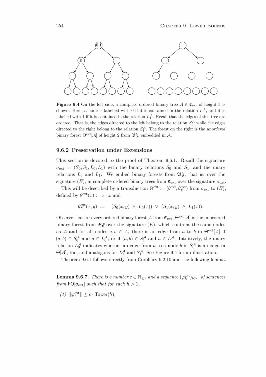
254 Chapter 9. Lower Bounds
0,1
0
Figure 9.4 On the left side, a complete ordered binary tree A ∈ Cext of height 3 isshown. Here, a node is labelled with 0 if it is contained in the relation LA0 , and it islabelled with 1 if it is contained in the relation LA1 . Recall that the edges of this tree areordered. That is, the edges directed to the left belong to the relation SA0 while the edgesdirected to the right belong to the relation SA1 . The forest on the right is the unorderedbinary forest Θext[A] of height 2 from BF, embedded in A.
9.6.2 Preservation under Extensions
This section is devoted to the proof of Theorem 9.6.1. Recall the signatureσext = (S0, S1, L0, L1) with the binary relations S0 and S1, and the unaryrelations L0 and L1. We embed binary forests from BF, that is, over thesignature (E), in complete ordered binary trees from Cext over the signature σext.This will be described by a transduction Θext := (θext, θext
E ) from σext to (E),defined by θext(x) := x=x and
θextE (x, y) :=
(S0(x, y) ∧ L0(x)
)∨(S1(x, y) ∧ L1(x)
).
Observe that for every ordered binary forest A from Cext, Θext[A] is the unorderedbinary forest from BF over the signature (E), which contains the same nodesas A and for all nodes a, b ∈ A, there is an edge from a to b in Θext[A] if(a, b) ∈ SA0 and a ∈ LA0 , or if (a, b) ∈ SA1 and a ∈ LA1 . Intuitively, the unaryrelation LA0 indicates whether an edge from a to a node b in SA0 is an edge inΘ[A], too, and analogous for LA1 and SA1 . See Figure 9.4 for an illustration.
Theorem 9.6.1 follows directly from Corollary 9.2.10 and the following lemma.
Lemma 9.6.7. There is a number c ∈ N≥1 and a sequence (ϕexth )h>1 of sentences
from FO[σext] such that for each h > 1,
(1) ||ϕexth || ≤ c · Tower(h),
9.6 Preservation Theorems 255
(2) every existential FO[σext]-sentence that is Cext-equivalent to ϕexth has size
> Tower(h+3), and
(3) ϕexth is preserved under extensions on Cext.
Proof. Recall that each extension of a structure A contains A as an inducedsubstructure. Consider a complete ordered binary tree A ∈ Cext of height n ≥ 1and let a be its root node. Assume that SΘext[A](a) is a binary tree of heightat most n − 1. Then, every leaf b of SΘext[A](a) has an S0-successor and anS1-successor in A but is neither contained in LA0 nor in LA1 . Therefore, foreach extension B of A from Cext we have that SΘext[A](a) and SΘext[B](a) areisomorphic.
We will use the latter observation to protect binary tree encodings, embeddedin ordered binary trees from Cext, against modifications by extensions to theunderlying ordered binary tree. Towards this aim, recall that we know byLemma 9.6.6 that for each h > 1 and every i ∈ [0,Tower(h+3)), each binary treein Bh(i) has height < 2 · Tower(h+1).
Similar to the FO[E]-formula completen(x) defined in the proof of Lemma 9.6.4,we can define an FO[σext]-formula complete′n(x) of size log(n) for n ≥ 1 that issatisfied by a node a in an ordered binary forest A from Cext or Chom if and onlyif SAn (a) is complete with height n.In the following, we aim to transform Sentence (9.1), for each h > 1, into an
FO[σext]-sentence that not only has large Cext-minimal models but that is alsopreserved under extensions on Cext. To this end, we use the Θext-reducts of theFO[E]-formulae of Lemma 9.6.4 and Lemma 9.6.5.
For each h > 1, we let
ϕexth := ∃x
(encext
h (x) ∧ min−Θext
h (x))∧
∀x(
encexth (x) →
(max−Θext
h (x) ∨ ∃y(encext
h (y) ∧ succ−Θext
h (x, y))))
withencext
h (x) := enc−Θext
h (x) ∧ complete′2·Tower(h+1)(x).
For the fixed transduction Θext it follows from Lemma 2.6.4 that for eachformula ϕ from FO[E], the size of the Θext-reduct ϕ−Θext is linear in the size of ϕ.
256 Chapter 9. Lower Bounds
Therefore, by Lemma 9.6.4 and Lemma 9.6.5, and since complete′2·Tower(h+1)(x)has size in O(Tower(h)), the following claim holds.
Claim 1. There is a c ∈ N≥1 such that ||ϕexth || ≤ c · Tower(h) for each h > 1.
For the following, we fix a number h > 1. The proof of Lemma 9.6.7 iscompleted by showing the following to claims.
Claim 2. Every existential FO[σext]-sentence that is Cext-equivalent to ϕexth has
size > Tower(h+3).
Proof of Claim 2. It is straightforward to see that there are structures in Cext thatsatisfy ϕext
h . In particular, by definition of the subformulae of ϕexth in Lemma 9.6.4
and Lemma 9.6.5, each model A ∈ Cext of ϕexth has to contain at least a number
of Tower(h+3) pairwise distinct nodes a0, . . . , aTower(h+3)−1 such that, for eachi ∈ [0,Tower(h+3)), SΘext[A](ai) ∈ Bh(i), that is, SΘext[A](ai) is a binary treeencoding of the number i with parameter h. Thus, since Cext is closed underinduced substructures, Claim 2 follows from Lemma 9.6.3.
Claim 3. ϕexth is preserved under extensions on Cext.
Proof of Claim 3. Consider a model A ∈ Cext of ϕexth . By construction of the
sentence ϕexth , there are pairwise distinct nodes a0, . . . , aTower(h+3)−1 in A such
that, for each i ∈ [0,Tower(h+3)), SΘext[A](ai) belongs to the set Bh(i) and, inparticular, has height < 2 · Tower(h+1).
Let B ∈ Cext be an extension of A. By construction of the subformula encexth (x)
of ϕexth , for each i ∈ [0,Tower(h+3)), the substructure SA2·Tower(h+1)(ai) is a
complete ordered binary tree of height 2 · Tower(h+1). Therefore, SΘext[A](ai)and SΘext[B](ai) are isomorphic and thus, also SΘext[B](ai) belongs to the set Bh(i).On the other hand, let b be a node from B such that B |= encext
h [b]. Then, thereis an i ∈ [0,Tower(h+3)) such that SΘext[B](b) belongs to Bh(i) and hence, eitherB |= max−Θext
h [b] or B |= succ−Θext
h [b, ai+1]. In both cases, B |= ϕexth .
This completes the proof of Claim 3 and thus also the proof of Lemma 9.6.7.
9.6.3 Preservation under Homomorphisms
This section is devoted to the proof of Theorem 9.6.2. Here, we need to constructFO[σhom]-sentences with large Chom-minimal models that are preserved underhomomorphism on Chom. Recall that σhom is the signature consisting of the binaryrelation symbols S0 and S1, and a unary relation symbol LM for eachM ⊆ 0, 1.
9.6 Preservation Theorems 257
Furthermore, recall that in any A ∈ Chom, each node belongs to precisely oneof the unary relations LAM ,M ⊆ 0, 1. In other words, LAM , M ⊆ 0, 1 area colouring of the nodes of A. In particular, this implies that, if there is ahomomorphism h from A to a structure B ∈ Chom, then
a ∈ LAM iff h(a) ∈ LBM for all a ∈ A and M ⊆ 0, 1. (9.2)
In the following, we embed binary forest from BF in complete ordered binarytrees from Chom. Similar to Section 9.6.2, we describe this embedding as atransduction Θhom := (θhom, θhom
E ) from σhom to (E), defined by θhom(x) := x=xand
θhomE (x, y) :=
∨i∈0,1
(Si(x, y) ∧
∨M⊆0,1,i∈M
LM (x)).
Thus, for every ordered binary forest A from Chom, Θhom[A] is the unorderedbinary forest from BF which contains the same nodes as A and for all nodesa, b ∈ A, there is an edge from a to b if there is an i ∈ 0, 1 such that (a, b) ∈ SAiand a ∈ LAM for an M ⊆ 0, 1 with i ∈M . Intuitively, the unique M ⊆ 0, 1for which a ∈ LAM tells us whether an edge from a to a node b in the successorrelations SA0 and SA1 is also an edge in Θhom[A].
Note that we can interpret Figure 9.4 also as an illustration for the embeddingdescribed here. The only difference is that we have to understand the labelling ofthe nodes as an indicator for which unique unary relation LAM the node belongs to.That is, all unlabelled nodes belong to LA∅ , all nodes labelled with 0 and 1 belongto LA0,1, and all nodes labelled with 0 or 1 belong to LA0 or L
A1, respectively.
Theorem 9.6.2 follows directly from Corollary 9.2.10 and the following lemma.
Lemma 9.6.8. There is a number c ∈ N≥1 and a sequence (ϕhomh )h>1 of sen-
tences from FO[σhom] such that for each h > 1,
(1) ||ϕhomh || ≤ c · Tower(h),
(2) every existential-positive FO[σhom]-sentence that is Chom-equivalent to ϕhomh
has size > Tower(h+3), and
(3) ϕhomh is preserved under homomorphisms on Chom.
Proof. Consider a complete ordered binary tree A ∈ Chom with height n ≥ 1 andlet a its root node. Observe that every homomorphism h from A to an ordered
258 Chapter 9. Lower Bounds
binary forest B ∈ Chom is injective. Furthermore, if SΘhom[A](a) is a binary treeof height at most n− 1, then SΘhom[A](a) and SΘhom[B](h(a)) are isomorphic.The remainder of the proof is very similar to the one of Lemma 9.6.7. We
define a sequence (ϕhomh )h>1 of FO[σhom]-sentences in the same way as the se-
quence (ϕexth )h>1 in the proof of Lemma 9.6.7, with the only difference being
that we use reducts in respect to the transduction Θhom instead of the transduc-tion Θext. That is, for each h > 1, we let
ϕhomh := ∃x
(enchom
h (x) ∧ min−Θhom
h (x))∧
∀x(
enchomh (x) →
(max−Θhom
h (x) ∨ ∃y(enchom
h (y) ∧ succ−Θhom
h (x, y))))
withenchom
h (x) := enc−Θhom
h (x) ∧ complete′2·Tower(h+1)(x).
By this construction, we immediately obtain that Statement (1) holdsLet h > 1. In an analogous way to Claim 2 in the proof of Lemma 9.6.7,
we obtain that each model of ϕhomh from Chom, has a universe of size at least
Tower(h+3). Since every existential-positive sentence is, in particular, an exist-ential sentence and since Chom is closed under induced substructures, we obtainStatement (2) from Lemma 9.6.3.To show that ϕhom
h is preserved under extensions on Chom and thus, State-ment (3) is satisfied, we also can proceed in a similar fashion as in the proof ofLemma 9.6.7. Consider a model A ∈ Chom of ϕhom
h . By construction of ϕhomh ,
there are pairwise distinct nodes a0, . . . , aTower(h+3)−1 in A such that, for eachi ∈ [0,Tower(h+3)), SΘhom[A](ai) belongs to the set Bh(i) and thus has height< 2 · Tower(h+1).Let B ∈ Chom such that there is a homomorphism h from A to B. By
construction of the subformula enchomh (x) of ϕhom
h , for each i ∈ [0,Tower(h+3)),the substructure SA2·Tower(h+1)(ai) is a complete ordered binary tree of height
2 · Tower(h+1). Therefore, SΘhom[A](ai) and SΘhom[B]h(ai) are isomorphic and thus,
also SΘhom[B](h(ai)) belongs to the set Bh(i). On the other hand, let b be anode from B such that B |= enchom
h [b]. Then, there is an i ∈ [0,Tower(h+3))such that SΘhom[B](b) belongs to Bh(i) and hence, either B |= max−Θhom
h [b] orB |= succ−Θhom
h [b, h(ai+1)]. We can conclude that B |= ϕhomh .
This completes the proof of Lemma 9.6.8.
9.7 Conclusion 259
9.7 Conclusion
In this chapter, we have proven lower bounds for the time complexity of thealgorithms presented in the previous chapters. While most of these algorithmswere generalised to extensions of first-order logic by ultimately periodic countingquantifiers that were even allowed to count tuples, all lower bounds already holdfor plain first-order logic FO.
For the construction of Hanf normal form, Gaifman normal form, and Feferman-Vaught decompositions, the lower bounds are 3-fold exponential in the size ofthe input formula for degree bounds d ≥ 3, and 2-fold exponential for d = 2,showing that our corresponding algorithms are basically worst-case optimal.For the construction of existential sentences for sentences that are preserved
under extensions on structures of degree d ≥ 3, we have proven a non-matching3-fold exponential lower bound. The same holds for the construction of existential-positive sentences for sentences that are preserved under extensions.All lower bounds rely on encodings of large initial segments of the natural
numbers by tree-like structures of bounded degree that can be compared bysmall formulae. In particular, for Hanf normal form, Gaifman normal form, andFeferman-Vaught decompositions, the combinatorial essence of the proofs wasstated in such a way that it can be applied to various classes of structures.

10 Conclusion
This chapter concludes the thesis with a short summary of its main resultsand some directions for further research. The aim of this thesis was to invest-igate the complexity of normal forms for (extensions of) first-order logic onclasses of structures of bounded degree. This was motivated by the fact that,already on classes of acyclic structures without degree limit, normal forms likeGaifman normal form [Gai82], Feferman-Vaught decompositions [FV59], andexistential(-positive) formulae for formulae that are preserved under extensions(homomorphisms) (cf., e.g., [Lyn59, Hod93, Ros08]), have a non-elementaryblow-up [DGKS07, Ros08]. The main results of this thesis are, contrary to this,elementary and, for Gaifman normal form and Feferman-Vaught decompositions,worst-case optimal algorithms for classes of structures of bounded degree.
In another direction, extensions of first-order logic (FO) by sets of unarycounting quantifiers are characterised that permit suitable generalisations ofHanf normal form [BK12]. It turns out that these are precisely sets of ultimatelyperiodic quantifiers. For the respective extensions of FO, it was shown that Hanfnormal form can be computed in worst-case optimal time. In particular, this ledto corresponding generalisations of the aforementioned algorithms for Feferman-Vaught decompositions and preservation theorems. Furthermore, following awell-known construction (described, e.g., in [Str94]), these algorithms could evenbe extended to formulae with tuple-counting quantifiers.
This thesis’ results were largely published in [HKS13, HHS14, HHS15, HKS16].In the following, we fix a degree bound d ≥ 2, let Cd denote the class of all
d-bounded structures over a relational signature σ, and restrict attention toformulae over this signature.
Results for First-Order Logic
Let us first focus on the special case of FO. This thesis’ main results concerningGaifman normal form and Feferman-Vaught decompositions can be stated asfollows:
261

262 Chapter 10. Conclusion
(G) For each formula ϕ of FO[σ], a d-equivalent Gaifman normal form can beconstructed in 3-fold (2-fold) exponential time for d ≥ 3 (d = 2).
(FV) For each formula ϕ of FO[σs], for s ≥ 1, a decomposition with respectto s-ary disjoint sums of structures from Cd can be constructed in 3-fold(2-fold) exponential time for d ≥ 3 (d = 2).
The latter result (FV) was, moreover, adapted to decompositions with respect todirect products and, more generally, decompositions with respect to transductionsover disjoint sums. For (G) as well as for (FV) matching lower bounds were shown,implying the worst-case optimality of both algorithms. The construction forGaifman normal form (G) and the matching lower bound are based on [HKS13],while (FV) and the corresponding matching lower bound are based on [HHS14,HHS15]. In both algorithms, the first step is the construction of a d-equivalentHanf normal form. This is followed by a transformation of the sphere-formulaeand counting-sentences in the Hanf normal form, which is irrespective of thedegree bound.
Concerning the preservation theorems of Lyndon, Łoś, and Tarski, this thesisprovides the following results:
(PE) For each formula ϕ of FO[σ] that is preserved under extensions on Cd, ad-equivalent existential FO[σ]-formula can be constructed in 5-fold (3-fold)exponential time for d ≥ 3 (d = 2).
(PH) For each formula ϕ of FO[σ] that is preserved under homomorphisms on Cd,a d-equivalent existential-positive FO[σ]-formula can be constructed in4-fold (3-fold) exponential time for d ≥ 3 (d = 2).
Note that (PE) and (PH) do not only hold on the class Cd, but on all classesof d-bounded σ-structures that are closed under disjoint unions and inducedsubstructures and that, for (PH), are decidable in 1-fold exponential time.Furthermore, both closure properties were actually shown to be unavoidable.The upper bounds of (PE) and (PH) are complemented by (non-matching) 3-foldexponential lower bounds. (PE) and (PH), as well as counterexamples for theclosure properties and the lower bounds, were first published in [HHS14, HHS15].There, both results already extend to FO-sentences with one modulo-countingquantifier, but only consider formulae without free variables.The crucial ingredient in both algorithms is an upper bound on the size of
Cd-minimal models for the input formula, which is obtained by using Hanf’s
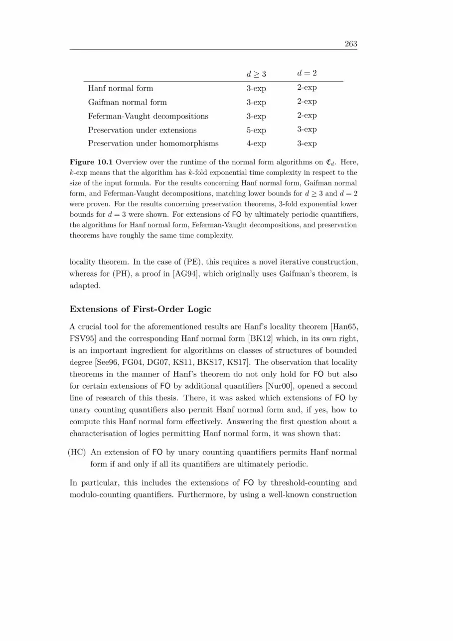
263
d ≥ 3 d = 2
Hanf normal form 3-exp 2-exp
Gaifman normal form 3-exp 2-exp
Feferman-Vaught decompositions 3-exp 2-exp
Preservation under extensions 5-exp 3-expPreservation under homomorphisms 4-exp 3-exp
Figure 10.1 Overview over the runtime of the normal form algorithms on Cd. Here,k-exp means that the algorithm has k-fold exponential time complexity in respect to thesize of the input formula. For the results concerning Hanf normal form, Gaifman normalform, and Feferman-Vaught decompositions, matching lower bounds for d ≥ 3 and d = 2were proven. For the results concerning preservation theorems, 3-fold exponential lowerbounds for d = 3 were shown. For extensions of FO by ultimately periodic quantifiers,the algorithms for Hanf normal form, Feferman-Vaught decompositions, and preservationtheorems have roughly the same time complexity.
locality theorem. In the case of (PE), this requires a novel iterative construction,whereas for (PH), a proof in [AG94], which originally uses Gaifman’s theorem, isadapted.
Extensions of First-Order Logic
A crucial tool for the aforementioned results are Hanf’s locality theorem [Han65,FSV95] and the corresponding Hanf normal form [BK12] which, in its own right,is an important ingredient for algorithms on classes of structures of boundeddegree [See96, FG04, DG07, KS11, BKS17, KS17]. The observation that localitytheorems in the manner of Hanf’s theorem do not only hold for FO but alsofor certain extensions of FO by additional quantifiers [Nur00], opened a secondline of research of this thesis. There, it was asked which extensions of FO byunary counting quantifiers also permit Hanf normal form and, if yes, how tocompute this Hanf normal form effectively. Answering the first question about acharacterisation of logics permitting Hanf normal form, it was shown that:
(HC) An extension of FO by unary counting quantifiers permits Hanf normalform if and only if all its quantifiers are ultimately periodic.
In particular, this includes the extensions of FO by threshold-counting andmodulo-counting quantifiers. Furthermore, by using a well-known construction
264 Chapter 10. Conclusion
(cf. [Str94]), it also includes extensions of FO by ultimately periodic countingquantifiers that are allowed to count over tuples of elements instead of singleelements of structures.To show that ultimately periodic quantifiers permit Hanf normal form, we
first generalised the algorithm of [BK12] to extensions of FO by modulo-countingquantifiers. In a second step, we have expressed ultimately periodic quantifiersby modulo-counting quantifiers and vice versa. On the other hand, even a verysimple sentence over the signature (P ), where P is a unary relation symbol,stating that the cardinality of a structure belongs to a set that is not ultimatelyperiodic, can not be expressed by a Hanf normal form.
The second result in this direction shows that, if an extension of FO by unarycounting quantifiers permits Hanf normal form, then such Hanf normal formscan also be computed efficiently:
(HA) For each extension of FO that permits Hanf normal form, every formula ϕcan be turned into a d-equivalent Hanf normal form in 3-fold (2-fold)exponential time for d ≥ 3 (d = 2).
This algorithm follows directly from an analysis of the proof of (HC). Matchinglower bounds, already presented in [BK12], show the worst-case optimality ofthe algorithm implied by (HA). As an application, (HA) leads to straightforwardextensions of Seese’s fixed-parameter model-checking algorithm on Cd [See96] forformulae with ultimately periodic quantifiers.Moreover, (HC) and (HA) allow the generalisation of the results (FV), (PE),
and (PH) to extensions of FO by ultimately periodic quantifiers. In all these cases,we obtain algorithms with basically the same time complexity as in the case ofFO, which are therefore worst-case optimal. For the case of Feferman-Vaughtdecompositions, it was proven that a similar characterisation as (HC) holds:
(FVC) An extension of FO by unary counting quantifiers permits decompositionswith respect to disjoint sums if and only if all its quantifiers are ultimatelyperiodic.
(HC) as well as (HA) were first published in [HKS16], although without regardto tuple-quantifiers. The variants of (PE) and (PH) for the case of FO with anadditional modulo-counting quantifier were published in [HHS14, HHS15].
Note that recently it was shown in [KS17] that a weaker variant of Hanf normalform, where counting-sentences may count over disjunctions of types, can be
265
constructed for arbitrary sets of unary counting quantifiers and not only forultimately periodic quantifiers.For Gaifman normal form, [KS18] presents a generalisation to extensions of
FO by unary counting quantifiers and shows that (on all structures) equivalentformulae in Gaifman normal form can be computed if and ony if all quantifiersinvolved are ultimately periodic. This is used in [KS18] to extend a resultof [FG01] in order to show the fixed-parameter tractability of the model-checkingproblem for such logics on classes of structures of bounded local tree-width. Forclasses of structures of bounded degree, [KS18] shows that Gaifman normal formexists even for arbitrary unary counting quantifiers and can be constructed inworst-case optimal 3-fold exponential time if all quantifiers involved are ultimatelyperiodic.
Further Research
The results of this thesis are stated for the setting of finite structures. One aimwould be to determine which of these results also hold for infinite structures.
For applications of Hanf normal form in model-checking and related tasks, apossible direction of further research would be to examine constructions of Hanfnormal form which are guided by the specific task, e.g., by only performing apartial construction of the Hanf normal form with respect to a fixed structure.
Concerning preservation theorems, an obvious direction of further research isto close the gap between the upper and the lower bounds provided in this thesis.For (PE), there might be potential for finding a better upper bound on the sizeof minimal models. For (PH), an alternative to the Chandra-Merlin theorem[CM77, AHV95], e.g., in a similar way to the relativisation of quantifiers usedfor (PE), could lead to a better upper bound.Similarly to the Łoś-Tarski-theorem, Lyndon’s positivity theorem [Lyn59],
stating that an FO-sentence is preserved under surjective homomorphisms ifand only if it is equivalent to a positive sentence, is known to fail on finitestructures [AG87, Sto95]. To the author’s knowledge, it is not known whetherthere are classes of finite structures for which it can be reestablished. It wouldbe interesting to identify such classes and then, to examine the complexity ofconstructing the positive sentences with respect to these classes.
Finally, besides Gaifman normal form and Hanf normal form, there is a furtherlocal normal form, described in [SB99], that invites an investigation into itsefficiency.

Bibliography
[ADG08] Albert Atserias, Anuj Dawar, and Martin Grohe. Preservation un-der extensions on well-behaved finite structures. SIAM Journal onComputing, 38(4):1364–1381, 2008.
[ADK06] Albert Atserias, Anuj Dawar, and Phokion G. Kolaitis. On pre-servation under homomorphisms and unions of conjunctive queries.Journal of the ACM, 53(2):208–237, 2006.
[AG87] Miklós Ajtai and Yuri Gurevich. Monotone versus positive. Journalof the ACM, 34(4):1004–1015, 1987.
[AG94] Miklós Ajtai and Yuri Gurevich. Datalog vs first-order logic. Journalof Computer and System Sciences, 49(3):562–588, 1994.
[AHV95] Serge Abiteboul, Richard Hull, and Victor Vianu, editors. Foundationsof Databases: The Logical Level. Addison-Wesley Longman PublishingCo., Inc., Boston, MA, USA, 1st edition, 1995.
[BK12] Benedikt Bollig and Dietrich Kuske. An optimal construction of Hanfsentences. Journal of Applied Logic, 10(2):179–186, 2012.
[BKS17] Christoph Berkholz, Jens Keppeler, and Nicole Schweikardt. Answer-ing FO+MOD queries under updates on bounded degree databases.In Michael Benedikt and Giorgio Orsi, editors, 20th InternationalConference on Database Theory (ICDT 2017), volume 68 of LeibnizInternational Proceedings in Informatics (LIPIcs), pages 8:1–8:18,Dagstuhl, Germany, 2017. Schloss Dagstuhl–Leibniz-Zentrum fuerInformatik.
[Clo12] Martin Clochard. Énumération de requêtes du premier ordre sur lesstructures de degré borné, 2012. Report on internship at Équipe deLogique Mathématique Université Denis-Diderot Paris 7, supervisedby Arnaud Durand.
267
268 Bibliography
[CM77] Ashok K. Chandra and Philip M. Merlin. Optimal implementation ofconjunctive queries in relational data bases. In Proceedings of the 9thAnnual ACM Symposium on Theory of Computing, STOC’77, pages77–90, 1977.
[Daw10] Anuj Dawar. Homomorphism preservation on quasi-wide classes.Journal of Computer and System Sciences, 76(5):324–332, 2010.
[DG07] Arnaud Durand and Etienne Grandjean. First-order queries onstructures of bounded degree are computable with constant delay.ACM Transactions on Computational Logic, 8(4), 2007.
[DGKS06] Anuj Dawar, Martin Grohe, Stephan Kreutzer, and Nicole Sch-weikardt. Approximation schemes for first-order definable optim-isation problems. In Proceedings of the 21th Annual IEEE Symposiumon Logic in Computer Science (LICS 2006), pages 411–420, 2006.
[DGKS07] Anuj Dawar, Martin Grohe, Stephan Kreutzer, and Nicole Sch-weikardt. Model Theory Makes Formulas Large. In Proceedingsof the 34th International Colloquium on Automata, Languages andProgramming (ICALP 2007), pages 1076–1088, 2007. Full versionavailable as preprint NI07003-LAA, Isaac Newton Institute of Math-ematical Sciences (2007).
[DSS14] Arnaud Durand, Nicole Schweikardt, and Luc Segoufin. Enumerat-ing Answers to First-Order Queries over Databases of Low Degree.In Proceedings of the 33th ACM SIGMOD/PODS Symposium onPrinciples of Database Systems (PODS 2014), Snowbird, USA, 2014.
[EF99] Heinz-Dieter Ebbinghaus and Jörg Flum. Finite Model Theory.Springer, 1999.
[FG01] Markus Frick and Martin Grohe. Deciding first-order properties oflocally tree-decomposable structures. Journal of the ACM, 48(6):1184–1206, 2001.
[FG04] Markus Frick and Martin Grohe. The complexity of first-order andmonadic second-order logic revisited. Annals of Pure and AppliedLogic, 130(1-3):3–31, 2004.
Bibliography 269
[FG06] Jörg Flum and Martin Grohe. Parameterized Complexity Theory.Springer-Verlag Berlin Heidelberg, 2006.
[FSV95] Ronald Fagin, Larry J. Stockmeyer, and Moshe Y. Vardi. On monadicNP vs. monadic co-NP. Information and Computation, 120(1):78–92,1995.
[FV59] Solomon Feferman and Robert L. Vaught. The first order properties ofproducts of algebraic systems. Fundamenta Mathematicae, 47:57–103,1959.
[Gai82] Haim Gaifman. On local and non-local properties. In J. Stern, editor,Proceedings of the Herbrand Symposium, Logic Colloquium ’81, pages105–135. North Holland, 1982.
[GJL12] Stefan Göller, Jean Christoph Jung, and Markus Lohrey. The com-plexity of decomposing modal and first-order theories. In Proceedingsof the 27th Annual IEEE Symposium on Logic in Computer Science(LICS 2012), pages 325–334, 2012.
[GKS14] Martin Grohe, Stephan Kreutzer, and Sebastian Siebertz. Decidingfirst-order properties of nowhere dense graphs. In David B. Shmoys,editor, Symposium on Theory of Computing, STOC 2014, New York,NY, USA, May 31 - June 03, 2014, pages 89–98. ACM, 2014.
[Gro17] Martin Grohe. Descriptive Complexity, Canonisation, and Defin-able Graph Structure Theory. Lecture Notes in Logic. CambridgeUniversity Press, 2017. To appear. Preliminary version avail-able at https://www.lii.rwth-aachen.de/de/13-mitarbeiter/professoren/39-book-descriptive-complexity.html.
[Gru16] Berit Grußien. Capturing Polynomial Time and Logarithmic Spaceusing Modular Decompositions and Limited Recursion. PhD thesis,Department of Computer Science, Humboldt-Universität zu Berlin,2016.
[GS04] Martin Grohe and Nicole Schweikardt. Comparing the succinctnessof monadic query languages over finite trees. RAIRO - TheoreticalInformatics and Applications, 38(4):343–373, 2004.
270 Bibliography
[GS05] Martin Grohe and Nicole Schweikardt. The succinctness of first-orderlogic on linear orders. Logical Methods in Computer Science, 1(1),2005.
[Gur84] Yuri Gurevich. Toward logic tailored for computational complexity.In M. Richter et al., editor, Computation and Proof Theory, volume1104 of Lecture Notes in Mathematics, pages 175–216. Springer, 1984.
[Gur90] Yuri Gurevich. On Finite Model Theory (Extended Abstract), pages211–219. Birkhäuser Boston, Boston, MA, 1990.
[GW04] Martin Grohe and Stefan Wöhrle. An existential locality theorem.Annals of Pure and Applied Logic, 129(1-3):131–148, 2004.
[Han65] William Hanf. Model-theoretic methods in the study of elementarylogic. In J.W. Addison, L. Henkin, and A. Tarski, editors, The Theoryof Models, pages 132–145. North Holland, 1965.
[Hei12] Lucas Heimberg. Gaifman-Normalformen auf Strukturklassen be-schränkten Grades. Diplomarbeit, HU Berlin, 2012.
[HHS14] Frederik Harwath, Lucas Heimberg, and Nicole Schweikardt. Preser-vation and decomposition theorems for bounded degree structures. InJoint Meeting of the 23rd EACSL Annual Conference on ComputerScience Logic (CSL) and the 29th Annual ACM/IEEE Symposiumon Logic in Computer Science (LICS), (CSL-LICS 2014), pages 49:1–49:10. ACM, 2014.
[HHS15] Frederik Harwath, Lucas Heimberg, and Nicole Schweikardt. Preser-vation and decomposition theorems for bounded degree structures.Logical Methods in Computer Science, 11(4), 2015.
[HKS13] Lucas Heimberg, Dietrich Kuske, and Nicole Schweikardt. An optimalGaifman normal form construction for structures of bounded degree.In Proceedings of the 28th Annual ACM/IEEE Symposium on Logicin Computer Science, (LICS 2013), pages 63–72, 2013.
[HKS16] Lucas Heimberg, Dietrich Kuske, and Nicole Schweikardt. Hanfnormal form for first-order logic with unary counting quantifiers. InProceedings of the 31th Annual ACM/IEEE Symposium on Logic inComputer Science, (LICS 2016), pages 63–72, 2016.
Bibliography 271
[HLN99] Lauri Hella, Leonid Libkin, and Juha Nurmonen. Notions of localityand their logical characterizations over finite models. Journal ofSymbolic Logic, 64(4):1751–1773, 1999.
[Hod93] Wilfrid Hodges. Model Theory. Cambridge University Press, 1993.
[KM14] Tomer Kotek and Johann A. Makowsky. Connection matrices andthe definability of graph parameters. Logical Methods in ComputerScience, 10(4), 2014.
[Kre11] Stephan Kreutzer. Algorithmic meta-theorems. In Finite and Al-gorithmic Model Theory. Cambridge University Press, 2011. LondonMathematical Society Lecture Notes, No. 379.
[KS11] Wojciech Kazana and Luc Segoufin. First-order query evaluation onstructures of bounded degree. Logical Methods in Computer Science,7(2), 2011.
[KS17] Dietrich Kuske and Nicole Schweikardt. First-order logic with count-ing: At least, weak Hanf normal forms always exist and can becomputed! In Proceedings of the 32nd Annual ACM/IEEE Sym-posium on Logic in Computer Science, (LICS 2017), 2017. To appear.Full version available at https://arxiv.org/abs/1703.01122.
[KS18] Dietrich Kuske and Nicole Schweikardt. Gaifman normal forms forcounting extensions of first-order logic. In Proceedings of the 45thInternational Colloquium on Automata, Languages, and Programming(ICALP 2018), 2018. To appear.
[Lib97] Leonid Libkin. On the forms of locality over finite models. In Pro-ceedings of the 12th Annual IEEE Symposium on Logic in ComputerScience (LICS 1997), pages 204–215, 1997.
[Lib98] Leonid Libkin. On counting logics and local properties. In Proceedingsof the 13th Annual IEEE Symposium on Logic in Computer Science,LICS 1998, pages 501–, Washington, DC, USA, 1998. IEEE ComputerSociety.
[Lib04] Leonid Libkin. Elements of Finite Model Theory. Springer, 2004.
272 Bibliography
[Lin08] Steven Lindell. A normal form for first-order logic over doubly-linkeddata structures. International Journal of Foundations of ComputerScience, 19(1):205–217, 2008.
[LN00] Leonid Libkin and Juha Nurmonen. Counting and locality over finitestructures: A survey. In Revised Lectures from the 9th EuropeanSummer School on Logic, Language, and Information: GeneralizedQuantifiers and Computation, ESSLLI ’97, pages 18–50, London, UK,UK, 2000. Springer-Verlag.
[Lot84] M. Lothaire. Combinatorics on words. Cambridge University Press,1984.
[Lyn59] Roger C. Lyndon. Properties preserved under homomorphism. PacificJournal of Mathematics, 9(1):143–154, 1959.
[Mak04] Johann A. Makowsky. Algorithmic uses of the Feferman-Vaughttheorem. Annals of Pure and Applied Logic, 126(1-3):159–213, 2004.
[Mat94] Armando B. Matos. Periodic sets of integers. Theoretical ComputerScience, 127(2):287–312, 1994.
[NSST15] Frank Neven, Nicole Schweikardt, Frédéric Servais, and Tony Tan.Distributed streaming with finite memory. In Proc. 18th InternationalConference on Database Theory (ICDT 2015), pages 324–341, 2015.Full version available at https://www.csie.ntu.edu.tw/~tonytan/research/2015-icdt-dstj.pdf.
[Nur96] Juha Nurmonen. On winning strategies with unary quantifiers.Journal of Logic and Computation, 6:779–798, 1996.
[Nur00] Juha Nurmonen. Counting modulo quantifiers on finite structures.Information and Computation, 160(1–2):62–87, 2000.
[PV06] Guoqiang Pan and Moshe Y. Vardi. Fixed-parameter hierarchies insidePSPACE. In 21th IEEE Symposium on Logic in Computer Science(LICS 2006), 12-15 August 2006, Seattle, WA, USA, Proceedings,pages 27–36. IEEE Computer Society, 2006.
[Ros08] Benjamin Rossman. Homomorphism preservation theorems. Journalof the ACM, 55(3), 2008.
Bibliography 273
[Ros16] Benjamin Rossman. An improved homomorphism preservation the-orem from lower bounds in circuit complexity. SIGLOG News, 3(4):33–46, 2016.
[SB99] Thomas Schwentick and Klaus Barthelmann. Local normal forms forfirst-order logic with applications to games and automata. DiscreteMathematics and Computer Science, 3:109–124, 1999.
[See96] Detlef Seese. Linear time computable problems and first-order descrip-tions. Mathematical Structures in Computer Science, 6(6):505–526,1996.
[Seg14] Luc Segoufin. A glimpse on constant delay enumeration (invited talk).In Proceedings of the 31st International Symposium on TheoreticalAspects of Computer Science (STACS 2014), pages 13–27, 2014.
[SM73] Larry J. Stockmeyer and Albert R. Meyer. Word problems requiringexponential time (preliminary report). In Proceedings of the FifthAnnual ACM Symposium on Theory of Computing, STOC ’73, pages1–9, New York, NY, USA, 1973. ACM.
[Sto95] Alexei P. Stolboushkin. Finitely monotone properties. In Proceedings,10th Annual IEEE Symposium on Logic in Computer Science, SanDiego, California, USA, June 26-29, 1995, pages 324–330. IEEEComputer Society, 1995.
[Str94] Howard Straubing. Finite Automata, Formal Logic, and CircuitComplexity. Birkhauser Verlag, Basel, Switzerland, Switzerland, 1994.
[Tai59] William W. Tait. A counterexample to a conjecture of Scott andSuppes. Journal of Symbolic Logic, 24:15–16, 1959.
[Wil94] Ross Willard. Hereditary undecidability of some theories of finitestructures. Journal of Symbolic Logic, 59(4):1254–1262, 1994.

Index
(A, a), 27(b1; . . . ; bn), 30E, 35[n,m), 17[n,m], 17Θ[A], 30χQ, 28γ(A,a)(x), 140|=, 22, 26, 99ϕ(x), 27ϕ−Θ, 31⟨δij⟩≡ rmod pM
, 44⟨δij⟩>kM
, 46
A−B, 21A[B], 21ar(R), 20additive, 178alphabet, 18atomic formula, 22
Bh(i), 216BF, 216BT, 216bit(j, i), 17basic local sentence, 82binary forest, 216binary tree, 216bit string, 214Boolean connective, 22
Cd,σ, 37Call, 23Const, 20canonical conjunctive query, 140centre, 38characteristic sequence, 28child, 208complete, 210, 216composition, 97counting-formula, 50
proper, 50counting-sentence, 50
Dall, 24DU , 178Dp, 24(Dp+r), 24distA(a, b), 37d-bounded
graph, 35structure, 37
decompositionΘ-, 107⊕-, 100⊗-, 111
degreegraph, 35node, 35
degree bound, 35
275

276 Index
dimension, 26direct product, 111disjoint
structures, 21sum, 98union, 21
(∃+k), 23∃≡ kmod p, 25∃, 23∃=0, 25∃=k, 25∃>k, 25∃≥k, 25σ-expansion, 21k-fold exponential, 18edge, 35elementary, 18equivalent, 27
C-, 27d-, 37with respect to τ , 56
existential, 118existential-positive, 118extension, 117
disjoint, 126
F, 209Fd, 210FO, 24FO+unC, 25FO+unC(C), 25FO+unT, 24FO+unM, 24FO+unM(D), 24FO+unC(C)tpl, 53FO+unM(D)tpl, 53
FO+unTtpl, 53free(ϕ), 25fd(h), 210first-order logic, 24forest, 208forest-like, 209free variables, 25
GA, 37gnf-formula, 83gnf-sentence, 83Gaifman graph, 37Gaifman normal form, 83graph, 35
loop-free, 35undirected, 35
hnf-formula, 53hnf-sentence, 51Hanf normal form, 51, 53
formula, 53sentence, 51
heightforest, 208node, 208
homomorphism, 118
σ-interpretation, 26isomorphic, 21
L, 22L[σ], 23Ltpl, 25log r, 18r-local, 82labelled and ordered tree, 209labelled chain, 214leaf, 208
Index 277
least common multiple, 17length
labelled chain, 214path, 35word, 18
locality radius, 51, 53counting-formula, 50
C-minimal model, 122
N, 17N≥t, 17NAr (W ), 38NAr (a), 38NAr (a), 38νd(r), 39neighbourhood, 38node, 35
O(f), 18o(f), 18offset, 28
PL, 22PS, 22poly(f), 18parent, 208path, 35period, 28
maximum, 26prefix, 19preserved under
extensions, 118homomorphisms, 118
propositionalformula, 22interpretation, 22symbol, 22
Q, 23(Q+k), 23qr(Θ), 30qr(ϕ), 25quantifier
modulo-counting, 24threshold-counting, 23tuple-counting, 25unary counting quantifier, 23
quantifier rank, 25quantifier weight, 179
R, 18R≥0, 18ram, 19Θ-reduct, 31rep(A), 20rep(ϕ), 22, 29rep(Q), 29rep(σ), 20τ -reduct, 21Rel, 20radius, 38realise, 39reduction sequence, 99
model, 99reference, 98
back, 98relational, 20root, 208run time, 19
SF (a), 209SF` (a), 208Sd,s(r), 124SF (a), 209SF` (a), 208
278 Index
Σ∗, 18Σω, 19||A||, 21||∆||, 99||Θ||, 30||ϕ||, 22, 29||Q||, 29||σ||, 20sphτ (x), 41s-scattered, 37sphere, 38structure, 20substructure, 21
induced, 21substructure-free, 221successor, 208
T (i), 215T, 209Td,σr (n), 40Td, 210Td,`, 210Tower(n), 18Tower(n, r), 18τ(A), 39threshold, 26transduction, 30
quantifier rank, 30size, 30
tree, 208tree encoding, 215tree-like, 209tuple, 19
subtuple, 19type, 38
Uall, 28
ultimately periodic, 28uniform cost measure, 19union, 21universe, 20
Var, 22
w(i, j], 19w[i, j], 19w[n], 18word
ω-, 18empty, 18finite, 18primitive, 28primitive root, 28
Z, 17
Erklärung
Ich erkläre hiermit, dass
• ich die vorliegende Dissertation
Complexity of Normal Forms on Structures of Bounded Degree
selbstständig und ohne unerlaubte Hilfe angefertigt habe;
• ich mich weder bereits anderwärts um einen Doktorgrad im mathematisch-naturwissenschaftlichen Bereich beworben habe, noch einen solchen besitze;
• mir die Promotionsordnung der Mathematisch-Naturwissenschaftlichen Fa-kultät der Humboldt-Universität zu Berlin vom 30. Juni 2014, veröffentlichtim Amtlichen Mitteilungsblatt Nr. 126/2014, bekannt ist.
Berlin, den 4. 4. 2017
Lucas Heimberg