complete primitives for information-theoretically secure two
TRANSCRIPT

Complete Primitives forInformation-Theoretically Secure
Two-Party Computation
zur Erlangung des akademischen Grades eines
Doktors der Naturwissenschaften
von der Fakultät für Informatikdes Karlsruher Instituts für Technologie (KIT)
genehmigte
Dissertation
von
Daniel Kraschewski
aus Bad Pyrmont
Tag der mündlichen Prüfung: 25. Januar 2013
Erster Gutachter: Prof. Dr. Jörn Müller-Quade
Zweiter Gutachter: Prof. Dr. Yuval Ishai
KIT – University of the State of Baden-Wuerttemberg and National Laboratory of the Helmholtz Association www.kit.edu


Acknowledgements
First of all, I want to express my deep gratitude to Jörn Müller-Quade. I am very grateful forhis support and the exceptional freedom of research I enjoyed under his doctorate supervision.His fascination for the wonders of modern cryptography were a great source of inspiration, and Ipersonally benefited also a lot from numerous non-technical discussions about science in general,ways of life and philosophy. No less I want to thank Yuval Ishai for co-refereeing this thesis andall his support far beyond that. I am especially impressed, how every discussion with him wascharacterized by a notably kind atmosphere and always turned out fruitful.
For proofreading, help with LATEX on various occasions and his invaluable friendship I am ingreat debt to my former colleague Christian Henrich. I am also very thankful to all my colleaguesfor the familiar working atmosphere. In particular, I want to thank Nico Döttling for always havingtime for any technical discussion, and I thank Dennis Hofheinz for many helpful comments and thehonor and pleasure to work with him. My sincerest thanks go to Carmen Manietta and HolgerHellmuth, who at all times wondrously managed to keep any administrative and technical troublebehind the scenes.
Special thanks go to the mathoverflow community and especially Felipe Voloch for pointing meto the Łojasiewicz Inequality.
Last but not least, I would like to express my heartfelt gratitude to my family members andpersonal friends who encouraged and supported me throughout my studies.
iii


Contents
Abstract vii
Zusammenfassung ix
Preamble 1Background and motivation . . . . . . . . . . . . . . . . . . . . . . . . . . . . . . . . . . . 3Contribution and structure of this thesis . . . . . . . . . . . . . . . . . . . . . . . . . . . . 6General notations . . . . . . . . . . . . . . . . . . . . . . . . . . . . . . . . . . . . . . . . . 7
I Completeness Theorems 9
1 Introduction 111.1 Related work . . . . . . . . . . . . . . . . . . . . . . . . . . . . . . . . . . . . . . . . 111.2 Our contribution . . . . . . . . . . . . . . . . . . . . . . . . . . . . . . . . . . . . . . 121.3 Organization of Part I . . . . . . . . . . . . . . . . . . . . . . . . . . . . . . . . . . . 12
2 Presentation of our results 132.1 Notion of security . . . . . . . . . . . . . . . . . . . . . . . . . . . . . . . . . . . . . . 132.2 Basic concepts . . . . . . . . . . . . . . . . . . . . . . . . . . . . . . . . . . . . . . . 142.3 Completeness criteria for all finite randomized 2-party functions . . . . . . . . . . . 162.4 Comparison with criteria from the literature . . . . . . . . . . . . . . . . . . . . . . . 16
3 How to prove the Classification Theorem 193.1 Secure generation of correlated data . . . . . . . . . . . . . . . . . . . . . . . . . . . 20
3.1.1 The protocol for generating correlated data . . . . . . . . . . . . . . . . . . . 203.1.2 Idealized attack strategies . . . . . . . . . . . . . . . . . . . . . . . . . . . . . 213.1.3 Robust OT-cores . . . . . . . . . . . . . . . . . . . . . . . . . . . . . . . . . . 243.1.4 Robust OT-cores in real protocol runs . . . . . . . . . . . . . . . . . . . . . . 26
3.2 Reduction of OT to correlated data . . . . . . . . . . . . . . . . . . . . . . . . . . . . 303.2.1 Refining the correlated data . . . . . . . . . . . . . . . . . . . . . . . . . . . . 303.2.2 Building OT from the refined correlated data . . . . . . . . . . . . . . . . . . 33
4 Formal basis 354.1 Basic notions and notations . . . . . . . . . . . . . . . . . . . . . . . . . . . . . . . . 354.2 Linear properties of cheating situations . . . . . . . . . . . . . . . . . . . . . . . . . . 364.3 Cheating situations for redundant input symbols . . . . . . . . . . . . . . . . . . . . 394.4 Existence of robust OT-cores . . . . . . . . . . . . . . . . . . . . . . . . . . . . . . . 434.5 Protocol for generation of correlated data . . . . . . . . . . . . . . . . . . . . . . . . 464.6 Real protocol runs versus idealized cheating situations . . . . . . . . . . . . . . . . . 474.7 Secure generation of correlated data . . . . . . . . . . . . . . . . . . . . . . . . . . . 534.8 Conclusion of the formal basis for our completeness criteria . . . . . . . . . . . . . . 56
v

vi Contents
II David & Goliath OAFE 57
5 Introduction 595.1 Related work . . . . . . . . . . . . . . . . . . . . . . . . . . . . . . . . . . . . . . . . 595.2 Our contribution . . . . . . . . . . . . . . . . . . . . . . . . . . . . . . . . . . . . . . 615.3 Outline of Part II . . . . . . . . . . . . . . . . . . . . . . . . . . . . . . . . . . . . . . 63
6 Preliminaries 656.1 Notations . . . . . . . . . . . . . . . . . . . . . . . . . . . . . . . . . . . . . . . . . . 656.2 Framework & notion of security . . . . . . . . . . . . . . . . . . . . . . . . . . . . . . 656.3 Modeling tamper-proof hardware . . . . . . . . . . . . . . . . . . . . . . . . . . . . . 66
6.3.1 The hybrid functionality F statefulwrap . . . . . . . . . . . . . . . . . . . . . . . . . 66
6.3.2 Real world meaning of our hardware assumption and proof techniques . . . . 676.4 Sequential one-time OAFE and its relation to OTMs and OT . . . . . . . . . . . . . 67
7 Semi-interactive seq-ot-OAFE from one tamper-proof token 717.1 The basic protocol . . . . . . . . . . . . . . . . . . . . . . . . . . . . . . . . . . . . . 717.2 Refinements and applications of our construction . . . . . . . . . . . . . . . . . . . . 74
7.2.1 Unidirectional string-OT and OTMs with optimal communication complexity 747.2.2 Achieving optimal communication complexity for bidirectional string-OT . . 757.2.3 Reducing the number of rounds, e.g. for one-time programs . . . . . . . . . . 777.2.4 Computational solution for unlimited token reusability . . . . . . . . . . . . . 777.2.5 Efficient protocol for string-commitments in any direction . . . . . . . . . . . 777.2.6 Non-interactive solution with two tokens . . . . . . . . . . . . . . . . . . . . . 797.2.7 A note on optimal communication complexity . . . . . . . . . . . . . . . . . . 79
8 Correctness and security of our protocol 818.1 Correctness . . . . . . . . . . . . . . . . . . . . . . . . . . . . . . . . . . . . . . . . . 818.2 Security against a corrupted receiver . . . . . . . . . . . . . . . . . . . . . . . . . . . 818.3 Security against a corrupted sender . . . . . . . . . . . . . . . . . . . . . . . . . . . . 83
8.3.1 Independence of the token view . . . . . . . . . . . . . . . . . . . . . . . . . . 838.3.2 Committing the token to affine behavior . . . . . . . . . . . . . . . . . . . . . 858.3.3 Uniqueness of affine approximations of the token functionality . . . . . . . . . 888.3.4 Utilizing the Leftover Hash Lemma . . . . . . . . . . . . . . . . . . . . . . . . 888.3.5 The simulator for a corrupted Goliath . . . . . . . . . . . . . . . . . . . . . . 918.3.6 A sequence of hybrid games . . . . . . . . . . . . . . . . . . . . . . . . . . . . 938.3.7 Transformation of successive hybrid games . . . . . . . . . . . . . . . . . . . 938.3.8 Concluding the security proof . . . . . . . . . . . . . . . . . . . . . . . . . . . 105
9 No-go arguments & conclusion 1079.1 Impossibility of polynomially bounded simulation runtime . . . . . . . . . . . . . . . 1079.2 Impossibility of random access solutions with a constant number of tokens . . . . . . 1079.3 Lower bounds for David’s communication overhead . . . . . . . . . . . . . . . . . . . 1089.4 Conclusion & improvement opportunities . . . . . . . . . . . . . . . . . . . . . . . . 108
Appendices 111Table of symbols . . . . . . . . . . . . . . . . . . . . . . . . . . . . . . . . . . . . . . . . . 113List of figures . . . . . . . . . . . . . . . . . . . . . . . . . . . . . . . . . . . . . . . . . . . 115Bibliography . . . . . . . . . . . . . . . . . . . . . . . . . . . . . . . . . . . . . . . . . . . 117

Abstract
In 1988, Joe Kilian showed that arbitrary multi-party computation can be securely realized froma quite simple primitive, namely oblivious transfer (OT). This primitive in its basic form is just atrusted erasure channel: The sender can enter a bit of his choice, which is then transferred to thereceiver with probability 1
2 and otherwise replaced by a special erasure symbol. Since the discoverythat OT is complete in the above-mentioned sense, cryptographers are working on reductions ofOT (and thus general secure multi-party computation) to various other primitives. The presentthesis contributes two results to this research area.
The first contribution of this thesis exhaustively solves the long-standing open question, whichcryptogates allow for information-theoretically secure implementation of OT and are thus complete,too. I.e., comprehensive but easily checkable completeness criteria are provided for any trusted blackbox that can be jointly queried by two parties, has finite input and output alphabets, and does notchange behavior depending on time or input history. The criteria existing so far only cover specialclasses of cryptogates, e.g. cryptogates that do not use any internal randomness, or noisy channels(i.e., one party gets no output and the other party cannot provide any input). The novel approachof this thesis, by which the limitations of former results are overcome, is the definition and thoroughinvestigation of a very specific algebraic structure of “idealized cheating strategies”. Then, powerfulestimation techniques from probability theory and real algebraic geometry are adapted to base thecryptographic security proof for a generic reduction protocol on the mathematical properties of thisstructure.
The second contribution of this thesis builds on a tamper-proof hardware assumption, wherethe hardware issuer is one of the mutually mistrusting parties. In the literature one finds a rash ofprotocol constructions for OT based on untrusted tamper-proof hardware, aiming at• a decrease of the number of exchanged hardware tokens,• saving communication and computation costs, and• reduction of the required computational assumptions.
The approach in this thesis needs only a single token to be exchanged and has asymptotically opti-mal communication overhead. The computational costs are still remarkably low, and there just arenot any computational assumptions used. This comes at the cost of only bounded token reusabil-ity and a fairly involved security proof. However, unbounded token reusability can be achievedstraightforwardly by the weakest common complexity assumption, namely the existence of a pseu-dorandom number generator. The basis for these results is a special technique for implementationof affine functions on a tamper-proof token, such that the token receiver can verify correctness ofthe implementation but does not learn the concrete function parameters.
vii


Zusammenfassung
Moderne Kryptographie ist weit mehr als die Wissenschaft der Verschlüsselung. Datenschutzkon-former Abgleich von Fahndungslisten, elektronische Wahlverfahren, e-Commerce und betriebswirt-schaftliches Benchmarking stellen Herausforderungen, welche allein mit abhör- und manipulations-sicherem Datentransfer nicht gelöst werden können. Für den Entwurf entsprechender Protokollewerden hinreichend mächtige Primitive benötigt.
In meiner Dissertation liefere ich ein einfaches kombinatorisches Kriterium, mittels welchemfür jede zustandslose Zweiparteien-Primitive mit endlichem Eingabealphabet (effizient) entscheid-bar ist, ob sie für allgemeine sichere Berechnungen ausreicht. Ferner zeige ich, dass es für sichereZweiparteien-Berechnungen bereits hinreichend ist, wenn eine der beteiligten Parteien ein manipu-lationssicheres Hardware-Token erstellen kann (welchem die andere Partei in keiner Weise vertraut).
Hintergrund: kryptographisch sichere BerechnungenDer Ursprung des Forschungsgebiets der sog. „sicheren Mehrparteien-Berechnungen“ wird gemein-hin in einer 1982 von Andrew Yao aufgestellten Frage gesehen, welche als „Yaos Millionärsproblem“bekannt geworden ist:
Wie können zwei sich gegenseitig misstrauende Millionäre herausfinden, wer von ihnenreicher ist, ohne dass einer von ihnen irgendeine weitergehende Information über denkonkreten Wert seines Besitzes offenlegen muss?
Die Verallgemeinerung dieses Problems ist recht naheliegend: Eine Gruppe von Parteien P1, . . . , Pnwill gemeinsam einen Funktionswert f(x1, . . . , xn) berechnen mit geheimer Eingabe xi von Par-tei Pi. Keine Partei Pi, selbst wenn sie sich beliebig bösartig verhält, darf dabei etwas über(x1, . . . , xi−1, xi+1, . . . , xn) erfahren, was nicht direkt aus ihrer Eingabe xi und dem öffentlichenFunktionsergebnis f(x1, . . . , xn) berechnet werden kann. Außerdem soll die Berechnung sicher ge-gen Verfälschung des Ergebnisses sein, d. h. keine Partei Pi darf das Berechnungsergebnis andersbeeinflussen können als durch entsprechende Wahl ihrer Eingabe xi. Zudem sollen selbst gegenüberGruppen aus mehreren bösartig kollaborierenden Parteien entsprechende Sicherheitseigenschaftengelten.
Hauptergebnisse der DissertationVollständigkeitssatz für zustandslose Zweiparteien-Primitive. Joe Kilian konnte 1988 zeigen,dass jede beliebige Mehrparteien-Berechnung kryptographisch sicher auf einer Primitive namens„Oblivious Transfer“ (OT) aufbauend realisiert werden kann. Diese Primitive erlaubt es einer Par-tei, zwei Bits s0, s1 an einen dedizierten Empfänger zu senden, sodass der Empfänger nur einesder beiden lernt, im Folgenden sc genannt. Der Empfänger kann die Auswahl c selbst festlegen,lernt aber nichts über s1−c; umgekehrt bleibt c dem Sender gegenüber geheim. Das Ergebnis vonKilian wirft die natürliche Frage auf, welche anderen Primitive ebenfalls in diesem Sinne vollstän-dig sind. Für zustandslose, deterministische Zweiparteien-Primitive mit endlichem Eingabealphabetund symmetrischer Ausgabe (beide Parteien erhalten dasselbe Ergebnis) wurde diese Frage 1991und für Primitive mit asymmetrischer Ausgabe (nur eine der beiden Parteien erhält das Berech-nungsergebnis) im Jahr 2000 von Kilian selbst beantwortet.
ix

x Zusammenfassung
In meiner Dissertation werden die Vollständigkeitskriterien von Kilian vereinheitlicht und aufbeliebige zustandslose (aber nicht mehr notwendigerweise deterministische) Zweiparteien-Primitivemit endlichem Eingabealphabet erweitert. Damit wird die Vollständigkeitsfrage erstmals auch fürZweiparteien-Primitive geklärt, welche unterschiedliche Ergebnisse an die beteiligten Parteien aus-geben und/oder in die Berechnung internen Zufall einfließen lassen. Hierzu ist anzumerken, dass sichdie Ansätze von Kilian nicht ohne Weiteres verallgemeinern lassen, zumal er fundamental verschie-dene Techniken für den symmetrischen und den asymmetrischen Fall verwendet. Meine neuartigeHerangehensweise besteht in einer allgemeinen Protokollkonstruktion, für welche alle perfekt un-entdeckbaren Angriffsstrategien gewissen Polynomgleichungen genügen müssen. Damit lässt sichdie Menge aller perfekten Angriffe als entsprechende Nullstellenmenge (algebraische Varietät) be-schreiben und ich kann Protokollparameter angeben, für welche ausschließlich triviale Angriffeexistieren, die die Sicherheit nicht bedrohen. Unter Verwendung geeigneter Abschätzungsmethodenaus Wahrscheinlichkeitstheorie (Hoeffding-Ungleichung) und der reellen algebraischen Geometrie(Łojasiewicz-Ungleichung) kann ich außerdem zeigen, dass jeder Angriff hinreichend nahe an einerperfekten Angriffsstrategie liegt, sodass die Sicherheit meiner Protokollkonstruktion gegen perfekteAngriffe bereits Sicherheit gegen allgemeine Angriffe impliziert.
Sichere Mehrparteien-Berechnungen mittels manipulationssicherer Hardware. Für die Reali-sierung sicherer Mehrparteien-Berechnungen sind kryptographische Grundannahmen unabdingbar.Darüberhinaus sind besonders restriktive Sicherheitsbegriffe wie die sog. „universelle Komponier-barkeit“ allein mit Komplexitätsannahmen (z. B., dass die Faktorisierung großer Zahlen nicht prak-tikabel ist) beweisbar nicht zu erfüllen; es werden zusätzliche Setup-Annahmen benötigt (z. B., dasseine Public-Key-Infrastruktur gegeben ist). Manipulationssichere Hardware bietet hier einen alter-nativen Ansatz und überraschenderweise darf die Hardware sogar von einer der sich gegenseitigmisstrauenden Protokollparteien stammen. In der Literatur sind entsprechende Konstruktionen fürsichere Zweiparteien-Berechnungen zu finden, die die prinzipielle Machbarkeit demonstrieren.
In meiner Dissertation stelle ich das erste Resultat für informationstheoretisch sichere, univer-sell komponierbare Zweiparteien-Berechnungen vor, welches lediglich den Austausch eines einzigenHardware-Tokens benötigt. Frühere Konstruktionen benötigten entweder zusätzliche Komplexitäts-annahmen oder es musste eine Vielzahl an Token ausgetauscht werden. Des Weiteren werden diebekannten Lösungen aus der Literatur dahingehend übertroffen, dass ich für verschiedene Primitive(darunter auch OT) erstmals informationstheoretisch sichere Protokolle mit optimaler Kommunika-tionskomplexität angeben kann. Auch der benötigte Rechenaufwand fällt auffallend gering aus, wasinsofern von spezieller Bedeutung ist, als manipulationssichere Hardware-Token i. A. nicht als leis-tungsstark angenommen werden können. Basis für diese Resultate ist eine neu entwickelte Technik,mit der sich auf besonders effiziente Weise affine Funktionen über endlichen Körpern so auf dem To-ken implementieren lassen, dass gegenüber einer misstrauischen Empfängerpartei ohne Offenlegungder Funktionsparameter die Korrektheit nachgewiesen werden kann.

Preamble
1


3
Background and motivationSecure multi-party computation/secure function evaluation. Modern cryptography is far morethan development and analysis of cypher schemes. Today, there are many challenges that cannotbe dealt with just by secure message transfer:• comparing national wanted lists without violating data privacy laws,• benchmarking of business competitors that refuse to disclose their business data,• electronic elections,• online poker without a trusted game server,
to name only a few. Basically, all these problems necessitate some kind of “game rules” (protocol)that allow the involved parties to commonly perform the desired computation without the need totrust each other. The design and security analysis of such protocols is subject of the research areaof secure multi-party computation (MPC), whose origin goes back to Yao’s Millionaire’s Problem:
“Two millionaires wish to know who is richer; however, they do not want to find outinadvertently any additional information about each other’s wealth. How can they carryout such a conversation?” [Yao82]
A bit more formally, the fundamental task of MPC consists in the following, quite natural gen-eralization of Yao’s Millionaire’s Problem: Some parties P1, . . . , Pn want to commonly evaluate afunction f(x1, . . . , xn), where xi is a secret input from party Pi, and no party Pi should learn moreabout the other parties’ secrets x1, . . . , xi−1, xi+1, . . . , xn than what can be inferred from its owninput xi and the public computation result f(x1, . . . , xn). Further, no party Pi should be able toinfluence the final computation result f(x1, . . . , xn) other than by choosing xi. This task is usuallyreferred to as secure function evaluation (SFE).
Given a general SFE solution, one could cope with all the challenges presented at the beginning,some of which can be reformulated as an SFE instance more obviously than others. In particular,the reduction to SFE is fairly straightforward for privacy preserving comparison of wanted lists,business benchmarking and electronic elections.comparison of wanted lists: The parties’ secret inputs xi are sets of data records (one record
for each wanted person), and the function f computes and outputs a simple set intersection.More sophisticated variants, where similar but not perfectly matching records are also partof the output, are as well possible.
benchmarking: This is the most straightforward example. Each party inputs its private businessdata, and the function output is the respective benchmark.
electronic elections: At its basics, an electronic election can also be translated into the terms ofSFE very simply; the votes are the secret inputs and the tally is the public function outcome.Complex elections might consist of more than one round, but still in most cases this can justbe handled as a sequence of individual elections.
Online poker stands out from our list in the sense that the respective reduction to SFE requiressome more sophisticated techniques, which was the main reason to include also such a not so seriousexample. First of all, a poker game needs some trusted source of randomness. Since no party istrusted by the others, we have no designated dealer to “shuffle” the cards. Secondly, a poker gameconsists of several rounds, which cannot be treated independently. Last but not least, some of theplayers’ information during the game is non-public, since nobody can see the others’ cards. Thus,the intermediate game state cannot be a public function output. However, all these issues can besolved by means of SFE.
Providing the function f in an SFE protocol with some additional randomness can be done bythe following generic trick. If l random bits are needed, each participant just has to additionallyinput a uniformly random l-bit string. Then, if at least one party honestly follows the protocol,the bitwise XOR of these additional input strings can be used as trusted randomness. Note that it
4 Preamble – Background and motivation
usually suffices to protect only the honest parties, and thus there is no need to care about the outputdistribution if all parties are corrupted. Now, with such a randomized SFE solution one can alreadyimplement a poker game in a very abstract way: Each player’s function input is an algorithmicdescription of his strategy, and the public function output is the corresponding simulation of apoker game. However, this is usually not what people want, and therefore we present next how toimplement a “real” interactive poker game with multiple rounds based on SFE.
We already have seen how to implement randomized SFE from deterministic SFE, but still allparties learn the complete function output. However, the output of an SFE protocol can be madenon-public by a technique quite similar to the randomization trick. Each party Pi just has toadditionally input a secret one-time pad ki of sufficient length, and the public SFE output canthen be computed as (y1 ⊕ k1, . . . , yn ⊕ kn), where yi is Pi’s private output. Knowing his secretkey ki, each player Pi can decrypt his (and only his) output yi. Thereby, we can now implementrandomized SFE with non-public output, e.g. the card dealing phase in a poker game.
It finally remains to reduce a stateful multi-round game to stateless SFE. If the game statesolely consists of public information, each game round can just be handled as an individual SFEinstance, where the function to be evaluated depends on the current round’s public game state. Ifthe game state contains some inherently non-public information, like the players’ secret cards in apoker game, we need that somehow a secret state variable s is passed on from each round to thenext. Again, this can be done using one-time pads. The idea of how a game round proceeds is asfollows:• Each player Pi knows a one-time pad kold
i and sold := sold⊕kold1 ⊕ . . .⊕kold
n , where sold denotesthe current game state. Further, each player Pi knows some yold
i , which denotes his currentview of the game (e.g. his secret cards and all public information about the game state). Notethat sold is an encryption of sold with all players’ secret one-time pads and thus does notreveal any information about the secret game state sold to any collusion of corrupted parties.• Each player Pi chooses his next game move xi depending on his current game view yold
i anda fresh one-time pad knew
i . His next round SFE input is the tuple(koldi , knew
i , sold, xi).
• Finally, by means of randomized SFE with non-public output as described above, the gamestate for the next round is computed: If all players’ inputs contain the same sold, the func-tion secretly decrypts the current game state sold, computes the new game state snew from(sold, x1, . . . , xn), and outputs snew := snew ⊕ knew
1 ⊕ . . . ⊕ knewn to all players. Further, each
player Pi privately receives his respectively updated game view ynewi .
Note that by this procedure all players choose their moves simultaneously in each game round. Ifplayers may move only sequentially, each player’s move must be handled as a separate game round.
Further note that although the above procedure perfectly hides the secret game states sold andsnew from any collusion of malicious players, a corrupted party Pi can still flip some bits of sold
just by flipping the corresponding bits of koldi . Thus, players might cheat and maliciously alter
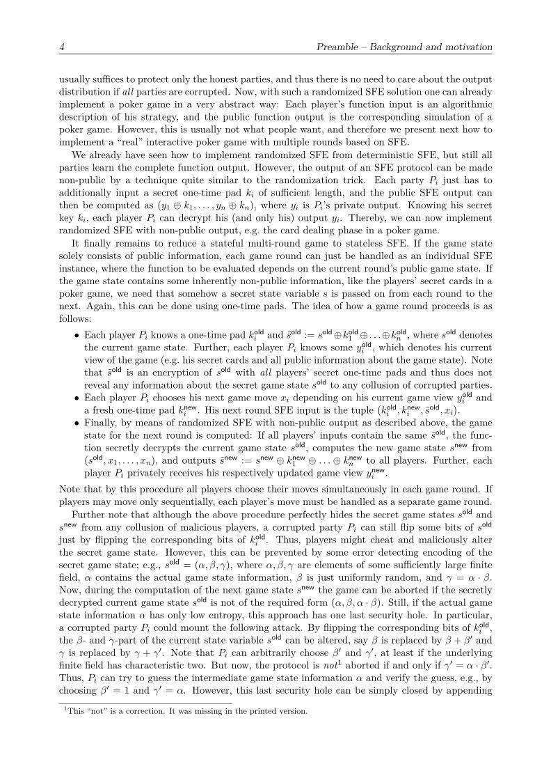
the secret game state. However, this can be prevented by some error detecting encoding of thesecret game state; e.g., sold = (α, β, γ), where α, β, γ are elements of some sufficiently large finitefield, α contains the actual game state information, β is just uniformly random, and γ = α · β.Now, during the computation of the next game state snew the game can be aborted if the secretlydecrypted current game state sold is not of the required form (α, β, α · β). Still, if the actual gamestate information α has only low entropy, this approach has one last security hole. In particular,a corrupted party Pi could mount the following attack. By flipping the corresponding bits of kold
i ,the β- and γ-part of the current state variable sold can be altered, say β is replaced by β + β′ andγ is replaced by γ + γ′. Note that Pi can arbitrarily choose β′ and γ′, at least if the underlyingfinite field has characteristic two. But now, the protocol is not1 aborted if and only if γ′ = α · β′.Thus, Pi can try to guess the intermediate game state information α and verify the guess, e.g., bychoosing β′ = 1 and γ′ = α. However, this last security hole can be simply closed by appending
1This “not” is a correction. It was missing in the printed version.

5
sufficiently many bits of independent randomness to the α-part of sold, so that it becomes practicallyunpredictable.
After all, we have seen that general SFE has not only straightforward business applications, butit even allows for secure execution of complex multi-round processes. Since SFE is such a power-ful cryptographic tool, this motivates thorough investigation of its elements and related problemstructures.
Security definitions. Classically, cryptographic protocols were considered secure when some spe-cific security properties could be shown. We have already seen two such properties, namely privacyand correctness. Correctness means that the protocol implements the desired functionality, andprivacy guarantees that even corrupted parties do not learn more during a protocol run than whatcan be inferred from their own input and output. At first glance, it might seem intuitively clearthat these two properties are exactly what is usually meant by “security”. On closer inspectionhowever, things turn out pretty complicated. Giving a formal definition for the privacy property,for example, just does not work as straightforward as suggested above. Since a malicious party’sbehavior during a protocol run might not match any valid input value, it is initially not well-definedat all what can be inferred from this party’s “input” and output. But above all, the approach ofchecking individual security properties yields one severe problem: How can one guarantee that agiven list of security properties covers all potential attacks in every possible context? Consideras an illustrating example the secure computation of the boolean XOR operation; i.e. Alice andBob each choose a secret input bit and the public output is the respective XOR. Obviously, Alicecan always perfectly reconstruct Bob’s input bit from her own input and the public output, andanalogously Bob always learns Alice’s input. Thus, privacy is no issue here. However, if e.g. Alicelearns Bob’s input before she chooses her own input, she has just full control over the computationresult. The latter is not what one would expect from a secure XOR gate. So, in addition to privacyand correctness some kind of independence of inputs seems essential for secure computations.
The need for a more generic notion of security motivated several simulation based approaches[Bea92, MR92, Can01, Gol04]. The main idea there is that every possible behavior of the corruptedparties (coordinated by some adversary A) should be imitable by a simulator S in an ideal model,which is secure by definition. The first simulation based notions of security only demanded forsimulatability in retrospect, i.e. the adversary A produces output only once (at the end of theprotocol) and the simulator S has to generate some output, such that conditioned to each possibleinput of the honest parties the simulator’s output and the adversary’s output are indistinguishable.This stand-alone simulatability allows for sequential protocol composition, but in case of concur-rent composition there are no security guarantees any more. Security models that aim towardsparallel protocol composition additionally bring an environment into play that interacts with theadversary or simulator respectively and coordinates the input behavior of the honest parties. If theenvironment provably cannot tell apart between real model and ideal model, the protocol is a uni-versally composable implementation of the ideal functionality. Moreover, compared to stand-alonesimulatability approaches, the concept of an environment machine coordinating the parties’ inputbehavior also makes it possible to consider security of arbitrarily complex multi-round processes(like our poker example) in a more natural way.
All results of this thesis are stated and proven with respect to the universal composability (UC)framework of [Can01], which is usually referred to as one of the strongest commonly used securitynotions. See also Section 2.1 and Section 6.2.
Oblivious transfer (OT). Oblivious transfer is one of the most important primitives for SFE. Itsconceptual strength, which also makes it a subject of great interest within the scope of this thesis,lies in its ability to serve as a building block for more complex cryptographic protocols. This wasfirst demonstrated by [Yao86] in a generic construction for oblivious circuit evaluation. What is

6 Preamble – Contribution and structure of this thesis
more, OT even turned out to be complete in the sense that general SFE can be implemented fromit [Kil88, GL91, CGT95, IPS08].
Oblivious transfer in its basic form was introduced by [Rab81] as a two-party primitive thatmodels a trusted erasure channel: The sender party can enter a bit b, which is transmitted withprobability 1
2 to the receiver party and else replaced by a special erasure symbol ⊥. A seeminglymore useful variant of OT,
(21)-OT, was introduced by [EGL85] to securely implement commitments
(see below) and coin tossing. In the(21)-variant of OT, the receiver party can choose to learn exactly
one out of two bits provided by the sender, while the sender does not learn which bit was chosen.This variant usually is what people refer to when speaking of “oblivious transfer”. However bothflavors of OT are equivalent, i.e. they can be securely implemented from each other [Cré88].
As a straightforward generalization of OT, one often also considers string-OT, where the sender’sinputs are complete strings instead of single bits.
Commitments. A commitment scheme allows a sender party (e.g. Alice) to commit to a chosenbit value b and later unveil b to a receiver party (e.g. Bob), such that the receiver Bob learns nothingabout b before it is unveiled, and the sender Alice cannot change b after she committed herself.Thus, a commitment protocol consists of two phases, the Commit Phase and the Unveil Phase, andbetween these phases the bit value is fixed but hidden. This primitive also has many applicationsin cryptography, especially if additional computational assumptions are used.
Contribution and structure of this thesisThis thesis contributes two results to the research area of SFE. The first contribution consistsin simple but comprehensive completeness criteria for finite stateless two-party primitives. Moreconcretely, the considered primitives are secure black boxes that can be jointly queried by twoparties, have finite input and output alphabets, and do not change behavior depending on time orinput history. Given any such primitive, the completeness criteria from this thesis can be used todecide efficiently whether it allows for information-theoretically secure implementation of OT (andis thus complete) or not. The other contribution of this thesis is a protocol construction that allowsfor information-theoretically secure implementation of OT on top of an untrusted tamper-proofhardware token.
Although both contributions have the same objective (information-theoretically secure imple-mentation of OT), the respective techniques are completely different. Therefore, it seemed mostreasonable to split up the main body of the thesis into two parts, each of which is totally self-contained and can be read independently.
Completeness criteria (Part I)
Since Kilian showed in 1988 that OT is complete in the sense that every secure multi-party com-putation can be realized from this primitive, cryptographers are working on reductions of OT toother primitives (cf. Section 1.1). A long-standing open question in this context is the classificationof finite stateless two-party primitives (so-called “cryptogates”). Over the decades, completenesscriteria have been found for deterministic cryptogates (i.e. primitives without internal randomness),noisy channels, and symmetric (i.e., both parties receive the same output) or asymmetric (i.e., onlyone party receives any output at all) randomized cryptogates. However, the known criteria forrandomized primitives other than noisy channels only hold in presence of passive adversaries (i.e.,even corrupted parties still follow the protocol). This thesis now completes this line of research byproviding simple but comprehensive combinatorial completeness criteria for all finite stateless two-party primitives. I.e., for the first time there are completeness criteria for randomized primitivesthat are neither symmetric nor asymmetric (but give different outputs to the querying parties),and we overcome the limitation that previous results for randomized primitives with input fromboth parties only regarded passive adversaries. This big step is only possible by a completely novel

7
approach. The core element of this novel approach is the definition of an algebraic structure of“idealized cheating strategies” and its thorough investigation (q.v. sections 3.1.2–3.1.3 and 4.1–4.4).The motivation for this approach is by a rather generic protocol construction (q.v. Section 3.1.1and Section 4.5). Utilizing estimation methods from probability theory (the Hoeffding Inequality)and real algebraic geometry (the Łojasiewicz Inequality), the security proof for this protocol schemecan be based on the gained algebraic insights (q.v. sections 3.1.4 and 4.6–4.8).
A short version of the analogous classification results for the spacial case of deterministic primi-tives appeared in [KMQ11]. The respective full version with all proofs is online available [KMQ10]but not published elsewhere yet. Part I follows the basic structure of [KMQ10], though nearly alltechnical details are way more complex than in the deterministic case.
Secure computation from untrusted tamper-proof hardware (Part II)
Consider the following scenario. A powerful party, henceforth called Goliath, can issue tamper-proofhardware tokens and hand them over to some other party, which we henceforth call David. Eachsuch token has a dedicated interface, so that David can communicate with it, but the token’s internalstate is out of reach for David. The question now is, if in this setting OT is possible, although bothparties mistrust each other. The technical difficulty to be overcome is twofold. Firstly, a corruptedGoliath can program the token maliciously. Secondly, a corrupted David can query the token onwhatever he likes, and he can do so whenever he likes. Interestingly, various results in the literature(q.v. Section 5.1) demonstrate the feasibility of arbitrary secure computations, based on the tokens’tamper-proofness and the assumption that Goliath cannot communicate directly with any tokenin David’s hands. However, all these results use additional complexity assumptions and/or a largenumber of tokens must be exchanged. Especially the latter is usually considered a quite severeobstacle for practical realizations, and reduction of the number of tokens has been a researchobjective for years. For example, [MS08] stated it as an open problem to implement a bidirectionaland reusable commitment functionality, which is a strictly weaker primitive than OT, from a singletoken. This thesis now provides the first information-theoretically secure single-token solution, andbeyond that the provided solution even allows for asymptotically optimal implementation of OTand commitments (q.v. Section 5.2). The basic protocol construction, on which everything else isbuilt, is a newly developed method for verifiable affine function evaluation (q.v. Section 6.4 andSection 7.1).
A short version of these results appeared in [DKMQ11], containing a less general protocol con-struction, which only required a much less complicated security proof but also lacks all the opti-mality features presented in this thesis. A draft of Part II is online available [DKMQ12a] but notpublished elsewhere yet.
Some general notationsThroughout this thesis we will denote by R the set of real numbers and by N the set of all naturalsincluding zero. If we want to exclude negative values or zero, for example, we denote that by R≥0or N>0 respectively.
Random variables are denoted as bold characters, e.g. x. We refrain from the standard approachof using capitals letters for marking random variables, since we want to use them to distinguishmatrices from vectors. Thus, a random matrix is denoted as M and a random vector as v, forexample. We denote the probability operator by P, i.e. a random variable x takes some specificvalue x with probability P[x =x]. The expected value of x is denoted by E(x). This notation ofprobabilities and expected values yields the least possible danger of confusion when combined withthe other notations used in this thesis.
Further notations are introduced where needed. Additionally, a table of symbols is providedclose to the end of this thesis.


Part I
Completeness Theorems forAll Finite Stateless 2-Party Primitives
9


1 Introduction
Oblivious transfer was introduced in [Rab81] as a trusted erasure channel. Later, in [Cré88] itwas proven to be equivalent to
(21)-OT, its currently most used variant, which allows a designated
receiver Bob to learn only one of two bits sent by a designated sender Alice. Since the OT primitiveturned out to be complete in the sense that it allows for arbitrary secure multi-party computation[Kil88, GL91, CGT95, IPS08], for numerous primitives it has been investigated whether OT canbe reduced to them. In this thesis, we exhaustively treat this question for a class of primitivesthat we call “finite randomized 2-party functions”. Each such primitive is characterized by somefinite alphabets ΥA,ΥB,ΩA,ΩB, a probability distribution R with finite support R and a mappingf : ΥA×ΥB×R → ΩA×ΩB. Upon input x ∈ ΥA from Alice and y ∈ ΥB from Bob, the primitiveinternally samples a random r ← R, computes (a, b) = f(x, y, r) and outputs a to Alice and b toBob. Equally, one can characterize any finite randomized 2-party function by its input and outputalphabets ΥA,ΥB,ΩA,ΩB and a family φx,yx∈ΥA,y∈ΥB of probability mass functions over ΩA×ΩB,such that on input x ∈ ΥA from Alice and y ∈ ΥB from Bob the primitive with probability φx,y(a, b)outputs a to Alice and b to Bob. Regarding our work, the latter notation turns out much moreconvenient and therefore will be used throughout the body of this part of the thesis.
This thesis generalizes the results of [KMQ11], where the completeness question was solved forthe special case of deterministic 2-party functions, i.e. f(x, y, r) is independent of the randomness r,or alternatively φx,yx∈ΥA,y∈ΥB ⊆ 0, 1ΩA×ΩB . Although some general ideas from the deterministiccase do carry over straightforwardly, crucial techniques do not—cf. [KMQ10, Section 5]. In additionto an appropriate representation of randomized functions, we need to develop an entire tool set oftechnical lemmata, some of which may be of independent interest.
1.1 Related workGeneral related work. In the literature one finds OT protocols for bounded-classical-storage[CCM98] and bounded-quantum-storage models [DFR+07] as well as noisy classical [CMW05,Wul09, IKO+11] and quantum channels [Yao95, May95, May96], the latter taking commitments forgranted. An entire line of research deals with implementing OT from tamper-proof hardware as-sumptions [BOGKW88, GKR08, CGS08, Kol10, GIMS10, GIS+10, DKMQ11, CKS+11]. There arereductions of
(21)-OT to weaker OT versions that leak additional information [CK90, DKS99, Wul07]
and to Rabin-OT [Cré88]. OT-combiners implement OT from granted sets of OTs with faulty mem-bers [MPW07, HIKN08]. For reversing the direction of
(21)-OT a protocol is known with optimal
number of OT queries [WW06]. Relative to computational assumptions, all-or-nothing laws havebeen shown [BMM99, HNRR06, MPR10], i.e. all considered non-trivial primitives are complete.
Precursory results to this work. The line of research we deal with was initiated by [Kil91], wherecompleteness criteria for deterministic symmetric 2-party functions (i.e., both parties receive thesame output, computed deterministically from their inputs) without any additional computationalassumptions were provided. This line of research was continued by [Kil00], providing completenesscriteria for deterministic asymmetric 2-party functions (i.e., only one party receives any meaningfuloutput, computed deterministically from both parties’ inputs). Randomized symmetric and asym-metric 2-party functions (i.e., a single output symbol, computed from both parties inputs and somesecret randomness, is handed over either to both parties or only to one party) were also treatedin [Kil00], but only with respect to passive adversaries (i.e., even corrupted parties still follow the
11

12 Completeness Theorems – Introduction
protocol). Rather recently, the completeness criteria of [Kil91, Kil00] for deterministic 2-party func-tions were unified and generalized by [KMQ11], now covering all deterministic 2-party functions,what for the first time in the literature also included 2-party functions that give different outputsto Alice and Bob. Meanwhile, [CMW05] also provided exhaustive completeness criteria with re-spect to active adversaries (i.e., corrupted parties may arbitrarily deviate from the protocol) for aspecial class of randomized asymmetric 2-party functions, namely noisy channels. This thesis nowcompletes this line of research. The main theorem in Section 2.3 unifies and generalizes all knowncompleteness criteria for symmetric, asymmetric, deterministic and randomized 2-party functions.
Independently of this thesis, a unified and generalized formulation of the completeness criteriafrom [Kil91, Kil00, CMW05, KMQ11] was found by [MPR12]. Their result is equivalent to thecriteria provided by this thesis, but they only give a proof with respect to passive adversaries.Proving their conjecture for active adversaries was left as an open problem.
1.2 Our contributionResults. We give a complete characterization of all finite randomized 2-party functions that allowfor information-theoretically secure implementation of OT. For the reduction we provide a protocolscheme, which is universally composable—cf. [Can01]. Our characterization is based on surprisinglysimple combinatorial criteria and our results are tight: Necessity of our criteria still holds, even ifonly correctness and privacy of the implemented OT are required. As a remarkable corollary of ourwork all non-complete finite 2-party functions turn out essentially symmetric.
Our work exceeds the precursory completeness criteria in two ways. Firstly, we overcome thelimitation that results for randomized primitives with input from both parties only regarded passiveadversaries. Secondly, our results also cover randomized primitives that are neither symmetric norasymmetric (but give different meaningful outputs to Alice and Bob).
Techniques. Our starting point is a very generic protocol scheme, such that all perfectly unde-tectable attack strategies do comply with certain polynomial equations and hence form an algebraicvariety. One major part of our work consists in finding protocol parameters, such that this algebraicvariety collapses to trivial attack strategies that do not affect security at all. Using powerful toolsfrom real algebraic geometry (namely the Łojasiewicz Inequality) and probability theory (namelythe Hoeffding Inequality), we can then link real protocol runs to idealized attack strategies andthereby prove cryptographic security of our construction. This approach for protocol design andproving security might be of further interest, independently of our concrete classification results.
1.3 Organization of Part IThe basic structure of this part follows [KMQ11], though nearly all technical details in our caseare way more complex. We briefly present our results in Section 2, where we first refer to the usednotion of security (Section 2.1), then introduce the basic concepts needed for formulation of ourresults (Section 2.2), state our classification results (Section 2.3), and finally give a short overviewabout how our approach matches former completeness criteria in the literature (Section 2.4). InSection 3 we give an exposition of how one can prove our results. All formal proofs of our maintechnical contribution are located in Section 4; to make it self-contained, all needed definitions,notations and lemmata are also restated there.

2 Presentation of our results
Before we get started, we introduce two handy notations, which will make things much easier inthe upcoming sections.Finite sums of function values: Given any set T with finite subset S ⊆ T and some mapping
g : T → R, we set g(S) :=∑ω∈S g(ω) for convenience. For functions with more arguments
and also for function families we use the canonical extension of this notation, e.g.:
φΥA,y(ΩA, b) :=∑
x∈ΥA, a∈ΩAφx,y(a, b)
Spaces of probability mass functions: Given some finite alphabet Ω, we denote the set of allprobability mass functions over Ω by pmf(Ω), i.e. pmf(Ω) =
ρ : Ω→ R≥0
∣∣ ρ(Ω) = 1.
We also use the following standard notions.Negligibility: A function µ : N→ R≥0 is negligible (in the parameter k), if limk→∞ µ(k)·f(k) = 0
for every polynomial f ∈ R[X].Indistinguishability: Two random variables x,y are (statistically) indistinguishable, if their sta-
tistical distance 12∑α
∣∣P[x = α]−P[y = α]∣∣ is negligible in some security parameter.
2.1 Notion of securityOur main contribution is the construction and security proof of a generic reduction protocol thatimplements OT from any appropriate 2-party function. For the definition what “security” means,we lean on one of the strongest commonly used notions of security: the Universal Composability(UC) framework of [Can01]. However, our results also hold with respect to all weaker securitynotions that still require secure function evaluation to be private (i.e., no party can learn anythingthat cannot be learned from its function input and function output) and correct (i.e., if all partiesfollow the protocol, the desired function value is evaluated correctly).
In the UC framework, security is defined by comparison of an ideal model and a real model.The protocol of interest is running in the latter, where an adversary A coordinates the behaviorof all corrupted parties. In the ideal model, which is secure by definition, an ideal functionalityF implements the desired protocol task and a simulator S tries to mimic the actions of A. Anenvironment Z is plugged either to the ideal or the real model and has to guess, which model itis actually plugged to. When Z cannot distinguish between ideal and real model, the protocol isconsidered UC-secure. More formally, UC-security requires that for every adversary A there existsa simulator S, such that for all environments Z the view of Z in the real model (with adversaryA) is indistinguishable from the view of Z in the ideal model (with simulator S). Since all ourresults are of information-theoretic nature, the adversarial entities A,S and the environment Zare computationally unbounded (but nonetheless the running time of a simulator S will always bepolynomial in the running time of the according adversary A, as it is usually desired).
If the views of Z in the ideal model and the real model are distributed identically, we speakof perfect security; if there is some negligible statistical distance between these views, we haveonly statistical security. As already mentioned, one also differentiates between passive adversaries(i.e., corrupted parties still follow the protocol) and active adversaries (i.e., corrupted parties maydeviate from the protocol arbitrarily). For further details see [Can01].
Since our protocol scheme implements(21)-OT from some given 2-party function, we also need a
so-called hybrid functionality in the real model that provides access to the latter. See Figure 2.1
13

14 Completeness Theorems – Presentation of our results
Functionality: F (F )SFE
Let F be characterized by a family of probability mass functions φx,yx∈ΥA,y∈ΥB ⊆ pmf(ΩA×ΩB), whereΥA,ΩA are Alice’s input and output alphabet and ΥB,ΩB are Bob’s input and output alphabet.
• Upon receiving input (x, i) from Alice, verify that (x, i) ∈ ΥA×N and that there is no recorded tuple(x, i, Alice); else ignore that input. Next, record (x, i, Alice) and send (processing, Alice, i) tothe adversary.
• Upon receiving input (y, i) from Bob, verify that (y, i) ∈ ΥB×N and that there is no recordedtuple (y, i, Bob); else ignore that input. Next, record (y, i, Bob) and send (processing, Bob, i) to theadversary.
• As soon as there are recorded tuples (x, i, Alice) and (y, i, Bob) for the same index i, generaterandomly (a, b) ∈ ΩA× ΩB according to the distribution specified by φx,y, and store (a, b, i).
• Upon receiving a message (Delivery, Alice, i) from the adversary, verify that there is a stored tuple(a, b, i); else ignore that message. Next, output (a, i) to Alice and henceforth ignore all messages(Delivery, Alice, i) with the same index i.
• Upon receiving a message (Delivery, Bob, i) from the adversary, verify that there is a stored tuple(a, b, i); else ignore that message. Next, output (b, i) to Bob and henceforth ignore all messages(Delivery, Bob, i) with the same index i.
When a party is corrupted, the adversary is granted unrestricted access to the channel between F (F )SFE and
the corrupted party, including the ability of deleting and/or forging arbitrary messages; i.e., the adversarycan arbitrarily send and receive messages on behalf of the corrupted party.
Figure 2.1: The ideal functionality for secure evaluation of a 2-party function F . Adapted andsimplified version of the Secure Function Evaluation functionality in [Can01]. Note that via theparameter i just the same multi-session ability is achieved as in [Can01] by multiple session IDs.
for a formal definition of the hybrid functionality used. As(21)-OT itself is just a special 2-party
function that on input (b0, b1) ∈ 0, 12 from Alice and c ∈ 0, 1 from Bob with probability 1outputs bc to Bob and a special “nothing” symbol ⊥ to Alice, we can omit an explicit definition ofthe ideal OT functionality and instead use an accordingly instantiated version of the functionalityfrom Figure 2.1.
2.2 Basic concepts
Finite randomized 2-party functions. A finite randomized 2-party function can be characterizedby its input and output alphabets and output distributions (cf. Figure 2.1). By Ffin we denotethe set of all tuples (ΥA,ΥB,ΩA,ΩB, φ), where ΥA,ΥB,ΩA,ΩB are non-empty finite alphabets andφ := φx,yx∈ΥA,y∈ΥB is a family of probability mass functions over ΩA×ΩB, i.e. φ ⊆ pmf(ΩA×ΩB).For convenience we will not always differentiate pedantically between the mathematical objectF ∈ Ffin and the corresponding primitive F (F )
SFE, but from the context should always be clear whatis meant.
Canonical and condensed canonical representations. Our notion of Ffin turns out a bit toodetailed, since Alice and Bob can always locally relabel their input-output tuples without any sideeffects. For our purposes there is no need to distinguish between some F ∈ Ffin and any relabeledversion of F . Therefore, we introduce the concept of canonical representations. Given any F ∈ Ffin,we cannot just write down a function table for F , since each input tuple only specifies an outputdistribution rather than a concrete output tuple. However, for each individual input tuple we canrepresent the respective joint output distribution by a probability matrix with rows labeled by

2.2. Basic concepts 15
0 1 20 1 0 1 0 1
0 0 14
14
14
14 0 1
21 1
414
14
14 0 1
2
1 0 14
14 0 1
3 0 01 1
414
13
13 0 1
14
14
14
14
12
14
14
14
14
12
14
14
13
14
14
13
13 1
1 12
12 1
12
13
12
13
13 1
Figure 2.2: Different representations of a 2-party function that on input x ∈ 0, 1 from Alice andy ∈ 0, 1, 2 from Bob outputs some uniformly random a, b ∈ 0, 1, subject to the conditionsthat a + b ≥ x · y and b ≥ y − 1. To the left, inputs (bold) and outputs (italic) are displayedgrayed out. The matrix in the middle is a canonical representation of the same 2-party functionwith zero probabilities omitted for better readability; the right matrix is a condensed canonicalrepresentation.
Alice’s output symbols and columns labeled by Bob’s output symbols. Then, we can arrange these“inner” probability matrices in an “outer” block matrix with rows labeled by Alice’s input symbolsand columns labeled by Bob’s input symbols (see first two tables in Figure 2.2 for an example).
Moreover, we also want to abstract from the fact that, e.g., Bob could always concatenate theresult of a local coin toss to his output, thus formally doubling the size of his output alphabet just byan easily reversible local computation. Such local coin tosses appear in a canonical representation aspairwise linearly dependent columns within the same block column, or pairwise linearly dependentrows within the same block row respectively. However, we can easily get rid of them just by addingup the respective linearly dependent rows or columns. If all local coin tosses are removed from acanonical representation this way, we call it condensed (cf. last table in Figure 2.2).
Isomorphism. Note that the condensed canonical representation of a finite 2-party function isunique up to permutations of rows within single block rows, permutations of columns within singleblock columns, and permutation of rows and/or columns of the outer block matrix. Now, if twogiven 2-party functions F, F ′ ∈ Ffin have the same (set of) condensed canonical representations,we call them isomorphic. Obviously, isomorphism is an equivalence relation on Ffin and any twoisomorphic 2-party functions F, F ′ ∈ Ffin can be straightforwardly implemented from each otherwith perfect security.
Redundancy and equivalence. Our notion of isomorphism will turn out very handy for formula-tion of our classification results with respect to passive adversaries, but for active adversaries weneed one additional concept. In particular, there may exist input symbols that a corrupted partynever needs to use, since one can always learn strictly more by inputting something else. Givenany F := (ΥA,ΥB,ΩA,ΩB, φ) ∈ Ffin, we call an input symbol y′ ∈ ΥB redundant, if a corruptedBob instead of sending y′ to F can always replace this input by an appropriately distributed ran-dom choice from ΥB\y′ and still perfectly simulate honest behavior. This is possible, if Alice’soutput distribution is not changed at all and Bob can reconstruct an appropriately distributedoutput b′ ∈ ΩB from his actual input-output tuple (y, b). Formally, y′ ∈ ΥB is redundant, ifthere exist an “input replacement strategy” τ ∈ pmf(ΥB) and an “output reconstruction strategy”λy,by∈ΥB,b∈ΩB ⊆ pmf(ΩB), such that τ(y′) = 0 and for all x ∈ ΥA, a ∈ ΩA, b
′ ∈ ΩB it holds:
φx,y′(a, b′) =∑
y∈ΥB, b∈ΩBτ(y) · φx,y(a, b) · λy,b(b′)
For input symbols x ∈ ΥA, redundancy is defined analogously. If neither ΥA nor ΥB contains anyredundant input symbols, we say that F is redundancy-free.
W.l.o.g., malicious parties never use redundant input symbols, since they can gather exactlythe same or even strictly more information by the respective input replacement and output recon-

16 Completeness Theorems – Presentation of our results
struction strategies. Also, there is no need to constrain what honest parties may learn. Therefore,regarding active adversaries we can consider any 2-party functions equivalent when they only differin some redundant input symbols. Formally, any 2-party functions F, F ′ ∈ Ffin are equivalent, ifthey can be made isomorphic by successive removal of redundant input symbols. Note that a step-by-step removal of one symbol at a time is crucial here: There may exist two input symbols that areboth redundant, but after removing one of them, the other one is not redundant any more—e.g.,ΥB = y, y′ with φx,y(a, b) = φx,y′(a, b) for all x ∈ ΥA, a ∈ ΩA, b ∈ ΩB.
It will turn out that the redundancy-free version of any given F ∈ Ffin is unique up to isomorphismand thus equivalence of 2-party functions in the sense above is indeed an equivalence relation onFfin. However, due to lack of some required technical tools at this point, we postpone the proof toSection 4.3 (see Corollary 19).
2.3 Completeness criteria for all finite randomized 2-party functionsWith the concepts from Section 2.2 we can now formulate our classification results. We just statethe mere assertions here; for an outline of the proof see Section 3.
Definition (OT-cores). Given F := (ΥA,ΥB,ΩA,ΩB, φ) ∈ Ffin, an OT-core of F is a non-diagonalfull-rank 2×2-submatrix of the canonical representation; i.e., for the corresponding input-outputtuples (x, a), (x′, a′) ∈ ΥA×ΩA and (y, b), (y′, b′) ∈ ΥB×ΩB we have the following inequation withat most one zero factor:
φx,y(a, b) · φx′,y′(a′, b′) 6= φx′,y(a′, b) · φx,y′(a, b′)
In this situation, we also call(x, a), (x′, a′)
×(y, b), (y′, b′)
an OT-core of F .
Theorem (Classification Theorem). For every F ∈ Ffin it holds:1. OT can be implemented from F (F )
SFE statistically secure against passive adversaries, iff F hasan OT-core.
2. OT can be implemented from F (F )SFE statistically secure against active adversaries, iff the
redundancy-free version of F has an OT-core.
Definition (Symmetric 2-party functions). A 2-party function F := (ΥA,ΥB,ΩA,ΩB, φ) ∈ Ffin issymmetric, if φx,y(a, b) = 0 for all x ∈ ΥA, y ∈ ΥB, a ∈ ΩA, b ∈ ΩB with a 6= b.
Lemma (Symmetrization Lemma). Every 2-party function F ∈ Ffin that has no OT-core is isomor-phic to a symmetric 2-party function.
2.4 Comparison with criteria from the literatureThe latest known completeness criteria1 for finite 2-party functions can be subsumed by the fol-lowing four theorems.[KMQ11, Theorem 1]: A deterministic 2-party function F := (ΥA,ΥB,ΩA,ΩB, φ) ∈ Ffin allows
for implementation of OT statistically secure against passive adversaries, iff for the mappingsfA : ΥA×ΥB → ΩA defined by fA(x, y) = a :⇔ φx,y(a,ΩB) = 1 and fB : ΥA×ΥB → ΩBdefined by fB(x, y) = b :⇔ φx,y(ΩA, b) = 1 there exist x, x′ ∈ ΥA and y, y′ ∈ ΥB, such thatfA(x, y) = fA(x, y′), fB(x, y) = fB(x′, y), and
(fA(x′, y), fB(x, y′)
)6=(fA(x′, y′), fB(x′, y′)
).
A deterministic 2-party function F ∈ Ffin allows for implementation of OT statistically secureagainst active adversaries, iff its redundancy-free version allows for implementation of OTstatistically secure against passive adversaries by the criterion above.
1Meanwhile, a unification and generalization of these criteria has been found by an independent work [MPR12].Their criteria are equivalent to those in this thesis, but they give only a proof with respect to passive adversaries.

2.4. Comparison with criteria from the literature 17
[CMW05, Main result]: A noisy channel allows for implementation of OT statistically secureagainst active adversaries, iff its redundancy-free version is no parallel composition of noiselessand/or capacity-zero channels.
[Kil00, Theorem 1.3]: An asymmetric F := (ΥA,ΥB, ⊥,Ω, φ) ∈ Ffin allows for implementationof OT statistically secure against passive adversaries, iff there exist x, x′ ∈ ΥA, y, y
′ ∈ ΥB andz, z′ ∈ Ω, such that φx,y(⊥, z) > φx′,y(⊥, z) > 0 or it holds that φx,y(⊥, z) > 0, φx′,y(⊥, z) > 0,φx,y′(⊥, z′) > 0 and φx′,y′(⊥, z′) = 0.
[Kil00, Theorem 1.2]: A symmetric F := (ΥA,ΥB,Ω,Ω, φ) ∈ Ffin allows for implementation ofOT statistically secure against passive adversaries, iff there exist x, x′ ∈ ΥA, y, y
′ ∈ ΥB, z ∈ Ω,such that φx,y(z, z) > 0, φx,y′(z, z) > 0 and φx,y(z, z) · φx′,y′(z, z) 6= φx,y′(z, z) · φ′x,y(z, z).
All these completeness criteria are direct corollaries of our Classification Theorem. However, theliterature cited above differs substantially in the used protocol constructions and also the proof tech-niques. This thesis generalizes the results and techniques of [KMQ11], where also a SymmetrizationLemma were provided for deterministic 2-party functions. In particular, we adapt from [KMQ11]and generalize the notions of “redundancy” (q.v. Section 2.2), “OT-cores” (q.v. Section 2.3) and“cheating situations” (q.v. Section 3.1.2), and we also adopt the basic protocol scheme for genera-tion of correlated data (q.v. Section 3.1.1). However, due to increased complexity the similaritiesare limited to a fairly abstract level. Core proof techniques of [KMQ11] are strictly bound tothe deterministic case—cf. [KMQ10, Section 5]—and therefore new solutions (including a powerfullemma from real algebraic geometry, q.v. Section 4.6) are needed for randomized primitives.


3 How to prove the Classification Theorem
Necessity of our criteria. By our Symmetrization Lemma and [Kil00, Theorem 1.2] it directlyfollows that OT-cores are necessary for completeness with respect to passive adversaries. Moreover,the proof in [Kil00, Section 4.1] for necessity of OT-cores holds in the same way with respect toactive adversaries. So, at this point we only need to give a proof for the Symmetrization Lemma.
Proof-sketch. Let some arbitrary F := (ΥA,ΥB,ΩA,ΩB, φ) ∈ Ffin be given that has no OT-core. Wehave to show that F is symmetric up to isomorphism. Our first observation is that we can replaceBob’s output symbols by normalized versions of the respective column vectors in the condensedcanonical representation of F , i.e. upon Bob’s input y we replace his function output b by thefollowing RΥA×ΩA-vector:
1φΥA,y(ΩA, b)
·(φx,y(a, b)
)x∈ΥA,a∈ΩA
Since by construction there are never any two linearly dependent columns within the same blockcolumn of a condensed canonical representation, this replacement of output symbols is an isomor-phism of 2-party functions. Analogously, we can replace Alice’s output symbols; let ΩA ⊆ RΥB×ΩB
and ΩB ⊆ RΥA×ΩA denote the new output alphabets.Now we exploit that F has no OT-core. Given any a ∈ ΩA and b, b′ ∈ ΩB with φΥA,ΥB(a, b) > 0
and φΥA,ΥB(a, b′) > 0, it must hold that b = b′, as otherwise the two-column matrix (b, b′) wouldcontain a non-diagonal full-rank 2×2-matrix and thereby we had an OT-core. Analogously, for alla, a′ ∈ ΩA and b ∈ ΩB with φΥA,ΥB(a, b) > 0 and φΥA,ΥB(a′, b) > 0 it must hold that a = a′. Thus,Alice and Bob have always full information about each other’s output and the function can as wellannounce the complete output tuple (a, b) to both of them in the first place.
Sufficiency in the passive case. Given some F := (ΥA,ΥB,ΩA,ΩB, φ) ∈ Ffin that has an OT-core,and given that there is only a passive adversary, we can easily implement a non-trivial noisy channel(shown to be complete in [CMW05, Wul09, IKO+11]) by the following protocol:
0. Alice and Bob agree on a bijection σ : ΥA×ΩA →0, . . . , |ΥA×ΩA| − 1
. The image S of σ
also serves as Alice’s channel input alphabet.1. Alice and Bob query F once with uniformly random input, thus generating input-output
tuples (x, a) ∈ ΥA×ΩA and (y, b) ∈ ΥB×ΩB respectively.2. Alice announces to Bob her intended channel input encrypted with (x, a) as follows: If she
wants to send some m ∈ S via the noisy channel, she announces m := m+ σ(x, a) mod |S|.3. Bob’s noisy channel output is (m, y, b).
Since F has an OT-core and even corrupted parties still follow the protocol, the implementedchannel is not completely decomposable into noiseless channels and/or channels with zero capacity.This is straightforward to verify and suffices to implement OT by the above-mentioned literature.
Sufficiency in the active case. As we are already done with necessity of our criteria in theactive and passive case and sufficiency in the passive case, so to speak “75%” of our ClassificationTheorem are proven. However, the vastly major part still lies ahead of us. For proving sufficiencyin the active case, i.e. proving that in presence of an active adversary OT can still be reduced toany redundancy-free 2-party function that has some OT-core, we need an entire new tool set oftechnical lemmata and several sophisticated results from the literature. The high level idea of thereduction approach is as follows. First, Alice and Bob generate some amount of correlated data by
19

20 Completeness Theorems – How to prove the Classification Theorem
a)
13
23
12
23
13
12
1 12
1 12
b)
12
12 1
12
12 1
12
49 1
12
59 1
Figure 3.1: a) Example for illustration that not every OT-core is useful for us: The first two blockcolumns contain an OT-core, but can be subsumed by the last block column.b) Example for illustration that redundancy here is more complex than in the deterministic case:The first block column is redundant (it can be subsumed by the last two), but the second is not.
repeatedly querying the given 2-party function with random input. Within a subsequent test stepeach party has to partially unveil its data, so that significant cheating can be detected. Then, in asimilar approach as in the passive case, the remaining data is used for implementation of non-trivialnoisy channels: Alice just announces her channel inputs one-time-pad encrypted with her part ofthe correlated data, and Bob, since his view gives him only partial information about the usedone-time pads, can only recover noisy versions of Alice’s channel inputs. However, things will turnout a bit more complicated than in the passive case, since corrupted parties can try to gather someadditional information by occasionally deviating from the protocol.
The first part (secure generation of correlated data, q.v. Section 3.1) is much more challengingthan the second part (building OT from correlated data, q.v. Section 3.2). The former needsnumerous novel techniques (see Section 4 for the formal proofs), whereas the latter mainly consistsin rather straightforward adaptions of nowadays folklore techniques from the literature.
3.1 Secure generation of correlated data
In this section we explain how one can securely generate non-trivially correlated data from anyredundancy-free 2-party function that has some OT-core. The main idea is to use inputs belongingto a specific OT-core with relatively high probability and all other inputs only with relatively lowprobability—the latter will just serve for test purposes. Notably, an all-over uniform input distri-bution is not suitable in general, but still all input symbols have to be used with some significantprobability. We illustrate this by two examples. Our first example, given by in Figure 3.1.a, illus-trates the problem with all-over uniform input distributions. In this example, a corrupted Bob cansubstitute a query on the first input symbol and a query on the second input symbol by two querieson the third input symbol. So, instead of uniformly choosing from his complete input alphabet,he can always input the last input symbol and thereby always get full information about Alice’sinput-output tuple. Our second example, given by Figure 3.1.b, illustrates that in general onecannot completely neglect all input symbols that do not belong to the chosen OT-core. In thisexample, if Alice only uses one of her input symbols all the time, this means that effectively wecan remove one of the block rows and all of a sudden the redundancy-free version of the remainingpart even has no OT-core any more.
3.1.1 The protocol for generating correlated data
Basic scheme. Basically, our protocol for generation of correlated data follows the very genericconstruction of [KMQ11]. It roughly proceeds as follows (for a formal description see Section 4.5).
1. Invocation of F : Alice and Bob query the underlying 2-party function F with random inputfor k times (k being the security parameter) and record their respective input-output tuples.A protocol parameter assigns what concrete input distributions are to be used.
2. Check A: Alice challenges Bob on some polynomial subset of the recorded data, where hehas to reveal his input-output tuples. Alice aborts the protocol, if the joint distribution of

3.1. Secure generation of correlated data 21
her own input-output tuples and Bob’s claimed input-output tuples appears faulty. The testset is then removed from the recorded data.
3. Check B: This step equals the previous one with the roles of Alice and Bob interchanged.4. Output: Both parties announce where they have used input symbols that were only for test
purposes. All corresponding elements are removed from the recorded data. When too muchof the recorded data has been deleted, the protocol is aborted; else each party outputs itsremaining string of recorded input-output tuples.
At this point, a remark on the increased difficulty compared to the deterministic case seems in-dicated. In particular, there is one crucial difference between our scheme here and the protocolscheme of [KMQ11]. This difference is in the check steps Check A and Check B. In the schemeof [KMQ11], Alice checks in Check A that each of Bob’s claimed input-output tuples (y′, b′) isconsistent with her own respective input-output tuple (x, a) in the sense that φx,y′(a, b′) 6= 0, andthat each of Bob’s claimed input symbols occurs with the right frequency independently of herown input. This does not suffice in the randomized setting any more, as one can also see from theexample in Figure 3.1.b. In this example, the redundant first block column and the non-redundantsecond block column differ only very slightly in their output distributions. Thus, if Alice onlychecked that Bob’s claimed input-output tuples do not directly contradict her own input-outputtuples, then Bob could substitute his second input symbol in this example right the same way hecan already substitute the first input symbol. For this reason, in the check steps Check A andCheck B of our protocol scheme described above each party must examine the joint distribution ofits own input-output tuples and the other party’s claimed input-output tuples.
Parameter choice. We have the following wish list to our protocol scheme:• The challenge sets in the protocol steps Check A and Check B must be sufficiently large, so
that any significant deviation from the prescribed input distributions can be detected.• We want that even a malicious choice of the challenge sets does not substantially influencethe joint distribution of the recorded input-output tuples.• All input symbols must be used with sufficiently high probability, so that the problem illus-trated in Figure 3.1.b does not emerge.• In the last protocol step, where all data is deleted that does not belong to the chosen OT-coreinputs, no corrupted party should be able to modify the recorded data’s joint distributionmore than by a vanishingly small amount.
Obviously, the first two objectives conflict with each other, and so do the last two. However, whatmight first sound like a paradox, can be achieved by a polynomially vanishing lower bound forthe input probabilities and also a polynomially vanishing relative size of the challenge sets. Moreconcretely, for every input symbol that is only for test purposes we choose an input probability ofmagnitude O(k−α) with constant α > 0, and the challenge sets have size O(k
12 +β) with constant
β < 12 (cf. Section 4.5)—for technical reasons we even choose β < 1
6 . Thus, there exists someconstant ε > 0, such that k−k1−ε recorded input-output tuples from the first protocol step remainuntouched throughout the rest of the protocol and are finally part of the output.
3.1.2 Idealized attack strategies
In the step Check A of the protocol scheme introduced in Section 3.1.1, instantiated with anyF := (ΥA,ΥB,ΩA,ΩB, φ) ∈ Ffin, a corrupted Bob can of course try to pretend to have used anotherinput distribution than he actually did. Analogously, a corrupted Alice can try to cheat in Check B,but for symmetry reasons it will suffice to consider the case of a corrupted Bob. We start our securityconsiderations by introducing a very idealized notion of attack startegies. This notion comprisesonly perfectly undetectable attacks, but it will turn out later that every possible attack strategy isclose to such a perfect strategy.

22 Completeness Theorems – How to prove the Classification Theorem
Cheating strategies. A cheating strategy of Bob is a triple (τ, λ, ω), consisting of• an “actual input distribution” τ ∈ pmf(ΥB),• a “lying strategy” λ := (λy,b)y∈ΥB,b∈ΩB ⊆ pmf(ΥB×ΩB) in the sense that in Check A aninput-output tuple (y, b) is claimed as (y′, b′) with probability λy,b(y′, b′),• and a “claimed input distribution” ω ∈ pmf(ΥB),
such that for all x ∈ ΥA, a ∈ ΩA, y′ ∈ ΥB, b
′ ∈ ΩB and with υ ∈ pmf(ΥA) denoting Alice’s inputdistribution it holds:
υ(x) · ω(y′) · φx,y′(a, b′)︸ ︷︷ ︸expected joint probability of (x, a) and (y′, b′)
=∑
y∈ΥB, b∈ΩBυ(x) · τ(y) · φx,y(a, b) · λy,b(y′, b′)︸ ︷︷ ︸
claimed joint probability of (x, a) and (y′, b′)
Note that we can cancel υ(x) on both sides, since Alice uses her complete input alphabet andthus υ(x) > 0 for all x ∈ ΥA. I.e., Bob’s cheating strategies are actually independent of Alice’sinput distribution; they either work for all of them or for none. Further note that ω is no arbitrarilyselectable parameter but already completely fixed by τ and λ. In particular, for all x ∈ ΥA, y
′ ∈ ΥBit holds:
ω(y′) = ω(y′) · φx,y′(ΩA,ΩB) =∑
y∈ΥB, b∈ΩBτ(y) · φx,y(ΩA, b) · λy,b(y′,ΩB)
Last but not least, an easily verifiable but very important feature of cheating strategies lies in theirrelation to redundancy: An input symbol y′ ∈ ΥB is redundant, iff there exists a cheating strategy(τ, λ, ω), such that τ(y′) = 0 and ω(y′) = 1. This directly follows from our definitions.
Cheating situations. Our notion of cheating strategies turns out a bit cumbersome for the follow-ing reason. Obviously, a corrupted Bob can follow a mixed strategy, e.g. by following half the timesome cheating strategy (τ, λ, ω) and half the time some other cheating strategy (τ ′, λ′, ω′). For theresulting cheating strategy (τ , λ, ω) it is intuitively clear that τ = 1
2 · τ + 12 · τ
′ and ω = 12 ·ω+ 1
2 ·ω′.
On first glance one might also expect that λ = 12 ·λ+ 1
2 ·λ′, but this will not be true in general! E.g.,
if τ(y) = 0 < τ ′(y) for some y ∈ ΥB, then we have that λy,b = λ′y,b for all b ∈ ΩB. To circumventthis inconvenience, we introduce the equivalent but more practical notion of cheating situations.Given Bob’s cheating strategy (τ, λ, ω) and Alice’s input distribution υ ∈ pmf(ΥA), we define thecorresponding cheating situation η ∈ pmf
((ΥA×ΩA)×(ΥB×ΩB)2) as follows:
η((x, a), (y, b), (y′, b′)
):= υ(x) · τ(y) · φx,y(a, b) · λy,b(y′, b′)
The intuition behind this is that instead of focusing on the cheating party’s plan, we just counthow often which kind of situation occurs during Check A. More precisely, η
((x, a), (y, b), (y′, b′)
)stands for the relative frequency of the event that Alice’s input-output tuple is (x, a), Bob’s actualinput-output tuple is (y, b), and Bob’s claimed input-output tuple is (y′, b′). Consequently, we canwrite:
η|A(x) := η((x,ΩA), (ΥB,ΩB), (ΥB,ΩB)
)= υ(x)
η|trueB (y) := η
((ΥA,ΩA), (y,ΩB), (ΥB,ΩB)
)= τ(y)
η|fakeB (y′) := η
((ΥA,ΩA), (ΥB,ΩB), (y′,ΩB)
)= ω(y′)
Our definition directly implies that every cheating situation η fulfills the following four conditions.1. For all x ∈ ΥA it holds that η|A(x) > 0.2. For all x ∈ ΥA, a ∈ ΩA, y ∈ ΥB, b ∈ ΩB it holds:
η((x, a), (y, b), (ΥB,ΩB)
)= η|A(x) · η|true
B (y) · φx,y(a, b)

3.1. Secure generation of correlated data 23
3. For all x ∈ ΥA, a ∈ ΩA, y′ ∈ ΥB, b
′ ∈ ΩB it holds:
η((x, a), (ΥB,ΩB), (y′, b′)
)= η|A(x) · η|fake
B (y′) · φx,y′(a, b′)
4. For all x ∈ ΥA, a ∈ ΩA, y, y′ ∈ ΥB, b, b
′ ∈ ΩB with η((ΥA,ΩA), (y, b), (ΥB,ΩB)
)> 0 it holds:
η((x, a), (y, b), (y′, b′)
)= η
((ΥA,ΩA), (y, b), (y′, b′)
)·
η((x, a), (y, b), (ΥB,ΩB)
)η((ΥA,ΩA), (y, b), (ΥB,ΩB)
)Note that these conditions basically are a polynomial equation system, of which we will take greatadvantage later. Let N(F )
B denote the set of all η ∈ pmf((ΥA×ΩA)×(ΥB×ΩB)2) that fulfill them. We
show now that actually N(F )B is just the set of all cheating situations. Given any η ∈ N
(F )B , we find
some τ, ω ∈ pmf(ΥB) and λ := (λy,b)y∈ΥB,b∈ΩB ⊆ pmf(ΥB×ΩB), such that for all y, y′ ∈ ΥB, b, b′ ∈ ΩB
we have:
τ(y) = η|trueB (y)
ω(y′) = η|fakeB (y′)
λy,b(y′, b′) =η((ΥA,ΩA), (y, b), (y′, b′)
)η((ΥA,ΩA), (y, b), (ΥB,ΩB)
) if η((ΥA,ΩA), (y, b), (ΥB,ΩB)
)> 0
Since η meets the four conditions above, we have that (τ, λ, ω) is a cheating strategy:
∑y∈ΥB, b∈ΩB
τ(y) · φx,y(a, b) · λy,b(y′, b′) =∑
y∈ΥB, b∈ΩB
η((x, a), (y, b), (ΥB,ΩB)
)· λy,b(y′, b′)
η|A(x)= 1
η|A(x) ·∑
y∈ΥB, b∈ΩBη((x, a), (y, b), (y′, b′)
)= ω(y′) · φx,y′(a, b′)
Likewise, η is a corresponding cheating situation:
η|A(x) · τ(y) · φx,y(a, b) · λy,b(y′, b′) = η((x, a), (y, b), (ΥB,ΩB)
)· λy,b(y′, b′) = η
((x, a), (y, b), (y′, b′)
)Advantages of our notion of cheating situations. In contrast to the more intuitive notion ofcheating strategies, our definition of cheating situations enjoys some very handy structure: Whenwe fix Alice’s input distribution, the remaining set of cheating situations is a bounded convexpolytope in the affine space R(ΥA×ΩA)×(ΥB×ΩB)2 , spanned by finitely many vertices (cf. Lemma 10).Furthermore, cheating situations inherit two important features from cheating strategies. Firstly,cheating situations can be considered independent of (honest) Alice’s input distribution, since theycan be rescaled canonically to any input distribution that assigns non-zero probability to everyx ∈ ΥA (q.v. Lemma 8). Secondly, an input symbol y′ ∈ ΥB is redundant, iff there exists a cheatingsituation η ∈ N
(F )B , such that η|true
B (y′) = 0 and η|fakeB (y′) = 1. For redundancy of y′ it even suffices
that η|trueB (y′) < η|fake
B (y′) and η|trueB (y) ≥ η|fake
B (y) for all y ∈ ΥB\y′. This results from some usefuldecomposability features of the algebraic structure N
(F )B , but for now we skip all the technical
details and instead just refer to Section 4.3.Last but not least, cheating situations are also unaffected by another disadvantage of cheating
strategies that misleads intuition: If λy,b(y′, b′) > 0, this does not necessarily mean that Bob everreally replaces an input-output tuple (y, b) by (y′, b′); as well, it might be the case that τ(y) = 0(i.e., Bob did not use the input symbol y at all). In contrast, if η
((ΥA,ΩA), (y, b), (y′, b′)
)> 0, then
Bob has in fact replaced the corresponding portion of actual input-output tuples (y, b) by claimedinput-output tuples (y′, b′).

24 Completeness Theorems – How to prove the Classification Theorem
3.1.3 Robust OT-cores
We aim at an instantiation of the protocol scheme described in Section 3.1.1, such that the inputsbelonging to some chosen OT-core of the underlying 2-party function F are used with relativelyhigh probability and all other inputs have relatively low probability. However, if y, y′ are Bob’sOT-core inputs and there exists a cheating situation η ∈ N
(F )B , such that η|true
B (y, y′) = 0 andη|fake
B (y, y′) = 1, then we have no security guarantee (cf. Figure 3.1.a). We need at least thatη|true
B (y, y′) = 1 for all η ∈ N(F )B with η|fake
B (y, y′) = 1; otherwise a corrupted Bob can alwayssubstitute a substantial fraction of his OT-core queries by other inputs. Surprisingly, this is notonly a necessary precondition for security, but it will even turn out sufficient. The key idea isto choose protocol parameters, such that the prescribed probability of non-OT-core inputs is highenough for cheating detection, but still so small that only cheating strategies (τ, λ, ω) with ω(y) = 0for all non-OT-core inputs y may work. This might first sound like a paradox, but can be achievedby polynomially vanishing probabilities for the non-OT-core inputs (cf. Section 3.1.1).
However, first and foremost we need to show that there always exists an OT-core fulfilling theabove-mentioned criterion, if only the redundancy-free version of the considered 2-party functionhas any OT-core at all (see Figure 3.1.a for a negative example). Moreover, we also need analogoussecurity against a possibly cheating Alice, and we must rule out that every OT-core found secureagainst a cheating Bob is insecure against a cheating Alice and vice versa. We achieve this all atonce by the next lemma (cf. Lemma 25).
Lemma. Let some F := (ΥA,ΥB,ΩA,ΩB, φ) ∈ Ffin be given that is redundancy-free and has anOT-core. Then there also exists an OT-core within the same rows of the canonical representationof F , such that for Bob’s corresponding input symbols y, y′ and every cheating situation η ∈ N
(F )B
with η|fakeB (y, y′) = 1 we have that η|true
B (y, y′) = 1.
By this lemma, given any OT-core, we find an OT-core within the same rows of the canonical rep-resentation, such that this new OT-core is secure against a potentially cheating Bob. Analogously,starting from the OT-core secure against Bob, we find an OT-core within the same columns of thecanonical representation, such that this new OT-core is secure against a potentially cheating Alice.Since in the second step Bob’s involved input symbols stay the same, the finally found OT-core isalso still secure against a cheating Bob.
Now, we give a proof-sketch for this lemma, which is a core element of our line of argument. Notethat, although our notion of cheating situations can be seen as a generalization of the correspondingconcept in [KMQ11], this proof is independent—cf. [KMQ10, Section 5].
Proof-sketch. Let (x, a), (x′, a′) ∈ ΥA×ΩA and (y, b), (y′, b′) ∈ ΥB×ΩB denote Alice’s and Bob’s input-output tuples belonging to the initially given OT-core. W.l.o.g., φx,y(a, b) > 0 and φx′,y(a′, b) > 0.
If y = y′, i.e. the initially given OT-core lies within a single block column of the canonical rep-resentation, then existence of a cheating situation η ∈ N
(F )B with η|fake
B (y, y′) = 1 > η|trueB (y, y′)
would imply that the input symbol simultaneously denoted by y and y′ is redundant (cf. Corol-lary 18). So, in this case things are easy. Else, i.e. if y 6= y′, we need a more abstract view of cheatingsituations to keep arguments traceable. Let X
(F )B denote the set of all mappings ξ : ΥB → R for
that there exist some η ∈ N(F )B and γ ∈ R>0, such that γ · ξ(y) = η|fake
B (y)− η|trueB (y) for all y ∈ ΥB.
The intuition behind this is merely that ξ(y) > 0 if Bob claims to have input y more often than heactually did, and ξ(y) < 0 if Bob claims to have input y less often than he actually did. We willmake use of the following properties of this notation:• The set X
(F )B is closed under positive linear combination, i.e. γ · ξ + γ′ · ξ′ ∈ X
(F )B for all
γ, γ′ ∈ R>0 and ξ, ξ′ ∈ X(F )B . This directly follows from the fact that Alice’s input distribution
η|A of every cheating situation η ∈ N(F )B can be canonically rescaled, and the fact that the
set of all cheating situations with the same input distribution of Alice is convex.

3.1. Secure generation of correlated data 25
y y′ Y Y ′ Y0
......
......
......
......
......
......
......
......
......
......
· · · 14
14
16
12
16
16
16
124
112
18
16
18
59 1 1
4 0 0 0 0 0 · · ·· · · 1
414
12
12
16
16
16
124
112
18
13
14
49 0 0 1
314 0 0 0 · · ·
......
......
......
......
......
......
......
......
......
......
Figure 3.2: Illustration of the construction of the input sets Y , Y ′, Y0. Input symbols from Y havean OT-core together with y′, but not with y; inputs from Y ′ have an OT-core together with y;inputs from Y0 cannot be completed by y or y′ to have an OT-core. Note that always y ∈ Y andy′ ∈ Y ′, which is not displayed in order to keep the graphic simple.
• If for some y′ ∈ ΥB there exists a ξ ∈ X(F )B with ξ(y′) > 0 and ξ(y) ≤ 0 for all y ∈ ΥB\y′,
then y′ is redundant. This is just a reformulation of the redundancy criterion that there existsan η ∈ N
(F )B with η|true
B (y′) < η|fakeB (y′) and η|true
B (y) ≥ η|fakeB (y) for all y ∈ ΥB\y′.
Further, for any Y ⊆ ΥB let ΨF (Y ) denote the set of all input symbols y that a corrupted Bob canuse although the protocol prescribes to use only input symbols from Y , i.e.:
ΨF (Y ) =y ∈ ΥB
∣∣ there exists an η ∈ N(F )B , such that η|true
B (y) > 0 and η|fakeB (Y ) = 1
Note that by the convex combinability of cheating situations we always find some η ∈ N
(F )B , such
that η|fakeB (Y ) = 1 and η|true
B (y) > 0 for all y ∈ ΨF (Y ). Thus, we also always have some ξ ∈ X(F )B ,
such that ξ(y) = 0 for all y /∈ ΨF (Y ) and ξ(y) < 0 for all y ∈ ΨF (Y )\Y . Further note that alwaysΨF (Y ) ⊆ ΨF (Y ′) for all Y ⊆ Y ′, that ΨF (ΨF (Y ′)) = ΨF (Y ′), and that hence ΨF (Y ) ⊆ ΨF (Y ′)for all Y ⊆ ΨF (Y ′) (cf. Lemma 23).
Now we can start with our argumentation. First of all, we divide ΨF (y, y′) into the followingthree subsets (cf. Figure 3.2):• Let Y ′ denote the set of all y′ ∈ ΨF (y, y′), such that for some b′ ∈ ΩB the (x, a), (x′, a′)×(y, b), (y′, b′)-submatrix of the canonical representation of F is an OT-core; i.e., since byassumption φx,y(a, b) > 0 and φx′,y(a′, b) > 0, we just need:
φx,y(a, b) · φx′,y′(a′, b′) 6= φx′,y(a′, b) · φx,y′(a, b′)
• Let Y denote the set of all y ∈ ΨF (y, y′)\Y ′, such that for some b ∈ ΩB the (x, a), (x′, a′)×(y, b), (y′, b′)-submatrix of the canonical representation of F is an OT-core; i.e., φx,y(a, b) >0 and φx′,y(a′, b) > 0 and for all b ∈ ΩB we have:
φx,y(a, b) · φx′,y(a′, b) = φx,y(a, b) · φx′,y(a′, b)
• Let Y0 denote the set of all y0 ∈ ΨF (y, y′), such that for all b0 ∈ ΩB neither the (x, a), (x′, a′)×(y, b), (y0, b0)-submatrix nor the (x, a), (x′, a′)×(y0, b0), (y′, b′)-submatrix of the canon-ical representation of F is an OT-core; i.e., φx,y0(a,ΩB) = φx′,y0(a′,ΩB) = 0.
Our proof is by contradiction and hence w.l.o.g. we assume that ΨF (y, y′) = ΨF (y, y′) for ally ∈ Y and ΨF (y, y′) = ΨF (y, y′) for all y′ ∈ Y ′—keep in mind that ΨF (Z) ⊆ ΨF (y, y′) for allZ ⊆ ΨF (y, y′) as mentioned above. Now we pick some arbitrary y′ ∈ ΨF (y, y′); w.l.o.g. y′ ∈ Y ′.By assumption we find some ξ′, ξ′′ ∈ X
(F )B , such that for all y ∈ ΥB it holds:
ξ′(y) > 0 if y ∈ y, y′ ξ′′(y) > 0 if y ∈ y, y′ξ′(y) = 0 if y /∈ ΨF (y, y′) ξ′′(y) = 0 if y /∈ ΨF (y, y′)ξ′(y) < 0 if y ∈ ΨF (y, y′)\y, y′ ξ′′(y) < 0 if y ∈ ΨF (y, y′)\y, y′

26 Completeness Theorems – How to prove the Classification Theorem
Let ξ := ξ′(y′) · ξ′′ − ξ′′(y′) · ξ′, whereby for all y ∈ ΥB we get:
ξ(y) > 0 if y = y
ξ(y) = 0 if y /∈ ΨF (y, y′) or y = y′
ξ(y) < 0 if y ∈ ΨF (y, y′)\y, y,′ y′
Moreover, it must hold that ξ(y′) > 0, since otherwise ξ(y) ≤ 0 for all y ∈ ΥB\y and hence ywould be redundant. Iteration of this construction yields some ξ ∈ X
(F )B , such that for all y ∈ ΥB
we have:
ξ(y) > 0 if y ∈ y, y′ξ(y) = 0 if y /∈ y, y′ ∪ Y0
ξ(y) < 0 if y ∈ Y0
Switching back to cheating situations or cheating strategies respectively, this means that Bob canuse his input symbols y, y′ less frequently than prescribed and substitute them by input symbolsfrom Y0. However, this cannot be (the following arguments can probably be followed best through aconcrete example, e.g. Figure 3.2): Since φx,Y0(a,ΩB) = 0 and φx′,Y0(a′,ΩB) = 0, but φx,y(a, b) > 0and φx′,y(a′, b) > 0 and also φx,y′(a, b′)+φx′,y′(a′, b′) > 0, this substantially decreases Alice’s overallfrequency of input-output tuples (x, a) and (x′, a′) and thus cannot be an undetectable cheatingstrategy.
3.1.4 Robust OT-cores in real protocol runsIn this section we consider real protocol runs of the protocol scheme introduced in Section 3.1.1,instantiated with some arbitrary F := (ΥA,ΥB,ΩA,ΩB, φ) ∈ Ffin. Unfortunately, there is no guar-antee that a corrupted Bob always follows exactly a cheating strategy in the idealized sense ofSection 3.1.2. For instance, he can as well try to exploit that Alice has to tolerate some statisticalnoise in the protocol step Check A. However, we show now that indeed our notion of cheatingsituations is a very suitable approximation of what may happen during a real protocol run. Tomake formulas more readable, we use the following self-suggesting notation.Notation (Almost equality). For any a, b, c ∈ R, by “a = b± c” we denote that |a− b| ≤ c.
Linking real protocol runs to idealized attack strategies. Our starting point for linking realprotocol runs to idealized attack strategies is the Hoeffding Inequality. We need it in the followingform, which directly follows by [Hoe63, Theorem 1].
Lemma (Hoeffding Inequality). Let any n ∈ N, c ∈ R>0 and a binomially distributed randomvariable x with expected value E(x) be given. Further let P[0 ≤ x ≤ n] = 1. Then it holds:
P[|x−E(x)| ≥ c
]≤ 2 · exp
(−2c2n
)By [Hoe63, Section 6], this lemma also holds true if x is distributed hypergeometrically.
Following [KMQ10, Lemma 15], we instantiate the Hoeffding Inequality with n := k and c := k∆,where k denotes our security parameter and ∆ > 1
2 is constant. Thereby we get that the probabilityP[|x−E(x)| ≥ k∆] is upper bounded by 2 · exp
(−2k2∆−1). I.e., it vanishes exponentially in k and
hence is negligible, or in other words, x = E(x)± k∆ with overwhelming probability.The most apparent application of the Hoeffding Inequality is Alice’s choice of the challenge
set in the protocol step Check A. This random choice is a hypergeometric sampling process andby the hypergeometric version of the Hoeffding Inequality it follows that the joint distribution ofAlice’s and Bob’s input-output tuples in the challenge set is a good approximation of their overall

3.1. Secure generation of correlated data 27
joint distribution of input-output tuples. Moreover, for any x ∈ ΥA, a ∈ ΩA, y ∈ ΥB, b ∈ ΩB andwith υ ∈ pmf(ΥA) denoting Alice’s input distribution it holds: Whenever in the first protocol stepBob inputs y, then with probability υ(x) · φx,y(a, b) this counts to the number of events whereAlice’s input-output tuple is (x, a) and Bob’s input-output tuple is (y, b). Therefore, Bob’s inputstrategy can be seen as a binomial sampling process, and thus the binomial version of the HoeffdingInequality applies. Analogously, the hypergeometric version of the Hoeffding Inequality applies toBob’s lying strategy in the step Check A. Skipping some further details, in the end this yields: Iffor each (x, a, y, b, y′, b′) ∈ ΥA×ΩA×ΥB×ΩB×ΥB×ΩB we count the relative frequency of the eventthat Alice’s input-output tuple is (x, a), Bob’s actual input-output tuple is (y, b) and Bob’s claimedinput-output tuple is (y′, b′), then with overwhelming probability the resulting R(ΥA×ΩA)×(ΥB×ΩB)2-vector ν fulfills the defining conditions of cheating strategies as introduced in Section 3.1.2, up tosome error of magnitude k−ε with constant ε > 0 (cf. Lemma 34). In particular, with υ ∈ pmf(ΥA)denoting Alice’s prescribed input distribution, we have:
1. For all x ∈ ΥA it holds that ν|A(x) := ν((x,ΩA), (ΥB,ΩB), (ΥB,ΩB)
)= υ(x)± k−ε.
2. For all x ∈ ΥA, a ∈ ΩA, y ∈ ΥB, b ∈ ΩB it holds:
ν((x, a), (y, b), (ΥB,ΩB)
)= ν|A(x) · ν
((ΥA,ΩA), (y,ΩB), (ΥB,ΩB)
)· φx,y(a, b)± k−ε
3. For all x ∈ ΥA, a ∈ ΩA, y′ ∈ ΥB, b
′ ∈ ΩB it holds:
ν((x, a), (ΥB,ΩB), (y′, b′)
)= ν|A(x) · ν
((ΥA,ΩA), (ΥB,ΩB), (y′,ΩB)
)· φx,y′(a, b′)± k−ε
4. For all x ∈ ΥA, a ∈ ΩA, y, y′ ∈ ΥB, b, b
′ ∈ ΩB with ν((ΥA,ΩA), (y, b), (ΥB,ΩB)
)> 0 it holds:
ν((x, a), (y, b), (y′, b′)
)= ν
((ΥA,ΩA), (y, b), (y′, b′)
)·
ν((x, a), (y, b), (ΥB,ΩB)
)ν((ΥA,ΩA), (y, b), (ΥB,ΩB)
) ± k−εThe last three items1 above can be seen as a polynomial equation system over R(ΥA×ΩA)×(ΥB×ΩB)2 ,such that the defining multivariate polynomials solely depend on F , the cheating situations fromSection 3.1.2 are always in the zero locus of these polynomials, and all these polynomials evaluateon ν to something bounded by k−ε. Now, we are going to exploit the latter and derive an estimationfor the distance of ourR(ΥA×ΩA)×(ΥB×ΩB)2-vector ν from N
(F )B . This is where real algebraic geometry
comes into play.
Lemma (Łojasiewicz Inequality [Łoj59, Theorem 17]). Let some n ∈ N, an open set U ⊆ Rn, acompact set K ⊂ U , and a real analytic function h : U → R with non-empty zero locus Z be given.Then, there exist some constants c, d ∈ R>0, such that for all ν ∈ K it holds:
infη∈Z ‖ν − η‖ ≤ c ·∣∣h(ν)
∣∣dUnfortunatley, the Łojasiewicz Inequality is not directly applicable in our case. The primary reasonis that each cheating strategy η ∈ N
(F )B does not only have to fulfill the above-mentioned polynomial
equations (which translates to η ∈ Z in terms of the Łojasiewicz Inequality), but it must also holdthat η ∈ pmf
((ΥA×ΩA)×(ΥB×ΩB)2). Therefore, we needed to develop the following non-obvious
adaption of the Łojasiewicz Inequality (q.v. Lemma 35).
Lemma. Let n ∈ N and some polynomial f ∈ R[X1, . . . , Xn] be given, such that the variety V :=ν ∈ Rn
∣∣ f(ν) = 0is not empty. Furthermore, let a bounded convex polytope P ⊂ Rn be given,
such that V ∩ P 6= ∅. Then for every norm there exist some constants c, d ∈ R>0, such that for allν ∈ P it holds:
minη∈V ∩P ‖ν − η‖ ≤ c ·∣∣f(ν)
∣∣d1We shall just ignore the first item in this more intuitive overview. It will be formally needed to bound
minx∈ΥA ν|A(x) away from zero, but it plays a somewhat special role, since Alice’s input distribution υ dependson the security parameter k (cf. Section 3.1.1). All other equations are independent of k, except for the respectiveerror terms k−ε.

28 Completeness Theorems – How to prove the Classification Theorem
OT-core OT-core
12
ϑF
k−δ
OT-core
Figure 3.3: What we know (left), what we have (middle), and what we can conclude (right). Filledbars stand for claimed input probabilities, non-filled bars stand for actual input probabilities.Left diagram: When Bob claims to have used only inputs that belong to the chosen OT-core, weknow that he actually has done so.Middle diagram: In real protocol runs we must tolerate that Bob sometimes claims to have usedinputs not belonging to the chosen OT-core.Right diagram: Decomposition of the claimed input distribution from the middle diagram into alarge part, where the guarantee from the left diagram applies, and a polynomially vanishing rest.
We instantiate this lemma with P := pmf((ΥA×ΩA)×(ΥB×ΩB)2) and f :=
∑p∈S p
2, where the setS just contains the polynomials from our polynomial equation system above. Thereby, we can showthat with overwhelming probability either the considered protocol run is aborted or the vector νdescribed above is
(c · |S| ·k−2εd)-close to a cheating strategy η ∈ N
(F )B . We skip all further technical
details here (q.v. Section 4.6), but a final caveat seems in place: In general, the last lemma aboveis not true without the condition that P is a polytope, even if P is still assumed to be convexand compact! Also note that our whole line of argument would be vastly more complicated withcheating strategies instead of cheating situation, what again proves usefulness of the latter concept.
Exploiting decomposability of cheating situations. So far, we have reached two essential in-sights. On the one hand, by Section 3.1.3 we can find OT-cores, such that for Bob’s correspondinginput symbols y, y′ and every cheating situation η ∈ N
(F )B with η|fake
B (y, y′) = 1 we have thatη|true
B (y, y′) = 1 (cf. left diagram in Figure 3.3). On the other hand, by the considerations abovewe know that a real protocol run with overwhelming probability is either aborted or there existsa cheating situation η ∈ N
(F )B , such that η|true
B is k−ε-close to Bob’s actual input distribution andη|fake
B is k−ε-close to Bob’s claimed input distribution. Since otherwise Alice aborts the protocol,the latter also implies that η|fake
B is k−ε-close to Bob’s prescribed input distribution.Now we want to tie these two things together, but we have the following problem. As discussed
right at the start of Section 3.1, the support of Bob’s prescribed input distribution must be hiscomplete input alphabet ΥB. Hence, we must also tolerate in the protocol step Check A thatBob sometimes claims to have used an input symbol that does not belong to the chosen OT-core.Thereby, we only get that η|fake
B (y′) ≤ k−δ for all y′ ∈ ΥB\y, y′ with constant δ > 0, rather thanη|fake
B (ΥB\y, y′) = 0 (cf. middle diagram in Figure 3.3).We solve this problem by exploiting the fact that, up to rescaling of Alice’s input distribution
η|A, the set N(F )B is the convex hull of a finite spanning set η1, . . . , ηn ⊆ N
(F )B . Since k−δ becomes
arbitrarily small for increasing security parameter k, but there exists some constant ϑF > 0 withηi|fake
B (y′) /∈ (0, ϑF ) for all y′ ∈ ΥB, i ∈ 1, . . . , n, we can conclude that our initially given cheatingsituation η consists only in small part of cheating situations ηi with ηi|fake
B (ΥB\y, y′) > 0 (cf. rightdiagram in Figure 3.3). Thus, we only introduce an additional error of magnitude O(k−δ), if weapproximate a cheating Bob’s behavior by a cheating situation η ∈ N
(F )B with η|fake
B (y, y′) = 1. So,after all we can utilize that our chosen OT-core does not allow for non-trivial cheating situations,and we can conclude that Bob has to play honestly up to some polynomially vanishing fraction ofhis inputs.

3.1. Secure generation of correlated data 29
Functionality F (G,ε)SMCD
Parametrized by a constant ε > 0 and G := (ΛA,ΛB, ψ), where ΛA and ΛB are finite alphabets andψ ∈ pmf(ΛA×ΛB), such that ψ(α,ΛB) > 0 for all α ∈ ΛA and ψ(ΛA, β) > 0 for all β ∈ ΛB. Let k denotethe security parameter and let ∆ := 1− ε.
• Wait for the adversary to send a compound string tA×tB, such that k− k1−ε ≤ |tA×tB| ≤ k and forall α ∈ ΛA, β ∈ ΛB it holds:
|tA×tB|(α,β) = k · ψ(α, β)± k∆
Further, if Alice is uncorrupted, it must hold that tA ∈ Λ∗A (but not necessarily tB ∈ Λ∗B). Analo-gously, if Bob is uncorrupted, it must hold that tB ∈ Λ∗B (but not necessarily tA ∈ Λ∗A).If such a compound string tA×tB is sent for the first time, resample each tA[i] and/or tB[i] as follows:
– If no party is corrupted, resample the complete tuple(tA[i], tB[i]
)according to ψ.
– If only Alice is corrupted and tA[i] ∈ ΛA, then resample tB[i], s.t. P[tB[i] = β
]= ψ(tA[i],β)
ψ(tA[i],ΛB) .– If only Bob is corrupted and tB[i] ∈ ΛB, then resample tA[i], s.t. P
[tA[i] = α
]= ψ(α,tB[i])
ψ(ΛA,tB[i]) .– If both parties are corrupted or
(tA[i], tB[i]
)/∈ ΛA× ΛB, then neither resample tA[i] nor tB[i].
Next, record the resulting compound string tA×tB. Henceforth, ignore any further tA×tB-messagesfrom the adversary.
• Upon receiving a message (Delivery, Alice) from the adversary, verify that there is a stored com-pound string tA×tB; else ignore that message. Next, output tA to Alice and henceforth ignore allmessages (Delivery, Alice).
• Upon receiving a message (Delivery, Bob) from the adversary, verify that there is a stored compoundstring tA×tB; else ignore that message. Next, output tB to Bob and henceforth ignore all messages(Delivery, Bob).
• Upon receiving any message from Alice or Bob, just forward it to the adversary, inclusive the originalsender ID.
Figure 3.4: Ideal functionality for correlated data generation by our protocol scheme based on finiterandomized 2-party functions. Corrupted parties have full control over the order of their outputstring, since order is nowhere checked in our protocol scheme. The resampling just ensures thatcorrupted parties have no information about honest parties’ outputs, other than what they learnby their own output. The condition that ψ(α,ΛB) > 0 and ψ(ΛA, β) > 0 for all α ∈ ΛA, β ∈ ΛB isneeded to avoid division by zero during the resampling process. The constant ∆ is motivated bythe Hoeffding Inequality (q.v. Section 3.1.4); w.l.o.g. we always have that ε < 1
2 and thus ∆ > 12 .
Secure generation of correlated data. Putting things together, we have shown that in the proto-col scheme introduced in Section 3.1.1, if instantiated appropriately, even corrupted parties cannotdeviate too much from the prescribed input distributions without being caught cheating. Further-more, the final protocol output consists for the most part of such “almost honestly” generateddata (cf. the final discussion of Section 3.1.1), even if a corrupted party chooses a challenge setmaliciously in one of the check steps, and/or lies in the final output step about which inputs didnot belong to the chosen OT-core. Altogether, our protocol produces some “slightly manipulablecorrelated data” (SMCD). We want to grasp this by defining an according functionality, which isimplemented by our protocol in the UC sense, but first we need to introduce some suitable notation.
Notation. Given a finite string s over some alphabet Ω, let |s| denote the length of s. By |s|α withα ∈ Ω we denote the number of appearances of α in s. By s[i] with i ∈ 1, . . . , |s| we denote thei-th element of s. For some given strings sA and sB of the same length, we define the compoundstring sA×sB, whose i-th element is just the tuple
(sA[i], sB[i]
).

30 Completeness Theorems – How to prove the Classification Theorem
a)16
13
12
16
13
12
b)112
16
14
112
16
14
c)14
14
14
14
Figure 3.5: Canonical representation of a 2-party function (a), the resulting correlated data distri-bution (b), and condensed version of the latter (c).
Now, let us consider the protocol scheme from Section 3.1.1, instantiated as follows.• The underlying 2-party function F := (ΥA,ΥB,ΩA,ΩB, φ) ∈ Ffin is redundancy-free.• The canonical representation of F has an OT-core that is robust in the sense of Section 3.1.3.• Alice and Bob each have to use their respective OT-core inputs x, x′ and y, y′ with equal
probability, and all other input symbols with some polynomially vanishing probability.• There exists some constant ε > 0, such that k − k1−ε elements of the final output strings aregenerated honestly, even if one party is corrupted (cf. the final discussion in Section 3.1.1).
Given such a setting, our protocol implements the functionality F (G,ε)SMCD defined in Figure 3.4, where
G = (ΛA,ΛB, ψ), instantiated as follows (cf. Section 4.8):
ΛA = x, x′×ΩA ΛB = y, y′×ΩB ψ((x, a), (y, b)
)= φx,y(a, b)∣∣x, x′×y, y′∣∣
3.2 Reduction of OT to correlated data
In Section 3.1 we have seen how to securely generate non-trivially correlated data from anyredundancy-free 2-party function that has some OT-core. Now we have to implement OT fromsuch data, i.e. we have to construct an OT protocol based on the functionality F (G,ε)
SMCD in Fig-ure 3.4. This protocol construction is only a minor contribution, since in large part the usedtechniques are just adopted from the standard literature (cf. Section 1.1) and in particular from[CMW05].
Note that in a straightforward manner we can identify G := (ΛA,ΛB, ψ) with a special 2-partyfunction F := (ε, ε,ΛA,ΛB, φ) ∈ Ffin with φε,ε = ψ, although the functionality F (G,ε)
SMCD workscompletely different from F (F )
SFE. However, our notions of canonical representations, condensedcanonical representations, isomorphism (q.v. Section 2.2) and OT-cores (q.v. Section 2.3) directlycarry over (cf. also Figure 3.5). Our notion of redundancy does not apply, since there are nomeaningful inputs anymore. In the upcoming sections we always consider the functionality F (G,ε)
SMCD,where G = (ΛA,ΛB, ψ) and G has some OT-core. W.l.o.g., G is always given in condensed form,meaning that the rows of its canonical representation are pairwise linearly independent and so arethe columns.
3.2.1 Refining the correlated data
Removal of unnecessary output symbols. The joint distribution ψ can still be fairly complex, butby the following protocol we can iteratively remove specific symbols from ΛA and also analogouslyfrom ΛB, until |ΛA| = |ΛB| = 2 and thus w.l.o.g. ΛA = ΛB = 0, 1. Let α denote the symbol to beremoved from ΛA. W.l.o.g., G is given in condensed form, i.e. there is no other row in the canonicalrepresentation that linearly depends on the α-row. For our upcoming protocol we will also needthat the α-row in the canonical representation of G is no convex combination of any other rows.And since we do not want to destroy the last OT-core of G by removal of α, there must exist someOT-core outside of the α-row. However, as one verifies straightforwardly, α can always be chosenthis way, if only |ΛA| > 2 (remember that we assumed G to be given in condensed form) and G hasan OT-core at all. The protocol for removing α now just proceeds as follows.

3.2. Reduction of OT to correlated data 31
1. Alice announces the index set I :=i ∈ N
∣∣ tA[i] = α.
2. Bob verifies that∣∣tB[I]
∣∣β
= k · ψ(α, β)± k∆ for all β ∈ ΛB, where tB[I] denotes the substringof tB indexed by I; otherwise he aborts the protocol. If there exists any β ∈ ΛB, such thatψ(ΛA\α, β
)= 0 and
∣∣tB[I]∣∣β<∣∣tB∣∣β, he also aborts the protocol.
3. Alice and Bob remove the elements indexed by I from tA and tB respectively.Note that Alice cannot lie substantially often, if only the α-row in the canonical representationis no convex combination of other rows. Thus, we can implement this way FG
′,ε′
SMCD from FG,εSMCD,where 0 < ε′ < ε and G′ is obtained from G just by removing α from ΛA and some rescalingof ψ. In particular, we have that G′ = (Λ′A,ΛB, ψ
′), where Λ′A = ΛA\α and ψ′(α, β) = ψ(α,β)1−ψ(α,ΛB)
for all α ∈ Λ′A, β ∈ ΛB. Note that this also linearly scales down the security parameter by thefactor 1 − ψ(α,ΛB). Moreover, after removing the α-row from the canonical representation of G,several columns may become pairwise linearly dependent, what results in a considerably smallercondensed canonical representation of G′. However, as long as the canonical representation of Gwithout the α-row still contains an OT-core, G′ will also have one—full-rank submatrices cannotbe completely destroyed by just adding up pairwise linearly dependent columns. So, by iteratedremoval of single input symbols, we end up with a condensed canonical representation that just isan OT-core. Finally, if ψ(α,ΛB) > ψ(α′,ΛB) for some α, α′ ∈ ΛA, we let Alice analogously removesome α-elements from tA, so that afterwards ψ(α,ΛB) = ψ(α′,ΛB) for all α, α′ ∈ ΛA.
This removal of unnecessary output symbols and balancing of Alice’s output distribution is UC-secure; the simulator construction and security proof can be sketched as follows. Talking in terms ofthe UC framework, we are in the F (G,ε)
SMCD-hybrid model and want to implement the ideal functionalityFG
′,ε′
SMCD. If no party is corrupted, the simulator basically needs to send a compound string of correctlength to the ideal functionality FG
′,ε′
SMCD, and he can produce such a string simply by simulating acomplete protocol run with honest parties. If Alice is corrupted, basically all she can do is trying tochoose the index set I maliciously. Note that |tA|ΛA ≥ k−|ΛA×ΛB|·k∆ by the construction of F (G,ε)
SMCD,i.e. tA[i] /∈ ΛA for at most |ΛA×ΛB| · k∆ indices i. Further, by the Hoeffding Inequality we have forevery β ∈ ΛB that with overwhelming probability
∣∣tA×tB[I]∣∣ΛA×β
=∑α∈ΛA
∣∣tA[I]∣∣α· ψ(α,β)ψ(α,ΛB) ± k
∆,and hence
∣∣tB[I]∣∣β
=∑α∈ΛA
∣∣tA[I]∣∣α· ψ(α,β)ψ(α,ΛB) ±
(1 + |ΛA×ΛB|
)k∆. Since otherwise Bob aborts the
protocol, this implies that∑α∈ΛA
∣∣tA[I]∣∣α· ψ(α,β)ψ(α,ΛB) = k · ψ(α, β) ±
(2 + |ΛA×ΛB|
)k∆, or in other
words: ∑α∈ΛA
|tA[I]|αk·ψ(α,ΛB) · ψ(α, β) = ψ(α, β)±
(2 + |ΛA×ΛB|
)k−ε
Since by assumption the α-row in the canonical representation of G is bounded away from theconvex hull of all other rows, this eventually yields that Alice must choose the index set I correctlyup to some O(k1−ε)-error. This is simulatable, since the ideal functionality FG
′,ε′
SMCD even toleratesk1−ε′-errors, and we have chosen ε′ < ε. Finally, a corrupted Bob can just maliciously abort theprotocol, which can be simulated trivially.
Balancing of Bob’s output distribution. By the method above we have implemented F (G,ε)SMCD
with G = (ΛA,ΛB, ψ), such that w.l.o.g. ΛA = ΛB = 0, 1 and ψ(0,ΛB) = ψ(1,ΛB). Moreover,w.l.o.g. we have that ψ(0, 0) · ψ(1, 1) > ψ(1, 0) · ψ(0, 1). We now further refine the correlateddata, such that afterwards the joint distribution is completely balanced in 0 and 1. Therefor, weneed to extend Bob’s alphabet ΛB by a special erasure symbol “⊥”. In particular, we implementsomething similar to F (G′,ε′)
SMCD with G′ = (0, 1, 0, 1,⊥, ψ′), such that ψ′(0,⊥) = ψ′(1,⊥) > 0 andψ′(0, 0) = ψ′(1, 1) > ψ′(1, 0) = ψ′(0, 1). However, in doing so we will halve the security parameter.
1. Alice deletes∣∣|tA|0 − |tB|1∣∣ elements from tA, such that afterwards |tA|0 = |tB|1. She an-
nounces the corresponding indices to Bob, who deletes the according elements from tB, too.If afterwards |tB| is not an even number or Alice announced more than k∆ indices, Bob aborts.

32 Completeness Theorems – How to prove the Classification Theorem
2. Alice randomly permutes tA subject to the condition that afterwards tA[i] 6= tA[i+ 1] for allodd indices i. She announces the permutation to Bob, who permutes tB the same way.
3. Alice and Bob locally generate new strings t′A ∈ 0, 1∗ and t′B ∈ 0, 1,⊥∗ of half length asfollows:
t′A[i] := 0 if(tA[2i− 1], tA[2i]
)= (0, 1) t′B[i] := 0 if
(tB[2i− 1], tB[2i]
)= (0, 1)
t′A[i] := 1 if(tA[2i− 1], tA[2i]
)= (1, 0) t′B[i] := 1 if
(tB[2i− 1], tB[2i]
)= (1, 0)
t′B[i] := ⊥ if tB[2i− 1] = tB[2i]
4. Bob aborts the protocol, if it holds:
|t′B|⊥ >k
2 ·ψ(0, 0) · ψ(1, 0) + ψ(0, 1) · ψ(1, 1)
ψ(0,ΛB) · ψ(1,ΛB) + k∆
5. Alice outputs t′A and Bob outputs t′B.
This way we get:
ψ′(0, 0) = ψ(0, 0) · ψ(1, 1)2 · ψ(0,ΛB) · ψ(1,ΛB) ψ′(0,⊥) = ψ(0, 0) · ψ(1, 0) + ψ(0, 1) · ψ(1, 1)
2 · ψ(0,ΛB) · ψ(1,ΛB)
ψ′(0, 1) = ψ(0, 1) · ψ(1, 0)2 · ψ(0,ΛB) · ψ(1,ΛB) ψ′(1,⊥) = ψ(1, 0) · ψ(0, 0) + ψ(1, 1) · ψ(0, 1)
2 · ψ(0,ΛB) · ψ(1,ΛB)
ψ′(1, 0) = ψ(1, 0) · ψ(0, 1)2 · ψ(0,ΛB) · ψ(1,ΛB)
ψ′(1, 1) = ψ(1, 1) · ψ(0, 0)2 · ψ(0,ΛB) · ψ(1,ΛB)
Note that Bob cannot cheat at all, but he must prevent Alice from maliciously choosing a permu-tation that yields tA[i] = tA[i + 1] for substantially many odd indices i in the first step. This iswhat the fourth protocol step is needed for. According to the Hoeffding Inequality, |t′B|⊥ is raisedasymptotically by Ω(n − k∆), where n denotes the number of odd indices i with tA[i] = tA[i + 1]after the permutation. Thus, a corrupted Alice is caught cheating with overwhelming probability,if n /∈ O(k∆). Moreover, a corrupted Bob has no control over the order of the final output stringsany more, due to Alice’s random permutation in the first protocol step. Putting things together,there exist some constants ε′, ε′′, ε, ν ∈ (0, 1), particularly ν = ψ′(0, 1,⊥) and ε = ψ′(0,1)+ψ′(1,0)
1−ν ,such that we have now the following situation with κ denoting the new security parameter.• Alice’s output is a uniformly random string t′A ∈ 0, 1κ.• Bob’s output t′B ∈ 0, 1,⊥κ is randomly generated according to the following probabilities:
P[t′B[i] = t′A[i]
]= (1− ν) · (1− ε)
P[t′B[i] = ¬t′A[i]
]= (1− ν) · ε
P[t′B[i] = ⊥
]= ν
• If Alice is corrupted, she may choose her output t′A ∈ 0, 1κ arbitrarily and afterwards learnsome additional information about up to κ1−ε′ arbitrarily chosen elements of t′B.• For up to κ1−ε′′ random indices i ∈ 1, . . . , κ, a corrupted Bob my learn some additionalinformation about t′A[i].
Note that ε < 12 , since ψ
′(0, 0) = ψ′(1, 1) > ψ′(1, 0) = ψ′(0, 1) by construction. The implementedfunctionality is different from F (G′,ε′)
SMCD , insofar as a corrupted Bob has no longer control over hisoutput order or for which indices i he gets additional information about t′A[i], but a corrupted Alicecan now arbitrarily choose her output string t′A provided that |t′A|0,1 ≥ κ−κ1−ε′ . Nonetheless, westill have a UC-secure implementation of this modified version of F (G′,ε′)
SMCD . The respective simulatorconstruction and security proof are pretty similar to those for our protocol above for removal ofunnecessary output symbols.

3.2. Reduction of OT to correlated data 33
3.2.2 Building OT from the refined correlated data
Let ε′, ε′′, ε, ν, κ, t′A, t′B as above. If Alice is honest, we can easily implement from this a non-trivialbinary symmetric erasure channel (BSEC) that allows Alice to send κ bits and then shuts down:To send the i-th bit, say m[i], Alice just has to announce m[i] := m[i]⊕ t′A[i] to Bob. Bob then canrecover a noisy version m′[i] of m[i] by computing m′(i) = m[i] ⊕ t′B[i] with the convention that0⊕⊥ = 1⊕⊥ = ⊥. Obviously, the implemented BSEC has the following properties:• If Bob is honest, the erasure probability is ν.• If Bob is corrupted, the erasure probability is still lower bounded by ν − κ−ε′′ .• If Bob is honest, the error probability is (1− ν) · ε.• If Bob is corrupted, the error probability is still lower bounded by (1− ν) · ε− κ−ε′′ .
I.e., the differences between the channel characteristics for an uncorrupted and a corrupted Bobare polynomially vanishing in the security parameter. Especially, the channel parameters for acorrupted Bob do converge to the corresponding parameters of the honest case. This is good enough,so that our BSEC can be transformed into OT statistically secure against a corrupted receiver partyBob just by applying one of the protocols from the literature [CMW05, Wul09, IKO+11]. Notethat although only [IKO+11] is explicitly stated in the UC framework, the security proofs of theother approaches can also be turned into UC proofs rather simply.
However, we still have to take care of a corrupted Alice, who can additionally learn t′B[i] forup to κ1−ε′ arbitrarily chosen indices i. We deal with this as follows. Instead of implementing asingle BSEC that can be used κ times, we implement ` := bκ1−ε′ + 1c BSECs that each can beused λ := bκ/`c times. We just use the first λ elements of t′A and t′B for the first BSEC, the nextλ elements of t′A and t′B for the second BSEC, and so on. Analogously to above, this gives us `OTs with polynomially downscaled security parameter λ, each of which is statistically UC-secureagainst a corrupted receiver Bob. But now, since a corrupted Alice can cheat at most κ1−ε′ times,at last one of these OTs is also statistically UC-secure against Alice. Finally, we can use a simplestandard combiner to achieve a fully (i.e. against both parties) UC-secure OT instance:
0. Let (b0, b1) denote Alice’s respective sender input and let c denote Bob’s choice bit.1. Alice chooses two `-bit strings b0, b1 ∈ 0, 1` uniformly at random, subject to the condition
that⊕`i=1 b0[i] = b0 and b0[i]⊕ b1[i] = b0 ⊕ b1 for all i ∈ 1, . . . , `.
Bob chooses c ∈ 0, 1` uniformly at random, subject to the condition that⊕`i=1 c[i] = c.
2. For each i ∈ 1, . . . , `, Alice and Bob run OT with sender input(b0[i], b1[i]
)from Alice and
choice bit c[i] from Bob, such that all ` OT instances are secure against Bob and at least oneinstance is secure against Alice.
3. Bob computes and outputs bc =⊕`i=1 bc[i][i].
It is not hard to verify that this protocol is correct, hides c from Alice, and Bob may learn at mostone of the bit values b0, b1. Even if Alice maliciously chooses (b0, b1) such that b0[i]⊕ b1[i] is not thesame for all i ∈ 1, . . . , `, this means no security violation: It only randomizes Bob’s final output,which she could as well achieve by choosing her protocol input (b0, b1) just uniformly at random inthe first place.
This whole construction can easily be proven UC-secure, since by UC-security of the ` OT sub-protocols in step 2 of our combiner even for corrupted parties the corresponding inputs
(b0[i], b1[i]
)and c[i] are always well-defined. We only have to take into account that a corrupted Alice mayadditionally learn up to ` − 1 bits of c. However, this is just pure randomness, uncorrelated witheverything else. The general idea of how the simulation in the ideal model works can be describedas follows.
• If Alice is corrupted, the simulator lets her run the protocol with a simulated instance of Bob,whose choice bit c is just uniform randomness. After step 2 the simulator can easily extractbc =
⊕`i=1 bc[i][i], compute b¬c = bc ⊕ bo[j] ⊕ b1[j] with j corresponding to an OT instance
that were secure against Alice, and finally send (b0, b1) to the ideal functionality.

34 Completeness Theorems – How to prove the Classification Theorem
• If Bob is corrupted, the simulator lets him run the protocol with a simulated instance of Alice,whose sender input (b0, b1) is just uniform randomness. At the beginning of the final iterationof step 2 the simulator can easily extract c =
⊕`i=1 c[i], send c to the ideal functionality,
and thus learn bc. Then, if bc 6=⊕`
i=1 bc[i][i], he just has to flip the bit values of b0[`] andb1[`] in the simulated Alice’s memory before he resumes simulating the rest of step 2. Thisis perfectly indistinguishable from a real protocol run, unless a corrupted Bob can gathersome information about b0[i]⊕ b1[i] for any i ∈ 1, . . . , `. However, the latter is ruled out bysecurity against Bob of the underlying ` OT instances.
Once again, we omit the fully detailed UC proof, since it does not contain any additional technicalinsights. This concludes our more informal exposition of how one can prove the ClassificationTheorem from Section 2.3.

4 Formal basis
In this chapter, we formally prove that secure generation of correlated data (in the sense of Fig-ure 3.4) can be implemented from any redundancy-free 2-party function F ∈ Ffin that has someOT-core. This is our main technical contribution, since OT can be reduced to such correlated databy rather standard techniques (q.v. Section 3.2).
4.1 Basic notions and notationsWe start off with a collective (re)statement of all definitions and notations that are used throughoutthe rest of this part of the thesis.Notation 1 (Finite sums of function values). Given a set T with finite subset S ⊆ T and some mappingg : T → R, we set g(S) :=
∑ω∈S g(ω). For functions with more arguments we use the canonical
extension of this notation, e.g. h(a,B,C, d) :=∑β∈B, γ∈C h(a, β, γ, d).
Notation 2 (Spaces of probability mass functions). Given some finite alphabet Ω, we denote the setof all probability mass functions over Ω by pmf(Ω), i.e. pmf(Ω) =
ρ : Ω→ R≥0
∣∣ ρ(Ω) = 1.
Notation 3 (Finite randomized 2-party functions). Let Ffin denote the set of all quintuples (ΥA,ΥB,ΩA,ΩB, φ), where ΥA,ΥB,ΩA,ΩB are non-empty finite alphabets and φ = φx,yx∈ΥA,y∈ΥB is afamily of probability mass functions over ΩA×ΩB, i.e. φ ⊆ pmf(ΩA×ΩB).
Definition 4 (Redundancy). Let F := (ΥA,ΥB,ΩA,ΩB, φ) ∈ Ffin. An input symbol y′ ∈ ΥB iscalled redundant, if there exist some τ ∈ pmf(ΥB) and a family of probability mass functionsλy,by∈ΥB,b∈ΩB ⊆ pmf(ΩB), such that τ(y′) = 0 and for all x ∈ ΥA, a ∈ ΩA, b
′ ∈ ΩB it holds:
φx,y′(a, b′) =∑
y∈ΥB, b∈ΩBτ(y) · φx,y(a, b) · λy,b(b′)
For input symbols x ∈ ΥA redundancy is defined analogously. If neither ΥA nor ΥB contains anyredundant input symbols, F is called redundancy-free.
Definition 5 (Cheating situations). For F := (ΥA,ΥB,ΩA,ΩB, φ) ∈ Ffin let N(F )B denote the set of all
probability mass functions η ∈ pmf((ΥA×ΩA)×(ΥB×ΩB)2) that meet the following conditions.
1. For all x ∈ ΥA it holds that η|A(x) := η((x,ΩA), (ΥB,ΩB), (ΥB,ΩB)
)> 0.
2. For all x ∈ ΥA, a ∈ ΩA, y ∈ ΥB, b ∈ ΩB, with η|trueB (y) := η
((ΥA,ΩA), (y,ΩB), (ΥB,ΩB)
), it
holds:η((x, a), (y, b), (ΥB,ΩB)
)= η|A(x) · η|true
B (y) · φx,y(a, b)
3. For all x ∈ ΥA, a ∈ ΩA, y′ ∈ ΥB, b
′ ∈ ΩB, with η|fakeB (y′) := η
((ΥA,ΩA), (y′,ΩB), (ΥB,ΩB)
), it
holds:η((x, a), (ΥB,ΩB), (y′, b′)
)= η|A(x) · η|fake
B (y′) · φx,y′(a, b′)
4. For all x ∈ ΥA, a ∈ ΩA, y, y′ ∈ ΥB, b, b
′ ∈ ΩB with((ΥA,ΩA), (y, b), (ΥB,ΩB)
)> 0 it holds:
η((x, a), (y, b), (y′, b′)
)= η
((ΥA,ΩA), (y, b), (y′, b′)
)·
η((x, a), (y, b), (ΥB,ΩB)
)η((ΥA,ΩA), (y, b), (ΥB,ΩB)
)
35

36 Completeness Theorems – Formal basis
The mappings η ∈ N(F )B are called Bob’s cheating situations for F . The set N(F )
A of Alice’s cheatingsituations for F is defined analogously.
Definition 6 (Special cheating situations). Let F := (ΥA,ΥB,ΩA,ΩB, φ) ∈ Ffin. We define thefollowing subsets of N(F )
B .
Normalized cheating situations: A cheating situation η ∈ N(F )B is called normalized, if η|A(x) = 1
|ΥA|for all x ∈ ΥA.
Trivial cheating situations: A cheating situation η ∈ N(F )B is called trivial, if for all y, y′ ∈ ΥB and
b, b′ ∈ ΩB the following implication holds true:
(y, b) 6= (y′, b′) ⇒ η((ΥA,ΩA), (y, b), (y′, b′)
)= 0
Direct cheating situations: A cheating situation η ∈ N(F )B is called direct, if for each (y, b) ∈ ΥB×ΩB
at least one of the following two equalities holds true:
η((ΥA,ΩA), (y, b), (ΥB,ΩB)
)= η
((ΥA,ΩA), (y, b), (y, b)
)η((ΥA,ΩA), (ΥB,ΩB), (y, b)
)= η
((ΥA,ΩA), (y, b), (y, b)
)Straight cheating situations: A cheating situation η ∈ N
(F )B is called straight, if for each y ∈ ΥB at
least one of the following two equalities holds true:
η|trueB (y) = 0 or η|fake
B (y) = 0
Definition 7 (Cheating characteristics). For F := (ΥA,ΥB,ΩA,ΩB, φ) ∈ Ffin let X(F )B denote the set
of all mappings ξ : ΥB → R for that exist some cheating situation η ∈ N(F )B and some γ ∈ R>0,
such that for all y ∈ ΥB it holds:
γ · ξ(y) = η|fakeB (y)− η|true
B (y)
4.2 Linear properties of cheating situationsIn this section we show that cheating situations can be considered independent from the honestparty’s input distribution, since they can be canonically rescaled (Lemma 8 and Corollary 9).Further, we show how the algebraic structures N
(F )B and X
(F )B allow for basic composition and/or
decomposition of mixed strategies (Lemma 10 and Corollary 11).
Lemma 8 (Rescalability of cheating situations). Let F := (ΥA,ΥB,ΩA,ΩB, φ) ∈ Ffin and η ∈ N(F )B .
Further, let σ : ΥA → R>0, such that∑x∈ΥA
σ(x) · η|A(x) = 1. Then, the following mapping is acheating situation for F :
η : (ΥA×ΩA)×(ΥB×ΩB)2 → R≥0,((x, a), (y, b), (y′, b′)
)7→ σ(x) · η
((x, a), (y, b), (y′, b′)
)Proof. We just have to check the conditions of Definition 5.
0. First note that η ∈ N(F )B , since Image(η) ⊆ R≥0 and by construction we have:
η((ΥA,ΩA), (ΥB,ΩB), (ΥB,ΩB)
)=∑
x∈ΥAσ(x) · η
((x,ΩA), (ΥB,ΩB), (ΥB,ΩB)
)= 1
1. For all x ∈ ΥA it holds that η|A(x) = σ(x) · η|A(x) > 0.

4.2. Linear properties of cheating situations 37
2. For all x ∈ ΥA, a ∈ ΩA, y ∈ ΥB, b ∈ ΩB it holds:
η((x, a), (y, b), (ΥB,ΩB)
)= σ(x) · η|A(x) · η|true
B (y) · φx,y(a, b)
By taking the sum over x, a, b it follows that η|trueB = η|true
B . This yields:
η((x, a), (y, b), (ΥB,ΩB)
)= σ(x) · η|A(x)︸ ︷︷ ︸
η|A(x)
· η|trueB (y)︸ ︷︷ ︸η|true
B (y)
·φx,y(a, b)
3. For all x ∈ ΥA, a ∈ ΩA, y′ ∈ ΥB, b
′ ∈ ΩB it holds:
η((x, a), (ΥB,ΩB), (y′, b′)
)= σ(x) · η|A(x) · η|fake
B (y) · φx,y(a, b)
By taking the sum over x, a, b′ it follows that η|fakeB = η|fake
B . This yields:
η((x, a), (ΥB,ΩB), (y′, b′)
)= σ(x) · η|A(x)︸ ︷︷ ︸
η|A(x)
· η|fakeB (y)︸ ︷︷ ︸η|fake
B (y)
·φx,y(a, b)
4. For all x ∈ ΥA, a ∈ ΩA, y, y′ ∈ ΥB, b, b
′ ∈ ΩB with η((x, a), (y, b), (ΥB,ΩB)
)> 0 it holds:
η((x, a), (y, b), (y′, b′)
)η((x, a), (y, b), (ΥB,ΩB)
) =η((ΥA,ΩA), (y, b), (y′, b′)
)η((ΥA,ΩA), (y, b), (ΥB,ΩB)
)Thereby for all y, y′ ∈ ΥB, b, b
′ ∈ ΩB we can conclude:
η((ΥA,ΩA), (y, b), (y′, b′)
)·∑
x∈ΥA, a∈ΩAσ(x) · η
((x, a), (y, b), (ΥB,ΩB)
)=∑
x∈ΥA, a∈ΩAσ(x) · η
((ΥA,ΩA), (y, b), (y′, b′)
)· η((x, a), (y, b), (ΥB,ΩB)
)=∑
x∈ΥA, a∈ΩAσ(x) · η
((x, a), (y, b), (y′, b′)
)· η((ΥA,ΩA), (y, b), (ΥB,ΩB)
)= η
((ΥA,ΩA), (y, b), (ΥB,ΩB)
)·∑
x∈ΥA, a∈ΩAσ(x) · η
((x, a), (y, b), (y′, b′)
)In other words, for all y, y′ ∈ ΥB, b, b
′ ∈ ΩB with η((ΥA,ΩA), (y, b), (ΥB,ΩB)
)> 0 it holds:
η((ΥA,ΩA), (y, b), (y′, b′)
)η((ΥA,ΩA), (y, b), (ΥB,ΩB)
) =∑x∈ΥA, a∈ΩA
σ(x) · η((x, a), (y, b), (y′, b′)
)∑x∈ΥA, a∈ΩA
σ(x) · η((x, a), (y, b), (ΥB,ΩB)
)For all x ∈ ΥA, a ∈ ΩA, y, y
′ ∈ ΥB, b, b′ ∈ ΩB with η
((x, a), (y, b), (ΥB,ΩB)
)> 0 now follows:
η((x, a), (y, b), (y′, b′)
)η((x, a), (y, b), (ΥB,ΩB)
) =σ(x) · η
((x, a), (y, b), (y′, b′)
)σ(x) · η
((x, a), (y, b), (ΥB,ΩB)
)=
η((x, a), (y, b), (y′, b′)
)η((x, a), (y, b), (ΥB,ΩB)
)=
η((ΥA,ΩA), (y, b), (y′, b′)
)η((ΥA,ΩA), (y, b), (ΥB,ΩB)
)=
∑x′∈ΥA, a′∈ΩA
σ(x′) · η((x′, a′), (y, b), (y′, b′)
)∑x′∈ΥA, a′∈ΩA
σ(x′) · η((x′, a′), (y, b), (ΥB,ΩB)
)=
η((ΥA,ΩA), (y, b), (y′, b′)
)η((ΥA,ΩA), (y, b), (ΥB,ΩB)
)

38 Completeness Theorems – Formal basis
Corollary 9 (Normalizability of cheating situations). Let F := (ΥA,ΥB,ΩA,ΩB, φ) ∈ Ffin and letη ∈ N
(F )B . Then there exists a unique normalized cheating situation η ∈ N
(F )B , such that for all
x ∈ ΥA, a ∈ ΩA, y, y′ ∈ ΥB, b, b
′ ∈ ΩB it holds:
η((x, a), (y, b), (y′, b′))η|A(x) = η((x, a), (y, b), (y′, b′))
η|A(x)
Proof. This directly follows by Lemma 8, instantiated as follows:
σ : ΥA → R>0, x 7→1
|ΥA| · η|A(x)
Lemma 10 (Convex combinability of cheating situations). Let F := (ΥA,ΥB,ΩA,ΩB, φ) ∈ Ffin andυ ∈ pmf(ΥA), such that υ(x) > 0 for all x ∈ ΥA. Then the set of all cheating situations η ∈ NB(F )with η|A = υ is the convex hull of some finite set of vertices in the affine space R(ΥA×ΩA)×(ΥB×ΩB)2.In particular, for all η, η′ ∈ N
(F )B with η|A = η′|A = υ and each s ∈ R the mapping η := s·η+(1−s)·η′
is a normalized cheating situation for F , if only Image(η) ⊆ R≥0.
Proof. It suffices to give a proof for the case that υ is the uniform distribution, i.e. υ(x) = 1|ΥA| for
all x ∈ ΥA and thus all considered cheating situations are normalize (q.v. Definition 6). Everythingelse then follows straightforwardly by Corollary 9.
We just have to adapt the four conditions of Definition 5 to normalized cheating situations. Asone verifies quite straightforwardly, the set of all normalized cheating situations for F is the set ofall η ∈ pmf
((ΥA×ΩA)×(ΥB×ΩB)2) that meet the following conditions.
1. For all x ∈ ΥA it holds that η((x,ΩA), (ΥB,ΩB), (ΥB,ΩB)
)= 1|ΥA| .
2. For all x ∈ ΥA, a ∈ ΩA, y ∈ ΥB, b ∈ ΩB it holds:
η((x, a), (y, b), (ΥB,ΩB)
)= 1|ΥA| · η
((ΥA,ΩA), (y,ΩB), (ΥB,ΩB)
)· φx,y(a, b)
3. For all x ∈ ΥA, a ∈ ΩA, y′ ∈ ΥB, b
′ ∈ ΩB it holds:
η((x, a), (ΥB,ΩB), (y′, b′)
)= 1|ΥA| · η
((ΥA,ΩA), (ΥB,ΩB), (y′,ΩB)
)· φx,y′(a, b′)
4. For all x ∈ ΥA, a ∈ ΩA, y, y′ ∈ ΥB, b, b
′ ∈ ΩB with φΥA,y(ΩA, b) > 0 it holds:
η((x, a), (y, b), (y′, b′)
)= η
((ΥA,ΩA), (y, b), (y′, b′)
)· φx,y(a, b)φΥA,y(ΩA, b)
Since all these conditions are linear, they define a convex polytope inR(ΥA×ΩA)×(ΥB×ΩB)2 . Note thatthis polytope is a subset of the bounded set pmf
((ΥA×ΩA)×(ΥB×ΩB)2) and hence also is bounded.
Further, as the polytope is described by a finite number of linear constraints, it is the convexhull of a finite set of vertices. Finally, the only inequation that normalized cheating situationsmust fulfill, is that they have non-negative image space. Thus, for all normalized η, η′ ∈ N
(F )B and
each s ∈ R the mapping η := s · η + (1 − s) · η′ is a normalized cheating situation for F , if onlyImage(η) ⊆ R≥0.
Corollary 11 (Positive linearity of cheating characteristics). Let any F ∈ Ffin and ξ, ξ′ ∈ X(F )B ,
γ, γ′ ∈ R>0 be given. Then it holds that γ · ξ + γ′ · ξ′ ∈ X(F )B .
Proof. This directly follows by Definition 7 and the combination of Corollary 9 and Lemma 10.

4.3. Cheating situations for redundant input symbols 39
4.3 Cheating situations for redundant input symbolsWe expose now the inherent structure of cheating strategies by decomposing them into more easilyunderstandable parts. This decomposition consists of two steps.
1. Every cheating situation η ∈ N(F )B is equivalent to a direct cheating situation η ∈ N
(F )B , in
the sense that η|trueB (y) = η|true
B (y) and η|fakeB (y′) = η|fake
B (y′) for all y, y′ ∈ ΥB, and for each(y, b) ∈ ΥB×ΩB at least one of the following two equalities holds true:
η((ΥA,ΩA), (y, b), (ΥB,ΩB)
)= η
((ΥA,ΩA), (y, b), (y, b)
)η((ΥA,ΩA), (ΥB,ΩB), (y, b)
)= η
((ΥA,ΩA), (y, b), (y, b)
)The intuition behind calling a cheating situation “direct” is that Bob does not sometimesclaim an actual input-output tuple (y, b) to be (y′, b′) and also sometimes claim an actualinput-output tuple (y′, b′) to be (y′′, b′′), but instead always goes the direct way: He claims(y, b) to be (y′′, b′′) in the first place and is just honest about (y′, b′).
2. Every direct cheating situation η ∈ N(F )B is a convex combination of a trivial and a straight
cheating situation η, η ∈ N(F )B , in the sense that η
((ΥA,ΩA), (y, b), (y′, b′)
)= 0 for all distinct
(y, b), (y′, b′) ∈ ΥB×ΩB, and for each y ∈ Υ at least one of the following two equalities holdstrue:
η|trueB (y) = 0 or η|fake
B (y) = 0
The intuition behind trivial cheating situations is that Bob is simply always honest, and theintuition behind straight cheating situations is that Bob always claims to have used someinput symbol that he actually did never use at all.
This yields a more abstract redundancy criterion (Corollary 18), which plays a major role in provingexistence of appropriate OT-cores for secure generation of correlated data. Moreover, this insightalso helps proving that the redundancy-free version of any F ∈ Ffin is unique up to isomorphism(Corollary 19).
Notation 12 (Equivalent cheating situations). Let any F ∈ Ffin be given and η, η′ ∈ N(F )B , such that
η|trueB = η′|true
B and η|fakeB = η′|fake
B . Then η and η′ are called equivalent, what we denote by η ∼ η′.Remark 13. As a direct consequence of the conditions 2 and 3 of Definition 5, every cheatingsituation is equivalent to its normalized version (cf. Corollary 9).
Notation 14 (Containedness). Let F := (ΥA,ΥB,ΩA,ΩB, φ) ∈ Ffin and let η, η′ ∈ N(F )B , such that for
all x ∈ ΥA, a ∈ ΩA, y, y′ ∈ ΥB, b, b
′ ∈ ΩB the following implication holds true:
η′((x, a), (y, b), (y′, b′)
)> 0 ⇒ η
((x, a), (y, b), (y′, b′)
)> 0
Then we say that η contains η′ and we denote that by η w η′. Let η A η′ denote that η w η′ 6w η.
Lemma 15 (Generality of direct cheating situations). Let any F := (ΥA,ΥB,ΩA,ΩB, φ) ∈ Ffin andη ∈ N
(F )B be given. Then there exists a direct cheating situation η ∈ N
(F )B , such that η ∼ η.
Proof. First note that by Remark 13, w.l.o.g. η is normalized. Since otherwise we just can setη := η, w.l.o.g. we find some y, y′ ∈ ΥB, b, b
′ ∈ ΩB, such that (y, b) 6= (y′, b′) and:
η((ΥA,ΩA), (ΥB,ΩB), (y, b)
)> η
((ΥA,ΩA), (y, b), (y, b)
)η((ΥA,ΩA), (y, b), (y′, b′)
)> 0
We will now construct a normalized cheating situation η′ ∈ N(F )B with the following properties.
(a) It holds that η′ ∼ η.

40 Completeness Theorems – Formal basis
(b) At least one of the following two equalities does hold true:
η′((ΥA,ΩA), (ΥB,ΩB), (y, b)
)= η′
((ΥA,ΩA), (y, b), (y, b)
)η′((ΥA,ΩA), (y, b), (y′, b′)
)= 0
(c) For all y′ ∈ ΥB, b′ ∈ ΩB with (y, b) 6= (y′, b′) and η
((ΥA,ΩA), (y, b), (y′, b′)
)= 0 it still does
hold that η′((ΥA,ΩA), (y, b), (y′, b′)
)= 0.
(d) For all y ∈ ΥB, b ∈ ΩB with η((ΥA,ΩA), (ΥB,ΩB), (y, b)
)= η
((ΥA,ΩA), (y, b), (y, b)
)it still
does hold that η′((ΥA,ΩA), (ΥB,ΩB), (y, b)
)= η′
((ΥA,ΩA), (y, b), (y, b)
).
Our lemma then follows by induction. For our construction of η′ we first define the auxiliary valuesγ, γ′, δ ∈ R>0 as follows:
γ := η((ΥA,ΩA), (ΥB,ΩB), (y, b)
)− η
((ΥA,ΩA), (y, b), (y, b)
)γ′ := η
((ΥA,ΩA), (y, b), (y′, b′)
)δ := min(γ, γ′)
Now we define the mapping ∆ : ΥA×ΩA×(ΥB×ΩB)2 → R by:
∆((x, a), (y, b), (y′, b′)
):=
− δ·η((x,a),(y,b),(y,b))γ if (y, b) 6= (y, b) and (y′, b′) = (y, b)
δ·η((x,a),(y,b),(y,b))γ if (y, b) 6= (y, b) and (y′, b′) = (y′, b′)
− δ·η((x,a),(y,b),(ΥB,ΩB))η((ΥA,ΩA),(y,b),(ΥB,ΩB)) if (y, b) = (y, b) and (y′, b′) = (y′, b′)δ·η((x,a),(y,b),(ΥB,ΩB))η((ΥA,ΩA),(y,b),(ΥB,ΩB)) if (y, b) = (y, b) and (y′, b′) = (y, b)
0 else
Since η is normalized, it is straightforward to verify that ∆((x, a), (ΥB,ΩB), (y′, b′)
)= 0 and
∆((x, a), (y, b), (ΥB,ΩB)
)= 0 for all x ∈ ΥA, a ∈ ΩA, y, y
′ ∈ ΥB, b, b′ ∈ ΩB. Hence, the map-
ping η′ := η + ∆ fulfills the conditions 1–3 of Definition 5, and η′ ∼ η. Further, by Condition 4of Definition 5 one can conclude quite easily that ∆
((x, a), (y, b), (y′, b′)
)≥ −η
((x, a), (y, b), (y′, b′)
)for all x ∈ ΥA, a ∈ ΩA, y, y
′ ∈ ΥB, b, b′ ∈ ΩB and therefore η′
((x, a), (y, b), (y′, b′)
)≥ 0. Finally,
by a simple case analysis one can show that for all x ∈ ΥA, a ∈ ΩA, y, y′ ∈ ΥB, b, b
′ ∈ ΩB withη((x, a), (y, b), (ΥB,ΩB)
)> 0 it holds:
∆((x, a), (y, b), (y′, b′)
)η((x, a), (y, b), (ΥB,ΩB)
) =∆((ΥA,ΩA), (y, b), (y′, b′)
)η((ΥA,ΩA), (y, b), (ΥB,ΩB)
)Thereby, since ∆
((x, a), (y, b), (ΥB,ΩB)
)= 0, for all x ∈ ΥA, a ∈ ΩA, y, y
′ ∈ ΥB, b, b′ ∈ ΩB with
η′((x, a), (y, b), (ΥB,ΩB)
)> 0 follows:
η′((x, a), (y, b), (y′, b′)
)η′((x, a), (y, b), (ΥB,ΩB)
) =η′((ΥA,ΩA), (y, b), (y′, b′)
)η′((ΥA,ΩA), (y, b), (ΥB,ΩB)
)Thus, η′ is a normalized cheating situation for F with η′ ∼ η. Yet, there are just the properties(b), (c) and (d) left to prove.
Proof for (b): The property (b) follows by our choice of δ. In the case that δ = γ, we havethat ∆
((ΥA,ΩA), (y, b), (y, b)
)= −η
((ΥA,ΩA), (y, b), (y, b)
)for all (y, b) ∈ (ΥB×ΩB)\
(y, b)
,
whereby follows that η′((ΥA,ΩA), (ΥB,ΩB), (y, b)
)= η′
((ΥA,ΩA), (y, b), (y, b)
). In the case
that δ = γ′, we have that ∆((ΥA,ΩA), (y, b), (y′, b′)
)= −η
((ΥA,ΩA), (y, b), (y′, b′)
), whereby
follows that η′((ΥA,ΩA), (y, b), (y′, b′)
)= 0.

4.3. Cheating situations for redundant input symbols 41
Proof for (c): By construction of ∆, for all x ∈ ΥB, a ∈ ΩB, y′ ∈ ΥB, b
′ ∈ ΩB with (y′, b′) 6= (y, b)it holds that ∆
((x, a), (y, b), (y′, b′)
)≤ 0, what yields:
η′((x, a), (y, b), (y′, b′)
)≤ η
((x, a), (y, b), (y′, b′)
)Proof for (d): Let us assume that we could find some y ∈ ΥB, b ∈ ΩB with:
η((ΥA,ΩA), (y, b), (ΥB,ΩB)
)= η
((ΥA,ΩA), (y, b), (y, b)
)η′((ΥA,ΩA), (y, b), (ΥB,ΩB)
)> η′
((ΥA,ΩA), (y, b), (y, b)
)This would directly yield that ∆
((ΥA,ΩA), (y, b), (ΥB,ΩB)
)> ∆
((ΥA,ΩA), (y, b), (y, b)
), but
by construction of ∆ for all x ∈ ΥA, a ∈ ΩA, y ∈ ΥB, b ∈ ΩB it holds:
∆((x, a), (y, b), (ΥB,ΩB)
)= 0
∆((x, a), (y, b), (y, b)
)≥ 0
Lemma 16 (Decomposition of direct cheating situations). Let F := (ΥA,ΥB,ΩA,ΩB, φ) ∈ Ffin and letη ∈ N
(F )B be direct. Then η is straight or it contains a trivial cheating situation for F .
Proof. W.l.o.g. we assume that η is not straight, i.e. we find some y ∈ ΥB, such that η|true(y) > 0and η|fake(y) > 0. We now construct a trivial cheating situation η, such that η v η. We define thefollowing mapping:
η : (ΥA×ΩA)×(ΥB×ΩB)2 → R≥0,((x, a), (y, b), (y′, b′)
)7→
φx,y(a,b)|ΥA| if y = y′ = y and b = b′
0 else
It is pretty obvious that η is a trivial cheating situation for F . So there is just left to show thatη v η. So, let some arbitrary x ∈ ΥA, a ∈ ΩA, y, y
′ ∈ ΥB, b, b′ ∈ ΩB be given with:
η((x, a), (y, b), (y′, b′)
)> 0
By construction of η this means that y = y′ = y and b = b′ and φx,y(a, b) > 0. By our choice of yand the conditions 2 and 3 of Definition 5 follows:
η((x, a), (y, b), (ΥB,ΩB)
)> 0
η((x, a), (ΥB,ΩB), (y, b)
)> 0
Since η is direct by assumption, this implies that η((x, a), (y, b), (y, b)
)> 0. Since y = y′ = y and
b = b′, this means that η((x, a), (y, b), (y′, b′)
)> 0. This is what we had to show.
Corollary 17 (General decomposition of cheating situations). Let F := (ΥA,ΥB,ΩA,ΩB, φ) ∈ Ffin andlet η ∈ N
(F )B . Then η is equivalent to a trivial cheating situation for F or there exists a convex
combination η′ := t · η + (1− t) · η of a trivial cheating situation η ∈ N(F )B and a straight cheating
situation η ∈ N(F )B , such that η ∼ η′.
Proof. W.l.o.g. we assume that η is a direct cheating situation (cf. Lemma 15). Further, w.l.o.g.we assume that η is neither trivial nor straight. We will now construct some cheating situationsη′, η′ ∈ N
(F )B meeting the following four conditions:
η′ v η η′ @ η η′ is trivial η is a convex combination of η′ and η′
Since every convex combination of trivial cheating situations for F itself is a trivial cheating situa-tion, our lemma then follows by induction.
By Lemma 16, we find some trivial cheating situation η′ ∈ N(F )B , such that η′ v η. Now, let
t := maxs ∈ R | Image(η − s · η′) ⊆ R≥0
. Note that 0 < t < 1 by our choice of η and η′. We set
η′ := (1− t)−1 · (η − t · η′). By Lemma 10, it follows that η′ ∈ N(F )B . Moreover, by our choice of t
we have that η′ @ η.

42 Completeness Theorems – Formal basis
Corollary 18 (Characteristic-based redundancy criterion). Let F := (ΥA,ΥB,ΩA,ΩB, φ) ∈ Ffin and lety′ ∈ ΥB, ξ ∈ X
(F )B , such that ξ(y) ≤ 0 for all y ∈ ΥB\y′ and ξ(y′) > 0. Then y′ is redundant.
Proof. By Definition 7 we find some normalized cheating situation η ∈ N(F )B , such that for all
y ∈ ΥB it holds:
η|fakeB (y) > η|true
B (y) if y = y′
η|fakeB (y) ≤ η|true
B (y) else
By Corollary 17 we can choose η to be straight (we just discard the trivial part), whereby it follows:
η|fakeB (y′) = 1 and η|true
B (y′) = 0
Now, let τ := η|trueB . We also find some family of probability mass functions λ := (λy,b)y∈ΥB,b∈ΩB ⊆
pmf(ΩB), such that for all y ∈ ΥB, b, b′ ∈ ΩB with η(
(ΥA,ΩA), (y, b), (ΥB,ΩB)
)> 0 we have:
λy,b(b′) =η((ΥA,ΩA), (y, b), (y′, b′)
)η((ΥA,ΩA), (y, b), (ΥB,ΩB)
)Exploiting the conditions 2, 4 and 3 of Definition 5, we get for all x ∈ ΥA, a ∈ ΩA, b
′ ∈ ΩB:∑y∈ΥB, b∈ΩB
τ(y) · φx,y(a, b) · λy,b(b′) =∑
y∈ΥB, b∈ΩB
η((x, a), (y, b), (ΥB,ΩB)
)· λy,b(b′)
η|A(x)
=∑
y∈ΥB, b∈ΩB
η((x, a), (y, b), (y′, b′)
)η|A(x) = η|fake
B (y′) · φx,y′(a, b′) = φx,y′(a, b′)
Corollary 19 (Uniqueness of redundancy-free versions). Let any F := (ΥA,ΥB,ΩA,ΩB, φ) ∈ Ffin begiven. Then the redundancy-free version of F is unique up to isomorphism.Proof. We have to show: For any two redundant input symbols y′, y′′ ∈ ΥB, such that after removingone of them the other is not redundant any more, the respective block columns in the condensedcanonical representation are equal up to internal permutation of columns. This implies that it doesnot matter in which order redundant input symbols are removed from ΥB (or ΥA respectively).
So, let any such y′, y′′ ∈ ΥB be given. Since y′ is redundant, we find some τ ∈ pmf(ΥB) andλy,by∈ΥB,b∈ΩB ⊆ pmf(ΩB), such that τ(y′) = 0 and for all x ∈ ΥA, a ∈ ΩA, b
′ ∈ ΩB it holds:
φx,y′(a, b′) =∑
y∈ΥB, b∈ΩBτ(y) · φx,y(a, b) · λy,b(b′)
Thus, we can construct a (normalized) cheating situation as follows:
η′((x, a), (y, b), (y′, b′)
):=
1|ΥA| · τ(y) · φx,y(a, b) · λy,b(b′) if y 6= y′ and y′ = y′
0 else
Note that by construction η′ is straight and η′|fakeB (y′) = 1. Further note that η′|true
B (y′′) > 0 byour choice of y′, y′′. Analogously, we find some straight cheating situation η′′ ∈ B
(F )B , such that
η′′|fakeB (y′′) = 1 and η′′|true
B (y′) > 0. Let t := η′′|trueB (y′). Now, by Lemma 10, we can construct a new
cheating strategy η as follows:η := 1
1+t · η′′ + t
1+t · η′
By construction we have that η|fakeB (y′, y′′) = 1 and η|fake
B (y′) = η|trueB (y′) = t
1+t . By Corollary 17we can conclude that η is either equivalent to a trivial cheating situation, or there exists a straightcheating situation η ∈ B
(F )B such that η|fake
B (y′′) = 1 and η|fakeB (y′) = η|true
B (y′) = 0. Since the latteris ruled out by our choice of y′, y′′, we have that η|fake
B (y′′) = η|trueB (y′′) = 1
1+t , whereby it follows:
η′|fakeB (y′) = η′|true
B (y′′) = 1 and η′′|fakeB (y′′) = η′′|true
B (y′) = 1
Intuitively speaking, a corrupted Bob can replace the input symbols y′ and y′′ just by each other.It is straightforward now to verify that in the condensed canonical representation of F the blockcolumns belonging to y′ and y′′ are equal up to internal permutation of columns.

4.4. Existence of robust OT-cores 43
4.4 Existence of robust OT-coresIn this section we show for every redundancy-free 2-party function F ∈ Ffin that it has some OT-core useful for us, if it has any OT-core at all. This is the core argumentation of the algebraic partof our security proof.
Definition 20 (OT-cores). Let F := (ΥA,ΥB,ΩA,ΩB, φ) ∈ Ffin and some (x, a), (x′, a′) ∈ ΥA×ΩA,(y, b), (y′, b′) ∈ ΥB×ΩB be given. We call
(x, a), (x′, a′)
×(y, b), (y′, b′)
an OT-core of F , if
φx,y(a, b) · φx′,y′(a′, b′) 6= φx′,y(a′, b) · φx,y(a, b′) and at most one of the factors is zero.
Notation 21 (Hideable inputs). Let F := (ΥA,ΥB,ΩA,ΩB, φ) ∈ Ffin. For Y ⊆ ΥB we define:
ΨF (Y ) :=y ∈ ΥB
∣∣ ∃ η ∈ N(F )B : η|true
B (y) > 0 ∧ η|fakeB (Y ) = 1
Given any y, y′ ∈ ΥB, we write ΨF (y, y′) instead of ΨF (y, y′) for convenience.Remark 22. Let F := (ΥA,ΥB,ΩA,ΩB, φ) ∈ Ffin. Then for all Y ⊆ ΥB it holds:
ΨF (Y ) = Y ∪y ∈ ΥB
∣∣ ∃ ξ ∈ X(F )B : ξ(y) < 0 ∧ ∀ y′ ∈ ΥB\Y : ξ(y′) ≤ 0
Lemma 23 (Monotonicity of ΨF ). Let F := (ΥA,ΥB,ΩA,ΩB, φ) ∈ Ffin and let Y ′ ⊆ ΥB. Then forall Y ⊆ ΨF (Y ′) we have that ΨF (Y ) ⊆ ΨF (Y ′).
Proof. Let Y ⊆ ΨF (Y ′). By Remark 22 and Corollary 11 we find some cheating characteristicsξ′, ξ′′ ∈ X
(F )B , such that for all y ∈ ΥB it holds:
ξ′(y) < 0 if y ∈ ΨF (Y )\Y ξ′′(y) < 0 if y ∈ ΨF (Y ′)\Y ′
ξ′(y) ≤ 0 if y ∈ ΥB\ΨF (Y ) ξ′′(y) ≤ 0 if y ∈ ΥB\ΨF (Y ′)
Now we find some γ ∈ R>0, such that γ · ξ′′(y) < −ξ′(y) for all y ∈ ΨF (Y ′)\Y ′. Since Y ⊆ ΨF (Y ′)by assumption, we especially have that γ · ξ′′(y) + ξ′(y) < 0 for all y ∈ Y \Y ′. Let ξ := ξ′ + γ · ξ′′(cf. Corollary 11). Thereby, for all y ∈ ΥB we can conclude:
ξ(y) < 0 if y ∈ ΨF (Y )\Y ′
ξ(y) ≤ 0 if y /∈ Y ′
Hence, by Remark 22 it must hold that ΨF (Y ) ⊆ ΨF (Y ′).
Lemma 24. Let F := (ΥA,ΥB,ΩA,ΩB, φ) ∈ Ffin, such that ΥB does not contain any redundant inputsymbols. Further let y, y′ ∈ ΥB and Y , Y ′ ⊆ ΨF (y, y′), such that ΨF (y, y′) ) y, y′ and for ally ∈ Y , y′ ∈ Y ′ it holds that ΨF (y, y′) = ΨF (y, y′). Then for all y ∈ Y , y′ ∈ Y ′, Y ⊆ Y ∪ Y ′ withy, y′ /∈ Y there exists some ξ ∈ X
(F )B , such that for all y ∈ ΥB it holds:
ξ(y) > 0 if y ∈ y, y′ξ(y) = 0 if y ∈ Y or y /∈ ΨF (y, y′)ξ(y) < 0 else
Proof. Our proof is by induction on |Y |. So in the first instance we assume that Y = ∅. Let y ∈ Yand y′ ∈ Y ′ be arbitrary. Since ΨF (y, y′) = ΨF (y, y′) by assumption, we find some ξ ∈ X
(F )B by
Remark 22 and Corollary 11, such that for all y ∈ ΥB it holds:
ξ(y) = 0 if y /∈ ΨF (y, y′)ξ(y) < 0 if y ∈ ΨF (y, y′)\y, y′

44 Completeness Theorems – Formal basis
Moreover, since ΨF (y, y′)\y, y′ 6= ∅ by assumption and ξ(ΥB) = 0 by definition, it must holdthat ξ(y) > 0; else y′ would be redundant by Corollary 18. Analogously it follows that ξ(y′) > 0.Thereby we have proven our lemma for the case that |Y | = 0.
Now, let Y ⊆ Y ∪ Y ′ with Y 6= ∅ and let y ∈ Y , y′ ∈ Y ′, such that y, y′ /∈ Y . Furthermore, lety′ ∈ Y . There are two cases to be considered: y′ ∈ Y and y′ ∈ Y ′. Since both cases can be handledanalogously, we just consider the latter. By induction hypothesis we find some ξ′, ξ′′ ∈ X
(F )B , such
that for all y ∈ ΥB it holds:
ξ′(y) > 0 if y ∈ y, y′ ξ′′(y) > 0 if y ∈ y, y′ξ′(y) = 0 if y ∈ Y \y′ or y /∈ ΨF (y, y′) ξ′′(y) = 0 if y ∈ Y \y′ or y /∈ ΨF (y, y′)ξ′(y) < 0 else ξ′′(y) < 0 else
We set ξ := ξ′(y′) ·ξ′′−ξ′′(y′) ·ξ′; note that ξ ∈ X(F )B by Corollary 11, since ξ′(y′) > 0 and ξ′′(y′) < 0.
By construction, for all y ∈ ΥB it follows:
ξ(y) > 0 if y = y
ξ(y) = 0 if y ∈ Y or y /∈ ΨF (y, y′)ξ(y) < 0 if y ∈ ΨF (y, y′) and y /∈ Y ∪ y, y′
Finally, we still must have that ξ(y′) > 0, since otherwise y would be redundant by Corollary 18.
Lemma 25. Let F := (ΥA,ΥB,ΩA,ΩB, φ) ∈ Ffin, such that ΥB does not contain any redundant inputsymbols. Further let (x, a), (x′, a′)×(y, b), (y′, b′) ⊆ (ΥA×ΩA)2×(ΥB×ΩB)2 be an OT-core of F .Then there exist some (y, b), (y′, b′) ∈ ΥB×ΩB, such that (x, a), (x′, a′)×(y, b), (y′, b′) also is anOT-core of F and ΨF (y, y′) = y, y′.
Proof. W.l.o.g., φx,y(a, b) > 0 and φx′,y(a′, b) > 0, i.e. we can write φx,y′ (a,b′)φx,y(a,b) 6=
φx′,y′ (a′,b′)φx′,y(a′,b) ; else we
interchange (y, b) and (y′, b′). We define the following input sets:
Y ′ :=y′ ∈ ΥB
∣∣ for some b′ ∈ ΩB, (x, a), (x′, a′)×(y, b), (y′, b′) is an OT-core of F
Y :=y ∈ ΥB\Y ′
∣∣ for some b ∈ ΩB, (x, a), (x′, a′)×(y, b), (y′, b′) is an OT-core of F
Y0 :=y0 ∈ ΥB
∣∣ φx,y0(a,ΩB) = φx′,y0(a′,ΩB) = 0
Further we set Y := Y ∩ ΨF (y, y′) and Y ′ := Y ′ ∩ ΨF (y, y′) and Y0 := Y0 ∩ ΨF (y, y′). Note thatY ∪ Y ′ ∪ Y0 = ΥB and thereby Y ∪ Y ′ ∪ Y0 = ΨF (y, y′). Further note that y ∈ Y and y′ ∈ Y ′.
We prove our lemma by contradiction. So, we assume that our initially given OT-core is aminimal counterexample in the sense that ΨF (y, y′) ) y, y′ and for all y ∈ Y , y′ ∈ Y ′ it holds thatΨF (y, y′) = ΨF (y, y′) (cf. Lemma 23). Now, by Lemma 24 instantiated with Y := (Y ∪ Y ′)\y, y′,we find some ξ ∈ X
(F )B , such that for all y ∈ ΥB it holds:
ξ(y) > 0 if y ∈ y, y′ξ(y) = 0 if y ∈ Y or y /∈ ΨF (y, y′)ξ(y) < 0 else
In other words, since ΨF (y, y′) = Y ∪ Y ′ ∪ Y0 and Y0 ∩ Y = Y0 ∩ Y ′ = ∅, for all y ∈ ΥB it holds:
ξ(y) > 0 if y ∈ y, y′ξ(y) < 0 if y ∈ Y0
ξ(y) = 0 else

4.4. Existence of robust OT-cores 45
Thereby we find a cheating situation η ∈ N(F )B , such that for all y ∈ ΥB it holds:
η|fakeB (y) > η|true
B (y) if y ∈ y, y′η|fake
B (y) < η|trueB (y) if y ∈ Y0
η|fakeB (y) = η|true
B (y) else
By Corollary 17 we can decompose η into a trivial and a straight part. Let η denote the straightpart. By construction it holds:
η|trueB (Y0) = 1η|fake
B (y) > 0
However, by our choice of Y0 we have:
0 = η|A(x) ·∑
y∈Y0η|true
B (y) · φx,y(a,ΩB) ≥ η|A(x) ·∑
y∈Y0η|true
B (y) · φx,y(a,ΩB)
Hence, by Condition 2 of Definition 5 we can conclude that 0 ≥ η((x, a), (Y0,ΩB), (ΥB,ΩB)
). Be-
cause η|trueB (Y0) = 1 and thus η
((x, a), (ΥB\Y0,ΩB), (ΥB,ΩB)
)= 0, we also have:
η((x, a), (Y0,ΩB), (ΥB,ΩB)
)= η
((x, a), (ΥB,ΩB), (ΥB,ΩB)
)≥ η
((x, a), (ΥB,ΩB), (y, b)
)Now, since φx,y(a, b) > 0 by assumption and we found η|fake
B (y) > 0, we can finally estimate by theconditions 1 and 2 of Definition 5:
η((x, a), (ΥB,ΩB), (y, b)
)= η|A(x) · η|fake
B (y) · φx,y(a, b) > 0
Putting things together, we get the contradiction that 0 > 0, what concludes our proof.
Corollary 26 (Existence of robust OT-cores). Let F := (ΥA,ΥB,ΩA,ΩB, φ) ∈ Ffin, such that ΥB doesnot contain any redundant input symbols. Further let (x, a), (x′, a′)×(y, b), (y′, b′) ⊆ (ΥA×ΩA)2×(ΥB×ΩB)2 be an OT-core of F . Then there exist some (y, b), (y′, b′) ∈ ΥB×ΩB, such that(x, a), (x′, a′)×(y, b), (y′, b′) also is an OT-core of F and for every cheating situation η ∈ N
(F )B
with η|fakeB (y, y′) = 1 and all y ∈ ΥB it holds:
η|fakeB (y) = η|true
B (y)
Proof. By Lemma 25 we find some (y, b), (y′, b′) ∈ ΥB×ΩB, such that (x, a), (x′, a′)×(y, b), (y′, b′)also is an OT-core of F and ΨF (y, y′) = y, y′. Now, let any η ∈ N
(F )B with η|fake
B (y, y′) = 1 begiven. We just have to show:
η|fakeB (y) = η|true
B (y)η|fake
B (y′) = η|trueB (y′)
We pick the following cheating characteristic (q.v. Definition 7):
ξ : ΥB → R, y 7→ η|fakeB (y)− η|true
B (y)
Since η|fakeB (y, y′) = 1 and thus η|fake
B (ΥB\y, y′) = 0, for all y ∈ ΥB\y, y′ it must hold thatξ(y) ≤ 0. Moreover, since ΨF (y, y′) = y, y′, for all y ∈ ΥB\y, y′ we actually have that ξ(y) = 0by Remark 22. Since ξ(ΥB) = 0, it follows that ξ(y) = −ξ(y′). Now, if ξ(y) 6= 0, this would rendereither y or y′ redundant by Corollary 18. Thus, it must hold that ξ(y) = ξ(y′) = 0.

46 Completeness Theorems – Formal basis
Protocol πF (X,Y, α, β, γ)
Parametrized by a 2-party function F := (ΥA,ΥB,ΩA,ΩB, φ) ∈ Ffin and (X,Y, α, β, γ) ∈ ΠF . Let k denotethe security parameter and let K := 1, . . . , k. The protocol proceeds as follows.
0. Initialization: Alice initializes two empty strings sinA, s
outA and an index set KA ← K. Bob analo-
gously initializes sinB, s
outB ,KB. Let the probability mass functions nA, nB be defined by:
nA : ΥA → R>0, x 7→
(1− k−α) · |X|−1 + k−α · |ΥA|−1 if x ∈ X
k−α · |ΥA|−1 else
nB : ΥB → R>0, y 7→
(1− k−α) · |Y |−1 + k−α · |ΥB|−1 if y ∈ Y
k−α · |ΥB|−1 else
1. Invocation of F : According to nA Alice randomly chooses some input symbol x ∈ ΥA; Bobrandomly chooses some y ∈ ΥB according to nB. Then F is invoked with the input tuple (x, y), i.e.Alice learns some a ∈ ΩA and Bob learns some b ∈ ΩB with (a, b) distributed according to φx,y.Alice concatenates x to sin
A and a to soutA respectively; Bob concatenates y to sin
B and b to soutB .
This protocol step is executed for k times.
2. Check A: Alice picks some uniformly random index set KA ⊆ KA witha |KA| = k12 +β and sends
KA to Bob, who announces(sin
B[KA], soutB [KA]
):=(sin
B[KA], soutB [KA]
). Alice aborts the protocol, if
she finds some x ∈ ΥA, y ∈ ΥB, a ∈ ΩA, b ∈ ΩB with:∣∣sinA×sout
A ×sinB×sout
B [KA]∣∣(x,a,y,b) 6= k
12 +β · nA(x) · nB(y) · φx,y(a, b)± k 1
4 +β
At the end of this protocol step, Alice sets KA ← KA\KA and Bob sets KB ← KB\KA.
3. Check B: This protocol step proceeds analogously to Check A with interchanged roles of Alice andBob.
4. Output: Alice announces the index set K ′A :=i ∈ KA
∣∣ sinA[i] ∈ X
, then Bob announces K ′B :=
i ∈ KB∣∣ sin
B[i] ∈ Y; let K ′ := K ′A ∩K ′B. If |K ′| < k − k1−γ , the protocol is aborted; else Alice
outputs the compound string sinA×sout
A [K ′] and Bob outputs sinB×sout
B [K ′].
aW.l.o.g. we have that k 12 +β ∈ N, since β ∈ Q and w.l.o.g. k ∈
lζ∣∣ l, ζ ∈ N, such that ζ · ( 1
2 + β) ∈ N.
Figure 4.1: Protocol scheme for secure generation of correlated data from a given 2-party function.
4.5 Protocol for generation of correlated data
Now we give the formal description of our generic protocol scheme for generation of correlated data(q.v. Figure 4.1). For convenience, we use the following quite self-suggesting notations.
Notation 27. Let “a = b± c” denote that |a− b| < |c|, i.e. the value a differs from b at most by c.
Notation 28. Let s be a finite string over some alphabet Ω. By |s| we denote the length of s. By |s|αwith α ∈ Ω we denote the number of appearances of α in s. We canonically extend this notation tosubalphabets T ⊆ Ω by |s|T :=
∑α∈T |s|α. By s[i] with i ∈ 1, . . . , |s| we denote the i-th element
of s. For n ∈ N and a given index set K = k1, . . . , kn ⊂ N with 0 < k1 < . . . < kn ≤ |s|, wedenote the string s[k1] s[k2] . . . s[kn] by s[k1, . . . , kn], or simply by s[K]. Further, for some givenstrings sA and sB of the same length, we define the compound string sA×sB, whose i-th element isjust the tuple
(sA[i], sB[i]
). We denote the i-th element of such a compound string by sA×sB[i].
Notation 29. Given any F := (ΥA,ΥB,ΩA,ΩB, φ) ∈ Ffin, let ΠF denote the set of all quintuples(X,Y, α, β, γ), where X ⊆ ΥA, Y ⊆ ΥB, α, β, γ ∈ R>0, such that X,Y 6= ∅ and β ∈ Q with β < 1
6 .
Notation 30. Given any F ∈ Ffin and (X,Y, α, β, γ) ∈ ΠF , we define the following characteristics

4.6. Real protocol runs versus idealized cheating situations 47
for non-aborted protocol runs of πF (X,Y, α, β, γ):
νB((x, a), (y, b), (y′, b′)
):=
∣∣∣sinA×sout
A ×sinB×sout
B ×sinB×sout
B [KA]∣∣∣(x,a,y,b,y′,b′)∣∣∣KA
∣∣∣νA((x, a), (x′, a′), (y, b)
):=
∣∣∣sinA×sout
A ×sinA×sout
A ×sinB×sout
B [KB]∣∣∣(x,a,x′,a′y,b)∣∣∣KB
∣∣∣For convenience, we also write:
νB|A(x) := νB((x,ΩA), (ΥB,ΩB), (ΥB,ΩB)
)νA|B(y) := νA
((ΥA,ΩA), (ΥB,ΩB), (y,ΩB)
)νB|true
B (y) := νB((ΥA,ΩA), (y,ΩB), (ΥB,ΩB)
)νA|true
A (x) := νA((x,ΩA), (ΥA,ΩA), (ΥB,ΩB)
)νB|fake
B (y′) := νB((ΥA,ΩA), (ΥB,ΩB), (y′,ΩB)
)νA|fake
A (x′) := νA((ΥA,ΩA), (x′,ΩA), (ΥB,ΩB)
)4.6 Real protocol runs versus idealized cheating situationsWe show now that our notion of cheating situations is close to what may ever happen during realprotocol runs. Therefor, we utilize some powerful tools from probability theory (Lemma 31 andCorollary 32) and real algebraic geometry (Lemma 35 and Corollary 36). The former are borrowedfrom [KMQ10], but the latter are completely novel tools, which were necessary because our notionof cheating situations is more complex than that of [KMQ10, KMQ11]. In particular, normalizedcheating situations in [KMQ10] can be described by linear constraints, which is not true in our casedue to Condition 4 of Definition 5.
Lemma 31 (Stability of random distributions, [KMQ10, Lemma 15]). Let some sequence (xk)k∈N of bi-nomially and/or hypergeometrically distributed random variables xk be given, such thatP[0≤xk≤k] = 1 for all k ∈ N. Further let ∆ > 1
2 . Then the probability P[|xk −E(xk)| ≥ k∆] is
negligible in k.
Proof. By [Hoe63, Theorem 2], for all n ∈ N, c ∈ R>0 and every binomially distributed randomvariable x with P[0≤x≤n] = 1 it holds that P
[|x−E(x)| ≥ c
]≤ 2 · exp
(−2c2 · n−1). In [Hoe63,
Section 6] it was shown that this estimation holds for hypergeometrically distributed X, too. Forall k ∈ N, we can conclude:
P[|xk −E(xk)| ≥ k∆] ≤ 2 · exp
(−2k2∆−1
)Corollary 32 ([KMQ10, Corollary 16]). Let H be some memoryless random source that samples fromsome finite alphabet Ω. Let p : Ω → R, x 7→ P[H outputs x]. Further let A be some arbitraryalgorithm that on input k ∈ N sequentially samples up to k random symbols x1, . . . ,xn ← H, i.e. nis a random variable with P[1≤n≤k] = 1 and n may be correlated with (x1, . . . ,xn). Then for allconstants ∆ > 1
2 and all S ⊆ Ω the probability P[∣∣|x1 . . .xn|S − n · p(S)
∣∣ ≥ k∆]is negligible in k.
Proof. For our proof we make A a bit more powerful: A always samples exactly k random symbolsx1, . . . ,xk ← H and then computes and outputs n.
Now, for n ∈ 1, . . . , k, S ⊆ Ω let Xn(S) := |x1 . . .xn|S . Analogously to the proof of Lemma 31,for all n ∈ 0, . . . , k and S ⊆ Ω it always holds:
P[|Xn(S)− n · p(S)| ≥ k∆] ≤ P
[|Xn(S)− n · p(S)| ≥ n∆] ≤ 2 · exp
(−2n2∆−1)
Further, for n < k∆ it trivially holds that P[|Xn(S)− n · p(S)| ≥ k∆] = 0. Hence follows:
P[|Xn(S)− n · p(S)| ≥ k∆] ≤ k∑
n=dk∆eP[|Xn(S)− n · p(S)| ≥ k∆] ≤ 2(k − k∆)
exp(2k∆(2∆−1))

48 Completeness Theorems – Formal basis
Corollary 33. Let some arbitrary F := (ΥA,ΥB,ΩA,ΩB, φ) ∈ Ffin and (X,Y, α, β, γ) ∈ ΠF begiven, as well as some constant ∆ > 1
2 . Let π := πF (X,Y, α, β, γ) and let k denote the securityparameter. Then, if Alice is honest, a protocol run of π with overwhelming probability is eitheraborted or for all x ∈ ΥA, a ∈ ΩA, y ∈ ΥB and b ∈ ΩB we have that νB
((x, a), (y, b), (ΥB,ΩB)
)=
k−1∣∣sinA × sout
A × sinB × sout
B∣∣(x,a,y,b) ± k
∆−( 12 +β). If Bob is honest, the analog holds for νA.
Proof. Let us consider some arbitrary but fixed x ∈ ΥA, a ∈ ΩA, y ∈ ΥB and b ∈ ΩB. Once thecompound string sin
A× soutA × sin
B × soutB is generated by Alice and Bob calling F in the protocol step
Invocation of F , we can consider an honest Alice’s random choice of KA as a random experimentwith hypergeometrically distributed outcome
∣∣sinA×sout
A ×sinB×sout
B [KA]∣∣(x,a,y,b). Now, by Lemma 31
we have with overwhelming probability:
∣∣sinA × sout
A × sinB × sout
B [KA]∣∣(x,a,y,b) = k
12 +β ·
∣∣sinA × sout
A × sinB × sout
B∣∣(x,a,y,b)
k± k∆
As νB((x, a), (y, b), (ΥB,ΩB)
)= k−( 1
2 +β)∣∣sinA × sout
A × sinB × sout
B [KA]∣∣(x,a,y,b) by definition (cf. Nota-
tion 30), we can conclude:
νB((x, a), (y, b), (ΥB,ΩB)
)= k−1∣∣sin
A × soutA × sin
B × soutB∣∣(x,a,y,b) ± k
∆−( 12 +β)
If Bob is honest, we have to take into account that a corrupted Alice might choose KA maliciouslyand thereby introduce an additional error of at most kβ−
12 into our estimation, i.e.:
νA((x, a), (ΥA,ΩA), (y, b)
)= k−1∣∣sin
A × soutA × sin
B × soutB∣∣(x,a,y,b) ±
(k∆−( 1
2 +β) + kβ−12)
However, since β < 16 by definition (cf. Notation 29) and the estimation also holds for any ∆′ with
12 < ∆′ < ∆, we can argue:
k∆′−( 12 +β) + kβ−
12 = k∆−( 1
2 +β) · k∆′−∆ ·(1 + k−∆′+2β) < k∆−( 1
2 +β) · k∆′−∆ ·(1 + k−
16)︸ ︷︷ ︸
≤ 1 for almost all k
Hence, if Bob is honest, a protocol run of π with overwhelming probability is either aborted or forall x ∈ ΥA, a ∈ ΩA, y ∈ ΥB and b ∈ ΩB we have:
νA((x, a), (ΥA,ΩA), (y, b)
)= k−1∣∣sin
A × soutA × sin
B × soutB∣∣(x,a,y,b) ± k
∆−( 12 +β)
Lemma 34. Let some arbitrary F := (ΥA,ΥB,ΩA,ΩB, φ) ∈ Ffin and (X,Y, α, β, γ) ∈ ΠF be given,as well as some constant ∆ > 1
2 . Let π := πF (X,Y, α, β, γ) and let k denote the security parameter.Then, if Alice is honest, a protocol run of π with overwhelming probability is either aborted or wehave:
1. For all x ∈ ΥA it holds that νB|A(x) = nA(x)± k( 12 +β)(∆−1).
2. For all x ∈ ΥA, a ∈ ΩA, y ∈ ΥB, b ∈ ΩB it holds:
νB((x, a), (y, b), (ΥB,ΩB)
)= νB|A(x) · νB|true
B (y) · φx,y(a, b)± k( 12 +β)(∆−1)
3. For all x ∈ ΥA, a ∈ ΩA, y′ ∈ ΥB, b
′ ∈ ΩB it holds:
νB((x, a), (ΥB,ΩB), (y′, b′)
)= νB|A(x) · νB|fake
B (y′) · φx,y(a, b)± k∆−1
2
4. For all x ∈ ΥA, a ∈ ΩA, y, y′ ∈ ΥB, b, b
′ ∈ ΩB with νB((ΥA,ΩA), (y, b), (ΥB,ΩB)
)> 0 it holds:
νB((x, a), (y, b), (y′, b′)
)= νB
((ΥA,ΩA), (y, b), (y′, b′)
)· νB((x,a),(y,b),(ΥB,ΩB))νB((ΥA,ΩA),(y,b),(ΥB,ΩB)) ± k
( 12 +β)(∆−1)

4.6. Real protocol runs versus idealized cheating situations 49
If Bob is honest, the analog holds for νA.
Proof. The techniques needed here are pretty much the same as for the proof of Corollary 33.The assertions 1 and 4 are direct consequences of Lemma 31, as we can consider k
12 +β · νB|A(x)
a binomially distributed random variable and k12 +β · νB
((x, a), (y, b), (y′, b′)
)a hypergeometrically
distributed random variable in the respective context. Assertion 2 can be derived from Corol-lary 32, as a corrupted Bob’s view in the protocol step Invocation of F can be seen as maliciouslysampling from |ΥB| mutually independent memoryless random sources. Finally, an honest Aliceenforces assertion 3 in the protocol step Check A, what can be shown as follows. Alice directlyenforces that νB
((x, a), (ΥB,ΩB), (y′, b′)
)= nA(x) · nB(y′) ·φx,y′(a, b′)± k−
14 for all x ∈ ΥA, a ∈ ΩA,
y′ ∈ ΥB, b′ ∈ ΩB, whereby especially follows:
νB|A(x) = nA(x)± |ΩA× ΩB| · k−14
νB|fakeB (y′) = nB(y′)± |ΩA× ΩB| · k−
14
Thereby, we already have:
νB((x, a), (ΥB,ΩB), (y′, b′)
)= νB|A(x) · νB|fake
B (y′) · φx,y′(a, b′)±(2 · |ΩA× ΩB|+ 1
)k−
14
Furthermore, we can estimate the error term(2 · |ΩA×ΩB|+ 1
)k−
14 from above by k
∆−12 for almost
all k ∈ N, since ∆ > 12 by assumption.
If Bob is honest, we have to take into account that a corrupted Alice might choose KA maliciously.This will only introduce an additional error of at most kβ−
12 in the analog of our estimations
for the assertions 1 and 2, i.e. there we formally have to replace the error term k( 12 +β)(∆−1) by(
k( 12 +β)(∆−1) + kβ−
12). However, since β < 1
6 by definition (cf. Notation 29) and our estimationsalso hold for any ∆′ with 1
2 < ∆′ < ∆, we can argue:
k( 12 +β)(∆′−1) + kβ−
12 = k( 1
2 +β)(∆−1) ·(k( 1
2 +β)(∆′−∆) + k−∆2 +(2−∆)β)
< k( 12 +β)(∆−1) ·
(k
13 (∆′−∆) + k−
∆2 + 1
4)︸ ︷︷ ︸
≤ 1 for almost all k
Lemma 35. Let n ∈ N and some polynomial f ∈ R[X1, . . . , Xn] be given, such that the varietyV :=
x ∈ Rn
∣∣ f(x) = 0is not empty. Furthermore, let a bounded convex polytope P ⊂ Rn be
given, such that V ∩ P 6= ∅. Then for every norm there exist some constants c, δ ∈ R>0, such thatfor all x ∈ P it holds:
miny∈V ∩P ‖x− y‖ ≤ c ·∣∣f(x)
∣∣δProof. Our proof is based on the Łojasiewicz Inequality [Łoj59, Theorem 17], by which for everyopen set U ⊆ Rn, every real analytic function h : U → R with non-empty zero locus Z and everycompact set K ⊂ U there exist some constants c, δ ∈ R>0, such that for all x ∈ K it holds:
infz∈Z ‖x− z‖ ≤ c ·∣∣h(x)
∣∣δNote that we do not need to specify the norm used, since all norms on Rn are equivalent. In thefollowing, for any x ∈ Rn and S ⊆ Rn let dist(x, S) := infy∈S ‖x− y‖.
We want to prove our lemma by contradiction, i.e. we assume that for all c, δ ∈ R>0 thereexists some x ∈ P , such that dist(x, V ∩ P ) > c · |f(x)|δ. In particular, we find some sequence(xi)i∈N ⊆ P , such that dist(xi, V ∩ P ) > i · i
√|f(x)| for all i ∈ N. Since P is closed and bounded
and thus compact, the sequence (xi)i∈N has some limit point x ∈ P . Moreover, we can choose xsuch that f(x) = 0 and thus x ∈ V , since otherwise we had the following contradiction:
∞ = lim inf i∈N i · i√|f(xi)| ≤ lim inf i∈N dist(xi, V ∩ P ) ≤ dist(x, V ∩ P )

50 Completeness Theorems – Formal basis
Hence, we have that |f(xi)| ≤ 1 for infinitely many i ∈ N and can discard all other membersof the sequence (xi)i∈N, while preserving the property that dist(xi, V ∩ P ) > i · i
√|f(xi)| for all
i ∈ N. Moreover, we can now discard any members of the sequence (xi)i∈N and still preserve thatproperty. We will exploit this extensively. In the first instance, w.l.o.g. the whole sequence (xi)i∈Ndoes converge to x. Further, we find the following sequences:
• (zi)i∈N ⊆ V , such that dist(xi, zi) = dist(xi, V )
• (wi)i∈N ⊆ P , such that wi is a convex combination of xi and zi, and dist(wi, zi) is minimized
We also find some finite set of degree-one polynomials T ⊂ R[X1, . . . , Xn], such that we can write:
P =x ∈ Rn
∣∣ maxg∈T g(x) ≤ 0
Note that limi→∞wi = x and hence for almost all (w.l.o.g. all) i ∈ N it holds:
∀ g ∈ T : g(wi) = 0 ⇒ g(x) = 0
Moreover, by the Łojasiewicz Inequality there exist some constants c′, δ′ ∈ R>0, such that for allx ∈ P it holds:
dist(x, V ) ≤ c′ ·∣∣f(x)
∣∣δ′Hence, it must hold that zi /∈ P and thus maxg∈T g(wi) = 0 for almost all (w.l.o.g. all) i ∈ N,since otherwise we had a contradiction to our choice of (xi)i∈N. Now, as maxg∈T g(wi) = 0 forall i ∈ N, by a pigeonhole argument there must exist some g ∈ T , such that g(wi) = 0 forinfinitely many (w.l.o.g. all) i ∈ N. Let g be such a polynomial. We define the affine subspaceA :=
x ∈ Rn
∣∣ g(x) = 0and the polytope Q := P ∩ A. Note that V ∩ Q 6= ∅, as x ∈ V ∩ Q.
Now we can utilize induction on the dimension n; or to be more precise, w.l.o.g. we may assumethat n is minimal in the sense that for smaller n there would not exist any counterexample for ourlemma. In particular, since for n = 0 our lemma is trivially true, we must have that n > 0. By theTriangle Inequality we can estimate:
∀ i ∈ N : dist(xi, V ∩ P ) ≤ dist(xi, wi) + dist(wi, V ∩Q)
However, since (wi)i∈N ⊆ Q ⊂ A by construction, we have that estimating dist(wi, V ∩ Q) is theoriginal problem with dimension n− 1. Since by assumption there cannot be a counterexample forour lemma with dimension n− 1, we find c′′, δ′′ ∈ R>0, such that for all w ∈ Q it holds:
dist(w, V ∩Q) ≤ c′′ ·∣∣f(w)
∣∣δ′′Let b := maxa∈P ‖∇f(a)‖. For all i ∈ N it holds:
dist(xi, V ∩ P ) ≤ dist(xi, wi) + dist(wi, V ∩Q)
≤ dist(xi, wi) + c′′ ·∣∣f(wi)
∣∣δ′′≤ dist(xi, wi) + c′′ ·
(|f(xi)|+ dist(xi, wi) ·maxa∈P ‖∇f(a)‖
)δ′′= dist(xi, wi) + c′′ ·
(|f(xi)|+ b · dist(xi, wi)
)δ′′Now we can put things together. Since each wi is a convex combination of the respective xi andzi, we can estimate:
dist(xi, wi) ≤ dist(xi, zi) = dist(xi, V ) ≤ c′ ·∣∣f(xi)
∣∣δ′Thus, for all i ∈ N we have:
dist(xi, V ∩ P ) ≤ c′ ·∣∣f(xi)
∣∣δ′ + c′′ ·(∣∣f(xi)
∣∣+ b · c′ ·∣∣f(xi)
∣∣δ′)δ′′

4.6. Real protocol runs versus idealized cheating situations 51
We set δ := min1, δ′, δ′′
and c := (c′ + c′′) · (1 + b · c′)δ. Since limi→∞ f(xi) = f(x) = 0, we have
for almost all (w.l.o.g. all) i ∈ N that |f(xi)| is sufficiently small, so that we can estimate:
c′ ·∣∣f(xi)
∣∣δ′ + c′′ ·(∣∣f(xi)
∣∣+ b · c′ ·∣∣f(xi)
∣∣δ′)δ′′ ≤ c′ ·∣∣f(xi)
∣∣δ + c′′ ·(∣∣f(xi)
∣∣+ b · c′ ·∣∣f(xi)
∣∣δ)δIn conclusion, we have for all i ∈ N:
dist(xi, V ∩ P ) ≤ c′ ·∣∣f(xi)
∣∣δ + c′′ ·(∣∣f(xi)
∣∣+ b · c′ ·∣∣f(xi)
∣∣δ)δ≤ (c′ + c′′) ·
(∣∣f(xi)∣∣+ b · c′ ·
∣∣f(xi)∣∣δ)δ
≤ (c′ + c′′) ·((1 + b · c′) ·
∣∣f(xi)∣∣δ)δ
= c ·∣∣f(xi)
∣∣δ2
This contradicts our choice of the sequence (xi)i∈N and thus concludes this proof.
Corollary 36. Let n ∈ N and some finite set of polynomials S ⊂ R[X1, . . . , Xn] be given, such thatthe variety V :=
x ∈ Rn
∣∣ ∀ f ∈ S : f(x) = 0is not empty. Furthermore, let a bounded convex
polytope P ⊂ Rn be given, such that V ∩ P 6= ∅. Then for every norm there exist some constantsc, δ ∈ R>0, such that for all x ∈ P it holds:
miny∈V ∩P ‖x− y‖ ≤ c ·maxf∈S∣∣f(x)
∣∣δProof. We define the polynomial g :=
∑f∈S f
2, whereby we get that V =x ∈ Rn
∣∣ g(x) = 0.
Now, by Lemma 35 we find some constants c′, δ′ ∈ R>0, such that for all x ∈ P it holds:
miny∈V ∩P ‖x− y‖ ≤ c′ ·∣∣g(x)
∣∣δ′Thus, our proof is concluded by the observation that for all x ∈ Rn we have:
c′ ·∣∣g(x)
∣∣δ′ ≤ c′ · |S| ·maxf∈S∣∣f(x)
∣∣2δ′Lemma 37. Let any F := (ΥA,ΥB,ΩA,ΩB, φ) ∈ Ffin be given. Then, if Alice is honest, there existsome constants ε, ε′ ∈ R>0, such that for any π := πF (X,Y, α, β, γ) with (X,Y, α, β, γ) ∈ ΠF andα < ε′ a protocol run of π with overwhelming probability is either aborted or we have:
∃ η ∈ N(F )B :
∑x∈ΥA, a∈ΩA, y,y′∈ΥB, b,b′∈ΩB
∣∣η((x, a), (y, b), (y′, b′))− νB
((x, a), (y, b), (y′, b′)
)∣∣ ≤ 1kε
If Bob is honest, the analog holds for νA.
Proof. For symmetry reasons it suffices to consider the case of an honest Alice.First note that P := pmf
((ΥA×ΩA)×(ΥB×ΩB)2) is a bounded convex polytope in the linear
space R(ΥA×ΩA)×(ΥB×ΩB)2 . Moreover, consider the variety V ⊆ R(ΥA×ΩA)×(ΥB×ΩB)2 defined by thefollowing polynomial equations:
η((x, a), (y, b), (ΥB,ΩB)
)= η
((x,ΩA), (ΥB,ΩB), (ΥB,ΩB)
)· η((ΥA,ΩA), (y,ΩB), (ΥB,ΩB)
)· φx,y(a, b)
η((x, a), (ΥB,ΩB), (y′, b′)
)= η
((x,ΩA), (ΥB,ΩB), (ΥB,ΩB)
)· η((ΥA,ΩA), (ΥB,ΩB), (y′,ΩB)
)· φx,y′(a, b′)
η((x, a), (y, b), (y′, b′)
)· η((ΥA,ΩA), (y, b), (ΥB,ΩB)
)= η
((ΥA,ΩA), (y, b), (y′, b′)
)· η((x, a), (y, b), (ΥB,ΩB)
)Note that Bob’s cheating situations for F (q.v. Definition 5) are just the mappings η ∈ V ∩P withminx∈ΩA η
((x,ΩA), (ΥB,ΩB), (ΥB,ΩB)
)> 0, i.e. we have:
N(F )B =
η ∈ V ∩ P
∣∣ ∀x ∈ ΩA : η((x,ΩA), (ΥB,ΩB), (ΥB,ΩB)
)> 0
(4.1)

52 Completeness Theorems – Formal basis
Now, by Corollary 36 instantiated with the L1-norm we find some constants c, δ ∈ R>0, such thatfor every probability mass function η ∈ P that fulfills our polynomial equations stated above up tosome error ρ it holds:
minη∈V ∩P ‖η − η‖1 ≤ c · ρδ
Hence by Lemma 34, with some arbitrary but constant ∆ > 12 , a protocol run of π with overwhelm-
ing probability is either aborted or there exists a mapping η ∈ V ∩ P with:∑x∈ΥA, a∈ΩA, y,y′∈ΥB, b,b′∈ΩB
∣∣η((x, a), (y, b), (y′, b′))− νB
((x, a), (y, b), (y′, b′)
)∣∣ ≤ c · kδ(12 +β)(∆−1)
Further, by Lemma 34 we still have that a protocol run of π with overwhelming probability is eitheraborted or for all x ∈ ΥA it holds:
νB((x,ΩA), (ΥB,ΩB), (ΥB,ΩB)
)≥ nA(x)− k( 1
2 +β)(∆−1) ≥ k−α · |ΥA|−1 − k( 12 +β)(∆−1)
Now, if k−α · |ΥA|−1 − k( 12 +β)(∆−1) > c · kδ(
12 +β)(∆−1), we can by (4.1) conclude that a protocol run
of π with overwhelming probability is either aborted or there exists a cheating situation η ∈ N(F )B
with:∑x∈ΥA, a∈ΩA, y,y′∈ΥB, b,b′∈ΩB
∣∣η((x, a), (y, b), (y′, b′))− νB
((x, a), (y, b), (y′, b′)
)∣∣ ≤ c · kδ(12 +β)(∆−1)
Note that w.l.o.g. δ ≤ 1, i.e. it suffices that α < ω′ := δ(12 + β)(1 −∆) and hence k−α · |ΥA|−1 >
(c+ 1)kδ(12 +β)(∆−1) for almost all k ∈ N. Moreover, we could have chosen ∆ < 1, so that finally we
can set ε := δ(12 + β)(1 −∆′) with ∆ < ∆′ < 1. Thereby, we have that c · kδ(
12 +β)(∆−1) ≤ k−ε for
almost all k ∈ N and it follows:∑x∈ΥA, a∈ΩA, y,y′∈ΥB, b,b′∈ΩB
∣∣η((x, a), (y, b), (y′, b′))− νB
((x, a), (y, b), (y′, b′)
)∣∣ ≤ k−ε
Lemma 38. Let any F := (ΥA,ΥB,ΩA,ΩB, φ) ∈ Ffin be given. Then, if Alice is honest, there existsome constants ε, ε′ ∈ R>0, such that for any π := πF (X,Y, α, β, γ) with (X,Y, α, β, γ) ∈ ΠF andα < ε′ a protocol run of π with overwhelming probability is either aborted or there exists a cheatingsituation η ∈ N
(F )B with the following properties:
1. We have that η((x, a), (y, b), (ΥB,ΩB)
)=∣∣sin
A×soutA ×sin
B×soutB∣∣(x,a,y,b) · k
−1± k−ε for all x ∈ ΥA,
a ∈ ΩA, y ∈ ΥB, b ∈ ΩB.
2. We have that η|A(x) = 1|X| ± k
−ε for all x ∈ X.
3. We have that η|fakeB (y) = 1
|Y | ± k−ε for all y ∈ Y .
4. We have that η|fakeB (y) ≤ k−ε for all y ∈ ΥB\Y .
If Bob is honest, the analog holds with η ∈ N(F )A .
Proof. We just consider the case that Alice is honest; the analogous assertions for an honest Bobfollow by symmetry reasons.
Let ∆ > 12 . Corollary 33 states that a protocol run of π is either aborted or for all x ∈ ΥA,
a ∈ ΩA, y ∈ ΥB, b ∈ ΩB it holds:
νB((x, a), (y, a), (ΥB,ΩB)
)=∣∣sin
A×soutA ×sin
B×soutB∣∣(x,a,y,b) · k
−1 ± k∆−( 12 +β)
Further, by Lemma 37 we find some constants ε, ε′ ∈ R>0, such that for any π = πF (X,Y, α, β, γ)with (X,Y, α, β, γ) ∈ ΠF and α < ε′ a protocol run of π with overwhelming probability is eitheraborted or we have:
∃ η ∈ N(F )B :
∑x∈ΥA, a∈ΩA, y,y′∈ΥB, b,b′∈ΩB
∣∣η((x, a), (y, b), (y′, b′))− νB
((x, a), (y, b), (y′, b′)
)∣∣ ≤ 1kε

4.7. Secure generation of correlated data 53
Now, all we have to do is looking for some ε > 0, such that the four assertions of our propositionhold true for such an η. Assertion 1 directly follows by our considerations so far and the fact thatwe could have chosen ∆ < 1
2 + β. In particular, for all x ∈ ΥA, a ∈ ΩA, y ∈ ΥB, b ∈ ΩB we have:
η((x, a), (y, b), (ΥB,ΩB)
)=∣∣sin
A×soutA ×sin
B×soutB∣∣(x,a,y,b) · k
−1 ±(k∆−( 1
2 +β) + k−ε)
I.e., we just need that ε < 12 + β − ∆ and ε < ε. The remaining three assertions follow by the
observation that in the protocol step Check A (q.v. Figure 4.1) an honest Alice for all x ∈ ΥA, y ∈ ΥBenforces the following inequality:∣∣sin
A×sinB[KA]
∣∣(x,y) = k
12 +β · nA(x) · nB(y)± k
14 +β · |ΩA×ΩB|
By definition of νB (q.v. Notation 30) this expression is equivalent to the following:
νB((x,ΩA), (y,ΩB), (ΥB,ΩB)
)= nA(x) · nB(y)± k−
14 · |ΩA×ΩB|
Thus, by construction of nA and nB (q.v. Figure 4.1) it follows for our η:
η|A(x) = 1|X| ±
(k−α
|X| −k−α
|ΥA| + k−14 · |ΥB×ΩA×ΩB|+ k−ε
)for all x ∈ X
η|fakeB (y) = 1
|Y | ±(k−α
|Y | −k−α
|ΥB| + k−14 · |ΥA×ΩA×ΩB|+ k−ε
)for all y ∈ Y
η|fakeB (y) ≤ k−α
|ΥB| + k−14 · |ΥA×ΩA×ΩB|+ k−ε for all y ∈ ΥB\Y
So, we only additionally need that ε < α and ε < 14 and we are done.
4.7 Secure generation of correlated dataIn this section we put things together by combining the results of Section 4.4 and Section 4.6. Inparticular, we show that our generic protocol scheme from Section 4.5 can always be instantiatedsuch that no corrupted party can deviate from the prescribed input probabilities too much, and thusthe generated data is non-trivially correlated. This suffices for implementation of OT as describedin Section 3.2.Notation 39 (Cheating quantum). For F = (ΥA,ΥB,ΩA,ΩB, φ) ∈ Ffin, with NF denoting the minimalspanning set of all normalized cheating situations for F (q.v. Lemma 10), we define:
ϑF := minη|fake
B (y′)∣∣ y′ ∈ ΥB, η ∈ NF : η|fake
B (y′) > 0
Lemma 40 (Quantizability of cheating situations). Let F := (ΥA,ΥB,ΩA,ΩB, φ) ∈ Ffin. Further, letη ∈ N
(F )B , ω ∈ R≥0, such that ω < 1
|ΥB| . Then there exists some η′ ∈ N(F )B that fulfills the following
two conditions:
1. For all y′ ∈ ΥB we have the following implication:
η|fakeB (y′) ≤ ω · ϑF ⇒ η′|fake
B (y′) = 0
2. For all x ∈ ΥA, a ∈ ΩA, y, y′ ∈ ΥB, b, b
′ ∈ ΩB we have:∣∣η((x, a), (y, b), (y′, b′))− η′
((x, a), (y, b), (y′, b′)
)∣∣ ≤ 2ω · |ΥA×ΥB|
Proof. As stated in Lemma 10, the set of all normalized cheating situations for F is the convex hullof a finte set of vertices, say η1, . . . , ηn. Note that for all i ∈ 1, . . . , n and all y′ ∈ ΥB we have

54 Completeness Theorems – Formal basis
that either 0 < ϑF ≤ ηi|fakeB (y′) or ηi|fake
B (y′) = 0 by definition of ϑF (q.v. Notation 39). Now, let ηdenote the normalized version of η (cf. Corollary 9). We define:
Y ′ :=y′ ∈ ΥB
∣∣ 0 < η|fakeB (y′) ≤ ω · ϑF
W.l.o.g., we assume that Y ′ 6= ∅, as otherwise we could just set η′ := η (cf. Remark 13). Moreover,we find some a1, . . . , an ∈ R≥0, such that
∑ni=1 ai · ηi = η and especially
∑ni=1 ai = 1. We define
the index set I :=i ∈ 1, . . . , n
∣∣ ηi|fakeB (y′) > 0
, whereby we get:∑
i∈Iai · ϑF ≤
∑i∈I
ai · ηi|fakeB (Y ′) ≤ η|fake
B (Y ′) ≤ ω · ϑF · |Y ′|
Since ω < 1|ΥB| by assumption, this especially yields that
∑i∈I ai ≤ ω · |Y ′| < 1. So, we can set
J := 1, . . . , n\I and η′ := (∑i∈J ai)−1 ·
∑i∈J ai · ηi, whereby for all x ∈ ΥA, a ∈ ΩA, y, y
′ ∈ ΥB,b, b′ ∈ ΩB we get:∣∣η((x, a), (y, b), (y′, b′)
)− η′
((x, a), (y, b), (y′, b′)
)∣∣=∣∣∣∣∣n∑i=1
ai · ηi((x, a), (y, b), (y′, b′)
)−∑i∈J ai · ηi
((x, a), (y, b), (y′, b′)
)∑i∈J ai
∣∣∣∣∣≤∣∣∣∣∣∑i∈I
ai · ηi((x, a), (y, b), (y′, b′)
)∣∣∣∣∣+∣∣∣∣∣(
1− 1∑i∈J ai
)·∑i∈J
ai · ηi((x, a), (y, b), (y′, b′)
)∣∣∣∣∣≤∣∣∣∣∣∑i∈I
ai
∣∣∣∣∣+∣∣∣∣∣(
1− 1∑i∈J ai
)·∑i∈J
ai
∣∣∣∣∣ = 2∑i∈I
ai ≤ 2ω · |Y ′| ≤ 2ω · |ΥB|
Finally, we define the mapping η′ : (ΥA×ΩA)×(ΥB×ΩB)2 → R≥0 by:
η′((x, a), (y, b), (y′, b′)
):= |ΥA| · η|A(x) · η′
((x, a), (y, b), (y′, b′)
)Since η′ is normalized, by Lemma 8 it follows that η′ ∈ N
(F )B . Now we can put things together. On
the one hand, by our choice of η for all x ∈ ΥA, a ∈ ΩA, y′ ∈ ΥB, b
′ ∈ ΩB we have (q.v. Corollary 9):
η((x, a), (ΥB,ΩB), (y′, b′))η|A(x) = η((x, a), (ΥB,ΩB), (y′, b′))
η|A(x)
Thus, by Condition 3 of Definition 5, for all y′ ∈ ΥB it follows:
η|fakeB (y′) = η|fake
B (y′)
So, for all y′ ∈ ΥB with η|fakeB (y′) ≤ ω ·ϑF it holds that y′ ∈ Y ′ and hence η′|fake
B (y′) = η′|fakeB (y′) = 0
by construction. On the other hand, for all x ∈ ΥA, a ∈ ΩA, y, y′ ∈ ΥB, b, b
′ ∈ ΩB we can rewritethe distance
∣∣η((x, a), (y, b), (y′, b′))− η′
((x, a), (y, b), (y′, b′)
)∣∣ as follows:|ΥA| · η|A(x)︸ ︷︷ ︸
≤1
·∣∣η((x, a), (y, b), (y′, b′)
)− η′
((x, a), (y, b), (y′, b′)
)∣∣︸ ︷︷ ︸≤2ω·|ΥB|
Corollary 41. Let any F := (ΥA,ΥB,ΩA,ΩB, φ) ∈ Ffin be given. Then, if Alice is honest, there existsome constants ε, ε′ ∈ R>0, such that for any π := πF (X,Y, α, β, γ) with (X,Y, α, β, γ) ∈ ΠF andα < ε′ a protocol run of π with overwhelming probability is either aborted or there exists a cheatingsituation η ∈ N
(F )B with the following properties:
1. It holds that η((x, a), (y, b), (ΥB,ΩB)
)=∣∣sin
A×soutA ×sin
B×soutB∣∣(x,a,y,b) · k
−1 ± k−ε for all x ∈ ΥA,
a ∈ ΩA, y ∈ ΥB, b ∈ ΩB.

4.7. Secure generation of correlated data 55
2. It holds that η|A(x) = 1|X| ± k
−ε for all x ∈ X.
3. It holds that η|fakeB (y) = 1
|Y | ± k−ε for all y ∈ Y .
4. It holds that η|fakeB (y) = 0 for all y ∈ ΥB\Y .
If Bob is honest, the analog holds with η ∈ N(F )A .
Proof. The proof is straightforward; we just need to combine Lemma 38 and Lemma 40.
Lemma 42. Let some redundancy-free F := (ΥA,ΥB,ΩA,ΩB, φ) ∈ Ffin be given that has some OT-core. Then there also exist an OT-core (x, a), (x′, a′)×(y, b), (y′, b′) ⊆ (ΥA×ΩA)2×(ΥB×ΩB)2, aprotocol π := πF (x, x′, y, y′, α, β, γ) with (x, x′, y, y′, α, β, γ) ∈ ΠF and a constant ε ∈ R>0with the following property: If at least one party (Alice or Bob) is honest, a protocol run of π withoverwhelming probability is either aborted or in the end for all x ∈ x, x′, a ∈ ΩA, y ∈ y, y′,b ∈ ΩB it holds:
1k ·∣∣sin
A×soutA ×sin
B×soutB [K ′]
∣∣(x,a,y,b) = 1
|x,x′×y,y′| · φx,y(a, b)± k−ε
Proof. By assumption we have an OT-core (x, a), (x′, a′)×(y, b), (y′, b′) ⊆ (ΥA×ΩA)2×(ΥB×ΩB)2.By Corollary 26 we find some (y, b), (y′, b′) ∈ ΥB×ΩB, such that (x, a), (x′, a′)×(y, b), (y′, b′) alsois an OT-core and every cheating situation η ∈ N
(F )B with η|fake(y, y′) = 1 is equivalent to a trivial
cheating situation (cf. Definition 6). Analogously, we find some (x, a), (x′, a′) ∈ ΥA×Ωa, such that(x, a), (x′, a′)×(y, b), (y′, b′) is still an OT-core and for every η ∈ N
(F )A with η|fake
A (x, x′) = 1and all x ∈ ΥA we also have:
η|fakeA (x) = η|true
A (x)
Now, let π := πF (x, x′, y, y′, α, β, γ) with (x, x′, y, y′, α, β, γ) ∈ ΠF and let α be suffi-ciently small, so that we can apply Corollary 41. Henceforth, for symmetry reasons it suffices toconsider the case that Alice is honest. In this case, we find by Corollary 41 some constant ε ∈ R>0,such that a protocol run of π with overwhelming probability is either aborted or there exists a cheat-ing situation η ∈ N
(F )B fulfilling the following conditions for all x ∈ ΥA, a ∈ ΩA, y ∈ ΥB, b ∈ ΩB:
η((x, a), (y, b), (ΥB,ΩB)
)=∣∣sin
A×soutA ×sin
B×soutB∣∣(x,a,y,b) · k
−1 ± k−ε (4.2)
η|A(x) = 1|x,x′| ± k
−ε if x ∈ x, x′ (4.3)
η|fakeB (y) = 1
|y,y′| ± k−ε if y ∈ y, y′ (4.4)
η|fakeB (y) = 0 if y ∈ ΥB\y, y′ (4.5)
Note that (4.5) can be reformulated as η|fakeB (y, y′) = 1, and thus our choice of y, y′ yields that
(4.4) is equivalent to the following:
η|trueB (y) = 1
|y,y′| ± k−ε for all y ∈ y, y′
Hence, by (4.3) and Condition 2 of Definition 5 we have for all x ∈ x, x′, a ∈ ΩA, y ∈ y, y′,b ∈ ΩB:
η((x, a), (y, b), (ΥB,ΩB)
)= φx,y(a, b)|x, x′×y, y′|
± k−ε( 1|x, x′|
+ 1|y, y′|
+ k−ε)
By (4.2), this yields for all x ∈ x, x′, a ∈ ΩA, y ∈ y, y′, b ∈ ΩB:
1k ·∣∣sin
A×soutA ×sin
B×soutB∣∣(x,a,y,b) = φx,y(a, b)
|x, x′×y, y′|± k−ε
(1 + 1|x, x′|
+ 1|y, y′|
+ k−ε)

56 Completeness Theorems – Formal basis
Since in the protocol step Output of π every honest party enforces that |K ′| ≥ k − k1−γ (q.v.Figure 4.1), we finally have for all x ∈ x, x′, a ∈ ΩA, y ∈ y, y′, b ∈ ΩB:
1k ·∣∣sin
A×soutA ×sin
B×soutB [K ′]
∣∣(x,a,y,b) = φx,y(a, b)
|x, x′×y, y′|±(k−ε
(1 + 1|x, x′|
+ 1|y, y′|
+ k−ε)
+ k−γ)
This concludes our proof, since we can choose an arbitrary constant ε > 0 with ε < minε, γ andthen for almost all k ∈ N estimate the error term by k−ε.
4.8 Conclusion of the formal basis for our completeness criteriaBy Lemma 42, one can now show quite straightforwardly our final theorem. This final theoremjust states that we can implement the functionality F (G,ε)
SMCD (q.v. Figure 3.4), instantiated such thatG has some OT-core, from any redundancy-free 2-party function F ∈ Ffin that has some OT-coreitself. Since OT can be implemented from such instantiations of F (G,ε)
SMCD by standard techniques(q.v. Section 3.2), this concludes the formal basis of our classification results for stateless primitives.
Theorem. Let any redundancy-free 2-party function F ∈ Ffin be given that has some OT-core. Thenthere exist a constant ε ∈ R>0 and a tuple of protocol parameters (X,Y, α, β, γ) ∈ ΠF , such that theprotocol π := πF (X,Y, α, β, γ) implements UC-securely the functionality F (G,ε)
SMCD (q.v. Figure 3.4)with some G that also has an OT-core.
Proof. We instantiate ε and the protocol parameters (X,Y, α, β, γ) as needed for Lemma 42,with X = x, x′ and Y = y, y′. In particular, there exist a, a′ ∈ ΩA, b, b
′ ∈ ΩB, such that(x, a), (x′, a′)×(y, b), (y′, b′) is an OT-core. Further, we define G := (ΛA,ΛB, ψ) as follows:
ΛA :=(x, a) ∈ X× ΩA
∣∣ φX,Y (a,ΩB) > 0
ΛB :=(y, b) ∈ Y × ΩB
∣∣ φX,Y (ΩA, b) > 0 ψ
((x, a), (y, b)
):= φx,y(a, b)|X×Y |
Note that G has some OT-core by construction. Furthermore, w.l.o.g. we have that ε ≤ γ. Nowwe have to show that π := πF (X,Y, α, β, γ) implements UC-securely F (G,ε)
SMCD.If no party is corrupted, it follows straightforwardly by Lemma 31 that π is aborted only with
some negligible probability. Further, the simulator in the ideal model just has to send a compoundstring tA×tB of right length to the ideal functionality F (G,ε)
SMCD, so that the joint output distributionof non-aborted protocol runs in the real model is identical to the joint output distribution in theideal model. Thus, simulation in a totally uncorrupted setting is just straightforward.
If Alice (and only Alice) or Bob (and only Bob) is corrupted, we need only a slightly moresophisticated simulator program. For symmetry reasons it suffices to consider a corrupted Bob. Inthis case, our simulator works as follows: He lets the corrupted Bob play with a simulated versionof the honest Alice and a simulated version of the hybrid functionality F (F )
SFE, thus generating somejoint output string (sin
A×soutA )× (sin
B×soutB )[K ′] with k − k1−γ < |K ′| ≤ k (if the protocol is not
aborted). By Lemma 42, this simulated protocol run of π with overwhelming probability is eitheraborted or in the end for all x ∈ x, x′, a ∈ ΩA, y ∈ y, y′, b ∈ ΩB it holds:
1k ·∣∣sin
A×soutA ×sin
B×soutB [K ′]
∣∣(x,a,y,b) = 1
|x,x′×y,y′| · φx,y(a, b)± k−ε
Thus, if the simulated protocol run is not aborted, the simulator can just set tA := sinA×sout
A [K ′] andtB := sin
B×soutB [K ′] and then send tA×tB to the ideal functionality F (G,ε)
SMCD. Else, i.e. if the simulatedprotocol run is aborted, the simulator just needs to terminate, too. Again, it is straightforward toverify that the ideal model is statistically indistinguishable from the real model.
If both parties are corrupted, there is nothing to prove, since the simulator can just perfectlysimulate the complete real model.

Part II
David & GoliathOblivious Affine Function EvaluationAsymptotically Optimal Building Blocks for UniversallyComposable Two-Party Computation from a SingleUntrusted Stateful Tamper-Proof Hardware Token
57


5 Introduction
Recently, tamper-proof hardware tokens have received increasing attention. Tamper-proof hardwaretokens allow information-theoretically secure protocols that are universally composable [Can01],they can be employed for protocols in the globalized UC framework [HMQU05, CDPW07], andthey even allow for one-time programs, i.e. circuits that can be evaluated only once [GKR08].However, almost all known protocols employing tamper-proof hardware are either indirect, i.e.the secure hardware is used to implement commitments or zero-knowledge proofs and additionalcomputational assumptions must be used to obtain general two party computations [Kat07, CGS08,DNW08, MS08, DNW09], or a large number of devices must be used [GKR08, GIS+10]. However,issuing multiple independent tamper-proof devices requires much stronger isolation assumptions.Not only the communication between the devices and the issuer must be prevented, but also themany devices must be mutually isolated. This is especially difficult as the devices are not necessarilytrusted—e.g., see [BKMN09] for the difficulty of isolating two devices in one location.
In this work, we present a protocol that realizes universally composable two-party computationswith information-theoretic security using only a single (untrusted) tamper-proof device. The mainchallenge when using only a single piece of tamper-proof hardware is to prevent a corrupted tokenfrom encoding previous inputs in subsequent outputs.
5.1 Related work
The idea of secure computation based on separation assumptions was introduced in [BOGKW88]to construct multi-prover interactive proof systems. In particular, [BOGKW88] proposes an uncon-ditionally secure protocol for Rabin-OT [Rab81] between two provers and a verifier. Even thoughthis result is not explicitly stated in the context of tamper-proof hardware1 and is proven secure ina standalone, synchronous model, it seems reasonable that an amplified variant of the protocol of[BOGKW88] can be proven UC-secure. However, this lies beyond the scope of this thesis.
The idea of explicitly using tamper-proof hardware for cryptographic purposes was introducedby [GO96], where it was shown that tamper-proof hardware can be used for the purpose of software-protection. The interest in secure hardware and separation assumptions was renewed, when it wasrealized that universally secure multi-party computation can be based on the setup assumption oftamper-proof hardware tokens. The tamper-proof hardware must suffice strong separation condi-tions, even though a more recent result showed that the assumptions about the physical separationcan be relaxed to some extent [DNW08, DNW09].
Generally, the work on secure multi-party computation with tamper-proof hardware assump-tions can be divided in works dealing with either stateful or stateless hardware-tokens. In [Kat07]a scenario is considered where all parties can create and issue stateful tamper-proof hardwaretokens. Using additional number-theoretic assumptions, [Kat07] implements a reusable commit-ment functionality in this scenario. Subsequently, [MS08] improved upon [Kat07] by constructinginformation-theoretically secure commitments in an asymmetric scenario, where only one out of twoparties is able to issue stateful tamper-proof hardware tokens. Another improvement upon [Kat07]was by [CGS08] with stateless tokens, but still bidirectional token exchange and use of enhancedtrapdoor permutations (eTDP). [HMQU05] use (stateless) signature cards, issued by a trusted au-thority, to achieve universal composability with respect to global setup assumptions [CDPW07].
1The authors of [BOGKW88] mention that the provers in their protocol might be implemented as bank-cards.
59

60 David & Goliath OAFE – Introduction
In [FPS+11] it is shown how set intersection can be computed securely using a single untrustedtamper-proof hardware token and additional computational assumptions.
[GKR08] show that using a minimalistic stateful tamper-proof hardware assumption called one-time memory (OTM), a new cryptographic primitive called one-time program (OTP) can be imple-mented, i.e. programs that can be evaluated exactly once. An OTM can be seen as a non-interactiveversion of the well-known
(21)-string-OT functionality: The OTM sender stores two l-bit strings on
the token and sends it to the receiver party, who can arbitrarily later choose to learn one (and onlyone) out of the two stored values (q.v. Figure 5.1).
Functionality FOTM
Parametrized by a string length l. The variable state is initialized by state ← waiting.
Creation:• Upon receiving input (s0, s1) from the sender party Goliath, verify that state = waiting and s0, s1 ∈0, 1l; else ignore that input. Next, update state ← sent, record (s0, s1) and send (sent) to theadversary.
• Upon receiving a message (Delivery) from the adversary, verify that state = sent; else ignore thatinput. Next, update state ← delivered and send (ready) to the receiver party David.
Query:• Upon receiving input (x) from the receiver party David, verify that state = delivered and x ∈ 0, 1;
else ignore that input. Next, update state ← queried and output (sx) to David.
When a party is corrupted, the adversary is granted unrestricted access to the channel between FOTM andthe corrupted party, including the ability of deleting and/or forging arbitrary messages.
Figure 5.1: The ideal/hybrid functionality modeling a single one-time memory (OTM). Following[MS08], we call the token issuer “Goliath” and the receiver party “David”; see also Section 6.3.1.
Recently, [Kol10] implemented string-OT with stateless tamper-proof hardware tokens, butachieved only covert security [AL07]. A unified treatment of tamper-proof hardware assumptionsis proposed by [GIS+10]. Important in the context of our work, they show that in a mutually mis-trusting setting, trusted OTPs can be implemented statistically secure from a polynomial numberof OTMs. In [GIMS10], statistically secure commitments and statistical zero-knowledge are imple-mented on top of a single stateless tamper-proof token. Furthermore, if tokens can be encapsulatedinto other tokens, general statistically secure composable multi-party computation is possible inthis setting. [GIMS10] also show that unconditionally secure OT cannot be realized from statelesstamper-proof hardware alone. Finally, the latest result in this research field is by [CKS+11], thatcombine techniques of [GIS+10] and a preliminary version of our work [DKMQ11], resulting in acomputationally secure, constant-round protocol for OT with unlimited token reusability. Theyonly need stateless tokens and show black-box simulatability. However, this comes at the cost ofbidirectional token exchange and the assumption that collision resistant hashfunctions (CRHF)exist.
Except for [BOGKW88], all of the above schemes based on untrusted tamper-proof hardwareeither use additional complexity assumptions to achieve secure two-party computations [HMQU05,Kat07, MS08, GKR08, DNW08, DNW09, Kol10, CKS+11] or a large number of hardware tokensmust be issued [GKR08, GIS+10].

5.2. Our contribution 61
5.2 Our contribution
In this thesis we show that general, information-theoretically secure, composable two-party com-putations are possible in a setting where a single untrusted stateful tamper-proof hardware tokenis issued by one party. Previous solutions required that either the creator of the tamper-proofhardware is honest, that additional complexity assumptions are used, or that a large number ofindependent tamper-proof hardware tokens is issued. Our approach uses only a single tamper-prooftoken and apart from that solely relies on some linear algebra and combinatorics, what may be of in-dependent interest. As a drawback our protocols allow only for limited token reusability. However,they can be transformed straightforwardly into computationally secure solutions with unlimitedtoken reusability. Remarkably, for this transformation only a very weak complexity assumption isneeded, namely the existence of a pseudorandom number generator (PRNG), and only the tokenreceiver needs to be computationally bounded.
As a reasonable abstraction for the primitives that can be implemented in our setting, we intro-duce a new primitive, which we call sequential one-time OAFE (q.v. Section 6.4). We show thatOT can be realized straightforwardly using this primitive; thus our results for statistically secure,composable two-party computations follow immediately by the completeness of OT [Kil88, IPS08].At the same time, we improve upon the results of [DKMQ11] in several ways. Firstly, the com-putational variant of our construction allows for unlimited reuse of the tamper-proof hardware, asmentioned above, whereas in [DKMQ11] the number of token queries always was a priori bounded.Furthermore, we can still straightforwardly adapt the results of [GIS+10] to implement trustedOTPs at the cost of one tamper-proof hardware token per OTP (cf. Section 6.4). Last but notleast, we achieve a better complexity than in [DKMQ11] (cf. Section 7.2.3 and Section 7.2.1). Inparticular, with our new approach one can implement several widely-used building blocks for securemulti-party computation and these constructions have some remarkable optimality features.
Sequentially queriable OTMs: We propose an information-theoretically secure construction foran arbitrary polynomial number of OTM functionalities from a single tamper-proof token.The number of OTMs must be chosen when the token is issued and cannot be increasedlater, unless the token contains a PRNG and the receiver is computationally bounded (i.e.we partly give up information-theoretic security). The implemented OTM instances are onlyqueriable in a predefined order, but this can definitely be considered an advantage, since ittrivially rules out the out-of-order attacks dealt with in [GIS+10]. Our construction is nottruly non-interactive; it needs some interaction during an initialization phase. However, afterthe initialization phase no further interaction between the token receiver and the token issueris necessary. Therefore we say that our construction is “semi-interactive”. What is more, weneed only two rounds of interaction, not counting for the token transmission. This is optimalfor a single-token solution. Besides, our construction can be straightforwardly transformedinto a truly non-interactive solution with two mutually isolated tokens. Last but not least, weachieve an asymptotically optimal communication complexity in the sense that the number oftransferred bits is linear in the number and string length of the implemented OTM instances.
Admittedly, for information-theoretically secure implementation of a large number of OTMswe need that our token stores a large (though still linear) amount of data. Now, if these OTMsare used to implement a one-time program, one may ask why we do not just implement theone-time program directly on the token. There are at least three good reasons to implementan OTP via OTMs. Firstly, the token can be transferred a long time before the sender chooseswhich OTP to send. Secondly, via OTMs one can implement trusted OTPs, i.e. sender andreceiver agree on a circuit to be evaluated and only the inputs for this circuit are kept secret.The crucial security feature of a trusted OTP is that even a corrupted sender cannot changethe circuit. Thirdly, since our token only needs to store random values, we can dramaticallycompress its size at the cost of only a very weak computational assumptions, namely the

62 David & Goliath OAFE – Introduction
existence of a PRNG. Moreover, this computational assumption is only needed to hold forthe token receiver; all our computational protocol variants are still statistically secure againsta malicious token issuer and even the token may be computationally unbounded.To sum things up, our construction has the following features:• many OTMs (arbitrary polynomial) by a single token; upper bound fixed at initialization• implemented OTM instances only queriable in predefined order• optimal round complexity: two rounds using one token or one round using two tokens• optimal communication complexity (linear in number and size of implemented OTMs)• information-theoretic security (but large token; compression possible by PRNG)
Commitments in both directions: We also propose a constant-round construction for a bidi-rectional and reusable string-commitment functionality from a single tamper-proof token.We offer several protocol variants, so that one can choose between limited reusability andinformation-theoretic security on the one side, and unlimited reusability at the cost of com-putational assumptions on the other side. Anyway, for unlimited reusability we only needa PRNG and a computationally bounded token receiver; the token issuer (and even the to-ken) may still have arbitrary computing power. What is more, by our construction one canimplement an arbitrary polynomial number of commitments in parallel with O(1) roundsof communication. Besides, our construction can be straightforwardly transformed into anon-interactive solution with two mutually isolated tokens, so that the whole communica-tion of each commit and unveil phase only consists of a single message sent by the commit-ting/unveiling party. Last but not least, we achieve an asymptotically optimal communicationcomplexity in the sense that the number of transferred bits is linear in the number and stringlength of the implemented commitments. To the best of our knowledge, except for [MS08]all other constructions based on tamper-proof hardware have higher communication com-plexity and either use stronger complexity assumptions or have ω(1) rounds. However, theconstruction of [MS08] is only unidirectional (from the token issuer to the token receiver).To sum things up, our construction has the following features:• bidirectional and reusable string-commitment functionality from a single token• unlimited reusability at the cost of a minimal complexity assumption (PRNG)• multiple commitments with O(1) rounds by one token or non-interactively by two tokens• optimal communication complexity (linear in number and size of commitments)
String-OT: Our OT protocol enjoys the same features as our commitment protocol. We omit anexplicit itemization of the features of our OT construction; it is just exactly the same as theabove feature list of our commitment construction. Instead, by Figure 5.2 we compare ourOT protocol with earlier results in the literature.At this point, it is important to mention that optimal communication complexity for onlycomputationally secure OT is no great achievement at all. The string length of any compu-tationally secure OT protocol can be polynomially extended by standard techniques, whataccordingly improves its efficiency: The sender party just uses the OT for transmission of tworandom PRNG seeds and announces the actual OT inputs one-time pad encrypted with therespective pseudorandomness. In particular, by this simple trick and some rescaling of thesecurity parameter, one can transform any OT protocol with polynomial communication com-plexity into a protocol with linear (and thus optimal) communication complexity. However,we stress that nevertheless we present the first information-theoretically secure constructionfor multiple OT with optimal communication complexity based on reusable tamper-proofhardware. Moreover, note that an analogous approach for extending the string length ofcommitments or OTMs would destroy composability. We discuss this in further detail inSection 7.2.7.
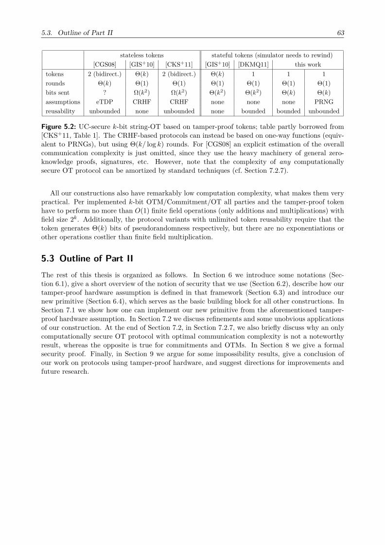
5.3. Outline of Part II 63
stateless tokens stateful tokens (simulator needs to rewind)[CGS08] [GIS+10] [CKS+11] [GIS+10] [DKMQ11] this work
tokens 2 (bidirect.) Θ(k) 2 (bidirect.) Θ(k) 1 1 1rounds Θ(k) Θ(1) Θ(1) Θ(1) Θ(1) Θ(1) Θ(1)bits sent ? Ω(k2) Ω(k2) Θ(k2) Θ(k2) Θ(k) Θ(k)assumptions eTDP CRHF CRHF none none none PRNGreusability unbounded none unbounded none bounded bounded unbounded
Figure 5.2: UC-secure k-bit string-OT based on tamper-proof tokens; table partly borrowed from[CKS+11, Table 1]. The CRHF-based protocols can instead be based on one-way functions (equiv-alent to PRNGs), but using Θ(k/ log k) rounds. For [CGS08] an explicit estimation of the overallcommunication complexity is just omitted, since they use the heavy machinery of general zero-knowledge proofs, signatures, etc. However, note that the complexity of any computationallysecure OT protocol can be amortized by standard techniques (cf. Section 7.2.7).
All our constructions also have remarkably low computation complexity, what makes them verypractical. Per implemented k-bit OTM/Commitment/OT all parties and the tamper-proof tokenhave to perform no more than O(1) finite field operations (only additions and multiplications) withfield size 2k. Additionally, the protocol variants with unlimited token reusability require that thetoken generates Θ(k) bits of pseudorandomness respectively, but there are no exponentiations orother operations costlier than finite field multiplication.
5.3 Outline of Part IIThe rest of this thesis is organized as follows. In Section 6 we introduce some notations (Sec-tion 6.1), give a short overview of the notion of security that we use (Section 6.2), describe how ourtamper-proof hardware assumption is defined in that framework (Section 6.3) and introduce ournew primitive (Section 6.4), which serves as the basic building block for all other constructions. InSection 7.1 we show how one can implement our new primitive from the aforementioned tamper-proof hardware assumption. In Section 7.2 we discuss refinements and some unobvious applicationsof our construction. At the end of Section 7.2, in Section 7.2.7, we also briefly discuss why an onlycomputationally secure OT protocol with optimal communication complexity is not a noteworthyresult, whereas the opposite is true for commitments and OTMs. In Section 8 we give a formalsecurity proof. Finally, in Section 9 we argue for some impossibility results, give a conclusion ofour work on protocols using tamper-proof hardware, and suggest directions for improvements andfuture research.


6 Preliminaries
6.1 NotationsFinite fields: By Fq we denote the finite field of size q.
Outer products: Given any field F and k, l ∈ N>0, we identify vectors in Fk by (k×1)-matrices,so that for all x ∈ Fk and y ∈ F1×l the matrix product xy ∈ Fk×l is well-defined.
Complementary matrices: Given any field F, some k, l ∈ N>0 with k < l and any two matricesC ∈ F(l−k)×l, G ∈ Fk×l, we say that G is complementary to C, if the matrix M ∈ Fl×l gen-erated by writing G on top of C has maximal rank in the sense that rank(M) = rank(C) + k.Note that, given any C ∈ F(l−k)×l, G ∈ Fk×l, x ∈ Fl, y ∈ Fk with G complementary to C,we can always find some x′ ∈ Fl, such that Cx′ = Cx and Gx′ = y.
Uniform distribution: Given any random variable x that is uniformly random over some set X,we denote that by x r← X.
Probabilities, expected values and collision entropy: We denote the probability of a ran-dom event E by P[E ]. The expected value of a random variable x is denoted by E(x) and itscollision entropy by H2(x) := − log2
(∑α
(P[x = α]
)2).Statistical distance: We denote the statistical distance of two given random variables x,y by
SD(x,y), using the following standard notion of statistical distance:
SD(x,y) = 12∑
α
∣∣P[x = α]−P[y = α]∣∣
Correlation of random variables: We define the following measure for the correlation of ran-dom variables. Given any two random variables x,y that may depend on each other, we setι(x,y) := SD
((x,y), (x, y)
)with x and y denoting independent versions of x and y respec-
tively. Note that ι(x,y) = 0 if and only if x and y are statistically independent. Furthernote that P
[Q(x,y)
]≤ P
[Q(x, y)
]+ ι(x,y) for every predicate Q. We will use the latter
extensively.
Negligibility: A function µ : N→ R≥0 is negligible (in the parameter k), if limk→∞ µ(k)·f(k) = 0for every polynomial f ∈ R[X].
Indistinguishability: Two random variables x,y are (statistically) indistinguishable, if their sta-tistical distance SD(x,y) is negligible in some security parameter.
6.2 Framework & notion of securityWe state and prove our results in the Universal-Composability (UC) framework of [Can01]. In thisframework, security is defined by comparison of an ideal model and a real model. The protocol ofinterest is running in the latter, where an adversary A coordinates the behavior of all corruptedparties. In the ideal model, which is secure by definition, an ideal functionality F implements thedesired protocol task and a simulator S tries to mimic the actions of A. An environment Z isplugged either to the ideal or the real model and has to guess, which model it is actually plugged
65

66 David & Goliath OAFE – Preliminaries
to. A protocol Π is a universally composable (UC-secure) implementation of an ideal functionalityF , if for every adversary A there exists a simulator S, such that for all environments Z the entireview of Z in the real model (with Π and A) is statistically close to its view in the ideal model (withF and S).
In our case the adversarial entities A,S and the environment Z are computationally unboundedand a hybrid functionality F stateful
wrap models our tamper-proof hardware assumption (q.v. Sec-tion 6.3). If the views of Z in the ideal model and the real model are distributed identically,we speak of perfect security; if there is some negligible statistical distance between these views, wehave only statistical security.
6.3 Modeling tamper-proof hardware
6.3.1 The hybrid functionality F statefulwrap
Our formulation of general stateful tamper-proof hardware resembles the meanwhile standard def-initions of [Kat07, MS08]. Following [MS08], we call the token issuer “Goliath” and the receiverparty “David”. This naming is also motivated by the fact that all computational versions of our pro-tocols only need David’s computing power to be polynomially bounded in the security parameter;Goliath (and even the token) may be far more powerful.
To model tamper-proof hardware, we employ the F statefulwrap wrapper functionality (q.v. Figure 6.1).
The sender party Goliath provides as input a Turing machine M to F statefulwrap . The receiver party
David can now query F statefulwrap on arbitrary input words w, whereupon F stateful
wrap runs M on inputw, sends the output thatM produced to David and stores the new state ofM. Every time Davidsends a new query w′ to F stateful
wrap , it resumes simulating M with its most recent state, sends theoutput to David and updates the stored state ofM.
Functionality F statefulwrap
The variable state is initialized by state ← wait.
Creation:• Upon receiving a message (Create,M, b) from Goliath, whereM is the program of a deterministic
interactive Turing machine and b ∈ N, verify that state = wait; else ignore that input. Next,initialize a simulated version ofM, store b, set state ← sent and send (created) to the adversary.
• Upon receiving a message (Delivery) from the adversary, verify that state = sent; else ignore thatinput. Next, set state ← execute and send (ready) to David.
Execution:• Upon receiving a message (Run, w) from David, where w is an input word, verify that state = execute;
else ignore that input. Next, write w on the input tape of the simulated machine M and carry onrunningM for at most b steps, starting from its most recent state. WhenM halts (or b steps havepassed) without generating output, send a special symbol ⊥ to David; else send the output ofM.
When a party is corrupted, the adversary is granted unrestricted access to the channel between F statefulwrap
and the corrupted party, including the ability of deleting and/or forging arbitrary messages.
Figure 6.1: The wrapper functionality by which we model stateful tamper-proof hardware sentfrom Goliath to David. Note that delivery of the token in the creation phase is scheduled by theadversary, whereas afterwards all communication between David and the token is immediate.

6.4. Sequential one-time OAFE and its relation to OTMs and OT 67
This captures the following properties one expects from tamper-proof hardware. On the onehand, Goliath is unable to revokeM once he has sent it to David. On the other hand, David canrunM on inputs of his choice, but the program code and state ofM are out of reach for him, dueto the token’s tamper-proofness. Note thatM does not need a trusted source of randomness, as itcan be provided with a sufficiently long hard-coded random tape. Thus, w.l.o.g. we can restrictMto be deterministic.
For formal reasons we require that the sender party Goliath not only specifies the programcode of M, but also an explicit runtime bound b ∈ N. This just ensures that even a corruptedGoliath cannot make F stateful
wrap run perpetually. As we will state and prove all our results withoutany computational assumptions regarding the token, a corrupted Goliath may choose b arbitrarilylarge. However, when Goliath is honest, we will only need that the number of computing stepsperformed by the token is polynomial in the security parameter. We will henceforth implicitlyassume that an honest Goliath always adjusts the parameter b accordingly.
6.3.2 Real world meaning of our hardware assumption and proof techniques
In Section 8 we will show that our construction from Section 7.1 is universally composable. However,the respective simulator for a corrupted sender party Goliath will need to rewind the token andthus has to know the token code. At first glance, it might seem a rather strong assumption thata corrupted token manufacturer always knows the internal program code of his tokens. How cansuch a party be prevented from just passing on a token received during another protocol from someuncorrupted token issuer?
We argue that tokens can be bound to the corresponding issuer IDs by not too unrealisticassumptions. The conceptually simplest (but a bit overoptimistic) way are standardized and un-forgeable token cases, branded with the respective issuer ID, and that cannot be removed withoutdestroying the token completely. However, we can go with a bit less rigorous assumptions. Wejust need that undetectable token encapsulation is infeasible (e.g., since the token’s weight and sizewould be altered) and that every honestly programmed token initially outputs its manufacturer’sID. Then, only tokens of corrupted manufacturers can be successfully passed on. Since w.l.o.g. allcorrupted parties collude, now every token issuer automatically knows the internal program codeof all his issued and/or passed on tokens. Infeasibility of token encapsulation is also needed by[HMQU05, Kat07, MS08, GKR08].
We also argue that using a stateful token does not necessarily mean a categorical disadvantagecompared to protocols based on stateless tokens. In the literature one can find the opposite pointof view, usually motivated by resetting attacks. These attacks only affect stateful approaches,whereas stateless approaches stay secure. By a resetting attack a corrupted token receiver tries torewind the token (e.g. by cutting off the power supply) and then run it with new input. Such anattack, if successful, would break security of all our protocols. However, as a countermeasure thetamper-proof token could delete its secrets or just switch to a special “dead state” when a resettingattempt is detected. For the technical realization we suggest, e.g., that the state information isstored as a code word of an error correcting code and the token does not work unless the stored stateinformation is an error-free, non-trivial code word. Anyway, we consider a thorough investigationof this issue an interesting direction for future research.
6.4 Sequential one-time OAFE and its relation to OTMs and OTThere is a two-party functionality that we call oblivious affine function evaluation (OAFE), in theliterature sometimes referred to as oblivious linear function evaluation (OLFE), which is closelyrelated to OT and of particular interest for our constructions. In Fkq -OAFE, with q and k publiclyknown but not necessarily constant, the sender chooses an affine function parametrized by twovectors a, b ∈ Fkq and the receiver chooses a preimage x ∈ Fq. The receiver gets as output the

68 David & Goliath OAFE – Preliminaries
Fkq -vector y := ax + b and the sender’s output is empty. The receiver does not learn more aboutthe sender’s input (a, b) than he can infer from (x, y) and the sender does not learn anything aboutthe receiver’s input x. As one can see quite easily, F2-OAFE and OT can be reduced to each otherwithout any overhead (q.v. Figure 6.2). Note that the reductions in Figure 6.2 also work perfectlyfor Fk2-OAFE and k-bit string-OT respectively.
OT
OAFE from OTs0bs1a+ b
c x
sc ax+ b
OAFE
OT from OAFEas0 ⊕ s1
bs0
x c
ax+ b sc
Figure 6.2: Reductions between bit-OT and F2-OAFE; protocols borrowed from [WW06].
We implement a variant of OAFE that we call “sequential one-time OAFE”, or “seq-ot-OAFE”for short. By one-time OAFE we mean a primitive that works analogously to an OTM. The sendercreates a token parametrized by a, b ∈ Fkq and sends it to the receiver. Arbitrarily later the receivermay once input some x ∈ Fq of his choice into the token, whereupon the token outputs y := ax+ band then terminates. Sequential one-time OAFE lets the sender send up to a polynomial numberof single one-time OAFE tokens, but the receiver may only query them in the same order as theywere sent. However, when the receiver has queried some of the tokens he already received, this doesnot vitiate the sender’s ability to send some additional tokens, which in turn can be queried by thereceiver afterwards, and so on. For a formal definition of the ideal seq-ot-OAFE functionality seeFigure 6.3.
Functionality F seq−otOAFE
Parametrized by a finite vector space Fkq and some runtime bound n that is polynomially bounded in thesecurity parameter λ := k log q. The counters jcreated, jsent, jqueried are all initialized to 0.
Send phases:• Upon receiving input (a, b, i) from Goliath, verify that a, b ∈ Fkq and i = jcreated + 1 ≤ n; else ignore
that input. Next, update jcreated ← i, record (a, b, i) and send (created, i) to the adversary.
• Upon receiving a message (Delivery, i) from the adversary, verify that i = jsent + 1 ≤ jcreated; elseignore that message. Next, update jsent ← i and send (ready, i) to David.
Choice phases:• Upon receiving input (x, i) from David, verify that x ∈ Fq and i = jqueried +1 ≤ jsent; else ignore that
input. Next, update jqueried ← i and for the recorded tuple (a, b, i) compute y ← ax+ b and output(y, i) to David.
When a party is corrupted, the adversary is granted unrestricted access to the channel between F seq−otOAFE
and the corrupted party, including the ability of deleting and/or forging arbitrary messages.
Figure 6.3: The ideal functionality for sequential one-time OAFE (seq-ot-OAFE). Note that sendand choice phases can be executed in mixed order with the only restriction that the i-th send phasemust precede the i-th choice phase. Further note that David’s notifications about Goliath’s inputsin the send phases are scheduled by the adversary, whereas all messages in the choice phases aredelivered immediately.

6.4. Sequential one-time OAFE and its relation to OTMs and OT 69
Note that the reduction protocols in Figure 6.2 still can be adapted canonically to transform k-bit string-OTMs into Fk2-OAFE tokens and vice versa. Hence, using the seq-ot-OAFE functionality(q.v. Figure 6.3), a polynomial number of OTMs can be implemented very efficiently, but thereceiver can query the single OTM tokens only in the same order as they were sent. However,the construction of [GIS+10] for trusted OTPs from OTMs still works, as there an honest receiverqueries all OTM tokens in a fixed order anyway. Interestingly, the technical challenges dealt within [GIS+10] arise from the fact that a malicious receiver might query the OTMs out of order.Moreover, the restriction to sequential access can be exploited to securely notify the sender thatthe receiver has already queried some OTM token. Therefor, every other OTM token is issued withpurely random input from the sender and the receiver just announces his corresponding input-output tuple. A corrupted receiver that tries to adversarially delay his OTM queries is caughtcheating with overwhelming probability, as he has only a negligible chance to correctly guess thenext check announcement. Thus, we can implement a polynomial number of OT instances that areperfectly secure against the OT sender and statistically secure against the OT receiver. Still, thereceiver can query the single OT instances only in the same order as they were sent, but in factthis is already premised in most protocols that build on OT. Noting that OT and OAFE can bestored and reversed [Bea96, WW06, Wul07], we conclude that in the seq-ot-OAFE hybrid modelOT can be implemented in both ways (from the token sender to the token receiver and vice versa).
Finally, a remark is in place. Even though seq-ot-OAFE can be used to implement severalOTPs, the sequential nature of seq-ot-OAFE demands that those OTPs can only be executed in apredefined order. If one wishes to implement several OTPs that can be evaluated in random order,as many seq-ot-OAFE functionalities have to be issued.


7 Semi-interactive seq-ot-OAFE from onetamper-proof token
7.1 The basic protocolWe want to implement seq-ot-OAFE (q.v. Section 6.4), using a single tamper-proof hardware tokenthat is issued by one of the mutually distrusting parties. The technical challenge in doing so istwofold. Firstly, the receiver David must be able to verify that no token output does depend onany input of previous choice phases. Secondly, each token output must be an affine function ofthe corresponding input. However, note that the latter difficulty is only relevant if q > 2, as everyfunction f : F2 → Fk2 is affine: f(x) =
(f(0) + f(1)
)· x+ f(0) for all x ∈ F2.
Our approach to solving these problems is enlarging the token’s output space to dimension(1 + α)k and letting the sender Goliath announce αk-dimensional linear hash values of the token’sfunction parameters, which can be used by David for a consistency check; then there remains ak-dimensional part of the token’s output for generation of the intended OAFE result. For technicalreasons we choose α = 3. In particular, a preliminary protocol idea can be sketched as follows:
• Goliath chooses the i-th token parameters uniformly at random, say r, s r← F4kq .
• Upon receiving the token, David announces a random check matrix C r← F3k×4kq .
• Goliath in turn announces r := Cr and s := Cs.
• When David queries the token the i-th time, say he inputs some x ∈ Fq and receives outputw ∈ F4k
q , he checks whether Cw = rx + s. When the check is not passed, David has caughtGoliath cheating and henceforth always outputs a default value.
This way, we can implement some kind of “weak” OAFE, where the receiver additionally learnssome linear projection of the sender’s inputs, but by announcing (r, s) Goliath has committedthe token to affine behavior. Otherwise, if the check would be passed for a large set of tokeninputs X ⊆ Fq and there do not exist any r, s ∈ F4k
q such that τ(x) = rx+ s for all x ∈ X with τdenoting the token functionality in the i-th round, then the token could as well form collisions for theuniversal hash function C, of which it is oblivious. Moreover, we can nullify the receivers additionalknowledge about (r, s) by multiplication with any matrix G ∈ Fk×4k
q that is complementary to C.When David just outputs Gw, we have implemented OAFE with random input (Gr,Gs) fromGoliath and arbitrarily selectable input x from David. Finally, Goliath can derandomize his inputto arbitrarily selectable a, b ∈ Fkq by announcing a := a−Gr and b := b−Gs. David then just hasto replace his output by y := Gw + ax+ b.
However, there is still a security hole left, as the token might act honestly only on some spe-cific input set X ( Fq or even only on some specific type of input history. Now, when David’sinputs match this adversarially chosen specification, he will produce regular output; else a protocolabortion is caused with overwhelming probability (i.e. David produces default output). Such abehavior cannot be simulated in the ideal model, unless the simulator gathers some informationabout David’s input. Thus, David must keep his real input x secret from the token (and as wellfrom Goliath, of course). However, David’s input must be reconstructible from the joint view ofGoliath and the token, as otherwise a corrupted David could evaluate the function specified byGoliath’s input (a, b) on more than one input x. Our way out of this dilemma is by a linear secret
71

72 David & Goliath OAFE – Semi-interactive seq-ot-OAFE from one tamper-proof token
sharing scheme, whereby David shares his input x between Goliath and the token. In particular,the protocol now roughly proceeds as follows:
• Goliath initializes the token with uniformly random parameters r r← F4kq and S r← F4k×k
q .
• Upon receiving the token, David announces a random check matrix C r← F3k×4kq and a random
share h r← Fkq \ 0. David and Goliath also agree on some G ∈ Fk×4kq complementary to C.
• Goliath announces the check information r := Cr and S := CS and the derandomizationinformation a := a−Gr and b := b−GSh, where (a, b) ∈ Fkq ×Fkq is his OAFE input.
• David randomly picks a second share z r← z ∈ F1×kq | zh = x, where x ∈ Fq is his
OAFE input. He inputs z into the token, whereupon the token has to compute and outputW := rz + S. When the check CW
?= rz + S is passed, David computes and outputsy := GWh+ ax+ b; else he outputs some default value.
Now, neither Goliath nor the token can gather non-negligible information about David’s OAFEinput x. Given any set of token inputs Z ⊆ F1×k
q adversarially chosen in advance, the hyperplanesz ∈ F1×k
q | zh = xx∈Fq will partition Z into q subsets of roughly equal size, since h is uniformlyrandom. In other words, when the token behaves dishonestly on some input set Z ( F1×k
q , theabort probability is practically independent of David’s input x.
A remarkable property of our protocol is that David’s input x is only needed in the last step,where no further communication with Goliath takes place. So, we can partition the protocol intoan interactive phase (where Goliath provides his OAFE input) and a non-interactive phase (whereDavid provides his input and learns his output). Therefore, we say that our protocol is “semi-interactive”. A formal description of the full protocol Πsemi−int
OAFE is given in Figure 7.1.There are two crucial differences between Πsemi−int
OAFE and the construction in [DKMQ11]. Firstly,we changed from F2 to Fq with the explicit option that q may depend on the security parameter.This will enable us to implement OTMs, string-OT and string-commitments at optimal communi-cation rate (cf. Section 7.2.1 and Section 7.2.5). Secondly, due to a new security proof we no longerneed that Goliath’s “commitments” (r1, S1), . . . , (rn, Sn) are statistically independent of David’sinput shares h1, . . . , hn. This allows for multiple send phases and choice phases in mixed order, sothat a token that shares some random source with its issuer Goliath can be reused over and overagain without any predefined limit (cf. Section 7.2.4).
At this point we also want to point out that in the protocol description of Figure 7.1 we purposelydo not exactly specify how the parameters k and q depend on the security parameter λ. In fact, forour security proof we only need that k · log q = λ and k ≥ 5; e.g. one can choose k to be constantand q to increase exponentially. With parameters chosen this way, our protocol Πsemi−int
OAFE has onlylinear communication complexity, what is clearly optimal. The condition that k ≥ 5 results fromour proof techniques and is probably not tight. If k = 1, the protocol is not UC-secure against acorrupted sender party (see Remark 43 below), but for 2 ≤ k ≤ 4 we are not aware of any potentialattack. However, note that F seq−ot
OAFE with k < 5 can be implemented from F seq−otOAFE with k = 5
straightforwardly and the reduction protocol itself has only linear overhead. Thus, the asymptoticoptimality of our construction with k = 5 does directly carry over to the case that k < 5.
Finally, we want to note that our protocol allows any polynomial number of send phases to beperformed in parallel, so that one can still issue the polynomially many OTMs needed for an OTPby just constantly many rounds of communication (cf. Section 7.2.3).
Remark 43. Our protocol Πsemi−intOAFE is not UC-secure against a corrupted sender Goliath, if k = 1.
Proof. The problem with k = 1 basically arises from the fact that in this case Goliath’s shares hiof David’s inputs xi are invertible field elements. Consider a maliciously programmed token thatstops functioning after the first choice phase, if z1 ∈ Z for some adversarially chosen Z ⊆ Fq, e.g.

7.1. The basic protocol 73
with |Z| = q2 , and otherwise just follows the protocol. Since Goliath knows Z and learns h1 during
the protocol, he also knows exactly on which inputs x1 the token breaks: It breaks, if x1h−11 ∈ Z.
In other words, it depends on x1, if David’s outputs y2, . . . , yn are all-zero or not. This is notsimulatable in the ideal model, because the simulator gets absolutely no information about theuncorrupted David’s inputs.
Protocol Πsemi−intOAFE
Parametrized by a finite vector space Fkq and some runtime bound n that is polynomially bounded in thesecurity parameter λ := k log q. The setup phase is executed right at the start of the first send phase.
Setup phase:i. For i = 1, . . . , n, Goliath chooses a random vector ri
r← F4kq and a random matrix Si
r← F4k×kq ,
creates a token T with parameters (r1, S1), . . . , (rn, Sn) and sends T to David via F statefulwrap . The
token also contains a counter j′queried and Goliath has a counter jcreated, both initialized to 0.
ii. Having received T , David chooses a random matrix Cr← F
3k×4kq , computes some G ∈ Fk×4k
q
complementary to C and sends (C,G) to Goliath. Furthermore, David initializes two countersjqueried, jsent ← 0 and an initial flag f0 ← >.
iii. If Goliath finds G not complementary to C, he aborts the protocol.
Send phases:1. Upon input (ai, bi, i) from the environment, Goliath verifies that ai, bi ∈ Fkq and i = jcreated + 1 ≤ n;
else he ignores that input. Next, Goliath updates jcreated ← i, computes ri ← Cri and Si ← CSi andsends (ri, Si, i) to David.
2. David chooses a random vector hir← F
kq \ 0 and sends (hi, i) to Goliath.
3. Goliath computes ai ← ai−Gri and bi ← bi−GSihi and sends (ai, bi, i) to David, who ignores thatmessage if not i = jsent + 1 ≤ n.
4. David updates jsent ← i and outputs (ready, i) to the environment.
Throughout the whole send phase, obviously malformed messages are just ignored by the respective receiver.
Choice phases:5. Upon input (xi, i) from the environment, David verifies that xi ∈ Fq and i = jqueried+1 ≤ jsent; else he
ignores that input. Next, he updates jqueried ← i, chooses a random vector zir← z ∈ F1×k
q | zhi = xiand inputs (zi, i) into the token T .
6. The token verifies that zi ∈ F1×kq and i = j′queried + 1 ≤ n; else it ignores that input. Next, the token
updates j′queried ← i, computes Wi ← rizi + Si and outputs Wi to David.
7. David verifies that fi−1 = > and CWi = rizi+Si; ifWi /∈ F4l×kq , it is treated as an encoding of the all-
zero matrix in F4l×kq . If the check is passed, David sets fi ← > and computes yi ← GWihi+ aixi+ bi;
otherwise he sets fi ← ⊥ and yi ← 0 (such that yi ∈ Fkq ). Then he outputs (yi, i) to the environment.
Figure 7.1: A protocol for semi-interactive sequential OAFE, using one tamper-proof token. Notethat several send and choice phases can be executed in mixed order with the only restriction thatan honest David will not enter the i-th choice phase before the i-th send phase has been completed.

74 David & Goliath OAFE – Semi-interactive seq-ot-OAFE from one tamper-proof token
7.2 Refinements and applications of our construction
Before we give a formal security proof for our protocol Πsemi−intOAFE , we first want to present how the
claimed optimal constructions for multiple OTMs, Commitments and OT (cf. Section 5.2) do work.As mentioned above, we will prove security of our protocol Πsemi−int
OAFE only for the case that k ≥ 5.However, F seq−ot
OAFE with k < 5 can be implemented from F seq−otOAFE with k = 5 straightforwardly and
the reduction protocol itself has only linear overhead. Thus, the asymptotic optimality of ourconstruction for F seq−ot
OAFE with k = 5 does directly carry over to the case that k < 5.At the end of this section, in Section 7.2.7, we also discuss why for computationally secure OT
protocols an improvement of the communication complexity is not a noteworthy result. However,this does neither affect statistically secure OT nor any commitment or OTM constructions.
7.2.1 Unidirectional string-OT and OTMs with optimal communication complexity
As discussed in Section 6.4, one can reduce k-bit string-OT and Fk2-OAFE to each other without anyoverhead. However, our construction for seq-ot-OAFE has communication complexity Θ(nk2 log q).I.e., by the aforementioned reduction approach we would end up with a communication complexityof Θ(k2) per implemented instance of k-bit string-OT, as it happened in [DKMQ11]. In contrast, ifk is constant and q grows exponentially in the security parameter, we have only a communicationcomplexity of O(log q) for each implemented instance of Fkq -OAFE (q.v. Figure 7.1), what is clearlyoptimal. Therefore, it is desirable to implement l-bit string-OT by a constant number of Fd2l-OAFE instances with constant dimension d. We present such a reduction protocol in Figure 7.2;our construction needs only a single instance of F2
2l-OAFE and the protocol idea is as follows. TheF2
2l-OAFE primitive allows the sender party to specify two affine functions f0, f1 : F2l → F2l , suchthat the receiver party can evaluate both functions only once and only simultaneously on the sameinput. Thus, if the sender party announces its OT-inputs s0 and s1 encrypted with f0(0) and f1(1)respectively, then the receiver party may learn at most one of the values needed for decryption ofs0 and s1. One can even go without transmitting any ciphertexts: The sender party just has tochoose f0, f1, such that f0(0) = s0 and f1(1) = s1, whereas f0(1) and f1(0) are completely random.
a, br← F
22l
m0 := s0 ⊕ (e0 · b)m1 := s1 ⊕
(e1 · (a+ b)
) m0,m1
with e0, e1 beingany public basis ofthe linear space F1×2
2l
F22l -OAFE
a
b
c
ac+ b y
l-bit string-OT
s0
s1
c
mc ⊕ (ec · y) sc
Figure 7.2: Reduction of l-bit string-OT to F22l-OAFE. Note that the transmission of m0 and m1 is
not essential; instead the sender party can just choose (a, b) subject to the condition that e0 · b = s0and e1 · (a+ b) = s1.
The protocol in Figure 7.2 is perfectly UC-secure, what can be shown straightforwardly, and italso works perfectly for implementation of sequentially queriable OTM tokens from seq-ot-OAFE(cf. the respective discussion in Section 6.4). Thus, in the outcome we also have a constructionfor sequentially queriable log(q)-bit OTM tokens, using only Θ(log q) bits of communication perimplemented OTM token. This communication complexity is clearly optimal and to the best of ourknowledge our approach is the first to implement statistically secure OT (or OTMs respectively)with optimal communication complexity, while based only on untrusted tamper-proof hardware.

7.2. Refinements and applications of our construction 75
Note that our protocols with linear communication complexity also have very low computationcomplexity. Per implemented log(q)-bit string-OT (or log(q)-bit OTM respectively) every party(and in particular the exchanged token) has only to perform O(1) finite field operations with fieldsize q, what is considerably faster than, e.g., something based on modular exponentiation.
7.2.2 Achieving optimal communication complexity for bidirectional string-OTIn Section 7.2.1 we have shown how one can implement unidirectional string-OT (from the tokenissuer to the token receiver) with optimal communication complexity, using our protocol Πsemi−int
OAFEas a building block. Implementing string-OT in the other direction (from the token receiver tothe token issuer) with optimal communication complexity turns out a bit more challenging. Thestarting point for our construction is the protocol in Figure 7.3 for reversing the direction of agiven Fq-OAFE primitive. Note that this protocol is not UC-secure, since a corrupted sender cancause the receiver to output some y before a and b are fixed: The corrupted sender can just send arandom m ∈ Fq and arbitrarily later input some a ∈ Fq of his choice into the underlying Fq-OAFEinstance (and then compute b := m − z). This breaches UC-security, since an ideal version of thereversed Fq-OAFE primitive would not send y to the receiver party before the sender’s inputs a andb are fixed. However, in our case this problem has a simple solution: Since our protocol Πsemi−int
OAFEimplements sequentially queriable OAFE instances, it suffices to use every other OAFE instance fora check announcement, i.e. both parties just input randomness and the receiver has to announcehis input-output tuple (cf. Section 6.4).
Fq-OAFEx
Fqr→ r
a
ax+ r z
m := z + b
reversed Fq-OAFE
x a
b
m− ry
Figure 7.3: Basic approach for reversing the direction of a given Fq-OAFE primitive; protocoltaken from [WW06]. Note that this protocol is not UC-secure, unless input of a into the underlyingFq-OAFE instance is enforced before the receiver outputs y; otherwise a corrupted sender canmaliciously delay his choice of a (and b).
Obviously, the approach in Figure 7.3 does not work for Fkq -OAFE with k > 1, but we needF2q-OAFE for our aimed at OT protocol. Thus, a construction for Fkq -OAFE from some instances
of Fq-OAFE would come in very handy. In [DKMQ12b] one can find such a construction and asecurity proof for the case that k log q increases polynomially in the security parameter. For thesake of self-containedness we recap in Figure 7.4 the approach of [DKMQ12b] with k = 2. Bycombining this with the protocol in Figure 7.3 and some optimization in the number of Fq-OAFEinstances used for check announcements we end up with the protocol depicted in Figure 7.5.
Now, by plugging the protocol of Figure 7.5 on top of Πsemi−intOAFE (q.v. Figure 7.1) we get sequen-
tially queriable F2q-OAFE from the token receiver to the token sender with an overall communication
complexity of O(log q) per implemented F2q-OAFE instance. So finally, we can apply again the pro-
tocol of Figure 7.2 and thereby implement string-OT with optimal communication complexity alsoin the direction from the token receiver to the token issuer.

76 David & Goliath OAFE – Semi-interactive seq-ot-OAFE from one tamper-proof token
Fq-OAFErandom αi
random βi
x
αix+ βi γi
for i ∈ 1, . . . , 5
Hr← F
2×5q
α′ := a−H · (α1, . . . , α5)T
β′ := b−H · (β1, . . . , β5)T
F2q-OAFE
xa
b
α′x+ β′ +H · (γ1, . . . , γ5)T y
Figure 7.4: Implementation of F2q-OAFE from five instances of Fq-OAFE; protocol taken from
[DKMQ12b]. Additional measures must be taken so that H is not announced before the receiverparty has provided some input to all five underlying Fq-OAFE instances in the dashed box; other-wise the protocol is inherently insecure, as shown in [DKMQ12b, Lemma 1].
Fq-OAFEx
Fqr→ γi
αir← Fq
αix+ γi βi
for i ∈ 1, . . . , 5
Fq-OAFE0Fq
r→ ρ
0
ρ
ρ
Hr← F
2×5q
α′ := a−H · (α1, . . . , α5)T
β′ := b−H · (β1, . . . , β5)T
reversed F2q-OAFE
x a
b
α′x− β′ −H · (γ1, . . . , γ5)Ty
Figure 7.5: Combined protocol for UC-secure reversed F2q-OAFE from six sequentially queriable
instances of Fq-OAFE. Note that the receiver must not output y unless ρ was announced correctlyby the sender party.

7.2. Refinements and applications of our construction 77
7.2.3 Reducing the number of rounds, e.g. for one-time programsIn [GIS+10] so-called trusted OTPs are implemented from a polynomial amount of OTM tokens. Asan honest receiver will query these tokens in some predefined (and publicly known) order, we canadapt the results of [GIS+10] to implement trusted OTPs from a single untrusted hardware token(cf. Section 6.4). However, if one implements some polynomial number (say l) of sequentially que-riable OTM tokens by the construction we proposed in Section 6.4, one will end up with more thanthrice as many (i.e. 3l) rounds of communication between David and Goliath. This round complex-ity can be dramatically reduced as follows: In our protocol Πsemi−int
OAFE (q.v. Figure 7.1), instead ofperforming a large number of individual send phases, David can already announce h1, . . . , hl alongwith the check matrix C in step ii of the setup phase and Goliath can send all his announcements ofthe corresponding l send phases in one single message
((r1, S1, 1), (a1, b1, 1), . . . , (rl, Sl, l), (al, bl, l)
).
Thereby we end up with two rounds of communication, not counting for the transmission of thetoken. This modification of the protocol Πsemi−int
OAFE does not breach its security: In our formal secu-rity proof we even assume that a corrupted Goliath’s announcement of
((r1, S1), . . . , (rn, Sn)
)may
arbitrarily depend on (h1, . . . , hn). Hence, our security proof does directly carry over to the modi-fied protocol. Note that analogously we just can arbitrarily parallelize multiple send phases of ourprotocol Πsemi−int
OAFE without jeopardizing security. This can be used, e.g., to implement polynomiallymany OTs (cf. Section 7.2.1) or commitments (cf. Section 7.2.5) with constant round complexity.
It is quite straightforward to see that a two-round protocol for implementation of polynomi-ally many OTM tokens from a single piece of untrusted tamper-proof hardware is optimal—cf. [DKMQ11, Theorem 1]. Furthermore, our new two-round protocol is an improvement upon[DKMQ11], where we needed four rounds of communication between David and Goliath.
7.2.4 Computational solution for unlimited token reusabilityOur protocol Πsemi−int
OAFE (q.v. Figure 7.1) guarantees perfect security against David (cf. Section 8.2).However, to achieve this, the token needs to be able to store Θ(nk2 log q) bits of information. Thiscontradicts the idea of a tamper-proof hardware token being a small and simple device. In [MS08]it was noted, that if David is computationally bounded, then the functions stored on the tokencould be chosen to be pseudorandom [GGM86, HILL99]. The same is true for our construction.It suffices that the token stores a succinct seed of length Θ(k log q) for a pseudorandom numbergenerator F . Upon input (zi, i) the token can compute the next pseudorandom value (ri, Si) = F (i)and output Wi = rizi + Si.
Moreover, in such a setting we do not need our protocol Πsemi−intOAFE and the ideal functionality
F seq−otOAFE to be parametrized by an explicit runtime bound n, as David’s computational boundedness
implies a polynomial upper bound for the number of token queries.
7.2.5 Efficient protocol for string-commitments in any directionAt this point we also want to note that string commitments can be implemented directly from seq-ot-OAFE, even if the dimension k is constant (i.e. q grows exponentially in the security parameter).See Figure 7.6 for the reduction protocols; they work analogously to the standard constructionsfor commitments from OT. As our protocol for seq-ot-OAFE with constant dimension k has onlylinear complexity, we thus get asymptotically optimal protocols for string commitments.

78 David & Goliath OAFE – Semi-interactive seq-ot-OAFE from one tamper-proof token
Protocol ΠforwardCOM (Goliath is the committing/unveiling party)
Parametrized by a string length l, which also serves as security parameter, and some runtime bound n thatis polynomially bounded in l. All parties have access to a hybrid functionality F seq−ot
OAFE parametrized by thefinite vector space F1
2l and with runtime bound n. Bit strings of length l and elements of F2l are identifiedwith each other. The counter j, held by Goliath, is initialized to 0.
Commit phases:1. Upon input (Commit, si, i) from the environment, Goliath verifies that si ∈ 0, 1l and i = j+ 1 ≤ n;
else he ignores that input. Next, Goliath updates j ← i, chooses some random bir← F2l and sends
(si, bi, i) to F seq−otOAFE .
2. David, upon receiving the message (ready, i) from F seq−otOAFE , picks some random xi
r← F2l . He sends(xi, i) to F seq−ot
OAFE , receives some (yi, i) and outputs (committed, i).
Unveil phases:3. Upon input (Unveil, i) from the environment, Goliath verifies that i ≤ j; else he ignores that input.
Next, Goliath sends (si, bi, i) to David.
4. David verifies that sixi + bi = yi. If the check is passed, he outputs (si, i); otherwise he outputs(⊥, i).
Protocol ΠbackwardCOM (David is the committing/unveiling party)
Parametrized by a string length l, which also serves as security parameter, and some runtime bound nthat is polynomially bounded in l. All parties have access to a hybrid functionality F seq−ot
OAFE parametrizedby the finite vector space F1
2l and with runtime bound 2n. Bit strings of length l and elements of F2l areidentified with each other. The counter j, held by David, is initialized to 0.
Commit phases:1. Upon input (Commit, si, i) from the environment, David verifies that si ∈ 0, 1l and i = j + 1 ≤ n;
else he ignores that input. Next, David updates j ← i and sends (i) to Goliath.
2. Goliath randomly picks ai, bi, ci, dir← F2l and sends (ai, bi, 2i− 1) and (ci, di, 2i) to F seq−ot
OAFE .
3. David, after receiving the messages (ready, 2i − 1) and (ready, 2i) from F seq−otOAFE , sends (si, 2i − 1)
and (0, 2i) to F seq−otOAFE . He receives some (yi, 2i− 1) and (ri, 2i) and announces (ri, i) to Goliath.
4. Goliath outputs (committed, i).
Unveil phases:5. Upon input (Unveil, i) from the environment, David verifies that i ≤ j; else he ignores that input.
Next, David sends (si, yi, i) to Goliath.
6. Goliath verifies that ri = di and yi = aisi + bi. If the check is passed, he outputs (si, i); otherwisehe outputs (⊥, i).
Figure 7.6: Asymptotically optimal protocols for string commitments from seq-ot-OAFE. Notethat in a straightforward manner one can use the same instance of F seq−ot
OAFE for both protocolssimultaneously.

7.2. Refinements and applications of our construction 79
7.2.6 Non-interactive solution with two tokensOur approach still needs the receiver party David to send some messages to the sender party Goliath.In particular, for each implemented instance of Fkq -OAFE we have an interactive send phase anda non-interactive choice phase (q.v. Figure 7.1). Therefore, we say that our protocol Πsemi−int
OAFE is“semi-interactive”. It is quite straightforward to see that one cannot implement F seq−ot
OAFE from asingle instance of F stateful
wrap by any non-interactive protocol—cf. [DKMQ11, Theorem 1]. However,we can easily give a generic non-interactive protocol for F seq−ot
OAFE , if two instances of F statefulwrap are in
place, i.e. the sender party Goliath issues two tamper-proof tokens and the receiver party Davidcan trust that the tokens are mutually isolated. Then, the second token can play Goliath’s role inthe protocol Πsemi−int
OAFE with random inputs ai and bi. As Goliath knows the second token’s randomcoins, derandomization of his inputs can be done as follows: If Goliath wants to replace the randominput tuple (ai, bi) by some arbitrarily chosen (a′i, b′i), he just sends (a′i−ai, b′i− bi, i) to David, whothen has to replace his output yi by y′i := yi + (a′i − ai)xi + (b′i − bi).
Note that based on the two-token protocol that implements F seq−otOAFE with random Goliath inputs,
step 2 of ΠbackwardCOM (q.v. Figure 7.6) can be made non-interactive, as Goliath does not need to
derandomize any of his inputs. All other protocols become non-interactive straightforwardly.
7.2.7 A note on optimal communication complexityThe string length of any computationally secure OT protocol can be polynomially extended bystandard techniques (cf. protocol Πenlarge
OT in Figure 7.7). It is straightforward to show UC-securityof this approach. Hence, optimal communication complexity of the computational versions ofour OT solution is not a noteworthy result. However, applying an analogous transformation tocommitments or OTMs would destroy UC-security (see Remark 44 below) and we are not awareof any universally composable amortization techniques for these primitives that do not come alongwith additional setup assumptions.
Remark 44. The protocols ΠenlargeCOM and Πenlarge
OTM in Figure 7.7 are not UC-secure.
Proof. We just show that ΠenlargeCOM is not UC-secure. For Πenlarge
OTM one can argue analogously. Considera passively corrupted receiver party that just hands over every message to the environment. Forthe real model, this means that in the commit phase the environment learns some k-bit string rand in the unveil phase it learns a seed s ∈ 0, 1l, such that r ⊕ F (s) is the honest sender party’sinput c. Now, if the environment chooses the honest sender party’s input c ∈ 0, 1k uniformly atrandom, this is not simulatable in the ideal model. The simulator has to choose r before he learnsc. Thus, using a simple counting argument, the probability that there exists any seed s ∈ 0, 1lwith r⊕F (s) = c can be upper bounded by 2l−k. In other words, the simulation fails at least withprobability 1− 2l−k.

80 David & Goliath OAFE – Semi-interactive seq-ot-OAFE from one tamper-proof token
Protocol ΠenlargeOT
Parametrized by two security parameters k and l with k > l, a hybrid functionality FOT for l-bit string-OTand a PRNG function F with seed length l and output length k, i.e. F : 0, 1l → 0, 1k.
1. Upon input (s0, s1) from the environment, the sender party verifies that s0, s1 ∈ 0, 1k; else thatinput is ignored. Next, the sender party chooses two random seeds s0, s1
r← 0, 1l and inputs (s0, s1)into FOT.
2. Upon input x from the environment, the receiver party verifies that x ∈ 0, 1; else that input isignored. Next, the receiver party inputs x into FOT, thus receiving sx.
3. The sender party, after being notified that everybody did provide some input to FOT, announcesr0 := s0 ⊕ F (s0) and r1 := s1 ⊕ F (s1).
4. The receiver party computes and outputs sx = rx ⊕ F (sx).
Protocol ΠenlargeCOM
Parametrized by two security parameters k and l with k > l, a hybrid functionality FCOM for l-bit string-commitment and a PRNG function F with seed length l and output length k, i.e. F : 0, 1l → 0, 1k.
Commit phase:1. Upon input (Commit, c) from the environment, the sender party verifies that c ∈ 0, 1k; else that
input is ignored. Next, the sender party chooses some random sr← 0, 1l, commits to s via FCOM
and sends r := c⊕ F (s) to the receiver party.
2. The receiver party outputs (committed).
Unveil phase:3. Upon input (Unveil) from the environment, the sender party unveils s.
4. If the unveil is successful, the receiver party computes and outputs r⊕F (s); otherwise it outputs ⊥.
Protocol ΠenlargeOTM
Parametrized by two security parameters k and l with k > l, a hybrid functionality FOTM for l-bit OTMand a PRNG function F with seed length l and output length k, i.e. F : 0, 1l → 0, 1k.
Creation:1. Upon input (s0, s1) from the environment, the sender party verifies that s0, s1 ∈ 0, 1k; else that
input is ignored. Next, the sender party chooses two random seeds s0, s1r← 0, 1l, sends (s0, s1)
via FOTM to the receiver party and announces r0 := s0 ⊕ F (s0) and r1 := s1 ⊕ F (s1).
2. The receiver party outputs (ready).
Query:3. Upon input x from the environment, the receiver party verifies that x ∈ 0, 1; else that input is
ignored. Next, the receiver party inputs x into FOTM, thus receiving sx, and computes and outputssx = rx ⊕ F (sx).
Figure 7.7: Straightforward approaches for enlarging the string length of some given OT, commit-ment or OTM functionality, using a PRNG. The protocol Πenlarge
OT is UC-secure, but ΠenlargeCOM and
ΠenlargeOTM are not (q.v. Remark 44).

8 Correctness and security of our protocol
In this section we show that in the F statefulwrap -hybrid model our protocol Πsemi−int
OAFE (q.v. Figure 7.1)is a universally composable implementation of the ideal functionality F seq−ot
OAFE (q.v. Figure 6.3), ifonly k ≥ 5. In particular, in Section 8.2 we will prove perfect security against a corrupted Davidfor all k and in Section 8.3 we will prove statistical security against a corrupted Goliath for thecase that k ≥ 5. However, first of all we will show that Πsemi−int
OAFE always works correctly when noparty is corrupted (Section 8.1).
8.1 CorrectnessIn a totally uncorrupted setting, simulation is straightforward. Since the simulator always is notifiedwhen the ideal Goliath receives input from the environment and the simulator also may arbitrarilydelay the ideal David’s corresponding ready-message, he can perfectly simulate any scheduling ofthe messages in the send phase. In turn, the choice phase cannot be influenced by the real modeladversary and therefore can be simulated trivially. Furthermore, whenever in the real model thereceiver David outputs some (yi, i), it holds that yi = aixi + bi, as one can verify as follows:
yi = G (rizi + Si)︸ ︷︷ ︸=Wi
hi + (ai −Gri)︸ ︷︷ ︸=ai
xi + bi −GSihi︸ ︷︷ ︸=bi
= Gri (zihi − xi)︸ ︷︷ ︸=0
+aixi + bi
Also note that in a totally uncorrupted setting David’s consistency checks are always passed.
8.2 Security against a corrupted receiverWe first show security against a corrupted receiver party David, as this is the easy case. Basically,there are only two things a corrupted David can do: follow the protocol honestly, or query thetoken before the respective send phase is over. We will refer to the former as the regular case andto the latter as the irregular case. A bit more formally, regarding some specific i ∈ 1, . . . , n wespeak of the regular case if David sends (hi, i) to Goliath before inputting (zi, i) into the token,and we speak of the irregular case if David sends (hi, i) to Goliath after inputting (zi, i) into thetoken. Note that, although David is corrupted, hi and zi are still well-defined since Goliath and thetoken accept only well-formed messages (hi, i) and (zi, i) respectively. It is quite straightforwardto see that due to the randomness of (ri, Si) every value seen by David, namely ri, Si, ai, bi,Wi, isjust uniformly random subject to the sole condition that in the end the correct result yi can becomputed. We formalize this by the next lemma.
Lemma 45. In our protocol Πsemi−intOAFE , if Goliath is honest, the variables ri, Si, ai, bi,Wi are just
uniformly random subject to the condition that CWi = rizi+Si and GWihi+aizihi+ bi = aizihi+bi.
Proof. We give a proof by cases and start off with the regular case, i.e. David first sends (hi, i) toGoliath and later on inputs (zi, i) into the token. In this case, Goliath obviously just announces someri, Si, ai, bi uniformly at random. Consequently, we have to show now that the token output Wi isuniformly random subject to the condition that CWi = rizi+Si and GWihi+aizihi+bi = aizihi+bi.However, we can imagine that right before the computation of Wi the token’s stored randomnessSi is uniformly resampled subject to the condition that CSi = Si and GSihi = bi− bi. This clearly
81

82 David & Goliath OAFE – Correctness and security of our protocol
does not change David’s view at all. In other words, we can replace Si by Si + S′, where S′ isuniformly random subject to the condition that CS′ = 0 and GS′h = 0. Thereby, Wi is alsoreplaced by Wi + S′ and hence becomes uniformly random subject to the sole condition that CWi
and GWihi are not changed. This means that Wi is uniformly random subject to the conditionthat CWi = rizi + Si and GWihi = (ai − ai)zihi + bi − bi. This concludes our proof for the regularcase.
Now we consider the irregular case, i.e. the corrupted David inputs (zi, i) into the token beforehe sends (hi, i) to Goliath. In this case, (ri, Si) announced by Goliath and the token’s output Wi
are just uniformly random subject to the condition that CWi = rizi + Si. Consequently, we haveto show now that the honest Goliath’s announcement of (ai, bi) is uniformly random subject tothe condition that GWihi + aizihi + bi = aizihi + bi. However, we can imagine that right beforethe computation of (ai, bi) the stored randomness ri in Goliath’s memory is uniformly resampledsubject to the condition that Cri = ri, and Si is replaced by the new value of Wi − rizi. It isstraightforward to verify that this does not change the corrupted David’s view at all. In otherwords, we can replace (ri, Si) by (ri + r′, Si − r′zi), where r′ is uniformly random subject to thecondition that Cr′ = 0. Thereby, ai is replaced by ai − Gr′ and hence becomes just uniformlyrandom over Fkq , since G is complementary to C and thus Gr′ itself is uniformly random over Fkq .Analogously, bi is replaced by bi +Gr′zihi, and it still holds:
GWihi + (ai −Gr′)︸ ︷︷ ︸new ai
zihi + (bi +Gr′zihi)︸ ︷︷ ︸new bi
= GWihi + aizihi + bi = aizihi + bi
This means that ai, bi are uniformly random subject to the sole condition that GWihi+ aizihi+ bi =aizihi + bi. This concludes our proof for the irregular case.
This lemma leads to a very straightforward simulator construction for the UC framework. Whenthe corrupted David queries the token after he already got the derandomization information (ai, bi)from Goliath in the corresponding send phase, the simulator can revise the token’s output Wi
so that the check CWi?= rizi + Si is still passed, but GWi now matches a protocol run in the
real model: When the token is to output Wi, the simulator has already seen both shares zi, hithat are needed to extract David’s input xi. The simulator can then query the ideal functionalityF seq−ot
OAFE on this input xi, thus receiving yi, and then revise Wi by some W ′ so that CW ′ = CWi
and yi = GW ′hi + aixi + bi. Note that existence of such a W ′ is always guaranteed, since G iscomplementary to C (i.e. especially G has full rank) and h 6= 0.
When the corrupted David queries the token before he got the derandomization information(ai, bi) from Goliath in the corresponding send phase, the simulator can easily revise Goliath’sannouncement of the derandomization information so that it matches a protocol run in the realmodel: When Goliath is to announce the derandomization information (ai, bi), the simulator hasalready seen both shares zi, hi that are needed to extract David’s input xi. The simulator can thenquery the ideal functionality F seq−ot
OAFE on this input xi, thus receiving yi, and then just revise bi sothat yi = GWihi + aixi + bi.
A formal description of this simulator construction is given in Figure 8.1. We conclude thissection with the corresponding security theorem.
Theorem 46. Let some arbitrary environment Z be given and some adversary A that corrupts thereceiver David. Then the view of Z in the ideal model with ideal functionality F seq−ot
OAFE and simulatorSDavid(A) is identically distributed to the view of Z in the real model with protocol Πsemi−int
OAFE andadversary A.
Proof. This directly follows by Lemma 45.

8.3. Security against a corrupted sender 83
Simulator SDavid(A)
• Set up an honest Goliath-machine G; also set up simulated versions of F statefulwrap and the given real
model adversary A (which especially impersonates the corrupted David). Wire the simulated ma-chines A,G,F stateful
wrap to each other and A to the environment right the way they would be wired inthe real model with protocol Πsemi−int
OAFE (q.v. Figure 7.1).
• Upon receiving a message (created, i) from the ideal functionality F seq−otOAFE , reply with (Delivery, i).
Then, upon receiving (ready, i) on behalf of the corrupted David, choose some random vectorsai, bi
r← Fkq and let G start the i-th send phase with input (ai, bi, i).
• Whenever G is to send some (ai, bi, i) to the corrupted David in step 3 of Πsemi−intOAFE , extract the
current state j of j′queried from the view of the simulated F statefulwrap . If j ≥ i, replace the announcement
(ai, bi, i) by (ai, b′, i), with b′ computed as follows:0. Extract G, hi from the view of G and zi,Wi from the view of the simulated F stateful
wrap .1. Compute xi ← zihi and (on behalf of the corrupted David) send (xi, i) to the ideal functionalityF seq−ot
OAFE ; let (yi, i) denote the respective answer from F seq−otOAFE .
2. Set b′ ← yi −GWihi − aixi.
• Whenever the token is to output some matrix W to the corrupted David in step 6 of Πsemi−intOAFE ,
extract the current state i of j′queried from the view of the simulated F statefulwrap . When G has already
received (and not ignored) a message (hi, i) in step 3 of Πsemi−intOAFE , replace the token’s output by W ′,
computed as follows:0. Extract C,G, ri, Si, hi, ai, bi from the view of G and zi from the view of the simulated F stateful
wrap .1. Compute xi ← zihi and (on behalf of the corrupted David) send (xi, i) to the ideal functionalityF seq−ot
OAFE ; let (yi, i) denote the respective answer from F seq−otOAFE .
2. Choose randomly W ′ r←W ∈ F4k×k
q
∣∣ CW = rizi + Si ∧ GWhi + aixi + bi = yi.
Figure 8.1: The simulator program SDavid(A), given an adversary A that corrupts David.
8.3 Security against a corrupted sender
The case of a corrupted sender Goliath is the technically challenging part of the security proof. How-ever, before we give our simulator construction for a corrupted sender Goliath (q.v. Section 8.3.5),we first take a closer look at the problems we have to deal with, and introduce the respectivesolution tools (Section 8.3.1, Section 8.3.3, Section 8.3.2 and Section 8.3.4).
8.3.1 Independence of the token view
We start our security considerations with showing that an honest David’s token inputs z1, . . . , znare statistically indistinguishable from uniform randomness. This is necessary for security, sinceotherwise David’s OAFE inputs x1, . . . , xn would be non-negligibly correlated with the token viewand a malicious token’s behavior in the n-th choice phase could depend on x1, . . . , xn−1.
W.l.o.g., we can assume that David’s random tape is chosen after all other random tapes, i.e.we can consider everything to be deterministic except for David’s random choice of h1, . . . , hn andz1, . . . , zn. However, as we are aiming for universal composability, we must take into account thatDavid’s i-th OAFE input xi might depend on everything that Goliath learned so far. In particular,all n send phases might already be over, i.e. Goliath already knows h1, . . . , hn, and there might haveleaked some little information about z1, . . . , zi−1 during past choice phases. Therefore, we have tomodel David’s i-th OAFE input xi as a function value xi(h1, . . . , hn, z1, . . . , zi−1).

84 David & Goliath OAFE – Correctness and security of our protocol
Lemma 47. Let Fq be some arbitrary field of size q ≥ 2 and let k, n ∈ N>0. Let U := F1×kq and
H := Fkq \ 0. Further, for i = 1, . . . , n let any mapping xi : Hn × U i−1 → Fq be given. Finally,for i = 1, . . . , n we define the following random variables:
hir← H zi
r←z ∈ U
∣∣ zhi = xi(h1, . . . ,hn, z1, . . . , zi−1)
uir← U
Then it holds that SD((z1, . . . , zn), (u1, . . . ,un)
)< 1
2
√exp
(n · q2−k)− 1.
Proof. We show this by estimation techniques borrowed from a proof for the Leftover Hash Lemma[AB09, proof of Lemma 21.26]. Let ~z ∈ RUn denote the probability vector of (z1, . . . , zn) and let~u ∈ RUn denote the probability vector of (u1, . . . ,un). Note that ~z − ~u is orthogonal to ~u:
〈~z − ~u | ~u〉 = 〈~z | ~u〉 − 〈~u | ~u〉 = ‖~z‖1|Un| −
‖~u‖1|Un| = 1
|Un| −1|Un| = 0
Let the 2n-tuple of random variables (h′1, . . . ,h′n, z′1, . . . , z′n) be identically distributed as its un-primed counterpart (h1, . . . ,hn, z1, . . . , zn). The following equation system has exactly qk−2 differ-ent solutions z ∈ U if hi and h′i are linearly independent, and at most qk−1 solutions otherwise:
zhi = xi(h1, . . . ,hn, z1, . . . , zi−1)zh′i = xi(h′1, . . . ,h′n, z′1, . . . , z′i−1)
Using the auxiliary random variable m := #i ∈ 1, . . . , n
∣∣ hi and h′i are linearly independent,
we can thus estimate:
P[(z1, . . . , zn) = (z′1, . . . , z′n)
∣∣ m = m]≤(
qk−2
qk−1 · qk−1
)m·(
qk−1
qk−1 · qk−1
)n−m
Further, we have that P[m = m] =(nm
)·(|H|−(q−1)|H|
)m·(q−1|H|
)n−mby construction. It follows:
‖~z‖22 = P[(z1, . . . , zn) = (z′1, . . . , z′n)
]=
n∑m=0
P[m = m] ·P[(z1, . . . , zn) = (z′1, . . . , z′n)
∣∣ m = m]
≤n∑
m=0
(n
m
)·( |H| − (q − 1)
|H|
)m·(q − 1|H|
)n−m·(
qk−2
qk−1 · qk−1
)m·(
qk−1
qk−1 · qk−1
)n−m=(1 + (q−1)2
|H|
)n· q−nk
Using the Pythagorean Theorem, we can now estimate:
‖~z − ~u‖22 = ‖~z‖22 − ‖~u‖22 ≤(1 + (q−1)2
|H|
)n· q−nk − q−nk
Since ‖~v‖1 ≤√m · ‖~v‖2 for all m ∈ N, ~v ∈ Rm, this yields:
SD((z1, . . . , zn), (u1, . . . ,un)
)= 1
2‖~z − ~u‖1 ≤12
√|Un| · ‖~z − ~u‖2 ≤ 1
2
√(1 + (q−1)2
|H|
)n− 1
To conclude our proof, we further estimate:(1 + (q−1)2
|H|
)n= exp
(n · ln
(1 + (q−1)2
|H|
))< exp
(n·(q−1)2
|H|
)< exp
(n · q2−k
)We will use this lemma not directly but for showing that the token functionality in the (m+ 1)-
th choice phase can be considered to be independent of C and hm+1, . . . , hn. So in the followingcorollary, the random variable R can be thought of as David’s random choice of (C, hm+1, . . . , hn).

8.3. Security against a corrupted sender 85
Corollary 48. Let Fq be some arbitrary field of size q ≥ 2 and let k,m ∈ N>0. Let U := F1×kq
and H := Fkq \ 0. Further, let R be some arbitrary random variable with finite support R. Fori = 1, . . . ,m let any mapping xi : R × Hm × U i−1 → Fq be given. Finally, for i = 1, . . . ,m wedefine the following random variables:
hir← H zi
r←z ∈ U
∣∣ zhi = xi(R,h1, . . . ,hm, z1, . . . , zi−1)
Then it holds that ι(R, (z1, . . . , zm)
)<√
exp(mq2−k)− 1.
Proof. By the Triangle Inequality (and the definition of ι, q.v. Section 6.1), we already have thatι(R, (z1, . . . , zm)
)≤ 2 ·SD
((z1, . . . , zm), (u1, . . . ,um)
)for any random variables u1, . . . ,um that are
statistically independent from R. Hence, our corollary directly follows by Lemma 47.
After all, note that independence between the token view and David’s OAFE inputs x1, . . . , xnis only a starting point for our security proof. E.g., we have not used so far David’s consistencycheck CWi
?= rizi + Si in the final step of the choice phases. Lemma 47 and Corollary 48 wouldstill hold true without this consistency check, but the protocol would become susceptible to attackswhere the token encodes zi−1 into Wi. Now, if this information about zi−1 is unveiled to Goliath,e.g. through the unveil message in a commitment protocol (q.v. Protocol Πbackward
COM in Figure 7.6),he can possibly reconstruct David’s secret OAFE input xi−1, although the token still learns nothingbut uniform randomness. Thus, what we have shown so far can only be one core argument amongstseveral others.
8.3.2 Committing the token to affine behavior
In Section 7.1 we argued that David’s check CWi?= rizi + Si enforces affine behavior of the token,
since otherwise the token could form collisions for the universal hash function C. However, this isonly half the truth. In fact, with τi : F1×k
q → F4k×kq denoting the token functionality in the i-th
choice phase, for each possible token input z ∈ F1×kq there are always exactly q4k different parameter
tuples (r, S) ∈ F4kq × F4k×k
q , such that τi(z) = rz + S. In particular, for all z ∈ F1×kq , r ∈ F4k
q wecan complement r to a matching parameter tuple by S := τi(z)− rz. In total, there might exist upto q5k different parameter tuples belonging to any image of τi and we must somehow rule out thatthere are too many collisions of the form (Cr,CS) = (Cr′, CS′) with distinct (r, S), (r′, S′).
Since the space of potential parameter tuples is that large, pure counting arguments (e.g. byconsidering the random matrix C as a 2-universal hash function) cannot be sufficient as long as thespecial structure of our problem is ignored: For example, consider the hypothetical case that everyparameter tuple (r, S) has to be taken into account where each column of S equals r. Althoughthis yields only q4k different parameter tuples, we would always have that equivalence classes of qkdifferent parameter tuples do collide. However, this is exactly the size of the preimage space of τi.Thereby we just cannot rule out that τi is non-affine on every Z ⊆ F1×k
q with |Z| > 1, but enoughparameter tuples collide so that C · τi is affine on the complete input space F1×k
q . Note also thatthis problem cannot be circumvent by enlarging the token input space to F1×αk
q for some α > 1,since in that case we can still argue analogously with the condition |Z| > 1 replace by |Z| > q(α−1)k.
So, we explicitly have to exploit that the space of affine mappings F1×kq → F4k×k
q has somespecific structure. In fact, we only need the random matrix C to have some rank-preservingproperty when operating on the image space of τi. Given this (and a not too large overall abortionprobability in the current choice phase), we can show that τi is affine on all token inputs that donot cause a protocol abortion.

86 David & Goliath OAFE – Correctness and security of our protocol
Lemma 49. Let Fq be some finite field of size q ≥ 2 and let l,m, k ∈ N>0. Let τ : F1×kq → Fm×kq be
some arbitrary mapping and let C ∈ Fl×mq , r ∈ Flq, S ∈ Fl×kq , V :=v ∈ F1×k
q
∣∣ C ·τ(v) = r ·v+S,
such that |V | > q and for all v, v′ ∈ V the following implications hold true:
rank(τ(v)− τ(v′)
)> 0 ⇒ rank
(C · τ(v)− C · τ(v′)
)> 0
rank(τ(v)− τ(v′)
)> 1 ⇒ rank
(C · τ(v)− C · τ(v′)
)> 1
Then there exists a unique tuple (r, S) ∈ Fmq × Fm×kq , such that τ(v) = r · v + S for all v ∈ V .Further, for this unique tuple it holds that (Cr,CS) = (r, S).
Proof. We just need to show existence of (r, S); everything else follows straightforwardly. Moreover,if r = 0, the proof is trivial. In this case, since by assumption τ(v) = τ(v′) for all v, v′ ∈ V withC · τ(v) = C · τ(v′), we have that τ is constant on the entire input set V . So, w.l.o.g. let r 6= 0.
First of all, we now observe for all v, v′ ∈ V that rank(τ(v) − τ(v′)) ≤ 1, since else by therank-preserving properties of C we had the contradiction that 1 < rank
(C · τ(v) − C · τ(v′)
)=
rank(r · (v − v′)
)≤ 1. Thereby, for all v, v′ ∈ V we find some r ∈ Fmq , v ∈ F1×n
q , such thatτ(v)− τ(v′) = r · v. Moreover, we can always choose v := v − v′, since r · (v − v′) = Cr · v and weassumed that r 6= 0. Thus we have:
∀ v, v′ ∈ V ∃ r ∈ Fmq : τ(v)− τ(v′) = r · (v − v′)
We will show now that r in fact is independent of v, v′. More precisely, we will show that forarbitrary v, v′, v′′ ∈ V with linearly independent v− v′, v′ − v′′ there always exists an r ∈ Fmq , suchthat τ(v)− τ(v′) = r · (v − v′) and τ(v′)− τ(v′′) = r · (v′ − v′′). It is sufficient to consider the caseof linearly independent v − v′, v′ − v′′, since |V | > q by assumption and hence the affine span of Vmust have dimension 2 or higher; therefore for all v, v′, v′′ ∈ V with linearly dependent v−v′, v′−v′′there exists some v ∈ V , such that v− v′, v′− v are linearly independent and also are v− v′, v′− v′′.So, let any v, v′, v′′ ∈ V , r, r′ ∈ Fmq be given with linearly independent v − v′, v′ − v′′ and:
τ(v)− τ(v′) = r · (v − v′)τ(v′)− τ(v′′) = r′ · (v′ − v′′)
Thereby follows:
rank(r · (v − v′) + r′ · (v′ − v′′)
)= rank
(τ(v)− τ(v′′)
)≤ 1
Since v − v′, v′ − v′′ are linearly independent, this yields that r, r′ must be linearly dependent.Hence, on the one hand we find some r ∈ Fmq and α, α′ ∈ Fq, such that r = αr and r′ = α′r. Onthe other hand, since v, v′ ∈ V , we also have:
r · (v − v′) = C ·(τ(v)− τ(v′)
)= Cr · (v − v′)
Since v− v′ 6= 0, this yields that Cr = r and analogously it must hold that Cr′ = r. Thus we havethat αCr = α′Cr = r. Since we assumed that r 6= 0, we can conclude that α = α′ and hence r = r′.
So, once we have shown that r is unique, we can finally pick some arbitrary v ∈ V and setS := τ(v)− r · v, whereby for every v′ ∈M it follows:
τ(v′) =(τ(v′)− τ(v)
)+ τ(v) =
(r · (v′ − v)
)+(r · v + S
)= r · v′ + S
To make this lemma applicable, yet we need to show that with overwhelming probability therandom matrix C has the required rank-preserving properties. As a formal preparation we stateour next technical lemma, where the matrix set W should be thought of as all possible tokenoutput differences τi(z)− τi(z′) and l := 3k and m := 4k. Thereby, since |W| < |image(τi)|2 ≤ q2k,we get that the random matrix C has the required rank-preserving properties with overwhelmingprobability. For convenience, we state this lemma only for the case that the random matrix C isstatistically independent from the token functionality τi (and W respectively). However, the errorintroduced by this assumption can be estimated by ι(C, τi), and then Corollary 48 does apply.

8.3. Security against a corrupted sender 87
Lemma 50. Let Fq be some finite field of size q ≥ 2 and let l,m, k, r ∈ N>0 with r ≤ min(l,m, k).Then for arbitrary W ⊆ Fm×kq and C r← Fl×mq it holds:
P[∃W ∈ W : rank(W ) ≥ r > rank(CW )
]< qr−l|W|
Proof. We first estimate the number of matrices in Fl×rq that have full rank r. Given i ∈ 1, . . . , rand any matrix C ∈ Fl×iq with full rank i, there exist exactly ql− qi columns in Flq (only the linearcombinations of the columns of C are excluded) by which we can extend C to a matrix of dimensionl × (i+ 1) and rank i+ 1. By induction on i follows:
#C ∈ Fl×rq
∣∣ rank(C) = r
=r−1∏i=0
ql − qi
Since the term∏r−1i=0 q
l − qi is a bit unhandy, we estimate it from below:
r−1∏i=0
ql − qi = qlrr−1∏i=0
1− qi−l ≥ qlr(
1−r−1∑i=0
qi−l)
= qlr(
1− qr − 1ql(q − 1)
)> qlr
(1− qr−l
)
Now, let W ∈ Fm×kq be some arbitrary matrix with r := rank(W ) ≥ r. Further let B ∈ Fr×kq ,such that B only consists of linearly independent rows of W ; i.e. especially B has full rank r. LetB ∈ Fm×kq , such that the first r rows of B are B and the rest of B is all-zero. Note that we canfind an invertible matrix M ∈ Fm×mq , such that W = MB. Hence we can estimate:
#C ∈ Fl×mq
∣∣ rank(CW ) < r
= qlm −#C ∈ Fl×mq
∣∣ rank(CW ) ≥ r
= qlm −#C ∈ Fl×mq
∣∣ rank(CMB) ≥ r
= qlm −#C ∈ Fl×mq
∣∣ rank(CB) ≥ r
= qlm −#C ∈ Fl×rq
∣∣ rank(CB) ≥ r· ql(m−r)
= qlm −#C ∈ Fl×rq
∣∣ rank(C) ≥ r· ql(m−r)
≤ qlm −#C ∈ Fl×rq
∣∣ rank(C) = r· ql(m−r)
< qlm − qlm(1− qr−l
)= qlm+r−l
Thereby, for arbitrary W ∈ Fm×nq and C r← Fl×mq we can conclude:
P[rank(W ) ≥ r > rank(CW )
]< qr−l
The assertion of our lemma now follows by the Union Bound.
Basically, in each choice phase of our protocol Πsemi−intOAFE (with honest receiver party David) we
have now with overwhelming probability one of the following two cases:• Either #
z ∈ F1×k
q
∣∣ C · τi(z) = riz + Si≤ q, i.e. only few token inputs pass David’s
consistency check and thus the protocol is aborted with overwhelming probability,• or there exist some r ∈ F4k
q , S ∈ F4k×kq , such that τi(z) = rz + S for all z ∈ F1×k
q withC · τi(z) = riz+ Si, i.e. the token functionality is affine on all inputs that pass the consistencycheck.

88 David & Goliath OAFE – Correctness and security of our protocol
8.3.3 Uniqueness of affine approximations of the token functionalityBy our technical tools developed so far, we already have that the token functionality in each choicephase is piecewise affine, and the protocol is aborted if the affine pieces are too small. However, forour formal security proof we will need that the larger affine pieces yield a disjoint decompositionof the preimage space. This motivates our next lemma.
Lemma 51. Let Fq be some finite field of size q ≥ 2, let ε > 0 and let k, l ∈ N>0, such thatqk ≥ 21/ε. Further, let τ : F1×k
q → Fl×kq be an arbitrary mapping and let V ′ denote the set of allv ∈ F1×k
q for that exist more than one tuple (r, S) ∈ Flq ×Fl×kq with the following property:
τ(v) = rv + S and #v ∈ F1×k
q
∣∣ τ(v) = rv + S≥ q(2/3+ε)k
Then we have that |V ′| < q2k/3.
Proof. We call a mapping γ : F1×kq → Fl×kq a straight line, if there exist r ∈ Fkq and S ∈ Fl×kq , such
that γ(v) = rv+S for all v ∈ F1×kq . Given two straight lines γ, γ′, we call v ∈ F1×k
q an intersectionof γ and γ′, if γ(v) = γ′(v). Given a straight line γ, we say that γ intersects with τ for m times,if τ(v) = γ(v) for exactly m different v ∈ F1×k
q . Note that two straight lines are identical, iff theyhave two or more common intersections.
Now, let Γ denote the set of all straight lines that intersect with τ for at least q(2/3+ε)k times.Thus, V ′ is a subset of all intersections of distinct straight lines γ, γ′ ∈ Γ. However, as two distinctstraight lines may have no more than one common intersection, m straight lines have always lessthan m2 intersections in total. Thus, if |V ′| ≥ q2k/3, there would be more than qk/3 straight lines inΓ, i.e. we could find some Γ′ ⊆ Γ with |Γ′| = dqk/3e. However, this leads to a contradiction, as onecan see as follows. Each of the straight lines in Γ′ has less than qk/3 intersections with all the otherstraight lines in Γ′, what leaves more than q(2/3+ε)k − qk/3 intersections with τ that are not sharedwith other straight lines in Γ′. Hence, overall τ must have more than
⌈qk/3
⌉·(q(2/3+ε)k − qk/3
)of such non-shared intersections with straight lines in Γ′, i.e.
∣∣τ(F1×kq )
∣∣ > q(1+ε)k − q2k/3. Sinceqεk ≥ 2 by assumption and thus q(1+ε)k − q2k/3 ≥ qk
(2− q−k/3
)> qk, this is impossible.
8.3.4 Utilizing the Leftover Hash LemmaWe introduce now our final technical tool, a fairly technical partitioning argument, which willbe needed to show that the abort behavior in the real model is indistinguishable from the abortbehavior in the ideal model. Before we take a closer look at the technical details, we briefly recapthe involved elements of our protocol Πsemi−int
OAFE (q.v. Section 7.1):
• First of all, by programming the token the adversary commits to a disjoint decompositionof the i-th round token input space F1×k
q , in the sense that each part of this decompositioncorresponds to another affine token behavior in a later round.
• Next, the honest David announces a 2-universal hash function hir← Fkq \ 0.
• Then, Goliath announces some check information corresponding to one part of the disjointdecomposition he committed to. The protocol will be aborted, iff David’s i-th token input ziis not an element of this part.
• Finally, David gets his i-th OAFE input xi ∈ Fq from the environment, inputs a sharezi
r←z ∈ F1×k
q
∣∣ zhi = xiinto the token, and aborts the protocol if the token output does
not match Goliath’s check information.
One the one hand, since the environment w.l.o.g. knows how the corrupted Goliath programmedthe token and what check information he announced, the environment can exactly determine the

8.3. Security against a corrupted sender 89
abort probability in the real model. On the other hand, since the simulator does not know theideal David’s OAFE input xi, the abort probability in the ideal model is independent of xi. Thus,we have to show that the abort probability in the real model also is not noticeably correlated withxi. A bit more formally, the security proof basically boils down to the following problem:
• There are two adversarially chosen mappings, x : Fkq \ 0 → Fq and A : Fkq \ 0 → P(F1×kq )
(with P(F1×kq ) denoting the power set of F1×k
q ), such that for all h, h′ ∈ Fkq \0 the followingimplication holds true:
A(h) 6= A(h′) ⇒ A(h) ∩A(h′) = ∅
• There are the following three random variables:
h r← Fkq \ 0 z r←z ∈ F1×k
q
∣∣ zh = x(h)
u r← F1×kq
• We have to show that SD((z∈A(h),h), (u∈A(h),h)
)is negligible, where z∈A(h) denotes a
predicate that is true iff z is an element of A(h), and analogously for u∈A(h).
We address this problem by showing that h partitions A(h) into parts of roughly equal size. Ourstarting point is the well-known Leftover Hash Lemma, which we first recap for the sake of self-containedness (Lemma 52). If x(h) and A(h) were independent of h, the Leftover Hash Lemmawould already suffice to straightforwardly solve our problem. However, our problem is more complexand there seems no apparent way to directly apply the Leftover Hash Lemma. Nonetheless, we canutilize the Leftover Hash Lemma to get an estimation for the case that only A(h) is independent ofh; q.v Lemma 53. Finally, this estimation is used to develop our technical partitioning argument(Corollary 54).
Lemma 52 (Leftover Hash Lemma [BBR88, ILL89]). Let G be a 2-universal class of functions X → Yand let g r← G, i.e. for any distinct x, x′ ∈ X it holds that P
[g(x) = g(x′)
]≤ 1|Y| . Further let x ∈ X
be some random variable with collision entropy H2(x). Then, if x and g are independent, for thestatistical distance between
(g(x),g
)and uniform randomness (u,g), i.e. u r← Y, it holds:
SD((g(x),g), (u,g)
)≤ 1
2
√2−H2(x) · |Y|
Proof. We adapt the proof from [AB09, proof of Lemma 21.26]. Let (g′,x′) be identically distributedas its unprimed counterpart (g,x). Thereby, when we treat the distribution of
(g(x),g
)as a
probability vector ~p ∈ RY×G , we get:
‖~p‖22 = P[(g(x),g) = (g′(x′),g′)
]= P[g = g′] ·P
[g(x) = g′(x′)
∣∣g = g′]
= P[g = g′] ·P[g(x) = g(x′)
]= P[g = g′] ·
(P[x = x′] +P[x 6= x′] ·P
[g(x) = g(x′)
∣∣x 6= x′])
≤ P[g = g′] ·(P[x = x′] +P
[g(x) = g(x′)
∣∣x 6= x′])
= |G|−1 ·(2−H2(x) +P
[g(x) = g(x′)
∣∣x 6= x′])
≤ |G|−1 ·(2−H2(x) + |Y|−1
)Now, let ~u ∈ RY×G denote the probability vector corresponding to the uniform distribution overY×G. Note that ~p− ~u is orthogonal to ~u:
〈~p− ~u | ~u〉 = 〈~p | ~u〉 − 〈~u | ~u〉 = ‖~p‖1|Y×G| −
‖~u‖1|Y×G| = 1
|Y×G| −1
|Y×G| = 0

90 David & Goliath OAFE – Correctness and security of our protocol
By the Pythagorean Theorem follows:
‖~p− ~u‖22 = ‖~p‖22 − ‖~u‖22 ≤ |G|−1 ·
(2−H2(x) + |Y|−1
)− |Y × G|−1 = |G|−1 · 2−H2(x)
Finally, since ‖~v‖1 ≤√m · ‖~v‖2 for all m ∈ N, ~v ∈ Rm, we can conclude:
SD((g(x),g), (u,g)
)= 1
2‖~p− ~u‖1 ≤12
√|Y×G| · ‖~p− ~u‖2 ≤
12
√2−H2(x) · |Y|
Lemma 53. Let Fq be some finite field of size q ≥ 2 and let k ∈ N>0. For each α ∈ Fq, h ∈ Fkqlet Zα(h) :=
z ∈ F1×k
q
∣∣ zh = α. Further, let x : H → Fq be some arbitrary mapping. Then, for
h r← H := Fkq \ 0 and arbitrary A ⊆ F1×kq it holds:
E∣∣∣∣∣A ∩ Zx(h)(h)
∣∣− 1q
∣∣A∣∣∣∣∣ ≤ √q · |A|
Proof. W.l.o.g., A 6= ∅. Let a r← A and u r← Fq. On the one hand, since P[ah = a′h] =P[(a− a′)h = 0] = qk−1−1
qk−1 < 1|Fq | for all distinct a, a
′ ∈ A, we can estimate the statistical distanceSD((ah,h), (u,h)
)by the Leftover Hash Lemma (Lemma 52) as follows:
SD((ah,h), (u,h)
)≤ 1
2
√2−H2(a) · |Fq| = 1
2
√q|A|
On the other hand, we have:
SD((ah,h), (u,h)
)= 1
2∑
α∈Fq , h∈H
∣∣P[ah = α ∧ h = h]−P[u = α ∧ h = h]∣∣
= 12∑
α∈Fq , h∈HP[h = h] ·
∣∣P[ah = α]−P[u = α]∣∣
= 12∑
α∈Fq , h∈HP[h = h] ·
∣∣∣ |A∩Zα(h)||A| − 1
q
∣∣∣≥ 1
2∑
h∈HP[h = h] ·
∣∣∣ |A∩Zx(h)(h)||A| − 1
q
∣∣∣= 1
2 E∣∣∣ |A∩Zx(h)(h)|
|A| − 1q
∣∣∣By the linearity of expected values follows:
E∣∣∣∣∣A ∩ Zx(h)(h)
∣∣− 1q
∣∣A∣∣∣∣∣ ≤ 2 |A| · SD((ah,h), (u,h)
)≤
√q · |A|
Corollary 54. Let Fq be some finite field of size q ≥ 2 and let k ∈ N>0. Let H := Fkq \ 0 and letR,Q be some arbitrary finite sets. Moreover, let some mapping A : R × Q → P(F1×k
q ) be given,such that for all ν, ν ′ ∈ R, t ∈ Q the following implication holds true:
A(ν, t) 6= A(ν ′, t) ⇒ A(ν, t) ∩A(ν ′, t) = ∅
For each (α, h) ∈ Fq ×H let Zα(h) :=z ∈ F1×k
q
∣∣ zh = α. Finally, let h r← H. Then for every
random variable t ∈ Q and arbitrary γ ∈ R>0 it holds:
P[∃α ∈ Fq, ν ∈ R :
∣∣∣∣∣A(ν, t) ∩ Zα(h)∣∣− 1
q
∣∣A(ν, t)∣∣∣∣∣ > γ
]≤ qk+1/2
γ3/2 + ι(h, t)
Proof. It obviously suffices to give a proof for the case that t and h are statistically independent,i.e. ι(h, t) = 0. Now, as t and h are independent, we may just assume that w.l.o.g. P[t = t] = 1for some worst case constant t ∈ Q. However, once we have fixed t, we can consider α and ν asfunction values of h, which we denote by α(h) and νh respectively. Thereby, for each h ∈ H wecan define the equivalence class [h] :=
h′ ∈ H
∣∣ A(t, νh′) = A(t, νh). Further, let H ⊆ H denote

8.3. Security against a corrupted sender 91
a representative system for these equivalence classes, i.e.∣∣H ∩ [h]
∣∣ = 1 for all h ∈ H. Let somearbitrary γ ∈ R>0 be given. By construction we have:
P[∣∣∣∣∣A(νh, t) ∩ Zα(h)(h)
∣∣− 1q
∣∣A(νh, t)∣∣∣∣∣ > γ
]≤
∑h∈H
P[∣∣∣∣∣A(νh, t) ∩ Zα(h)(h)
∣∣− 1q
∣∣A(νh, t)∣∣∣∣∣ > γ
]Note that we can discard all summands with
∣∣A(t, νh)∣∣< γ on the right side, since for any X ⊆ F1×k
q ,
α ∈ Fq, h ∈ H it trivially holds that∣∣|X∩Zα(h)|− 1
q |X|∣∣ < |X|. With H :=
h ∈ H
∣∣ γ < |A(t, νh)|
we get:
P[∣∣∣∣∣A(νh, t) ∩ Zα(h)(h)
∣∣− 1q
∣∣A(νh, t)∣∣∣∣∣ > γ
]≤
∑h∈H
P[∣∣∣∣∣A(νh, t) ∩ Zα(h)(h)
∣∣− 1q
∣∣A(νh, t)∣∣∣∣∣ > γ
]However, since E(x) ≥ γ ·P[x ≥ γ] for every random variable x ∈ R, we can estimate by Lemma 53for all ν ∈ Q:
P[∣∣∣∣∣A(ν, t) ∩ Zα(h)(h)
∣∣− 1q
∣∣A(ν, t)∣∣∣∣∣ ≥ γ] ≤ 1
γ
√q ·∣∣A(ν, t)
∣∣It follows:
P[∣∣∣∣∣A(νh, t) ∩ Zα(h)(h)
∣∣− 1q
∣∣A(νh, t)∣∣∣∣∣ > γ
]≤ 1
γ
∑h∈H
√q ·∣∣A(νh, t)
∣∣Since ‖~v‖1 ≤
√m · ‖~v‖2 for all m ∈ N, ~v ∈ Rm, we can conclude that
∑mi=1 |ai| ≤
√m ·
∑mi=1 a
2i for
any a1, . . . , am ∈ R. Thus, it holds:∑h∈H
√∣∣A(t, νh)∣∣ ≤ √
|H| ·∑
h∈H
∣∣A(t, νh)∣∣
Since by constructionA(t, νh)
h∈H is a disjoint decomposition of some subset of F1×k
q , we canfurther estimate: ∑
h∈H
∣∣A(t, νh)∣∣ ≤ ∣∣F1×k
q
∣∣ = qk
Further note that by construction |H| < 1γ · q
k. Putting things together, we have shown:
P[∣∣∣∣∣A(t, νh) ∩ Zα(h)(h)
∣∣− 1q
∣∣A(t, νh)∣∣∣∣∣ > γ
]<
qk+1/2
γ3/2
8.3.5 The simulator for a corrupted GoliathIn each choice phase, the simulator for a corrupted Goliath has to extract the correct affine functionparameters (ai, bi) ∈ Fkq × Fkq and send them to the ideal functionality F seq−ot
OAFE (q.v. Figure 6.3).Note that the simulator has no influence on the choice phases (he even is not activated at all), aslong as David is not corrupted.
Our simulator for a corrupted Goliath is given in Figure 8.2. The high level picture how thissimulator works is as follows. The send phases are simulated straightforwardly: Z just interacts witha simulated version of the complete real model. When the i-th send phase is over, the simulatormust extract a valid Goliath input (ai, bi, i), i.e. the simulator needs a description of the tokenfunctionality for the i-th choice phase. Therefor, the simulator first checks whether the token actshonestly on random input. If the token’s output appears faulty, the simulator henceforth givesdefault input (0, 0, i) to the ideal functionality; otherwise he rewinds the token to the beginning ofthe i-th choice phase and inputs other vectors vi ∈ F1×k
q until he can extract an affine function thatdescribes the token behavior in this phase. Once having extracted this affine description of the tokenfunctionality, the simulator can easily compute the unique Goliath input (ai, bi, i) corresponding tothis token functionality and the messages of the i-th send phase. Note that the running time ofSGoliath(A) is not a priori polynomially bounded in the security parameter λ := k log q, but theremay be up to qk simulated token queries in step 2 of the simulator’s extraction program. However,the expected number of iterations in that step is constant. We also refer to Section 9.1 for a furtherdiscussion on this issue.

92 David & Goliath OAFE – Correctness and security of our protocol
Simulator SGoliath(A)
• Set up an honest David-machine D; also set up a simulated version of F statefulwrap and the given real
model adversary A (which especially impersonates the corrupted Goliath). Wire the simulatedmachines A,D,F stateful
wrap to each other and A to the environment right the way they would be wiredin the real model with protocol Πsemi−int
OAFE (q.v. Figure 7.1). Further, initialize f0 ← >.
• Whenever D outputs (ready, i), extract a snapshot T ′ of T (including its current internal state)from the view of the simulated F stateful
wrap and extract C,G, ri, Si, hi, ai, bi from the view of D. Thenrun the following extraction program:
1. Pick a random vector uir← F
1×kq and input (ui, i) into the token T ; let Wi denote the token’s
output (w.l.o.g. Wi ∈ F4l×kq ). If fi−1 = ⊥ or CWi 6= riui + Si, set fi ← ⊥ and go to step 4 of
this extraction program; else just set fi ← >.2. Pick a random vector vi
r← F1×kq and input (vi, i) into a copy of T ′; let W ′ denote the token’s
output (w.l.o.g. W ′ ∈ F4l×kq ). Retry this step until CW ′ = rivi + Si or qk iterations have
past; in the latter case give up, i.e. send (?, i) to the environment and terminate. If afterwardsui = vi or any row of the matrix Wi −W ′ is linearly independent of ui − vi, also give up.
3. Compute the unique vector ri ∈ F4lq , such that Wi −W ′ = ri(ui − vi), and set Si ←Wi − riui.
Then compute ai ← ai +Gri and bi ← bi +GSihi.4. If fi = >, send (ai, bi, i) on behalf of the corrupted Goliath to the ideal functionality F seq−ot
OAFE ;else send (0, 0, i).
Finally, upon receiving (created, i) from the ideal functionality F seq−otOAFE , reply with (Delivery, i).
Figure 8.2: The simulator program SGoliath(A), given an adversary A that corrupts Goliath.
Lemma 55. Let some arbitrary environment Z be given and some adversary A that corruptsthe sender Goliath. Then the expected running time of the simulator SGoliath(A) is polynomiallybounded in the running time of A and the corresponding token T . In particular, for each simu-lated send phase the expected number of iterations performed in step 2 of the simulator’s extractionprogram (q.v. Figure 8.2) is constant.
Proof. When the simulator enters his extraction program, we can express by a variable p theprobability that he picks some ui passing the check in step 1. Then, in each iteration of step 2 withprobability 1− p he will pick some vi that does not pass the check. Hence, if the simulator wouldnot give up after qk iterations but try on infinitely, we had the following probability that exactly titerations are performed:
1− p for t = 0p2 · (1− p)t−1 for t > 0
This yields the following upper bound for the expected number of iterations:
p2 ·∑∞
t=1t · (1− p)t−1
Note that w.l.o.g. p > 0, as otherwise step 2 of the extraction program is not entered at all. However,if p > 0, we can use the well-known formula for the expectation of a geometric distribution:
p ·∑∞
t=1t · (1− p)t−1 = 1
p
Putting things together, we have shown that the expected number of iterations is at most 1.

8.3. Security against a corrupted sender 93
Functionality F ′
Parametrized by a finite vector space Fkq and some runtime bound n that is polynomially bounded in thesecurity parameter λ := k log q. The counters jcreated, jsent, jqueried are all initialized to 0.
Send phases:• Upon receiving input (a, b, i) from Goliath, verify that a, b ∈ Fkq and i = jcreated + 1 ≤ n; else ignore
that input. Next, update jcreated ← i and send (created, i) to the simulator.
• Upon receiving a message (Delivery, i) from the simulator, verify that i = jsent + 1 ≤ jcreated; elseignore that message. Next, update jsent ← i and send (ready, i) to David.
Choice phases:• Upon receiving input (x, i) from David, verify that x ∈ Fq and i = jqueried +1 ≤ jsent; else ignore that
input. Next, update jqueried ← i, send (queried, x, i) to the simulator and wait for the simulator’snext message. Then, upon receiving (Reply, y, i) from the simulator, output (y, i) to David.
When a party is corrupted, the simulator is granted unrestricted access to the channel between F ′ and thecorrupted party, including the ability of deleting and/or forging arbitrary messages.
Figure 8.3: The ideal functionality for the hybrid games Game0, . . . ,Gamen. The difference tothe ideal functionality F stateful
wrap (q.v. Figure 6.3) is that in the choice phases the simulator learnsDavid’s input x and may overwrite the respective output y. The inputs a, b in the send phase arejust meaningless.
8.3.6 A sequence of hybrid gamesWe prove indistinguishability between the ideal model and the real model by a hybrid argument.In particular, we will show that for l = 1, . . . , n no environment can distinguish non-negligiblybetween some hybrid games Gamel−1 and Gamel, where Game0 and Gamen are indistinguishablefrom the ideal and real model respectively. Each hybrid game Gamel works like an ideal modelwith ideal functionality F ′ and (non-efficient) simulator S ′l(A). The functionality F ′ resembles theideal functionality F seq−ot
OAFE , but the simulator learns the ideal David’s inputs and may overwritethe corresponding outputs of F ′. For a formal description see Figure 8.3. Each simulator S ′l(A)overwrites the first l outputs, so that they exactly equal the first l David outputs in the realmodel. The remaining n− l outputs are computed from an extracted affine description of the tokenfunctionality, very similar to the ideal model. For a formal description of the simulators S ′l(A) seeFigure 8.4.
Corollary 56. Given any adversary A that corrupts the sender party Goliath, our hybrid gameGame0 with simulator S ′0(A) is statistically indistinguishable from the ideal model with simulatorSGoliath(A), and our hybrid game Gamen with simulator S ′n(A) is perfectly indistinguishable fromthe real model with adversary A.
Proof. It is straightforward to see that Gamen is perfectly indistinguishable from the real model.It is also straightforward to see that Game0 is perfectly indistinguishable from the ideal modelconditioned to the event that the simulator SGoliath(A) does not reach the iteration bound qk instep 2 of his extraction program. However, by Lemma 55 this iteration bound is only reached withnegligible probability and thus Game0 is statistically indistinguishable from the ideal model.
8.3.7 Transformation of successive hybrid gamesFor our security proof we have to show that from the environment’s view any successive hybridgames Gamel−1,Gamel, parametrized with the finite vector space Fkq and runtime bound n, are

94 David & Goliath OAFE – Correctness and security of our protocol
Simulator S ′l(A)
• Set up an honest David-machine D; also set up a simulated version of F statefulwrap and the given real
model adversary A (which especially impersonates the corrupted Goliath). Wire the simulatedmachines A,D,F stateful
wrap to each other and A to the environment right the way they would be wiredin the real model. Further, initialize f0 ← >.
• Whenever D outputs (ready, i), choose any a, b ∈ Fkq and send (a, b, i) on behalf of the corruptedGoliath to the functionality F ′. Then, upon receiving (created, i) from F ′, reply with (Delivery, i).
• Upon receiving (queried, xi, i) from the functionality F ′, extract the token function τi of the currentchoice phase from the view of the simulated F stateful
wrap , in the sense that on input (v, i) the token Tcurrently would output τi(v). If τi(v) /∈ F4k×k
q for some v ∈ F1×kq , treat this as an encoding of the
all-zero matrix; thus w.l.o.g. τi : F1×kq → F
4k×kq . Further, extract C,G, ri, Si, hi, ai, bi from the view
of D. Then, if i > l, run the following extraction program:1. Pick randomly ui
r← F1×kq and input (ui, i) into the token T , thus progressing its internal state.
2. If fi−1 = > and C · τi(ui) = riui + Si, set fi ← >; otherwise set fi ← ⊥.3. If fi = >, pick a random vector vi
r←v ∈ F1×k
q
∣∣ C · τi(v) = riv + Si. Then, if vi = ui
or any row of the matrix τi(ui) − τi(vi) is linearly independent of ui − vi, send (?, i) to theenvironment and terminate; else compute yi ← (ai+Gri)xi+ bi+GSihi, where ri ∈ F4k
q is theunique vector with τi(ui)− τi(vi) = ri · (ui − vi), and Si := τi(ui)− riui.If fi = ⊥, just set yi ← 0 (such that yi ∈ Fkq ).
4. Send (Reply, yi, i) to F ′.If i ≤ l, just run the following program instead:
1. Pick a random vector zir← z ∈ F1×k
q | zhi = xi and input (zi, i) into the token T , thusprogressing its internal state.
2. If fi−1 = > and C · τi(zi) = rizi + Si, set fi ← >; otherwise set fi ← ⊥.3. If fi = >, compute yi ← G · τi(zi) · hi + aixi + bi.
If fi = ⊥, just set yi ← 0 (such that yi ∈ Fkq ).4. Send (Reply, yi, i) to F ′.
Figure 8.4: The simulator program S ′l(A) for the hybrid game Gamel, given an adversary A thatcorrupts the sender Goliath. The hybrid games Gamen and Game0 are indistinguishable from thereal model with adversary A and the ideal model with simulator SGoliath(A) respectively.
statistically indistinguishable. Our approach is to transform these hybrid games into an indistin-guishability game Γ0(Fq, n, l), so that every environment Z that can distinguish Gamel−1 fromGamel corresponds to a player that wins in Γ0(Fq, n, l) with some non-negligible advantage. Thisapproach allows us to successively modify the obtained indistinguishability game Γ0(Fq, n, l), sothat it becomes feasible to derive a maximum winning probability from which we can then infer anegligible upper bound for the statistical distance between Z’s views in Gamel−1 and Gamel. Theintuition behind this sequence of indistinguishability games can be sketched as follows.
Γ0(Fq, n, l): This is just a straightforward reformulation of what the environment Z sees in thehybrid games Gamel−1 and Gamel respectively.
Γ1(Fq, n, l): We make the player a bit stronger by giving him more direct access to the internalgame state.
Γ2(Fq, n, l, ε): We exploit that the token is somehow committed to affine behavior (cf. Section 8.3.2).This allows us to unify the way, David’s outputs are computed in the hybrid real part andthe hybrid ideal part: Basically, David’s outputs in the hybrid real part are now also com-puted from an extracted affine approximation of the token functionality. The additional game

8.3. Security against a corrupted sender 95
parameter ε is introduced for technical reasons; it will be needed later to apply Lemma 51.
Γ3(Fq, n, l, ε): We replace the simulator’s abort message (?, i), q.v. step 2 in Figure 8.2. Thiscorresponds to a simulator modification, so that he may not give up any more, but insteadswitches to the mode where David henceforth produces default (all-zero) output.
Γ4(Fq, n, l, ε): We exploit that the token functionality for most inputs can be approximated by nomore than one affine function (cf. Section 8.3.3). This allows us to consider the extracted affinefunction parameters as token outputs rather than approximations of the token functionality.
Γ5(Fq, n, l): We no longer only consider the extracted affine function parameters as token outputs;now they are.
Γ6(Fq, n, l): We make the player stronger. We let him learn the first l− 1 token inputs and let himchoose the last n − l token inputs. Thus only the stage l, which is the only stage in whichGamel−1 differs from Gamel, stays out of control of the player.
Γ7(Fq, n, l): We just exploit that several variables have become obsolete, and get rid of them.
Γ8(Fq, n, l): We get rid of the challenge matrix C. The player must now exactly forecast tokenoutputs rather than only linear projections.
Γ9(Fq, n, l): We make it explicit that w.l.o.g. the player follows a deterministic strategy, solelydepending on what he learns during the game run. This is the final version of our indistin-guishability game.
We give now a detailed description of our indistinguishability game (Figure 8.5) and its relation toGamel−1 and Gamel (Lemma 57). Then we successively transform it and show how this affects thewinning probability.
Lemma 57. Let 12 + δ be the maximal winning probability in the game Γ0(Fkq , n, l). Then the statis-
tical distance between the environment’s view in Gamel−1 and its view in Gamel, both parametrizedwith the finite vector space Fkq and runtime bound n, is upper bounded by 2δ.
Proof. The proof is absolutely straightforward. Basically, we just have to show how the player Kin Γ0(Fkq , n, l) can perfectly emulate the hybrid game Gamel−d for an environment Z, where d isthe secret challenge bit that K finally tries to guess. Our player K just works as follows:
• Setup a simulated version of the given environment Z and the complete hybrid game Gamel.
• As soon as in the game Gamel the token T is fixed, specify the mappings τ1, . . . , τn suchthat the token functionality in the i-th choice phase on input history (w1, 1), . . . , (wi−1, i− 1)implements the function (wi, i) 7→ τi(w1, . . . , wi). This is step 1 of Γ0(Fkq , n, l).
• Always overwrite the simulated David’s random choices of C,G, h1, . . . , hn by the respectivevalues learned in step 2 of Γ0(Fkq , n, l).
• Whenever some ri, Si, ai, bi are to be chosen in step 4a or step 5a of Γ0(Fkq , n, l), just take therespective values from the simulated David’s view. Analogously take xi from the view of thesimulated functionality F ′.
• Whenever the simulated functionality F ′ outputs some (yi, i), overwrite yi by the respectivevalue learned in step 4c or step 5c of Γ0(Fkq , n, l) respectively.
• Upon receiving a special message (?, i), just forward it to the simulated environment Z andstop the simulated hybrid game.

96 David & Goliath OAFE – Correctness and security of our protocol
Game Γ0(Fkq , n, l)
Parametrized by a finite vector space Fkq and some n, l ∈ N>0 with l ≤ n. Let U := F1×kq andH := Fkq \0.
The player K is computationally unbounded.
1. For each i ∈ 1, . . . , n the player K specifies some mapping τi : U i → F4k×kq .
2. The player K learns n random vectors h1, . . . , hnr← H, a random matrix C r← F
3k×4kq and some
G ∈ Fk×4kq complementary to C.
3. A challenge bit d r← 0, 1 is chosen secretly.
4. For i = 1, . . . , l − d:a) The player K chooses some ri ∈ F3k
q , Si ∈ F3k×kq , ai, bi ∈ Fkq and xi ∈ Fq.
b) Let wi := zir← z ∈ U | zhi = xi, chosen secretly.
c) If C · τj(w1, . . . , wj) 6= rjwj + Sj for any j ≤ i, the player K learns yi := 0 ∈ Fkq .Otherwise, K learns yi := G · τi(w1, . . . , wi) · hi + aixi + bi.
5. For i = l − d+ 1, . . . , n:a) The player K chooses some ri ∈ F3k
q , Si ∈ F3k×kq , ai, bi ∈ Fkq and xi ∈ Fq.
b) Let wi := uir← U , chosen secretly.
c) If C · τj(w1, . . . , wj) 6= rjwj + Sj for any j ≤ i, the player K learns yi := 0 ∈ Fkq .
Otherwise, a random vector vir←v ∈ U
∣∣ C · τi(w1, . . . , wi−1, v) = riv + Si
is chosensecretly. Then, if vi = wi or any row of the matrix τi(w1, . . . , wi) − τi(w1, . . . , wi−1, vi) islinearly independent of wi − vi, the player K receives a special message (?, i) and the game isaborted in the sense that step 6 follows next; else K learns yi := (ai + Gri)xi + bi + GSihi,where ri ∈ F4k
q is the unique vector with τi(w1, . . . , wi)− τi(w1, . . . , wi−1, vi) = r(wi− vi), andSi := τi(w1, . . . , wi)− riwi.
6. The player K computes and outputs a guess bit d ∈ 0, 1. He wins the game, if d = d.
Figure 8.5: Definition of a stand-alone indistinguishability game that captures the difference be-tween the hybrid games Gamel−1 and Gamel. The player’s view in the indistinguishability gameΓ0(Fkq , n, l) corresponds straightforwardly to the environment’s view in the hybrid game Gamel−d,where d is the secret challenge bit from step 3 of Γ0(Fkq , n, l). Thus, the statistical distance betweenthe its view in Gamel−1 and the environment’s view in Gamel is upper bounded by 2δ, where 1
2 + δis the maximum winning probability in the indistinguishability game Γ0(Fkq , n, l).
It is straightforward to see that this way the player K perfectly emulates a view of Z in the hybridgame Gamel−d; this is just how we constructed the game Γ0(Fkq , n, l).
Now, let the random variable viewZ denote this emulated view of Z, and let the random variabled denote the secret challenge bit that K tries to guess in step 6 of Γ0(Fkq , n, l). Since by assumptionthe player K wins the game Γ0(Fkq , n, l) at most with probability 1
2 + δ, it must hold for everypredicate P that P
[P (viewZ) = 0 ∧ d = 0
]+P
[P (viewZ) = 1 ∧ d = 1
]≤ 1
2 + δ. Furthermore,note that there does exist a predicate P such that we can write the statistical distance distl betweenthe views of Z in Gamel−1 and Gamel as follows:
distl =
=P[P (view of Z in Gamel−1)=1]︷ ︸︸ ︷P[P (viewZ) = 1
∣∣ d = 1]−
=P[P (view of Z in Gamel)=1]︷ ︸︸ ︷P[P (viewZ) = 1
∣∣ d = 0]
Thus we can conclude:
distl = P[P (viewZ) = 1
∣∣ d = 1]︸ ︷︷ ︸
=2·P[P (viewZ)=1∧d=1]
−(1−P
[P (viewZ) = 0
∣∣ d = 0]︸ ︷︷ ︸
=2·P[P (viewZ)=0∧d=0]
)≤ 2δ

8.3. Security against a corrupted sender 97
Game Γ1(Fkq , n, l)
Parametrized by a finite vector space Fkq and some n, l ∈ N>0 with l ≤ n. Let U := F1×kq andH := Fkq \0.
The player K is computationally unbounded.
1. For each i ∈ 1, . . . , n the player K specifies some mapping τi : U i → F4k×kq .
2. The player K learns n random vectors h1, . . . , hnr← H and a random matrix C r← F
3k×4kq .
3. A challenge bit d r← 0, 1 is chosen secretly.
4. For i = 1, . . . , l − d:a) The player K chooses some ri ∈ F3k
q , Si ∈ F3k×kq , xi ∈ Fq.
b) Let wi := zir← z ∈ U | zhi = xi, chosen secretly.
c) If C · τi(w1, . . . , wi) 6= riwi + Si, the player K receives a special message (⊥, i) and the game isaborted in the sense that step 6 follows next.Otherwise, the player K learns τi(w1, . . . , wi) · hi.
5. For i = l − d+ 1, . . . , n:a) The player K chooses some ri ∈ F3k
q , Si ∈ F3k×kq , xi ∈ Fq.
b) Let wi := uir← U , chosen secretly.
c) If C · τi(w1, . . . , wi) 6= riwi + Si, the player K receives a special message (⊥, i) and the game isaborted in the sense that step 6 follows next.Otherwise, a random vector vi
r←v ∈ U
∣∣ C · τi(w1, . . . , wi−1, v) = riv+ Siis chosen secretly.
Then, if vi = wi or any row of the matrix τi(w1, . . . , wi) − τi(w1, . . . , wi−1, vi) is linearlyindependent of wi − vi, the player K receives a special message (?, i) and the game is abortedin the sense that step 6 follows next; else K learns rixi + Sihi, where ri ∈ F4k
q is the uniquevector with τi(w1, . . . , wi)− τi(w1, . . . , wi−1, vi) = r(wi − vi), and Si := τi(w1, . . . , wi)− riwi.
6. The player K computes and outputs a guess bit d ∈ 0, 1. He wins the game, if d = d.
Figure 8.6: First transformation of our stand-alone indistinguishability game. There are two differ-ences to the game Γ0(Fkq , n, l). Firstly, where Γ0(Fkq , n, l) in step 4c or step 5c switched to a modesuch that the player K henceforth only receives all-zero outputs, now K is notified about that by aspecial message (⊥, i) and the game is aborted. Secondly, K now directly learns τi(w1, . . . , wi) · hiin step 4c and rixi + Sihi in step 5c instead of the corresponding image of ϑ 7→ Gϑ + aixi + bi.These game modifications just make K strictly stronger and G, (a1, b1), . . . , (an, bn) obsolete.
Lemma 58. The maximum winning probability in the game Γ0(Fkq , n, l) is upper bounded by themaximum winning probability in the game Γ1(Fkq , n, l).
Proof. This holds trivially, since the player in Γ1(Fkq , n, l) is strictly stronger than in Γ0(Fkq , n, l).
Lemma 59. The probability that the game Γ2(Fkq , n, l, ε) is aborted in step 4d, is upper bounded by:
n ·(q1−(1/3−ε)k + q1−k + q2−k)+
√exp
(n · q2−k)− 1
Proof. Let some arbitrary player K be given and let the random variables C,w1, . . . ,wn representthe same-named values in the game Γ2(Fkq , n, l, ε). It is straightforward to see that for each stagei ∈ 1, . . . , n the case 4(d)i occurs at most with probability p := q(2/3+ε)k/qk−1. Further, for eachstage i ∈ 1, . . . , n we have by Lemma 50 that the case 4(d)ii occurs at most with probabilityp′ := (q1−3k + q2−3k) · |U|2, if C and (w1, . . . ,wi−1) are statistically independent. Thus, by theUnion Bound we can estimate the overall probability that the game Γ2(Fkq , n, l, ε) is aborted in

98 David & Goliath OAFE – Correctness and security of our protocol
Game Γ2(Fkq , n, l, ε)
Parametrized by a finite vector space Fkq , some n, l ∈ N>0 with l ≤ n, and ε ∈ R>0 such that q(2/3+ε)k ≥ q.Let U := F1×k
q and H := Fkq \ 0. The player K is computationally unbounded.
1. For each i ∈ 1, . . . , n the player K specifies some mapping τi : U i → F4k×kq .
2. The player K learns n random vectors h1, . . . , hnr← H and a random matrix C r← F
3k×4kq .
3. A challenge bit d r← 0, 1 is chosen secretly.
4. For i = 1, . . . , n:a) The player K chooses some ri ∈ F3k
q , Si ∈ F3k×kq , xi ∈ Fq.
b) If i ≤ l − d, let wi := zir← z ∈ U | zhi = xi, else let wi := ui
r← U , chosen secretly.c) If C · τi(w1, . . . , wi) 6= riwi + Si, the player K receives a special message (⊥, i) and the game is
aborted in the sense that step 5 follows next.d) In the following cases the player K receives a special message (?, i) and the game is aborted in
the sense that step 5 follows next:i. C ·τi(w1, . . . , wi) = riwi+ Si and #
v ∈ U
∣∣ C ·τi(w1, . . . , wi−1, v) = riv+ Si≤ q(2/3+ε)k.
ii. There exist some W,W ′ ∈ τi(w1, . . . , wi−1,U), such that rank(CW − CW ′) ≤ 1 andrank(W −W ′) > rank(CW − CW ′).
Otherwise, K learns rixi + Sihi, where (ri, Si) ∈ F4kq × F4k×k
q is the unique tuple such thatτi(w1, . . . , wi−1, v) = riv + Si for all v ∈
v ∈ U
∣∣ C · τi(w1, . . . , wi−1, v) = riv + Si.
5. The player K computes and outputs a guess bit d ∈ 0, 1. He wins the game, if d = d.
Figure 8.7: Second transformation of our stand-alone indistinguishability game. The difference tothe game Γ1(Fkq , n, l) is the now uniform way to compute outputs for K. Note that the tuple (ri, Si)in step 4d is well-defined by Lemma 49.
step 4d by n · (p+ p′) + ι(C, (w1, . . . ,wn)
). Estimating ι
(C, (w1, . . . ,wn)
)by Corollary 48 yields:
n · (p+ p′) + ι(C, (w1, . . . ,wn)
)< n ·
(q1−(1/3−ε)k + q1−k + q2−k)+
√exp
(n · q2−k)− 1
Lemma 60. The statistical distance between K’s view in the game Γ1(Fkq , n, l) and K’s view in thegame Γ2(Fkq , n, l, ε) is upper bounded by:
n ·(q−(2/3+ε)k + q1−(1/3−ε)k + q1−k + q2−k)+
√exp
(n · q2−k)− 1
Proof. Let some arbitrary player K for the game Γ2(Fkq , n, l, ε) be given. Note that the onlydifference to the game Γ1(Fkq , n, l) is the computation of K’s output in step 4d, which is now thesame for i ≤ l − d and i > l − d. Since by Lemma 59 we already have an estimation for the abortprobability in step 4d, it suffices to consider the case that K actually learns rixi+Sihi. If i ≤ l−d,we can just argue that rixi + Sihi = (riwi + Si)hi = τi(w1, . . . , wi) · hi by construction, and thusthe player K receives exactly the same as he would have received in step 4c of Γ1(Fkq , n, l). Fori > l − d, we exploit the following facts:
• If the game is not aborted afore, in step 4d of Γ2(Fkq , n, l, ε) the player K learns rixi + Sihi,where (ri, Si) ∈ F4k
q × F4k×kq is the unique tuple such that τi(w1, . . . , wi−1, v) = riv + Si for
all v ∈v ∈ U
∣∣ C · τi(w1, . . . , wi−1, v) = riv + Si.
• Thus, for every v ∈v ∈ U
∣∣ C · τi(w1, . . . , wi−1, v) = riv + Sieither v = wi, or ri is
the unique vector with τi(w1, . . . , wi) − τi(w1, . . . , wi−1, vi) = r(wi − vi) and it holds thatSi = τi(w1, . . . , wi)− riwi.

8.3. Security against a corrupted sender 99
Game Γ3(Fkq , n, l, ε)
Parametrized by a finite vector space Fkq , some n, l ∈ N>0 with l ≤ n, and ε ∈ R>0 such that q(2/3+ε)k ≥ q.Let U := F1×k
q and H := Fkq \ 0. The player K is computationally unbounded.
1. For each i ∈ 1, . . . , n the player K specifies some mapping τi : U i → F4k×kq .
2. The player K learns n random vectors h1, . . . , hnr← H and a random matrix C r← F
3k×4kq .
3. A challenge bit d r← 0, 1 is chosen secretly.
4. For i = 1, . . . , n:a) The player K chooses some ri ∈ F3k
q , Si ∈ F3k×kq , xi ∈ Fq.
b) If i ≤ l − d, let wi := zir← z ∈ U | zhi = xi, else let wi := ui
r← U , chosen secretly.c) In the following cases the player K receives a special message (⊥, i) and the game is aborted in
the sense that step 5 follows next:i. It holds that C · τi(w1, . . . , wi) 6= riwi + Si.ii. It holds that #
v ∈ U
∣∣ C · τi(w1, . . . , wi−1, v) = riv + Si≤ q(2/3+ε)k.
iii. There exist some W,W ′ ∈ τi(w1, . . . , wi−1,U), such that rank(CW − CW ′) ≤ 1 andrank(W −W ′) > rank(CW − CW ′).
Otherwise, K learns rixi + Sihi, where (ri, Si) ∈ F4kq × F4k×k
q is the unique tuple such thatτi(w1, . . . , wi−1, v) = riv + Si for all v ∈
v ∈ U
∣∣ C · τi(w1, . . . , wi−1, v) = riv + Si.
5. The player K computes and outputs a guess bit d ∈ 0, 1. He wins the game, if d = d.
Figure 8.8: Third transformation of our stand-alone indistinguishability game. The only differenceto the game Γ2(Fkq , n, l, ε) is that the abort message (?, i) was replaced by (⊥, i).
• Moreover, since #v ∈ U
∣∣ C · τi(w1, . . . , wi−1, v) = riv + Si> q(2/3+ε)k for non-aborted
stages, a uniformly random v may equal wi with probability less than q−(2/3+ε)k.
Putting these three observations together, we can conclude that with probability higher thanq−(2/3+ε)k in step 5c of Γ1(Fkq , n, l) the same tuple (ri, Si) and hence the same output rixi + Sihiwould be generated as in step 4d of Γ2(Fkq , n, l, ε). Thus, conditioned to the event that Γ2(Fkq , n, l, ε)is not aborted in step 4d, the statistical distance between K’s view in Γ2(Fkq , n, l, ε) and K’s viewin Γ1(Fkq , n, l) is upper bounded by n · q−(2/3+ε)k. Finally, we just have to add the estimationfrom Lemma 59 to get the claimed upper bound for the statistical distance between K’s view inΓ1(Fkq , n, l) and K’s view in Γ2(Fkq , n, l, ε) without any conditions.
Corollary 61. The statistical distance between K’s view in the game Γ2(Fkq , n, l, ε) and K’s view inthe game Γ3(Fkq , n, l, ε) is upper bounded by:
n ·(q1−(1/3−ε)k + q1−k + q2−k)+
√exp
(n · q2−k)− 1
Proof. The only difference between Γ2(Fkq , n, l, ε) and Γ2(Fkq , n, l, ε) is that the abort message (?, i)in step 4d of Γ2(Fkq , n, l, ε) was replaced by (⊥, i). Thus, the statistical distance between K’srespective views is just the probability that the game Γ2(Fkq , n, l, ε) is aborted in step 4d. Wealready estimated this abort probability by the claimed term in Lemma 59.
Lemma 62. The statistical distance between K’s view in the game Γ3(Fkq , n, l, ε) and K’s view inthe game Γ4(Fkq , n, l, ε) is upper bounded by n · q1−k/3, if qk ≥ 21/ε.

100 David & Goliath OAFE – Correctness and security of our protocol
Game Γ4(Fkq , n, l, ε)
Parametrized by a finite vector space Fkq , some n, l ∈ N>0 with l ≤ n, and ε ∈ R>0 such that q(2/3+ε)k ≥ q.Let U := F1×k
q and H := Fkq \ 0. The player K is computationally unbounded.
1. For each i ∈ 1, . . . , n the player K specifies some mapping τi : U i → F4k×kq .
2. The player K learns n random vectors h1, . . . , hnr← H and a random matrix C r← F
3k×4kq .
3. A challenge bit d r← 0, 1 is chosen secretly.
4. For i = 1, . . . , n:a) The player K chooses some ri ∈ F3k
q , Si ∈ F3k×kq , xi ∈ Fq.
b) If i ≤ l − d, let wi := zir← z ∈ U | zhi = xi, else let wi := ui
r← U , chosen secretly.c) If there exists a unique tuple (ri, Si) ∈ F4k
q × F4k×kq such that τi(w1, . . . , wi) = riwi + Si and
#v ∈ U
∣∣ τi(w1, . . . , wi−1, v) = riv + Si> q(2/3+ε)k, and for this unique tuple it holds that
(Cri, CSi) = (ri, Si), then K learns rixi + Sihi.Otherwise, K receives a special message (⊥, i) and the game is aborted in the sense that step 5follows next.
5. The player K computes and outputs a guess bit d ∈ 0, 1. He wins the game, if d = d.
Figure 8.9: Fourth transformation of our stand-alone indistinguishability game. The only differenceto Γ3(Fkq , n, l, ε) is the way the tuple (ri, Si) is computed in step 4c.
Proof. The only difference between Γ4(Fkq , n, l, ε) and Γ3(Fkq , n, l, ε) is in the computation of thetuple (ri, Si). It is straightforward to verify (see also Lemma 49) that by construction in step 4cof Γ3(Fkq , n, l, ε) it always holds: Either the game is aborted, or τi(w1, . . . , wi) = riwi + Si and#v ∈ U
∣∣ τi(w1, . . . , wi−1, v) = riv + Si> q(2/3+ε)k and (Cri, CSi) = (ri, Si). Thus, we just have
to estimate the probability that there exists some other tuple (r′, S′) ∈ F4kq ×F4k×k
q \(ri, Si) withτi(w1, . . . , wi) = r′wi + S′ and #
v ∈ U
∣∣ τi(w1, . . . , wi−1, v) = r′v + S′> q(2/3+ε)k. Now given
that qk ≥ 21/ε, we have by Lemma 51 that only for less than q2k/3 different choices of wi theremay exist such a second tuple (r′, S′). For each stage i ∈ 1, . . . , n, since wi is chosen uniformlyrandom with support size qk−1 or larger, we can hence upper bound the probability that such asecond tuple (r′, S′) exists by q2k/3/qk−1. Thus, our lemma follows by the Union bound.
Lemma 63. The maximum winning probability in the game Γ4(Fkq , n, l, ε) is upper bounded by themaximum winning probability in the game Γ5(Fkq , n, l).
Proof. This holds trivially, since the player in Γ5(Fkq , n, l) is strictly stronger than in Γ4(Fkq , n, l, ε).
Lemma 64. The maximum winning probability in the game Γ5(Fkq , n, l) is upper bounded by themaximum winning probability in the game Γ6(Fkq , n, l).
Proof. This holds trivially, since the player in Γ6(Fkq , n, l) is strictly stronger than in Γ5(Fkq , n, l).
Lemma 65. The games Γ6(Fkq , n, l) and Γ7(Fkq , n, l) have the same maximum winning probability.
Proof. This holds trivially, since the changes from Γ6(Fkq , n, l) to Γ7(Fkq , n, l) are just cosmetic.

8.3. Security against a corrupted sender 101
Game Γ5(Fkq , n, l)
Parametrized by a finite vector space Fkq and some n, l ∈ N>0 with l ≤ n. Let U := F1×kq andH := Fkq \0.
The player K is computationally unbounded.
1. For each i ∈ 1, . . . , n the player K specifies some mapping τi : U i → F4k×(1+k)q ∪ ⊥.
2. The player K learns n random vectors h1, . . . , hnr← H and a random matrix C r← F
3k×4kq .
3. A challenge bit d r← 0, 1 is chosen secretly.
4. For i = 1, . . . , n:a) The player K chooses some ri ∈ F3k
q , Si ∈ F3k×kq , xi ∈ Fq.
b) If i ≤ l − d, let wi := zir← z ∈ U | zhi = xi, else let wi := ui
r← U , chosen secretly.c) If C · τi(w1, . . . , wi) = (ri, Si), then K learns (ri, Si) := τi(w1, . . . , wi).
Otherwise, K receives a special message (⊥, i) and the game is aborted in the sense that step 5follows next.
5. The player K computes and outputs a guess bit d ∈ 0, 1. He wins the game, if d = d.
Figure 8.10: Fifth transformation of our stand-alone indistinguishability game. There are twodifferences to the game Γ4(Fkq , n, l, ε), which just make the player K strictly stronger. Firstly, theplayer K directly learns (ri, Si) instead of only rixi +Sihi in step 4c. Secondly, the tuple (ri, Si) instep 4c is no longer generated deterministically from τi and w1, . . . , wi by the game, but the playerK may specify an arbitrary mapping τi instead that directly generates (ri, Si) from w1, . . . , wi.
Lemma 66. The maximum winning probability in the game Γ7(Fkq , n, l) and the maximum winningprobability in the game Γ8(Fkq , n, l) differ at most by:
n · q1−k +√
exp(n · q2−k)− 1
Proof. Let some arbitrary player K be given and let the random variables C,w1, . . . ,wl denote thesame-named values in the game Γ7(Fkq , n, l). First of all, we just arbitrarily fix the random coinsof K and hence get some fixed mappings τl, . . . , τn : U l → F
4k×(1+k)q ∪ ⊥ in step 1 of Γ7(Fkq , n, l).
Now note that, if CM 6= CM ′ for all distinct M,M ′ ∈ τi(w1, . . . ,wl−1,U), then τi(w1, . . . ,wl) iscompletely determined by
(C,w1, . . . ,wl−1,C · τi(w1, . . . ,wl)
)and the specification of τi. Thus,
conditioned to the event that CM 6= CM ′ for all distinct M,M ′ ∈ τi(w1, . . . ,wl−1,U) for alli ∈ l, . . . , n in both games Γ7(Fkq , n, l) and Γ8(Fkq , n, l), we can straightforwardly transform aplayer for Γ7(Fkq , n, l) into a player for Γ8(Fkq , n, l) with exactly the same winning probability.In other words, the maximum winning probability in the game Γ7(Fkq , n, l) may differ from themaximum winning probability in the game Γ8(Fkq , n, l) at most by the probability that CM = CM ′for some distinct M,M ′ ∈ τi(w1, . . . ,wl−1,U) with i ∈ l, . . . , n. However, by Lemma 50 and theUnion Bound we can estimate this probability by (n − l + 1) · q1−3k ·
∣∣U ∣∣2 + ι(C, (w1, . . . ,wl−1)
).
Further, by Corollary 48 we have that ι(C, (w1, . . . ,wl−1)
)<√
exp((l − 1)q2−k)− 1. Together this
yields the claimed estimation.
Lemma 67. The games Γ8(Fkq , n, l) and Γ9(Fkq , n, l) have the same maximum winning probability.
Proof. This holds trivially, since w.l.o.g. we only need to consider deterministic players.
Lemma 68. The maximum winning probability in the game Γ9(Fkq , n, l) is upper bounded by:
12 + n ·
(2q(4−k)/3 + q ·
√exp
(n · q2−k)− 1
)

102 David & Goliath OAFE – Correctness and security of our protocol
Game Γ6(Fkq , n, l)
Parametrized by a finite vector space Fkq and some n, l ∈ N>0 with l ≤ n. Let U := F1×kq andH := Fkq \0.
The player K is computationally unbounded.
1. a) For each i ∈ l, . . . , n the player K specifies some mapping τi : U i → F4k×(1+k)q ∪ ⊥.
b) For each i ∈ l + 1, . . . , n the player K chooses some ui ∈ U .
2. The player K learns n random vectors h1, . . . , hnr← H and a random matrix C r← F
3k×4kq .
3. For i = 1, . . . , l − 1: The player K chooses some xi ∈ Fq and learns wi := zir← z ∈ U | zhi = xi.
4. a) A challenge bit d r← 0, 1 is chosen secretly, and K chooses some rl ∈ F3kq , Sl ∈ F3k×k
q , xl ∈ Fq.
b) If d = 0, let wl := zlr← z ∈ U | zhl = xl, else let wl := ul
r← U , chosen secretly.c) If C · τl(w1, . . . , wl) = (rl, Sl), then K learns (rl, Sl) := τl(w1, . . . , wl).
Otherwise, K receives a special message (⊥, l) and the game is aborted in the sense that step 6follows next.
5. For i = l + 1, . . . , n:a) The player K chooses some ri ∈ F3k
q , Si ∈ F3k×kq . Let wi := ui.
b) If C · τi(w1, . . . , wi) = (ri, Si), then K learns (ri, Si) := τi(w1, . . . , wi).Otherwise, K receives a special message (⊥, i) and the game is aborted in the sense that step 6follows next.
6. The player K computes and outputs a guess bit d ∈ 0, 1. He wins the game, if d = d.
Figure 8.11: Sixth transformation of our stand-alone indistinguishability game. There are twodifferences to the game Γ5(Fkq , n, l), which just make the player K strictly stronger. Firstly, thelast n− l “token inputs” wl+1, . . . , wn are no longer chosen uniformly at random, but the player Kmay choose them at the start of the game in step 1b. Secondly, in the first l − 1 stages the gamemay no longer be aborted, and the player K directly learns wi instead of only τi(w1, . . . , wi), whichmakes the mappings τ1, . . . , τl−1 obsolete.
Proof. W.l.o.g. we consider a deterministic player K, i.e. the mappings τi, xi, σi are all fixed. Letthe random variables h1, . . . ,hn, z1, . . . , zl−1,w,d represent the same-named random values in thegame Γ9(Fkq , n), i.e. it holds:
d r← 0, 1 h1, . . . ,hlr← H zi
r←z ∈ U
∣∣ zhi = xi(h1, . . . ,hl, z1, . . . , zi−1)
For convenience we set:
H := (h1, . . . ,hl) H′ := (h1, . . . ,hl−1) T := (z1, . . . , zl−1,w) T′ := (z1, . . . , zl−1)
Further, let the random variable m ∈ l − 1, . . . , n represent the index of the latest stage wherethe game is not aborted; i.e. τi(T) = σi(H,T′) for all i ∈ l, . . . ,m, and τm+1(T) 6= σm+1(H,T′)if not m = n. Note that K’s complete view can be deterministically reconstructed from (H,T′,m)and K’s program code. Thus, with the random variable d representing K’s final guess, we have:
P[d = d
](8.1)
= P[d = 0
∣∣d = 0]·P[d = 0
]+P
[d = 1
∣∣d = 1]·P[d = 1
]= 1
2
(P[d = 0
∣∣d = 0]
+P[d = 1
∣∣d = 1])
= 12
(P[d = 0
∣∣d = 0]
+ 1−P[d = 0
∣∣d = 1])
≤ 12 + 1
2
∣∣∣P[d = 0∣∣d = 0
]−P
[d = 0
∣∣d = 1]∣∣∣
≤ 12 + 1
2∑
H,T ′,m
∣∣∣P[(H,T′,m) = (H,T ′,m)∣∣d = 0
]−P
[(H,T′,m) = (H,T ′,m)
∣∣d = 1]∣∣∣

8.3. Security against a corrupted sender 103
Game Γ7(Fkq , n, l)
Parametrized by a finite vector space Fkq and some n, l ∈ N>0 with l ≤ n. Let U := F1×kq andH := Fkq \0.
The player K is computationally unbounded.
1. For each i ∈ l, . . . , n the player K specifies some mapping τi : U l → F4k×(1+k)q ∪ ⊥.
2. The player K learns l random vectors h1, . . . , hlr← H and a random matrix C r← F
3k×4kq .
3. For i = 1, . . . , l − 1: The player K chooses some xi ∈ Fq and learns wi := zir← z ∈ U | zhi = xi.
4. a) A challenge bit d r← 0, 1 is chosen secretly, and K chooses some xl ∈ Fq.b) If d = 0, let wl := zl
r← z ∈ U | zhl = xl, else let wl := ulr← U , chosen secretly.
5. For i = l, . . . , n:a) The player K chooses some ri ∈ F3k
q , Si ∈ F3k×kq .
b) If C · τi(w1, . . . , wl) = (ri, Si), then K learns (ri, Si) := τi(w1, . . . , wl).Otherwise, K receives a special message (⊥, i) and the game is aborted in the sense that step 6follows next.
6. The player K computes and outputs a guess bit d ∈ 0, 1. He wins the game, if d = d.
Figure 8.12: Seventh transformation of our stand-alone indistinguishability game. This is just a“cleaned” version of Γ6(Fkq , n, l). Firstly, instead of letting the player K choose the last n − l“token inpute” wl+1, . . . , wn at the start of the game explicitly, they are now implicitly hard-coded.Secondly, the meanwhile obsolete random vectors hl+1, . . . , hn are omitted. Thirdly, we moved K’schoice of (rl, Sl) and the subsequent output generation from step 4 to step 5.
Now, for H ∈ Hl, T ′ ∈ U l−1, m ∈ l − 1, . . . , n we define the following sets:
Am(H,T ′) :=v ∈ U
∣∣ ∀ j ∈ l, . . . ,m : τj(T ′, v) = σj(H,T ′)
Am(H,T ′) := Am\Am+1 with the convention that An+1(H,T ′) = ∅
The intuition behind this is that Am(H,T′) consists of all token inputs for stage l, such that thegame is not aborted before stage m. Accordingly, Am(H,T′) consists of all token inputs for stagel, such that stage m is the latest non-aborted stage. In other words, it holds:
Am(H,T ′) =w ∈ U
∣∣ (H,T′,w) = (H,T ′, w) ⇒ m ≥ m
Am(H,T ′) =w ∈ U
∣∣ (H,T′,w) = (H,T ′, w) ⇒ m = m
Further, for all h ∈ H, α ∈ Fq we define:
Zα(h) := z ∈ U | zh = α
Note that w r← Zxl(H,T′)(hl) if d = 0, and w r← U if d = 1. Hence, given H := (h1, . . . , hl) ∈ Hl,T ′ ∈ U l−1, m ∈ l − 1, . . . , n, we can compute:∣∣∣P[m = m
∣∣ (d,H,T′) = (0, H, T ′)]− P
[m = m
∣∣ (d,H,T′) = (1, H, T ′)]∣∣∣
=∣∣∣P[w ∈ Am(H,T ′)
∣∣ (d,H,T′) = (0, H, T ′)]− P
[w ∈ Am(H,T ′)
∣∣ (d,H,T′) = (1, H, T ′)]∣∣∣
=∣∣∣∣∣∣∣Zxl(H,T ′)(hl) ∩ Am(H,T ′)
∣∣∣∣Zxl(H,T ′)(hl)∣∣ −∣∣Am(H,T ′)
∣∣∣∣U|∣∣∣∣∣
= q1−k ·∣∣∣∣∣Zxl(H,T ′)(hl) ∩ Am(H,T ′)
∣∣− 1q
∣∣Am(H,T ′)∣∣∣∣∣

104 David & Goliath OAFE – Correctness and security of our protocol
Game Γ8(Fkq , n, l)
Parametrized by a finite vector space Fkq and some n, l ∈ N>0 with l ≤ n. Let U := F1×kq andH := Fkq \0.
The player K is computationally unbounded.
1. For each i ∈ l, . . . , n the player K specifies some mapping τi : U l → F4k×(1+k)q ∪ ⊥.
2. The player K learns l random vectors h1, . . . , hlr← H and a random matrix C r← F
3k×4kq .
3. For i = 1, . . . , l − 1: The player K chooses some xi ∈ Fq and learns wi := zir← z ∈ U | zhi = xi.
4. a) A challenge bit d r← 0, 1 is chosen secretly, and K chooses some xl ∈ Fq.b) If d = 0, let wl := zl
r← z ∈ U | zhi = xi, else let wl := ulr← U , chosen secretly.
5. For i = l, . . . , n:a) The player K chooses some ri ∈ F4k
q , Si ∈ F4k×kq .
b) If τi(w1, . . . , wl) = (ri, Si), then K is notified about that by a special message (>, i).Otherwise, K receives a special message (⊥, i) and the game is aborted in the sense that step 6follows next.
6. The player K computes and outputs a guess bit d ∈ 0, 1. He wins the game, if d = d.
Figure 8.13: Eighth transformation of our stand-alone indistinguishability game. The only differ-ence to Γ7(Fq, n, l) is that in step 5b the player K now must exactly forecast τi(w1, . . . , wl) ratherthan only the linear projection C · τi(w1, . . . , wl).
Plugging this into (8.1), we get:
P[d = d] ≤ 12 + q1−k
2
n∑m=l−1
E∣∣∣∣∣Zxl(H,T′)(hl) ∩ Am(H,T′)
∣∣− 1q
∣∣Am(H,T′)∣∣∣∣∣
Now we exploit that∣∣Am(H,T ′)
∣∣ =∣∣Am(H,T ′) \ Am−1(H,T ′)
∣∣ =∣∣Am(H,T ′)
∣∣ − ∣∣Am−1(H,T ′)∣∣ by
construction and analogously∣∣Z ∩ Am(H,T ′)
∣∣ =∣∣Z ∩ Am(H,T ′)
∣∣ − ∣∣Z ∩ Am−1(H,T ′)∣∣ for every
Z ⊆ U . Using this and the Triangle Inequality, we can derive:
P[d = d] ≤ 12 + q1−k
n+1∑m=l−1
E∣∣∣∣∣Zxl(H,T′)(hl) ∩Am(H,T′)
∣∣− 1q
∣∣Am(H,T′)∣∣∣∣∣
Since always Al−1(H,T′) = F1×kq and An+1(H,T′) = ∅ by definition, the first and last summand
of this expression are always zero and can be discarded; i.e. it holds:
P[d = d] ≤ 12 + q1−k
n∑m=l
E∣∣∣∣∣Zxl(H,T′)(hl) ∩Am(H,T′)
∣∣− 1q
∣∣Am(H,T′)∣∣∣∣∣ (8.2)
Now we exploit thatAm(H,T ′)
H∈Hl can be considered as a disjoint decomposition of some subset
of F1×kq , since by construction we have:
Am(H1, T′) 6= Am(H2, T
′) ⇒ Am(H1, T′) ∩Am(H2, T
′) = ∅
Thus, for arbitrary γ ∈ R>0 by Corollary 54 follows:
P[∃α ∈ Fq, H ∈ Hl :
∣∣∣∣∣Zα(hl) ∩Am(H,T′)∣∣− 1
q
∣∣Am(H,T′)∣∣∣∣∣ > γ
]≤ qk+1/2
γ3/2 + ι(hl,T′)
We instantiate α in this inequality by xl(H,T′) and H by H, which yields:
P[∣∣∣∣∣Zxl(H,T′)(hl) ∩Am(H,T′)
∣∣− 1q
∣∣Am(H,T′)∣∣∣∣∣ > γ
]≤ qk+1/2
γ3/2 + ι(hl,T′)

8.3. Security against a corrupted sender 105
Game Γ9(Fkq , n, l)
Parametrized by a finite vector space Fkq and some n, l ∈ N>0 with l ≤ n. Let U := F1×kq andH := Fkq \0.
The player K is computationally unbounded.
1. a) For each i ∈ 1, . . . , l the player K specifies some mapping xi : Hl × U i−1 → Fq.
b) For each i ∈ l, . . . , n the player K specifies some mapping τi : U l → F4k×(1+k)q ∪ ⊥.
c) For each i ∈ l, . . . , n the player K specifies some mapping σi : Hl × U l−1 → F4k×(1+k)q .
2. The player K learns l random vectors h1, . . . , hlr← H.
3. For i = 1, . . . , l − 1: The player K learns zir←z ∈ U
∣∣ zhi = xi(h1, . . . , hl, z1, . . . , zi−1).
4. a) A challenge bit d r← 0, 1 is chosen secretly.b) If d = 0, let w r←
z ∈ U
∣∣ zhl = xl(h1, . . . , hn, z1, . . . , zl−1), else let w r← U , chosen secretly.
5. For i = l, . . . , n: If τi(z1, . . . , zl−1, w) = σi(h1, . . . , hl, z1, . . . , zl−1), then K is notified about that bya special message (>, i); else K receives a special message (⊥, i) and the game is aborted in the sensethat step 6 follows next.
6. The player K computes and outputs a guess bit d ∈ 0, 1. He wins the game, if d = d.
Figure 8.14: Final transformation of our stand-alone indistinguishability game. The difference tothe game Γ8(Fkq , n, l) is that the player Kmust specify in step 1 how all his future choices will dependon the information gathered so far, and the meanwhile obsolete random matrix C is omitted.
Since E(x) =∫∞
0 P[x > γ] dγ for every real-valued random variable x ∈ R≥0, this directly implies:
E∣∣∣∣∣Zxl(H,T′)(hl) ∩Am(H,T′)
∣∣− 1q
∣∣Am(H,T′)∣∣∣∣∣ ≤ ∫ qk
0min
1, q
k+1/2
γ3/2
+ ι(hl,T′) dγ
= q(2k+1)/3 +∫ qk
q(2k+1)/3
qk+1/2
γ3/2 dγ + qk · ι(hl,T′) = 2q(2k+1)/3 − q(k+1)/2 + qk · ι(hl,T′)
Moreover, by Corollary 48 we have that ι(hl,T′) <√
exp((l − 1)q2−k)− 1. Using (8.2), we con-
clude:
P[d = d] < 12 + q1−k · (n− l + 1) ·
(2q(2k+1)/3 − q(k+1)/2 + qk ·
√exp
((l − 1) · q2−k)− 1
)< 1
2 + n ·(
2q(4−k)/3 + q ·√
exp(n · q2−k)− 1
)
8.3.8 Concluding the security proof
We can now finally conclude our security proof by just putting things together. We first sum upwhat we know so far about successive hybrid games; then we conclude this whole section with ourfinal security theorem.
Corollary 69. For any l ∈ 1, . . . , n, the hybrid games Gamel−1 and Gamel are statistically indis-tinguishable, if k ≥ 5. More particular, the statistical distance between the environment’s respectiveviews is negligible in the security parameter λ := k log q, if only k ≥ 5.

106 David & Goliath OAFE – Correctness and security of our protocol
Proof. For i = 0, . . . , 9, let δi denote the player’s advantage in the respective indistinguishabilitygame; i.e. the maximum winning probability in the game Γi(Fkq , n, l), or Γi(Fkq , n, l, ε) respectively,is 1
2 + δi. By Lemma 57, the statistical distance between the environment’s views in Gamel−1 andGamel is upper bounded by 2δ0. Furthermore, given any ε ∈ R>0 with q(2/3+ε)k ≥ q, it holds:
δ0 ≤ δ1 by Lemma 58
δ1 ≤ δ2 + n ·(q−(2/3+ε)k + q1−(1/3−ε)k + q1−k + q2−k)+
√exp
(n · q2−k)− 1 by Lemma 60
δ2 ≤ δ3 + n ·(q1−(1/3−ε)k + q1−k + q2−k)+
√exp
(n · q2−k)− 1 by Corollary 61
δ3 ≤ δ4 + n · q1−k/3, if qk ≥ 21/ε by Lemma 62δ4 ≤ δ5 by Lemma 63δ5 ≤ δ6 by Lemma 64δ6 = δ7 by Lemma 65
δ7 ≤ δ8 + n · q1−k +√
exp(n · q2−k)− 1 by Lemma 66
δ8 = δ9 by Lemma 67
δ9 ≤ n ·(
2q(4−k)/3 + q ·√
exp(n · q2−k)− 1
)by Lemma 68
Now, let ε := 112 and let k ≥ 5, which especially yields that q(2/3+ε)k ≥ q and allows us to estimate:
q−(2/3+ε)k, q1−(1/3−ε)k, q1−k, q2−k, q1−(1/3−ε)k, q1−k/3, q(4−k)/3 ≤ q−k/5
Further let qk ≥ n25/3. This, together with k ≥ 5, allows us to estimate:
q ·√
exp(n · q2−k)− 1 ≤ q ·
√exp
(q2−22k/25)− 1 < q ·
√4q2−22k/25 = 2q2−11k/25 ≤ 2q−k/5
Putting things together, we have shown that the statistical distance between the environment’sviews in the hybrid games Gamel−1 and Gamel is upper bounded by (13n+ 3) · exp(−λ/5), whereλ := k log q is the security parameter and we need that exp(λ) ≥ max
(212, n25/3).
Theorem 70. Let some arbitrary environment Z be given and some adversary A that corrupts thesender Goliath. Then the view of Z in the ideal model with ideal functionality F seq−ot
OAFE and simulatorSGoliath(A) is statistically indistinguishable (with security parameter λ := k log q) from the view ofZ in the real model with protocol Πsemi−int
OAFE and adversary A, if only k ≥ 5.
Proof. By Corollary 69 we have that the statistical distance between the environment’s views insuccessive hybrid games Gamel−1,Gamel is negligible in the security parameter λ, if only k ≥ 5. Bythe Union Bound, we can conclude that the statistical distance between the environment’s viewsin Game0 and Gamen may be at most by a factor n bigger, and hence is still negligible. Finally, byCorollary 56 we have that Game0 is statistical indistinguishable from the ideal model, and Gamenis perfectly indistinguishable from the real model. Thus, the ideal model and the real model mustbe statistical indistinguishable.

9 No-go arguments & conclusion
In this section we conclude our work by a short summery of what we achieved so far, what furtherimprovement opportunities are left open and which drawbacks of our work seem unavoidable (or atleast hard to circumvent). We start with the negative aspects; they highlight that our results arequite close to optimal. Though, we only give rather intuitive arguments than full formal proofs.
9.1 Impossibility of polynomially bounded simulation runtime
The running time of our simulator SGoliath(A) for a corrupted sender is not a priori polynomiallybounded (cf. Section 8.3). Instead, we have only a polynomial bound for the expected running time(cf. Lemma 55). The same problem occurred in [MS08] and they stated it as an open problem tofind a protocol with strict polynomial-time simulation. We argue that such a protocol seems veryhard to find, unless computational assumptions are used.
Since information-theoretically secure OT cannot be realized from stateless tokens, as shown by[GIMS10], it suffices to consider stateful solutions. However, simulatability is only possible if acorrupted sender’s inputs can be extracted from his messages sent to the receiver party and theprogram code of the token(s). The straightforward approach of extraction is to rewind the token,but as the token may act honestly only on some fraction of inputs, the simulator will have to rewindthe token repeatedly. In particular, a corrupted token issuer can choose some arbitrary probabilityp, such that the token acts honestly only with this probability p. Unless p is negligible, this willnecessitate a simulator that can rewind the token for about 1
p times. Since p may be effectivelychosen by the adversary (and thus by the environment) during runtime, strict polynomial-timesimulation with repeated token rewinding seems impossible. Moreover, we are not aware of anyinformation-theoretic approach (i.e. without computational assumptions) that would allow us toavoid repeated token rewinding.
9.2 Impossibility of random access solutions with a constant number oftokens
Via our protocol Πsemi−intOAFE one can implement sequentially queriable OTM tokens from a single
piece of untrusted tamper-proof hardware (cf. Section 7.1 and Section 6.4). We discuss now, whyit seems impossible to implement multiple OTMs that the token receiver can access in arbitraryorder. The main argument is that a corrupted token issuer can try to let the token work only forthe first OTM query and then shut down. This is not simulatable in the ideal model, since thesimulator does not learn which OTM is queried first—the decision which OTM to query first evenmight be made not until the interactive part of the protocol is over.
In particular, the attack idea is as follows. Given any hypothetical protocol for random accessOTMs from a single token, let b denote a lower bound of token queries that are needed for the firstOTM access and let B denote an upper bound. W.l.o.g., b and B are polynomially bounded inthe security parameter. The corrupted token issuer randomly picks j r← b, . . . , B and programsthe token such that it shuts down after the j-th query. Now, with probability 1
B−b+1 the receiverparty will be able to access only the very OTM that is queried first. Note that this probabilityis independent of the access order to the implemented OTMs. Further note that by this attack itcannot happen that the OTM accessed first is malformed and any other is not. For the simulator
107

108 David & Goliath OAFE – No-go arguments & conclusion
this means an unsolvable dilemma. With non-negligible probability, all but one of the sent OTMsmust be malformed and the non-malformed OTM must always be that one that will be accessedfirst.
9.3 Lower bounds for David’s communication overhead
Even our refined construction for l-bit string-OT (q.v. Section 7.2.1) needs that David inputs Θ(l)bits into the token. One could wonder, if it is possible to implement multiple instances of OT fromreusable tamper-proof tokens, such that for each implemented instance of OT the communicationcomplexity for the receiver party David is constant. We argue that this seems very improbable.The main argument is that a corrupted sender Goliath can correctly guess David’s token inputs forthe first OT instances with some constant probability. Thus, he can maliciously create the tokensso that they immediately shut down, if David’s first token inputs do not match Goliath’s guess.Thereby, when Goliath learns that the protocol was not aborted, he can reconstruct David’s firstOT input. Such a protocol cannot be UC-secure, since in the ideal model the abort probabilitymay not depend on Davids inputs. Moreover, the whole argumentation still seems valid, even if weallow that David inputs polylogarithmically many bits per OT into the tokens.
9.4 Conclusion & improvement opportunities
We showed that a single untrusted tamper-proof hardware token is sufficient for non-interactive (orto be more precise, semi-interactive), composable, information-theoretically secure computation.Our approach is the first to implement several widely used primitives (namely string-commitments,string-OT and sequentially queriable OTMs) at optimal rates. Moreover, our constructions haveremarkably low computation complexity, way more efficient than any other construction in theliterature. As a drawback, our information-theoretically secure protocols have only limited tokenreusability, but can be transformed straightforwardly into computationally secure protocols withunlimited token reusability. The computational assumption needed is the weakest standard as-sumption in cryptography, namely the existence of a pseudorandom number generator, and beyondthat we only need the receiver party David to be computationally bounded. After all, our workcan be regarded as a substantial gain towards practical two-party computation, but there are stillsome issues that need some further improvement.
Smaller constants for better practicability. Even though we achieve asymptotically optimal com-munication complexity, there are some nasty constants left that might make our protocols somewhatslow in practice. In particular, for every l-bit string-OT (or l-bit OTM respectively) the token hasto compute and output an F20×5
2l -matrix, i.e. we have a blow-up factor of 100. This enormous factorresults from two technical artifacts. Firstly, we were only able to prove that our protocol Πsemi−int
OAFEsecurely realizes Fkq -OAFE, if k ≥ 5 (cf. Section 8). In contrast, we only need F2
2l-OAFE for ouroptimal l-bit string-OT protocol (cf. Section 7.2.1) and there seems to be no potential attack againstΠsemi−int
OAFE with k = 2. Secondly, for technical reasons we need that David chooses a check matrixC of dimension 3k × 4k in step ii of the setup phase (q.v. Figure 7.1) and later computes a checkvalue CWi from the i-th token output Wi, i.e. we especially need that Wi has dimension 4k × k.However, no potential attack is known, if only C ∈ Fαk×(1+α)k
q with constant α > 0. Now, if wechoose α = 1
2 and k = 2, this means that David chooses a check matrix C of dimension 1× 3 andthe token just needs to compute and output F3×2
2l -matrices. In other words, it could be possible toreduce the blow-up factor from 100 to 6 just by more sophisticated proof techniques and a slightmodification of the protocol.

9.4. Conclusion & improvement opportunities 109
Less interaction. Our protocol Πsemi−intOAFE (q.v. Figure 7.1) is semi-interactive in the sense that it
consists of send and choice phases, such that communication between the sender party Goliath andthe receiver party David does only take place in the send phases, whereas Goliath is not involvedin the choice phases at all. Moreover, even if Goliath learns all of David’s send phase messages inadvance (but not before the token is transmitted!), the protocol stays secure. Thus, as David’s sendphase messages only consist of randomness, we can go with a total of only one single message fromDavid to Goliath, which is sent during the initialization phase of the protocol (cf. Section 7.2.3).However, this approach comes along with two drawbacks. Firstly, the single message from Davidto Goliath will be quite large. Secondly, David needs to know an upper bound for the number ofupcoming send phases, what clearly rules out unlimited token reusability. As a solution for bothdrawbacks, David could just send a random seed of a pseudorandom number generator. However,it is completely unclear if this does breach security, and how to prove security even if Goliath andthe token are computationally bounded.
More realistic hardware assumptions. For security of our protocol Πsemi−intOAFE (q.v. Figure 7.1)
against a corrupted sender party Goliath we need that the tamper-proof token in David’s handsand the token issuer Goliath are perfectly isolated from each other. This assumption is questionable,since one cannot prevent Goliath from placing a very powerful communication device near David’slab. At least, this will enable Goliath to send some messages to the token. However, one can holdthe view that the token’s transmitting power can be reliably bounded by its weight and size, sothat it cannot send any messages back to Goliath. Still, even a unidirectional channel from Goliathto the token suffices to break our protocols.
Therefore, we propose a two-token solution (namely that of Section 7.2.6), where one tokenjust plays Goliath’s role of the original protocol. As long as neither token can send any message,the tokens are mutually isolated and everything seems well except for one subtle issue: Goliathcan change the behavior of the tokens during runtime und thus change his OAFE inputs withoutbeing noticed. However, this may be considered unavoidable in real world applications, since a verysimilar attack could also be mounted if adversarially issued tokens contain clocks.
Closing the gap between primitives and general two-party computation. By our approach weimplement OT (and OTMs respectively) via some quite general Fkq -OAFE functionality (cf. Sec-tion 6.4). However, Fkq -OAFE is strictly stronger than OT in the sense that in general many OTinstances and a quite sophisticated protocol are needed to implement Fkq -OAFE, whereas l-bitstring-OT can be implemented rather straightforwardly from a single instance of Fl2-OAFE orF2
2l-OAFE (cf. also Section 7.2.1). This raises the question, whether one could base general two-party computation directly on Fkq -OAFE rather than OT, e.g. via (garbled) arithmetic circuits[Cle91, CFIK03, AIK11], and thereby possibly reduce the computational overhead. More generally,one could also try to implement other sorts of functions directly on the tamper-proof hardware.


Appendices
111


Table of symbols
General notations
N naturals including zero; without zero denoted as N>0
R real numbers; without negative values denoted as R≥0; positive values denoted as R>0
P[E ] probability of the random event E
E(x) expected value of the random variable x
H2(x) collision entropy of the random variable x
Notations in Part I
pmf(Ω) set of all probability mass functions over the alphabet Ω
Ffin set of all randomized finite 2-party functions; see Secion 2.2 or Notation 3 in Section 4
F usually an element of Ffin; cf. Notation 3 in Section 4
ΥA,ΥB Alice’s/Bob’s input alphabet in a randomized finite 2-party function F
ΩA,ΩB Alice’s/Bob’s output alphabet in a randomized finite 2-party function F
φx,y(a, b) probability of the output tuple (a, b) on input x from Alice and y from Bob
η ∈ N(F )B idealized cheating situation; see Section 3.1.2 and Definition 5 in Section 4.1
η|A(x) Alice’s input probability of x in the cheating situation η
η|trueB (y) Bob’s actual input probability of y in the cheating situation η
η|fakeB (y) Bob’s claimed input probability of y in the cheating situation η
ξ ∈ X(F )B set of Bob’s cheating characteristics for F ; see Definition 7 in Section 4.1
F (G,ε)SMCD ideal functionality for correlated data distribution; see Figure 3.4
G usually a characterization of a correlated data distribution; see Figure 3.4
ΛA,ΛB Alice’s/Bob’s alphabet of a correlated data distribution G
ψ probability mass function of a correlated data distribution G
πF protocol for generation of correlated data from the 2-party function F ; see Figure 4.1
ΠF set of possible parameter tuples for πF ; see Notation 29 in Section 4.5
νB joint distribution of Alice’s and Bob’s actual and claimed input-output tuples in theprotocol step Control A; see Notation 30 in Section 4.5
113

114 Table of symbols
νB|A marginal distribution of Alice’s inputs in the protocol step Control A; see Notation 30 inSection 4.5
νB|trueB marginal distribution of Bob’s actual inputs in the protocol step Control A; see Nota-
tion 30 in Section 4.5
νB|fakeB marginal distribution of Bob’s claimed inputs in the protocol step Control A; see Nota-
tion 30 in Section 4.5
∼ equivalence of cheating situations; see Notation 12 in Section 4.3
w,A containedness-relation for cheating situations; see Notation 14 in Section 4.3
ΨF (Y ) input symbols that Bob can use instead of symbols from Y without being caught cheating;see Notation 21 in Section 4.4
|s|α number of occurrences of the symbol α in the string s; see Notation 28 in Section 4.5
s[i] i-th element of the string s; see Notation 28 in Section 4.5
s[K] substring of s, indexed by K; see Notation 28 in Section 4.5
sA×sB compound string, whose i-th element is(sA[i], sB[i]
); see Notation 28 in Section 4.5
± almost equality; “a = b± c” stands for “|a− b| ≤ c”
Notations in Part II
Fq finite field with q elements
Fkq k-dimensional vector space over Fq
Fk×lq set of all (k × l)-matrices over Fq
x r← X the random variable x is uniformly random over the set X
SD statistical distance; see Section 6.1
ι measure for statistical correlation; see Section 6.1
FOTM ideal functionality for one-time memories; see Figure 5.1
F statefulwrap wrapper functionality for modeling tamper-proof hardware; see Figure 6.1
F seq−otOAFE ideal functionality for sequential one-time OAFE; see Figure 6.3
Πsemi−intOAFE protocol for implementation of F seq−ot
OAFE from a single tamper-proof token; see Figure 7.1
T tamper-proof token; cf. Figure 7.1
SDavid simulator for a corrupted token receiver David; see Figure 8.1
SGoliath simulator for a corrupted token issuer Goliath; see Figure 8.2
Gamel hybrid game in the security proof for Πsemi−intOAFE ; see Section 8.3.6
F ′ ideal functionality in Gamel; see Figure 8.3
S ′l simulator in Gamel; see Figure 8.4
P(S) power set of S

List of figures
2.1 Ideal functionality F (F )SFE for secure evaluation of a 2-party function F . . . . . . . . . 14
2.2 Canonical representation of randomized 2-party functions . . . . . . . . . . . . . . . 15
3.1 Examples for illustration of cheating strategies that prevent easy protocol constructions 203.2 Construction of the input sets Y , Y ′, Y0 . . . . . . . . . . . . . . . . . . . . . . . . . 253.3 Illustration, how we exploit decomposability of cheating situations . . . . . . . . . . 283.4 Ideal functionality F (G,ε)
SMCD for correlated data generation . . . . . . . . . . . . . . . . 293.5 Canonical representation of correlated data . . . . . . . . . . . . . . . . . . . . . . . 30
4.1 Protocol scheme πF (X,Y, α, β, γ) for secure generation of correlated data . . . . . . 46
5.1 Ideal functionality FOTM for one-time memories . . . . . . . . . . . . . . . . . . . . . 605.2 Comparison with token-based OT protocols in the literature . . . . . . . . . . . . . . 63
6.1 Wrapper functionality F statefulwrap for modeling hardware tokens in the UC framework . 66
6.2 Reductions between bit-OT and F2-OAFE . . . . . . . . . . . . . . . . . . . . . . . . 686.3 Ideal functionality F seq−ot
OAFE for sequential one-time OAFE . . . . . . . . . . . . . . . 68
7.1 Protocol Πsemi−intOAFE for semi-interactive sequential OAFE from one tamper-proof token 73
7.2 Reduction of l-bit string-OT to F22l-OAFE . . . . . . . . . . . . . . . . . . . . . . . . 74
7.3 Protocol for reversing the direction of a given Fq-OAFE primitive . . . . . . . . . . 757.4 Basic approach for implementation of F2
q-OAFE from five instances of Fq-OAFE . . 767.5 Combined protocol for UC-secure reversed F2
q-OAFE from six instances of Fq-OAFE 767.6 Asymptotically optimal protocols for string commitments from seq-ot-OAFE . . . . 787.7 Straightforward approaches for enlarging the string length of OT, COM or OTM . . 80
8.1 Simulator SDavid(A) for an adversary A that corrupts David . . . . . . . . . . . . . 838.2 Simulator SGoliath(A) for an adversary A that corrupts Goliath . . . . . . . . . . . . 928.3 Ideal functionality F ′ for the hybrid games Game0, . . . ,Gamen . . . . . . . . . . . . . 938.4 Simulator S ′l(A) for the hybrid game Gamel, given an adversary A . . . . . . . . . . 948.5 Indistinguishability game Γ0(Fkq , n, l) . . . . . . . . . . . . . . . . . . . . . . . . . . . 968.6 Indistinguishability game Γ1(Fkq , n, l) . . . . . . . . . . . . . . . . . . . . . . . . . . . 978.7 Indistinguishability game Γ2(Fkq , n, l, ε) . . . . . . . . . . . . . . . . . . . . . . . . . . 988.8 Indistinguishability game Γ3(Fkq , n, l, ε) . . . . . . . . . . . . . . . . . . . . . . . . . . 998.9 Indistinguishability game Γ4(Fkq , n, l, ε) . . . . . . . . . . . . . . . . . . . . . . . . . . 1008.10 Indistinguishability game Γ5(Fkq , n, l) . . . . . . . . . . . . . . . . . . . . . . . . . . . 1018.11 Indistinguishability game Γ6(Fkq , n, l) . . . . . . . . . . . . . . . . . . . . . . . . . . . 1028.12 Indistinguishability game Γ7(Fkq , n, l) . . . . . . . . . . . . . . . . . . . . . . . . . . . 1038.13 Indistinguishability game Γ8(Fkq , n, l) . . . . . . . . . . . . . . . . . . . . . . . . . . . 1048.14 Indistinguishability game Γ9(Fkq , n, l) . . . . . . . . . . . . . . . . . . . . . . . . . . . 105
115


Bibliography[AB09] Sanjeev Arora and Boaz Barak. Computational Complexity - A Modern Approach.
Cambridge University Press, 2009.
[AIK11] Benny Applebaum, Yuval Ishai, and Eyal Kushilevitz. How to garble arithmeticcircuits. In Rafail Ostrovsky, editor, Proceedings of FOCS 2011, pages 120–129.IEEE, 2011.
[AL07] Yonatan Aumann and Yehuda Lindell. Security against covert adversaries: Efficientprotocols for realistic adversaries. In Salil P. Vadhan, editor, Theory of Cryptography,Proceedings of TCC 2007, volume 4392 of Lecture Notes in Computer Science, pages137–156. Springer, 2007.
[BBR88] Charles H. Bennett, Gilles Brassard, and Jean-Marc Robert. Privacy amplificationby public discussion. SIAM J. Comput., 17(2):210–229, 1988.
[Bea92] Donald Beaver. Foundations of secure interactive computing. In Joan Feigenbaum,editor, Advances in Cryptology, Proceedings of CRYPTO ’91, volume 576 of LectureNotes in Computer Science, pages 377–391. Springer, 1992.
[Bea96] Donald Beaver. Correlated pseudorandomness and the complexity of private compu-tations. In Proceedings of STOC 1996, pages 479–488. ACM, 1996.
[BKMN09] Julien Brouchier, Tom Kean, Carol Marsh, and David Naccache. Temperature at-tacks. IEEE Security & Privacy, 7(2):79–82, 2009.
[BMM99] Amos Beimel, Tal Malkin, and Silvio Micali. The all-or-nothing nature of two-partysecure computation. In Michael J. Wiener, editor, Advances in Cryptology, Proceed-ings of CRYPTO ’99, volume 1666 of Lecture Notes in Computer Science, pages80–97. Springer, 1999.
[BOGKW88] Michael Ben-Or, Shafi Goldwasser, Joe Kilian, and Avi Wigderson. Multi-proverinteractive proofs: How to remove intractability assumptions. In Proceedings of STOC1988, pages 113–131. ACM, 1988.
[Can01] Ran Canetti. Universally composable security: A new paradigm for cryptographicprotocols. In Proceedings of FOCS 2001, pages 136–145, 2001. Revised full versiononline available at http://eprint.iacr.org/2000/067.
[CCM98] Christian Cachin, Claude Crépeau, and Julien Marcil. Oblivious transfer with amemory-bounded receiver. In Proceedings of FOCS 1998, pages 493–502, 1998.
[CDPW07] Ran Canetti, Yevgeniy Dodis, Rafael Pass, and Shabsi Walfish. Universally compos-able security with global setup. In Salil P. Vadhan, editor, Theory of Cryptography,Proceedings of TCC 2007, volume 4392 of Lecture Notes in Computer Science, pages61–85. Springer, 2007.
[CFIK03] Ronald Cramer, Serge Fehr, Yuval Ishai, and Eyal Kushilevitz. Efficient multi-partycomputation over rings. In Eli Biham, editor, Advances in Cryptology, Proceedingsof EUROCRYPT 2003, volume 2656 of Lecture Notes in Computer Science, pages596–613. Springer, 2003.
117

118 Bibliography
[CGS08] Nishanth Chandran, Vipul Goyal, and Amit Sahai. New constructions for UC securecomputation using tamper-proof hardware. In Nigel P. Smart, editor, Advances inCryptology, Proceedings of EUROCRYPT 2008, volume 4965 of Lecture Notes inComputer Science, pages 545–562. Springer, 2008.
[CGT95] Claude Crépeau, Jeroen van de Graaf, and Alain Tapp. Committed oblivious transferand private multi-party computation. In Don Coppersmith, editor, Advances inCryptology, Proceedings of CRYPTO ’95, volume 963 of Lecture Notes in ComputerScience, pages 110–123. Springer, 1995.
[CK90] Claude Crépeau and Joe Kilian. Weakening security assumptions and oblivious trans-fer (abstract). In Shafi Goldwasser, editor, Advances in Cryptology, Proceedings ofCRYPTO ’88, volume 403 of Lecture Notes in Computer Science, pages 2–7. Springer,1990.
[CKS+11] Seung Geol Choi, Jonathan Katz, Dominique Schröder, Arkady Yerukhimovich, andHong-Sheng Zhou. (Efficient) universally composable two-party computation usinga minimal number of stateless tokens. IACR Cryptology ePrint Archive, 2011:689,2011.
[Cle91] Richard Cleve. Towards optimal simulations of formulas by bounded-width programs.Computational Complexity, 1:91–105, 1991.
[CMW05] Claude Crépeau, Kirill Morozov, and Stefan Wolf. Efficient unconditional oblivioustransfer from almost any noisy channel. In Carlo Blundo and Stelvio Cimato, editors,SCN 2004, volume 3352 of Lecture Notes in Computer Science, pages 47–59. Springer,2005.
[Cré88] Claude Crépeau. Equivalence between two flavours of oblivious transfers. In CarlPomerance, editor, Advances in Cryptology, Proceedings of CRYPTO ’87, volume 293of Lecture Notes in Computer Science, pages 350–354. Springer, 1988.
[DFR+07] Ivan Damgård, Serge Fehr, Renato Renner, Louis Salvail, and Christian Schaffner. Atight high-order entropic quantum uncertainty relation with applications. In AlfredMenezes, editor, Advances in Cryptology, Proceedings of CRYPTO 2007, volume 4622of Lecture Notes in Computer Science, pages 360–378. Springer, 2007.
[DKMQ11] Nico Döttling, Daniel Kraschewski, and Jörn Müller-Quade. Unconditional and com-posable security using a single stateful tamper-proof hardware token. In Yuval Ishai,editor, Theory of Cryptography, Proceedings of TCC 2011, volume 6597 of LectureNotes in Computer Science, pages 164–181. Springer, 2011. Extended full versiononline available at http://eprint.iacr.org/2012/135.
[DKMQ12a] Nico Döttling, Daniel Kraschewski, and Jörn Müller-Quade. David & Goliath oblivi-ous affine function evaluation - asymptotically optimal building blocks for universallycomposable two-party computation from a single untrusted stateful tamper-proofhardware token. IACR Cryptology ePrint Archive, 2012:135, 2012. Extended fullversion of [DKMQ11].
[DKMQ12b] Nico Döttling, Daniel Kraschewski, and Jörn Müller-Quade. Statistically securelinear-rate dimension extension for oblivious affine function evaluation. In AdamSmith, editor, Information Theoretic Security, Proceedings of ICITS 2012, volume7412 of Lecture Notes in Computer Science, pages 111–128. Springer, 2012.

Bibliography 119
[DKS99] Ivan Damgård, Joe Kilian, and Louis Salvail. On the (im)possibility of basing oblivi-ous transfer and bit commitment on weakened security assumptions. In Advances inCryptology, Proceedings of EUROCRYPT ’99, pages 56–73, 1999.
[DNW08] Ivan Damgård, Jesper Buus Nielsen, and Daniel Wichs. Isolated proofs of knowledgeand isolated zero knowledge. In Nigel P. Smart, editor, Advances in Cryptology, Pro-ceedings of EUROCRYPT 2008, volume 4965 of Lecture Notes in Computer Science,pages 509–526. Springer, 2008.
[DNW09] Ivan Damgård, Jesper Buus Nielsen, and Daniel Wichs. Universally composablemultiparty computation with partially isolated parties. In Omer Reingold, editor,Theory of Cryptography, Proceedings of TCC 2009, volume 5444 of Lecture Notes inComputer Science, pages 315–331. Springer, 2009.
[EGL85] Shimon Even, Oded Goldreich, and Abraham Lempel. A randomized protocol forsigning contracts. Commun. ACM, 28(6):637–647, 1985.
[FPS+11] Marc Fischlin, Benny Pinkas, Ahmad-Reza Sadeghi, Thomas Schneider, and IvanVisconti. Secure set intersection with untrusted hardware tokens. In Proceedingsof the 11th international conference on Topics in cryptology: CT-RSA 2011, CT-RSA’11, pages 1–16, Berlin, Heidelberg, 2011. Springer-Verlag.
[GGM86] Oded Goldreich, Shafi Goldwasser, and Silvio Micali. How to construct randomfunctions. J. ACM, 33(4):792–807, 1986.
[GIMS10] Vipul Goyal, Yuval Ishai, Mohammad Mahmoody, and Amit Sahai. Interactive lock-ing, zero-knowledge PCPs, and unconditional cryptography. In Tal Rabin, editor,Advances in Cryptology, Proceedings of CRYPTO 2010, volume 6223 of Lecture Notesin Computer Science, pages 173–190. Springer, 2010.
[GIS+10] Vipul Goyal, Yuval Ishai, Amit Sahai, Ramarathnam Venkatesan, and AkshayWadia.Founding cryptography on tamper-proof hardware tokens. In Daniele Micciancio,editor, Theory of Cryptography, Proceedings of TCC 2010, volume 5978 of LectureNotes in Computer Science, pages 308–326. Springer, 2010.
[GKR08] Shafi Goldwasser, Yael Tauman Kalai, and Guy N. Rothblum. One-time programs.In David Wagner, editor, Advances in Cryptology, Proceedings of CRYPTO 2008,volume 5157 of Lecture Notes in Computer Science, pages 39–56. Springer, 2008.
[GL91] Shafi Goldwasser and Leonid A. Levin. Fair computation of general functions inpresence of immoral majority. In Alfred Menezes and Scott A. Vanstone, editors,Advances in Cryptology, Proceedings of CRYPTO ’90, volume 537 of Lecture Notesin Computer Science, pages 77–93. Springer, 1991.
[GO96] Oded Goldreich and Rafail Ostrovsky. Software protection and simulation on oblivi-ous rams. J. ACM, 43(3):431–473, 1996.
[Gol04] Oded Goldreich. Foundations of Cryptography, Volume II: Basic Applications. Cam-bridge University Press, 2004.
[HIKN08] Danny Harnik, Yuval Ishai, Eyal Kushilevitz, and Jesper Buus Nielsen. OT-combinersvia secure computation. In Ran Canetti, editor, Theory of Cryptography, Proceedingsof TCC 2008, volume 4948 of Lecture Notes in Computer Science, pages 393–411.Springer, 2008.

120 Bibliography
[HILL99] Johan Håstad, Russell Impagliazzo, Leonid A. Levin, and Michael Luby. A pseudo-random generator from any one-way function. SIAM J. Comput., 28(4):1364–1396,1999.
[HMQU05] Dennis Hofheinz, Jörn Müller-Quade, and Dominique Unruh. Universally composablezero-knowledge arguments and commitments from signature cards. In Proceedings ofthe 5th Central European Conference on Cryptology MoraviaCrypt 2005, 2005.
[HNRR06] Danny Harnik, Moni Naor, Omer Reingold, and Alon Rosen. Completeness in two-party secure computation: A computational view. Journal of Cryptology, 19(4):521–552, 2006.
[Hoe63] Wassily Hoeffding. Probability inequalities for sums of bounded random variables.Journal of the American Statistical Association, 58(301):13–30, 1963.
[IKO+11] Yuval Ishai, Eyal Kushilevitz, Rafail Ostrovsky, Manoj Prabhakaran, Amit Sahai, andJürg Wullschleger. Constant-rate oblivious transfer from noisy channels. In PhillipRogaway, editor, Advances in Cryptology, Proceedings of CRYPTO 2011, volume6841 of Lecture Notes in Computer Science, pages 667–684. Springer, 2011.
[ILL89] Russell Impagliazzo, Leonid A. Levin, and Michael Luby. Pseudo-random generationfrom one-way functions (extended abstract). In Proceedings of STOC 1989, pages12–24. ACM, 1989.
[IPS08] Yuval Ishai, Manoj Prabhakaran, and Amit Sahai. Founding cryptography on obliv-ious transfer - efficiently. In David Wagner, editor, Advances in Cryptology, Proceed-ings of CRYPTO 2008, volume 5157 of Lecture Notes in Computer Science, pages572–591. Springer, 2008.
[Kat07] Jonathan Katz. Universally composable multi-party computation using tamper-proofhardware. In Moni Naor, editor, Advances in Cryptology, Proceedings of EURO-CRYPT 2007, volume 4515 of Lecture Notes in Computer Science, pages 115–128.Springer, 2007.
[Kil88] Joe Kilian. Founding cryptography on oblivious transfer. In Proceedings of STOC1988, pages 20–31. ACM, 1988.
[Kil91] Joe Kilian. A general completeness theorem for two-party games. In Proceedings ofSTOC 1991, pages 553–560. ACM, 1991.
[Kil00] Joe Kilian. More general completeness theorems for secure two-party computation.In Proceedings of STOC 2000, pages 316–324. ACM, 2000.
[KMQ10] Daniel Kraschewski and Jörn Müller-Quade. Completeness theorems with construc-tive proofs for finite deterministic 2-party functions (full version). IACR CryptologyePrint Archive, 2010:654, 2010. Full version of [KMQ11].
[KMQ11] Daniel Kraschewski and Jörn Müller-Quade. Completeness theorems with construc-tive proofs for finite deterministic 2-party functions. In Yuval Ishai, editor, The-ory of Cryptography, Proceedings of TCC 2011, volume 6597 of Lecture Notes inComputer Science, pages 364–381. Springer, 2011. Full version online available athttp://eprint.iacr.org/2010/654.
[Kol10] Vladimir Kolesnikov. Truly efficient string oblivious transfer using resettable tamper-proof tokens. In Daniele Micciancio, editor, Theory of Cryptography, Proceedingsof TCC 2010, volume 5978 of Lecture Notes in Computer Science, pages 327–342.Springer, 2010.

Bibliography 121
[Łoj59] Stanisław Łojasiewicz. Sur le problème de la division. Polska Akademia Nauk. InstytutMatematyczny. Studia Mathematica, 18:87–136, 1959.
[May95] Dominic Mayers. On the security of the quantum oblivious transfer and key distri-bution protocols. In Don Coppersmith, editor, Advances in Cryptology, Proceedingsof CRYPTO ’95, volume 963 of Lecture Notes in Computer Science, pages 124–135.Springer, 1995.
[May96] Dominic Mayers. Quantum key distribution and string oblivious transfer in noisychannels. In Neal Koblitz, editor, Advances in Cryptology, Proceedings of CRYPTO’96, volume 1109 of Lecture Notes in Computer Science, pages 343–357. Springer,1996.
[MPR10] Hemanta K. Maji, Manoj Prabhakaran, and Mike Rosulek. A zero-one law for crypto-graphic complexity with respect to computational UC security. In Tal Rabin, editor,Advances in Cryptology, Proceedings of CRYPTO 2010, volume 6223 of Lecture Notesin Computer Science, pages 595–612. Springer, 2010.
[MPR12] Hemanta K. Maji, Manoj Prabhakaran, and Mike Rosulek. A unified characterizationof completeness and triviality for secure function evaluation. In Steven D. Galbraithand Mridul Nandi, editors, Progress in Cryptology, Proceedings of INDOCRYPT2012, volume 7668 of Lecture Notes in Computer Science, pages 40–59. Springer,2012.
[MPW07] Remo Meier, Bartosz Przydatek, and Jürg Wullschleger. Robuster combiners foroblivious transfer. In Salil P. Vadhan, editor, Theory of Cryptography, Proceedingsof TCC 2007, volume 4392 of Lecture Notes in Computer Science, pages 404–418.Springer, 2007.
[MR92] Silvio Micali and Phillip Rogaway. Secure computation (abstract). In Joan Feigen-baum, editor, Advances in Cryptology, Proceedings of CRYPTO ’91, volume 576 ofLecture Notes in Computer Science, pages 392–404. Springer, 1992.
[MS08] Tal Moran and Gil Segev. David and Goliath commitments: UC computation forasymmetric parties using tamper-proof hardware. In Nigel P. Smart, editor, Advancesin Cryptology, Proceedings of EUROCRYPT 2008, volume 4965 of Lecture Notes inComputer Science, pages 527–544. Springer, 2008.
[Rab81] Michael O. Rabin. How to exchange secrets by oblivious transfer. Technical report,Aiken Computation Laboratory, Harvard University, 1981.
[Wul07] Jürg Wullschleger. Oblivious-transfer amplification. In Moni Naor, editor, Advancesin Cryptology, Proceedings of EUROCRYPT 2007, volume 4515 of Lecture Notes inComputer Science, pages 555–572. Springer, 2007.
[Wul09] Jürg Wullschleger. Oblivious transfer from weak noisy channels. In Omer Reingold,editor, Theory of Cryptography, Proceedings of TCC 2009, volume 5444 of LectureNotes in Computer Science, pages 332–349. Springer, 2009.
[WW06] Stefan Wolf and Jürg Wullschleger. Oblivious transfer is symmetric. In Serge Vau-denay, editor, Advances in Cryptology, Proceedings of EUROCRYPT 2006, volume4004 of Lecture Notes in Computer Science, pages 222–232. Springer, 2006.
[Yao82] Andrew Chi-Chih Yao. Protocols for secure computations (extended abstract). InProceedings of FOCS 1982, pages 160–164. IEEE Computer Society, 1982.

122 Bibliography
[Yao86] Andrew Chi-Chih Yao. How to generate and exchange secrets (extended abstract).In Proceedings of FOCS 1986, pages 162–167. IEEE Computer Society, 1986.
[Yao95] Andrew Chi-Chih Yao. Security of quantum protocols against coherent measure-ments. In Frank Thomson Leighton and Allan Borodin, editors, Proceedings of STOC1995, pages 67–75. ACM, 1995.