Prefix Filter: Practically and Theoretically Better Than BloomTomer Even

Tel Aviv University

Israel

Guy Even

Tel Aviv University

Israel

Adam Morrison

Tel Aviv University

Israel

ABSTRACTMany applications of approximate membership query data struc-

tures, or filters, require only an incremental filter that supportsinsertions but not deletions. However, the design space of incre-

mental filters is missing a “sweet spot” filter that combines space

efficiency, fast queries, and fast insertions. Incremental filters, such

as the Bloom and blocked Bloom filter, are not space efficient. Dy-

namic filters (i.e., supporting deletions), such as the cuckoo or vector

quotient filter, are space efficient but do not exhibit consistently

fast insertions and queries.

In this paper, we propose the prefix filter, an incremental filter

that addresses the above challenge: (1) its space (in bits) is similar to

state-of-the-art dynamic filters; (2) query throughput is high and is

comparable to that of the cuckoo filter; and (3) insert throughput is

high with overall build times faster than those of the vector quotient

filter and cuckoo filter by 1.39×–1.46× and 3.2×–3.5×, respectively.We present a rigorous analysis of the prefix filter that holds also

for practical set sizes (i.e., 𝑛 = 225). The analysis deals with the

probability of failure, false positive rate, and probability that an

operation requires accessing more than a single cache line.

PVLDB Reference Format:Tomer Even, Guy Even, and Adam Morrison. Prefix Filter: Practically and

Theoretically Better Than Bloom. PVLDB, 15(7): XXX-XXX, 2022.

doi:10.14778/3523210.3523211

PVLDB Artifact Availability:The source code, data, and/or other artifacts have been made available at

https://github.com/tomereven/Prefix-Filter.

1 INTRODUCTIONWhat is a filter? An approximate membership query (AMQ) data

structure, or filter [9], is a data structure for approximately main-

taining a set of keys. A filter is specified by three parameters:U -

the universe from which keys are taken, 𝑛 - an upper bound on the

number of keys in the set, and Y - an upper bound on the false posi-

tive rate. A query for a key in the set must output “Yes”, while theoutput of a query for a key not in the set is “Yes” with probability

at most Y.

What are filters used for? The main advantage of filters over

data structures that offer exact representations of sets (i.e., dictio-

naries/hash tables) is the reduced space consumption which leads to

increased throughput. Exact representation of a set of 𝑛 keys from

This work is licensed under the Creative Commons BY-NC-ND 4.0 International

License. Visit https://creativecommons.org/licenses/by-nc-nd/4.0/ to view a copy of

this license. For any use beyond those covered by this license, obtain permission by

emailing info@vldb.org. Copyright is held by the owner/author(s). Publication rights

licensed to the VLDB Endowment.

Proceedings of the VLDB Endowment, Vol. 15, No. 7 ISSN 2150-8097.

doi:10.14778/3523210.3523211

a universe of size 𝑢 requires at least log2(𝑢/𝑛) bits per key.1 On

the other hand, a filter requires at least log2(1/Y) bit per key [13].

Namely, the space per key in a filter need not depend on the uni-

verse size. The reduced space allows for storing the filter in RAM,

which leads to higher throughput.

The typical setting in which filters help in increasing perfor-

mance is by saving futile searches in some slow (compared to a

filter) data store. To reduce the frequency of negative queries (i.e.,queries for keys that are not in the data store), every lookup is

preceded by a query to a filter. A negative filter response guaran-

tees that the key is not in the data store, and saves the need for a

slow futile access to the data store. The filter reduces the frequency

of negative queries by a factor of at least 1/Y, where Y is the up-per bound on filter’s false positive rate. It is therefore important to

design filters with high throughput specifically for negative queries.

Examples of applications that employ the above paradigm in-

clude databases [10], storage systems [36], massive data process-

ing [17], and similar domains. Filter efficiency can dictate overall

performance, as filters can consumemuch of the system’s execution

time [16, 20, 46] and/or memory [18, 45, 49].

Importance of incremental filters. Many filter use cases require

only an incremental filter, which supports only insertions, and

do not require a dynamic filter that also supports deletions. For

instance, numerous systems [4, 12, 14–16, 18–20, 22, 29, 34, 45,

47, 48] use log-structured merge (LSM) tree [38] variants as their

storage layer. In these systems, the LSM tree data in secondary

storage consists of multiple immutable files called runs. Each run

has a corresponding filter in main memory, which is built when

the run is created and is subsequently only queried (as runs are

immutable). Consequently, these systems only need an incremental

filter.

The problem. The design space of incremental filters is missing

a “sweet spot” filter that combines space efficiency, fast queries,

and fast insertions. Incremental filters, such as the blocked Bloom

filter [44], are fast but not space efficient. For a typical error rate of

Y = 2.5%, the blocked Bloom filter uses up to 1.6× the space of the

information theoretic lower bound of 𝑛 log2(1/Y) bits [13]. State-

of-the-art dynamic filters (which can serve as incremental filters)

are space efficient but do not exhibit consistently fast insertions

and queries. The cuckoo filter [27] has the fastest queries, but its

insertions slow down to a crawl as filter occupancy grows close to

𝑛—e.g., we observe a 27× slowdown (see § 7). In the vector quotient

filter [41], insertion throughput does not decline as dramatically

as filter occupancy grows, but query throughput is lower than the

cuckoo filter. When filter occupancy is high, the cuckoo filter’s

query throughput is about 52%/79% faster for negative/positive

1Cuckoo hashing, for example, requires in practice 2 log𝑢 bit per keys [35, 39] (through-

put deteriorates when a cuckoo hash table is more than half full).

arX

iv:2

203.

1713

9v1

[cs

.DS]

31

Mar

202

2

queries, respectively. Finally, in the quotient filter [5] insertions

and queries are slower than in the vector quotient filter.

The prefix filter. In this paper, we propose the prefix filter, an

incremental filter that addresses the above challenge: (1) its space

is close to optimal, similarly to state-of-the-art dynamic filters;

(2) it has fast queries, comparable to those of the cuckoo filter;

and (3) it has fast insertions, with overall build time faster than

those of the vector quotient filter and cuckoo filter by 1.39×–1.46×and 3.2×–3.5×, respectively. Compared to the blocked Bloom filter

(BBF), the prefix filter is slower, but far more space efficient at low

error rates. The prefix filter exhibits a good trade-off in many cases,

where the BBF’s high space usage is limiting but dynamic filter

speeds (of < 35 nanoseconds/query [41]) are not.

The prefix filter shares the common high-level structure of mod-

ern dynamic filters (hence, its space efficiency) but it exploits the

lack of deletion support to simultaneously obtain fast queries and

insertions. This common structure is a hash table that stores short

hashes of the keys, called fingerprints, with filters differing in how

they resolve hash table collisions. For example, the cuckoo filter

employs cuckoo hashing [39], whose insertion time depends on

table occupancy, whereas the vector quotient filter uses power-of-

two-choices hashing, whose insertions are constant-time. Crucially,

however, these collision resolution schemes result in every filter

query performing two memory accesses for negative queries, typi-

cally incurring two cache misses (because each memory access is

to a random address).

The prefix filter uses a novel solution to the collision resolution

problem, in which typically only a single cache line is accessed per

filter operation. Our starting point is the theoretical work of [6, 7],

which describes a dynamic space-efficient filter that we call the

BE filter. In a nutshell, the BE filter is a two-level hash table for

fingerprints, where the first level stores most of the fingerprints.

In contrast to cuckoo or power-of-two-choice hashing, insertions

try to insert the new key’s fingerprint into a single bin in the first

level. If that bin is full, the fingerprint is inserted into the second

level, called the spare. Bins are implemented with a space-efficient

data structure called a pocket dictionary (PD), which employs the

Fano-Elias encoding [13, 24, 28]. The spare, however, can be any

hash table scheme that reaches high occupancy (about 95%) with

low failure probability.

The BE filter always accesses two cache lines per negative query

because the key is searched for in both levels. The prefix filter solves

this problem by choosing which key to forward to the spare (upon

insertion to a full bin) instead of simply forwarding the currently

inserted key. Specifically, upon insertion to a full bin, the prefix filter

forwards the maximal fingerprint among the fingerprints stored

in the full bin plus the new key. This maintains the invariant that

each bin stores a maximal prefix of the fingerprints that are mapped

to it. We refer to this invariant as the Prefix Invariant. The PrefixInvariant saves the need of forwarding a negative query to the

spare if the searched fingerprint should have resided in the stored

prefix. This simple idea results in most queries completing with

one cache line access. We prove that the probability that a query

searches the spare is at most1√2𝜋𝑘

, where 𝑘 is the capacity of the

first-level bins (§ 6.2). In our prototype with 𝑘 = 25, roughly 92% of

negative queries access one cache line.

To further improve the filter’s speed, we design a novel imple-

mentation of the pocket dictionary structure that implements a

first-level bin. Our implementation exploits vector (SIMD) instruc-

tions to decode the Elias-Fano encoding [13, 24, 28] used in the

PD without performing expensive Select [37, 40, 43] computations.

Our implementation may be of independent interest, as the PD (or

variants) is at the heart of other filters [23, 41].

Another challenge in achieving a practical filter based on the

BE filter has to do with the size and implementation of the spare.

The asymptotic analysis of the BE filter (and [3]) proves that the

number of keys stored in the spare is negligible, and it is therefore

suggested to implement the spare using a dictionary. In practice,

however, 6%–8% of the keys are forwarded to the spare because

the asymptotics “start working” for impractically large values of

𝑛. Therefore, a practical implementation needs to provide a high

throughput implementation of the spare that is also space efficient.

To this end, the prefix filter implements the spare using a filter.

We rigorously analyze the prefix filter. The mathematical analy-

sis of the false positive rate, size of the spare, and the fraction of

queries that access one cache line does not “hide” any constants.

Therefore, this analysis holds both for practical parameter values

(e.g., 𝑛 as small as 225) and asymptotically. This is in contrast to

filters such as the cuckoo filter, whose theoretical asymptotic space

requirements are worse than the Bloom filter [27]. We also empir-

ically demonstrate the prefix filter’s high throughput and space

efficiency.

Contributions. The contributions of this paper are summarized

below.

• The prefix filter: The prefix filter is space-efficient, supports

insertions and membership queries, and supports sets of arbitrary

size (i.e., not restricted to powers of two).

• Rigorous analysis: The prefix filter is accompanied by a math-

ematical analysis that proves upper bounds on the probability

of failure, false positive rate, and probability that an operation

requires accessing more than a single cache line.

• Implementation: We implement the prefix filter in C++. The

implementation includes an efficient PD that avoids expensive

computations such as Select computations (§ 5). The prefix filter

code is available at https://github.com/tomereven/Prefix-Filter.

• Evaluation: We show that the prefix filter’s build time (from

empty to full) is faster than that of the vector quotient filter

and cuckoo filter by 1.39×–1.46× and 3.2×–3.5×, respectively.Throughput of negative queries in the prefix filter is comparable

to that of the cuckoo filter and faster than the vector quotient

filter by about 1.38×–1.46× (§ 7).

2 PRELIMINARIESProblem statement: Filters. A filter is a data structure used for

approximate representation of a set a of keys. A filter receives three

parameters upon creation: (1) U, the universe from which keys

are taken; (2) 𝑛, an upper bound on the cardinality of the set; and

(3) Y, an upper bound on the false positive rate. An incrementalfilter supports two types of operations: insert(𝑥) and query(𝑥).An insert(𝑥) adds 𝑥 to the set. We denote by D the set defined

by the sequence of insert operations. Responses for queries allowone-sided errors: if 𝑥 ∈ D, then query(𝑥) = “Yes”; if 𝑥 ∉ D,

then Pr [query(𝑥) = “Yes”] ≤ Y. The probability space is over the

randomness of the filter (e.g., choice of hash function) and does not

depend on the set or the queried key.

Types of queries. A query for a key in the set is a positive query.A query for a key not in the set is a negative query.

2.1 TerminologyIn this section we define various terms used throughout the paper.

The reader may wish to skip this section and return to it upon

encountering unfamiliar terms and notation.

Notation. All logarithms in this paper are base 2. For 𝑥 > 0, we

use [𝑥] to denote the set {0, 1, . . . , ⌊𝑥⌋ − 1}.

Dictionary. Amembership-dictionary (or dictionary) is a data struc-ture used for exact representation of sets D ⊆ U. Namely, re-

sponses to membership queries are error-free.

Bins. Dictionaries and filters often employ a partitioning technique

that randomly maps keys to bins. This partitioning reduces the sizeof the problem from the size of the set to (roughly) the average

size of a bin. Each bin is a membership-dictionary that stores keys

mapped to the same bin. The capacity of a bin is the maximum

number of keys it can store. A bin is full if it contains the maximal

number of keys it can store. A bin overflows if one attempts to insert

a new key to it while it is full.

Load vs. load factor The load of a filter is the ratio between the

cardinality of the set stored in the filter and its maximum size, i.e.,

|D|/𝑛. The load factor of a table of𝑚 bins, each of capacity 𝑘 , is the

ratio between the total number of keys stored in the bins and𝑚 · 𝑘 .We purposefully distinguish between the concepts of load and load

factor. “Load” is well-defined for every filter, whereas “load factor”

is defined only for a table of bins—and a filter is not necessarily

such a table, and even when it is, typically𝑚𝑘 > 𝑛 (see § 3).

Failure. A filter fails if it is unable to complete an insert(𝑥) oper-ation although |D| < 𝑛. Filter designs aspire to minimize failure

probability.

Fingerprint. The fingerprint fp(𝑘) of a key 𝑘 is the image of a

random hash function. The length of a fingerprint is usually much

shorter than the length of the key.

Quotienting. Quotienting is a technique for reducing the number

of bits needed to represent a key [33]. Let 𝑄, 𝑅 > 0. Consider a

universe [𝑄] × [𝑅]. Consider a key 𝑥 = (𝑞, 𝑟 ) ∈ [𝑄] × [𝑅]. We refer

to 𝑟 as the remainder of 𝑥 and refer to 𝑞 as the quotient of 𝑥 . Inquotienting, a setD ⊂ [𝑄]×[𝑅] is stored in an array𝐴[0 : (𝑄−1)])of “lists” as follows: a key (𝑞, 𝑟 ) ∈ [𝑄] × [𝑅] is inserted by adding 𝑟

to the list 𝐴[𝑞].

3 RELATEDWORKThere are two main families of filter designs: bit-vector and hashtable of fingerprints designs. We compare filter designs that have

been implemented according to their space requirements (bits per

key), number of cache misses incurred by a negative query, and

(for hash tables of fingerprints) the maximal load factor of the

underlying hash table, beyond which the filter might occasionally

Table 1: Comparison of practical filters’ space requirements,average cache misses per negative query (CM/NQ), and max-imal load factor (for hash tables of fingerprints). For the pre-fix filter, 𝛾 ≜ 1√

2𝜋𝑘, where 𝑘 denotes the capacity of its hash

table bins. The space formula is derived in § 4.3.†Weassume (throughout the paper) a cuckoofilterwith binsof 4 fingerprints and 3 bits of space overhead (which is fasterthan other cuckoo filter variants [27, 41]) and 𝑛 < 2

64, asasymptotically CF fingerprints are not constant in size [27].

Filter Bits Per Key CM/NQMax. LoadFactor

BF 1.44 · log(1/Y) ≈ 2 -

BBF ≈ 10–40% above BF 1 -

CF† 1/𝛼 (log(1/Y) + 3) 2 94%

VQF 1/𝛼 (log(1/Y) + 2.9) 2 94.5%

PF (1+𝛾 )𝛼 · (log(1/Y) + 2) + 𝛾

𝛼

(1+𝛾 )𝛼 · (log(1/Y) + 2) + 𝛾

𝛼(1+𝛾 )𝛼 · (log(1/Y) + 2) + 𝛾

𝛼 ≤ 1 + 2𝛾≤ 1 + 2𝛾≤ 1 + 2𝛾 100%100%100%

fail. Table 1 summarizes the following discussion and the properties

of the prefix filter’s.

In a bit-vector design, every key is mapped to a subset of locations

in a bit-vector, and is considered in the set if all the bits of the

bit-vector in these locations are set. Bit-vector filters, such as the

Bloom [9] and blocked Bloom [44] filter (BF and BBF), have a non-

negligible multiplicative space overhead relative to the information

theoretic minimum. For example, a Bloom filter uses 1.44× bits per

key than the minimum of log(1/Y).The hash table of fingerprints design paradigm was proposed by

Carter et al. [13]. In this paradigm, keys are hashed to short finger-

prints which are inserted in a hash table. Designs differ in (1) table

load balancing technique (e.g., cuckoo [11, 27], Robin Hood [5],

or power-of-two-choices [41] hashing); and (2) fingerprint stor-

age techniques (e.g., explicitly storing full fingerprints [27], using

quotienting to explicitly store only fingerprint suffixes [5], lookup

tables [3], or using the Fano-Elias encoding [23, 41]).

Modern hash table of fingerprint designs use essentially the

same space. The hash table explicitly stores log(1/Y) fingerprintbits, resulting in space requirement of (log(1/Y + 𝑐)) · 1/𝛼 bits per

key, where 𝑐 depends on the (per-key) overhead of hash table and

encoding metadata, and 𝛼 is the hash table’s load factor. Ideally, 𝛼

can reach 1, but load balancing techniques often have a maximal

feasible load factor, 𝛼max, beyond which insertions are likely to fail

(or drastically slow down) [5, 11, 27, 41]. The relevant filters thus

size their tables with 𝑛/𝛼max entries, so that at full filter load, the

load factor is 𝛼max.

Viewed as incremental filters, existing hash table of fingerprints

filters have limitations that are solved by the prefix filter (PF). In

the Cuckoo filter (CF) [27], insertions slow down dramatically (over

27×) as load increases, resulting in slow build times. The vector

quotient filter (VQF) has stable insertion speed, but in return, its

queries are slower than the cuckoo filter’s [41]. Negative queries in

the cuckoo and vector quotient filters always access two table bins

and thus incur two cache misses. The Morton [11] and quotient [5]

filters both have insertions and queries that are slower than those

of the vector quotient filter.

The prefix filter has both fast insertions and queries that typically

incur only one cache miss, and comparable space requirements to

other hash table of fingerprints designs. Like the vector quotient

filter and TinySet [23], the prefix filter’s hash table bins are succinct

data structure based on the Fano-Elias encoding [24, 28]. While

TinySet queries also access a single bin, its elaborate encoding has

no practical, efficient implementation. In contrast, we describe a

practical bin implementation based on vector (SIMD) instructions.

4 THE PREFIX FILTERThe prefix filter is a “hash table of fingerprints” incremental filter

design, distinguished by the property that its load balancing scheme

requires queries and insertions to typically access only a single hashtable bin, even at high load factors. This property translates into

filter operations requiring a single cache miss (memory access) in

practical settings, where the parameters are such that each prefix

filter bin fits in one cache line.

High-level description. The prefix filter is a two-level structure,with each level storing key fingerprints. The first level, called the

bin table, is an array of bins to which inserted fingerprints are

mapped (§ 4.1). Each bin is a dictionary with constant-time opera-

tions, whose capacity and element size depend on the desired false

positive rate. The second level, called the spare, is an incremental

filter whose universe consists of key fingerprints (§ 4.2).

The bin table stores most fingerprints. The spare stores (i.e.,

approximates) the multiset of fingerprints which do not “fit” in the

bin table; specifically, these are fingerprints whose bins are full and

are larger than all fingerprints in their bin. We prove that typically,

at most1.1√2𝜋𝑘

of the fingerprints are thus forwarded for storage in

the spare, where 𝑘 is the capacity of the bins (§ 6.1).

The crux of the algorithm is its above policy for choosing which

fingerprints to store in the spare. This policymaintains the invariant

that each bin stores a maximal prefix of the fingerprints that are

mapped to it, which allows queries to deduce if they need to search

the spare. We prove that as a result, queries need to search the

spare only with probability at most1√2𝜋𝑘

(§ 6.2), so most queries

complete with a single bin query.

Due to the influence of 𝑘 on the spare’s dataset size and its prob-

ability of being accessed, the prefix filter needs 𝑘 to be as large as

possible while simultaneously fitting a bin within a single cache

line. To this end, our prefix filter prototype implements bins with a

succinct dictionary data structure called a pocket dictionary (§ 5).

Conceptually, however, the prefix filter can work with any dictio-

nary, and so in this section, we view a bin simply as an abstract

dictionary datatype.

4.1 First Level: Bin TableThe bin table consists of an array of𝑚 bins. Each bin has capac-

ity 𝑘 and holds elements from [𝑠]. The values of 𝑚, 𝑘 , and 𝑠 are

determined by the dataset size 𝑛 and desired false positive rate Y,

specified at filter creation time. We defer discussion of these value

settings to § 4.3.

Algorithm 1: Prefix filter insertion procedure

Input: 𝑥 ∈ U.

1 if bin(𝑥) is not full then2 bin(𝑥) . insert(fp(𝑥)) ;3 else4 fp

max← max {fp | fp ∈ bin(𝑥)} ; ⊲ Computed in 𝑂 (1)

time (§ 5.2.3)

5 if fp(𝑥) > fpmax

then6 spare.insert(FP(𝑥)) ;7 else8 spare.insert((bin(𝑥), fp

max)) ;

9 replace fpmax

with fp(𝑥) in bin(𝑥) ;10 bin(𝑥) .overflowed = TRUE ;

Keys are mapped to fingerprints with a universal hash func-

tion FP. The bin table applies quotienting to store these finger-

prints without needing to explicitly store all bits of each finger-

print. Specifically, we view the fingerprint of a key 𝑥 as a pair

FP(𝑥) = (bin(𝑥), fp(𝑥)), where bin(𝑥) : U → [𝑚] maps 𝑥 to one

of the𝑚 bins, which we call 𝑥 ’s bin, and fp(𝑥) : U → [𝑠] maps

𝑥 to an element in the bin’s element domain, which we call 𝑥 ’s

mini-fingerprint. At a high level, the bin table attempts to store

fp(𝑥) in bin(𝑥) (abusing notation to identify a bin by its index).

Insertion. Algorithm 1 shows the prefix filter’s insertion proce-

dure. An insert(𝑥) operation first attempts to insert fp(𝑥) intobin(𝑥). If bin(𝑥) is full, the operation applies an eviction policy

that forwards one of the fingerprints mapping to bin(𝑥) (possiblyfp(𝑥) itself) to the spare. The policy is to forward the maximum

fingerprint among FP(𝑥) and the fingerprints currently stored in

bin(𝑥). The full maximum fingerprint can be computed from the

mini-fingerprints in the bin because they all have the same bin

index. If FP(𝑥) is not forwarded to the spare, then fp(𝑥) in inserted

into bin(𝑥) in place of the evicted fingerprint. Finally, the bin is

marked as overflowed, to indicate that a fingerprint that maps to it

was forwarded to the spare.

The prefix filter’s eviction policy is crucial for the filter’s opera-

tion. It is what enables most negative queries to complete without

searching the spare, incurring a single cache miss. The eviction

policy maintains the following Prefix Invariant at every bin:

Invariant 1 (Prefix Invariant). For every 𝑖 ∈ [𝑚], let

D𝑖 ≜ {fp(𝑥) | 𝑥 ∈ D and bin(𝑥) = 𝑖}

be the mini-fingerprints of dataset keys whose bin index is 𝑖 insertedinto the filter so far (i.e., including those forwarded to the spare).Let 𝑆𝑜𝑟𝑡 (D𝑖 ) be the sequence obtained by sorting D𝑖 in increasinglexicographic order. Then bin 𝑖 contains a prefix of 𝑆𝑜𝑟𝑡 (D𝑖 ).

Crucially, maintaining the Prefix Invariant makes it impossible

for the prefix filter to support deletions. The problem is that when

the maximum mini-fingerprint is deleted from an overflowed bin,

there is no way to extract the fingerprint that should “take its place”

from the spare.

Algorithm 2: Prefix filter query procedure

Input: 𝑥 ∈ U.

Output: Output “Yes” if fp(𝑥) was previously inserted into

bin(𝑥). Otherwise, output “No”.1 if bin(𝑥) .overflowed and (fp(𝑥) > max {fp | fp ∈ bin(𝑥)}

then2 return spare.query(FP(𝑥)) ;3 else4 return bin(𝑥) . query(fp(𝑥)) ;

Query. The prefix invariant enables a query(𝑥) operation that doesnot find 𝑥 in bin(𝑥) to deduce whether it needs to search the spare

for FP(𝑥). This search need to happen only if bin(𝑥) has overflowedand fp(𝑥) is greater than all mini-fingerprints currently stored in the

bin. Algorithm 2 shows the pseudo code. Our bin implementation

supports finding the bin’s maximum mini-fingerprint in constant

time (§ 5.2.3).

4.2 Second Level: The SpareThe spare can be any incremental filter for the universeU ′ of keyfingerprints (i.e.,U ′ = {𝐹𝑃 (𝑥) | 𝑥 ∈ U}). § 4.2.1 describes how the

spare is parameterized, i.e., which dataset size and false positive rate

it is created with. Determining the spare’s dataset size, in particular,

is not trivial: the number of fingerprints forwarded to the spare

over the lifetime of the prefix filter is a random variable, but the

prefix filter must provide some bound to the spare upon creation.

§ 4.2.2 discusses how the spare’s speed and space requirement affect

the prefix filter’s overall speed and space requirement.

4.2.1 Spare ParametersHere we describe how the prefix filter chooses the spare’s dataset

size bound and false positive rate, both of which must be chosen

when the filter is constructed.

Dataset size. The problem with specifying the spare’s dataset size,

denoted𝑛′, is that the number of fingerprints forwarded to the spare

is a random variable. If we overestimate 𝑛′, the spare will consume

space needlessly. But if we underestimate 𝑛′, spare insertions might

fail if it receives more than 𝑛′ insertions—causing the prefix filterto fail. (This is akin to the situation in other hash table-based filters,

which might fail with some probability.)

To set 𝑛′ to a value that yields a low prefix filter failure proba-

bility, we (1) prove that the expectation of the random variable 𝑋

whose value is the number of fingerprints forwarded to the spare is

E[𝑋 ] ≈ 𝑛/√2𝜋𝑘 and (2) bound the probability that 𝑋 deviates from

its expectation by a factor of 1 + 𝛿 (§ 6.1). Based on this bound, we

suggest setting 𝑛′ = 1.1 · E[𝑋 ], which yields a prefix filter failure

probability (due to 𝑋 > 𝑛′) of at most200𝜋𝑘0.99·𝑛 .

Spare false positive rate. The spare’s false positive rate Y ′ onlymarginally affects the prefix filter’s false positive rate. We prove

in § 6.3 that the prefix filter’s false positive rate is bounded by

𝛼 ·𝑘𝑠 +

1√2𝜋𝑘

Y ′. Therefore, the main determining factor for the prefix

filter’s false positive rate is the choice of bin table parameters (see

further discussion in § 4.3).

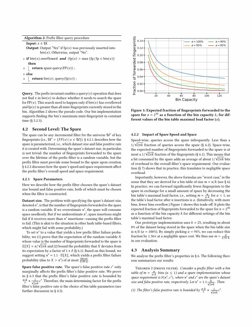
20 40 60 80 100 120Bin Capacity

0.00

0.02

0.04

0.06

0.08

0.10

0.12

0.14

Frac

tion

of fo

rwar

ded

finge

rprin

ts

= 100%= 95%

= 90%= 85%

Figure 1: Expected fraction of fingerprints forwarded to thespare for 𝑛 = 2

30 as a function of the bin capacity 𝑘 , for dif-ferent values of the bin table maximal load factor (𝛼).

4.2.2 Impact of Spare Speed and SpaceSpeed-wise, queries access the spare infrequently. Less than a

1/√2𝜋𝑘 fraction of queries access the spare (§ 6.2). Space-wise,

the expected number of fingerprints forwarded to the spare is at

most a 1/√2𝜋𝑘 fraction of the fingerprints (§ 6.1). This means that

a bit consumed by the spare adds an average of about 1/√2𝜋𝑘 bits

of overhead to the overall filter’s space requirement. Our evalua-

tion (§ 7) shows that in practice, this translates to negligible space

overhead.

Importantly, however, the above formulas are “worst case,” in the

sense that they are derived for a bin table of size𝑚 = 𝑛/𝑘 (see § 6).

In practice, we can forward significantly fewer fingerprints to the

spare in exchange for a small amount of space by decreasing the

bin table’s maximal load factor, i.e., setting𝑚 = 𝑛𝛼 ·𝑘 for 𝛼 < 1, so

the table’s load factor after 𝑛 insertions is 𝛼 . (Intuitively, with more

bins, fewer bins overflow.) Figure 1 shows this trade-off. It plots the

expected fraction of fingerprints forwarded to the spare for 𝑛 = 230

as a function of the bin capacity 𝑘 for different settings of the bin

table’s maximal load factor.

Our prototype implementation uses 𝑘 = 25, resulting in about

8% of the dataset being stored in the spare when the bin table size

is 𝑛/𝑘 (𝛼 = 100%). By simply picking 𝛼 = 95%, we can reduce this

fraction by 1.36× at a negligible space cost. We thus use𝑚 = 𝑛0.95·𝑘

in our evaluation.

4.3 Analysis SummaryWe analyze the prefix filter’s properties in § 6. The following theo-

rem summarizes our results:

Theorem 2 (prefix filter). Consider a prefix filter with a bintable of𝑚 = 𝑛

𝛼 ·𝑘 bins (𝛼 ≤ 1) and a spare implementation whosespace requirement is 𝑆 (𝑛′, Y ′), where 𝑛′ and Y ′ are the spare’s datasetsize and false positive rate, respectively. Let 𝑛′ = 1.1 𝑛√

2𝜋𝑘. Then:

(1) The filter’s false positive rate is bounded by 𝛼 ·𝑘𝑠 +

1√2𝜋𝑘

Y ′.

(2) For every sequence of operations containing at most 𝑛 insertions,the filter does not fail with probability ≥ 1 − 200𝜋𝑘

0.99·𝑛 .(3) If the filter does not fail, then every query accesses a single cache

line with probability ≥ 1 − 1√2𝜋𝑘

. The fraction of insertions that

access the spare is at most 1.1√2𝜋𝑘

with probability ≥ 1 − 200𝜋𝑘0.99·𝑛 .

(4) The filter uses 1

𝛼 · 𝑛 · (log(𝑠/𝑘) + 2) + 𝑆 (𝑛′, Y ′) bits of memory.

Proof. Property (1) is proven in § 6.3. Property (2) is proven

in § 6.1. Property (3) is proven in § 6.2. Property (4) follows by

combining the space requirement of the spare and the pocket dic-

tionary bin implementation (§ 5), which uses 𝑘 (log(𝑠/𝑘) + 2) bitsper bin. □

Parameter and spare selection. Theorem 2 implies that the pre-

fix filter can achieve a desired false positive rate Y in many ways, as

long as𝛼 ·𝑘𝑠 +

1√2𝜋𝑘

Y ′ ≤ Y. In practice, implementation efficiency con-

siderations in our prototype dictate that 𝑘/𝑠 = 1/256, which leads

to a choice of 𝑘 = 25 (§ 5.2.1) mini-fingerprints per bin (each mini-

fingerprint is in [𝑠]). This is similar to the situation in other practical

filters, such as the cuckoo and vector quotient filters, where effi-

cient implementations support only a few discrete false positive

rates [27, 41]. Importantly, the prefix filter can obtain a false posi-

tive rate below 1/256 by using 𝛼 < 1. Our prototype uses 𝛼 = 0.95,

which pays a negligible space cost to achieve Y < 1/256 and also

reduces the fraction of fingerprints stored in the spare (§ 4.2.2). The

spare’s false positive rate is not a major factor in the filter’s false

positive rate, since it gets downweighted by a factor of 1/√𝑘 .

Theorem 2 also implies that the prefix filter requires1

𝛼 (log(1/Y)+2) + 𝑆 (𝑛′, Y ′)/𝑛 bits per key, assuming 𝑘/𝑠 = Y. The choice of spare

thus marginally affects the space requirement. For instance, Ta-

ble 1 shows the space requirement obtained when using a cuckoo

filter with Y ′ = Y for a spare. This spare consumes 𝑆 (𝑛′, Y) =

𝑛′(log(1/Y) + 3) bits, which for the overall filter translates to at

most1.1· (log(1/Y)+3)√

2𝜋𝑘additional bits per key.

4.4 DiscussionConcurrency support. The prefix filter admits a highly scalable

concurrent implementation. Assuming a concurrent spare imple-

mentation, the prefix filter needs only to synchronize accesses to the

bin table. Since prefix filter operations access one bin, this synchro-

nization is simple to implement with fine-grained per-bin locking.

This scheme is simpler than in other load balancing schemes, such

as cuckoo or power-of-two-choices hashing, which may need to

hold locks on two bins simultaneously.

While a concurrent implementation and its evaluation is not in

the scope of this paper, we expect it to be highly scalable. Indeed,

a similar (per-bin locking) scheme is used by the vector quotient

filter, whose throughput is shown to scale linearly with the number

of threads [41].

Comparison to the BE filter. The prefix filter’s two-level archi-tecture is inspired by the theoretic dynamic BE filter [7]. The prefix

filter does not need to support deletions, which allows us to change

the BE filter architecture in several important ways that are crucial

for making the prefix filter a fast, practical filter:

(1) Eviction policy. In the BE filter, no evictions take place. A key

is sent to the spare if its bin is full upon insertion. As a result,

a query has no way of knowing in which level its key may be

stored, and must always search both the bin table and the spare.

(2) Datatype of the spare. In the BE filter, the spare is a dictionaryof keys. While a dictionary is not space efficient, the BE filter’s

spare holds only 𝑜 (𝑛/log𝑛) keys and its size is 𝑜 (𝑛) bits [7], i.e.,asymptotically negligible. For practical values of both 𝑛 and

𝑘 , however, the spare stores about 6%–8% of the keys—which

is far from negligible. The prefix filter solves this problem by

implementing the spare as a filter.

(3) Universe of the spare. In the BE filter, the spare stores actual

keys from U, which are forwarded if their bin is full upon

insertion. In the prefix filter, the spare “stores” key fingerprints

from the range of FP, because forwarding (through eviction)

can occur when the key itself is no longer available.

5 POCKET DICTIONARY IMPLEMENTATIONThe prefix filter’s query speed is dictated by the speed of searching

a first-level bin. In particular, a bin should fit into a single cache line,

as otherwise queries may incur multiple cache misses. On the other

hand, we want to maximize the bin capacity 𝑘 , as that improves load

balancing, which affects the spare’s size (§ 6.1) and the probability

that negative queries need to search the spare (§ 6.2).

To meet these conflicting demands, each first-level bin in the

prefix filter is implemented with a pocket dictionary (PD) data struc-

ture, introduced in the BE filter [6]. The PD is a space-efficient

representation of a bounded-size set, which uses the Elias-Fano

encoding [24, 28] to encode the elements it stores (see § 5.1).

The PD has constant-time operations, but in practice, all existing

PD implementations [23, 41] perform (relatively) heavy computa-

tions to search the compact encoding. In comparison, a cuckoo filter

query—whose speed we would like to match or outperform—reads

twomemory words and performs simple bit manipulations on them,

so computation is a negligible fraction of its execution time.

This section describes the prefix filter’s novel PD implementa-

tion. Our implementation employs a query cutoff optimization that

exploits SIMD instructions to avoid executing heavy computations

for > 99% of negative queries (§ 5.2). We further extend the PD to

support new operations required by the prefix filter (§ 5.2.3).

Our PD implementation can be independently useful, as the PD

(or a similar structure) is at the heart of filters such as the vec-

tor quotient filter (where PDs are called “mini-filters” [41]) and

TinySet [23] (where they are called “blocks”). Indeed, we find that

implementing the vector quotient filter using our PD outperforms

the authors’ original implementation, and therefore use our imple-

mentation in the evaluation (§ 7).

5.1 Background: Pocket DictionaryA pocket dictionary encodes a set of at most 𝑘 “small” elementsusing a variant of the quotienting technique. In the prefix filter,

each PD element is the mini-fingerprint of some prefix filter key.

Conceptually, a PD encodes 𝑄 “lists” each of which contains 𝑅-bit

values, subject to the constraint that at most 𝑘 values are stored

overall. We use 𝑃𝐷 (𝑄, 𝑅, 𝑘) to denote a concrete PD implementation

with fixed values for these parameters.

Each PD element is a pair (𝑞, 𝑟 ) ∈ [𝑄] × [2𝑅]. We refer to 𝑞

and 𝑟 as the quotient and remainder, respectively. The client of a𝑃𝐷 (𝑄, 𝑅, 𝑘) is responsible for ensuring that the most significant

bits of elements can be viewed as a 𝑞 ∈ 𝑄 , as 𝑄 is not necessarily a

power of two. In the prefix filter, our mini-fingerprint hash fp(·)takes care of this.

Encoding. A 𝑃𝐷 (𝑄, 𝑅, 𝑘) encodes 𝑘 elements using 𝑅 + 2 bits perelement. In general, a 𝑃𝐷 (𝑄, 𝑅, 𝑘) represents 𝑡 ≤ 𝑘 elements with

𝑄 + 𝑡 + 𝑡𝑅 bits using the following encoding. We think of the PD

as having 𝑄 lists, where inserting element (𝑞, 𝑟 ) to the PD results

in storing 𝑟 in list 𝑞. The PD consists of two parts, a header and

body. The header encodes the occupancy of each list. These counts

(including for empty lists) appear in quotient order, encoded in

unary using the symbol 0 and separated by the symbol 1. The

body encodes the contents of the lists: the remainders of the PD’s

elements are stored as 𝑟 -bit strings in non-decreasing order with

respect to their quotient, thereby forming the (possibly empty) lists

associated with each quotient.

Consider, for example, a 𝑃𝐷 (8, 4, 7) storing the following set:

{(1, 13), (2, 15), (3, 3), (5, 0), (5, 5), (5, 15), (7, 6)}

Then

header ≜ 1 ◦ 01 ◦ 01 ◦ 01 ◦ 1 ◦ 0001 ◦ 1 ◦ 01body ≜ 13 ◦ 15 ◦ 3 ◦ 0 ◦ 5 ◦ 15 ◦ 6,

where the “◦” symbol denotes concatenation and does not actu-

ally appear in the PD’s encoding.

Operations. For 𝑞 ∈ 𝑄 , we denote the occupancy of list 𝑞 by

𝑜𝑐𝑐 (𝑞), and the sum of occupancies of all PD lists smaller than 𝑞 by

𝑆𝑞 =∑𝑞′<𝑞 𝑜𝑐𝑐 (𝑞′). PD operations are executed as follows.

query(𝑞, 𝑟 ): Compute 𝑆𝑞 and 𝑜𝑐𝑐 (𝑞). Then, for every 𝑆𝑞 ≤ 𝑖 <

𝑆𝑞 + 𝑜𝑐𝑐 (𝑞), compare the input remainder 𝑟 with the remainder at

body[𝑖]. If a match is found, return “Yes”; otherwise, return “No”.

insert(𝑞, 𝑟 ): If the PD is full (contains 𝑘 remainders), the insertion

fails. Otherwise, the header is rebuilt by inserting a 0 after the first

𝑆𝑞 + 𝑞 bits. Then, the body is rebuilt by moving the remainders of

lists𝑞+1, . . . , 𝑄 (if any) one position up, from body[ 𝑗] to body[ 𝑗+1],and inserting 𝑟 at body[𝑆𝑞 + 𝑜𝑐𝑐 (𝑞)].

Implementation. Existing PD implementations use rank and se-

lect operations [32] to search the PD. For a 𝑏-bit vector 𝐵 ∈ {0, 1}𝑏 ,Rank(𝐵, 𝑗) returns the number of 1s in the prefix 𝐵 [0, . . . , 𝑗] of Band Select(𝐵, 𝑗) returns the index of the 𝑗-th 1 bit. Formally:

Rank(𝐵, 𝑗) = |{𝑖 ∈ [0 . . . 𝑗] | 𝐵 [𝑖] = 1}|Select(𝐵, 𝑗) = min{0 ≤ 𝑖 < 𝑏 | Rank(𝐵, 𝑖) = 𝑗},

where min (∅) is defined to be 𝑏.

To perform a PD query(𝑞, 𝑟 ), the implementation uses Select onthe PD’s header to retrieve the position of the (𝑞 − 1)-th and 𝑞-th

1 bits, i.e., the endpoints of the interval representing list 𝑞 in the

body. It then searches the body for 𝑟 in that range. If 𝑅 is small

enough so that remainders can be represented as elements in an

AVX/AVX-512 vector register, this search can be implemented with

AVX vector instructions. Unfortunately, implementing the Select

primitive efficiently is challenging, with several proposals [37, 40,

43], none of which is fast enough for our context (see § 5.2.2).

5.2 Optimized Pocket DictionaryHere we describe the prefix filter’s efficient PD implementation. We

explain the PD’s physical layout and parameter choices (§ 5.2.1),

the PD’s search algorithm—its key novelty—that avoids executing

a Select for > 99% of random queries (§ 5.2.2), and PD extensions

for supporting the prefix filter’s insertion procedure (§ 5.2.3).

5.2.1 Physical Layout and ParametersOur implementation has a fixed-sized header, capable of represent-

ing the PD’s maximum capacity. Three considerations dictate our

choice of the 𝑄 , 𝑅, and 𝑘 parameters:

1 Each PD in the prefix filter should reside in a single 64-byte cache line. This constraint guarantees that the first-level

search of every prefix filter query incurs one cache miss. Satisfying

this constraint effectively restricts possible PD sizes to 32 or 64

bytes, which are sizes that naturally fit within a 64-byte cache line

when laid out in a cache line-aligned array. (Other sizes would

require either padding the PDs—wasting space—or would result

in some PDs straddling a cache line boundary, necessitating two

cache misses to fetch the entire PD.)

2 The PD’s header should fit in a 64-bit word. This constraintarises because our algorithm needs to perform bit operations on

the header. A header that fits in a single word enables efficiently

executing these operations with a handful of machine instructions.

3 The PD’s body can be manipulated with SIMD (vector) in-structions. The AVX/AVX-512 instruction set extensions include

instructions for manipulating the 256/512-bit vectors as vectors of

8, 16, 32, or 64-bit elements [1]. This means that R must be one of

{8, 16, 32, 64}.

Parameter choice. We choose parameters that maximize 𝑘 sub-

ject to the above constraints: 𝑄 = 25, 𝑅 = 8, and 𝑘 = 25. The

PD(25, 8, 25) has a maximal size of 250 = 25 + 25 + 25 · 8 bits, whichfit in 32 bytes with 6 bits to spare (for, e.g., maintaining PD overflow

status), while having a maximal header size of 50 = 25 + 25 bits,which fits in a machine word.

5.2.2 Cutting Off QueriesOur main goal is to optimize negative queries (§ 2). For the prefix

filter to be competitive with other filters, a PD query must complete

in a few dozen CPU cycles. This budget is hard to meet with the

standard PD search approach that performs multiple Selects on the

PD header (§ 5.1). The problem is that even the fastest x86 Selectimplementation we are aware of [40] takes a non-negligible fraction

of a PD query’s cycle budget, as it executes a pair of instructions

(PDEP and TZCNT) whose latency is 3–8 CPU cycles each [2].

We design a PD search algorithm that executes a negative query

without computing Select for > 99% of queries, assuming uniformly

random PD elements—which is justified by the fact that our ele-

ments are actually mini-fingerprints, i.e., the results of hashing

keys.

Our starting point is the observation that most negative queries

can be answered without searching the header at all; instead, we

can search the body for the remainder of the queried element, and

answer “No” if it is not found. Given a queried element (𝑞, 𝑟 ), search-ing the body for a remainder 𝑟 can be implemented efficiently using

two AVX/AVX-512 vector instructions: we first use a “broadcast”

instruction to create a vector 𝑥 where 𝑥 [𝑖] = 𝑟 for all 𝑖 ∈ [𝑘], andthen compare 𝑥 to the PD’s body with a vector compare instruction.

The result is a word containing a bitvector v𝑟 , defined as follows

∀𝑖 ∈ [𝑘] v𝑟 [𝑖] ≜{1 if 𝑟 = body[𝑖]0 otherwise

Then if v𝑟 = 0, the search’s answers is “No”.For the prefix filter’s choice of PD parameters, the above “cutoff”

can answer “No” for at least 90% of the queries (Claim 3 below).

The question is how to handle the non-negligible ≈ 10% of queries

for which the “cutoff” cannot immediately answer “No”, withoutfalling back to the standard PD search algorithm that performs

multiple Selects.Our insight is that in the vast majority of cases where a query

(𝑞, 𝑟 ) has v𝑟 ≠ 0, then 𝑟 appears once in the PD’s body (Claim 4

below). Our algorithm therefore handles this common case without

executing Select, and falls back to the Select-based solution only

in the rare cases where 𝑟 appears more than once in the PD’s body.

Algorithm 3 shows the pseudo code of the prefix filter’s PD

search algorithm. The idea is that if body[𝑖] = 𝑟 (0 ≤ 𝑖 < 𝑘), we can

check if index 𝑖 belongs to list 𝑞 by verifying in the header that (1)

list 𝑞 − 1 ends before index 𝑖 and (2) list 𝑞 ends after index 𝑖 . We can

establish these conditions by checking that Rank(header, 𝑞+𝑖−1) =𝑞, which implies (1), and that list 𝑞 is not empty, which implies (2).

For example, suppose 𝑞 = 4, 𝑖 = 3, and header = 101010110001101.

Then list 3 ends before index 3 but list 4 is empty (bit 𝑞 + 𝑖 is 1).Computing Rank costs a single-cycle POPCOUNT instruction.

We further optimize by avoiding explicitly extracting 𝑖 from v𝑟 ;instead, we leverage the fact that the only set bit in v𝑟 is bit 𝑖 , so(v𝑟 ≪ 𝑞) − 1 is a bitvector of 𝑞 + 𝑖 ones, which we bitwise-AND

with the header to keep only the relevant bits for our computation.

Algorithm 3: PD search algorithm.

Input: Queried element (𝑞, 𝑟 ).Output:Whether (𝑞, 𝑟 ) is in the PD.

1 construct 64-bit bitvector v𝑟 ; ⊲ Using VPBROADCAST & VPCMP

2 if v𝑟 = 0 then3 return “No”

4 if (v𝑟 & (v𝑟 − 1)) = 0 then ⊲ v𝑟 has one set bit?

5 𝑤 ← v𝑟 ≪ 𝑞 ;

6 if Rank(header & (𝑤 − 1), 64) = 𝑞 and(header &𝑤) = 0 then

7 return “Yes”8 else9 return “No”

10 else11 use Select-based algorithm ;

Analysis. We prove that if PD and query elements are uniformly

random, then a query (𝑞, 𝑟 ) has v𝑟 = 0 with probability > 0.9

(Claim 3), and if v𝑟 ≠ 0, then with probability > 0.95, 𝑟 will appear

once in the PD’s body (Claim 4).

Claim 3. Consider a PD(25, 8, 25) containing uniformly randomelements. Then the probability over queries (𝑞, 𝑟 ) that v𝑟 = 0 is > 0.9.

Proof. Consider a PD(𝑄, 𝑅, 𝑘). Let the number of distinct re-

mainders in the PD’s body be 𝑠 ≤ 𝑘 . For a uniformly random

remainder 𝑟 ,

Pr [v𝑟 = 0] = 1 − Pr [v𝑟 ≠ 0] = 1 − 𝑠/2𝑅 ≥ 1 − 𝑘/2𝑅

For the prefix filter’s choice of PD parameters, we have 1−𝑘/2𝑅 𝑘=25,𝑅=8≈0.902. □

Claim4. Consider an element (𝑞, 𝑟 ). The probability (overPD(25, 8, 25)with uniformly random elements) that a PD’s body contains 𝑟 once,conditioned on v𝑟 ≠ 0, is > 0.95.

Proof. Consider a PD(𝑄, 𝑅, 𝑘) whose body contains 𝑠 ≤ 𝑘 dis-

tinct remainders. The probability that the PD’s body contains 𝑟

once, conditioned on it containing 𝑟 at all, is

𝑠 · 1/2𝑅 · (1 − 1/2𝑅)𝑠−1

1 − (1 − 1/2𝑅)𝑠≥ 𝑘 · 1/2𝑅 · (1 − 1/2𝑅)𝑘−1

1 − (1 − 1/2𝑅)𝑘𝑘=25,𝑅=8≈ 0.953

The first inequality holds because for 𝛽 ∈ (1/2, 1) and 𝑖 ≥ 1,

𝑇 (𝑖) ≜ 𝑖 ·𝛽𝑖−11−𝛽𝑖 is monotonically decreasing; in our case, 𝛽 = 1−1/2𝑅 .

The claim then follows since the bound holds for any 1 ≤ 𝑠 ≤ 𝑘 . □

5.2.3 Prefix Filter Support: Finding the MaximumElement

A prefix filter insertion that tries to insert an element into a full

PD must locate (and possibly evict) the maximum element stored

in the PD. Here, we describe the extensions to the PD algorithm

required to support this functionality.

Computing the remainder. In a standard PD (§ 5.1), the body

stores the remainders according to the lexicographic order of the

elements. Maintaining this “lexicographic invariant” is wasteful,

hence we use the following relaxed invariant: if the PD has over-

flowed, then the remainder of the maximum element is stored in the

last (𝑘-th) position of the body. Maintaining this relaxed invariant

requires finding the maximum remainder in the last non-empty

list only when the PD first overflows or when the the maximum

element is evicted.

Computing the quotient. In a standard PD, the maximum ele-

ment’s quotient needs to be computed from the header: it is equal to

the quotient of the last non-empty list. This quotient can be derived

from the number of ones before the 𝑘-th zero bit in the header or

from the number of consecutive (trailing) ones in the header. We

find, however, that computing these numbers adds non-negligible

overhead for a filter operation. To avoid this overhead, the prefix

filter’s PD reserves a log𝑄-bit field in the PD which stores (for a PD

that has overflowed) the quotient of the maximum element stored

in the PD.

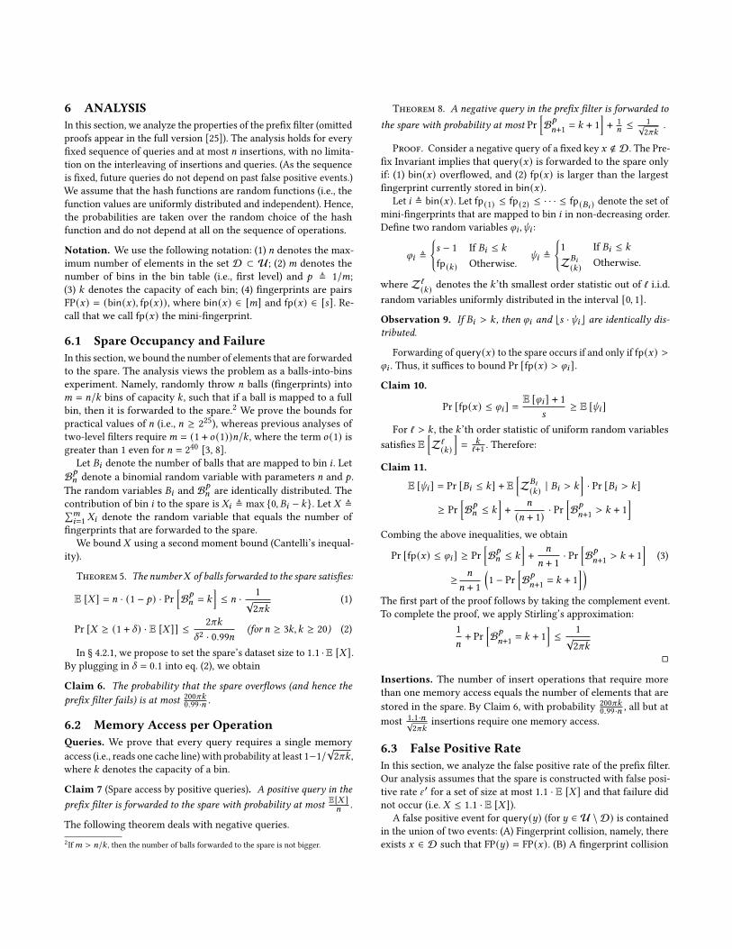
6 ANALYSISIn this section, we analyze the properties of the prefix filter (omitted

proofs appear in the full version [25]). The analysis holds for every

fixed sequence of queries and at most 𝑛 insertions, with no limita-

tion on the interleaving of insertions and queries. (As the sequence

is fixed, future queries do not depend on past false positive events.)

We assume that the hash functions are random functions (i.e., the

function values are uniformly distributed and independent). Hence,

the probabilities are taken over the random choice of the hash

function and do not depend at all on the sequence of operations.

Notation. We use the following notation: (1) 𝑛 denotes the max-

imum number of elements in the set D ⊂ U; (2)𝑚 denotes the

number of bins in the bin table (i.e., first level) and 𝑝 ≜ 1/𝑚;

(3) 𝑘 denotes the capacity of each bin; (4) fingerprints are pairs

FP(𝑥) = (bin(𝑥), fp(𝑥)), where bin(𝑥) ∈ [𝑚] and fp(𝑥) ∈ [𝑠]. Re-call that we call fp(𝑥) the mini-fingerprint.

6.1 Spare Occupancy and FailureIn this section, we bound the number of elements that are forwarded

to the spare. The analysis views the problem as a balls-into-bins

experiment. Namely, randomly throw 𝑛 balls (fingerprints) into

𝑚 = 𝑛/𝑘 bins of capacity 𝑘 , such that if a ball is mapped to a full

bin, then it is forwarded to the spare.2We prove the bounds for

practical values of 𝑛 (i.e., 𝑛 ≥ 225), whereas previous analyses of

two-level filters require𝑚 = (1 + 𝑜 (1))𝑛/𝑘 , where the term 𝑜 (1) isgreater than 1 even for 𝑛 = 2

40[3, 8].

Let 𝐵𝑖 denote the number of balls that are mapped to bin 𝑖 . Let

B𝑝𝑛 denote a binomial random variable with parameters 𝑛 and 𝑝 .

The random variables 𝐵𝑖 and B𝑝𝑛 are identically distributed. The

contribution of bin 𝑖 to the spare is 𝑋𝑖 ≜ max {0, 𝐵𝑖 − 𝑘}. Let 𝑋 ≜∑𝑚𝑖=1 𝑋𝑖 denote the random variable that equals the number of

fingerprints that are forwarded to the spare.

We bound 𝑋 using a second moment bound (Cantelli’s inequal-

ity).

Theorem 5. The number𝑋 of balls forwarded to the spare satisfies:

E [𝑋 ] = 𝑛 · (1 − 𝑝) · Pr[B𝑝𝑛 = 𝑘

]≤ 𝑛 · 1

√2𝜋𝑘

(1)

Pr [𝑋 ≥ (1 + 𝛿) · E [𝑋 ]] ≤ 2𝜋𝑘

𝛿2 · 0.99𝑛(for 𝑛 ≥ 3𝑘, 𝑘 ≥ 20) (2)

In § 4.2.1, we propose to set the spare’s dataset size to 1.1 ·E [𝑋 ].By plugging in 𝛿 = 0.1 into eq. (2), we obtain

Claim 6. The probability that the spare overflows (and hence theprefix filter fails) is at most 200𝜋𝑘

0.99·𝑛 .

6.2 Memory Access per OperationQueries. We prove that every query requires a single memory

access (i.e., reads one cache line) with probability at least 1−1/√2𝜋𝑘 ,

where 𝑘 denotes the capacity of a bin.

Claim 7 (Spare access by positive queries). A positive query in theprefix filter is forwarded to the spare with probability at most E[𝑋 ]𝑛 .

The following theorem deals with negative queries.

2If𝑚 > 𝑛/𝑘 , then the number of balls forwarded to the spare is not bigger.

Theorem 8. A negative query in the prefix filter is forwarded to

the spare with probability at most Pr[B𝑝𝑛+1 = 𝑘 + 1

]+ 1

𝑛 ≤1√2𝜋𝑘

.

Proof. Consider a negative query of a fixed key 𝑥 ∉ D. The Pre-

fix Invariant implies that query(𝑥) is forwarded to the spare only

if: (1) bin(𝑥) overflowed, and (2) fp(𝑥) is larger than the largest

fingerprint currently stored in bin(𝑥).Let 𝑖 ≜ bin(𝑥). Let fp(1) ≤ fp(2) ≤ · · · ≤ fp(𝐵𝑖 ) denote the set of

mini-fingerprints that are mapped to bin 𝑖 in non-decreasing order.

Define two random variables 𝜑𝑖 ,𝜓𝑖 :

𝜑𝑖 ≜

{𝑠 − 1 If 𝐵𝑖 ≤ 𝑘

fp(𝑘) Otherwise.

𝜓𝑖 ≜

{1 If 𝐵𝑖 ≤ 𝑘

Z𝐵𝑖

(𝑘) Otherwise.

where Zℓ(𝑘) denotes the 𝑘’th smallest order statistic out of ℓ i.i.d.

random variables uniformly distributed in the interval [0, 1].

Observation 9. If 𝐵𝑖 > 𝑘 , then 𝜑𝑖 and ⌊𝑠 ·𝜓𝑖 ⌋ are identically dis-tributed.

Forwarding of query(𝑥) to the spare occurs if and only if fp(𝑥) >𝜑𝑖 . Thus, it suffices to bound Pr [fp(𝑥) > 𝜑𝑖 ].

Claim 10.

Pr [fp(𝑥) ≤ 𝜑𝑖 ] =E [𝜑𝑖 ] + 1

𝑠≥ E [𝜓𝑖 ]

For ℓ > 𝑘 , the 𝑘’th order statistic of uniform random variables

satisfies E[Zℓ(𝑘)

]= 𝑘

ℓ+1 . Therefore:

Claim 11.

E [𝜓𝑖 ] = Pr [𝐵𝑖 ≤ 𝑘] + E[Z𝐵𝑖

(𝑘) | 𝐵𝑖 > 𝑘

]· Pr [𝐵𝑖 > 𝑘]

≥ Pr

[B𝑝𝑛 ≤ 𝑘

]+ 𝑛

(𝑛 + 1) · Pr[B𝑝𝑛+1 > 𝑘 + 1

]Combing the above inequalities, we obtain

Pr [fp(𝑥) ≤ 𝜑𝑖 ] ≥ Pr

[B𝑝𝑛 ≤ 𝑘

]+ 𝑛

𝑛 + 1 · Pr[B𝑝𝑛+1 > 𝑘 + 1

](3)

≥ 𝑛

𝑛 + 1

(1 − Pr

[B𝑝𝑛+1 = 𝑘 + 1

] )The first part of the proof follows by taking the complement event.

To complete the proof, we apply Stirling’s approximation:

1

𝑛+ Pr

[B𝑝𝑛+1 = 𝑘 + 1

]≤ 1

√2𝜋𝑘

□

Insertions. The number of insert operations that require more

than one memory access equals the number of elements that are

stored in the spare. By Claim 6, with probability200𝜋𝑘0.99·𝑛 , all but at

most1.1·𝑛√2𝜋𝑘

insertions require one memory access.

6.3 False Positive RateIn this section, we analyze the false positive rate of the prefix filter.

Our analysis assumes that the spare is constructed with false posi-

tive rate Y ′ for a set of size at most 1.1 · E [𝑋 ] and that failure did

not occur (i.e. 𝑋 ≤ 1.1 · E [𝑋 ]).A false positive event for query(𝑦) (for 𝑦 ∈ U \ D) is contained

in the union of two events: (A) Fingerprint collision, namely, there

exists 𝑥 ∈ D such that FP(𝑦) = FP(𝑥). (B) A fingerprint collision

did not occur and the spare is accessed to process query(𝑦) andanswers “yes”. Let Y1 ≜ Pr [𝐴] and 𝛿2 ≜ Pr [𝐵]. To bound the false

positive rate it suffices to bound Y1 + 𝛿2.

Claim 12. Y1 ≤ 𝑛𝑚 ·𝑠 and 𝛿2 ≤ Y′√

2𝜋𝑘.

Proof. Fix𝑦 ∈ U\D. The probability that FP(𝑥) = FP(𝑦) is 1

𝑚 ·𝑠because FP is chosen from a family of 2-universal hash functions

whose range is [𝑚 · 𝑠]. The bound on Y1 follows by applying a

union bound over all 𝑥 ∈ D. To prove the bound on 𝛿2, note that

every negative query to the spare generates a false positive with

probability at most Y ′. However, not every query is forwarded to thespare. In Claim 7 we bound the probability that a query is forwarded

to the spare by 1/√2𝜋𝑘 , and the claim follows. □

Corollary 13. The false positive rate of the prefix filter is at most𝑛

𝑚 ·𝑠 +Y′√2𝜋𝑘

.

7 EVALUATIONIn this section, we empirically compare the prefix filter to other

state-of-the-art filters with respect to several metrics: space usage

and false positive rate (§ 7.2), throughput of filter operations at

different loads (§ 7.3), and build time, i.e., overall time to insert 𝑛

keys into an empty filter (§ 7.4).

7.1 Experimental SetupPlatform. We use an Intel Ice Lake CPU (Xeon Gold 6336Y CPU

@ 2.40GHz), which has per-core, private 48 KiB L1 data caches and

1.25MiB L2 caches, and a shared 36MiB L3 cache. The machine

has 64GiB of RAM. Code is compiled using GCC 10.3.0 and run on

Ubuntu 20.04. Reported numbers are medians of 9 runs. Medians

are within −3.41% to +4.4% of the corresponding averages, and 98%

of the measurements are less than 1% away from the median.

False positive rate (Y). Our prefix filter prototype supports a falsepositive rate of Y = 0.37% ⪅ 2

−8(§ 5.2.1). However, not all filters

support this false positive rate (at least not with competitive speed),

thus making an apples-to-apples comparison difficult. We therefore

configure each filter with a false positive rate that is as close as

possible to 2−8

without deteriorating its speed. § 7.1.1 expands on

these false positive rate choices.

Dataset size (𝑛). We use a dataset size (maximum number of keys

that can be inserted into the filter) of 𝑛 = 0.94 · 228 (252M), which

ensures that filter size exceeds the CPU’s cache capacity. We pur-

posefully do not choose 𝑛 to be a power of 2 as that would unfairly

disadvantage some implementations, for the following reason.

Certain hash table of fingerprints designs, such as the cuckoo

and vector quotient filter, become “full” and start failing insertions

(or slow down by orders of magnitude) when the load factor of the

underlying hash table becomes “too high” (Table 1). For instance,

the cuckoo filter occasionally fails if its load factor exceeds 94% [31].

It should thus size its hash table to fit 𝑛/0.94 keys. Unfortunately,the fastest implementation of the cuckoo filter (by its authors [27])

cannot do this. This implementation is what we call non-flexible: itrequires𝑚, the number of hash table bins, to be a power of 2, so that

the code can truncate a value to a bin index with a bitwise-ANDs

instead of an expensive modulo operation. The implementation

uses bins with capacity 4 and so its default𝑚 is 𝑛/4 rounded up to

a power of 2. The maximal load factor when 𝑛 is a power of 2 is

thus 1, so it must double𝑚 to avoid failing, which disadvantages it

in terms of space usage.

Our choice of an 𝑛 close to a power of 2 avoids this disadvantage.

When created with our 𝑛 = 0.94 · 228, the cuckoo filter uses𝑚 =

228/4 bins, and thus its load factor in our experiments never exceeds

the supported load factor of 94%.

Implementation issues. We pre-generate the sequences of opera-

tions (and arguments) so that measured execution times reflect only

filter performance. While the keys passed to filter operations are

random, we do not remove any internal hashing in the evaluated

filters, so that our measurements reflect realistic filter use where

arguments are not assumed to be uniformly random. All filters use

the same hash function, by Dietzfelbinger [21, Theorem 1].

7.1.1 Compared FiltersWe evaluate the following filters:

Bloom filter (BF-𝑥 [𝑘 = ·]). We use an optimized Bloom filter

implementation [31], which uses two hash functions to construct 𝑘

hash outputs. The parameter 𝑥 denotes the number of bits per key.

Cuckoo Filter (CF-𝑥). “CF-𝑥” refers to a cuckoo filter with fin-

gerprints of 𝑥 bits with buckets of 4 fingerprints (the bucket size

recommended by the cuckoo filter authors). The cuckoo filter’s

false positive rate is dictated by the fingerprint length, but compet-

itive speed requires fingerprint length that is a multiple of 4. Thus,

while a CF-11 has a false positive rate of ≈ 2−8, it is very slow due

non-word-aligned bins or wastes space to pad bins. We therefore

evaluate CF-8 and CF-12, whose false positive rates of 2.9% and

0.18%, respectively, “sandwich” the prefix filter’s rate of 0.37%.

We evaluate two cuckoo filter implementations: the authors’

implementation [26], which is non-flexible, and a flexible imple-

mentation [30], denoted by a “-Flex” suffix, which does not require

the number of bins in the hash table to be a power of 2.

Blocked Bloom filter (BBF). We evaluate two implementations

of this filter: a non-flexible implementation (i.e., the bit vector length

is a power of 2) from the cuckoo filter repository and a flexible

version, BBF-Flex, taken from [31]. The false positive rate of these

implementations cannot be tuned, as they set a fixed number of bits

on insertion, while in a standard Bloom filter the number of bits

set in each insertion depends on the desired false positive rate. It

is possible to control the false positive rate by decreasing the load

(i.e., initializing the blocked Bloom filter with a larger 𝑛 than our

experiments actually insert), but then its space consumption would

be wasteful. We therefore report the performance of the blocked

Bloom filter implementations with the specific parameters they are

optimized for.

TwoChoicer (TC). This is our implementation of the vector quo-

tient filter [41]. Its hash table bins are implemented with our pocket

dictionary, which is faster than the bin implementation of the vec-

tor quotient filter authors [42].3We use the same bin parameters

3In our throughput evaluation (§ 7.3), the throughput of the TC is higher than the vector

quotient filter by at least 1.26× in negative queries at any load, and is comparable at

insertions and positive queries.

as in the original vector quotient filter implementation: a 64-byte

PD with a capacity of 48 with parameters𝑄 = 80 and 𝑅 = 8. Setting

𝑅 = 8 leads to an empirical false positive rate of 0.44%.

Prefix-Filter (PF[Spare]). We use a PF whose bin table contains

𝑚 = 𝑛0.95·𝑘 bins (see § 4.2.2). We evaluate the prefix filter with

three different implementations of the spare: a BBF-Flex, CF-12-

Flex, and TwoChoicer, denoted PF[BBF-Flex], P[CF12-Flex], and

PF[TC], respectively. Let 𝑛′ denote the spare’s desired dataset size

derived from our analysis (§ 4.2.1). We use a spare dataset size of

2𝑛′, 𝑛′/0.94, 𝑛′/0.935 for PF[BBF-Flex], PF[CF12-Flex], and PF[TC],

respectively. The purpose of the BBF-Flex setting is to obtain the

desired false positive rate, and the only purpose of the other settings

is to avoid failure.

Omitted filters. We evaluate but omit results of the Morton [11]

and quotient filter [5], because they are strictly worse than the

vector quotient filter (TC).4This result is consistent with prior

work [41].

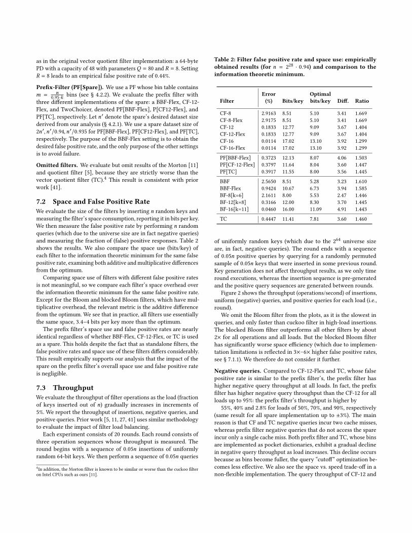
7.2 Space and False Positive RateWe evaluate the size of the filters by inserting 𝑛 random keys and

measuring the filter’s space consumption, reporting it in bits per key.

We then measure the false positive rate by performing 𝑛 random

queries (which due to the universe size are in fact negative queries)

and measuring the fraction of (false) positive responses. Table 2

shows the results. We also compare the space use (bits/key) of

each filter to the information theoretic minimum for the same false

positive rate, examining both additive andmultiplicative differences

from the optimum.

Comparing space use of filters with different false positive rates

is not meaningful, so we compare each filter’s space overhead over

the information theoretic minimum for the same false positive rate.

Except for the Bloom and blocked Bloom filters, which have mul-

tiplicative overhead, the relevant metric is the additive difference

from the optimum. We see that in practice, all filters use essentially

the same space, 3.4–4 bits per key more than the optimum.

The prefix filter’s space use and false positive rates are nearly

identical regardless of whether BBF-Flex, CF-12-Flex, or TC is used

as a spare. This holds despite the fact that as standalone filters, the

false positive rates and space use of these filters differs considerably.

This result empirically supports our analysis that the impact of the

spare on the prefix filter’s overall space use and false positive rate

is negligible.

7.3 ThroughputWe evaluate the throughput of filter operations as the load (fraction

of keys inserted out of 𝑛) gradually increases in increments of

5%. We report the throughput of insertions, negative queries, and

positive queries. Prior work [5, 11, 27, 41] uses similar methodology

to evaluate the impact of filter load balancing.

Each experiment consists of 20 rounds. Each round consists of

three operation sequences whose throughput is measured. The

round begins with a sequence of 0.05𝑛 insertions of uniformly

random 64-bit keys. We then perform a sequence of 0.05𝑛 queries

4In addition, the Morton filter is known to be similar or worse than the cuckoo filter

on Intel CPUs such as ours [11].

Table 2: Filter false positive rate and space use: empiricallyobtained results (for 𝑛 = 2

28 · 0.94) and comparison to theinformation theoretic minimum.

FilterError(%) Bits/key

Optimalbits/key Diff. Ratio

CF-8 2.9163 8.51 5.10 3.41 1.669

CF-8-Flex 2.9175 8.51 5.10 3.41 1.669

CF-12 0.1833 12.77 9.09 3.67 1.404

CF-12-Flex 0.1833 12.77 9.09 3.67 1.404

CF-16 0.0114 17.02 13.10 3.92 1.299

CF-16-Flex 0.0114 17.02 13.10 3.92 1.299

PF[BBF-Flex] 0.3723 12.13 8.07 4.06 1.503

PF[CF-12-Flex] 0.3797 11.64 8.04 3.60 1.447

PF[TC] 0.3917 11.55 8.00 3.56 1.445

BBF 2.5650 8.51 5.28 3.23 1.610

BBF-Flex 0.9424 10.67 6.73 3.94 1.585

BF-8[k=6] 2.1611 8.00 5.53 2.47 1.446

BF-12[k=8] 0.3166 12.00 8.30 3.70 1.445

BF-16[k=11] 0.0460 16.00 11.09 4.91 1.443

TC 0.4447 11.41 7.81 3.60 1.460

of uniformly random keys (which due to the 264

universe size

are, in fact, negative queries). The round ends with a sequence

of 0.05𝑛 positive queries by querying for a randomly permuted

sample of 0.05𝑛 keys that were inserted in some previous round.

Key generation does not affect throughput results, as we only time

round executions, whereas the insertion sequence is pre-generated

and the positive query sequences are generated between rounds.

Figure 2 shows the throughput (operations/second) of insertions,

uniform (negative) queries, and positive queries for each load (i.e.,

round).

We omit the Bloom filter from the plots, as it is the slowest in

queries, and only faster than cuckoo filter in high-load insertions.

The blocked Bloom filter outperforms all other filters by about

2× for all operations and all loads. But the blocked Bloom filter

has significantly worse space efficiency (which due to implemen-

tation limitations is reflected in 3×–6× higher false positive rates,

see § 7.1.1). We therefore do not consider it further.

Negative queries. Compared to CF-12-Flex and TC, whose false

positive rate is similar to the prefix filter’s, the prefix filter has

higher negative query throughput at all loads. In fact, the prefix

filter has higher negative query throughput than the CF-12 for all

loads up to 95%: the prefix filter’s throughput is higher by

55%, 40% and 2.8% for loads of 50%, 70%, and 90%, respectively

(same result for all spare implementation up to ±3%). The main

reason is that CF and TC negative queries incur two cache misses,

whereas prefix filter negative queries that do not access the spare

incur only a single cache miss. Both prefix filter and TC, whose bins

are implemented as pocket dictionaries, exhibit a gradual decline

in negative query throughput as load increases. This decline occurs

because as bins become fuller, the query “cutoff” optimization be-

comes less effective. We also see the space vs. speed trade-off in a

non-flexible implementation. The query throughput of CF-12 and

6.5

7.01e7

0.2 0.4 0.6 0.8 1.0

0.5

1.0

1.5

2.0

2.5

3.0

3.51e7

Load

ops/

sec

(a) Insertions

7.0

7.51e7

0.2 0.4 0.6 0.8 1.0

2.5

3.0

3.5

4.0

4.5

5.0

5.5

6.0

1e7

Loadop

s/se

c

(b) Uniform lookups

7.0

7.51e7

0.2 0.4 0.6 0.8 1.0

2.0

2.5

3.0

3.5

4.0

1e7

Load

ops/

sec

(c) Yes lookups

BBFBBF-Flex

CF-8CF-12

CF-12-FlexPF[BBF-Flex]

PF[CF12-Flex]PF[TC]

TC

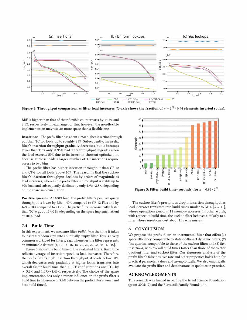
Figure 2: Throughput comparison as filter load increases (𝑋 -axis shows the fraction of 𝑛 = 228 · 0.94 elements inserted so far).

BBF is higher than that of their flexible counterparts by 14.5% and

8.1%, respectively. In exchange for this, however, the non-flexible

implementation may use 2× more space than a flexible one.

Insertions. The prefix filter has about 1.25× higher insertion through-put than TC for loads up to roughly 85%. Subsequently, the prefix

filter’s insertion throughput gradually decreases, but it becomes

lower than TC’s only at 95% load. TC’s throughput degrades when

the load exceeds 50% due to its insertion shortcut optimization,

because at these loads a larger number of TC insertions require

access to two bins.

The prefix filter has higher insertion throughput than CF-12

and CF-8 for all loads above 10%. The reason is that the cuckoo

filter’s insertion throughput declines by orders of magnitude as

load increases, whereas the prefix filter’s throughput is stable up to

60% load and subsequently declines by only 1.9×–2.8×, dependingon the spare implementation.

Positive queries. At 100% load, the prefix filter’s positive query

throughput is lower by 28% − 40% compared to CF-12-Flex and by

46%− 60% compared to CF-12. The prefix filter is consistently faster

than TC, e.g., by 12%-22% (depending on the spare implementation)

at 100% load.

7.4 Build TimeIn this experiment, we measure filter build time: the time it takes

to insert 𝑛 random keys into an initially empty filter. This is a very

common workload for filters, e.g., whenever the filter represents

an immutable dataset [4, 12, 14–16, 18–20, 22, 29, 34, 45, 47, 48].

Figure 3 shows the build time of the evaluated filters. Build time

reflects average of insertion speed as load increases. Therefore,

the prefix filter’s high insertion throughput at loads below 80%,

which decreases only gradually at higher loads, translates into

overall faster build time than all CF configurations and TC—by

> 3.2× and 1.39×–1.46×, respectively. The choice of the spare

implementation has only a minor influence on the prefix filter’s

build time (a difference of 5.6% between the prefix filter’s worst and

best build times).

BBF

BBF-

Flex

PF[B

BF-F

lex]

PF[T

C]

PF[C

F12-

Flex

]

TC

BF-8

[k=6

]

BF-1

2[k=

8]

CF-8

CF-8

-Fle

x

BF-1

6[k=

11]

CF-1

2

CF-1

2-Fl

ex

0

5

10

15

20

25

30

35

40

Seco

nds

Figure 3: Filter build time (seconds) for 𝑛 = 0.94 · 228.

The cuckoo filter’s precipitous drop in insertion throughput as

load increases translates into build times similar to BF-16[𝑘 = 11],

whose operations perform 11 memory accesses. In other words,

with respect to build time, the cuckoo filter behaves similarly to a

filter whose insertions cost about 11 cache misses.

8 CONCLUSIONWe propose the prefix filter, an incremental filter that offers (1)

space efficiency comparable to state-of-the-art dynamic filters; (2)

fast queries, comparable to those of the cuckoo filter; and (3) fast

insertions, with overall build times faster than those of the vector

quotient filter and cuckoo filter. Our rigourous analysis of the

prefix filter’s false positive rate and other properties holds both for

practical parameter values and asymptotically. We also empirically

evaluate the prefix filter and demonstrate its qualities in practice.

ACKNOWLEDGMENTSThis research was funded in part by the Israel Science Foundation

(grant 2005/17) and the Blavatnik Family Foundation.

REFERENCES[1] 2021. Intel Architecture Instruction Set Extensions and Future Fea-

tures. https://software.intel.com/sites/default/files/managed/c5/15/architecture-

instruction-set-extensions-programming-reference.pdf.

[2] Andreas Abel and Jan Reineke. 2019. uops. info: Characterizing latency, through-

put, and port usage of instructions on intel microarchitectures. In Proceedings ofthe Twenty-Fourth International Conference on Architectural Support for Program-ming Languages and Operating Systems. 673–686.

[3] Yuriy Arbitman, Moni Naor, and Gil Segev. 2010. Backyard cuckoo hashing:

Constant worst-case operations with a succinct representation. In 2010 IEEE 51stAnnual Symposium on Foundations of Computer Science. IEEE, 787–796. See alsoarXiv:0912.5424v3.

[4] Berk Atikoglu, Yuehai Xu, Eitan Frachtenberg, Song Jiang, and Mike Paleczny.

2012. Workload Analysis of a Large-Scale Key-Value Store. In Proceedings ofthe 12th ACM SIGMETRICS/PERFORMANCE Joint International Conference onMeasurement and Modeling of Computer Systems (SIGMETRICS ’12). 53–64.

[5] Michael A. Bender, Martin Farach-Colton, Rob Johnson, Russell Kraner, Bradley C.

Kuszmaul, Dzejla Medjedovic, Pablo Montes, Pradeep Shetty, Richard P. Spillane,

and Erez Zadok. 2012. Don’t Thrash: How to Cache Your Hash on Flash. PVLDB5, 11 (2012), 1627–1637. https://doi.org/10.14778/2350229.2350275

[6] Ioana O. Bercea and Guy Even. 2019. Fully-Dynamic Space-Efficient Dictionaries

and Filters with Constant Number of Memory Accesses. CoRR abs/1911.05060

(2019). arXiv:1911.05060 http://arxiv.org/abs/1911.05060

[7] Ioana O. Bercea and Guy Even. 2020. A Dynamic Space-Efficient Filter with

Constant Time Operations. In 17th Scandinavian Symposium and Workshops onAlgorithm Theory, SWAT 2020, June 22-24, 2020, Tórshavn, Faroe Islands (LIPIcs),Susanne Albers (Ed.), Vol. 162. Schloss Dagstuhl - Leibniz-Zentrum für Informatik,

11:1–11:17. https://doi.org/10.4230/LIPIcs.SWAT.2020.11

[8] Ioana O. Bercea and Guy Even. 2020. A Dynamic Space-Efficient Filter with

Constant Time Operations. CoRR abs/2005.01098 (2020). arXiv:2005.01098 https:

//arxiv.org/abs/2005.01098

[9] Burton H. Bloom. 1970. Space/Time Trade-offs in Hash Coding with Allowable

Errors. Commun. ACM 13, 7 (1970), 422–426. https://doi.org/10.1145/362686.

362692

[10] Kjell Bratbergsengen. 1984. Hashing Methods and Relational Algebra Operations.

In Proceedings of the 10th International Conference on Very Large Data Bases (VLDB’84). 323–333.

[11] Alex D Breslow and Nuwan S Jayasena. 2018. Morton filters: faster, space-

efficient cuckoo filters via biasing, compression, and decoupled logical sparsity.

Proceedings of the VLDB Endowment 11, 9 (2018), 1041–1055.[12] Zhichao Cao, Siying Dong, Sagar Vemuri, and David H.C. Du. 2020. Characteriz-

ing, Modeling, and Benchmarking RocksDB Key-Value Workloads at Facebook.

In 18th USENIX Conference on File and Storage Technologies (FAST 20). 209–223.[13] Larry Carter, Robert Floyd, John Gill, George Markowsky, and Mark Wegman.

1978. Exact and approximate membership testers. In Proceedings of the tenthannual ACM symposium on Theory of computing. ACM, 59–65.

[14] Fay Chang, Jeffrey Dean, Sanjay Ghemawat, Wilson C Hsieh, Deborah A Wal-

lach, Mike Burrows, Tushar Chandra, Andrew Fikes, and Robert E Gruber. 2008.

Bigtable: A distributed storage system for structured data. ACM Transactions onComputer Systems (TOCS) 26, 2 (2008), 1–26.

[15] Alex Conway, Martín Farach-Colton, and Philip Shilane. 2018. Optimal Hashing

in External Memory. In 45th International Colloquium on Automata, Languages,and Programming (ICALP 2018). 39:1–39:14.

[16] Alexander Conway, Abhishek Gupta, Vijay Chidambaram, Martin Farach-Colton,

Richard Spillane, Amy Tai, and Rob Johnson. 2020. SplinterDB: Closing the

Bandwidth Gap for NVMe Key-Value Stores. In 2020 USENIX Annual TechnicalConference (USENIX ATC 20). 49–63.

[17] Graham Cormode, Minos Garofalakis, Peter J. Haas, and Chris Jermaine. 2011. .

Now Foundations and Trends.

[18] Niv Dayan, Manos Athanassoulis, and Stratos Idreos. 2017. Monkey: Optimal

navigable key-value store. In Proceedings of the 2017 ACM International Conferenceon Management of Data (SIGMOD ’17). 79–94.

[19] Niv Dayan and Stratos Idreos. 2018. Dostoevsky: Better Space-Time Trade-

Offs for LSM-Tree Based Key-Value Stores via Adaptive Removal of Superfluous

Merging. In Proceedings of the 2018 International Conference on Management ofData (SIGMOD ’18). 505–520.

[20] Niv Dayan and Moshe Twitto. 2021. Chucky: A Succinct Cuckoo Filter for LSM-

Tree. In Proceedings of the 2021 International Conference on Management of Data(SIGMOD ’21). 365–378.

[21] Martin Dietzfelbinger. [n.d.]. Universal Hashing via Integer Arithmetic WithoutPrimes, Revisited.

[22] Siying Dong, Mark Callaghan, Leonidas Galanis, Dhruba Borthakur, Tony Savor,

and Michael Strum. 2017. Optimizing Space Amplification in RocksDB. In CIDR,

Vol. 3. 3.

[23] Gil Einziger and Roy Friedman. 2017. TinySet—an access efficient self adjusting

Bloom filter construction. IEEE/ACM Transactions on Networking 25, 4 (2017),

2295–2307.

[24] Peter Elias. 1974. Efficient storage and retrieval by content and address of static

files. Journal of the ACM (JACM) 21, 2 (1974), 246–260.[25] Tomer Even, Guy Even, and Adam Morrison. 2022. Prefix Filter: Practically and

Theoretically Better Than Bloom. arXiv e-prints (2022).[26] Bin Fan, David G. Andersen, and Michael Kaminsky. 2014. Cuckoo Filter C++

implementation. https://github.com/efficient/cuckoofilter

[27] Bin Fan, David G. Andersen, Michael Kaminsky, and Michael Mitzenmacher. 2014.

Cuckoo Filter: Practically Better Than Bloom. In CoNEXT. ACM, 75–88.

[28] Robert Mario Fano. 1971. On the number of bits required to implement an

associative memory. Memorandum 61. Computer Structures Group, Project MAC,MIT, Cambridge, Mass. (1971).

[29] Guy Golan-Gueta, Edward Bortnikov, Eshcar Hillel, and Idit Keidar. 2015. Scaling

Concurrent Log-Structured Data Stores. In Proceedings of the Tenth EuropeanConference on Computer Systems (EuroSys ’15).

[30] Thomas Mueller Graf and Daniel Lemire. 2018. Fast Filter: Fast approximate mem-

bership filter implementations (C++). https://github.com/FastFilter/fastfilter_cpp

[31] Thomas Mueller Graf and Daniel Lemire. 2020. Xor filters: Faster and smaller

than bloom and cuckoo filters. Journal of Experimental Algorithmics (JEA) 25(2020), 1–16.

[32] Guy Jacobson. 1989. Space-efficient static trees and graphs. In 30th AnnualSymposium on Foundations of Computer Science (FOCS ’89). 549–554.

[33] Donald E Knuth. 1973. The art of computer programming, vol. 3: Searching and

sorting. Reading MA: Addison-Wisley (1973).

[34] Avinash Lakshman and Prashant Malik. 2010. Cassandra: A Decentralized Struc-

tured Storage System. SIGOPS Oper. Syst. Rev. 44, 2 (April 2010), 35–40.[35] Xiaozhou Li, David G. Andersen, Michael Kaminsky, and Michael J. Freedman.

2014. Algorithmic Improvements for Fast Concurrent Cuckoo Hashing. In Pro-ceedings of the Ninth European Conference on Computer Systems (Amsterdam, The

Netherlands) (EuroSys ’14). Association for Computing Machinery, New York,

NY, USA, Article 27, 14 pages. https://doi.org/10.1145/2592798.2592820

[36] Chen Luo and Michael J. Carey. 2020. LSM-based storage techniques: a survey.

The VLDB Journal 29 (2020), 393–418. Issue 1.[37] Wojciech Mula, Nathan Kurz, and Daniel Lemire. 2016. Faster Population Counts

using AVX2 Instructions. CoRR abs/1611.07612 (2016). arXiv:1611.07612 http:

//arxiv.org/abs/1611.07612

[38] Patrick E. O’Neil, Edward Cheng, Dieter Gawlick, and Elizabeth J. O’Neil. 1996.

The Log-Structured Merge-Tree (LSM-Tree). Acta Informatica 33, 4 (1996), 351–385. https://doi.org/10.1007/s002360050048

[39] Rasmus Pagh and Flemming Friche Rodler. 2004. Cuckoo hashing. J. Algorithms51, 2 (2004), 122–144.

[40] Prashant Pandey, Michael A. Bender, and Rob Johnson. 2017. A Fast x86

Implementation of Select. CoRR abs/1706.00990 (2017). arXiv:1706.00990

http://arxiv.org/abs/1706.00990

[41] Prashant Pandey, Alex Conway, Joe Durie, Michael A Bender, Martin Farach-

Colton, and Rob Johnson. 2021. Vector Quotient Filters: Overcoming the

Time/Space Trade-Off in Filter Design. In Proceedings of the 2021 InternationalConference on Management of Data (SIGMOD’21). 1386–1399.

[42] Prashant Pandey, Alex Conway, and Rob Johnson. 2021. Vector Quotient Filter

C++ implementation. https://github.com/splatlab/vqf

[43] Giulio Ermanno Pibiri and Shunsuke Kanda. 2021. Rank/select queries over

mutable bitmaps. Information Systems 99 (2021), 101756.[44] Felix Putze, Peter Sanders, and Johannes Singler. 2010. Cache-, hash-, and space-

efficient bloom filters. Journal of Experimental Algorithmics (JEA) 14 (2010),

4–4.

[45] Pandian Raju, Rohan Kadekodi, Vijay Chidambaram, and Ittai Abraham. 2017.

PebblesDB: Building Key-Value Stores Using Fragmented Log-Structured Merge

Trees. In Proceedings of the 26th Symposium on Operating Systems Principles (SOSP’17). 497–514.

[46] Kai Ren, Qing Zheng, Joy Arulraj, and Garth Gibson. 2017. SlimDB: A Space-

Efficient Key-Value Storage Engine for Semi-Sorted Data. Proc. VLDB Endow. 10,13 (Sept. 2017), 2037–2048.

[47] Russell Sears and Raghu Ramakrishnan. 2012. bLSM: A General Purpose Log

Structured Merge Tree. In Proceedings of the 2012 ACM SIGMOD InternationalConference on Management of Data (SIGMOD ’12).

[48] Peng Wang, Guangyu Sun, Song Jiang, Jian Ouyang, Shiding Lin, Chen Zhang,

and Jason Cong. 2014. An Efficient Design and Implementation of LSM-Tree Based

Key-Value Store on Open-Channel SSD. In Proceedings of the Ninth EuropeanConference on Computer Systems (EuroSys ’14).

[49] Maysam Yabandeh. 2017. Partitioned Index/Filters. https://rocksdb.org/blog/

2017/05/12/partitioned-index-filter.html.