Journal

&dogy ELSEVIER Journal of Hydrology 199 (1997) 295-3 18

Comparison of three hydraulic property measurement methods

Dirk Mallama**, Diederik Jacques’, Peng-Hsiaug Tseng’ b, Martinus Th. van Genuchtenb, Jan Feyena

‘institute for Land and Water Management, Faculty of Agriculttual and Applied Biological Sciences, University of Luuven, Decosterstraat 102 B-3000 Leuve~ Belgium

bU.S. Salinity L.ubomtory, USDA-ARS, 450 West Big Springs Road, Riverside, CA 92507, USA

Received 5 February 19%; revised 18 October 1996; accepted 21 November 1996

Hydraulic functions of soils may differ depending on the different measuring methods used. The performance of three different methods for measuring soil-hydraulic properties of a heterogeneous field were evaluated. The experiments were conducted using three different sizes of undisturbed soil cores collected systematically along a 31 m long transect of a well drained sandy loam soil having three soil horizons (Ap, O-O.25 m; Cl. 0.25-0.55 m; C2,0.55-1.00 m). The laboratory studies involved: (1) detailed unsteady drainage-flux experiments perfotmed on fifteen columns of 1 m length and 0.3 m diameter; (2) combined crust test and hot-air methods applied to thirty columns of 0.2 m length and 0.2 m diameter and to a subset of sixty cylinders of 0.1 m length and 0.045 m diameter, respectively, taken from the Ap horizon; and (3) desorption experiments carried out on a total of one hundred eighty cores of 0.05 1 m length and 0.05 m diameter collected evenly from the thme horizons. Mean soil hydraulic properties were inferred from experimental data characterizing either selected depths or the soil profile as a whole. The results revealed considerable differences among estimated mean soil properties as obtained with different measuring techniques. Although the application of scaling theory substantially reduced variation in the measured pressure heads (h) and conductivities (K), the results revealed that scaling parameters determined from soil pressure head were not identical to scaling factors determined from hydraulic conductivity. The results also show that K scaling factors in general were much more variable than h scaling factors, and that the observed variability in scaling factors also depend upon the measurement technique used. 0 1997 Elsevier Science B.V.

Keywords: Soil hydraulic properties; Measurement techniques; Similar-media scaling; Spatial variability; Variably-saturated flow

+ comsponding author. ’ Resent addmxx Institute of Geophysics and Planetary Physics, Univmity of California. Riverside, CA

92521-0412, USA.

CQ22-1694/97/317.00 Q 1997- Elsevier Science B.V. All rights ttxerved PII SOO22-1694(96)03331-8

2%

1. Introduction

D. Mallants et al./Jounvll of Hydrology 199 (1997) 295-318

Soil variability is a major factor impeding the accuracy of measured soil hydraulic properties, i.e. the soil water retention characteristic, B(h), and the unsaturated hydraulic conductivity curve, K(8) or K(h), where 8 is the volume fraction of water and h is the pressure head of the soil. The effects of spatial variability in hydraulic properties on subsurface water flow (including infiltration and drainage), and the transport of surface- applied chemicals, have been widely studied (Warrick et al., 1977; Hopmans, 1992; Mallants et al., 1996c). A major problem related to field-scale water flow and solute transport modeling is how to deal with variability in the soil hydraulic properties.

One popular way for estimating the hydraulic properties of unsaturated soils has been to statistically relate B(h) and K(B) or K(h) to soil texture, bulk density, organic matter content, clay mineralogy, and soil structure (for an overview see van Genuchten et al. (1992)). Although attractive from a practical and economical point of view, the accuracy of such methods is often incommensurate with the type of problem being investigated (Among many others, W&ten and Bouma, 1992; Espino et al., 1995). Another approach is to predict the hydraulic conductivity from. more easily measured soil water retention data using closed-form analytical expressions (van Genuchten, 1980; Mualem, 1992). Rredic- tive models of this type tend to work reasonably well for coarse- and medium-textured soils, but often fail to represent the unsaturated hydraulic conductivity of structured soils, as was demonstrated in a recent study by Mallants et al. (1996a).

The use of direct measurements, whether in-situ or ex-situ, generally remains the only viable means to characterize f?(h) and K(8) or K(h), and to fully explore the reliability of indirect methods such as those described above. In situ measurement procedures often used are the steady flux method (Hillel and Gardner, 1970) and the unsteady drainage method (Green et al., 1986). A typical example of the former is the introduction of a low permeability crust to achieve a steady water flux. The unsteady drainage flux method, on the other hand, comprises the simultaneous monitoring of soil water content and pressure head following the commencement of water redistribution from an initially saturated soil profile. Although the drainage method has been mainly used for field conditions (FlUhler et al., 1976a; Rose et al., 1965; Sisson and van Genuchten, 1991), this method can be applied equally well to laboratory soil columns (Richards and Weeks, 1953; Mallants et al., 1996a). Ex-situ determination of the hydraulic properties using undisturbed soil columns has progressed through a variety of methods, including the crust test (Bouma et al., 1983), the sorptivity method (Dirksen, 1979). the hot-air method (Arya et al., 1975). the evapora- tion method (Boels et al., 1978), and desorption tables (Hillel, 1980). Comparison of hydraulic properties determined by means of in-situ field and ex-situ laboratory techniques has revealed significant differences for fine-textured soils (Fltihler et al., 1976b). although better agreement often has been noted for relatively coarse-textured media (Roulier et al., 1972). Because the unsaturated soil hydraulic functions are necessary inputs to numerical simulation models evaluating alternative soil and water management practices, there is a need to continuously assess the accuracies and limitations of in-situ and ex-situ methods.

A potentially attractive method to describe variability of laboratory or field-measured hydraulic properties involves the use of scaling (Miller and Miller, 1955a, b; Warrick et al., 1977; Sharma and Luxmoore, 1979; Ahuja et al., 1984; Hopmans, 1987). Because

D. Mallants et alJJounm1 of Hydrology 199 (1997) 295-318 291

frequency distributions of scaling factors can be conveniently incorporated into numerical field-scale or even watershed-scale flow and transport models, their application has received considerable attention in the literature (Warrick and Amoozegar-Fard, 1979; van Gmmen et al., 1989; Hopmans, 1992). Still, the appropriateness of doing so has not been fully investigated.

The purpose of this study is to compare the performance of three measurement tech- niques for quantifying the soil-hydraulic properties of a heterogeneous soil profile. Data of 8(h) and K(h) obtained from a detailed unsteady drainage experiment on large undisturbed soil columns will be analyzed and compared with those obtained from two other laboratory methods, i.e. desorption of 100 cm3 soil cores to determine B(h), and the crust test/hot-air method to measure K(h). Scaling is subsequently used to simplify the description of spatial variability in the measured soil hydraulic properties and to obtain average functions of conductivity, K,, and pressure head, h,, in terms of soil water content, 13. The suitability of applying scaling to characterize spatial variability of soils is examined and discussed. The set of scaling factors obtained here together with the average hydraulic functions will be used in a future study to predict field-scale water flow processes.

2. Materials and methods

2.1. Transect lay-out

The experimental field site was located in Bekkevoort, near Leuven (Belgium). The site involves a well-drained, macroporous sandy loam (Mallants et al., 1996b). Soil cores of different dimensions were collected along a 31 m long transect. A total of 30 columns of 1 m length and 0.3 m diameter, 30 columns of 0.2 m length and 0.2 m diameter, and 180 soil cores of 0.05 1 m length and 0.05 m diameter were used for the laboratory experiments. Three soil horizons (Ap, O-O.25 m; Cl, 0.25-0.55 m; C2,0.55-1.0 m) were contained in the columns of 1 m length, whereas the columns of 0.2 m length were collected only in the Ap horizon. Sixty cores of 0.051 m length were collected in each soil horizon, giving a total of 180 samples. The sampling interval between columns of the same size was generally 1 m, with sampling locations of the two smaller columns located in between those of the columns of 1 m length. Details of the sampling scheme are given in Mallants et al. (1996a).

2.2. Method 1: unsteady drainage jux method

The soil water retention curve, 8(h), and the hydraulic conductivity curve, K(8) or K(h), were characterized using the unsteady drainage-flux method (Green et al., 1986) as applied to a subset of 15 columns of 1 m length. Saturated soil columns were allowed to drain for a period of 30 days while the outflow was recorded continuously. Soil water contents and pressure heads during redistribution were measured simultaneously using an automated 9O-channel time-domain reflectometry (TDR) system and tensiometers, respectively, located at depths of 0.05, 0.15, 0.30, 0.45, 0.60, and 0.80 m (Mallants et al., 1996a). Observations of 8 and h were taken at 0.5 h intervals for the first seven hours of drainage,

298 D. Mallants et aUJouma1 of Hydrology 199 (1997) 295-318

and at 1.8, and 12 h intervals as the experiments progressed. When measurements of B and h are made at different depths and times during the drainage experiment, K(8) at various depths in the soil profile may be found by time integration of the Richards’ equation (Green et al., 1986) with a zero flux condition assumed at the soil surface (z = 0), i.e.

i J ; edz=K(e)~[h(z,t)-21 ZI

where zi is an arbitrary depth in the soil, z is vertical coordinate (positive downward), and t is time.

2.3. Method 2: combined crust rest and hot-air method

A second method used to obtain the unsaturated hydraulic conductivity was by com- bining the suction crust test (Bouma et al., 1983) and the hot-air method (Arya et al., 1975). The crust test was performed on thirty soil columns of 0.2 m length and 0.2 m diameter collected from the Ap horizon located in between the large columns of 1 m length. We first measured the saturated hydraulic conductivity, K,, by putting the saturated soil cylinder on a perforated disk to which a filter cloth was attached to prevent soil from falling out. One tensiometer was installed at 0.1 m below the soil surface and was con- nected to a pressure. transducer. Water was ponded on the soil surface to a depth of 0.01 m. Values of K, were obtained by measuring outflow with time when pressure was zero. The unsaturated hydraulic conductivity was subsequently measured on the same cores after a crust was constructed (Mallants et al., 1996a). Unlike the classical crust test, crusts were not removed but installed on top of an old crust. In this way, the initial contact between crust and soil was not disturbed.

From each column of 0.2 m length, two cylinders of 0.1 m length and 0.045 m diameter were taken to perform the hot-air method. In total 60 cores were exposed to a hot-air blower for 11 min. The soil was then sliced into 0.001-0.002 m increments near the exposed end and 0.007-0.01 m increments at the non-exposed end. Weighing of all sections was done before and after oven drying. Volumetric water content of each section was determined assuming a uniform bulk density along the core. Soil water diffusivity, D(0), was computed for each core using the water content distribution following enhanced evaporation (Arya et al., 1975; Anderson and Cassel, 1986). From the soil-water diffu- sivity, D(e), we calculated the unsaturated hydraulic conductivity, K(B), by multiplying D(e) by the soil-water capacity, C(0) = de/d$, in the pressure range of h = 0 to h = -30000 cm (pF = 4.5).

2.4. Method 3: &sorption on core samples

As described by Mallants et al. (1996c), 8(h) curves were obtained by desorption of soil cores of 0.051 m length and 0.05 m diameter from saturation to h = -16000 cm, using standard techniques (Klute, 1986). Three groups of 60 retention curves (180 in total) representing three horizons were analyzed. The pooled data of the sixty locations were

D. Mallants et alJJouma1 of Hydrology 199 (1997) 295-318

analyzed in terms of the empirical retention model of van Genuchten (1980), i.e.

es-4 e=er+ [1 +(alhl)qm

where the subscripts r and s refer to residual and saturated water contents, respectively, and a a-‘), n, and m are curve-shape parameters. Assuming m = 1 - l/n, the hydraulic conductivity function, K(h) can be described by combining Mualem’s pore-size distribu- tion model with Eq. (2):

K(h)=K (l-larhl~[l+larhl”]-m)2 I [ 1 + ICYhI”]“’

(3)

or in terms of the effective saturation, S, = (0 - ery(e, - erj, (0 5 S, 5 1):

K(S,)=K,S,‘[l -(l-S;‘“)“]2 (4)

where T is a pore-interaction parameter often considered to be 0.5 (Mualem, 1976).

2.5. Scaling of soil hydraulic properties

The description of spatially variable soil hydraulic functions can be simplified by invoking scaling. In this approach, spatial variability is described by a set of scale factors, a,, which relate the soil hydraulic functions at each spatial location r to a single curve or some representative mean (Warrick et al., 1977). Scaling theory is based on the similar media concept which assumes that porous media differ only in the scale of their internal microscopic geometries, while their porosities are assumed identical (Miller and Miller, 1955a, b).

By means of scaling, the soil pressure head, h, at any spatial location r can be related to some mean pressure head, h,, as

hr=hm/or (5)

where r = l,...,R is spatial location. In a similar way, the hydraulic conductivity, K,., can be related to a mean K,:

K, = K,,,cY; 0%

In the case of similar media, Eqs. (5) and (6) hold for the complete range of water contents at which h, and K, have been measured. Since field soils generally have spatially variable porosities, h, and K, are not expressed here in terms of the volumetric water content, 8, but in terms of the effective saturation, SC, assuming that 8, = 0, such that S, = 818,.

The method used here for scaling soil water retention data is the same as initially introduced by Warrick et al. (1977). but with some minor modifications. The scaling factors, a,, were obtained by minimizing the sum of squares:

SS = ,7 [MSe, 9 - arhr(Se, i)] ’ (7)

where &,(S,,J is the mean pressure head at a given degree of saturation, and i = l,..., I(r) are pressure head steps at location r. Differentiation of Eq. (7) with respect to aI and

300 D. Makmts et aNJouma1 of Hydrology 199 (1997) 295-318

setting each of the equations equal to zero, lead to a linear system of equations which is solved subject to the constraint

(ar,+fX~+...+cr/J/R=l (8)

Estimates of h, as a function of S, were obtained by employing a third degree polynomial similar to that used by Hopmans (1987), i.e.

ln(h,)=ao+alS,+a2SZ+a3S,3 (9)

where uO,..., a3 are constants. Eq. (9) will be applied to all h(S,) data of all R locations. An iterative procedure was developed to minimize Eq. (7) subject to Eq. (8). An

estimate of h, was first made by applying Eq. (9) to the unscaled data. Next, best-fit values of CX, were obtained using the procedures described above to scale the h(S,) data. Eq. (9) was subsequently applied to the scaled data and the procedure repeated until SS reached its minimum.

The method used for scaling hydraulic conductivity is identical to the procedures developed by Warrick et al. (1977) whereby the mean K, was calculated at all R locations according to the regression equation

In(K,)=bo+b,S,+bzS,2+b3S,3 (10)

where bs, bt,...,bs are constants. Estimates of ln(K,) were used to obtain approximate values of Q,’ according to:

(11)

which were normalized to give the Q, values:

cq=Ra,‘/ Za,’ r (12)

Eqs. (11) and (12) were solved iteratively to obtain optimal values for the constants of Eq. (10). This procedure resulted in a minimum sum of squares between K, and K,i. The sum of squares is now defined as:

SS = I: [In&, i) + 2ln(cf,) - ln(&, i)]* (13) r. i

In the following discussion we compare results in terms of the mean squared error, MSE = SSldf, with &being the degrees of freedom, rather than SS, since the number of pressure steps is not identical for different depths to which the method is applied.

3. Results and discussion

3.1. Unsteady drainage jlux method

Data of 8 and h at five selected depths and ten observation times (t = 0.5,1,2,4,16,32, 64, 128, 256, and 512 h) were analyzed to evaluate their probability density functions (PDF). The results revealed that a normal PDF better described the data than a log-normal

D. Mallants et alJJouma1 of Hydrology 199 (1997) 295-318 301

Table 1

Statistics of observed soil water content as a function of elapsed time at five soil depths along a 3 1 m long transect during a drainage experiment.

Time

01) Soil depth

(m) Mean (cm3 cm”)

StalKhi deviation (cm’ cmJ)

cv Maximum Minimum (S) (cm’ cm”) (cm3 cm”)

1 0.05 0.319 0.15 0.334 0.30 0.336 0.45 0.350 0.60 0.361

4 0.05 0.354 0.15 0.319 0.30 0.325 0.45 0.339 0.60 0.353

32 0.05 0.321 0.15 0.306 0.30 0.313 0.45 0.325 0.60 0.342

128 0.05 0.314 0.15 0.302 0.30 0.306 0.45 0.317 0.60 0.335

512 0.05 0.310 0.15 0.299 0.30 0.300 0.45 0.308 0.60 0.329

0.035 0.027 0.017 0.018 0.016 0.025 0.023 0.012 0.016 0.016 0.021 0.015 0.009 0.014 0.015 0.021 0.016

0.012 0.015 0.022 0.017 0.008 0.011 0.015

9.3 0.424 0.302 8.2 0.388 0.279 5.1 0.370 0.300 5.1 0.393 0.314 4.5 0.387 0.334 6.9 0.393 0.298 7.1 0.376 0.279 3.7 0.345 0.300 4.8 0.363 0.299 4.6 0.378 0.316 6.6 0.365 0.292 5.1 0.331 0.276 3.1 0.328 0.297 4.3 0.337 0.290 4.5 0.366 0.307 6.6 0.359 0.279 5.2 0.326 0.268 2.9 0.320 0.292 3.8 0.331 0.288 4.5 0.361 0.307 7.0 0.354 0.268 5.7 0.323 0.262 2.9 0.313 0.284 3.6 0.327 0.287 4.5 0.355 0.301

PDF. Statistics of the soil water content at five selected depths and observation times are listed in Table 1. The coefficient of variation (CV) was generally the highest at the shallowest observation depth, and lowest at 0.3 m depth, thus suggesting a more homo- geneous structure of the Cl horizon. The CV generally decreased slightly when the soil dried, a result of the decrease, though small, of the standard deviation with time.

Table 2 gives the statistics of the pressure head at the same selected depths and times as in Table 1. The surface horizon (0.05 m and 0.15 m deep) shows the most variation in the pressure head, whereas the second horizon (0.30 m and 0.45 m deep) generally shows the least. All CVs decrease considerably with time.

Soil water retention curves were obtained from simultaneous measurements of 8 and h at the five soil depths. The van Genuchten soil water retention model (Eq. (2)) was used to analyze the unscaled data for each depth. Estimated model parameters were obtained by using the non-linear parameter optimization program RETC (van Genuchten et al., 1991). The retention parameters thus obtained will be compared with retention parameters obtained with scaled data (to be discussed later). Preliminary estimates with Eq. (2) indicated that values of 0, were generally zero, and very close to zero, probably because

302 D. Mallants et alJJouma1 of Hydrology 199 (1997) 295-318

Table 2

Statistics of the soil water pressure head, h, as a timction of elapsed time measured at five soil depths along a 31 m long transect during a drainage experiment

Time

01)

Soil depth

(m) Mean (cm)

standard deviation

(cm)

cv Maximum Minimum

@I (cm) (cm)

1 0.05 14.4 10.2 70.9 31.0 1.0 0.15 14.6 9.2 62.8 31.0 0.0 0.30 15.3 8.8 51.4 33.0 2.0 0.45 16.3 5.1 31.4 27.0 11.0 0.60 13.4 6.5 48.5 24.0 3.0

4 0.05 29.7 16.2 54.4 52.0 1.0 0.15 28.4 10.5 37.0 44.0 1.0 0.30 26.3 7.7 29.1 44.0 16.0 0.45 23.2 8.1 35.1 38.0 7.0 0.60 23.8 6.2 26.2 33.0 8.0

32 0.05 60.2 15.2 25.3 79.0 14.0 0.15 51.7 13.7 26.5 69.0 10.0 0.30 43.8 6.7 15.2 58.0 35.0 0.45 35.4 6.8 19.3 43.0 19.0 0.60 27.6 1.3 26.5 34.0 15.0

128 0.05 74.4 16.1 21.6 94.0 23.0 0.15 63.9 14.9 23.4 85.0 18.0 0.30 58.4 9.2 15.7 76.0 45.0 0.45 45.3 6.7 14.1 56.0 32.0 0.60 33.4 1.7 22.9 43.0 18.0

512 0.05 88.9 15.5 17.4 103.0 42.0 0.15 18.5 18.0 22.9 95.0 21.0 0.30 70.2 8.7 12.4 85.0 54.0 0.45 55.9 9.8 11.7 71.0 36.0 0.60 44.0 8.3 18.8 60.0 27.0

of the relatively narrow pressure head range used in our experiments, A fixed value of 8, = 0 was therefore assumed for cases similar to those used by Greminger et al. (1985) and W&ten and van Genuchten (1988), unless stated otherwise. Two cases were considered: (i) the relationship m = 1 - l/n was assumed, leading to the parameter vector { Qs,txr n); and (ii) the parameters IZ and m were both assumed to be variable, giving the parameter vector (O,, a, n, m). Keeping m and II independent adds additional flexibility to the parameter optimization process, but its use is recommended only for data showing little scatter and covering a wide range of pressure head data (van Genuchten et al., 1991). In our study, both cases described the data equally well. Fig. l(a) shows the soil water retention curve Eq. (2) fitted to all data points for the 0.3 m depth with parameter values for the condition where m = 1 - l/n. Measured values of B exhibited a range of approximately 20.02 cm3 cmS3 about the fitted curve. We note the minor differences between the two fitted curves representing the cases where m and II were both variable and m = 1 - l/n. For the case where no restrictions were put on m and n we found correlations between the estimated values of m and n parameters to be between -0.98 and -1.00. This strong correlation justifies the restriction m = 1 - l/n. Table 3 gives the estimated parameters of Eq. (2) for

0 L,

Rel

atiie

hyd

raul

ic c

ondu

ctiv

ity,

K,

LPL’O ZEV I 6510’0 oz’o-0 2 9OE’O 9997 PS90’0 09’0 LZL’O IS8’Z EZSO’O svo 6ZL’O L9L’Z ESPO’O ot’o 919’0 829’2 OEWO SI’O POLO 06L’Z 6LE0’0 so’0 I

asoql30 palqnop uw.p avow sea p a1qaL ui u 30 an@h au *pasn SBM w3p QngDnpuoD uaqM JaWI saug aanp OJ 0~1 %u!aq ‘(UOZIJO~ 23 pus 13) sqldap I!OS Jaqlo aql 103 pasJaAaJ aJaM spoqlaur 0~1 aql~o3 sari@@@ x) palewysa aql uaalnlaq sawaraJJ!a *(c aIqt3L)

twp uoyualaJ aw 01 pauy uaqm ueql JaIIw.us sauxp aanjl AIaleyxoJdde aram wp ~~Ay3npuo3 aql uo paseq (uoz!.~oq dv) sqldap Jamol@qs 0~1 aql~o3 a~ 30 sanpA paleurysa aru, *elep AlpyvnpuoB ~gne&q pamsaaw 01 (E) *bg %u*y 30 sqnsar aql sazywnuns p aIqeL *as+tuaqlo palels ssapn ‘U/I - 1 = w aatpi at333 aw Japisuo:, Quo ~pqs aM

Jaded sg30 JapuFuxar aql u! pun ‘aIqt+nw tu pue u qwq zurdaaq 103 sa%wm~pe luwy~ -%rs ou am araql ‘acwaH *saw3 04 asaq uaamiaq w+a aDuuaraJJlp ou 1sou1~ ‘(q)r -%M u! palwlsn~~! sy ‘{w ‘u ‘D} 30 las wau.mmd a u! %UpInSaJ ‘parapyuo~ OS@ S%?M luap -uadapu! paumsse a.112 u pne u1 a.xaqm asz3 aru, * (u‘a) ‘sumoqun OMJ JO ~01~3~ ra]aumsed

8 u! palpwu qD!qrn ‘(9L61 ‘urapm~) ~‘0 aq 01 paumssa SvM I Jalaumred LI~AIJ~UUO~ -arod aa **y/(q)2 = ‘;y JO stum u! passaJdxa ‘((g) ‘bg) uop~~ry Dyg~npuo3 pauy aql qlim &ago1 qldap I!OS UI 6’0 aql.103 sari@@@ D!ApDnpuo:, ~~nk?.Ipbq an!leIar %u~puodsa.uo:, smoqs (q)I -%!d *ux3 WI- 01 0 30 aSmu y aql u! sari@@@ Io!glcwtpuo:, DynwpAq aq3p.J

u! palInsar sias e)ap y pue 0 pamseatu dlsnoautyn~s aql 01 (I) -bg 30 uopDgddv

St60 SIX1 POO’O EEVO 06’0 M6’0 IIE’I EIO’O s9E’o OS0 Ip6’0 ZIP’1 800’0 EIP’O 01’0 E LPO’O 660’1 LIO’O SK0 09’0 6Ls’O WI'1 IfxrO L9c-0 SP'O LSCO ZEI'I IZO'O 8EE'O OS-0 661'0 OSO'I LtiI.0 WE’0 SI'O LSE’O 001'1 EOI'O %E'O so'0 I

21 u (,_W 10 CE_U3 p) 'e

D. Mallam et al./Joutml of Hydrology 199 (1997) 295-318 305

obtained from the retention data, irrespective of the depth. A simultaneous fit of both Eqs. (2) and (3) to the observed (8,h) and (K,h) data, with weighting coefficient Wl in the objective function (van Genuchten et al., 1991) set to unity, resulted in estimated K(h) curves which deviated considerably from those obtained with separate fits, and gave visibly poor descriptions of the data. Using values between l’and 0.1 for W 1 did improve the fitting of the retention data somewhat, but not for the conductivity data. For these reasons, parameter values for the simultaneous fit were not given in the corresponding tables. Including the connectivity parameter T in the parameter optimization process did also not improve the results in any of the above cases, presumably due to the scatter in the data and the limited range of conductivities.

3.2. Combined crust test and hot-air method

Fig. 2 shows a combination of all data points obtained from the crust test and hot-air method. At saturation, the range in K, values was more than two orders of magnitude. Between saturation and h = - 32 cm, the range of variation in crust-based K values decreased from almost three orders of magnitude to one order of magnitude. However,

1410 DATA PaNrs

I I 0 1 2 3 4 5

Pressure head, kg(h)

Fig. 2. Observed (mcrhod 2) and fitted hydraulic conductivity..

306 D. Mallants et al./Joumal of Hydrology 199 (1997) 295-318

K values obtained from the hot-air method showed a much larger variation than K values from the crust method. This is likely due in part to the fact that the hot-air method is a diffusivity-based approach which requires retention (soil-water capacity) data to convert diffusivities to conductivities. The retention parameters used for this purpose were obtained independently from the soil cores discussed above, thereby possibly introducing additional spatial variability (Mallants et al., 1996c). Note that Mallants et al. (19961~) illustrated that a different functional form for C(O), e.g. by considering a multimodal retention function, may lead to different conductivities, especially in the dry range. The solid line in Fig. 2 represents the best fit of Mualem’s conductivity model with estimated values for the parameter vector ((Y, n ) given in Table 4. In the estimation process the value of the weighting coefficient for the data from the crust test, excluding K,, was increased from 1 to 4, thus accounting for the fact that the crust test is generally judged to be more reliable than the hot-air method. Using different weightings for the crust-based K values also accounts for the smaller number of observations compared to the hot-air data.

1EM

1 E-l

1 E-2

lE-3

lE-4

E

z lE+O

g 1 E-l -u # lE-2 L

lE-3

lE-4

lE-5

lE-8

lE+O

1 E-l

1 E-2

1 E-S

lE-4

lE-5

lE-8

1 E-7 0.45-m DEPTH

I I 1 I 1 I 1 I

0 P~8urka~ 80 100 h (cm)

0 20 40 80 80 loo Pre88w-e head, -h (cm)

Fig. 3. Comparison between different methods to derive the unsaturated hydraulic conductivity: (i) gravity- drainage eXperiment (method 1). (ii) combined crust test/hot-air method (method 2), end (iii) indirectly estimated from nmion parameters determined on small soil cams (method 3).

D. Mallanu et al./Joumai 6f Hydrology 199 (1997) 295-318 301

Fig. 3 presents the conductivities for all three methods. The K values obtained with method 2 (crust/hot-air data) compared favorably with those based on (analytic prediction) method 1 in the pressure range of 0 to -50 cm, but were higher in the range of -50 to -100 cm (Fig. 3, upper left panel). The maximum difference in conductivity between methods 1 and 2 in the pressure range considered here was about 1.5 orders of magnitude.

Possible errors introduced in the hot-air measurements are related to violations of its assumptions. These assumptions include a homogeneous soil sample and representative retention curves obtained from independent measurements. Furthermore, water redistribu- tion after the heating is stopped and before the sample is sliced into pieces is assumed to be negligible. van Grinsven et al. (1985) analysed the effect of the temperature gradient on thermal vapor and liquid flow as well as on the viscosity of water. Their results indicated that the errors may be large but seem to compensate each other. An evaluation of the temperature effects on the calculated conductivities for the hot-air method is beyond the scope of this paper.

3.3. Desorption on core samples

For each horizon, Eq. (2) was fitted to the pooled data of sixty locations. Estimated soil water retention parameters are summarized in Table 3. In only one instance was the estimated parameter B, different from zero, i.e. 8 r = 0.021 for 0.90 m depth. The estimated curves, together with their 90% confidence intervals, were given in Pig. 4 and compared with the estimated retention curves obtained with the drainage method. The 90% con- fidence intervals for the fitted curves correspond to + 1.65 times the standard deviations of the differences between fitted and measured values of 8 at nine values of h. Retention curves obtained from the drainage method (fitted to the retention data separately) at the 0.3 m and 0.45 m soil depths fell entirely in the 90% confidence interval of the predicted curve derived from the desorption method. Such an agreement between methods 1 and 3 did not hold for the Ap and C2 horizons, for which the drainage method gave consistently lower water contents than method 3 for the entire range of measured h. We believe that the observed disparities between the retention curves of methods 1 and 3 may have been caused by air entrapment during initial saturation of the large columns.

Predicted unsaturated conductivity curves (Eq, (3)) using method 3 considerably over- predicted the conductivities obtained with the drainage method (Fig. 3). Fig. 3 further reveals that measured conductivity curves (method 1) pertaining to the same horizon, i.e. 0.05 m and 0.15 m for Ap and 0.3 m and 0.45 m for Cl, agreed fairly well. Moreover, a comparison of conductivities for the first horizon indicates that K values obtained with the combined crust test and hot-air method (method 2) were always lower than those obtained with method 3. Indirect estimates of K (method 3) are influenced by inaccuracies con- nected with the determination of the retention curve and assume the adequacy of the capillary model theory (Mualem, 1976). The latter assumption, which gives a very sim- plified picture of actual soils, generally does not work well when water flow through macropores and interaggregate regions occurs, as was most likely the case in our soil. It is clear from these comparisons that different measurement methods yield different conductivities. Stolte et al. (1994) found that diffisivity based methods, e.g. the hot-air method, do not compare well with methods that directly yield a conductivity curve,

D.Mallants etalfJoumalofHydrology 199(1997)295-318 308

0.48 - -.- -0.45-mDEPrn 0.44 - -<:*- -0.3-m DEPlH 0.42

&q(a), , , , E 8 O Pressure h&J, -h (cm)

100

$

0.40

0.38

0.38

0.34

0.32 0.30 0.28 0.28 ) I 1

0 Pressure tEki, h (cm)

100

0.48 0.48 0.44 0.42 0.40 0.38 0.38 0.34 - - g - _ _ _ 0.32 -w-__

0.30 0.28 w

0.28 1, 0

Pressure II%, -h (cm) 100

Fig. 4. Comparison between different methods to estimate the van Genuchten retention model using retention data from drainage experiment. Estimation based on retemtion data measud on small soil cores is also shown, together with the 90% confidence interval (shaded area).

especially in coarse-textured materials. Furthermore, the large variability in K values obtained from hot-air measurements (Fig. 2) may indicate its inappropriateness for spatial variability studies. Introducing several improvements to the hot-air method such as those discussed by van Grinsven et al. (1985) may reduce some of the scatter in the data.

Note that methods 2 and 3 have a much wider application range than method 1. Also, the sample volume and experimental efforts for methods 2 and 3 are much smaller than that of method 1. Therefore, from a practical point of view, methods 2 and 3 might be preferred over method 1 for routine investigations.

3.4. Scaling retention and conductivity data

All three measurement methods discussed above show a considerable variability in the

D.MollantsetaUJourmlofHydrology199(1997)295-318 309

retention and/or conductivity data. To reduce this variability, in an attempt to obtain an average curve characteristic for the entire dataset, scaling was applied to the water retention and hydraulic conductivity data obtained with the three measuring methods. Fig. 5 gives the unscaled and scaled retention data from the drainage experiments when all five soil depths are combined (i.e. pooled data). The solid line in Fig. 5(a) is the b&t fit of Eq. (9) for the unscaled data. At h = -50 cm, the width of the scattering range in S, is about 0.33. After scaling, the data are confined to a fairly narrow band around the mean

E 3

3 al 1 0.7

0.6

0.5

1.0

b? 0.0

SCALED

k = a@p5.10 - 247.13 G+ 333.m qhw!3 s@q 0.5 I I I I I I I

0 20 40 50 60 loo 120 140

Press6e head, h (cm)

Fig. 5. Unscaled (a) and acaled (b) soil water retention data for all five soil depths.

310 D. Malhnts et alJJouma1 of Hydrology 199 (1997) 295-318

Table 5 Efficiency of scaling

MCtbOd Depth W scaled II(&) scaled K(S,)

Reduction in MSE r* Reduction in MSE r*

WI W)

1 0.05 50 0.722 66 0.807

0.15 49 0.765 70 0.859

0.30 60 0.793 82 0.918

0.45 44 0.665 81 0.919 0.60 49 0.587 86 0.917

pool4 48 0.642 76 0.863

2 o-o.2 77 0.885

3 pooled ’ 7 0.899 -

’ Data for three depths (0.10.0.50.0.90 m) was combined.

h,(S,) curve, although a considerable amount of the original variability is still present (e.g. a band width of 0.22 in 5, remains at h = -50 cm). For this case, the MSE reduced from 0.481 for the unscaled data to 0.252 after scaling.

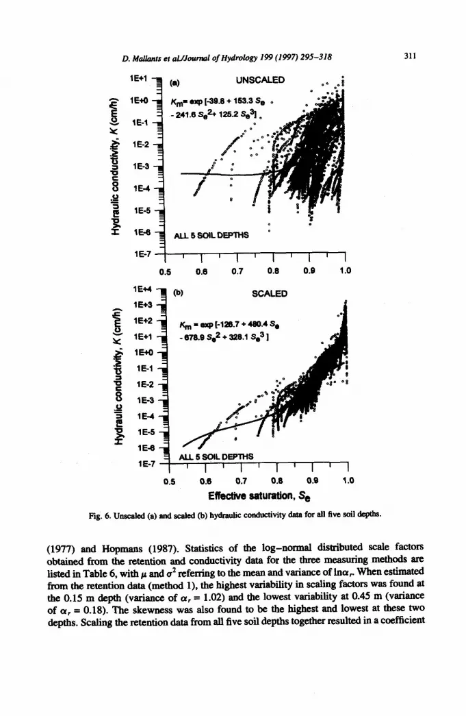
The pooled unscaled K values for all five depths together with the best-fitted third- degree polynomial are given in Fig. 6(a). Scaling was again very effective in reducing the variability (Fig. 6(b)) and now narrowly confined the scaled K values around the mean curve K,(S,). A reduction of the h4SE of 76% was obtained. The reduction in variability was somewhat less significant at saturation, presumably due to the large variability in K, of our macroporous soils (Mallants et al., 1997).

Table 5 summarizes the efficiency of scaling in terms of the percent reduction in the mean sum of squared error of the retention and hydraulic conductivity data for all three measuring methods. Notice the consistently higher reduction in h4SE values for scaling the conductivity data in comparison with the scaled retention data. This somewhat artificial behaviour is partly due to the use of logarithmic transformed conductivity data in the calculation of the SS. Therefore, a comparison of scaling of retention and conductivity data on the basis of the MSE values can only be of limited use.

Differences in scaling efficiency between different depths are fairly small for both the retention and conductivity data (Table 5). Notice, however, that reduction in lUSE for K(S,) increases with depth indicating that the conductivity data are better scaled at greater depths, presumably because of reduced spatial variability and less macropores (Mallants et al., 1996c). Table 5 also shows the r2 values obtained from a regression analysis between unscaled and estimated values of h, or K, using the optimized mean curve h, or K, (Eqs. (9) and (10)). Higher r2 values were obtained for scaling the conductivity data as compared to the retention data. Hence our scaling procedure was more effective in reducing the variability in hydraulic conductivity data than in retention data.

Probability plots or fiactile diagrams of the scaling factors (Y, and their logarithmic transformed values, lncx, calculated from water retention data and conductivity data revealed a better description with a log-normal distribution than with a normal distribu- tion (Mallants, 1996). These results are consistent with earlier findings of Wanick et al.

D. MaUants et alJJouma1 of Hyhlogy I99 (1997) 295-318

lE+l W UNSCALED 00 i

- lE+O-

f

_ /$,,I exp t-30.8 + 183.3 Se o = -

z lE-1

241.8 S& 125.2 .$q o 3

.& lE-2 1_

*s s lE-3

E lE-4 y 2 lE-5

0 . lE-8 ALL5SOlLDEMliS ’

1 E-7 0.S 0.8 0.7 0.8 0.8 1.0

311

K, = exp (-128.7 + 480.4 s, - 878.9 Se2 + 328.1 Se3 ]

0.5 0.6 0.7 0.8 0.0 1.0 Effective saturation, S,

Fig. 6. Unscakd (a) and scaled @I) hydraulic cunductivity data for all five soil depths.

(1977) and Hopmaus (1987). Statistics of the log-normal distributed scale factors obtained from the retention and conductivity data for the three measming methods are listed in Table 6, with p and a2 referring to the mean and variance of lnar, When estimated from the retention data (method l), the highest variability in scaling factors was found at the 0.15 m depth (variance of a, = 1.02) and the lowest variability at 0.45 m (variance of a, = 0.18). The skewness was also found to be the highest and lowest at these two depths. Scaling the retention data from all five soil depths together resulted in a coefficient

312

Table 6

D. Mallants et aNJouma1 of Hydrology 199 (1997) 295-318

Statistics of scale factors Q, estimated from retention and conductivity data

Method De@(m) Scaled II(&) scaled K(S,)

Mean’ Varb CVc Skew. * Mean’ Var. b CV’ Skew. *

1 0.05 0.99 0.35 59 1.97 1.30 22.7 365 59.6 0.15 1.03 1.02 98 3.89 2.84 478 1510 3488 0.30 1.04 0.36 57 1.89 1.79 41.9 360 57.5 0.45 1.00 0.18 42 1.33 1.12 2.24 134 6.43 0.60 0.99 0.21 46 1.48 1.00 0.64 80 0.605 pooled c 1.01 0.31 55 1.82 1.43 24.2 340 49.5

2 o-o.2 - - - - 0.99 2.08 145 7.38 3 pooled f 0.98 0.16 41 1.29 - - - -

’ Mean = exp@ + 0*/2). b variance = exp(& + uZ)[exp@) - 11. ’ CV = 100[exp(0*) - I]“. * Skewness coefficient = 3 CV + (CV)‘. ’ Data for five depths was combined. ‘Date for three depths (0.10, 0.50, 0.90 m) was combined.

of variation of 55%. Scale factors calculated from conductivity data for method 1 exhibited a much larger variability in comparison with the 01, values estimated from retention data (Table 6). The extremely large variation may be due to the small number of observations from which we estimated the statistics. Scaling of hydraulic conductivity data for all five depths combined resulted in a CV of 340% for ar,.. This value is considerably larger than the values previously found by Warrick et al. (1977) and Hopmans (1987). Although h(S,) and K(S,) were both obtained from simultaneous measured (0, h) data during the drainage experiment, the estimated conductivity showed a much higher variability in scale factors. This may be due in part to errors introduced in the calculation of the conductivities based on a too coarse grid of vertically spaced (6, h) data. Also, K values are more sensitive to changes in S, than h values. In a previous study by Ahuja et al. (1984), scale factors were also found to be more variable for saturated hydraulic conductivity than for water retention.

Table 6 shows that scale factors calculated from h(S,) and K(S,) may not be. identical. If soils behaved as Miller-Miller type similar media, scale factors obtained from retention and conductivity data (Eqs. (5) and (6)) should follow closely the 1:l line (Luxmoore and Sharma, 1980; Hopmans, 1987). This was not the case for our soil (Mallants, 1996). As a result, two different sets of scale factors must be estimated.

Unsaturated hydraulic conductivity data determined by means of the combined crust/ hot-air technique (method 2) for the Ap horizon were also scaled using the techniques described above. Scaling was again found to be very effective in reducing spatial varia- bility, with the mean sum of squares reduced from 7.84 to 1.77 (Table 5). Values of the mean, variance, CV, and skewness based on the log-normal distribution for (r, are given in Table 6. The variance of 2.08 was considerably smaller than the variance obtained with method 1 for the same observation depth (0.05 and 0.15 m). The larger variability of scaling factors for method 1 may be the result of the experimental methodology and/or the

D. Mallants et aUJoumal of Hydrology 199 (1997) 295-318 313

computational procedure used in the calculation of the hydraulic conductivity. Especially the limited vertical resolution of the measured (B,h) data may have been insufficient to accurately evaluate Eq. (1) in the calculation of K.

Scaling of the retention data obtained from desorption on small soil cores was pre- viously performed by Jacques et al. (1996). Table 6 shows a reduced variability in the h scaling factor for method 3 in comparison with method 1. The larger variability of scaling factors for method 1 in comparison with those for methods 2 and 3 may be the result of the larger experimental errors associated with the drainage data.

Scaled retention and conductivity dam obtained from method 1 were subsequently used to estimate parameters (cr. n) in the van Genuchten retention model (Eq. (2)) and para- meters {n, m, K,} for the Mualem conductivity model with r = 0.5. Two cases were considered: the first data set contained the data scaled separately by depth whereas the second set was obtained after splitting the scaled pooled data into five groups according to their measurement depth.

Another choice to obtain the mean van Genuchten curve together with a set of scaling parameters would have been to fit the van Genuchten model directly to the unscaled data. This method was presented by Hopmans (1987) (his Method III) and compared to three other methods. However, Hopmans found that use of the method of Wanick et al. (1977) (Hopmans’ Method I and IV) was superior to Hopmans’ Method III, because the poly- nomials better described the scatter in the data. This is not surprising, as the polynomial, generally of the third or fourth degree, has a higher flexibility in fitting highly variable data.

Results for the estimated soil water retention parameters {ar, n} are summarized in Table 7. As could be expected, the retention data scaled by depth could be better described than the pooled data. The estimated retention curves shown in Fig. 7(a) for the 0.05 and 0.15 m depth are based on the parameter values from Table 7 (scaling by depth) and estimated values for 0, taken from Table 3. We assumed 8, = 0 at all depths. Differences between the fitted water retention curves for the unscaled (Table 3) and scaled retention data appear mainly as a result of having a steeper slope (higher n values), especially for the 0.05 m and 0.60 m depth.

Similar results were obtained for the scaled conductivity data (Table 8), although the differences in performance and estimated parameter values between the two data sets were smaller in comparison with the retention data. The results given here are for the case where n and m are treated as independent variables. Parameter estimations with the constraint m =

Table I

EAnated pammeters of Eq. (2) using scaled retention data (tn = 1 - l/n)

Depth Cm) Scaling by depth Scaling pooled data

cc (cm-‘) n I.1 u (cm-‘) n r*

0.05 0.019 1.433 0.736 0.019 1.471 0.686 0.15 0.044 1.113 0.836 0.027 1.038 0.825 0.30 0.037 1.115 0.891 0.032 1.153 0.869 0.45 0.027 1.183 0.888 0.018 1.246 0.848 0.60 0.026 1.198 0.846 0.014 1.325 0.779

314 D. Mallants et aLLJournal of Hydrology 199 (1997) 295-318

0.30 - - _ O.l&mDEPTH

0.25 - - 0.05-m DEPTH

u‘ lE-1

Q ‘a lE-2 s -o.oknmPlH 8 lE-3 ---c- 0.15-m DEPnl / Y ‘3 e ‘E-4 u P

% 1 E-5 -unseabdconducthMydata

‘z 2 lE6

1 E-7

Fig. 7. (a) Estimated retention functions besed on unscaled and scated drainage data. (b) Estimated conductivity funclion~ bawd on unscaled and scaled drainage data.

1 -‘l/n were also carried out but the goodness of fit in terms of r2 was reduced somewhat as compared to the variable case (results not further shown here). Differences in estimated hydraulic conductivity between the unscaled and scaled data (scaling by depth) are con- siderable as exemplified for the 0.05 and 0.15 m depths (Fig. 7(b)). In all cases, using the scaled K(S,) data resulted into much lower conductivities in comparison with the unscaled

D. Malkmts et aLLJournal of Hydrolosy 199 (1997) 295-318 315

Table 8 Estimated parameters of Mualem’s conductivity model using scaled conductivity data

Depth (m) Scaling by depth Scaling pooled data

?I ma K* 2 n m’ KS t* (cm h-l) (cm h-‘)

0.05 8.09 0.010 0.15 0.746 7.08 0.011 0.27 0.714 0.15 1.26 0.030 107.5 0.846 1.23 0.034 52.8 0.828 0.30 7.34 0.004 8.92 0.916 7.57 0.004 10.4 0.910 0.45 6.69 0.005 2.69 0.883 7.02 0.005 4.46 0.874 0.60 3.34 0.009 2.34 0.899 2.48 0.014 9.14 0.892

’ Variable tn case.

data. This is because the estimated II parameter generally was much larger for the scaled data than for the unscaled data (Table 8).

4. conclusions

Both water retention and hydraulic conductivity functions are influenced by the measurement method. Comparison of soil water retention functions calculated from a gravity-drainage experiment involving 15 undisturbed soil cores of 1 m length taken from a layered sandy loam with those obtained from desorption on small soil cores showed that the former gave consistently lower water contents in the Ap and C2 horizon. These disparities could be the result of air entrapment during initial saturation of the large columns. The agreement between retention functions was relatively good for the Cl horizon.

predicted unsaturated conductivities using estimated van Genuchten parameters from small soil cores were higher than conductivities calculated from the gravity-drainage experiment. This is partly due to the above-mentioned difference between the retention curves for both methods, i.e. for given pressure head values, lower water contents for method 1 will result in lower unsaturated conductivities compared to method 3. Another reason may be the inadequacy of the capillary model theory to describe the hydraulic conductivity of our structured soil. A good agreement in the pressure head range of 0 to -50 cm was found when the unsaturated hydraulic conductivity relationship computed from the drainage data, was compared with K values obtained from combined crust/hot-air data. However, the combined crust/hot-air method gave higher values in the range of -50 to -100 cm. These disparities together with the high variability in conductivities derived from hot-air measurements may be attributed to the fact that diffusivities had to be translated to conductivities. There also is a difference in application range: (i) a rather narrow range for the gravity-drainage method; (ii) a wide range for the crust/hot-air method and the desorption method. Finally, experimental efforts for (i) are much larger than for (ii), especially in view of spatial variability studies.

Scaling soil water retention and hydraulic conductivities was found to be very effective in coalescing large data sets, irrespective of the measuring technique. Variability of

316 D. Mallants et al./Journal of Hydrology 199 (1997) 295-318

scaling factors was much higher for scaled K than for scaled h data. No relationship was found between h and K scaling factors obtained from the drainage experiment, indicating that for our soil different sets of scaling parameters have to be determined for hydraulic conductivity and pressure head. K scaling factors obtained from the combined crust/hot-air data were less variable in comparison with those obtained from the scaled drainage data. We also found that h scaling factors determined from retention data measured on small soil cores showed less variability than those obtained from the drainage data. These results indicate that statistics of scaling factors are also influenced by the measurement method used.

For the shallower two depths, fitting of the van Genuchten function to scaled retention data obtained from the drainage experiment resulted in CT values that were considerably different from those estimated from unscaled retention data. For the remaining depths, differences between the estimated van Genuchten parameters were smaller when using either scaled or unscakl retention data. A comparison between estimated conductivity functions using either unscaled or scaled K data (from drainage experiment) revealed large differences for all depths considered. Mean retention and conductivity functions obtained by direct fitting of unscaled data or alternatively by fitting scaled data will be used for solutions of water flow problems in heterogeneous soils. An evaluation of the effect of using different sets of hydraulic functions in calculations of water flow problems is the subject of a future study.

Acknowledgements

The authors give special thanks to the anonymous reviewers for their comments which improved the readability of the paper. We also thank Nobuo Toride for discussions on an earlier version of this manuscript.

References

Anderson. S.H., Camel. D.K.. 1986. Statistical and autoregressive analysis of soil physical properties of Ports- mouth Sandy Loam. Soil Sci. Sot. Am. J.. 50,1096-1104.

Ahuja, L.R., Naney, J.W., Nielsen. D.R., 1984. Scaling soil water properties and infiltration modeling. Soil Sci. Sot. Am. J., 48.970-973.

Arya. L-M.. Farrell, D.A., Blake, G.R.. 1975. A field study of soil water depletion patterns in presence of growing soybean roots. I. Determination of hydraulic ptoperties of the soil. Soil Sci. Sot. Am. Proc., 39.424-430.

Bo&, I)., Van Gils. J.B.H.M.. Veerman, G.J.. Wit, K.E.. 1978. Theory and system of automatic detcmination of soil moisture chsracteristics and unsaturated hydraulic conductivities. Soil Sci.. 126. 191-199.

Bourna, J.. B&nans, C.. Dekker, L.W., Jeurissen. W.J.M.. 1983. Assessing the suitability of soils with macro- pores for subsurface liquid waste disposal. J. Environ. Qual.. 12.305-311.

Dhhsen, C., 1979. Fhrx-controkd sorptivity measurements to determine soil hydraulic property functions. Soil Sci. Sot. Am. J., 43.827-834.

EsPino. A.. MaRants. D., Vanclooster, M., Feyen. J., 1995. Cautionary notes on the use of pedotmmfer functions for estimating soil hydraulic properties. Agric. Water Management, 29.235-253.

FMhler, H.. Ardakani, M.S.. Stolzy, L.H., 1976. Error propagation in determining hydraulic conductivities from successive water content and pressure head profiles. Soil Sci. Sot. Am. J., 40.830-836.

FMhJer. H., Germann, P., Richard, F., Leuenberger, J.. 1976. Bestimmung von hydraulischen Pammetem fth die

D. Ma&mu et aNJournal of Hydrology 199 (1997) 295-318 317

Wasserhaushaltsuntersuchungen im nathrlichen gelagerten Boden. Ein Vergleich von Feld- und Laboratoriumsmthoden. Z. P8anznernaehr. Bode& 3.329-342.

Green, R.E.. Ahuja, L.R., Chong, S.K., 1986. Hydraulic conductivity, diffusivity, and sorptivity of unsatumted soils: Field methods, in Methods of Soil Analysis, Patt 1, Physical and Mineralogical Methods, Agron. Monogr. 9, American Society of Agronomy, Madison, WI.

Gmminger, PJ., Sud, Y.K.. Nielsen, DR., 1985. Spatial variability of field-measured soil-water characteristics. Soil Sci. Sot. Am. J., 49.1075-7082.

Hillel, D., 1980. Applications of Soil Physics. Academic Press, New York. Hillel, D., Gardner, W.R., 1970. Measurement of unsaturated conductivity and diffisivity by infiltration through

an impeding layer. Soil Sci., 109, 149-153. Hopmans, J.W., 1987.Acompsrisonofvariousmethodstoscale soilhydraulicprope&s. J. Hydml., 93.241-256. Hopmans, J.W., 1992. Scaling applications in soil characterixation. In M. ‘Ih. van Genuchten, F.J. Leij,, J.L. Lund

(ed.), Proc. Int. Workshop on Indimct Methods for Estimating the Hydraulic Properties of Unmtmated Soils. University of California, Riverside, CA, pp. 539-551.

Jacques, D., Vanderborght, J., Mallants. D., Mohanty, B.P.. Feyen, J.. 1996. Analysis of solute redistribution in heterogeneous soil. In: Soares, A., Hemandex, J., Froideveaux, R. @Is.) I. Geostatistical approach to describe the spatial scaling factors. First European Conference on Geostatistics for Environmental Applications, Kluwer Academic Publishers, Dordrecht.

Klute. A., 1986. Water retention: Laboratory methods, in Methods of Soil Analysis, Part 1, Physical and Mineralogical Methods, Agron. Monogr. 9, American Society of Agronomy, Madison, WI.

Luxmote, R.J., Sharma, M.L., 1980. Runoff response to soil heterogeneity: Experimental and simulation com- parisons for two contrasting watersheds. Water Resour. Res., 16.675-684.

Mallants, D., 1996. Water flow and solute transport in a heterogeneous soil profile. Ph.D. thesis, No. 309, Faculty of Agricultural and Applied Biological Sciences, Katholieke Universiteit Leuven, 316 pp.

Mallants, D., Tseng, P.-H., Toride, N.. Timmerman. A., Feyen, J., 1996a. Evaluation of multimodal hydraulic functions in characterizing a heterogeneous field soil. J. Hydrol., in press.

Mallants, D., Mohanty, BP., Jacques, D., Feyen, J., 1996. Spatial variability of hydraulic properties in a multi- layered soil profile. Soil Sci., 161. 167-181.

Mallants, D., Jacques, D., Vanclooster, M.. Diels, J., Feyen, J., 1996. A stochastic approach to simulate water flow in a macroporous soil. Geoderma. 70.299-324.

Mallants, D., Mohanty, B.P., Vervoort, A., Feyen. J., 1997. Spatial analysis of saturated hydraulic conductivity in a soil with macropores. Soil Technol., 10. 115-131.

Miller, E.E., Miller, R.D.. 1955. Theory of capillary flow, I. Practical implications. Soil Sci. Sot. Am. Proc., 19, 267-271.

Miller, R.D., Miller, E.E., 1955. Theory of capillary flow, II. Experimental information. Soil Sci. Sot. Am. Proc., 19.271-275.

Mualem, Y., 1976. A new model for predicting the hydraulic conductivity of unsaturated porous media. Water Resour. Res.. 12.513-522.

Mualem, Y., 1992. Modeling the hydraulic conductivity of unsaturated porous media. In M. Th. van Genuchtcn, F.J. Leij, J.L. Lund (eds.), Pmt. Int. Workshop on Indirect Methods for Estimating the Hydraulic Properties of Unsaturated Soils. University of California, Riverside, CA, pp. 15-36.

Richards, S-J., Weeks, L.V., 1953. Capillary conductivity values from moisture yield and tension measurements on soil columns. Soil Sci. Sot. Am. Proc., 17.206-209.

Rose, C.W., Stem, W.R., Drummond, J.E., 1%5. Determination of hydraulic conductivity as a function of depth and water content for soil in situ. Aust. J. Soil Res., 3, l-9.

Roulier, M.H., Stolzy. L.H., Letey, J., Weeks, L.V., 1972. Approximation of field hydraulic conductivity by laboratory procedures on intact cores. Soil Sci. Sot. Am. Proc., 36.387-393.

Shatma, M.L., Luxmoore, R.J.. 1979. Soil spatial variability and its consequences on simulated water balance. Water Resour. Res., 15.1567-1573.

Simon. J.B.. van Genuchten, M.Th., 1991. An improved analysis of gravity drainage experiments for estimating the unsaturated soil hydraulic functions. Water Resour. Res., 27.569-575.

Stoke. J., Freijer, J.I.. Bouten, W., Dirksen, C.. Halbertsma, J.M.. Van Dam, J.C., Van den Berg, J.A., Veerman, G.J., W&ten, J.H.M.. 1994. ComParison of six methods to determine unsaturated soil hydraulic conductivity. Soil Sci. Sot. Am. J.. 58, 15%-1603.

318 D. Malhnts et aUJouma1 of Hydrology 199 (1997) 295-318

van Genuchten, I&lb., 1980. A closed-form equation for predicting the hydraulic conductivity of unsaturated soils. Soil Sci. Sot. Am. J., 44, 892-989.

van Gem&en, M. ‘Dr., Leij, F.J., Yates, S.R., 1991. The RETC code for quantifying the hydraulic functions of unsaturated soils. U.S. Salinity Laboratory, CA, 85 pp.

van Genuchten, M.Tb., Leij, F.J., Lund, L.J., 1992. Indirect methods for estimating the hydraulic properties of unsaturated soils. Proc. Int. Workshop, University of California, Riverside, CA, 7 18 pp.

van Grinsven. J.J.M., Dirksen, C., Bouten, W., 1985. Evaluation of the hot air method for measuring soil water diftitsivity. Soil Sci. Sot. Am. J., 49, 1093-1099.

van Gmmen, H.C., Hopmans, J.W., van der Zee, S.E.A.T.M., 1989. Pmdiction of solute breakthrough from scaled soil physical properties. J. Hydrol., 105, 263-273.

Warrick, A.W., Mullen, G.J., Nielsen, D.R.. 1977. Scaling field-measured soil hydraulic properties using a similar media concept. Water Resour. Res., 13.355-362.

Waoick. A.W.. Amoozegar-Fard, A., 1979. Infiltration and drainage calculations using spatially scaled hydraulic properties. Water Resour. Res., 15. 1116-l 120.

W&ten, J.H.M., van Genuchten, M.Th., 1988. Using texture and other soil properties to predict the unsaturated soil hydraulic functions. Soil Sci. Sot. Am. J. 52, 1762-1770.

Wtisten. J.H.M., Bouma, J., 1992. Applicability of soil survey data to estimate hydraulic properties of unsaturated soil. In M. Th. van Genuchten, F.J. L&j, J.L. Lund (ed.), Rroc. Int. Workshop on Indirect Methods for Estimating the Hydraulic Properties of Unsaturated Soils. University of California. Riverside, CA, pp. 463-472.