comparison between the standard aashto bridge design
TRANSCRIPT
COMPARISON BETWEEN THE STANDARD AASHTO BRIDGE DESIGN
SPECIFICATIONS AND THE AASHTO LRFD BRIDGE DESIGN
SPECIFICATIONS FOR BURIED CONCRETE STRUCTURES
by
Larry James Miller
B.S.C.E., Univer ity of Colorado at Denver, 1998
'
A thesis submitted to the
University of Colorado at Denver
in partial fulfillment
of the requirement for the degree of
Ma ter of Science
Civil Engineering
2006

Thi thesis for the Master of Science
degree by
Larry James Miller
has been approved
by
Stephan A. Durham
Bruce Janson
Date

Miller, Larry James (MSCE, Department of Civil Engineering)
Comparison Between the Standard AASHTO Bridge Design Specification and the
AASHTO LRFD Bridge Design Specifications for Buried Concrete Structures
Thesis Directed by Assistant Professor Stephan A. Durham
ABSTRACT
For the past thirty years it has been common practice to use the American A sociation
of State Highway and Transportation Officials (AASHTO) Standard Design
Specifications for underground precast concrete structures. Today, the bridge
engineering profes ion i transitioning from the Standard AASHTO Bridge Design
Specifications (Load Factor Design, LFD) to the Load and Resistance Factor Design
Specifications (LRFD). The Federal Highway Administration (FHW A) has mandated
that all concrete bridges designed after October 2007 must be designed using the
AASHTO LRFD Bridge Design Specifications if federal funding is to be provided.
This extends to buried precast concrete structures as these types of structures are
included in the LRFD Specifications. The new LRFD Design Specifications utilize
state-of-the-art analysis and design methodologies, and make use of load and
resistance factors based on the known variability of applied loads and material
properties. Structures de igned with the LRFD specifications have a more uniform
level of safety. Consequently, designs utilizing the LRFD Specifications will have
superior serviceability and long-term maintainability. This thesis examines the current
LRFD Design Specifications and the Standard AASHTO Specifications used in
de igning underground concrete structures such a underground utility structures,
drainage inlets, three-sided structures, and box culverts. Although many of the
provisions of these two codes are the same, there are important differences that can
have a significant impact on the amount of reinforcement, member geometry, and
co t to produce buried reinforced concrete structure . This the is compare related
provisions from both design specifications. Many of the AASHTO LRFD Code
provisions that differ from the Standard Specifications include terminology, load
factors, implementation of load modifiers, load combinations, multiple presence
factors, design vehicle live loads, distribution of live load to slab and earth fill, live
load impact, live load surcharge, and the concrete de ign methodology for fatigue,
shear strength, and crack control. The addition of the distributed Jane load required in
the LRFD Specifications significantly increases the service moment. The maximum
increase in live load as a result of the impact factor is 21% at a fill depth of 3ft. The
intent of this thesis is to act as a reference on how to apply the current provisions
from the LRFD Design Specifications to underground precast concrete structures.
This research shows there is greater reliability and a more uniform factor of safety
when utilizing the LRFD Specifications. The provisions in the LRFD Specifications

are more concise and more beneficial to design engineer with the addition of the
commentary. Therefore, the code is simpler to apply than the Standard
Specifications.
Thi abstract accurately represents the content of the candidate's thesis. I recommend
its publication.
Stephan A. Durham

ACKNOWLEDGEMENT
I would like to express my deepest appreciation to Dr. Stephan Durham for his
patience over the past year. Thanks for hanging in there with me and giving me
words of encouragement. I would like to thank Dr. Kevin Rens and Dr. Bruce Janson
for participating on my thesis committee.
Thanks to my colleges Ray Rhee , Clint Brookhart, and Jim Baker for giving
me the opportunity to pursue this degree. I appreciate the support and all of the
wonderful advice you have given me.
I would like to thank my mom and dad who probably think I am crazy for
going back to school, and spending countless nights in front of my computer. It's
finally over! I want to especially thank my beloved wife, Julie Miller for putting up
with me while working on this project. 1 know it has not been easy, thanks for
hanging in there. I would also like to acknowledge by beautiful daughter, Abigail
Marie Miller in hopes that she will pursue her dreams as well. I love you all.
TABLE OF CONTENTS
Figures ..... . ...... . .......... . ..... .. . .. . .. . .. ... . . . . . . . ...... . . . .. . . .. ....... . ............ x
Tables ...... . . . .... .. ........ . ..... . . .. .... .. ... .. ... ..... . .. .......... .. . . . ........ ..... xi v
CHAPTER
1. INTRODUCTION ..... . .................... . .... ... ... .. .. . ...................... 1
Historical Development of LRFD Specifications ..... . ... ........ 2
Problem Statement and Research Significance ..... . .. . . . . ..... ... 9
2. LITERATURE REVIEW ......... ....... . .... . .... ... .. . ...... . . . ........... 11
Comparison of Standard Specifications and LRFD
Specifications ... . . .. .... . .. .. .. . .... . . . ....... . ....................... 11
American Concrete Pipe Association Study ............... .. ..... 13
Flexural Crack Control in Concrete Bridges ................ .. ... 13
National Cooperative Highway Research Program
(NCHRP), Project 15 29 ... . ................................ . ........ 14
Design Live Loads on Box Culverts, University
ofFlorida . . . .. . .. .. . . ........................... . .......... . ........... 16
3. AASHTO LFD STANDARD SPECIFICATIONS .... .... .......... .. .. . 23
Load Factors and Load Combinations ............................ . 23
AASHTO Standard Vehicular Design Live Loads ............ .. 29
Earth Fill and Vertical Earth Pressure Loading .................. . 35
vi
Distribution of Live Loads for Depths of Fill
Greater Than 2 ft. ................. .................. ..... ........... .. 38
Case 1 - Distribution of Wheel Loads that do not
Overlap ............................................. .. ... .. .... 40
Case 2 -Distribution of Wheel Load from a Single
Axle Overlap ..................................... . .......... .41
Case 3 -Full Distribution of Wheel Loads from
Multiple Axles ..... ....... .. ............... ............ ...... 42
Distribution of Live Loads for Depths of Fill Less
Than 2ft. ... .. ..... . ...... ...................... ....... ...... .... ... ... 47
Impact Factor ......................................................... 50
Lateral Live Load Surcharge ................... . ................... 51
4. LRFD STANDARD DESIGN SPECIFICATIONS ...................... 53
Load Factors and Load Combinations ................... .......... 53
Load Modifiers .................. .................... .. .......... ... . .. 59
AASHTO Standard Vehicular Design Live Loads ............... 62
Earth Fill and Vertical Earth Pressure Loading .................. 64
Multiple Presence Factors ............... . ........................... 66
Case 1 -Depth of Fill is equal to or Greater
Than 2 ft .. . ...... . . . ...... . ... . ... . ... ... ... ...... ............ 66
Vll
Case 2 - Depth of fill is less than 2 ft, and the direction
of traffic is parallel to span .... . ...... . . . . . ............ . .. . 67
Case 3 - Depth of fill is less than 2 ft, and the direction
of traffic is perpendicular to span ........... .. ... ... . ..... 67
Distribution of Live Loads for Depths of Fill Greater
Than 2ft. .. .. .. . .. .. .. . .......... .. . ... . . ... . . ..... . ... ... . . . .......... 68
Case 1 -Distribution of Wheel Loads that
do not Overlap .... .... ......................... .. ... . ........ 71
Case 2- Distribution of Wheel Loads from a
Single Axle Overlap . .. .... . .. . . . .. .......... . .......... .. . .. 72
Case 3 - Full Distribution of Wheel Loads
from Multiple Axles Overlap .............................. 73
Case 4 -Distribution of Wheel Loads from
Passing Vehicles ...................... . ..... ..... ... ...... .. 74
Distribution of Live Loads for Depths of Fill Less
Than 2ft. .... ... . . . .. . . ... .. ... ......... .. . ... .. . ..... . .... .. . .. ........ 76
Dynamic Load Allowance, Impact (IM) ........... . ....... . ...... 78
Lateral Live Load Surcharge ................................. . ..... 79
5. COMPARISONS BETWEEN LFD AND LRFD .. ... ......... .. .. . ...... 82
Design Vehicular Live Loads ................... . . . ... ... .. ... .. ... 82
Vlll
Multiple Presence Factor. . .... .. . .. .. . .. ... ...... . .. . . .... .......... 84
Dynamic Load Allowance, Impact. . . . ... .. ......... . . ......... .... 82
Lateral Live Load Surcharge .. .......... .. ...... ............ .. ...... 88
Distribution of Wheel Loads through Earth
Fills for Depths of Fill Greater Than 2 ft.. ...................... . 90
Distribution of Live Loads for Depths of Fill
Less than 2 ft. ..... . ..... . ....... . .. ..... . ..... ....................... 96
Load Factors and Load Combinations .. .. ........................ 98
6. DESIGN EXAMPLES .. . .... .......... ... .......... ........... .......... .... l03
Design Example #1 ................................ ... . . .. .. ........ 103
Design Parameters .......................... .. .................. . ..... 103
Standard AASHTO Specifications .. .. ................. . 104
Standard LRFD Specifications .............. ................ .. 126
Design Example #2 . ... . .. ...... .. . ..... ................ . ........... 153
Standard AASHTO Specifications ......... . ............ 153
Standard LRFD Specifications .......................... 174
7. SUMMARY AND CONCLUSIONS . .. ............. . ................... . 199
REFERENCES ......... . ........ . . . .... . ............... . ................. .. ......... .. . . ...... 202
IX
LIST OF FIGURES
Figure
2.1 Boussinesq Point Load .. ............... ...... ... ... . ... . .. . . .. .................... .. ... .... 18
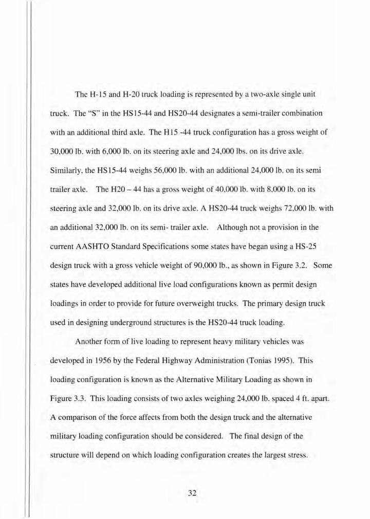
3.1 AASHO 1935 Truck Train Loading ........ ............ .. ...... .............. .. ......... 29
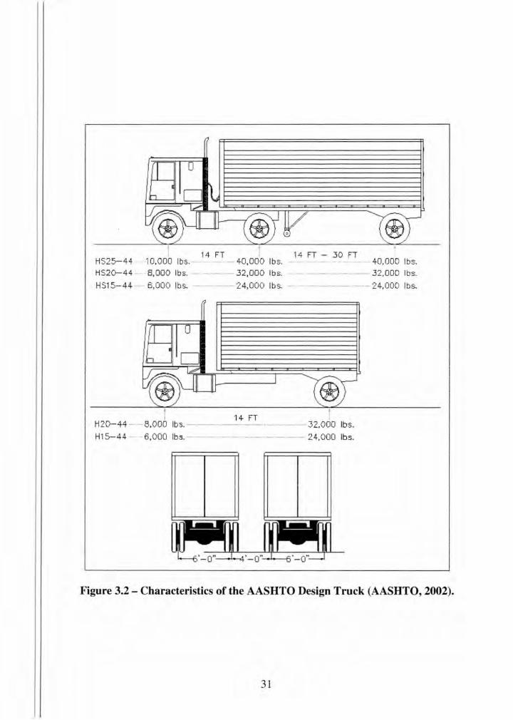
3.2 Characteristics of th~ AASHTO Design Truck .... .. ............ .... .. .... ............ 31
3.3 Characteristics of Alternative Military Loading ... .. ... . .. ............ . .............. .. 33
3.4 Tire Contact Area ......................... .. ............ .. ........ .. ............................................... 34
3.5 Earth Fill Depth and Vertical Earth Pressure Loading ................................ 36
3.6 LFD Wheel Load Distribution through Earth Fill.. ................ .............. .... .. .. .. ...... 39
3.7 Overlapping Wheel Load Distribution through Earth Fill. ...................... ...... ....... 39
3.8 Case 1, Wheel Load Distribution through Earth Fill .................................. 40
3.9 Case 2- Overlapping Wheel Load Distribution through Earth Fill. ................ 41
3.10 Case 3- Overlapping Wheel and Axle load Distribution through Earth Fill. .... 43
3.11 LFD Live Load Pressures through Earth Fill .. .... .. .................................. 44
3.12 -LFD Live Load Spread For 3ft Overburden .... .... ................ .. ...... .... .... 45
3.13 LFD Live Load Service Moments vs. Increasing Design Spans .... .. ....... ...... 46
3.14 LFD Distribution Width, E for a Single Wheel Load ....... ... . . ... .. ..... . . . ...... .48
3.15 Effective Distribution Widths on Slabs ... . ... ..... . ........ ... . ..... . . .. . . ..... .. .... .48
3.16 Reduced Distribution Widths on Slabs .... ... . . .. ..................... . ....... . . .... . .49
X
3.17 LFD Equivalent Height. . . ..... ... ... ...... . .. . . .. ...... . .. . . .......... ... . ............... 52
3.18 Live Load Surcharge Pressure ............... . ... . ... .. ........ . ........... .... ..... . ... 52
4.1 Characteristics of LRFD Design Truck and Wheel Footprint. ...... . ....... . . . ...... 62
4.2 Characteristics of the Design Tandem .. . . . ............... . .... .............. . .... ....... 63
4.3 Earth Fill Depth and Vertical Earth Pressure Loading ........ . .. . ....... .. ... . ....... 65
4.4 LRFD Wheel Load Distribution through Earth Fill ........ ..... ............ . . . ...... .. 69
4.5 Overlapping Wheel Load Distribution through Earth Fill .. . . . ... . ........ ...... ..... 70
4.6 Wheel Load Distribution through Earth Fill . ............... . ..................... . .. ... 71
4.7 Overlapping Wheel Load Distribution through Earth Fill.. ....... ..... . ..... . ........ 72
4.8 Overlapping Wheel and Axle Load Distribution through Earth Fill. .. .... . ....... . 74
4.9 Overlapping Wheel Load Distribution by Passing Vehicles . .. .... . ... . . .. .. ... ..... 75
4.10 Overlapping Axle Load Distribution by Passing Vehicles . ......................... 75
4.12 Dynamic Load Allowance vs. Burial Depth . . .... . ....... . . . . ................... .. .... 79
4.13 Wall Height for Live Load Surcharge Pressures ...... ....... . ... . ... .... .. .. . ....... 81
5.1 Alternative Military Loading vs. Design Tandem Loading ...... . . ......... ... . ..... . 83
5.2 Increase of Force Effects due to Design Truck vs. Design Truck+ Lane Load ............. 85
5.3 Dynamic Load Allowance vs. Impact. .............................. .. ................... 87
5.4 Percent Increase in Dynamic Load Allowance LRFD vs. LFD ................ . .. . .. 87
5.5 Live Load Surcharge Equivalent Heights, heq ................ .......... . . ... . ......... 89
5.6 Live Load Distribution Areas for a Single Wheel.. .............................. . .... 92
Xl
5.7 Overlapping Wheel Load Distribution by Passing Vehicles . .. . ....... .... . . .. . .... . 93
5.8 Overlapping Axle Load Distribution by Passing Vehicles .. . .. .... ....... . .. . ..... . . 93
5.9 Distributed Service Live Load Values through Earth Fill with Impact. ....... .... . 95
5.10 Distributed Factored Live Load Values through Earth Fill with Impact.. ........ 95
5.11 Service Moment- LRFD vs. LFD Design Live Loads (Multiple presence
factor and impact neglected) . .... . . .. . .. . . .. . ..... . . .. ..... .. ........... ....... . . . ... 98
5.12 Service Moment- LRFD vs. LFD Design Live Loads (Multiple presence
factor and impact included) ... . .. . ....... .. ... ......... . .... . ... .. .. .. .............. .. 99
5.13 Loads on a Three-Sided Culvert ...... . .. . ..... . ... .. .... . ...... . .. . ........ . .......... 101
6.1 Design Example #1 , Geometry .. .. .. ................ .. ....... ......... . ................. 105
6.2 LFD Vertical and Lateral Earth Pressures .. . . . .... .. . . ... ... ....... .... . ... .. .. . ...... 106
6.3 LFD Live Load Surcharge Pressure .. ..... . .... . ..... . . ....... .................. .. ..... 107
6.4 HS-20 Distribution through Earth Fill ... . .. . . .. ... . . ... .... . . .. ..... . .. . ..... ........ . 108
6.5 Alternative Military Distribution through Earth Fill .......... ..... ..... .. . .. ..... ... 109
6.6 LFD Service Loading Configuration, Cases 1- 3 ... .. . . ..... .. .. . ........ ...... .. ... 112
6.7 Critical Locations for Stresses . ....... .. ... . .... . . ... . .... . . ... . . .... .... .. . .... . .. .. ... 113
6.8 LFD Reinforcement Placement for Design Example #1 . ... ............ ................... . 126
6.9 LRFD Vertical and Lateral Earth Pressures ...... . ... ... ..... .. .. ............... ..... 127
6.10 LRFD Wall Height, Example #1. . ............. . ... . ... ........ ..... .. .... .... . . . .... . 128
6.11 LRFD Live Load Surcharge Pressure ................................. : .. ... ........ . 129
Xll
6.12 Distribution area for Design Truck ..... ...... . ............. . .... ... ............. ... .. . 131
6.13 Distribution area for two adjacent design vehicles .......... .. .... .. ................ 132
6.14 Distribution area for Design Tandem .. .. ..... ........................................ 132
6.15 Design Example #1 , LRFD Service Loading Configuration, Cases 1- 3 .. ..... 136
6.16 Critical Locations for Stresses ....... . .. ......... . .. . ... .... ... ... ... ...... .. .......... 137
6.17 LRFD Reinforcement Placement for Design Example #1 ................. ......... 153
6.18 LFD Vertical and Lateral Earth Pressures .................................... ....... 155
6.19 LFD Live Load Surcharge Pressure ...... ...... .............. ...... ...... ...... ....... 156
6.20 LFD Service Loading Configuration, Cases 1 - 3 ................................... 159
6.2 1 LFD Critical Locations for Stresses .. .. ............................................... 160
6.22 LFD Reinforcement Placement for Design Example #2 ........................... 173
6.23 LRFD Vertical and Lateral Earth Pressures ........ ...... ............................ 175
6.24 LRFD Wall Height. .. . .... ................................ ..... .. . .. .... . . ..... ..... . .... 176
6.25 LRFD Live Load Surcharge Pressure ...... .. ......................................... 177
6.26 Loading Configuration, Cases 1- 3 ................................................... 182
6.27 Locations of Critical Stresses ............................. ... .... ...... ... .............. 183
6.28 LRFD Reinforcement Placement for Design Example #2 .......................... 197
Xlll
TABLES
Table
3.1 AASHTO Group Loading Coefficients and Load Factors ... .......... . . . . . . . . . . .. .. 26
3.2 AASHTO Earth Pressure and Dead Load Coefficients ..... ..... . .... .. . .... . ......... 27
3.3 AASHTO Resistance Factors for Underground Concrete Structures ................ 29
3.4 AASHTO Standard HS Design Truck Classes .. .... .. .............. .. .. ............ .. . 30
3.5 Case 1 .. . ....... . .... .. . . . . ........... .. .. .. . . ... ........ ... .. . . .......... .. .... .. .... ... .. .. .. 40
3.6 Case 2 ... .. .. ......... ......... . ....... . ..... . .... . .. ... .... .. . . ......... ... . . .. . . ....... . . ... 41
3.7 Case 3 ... . ... ..... . .... . ... . .. .. ...... ... . . .. . ... ... . ..... .. .. .. . . .. .. .. ....... ........ .. .. ... 42
3.8 Service Moments from HS-20, HS-25, and Alternative Military Loads ............ 46
3.9 linpact Factor. ...................... . ...... . .... ... ... ..... . ......... . .. . .. . .. . . . . . ..... ..... 50
4.1 Load Combinations and Load Factors ............ ...... .... ............ ........ .. ....... 57
4.2 Load Factors for Permanent Loads, yp ....... ... ............. ... ........ .. .... ... .. ..... 59
4.3 Multiple Presence Factors ..... . . . .............. . ....... . .. . .. ..... . . .. . ..... .... ......... . 67
4.4 Case 1 ... . .. .. ......... . .. . ... . ....... . ......... . .... . ...... . ....... . . ... . . ....... .. . . ........ 71
4.5 Case 2 .... . ............ . ... . .. . .. . . . ............ . ..................... .. .. . ..... . . . ............ 72
4.6 Case 3 .................... .. .. .. ............... .. .. . ...................... . .. . ... . ............. 73
4.7 Equivalent Heights .... ...... . . ... ...... ..... . . .. . .... ... . ........ . ........... . .... . ... . .... 80
5.1 Load Factors for LRFD and LFD Specifications .. ........ .. ...... .. .......... .. .... .. 100
6.1 LFD - Structural Analysis Results per Foot Width, Example 1 .. .... ........ ...... 113
XIV
6.2 LRFD- Structural Analysis Results per Foot Width, Example 1. .... . .. . . ...... .. 138
6.3 Area of Steel comparison ........... .. ... . ... . . . . . ..... ................. . . . ... ..... .. .. ... 152
6.4 Impact Factor. .. .. . . .................. . .. ......... .. .. .......... . .. . ............. .......... 156
6.5 LFD- Structural Analysis Results per Foot Width, Example 2 .. . .. .. .... ..... .... 161
6.6 LRFD- Structural Analysis Results per Foot Width, Example 2 ..... .. ....... : ... 183
6.7 Area of Steel comparison ............................ ... ... . ....... ............... . ....... 152
XV
Chapter 1 Introduction
Historically, much of the design methodology and design loads for
underground concrete structures such as pipe and box culvert came from the
American Association of State Highway and Transportation Officials (AASHTO). In
the 1930's AASHTO began publishing the Standard Specification for Highway
Bridges. The standard practice at the time was to use one factor of safety. This
methodology is commonly known as allowable stress design (ASD). In the 1970s,
AASHTO began varying the factor of safety for each load in relation to the engineer's
ability to predict the corresponding load. This corre pending bridge design
methodology was referred to a load factor design (LFD). The change from ASD to
LFD was made in the form of interim revisions by AASHTO. In fact, the Standard
Specifications have never been completely revised and till include provisions from
both the LFD and ASD methodologies ("LRFD: State Department" 2006).
AASHTO introduced the Load and Resistance Factor Design (LRFD) Bridge
Design Specification in 1994, with the intent of replacing the Standard Specifications
for Highway bridges with this reliability ba ed code that provides a more uniform
safety for all elements of bridges. The AASHTO LRFD Highway Bridge Design
Specifications were developed with the intent of implementing a more rational
approach for the design of highway structures. The LRFD Specifications utilize load
1

and resistance factots based on the known variability of applied loads and material
properties. The load and resistance factors were calibrated from actual bridge
statistics ensuring a more uniform level of safety ("LRFD: State Department" 2006).
1.1 Historical Development of LRFD Specifications
In the late 1970's the Ontario Ministry of Transportation and Communication,
now known as the Ministry of Transportation, developed its own bridge design
specifications, rather than continue to use the AASHTO Standard Specifications for
Highway Bridges. The Ontario Ministry of Transportation and Communication
required that the new design specifications be based on probabilistic limit states. As a
result, the first edition of the Ontario Highway Bridge Design Code (OHBDC) was
released in 1979 to the design community as North Americas first calibrated,
reliability-based limit state specification (NCHRP 1998). The OHBDC is currently in
its third edition after being updated in 1983 and 1993. In addition, the OHBDC
included a companion volume of commentary in which the AASHTO Standard
Specifications did not. Over time, more and more U.S . engineers became familiar
with the OHBDC. They recognized certain logic in the calibrated limit states design.
Many American engineers began to question the Standard AASHTO Specifications
and whether it should be based on comparable philosophy.
2

The National Cooperative Highway Research Program (NCHRP), National
Science Foundation (NSF), and various states completed numerous research projects.
These organizations were collecting new information on bridge design faster than it
could be critically reviewed and were appropriately adopted to form the AASHTO
Standard Specifications. Later research revealed that many of the revisions that have
occurred to the Standard AASHTO Specifications since its inception had resulted in
numerous inconsistencies and it made the document appear patchwork.
In the spring of 1986, a group of state bridge engineers or their representatives
met in Denver and drafted a letter to the AASHTO Highway Subcommittee on
Bridges and Structures (HSCOBS) indicating their concern that the AASHTO
Standard Specifications must be revised. They also raised concerns that the Technical
Committee Structure, operating under the HSCOBS, was not able to keep up with
emerging technologies. As a result, this group of state bridge engineers began the
process leading to the development of the LRFD Specifications. A group of state
bridge engineers met with the staff of the NCHRP in July of 1986 to consider whether
a project could be developed to explore the concerns raised in the letter submitted at
the meeting in Denver. This led to the NCHRP project 12-28(7) "Development of
Comprehensive Bridge Specifications and Commentary." A pilot study was
conducted by Modjeski and Masters, Inc. with Dr. John M Kulicki as Principle
3

Investigator. The list of task for this project and the brief outcome are li ted below
(NCHRP 1998).
• Task 1 -Review other specifications, and the philosophy of safety and
coverage provided. Information collected from various sources around
the world indicated that most of the First World Countries appeared to
be moving in the direction of a calibrated, reliability-based, limit states
specification.
• Task 2- Other than the Standard Specification , review other
AASHTO documents for their inclusion into a revised standard
specification. This can be best described as a search for gaps and
inconsistencies in the 13th edition of the AASHTO Standard
Specification for Highway Bridges. "Gaps" were areas where
coverage was missing; "Inconsistencies" were internal conflicts, or
contradictions of wording or philosophy. Numerous gaps and
inconsistencies were found in the Standard Specifications.
• Task 3 -As ess the feasibility of a probability-based specification.
The design philosophy u ed in a variety of specifications wa
reviewed. They were the ASD, LFD, and the Reliability Based
4

Design. It wa generally agreed upon that the probability-ba ed
specification was more suitable.
• Task 4 -Prepare an outline for a revi ed AASHTO Specification for
Highway Bridge Design and commentary, and present a proposed
organizational process for completing such a document.
The findings of NCHRP Project 12-28(7) were presented to the AASHTO
HSCOBS in May of 1987. There were 7 options that were available:
• Option 1 - Keep the Statu Quo
• Option 2 -Table Consideration of LRFD for the Short Term
• Option 3 - Immediate Adoption of the OHBDC
• Option 4 -Replace Current with LRFD Immediately
• Option 5 - Replace Current LFD with LRFD in the Near Term
• Option 6- Develop LRFD for Evaluation Only, or
• Option 7 -Develop LRFD as a Guide Specification
A recommendation was made to develop a probability-based limit states
specification, revise as many of the gaps and inconsistencies as possible, and develop
a commentary specification. Thus NCHRP Project 12-33, entitled "Development of
Comprehensive Specification and Commentary," began in July of 1988. The primary
objective was to develop a recommended LRFD-ba ed bridge design specifications
5
and commentary for consideration by the AASHTO Subcommittee on Bridges and
Structures. Thirteen task groups were responsible for developing the recommended
specifications. The task groups were: general features, loads, analysis and evaluation,
deck systems, concrete structures, metal structures, timber structures, joints, bearings,
and accessories; foundations ; soil-structure interaction systems, moveable bridges,
bridge rail, and specification calibration. The project consisted of four contractors
and 47 consultants employed to assist with the development of the specification and
commentary. In addition, more than 20 state, federal , and industry engineers worked
on the project volunteering their time (Project 12-33 2006). The project was
completed on December 31 , 1993. The LRFD specifications were adopted by
AASHTO and published as the AASHTO LRFD Bridge Design Specifications. The
1994 edition was the first version, with both SI unit and customary U.S. unit
specifications available. Currently, the 2006 interim revision edition is the third
edition of the AASHTO LRFD Bridge Design Specifications.
Today, the Federal Highway Administration (FHWA) and State Departments
of Transportation have established as a goal that the LRFD Standard Specifications be
used on all new bridge designs after 2007. In fact, AASHTO in concurrence with
FHW A has set a deadline of October 1 sr, 2007 for full implementation by all states.
States must design all new bridges according to the LRFD Specifications. At least 46
states have fully or partially implemented the LRFD Specifications to date, or are
6

working with the FHW A to develop a plan for implementation. A 2004 AASHTO
Oversight Committee survey found that 12 states have fully implemented the
specifications. Another 34 states have partially implemented the LRFD
Specifications or are currently in the stage of developing implementation plans and
designing pilot projects ("LRFD: Achieving Greater Reliability" 2004). The FHW A
is providing assistance to states in transition by providing a number of resources that
include a team of structural, geotechnical, and research engineers who can meet with
individual state and provide guidance in developing a State-Specific LRFD
implementation plan, training courses, and LRFD Design Workshops. In fact, the
FHW A lists tips for successful implementation on the following website,
http://www.fhwa.dot.gov/BRIDGE/lrfd/tips.cfm. Tips on the website include:
• Staff: Dedicate staff for LRFD planning and design (and studie if
necessary) and train the initial design and study squad in LRFD.
Utilize FHW A and other State Departments of Transportation
assistance.
• Design Transition Strategy: Set a target date for full LRFD
implementation on all new and replacement bridges and on all in
house and consultant projects. Perform in-house trial LRFD design of
LFD projects (or have pilot LRFD projects) to develop questions and
7

resolution . These trials also help to gain familiarity with the LRFD
Specifications. After the completion of the triaVpilot project , utilize
the LRFD design in increments up to the target date or have a one-step
conversion to LRFD. The latter should help you minimize the problem
of maintaining two separate design specifications and manuals. The
pilot projects hould be selected carefully to represent low priority,
routinely designed bridges.
• Software: Acquire a computer program that utilizes LRFD. There are
many state and private LRFD software programs available for steel
and concrete bridge superstructures and concrete substructures
• Training: Sponsor in-house training courses for all designers (by in
house instructors, local universities in tructors, industry, or by
FHW A). Acquire LRFD design examples and software for hands-on
training. Require that consultants attend LRFD training before they
perform LRFD designs in a particular state.
• Technical Support: Develop a technical support group that is readily
available to answer questions pertaining to the LRFD Specifications.
Utilize LRFD support teams, states, industry, universities, and FHW A
resources. In addition, retaining a firm experienced in LRFD for
questions may prove to be beneficial.
8

• Documentation Support: Update standards, manuals, and guidance to
coordinate with the LRFD Specifications. Develop pre-designed
LRFD decks and barriers to shorten the design process if standardized
designs are not available. Contract services to update existing design
materials to LRFD.
• Fine-Tune Documentations: After the completion of the pilot project
and/or full LRFD conversion, fine-tune the LRFD standards, manuals,
and guidance if and when needed.
1.2 Problem Statement and Research Significance
This thesis examines the current LRFD Design Specifications and the Standard
AASHTO Specifications used in designing underground concrete structures such as
underground utility structures, drainage inlets, three-sided structures, and box
culverts. Many of the AASHTO LRFD Code provisions that differ from the Standard
Specifications include terminology, load factors, implementation of load modifiers,
load combinations, multiple presence factors, design vehicle live loads, distribution of
live load to slabs and earth fill, live load impact, live load surcharge, and the concrete
design methodology for fatigue, shear strength, and crack control. The October 151,
2007 deadline that AASHTO in concurrence with the Federal Highway
Administration has set for all states to be completely converted to the AASHTO
9

LRFD Bridge Design Specifications is soon approaching. Although there are many
training tools available to utilize the LRFD Specifications on highway bridges, there
are very little resources available for designing underground precast concrete. This
thesis addresses how to transition from the Standard Specifications to the LRFD
Specifications when designing underground precast concrete. This thesis includes:
• A comprehensive literature review of existing and current studies
associated with the Standard LFD and LRFD Specifications.
• A detailed summary of the variables and design methodology for
buried precast concrete structures using the AASHTO LFD Standard
Specifications.
• A detailed summary of the variables and design methodology for
buried precast concrete stmctures using the AASHTO LRFD Bridge
Design Specifications.
• A thorough comparison between the LRFD and LFD specifications.
• Two design examples illustrating the u e of both specifications. The
examples are of a buried three-side precast concrete stmcture.
• A summary of this thesis document.
10

Chapter 2 Literature Review
Currently, b1idge de igners are transitioning from the Standard AASHTO
Bridge Design Specifications to the Load and Resistance Factor Design
Specifications. The LRFD Bridge Design Specifications were developed in 1994;
however, bridge designers were given the option of using either pecification. The
new specifications utilize state-of-the-art analysis and design methodologies. In
addition, the LRFD Specifications make use of load and resistance factors based on
the known variability of applied loads and material properties. Difference between
the two specifications include terminology, load factors, implementation of load
modifiers, load combinations, multiple presence factors , design vehicle loads,
distribution of live load to slabs and earth fill, live load impact, live load surcharge,
and the concrete design methodology for fatigue, shear strength, and control of
cracking. There has been very little research comparing all of the provisions from
both specifications when designing underground concrete structures. However, there
has been research completed comparing specific topics from both specifications and
impact the LRFD Specification has had on the engineering community.
2.1 Comparison of Standard Specifications and LRFD Specifications
Rund and McGrath (2000) compared all of the provisions from AASHTO
Standard Specifications and the LRFD Specifications for precast concrete box
11
culverts. The research analyzed several combinations of box culvert sizes and fill
depths utilizing both specifications. Typically, the provisions from the LRFD
Specifications yielded greater design loads and therefore required more area of steel
reinforcement. The differences in reinforcement areas were the most pronounced for
fill depths less than 2 ft. This was primarily the result of the differences in
distributing the live load to the top slab into equivalent strip widths . The equivalent
strip width is the effective width of slab that resists the applied load. In addition, for
culvert spans up to 10ft, the LRFD Specifications required shear reinforcement.
Analysis utilizing the Standard AASHTO Specifications also show required shear
reinforcement for a similar range of spans, but provisions permit the shear effects to
be neglected. For depths of fill between 2 and 3 feet , the differences in reinforcement
areas were due to fatigue requirements. The provisions in the Standard Specifications
for fatigue were not present in the LRFD Specifications. For depths of overburden
greater than 3ft, the differences in the reinforcing areas decreased slightly. However,
with increasing depth, the LRFD Specifications required greater required area of steel
reinforcement. This was primarily due to the distribution of live load through earth
fill. The provisions in the LRFD Specifications often yield higher design forces from
wheel loads than the Standard Specification. It is important to note that the research
utilized the first edition of the LRFD Specifications, which has since been revised and
12
is in its 3rd edition. Many of the provisions from this research have been modified
slightly.
2.2 American Concrete Pipe Association Study
The American Concrete Pipe Association wrote a short article comparing the
live loads on concrete pipe from both specifications (ACPA 2001). The primary
objective of this research was to compare the live load model and distribution
methods used in both specifications. The article included four design examples
illustrating the design steps that are required to be taken when designing reinforced
concrete pipe using the Standard LRFD Specifications . . Similar to the article written
by Rund, and McGrath (2000), the paper concluded that the LRFD Specifications
typically produced greater design forces than the Standard Specification.
2.3 Flexural Crack Control in Concrete Bridges
Several States have found that crack control requirements tend to govern the
design of flexural steel in concrete st.mctures more frequently with the provisions of
the 1994 LRFD Specifications than under the Standard AASHTO Specifications
(DeStefano, Evans, Tadros, and Sun 2004). At the time it was believed that this was
primarily due to the higher loads specified in the LRFD Specifications. In the 1994
AASHTO LRFD Specifications, flexural crack control requirements were based on
the Z factor method developed by Gergely and Lutz in 1968 (DeStefano, Evans,
13
Tadros, and Sun 2004). Re earch completed by DeStefano et al. (2004) suggested a
new equation be adopted in the LRFD Specifications. Their recommendation for a
new equation was for the development of a simple, straight forward equation that
accounts for the differences between bridge and building structures. The proposed
revised crack control requirements identified a number of short comings identified
with the Z factor method. Example de igns were included on box culverts to
compare the allowable stresses in the existing Z factor method and the proposed crack
control method. The results indicated reasonable increases in allowable stresses, thus
permitting more economical designs without sacrificing long term durability. The
proposed equation developed in this research has been adopted in the current edition
of the LRFD Specifications.
2.4 National Cooperative Highway Research Program, Project 15 - 29
The NCHRP funded a project that examined the distribution of live load
through earth fill (Project 15-29 2006). This research compared provisions form both
specifications regarding disuibution of live load through earth fill . The design and
evaluation of buried structures requires an understanding of how vertical earth loads
and vehicular live loads are transmitted through earth fill . When the depth of
overburden i equal to or greater than 2 ft, both the Standard AASHTO Specifications
and the LRFD Specifications allow for the wheel load to be distributed throughout the
14
earth fill. Both specifications utilize approximate methods for estimating the
distribution of vehicular live loads through earth fill . The Standard LRFD
Specification takes into account the contact area between the footprint of the tire and
ground surface. The distribution area is equal to the tire footprint, with the footprint
dimensions increased by either 1.15 times the earth fill depth for select granular
backfill, or 1.0 for other types of backfill. The Standard AASHTO Specifications
does not account for the dimensions of the tire. Instead the wheel load is considered
to be a concentrated point load. The wheel load is distributed over a square equal to
1.75 times the depth of fill, regardless of the type of backfill. One major difference
between the two specification is the AASHTO LRFD Bridge Design Specification
uses different approximate methods that ignificantly increase live load pressures on
buried structures when compared to the Standard Specifications. In addition, the
basi for the methodology in which the live load is distributed through soil is not well
documented or understood. As a result the NCHRP developed project 15-29, Design
Specifications for Live Load Distribution to Buried Structures. Administered by the
Transportation Research Board (TRB) and sponsored by the member departments
(i.e., individual state departments of tran portation) of the American Association of
State Highway and Transportation Officials, in cooperation with the FHW A, the
NCHRP was created in 1962 as a means to conduct research in acute problem areas
that affect highway planning, design, construction, operation, and maintenance
15
nationwide. The objective of Project 15-29 is to develop recommended revisions to
the AASHTO LRFD Bridge Design Specifications relating to the distribution of live
load to buried structures. The project completion date is scheduled for October 20th'
2007. The status of the project is unknown at this time.
2.5 Design Live Loads on Box Culverts, University of Florida
Other research that ha been completed with regards to the distribution of live
load through earth fill was performed by Bloomquist and Gutz (2002) at the
University of Florida. The research was sponsored by the Florida Department of
Transportation and prepared in cooperation with the Federal Highway
Administration. The Florida Department of Transportation adopted the Standard
LRFD Specifications a the de ign standard for all structures beginning in 1998. The
research report discusses the development of equations to calculate the distribution of
live loads through earth fill for the design of precast concrete box culverts. The
objective of there earch was to develop a new method and establish a single design
equation for distributing live loads to the tops of precast concrete box culverts . The
existing LRFD methodology is considered to be a rigorous design procedure that is
extremely difficult to apply and too conservative when compared to the Standard
AASHTO Specification . A ignificant amount of design time can be shortened by
simplifying this process. Also, the work was aimed at producing a simplified design
16

equation that would be thorough but not overly conservative. The approach of the
research was to use theoretical methods to calculate the distribution of live loads
through varying earth fill depths and compare them with the current LRFD
provisions. The first method that was reviewed was developed by Boussinesq in
1855 (Bloomquist and Gutz 2002). His method considers the stress increase based on
a point load at the surface of a semi-infinite, homogenous, isotropic, weightless,
elastic half-space, shown in Figure 2.1. The value of the vertical stress can be
calculated using Equation 2.1.
Equation 2.1
Where:
P = Point load
Z = Depth from ground surface to where <Jz is desired
r = Horizontal distance from point load to where <Jz is desired
17

p
l Figure 2.1 - Boussinesq Point Load
Natural soil deposits do not approach ideal conditions that the Boussinesq
equation was based upon. Many soil deposits consist of layered strata of fine and
course materials or alternating layers of clay and sand. In 1938, Westergaard
proposed a solution that was applicable for these types of deposits (Bloomquist and
Gutz 2002). Using the Westergaard theory, the vertical stress can be calculated using
Equation 2.2.
Equation 2.2
Both the Boussinesq and Westergaard theory assume the loading acts as a
point load. The provisions in the Standard LRFD Specifications require the
18

dimension of the tire be utilized. Newmark integrated the Bous inesq solution over
an area to calculate the distribution of a patch load through soil in 1935. This lead to
the development of Equation 2.3, and is known as the superposition method.
Equation 2.3
Where:
qo = Contact stress at the surface
m=xlz
n = y/z
x,y = Length and width of the uniformly loaded area
z = Depth of surface point where stress increase is desired
Another method that was reviewed was the buried pipe method. The buried
pipe method is also based of the Boussinesq solution. The equation for the buried
pipe method is shown in Equation 2.4
Equation 2.4
19

Where:
W d = Load on pipe in lb/unit length
P = Intensity of di tributed load (psf)
F' = Impact Factor
Be = Diameter of pipe (ft)
C = Load coefficient which is a function of D/(2H) and
M/(2H), where D and Mare the width and length, respectively,
of the area over which the di tributed load acts.
The last method to be reviewed and one of the simplest methods to calculate
the di tribution of load with depth is known a the 2:1 method calculated in Equation
2.5.
Where:
Load a_=-----(B + Z)(L+ Z)
crz = Live load stress
Z = Depth of fill
Equation 2.5
B, L =Width and length, respectively, of the loaded area at
the surface
20
The 2:1 method i an empirical approach that assumes the area over which the
load acts increases in a sy tematic way with depth. The methodology in the Standard
LRFD Specifications is ba ed on a variation of this method.
Each of the methods described above were used to calculate the live load
pressure through earth fill and compared to the current LRFD Specifications. The
objective was to compare methods of live load distribution and determine suitable
alternatives. The Design Truck and Design Tandem vehicles were used when
examining the methods. The findings sugge t that the superposition method be used
in place of the provisions in the Standard LRFD Specifications. Once the different
methods to di tribute live load were compared, the next step was to develop a
simplified equation that would produce the arne force effects as the current LRFD
Specifications. Based on the superposition method, shears and moments acting on the
top slab of box culverts were calculated for varying design spans and earth fill depths.
An equivalent uniform load model was developed by statistical modeling and curve
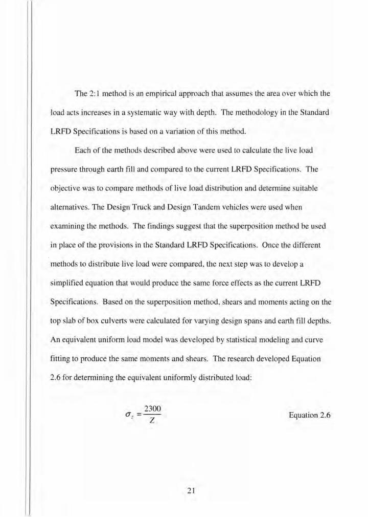
fitting to produce the same moments and shears. The research developed Equation
2.6 for determining the equivalent uniformly distributed load:
2300 a=-
z z
21
Equation 2.6

Where:
crz =Equivalent Load (plf)
Z = Depth of fill (ft)
The researcher recommend that Equation 2.6 only be used for box culverts
with pan lengths that were in the cope of the re earch. Further refinement of the
equation may be accomplished with a more rigorou tati tical analysis .
22
Chapter 3 AASHTO LFD Standard Specifications
3.1 Load Factors and Load Combinations
All structures must be designed to withstand multiple loads acting
simultaneously at once. Vehicle live loads may act on a structure at the same time as
lateral earth pressure. The de ign engineer is responsible for ensuring the de ign is
ized and reinforced properly to safely resist combination of loads. To account for
this the Standard AASHTO Specifications contain load combinations, subdivided into
groups, which represent a combination of simultaneous loadings on the structure.
The general equation used to define a group load is given by Equation 3.1 (AASHTO
2002).
Where:
Group(N) = y[~ 0D + ~L (L + D + ~cCF + ~ EE
+~BB+~sSF+~w W +~wL WL
+ ~ L LF + ~ R (R + s + T)
+ ~ EQEQ +~IcE ICE]
N =group number
y = load factor from Table 3.1
~=coefficient from Table 3.1
D =dead load
23
Equation 3.1
L =live load
I = impact factor
E =earth pre ure
B =buoyancy
W = wind load on structure
WL =wind load on live load
LF = longitudinal force from live load
CF = centrifugal force
R = rib shortening
S = shrinkage
T = temperature
EQ = earthquake
SF = stream flow pre sure
ICE = ice pressure
Table 3.1lists values for both y and p. These values are based on the service
load and load factor design. The coefficient p varie ba ed on the type of load. The
load factory is the arne for ervice loads; however, it varies for different load factor
design groupings. The p coefficients for both dead load and earth pre sure vary
depending on the load group and design method shown in Table 3.1. This variation
24

results from different values being applied for different types of elements or
components. A de cription of the dissimilar results is illustrated in Table 3.2.
The Standard AASHTO Specification incorporates two principle de ign
methods:
• Service Load De ign (Allowable Stres Design or Working Stre s
Design)
• Strength Design (Load Factor Design or Ultimate Strength Design)
The service load design method is an approach in which the structural
members are designed so that the unit stresses do not exceed predefined allowable
stresses. The allowable stress is defined by the material strength reduced by a factor
of safety. In other words the total stress caused by the load effects must not exceed
this allowable stress. This is further expressed in Equation 3.2.
f actual :s; !allowable Equation 3.2
25
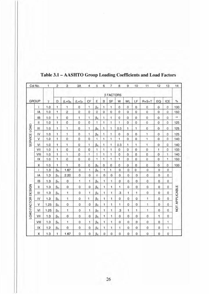
Table 3.1 - AASHTO Group Loading Coefficients and Load Factors
Col No. 1 2 3 3A 4 5 6 7 8 9 10 11 12 13 14
p FACTORS
GROUP y D (l+I)N (L+I)p CF E B SF w WL LF R+S+T EQ ICE %
I 1.0 1 1 0 1 PE 1 1 0 0 0 0 0 0 100
lA 1.0 1 2 0 0 0 0 0 0 0 0 0 0 0 150
IB 1.0 1 0 1 1 BE 1 1 0 0 0 0 0 0 .. II 1.0 1 0 0 0 1 1 1 1 0 0 0 0 0 125
0 <(
Ill 1.0 1 1 0 1 PE 1 1 0.3 1 1 0 0 0 125 0 ....J w IV u 1.0 1 1 0 1 PE 1 1 0 0 0 1 0 0 125
> v 1.0 1 0 0 0 1 1 1 1 0 0 1 0 0 140 a: UJ VI 1.0 1 1 0 1 BE 1 1 0.3 1 1 1 0 0 140 (/)
VII 1.0 1 0 0 0 1 1 1 0 0 0 0 1 0 133
VIII 1.0 1 1 0 1 1 1 1 0 0 0 0 0 1 140
IX 1.0 1 0 0 0 1 1 1 1 0 0 0 0 1 150
X 1.0 1 1 0 0 BE 0 0 0 0 0 0 0 0 100
I 1.3 Po 1.67 0 1 PE 1 1 0 0 0 0 0 0
lA 1.3 Bo 2.20 0 0 0 0 0 0 0 0 0 0 0
IB 1.3 Po 0 1 1 PE 1 1 0 0 0 0 0 0 z
II 1.3 Po 0 0 0 PE 1 1 1 0 0 0 0 0 UJ (!) ....J ii5
13o BE CD
UJ Ill 1.3 1 0 1 1 1 .3 1 1 0 0 0 <(
0 u a: IV 1.3 Po 1 0 1 BE 1 1 0 0 0 1 0 0
::J 0 a...
a... 1- v 1.25 Po 0 0 0 PE 1 1 1 0 0 1 0 0
<( u 1-<(
lL VI 1.25 Bo 1 0 1 13E 1 1 .3 1 1 1 0 0
0 0 z <(
13o BE 0 VII 1.3 0 0 0 1 1 0 0 0 0 1 0 ....J
VIII 1.3 Po 1 0 1 PE 1 1 0 0 0 0 0 1
IX 1.2 Bo 0 0 0 BE 1 1 1 0 0 0 0 1
X 1.3 1 1.67 0 0 PE 0 0 0 0 0 0 0 0
26

Table 3.2 - AASHTO Earth Pressure and Dead Load Coefficients
13 Load Value Element
13E Earth Pressure 1.0 Vertical and lateral loads on all other structures
Lateral loads on rigid frames (check both loadings to 13E Earth Pressure 1.0 and 0.5 see which one governs)
Lateral earth pressure for retaining walls and rigid 13E Earth Pressure 1.3 frames excluding rigid culverts
Lateral earth pressure when checking positive 13E Earth Pressure 0.5 moments in rigid frames
13E Earth Pressure 1.0 Rigid culverts
13E Earth Pressure 1.5 Flexible culverts
Columns, when checking member for minimum axial
~0 Dead Load 0.75 load and maximum moment or maximum eccentricity
Columns, when checking member for maximum axial ~D Dead Load 1.0 load and minimum moment
13o Dead Load 1.0 Flexural and tension members
Bridge substructures such as foundations and abutments have traditionally
been designed using the Service Load Design methodology. Underground precast
concrete box culverts and three- ided structures are designed by the load fac tor
design, thus this thesis focuses solely on the load factor design methodology. In this
methodology, the general relationship is defined utilizing Equation 3.3 .
Equation 3.3
27
Where:
'Yi = Load factors
Qi = Force effects
<1> = Resistance factors
Rn =Nominal resistance
RR = Factored resistance
The nominal re istance of a member, Rn, is calculated utilizing procedures
given in the current AASHTO Specifications. A resistance factor, <J>, is used to obtain
the factored resistance RR. The appropriate resistance factors are determined for
specific conditions of design and construction process. Typical values for
underground concrete structures are listed in Table 3.3. The force effects, Qi, that
should be considered when designing underground concrete structures are live load,
impact, live load surcharge pressures, self weight, and vertical and horizontal earth
pressures. Loads considered important for other types of structures such as wind,
temperature, and vehicle breaking are insignificant compared to the force effects
previously mentioned for buried concrete structures. The following sections will
examine these critical force effects when designing underground concrete structures,
specifically reinforced precast concrete box culverts and three-sided concrete
structures, using the Standard AASHTO Specifications.
28
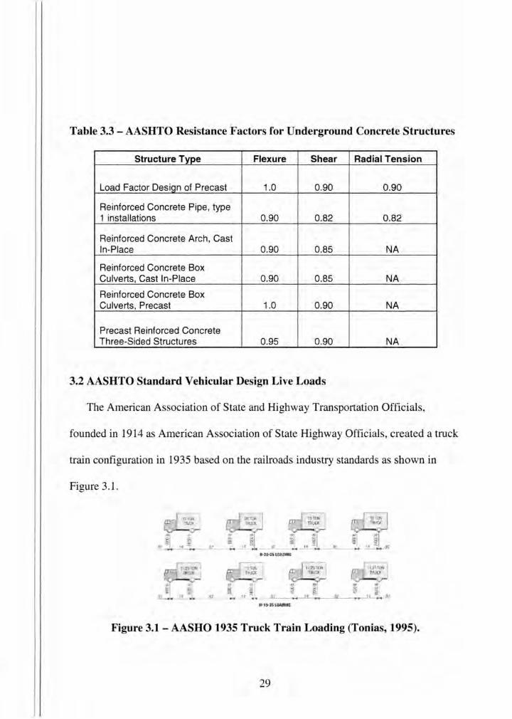
Table 3.3- AASHTO Resistance Factors for Underground Concrete Structures
Structure Type Flexure Shear Radial Tension
Load Factor Design of Precast 1.0 0.90 0.90
Reinforced Concrete Pipe, type 1 installations 0.90 0.82 0.82
Reinforced Concrete Arch, Cast In-Place 0.90 0.85 NA
Reinforced Concrete Box Culverts, Cast In-Place 0.90 0.85 NA
Reinforced Concrete Box Culverts, Precast 1.0 0.90 NA
Precast Reinforced Concrete Three-Sided Structures 0.95 0.90 NA
3.2 AASHTO Standard Vehicular Design Live Loads
The American Association of State and Highway Transportation Officials,
founded in 1914 as American Association of State Highway Officials, created a truck
train configuration in 1935 based on the railroads industry standards as shown in
Figure 3.1.
'"I ""' ~ ,· mi ~"~~
til
s 4: .:.... ______ n_ ______ ____...,,___.!:l _ _ _...__~,....._J"-+oo.
IHS.lS t.OADIItG
Figure 3.1- AASHO 1935 Truck Train Loading (Tonias, 1995).
29
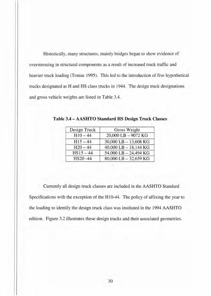
Hi torically, many structures, mainly bridges began to show evidence of
overstressing in structural components as a result of increased truck traffic and
heavier truck loading (Toni as 1995). Thi led to the introduction of five hypothetical
trucks designated a H and HS class trucks in 1944. The design truck designations
and gross vehicle weights are listed in Table 3.4.
Table 3.4 - AASHTO Standard HS Design Truck Classes
Design Truck Gross Weight H10- 44 20,000 LB - 9072 KG H15 -44 30,000 LB - 13,608 KG H20-44 40,000 LB- 18,144 KG
HS15- 44 54,000 LB - 24,494 KG HS20 -44 80,000 LB - 32,659 KG
Currently all design truck classes are included in the AASHTO Standard
Specifications with the exception of the Hl0-44. The policy of affixing the year to
the loading to identify the design truck class was instituted in the 1994 AASHTO
edition. Figure 3.2 illustrates these design trucks and their associated geometries.
30
0
I • I 1 4 FT I 1 4 FT - 30 FT
HS25-44 ---10.000 lbs.-· -· ----·- 40.000 lbs. -··-·--- ·- ··-· -·-- 40.000 lbs. HS20-44 --- 8,000 lbs. - -------- 32,000 lbs. - -- - ·-· - ----- - 32,000 lbs.
HS15-44 - 6,000 lbs. - - ---24,000 lbs. -· ----·--·-·--- -- 24,000 lbs.
d 0
D
®l lr l
~ I 14-FT !
H20-44 -·-8.000 lbs. - ----··-----··---· --·-·-·-- 32.000 lbs.
H15-44 ---6,000 lbs.-------··------·-----------·---·- 24,000 lbs.
Figure 3.2 - Characteristics of the AASHTO Design Truck (AASHTO, 2002).
31
The H-15 and H-20 truck loading is represented by a two-axle single unit
truck. The "S" in the HS 15-44 and HS20-44 designates a semi-trailer combination
with an additional third axle. The H15 -44 truck configuration has a gross weight of
30,000 lb. with 6,000 lb. on its steering axle and 24,000 lbs. on its drive axle.
Similarly, the HS 15-44 weighs 56,000 lb. with an additional 24,000 lb. on its em1
trailer axle. The H20- 44 ha a gross weight of 40,000 lb. with 8,000 lb. on its
steering axle and 32,000 lb. on its drive axle. A HS20-44 truck weighs 72,000 lb. with
an additional 32,000 lb. on its semi- trailer axle. Although not a provision in the
current AASHTO Standard Specifications some states have began using a HS-25
design truck with a gross vehicle weight of 90,000 lb., as shown in Figure 3.2. Some
states have developed additional live load configurations known as permit design
loadings in order to provide for future overweight trucks. The primary design truck
used in designing underground structure is the HS20-44 truck loading.
Another form of live loading to represent heavy military vehicles was
developed in 1956 by the Federal Highway Administration (Tonias 1995). This
loading configuration is known as the Alternative Military Loading as shown in
Figure 3.3. Thi loading consists of two axles weighing 24,000 lb. spaced 4ft. apart.
A comparison of the force affects from both the design truck and the alternative
military loading configuration should be considered. The final design of the
structure will depend on which loading configuration creates the largest stress.
32
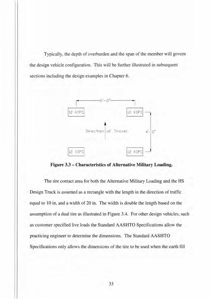
Typically, the depth of overburden and the pan of the member will govern
the design vehicle configuration. This will be further illustrated in subsequent
sections including the design examples in Chapter 6.
14 6'-0"
l12 KIPSI l12 KIPSI
Direction i oF TrCl vel 4'-o"
112 KIPSI 112 KIPSI
Figure 3.3 - Characteristics of Alternative Military Loading.
The tire contact area for both the Alternative Military Loading and the HS
Design Truck is assumed as a rectangle with the length in the direction of traffic
equal to 10 in, and a width of 20 in. The width is double the length based on the
assumption of a dual tire as illustrated in Figure 3.4. For other design vehicles, such
as customer pecified live loads the Standard AASHTO Specifications allow the
practicing engineer to determine the dimensions. The Standard AASHTO
Specifications only allows the dimensions of the tire to be used when the earth fill
33
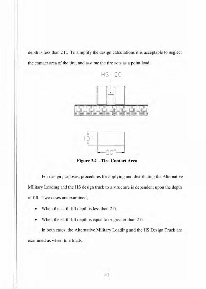
depth is less than 2ft. To simplify the design calculations it i acceptable to neglect
the contact area of the tire, and assume the tire acts as a point load.
HS- 20
Figure 3.4 - Tire Contact Area
For design purposes, procedures for applying and distributing the Alternative
Military Loading and the HS design truck to a structure is dependent upon the depth
of fill. Two cases are examined,
• When the earth fill depth is less than 2 ft.
• When the earth fill depth is equal to or greater than 2 ft.
In both cases, the Alternative Military Loading and the HS Design Truck are
examined as wheel line loads.
34
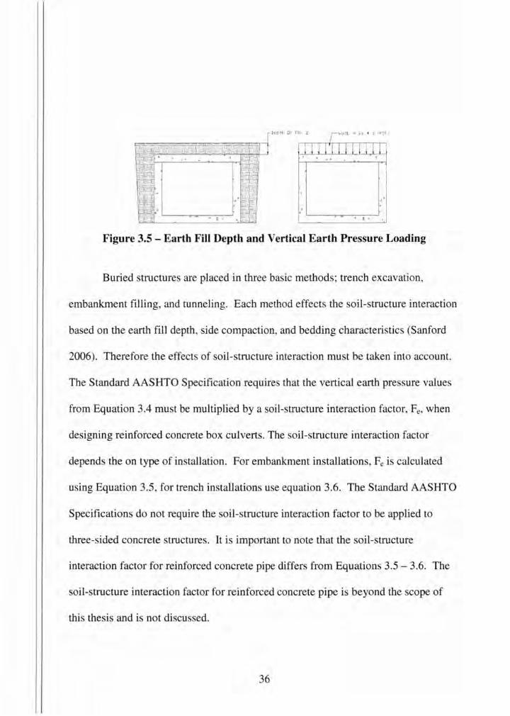
3.3 Earth Fill and Vertical Earth Pressure Loading
Initially when designing underground concrete structures the earth fill depth or
depth of overburden on the structure must be determined. The earth fill depth dictates
load combinations, impact, allowable shear, concrete cover, live load surcharge, and
particularly live load application. The earth fill is the backfill or fill placed on the top
slab. Earth fill depth is defined as the distance between the top of the top slab to the
top of earth fill or roadway surface. Typical unit weights, "(5, of earth fill are 110 pcf.
- 130 pcf, and are typically governed by the geotechnical report. The vertical earth
pressure values from the earth fill can be calculated using Equation 3.4. The depth of
fill and vertical earth pressure are illustrated in Figure 3.5.
Where:
WuSL = Ys * z
W uSL = Constant vertical earth pressure (psf)
Ys =Unit weight of soil (pcf)
z =Earth Fill Depth (ft)
35
Equation 3.4
Ilepth Of r IU, :: /'w'uSL : ys + z CF!:r>
l l l l l l I l II .. .
4
4 .. Figure 3.5 - Earth Fill Depth and Vertical Earth Pressure Loading
Buried structures are placed in three basic methods; trench excavation,
embankment filling, and tunneling. Each method effects the soil-structure interaction
based on the earth fill depth, side compaction, and bedding characteristics (Sanford
2006). Therefore the effects of soil-structure interaction must be taken into account.
The Standard AASHTO Specification requires that the vertical earth pre sure values
from Equation 3.4 must be multiplied by a soil-structure interaction factor, Fe, when
designing reinforced concrete box culverts. The soil- tructure interaction factor
depends the on type of installation. For embankment installations, Fe is calculated
using Equation 3.5 , for trench installations use equation 3.6. The Standard AASHTO
Specifications do not require the soil-structure interaction factor to be applied to
three-sided concrete structures. It is important to note that the soil-structure
interaction factor for reinforced concrete pipe differs from Equations 3.5- 3.6. The
soil-structure interaction factor for reinforced concrete pipe i beyond the scope of
this thesis and is not discussed.
36
Where:
Where:
H Fel = 1 +0.20-
Bc Equation 3.5
Fe1 = Soil-structure interaction for embankment installations
:::; 1.15 for in tallations with compacted fill at the side
:::; 1.4 for installations with un-compacted fill at the ides
H = Earth fill depth, ft.
Be = Out-to-out horizontal span of pipe or box, ft.
Equation 3.6
Fe2 = Soil-structure interaction for trench installations
H = Earth fill depth, ft.
Be = Out-to-out horizontal span of pipe or box, ft.
Cct =Load coefficient for trench installations, Figure 3.6.
37

3.4 Distribution of Live Loads for Depths of Fill Greater Than 2 ft.
When the depth of fill is equal to or greater than 2ft., the Standard AASHTO
Specifications allows for the wheel load to be distributed over a square equal to 1.75
times the depth of fill. Figure 3.6 illustrates that the Standard AASHTO
Specification does not account for the dimensions of the tire, instead the wheel load
is considered as a concentrated point load. The distributed live load value, WuLL for
a single wheel load is calculated using Equation 3.7. When the dimension of the load
area exceeds the design span, only the portion of the distributed load on the span is
considered in the design.
WuLL =Wheel Load I (1.75 * H) 2 Equation 3.7
Where:
H =Earth Fill Depth (ft)
38
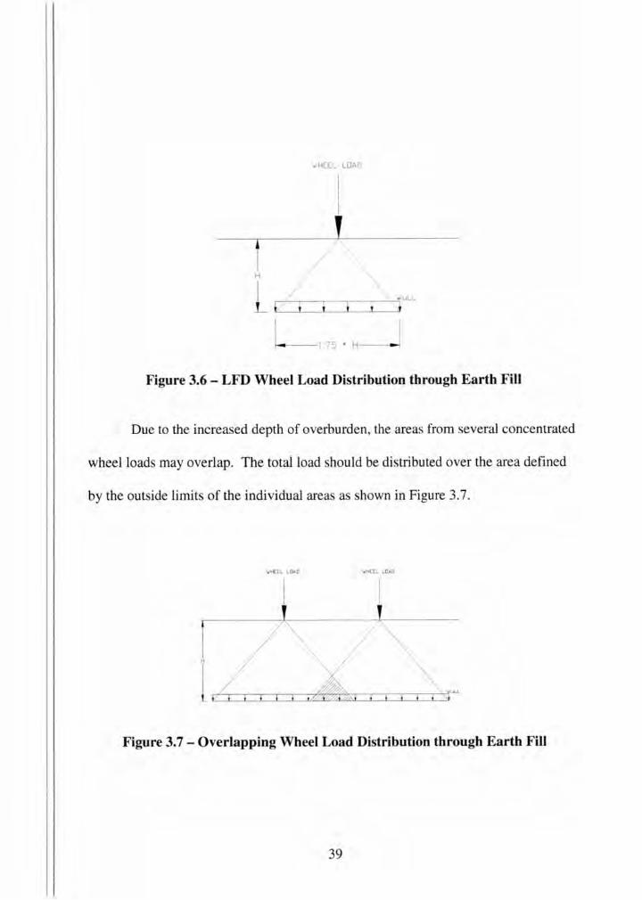
I./HEEL LOAD
Figure 3.6 - LFD Wheel Load Distribution through Earth Fill
Due to the increased depth of overburden, the areas from several concentrated
wheel loads may overlap. The total load hould be distributed over the area defined
by the outside limits of the individual area as hown in Figure 3.7.
\JHE:EL LOAD IJHEEL LOAD
Figure 3. 7 - Overlapping Wheel Load Distribution through Earth Fill
39
As the earth fill depth increases, distributed wheel load areas created by
adjacent wheels or axles begin to overlap. This complicates the distributed live load
area and load value calculation. There are 3 cases that are considered:
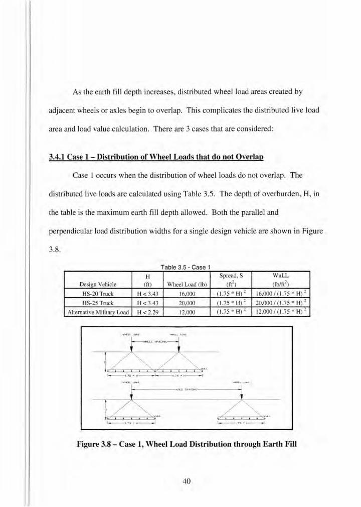
3.4.1 Case 1 -Distribution of Wheel Loads that do not Overlap
Case 1 occurs when the distribution of wheel loads do not overlap. The
distributed live loads are calculated using Table 3.5. The depth of overburden, H, in
the table is the maximum earth fill depth allowed. Both the parallel and
perpendicular load dist1ibution widths for a single design vehicle are shown in Figure
3.8.
Table 3 5- Case 1
H Spread, S WuLL
Design Vehicle (ft) Wheel Load (lb) (ft2) (lblft2)
HS-20 Truck H < 3.43 16,000 (1.75 * H) 2 16,000 I (1.75 * H) 2
HS-25 Truck H < 3.43 20,000 ( l.75 * H) 2 20.000 I (1.75 * H) 2
Alternative Military Load H < 2.29 12,000 (1.75 * H) 2 12.000 I (1 .75 * H) 2
Figure 3.8 - Case 1, Wheel Load Distribution through Earth Fill
40
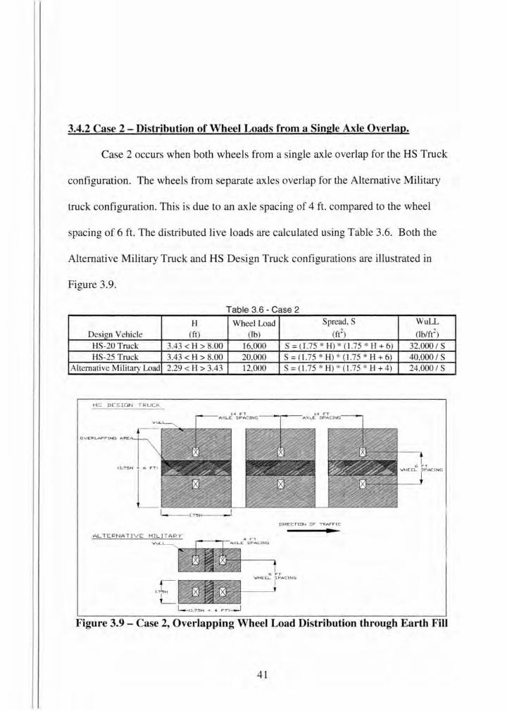
3.4.2 Case 2 - Distribution of Wheel Loads from a Single Axle Overlap.
Case 2 occurs when both wheels from a single axle overlap for the HS Truck
configuration. The wheel from separate axles overlap for the Alternative Military
truck configuration. This is due to an axle pacing of 4 ft. compared to the wheel
spacing of 6ft. The distributed live loads are calculated using Table 3.6. Both the
Alternative Military Truck and HS Design Truck configuration are illustrated in
Figure 3.9.
H Design Vehicle (ft)
HS-20 Truck 3.43 < H > 8.00 HS-25 Truck 3.43 < H > 8.00
Alternative Mjlitary Load 2.29 < H > 3.43
H S DES IGN TRUCK
Table 3 6- Case 2
Wheel Load Spread, S
(!b) (ft2)
16,000 S = (1.75 * H)* (1.75 * H + 6) 20,000 S = ( 1.75 * H)* (1.75 * H + 6) 12,000 S = (1.75 * H)* (1.75 * H +4)
DI RECTION O F"' TRAF"FT C
WuLL
(lblft2)
32,000 IS 40,000 IS 24,000 IS
6 VHEEL
Figure 3.9 - Case 2, Overlapping Wheel Load Distribution through Earth Fill
41
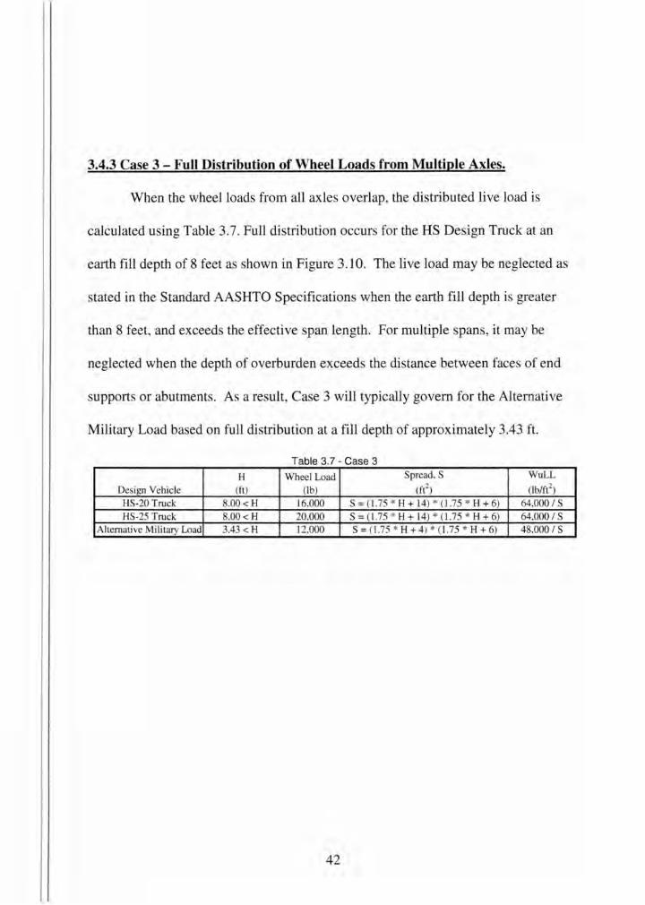
3.4.3 Case 3 - Full Distribution of Wheel Loads from Multiple Axles.
When the wheel loads from all axles overlap, the distributed live load is
calculated u ing Table 3.7. Full distribution occurs for the HS Design Truck at an
earth fill depth of 8 feet as shown in Figure 3.10. The live load may be neglected as
stated in the Standard AASHTO Specifications when the earth fi ll depth is greater
than 8 feet, and exceeds the effective span length. For multiple spans, it may be
neglected when the depth of overburden exceeds the distance between faces of end
supports or abutments. A a result, Case 3 will typically govern for the Alternative
Military Load based on full distribution at a fill depth of approximately 3.43 ft.
Table 3 7- Case 3
H Wheel Load Spread, S WuLL
Desilm Vehicle (ft) (I b) (ft2) (lblft1)
HS-20 Truck 8.00 < H 16,000 S = (1.75 * H + 14) * (1.75 * H + 6) 64,000 IS HS-25 Truck 8.00< H 20,000 S = (1.75 * H + 14) * (1.75 * H + 6) 64.000 IS
Alternative MiJhary Load 3.43 < H 12.000 S = (1.75 * H + 4) * (1.75 * H + 6) 48.000 IS
42
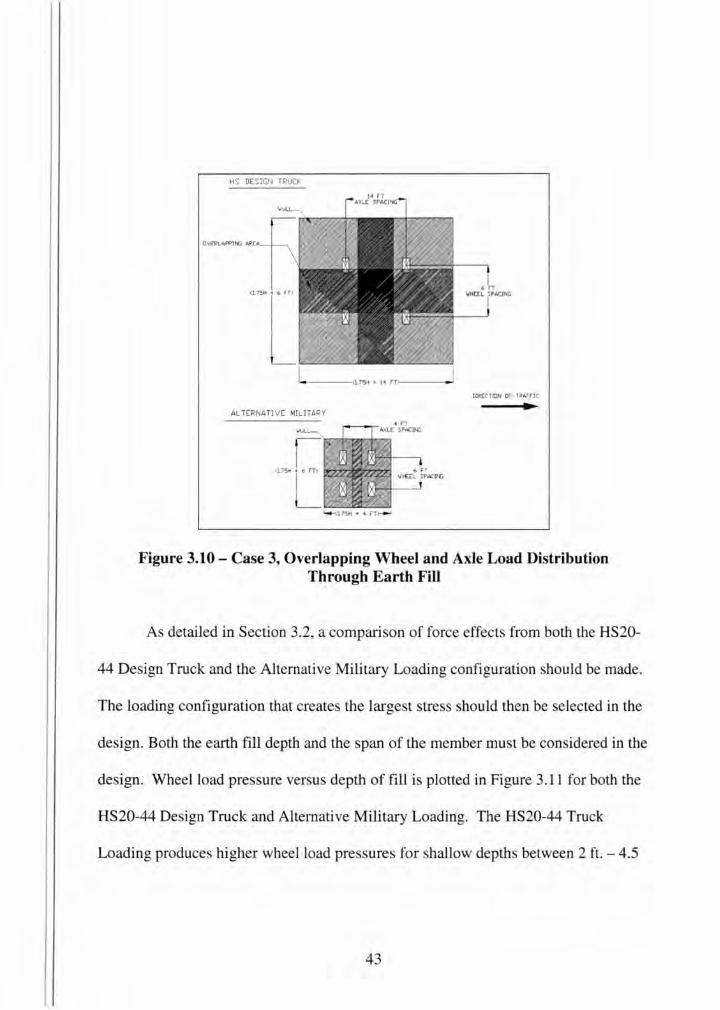
HS DESIGN TRUCK
• 'W'HC:tl
DJR£CtmN or tRArnc ..
Figure 3.10- Case 3, Overlapping Wheel and Axle Load Distribution Through Earth Fill
As detailed in Section 3.2, a comparison of force effects from both the HS20-
44 Design Truck and the Alternative Military Loading configuration should be made.
The loading configuration that creates the largest stress should then be selected in the
design. Both the earth fill depth and the span of the member must be considered in the
design. Wheel load pressure versus depth of fill is plotted in Figure 3.11 for both the
HS20-44 Design Truck and Alternative Military Loading. The HS20-44 Truck
Loading produces higher wheel load pressures for shallow depths between 2 ft. - 4.5
43
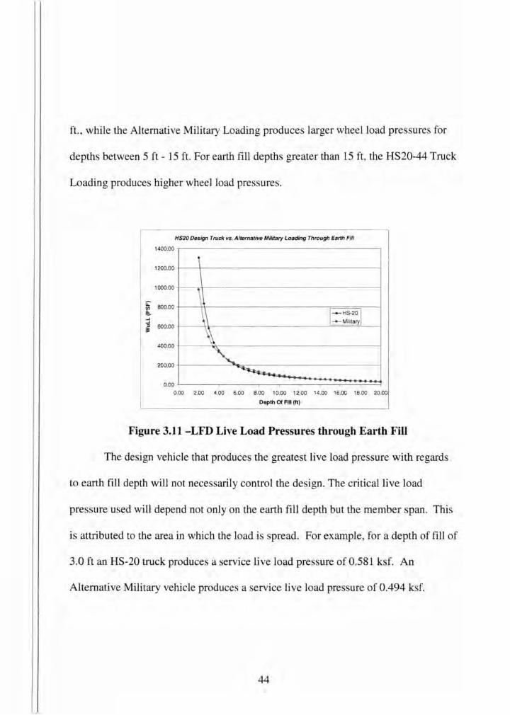
ft. , while the Alternative Military Loading produces larger wheel load pressures for
depths between 5 ft- 15ft. For earth fill depths greater than 15ft, the HS20-44 Truck
Loading produces higher wheel load pressures.
HS20 Design Truck vs. Alternative Military Loading Through Earth Fill
1400.00
i 1200.00
1000.00
iL 800.00 Vl e:. ..J ..J
" 600.00 ;=
400.00
200.00
\ ~ --- HS-20v I ...._ MililafY I
\ .~ ~
0.00 0.00 2.00 4.00 6.00 8.00 10.00 12.00 14.00 16.00 18.00 20.00
Depth Of Fill (It)
Figure 3.11 -LFD Live Load Pressures through Earth Fill
The design vehicle that produces the greatest live load pressure with regards
to earth fill depth will not necessarily control the design. The critical live load
pressure used will depend not only on the earth fill depth but the member span. This
is attributed to the area in which the load is spread. For example, for a depth of fill of
3.0 ft an HS-20 truck produces a service live load pressure of 0.581 ksf. An
Alternative Military vehicle produces a service live load pressure of 0.494 ksf.
44
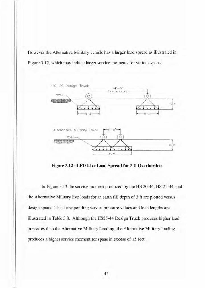
However the Alternative Military vehicle has a larger load spread as illustrated in
Figure 3 .1 2, which may induce larger service moments for various spans.
HS-20 Design Truck
Alte rn ative Military Truck
WsLL----...
1 4 ' - 0" Ax le sp a cing
Figure 3.12 -LFD Live Load Spread for 3 ft Overburden
3"-o"
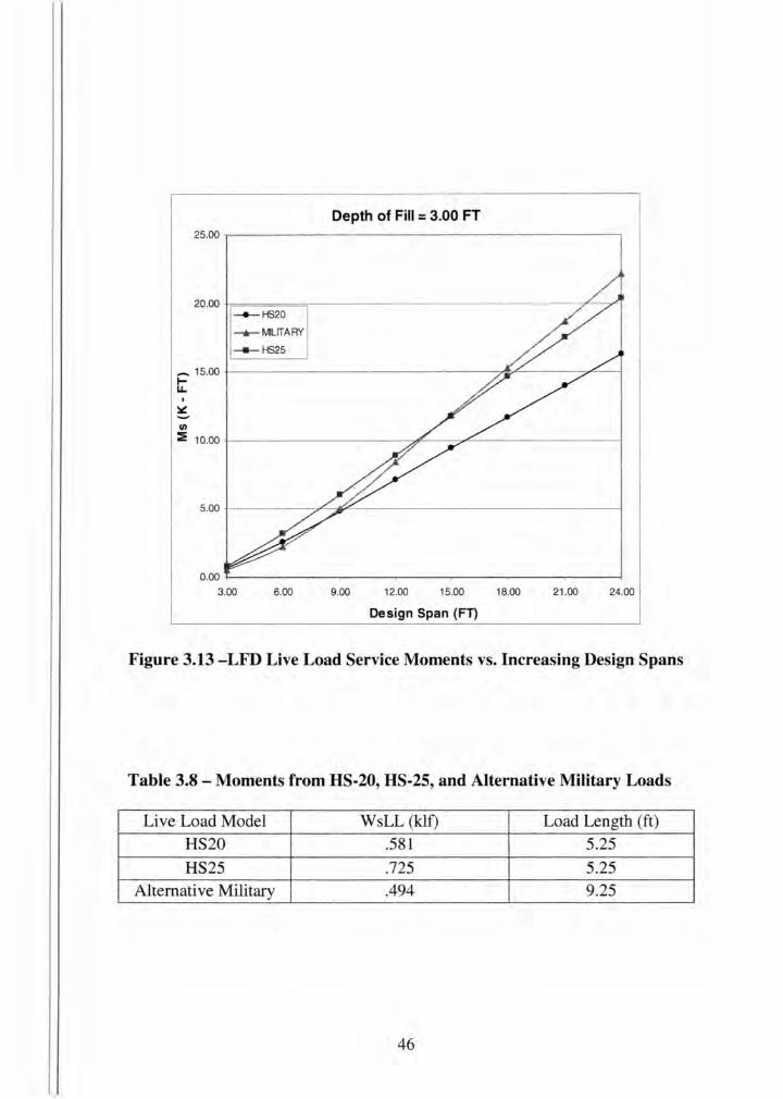
In Figure 3.13 the ervice moment produced by the HS 20-44, HS 25-44, and
the Alternative Military live loads for an earth fill depth of 3 ft are plotted versus
design spans. The corresponding service pressure values and load lengths are
illustrated in Table 3.8. Although the HS25-44 Design Truck produces higher load
pressures than the Alternative Military Loading, the Alternative Military loading
produces a higher service moment for spans in excess of 15 feet.
45
Depth of Fill = 3.00 FT 25.00 .,...-----------------------,
I
~
1/)
- HS20
__..._ IV.IUTARY
-HS25
::!: 10.00 +-----------#-- -7'"'-------------j
0.00 +--~-.,...----.-------.,...---.,...----.---------1
3.00 6.00 9.00 12.00 15.00 18.00 21 .00 24.00
Design Span (FT)
Figure 3.13 -LFD Live Load Service Moments vs. Increasing Design Spans
Table 3.8 - Moments from HS-20, HS-25, and Alternative Military Loads
Live Load Model WsLL (klf) Load Length (ft) HS20 .581 5.25
HS25 .725 5.25 Alternative Military .494 9.25
46
3.5 Distribution of Live Loads for Depths of Fill Less Than 2 ft.
For depths of overburden less than 2ft the Standard AASHTO Specifications
simplify the design procedures by providing a single equation for distributing the live
load to the top slabs of buried concrete structure . The live load is divided into
equivalent strip widths, which is the effective width of slab that resists the applied
load. The live load is modeled as a concentrated wheel load distributed over a
di tribution width, E. The distribution width is calculated using Equation 3.8.
Where:
E = 4 + .06 * S <7ft. For H <2ft. Equation 3.8
E = Width of slab over which a wheel load is distributed (ft)
S =Effective span length (ft)
H = Cover depth from top of structure to top of Pavement (ft)
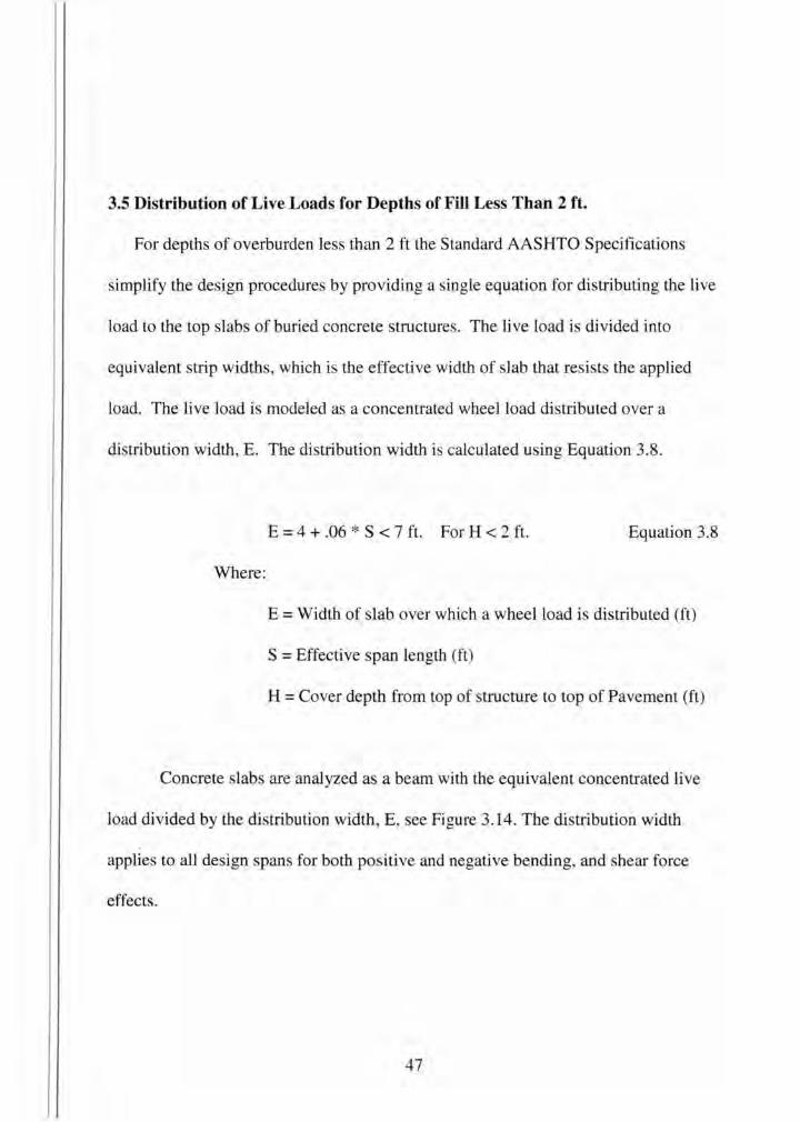
Concrete slabs are analyzed a a beam with the equivalent concentrated live
load divided by the distribution width, E, see Figure 3.14. The distribution width
applies to all design spans for both positive and negative bending, and shear force
effects.
47
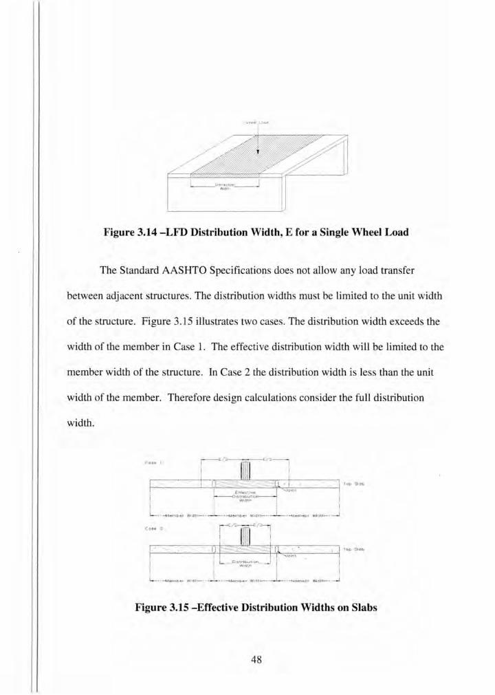
Figure 3.14 -LFD Distribution Width, E for a Single Wheet ·Load
The Standard AASHTO Specifications does not allow any load transfer
between adjacent tructures. The distribution widths must be limited to the unit width
of the structure. Figure 3.15 illustrates two cases. The distribution width exceeds the
width of the member in Case 1. The effective distribution width will be limited to the
member width of the structure. In Case 2 the distribution width is less than the unit
width of the member. Therefore design calculations consider the full distribution
width.
C ase I
r--1 '-'·-· :~~-----'r'r'---"'=-.:.:,=...,_=t-..,.,....,_~----'-~·'-1' 1 Top Slob
i
L .. ~ember Width-··
Figure 3.15 -Effective Distribution Widths on Slabs
48

The tire is assumed to act in the center of the member, as shown in Figure
3.15. One provision that is unclear in the Standard AASHTO Specifications is when
the tire is placed at the edge of a member as illustrated in Figure 3.16, Case 3. Case 3
is not addressed in the current Standard AASHTO Specifications; however it is a
common practice to assume a reduced distribution width. Thi new distribution width
i calculated using Equation 3.9.
Equation 3.9
Where:
Er = reduced distribution width (ft)
s. =effective span length (ft)
WT =width of tire contact area parallel to span, as specified in
Case 3
section 3.2 (ft)
! Joint
i i
L -- --Mem ber Widlh-- · _L ----Member Widlh---_L·---Memebr Width---
Figure 3.16 -Reduced Distribution Widths on Slabs
49
Top S lob
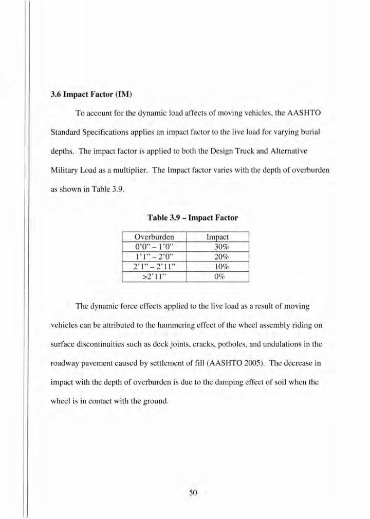
3.6 Impact Factor (IM)
To account for the dynamic load affects of moving vehicles , the AASHTO
Standard Specifications applies an impact factor to the live load for varying burial
depths. The impact factor is applied to both the Design Truck and Alternative
Military Load as a multiplier. The Impact factor varies with the depth of overburden
as shown in Table 3.9.
Table 3.9 - Impact Factor
Overburden Impact 0'0" - 1 '0" 30% 1 , 1, - 2, 0" 20%
2'1"-2'11" 10% >2' 11" 0%
The dynamic force effects applied to the live load as a result of moving
vehicle can be attributed to the hammering effect of the wheel assembly riding on
surface discontinuities such as deck joints, cracks, potholes, and undulations in the
roadway pavement caused by settlement of fill (AASHTO 2005). The decrease in
impact with the depth of overburden is due to the damping effect of soil when the
wheel is in contact with the ground.
50
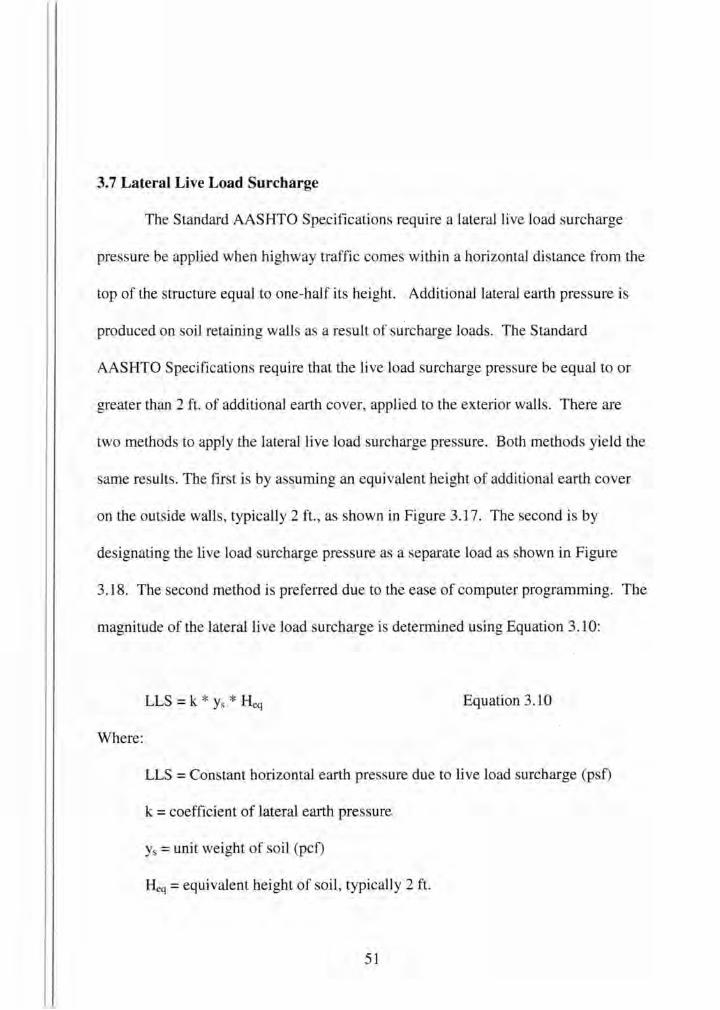
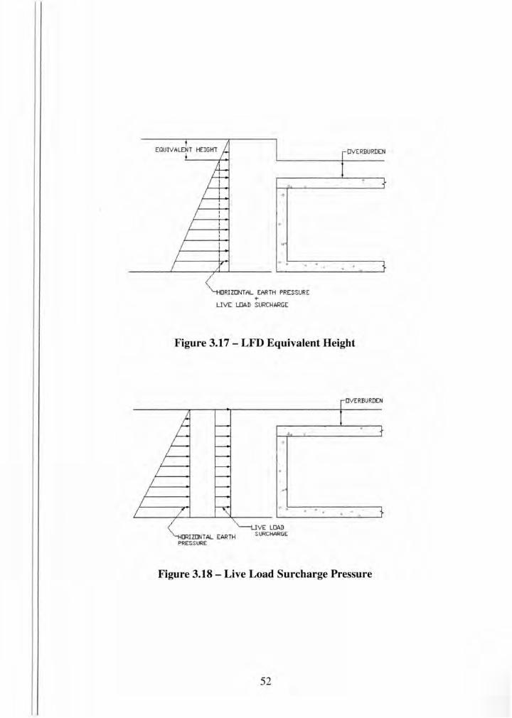
3.7 Lateral Live Load Surcharge
The Standard AASHTO Specification require a lateral live load surcharge
pressure be applied when highway traffic comes within a horizontal distance from the
top of the structure equal to one-half its height. Additional lateral eatth pressure is
produced on soil retaining walls as a result of surcharge loads. The Standard
AASHTO Specifications require that the live load surcharge pressure be equal to or
greater than 2 ft. of additional earth cover, applied to the exterior walls. There are
two methods to apply the lateral live load surcharge pressure. Both methods yield the
same results. The first i by a suming an equivalent height of additional earth cover
on the outside walls, typically 2ft., as shown in Figure 3.17. The second is by
designating the live load surcharge pressure a a separate load a shown in Figure
3.18. The second method is preferred due to the ease of computer programming. The
magnitude of the lateral live load surcharge is determined using Equation 3.10:
Where:
LLS = k * Ys * Heq Equation 3.10
LLS =Constant horizontal earth pressure due to live load surcharge (psf)
k = coefficient of lateral earth pressure
Ys = unit weight of soil (pcf)
Heq =equivalent height of soil, typically 2 ft.
51
~· .~--.~.-.~ .. --~-------,
ORIZDNTAL EARTH PRESSURE +
LIVE LOAD SURCHARGE
Figure 3.17 - LFD Equivalent Height
ORI ZDNTAL EARTH PRESSURE
~ .~--"--.--, ----------~
IVE LOAD SURCHARG E
Figure 3.18 - Live Load Surcharge Pressure
52
Chapter 4 AASHTO LRFD Bridge Design Specifications
4.1 Load Factors and Load Combinations
In LRFD, the design framework consists of satisfying what are called limit
states. All limit states shall satisfy Equation 4.1.
Equation 4.1
Where:
Tli =Load modifier
Yi = Load factors
Qi = Force effects
<P = Resistance factors
Rn =Nominal resistance
Rr = Factored resistance
Selection of the load factors to be used is a function of the type of load and
limit state being evaluated. To obtain an understanding of this concept, it is helpful to
refer to the actual definition of "limit state" contained in the LRFD Specifications . A
Limit State is a condition beyond which the bridge or component ceases to satisfy the
provisions for which it wa designed. There are four limit states prescribed by the
53
LRFD Specifications (AASHTO 2005). Each of the four limit states are described
below:
• STRENGTH- Requires the strength and stability be adequate for
specified load combinations.
• EXTREME EVENT - Relates to events with extremely long periods of
return (earthquakes, ice loads, vehicle collision, and vessel collision).
• SERVICE- Relates to stresses, deformations, and cracking.
• FA TIGUE - Places restrictions on stre ranges in reinforcement from
application of a single design truck under service load conditions.
When designing underground concrete structures, the LRFD Specifications
require that all applicable limit states be evaluated. The load for each limit state
should be modified by the appropriate load factor, y, and the factored loads for each
limit state combined in a prescribed manner. The limit states, load factors and load
combinations from the AASHTO LRFD Specification are listed in Table 4.1 and
Table 4.2. Based on applicable load combinations the limit states are further
subdivided as follows (AASHTO 2005):
• STRENGTH I- Basic load combination related to normal vehicular
use of the bridge without wind.
54
• STRENGTH II- Load combination relating to the use of the bridge by
owner specified special design vehicles and/or evaluation permit
vehicles without wind.
• STRENGTH III- Load combination relating to the bridge exposed to
wind velocity exceeding 55 mph without live load.
• STRENGTH IV -Load combinations relating to very high dead load
to live load force effect ratios.
• STRENGTH V - Load combinations relating to normal vehicular use
of the bridge with wind velocity of 55 mph.
• EXTREME EVENT I- Load combinations including earthquake and
flood.
• EXTREME EVENT II - Load combination relating to ice load or
collision by vessels and vehicles.
• SERVICE I- Load combination relating to the normal operational use
of the bridge with 55 mph winds and all the loads taken at their
nominal value .
• SERVICE II- Load combinations intended to control yielding of steel
structures and slip-critical connections due to vehicular live load.
55
• SERVICE lli- Load combination for longitudinal analysis relating to
tension in pre tressed concrete superstructures.
• SERVICE IV- Load combinations relating only to tension in
prestressed concrete substructures with the objective of crack control.
• FA TIGUE -Fatigue and fracture load combinations relating to the
repetitive gravitational vehicular live load and dynamic respon es
under a single design truck.
A majority of the loads and loading combination specified in the Standard
AASHTO Specifications are eliminated for buried structures. Buried structures are
sheltered by earth cover which reduces much of the concern. Buried structures need
to be designed to resist the force effects resulting from horizontal and ve1tical earth
pressures, pavement load, vehicular live load and impact, and surcharge loads. Wind,
temperature, vehicle breaking, and centrifugal forces typically have little effect due to
earth protection.
56
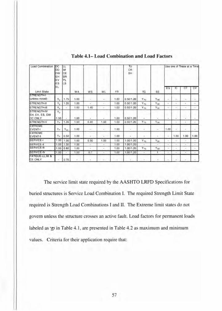
Table 4.1- Load Combination and Load Factors
Load Combination DC LL TU Use one of These at a Time DD IM CR ow CE SH EH BR EV PL ES LS EL EO IC CT CV
Limit State WA WS W L FR TG SE ::; I HI::N(j IH-1 (unless noted) Yp 1.75 1.00 1.00 0.50/1.20 Yra YsE
STRENGTH-II Yp 1.35 1.00 - 1.00 0.50/ 1.20 Ym YsE
STRENGTH-Ill Yp 1.00 1.40 1.00 0.50/1.20 Ym YsE STRENGTH-IV Yp EH, EV , ES, OW DC ONLY 1.50 1.00 1.00 0.50/1.20 -STRENGTH-V Yp 1.35 1.00 0.40 1.00 1.00 0.50/1.20 Yra YsE
EXTREME EVENT-I Yp Yeq 1.00 1.00 1.00
EXTREME EVENT-II Yp 0.50 1.00 1.00 1.00 1.00 1.00
SERVICE-I 1.00 1.00 1.00 0.30 1.00 1.00 1.00/1.20 Ym YsE SERVICE-II 1.00 1.30 1.00 1.00 1.00/1.20 -SERVIGE-111 1.00 0.80 1.00 1.00 1.00/1.20 Ym YsE
SERVI<.;E-IV 1.00 1.00 0.7 1.00 1.00/1.20 1 FATIGUE-LL,IM & CE ONLY 0.75
The service limit state required by the AASHTO LRFD Specifications for
buried structures is Service Load Combination L The required Strength Limit State
required is Strength Load Combinations I and II. The Extreme limit states do not
govern unless the structure crosses an active fault. Load factors for permanent loads
labeled as yp in Table 4.1, are presented in Table 4.2 as maximum and minimum
values. Criteria for their application require that:
57

• For each combination, load factors should be selected to produce the total
extreme factored force effect. Both maximum and minimum extremes should
be investigated.
• Maximum and minimum load factors are utilized for load combinations where
one force effect decreases the effect of another force. The minimum value
shall be applied to the load that reduces the force effect.
• The load factor which produces the more critical combination for permanent
force effects should be selected from Table 4.2.
• If a permanent load increases the stability or load carrying capacity of a
structure component, the minimum value for that permanent load should also
be investigated.
58
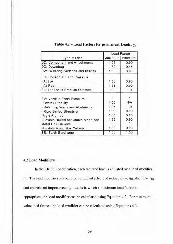
Table 4.2 - Load Factors for permanent Loads, 'YP
Load Factor Type of Load Maximum Minimum
DC: Component and Attachments 1.25 0.90 DD: Downdrag 1.80 0.45 DW: Wearing Surfaces and Utilities 1.50 0.65
EH: Horizontal Earth Pressure -Active 1.50 0 .90 -At-Rest 1.35 0.90 EL: Locked in Erection Stresses 1.0 1.0
EV: Verticle Earth Pressure I I
- Overall Stability 1.00 N/A
- Retaining Wails and Abutments 1.35 1.0
-Rigid Buried Sturcture 1.30 0.90
-Rigid Frames 1.35 0.90
-Flexible Buried Structures other than 1.95 0.90
Metal Box Culverts I I
-Flexible Metal Box Culverts 1.50 0.90
ES : Earth Surcharge 1.50 1.50
4.2 Load Modifiers
In the LRFD Specification, each factored load is adjusted by a load modifier,
Tli· The load modifiers account for combined effects of redundancy, 11R, ductility, Tlo,
and operational importance, 11 1. Loads in which a maximum load factor is
appropriate, the load modifier can be calculated using Equation 4.2. For minimum
value load factors the load modifier can be calculated using Equations 4.3.
59

Equation 4.2
Equation 4.3
Where:
Tl i =Load modifier
Tl o =factor for ductility
TlR = factor for redundancy
Tlr =factor for importance
The values for the ductility, redundancy, and importance factor are listed below:
• Ductility, Tlo
::::: 1.05 for non-ductile components and connections
= 1.00 for conventional designs and details
:::::0.95 for components and connections for which additional ductility
enhancing measures are required
For all other limit states: Tlo = 1.00
• Redundancy, TlR
60
~ 1.05 for non-redundant component and connection
= 1.00 for conventional level of redundancy
~ 0.95 for exceptional level of redundancy
For all other limit states: 11R = 1.00
• Importance, 111
~ 1.05 for important structures
= 1.00 for typical tructures
~ 0.95 for relatively less important tructures
For all other limit states: 11 1 = 1.00
When designing at the Service Limit State, 11o = 11R = 111 = 1.00
Typically the ductility of buried structure i 1.00. Buried tructures are
con idered non-redundant under earth fill , and redundant under live load and dynamic
load allowance. The importance is determined on an evaluation of necessity for
continued function and afety.
61
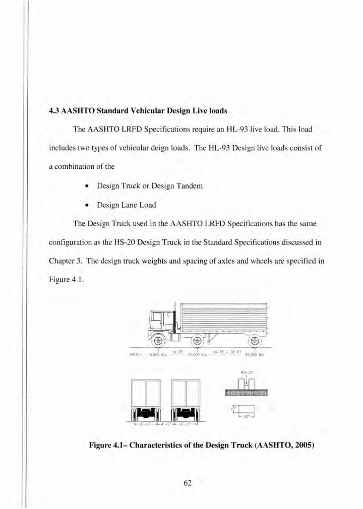
4.3 AASHTO Standard Vehicular Design Live loads
The AASHTO LRFD Specifications require an HL-93live load. This load
includes two types of vehicular deign loads. The HL-93 Design live loads consist of
a combination of the
• Design Truck or Design Tandem
• Design Lane Load
The Design Truck used in the AASHTO LRFD Specifications has the same
configuration as the HS-20 Design Truck in the Standard Specifications discussed in
Chapter 3. The de ign truck weights and spacing of axles and wheels are specified in
Figure 4.1.
HS20 8. 000 lbs.
HS-20
,fTI '--t;;:=j
Figure 4.1- Characteristics of the Design Truck (AASHTO, 2005)
62
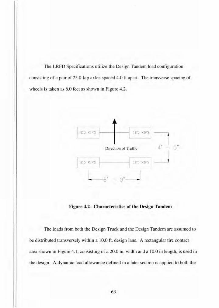
The LRFD Specifications utilize the Design Tandem load configuration
consisting of a pair of 25 .0-kip axles spaced 4.0 ft apart. The transverse spacing of
wheels is taken as 6.0 feet as shown in Figure 4.2.
Direction of Traffic 4' - 0 "
1 12.5 KIPS 12 5 KIPS I
------6 , - 0 "----~
Figure 4.2- Characteristics of the Design Tandem
The loads from both the Design Truck and the Design Tandem are as umed to
be distributed transversely within a 10.0 ft. design lane. A rectangular tire contact
area shown in Figure 4.1, consisting of a 20.0 in. width and a 10.0 in length, is used in
the design. A dynamic load allowance defined in a later section is applied to both the
63
Design Truck and Design Tandem. Both the Design Truck and Design Tandem
loading configuration are u ed in conjunction with the Design Lane Load to
determine the worst case force effects on the structure. This will primarily depend on
the depth of overburden and/or the span of the structure. The Design Lane Load
consists of a load of 0.64 klf, uniformly di tributed in the longitudinal direction.
Transversely, the Design Lane Load i assumed to be uniformly distributed over a
10.0 ft. design lane width. This lane load converts to an additional live load of .064
ksf, applied to the top of the structure for any depth of burial less than 8ft. The force
effects from the Design Lane Load are not subject to a dynamic load allowance.
4.4 Earth Fill and Vertical Earth Pressure Loading
Similar to the Standard AASHTO Specifications, when designing underground
concrete structures the earth fill depth or depth of overburden on the structure must be
determined. The earth fill depth dictates load combinations, impact, allowable shear,
concrete cover, live load surcharge, and particularly live load application. The earth
fill is the backfill or fill placed on the top lab. Earth fill depth is defined as the
distance between the top of the top slab to the top of earth fill or roadway surface.
Typical unit weights, "(5, of earth fill are 110 pcf.- 130 pcf, and are generally
governed by the geotechnical report. The vertical earth pressure values from the earth
64
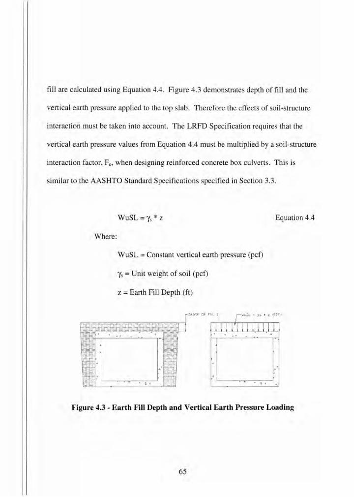
fill are calculated using Equation 4.4. Figure 4.3 demonstrates depth of fill and the
vertical earth pressure applied to the top slab. Therefore the effects of soil-structure
interaction must be taken into account. The LRFD Specification requires that the
vertical earth pressure values from Equation 4.4 must be multiplied by a soil-structure
interaction factor, Fe, when designing reinforced concrete box culverts. This is
similar to the AASHTO Standard Specifications specified in Section 3.3.
Where:
WuSL = 'Ys * z
WuSL =Constant vertical earth pressure· (pcf)
'Ys = Unit weight of soil (pcf)
z =Earth Fill Depth (ft)
• ! •
Equation 4.4
Figure 4.3 - Earth Fill Depth and Vertical Earth Pressure Loading
65
4.5 Multiple Presence Factors
The LRFD Specifications require the use of multiple presence factors, Table 4.3,
to account for the effects of multiple lanes on a bridge. Multiple presence factors are
based on the number of loaded lanes. The table provides factors for the cases of one
lane, two lanes, three lanes, and three or more loaded lanes. For underground concrete
structures, there are three cases that must be examined.
4.5.1 Case 1 - Depth of fill is equal to or greater than 2 ft.
Case 1 occurs for depths of fill equal to or greater than 2 ft. The Standard
LRFD Specifications require two checks.
• A check to determine the force effects from multiple truck axles
positioned 4 ft side by side with a multiple presence factor of 1.00.
• A check to determine the force effects from a single design vehicle
with a multiple presence factor of 1.20.
The loading combination with the worst case force effects on the structure will
control the design. This will typically depend on the overburden depth and/or the
span of the structure. This is further discussed in Section 4.6.
66
4.5.2 Case 2 - Depth of fill is less than 2 ft, and direction of traffic is parallel to
span.
When the traffic travels parallel to the design pan, the structure is analyzed
using a single loaded lane. The Standard LRFD Specifications distribute a single
loaded lane into strip widths. This strip width is the effective width of the slab that
resists the applied load. Therefore, the multiple presence factor is 1.20
4.5.3 Case 3 - Depth of flU is less than 2ft, and direction of traffic is
perpendicular to span.
When the depth of fill is less than 2 ft and the direction of traffic is perpendicular
to the span, the appropriate multiple pre ence factors must be cho en from Table 4.3 .
The number of loaded lanes is a function of span length.
Table 4.3 Multiple Presence Factors
Number of Loaded Multiple Presence Lanes Factor "m"
1 1.2
2 1.00
3 0.85
>3 0.65
67
4.6 Distribution of Live Loads for Depths of Fill Greater Than 2 ft.
When the depth of overburden is equal to or greater than 2 ft, the Standard LRFD
Specifications allows for the wheel load to be distributed throughout the earth fill.
The Standard LRFD Specifications use an approach similar to the 2: 1 method. The
2: 1 method is an empirical approach that assumes the total applied load on the surface
of soil is distributed over an area of the same shape as the loaded area on the surface.
The dimensions of the loaded area are increased by the amount equal to the depth
below the surface. The AASHTO LRFD method is a variation of this method. The
distribution area is equal to the tire footprint, with the footprint dimensions increased
by either 1.15 times the earth fill depth for select granular backfill, or 1.0 for other
types of backfill, shown in Figure 4.4. The distributed live load value, WuLL for a
single wheel load can be calculated using Equation 4.5.
Where:
WuLL =Wheel Load I (LLDF*H + WT) * (LLDF*H + LT) Equation 4.5
WuLL =Uniform Distributed Live Load (psf)
H = Earth fill depth (ft)
WT =Tire Width (in)
LT = Tire Length (in)
68
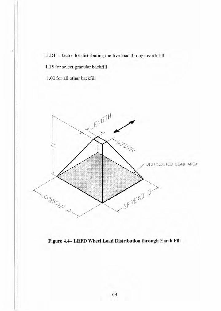
LLDF =factor for distributing the live load through earth fill
1.15 for select granular backfill
1.00 for all other backfill
DISTR IBUTED LOA D AREA
Figure 4.4- LRFD Wheel Load Distribution through Earth Fill
69
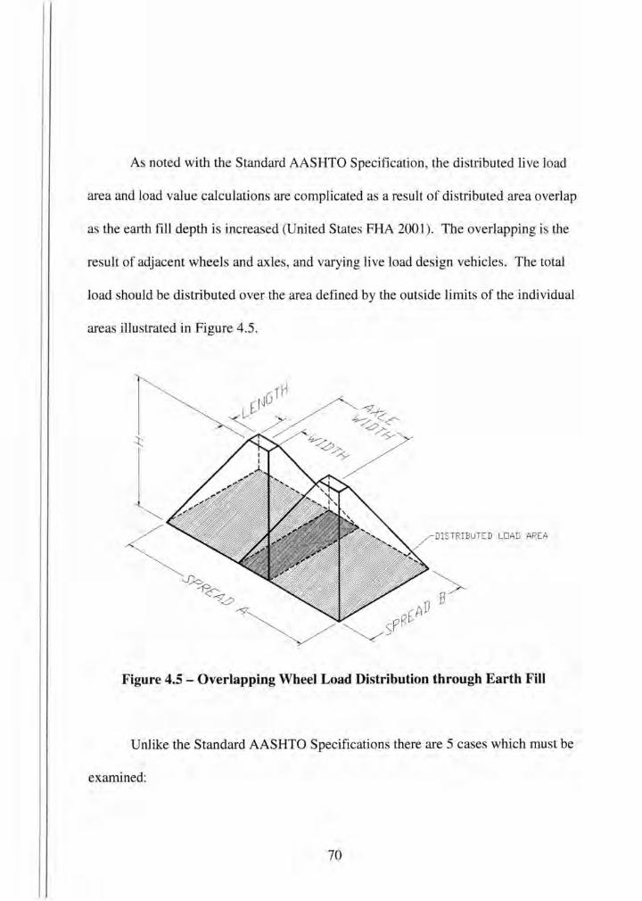
As noted with the Standard AASHTO Specification, the distributed live load
area and load value calculations are complicated as a result of distributed area overlap
as the earth fill depth is increased (United States FHA 2001). The overlapping is the
result of adjacent wheels and axles, and varying live load design vehicles. The total
load should be distributed over the area defined by the outside limits of the individual
areas illustrated in Figure 4.5.
DISTRIBUTE D LOAD AREA
Figure 4.5 - Overlapping Wheel Load Distribution through Earth Fill
Unlike the Standard AASHTO Specifications there are 5 cases which must be
examined:
70
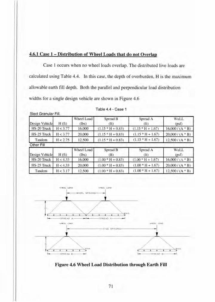
4.6.1 Case 1 - Distribution of Wheel Loads that do not Overlap
Case 1 occurs when no wheel loads overlap. The distributed live loads are
calculated using Table 4.4. In this case, the depth of overburden, H is the maximum
allowable earth fill depth. Both the parallel and perpendicular load distribution
widths for a single design vehicle are shown in Figure 4.6
Table 4.4- Case 1 Sleet Granular Fill
Wheel Load Spread B Spread A WuLL Design Vehicle H (ft) (lbs) (ft) (ft) (psf) HS-20 Truck H < 3.77 16,000 ( 1.15 * H + 0.83) (1.15 * H + 1.67) 16,000 I (A* B)
HS-25 Truck H < 3.77 20,000 (1.1 5 * H + 0.83) (1.15 * H + 1.67) 20,000 I (A* B)
Tandem H < 2.75 12,500 (1.15 * H + 0.83) (1.15 * H + 1.67) 12,500 I (A * B) Other F1ll
Wheel Load Spread B Spread A WuLL Design Vehicle H (ft) (lbs) (ft) (ft) (psf)
HS-20 Truck H <4.33 16.000 (1.00 * H + 0.83) (1.00 * H + 1.67) 16,000 I (A* B)
HS-25 Truck H < 4.33 20,000 (1.00 * H + 0.83) (1.00 * H + 1.67) 20,000 I (A * B)
Tandem H < 3.17 12,500 ( 1.00 * H + 0.83) (1.00 * H + 1.67) 12,500 I (A * B)
I----SPREAD A-~-r-~-SPREAD A-~-l
\.'HEEL LOAD
I--------AX LE SPACING--------I
I----SPREAD B---l I----SPREAD B'---1
Figure 4.6 Wheel Load Distribution through Earth Fill
71
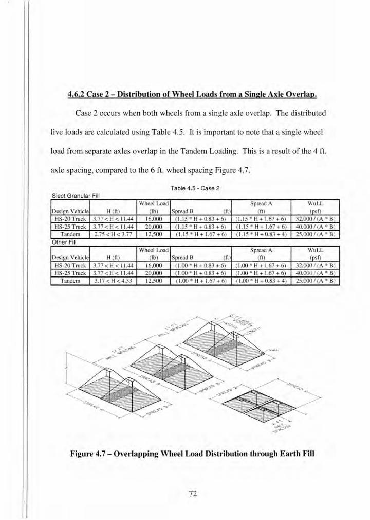
4.6.2 Case 2 - Distribution of Wheel Loads from a Single Axle Overlap.
Case 2 occurs when both wheels from a single axle overlap. The distributed
live loads are calculated using Table 4.5 . It is important to note that a single wheel
load from eparate axle overlap in the Tandem Loading. This is a result of the 4 ft.
axle spacing, compared to the 6ft. wheel spacing Figure 4.7.
Table 4.5 -Case 2 Sleet Granular Fill
Wheel Load Spread A WuLL Design Vehicle H (ft) (I b) Spread B (ft ) (ft) (psf)
HS-20 Truck 3. 77 < H < I 1.44 16.000 (1.15 * H + 0.83 + 6) (1.15 * H + 1.67 + 6) 32,000 I (A * B )
HS-25 Truck 3. 77 < H < 1 1.44 20,000 (1.15 * H + 0.83 + 6) (1.15 * H + 1.67 + 6) 40.000 I (A * B) Tandem 2.75 < H < 3.77 12,500 ( 1.1 5 * H + 1.67 + 6) (1.15 * H + 0.83 + 4) 25.000 I (A * B)
Other Ftll Wheel Load Spread A WuLL
Design Vehicle H (ft) (I b) Spread B (ft) (ft) (psf)
HS-20 Truck 3.77 < H < 11.44 16,000 ( 1.00 * H + 0.83 + 6) (1.00 * H + 1.67 + 6) 32,000 I (A * B) HS-25 Truck 3.77 < H < 11.44 20,000 (1.00 * H + 0.83 + 6) (1.00 * H + 1.67 + 6) 40.000 I (A * B)
Tandem 3.17 < H < 4.33 12.500 (1.00 * H + 1.67 + 6) (1.00 * H + 0.83 + 4) 25.000 I (A * B)
Figure 4. 7 - Overlapping Wheel Load Distribution through Earth Fill
72
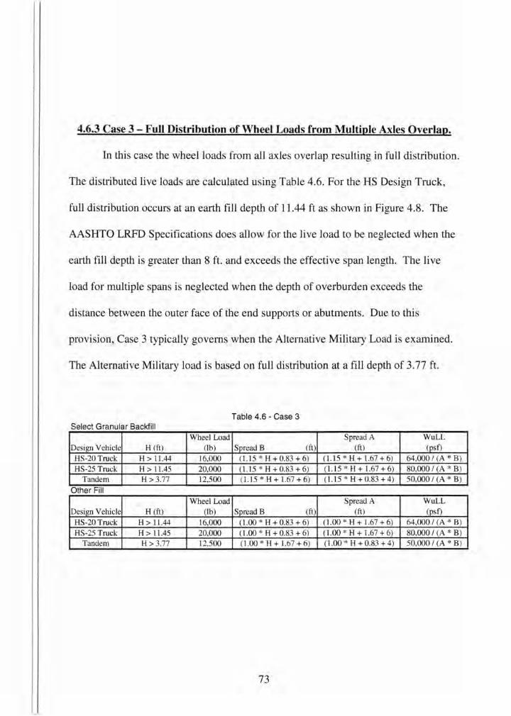
4.6.3 Case 3 - Full Distribution of Wheel Loads from Multiple Axles Overlap.
In this case the wheel loads from all axles overlap resulting in full distribution.
The distributed live loads are calculated using Table 4.6. For the HS Design Truck,
full distribution occurs at an earth fill depth of 11.44 ft as shown in Figure 4.8. The
AASHTO LRFD Specifications does allow for the live load to be neglected when the
earth fill depth is greater than 8ft. and exceeds the effective span length. The live
load for multiple spans is neglected when the depth of overburden exceeds the
distance between the outer face of the end supports or abutments. Due to this
provision, Case 3 typically governs when the Alternative Military Load is examined.
The Alternative Military load is based on full distribution at a fill depth of 3.77 ft.
Table 4.6- Case 3 Select Granular Backfil l
Wheel Load Spread A WuLL Design Vehicle H (ft) (I b) Spread B (ft) (ft) (psf)
HS-20 Truck H > 11.44 16,000 (l.l5 * H + 0.83 + 6) (1.15 * H + 1.67 + 6) 64,000 I (A* B) HS-25 Truck H > 11.45 20,000 (1.15 * H + 0.83 + 6) ( 1.1 5 * H + 1.67 + 6) 80,000 I (A * B)
Tandem H > 3.77 12,500 (1. 15 * H + 1.67 + 6) (1.15 * H + 0.83 + 4) 50,000 I (A * B)
Other F1ll Wheel Load Spread A WuLL
Design Vehicle H (ft ) (lb) Spread B (ft) (ft) (psf)
HS-20Truck H>ll.44 16,000 (1.00 * H + 0.83 + 6) (1.00 * H + 1.67 + 6) 64,000 I (A * B) HS-25 Truck H > 11.45 20,000 (1.00 * H + 0.83 + 6) (1.00 * H + 1.67 + 6) 80,000 I (A * B)
Tandem H > 3.77 12,500 (1.00 * H + 1.67 + 6) (1.00 * H + 0.83 + 4) 50,000 I (A * B)
73
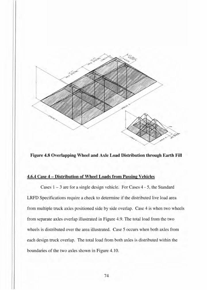
Figure 4.8 Overlapping Wheel and Axle Load Distribution through Earth Fill
4.6.4 Case 4- Distribution of Wheel Loads from Passing Vehicles
Cases 1 - 3 are for a single design vehicle. For Cases 4 - 5, the Standard
LRFD Specifications require a check to determine if the distributed live load area
from multiple truck axle positioned side by side overlap. Case 4 is when two wheels
from separate axles overlap illustrated in Figure 4.9. The total load from the two
wheels is distributed over the area illustrated. Case 5 occurs when both axles from
each de ign truck overlap. The total load from both axles is distributed within the
boundaries of the two axles shown in Figure 4.1 0.
74
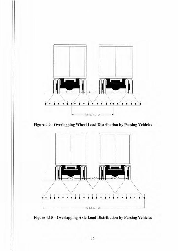
Figure 4.9 - Overlapping Wheel Load Distribution by Passing Vehicles
~-----------------S~HEAO A-----------------~
Figure 4.10- Overlapping Axle Load Distribution by Passing Vehicles
75
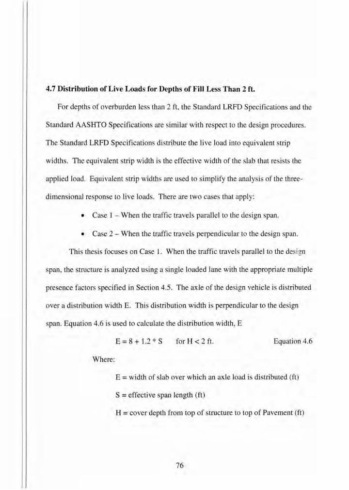
4. 7 Distribution of Live Loads for Depths of Fill Less Than 2 ft.
For depths of overburden less than 2ft, the Standard LRFD Specifications and the
Standard AASHTO Specifications are similar with respect to the design procedures.
The Standard LRFD Specifications distribute the live load into equivalent strip
widths. The equivalent strip width is the effective width of the slab that resists the
applied load. Equivalent strip widths are used to simplify the analysis of the three
dimensional response to live loads. There are two cases that apply:
• Case 1 - When the traffic travels parallel to the design span.
• Case 2 - When the traffic travels perpendicular to the design span.
This thesis focuses on Case 1. When the traffic travels parallel to the design
span, the structure is analyzed using a single loaded lane with the appropriate multiple
presence factors specified in Section 4.5. The axle of the design vehicle is distributed
over a distribution width E. This distribution width is perpendicular to the design
span. Equation 4.6 is used to calculate the distribution width, E
Where:
E = 8 + 1.2 * S for H <2ft. Equation 4.6
E = width of slab over which an axle load is distributed (ft)
S =effective span length (ft)
H = cover depth from top of structure to top of Pavement (ft)
76
The Standard LRFD Specifications also take into account the length of the
load due to the tire contact area and the parallel distribution length of the tire through
earth fill, Figure 4.11. The load length, Espan is determined using Equation 4. 7.
Where:
Espan= LT + LLDF * (H) Equation 4.7
Espan= equivalent distribution length parallel to span, load
length (ft)
LT = length of tire contact area parallel to span, specified in
section 4.6 (ft)
LLDF = factor for distributing factor through earth fill ,
specified in Section 4.6
H = earth fill depth from top of structure to top of Pavement
(ft)
The concrete slabs are analyzed as a 1.00 ft wide beam with an equivalent
axle load divided by the distribution width, E, and a load length Espan shown in Figure
4.11. The distribution width is applied to all design spans for both positive and
negative bending, and shear force effects.
77
4.8 Dynamic Load Allowance, Impact (IM)
To account for the dynamic load affects of moving vehicles, the AASHTO
LRFD Specifications includes an Impact Factor or Dynamic Load Allowance, to the
live load for varying burial depths. The impact is only applied to the Design Truck or
Tandem Load, and not the Lane Load. The Dynamic Load Allowance varies linearly
from a 33% increase at 0 ft. of fill to a 0% increase at 8ft. of fill, as shown in Figure
4.12. The Dynamic Load Allowance in the LRFD Specifications is calculated using
Equation 4.8
1M= 33(1-0.125DE) I 0% Equation 4.8
Where:
DE= the minimum depth of earth cover above the structure (ft)
Similar to the Standard Specifications the dynamic force effects applied to
moving vehicles is attributed to the hammering effect of the wheel assembly traveling
across surface discontinuities such as deck joints, cracks, potholes, and undulations in
the roadway pavement caused by settlement of fill (AASHTO 2005).
78
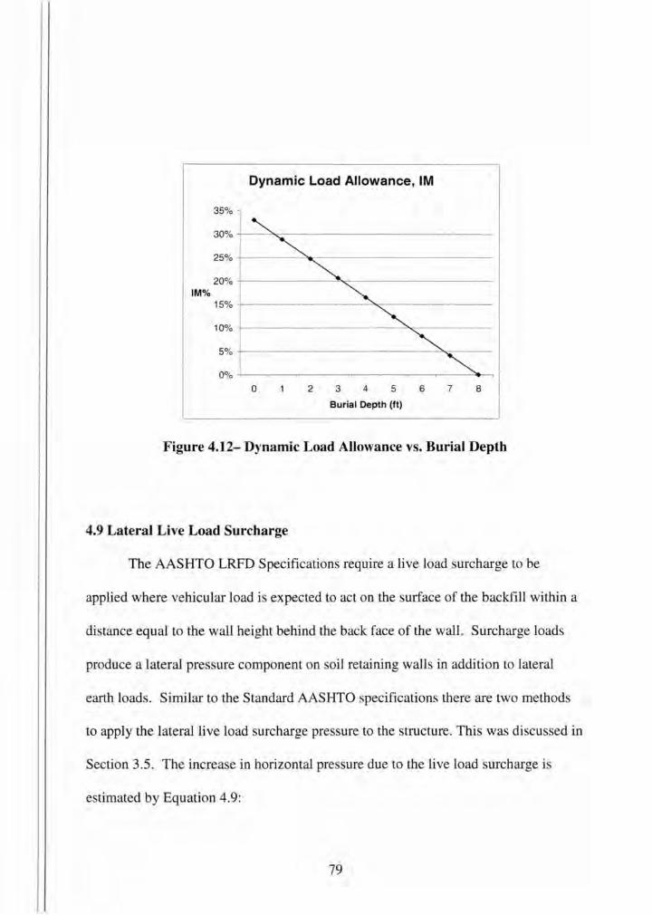
Dynamic Load Allowance, IM
35%
30%
25%
20% IM%
15%
10%
5%
0%
0 2 3 4 5 6 7 8
Burial Depth (ft)
Figure 4.12- Dynamic Load Allowance vs. Burial Depth
4.9 Lateral Live Load Surcharge
The AASHTO LRFD Specifications require a live load surcharge to be
applied where vehicular load is expected to act on the surface of the backfill within a
distance equal to the wall height behind the back face of the wall. Surcharge loads
produce a lateral pressure component on oil retaining walls in addition to lateral
earth loads. Similar to the Standard AASHTO specifications there are two methods
to apply the lateral live load surcharge pressure to the structure. This was discussed in
Section 3.5. The increase in horizontal pressure due to the live load surcharge is
estimated by Equation 4.9:
79
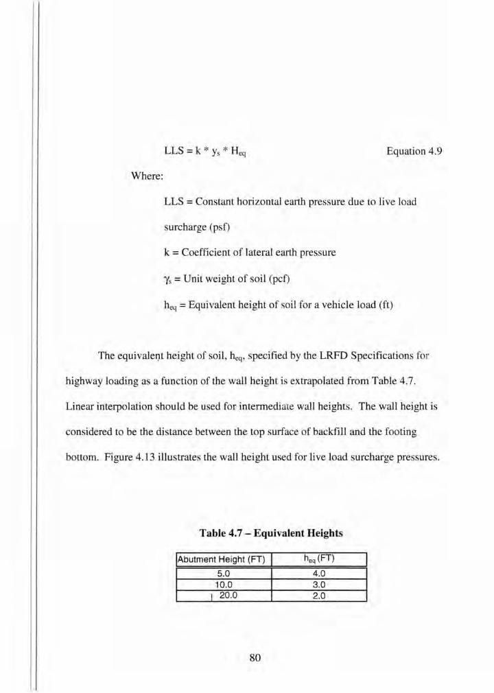
LLS = k * Ys * Heq Equation 4.9
Where:
LLS = Constant horizontal earth pressure due to live load
surcharge (psf)
k = Coefficient of lateral earth pressure
Ys =Unit weight of soil (pcf)
heq =Equivalent height of soil for a vehicle load (ft)
The equivalei).t height of soil, heq, specified by the LRFD Specifications fo r
highway loading as a function of the wall height is extrapolated from Table 4. 7.
Linear interpolation should be used for intermediate wall heights. The wall height is
considered to be the distance between the top surface of backfill and the footing
bottom. Figure 4.13 illustrates the wall height used for live load surcharge pressures.
Table 4. 7 - Equivalent Heights
!Abutment Height (FT) I h eq (FT)
4.0 3.0 2.0
80
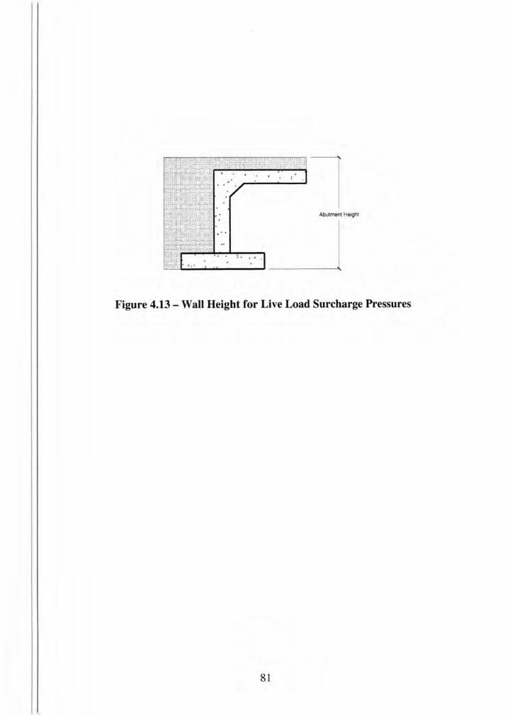
Abutment Height
Figure 4.13- Wall Height for Live Load Surcharge Pressures
81
Chapter 5 Comparison Between LFD AND LRFD Specifications
5.1 Design Vehicular Live Loads
The most significant change introduced in the Standard LRFD Specifications i
the new vehicular live load model. In the Standard AASHTO Specifications, the
vehicular design live load is considered to be either the HS Design Truck Loading or
an Alternate Military Loading. The design includes the configuration that produces
the critical conditions. The LRFD Specifications include three component of the live
load:
• Design Truck
• Design Tandem
• Design Lane Load
A combination of the Design Truck or Design Tandem plus the Lane Load is
used as the vehicular live load in the LRFD Specifications. The force effects from
both the Design Truck and the Design Tandem must be compared. The LRFD design
truck is identical to the axle load portion of the HS20 truck of the Standard AASHTO
Specifications. However, the LRFD design truck is not scaleable like the HS20
truck. For example, there is no HS 15 or HS25 equivalent under the Standard LRFD
82
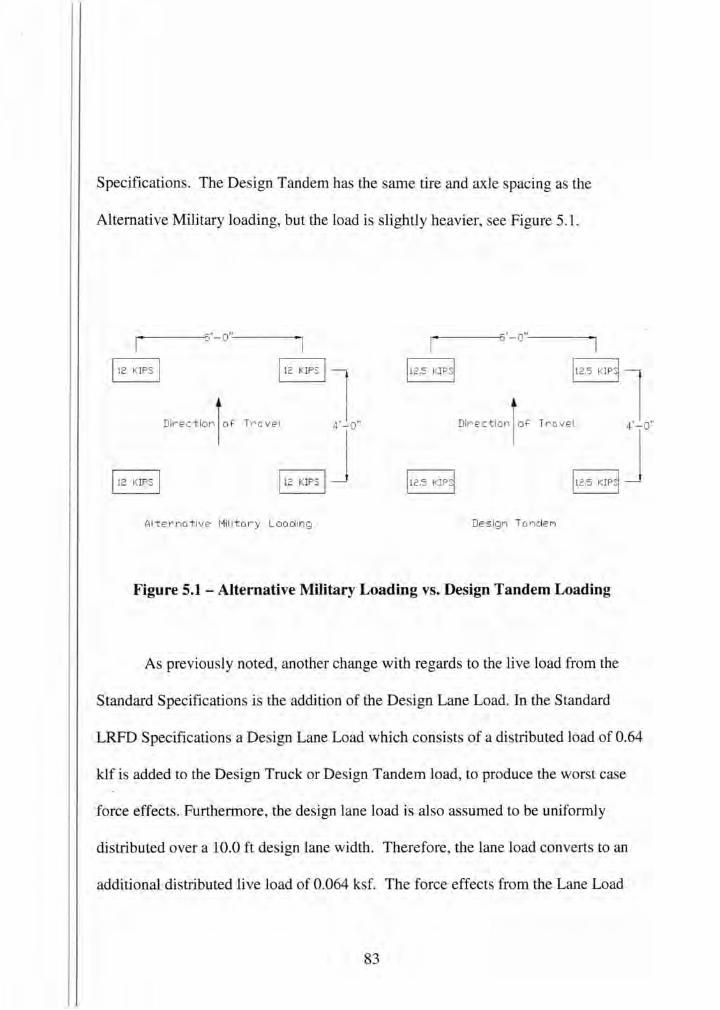
Specifications. The Design Tandem has the same tire and axle spacing as the
Alternative Military loading, but the load is slightly heavier, see Figure 5.1.
8l Trm; 12 KIPs I J
~l T r o. vel 4- ' o"
~J Al -terno-ti ve Ml ll tot~y Loodlng Design T o.ncleM
Figure 5.1 - Alternative Military Loading vs. Design Tandem Loading
As previously noted, another change with regards to the live load from the
Standard Specifications is the addition of the Design Lane Load. In the Standard
LRFD Specifications a Design Lane Load which consists of a distributed load of 0.64
klf is added to the Design Truck or Design Tandem load, to produce the worst case
force effects. Furthermore, the design lane load is also assumed to be uniformly
distributed over a 10.0 ft design lane width. Therefore, the lane load converts to an
additional distributed live load of 0.064 ksf. The force effects from the Lane Load
83
directly correlate with the design span, as the span increases the force effects
increases, and vise versa. The increase of the force effects from the Lane Load is
shown in Figure 5.2. The percent increase in service moment due to the Lane Load
plus Design Truck for various depths of fill and increasing span lengths are shown.
For short spans of approximately 4 ft., the increase in service moment is
approximately 4%, depending on the earth fill. The increase in the service moment
approaches 18% with the addition of the Lane Load for a span of 16ft..
5.2 Multiple Presence Factor
The LRFD Specifications require the use of multiple presence factors to account
for the effects of multiple loaded lanes on a bridge, Table 4.3 . Multiple presence
factors are provided for the cases of one, two, three, and three or more loaded lanes.
For a single loaded lane the multiple presence factor is 1.2, whereas 1.00 for· 2 loaded
lanes.
84
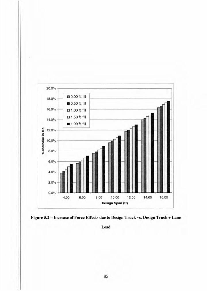
20.0%
18.0% f--0 0.00 ft. fill
• 0.50 ft. fill
16.0% f-- 0 1.00 ft. fill
14.0% f--0 1.50 ft. fill
-• 1.99 ft. fill
IIJ 12.0% :::!: f- -
c: Q) IIJ 10.0% f- f- -., Ill ~ u
-= 8.0% - f- f- -:::!! 0
6 .0% f- - f- f- -
4.0% 1- - - '-- f- f- -
2.0% f- - - f- f- -
0.0%
4.00 6.00 8.00 10.00 12.00 14.00 16.00
Design Span (ft)
Figure 5.2- Increase of Force Effects due to Design Truck vs. Design Truck + Lane
Load
85
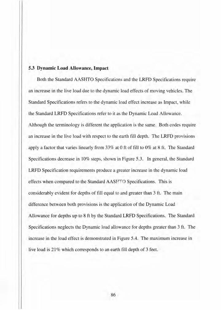
5.3 Dynamic Load Allowance, Impact
Both the Standard AASHTO Specifications and the LRFD Specifications require
an increase in the live load due to the dynamic load effects of moving vehicles. The
Standard Specifications refers to the dynamic load effect increase as Impact, while
the Standard LRFD Specifications refer to it as the Dynamic Load Allowance.
Although the terminology is different the application is the same. Both codes require
an increase in the live load with respect to the earth fill depth . The LRFD provisions
apply a factor that varies linearly from 33% at 0 ft of fill to 0% at 8 ft. The Standard
Specifications decrease in 10% steps, shown in Figure 5.3. In general, the Standard
LRFD Specification requirements produce a greater increase in the dynamic load
effects when compared to the Standard AASH 0 Specifications. This is
considerably evident for depths of fill equal to and greater than 3ft. The main
difference between both provisions is the application of the Dynamic Load
Allowance for depths up to 8 ft by the Standard LRFD Specifications. The Standard
Specification neglects the Dynamic load allowance for depths greater than 3 ft. The
increase in the load effect is demonstrated in Figure 5.4. The maximum increase in
live load is 21% which corre ponds to an earth fill depth of 3 feet.
86
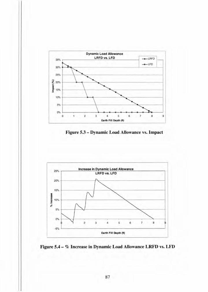
35%
30%
25%
~ 20% ti .. .§ 15%
10%
5%
0%
0
25%
20"/o
15"/o
5: .. ~ 10"/o u .: ~
5"/o
O"'o
-5%
2
Dynamic Load Allowance LRFD vs . LFD
3 4 5
Earth Fill Depth (It)
~LRFD
6 7 8 9
Figure 5.3 - Dynamic Load Allowance vs. Impact
Increase in D namic Load Allowance LRFD vs. LFD
5 6 7 8
Earth Fill Depth (It)
Figure 5.4 - % Increase in Dynamic Load Allowance LRFD vs. LFD
87
5.4 Lateral Live Load Surcharge
Both the Standard AASHTO Specifications and the LRFD Specifications require
a live load surcharge pressure. The live load surcharge pressure is an increase of the
lateral earth pres ure due to the live load. The increase in horizontal pressure is
calculated by Equation 5.1.
Where:
LLS = k * Ys * heq Equation 5.1
LLS = Constant horizontal earth pressure due to live load
surcharge (psf)
k = Coefficient of lateral earth pre ure
Ys =Unit weight of soil (pcf)
heq =Equivalent height of soil for a vehicle load (ft)
The equivalent height of soil, heq, specified by the Standard Specifications is
2ft. The Standard LRFD Specifications calculate the equivalent height of soil as a
function of the wall height extrapolated from Table 4.7. Linear interpolation should
be used for intermediate wall heights. The wall height is considered to be the
distance between the top surface of backfill and the footing bottom. See Figure 4.12.
88
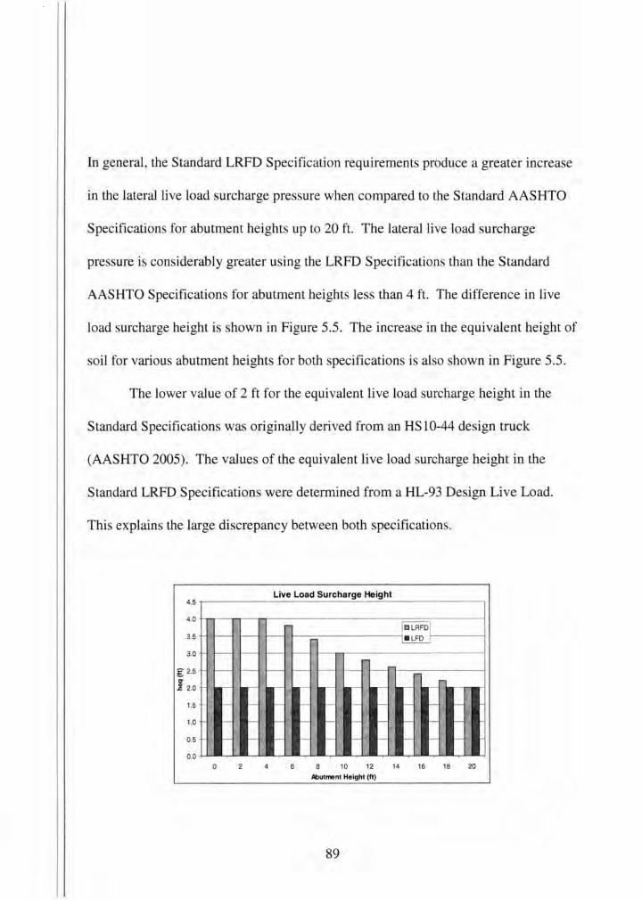
In general, the Standard LRFD Specification requirements produce a greater increase
in the lateral live load surcharge pressure when compared to the Standard AASHTO
Specifications for abutment heights up to 20 ft. The lateral live load surcharge
pressure is considerably greater using the LRFD Specifications than the Standard
AASHTO Specifications for abutment heights less than 4 ft. The difference in live
load surcharge height is shown in Figure 5.5. The increase in the equivalent height of
soil for various abutment heights for both specifications is also shown in Figure 5.5.
The lower value of 2ft for the equivalent live load surcharge height in the
Standard Specifications was originally derived from an HSl0-44 design truck
(AASHTO 2005). The values of the equivalent live load surcharge height in the
Standard LRFD Specifications were determined from a HL-93 Design Live Load.
This explains the large discrepancy between both specifications.
Live Load Surcharge Height 4.5
4.0 Jc LRFDl 3.5 - - 1- .LFD
3.0 - - - 1-
g 2.5 - - - 1- - -:~ 1-
I 2.0 ,.- ,.- r- - r- r- - - -1.5 1- r- r- - r-- r-- ,_ - r- -
1.0 - r- r- r- - r-- r-- f·' - - ,_ r--
0.5 1- r- r- - r-- r-- - - ,_ r--
0.0
0 2 4 6 8 10 12 14 16 18 20
Abutrrent Height (It)
89
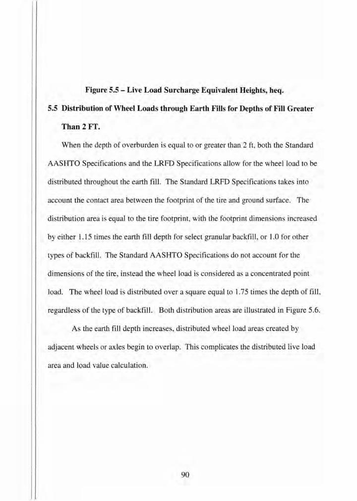
Figure 5.5- Live Load Surcharge Equivalent Heights, heq.
5.5 Distribution of Wheel Loads through Earth Fills for Depths of Fill Greater
Than 2FT.
When the depth of overburden is equal to or greater than 2 ft, both the Standard
AASHTO Specifications and the LRFD Specifications allow for the wheel load to be
distributed throughout the earth fill. The Standard LRFD Specifications takes into
account the contact area between the footprint of the tire and ground surface. The
distribution area is equal to the tire footprint, with the footprint dimensions increased
by either 1.15 times the earth fill depth for select granular backfill, or 1.0 for other
types of backfill. The Standard AASHTO Specifications do not account for the
dimensions of the tire, instead the wheel load is considered as a concentrated point
load. The wheel load is distributed over a square equal to 1.75 times the depth of fill,
regardless of the type of backfill. Both distribution areas are illustrated in Figure 5.6.
As the earth fill depth increases, distributed wheel load areas created by
adjacent wheels or axles begin to overlap. This complicates the distributed live load
area and load value calculation.
90
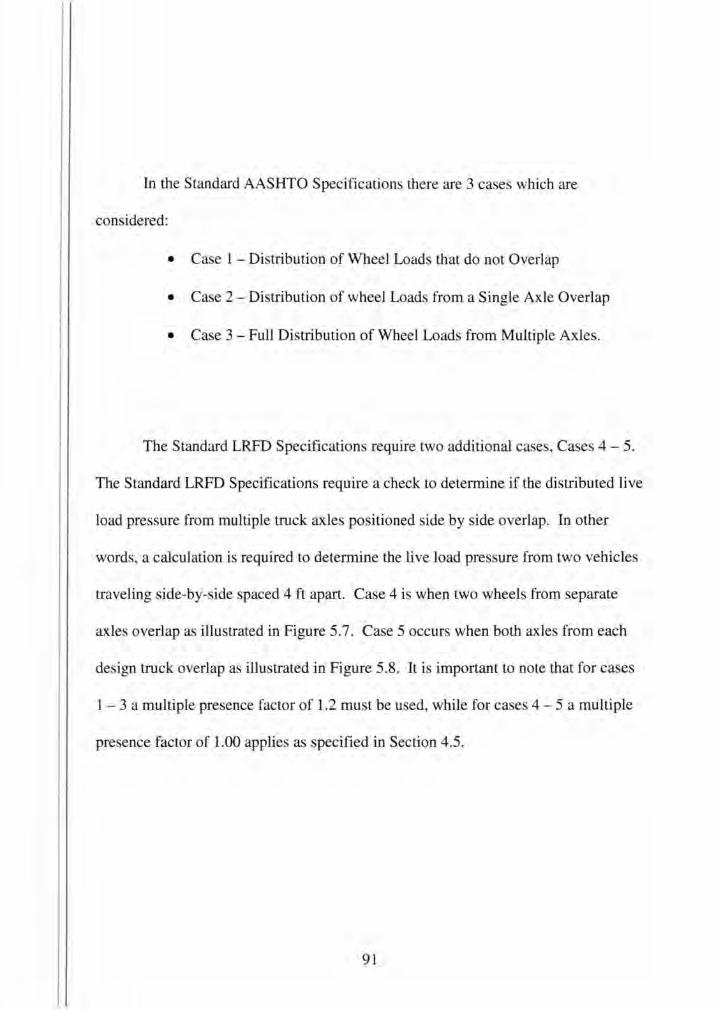
In the Standard AASHTO Specifications there are 3 cases which are
considered:
• Ca e 1 - Di tribution of Wheel Loads that do not Overlap
• Case 2 -Distribution of wheel Load from a Single Axle Overlap
• Case 3 -Full Distribution of Wheel Loads from Multiple Axles.
The Standard LRFD Specifications require two additional cases, Cases 4- 5.
The Standard LRFD Specifications require a check to determine if the distributed live
load pressure from multiple truck axles positioned side by side overlap. In other
words, a calculation is required to determine the live load pressure from two vehicles
traveling side-by-side spaced 4 ft apart. Case 4 is when two wheels from separate
axles overlap as illustrated in Figure 5.7. Case 5 occurs when both axles from each
design truck overlap as illustrated in Figure 5.8. It i important to note that for cases
1- 3 a multiple presence factor of 1.2 must be used, while for ca es 4- 5 a multiple
presence factor of 1.00 applies as specified in Section 4.5.
91
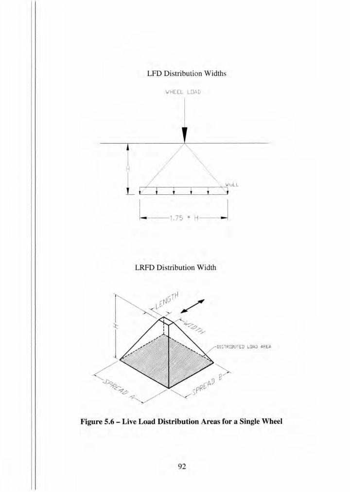
LFD Distribution Widths
IJH EEL LOAD
H
LRFD Distribution Width
DI STRIBUTED LOAD AREA
Figure 5.6 - Live Load Distribution Areas for a Single Wheel
92
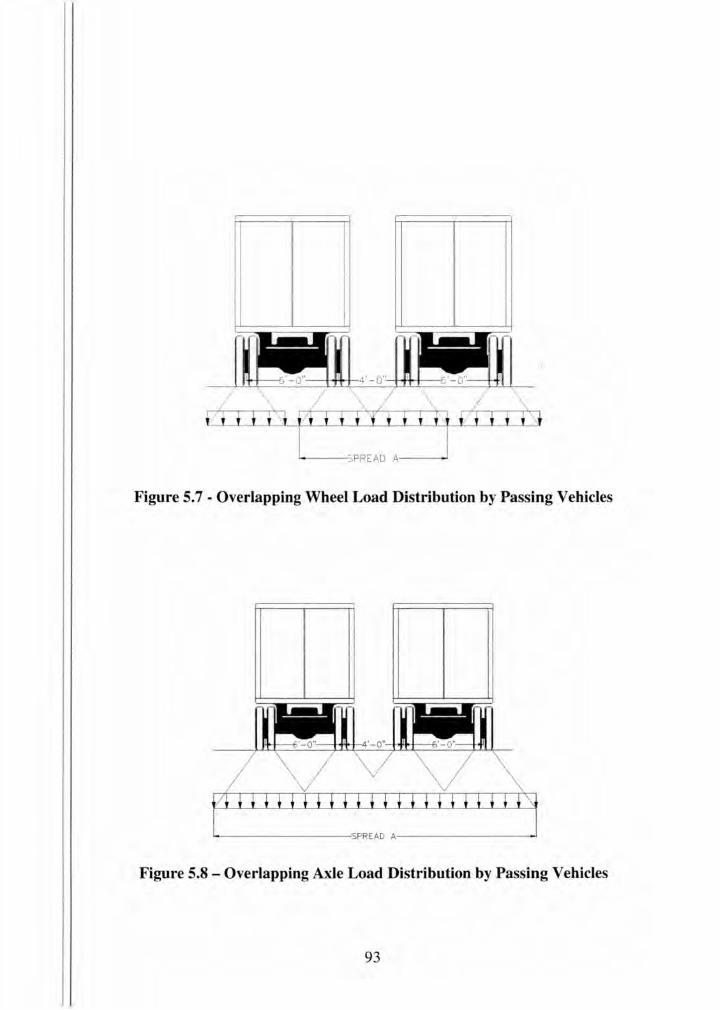
~---SPREAD A---~
Figure 5.7- Overlapping Wheel Load Distribution by Passing Vehicles
~-------------SP'READA-------------~
Figure 5.8- Overlapping Axle Load Distribution by Passing Vehicles
93
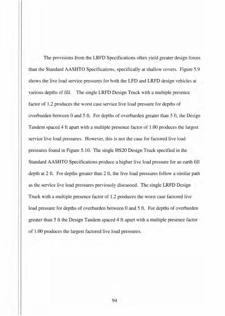
The provisions from the LRFD Specifications often yield greater design forces
than the Standard AASHTO Specifications, specifically at shallow covers. Figure 5.9
show the live load service pres ures for both the LFD and LRFD design vehjcles at
various depths of fill . The single LRFD Design Truck with a multiple presence
factor of 1.2 produces the worst case service live load pressure for depths of
overburden between 0 and 5 ft. For depths of overburden greater than 5 ft, the Design
Tandem spaced 4 ft apart with a multiple presence factor of 1.00 produces the largest
service live load pressures. However, thj is not theca e for factored live load
pressures found in Figure 5.10. The single HS20 Design Truck specified in the
Standard AASHTO Specifications produce a higher live load pressure for an earth fill
depth at 2ft. For depths greater than 2ft, the live load pressures follow a sirrular path
as the service live load pres ure previously discussed. The single LRFD Design
Truck with a multiple presence factor of 1.2 produces the worst case factored live
load pressure for depths of overburden between 0 and 5 ft. For depths of overburden
greater than 5 ft the Design Tandem spaced 4ft apart with a multiple presence factor
of 1.00 produces the largest factored live load pressures.
94
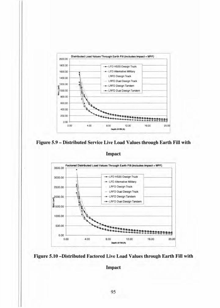
Distributed Load Values Through Earth Fill (includes Impact+ MPF) 2000.00
1800.00
1600.00
1400.00
1200.00
! j1000.00
~ 800.00
600.00
400.00
200.00
0.00
0.00
-+- LFD HS20 Design Truck
~· ..-- LFD AHemative Military
LRFD Design Truck
~ ~ ~ LRFD Dual Design Truck
_,._ LRFD Design Tandem
__._ LRFD Dual Design Tandem
I %' ,, ~' ~~ ~
4.00 8.00 12.00 16.00
Depth Of All (It)
20.
Figure 5.9 - Distributed Service Live Load Values through Earth Fill with
Impact
3500.00 Factored Distributed Load Values Through Earth Fill (includes Impact+ MPF)
3000.00
2500.00
.,2000.00 a. ; i 1500.00
1000.00
500.00
0.00 0.00
. I
d ,
-+- LFD HS20 Design Truck
_.._ LFD Memative Military
LRFD Design Truck
_,. LRFD Dual Design Truck
\ -+- LRFD Design Tandem
\ __._ LRFD Dual Design Tandem
\
~ ~ ~~ ..
4.00 8.00 12.00 16.00 Dopth or All (Ill
20.00
Figure 5.10 -Distributed Factored Live Load Values through Earth Fill with
Impact
95
5.6 Distribution of Live Loads for Depths of Fill Less Than 2 Feet.
Underground concrete structures are typically analyzed as two-dimensional
frames. For depths of overburden less than 2ft, equivalent strip widths are used in
both Specifications to simplify the analysis of the three-dimensional respon e due to
live loads. Both specifications examine the live load in strip widths. This strip width
is the effective width of slab that resists the applied load. The primary differences are
summarized in the following sections:
Truck Configuration:
The Standard AASHTO Specification breaks the design vehicle into a line of
wheel loads, whereas the Standard LRFD Specifications utilizes a full axle on the
member. Both codes allow the respected live loads to then be distributed by a
distribution width, E.
Distribution Width:
The values of the distribution widths from both specifications are identical.
However, the distribution width in the Standard LRFD Specifications is twice the
distribution width found from the Standard Specifications. This increase i a result of
the LRFD Specification u ing a full axle instead of a single wheel.
• LFD Specifications: Pwheel IE =Wheel Load I (4 + .06 * Span)
• LRFD Specifications: Paxle IE = Axle Load I (8 + 1.2 * Span )
96
Tire Contact Area:
Both specifications assume the tire contact as a rectangle with the length in
the direction of traffic equal to 10 in, and a width of 20 in.
Lateral Distribution (load length):
The Standard AASHTO Specifications does not take into account earth fill
that is placed on the structure. The wheel load is simply assumed to act as a point
load. The Standard LRFD specifications allow the designer to take advantage of
earth fill by assuming the axle load to be di tributed laterally increasing the load
length. As a result of thi s provision, the Standard LRFD Specifications produces
smaller service moments when compared to the Standard AASHTO Specifications for
earth fill depths less than 2 ft.
This is comparison is hown in Figure 5.11. The live load service moments
for both the LFD (HS-20) and LRFD design vehicles at various design spans and an
earth fill depth of 1.00 ft are included in the figure. For each case the service
moments caused by the Standard Specifications control the design. This is attributed
to the load effect from the Standard LRFD Specifications acting more like distributed
load than a concentrated load. However, it is important to note that when the multiple
presence factors and the dynamic load allowance are taken into account the service
moments from the Standard LRFD Specifications control the design, Figure 5.12.
97
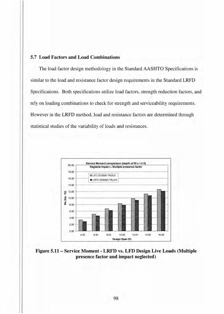
5. 7 Load Factors and Load Combinations
The load factor design methodology in the Standard AASHTO Specifications is
similar to the load and resistance factor design requirements in the Standard LRFD
Specifications. Both specifications utilize load factors, strength reduction factors, and
rely on loading combinations to check for strength and serviceability requirements.
However in the LRFD method, load and resistance factors are determined through
statistical studies of the variability of loads and resistances.
20.00
18.00
16.00
14.00
E' 12.00
;! 10.00 .. :::E 8.00
6.00
4.00
2.00
0.00
Service Moment comparison (depth offill = 1.0 ft) Neglects Impact+ Multiple presence factor
I 0 LFD DESIGN TRUCK
I • LRFD DESIGN TRUCK J
--;; -..... - _H
r- -'~ -r~ --
f-- - ,_ -
[l:_ I' ,J f-- - ,_ -~
~..::.. '-- .__ '--
4.00 6.00 8.00 10.00 12.00 14.00
Design Span (ft)
-
f--
f--
f--
f--
f--
'--r--
16.00
Figure 5.11 - Service Moment - LRFD vs. LFD Design Live Loads (Multiple presence factor and impact neglected)
98
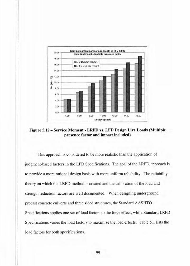
20.00
18.00
16.00
14.00
£ 12.00
g 10.00
rn :::; 8.00
6.00
4.00
2.00
0.00
1-r-
1-
t-L..
4.00
Service Moment comparison (depth of fill= 1.0 ft) Includes Impact + Multiple presence factor
1---I [] LFD DESIGN TRUCK
f-- .-- 1-I • LRFD DESIGN TRUCK
1-r- f.-- 1---
.--1- 1- 1- 1-
r-f.-- 1- f.-- 1---
r-f.-- f.-- 1- r-- 1-
,-- - 1- 1- 1- 1- 1-
r-- ·- 1- 1- 1- t- 1-
- - - - 1- 1- 1-
L.. L.,_ L.,_ ._ L--L- L.. L
6.00 8.00 10.00 12.00 14.00 16.00
Design Span (It)
Figure 5.12 - Service Moment - LRFD vs. LFD Design Live Loads (Multiple presence factor and impact included)
This approach is considered to be more realistic than the application of
judgment-based factors in the LFD Specifications. The goal of the LRFD approach is
to provide a more rational design basis with more uniform reliability. The reliability
theory on which the LRFD method is created and the calibration of the load and
strength reduction factors are well documented. When designing underground
precast concrete culverts and three sided tructures, the Standard AASHTO
Specifications applies one set of load factors to the force effect, while Standard LRFD
Specification varies the load factors to maximize the load effects. Table 5.1 lists the
load factors for both specifications.
99
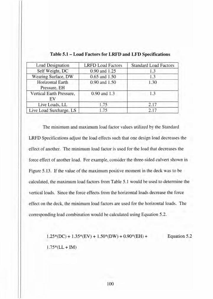
Table 5.1 - Load Factors for LRFD and LFD Specifications
Load Designation LRFD Load Factors Standard Load Factors Self Weight, DC 0.90 and 1.25 1.3
Wearing Surface, DW 0.65 and 1.50 1.3 Horizontal Earth 0.90 and 1.50 1.30
Pressure, EH Vertical Earth Pressure, 0.90 and 1.3 1.3
EV Live Loads, LL 1.75 2.17
Live Load Surcharge, LS 1.75 2.17
The minimum and maximum load factor values utilized by the Standard
LRFD Specifications adjust the load effects such that one design load decreases the
effect of another. The minimum load factor is used for the load that decreases the
force effect of another load. For example, consider the three-sided culvert shown in
Figure 5.13. If the value of the maximum positive moment in the deck was to be
calculated, the maximum load factors from Table 5.1 would be used to determine the
vertical loads. Since the force effects from the horizontal loads decrease the force
effect on the deck, the minimum load factors are used for the horizontal loads. The
corresponding load combination would be calculated using Equation 5.2.
1.25*(DC) + 1.35*(EV) + 1.50*(DW) + 0.90*(EH) + Equation 5.2
1.75*(LL + IM)
100
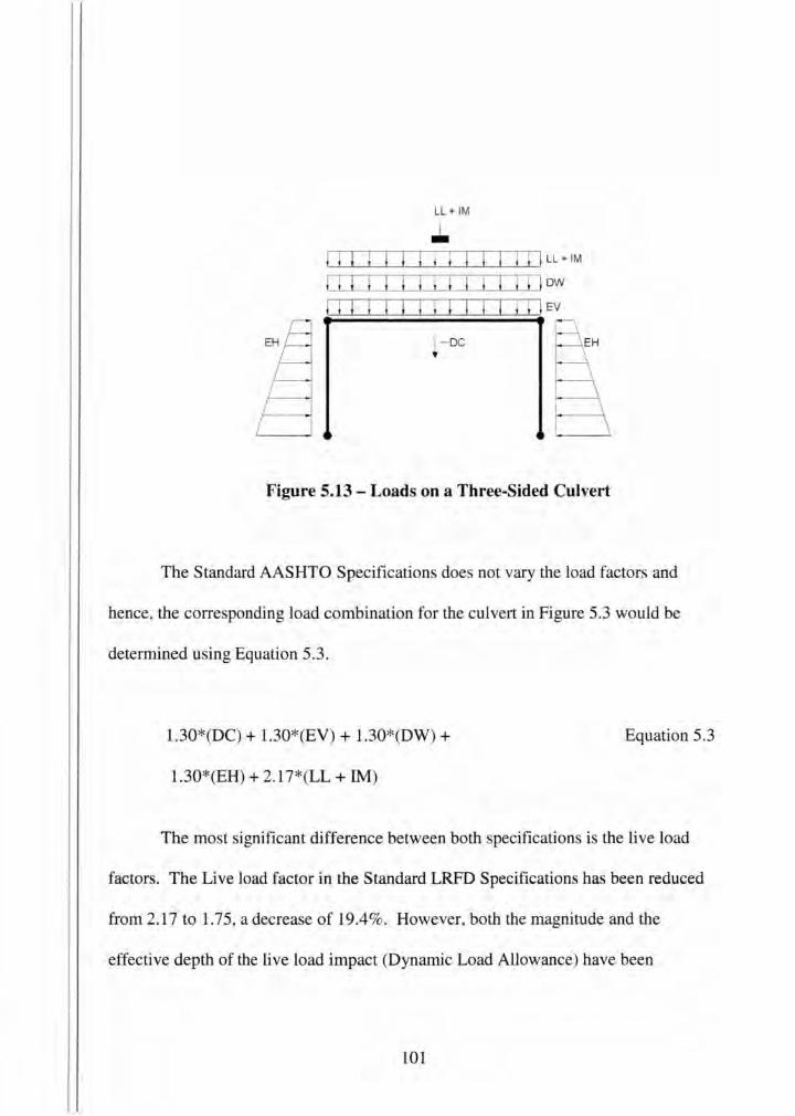
LL + IM
.J. ! I l I I I I I I LL+ IM
ow
I I l I I I I I I EV
1-oc '
Figure 5.13 - Loads on a Three-Sided Culvert
The Standard AASHTO Specifications does not vary the load factors and
hence, the corresponding load combination for the culvert in Figure 5.3 would be
determined using Equation 5.3.
1.30*(DC) + 1.30*(EV) + 1.30*(DW) + Equation 5.3
1.30*(EH) + 2.17*(LL + IM)
The most significant difference between both specifications is the live load
factors. The Live load factor in the Standard LRFD Specifications has been reduced
from 2.17 to 1.75, a decrease of 19.4%. However, both the magnitude and the
effective depth of the live load impact (Dynamic Load Allowance) have been
101

increased. A multiple presence factor of 1.2 has also been introduced in the Standard
LRFD Specifications for a single loaded lane. Therefore, the load factor for a single
loaded lane equates to 2.1. Overall the load effect from the LRFD Specifications
produces greater live load effects.
102
Design Example #1
6.1 Problem Statement
Chapter 6 Design Examples
This example illustrates the design of a three-sided precast concrete structure.
The three-sided tructure was analyzed utilizing both the Standard AASHTO
Specifications, and the Standard AASHTO LRFD Specifications. After determining
the individual load components and assembling the design load combinations, the
design of the flexural reinforcement is presented. The design example conclude with
the shear calculations from both specifications.
The inside dimen ions of the three-sided structure are 20ft. x lOft,. The deck
thickness is 14in., and the wall thickness is lOin. with a 1ft. x 1ft. haunch. Earth fill
will be placed on top of the precast structure to a depth of 5ft. A typical section of the
culvert is shown in Figure 6.1.
6.1.2 Design Parameters
Material Properties:
Yield Strength, fy = 60,000 psi
Compressive Strength, f ' c = 6000 psi
Minimum concrete cover = 2 in
103

Maximum aggregate ize, Ag = 0.75 in
Design Loads:
Depth of earth fill = 5 ft
Unit weight of concrete, yc=150 pcf
Unit weight of soil, ys = 120 pcf
Equivalent fluid pressure, EFP = 30 pcf
Backfill Material= Select granular
Live load specified in applicable codes
Strength Reduction Factors:
Flexure, <P = 0.95
Shear <P = 0.90
6.1.3 Standard AASHTO Specifications:
6.1.3.1 Vertical and Horizontal Earth Pressures:
The design vertical earth pre ure on the top of the culvert is calculated as:
WuSL= y * Z
WuSL = (120 pcf) * (5 ft) = 600 psf
104
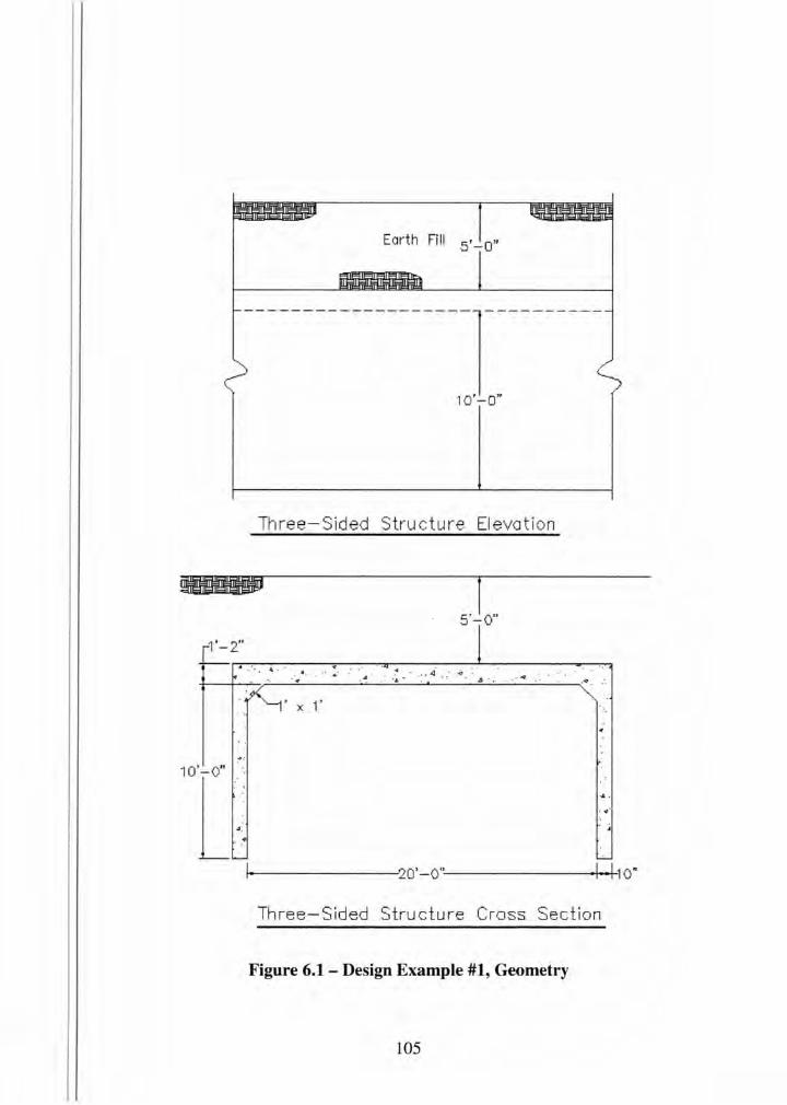
Earth Fill
____________________ ] __________ _
1o'-o"
Three-S ided Stru c ture Elevation
1'-2" r--- ot •• • ·. •
L. . A . 4 . , . ' 4 . -4 +--+~~~~·-·-· --· ~~~·--~--~- ~~- ~· ~--~- ~~~~-·~ .
· - .~ · X 1'
...
. .. .. . 10'[~
. . f-----------------'20 ' -0 "'----------------f.-+'1 0.
Three-Sided Structure Cross Section
Figure 6.1 - Design Example #1, Geometry
105
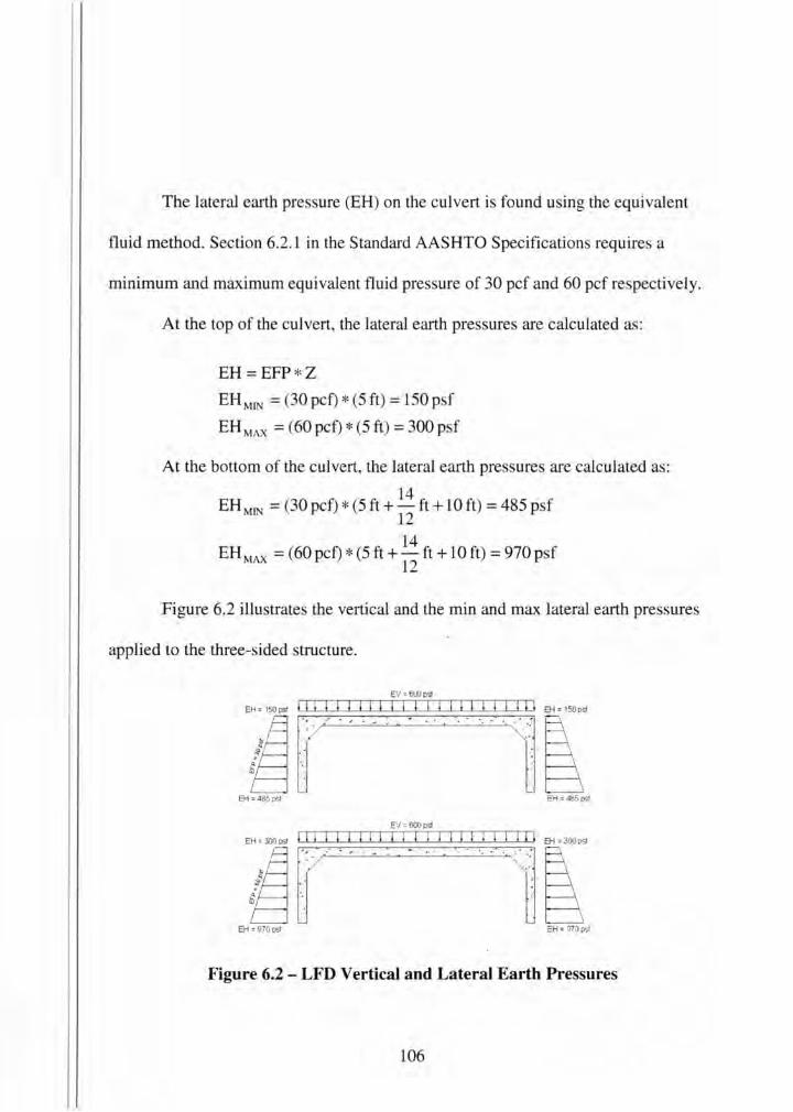
The lateral earth pressure (EH) on the culvert is found using the equivalent
fluid method. Section 6.2.1 in the Standard AASHTO Specifications require a
minimum and maximum equivalent fluid pres ure of 30 pcf and 60 pcf respectively.
At the top of the culvert, the lateral earth pressures are calculated as:
EH =EFP * Z
EH MIN = (30 pcf) * (5 ft) = 150 psf
EHMAX = (60 pcf) * (5 ft) = 300 psf
At the bottom of the culvert, the lateral earth pressures are calculated as:
14 EHMIN = (30 pcf) * (5 ft +- ft +10ft)= 485 psf
12 14
EH MAX = (60 pcf) * (5 ft +- ft +10ft) = 970 psf 12
Figure 6.2 illustrates the vertical and the min and max lateral earth pressures
applied to the three-sided structure.
EV: 600pst
E~""'"'" ~;.' I_ I_ I. 1 __ 1 :' 1.1 I I' I I I I _1 11 ~~:,sopst ..
: . /!J • •.
EH : 485 pst EH : 485 psf
EV: 600pst
,~ rll ~!Ill II II I I I I I I I I t EH: 300 ps~
1~ EH: 970 pst EH: 970 psf
Figure 6.2 - LFD Vertical and Lateral Earth Pressures
106
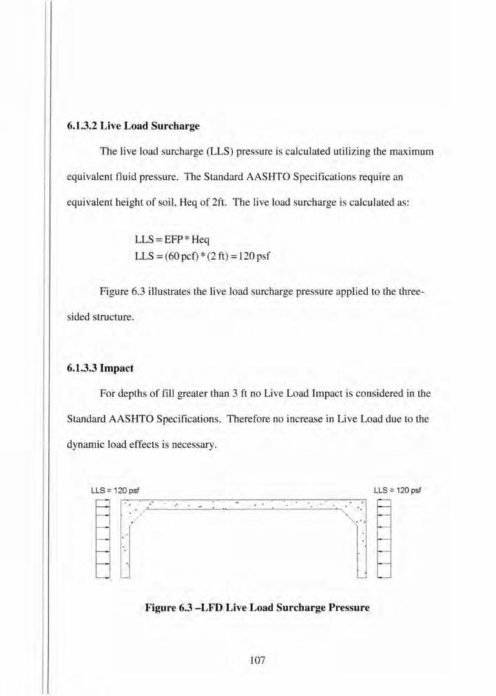
6.1.3.2 Live Load Surcharge
The live load surcharge (LLS) pressure is calculated utilizing the maximum
equivalent fluid pressure. The Standard AASHTO Specifications require an
equivalent height of soil, Heq of 2ft. The live load surcharge is calculated as:
LLS = EFP * Heq
LLS = (60 pcf) *(2ft) = 120 psf
Figure 6.3 illustrates the live load surcharge pressure applied to the three-
sided structure.
6.1.3.3 Impact
For depths of fill greater than 3 ft no Live Load Impact is considered in the
Standard AASHTO Specifications. Therefore no increase in Live Load due to the
dynamic load effects is necessary.
LLS = 120 psf LLS = 120 psf
. ' .
Figure 6.3 -LFD Live Load Surcharge Pressure
107
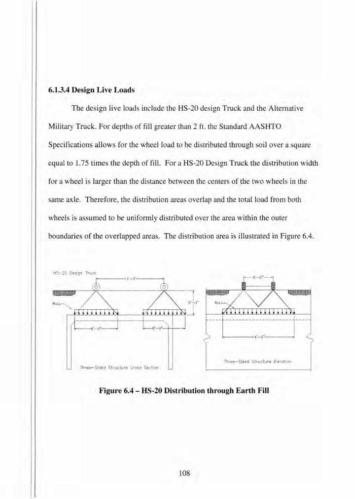
6.1.3.4 Design Live Loads
The design live loads include the HS-20 design Truck and the Alternative
Military Truck. For depths of fill greater than 2 ft. the Standard AASHTO
Specifications allows for the wheel load to be distributed through soil over a square
equal to 1.75 times the depth of fill. For a HS-20 Design Truck the distribution width
for a wheel is larger than the distance between the centers of the two wheels in the
same axle. Therefore, the distribution area overlap and the total load from both
wheels is assumed to be uniformly distributed oyer the area within the outer
boundaries of the overlapped areas. The distribution area is illustrated in Figure 6.4.
HS-20 Design Truck
WuLL
Three - Sided Structure Elevation
Three- Sided Structure Cross Section
Figure 6.4 - HS-20 Distribution through Earth Fill
108
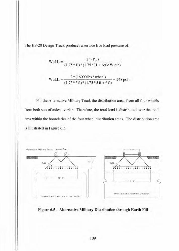
The HS-20 Design Truck prodl}ces a service live load pressure of:
WuLL= 2 * (Pw) (1.75 * H)* (1.75 * H +Axle Width)
WuLL = 2 * (16000 lb I wheel) "" 248 sf (1.75 * 5ft)*( l.75 * 5ft+6ft) p
For the Alternative Military Truck the distribution areas from all four wheels
from both sets of axles overlap. Therefore, the total load is distributed over the total
area within the boundaries of the four wheel distribution areas. The distribution area
is illustrated in Figure 6.5.
Alternative Military Truck
f----12"-9"'------1
Three- Sided Struc ture Elevation Th ree-Sided Stru cture Cross Sec tion
Figure 6.5 - Alternative Military Distribution through Earth Fill
109
The Alternative Military load produces a service live load pressure of:
4*(Pw) WuLL = _________ ____;c_ _______ _
(1.75 * H +Axle Spacing) * (1.75 * H +Axle Width)
WuLL = 4 * (12000 lbs I wheel) "" 255 sf (1.75 * 5 ft +4ft)* (1.75 * 5 ft +6ft) p
The Alternative Military Truck produces live load intensity slightly higher
than that of the HS-20 Design Truck. It also has a larger influence area than the HS-
20 Design Truck. Therefore the Alternative Military load controls the design. Thus,
the Alternative Military Truck will be used to design for the strength and limit states.
6.1.3.5 Load combinations:
For both the strength and service limit states, three load cases are considered as
shown in Figure 6.6. The load cases are described in detail below.
• Case 1: Maximum vertical loads on deck, minimum lateral loads on legs.
This case produces maximum stresses in the bottom of the deck.
• Case 2: Maximum vertical and horizontal loads on the structure. This case
produces maximum stresses on the corner of the ~eck, and outside walls.
110
• Case 3: Minimum vertical loads on deck, and maximum horizontal loads on
walls. This case produces maximum stresses on the inside of the leg.
The load combinations are as follows:
Strength: 1. u = 1.3 * DL + 1.3 * EV + 1.3 * EHMIN + 2.17 * LL
2. U = 1.3 * DL + 1.3 * EV + 1.3 * EHMAX + 1.3 * LLSurcharge + 2.17 * LL
3. U = 1.3 * DL + 1.3 * EV + 1.3 * EHMAX + 1.3 * LLSurcharge Service:
1. u = 1.0 * (DL + EV + EHM[N + LL)
2. U = 1.0 * (DL + EV + EHMAX + LLsurcharge + LL)
3. U = 1.0 * (DL + EV + EHMAX + LLsurcharge)
A structural analysis was performed utilizing a commercial software package,
SAP2000. The structure was modeled and analyzed for a 1 foot wide design strip
oriented parallel to the direction of traffic. The structure was modeled assuming a
pin-pin connection as specified in 16.8.5 of the Standard AASHTO Specifications.
The axial forces were neglected to simplify the design calculations. The location of
the live load was positioned to create maximum stresses. The critical locations of the
internal forces are illustrated in Figure 6.7. Table 6.1 lists the critical stresses for
each load combination at the critical locations. The values in bold are the maximum
stresses that occur between load cases 1 - 3 for the specified section in Figure 6. 7.
Both the factored and service values are listed per foot width in Table 6.1.
Ill
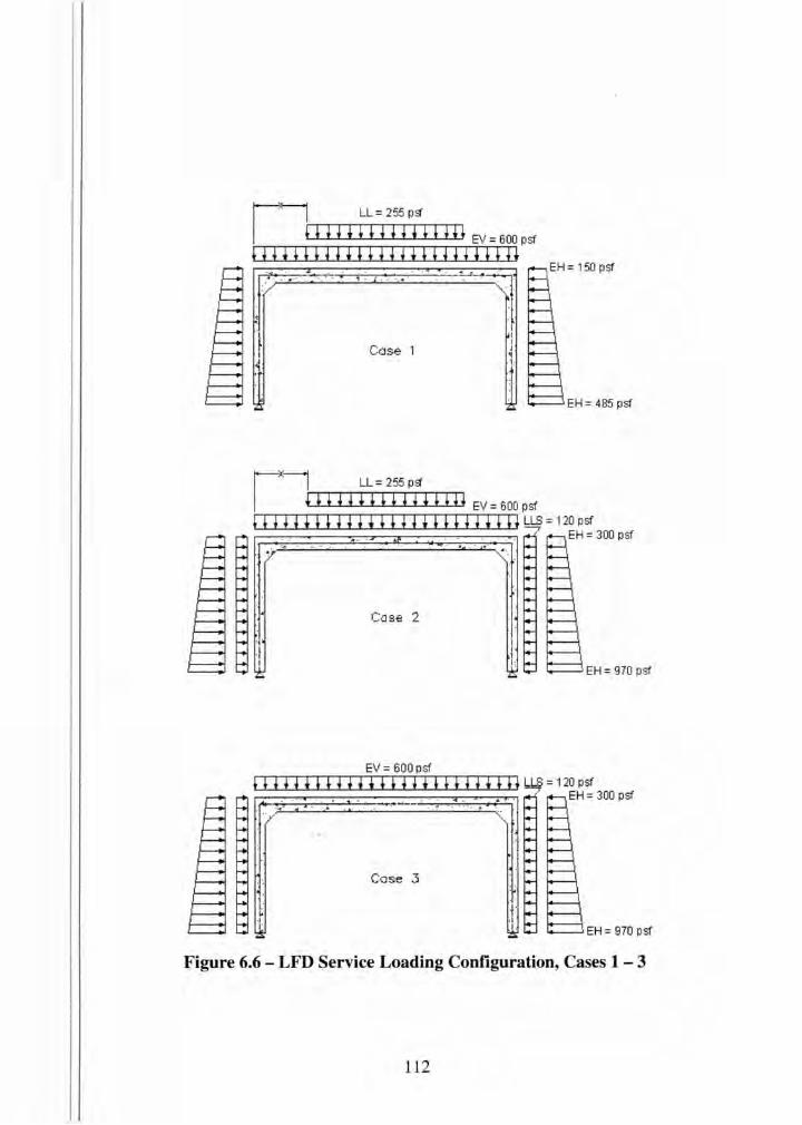
Case 1
--.-L-f-":::\l . . . I I ., I l , 1;
r:xl LL= 255 ps
+ o n * l l l n o o + Ev- 6oo psf
EH = 485 psf
t } ~ ~ ~ + ' ' + i i + } I + + + } } I + + + } } ~ u.s = 120 psf EH = 300 psf
... . · ..
Case 2
EH = 970 psf
EV = 600 psf
t t J J J * f f J i ~ * f + J J * + + + J J * + + ~ u.s = 120 psf . .....,.. ~....: ; .. - ~ . ~ . ·. · .. EH = 300 psf
Case .3
EH = 970 psf
Figure 6.6 - LFD Service Loading Configuration, Cases 1 - 3
11 2
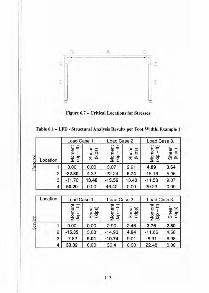
@) .----- --------------------------------------------------------------·-----, l ! ' '
~ t i ~ ' ' ' ' ' ' ' ' ' ' ' ' ' ' ' ' ' ' ' ' ' ' ' ' ' '
~ ! ! ® ' ' ' ' ' ' ' ' ' ' ' '
' i
Figure 6.7- Critical Locations for Stresses
Table 6.1 - LFD - Structural Analysis Results per Foot Width, Example 1
Load Case 1. Load Case 2. Load Case 3 . ..... .--. Cd en Q)Q.. ..c ·(j)C
~ 1 ~0_._00 __ +-_0._0_0~ __ 3_.0_7~ __ 2_.9_1-+ __ 4_.8_9 __ ~3_.6_4~ 2 -22.80 4.32 -22 .24 6.74 -15.16 5.96 ~-----+-----1-------r----~-------r----~
3 -11.76 13.48 -15.56 13.48 -11.58 9.07 ~-----+----~-------r----~-------r----~
4 50.20 0.00 46.40 0.00 29.23 0.00
Location Load Case 1. Load Case 2 . Load Case 3. ... .--. ... .--. ... .--. c.:= ..... .--. c.:= ..... .--. c.:= ..... .--. a> I Cd en a> I Cd en a> I Cd en E c.. Q) c.. Ea. Q)Q.. E c..
Q)Q.. ..c ·- ..c ·- ..c ·-
0 ·- (j)c 0 ·- (j)c 0 ·- (j)c .::: ::::22£ ::::22£ ::::22£
~ 1 0.00 0.00 2.90 2.46 3.76 2.80 2 -15.35 3.08 -14.93 4.94 -11.66 4.58
3 -7.82 9.01 -10.74 9.01 -8 .91 6.98 4 33.32 0.00 30.4 0.00 22.48 0.00
113
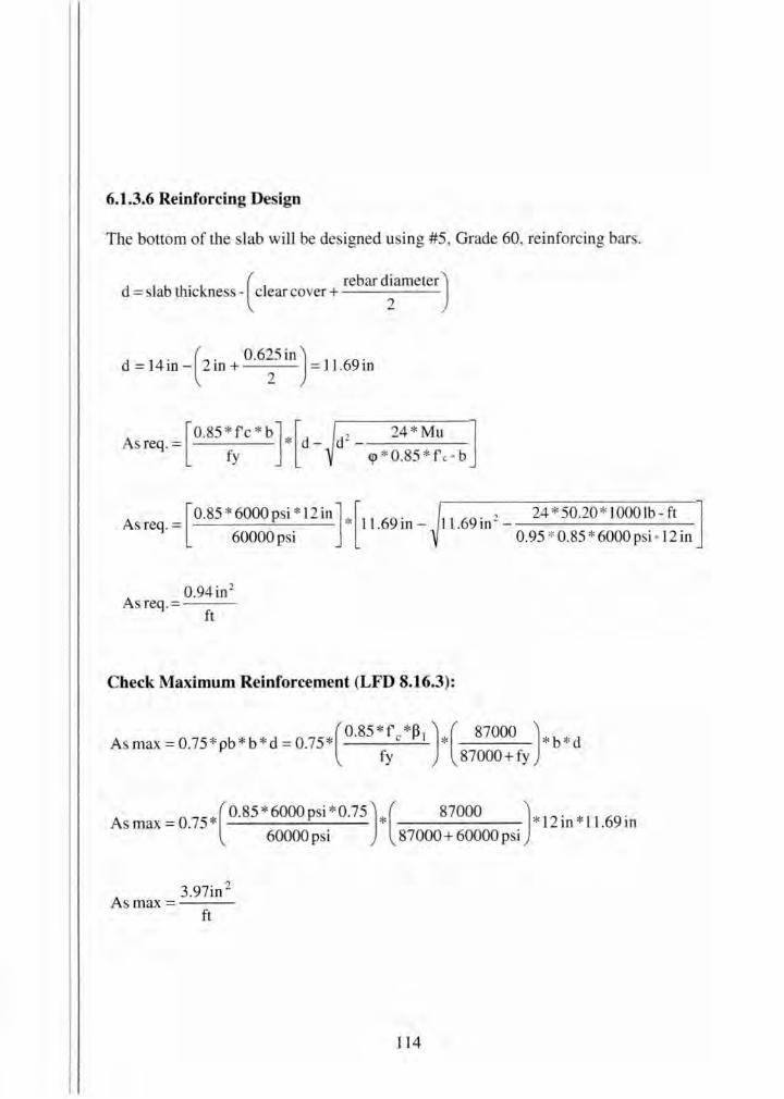
6.1.3.6 Reinforcing Design
The bottom of the slab will be designed using #5, Grade 60, reinforcing bar .
. ( rebar diameter) d =slab thickness- clear cover+ 2
d = 14in -( 2in + 0 · 6~5 in) = 11.69in
Asreq.=[0.85 *fc * b] *[d- d2 - 24 * Mu ] fy q> * 0.85 * f c. b
Asreq.=[0.85 *6000p i *l2in] *[ll.69 in- ll.69 in 2 - 24 *50.20 *1000lb-ft ] 60000 psi 0.95 * 0.85 * 6000 psi •12 in
A 0.94in 2
s req .= ft
Check Maximum Reinforcement (LFD 8.16.3):
Asmax=0.75 * pb*b * d = 0.75*[ 0 ·85 *fc *~ 1 J * [ 87000 ]*b *d
fy 87000+fy
As max= 0.75 *[ 0.85 * 6000 p i *0.75 ]*[ 87000 ]* 12 in * 11.69 in 60000p i 87000+60000psi
A 3.97in 2
smax=--ft
114
Check Minimum Reinforcement (LFD 16.8.5.8):
As min = 0.002 * b * h
As min= 0.002 * 12 in * 14 in
A . 0.34in 2
s!Tiln =---ft
Try #5's @ 3 inches on center:
As provided= 12
in * .307 in 2 = 1.23 in 2
3
Check Crack Control (LFD 16.8.5.7):
The crack control equations are checked to ensure the primary reinforcement
is well distributed. Typically the crack control equations will govern the spacing, and
amount of reinforcement. The size of rebar and spacing were already chosen to
ensure the crack control requirements are met.
Calculate Allowable Stress, fsa:
f f 98 ksi
s $: sa = --=== 'Vdc * A
d I rebar diameter
2. 0.625 in
2 31.
c=c earcover+ = m + = . m 2 2
115
2*dc *b 2 *2.31 *12in A= _N_u_m_b-er_o_f_b-ar_s_, - = 12 = 13.86
3
98 k i . fsa = =30.86k 1
V2.31 in * 13.86
Calculate Actual Stress in Reinforcement:
E 29000000 psi n=-=----~=
Ec wcl.5 * 33 *Fc
n = 29000000 psi = 6.18 use 6 (150 lb/ft3l 5 * 33 * (~6000 psi)
b * x * (%) = (n * As prov.) * (d- x)
b * x2
--- n * A prov. * (d- x) = 0 2
12 in * x2
----6 * l.23in 2 * (11.69in- x) =0 2
x=3.22in
116

"*d-d x-1169" 3·22 in_l062" J - --- . m---- . In 3 3
fs = Ms = 33·32 k- ft * 12 = 30.62 ksi $ 30.86 ksi ok As* j *d 1.23in *10.62in
Next, the reinforcing steel will be designed for the top of the slab. Further, #5, Grade 60, reinforcing bars will be used for the design.
d = 14in - ( 2in + 0 ·6~5 in) = 11.69in
As= [0.85 * 6000 psi * 12 in] *[11.69 in_ 11.69 in2 _ 24 * 15.56*1000 lb- ft ] 60000 psi 0.95 * 0.85 * 6000 psi •12 in
A 0.28 in 2
s req. = --ft-
Check Maximum Reinforcement (LFD 8.16.3):
As max= 0.75 *(0.85 * 6000 psi *0.75) * ( 87000 ) * 12 in * 11.69 in 60000 psi 87000 + 60000 psi
A 3.97 in 2
smax= ---ft
117

Check Minimum Reinforcement (LFD 16.8.5.8):
Asrnin = 0.002 * 12in * 14 in
A . 0.34in 2
srrun =---ft
Try #5' s @ 3 inches on center:
p· As provided = - m * .307 in 2 = 1.23 in 2
3
Check Crack Control (LFD 16.8.5.7):
Calculate Allowable Stress, fsa:
f < f 98 ksi
s _ sa = -:-;:::::== V dc * A
d 2. 0.625 in
2 31.
c= m+ = . m 2
A= 2 *2.31 *12in = l3.86 12
3
fsa = 98 ksi = 30.86 ksi V2.31in *13.86
118

Calculate Actual Stress in Reinforcement:
n = 29000000 psi = 6_18 use 6 ( 150 lb/ft 3 ) 1.s * 33 * ( ~6000 psi)
12 . * 2 10 x - 6 * 1.23 in 2 * (11.69 in- x) = 0
2
x = 3.22in
j * d=d-~=11.69in - 3·22
in =10.62in 3 3
Ms 10.74k -ft*12 fs = = = 9.86 ksi ~ 30.86 ksi ok
As* j *d 1.23in *10.62in
The reinforcing pattern for the outside walls will now be designed. Once again, #5,
Grade 60, reinforcing bars will be utilized in the design.
d =lOin-( 2 in+ 0·6~Sin) = 7.69 in
As req. = [0.85 * 6000psi * 12 in]* [ 7.69 in_ 7_69 in2 _ 24 * 22.80 * 1000 lb- ft ] 60000 psi 0.95 * 0.85 * 6000 psi •12 in
A 0.65in 2
s req.= ft
119
Check Maximum Reinforcement (LFD 8.16.3):
As max= 0.75 *(0.85 * 6000 psi * 0.75 ) * ( 87000 ) * 12 in * 7.69 in 60000 psi 87000 + 60000 psi
A 2.61in 2
smax= ---ft
Check Minimum Reinforcement (LFD 16.8.5.8):
Asmin = 0.002 * 12 in* 10 in
A . 0.24 in 2
siTIJn =---ft
Try #5 ' s @ 3 inches on center:
As provided = 12
in * .307 in 2 = 1.23 in 2
3
120

Check Crack Control (LFD 16.8.5.7):
Calculate Allowable Stress, fsa:
f < f 98 ksi
s _ sa = ---;:::== Vctc*A
d 2. 0.625 in
2 31 ."
c= m+ = . m 2
A= 2 *2.31 *12in = 13.86 12
3
fsa = 98 ksi = 30.86 ksi V2.31 in *13.86
Calculate Actual Stress in Reinforcement:
n = 29000000psi = 6.18 use 6 ( 150 lb/ft3l 5 * 33 * ( ~ 6000 psi)
12 . * 2 m · x -6*1.23in2 *(7.69in-x)=0
2
x = 2.52in
121

· * d d x 7 69 · 2·52 in 6 85 · J . = --= . lll- = . lll 3 3
fs = Ms = 15·35 k- ft * 12 = 21.86 ksi ~ 30.86 ksi ok As * j *d 1.23in *6.85in
Finally, the inside of the walls will be designed using #4, Grade 60, reinforcing bars.
d =lOin- ( 2in + O.S~in) = 7.75 in
As req. = [0.85 * 6000 psi * 12 in]* [ 7 .75 in_ 7.75 in 2 _ 24 * 4.89 * 1000 lb- ft ] 60000 psi 0.95 * 0.85 * 6000 psi • 12 in
A 0.13in 2
s req.= ft
Check Maximum Reinforcement (LFD 8.16.3):
As max= 0.75 *(0.85 * 6000 psi* 0.75] * ( 87000 J * 12 in* 7.75 in 60000 psi 87000 + 60000 psi
A 2.63in 2
smax= ---ft
122

Check Minimum Reinforcement (LFD 16.8.5.8):
Asmin = 0.002 * 12 in * 10 in
A . 0.24in 2
smm=--ft
Try #4' s @ 6 inches on center:
"d d 12 in · 96 · 2 0 392 · 2 As prov1 e = -- ~' .1 m = . m 6
Check Crack Control (LFD 16.8.5.7):
Calculate Allowable Stress, fsa:
f f 98 ksi
s :::; sa = -:r=== Vctc * A
d 2. 0.50 in
2 25 .
c = m+ = . m 2
A= 2 *2.25 *12in = 27 12
6
98ksi fsa = = 24.93 ksi
V2.25in * 27
123
Calculate Actual Stress in Reinforcement:
n = · 29000000psi = 6.18 use 6 (150 lb/ft 3 ) t.s * 33 * ( ~6000 psi)
12 . * 2 m x -6 *0.39in 2 *(7.75in-x) =O
2
x = 1.56in
j * d = d -~ = 7. 7 5 in - 1.56
in = 7.23 in 3 3
Ms 3.76 k- ft * 12 fs = = = 16.00 ksi::; 24.93 ksi ok
As * j *d 0.39in *7.23in
6.1.3.7 Calculate shear (LFD 8.16.6.2):
The allowable shear in the three-sided structure was calculated using the simplified
equation.
Shear in the Deck:
·evc~Vu
Vu = 13.48 kips
eve =e * 2 *~* b * d
eve= 0.90 * 2 * ~6000 psi *12 in * 11.69 in= 19558.9lb = 19.56 kips
= 19.56 kips> 13.48 kips OK
124
Shear in the Walls:
·eve~ Vu
Vu = 6.74 kips
eve =e *2*Fc *b*d
eve= 0.90 * 2 * ~6000 psi *12 in *7.69 in= 12866.4lb = 12.87 kips
= 12.87 kips> 6.74 kips OK
6.1.3.8 Summary
Figure 6.8 illustrates the required reinforcement for the inside face and outside
face of the side walls, top slab, and bottom slab. Note that the reinforcement spacing
is the same or on increments of one another. This is typical in precast concrete in
order to simplify the construction of the cage. There are numerous combinations of
rebar size and spacing. As long as all requirements are met the designer should
choose the most economical and practical design.
125
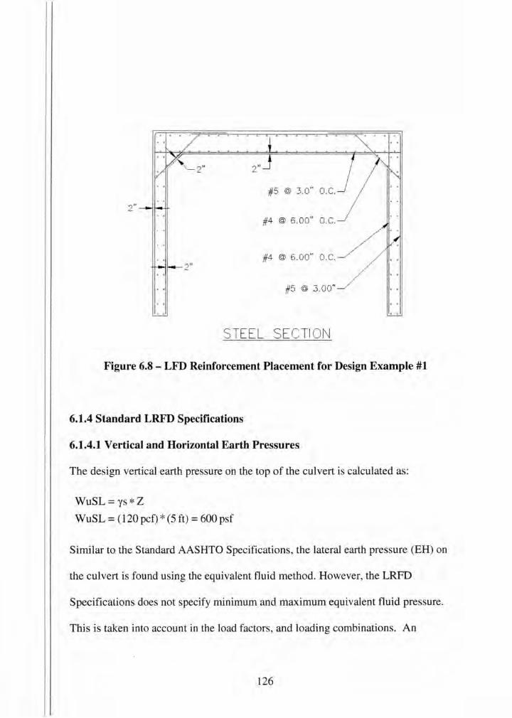
2"
#5 @ .3.0" O.C.
2" #4 @ 6.00" O.C.
#4 @ 6.00" o.c. 2"
#5 @ 3.00"
STEEL SECTION
Figure 6.8 - LFD Reinforcement Placement for Design Example #1
6.1.4 Standard LRFD Specifications
6.1.4.1 Vertical and Horizontal Earth Pressures
The design vertical earth pressure on the top of the culvert is calculated as:
WuSL= ys*Z
WuSL = (120 pet)* (5 ft) = 600 psf
Similar to the Standard AASHTO Specifications, the lateral earth pressure (EH) on
the culvert is found using the equivalent fluid method. However, the LRFD
Specifications does not specify minimum and maximum equivalent fluid pressure.
This is taken into account in the load factors , and loading combinations. An
126
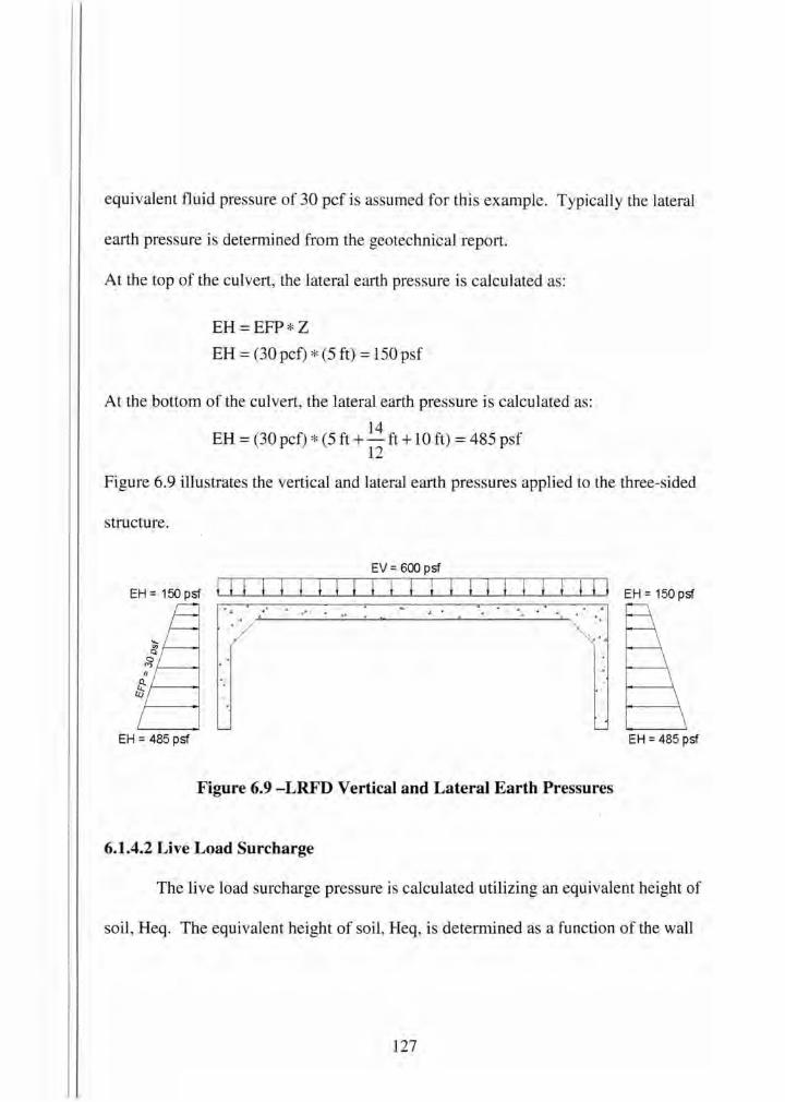
equivalent fluid pressure of 30 pcf is assumed for this example. Typically the lateral
earth pressure is determined from the geotechnical report.
At the top of the culvert, the lateral earth pressure is calculated as:
EH=EFP * Z
EH = (30 pet)* (5 ft) = 150 psf
At the bottom of the culvert, the lateral earth pressure is calculated as:
14 EH = (30 pet)* (5 ft +- ft +10ft)= 485 psf
12
Figure 6.9 illustrates the vertical and lateral earth pressures applied to the three-sided
structure.
EV = 600 psf
EH = 150 psf I I I I I I I I I I I I I I I I I l EH = 150 psf o,.
" . .. . ~ .. . .. · .
·.
EH = 485 psf EH = 485 psf
Figure 6.9 -LRFD Vertical and Lateral Earth Pressures
6.1.4.2 Live Load Surcharge
The live load surcharge pressure is calculated utilizing an equivalent height of
soil, Heq. The equivalent height of soil, Heq, is determined as a function of the wall
127
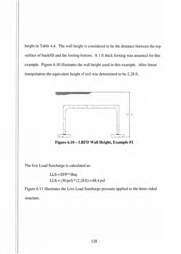
height in Table 4.4. The wall height is considered to be the di stance between the top
urface of backfill and the footing bottom. A 1 ft thick footing was assumed for this
example. Figure 6.10 illustrates the wall height used in this example. After linear
interpolation the equivalent height of soil was determined to be 2.28 ft.
,~_,__ _ __:_____,_ __ _._____;:__---;· .
17'-2"
~ • - I L .. ~-
Figure 6.10- LRFD Wall Height, Example #1
The live Load Surcharge is calculated as:
LLS = EFP * Heq
LLS = (30 pcf) * (2.28 ft) = 68.4 psf
Figure 6.11 illustrates the Live Load Surcharge pressure applied to the three-sided
structure.
128
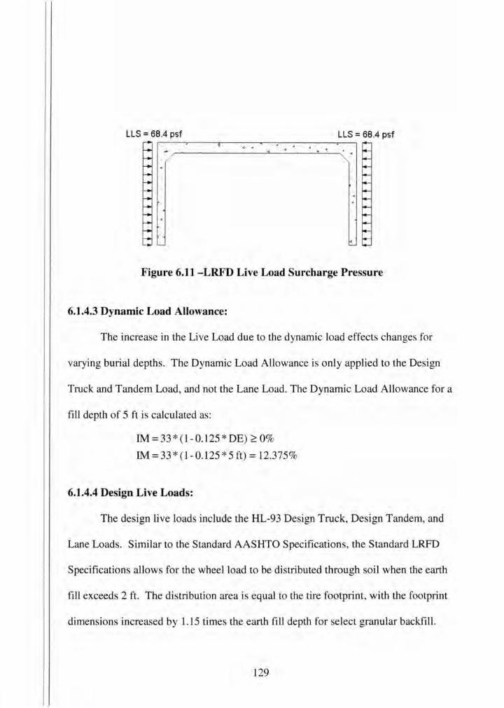
LLS = 68.4 psf LLS = 68.4 psf . . .. .
- ~- 4 . ' . .... .
Figure 6.11 -LRFD Live Load Surcharge Pressure
6.1.4.3 Dynamic Load Allowance:
The increase in the Live Load due to the dynamic load effects changes for
varying burial depths. The Dynamic Load Allowance is only applied to the Design
Truck and Tandem Load, and not the Lane Load. The Dynamic Load Allowance for a
fill depth of 5 ft is calculated as:
IM=33 *(1-0.125*DE) ~ 0%
IM = 33 * (1- 0.125 * 5 ft) = 12.375%
6.1.4.4 Design Live Loads:
The design live loads include the HL-93 Design Truck, Design Tandem, and
Lane Loads. Similar to the Standard AASHTO Specifications, the Standard LRFD
Specifications allows for the wheel load to be distributed through soil when the earth
fill exceeds 2 ft. The di stribution area is equal to the tire footprint, with the footprint
dimensions increased by 1.15 times the earth fill depth for select granular backfill.
129
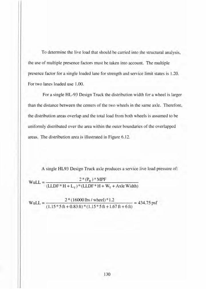
To determine the li ve load that should be carried into the structural analysis,
the use of multiple presence factors must be taken into account. The multiple
presence factor for a single loaded lane for strength and service limit states is 1.20.
For two lanes loaded use 1.00.
For a single HL-93 Design Truck the distribution width for a wheel is larger
than the distance between the centers of the two wheels in the same axle. Therefore,
the distribution areas overlap and the total load from both wheels is assumed to be
uniformly distributed over the area within the outer boundaries of the overlapped
areas. The di stribution area is illustrated in Figure 6.12.
A single HL93 Design Truck axle produces a service live load pressure of:
WuLL = 2 * cPw) * MPF (LLDF * H + LT) * (LLDF * H + WT +Axle Width)
WuLL = 2 * (16000 lbs I wheel)* 1.2 :::; 434.75 psf (1.15 * 5 ft + 0.83 ft) * (1 .15 * 5 ft + 1.67 ft +6ft)
130
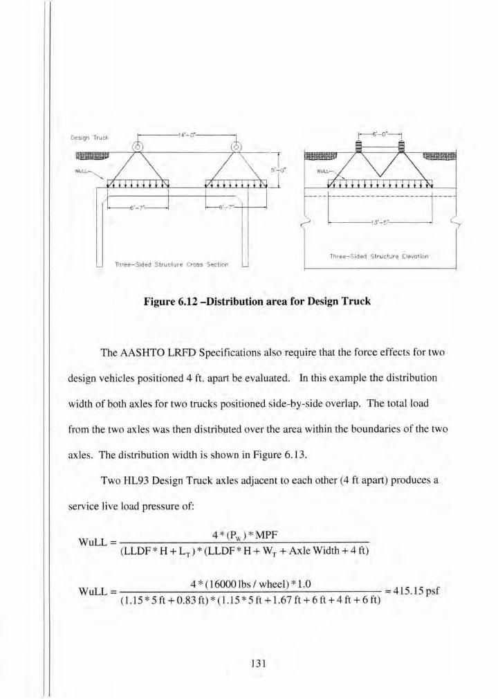
Design Truck
WuLL
Three-Sided St ructure Elevation Three-Sided Structure Cross Section
Figure 6.12 -Distribution area for Design Truck
The AASHTO LRFD Specifications also require that the force effects for two
design vehicles positioned 4ft. apart be evaluated. In this example the distribution
width of both axles for two trucks positioned side-by-side overlap. The total load
from the two axles was then distributed over the area within the boundaries of the two
axles. The distribution width is shown in Figure 6.13.
Two HL93 Design Truck axles adjacent to each other (4ft apart) produces a
service live load pressure of:
4 * cPw)* MPF WuLL = ________ __:_....:..:....:.. _________ _ (LLDF * H + LT) * (LLDF * H + WT +Axle Width+ 4ft)
WuLL = 4 * (16000 lbs I wheel)* 1.0 "" 415_15 psf ( 1. 15 * 5 ft + 0. 8 3 ft) * ( 1.15 * 5 ft + 1. 6 7 ft + 6 ft + 4 ft + 6 ft)
131
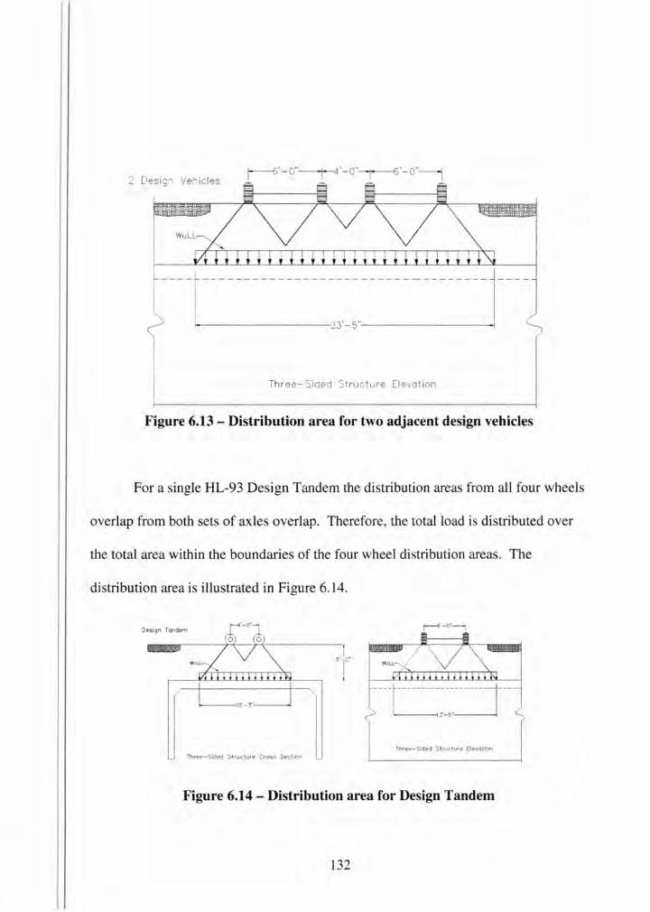
2 Design Vehicles
Three- Sided Structure Elevation
Figure 6.13 - Distribution area for two adjacent design vehicles
For a single HL-93 Design Tandem the distribution areas from all four wheels
overlap from both sets of axles overlap. Therefore, the total load is distributed over
the total area within the boundaries of the four wheel di tribution areas. The
distribution area is illustrated in Figure 6.14.
s·-c·
Three-Sided Structure Elevation Three-Sided Structure Cross Section
Figure 6.14- Distribution area for Design Tandem
132
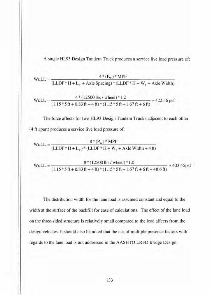
A single HL93 Design Tandem Truck produces a service live load pressure of:
4*(Pw) *MPF WuLL=------------------~~----------------------
(LLDF * H + LT +Axle Spacing)* (LLDF* H + WT +Axle Width)
WuLL = 4 * (12500 lbs I wheel) * 1.2 "" 422.56 sf (1.15 * 5ft +0.83ft +4ft)* (1.15 * 5 ft+ 1.67 ft +6ft) p
The force affects for two HL93 Design Tandem Trucks adjacent to each other
( 4 ft apart) produces a service live load pressure of:
8*(Pw)*MPF WuLL = -------------_:___::c._:__ ________________ _ (LLDF* H + LT) * (LLDF* H + WT +Axle Width+ 4ft)
WuLL = 8 * (12500 lbs I wheel)* 1.0 "" 403 .45 sf (1.15 * 5 ft + 0.83 ft +4ft)* (1.15 * 5 ft + 1.67 ft +6ft+ 4ft 6ft) p
The distribution width for the lane load is assumed constant and equal to the
width at the surface of the backfill for ease of calculations. The effect of the lane load
on the three-sided structure is relatively small compared to the load affects from the
design vehicles. It should also be noted that the use of multiple presence factors with
regards to the lane load is not addressed in the AASHTO LRFD Bridge Design
133
Specifications. However this example assumes the lane load does get multiplied by
the appropriate multiple presence factor.
The Lane Load produces a service live load pressure of:
WuLL = 640 plf * MPF = 64psf * MPF 10ft
The Single Design Truck produces the maximum live load intensity; however
the Single Design Tandem has a larger influeqce area. After analysis it was
determined the Single Design Tandem with a multiple presence factor of 1.2
controlled the design. Therefore the Lane Load produces a live load pressure of:
WuLL = 640
plf * 1.2
= 64 psf * 1.2 = 76.8 psf lOft
6.1.4.5 Load combinations:
Similar to the LFD Specifications, for both the strength and service limit states,
three load configurations are considered as illustrated in Figure 6.15. The load cases
correspond to:
134

• Case 1: Maximum vertical load on deck, minimum lateral loads on legs.
This case produces maximum stresses in the bottom of the deck.
• Case 2: Maximum vertical and horizontal loads on the structure. The case
produces maximum stresses on the comer of the deck, and outside walls.
• Case 3: Minimum vertical loads on deck, and maximum horizontal loads on
walls. This case produces maximum stresses on the inside of the leg.
The load combinations are as follows:
Strength: 1. U = 1.25 * DC+ 1.30* EV +0.90 * EH + 1.75 * (LL+ IM)
2. U = 1.25 *DC+ 1.30* EV + 1.50 * EH + 1.75 * LS + 1.75 * (LL + IM)
3. U = 0.90 * DC+0.90*EV + 1.50 * EH + 1.75 * LS
Service: 1. U = 1.00 * (DC+ EV + EH + (LL+ IM))
2. U = l.OO *(DC+ EV +EH+LS+ (LL+ IM) )
3. U = l.OO * (DC+ EV + EH + LS)
135
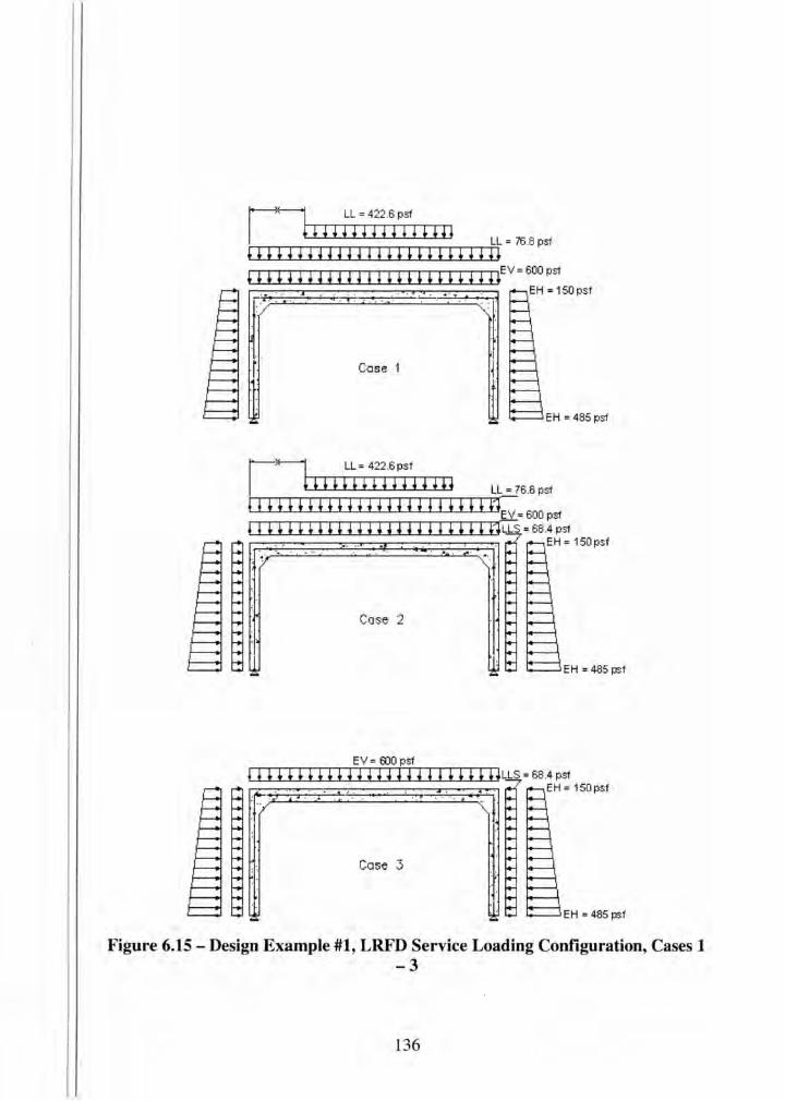
Case 1
EH = 485 psf
rlf-----J LL= 422.6psf
1 ' ' ' ' * ' ' 1 ~ 1 11 1 n Llo..:J6 .8 psf ~ ! H H t H H H H H ~ J ! 0 H nfY. = 600 pst
' + o o o o n n n o + + o o t1LLs = 68 4 psf . • EH=150psf
Case 2
EH = 485 psf
EV = 600 psf
' + o o o o n n n n + + o o OLLs = 68 4 pst EH = 150psf
~ . . . . t
Case 3
EH = 485 psf
Figure 6.15 - Design Example #1, LRFD Service Loading Configuration, Cases 1 -3
136
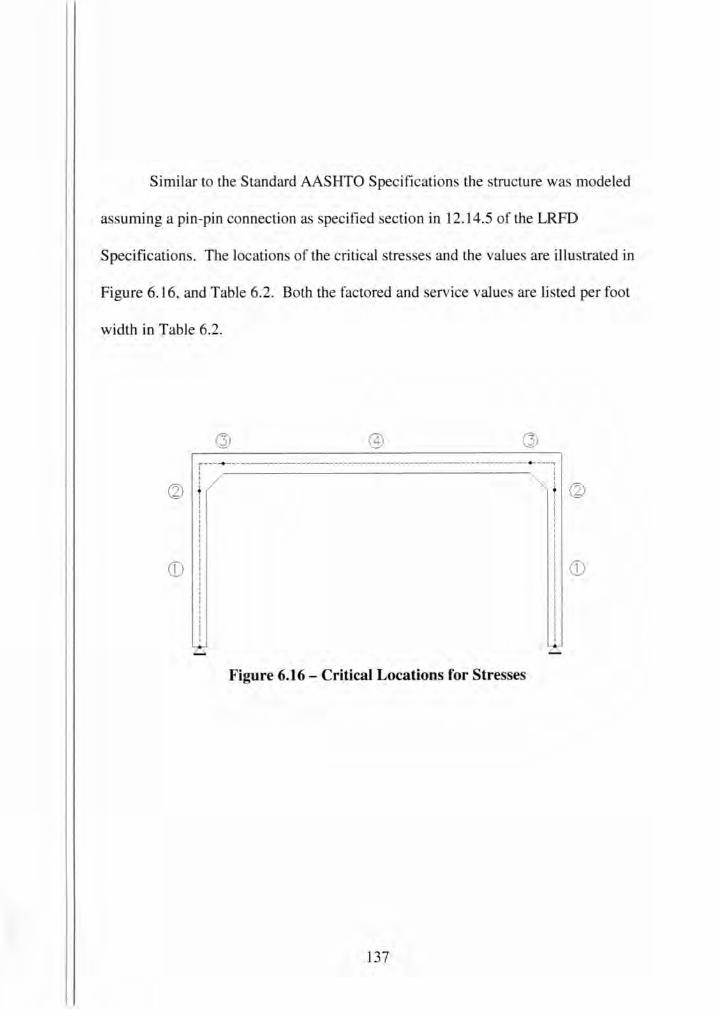
Sirrtilar to the Standard AASHTO Specifications the structure was modeled
as urrting a pin-pin connection as specified section in 12.14.5 of the LRFD
Specification . The locations of the critical stres es and the value are illustrated in
Figure 6.16, and Table 6.2. Both the factored and service values are listed per foot
width in Table 6.2.
@ ~ --- -+-------------------- ----- -------------------------------------- --------, I I I I I I
~ t t ~ I I
I I I I I I I I I I I I
~ l ®
Figure 6.16- Critical Locations for Stresses
137
I I I I I I I I I I I
:
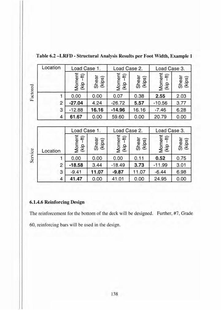
Table 6.2 -LRFD - Structural Analysis Results per Foot Width, Example 1
Location Load Case 1. Load Case 2. Load Case 3 . ....... _ ....... _ ....... _ C.t::
..... _ C.t::
..... _ c ...... ..... _ a> I ctl (/) a> I ctl (/) Q)- ctl (/)
E c.. Q) c.. E c.. Q) c.. E 6_ Q) c.. ..c ·- ..c ·- ..c ·-0 ·- Cf)6 0 ·- Cf)6 0 ·- Cf)~ ~~ ~~ ~~
1 0.00 0.00 0.07 0.38 2.55 2.03
2 -27.04 4.24 -26.72 5.57 -10.56 3.77
3 -12.88 16.16 -14.96 16.16 -7.46 6.28 4 61.67 0.00 59.60 0.00 20.79 0.00
Load Case 1. Load Case 2. Load Case 3 . ....... _ ....... _ ....... _ C.t::
..... _ c ...... ..... _ c ...... ..... _
a> I ctl (/) Q)- ctl (/) Q)- ctl (/)
Ea. Q) c.. E 6_ Q)Q. E6_ Q)Q. ..c ·- ..c ·- ..c ·-
0 ·- Cf)~ 0 ·- Cf)6 0 ·- (f)~ Location ~~ ~~ ~~
1 0.00 0.00 0.00 0.11 0.52 0.75
2 -18.58 3.44 -18.49 3.73 -11 .99 3.01
3 -9.41 11.07 -9.87 11.07 -6.44 6.98
4 41.47 0.00 41.01 0.00 24.95 0.00
6.1.4.6 Reinforcing Design
The reinforcement for the bottom of the deck will be designed. Further, #7, Grade
60, reinforcing bars will be used in the design.
138
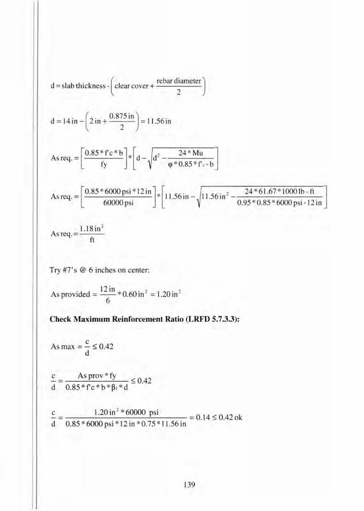
. ( rebar diameter) d =slab thickness - clear cover+ 2
d = 14in - ( 2in + 0 · 8~5 in ) = 11.56in
Asreq.=[0.85*fc * b] *[d- d2 - 24 * Mu ] fy <p * 0.85 * f c. b
As req. =[0.85 *6000psi * l2in] *[ll.56 in- l1.56 in 2 - 24 *61.67 *1000lb-ft ] 60000 psi 0.95 * 0.85 * 6000 p i · 12 in
A 1.18in2
sreq.= ft
Try #7' s @ 6 inche on center:
As provided = 12
in * 0.60 in 2 = 1.20 in 2
6
Check Maximum Reinforcement Ratio (LRFD 5.7.3.3):
c As max = - :::; 0.42
d
c = As prov * fy :::; 0.42 d 0.85 *fc * b * ~ 1 * d
c = 1.20 in 2 * 60000 psi = 0_14 :::; 0.42 ok
d 0.85 * 6000 p i * 12 in * 0.75 * 11.56 in
139

Check Minimum Reinforcement (LRFD 12.14.5.8):
As min = 0.002 * b * h
A min= 0.002 * 12 in * 14 in
A . 0.34 in 2
rrun =---ft
Check Crack Control (LRFD 12.14.5.7):
Calculate minimum allowable spacing to satisfy cracking (LRFD 5. 7.3.4):
::; 700 * y e - 2 *de A *f tJ s s
d 2. 0.875in
244.
c= m+ = . m 2
~ = 1 + de = 1 + 2.44 in = 1.30 0. 7 * (h -de) 0. 7 * (14 in- 2.44 in )
ye = exposure factor = 1.00
140
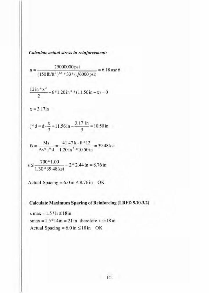
Calculate actual stress in reinforcement:
n = 29000000 psi = 6_18 use 6 (150lb/ft3 )t.5 * 33 *(~6000psi)
12 ° * 2 m x -6 *1.20in 2 * (11.56in-x) =O
2
x = 3.17in
j * d=d-~=11.56in- 3 · 17 in =10.50in 3 3
fs= Ms = 41.47k-ft *12 = 39.4Sksi As * j *d 1.20in 2 *10.50in
700 *1.00 ~ -2 * 2.44in=8.76in
1.30* 39.48 ksi
Actual Spacing= 6.0 in~ 8.76 in OK
Calculate Maximum Spacing of Reinforcing (LRFD 5.10.3.2)
s max= l.S *h ~ 18in
smax = 1.5 * 14in = 21 in therefore use 18 in
Actual Spacing= 6.0 in~ 18 in OK
141

Calculate Minimum Spacing of Reinforcing (LRFD 5.10.3.1)
min~
-db= .625in
-1.33 * Ag = 1.33 * 0. 75 in = 1.0 in
-1.0 in
Actual spacing= 6 in OK
Next the reinforcement for the top of the lab will be designed with #4, Grade 60,
reinforcing bar .
d ~ 14in -( 2in + O.S~in) ~ 11.75in
A = [0.85 * 6000 psi * 12 in]* [11 .75 in_ 11 .75 in 2 _ 24 * 14.96 * 1000 lb- ft ] 60000 psi 0.95 * 0.85 * 6000 psi •12 in
A 0.27 in 2
s req.= ft
Try #4' s @ 3 inches on center:
. d 12 in * 0 196. 2 0 78. 2 As provtde = -- . m = . m 3
142

Check Maximum Reinforcement Ratio (LRFD 5.7.3.3):
c 0.78 in 2 * 60000 psi = = 0.09 $ 0.42 ok d 0.85 * 6000 psi * 12 in* 0.75 * 11.75 in
Check Minimum Reinforcement (LRFD 12.14.5.8):
A min= 0.002 * 12 in * 14 in
A . 0.34 in 2
srru n = ---ft
Check Crack Control (LRFD 12.14.5.7):
Calculate minimum allowable spacing to satisfy cracking (LRFD 5. 7.3.4):
700 * 'Y e s $ 2*dc
~ s* f
d 2 . 0.50 in
2 25 .
c= m+ = . m 2
~ = 1 + de = 1 + 2.25 in = 1.27 s 0.7 *(h-dc) 0.7 *(14 in-2.25in)
ye = exposure factor= 1.00
143
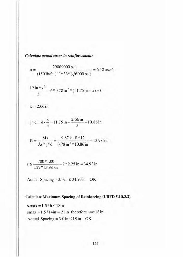
Calculate actual stress in reinforcement:
n = 29000000 psi = 6_18 use 6 (150lb/ft 3 ) 1.5 * 33 *(~6000p i)
12 . :1< 2
m . x -6 *0.78in 2 * (11.75in-x) =O 2
x = 2.66in
· * d x 1 75 · 2·66 in 0 86 · J =d--=1 . m- =1 . m 3 3
fs = M = 9.87 k2 -ft *12 = 13.98 ksi As * j *d 0.78in *10.86in
700 *1.00 s :s; - 2 * 2.25in =34.93in
1.27 * 13.98 ksi
Actual Spacing = 3.0 in ::;; 34.93 in OK
Calculate Maximum Spacing of Reinforcing (LRFD 5.10.3.2)
s max = 1.5 * h ::;; 18in
max= 1.5 *14in = 21 in therefore use 18 in
Actual Spacing= 3.0 in ::;; 18 in OK
144

Calculate Minimum Spacing of Reinforcing (LRFD 5.10.3.1)
smin ~
-db= .625in
-1 .33 * Ag = 1.33 * 0.75 in = 1.0 in
-1.0 in
Actual spacing = 3 in OK
The outside reinforcement for the walls will include #4, Grade 60, reinforcing bars.
d =JOin-( 2in + O.S~in ) = 7.75in
·As= [0.85 * 6000psi * 12 in] * [ 7_75 in_ 7_75 in 2 _ 24 * 27.04 * 1000 lb- ft ] 60000psi 0.95 *0.85*6000psi •12in
A 0.77 in 2
s req.=---ft
Try #4's @ 3 inches on center:
As provided= 12
in *0.196in 2 = 0.78in 2
3
Check Maximum Reinforcement Ratio (LRFD 5.7.3.3):
c = 0.78 in2
*60000 psi = O.l3 $0.42 d 0.85 * 6000 psi * 12 in * 0.75 * 7.75 in
145

Check Minimum Reinforcement (LRFD 12.14.5.8):
Asmin = 0.002 * 12 in * 10 in
0 ?4. 2
A . ·- Jn srrun =---ft
Check Crack Control (LRFD 12.14.5.7):
Calculate minimum allowable spacing to satisfy cracking (LRFD 5.7.3.4):
700 *y S ~ e -2 *de
~ s * f
d 2. 0.50 in
2 25.
c= m+ = . m 2
~ s = 1 + de = 1 + . 2 .. 25 in . = 1.41 0.7 * (h -de) 0.7 * (10m- 2.25 m)
ye = exposure factor = 1.00
146
Calculate actual stress in reinforcement:
n = 29000000p i = 6.18 use 6 (150 lb/ft 3 ) 1.s * 33 * ( .J6000 psi)
12in*x 2
6 *0.78in 2 *(7.75in-x)= O 2
x = 2.10in
· * d - d x - 7 75 · 2·1 0 in - 7 05 · J - --- . m- - . m 3 3
fs= M = 18.58k-ft *12 = 40.54 ksi As * j *d 0.78in 2 *7.05in
700 *1.00 s~ 2*2.25in=7.74in
1.41 * 40.54 ksi
Actual Spacing= 3.00 in ~ 7.74 in OK
Calculate Maximum Spacing of Reinforcing (LRFD 5.10.3.2)
s max= 1.5 *h ~ 18in
max= 1.5 *14in = 21 in therefore u e 18 in
Actual Spacing= 6.0in ~ 18in OK
147

Calculate Minimum Spacing of Reinforcing (LRFD 5.10.3.1 )
s min;::::
-db= .625in
-1.33 * Ag = 1.33 * 0.75 in= 1.0 in
- 1.0 in
Actual spacing= 6 in OK
The reinforcement on the inside of the walls will be designed using #4, Grade 60,
reinforcing bars.
d =JOin- ( 2in + O.S~in) = 7.75 in
As= [0.85 * 6000psi * 12 in] *[7.75 in_ 7.75 in 2 _ 24 * 2.55 * 1000 lb- ft ] 60000p i 0.95 *0.85 * 6000psi • 12in
A 0.07in 2
s req.= ft
Try #4 's @ 12 inches on center:
As provided= 12
in * 0.196 in 2 = 0.196 in 2
12
148

Check Maximum Reinforcement Ratio (LRFD 5.7.3.3):
e 0.196in 2 * 60000 psi = = 0.03 :5 0.42
d 0.85 * 6000 psi * 12 in * 0.75 * 7.75 in
Check Minimum Reinforcement (LRFD 12.14.5.8):
Asntin = 0.002 * 12 in * 10 in
0 ?4 . 2
A . ·-In snun=---
ft
Check Crack Control (LRFD 12.14.5.7):
Calculate minimum allowable spacing to satisfy cracking (LRFD 5. 7.3.4):
700 *y S $; e 2 *de
~ s* f
d 2. 0.50 in
2 25.
e= m+ = . m 2
~ = 1+ de = 1+ 2.25in =1.41 s 0.7 * (h-de) 0.7 *(10in-2.25in)
ye = exposure factor = 1.00
149
Calculate actual stress in reinforcement:
n = 29000000 psi = 6.18 use 6 (150 lb/ft3)1.5 * 33 * (~6000 psi)
12. * 2
m x -6 * 0.196in 2 *(7.75in-x) =0 2
x=l.14in
· * d - d x - 7 75 · 1. 14 in - 7 37 · J - --- . m - - . m 3 3
Ms 0.52k-ft *l2 fs = = = 4.32 ksi
As * j * d 0.196in 2 *7.37in
s ~ 700 * l.OO -2 * 2.25in = 110.42in 1.41 * 4.32 ksi
Actual Spacing = 6.0 in ~ II 0.42 in OK
Calculate Maximum Spacing of Reinforcing (LRFD 5.10.3.2)
max = 1.5 * h ~ 18in
smax = 1.5 * 14in = 21 in therefore use 18 in
Actual Spacing= 6.0 in~ 18 in OK
150
Calculate Minimum Spacing of Reinforcing (LRFD 5.10.3.1)
min~
-db= .625 in
-1.33 * Ag = 1.33 * 0.75 in= 1.0 in
-1.0 in
Actual spacing = 9 in 0 K
6.1.4.7 Calculate shear (LRFD 5.8.3.3):
The allowable hear in the three-sided structure i calculated using the implified
equation.
Shear in the Deck:
· eve~Vu
Vu = 16.16 kips
eve= e *p *Fc * b *dv
dv = maximum vulue of
0.9 *d or 0.72 * h
0.9 *de= 0.9 * 11.56 = 10.40
0.72 * h = 0.72 *14 = 10.08
eve= 0.90 * 2 * ~6000 psi * 12 in *10.40 in= 17400.51b = 17.40 kip
=17.40kips>16.16k.ip OK
151
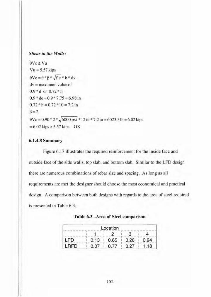
Shear in the Walls:
eVc:2:: Vu
Vu = 5.57 ldps
ev c = e * p * .Jh * b * dv
dv = maximum vulue of
0.9 * d or 0.72 * h
0.9 * de=0.9 * 7.75 = 6.98in
0.72 * h = 0.72 * 10 = 7.2in
P= 2
eve= 0.90 * 2 * ~6000 psi * 12 in * 7.2 in= 6023.3Ib = 6.02ldps
= 6.02ldps > 5.57 ldps OK
6.1.4.8 Summary
Figure 6.17 illu trates the required reinforcement for the inside face and
outside face of the side walls, top slab, and bottom slab. Similar to the LFD design
there are numerous combinations of rebar size and spacing. As long as all
requirements are met the designer should choose the most economical and practical
design. A comparison between both designs with regards to the area of steel required
is presented in Table 6.3.
Table 6.3 -Area of Steel comparison
Location --------------- ---------------------- ----------- -----------
1 : 2 3 4 -LFo ________ -·a.-13·--:---<i65 -- ---6~28 -- -- o:94 __ _ ----- -- ----- --- ---- - - ----~----------- ----------- -----------LRFD 0.07 : 0.77 0.27 1.18
152
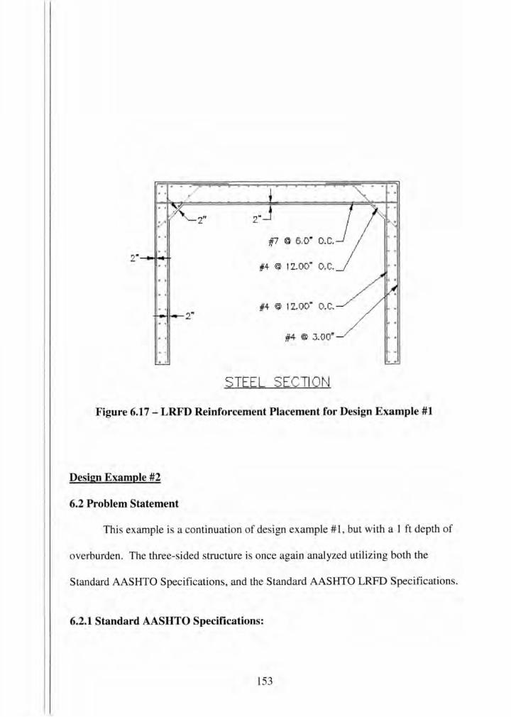
..
#7 @ 6 .0~ D.C.
I+ @ 1 2.00M o.c.
I+ @ 12.00M o.c.
#4 @ 3.00"
STEEL SECTION
Figure 6.17 - LRFD Reinforcement Placement for Design Example #1
Design Example #2
6.2 Problem Statement
This example i a continuation of de ign example# 1, but with a 1 ft depth of
overburden. The three- ided structure is once again analyzed utilizing both the
Standard AASHTO Specifications, and the Standard AASHTO LRFD Specifications.
6.2.1 Standard AASHTO Specifications:
153

6.2.1.1 Vertical and Horizontal Earth Pressures:
The design vertical earth pressure on the top of the culvert is calculated as:
WuSL = ys * Z
WuSL = (120 pcf) * (1.0 ft) = 120 psf
The lateral earth pressure (EH) on the culvert is found using the equivalent
fluid method. Section 6.2.1 in the Standard AASHTO Specifications requires a
minimum and maximum equivalent fluid pressure of 30 pcf and 60 pcf respectively.
At the top of the culvert, the lateral earth pressures are calculated as:
EH = EFP*Z
EHMJN = (30 pcf) * ( 1.0 ft) = 30 psf
EHMAX = (60 pcf) * (1.0 ft) = 60 psf
At the bottom of the culvert, the lateral earth pressures are calculated as :
14 EHMIN = (30 pcf) * (1.0 ft +
12 ft +10ft) = 365 psf
14 EHMAX = (60 pcf) * (1.0 ft +- ft +10ft)= 730 psf
12 Figure 6.18 illustrates the vertical and the min and max lateral earth pressures
applied to the three-sided structure.
154
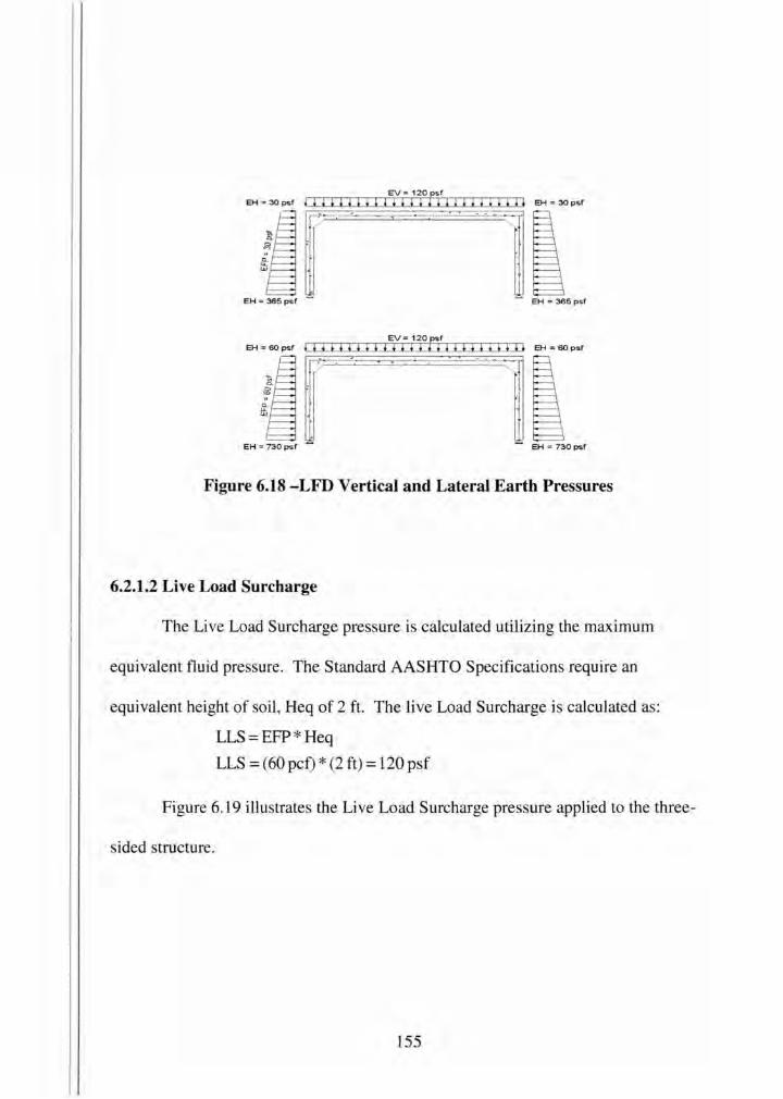
EVz 120psf
EH = 30 psf j t t t l l t t I l t t l t l t I l t l t I I t l t EH = 30 psf 1r - ~-- - . 1 EH = 365 psf EH = 365 psf
EV = 120psf EH=60psf I I 0 0 0 tl 0 I I 0 lit 0 II O t EH=60psr 1r · ~ ,
EH = 730 psf EH = 730 psf
Figure 6.18 -LFD Vertical and Lateral Earth Pressures
6.2.1.2 Live Load Surcharge
The Live Load Surcharge pressure is calculated utilizing the maximum
equivalent fluid pressure. The Standard AASHTO Specifications require an
equivalent height of soil, Heq of 2ft. The live Load Surcharge is calculated as:
LLS = EFP * Heq
LLS = (60 pet)* (2ft) = 120 psf
Figure 6.19 illustrates the Live Load Surcharge pressure applied to the three-
sided structure.
155
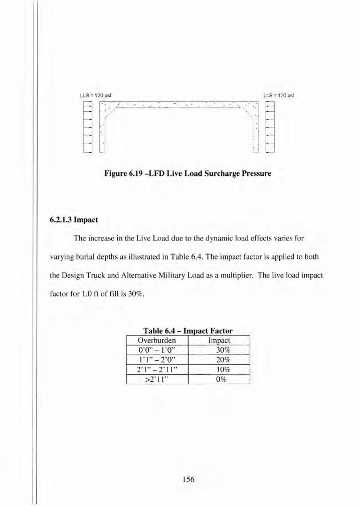
LLS = 120 psf LLS = 120 psf
. ~ . ..
Figure 6.19 -LFD Live Load Surcharge Pressure
6.2.1.3 Impact
The increase in the Live Load due to the dynamic load effects varies for
varying burial depths as illustrated in Table 6.4. The impact factor is applied to both
the Design Truck and Alternative Military Load as a multiplier. The live load impact
factor for 1.0 ft of fill is 30%.
T bl 6 4 I a e . - mpac tF t ac or Overburden Impact 0'0"- 1 '0" 30% 1 ' 1" - 2 '0" 20%
2' 1"-2'11" 10% >2 ' 11" 0%
156
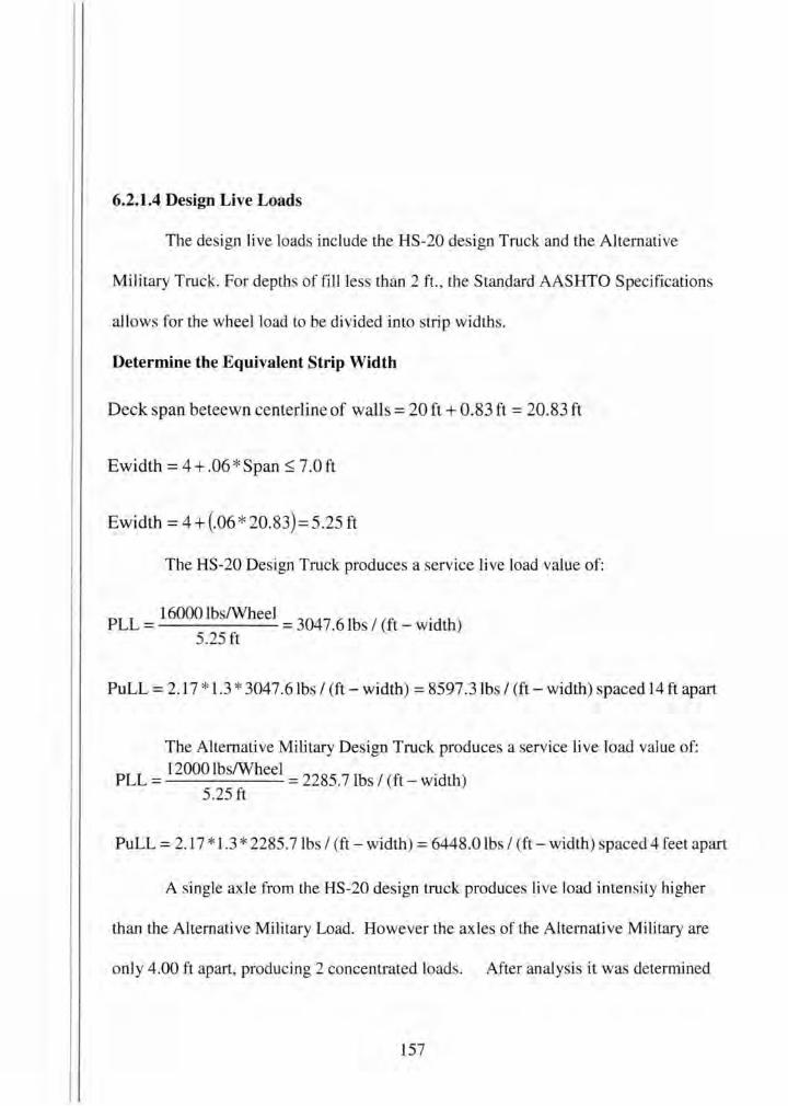
6.2.1.4 Design Live Loads
The de ign live loads include the HS-20 design Truck and the Alternative
Military Truck. For depth of fill less than 2ft., the Standard AASHTO Specifications
allows for the wheel load to be divided into strip widths.
Determine the Equivalent Strip Width
Deck span beteewn centerline of walls= 20ft+ 0.83 ft = 20.83 ft
Ewidth = 4+ .06 *Span::; 7.0ft
Ewidth = 4 + (.06 * 20.83 )= 5.25 ft
The HS-20 Design Truck produces a service live load value of:
PLL = 16000 lb !Wheel= 3047.6lbs I (ft- width) 5.25 ft
PuLL= 2.17 * 1.3 * 3047.6lbs I (ft- width)= 8597 .3lbs I (ft- width) spaced 14ft apart
The Alternative Military Design Truck produces a service live load value of:
PLL = 12000 lbs/Wheel = 2285.7lbs I (ft- width) 5.25 ft
PuLL= 2.17 * 1.3 * 2285.7 lbs I (ft - width)= 6448.0 lbs I (ft- width) spaced 4 feet apart
A single axle from the HS-20 design truck produces live load intensity higher
than the Alternative Military Load. However the axle of the Alternative Military are
only 4.00 ft apart, producing 2 concentrated loads. After analysis it was determined
157

that the Alternative Military load controls the design. Use the Alternative Military to
design for the strength and limit states.
6.2.1.5 Load combinations:
For both the strength and service limit states, three load cases are considered. The
load cases are as follows. The loading configurations are illustrated in Figure 6.20.
The load cases correspond to:
• Case 1: Maximum vertical loads on deck, minimum lateral loads on legs.
This case produces maximum stresses in the bottom of the deck.
• Case 2: Maximum vertical and horizontal loads on the structure. The case
produces maximum stresses on the corner of the deck, and outside walls.
• Case 3: Minimum vertical loads on deck, and maximum horizontal loads on
walls. This ca e produces maximum stres es on the inside of the leg.
The load combinations are as follows:
Strength: 1. u = 1.3 * DL + 1.3 * EV + 1.3 * ERMIN + 2.17 * (LL + IM)
2. U = 1.3*DL+l.3 *EV +1.3 * EHMAX +2.17*(LL+IM)
3. u = 1.3 * DL+ 1.3 * EV + 1.3 * EHMAX
158
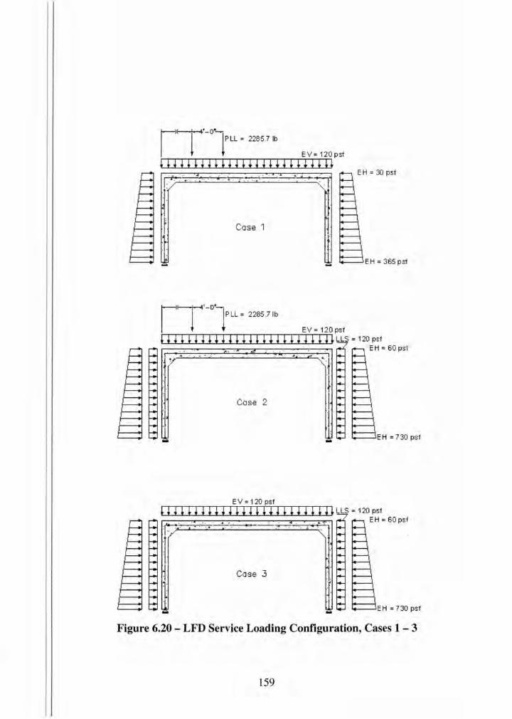
~~·-o•-lP LL = 2285.71b
I ~ EV= 120 psf
',.I' 'I J ''I J '*J J t+I t t+I t 0 - ~ - ~ :~ ·
Case 1
EH = 365 psf
~~·-o·-lPLL = 2285.7 1b
I J EV= 120psf
0 I t 0 0 U J 0 I t 0 J t 0 I t 0 l L LS = 120 psf ., ~ .
• ::i:q . ... . -EH=60psf
Case 2
EH = 730 psf
EV = 120 psf
0 I t 0 I t u J 0 0 0 J t 0 I t t n L LS = 120 psf . ' · " ,. . . : ' . .. -.~--~ -- - ·
EH=60psf
Case 3
EH = 730 psf
Figure 6.20 - LFD Service Loading Configuration, Cases 1 - 3
159
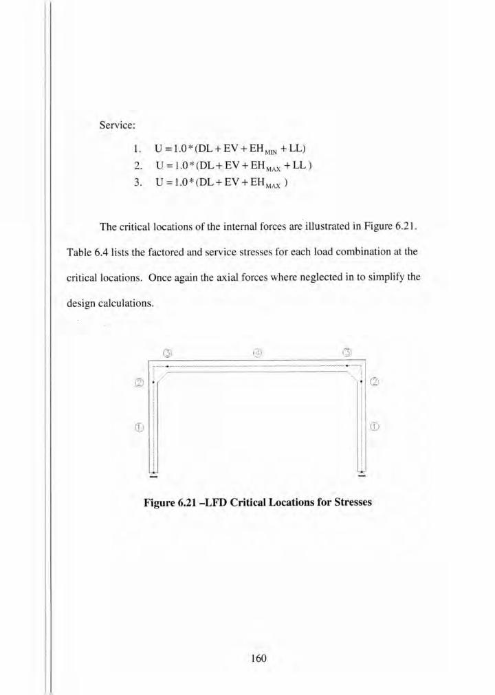
Service:
1. u = 1.0 * (DL + EV + EH MIN + LL)
2. U = l.O *(DL+ EV +EHMAX + LL)
3. u = 1.0 * (DL+ EV + EHMAX)
The critical locations of the internal forces are illustrated in Figure 6.21.
Table 6.4 lists the factored and service stresses for each load combination at the
critical locations. Once again the axial forces where neglected in to simplify the
design calculations .
..----- ------------------------------------------ ---------------·----., ' ' ' ' ' '
:I ·: ! ! '-
Figure 6.21 -LFD Critical Locations for Stresses
160
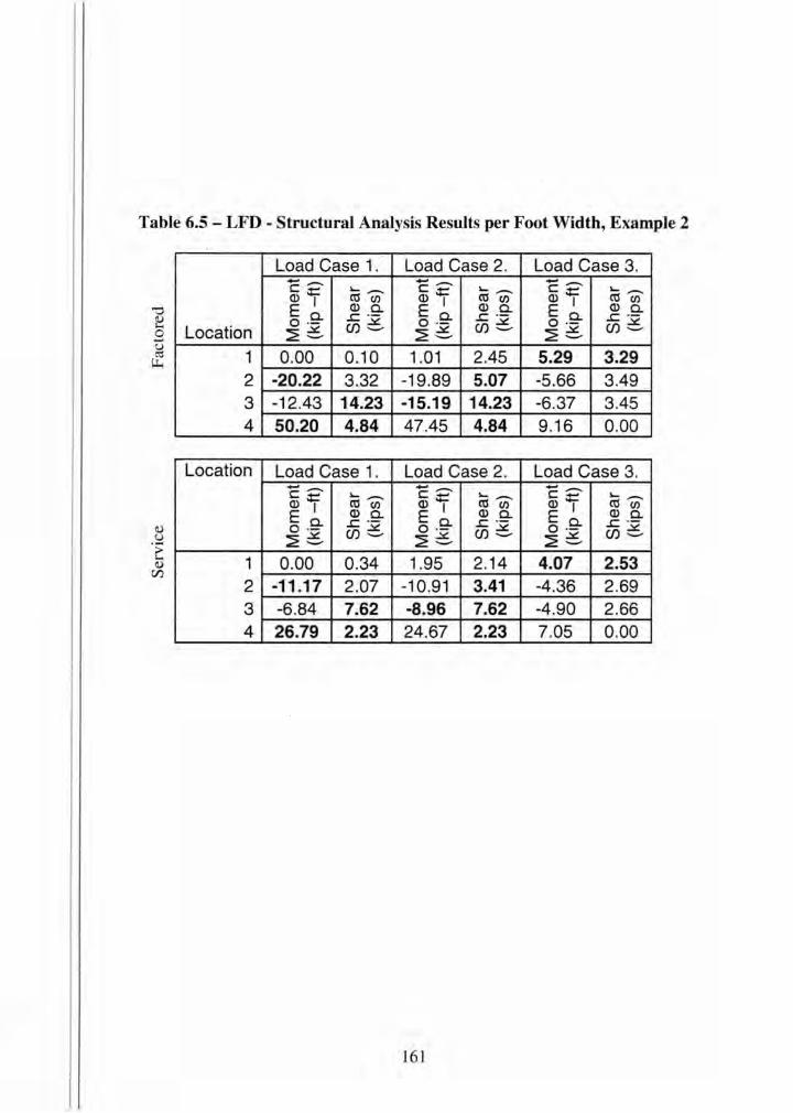
Table 6.5 - LFD - Structural Analysis Results per Foot Width, Example 2
Load Case 1. Load Case 2. Load Case 3. -- -- --c- ..... _ c- ..... _ C.t::
..... _ Q)- ctl (/) Q)- ctl (/) Q) I ctl (/) E~ Q)Q. E~ Q) Cl. E o. Q)Q.
..c ·- ..c ·- ..c ·-Location
0 ·- ({)6 0 ·- ({)6 0 ·- ({)6 ~6 ~6 ~6
1 0.00 0.10 1.01 2.45 5.29 3.29 2 -20.22 3.32 -19.89 5.07 -5.66 3.49 3 -12.43 14.23 -15.19 14.23 -6 .37 3.45 4 50.20 4.84 47.45 4.84 9.16 0.00
Location Load Case 1. Load Case 2 . Load Case 3. -- -- ...... _ c ...... ..... _ c-
..... _ c ...... ....._
Q)- ctl (/) Q)- ctl (/) IDI ctl (/)
E ~ Q)Q. E ~ Q)Q. E o. Q) Cl. ..c ·- ..c ·- ..c ·-
0 ·- ({)6 0 ·- ({)6 0 ·- ({)6 ~6 ~6 ~6
1 0.00 0.34 1.95 2.14 4.07 2.53 2 -11.17 2.07 -10.91 3.41 -4.36 2.69 3 -6.84 7.62 -8.96 7.62 -4.90 2.66 4 26.79 2.23 24.67 2.23 7.05 0.00
161

6.2.1.6 Reinforcing De ign
The bottom reinforcement for the slab will be designed with #5, Grade 60, reinforcing
bars.
. ( rebar diameter ) d = lab th1ckne s- clear cover+ 2
d = 14in - ( 2in + 0 ·6~5 in )= I 1.69in
As req.=[0.85 *fc*b] *[ d- d2 - 24 * Mu ] fy <p * 0.85 * f c . b
As req. = [0.85 * 6000 psi * 12in] * [11.69 in_ 11.69 in 2 _ 24 * 50.20 * 1000 lb- ft ] 60000 psi 0.95 * 0.85 * 6000 p i • 12 in
A 0.94in 2
sreq.=--ft
162
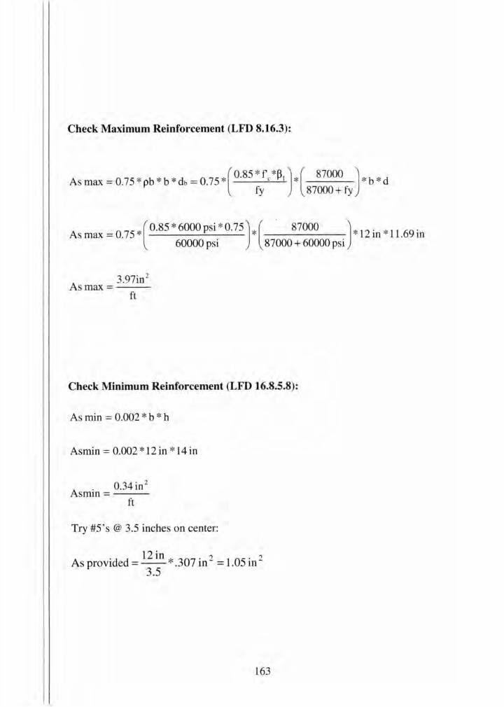
Check Maximum Reinforcement (LFD 8.16.3):
A max=0.75 *pb * b *db=0.75 *(0
·85
*f c*P1)*( 87000
)* b * d fy 87000+ fy
Asmax=0.75 *(0.85 * 6000psi *0.75 )* ( . 87000 )* 12in *11.69in 60000 psi 87000 + 60000 psi
A 3.97in 2
s max=---ft
Check Minimum Reinforcement (LFD 16.8.5.8):
As min = 0.002 * b * h
Asmin = 0.002 * 12 in * 14 in
A . 0.34 in 2
srrun =---ft
Try #S 's @ 3.5 inches on center:
As provided= 12
in * .307 in 2 = 1.05 in 2
3.5
163

Check Crack Control (LFD 16.8.5.7):
Calculate Allowable Stress, fsa:
f f 98 ksi
s:::; sa=--=== Vdc * A
d 1 rebar diameter
2. 0.625 in
2 31.
c = c ear cover + = m + = . m 2 2
A= 2 *dc * b =2 *2.31 *12in=l6.17 Number of bars, N 12
3.5
fsa = 98 ksi = 29.31 ksi V2.31in *l6.17
Calculate actual stress in reinforcement:
Es 29000000psi n ---___ ____;:;...___ - Ec- wcl.5 *33*Fc
n= 29000000psi = 6.18 use 6 (150 lb/ft3 )1.5 * 33 * (~6000 psi)
164

b * x *( ; ) = (n *As prov.)*(d - x)
b * X 2
---n *As prov. *(d- x) = 0 2
12 in * x2
2
x = 3.02 in
6 *1.05 in 2 *( 11.69 in- x) = 0
j * d = d-~=ll.69in 3·02
in =10.68in 3 3
Ms 26.79k-ft *12 fs = As* J.* d = 2 = 28.67 ksi ~ 30.86 ksi ok
1.05 in * 10.68 in
The top reinforcement in the deck is designed using #4, Grade 60, reinforcing bars.
d = 14in - ( 2in + O.S~in) = 11.75in
As = [0.85 * 6000psi * 12 in] * [11.75 in_ 11.75 in2 _ 24 *15.15.19 * 100~ lb- ~t ]
60000psi 0.95 *0.85 *6000ps1* 12m
A 0.28in 2
s req.= ft
165

Check Maximum Reinforcement (LFD 8.16.3):
As max = 0.75 * (0.85 * 6000 psi * 0.75 ] * ( 87000 J * 12 in * 11.75 in 60000 psi 87000 + 60000 psi
A 3.99in 2
smax= ---ft
Check Minimum Reinforcement (LFD 16.8.5.8):
A min = 0. 002 * 12 in * 14 in
A . 0.34in 2
smm= ft
Try #4 's @ 3.5 inches on center:
A provided= 12
in * .196 in 2 = 0.67 in 2
3.5
Check Crack Control (LFD 16.8.5.7):
Calculate Allowable Stress, fsa:
f < f 98 ksi
s_ sa=-::r:::.== Vctc *A
d 2. 0.50 in
2 25.
c = m + = . In 2
166

A= 2 * 2.2152*12 in = 15.75
3.5
fsa = 98 ksi = 29.84 ks V2.25in *15.75
Calculate actual stress in reinforcement:
n = 29000000 psi = 6.1 8 use 6 (150 lb/ft 3 l 5 * 33 * (~6000 psi)
12 in*x2
-6 *0.67in 2 *(1 1.75in-x)=O 2
x = 2.50 in
.* d d x . 2.50in 10 92. J = --=11.75tn---= . tn 3 3
fs = Ms = 8 ·96 ~-ft * l 2 = 14.69ksi~29.84 ksi ok As * j *d 0.67in *10.92in
167

The outside reinforcement in the walls is designed using #4, Grade 60, reinforcing bars.
d 10· . ( 2 . 0.50in ) 7 75 . = In- In+-- = . 10 2
Asreq . =[0.85 *6000psi * l2 in] *[7.75 in- 7_75 in 2 _ 24 *20.22 *10001b-ft l 60000psi 0.95 *0.85 *6000psi • l2in
A 0.57 in 2
s req.= ft
Check Maximum Reinforcement (LFD 8.16.3):
As max =0.75 *(0.85 *6000psi *0.75) *( 87000 ) *12in *7.75in 60000 psi 87000 + 60000 psi
A 2.63 in 2
smax=---ft
Check Minimum Reinforcement (LFD 16.8.5.8):
Asmin = 0.002 * 12 in * 10 in
A . 0.24in 2
smm= ---ft
Try #4 ' s @ 3.5 inches on center:
As provided = 12 in * .196 in 2 = 0.67 in 2
3.5
168

Check Crack Control (LFD 16.8.5.7):
Calculate Allowable Stress, fsa:
f < f 98 k i
s _ sa=-=== 'J./dc * A
d 2. 0.50 in
2 25.
c= m+ = . m 2
A= 2*2.25 * 12in =] 5_75 12
3.5
fsa = 98 ksi = 29.84 ksi 'J./2.25 in * 15.75
Calculate actual stress in reinforcement:
n = 29000000 psi = 6_18 use 6 (150 lb/ft3 )1.5 * 33 * (~6000 p i)
12 in*x2
-6 *0.67in 2 * (7.75in-x)= O 2
x = 1.97 in
169

· * d - d x - 7 75 · 1.97 in - 7 12 · J - --- . In---- . In 3 3
Ms fs =---
As* j * d
11.17k- ft * l2 2
= 28.09 ksi ~ 29.84 ksi ok 0.67 in * 7.12 in
The inside reinforcement in the walls will be designed using #4, Grade 60,
reinforcing bars.
d = 10 in- ( 2 in+ 0 ·5~in ) = 7.75 in
As req. = [0.85 * 6000 psi * 12 in] * [7.75 in_ 7.75 in 2 _ 24 * 5.29 *1 000 lb - ft ] 60000 psi 0.95 * 0.85 * 6000 psi * 12 in
A 0.15in 2
s req.=--ft
Check Maximum Reinforcement (LFD 8.16.3):
As max = 0.75 * (0.85 * 6000 psi * 0.75 ] * ( 87000 J * 12 in * 7.75 in 60000 psi 87000 + 60000 psi
A 2.63in 2
smax=---ft
170

Check Minimum Reinforcement (LFD 16.8.5.8):
A min = 0. 002 * 12 in * 10 in
0 ?4 . 2
A . ·- In min=---ft
Try #4's @ 7 inches on center:
A provided= 12
in *.196in 2 = 0.34in 2
7
Check Crack Control (LFD 16.8.5.7):
Calculate Allowable Stress, fsa:
f ~ fsa = 98 k i 'Vdc * A
d 2. 0.50 in
2 25.
c= m+ = . m 2
A= 2*2.25*12in = 31.50 l2
7
f a= 98 ksi = 23 .68 ksi V2.25 in * 3I.5o
171

Calculate actual stress in reinforcement:
n = 29000000 psi = 6.18 use 6 (1501b/ft3 l 5 *33*(~6000ps i)
12 . * 2 m · x -6 * 0.34in 2 *(7.75in-x)= O
2
x = 1.46 in
· * d - d ~ - 7 75 · - l.46 in - 7 26 · J- - -. m - . m 3 3
fs= Ms = 4 ·07 k-ft * l 2 =19.79ksi~23 .68ksi ok As * j * d 0 .34 in 2 * 7.26 in
6.2.1.7 Calculate shear (LFD 8.16.6.2)
The allowable hear in the three-sided structure is calculated using the simplified
equation.
Shear in the Deck:
eve~ Vu
Vu = 14.23 kip
eve= e * 2 * Jfc, * b * d
eve= 0.90 * 2 * ~6000 p i * 12 in * 11.75 in = 19659.26lb = 19.65 kips
= 19.65 kips> 14.23 kip OK
172
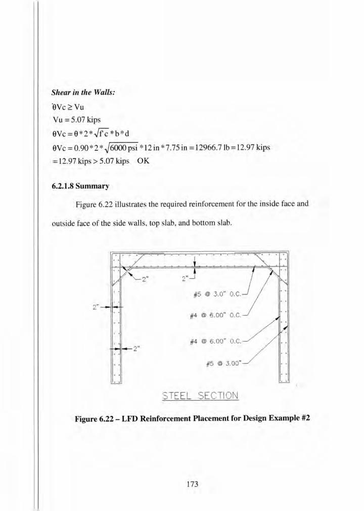
Shear in the Walls:
·evc~Vu
Vu = 5.07 kips
eve= e *2 *Fc *b *d
eve= 0.90 *2 * ~6000 psi *12 in *7.75 in= 12966.7lb = 12.97 kips
= 12.97 kip > 5.07 kips OK
6.2.1.8 Summary
Figure 6.22 illustrates the required reinforcement for the inside face and
outside face of the side walls, top slab, and bottom slab.
2"
#5 @ 3.0" o.c.
2" #4 @ 6.00" O.C.
#4 @ 6.00" O.C. *-1~ 2"
STEE L SECTION
Figure 6.22 - LFD Reinforcement Placement for Design Example #2
173

6.2.2 Standard LRFD Specifications
6.2.2.1 Vertical and Horizontal Earth Pressures:
The design vertical earth pressure on the top of the culvert is calculated as :
WuSL = ys * Z
WuSL = (120 pcf) * (1.0 ft) = 120 psf
Similar to the Standard AASHTO Specifications, the lateral earth pressure
(EH) on the culvert i found using the equivalent fluid method. However, the LRFD
Specifications does not pecify minimum and maximum equivalent fluid pressure.
This is taken into account in the load factors, and loading combinations. An
equivalent fluid pressure of 30 pcf is assumed.
At the top of the culvert, the lateral earth pressure is calculated as:
EH =EFP * Z
EH = (30 pcf) * (1ft) = 30 psf
At the bottom of the culvert, the lateral earth pressure is calculated as:
14 EH = (30 pcf) *(1ft+- ft +10ft)= 365 psf
12
Figure 6.23 illu trates the vertical and lateral earth pressures applied to the three-sided structure.
174
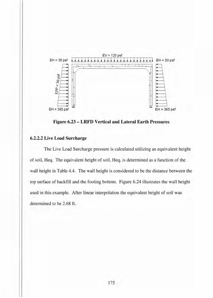
EV = 120 psf
EH = 30 psf ~ l l l l I I I I l I I I I I I l I I I l I I I Il EH = 30 psf
EH = 365 psf
7.----~-~-------.~-;~-~-~-:--~:-L.-~--....-l . :
EH = 365 psf
Figure 6.23 - LRFD Vertical and Lateral Earth Pressures
6.2.2.2 Live Load Surcharge
The Live Load Surcharge pressure is calculated utilizing an equivalent height
of oil, Heq. The equivalent height of soi l, Heq, is determined as a function of the
wall height in Table 4.4. The wall height is considered to be the distance between the
top surface of backfill and the footing bottom. Figure 6.24 illustrates the wall height
used in this example. After linear interpolation the equivalent height of soil was
determined to be 2.68 ft.
175
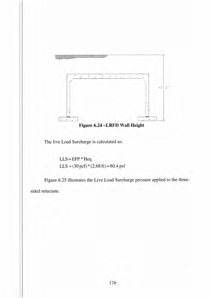
13'- 2"
I • .. I r
Figure 6.24 -LRFD Wall Height
The live Load Surcharge is calculated as:
LLS = EFP * Heq
LLS = (30 pcf) * (2.68 ft) = 80.4 p f
Figure 6.25 illustrate the Live Load Surcharge pressure applied to the three-
sided structure.
176
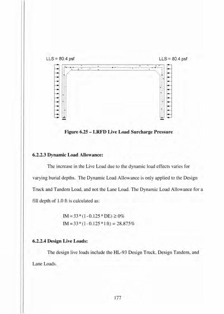
LLS = 80.4 psf LLS = 80.4 psf
~4-- .... -----.------=----~--------... ---------q-7'~------.--•- :.. --, . I e1 43 4 .a · • 1
i . 1 . t ' I 1 l l I , I I
I 1. I I I • I
~ i I .I I . I
~ ~ i~ " I I I I
I I · I , ~ I
i I I I
Figure 6.25 - LRFD Live Load Surcharge Pressure
6.2.2.3 Dynamic Load Allowance:
The increa e in the Live Load due to the dynamic load effect vane for
varying burial depths. The Dynamic Load Allowance is only applied to the Design
Truck and Tandem Load, and not the Lane Load. The Dynamic Load Allowance for a
fill depth of 1.0 ft is calculated as:
1M =33 * (1- 0.125 * DE) ~ 0%
1M= 33 * (1- 0.125 *1ft) = 28.875%
6.2.2.4 Design Live Loads:
The design live loads include the HL-93 Design Truck, Design Tandem, and
Lane Loads.
177
Similar to the Standard AASHTO Specifications, the Standard LRFD
Specifications allows for the live load to be divided into strip widths. However the
LRFD Specifications require that the axle is distributed over a distribution width E in
instead of a line of wheels.
Determine the Equivalent Strip Width:
Deck span betewwn centerline of walls= 20ft+ 0.83 ft = 20.83 ft
Ewidth = 8 + 0.12 *Span
Ewidth = 8+ (0.12 * 20.83)=10.5 ft
The Design Truck produces a live load value of:
PLL = 32000 lbsiAxle = 3047.6lbs I (ft- width) 10.5 ft
PuLL= 1.75 * 1.29 * 3047.6lb I (ft- width)= 6880 lbs I (ft- width)
The Standard LRFD Specifications also take into account the tire contact area and the
distribution of the tire through any earth fill. The load can then be converted from a
point load to a patch load. The length of the patch load is calculated as:
Espan = Lt + LLDF *(H)
Espan = 0.83FT + 1.15 * l.Oft z 2.0ft
178
The Design Truck produces a live load pressure of:
Wull = PuLL Espan
Wull = 6880lb I (ft- width) = 3440 psf 2ft
The Design Tandem produces a live load value of:
PLL = 25000 lb I Axle = 2381.0 lbs I (ft- width) 10.5 ft
PuLL= 1.75 * 1.29 * 2381lbs I (ft- width)= 5375.0 lbs I (ft- width)
The Design Tandem produces a live load pressure of:
Wull =PuLL Epan
Wull = 5375.0 lb I (ft- width) = 2687 .5 p f 2ft
The Lane Load produces a live load pressure of:
WuLL = 640 plf * MPF = 64psf * MPF 10ft
The Single Design Truck produces the maximum live load intensity; however
the Single De ign Tandem has a larger influence area. After analysis it was
179
determined the Single Design Tandem controlled the design. Therefore the Lane
Load produce a live load pressure of:
WuLL = 640 plf * 1.
2 = 64 psf * 1.2 = 76.8 psf 10ft
6.2.2.5 Load combinations:
For both the strength and service limit states, three load cases are considered. The
load cases are as follow . The loading configurations are illustrated in Figure 6.26.
The load cases correspond to:
• Case 1: Maximum vertical loads on deck, minimum lateral loads on legs.
Thi case produces maximum stresses in the bottom of the deck.
• Case 2: Maximum vertical and horizontal loads on the structure. The case
produces maximum stresses on the comer of the deck, and outside walls.
• Case 3: Minimum vertical loads on deck, and maximum horizontal loads on
walls. This case produces maximum stresses on the inside of the leg.
The load combination are as follows:
Strength: 1. U = 1.25 * DC+ 1.30 * EV + 0.90*EH + 1.75 * (LL+ IM)
2. U = 1.25 * DC+l.30 *EV +1.50 * EH+l.75 * LS+l.75 * (LL+IM)
3. U = 0.90 * DC+ 0.90 * EV + 1.50 * EH + 1.75 * LS
180

Service: 1. U=l.OO*(DC+EV+EH+(LL+IM))
2. U = 1.00 *(DC+ EV + EH + LS + (LL + IM) )
3. U = 1.00 *(DC+ EV + EH + LS)
Similar to the Standard AASHTO Specifications the structure wa modeled
assuming a pin-pin connection specified in ection 12.14.5 of the LRFD
Specifications. Table 6.5 U ts the critical tre es for each load combination at the
critical locations. The location of the critical tresses are shown in Figure 6.26.
181
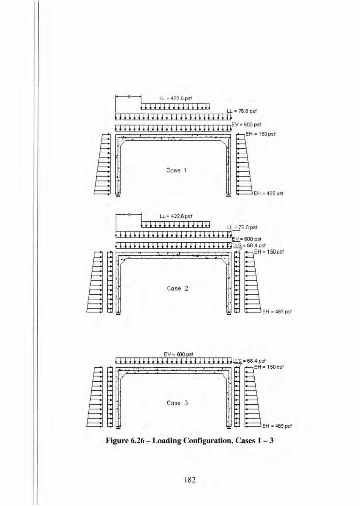
I• ll 1 LL = 422 .6 psf
t t + + + + + + + 4 4 t t + 4 LL = 76 _8 psf
oonnnnJIOOOOOH t t t t ~ ~ 4 4 4 4 4 4 I I t t t t t t t t 4 4 4 t E v = 600
psf . • . .. . . • . • EH = 150psf
Cas e 1
EH = 485 psf
r t LL = 422 .6 psf
o too n n no u~6.8psf
+ + + + l l l l l l • • l • • • • • f f + + l + ntt = 600 psf
! 1 4 ' + ' ' ' ' + 4 4 4 4 4 4 4 4 1 1 t ' ' + nLLs = 68.4 psf EH = 150psf . ..
Case 2
EH = 485 psf
EV = EDO psf
4 1 o o o o n n n o 1 1 o o ULLs = 68.4 psf
:t.-. . ·. t/
Case 3
EH = 150 psf
EH = 485 psf
Figure 6.26 - Loading Configuration, Cases 1 - 3
182

----.----------------------------------------------------------------·----,
Figure 6.27 - Locations of Critical Stresses
I I I I
t (2) I I I I I I I I I I I I I
! CD I I I I I I I I I I I I I
!
Table 6. 7 - LRFD - Structural Analysis Results per Foot Width, Example 2
Load Case 1. Load Case 2. Load Case 3. --- --- ---c..- ,_-- c..- ,_-- c..- ,_--
~ Q)- ctl (/) Q)- ctl (/) Q)- ctl (/) E 6_ Q) c.. E6_ Q) c.. E6_ Q) c..
..c ·- ..c ·- ..c ·-~Location 0 ·- Cf)6 0 ·- Cf)6 0 ·- Cf)6
~6 ~6 ~6 '-< 1 0.00 0.00 0.32 0.66 3.37 2.09
2 -21.84 3.18 -21.58 4.31 -3.89 2.34
3 -12.36 14.54 -14.14 14.54 -4.28 2.39 4 53.82 3.54 52.05 3.54 6.47 0.00
Location Load Case 1. Load Case 2. Load Case 3. --- --- ---c..- ,_- C.t:: ,_- c..- ,_-Q)- ctl (/) Q) I ctl (/) Q)j" ctl (/) E 6_ Q) c.. E c.. Q) c.. E c.. Q) c..
..c ·- ..c ·- ..c ·-0 ·- Cf)6 0 ·- Cf)6 0 ·- Cf)6 ~6 ~6 ~6
1 0.00 0.00 0.00 0.41 1.47 1.12 2 -13.73 2.36 -13.61 2.72 -4.49 1.71
3 -8.11 9.03 -8.67 9.03 -3.35 2.65 4 32.98 2.02 32.42 2.02 8.60 0.00
183

6.2.2.6 Reinforcing Design
The bottom reinforcement for the deck will be designed using #7 , Grade 60,
reinforcing bars.
. ( rebar diameter] d =slab thtckness- clear cover+ 2
d = 14 in- ( 2 in + 0 · 8~5 in )= 11.56 in
A req.=[0.85 *fc *b] *[d- d 2 _ 24 *Mu l fy <p * 0.85 * f c * b
A [0.85 *6000 psi *12 in]"'[ 56 . 11 .561.n 2 _ 24 *53.82 * 1000 lb- ft l s req. = ·· 11. m -
60000 psi 0.95 * 0.85 * 6000 psi * 12 in
A 1.03 in 2
s req.= ft
Try #7's @ 7 inches on center:
As provided= 12
in * 0.60 in 2 = 1.03 in 2
7
184

Check Maximum Reinforcement Ratio (LRFD 5.7.3.3):
c As max =- ~ 0.42
d
c A prov *fy = :5; 0.42
d 0.85 *f C * b * ~I * d
c 1.03 in 2 * 60000 psi = = 0.12:5 0.42ok
d 0.85 * 6000 psi * 12 in *0.75 * 11.56 in
Check Minimum Reinforcement (LRFD 12.14.5.8):
As min = 0.002 * b * h
Asrnin = 0.002 * 12 in * 14 in
. 0.34 in 2
Asmm=--ft
185

Check Crack Control (LRFD 12.14.5.7):
Calculate minimum allowable spacing to satisfy cracking (LRFD 5. 7.3.4):
700 *y s ~ e -2 *de
~ s *fs
d 2. 0.875in
244.
c= m+ = . m 2
~ = 1 + de = 1 + 2.44 in = 1.30 s 0.7 *(h-dc) 0.7 *(14in-2.44in)
ye =exposure factor= 1.00
Calculate actual stress in reinforcement:
n = 29000000psi = 6.lSu e 6 (150 lb/ft3)1.s * 33 * (~6000 psi)
12 . * 2 m x -6 *1.03in2 *(11.56in-x)=O
2
x = 2.98in
186
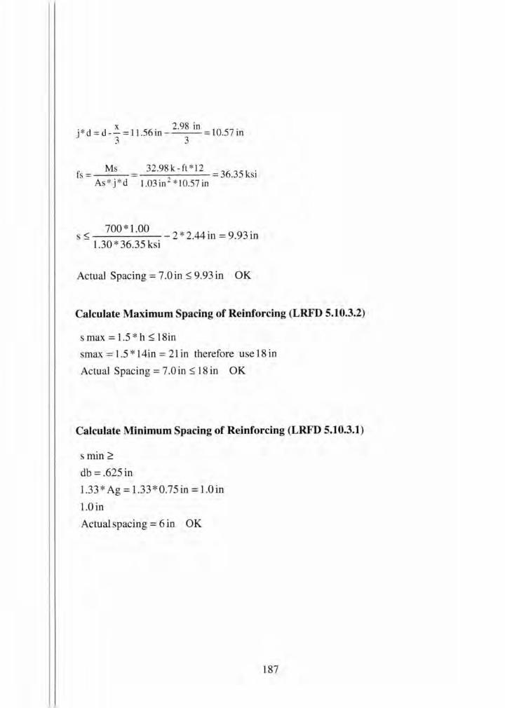
j * d = d -~ = 1 1.56 in -2
·98
in = 1 0.57 in 3 3
Ms 32.98 k - ft * 12 fs = = = 36.35 ksi
As* j * d 1.03 in 2 * 10.57 in
700 * 1.00 $ - 2 * 2.44 in = 9.93 in
1.30 * 36.35 ksi
Actual Spacing= 7.0in $ 9.93in OK
Calculate Maximum Spacing of Reinforcing (LRFD 5.10.3.2)
s max= 1.5 * h $ 18in
smax = 1.5 * 14in = 21 in therefore use 18 in
Actual Spacing = 7.0 in $ 18 in OK
Calculate Minimum Spacing of Reinforcing (LRFD 5.10.3.1)
s min~
db= .625 in
1.33 * Ag = 1.33 * 0.75 in= 1.0 in
1.0 in
Actual spacing = 6 in OK
187

The top reinforcement in the deck will be designed using #4, Grade 60, reinforcing bars .
d 14 . ( 2 . 0.50 in) 11 75 . = m - m+-- = . m 2
As= [0.85 *6000psi *12in] *[l1.?5 in- ll.?5 i0 2 _ 24* 14.14*1 0001b-ft l 60000psi 0.95 *0.85*6000psi • 12 in
A 0.26 in 2
s req.= ft
Try #4's @ 3.5 inche on center:
A provided= 12
in *0.196 in 2 = 0.67 in 2
3.5
Check Maximum Reinforcement Ratio (LRFD 5.7.3.3):
Check Minimum Reinforcement (LRFD 12.14.5.8):
Asmin = 0.002 * 12 in * 14 in
A . 0.34 in 2
smm=---ft
188

Check Crack Control (LRFD 12.14.5.7):
Calculate minimum allowable spacing to satisfy cracking (LRFD 5.7.3.4):
700 * S :5 'Y e - 2 * de
~ s *fs
d 2 . 0.50 in
2 25 .
c= m+ = . m 2
~ s = 1 + de = 1 + 2?5 in . = 1.27 0.7 *(h-dc) 0.7 *(14m-2.25m)
ye = exposure factor = 1.00
Calculate actual stress in reinforcement:
n = 29000000 psi = 6_18 u e 6 (1501b/ft 3 )J.5 * 33 *(~6000psi)
12 . * 2 m x -6 * 0.67in 2 * (11.75in - x) = 0
2
x = 2.50in
j * d = d- ~ = 11.75 in-2
·50
in = l 0.92 in 3 3
fs= Ms = 8.67k-ft *12 =l 4.22 ksi As * j * d 0.67 in 2 * 10.92 in
189

700 * 1.00 s :::; - 2 * 2.25 in = 34.32 in
1.27 * 14.22 ksi
Actual Spacing= 3.5 in:::; 34.32 in OK
Calculate Maximum Spacing of Reinforcing (LRFD 5.10.3.2)
s max= 1.5 * h:::; 18in
smax = 1.5 * 14in = 21 in therefore use 18 in
Actual Spacing= 3 .. 5 in:::; 18 in OK
Calculate Minimum Spacing of Reinforcing (LRFD 5.10.3.1)
s min 2::
db= .625 in
1.33 * Ag = 1.33 * 0.75 in = 1.0 in
1.0 in
Actual spacing= 3.5 in OK
The outside reinforcement in the walls will be designed using #4, Grade 60,
reinforcing bars.
d 10 . ( 2 . 0.50 in ) 7 75 . = m- m+-- = . m 2 .
As= [0.85 *6000psi *12in] *[ 7.75 in_ 7.75 in 2 _ 24 *2 1.84*1000lb-ft l 60000 psi 0.95 * 0.85 * 6000 psi •12 in
A 0.62in 2
s req.= ft
190

Try #4's @ 3.5 inches on center:
As provided= 12
in *0.196 in 2 = 0.67 in 2
3.5
Check Maximum Reinforcement Ratio (LRFD 5.7.3.3):
c 0.67 in 2 * 60000 psi = = 0.11 $ 0.42
d 0.85 *6000 psi *12 in *0.75 *7.75 in
Check Minimum Reinforcement (LRFD 12.14.5.8):
A min= 0.002 * 12 in * 10 in
A . 0.24in 2
srrun =---ft
Check Crack Control (LRFD 12.14.5.7):
Calculate minimum allowable spacing to satisfy cracking (LRFD 5.7.3.4):
700 *y s ~ e -2 * de
~ s* f
d 2 . 0.50 in
2 25 .
c= m+ = . m 2
~ = 1 + de = 1 + 2.25 in = 1.41 s 0.7 * (h- de) 0.7 * (1 0 in- 2.25 in)
ye =exposure factor= 1.00
191
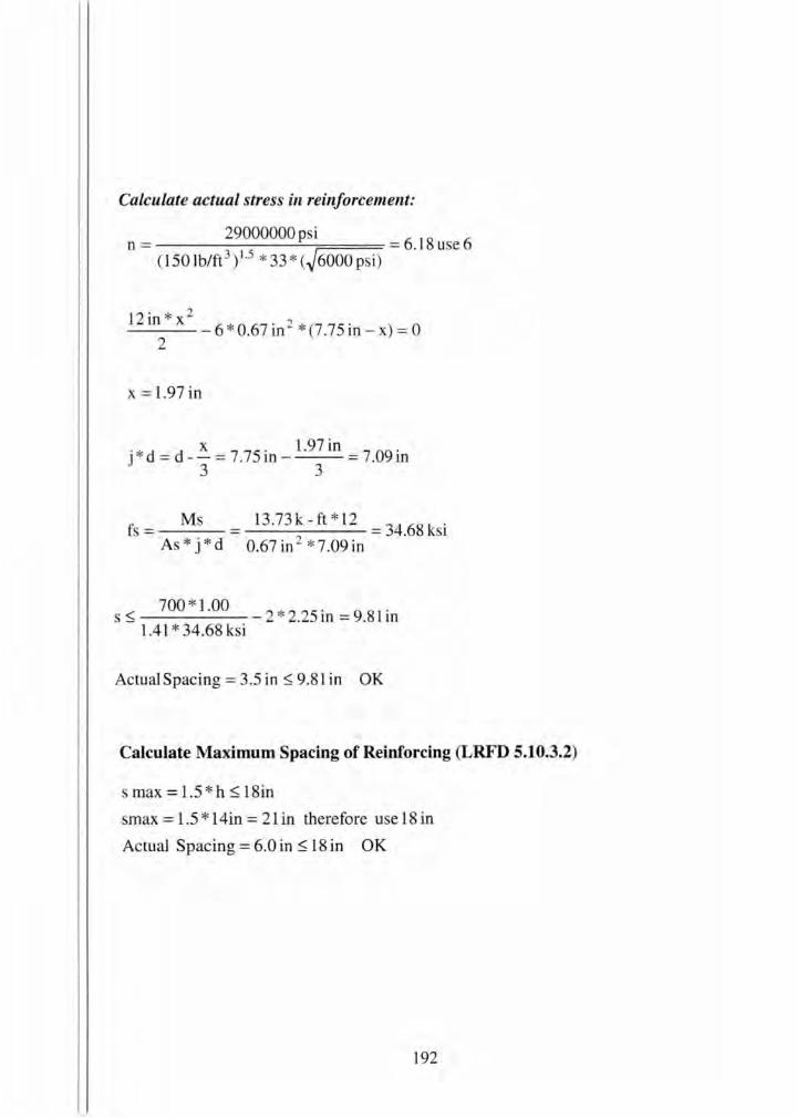
Calculate actual stress in reinforcement:
n = 29000000 psi = 6_18 use 6 (150 lb/ft3
) 1.s * 33 * (~6000 psi)
12 . * 2 10 ·x -6 *0.67in 2 *(7.75in-x)= O
2
x = 1.97 in
j * d = d- ~ = 7.75 in - 1.97
in = 7.09 in 3 3
fs = M = 13.73k-ft *12 = 34_68 ksi As* j * d 0.67in 2 *7.09in
700 * 1.00 s ~ - 2 * 2.25 in = 9.8 Lin
1.41 * 34.68 ksi
Actua1Spacing=3.5in~9.8lin OK
Calculate Maximum Spacing of Reinforcing (LRFD 5.10.3.2)
max= 1.5 * h ~ 18in
smax = 1.5 * 14in = 21 in therefore use 18 in
Actual Spacing= 6.0 in~ 18 in OK
192

Calculate Minimum Spacing of Reinforcing (LRFD 5.10.3.1)
s min~
db= .625 in
1.33 * Ag = 1.33 * 0.75 in = 1.0 in
1.0 in
Actual spacing= 3.5 in OK
The inside reinforcement will be designed using #5, Grade 60, reinforcing bars.
d = lOin -( 2 in + 0 · 6~5 in ) = 7.69 in
As =[0.85 *6000psi *l2in] *[?.69 in- 7.69 i11 2 _ 24 *3.37 *1000lb-ft l 60000 psi 0.95 *0.85 *6000 psi * 12 in
A 0.09in 2
s req .=--ft
Try #5 's @ 14.00 inches on center:
As provided= 12
in * 0.306 in 2 = 0.262 in 2
14.00
Check Maximum Reinforcement Ratio (LRFD 5.7.3.3):
c 0.262 in 2 * 60000 psi = = 0.04 ~ 0.42 d 0.85 *6000psi *12in *0.75 *7.69in
193

Check Minimum Reinforcement (LRFD 12.14.5.8):
Asmin = 00002 * 12 in * 10 in
A 0 Oo24in 2
srrun = ---ft
Check Crack Control (LRFD 12.14.5.7):
Calculate minimum allowable spacing to satisfy cracking (LRFD 5.7.3.4):
700 * s ~ Ye -2 *de
~ s * fs
d 2 0 00625 in
2 31 0
c= m+ = 0 m 2
~ = 1 + de = 1 + 2031 in = 1.43 5 007 * (h-dc) 007*(10in-2o3lin)
ye =exposure factor= 1000
194
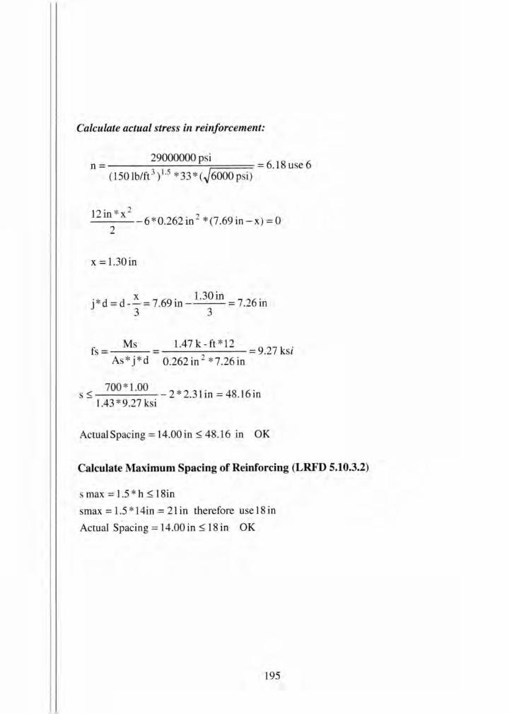
Calculate actual stress in reinforcement:
n = 29000000 p i = 6.18 use 6 (150 lb/ft 3 l 5 * 33 * (~6000 psi)
12 in * x 2
6 * 0.262 in 2 * (7 .69 in- x) = 0 2
x = 1.30in
j *d = d -~ = 7.69 in- 1.30in = 7.26 in
3 3
Ms 1.47 k-ft *12 fs= =
2 =9.27ksi
A * j * d 0.262 in * 7.26 in
700 *1.00 s ~ 2 * 2.31 in = 48.16 in
1.43 * 9.27 k i
Actual Spacing = 14.00 in ~ 48.16 in OK
Calculate Maximum Spacing of Reinforcing (LRFD 5.10.3.2)
s max= 1.5 * h ~ 18in
smax = 1.5 * 14in = 21 in therefore use 18 in
Actual Spacing = 14.00 in ~ 18 in OK
195

Calculate Minimum Spacing of Reinforcing (LRFD 5.10.3.1)
s min~
db= .625 in
1 .33 * Ag = 1.33 * 0.75 in = 1.0 in
l.Oin
Actual spacing= 14.00 in OK
6.2.2.7 Calculate shear (LRFD 5.8.3.3):
The allowable shear in the three-sided structure i calculated using the simplified
equation.
Shear in the Deck:
· evc~Vu
Vu = 14.54 kip
9Vc=9 * ~ *~ * b * dv
dv = maximum vulue of
0.9 * d or 0.72 * h
0.9 * de= 0.9 * 11.75 = 10.58
0.72 * h = 0.72 * 14 = 10.08
eve= 0.90 * 2 * ~6000 psi * 12 in * 10.58 in = 17701.7lb = 17.70 kips
= 17.70 kips> 14.54 kips OK
196
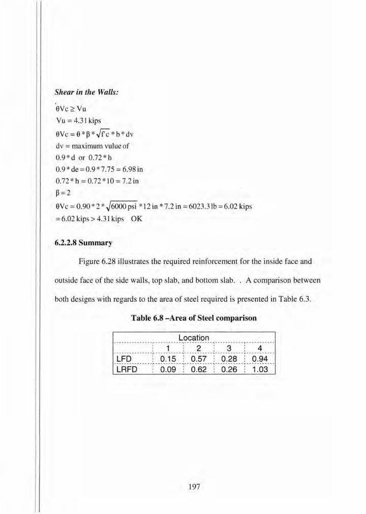
Shear in the Walls:
eve~ Vu
Vu = 4.31 kips
eVe=e * p *Fc" * b *dv
dv =maximum vulue of
0.9 *d or 0.72 * h
0.9 *de=0.9 *7.75 = 6.98in
0.72 * h =0.72*1 0=7.2in
P=2
eve= 0.90 * 2 * ~6000 psi * 12 in * 7.2 in= 6023.31b = 6.02 kips
= 6.02ldp > 4.31 kips OK
6.2.2.8 Summary
Figure 6.28 illustrates the required reinforcement for the inside face and
outside face of the side walls, top lab, and bottom slab. . A comparison between
both designs with regards to the area of steel required is pre ented in Table 6.3.
Table ().8 -Area of Steel comparison
Location ---------------r----------,----------- ----------- -----------
: 1 : 2 3 4 ---------- -- ---~----------,----------- ----------- ------- ----LFD : 0.15 : 0.57 0.28 0.94 ---------------~----------,----------- -- -- ------ - -----------LRFD : 0.09 : 0.62 0.26 1.03
197
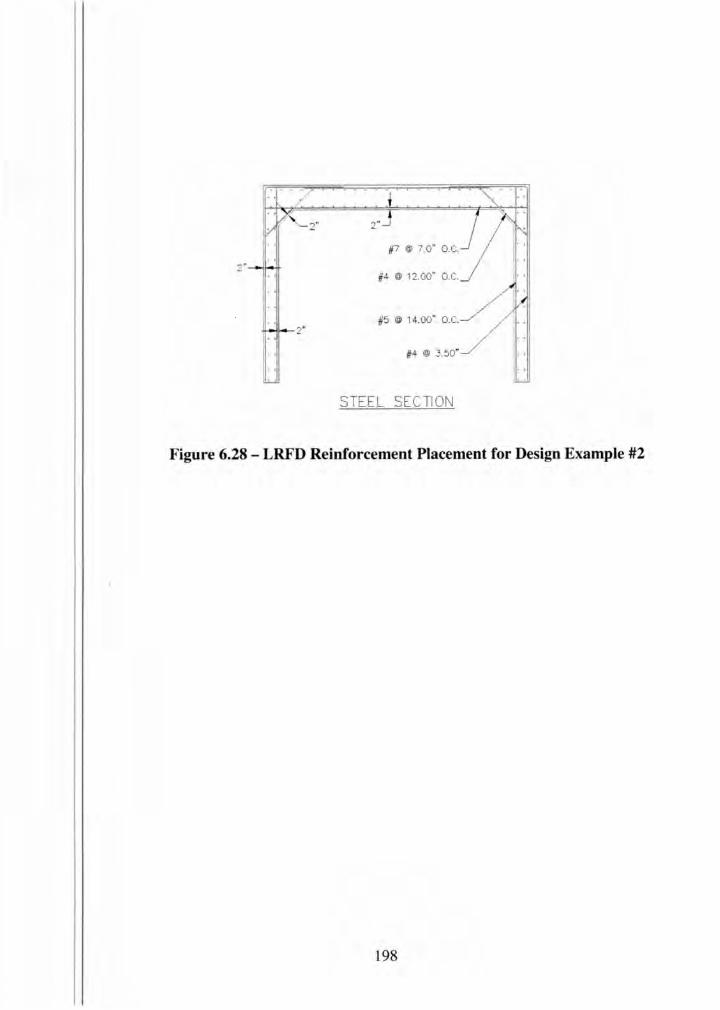
2"
2"
#7 @ 7.0" O.C.
#4 @ 12.00" O.C.
#5 @ 14.00" o.c.
#4 @ .3.50"
STEEL SECTION
Figure 6.28 - LRFD Reinforcement Placement for Design Example #2
198
Chapter 7 Summary and Conclusions
The objective of this thesi s was to examine and compare the current LRFD
Design Specifications and the Standard AASHTO Specifications used in designing
underground precast concrete structures such as underground utility structures,
drainage inlets, three-sided structures, and box culverts. This thesis compares
relevant provi ions from both specifications. Provisions discussed within this
document include: terminology, load factors, implementation of load modifiers, load
combinations, multiple presence factors, design vehicle live loads, distribution of live
load to slabs, and through earth fill, live load impact, and live load surcharge. A
brief summary of each as major provision and its impact on design is as fo llows:
• Design Vehicular Live Loads- The design truck, and application is
identical in both specifications. However, the LRFD provisions require
an additional distributed load of 0.64 kif be added to the live load
model. In addition, the Design Tandem Truck, which replaced the
Alternative Military Loading from the Standard Specifications, is 4%
heavier.
• The LRFD Specifications introduced the use of a multiple presence
factor. For a single loaded lane the multiple presence factor is 1.2. The
multiple presence factor is similar to the load reduction factor in the
199
Standard Specifications. The load reduction factor for a single loaded
lane is 1.0. Thus, comparing the two factors result in an increase from
1.0 to 1.2 for one loaded lane. This balances the reduction in the live
load factor. The Standard Specifications require a live load factor of
2.17, while the LRFD Specifications require 1.75. With the
introduction of the multiple presence factor, the live load factor in the
LRFD Specifications converts to 2.1.
• Dynamic Load Allowance (Impact) -Both specifications require an
increase in the live load with respect to the earth fill depth . The LRFD
Specifications require an impact factor be applied up to a fill depth of
8 ft. The Standard Specifications neglects the effects of impact for
depth greater than 3 ft. In general, the requirements in the Standard
LRFD Speciation produce a greater load effect than does the Standard
Specifications.
• Lateral Live Load Surcharge- Both specifications require an increase
in the lateral earth pressure due to the live load. The Standard
AASHTO Specifications require a live load surcharge pressure of 2ft,
regardless of structure type and geometry. The Standard LRFD
Specifications calculates the live load surcharge height as a function of
the structure's wall height. The lateral live load surcharge pressure is
200
significantly greater in the Standard LRFD Specification than the
Standard AASHTO Specifications.
• Distribution of Wheel Loads Through Earth Fill -Both specifications
allow for the live load to be distributed through earth fill. The LRFD
Specifications allow the dimensions of the tire to be utilized. However
the LRFD Specifications generally produce greater load effects. The
live load di stribution areas are complicated; particularly when multiple
load from several vehicles overlap. There is continuing research
being performed by the FHW A in order to simplify the calculations.
• Load Factors and Load Combinations -Both specifications utilize
load factors and strength reduction factors. However, the load and
resistance factors are determined through statistical studie and are
more accurate in the Standard LRFD Specification.
There is greater reliability and a more uniform factor of safety when utilizing
the LRFD Specifications. The provisions in the LRFD Specifications are more
concise and more beneficial to design engineers with the addition of the commentary.
Therefore, the code i si mpler to apply than the Standard Specifications. There is still
a great amount of research that must be performed, especially when examining the
distribution of live load through earth fill. Design engineers proficient with the
201

Standard AASHTO Specifications should have little trouble converting to LRFD
Specifications as some level of familiarity and comfort is attained.
202
References
American Association of State Highway and Transportation Officials (AASHTO).
Standard Specifications for Highway Bridges. 17th ed. Washington: GPO,
2002.
LRFD Bridge Design Specifications. 3rd ed. Washington: GPO, 2005 .
American Concrete Pipe Association (ACPA). Highway Live Loads on Concrete
Pipe. Irving, TX: ACPA, 2001.
Bloomquist, D. G., and Gutz, A. 1. Evaluation of Precast Box Culve1t Svstems Design
Live Loads on Box Culverts. Gainesvi lle, FL: University of Flmida, 2002.
DeStefano, R. 1. , Evans, J. , Tadros, M. K. , and Sun, C. "Flexural Crack Control in
Concrete Bridge Structures." Florida Department of T_ransportation.2004.
1 May .2006<www .dot. state.fl. us/structures/Research% 20Projects/researchProj
ect Reports.htm>
"LRFD: Achieving Greater Reliability and Service for Bridge ."Focus. July 2004.
U.S. Department of Transportation Federal Highway Division .
10 May.2006 <http://www.tfurc.gov/focus/july04/0l .htm>.
"LRFD: State Department of Transpmtation LRFD Implementation Plan Initial
Draft." B1idge Technology. 15 Apr. 2006. U.S . Department of Transportation
203

Federal Highway Division. 16 Apr. 2006
<http://www.fhwa.dot.gov/bJidge/lrfd/plan.cfm>.
National Cooperative Highway Research Program (NCHRP). "Development of
Comprehensive Bridge Specifications and Commentary." Research Results
Digest 198 (1998).
"Project 15-29: Design Specifications for Live Load Distribution to Buried
Structures." National Cooperative Highway Research Program. 6 Apr. 2006.
Transportation Re earch Board. 6 Apr. 2006
<http://www4.trb.org/trb/crp.nsf/ All+Projects/NCHRP+ 15-29>.
"Project 12-33: Development of a Comprehensive Bridge Specification and
Commentary." National Cooperative Highway Research Program. 24 May.
2006. Transportation Research Board. 26 May 2006
<http://www4.trb.org/trb/crp.nsf/ All+Projects/NCHRP+ 12-33>.
Rund, R. E., and McGrath, T. J. "Comparison of AASHTO Standard and LRFD Code
Provisions for Buried Concrete Box Culverts." Concrete Pipe for the New
Millennium: ASTM STP 1368. Ed. I. I. Kaspar and J. I. Enyart. West
Conshohocken, PA: American Society for Testing and Materials, 2000. 45 -
60.
204
Sanford, T. C. "Soil-Structure interaction of buried Structures." Transportation
Research Board. 2000. 2 Apr 2006.
<www.trb.org/publications/millenniurn/00103 .pdf >.
Tonias, D. E. Bridge Engineering. United States of America: McGraw-Hill, 1995.
United States. Federal Highway Administration (FHA). Load and Resistance Factor
Design (LRFD) for Highway Bridge Substructures: NHJ Course No. J 32068.
HI-98-032. Washington: GPO, 2001.
205