community medicine biostatistics and epidemiology

1

PRAVARA INSTITUTE OF MEDICAL SCIENCES (DEEMED TO BE UNIVERSITY)

RURAL MEDICAL COLLEGE, LONI

COMMUNITY MEDICINE

BIOSTATISTICS AND EPIDEMIOLOGY JOURNAL

2

Certificate of Completion

This is to certify that

Mr.

of the batch

has successfully completed Biostatistics and Epidemiology journal under Department of

Community Medicine and has acquired the requisite competencies

Batch in charge Head of the Department

3

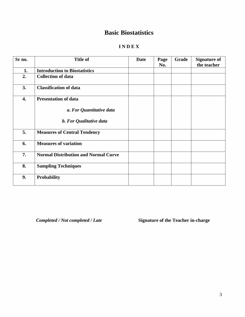
Basic Biostatistics

I N D E X

Sr no. Title of Date Page

No.

Grade Signature of

the teacher

1. Introduction to Biostatistics

2. Collection of data

3. Classification of data

4. Presentation of data

a. For Quantitative data

b. For Qualitative data

5. Measures of Central Tendency

6. Measures of variation

7. Normal Distribution and Normal Curve

8. Sampling Techniques

9. Probability

Completed / Not completed / Late Signature of the Teacher in-charge

4

INSTRUCTIONS FOR STUDENTS

• Read the Journal carefully and try to understand, do your own work in this Journal, don’t

copy from other student’s Journal.

• Use graph papers for charts and graphs.

• Get the Journal checked and signed by teachers on same day. If you remain absent for

particular practical then complete the Journal within one week after that practical.

• DO NOT COPY from other students’ Journal. This is part of your study and

internalization of the working concepts of the subject.

• You can use pocket calculator for calculations in the examinations.

• You have to carry the Journal for your oral examinations.

5

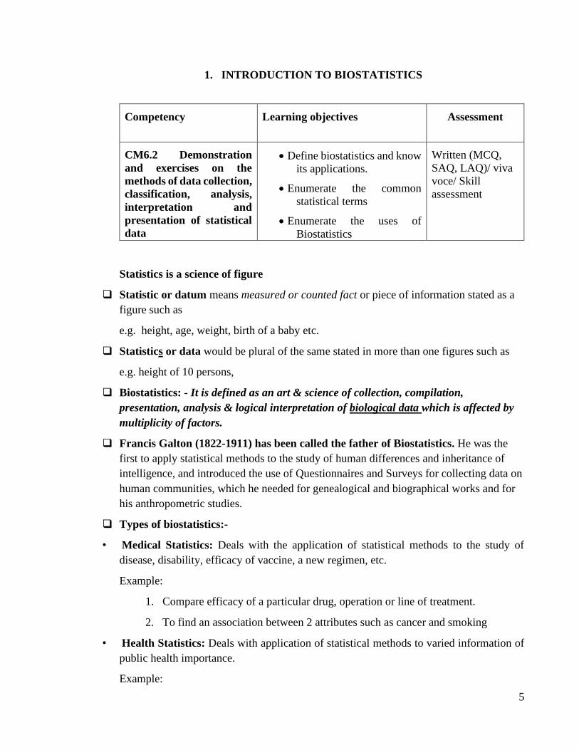
1. INTRODUCTION TO BIOSTATISTICS

Competency Learning objectives Assessment

CM6.2 Demonstration

and exercises on the

methods of data collection,

classification, analysis,

interpretation and

presentation of statistical

data

• Define biostatistics and know

its applications.

• Enumerate the common

statistical terms

• Enumerate the uses of

Biostatistics

Written (MCQ,

SAQ, LAQ)/ viva

voce/ Skill

assessment

Statistics is a science of figure

❑ Statistic or datum means measured or counted fact or piece of information stated as a

figure such as

e.g. height, age, weight, birth of a baby etc.

❑ Statistics or data would be plural of the same stated in more than one figures such as

e.g. height of 10 persons,

❑ Biostatistics: - It is defined as an art & science of collection, compilation,

presentation, analysis & logical interpretation of biological data which is affected by

multiplicity of factors.

❑ Francis Galton (1822-1911) has been called the father of Biostatistics. He was the

first to apply statistical methods to the study of human differences and inheritance of

intelligence, and introduced the use of Questionnaires and Surveys for collecting data on

human communities, which he needed for genealogical and biographical works and for

his anthropometric studies.

❑ Types of biostatistics:-

• Medical Statistics: Deals with the application of statistical methods to the study of

disease, disability, efficacy of vaccine, a new regimen, etc.

Example:

1. Compare efficacy of a particular drug, operation or line of treatment.

2. To find an association between 2 attributes such as cancer and smoking

• Health Statistics: Deals with application of statistical methods to varied information of

public health importance.

Example:

6

1. Test usefulness of sera and vaccines in the field- death/ attack among vaccinated and

unvaccinated

2. Epidemiological study: role of causative factor is tested statistically- iodine

deficiency causes goiter

• Vital Statistics: It is the ongoing collection by government agencies of data relating to

vital events such as births, deaths, marriages, divorces and health and disease related states

and events which are deemed reportable by local authorities.

❑ Common statistical terms:

• Characteristics: qualities and measurements of a person/ object.

• Attribute: a characteristic / label that is recorded as text

• Variate /variable: Characteristic which is recorded as numerals

• Population: It is an entire group of people or study elements – persons, things or

measurements for which we have interest at a particular time. It is the sum total of all

persons, objects or events about which we want to obtain information. E.g. if we want to

collect information about disease status of employees of a factory, then all employees will

form the population.

• Sampling unit: Each member of a population.

• Sample: It is a portion of population selected by a pre-decided and scientific method in such

a way that it represents all units. A sample is used to make certain predictions and

estimates about the population.

• Parameter: The constant which describes the population.

• Statistic: The constant which describes a sample

• Parametric tests

• Non parametric tests

❑ USES OF BIOSTATISTICS:

• Four basic uses:

1. Making estimates based on observations made in sample

2. Making forecast: making estimate about future based on the observations made

presently. (trends in observations, rates of increase/ decrease in particular event)

3. Deciding common/ uncommon/ rare observation and normal/abnormal

4. Establishing relationship between two characteristics: Association and correlation

7

• Uses of biostatistics for health administrator:

1. Making reasonable estimate of the problem

2. Deciding priorities among various problems

3. Making choice between different interventions

4. Evaluating impact of intervention

5. Programme planning and evaluation

6. Forecasting the needs of various resources in future

7. Establishing relationship between a suspected cause and the health problem

8. Health education

• Uses of biostatistics for a student in medicine:

1. Organization and planning of a clinical trial.

2. Identification of syndromes by establishing associations and correlations.

3. Establishing normal limits for various biological characteristics.

4. Helpful for standardization of various techniques / instruments used for diagnosis

5. To compare effect of two drugs or different doses of same drug

6. Useful to find out sensitivity and specificity of a diagnostic test / kit

7. Used to determine the risk factor for a disease

10

2. COLLECTION OF DATA


CM6.2 Demonstration and

exercises on the methods of

data collection,


interpretation and


data

• Enumerate the methods of data

collection

• Explain various sources of data

collection

• Explain How to minimize Mistakes

and Errors during data collection

Written (MCQ,

SAQ, LAQ)/ /

viva voce/ Skill

assessment

Introduction: Data collection is a crucial step in all scientific enquiries. Success of any statistical

investigation depends upon the availability of accurate and reliable data. Collection of data is a

very basic activity in decision making.

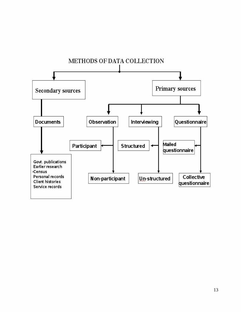
DATA COLLECTION METHODS:

1. Measurement: In this method the required information is collected by actual measurement in the

object, element or person. If we are interested in hemoglobin percentage of the individuals, we

actually measure the hemoglobin levels by appropriate method. The measurement and actual

enumeration generates primary data.

2. Questionnaire: Here, a standardized and pre-tested questionnaire is given/sent and the

respondents are expected to give the information by answering it. The success of this method

depends on the quality of questionnaire, the enthusiasm of the respondents and the ability of the

respondents to give accurate and complete information. By this method, the information about a

large number of attributes and variates can be collected in a short time.

3. Interview: This method can be used as a supplement to the questionnaire or can be used

independently. Here the information is collected by face to face dialogue with the respondents.

The success of this method depends on the rapport established between the interviewer and the

respondent, ability of the interviewer to extract the required information from the respondent and

the readiness of the respondent to part with the information.

4. Records: Sometimes the information required can be available in various records like census,

survey records, hospital records, service records, etc. The utility of the information depends on

its uniformity, completeness, standardization, accuracy and the reasons for which the information

was recorded.

Primary and Secondary data :

11

Data used in different studies is terms either ‘primary’ and ‘secondary’ depending upon whether

it was collected specifically for the study in question or for some other purpose.

Primary data: data which is collected under the control and direct supervision of the investigator

(investigator collects the data himself) is called as primary data or direct data. (Direct or Primary

method)

Secondary data: data, which is not collected by an investigator, but is derived from other sources,

is called as secondary or indirect data (Indirect or Secondary method) Sources of Primary data:

Survey

Sources of Secondary data:: Published and Unpublished

Published sources: National and International organizations which collects statistical data and

publish their findings in terms of statistical reports etc.

National Organizations: Census, Sample Registration System (SRS), National Sample Survey

Organizations (NSSO), National Family Planning Association (NFPA), Ministry of health,

Magazines, Journals, Institutional reports etc.

International Organizations: World Health Organization (WHO), United Nations

Organizations (UNO), UNICEF, UNFPA, World Bank etc. Unpublished sources: Records

maintained by various Govt. and private offices, studies made by research institutes, schools etc.

This data based on internal records. Provides authentic statistical data and is much cheaper than

primary data.

Sources for data collection:

1. Census

2. Registration of vital events

3. Sample registration system (SRS)

4. Notification of diseases

5. Hospital records

6. Epidemiological surveillance

7. Surveys

8. Research findings

The data that we collect from various sources should be:

Accurate: it measures true value of what is under study

Valid: it measures only what it is supposed to measure

Precise: it gives adequate details of the measurement

Reliable: it should be dependable

12

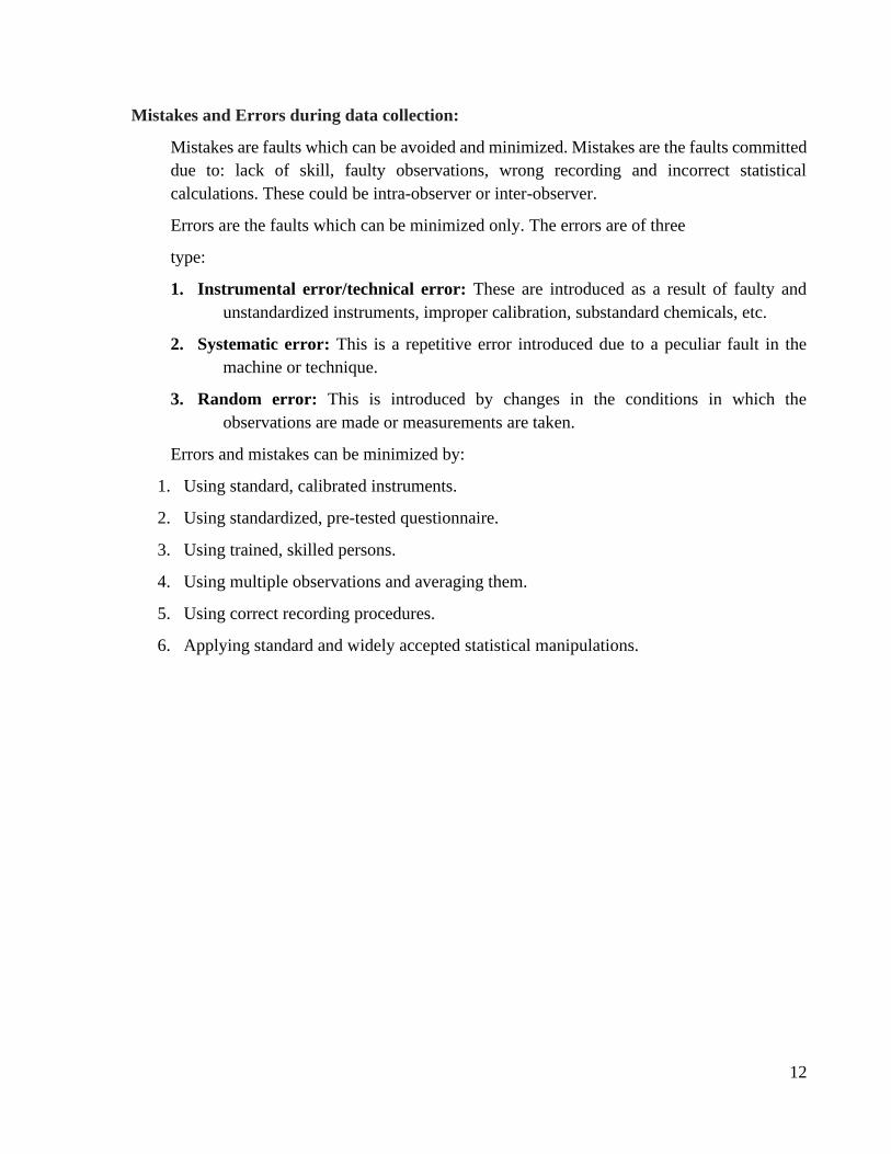
Mistakes and Errors during data collection:

Mistakes are faults which can be avoided and minimized. Mistakes are the faults committed

due to: lack of skill, faulty observations, wrong recording and incorrect statistical

calculations. These could be intra-observer or inter-observer.

Errors are the faults which can be minimized only. The errors are of three

type:

1. Instrumental error/technical error: These are introduced as a result of faulty and

unstandardized instruments, improper calibration, substandard chemicals, etc.

2. Systematic error: This is a repetitive error introduced due to a peculiar fault in the

machine or technique.

3. Random error: This is introduced by changes in the conditions in which the

observations are made or measurements are taken.

Errors and mistakes can be minimized by:

1. Using standard, calibrated instruments.

2. Using standardized, pre-tested questionnaire.

3. Using trained, skilled persons.

4. Using multiple observations and averaging them.

5. Using correct recording procedures.

6. Applying standard and widely accepted statistical manipulations.

17

3. Classification of data




data collection,


interpretation and


data

The student should be able to

• Classify the data based on

characteristics, source and

continuous/ discrete

• Identify the Scale of measurement for

a particular variable

Written (MCQ,

SAQ, LAQ)/

viva voce/ Skill

assessment

The process of arranging data in different groups according to similarities is called as

classification. The process of classification can be compared with the process of sorting out letters

in post office.

❑ SIGNIFICANCE

Classification is fundamental to the quantitative study of any phenomenon. It is recognized as the

basis of all scientific generalization and is therefore an essential element in statistical

methodology.

❑ WHAT IS CLASSIFICATION?

Classification is a process of arranging a huge mass of heterogeneous data into homogeneous

groups to know the salient features of the data.

❑ WHY CLASSIFICATION?

It facilitates comparison of data within and between the classes and it renders the data more

reliable because homogeneous figures are separated from heterogeneous figures. It helps in proper

analysis and interpretation of the data.

❑ Objectives

1. To condense the mass of data in such a way that salient features can readily noticed.

2. To compare two variables.

3. To prepare data this can be presented in tabular form.

4. To highlight the significance features of data at a glance.

5. It reveals pattern

6. It gives prominence to important figures.

18

7. It enables to analyze data.

8. It helps in drafting a report

Common types of classifications are: 1. Geographical i.e. according to area or region 2.

Chronological i.e. according to occurrence of an event in time 3. Quantitative i.e. according to

magnitude 4. Qualitative i.e. according to attributes

❑ Classification of data:

1) Classification of data Based on characteristic/attribute: qualitative/ quantitative

2) Classification of data Based on source: primary/ secondary

3) Classification of data Discrete / continuous data

1) Based on characteristic/attribute:

A. Qualitative data: Any statistical data, which are described only counting not by

measurement, is called as qualitative data. Also known as

enumeration/discrete/counted data

• It represents particular quality/attribute

• Characteristic or attribute cannot be measured but classified by counting the number of

individual who is having the same characteristic

• Expressed as number without unit of measurement (only frequency, no measurement

unit)

• Always discrete in nature i.e. whole number

• The statistical methods commonly employed in analysis of such data are standard error

of proportion and chi square test.

• Example: Gender, Blood group, Births, Deaths, No. of patients suffering from a disease,

SE classification such as Lower, middle and upper, No. of vaccinated, not vaccinated

etc.

B. Quantitative data: Any statistical data, which are described both by measurement

and counting is called as quantitative data. It is also known as

continuous/measurement data

• Quantitative data have a magnitude

• The characteristic can be measured

• Two variable i.e. characteristic & frequency

• Expressed as number with or without unit of measurement

19

• Measurement can be fractional i.e. continuous e.g. chest circumference- 33 cm, 34.5 cm,

35.2 cm OR can be discrete whole numbers only e.g. blood pressure, pulse rate, blood

sugar, respiratory rate

• The statistical methods employed in analysis of such data are mean, range, standard

deviation, coefficient of variation and correlation coefficient.

• For example: Height, Weight, Pulse Rate, BP, BSL, Age, RR, Age, Income, etc.

Technical terms for quantitative classification:

a. Variable: a quantity which changes its values is called as variable. e.g. age, height, weight, etc

Continuous variable: age, height, weight etc. Discrete variable: Population of a city,

production of a machine, spare parts etc.

b. Class Limits: the lowest and highest value of the class are called as class limits.

c. Class frequency: the number of items belonging to the same class

d. Class magnitude or class interval: the length of class i.e. the difference between the upper limit

and lower limit of the class.

2) Classification of data Based on source: primary/ secondary

A. Primary data:-

• These are the data obtained directly from an individual.

• Data derived from actual measurement

• It gives precise information.

• e.g. Height, Weight, disease of an individual interviewed is primary data

B. Secondary data:-

• These data obtained from outside source

• If we are studying hospital records and wish to use the census data, then census data

becomes secondary data.

3) Classification of data Discrete / continuous data

Discrete data:

• Here we always get a whole number.

• e.g. no. of persons cured, no. of persons suffering from the disease

Continuous data:

20

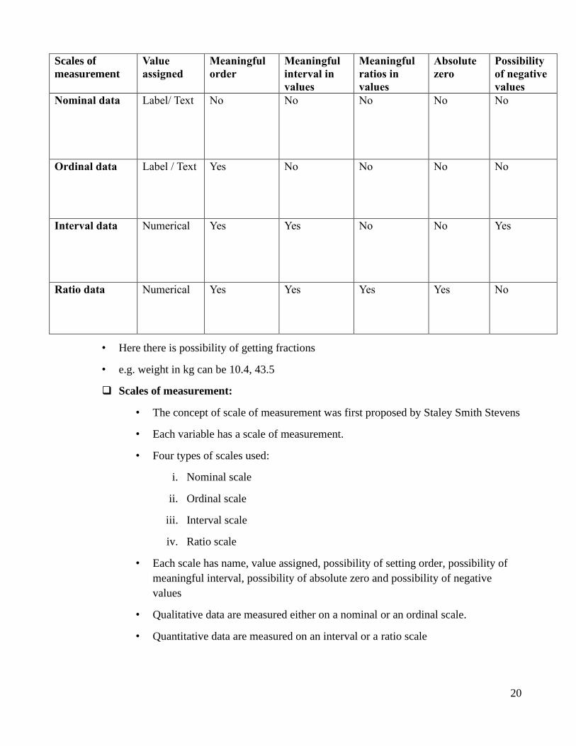
• Here there is possibility of getting fractions

• e.g. weight in kg can be 10.4, 43.5

❑ Scales of measurement:

• The concept of scale of measurement was first proposed by Staley Smith Stevens

• Each variable has a scale of measurement.

• Four types of scales used:

i. Nominal scale

ii. Ordinal scale

iii. Interval scale

iv. Ratio scale

• Each scale has name, value assigned, possibility of setting order, possibility of

meaningful interval, possibility of absolute zero and possibility of negative

values

• Qualitative data are measured either on a nominal or an ordinal scale.

• Quantitative data are measured on an interval or a ratio scale

Scales of

measurement

Value

assigned

Meaningful

order

Meaningful

interval in

values

Meaningful

ratios in

values

Absolute

zero

Possibility

of negative

values

Nominal data Label/ Text No No No No No

Ordinal data Label / Text Yes No No No No

Interval data Numerical Yes Yes No No Yes

Ratio data Numerical Yes Yes Yes Yes No

21

❑ Reasons of knowing the type of data and scales of measurement:

1. Knowing the type of data will help in data presentation

2. You should know the type of data and scales of measurement to calculate the

Descriptive statistics permissible for that particular data

3. Choice of inferential statistics (Test of significance) depends on the type of data and

scales of measurement

25

4. PRESENTATION OF DATA




data collection,


interpretation and


data


• Enumerate principles and methods

of Data Presentation

• Prepare frequency distribution table,

association table as per Rules and

guidelines of tabular presentation

• Present qualitative and quantitative

data graphically

Written (MCQ,

SAQ, LAQ)/

viva voce/ Skill

assessment

Information collected from various sources is called as Raw data. Raw data does not lead to any

understanding of the situation. Hence it should be compiled, classified and presented in a

purposive manner to bring out important points clearly and strikingly.

❑ Objectives of data presentation: Data presentation can have one or more of the

following objectives:

1. It is a step before analysis/interpretation of the data.

2. It involves reduction in the volume of the data. This facilitates the better

understanding.

3. When the data is presented in the form of tables, graphs or pictures it makes the data

interesting.

❑ Principles of Data Presentation:

It is a step before analysis/interpretation of the data.

1. The data should be arranged in such a way that it will arouse interest in a reader.

2. Data should be made sufficiently concise without losing important details.

3. The data should be presented in a simple form to enable the reader to form quick

impressions and to draw some conclusions, directly or indirectly.

4. It should facilitate further statistical analysis.

5. It should define the problem and suggest its solution.

26

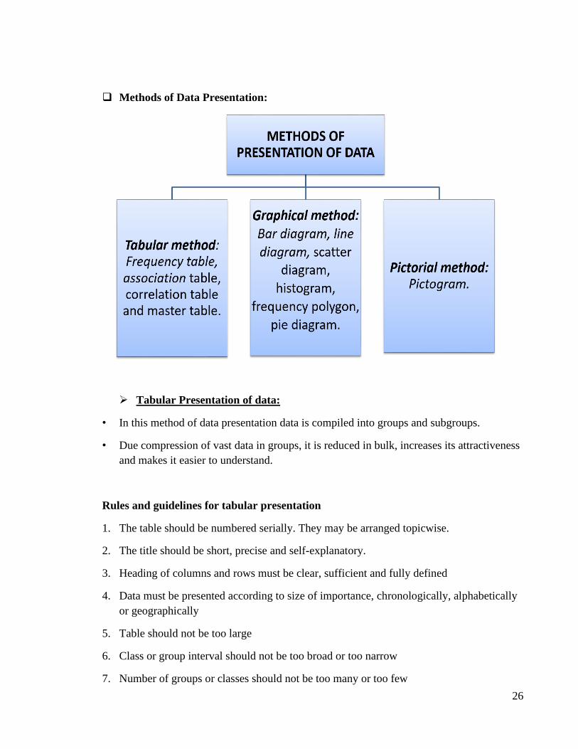
❑ Methods of Data Presentation:

➢ Tabular Presentation of data:

• In this method of data presentation data is compiled into groups and subgroups.

• Due compression of vast data in groups, it is reduced in bulk, increases its attractiveness

and makes it easier to understand.

Rules and guidelines for tabular presentation

1. The table should be numbered serially. They may be arranged topicwise.

2. The title should be short, precise and self-explanatory.

3. Heading of columns and rows must be clear, sufficient and fully defined

4. Data must be presented according to size of importance, chronologically, alphabetically

or geographically

5. Table should not be too large

6. Class or group interval should not be too broad or too narrow

7. Number of groups or classes should not be too many or too few

27

8. Class interval should be same throughout

9. Group should be tabulated in ascending or descending order

10. The groups should be mutually exclusive and should not overlap.

11. Each column and row should be appropriately demarcated.

12. Avoid short forms as far as possible

13. No cell should be left blank. Write ‘Nil’ if the frequency for that group is zero.

14. Total for each row and column must be given. If required, subtotal can be given.

❑ Anatomy of table:

• A typical table has number, title, columns, rows, cells and footnote. Tables are numbered

chronologically as they appear in the text.

• The “body” of the table consists of columns, rows, cells and total.

• Columns and rows indicate the demarcations of various groups/ subgroups compiled out

of the data.

• The figures in the “cells” pertain to the corresponding row and column.

• In the ‘cell’ corresponding to the last column and last row grand total is given.

• The “footnote” of the table is used for:

Indicating the source of the data.

Explaining the discrepancies, if any, in the data.

Providing additional information not given in the title and body of the table (e.g. explanation of

the abbreviations used).

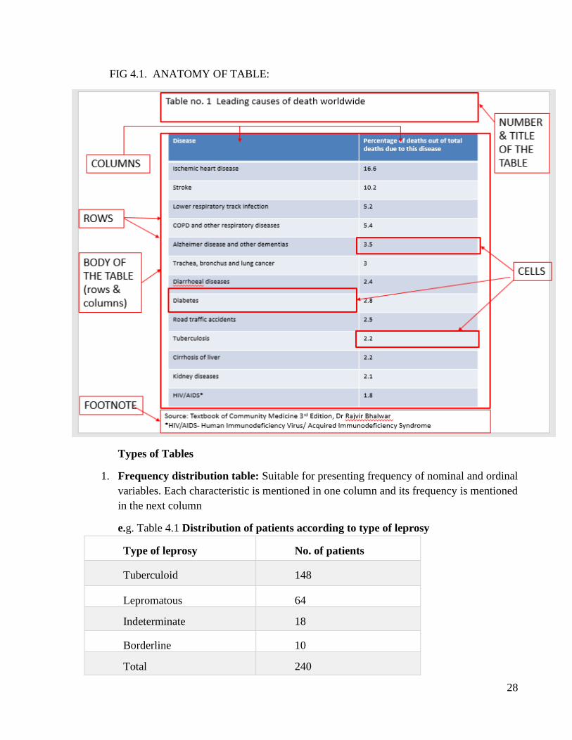
28

FIG 4.1. ANATOMY OF TABLE:

Types of Tables

1. Frequency distribution table: Suitable for presenting frequency of nominal and ordinal

variables. Each characteristic is mentioned in one column and its frequency is mentioned

in the next column

e.g. Table 4.1 Distribution of patients according to type of leprosy

Type of leprosy No. of patients

Tuberculoid 148

Lepromatous 64

Indeterminate 18

Borderline 10

Total 240

29

2. Association table: When we have to show association between two variables measured

on nominal/ordinal scale we use this form of table. It is also called 2 × 2 table because it

consists of two rows and two columns, excluding total. If more number of individuals are

in cells a and d (than in cells b and c) there is a possibility of positive association between

the attributes. On the contrary, if more individuals are represented in the cells b and c

(than in the cells a and d) there is a possibility of negative association between the

attributes.

e.g. table 4.2 association between smoking and lung cancer

Presence of exposure Cases

(with lung cancer)

Control

(without lung cancer)

Smokers 33(a) 55(b)

Nonsmokers 2(c) 27(d)

Total 35 (a+c) 82 (b+d)

3. Master table: Sometimes the data which can be presented in numerous smaller tables is

presented in one table only. Such table is called master table. This type of table gives

maximum information at a glance.

➢ Graphical presentation of data:

❑ General Precautions for Graphical presentation

• Use simplest type of graph consistent with the purpose

• Title: This should be like the title of the table. If there are many graphs they should be

numbered.

• Scale: Usually it should start from zero. If not, a break in the continuity may be shown.

The scale selected should be such that the calculations and presentations are facilitated.

• Use of color/shade: The use of color and shade gives attractiveness to the graph. Key to

colors must be given.

• Dependent/independent variate: By convention independent variate is presented on X-

axis (i.e. horizontal axis) while the dependent variate is presented in Y-axis (i.e. vertical

axis).

30

Graphs / Diagrams for Qualitative data:

1. Simple Bar diagram

2. Multiple Bar diagram

3. Proportional (Component) Bar Diagram

4. Pie Chart (Sector Diagram)

5. Pictogram

6. Map Diagram

I) BAR DIAGRAM: -

Indication: Comparing frequency of a variable expressed in nominal or ordinal scale. Data is

qualitative or quantitative discrete type.

Method:

The data is presented in the form of rectangular bars of equal breadth. Each bar

represents one attribute/variate.

The length of the bars indicates the frequency of the attribute or variate.

Different categories are indicated in one axis

Frequency of one data in each category is indicated in other axis

Precautions:

Scale must start from zero. If not it may be indicated by broken bar.

The distance between the bars should be equal to or lesser than the breadth of each bar.

31

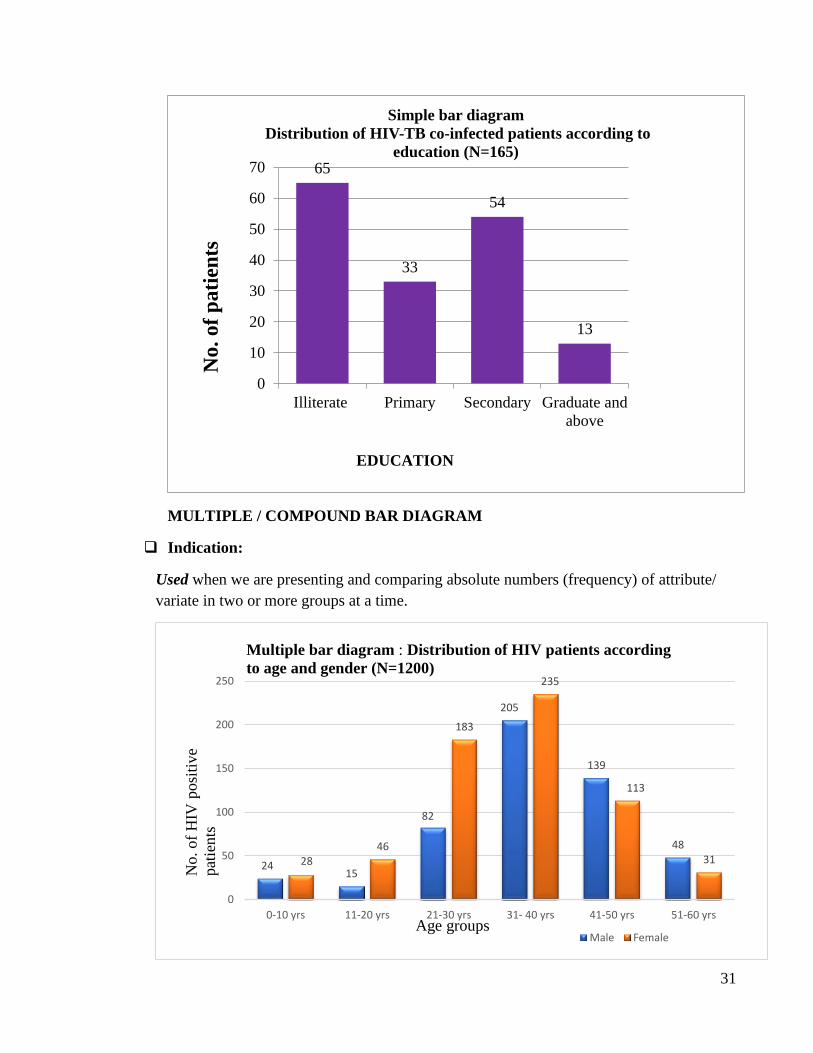
MULTIPLE / COMPOUND BAR DIAGRAM

❑ Indication:

Used when we are presenting and comparing absolute numbers (frequency) of attribute/

variate in two or more groups at a time.

65

33

54

13

0

10

20

30

40

50

60

70

Illiterate Primary Secondary Graduate and

above

Simple bar diagram

Distribution of HIV-TB co-infected patients according to

education (N=165)

EDUCATION

No

.o

f p

ati

ents

2415

82

205

139

48

2846

183

235

113

31

0

50

100

150

200

250

0-10 yrs 11-20 yrs 21-30 yrs 31- 40 yrs 41-50 yrs 51-60 yrs

Male Female

Multiple bar diagram : Distribution of HIV patients according

to age and gender (N=1200)

No.of

HIV

posi

tive

pat

ients

Age groups

32

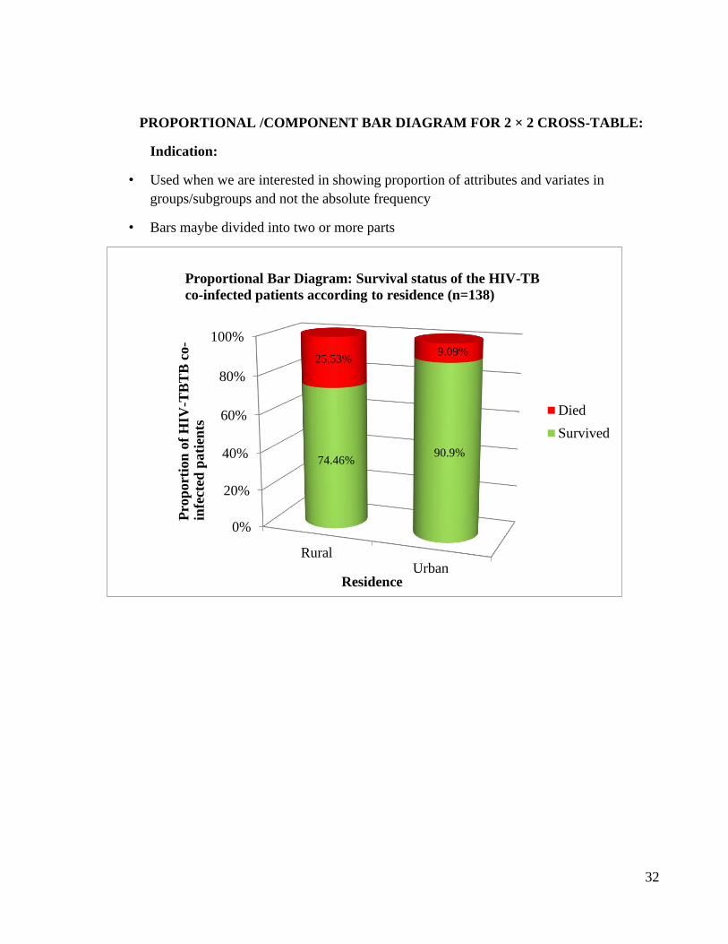
PROPORTIONAL /COMPONENT BAR DIAGRAM FOR 2 × 2 CROSS-TABLE:

Indication:

• Used when we are interested in showing proportion of attributes and variates in

groups/subgroups and not the absolute frequency

• Bars maybe divided into two or more parts

0%

20%

40%

60%

80%

100%

RuralUrban

74.46%90.9%

25.53%9.09%

Died

Survived

Proportional Bar Diagram: Survival status of the HIV-TB

co-infected patients according to residence (n=138)

Pro

port

ion

of

HIV

-TB

TB

co-

infe

cted

pati

ents

Residence

33

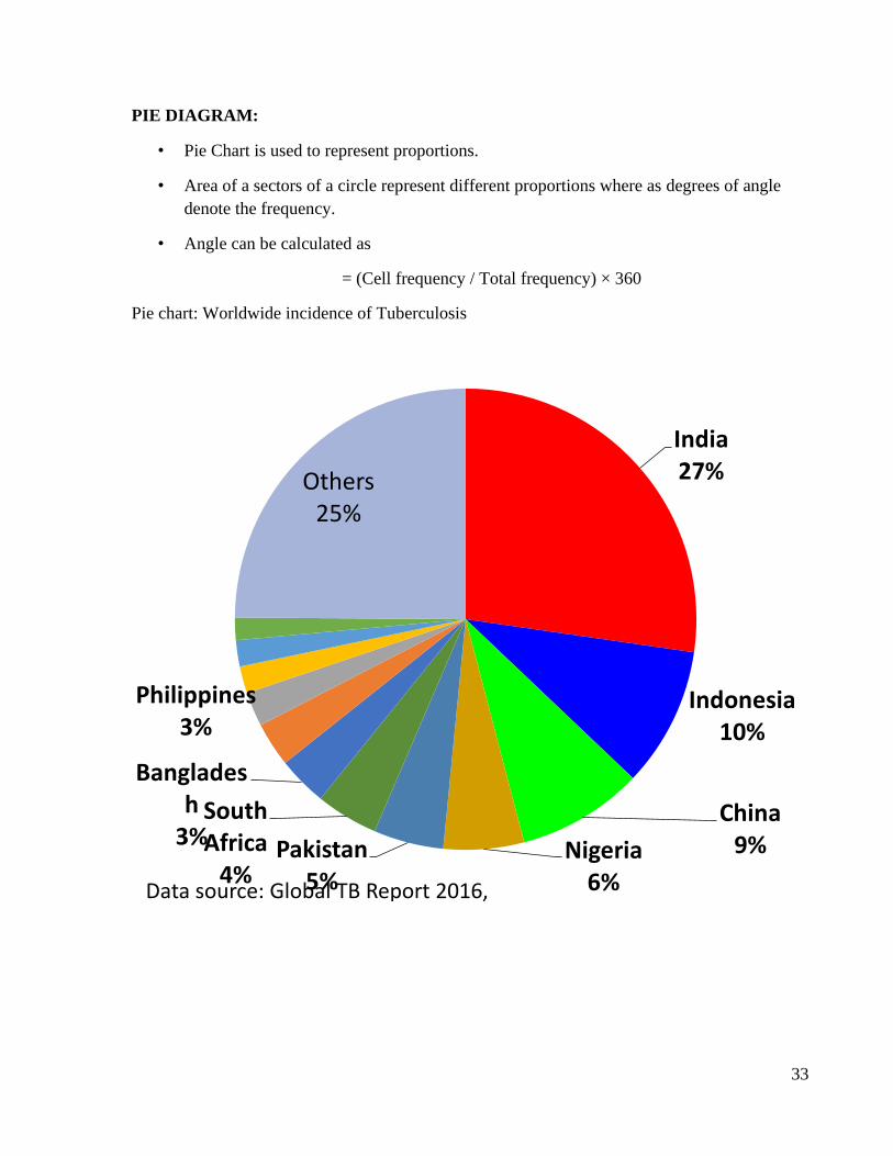
PIE DIAGRAM:

• Pie Chart is used to represent proportions.

• Area of a sectors of a circle represent different proportions where as degrees of angle

denote the frequency.

• Angle can be calculated as

= (Cell frequency / Total frequency) × 360

Pie chart: Worldwide incidence of Tuberculosis

India27%

Indonesia10%

China9%Nigeria

6%

Pakistan5%

South Africa

4%

Bangladesh

3%

Philippines3%

Others25%

Data source: Global TB Report 2016, WHO, Geneva

34

VENN DIAGRAM:

• It shows degrees of overlap and exclusivity for two or more characteristics or factors

within a sample or population

• Figure : Number of deaths as per reporting agency

PICTOGRAM:

• Pictogram is technique of presenting statistical data through appropriate pictures.

It is popularly used when the facts are to be presented to layman and less educated

masses.

35

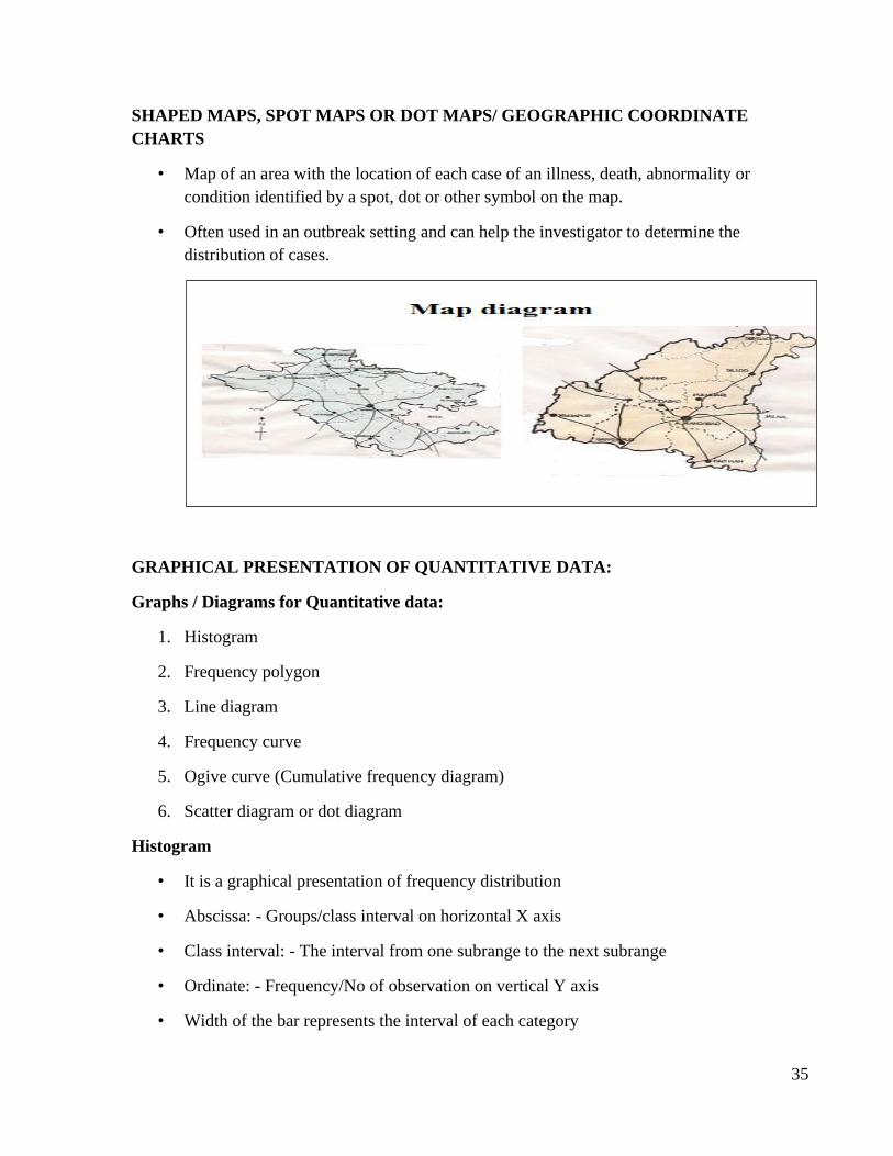
SHAPED MAPS, SPOT MAPS OR DOT MAPS/ GEOGRAPHIC COORDINATE

CHARTS

• Map of an area with the location of each case of an illness, death, abnormality or

condition identified by a spot, dot or other symbol on the map.

• Often used in an outbreak setting and can help the investigator to determine the

distribution of cases.

GRAPHICAL PRESENTATION OF QUANTITATIVE DATA:

Graphs / Diagrams for Quantitative data:

1. Histogram

2. Frequency polygon

3. Line diagram

4. Frequency curve

5. Ogive curve (Cumulative frequency diagram)

6. Scatter diagram or dot diagram

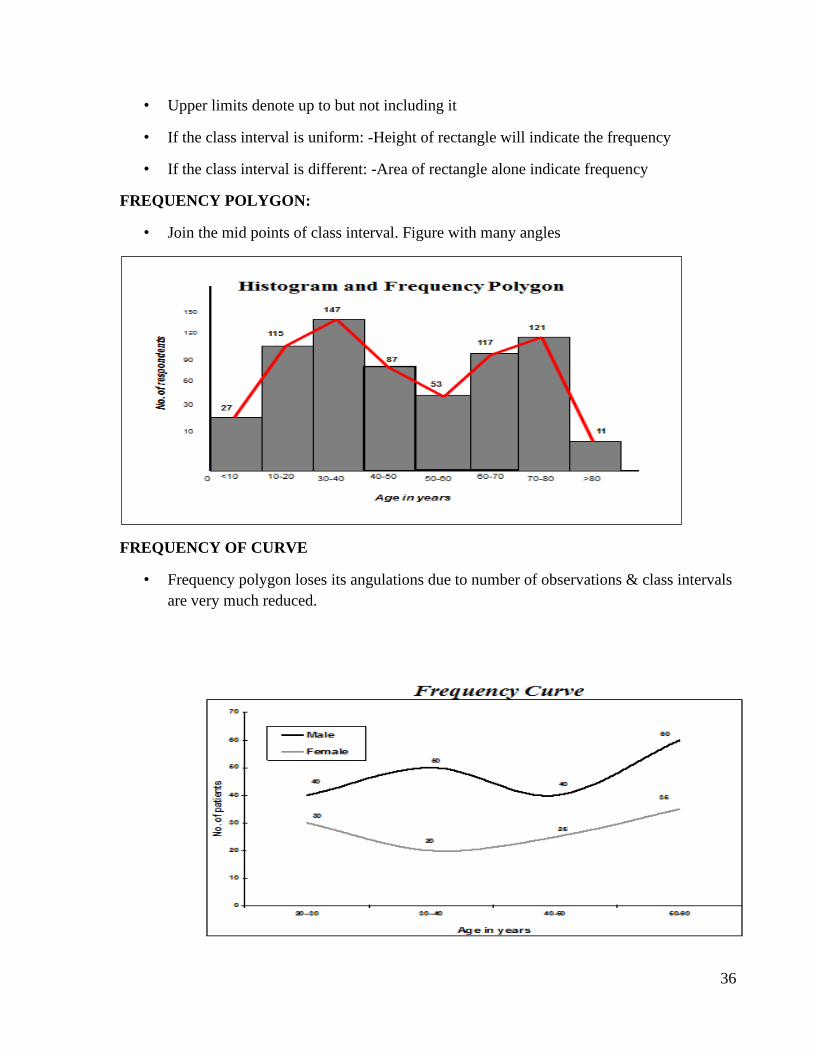
Histogram

• It is a graphical presentation of frequency distribution

• Abscissa: - Groups/class interval on horizontal X axis

• Class interval: - The interval from one subrange to the next subrange

• Ordinate: - Frequency/No of observation on vertical Y axis

• Width of the bar represents the interval of each category

36

• Upper limits denote up to but not including it

• If the class interval is uniform: -Height of rectangle will indicate the frequency

• If the class interval is different: -Area of rectangle alone indicate frequency

FREQUENCY POLYGON:

• Join the mid points of class interval. Figure with many angles

FREQUENCY OF CURVE

• Frequency polygon loses its angulations due to number of observations & class intervals

are very much reduced.

37

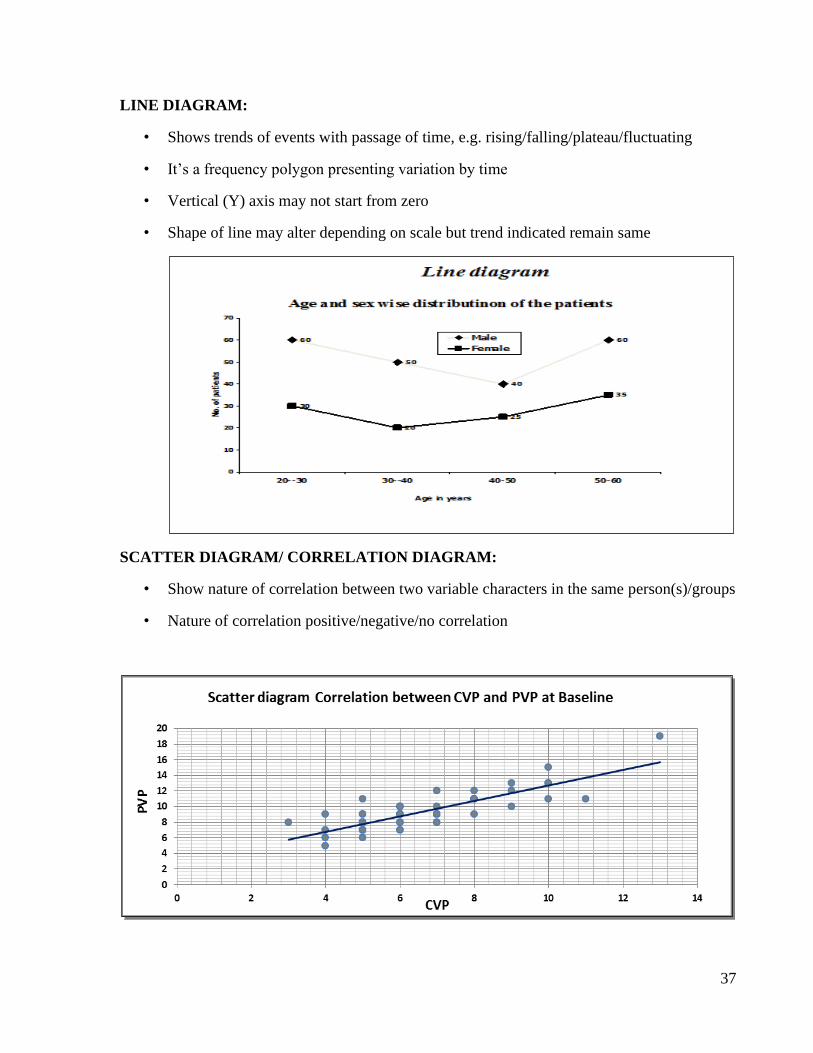
LINE DIAGRAM:

• Shows trends of events with passage of time, e.g. rising/falling/plateau/fluctuating

• It’s a frequency polygon presenting variation by time

• Vertical (Y) axis may not start from zero

• Shape of line may alter depending on scale but trend indicated remain same

SCATTER DIAGRAM/ CORRELATION DIAGRAM:

• Show nature of correlation between two variable characters in the same person(s)/groups

• Nature of correlation positive/negative/no correlation

42

ADD 10 GRAPH PAGES

43

5. MEASURES OF CENTRAL TENDENCY (Centering Constants)



exercises on Common

sampling techniques, simple

statistical methods,

frequency

distribution, measures of

central tendency and

dispersion


• Calculate mean, mode and median

• Enumerate merits and demerits of

centering constants

Written (MCQ,

SAQ, solving

exercise)/ viva

voce/ Skill

assessment

Significance: The mass of data in one single value enables us to get an idea of the entire data. It

also enables us to compare two or more sets of data to facilitate comparison. It represents whole

data / distribution with unique value.

Characteristics of good measure of central tendency:

It should be easy to understand. It should be simple to calculate.

It should be based on all observations.

It should be uniquely defined.

It should be capable of further algebraic treatment.

It should not be unduly affected by extreme values.

• Important measures of central tendency or Centering constants which are commonly

used in medical science, are:

1. Mean (Average) 2. Median 3. Mode

1. Mean:

The ratio of addition of the all values to the total number of observations in a series of data is

called as Mean or Average.

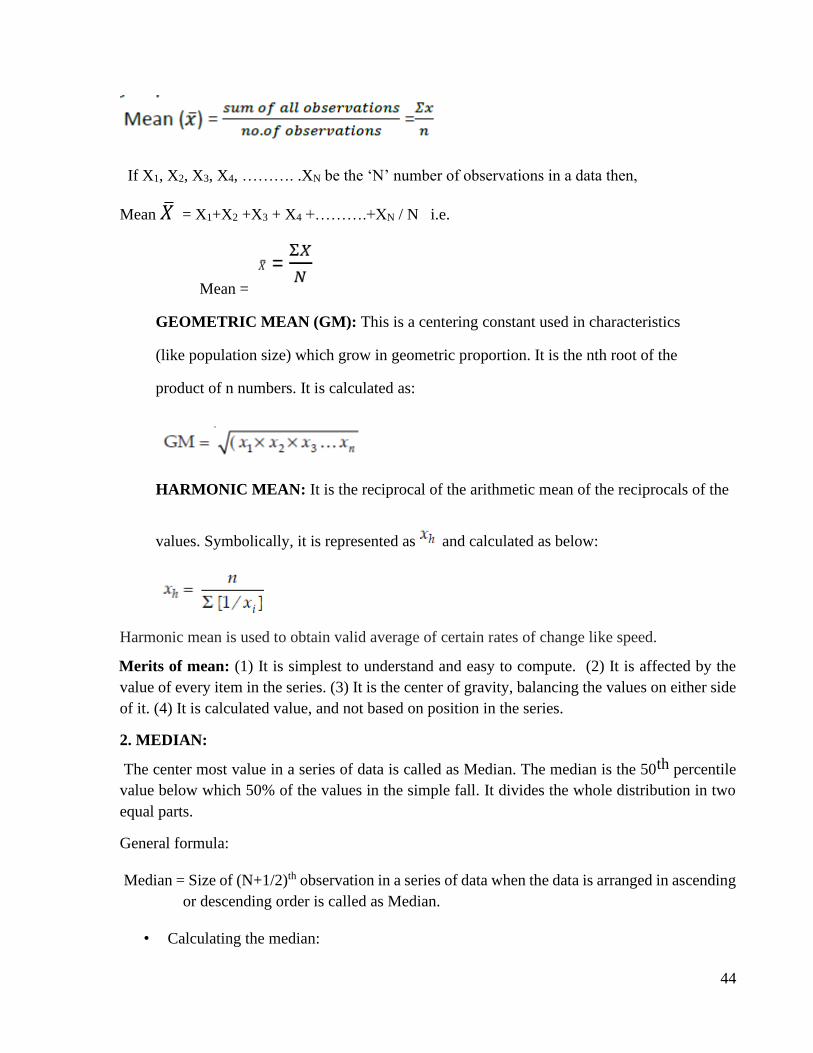
General Formula for arithmetic mean:

44

If X1, X2, X3, X4, ………. .XN be the ‘N’ number of observations in a data then,

Mean �̅� = X1+X2 +X3 + X4 +……….+XN / N i.e.

Mean =

GEOMETRIC MEAN (GM): This is a centering constant used in characteristics

(like population size) which grow in geometric proportion. It is the nth root of the

product of n numbers. It is calculated as:

HARMONIC MEAN: It is the reciprocal of the arithmetic mean of the reciprocals of the

values. Symbolically, it is represented as and calculated as below:

Harmonic mean is used to obtain valid average of certain rates of change like speed.

Merits of mean: (1) It is simplest to understand and easy to compute. (2) It is affected by the

value of every item in the series. (3) It is the center of gravity, balancing the values on either side

of it. (4) It is calculated value, and not based on position in the series.

2. MEDIAN:

The center most value in a series of data is called as Median. The median is the 50th percentile

value below which 50% of the values in the simple fall. It divides the whole distribution in two

equal parts.

General formula:

Median = Size of (N+1/2)th observation in a series of data when the data is arranged in ascending

or descending order is called as Median.

• Calculating the median:

45

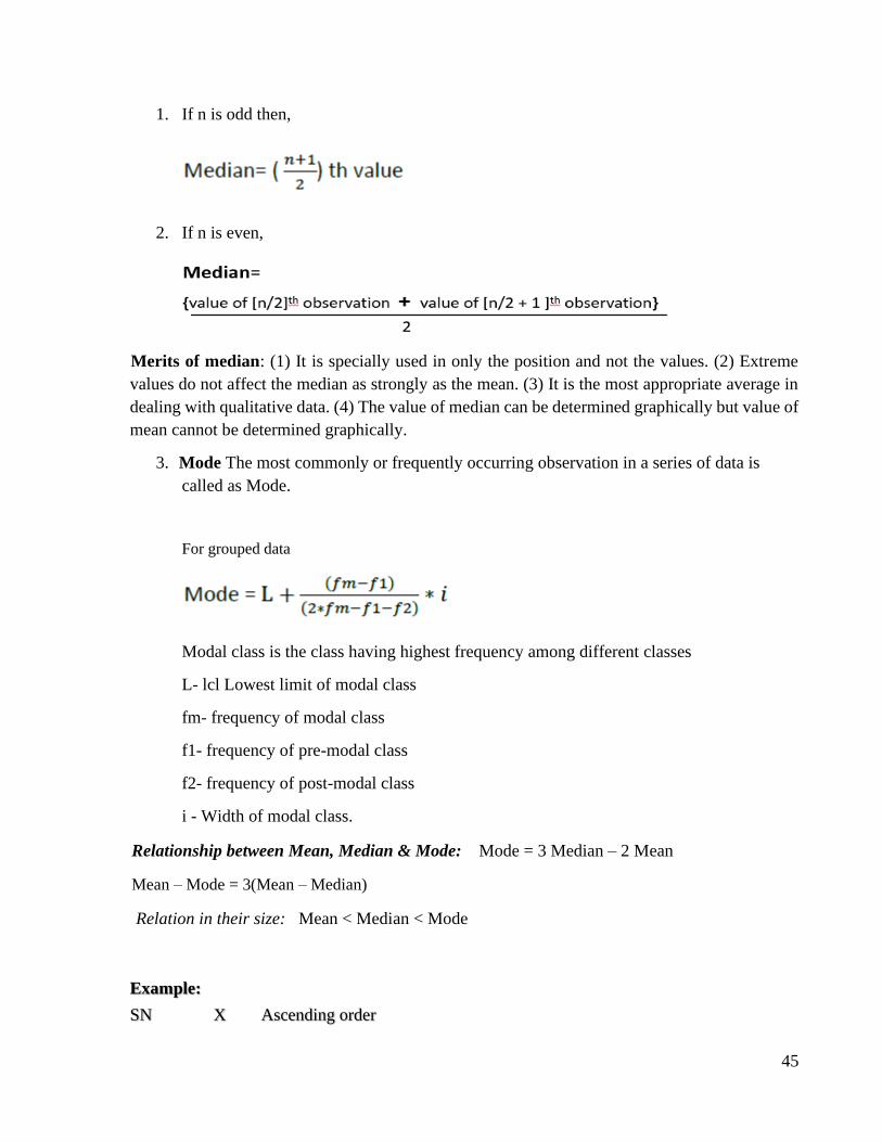
1. If n is odd then,

2. If n is even,

Merits of median: (1) It is specially used in only the position and not the values. (2) Extreme

values do not affect the median as strongly as the mean. (3) It is the most appropriate average in

dealing with qualitative data. (4) The value of median can be determined graphically but value of

mean cannot be determined graphically.

3. Mode The most commonly or frequently occurring observation in a series of data is

called as Mode.

For grouped data

Modal class is the class having highest frequency among different classes

L- lcl Lowest limit of modal class

fm- frequency of modal class

f1- frequency of pre-modal class

f2- frequency of post-modal class

i - Width of modal class.

Relationship between Mean, Median & Mode: Mode = 3 Median – 2 Mean

Mean – Mode = 3(Mean – Median)

Relation in their size: Mean < Median < Mode

Example:

SN X Ascending order

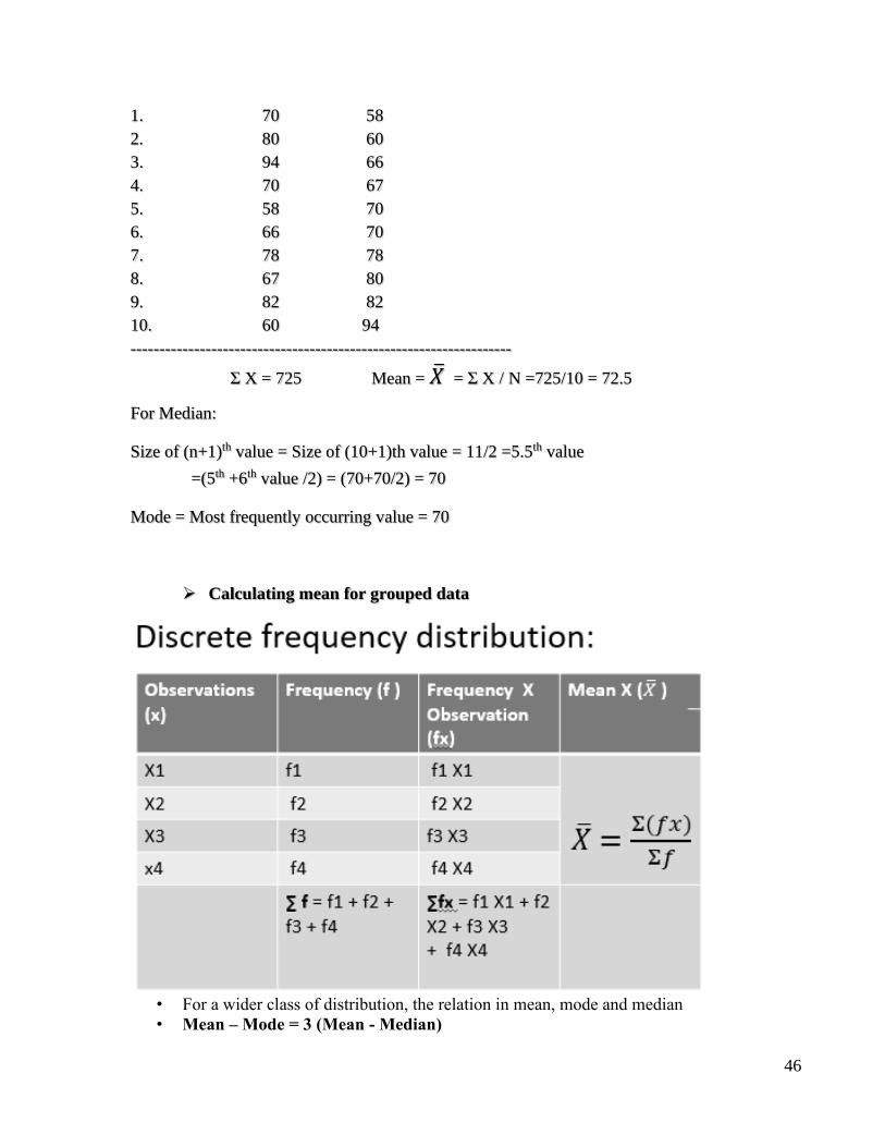
46

1. 70 58

2. 80 60

3. 94 66

4. 70 67

5. 58 70

6. 66 70

7. 78 78

8. 67 80

9. 82 82

10. 60 94

------------------------------------------------------------------

Σ X = 725 Mean = �̅� = Σ X / N =725/10 = 72.5

For Median:

Size of (n+1)th value = Size of (10+1)th value = 11/2 =5.5th value

=(5th +6th value /2) = (70+70/2) = 70

Mode = Most frequently occurring value = 70

➢ Calculating mean for grouped data

• For a wider class of distribution, the relation in mean, mode and median

• Mean – Mode = 3 (Mean - Median)

47

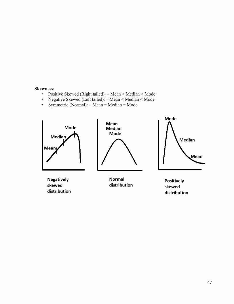
Skewness:

• Positive Skewed (Right tailed): – Mean > Median > Mode

• Negative Skewed (Left tailed): – Mean < Median < Mode

• Symmetric (Normal): – Mean = Median = Mode

53

6. VARIABILITY, VARIATION OR DISPERSION



exercises on Common



frequency



dispersion


• Calculate range, interquartile range

and standard deviation (SD)

• Enumerate merits and demerits of

measures of variation

Written (MCQ,

SAQ, LAQ,

solving

exercises) / viva

voce/ Skill

assessment

To measure the variability among the different variables or distributions there are several

measurements which is called as Measures of variation.

Concept:

It describes the spread or scattering of the individual values around the central value.

Objective:- The main objective of the measures of variation / variability / dispersion is “How the

individual observations are dispersed around the mean”.

Significance: (1) It determines the reliability of an average. (2) To determine the nature and cause

of variation in order to control the variability. (3) To compare two or more than two distributions

with regards to their variability. (4) It is of great importance to advanced statistical analysis. (5)

To find out the variation in a distribution.

Following are some important measures of variation:

1. Range 2. Inter-quartile range 3. Mean Deviation 4. Standard Deviation (S.D.) and 5.

Coefficient of Variation (C.V.)

1. Range: This is a crude measure of variation since it uses only two extreme values.

Definition: It is defined as the difference between highest and lowest value in a set of data.

Symbolically, Range can be given as Range = X max. - X min Range is useful in quality control

of drug, maximum and minimum temperature in a case of enteric fever etc.

2. Interquartile Range: The difference between third and first quartile.

54

Symbolically, Q = Q3 – Q1 Where, Q1 = First quartile- 25% Q3 = Third quartile- 75%

The interquartile range is superior to the range as it is based on two extreme values but rather on

middle 50% observations.

3. Mean Deviation:

Ratio of sum of deviations from mean of individual observations to the number of observations

after ignoring the sign is called as Mean Deviation. Although the mean deviation is good measure

of variability, its use is limited. It measures and compare variability among several sets of data.

4. Standard Deviation (SD):

Karl Pearson introduced in 1893. Most widely used & important measures of variation. It is based

on all observations. Even if one of the observations is changed, SD also changes. It is least

affected by the fluctuations of sampling.

Definition: SD is Root Mean Square Deviation i.e. it is the square root of the mean of squares of

deviation from individual observation to mean. Generally, it is denoted by δ (sigma)

Greater/smaller the value of SD in data, greater/smaller will be the variation among data.

Steps to calculate SD:

If X1, X2, X3, X4, .,.,.,.,.,., XN be the 'N' numbers of observations in a series of data then value of

SD can be calculated as follows:

1.Calculate Mean (i.e. �̅� = ΣX / N)

2.Take the differences from the mean from each value in data (i.e. X1-�̅�, X2-�̅�, X3-�̅�, X4-�̅�,

...... XN-�̅�) Do not ignore positive/negative sign

3. Take the squares of the differences taken from the mean from all individual observations {i.e.

(X1-�̅�)², (X2-�̅�)², (X3-�̅�)²,(X4-�̅�)²,......(XN-�̅�)²}

4.Take the sum/ addition of the squares of the differences taken from the mean from all

individual observations i. e. Σ (X- �̅�)²

5. Divide the sum/addition of the squares of the differences taken from the mean from all

55

individual observations by N-1. i. e. Σ (X- �̅�)² / N-1

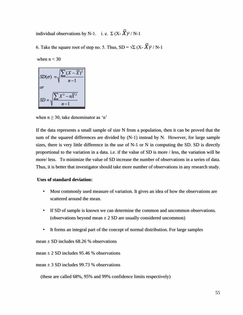
6. Take the square root of step no. 5. Thus, SD = √Σ (X- �̅�)² / N-1

when n < 30

when n ≥ 30, take denominator as ‘n’

If the data represents a small sample of size N from a population, then it can be proved that the

sum of the squared differences are divided by (N-1) instead by N. However, for large sample

sizes, there is very little difference in the use of N-1 or N in computing the SD. SD is directly

proportional to the variation in a data. i.e. if the value of SD is more / less, the variation will be

more/ less. To minimize the value of SD increase the number of observations in a series of data.

Thus, it is better that investigator should take more number of observations in any research study.

Uses of standard deviation:

• Most commonly used measure of variation. It gives an idea of how the observations are

scattered around the mean.

• If SD of sample is known we can determine the common and uncommon observations.

(observations beyond mean ± 2 SD are usually considered uncommon)

• It forms an integral part of the concept of normal distribution. For large samples

mean ± SD includes 68.26 % observations

mean ± 2 SD includes 95.46 % observations

mean ± 3 SD includes 99.73 % observations

(these are called 68%, 95% and 99% confidence limits respectively)

56

• It is used in various tests of significance

• Used to calculate coefficient of variation

• Merits of standard deviation: Based on all the observations. Does not ignore algebraic

signs of deviations. Capable of further mathematical treatment. Not much affected by

sampling fluctuations.

• Demerits: Difficult to understand and calculate. Used only for quantitative data. Unduly

affected by extreme observations

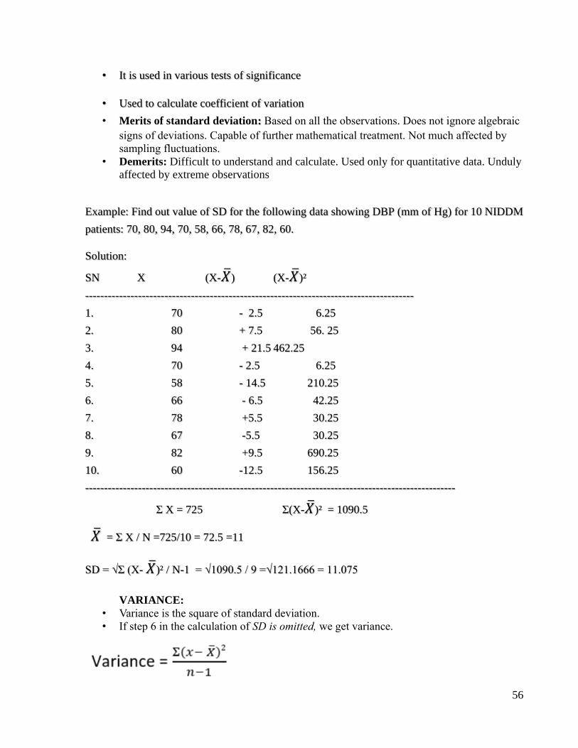
Example: Find out value of SD for the following data showing DBP (mm of Hg) for 10 NIDDM

patients: 70, 80, 94, 70, 58, 66, 78, 67, 82, 60.

Solution:

SN X (X-�̅�) (X-�̅�)²

---------------------------------------------------------------------------------------

1. 70 - 2.5 6.25

2. 80 + 7.5 56. 25

3. 94 + 21.5 462.25

4. 70 - 2.5 6.25

5. 58 - 14.5 210.25

6. 66 - 6.5 42.25

7. 78 +5.5 30.25

8. 67 -5.5 30.25

9. 82 +9.5 690.25

10. 60 -12.5 156.25

--------------------------------------------------------------------------------------------------

Σ X = 725 Σ(X-�̅�)² = 1090.5

�̅� = Σ X / N =725/10 = 72.5 =11

SD = √Σ (X- �̅�)² / N-1 = √1090.5 / 9 =√121.1666 = 11.075

VARIANCE:

• Variance is the square of standard deviation.

• If step 6 in the calculation of SD is omitted, we get variance.

57

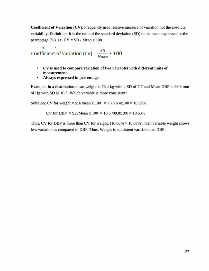
Coefficient of Variation (CV): Frequently used relative measure of variation not the absolute

variability. Definition: It is the ratio of the standard deviation (SD) to the mean expressed as the

percentage (%). i.e. CV = SD / Mean x 100

• CV is used to compare variation of two variables with different units of

measurement.

• Always expressed in percentage

Example: In a distribution mean weight is 76.4 kg with a SD of 7.7 and Mean DBP is 98.8 mm

of Hg with SD as 10.5. Which variable is more consistent?

Solution: CV for weight = SD/Mean x 100 = 7.7/76.4x100 = 10.08%

CV for DBP = SD/Mean x 100 = 10.5 /98.8x100 = 10.63%

Thus, CV for DBP is more than CV for weight, (10.63% > 10.08%), then variable weight shows

less variation as compared to DBP. Thus, Weight is consistent variable than DBP.

63

7. NORMAL DISTRIBUTION AND NORMAL CURVE


CM6.4, CM6.2

Describe and discuss the

principles and

demonstrate the methods

of collection, classification,

analysis, interpretation

and presentation of

statistical data


• Enumerate properties of normal

curve

• Explain applications of the normal

distribution

• Calculate confidence limits and Find

out probability or percentage for

normal variables from normal

distribution for given examples

Written (MCQ,

SAQ, exercises)/

viva voce/ Skill

assessment

A histogram of a quantitative data obtained from a single measurement or different subjects a

‘bell shaped’ distribution is known as Normal distribution. The Normal distribution is completely

described by two parameters Mean and SD.

Confidence Intervals (limits):

A range of values within which population mean likely to lie

68% C.I. = Mean ± 1SD contains 68% of all the observations.

95% C.I. = Mean ± 2SD contains 95% of all the observations

99% C.I. = Mean ± 3SD contains 99% of all the observations.

Normal distribution can be expressed arithmetically with confidence intervals (limits) as follows:

• Mean ± 1SD limits include 68% or roughly 2-3rd of all the observations, 32% lie outside

the range Mean ± 1SD.

• Mean ± 2SD limits include 95% of all the observations and 5% lie outside the range Mean

± 2SD.

• Mean ± 3SD limits include 99% of all the observations and only 1% lie outside the range

Mean ± 3SD.

Normal Curve/ Gaussian Curve:

If an Area diagram of Histogram of such type of distribution is constructed then this diagram is

called as Normal curve.

- Characteristics of Normal Curve:

1. It is bell shaped.

2. It is bilaterally symmetrical around the mean.

3. Mean, Median and Mode coincide.

64

4. It has two points of inflections.

5. Area under the curve is always equal to one.

6. It does not touch the base line.

7. first half of standard normal curve is the mirror image of the second half

8. it is also called as ‘Ogive curve’

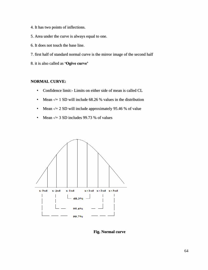
NORMAL CURVE:

• Confidence limit:- Limits on either side of mean is called CL

• Mean -/+ 1 SD will include 68.26 % values in the distribution

• Mean -/+ 2 SD will include approximately 95.46 % of value

• Mean -/+ 3 SD includes 99.73 % of values

Fig. Normal curve

65

Standard normal curve:

In a simple frequency distribution curve, we represent the frequencies with reference to actual

numbers.

But different characteristics have different units of measurement, so the frequency distributions

will not look same.

This problem is solved by what is called “standardization of normal curve”. Here, we assume

mean equal to zero (i.e. x = 0) and represent on the graph, each measurement not in terms of its

actual value, but in terms of “units of standard deviation” it is more or less than the mean.

This “unit of standard deviation” is expressed by letter “z” and is called “relative deviate” (RD).

Properties of standard normal curve:

1. It is bell shaped, smooth curve

2. Perfectly symmetrical curve & has two tails

3. It doesn’t touch the base line

4. Area of curve is 1 & mean is zero

5. Mean, median & mode coincide

6. Roughly Area included in m ± 1z = 68%,, m ± 2z = 95%, m ± 3z = 99%is of the total

area.

7. No portion of curve is below base line

66

Applications/ uses of the concept of normal curve:

1. Making estimate of the number of individuals in any range of measurements.

2. Deciding common/uncommon measurements: The concept of normal distribution helps in

deciding a cut-off point which can decide rare values.

For usual purposes the measurements beyond the range of m ± 2z are considered uncommon or

rare. This is because only 5% individuals are likely to have such measurements.

Example:

Systolic blood pressure (mm of Hg) follows a normal distribution with mean 118 and SD as

15.5. Find out 95% and 99% confidence limits for the SBP.

Solution:

Given that mean SBP=118 and SD=15.5Then, 95% confidence limits can be given as follows:

Mean ±2SD = 118 ± 2 x 15.5 = 118 ± 31 = 87 to 149mm of Hg

Thus, SBP will be lie in between 87 to 149mm of Hg at 95% of all the cases.

Now, 99% confidence limits can be given as follows:

Mean ±3SD=118±3 x 15.5=118±46.5=61.5 to 164.5 mm of Hg

Thus, SBP will be lie in between 61.5 to 64.5 mm of Hg at 99% of all the cases.

71

8. SAMPLING TECHNIQUES



exercises on Common



frequency



dispersion


• Explain common sampling

techniques

• Demonstrate sampling techniques

with appropriate example

Written (solving

exercises)/ viva

voce/ Skill

assessment

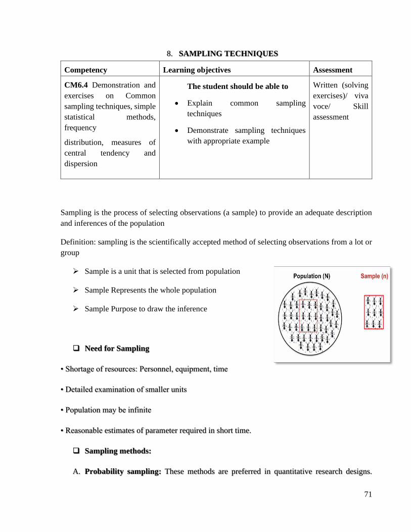
Sampling is the process of selecting observations (a sample) to provide an adequate description

and inferences of the population

Definition: sampling is the scientifically accepted method of selecting observations from a lot or

group

➢ Sample is a unit that is selected from population

➢ Sample Represents the whole population

➢ Sample Purpose to draw the inference

❑ Need for Sampling

• Shortage of resources: Personnel, equipment, time

• Detailed examination of smaller units

• Population may be infinite

• Reasonable estimates of parameter required in short time.

❑ Sampling methods:

A. Probability sampling: These methods are preferred in quantitative research designs.

72

These are named so, because, investigators know the probability of sampling unit entering

in the sample, because it is predecided.

i.Simple Random

ii.Stratified Random

iii.Systematic Random

iv.Cluster

v.Multi Stage

B. Non-Probability sampling: Non-probability sampling methods are used in qualitative

methods of research.

i.Convenience

ii.Purposive

iii.Quota

iv.Snowball

A.i. Simple Random Sampling:

• All subsets of the frame are given an equal probability

• Steps in a typical simple random sampling:

i. Enlist all sampling units: if, the sampling unit is the students. So, we make a list of all

students who are eligible to enter in the list as per inclusion/exclusion criteria. This is

arranged in alphabetical order. Suppose the number is 1000. Each student is given unique

number. It will be appropriate that the numbers start from 000 and end-up with 999. This

will ensure that all students will have a three-digit ID.

ii. Decide the sample size: The sample size would be calculated as per methods

recommended. Say this is 100.

iii. Select those to be included in sample: This can be done by 3 methods.

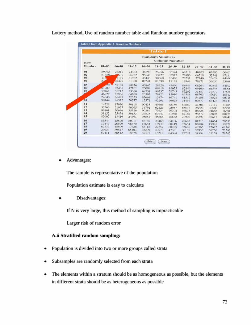
73

Lottery method, Use of random number table and Random number generators

• Advantages:

The sample is representative of the population

Population estimate is easy to calculate

• Disadvantages:

If N is very large, this method of sampling is impracticable

Larger risk of random error

A.ii Stratified random sampling:

• Population is divided into two or more groups called strata

• Subsamples are randomly selected from each strata

• The elements within a stratum should be as homogeneous as possible, but the elements

in different strata should be as heterogeneous as possible

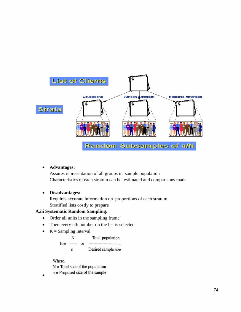
74

• Advantages:

Assures representation of all groups in sample population

Characteristics of each stratum can be estimated and comparisons made

• Disadvantages:

Requires accurate information on proportions of each stratum

Stratified lists costly to prepare

A.iii Systematic Random Sampling:

• Order all units in the sampling frame

• Then every nth number on the list is selected

• K = Sampling Interval

•

75

• Advantages:

Moderate cost; moderate usage

Simple to draw sample

Easy to verify

• Disadvantages:

Periodic ordering required

Carried out in stages

Using smaller and smaller sampling units at each stage

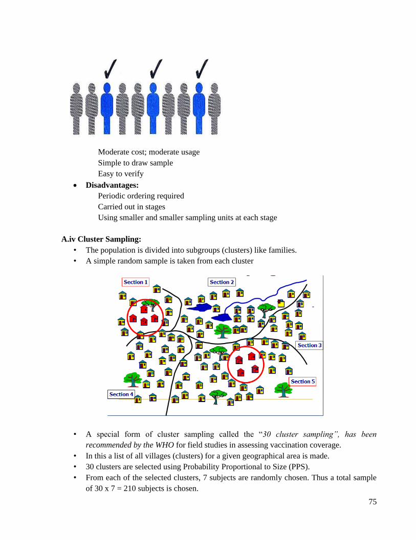
A.iv Cluster Sampling:

• The population is divided into subgroups (clusters) like families.

• A simple random sample is taken from each cluster

• A special form of cluster sampling called the “30 cluster sampling”, has been

recommended by the WHO for field studies in assessing vaccination coverage.

• In this a list of all villages (clusters) for a given geographical area is made.

• 30 clusters are selected using Probability Proportional to Size (PPS).

• From each of the selected clusters, 7 subjects are randomly chosen. Thus a total sample

of 30 x 7 = 210 subjects is chosen.

76

• The advantage of cluster sampling is that sampling frame is not required and in practice

when complete lists are not available.

• Advantages: Can estimate characteristics of both cluster and population

• Disadvantages:

The cost to reach an element to sample is very high

Each stage in cluster sampling introduces sampling error—the more stages there are, the

more error there tends to be

•

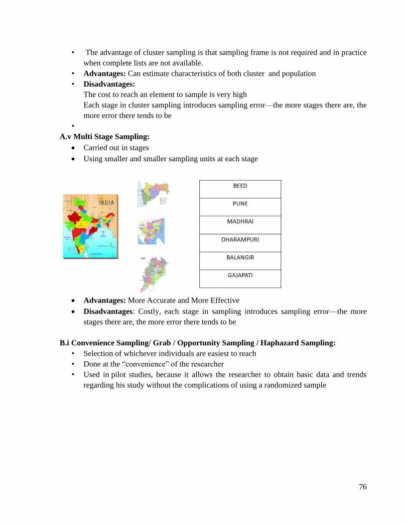
A.v Multi Stage Sampling:

• Carried out in stages

• Using smaller and smaller sampling units at each stage

• Advantages: More Accurate and More Effective

• Disadvantages: Costly, each stage in sampling introduces sampling error—the more

stages there are, the more error there tends to be

B.i Convenience Sampling/ Grab / Opportunity Sampling / Haphazard Sampling:

• Selection of whichever individuals are easiest to reach

• Done at the “convenience” of the researcher

• Used in pilot studies, because it allows the researcher to obtain basic data and trends

regarding his study without the complications of using a randomized sample

77

• Advantages: Fast, inexpensive, easy, subject readily available, immediately known

population group and good response rate

• Disadvantages:

Sampling Error

Sample is not representative of the entire population

Cannot generalise findings to the Population

B.ii Purposive/Authoritative Sampling:

• The researcher chooses the sample based on who they think would be appropriate

for the study

• Selected based on their knowledge and professional judgement

• Used when a limited number or category of individuals possess the trait of interest

• It is the only viable sampling technique in obtaining information from a very

specific group of people

• Advantages: There is a assurance of quality response. Meet the specific objective

• Disadvantages: Selection bias. Problem of generalizability

B.iii Quota Sampling:

• The population is first segmented into mutually exclusive sub-groups

• Then judgement/convenience used to select subjects or units from each segment based on

a specified proportion

• In quota sampling the selection of the sample is non-random

• When to Use Quota Samples

It allows the researchers to sample a subgroup that is of great interest to the study

Also allows to observe relationships between subgroups

• Advantages:

Contains specific subgroups in the proportions desired

Used when research budget is limited

Easy to manage, less time consuming

• Disadvantages:

Only reflects population in terms of the quota

Not possible to generalize

78

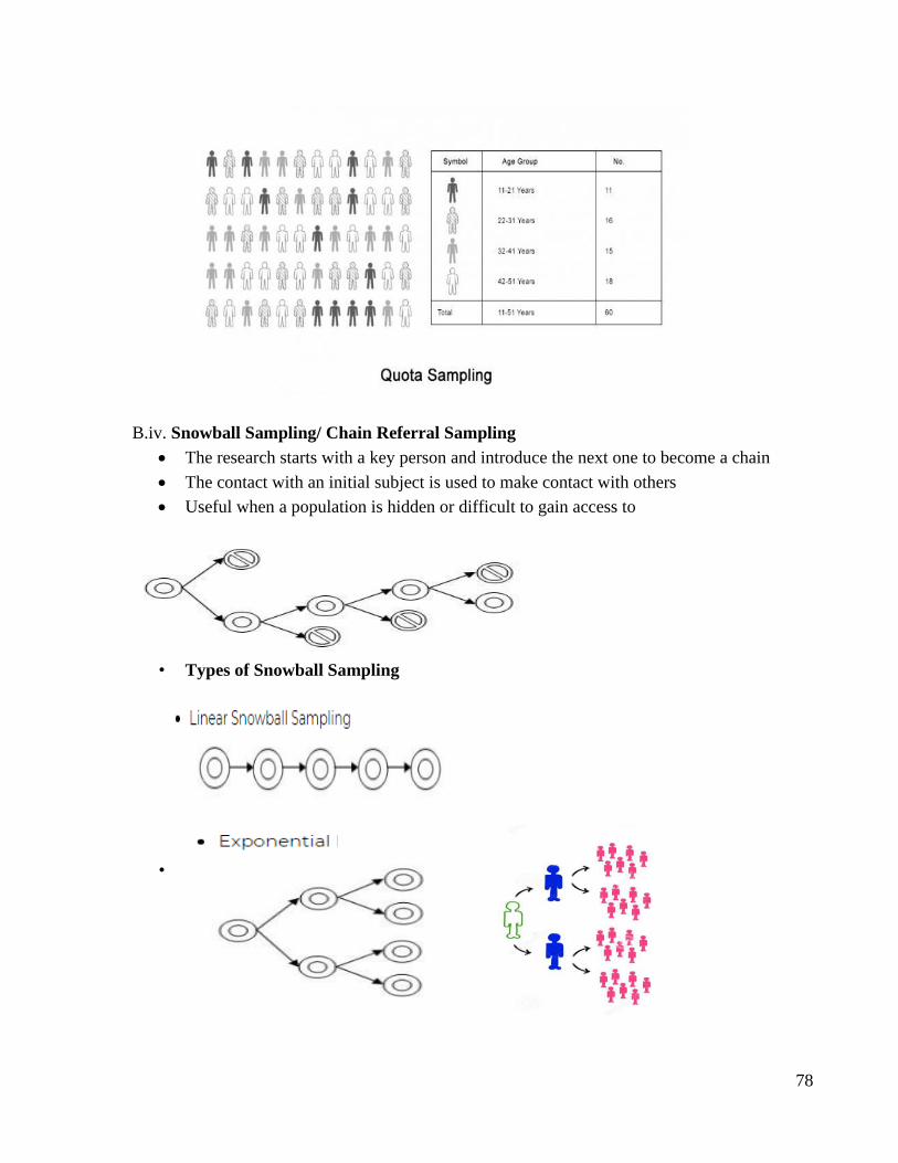
B.iv. Snowball Sampling/ Chain Referral Sampling

• The research starts with a key person and introduce the next one to become a chain

• The contact with an initial subject is used to make contact with others

• Useful when a population is hidden or difficult to gain access to

• Types of Snowball Sampling

• Uses

79

To identify potential subjects in studies where subjects are hard to locate

If the sample for the study is very rare or is limited to a very small subgroup of the population

• Advantages:

Simple & cost efficient

Useful in specific circumstances & for Identifying small, hard-to reach, uniquely defined target

population

Needs little planning and fewer workforce

• Disadvantages:

Not independent

Projecting data beyond sample not justified (Limited generalizability)

84

9. PROBABILITY


CM6.2 Methods of

collection, classification,

analysis, interpretation and


data


• Define probability

• Explain and demonstrate laws of

probability

Written/ viva

voce/ Skill

assessment

• The probability of specified event is the fraction or proportion of all possible events of a

specified type in a sequence of almost unlimited random trials under similar conditions.

• Probability is a measure of the likelihood of a random phenomenon or chance behavior.

Probability describes the long-term proportion with which a certain outcome will occur in

situations with short-term uncertainty.

• Probability may be defined as relative frequency or probable chances of occurrence with

which an event is expected to occur on an average.

• An element of uncertainty is associated with every conclusion because information on all

happenings is not available. This uncertainty is numerically expressed as “Probability.”

• If there are 'n' equally likely possibilities, of which one must occur and 's' is regarded as

favorable or as "success',

The probability of a "success" is given by the

Ratio= s/n.

• Probability is denoted by p and it ranges from 0 to 1

‘q’ i.e probability of not happening event is given as

q=1-p OR p + q =1

• Eg: the probability of getting Head or Tail in one toss are fifty-fifty or half and half, i.e.,

p = ½

• When the occurrence of an event is an absolute certainty then the probability of its

occurrence i.e. p=1

Eg.- Death of any living being

• Similarly chances of survival after rabies, in this case the probability of its occurrence i.e.

p=0

Random experiment & sample space

Random experiment—

• All the trials conducted under same set of condition form a random experiment.

• An event is the result or outcome of an experiment.

• Event is denoted using capital letters such as ‘E’

85

SAMPLE SPACE:

• denoted by ‘S’ of a probability experiment is the collection of all possible events.

• In other words, the sample space is a list of all possible outcomes of a probability

experiment.

UNION

• The union is a basic operation in set theory that provides a way to group the elements from

two sets into one new set.

• So the statement, "x is an element of A or an element of B" means that one of the three is

possible:

– x is an element of just A

– x is an element of just B

– x is an element of Both A&B

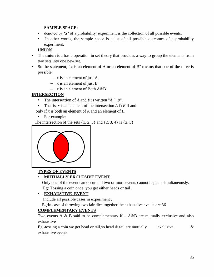
INTERSECTION

• The intersection of A and B is written "A ∩ B".

• That is, x is an element of the intersection A ∩ B if and

only if x is both an element of A and an element of B.

• For example:

The intersection of the sets {1, 2, 3} and {2, 3, 4} is {2, 3}.

TYPES OF EVENTS

• MUTUALLY EXCLUSIVE EVENT

Only one of the event can occur and two or more events cannot happen simultaneously.

Eg: Tossing a coin once, you get either heads or tail .

• EXHAUSTIVE EVENT

Include all possible cases in experiment .

Eg:In case of throwing two fair dice together the exhaustive events are 36.

COMPLEMENTARY EVENTS

Two events A & B said to be complementary if – A&B are mutually exclusive and also

exhaustive

Eg.-tossing a coin we get head or tail,so head & tail are mutually exclusive &

exhaustive events

86

INDEPENDENT EVENT

Events are said to be independent if the happening (or non happening ) of an event is not

affected by the supplementary knowledge about occurrence of remaining Events.

p-VALUE

• When you perform a hypothesis test in statistics, a p-value helps you determine the

significance of your results.

• It helps to determine the likelihood of an event to have occurred by chance

• Hypothesis tests are used to test the validity of a claim that is made about a population.

This claim that’s on trial, in essence, is called the null hypothesis.

• The alternative hypothesis is the one you would believe if the null hypothesis is concluded

to be untrue.

• The p-value is a number between 0 and 1 and interpreted in the following way

A small p-value (typically < 0.05) indicates strong evidence against the null hypothesis,

so you reject the null hypothesis.

A large p-value (> 0.05) indicates weak evidence against the null hypothesis, so you fail

to reject the null hypothesis.

ADDITION RULE OF PROBABILITY

• The addition rule is concerned with determining the probability of occurrence of any one

of several possible events.

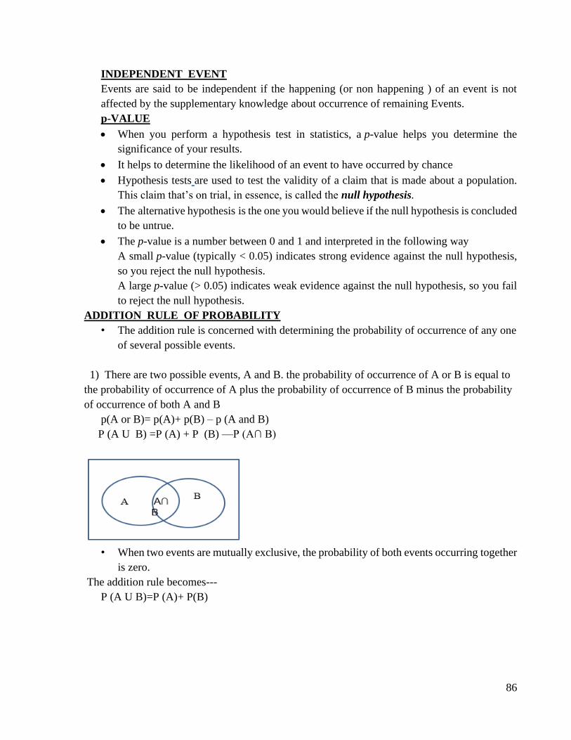
1) There are two possible events, A and B. the probability of occurrence of A or B is equal to

the probability of occurrence of A plus the probability of occurrence of B minus the probability

of occurrence of both A and B

p(A or B)= p(A)+ p(B) – p (A and B)

P (A U B) =P (A) + P (B) —P (A∩ B)

• When two events are mutually exclusive, the probability of both events occurring together

is zero.

The addition rule becomes---

P (A U B)=P (A)+ P(B)

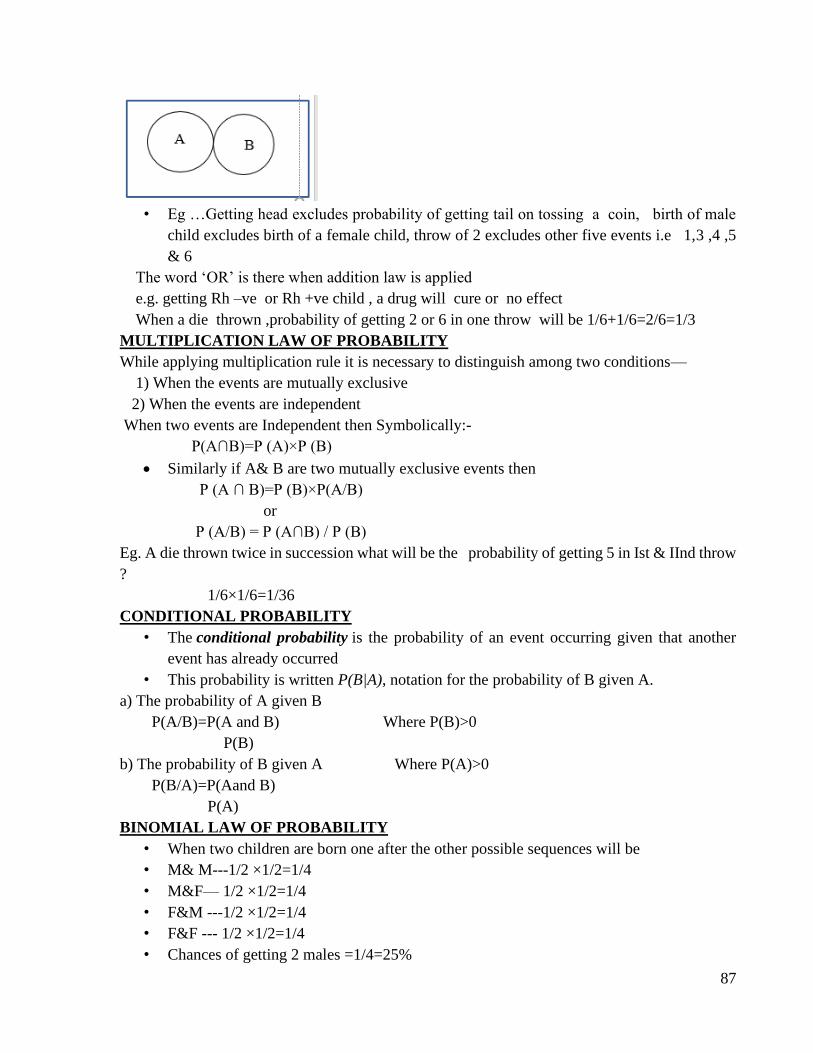
http://www.dummies.com/education/math/statistics/how-hypothesis-tests-are-used-in-statistics/

87

• Eg …Getting head excludes probability of getting tail on tossing a coin, birth of male

child excludes birth of a female child, throw of 2 excludes other five events i.e 1,3 ,4 ,5

& 6

The word ‘OR’ is there when addition law is applied

e.g. getting Rh –ve or Rh +ve child , a drug will cure or no effect

When a die thrown ,probability of getting 2 or 6 in one throw will be 1/6+1/6=2/6=1/3

MULTIPLICATION LAW OF PROBABILITY

While applying multiplication rule it is necessary to distinguish among two conditions—

1) When the events are mutually exclusive

2) When the events are independent

When two events are Independent then Symbolically:-

P(A∩B)=P (A)×P (B)

• Similarly if A& B are two mutually exclusive events then

P (A ∩ B)=P (B)×P(A/B)

or

P (A/B) = P (A∩B) / P (B)

Eg. A die thrown twice in succession what will be the probability of getting 5 in Ist & IInd throw

?

1/6×1/6=1/36

CONDITIONAL PROBABILITY

• The conditional probability is the probability of an event occurring given that another

event has already occurred

• This probability is written P(B|A), notation for the probability of B given A.

a) The probability of A given B

P(A/B)=P(A and B) Where P(B)>0

P(B)

b) The probability of B given A Where P(A)>0

P(B/A)=P(Aand B)

P(A)

BINOMIAL LAW OF PROBABILITY

• When two children are born one after the other possible sequences will be

• M& M---1/2 ×1/2=1/4

• M&F— 1/2 ×1/2=1/4

• F&M ---1/2 ×1/2=1/4

• F&F --- 1/2 ×1/2=1/4

• Chances of getting 2 males =1/4=25%

88

• Chances of getting 2 females=1/4=25%

BAYES’ THEOREM

• Bayes’ rule also called as Bayes’ Theorem or Inverse Probability is named after English

mathematician “Reverend Thomas Bayes.”

In health sciences, it is used to compute the predictive value of probability of disease, given

that particular symptoms have occurred.

According to BAYES’ rule;

91

Applied Biostatistics

I N D E X

Sr.

No.

Title of Date Page

No.

Grade Signature of the

teacher

1. Population Estimation

a. For Quantitative data


2. Test of significance

‘Z’ test a. For Quantitative data


3. Student ‘t’ test

a. Paired ‘t’ test

b. Unpaired ‘t’ test

4. Chi-Square test

5. Correlation coefficient and Rank correlation

6. Regression

7. Vital Statistics - rates and ratios

8. Applications of computer in

Medical Sciences


92

1. Population Estimation


CM6.2/6.3 Demonstration


application of elementary

statistical methods including

test of

significance in various study

designs and interpretation of

statistical tests.


• Estimate 95%, 99% confidence

limits for population mean

• Test whether sample is drawn from

sample having population mean

equal to some specified value

Written (MCQ,

SAQ, Solve

exercises)/ viva

voce/ Skill

assessment

• The phenomenon of variation in the sample statistics from population parameter is

called “sampling variation”.

• The limits within which sample statistics will vary from population parameter are called

“confidence limits”.

• The sampling variation is quantified by “standard error”.

• For quantitative variables standard error is called standard error of mean (SEM).

• For qualitative variables it is called standard error of proportion (SEP).

❑ SEM (Standard error of mean): Standard error of mean is a measure of variation for

quantitative data. To estimate population mean, S.E. of sample mean can be given as

follows:

SEM = σ/ √n

Where σ = Standard deviation of population

and n = sample size.

• If population SD (σ) not known, it is replaced

by sample SD (s). The formula becomes

SEM =s/ √n

• The relative deviate (z) for any given value of sample mean m1 can be calculated by

following equation

93

Interpretation/Use of SEM:

1. To find out the confidence limit within which the population mean would lie at

specified level of significance.

2. To test whether the sample mean is drawn from population with known population

mean (M).

➢ When M - the population mean (M) is known:

• We have to decide whether a sample with mean m1, size = n and standard deviation = s

is likely to have been drawn from the population with mean M (here we do not know

population SD, i.e. σ).

• Under such circumstances, at the outset we make following assumptions.

i. That the sample is drawn from the population in question and then proceed to test

whether the assumption is correct or wrong.

ii. That the s is the best estimate of S or so that SEM is calculated as below:

SEM = s/ √n

• Thus, now if the mean of the sample (m1) is within the range of M ± 2SEM, we can say

that it is likely to be drawn from the population with mean M. Else, it is less likely to be

drawn from the population with mean M.

➢ When M is unknown:

• This is a common situation.

• Here, with the help of mi and s we can make a reasonable estimate of M that is unknown.

• Two commonly accepted estimates are of 95% and 99% confidence as given below:

1. M = mi ± 2SEM (estimate with 95% confidence).

2. M = mi ± 3SEM (estimate with 99% confidence

❑ The confidence limits for the population mean can be given as:

• 95% confidence limits for population mean = Sample mean ±2 SEM

• 99% confidence limits for population mean= Sample mean ±3 SEM

If we draw a large number of samples (say ‘K’ numbers) from infinite population and we designate

the means of each sample as m1, m2, m3, m4 … mk, etc. then in such situations it has been shown

that:

• About 68% sample means would be within the range of M ± 1SEM;

• 95% would be within the range of M ± 2SEM and

• about 99% would be within the range of M ± 3SEM. These are called 68%, 95% and 99%

confidence limits respectively.

• A sample mean beyond the range M ± 2SEM would be considered as uncommon. The

possibility of such samples would be 5% or less. So a sample with mean beyond the range

of M ± 2SEM is less likely to be drawn from the population with mean M.

94

❑ SEP (standard error of proportion): It is a measure that describes the sampling variation

of a variable that is measured in nominal/ordinal scale as a dichotomous variable.

• Suppose in a population of size N; A is the number of persons with an attribute, so that the

number of persons who do not have that attribute is (N – A).

• The probability that a randomly selected person from the population has that attribute is

designated as P and the probability that a person does not have the attribute in question

will be (1 – P).

• The value of P is obtained by: P = A/N

• For sample the equation is: p = a/n

➢ The confidence limits for the population proportion can be given as:

• If we draw a large number of samples (say ‘k’ numbers) from an infinite population and

designate the proportion of the attribute in them as p1, p2, p3, … pk, etc. then in this

situation it has been shown that:

1. About 68% of samples would have p within the range of P ± 1SEP, about 95% would

have within the range of P ± 2SEP and about 99% would have within the range of P ±

3SEP.

2. Proportion of an attribute in a sample beyond the range of P ± 2SEP would be rare or

uncommon as it is beyond 95% confidence limit. The probability of such samples would

be 5% or less.

3. If a sample shows p beyond the range of P ± 2SEP, then it is less likely to belong to the

population where the proportion of that attribute is equal to P.

➢ Interpretation/Use of SEP:

1. To find the confidence interval for population proportion from sample.

2. To test whether the sample is drawn from population with proportion P.

When P is known:

• In this situation we have to decide whether a sample with p as the proportion of the

attribute in it, is likely to belong to the population in which the proportion of the attribute

is P.

• Here, at the outset we make the assumption that the sample is drawn from the population

under question and then proceed to test whether the assumption is correct.

• To do so we calculate the SEP , and find out if p is in the range P ± 2SEP. If yes, then the

sample is likely to belong to the population in question, if not, then it is less likely to

belong to the population in question.

If P is unknown:

• Under these circumstances we use p to make estimate of P.

• Estimates of 95% and 99% respectively are given by:

1. P(est) = p ± 2SEP …estimate of 95% confidence.

2. P(est) = p ± 3SEP …estimate of 99% confidence.

95

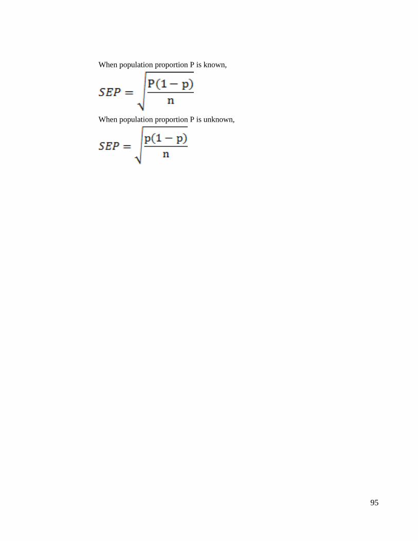
When population proportion P is known,

When population proportion P is unknown,

101

2. TEST OF SIGNIFICANCE





statistical methods

including test of



statistical tests.


• Explain choice of test of

significance as per the type of

variable, sample size, objective

of the test

• State Null hypothesis and

Alternate hypothesis

• Perform and interpret Z-test: Test

of significance of difference

between two means step by step

• Perform and interpret Z test: Test of

significance of difference between

two proportions step by step

Written (MCQ,

SAQ, Solve

exercises)/ viva

voce/ Skill

assessment

➢ A test of significance is required to decide whether

i. The observed difference/ association/ correlation in two or more variables is due to chance

(sampling variation) or

ii. It is due to the difference in the populations from which these samples are drawn.

➢ Steps in a Typical Test of Significance

1. Identify the type of data and variable

2. Choose appropriate test

3. State the NH and AH

4. Apply the chosen test and calculate P

5. Interpret (accept/reject NH, accept/reject

AH).

➢ Choice of test of significance depends on:

A. Objective of the test

B. Type of variable

C. Distribution of variable: Normal or not

D. Sample size

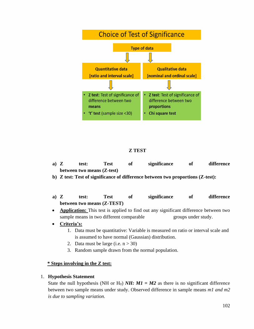
102

Z TEST

a) Z test: Test of significance of difference

between two means (Z-test)

b) Z test: Test of significance of difference between two proportions (Z-test):

a) Z test: Test of significance of difference

between two means (Z-TEST)

• Application: This test is applied to find out any significant difference between two

sample means in two different comparable groups under study.

• Criteria’s:

1. Data must be quantitative: Variable is measured on ratio or interval scale and

is assumed to have normal (Gaussian) distribution.

2. Data must be large (i.e. n > 30)

3. Random sample drawn from the normal population.

* Steps involving in the Z test:

1. Hypothesis Statement

State the null hypothesis (NH or H0) NH: M1 = M2 as there is no significant difference

between two sample means under study. Observed difference in sample means m1 and m2

is due to sampling variation.

103

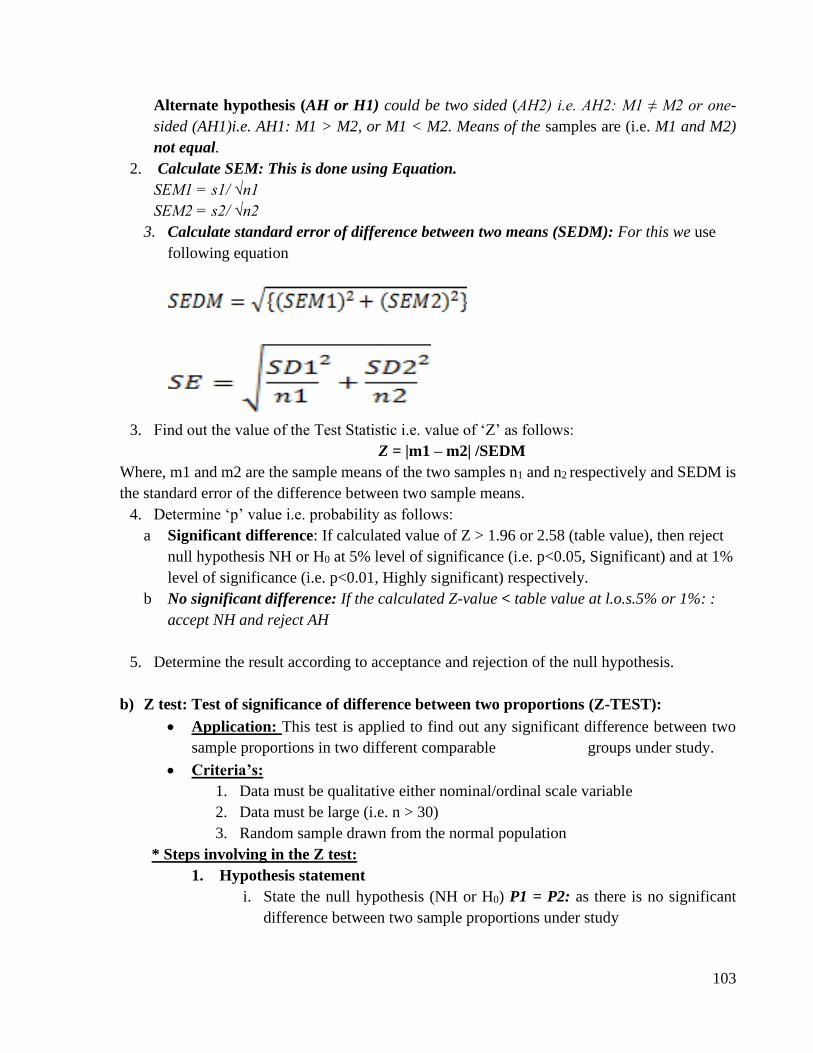
Alternate hypothesis (AH or H1) could be two sided (AH2) i.e. AH2: M1 ≠ M2 or one-

sided (AH1)i.e. AH1: M1 > M2, or M1 < M2. Means of the samples are (i.e. M1 and M2)

not equal.

2. Calculate SEM: This is done using Equation.

SEM1 = s1/ √n1

SEM2 = s2/ √n2

3. Calculate standard error of difference between two means (SEDM): For this we use

following equation

3. Find out the value of the Test Statistic i.e. value of ‘Z’ as follows:

Z = |m1 – m2| /SEDM

Where, m1 and m2 are the sample means of the two samples n1 and n2 respectively and SEDM is

the standard error of the difference between two sample means.

4. Determine ‘p’ value i.e. probability as follows:

a Significant difference: If calculated value of Z > 1.96 or 2.58 (table value), then reject

null hypothesis NH or H0 at 5% level of significance (i.e. p<0.05, Significant) and at 1%

level of significance (i.e. p<0.01, Highly significant) respectively.

b No significant difference: If the calculated Z-value < table value at l.o.s.5% or 1%: :

accept NH and reject AH

5. Determine the result according to acceptance and rejection of the null hypothesis.

b) Z test: Test of significance of difference between two proportions (Z-TEST):

• Application: This test is applied to find out any significant difference between two

sample proportions in two different comparable groups under study.

• Criteria’s:

1. Data must be qualitative either nominal/ordinal scale variable

2. Data must be large (i.e. n > 30)

3. Random sample drawn from the normal population

* Steps involving in the Z test:

1. Hypothesis statement

i. State the null hypothesis (NH or H0) P1 = P2: as there is no significant

difference between two sample proportions under study

104

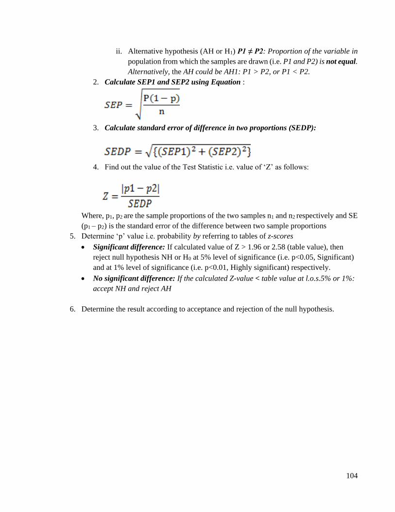
ii. Alternative hypothesis (AH or H1) P1 ≠ P2: Proportion of the variable in

population from which the samples are drawn (i.e. P1 and P2) is not equal.

Alternatively, the AH could be AH1: P1 > P2, or P1 < P2.

2. Calculate SEP1 and SEP2 using Equation :

3. Calculate standard error of difference in two proportions (SEDP):

4. Find out the value of the Test Statistic i.e. value of ‘Z’ as follows:

Where, p1, p2 are the sample proportions of the two samples n1 and n2 respectively and SE

(p1 – p2) is the standard error of the difference between two sample proportions

5. Determine ‘p’ value i.e. probability by referring to tables of z-scores

• Significant difference: If calculated value of Z > 1.96 or 2.58 (table value), then

reject null hypothesis NH or H0 at 5% level of significance (i.e. p<0.05, Significant)

and at 1% level of significance (i.e. p<0.01, Highly significant) respectively.

• No significant difference: If the calculated Z-value < table value at l.o.s.5% or 1%:

accept NH and reject AH

6. Determine the result according to acceptance and rejection of the null hypothesis.

110

3. ‘t’ Test or Student’s t test





statistical methods

including test of



statistical tests.


• Explain Applications of paired

and unpaired ‘t’ test



• To compare difference between

paired observations and compare

difference between unpaired

observations

• Test if two sample means are

significantly different or not for

small sample sizes

Written (MCQ,

SAQ, Solve

exercises)/ viva

voce/ Skill

assessment

• ‘t’ test was designed by W. S. Gossett whose pen name was ‘Student’ hence also

called Student’s t test.

• Student’s ‘t’ distribution: a sampling distribution used in test of hypothesis dealing

with specified value of mean (one sample problem) or equality of two population

means (two sample problem)

• Properties of t distribution:

1. It has mean 0

2. Variance greater than one

3. Bell shaped symmetrical distribution about mean

4. Compared to normal distribution it is flatter with thicker tails

5. For large values of n (> 30) t distribution approches normal distribution

• It is one of the small sample tests used when sample size is small i.e. less than or

equal to 30.

• ‘t’ test was designed by W. S. Gossett whose pen name was ‘Student’ hence also

called Student’s t test.

• The assumptions for t test:

1. Sample must be random

2. Population standard deviation is not known

3. Distribution of population from which sample is drawn is normal

• Uses of t test: Testing the significance of

1. The mean of the sample

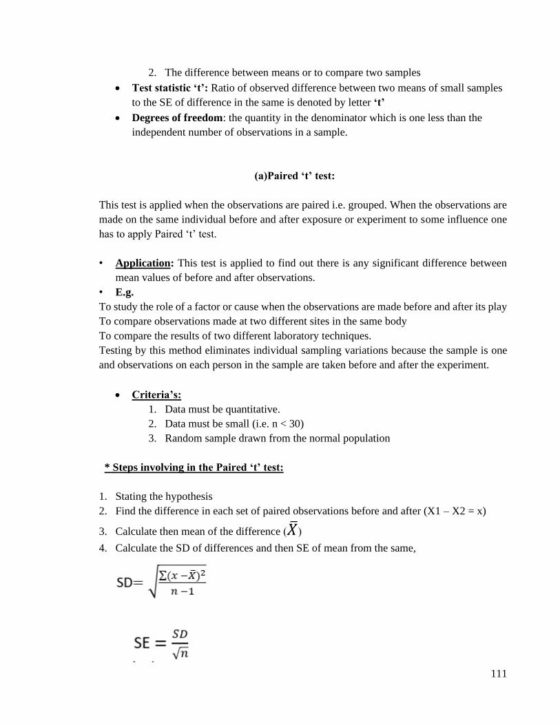
111

2. The difference between means or to compare two samples

• Test statistic ‘t’: Ratio of observed difference between two means of small samples

to the SE of difference in the same is denoted by letter ‘t’

• Degrees of freedom: the quantity in the denominator which is one less than the

independent number of observations in a sample.

(a)Paired ‘t’ test:

This test is applied when the observations are paired i.e. grouped. When the observations are

made on the same individual before and after exposure or experiment to some influence one

has to apply Paired ‘t’ test.

• Application: This test is applied to find out there is any significant difference between

mean values of before and after observations.

• E.g.

To study the role of a factor or cause when the observations are made before and after its play

To compare observations made at two different sites in the same body

To compare the results of two different laboratory techniques.

Testing by this method eliminates individual sampling variations because the sample is one

and observations on each person in the sample are taken before and after the experiment.

• Criteria’s:

1. Data must be quantitative.

2. Data must be small (i.e. n < 30)


* Steps involving in the Paired ‘t’ test:

1. Stating the hypothesis

2. Find the difference in each set of paired observations before and after (X1 – X2 = x)

3. Calculate then mean of the difference (�̅�)

4. Calculate the SD of differences and then SE of mean from the same,

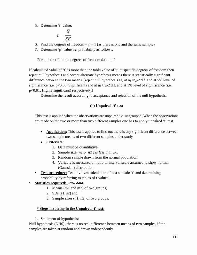
112

5. Determine ‘t’ value:

6. Find the degrees of freedom = n – 1 (as there is one and the same sample)


For this first find out degrees of freedom d.f. = n-1

If calculated value of ‘t’ is more than the table value of ‘t’ at specific degrees of freedom then

reject null hypothesis and accept alternate hypothesis means there is statistically significant

difference between the two means. [reject null hypothesis H0 at n1+n2-2 d.f. and at 5% level of

significance (i.e. p<0.05, Significant) and at n1+n2-2 d.f. and at 1% level of significance (i.e.

p<0.01, Highly significant) respectively.]

Determine the result according to acceptance and rejection of the null hypothesis.

(b) Unpaired ‘t’ test

This test is applied when the observations are unpaired i.e. ungrouped. When the observations

are made on the two or more than two different samples one has to apply unpaired ‘t’ test.

• Application: This test is applied to find out there is any significant difference between

two sample means of two different samples under study

• Criteria’s:

1. Data must be quantitative.

2. Sample size (n1 or n2 ) is less than 30.


4. Variable is measured on ratio or interval scale assumed to show normal

(Gaussian) distribution.

• Test procedure: Test involves calculation of test statistic ‘t’ and determining

probability by referring to tables of t-values.

• Statistics required: Raw data:

1. Means (m1 and m2) of two groups,

2. SDs (s1, s2) and

3. Sample sizes (n1, n2) of two groups.

* Steps involving in the Unpaired ‘t’ test:

1. Statement of hypothesis:

Null hypothesis (NH0)- there is no real difference between means of two samples, if the

samples are taken at random and drawn independently.

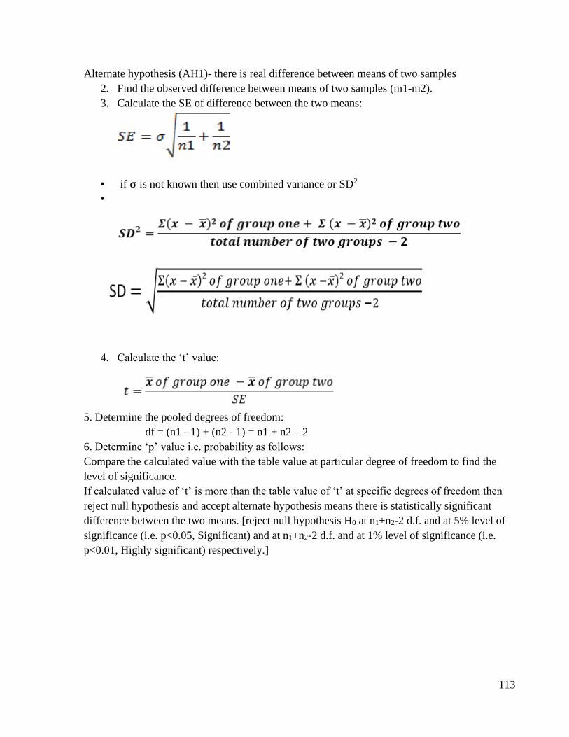
113

Alternate hypothesis (AH1)- there is real difference between means of two samples

2. Find the observed difference between means of two samples (m1-m2).

3. Calculate the SE of difference between the two means:

• if 𝛔 is not known then use combined variance or SD2

•

4. Calculate the ‘t’ value:

5. Determine the pooled degrees of freedom:

df = (n1 - 1) + (n2 - 1) = n1 + n2 – 2


Compare the calculated value with the table value at particular degree of freedom to find the

level of significance.

If calculated value of ‘t’ is more than the table value of ‘t’ at specific degrees of freedom then

reject null hypothesis and accept alternate hypothesis means there is statistically significant

difference between the two means. [reject null hypothesis H0 at n1+n2-2 d.f. and at 5% level of

significance (i.e. p<0.05, Significant) and at n1+n2-2 d.f. and at 1% level of significance (i.e.

p<0.01, Highly significant) respectively.]

119

4. Tests of significance Chi-Square test (χ2)





statistical methods

including test of



statistical tests.


• Explain Applications of Chi-

square (χ2)



• To test whether there is

association or relation between

two qualitative variables

Written (MCQ,

SAQ, Solve

exercises)/ viva

voce/ Skill

assessment

This is a Non-parametric test of significance, which is used to find significant association between

two variables e.g. smoking and cancer.

Application: To find out significant association between two variables under study

e.g. smoking and cancer, attack rate and vaccination, occupation and literacy etc.

• Test of proportion: To find the significance of difference in 2 or more than 2

proportions

• Test of association: Test of association between two events in binomial or

multinomial samples. It measures the probability of association between 2 discrete

attributes. Test for independence of attributes: 2 possibilities: either they influence

(dependent on each other)/ affect each other or they do not (independent of each other)

e.g. complications and severity of disease. It can be applied to find association/

relationship between two discrete attributes when there are more than two classes or

groups as happens in multinominal samples

• Goodness of fit: to test whether the difference between the theoretical and observed

values can be attributed to chance or not

• Criteria’s:

1. Data must be qualitative

2. Data must be large (n>30)

3. Random samples selected from the normal population

4. Expected frequency in any of the cell in 2x2 contingency table (two rows and

two columns) should no be less than 5.

• Test procedure: Test involves calculation of test statistics of Chi-square (χ2) and

determining the probability by referring to tables of Chi-square.

• Statistics required:

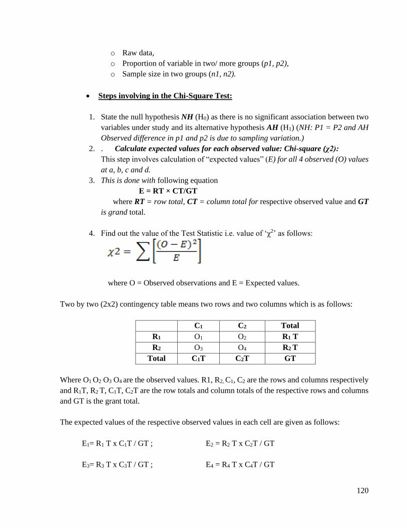
120

o Raw data,

o Proportion of variable in two/ more groups (p1, p2),

o Sample size in two groups (n1, n2).

• Steps involving in the Chi-Square Test:

1. State the null hypothesis NH (H0) as there is no significant association between two

variables under study and its alternative hypothesis AH (H1) (NH: P1 = P2 and AH

Observed difference in p1 and p2 is due to sampling variation.)

2. . Calculate expected values for each observed value: Chi-square (χ2):

This step involves calculation of “expected values” (E) for all 4 observed (O) values

at a, b, c and d.

3. This is done with following equation

E = RT × CT/GT

where RT = row total, CT = column total for respective observed value and GT

is grand total.

4. Find out the value of the Test Statistic i.e. value of ‘χ2’ as follows:

where O = Observed observations and E = Expected values.

Two by two (2x2) contingency table means two rows and two columns which is as follows:

C1 C2 Total

R1 O1 O2 R1 T

R2 O3 O4 R2 T

Total C1T C2T GT

Where O1 O2 O3 O4 are the observed values. R1, R2, C1, C2 are the rows and columns respectively

and R1T, R2 T, C1T, C2T are the row totals and column totals of the respective rows and columns

and GT is the grant total.

The expected values of the respective observed values in each cell are given as follows:

E1= R1 T x C1T / GT ; E2 = R2 T x C2T / GT

E3= R3 T x C3T / GT ; E4 = R4 T x C4T / GT

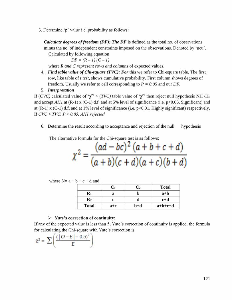
121


Calculate degrees of freedom (DF): The DF is defined as the total no. of observations

minus the no. of independent constraints imposed on the observations. Denoted by ‘neu’.

Calculated by following equation

DF = (R – 1) (C – 1)

where R and C represent rows and columns of expected values.

4. Find table value of Chi-square (TVC): For this we refer to Chi-square table. The first

row, like table of t test, shows cumulative probability. First column shows degrees of

freedom. Usually we refer to cell corresponding to P = 0.05 and our DF.

5. Interpretation

If (CVC) calculated value of ‘χ2’ > (TVC) table value of ‘χ2’ then reject null hypothesis NH /H0

and accept AH1 at (R-1) x (C-1) d.f. and at 5% level of significance (i.e. p<0.05, Significant) and

at (R-1) x (C-1) d.f. and at 1% level of significance (i.e. p<0.01, Highly significant) respectively.

If CVC ≤ TVC, P ≥ 0.05, AH1 rejected

6. Determine the result according to acceptance and rejection of the null hypothesis

The alternative formula for the Chi-square test is as follows:

where N= a + b + c + d and

C1 C2 Total

R1 a b a+b

R2 c d c+d

Total a+c b+d a+b+c+d

➢ Yate’s correction of continuity:

If any of the expected value is less than 5, Yate’s correction of continuity is applied. the formula

for calculating the Chi-square with Yate’s correction is

127

5. Correlation






test of



statistical tests.


• Calculate the correlation between

two qualitative variables

• Interpret correlation coefficient

Written (MCQ,

SAQ, Solve

exercises)/ viva

voce/ Skill

assessment

Introduction: Correlation measures the degree of relationship between the variables.The relationship of

quantitative nature, the appropriate statistical tool for discovering and measuring the relationship,

and expressing it in a brief formula is known as Correlation. Correlation is a statistical device

which helps us in analyzing the covariance of two or more than two variables.

TYPES OF CORRELATION Positive or negative Simple, partial and multiple Linear and

Non-linear

Correlation is positive (direct) or negative (inverse) would depend upon the direction is a change

of the variables. If both variables are varying in the same direction, i.e. if one variable is increasing

(decreasing) the other is also increasing (decreasing) – Positive correlation If one variable is

increasing (decreasing) the other is decreasing (increasing) – negative correlation

METHODS OF CO-RELATION

1. Scatter diagram (dot diagram)

2. Karl Pearson’s coefficient of correlation

3. Spaerman’s rank correlation coefficient

2. Karl Pearson’s correlation coefficient:

It is denoted by ‘r’ Range of r: - 1<= r <= 1

Formula: r = Σ xy / N δx δy where x= (X-X) and y=(Y-Y) and δx= SD of X, δy=SD of Y

Direct method:

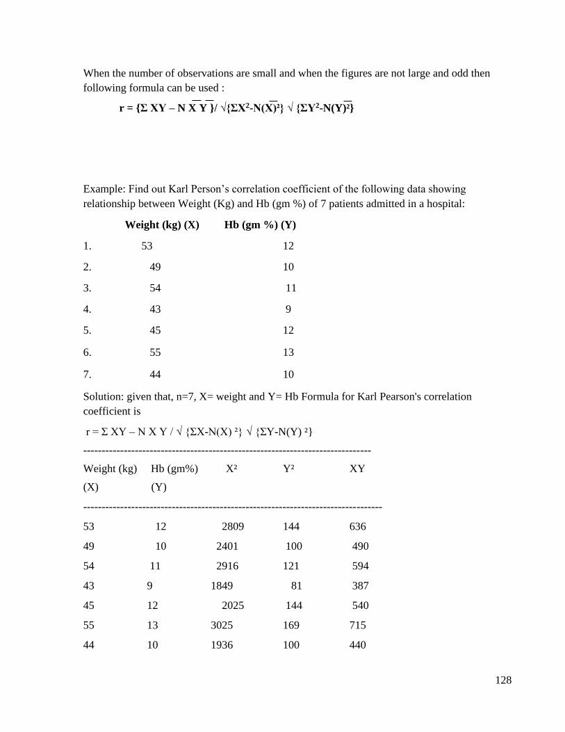
128

When the number of observations are small and when the figures are not large and odd then

following formula can be used :

r = {Σ XY – N X Y }/ √{ΣX2-N(X)²} √ {ΣY2-N(Y)²}

Example: Find out Karl Person’s correlation coefficient of the following data showing

relationship between Weight (Kg) and Hb (gm %) of 7 patients admitted in a hospital:

Weight (kg) (X) Hb (gm %) (Y)

1. 53 12

2. 49 10

3. 54 11

4. 43 9

5. 45 12

6. 55 13

7. 44 10

Solution: given that, n=7, X= weight and Y= Hb Formula for Karl Pearson's correlation

coefficient is

r = Σ XY – N X Y / √ {ΣX-N(X) ²} √ {ΣY-N(Y) ²}

------------------------------------------------------------------------------

Weight (kg) Hb (gm%) X² Y² XY

(X) (Y)

---------------------------------------------------------------------------------

53 12 2809 144 636

49 10 2401 100 490

54 11 2916 121 594

43 9 1849 81 387

45 12 2025 144 540

55 13 3025 169 715

44 10 1936 100 440

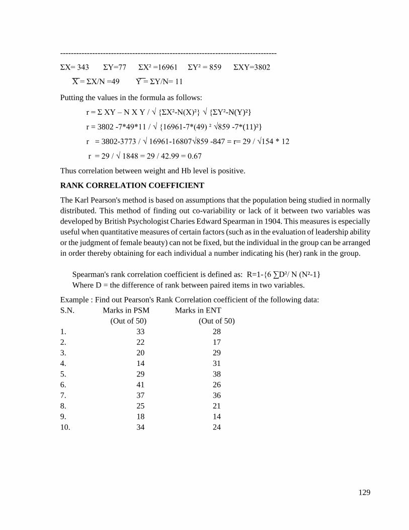
129

---------------------------------------------------------------------------------

ΣX= 343 ΣY=77 ΣX² =16961 ΣY² = 859 ΣXY=3802

X = ΣX/N =49 Y = ΣY/N= 11

Putting the values in the formula as follows:

r = Σ XY – N X Y / √ {ΣX²-N(X)²} √ {ΣY²-N(Y)²}

r = 3802 -7*49*11 / √ {16961-7*(49) ² √859 -7*(11)²}

r = 3802-3773 / √ 16961-16807√859 -847 = r= 29 / √154 * 12

r = 29 / √ 1848 = 29 / 42.99 = 0.67

Thus correlation between weight and Hb level is positive.

RANK CORRELATION COEFFICIENT

The Karl Pearson's method is based on assumptions that the population being studied in normally

distributed. This method of finding out co-variability or lack of it between two variables was

developed by British Psychologist Charies Edward Spearman in 1904. This measures is especially

useful when quantitative measures of certain factors (such as in the evaluation of leadership ability

or the judgment of female beauty) can not be fixed, but the individual in the group can be arranged

in order thereby obtaining for each individual a number indicating his (her) rank in the group.

Spearman's rank correlation coefficient is defined as: R=1-{6 ∑D²/ N (N²-1}

Where D = the difference of rank between paired items in two variables.

Example : Find out Pearson's Rank Correlation coefficient of the following data:

S.N. Marks in PSM Marks in ENT

(Out of 50) (Out of 50)

1. 33 28

2. 22 17

3. 20 29

4. 14 31

5. 29 38

6. 41 26

7. 37 36

8. 25 21

9. 18 14

10. 34 24

130

Solution: X-Marks in PSM Y-Marks in ENT N = 10

S.N. X Y Rx Ry D = Rx-Ry D²

---------------------------------------------------------------------------------

1. 33 28 4 5 -1 1

2. 22 17 7 9 -2 4

3. 20 29 8 4 4 16

4. 14 31 10 3 7 49

5. 29 38 5 1 4 16

6. 41 26 1 6 -5 25

7. 37 36 2 2 0 0

8. 25 21 6 8 -2 4

9. 18 14 9 10 -1 1

10. 34 24 3 7 -4 16

-------------------------------------------------------------------------------

∑D² = 132

Applying formula for pearson's Rank Correlation coefficient as follows:

R = 1-6 ∑D2 / N3 -N

= 1- {6*132 / (103 – 10)}

= 1-{792 / (1000 – 10)}

= 1-{792 / 990}

= 1-0.8

R = 0.2

133

6. REGRESSION






test of



statistical tests.


• To predict the unknown values of

one variable from known values of

another variable

Written/ viva

voce/ Skill

assessment

Regression analysis reveals average relationship between two variables and this makes possible

estimation of prediction. The meaning of the term regression is the act of returning of going back.

Regression analysis is a statistical device with the help of which we are in a position to estimate

(predict) the unknown values of one variable from known values of another variable. The

variables which are used to predict the variable of interest is called the ‘independent variable’ and

the variable we are trying to predict is called the ‘depending variable’. The independent variable

is denoted by ‘X’ and dependent variable is denoted by ‘Y’. The analysis used is called the simple

linear regression analysis. The liner means that an equation of a straight line of the form Y =a +

bX.

Line of regression

There are two lines of regression for analysis of two variables under study and to estimate the

unknown value.

1. Line of regression of X on Y is given as:

X – X = bxy (Y-Y)

Where, X and Y are the means of X and Y respectively. bxy = Regression coefficient of X on Y

and is calculated as follows: bxy = rσx / σy, Where, r is correlation coefficient between x and y

and σx and σy are the SD's of x and y respectively.

2. Line of regression of Y on X is given as:

Y-Y = b yx (X-X)

Where, X and Y are the means of X and Y respectively. b yx = Regression coeff. of X on Y and

is calculated as follows: byx = r σy / σx, where, r is correlation coefficient between x and y and

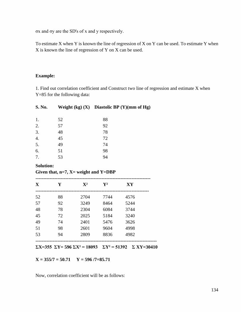
134

σx and σy are the SD's of x and y respectively.

To estimate X when Y is known the line of regression of X on Y can be used. To estimate Y when

X is known the line of regression of Y on X can be used.

Example:

1. Find out correlation coefficient and Construct two line of regression and estimate X when

Y=85 for the following data:

S. No. Weight (kg) (X) Diastolic BP (Y)(mm of Hg)

1. 52 88

2. 57 92

3. 48 78

4. 45 72

5. 49 74

6. 51 98

7. 53 94

Solution:

Given that, n=7, X= weight and Y=DBP

-------------------------------------------------------------------------

X Y X² Y² XY

------------------------------------------------------------------------

52 88 2704 7744 4576

57 92 3249 8464 5244

48 78 2304 6084 3744

45 72 2025 5184 3240

49 74 2401 5476 3626

51 98 2601 9604 4998

53 94 2809 8836 4982

-----------------------------------------------------------------------------

ΣX=355 ΣY= 596 ΣX² = 18093 ΣY² = 51392 Σ XY=30410

X = 355/7 = 50.71 Y = 596 /7=85.71

Now, correlation coefficient will be as follows:

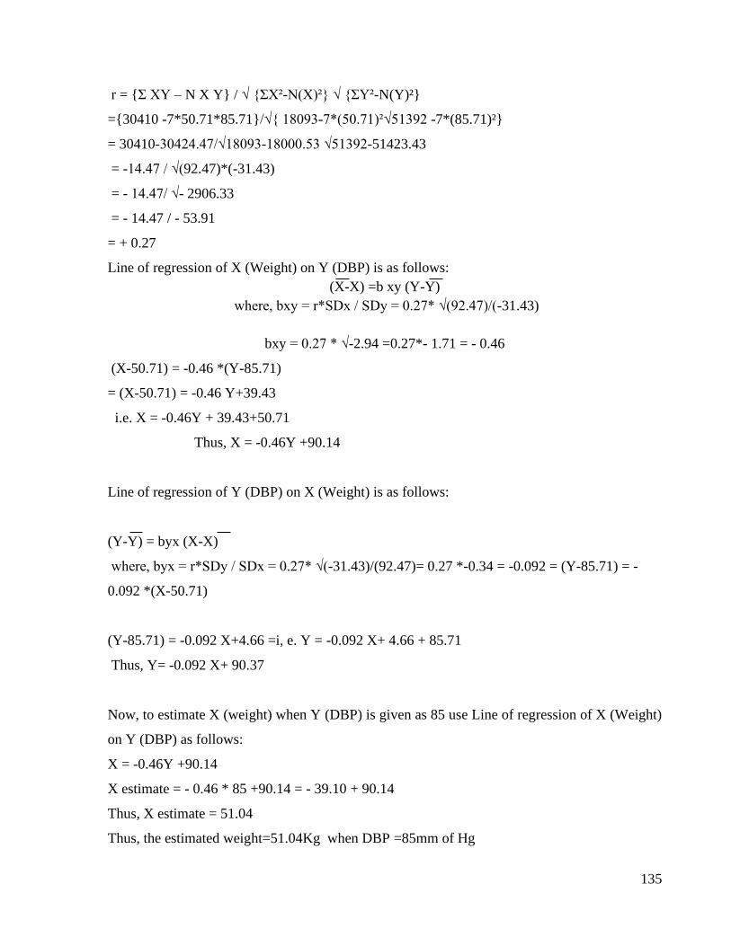
135

r = {Σ XY – N X Y} / √ {ΣX²-N(X)²} √ {ΣY²-N(Y)²}

={30410 -7*50.71*85.71}/√{ 18093-7*(50.71)²√51392 -7*(85.71)²}

= 30410-30424.47/√18093-18000.53 √51392-51423.43

= -14.47 / √(92.47)*(-31.43)

= - 14.47/ √- 2906.33

= - 14.47 / - 53.91

= + 0.27

Line of regression of X (Weight) on Y (DBP) is as follows:

(X-X) =b xy (Y-Y)

where, bxy = r*SDx / SDy = 0.27* √(92.47)/(-31.43)

bxy = 0.27 * √-2.94 =0.27*- 1.71 = - 0.46

(X-50.71) = -0.46 *(Y-85.71)

= (X-50.71) = -0.46 Y+39.43

i.e. X = -0.46Y + 39.43+50.71

Thus, X = -0.46Y +90.14

Line of regression of Y (DBP) on X (Weight) is as follows:

(Y-Y) = byx (X-X)

where, byx = r*SDy / SDx = 0.27* √(-31.43)/(92.47)= 0.27 *-0.34 = -0.092 = (Y-85.71) = -

0.092 *(X-50.71)

(Y-85.71) = -0.092 X+4.66 =i, e. Y = -0.092 X+ 4.66 + 85.71

Thus, Y= -0.092 X+ 90.37

Now, to estimate X (weight) when Y (DBP) is given as 85 use Line of regression of X (Weight)

on Y (DBP) as follows:

X = -0.46Y +90.14

X estimate = - 0.46 * 85 +90.14 = - 39.10 + 90.14

Thus, X estimate = 51.04

Thus, the estimated weight=51.04Kg when DBP =85mm of Hg

137

7. VITAL STATISTICS


CM9.2 Calculation and

interpretation of

demographic indices

including birth rate, death

rate, fertility rates


• Define vital statistics

• Calculate and interpret important

vital rates and ratios

• Discuss current National Vital

statistics

Written/ viva

voce/ Skill

assessment

DEFINITION

“Vital Statistics” has been used to denote facts systematically collected and compiled in

numerical form relating to or derived from records of vital events, namely live birth, death, foetal

death, marriage, divorce, adoption, legitimating, recognition, annulment, or legal separation. In

essence, vital statistics are derived from legally registerable events without including population

data or morbidity data.

USES OF VITAL STATISTICS

1) To describe the level of community health. 2) To diagnose community ills and determine the

met and unmet health needs, 3) To disseminate reliable information on the health situation and

health programmes. 4) To direct or maintain control during execution of program. 5) To develop

procedures, definitions and techniques such as recording system, sampling schemes etc. 6)To

undertake overall evaluation of health programmes and public health work.

For instance, carefully compiled causes of death in a city can provide answers to

1) The leading cause of death in the city? (Malaria, TB etc.) 2) At what age is the mortality

highest and from what disease?

3) What sections of the city (women or children or individuals following certain occupation) are

the unhealthiest and what is the outstanding cause of death there. 4) Comparison of cities in

relation to their health status, health facilities to cope with the problem

IMPORTANT VITAL RATES AND RATIOS

A) FERTILITY RATES/INDICES

1) Crude birth rate : An index of the relative speed at which additions are being made to

the population through child birth.

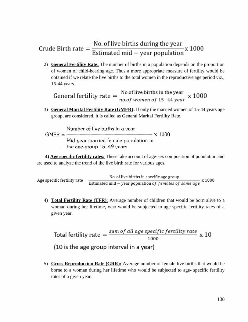
138

2) General Fertility Rate: The number of births in a population depends on the proportion

of women of child-bearing age. Thus a more appropriate measure of fertility would be

obtained if we relate the live births to the total women in the reproductive age period viz.,

15-44 years.

3) General Marital Fertility Rate (GMFR): If only the married women of 15-44 years age

group, are considered, it is called as General Marital Fertility Rate.

4) Age specific fertility rates: These take account of age-sex composition of population and

are used to analyze the trend of the live birth rate for various ages.

4) Total Fertility Rate (TFR): Average number of children that would be born alive to a

woman during her lifetime, who would be subjected to age-specific fertility rates of a

given year.

5) Gross Reproduction Rate (GRR): Average number of female live births that would be

borne to a woman during her lifetime who would be subjected to age- specific fertility

rates of a given year.

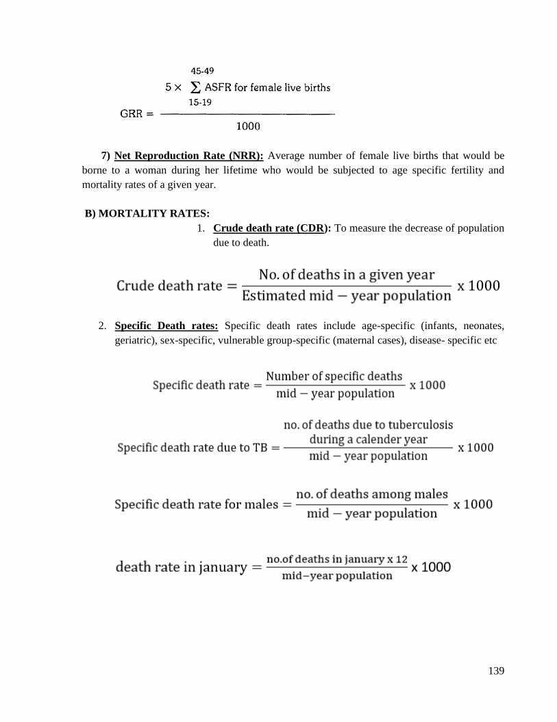
139

7) Net Reproduction Rate (NRR): Average number of female live births that would be

borne to a woman during her lifetime who would be subjected to age specific fertility and

mortality rates of a given year.

B) MORTALITY RATES:

1. Crude death rate (CDR): To measure the decrease of population

due to death.

2. Specific Death rates: Specific death rates include age-specific (infants, neonates,

geriatric), sex-specific, vulnerable group-specific (maternal cases), disease- specific etc

140

3. PROPORTIONAL MORTALITY RATE:

4. CASE FATALITY RATE:

5. MATERNAL MORTALITY RATE : The risk of dying from causes associated with

childbirth is measured by the maternal mortality rate. MMR =

6. AGE SPECIFIC DEATH RATES:

a) INFANT MORTALITY RATE : It is one of the most sensitive indexes of health

conditions of the general population. It is sensitive measure because a baby in its

extrauterine life is suddenly exposed to a multitude of new environmental factors and their

reactions are reflected in this rate. Under ideal conditions of social welfare no normal baby

should die.

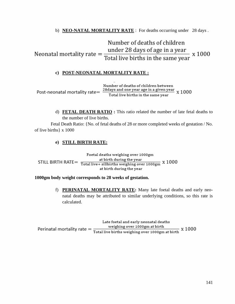
141

b) NEO-NATAL MORTALITY RATE : For deaths occurring under 28 days .

c) POST-NEONATAL MORTALITY RATE :

d) FETAL DEATH RATIO : This ratio related the number of late fetal deaths to

the number of live births.

Fetal Death Ratio: {No. of fetal deaths of 28 or more completed weeks of gestation / No.

of live births} x 1000

e) STILL BIRTH RATE:

1000gm body weight corresponds to 28 weeks of gestation.

f) PERINATAL MORTALITY RATE: Many late foetal deaths and early neo-

natal deaths may be attributed to similar underlying conditions, so this rate is

calculated.

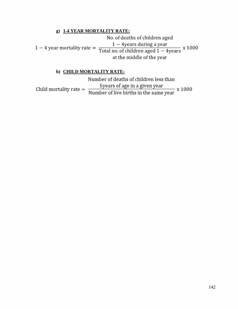
142

g) 1-4 YEAR MORTALITY RATE:

h) CHILD MORTALITY RATE:

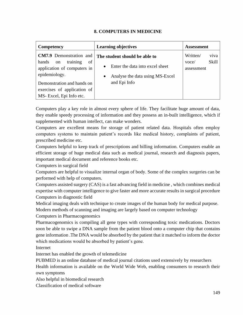
149

8. COMPUTERS IN MEDICINE



hands on training of

application of computers in

epidemiology.

Demonstration and hands on

exercises of application of

MS- Excel, Epi Info etc.


• Enter the data into excel sheet

• Analyse the data using MS-Excel

and Epi Info

Written/ viva

voce/ Skill

assessment

Computers play a key role in almost every sphere of life. They facilitate huge amount of data,

they enable speedy processing of information and they possess an in-built intelligence, which if

supplemented with human intellect, can make wonders.

Computers are excellent means for storage of patient related data. Hospitals often employ

computers systems to maintain patient’s records like medical history, complaints of patient,

prescribed medicine etc.

Computers helpful to keep track of prescriptions and billing information. Computers enable an

efficient storage of huge medical data such as medical journal, research and diagnosis papers,

important medical document and reference books etc.

Computers in surgical field

Computers are helpful to visualize internal organ of body. Some of the complex surgeries can be

performed with help of computers.

Computers assisted surgery (CAS) is a fast advancing field in medicine , which combines medical

expertise with computer intelligence to give faster and more accurate results in surgical procedure

Computers in diagnostic field

Medical imaging deals with technique to create images of the human body for medical purpose.

Modern methods of scanning and imaging are largely based on computer technology

Computers in Pharmacogenomics

Pharmacogenomics is compiling all gene types with corresponding toxic medications. Doctors

soon be able to swipe a DNA sample from the patient blood onto a computer chip that contains

gene information .The DNA would be absorbed by the patient that it matched to inform the doctor

which medications would be absorbed by patient’s gene.

Internet

Internet has enabled the growth of telemedicine

PUBMED is an online database of medical journal citations used extensively by researchers

Health information is available on the World Wide Web, enabling consumers to research their

own symptoms

Also helpful in biomedical research

Classification of medical software

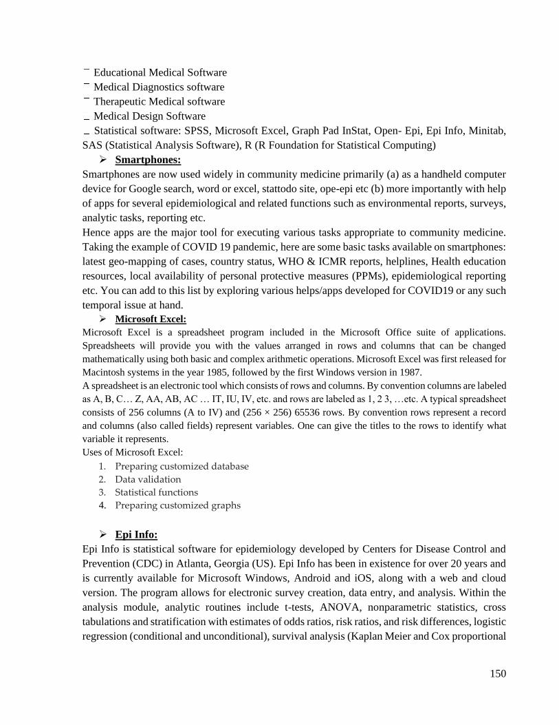
150

Educational Medical Software

Medical Diagnostics software

Therapeutic Medical software

Medical Design Software

Statistical software: SPSS, Microsoft Excel, Graph Pad InStat, Open- Epi, Epi Info, Minitab,

SAS (Statistical Analysis Software), R (R Foundation for Statistical Computing)

➢ Smartphones:

Smartphones are now used widely in community medicine primarily (a) as a handheld computer

device for Google search, word or excel, stattodo site, ope-epi etc (b) more importantly with help

of apps for several epidemiological and related functions such as environmental reports, surveys,

analytic tasks, reporting etc.

Hence apps are the major tool for executing various tasks appropriate to community medicine.

Taking the example of COVID 19 pandemic, here are some basic tasks available on smartphones:

latest geo-mapping of cases, country status, WHO & ICMR reports, helplines, Health education

resources, local availability of personal protective measures (PPMs), epidemiological reporting

etc. You can add to this list by exploring various helps/apps developed for COVID19 or any such

temporal issue at hand.

➢ Microsoft Excel:

Microsoft Excel is a spreadsheet program included in the Microsoft Office suite of applications.

Spreadsheets will provide you with the values arranged in rows and columns that can be changed

mathematically using both basic and complex arithmetic operations. Microsoft Excel was first released for

Macintosh systems in the year 1985, followed by the first Windows version in 1987.

A spreadsheet is an electronic tool which consists of rows and columns. By convention columns are labeled

as A, B, C… Z, AA, AB, AC … IT, IU, IV, etc. and rows are labeled as 1, 2 3, …etc. A typical spreadsheet

consists of 256 columns (A to IV) and (256 × 256) 65536 rows. By convention rows represent a record

and columns (also called fields) represent variables. One can give the titles to the rows to identify what

variable it represents.

Uses of Microsoft Excel:

1. Preparing customized database

2. Data validation

3. Statistical functions

4. Preparing customized graphs

➢ Epi Info:

Epi Info is statistical software for epidemiology developed by Centers for Disease Control and

Prevention (CDC) in Atlanta, Georgia (US). Epi Info has been in existence for over 20 years and

is currently available for Microsoft Windows, Android and iOS, along with a web and cloud

version. The program allows for electronic survey creation, data entry, and analysis. Within the

analysis module, analytic routines include t-tests, ANOVA, nonparametric statistics, cross

tabulations and stratification with estimates of odds ratios, risk ratios, and risk differences, logistic

regression (conditional and unconditional), survival analysis (Kaplan Meier and Cox proportional

151

hazard), and analysis of complex survey data. The software is an open-source project with limited

support.

➢ SPSS:

SPSS means “Statistical Package for the Social Sciences” and was first launched in

1968. Since SPSS was acquired by IBM in 2009, it's officially known as IBM SPSS

Statistics but most users still just refer to it as “SPSS”. SPSS is a widely used program

for statistical analysis in social science. It is also used by market researchers, health

researchers, survey companies, government, education researchers, marketing

organizations, data miners, and others. SPSS is software for editing and analyzing all

sorts of data. The data can be from any source: scientific research, a customer database,

Google Analytics or even the server log files of a website. SPSS can open all file formats

that are commonly used for structured data such as

• spreadsheets from MS Excel or OpenOffice;

• plain text files (.txt or .csv);

• relational (SQL) databases;

• Stata and SAS.

Statistics included in the base software:

• Descriptive statistics: Cross tabulation, Frequencies, Descriptives, Explore,

Descriptive Ratio Statistics

• Bivariate statistics: Means, t-test, ANOVA, Correlation (bivariate, partial,

distances), Nonparametric tests, Bayesian

• Prediction for numerical outcomes: Linear regression

• Prediction for identifying groups: Factor analysis, cluster analysis (two-step, K-

means, hierarchical), Discriminant

• Geo spatial analysis, simulation

• R extension (GUI), Python

https://www.openoffice.org/

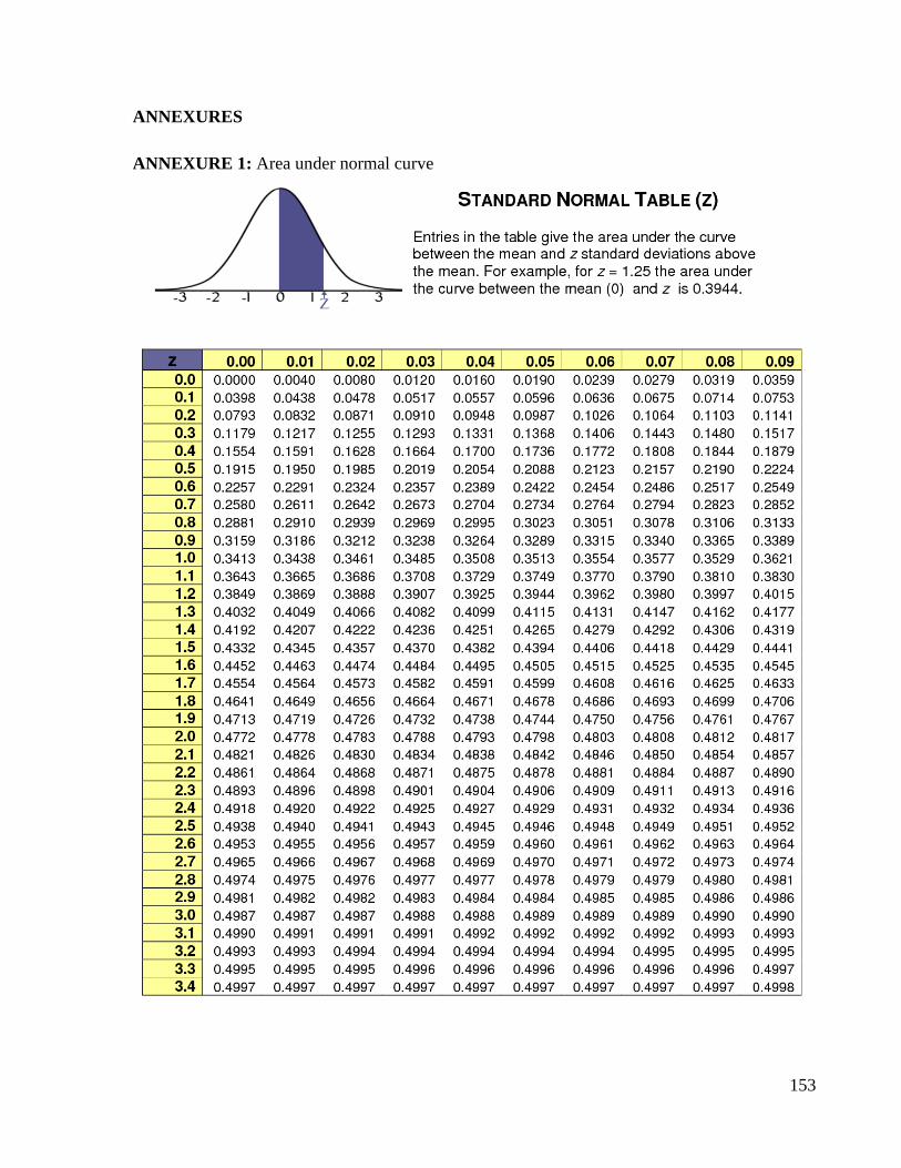
153

ANNEXURES

ANNEXURE 1: Area under normal curve

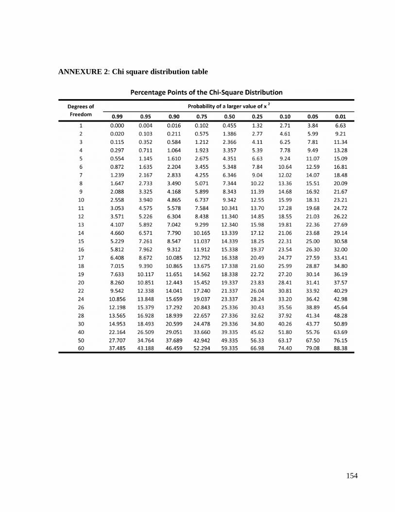
154

ANNEXURE 2: Chi square distribution table

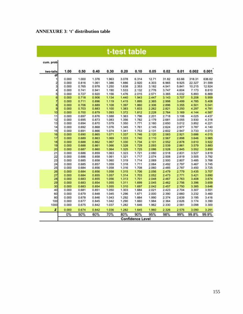
155

ANNEXURE 3: ‘t’ distribution table

156

Epidemiology

I N D E X

Sr no. Title of Date Page

No.

Grade Signature of

the teacher

1. Epidemiological exercises based on

water


nutrition


mortality and morbidity indicators

4. Exercises based on Communicable

diseases

5. Immunization

6. Disinfection and sterilization

7. Concept of research

8. Epidemiological study designs

9. Exercises based on screening

10. Investigation of an epidemic

11. Emporiatrics

12. Writing a research


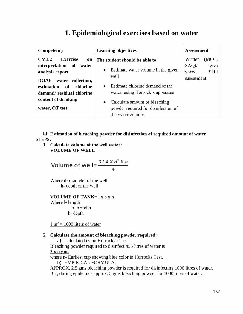
157

1. Epidemiological exercises based on water


CM3.2 Exercise on

interpretation of water

analysis report

DOAP- water collection,

estimation of chlorine

demand/ residual chlorine

content of drinking

water, OT test


• Estimate water volume in the given

well

• Estimate chlorine demand of the

water, using Horrock’s apparatus

• Calculate amount of bleaching

powder required for disinfection of

the water volume.

Written (MCQ,

SAQ)/ viva

voce/ Skill

assessment

❑ Estimation of bleaching powder for disinfection of required amount of water

STEPS:

1. Calculate volume of the well water:

VOLUME OF WELL

Where d- diameter of the well

h- depth of the well

VOLUME OF TANK= l x b x h

Where l- length

b- breadth

h- depth

1 m3 = 1000 liters of water

2. Calculate the amount of bleaching powder required:

a) Calculated using Horrocks Test:

Bleaching powder required to disinfect 455 litres of water is

2 x n gms

where n- Earliest cup showing blue color in Horrocks Test.

b) EMPIRICAL FORMULA:

APPROX. 2.5 gms bleaching powder is required for disinfecting 1000 litres of water.

But, during epidemics approx. 5 gms bleaching powder for 1000 litres of water.

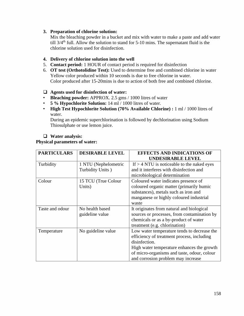
158

3. Preparation of chlorine solution:

Mix the bleaching powder in a bucket and mix with water to make a paste and add water

till 3/4th full. Allow the solution to stand for 5-10 mins. The supernatant fluid is the

chlorine solution used for disinfection.

4. Delivery of chlorine solution into the well

5. Contact period: 1 HOUR of contact period is required for disinfection

6. OT test (Orthotolidine Test): Used to determine free and combined chlorine in water

Yellow color produced within 10 seconds is due to free chlorine in water.

Color produced after 15-20mins is due to action of both free and combined chlorine.

❑ Agents used for disinfection of water:

• Bleaching powder: APPROX. 2.5 gms / 1000 litres of water

• 5 % Hypochlorite Solution: 14 ml / 1000 litres of water.

• High Test Hypochlorite Solution (70% Available Chlorine) : 1 ml / 1000 litres of

water.

During an epidemic superchlorination is followed by dechlorination using Sodium

Thiosulphate or use lemon juice.

❑ Water analysis:

Physical parameters of water:

PARTICULARS DESIRABLE LEVEL EFFECTS AND INDICATIONS OF

UNDESIRABLE LEVEL

Turbidity 1 NTU (Nephelometric

Turbidity Units )

If > 4 NTU is noticeable to the naked eyes

and it interferes with disinfection and

microbiological determination

Colour 15 TCU (True Colour

Units)

Coloured water indicates presence of

coloured organic matter (primarily humic

substances), metals such as iron and

manganese or highly coloured industrial

waste

Taste and odour No health based

guideline value

It originates from natural and biological

sources or processes, from contamination by

chemicals or as a by-product of water

treatment (e.g. chlorination)

Temperature No guideline value Low water temperature tends to decrease the

efficiency of treatment process, including

disinfection.

High water temperature enhances the growth

of micro-organisms and taste, odour, colour

and corrosion problem may increase

159

Inorganic constituents of water:

PARTICULARS DESIRABLE

LEVEL

EFFECTS AND INDICATIONS OF

UNDESIRABLE LEVEL

Chlorides 200 mg/litre to 600 mg/litre

water contamination

Hardness 50 – 150 mg/litr Higher range causes scale deposition in the distribution system and will result in excessive soap consumption and subsequent scum formation. On heating, hard water forms deposits of calcium carbonate scale. Soft water, with a hardness of less than 100 mg/litre is more corrosive for water pipes

Ammonia below 0.2 mg/litre Ammonia in water is an indicator of possible bacterial, sewage and animal waste pollution. Compromise disinfection efficiency, result in nitrite formation in distribution systems, can cause the failure of filters and cause taste and odour problems.

pH 6.5 and 8.5 pH levels of less than 7 may cause severe corrosion of metals in the distribution pipes and elevated levels of certain chemical substances, such as lead, may result. At pH levels above 8, there is a progressive decrease in the efficiency of the chlorine disinfection process

Hydrogen sulphide 0.05 and 0.1 mg/litre

The "rotten eggs" odour of hydrogen sulphide is particularly noticeable in some ground waters and in stagnant drinking water in the distribution system, as a result of oxygen depletion and the subsequent reduction of sulphate by bacterial activity

Iron < 0.3 mg/litre Brown colour to the water, iron stains laundry and plumbing fixtures Promotes the growth of "iron bacteria", which derive their energy from the oxidation of ferrous iron to ferric iron, and in the process deposit a slimy coating on the pipe.

Total dissolved solids (TDS)

Upto 1000 mg/lit Excessive scaling in water pipes, heaters, boilers and household appliances.

Fluoride 0.5 – 0.8 mg/litre High levels: dental or skeletal fluorosis Low levels: dental caries

Nitrate Nitrite

50 mg/litre 3 mg/litre

Combined nitrate

+ nitrite: should

not exceed 1

Protective against methaemoglobi- naemia and

thyroid effects in the most sensitive subpopulation,

bottle-fed infants,

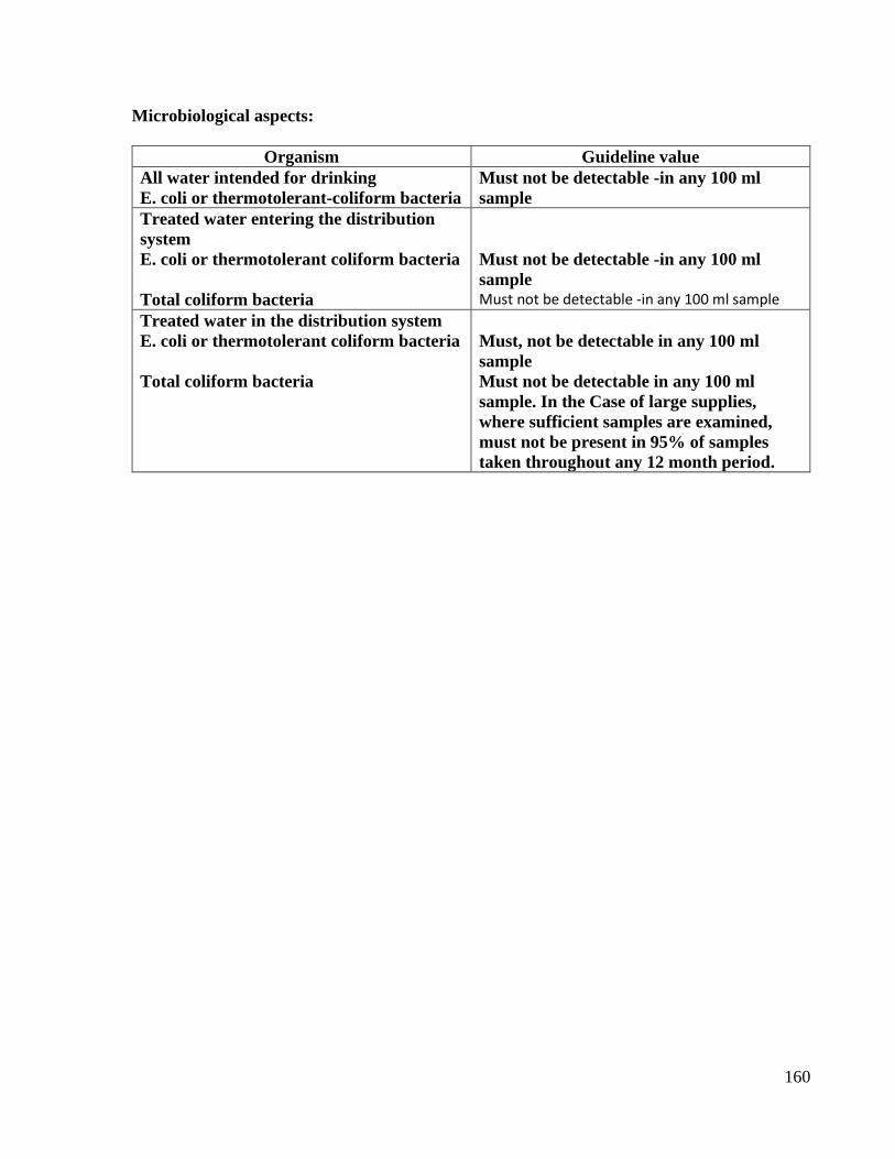
160

Microbiological aspects:

Organism Guideline value

All water intended for drinking

E. coli or thermotolerant-coliform bacteria

Must not be detectable -in any 100 ml

sample

Treated water entering the distribution

system

E. coli or thermotolerant coliform bacteria

Total coliform bacteria

Must not be detectable -in any 100 ml

sample Must not be detectable -in any 100 ml sample

Treated water in the distribution system

E. coli or thermotolerant coliform bacteria

Total coliform bacteria

Must, not be detectable in any 100 ml

sample

Must not be detectable in any 100 ml

sample. In the Case of large supplies,

where sufficient samples are examined,

must not be present in 95% of samples

taken throughout any 12 month period.

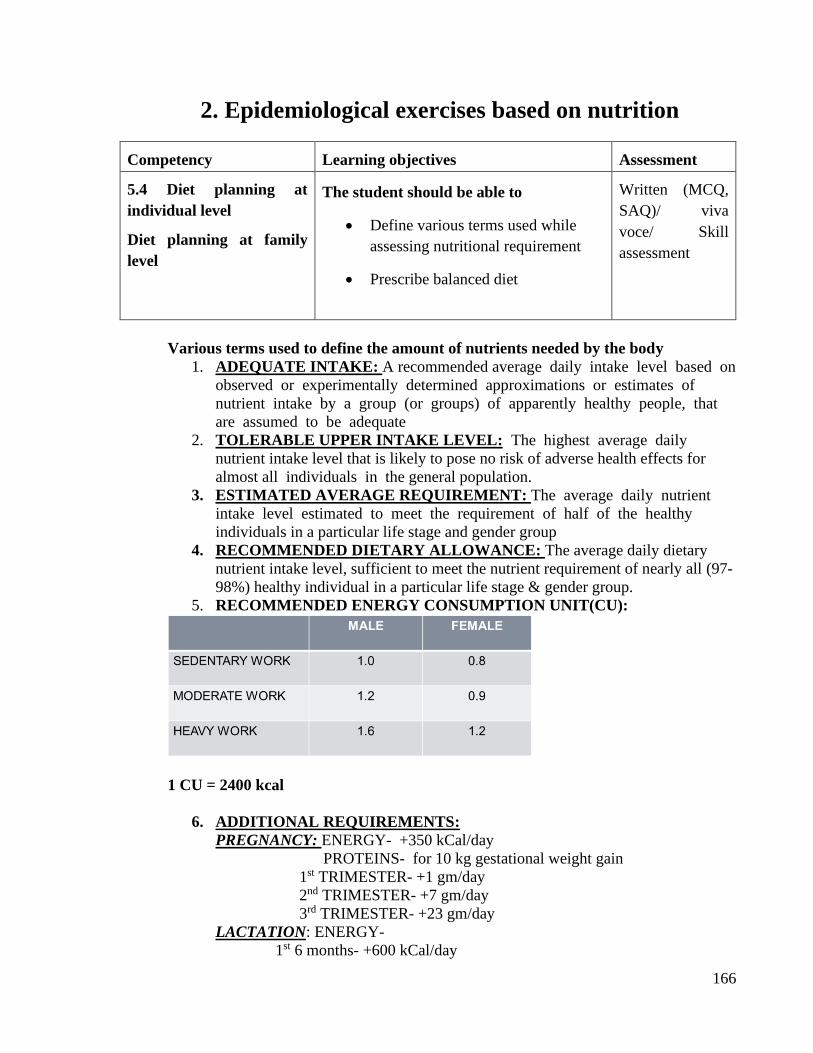
166

2. Epidemiological exercises based on nutrition


5.4 Diet planning at

individual level

Diet planning at family

level


• Define various terms used while

assessing nutritional requirement

• Prescribe balanced diet

Written (MCQ,

SAQ)/ viva

voce/ Skill

assessment

Various terms used to define the amount of nutrients needed by the body

1. ADEQUATE INTAKE: A recommended average daily intake level based on

observed or experimentally determined approximations or estimates of

nutrient intake by a group (or groups) of apparently healthy people, that

are assumed to be adequate

2. TOLERABLE UPPER INTAKE LEVEL: The highest average daily

nutrient intake level that is likely to pose no risk of adverse health effects for

almost all individuals in the general population.

3. ESTIMATED AVERAGE REQUIREMENT: The average daily nutrient

intake level estimated to meet the requirement of half of the healthy

individuals in a particular life stage and gender group

4. RECOMMENDED DIETARY ALLOWANCE: The average daily dietary

nutrient intake level, sufficient to meet the nutrient requirement of nearly all (97-

98%) healthy individual in a particular life stage & gender group.

5. RECOMMENDED ENERGY CONSUMPTION UNIT(CU):

1 CU = 2400 kcal

6. ADDITIONAL REQUIREMENTS:

PREGNANCY: ENERGY- +350 kCal/day

PROTEINS- for 10 kg gestational weight gain

1st TRIMESTER- +1 gm/day

2nd TRIMESTER- +7 gm/day

3rd TRIMESTER- +23 gm/day

LACTATION: ENERGY-

1st 6 months- +600 kCal/day

167

Next 6 months- +520kCal/day

PROTEIN-

1st 6 months- +13 gm/day

ENERGY OBTAINED FROM MACRONUTRIENTS:

PROTEIN - 4 kcal/gm

FAT - 9 kcal/gm

CARBOHYDRATE - 4 kcal/gm

DIETARY FIBRE - 2 kcal/gm

❑ Recommended dietary allowance (RDA):- The average daily dietary nutrient intake

level, sufficient to meet the nutrient requirement of nearly all (97-98%) healthy individual

in a particular life stage & gender group.

❑ Balanced diet: Diet which contains a variety of foods in such quantities and proportions

that the need for energy, proteins, carbohydrates, vitamins etc. is adequately met for

aintaining health well being& vitality along with small provision of extra nutrients to

withstand short duration of leanness.

❑ Dietary goals (Prudent diet) recommended by various expert committies of WHO:

1. Dietary fat should be 15-30% of total daily intake.

2. Saturated fats should not be more than 10% of total energy intake.

3. Excessive consumption of refined carbohydrates should be avoided.

4. Sources rich in energy (fats/alcohol) should be restricted

5. Salt intake should not be more than 5g/day

6. Protein should be 10-15% of daily energy intake.

7. Empty calories should be avoided e.g. junk foods, colas, ketchups, etc.

168

Recommended Dietary Allowances(RDA) for Indians - 2020

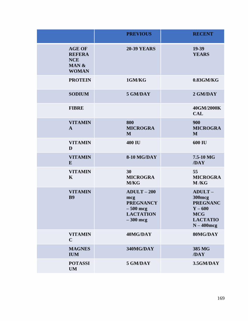
169

PREVIOUS RECENT

AGE OF

REFERA

NCE

MAN &

WOMAN

20-39 YEARS 19-39

YEARS

PROTEIN 1GM/KG 0.83GM/KG

SODIUM 5 GM/DAY 2 GM/DAY

FIBRE

40GM/2000K

CAL

VITAMIN

A

800

MICROGRA

M

900

MICROGRA

M

VITAMIN

D

400 IU 600 IU

VITAMIN

E

8-10 MG/DAY 7.5-10 MG

/DAY

VITAMIN

K

30

MICROGRA

M/KG

55

MICROGRA

M /KG

VITAMIN

B9

ADULT – 200

mcg

PREGNANCY

– 500 mcg

LACTATION

– 300 mcg

ADULT –

300mcg

PREGNANC

Y – 600

MCG

LACTATIO

N – 400mcg

VITAMIN

C

40MG/DAY 80MG/DAY

MAGNES

IUM

340MG/DAY 385 MG

/DAY

POTASSI

UM

5 GM/DAY 3.5GM/DAY

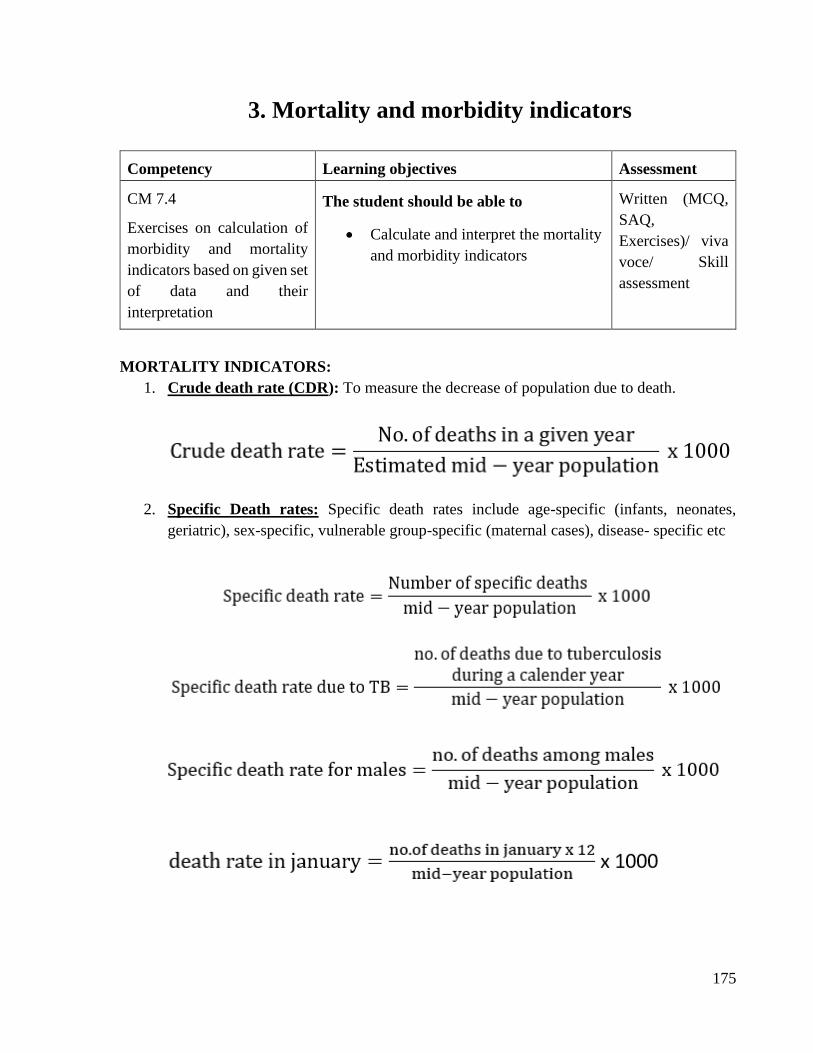
175

3. Mortality and morbidity indicators


CM 7.4

Exercises on calculation of

morbidity and mortality

indicators based on given set

of data and their

interpretation


• Calculate and interpret the mortality

and morbidity indicators

Written (MCQ,

SAQ,

Exercises)/ viva

voce/ Skill

assessment

MORTALITY INDICATORS:

1. Crude death rate (CDR): To measure the decrease of population due to death.

2. Specific Death rates: Specific death rates include age-specific (infants, neonates,

geriatric), sex-specific, vulnerable group-specific (maternal cases), disease- specific etc

176

3. PROPORTIONAL MORTALITY RATE:

4. CASE FATALITY RATE:

5. SURVIVAL RATE:

Survival rate =total no. of patients alive after 5 years

total no. of pts diagnosed or treated x 100

Survival rate = 100 – case fatality rate

6. MATERNAL MORTALITY RATE : The risk of dying from causes associated with

childbirth is measured by the maternal mortality rate. MMR =

7. AGE SPECIFIC DEATH RATES:

INFANT MORTALITY RATE : It is one of the most sensitive indexes of health

conditions of the general population. It is sensitive measure because a baby in its

extrauterine life is suddenly exposed to a multitude of new environmental factors and their

reactions are reflected in this rate. Under ideal conditions of social welfare no normal baby

should die.

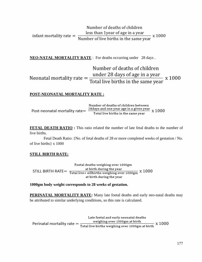
177

NEO-NATAL MORTALITY RATE : For deaths occurring under 28 days .

POST-NEONATAL MORTALITY RATE :

FETAL DEATH RATIO : This ratio related the number of late fetal deaths to the number of

live births.

Fetal Death Ratio: {No. of fetal deaths of 28 or more completed weeks of gestation / No.

of live births} x 1000

STILL BIRTH RATE:

1000gm body weight corresponds to 28 weeks of gestation.

PERINATAL MORTALITY RATE: Many late foetal deaths and early neo-natal deaths may

be attributed to similar underlying conditions, so this rate is calculated.

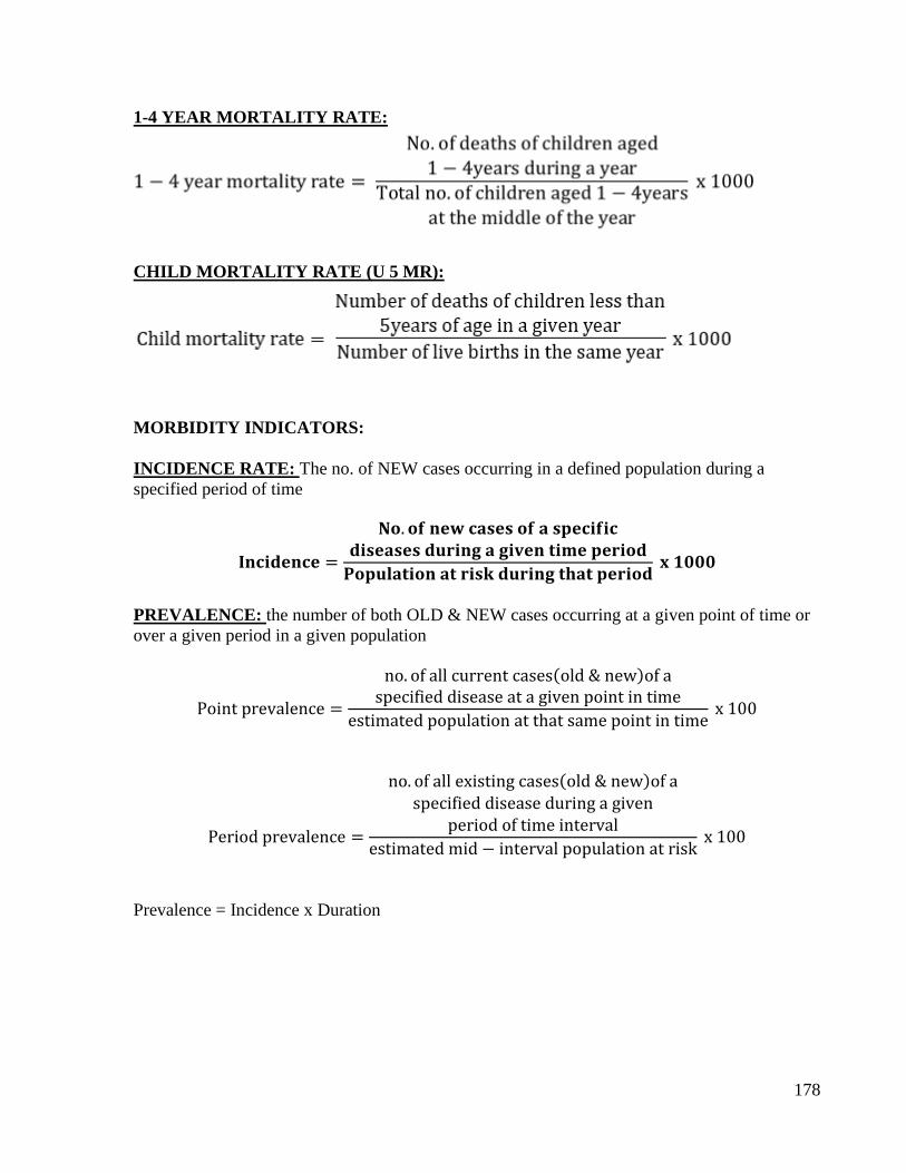
178

1-4 YEAR MORTALITY RATE:

CHILD MORTALITY RATE (U 5 MR):

MORBIDITY INDICATORS:

INCIDENCE RATE: The no. of NEW cases occurring in a defined population during a

specified period of time

𝐈𝐧𝐜𝐢𝐝𝐞𝐧𝐜𝐞 =

𝐍𝐨. 𝐨𝐟 𝐧𝐞𝐰 𝐜𝐚𝐬𝐞𝐬 𝐨𝐟 𝐚 𝐬𝐩𝐞𝐜𝐢𝐟𝐢𝐜𝐝𝐢𝐬𝐞𝐚𝐬𝐞𝐬 𝐝𝐮𝐫𝐢𝐧𝐠 𝐚 𝐠𝐢𝐯𝐞𝐧 𝐭𝐢𝐦𝐞 𝐩𝐞𝐫𝐢𝐨𝐝

𝐏𝐨𝐩𝐮𝐥𝐚𝐭𝐢𝐨𝐧 𝐚𝐭 𝐫𝐢𝐬𝐤 𝐝𝐮𝐫𝐢𝐧𝐠 𝐭𝐡𝐚𝐭 𝐩𝐞𝐫𝐢𝐨𝐝 𝐱 𝟏𝟎𝟎𝟎

PREVALENCE: the number of both OLD & NEW cases occurring at a given point of time or

over a given period in a given population

Point prevalence =

no. of all current cases(old & new)of aspecified disease at a given point in time

estimated population at that same point in time x 100

Period prevalence =

no. of all existing cases(old & new)of aspecified disease during a given

period of time interval

estimated mid − interval population at risk x 100

Prevalence = Incidence x Duration

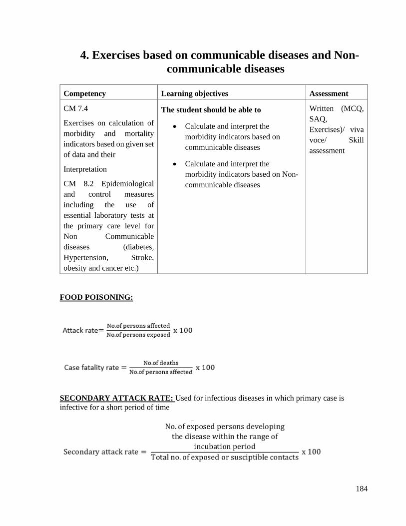
184

4. Exercises based on communicable diseases and Non-

communicable diseases


CM 7.4

Exercises on calculation of

morbidity and mortality

indicators based on given set

of data and their

Interpretation

CM 8.2 Epidemiological

and control measures

including the use of

essential laboratory tests at

the primary care level for

Non Communicable

diseases (diabetes,

Hypertension, Stroke,

obesity and cancer etc.)


• Calculate and interpret the

morbidity indicators based on


• Calculate and interpret the

morbidity indicators based on Non-


Written (MCQ,

SAQ,

Exercises)/ viva

voce/ Skill

assessment

FOOD POISONING:

SECONDARY ATTACK RATE: Used for infectious diseases in which primary case is

infective for a short period of time

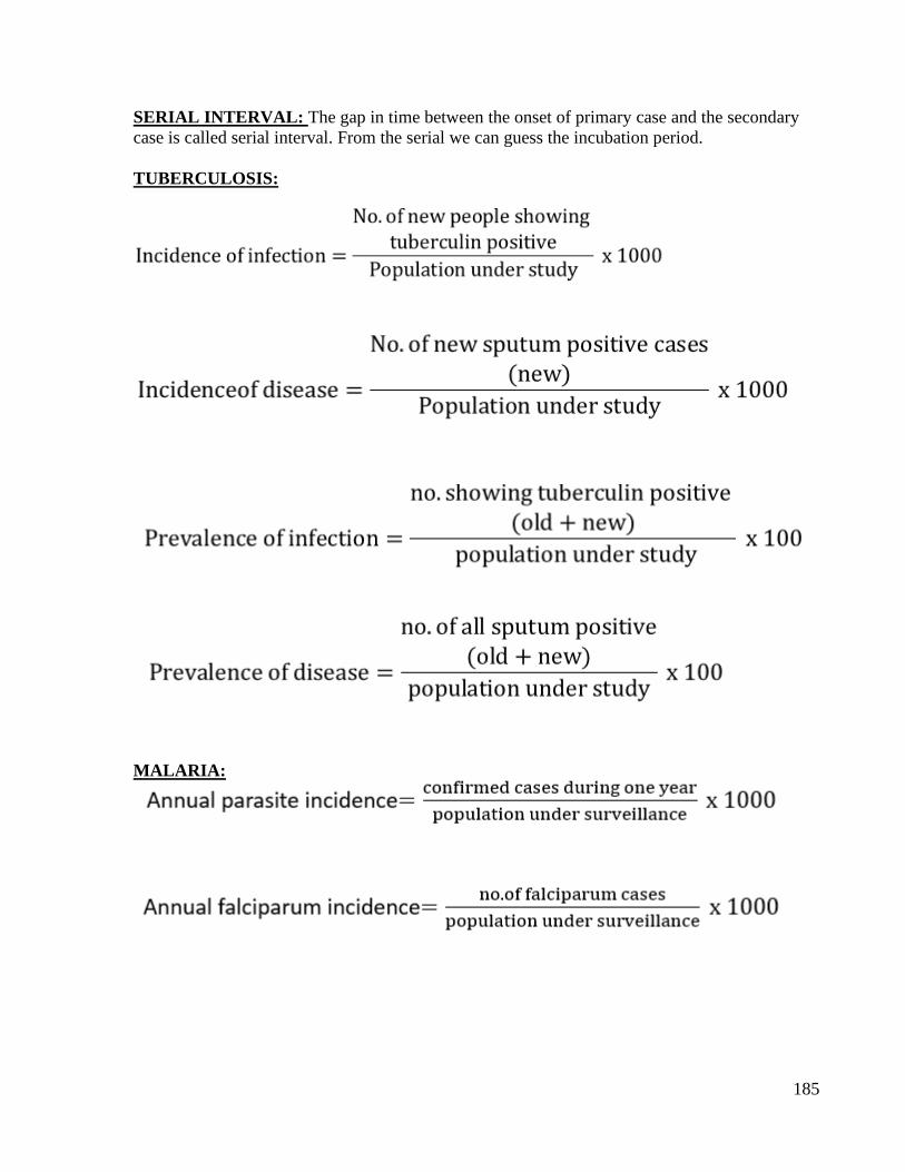
185

SERIAL INTERVAL: The gap in time between the onset of primary case and the secondary

case is called serial interval. From the serial we can guess the incubation period.

TUBERCULOSIS:

MALARIA:

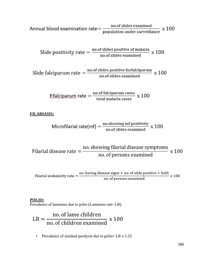
186

FILARIASIS:

POLIO:

Prevalence of lameness due to polio (Lameness rate- LR)

• Prevalence of residual paralysis due to polio= LR x 1.25

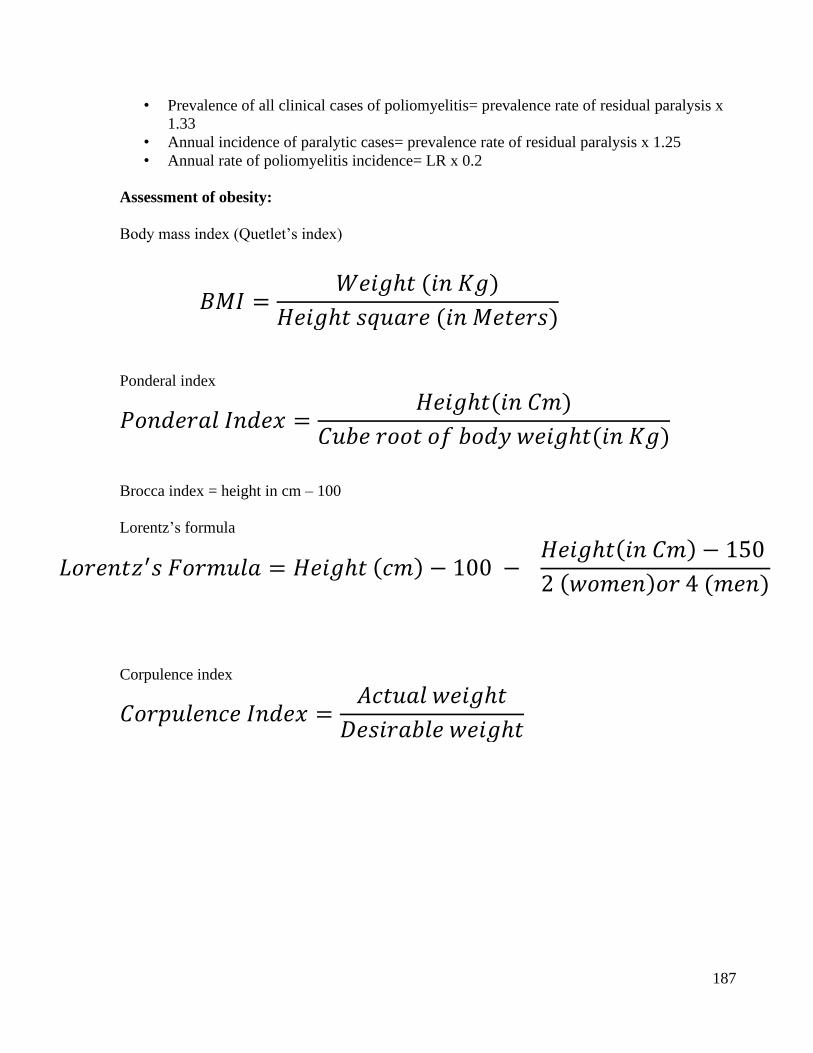
187

• Prevalence of all clinical cases of poliomyelitis= prevalence rate of residual paralysis x

1.33

• Annual incidence of paralytic cases= prevalence rate of residual paralysis x 1.25

• Annual rate of poliomyelitis incidence= LR x 0.2

Assessment of obesity:

Body mass index (Quetlet’s index)

Ponderal index

Brocca index = height in cm – 100

Lorentz’s formula

Corpulence index

𝐵𝑀𝐼 =𝑊𝑒𝑖𝑔ℎ𝑡 (𝑖𝑛 𝐾𝑔)

𝐻𝑒𝑖𝑔ℎ𝑡 𝑠𝑞𝑢𝑎𝑟𝑒 (𝑖𝑛 𝑀𝑒𝑡𝑒𝑟𝑠)

𝑃𝑜𝑛𝑑𝑒𝑟𝑎𝑙 𝐼𝑛𝑑𝑒𝑥 =𝐻𝑒𝑖𝑔ℎ𝑡(𝑖𝑛 𝐶𝑚)

𝐶𝑢𝑏𝑒 𝑟𝑜𝑜𝑡 𝑜𝑓 𝑏𝑜𝑑𝑦 𝑤𝑒𝑖𝑔ℎ𝑡(𝑖𝑛 𝐾𝑔)

𝐿𝑜𝑟𝑒𝑛𝑡𝑧′𝑠 𝐹𝑜𝑟𝑚𝑢𝑙𝑎 = 𝐻𝑒𝑖𝑔ℎ𝑡 (𝑐𝑚) − 100 − 𝐻𝑒𝑖𝑔ℎ𝑡(𝑖𝑛 𝐶𝑚) − 150

2 (𝑤𝑜𝑚𝑒𝑛)𝑜𝑟 4 (𝑚𝑒𝑛)

𝐶𝑜𝑟𝑝𝑢𝑙𝑒𝑛𝑐𝑒 𝐼𝑛𝑑𝑒𝑥 =𝐴𝑐𝑡𝑢𝑎𝑙 𝑤𝑒𝑖𝑔ℎ𝑡

𝐷𝑒𝑠𝑖𝑟𝑎𝑏𝑙𝑒 𝑤𝑒𝑖𝑔ℎ𝑡

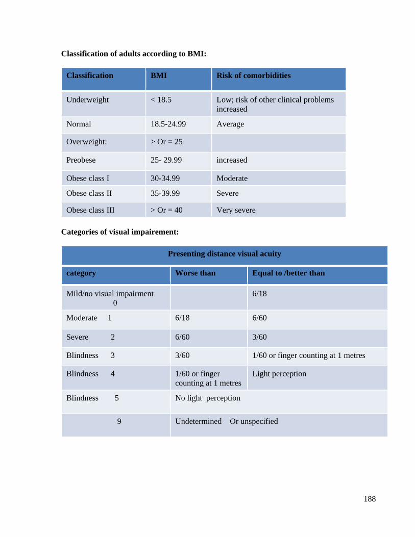
188

Classification of adults according to BMI:

Classification BMI Risk of comorbidities

Underweight < 18.5 Low; risk of other clinical problems

increased

Normal 18.5-24.99 Average

Overweight: > Or = 25

Preobese 25- 29.99 increased

Obese class I 30-34.99 Moderate

Obese class II 35-39.99 Severe

Obese class III > Or = 40 Very severe

Categories of visual impairement:

Presenting distance visual acuity

category Worse than Equal to /better than

Mild/no visual impairment

0

6/18

Moderate 1 6/18 6/60

Severe 2 6/60 3/60

Blindness 3 3/60 1/60 or finger counting at 1 metres

Blindness 4 1/60 or finger

counting at 1 metres

Light perception

Blindness 5 No light perception

9 Undetermined Or unspecified

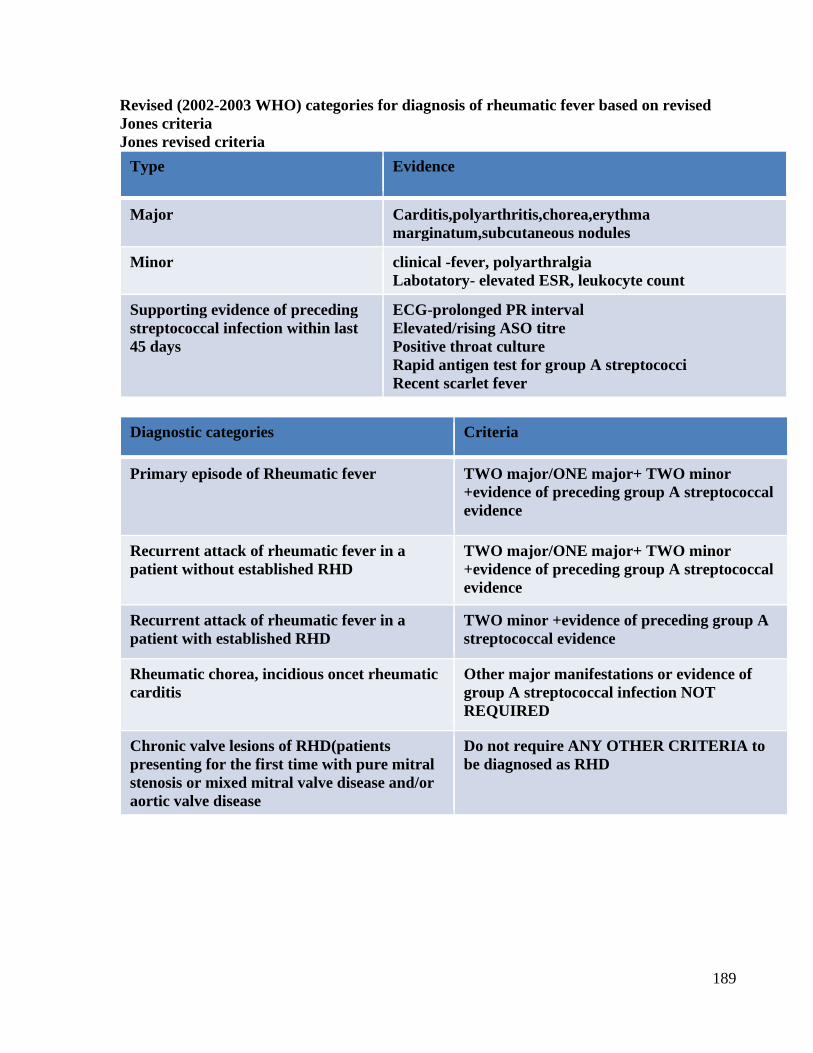
189

Revised (2002-2003 WHO) categories for diagnosis of rheumatic fever based on revised

Jones criteria

Jones revised criteria

Type Evidence

Major Carditis,polyarthritis,chorea,erythma

marginatum,subcutaneous nodules

Minor clinical -fever, polyarthralgia

Labotatory- elevated ESR, leukocyte count

Supporting evidence of preceding

streptococcal infection within last

45 days

ECG-prolonged PR interval

Elevated/rising ASO titre

Positive throat culture

Rapid antigen test for group A streptococci

Recent scarlet fever

Diagnostic categories Criteria

Primary episode of Rheumatic fever TWO major/ONE major+ TWO minor

+evidence of preceding group A streptococcal

evidence

Recurrent attack of rheumatic fever in a

patient without established RHD

TWO major/ONE major+ TWO minor

+evidence of preceding group A streptococcal

evidence

Recurrent attack of rheumatic fever in a

patient with established RHD

TWO minor +evidence of preceding group A

streptococcal evidence

Rheumatic chorea, incidious oncet rheumatic

carditis

Other major manifestations or evidence of

group A streptococcal infection NOT

REQUIRED

Chronic valve lesions of RHD(patients

presenting for the first time with pure mitral

stenosis or mixed mitral valve disease and/or

aortic valve disease

Do not require ANY OTHER CRITERIA to

be diagnosed as RHD

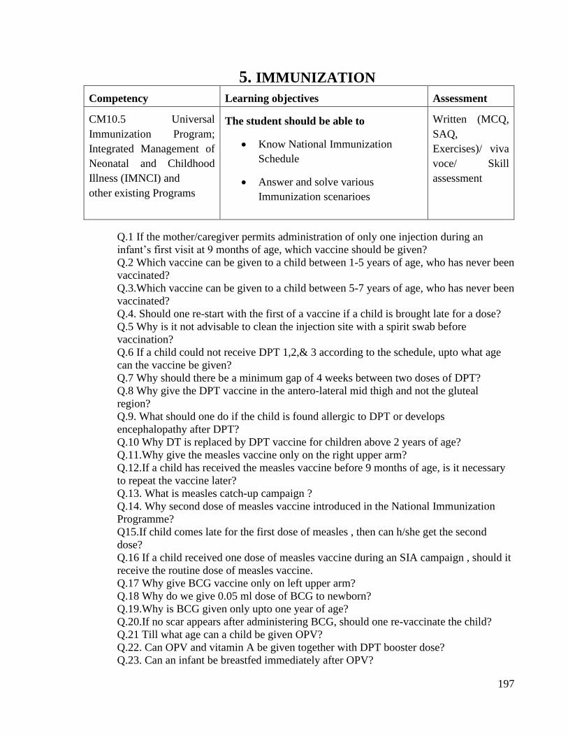
197

5. IMMUNIZATION


CM10.5 Universal

Immunization Program;

Integrated Management of

Neonatal and Childhood

Illness (IMNCI) and

other existing Programs


• Know National Immunization

Schedule

• Answer and solve various

Immunization scenarioes

Written (MCQ,

SAQ,

Exercises)/ viva

voce/ Skill

assessment

Q.1 If the mother/caregiver permits administration of only one injection during an

infant’s first visit at 9 months of age, which vaccine should be given?

Q.2 Which vaccine can be given to a child between 1-5 years of age, who has never been

vaccinated?

Q.3.Which vaccine can be given to a child between 5-7 years of age, who has never been

vaccinated?

Q.4. Should one re-start with the first of a vaccine if a child is brought late for a dose?

Q.5 Why is it not advisable to clean the injection site with a spirit swab before

vaccination?

Q.6 If a child could not receive DPT 1,2,& 3 according to the schedule, upto what age

can the vaccine be given?

Q.7 Why should there be a minimum gap of 4 weeks between two doses of DPT?

Q.8 Why give the DPT vaccine in the antero-lateral mid thigh and not the gluteal

region?

Q.9. What should one do if the child is found allergic to DPT or develops

encephalopathy after DPT?

Q.10 Why DT is replaced by DPT vaccine for children above 2 years of age?

Q.11.Why give the measles vaccine only on the right upper arm?

Q.12.If a child has received the measles vaccine before 9 months of age, is it necessary

to repeat the vaccine later?

Q.13. What is measles catch-up campaign ?

Q.14. Why second dose of measles vaccine introduced in the National Immunization

Programme?

Q15.If child comes late for the first dose of measles , then can h/she get the second

dose?

Q.16 If a child received one dose of measles vaccine during an SIA campaign , should it

receive the routine dose of measles vaccine.

Q.17 Why give BCG vaccine only on left upper arm?

Q.18 Why do we give 0.05 ml dose of BCG to newborn?

Q.19.Why is BCG given only upto one year of age?

Q.20.If no scar appears after administering BCG, should one re-vaccinate the child?

Q.21 Till what age can a child be given OPV?

Q.22. Can OPV and vitamin A be given together with DPT booster dose?

Q.23. Can an infant be breastfed immediately after OPV?

198

Q.24 If a girl has received all doses of DPT and TT as per the NIS till 16 years of age

and she gets pregnant at 20 years, should she get one dose of TT during pregnancy?

Q.25. Can TT be given in the first trimester of pregnancy?

Q.26 Up to what age can hepatitis B vaccine be given?

Q.27 Why give the birth dose of hepatitis B vaccine only within 24 hours of birth?

Q.28 Up to what age can hepatitis B vaccine be given?

Q.29 Why give the birth dose of hepatitis B vaccine only within 24 hours of birth?

Q.30 If a with child 16-24 months of age has been immunized with JE vaccine during an

SIA, can it receive the JE vaccine again, as part of routine immunization?

Q31.If a child above 2 years of age has not received the JE vaccine through either RI or

an SIA should she/he be given the JE vaccine?

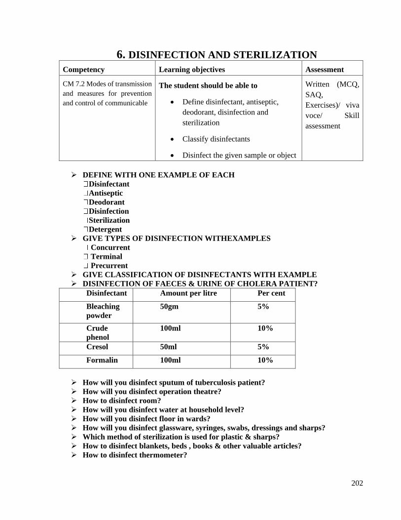
202

6. DISINFECTION AND STERILIZATION


CM 7.2 Modes of transmission

and measures for prevention

and control of communicable


• Define disinfectant, antiseptic,

deodorant, disinfection and

sterilization

• Classify disinfectants

• Disinfect the given sample or object

Written (MCQ,

SAQ,

Exercises)/ viva

voce/ Skill

assessment

➢ DEFINE WITH ONE EXAMPLE OF EACH

Disinfectant

Antiseptic

Deodorant

Disinfection

Sterilization

Detergent

➢ GIVE TYPES OF DISINFECTION WITHEXAMPLES

Concurrent

Terminal

Precurrent

➢ GIVE CLASSIFICATION OF DISINFECTANTS WITH EXAMPLE

➢ DISINFECTION OF FAECES & URINE OF CHOLERA PATIENT?

Disinfectant Amount per litre Per cent

Bleaching

powder

50gm 5%

Crude

phenol

100ml 10%

Cresol 50ml 5%

Formalin 100ml 10%

➢ How will you disinfect sputum of tuberculosis patient?

➢ How will you disinfect operation theatre?

➢ How to disinfect room?

➢ How will you disinfect water at household level?

➢ How will you disinfect floor in wards?

➢ How will you disinfect glassware, syringes, swabs, dressings and sharps?

➢ Which method of sterilization is used for plastic & sharps?

➢ How to disinfect blankets, beds , books & other valuable articles?

➢ How to disinfect thermometer?

203

➢ How to disinfect inexpensive articles such as contaminated dressings, rags and

swabs etc?

➢ Which method is used for sterilization of bandages, dressings, catgut and Cu T?

➢ Oils and powders are sterilized by.

➢ How to disinfect ambulance which was used to transport covid 19 positive patient.

➢ How will you disinfect your mobile phones and labtops?

➢ How to disinfect spectacles, pens and stethoscopes.

➢ How to carry and dispose of dead body of Covid 19 positive patients?

➢ How to clean blood spillage or infective discharges on the floor.

208

7. CONCEPT OF RESEARCH


CM6.1

Demonstration and

exercises on Formulation of

a research problem, research

question & research

hypothesis for a study


• Formulate a research problem,

research question & research,

hypothesis

Written/ viva

voce/ Skill

assessment

Research is a systematic process aimed at obtaining new knowledge through verifiable

examination of data and empirical testing of hypothesis. Research activities are directed towards

finding answers, seeking solutions or looking for improved designs of functioning. Very often,

no positive results emerge and a probable hypothesis may be negated. This in no way undermines

the effort. In general, research activities in community medicine are more concerned with

‘applied’ aspects but basic research can also be undertaken.

Designing Research Protocol:

It is essential to formulate a detailed research protocol so that the research effort is meaningful

and productive. The research protocol should follow a systematic format. This does not mean that

the subsequent step can only be undertaken after completion of the preceding step, because there

is often an overlap. However, following the format ensures that every aspect is carefully

addressed. The essential steps are given below. Selecting a Researchable Topic A general topic

of study or broad area of research may present itself in relation to some practical concern or a

scientific or intellectual interest. The decision-making process may be guided by the following:

1. Need for additional information on some specific disease, health care facility or service.

2. Need for evaluation of the effects of a particular component of health care facilities or

services.

3. Need for comparing alternative treatment modalities.

4. Need for future projections of the magnitude of specific health problems or health care

infrastructure or services.

Formulating the Research Problem:

Once the research topic is selected, the research problem needs to be formulated in detail. The

following steps are useful for this purpose and have been abridged from the WHO/WPRO format:

• Statement of the problem:

The first step in the development of a research project is a clear enunciation of the research

problem. The statement of the problem is essential for constructing a research protocol. It guides

and puts into sharper focus the research design being considered for solving the problem. It allows

the investigator to describe the problem systematically and to reflect on its importance, its priority

in the country or region and the rationale for undertaking the research.

• Relevance of the problem:

It should be ensured that the problem to be researched is relevant to national, regional or local

health needs and activities. It should preferably fall under the priority areas in reference to national

health.

209

• Field of application:

One must clearly spell out how the findings of the proposed research would benefit policy makers,

health administrators or health services research scientists. It should also be indicated as to how

the results would be transmitted to them.

Search for Related Work:

A thorough scan of all available literature or information on the research problem should be

undertaken. A review of existing information is important for the following reasons:

• It helps in further understanding of the proposed research problem and may lead to refining of

the

statement of the problem.

• It helps in identifying the study variables and conceptualizing their relationships.

• It helps in the formulation and selection of research hypotheses.

• It helps in finding out what others have already reported on the topic, so that account can be

taken

of this in the design of research.

• It provides familiarity with various methods that might be used in research.

The search can be undertaken in the following ways:

– Thorough literature scan for related work.

– Discussion with experts in the specific area of interest.

– First hand experience or observation.

The sources of information include:

a. Library catalogues, literature.

b. Indices (e.g. Index Medicus and Excerpta Medica, which identify articles

appearing in selected journals by subject, author and title), computer search

facilities (such as Medline, Medlar, Popline).

c. Bibliographies (e.g. current contents).

d. Statistical reports.

Statement of Objective:

Before undertaking any research investigation, its purpose should be clearly spelled out in the

research

protocol in terms of goals, objectives and targets.

A goal is a broad definition of policy, not constrained by time. For example, an applied research

project related to school health may state its goal as: “Health care facilities will be provided to

maintain and improve health status of preschool children”. No mention need be made as to how

the goal is to be fulfiled. This is addressed by the objectives.

Objectives are defined more precisely than the goal. An objective is a broad statement of purpose

reflecting the conditions one wants at some future time. The relationship between goals and

objectives is that objectives are essentially steps towards a goal. The specific objectives are the

specific aims of the

research project. What is to be accomplished is often broken down into smaller logical

components. Specific objectives relate to specific research questions, which the investigator

wants to answer through the proposed research. For example, the general objective “To improve

ocular health of preschool children” may have the following specific objectives:

• To provide vitamin A supplementation to all underfives

• To screen eyes of preschool children at ‘anganwadis’ at six monthly intervals

• To provide nutrition education to mothers.

210

A target is an indicator with a magnitude. It points out what should be realised by a specific date.

Targets should be quantitatively measurable. They represent the measurable and attainable aims

directed towards objectives which, in turn, are directed towards the ultimate goal. For example, a

target may be “100 percent coverage of preschool children by vitamin A prophylaxis.”

At this stage, while objectives and targets, etc. are outlined by the investigator, it is also necessary

to clarify the concepts related to the study and to give working definitions of the terms used.

It should be borne in mind that each study rests on earlier ones and provides a basis for future

research

efforts. More the links that can be established between a given study and other studies or a body

of theory, greater the probable contribution of the study.

Selection of Variables:

Variables that are sought to be measured should be clearly spelled out. The different types of

variables are:

• Independent variables (Input, antecedent, etc):

These are manipulated under study conditions to see what effect differences in them will have on

those

variables proposed as being dependent on them.

• Dependent variables (Outcome, effect, etc):

These are the ones in which changes result due to the effect of the independent variables.

• Confounding variables (Intervening variables):

These should be studied because they may influence or confound the effect of the independent

variables on the dependent variable.

• Background variables:

Variables like sex, age, race, literacy, SES, marital status, etc. are so often of relevance in

investigations of groups or populations that they should be considered for possible inclusion in

all studies.

The variables in a study should be clearly identified and their method of measurement as well as

the

unit of measurement should be cleary indicated.

Formulation of Research Hypothesis:

A hypothesis can be defined as a tentative prediction or explanation of the relationship between

two or more variables. Formulation of hypothesis requires the investigator to predict an answer

to the research question based on knowledge of the field and logical analysis. The formulation of

a hypothesis should:

• Suggest explanations for certain facts

• Guide in investigation of related facts

• Investigate characteristics that determine the occurrence of disease.

A hypothesis translates the problem statement into a precise, unambiguous prediction of expected

outcomes.

A hypothesis is not meant to be a haphazard guess. Rather, it should reflect the depth of

knowledge, imagination and experience of the investigator.

The formulation and verification of a hypothesis is the major goal of scientific enquiry. The

researcher should try to identify alternative competing or rival hypotheses which should then be

carefully considered. Purely descriptive studies do not need a formal hypothesis.

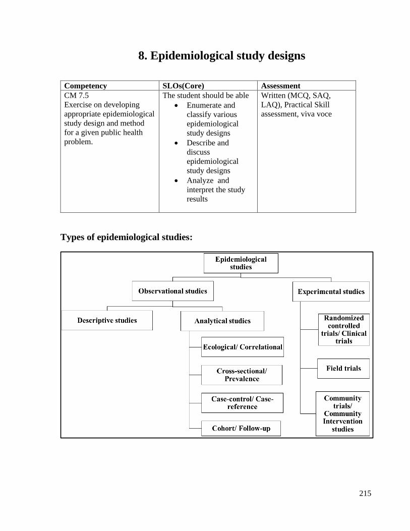
215

8. Epidemiological study designs

Competency SLOs(Core) Assessment

CM 7.5

Exercise on developing

appropriate epidemiological

study design and method

for a given public health

problem.

The student should be able

• Enumerate and

classify various

epidemiological

study designs

• Describe and

discuss

epidemiological

study designs

• Analyze and

interpret the study

results

Written (MCQ, SAQ,

LAQ), Practical Skill

assessment, viva voce

Types of epidemiological studies:

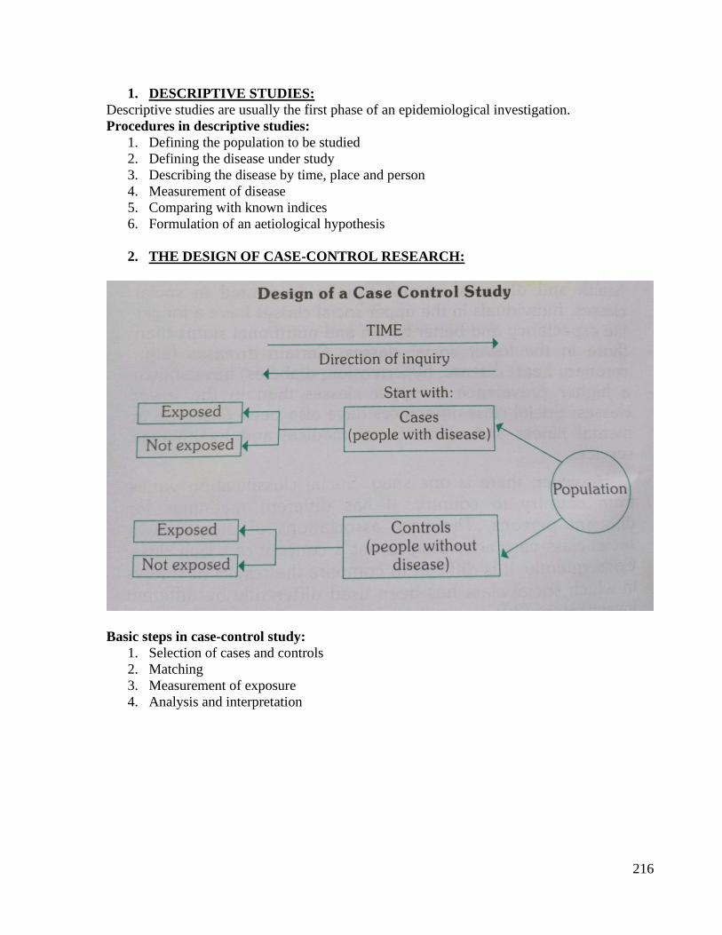
216

1. DESCRIPTIVE STUDIES:

Descriptive studies are usually the first phase of an epidemiological investigation.

Procedures in descriptive studies:

1. Defining the population to be studied

2. Defining the disease under study

3. Describing the disease by time, place and person

4. Measurement of disease

5. Comparing with known indices

6. Formulation of an aetiological hypothesis

2. THE DESIGN OF CASE-CONTROL RESEARCH:

Basic steps in case-control study:

1. Selection of cases and controls

2. Matching

3. Measurement of exposure

4. Analysis and interpretation

217

Risk factor/

Suspected cause

Cases

(Disease present)

Controls

(Disease absent)

Present a b

Absent c d

Total a+c b+d

Exposure rates

1.Cases=a/a+c

2.Controls=b/b+d

Test for statistical association between 1 & 2

Odds ratio or cross product ratio: gives idea about strength of association

Odds ratio = 𝑎𝑑

𝑏𝑐

Interpretation: “risk of disease is __ times in exposed than non exposed”

3. FRAME WORK OF COHORT STUDY:

Elements of a cohort study:

1. Selection of study subjects

2. Obtaining data on exposure

3. Selection of comparison groups

4. Follow-up

5. Analysis

218

Risk factor Disease Total

Yes No

Risk Factor present a b a + b

Risk factor Absent c d c + d

Incidence rate among exposed group = a / a + b

Incidence rate among not exposed group = c / c + d

RELATIVE RISK: Ratio of the incidence of the disease among exposed & incidence among

non exposed. It is Index of strength of association

Relative Risk = Incidence among exposed

Incidence among non−exposed

Interpretation: “exposed are ___ times at greater risk of having disease”

ATTRIBUTABLE RISK: Indicates the extent the disease under study

can be attributed to the exposure.

Attributable risk = Incidence(exposed)−Incidence(non−exposed)

Incidence(exposed) x 100

Interpretation: “___ % of the disease can be attributed to the exposure”

219

POPULATION ATTRIBUTABLE RISK: provide an estimate of the amount by

which disease could be reduced in that population if the suspected factor

was eliminated/modified

Population attributable risk= 𝑑𝑒𝑎𝑡ℎ 𝑖𝑛 𝑡𝑜𝑡𝑎𝑙 𝑝𝑜𝑝𝑢𝑙𝑎𝑡𝑖𝑜𝑛 −𝑑𝑒𝑎𝑡ℎ 𝑟𝑎𝑡𝑒 𝑎𝑚𝑜𝑛𝑔 𝑛𝑜𝑛−𝑒𝑥𝑝𝑜𝑠𝑒𝑑 𝑔𝑟𝑜𝑢𝑝

𝑑𝑒𝑎𝑡ℎ 𝑟𝑎𝑡𝑒 𝑖𝑛 𝑡𝑜𝑡𝑎𝑙 𝑝𝑜𝑝𝑢𝑙𝑎𝑡𝑖𝑜𝑛 X 100

4. RANDOMIZED CONTROLLED TRIALS:

Design of randomized controlled trials:

220

Basic steps in conducting a RCT include the following:

1. Drawing up a protocol

2. Selecting reference and experimental populations

3. Randomization

4. Manipulation or intervention

5. Follow-up

6. Assessment of outcome

226

9. Screening

Competency SLOs (Core) Assessment

CM 7.6

Screening


• Define, calculate

and interpret

sensitivity

• Define calculate and

interpret specificity

Written (MCQ, SAQ,



2 x 2 TABLE

Screening test

results

Diagnosis Total

Diseased Not Diseased

Positive a

(true positive)

b

(false positive)

a + b

Negative c

(false negative)

d

(true negative)

c + d

Total a + c b + d a + b + c + d

SENSITIVITY: Identify the true positives

Sensitivity =a

(a + c) x 100

SPECIFICITY: Identify the true negatives

𝐒𝐩𝐞𝐜𝐢𝐟𝐢𝐜𝐢𝐭𝐲 =𝐝

(𝐛 + 𝐝) 𝐱 𝟏𝟎𝟎

PREDICTIVE VALUE OF A POSITIVE TEST:

Predictive value of a positive test =a

(a+b) x 100

PREDICTIVE VALUE OF A NEGATIVE TEST:

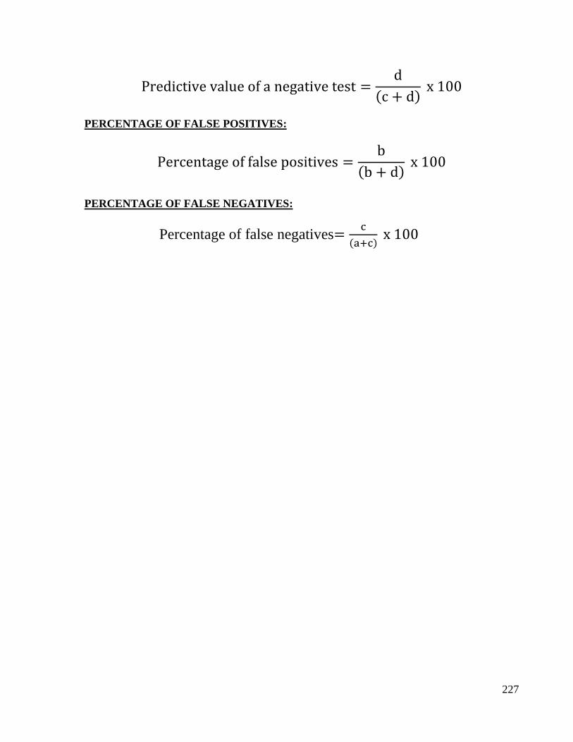
227

Predictive value of a negative test =d

(c + d) x 100

PERCENTAGE OF FALSE POSITIVES:

Percentage of false positives =b

(b + d) x 100

PERCENTAGE OF FALSE NEGATIVES:

Percentage of false negatives=c

(a+c) x 100

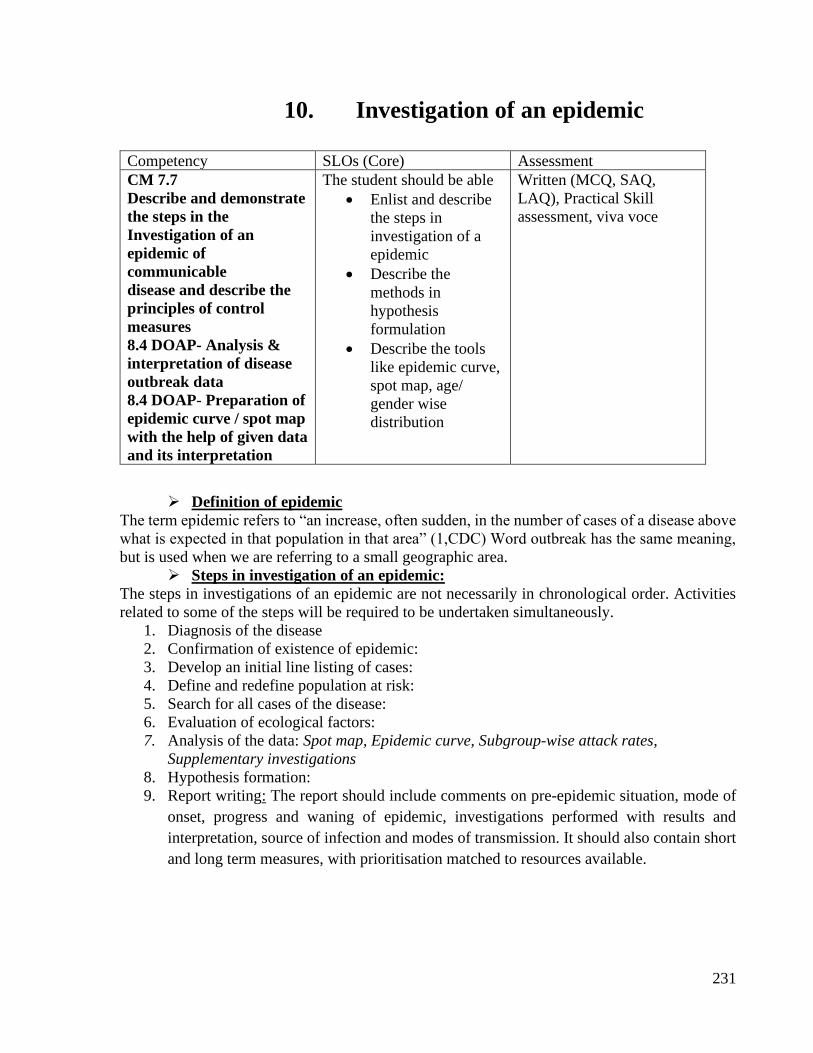
231

10. Investigation of an epidemic

Competency SLOs (Core) Assessment

CM 7.7

Describe and demonstrate

the steps in the

Investigation of an

epidemic of

communicable

disease and describe the

principles of control

measures

8.4 DOAP- Analysis &

interpretation of disease

outbreak data

8.4 DOAP- Preparation of

epidemic curve / spot map

with the help of given data

and its interpretation


• Enlist and describe

the steps in

investigation of a

epidemic

• Describe the

methods in

hypothesis

formulation

• Describe the tools

like epidemic curve,

spot map, age/

gender wise

distribution

Written (MCQ, SAQ,



➢ Definition of epidemic

The term epidemic refers to “an increase, often sudden, in the number of cases of a disease above

what is expected in that population in that area” (1,CDC) Word outbreak has the same meaning,

but is used when we are referring to a small geographic area.

➢ Steps in investigation of an epidemic:

The steps in investigations of an epidemic are not necessarily in chronological order. Activities

related to some of the steps will be required to be undertaken simultaneously.

1. Diagnosis of the disease

2. Confirmation of existence of epidemic:

3. Develop an initial line listing of cases:

4. Define and redefine population at risk:

5. Search for all cases of the disease:

6. Evaluation of ecological factors:

7. Analysis of the data: Spot map, Epidemic curve, Subgroup-wise attack rates,

Supplementary investigations

8. Hypothesis formation:

9. Report writing: The report should include comments on pre-epidemic situation, mode of

onset, progress and waning of epidemic, investigations performed with results and

interpretation, source of infection and modes of transmission. It should also contain short

and long term measures, with prioritisation matched to resources available.

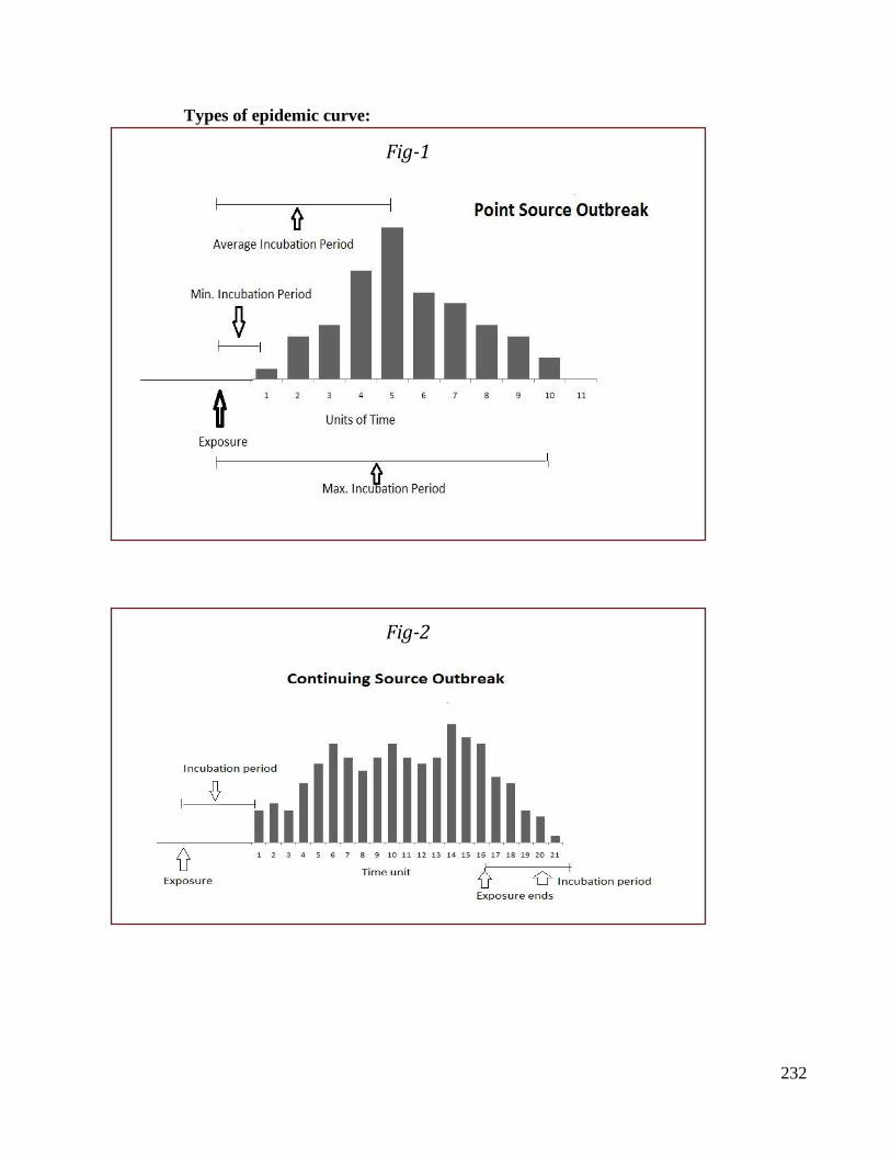
232

Types of epidemic curve:

Fig-1

Fig-2

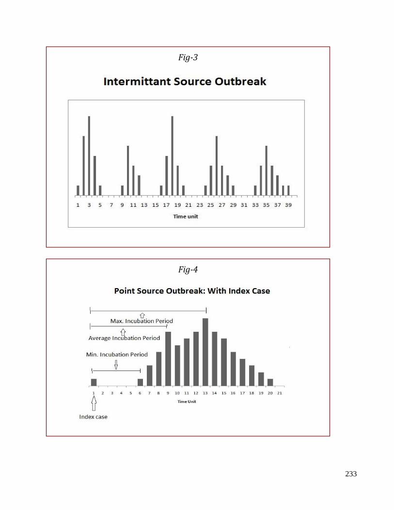
233

Fig-3

Fig-4

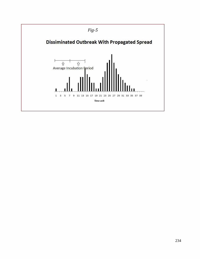
234

Fig-5

240

11. Emporiatrics Competency SLOs (Core) Assessment

CM 7.1

Epidemiology- definition ,

principles, concepts and

uses


• Define Emporiatrics

• Enumerate Recommendations to travelers

• Enumerate contents

of a basic medical

kit

Written (MCQ, SAQ,



➢ Emporiatrics:

Emporiatrics is the term coined to describe the science of the health of

travelers. Travellers face special health risks. In the age of jet travel, international

travellers are subject to various forms of stress that may reduce their resistance to

disease, e.g., crowding, long hours of waiting, disruption of eating habit, change

in the climate and time zone. Travel on a global scale exposes many people to a

range of health risks varying from exposure to different disease agents to changes

in the physical/biological environment, all of which can lead to ill-health. many of

these risks can be minimized by appropriate travel planning and precautionary

measures.

The mitigation measures should start right from the assessment of the determinants

of the health risks to which travelers are exposed: e.g., health status before

undertaking travel (viz. underlying chronic disease/low immunity); place of travel

(viz. facility of accommodation/ hygiene-sanitation/provision of medical

services); purpose and duration of travel and travelers’ behavior.6 Preventive

strategies can be planned based on the risks to which travelers can be exposed. The

travel must be planned well in advance and safeguard measures should be taken

before, during and after travel.

Actions which the traveler must take prior to the commencement of the journey

should be learning about the destination (ascertaining health risks prevalent in the

area, climate, availability of health care facilities, etc.); medical consultation for

necessary immunizations or for an ongoing health concern;7 obtaining special

travelers health insurance for destinations where health risks are significant and

medical care is expensive/not readily available; and carrying a medical/first-aid

kit.

➢ Recommendations to travelers:

(1) Avoid bathing with polluted water as this may result in ear, eye and skin

infections. Excessive heat and humidity or over—exertion in these conditions may

lead to exhaustion from loss of water and salt.

(2) The measures for prevention of insect bites.

(3) Diarrheal Diseases: "Be careful what you eat" is common advice to travelers,

Contaminated food drinks are the most common source of these infections. Careful

241

selection and preparation of food and drink offer the best protection. The food

should be thoroughly and freshly cooked. Use boiled water or bottled mineral

water (now available everywhere). Travellers should be aware of the importance

of oral rehydration fluids containing salt and glucose for countering dehydration.

(4) Malaria: There is a high risk of acquiring malaria in endemic areas. Travellers

are advised to protect themselves by chemoprophylaxis. Drug prophylaxis should

begin at the latest on the day of arrival in the malarious areas and continued for

4—6 weeks after leaving the malarious areas.

(5) Hepatitis A: Normal human immunoglobulin in a dose of 0.02—0.05 mg/kg

of body weight has been recommended every 4 months. Ideally immunoglobulin

should not be given within 3 weeks before, or until 2 weeks after administration

of a live vaccine. A highly safe, inactivated HAV vaccine is available in several

European countries.

(6) Hepatitis E: There is no vaccine against hepatitis E. Avoidance of

contaminated food and water is the only effective protective measure.

(7) Hepatitis B: Hepatitis B vaccines are available and are safe. Three doses of

vaccine constitute the complete course. The first two doses are given one month

apart and the third dose about 6 months later.

(8) STD and HIV: Measures for preventing STD are the same whether the

individual is travelling abroad or not, i.e., avoidance of sex altogether or limit it to

a single faithful, uninfected partner. Use of condom is an important preventive

measure. To reduce the risk of acquiring HIV and hepatitis B from syringes and

needles, travellers should avoid injectable drugs and if an injection is essential they

should make sure that the needle and syringe come from sterile pack.

(9) Yellow fever: Vaccination certificate for yellow fever is the only certificate

required for international travel. Yellow fever vaccine is recommended for

travellers to countries designated as yellow fever endemic zone.

(10) Tetanus: It is a wise precaution for the traveller to have a booster dose of

tetanus toxoid if 10 years or more have elapsed since the last injection of a

complete course or booster.

➢ Medical kit and toilet items:

Sufficient medical supplies should be carried to meet foreseeable needs for the

duration of the trip. A medical kit should be carried for all destinations where there

may be significant health risks, particularly those in developing countries and/or

where the local availability of specific medications is uncertain. This kit will

include basic medicines to treat common ailments, first-aid articles, and any other

special medical items, such as syringes and needles (to minimize exposure to

bloodborne viruses), that may be needed and can in some cases be used by the

individual traveller.

Certain categories of prescription medicine or special medical items should be

carried together with a medical attestation on letterhead, signed by a physician,

certifying that the traveller requires the medication or the items for a medical

condition. Some countries require that this attestation be signed not only by a

physician but also by the national health administration.

Toilet items should also be carried in sufficient quantity for the entire visit unless

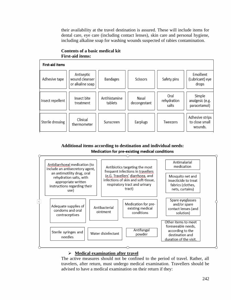
242

their availability at the travel destination is assured. These will include items for

dental care, eye care (including contact lenses), skin care and personal hygiene,

including alkaline soap for washing wounds suspected of rabies contamination.

Contents of a basic medical kit

First-aid items:

Additional items according to destination and individual needs:

➢ Medical examination after travel

The active measures should not be confined to the period of travel. Rather, all

travelers, after return, must undergo medical examination. Travellers should be

advised to have a medical examination on their return if they:

243

• Return with a fever from a country where malaria is or may be present, so that malaria

can be excluded as a cause of their illness

• Suffer from a chronic disease, such as cardiovascular disease, diabetes mellitus, or chronic

respiratory disease or have been taking anticoagulants;

o Experience illness in the weeks following their return home, particularly if fever,

persistent diarrhoea, vomiting, jaundice, urinary disorders, skin disease or genital

infection occurs;

o They received treatment for malaria while travelling;

o May have been exposed to a serious infectious disease while travelling;

o Have spent more than 3 months in a developing country.

Travellers should provide medical personnel with information on recent travel,

including destination, and purpose and duration of visit. Frequent travellers should

give details of all journeys that have taken place in the preceding weeks and

months including pre-travel vaccinations received and malaria chemoprophylaxis

taken.

Note. Fever after returning from a malaria-endemic area is a medical

emergency and travellers who develop fever should seek medical attention

immediately, explaining that they may have contracted malaria.

➢ For the benefit of travellers, the WHO publishes every year a booklet, now

entitled "International Travel and Health, Vaccination requirements and

Health advice” provides guidance on some of the main health risks to which

travellers may be exposed in different parts of the world and advice on

precautions that may be taken against them.

247

12. Writing a research


CM6.1

Demonstration and

exercises on Formulation of

a research problem, research

question & research

hypothesis for a study


• Write a research study in

recommended format

Written/ viva

voce/ Skill

assessment

IMRAD structure

Introduction, Methods, Results, Analysis, Discussion.

1. Title of the study:

Should be Concise, but informative and don’t use abbreviations in the title. It should

indicate

• Objective of the study. E.g. Prevalence of Tuberculosis

• Type of the study i.e. study design e.g.an observational study; a case-control study, a

randomized controlled trial etc.

• Place the study e.g. RMC, Loni

2. Introduction:

Introduction or background should be brief, but, at the same time clear.

It should bring out Definition of the disease/health problem. Magnitude of the problem in study

in terms of morbidity, mortality and suffering. It should give Brief note on:

a -What is already known.

b -What is unknown.

Mention gaps in the present knowledge which prompted the present research work. Should answer

- why present study? Need for the study. The purpose of the study. The hypothesis being tested

and Likely scientific contribution.

3. Aims and objectives:

Aim of the study point out the general purpose of the study.

Objectives spell out specifically what one intends to do in the study. Define the objectives clearly

and in measurable terms; mention as primary and secondary objectives if necessary. Do not write

too many objectives.

4. Materials & Methods:

In methodology give

➢ Study design/ Details of study - Descriptive cross sectional, Analytical case control or

cohort, randomized controlled trials, etc. Proposed study design should be appropriate to

fulfill all the objectives

➢ Study setting and Study period – Mention the Place or setting where the study is planned

or will be conducted e.g. RMC, Loni. Mention the study period i.e. Duration of the study.

E.g. March 2020 to December 2020.

248

➢ Study population/ Details of subjects -adequate description of study population should

be provided. Explain the rationale of selection of the research participants and controls

(humans or laboratory animals), whether chosen randomly, consecutively etc. with

inclusion and exclusion criteria, rules for discontinuation, definitions of cases, controls

and lost to follow up etc.

➢ Sample size- Details of sample size and/or power calculation should be described with references where needed. A flow chart indicating study design with number of participants should be given where applicable.

➢ Details of procedures- In case of Intervention studies a detailed description of

Intervention (drug/device/behavioral intervention) should be given.

➢ Details of data collection- Describe in detail the procedure of data collection and tools

used such as the method of data collection whether it is Interview method, observations,

or record based, etc. Describe the key variables of the study, how will they be measured

and unit of measurement.

➢ Details of statistical methods- Present data analysis plan comprehensively mentioning

appropriate statistical methods to be used such as descriptive statistic like mean and

standard deviation for quantitative data whereas percentage for qualitative data; mention

various statistical tests applicable like Chi square test, t test, etc.

➢ Details of ethical issues- Give details of obtaining informed consent and its

documentation should be described along with risks and benefits to the participants

Address review requirements including ethics review [human or animal], approval for

use of stem cells, biologicals etc. and other regulatory reviews/approvals.

5. Results:

Should precisely state – Present the Findings or observations in the form of Tables, Diagrams,

Charts and Photographs. These must have Number (usually in Arabic numerals), Title,

Content & Foot note and should be referred clearly at the appropriate place in the text. Indicate

the percentages along with the numbers. Write in detail Analysis, Statistical measures

employed, Confidence intervals, Level of significance, etc.

6. Discussion:

Summarise main results at the beginning. Include What do the result mean?

Present- principles, relationships & generalizations shown by the results. Point out

NEGATIVE FINDINGS. Compare or Indicate agreement/disagreement with other study

results. State the implications of results. Mention limitations. Indicate scope for future

work.

7. Conclusion and recommendations: Give reasons for conclusions and

recommendations should be based on your study results only and NOT from possible

factors which you have NOT studied and should NOT be simply a repetition of

standard recommendations from the text book. Mention why research hypothesis (if

any) -Accepted or rejected.

8. REFERENCES:

Quote the References as they appear in text. Give the references preferably in

Vancouver style (Number in superscript). Other method is Harvard method (Names

& year)

.

community medicine biostatistics and epidemiology

Documents