RICE UNIVERSITY

Combining Analyses,

Combining Optimizations

by

Clifford Noel Click, Jr.

A THESIS SUBMITTED

IN PARTIAL FULFILLMENT OF THE

REQUIREMENTS FOR THE DEGREE

Doctor of Philosophy

APPROVED, THESIS COMMITTEE:

Chair Keith D. Cooper

Associate Professor of Computer Science

Robert Bixby

Professor of Computational and AppliedMathematics

Mark W. Krentel

Assistant Professor of Computer Science

Linda Torczon

Faculty Fellow of Computer Science

Houston, Texas

February, 1995

Combining Analyses,

Combining Optimizations

Clifford Noel Click, Jr.

Abstract

This thesis presents a framework for describing optimizations. It shows how to com-

bine two such frameworks and how to reason about the properties of the resulting frame-

work. The structure of the framework provides insight into when a combination yields

better results. Also presented is a simple iterative algorithm for solving these frameworks.

A framework is shown that combines Constant Propagation, Unreachable Code Elimina-

tion, Global Congruence Finding and Global Value Numbering. For these optimizations,

the iterative algorithm runs in O(n2) time.

This thesis then presents an O(n log n) algorithm for combining the same optimiza-

tions. This technique also finds many of the common subexpressions found by Partial Re-

dundancy Elimination. However, it requires a global code motion pass to make the opti-

mized code correct, also presented. The global code motion algorithm removes some

Partially Dead Code as a side-effect. An implementation demonstrates that the algorithm

has shorter compile times than repeated passes of the separate optimizations while produc-

ing run-time speedups of 4% – 7%.

While global analyses are stronger, peephole analyses can be unexpectedly powerful.

This thesis demonstrates parse-time peephole optimizations that find more than 95% of

the constants and common subexpressions found by the best combined analysis. Finding

constants and common subexpressions while parsing reduces peak intermediate represen-

tation size. This speeds up the later global analyses, reducing total compilation time by

10%. In conjunction with global code motion, these peephole optimizations generate ex-

cellent code very quickly, a useful feature for compilers that stress compilation speed over

code quality.

Acknowledgments

First and foremost I wish to thank Melanie, my wife of six years. Her courage and

strength (and level-headedness!) has kept me plowing ahead. I must also mention Karen,

my daughter of 1 year, whose bright smiles lighten my days. I wish to thank Keith Coo-

per, my advisor, for being tolerant of my wild ideas. His worldly views helped me keep

track of what is important in computer science, and helped me to distinguish between the

style and the substance of my research. I also thank Mark Krentel and his “Big, Bad,

Counter-Example Machine” for helping me with the devilish algorithmic details, Bob

Bixby for his large numerical C codes, and Linda Torczon for her patience.

While there are many other people in the Rice community I wish to thank, a few stand

out. Michael Paleczny has been an invaluable research partner. Many of the ideas pre-

sented here were first fleshed out between us as we sat beneath the oak trees. I hope that

we can continue to work (and publish) together. Chris Vick has been a great sounding

board for ideas, playing devil’s advocate with relish. Without Preston Briggs and the rest

of the Massively Scalar Compiler Group (Tim Harvey, Rob Shillingsburg, Taylor Simp-

son, Lisa Thomas and Linda Torczon) this research would never have happened. Lorie

Liebrock and Jerry Roth have been solid friends and fellow students through it all.

Last I would like to thank Rice University and the cast of thousands that make Rice

such a wonderful place to learn. This research has been funded by ARPA through ONR

grant N00014-91-J-1989.

Table of Contents

Abstract.....................................................................................................................iiAcknowledgements...................................................................................................iiiIllustrations...............................................................................................................viPreface....................................................................................................................viii

1. Introduction 1

1.1 Background.........................................................................................................11.2 Compiler Optimizations........................................................................................21.3 Intermediate Representations...............................................................................41.4 Organization........................................................................................................6

2. The Optimistic Assumption 8

2.1 The Optimistic Assumption Defined.....................................................................92.2 Using the Optimistic Assumption.......................................................................122.3 Some Observations about the Optimistic Assumption.........................................14

3. Combining Analyses, Combining Optimizations 16

3.1 Introduction.......................................................................................................163.2 Overview...........................................................................................................173.3 Simple Constant Propagation.............................................................................213.4 Finding the Greatest Fixed Point........................................................................243.5 Efficient Solutions..............................................................................................253.6 Unreachable Code Elimination...........................................................................263.7 Combining Analyses...........................................................................................273.8 Global Value Numbering....................................................................................313.9 Summary............................................................................................................35

4. An O(n log n) Conditional Constant Propagation and Global ValueNumbering Algorithm 36

4.1 Introduction.......................................................................................................364.2 Hopcroft's Algorithm and Runtime Analysis.......................................................394.3 Adding Unreachable Code Elimination...............................................................424.4 Adding in Constant Propagation.........................................................................454.5 Allowing Constants and Congruences to Interact................................................504.6 Subtract and Compare........................................................................................514.7 Adding the Identity Function Congruences.........................................................52

v

4.8 The Algebraic, 1-Constant Identities: x + 0 and x × 1 .........................................584.9 The Algebraic 2-Congruent-Input Identities: PHI and MAX .................................614.10 Using the Results.............................................................................................644.11 Summary..........................................................................................................64

5. Experimental Data 66

5.1 Experimental Method.........................................................................................665.2 Executing ILOC...................................................................................................665.3 The Test Suite....................................................................................................675.4 Comparing the Combined Algorithm..................................................................685.5 The Experiments................................................................................................715.6 The Compile-Time Numbers..............................................................................79

6. Optimizing Without the Global Schedule 85

6.1 Removing the Control Dependence....................................................................856.2 Improving Optimizations....................................................................................866.3 Finding a New Global Schedule..........................................................................876.4 Scheduling Strategies.........................................................................................98

7. Parse-time Optimizations 100

7.1 Introduction.....................................................................................................1007.2 The Parser Design............................................................................................1007.3 The Peephole Optimizer...................................................................................1047.4 Experimental Data............................................................................................1077.5 Summary..........................................................................................................108

8. Summary and Future Directions 109

8.1 Future Directions.............................................................................................1098.2 Summary..........................................................................................................112

Bibliography 114

A. Engineering 119

A.1 Introduction....................................................................................................119A.2 Object-Oriented Intermediate Representation Design.......................................120A.3 Engineering Concerns......................................................................................123A.4 Two Tiers to One............................................................................................129A.5 More Engineering Concerns............................................................................134A.6 Related Work..................................................................................................138A.7 Summary.........................................................................................................140

Illustrations

Figure 2.1 Defining a set using f() = 1 and g(x) = x + 2................................................10Figure 2.2 Defining a set using f() = 1 and g(x) = x.......................................................11Figure 3.1 Sample code in SSA form...........................................................................17Figure 3.2 Extending functions to Lc ............................................................................22Figure 3.3 The constant propagation lattice Lc and meet operator................................22Figure 3.4 Extending multiply to Lc..............................................................................23Figure 3.5 Simple constant propagation example..........................................................23Figure 3.6 Or, And defined over Lu ..............................................................................26Figure 3.7 Unreachable code elimination example........................................................26Figure 3.8 Mixed functions for the combined equations................................................28Figure 3.9 Combined example......................................................................................29Figure 3.10 Solving the combined example..................................................................30Figure 3.11 A subtle congruence, a little dead code......................................................33Figure 3.12 Using undefined variables..........................................................................34Figure 4.1 Partition X causing partition Z to split.........................................................41Figure 4.2 The modified equivalence relation...............................................................46Figure 4.3 Splitting with “top”.....................................................................................48Figure 4.4 Does SUB compute 0 or 1?..........................................................................52Figure 4.5 No splitting required in partition Y...............................................................55Figure 4.6 Racing the halves of partition Y. ..................................................................55Figure 4.7 The algorithm, modified to handle Leaders and Followers...........................58Figure 4.8 Splitting with PHIs.......................................................................................62Figure 5.1 The test suite...............................................................................................68Figure 5.2 Optimization strategy for “best code, reasonable compile times"..................72Figure 5.3 Best code, reasonable compile times............................................................73Figure 5.4 Optimization strategy for “best code at any cost".........................................74Figure 5.5 Best code at any cost..................................................................................75Figure 5.6 Strategy for “Reassociate, then best code, reasonable compile times"..........75Figure 5.7 Reassociate, then best code, reasonable compile times.................................76Figure 5.8 Optimization strategy for “best code at any cost".........................................77Figure 5.9 Reassociate, then best code at any cost........................................................78Figure 5.10 Best simple................................................................................................79Figure 5.11 Optimization time vs. size..........................................................................81Figure 5.12 Optimization times....................................................................................83Figure 6.1 Some code to optimize................................................................................87Figure 6.2 A loop, and the resulting graph to be scheduled...........................................88Figure 6.3 Our loop example, after finding the CFG.....................................................90Figure 6.4 CFG, dominator tree, and loop tree for our example....................................91

vii

Figure 6.5 x’s definition does not dominate its use........................................................93Figure 6.6 Now x’s definitions dominate its uses..........................................................93Figure 6.7 The PHI Node on line 4 is critical.................................................................94Figure 6.8 Our loop example, after scheduling early.....................................................94Figure 6.9 Our loop example, after scheduling late.......................................................97Figure 6.10 A path is lengthened..................................................................................98Figure 6.11 Splitting “a + b” allows a better schedule..................................................99Figure 7.1 Building use-def chains for the expression a := b + c.................................101Figure 7.2 Incrementally building SSA in the presence of control flow.......................102Figure 7.3 Incrementally building SSA; before the label..............................................103Figure 7.4 Incrementally building SSA; after referencing b .........................................104Figure 7.5 Incrementally building SSA; after defining b..............................................104Figure 7.6 Incrementally building SSA in the presence of control flow.......................105Figure 7.7 Peephole optimization...............................................................................106Figure 7.8 Peephole vs global optimizations...............................................................108Figure A.1 Part of the class Node hierarchy...............................................................121Figure A.2 Object layout and code for class Node......................................................122Figure A.3 Object layout and code for class Node2....................................................123Figure A.4 Definitions for the new Node classes........................................................124Figure A.5 Virtual hash functions...............................................................................124Figure A.6 Virtual identity finder................................................................................125Figure A.7 Lattice structure.......................................................................................125Figure A.8 Integer lattice structure............................................................................126Figure A.9 Class hierarchy for the class Type.............................................................127Figure A.10 Code sample for the class Type..............................................................127Figure A.11 Fast allocation with arenas......................................................................128Figure A.12 The implementation of dependence edges...............................................130Figure A.13 Explicit control dependence....................................................................130Figure A.14 PHI Nodes for merging data....................................................................132Figure A.15 An example IF construct.........................................................................133Figure A.16 An example loop....................................................................................133Figure A.17 PROJECTION Nodes.................................................................................135Figure A.18 Projections following an IF Node............................................................136Figure A.19 IF Node and optimizations......................................................................136Figure A.20 Treatment of memory (STORE)................................................................137

Preface

My first introduction to compiler writing occurred in 1978 when, at the prompting of a

Byte magazine article, I implemented a tiny Pascal compiler. The compiler ran in 4K, took

two passes and included a peephole optimizer. While it was many years before I would

write another compiler, I still feel that compilers are “neat” programs.

In 1991, when I began studying compilers in earnest, I found that many forms of pro-

gram analysis share a common theme. In most data-flow analysis frameworks, program

variables are initialized to a special value, T. This special value represents an optimistic

assumption in the analysis. The analysis must do further work to prove the correctness of

the T choice. When I began my work on combining analyses, I used my intuition of the

optimistic assumption to guide me. It was clear that constant propagation used the opti-

mistic assumption and that I could formulate unreachable code elimination as an optimistic

data-flow framework. But the combination, called conditional constant propagation [49],

was strictly stronger. In essence, Wegman and Zadeck used the optimistic assumption

between two analyses as well as within each separate analysis. This work states this intui-

tion in a rigorous mathematical way, and then uses the mathematical formalism to derive a

framework for combining analyses. The framework is instantiated by combining condi-

tional constant propagation, global value numbering [2, 37, 36, 18], and many techniques

from hash table based value numbering optimizations [12, 13].

1

1. Intr oduction

1

Chapter 1

Intr oduction

This thesis is about optimizing compilers. Optimizing compilers have existed since the

1950s, and have undergone steady, gradual improvement [3]. This thesis discusses the

compilation process and provides techniques for improving the code produced as well as

the speed of the compiler.

1.1 Background

Computers are machines; they follow their instructions precisely. Writing precisely

correct instructions is hard. People are fallible; programmers have difficulty understanding

large programs; and computers require a tremendous number of very limited instructions.

Therefore, programmers write programs in high-level languages, languages more easily

understood by a human. Computers do not understand high-level languages. They re-

quire compilers to translate high-level languages down to the very low-level machine lan-

guage they do understand.

This thesis is about optimizing compilers. Translation from a high-level to a low-level

language presents the compiler with myriad choices. An optimizing compiler tries to se-

lect a translation that makes reasonable use of machine resources. Early optimizing

compilers helped bring about the acceptance of high-level languages by generating low-

level code that was close to what an experienced programmer might generate. Indeed, the

first FORTRAN compiler surprised programmers with the quality of code it generated [3].

2

1.2 Compiler Optimizations

One obvious method for improving the translated code is to look for code fragments

with common patterns and replace them with more efficient code fragments. These are

called peephole optimizations because the compiler looks through a “peephole”, a very

small window, into the code [16, 42, 17, 23, 24]. However, peephole optimizations are

limited by their local view of the code. A stronger method involves global analysis, in

which the compiler first inspects the entire program before making changes.

A common global analysis is called data-flow analysis, in which the compiler studies

the flow of data around a program [12, 29, 30, 31, 45, 1]. The first data-flow analyses

carried bit vectors to every part of the program, modified the bits, and moved them on to

the next section. Bit-vector data-flow analyses require several passes over the program to

encode the facts they are discovering in the bits. Since different analyses give different

meanings to the bits, the compiler requires many passes to extract all the desired knowl-

edge. Thus bit-vector analysis runs a little slower and uses more memory than peephole

analysis. However, its global view allows the compiler to generate better code.

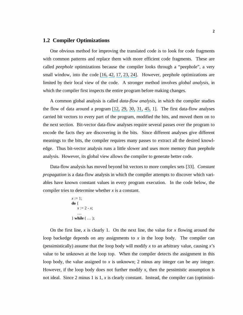
Data-flow analysis has moved beyond bit vectors to more complex sets [33]. Constant

propagation is a data-flow analysis in which the compiler attempts to discover which vari-

ables have known constant values in every program execution. In the code below, the

compiler tries to determine whether x is a constant.

x := 1;do {

x := 2 - x;…

} while ( … );

On the first line, x is clearly 1. On the next line, the value for x flowing around the

loop backedge depends on any assignments to x in the loop body. The compiler can

(pessimistically) assume that the loop body will modify x to an arbitrary value, causing x’s

value to be unknown at the loop top. When the compiler detects the assignment in this

loop body, the value assigned to x is unknown; 2 minus any integer can be any integer.

However, if the loop body does not further modify x, then the pessimistic assumption is

not ideal. Since 2 minus 1 is 1, x is clearly constant. Instead, the compiler can (optimisti-

3

cally) assume that x remains unchanged in the loop body, so that x’s value on the loop

backedge is 1. When the compiler inspects the loop body, it finds that the assignment

does not change x. The compiler’s assumption is justified; x is known to be constant.

In the modern version of constant propagation, the compiler makes the optimistic as-

sumption. [49] It assumes variables are constant and then tries to prove that assumption.

If it cannot, it falls back to the more pessimistic truth (i.e., the variable was not a con-

stant).

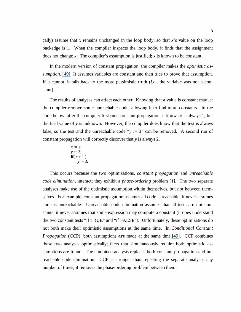
The results of analyses can affect each other. Knowing that a value is constant may let

the compiler remove some unreachable code, allowing it to find more constants. In the

code below, after the compiler first runs constant propagation, it knows x is always 1, but

the final value of y is unknown. However, the compiler does know that the test is always

false, so the test and the unreachable code “y := 3” can be removed. A second run of

constant propagation will correctly discover that y is always 2.

x := 1;y := 2;if ( x ≠ 1 )

y := 3;

This occurs because the two optimizations, constant propagation and unreachable

code elimination, interact; they exhibit a phase-ordering problem [1]. The two separate

analyses make use of the optimistic assumption within themselves, but not between them-

selves. For example, constant propagation assumes all code is reachable; it never assumes

code is unreachable. Unreachable code elimination assumes that all tests are not con-

stants; it never assumes that some expression may compute a constant (it does understand

the two constant tests “if TRUE” and “if FALSE”). Unfortunately, these optimizations do

not both make their optimistic assumptions at the same time. In Conditional Constant

Propagation (CCP), both assumptions are made at the same time [49]. CCP combines

these two analyses optimistically; facts that simultaneously require both optimistic as-

sumptions are found. The combined analysis replaces both constant propagation and un-

reachable code elimination. CCP is stronger than repeating the separate analyses any

number of times; it removes the phase-ordering problem between them.

4

Part of my work concerns combining optimizations. This thesis discusses under what

circumstances an optimization can be described with a monotone analysis framework.

Two analyses described with such frameworks can be combined. This thesis also dis-

cusses situations in which it is profitable to combine such optimizations and provides a

simple technique for solving the combined optimization.

1.3 Intermediate Representations

Compilers do not work directly on the high-level program text that people write.

They read it once and convert it to a form more suitable for a program to work with (after

all, compilers are just programs). This internal form is called an intermediate representa-

tion, because it lies between what the programmer wrote and what the machine under-

stands. The nature of the intermediate representation affects the speed and power of the

compiler.

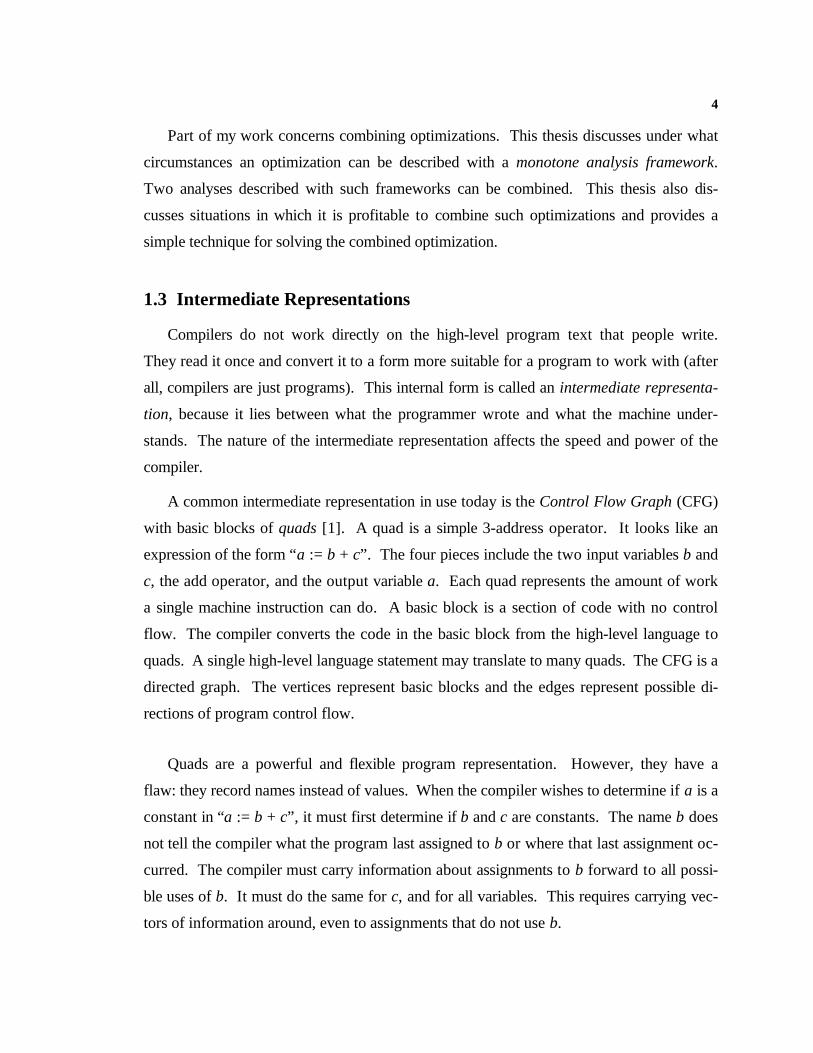
A common intermediate representation in use today is the Control Flow Graph (CFG)

with basic blocks of quads [1]. A quad is a simple 3-address operator. It looks like an

expression of the form “a := b + c”. The four pieces include the two input variables b and

c, the add operator, and the output variable a. Each quad represents the amount of work

a single machine instruction can do. A basic block is a section of code with no control

flow. The compiler converts the code in the basic block from the high-level language to

quads. A single high-level language statement may translate to many quads. The CFG is a

directed graph. The vertices represent basic blocks and the edges represent possible di-

rections of program control flow.

Quads are a powerful and flexible program representation. However, they have a

flaw: they record names instead of values. When the compiler wishes to determine if a is a

constant in “a := b + c”, it must first determine if b and c are constants. The name b does

not tell the compiler what the program last assigned to b or where that last assignment oc-

curred. The compiler must carry information about assignments to b forward to all possi-

ble uses of b. It must do the same for c, and for all variables. This requires carrying vec-

tors of information around, even to assignments that do not use b.

5

A better method is to record use-def chains with each quad [32, 1]. Use-def chains

represent quick pointers from uses of a variable (like b) to the set of its last definitions.

The compiler can now quickly determine what happened to b in the instructions before “a

:= b + c” without carrying a large vector around. Use-def chains allow the formalism of a

number of different data-flow analyses with a single framework. As long as there is only a

single definition that can reach the quad, there is only one use-def chain for b. However,

many definitions can reach the quad, each along a different path in the CFG. This requires

many use-def chains for b in just this one quad. When deciding what happened to b, the

compiler must merge the information from each use-def chain.

Instead of merging information about b just before every use of b, the compiler can

merge the information at points where different definitions of b meet. This leads to Static

Single Assignment (SSA) form, so called because each variable is assigned only once in

the program text [15]. Because each variable is assigned only once, we only need one

use-def chain per use of a variable. However, building SSA form is not trivial; program-

mers assign to the same variable many times. The compiler must rename the target vari-

able in each assignment to a new name; it must also rename the uses to be consistent with

the new names. Any time two CFG paths meet, the compiler needs a new name, even

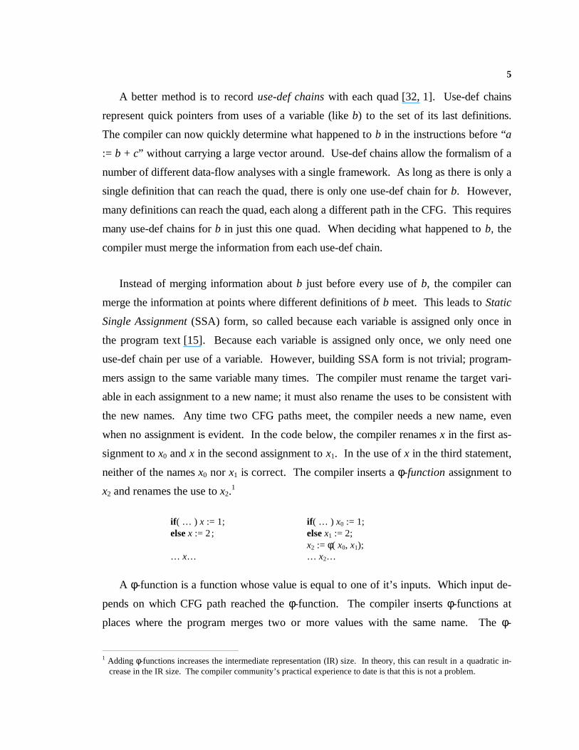
when no assignment is evident. In the code below, the compiler renames x in the first as-

signment to x0 and x in the second assignment to x1. In the use of x in the third statement,

neither of the names x0 nor x1 is correct. The compiler inserts a φ-function assignment to

x2 and renames the use to x2.1

if ( … ) x := 1; if ( … ) x0 := 1;else x := 2; else x1 := 2;

x2 := φ( x0, x1);… x… … x2…

A φ-function is a function whose value is equal to one of it’s inputs. Which input de-

pends on which CFG path reached the φ-function. The compiler inserts φ-functions at

places where the program merges two or more values with the same name. The φ-

1 Adding φ-functions increases the intermediate representation (IR) size. In theory, this can result in a quadratic in-

crease in the IR size. The compiler community’s practical experience to date is that this is not a problem.

6

function is not an executable statement in the same sense that other assignments are;

rather, it gives a unique name to the merged value of x.

SSA form allows the convenient expression of a variety of data-flow analyses. Quick

access through use-def chains and the manifestation of merge points simplify a number of

problems. In addition, use-def chains and SSA form allow the old bit vector and integer

vector analyses to be replaced with sparse analyses. A sparse analysis does not carry a

vector of every interesting program datum to every instruction. Instead, it carries just the

information needed at an instruction to that instruction. For these reasons, this thesis will

make extensive use of SSA form.

The main results of this thesis are (1) a framework for expressing and combining

analyses, (2) a method for showing when this is profitable, (3) a sparse analysis combining

Conditional Constant Propagation [49] and Global Congruence Finding [2] in O(n log n)

time, and (4) an implementation with experimental results. Additionally, the thesis dis-

cusses a global code motion technique that, when used in conjunction with the combined

analysis, produces many of the effects of Partial Redundancy Elimination [36, 18] and

Global Value Numbering [37].

1.4 Organization

To make the presentation clearer, we will use integer arithmetic for all our examples.

All the results apply to floating-point arithmetic, subject to the usual caveats concerning

floating point. Floating-point arithmetic is neither distributive nor associative, and inter-

mediate results computed at compile time may be stored at a different precision than the

same results computed at run time.

This thesis has nine chapters. Chapter 2 states the optimistic assumption in a mathe-

matically rigorous way with examples. It then furnishes minimum requirements for any

optimistic analysis.

Chapter 3 defines a general data-flow framework. It uses the optimistic assumption to

demonstrate when two optimizations can be profitably combined. Constant propagation,

7

unreachable code elimination, and global congruence finding are combined with a simple

O(n2) algorithm.

Chapter 4 presents a more efficient O(n log n) algorithm for combining these optimi-

zations. This combined algorithm also folds in various techniques from local value num-

bering.

For efficient analysis, quads contain use-def chains along with variable names. Chap-

ter 5 shows how to remove the redundant names, leaving only the use-def chains. It also

folds the CFG into the use-def chains, making a single level intermediate representation.

The resulting representation is compact and efficient.

Chapter 6 shows the results of the complete implementation. It compares program

improvement times for the combined algorithm versus the classic, separate pass approach.

The chapter also shows the compile times for the different approaches.

Chapter 7 presents a powerful global code motion algorithm. When used in conjunc-

tion with the intermediate representation in Chapter 5, the combined algorithm becomes

much stronger. Removing some control dependencies allows the combined algorithm to

mimic some of the effects of Partial Redundancy Elimination and Global Value Number-

ing.

Optimistic analysis must be global, but pessimistic analysis can be local (i.e., peep-

hole). Chapter 8 presents a strong peephole technique, one that gets within 95% of what

the best global technique does. This peephole optimization can occur during parsing if

SSA form is available. The chapter also presents a method for incrementally building SSA

form and experimental results for this technique.

Finally, Chapter 9 presents conclusions and directions for future research.

8

2. The Optimistic Assumption

8

Chapter 2

The Optimistic Assumption

If all the arts aspire to the condition of music,

all the sciences aspire to the condition of mathematics.

— George Santayana (1863-1952)

Before a compiler can improve the code it generates, it must understand that code.

Compilers use many techniques for understanding code, but a common one is called data-

flow analysis. Data-flow analysis tracks the flow of data around a program at compile

time. The type of data depends on the desired analysis. Central to most data-flow analy-

ses is the idea of a set of facts. During analysis, this set of facts is propagated around the

program. Local program facts are added or removed as appropriate. When the analysis

ends, the facts in the set hold true about the program. It is fitting that we begin our jour-

ney into program analysis with a look at sets.

I will start by discussing what it takes to discover a set. Then I will talk about data-

flow frameworks in terms of discovering a set. The set view of data-flow analysis gives us

a better intuition of what it means to combine analyses. In this chapter we will briefly look

at a constant propagation framework. In the next chapter we will specify data-flow

frameworks for constant propagation, unreachable code elimination and global value num-

bering, and find that they can be easily combined. For each analysis (and the combination)

we will look at some small example programs.

Central to most data-flow frameworks is the concept of a lattice. Points of interest in

the program are associated with lattice elements. Analysis initializes program points to

some ideal lattice element, usually called “top” and represented as T. At this point, some

of the lattice values may conflict with the program. Analysis continues by strictly lowering

the lattice elements until all conflicts are removed. This stable configuration is called a

fixed point. If the analysis stops before reaching a fixed point, the current program point

9

values are potentially incorrect. In essence, T represents an optimistic choice that must be

proven to be correct.

An alternative approach is to start all program points at the most pessimistic lattice

element, ⊥ (pronounced “bottom”). At this point there are no conflicts, because ⊥ means

that the compiler knows nothing about the run-time behavior of the program. Analysis

continues by raising lattice elements, based on the program and previously raised lattice

elements. If analysis stops before reaching a fixed point, the current program point values

are correct, but conservative — the analysis fails to discover some facts which hold true.

In many data-flow frameworks, there exist programs for which the pessimal approach

will never do as well as the optimistic approach. Such programs appear several times in

the test suite used by the author. This chapter explores the “optimistic assumption” and

why it is critical to the ability of an optimistic analysis to best a pessimistic analysis.

2.1 The Optimistic Assumption Defined

Enderton [19] defines a set as a collection of rules applied to some universe. Think of

the rules as assertions that all hold true when applied to the desired set. While these rules

can define a set, they do not tell how to construct the set.

We will restrict our rules to being monotonic with subset as the partial order relation.

Now we can view our restricted rules as functions, mappings from universe to universe.

Since all rules must hold true on the desired set, we will form a single mapping function

that applies all rules simultaneously and unions the resulting sets.2

We can apply this mapping function until we reach a fixed point, a set of elements that,

when the mapping function is applied to the set, yields the same set back. There are two

ways to apply the mapping function to build a set:

1. Bottom-up: Start with the empty set. Apply the mapping function. Initially only

the base-cases, or zero-input rules, produce new elements out. Continue applying

the mapping function to the expanding set, until closure. Because our rules are

2 We could choose intersection instead of union, but this makes the appearance of the rules less intuitive.

10

monotonic, elements are never removed. This method finds the Least Fixed Point

(lfp).

2. Top-down: Start with the complete set, the set with every element in the uni-

verse. Apply all rules. Some elements will not be produced by any rule, and will

not be in the final conjuction. Continue applying the mapping function, removing

elements not produced by any rule, until closure. This finds the Greatest Fixed

Point (gfp).

In general, the top-down approach can yield a larger set. It never yields a smaller set. We

leave until Chapter 3 the proof that the top-down method finds the gfp.

Definition 1: We use the optimistic assumption when we find a set using the top-

down approach instead of the bottom-up approach.

The following two examples will make these ideas more concrete. The first example

defines sets that are equal for both approaches. The second example gives rules that de-

fine two different sets, depending on the approach.

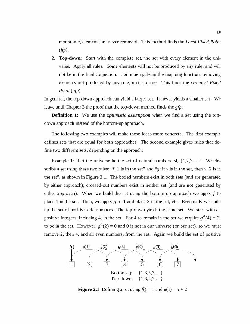
Example 1: Let the universe be the set of natural numbers N, {1,2,3,…}. We de-

scribe a set using these two rules: “f: 1 is in the set” and “g: if x is in the set, then x+2 is in

the set”, as shown in Figure 2.1. The boxed numbers exist in both sets (and are generated

by either approach); crossed-out numbers exist in neither set (and are not generated by

either approach). When we build the set using the bottom-up approach we apply f to

place 1 in the set. Then, we apply g to 1 and place 3 in the set, etc. Eventually we build

up the set of positive odd numbers. The top-down yields the same set. We start with all

positive integers, including 4, in the set. For 4 to remain in the set we require g-1(4) = 2,

to be in the set. However, g-1(2) = 0 and 0 is not in our universe (or our set), so we must

remove 2, then 4, and all even numbers, from the set. Again we build the set of positive

1

f()

3 5 72 4 6

g(1) g(3) g(5)g(2) g(4) g(6)

Bottom-up: {1,3,5,7,…}Top-down: {1,3,5,7,…}

Figure 2.1 Defining a set using f() = 1 and g(x) = x + 2

11

odd numbers.

Alternatively we can think of these rules as being a map from N to N. For the top-

down case, we start with an initial set, S0, of all the natural numbers. We then use the

rules to map S0 a S1. However, S1 does not have 2 in the set because neither f nor g pro-

duces 2 when applied to any natural number. If we repeat the mapping, S1 a S2, then S2

contains neither 2 nor 4 (4 is missing because 2 is missing in S1). When we repeat to a

fixed point, we find the set of positive odd integers.

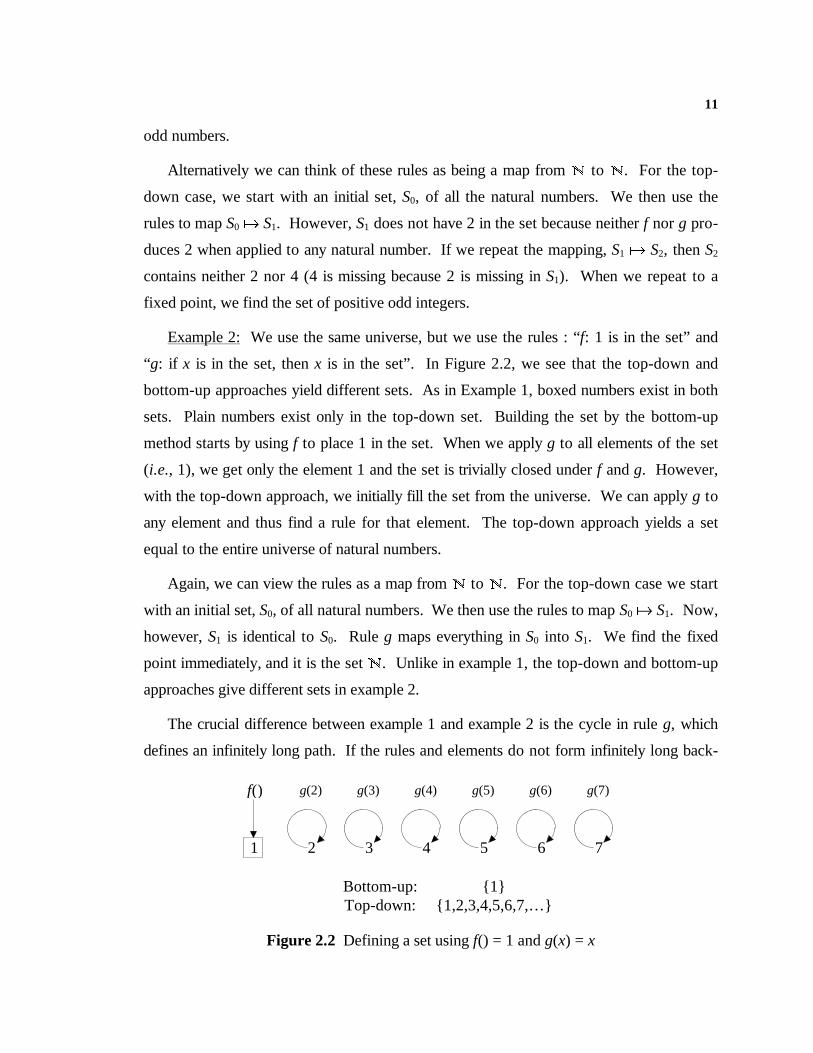
Example 2: We use the same universe, but we use the rules : “ f: 1 is in the set” and

“g: if x is in the set, then x is in the set”. In Figure 2.2, we see that the top-down and

bottom-up approaches yield different sets. As in Example 1, boxed numbers exist in both

sets. Plain numbers exist only in the top-down set. Building the set by the bottom-up

method starts by using f to place 1 in the set. When we apply g to all elements of the set

(i.e., 1), we get only the element 1 and the set is trivially closed under f and g. However,

with the top-down approach, we initially fill the set from the universe. We can apply g to

any element and thus find a rule for that element. The top-down approach yields a set

equal to the entire universe of natural numbers.

Again, we can view the rules as a map from N to N. For the top-down case we start

with an initial set, S0, of all natural numbers. We then use the rules to map S0 a S1. Now,

however, S1 is identical to S0. Rule g maps everything in S0 into S1. We find the fixed

point immediately, and it is the set N. Unlike in example 1, the top-down and bottom-up

approaches give different sets in example 2.

The crucial difference between example 1 and example 2 is the cycle in rule g, which

defines an infinitely long path. If the rules and elements do not form infinitely long back-

31

f()

5 72 4 6

g(7)g(3) g(5)g(2) g(4) g(6)

Bottom-up: {1}Top-down: {1,2,3,4,5,6,7,…}

Figure 2.2 Defining a set using f() = 1 and g(x) = x

12

wards paths, then the two approaches always give the same final set. The bottom-up ap-

proach can never form an infinitely long backwards path. The bottom-up approach cannot

“prime the pump”; it cannot produce the elements needed to complete a cycle. The top-

down approach starts with the elements in any cycle all existing; their existence allows the

application of the rules in the cycle which in turn define the cycle’s elements. The key idea

of this section is:

Sets are different when rules and elements form infinitely long paths of dependencies.

As we will see in later sections, the rules and elements from our data-flow frameworks will

form cycles of dependencies at program loops. Thus a top-down analysis can yield more

facts than a bottom-up analysis when working with loops. This also implies that for loop-

free programs, pessimistic and optimistic analyses perform equally well.

2.2 Using the Optimistic Assumption

In the chapters that follow we will express various common forms of analysis as find-

ing sets of elements. We achieve the best answer (i.e., the sharpest analysis) when these

sets are as large as possible.3 In general there is not a unique largest set, a gfp, for any

given collection of rules. For our specific problems there will always be a gfp.4

We want to express the data-flow analysis constant propagation as the discovery of a

set of facts. To make this discussion clearer, we place the program in SSA form, so the

program assigns each variable once. We also convert any high-level language expressions

into collections of quads.

Definition 2: We define constant propagation as a method for finding a set of vari-

ables that are constant on all executions for a given program in SSA form.

3 For some data-flow analyses, we will invert the usual sense of the set elements. For LIVE, elements of the universe

will be assertions that a particular variable is dead at a particular point in the program. The largest solution setmeans that the most variables are dead over the most program points.

4 Actually, with MEET defined as the subset relation and with a class of functions F: S a S (where S is a set fromabove) where each f ∈ F applies some rules to S and returns S augmented with the elements so defined, then each fis trivially monotonic and we have a gfp [46]. However, it is difficult to define constant propagation using the sub-set relation for MEET, so we will have to prove monotonicity on a function-by-function basis.

13

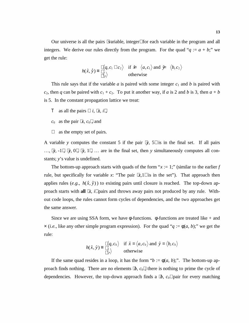
Our universe is all the pairs ⟨variable, integer⟩ for each variable in the program and all

integers. We derive our rules directly from the program. For the quad “q := a + b;” we

get the rule:

h x yq c c x a c y b c

( $, $ ), $ , $ ,

,≡

+ = =

1 2 1 2if and

otherwise

This rule says that if the variable a is paired with some integer c1 and b is paired with

c2, then q can be paired with c1 + c2. To put it another way, if a is 2 and b is 3, then a + b

is 5. In the constant propagation lattice we treat:

T as all the pairs ∀ i, ⟨x, i⟩ ,

c0 as the pair ⟨x, c0⟩ , and

⊥ as the empty set of pairs.

A variable y computes the constant 5 if the pair ⟨y, 5⟩ is in the final set. If all pairs

…, ⟨y, -1⟩ , ⟨y, 0⟩ , ⟨y, 1⟩ , … are in the final set, then y simultaneously computes all con-

stants; y’s value is undefined.

The bottom-up approach starts with quads of the form “x := 1;” (similar to the earlier f

rule, but specifically for variable x: “The pair ⟨x,1⟩ is in the set”). That approach then

applies rules (e.g., h x y( $, $ ) ) to existing pairs until closure is reached. The top-down ap-

proach starts with all ⟨x, i⟩ pairs and throws away pairs not produced by any rule. With-

out code loops, the rules cannot form cycles of dependencies, and the two approaches get

the same answer.

Since we are using SSA form, we have φ-functions. φ-functions are treated like + and

× (i.e., like any other simple program expression). For the quad “q := φ(a, b);” we get the

rule:

h x yq c x a c y b c

( $, $ ), $ , $ ,

,≡

= =

0 0 0if and

otherwise

If the same quad resides in a loop, it has the form “b := φ(a, b);”. The bottom-up ap-

proach finds nothing. There are no elements ⟨b, c0⟩ ; there is nothing to prime the cycle of

dependencies. However, the top-down approach finds a ⟨b, c0⟩ pair for every matching

14

⟨a, c0⟩ pair. To put it another way, if a constant is assigned to a before the loop and we

only merge a with the copy of itself from the loop, then a will be a constant in the loop.

2.3 Some Observations about the Optimistic Assumption

A bottom-up analysis can be stopped prematurely; a top-down analysis cannot.

Both the bottom-up and top-down approaches will iterate until reaching a fixed-point.

However, the bottom-up approach can be stopped prematurely. Every element in the set

exists because of some rule; optimizations based on the information in the set will be cor-

rect (but conservative). Stopping the top-down approach before reaching the gfp means

that there are elements in the set that do not have a corresponding rule. Optimizations

using these elements can be incorrect.

Top-down analysis requires checking an arbitrarily large number of rules and

elements. In bottom-up analysis, adding a new element requires only the application of

some rule to some set of elements. If we constrain the rules to have a constant number of

inputs and to run in constant time, then adding any element requires only a constant

amount of time. However, for top-down analysis, checking to see if some element should

remain in the set may require checking all the rules and elements in some arbitrarily large

cycle of dependencies. For each of the analyses we will examine, it is possible to apply the

bottom-up approach using strictly local5 techniques. We limit our top-down analyses to

global, batch-oriented techniques.

Bottom-up methods can transform as they analyze. Because the solution set for

bottom-up analyses is always correct, transformations based on intermediate solutions are

valid. Every time analysis adds new elements to the solution set, transformations based on

the new elements can be performed immediately. For some analyses, we can directly rep-

resent the solution set with the intermediate representation. To add new elements to the

solution, we transform the program. We will present online versions of pessimistic analy-

5 Local is used in the mathematical (as opposed to the data-flow) sense. To determine if we can add any given ele-

ment, we will inspect a constant number of other elements that are a constant distance (1 pointer dereference)away.

15

ses in Chapter 7, in which we solve a pessimistic analysis by repeatedly transforming the

program.

Many published data-flow analyses use the optimistic assumption separately, but

do not use the optimistic assumption between analyses.6 A combination of optimiza-

tions, taken as a single transformation, includes some optimistic analyses (each separate

phase) and some pessimistic analyses (information between phases).

6 Classic analysis have historically been pessimistic, presumably because proof of correctness is easier. In a bottom-

up analysis there is never a time when the information is incorrect.

16

3. Combining Analyses, Combining Optimizations

16

Chapter 3

Combining Analyses, Combining Optimizations

O that there might in England be

A duty on Hypocrisy,

A tax on humbug, an excise

On solemn plausibilities.

— Henry Luttrell (1765-1881)

3.1 Intr oduction

Modern optimizing compilers make several passes over a program's intermediate rep-

resentation in order to generate good code. Many of these optimizations exhibit a phase-

ordering problem. The compiler discovers different facts (and generates different code)

depending on the order in which it executes the optimizations. Getting the best code re-

quires iterating several optimizations until reaching a fixed point. This thesis shows that

by combining optimization passes, the compiler can discover more facts about the pro-

gram, providing more opportunities for optimization.

Wegman and Zadeck showed this in an ad hoc way in previous work — they pre-

sented an algorithm that combines two optimizations. [49] This thesis provides a more

formal basis for describing combinations and shows when and why these combinations

yield better results. We present a proof that a simple iterative technique can solve these

combined optimizations. Finally, we combine Conditional Constant Propagation [49] and

Value Numbering [2, 12, 13, 37] to get an optimization that is greater than the sum of its

parts.

17

3.2 Overview

Before we describe our algorithms, we need to describe our programs. We represent a

program by a Control Flow Graph (CFG), where the edges denote flow of control and the

vertices are basic blocks. Basic blocks contain a set of assignment statements represented

as quads. Basic blocks end with a special final quad that may be a return , an if or empty

(fall through). We write program variables in lower case letters (e.g., x, y). All variables

are initialized to T, which is discussed in the next section. To simplify the presentation, we

restrict the program to integer arithmetic. The set of all integers is represented by Z.

Assignment statements (quads) have a single function on the right-hand side and a

variable on the left. The function op is of a small constant arity (i.e., x := a op b). Op may

be a constant or the identity function, and is limited to being a k-ary function. This is a

reasonable assumption for our application. We run the algorithm over a low-level com-

piler intermediate representation, with k ó 3. We call the set of op functions OP.

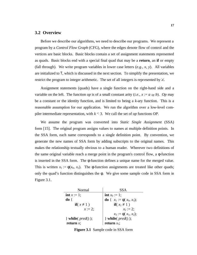
We assume the program was converted into Static Single Assignment (SSA)

form [15]. The original program assigns values to names at multiple definition points. In

the SSA form, each name corresponds to a single definition point. By convention, we

generate the new names of SSA form by adding subscripts to the original names. This

makes the relationship textually obvious to a human reader. Wherever two definitions of

the same original variable reach a merge point in the program's control flow, a φ-function

is inserted in the SSA form. The φ-function defines a unique name for the merged value.

This is written x1 := φ(x0, x2). The φ-function assignments are treated like other quads;

only the quad’s function distinguishes the φ. We give some sample code in SSA form in

Figure 3.1.

Normal SSAint x := 1; int x0 := 1;do { do { x1 := φ( x0, x3);

if ( x ≠ 1 ) if ( x1 ≠ 1 )x := 2; x2 := 2;

x3 := φ( x1, x2);} while( pred() ); } while( pred() ); return x; return x3;

Figure 3.1 Sample code in SSA form

18

After the renaming step, the program assigns every variable exactly once.7 Since ex-

pressions only occur on the right-hand side of assignments, every expression is associated

with a variable. There is a one-to-one correlation between variables and expressions; the

variable name can be used as a direct map to the expression that defines it. In our imple-

mentation, we require this mapping to be fast.8 Finally, we define N to be the number of

statements in the SSA form. In SSA form the number of φ-functions inserted can be

quadratic in the size of the original code; the community's practical experience to date has

shown that it is usually sublinear in the size of the original code.

3.2.1 Monotone Analysis Frameworks

To combine several optimizations, we first describe them in a common monotone

analysis framework [14, 30, 45]. Briefly, a monotone analysis framework is:

1. A lattice of inferences we make about the program. These are described as a complete

lattice L = {A, T, ⊥ , ∩} with height d, where:

a) A is a set of inferences.

b) T and ⊥ are distinguished elements of A, usually called “top” and “bottom” respec-

tively.

c) ∩ is the meet operator such that for any a, b ∈ A,

a ∩ a = a, (idempotent)

a ∩ b = b ∩ a, (commutative)

a ∩ (b ∩ c) = (a ∩ b) ∩ c, (associative)

a ∩ T = a,

a ∩ ⊥ = ⊥ ,

d) d is the length of the longest chain in L.

2. A set of monotone functions F with arity ó k used to approximate the program, de-

fined as F ⊆ { f : L → L } containing the identity function ι and closed under compo-

sition and pointwise meet.

7 This is the property for which the term static single assignment is coined.

8 In fact, our implementation replaces the variable name with a pointer to the expression that defines the variable.Performing the mapping requires a single pointer lookup.

19

3. A map γ : OP → F from program primitives to approximation functions. In general,

all the approximation functions are simple tables, mapping lattice elements to lattice

elements.9 We do not directly map the CFG in the framework because some frame-

works do not maintain a correspondence with the CFG. This means our solutions are

not directly comparable to a meet over all paths (MOP) solution like that described by

Kam and Ullman [30]. Our value-numbering solution is such a framework.

We say that a f b if and only if a ∩ b = b, and a f b if and only if a f b and a ≠ b. Be-

cause the lattice is complete, ∩ is closed on A.

The lattice height d is the largest n such that a sequence of elements x1, x2, …, xn in Lform a chain: xi f xi+1 for 1 ó i < n. We require that L have the finite descending chain

property – that is, d must be bounded by a constant. For the problems we will examine, d

will be quite small (usually 2 or 3).

We assume that we can compute f ∈ F in time O(k), where k is the largest number of

inputs to any function in F. Since k ≤ 3 in our implementation, we can compute f in con-

stant time.

3.2.2 Monotone Analysis Problems

When we apply a monotone analysis framework to a specific program we get a

monotone analysis problem – a set of simultaneous equations derived directly from the

program. Variables in the equations correspond to points of interest in the program; each

expression in the program has its own variable. Associated with each variable is a single

inference. Program analysis substitutes approximation functions (chosen from F using γ)

for the actual program primitive functions and solves the equations over the approxima-

tion functions. (In effect, analysis “runs” an approximate version of the program.) By

design, the equations have a maximal solution called the Greatest Fixed Point (gfp) [14,

46].10

9 Some of our mappings take into account information from the CFG. Here we are taking some notational liberty by

defining the mapping from only OP to F. We correct this in our implementation by using an operator-level (insteadof basic block level) Program Dependence Graph (PDG) in SSA form [21, 38]. Such a representation does nothave a CFG or any basic blocks. Control information is encoded as inputs to functions like any other program vari-able.

10 The properties described in Section 3.2.1 ensure the existence of a gfp [46]. These systems of equations can besolved using many techniques. These techniques vary widely in efficiency. The more expensive techniques can

20

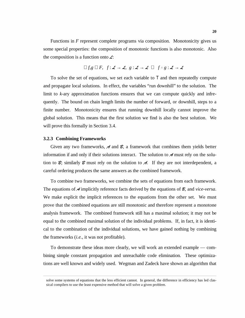
Functions in F represent complete programs via composition. Monotonicity gives us

some special properties: the composition of monotonic functions is also monotonic. Also

the composition is a function onto L:

∀ f,g ∈ F, f : L → L, g : L → L ⇒ f o g : L → LTo solve the set of equations, we set each variable to T and then repeatedly compute

and propagate local solutions. In effect, the variables “run downhill” to the solution. The

limit to k-ary approximation functions ensures that we can compute quickly and infre-

quently. The bound on chain length limits the number of forward, or downhill, steps to a

finite number. Monotonicity ensures that running downhill locally cannot improve the

global solution. This means that the first solution we find is also the best solution. We

will prove this formally in Section 3.4.

3.2.3 Combining Frameworks

Given any two frameworks, A and B, a framework that combines them yields better

information if and only if their solutions interact. The solution to A must rely on the solu-

tion to B; similarly B must rely on the solution to A. If they are not interdependent, a

careful ordering produces the same answers as the combined framework.

To combine two frameworks, we combine the sets of equations from each framework.

The equations of A implicitly reference facts derived by the equations of B, and vice-versa.

We make explicit the implicit references to the equations from the other set. We must

prove that the combined equations are still monotonic and therefore represent a monotone

analysis framework. The combined framework still has a maximal solution; it may not be

equal to the combined maximal solution of the individual problems. If, in fact, it is identi-

cal to the combination of the individual solutions, we have gained nothing by combining

the frameworks (i.e., it was not profitable).

To demonstrate these ideas more clearly, we will work an extended example — com-

bining simple constant propagation and unreachable code elimination. These optimiza-

tions are well known and widely used. Wegman and Zadeck have shown an algorithm that

solve some systems of equations that the less efficient cannot. In general, the difference in efficiency has led clas-sical compilers to use the least expensive method that will solve a given problem.

21

combines them, Conditional Constant Propagation (CCP) [49]. It is instructive to com-

pare their algorithm with our framework-based approach. As a final exercise, we combine

CCP with partition-based Global Value Numbering (GVN) [2, 37] to obtain a new opti-

mization strictly more powerful than the separate optimizations. The combination runs in

O(N 2) time. In Chapter 4, we derive a more complex algorithm which solves the problem

in time O(N log N).

In our technique, the equations are derived directly from the intermediate representa-

tion. For the purposes of this chapter, the intermediate representation is the equations.

We use a technique from abstract interpretation, and associate an approximation function

γ chosen from F with every primitive function in the program. Because we restrict the

form of the equations (see Section 3.2.1), we can find the maximal solution using an itera-

tive technique in time O(nk2d) where n is the number of equations to solve (often equal to

N, the number of statements in the program), k is largest number of inputs to any one

function, and d is the height of the lattice.

3.3 Simple Constant Propagation

Simple constant propagation looks for program expressions that compute the same

value on all executions of the program. It can be cast in a monotone analysis framework.

It conservatively approximates the program's control flow by assuming that all basic

blocks and all quads are executable. Thus, control flow has no explicit expression in the

data-flow equations. Each assignment defines an expression and a variable. The inference

the variable holds tells us whether the expression computes a constant.

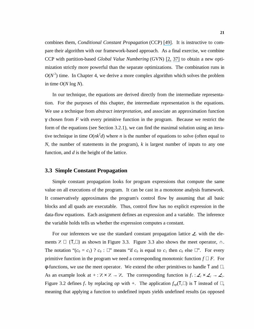
For our inferences we use the standard constant propagation lattice Lc with the ele-

ments Z ∪ { T,⊥ } as shown in Figure 3.3. Figure 3.3 also shows the meet operator, ∩.

The notation “(c0 = c1) ? c0 : ⊥ ” means “if c0 is equal to c1 then c0 else ⊥ ”. For every

primitive function in the program we need a corresponding monotonic function f ∈ F. For

φ-functions, we use the meet operator. We extend the other primitives to handle T and ⊥ .

As an example look at + : Z × Z → Z. The corresponding function is f+ : Lc × Lc → Lc.

Figure 3.2 defines f+ by replacing op with +. The application fop(T,⊥ ) is T instead of ⊥ ,

meaning that applying a function to undefined inputs yields undefined results (as opposed

22

to unknown results).11 This embodies the idea that we do not propagate information until

all the facts are known.

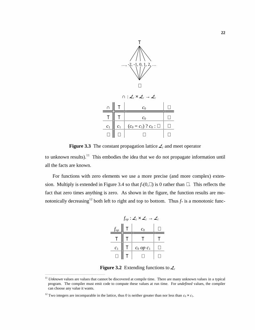
For functions with zero elements we use a more precise (and more complex) exten-

sion. Multiply is extended in Figure 3.4 so that f*(0,⊥ ) is 0 rather than ⊥ . This reflects the

fact that zero times anything is zero. As shown in the figure, the function results are mo-

notonically decreasing12 both left to right and top to bottom. Thus f* is a monotonic func-

11 Unknown values are values that cannot be discovered at compile time. There are many unknown values in a typical

program. The compiler must emit code to compute these values at run time. For undefined values, the compilercan choose any value it wants.

12 Two integers are incomparable in the lattice, thus 0 is neither greater than nor less than c0 × c1.

fop : Lc × Lc → Lc

fop T c0 ⊥

T T T T

c1 T c0 op c1 ⊥

⊥ T ⊥ ⊥

Figure 3.2 Extending functions to Lc

T

…, -2, -1, 0, 1, 2, …

⊥

∩ : Lc × Lc → Lc

∩ T c0 ⊥

T T c0 ⊥

c1 c1 (c0 = c1) ? c0 : ⊥ ⊥

⊥ ⊥ ⊥ ⊥

Figure 3.3 The constant propagation lattice Lc and meet operator

23

tion, but maintains information in more cases than the corresponding function without the

special case for zero.

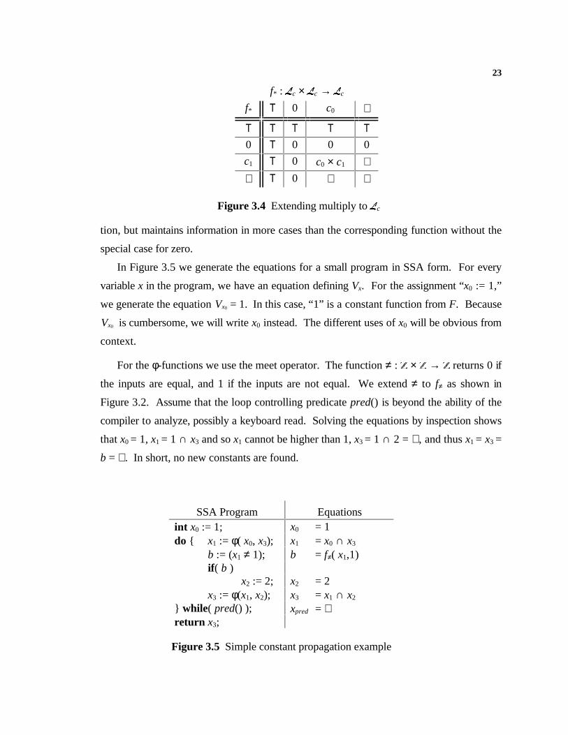
In Figure 3.5 we generate the equations for a small program in SSA form. For every

variable x in the program, we have an equation defining Vx. For the assignment “x0 := 1,”

we generate the equation Vx0 = 1. In this case, “1” is a constant function from F. Because

Vx0 is cumbersome, we will write x0 instead. The different uses of x0 will be obvious from

context.

For the φ-functions we use the meet operator. The function ≠ : Z × Z → Z returns 0 if

the inputs are equal, and 1 if the inputs are not equal. We extend ≠ to f≠ as shown in

Figure 3.2. Assume that the loop controlling predicate pred() is beyond the ability of the

compiler to analyze, possibly a keyboard read. Solving the equations by inspection shows

that x0 = 1, x1 = 1 ∩ x3 and so x1 cannot be higher than 1, x3 = 1 ∩ 2 = ⊥ , and thus x1 = x3 =

b = ⊥ . In short, no new constants are found.

f* : Lc × Lc → Lc

f* T 0 c0 ⊥

T T T T T

0 T 0 0 0

c1 T 0 c0 × c1 ⊥⊥ T 0 ⊥ ⊥

Figure 3.4 Extending multiply to Lc

SSA Program Equationsint x0 := 1; x0 = 1do { x1 := φ( x0, x3); x1 = x0 ∩ x3

b := (x1 ≠ 1); b = f≠( x1,1)if ( b )

x2 := 2; x2 = 2x3 := φ(x1, x2); x3 = x1 ∩ x2

} while( pred() ); xpred = ⊥return x3;

Figure 3.5 Simple constant propagation example

24

3.4 Finding the Greatest Fixed Point

In this section we show that the iterative technique works on monotone analysis

frameworks. That is, we show that initializing a system of monotonic equations to T and

successively solving the equations eventually yields the gfp. We start with Tarski [46],

who proved that every monotone function f : L → L has a gfp in a complete lattice L.

Since f is monotone, successive applications of f to T descend monotonically:

T f f(T) f f 2(T) f LSince the lattice is of bounded depth, a fixed point u = f d(T) = f d+1(T) is eventually

reached. We cannot have u f gfp because gfp is the greatest fixed point (and u is a fixed

point). Suppose we have the reverse situation, gfp f u. Then the applications of f must

form a descending chain that falls past the gfp. There must be some i such that L f i(T) fgfp f f i+1(T) L. By the monotonicity of f we have f i(T) f gfp ⇒ f i+1(T) f f(gfp). Since

f(gfp) = gfp we have f i+1(T) f gfp, a contradiction. Therefore u = gfp, and successive

applications of f to T yield the gfp.

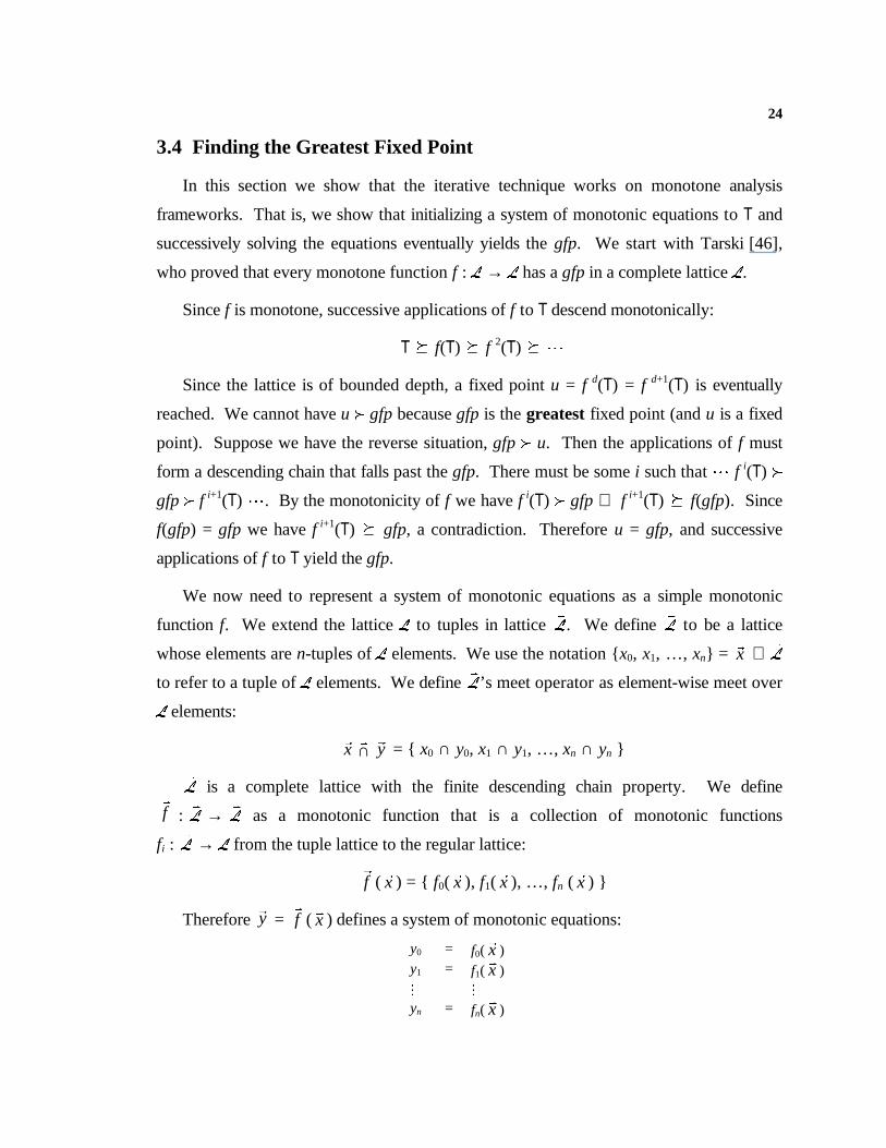
We now need to represent a system of monotonic equations as a simple monotonic

function f. We extend the lattice L to tuples in lattice vL. We define

vL to be a lattice

whose elements are n-tuples of L elements. We use the notation { x0, x1, …, xn} = rx ∈

vLto refer to a tuple of L elements. We define

vL’s meet operator as element-wise meet over

L elements:

rx

r∩

ry = { x0 ∩ y0, x1 ∩ y1, …, xn ∩ yn }

vL is a complete lattice with the finite descending chain property. We definerf :

vL → vL as a monotonic function that is a collection of monotonic functions

fi : vL → L from the tuple lattice to the regular lattice:

rf (

rx ) = { f0(

rx ), f1(

rx ), …, fn (

rx ) }

Therefore ry =

rf (

rx ) defines a system of monotonic equations:

y0 = f0(rx )

y1 = f1(rx )

M Myn = fn(

rx )

25

Each of the functions f0, f1, …, fn takes an n-length tuple of L elements. In the prob-

lems that we are solving, we require that only k (0 ≤ k ≤ n) elements from L are actually

used. That is, fi takes as input a k-sized subset of rx . Unfortunately the solution technique

of repeatedly applyingrf until a fixed point is reached is very inefficient.

vL has a lattice

height of O(nd), and each computation ofrf might take O(nk) work for a running time of

O(n2kd). The next section presents a more efficient technique based on evaluating the

single variable formulation (fi rather thanrf ).

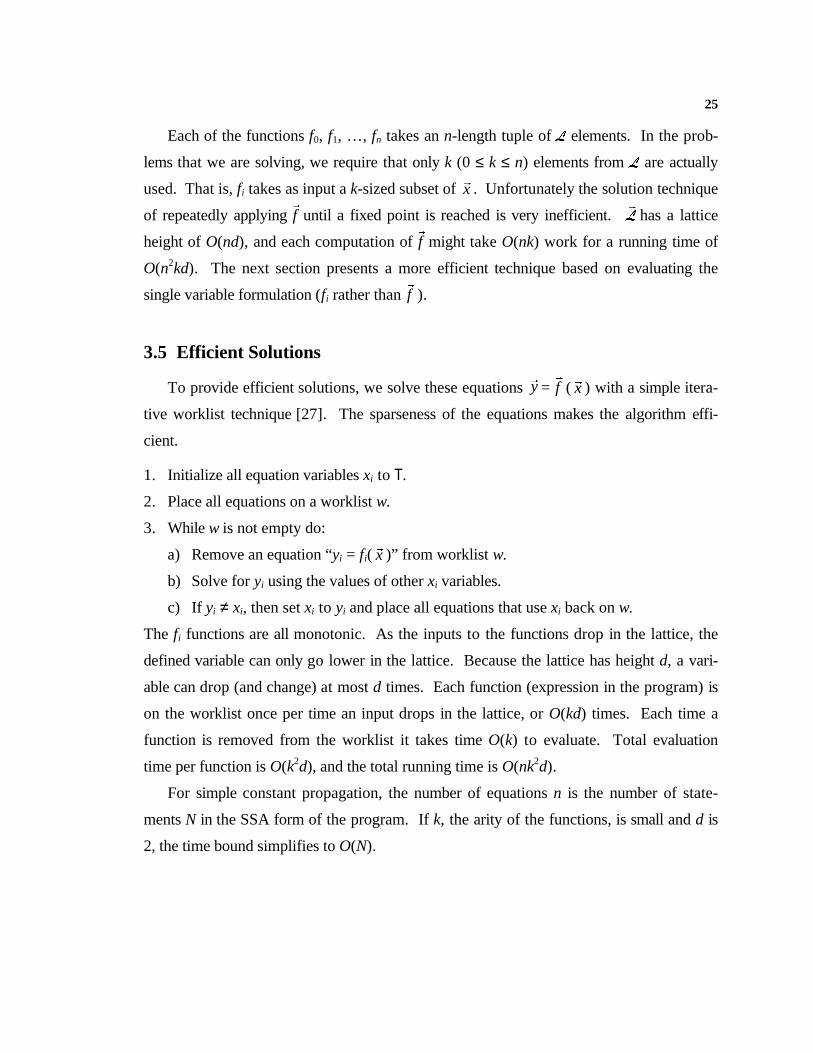
3.5 Efficient Solutions

To provide efficient solutions, we solve these equations ry =

rf (

rx ) with a simple itera-

tive worklist technique [27]. The sparseness of the equations makes the algorithm effi-

cient.

1. Initialize all equation variables xi to T.

2. Place all equations on a worklist w.

3. While w is not empty do:

a) Remove an equation “yi = fi(rx )” from worklist w.

b) Solve for yi using the values of other xi variables.

c) If yi ≠ xi, then set xi to yi and place all equations that use xi back on w.

The fi functions are all monotonic. As the inputs to the functions drop in the lattice, the

defined variable can only go lower in the lattice. Because the lattice has height d, a vari-

able can drop (and change) at most d times. Each function (expression in the program) is

on the worklist once per time an input drops in the lattice, or O(kd) times. Each time a

function is removed from the worklist it takes time O(k) to evaluate. Total evaluation

time per function is O(k2d), and the total running time is O(nk2d).

For simple constant propagation, the number of equations n is the number of state-

ments N in the SSA form of the program. If k, the arity of the functions, is small and d is

2, the time bound simplifies to O(N).

26

3.6 Unreachable Code Elimination

We do the same analysis for unreachable code elimination that we did for simple con-

stant propagation. We seek to determine if any code in the program is not executable, ei-

ther because a control-flow test is based on a constant value or because no other code

jumps to it. Our inferences are to determine if a section of code is reachable, expressed as

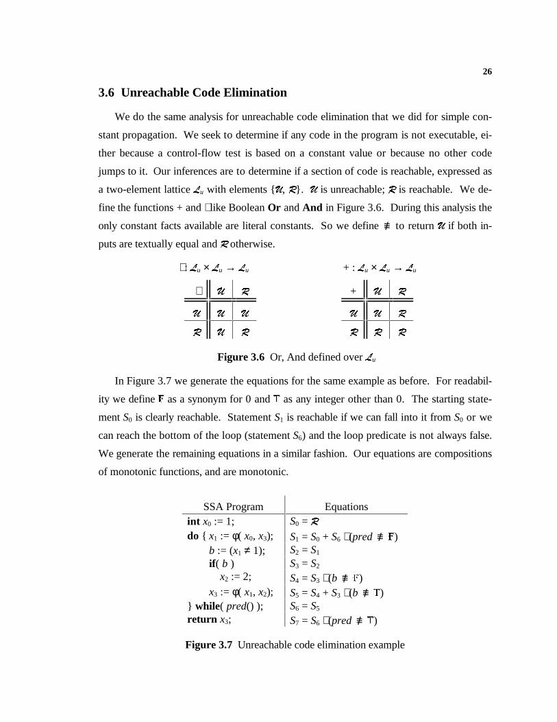
a two-element lattice Lu with elements {U, R}. U is unreachable; R is reachable. We de-

fine the functions + and ⋅ like Boolean Or and And in Figure 3.6. During this analysis the

only constant facts available are literal constants. So we define /≡ to return U if both in-

puts are textually equal and R otherwise.

Figure 3.6 Or, And defined over Lu

In Figure 3.7 we generate the equations for the same example as before. For readabil-

ity we define F as a synonym for 0 and T as any integer other than 0. The starting state-

ment S0 is clearly reachable. Statement S1 is reachable if we can fall into it from S0 or we

can reach the bottom of the loop (statement S6) and the loop predicate is not always false.

We generate the remaining equations in a similar fashion. Our equations are compositions

of monotonic functions, and are monotonic.

+ : Lu × Lu → Lu

+ U RU U RR R R

⋅ : Lu × Lu → Lu

⋅ U RU U UR U R

SSA Program Equationsint x0 := 1; S0 = Rdo { x1 := φ( x0, x3); S1 = S0 + S6 ⋅ (pred /≡ F)

b := (x1 ≠ 1); S2 = S1

if ( b ) S3 = S2

x2 := 2; S4 = S3 ⋅ (b /≡ F)x3 := φ( x1, x2); S5 = S4 + S3 ⋅ (b /≡ T)

} while( pred() ); S6 = S5

return x3; S7 = S6 ⋅ (pred /≡ T)

Figure 3.7 Unreachable code elimination example

27

Because b and pred are not literal constants, all the /≡ tests must return R. The solu-

tion is straightforward: everything is reachable.

If we look closely at this example we can see that when we run the program, x0 gets

set to 1, the if 's predicate b is always false, and the consequent of the if test (S4) never

executes. Neither simple constant propagation nor unreachable code elimination discovers

these facts because each analysis needs a fact that can only be discovered by the other.

3.7 Combining Analyses

To improve the results of optimization we would like to combine these two analyses.

To do this, we need a framework that allows us to describe the combined system, to rea-

son about its properties, and to answer some critical questions. In particular we would

like to know: is the combined transformation correct – that is, does it retain the meaning-

preserving properties of the original separate transformations? Is this combination profit-

able – that is, can it discover facts and improve code in ways that the separate techniques

cannot?

If the combined framework is monotonic, then we know a gfp exists, and we can find

it efficiently. We combine analyses by unioning the set of equations and making explicit

the implicit references between the equations. Unioning equations makes a bigger set of

unrelated equations. However, the equations remain monotonic so this is safe.

However, if the analyses do not interact there is no profit in combining them. We

make the analyses interact by replacing implicit references with functions that take inputs

from one of the original frameworks and produce outputs in the other. The reachable

equations for S3 and S4 use the variable b, which we defined in the constant propagation

equations. Instead of testing b against a literal constant we test against an Lc element. We

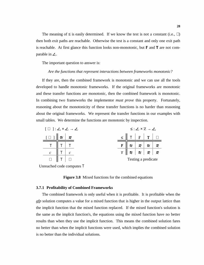
replace the /≡ function with ≤ : Lc × Z → Lu defined in Figure 3.8. The ≤ function is an

example of a function that mixes inputs and outputs between the frameworks. ≤ takes an

input from the Lc framework (variable b) and returns a result in the Lu framework

(reachability of the conditional statements).

28

The meaning of ≤ is easily determined. If we know the test is not a constant (i.e., ⊥ )

then both exit paths are reachable. Otherwise the test is a constant and only one exit path

is reachable. At first glance this function looks non-monotonic, but F and T are not com-

parable in Lc.

The important question to answer is:

Are the functions that represent interactions between frameworks monotonic?

If they are, then the combined framework is monotonic and we can use all the tools

developed to handle monotonic frameworks. If the original frameworks are monotonic

and these transfer functions are monotonic, then the combined framework is monotonic.

In combining two frameworks the implementor must prove this property. Fortunately,

reasoning about the monotonicity of these transfer functions is no harder than reasoning

about the original frameworks. We represent the transfer functions in our examples with

small tables. We determine the functions are monotonic by inspection.

Figure 3.8 Mixed functions for the combined equations

3.7.1 Profitability of Combined Frameworks

The combined framework is only useful when it is profitable. It is profitable when the

gfp solution computes a value for a mixed function that is higher in the output lattice than

the implicit function that the mixed function replaced. If the mixed function's solution is

the same as the implicit function's, the equations using the mixed function have no better

results than when they use the implicit function. This means the combined solution fares

no better than when the implicit functions were used, which implies the combined solution

is no better than the individual solutions.

≤ : Lc × Z → Lu

≤ T F T ⊥

F U R U RT U U R R

Testing a predicate

[ ⇒ ] : Lu × Lc → Lc

[ ⇒ ] U R T T T

c T c

⊥ T ⊥

Unreached code computes T

29

If we have functions from framework Lc to framework Lu but not vice-versa, we have

a simple phase-ordering problem. We can solve the Lc framework before the Lu frame-

work and achieve results equal to a combined framework. The combined framework is

only profitable if we also have functions from Lu to Lc and the combined gfp improves on

these mixed functions' results.

Back to our example: the value computed by unreachable code is undefined (T), so

each of the constant propagation equations gets an explicit reference to the appropriate

reachable variable. The reachable variable is used as an input to the monotonic infix func-

tion [ ⇒ ] : Lu × Lc → Lc, also defined in Figure 3.8.

Instead of one equation per statement we have two equations per statement. Each

equation has grown by, at most, a constant amount. So, the total size of all equations has

grown by a constant factor, and remains linear in the number of statements.

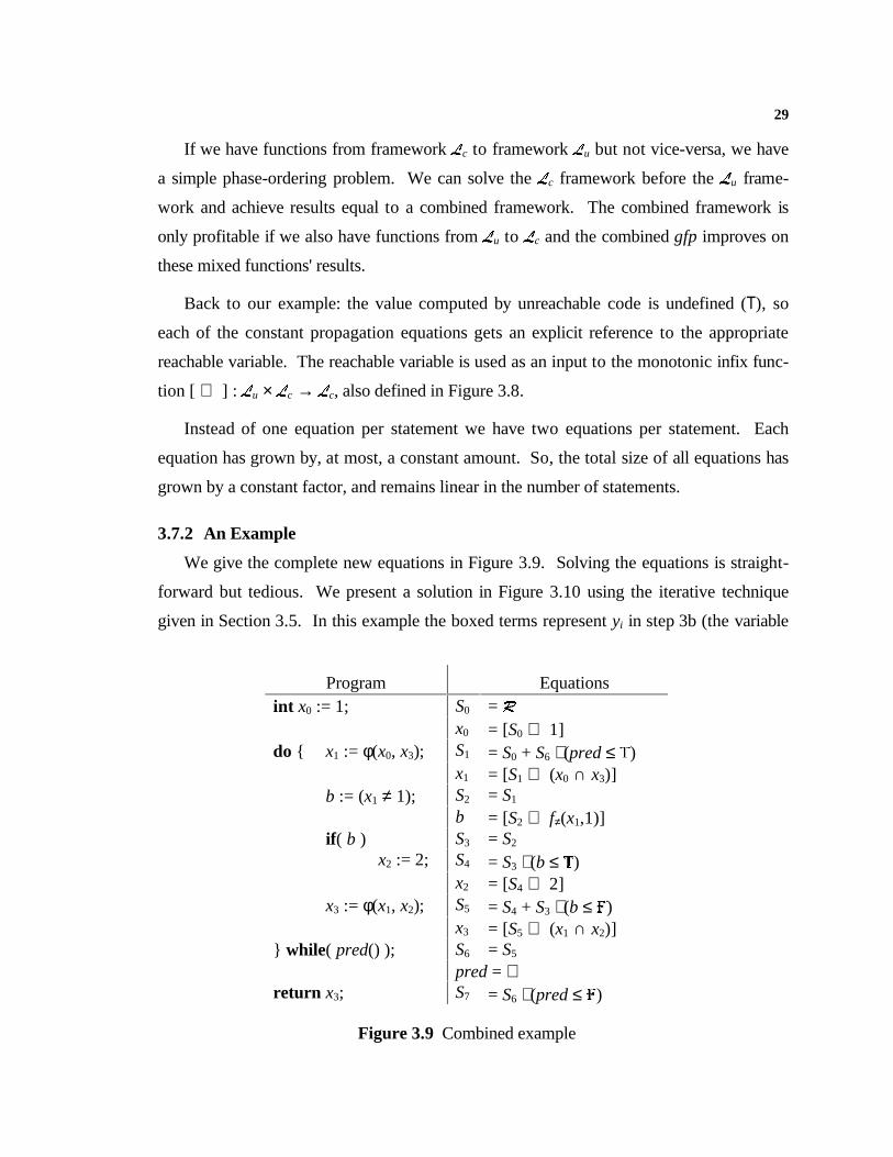
3.7.2 An Example

We give the complete new equations in Figure 3.9. Solving the equations is straight-

forward but tedious. We present a solution in Figure 3.10 using the iterative technique

given in Section 3.5. In this example the boxed terms represent yi in step 3b (the variable

Program Equationsint x0 := 1; S0 = R

x0 = [S0 ⇒ 1]do { x1 := φ(x0, x3); S1 = S0 + S6 ⋅ (pred ≤ T)

x1 = [S1 ⇒ (x0 ∩ x3)]b := (x1 ≠ 1); S2 = S1

b = [S2 ⇒ f≠(x1,1)]if ( b ) S3 = S2

x2 := 2; S4 = S3 ⋅ (b ≤ T)x2 = [S4 ⇒ 2]

x3 := φ(x1, x2); S5 = S4 + S3 ⋅ (b ≤ F)x3 = [S5 ⇒ (x1 ∩ x2)]

} while( pred() ); S6 = S5

pred = ⊥return x3; S7 = S6 ⋅ (pred ≤ F)

Figure 3.9 Combined example

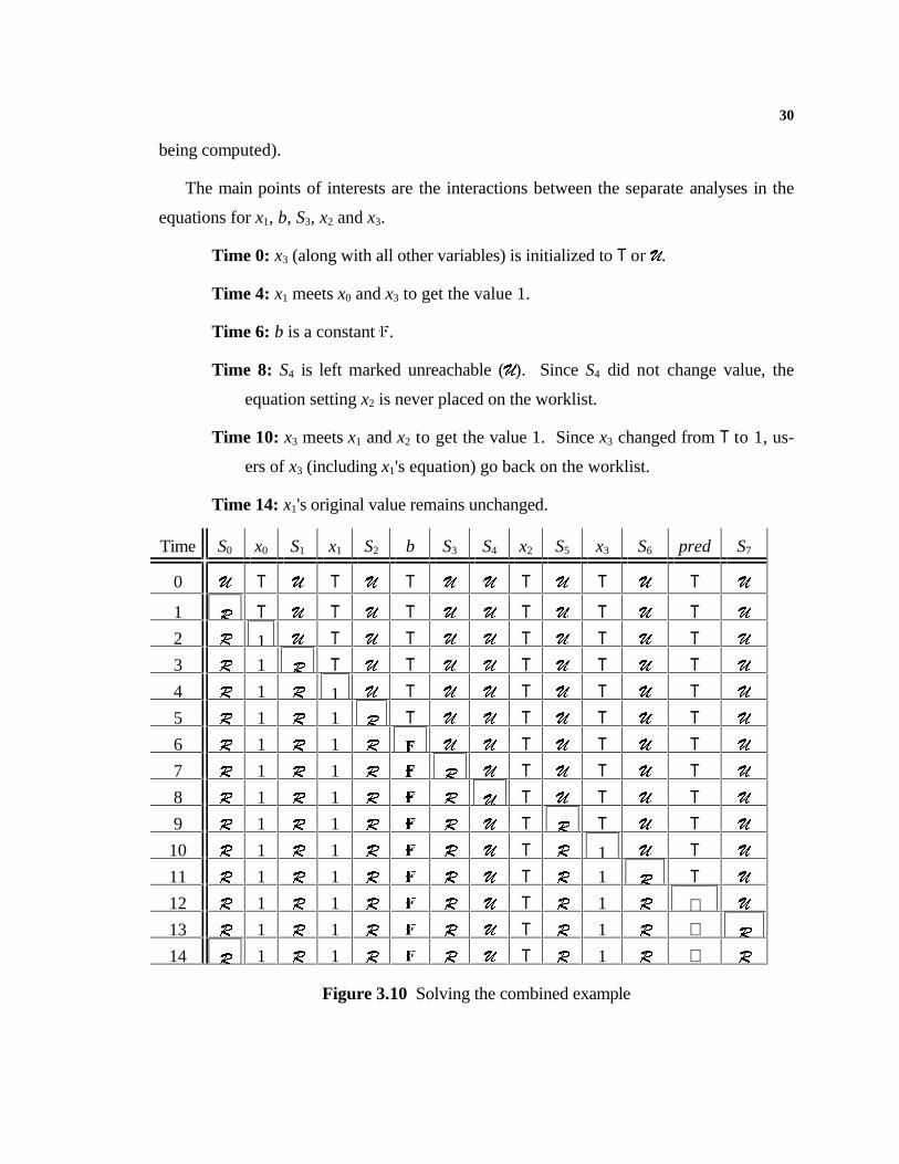
30

being computed).

The main points of interests are the interactions between the separate analyses in the

equations for x1, b, S3, x2 and x3.

Time 0: x3 (along with all other variables) is initialized to T or U.

Time 4: x1 meets x0 and x3 to get the value 1.

Time 6: b is a constant F.

Time 8: S4 is left marked unreachable (U). Since S4 did not change value, the

equation setting x2 is never placed on the worklist.

Time 10: x3 meets x1 and x2 to get the value 1. Since x3 changed from T to 1, us-

ers of x3 (including x1's equation) go back on the worklist.

Time 14: x1's original value remains unchanged.

Time S0 x0 S1 x1 S2 b S3 S4 x2 S5 x3 S6 pred S7

0 U T U T U T U U T U T U T U1 R T U T U T U U T U T U T U2 R 1 U T U T U U T U T U T U3 R 1 R T U T U U T U T U T U4 R 1 R 1 U T U U T U T U T U5 R 1 R 1 R T U U T U T U T U6 R 1 R 1 R F U U T U T U T U7 R 1 R 1 R F R U T U T U T U8 R 1 R 1 R F R U T U T U T U9 R 1 R 1 R F R U T R T U T U10 R 1 R 1 R F R U T R 1 U T U11 R 1 R 1 R F R U T R 1 R T U12 R 1 R 1 R F R U T R 1 R ⊥ U13 R 1 R 1 R F R U T R 1 R ⊥ R14 R 1 R 1 R F R U T R 1 R ⊥ R

Figure 3.10 Solving the combined example

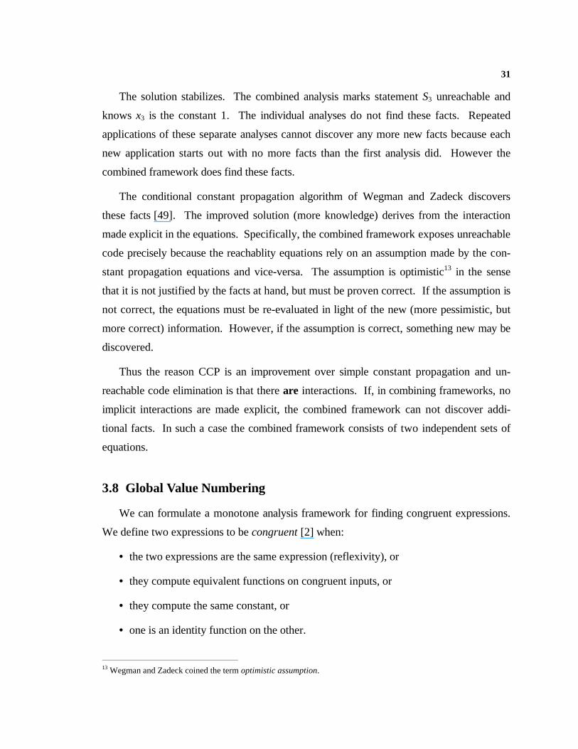
31

The solution stabilizes. The combined analysis marks statement S3 unreachable and

knows x3 is the constant 1. The individual analyses do not find these facts. Repeated

applications of these separate analyses cannot discover any more new facts because each

new application starts out with no more facts than the first analysis did. However the

combined framework does find these facts.

The conditional constant propagation algorithm of Wegman and Zadeck discovers

these facts [49]. The improved solution (more knowledge) derives from the interaction

made explicit in the equations. Specifically, the combined framework exposes unreachable

code precisely because the reachablity equations rely on an assumption made by the con-

stant propagation equations and vice-versa. The assumption is optimistic13 in the sense

that it is not justified by the facts at hand, but must be proven correct. If the assumption is

not correct, the equations must be re-evaluated in light of the new (more pessimistic, but

more correct) information. However, if the assumption is correct, something new may be

discovered.

Thus the reason CCP is an improvement over simple constant propagation and un-

reachable code elimination is that there are interactions. If, in combining frameworks, no

implicit interactions are made explicit, the combined framework can not discover addi-

tional facts. In such a case the combined framework consists of two independent sets of

equations.

3.8 Global Value Numbering

We can formulate a monotone analysis framework for finding congruent expressions.

We define two expressions to be congruent [2] when:

• the two expressions are the same expression (reflexivity), or

• they compute equivalent functions on congruent inputs, or

• they compute the same constant, or

• one is an identity function on the other.

13 Wegman and Zadeck coined the term optimistic assumption.

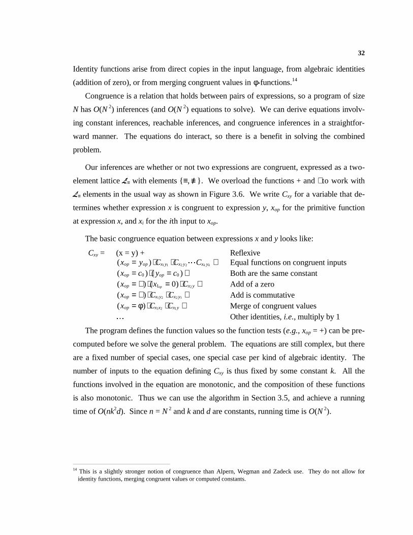
32

Identity functions arise from direct copies in the input language, from algebraic identities

(addition of zero), or from merging congruent values in φ-functions.14

Congruence is a relation that holds between pairs of expressions, so a program of size

N has O(N 2) inferences (and O(N 2) equations to solve). We can derive equations involv-

ing constant inferences, reachable inferences, and congruence inferences in a straightfor-

ward manner. The equations do interact, so there is a benefit in solving the combined

problem.

Our inferences are whether or not two expressions are congruent, expressed as a two-

element lattice L≡ with elements { ≡, /≡ }. We overload the functions + and ⋅ to work with

L≡ elements in the usual way as shown in Figure 3.6. We write Cxy for a variable that de-

termines whether expression x is congruent to expression y, xop for the primitive function

at expression x, and xi for the ith input to xop.

The basic congruence equation between expressions x and y looks like:

Cxy = (x = y) + Reflexive( )x y C C Cop op x y x y x yk k= ⋅ ⋅ +1 1 2 2L Equal functions on congruent inputs( ) ( )x c y cop op= ⋅ = +0 0 Both are the same constant( ) ( )x x Cop x yop= + ⋅ = ⋅ +1 0 2 Add of a zero( )x C Cop x y x y= + ⋅ ⋅ +1 2 2 1 Add is commutative( )x C Cop x x x y= ⋅ ⋅ +φ 1 2 1 Merge of congruent values

L Other identities, i.e., multiply by 1

The program defines the function values so the function tests (e.g., xop = +) can be pre-

computed before we solve the general problem. The equations are still complex, but there

are a fixed number of special cases, one special case per kind of algebraic identity. The

number of inputs to the equation defining Cxy is thus fixed by some constant k. All the

functions involved in the equation are monotonic, and the composition of these functions

is also monotonic. Thus we can use the algorithm in Section 3.5, and achieve a running

time of O(nk2d). Since n = N 2 and k and d are constants, running time is O(N 2).

14 This is a slightly stronger notion of congruence than Alpern, Wegman and Zadeck use. They do not allow for

identity functions, merging congruent values or computed constants.

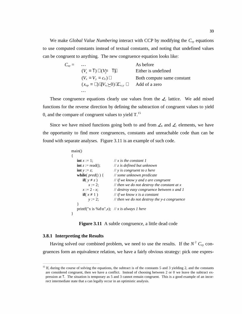
33

We make Global Value Numbering interact with CCP by modifying the Cxy equations

to use computed constants instead of textual constants, and noting that undefined values

can be congruent to anything. The new congruence equation looks like:

Cxy = L As before( ) ( )V Vx y= + = +T T Either is undefined

( )V V cx y= = +0 Both compute same constant( ) ( )x V Cop x x y= + ⋅ ⋅ +1 20f Add of a zero

LThese congruence equations clearly use values from the Lc lattice. We add mixed

functions for the reverse direction by defining the subtraction of congruent values to yield

0, and the compare of congruent values to yield T.15

Since we have mixed functions going both to and from L≡ and Lc elements, we have

the opportunity to find more congruences, constants and unreachable code than can be

found with separate analyses. Figure 3.11 is an example of such code.

3.8.1 Interpreting the Results

Having solved our combined problem, we need to use the results. If the N 2 Cxy con-

gruences form an equivalence relation, we have a fairly obvious strategy: pick one expres-

15 If, during the course of solving the equations, the subtract is of the constants 5 and 3 yielding 2, and the constants

are considered congruent, then we have a conflict. Instead of choosing between 2 or 0 we leave the subtract ex-pression at T. The situation is temporary as 5 and 3 cannot remain congruent. This is a good example of an incor-rect intermediate state that a can legally occur in an optimistic analysis.

main(){

int x := 1; // x is the constant 1int z := read(); // z is defined but unknownint y := z; // y is congruent to z herewhile( pred() ) { // some unknown predicate

if ( y ≠ z ) // if we know y and z are congruentx := 2; // then we do not destroy the constant at x

x := 2 - x; // destroy easy congruence between x and 1if ( x ≠ 1 ) // if we know x is a constant

y := 2; // then we do not destroy the y-z congruence}printf("x is %d\n",x); // x is always 1 here

}

Figure 3.11 A subtle congruence, a little dead code

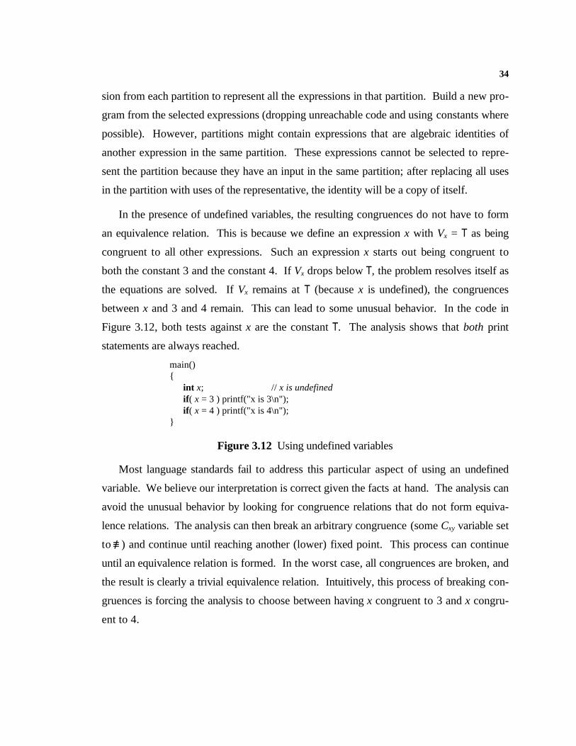
34

sion from each partition to represent all the expressions in that partition. Build a new pro-

gram from the selected expressions (dropping unreachable code and using constants where

possible). However, partitions might contain expressions that are algebraic identities of

another expression in the same partition. These expressions cannot be selected to repre-

sent the partition because they have an input in the same partition; after replacing all uses

in the partition with uses of the representative, the identity will be a copy of itself.

In the presence of undefined variables, the resulting congruences do not have to form

an equivalence relation. This is because we define an expression x with Vx = T as being

congruent to all other expressions. Such an expression x starts out being congruent to

both the constant 3 and the constant 4. If Vx drops below T, the problem resolves itself as

the equations are solved. If Vx remains at T (because x is undefined), the congruences

between x and 3 and 4 remain. This can lead to some unusual behavior. In the code in

Figure 3.12, both tests against x are the constant T. The analysis shows that both print

statements are always reached.

Most language standards fail to address this particular aspect of using an undefined

variable. We believe our interpretation is correct given the facts at hand. The analysis can

avoid the unusual behavior by looking for congruence relations that do not form equiva-

lence relations. The analysis can then break an arbitrary congruence (some Cxy variable set

to /≡ ) and continue until reaching another (lower) fixed point. This process can continue

until an equivalence relation is formed. In the worst case, all congruences are broken, and

the result is clearly a trivial equivalence relation. Intuitively, this process of breaking con-

gruences is forcing the analysis to choose between having x congruent to 3 and x congru-

ent to 4.

main(){

int x; // x is undefinedif ( x = 3 ) printf("x is 3\n");if ( x = 4 ) printf("x is 4\n");

}

Figure 3.12 Using undefined variables

35

3.9 Summary

In this chapter, we have shown how to combine two code improvement techniques.

We assume that the original transformations can be encoded as monotone analysis frame-

works. In our model, we can combine two frameworks, reason about the monotonicity of

the combined framework, and solve the combined framework efficiently. Furthermore, the

structure of the combined framework shows when a combination can produce better re-

sults than repeated application of the original transformations, and, equally important,

when it cannot.

To illustrate these points, we showed how to combine constant propagation with un-

reachable code elimination to derive an algorithm with properties similar to the conditional

constant propagation algorithm presented by Wegman and Zadeck [49]. Because the

combined framework includes transfer functions that take constant values into unreachable

code framework and vice-versa, it can discover more constants and more unreachable

code than repeated applications of the original transformations.

Finally, we showed how to combine constant propagation, unreachable code elimina-

tion, and global value numbering. It is an open question as to what other frameworks can

be combined and are profitable to combine. The asymptotic complexity of the presented

analysis is O(N 2). It can discover more facts than separate applications of the three

transformations.

In general, combining two frameworks is important when it removes a phase ordering

problem. The monotone analysis framework for the combined problem will run in O(nk2d)

time, where n is the number of equations, k is the arity of the functions used in the equa-

tions, and d is the height of the inference lattice.

36

4. An O(n log n) Conditional Constant Propagation and Global ValueNumbering Algorithm

36

Chapter 4

An O(n log n) Conditional Constant Propagation andGlobal Value Numbering Algorithm

Make haste, not waste

— anonymous?

4.1 Intr oduction

We have implemented an O(n log n) algorithm that combines the analysis portions of

Conditional Constant Propagation (CCP) [49], Global Value Numbering (GVN) [37],

and Global Congruence Finding [2]. We follow the analysis with a transformation that

replaces every set of congruent expressions with a single expression, removes dead and

unreachable code, and uses constants where possible. This transformation is followed by a

round of global code motion, to force expressions to dominate their uses. The global code

motion algorithm is discussed in Chapter 6.

The set of congruent expressions found by this algorithm overlap but do not cover

those found by Partial Redundancy Elimination (PRE) [36]. This algorithm finds value-

congruent expressions, but PRE finds some textually-congruent expressions that are not

value-congruent. In addition, the global code motion algorithm hoists loop-invariant code

more aggressively than PRE, occasionally lengthening execution paths. Thus, while the

combined algorithm with global code motion has many of the effects of PRE, it is not a

direct replacement for PRE.

The complexity of the combined algorithm is O(n log n) instead of the O(n2) algorithm

presented in Chapter 3. We have implemented it, and observed its behavior to be linear in

practice over a wide range of programs. Further, it is quite fast, being competitive with a

single run of all the above algorithms. The combined algorithm is much faster than the 2

37

or 3 iterations of all the above algorithms that a compiler requires in practice to reach a

fixed point. We give timing and program improvement measurements in Chapter 5.

Our simple algorithm runs in time O(n2) because we have O(n2) variables and equa-

tions. The O(n log n) approach requires that our O(n2) equations and variables form an

equivalence relation. The solution to the equations must form an equivalence relation at

every major step and at the final answer. In our simple worklist algorithm, we solve

equations in an arbitrary order determined by the worklist. This arbitrary order may not

maintain an equivalence relation. However, if no uninitialized variables are being used

then the final answer will be an equivalence relation (even if the intermediate steps are

not). Portions of this algorithm deal with choosing an order for worklist processing that

maintains an equivalence relation.

If the programmer uses an undefined (uninitialized) variable,16 then the equations may

not form an equivalence relation in the final solution. This is because T is congruent to

both 3 and 4, while 3 and 4 are not congruent. This solution is beyond our partitioning

algorithm to represent, so we do not try: the algorithm breaks such congruences arbitrarily

until it can form an equivalence relation. The final answer is a conservative approximation

to the truth. We justify this by claiming that a programmer who relies on undefined vari-

ables is depending on undefined behavior; the language implementor (the compiler writer)

may choose any answer he desires. We cover this in more detail in Section 4.4.

4.1.1 Equivalence Relations

We have to work to ensure our partial solutions always form an equivalence relation.

We can do this by choosing a careful ordering during the worklist solution. However, if

we always have an equivalence relation for our partial solutions we can represent the so-

lution to many variables with a single solution for their partition.

We will start with Hopcroft's DFA minimization algorithm [28]. We present it here

because a thorough understanding of it is required for what follows. We then present

Alpern, Wegman and Zadeck’s extensions that transform Hopcroft’s algorithm into a

Global Congruence Finding algorithm [2]. This algorithm discovers all the congruences of 16 Some languages initialize all variables to some known constant (like zero). From the compiler writer’s point of

view, such variables are defined.

38

the form: equal functions on congruent inputs. Next we add in elements from a constant

propagation lattice: T and ⊥ (no numbers yet). Any variable that computes T is congruent

to everything. We interleave T/⊥ propagation with the splitting algorithm. We then add

the constants and constant congruences (e.g., anything that computes 2 is congruent to

everything else that computes 2). We also note that the subtract (compare, divide) of

congruent values is zero (equal, one). Next, we add in the trivial COPY or identity func-

tion congruences. Then we add the algebraic identities, such as x + 0 and x × 1. Finally,

we add in merge, or ∩, -of-congruent-values congruences; the merge of x and x is x.

At each step we prove a running time of O(n log n). Because of the number of modi-

fications, we will be showing changes to the algorithm underlined. Changes to the proof

we will handle by presenting replacement paragraphs.

4.1.2 Notation

We cover our intermediate representation in detail in Appendix A. For now, we treat

expressions in a program as Nodes in a graph. Variables in expressions become input

edges in the graph. We use a special Node, the REGION, to represent basic blocks. Nodes

have an input from the basic block (REGION) in which they reside. We treat this input like

any other data input. The simplicity of our algorithm relies on this crucial detail: we treat

control dependences just like data dependences. The algorithm makes no distinction be-

tween them. As a pleasant side effect, the algorithm handles irreducible loops.

Nodes and program variables are equivalent here, and are named with lowercase italic

letters such as x and y. Partitions are sets of congruent Nodes and are named with upper-

case italic letters, X and Y. The partition of x is x.partition. X.any is any Node from par-

tition X.

A program is a set of Nodes with a distinguished START Node. Nodes and expressions

are equivalent here as well. The expression “x = y + z” defines the Node x to have an ADD

opcode and 2 inputs, from Nodes y and z. We denote the ADD opcode as x.opcode. We

denote the ith input to Node x as x[i]; these inputs amount to use-def chains. Thus, x[0] is

y and x[1] is z.

39

We also have the set of def-use chains, denoted x.def_use. We further subdivide them

into def-use chains for each ordered input. Thus x.def_use0 is the set of Nodes that use x

on input 0. If y ∈ x.def_use1 then y[1] is x.

4.1.3 Implementation

In our implementation, each Node is a C++ object (i.e., a C structure). The opcode

field is the C++ class (implemented by the compiler as a hidden virtual function table

pointer). The C equivalent would be an enum field. We encode the inputs as an array of

pointers to Nodes; the opcode implicitly determines the size of the array. The inputs

double as the use-def chains; we do not maintain a separate use-def data structure. This

allows our algorithm to traverse use-def edges with a single array lookup.

We implement the def-use chains as a single large array of Node pointers. Each Node

holds an internal pointer and the length of a subarray. A mirror array holds the reverse

index number of each def-use pointer (i.e., the use-def input number for which this def-use

pointer is the reverse of). We build this dense structure with two passes over the use-def

edges before running the combined optimization algorithm. It allows efficient iteration

over the def-use chains.

4.2 Hopcroft's Algorithm and Runtime Analysis

In this section we discover:

1. Two Nodes are congruent if they compute equal functions on ordered congruent

inputs.

We show Hopcroft’s algorithm here [28]. We modify the presentation slightly to bet-

ter fit our problem. In particular, we need to be very precise about where and when we

count work in the algorithm. As done in Alpern, Wegman, and Zadeck [2] we use a pro-

gram graph instead of a DFA. We use ordered edges instead of the usual DFA notation of

transition symbols from some alphabet. Instead of a final state, we will use the Program’s

START Node. The resulting algorithm partitions the program Nodes into congruence

classes. Two Nodes are congruent if they compute equal functions and if their ordered

inputs come from the same congruence class.

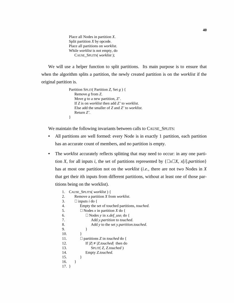
40

Place all Nodes in partition X.Split partition X by opcode.Place all partitions on worklist.While worklist is not empty, do

CAUSE_SPLITS( worklist );

We will use a helper function to split partitions. Its main purpose is to ensure that

when the algorithm splits a partition, the newly created partition is on the worklist if the

original partition is.

Partition SPLIT( Partition Z, Set g ) {Remove g from Z.Move g to a new partition, Z’.If Z is on worklist then add Z’ to worklist.Else add the smaller of Z and Z’ to worklist.Return Z’.

}

We maintain the following invariants between calls to CAUSE_SPLITS:

• All partitions are well formed: every Node is in exactly 1 partition, each partition

has an accurate count of members, and no partition is empty.

• The worklist accurately reflects splitting that may need to occur: in any one parti-

tion X, for all inputs i, the set of partitions represented by { ∀ x∈ X, x[i].partition}

has at most one partition not on the worklist (i.e., there are not two Nodes in X

that get their ith inputs from different partitions, without at least one of those par-

titions being on the worklist).

1. CAUSE_SPLITS( worklist ) {2. Remove a partition X from worklist.3. ∀ inputs i do {4. Empty the set of touched partitions, touched.5. ∀ Nodes x in partition X do {6. ∀ Nodes y in x.def_usei do {7. Add y.partition to touched.8. Add y to the set y.partition.touched.9. }10. }11. ∀ partitions Z in touched do {12. If |Z| ≠ |Z.touched| then do13. SPLIT( Z, Z.touched )14. Empty Z.touched.15. }16. }17. }

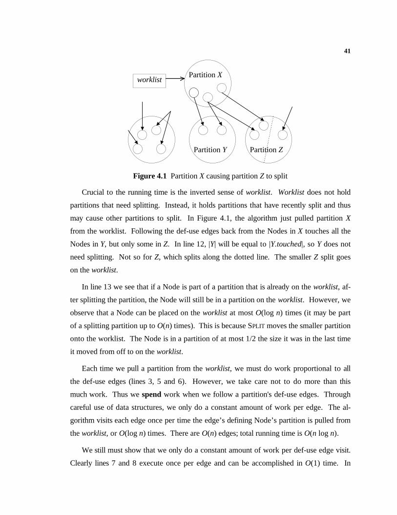
41

Crucial to the running time is the inverted sense of worklist. Worklist does not hold

partitions that need splitting. Instead, it holds partitions that have recently split and thus

may cause other partitions to split. In Figure 4.1, the algorithm just pulled partition X

from the worklist. Following the def-use edges back from the Nodes in X touches all the

Nodes in Y, but only some in Z. In line 12, |Y| will be equal to |Y.touched|, so Y does not

need splitting. Not so for Z, which splits along the dotted line. The smaller Z split goes

on the worklist.

In line 13 we see that if a Node is part of a partition that is already on the worklist, af-

ter splitting the partition, the Node will still be in a partition on the worklist. However, we

observe that a Node can be placed on the worklist at most O(log n) times (it may be part

of a splitting partition up to O(n) times). This is because SPLIT moves the smaller partition

onto the worklist. The Node is in a partition of at most 1/2 the size it was in the last time

it moved from off to on the worklist.

Each time we pull a partition from the worklist, we must do work proportional to all

the def-use edges (lines 3, 5 and 6). However, we take care not to do more than this

much work. Thus we spend work when we follow a partition's def-use edges. Through

careful use of data structures, we only do a constant amount of work per edge. The al-

gorithm visits each edge once per time the edge’s defining Node’s partition is pulled from

the worklist, or O(log n) times. There are O(n) edges; total running time is O(n log n).

We still must show that we only do a constant amount of work per def-use edge visit.

Clearly lines 7 and 8 execute once per edge and can be accomplished in O(1) time. In

Partition Xworklist

Partition Y Partition Z

Figure 4.1 Partition X causing partition Z to split

42

lines 12 and 14 at most 1 partition per edge is in touched and each line can happen in O(1)

time. The total of all Nodes moved from one partition to another in line 13 cannot be

more than the number of Nodes visited in lines 7 and 8, and again the moving itself can

happen in constant time.

4.2.1 Implementation

We implement the partitions as structures with a doubly linked list of Nodes for mem-

bers; constant time list removal being required in line 13. The algorithm maintains a count

of members for the tests in SPLIT and line 12. We implemented the worklist and touched

sets as singly linked lists of partitions, with an extra flag bit to perform the constant-time

membership test needed in SPLIT and line 7. The X.touched set was also implemented as a

singly linked list, again with a member count for the line 8 test.

4.3 Adding Unreachable Code Elimination

In this section we discover:

1. Two Nodes are congruent if they compute equal functions on ordered congruent

inputs.

2. Two PHI Nodes are congruent if their ordered inputs are congruent, ignoring in-

puts from unreachable paths.

3. The type of each Node, as an element from the lattice {U, R}. Types are deter-

mined by function and input types.

Nodes hold lattice elements, called types, that represent an approximation to the set of

values a Node can take at runtime. We refer to the type of a Node x with x.type. We are

adding in just the reachability lattice Lu {U, R}. REGION, IF, JUMP, and START Nodes

compute values from this lattice. The integer lattice will be added in the next section. For

now, the remaining nodes compute a data value and will have their type fields set to ⊥ .

In Chapter 3 we represented reachability with a variable per statement. In this chapter

we present a more convenient method; reachability is computed per basic block and un-

reachable computations are ignored at PHI Nodes. We use REGION Nodes to represent

basic blocks; the type at a REGION Node determines whether the block is reachable or not.

43

Two PHI Nodes are congruent if they have the same REGION Node input (occur in the

same basic block) and their ordered reachable inputs are congruent. In the code that fol-

lows, the unreachable inputs are ignored and the two PHI Nodes are congruent:

x0 := y0 := read(); // Read some unknown valueif ( False ) { // A condition that is never true

x1 := 2; // Unreachable codey1 := 3; // Unreachable code

}x2 := φ( x0, x1); // Merge x0 and an unreachable valuey2 := φ( y0, y1); // Merge y0 and an unreachable value

Since unreachable values are ignored, the Nodes computing those values are useless.

A round of dead code elimination will remove them. This dead code elimination is incor-

porated in the transformation phase of the algorithm, presented in section 4.10.

We do not want any values from unreachable paths causing a partition of PHIs to split.

So we allow PHI Nodes to ignore inputs from unreachable paths when determining con-

gruence. In the algorithm CAUSE_SPLITS we insert a test between lines 6 and 7:

6. ∀ Nodes y in x.def_usei do {6.5 If y is not a PHI or input i is a live path into y then do {7. Add y.partition to touched.8. Add y to the set y.partition.touched.8.5 }9. }

4.3.1 Accounting for work during Conditional Constant Propagation

The sparse CCP algorithm of Wegman and Zadeck runs in linear time [49]. As pre-

sented in section 3.5, we count work by edge visits. The algorithm visits a use-def edge

once each time the defining Node drops in the lattice (once in our case). Each edge visit

causes a constant time evaluation of the using Node’s type. We may also have to do a

constant amount of work adding or removing the Node’s partition from the cprop work-

list.

The same work analysis will hold when we interleave the propagation and the parti-

tioning algorithms. The major difference will be the order of visitation: we will propagate

types within a partition until the partition stabilizes before we propagate types outside a

partition. In addition, we will split partitions by type, so within a partition (and between

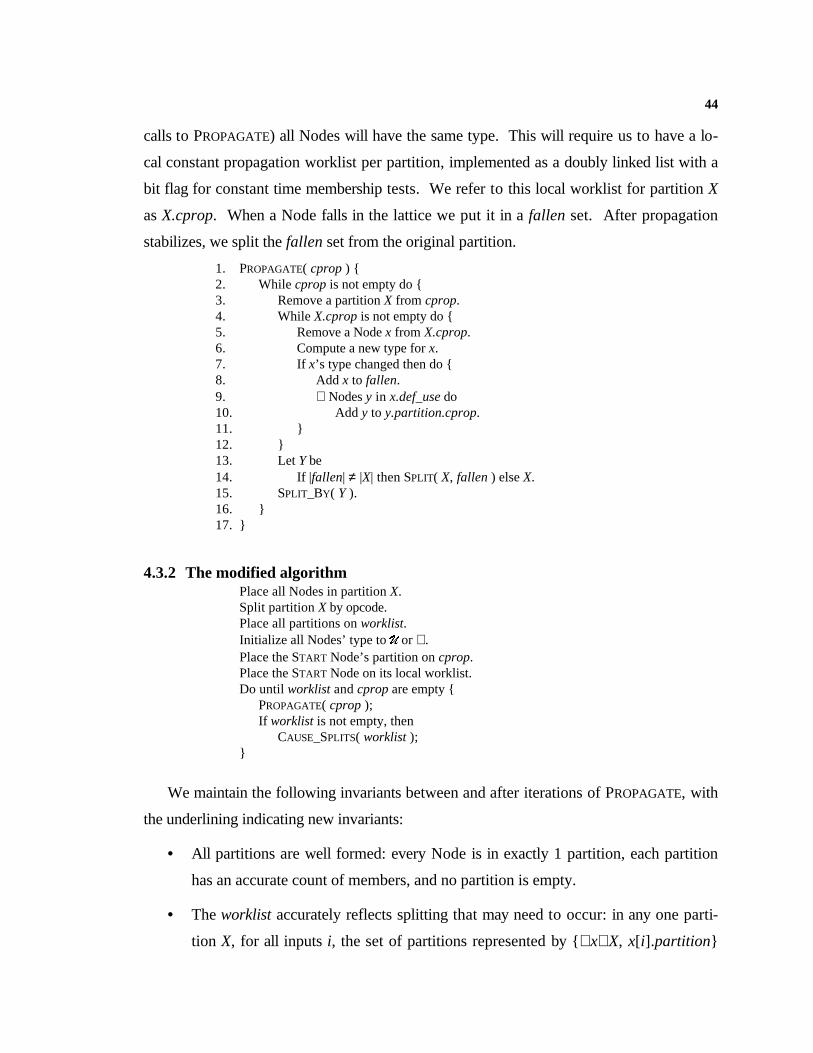
44

calls to PROPAGATE) all Nodes will have the same type. This will require us to have a lo-

cal constant propagation worklist per partition, implemented as a doubly linked list with a

bit flag for constant time membership tests. We refer to this local worklist for partition X

as X.cprop. When a Node falls in the lattice we put it in a fallen set. After propagation

stabilizes, we split the fallen set from the original partition.

1. PROPAGATE( cprop ) {2. While cprop is not empty do {3. Remove a partition X from cprop.4. While X.cprop is not empty do {5. Remove a Node x from X.cprop.6. Compute a new type for x.7. If x’s type changed then do {8. Add x to fallen.9. ∀ Nodes y in x.def_use do10. Add y to y.partition.cprop.11. }12. }13. Let Y be14. If |fallen| ≠ |X| then SPLIT( X, fallen ) else X.15. SPLIT_BY( Y ).16. }17. }

4.3.2 The modified algorithmPlace all Nodes in partition X.Split partition X by opcode.Place all partitions on worklist.Initialize all Nodes’ type to U or ⊥ .Place the START Node’s partition on cprop.Place the START Node on its local worklist.Do until worklist and cprop are empty {

PROPAGATE( cprop );If worklist is not empty, then

CAUSE_SPLITS( worklist );}

We maintain the following invariants between and after iterations of PROPAGATE, with

the underlining indicating new invariants:

• All partitions are well formed: every Node is in exactly 1 partition, each partition

has an accurate count of members, and no partition is empty.

• The worklist accurately reflects splitting that may need to occur: in any one parti-

tion X, for all inputs i, the set of partitions represented by { ∀ x∈ X, x[i].partition}

45

has at most one partition not on the worklist (i.e., there are not two Nodes in X

that get their ith inputs from different partitions, without at least one of those par-

titions being on the worklist).

• Within a partition, all Nodes have the same type.

• The local cprop worklist accurately reflects type propagation that may need to oc-

cur: the type of every Node in the partition is its function on the current inputs, or

the Node is on the cprop worklist.

• All partitions with Nodes on their local cprop worklist are on the global cprop

worklist.

4.4 Adding in Constant Propagation

In this section we discover:

1. Two Nodes are congruent if they compute equal functions on ordered congruent

inputs.

2. Two PHI Nodes are congruent if their ordered inputs are congruent, ignoring in-

puts from unreachable paths.

3. The type of each Node, as an element from the {U, R} lattice or the { T, Z, ⊥ } lat-

tice. Types are determined by function and input types.

4. Two Nodes are congruent if either Node computes T.

We are adding in both the reachability lattice Lu {U, R} and the constant propagation

lattice Lc { T, Z, ⊥ }. We treat them identically. Since the different values appear in dis-

joint kinds of Nodes, we use the same representation for both T and U. We distinguish

them by the Node opcode. In this algorithm we never need to make this distinction.

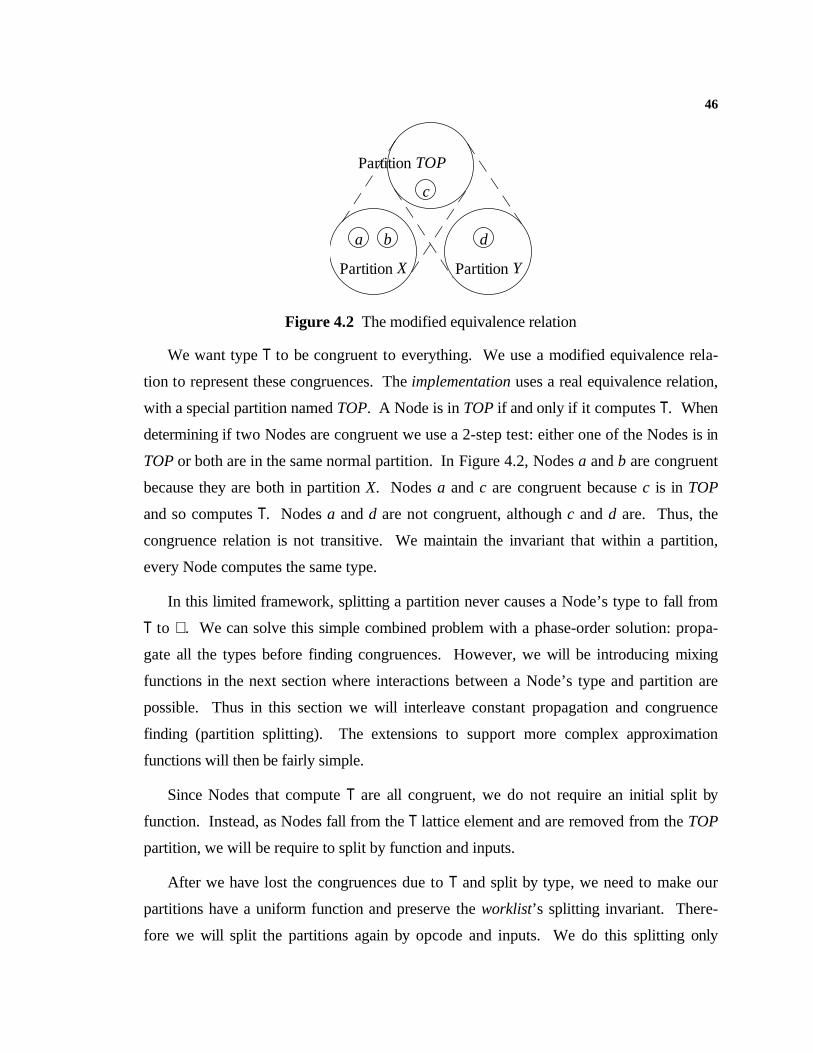
46

We want type T to be congruent to everything. We use a modified equivalence rela-

tion to represent these congruences. The implementation uses a real equivalence relation,

with a special partition named TOP. A Node is in TOP if and only if it computes T. When

determining if two Nodes are congruent we use a 2-step test: either one of the Nodes is in

TOP or both are in the same normal partition. In Figure 4.2, Nodes a and b are congruent

because they are both in partition X. Nodes a and c are congruent because c is in TOP

and so computes T. Nodes a and d are not congruent, although c and d are. Thus, the

congruence relation is not transitive. We maintain the invariant that within a partition,

every Node computes the same type.

In this limited framework, splitting a partition never causes a Node’s type to fall from

T to ⊥ . We can solve this simple combined problem with a phase-order solution: propa-

gate all the types before finding congruences. However, we will be introducing mixing

functions in the next section where interactions between a Node’s type and partition are

possible. Thus in this section we will interleave constant propagation and congruence

finding (partition splitting). The extensions to support more complex approximation

functions will then be fairly simple.

Since Nodes that compute T are all congruent, we do not require an initial split by

function. Instead, as Nodes fall from the T lattice element and are removed from the TOP

partition, we will be require to split by function and inputs.

After we have lost the congruences due to T and split by type, we need to make our

partitions have a uniform function and preserve the worklist’s splitting invariant. There-

fore we will split the partitions again by opcode and inputs. We do this splitting only

Partition X Partition Y

Partition TOP

a

c

db

Figure 4.2 The modified equivalence relation

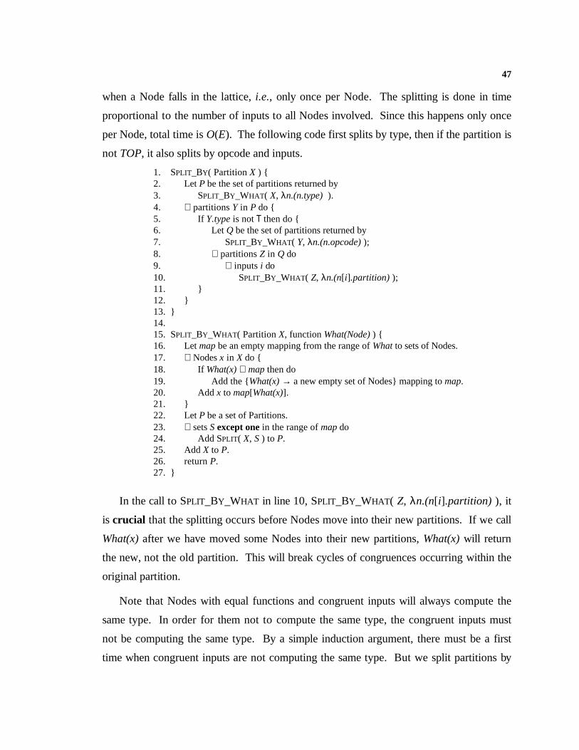
47

when a Node falls in the lattice, i.e., only once per Node. The splitting is done in time

proportional to the number of inputs to all Nodes involved. Since this happens only once

per Node, total time is O(E). The following code first splits by type, then if the partition is

not TOP, it also splits by opcode and inputs.

1. SPLIT_BY( Partition X ) {2. Let P be the set of partitions returned by3. SPLIT_BY_WHAT( X, λn.(n.type) ).4. ∀ partitions Y in P do {5. If Y.type is not T then do {6. Let Q be the set of partitions returned by7. SPLIT_BY_WHAT( Y, λn.(n.opcode) );8. ∀ partitions Z in Q do9. ∀ inputs i do10. SPLIT_BY_WHAT( Z, λn.(n[i].partition) );11. }12. }13. }14. 15. SPLIT_BY_WHAT( Partition X, function What(Node) ) {16. Let map be an empty mapping from the range of What to sets of Nodes.17. ∀ Nodes x in X do {18. If What(x) ∉ map then do19. Add the {What(x) → a new empty set of Nodes} mapping to map.20. Add x to map[What(x)].21. }22. Let P be a set of Partitions.23. ∀ sets S except one in the range of map do24. Add SPLIT( X, S ) to P.25. Add X to P.26. return P.27. }

In the call to SPLIT_BY_WHAT in line 10, SPLIT_BY_WHAT( Z, λn.(n[i].partition) ), it

is crucial that the splitting occurs before Nodes move into their new partitions. If we call

What(x) after we have moved some Nodes into their new partitions, What(x) will return

the new, not the old partition. This will break cycles of congruences occurring within the

original partition.

Note that Nodes with equal functions and congruent inputs will always compute the

same type. In order for them not to compute the same type, the congruent inputs must

not be computing the same type. By a simple induction argument, there must be a first

time when congruent inputs are not computing the same type. But we split partitions by

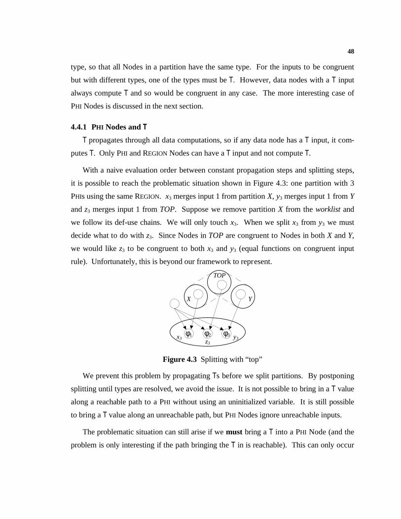
48

type, so that all Nodes in a partition have the same type. For the inputs to be congruent

but with different types, one of the types must be T. However, data nodes with a T input

always compute T and so would be congruent in any case. The more interesting case of

PHI Nodes is discussed in the next section.

4.4.1 PHI Nodes and T

T propagates through all data computations, so if any data node has a T input, it com-

putes T. Only PHI and REGION Nodes can have a T input and not compute T.

With a naive evaluation order between constant propagation steps and splitting steps,

it is possible to reach the problematic situation shown in Figure 4.3: one partition with 3

PHIs using the same REGION. x3 merges input 1 from partition X, y3 merges input 1 from Y

and z3 merges input 1 from TOP. Suppose we remove partition X from the worklist and

we follow its def-use chains. We will only touch x3. When we split x3 from y3 we must

decide what to do with z3. Since Nodes in TOP are congruent to Nodes in both X and Y,

we would like z3 to be congruent to both x3 and y3 (equal functions on congruent input

rule). Unfortunately, this is beyond our framework to represent.

φ1 φ2 φ3

X Y

TOP

x3 y3z3

Figure 4.3 Splitting with “top”

We prevent this problem by propagating Ts before we split partitions. By postponing

splitting until types are resolved, we avoid the issue. It is not possible to bring in a T value

along a reachable path to a PHI without using an uninitialized variable. It is still possible

to bring a T value along an unreachable path, but PHI Nodes ignore unreachable inputs.

The problematic situation can still arise if we must bring a T into a PHI Node (and the

problem is only interesting if the path bringing the T in is reachable). This can only occur

49

when the program actually uses an undefined value.17 We arbitrarily break a congruence

and stick z3 with y3. Since the semantics of using an undefined value are undefined,

breaking a congruence is a safe and conservative solution. It is not, however, the optimal

solution. The problematic code, in SSA form, follows:

int x0, y0, z0; // x0, y0, z0 are all undefined hereif ( pred() ) { // Some unknown predicate

t := read(); // Assign t with a keyboard readx1, y1, z1 := t; // Make x, y, and z all congruent

} else {x2 := read(); // Assign x and y with different valuesy2 := read(); // z is left undefined

}x3 := φ( x1, x2); // Merge x1 and x2

y3 := φ( y1, y2); // Merge y1 and y2

z3 := φ( z1, z0); // Merge z1 and z0; z0 has type T

The TOP partition itself never needs to be split because some inputs changed partitions

(it will be split when Nodes drop from T to some non-T type). Nodes in the TOP partition

are congruent because they compute T, irrespective of whether they also compute the

same function on congruent inputs. This leads us to modify CAUSE_SPLITS again:

6. ∀ Nodes y in x.def_usei do {6.1 Let Y be y.partition.6.5 If Y is not TOP and (y is not a PHI or input i is a live path into y) then {7. Add Y to touched.8. Add y to the set Y.touched.8.5 }9. }

4.4.2 The modified algorithm

We can now place all Nodes in the same initial partition, and rely on splitting work

done by PROPAGATE to do the splitting by opcode. The modified main loop is now:

Place all Nodes in partition X.Initialize all Nodes’ type to U or T.Place the START Node’s partition on cprop.Place the START Node on its local worklist.Do until worklist and cprop are empty {

PROPAGATE( cprop );If worklist is not empty, then

CAUSE_SPLITS( worklist );}

17 The problem appeared at least a dozen times in the 52 routines I tested.

50

4.5 Allowing Constants and Congruences to Interact

In this section we discover the following facts about a program:

1. Two Nodes are congruent if they compute equal functions on ordered congruent

inputs.

2. Two PHI Nodes are congruent if their ordered inputs are congruent, ignoring in-

puts from unreachable paths.

3. The type of each Node, as an element from the {U, R} lattice or the { T, Z, ⊥ } lat-

tice. Types are determined by function and input types.

4. Two Nodes are congruent if either Node computes T or they both compute the

same constant.

Any two Nodes that compute the same constant are congruent, regardless of how they

compute that constant. In addition to the integer constants, we can extend the type lattice

in many directions. We present just the integer constants, but our implementation includes

ranges of integer constants with strides, floating-point and double precision constants, and

code address labels. These extra types do not require changes to the algorithm. The only

changes required are in the approximation functions (meet, etc.).

Partitions of constants should not be split simply because their Nodes have unequal

functions or incongruent inputs. We need to change CAUSE_SPLITS to reflect this:

6.5 If y.type is neither T nor constant and(y is not a PHI or input i is a live path into y) then do {

After propagation stabilizes, we split by types. Then SPLIT_BY splits by function and in-

puts. Again we do not want to split partitions of constants, so we modify SPLIT_BY:

5. If Y.type is below T and all constants then do {

Nodes that fall from constants to ⊥ (or other non-constant types such as ranges) are han-

dled in the PROPAGATE code when the fallen set is passed to SPLIT_BY.

51

4.6 Subtract and Compare

So far we allow constants to affect congruences (by not splitting partitions of con-

stants, even when they have different functions or inputs). Here we allow mixing of in-

formation in the reverse direction: the subtraction of congruent values is zero. The same

behavior is applied to compare and T.18 This inference is fundamentally different than the

previous inferences, because we are allowing a congruence inference to affect a constant

inference. If we lose that congruence inference by splitting a partition which is being used

on both inputs to a SUB Node then we need to reevaluate the SUB Node’s type.

Since at least one of the two inputs to the SUB Node must end up on the worklist, we

will be visiting the SUB Nodes during the course of a future splitting operation. Thus,

during splitting operations we can place each Node visited along a def-use chain on the

local cprop worklist. This requires only a constant amount of work (put on worklist, take

off worklist, and check the type) per Node, an amount of work we already pay for just to

follow the def-use chain. This requires an extra visit for every Node involved in a split.

Instead, we only require SUB and COMPARE Nodes to have an extra visit:

6.1 Let Y be y.partition.6.2 If y.type is constant and y has opcode SUB or COMPARE then do6.3 Add y to Y.cprop.

One final difficulty: when we propagate constants through the TOP partition, it is

possible to bring unequal constants into a SUB Node still within TOP. As shown in

Figure 4.4, the approximation function for SUB has a dilemma; it can either subtract con-

gruent inputs and compute 0, or it can subtract constant inputs for a constant result.

In this case the two inputs to SUB can never be congruent in the final answer. We can

show this with an induction proof; there is never a first time that two Nodes compute une-

qual constants while remaining congruent. They will eventually be split. SUB should sub-

tract the constants. We give C++ code for a subtract Node’s approximation function be-

low:

18 We can also define x/x to be 1. This defines 0/0 as 1, a questionable choice. Discovering x/x to be 1 is unlikely to

significantly impact many programs.

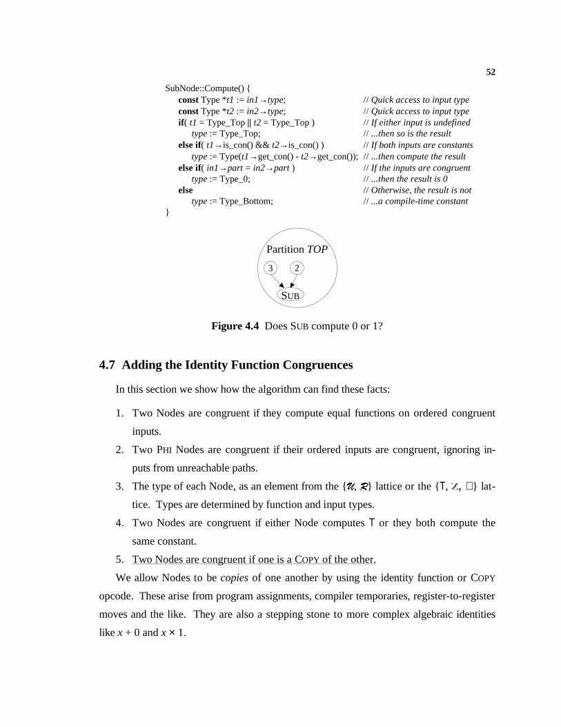
52

SubNode::Compute() {const Type *t1 := in1→type; // Quick access to input typeconst Type *t2 := in2→type; // Quick access to input typeif ( t1 = Type_Top || t2 = Type_Top ) // If either input is undefined

type := Type_Top; // ...then so is the resultelse if( t1→is_con() && t2→is_con() ) // If both inputs are constants

type := Type(t1→get_con() - t2→get_con()); // ...then compute the resultelse if( in1→part = in2→part ) // If the inputs are congruent

type := Type_0; // ...then the result is 0else // Otherwise, the result is not

type := Type_Bottom; // ...a compile-time constant}

4.7 Adding the Identity Function Congruences

In this section we show how the algorithm can find these facts:

1. Two Nodes are congruent if they compute equal functions on ordered congruent

inputs.

2. Two PHI Nodes are congruent if their ordered inputs are congruent, ignoring in-

puts from unreachable paths.

3. The type of each Node, as an element from the {U, R} lattice or the { T, Z, ⊥ } lat-

tice. Types are determined by function and input types.

4. Two Nodes are congruent if either Node computes T or they both compute the

same constant.

5. Two Nodes are congruent if one is a COPY of the other.

We allow Nodes to be copies of one another by using the identity function or COPY

opcode. These arise from program assignments, compiler temporaries, register-to-register

moves and the like. They are also a stepping stone to more complex algebraic identities

like x + 0 and x × 1.

Partition TOP

3 2

SUB

Figure 4.4 Does SUB compute 0 or 1?

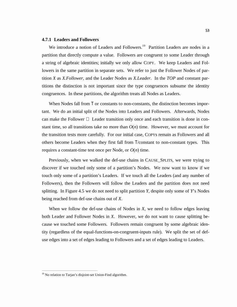
53

4.7.1 Leaders and Followers

We introduce a notion of Leaders and Followers.19 Partition Leaders are nodes in a

partition that directly compute a value. Followers are congruent to some Leader through

a string of algebraic identities; initially we only allow COPY. We keep Leaders and Fol-

lowers in the same partition in separate sets. We refer to just the Follower Nodes of par-

tition X as X.Follower, and the Leader Nodes as X.Leader. In the TOP and constant par-

titions the distinction is not important since the type congruences subsume the identity

congruences. In these partitions, the algorithm treats all Nodes as Leaders.

When Nodes fall from T or constants to non-constants, the distinction becomes impor-

tant. We do an initial split of the Nodes into Leaders and Followers. Afterwards, Nodes

can make the Follower ⇒ Leader transition only once and each transition is done in con-

stant time, so all transitions take no more than O(n) time. However, we must account for

the transition tests more carefully. For our initial case, COPYs remain as Followers and all

others become Leaders when they first fall from T/constant to non-constant types. This

requires a constant-time test once per Node, or O(n) time.

Previously, when we walked the def-use chains in CAUSE_SPLITS, we were trying to

discover if we touched only some of a partition’s Nodes. We now want to know if we

touch only some of a partition’s Leaders. If we touch all the Leaders (and any number of

Followers), then the Followers will follow the Leaders and the partition does not need

splitting. In Figure 4.5 we do not need to split partition Y, despite only some of Y’s Nodes

being reached from def-use chains out of X.

When we follow the def-use chains of Nodes in X, we need to follow edges leaving

both Leader and Follower Nodes in X. However, we do not want to cause splitting be-

cause we touched some Followers. Followers remain congruent by some algebraic iden-

tity (regardless of the equal-functions-on-congruent-inputs rule). We split the set of def-

use edges into a set of edges leading to Followers and a set of edges leading to Leaders.

19 No relation to Tarjan’s disjoint-set Union-Find algorithm.

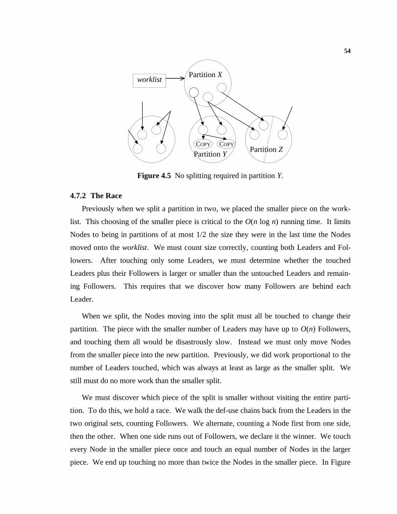
54

4.7.2 The Race

Previously when we split a partition in two, we placed the smaller piece on the work-

list. This choosing of the smaller piece is critical to the O(n log n) running time. It limits

Nodes to being in partitions of at most 1/2 the size they were in the last time the Nodes

moved onto the worklist. We must count size correctly, counting both Leaders and Fol-

lowers. After touching only some Leaders, we must determine whether the touched

Leaders plus their Followers is larger or smaller than the untouched Leaders and remain-

ing Followers. This requires that we discover how many Followers are behind each

Leader.

When we split, the Nodes moving into the split must all be touched to change their

partition. The piece with the smaller number of Leaders may have up to O(n) Followers,

and touching them all would be disastrously slow. Instead we must only move Nodes

from the smaller piece into the new partition. Previously, we did work proportional to the

number of Leaders touched, which was always at least as large as the smaller split. We

still must do no more work than the smaller split.

We must discover which piece of the split is smaller without visiting the entire parti-

tion. To do this, we hold a race. We walk the def-use chains back from the Leaders in the

two original sets, counting Followers. We alternate, counting a Node first from one side,

then the other. When one side runs out of Followers, we declare it the winner. We touch

every Node in the smaller piece once and touch an equal number of Nodes in the larger

piece. We end up touching no more than twice the Nodes in the smaller piece. In Figure

Partition Xworklist

Partition YPartition Z

COPY COPY

Figure 4.5 No splitting required in partition Y.

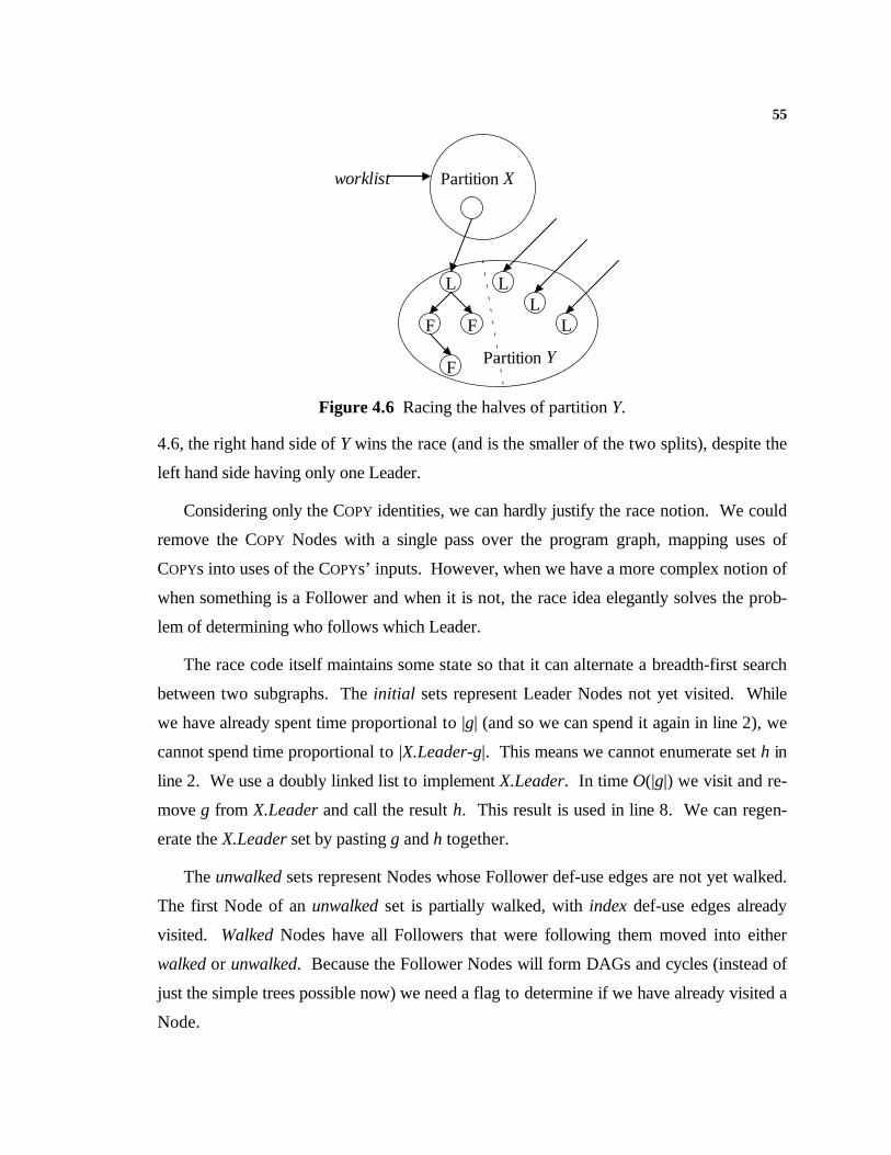
55

4.6, the right hand side of Y wins the race (and is the smaller of the two splits), despite the

left hand side having only one Leader.

Considering only the COPY identities, we can hardly justify the race notion. We could

remove the COPY Nodes with a single pass over the program graph, mapping uses of

COPYs into uses of the COPYs’ inputs. However, when we have a more complex notion of

when something is a Follower and when it is not, the race idea elegantly solves the prob-

lem of determining who follows which Leader.

The race code itself maintains some state so that it can alternate a breadth-first search

between two subgraphs. The initial sets represent Leader Nodes not yet visited. While

we have already spent time proportional to |g| (and so we can spend it again in line 2), we

cannot spend time proportional to |X.Leader-g|. This means we cannot enumerate set h in

line 2. We use a doubly linked list to implement X.Leader. In time O(|g|) we visit and re-

move g from X.Leader and call the result h. This result is used in line 8. We can regen-

erate the X.Leader set by pasting g and h together.

The unwalked sets represent Nodes whose Follower def-use edges are not yet walked.

The first Node of an unwalked set is partially walked, with index def-use edges already

visited. Walked Nodes have all Followers that were following them moved into either

walked or unwalked. Because the Follower Nodes will form DAGs and cycles (instead of

just the simple trees possible now) we need a flag to determine if we have already visited a

Node.

worklist Partition X

L LL

LF F

FPartition Y

Figure 4.6 Racing the halves of partition Y.

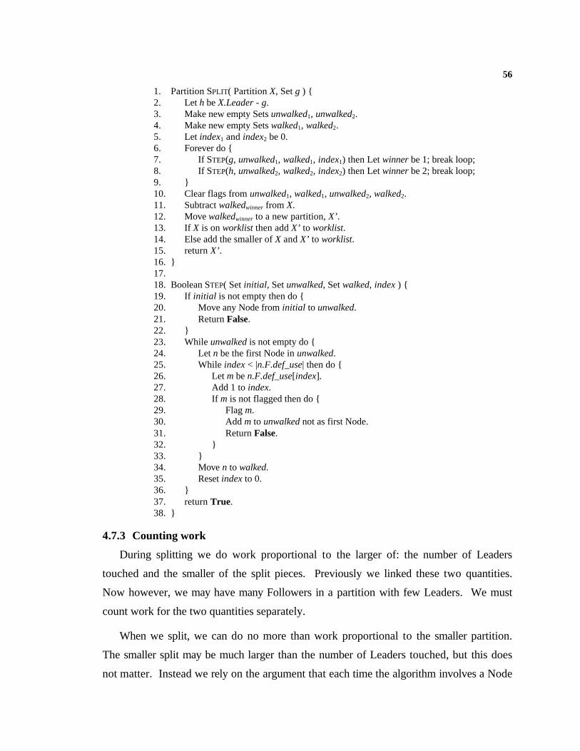
56

1. Partition SPLIT( Partition X, Set g ) {2. Let h be X.Leader - g.3. Make new empty Sets unwalked1, unwalked2.4. Make new empty Sets walked1, walked2.5. Let index1 and index2 be 0.6. Forever do {7. If STEP(g, unwalked1, walked1, index1) then Let winner be 1; break loop;8. If STEP(h, unwalked2, walked2, index2) then Let winner be 2; break loop;9. }10. Clear flags from unwalked1, walked1, unwalked2, walked2.11. Subtract walkedwinner from X.12. Move walkedwinner to a new partition, X’.13. If X is on worklist then add X’ to worklist.14. Else add the smaller of X and X’ to worklist.15. return X’.16. }17. 18. Boolean STEP( Set initial , Set unwalked, Set walked, index ) {19. If initial is not empty then do {20. Move any Node from initial to unwalked.21. Return False.22. }23. While unwalked is not empty do {24. Let n be the first Node in unwalked.25. While index < |n.F.def_use| then do {26. Let m be n.F.def_use[index].27. Add 1 to index.28. If m is not flagged then do {29. Flag m.30. Add m to unwalked not as first Node.31. Return False.32. }33. }34. Move n to walked.35. Reset index to 0.36. }37. return True.38. }

4.7.3 Counting work

During splitting we do work proportional to the larger of: the number of Leaders

touched and the smaller of the split pieces. Previously we linked these two quantities.

Now however, we may have many Followers in a partition with few Leaders. We must

count work for the two quantities separately.

When we split, we can do no more than work proportional to the smaller partition.

The smaller split may be much larger than the number of Leaders touched, but this does

not matter. Instead we rely on the argument that each time the algorithm involves a Node

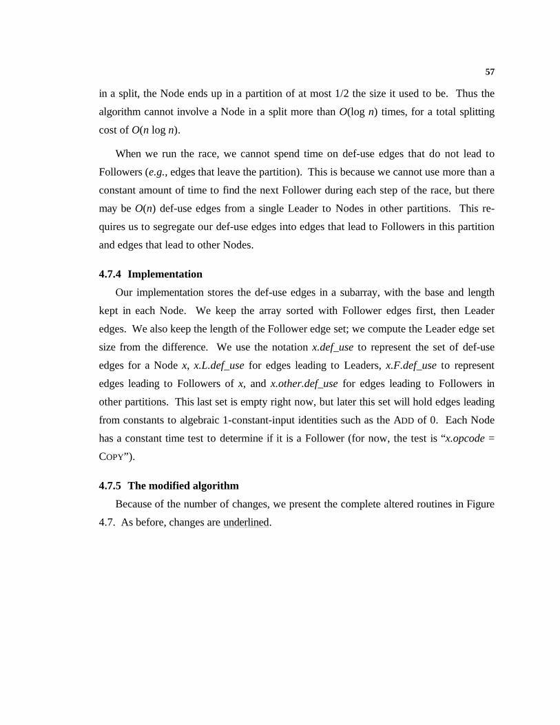
57

in a split, the Node ends up in a partition of at most 1/2 the size it used to be. Thus the

algorithm cannot involve a Node in a split more than O(log n) times, for a total splitting

cost of O(n log n).

When we run the race, we cannot spend time on def-use edges that do not lead to

Followers (e.g., edges that leave the partition). This is because we cannot use more than a

constant amount of time to find the next Follower during each step of the race, but there

may be O(n) def-use edges from a single Leader to Nodes in other partitions. This re-

quires us to segregate our def-use edges into edges that lead to Followers in this partition

and edges that lead to other Nodes.

4.7.4 Implementation

Our implementation stores the def-use edges in a subarray, with the base and length

kept in each Node. We keep the array sorted with Follower edges first, then Leader

edges. We also keep the length of the Follower edge set; we compute the Leader edge set

size from the difference. We use the notation x.def_use to represent the set of def-use

edges for a Node x, x.L.def_use for edges leading to Leaders, x.F.def_use to represent

edges leading to Followers of x, and x.other.def_use for edges leading to Followers in

other partitions. This last set is empty right now, but later this set will hold edges leading

from constants to algebraic 1-constant-input identities such as the ADD of 0. Each Node

has a constant time test to determine if it is a Follower (for now, the test is “x.opcode =

COPY”).

4.7.5 The modified algorithm

Because of the number of changes, we present the complete altered routines in Figure

4.7. As before, changes are underlined.

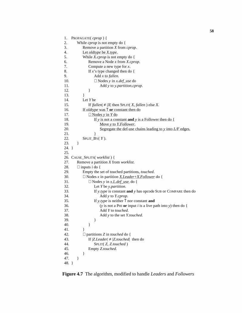
58

1. PROPAGATE( cprop ) {2. While cprop is not empty do {3. Remove a partition X from cprop.4. Let oldtype be X.type.5. While X.cprop is not empty do {6. Remove a Node x from X.cprop.7. Compute a new type for x.8. If x’s type changed then do {9. Add x to fallen.10. ∀ Nodes y in x.def_use do11. Add y to y.partition.cprop.12. }13. }14. Let Y be15. If |fallen| ≠ |X| then SPLIT( X, fallen ) else X.16. If oldtype was T or constant then do17. ∀ Nodes y in Y do18. If y is not a constant and y is a Follower then do {19. Move y to Y.Follower.20. Segregate the def-use chains leading to y into L/F edges.21. }22. SPLIT_BY( Y ).23. }24. }25. 26. CAUSE_SPLITS( worklist ) {27. Remove a partition X from worklist.28. ∀ inputs i do {29. Empty the set of touched partitions, touched.30. ∀ Nodes x in partition X.Leader+X.Follower do {31. ∀ Nodes y in x.L.def_usei do {32. Let Y be y.partition.33. If y.type is constant and y has opcode SUB or COMPARE then do34. Add y to Y.cprop.35. If y.type is neither T nor constant and36. (y is not a PHI or input i is a live path into y) then do {37. Add Y to touched.38. Add y to the set Y.touched.39. }40. }41. }42. ∀ partitions Z in touched do {43. If |Z.Leader| ≠ |Z.touched| then do44. SPLIT( Z, Z.touched )45. Empty Z.touched.46. }47. }48. }

Figure 4.7 The algorithm, modified to handle Leaders and Followers

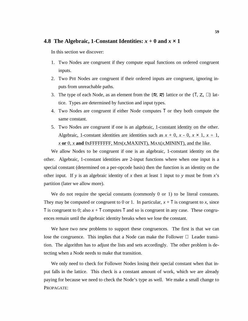
59

4.8 The Algebraic, 1-Constant Identities: x + 0 and x ×× 1

In this section we discover:

1. Two Nodes are congruent if they compute equal functions on ordered congruent

inputs.

2. Two PHI Nodes are congruent if their ordered inputs are congruent, ignoring in-

puts from unreachable paths.

3. The type of each Node, as an element from the {U, R} lattice or the { T, Z, ⊥ } lat-

tice. Types are determined by function and input types.

4. Two Nodes are congruent if either Node computes T or they both compute the

same constant.

5. Two Nodes are congruent if one is an algebraic, 1-constant identity on the other.

Algebraic, 1-constant identities are identities such as x + 0, x - 0, x × 1, x ö 1,

x or 0, x and 0xFFFFFFFF, MIN(x,MAXINT), MAX(x,MININT), and the like.

We allow Nodes to be congruent if one is an algebraic, 1-constant identity on the

other. Algebraic, 1-constant identities are 2-input functions where when one input is a

special constant (determined on a per-opcode basis) then the function is an identity on the

other input. If y is an algebraic identity of x then at least 1 input to y must be from x’s

partition (later we allow more).

We do not require the special constants (commonly 0 or 1) to be literal constants.

They may be computed or congruent to 0 or 1. In particular, x + T is congruent to x, since

T is congruent to 0; also x + T computes T and so is congruent in any case. These congru-

ences remain until the algebraic identity breaks when we lose the constant.

We have two new problems to support these congruences. The first is that we can

lose the congruence. This implies that a Node can make the Follower ⇒ Leader transi-

tion. The algorithm has to adjust the lists and sets accordingly. The other problem is de-

tecting when a Node needs to make that transition.

We only need to check for Follower Nodes losing their special constant when that in-

put falls in the lattice. This check is a constant amount of work, which we are already

paying for because we need to check the Node’s type as well. We make a small change to

PROPAGATE:

60

6. Remove a Node x from X.cprop.6.1 If x is a Follower and is not an identity then do …7. Compute a new type for x.

Once we decide to make x a Leader we need to move it from the Follower set to the

Leader set, update the def-use edges leading up to it and check for possible splitting. We

add the set of Nodes that changed from Follower to Leader to the fallen set. This set

contains Nodes that do not have the same type or opcode as the other Leaders in partition

X.

4. Let oldtype be X.type.4.1 Let oldopcode be X.opcode.5. While X.cprop is not empty do {6. Remove a Node x from X.cprop.6.1 If x is a Follower and is not an identity then do {6.2 If x.opcode is not oldopcode then add x to the fallen set6.3 Move x from X.Follower to X.Leader.6.4 Make all inputs to x from inside X no longer be F.def_use edges.6.9 }7. Compute a new type for x.

Adding X to worklist here handles any possible splitting problems. We have an edge

internal to X leading to the new Leader x. The algorithm would touch x when it follows

the def-use edges inside X. Touching x but not the other Leaders of X will split X. How-

ever, X could be quite large; placing all of X on the worklist will destroy our counting ar-

gument (Nodes enter the worklist in a partition of 1/2 the size they last entered the work-

list). Instead, we only place those Nodes that dropped in the lattice on the worklist. Since

Nodes can only drop twice, this adds 2 extra times a Node can come off the worklist.

Thus a Node can exit the worklist at most O(2 + log n) times. Since we do all constant

propagation possible before returning to splitting-on-inputs, any Nodes that need to make

the Follower to Leader transition get the opportunity to do so before we need to split

them by inputs. We need one more change to PROPAGATE:

16. If oldtype was T or constant then do16.5 Add Y to worklist.17. ∀ Nodes y in Y do

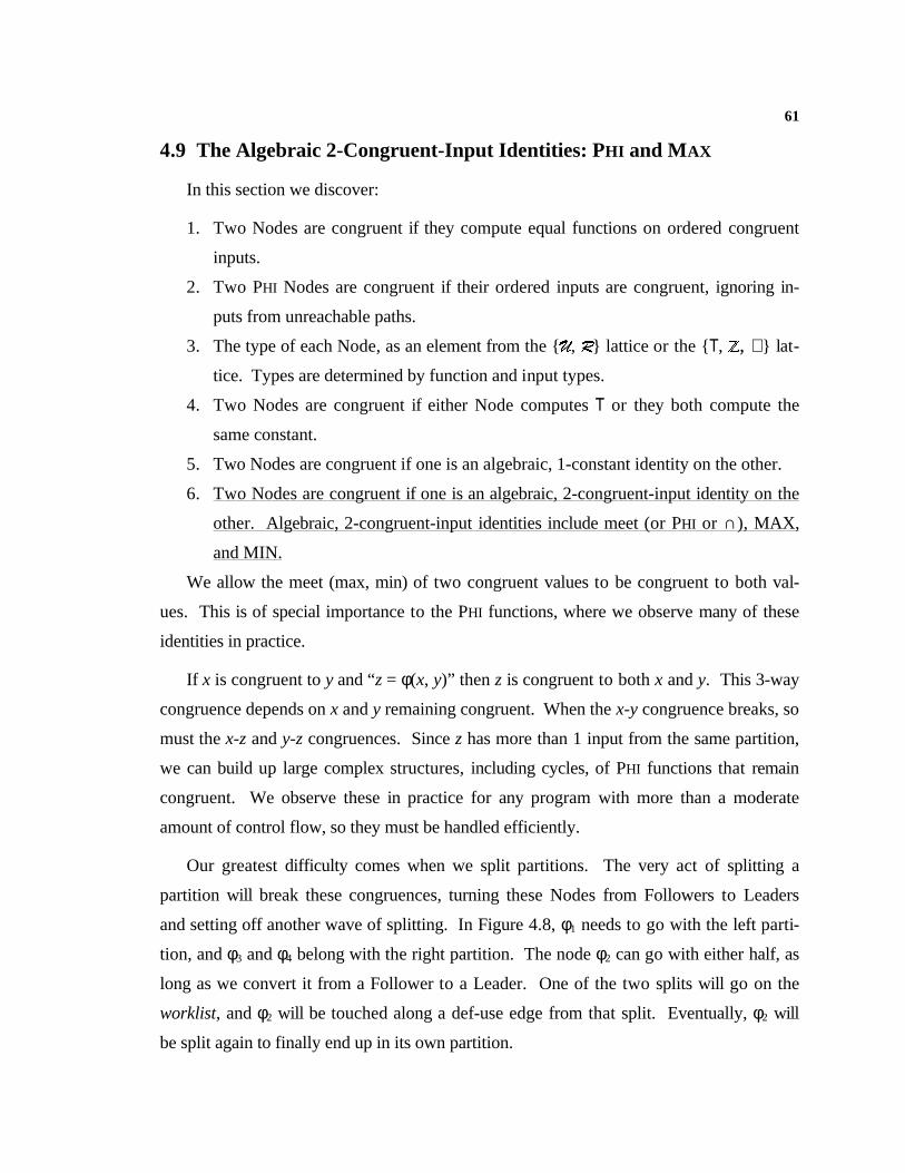
61

4.9 The Algebraic 2-Congruent-Input Identities: PHI and M AX

In this section we discover:

1. Two Nodes are congruent if they compute equal functions on ordered congruent

inputs.

2. Two PHI Nodes are congruent if their ordered inputs are congruent, ignoring in-

puts from unreachable paths.

3. The type of each Node, as an element from the {U, R} lattice or the { T, Z, ⊥ } lat-

tice. Types are determined by function and input types.

4. Two Nodes are congruent if either Node computes T or they both compute the

same constant.

5. Two Nodes are congruent if one is an algebraic, 1-constant identity on the other.

6. Two Nodes are congruent if one is an algebraic, 2-congruent-input identity on the

other. Algebraic, 2-congruent-input identities include meet (or PHI or ∩), MAX,

and MIN.

We allow the meet (max, min) of two congruent values to be congruent to both val-

ues. This is of special importance to the PHI functions, where we observe many of these

identities in practice.

If x is congruent to y and “z = φ(x, y)” then z is congruent to both x and y. This 3-way

congruence depends on x and y remaining congruent. When the x-y congruence breaks, so

must the x-z and y-z congruences. Since z has more than 1 input from the same partition,

we can build up large complex structures, including cycles, of PHI functions that remain

congruent. We observe these in practice for any program with more than a moderate

amount of control flow, so they must be handled efficiently.

Our greatest difficulty comes when we split partitions. The very act of splitting a

partition will break these congruences, turning these Nodes from Followers to Leaders

and setting off another wave of splitting. In Figure 4.8, φ1 needs to go with the left parti-

tion, and φ3 and φ4 belong with the right partition. The node φ2 can go with either half, as

long as we convert it from a Follower to a Leader. One of the two splits will go on the

worklist, and φ2 will be touched along a def-use edge from that split. Eventually, φ2 will

be split again to finally end up in its own partition.

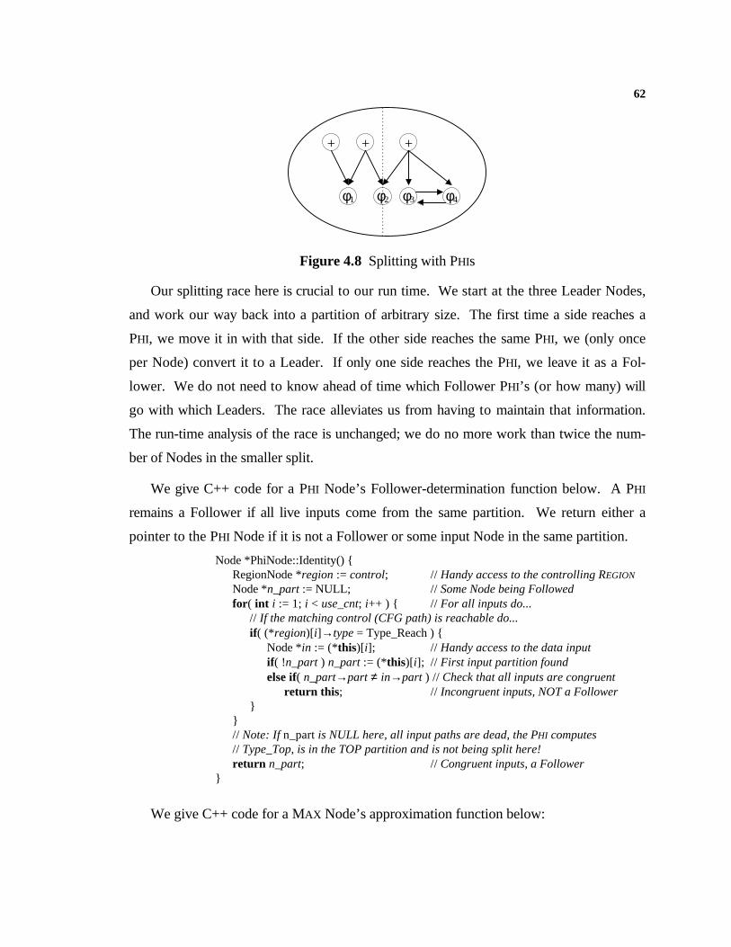
62

φ1

+

φ2 φ3

+ +

φ4

Figure 4.8 Splitting with PHIs

Our splitting race here is crucial to our run time. We start at the three Leader Nodes,

and work our way back into a partition of arbitrary size. The first time a side reaches a

PHI, we move it in with that side. If the other side reaches the same PHI, we (only once

per Node) convert it to a Leader. If only one side reaches the PHI, we leave it as a Fol-

lower. We do not need to know ahead of time which Follower PHI’s (or how many) will

go with which Leaders. The race alleviates us from having to maintain that information.

The run-time analysis of the race is unchanged; we do no more work than twice the num-

ber of Nodes in the smaller split.

We give C++ code for a PHI Node’s Follower-determination function below. A PHI

remains a Follower if all live inputs come from the same partition. We return either a

pointer to the PHI Node if it is not a Follower or some input Node in the same partition.

Node *PhiNode::Identity() {RegionNode *region := control; // Handy access to the controlling REGION

Node *n_part := NULL; // Some Node being Followedfor ( int i := 1; i < use_cnt; i++ ) { // For all inputs do...

// If the matching control (CFG path) is reachable do...if ( (*region)[i]→type = Type_Reach ) {

Node *in := (*this)[i]; // Handy access to the data inputif ( !n_part ) n_part := (*this)[i]; // First input partition foundelse if( n_part→part ≠ in→part ) // Check that all inputs are congruent

return this ; // Incongruent inputs, NOT a Follower}

}// Note: If n_part is NULL here, all input paths are dead, the PHI computes// Type_Top, is in the TOP partition and is not being split here!return n_part; // Congruent inputs, a Follower

}

We give C++ code for a MAX Node’s approximation function below:

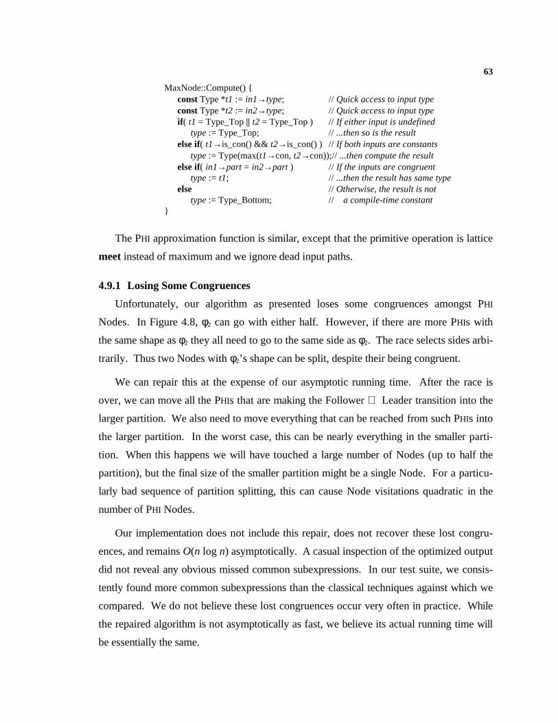
63

MaxNode::Compute() {const Type *t1 := in1→type; // Quick access to input typeconst Type *t2 := in2→type; // Quick access to input typeif ( t1 = Type_Top || t2 = Type_Top ) // If either input is undefined

type := Type_Top; // ...then so is the resultelse if( t1→is_con() && t2→is_con() ) // If both inputs are constants

type := Type(max(t1→con, t2→con));// ...then compute the resultelse if( in1→part = in2→part ) // If the inputs are congruent

type := t1; // ...then the result has same typeelse // Otherwise, the result is not

type := Type_Bottom; // a compile-time constant}

The PHI approximation function is similar, except that the primitive operation is lattice

meet instead of maximum and we ignore dead input paths.

4.9.1 Losing Some Congruences

Unfortunately, our algorithm as presented loses some congruences amongst PHI

Nodes. In Figure 4.8, φ2 can go with either half. However, if there are more PHIs with

the same shape as φ2 they all need to go to the same side as φ2. The race selects sides arbi-

trarily. Thus two Nodes with φ2’s shape can be split, despite their being congruent.

We can repair this at the expense of our asymptotic running time. After the race is

over, we can move all the PHIs that are making the Follower ⇒ Leader transition into the

larger partition. We also need to move everything that can be reached from such PHIs into

the larger partition. In the worst case, this can be nearly everything in the smaller parti-

tion. When this happens we will have touched a large number of Nodes (up to half the

partition), but the final size of the smaller partition might be a single Node. For a particu-

larly bad sequence of partition splitting, this can cause Node visitations quadratic in the

number of PHI Nodes.

Our implementation does not include this repair, does not recover these lost congru-

ences, and remains O(n log n) asymptotically. A casual inspection of the optimized output

did not reveal any obvious missed common subexpressions. In our test suite, we consis-

tently found more common subexpressions than the classical techniques against which we

compared. We do not believe these lost congruences occur very often in practice. While

the repaired algorithm is not asymptotically as fast, we believe its actual running time will

be essentially the same.

64

4.10 Using the Results

As my advisor is fond of saying, “Knowledge does not make code run faster.” We

need to make use of the analysis. When the algorithm stops, we have a partitioning over

our Nodes. All Nodes in a partition are congruent and compute the same value. The al-

gorithm replaces such Nodes by a single representative (Leader) from the partition. Fur-

ther, Nodes in the same partition compute the same Type and, if the Type is a constant,

the representative Node can be a load-immediate of the constant. Finally we note that all

unreachable code will be of type T.

We pre-order walk the program graph from the exit, following the use-def chains. For

every visited Node, we make sure the corresponding partition has a representative (O(N)

time), creating one if necessary. We also make the representative Nodes’ use-def chains

point to other representatives (O(E) time). Then the graph formed by the representatives

becomes our new program graph. We discard the old graph. We walk the representa-

tive’s use-def chains, so we do not walk the inputs to computations that compute con-

stants (instead, we walk the inputs to the load-immediate Node, i.e., none). Since we

walked the final program graph’s use-def chains, the replacements contain no dead code;

dead code is implicitly removed.

4.11 Summary

We have an O(n log n) algorithm for finding:

1. constants

2. unreachable code

3. global structural equivalencies

4. algebraic identities

It is optimistic, so it finds those algebraic identities that depend on structural equiva-

lences that depend on constants that depend on algebraic identities. In particular, in

Figure 3.11 we discover that the print statement always prints 1.

65

We implemented the algorithm and tested it on a large body of FORTRAN and C

codes. In practice it is fast and runs in essentially linear time. A complete listing of run

times and program improvements is in Chapter 5.

66

5. Experimental Data

66

Chapter 5

Experimental Data

An unexamined idea, to paraphrase Socrates, is not worth having;

and a society whose ideas are never explored for possible error may

eventually find its foundations insecure.

— Mark van Doren (1894-1973)

5.1 Experimental Method

We converted a large test suite into a low-level intermediate language, ILOC [8, 6].

The ILOC produced by translation is very naive and is intended to be optimized. We then

performed several machine-independent optimizations at the ILOC level. We ran the re-

sulting ILOC on a simulator to collect execution cycle counts for the ILOC virtual machine.

All applications ran to completion on the simulator and produced correct results.

The combined algorithm was implemented by the author. The classic optimization

phases were implemented by members of the Massively Scalar Compiler Project at Rice.

5.2 Executing ILOC

ILOC is a virtual assembly language for a virtual machine. The current simulator de-

fines a machine with an infinite register set and 1 cycle latencies for all operations, includ-

ing LOADs, STOREs and JUMPs. A single register can not be used for both integer and

floating-point operations (conversion operators exist). While the simulator can execute an

unlimited number of data-independent data operations in 1 cycle, we limited our output to

1 operation per cycle. ILOC is based on a load-store architecture; there are no memory

operations other than LOAD and STORE. LOADs and STOREs allow base+offset and

base+index addressing. Adds and subtracts also have an immediate operand form. All

67

immediate operands are 32 bits long. ILOC includes the usual assortment of logical, arith-

metic and floating-point operations.

The simulator is implemented by translating ILOC files into a simple form of C. The C

code is then compiled on the target system using a standard C compiler, linked against ei-

ther the FORTRAN or C libraries and executed as a native program. The executed code

contains annotations that collect statistics on the number of times each ILOC routine is

called, the dynamic number of each operation type executed and the dynamic cycle count.

The statistics are printed to stderr as the program executes. We use UNIX redirection to

capture the statistics in a separate file from the program output.

5.2.1 Quality of the simulation

The simulated ILOC clearly represents an unrealistic machine model. We argue that

while the simulation is overly simplistic, it makes measuring the separate effects of optimi-

zations possible. We are looking at machine-independent optimizations. Were we to in-

clude memory hierarchy effects, with long and variable latencies to memory and a fixed

number of functional units, we would obscure the effects we are trying to measure.

A production compiler clearly must deal with these issues. Building a high quality

back end is outside the scope of this thesis. We did not want the bad effects from a naive

back end obscuring the effects we are trying to measure.

5.3 The Test Suite

The test suite consists of a dozen applications with a total of 52 procedures. The pro-

cedures and their static instruction sizes are given in Figure 5.1. All the applications are

written in FORTRAN, except for cplex. Cplex is a large constraint solver written in C.

Doduc, tomcatv, matrix300 and fpppp are from the Spec89 benchmark suite. Ma-

trix300 performs various matrix multiplies. Since our machine model does not include a

memory hierarchy (single cycle LOAD latencies), we are not interested in memory access

patterns of the inner loops. Thus we choose matrix300 over matrix1000 for faster test-

ing times, even cutting the matrix size down to 50. The remaining procedures come from

the Forsythe, Malcom and Moler suite of routines. [20]

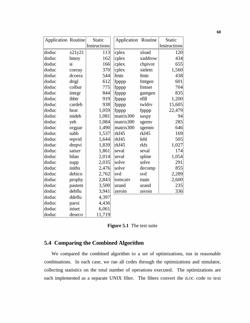
68

Application Routine StaticInstructions

Application Routine StaticInstructions

doduc x21y21 113 cplex xload 120doduc hmoy 162 cplex xaddrow 434doduc si 166 cplex chpivot 655doduc coeray 370 cplex xielem 1,560doduc dcoera 544 fmin fmin 438doduc drigl 612 fpppp fmtgen 601doduc colbur 775 fpppp fmtset 704doduc integr 844 fpppp gamgen 835doduc ihbtr 919 fpppp efill 1,200doduc cardeb 938 fpppp twldrv 15,605doduc heat 1,059 fpppp fpppp 22,479doduc inideb 1,081 matrix300 saxpy 94doduc yeh 1,084 matrix300 sgemv 285doduc orgpar 1,490 matrix300 sgemm 646doduc subb 1,537 rkf45 rkf45 169doduc repvid 1,644 rkf45 fehl 505doduc drepvi 1,839 rkf45 rkfs 1,027doduc saturr 1,861 seval seval 174doduc bilan 2,014 seval spline 1,054doduc supp 2,035 solve solve 291doduc inithx 2,476 solve decomp 855doduc debico 2,762 svd svd 2,289doduc prophy 2,843 tomcatv main 2,600doduc pastem 3,500 urand urand 235doduc debflu 3,941 zeroin zeroin 336doduc ddeflu 4,397doduc paroi 4,436doduc iniset 6,061doduc deseco 11,719

Figure 5.1 The test suite

5.4 Comparing the Combined Algorithm

We compared the combined algorithm to a set of optimizations, run in reasonable

combinations. In each case, we ran all codes through the optimizations and simulator,

collecting statistics on the total number of operations executed. The optimizations are

each implemented as a separate UNIX filter. The filters convert the ILOC code to text

69

form between each pass. We report both the raw cycle counts and speedups over unop-

timized code. We performed the following optimizations:

clean: Clean removes empty basic blocks (branches to branches) and turns long

chains of basic blocks into single large blocks.

coalesce: Many of the optimizations insert extraneous copy operations (e.g., common

subexpression elimination). Also, an easy algorithm for coming out of SSA form inserts a

large number of extra copies. We coalesced them using techniques from graph coloring

register allocators [5, 10].

combine: This phase combines logically adjacent instructions into more powerful in-

structions. This is commonly used to build addressing expressions for LOADs and STOREs.

It also performs a variety of peephole optimizations, such as removing two negates in a

row.

combo: The combined algorithm, as discussed in Chapter 4. This phase includes in-

ternally the effects of dead as part of the transformation step. Combo also includes a

round of combine, coalesce and clean after the analysis.20 The internal implementations

are slightly different from the UNIX filters. We looked for places where the test suite

used the differing idioms and changed one implementation or the other to match.21

cprop: Conditional constant propagation is an implementation of Wegman and

Zadeck’s algorithm [49]. It simultaneously removes unreachable code and replaces com-

putations of constants with load-immediates of constants. It is optimistic in the sense that

if a variable computing a constant allows a code section to be unreachable, and that be-

cause the code section is unreachable the variable computes a constant, cprop will dis-

cover this. After constant propagation, cprop runs a pass to fold algebraic identities that

use constants, such as x × 1 and x + 0, into simple copy operations.

20 Normally we avoid such duplication of efforts. Unfortunately, we needed these passes to reasonably study combo

before the separate Unix filter versions became available.

21 Differing implementations were a source of much confusion in getting comparable results. Compiler writers oftenextend published algorithms in minor ways, to find more common subexpressions or more constants. We were of-ten faced with the choice of upgrading our implementation or upgrading the Unix filters (leading to a sort of com-piler writer’s one-up-manship).

70

dead: Dead code elimination removes code that cannot affect the output, even if exe-

cuted. This algorithm starts at the program exit and walks the use-def chains to find all

operations that define a value used by output operations or that affect the final result. Op-

erations not visited in the walk do not affect the output and are removed. Our implemen-

tation is based on the work of Cytron, et. al. [15]

gval: Global value numbering implements Alpern, Wegman, and Zadeck’s global con-

gruence finding algorithm [2]. Instead of using dominance information, available expres-

sions (AVAIL) information is used to remove redundant computations. AVAIL is

stronger than dominance, so more computations are removed [41].

parse: Usually used to test ILOC parsing, this pass includes a flag to split control-

dependent basic blocks. This has the effect of creating basic blocks for loop landing pads

and partially redundant expressions.

partial: Partial Redundancy Elimination is an implementation of Morel and Renvoise’s

algorithm for removing partially redundant expressions, as modified by Drescher and Sta-

del [36, 18]. It also hoists code out of loops, if that code is not control dependent inside

the loop. Since it is a global algorithm, it also performs local common subexpression

elimination. Unfortunately, the algorithm has no understanding of algebraic identities and

relies solely on lexical equivalence.

shape: This phase reassociates and redistributes integer expressions allowing other

optimizations to find more loop invariant code [7]. This is important for addressing ex-

pressions inside loops, where the rapidly varying innermost index may cause portions of a

complex address to be recomputed on each iteration. Reassociation can allow all the in-

variant parts to be hoisted, leaving behind only an expression of the form

“base+index×stride” in the loop.

valnum: Valnum performs local value numbering with a hash table [13]. This

method handles algebraic identities such as x + 0 or copy operations, commutativity, con-

stant folding, and equal-functions-on-equal-inputs congruences, all within a single basic

block.

71

Optimizations not performed include strength reduction, any sort of loop transforma-

tions (unrolling, interchange, peeling, loop unswitching), software pipelining, blocking for

cache, scalar replacement, and register allocation. Scalar replacement and register alloca-

tion both change the address computations. They can speed up or slow down the simu-

lated ILOC run-time. Strength reduction and loop unswitching both have strong effects on

the amount of code executed in loops. The remaining optimizations have little effect on

our simple virtual machine.

5.5 The Experiments

Combo, the combined algorithm, combines cprop (conditional constant propagation)

with value numbering. If the global schedule is enforced (computations must remain in

their original basic block) then the value numbering effects are equal to valnum (local

value numbering) only. If the global schedule is ignored, the value numbering effects are

similar to a combined gval, partial , and valnum. We tested both ways.

Combo always ends with a round of dead code elimination (as part of using the

analysis results). We always followed any set of the classic optimizations with a round of

dead.

Most of the phases use SSA form internally with a naive translation out of SSA at the

end. Thus, most optimizations insert a large number of copies. We followed with a round

of coalesce to remove the copies. This tends to empty some basic blocks (those blocks

with only copies). We also used parse to split control-dependent blocks (combo, with the

global schedule ignored, has the same effect), and some of those blocks go unused. We

ran a round of clean to remove the empty blocks.

Combo and shape split complex ILOC instructions, such as LOAD from base+index

into a simple ADD and a LOAD. This allows more common subexpressions to be found.

However, a round of combine is required to reform the single LOAD instruction.

The global version of combo requires a round of global code motion to recover some

serial order. This global code motion pushes operations down, to make them as control

dependent as possible, without pushing them into loops. This heuristic both hoists loop

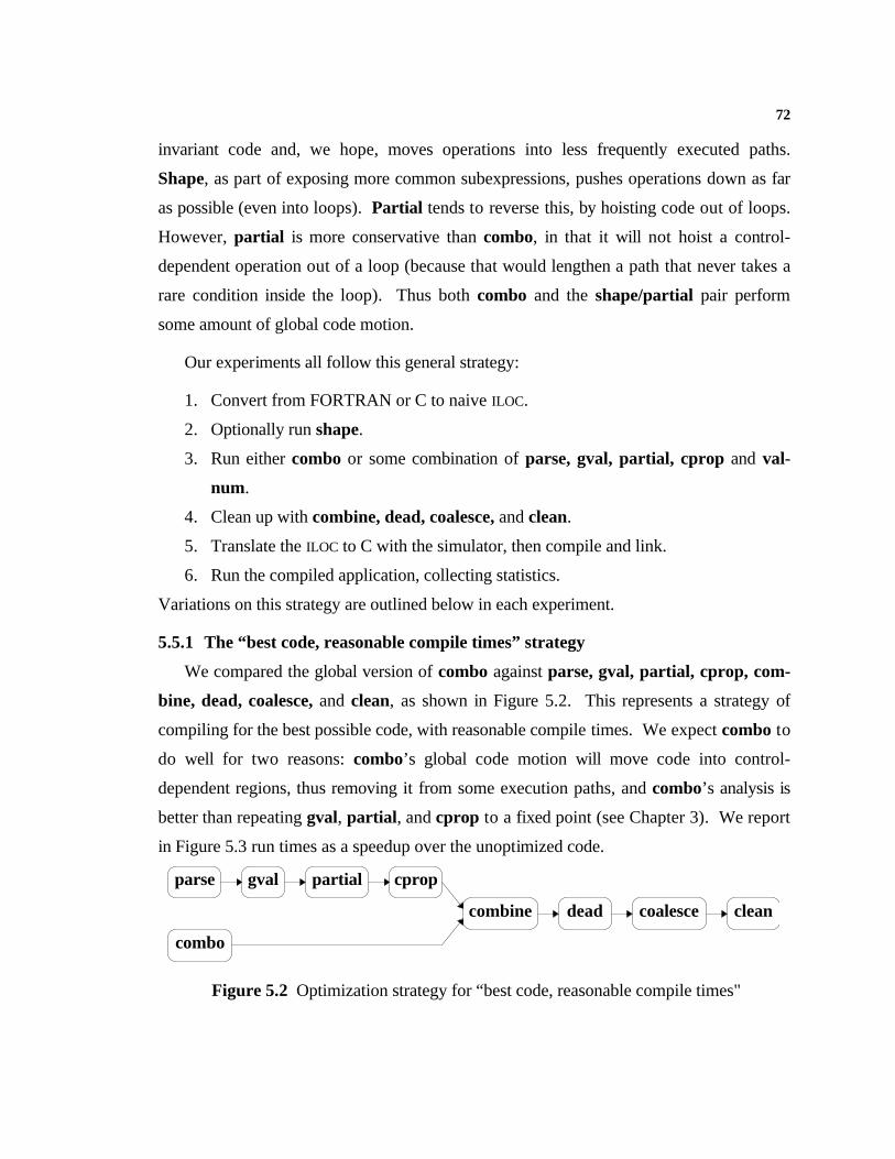
72

invariant code and, we hope, moves operations into less frequently executed paths.

Shape, as part of exposing more common subexpressions, pushes operations down as far

as possible (even into loops). Partial tends to reverse this, by hoisting code out of loops.

However, partial is more conservative than combo, in that it will not hoist a control-

dependent operation out of a loop (because that would lengthen a path that never takes a

rare condition inside the loop). Thus both combo and the shape/partial pair perform

some amount of global code motion.

Our experiments all follow this general strategy:

1. Convert from FORTRAN or C to naive ILOC.

2. Optionally run shape.

3. Run either combo or some combination of parse, gval, partial, cprop and val-

num.

4. Clean up with combine, dead, coalesce, and clean.

5. Translate the ILOC to C with the simulator, then compile and link.

6. Run the compiled application, collecting statistics.

Variations on this strategy are outlined below in each experiment.

5.5.1 The “best code, reasonable compile times” strategy

We compared the global version of combo against parse, gval, partial, cprop, com-

bine, dead, coalesce, and clean, as shown in Figure 5.2. This represents a strategy of

compiling for the best possible code, with reasonable compile times. We expect combo to

do well for two reasons: combo’s global code motion will move code into control-

dependent regions, thus removing it from some execution paths, and combo’s analysis is

better than repeating gval, partial , and cprop to a fixed point (see Chapter 3). We report

in Figure 5.3 run times as a speedup over the unoptimized code.

combo

gval partial cprop

combine dead coalesce clean

parse

Figure 5.2 Optimization strategy for “best code, reasonable compile times"

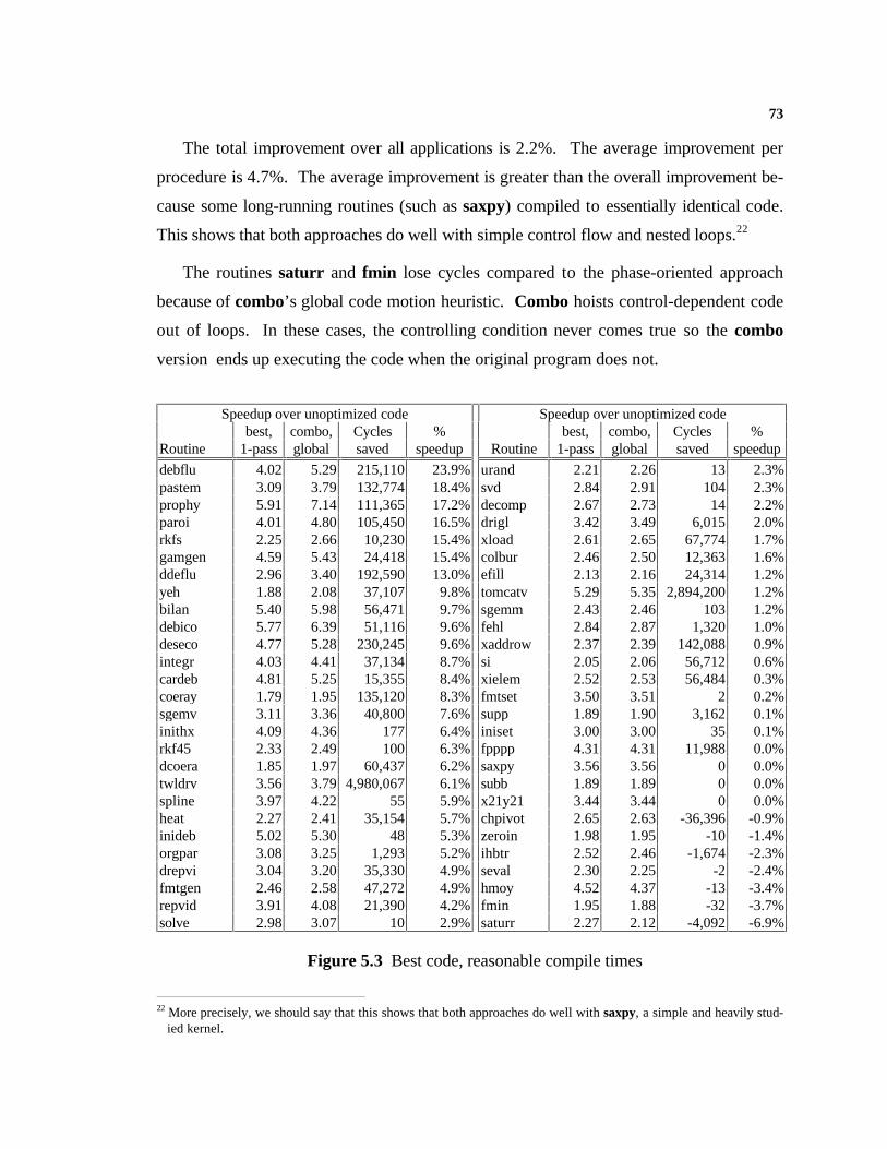
73

The total improvement over all applications is 2.2%. The average improvement per

procedure is 4.7%. The average improvement is greater than the overall improvement be-

cause some long-running routines (such as saxpy) compiled to essentially identical code.

This shows that both approaches do well with simple control flow and nested loops.22

The routines saturr and fmin lose cycles compared to the phase-oriented approach

because of combo’s global code motion heuristic. Combo hoists control-dependent code

out of loops. In these cases, the controlling condition never comes true so the combo

version ends up executing the code when the original program does not.

22 More precisely, we should say that this shows that both approaches do well with saxpy, a simple and heavily stud-

ied kernel.

Speedup over unoptimized code Speedup over unoptimized codebest, combo, Cycles % best, combo, Cycles %

Routine 1-pass global saved speedup Routine 1-pass global saved speedup

debflu 4.02 5.29 215,110 23.9% urand 2.21 2.26 13 2.3%pastem 3.09 3.79 132,774 18.4% svd 2.84 2.91 104 2.3%prophy 5.91 7.14 111,365 17.2% decomp 2.67 2.73 14 2.2%paroi 4.01 4.80 105,450 16.5% drigl 3.42 3.49 6,015 2.0%rkfs 2.25 2.66 10,230 15.4% xload 2.61 2.65 67,774 1.7%gamgen 4.59 5.43 24,418 15.4% colbur 2.46 2.50 12,363 1.6%ddeflu 2.96 3.40 192,590 13.0% efill 2.13 2.16 24,314 1.2%yeh 1.88 2.08 37,107 9.8% tomcatv 5.29 5.35 2,894,200 1.2%bilan 5.40 5.98 56,471 9.7% sgemm 2.43 2.46 103 1.2%debico 5.77 6.39 51,116 9.6% fehl 2.84 2.87 1,320 1.0%deseco 4.77 5.28 230,245 9.6% xaddrow 2.37 2.39 142,088 0.9%integr 4.03 4.41 37,134 8.7% si 2.05 2.06 56,712 0.6%cardeb 4.81 5.25 15,355 8.4% xielem 2.52 2.53 56,484 0.3%coeray 1.79 1.95 135,120 8.3% fmtset 3.50 3.51 2 0.2%sgemv 3.11 3.36 40,800 7.6% supp 1.89 1.90 3,162 0.1%inithx 4.09 4.36 177 6.4% iniset 3.00 3.00 35 0.1%rkf45 2.33 2.49 100 6.3% fpppp 4.31 4.31 11,988 0.0%dcoera 1.85 1.97 60,437 6.2% saxpy 3.56 3.56 0 0.0%twldrv 3.56 3.79 4,980,067 6.1% subb 1.89 1.89 0 0.0%spline 3.97 4.22 55 5.9% x21y21 3.44 3.44 0 0.0%heat 2.27 2.41 35,154 5.7% chpivot 2.65 2.63 -36,396 -0.9%inideb 5.02 5.30 48 5.3% zeroin 1.98 1.95 -10 -1.4%orgpar 3.08 3.25 1,293 5.2% ihbtr 2.52 2.46 -1,674 -2.3%drepvi 3.04 3.20 35,330 4.9% seval 2.30 2.25 -2 -2.4%fmtgen 2.46 2.58 47,272 4.9% hmoy 4.52 4.37 -13 -3.4%repvid 3.91 4.08 21,390 4.2% fmin 1.95 1.88 -32 -3.7%solve 2.98 3.07 10 2.9% saturr 2.27 2.12 -4,092 -6.9%

Figure 5.3 Best code, reasonable compile times

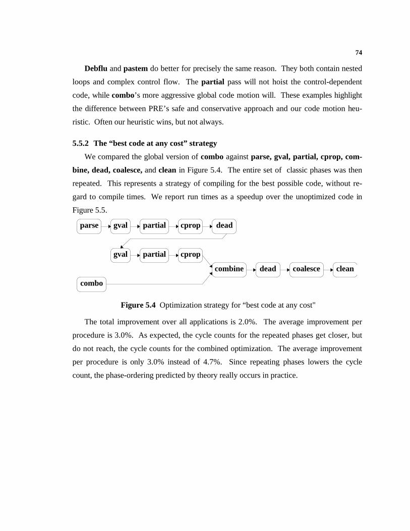
74

Debflu and pastem do better for precisely the same reason. They both contain nested

loops and complex control flow. The partial pass will not hoist the control-dependent

code, while combo’s more aggressive global code motion will. These examples highlight

the difference between PRE’s safe and conservative approach and our code motion heu-

ristic. Often our heuristic wins, but not always.

5.5.2 The “best code at any cost” strategy

We compared the global version of combo against parse, gval, partial, cprop, com-

bine, dead, coalesce, and clean in Figure 5.4. The entire set of classic phases was then

repeated. This represents a strategy of compiling for the best possible code, without re-

gard to compile times. We report run times as a speedup over the unoptimized code in

Figure 5.5.

combo

gval partial cprop

combine dead coalesce clean

parse dead

gval partial cprop

Figure 5.4 Optimization strategy for “best code at any cost"

The total improvement over all applications is 2.0%. The average improvement per

procedure is 3.0%. As expected, the cycle counts for the repeated phases get closer, but

do not reach, the cycle counts for the combined optimization. The average improvement

per procedure is only 3.0% instead of 4.7%. Since repeating phases lowers the cycle

count, the phase-ordering predicted by theory really occurs in practice.

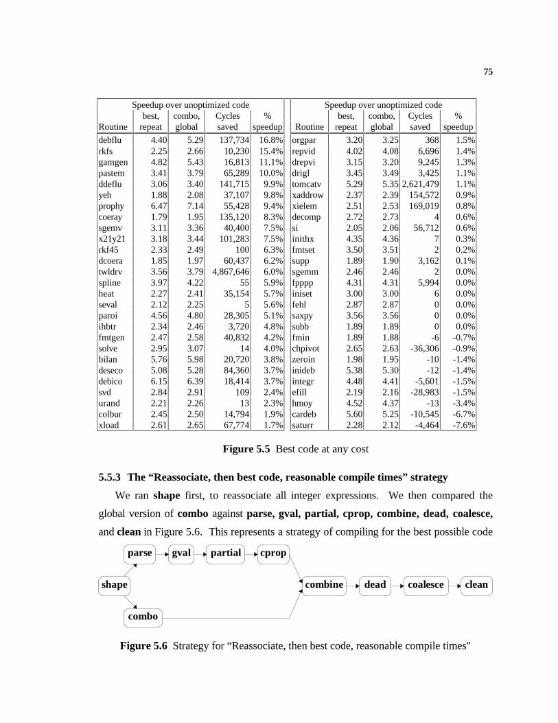
75

5.5.3 The “Reassociate, then best code, reasonable compile times” strategy

We ran shape first, to reassociate all integer expressions. We then compared the

global version of combo against parse, gval, partial, cprop, combine, dead, coalesce,

and clean in Figure 5.6. This represents a strategy of compiling for the best possible code

Speedup over unoptimized code Speedup over unoptimized codebest, combo, Cycles % best, combo, Cycles %

Routine repeat global saved speedup Routine repeat global saved speedup

debflu 4.40 5.29 137,734 16.8% orgpar 3.20 3.25 368 1.5%rkfs 2.25 2.66 10,230 15.4% repvid 4.02 4.08 6,696 1.4%gamgen 4.82 5.43 16,813 11.1% drepvi 3.15 3.20 9,245 1.3%pastem 3.41 3.79 65,289 10.0% drigl 3.45 3.49 3,425 1.1%ddeflu 3.06 3.40 141,715 9.9% tomcatv 5.29 5.35 2,621,479 1.1%yeh 1.88 2.08 37,107 9.8% xaddrow 2.37 2.39 154,572 0.9%prophy 6.47 7.14 55,428 9.4% xielem 2.51 2.53 169,019 0.8%coeray 1.79 1.95 135,120 8.3% decomp 2.72 2.73 4 0.6%sgemv 3.11 3.36 40,400 7.5% si 2.05 2.06 56,712 0.6%x21y21 3.18 3.44 101,283 7.5% inithx 4.35 4.36 7 0.3%rkf45 2.33 2.49 100 6.3% fmtset 3.50 3.51 2 0.2%dcoera 1.85 1.97 60,437 6.2% supp 1.89 1.90 3,162 0.1%twldrv 3.56 3.79 4,867,646 6.0% sgemm 2.46 2.46 2 0.0%spline 3.97 4.22 55 5.9% fpppp 4.31 4.31 5,994 0.0%heat 2.27 2.41 35,154 5.7% iniset 3.00 3.00 6 0.0%seval 2.12 2.25 5 5.6% fehl 2.87 2.87 0 0.0%paroi 4.56 4.80 28,305 5.1% saxpy 3.56 3.56 0 0.0%ihbtr 2.34 2.46 3,720 4.8% subb 1.89 1.89 0 0.0%fmtgen 2.47 2.58 40,832 4.2% fmin 1.89 1.88 -6 -0.7%solve 2.95 3.07 14 4.0% chpivot 2.65 2.63 -36,306 -0.9%bilan 5.76 5.98 20,720 3.8% zeroin 1.98 1.95 -10 -1.4%deseco 5.08 5.28 84,360 3.7% inideb 5.38 5.30 -12 -1.4%debico 6.15 6.39 18,414 3.7% integr 4.48 4.41 -5,601 -1.5%svd 2.84 2.91 109 2.4% efill 2.19 2.16 -28,983 -1.5%urand 2.21 2.26 13 2.3% hmoy 4.52 4.37 -13 -3.4%colbur 2.45 2.50 14,794 1.9% cardeb 5.60 5.25 -10,545 -6.7%xload 2.61 2.65 67,774 1.7% saturr 2.28 2.12 -4,464 -7.6%

Figure 5.5 Best code at any cost

combo

gval parti al cprop

combine dead coalesce clean

parse

shape

Figure 5.6 Strategy for “Reassociate, then best code, reasonable compile times"

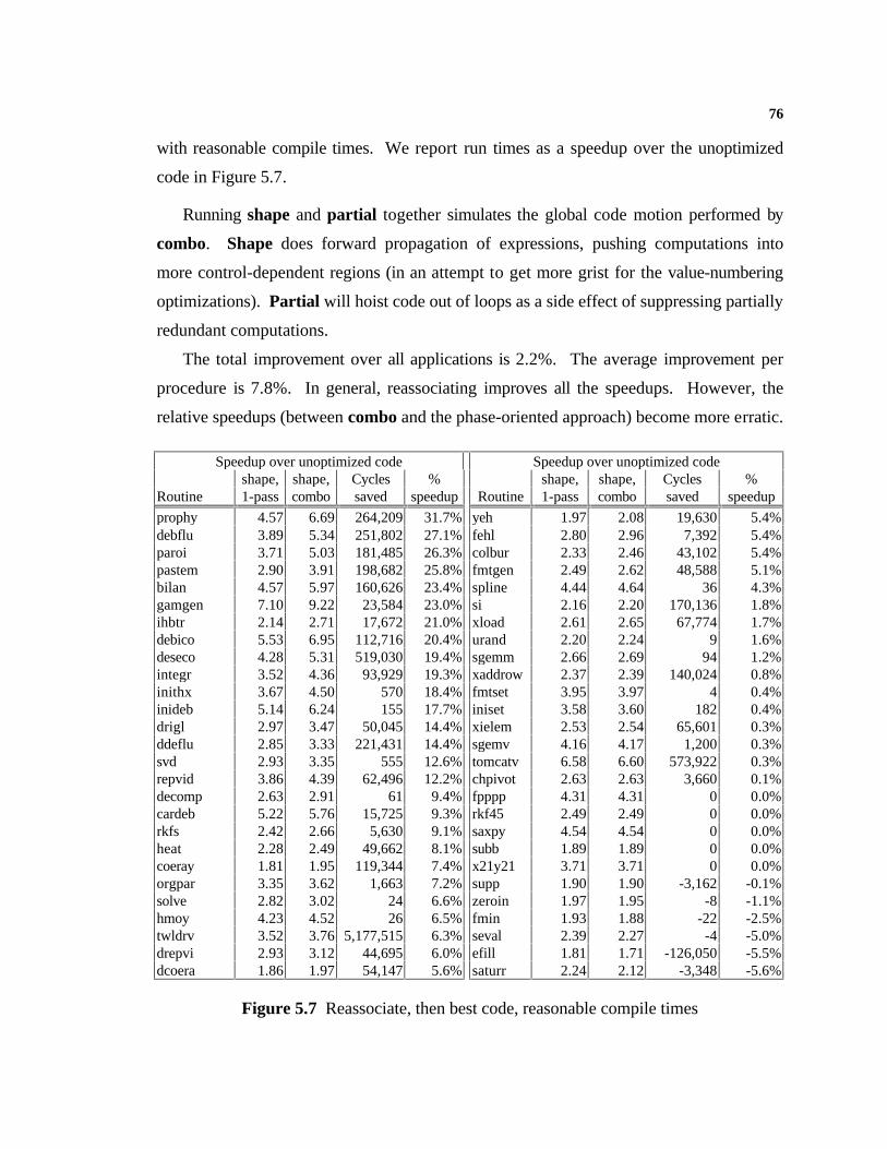
76

with reasonable compile times. We report run times as a speedup over the unoptimized

code in Figure 5.7.

Running shape and partial together simulates the global code motion performed by

combo. Shape does forward propagation of expressions, pushing computations into

more control-dependent regions (in an attempt to get more grist for the value-numbering

optimizations). Partial will hoist code out of loops as a side effect of suppressing partially

redundant computations.

The total improvement over all applications is 2.2%. The average improvement per

procedure is 7.8%. In general, reassociating improves all the speedups. However, the

relative speedups (between combo and the phase-oriented approach) become more erratic.

Speedup over unoptimized code Speedup over unoptimized codeshape, shape, Cycles % shape, shape, Cycles %

Routine 1-pass combo saved speedup Routine 1-pass combo saved speedup

prophy 4.57 6.69 264,209 31.7% yeh 1.97 2.08 19,630 5.4%debflu 3.89 5.34 251,802 27.1% fehl 2.80 2.96 7,392 5.4%paroi 3.71 5.03 181,485 26.3% colbur 2.33 2.46 43,102 5.4%pastem 2.90 3.91 198,682 25.8% fmtgen 2.49 2.62 48,588 5.1%bilan 4.57 5.97 160,626 23.4% spline 4.44 4.64 36 4.3%gamgen 7.10 9.22 23,584 23.0% si 2.16 2.20 170,136 1.8%ihbtr 2.14 2.71 17,672 21.0% xload 2.61 2.65 67,774 1.7%debico 5.53 6.95 112,716 20.4% urand 2.20 2.24 9 1.6%deseco 4.28 5.31 519,030 19.4% sgemm 2.66 2.69 94 1.2%integr 3.52 4.36 93,929 19.3% xaddrow 2.37 2.39 140,024 0.8%inithx 3.67 4.50 570 18.4% fmtset 3.95 3.97 4 0.4%inideb 5.14 6.24 155 17.7% iniset 3.58 3.60 182 0.4%drigl 2.97 3.47 50,045 14.4% xielem 2.53 2.54 65,601 0.3%ddeflu 2.85 3.33 221,431 14.4% sgemv 4.16 4.17 1,200 0.3%svd 2.93 3.35 555 12.6% tomcatv 6.58 6.60 573,922 0.3%repvid 3.86 4.39 62,496 12.2% chpivot 2.63 2.63 3,660 0.1%decomp 2.63 2.91 61 9.4% fpppp 4.31 4.31 0 0.0%cardeb 5.22 5.76 15,725 9.3% rkf45 2.49 2.49 0 0.0%rkfs 2.42 2.66 5,630 9.1% saxpy 4.54 4.54 0 0.0%heat 2.28 2.49 49,662 8.1% subb 1.89 1.89 0 0.0%coeray 1.81 1.95 119,344 7.4% x21y21 3.71 3.71 0 0.0%orgpar 3.35 3.62 1,663 7.2% supp 1.90 1.90 -3,162 -0.1%solve 2.82 3.02 24 6.6% zeroin 1.97 1.95 -8 -1.1%hmoy 4.23 4.52 26 6.5% fmin 1.93 1.88 -22 -2.5%twldrv 3.52 3.76 5,177,515 6.3% seval 2.39 2.27 -4 -5.0%drepvi 2.93 3.12 44,695 6.0% efill 1.81 1.71 -126,050 -5.5%dcoera 1.86 1.97 54,147 5.6% saturr 2.24 2.12 -3,348 -5.6%

Figure 5.7 Reassociate, then best code, reasonable compile times

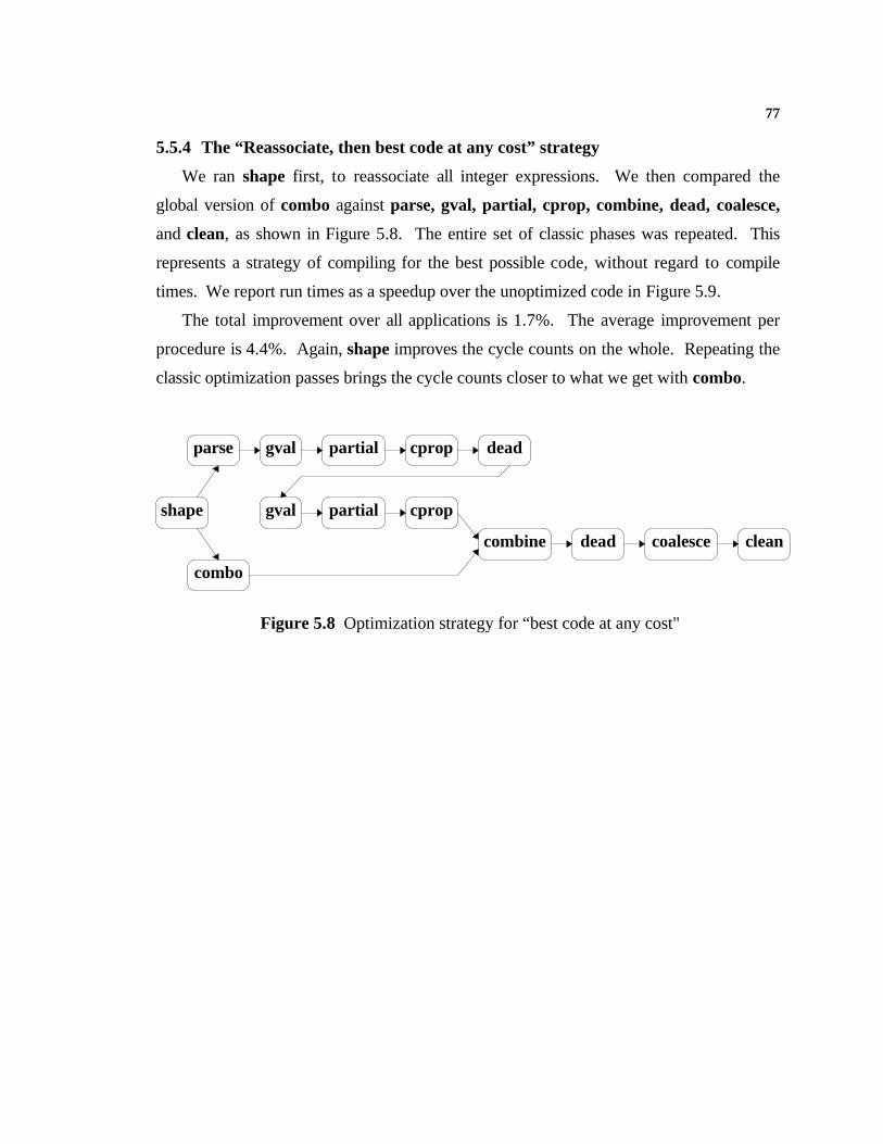
77

5.5.4 The “Reassociate, then best code at any cost” strategy

We ran shape first, to reassociate all integer expressions. We then compared the

global version of combo against parse, gval, partial, cprop, combine, dead, coalesce,

and clean, as shown in Figure 5.8. The entire set of classic phases was repeated. This

represents a strategy of compiling for the best possible code, without regard to compile

times. We report run times as a speedup over the unoptimized code in Figure 5.9.

The total improvement over all applications is 1.7%. The average improvement per

procedure is 4.4%. Again, shape improves the cycle counts on the whole. Repeating the

classic optimization passes brings the cycle counts closer to what we get with combo.

combo

gval partial cprop

combine dead coalesce clean

parse dead

gval partial cpropshape

Figure 5.8 Optimization strategy for “best code at any cost"

78

5.5.5 The “best simple” strategy

We compared the local version of combo against parse, valnum, cprop, combine,

dead, coalesce, and clean. The local version of combo only finds common subexpres-

sions within a single basic block, in addition to global constants and unreachable code.

This represents a strategy of compiling using well known and simple to implement tech-

niques. We report run times as a speedup over the unoptimized code in Figure 5.10.

Note that no global code motion is done, in particular, loop invariant code is not hoisted.

The total improvement over all applications is 11.8%. The average improvement per

procedure is 2.6%. We studied the differences, and determined that most of the differ-

ences were due to the inconsistent implementation of valnum. As an example, valnum

Speedup over unoptimized code Speedup over unoptimized codeshape, shape, Cycles % shape, shape, Cycles %

Routine repeat combo saved speedup Routine repeat combo saved speedup

debflu 4.39 5.34 146,720 17.8% inithx 4.38 4.50 70 2.7%ihbtr 2.25 2.71 13,394 16.7% orgpar 3.52 3.62 553 2.5%inideb 5.34 6.24 122 14.5% decomp 2.85 2.91 11 1.8%drigl 2.97 3.47 50,045 14.4% si 2.16 2.20 170,136 1.8%debico 6.02 6.95 68,076 13.4% xload 2.61 2.65 67,774 1.7%pastem 3.43 3.91 80,366 12.3% efill 1.69 1.71 39,772 1.6%prophy 5.88 6.69 78,444 12.1% urand 2.20 2.24 9 1.6%ddeflu 2.98 3.33 154,091 10.5% xielem 2.50 2.54 303,931 1.5%rkfs 2.38 2.66 6,502 10.4% xaddrow 2.37 2.39 152,508 0.9%bilan 5.39 5.97 56,610 9.7% fmtset 3.95 3.97 4 0.4%paroi 4.57 5.03 51,245 9.2% iniset 3.58 3.60 153 0.3%repvid 3.99 4.39 45,012 9.1% supp 1.89 1.90 3,162 0.1%heat 2.29 2.49 48,546 8.0% sgemv 4.17 4.17 400 0.1%deseco 4.92 5.31 172,790 7.4% chpivot 2.63 2.63 3,750 0.1%coeray 1.81 1.95 119,344 7.4% rkf45 2.49 2.49 0 0.0%svd 3.12 3.35 283 6.8% saxpy 4.54 4.54 0 0.0%hmoy 4.23 4.52 26 6.5% subb 1.89 1.89 0 0.0%twldrv 3.54 3.76 4,652,841 5.7% x21y21 3.71 3.71 0 0.0%dcoera 1.86 1.97 54,147 5.6% tomcatv 6.60 6.60 -10,714 0.0%fehl 2.80 2.96 7,392 5.4% fpppp 4.31 4.31 -5,994 0.0%gamgen 8.77 9.22 3,986 4.8% sgemm 2.69 2.69 -8 -0.1%colbur 2.35 2.46 35,887 4.5% zeroin 1.95 1.95 -1 -0.1%fmtgen 2.51 2.62 40,393 4.2% integr 4.38 4.36 -2,086 -0.5%seval 2.20 2.27 3 3.4% fmin 1.89 1.88 -6 -0.7%drepvi 3.02 3.12 24,530 3.4% solve 3.05 3.02 -4 -1.2%spline 4.49 4.64 28 3.4% cardeb 5.84 5.76 -2,035 -1.3%yeh 2.01 2.08 11,868 3.3% saturr 2.26 2.12 -3,720 -6.2%

Figure 5.9 Reassociate, then best code at any cost

79

would not find two LOADs of the same address with no intervening STORE to be common

subexpressions. There are numerous other missing identities, most of which are being cor-

rected in a new version of valnum. Instead of a completely different implementation,

combo relies on a simple command-line flag to switch between local and global value-

numbering. Thus combo implements the same identities with the same code.

Speedup over unoptimized code Speedup over unoptimized codebest, combo, Cycles % best, combo, Cycles %

Routine simple local saved speedup Routine simple local saved speedup

fpppp 3.31 4.31 8,121,870 23.2% inideb 3.81 3.86 14 1.2%gamgen 3.73 4.58 36,413 18.6% urand 2.20 2.22 4 0.7%twldrv 3.03 3.61 15,336,646 16.1% xielem 2.31 2.32 138,652 0.6%tomcatv 3.51 4.01 45,755,765 12.5% xaddrow 2.26 2.27 90,065 0.5%fmtset 2.54 2.86 164 11.1% rkfs 2.13 2.14 334 0.5%yeh 1.82 2.01 37,324 9.5% debflu 3.33 3.34 4,976 0.5%coeray 1.77 1.93 135,120 8.2% drigl 2.76 2.77 1,670 0.4%debico 4.24 4.58 53,906 7.5% supp 1.89 1.89 3,162 0.1%fmtgen 2.15 2.31 74,166 6.7% chpivot 2.48 2.48 42 0.0%si 1.70 1.82 793,948 6.6% fehl 2.49 2.49 0 0.0%sgemv 2.70 2.89 40,000 6.5% saturr 2.33 2.33 0 0.0%rkf45 2.33 2.49 100 6.3% saxpy 3.32 3.32 0 0.0%dcoera 1.83 1.94 60,437 6.1% subb 1.89 1.89 0 0.0%seval 1.80 1.91 6 5.7% x21y21 2.63 2.63 0 0.0%solve 2.73 2.87 18 4.8% xload 2.55 2.55 0 0.0%heat 1.91 2.01 34,410 4.7% sgemm 2.10 2.10 -8 -0.1%deseco 3.45 3.60 143,117 4.3% bilan 3.99 3.95 -7,631 -1.0%spline 3.69 3.85 42 4.2% paroi 3.41 3.36 -11,840 -1.6%svd 2.27 2.34 165 2.9% cardeb 3.65 3.57 -4,995 -2.1%ddeflu 2.67 2.74 44,173 2.7% prophy 3.93 3.85 -20,147 -2.1%colbur 2.21 2.26 19,950 2.3% efill 1.79 1.75 -62,717 -2.7%pastem 2.11 2.16 24,091 2.3% repvid 2.57 2.50 -23,064 -3.0%fmin 1.57 1.61 24 2.2% integr 3.13 2.99 -26,136 -4.8%inithx 3.16 3.22 76 2.1% ihbtr 2.13 2.01 -4,644 -5.5%decomp 2.20 2.24 15 1.9% hmoy 3.85 3.64 -26 -5.9%zeroin 1.52 1.54 14 1.5% orgpar 2.49 2.34 -2,037 -6.6%drepvi 2.47 2.50 12,690 1.4% iniset 2.01 1.82 -8,961 -10.6%

Figure 5.10 Best simple

5.6 The Compile-Time Numbers

One of a compiler writer’s concerns is compile time, the time it takes to compile code.

Programmers doing development work will use a compiler many times a day and expect

80

the compiler to be fast. The pragmatic compiler writer must consider the running time of

an optimization pass versus its expected gain on the compiled programs.

We measured the time to run the optimizations and perform the transformations of all

the phases. We expect a real compiler implementation to keep a single intermediate repre-

sentation between all passes; it would not convert to text between each pass. When we

measured compile times we ignored time to parse the input, print the output, and pipe the

text form from one process to the next. In the combo pass, our timings do not include the

internal clean, combine and coalesce phases.

All timing runs are on an IBM RS/6000 Model 540, with 64M of memory. The test

machine was lightly loaded (all other users logged off) and had no other running jobs.

Each pass was timed running on each input file, with the output piped to /dev/null. We

ran the pass on the input once to load disk pages and processor cache, then timed and av-

eraged the next three runs. We measured wall-clock time.

Most of the classic passes have been carefully engineered to run fast, while still

being written in a readable and maintainable style. Further speed improvements are cer-

tainly possible; often a single pass over the intermediate representation can serve for sev-

eral analysis phases.

5.6.1 Combo timings

We looked at the time to run combo and correlated it with the static instruction count.

In the “Parse, Combo” column of Figure 5.11, we show the times to run combo when we

do parse-time optimizations, discussed in Chapter 7, beforehand. The parse-time optimi-

zations are integrated pessimistic versions of the constant propagation, unreachable code

elimination and global value numbering. Doing some optimization at parse-time reduces

the size of the intermediate representation run against combo, which improves combo’s

running time.

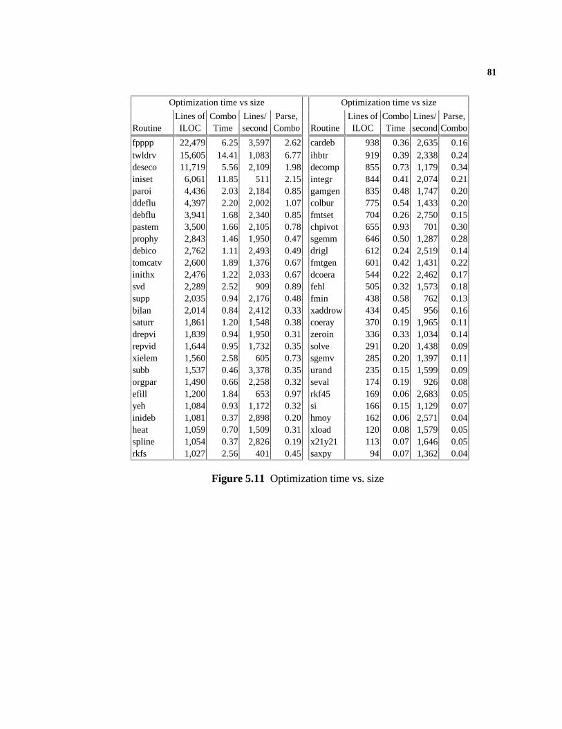
81

Optimization time vs size Optimization time vs size

Lines of Combo Lines/ Parse, Lines of Combo Lines/ Parse,Routine ILOC Time second Combo Routine ILOC Time secondCombo

fpppp 22,479 6.25 3,597 2.62 cardeb 938 0.36 2,635 0.16twldrv 15,605 14.41 1,083 6.77 ihbtr 919 0.39 2,338 0.24deseco 11,719 5.56 2,109 1.98 decomp 855 0.73 1,179 0.34iniset 6,061 11.85 511 2.15 integr 844 0.41 2,074 0.21paroi 4,436 2.03 2,184 0.85 gamgen 835 0.48 1,747 0.20ddeflu 4,397 2.20 2,002 1.07 colbur 775 0.54 1,433 0.20debflu 3,941 1.68 2,340 0.85 fmtset 704 0.26 2,750 0.15pastem 3,500 1.66 2,105 0.78 chpivot 655 0.93 701 0.30prophy 2,843 1.46 1,950 0.47 sgemm 646 0.50 1,287 0.28debico 2,762 1.11 2,493 0.49 drigl 612 0.24 2,519 0.14tomcatv 2,600 1.89 1,376 0.67 fmtgen 601 0.42 1,431 0.22inithx 2,476 1.22 2,033 0.67 dcoera 544 0.22 2,462 0.17svd 2,289 2.52 909 0.89 fehl 505 0.32 1,573 0.18supp 2,035 0.94 2,176 0.48 fmin 438 0.58 762 0.13bilan 2,014 0.84 2,412 0.33 xaddrow 434 0.45 956 0.16saturr 1,861 1.20 1,548 0.38 coeray 370 0.19 1,965 0.11drepvi 1,839 0.94 1,950 0.31 zeroin 336 0.33 1,034 0.14repvid 1,644 0.95 1,732 0.35 solve 291 0.20 1,438 0.09xielem 1,560 2.58 605 0.73 sgemv 285 0.20 1,397 0.11subb 1,537 0.46 3,378 0.35 urand 235 0.15 1,599 0.09orgpar 1,490 0.66 2,258 0.32 seval 174 0.19 926 0.08efill 1,200 1.84 653 0.97 rkf45 169 0.06 2,683 0.05yeh 1,084 0.93 1,172 0.32 si 166 0.15 1,129 0.07inideb 1,081 0.37 2,898 0.20 hmoy 162 0.06 2,571 0.04heat 1,059 0.70 1,509 0.31 xload 120 0.08 1,579 0.05spline 1,054 0.37 2,826 0.19 x21y21 113 0.07 1,646 0.05rkfs 1,027 2.56 401 0.45 saxpy 94 0.07 1,362 0.04

Figure 5.11 Optimization time vs. size

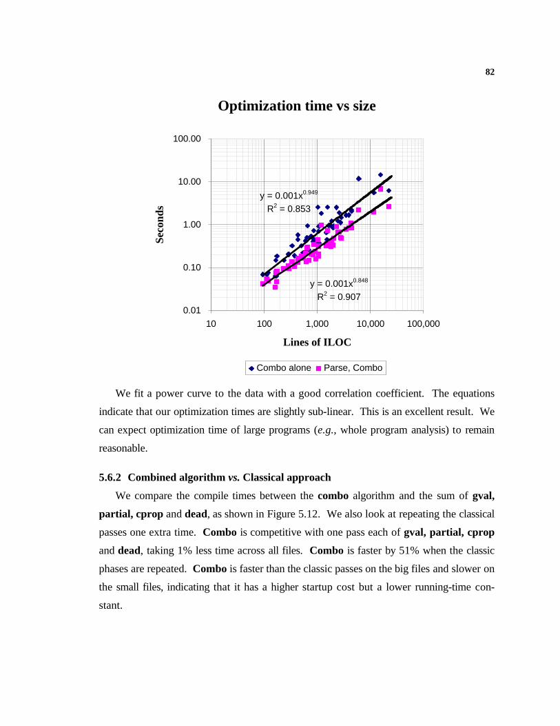
82

Optimization time vs size

y = 0.001x0.848

R2 = 0.907

y = 0.001x0.949

R2 = 0.853

0.01

0.10

1.00

10.00

100.00

10 100 1,000 10,000 100,000

Lines of ILOC

Sec

onds

Combo alone Parse, Combo

We fit a power curve to the data with a good correlation coefficient. The equations

indicate that our optimization times are slightly sub-linear. This is an excellent result. We

can expect optimization time of large programs (e.g., whole program analysis) to remain

reasonable.

5.6.2 Combined algorithm vs. Classical approach

We compare the compile times between the combo algorithm and the sum of gval,

partial, cprop and dead, as shown in Figure 5.12. We also look at repeating the classical

passes one extra time. Combo is competitive with one pass each of gval, partial, cprop

and dead, taking 1% less time across all files. Combo is faster by 51% when the classic

phases are repeated. Combo is faster than the classic passes on the big files and slower on

the small files, indicating that it has a higher startup cost but a lower running-time con-

stant.

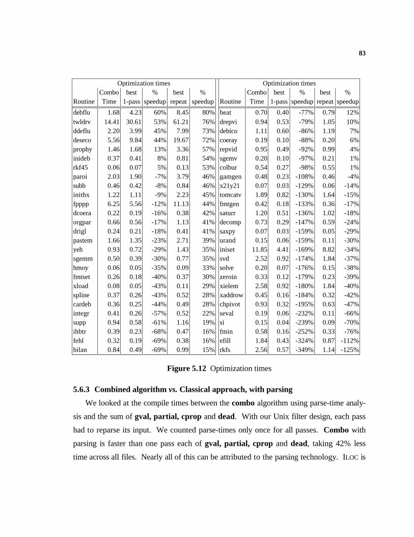
83

Optimization times Optimization timesCombo best % best % Combo best % best %

Routine Time 1-passspeeduprepeat speedup Routine Time 1-passspeeduprepeatspeedup

debflu 1.68 4.23 60% 8.45 80% heat 0.70 0.40 -77% 0.79 12%twldrv 14.41 30.61 53% 61.21 76% drepvi 0.94 0.53 -79% 1.05 10%ddeflu 2.20 3.99 45% 7.99 73% debico 1.11 0.60 -86% 1.19 7%deseco 5.56 9.84 44% 19.67 72% coeray 0.19 0.10 -88% 0.20 6%prophy 1.46 1.68 13% 3.36 57% repvid 0.95 0.49 -92% 0.99 4%inideb 0.37 0.41 8% 0.81 54% sgemv 0.20 0.10 -97% 0.21 1%rkf45 0.06 0.07 5% 0.13 53% colbur 0.54 0.27 -98% 0.55 1%paroi 2.03 1.90 -7% 3.79 46% gamgen 0.48 0.23 -108% 0.46 -4%subb 0.46 0.42 -8% 0.84 46% x21y21 0.07 0.03 -129% 0.06 -14%inithx 1.22 1.11 -9% 2.23 45% tomcatv 1.89 0.82 -130% 1.64 -15%fpppp 6.25 5.56 -12% 11.13 44% fmtgen 0.42 0.18 -133% 0.36 -17%dcoera 0.22 0.19 -16% 0.38 42% saturr 1.20 0.51 -136% 1.02 -18%orgpar 0.66 0.56 -17% 1.13 41% decomp 0.73 0.29 -147% 0.59 -24%drigl 0.24 0.21 -18% 0.41 41% saxpy 0.07 0.03 -159% 0.05 -29%pastem 1.66 1.35 -23% 2.71 39% urand 0.15 0.06 -159% 0.11 -30%yeh 0.93 0.72 -29% 1.43 35% iniset 11.85 4.41 -169% 8.82 -34%sgemm 0.50 0.39 -30% 0.77 35% svd 2.52 0.92 -174% 1.84 -37%hmoy 0.06 0.05 -35% 0.09 33% solve 0.20 0.07 -176% 0.15 -38%fmtset 0.26 0.18 -40% 0.37 30% zeroin 0.33 0.12 -179% 0.23 -39%xload 0.08 0.05 -43% 0.11 29% xielem 2.58 0.92 -180% 1.84 -40%spline 0.37 0.26 -43% 0.52 28% xaddrow 0.45 0.16 -184% 0.32 -42%cardeb 0.36 0.25 -44% 0.49 28% chpivot 0.93 0.32 -195% 0.63 -47%integr 0.41 0.26 -57% 0.52 22% seval 0.19 0.06 -232% 0.11 -66%supp 0.94 0.58 -61% 1.16 19% si 0.15 0.04 -239% 0.09 -70%ihbtr 0.39 0.23 -68% 0.47 16% fmin 0.58 0.16 -252% 0.33 -76%fehl 0.32 0.19 -69% 0.38 16% efill 1.84 0.43 -324% 0.87 -112%bilan 0.84 0.49 -69% 0.99 15% rkfs 2.56 0.57 -349% 1.14 -125%

Figure 5.12 Optimization times

5.6.3 Combined algorithm vs. Classical approach, with parsing

We looked at the compile times between the combo algorithm using parse-time analy-

sis and the sum of gval, partial, cprop and dead. With our Unix filter design, each pass

had to reparse its input. We counted parse-times only once for all passes. Combo with

parsing is faster than one pass each of gval, partial, cprop and dead, taking 42% less

time across all files. Nearly all of this can be attributed to the parsing technology. ILOC is

84

a syntactically simple language, allowing combo to sport a simple hand-coded parser. The

classic phases are using a lex/yacc coded parser.

85

6. Optimizing Without the Global Schedule

85

Chapter 6

Optimizing Without the Global Schedule

When they began looking at the problem it rapidly became clear

that it was not going to be easy to treat it optimally. At that point I

proposed that they should produce a program for a 704 with an un-

limited number of index registers, and that later sections would

...make index register assignments so as to minimize the transfers of

items between the store and the index registers.

— John Backus on the separation of concerns in the Fortran I

compiler, “History of Fortran I, II, and III”, History of Program-

ming Languages Conference, 1978

We believe that optimizing compilers should treat the machine-independent optimiza-

tions (e.g., conditional constant propagation, global value numbering) and scheduling

separately. We argue that modern microprocessors with superscalar or VLIW execution

already require global code motion. Removing the schedule from the machine-

independent optimizations allows stronger optimizations using simpler algorithms. Pre-

serving a legal schedule is one of the prime sources of complexity in algorithms like

PRE [36, 18] or global congruence finding [2, 41].

6.1 Removing the Control Dependence

Nodes in our intermediate representation have a control field. Section A.2.3 discusses

viewing the control field as a use-def chain linking the Node to the basic block controlling

the Node’s execution. This implementation of control dependence is identical to the other

data dependences in the program: it is represented simply as a Node pointer. When we

say control dependence, we mean a dependence on some controlling Node. This is not

86

the notion of control dependence discussed by Ferrante, Ottenstein and Warren in their

paper “The Program Dependence Graph and Its Use in Optimization” [21].

We can remove the control dependence for any given Node simply by replacing the

pointer value with the special value NULL. This operation only makes sense for Nodes

that represent data computations. PHI, IF, JUMP and STOP Nodes all require the control

input for semantic correctness. REGION Nodes require several control inputs (one per

CFG input to the basic block they represent). Almost all other Nodes can live without a

control dependence.23 A data computation without a control dependence does not exactly

reside in any particular basic block. Its correct behavior depends solely on the remaining

data dependences. It, and the Nodes that depend on it or on which it depends, exists in a

“sea” of Nodes, with little control structure.

The “sea” of Nodes is useful for optimization, but does not represent any traditional

intermediate representation such as a CFG. We need a way to serialize the graph and get

back the control dependences. We do this with a simple global code motion algorithm.

The job of the global code motion algorithm then is to build a CFG and populate the

basic blocks with all the “free-floating” Nodes. It must preserve any existing control de-

pendences (divides, subroutine calls and other possibly faulting operations keep their con-

trol dependences) and all data dependences. Beyond that, the scheduler has some flexibil-

ity. We use a simple heuristic: place code outside as many loops as possible, then on as

few execution paths as possible.

6.2 Impr oving Optimizations

Removing the control dependences allows the combined optimization algorithm, with

no other changes, to find global congruences. When the control dependences are intact,

distinct control inputs from otherwise identical computations will force combo to treat the

computations as being different. For example, in Figure 6.1 below the computation of

a + b is partially redundant. With the control dependences removed, the two ADD Nodes

that implement the two expressions are identical (and congruent).

23 The exceptions are Nodes which can cause exceptions: loads, stores, division, subroutine calls, etc. Stores also

require the control input to handle the example shown in Section 6.4.

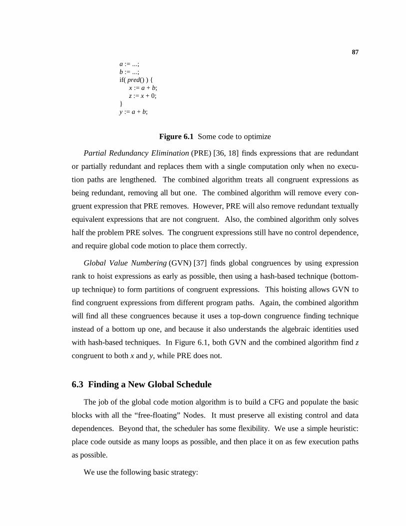
87

a := ...;b := ...;if( pred() ) {

x := a + b;z := x + 0;

}y := a + b;

Figure 6.1 Some code to optimize

Partial Redundancy Elimination (PRE) [36, 18] finds expressions that are redundant

or partially redundant and replaces them with a single computation only when no execu-

tion paths are lengthened. The combined algorithm treats all congruent expressions as

being redundant, removing all but one. The combined algorithm will remove every con-

gruent expression that PRE removes. However, PRE will also remove redundant textually

equivalent expressions that are not congruent. Also, the combined algorithm only solves

half the problem PRE solves. The congruent expressions still have no control dependence,

and require global code motion to place them correctly.

Global Value Numbering (GVN) [37] finds global congruences by using expression

rank to hoist expressions as early as possible, then using a hash-based technique (bottom-

up technique) to form partitions of congruent expressions. This hoisting allows GVN to

find congruent expressions from different program paths. Again, the combined algorithm

will find all these congruences because it uses a top-down congruence finding technique

instead of a bottom up one, and because it also understands the algebraic identities used

with hash-based techniques. In Figure 6.1, both GVN and the combined algorithm find z

congruent to both x and y, while PRE does not.

6.3 Finding a New Global Schedule

The job of the global code motion algorithm is to build a CFG and populate the basic

blocks with all the “free-floating” Nodes. It must preserve all existing control and data

dependences. Beyond that, the scheduler has some flexibility. We use a simple heuristic:

place code outside as many loops as possible, and then place it on as few execution paths

as possible.

We use the following basic strategy:

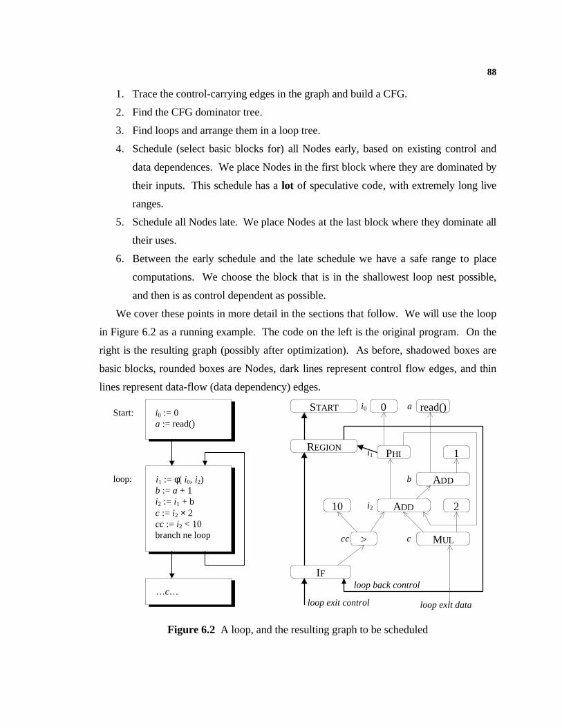
88

1. Trace the control-carrying edges in the graph and build a CFG.

2. Find the CFG dominator tree.

3. Find loops and arrange them in a loop tree.

4. Schedule (select basic blocks for) all Nodes early, based on existing control and

data dependences. We place Nodes in the first block where they are dominated by

their inputs. This schedule has a lot of speculative code, with extremely long live

ranges.

5. Schedule all Nodes late. We place Nodes at the last block where they dominate all

their uses.

6. Between the early schedule and the late schedule we have a safe range to place

computations. We choose the block that is in the shallowest loop nest possible,

and then is as control dependent as possible.

We cover these points in more detail in the sections that follow. We will use the loop

in Figure 6.2 as a running example. The code on the left is the original program. On the

right is the resulting graph (possibly after optimization). As before, shadowed boxes are

basic blocks, rounded boxes are Nodes, dark lines represent control flow edges, and thin

lines represent data-flow (data dependency) edges.

i0 := 0 a := read()

i1 := φ( i0, i2) b := a + 1 i2 := i1 + b c := i2 × 2 cc := i2 < 10 branch ne loop

Start:

loop:

…c…

START

REGIONPHI

ADD

>

IF

0

1

i0

i1

i2

cc

loop exit control

loop back control

loop exit data

read() a

ADD b

2

MUL c

10

Figure 6.2 A loop, and the resulting graph to be scheduled

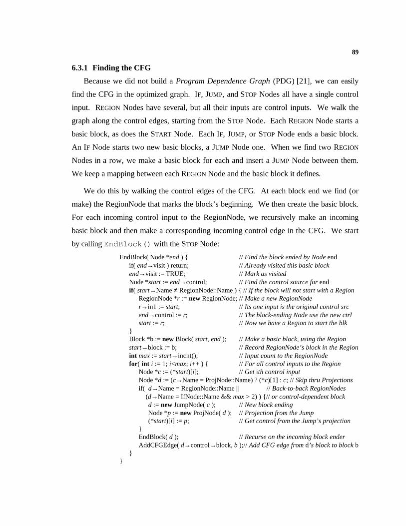
89

6.3.1 Finding the CFG

Because we did not build a Program Dependence Graph (PDG) [21], we can easily

find the CFG in the optimized graph. IF, JUMP, and STOP Nodes all have a single control

input. REGION Nodes have several, but all their inputs are control inputs. We walk the

graph along the control edges, starting from the STOP Node. Each REGION Node starts a

basic block, as does the START Node. Each IF, JUMP, or STOP Node ends a basic block.

An IF Node starts two new basic blocks, a JUMP Node one. When we find two REGION

Nodes in a row, we make a basic block for each and insert a JUMP Node between them.

We keep a mapping between each REGION Node and the basic block it defines.

We do this by walking the control edges of the CFG. At each block end we find (or

make) the RegionNode that marks the block’s beginning. We then create the basic block.

For each incoming control input to the RegionNode, we recursively make an incoming

basic block and then make a corresponding incoming control edge in the CFG. We start

by calling EndBlock() with the STOP Node:

EndBlock( Node *end ) { // Find the block ended by Node endif( end→visit ) return; // Already visited this basic blockend→visit := TRUE; // Mark as visitedNode *start := end→control; // Find the control source for endif ( start→Name ≠ RegionNode::Name ) { // If the block will not start with a Region

RegionNode *r := new RegionNode;// Make a new RegionNoder→in1 := start; // Its one input is the original control srcend→control := r; // The block-ending Node use the new ctrlstart := r; // Now we have a Region to start the blk

}Block *b := new Block( start, end ); // Make a basic block, using the Regionstart→block := b; // Record RegionNode’s block in the Regionint max := start→incnt(); // Input count to the RegionNodefor ( int i := 1; i<max; i++ ) { // For all control inputs to the Region

Node *c := (*start)[i]; // Get ith control inputNode *d := (c→Name = ProjNode::Name) ? (*c)[1] : c; // Skip thru Projectionsif( d→Name = RegionNode::Name || // Back-to-back RegionNodes (d→Name = IfNode::Name && max > 2) ) {// or control-dependent block

d := new JumpNode( c ); // New block endingNode *p := new ProjNode( d ); // Projection from the Jump(*start)[i] := p; // Get control from the Jump’s projection

}EndBlock( d ); // Recurse on the incoming block enderAddCFGEdge( d→control→block, b );// Add CFG edge from d’s block to block b

}}

90

This algorithm makes a simple DFS over the program graph. It visits 2 Nodes for

each basic block in the final CFG, so takes time linear in the CFG size. After running on

our example program fragment, we have the CFG and graph given in Figure 6.3. REGION

and JUMP Nodes have been inserted to complete the first and third basic blocks. The con-

trol-flow related Nodes are shown with the corresponding basic block.

PHI

ADD

>

IF

0

1

i0

i1

i2

cc

loop back control

loop exit data

read() a

ADD b

2

MUL c

10

START

JUMP

REGION

REGION

loop exit control

Figure 6.3 Our loop example, after finding the CFG

6.3.2 Dominators and Loops

With the CFG in hand, we find the dominator tree by running Lengauer and Tarjan’s

fast dominator finding algorithm [35]. We find loops using a slightly modified version of

Tarjan’s “Testing flow graph reducibility” [44]. Chris Vick has an excellent write-up of

the modifications and on building the loop tree [47]. We used his algorithm directly, and

only mention the high points here.

1. The CFG is visited in a pre-order Depth First Search (DFS).

2. Any edge going from a high pre-order to a lower pre-order is a loop back-edge.

3. All blocks on a path from the loop exit to the loop header are in the loop.

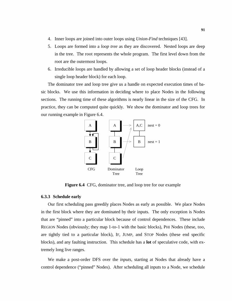
91

4. Inner loops are joined into outer loops using Union-Find techniques [43].

5. Loops are formed into a loop tree as they are discovered. Nested loops are deep

in the tree. The root represents the whole program. The first level down from the

root are the outermost loops.

6. Irreducible loops are handled by allowing a set of loop header blocks (instead of a

single loop header block) for each loop.

The dominator tree and loop tree give us a handle on expected execution times of ba-

sic blocks. We use this information in deciding where to place Nodes in the following

sections. The running time of these algorithms is nearly linear in the size of the CFG. In

practice, they can be computed quite quickly. We show the dominator and loop trees for

our running example in Figure 6.4.

nest = 0

CFG DominatorTree

LoopTree

nest = 1

A

B

A

C C

B B

A,C

Figure 6.4 CFG, dominator tree, and loop tree for our example

6.3.3 Schedule early

Our first scheduling pass greedily places Nodes as early as possible. We place Nodes

in the first block where they are dominated by their inputs. The only exception is Nodes

that are “pinned” into a particular block because of control dependences. These include

REGION Nodes (obviously; they map 1-to-1 with the basic blocks), PHI Nodes (these, too,

are tightly tied to a particular block), IF, JUMP, and STOP Nodes (these end specific

blocks), and any faulting instruction. This schedule has a lot of speculative code, with ex-

tremely long live ranges.

We make a post-order DFS over the inputs, starting at Nodes that already have a

control dependence (“pinned” Nodes). After scheduling all inputs to a Node, we schedule

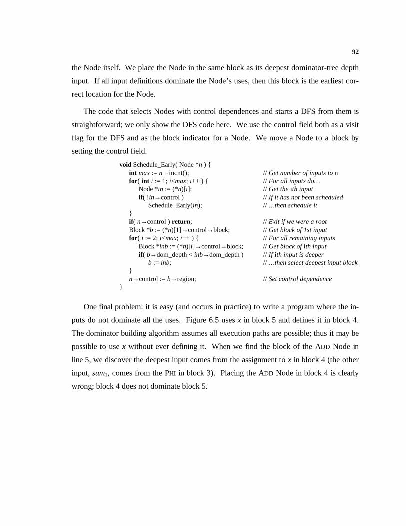
92

the Node itself. We place the Node in the same block as its deepest dominator-tree depth

input. If all input definitions dominate the Node’s uses, then this block is the earliest cor-

rect location for the Node.

The code that selects Nodes with control dependences and starts a DFS from them is

straightforward; we only show the DFS code here. We use the control field both as a visit

flag for the DFS and as the block indicator for a Node. We move a Node to a block by

setting the control field.

One final problem: it is easy (and occurs in practice) to write a program where the in-

puts do not dominate all the uses. Figure 6.5 uses x in block 5 and defines it in block 4.

The dominator building algorithm assumes all execution paths are possible; thus it may be

possible to use x without ever defining it. When we find the block of the ADD Node in

line 5, we discover the deepest input comes from the assignment to x in block 4 (the other

input, sum1, comes from the PHI in block 3). Placing the ADD Node in block 4 is clearly

wrong; block 4 does not dominate block 5.

void Schedule_Early( Node *n ) {int max := n→incnt(); // Get number of inputs to nfor ( int i := 1; i<max; i++ ) { // For all inputs do…

Node * in := (*n)[i]; // Get the ith inputif ( !in→control ) // If it has not been scheduled

Schedule_Early(in); // …then schedule it}if ( n→control ) return ; // Exit if we were a rootBlock *b := (*n)[1]→control→block; // Get block of 1st inputfor ( i := 2; i<max; i++ ) { // For all remaining inputs

Block *inb := (*n)[i]→control→block; // Get block of ith inputif ( b→dom_depth < inb→dom_depth ) // If ith input is deeper

b := inb; // …then select deepest input block}n→control := b→region; // Set control dependence

}

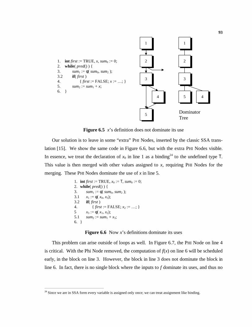
93

1. int first := TRUE, x, sum0 := 0;2. while( pred() ) {3. sum1 := φ( sum0, sum2 );3.2 if ( first )4. { first := FALSE; x := …; }5. sum2 := sum1 + x;6. }

1

2

3

4

5

1

2

3

45

DominatorTree

Figure 6.5 x’s definition does not dominate its use

Our solution is to leave in some “extra” PHI Nodes, inserted by the classic SSA trans-

lation [15]. We show the same code in Figure 6.6, but with the extra PHI Nodes visible.

In essence, we treat the declaration of x0 in line 1 as a binding24 to the undefined type T.

This value is then merged with other values assigned to x, requiring PHI Nodes for the

merging. These PHI Nodes dominate the use of x in line 5.

6. }

This problem can arise outside of loops as well. In Figure 6.7, the PHI Node on line 4

is critical. With the Phi Node removed, the computation of f(x) on line 6 will be scheduled

early, in the block on line 3. However, the block in line 3 does not dominate the block in

line 6. In fact, there is no single block where the inputs to f dominate its uses, and thus no

24 Since we are in SSA form every variable is assigned only once; we can treat assignment like binding.

1. int first := TRUE, x0 := T, sum0 := 0;2. while( pred() ) {3. sum1 := φ( sum0, sum2 );3.1 x1 := φ( x0, x3);3.2 if ( first )4. { first := FALSE; x2 := …; }5 x3 := φ( x1, x2);5.1 sum2 := sum1 + x3;

Figure 6.6 Now x’s definitions dominate its uses

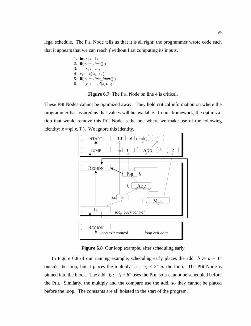
94

legal schedule. The PHI Node tells us that it is all right; the programmer wrote code such

that it appears that we can reach f without first computing its inputs.

These PHI Nodes cannot be optimized away. They hold critical information on where the

programmer has assured us that values will be available. In our framework, the optimiza-

tion that would remove this PHI Node is the one where we make use of the following

identity: x = φ( x, T ). We ignore this identity.

PHI

ADD

>

IF

0

1

i0

i1

i2

cc

loop back control

loop exit data

read() a

ADD b 2

MUL c

10START

JUMP

REGION

REGION loop exit control

Figure 6.8 Our loop example, after scheduling early

In Figure 6.8 of our running example, scheduling early places the add “b := a + 1”

outside the loop, but it places the multiply “c := i2 × 2” in the loop. The PHI Node is

pinned into the block. The add “i2 := i1 + b” uses the PHI, so it cannot be scheduled before

the PHI. Similarly, the multiply and the compare use the add, so they cannot be placed

before the loop. The constants are all hoisted to the start of the program.

1. int x0 := T;2. if ( sometime() )3. x1 := …;4. x2 := φ( x0, x1 );5. if ( sometime_later() )6. y := …f(x2)…;

Figure 6.7 The PHI Node on line 4 is critical.

95

6.3.4 Schedule late

We place Nodes at the lowest common ancestor (LCA) in the dominator tree of all

uses. Finding the LCA could take O(n) time for each Node, but in practice it is a small

constant. We use a post-order DFS over uses, starting from the “pinned” Nodes. After

visiting (and scheduling late) all of a Node’s children, we schedule the Node itself. Before

scheduling, it is in the earliest legal block; the LCA of its uses represents the latest legal

block. The earliest block dominates the latest block (guaranteed by the PHI Nodes we did

not remove). There is a line in the dominator tree from the latest to the earliest block; this

represents a safe range where we can place the Node. We can place the Node in any

block on this line. We choose the lowest (most control dependent) position in the shal-

lowest loop nest.

For most Nodes, uses occur in the same block as the Node itself. For PHI Nodes,

however, the use occurs in the previous block of the corresponding control edge. In

Figure 6.7 then, the use of x0 occurs in the block on line 2 (not in block 4, where the φ is)

and the use of x1 occurs in the block on line 3.

As before, the code that selects Nodes with control dependences and starts a DFS

from them is straightforward; we only show the DFS code here. Since the control field

now holds useful information (earliest legal block for this Node) we require an explicit

DFS visit flag.

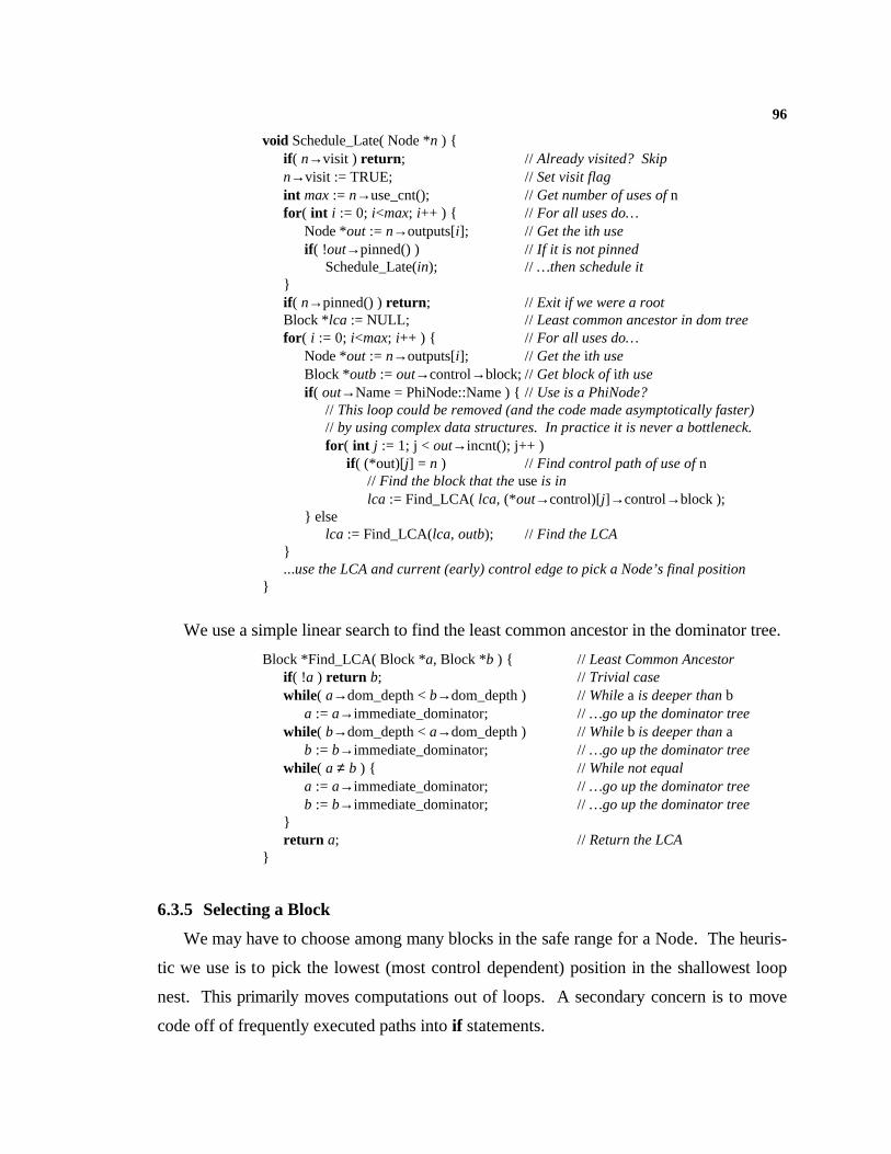
96

We use a simple linear search to find the least common ancestor in the dominator tree.

6.3.5 Selecting a Block

We may have to choose among many blocks in the safe range for a Node. The heuris-

tic we use is to pick the lowest (most control dependent) position in the shallowest loop

nest. This primarily moves computations out of loops. A secondary concern is to move

code off of frequently executed paths into if statements.

void Schedule_Late( Node *n ) {if ( n→visit ) return ; // Already visited? Skipn→visit := TRUE; // Set visit flagint max := n→use_cnt(); // Get number of uses of nfor ( int i := 0; i<max; i++ ) { // For all uses do…

Node *out := n→outputs[i]; // Get the ith useif ( !out→pinned() ) // If it is not pinned

Schedule_Late(in); // …then schedule it}if ( n→pinned() ) return ; // Exit if we were a rootBlock *lca := NULL; // Least common ancestor in dom treefor ( i := 0; i<max; i++ ) { // For all uses do…

Node *out := n→outputs[i]; // Get the ith useBlock *outb := out→control→block; // Get block of ith useif ( out→Name = PhiNode::Name ) {// Use is a PhiNode?

// This loop could be removed (and the code made asymptotically faster)// by using complex data structures. In practice it is never a bottleneck.for ( int j := 1; j < out→incnt(); j++ )

if ( (*out)[j] = n ) // Find control path of use of n// Find the block that the use is inlca := Find_LCA( lca, (*out→control)[j]→control→block );

} elselca := Find_LCA(lca, outb); // Find the LCA

}...use the LCA and current (early) control edge to pick a Node’s final position

}

Block *Find_LCA( Block *a, Block *b ) { // Least Common Ancestorif ( !a ) return b; // Trivial casewhile( a→dom_depth < b→dom_depth ) // While a is deeper than b

a := a→immediate_dominator; // …go up the dominator treewhile( b→dom_depth < a→dom_depth ) // While b is deeper than a

b := b→immediate_dominator; // …go up the dominator treewhile( a ≠ b ) { // While not equal

a := a→immediate_dominator; // …go up the dominator treeb := b→immediate_dominator; // …go up the dominator tree

}return a; // Return the LCA

}

97

When we select a Node’s final position, we affect other Nodes’ latest legal position.

In Figure 6.9, when the Node “b := a + 1” is scheduled before the loop, the latest legal

position for “1” is also before the loop. To handle this interaction, we select Nodes’ final

positions while we find the latest legal position. Here is the code to select a Node’s final

position:

...find LCA, the latest legal position for this Node. We already have the early block.Block *best := lca; // The best place for nwhile( lca ≠ n→control ) { // While not at earliest block do …

if( lca→loop→nest < best→loop→nest ) // Shallower loop nest?best := lca; // Save deepest block at shallower nest

lca := lca→immediate_dominator; // Walk up the dominator tree}n→control := best→region; // Set control dependence

}

The final schedule for our running example is in Figure 6.9. The MUL Node’s only use

was after the loop. Late scheduling starts at the LCA of all uses (the last block in the pro-

gram), and searches up the dominator tree for a shallower loop nest. In this case, the last

PHI

ADD

>

IF

0

1

i0

i1

i2

cc

loop back control

loop exit data

read() a

ADD b

2

MUL c

10START

JUMP

REGION

REGION

loop exit control

i0 := 0 a := read() c1 := 1 b := a + c1

c10 := 10

i1 := φ( i0, i2) i2 := i1 + b cc := i2 < c10

branch ne loop

c2 := 2 c := i2 × c2

…

Start:

loop:

Figure 6.9 Our loop example, after scheduling late

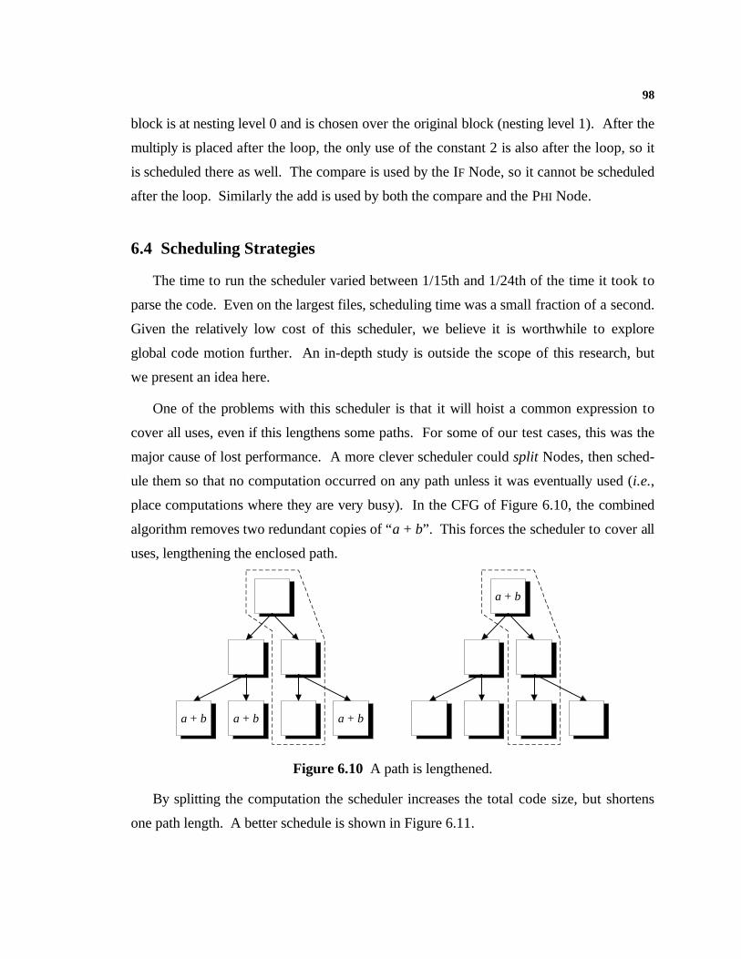
98

block is at nesting level 0 and is chosen over the original block (nesting level 1). After the

multiply is placed after the loop, the only use of the constant 2 is also after the loop, so it

is scheduled there as well. The compare is used by the IF Node, so it cannot be scheduled

after the loop. Similarly the add is used by both the compare and the PHI Node.

6.4 Scheduling Strategies

The time to run the scheduler varied between 1/15th and 1/24th of the time it took to

parse the code. Even on the largest files, scheduling time was a small fraction of a second.

Given the relatively low cost of this scheduler, we believe it is worthwhile to explore

global code motion further. An in-depth study is outside the scope of this research, but

we present an idea here.

One of the problems with this scheduler is that it will hoist a common expression to

cover all uses, even if this lengthens some paths. For some of our test cases, this was the

major cause of lost performance. A more clever scheduler could split Nodes, then sched-

ule them so that no computation occurred on any path unless it was eventually used (i.e.,

place computations where they are very busy). In the CFG of Figure 6.10, the combined

algorithm removes two redundant copies of “a + b”. This forces the scheduler to cover all

uses, lengthening the enclosed path.

a + b a + b a + b

a + b

Figure 6.10 A path is lengthened.

By splitting the computation the scheduler increases the total code size, but shortens

one path length. A better schedule is shown in Figure 6.11.

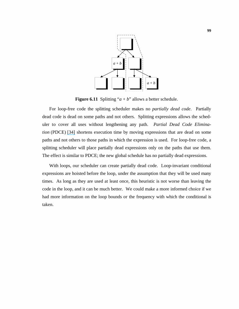
99

a + b

a + b

Figure 6.11 Splitting “a + b” allows a better schedule.

For loop-free code the splitting scheduler makes no partially dead code. Partially

dead code is dead on some paths and not others. Splitting expressions allows the sched-

uler to cover all uses without lengthening any path. Partial Dead Code Elimina-

tion (PDCE) [34] shortens execution time by moving expressions that are dead on some

paths and not others to those paths in which the expression is used. For loop-free code, a

splitting scheduler will place partially dead expressions only on the paths that use them.

The effect is similar to PDCE; the new global schedule has no partially dead expressions.

With loops, our scheduler can create partially dead code. Loop-invariant conditional

expressions are hoisted before the loop, under the assumption that they will be used many

times. As long as they are used at least once, this heuristic is not worse than leaving the

code in the loop, and it can be much better. We could make a more informed choice if we

had more information on the loop bounds or the frequency with which the conditional is

taken.

100

7. Parse-time Optimizations

100

Chapter 7

Parse-time Optimizations

7.1 Intr oduction

With a minor change to the parser, we can do optimization while parsing. Parse-time

optimizations remove simple constant computations and common subexpressions early on,

before the slower global optimizations. This reduces the peak memory required by the

optimizer and speeds the global optimizations that follow.

Parse-time optimizations must be pessimistic (as opposed to optimistic), because we

do not know what the not-yet-parsed program will do. They do not find as many con-

stants or common subexpressions as the global techniques, particularly around loops. For

this reason they are not a replacement for optimistic transformations.

Our pessimistic analysis requires only use-def information, which we can gather as we

parse the code. The compiler looks at (and changes) a fixed-size region of the intermedi-

ate representation. Code outside the region is not affected by the transformation; code

inside the region is transformed without knowledge of what is outside the region. Thus

our pessimistic analysis is also a local, or peephole, analysis. Optimistic transformations

require def-use information, generally not available during parsing, and global analysis (see

Section 2.3).

7.2 The Parser Design

The parser needs to build use-def information incrementally, because the peephole op-

timizations require it. Use-def information, in turn, relies on SSA form. So we want our

parser to build SSA form incrementally. We begin with building use-def information on

the fly.

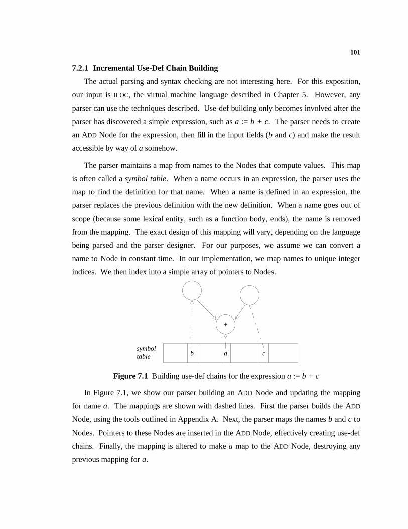
101

7.2.1 Incremental Use-Def Chain Building

The actual parsing and syntax checking are not interesting here. For this exposition,

our input is ILOC, the virtual machine language described in Chapter 5. However, any

parser can use the techniques described. Use-def building only becomes involved after the

parser has discovered a simple expression, such as a := b + c. The parser needs to create

an ADD Node for the expression, then fill in the input fields (b and c) and make the result

accessible by way of a somehow.

The parser maintains a map from names to the Nodes that compute values. This map

is often called a symbol table. When a name occurs in an expression, the parser uses the

map to find the definition for that name. When a name is defined in an expression, the

parser replaces the previous definition with the new definition. When a name goes out of

scope (because some lexical entity, such as a function body, ends), the name is removed

from the mapping. The exact design of this mapping will vary, depending on the language

being parsed and the parser designer. For our purposes, we assume we can convert a

name to Node in constant time. In our implementation, we map names to unique integer

indices. We then index into a simple array of pointers to Nodes.

ab c

+

symbol table

Figure 7.1 Building use-def chains for the expression a := b + c

In Figure 7.1, we show our parser building an ADD Node and updating the mapping

for name a. The mappings are shown with dashed lines. First the parser builds the ADD

Node, using the tools outlined in Appendix A. Next, the parser maps the names b and c to

Nodes. Pointers to these Nodes are inserted in the ADD Node, effectively creating use-def

chains. Finally, the mapping is altered to make a map to the ADD Node, destroying any

previous mapping for a.

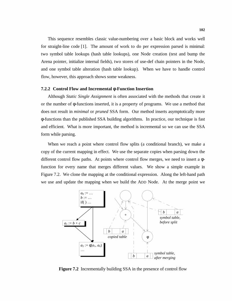
102

This sequence resembles classic value-numbering over a basic block and works well

for straight-line code [1]. The amount of work to do per expression parsed is minimal:

two symbol table lookups (hash table lookups), one Node creation (test and bump the

Arena pointer, initialize internal fields), two stores of use-def chain pointers in the Node,

and one symbol table alteration (hash table lookup). When we have to handle control

flow, however, this approach shows some weakness.

7.2.2 Control Flow and Incremental φφ-Function Insertion

Although Static Single Assignment is often associated with the methods that create it

or the number of φ-functions inserted, it is a property of programs. We use a method that

does not result in minimal or pruned SSA form. Our method inserts asymptotically more

φ-functions than the published SSA building algorithms. In practice, our technique is fast

and efficient. What is more important, the method is incremental so we can use the SSA

form while parsing.

When we reach a point where control flow splits (a conditional branch), we make a

copy of the current mapping in effect. We use the separate copies when parsing down the

different control flow paths. At points where control flow merges, we need to insert a φ-

function for every name that merges different values. We show a simple example in

Figure 7.2. We clone the mapping at the conditional expression. Along the left-hand path

we use and update the mapping when we build the ADD Node. At the merge point we

a0 := … b := … if( ) …

a1 := b + c

a2 := φ(a1, a0) …

ab+

φ

symbol table, before split

symbol table, after merging

copied table

ab

ab

Figure 7.2 Incrementally building SSA in the presence of control flow

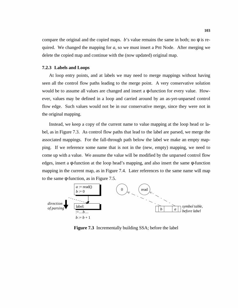
103

compare the original and the copied maps. b’s value remains the same in both; no φ is re-

quired. We changed the mapping for a, so we must insert a PHI Node. After merging we

delete the copied map and continue with the (now updated) original map.

7.2.3 Labels and Loops

At loop entry points, and at labels we may need to merge mappings without having

seen all the control flow paths leading to the merge point. A very conservative solution

would be to assume all values are changed and insert a φ-function for every value. How-

ever, values may be defined in a loop and carried around by an as-yet-unparsed control

flow edge. Such values would not be in our conservative merge, since they were not in

the original mapping.

Instead, we keep a copy of the current name to value mapping at the loop head or la-

bel, as in Figure 7.3. As control flow paths that lead to the label are parsed, we merge the

associated mappings. For the fall-through path below the label we make an empty map-

ping. If we reference some name that is not in the (new, empty) mapping, we need to

come up with a value. We assume the value will be modified by the unparsed control flow

edges, insert a φ-function at the loop head’s mapping, and also insert the same φ-function

mapping in the current map, as in Figure 7.4. Later references to the same name will map

to the same φ-function, as in Figure 7.5.

a := read() b := 0

ab symbol table, before label

label: direction of parsing

:=…b…

b := b + 1

0 read

Figure 7.3 Incrementally building SSA; before the label

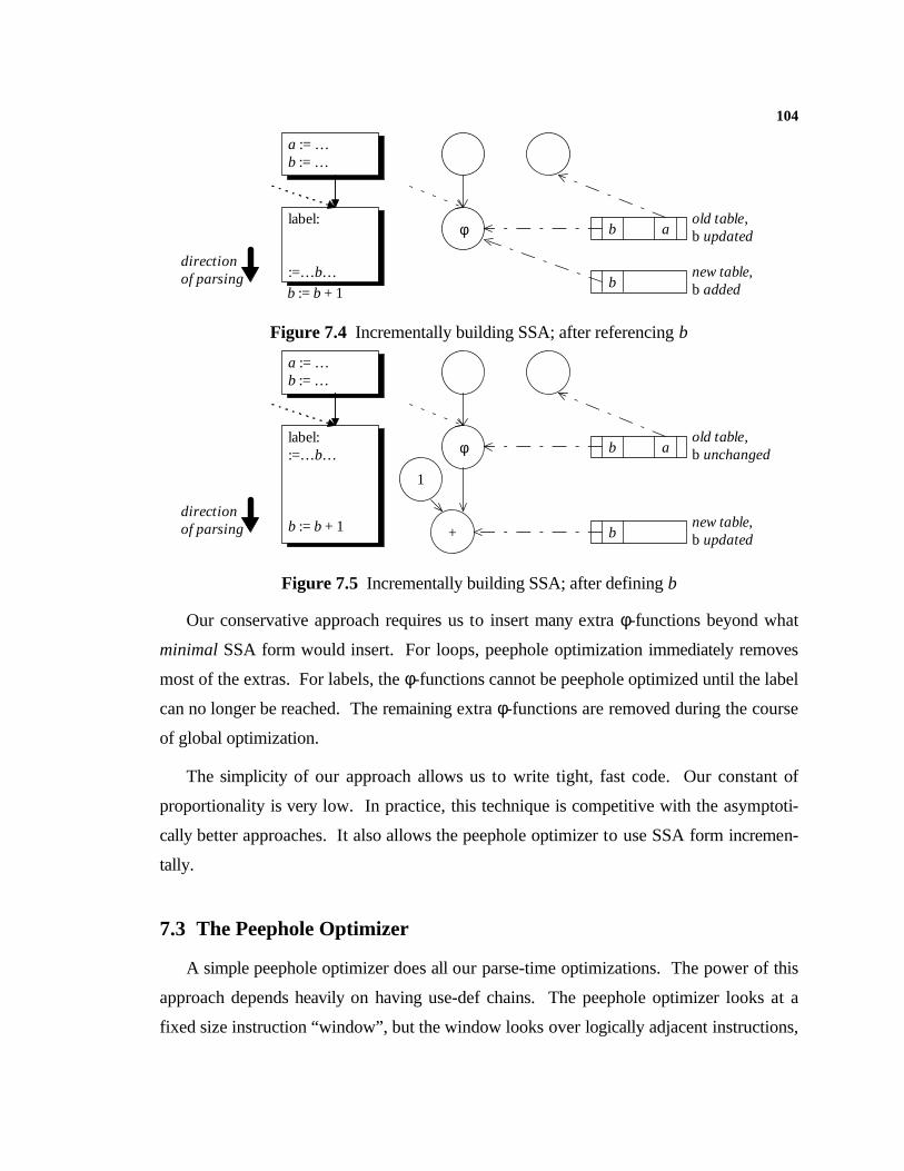
104

a := … b := …

label:

:=…b… direction of parsing

b := b + 1

φ b a

b

old table, b updated

new table, b added

Figure 7.4 Incrementally building SSA; after referencing b

a := … b := …

label: :=…b…

b := b + 1 direction of parsing

φ b a

b

old table, b unchanged

new table, b updated+

1

Figure 7.5 Incrementally building SSA; after defining b

Our conservative approach requires us to insert many extra φ-functions beyond what

minimal SSA form would insert. For loops, peephole optimization immediately removes

most of the extras. For labels, the φ-functions cannot be peephole optimized until the label

can no longer be reached. The remaining extra φ-functions are removed during the course

of global optimization.

The simplicity of our approach allows us to write tight, fast code. Our constant of

proportionality is very low. In practice, this technique is competitive with the asymptoti-

cally better approaches. It also allows the peephole optimizer to use SSA form incremen-

tally.

7.3 The Peephole Optimizer

A simple peephole optimizer does all our parse-time optimizations. The power of this

approach depends heavily on having use-def chains. The peephole optimizer looks at a

fixed size instruction “window”, but the window looks over logically adjacent instructions,

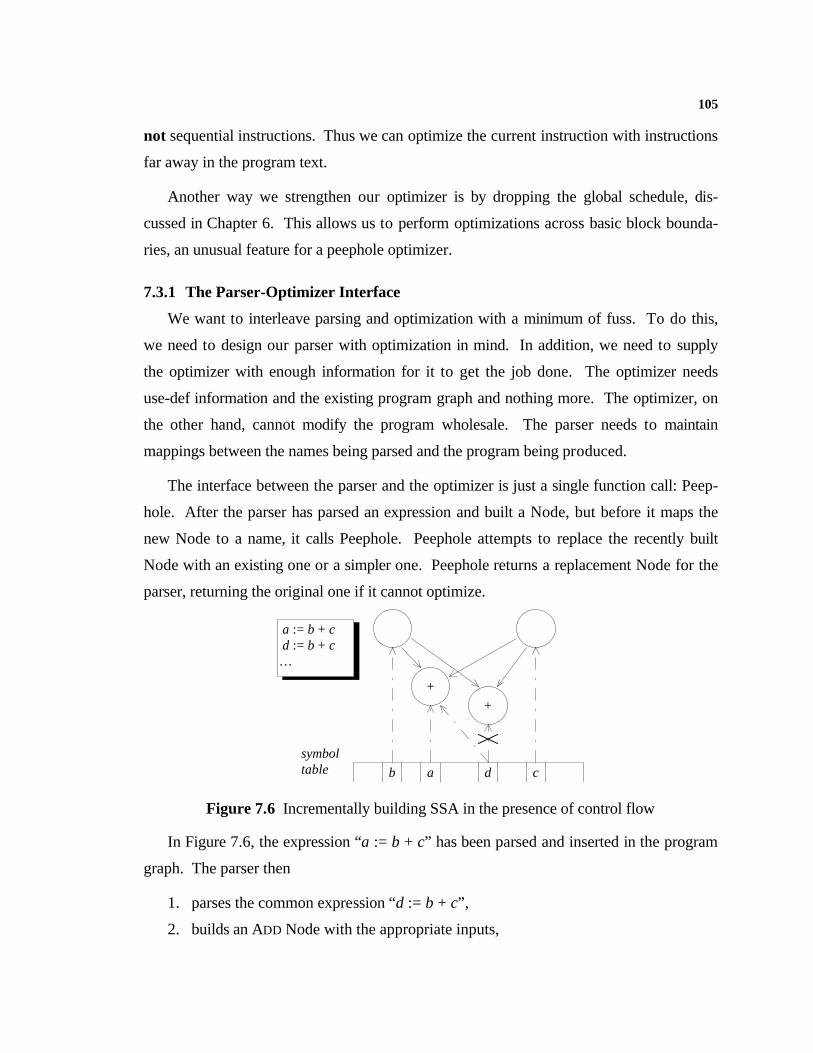
105

not sequential instructions. Thus we can optimize the current instruction with instructions

far away in the program text.

Another way we strengthen our optimizer is by dropping the global schedule, dis-

cussed in Chapter 6. This allows us to perform optimizations across basic block bounda-

ries, an unusual feature for a peephole optimizer.

7.3.1 The Parser-Optimizer Interface

We want to interleave parsing and optimization with a minimum of fuss. To do this,

we need to design our parser with optimization in mind. In addition, we need to supply

the optimizer with enough information for it to get the job done. The optimizer needs

use-def information and the existing program graph and nothing more. The optimizer, on

the other hand, cannot modify the program wholesale. The parser needs to maintain

mappings between the names being parsed and the program being produced.

The interface between the parser and the optimizer is just a single function call: Peep-

hole. After the parser has parsed an expression and built a Node, but before it maps the

new Node to a name, it calls Peephole. Peephole attempts to replace the recently built

Node with an existing one or a simpler one. Peephole returns a replacement Node for the

parser, returning the original one if it cannot optimize.

+

b

symbol table

a := b + c d := b + c…

+

a d c

Figure 7.6 Incrementally building SSA in the presence of control flow

In Figure 7.6, the expression “a := b + c” has been parsed and inserted in the program

graph. The parser then

1. parses the common expression “d := b + c”,

2. builds an ADD Node with the appropriate inputs,

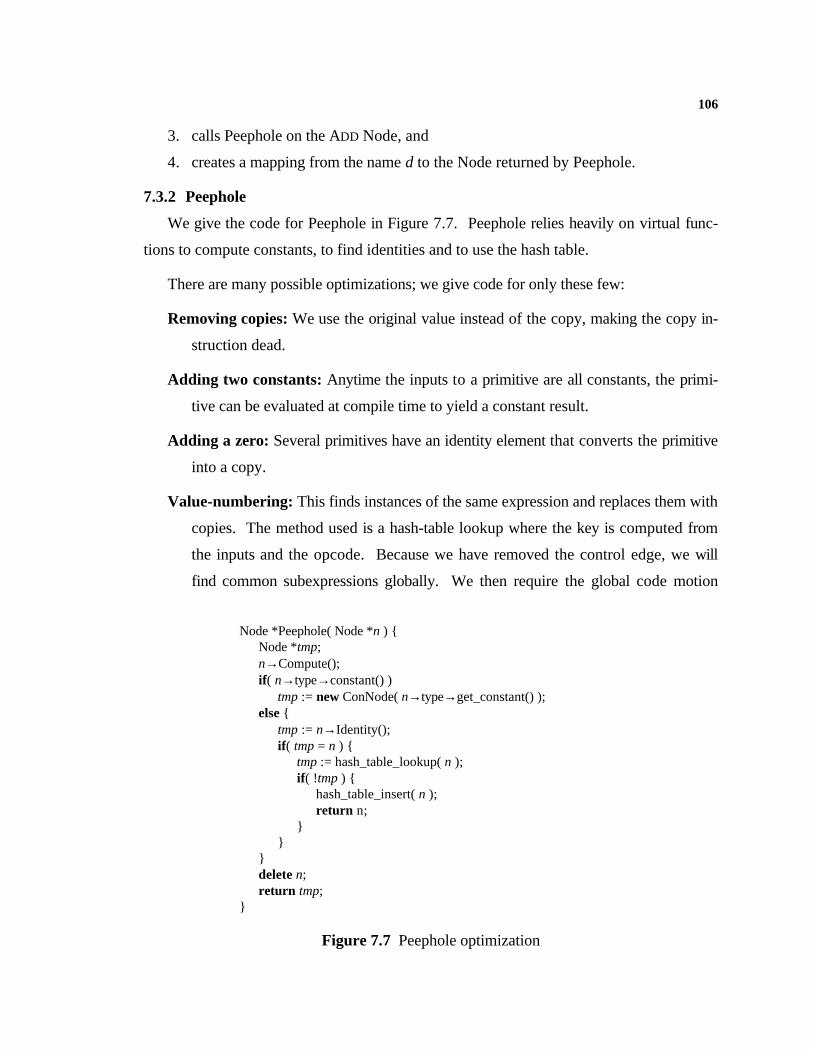
106

3. calls Peephole on the ADD Node, and

4. creates a mapping from the name d to the Node returned by Peephole.

7.3.2 Peephole

We give the code for Peephole in Figure 7.7. Peephole relies heavily on virtual func-

tions to compute constants, to find identities and to use the hash table.

There are many possible optimizations; we give code for only these few:

Removing copies: We use the original value instead of the copy, making the copy in-

struction dead.

Adding two constants: Anytime the inputs to a primitive are all constants, the primi-

tive can be evaluated at compile time to yield a constant result.

Adding a zero: Several primitives have an identity element that converts the primitive

into a copy.

Value-numbering: This finds instances of the same expression and replaces them with

copies. The method used is a hash-table lookup where the key is computed from

the inputs and the opcode. Because we have removed the control edge, we will

find common subexpressions globally. We then require the global code motion

Node *Peephole( Node *n ) {Node *tmp;n→Compute();if ( n→type→constant() )

tmp := new ConNode( n→type→get_constant() );else {

tmp := n→Identity();if ( tmp = n ) {

tmp := hash_table_lookup( n );if ( !tmp ) {

hash_table_insert( n );return n;

}}

}delete n;return tmp;

}

Figure 7.7 Peephole optimization

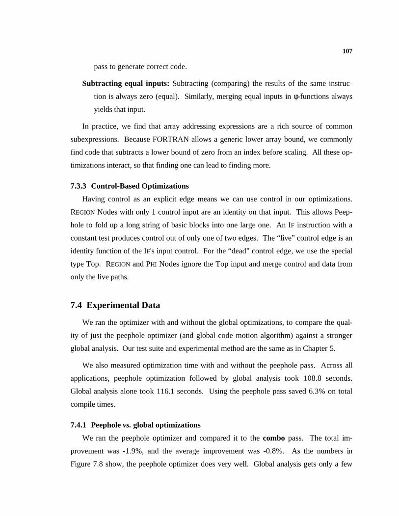
107

pass to generate correct code.

Subtracting equal inputs: Subtracting (comparing) the results of the same instruc-

tion is always zero (equal). Similarly, merging equal inputs in φ-functions always

yields that input.

In practice, we find that array addressing expressions are a rich source of common

subexpressions. Because FORTRAN allows a generic lower array bound, we commonly

find code that subtracts a lower bound of zero from an index before scaling. All these op-

timizations interact, so that finding one can lead to finding more.

7.3.3 Control-Based Optimizations

Having control as an explicit edge means we can use control in our optimizations.

REGION Nodes with only 1 control input are an identity on that input. This allows Peep-

hole to fold up a long string of basic blocks into one large one. An IF instruction with a

constant test produces control out of only one of two edges. The “live” control edge is an

identity function of the IF's input control. For the “dead” control edge, we use the special

type Top. REGION and PHI Nodes ignore the Top input and merge control and data from

only the live paths.

7.4 Experimental Data

We ran the optimizer with and without the global optimizations, to compare the qual-

ity of just the peephole optimizer (and global code motion algorithm) against a stronger

global analysis. Our test suite and experimental method are the same as in Chapter 5.

We also measured optimization time with and without the peephole pass. Across all

applications, peephole optimization followed by global analysis took 108.8 seconds.

Global analysis alone took 116.1 seconds. Using the peephole pass saved 6.3% on total

compile times.

7.4.1 Peephole vs. global optimizations

We ran the peephole optimizer and compared it to the combo pass. The total im-

provement was -1.9%, and the average improvement was -0.8%. As the numbers in

Figure 7.8 show, the peephole optimizer does very well. Global analysis gets only a few

108

percentage points more improvement. Rather suprisingly, this means that most constants

and common subexpressions are easy to find.

7.5 Summary

We found that most constants and common subexpressions are easy to find; they can

be found using a simple peephole analysis technique. This peephole analysis was done at

parse-time, lowering total compilation time by over 6%. To do strong peephole analysis

at parse-time requires SSA form and use-def chains. We implemented a parser that builds

SSA form and use-def chains incrementally, while parsing.

Speedup over unoptimized code Speedup over unoptimized codecombo, combo, Cycles % combo, combo, Cycles %

Routine global parse saved speedup Routine global parse saved speedup

cardeb 5.25 5.25 0 0.0% supp 1.90 1.90 0 0.0%coeray 1.95 1.95 0 0.0% urand 2.26 2.26 0 0.0%colbur 2.50 2.50 0 0.0% x21y21 3.44 3.44 0 0.0%dcoera 1.97 1.97 0 0.0% xaddrow 2.39 2.39 0 0.0%drepvi 3.20 3.20 0 0.0% xload 2.65 2.65 0 0.0%drigl 3.49 3.49 0 0.0% yeh 2.08 2.08 0 0.0%fehl 2.87 2.87 0 0.0% gamgen 5.43 5.43 -1 0.0%fmin 1.88 1.88 0 0.0% xielem 2.53 2.53 -2,767 0.0%fmtgen 2.58 2.58 0 0.0% inithx 4.36 4.36 -3 -0.1%fmtset 3.51 3.51 0 0.0% debico 6.38 6.39 -558 -0.1%fpppp 4.31 4.31 0 0.0% zeroin 1.95 1.95 -1 -0.1%heat 2.41 2.41 0 0.0% twldrv 3.78 3.79 -170,568 -0.2%hmoy 4.37 4.37 0 0.0% chpivot 2.61 2.63 -22,263 -0.5%iniset 3.00 3.00 0 0.0% debflu 5.25 5.29 -5,394 -0.8%integr 4.41 4.41 0 0.0% deseco 5.24 5.28 -17,575 -0.8%orgpar 3.25 3.25 0 0.0% paroi 4.76 4.80 -4,810 -0.9%repvid 4.08 4.08 0 0.0% inideb 5.22 5.30 -13 -1.5%rkf45 2.49 2.49 0 0.0% solve 3.02 3.07 -6 -1.8%rkfs 2.66 2.66 0 0.0% bilan 5.85 5.98 -12,025 -2.3%saturr 2.12 2.12 0 0.0% decomp 2.67 2.73 -15 -2.4%saxpy 3.56 3.56 0 0.0% ddeflu 3.30 3.40 -37,555 -2.9%seval 2.25 2.25 0 0.0% tomcatv 5.18 5.35 -7,805,918 -3.2%sgemm 2.46 2.46 0 0.0% ihbtr 2.38 2.46 -2,418 -3.3%sgemv 3.36 3.36 0 0.0% prophy 6.90 7.14 -18,786 -3.5%si 2.06 2.06 0 0.0% svd 2.81 2.91 -158 -3.6%spline 4.22 4.22 0 0.0% pastem 3.57 3.79 -36,260 -6.2%subb 1.89 1.89 0 0.0% efill 2.04 2.16 -118,983 -6.2%

Figure 7.8 Peephole vs global optimizations

109

8. Summary and Future Directions

109

Chapter 8

Summary and Future Directions

8.1 Futur e Directions

The combined algorithm is powerful, but not so powerful that it can not be extended

again. Currently, the constant propagation lattice supports floating-point and double pre-

cision constants, integer ranges with a stride and code address (label) constants (useful for

tracking indirect jumps and function calls). We could enhance the lattice to support

propagation of pointer constants, as a first step in doing pointer analysis. We could also

enhance the congruence finding portion, by using dominance information or by allowing

Nodes to be congruent within an affine function.

8.1.1 Improving Memory Analysis

Right now the memory analysis is very weak: the analysis lumps all arrays and vari-

ables into one simple state. We could clearly generate a more precise (and larger) pro-

gram graph by breaking this state up into pieces. We would generate one STORE for each

chunk of memory not dynamically allocated. These would all be produced by the START

Node, and sliced out by the appropriate PROJECTION. LOADs and STOREs to specific

STOREs would have a dependence to the right PROJECTION. The analysis can handle alias-

ing by forcing many STOREs to mingle in a UNION Node. LOADs from the UNION would

be affected by any STORE to the component parts, but not by unrelated STOREs. After a

STORE to a UNION (perhaps required because of an aliased address), the combined STOREs

would again be split apart to allow more precise analysis to follow.

8.1.2 Incremental Dominators and the PDG

Currently, our REGION Nodes connect to one another in the style of a CFG. The con-

trol edges correspond closely with the edges in a CFG, so that constructing a CFG from

the program graph is a simple exercise. A more powerful representation is an operator-

110

level PDG [21]. Here, control edges denote control dependence, a stronger notion than

the edges in a CFG. We could use PDG-like control edges instead of CFG-like control

edges to find more constants and congruences.

Here a and b clearly compute the same value. However, using the CFG notion of

control edges our intermediate representation will not discover this. Basically, the name a

is mapped to a φ-function merging 1 and 2, depending on a test of x in the first IF Node.

The name b is equivalent, except that the φ-function depends on the second IF Node. The

two IF Nodes are not equivalent; the first IF takes control from above and the second If

takes control from the merge point below the first IF.

Control dependence would allow the merged control below the first IF to be equiva-

lent to the control above the first IF. The two IF Nodes would take in congruent inputs

(same control, same test of x) and have equivalent opcodes. Analysis would find that they

are congruent. Likewise the two φ-functions will then be found congruent.

Building a PDG requires dominator information. To build the PDG in a combined al-

gorithm would require some type of incremental dominator algorithm. Control edges are

dead until proven reachable in the combined algorithm. As the algorithm finds control

flow-like edges to be reachable, the edges are (in essence) inserted into the CFG. The

CFG’s dominator tree would then need updating, possibly breaking some congruences

based on dominator information.

The advantage of building a PDG is the discovery of more congruences. The disad-

vantage is that serialization is more difficult. Some recent work has been done on serializ-

ing an operator-level PDG, but not in time for this work [40].

8.1.3 Loops and Induction Variables

One of the more powerful optimizations relies on discovering periodicity in the pro-

gram. Induction variable elimination and strength reduction take advantage of regular re-

curring patterns of computation. Our optimizations work on a Node (conditional constant

if ( x ) then a := 1;else a := 2;if ( x ) then b := 1;else b := 2;

111

propagation) or between two Nodes (congruence finding) but not on whole loops. We

would like to discover a way to fold entire loops into our analysis.

Currently, the congruence finding algorithm works around loops and will find congru-

ences between equivalent induction variables. However, it will not discover induction

variables related by an affine function. We could enhance our congruence finding by al-

lowing two Nodes to be affine-congruent if they are congruent within an affine function.

In each partition we would choose a base Node. Other Nodes would be related to the

base Node by an affine function kept for each Node during analysis.

Under the old congruences, two Nodes compute the same value if they are in the same

partition. In different partitions we cannot make any claim about whether they never have

the same value. If two Nodes are affine-congruent, then we can state whether they defi-

nitely compute the same value (same scale and offset) or never compute the same value

(same scale and different offset) or we can make no claim (different scale and offset).

With this analysis the combined algorithm would find congruences between induction

variables related by an affine function.

8.1.4 Commutativity

Two expressions “a + b” and “b + a” should be congruent. Our current combined al-

gorithm does not find them congruent, because the inputs to addition are treated as being

ordered. We partially alleviate this by placing all inputs in some canonical order during

our parse-time optimizations. However, sorting the inputs does not handle the more gen-

eral problem of discovering “a + b” and “d + c” to be congruent knowing that a and c are

congruent, as are b and d. Ordering the inputs requires that we know the a,c and b,d con-

gruences before we look for the (a + b),(d + c) congruence. We can construct an example

where the congruences are linked; to discover one requires discovering the other and vice-

versa. To avoid this phase-ordering problem we need to extend the combined algorithm

to discover these congruences optimistically.

112

8.2 Summary

We defined what it means to use the optimistic assumption: discover the facts in our

analysis in a top-down, instead of a bottom-up, fashion. Assume the best; all expressions

are undefined (instead of constant or unknown), all code is unreachable, and all expres-

sions are congruent. Then prove what is actually a constant, reachable or not congruent.

Similar to an inductive proof, you get to use the facts you assumed until proven otherwise.

In the presence of cycles in the analysised dependences, using the optimistic assumption

can allow you to find more facts.

We used the optimistic assumption in defining a very general framework for combining

optimizations. We showed a simple method to finding the optimistic solution to an analy-

sis in the framework. We showed how to mix, or combine, analyses, and under what

conditions the combined analysis would remain solvable and profitable. We then com-

bined Conditional Constant Propagation and Value Numbering. Because Value Number-

ing introduces an O(n2) number of equations, our solution time was also O(n2).

We then introduced a more complex algorithm that finds the solution to the combined

Conditional Constant Propagation and Value Numbering in O(n log n) time. The com-

bined algorithm is based on Hopcroft’s DFA minimization algorithm, then extended by

Alpern, Wegman and Zadeck to find congruences in program graphs. We extended the

algorithm again to propagate constants while finding congruences. We then introduced

other forms of congruences: those caused by constants and algebraic identities.

We ran a series of experiments to determine (1) if the combined algorithm improved

program run times over compiling with a series of separate phases and (2) if the combined

algorithm ran fast enough to be competitive. We discovered that the combined algorithm

improved some codes by as much as 30%, while almost never slowing down any code.

The combined algorithm was competitive in compile times as well, running about 1%

faster than a single pass of the separate pieces when counting optimization time alone. If

more separate optimization passes are desired (to get improved running times) the com-

bined algorithm becomes significantly faster. When we counted both parse-times and

compile-times, the combined algorithm was also significantly faster.

113

By dropping the control edges from data computing Nodes, we allowed the combined

algorithm to discover global congruences. However, Nodes without control edges exist in

a “sea of Nodes”, with no obvious serial order. To serialize the program graph, we must

find a global schedule. We presented an algorithm for globally scheduling the program

graph. We first discover the CFG, dominators and loops. We then schedule early, hoist-

ing code out of loops but making much speculative code and long live ranges. We then

schedule late, making code more control dependent as long as it does not go into any

loop. This scheduling is extremely fast and often hoists more code out of loops than Par-

tial Redundancy Elimination.

Because our intermediate representation has explicit use-def chains, we can perform

strong peephole optimizations on it. Peephole optimizations are a form of pessimistic

analysis and cannot find as many constants and congruences as analyses using the optimis-

tic assumption. Nonetheless, our peephole optimization finds most constants and congru-

ences. Since we can find use-def chains while we parse, we perform peephole optimiza-

tions while parsing. This speeds total compile time (parsing plus global optimization) by

6% and lowers peak memory. To find use-def chains while we parse, we presented a

method of building SSA form incrementally.

Finally we looked at a number of ways to improve the analysis. We can extend the

memory analysis to handle statically declared arrays and variables. We can use control

dependences as in the PDG. We can allow expressions to be congruent modulo an affine

function, allowing the combined algorithm to find induction variables.

We have shown that analyses can be combined, and that they can be profitably com-

bined. We have shown an O(n log n) algorithm for combining Conditional Constant

Propagation and Global Value Numbering. We ran experiments to prove that this combi-

nation runs fast in practice and improves program runtimes.

114

Bibliography

[1] A. Aho, R. Sethi, and J. Ullman. Compilers – Principles, Techniques, and Tools.

Addison-Wesley, 1985.

[2] B. Alpern, M. N. Wegman, and F. K. Zadeck. Detecting equality of variables in pro-

grams. In Conference Record of the Fifteenth ACM Symposium on the Principles of

Programming Languages, 1988.

[3] J. Backus. The History of FORTRAN I, II and III. In History of Programming La-

naguages, pages 25–45. Academic Press, 1981.

[4] R. A. Ballance, A. B. Maccabe, and K. J. Ottenstein. The program dependence web:

A representation supporting control-, data- and demand-driven interpretation of im-

perative languages. In Proceedings of the SIGPLAN ‘90 Conference on Program-

ming Languages Design and Implementation, June 1990.

[5] P. Briggs, Register Allocation via Graph Coloring. Ph.D. thesis, Rice University,

1992.

[6] P. Briggs. The Massively Scalar Compiler Project. Unpublished report. Preliminary

version available via ftp://cs.rice.edu/public/preston/optimizer/shared.ps. Rice Uni-

versity, July 1994.

[7] P. Briggs and K. Cooper. Effective partial redundancy elimination. In Proceedings

of the SIGPLAN ‘94 Conference on Programming Languages Design and Imple-

mentation, June 1994.

[8] P. Briggs and T. Harvey. Iloc '93. Technical report CRPC-TR93323, Rice Univer-

sity, 1993.

[9] R. Cartwright and M. Felleisen. The semantics of program dependence. In Proceed-

ings of the SIGPLAN ‘89 Conference on Programming Languages Design and Im-

plementation, June 1989.

115

[10] G. J. Chaitin. Register allocation and spilling via graph coloring. In Proceedings of

the SIGPLAN ‘82 Symposium on Compiler Construction, June 1982.

[11] D. R. Chase, M. N. Wegman, F. K. Zadeck. Analysis of pointers and structures. In

Proceedings of the SIGPLAN ‘90 Conference on Programming Languages Design

and Implementation, June 1990.

[12] J. Cocke. Global common subexpression elimination. In Proceedings of a Sympo-

sium on the Compiler Optimization, 1970.

[13] J. Cocke and J. T. Schwartz. Programming languages and their compilers. Cou-

rant Institute of Mathematical Sciences, New York University, April 1970.

[14] P. Cousot and R. Cousot. Systematic design of program analysis frameworks. In

Conference Record of the Sixth ACM Symposium on the Principles of Programming

Languages, pages 269–282, Jan. 1979.

[15] R. Cytron, J. Ferrante, B. K. Rosen, M. N. Wegman, and F. K. Zadeck. An efficient

method of computing static single assignment form. In Conference Record of the

Sixteenth ACM Symposium on the Principles of Programming Languages, Jan.

1989.

[16] J. W. Davidson and C. W. Fraser. Implementation of a retargetable peephole ana-

lyser. ACM Transactions on Programming Languages and Systems, 2(2):191, Apr.

1980.

[17] J. W. Davidson and C. W. Fraser. Code selection through object code optimization.

ACM Transactions on Programming Languages and Systems, 6(4):505–526, Oct.

1984.

[18] K. H. Drechsler and M. P. Stadel. A solution to a problem with Morel and Ren-

voise’s “Global optimization by suppression of partial redundancies”. ACM Trans-

actions on Programming Languages and Systems, 10(4):635–640, Oct. 1988.

[19] H. B. Enderton. A Mathematical Introduction to Logic. Academic Press, San Di-

ego, California 92101, 1972.

116

[20] G. E. Forstyhe, M. A. Malcom, and C. B. Moler. Computer Methods for Mathe-

matical Computations. Prentice-Hall, Englewood Cliffs, New Jersey, 1977.

[21] J. Ferrante, K. J. Ottenstein, and J. D. Warren. The program dependence graph and

its use in optimization. ACM Transactions on Programming Languages and Sys-

tems, 9(3):319–349, July, 1987.

[22] J. Field. A simple rewriting semantics for realistic imperative programs and its appli-

cation to program analysis. In Proceedings of the ACM SIGPLAN Workshop on

Partial Evaluation and Semantics-Based Program Manipulation, pages 98–107,

1990.

[23] C. W. Fraser and A. L. Wendt. Integrating code generation and optimization. In

Proceedings of the SIGPLAN ‘86 Symposium on Compiler Construction, June 1986.

[24] C. W. Fraser and A. L. Wendt. Automatic generation of fast optimizing code gen-

erators. In Proceedings of the ACM SIGPLAN ‘88 Conference on Programming

Languages Design and Implementation, June 1989.

[25] D. R. Hanson. Fast allocation and deallocation of memory based on object lifetimes.

Software Practice and Experience, 20(1):5–12, Jan. 1990.

[26] P. Havlak, Interprocedural Symbolic Analysis. Ph.D. thesis, Rice University, 1994.

[27] M. Hecht. Flow Analysis of Computer Programs. American Elsevier, North Hol-

land, 1977.

[28] J. E. Hopcroft. An n log n algorithm for minimizing the states of a finite automaton.

The Theory of Machines and Computations, pages 189–196, 1971.

[29] J. B. Kam and J. D. Ullman. Global data-flow analysis and iterative algorithms.

Journal of the ACM, 23(1):158-171, January 1976.

[30] J. B. Kam and J. D. Ullman. Monotone data-flow analysis frameworks. Acta Infor-

matica, 7, 1977.

[31] K. W. Kennedy. A survey of data-flow analysis techniques. In S. Muchnick and N.

Jones, editors, Program Flow Analysis, pages 5-54. Prentice-Hall, 1981.

117

[32] K. W. Kennedy. Use-definition chains with applications. Computer Languages, 3,

March 1978.

[33] G. A. Kildall. A unified approach to global program optimization. In Conference

Record of the First ACM Symposium on the Principles of Programming Languages,

Jan. 1979.

[34] J. Knoop, O. Rüthing, and B. Steffen. Partial dead code elimination. In Proceedings

of the SIGPLAN ‘94 Conference on Programming Languages Design and Imple-

mentation, June 1994.

[35] T. Lengauer and R. E. Tarjan. A fast algorithm for finding dominators in a flow-

graph. ACM Transactions on Programming Languages and Systems, 1(1):121–141,

July, 1979.

[36] E. Morel and C. Renvoise. Global optimization by suppression of partial redundan-

cies. Communications of the ACM, 22(2):96–103, Feb. 1979.

[37] B. K. Rosen., M. N. Wegman, and F. K. Zadeck, Global Value Numbers and Redun-

dant Computations. In Conference Record of the Fifteenth ACM Symposium on the

Principles of Programming Languages, Jan. 1988.

[38] R. K. Pingali, M. Beck, R. Johnson, M. Moudgill, and P. Stodghill. Dependence

flow graphs: An algebraic approach to program dependencies. Technical Report TR-

90–1152, Cornell University, 1990.

[39] R. P. Selke, A Semantic Framework for Program Dependence. Ph.D. thesis, Rice

University, 1992.

[40] B. Simons and J. Ferrante, An Efficient Algorithm for Constructing a Control Flow

Graph for Parallel Code. Technical report TR 03.465, IBM Technical Disclosure

Bulletin, Feb. 1993.

[41] T. Simpson, Global Value Numbering. Unpublished report. Available from

ftp://cs.rice.edu/public/preston/optimizer/gval.ps. Rice University, 1994.

118

[42] A. S. Tanenbaum, H. van Staveren, and J. W. Stevenson. Using peephole optimiza-

tion on intermediate code. ACM Transactions on Programming Languages and

Systems, 4(1):21-36, January 1982.

[43] R. E. Tarjan. Efficiency of a good but not linear set union algorithm. Journal of the

ACM, 22(2):215–225, 1975.

[44] R. E. Tarjan. Testing flow graph reducibility. Journal of Computer and System Sci-

ences, 9:355–365, 1974.

[45] R. E. Tarjan. A unified approach to path problems. Journal of the ACM, 28(3):577

–593, July 1981.

[46] A. Tarski. A lattice-theoretical fixpoint theorem and its applications. Pacific J.

Math, pages 285-309, 1955.

[47] C. Vick, SSA-Based Reduction of Operator Strength. Masters thesis, Rice Univer-

sity, pages 11–15, 1994.

[48] D. Weise, R. Crew, M. Ernst, and B. Steensgaard. Value dependence graphs: Rep-

resentation without taxation. In Proceedings of the 21st ACM SIGPLAN Symposium

on the Principles of Programming Languages, 1994.

[49] M. N. Wegman and F. K. Zadeck. Constant propagation with conditional branches.

ACM Transactions on Programming Languages and Systems, 13(2):181-210, April

1991.

[50] M. J. Wolfe. Beyond induction variables. In Proceedings of the SIGPLAN ‘92

Conference on Programming Languages Design and Implementation, June 1992.

119

A. Engineering

119

Appendix A

Engineering

A designer knows he has achieved perfection not when there is

nothing left to add, but when there is nothing left to take away.

— Antoine de Saint-Exup'ery (1900 -1944)†

A.1 Introduction

Intermediate representations do not exist in a vacuum. They are the stepping stone

from what the programmer wrote to what the machine understands. Intermediate repre-

sentations must bridge a large semantic gap (for example, from FORTRAN 90 vector op-

erations to a 3-address add in some machine code). During the translation from a high-

level language to machine code, an optimizing compiler repeatedly analyzes and trans-

forms the intermediate representation. As compiler users we want these analyses and

transformations to be fast and correct. As compiler writers we want optimizations to be

simple to write, easy to understand, and easy to change. Our goal is a representation that

is simple and lightweight while allowing easy expression of fast optimizations.

This chapter discusses the intermediate representation used in the compiler that im-

plements the analyses discussed in earlier chapters. The intermediate representation is a

graph-based, object-oriented structure, similar to an operator-level Program Dependence

Graph or Gated Single Assignment form [4, 21, 26, 38]. The final form contains all the

information required to execute the program. What is more important, the graph form

explicitly contains use-def information. Analyses can use this information directly without

having to calculate it. Transformations modify the use-def information directly without

requiring separate steps to modify the intermediate representation and the use-def infor-

† The French author, best known for his classic children's book “The Little Prince”, was also an aircraft designer.

120

mation. The graph form is a simple single-tiered structure instead of a two tiered Control-

Flow Graph containing basic blocks (tier 1) of instructions (tier 2). This single tier sim-

plifies the design and implementation of the combined algorithm.

A.1.1 Optimizations in the Front End

One of the reasons for having the intermediate representation contain use-def informa-

tion is that we can perform low-level pessimistic optimizations while we are parsing the

high-level input. These low-level optimizations (such as value numbering and constant

propagation) reduce the intermediate representation size, speeding later global optimistic

analyses. As we show in Chapter 7, these parse-time transformations by themselves do

almost as well as the global versions, but with significantly less compile-time cost.

Our pessimistic analysis requires use-def information and SSA form. We gather use-

def information and incrementally build SSA form as we parse the code. The compiler

looks at (and changes) a fixed-size region of the intermediate representation. The trans-

formation does not effect code outside the region. The analysis transforms code inside the

region without knowledge of what is outside the region.

A.1.2 Overview

In Section A.2, we introduce objects that make up our intermediate representation. In

Section A.3, we use C++'s inheritance to give more structure to our instructions and to

speed up their creation and deletion. In Section A.4, we drop the CFG altogether, replac-

ing it with instructions that deal with control. In Section A.5, we discuss how we handle a

variety of problematic instruction features, including subroutines, memory, and I/O. In

Section A.6 we look at related work, contrasting our intermediate representation with

other published representations. The rest of this chapter will demonstrate the intermediate

representation using concrete C++ code and the design decisions that lead us here.

A.2 Object-Oriented Intermediate Representation Design

The intermediate representation uses a simple 3-address, load/store, infinite register

virtual machine to represent programs. Internally we represent a virtual machine instruc-

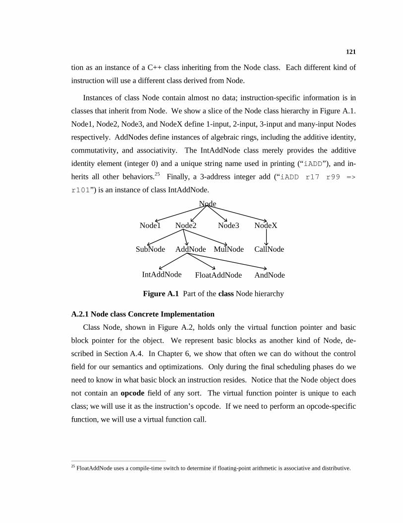
121

tion as an instance of a C++ class inheriting from the Node class. Each different kind of

instruction will use a different class derived from Node.

Instances of class Node contain almost no data; instruction-specific information is in

classes that inherit from Node. We show a slice of the Node class hierarchy in Figure A.1.

Node1, Node2, Node3, and NodeX define 1-input, 2-input, 3-input and many-input Nodes

respectively. AddNodes define instances of algebraic rings, including the additive identity,

commutativity, and associativity. The IntAddNode class merely provides the additive

identity element (integer 0) and a unique string name used in printing (“iADD”), and in-

herits all other behaviors.25 Finally, a 3-address integer add (“iADD r17 r99 =>

r101”) is an instance of class IntAddNode.

Node

Node1 Node2 Node3 NodeX

SubNode AddNode MulNode CallNode

IntAddNode FloatAddNode AndNode

Figure A.1 Part of the class Node hierarchy

A.2.1 Node class Concrete Implementation

Class Node, shown in Figure A.2, holds only the virtual function pointer and basic

block pointer for the object. We represent basic blocks as another kind of Node, de-

scribed in Section A.4. In Chapter 6, we show that often we can do without the control

field for our semantics and optimizations. Only during the final scheduling phases do we

need to know in what basic block an instruction resides. Notice that the Node object does

not contain an opcode field of any sort. The virtual function pointer is unique to each

class; we will use it as the instruction’s opcode. If we need to perform an opcode-specific

function, we will use a virtual function call.

25 FloatAddNode uses a compile-time switch to determine if floating-point arithmetic is associative and distributive.

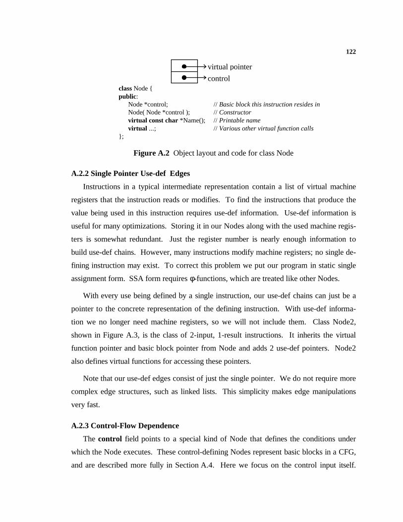
122

virtual pointer

controlclass Node {public:

Node *control; // Basic block this instruction resides inNode( Node *control ); // Constructorvirtual const char *Name(); // Printable namevirtual ...; // Various other virtual function calls

};

Figure A.2 Object layout and code for class Node

A.2.2 Single Pointer Use-def Edges

Instructions in a typical intermediate representation contain a list of virtual machine

registers that the instruction reads or modifies. To find the instructions that produce the

value being used in this instruction requires use-def information. Use-def information is

useful for many optimizations. Storing it in our Nodes along with the used machine regis-

ters is somewhat redundant. Just the register number is nearly enough information to

build use-def chains. However, many instructions modify machine registers; no single de-

fining instruction may exist. To correct this problem we put our program in static single

assignment form. SSA form requires φ-functions, which are treated like other Nodes.

With every use being defined by a single instruction, our use-def chains can just be a

pointer to the concrete representation of the defining instruction. With use-def informa-

tion we no longer need machine registers, so we will not include them. Class Node2,

shown in Figure A.3, is the class of 2-input, 1-result instructions. It inherits the virtual

function pointer and basic block pointer from Node and adds 2 use-def pointers. Node2

also defines virtual functions for accessing these pointers.

Note that our use-def edges consist of just the single pointer. We do not require more

complex edge structures, such as linked lists. This simplicity makes edge manipulations

very fast.

A.2.3 Control-Flow Dependence

The control field points to a special kind of Node that defines the conditions under

which the Node executes. These control-defining Nodes represent basic blocks in a CFG,

and are described more fully in Section A.4. Here we focus on the control input itself.

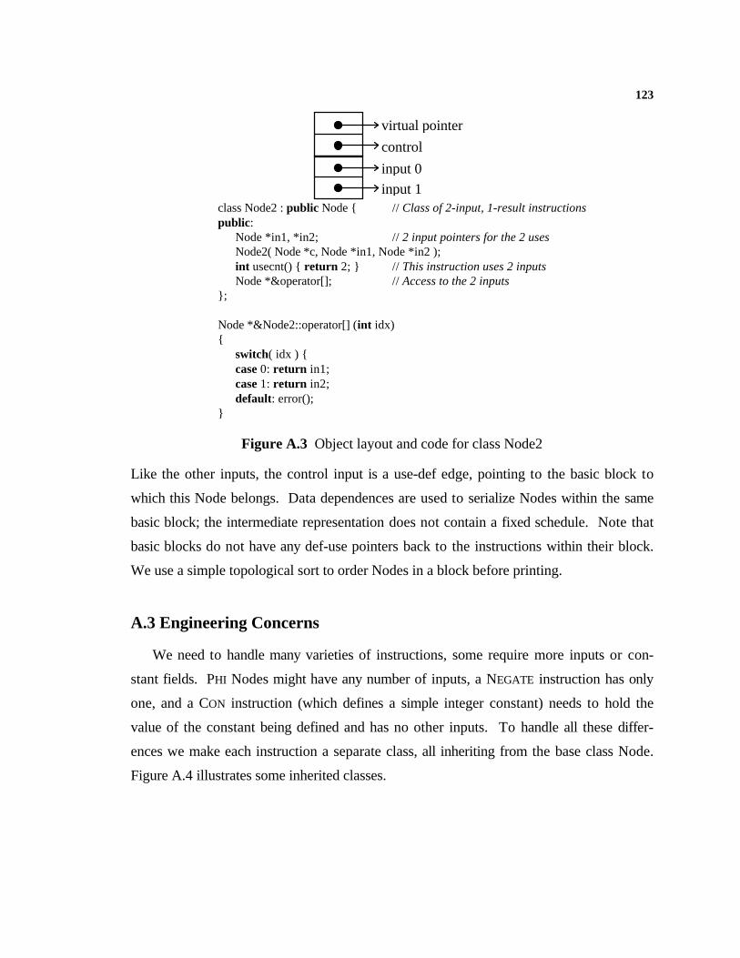
123

Like the other inputs, the control input is a use-def edge, pointing to the basic block to

which this Node belongs. Data dependences are used to serialize Nodes within the same

basic block; the intermediate representation does not contain a fixed schedule. Note that

basic blocks do not have any def-use pointers back to the instructions within their block.

We use a simple topological sort to order Nodes in a block before printing.

A.3 Engineering Concerns

We need to handle many varieties of instructions, some require more inputs or con-

stant fields. PHI Nodes might have any number of inputs, a NEGATE instruction has only

one, and a CON instruction (which defines a simple integer constant) needs to hold the

value of the constant being defined and has no other inputs. To handle all these differ-

ences we make each instruction a separate class, all inheriting from the base class Node.

Figure A.4 illustrates some inherited classes.

virtual pointer

control

input 0

input 1class Node2 : public Node { // Class of 2-input, 1-result instructionspublic:

Node *in1, *in2; // 2 input pointers for the 2 usesNode2( Node *c, Node *in1, Node *in2 );int usecnt() { return 2; } // This instruction uses 2 inputsNode *&operator[]; // Access to the 2 inputs

};

Node *&Node2::operator[] (int idx){

switch( idx ) {case 0: return in1;case 1: return in2;default: error();

}

Figure A.3 Object layout and code for class Node2

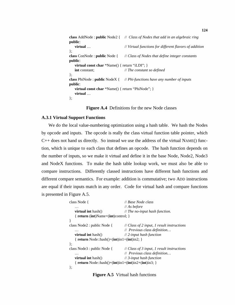
124

class AddNode : public Node2 { // Class of Nodes that add in an algebraic ringpublic:

virtual … // Virtual functions for different flavors of addition};class ConNode : public Node { // Class of Nodes that define integer constantspublic:

virtual const char *Name() { return “iLDI”; }int constant; // The constant so defined

};class PhiNode : public NodeX { // Phi-functions have any number of inputspublic:

virtual const char *Name() { return “PhiNode”; }virtual …

};

Figure A.4 Definitions for the new Node classes

A.3.1 Virtual Support Functions

We do the local value-numbering optimization using a hash table. We hash the Nodes

by opcode and inputs. The opcode is really the class virtual function table pointer, which

C++ does not hand us directly. So instead we use the address of the virtual NAME() func-

tion, which is unique to each class that defines an opcode. The hash function depends on

the number of inputs, so we make it virtual and define it in the base Node, Node2, Node3

and NodeX functions. To make the hash table lookup work, we must also be able to

compare instructions. Differently classed instructions have different hash functions and

different compare semantics. For example: addition is commutative; two ADD instructions

are equal if their inputs match in any order. Code for virtual hash and compare functions

is presented in Figure A.5.

class Node { // Base Node class… // As beforevirtual int hash() // The no-input hash function.{ return (int )Name+(int )control; }

}class Node2 : public Node { // Class of 2 input, 1 result instructions

… // Previous class definition…virtual int hash() // 2-input hash function{ return Node::hash()+(int )in1+(int )in2; }

};class Node3 : public Node { // Class of 3 input, 1 result instructions

… // Previous class definition…virtual int hash() // 3-input hash function{ return Node::hash()+(int )in1+(int )in2+(int )in3; }

};

Figure A.5 Virtual hash functions

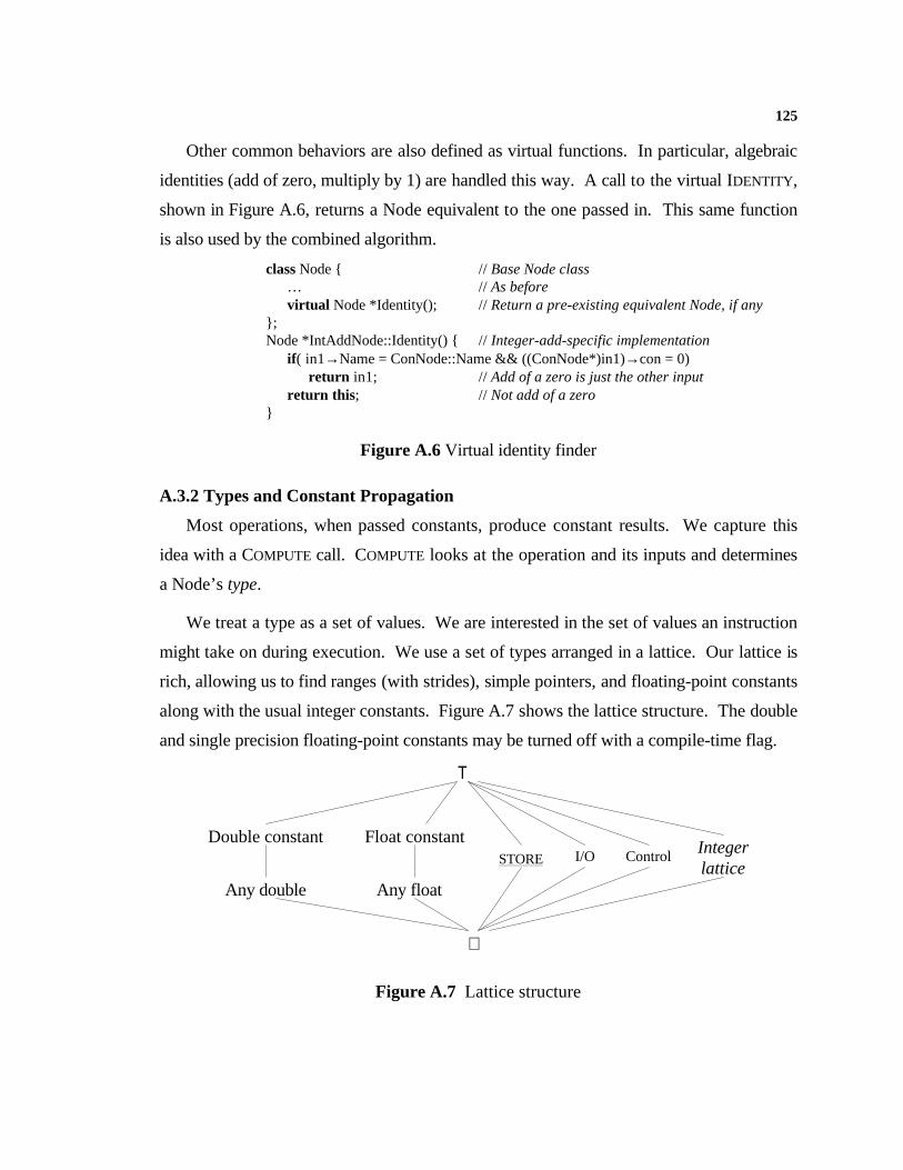
125

Other common behaviors are also defined as virtual functions. In particular, algebraic

identities (add of zero, multiply by 1) are handled this way. A call to the virtual IDENTITY,

shown in Figure A.6, returns a Node equivalent to the one passed in. This same function

is also used by the combined algorithm.

class Node { // Base Node class… // As beforevirtual Node *Identity(); // Return a pre-existing equivalent Node, if any

};Node *IntAddNode::Identity() { // Integer-add-specific implementation

if ( in1→Name = ConNode::Name && ((ConNode*)in1)→con = 0)return in1; // Add of a zero is just the other input

return this; // Not add of a zero}

Figure A.6 Virtual identity finder

A.3.2 Types and Constant Propagation

Most operations, when passed constants, produce constant results. We capture this

idea with a COMPUTE call. COMPUTE looks at the operation and its inputs and determines

a Node’s type.

We treat a type as a set of values. We are interested in the set of values an instruction

might take on during execution. We use a set of types arranged in a lattice. Our lattice is

rich, allowing us to find ranges (with strides), simple pointers, and floating-point constants

along with the usual integer constants. Figure A.7 shows the lattice structure. The double

and single precision floating-point constants may be turned off with a compile-time flag.

T

⊥

Double constant Float constant

Any double Any float

STORE I/O Control Integerlattice

Figure A.7 Lattice structure

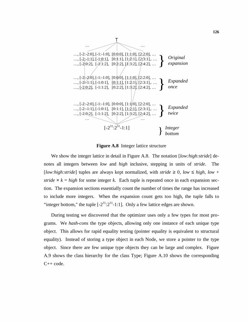
126

T

…, [-2:-2:0],[-1:-1:0], [0:0:0], [1:1:0], [2:2:0], ……, [-2:-1:1], [-1:0:1], [0:1:1], [1:2:1], [2:3:1],. ……, [-2:0:2], [-1:1:2], [0:2:2], [1:3:2], [2:4:2], …} Original

expansion

…, [-2:-2:0],[-1:-1:0], [0:0:0], [1:1:0], [2:2:0], ……, [-2:-1:1],[-1:0:1], [0:1:1], [1:2:1], [2:3:1],. ……, [-2:0:2], [-1:1:2], [0:2:2], [1:3:2], [2:4:2], …} Expanded

once

…, [-2:-2:0],[-1:-1:0], [0:0:0], [1:1:0], [2:2:0], ……, [-2:-1:1],[-1:0:1], [0:1:1], [1:2:1], [2:3:1],. ……, [-2:0:2], [-1:1:2], [0:2:2], [1:3:2], [2:4:2], … } Expanded

twice

[-231:231-1:1] } Integer bottom

… …

… …

Figure A.8 Integer lattice structure

We show the integer lattice in detail in Figure A.8. The notation [low:high:stride] de-

notes all integers between low and high inclusive, stepping in units of stride. The

[low:high:stride] tuples are always kept normalized, with stride ≥ 0, low ≤ high, low +

stride × k = high for some integer k. Each tuple is repeated once in each expansion sec-

tion. The expansion sections essentially count the number of times the range has increased

to include more integers. When the expansion count gets too high, the tuple falls to

“integer bottom," the tuple [-231:231-1:1]. Only a few lattice edges are shown.

During testing we discovered that the optimizer uses only a few types for most pro-

grams. We hash-cons the type objects, allowing only one instance of each unique type

object. This allows for rapid equality testing (pointer equality is equivalent to structural

equality). Instead of storing a type object in each Node, we store a pointer to the type

object. Since there are few unique type objects they can be large and complex. Figure

A.9 shows the class hierarchy for the class Type; Figure A.10 shows the corresponding

C++ code.

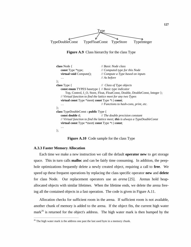
127

Type

TypeDoubleConst TypeFloatConst TypeStore TypeInteger

Figure A.9 Class hierarchy for the class Type

class Node { // Basic Node classconst Type *type; // Computed type for this Nodevirtual void Compute(); // Compute a Type based on inputs… // As before

};class Type { // Class of Type objects

const enum TYPES basetype { // Basic type indicatorTop, Control, I_O, Store, Float, FloatConst, Double, DoubleConst, Integer };

// Virtual function to find the lattice meet for any two Typesvirtual const Type *meet( const Type *t ) const;… // Functions to hash-cons, print, etc.

};class TypeDoubleConst : public Type {

const double d; // The double precision constant// Virtual function to find the lattice meet; this is always a TypeDoubleConstvirtual const Type *meet( const Type *t ) const;…

};

Figure A.10 Code sample for the class Type

A.3.3 Faster Memory Allocation

Each time we make a new instruction we call the default operator new to get storage

space. This in turn calls malloc and can be fairly time consuming. In addition, the peep-

hole optimizations frequently delete a newly created object, requiring a call to free. We

speed up these frequent operations by replacing the class specific operator new and delete

for class Node. Our replacement operators use an arena [25]. Arenas hold heap-

allocated objects with similar lifetimes. When the lifetime ends, we delete the arena free-

ing all the contained objects in a fast operation. The code is given in Figure A.11.

Allocation checks for sufficient room in the arena. If sufficient room is not available,

another chunk of memory is added to the arena. If the object fits, the current high water

mark26 is returned for the object's address. The high water mark is then bumped by the

26 The high water mark is the address one past the last used byte in a memory chunk.

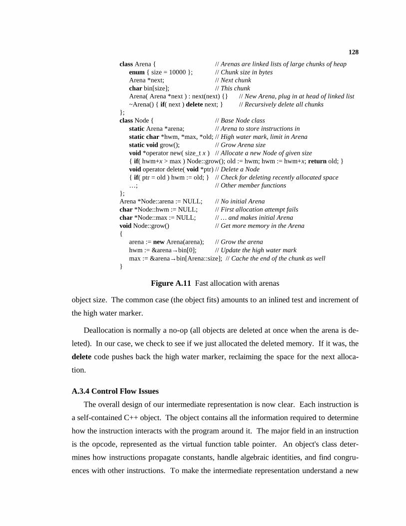
128

object size. The common case (the object fits) amounts to an inlined test and increment of

the high water marker.

Deallocation is normally a no-op (all objects are deleted at once when the arena is de-

leted). In our case, we check to see if we just allocated the deleted memory. If it was, the

delete code pushes back the high water marker, reclaiming the space for the next alloca-

tion.

A.3.4 Control Flow Issues

The overall design of our intermediate representation is now clear. Each instruction is

a self-contained C++ object. The object contains all the information required to determine

how the instruction interacts with the program around it. The major field in an instruction

is the opcode, represented as the virtual function table pointer. An object's class deter-

mines how instructions propagate constants, handle algebraic identities, and find congru-

ences with other instructions. To make the intermediate representation understand a new

class Arena { // Arenas are linked lists of large chunks of heapenum { size = 10000 }; // Chunk size in bytesArena *next; // Next chunkchar bin[size]; // This chunkArena( Arena *next ) : next(next) {} // New Arena, plug in at head of linked list~Arena() { if ( next ) delete next; } // Recursively delete all chunks

};class Node { // Base Node class

static Arena *arena; // Arena to store instructions instatic char *hwm, *max, *old; // High water mark, limit in Arenastatic void grow(); // Grow Arena sizevoid *operator new( size_t x ) // Allocate a new Node of given size{ if ( hwm+x > max ) Node::grow(); old := hwm; hwm := hwm+x; return old; }void operator delete( void *ptr) // Delete a Node{ if ( ptr = old ) hwm := old; } // Check for deleting recently allocated space…; // Other member functions

};Arena *Node::arena := NULL; // No initial Arenachar *Node::hwm := NULL; // First allocation attempt failschar *Node::max := NULL; // … and makes initial Arenavoid Node::grow() // Get more memory in the Arena{

arena := new Arena(arena); // Grow the arenahwm := &arena→bin[0]; // Update the high water markmax := &arena→bin[Arena::size]; // Cache the end of the chunk as well

}

Figure A.11 Fast allocation with arenas

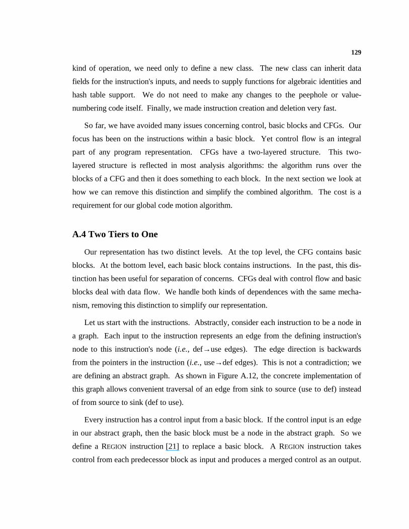
129

kind of operation, we need only to define a new class. The new class can inherit data

fields for the instruction's inputs, and needs to supply functions for algebraic identities and

hash table support. We do not need to make any changes to the peephole or value-

numbering code itself. Finally, we made instruction creation and deletion very fast.

So far, we have avoided many issues concerning control, basic blocks and CFGs. Our

focus has been on the instructions within a basic block. Yet control flow is an integral

part of any program representation. CFGs have a two-layered structure. This two-

layered structure is reflected in most analysis algorithms: the algorithm runs over the

blocks of a CFG and then it does something to each block. In the next section we look at

how we can remove this distinction and simplify the combined algorithm. The cost is a

requirement for our global code motion algorithm.

A.4 Two Tiers to One

Our representation has two distinct levels. At the top level, the CFG contains basic

blocks. At the bottom level, each basic block contains instructions. In the past, this dis-

tinction has been useful for separation of concerns. CFGs deal with control flow and basic

blocks deal with data flow. We handle both kinds of dependences with the same mecha-

nism, removing this distinction to simplify our representation.

Let us start with the instructions. Abstractly, consider each instruction to be a node in

a graph. Each input to the instruction represents an edge from the defining instruction's

node to this instruction's node (i.e., def→use edges). The edge direction is backwards

from the pointers in the instruction (i.e., use→def edges). This is not a contradiction; we

are defining an abstract graph. As shown in Figure A.12, the concrete implementation of

this graph allows convenient traversal of an edge from sink to source (use to def) instead

of from source to sink (def to use).

Every instruction has a control input from a basic block. If the control input is an edge

in our abstract graph, then the basic block must be a node in the abstract graph. So we

define a REGION instruction [21] to replace a basic block. A REGION instruction takes

control from each predecessor block as input and produces a merged control as an output.

130

Figure A.13 shows the change from basic blocks to REGION Nodes. The control field in

the base Node class points to the REGION Node defining control for the Node.

In edges

Out edges

Node…

… BasicBlock

REGION

Node

In edges

Out edges

class RegionNode : public NodeX {const char *Name() { return “Region”; }…

};class PhiNode : public NodeX {

const char *Name() { return “Phi”; }…

};

Figure A.13 Explicit control dependence

A.4.1 A Model of Execution

Having lost basic blocks and the CFG, we need to rethink our model of execution.

We take our cues from the design history of the intermediate representation. Like the

execution model for instructions, our model has two distinct sections. We have two dis-

tinct subgraphs embedded in our single graph representation. Optimizations make no dis-

tinction between the subgraphs; only the functions used to approximate opcodes differ. In

the graph figures below, heavy arrows are edges that carry control and light arrows de-

note data edges.

abstraction implementation

def

use

def

use

Figure A.12 The implementation of dependence edges

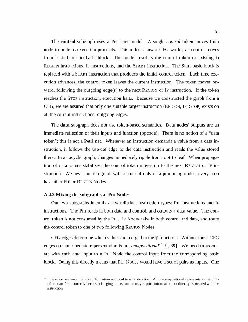
131

The control subgraph uses a Petri net model. A single control token moves from

node to node as execution proceeds. This reflects how a CFG works, as control moves

from basic block to basic block. The model restricts the control token to existing in

REGION instructions, IF instructions, and the START instruction. The Start basic block is

replaced with a START instruction that produces the initial control token. Each time exe-

cution advances, the control token leaves the current instruction. The token moves on-

ward, following the outgoing edge(s) to the next REGION or IF instruction. If the token

reaches the STOP instruction, execution halts. Because we constructed the graph from a

CFG, we are assured that only one suitable target instruction (REGION, IF, STOP) exists on

all the current instructions’ outgoing edges.

The data subgraph does not use token-based semantics. Data nodes' outputs are an

immediate reflection of their inputs and function (opcode). There is no notion of a “data

token”; this is not a Petri net. Whenever an instruction demands a value from a data in-

struction, it follows the use-def edge to the data instruction and reads the value stored

there. In an acyclic graph, changes immediately ripple from root to leaf. When propaga-

tion of data values stabilizes, the control token moves on to the next REGION or IF in-

struction. We never build a graph with a loop of only data-producing nodes; every loop

has either PHI or REGION Nodes.

A.4.2 Mixing the subgraphs at PHI Nodes

Our two subgraphs intermix at two distinct instruction types: PHI instructions and IF

instructions. The PHI reads in both data and control, and outputs a data value. The con-

trol token is not consumed by the PHI. IF Nodes take in both control and data, and route

the control token to one of two following REGION Nodes.

CFG edges determine which values are merged in the φ-functions. Without those CFG

edges our intermediate representation is not compositional27 [9, 39]. We need to associ-

ate with each data input to a PHI Node the control input from the corresponding basic

block. Doing this directly means that PHI Nodes would have a set of pairs as inputs. One

27 In essence, we would require information not local to an instruction. A non-compositional representation is diff i-

cult to transform correctly because changing an instruction may require information not directly associated with theinstruction.

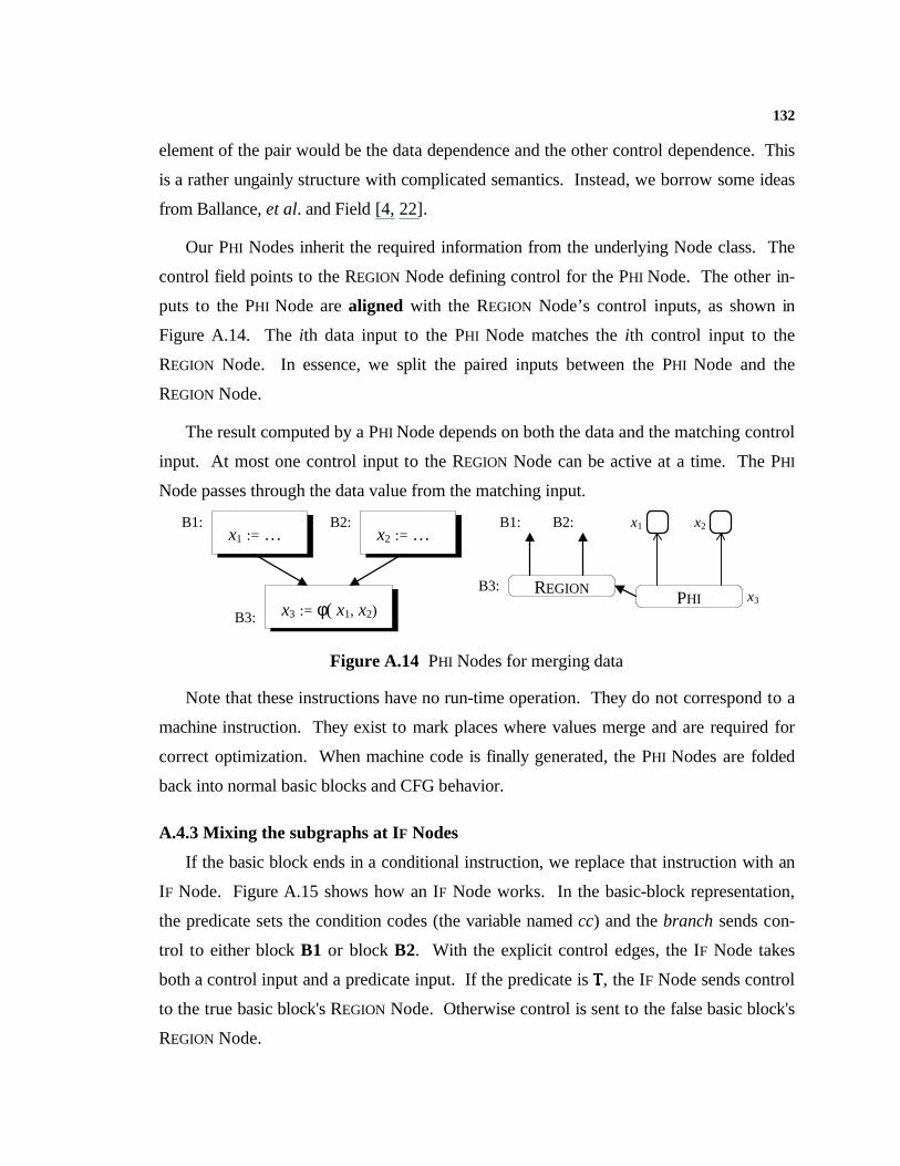
132

element of the pair would be the data dependence and the other control dependence. This

is a rather ungainly structure with complicated semantics. Instead, we borrow some ideas

from Ballance, et al. and Field [4, 22].

Our PHI Nodes inherit the required information from the underlying Node class. The

control field points to the REGION Node defining control for the PHI Node. The other in-

puts to the PHI Node are aligned with the REGION Node’s control inputs, as shown in

Figure A.14. The ith data input to the PHI Node matches the ith control input to the

REGION Node. In essence, we split the paired inputs between the PHI Node and the

REGION Node.

The result computed by a PHI Node depends on both the data and the matching control

input. At most one control input to the REGION Node can be active at a time. The PHI

Node passes through the data value from the matching input.

x1 := …B1:

x2 := …B2:

x3 := φ( x1, x2)B3:

REGIONPHI

B3: x3

B1: B2: x1 x2

Figure A.14 PHI Nodes for merging data

Note that these instructions have no run-time operation. They do not correspond to a

machine instruction. They exist to mark places where values merge and are required for

correct optimization. When machine code is finally generated, the PHI Nodes are folded

back into normal basic blocks and CFG behavior.

A.4.3 Mixing the subgraphs at IF Nodes

If the basic block ends in a conditional instruction, we replace that instruction with an

IF Node. Figure A.15 shows how an IF Node works. In the basic-block representation,

the predicate sets the condition codes (the variable named cc) and the branch sends con-

trol to either block B1 or block B2. With the explicit control edges, the IF Node takes

both a control input and a predicate input. If the predicate is T, the IF Node sends control

to the true basic block's REGION Node. Otherwise control is sent to the false basic block's

REGION Node.

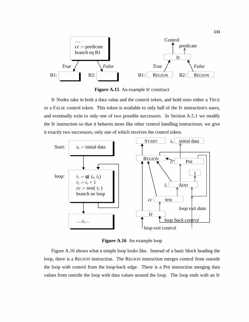
133

… cc := predicate branch eq B1

FalseTrue

B1: B2: REGIONB1: REGIONB2:

FalseTrue

IF

Controlpredicate

Figure A.15 An example IF construct

IF Nodes take in both a data value and the control token, and hold onto either a TRUE

or a FALSE control token. This token is available to only half of the IF instruction's users,

and eventually exits to only one of two possible successors. In Section A.5.1 we modify

the IF instruction so that it behaves more like other control handling instructions: we give

it exactly two successors, only one of which receives the control token.

i0 := initial data

i1 := φ( i0, i2) i2 := i1 + 1 cc := test( i2 ) branch ne loop

Start:

loop:

…i2…

START

REGIONPHI

ADD

test

IF

initial data

1

i0

i1

i2

cc

loop exit control

loop back control

loop exit data

Figure A.16 An example loop

Figure A.16 shows what a simple loop looks like. Instead of a basic block heading the

loop, there is a REGION instruction. The REGION instruction merges control from outside

the loop with control from the loop-back edge. There is a PHI instruction merging data

values from outside the loop with data values around the loop. The loop ends with an IF

134

instruction that takes control from the REGION at the loop head. The IF passes a true

control back into the loop head and a false control outside the loop.

A.4.4 Value Numbering and Control

If we encode the control input into our value numbering's hash and key-compare func-

tions, we no longer match two identical instructions in two different basic blocks; the

function and other inputs are equal but the control input differs. We end up doing only

local value numbering. Ignoring the control input (and doing some form of global value

numbering) is covered in Chapter 6.

A.5 More Engineering Concerns

In the original Node-based implementation, several instruction types defined more than

one value. Examples include instructions that set a condition code register along with

computing a result (i.e., subtract) and subroutine calls (which set at least the result regis-

ter, the condition codes, and memory). Previously these instructions have been dealt with

on an ad hoc basis. We use a more consistent approach.

Having a single instruction, such as an IF instruction, produce multiple distinct values

(the true control and the false control) is problematic. When we refer to an instruction,

we want to designate to a specific value. We fix this by making such multi-defining in-

structions produce a tuple value. Then we use PROJECTION Nodes to strip out the piece of

the tuple that we want. Each PROJECTION Node takes in the tuple from the defining Node

and produces a simple value. The PROJECTION Node also has a field specifying which

piece of the input tuple to project out.

These PROJECTION Nodes have no run-time operation (i.e., they “execute” in zero cy-

cles). When expressed in machine code, a tuple-producing Node is a machine instruction

with several results, such as a subroutine call or a subtract that computes a value and sets

the condition codes. The PROJECTION Nodes, when expressed as machine code, merely

give distinct names to the different results.

Computing a new Type for a PROJECTION Node is the responsibility of the tuple-

producer. The Compute code for a PROJECTION Node “passes the buck” by passing the

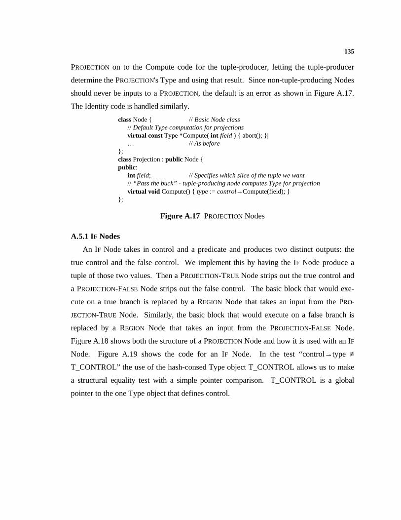
135

PROJECTION on to the Compute code for the tuple-producer, letting the tuple-producer

determine the PROJECTION's Type and using that result. Since non-tuple-producing Nodes

should never be inputs to a PROJECTION, the default is an error as shown in Figure A.17.

The Identity code is handled similarly.

class Node { // Basic Node class// Default Type computation for projectionsvirtual const Type *Compute( int field ) { abort(); }|… // As before

};class Projection : public Node {public:

int field; // Specifies which slice of the tuple we want// “Pass the buck” - tuple-producing node computes Type for projectionvirtual void Compute() { type := control→Compute(field); }

};

Figure A.17 PROJECTION Nodes

A.5.1 IF Nodes

An IF Node takes in control and a predicate and produces two distinct outputs: the

true control and the false control. We implement this by having the IF Node produce a

tuple of those two values. Then a PROJECTION-TRUE Node strips out the true control and

a PROJECTION-FALSE Node strips out the false control. The basic block that would exe-

cute on a true branch is replaced by a REGION Node that takes an input from the PRO-

JECTION-TRUE Node. Similarly, the basic block that would execute on a false branch is

replaced by a REGION Node that takes an input from the PROJECTION-FALSE Node.

Figure A.18 shows both the structure of a PROJECTION Node and how it is used with an IF

Node. Figure A.19 shows the code for an IF Node. In the test “control→type ≠

T_CONTROL” the use of the hash-consed Type object T_CONTROL allows us to make

a structural equality test with a simple pointer comparison. T_CONTROL is a global

pointer to the one Type object that defines control.

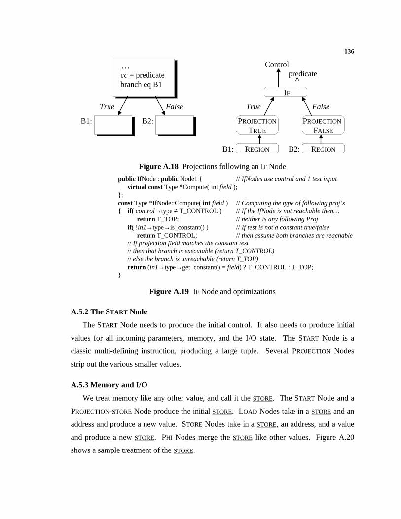
136

… cc = predicate branch eq B1

FalseTrue

B1: B2: PROJECTION

TRUE

B1:

PROJECTION

FALSE

B2:

FalseTrue

IF

Controlpredicate

REGION REGION

Figure A.18 Projections following an IF Node

public IfNode : public Node1 { // IfNodes use control and 1 test inputvirtual const Type *Compute( int field );

};const Type *IfNode::Compute( int field ) // Computing the type of following proj’s{ if( control→type ≠ T_CONTROL ) // If the IfNode is not reachable then…

return T_TOP; // neither is any following Projif ( !in1→type→is_constant() ) // If test is not a constant true/false

return T_CONTROL; // then assume both branches are reachable// If projection field matches the constant test// then that branch is executable (return T_CONTROL)// else the branch is unreachable (return T_TOP)return (in1→type→get_constant() = field) ? T_CONTROL : T_TOP;

}

Figure A.19 IF Node and optimizations

A.5.2 The START Node

The START Node needs to produce the initial control. It also needs to produce initial

values for all incoming parameters, memory, and the I/O state. The START Node is a

classic multi-defining instruction, producing a large tuple. Several PROJECTION Nodes

strip out the various smaller values.

A.5.3 Memory and I/O

We treat memory like any other value, and call it the STORE. The START Node and a

PROJECTION-STORE Node produce the initial STORE. LOAD Nodes take in a STORE and an

address and produce a new value. STORE Nodes take in a STORE, an address, and a value

and produce a new STORE. PHI Nodes merge the STORE like other values. Figure A.20

shows a sample treatment of the STORE.

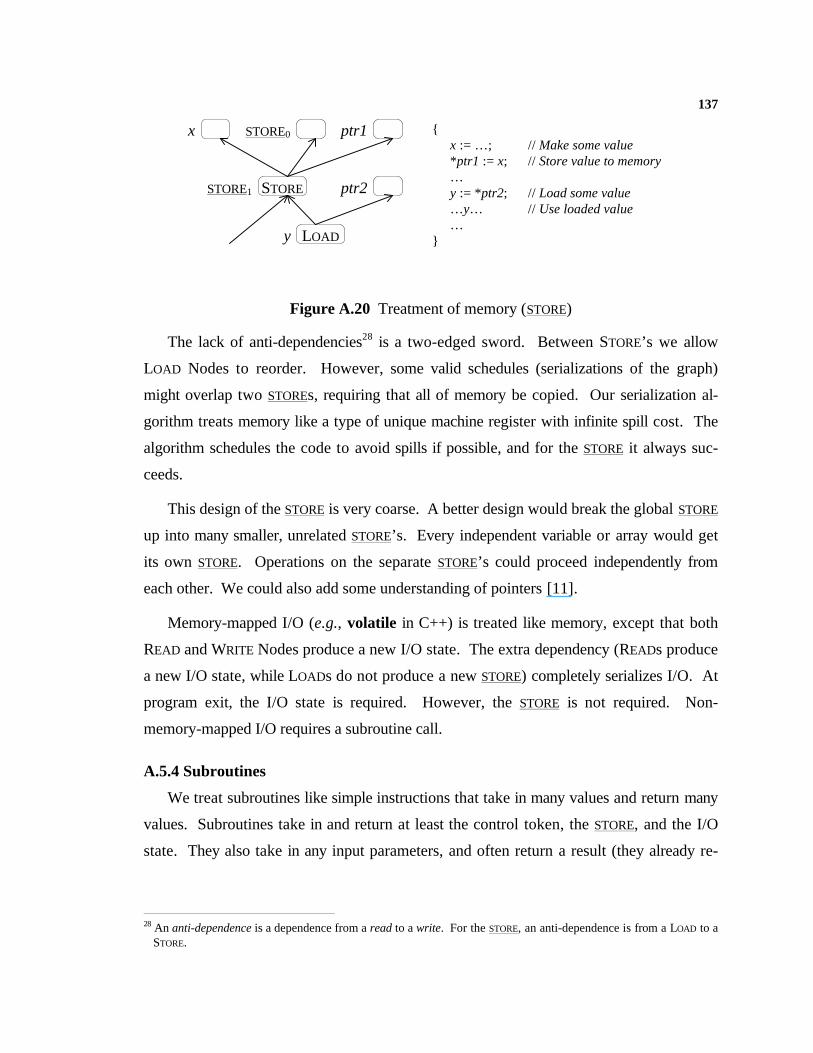
137

x STORE0

STORE1

y

ptr1

ptr2STORE

LOAD

{ x := …; // Make some value

*ptr1 := x; // Store value to memory…y := *ptr2; // Load some value…y… // Use loaded value…

}

Figure A.20 Treatment of memory (STORE)

The lack of anti-dependencies28 is a two-edged sword. Between STORE’s we allow

LOAD Nodes to reorder. However, some valid schedules (serializations of the graph)

might overlap two STOREs, requiring that all of memory be copied. Our serialization al-

gorithm treats memory like a type of unique machine register with infinite spill cost. The

algorithm schedules the code to avoid spills if possible, and for the STORE it always suc-

ceeds.

This design of the STORE is very coarse. A better design would break the global STORE

up into many smaller, unrelated STORE’s. Every independent variable or array would get

its own STORE. Operations on the separate STORE’s could proceed independently from

each other. We could also add some understanding of pointers [11].

Memory-mapped I/O (e.g., volatile in C++) is treated like memory, except that both

READ and WRITE Nodes produce a new I/O state. The extra dependency (READs produce

a new I/O state, while LOADs do not produce a new STORE) completely serializes I/O. At

program exit, the I/O state is required. However, the STORE is not required. Non-

memory-mapped I/O requires a subroutine call.

A.5.4 Subroutines

We treat subroutines like simple instructions that take in many values and return many

values. Subroutines take in and return at least the control token, the STORE, and the I/O

state. They also take in any input parameters, and often return a result (they already re-

28 An anti-dependence is a dependence from a read to a write. For the STORE, an anti-dependence is from a LOAD to a

STORE.

138

turn three other results). The peephole (and other) optimization calls can use any inter-

procedural information present.

A.6 Related Work

Ferrante, Ottenstein and Warren present the Program Dependence Graph [21]. The

PDG is more restrictive than our representation in that control edges are added to every

node. Also, the PDG lacks the control information required at merges for an execution

model. Cartwright and Felleisen extend the PDG to the Program Representation Graph

adding valve nodes to the PDG [9]. The PRG has a model of execution. Selke's thesis

gives a semantic framework for the PDG [39]. The PDG has fewer restrictions than our

representation where control edges are required. We would like to extend the combined

optimization algorithm so that it understands control dependence.

Cytron, Ferrante, Rosen, Wegman and Zadeck describe an efficient way to build the

SSA form of a program [15] which assigns only once to each variable. The SSA form is a

convenient way to express all data dependences, but it also lacks control information at φ-

functions.

Alpern, Wegman and Zadeck present the value graph [2]. The value graph is essen-

tially an SSA form of the program expressed as a directed graph. The authors extend the

value graph to handle structured control flow, but do not attempt to represent complete

programs this way. The value graph lacks control information at φ-functions and there-

fore does not have a model of execution.

Ballance, Maccabe and Ottenstein present the Program Dependence Web [4]. The

PDW is a combination of the PDG and SSA form and includes the necessary control in-

formation to have a model of execution. It also includes extra control edges that unnec-

essarily restrict the model of execution. The PDW includes µ and η nodes to support a

demand-driven data model. Our representation supports a data-driven model and does not

need these nodes. The PDW is complex to build, requiring several phases.

Pingali, Beck, Johnson, Moudgill and Stodghill present the Dependence Flow

Graph [38]. The DFG is executable and includes the compact SSA representation of data

139

dependences. The DFG has switched data outputs that essentially add the same unneces-

sary control dependences found in the PDW. The DFG includes anti-dependence edges to

manage the store; our representation does not require these. The DFG includes a deno-

tational semantics and has the one step Church-Rosser property.

Paul Havlak has done some recent work on the thinned Gated Single Assignment form

of a program [26]. This form is both executable and compact. Currently, the GSA is lim-

ited to reducible programs. The GSA can find congruences amongst DAGs of basic

blocks not found using our representation. We can find congruences amongst loop in-

variant expressions not found using the GSA. It is not clear if the forms can be combined,

or if one form is better than another. A promising implementation of thinned GSA exists

and has been used on a large suite of FORTRAN applications with good results.

Weise, Crew, Ernst, and Steensgaard present the Value Dependence Graph [48]. The

VDG is similar in spirit to our representation. It represents an independent line of re-

search, performed in parallel with our own. Weise, et al. stress the VDG for research in

partial evaluation, slicing and other optimizations; they have built visual display tools to

help transformations on the VDG. We stress compilation speed and code quality; our

compiler is much faster and includes a larger set of classic optimizations.

John Field gives a formal treatment of graph rewriting on a representation strongly re-

sembling our representation. We hope to be able to use his semantics with only minimal

modifications [22].

A.6.1 Summary of Related Intermediate Representations

As program representations have evolved they have gained an executable model; they

include all the information necessary to execute a program. Also, restrictions on the

evaluation order, expressed as edges in the graph, are lifted. The later representations are

both more compact and more complete and allow more optimizations. Our representation

is one more step along these lines. It has an executable model and has fewer restrictions

on the evaluation order than any of the previous models. This lifting of restrictions gives

analysis and optimization algorithms more freedom to discover facts and reorganize code

from disjoint sections of the original program.

140

A.7 Summary

To produce a faster optimizer, we decided to do some of the work in the front end.

We reasoned that inexpensive peephole optimizations done while parsing would reduce

the size of our intermediate representation and the expense of later optimization phases.

To do useful peephole optimizations we need use-def information and the static single as-

signment property.

We take advantage of C++'s inheritance mechanisms and structure our Nodes into

separate classes for each kind of instruction. A Node’s opcode is represented by the C++

virtual function table pointer. Each Node holds use-def pointers, represented as simple

C++ pointers to other Nodes. We make control dependence an explicit pointer to the

controlling block and make our model compositional by providing control information at

PHI Nodes.

We collapse the CFG edges into the representation, just like the data edges. This is

crucial to the good running time of the combined algorithm, which does not need to dif-

ferentiate between the two edge types. Instead of flow analysis over the CFG edges fol-

lowing analysis over the data edges, we replace the two-tier CFG and basic block struc-

ture with REGION Nodes.

We use virtual functions to define opcode semantics. Constant propagation, algebraic

identities and hash table behaviors are all inherited. We also use specialized allocate and

delete functions. We discussed convenient mechanisms to handle instructions that defined

several values, subroutines, memory, and I/O.