program optimizations and transformations in calculation form

Program Optimizations and Transformations

in Calculation Form

Zhenjiang Hu, Tetsuo Yokoyama, and Masato Takeichi

Department of Mathematical Informatics

Graduate School of Information Science and Technology

The University of Tokyo

7-3-1 Hongo, Bunkyo 113-8656, Tokyo, JAPAN

{hu, takeichi}@[email protected]

Abstract. The world of program optimization and transformation takes on a new

fascination when viewed through the lens of program calculation. Unlike the tra-

ditional fold/unfold approach to program transformation on arbitrary programs,

the calculational approach imposes restrictions on program structures, resulting in

some suitable calculational forms such as homomorphisms and mutumorphisms

that enjoy a collection of generic algebraic laws for program manipulation. In

this tutorial, we will explain the basic idea of program calculation, demonstrate

that many program optimizations and transformations, such as the optimization

technique known as loop fusion and the parallelization transformation, can be

concisely reformalized in calculational form, and show that program transforma-

tion in calculational forms is of higher modularity and more suitable for efficient

implementation.

Keywords: Program Transformation, Program Calculation, Program Optimiza-

tion, Meta Programming, Functional Programming.

1 Introduction

There is a well-known Chinese proverb: aFs (one cannot have both fishes and bear

palms at the same time), implying that one can hardly obtain two treasures simultane-

ously. The same thing happens in our programming: clarity is and is not next to good-

ness. Clearly written programs have the desirable properties of being easy to under-

stand, show correct, and modify, but they can also be extremely inefficient. In software

engineering, one major design technique for achieving clarity is modularity: breaking a

problem into independent components. But modularity can lead to inefficiency, because

of the overhead of communication between components, and because it may preclude

potential optimizations across component boundaries.

However, it is possible to have both fishes and bear palms at different times: we

start by writing clean and correct (but probably inefficient) programs, and then use

program calculation techniques to transform them to more efficient equivalents. To see

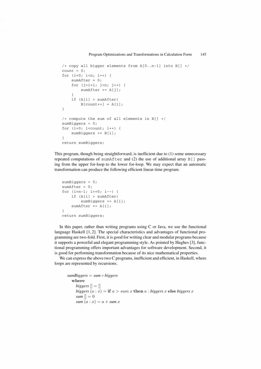
this, consider the problem of summing up all bigger elements in an array. An element is

bigger if it is greater than the sum of the elements that follow it till the end of the array.

We may start with the following C program, which clearly solves the problem.

R. Lammel, J. Saraiva, and J. Visser (Eds.): GTTSE 2005, LNCS 4143, pp. 144–168, 2006.

c© Springer-Verlag Berlin Heidelberg 2006

Program Optimizations and Transformations in Calculation Form 145

/* copy all bigger elements from A[0..n-1] into B[] */count = 0;for (i=0; i<n; i++) {

sumAfter = 0;for (j=i+1; j<n; j++) {

sumAfter += A[j];}if (A[i] > sumAfter)

B[count++] = A[i];}

/* compute the sum of all elements in B[] */sumBiggers = 0;for (i=0; i<count; i++) {

sumBiggers += B[i];}return sumBiggers;

This program, though being straightforward, is inefficient due to (1) some unnecessary

repeated computations of sumAfter and (2) the use of additional array B[] pass-

ing from the upper for-loop to the lower for-loop. We may expect that an automatic

transformation can produce the following efficient linear-time program.

sumBiggers = 0;sumAfter = 0;for (i=n-1; i>=0; i--) {

if (A[i] > sumAfter)sumBiggers += A[i];

sumAfter += A[i];}return sumBiggers;

In this paper, rather than writing programs using C or Java, we use the functional

language Haskell [1, 2]. The special characteristics and advantages of functional pro-

gramming are two-fold. First, it is good for writing clear and modular programs because

it supports a powerful and elegant programming style. As pointed by Hughes [3], func-

tional programming offers important advantages for software development. Second, it

is good for performing transformation because of its nice mathematical properties.

We can express the above two C programs, inefficient and efficient, in Haskell, where

loops are represented by recursions.

sumBiggers = sum ◦ biggers

where

biggers [] = []biggers (a : x) = if a > sum x then a : biggers x else biggers xsum [] = 0sum (a : x) = a + sum x

146 Z. Hu, T. Yokoyama, and M. Takeichi

sumBiggers x = let (b, c) = sumBiggers’ x in bwhere

sumBiggers’ [] = (0, 0)sumBiggers’ (a : x) = let (b, c) = sumBiggers’ x

in if a > c then (a + b, a + c) else (b, a + c)

One methodology that offers some scope for making the construction of efficient

programs more mathematical is transformational programming [4, 5, 6]. Program cal-

culation is a kind of program transformation based on the theory of Constructive

Algorithmics [7, 8, 9, 10, 11, 12]. It is a kind of transformational programming that

derives an efficient program in a step-by-step way through a series of ”transformations”

that preserve the meaning and hence the correctness. A significant practical problem

in traditional transformational programming is that a very large number of steps seem

needed: the individual steps are too small, while in program calculation, formalisms

and theories are developed with which a whole series of small steps can be combined

into one single step at a higher level.

Program calculation proceeds by means of manipulation of programs based on a

rich collection of identities and transformation laws. It resembles the manipulation of

formulas as in high school algebra: a formula F is broken up into its semantic relevant

constituents and the pieces are assembled together into a different but semantically

equivalent formula F ′, thus yielding the equality F ≡ F ′. The following example

shows a calculation of the solution of x for the equation x2 − c2 = 0.

x2 − c2 = 0≡ { by identity: a2 − b2 = (a − b)(a + b) }

(x − c)(x + c) = 0≡ { by law: ab = 0 ⇔ a = 0 or b = 0 }

x − c = 0 or x + c = 0≡ { by law: a = b ⇔ a ± d = b ± d }

x = c or x = −c

Here we calculate x rather than guess or just invent, based on some identities and laws

(rules). Particularly, we make use of the transformation law that a higher order equation

should be factored into several first order ones whose solution can be easily obtained.

In this tutorial, we will see that program calculation provides a powerful tool to for-

malize various kinds of program transformations [13, 14, 15, 16], besides its usefulness

in guiding people to derive efficient algorithms. We will explain the basic idea of pro-

gram calculation from the practical point of view, demonstrate that a lot of program

optimizations and transformations, including the well-known loop fusion and paral-

lelization, can be concisely reformalized in calculational forms, and show that program

transformation in calculational forms is of higher modularity and more suitable for ef-

ficient implementation.

It is worth noting that all transformations in this tutorial have been tested with the

Yicho system [17], a transformation system developed at the University of Tokyo. We

encourage the reader to play with the Yicho system when reading this material. The

Yicho system is available at the following site.

http://www.ipl.t.u-tokyo.ac.jp/yicho/


The rest of this tutorial is organized as follows. We start with a simple example to

illustrate the basic concepts of program calculation, and clarify its difference from the

traditional fold/unfold transformations in Section 2. Then, we demonstrate how to for-

malize two nontrivial transformations, namely loop fusion and parallelization, in calcu-

lational forms in Sections 3 and 4 respectively. And we show that program calculations

can be efficiently implemented by the Yicho system in Section 5. Finally, we conclude

the paper with a summary of the advantages of formalizing program transformations in

calculational forms in Section 6.

2 Program Calculation vs Fold/Unfold Transformations

In this section, we illustrate with a simple example the basic concepts of program cal-

culation, show the main idea of calculational approach to program transformation, and

clarify its difference from the traditional fold/unfold approach to program transforma-

tions and program optimizations.

2.1 Notational Conventions

First of all, we briefly review the notational conventions known as Bird-Meertens For-

malisms [7]. The notations are similar to those in Haskell [2].

Functions. Programs are defined as functions. Function application is denoted by jux-

taposition of function and argument. Thus f a means f (a). Functions are curried, and

application associates to the left. Thus f a b means (f a) b. Function application is re-

garded as more binding than any other operator, so f a ⊕ b means (f a) ⊕ b, but not

f (a ⊕ b). Function composition is denoted by a centralized circle ◦. By definition,

(f ◦ g) a = f (g a). Function composition is an associative operator, and the identity

function is denoted by id.

Lambda expressions are sometimes used to define a function without giving it a

name. So λx. e denotes a function, accepting an input x, computing e, and returning its

value as result. For example, λx.2 ∗ x simply denotes a function doubling the input.

Infix binary operators will often be denoted by ⊕, ⊗ and can be sectioned; an infix

binary operator like ⊕ can be turned into unary functions as follows.

(a⊕) b = a ⊕ b = (⊕ b) a

Lists. Lists are finite sequences of values of the same type. The type of the cons lists

with elements of type a is defined as follows.

data [a] = [] | a : [a]

A list is either empty or a list constructed by inserting a new element to a list. We write

[] for the empty list, [a] for the singleton list with element a (and [·] for the function

taking a to [a]), and x ++ y for the concatenation of two lists x and y. Concatenation is

associative, and [] is its unit. For example, the term [1] ++ [2] ++ [3] denotes a list with


three elements, often abbreviated to [1, 2, 3]. As seen above, we usually use a, b, c to

denote list elements, and x, y, z to denote lists.

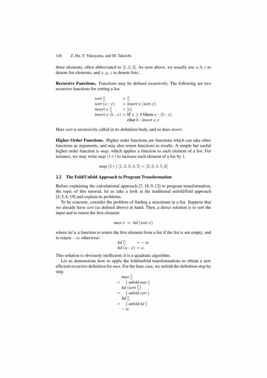
Recursive Functions. Functions may be defined recursively. The following are two

recursive functions for sorting a list.

sort [] = []sort (a : x) = insert a (sort x)insert a [] = [a]insert a (b : x) = if a ≥ b then a : (b : x)

else b : insert a x

Here sort is recursively called in its definition body, and so does insert.

Higher Order Functions. Higher order functions are functions which can take other

functions as arguments, and may also return functions as results. A simple but useful

higher order function is map, which applies a function to each element of a list. For

instance, we may write map (1+) to increase each element of a list by 1.

map (1+) [1, 2, 3, 4, 5] = [2, 3, 4, 5, 6]

2.2 The Fold/Unfold Approach to Program Transformation

Before explaining the calculational approach [7, 18, 9, 12] to program transformation,

the topic of this tutorial, let us take a look at the traditional unfold/fold approach

[4, 5, 6, 19] and explain its problems.

To be concrete, consider the problem of finding a maximum in a list. Suppose that

we already have sort (as defined above) in hand. Then, a direct solution is to sort the

input and to return the first element:

max x = hd (sort x)

where hd is a function to return the first element from a list if the list is not empty, and

to return −∞ otherwise:hd [] = −∞hd (a : x) = a.

This solution is obviously inefficient; it is a quadratic algorithm.

Let us demonstrate how to apply the fold/unfold transformations to obtain a new

efficient recursive definition for max. For the base case, we unfold the definition step by

step.

max []= { unfold max }

hd (sort [])= { unfold sort }

hd []= { unfold hd }

−∞


Then for the recursive case, we do unfolding similarly.

max (a : x)= { unfold max }

hd (sort (a : x))= { unfold sort }

hd (insert a (sort x))

We get stuck here; we cannot perform folding to get a recursive definition unless more

information is exposed. To expose more information, we unfold insert, by assuming

b : x′ = sort x, that is

b = hd (sort x)x′ = tail (sort x)

and continue our transformation.

hd (insert a (b : x′))= { unfold insert }

hd (if a ≥ b then a : (b : x′) else b : insert a x′)= { law: f (if b then e1 else e2) = if b then f e1 else f e2 }

if a ≥ b then hd (a : (b : x′)) else hd (b : insert a x′)= { unfold hd }

if a ≥ b then a else b= { unfold b }

if a ≥ hd (sort x) then a else hd (sort x)= { fold max }

if a ≥ max x then a else max x

The last folding step is the key to the success of the derivation of the following efficient

program.

max [] = −∞max (a : x) = if a ≥ max x then a else max x

The fold/unfold approach to program transformation is general and powerful, but it

suffers from several problems which often prevent it from being used in practice.

– It is difficult to decide when unfolding steps should stop while guaranteeing expo-

sition of enough information for later folding steps.

– It is expensive to implement, because it requires keeping records of all possible

folding patterns and have them checked upon any new subexpressions produced

during transformation.

– Each transformation step is very small, but an effective way is lacking to group

and/or structure them into bigger steps.

2.3 Program Transformations in Calculational Form

A distinguished feature of the calculational approach to program transformation is no

use of folding during transformation, which solves the first two problems the fold/unfold


approach has, and the challenge is how to formalize necessary folding steps by means

of calculation laws (rules). Transformations that are based on a set of calculation laws

but exclude the use of folding steps will be called transformation in calculation form

in this paper. The calculational approach to program transformation advocates more

structured programming, where the inner structure of a loop (recursion) is taken into

account.

Procedure to Formalize Transformations in Calculational Form

The procedure to formalize a program transformation in calculational form consists of

the following three major steps.

1. Define a specific form of programs that are best suitable for the transformation and

can be used to describe a class of interesting computations.

2. Develop calculational rules (laws) for implementing the transformation on pro-

grams in the specific form.

3. Show how to turn more general programs into those in the specific form and how

to apply the newly developed calculational rules systematically.

The first step plays a very important role in this formalization. The specific form de-

fined in the first step should meet two requirements. First, it should be powerful enough

to describe computations of our interest. Second, it should be manipulable and suitable

for later development of calculational laws. In fact, the Constructive Algorithmics the-

ory [7, 18, 9, 10] provides us a nice theoretical framework to define such specific forms

and to develop calculational rules.

In Constructive Algorithmics, the calculations are based on calculation rules that are

built upon the algebra of programs, a collection of identities. These identities can be

provided by exploiting the algebraic structure of the algebraic data concerned, such

as lists or trees. In particular, there is a close correspondence between data structures

(terms in an algebra) and control structures (homomorphisms mapping from that alge-

bra to another). This correspondence is well captured by categorical functors, which are

very theoretical and fall outside the scope of this tutorial.

Homomorphisms: General Structured Recursive Functions

Recall the structured programming methodology for imperative language, where the

use of arbitrary goto’s is abandoned in favor of structured control flow primitives such

as conditionals and while-loop so that program transformation becomes easier and el-

egant. For high level algorithmic programming like functional programming, recursive

definitions provide a powerful control mechanism for specifying programs. Consider

the following recursive definition on lists:

f (a : x) = · · · f x · · · f (g x) · · · f (f x) · · ·

There is usually no specific restriction on the right hand side; it can be any expression

where recursive calls to f may be of any form and appear anywhere. This somehow

resembles the arbitrary use of goto’s in imperative programs, which makes recursive


definitions hard to manipulate. In contrast, the calculational approach imposes suitable

restrictions on the right hand side resulting in a suitable calculation form. Homomor-

phisms are one of the most general and important calculational forms.

Homomorphisms are functions that manipulate algebraic data structures such as lists

and trees. They are derivable from the concerned structure of the algebraic data. Recall

the list data structure [α]. It can be considered as the algebra of

([α], [] :: [α], (:) :: a → [α] → [α])

in which the carrier [α] denotes all lists whose elements are of type α, and two opera-

tions, namely [] with type [α] and (:) with type a → [α] → [α], are the data constructors

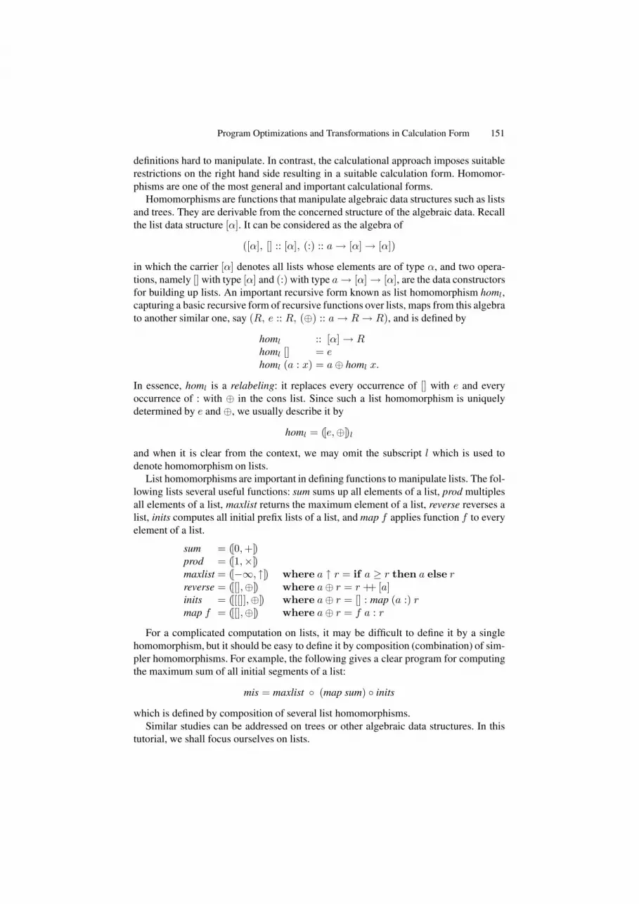
for building up lists. An important recursive form known as list homomorphism homl,

capturing a basic recursive form of recursive functions over lists, maps from this algebra

to another similar one, say (R, e :: R, (⊕) :: a → R → R), and is defined by

homl :: [α] → Rhoml [] = ehoml (a : x) = a ⊕ homl x.

In essence, homl is a relabeling: it replaces every occurrence of [] with e and every

occurrence of : with ⊕ in the cons list. Since such a list homomorphism is uniquely

determined by e and ⊕, we usually describe it by

homl = ([e, ⊕])l

and when it is clear from the context, we may omit the subscript l which is used to

denote homomorphism on lists.

List homomorphisms are important in defining functions to manipulate lists. The fol-

lowing lists several useful functions: sum sums up all elements of a list, prod multiples

all elements of a list, maxlist returns the maximum element of a list, reverse reverses a

list, inits computes all initial prefix lists of a list, and map f applies function f to every

element of a list.

sum = ([0, +])prod = ([1, ×])maxlist = ([−∞, ↑]) where a ↑ r = if a ≥ r then a else rreverse = ([[], ⊕]) where a ⊕ r = r ++ [a]inits = ([[[]], ⊕]) where a ⊕ r = [] : map (a :) rmap f = ([[], ⊕]) where a ⊕ r = f a : r

For a complicated computation on lists, it may be difficult to define it by a single

homomorphism, but it should be easy to define it by composition (combination) of sim-

pler homomorphisms. For example, the following gives a clear program for computing

the maximum sum of all initial segments of a list:

mis = maxlist ◦ (map sum) ◦ inits

which is defined by composition of several list homomorphisms.

Similar studies can be addressed on trees or other algebraic data structures. In this

tutorial, we shall focus ourselves on lists.


Promotion Rule

Homomorphisms enjoy many calculation properties. Among them, the following pro-

motion rule is of great importance, saying that a composition of a function with a ho-

momorphism can be merged into a single homomorphism under a certain condition.

promotion:f (a ⊕ x) = a ⊗ f x

f ◦ ([e, ⊕]) = ([f e,⊗])

If functions are defined only by homomorphisms rather than by arbitrary recursive

definitions, we can use the promotion rule to manipulate them. Recall the example of

computing the maximum from a list early this section:

max = hd ◦ sort

Inefficiency of this program lies in that sort x computes a result that contains too much

useless information for the later computation by hd. The standard way is to fuse the two

functions hd and sort into a single one which does not include unnecessary computation.

Fusion based on the fold/unfold transformations has been explained before. Let us see

how to calculate an efficient max with the promotion calculation rule. Notice that sort =([[], insert]). The promotion rule tells us that if we can derive ⊗ such that

∀a, x. hd (insert a x) = a ⊗ hd x

then we can transform hd◦sort to ([−∞, ⊗]). This ⊗ may be obtained via a higher order

matching algorithm [20]. Here, we show another concise calculation.

a ⊗ b = { let x be any list }

a ⊗ hd (b : x)= { the condition in the promotion rule }

hd (insert a (b : x))= { definition of insert }

hd (if a ≥ b then a : (b : x) else b : insert a x)= { if property }

if a ≥ b then hd (a : (b : x)) else hd (b : insert a x)= { definition of hd }

if a ≥ b then a else b

In summary, we have derived the following definition for max.

max = ([−∞, ⊗])where a ⊗ b = if a ≥ b then a else b

And it is equivalent to

max [] = −∞max (a : x) = if a ≥ max x then a else max x

which is the same as the result obtained by the fold/unfold program transformation

before. It is worth noting that the transformation here does not need any folding step,

rather we focus on deriving a new operator from the condition of the promotion rule.


3 Loop Fusion in Calculation Form

In this section, we demonstrate how to formalize loop fusion in calculational form.

Loop fusion, a well-known optimization technique in compiler construction [21, 22], is

to fuse some adjacent loops into one loop to reduce loop overhead and improve run-time

performance. In the introduction, we have seen an inefficient program for sumBiggers

which consists of three loops, and an equivalent efficient one which uses only a single

loop.

In our framework, loops are specified by recursive definitions. There are basically

three cases for two adjacent loops: (1) one loop is put after another and the result com-

puted by the first is used by the second; (2) one loop is put after another and the result

computed by the first is not used by the second; and (3) one loop is used inside another.

The second case is much simpler. We have seen the first and the third cases in the defi-

nition of sumBiggers in the introduction. Recall the following definition of sumBiggers:

sumBiggers = sum ◦ biggers

biggers [] = []biggers (a : x) = if a > sum x then a : biggers x else biggers xsum [] = 0sum (a : x) = a + sum x

The use of one loop after another is specified by a composition of two recursive func-

tions (sum ◦ biggers), and a nested loop is specified by other function calls applying

to the same input data in the definition body (sum x appears in the definition body of

biggers).

We shall illustrate how to formalize the loop fusion in calculational form by the three

steps in Section 2.3.

3.1 Structured Recursive Form for Loop Fusion

Now we are facing the problem of choosing a proper structured form for recursive

functions. There are two basic requirements for this form. First, it should be powerful

enough to describe computation that manipulates lists. Second, it should be suitable for

loop fusion, where the three cases of loop combination can be coped with. We would

like to show that list mutumorphism is a suitable form for this purpose.

Definition 1 ((List) Mutumorphism). A function f1 is said to be a list mutumorphism

with respect to other functions f2, . . . , fn if each fi (i = 1, 2, . . . , n) is defined in the

following form:

fi [] = ei

fi (a : x) = a ⊕i (f1 x, f2 x, . . . , fn x)

where ei (i = 1, 2, . . . , n) are given constants and ⊕i (i = 1, 2, . . . , n) are given binary

functions. We represent f1 as follows.

f1 = [[(e1, . . . , en), (⊕1, . . . ,⊕n)]].�


List mutumorphisms have strong expressive power, covering all primitive recursive

functions on lists. It should be noted that list homomorphisms are a special case of

list mutumorphisms:

([e, ⊕]) = [[(e), (⊕)]]

Recall the sumBiggers. We may redefine sum and biggers in terms of mutumorphisms

(or homomorphism) as below.

sumBiggers = ([0, +]) ◦ [[([], 0), (⊕1, ⊕2)]]where a ⊕1 (r, s) = if a > s then a : r else r

a ⊕2 (r, s) = a + s

3.2 Calculational Rules for Loop Fusion

After formalizing loops by mutumorphisms, we turn to develop calculation rules (laws)

for fusing such loops. We will consider the three cases for loop combination.

First, we consider merging nested loops. Mutumorphism itself is actually a nested

loop, as seen in the definition of biggers. We may flatten this kind of nested loops by

the following flattening calculation rule [14].

Lemma 1 (Flattening).

[[(e1, e2, . . . , en), (⊕1, ⊕2, . . . ,⊕n)]] = fst ◦ ([(e1, e2, . . . , en), ⊕])where a ⊕ r = (a ⊕1 r, a ⊕2 r, . . . , a ⊕n r)

Here, fst is a projection function returning the first element of a tuple. �

The flattening calculation rule, as its name suggests, flattens a nested loop represented

by a mutumorphism to a homomorphism. Consider, as an example, to apply the flatten-

ing rule to biggers to flatten the nested loop.

biggers

= { mutumorphism for biggers }

[[([], 0), (⊕1, ⊕2)]]= { flattening rule }

fst ◦ ([([], 0), ⊕])where a ⊕ (r, s) = (if a > s then a : r else r, a + s)

Inlining the homomorphism in the derived program gives the following readable recur-

sive program, which consists of a single loop.

biggers x = let (r, s) = hom x in rwhere hom [] = ([], 0)

hom (a : x) = let (r, s) = hom xin (if a > s then a : r else r, a + s)

Second, we try to merge two independent loops. Since mutumorphism can be trans-

formed into homomorphism, it is suffice to consider merging of two independent

homomorphisms that manipulate the same lists. This can be done by the tupling trans-

formation [23], whose calculation form is summarized as follows [14].


Lemma 2 (Tupling).

(([e1, ⊕1]) x, ([e2, ⊕2]) x) = ([(e1, e2), ⊕]) xwhere a ⊕ (r1, r2) = (a ⊕1 r1, a ⊕2 r2) �

For example, the following program to compute the average of a list:

average x = sum x/length x

which has two loops can be merged into a single loop by applying the tupling rule.

average x = let (s, l) = tup x in s/lwhere tup = ([(0, 0), λa (s, l). (a + s, 1 + l)])

Here, to save space we choose to use lambda expression to define the new binary oper-

ator, which accepts a and (s, l), and returns (a + s, 1 + l).Finally, we consider fusion of two loops where the result of one loop is used by the

other. When the loops are formalized as homomorphisms, we can use the promotion rule

in Section 2.3 for this fusion, as seen in the example of fusing hd ◦ sort. The promotion

rule fuses function f to a homomorphism from left:

f ◦ ([e, ⊕])

and the following calculation rule [24, 25] shows how to fuse a function to a homomor-

phism from right.

Lemma 3 (Shortcut Fusion).

([e, ⊕]) ◦ build g = g (e, ⊕)

Here, the function build is a list production function defined by1

build g = g ([], (:)).�

The shortcut fusion rule indicates that if one can express a function in build, then it can

be cheaply fused into a homomorphism from its right. Compared with the promotion

rule, the shortcut fusion rule is much simpler and cheap to implement, because it is just

a simple expression substitution. On the other hand, it needs a preparation of deriving a

build form from a homomorphism. The following warm-up rule is for this purpose.

Lemma 4 (Warm-up).

([e, ⊕]) = build (λ(d, ⊗). ([d, ⊗]) ◦ ([e, ⊕]))�

Note that the warm-up rule may introduce an additional loop, but this loop is usually

easier to be fused with others. Recall that we have obtained the following definition for

biggers.

1 Strictly speaking, it requires parametricity on the type of g, as studied in [24].


biggers = fst ◦ ([([], 0), ⊕])where a ⊕ (r, s) = (if a > s then a : r else r, a + s)

We can obtain the following build form:

biggers = build (λ(d, ⊗). fst ◦ ([(d, 0), ⊕′]))where a ⊕′ (r, s) = (if a > s then a ⊗ r else r, a + s)

Now applying the shortcut fusion rule to

sumBiggers = ([0, +]) ◦ bigger

soon yields the following single-loop program for sumBiggers:

sumBiggers = fst ◦ ([(0, 0), ⊗])where a ⊗ (r, s) = (if a > s then a + r else r, a + s)

which is actually the same as that in the introduction.

Before finishing our development of calculation rules for loop fusion, we give an-

other calculation rule for fusing a function with a mutumorphism. This may not be nec-

essary as mutumorphism can be transformed into homomorphism, but it may provide

us with more flexibility in rule application.

Lemma 5 (Mutumorphism Promotion).

fi(a ⊕i (x1, . . . , xn)) = a ⊗i (f1 x1, . . . , fn xn) (i = 1, . . . , n)

f1 ◦ [[(e1, . . . , en), (⊕1, . . . ,⊕n)]] = [[(f1 e1, . . . , fn en), (⊗1, . . . ,⊗n)]] �

3.3 A Calculational Algorithm for Loop Fusion

This is the last step, where we should make it clear how to turn a program into our

specific form and how to apply the newly developed calculational laws in a systematic

way for loop fusion, as seen in [26, 14, 15]. Below we summarize our calculational

algorithm for loop fusion.

1. Represent as many recursive functions on lists by mutumorphisms as possible.

2. Apply the flattening rule to transform all mutumorphism to homomorphisms.

3. Apply the promotion rule and shortcut fusion rule as much as possible.

4. Apply the tupling rule to merge independent homomorphisms.

5. Inline homomorphism/mutumorphism to output transformed program in a friendly

manner.

We have indeed followed this algorithm in fusing the three loops in sumBiggers.

One remark should be made on the first step above. It would be unnecessary if pro-

grams are restricted to be strictly written in terms of mutumorphisms, but there are two

reasons to have it. First, it makes our system extensible; we may extend our system by

showing that a wider class of functions can be transformed to mutumorphisms by some

preprocessing. For example, the following recursive function


foo [] = 0foo [a] = afoo (a : b : x) = a + foo (b : x) + foo x

may not be target for loop fusion at the start. When we find a way to express functions

like foo in terms of a mutumorphism, we can empower our system by adding it as a pre-

processing. In fact, it has been shown that foo belongs to the class of tuplable functions

which can be automatically transformed to a function defined in terms of homomor-

phisms [14]. Second, we may want to apply our loop fusion to legacy programs. As a

matter of fact, it is possible to obtain mutumorphism automatically from many recursive

functions on lists.

4 Parallelization in Calculation Form

Our second example is about Parallelization [27, 15], a transformation for automatically

generating parallel code from high level sequential description. Parallelization is of key

importance to the wide spread use of high performance machine architectures, but it is

a big challenge to clarify what kind of sequential programs can be parallelized and how

they can be systematically parallelized.

Program calculation suggests a new way to face this challenge. We know from the

theory of Constructive Algorithmics that the control structure of the program should

be determined by the data structure the program is to manipulate. For lists, there are

two possible views. One view is known as cons lists, which is “sequential”: a list is

constructed by an empty list, or from an element and a list.

ConsList a = [] | a : ConsList a

Another view is known as join lists, which is “parallel”: a list is an empty list, or a

singleton list, or a list joining two shorter lists.

JoinList a = [] | [.] a | JoinList a ++ JoinList a

So given a list [1, 2, 3, 4, 5, 6, 7, 8], we may represent it in the following two ways:

1 : (2 : (3 : (4 : (5 : (6 : (7 : (8 : [])))))))(([1] ++ [2]) ++ ([3] ++ [4])) ++ (([5] ++ [6]) ++ ([7] ++ [8]))

Programs defined on cons lists inherit sequentiality from cons lists, while programs

defined on join lists gain parallelism from join lists. The following are two such versions

for sum.

sumS (a : x) = a + sumS xsumP (x ++ y) = sumP x + sumP y

With the above in mind, we may consider parallelization of functions on lists as

mapping a function on cons lists (e.g., sumS) to an equivalent one on join lists (e.g.,

sumP).


4.1 J-Homomorphism: A Parallel Form for List Functions

As in loop fusion, we introduce a recursive form, J-homomorphism2, to capture parallel

computations on lists.

Definition 2 (J-Homomorphism). J-homomorphisms are those functions on finite lists

that promote through list concatenation — that is, function h for which there exists an

associative binary operator ⊕ such that, for all finite lists x and y, we have

h (x ++ y) = h x ⊕ h y

where ++ denotes list concatenation. �

In fact, it has been attracting wide attention to make use of J-homomorphisms in parallel

programming [28, 30, 31]. Intuitively, the definition of J-homomorphisms means that

the value of h on the larger list depends in a particular way (using binary operation ⊕)

on the values of h applied to the two pieces of the list. The computations of h x and

h y are independent of each other and can thus be carried out in parallel. This simple

equation can be viewed as expressing the well-known divide-and-conquer paradigm of

parallel programming.

As a running example, consider the maximum segment sum problem, which finds the

maximum of the sums of contiguous segments within a list of integers. For example,

mss [3, −4, 2, −1, 6, −3] = 7

where the result is contributed by the segment [2, −1, 6]. We may write the following

sequential function mss to solve the problem, where mis is to compute the maximum

initial-segment sum of a list.

mss [] = 0mss (a : x) = a ↑ (a + mis x) ↑ mss xmis [] = 0mis (a : x) = a ↑ (a + mis x)

How can we find an equivalent parallel program in J-homomorphism?

4.2 A Parallelizing Rule

In Section 3, we have seen that list homomorphisms play a very important role in de-

scribing computations on lists. Our parallelization rule is to show how to map a list

homomorphism to a J-homomorphism. As a preparation, we define the composition-

closed3 property of a function.

Definition 3 (Composition-closed). Let x denote a sequence x1 x2 · · · xn, and ydenote a sequence y1 y2 · · · yn. A function f x is said to be composition-closed if

there exist n functions gi (i = 1, · · · , n), so that

f x (f y) = f (g1 x y) (g2 x y) · · · (gn x y) r �

2 It is usually called list homomorphism in many literatures [7, 28, 29]. We call it

J-homomorphism here because we have used the word list homomorphism in loop fusion.3 This property is called context-preservation in [32].


For example, the function

f x1 x2 r = x1 ↑ (x2 + r)

is composition-closed, as seen in the following calculation.

f x1 x2 (f y1 y2 r)= { definition of f }

x1 ↑ (x2 + (y1 ↑ (y2 + r)))= { since a + (b ↑ c) = (a + b) ↑ (a + c) }

x1 ↑ ((x2 + y1) ↑ (x2 + (y2 + r)))= { associativity of + and ↑ }

(x1 ↑ (x2 + y1)) ↑ ((x2 + y2) + r)= { define g1 x1 x2 y1 y2 = (x1 ↑ (x2 + y1), g2 x1 x2 y1 y2 = x2 + y2 }

(g1 x1 x2 y1 y2) ↑ (g2 x1 x2 y1 y2 + r)

The following is our main calculation rule for parallelizing homomorphisms to

J-homomorphisms.

Lemma 6 (Parallelization of Homomorphism to J-Homomorphism). Given a ho-

momorphism ([e, ⊕]), if there exists a composition-closed function f with respect to

g1, g2, . . . , gn, such that

a ⊕ r = f e1 e2 · · · en r

where ei is an expression which may contain a but not r, then

([e, ⊕]) x = let (a1, a2, . . . , an) = h x in f a1 a2 · · · an e

where h is a J-homomorphism defined by

h [a] = (e1, e2, . . . , en)h(x ++ y) = h x ⊗ h y

where x ⊗ y = (g1 x y) (g2 x y) · · · (gn x y) �

To see how this parallelization rule works, consider to parallelize the function mis,

which is actually a homomorphism:

mis = ([0, ⊕]) where a ⊕ r = a ↑ (a + r)

The difficulty is to find a composition-closed function from ⊕. In fact, such function

f is

f x1 x2 r = x1 ↑ (x2 + r)

whose composition-closed property has been shown. Now we have

a ⊕ r = f a a r.

Applying Lemma 6 to mis gives the following parallel program:

mis x = let (a1, a2) = h x in a1 ↑ (a2 + e)


where

h [a] = (a, a)h (x ++ y) = h x ⊗ h y

where (x1, x2) ⊗ (y1, y2) = (x1 ↑ (x2 + y1), x2 + y2).

4.3 A Parallelization Algorithm

After developing a general calculation rule for parallelizing general homomorphisms

to J-homomorphisms, we propose the following algorithm to systematically apply it

to parallelize sequential programs in practice. The input to the algorithm is a program

defined in terms of mutumorphisms, and the output is a new program where parallelism

is explicitly described by J-homomorphisms.

1. Apply the loop fusion calculation to the program to obtain a compact program

defined in terms of homomorphisms.

2. Apply the parallelizing rule to map homomorphisms to J-homomorphisms.

The first step has been explained in details in Section 3. The second step is the core

of the algorithm, where the key to applying the parallelizing rule is to find a suitable

composition-closed function from the definition of the binary operator in a homomor-

phism. It has been shown in [33] that a powerful normalization algorithm can be applied

to derive such composition-closed functions. The details of the normalization algorithm

is beyond the scope of this tutorial.

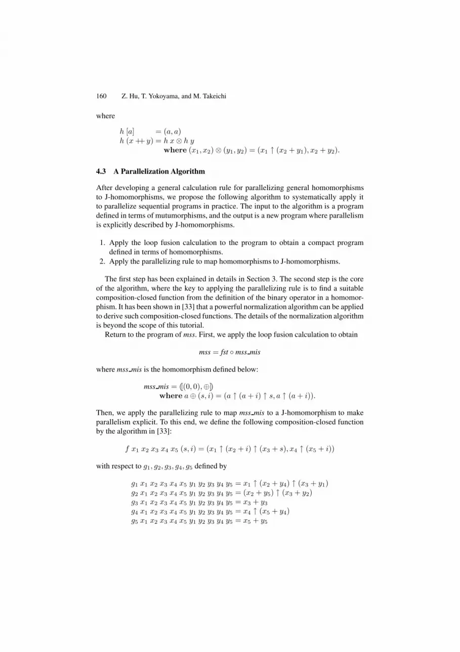
Return to the program of mss. First, we apply the loop fusion calculation to obtain

mss = fst ◦ mss mis

where mss mis is the homomorphism defined below:

mss mis = ([(0, 0), ⊕])where a ⊕ (s, i) = (a ↑ (a + i) ↑ s, a ↑ (a + i)).

Then, we apply the parallelizing rule to map mss mis to a J-homomorphism to make

parallelism explicit. To this end, we define the following composition-closed function

by the algorithm in [33]:

f x1 x2 x3 x4 x5 (s, i) = (x1 ↑ (x2 + i) ↑ (x3 + s), x4 ↑ (x5 + i))

with respect to g1, g2, g3, g4, g5 defined by

g1 x1 x2 x3 x4 x5 y1 y2 y3 y4 y5 = x1 ↑ (x2 + y4) ↑ (x3 + y1)g2 x1 x2 x3 x4 x5 y1 y2 y3 y4 y5 = (x2 + y5) ↑ (x3 + y2)g3 x1 x2 x3 x4 x5 y1 y2 y3 y4 y5 = x3 + y3

g4 x1 x2 x3 x4 x5 y1 y2 y3 y4 y5 = x4 ↑ (x5 + y4)g5 x1 x2 x3 x4 x5 y1 y2 y3 y4 y5 = x5 + y5


And we have

a ⊕ (s, i) = f a a 0 a a (i, s).

By applying the parallelizing rule we soon obtain the following efficient parallel pro-

gram for mss mis:

mss mis x = let (a1, a2, a3, a4, a5) = h x in f a1 a2 a3 a4 a5 (0, 0)

where h is a J-homomorphism defined as follows.

h [a] = (a, a, 0, a, a)h(x ++ y) = h x ⊗ h y

where (x1, x2.x3.x4.x5) ⊗ (y1, y2, y3, y4, y5)= (x1 ↑ (x2 + y4) ↑ (x3 + y1),

(x2 + y5) ↑ (x3 + y2),x3 + y3,x4 ↑ (x5 + y4),x5 + y5)

As an exercise, the readers are invited to parallelize the homomorphism for

sumBiggers in Section 3.

5 Yicho: An Environment for Implementing Transformations in

Calculational Forms

Program Calculation rules are short and concise, but their implementations are not as

easy as one may expect. Many attempts [20, 17] have been made to develop systems

for supporting direct and efficient implementation of calculation rules. Yicho is such a

system built upon Template Haskell [34] and designed for concise specification of pro-

gram calculations [35]. Its main feature lies in its expressive deterministic higher-order

patterns [17] together with an efficient deterministic higher-order matching algorithm.

This leads to a straightforward description of calculation rules.

In this section, we briefly review the Yicho system, before illustrating with some ex-

amples how calculation rules and calculation algorithms can be implemented efficiently.

5.1 Program Representation

We manipulate programs as values by meta-programming. Template Haskell [34] pro-

vides a mechanism to handle abstract syntax trees of Haskell in Haskell itself. Enclosing

a program in brackets [| |] yields its abstract syntax tree of type ExpQ, and the in-

verse operation is unquote described by a dollar $. For example, given a function to

calculate the sum of a given list, sum, which has type4 [Int] -> Int. Quotation

of this function [| sum |] has type ExpQ, whereas $([| sum |]) has the same

type as sum, i.e., [Int] -> Int.

4 Strictly speaking, the type of function sum is Num a ⇒ [a] → a in Haskell. Here, for

simplicity, we ignore type classes and polymorphism.


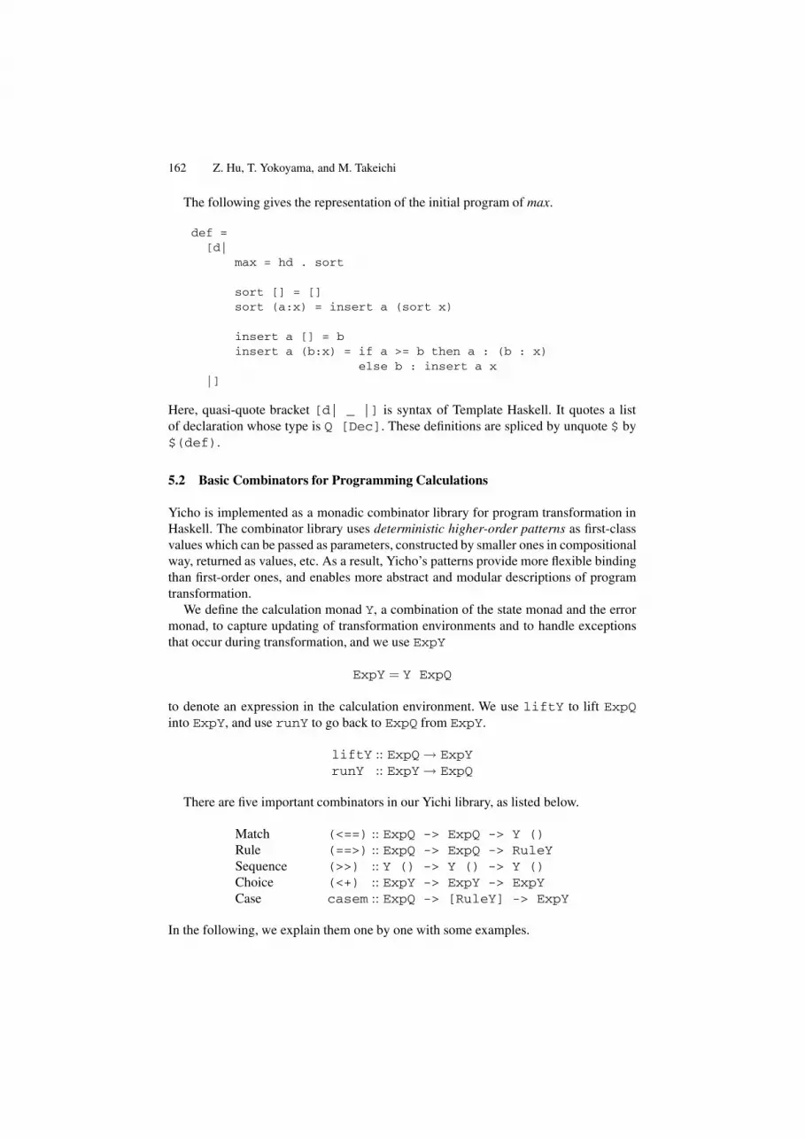
The following gives the representation of the initial program of max.

def =[d|

max = hd . sort

sort [] = []sort (a:x) = insert a (sort x)

insert a [] = binsert a (b:x) = if a >= b then a : (b : x)

else b : insert a x|]

Here, quasi-quote bracket [d| _ |] is syntax of Template Haskell. It quotes a list

of declaration whose type is Q [Dec]. These definitions are spliced by unquote $ by

$(def).

5.2 Basic Combinators for Programming Calculations

Yicho is implemented as a monadic combinator library for program transformation in

Haskell. The combinator library uses deterministic higher-order patterns as first-class

values which can be passed as parameters, constructed by smaller ones in compositional

way, returned as values, etc. As a result, Yicho’s patterns provide more flexible binding

than first-order ones, and enables more abstract and modular descriptions of program

transformation.

We define the calculation monad Y, a combination of the state monad and the error

monad, to capture updating of transformation environments and to handle exceptions

that occur during transformation, and we use ExpY

ExpY = Y ExpQ

to denote an expression in the calculation environment. We use liftY to lift ExpQinto ExpY, and use runY to go back to ExpQ from ExpY.

liftY :: ExpQ → ExpYrunY :: ExpY → ExpQ

There are five important combinators in our Yichi library, as listed below.

Match (<==) :: ExpQ -> ExpQ -> Y ()Rule (==>) :: ExpQ -> ExpQ -> RuleYSequence (>>) :: Y () -> Y () -> Y ()Choice (<+) :: ExpY -> ExpY -> ExpYCase casem :: ExpQ -> [RuleY] -> ExpY

In the following, we explain them one by one with some examples.


Match

The most essential combinator is the match combinator, which is used to match a pattern

with a term and produce a substitution (embedded in monadic Y).

(<==) :: ExpQ -> ExpQ -> Y ()pat <== term

As an example, consider that we want to express the expression

\a x -> if a >= sum x then a : biggers xelse biggers x

in the form of a ⊕ (biggers x, sum x) where ⊕ is a binary operator. We may code this

intention by

[| \a x -> $oplus a (biggers x, sum x) |]<== [| \a x -> if a >= sum x then a : biggers x

else biggers x |]

which will yield the following match:

{ $oplus := \x (b,s) ->if x > s then x : b else b }.

Note that Function $oplus is a second-order pattern variable and can be efficiently

obtained by the deterministic higher-order matching algorithm [17]. Note also that $means unquote, so the above match is equivalent to

{ oplus := [| \x (b,s) ->if x > s then x : b else b |] }.

Rule

The rule combinator is used to build a transformation rule mapping from one program

pattern to another. A rule is described in the form of

(==>) :: ExpQ -> ExpQ -> RuleYlhs ==> rhs

where RuleY, which is defined by RuleY = ExpQ -> Y ExpQ, is to map a pro-

gram to another under the transformation environment Y. For instance, we may define

the shortcut fusion rule by

[| hom $e $oplus . build $g |] ==> [| g $e $oplus |]

where we represent a homomorphism ([e, ⊕]) by (hom e oplus). The semantics of a

rule may be clear from the following where we define a rule by the Match combinator.

(==>) :: ExpQ -> ExpQ -> RuleY(pat ==> body) term = do pat <== term

ret body

Note that in the above, the function ret implicitly applies the match (i.e., substitution)

kept in the transformation monad to body.


Sequence

Sequential updates of transformation environments can be realized by combining

matches with the sequence combinator (>>).

(>>) :: Y () -> Y () -> Y ()(pat1 <== term1) >> (pat2 <== term2)

which can be written as sequence of matchings using do notation.

do pat1 <== term1pat2 <== term2

Deterministic Choice and Case

The combinator (<+) is designed to express deterministic choice.

(<+) :: ExpY -> ExpY -> ExpYtransExp1 <+ transExp2

It returns the first argument if the transformation in it succeeds. Otherwise, it returns

the second argument as the result. For instance, we may write

(rule1 e) <+ (rule2 e)

to first apply rule1 to transform e, and if it succeeds, we return the result; otherwise

we try to apply rule2 to e.

Using the choice combinator, we can define a meta version of the case expression,

which tries to apply a list of rules one by one until one rule succeeds.

casem :: ExpQ -> [RuleY] -> ExpYcasem sel (r:rs) = r sel <+ casem sel rs

5.3 Code Calculation Rules in Yicho

To get a flavor of Yicho, we show how to use Yicho to code the promotion rule in

Section 2, and how it is used to optimize the program. Since the list homomorphism

([e, ⊕]) is in fact the standard Haskell function foldr (⊕) e, we rewrite the promotion

theorem as follows.

promotion:f(a ⊕ x) = a ⊗ f x

f ◦ foldr (⊕) e = foldr (⊗) (f e)

This rule is defined in Yicho as follows.

promotion :: ExpQ -> Y ExpQpromotion exp = do

[f,oplus,e,otimes] <- pvars ["f","oplus","e","otimes"][| $f . foldr $oplus $e |] <== exp[| \a x -> $otimes a ($f x) |]

<== [| \a x -> $f ($oplus a x) |]ret [| foldr $otimes ($f $z) |]

The promotion rule is defined as a function that takes code and returns code with its

environment. In the third line, f,oplus,e,otimes are declared to be variables; the


unquote $ is actually splicing the expression, but, intuitively we can regard expression

$x as meta variable with the name of $x. In the fourth line, exp is matched with the pat-

tern [| $f . foldr $oplus $e |], with the variables $f,$oplus,$e being

bound in the environment. The next two lines are a straightforward translation of the

original promotion rule. $f and $oplus are instantiated and the both sides of <== are

matched and the resulting match is added to the environment. The pattern instantiation

contributes to the modularity of patterns. It should be noted here that the higher-order

patterns such as

[| \a x -> $otimes a ($f x) |]

play an important role in this concise definition. Finally, the result expression with its

environment are returned by ret.

We can enhance the promotion rule with a rule (say for unfolding the definition or

simplification), and add it as an argument to the promotion function.

promotionWithRule :: RuleY -> ExpQ -> Y ExpQpromotionWithRule rule exp = do

[f,oplus,e,otimes] <- pvars ["f","oplus","e","otimes"][| $f . foldr $oplus $e |] <== rule exp[| \a x -> $otimes a ($f x) |]

<== rule [| \a x -> $f ($oplus a x) |]ret [| foldr $otimes ($f $z) |]

To see how to apply the promotion rule, consider the following expression

oldExp = [| sum . foldr (\x y -> 2 * x : y) [] |]

and suppose that we hope to apply to this code the promotion rule together with some

other rule rule to obtain a new efficient expression, say newExp. We can define this

newExp as follows.

newExp = runY (promotionWithRule rule ex1)

We may confirm the result of newExp under the GHCi Environment:

GHCi> prettyExpQ newExpfoldr (\x_1 -> (+) (2 * x_1)) 0

where we use function prettyExpQ :: ExpQ -> IO () to print out an expression.

Now we can compare efficiency of the two expressions.

GHCi> $oldExp (take 100000 [1..])10000100000(0.33 secs, 21243136 bytes)

GHCi> $newExp (take 100000 [1..])10000100000(0.27 secs, 19581216 bytes)

It is worth noting that the promotion theorem is applied at compile time, and the func-

tion $newExp is actually improved both in the execution time and consumed heap

size.


The other calculation rules in this tutorial can be specified similarly. The readers are

invited to visit the Yicho home page for more examples.

6 Concluding Remarks

In this tutorial, we explain the basic technique of formalizing and implementing pro-

gram transformations and optimization in calculational form based on the Constructive

Algorithmics theory. We illustrate the idea with two important transformations, loop

fusion and parallelization, and we show how the transformations in calculational form

can be efficiently implemented with Yicho.

We summarize the main advantages of program transformations in calculational form

as follows.

– Modularity. A program transformation in calculational form does not require any

global analysis as other transformation systems often need. Instead, it only uses

a local program analysis to obtain the specialized form, and it can check locally

the applicability of their calculational rules. Therefore, it can be implemented in a

modular way, and is guaranteed to terminate.

– Generality. In this tutorial, we focus on the transformation of programs on lists.

In fact, most of our calculational laws are polytypic, i.e., parameterized with data

types. They can be generalized to transformation of programs on any algebraic data

types.

– Cheap Implementation. Transformations in calculational form are more practical

than the well-known fold-unfold transformations [4]. Fold/unfold transformation

basically has to keep track of all occurring function calls and introduce function

definitions to be searched in the folding step. The process of keeping track of

function calls and controlling the steps cleverly to avoid infinite unfolding intro-

duces substantial cost and complexity, which often prevents it from being practi-

cally implemented. Though they may be less general than fold/unfold transforma-

tions, transformations in calculational form can be implemented in a cheap way

[24, 36, 25, 14] by means of a local program analysis and simple rule application.

– Compatibility. It is usually difficult to make several transformations coexist well in

a single system, but transformations in calculational form can solve this problem

well. For instance, fusion calculation can coexist well with tupling calculation [14].

There are two reasons. First, each transformation is based on the same theoretical

framework, Constructive Algorithmics. Second, local program analysis and local

application of laws make it easier to check compatibility of transformations.

It should be noted that program transformations in calculation forms can be applied

only to those programs that can be turned into the form a calculation rule is applicable.

To increase the power, as seen in Section 4.3, we may have to design a normaliza-

tion algorithms with global analysis in order to obtain the required form. We believe

that more optimizations and transformations can be formalized in calculational form to

gain the advantages discussed above, and we are looking forward to see more practical

applications.


References

1. Jones, S.P., et al., J.H., eds.: Haskell 98: A Non-strict, Purely Functional Language. Available

online: http://www.haskell.org (1999)

2. Bird, R.: Introduction to Functional Programming using Haskell. Prentice Hall (1998)

3. Hughes, J.: Lazy memo-functions. In: Proc. Conference on Functional Programming Lan-

guages and Computer Architecture (LNCS 201), Nancy, France, Springer-Verlag, Berlin

(1985) 129–149

4. Burstall, R., Darlington, J.: A transformation system for developing recursive programs.

Journal of the ACM 24 (1977) 44–67

5. Feather, M.: A survey and classification of some program transformation techniques. In: TC2

IFIP Working Conference on Program Specification and Transformation, Bad Tolz, Germany,

North Holland (1987) 165–195

6. Darlington, J.: An experimental program transformation system. Artificial Intelligence 16

(1981) 1–46

7. Bird, R.: An introduction to the theory of lists. In Broy, M., ed.: Logic of Programming and

Calculi of Discrete Design, Springer-Verlag (1987) 5–42

8. Backhouse, R.: An exploration of the Bird-Meertens formalism. In: STOP Summer School

on Constructive Algorithmics, Ameland. (1989)

9. Meijer, E., Fokkinga, M., Paterson, R.: Functional programming with bananas, lenses, en-

velopes and barbed wire. In: Proc. Conference on Functional Programming Languages and

Computer Architecture (LNCS 523), Cambridge, Massachuetts (1991) 124–144

10. Fokkinga, M.: A gentle introduction to category theory — the calculational approach —.

Technical Report Lecture Notes, Dept. INF, University of Twente, The Netherlands (1992)

11. Jeuring, J.: Theories for Algorithm Calculation. Ph.D thesis, Faculty of Science, Utrecht

University (1993)

12. Bird, R., de Moor, O.: Algebras of Programming. Prentice Hall (1996)

13. Hu, Z., Iwasaki, H., Takeichi, M.: Deriving structural hylomorphisms from recursive defini-

tions. In: ACM SIGPLAN International Conference on Functional Programming, Philadel-

phia, PA, ACM Press (1996) 73–82

14. Hu, Z., Iwasaki, H., Takeichi, M., Takano, A.: Tupling calculation eliminates multiple data

traversals. In: ACM SIGPLAN International Conference on Functional Programming, Am-

sterdam, The Netherlands, ACM Press (1997) 164–175

15. Hu, Z., Takeichi, M., Chin, W.: Parallelization in calculational forms. In: 25th ACM Sympo-

sium on Principles of Programming Languages, San Diego, California, USA (1998) 316–328

16. Hu, Z., Iwasaki, H., Takeichi, M.: Calculating accumulations. New Generation Computing

17 (1999) 153–173

17. Yokoyama, T., Hu, Z., Takeichi, M.: Deterministic second-order patterns. Information Pro-

cessing Letters 89 (2004) 309–314

18. Malcolm, G.: Data structures and program transformation. Science of Computer Program-

ming (1990) 255–279

19. Pettorossi, A., Proiett, M.: Rules and strategies for transforming functional and logic pro-

grams. Computing Surveys 28 (1996) 360–414

20. de Moor, O., Sittampalam, G.: Higher-order matching for program transformation. Theor.

Comput. Sci. 269 (2001) 135–162

21. Goldberg, A., Paige, R.: Stream processing. In: LISP and Functional Programming. (1984)

53–62

22. Aho, A., Sethi, R., Ullman, J.: Compilers – Principles, Techniqies and Tools. Addison-

Wesley (1986)


23. Chin, W.: Towards an automated tupling strategy. In: Proc. Conference on Partial Evaluation

and Program Manipulation, Copenhagen, ACM Press (1993) 119–132

24. Gill, A., Launchbury, J., Jones, S.P.: A short cut to deforestation. In: Proc. Conference on

Functional Programming Languages and Computer Architecture, Copenhagen (1993) 223–

232

25. Takano, A., Meijer, E.: Shortcut deforestation in calculational form. In: Proc. Conference on

Functional Programming Languages and Computer Architecture, La Jolla, California (1995)

306–313

26. Onoue, Y., Hu, Z., Iwasaki, H., Takeichi, M.: A calculational fusion system HYLO. In: IFIP

TC 2 Working Conference on Algorithmic Languages and Calculi, Le Bischenberg, France,

Chapman&Hall (1997) 76–106

27. Banerjee, U., Eigenmann, R., Nicolau, A., Padua, D.A.: Automatic program parallelization.

Proceedings of the IEEE 81 (1993) 211–243

28. Cole, M.: Parallel programming, list homomorphisms and the maximum segment sum prob-

lems. Report CSR-25-93, Department of Computing Science, The University of Edinburgh

(1993)

29. Hu, Z., Iwasaki, H., Takeichi, M.: Formal derivation of efficient parallel programs by con-

struction of list homomorphisms. ACM Transactions on Programming Languages and Sys-

tems 19 (1997) 444–461

30. Skillicorn, D.: Foundations of Parallel Programming. Cambridge University Press (1994)

31. Gorlatch, S.: Constructing list homomorphisms. Technical Report MIP-9512, Fakultat fur

Mathematik und Informatik, Universitat Passau (1995)

32. Chin, W., Takano, A., Hu, Z.: Parallelization via context preservation. In: IEEE Com-

puter Society International Conference on Computer Languages, Loyola University Chicago,

Chicago, USA (1998)

33. Xu, D.N., Khoo, S.C., Hu, Z.: Ptype system : A featherweight parallelizability detector.

In: Second ASIAN Symposium on Programming Languages and Systems(APLAS 2004),

Taipei, Taiwan, Springer, LNCS 3302 (2004) 197–212

34. Sheard, T., Peyton Jones, S.L.: Template metaprogramming for Haskell. In: Haskell Work-

shop, Pittsburgh, Pennsylvania (2002) 1–16

35. Yokoyama, T., Hu, Z., Takeichi, M.: Deterministic second-order patterns and its application

to program transformation. In: International Symposium on Logic-based Program Synthesis

and Transformation (LOPSTR 2003), Springer, LNCS 3018 (2003) 165–178

36. Sheard, T., Fegaras, L.: A fold for all seasons. In: Proc. Conference on Functional Program-

ming Languages and Computer Architecture, Copenhagen (1993) 233–242

program optimizations and transformations in calculation form

Documents