climate change and algal blooms by shengpan lin
TRANSCRIPT

CLIMATE CHANGE AND ALGAL BLOOMS
By
Shengpan Lin
A DISSERTATION
Submitted to Michigan State University
in partial fulfillment of the requirements for the degree of
Integrative Biology—Doctor of Philosophy
2017
ABSTRACT
CLIMATE CHANGE AND ALGAL BLOOMS
By
Shengpan Lin
Algal blooms are new emerging hazards that have had important social impacts in recent years.
However, it was not very clear whether future climate change causing warming waters and stronger
storm events would exacerbate the algal bloom problem. The goal of this dissertation was to evaluate
the sensitivity of algal biomass to climate change in the continental United States. Long-term large-scale
observations of algal biomass in inland lakes are challenging, but are necessary to relate climate change
to algal blooms. To get observations at this scale, this dissertation applied machine-learning algorithms
including boosted regression trees (BRT) in remote sensing of chlorophyll-a with Landsat TM/ETM+. The
results show that the BRT algorithm improved model accuracy by 15%, compared to traditional linear
regression. The remote sensing model explained 46% of the total variance of the ground-measured
chlorophyll-a in the first National Lake Assessment conducted by the US Environmental Protection
Agency. That accuracy was ecologically meaningful to study climate change impacts on algal blooms.
Moreover, the BRT algorithm for chlorophyll-a would not have systematic bias that is introduced by
sediments and colored dissolved organic matter, both of which might change concurrently with climate
change and algal blooms. This dissertation shows that the existing atmospheric corrections for Landsat
TM/ETM+ imagery might not be good enough to improve the remote sensing of chlorophyll-a in inland
lakes. After deriving long-term algal biomass estimates from Landsat TM/ETM+, time series analysis was
used to study the relations of climate change and algal biomass in four Missouri reservoirs. The results
show that neither temperature nor precipitation was the only factor that controlled temporal variation
of algal biomass. Different reservoirs, even different zones within the same reservoir, responded
differently to temperature and precipitation changes. These findings were further tested in 1157 lakes

across the continental United States. The results show that mean annual algal biomass generally
increased with annual temperature. Greater increase was found in lakes with more nutrients. Mean
annual algal biomass generally decreased with annual total precipitation. In both the “low” and the
“high” greenhouse-gas emission scenarios, mean annual algal biomass in lakes generally increased with
climate change, and greater increases are predicted from the high emission scenario.
Keywords: climate change, algal bloom, remote sensing, machine learning

Copyright by SHENGPAN LIN 2017

v
ACKNOWLEDGEMENTS
I would like to express my sincere gratitude to my committee chair, Professor R. Jan Stevenson, who
continually conveys the patience of a mentor, the intelligence of a discoverer, the integrity of a scientist,
and the passion of a teacher. This dissertation is made possible by his persistent guidance.
I thank my committee members, Professor Jiaguo Qi, Professor David W. Hyndman, and Professor
Stephen K. Hamilton, who helped me all the way from course selection to the proposal and completion
of this dissertation. They are genuinely willing to help guide me to succeed in my career. I still remember
the comment from Professor Hamilton during my comprehensive examination. He encouraged me not
to give up pursuing a career in academia simply because that I was not fully comfortable in speaking
English. It turns out that as he said, time would solve the problem. The feedbacks from the committee
have greatly improved the quality of my dissertation. They polished my writing almost sentence by
sentence, far exceeding my expectation.
Professor John R. Jones at University of Missouri kindly provided 28 years of reservoir data for my study.
Professor Charles P. Hawkins at Utah State University shared his spatial data corresponding to the lakes
sampled by the first National Lake Assessment. These data are the basis of part of my dissertation
research, and I deeply appreciate their generosity. I thank Professor Bryan Pijanowski at Purdue
University for providing land use projection data. I did not finally use the data in the dissertation, but his
kindness is appreciated.
This research was funded by US Environmental Protection Agency (EPA) (Grant #: R835203). Thanks to
the PI and co-PIs who spent a lot of time to pursue this funding and made it available to me. The group
members in the project, including Dr. Nathan Moore, Dr. Sherry Martin, and Dr. Anthony Kendall, have
offered useful comments on my dissertation research.

vi
My friends Brad Peter, Dr. Linda Novitski, and Dr. Timothy Cefai improved the language in parts of this
dissertation. Visiting scholar Tao Tang from China provided the idea of gradient forest in the
atmospheric correction analysis. Di Liang at the Kellogg Biological Station inspired me on the watershed
impacts of climate change. I am lucky to have a lot of great friends and colleagues who emotionally and
intellectually supported me in this dissertation, and filled my life with beer, laughter, and joy. I cannot
list them all here. Their help extended far beyond this dissertation.
Last but not the least, thanks to my father Jiatian Lin and my mother Wenfang Xie for their
unconditional love.
vii
TABLE OF CONTENTS
LIST OF TABLES ............................................................................................................................................. xi
LIST OF FIGURES .......................................................................................................................................... xii
1 GENERAL INTRODUCTION ..................................................................................................................... 1 1.1 Algal blooms .................................................................................................................................. 1
1.1.1 Species .................................................................................................................................. 1 1.1.2 Public health impacts ............................................................................................................ 1 1.1.3 Economic and social impacts ................................................................................................ 2 1.1.4 Perceptions ........................................................................................................................... 3
1.2 Climate change .............................................................................................................................. 4 1.3 Climate change impacts on algal blooms ...................................................................................... 5
1.3.1 Temperature ......................................................................................................................... 7 1.3.2 Precipitation .......................................................................................................................... 9 1.3.3 Watershed effects ............................................................................................................... 10
1.4 Remote sensing of algal blooms ................................................................................................. 10 1.4.1 The theory of remote sensing ............................................................................................. 11 1.4.2 Remote sensing algorithms ................................................................................................. 12
1.5 Dissertation structure ................................................................................................................. 13 REFERENCES ............................................................................................................................................ 15
2 MACHINE-LEARNING ALGORITHMS FOR CHLOROPHYLL-A MEASUREMENTS IN INLAND LAKES USING LANDSAT TM/ETM+ .................................................................................................................................... 21
Abstract ................................................................................................................................................... 21 Highlights ................................................................................................................................................ 22 2.1 Introduction ................................................................................................................................ 22
2.1.1 Long-term large-scale measurement of algal biomass is needed ...................................... 22 2.1.2 Remote sensing of algae in inland water bodies is challenging .......................................... 22 2.1.3 Objective and research questions ....................................................................................... 24
2.2 Methodology ............................................................................................................................... 25 2.2.1 Model comparison .............................................................................................................. 25
2.2.1.1 Model data ...................................................................................................................... 25 2.2.1.1.1 Ground-measured water quality data ...................................................................... 25 2.2.1.1.2 Remote sensing data................................................................................................. 26 2.2.1.1.3 Data screening .......................................................................................................... 27
2.2.1.2 Model performance comparison .................................................................................... 29 2.2.1.3 Model development ........................................................................................................ 29
2.2.2 Evaluation of model applications ........................................................................................ 31 2.2.2.1 Algal bloom detection ..................................................................................................... 31 2.2.2.2 Validation by relation with total phosphorus ................................................................. 31
2.3 Results ......................................................................................................................................... 32 2.3.1 Algorithm comparison ........................................................................................................ 32 2.3.2 Performance for algal bloom identification ........................................................................ 34 2.3.3 Relation with total phosphorus .......................................................................................... 35
viii
2.4 Discussion .................................................................................................................................... 37 2.4.1 Are machine-learning algorithms our best choice? ............................................................ 37 2.4.2 Error sources ....................................................................................................................... 40
2.4.2.1 Phytoplankton spatial and temporal heterogeneity ....................................................... 40 2.4.2.2 Image quality ................................................................................................................... 41 2.4.2.3 Lake condition ................................................................................................................. 43
2.4.3 Are machine-learning algorithms good enough? ............................................................... 43 2.5 Conclusion ................................................................................................................................... 44 Acknowledgement .................................................................................................................................. 44 REFERENCES ............................................................................................................................................ 45
3 EFFECTS OF SEDIMENTS AND COLORED DISSOLVED ORGANIC MATTER ON REMOTE SENSING OF CHLOROPHYLL-A USING LANDSAT TM/ETM+ OVER TURBID WATERS ....................................................... 51
Abstract ................................................................................................................................................... 51 Highlights ................................................................................................................................................ 51 3.1 Introduction ................................................................................................................................ 52
3.1.1 Remote sensing of chlorophyll-a in inland lakes................................................................. 52 3.1.2 Sediment effects ................................................................................................................. 53 3.1.3 CDOM effects ...................................................................................................................... 54 3.1.4 Landsat chlorophyll-a algorithms ........................................................................................ 54 3.1.5 Objective ............................................................................................................................. 55
3.2 Methodology ............................................................................................................................... 56 3.2.1 Data ..................................................................................................................................... 56
3.2.1.1 In-situ data ...................................................................................................................... 56 3.2.1.2 Remote sensing data ....................................................................................................... 58
3.2.2 Chlorophyll-a model development ..................................................................................... 59 3.2.3 Residual analyses ................................................................................................................ 60
3.3 Results ......................................................................................................................................... 63 3.4 Discussion .................................................................................................................................... 67
3.4.1 Model performance ............................................................................................................ 67 3.4.2 Sediments and CDOM effects ............................................................................................. 68
3.4.2.1 The method for detecting effects ................................................................................... 68 3.4.2.2 Explanations for the insensitivity to suspended sediments and CDOM ......................... 69
3.4.3 Model correction ................................................................................................................ 70 3.4.4 Application of the findings .................................................................................................. 71
3.5 Conclusion ................................................................................................................................... 72 Acknowledgement .................................................................................................................................. 72 REFERENCES ............................................................................................................................................ 73
4 LANDSAT SURFACE REFLECTANCE PRODUCTS FOR REMOTE SENSING OF INLAND LAKES: THE PROBLEM OF ATMOSPHERIC INTERFERENCE ............................................................................................. 79
Abstract ................................................................................................................................................... 79 Highlights ................................................................................................................................................ 79 4.1 Introduction ................................................................................................................................ 80 4.2 Methodology ............................................................................................................................... 81
4.2.1 Study area and data ............................................................................................................ 81 4.2.2 Signal enhancement evaluation .......................................................................................... 82 4.2.3 Remote sensing of water optical characteristics ................................................................ 83
ix
4.3 Results ......................................................................................................................................... 84 4.3.1 Signal change ...................................................................................................................... 84 4.3.2 Remote sensing of water optics .......................................................................................... 86
4.4 Discussion .................................................................................................................................... 86 4.4.1 Why did the atmospheric correction produce no obvious signal enhancement? .............. 86 4.4.2 Remote sensing of water optical characteristics ................................................................ 93
4.5 Conclusion ................................................................................................................................... 94 Acknowledgement .................................................................................................................................. 94 REFERENCES ............................................................................................................................................ 95
5 ALGAL BIOMASS RESPONSES TO CLIMATE CHANGE IN MISSOURI RESERVOIRS ................................ 98 Abstract ................................................................................................................................................... 98 Highlights ................................................................................................................................................ 98 5.1 Introduction ................................................................................................................................ 99
5.1.1 Climate change .................................................................................................................... 99 5.1.2 Harmful algal blooms .......................................................................................................... 99 5.1.3 Complex system ................................................................................................................ 100 5.1.4 Objective and research questions ..................................................................................... 101
5.2 Methodology ............................................................................................................................. 102 5.2.1 Study reservoirs ................................................................................................................ 102 5.2.2 Data ................................................................................................................................... 103 5.2.3 Spatial and temporal patterns .......................................................................................... 105 5.2.4 Univariate analyses ........................................................................................................... 106 5.2.5 Multivariate analyses ........................................................................................................ 107
5.3 Results ....................................................................................................................................... 108 5.3.1 Spatial and temporal patterns .......................................................................................... 108 5.3.2 Single-factor analyses ....................................................................................................... 113
5.3.2.1 Lake surface temperature effects on chlorophyll ......................................................... 113 5.3.2.2 Total precipitation effects on chlorophyll ..................................................................... 114 5.3.2.3 Precipitation intensity effects on chlorophyll ............................................................... 116
5.3.3 Multiple-factor analyses ................................................................................................... 117 5.4 Discussion .................................................................................................................................. 119
5.4.1 Temperature effects ......................................................................................................... 119 5.4.2 Precipitation effects .......................................................................................................... 121
5.4.2.1 Nutrient and light availability........................................................................................ 121 5.4.2.2 Residence time of water in the reservoirs .................................................................... 122 5.4.2.3 Time lags in algal biomass responses ............................................................................ 123 5.4.2.4 Internal nutrient legacy sources ................................................................................... 123 5.4.2.5 Phytoplankton adaptation ............................................................................................ 124
5.5 Conclusion ................................................................................................................................. 124 Acknowledgement ................................................................................................................................ 125 APPENDIX .............................................................................................................................................. 126 REFERENCES .......................................................................................................................................... 136
6 ALGAL BIOMASS RESPONSES TO CLIMATE CHANGE IN LAKES ACROSS THE CONTINENTAL UNITED STATES ....................................................................................................................................................... 140
Abstract ................................................................................................................................................. 140 Highlights .............................................................................................................................................. 140
x
6.1 Introduction .............................................................................................................................. 141 6.2 Methodology ............................................................................................................................. 144
6.2.1 Study lakes ........................................................................................................................ 144 6.2.2 Sensitivity and partial dependence analyses .................................................................... 145
6.2.2.1 Chl sensitivity to temperature ...................................................................................... 148 6.2.2.2 Chl sensitivity to precipitation ...................................................................................... 149
6.2.3 Future scenario analyses ................................................................................................... 152 6.3 Results ....................................................................................................................................... 153
6.3.1 Chl sensitivity to temperature .......................................................................................... 153 6.3.2 Chl sensitivity to precipitation .......................................................................................... 155 6.3.3 Future scenario analyses ................................................................................................... 161
6.4 Discussion .................................................................................................................................. 167 6.4.1 Chl increased with temperature but regulated by nutrients (Hypotheses A & B) ............ 167 6.4.2 Chl sensitivity to precipitation (Hypothesis C) and its variations with natural hydraulic conditions (Hypothesis D) ................................................................................................................. 168 6.4.3 Future scenario analyses ................................................................................................... 171 6.4.4 Long-term temperature and precipitation effects............................................................ 174 6.4.5 Climate change mitigation ................................................................................................ 177
6.5 Conclusion ................................................................................................................................. 177 Acknowledgement ................................................................................................................................ 178 REFERENCES .......................................................................................................................................... 179
7 SUMMARY ......................................................................................................................................... 185 7.1 Dissertation summary ............................................................................................................... 185
7.1.1 Model development .......................................................................................................... 185 7.1.2 Interference from optically active agents in water ........................................................... 186 7.1.3 Interference from the atmosphere ................................................................................... 187 7.1.4 Time series analyses .......................................................................................................... 188 7.1.5 Spatial Analyses ................................................................................................................. 189
7.2 Future directions ....................................................................................................................... 191 7.2.1 Impacts of temperature increase...................................................................................... 191 7.2.2 Impacts of precipitation change ....................................................................................... 192 7.2.3 Remote sensing of algal species ....................................................................................... 193
xi
LIST OF TABLES
Table 2-1 Model performance differences indicated by p values of paired t-tests.................................... 33
Table 2-2 Correlation coefficient (Pearson r) between ground-measured total phosphorus (TP) and chlorophyll-a (Chl) measured on ground as well as by remote sensing (RS). “Rev. N” is the number of revisit times of Chl measurement for each lake. Chl for each lake is the average value of revisited measurements when Rev. N > 1. The measurement times (“Meas. N”) used in each average Chl are indicated in the first column. For a lake that was revisited four times (Rev. N = 4), Chl could be averaged from one, two, three, or four measurements (i.e., Meas. N = 1, 2, 3, or 4). .............................................. 36
Table 3-1 Statistics summary of in-situ measurements .............................................................................. 57
Table 3-2 The range of residual trend decreased after parsing out the sediment and CDOM correlations with chlorophyll-a. ...................................................................................................................................... 67
Table 4-1 Effects of the atmospheric correction on performances of water color models when using MLR and RF algorithms for models. The t-test compares the R2 for 10 cross validations of TOA and SR models with either MLR or RF algorithms. .............................................................................................................. 87
Table 5-1 Number of models with slope > 0 and number of models with p-value < 0.05 (in brackets) in linear regression models for individual zones (N = 13) of study reservoirs (N = 4). ................................. 115
Table 5-2 Variations of daily chlorophyll contributed mostly by lake surface temperature (Ts) other than precipitation (Pre), indicated by 10-fold cross validation R2 of the daily chlorophyll models. ................ 119
Table 5-3 Reservior characteristics that may affect algal biomass responses to precipitation. Z scores of reservoir characteristics are compared to the first National Lake Assessment (NLA) lakes. Algal biomass responses are indicated by number of slope β > 0 in linear regression models: July-August chlorophyll = LM (total precipitation with time lag). ...................................................................................................... 122
Table A. 5-1 Magnitude (Sen’s slope, k) and significance (p) of yearly mean algal biomass and climate during 1984-2011 at upstream, midstream, and dam zones of Smithville, Pomme de Terre, Clearwater, and Wappapello in Missouri, United States. Table indicates significant increase trends in precipitation intense (Pre.I), while different responses of chlorophyll at different reservoir zones. ............................ 130
Table A. 5-2 Slope (β) and p-value of linear regression models (LMs). P < 0.05 is marked as red. .......... 131
Table 6-1 Diagnostic models. See Table 6-2 for variable descriptions. Grey background indicates a new variable compared to the previous model. .............................................................................................. 147
Table 6-2 Model variables and data sources. ........................................................................................... 147
Table 6-3 Variable interactions in Model 2 indicated by Friedman's H-statistic. Grid colors: green = low; red = high. See Table 6-2 for variable explanations. ................................................................................. 159
xii
LIST OF FIGURES
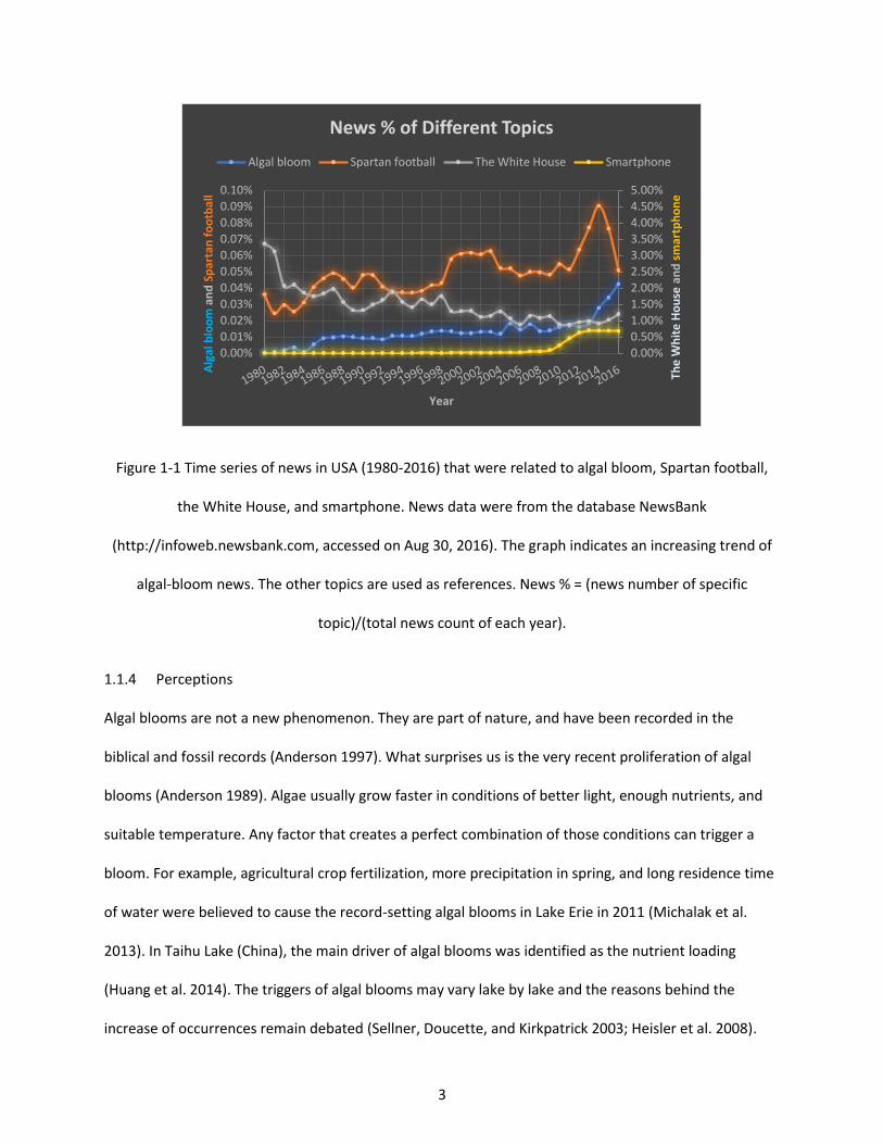
Figure 1-1 Time series of news in USA (1980-2016) that were related to algal bloom, Spartan football, the White House, and smartphone. News data were from the database NewsBank (http://infoweb.newsbank.com, accessed on Aug 30, 2016). The graph indicates an increasing trend of algal-bloom news. The other topics are used as references. News % = (news number of specific topic)/(total news count of each year). ........................................................................................................ 3
Figure 1-2 Percentage of news that mentioned different causation words. The graph shows public perceptions about causes of algal blooms. Algal-bloom news in USA (1980-2016) was from the database NewsBank (http://infoweb.newsbank.com, accessed on Aug 30, 2016). News % = (news number of specific cause)/(total algal-bloom news). ..................................................................................................... 4
Figure 1-3 The number of publications (y-axis) that cite Paerl and Huisman (2008) changes over years (x-axis). Publications are those in the Web of Science Core Collection (http://www.webofknowledge.com) as of February 7, 2017. Total publication number = 687. ............................................................................. 6
Figure 1-4 Possible pathways of climate change impacts on algal blooms. Summarized from Paerl and Huisman (2008). The red frame indicates a decrease of algal abundance due to climate change. ............. 7
Figure 1-5 Absolute abundance (bio-volume) of algal divisions as a function of lake surface temperature. Data source: U.S. EPA National Lake Assessment, 2007 (http://www.usepa.gov, accessed on Jan 20, 2014). Lake number = 1157. Figure indicates that algal abundance did not necessarily increase with temperature in the normal US summer range of about 20-30 °C. There might be other factors other than lake temperature controlling algal abundance. ............................................................................................ 8
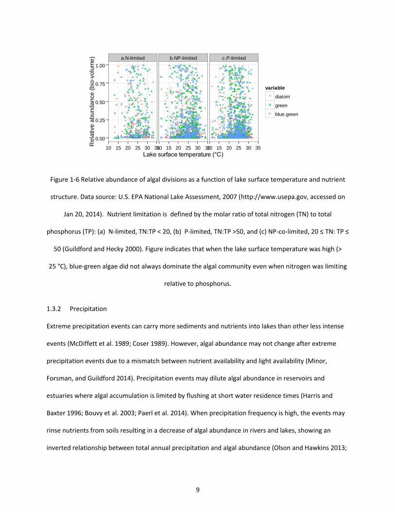
Figure 1-6 Relative abundance of algal divisions as a function of lake surface temperature and nutrient structure. Data source: U.S. EPA National Lake Assessment, 2007 (http://www.usepa.gov, accessed on Jan 20, 2014). Nutrient limitation is defined by the molar ratio of total nitrogen (TN) to total phosphorus (TP): (a) N-limited, TN:TP < 20, (b) P-limited, TN:TP >50, and (c) NP-co-limited, 20 ≤ TN: TP
≤ 50 (Guildford and Hecky 2000). Figure indicates that when the lake surface temperature was high (>
25 °C), blue-green algae did not always dominate the algal community even when nitrogen was limiting relative to phosphorus. ................................................................................................................................. 9
Figure 1-7 Analytical models to relate remote sensing signals to water constituents. .............................. 11
Figure 2-1 Chlorophyll-a (Chl) concentration in the first National Lake Assessment sample sites. ........... 26
Figure 2-2 Chlorophyll-a (Chl) concentration of Maumee River (part) in Ohio (USA) as an example of data screening results. Band reflectance (B1-B5, and B7) of (a) water, (b) land, (c) cloud shadow, and (d) cloud, whose locations are indicated on (e). (e) Chl map overlaid on Landsat 5 Surface Reflectance (SR) image. .......................................................................................................................................................... 28
Figure 2-3 Variable reduction test for the BRT algorithm. Variable ln.SR.B7 reads log-transformed surface reflectance of Band 7. B2v7 reads the ratio of Band 2 vs. Band 7. Dropping order was based on relative importance of variables. The two most important variables, i.e., ln.SR.B1v3 and ln.SR.B1v2, were always included in the model. ................................................................................................................................ 30
xiii
Figure 2-4 Scatter plot of ground-measured chlorophyll-a (ground Chl, µg/L) and remotely sensed chlorophyll-a (RS Chl, µg/L) in 10-fold cross validation. Algorithms include (a) multiple linear regression (MLR), (b) general additive models (GAM), (c) boosted regression trees (BRT), and (d) random forest (RF). Results of each fold in 10-fold validation are coded with numbers. Dashed lines are the 1:1 ratio lines. ............................................................................................................................................................ 33
Figure 2-5 Example of an algal bloom event around Pelee Island in Lake Erie on September 4, 2009. (a) Landsat 5 TM image of the bloom area. The island location is indicated by the red dot on the bottom left map. (b) Chlorophyll-a concentrations estimated from Landsat-5 TM data using the random forest (RF) algorithm. (c) The bloom is indicated by the time series of mean chlorophyll-a over the south shore of the island (i.e., the triangle area indicated in a) predicted using the RF algorithm. .................................. 34
Figure 2-6 Change of Chlorophyll-a (Chl) and total phosphorus (TP) between two samplings of a subset of lakes in the first National Lake Assessment, 2007. Each point represents one lake (N = 36). For the first measurements, median Chl = 42.2 µg/L, median TP = 20.0 µg/L. Let x1 = the first measurement, and x2 = the second measurement, then abs. change = absolute (x1 – x2), and relative change (%) = (abs. change) /x1. ............................................................................................................................................................... 35
Figure 2-7 Cross-dataset validation of the chlorophyll-a (Chl, µg/L) random forest model. The random forest model was trained by the dataset of the first National Lake Assessment, then validated by the dataset of 24 years (1989-2012) and 39 reservoirs in Missouri, USA. Validation NSE = -0.137, indicating a model failure. Dashed line is the 1:1 ratio line. .......................................................................................... 39
Figure 2-8 The absolute residual of the random forest model did not change with the pixel numbers less than 9 or day difference less than 8 between the ground measure dates and remote sensing dates. ..... 40
Figure 2-9 Landsat TM abnormal stripes on chlorophyll map of Maumee Bay (USA). Landsat image ID = “LT50200312009199GNC02”. The chlorophyll map was overlain on the Landsat image. White areas are clouds. ......................................................................................................................................................... 42
Figure 3-1 Schematic diagram of water reflectance affected by algae, sediments, and CDOM (colored dissolved organic matter). Arrows indicate the expected change in the curve when concentrations of corresponding substances increase (after Carder et al. 1989; Han 1997). ................................................. 53
Figure 3-2 Thirty-nine sampling locations (indicated by dots) in Missouri, USA. ....................................... 57
Figure 3-3 Spearman correlation matrix between ln-transformed chlorophyll-a concentration (ln.CHLA), ln-transformed absorption coefficient at 440 nm wavelength (ln.A440nm), and ln-transformed concentration of non-volatile suspended solids (ln.NVSS). The solid line in the scatter plot is the LOWESS (locally weighted scatterplot smoothing) smooth line. All correlations are significant (p < 0.05). ............ 63
Figure 3-4 Ten-fold cross-validation for remote sensing (RS) of chlorophyll-a concentrations (Chl, µg/L) using two different algorithms: (a) multiple linear regression (MLR), and (b) boosted regression trees (BRT). The dashed line is the one-to-one ratio line. Predicted values of 10 cross-validations are coded with corresponding numbers where number i indicates the i-th validation. ............................................. 65
Figure 3-5 Residual plot of the remote sensing BRT model for chlorophyll-a (Chl). The solid line is the GAM (generalized additive models) smooth line with 95% confidence intervals on two sides. ................ 65
xiv
Figure 3-6 Residuals related to (a) sediments and (b) CDOM (colored dissolved organic matter). Solid lines are GAM (generalized additive models) smooth lines with 95% confidence intervals on two sides. NVSS – non-volatile suspended solids; A440nm – absorbance coefficient measured at 440 nm wavelength. ................................................................................................................................................. 66
Figure 3-7 Partial dependence plots indicating residual changes over (a) ln(NVSS) (suspended sediments), and (b) ln(A440nm) (colored dissolved organic matter, CDOM). The bars on the top indicate data distribution in deciles. ........................................................................................................................ 66
Figure 3-8 Theoretical residual changes: (a) residual increases with higher sediment concentrations then reaches a plateau, and (b) residual decreases with higher CDOM (colored dissolved organic matter) concentrations then reaches a plateau. ..................................................................................................... 67
Figure 3-9 Model bias correction using deshrinking. Solid line is the linear regression line with its equation on the top and 95% confidence intervals shown in grey. ........................................................... 71
Figure 4-1 Water color signal in Landsat TM/ETM+ as changed by the atmospheric correction. The image signal is indicated by R2 of models for bands/band ratios: Bi = RF (Chl, NVSS, A440nm), where Bi is the TOA (top of atmosphere) or SR (surface reflectance) band/band ratio with i indicating the band number or combination of bands in ratios, e.g., B1 = Band 1, and B1v2 = ratio of Band 1 vs. Band 2. RF is the random forest algorithm. Chl is chlorophyll-a concentration. NVSS is concentration of non-volatile suspended solids. A440nm is absorbance coefficient at 440 nm wavelength (indicator of colored dissolved organic matter). Figure a has the same information as b-e, which are scatter plots comparing either the total or partial R2 before and after the atmospheric correction. The dashed line is the 1:1 line in b-e. .......................................................................................................................................................... 85
Figure 4-2 (a) Average reflectance in the 39 reservoirs as changed by the atmospheric correction; (b) band signal (indicated by R2) as changed by the atmospheric correction. Figure 4-2 b is the same as Figure 4-1 a except that the band ratios are excluded and the bands are in a different order for comparison with Figure 4-2 a. See Figure 4-1 for abbreviations. .............................................................. 88
Figure 4-3 (a) Sumer wind speed at Maryville, Missouri, USA; (b) whitecap effect for each Landsat TM/ETM+ band, i.e., B1, B2, B3 etc. Wind speed data are from GRIDMET (University of Idaho Gridded Surface Meteorological Dataset) (Abatzoglou 2013). Y-axe in (b) is (ρfoam/ρTOA) * 100%, where ρfoam is reflectance of foam caused by wind, calculated by empirical equations (Koepke 1984; Monahan and Muircheartaigh 1980); ρTOA is average TOA reflectance in the Missouri reservoirs. .................................. 90
Figure 4-4 Spatial and temporal variations of aerosol optical thickness (AOT, dimensionless) in 2013 measured at the AERONET stations: (a) Mingo, Missouri; (b) St. Louis University, Missouri (data source: Pendley, http://aeronet.gsfc.nasa.gov, accessed on Jan 2nd, 2016). Locations of the stations are indicated on the right map: top solid dot as St. Louis University Station; bottom solid dot as Mingo Station. 550 nm, 675 nm, 870nm, and 1640nm is in the range of Landsat TM/ETM+ B1, B3, B4, and B5, respectively. .................................................................................................................................................................... 91
Figure 4-5 Violin plot of the atmospheric correction in band 1 (the band with the strongest atmospheric effect) in five of the Missouri reservoirs as examples. Corrected percentage = (SR-TOA)/TOA × 100%, where SR is surface reflectance and TOA is top of atmospheric reflectance. Each side of a violin is a kernel density estimation line..................................................................................................................... 92
xv
Figure 5-1 Map of study reservoirs and associated catchment basins. Locations of basins are indicated by middle maps. Polygons on reservoirs indicate study zones. Names of reservoirs are Smithville, Pomme de Terre, Wappapello, and Clearwater (from West to East). ................................................................... 103
Figure 5-2 Missouri reservoir chlorophyll (Chl, natural logarithm of concentrations, µg/L) showing ground measurements compared to model remotely sensed (RS) measurements (R2 = 0.347) indicated by 10-fold cross validations. Dashed line is a one-to-one ratio. ............................................................... 104
Figure 5-3 Average chlorophyll concentration of Pomme de Terra Lake (Missouri) during July-August 2011. Higher chlorophyll was found in the upstream branches than the dam zone (on the top figure). Similar spatial patterns were found in the other study reservoirs. .......................................................... 109
Figure 5-4 Daily time series of chlorophyll concentration (Chl, µg/L), lake surface temperature (Ts, °C), discharge (Q, ft3/s, 1 ft = 30.48 cm), and precipitation (Pre, mm/d) from 1984 to 2011 at Wappapello Upstream West. Data gaps were interpolated with the method of “last one carried forward.” There was no discharge data available before 2008. ................................................................................................. 111
Figure 5-5 Chlorophyll (Chl), lake surface temperature (Ts), precipitation (Pre) and discharge (Q) changed over day of year (DOY) in four upstream zones that are associated corresponding main sub-basins of study reservoirs. Values were measured from 1984-2011, except for discharge data that were only available in 2008-2011. Solid lines are smooth lines with 95% confidence intervals. See Figure A. 5-2 for all zones of the reservoirs. ........................................................................................................................ 112
Figure 5-6 Annual average time series of mean annual chlorophyll (Chl.annual µg/L), chlorophyll in July-August (Chl.summer µg/L), lake surface temperature (Ts, °C), and precipitation intensity (Pre.I, mm/d, excluding days with precipitation < 1 mm/d) from 1984 to 2011 at four upstream zones that are associated to the main sub-basins of study reservoirs. Magnitude (Sen’s slope, k) and significance (p) of the trends are shown. Dashed lines are linear regression lines. See Table A. 5-1 for the full summary of all zones. ................................................................................................................................................... 113
Figure 5-7 Partial dependent plots of the Wappapello Upstream East chlorophyll (Chl, µg/L) model (10-fold cross validation R2 = 0.505). ΔChl (= max - min) indicates the magnitude of chlorophyll change over the variable of x-axis. Numbers in brackets are the relative importance of predictors. For comparison purposes, y-axis variable is centered to have a zero mean. Bars at the top of plots show distribution of x-axis variables in deciles. The model predictors include Ts0, Ts7n9, Ts16, Ts23n25, Ts32, Ts39n41, Pre0, Pre1, Pre2, Pre4, Pre8, Pre16, Pre32, Pre64, and Pre128, where the number at the end of each variable is the number of lag days, and “n” links two lags that are grouped together. Ts, lake surface temperature (°C); Pre, precipitation (mm/d) ................................................................................................................. 118
Figure A. 5-1 Basin Land use/cover changes of (a) Smithville, (b) Pomme de Terra, (c) Clearwater, and (d) Wappapello. Data source: USGS National Land Cover Database (Google Earth Image ID: USGS/NLCD). 127
Figure A. 5-2 Chlorophyll (Chl), lake surface temperature (Ts), precipitation (Pre) and discharge (Q) changed over day of year (DOY). Values were measured from 1984-2011, except for discharge data that were only available in 2008-2011. Solid line is smooth line with 95% confidence interval. .................... 128
Figure 6-1 Lake chlorophyll-a (Chl) from the 2007 National Lake Assessment (NLA), 2007 daily maximum temperature (TaMax), 2007 annual total precipitation (PreTot), and 2007 precipitation intensity (PreInt). Each Chl point represents one lake sample. Background maps are Google Map data. ........................... 144
xvi
Figure 6-2 Predictive accuracy of remotely sensed chlorophyll-a (RS Chl) indicated by 10-fold cross validations. NSE = 0.462 (δ = 0.086), sample N = 483. The dashed line is a 1:1 ratio line. Each point represents one lake sample. Ten validations were coded by corresponding numbers from 1 to 10. ..... 150
Figure 6-3 Partial dependence plots of Model 1. For comparison purposes, all plots have the same range of y-axis, and modeled Chl is centered to have a zero mean. Percentages in brackets are relative importance of the independent variables. Tick marks at the top are decile marks showing data distribution across the x-axis variable (data N = 1156). ∆Chl is the range of modeled Chl. See Table 6-2 for variable explanations. ......................................................................................................................... 154
Figure 6-4 Chlorophyll-a (Chl) sensitivity to lake surface temperature (Ts) changed with nutrient concentration, i.e., log-transformed total nitrogen (ln.TN) and log-transformed total phosphorus (ln.TP). Chl are modeled values from Model 1. Sensitivity to Ts here is the range of Chl change with Ts at the designated level of ln.TP and ln.TN. Tick marks at the top are decile positions showing the data distribution across the x-axis variable (data N = 1156). Each point on figures on the right is one of 50 interpolation points. ................................................................................................................................. 155
Figure 6-5 Model performance (indicated by Nash–Sutcliffe model efficiency coefficient, NSE) changes with dependent variable (y) in the model y = BRT (ln.TP, ln.TN, Ts). See Table 6-2 for variable explanations. Error bars represent one standard deviation. N is sample number of each model. For comparison purposes, lake samples were changed to have the same number and identity of lakes for each step of model comparison................................................................................................................ 156
Figure 6-6 Partial dependence plots of Model 2. For comparison purposes, all plots have the same range of y-axis, and modeled Chl is centered to have zero mean. Percentages in brackets are relative importance of the variables. Tick marks at the top are decile locations showing the data distribution across the x-axis variable (data N = 658). ∆Chl is the range of modeled Chl. See Table 6-2 for variable explanations. ............................................................................................................................................. 158
Figure 6-7 Chlorophyll-a (Chl) sensitivity to precipitation intensity (PreInt2007) changed with soil erodibility (kFactor) and soil conductivity. Chl values are modeled values from the two-variable partial dependence analyses with Model 2. Sensitivity to PreInt2007 is the range of Chl change with PreInt2007 at the designated level of PreInt2007. Tick marks at the top of figures on the right are decile locations showing the data distribution across the x-axis variable (data N = 658). Each point on figures on the right is one of 50 interpolation points. .............................................................................................................. 160
Figure 6-8 Chlorophyll-a (Chl) sensitivity to precipitation intensity (PreInt2007) changed with slope and 2007 total annual precipitation (PreTot2007). Chl values are modeled values from the two-variable partial dependence analyses with Model 2. Sensitivity to PreInt2007 is the range of Chl change with PreInt2007 at the designated level of PreInt2007. Tick marks at the top of figures on the right are decile locations showing the data distribution across the x-axis variable (data N = 658). Each point on figures on the right is one of 50 interpolation points. ............................................................................................... 161
Figure 6-9 Projected changes in daily air maximum temperature (TaMax), annual total precipitation (PreTot), and precipitation intensity (PreInt) in two CO2 emission scenarios, i.e., RCP 4.5 (low) and RCP 8.5 (high). The dashed lines are 1:1 ratio lines. The solid lines are linear regression fits with functions shown on top. RCP: representative concentration pathway. ................................................................... 164
xvii
Figure 6-10 Comparison of chlorophyll-a (Chl) in 2007 (a, modeled values) and 2099 regarding two scenarios, i.e., the “low” emission scenario (b, RCP 4.5) and the “high” emission scenario (c, RCP 8.5). Predicted change = 2099 predicted – 2007 fitted. Prediction model NSE = 0.428. .................................. 165
Figure 6-11 Predicted changes in chlorophyll-a (Chl) along 2007 Chl, daily maximum air temperature (TaMax,), annual total precipitation (PreTot), and precipitation intensity (PreInt). Predicted change = 2099 predicted – 2007 fitted, where 2099 weather was predicted in the “high” CO2 emission scenario (i.e. RCP 8.5). Solid lines are LOWESS (locally weighted smoothing) smooth lines with 95% confidence interval on sides. Each point represents one lake. ................................................................................... 166
Figure 6-12 Normalized Difference Vegetation Index (NDVI) and soil hydraulic conductivity. Solid line is the LOWESS smoothed line with 95% confidence interval. Each point represents one watershed. NDVI is summer (May-August) average calculated from Landsat 8-Day NDVI Composite (Google Earth Engine ImageCollection ID = “LANDSAT/LT5_L1T_8DAY_NDVI”). 1 in = 2.54 cm. ............................................... 170
Figure 6-13 Percentage of cultivated and developed lands (disturbance %) changed with watershed slope. Solid line is LOWESS smooth line with 95% confidence interval. Each point represents one watershed. ................................................................................................................................................ 171
Figure 6-14 Comparison between remotely sensed (RS) whole-lake average summer chlorophyll-a (Chl) with ground-measured Chl from the 2007 National Lake Assessment. Ground-measured Chl was one-time measures in the same summer of RS Chl. The dashed line is a 1:1 ratio line. Solid line is linear regression fit with the function shown on the top and 95% confidence interval in gray. Each point represents one lake (N = 591). .................................................................................................................. 172
Figure 6-15 Predicted changes in precipitation intensity (PreInt change = Year 2099 – Year 2007), and predicted changes in annual total precipitation (PreTot). 2099 precipitation projections are based on the “high” emission scenario. Solid line is linear regression fit (r2 = 0.542) with 95% confidence interval in gray. .......................................................................................................................................................... 174
1
1 GENERAL INTRODUCTION
1.1 Algal blooms
1.1.1 Species
Algal blooms are abnormally large accumulations of algae in oceanic or fresh water. There are two
commonly known kinds of harmful algal blooms: “red tides” and cyanobacteria blooms. Red tides are
oceanic algal blooms, often dominated by a group of algae called Dinoflagellates. Harmful algal blooms
in freshwater are usually dominated by blue-green algae (cyanobacteria). Dinoflagellates and planktonic
cyanobacteria are microscopic algae. However, “green tides”—caused by green macroalgae
(Enteromorpha prolifera, A.K.A. Ulva prolifera) — are newly emerging algal blooms such as those
occurred in waters along China’s eastern coast. The largest green tide was reported in Qingdao, China in
summer 2008, covering 1200 km2 along the Qingdao coast, the location of the 2008 summer Olympic
sailing regatta (Liu et al. 2009; Keesing et al. 2011). All the algal species that dominate in blooms are
common species that only bloom in certain conditions (Van Dolah 2000; Roelke and Buyukates 2001).
1.1.2 Public health impacts
Some dominant algal species in blooms can release toxins that are linked to fish kills and seafood
poisons (Falconer, Beresford, and Runnegar 1983). Some are nontoxic, but light-shading and the decay
of algae can lead to depletion of oxygen that also kills fish, creating dead zones (Anderson, Glibert, and
Burkholder 2002). Red tides and cyanobacteria blooms are usually toxigenic, while green tides are not.
Some other groups of algae, like euglenoids and marine diatoms, can also produce toxic blooms.
Toxigenic blooms may not always be toxic to animals or humans, depending on toxin concentration and
consumer sensitivity. The same algal species can form a toxic or non-toxic bloom, depending on genetic
strains and dominance/accumulation of the toxin producers. Algal toxins include neurotoxins, liver
toxins, and contract irritant-dermal toxins (Carmichael 2001).
2
1.1.3 Economic and social impacts
Due to algal blooms, costs for toxin detection and treatment in drinking water have increased; fisheries
resources are contaminated by algal toxins or even perish in dead zones; and beaches, rivers, and lakes
are closed. The annual economic loss due to algal blooms in the United States was estimated as: $37
million in public health, $38 million in commercial fisheries, $4 million in recreation and tourism, $3
million in monitoring and management, and $82 million in total per year in 1987-2000 (Hoagland and
Scatasta 2006). In addition to direct economic loss, algal blooms can cause wider indirect social impacts
such as litigation, legislation, political change, and related social movements. These indirect impacts are
difficult to measure and usually not included in existing assessments, which mostly focus on economic
costs (Lewitus et al. 2012). More and more public attention has been directed to the social impacts of
algal blooms, especially after 2013 when the number of algal-bloom news stories started to increase
(Figure 1-1). Several unprecedented events drew this public attention, showing that the water around us
could be a hazard. For example, on August 2, 2014, about half a million of people in Toledo (Ohio, USA)
were given notice that their tap water from Western Lake Erie might be toxic due to a harmful algal
bloom of the cyanobacterium Microcystis. In summer 2015, unprecedented harmful algal blooms hit the
U.S. West Coast, resulting in long-lasting closures of commercial and recreational fishing. In 2016, algal
blooms in Florida (USA) caused a state of emergency in four counties. The Florida blooms started from
an inland lake called Lake Okeechobee then stretched to the eastern and western coasts through rivers,
shaping a big “Green Slime” across Florida.
3
Figure 1-1 Time series of news in USA (1980-2016) that were related to algal bloom, Spartan football,
the White House, and smartphone. News data were from the database NewsBank
(http://infoweb.newsbank.com, accessed on Aug 30, 2016). The graph indicates an increasing trend of
algal-bloom news. The other topics are used as references. News % = (news number of specific
topic)/(total news count of each year).
1.1.4 Perceptions
Algal blooms are not a new phenomenon. They are part of nature, and have been recorded in the
biblical and fossil records (Anderson 1997). What surprises us is the very recent proliferation of algal
blooms (Anderson 1989). Algae usually grow faster in conditions of better light, enough nutrients, and
suitable temperature. Any factor that creates a perfect combination of those conditions can trigger a
bloom. For example, agricultural crop fertilization, more precipitation in spring, and long residence time
of water were believed to cause the record-setting algal blooms in Lake Erie in 2011 (Michalak et al.
2013). In Taihu Lake (China), the main driver of algal blooms was identified as the nutrient loading
(Huang et al. 2014). The triggers of algal blooms may vary lake by lake and the reasons behind the
increase of occurrences remain debated (Sellner, Doucette, and Kirkpatrick 2003; Heisler et al. 2008).
0.00%0.50%
1.00%
1.50%
2.00%
2.50%
3.00%3.50%
4.00%
4.50%
5.00%
0.00%0.01%
0.02%
0.03%
0.04%
0.05%
0.06%0.07%
0.08%
0.09%
0.10%
The
Wh
ite
Ho
use
an
d s
mar
tph
on
e
Alg
al b
loo
man
d S
par
tan
fo
otb
all
Year
News % of Different Topics
Algal bloom Spartan football The White House Smartphone
4
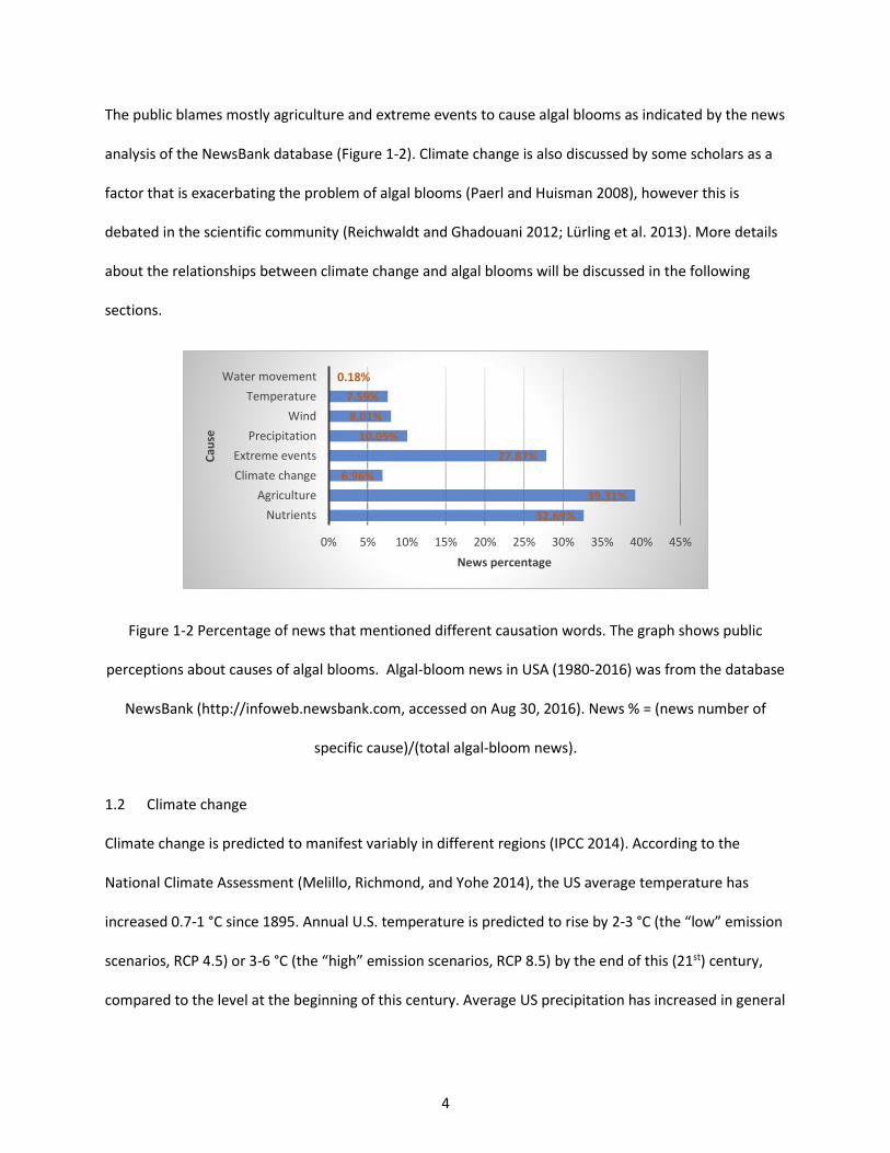
The public blames mostly agriculture and extreme events to cause algal blooms as indicated by the news
analysis of the NewsBank database (Figure 1-2). Climate change is also discussed by some scholars as a
factor that is exacerbating the problem of algal blooms (Paerl and Huisman 2008), however this is
debated in the scientific community (Reichwaldt and Ghadouani 2012; Lürling et al. 2013). More details
about the relationships between climate change and algal blooms will be discussed in the following
sections.
Figure 1-2 Percentage of news that mentioned different causation words. The graph shows public
perceptions about causes of algal blooms. Algal-bloom news in USA (1980-2016) was from the database
NewsBank (http://infoweb.newsbank.com, accessed on Aug 30, 2016). News % = (news number of
specific cause)/(total algal-bloom news).
1.2 Climate change
Climate change is predicted to manifest variably in different regions (IPCC 2014). According to the
National Climate Assessment (Melillo, Richmond, and Yohe 2014), the US average temperature has
increased 0.7-1 °C since 1895. Annual U.S. temperature is predicted to rise by 2-3 °C (the “low” emission
scenarios, RCP 4.5) or 3-6 °C (the “high” emission scenarios, RCP 8.5) by the end of this (21st) century,
compared to the level at the beginning of this century. Average US precipitation has increased in general
32.69%
39.31%
6.96%
27.87%
10.05%
8.01%
7.59%
0.18%
0% 5% 10% 15% 20% 25% 30% 35% 40% 45%
Nutrients
Agriculture
Climate change
Extreme events
Precipitation
Wind
Temperature
Water movement
News percentage
Cau
se
5
since industrialization, but some areas have increased more and some areas have decreased. Annual
precipitation is predicted to increase in the northern US, but decrease in the southwest with climate
change. Precipitation is predicted to change more in winter and spring than in summer and fall. The
frequency and intensity of extreme precipitation events is predicted to increase in all areas of US.
Droughts—indicated by the number of consecutive dry days—are predicted to increase over much of
US.
1.3 Climate change impacts on algal blooms
The proliferation of algal blooms has triggered significant public attention and scientific investigation.
However, the interactions between climate change and algal biomass occur in and are regulated by
complex watershed systems. Therefore, the outcomes of algal abundance responding to climate change
may vary greatly among individual lakes depending on other factors including watershed vegetation,
watershed topography, soils, lake morphology and hydrology, internal nutrient sources, and food web
interactions (Blenckner 2005). Paerl et al. (2008) argued that algal blooms, especially harmful
cyanobacteria blooms, will increase with climate change based on some case studies (Paerl and Huisman
2008; Paerl and Huisman 2009; Paerl and Paul 2012). However, the evidence is not strong enough to
represent a majority of lakes and the argument is more a hypothesis. For example, the Paerl and
Huisman (2008) paper was published under the “perspective” category (not a research paper) in the
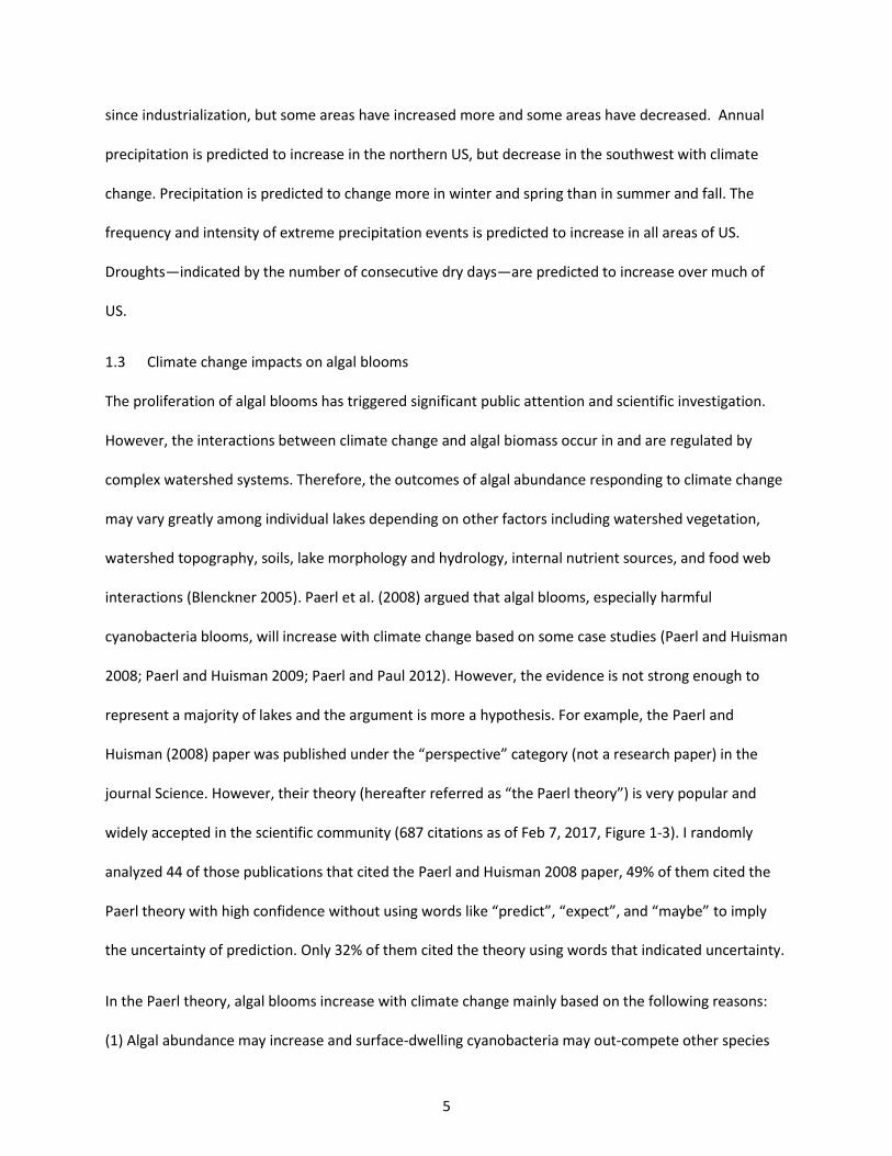
journal Science. However, their theory (hereafter referred as “the Paerl theory”) is very popular and
widely accepted in the scientific community (687 citations as of Feb 7, 2017, Figure 1-3). I randomly
analyzed 44 of those publications that cited the Paerl and Huisman 2008 paper, 49% of them cited the
Paerl theory with high confidence without using words like “predict”, “expect”, and “maybe” to imply
the uncertainty of prediction. Only 32% of them cited the theory using words that indicated uncertainty.
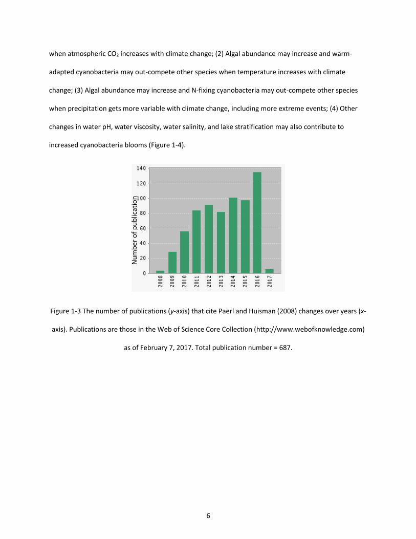
In the Paerl theory, algal blooms increase with climate change mainly based on the following reasons:
(1) Algal abundance may increase and surface-dwelling cyanobacteria may out-compete other species
6
when atmospheric CO2 increases with climate change; (2) Algal abundance may increase and warm-
adapted cyanobacteria may out-compete other species when temperature increases with climate
change; (3) Algal abundance may increase and N-fixing cyanobacteria may out-compete other species
when precipitation gets more variable with climate change, including more extreme events; (4) Other
changes in water pH, water viscosity, water salinity, and lake stratification may also contribute to
increased cyanobacteria blooms (Figure 1-4).
Figure 1-3 The number of publications (y-axis) that cite Paerl and Huisman (2008) changes over years (x-
axis). Publications are those in the Web of Science Core Collection (http://www.webofknowledge.com)
as of February 7, 2017. Total publication number = 687.
Nu
mb
er o
f p
ub
licat
ion
7
Figure 1-4 Possible pathways of climate change impacts on algal blooms. Summarized from Paerl and
Huisman (2008). The red frame indicates a decrease of algal abundance due to climate change.
1.3.1 Temperature
Accumulated literature has cast doubt on the Paerl theory. After a more thorough literature review,
Lürling et al. (2013) found that the optimal temperature for cyanobacteria species (N = 62) was not
significantly higher than for green algal species (N = 67). Moreover, they found that the cyanobacteria
growth rate at optimal temperatures was not significantly higher than that of green algae at their
8
optimal growth temperatures. They argued that higher growth rate due to higher temperature was not
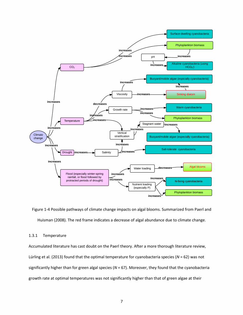
a major theoretical explanation for more harmful algal blooms in a warming climate. My preliminary
analyses of the first National Lake Assessment data set (USEPA 2007) also indicated a weak relationship
between lake surface temperature and algal biomass above about 20 °C (Figure 1-5), and that blue-
green algae (cyanobacteria) did not necessarily dominate the algal community at high lake surface
temperature, even when the nitrogen was limited favoring nitrogen-fixing species in cyanobacteria
(Figure 1-6).
Figure 1-5 Absolute abundance (bio-volume) of algal divisions as a function of lake surface temperature.
Data source: U.S. EPA National Lake Assessment, 2007 (http://www.usepa.gov, accessed on Jan 20,
2014). Lake number = 1157. Figure indicates that algal abundance did not necessarily increase with
temperature in the normal US summer range of about 20-30 °C. There might be other factors other than
lake temperature controlling algal abundance.
10 15 20 25 30
0e
+0
01
e+
07
2e
+0
73
e+
07
4e
+0
7
Lake surface temperature (°C)
Ab
so
lute
ab
un
da
nce
(m
3/m
L)
totaldiatomgreenblue-green
9
Figure 1-6 Relative abundance of algal divisions as a function of lake surface temperature and nutrient
structure. Data source: U.S. EPA National Lake Assessment, 2007 (http://www.usepa.gov, accessed on
Jan 20, 2014). Nutrient limitation is defined by the molar ratio of total nitrogen (TN) to total
phosphorus (TP): (a) N-limited, TN:TP < 20, (b) P-limited, TN:TP >50, and (c) NP-co-limited, 20 ≤ TN: TP ≤
50 (Guildford and Hecky 2000). Figure indicates that when the lake surface temperature was high (>
25 °C), blue-green algae did not always dominate the algal community even when nitrogen was limiting
relative to phosphorus.
1.3.2 Precipitation
Extreme precipitation events can carry more sediments and nutrients into lakes than other less intense
events (McDiffett et al. 1989; Coser 1989). However, algal abundance may not change after extreme
precipitation events due to a mismatch between nutrient availability and light availability (Minor,
Forsman, and Guildford 2014). Precipitation events may dilute algal abundance in reservoirs and
estuaries where algal accumulation is limited by flushing at short water residence times (Harris and
Baxter 1996; Bouvy et al. 2003; Paerl et al. 2014). When precipitation frequency is high, the events may
rinse nutrients from soils resulting in a decrease of algal abundance in rivers and lakes, showing an
inverted relationship between total annual precipitation and algal abundance (Olson and Hawkins 2013;
a.N-limited b.NP-limited c.P-limited
0.00
0.25
0.50
0.75
1.00
10 15 20 25 30 3510 15 20 25 30 3510 15 20 25 30 35
Lake surface temperature (°C)
Re
lative
ab
un
da
nce
(b
io-v
olu
me
)variable
diatom
green
blue.green
10
Stevenson, Zalack, and Wolin 2013). Reichwaldt and Ghadouani (2012) reviewed literature on a wide
range of lakes and commented that the Paerl theory is too simple for complex lake systems that respond
to precipitation differently.
1.3.3 Watershed effects
Temperature and precipitation may change not only in-lake processes, such as algal growth and
stratification, but also watershed processes, such as vegetation and soil properties (Davidson and
Janssens 2006). For example, vegetation cover is predicted to increase with temperature in wet areas
but decrease in dry areas (Breshears et al. 2005; Kardol et al. 2010). Watershed vegetation change may
also affect nutrient availability in lakes (Kalbitz et al. 2000). The increase in evapotranspiration due to
increasing temperature may neutralize the increase of precipitation (Chang, Evans, and Easterling 2001).
When temperature and precipitation increase, more bioactive phosphorus may be released from soil to
lakes due to more active bacterial activity, stronger ammonia nitrification, and lower soil pH (Stark and
Firestone 1995; Post et al. 1982). The Paerl theory did not account for these watershed processes.
Scholars are debating how climate change would affect soil properties such as soil organic matter
(Davidson and Janssens 2006), and it is under-researched how climate change would affect algal
abundance indirectly through changes in vegetation and soil properties.
1.4 Remote sensing of algal blooms
Algal abundance may change greatly over time and place even in the same lake, especially during
periods of algal blooms (Yacobi et al., 1995). It is costly to use traditional ground methods to measure
algal abundance for a period sufficiently long that it can be related to climate change. Remote sensors
onboard satellites have routinely measured earth surface for decades. For example, eight satellites have
been launched to continually observe the earth in the Landsat Missions since 1972. The newest one,
Landsat 8, was launched in 2013, and Landsat 9 is planned to launched in 2020
(https://landsat.usgs.gov, accessed on Feb 8, 2017).
11
1.4.1 The theory of remote sensing
Chlorophyll-a is a common photosynthetic pigment of phytoplankton and its concentration is often used
as a proxy of algal biomass. Remote sensing of algal abundance basically entails developing a
relationship between remote sensing of reflectance from water surfaces and the chlorophyll-a
concentration.
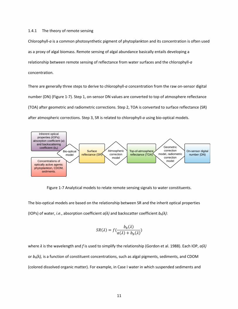
There are generally three steps to derive to chlorophyll-a concentration from the raw on-sensor digital
number (DN) (Figure 1-7). Step 1, on-sensor DN values are converted to top of atmosphere reflectance
(TOA) after geometric and radiometric corrections. Step 2, TOA is converted to surface reflectance (SR)
after atmospheric corrections. Step 3, SR is related to chlorophyll-a using bio-optical models.
Figure 1-7 Analytical models to relate remote sensing signals to water constituents.
The bio-optical models are based on the relationship between SR and the inherit optical properties
(IOPs) of water, i.e., absorption coefficient a(λ) and backscatter coefficient bb(λ):
𝑆𝑅(𝜆) = 𝑓(𝑏𝑏(𝜆)
𝑎(𝜆) + 𝑏𝑏(𝜆))
where λ is the wavelength and f is used to simplify the relationship (Gordon et al. 1988). Each IOP, a(λ)
or bb(λ), is a function of constituent concentrations, such as algal pigments, sediments, and CDOM
(colored dissolved organic matter). For example, in Case I water in which suspended sediments and
12
CDOM are low enough to assume it is zero, a(λ) can be related to chlorophyll-a concentration (C) using
the specific absorption coefficient, 𝑎𝑐∗, of chlorophyll-a:
𝑎(𝜆) = 𝑎𝑤 + 𝑎𝑐∗ 𝐶
where 𝑎𝑤 is the absorption coefficient of water (Bricaud et al. 1981). For Case II water, a(λ) is not only
contributed by water and phytoplankton, but also other constituents including CDOM, sediments,
mineral chemicals, and other organic debris.
1.4.2 Remote sensing algorithms
Generally, either empirical or analytical approaches are used to derive chlorophyll-a concentration using
remote sensing imagery. The analytical approach uses process-based models that include bio-optical
models and atmospheric radiative transfer models to calculate chlorophyll-a or other water constituents
from remotely sensed data (e.g., Dekker, Vos, and Peters 2002; Le et al. 2009). The empirical approach
uses statistical regression techniques to directly relate remote sensing data to chlorophyll-a based on an
experimental set of remote sensing and chlorophyll-a measurements (e.g., Brezonik, Menken, and Bauer
2005; Sudheer, Chaubey, and Garg 2006). Remote sensing data in the empirical approach could be the
raw DN values with only geometric corrections, or SR with all corrections including radiometric and
atmospheric corrections. The analytical approach is more complex than the empirical approach and
requires the knowledge of IOPs. Both approaches rely on training data and field work, but the empirical
approach usually measures fewer variables. The analytical approach has its physical limitation and it is
sensitive to atmospheric corrections (Defoin-Platel and Chami 2007). Some studies also try to use semi-
analytical approaches to simplify some processes in the analytical approach using empirical regressions
in parts of the processes (e.g., Gitelson et al. 2008; Le et al. 2009). The analytical approach is expected to
be more robust than the empirical approach, but in reality its transferability is as limited as the empirical
approach because of the complexity of IOPs and the problematic atmospheric correction in turbid water
13
(see review of Matthews 2011). Therefore, chlorophyll-a algorithms for inland lakes are still constrained
to a specific time and place. A new algorithm is required to relate climate change to historic remotely-
sensed imagery in a large number of lakes.
1.5 Dissertation structure
In the ocean, harmful algal blooms were predicted to “become more frequent (limited evidence,
medium agreement)” with future climate change (IPCC 2014). However, algal blooms in freshwater were
not included in the climate change evaluation in that IPCC report, perhaps due to the lack of strong
evidence of the climate change impacts. The overarching goal of this dissertation was to quantify the
sensitivity of freshwater algal blooms to climate change. This study focused on inland lakes across the
continental United States. I hypothesized that algal biomass in lakes increases with the higher
temperatures that are predicted to occur by the climate models. I also hypothesized that more extreme
precipitation events will amplify the temperature effects because more nutrients will be carried to the
lakes by these events. Long-term whole-lake measurements of algal biomass in a large number of lakes
were not available, so the analysis of climate effects on algal blooms was not possible with ground-
measurements from water samples.
Given limitations in available data, this dissertation includes two steps to tackle these problems:
Chapters 2 – 4 develop and test methods for remote sensing of algal blooms; and Chapters 5 – 6 analyze
climate change impacts on algal biomass. Specifically, Chapter 2 introduces a machine-learning
algorithm for remote sensing of algal blooms in inland lakes. Other color agents in water and
atmospheric effects are two major classes of factors that affect the accuracy of inland-water remote
sensing of algal biomass. Therefore, Chapter 3 evaluates the sensitivity of algorithms for remotely
sensing chlorophyll-a (RS-Chl) to interference by sediments and CDOM (colored dissolved organic
matter). Chapter 4 tests whether the existing atmospheric corrections in the standard USGS Landsat
Surface Reflectance products have improved the algorithm performance. After developing the remote

14
sensing models and having the long-term whole-lake algal biomass data, Chapter 5 uses time series
analysis to study the relationship between the climate change and algal biomass in four Missouri
reservoirs. Chapter 6 uses the approach of space as substitution of time to evaluate climate change
impacts on lakes across the continental United States. From Chapter 2 to Chapter 6, each chapter is
prepared as an independent manuscript for peer-reviewed journals. Chapter 1 (this chapter) is a general
introduction to the research topics, and it is not a thorough literature review. Chapter 7 (the last
chapter) summaries the findings and suggests some directions for future research. My dissertation
findings fill an important gap in the assessment of how climate change will likely affect freshwater
quality.

15
REFERENCES
16
REFERENCES
Anderson, Donald M. 1989. “Toxic Algal Blooms and Red Tides: A Global Perspective.” Red Tides: Biology, Environmental Science and Toxicology, 11–16.
———. 1997. “Turning Back the Harmful Red Tide.” Nature 388 (6642): 513–14. doi:10.1038/41415.
Anderson, Donald M., Patricia M. Glibert, and Joann M. Burkholder. 2002. “Harmful Algal Blooms and Eutrophication: Nutrient Sources, Composition, and Consequences.” Estuaries 25 (4): 704–26. doi:10.1007/BF02804901.
Blenckner, Thorsten. 2005. “A Conceptual Model of Climate-Related Effects on Lake Ecosystems.” Hydrobiologia 533 (1–3): 1–14. doi:10.1007/s10750-004-1463-4.
Bouvy, Marc, Silvia M. Nascimento, Renato J. R. Molica, Andrea Ferreira, Vera Huszar, and Sandra M. F. O. Azevedo. 2003. “Limnological Features in Tapacurá Reservoir (Northeast Brazil) during a Severe Drought.” Hydrobiologia 493 (1–3): 115–30. doi:10.1023/A:1025405817350.
Breshears, David D., Neil S. Cobb, Paul M. Rich, Kevin P. Price, Craig D. Allen, Randy G. Balice, William H. Romme, et al. 2005. “Regional Vegetation Die-off in Response to Global-Change-Type Drought.” Proceedings of the National Academy of Sciences of the United States of America 102 (42): 15144–48. doi:10.1073/pnas.0505734102.
Brezonik, Patrick, Kevin D. Menken, and Marvin Bauer. 2005. “Landsat-Based Remote Sensing of Lake Water Quality Characteristics, Including Chlorophyll and Colored Dissolved Organic Matter (CDOM).” Lake and Reservoir Management 21 (4): 373–82. doi:10.1080/07438140509354442.
Bricaud, Annick, Andre Morel, Louis Prieur, and others. 1981. “Absorption by Dissolved Organic Matter of the Sea (Yellow Substance) in the UV and Visible Domains.” Limnol. Oceanogr 26 (1): 43–53.
Carmichael, Wayne W. 2001. “Health Effects of Toxin-Producing Cyanobacteria: ‘The CyanoHABs.’” Human and Ecological Risk Assessment: An International Journal 7 (5): 1393–1407. doi:10.1080/20018091095087.
Chang, Heejun, Barry M. Evans, and David R. Easterling. 2001. “The Effects of Climate Change on Stream Flow and Nutrient Loading.” JAWRA Journal of the American Water Resources Association 37 (4): 973–85. doi:10.1111/j.1752-1688.2001.tb05526.x.
Coser, PR. 1989. “Nutrient Concentration-Flow Relationships and Loads in the South Pine River, South-Eastern Queensland. I. Phosphorus Loads.” Marine and Freshwater Research 40 (6): 613–30.
Davidson, Eric A., and Ivan A. Janssens. 2006. “Temperature Sensitivity of Soil Carbon Decomposition and Feedbacks to Climate Change.” Nature 440 (7081): 165–73. doi:10.1038/nature04514.
17
Defoin-Platel, Michael, and Malik Chami. 2007. “How Ambiguous Is the Inverse Problem of Ocean Color in Coastal Waters?” Journal of Geophysical Research: Oceans 112 (C3): C03004. doi:10.1029/2006JC003847.
Dekker, A. G., R. J. Vos, and S. W. M. Peters. 2002. “Analytical Algorithms for Lake Water TSM Estimation for Retrospective Analyses of TM and SPOT Sensor Data.” International Journal of Remote Sensing 23 (1): 15–35. doi:10.1080/01431160010006917.
Falconer, I.R., A.M. Beresford, and M.T. Runnegar. 1983. “Evidence of Liver Damage by Toxin from a Bloom of the Blue-Green Alga, Microcystis Aeruginosa.” The Medical Journal of Australia 1 (11): 511–14.
Gitelson, Anatoly A., Giorgio Dall’Olmo, Wesley Moses, Donald C. Rundquist, Tadd Barrow, Thomas R. Fisher, Daniela Gurlin, and John Holz. 2008. “A Simple Semi-Analytical Model for Remote Estimation of Chlorophyll-a in Turbid Waters: Validation.” Remote Sensing of Environment 112 (9): 3582–93. doi:10.1016/j.rse.2008.04.015.
Gordon, Howard R., Otis B. Brown, Robert H. Evans, James W. Brown, Raymond C. Smith, Karen S. Baker, and Dennis K. Clark. 1988. “A Semianalytic Radiance Model of Ocean Color.” Journal of Geophysical Research: Atmospheres 93 (D9): 10909–24. doi:10.1029/JD093iD09p10909.
Guildford, Stephanie J., and Robert E. Hecky. 2000. “Total Nitrogen, Total Phosphorus, and Nutrient Limitation in Lakes and Oceans: Is There a Common Relationship?” Limnology and Oceanography 45 (6): 1213–23. doi:10.4319/lo.2000.45.6.1213.
Harris, G.P., and G. Baxter. 1996. “Interannual Variability in Phytoplankton Biomass and Species Composition in a Subtropical Reservoir.” Freshwater Biology 35 (3): 545–60.
Heisler, J., P. M. Glibert, J. M. Burkholder, D. M. Anderson, W. Cochlan, W. C. Dennison, Q. Dortch, et al. 2008. “Eutrophication and Harmful Algal Blooms: A Scientific Consensus.” Harmful Algae, HABs and Eutrophication, 8 (1): 3–13. doi:10.1016/j.hal.2008.08.006.
Hoagland, P., and S. Scatasta. 2006. “The Economic Effects of Harmful Algal Blooms.” In Ecology of Harmful Algae, edited by Prof Dr Edna Granéli and Prof Dr Jefferson T. Turner, 391–402. Ecological Studies 189. Springer Berlin Heidelberg. doi:10.1007/978-3-540-32210-8_30.
Huang, Changchun, Yunmei Li, Hao Yang, Deyong Sun, Zhaoyuan Yu, Zhuo Zhang, Xia Chen, and Liangjiang Xu. 2014. “Detection of Algal Bloom and Factors Influencing Its Formation in Taihu Lake from 2000 to 2011 by MODIS.” Environmental Earth Sciences 71 (8): 3705–14. doi:10.1007/s12665-013-2764-6.
IPCC. 2014. “IPCC Fifth Assessment Report Climate Change 2014:Impacts, Adaptation, and Vulnerability.” IPCC-XXXVIII/DOC.4. (Intergovernmental Panel on Climate Change). http://www.ipcc.ch/.
Kalbitz, K., Stephen Solinger, J.-H. Park, B. Michalzik, and Egbert Matzner. 2000. “Controls on the Dynamics of Dissolved Organic Matter in Soils: A Review.” Soil Science 165 (4): 277–304.
18
Kardol, Paul, Courtney E. Campany, Lara Souza, Richard J. Norby, Jake F. Weltzin, and Aimee T. Classen. 2010. “Climate Change Effects on Plant Biomass Alter Dominance Patterns and Community Evenness in an Experimental Old-Field Ecosystem.” Global Change Biology 16 (10): 2676–87. doi:10.1111/j.1365-2486.2010.02162.x.
Keesing, John K., Dongyan Liu, Peter Fearns, and Rodrigo Garcia. 2011. “Inter- and Intra-Annual Patterns of Ulva Prolifera Green Tides in the Yellow Sea during 2007–2009, Their Origin and Relationship to the Expansion of Coastal Seaweed Aquaculture in China.” Marine Pollution Bulletin 62 (6): 1169–82. doi:10.1016/j.marpolbul.2011.03.040.
Le, Chengfeng, Yunmei Li, Yong Zha, Deyong Sun, Changchun Huang, and Heng Lu. 2009. “A Four-Band Semi-Analytical Model for Estimating Chlorophyll a in Highly Turbid Lakes: The Case of Taihu Lake, China.” Remote Sensing of Environment 113 (6): 1175–82. doi:10.1016/j.rse.2009.02.005.
Lewitus, Alan J., Rita A. Horner, David A. Caron, Ernesto Garcia-Mendoza, Barbara M. Hickey, Matthew Hunter, Daniel D. Huppert, et al. 2012. “Harmful Algal Blooms along the North American West Coast Region: History, Trends, Causes, and Impacts.” Harmful Algae 19 (September): 133–59. doi:10.1016/j.hal.2012.06.009.
Liu, Dongyan, John K. Keesing, Qianguo Xing, and Ping Shi. 2009. “World’s Largest Macroalgal Bloom Caused by Expansion of Seaweed Aquaculture in China.” Marine Pollution Bulletin 58 (6): 888–95. doi:10.1016/j.marpolbul.2009.01.013.
Lürling, Miquel, and Lisette N. De Senerpont Domis. 2013. “Predictability of Plankton Communities in an Unpredictable World.” Freshwater Biology 58 (3): 455–62. doi:10.1111/fwb.12092.
Lürling, Miquel, Fassil Eshetu, Elisabeth J. Faassen, Sarian Kosten, and Vera L. M. Huszar. 2013. “Comparison of Cyanobacterial and Green Algal Growth Rates at Different Temperatures.” Freshwater Biology 58 (3): 552–59. doi:10.1111/j.1365-2427.2012.02866.x.
Matthews, Mark William. 2011. “A Current Review of Empirical Procedures of Remote Sensing in Inland and near-Coastal Transitional Waters.” International Journal of Remote Sensing 32 (21): 6855–99. doi:10.1080/01431161.2010.512947.
McDiffett, Wayne F., Andrew W. Beidler, Thomas F. Dominick, and Kenneth D. McCrea. 1989. “Nutrient Concentration-Stream Discharge Relationships during Storm Events in a First-Order Stream.” Hydrobiologia 179 (2): 97–102. doi:10.1007/BF00007596.
Melillo, Jerry M., T. T. Richmond, and G. Yohe. 2014. “Climate Change Impacts in the United States.” Third National Climate Assessment. http://admin.globalchange.gov/sites/globalchange/files/Ch_0a_FrontMatter_ThirdNCA_GovtReviewDraft_Nov_22_2013_clean.pdf.
Michalak, Anna M., Eric J. Anderson, Dmitry Beletsky, Steven Boland, Nathan S. Bosch, Thomas B. Bridgeman, Justin D. Chaffin, et al. 2013. “Record-Setting Algal Bloom in Lake Erie Caused by Agricultural and Meteorological Trends Consistent with Expected Future Conditions.”
19
Proceedings of the National Academy of Sciences 110 (16): 6448–52. doi:10.1073/pnas.1216006110.
Minor, Elizabeth C., Brandy Forsman, and Stephanie J. Guildford. 2014. “The Effect of a Flood Pulse on the Water Column of Western Lake Superior, USA.” Journal of Great Lakes Research 40 (2): 455–62. doi:10.1016/j.jglr.2014.03.015.
Olson, John R., and Charles P. Hawkins. 2013. “Developing Site-Specific Nutrient Criteria from Empirical Models.” Freshwater Science 32 (3): 719–40. doi:10.1899/12-113.1.
Paerl, Hans W., Nathan S. Hall, Benjamin L. Peierls, and Karen L. Rossignol. 2014. “Evolving Paradigms and Challenges in Estuarine and Coastal Eutrophication Dynamics in a Culturally and Climatically Stressed World.” Estuaries and Coasts 37 (2): 243–58. doi:10.1007/s12237-014-9773-x.
Paerl, Hans W., and Jef Huisman. 2008. “Blooms Like It Hot.” Science 320 (5872): 57–58. doi:10.1126/science.1155398.
———. 2009. “Climate Change: A Catalyst for Global Expansion of Harmful Cyanobacterial Blooms.” Environmental Microbiology Reports 1 (1): 27–37. doi:10.1111/j.1758-2229.2008.00004.x.
Paerl, Hans W., and Valerie J. Paul. 2012. “Climate Change: Links to Global Expansion of Harmful Cyanobacteria.” Water Research, Cyanobacteria: Impacts of climate change on occurrence, toxicity and water quality management, 46 (5): 1349–63. doi:10.1016/j.watres.2011.08.002.
Post, Wilfred M., William R. Emanuel, Paul J. Zinke, and Alan G. Stangenberger. 1982. “Soil Carbon Pools and World Life Zones.” Nature 298 (5870): 156–59. doi:10.1038/298156a0.
Reichwaldt, Elke S., and Anas Ghadouani. 2012. “Effects of Rainfall Patterns on Toxic Cyanobacterial Blooms in a Changing Climate: Between Simplistic Scenarios and Complex Dynamics.” Water Research, Cyanobacteria: Impacts of climate change on occurrence, toxicity and water quality management, 46 (5): 1372–93. doi:10.1016/j.watres.2011.11.052.
Roelke, Daniel, and Yesim Buyukates. 2001. “The Diversity of Harmful Algal Bloom-Triggering Mechanisms and the Complexity of Bloom Initiation.” Human and Ecological Risk Assessment: An International Journal 7 (5): 1347–62. doi:10.1080/20018091095041.
Sellner, Kevin G., Gregory J. Doucette, and Gary J. Kirkpatrick. 2003. “Harmful Algal Blooms: Causes, Impacts and Detection.” Journal of Industrial Microbiology and Biotechnology 30 (7): 383–406. doi:10.1007/s10295-003-0074-9.
Stark, J. M., and M. K. Firestone. 1995. “Mechanisms for Soil Moisture Effects on Activity of Nitrifying Bacteria.” Applied and Environmental Microbiology 61 (1): 218–21.
Stevenson, R. Jan, Jason T. Zalack, and Julie Wolin. 2013. “A Multimetric Index of Lake Diatom Condition Based on Surface-Sediment Assemblages.” https://www.bioone.org/doi/full/10.1899/12-183.1.

20
Sudheer, K.p., Indrajeet Chaubey, and Vijay Garg. 2006. “Lake Water Quality Assessment from Landsat Thematic Mapper Data Using Neural Network: An Approach to Optimal Band Combination Selection1.” JAWRA Journal of the American Water Resources Association 42 (6): 1683–95. doi:10.1111/j.1752-1688.2006.tb06029.x.
Van Dolah, F M. 2000. “Marine Algal Toxins: Origins, Health Effects, and Their Increased Occurrence.” Environmental Health Perspectives 108 (Suppl 1): 133–41.
21
2 MACHINE-LEARNING ALGORITHMS FOR CHLOROPHYLL-A MEASUREMENTS IN INLAND LAKES USING
LANDSAT TM/ETM+
Abstract
Remote sensing of algae in inland lakes is challenging, and existing empirical models are limited to small
areas and short application periods, where and when conditions of water and atmosphere are relatively
the same. The goal of this study was to test algorithms that could be used to measure chlorophyll-a in
lakes across USA using Landsat TM/ETM+ imagery. This study hypothesized that machine-learning
algorithms (i.e., boosted regression trees and random forest) could estimate chlorophyll-a
concentrations from Landsat TM/ETM+ data when trained with ground-measured chlorophyll-a
concentrations from the 2007 National Lake Assessment conducted by the US Environmental Protection
Agency, predicting ecologically meaningful estimates of algal biomass for limnological studies. Results
showed significant improvements in accuracy using the machine-learning algorithms, compared to
traditional linear regressions. Specifically, the models using boosted regression trees and random forest
could explain respectively 45.8% and 44.5% of chlorophyll-a variance. The model using multiple linear
regression could only explain 39.8% of chlorophyll-a variance. Algal biomass maps derived from Landsat
TM/ETM+ identified the spatial distributions and temporal duration of the 2009 algal bloom in Lake Erie.
Compared to ground-measured algal biomass data, algal biomass measured by Landsat TM/ETM+ had a
comparable accuracy in relation with lake total phosphorus concentrations. These findings enable long-
term, large-scale, low-cost water quality observations for scientific research as well as environmental
management.
Keywords: phytoplankton, Landsat, chlorophyll-a, boosted regression trees, decision trees, surface
reflectance, remote sensing
22
Highlights
• Machine-learning algorithms are more accurate than traditional algorithms for estimation of
chlorophyll-a concentrations from Landsat satellite observations.
• Landsat chlorophyll-a information can be used to identify algal bloom events.
• Landsat chlorophyll-a are correlated as well as ground-measured chlorophyll-a to phosphorus
concentrations.
2.1 Introduction
2.1.1 Long-term large-scale measurement of algal biomass is needed
Algal blooms, especially involving toxic or otherwise harmful taxa, can cause severe problems for natural
systems and human society (Hudnell, 2010). Droughts, heat waves, and floods have been predicted to
increase with climate change (IPCC, 2014). Extreme floods, especially those after droughts, can
introduce nutrients into downstream water bodies, creating conditions conducive to algal blooms (Paerl
and Huisman, 2008). Long-term and large-scale observations of algae are needed to study the
relationship between climate change and algal blooms. However, long-term field samples are usually
limited to a small number of lakes, while large-scale surveys are limited to short periods. Remote
sensing is a potential tool for global, long-term, and low-cost measurements of algal blooms. The
overarching goal of this study was to develop and test a tool that can be used to produce long-term
large-scale data of algal blooms from the large library of existing remote sensing images.
2.1.2 Remote sensing of algae in inland water bodies is challenging
Oceanic color products, including chlorophyll-a (Chl) concentration, are measured by remote sensors
and have been available for public use for about two decades (http://oceancolor.gsfc.nasa.gov/,
accessed on Sep 8, 2015). However, remote sensing of Chl in inland lakes is problematic because of the
more variable optical characteristics, and particularly the presence of inorganic turbidity, and there is no
23
standard product available. Principal problems with Chl remote sensing in inland water bodies include
the following: (1) Traditional atmospheric correction methods for oceanic clear water (Case I water)
cannot be used in turbid water (Case II water) because suspended sediments violate the assumption of
zero remote sensing reflectance at infrared wavelengths (Gilerson et al., 2010); (2) Relative atmospheric
corrections such as dark-object subtraction are good for small areas where atmospheric conditions are
similar to reference objects (Chavez Jr., 1996). For a large area over a long time, it is hard to pick
reference objects that are assumed to have constant relationships with atmospheric effects; (3)
Analytical algorithms are theoretically able to discriminate Chl from sediments and CDOM (colored
dissolved organic matters), but they require inherent optical properties (IOPs) of water constituents,
which change over time and place and are usually unknown without measuring them at a particular time
and place (Dekker et al., 1997); (4) Semi-analytical algorithms indirectly estimate IPOs using reflectance
relations between bands or band ratios and their accuracies are also limited by the atmospheric
corrections (Carder et al., 1999); (5) Inland lakes require high spatial resolution because they are small,
but sensors with high spatial resolution often have low spectral resolution – indicated by band number
and width – which limit algorithm development. For example, algorithms based on red and infrared
bands, such as the fluorescence line high (FLH) method, have shown promising results in turbid water
with less impact of sediments and lake bottoms than traditional algorithms using blue and green bands
(Gower et al., 2005, 2004) However, the FLH algorithm requires at least two bands within the
wavelength range of fluorescence curve so FLH can be calculated. That requirement can be met by
using MERIS (MEdium Resolution Imaging Spectrometer) and MODIS (Moderate Resolution Imaging
Spectroradiometer), but they have spatial resolutions of 0.25 - 1.2 km which may be too coarse for
inland lakes. Thematic Mapper (TM) and Enhanced Thematic Mapper Plus (ETM+) onboard Landsat have
good spatial resolution (30 m), but they have only one red band and one near infrared band, which are
not sufficient for the FLH algorithm.
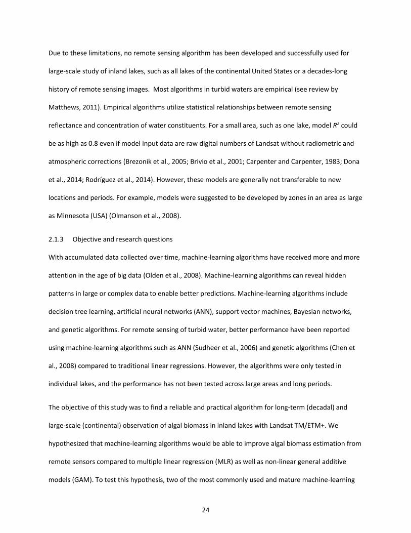
24
Due to these limitations, no remote sensing algorithm has been developed and successfully used for
large-scale study of inland lakes, such as all lakes of the continental United States or a decades-long
history of remote sensing images. Most algorithms in turbid waters are empirical (see review by
Matthews, 2011). Empirical algorithms utilize statistical relationships between remote sensing
reflectance and concentration of water constituents. For a small area, such as one lake, model R2 could
be as high as 0.8 even if model input data are raw digital numbers of Landsat without radiometric and
atmospheric corrections (Brezonik et al., 2005; Brivio et al., 2001; Carpenter and Carpenter, 1983; Dona
et al., 2014; Rodríguez et al., 2014). However, these models are generally not transferable to new
locations and periods. For example, models were suggested to be developed by zones in an area as large
as Minnesota (USA) (Olmanson et al., 2008).
2.1.3 Objective and research questions
With accumulated data collected over time, machine-learning algorithms have received more and more
attention in the age of big data (Olden et al., 2008). Machine-learning algorithms can reveal hidden
patterns in large or complex data to enable better predictions. Machine-learning algorithms include
decision tree learning, artificial neural networks (ANN), support vector machines, Bayesian networks,
and genetic algorithms. For remote sensing of turbid water, better performance have been reported
using machine-learning algorithms such as ANN (Sudheer et al., 2006) and genetic algorithms (Chen et
al., 2008) compared to traditional linear regressions. However, the algorithms were only tested in
individual lakes, and the performance has not been tested across large areas and long periods.
The objective of this study was to find a reliable and practical algorithm for long-term (decadal) and
large-scale (continental) observation of algal biomass in inland lakes with Landsat TM/ETM+. We
hypothesized that machine-learning algorithms would be able to improve algal biomass estimation from
remote sensors compared to multiple linear regression (MLR) as well as non-linear general additive
models (GAM). To test this hypothesis, two of the most commonly used and mature machine-learning
25
algorithms were chosen for testing: boosted regression trees (BRT) and random forest (RF). BRT builds
trees consecutively, with later trees built to reduce errors of the former tree. Trees in RF are built in
parallel. Each tree is built to explain a random subset of the sample with a random subset of
independent variables. RF was of special interest because the algorithm had a built-in function in Google
Earth Engine that could be used to efficiently process remote sensing imageries. Most empirical Landsat
models are based on MLR. GAM was included to test whether non-linear algorithms could improve
algorithm performance without using machine-learning algorithms. Our study was designed to answer
two specific questions:
• Are machine-learning algorithms—BRT and RF—better than MLR and GAM for remote sensing
of algal biomass in a large number of lakes using Landsat TM/ETM+?
• Is the accuracy of the machine-learning algorithms ecologically meaningful for lake
assessments?
2.2 Methodology
2.2.1 Model comparison
2.2.1.1 Model data
2.2.1.1.1 Ground-measured water quality data
Ground-measured water quality data were obtained from the first National Lake Assessment (NLA) in
2007 (http://water.epa.gov, accessed on Jan 20, 2015). The NLA dataset included 1252 water samples
from 1157 lakes, i.e., 8% of lakes were revisited. Samples were collected during May to October of 2007.
Lakes were selected randomly for the NLA with the intent that the sample of lakes would represent all
inland lakes in the continental United States. Lakes also met the criteria that they had areas greater
than 10 acres (0.004 km2) and depths greater than 1 m (Figure 2-1). Measurements included chlorophyll-
a (Chl) and total phosphorus (TP).
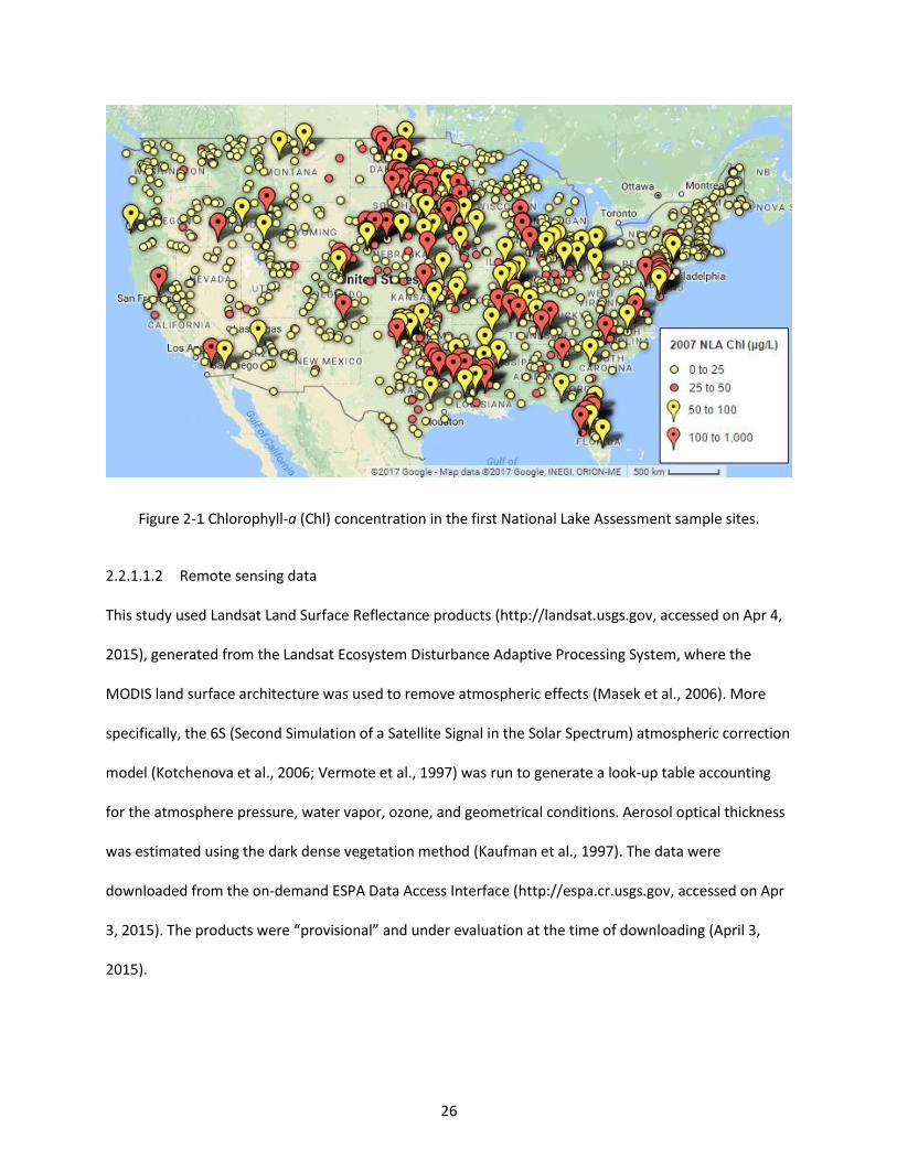
26
Figure 2-1 Chlorophyll-a (Chl) concentration in the first National Lake Assessment sample sites.
2.2.1.1.2 Remote sensing data
This study used Landsat Land Surface Reflectance products (http://landsat.usgs.gov, accessed on Apr 4,
2015), generated from the Landsat Ecosystem Disturbance Adaptive Processing System, where the
MODIS land surface architecture was used to remove atmospheric effects (Masek et al., 2006). More
specifically, the 6S (Second Simulation of a Satellite Signal in the Solar Spectrum) atmospheric correction
model (Kotchenova et al., 2006; Vermote et al., 1997) was run to generate a look-up table accounting
for the atmosphere pressure, water vapor, ozone, and geometrical conditions. Aerosol optical thickness
was estimated using the dark dense vegetation method (Kaufman et al., 1997). The data were
downloaded from the on-demand ESPA Data Access Interface (http://espa.cr.usgs.gov, accessed on Apr
3, 2015). The products were “provisional” and under evaluation at the time of downloading (April 3,
2015).
27
Ideally, we would have satellite images with the same dates and times as ground measurements.
However, the Landsat revisit period was 16 days, so the odds of having an image on the same date as
the ground sampling was low, even if cloudy pixels were not excluded. The study in Minnesota lakes
showed that water clarity correlated the most with TM reflectance on the same day, but the correlation
between water clarity in TM reflectance only decreased slightly when comparing measurements
separated by one day (R2 = 0.86) and seven days (R2 = 0.72) (Kloiber et al., 2002). Similar results were
found in Wisconsin: the correlation between water clarity in TM reflectance only slightly decreased from
R2 = 0.82 (1-3 day separation) to R2 = 0.75 (4-7 day separation) (Chipman et al., 2004). In this study, to
ensure as many data pairs of ground and satellite data as possible, we picked both TM and ETM+ images
that were close to but not separated by more than 8 days before or after the ground sampling dates.
Mean values of multiple pixels could remove some signal noise and improve image signal-to-noise ratio
(Kloiber et al., 2002; Ma and Dai, 2005). Therefore, we used a 3-by-3-pixel window from TM/ETM+
images surrounding the sample site to calculate a mean pixel value for bands and band ratios. Each
location was checked to make sure all pixels in the 3-by-3-pixel window were pure pixels of water. If a
sampling point was too close to the shoreline, its location was slightly adjusted with distances less than
100 m so the corresponding image pixels were water. Gaps due to the scan line corrector failure on
ETM+ were excluded.
2.2.1.1.3 Data screening
Image pixels with surface reflectance (SR) < 0 were excluded as abnormal values. Image pixels with SR >
15% indicated cloud cover and were excluded. Image pixels with Band 2 < Band 4 were excluded to
remove pixels of land and cloud shadows on water. Surface reflectance of water is normally less than
15% and with band 2 > band 4, even for waters with very high Chl and sediment concentration (Han,
1997; Rundquist et al., 1996). This image screening procedure, i.e., removing pixels with SR < 0, or SR >
15%, or Band 2 < Band 4, was able to remove land, cloud, and most cloud shadow pixels.
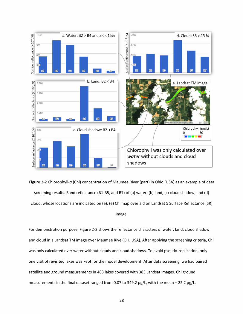
28
Figure 2-2 Chlorophyll-a (Chl) concentration of Maumee River (part) in Ohio (USA) as an example of data
screening results. Band reflectance (B1-B5, and B7) of (a) water, (b) land, (c) cloud shadow, and (d)
cloud, whose locations are indicated on (e). (e) Chl map overlaid on Landsat 5 Surface Reflectance (SR)
image.
For demonstration purpose, Figure 2-2 shows the reflectance characters of water, land, cloud shadow,
and cloud in a Landsat TM image over Maumee Rive (OH, USA). After applying the screening criteria, Chl
was only calculated over water without clouds and cloud shadows. To avoid pseudo-replication, only
one visit of revisited lakes was kept for the model development. After data screening, we had paired
satellite and ground measurements in 483 lakes covered with 383 Landsat images. Chl ground
measurements in the final dataset ranged from 0.07 to 349.2 µg/L, with the mean = 22.2 µg/L.
29
2.2.1.2 Model performance comparison
Models were developed with four different algorithms, i.e., multiple linear regression (MLR), general
additive models (GAM), boosted regression trees (BRT), and random forest (RF). Precision of model
performance was characterized by 10-fold cross validation. Specifically, the dataset was split into 10 lake
groups. In each cross-validation step, one of the lake groups (1/10 of the data) was withheld for
validation and the other nine lake groups (9/10 of the data) were used for model calibration. This cross-
validation step was repeated nine times with each of the other nine lake groups withheld from model
calibration at separate times. This provided independence between the datasets used for model
calibration and model testing. Model performance was characterized by the Nash–Sutcliffe model
efficiency coefficient (NSE).
The likelihood that performance of two models was the same was determined by using a paired sample
t-test. Specifically, each algorithm had 10 NSEs from validations of the 10 sample groups in the 10-fold
validation. NSEs of two algorithms were compared by pairing the NSEs for the same validation lake
group and calculating a pairwise t-test.
2.2.1.3 Model development
In the literature, Chl model variable combinations include: (1) a single band or single band ratio (Ma and
Dai, 2005); (2) one band combined with one band ratio (Brezonik et al., 2005); and (3) all bands (Keiner
and Yan, 1998). We tested all possible variable combinations with the algorithms and found that models
NSE = 1 −∑ (𝑦𝑖 − 𝑦�̂�)
2𝑖1
∑ (𝑦𝑖 − �̅�)2𝑖1
• 𝑦𝑖 is measued vlue
• 𝑦�̂� is modelled value
• �̅� is mean of 𝑦𝑖
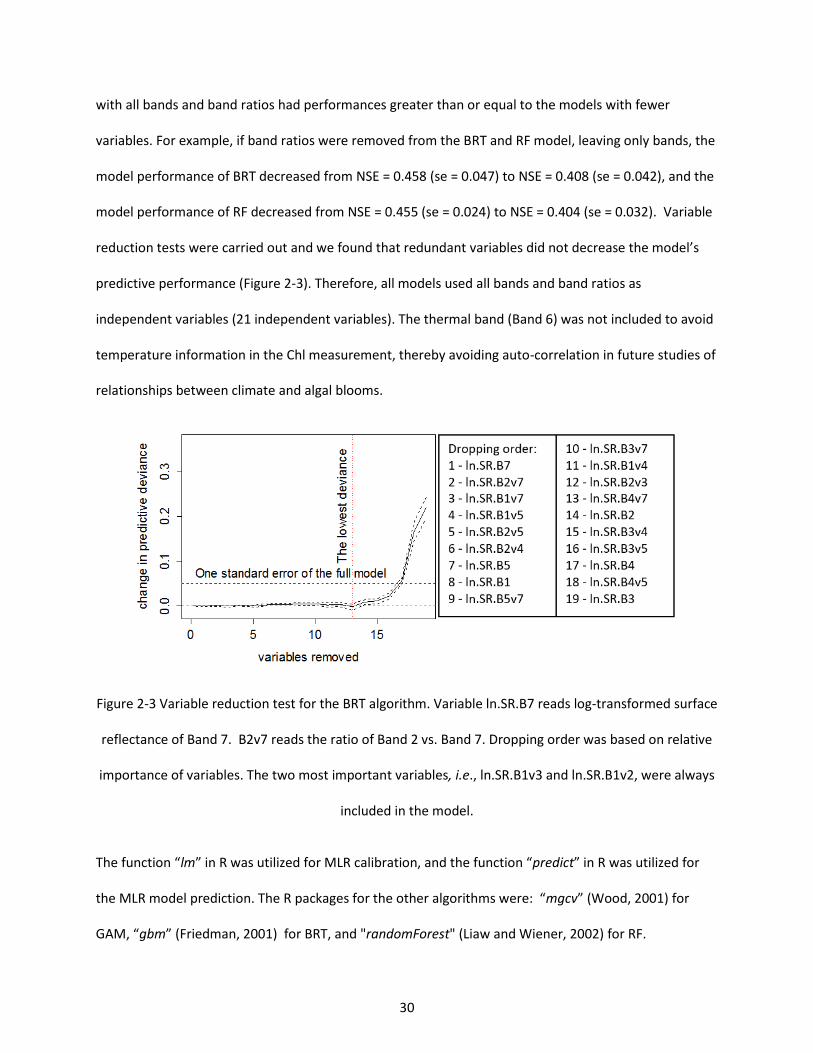
30
with all bands and band ratios had performances greater than or equal to the models with fewer
variables. For example, if band ratios were removed from the BRT and RF model, leaving only bands, the
model performance of BRT decreased from NSE = 0.458 (se = 0.047) to NSE = 0.408 (se = 0.042), and the
model performance of RF decreased from NSE = 0.455 (se = 0.024) to NSE = 0.404 (se = 0.032). Variable
reduction tests were carried out and we found that redundant variables did not decrease the model’s
predictive performance (Figure 2-3). Therefore, all models used all bands and band ratios as
independent variables (21 independent variables). The thermal band (Band 6) was not included to avoid
temperature information in the Chl measurement, thereby avoiding auto-correlation in future studies of
relationships between climate and algal blooms.
Figure 2-3 Variable reduction test for the BRT algorithm. Variable ln.SR.B7 reads log-transformed surface
reflectance of Band 7. B2v7 reads the ratio of Band 2 vs. Band 7. Dropping order was based on relative
importance of variables. The two most important variables, i.e., ln.SR.B1v3 and ln.SR.B1v2, were always
included in the model.
The function “lm” in R was utilized for MLR calibration, and the function “predict” in R was utilized for
the MLR model prediction. The R packages for the other algorithms were: “mgcv” (Wood, 2001) for
GAM, “gbm” (Friedman, 2001) for BRT, and "randomForest" (Liaw and Wiener, 2002) for RF.
31
2.2.2 Evaluation of model applications
2.2.2.1 Algal bloom detection
Landsat observations have an almost global coverage and potentially provide information about algal
blooms, such as occurrence time, place, area, and duration. An algal bloom event occurred in Lake Erie
around September 4, 2009, indicated by ground measurements and the aircraft and satellite imageries
from NOAA – Great Lakes Environmental Research Laboratory (NOAA-GLERL,
https://www.glerl.noaa.gov, accessed on February 22, 2017). RF was applied in Google Earth Engine
servers (Gorelick, 2012) to calculate Chl of Western Lake Erie in 2009 and verify if the algorithm could
identify the algal bloom event around September 4, 2009. RF was trained by the
“ee.Classifier.randomForest” function in the Google Earth Engine servers. Chl was predicted from
surface reflectance of Landsat TM 5 images (ImageCollection ID in Google Earth Engine =
"LEDAPS/LT5_L1T_SR"). Chl was calculated by the “classify” function in the Google Earth Engine servers.
2.2.2.2 Validation by relation with total phosphorus
Total phosphorus (TP) is associated with anthropogenic activities (e.g., fertilization), and has a causal
relationship with algal biomass in lakes (Stow and Cha, 2013). We hypothesized that (1) remotely sensed
Chl (RS-Chl) is sufficiently accurate and ecologically meaningful if its correlation with TP is as strong as
the correlation between ground-measured Chl (ground-Chl) and TP. Landsat TM/ETM+ provides
multiple measures of the same lake over a long time, and we further hypothesized that (2) the average
RS-Chl over a period as long as a summer would correlate with TP better than one-time estimates of RS-
Chl since average algal biomass is better estimated by multiple measures.
Revisited lake samples were used to test if average algal biomass is better estimated by multiple
measures by comparing correlations between ground-Chl and TP when using average ground-Chl of
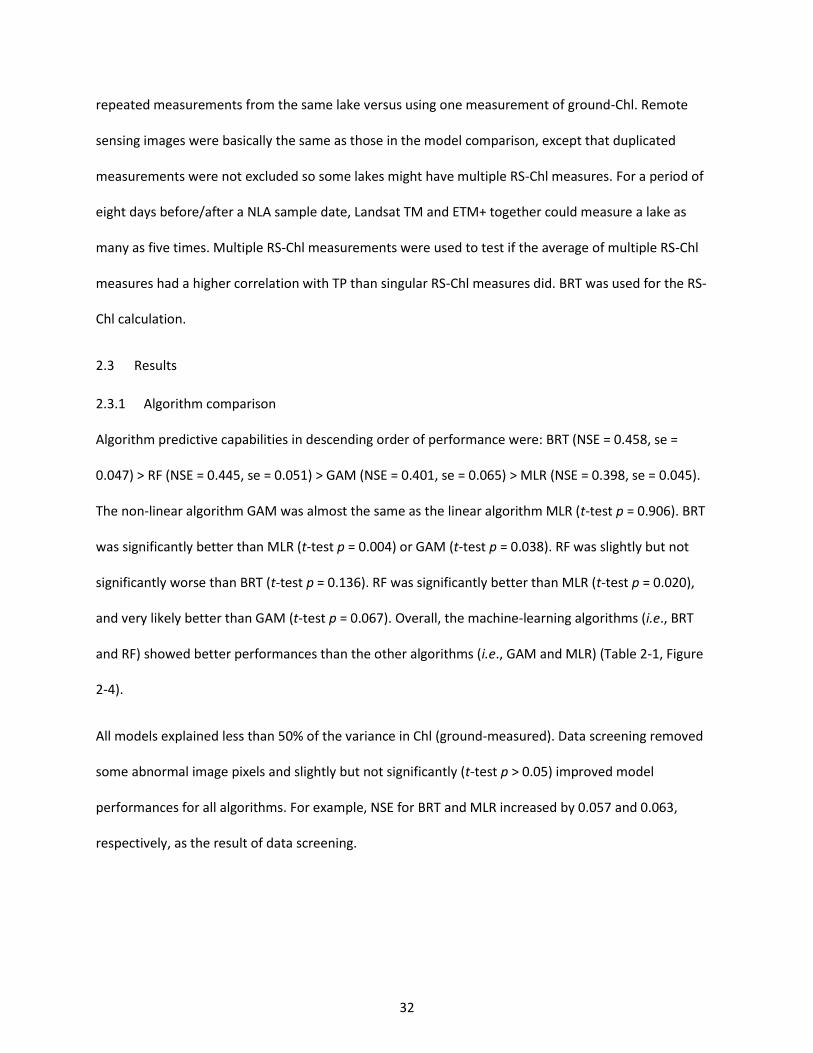
32
repeated measurements from the same lake versus using one measurement of ground-Chl. Remote
sensing images were basically the same as those in the model comparison, except that duplicated
measurements were not excluded so some lakes might have multiple RS-Chl measures. For a period of
eight days before/after a NLA sample date, Landsat TM and ETM+ together could measure a lake as
many as five times. Multiple RS-Chl measurements were used to test if the average of multiple RS-Chl
measures had a higher correlation with TP than singular RS-Chl measures did. BRT was used for the RS-
Chl calculation.
2.3 Results
2.3.1 Algorithm comparison
Algorithm predictive capabilities in descending order of performance were: BRT (NSE = 0.458, se =
0.047) > RF (NSE = 0.445, se = 0.051) > GAM (NSE = 0.401, se = 0.065) > MLR (NSE = 0.398, se = 0.045).
The non-linear algorithm GAM was almost the same as the linear algorithm MLR (t-test p = 0.906). BRT
was significantly better than MLR (t-test p = 0.004) or GAM (t-test p = 0.038). RF was slightly but not
significantly worse than BRT (t-test p = 0.136). RF was significantly better than MLR (t-test p = 0.020),
and very likely better than GAM (t-test p = 0.067). Overall, the machine-learning algorithms (i.e., BRT
and RF) showed better performances than the other algorithms (i.e., GAM and MLR) (Table 2-1, Figure
2-4).
All models explained less than 50% of the variance in Chl (ground-measured). Data screening removed
some abnormal image pixels and slightly but not significantly (t-test p > 0.05) improved model
performances for all algorithms. For example, NSE for BRT and MLR increased by 0.057 and 0.063,
respectively, as the result of data screening.
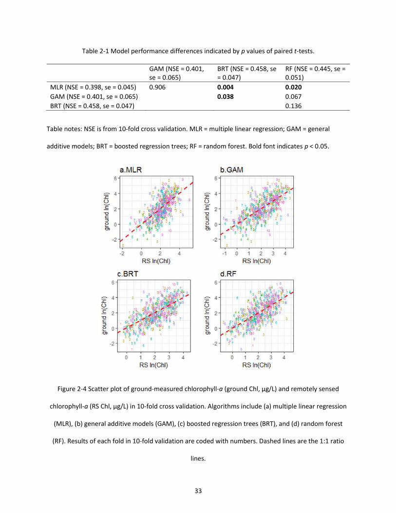
33
Table 2-1 Model performance differences indicated by p values of paired t-tests.
GAM (NSE = 0.401, se = 0.065)
BRT (NSE = 0.458, se = 0.047)
RF (NSE = 0.445, se = 0.051)
MLR (NSE = 0.398, se = 0.045) 0.906 0.004 0.020
GAM (NSE = 0.401, se = 0.065) 0.038 0.067
BRT (NSE = 0.458, se = 0.047) 0.136
Table notes: NSE is from 10-fold cross validation. MLR = multiple linear regression; GAM = general
additive models; BRT = boosted regression trees; RF = random forest. Bold font indicates p < 0.05.
Figure 2-4 Scatter plot of ground-measured chlorophyll-a (ground Chl, µg/L) and remotely sensed
chlorophyll-a (RS Chl, µg/L) in 10-fold cross validation. Algorithms include (a) multiple linear regression
(MLR), (b) general additive models (GAM), (c) boosted regression trees (BRT), and (d) random forest
(RF). Results of each fold in 10-fold validation are coded with numbers. Dashed lines are the 1:1 ratio
lines.
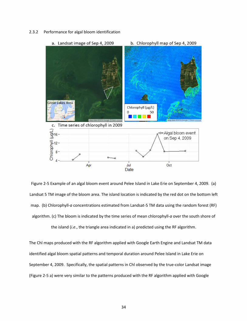
34
2.3.2 Performance for algal bloom identification
Figure 2-5 Example of an algal bloom event around Pelee Island in Lake Erie on September 4, 2009. (a)
Landsat 5 TM image of the bloom area. The island location is indicated by the red dot on the bottom left
map. (b) Chlorophyll-a concentrations estimated from Landsat-5 TM data using the random forest (RF)
algorithm. (c) The bloom is indicated by the time series of mean chlorophyll-a over the south shore of
the island (i.e., the triangle area indicated in a) predicted using the RF algorithm.
The Chl maps produced with the RF algorithm applied with Google Earth Engine and Landsat TM data
identified algal bloom spatial patterns and temporal duration around Pelee Island in Lake Erie on
September 4, 2009. Specifically, the spatial patterns in Chl observed by the true-color Landsat image
(Figure 2-5 a) were very similar to the patterns produced with the RF algorithm applied with Google
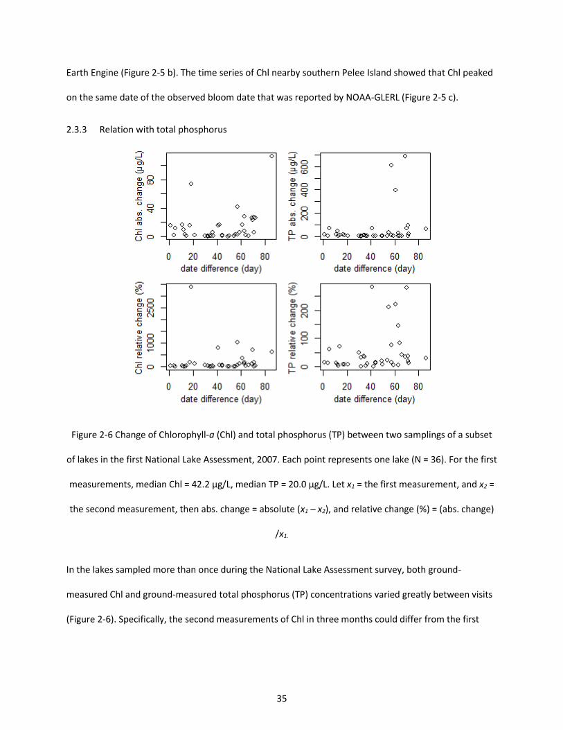
35
Earth Engine (Figure 2-5 b). The time series of Chl nearby southern Pelee Island showed that Chl peaked
on the same date of the observed bloom date that was reported by NOAA-GLERL (Figure 2-5 c).
2.3.3 Relation with total phosphorus
Figure 2-6 Change of Chlorophyll-a (Chl) and total phosphorus (TP) between two samplings of a subset
of lakes in the first National Lake Assessment, 2007. Each point represents one lake (N = 36). For the first
measurements, median Chl = 42.2 µg/L, median TP = 20.0 µg/L. Let x1 = the first measurement, and x2 =
the second measurement, then abs. change = absolute (x1 – x2), and relative change (%) = (abs. change)
/x1.
In the lakes sampled more than once during the National Lake Assessment survey, both ground-
measured Chl and ground-measured total phosphorus (TP) concentrations varied greatly between visits
(Figure 2-6). Specifically, the second measurements of Chl in three months could differ from the first
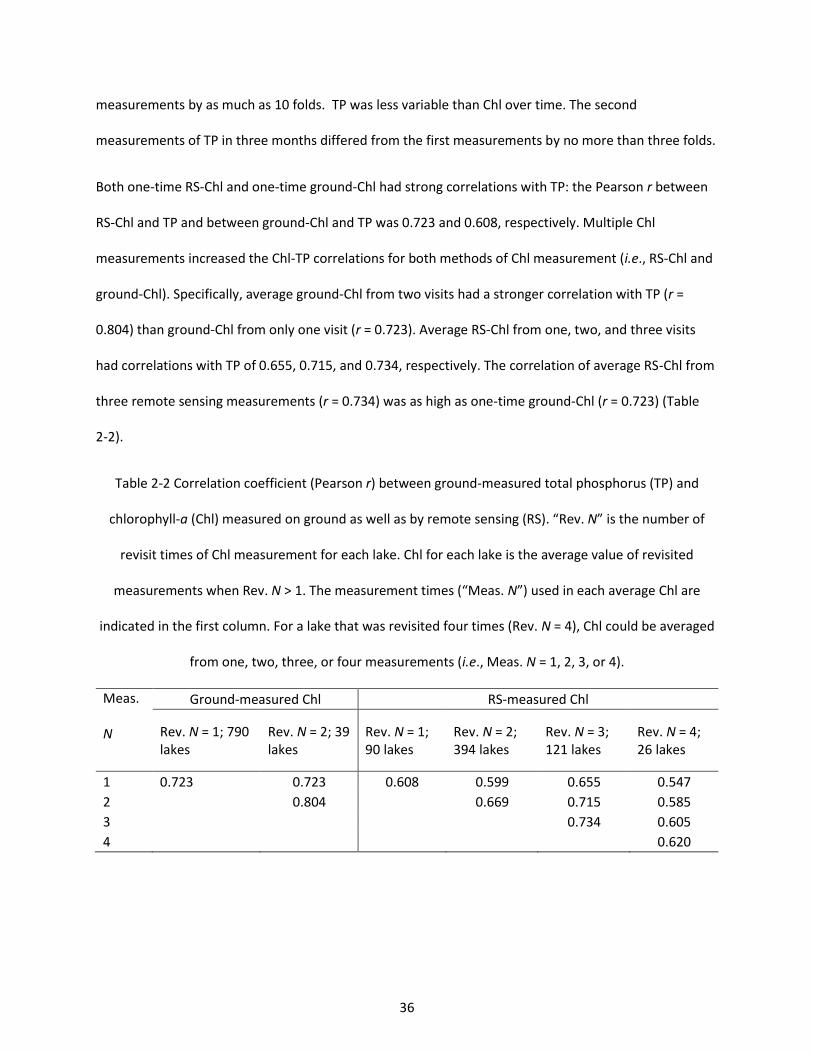
36
measurements by as much as 10 folds. TP was less variable than Chl over time. The second
measurements of TP in three months differed from the first measurements by no more than three folds.
Both one-time RS-Chl and one-time ground-Chl had strong correlations with TP: the Pearson r between
RS-Chl and TP and between ground-Chl and TP was 0.723 and 0.608, respectively. Multiple Chl
measurements increased the Chl-TP correlations for both methods of Chl measurement (i.e., RS-Chl and
ground-Chl). Specifically, average ground-Chl from two visits had a stronger correlation with TP (r =
0.804) than ground-Chl from only one visit (r = 0.723). Average RS-Chl from one, two, and three visits
had correlations with TP of 0.655, 0.715, and 0.734, respectively. The correlation of average RS-Chl from
three remote sensing measurements (r = 0.734) was as high as one-time ground-Chl (r = 0.723) (Table
2-2).
Table 2-2 Correlation coefficient (Pearson r) between ground-measured total phosphorus (TP) and
chlorophyll-a (Chl) measured on ground as well as by remote sensing (RS). “Rev. N” is the number of
revisit times of Chl measurement for each lake. Chl for each lake is the average value of revisited
measurements when Rev. N > 1. The measurement times (“Meas. N”) used in each average Chl are
indicated in the first column. For a lake that was revisited four times (Rev. N = 4), Chl could be averaged
from one, two, three, or four measurements (i.e., Meas. N = 1, 2, 3, or 4).
Meas.
N
Ground-measured Chl RS-measured Chl
Rev. N = 1; 790 lakes
Rev. N = 2; 39 lakes
Rev. N = 1; 90 lakes
Rev. N = 2; 394 lakes
Rev. N = 3; 121 lakes
Rev. N = 4; 26 lakes
1 0.723 0.723 0.608 0.599 0.655 0.547
2 0.804 0.669 0.715 0.585
3 0.734 0.605
4 0.620
37
2.4 Discussion
2.4.1 Are machine-learning algorithms our best choice?
Different bands and/or band ratios of Landsat TM/ETM+ have been recommended for RS-Chl models in
different studies (e.g., Carpenter and Carpenter, 1983; Kloiber et al., 2002; Papoutsa et al., 2014;
Rodríguez et al., 2014). The variety of selections of bands and/or band ratios reflects a variety of
possible relationships between Chl and remote sensing signals (hereafter referred as Chl-RS
relationship). Many factors have been known to affect this relationship, including atmospheric
interference, wind, sediments, CDOM (colored dissolved organic matter), and species composition of
algae. Empirical algorithms in the literature usually only work in specific areas and times with relatively
constant conditions. For instance, after trying all band/band ratio combinations, Ma and Dai (2005)
suggested a linear model with Band 3 was the best in Taihu Lake, China, with NSE = 0.551. However,
when the same model was applied in the National Lake Assessment (NLA) dataset, the 10-fold cross
validation NSE was only 0.164, which was the result after new model coefficients were fit by the NLA
dataset. For another example, Brezonik et al (2005) suggested a “band + band ratio” combination as
predictors and found that “Band 3 + Band 1/3” was the best to predict ln(Chl) (reported calibration NSE
= 0.89, N = 15 within one Landsat scene) after trying all variable combinations including the best model
of Ma and Dai. Validation NSE for this algorithm with the NLA dataset was only 0.240. These examples
indicate a variable Chl-RS relationship over time and place, thus those relationships are not transferable.
To account for regional and temporal variation in factors affecting the Chl-RS relationship, we could
build separate models for different regions, lake types, and weather conditions. However, decision-tree
algorithms, such as BRT and RF, have the potential to split data into stratified groups and thereby satisfy
the need for higher predictive performance and consistency with one model. For instance, CDOM
absorption mostly occurs in visual wavelengths, so the signal combination of algae and sediments can be
estimated with red and infrared wavelengths resulting in a minor CDOM effect (Gilerson et al., 2010).
38
After the discrimination of Chl from CDOM, Chl can further be discriminated from sediments since band
ratios can partly remove sediment interference in a Chl signal (Han, 1997). This stage-by-stage model
modification process is similar to decision tree processes in BRT and RF, which fully consider interactions
between predictors with multiple classification trees. Therefore, BRT and RF may be able to discriminate
Chl from sediments and CDOM and improve Chl estimation accuracy. Our results indicate that machine-
learning algorithms (i.e., BRT and RF) provide higher accuracy than the traditional linear algorithm MLR
or the non-linear algorithm GAM, although further research is required to confirm the discrimination
capability of BRT and RF. The improvement of machine-learning algorithms might be the result of: (1)
decision trees might have better corrected the Chl-RS relationship by accounting for interactions
between optical agents in water; and/or (2) machine-learning algorithms have found hidden rules in the
Chl-RS relationship that we may not know yet. GAM was not significantly better than MLR, indicating
that model performance did not improve by simply replacing a linear algorithm with a non-linear
algorithm. Our results indicated that the machine-learning algorithms, which were non-linear, better
address complex interactions among variables than simple non-linear algorithms like GAM.
To estimate Chl in turbid lakes over a large temporal and spatial scales, machine-learning algorithms
may be the best tools that we have to date. Interactions between optical agents are usually tested in
laboratories, which may not apply to complex realities. For example, Han (1997) found the Chl-RS
relationship was independent of suspended sediments. However, the size or color of sediments was the
same in the experiment. In reality, sediment size and color varies substantially, and we probably cannot
correct Chl estimates for sediment interference when using simple MLR. It is unrealistic to build a
traditional MLR model for a large spatial and/or temporal scale due to almost infinite combinations of
atmospheric and water optical conditions.
On the other hand, more Chl data have been collected from many sources and are available for use in
future model testing and updates, and this could improve the models. For example, after the first
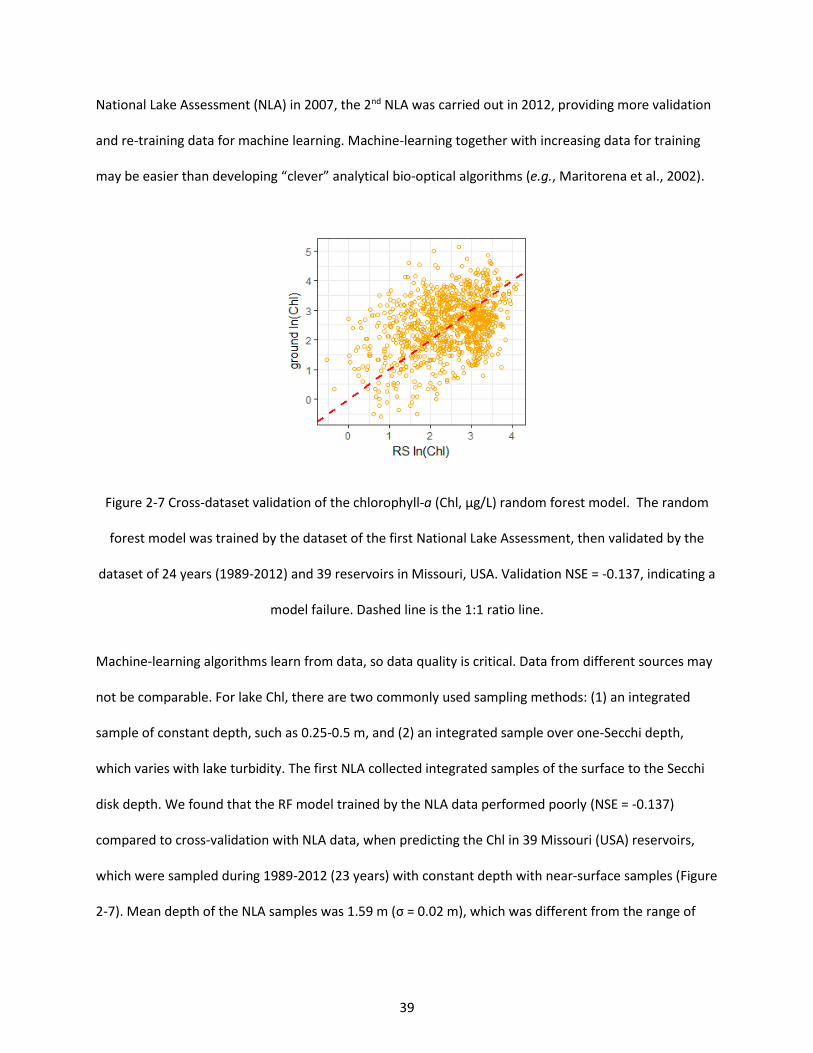
39
National Lake Assessment (NLA) in 2007, the 2nd NLA was carried out in 2012, providing more validation
and re-training data for machine learning. Machine-learning together with increasing data for training
may be easier than developing “clever” analytical bio-optical algorithms (e.g., Maritorena et al., 2002).
Figure 2-7 Cross-dataset validation of the chlorophyll-a (Chl, µg/L) random forest model. The random
forest model was trained by the dataset of the first National Lake Assessment, then validated by the
dataset of 24 years (1989-2012) and 39 reservoirs in Missouri, USA. Validation NSE = -0.137, indicating a
model failure. Dashed line is the 1:1 ratio line.
Machine-learning algorithms learn from data, so data quality is critical. Data from different sources may
not be comparable. For lake Chl, there are two commonly used sampling methods: (1) an integrated
sample of constant depth, such as 0.25-0.5 m, and (2) an integrated sample over one-Secchi depth,
which varies with lake turbidity. The first NLA collected integrated samples of the surface to the Secchi
disk depth. We found that the RF model trained by the NLA data performed poorly (NSE = -0.137)
compared to cross-validation with NLA data, when predicting the Chl in 39 Missouri (USA) reservoirs,
which were sampled during 1989-2012 (23 years) with constant depth with near-surface samples (Figure
2-7). Mean depth of the NLA samples was 1.59 m (σ = 0.02 m), which was different from the range of
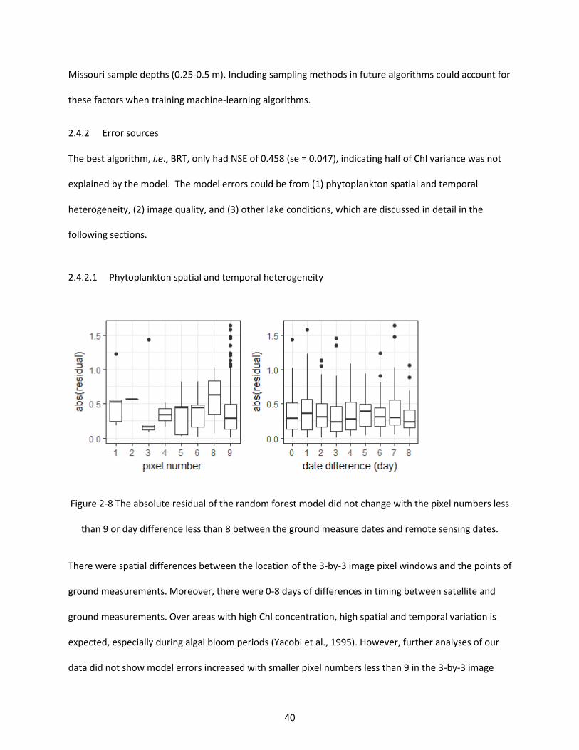
40
Missouri sample depths (0.25-0.5 m). Including sampling methods in future algorithms could account for
these factors when training machine-learning algorithms.
2.4.2 Error sources
The best algorithm, i.e., BRT, only had NSE of 0.458 (se = 0.047), indicating half of Chl variance was not
explained by the model. The model errors could be from (1) phytoplankton spatial and temporal
heterogeneity, (2) image quality, and (3) other lake conditions, which are discussed in detail in the
following sections.
2.4.2.1 Phytoplankton spatial and temporal heterogeneity
Figure 2-8 The absolute residual of the random forest model did not change with the pixel numbers less
than 9 or day difference less than 8 between the ground measure dates and remote sensing dates.
There were spatial differences between the location of the 3-by-3 image pixel windows and the points of
ground measurements. Moreover, there were 0-8 days of differences in timing between satellite and
ground measurements. Over areas with high Chl concentration, high spatial and temporal variation is
expected, especially during algal bloom periods (Yacobi et al., 1995). However, further analyses of our
data did not show model errors increased with smaller pixel numbers less than 9 in the 3-by-3 image
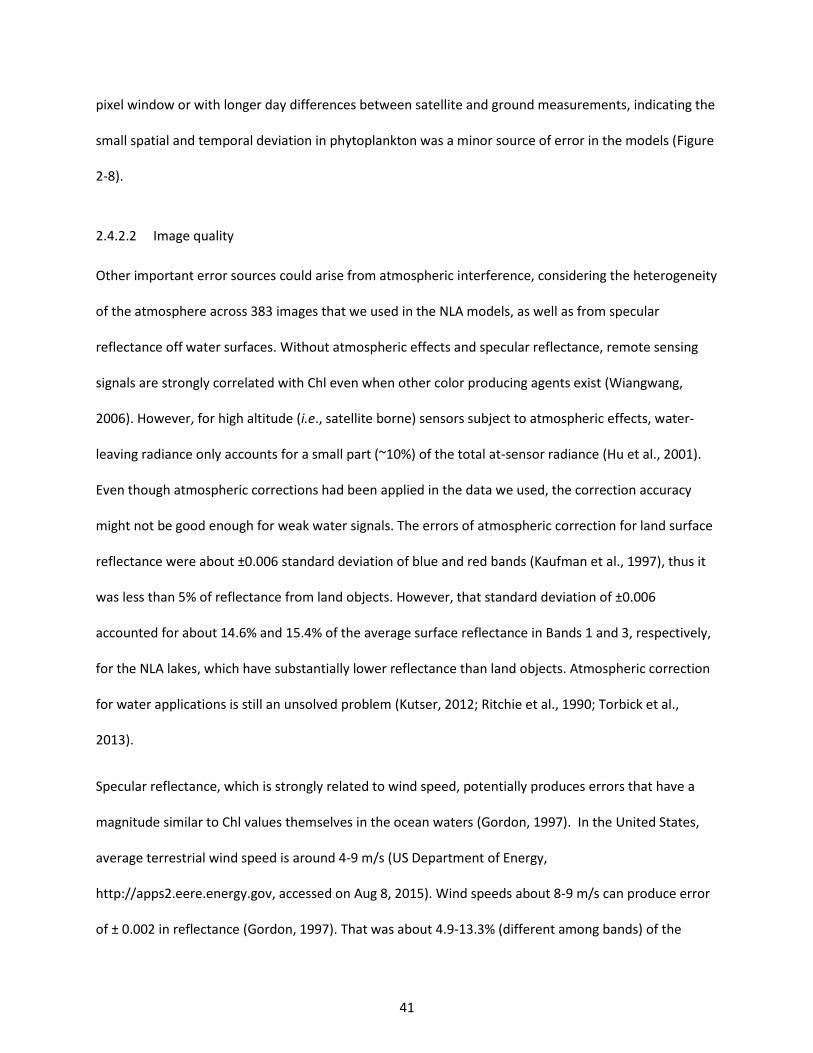
41
pixel window or with longer day differences between satellite and ground measurements, indicating the
small spatial and temporal deviation in phytoplankton was a minor source of error in the models (Figure
2-8).
2.4.2.2 Image quality
Other important error sources could arise from atmospheric interference, considering the heterogeneity
of the atmosphere across 383 images that we used in the NLA models, as well as from specular
reflectance off water surfaces. Without atmospheric effects and specular reflectance, remote sensing
signals are strongly correlated with Chl even when other color producing agents exist (Wiangwang,
2006). However, for high altitude (i.e., satellite borne) sensors subject to atmospheric effects, water-
leaving radiance only accounts for a small part (~10%) of the total at-sensor radiance (Hu et al., 2001).
Even though atmospheric corrections had been applied in the data we used, the correction accuracy
might not be good enough for weak water signals. The errors of atmospheric correction for land surface
reflectance were about ±0.006 standard deviation of blue and red bands (Kaufman et al., 1997), thus it
was less than 5% of reflectance from land objects. However, that standard deviation of ±0.006
accounted for about 14.6% and 15.4% of the average surface reflectance in Bands 1 and 3, respectively,
for the NLA lakes, which have substantially lower reflectance than land objects. Atmospheric correction
for water applications is still an unsolved problem (Kutser, 2012; Ritchie et al., 1990; Torbick et al.,
2013).
Specular reflectance, which is strongly related to wind speed, potentially produces errors that have a
magnitude similar to Chl values themselves in the ocean waters (Gordon, 1997). In the United States,
average terrestrial wind speed is around 4-9 m/s (US Department of Energy,
http://apps2.eere.energy.gov, accessed on Aug 8, 2015). Wind speeds about 8-9 m/s can produce error
of ± 0.002 in reflectance (Gordon, 1997). That was about 4.9-13.3% (different among bands) of the
42
average surface reflectance for the Landsat bands applied for the NLA lakes. Specular reflectance
increases according to a power function (power = 3.52) of wind speed (m/s) (Gordon and Wang, 1994;
Koepke, 1984). Therefore, specular reflectance might be another reason that no significant
improvement was seen in atmospherically corrected data compared to TOA (Kutser, 2012; Ritchie et al.,
1990; Torbick et al., 2013). Specular reflection can be estimated by wind speed above water and then
included in algorithms, but wind speed is not available for most inland lakes.
Some errors might be related to radiometric calibrations. On Chl maps of lakes, we often found
abnormal stripes (Figure 2-9). Chl concentration differences between neighbor stripes could be as high
as 10 µg/L. Those stripes might be caused by detector-to-detector mis-calibration or scan-to-scan mis-
calibration. Striping effects are corrected in Landsat 7 products but not Landsat 5.
Figure 2-9 Landsat TM abnormal stripes on chlorophyll map of Maumee Bay (USA). Landsat image ID =
“LT50200312009199GNC02”. The chlorophyll map was overlain on the Landsat image. White areas are
clouds.
43
2.4.2.3 Lake condition
Bottom effects, floating scum, aquatic macrophytes, suspended sediments, colored dissolved organic
matter (CDOM), or phytoplankton compositional variability may also introduce large uncertainty in the
models (Menken et al., 2006; Quibell, 1991). All these factors can change the leaving-water radiance.
Some impacts, such as the lake bottom, floating scum, and aquatic macrophytes, may be hard to
discriminate with Chl algorithms, so it is better to detect them and remove those pixels (Ackleson and
Klemas, 1987; Matthews et al., 2012). Our data screening process removed some areas covered by scum
and macrophytes, since they showed land reflectance traits. Some impacts such as sediments and
CDOM might have been minimized by the machine-learning algorithms as we discussed above, but
further research is required.
2.4.3 Are machine-learning algorithms good enough?
“Good” is a comparative judgement based on a specific application. Our results illustrated: (1) remote
sensing of Chl successfully identified algal bloom areas in Lake Erie; (2) the variation of the algal bloom
over time was identified; and (3) remotely sensed Chl was related to TP almost as well as ground
measured Chl, and was as good as was ground measured chlorophyll if multiple remote sensing Chl
measures were used. Therefore, remote sensing Chl is good enough for applications such as:
• Quantifying the extent of algal blooms within specific lakes.
• Monitoring lakes and identifying lakes with high algal biomass to prioritize lakes for
management.
• Providing a low cost and efficient tool for environmental management, e.g., monitoring
restoration of lakes with remotely sensed Chl before and after management plans are
implemented.
44
• Studying algal bloom mechanisms by building time series of algal biomass in one or more lakes
using historical remote sensing data and then linking measured algal biomass with
environmental factors.
Moreover, Chl is not the only water quality variable that can be measured by remote sensing. Our study
in Missouri reservoirs showed that CDOM as well as sediments can be estimated by BRT models with
even higher confidence than Chl (Lin et al. unpublished data). Therefore, remotely sensed Chl along with
sediments and CDOM are valuable data for limnological studies, especially for those on large spatial and
temporal scales.
2.5 Conclusion
Machine-learning algorithms (i.e., BRT and RF) were better than a traditional linear algorithm MLR for
remote sensing of Chl in inland lakes across the continental United States. The improvement in
algorithm performance was more likely from the automation of stage-by-stage learning and accounting
for complex interactions among variables than from the non-linear character of the machine-learning
algorithms. No matter how intelligent the algorithm was, remote sensing of inland lakes was still limited
by both training data quality and image quality. Nonetheless, remotely sensed Chl based on machine-
learning algorithms and Landsat TM/ETM+ was good enough for algal bloom detection and could be a
valuable measurement for environmental monitoring and management.
Acknowledgement
This report was made possible through support of the Environmental Protection Agency (EPA), USA
(Grant no. R835203). The opinions expressed herein are those of the authors and do not necessarily
reflect the views of the US EPA or the US Government.

45
REFERENCES
46
REFERENCES
Ackleson, S. G., and V. Klemas. 1987. “Remote Sensing of Submerged Aquatic Vegetation in Lower Chesapeake Bay: A Comparison of Landsat MSS to TM Imagery.” Remote Sensing of Environment 22 (2): 235–248.
Brezonik, Patrick, Kevin D. Menken, and Marvin Bauer. 2005. “Landsat-Based Remote Sensing of Lake Water Quality Characteristics, Including Chlorophyll and Colored Dissolved Organic Matter (CDOM).” Lake and Reservoir Management 21 (4): 373–382.
Brivio, P. A., C. Giardino, and E. Zilioli. 2001. “Determination of Chlorophyll Concentration Changes in Lake Garda Using an Image-Based Radiative Transfer Code for Landsat TM Images.” International Journal of Remote Sensing 22 (2–3): 487–502. doi:10.1080/014311601450059.
Carder, K. L., F. R. Chen, Z. P. Lee, S. K. Hawes, and D. Kamykowski. 1999. “Semianalytic Moderate-Resolution Imaging Spectrometer Algorithms for Chlorophyll a and Absorption with Bio-Optical Domains Based on Nitrate-Depletion Temperatures.” Journal of Geophysical Research: Oceans 104 (C3): 5403–5421. doi:10.1029/1998JC900082.
Carpenter, D. J., and S. M. Carpenter. 1983. “Modeling Inland Water Quality Using Landsat Data.” Remote Sensing of Environment 13 (4): 345–352. doi:10.1016/0034-4257(83)90035-4.
Chavez Jr., P.S. 1996. “Image-Based Atmospheric Corrections - Revisited and Improved.” Photogrammetric Engineering and Remote Sensing 62 (9): 1025–1036.
Chen, Li, Chih-Hung Tan, Shuh-Ji Kao, and Tai-Sheng Wang. 2008. “Improvement of Remote Monitoring on Water Quality in a Subtropical Reservoir by Incorporating Grammatical Evolution with Parallel Genetic Algorithms into Satellite Imagery.” Water Research 42 (1–2): 296–306. doi:10.1016/j.watres.2007.07.014.
Chipman, Jonathan W., Thomas M. Lillesand, Jeffrey E. Schmaltz, Jill E. Leale, and Mark J. Nordheim. 2004. “Mapping Lake Water Clarity with Landsat Images in Wisconsin, USA.” Canadian Journal of Remote Sensing 30 (1): 1–7.
Dekker, A. G., H. J. Hoogenboom, L. M. Goddijn, and T. J. M. Malthus. 1997. “The Relation between Inherent Optical Properties and Reflectance Spectra in Turbid Inland Waters.” Remote Sensing Reviews 15 (1–4): 59–74. doi:10.1080/02757259709532331.
Dona, C., J.M. Sanchez, V. Caselles, J.A Dominguez, and A Camacho. 2014. “Empirical Relationships for Monitoring Water Quality of Lakes and Reservoirs Through Multispectral Images.” IEEE Journal of Selected Topics in Applied Earth Observations and Remote Sensing 7 (5): 1632–1641. doi:10.1109/JSTARS.2014.2301295.
Friedman, Jerome H. 2001. “Greedy Function Approximation: A Gradient Boosting Machine.” Annals of Statistics, 1189–1232.
47
Gilerson, Alexander A., Anatoly A. Gitelson, Jing Zhou, Daniela Gurlin, Wesley Moses, Ioannis Ioannou, and Samir A. Ahmed. 2010. “Algorithms for Remote Estimation of Chlorophyll-a in Coastal and Inland Waters Using Red and near Infrared Bands.” Optics Express 18 (23): 24109–24125. doi:10.1364/OE.18.024109.
Gordon, Howard R. 1997. “Atmospheric Correction of Ocean Color Imagery in the Earth Observing System Era.” Journal of Geophysical Research: Atmospheres 102 (D14): 17081–17106. doi:10.1029/96JD02443.
Gordon, Howard R., and Menghua Wang. 1994. “Retrieval of Water-Leaving Radiance and Aerosol Optical Thickness over the Oceans with SeaWiFS: A Preliminary Algorithm.” Applied Optics 33 (3): 443–452.
Gorelick, Noel. 2012. “Google Earth Engine.” In AGU Fall Meeting Abstracts, 1:04. http://adsabs.harvard.edu/abs/2012AGUFM.U31A..04G.
Gower, J., L. Brown, and G A Borstad. 2004. “Observation of Chlorophyll Fluorescence in West Coast Waters of Canada Using the MODIS Satellite Sensor.” Canadian Journal of Remote Sensing 30 (1): 17–25. doi:10.5589/m03-048.
Gower, J., S. King, G. Borstad, and L. Brown. 2005. “Detection of Intense Plankton Blooms Using the 709 Nm Band of the MERIS Imaging Spectrometer.” International Journal of Remote Sensing 26 (9): 2005–2012. doi:10.1080/01431160500075857.
Han, Luoheng. 1997. “Spectral Reflectance with Varying Suspended Sediment Concentrations in Clear and Algae-Laden Waters.” Photogrammetric Engineering and Remote Sensing 63 (6): 701–705.
Hu, Chuanmin, Frank E. Muller-Karger, Serge Andrefouet, and Kendall L. Carder. 2001. “Atmospheric Correction and Cross-Calibration of LANDSAT-7/ETM+ Imagery over Aquatic Environments: A Multiplatform Approach Using SeaWiFS/MODIS.” Remote Sensing of Environment 78 (1): 99–107.
Hudnell, H. Kenneth. 2010. “The State of U.S. Freshwater Harmful Algal Blooms Assessments, Policy and Legislation.” Toxicon, Harmful Algal Blooms and Natural Toxins in Fresh and Marine Waters -- Exposure, occurrence, detection, toxicity, control, management and policy, 55 (5): 1024–1034. doi:10.1016/j.toxicon.2009.07.021.
IPCC. 2014. IPCC Fifth Assessment Report Climate Change 2014:Impacts, Adaptation, and Vulnerability. IPCC-XXXVIII/DOC.4. (Intergovernmental Panel on Climate Change). http://www.ipcc.ch/.
Kaufman, Y.J., AE. Wald, L.A Remer, Bo-Cai Gao, Rong-Rong Li, and L. Flynn. 1997. “The MODIS 2.1- Mu;m Channel-Correlation with Visible Reflectance for Use in Remote Sensing of Aerosol.” IEEE Transactions on Geoscience and Remote Sensing 35 (5): 1286–1298. doi:10.1109/36.628795.
Keiner, L. E., and X. H. Yan. 1998. “A Neural Network Model for Estimating Sea Surface Chlorophyll and Sediments from Thematic Mapper Imagery.” Remote Sensing of Environment 66 (2): 153–165. doi:10.1016/S0034-4257(98)00054-6.
48
Kloiber, Steven M., Patrick L. Brezonik, Leif G. Olmanson, and Marvin E. Bauer. 2002. “A Procedure for Regional Lake Water Clarity Assessment Using Landsat Multispectral Data.” Remote Sensing of Environment 82 (1): 38–47.
Koepke, Peter. 1984. “Effective Reflectance of Oceanic Whitecaps.” Applied Optics 23 (11): 1816. doi:10.1364/AO.23.001816.
Kotchenova, Svetlana Y., Eric F. Vermote, Raffaella Matarrese, and Jr. Klemm Frank J. 2006. “Validation of a Vector Version of the 6S Radiative Transfer Code for Atmospheric Correction of Satellite Data. Part I: Path Radiance.” Applied Optics 45 (26): 6762–6774. doi:10.1364/AO.45.006762.
Kutser, Tiit. 2012. “The Possibility of Using the Landsat Image Archive for Monitoring Long Time Trends in Coloured Dissolved Organic Matter Concentration in Lake Waters.” Remote Sensing of Environment 123 (August): 334–338. doi:10.1016/j.rse.2012.04.004.
Liaw, Andy, and Matthew Wiener. 2002. “Classification and Regression by randomForest.” R News 2 (3): 18–22.
Ma, Ronghua, and Jinfang Dai. 2005. “Investigation of Chlorophyll‐a and Total Suspended Matter Concentrations Using Landsat ETM and Field Spectral Measurement in Taihu Lake, China.” International Journal of Remote Sensing 26 (13): 2779–2795. doi:10.1080/01431160512331326648.
Maritorena, Stéphane, David A. Siegel, and Alan R. Peterson. 2002. “Optimization of a Semianalytical Ocean Color Model for Global-Scale Applications.” Applied Optics 41 (15): 2705. doi:10.1364/AO.41.002705.
Masek, Jeffrey G., Eric F. Vermote, Nazmi E. Saleous, Robert Wolfe, Forrest G. Hall, Karl F. Huemmrich, Feng Gao, Jonathan Kutler, and Teng-Kui Lim. 2006. “A Landsat Surface Reflectance Dataset for North America, 1990-2000.” Geoscience and Remote Sensing Letters, IEEE 3 (1): 68–72.
Matthews, Mark William. 2011. “A Current Review of Empirical Procedures of Remote Sensing in Inland and near-Coastal Transitional Waters.” International Journal of Remote Sensing 32 (21): 6855–6899. doi:10.1080/01431161.2010.512947.
Matthews, Mark William, Stewart Bernard, and Lisl Robertson. 2012. “An Algorithm for Detecting Trophic Status (Chlorophyll-A), Cyanobacterial-Dominance, Surface Scums and Floating Vegetation in Inland and Coastal Waters.” Remote Sensing of Environment 124 (September): 637–652. doi:10.1016/j.rse.2012.05.032.
Menken, Kevin D., Patrick L. Brezonik, and Marvin E. Bauer. 2006. “Influence of Chlorophyll and Colored Dissolved Organic Matter (CDOM) on Lake Reflectance Spectra: Implications for Measuring Lake Properties by Remote Sensing.” Lake and Reservoir Management 22 (3): 179–190. doi:10.1080/07438140609353895.
Olden, Julian D., Joshua J. Lawler, and N. LeRoy Poff. 2008. “Machine Learning Methods without Tears: A Primer for Ecologists.” The Quarterly Review of Biology 83 (2): 171–193.
49
Olmanson, Leif G., Marvin E. Bauer, and Patrick L. Brezonik. 2008. “A 20-Year Landsat Water Clarity Census of Minnesota’s 10,000 Lakes.” Remote Sensing of Environment 112 (11): 4086–4097.
Paerl, Hans W., and Jef Huisman. 2008. “Blooms Like It Hot.” Science 320 (5872): 57–58. doi:10.1126/science.1155398.
Papoutsa, Christiana, Adrianos Retalis, Leonidas Toulios, and Diofantos G. Hadjimitsis. 2014. “Defining the Landsat TM/ETM plus and CHRIS/PROBA Spectral Regions in Which Turbidity Can Be Retrieved in Inland Waterbodies Using Field Spectroscopy.” International Journal of Remote Sensing 35 (5): 1674–1692. doi:10.1080/01431161.2014.882029.
Quibell, G. 1991. “The Effect of Suspended Sediment on Reflectance from Freshwater Algae.” International Journal of Remote Sensing 12 (1): 177–182.
Ritchie, Jerry C., Charles M. Cooper, and Frank R. Schiebe. 1990. “The Relationship of MSS and TM Digital Data with Suspended Sediments, Chlorophyll, and Temperature in Moon Lake, Mississippi.” Remote Sensing of Environment 33 (2): 137–148. doi:10.1016/0034-4257(90)90039-O.
Rodríguez, Y. Chao, A. el Anjoumi, J. A. Domínguez Gómez, D. Rodríguez Pérez, and E. Rico. 2014. “Using Landsat Image Time Series to Study a Small Water Body in Northern Spain.” Environmental Monitoring and Assessment 186 (6): 3511–3522. doi:10.1007/s10661-014-3634-8.
Rundquist, Donald C., Luoheng Han, John F. Schalles, and Jeffrey S. Peake. 1996. “Remote Measurement of Algal Chlorophyll in Surface Waters: The Case for the First Derivative of Reflectance near 690 Nm.” Photogrammetric Engineering and Remote Sensing 62 (2): 195–200.
Stow, Craig A., and YoonKyung Cha. 2013. “Are Chlorophyll a–Total Phosphorus Correlations Useful for Inference and Prediction?” Environmental Science & Technology 47 (8): 3768–3773. doi:10.1021/es304997p.
Sudheer, K.p., Indrajeet Chaubey, and Vijay Garg. 2006. “Lake Water Quality Assessment from Landsat Thematic Mapper Data Using Neural Network: An Approach to Optimal Band Combination Selection1.” JAWRA Journal of the American Water Resources Association 42 (6): 1683–1695. doi:10.1111/j.1752-1688.2006.tb06029.x.
Torbick, Nathan, Sarah Hession, Stephen Hagen, Narumon Wiangwang, Brian Becker, and Jiaguo Qi. 2013. “Mapping Inland Lake Water Quality across the Lower Peninsula of Michigan Using Landsat TM Imagery.” International Journal of Remote Sensing 34 (21): 7607–7624. doi:10.1080/01431161.2013.822602.
Vermote, E.F., D. Tanre, J.-L. Deuze, M. Herman, and J.-J. Morcette. 1997. “Second Simulation of the Satellite Signal in the Solar Spectrum, 6S: An Overview.” IEEE Transactions on Geoscience and Remote Sensing 35 (3): 675–686. doi:10.1109/36.581987.
Wiangwang, N. 2006. “Assessment of Hyperspectral Data for Water Quality Studies in Michigan’s Inland Lakes.” PhD thesis. Michigan State University, East Lansing, USA.

50
Wood, Simon N. 2001. “Mgcv: GAMs and Generalized Ridge Regression for R.” R News 1 (2): 20–25.
51
3 EFFECTS OF SEDIMENTS AND COLORED DISSOLVED ORGANIC MATTER ON REMOTE SENSING OF
CHLOROPHYLL-A USING LANDSAT TM/ETM+ OVER TURBID WATERS
Abstract
In turbid inland waters, remote sensing of chlorophyll-a is challenging because waters commonly
contain inorganic suspended sediments (i.e., non-volatile suspended solids, NVSS) and colored dissolved
organic matter (CDOM). The effects of NVSS and CDOM on empirical models for chlorophyll-a using
remote sensing imagery in inland waters have not been determined on a broad spatial and temporal
scale. This study was conducted to evaluate these effects with a long-term (1989-2012) dataset that
included chlorophyll-a, NVSS, and CDOM for 39 reservoirs across Missouri (USA). Model comparison
indicated that the machine-learning algorithm BRT (boosted regression trees, validation R2 = 0.350) was
better than a traditional linear regression (validation R2 = 0.214) for chlorophyll-a measurement using
Landsat TM/ETM+ imagery. Minimal BRT model residuals could be explained by sediments or CDOM,
and the residual trends were different from the theoretical trends related to sediments and CDOM. The
results indicate that the BRT model had small systematic bias but the bias was not likely caused by
sediments or CDOM.
Keywords: turbid water, biomass; water quality, phytoplankton, remote sensing
Highlights
• The BRT machine-learning algorithm provided more accurate chlorophyll-a estimates than MLR
based on Landsat.
• The BRT model had systematic bias but this was not likely caused by sediments nor by dissolved
organic matter.
52
3.1 Introduction
3.1.1 Remote sensing of chlorophyll-a in inland lakes
Lake algal biomass assessments using traditional field-based sampling methods are challenging due to
the high spatial and temporal variation of phytoplankton, especially during bloom periods (Yacobi,
Gitelson, and Mayo 1995). Remote sensing has been used increasingly to map algal biomass at a higher
frequency, over a wider geographic coverage, and with a lower cost than traditional field measurements
(Sellner, Doucette, and Kirkpatrick 2003). Many operational ocean color sensors and algorithms have
been developed since 1970’s (see review Blondeau-Patissier et al. 2014). However, in turbid inland
waters, sediments and CDOM not only interfere with the characteristic chlorophyll-a spectral signal, but
they also make atmospheric correction complicated. Atmospheric effects can be estimated for Case I
water (i.e., clear water with a minor sediment effect) assuming the water-leaving radiance is zero at
infrared wavelengths (Gordon 1997). In turbid waters, the radiance from sediments violates the zero-
infrared assumption and has caused great concern for using satellites to measure chlorophyll-a
concentrations.
Landsat data are most often used in inland lakes for its relatively high spatial resolution and 16-day
revisit time compared to other images. Even though the atmospheric correction problem remains
unsolved for turbid waters, Landsat data have been tested over inland waters with fairly good
correlations (with r around 0.7) between chlorophyll-a and remote sensing bands and band ratios when
applied over relatively homogeneous areas (e.g., Ritchie, Cooper, and Schiebe 1990). However, these
relationships are not consistently good when considering multiple lakes, or lakes over a long duration, in
which lake conditions vary, especially their sediment concentrations varie (Sváb et al. 2005). Suspended
sediments and CDOM are therefore a major concern as interferences in the remote sensing of
chlorophyll-a in inland lakes
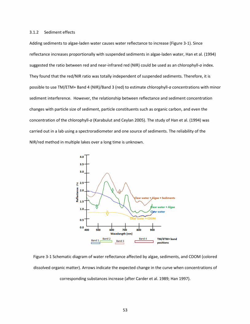
53
3.1.2 Sediment effects
Adding sediments to algae-laden water causes water reflectance to increase (Figure 3-1). Since
reflectance increases proportionally with suspended sediments in algae-laden water, Han et al. (1994)
suggested the ratio between red and near-infrared red (NIR) could be used as an chlorophyll-a index.
They found that the red/NIR ratio was totally independent of suspended sediments. Therefore, it is
possible to use TM/ETM+ Band 4 (NIR)/Band 3 (red) to estimate chlorophyll-a concentrations with minor
sediment interference. However, the relationship between reflectance and sediment concentration
changes with particle size of sediment, particle constituents such as organic carbon, and even the
concentration of the chlorophyll-a (Karabulut and Ceylan 2005). The study of Han et al. (1994) was
carried out in a lab using a spectroradiometer and one source of sediments. The reliability of the
NIR/red method in multiple lakes over a long time is unknown.
Figure 3-1 Schematic diagram of water reflectance affected by algae, sediments, and CDOM (colored
dissolved organic matter). Arrows indicate the expected change in the curve when concentrations of
corresponding substances increase (after Carder et al. 1989; Han 1997).
54
3.1.3 CDOM effects
CDOM is produced by degradation of phytoplankton, especially during periods of algal blooms, and of
organic matter of terrestrial and wetland origin (Zhao et al. 2009). CDOM absorption is high in the blue
spectral region, and decreases exponentially with wavelength, reaching almost zero absorption at the
infrared spectral region (Figure 3-1). The CDOM spectrum has no unique characteristics, like multiple
peaks and lows, which can be used for developing satellite algorithms for measuring CDOM. With the
interference of chlorophyll-a and sediments, remote sensing estimates of CDOM is even harder
(Menken, Brezonik, and Bauer 2006). The magnitude of CDOM effects in the visual spectral region can
be as high as moderate chlorophyll-a concentrations in the ocean (Bricaud et al. 1981). Gilerson et al.
(2010) found that the red/NIR algorithm for MERIS images was not very sensitive to CDOM absorption in
water with CDOM absorption coefficients ranging within 0-5 m−1. However, in freshwater, the CDOM
absorption coefficient is usually around 30 m−1, which is much higher than in open ocean waters (< 0.1
m−1), so the interference effect of CDOM on chlorophyll-a estimates with remote sensing in freshwater
is expected to be stronger than oceanic waters (Brezonik, Menken, and Bauer 2005). CDOM impacts on
chlorophyll-a estimates with remote sensing however have not been tested extensively over a large
region, over a long time, and in turbid water with both high concentrations of sediments and CDOM.
3.1.4 Landsat chlorophyll-a algorithms
In inland turbid waters, empirical algorithms such as linear regression, are more commonly used than
analytical or semi-analytical algorithms in chlorophyll-a estimation due to complexity of intrinsic optical
properties (IOPs), which are the basis for analytical or semi-analytical models (e.g., Kloiber et al. 2002;
Brezonik, Menken, and Bauer 2005; Kabbara et al. 2008; Dona et al. 2014; Rodríguez et al. 2014). Both
Landsat bands and band ratios have been used as independent variables in previous studies (e.g.,
Carpenter and Carpenter 1983; Brivio, Giardino, and Zilioli 2001; Olmanson, Bauer, and Brezonik 2008;
Papoutsa et al. 2014). More complex empirical algorithms have also been used, including: linear mixture
55
modelling using an algorithm called noise fraction transformation to enhance image quality when
applying spectral end members as variables (Tyler et al. 2006); and the spectral decomposition approach
using decomposition coefficients of optically active substitutes (i.e., phytoplankton, sediments, and
CDOM) as independent regression variables (Oyama et al. 2007). For optical complications in turbid
waters, using advanced machine-learning algorithms, i.e., artificial neural networks (ANN) and genetic
algorithms, has provided better performance than conventional linear regression (Sudheer, Chaubey,
and Garg 2006; Chen et al. 2008). A growing literature in ecology has shown stronger performance by
boosted regression trees (BRT) than linear regression or non-linear models such as GAM (general
additive models) when developing empirical models because BRT can account for complex interactions
among variables (Elith et al. 2006; Moisen et al. 2006). Machine-learning algorithms such as BRT could
be valuable for discriminating chlorophyll-a from sediments and CDOM by accounting for their
interactions on reflectance in different bands and band ratios of Landsat imagery.
3.1.5 Objective
To our knowledge, no study has quantified the effects of sediments and CDOM on chlorophyll-a
estimates using Landsat images in inland lakes considering effects of both sediments and CDOM.
Discriminating chlorophyll-a from sediments and CDOM is important for studying phytoplankton ecology
because sediments and CDOM often co-vary with storm events, runoff, nutrient loading, and algal
blooms (Zhang et al. 2009; Paerl and Paul 2012). The objective of this study was to quantify the effects
of sediment and CDOM on chlorophyll-a estimates using Landsat TM/ETM+ data. A Missouri reservoir
dataset provided a unique opportunity to assess these effects. The dataset has measurements of
chlorophyll-a, suspended sediments, and CDOM from water samples that were collected three or four
times per year over a long period (1989-2012, 24 years) and for 39 Missouri reservoirs. First, a remote
sensing model for chlorophyll-a using Landsat TM/ETM+ imagery was built with a BRT algorithm, and
then model residuals were related to sediments and CDOM to quantify their effects on chlorophyll-a
56
estimates. The magnitudes of sediment and CDOM effects were indicated by the range and significance
of their relationships to model residuals.
3.2 Methodology
3.2.1 Data
3.2.1.1 In-situ data
Data for this analysis were from 39 Missouri reservoirs (Figure 3-2) that were sampled from May to
September, 1989 to 2012. Water samples were collected from surface water (0.25 m to 0.5 m depth)
near reservoir dams on three or four occasions per year. Analyses of water samples included
chlorophyll-a, suspended sediments, and CDOM. Chlorophyll-a and sediments were measured from
1989 to 2012, while CDOM was measured from 2002 to 2012.
Suspended sediments were measured gravimetrically as non-volatile suspended solids (NVSS). NVSS was
the ash-mass of solids collected by filtration with Whatman 934-AH filters and then incineration of the
filter at 500°C. Samples for CDOM were filtered through 0.2 µm membrane filters. CDOM was measured
by the absorption coefficient at 440 nm wavelength (A440nm). A440nm could be affected by small
inorganic particles and colloids that pass through the filter, however that effect only contributes from
2% to 8% of the absorption (Sipelgas et al. 2003).
The dataset covered wide ranges of water quality: chlorophyll-a varied from 0.55 µg/L to 171.80 µg/L
with mean = 18.39 µg/L; NVSS varied from 0.01 mg/L to 36.20 mg/L with mean = 4.20 mg/L; and
A440nm varied from 1.00 m-1 to 798.00 m-1 with mean = 79.08 m-1. The data distributions for
chlorophyll-a, NVSS, and A440nm were skewed with mostly low values and a few samples having
extremely high values (Table 3-1). Linear regression is sensitive to extreme values and uneven
distributions. Therefore, chlorophyll-a, NVSS, and A440nm were natural log-transformed to meet the
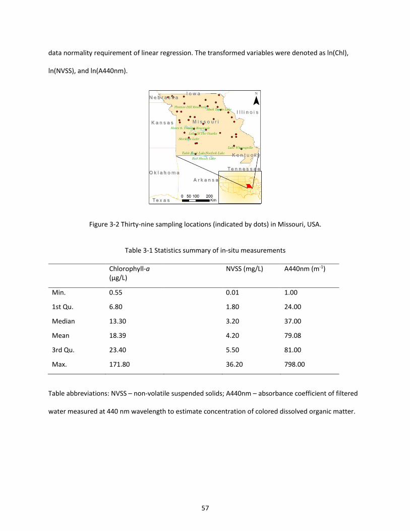
57
data normality requirement of linear regression. The transformed variables were denoted as ln(Chl),
ln(NVSS), and ln(A440nm).
Figure 3-2 Thirty-nine sampling locations (indicated by dots) in Missouri, USA.
Table 3-1 Statistics summary of in-situ measurements
Chlorophyll-a (µg/L)
NVSS (mg/L) A440nm (m-1)
Min. 0.55 0.01 1.00
1st Qu. 6.80 1.80 24.00
Median 13.30 3.20 37.00
Mean 18.39 4.20 79.08
3rd Qu. 23.40 5.50 81.00
Max. 171.80 36.20 798.00
Table abbreviations: NVSS – non-volatile suspended solids; A440nm – absorbance coefficient of filtered
water measured at 440 nm wavelength to estimate concentration of colored dissolved organic matter.
58
3.2.1.2 Remote sensing data
TM on board Landsat-5 had data from March 1984 to June 2013, which covered the entire period when
water quality data were collected (i.e., 1989-2012). Data of ETM+ on board Landsat-7 were available
from April 1999 to present (2017), which only partly overlapped with the time period of the water
quality data. ETM+ is similar to TM except for slight differences in Band 4 and Band 7: ETM+ Band 4
wavelength is 0.77-0.90 µm, compared to 0.76-0.90 µm in TM; ETM+ Band 7 wavelength is 2.09-2.35,
compared to 2.08-2.35 µm in TM. TM and ETM+ images from Landsat-5 and Landsat-7 were taken on
different dates. Regardless of the small differences, the images from both TM and ETM+ were used to
provide as many “ground-satellite” data pairs as possible.
TM and ETM+ images were downloaded from the on-demand ESPA Data Access Interface
(http://espa.cr.usgs.gov, accessed on July 1, 2014). The Land Surface Reflectance were products of the
Climate Data Record (CDR) (http://landsat.usgs.gov, accessed on July 1, 2014). Atmospheric correction
was processed in the Landsat Ecosystem Disturbance Adaptive Processing System (LEDAPS) reusing
MODIS land surface architecture based on the 6s algorithm (Masek et al. 2006). Even though the
atmospheric correction algorithm for the surface reflectance products was designed for terrestrial
surfaces without considering water-specific problems like specular reflectance, we chose it for
potentially less atmospheric impact than the top of atmospheric reflectance products.
To ensure a large amount of data as well as strong ground-satellite correlations, we picked both TM and
ETM+ images that were less than or equal to 8 days before or after the ground sampling dates. A 3 × 3
set of image pixels surrounding a ground sampling site was used in TM/ETM+ imagery to calculate a
mean reflectance value of each band corresponding to the ground sampling site. Each ground sampling
location was checked in Google Earth (Google, CA USA) to make sure all pixels in the 3 × 3 window were
pure water pixels. If a sampling point was too close to the shoreline, its location was adjusted. The
59
adjustment distance was less than 100 m. Gaps due to the scan line corrector (SLC) failures in ETM+
were excluded as well as saturated pixels. The “Fmask” layer in the land surface reflectance product was
used to mask clouds and cloud shadows. In addition to that, any pixel with Band 2 < Band 4 (land
character), or reflectance > 15% (land or cloud character), or reflectance < 0% (over-corrected in the
atmospheric correction) was excluded. Ground sampling records without corresponding satellite pixels
were excluded. As a result, the final dataset had 963 pairs of “ground-satellite” measurements.
3.2.2 Chlorophyll-a model development
BRT is a new machine-learning algorithm based on decision trees that has significant potential in remote
sensing of water. Some of our unpublished work with other datasets has shown that BRT performs
better than GAM or ANN. BRT uses a large number (commonly, thousands) of boosted decision trees to
minimize the model deviance (Friedman 2001). BRT inherits all the good features of decision tree
algorithms, such as low sensitivity to outliners, efficient treatment of collinear variables including
variable interactions, simulation of both non-linear and linear relationships, and no data distribution
requirements. Non-linear relationships between water quality and remote sensing reflectance have
been shown in previous studies (Han et al. 1994; Kutser et al. 2005).
Model predictors included all band ratios (i.e., Band 1/2, 1/3, 1/4, etc.) as well as all bands (i.e., Band 1,
2, 3, etc.) since bands and band ratio combinations might improve chlorophyll-a estimation for turbid
waters by partly removing atmospheric effects and enhancing remote sensing signals (Kloiber et al.
2002; Pattiaratchi et al. 1994). Band 6, the thermal band, was not included in the model predictors,
because it measured lake surface temperature instead of light reflectance. The remote sensing
chlorophyll-a (RS-Chl) model was:
ln (Chl) = 𝑓(bands, band ratios) Equation 3-1
60
where f is MLR (multiple linear regression) or BRT. An MLR model was included in our analysis to
compare a more traditional approach with a BRT model. All models were developed and analyzed using
R software (http://www.r-project.org, accessed on July 2, 2015). The MLR models were built with the
“lm” function in R. BRT models were built with the “gbm” package, version 1.5–7 (Ridgeway 2004). We
adapted codes from Elith et al. (2008) to calibrate parameters (i.e., tree number, learning rate, and
bagging rate) for the BRT models. Model performance was measured by the Nash–Sutcliffe model
efficiency coefficient (Nash and Sutcliffe 1970):
where NSE is the Nash–Sutcliffe model efficiency coefficient; Oi is the observation value with mean as �̅�;
and Mi is the modeled value. NSE ranges from −∞ to one, where one is a perfect fit and a negative value
indicates model failure. NSE indicates the proportion of the total measured variance explained by the
model.
Model predictive performance was estimated by 10-fold cross-validation. Specifically, the whole dataset
was divided into 10 groups. Each group was used once to validate the model that was calibrated by the
other nine groups. As a result, the predictive performance of each model was estimated 10 times to get
a mean NSE. MLR and BRT performance was compared with a t-test between the two mean NSEs from
10-fold cross-validation with variation in observed NSE calculated with the 10 NSE values calculated with
10-fold cross-validation.
3.2.3 Residual analyses
The chlorophyll-a model residual (εi) was calculated as:
where Oi is the observation value, and Mi is the modeled value. The sediment and CDOM relationships
NSE = 1 −∑ (𝑂𝑖−𝑀𝑖)2 𝑛
𝑖=1
∑ (𝑂𝑖−�̅�)2 𝑛𝑖=1
𝜀𝑖 = 𝑂𝑖 − 𝑀𝑖 Equation 3-3
Equation 3-2
61
with model residuals were characterized by GAM (generalized additive models) using the R “mgcv”
package, version 1.8-6 (Wood 2001). GAM was picked to account for potential non-linear trends. Only
the BRT model residuals were analyzed. The residuals were calibration residuals with the full dataset as
training data (not the residuals from 10-fold cross-validation). The BRT residuals were related to
ln(NVSS) and ln(A440nm), respectively using the GAM model:
where ε is residuals of the BRT model, and x is ln(NVSS) or ln(A440nm). The magnitude of residual trend
was indicated by (1) significance of the GAM model and (2) the percentage of the total residual
explained by the GAM model (i.e., R2 of the GAM model). Significance (p value) of the GAM model was
an approximate estimation using the “summary” function (Wood 2012) in the “mgcv” package.
In addition to the GAM smooth line, the residual trend was quantified by adding ln(NVSS) and
ln(A440nm) as independent variables in the RS-Chl model:
The increase in the model performance indicated the contribution of sediments and CDOM in the
residual of the original model, i.e., the one without ln(NVSS) and ln(A440nm).
ln(Chl) was correlated with ln(A440nm) (Spearman ρ = 0.30, p < 0.05) and ln(NVSS) (Spearman ρ = 0.35,
p < 0.05) in the Missouri dataset (Figure 3-3). The residual trends related to ln(NVSS) and ln(440nm)
could be correlated with ln(Chl) itself. Therefore, the model improvement in Equation 3-5 may be
misleading due to the correlations. To parse out the sediment and CDOM correlations with ln(Chl), a
residual BRT model was built:
𝜀 = 𝐺𝐴𝑀(𝑥)
ln (Chl) = BRT[bands, band ratios, ln(NVSS), ln(A440nm)]
𝜀 = BRT[ln(Chl), ln(A440nm), ln(NVSS)]
Equation 3-4
Equation 3-6
Equation 3-5
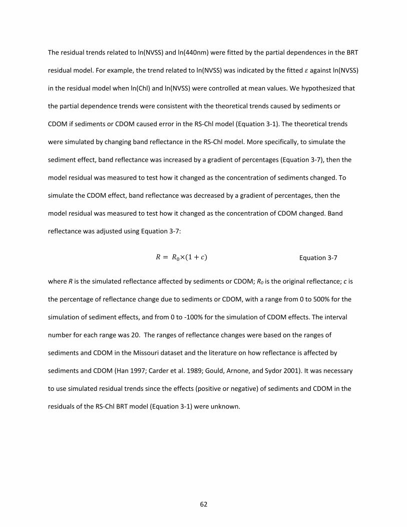
62
The residual trends related to ln(NVSS) and ln(440nm) were fitted by the partial dependences in the BRT
residual model. For example, the trend related to ln(NVSS) was indicated by the fitted 𝜀 against ln(NVSS)
in the residual model when ln(Chl) and ln(NVSS) were controlled at mean values. We hypothesized that
the partial dependence trends were consistent with the theoretical trends caused by sediments or
CDOM if sediments or CDOM caused error in the RS-Chl model (Equation 3-1). The theoretical trends
were simulated by changing band reflectance in the RS-Chl model. More specifically, to simulate the
sediment effect, band reflectance was increased by a gradient of percentages (Equation 3-7), then the
model residual was measured to test how it changed as the concentration of sediments changed. To
simulate the CDOM effect, band reflectance was decreased by a gradient of percentages, then the
model residual was measured to test how it changed as the concentration of CDOM changed. Band
reflectance was adjusted using Equation 3-7:
where R is the simulated reflectance affected by sediments or CDOM; R0 is the original reflectance; c is
the percentage of reflectance change due to sediments or CDOM, with a range from 0 to 500% for the
simulation of sediment effects, and from 0 to -100% for the simulation of CDOM effects. The interval
number for each range was 20. The ranges of reflectance changes were based on the ranges of
sediments and CDOM in the Missouri dataset and the literature on how reflectance is affected by
sediments and CDOM (Han 1997; Carder et al. 1989; Gould, Arnone, and Sydor 2001). It was necessary
to use simulated residual trends since the effects (positive or negative) of sediments and CDOM in the
residuals of the RS-Chl BRT model (Equation 3-1) were unknown.
𝑅 = 𝑅0×(1 + 𝑐) Equation 3-7
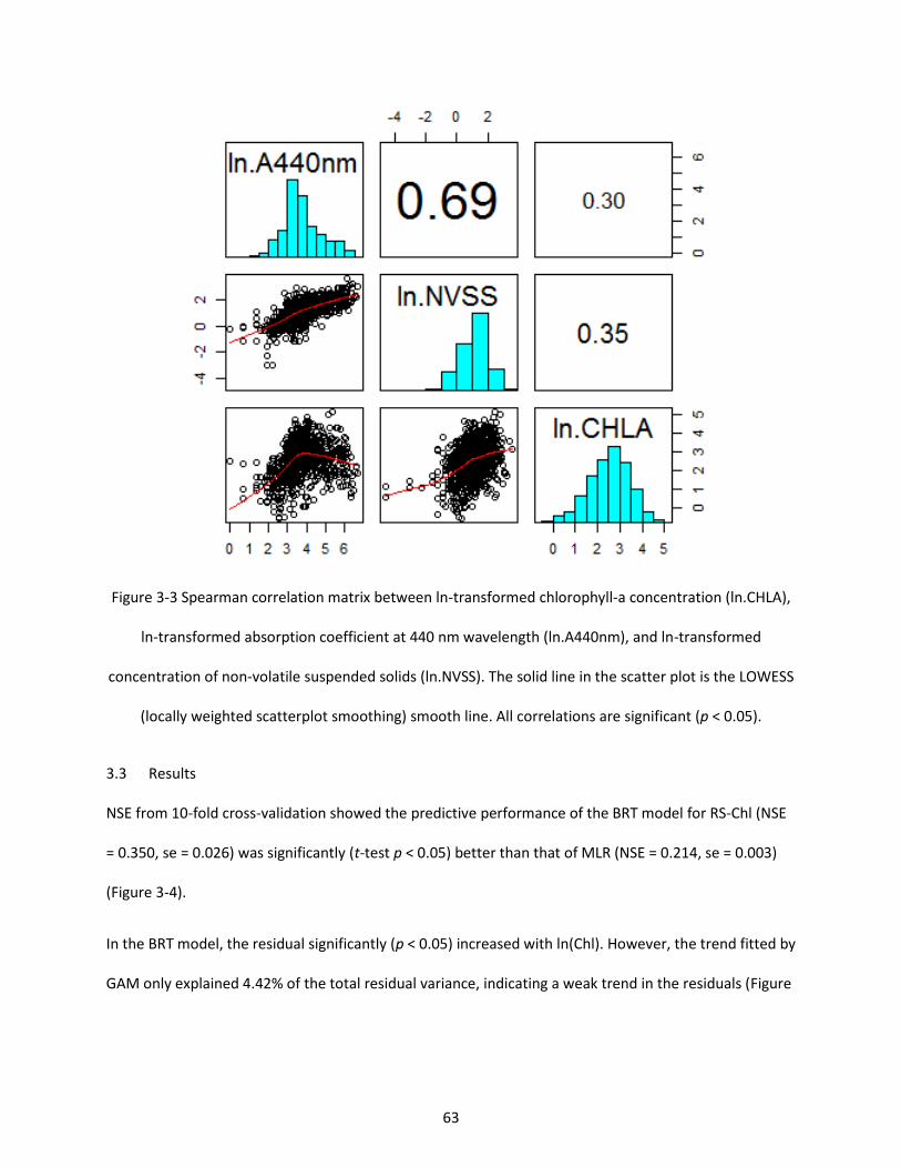
63
Figure 3-3 Spearman correlation matrix between ln-transformed chlorophyll-a concentration (ln.CHLA),
ln-transformed absorption coefficient at 440 nm wavelength (ln.A440nm), and ln-transformed
concentration of non-volatile suspended solids (ln.NVSS). The solid line in the scatter plot is the LOWESS
(locally weighted scatterplot smoothing) smooth line. All correlations are significant (p < 0.05).
3.3 Results
NSE from 10-fold cross-validation showed the predictive performance of the BRT model for RS-Chl (NSE
= 0.350, se = 0.026) was significantly (t-test p < 0.05) better than that of MLR (NSE = 0.214, se = 0.003)
(Figure 3-4).
In the BRT model, the residual significantly (p < 0.05) increased with ln(Chl). However, the trend fitted by
GAM only explained 4.42% of the total residual variance, indicating a weak trend in the residuals (Figure
64
3-5). After replacing GAM with the linear model, the trend explained 4.28% of the total residual
variance, which was even lower than GAM that accounted for non-linear trends.
Systematic trends (p < 0.05) in the RS-Chl BRT model residuals were related to ln(NVSS) (i.e., sediments)
and ln(A440nm) (i.e., CDOM), but the GAM functions indicated these trends were relatively weak (Figure
3-6). They only explained 6.73% and 4.64% of the total residual variance, respectively. The RS-Chl BRT
model residual increased with ln(NVSS), levelling off near zero with ln(A440nm).
Adding sediments and CDOM in the RS-Chl BRT model increased model performance significantly (p <
0.05), from NSE = 0.350 (se = 0.026) to NSE = 0.453 (se = 0.019). The improved performance confirmed
that the systematic errors were related to, but not necessarily caused by, sediments and CDOM. Parsing
out the chlorophyll-a correlations with sediments and CDOM, the new residual (i.e., partial residual)
trends were different from the corresponding theoretical ones (Figure 3-7, Figure 3-8). More specifically,
the partial residual slightly increased with ln(NVSS) at first and then dipped down and bounced up.
Theoretically, the residuals should have increased and then plateaued with higher reflectance due to
higher sediment concentrations. For CDOM, the partial residual dipped down then bounced up with
ln(A440nm). Theoretically, the residuals should have linearly decreased then plateaued with increasing
CDOM that resulted in lower reflectance. The differences in observed and theoretical relationships
indicated that the residual trends in the RS-Chl BRT model was not likely caused by sediments or CDOM.
Moreover, the magnitude of the partial residual change over ln(NVSS) or ln(A440nm) was much smaller
than the original ones without parsing out the chlorophyll-a correlation. Specifically, the range of
residual change over ln(NVSS) decreased from 1.2 to 0.11 after parsing out the chlorophyll-a correlation.
The range of residual change over ln(A440nm) decreased from 0.7 to 0.30 (Table 3-2). That indicated a
weaker trend related to sediments or CDOM after parsing out the chlorophyll-a correlation.
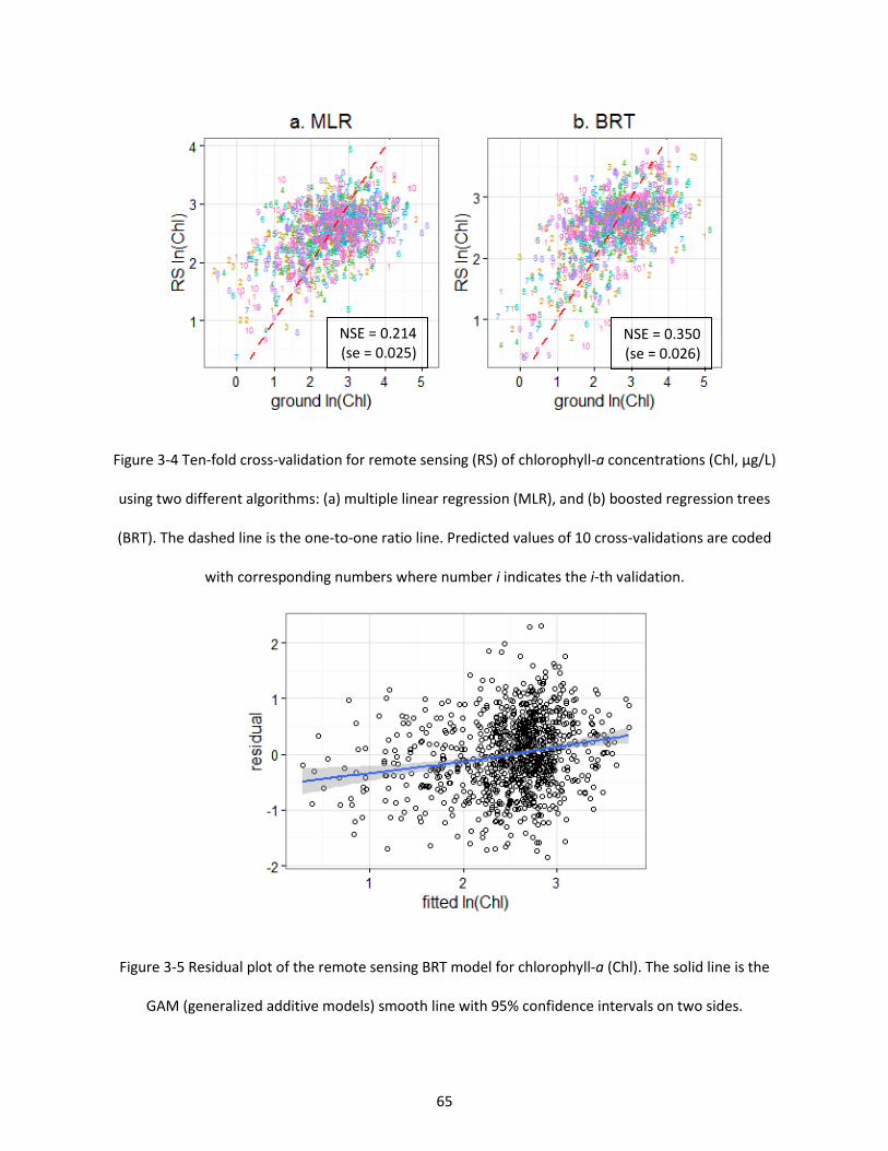
65
Figure 3-4 Ten-fold cross-validation for remote sensing (RS) of chlorophyll-a concentrations (Chl, µg/L)
using two different algorithms: (a) multiple linear regression (MLR), and (b) boosted regression trees
(BRT). The dashed line is the one-to-one ratio line. Predicted values of 10 cross-validations are coded
with corresponding numbers where number i indicates the i-th validation.
Figure 3-5 Residual plot of the remote sensing BRT model for chlorophyll-a (Chl). The solid line is the
GAM (generalized additive models) smooth line with 95% confidence intervals on two sides.
NSE = 0.214 (se = 0.025)
NSE = 0.350 (se = 0.026)
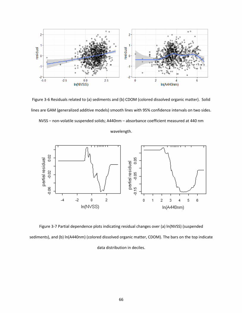
66
Figure 3-6 Residuals related to (a) sediments and (b) CDOM (colored dissolved organic matter). Solid
lines are GAM (generalized additive models) smooth lines with 95% confidence intervals on two sides.
NVSS – non-volatile suspended solids; A440nm – absorbance coefficient measured at 440 nm
wavelength.
Figure 3-7 Partial dependence plots indicating residual changes over (a) ln(NVSS) (suspended
sediments), and (b) ln(A440nm) (colored dissolved organic matter, CDOM). The bars on the top indicate
data distribution in deciles.
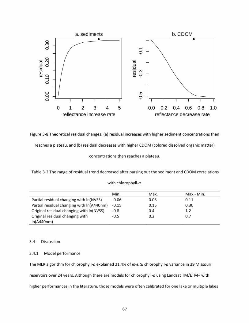
67
Figure 3-8 Theoretical residual changes: (a) residual increases with higher sediment concentrations then
reaches a plateau, and (b) residual decreases with higher CDOM (colored dissolved organic matter)
concentrations then reaches a plateau.
Table 3-2 The range of residual trend decreased after parsing out the sediment and CDOM correlations
with chlorophyll-a.
Min. Max. Max.- Min.
Partial residual changing with ln(NVSS) -0.06 0.05 0.11 Partial residual changing with ln(A440nm) -0.15 0.15 0.30 Original residual changing with ln(NVSS) -0.8 0.4 1.2 Original residual changing with ln(A440nm)
-0.5 0.2 0.7
3.4 Discussion
3.4.1 Model performance
The MLR algorithm for chlorophyll-a explained 21.4% of in-situ chlorophyll-a variance in 39 Missouri
reservoirs over 24 years. Although there are models for chlorophyll-a using Landsat TM/ETM+ with
higher performances in the literature, those models were often calibrated for one lake or multiple lakes
0 1 2 3 4 5
0.0
00
.10
0.2
00
.30
a. sediments
reflectance increase rate
resid
ua
l
0.0 0.2 0.4 0.6 0.8 1.0
-0.5
-0.3
-0.1
b. CDOM
reflectance decrease rate
resid
ua
l
68
covered by one scene of a satellite image where atmospheric conditions and perhaps water constituents
were more homogeneous than in our study. For example, Brivio et al. (2001) found that the model “Chl
= 9.82(Band 1 – Band 3)/Band 2” explained 81.8% of in-situ chlorophyll-a (Chl) variance over one TM
scene in March 1993 in Lake Garda, but the model explained less than 20% of variance in another TM
scene in February 1992. In the latter TM scene, a different model was the best, i.e., “ln(Chl) = 0.52
ln(Band 1) – 0.79 ln(Band 2)”. Even though they had applied an atmospheric correction using the
“integrally image-based” method in the TM images, the models still could not be transferred between
two scenes (dates) covering the same lake. In our study, TM/ETM+ images were gathered over 24 years,
and over a large area with 39 reservoirs that spanned 15 Landsat scenes. A relatively low MLR model
performance was therefore expected considering the spatial and temporal variations of atmosphere and
water optical characteristics.
BRT had better performance than MLR for estimating chlorophyll-a from Landsat TM/ETM+ surface
reflectance. That better performance might be due to (1) insensitivity to extreme values, (2) capability
to fit complicated non-linear relationships, and/or (3) machine learning to fit interactions among
variables. The predictive performance of BRT was stronger than MLR. Therefore, BRT is recommended
over MLR as the algorithm for chlorophyll-a remote sensing in the future.
3.4.2 Sediments and CDOM effects
3.4.2.1 The method for detecting effects
A relationship between sediments or CDOM with residuals from the RS-Chl model could be due to a
missing variable, a missing higher-order term of a variable, or a missing interaction between variables.
BRT had likely taken care of non-linear relations like having a higher-order term to explain non-
linearities in other model types, and BRT also likely accounted for interactions. Therefore, the residuals
are likely related to variables that were not included in the original model, such as sediments or CDOM.
69
However, BRT is based on thousands of decision/regression trees, which do not show direct relationship
between independent and dependent variables as MLR does. So, it was hard to predict how residuals
changed with sediments or CDOM based on the BRT model. Alternatively, this study simulated
theoretical residual trends by changing the bands and band ratios in the RS-Chl BRT model according to
the sediments and CDOM effects on band reflectance. Remote sensing reflectance may increase less at
very high sediment concentrations. However, within the range of our sediment data, it was reasonable
to assume reflectance decreased linearly with sediment concentrations (Han 1997). The same applied to
the CDOM effect. In water with very high CDOM concentrations, the reflectance is very low due to light
absorption of CDOM and a less reflectance decrease is expected at higher CDOM concentrations.
Nonetheless, the general increase or decrease in the theoretical trends still held even when sediments
or CDOM concentrations were very high.
3.4.2.2 Explanations for the insensitivity to suspended sediments and CDOM
After parsing out the chlorophyll-a correlation, the residual trends related to sediments and CDOM did
not agree well with the theoretical trends that generally increased with sediments and decreased with
CDOM. There is no doubt that sediments and CDOM can affect water-leaving radiance. However, at-
sensor radiance might not be sensitive to sediments or CDOM considering a great amount of errors
introduced by the atmosphere, specular reflectance, and so on. The water-leaving radiance in Landsat
TM/ETM+ bands only accounts for about 3%-13% of total sensor signal in visual bands, and most
radiance is from the atmosphere and from specular reflections from the water surface (Hu et al. 2001).
Although atmospheric corrections had been applied in the Landsat TM/ETM+ data we used, the
products were prepared for land surface applications and the correction accuracy might not meet the
higher requirements for waters and their weaker signals. Moreover, specular reflectance had not been
corrected in the Landsat products. When wind speed was high (> 10 m/s), the specular reflectance could
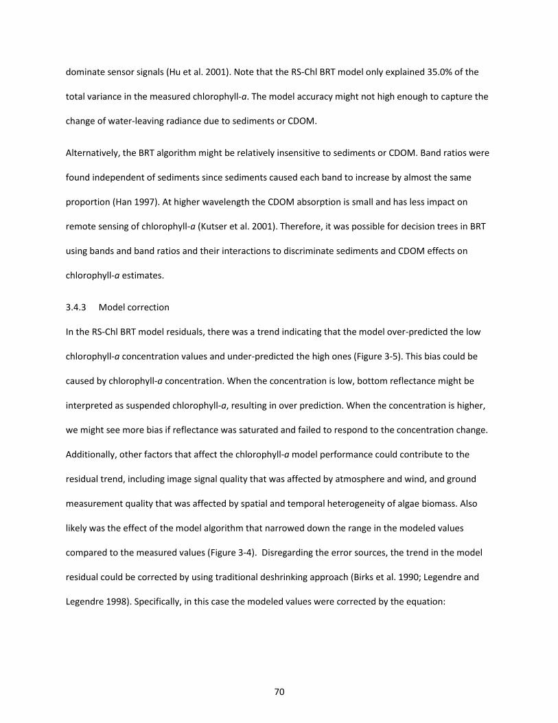
70
dominate sensor signals (Hu et al. 2001). Note that the RS-Chl BRT model only explained 35.0% of the
total variance in the measured chlorophyll-a. The model accuracy might not high enough to capture the
change of water-leaving radiance due to sediments or CDOM.
Alternatively, the BRT algorithm might be relatively insensitive to sediments or CDOM. Band ratios were
found independent of sediments since sediments caused each band to increase by almost the same
proportion (Han 1997). At higher wavelength the CDOM absorption is small and has less impact on
remote sensing of chlorophyll-a (Kutser et al. 2001). Therefore, it was possible for decision trees in BRT
using bands and band ratios and their interactions to discriminate sediments and CDOM effects on
chlorophyll-a estimates.
3.4.3 Model correction
In the RS-Chl BRT model residuals, there was a trend indicating that the model over-predicted the low
chlorophyll-a concentration values and under-predicted the high ones (Figure 3-5). This bias could be
caused by chlorophyll-a concentration. When the concentration is low, bottom reflectance might be
interpreted as suspended chlorophyll-a, resulting in over prediction. When the concentration is higher,
we might see more bias if reflectance was saturated and failed to respond to the concentration change.
Additionally, other factors that affect the chlorophyll-a model performance could contribute to the
residual trend, including image signal quality that was affected by atmosphere and wind, and ground
measurement quality that was affected by spatial and temporal heterogeneity of algae biomass. Also
likely was the effect of the model algorithm that narrowed down the range in the modeled values
compared to the measured values (Figure 3-4). Disregarding the error sources, the trend in the model
residual could be corrected by using traditional deshrinking approach (Birks et al. 1990; Legendre and
Legendre 1998). Specifically, in this case the modeled values were corrected by the equation:
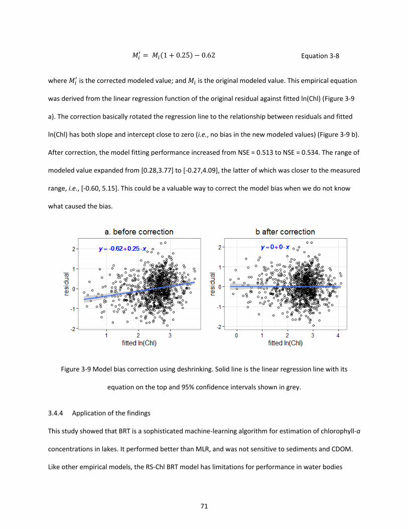
71
where 𝑀𝑖′ is the corrected modeled value; and 𝑀𝑖 is the original modeled value. This empirical equation
was derived from the linear regression function of the original residual against fitted ln(Chl) (Figure 3-9
a). The correction basically rotated the regression line to the relationship between residuals and fitted
ln(Chl) has both slope and intercept close to zero (i.e., no bias in the new modeled values) (Figure 3-9 b).
After correction, the model fitting performance increased from NSE = 0.513 to NSE = 0.534. The range of
modeled value expanded from [0.28,3.77] to [-0.27,4.09], the latter of which was closer to the measured
range, i.e., [-0.60, 5.15]. This could be a valuable way to correct the model bias when we do not know
what caused the bias.
Figure 3-9 Model bias correction using deshrinking. Solid line is the linear regression line with its
equation on the top and 95% confidence intervals shown in grey.
3.4.4 Application of the findings
This study showed that BRT is a sophisticated machine-learning algorithm for estimation of chlorophyll-a
concentrations in lakes. It performed better than MLR, and was not sensitive to sediments and CDOM.
Like other empirical models, the RS-Chl BRT model has limitations for performance in water bodies
𝑀𝑖′ = 𝑀𝑖(1 + 0.25) − 0.62 Equation 3-8
72
having conditions outside the ranges tested in this study. For water bodies with chlorophyll-a, CDOM,
and NVSS concentrations higher or lower than this study, the findings may not hold true. The data
distribution of chlorophyll-a concentrations in the reservoir dataset analyzed here is similar to that in
the 2007 National Lake Assessment (NLA) in USA (http://water.epa.gov, accessed on July 13, 2015). The
A440nm median (37.0 m-1) was higher than concentrations reported in other studies, e.g., 0.68 - 11.13
m−1 in 18 lakes over southern Finland and southern Sweden (Kutser et al. 2005) and 0.6 – 19.4 m−1 in 15
Minnesota lakes (Brezonik, Menken, and Bauer 2005). Extremely high NVSS values (NVSS > 200 mg/L)
have been reported in some lakes and rivers, but for most inland lakes, NVSS is less than 20 mg/L (e. g.,
Lenhart et al. 2009; Pollard et al. 1998; Graham et al. 2004). The NVSS concentrations ranged from 0.01
mg/L to 36.2 mg/L in this study. The RS-Chl BRT model was tested over a relatively wide range of
chlorophyll-a, sediments, and CDOM compared to other reported ranges, so the findings here can be
extended to many other lakes.
3.5 Conclusion
We used a long-term dataset covering 39 Missouri reservoirs and 24 years to compare algorithm
performances of MLR and BRT for chlorophyll-a estimates in turbid inland waters. We have found that
BRT was a better choice than MLR for empirical chlorophyll-a models using Landsat TM/ETM+ imagery.
Moreover, the BRT-Chl model was not sensitive to sediments and CDOM. Systematic trends were found
related to sediments and CDOM, but not caused by sediments and CDOM.
Acknowledgement
This work was supported by the Environmental Protection Agency (EPA), USA under Grant R835203. The
views and opinions expressed in this article are those of the authors and do not necessarily reflect the
official policy or position of U.S. EPA, or any other agency of the U.S. government.

73
REFERENCES
74
REFERENCES
Birks, H. John B., J. M. Line, Steve Juggins, A. C. Stevenson, and C. J. F. Ter Braak. 1990. “Diatoms and pH Reconstruction.” Philosophical Transactions of the Royal Society of London B: Biological Sciences 327 (1240): 263–278.
Blondeau-Patissier, David, James F. R. Gower, Arnold G. Dekker, Stuart R. Phinn, and Vittorio E. Brando. 2014. “A Review of Ocean Color Remote Sensing Methods and Statistical Techniques for the Detection, Mapping and Analysis of Phytoplankton Blooms in Coastal and Open Oceans.” Progress in Oceanography 123 (April): 123–144. doi:10.1016/j.pocean.2013.12.008.
Brezonik, Patrick, Kevin D. Menken, and Marvin Bauer. 2005. “Landsat-Based Remote Sensing of Lake Water Quality Characteristics, Including Chlorophyll and Colored Dissolved Organic Matter (CDOM).” Lake and Reservoir Management 21 (4): 373–382.
Bricaud, Annick, Andre Morel, Louis Prieur, and others. 1981. “Absorption by Dissolved Organic Matter of the Sea (Yellow Substance) in the UV and Visible Domains.” Limnology Oceanography 26 (1): 43–53.
Brivio, P. A., C. Giardino, and E. Zilioli. 2001. “Determination of Chlorophyll Concentration Changes in Lake Garda Using an Image-Based Radiative Transfer Code for Landsat TM Images.” International Journal of Remote Sensing 22 (2–3): 487–502. doi:10.1080/014311601450059.
Carder, Kendall L., Robert G. Steward, George R. Harvey, and Peter B. Ortner. 1989. “Marine Humic and Fulvic Acids: Their Effects on Remote Sensing of Ocean Chlorophyll.” Limnology and Oceanography 34 (1): 68–81.
Carpenter, D. J., and S. M. Carpenter. 1983. “Modeling Inland Water Quality Using Landsat Data.” Remote Sensing of Environment 13 (4): 345–352. doi:10.1016/0034-4257(83)90035-4.
Chen, Li, Chih-Hung Tan, Shuh-Ji Kao, and Tai-Sheng Wang. 2008. “Improvement of Remote Monitoring on Water Quality in a Subtropical Reservoir by Incorporating Grammatical Evolution with Parallel Genetic Algorithms into Satellite Imagery.” Water Research 42 (1–2): 296–306. doi:10.1016/j.watres.2007.07.014.
Dona, C., J.M. Sanchez, V. Caselles, J.A Dominguez, and A Camacho. 2014. “Empirical Relationships for Monitoring Water Quality of Lakes and Reservoirs Through Multispectral Images.” IEEE Journal of Selected Topics in Applied Earth Observations and Remote Sensing 7 (5): 1632–1641. doi:10.1109/JSTARS.2014.2301295.
Elith, J., J. R. Leathwick, and T. Hastie. 2008. “A Working Guide to Boosted Regression Trees.” Journal of Animal Ecology 77 (4): 802–813. doi:10.1111/j.1365-2656.2008.01390.x.
75
Elith, Jane, Catherine H. Graham, Robert P. Anderson, Miroslav Dudík, Simon Ferrier, Antoine Guisan, Robert J. Hijmans, et al. 2006. “Novel Methods Improve Prediction of Species’ Distributions from Occurrence Data.” Ecography 29 (2): 129–151. doi:10.1111/j.2006.0906-7590.04596.x.
Friedman, Jerome H. 2001. “Greedy Function Approximation: A Gradient Boosting Machine.” Annals of Statistics, 1189–1232.
Gilerson, Alexander A., Anatoly A. Gitelson, Jing Zhou, Daniela Gurlin, Wesley Moses, Ioannis Ioannou, and Samir A. Ahmed. 2010. “Algorithms for Remote Estimation of Chlorophyll-a in Coastal and Inland Waters Using Red and near Infrared Bands.” Optics Express 18 (23): 24109–24125. doi:10.1364/OE.18.024109.
Gordon, Howard R. 1997. “Atmospheric Correction of Ocean Color Imagery in the Earth Observing System Era.” Journal of Geophysical Research: Atmospheres 102 (D14): 17081–17106. doi:10.1029/96JD02443.
Gould, R. W., R. A. Arnone, and M. Sydor. 2001. “Absorption, Scattering, And, Remote-Sensing Reflectance Relationships in Coastal Waters: Testing a New Inversion Algorith.” Journal of Coastal Research 17 (2): 328–341.
Graham, Jennifer L., John R. Jones, Susan B. Jones, John A. Downing, and Thomas E. Clevenger. 2004. “Environmental Factors Influencing Microcystin Distribution and Concentration in the Midwestern United States.” Water Research 38 (20): 4395–4404. doi:10.1016/j.watres.2004.08.004.
Han, L., D. C. Rundquist, L. L. Liu, R. N. Fraser, and J. F. Schalles. 1994. “The Spectral Responses of Algal Chlorophyll in Water with Varying Levels of Suspended Sediment.” International Journal of Remote Sensing 15 (18): 3707–3718.
Han, Luoheng. 1997. “Spectral Reflectance with Varying Suspended Sediment Concentrations in Clear and Algae-Laden Waters.” Photogrammetric Engineering and Remote Sensing 63 (6): 701–705.
Hu, Chuanmin, Frank E. Muller-Karger, Serge Andrefouet, and Kendall L. Carder. 2001. “Atmospheric Correction and Cross-Calibration of LANDSAT-7/ETM+ Imagery over Aquatic Environments: A Multiplatform Approach Using SeaWiFS/MODIS.” Remote Sensing of Environment 78 (1): 99–107.
Kabbara, Nijad, Jean Benkhelil, Mohamed Awad, and Vittorio Barale. 2008. “Monitoring Water Quality in the Coastal Area of Tripoli (Lebanon) Using High-Resolution Satellite Data.” ISPRS Journal of Photogrammetry and Remote Sensing, Theme Issue: Remote Sensing of the Coastal Ecosystems, 63 (5): 488–495. doi:10.1016/j.isprsjprs.2008.01.004.
Karabulut, Murat, and Nihal Ceylan. 2005. “The Spectral Reflectance Responses of Water with Different Levels of Suspended Sediment in the Presence of Algae.” Turkish Journal of Engineering and Environmental Sciences 29: 351–360.
76
Kloiber, Steven M., Patrick L. Brezonik, Leif G. Olmanson, and Marvin E. Bauer. 2002. “A Procedure for Regional Lake Water Clarity Assessment Using Landsat Multispectral Data.” Remote Sensing of Environment 82 (1): 38–47.
Kutser, Tiit, Antti Herlevi, Kari Kallio, and Helgi Arst. 2001. “A Hyperspectral Model for Interpretation of Passive Optical Remote Sensing Data from Turbid Lakes.” Science of the Total Environment 268 (1): 47–58.
Kutser, Tiit, Donald C. Pierson, Kari Y. Kallio, Anu Reinart, and Sebastian Sobek. 2005. “Mapping Lake CDOM by Satellite Remote Sensing.” Remote Sensing of Environment 94 (4): 535–540. doi:10.1016/j.rse.2004.11.009.
Legendre, P., and Loic F. J. Legendre. 1998. Numerical Ecology. Elsevier.
Lenhart, Christian F., Kenneth N. Brooks, Daniel Heneley, and Joseph A. Magner. 2009. “Spatial and Temporal Variation in Suspended Sediment, Organic Matter, and Turbidity in a Minnesota Prairie River: Implications for TMDLs.” Environmental Monitoring and Assessment 165 (1–4): 435–447. doi:10.1007/s10661-009-0957-y.
Masek, Jeffrey G., Eric F. Vermote, Nazmi E. Saleous, Robert Wolfe, Forrest G. Hall, Karl F. Huemmrich, Feng Gao, Jonathan Kutler, and Teng-Kui Lim. 2006. “A Landsat Surface Reflectance Dataset for North America, 1990-2000.” Geoscience and Remote Sensing Letters, IEEE 3 (1): 68–72.
Menken, Kevin D., Patrick L. Brezonik, and Marvin E. Bauer. 2006. “Influence of Chlorophyll and Colored Dissolved Organic Matter (CDOM) on Lake Reflectance Spectra: Implications for Measuring Lake Properties by Remote Sensing.” Lake and Reservoir Management 22 (3): 179–190. doi:10.1080/07438140609353895.
Moisen, Gretchen G., Elizabeth A. Freeman, Jock A. Blackard, Tracey S. Frescino, Niklaus E. Zimmermann, and Thomas C. Edwards. 2006. “Predicting Tree Species Presence and Basal Area in Utah: A Comparison of Stochastic Gradient Boosting, Generalized Additive Models, and Tree-Based Methods.” Ecological Modelling 199 (2): 176–187. doi:10.1016/j.ecolmodel.2006.05.021.
Nash, J. E., and J. V. Sutcliffe. 1970. “River Flow Forecasting through Conceptual Models Part I — A Discussion of Principles.” Journal of Hydrology 10 (3): 282–290. doi:10.1016/0022-1694(70)90255-6.
Olmanson, Leif G., Marvin E. Bauer, and Patrick L. Brezonik. 2008. “A 20-Year Landsat Water Clarity Census of Minnesota’s 10,000 Lakes.” Remote Sensing of Environment 112 (11): 4086–4097.
Oyama, Y., B. Matsushita, T. Fukushima, T. Nagai, and A. Imai. 2007. “A New Algorithm for Estimating Chlorophyll‐a Concentration from Multi‐spectral Satellite Data in Case II Waters: A Simulation Based on a Controlled Laboratory Experiment.” International Journal of Remote Sensing 28 (7): 1437–1453. doi:10.1080/01431160600975295.
77
Paerl, Hans W., and Valerie J. Paul. 2012. “Climate Change: Links to Global Expansion of Harmful Cyanobacteria.” Water Research, Cyanobacteria: Impacts of climate change on occurrence, toxicity and water quality management, 46 (5): 1349–1363. doi:10.1016/j.watres.2011.08.002.
Papoutsa, Christiana, Adrianos Retalis, Leonidas Toulios, and Diofantos G. Hadjimitsis. 2014. “Defining the Landsat TM/ETM plus and CHRIS/PROBA Spectral Regions in Which Turbidity Can Be Retrieved in Inland Waterbodies Using Field Spectroscopy.” International Journal of Remote Sensing 35 (5): 1674–1692. doi:10.1080/01431161.2014.882029.
Pattiaratchi, C., P. Lavery, A. Wyllie, and P. Hick. 1994. “Estimates of Water Quality in Coastal Waters Using Multi-Date Landsat Thematic Mapper Data.” International Journal of Remote Sensing 15 (8): 1571–1584. doi:10.1080/01431169408954192.
Pollard, A. I., M. J. González, M. J. Vanni, and J. L. Headworth. 1998. “Effects of Turbidity and Biotic Factors on the Rotifer Community in an Ohio Reservoir.” Hydrobiologia 387–388 (0): 215–223. doi:10.1023/A:1017041826108.
Ridgeway, Greg. 2004. “The Gbm Package.” R Foundation for Statistical Computing, Vienna, Austria. http://132.180.15.2/math/statlib/R/CRAN/doc/packages/gbm.pdf.
Ritchie, Jerry C., Charles M. Cooper, and Frank R. Schiebe. 1990. “The Relationship of MSS and TM Digital Data with Suspended Sediments, Chlorophyll, and Temperature in Moon Lake, Mississippi.” Remote Sensing of Environment 33 (2): 137–148. doi:10.1016/0034-4257(90)90039-O.
Rodríguez, Y. Chao, A. el Anjoumi, J. A. Domínguez Gómez, D. Rodríguez Pérez, and E. Rico. 2014. “Using Landsat Image Time Series to Study a Small Water Body in Northern Spain.” Environmental Monitoring and Assessment 186 (6): 3511–3522. doi:10.1007/s10661-014-3634-8.
Sellner, Kevin G., Gregory J. Doucette, and Gary J. Kirkpatrick. 2003. “Harmful Algal Blooms: Causes, Impacts and Detection.” Journal of Industrial Microbiology and Biotechnology 30 (7): 383–406. doi:10.1007/s10295-003-0074-9.
Sipelgas, L., H. Arst, K. Kallio, A. Erm, P. Oja, and T. Soomere. 2003. “Optical Properties of Dissolved Organic Matter in Finnish and Estonian Lakes.” Nordic Hydrology 34 (4): 361–386.
Sudheer, K.p., Indrajeet Chaubey, and Vijay Garg. 2006. “Lake Water Quality Assessment from Landsat Thematic Mapper Data Using Neural Network: An Approach to Optimal Band Combination Selection1.” JAWRA Journal of the American Water Resources Association 42 (6): 1683–1695. doi:10.1111/j.1752-1688.2006.tb06029.x.
Sváb, E., A. N. Tyler, T. Preston, M. Présing, and K. V. Balogh. 2005. “Characterizing the Spectral Reflectance of Algae in Lake Waters with High Suspended Sediment Concentrations.” International Journal of Remote Sensing 26 (5): 919–928. doi:10.1080/0143116042000274087.
Tyler, A. N., E. Svab, T. Preston, M. Présing, and W. A. Kovács. 2006. “Remote Sensing of the Water Quality of Shallow Lakes: A Mixture Modelling Approach to Quantifying Phytoplankton in Water
78
Characterized by High‐suspended Sediment.” International Journal of Remote Sensing 27 (8): 1521–1537. doi:10.1080/01431160500419311.
Wood, Simon N. 2001. “Mgcv: GAMs and Generalized Ridge Regression for R.” R News 1 (2): 20–25.
Wood, Simon N. 2012. “On P-Values for Smooth Components of an Extended Generalized Additive Model.” Biometrika, October, ass048. doi:10.1093/biomet/ass048.
Yacobi, Yosef Z., Anatoly Gitelson, and Meir Mayo. 1995. “Remote Sensing of Chlorophyll in Lake Kinneret Using Highspectral-Resolution Radiometer and Landsat TM: Spectral Features of Reflectance and Algorithm Development.” Journal of Plankton Research 17 (11): 2155–2173. doi:10.1093/plankt/17.11.2155.
Zhang, Yunlin, Mark A. van Dijk, Mingliang Liu, Guangwei Zhu, and Boqiang Qin. 2009. “The Contribution of Phytoplankton Degradation to Chromophoric Dissolved Organic Matter (CDOM) in Eutrophic Shallow Lakes: Field and Experimental Evidence.” Water Research 43 (18): 4685–4697. doi:10.1016/j.watres.2009.07.024.
Zhao, Jun, Wenxi Cao, Guifen Wang, Dingtian Yang, Yuezhong Yang, Zhaohua Sun, Wen Zhou, and Shaojun Liang. 2009. “The Variations in Optical Properties of CDOM throughout an Algal Bloom Event.” Estuarine, Coastal and Shelf Science 82 (2): 225–232. doi:10.1016/j.ecss.2009.01.007.
79
4 LANDSAT SURFACE REFLECTANCE PRODUCTS FOR REMOTE SENSING OF INLAND LAKES: THE
PROBLEM OF ATMOSPHERIC INTERFERENCE
Abstract
Inland lake remote sensing has been problematic for both complexity of optical properties in water and
the difficulty of atmospheric correction. Atmospheric effects account for most satellite-borne at-sensor
radiance over waters. The Landsat surface reflectance products corrected for atmospheric interference
are new and have recently been made available. The atmospheric correction method was designed to
better account for land surface reflectance for Landsat products. However, whether the new,
atmospherically corrected products have the potential to improve inland lake water quality estimates
has not been tested. In this study, we examined the relationships between bands and band ratios with
three optically sensitive agents in inland lake water, chlorophyll-a, sediments, and colored dissolved
organic matter (CDOM), using Landsat imagery before and after the atmospheric correction. The results
indicated that the atmospheric correction did not improve the signal of chlorophyll-a, sediments, and
CDOM. The remote sensing accuracy of chlorophyll-a, sediments, and CDOM indicated by validation R2
was 0.329, 0.508, and 0.733, respectively. The atmospheric correction also did not significantly change
the predictive model performances. Our findings suggest that improvements for atmospheric correction
of Landsat imagery may still be insufficient for inland lake water quality assessments. A more
sophisticated method for atmospheric correction is still needed for water applications.
Keywords: Landsat, chlorophyll-a, sediment, CDOM, water quality, atmospheric correction
Highlights
• The existing Landsat imagery is useful to monitor water color.
• The corrected imagery did not significantly improve the water color measurements.
80
4.1 Introduction
Remote sensing of turbid inland lakes has been problematic because optically sensitive agents in water
are complex and variable in space and time (Witte et al., 1982) and because atmospheric correction of
remotely sensed reflectance is difficult (Wang & Shi, 2007). Hu et al. (2001) estimated that the radiance
off water in Landsat ETM+ Band 1 (B1), Band 2 (B2), and Band 3 (B3) respectively only accounted for
13%, 10%, and 3% of the total radiance measured by the sensor for a windless day (wind speed < 2 m/s),
the rest of which was mostly contributed by the atmosphere. Therefore, atmospheric correction is
critical for remote sensing of inland lakes, especially for long-term and/or large scale studies, where
atmospheric effects are variable.
The U.S. Geological Survey recently published a provisional version of surface reflectance (SR) products
for Landsat 4-5 TM and Landsat 7 ETM+ that can be freely downloaded (http://landsat.usgs.gov,
accessed on July 3rd, 2014). The SR products are derived from the TOA (top of atmosphere) reflectance
products by removing atmospheric effects using the Landsat Ecosystem Disturbance Adaptive
Processing System (LEDAPS), which has the same atmospheric correction routines as MODIS (Moderate
Resolution Imaging Spectroradiometer). The latter are based on the 6S (Second Simulation of a Satellite
Signal in the Solar Spectrum) radiative transfer models (Masek et al., 2006). The SR products are
designed for land applications and may improve the accuracy over waters where atmospheric effects
account for most of the at-sensor signal.
The goal of our work was to evaluate these two sets of Landsat data (i.e., SR and TOA) for long-term
and/or large-scale studies over inland lakes. More specifically, we evaluated the signal enhancement
provided by the atmospheric correction and its impact on remote sensing of water optical
characteristics in inland lakes. The image signal was indicated by the relationships between individual
bands or band ratios (band/band ratio) and three optically sensitive agents—chlorophyll-a (Chl), Non-
Volatile Suspended Sediment (NVSS), and Colored Dissolved Organic Matter (CDOM). Both linear and
81
non-linear empirical algorithms were used to demonstrate how the atmospheric correction affected
remote sensing of water optical characteristics. In our evaluation, we took advantage of a set of inland
water quality data that included simultaneous measurements of all water color variables over 23 years
from 39 reservoirs spanning the long history of Landsat TM/ETM+ images.
4.2 Methodology
4.2.1 Study area and data
Water quality data cover 24 years (1989-2012) of sampling of 39 reservoirs in Missouri, U.S.A. (Jones et
al. 2008). Water samples were taken 3-4 times per summer from the surface water column (0.25 m – 0.5
m) near dams in the reservoirs. Chl, NVSS, and CDOM concentrations were measured in composite
samples using standard methods (APHA, 1985). CDOM was measured by the absorption coefficient at
440 nm wavelength (A440nm, m-1). The dataset covered wide ranges of water quality: Chl varied from
0.40 µg/L to 184.70 µg/L with mean = 20.03 µg/L; NVSS varied from 0.00 mg/L to 107.38 mg/L with
mean = 3.39 mg/L; and A440nm varied from 0.40 m-1 to 184.70 m-1 with mean = 59.7 m-1.
Both the Landsat TM/ETM+ TOA and SR products were downloaded from the on-demand ESPA Data
Access Interface (http://espa.cr.usgs.gov, accessed on July 1st, 2014). Remote sensing reflectance of
each water quality sample was characterized by average values of a “3 × 3” pixel window with the water
quality sampling location as the center pixel. Sampling locations were adjusted (adjusted distance < 100
m) to make sure no mixed pixel with land and water was in the window. Both TM and ETM+ data within
8 days before or after the water quality sampling dates were used to provide as many data pairs with
water quality sampling as possible. Pixels with clouds, shadows, saturated values, and ETM+ gaps due to
SLC (Scan Line Corrector) failure were excluded using the “Fmask” layer in the SR products. We applied
extra criteria to remove any SR pixel with reflectance less than zero, or B2 < B4 (to remove pixels of land
or shadows), or B2 > 0.015 (to remove pixels of clouds or with strong “whitecap” reflectance). In total,
82
963 remote sensing records (SR and TOA) corresponding to in-situ water quality samples were
produced. This long-term dataset should cover Landsat TM/ETM+ with a variety of atmospheric
conditions.
4.2.2 Signal enhancement evaluation
We built a non-linear machine-learning model by using the random forest algorithm (RF) (Breiman,
2001) for each band/band ratio with the optically sensitive agents in water as independent variables:
where Bi is reflectance (dimensionless) of the ith Landsat TM/ETM+ band or band ratio from the SR or
TOA products, i.e, B1, B2, B4, B5, B7, B1v2 (ratio of B1 vs. B2), B1v3, B1v4, B2v3, B2v4, etc. (the thermal
band, B6, was not included since it indicates object temperature regardless of the agent concentration);
RF is the random forest algorithm; Chl, NVSS, and A440nm are indicators of optically sensitive agents. If
the signal of the SR products has been enhanced over the original TOA products, then the Bi of the SR
products should be better explained by the optically sensitive agents rather than the Bi of the TOA
products. The model performance was indicated by the coefficient of determination (R2) from the out-
of-bag validation.
The contribution of each optically sensitive agent in Model 4-1 was measured to further investigate the
signal combinations and their changes resulting from the atmospheric correction. The contribution is
indicated by a partial R2, which is the model total R2 multiplied by the relative importance of the
optically sensitive agent (predictor). The relative importance of each predictor is the sum of instances
that the predictor is used to split over a random forest, weighted by the model deviation decrease due
to each split, and rescaled to have a sum predictor importance of one.
Bi = RF (Chl, NVSS, A440nm) Model 4-1
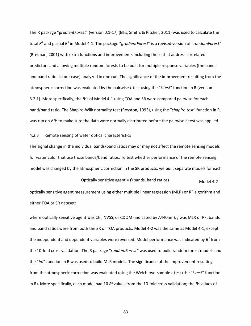
83
The R package “gradientForest” (version 0.1-17) (Ellis, Smith, & Pitcher, 2011) was used to calculate the
total R2 and partial R2 in Model 4-1. The package “gradientForest” is a revised version of “randomForest”
(Breiman, 2001) with extra functions and improvements including those that address correlated
predictors and allowing multiple random forests to be built for multiple response variables (the bands
and band ratios in our case) analyzed in one run. The significance of the improvement resulting from the
atmospheric correction was evaluated by the pairwise t-test using the “t.test” function in R (version
3.2.1). More specifically, the R2s of Model 4-1 using TOA and SR were compared pairwise for each
band/band ratio. The Shapiro-Wilk normality test (Royston, 1995), using the “shapiro.test” function in R,
was run on ΔR2 to make sure the data were normally distributed before the pairwise t-test was applied.
4.2.3 Remote sensing of water optical characteristics
The signal change in the individual bands/band ratios may or may not affect the remote sensing models
for water color that use those bands/band ratios. To test whether performance of the remote sensing
model was changed by the atmospheric correction in the SR products, we built separate models for each
optically sensitive agent measurement using either multiple linear regression (MLR) or RF algorithm and
either TOA or SR dataset:
where optically sensitive agent was Chl, NVSS, or CDOM (indicated by A440nm); f was MLR or RF; bands
and band ratios were from both the SR or TOA products. Model 4-2 was the same as Model 4-1, except
the independent and dependent variables were reversed. Model performance was indicated by R2 from
the 10-fold cross validation. The R package “randomForest” was used to build random forest models and
the “lm” function in R was used to build MLR models. The significance of the improvement resulting
from the atmospheric correction was evaluated using the Welch two-sample t-test (the “t.test” function
in R). More specifically, each model had 10 R2 values from the 10-fold cross validation; the R2 values of
Optically sensitive agent = f (bands, band ratios) Model 4-2
84
the TOA model were compared with the R2 values of the SR model using the t-test. The Shapiro-Wilk
normality test using the “shapiro.test” function in R was run on each group of R2s (N = 10) from the 10-
fold cross validation to make sure the data were normally distributed before the Welch two-sample t-
test was applied.
4.3 Results
4.3.1 Signal change
Indicated by the total R2 of Model 4-1, the atmospheric correction did not significantly (pairwise t-test p
= 0.602) improve relationships between individual bands or band ratios and the water optically sensitive
agents (i.e., Chl, NVSS, and CDOM) (Figure 4-1a, b). More specifically, some bands and band ratios
appeared to have relatively weaker relationships with the water optically sensitive agents after the
atmospheric correction, but the others did not. The R2 for TOA bands and band ratios ranged from 0 to
0.633 (mean = 0.271). The R2 for SR bands and band ratios ranged from 0 to 0.577 (mean = 0.226). B1v3,
B2v3, B1v2, and B3 were four bands/band ratios had total R2 ≥ 0.5 in the TOA models, with total R2 of
0.634, 0.624, 0.522, and 0.521. After the atmospheric correction, the total R2 did not increase but
decreased by 8.9%, 13.2%, 45.7%, and 4.5%. Some bands/band ratios had higher total R2 after the
atmospheric correction, such as B3v4 with total R2 increasing from 0.291 to 0.552.
The partial Chl R2 for most of the bands and band ratios significantly (pairwise t-test p = 0.011)
increased after the atmospheric correction, with the average (aggregated for all bands and band ratios)
partial R2 changing from 0.059 of the TOA models to 0.063 of the SR models (Figure 4-1 c). The partial R2
of NVSS and CDOM did not change significantly (pairwise t-test p = 0.844 for NVSS, 0.848 for CDOM)
with the atmospheric correction (Figure 4-1 d and e).
85
Figure 4-1 Water color signal in Landsat TM/ETM+ as changed by the atmospheric correction. The image
signal is indicated by R2 of models for bands/band ratios: Bi = RF (Chl, NVSS, A440nm), where Bi is the
TOA (top of atmosphere) or SR (surface reflectance) band/band ratio with i indicating the band number
or combination of bands in ratios, e.g., B1 = Band 1, and B1v2 = ratio of Band 1 vs. Band 2. RF is the
random forest algorithm. Chl is chlorophyll-a concentration. NVSS is concentration of non-volatile
suspended solids. A440nm is absorbance coefficient at 440 nm wavelength (indicator of colored
dissolved organic matter). Figure a has the same information as b-e, which are scatter plots comparing
either the total or partial R2 before and after the atmospheric correction. The dashed line is the 1:1 line
in b-e.
86
4.3.2 Remote sensing of water optics
No significant (two-sample t-test p > 0.05) improvement was found in remote sensing of water optical
characteristics with the new atmospheric correction of Landsat imagery, except for Chl measurements
when using the MLR algorithm (Table 4-1). More specifically, the Chl measurement accuracy indicated
by the R2 from 10-fold cross validation was improved significantly (two-sample t-test p = 0.038) by the
atmospheric correction when MLR was used as the algorithm, with R2 increasing from 0.148 (SD = 0.068)
to 0.219 (SD = 0.065). However, when the RF algorithm was used to measure Chl, which performed
better than the MLR algorithm, the improvement was not significant (two-sample t-test p = 0.585),
changing from 0.312 (SD = 0.061) to 0.329 (SD = 0.068). The NVSS and A440nm measurement accuracies
were not affected by the atmospheric correction no matter which algorithm was used (MLR or RF).
Remote sensing of NVSS and A440nm using RF algorithm had 10-fold cross validation R2 of 0.508 (SD =
0.042) and 0.733 (SD = 0.054), respectively.
4.4 Discussion
4.4.1 Why did the atmospheric correction produce no obvious signal enhancement?
The atmospheric correction with SR products did not significantly improve relationships between
Landsat data and optically sensitive agents (i.e., Chl, NVSS, and CDOM). The amount of variation
explained in bands and band ratios by the three optically sensitive agents varied with band/band ratio,
but was not consistently higher for SR than TOA products. The most informative bands and band ratios,
i.e. B1v3, B2v3, B1v2, and B3, even decreased after the atmospheric correction. Partial R2 values were
consistently but only slightly higher for Chl with SR versus TOA products, but there was no difference in
partial R2 for NVSS and CDOM.
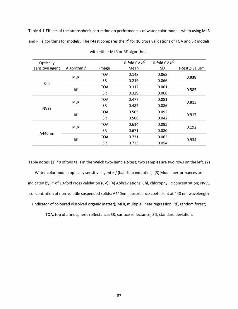
87
Table 4-1 Effects of the atmospheric correction on performances of water color models when using MLR
and RF algorithms for models. The t-test compares the R2 for 10 cross validations of TOA and SR models
with either MLR or RF algorithms.
Optically sensitive agent Algorithm f Image
10-fold CV R2
Mean 10-fold CV R2
SD t-test p value*
Chl MLR
TOA 0.148 0.068 0.038
SR 0.219 0.066
RF TOA 0.312 0.061
0.585 SR 0.329 0.068
NVSS MLR
TOA 0.477 0.081 0.813
SR 0.487 0.086
RF TOA 0.505 0.092
0.917 SR 0.508 0.042
A440nm MLR
TOA 0.614 0.095 0.192
SR 0.671 0.080
RF TOA 0.731 0.062
0.934 SR 0.733 0.054
Table notes: (1) *p of two tails in the Welch two-sample t-test; two samples are two rows on the left. (2)
Water color model: optically sensitive agent = f (bands, band ratios). (3) Model performances are
indicated by R2 of 10-fold cross validation (CV). (4) Abbreviations: Chl, chlorophyll a concentration; NVSS,
concentration of non-volatile suspended solids; A440nm, absorbance coefficient at 440 nm wavelength
(indicator of coloured dissolved organic matter); MLR, multiple linear regression; RF, random forest;
TOA, top of atmospheric reflectance; SR, surface reflectance; SD, standard deviation.
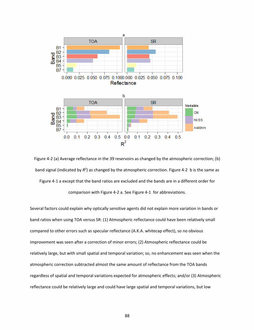
88
Figure 4-2 (a) Average reflectance in the 39 reservoirs as changed by the atmospheric correction; (b)
band signal (indicated by R2) as changed by the atmospheric correction. Figure 4-2 b is the same as
Figure 4-1 a except that the band ratios are excluded and the bands are in a different order for
comparison with Figure 4-2 a. See Figure 4-1 for abbreviations.
Several factors could explain why optically sensitive agents did not explain more variation in bands or
band ratios when using TOA versus SR: (1) Atmospheric reflectance could have been relatively small
compared to other errors such as specular reflectance (A.K.A. whitecap effect), so no obvious
improvement was seen after a correction of minor errors; (2) Atmospheric reflectance could be
relatively large, but with small spatial and temporal variation; so, no enhancement was seen when the
atmospheric correction subtracted almost the same amount of reflectance from the TOA bands
regardless of spatial and temporal variations expected for atmospheric effects; and/or (3) Atmospheric
reflectance could be relatively large and could have large spatial and temporal variations, but low
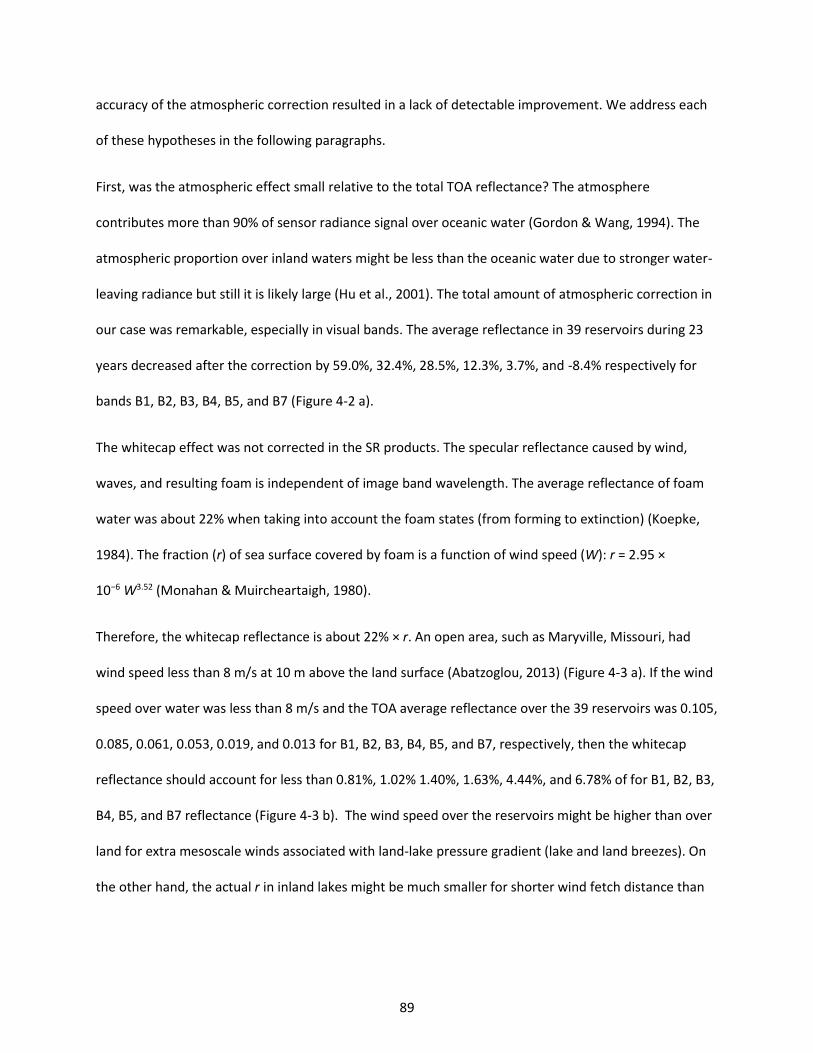
89
accuracy of the atmospheric correction resulted in a lack of detectable improvement. We address each
of these hypotheses in the following paragraphs.
First, was the atmospheric effect small relative to the total TOA reflectance? The atmosphere
contributes more than 90% of sensor radiance signal over oceanic water (Gordon & Wang, 1994). The
atmospheric proportion over inland waters might be less than the oceanic water due to stronger water-
leaving radiance but still it is likely large (Hu et al., 2001). The total amount of atmospheric correction in
our case was remarkable, especially in visual bands. The average reflectance in 39 reservoirs during 23
years decreased after the correction by 59.0%, 32.4%, 28.5%, 12.3%, 3.7%, and -8.4% respectively for
bands B1, B2, B3, B4, B5, and B7 (Figure 4-2 a).
The whitecap effect was not corrected in the SR products. The specular reflectance caused by wind,
waves, and resulting foam is independent of image band wavelength. The average reflectance of foam
water was about 22% when taking into account the foam states (from forming to extinction) (Koepke,
1984). The fraction (r) of sea surface covered by foam is a function of wind speed (W): r = 2.95 ×
10−6 W3.52 (Monahan & Muircheartaigh, 1980).
Therefore, the whitecap reflectance is about 22% × r. An open area, such as Maryville, Missouri, had
wind speed less than 8 m/s at 10 m above the land surface (Abatzoglou, 2013) (Figure 4-3 a). If the wind
speed over water was less than 8 m/s and the TOA average reflectance over the 39 reservoirs was 0.105,
0.085, 0.061, 0.053, 0.019, and 0.013 for B1, B2, B3, B4, B5, and B7, respectively, then the whitecap
reflectance should account for less than 0.81%, 1.02% 1.40%, 1.63%, 4.44%, and 6.78% of for B1, B2, B3,
B4, B5, and B7 reflectance (Figure 4-3 b). The wind speed over the reservoirs might be higher than over
land for extra mesoscale winds associated with land-lake pressure gradient (lake and land breezes). On
the other hand, the actual r in inland lakes might be much smaller for shorter wind fetch distance than
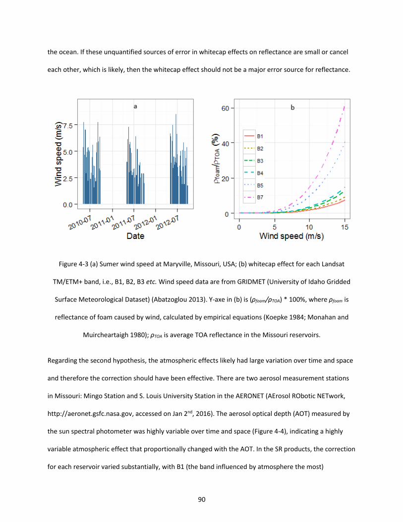
90
the ocean. If these unquantified sources of error in whitecap effects on reflectance are small or cancel
each other, which is likely, then the whitecap effect should not be a major error source for reflectance.
Figure 4-3 (a) Sumer wind speed at Maryville, Missouri, USA; (b) whitecap effect for each Landsat
TM/ETM+ band, i.e., B1, B2, B3 etc. Wind speed data are from GRIDMET (University of Idaho Gridded
Surface Meteorological Dataset) (Abatzoglou 2013). Y-axe in (b) is (ρfoam/ρTOA) * 100%, where ρfoam is
reflectance of foam caused by wind, calculated by empirical equations (Koepke 1984; Monahan and
Muircheartaigh 1980); ρTOA is average TOA reflectance in the Missouri reservoirs.
Regarding the second hypothesis, the atmospheric effects likely had large variation over time and space
and therefore the correction should have been effective. There are two aerosol measurement stations
in Missouri: Mingo Station and S. Louis University Station in the AERONET (AErosol RObotic NETwork,
http://aeronet.gsfc.nasa.gov, accessed on Jan 2nd, 2016). The aerosol optical depth (AOT) measured by
the sun spectral photometer was highly variable over time and space (Figure 4-4), indicating a highly
variable atmospheric effect that proportionally changed with the AOT. In the SR products, the correction
for each reservoir varied substantially, with B1 (the band influenced by atmosphere the most)
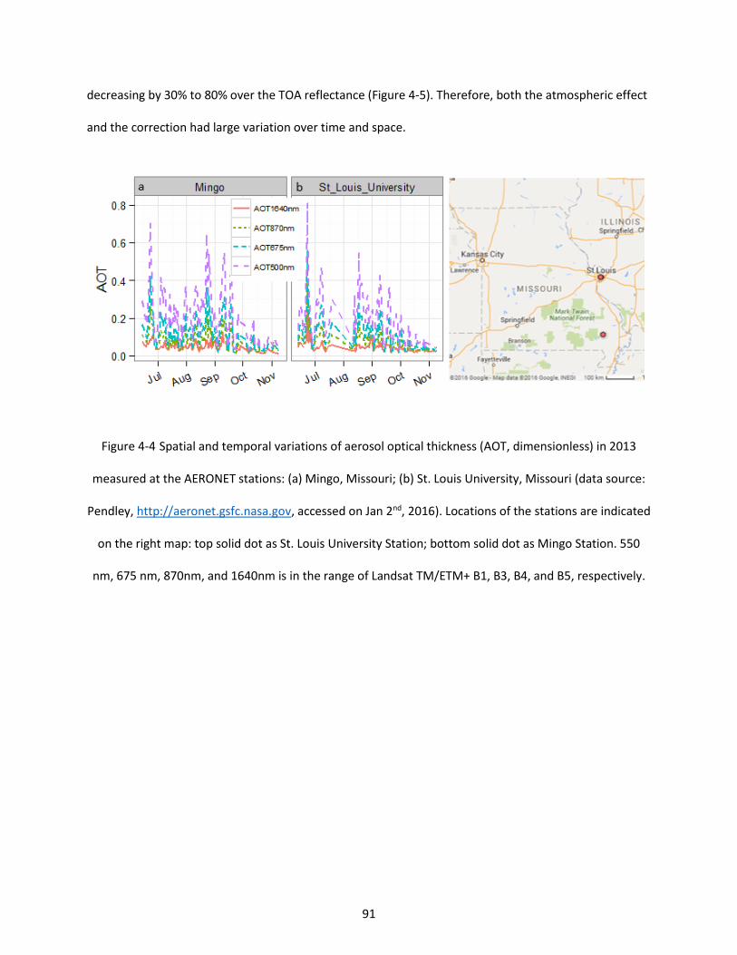
91
decreasing by 30% to 80% over the TOA reflectance (Figure 4-5). Therefore, both the atmospheric effect
and the correction had large variation over time and space.
Figure 4-4 Spatial and temporal variations of aerosol optical thickness (AOT, dimensionless) in 2013
measured at the AERONET stations: (a) Mingo, Missouri; (b) St. Louis University, Missouri (data source:
Pendley, http://aeronet.gsfc.nasa.gov, accessed on Jan 2nd, 2016). Locations of the stations are indicated
on the right map: top solid dot as St. Louis University Station; bottom solid dot as Mingo Station. 550
nm, 675 nm, 870nm, and 1640nm is in the range of Landsat TM/ETM+ B1, B3, B4, and B5, respectively.
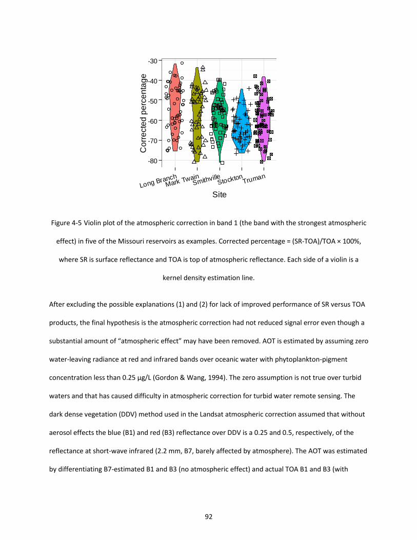
92
Figure 4-5 Violin plot of the atmospheric correction in band 1 (the band with the strongest atmospheric
effect) in five of the Missouri reservoirs as examples. Corrected percentage = (SR-TOA)/TOA × 100%,
where SR is surface reflectance and TOA is top of atmospheric reflectance. Each side of a violin is a
kernel density estimation line.
After excluding the possible explanations (1) and (2) for lack of improved performance of SR versus TOA
products, the final hypothesis is the atmospheric correction had not reduced signal error even though a
substantial amount of “atmospheric effect” may have been removed. AOT is estimated by assuming zero
water-leaving radiance at red and infrared bands over oceanic water with phytoplankton-pigment
concentration less than 0.25 µg/L (Gordon & Wang, 1994). The zero assumption is not true over turbid
waters and that has caused difficulty in atmospheric correction for turbid water remote sensing. The
dark dense vegetation (DDV) method used in the Landsat atmospheric correction assumed that without
aerosol effects the blue (B1) and red (B3) reflectance over DDV is a 0.25 and 0.5, respectively, of the
reflectance at short-wave infrared (2.2 mm, B7, barely affected by atmosphere). The AOT was estimated
by differentiating B7-estimated B1 and B3 (no atmospheric effect) and actual TOA B1 and B3 (with
-80
-70
-60
-50
-40
-30
Long Branch
Mark TwainSmithville
StocktonTruman
Site
Co
rre
cte
d p
erc
en
tag
e
93
aerosol effects). The uncertainty of the method was within 0.006 in both B1 and B3 (Kaufman et al.,
1997). The 0.006 of uncertainty in the Missouri reservoirs indicates errors of 56.9% and 97.6% compared
to the average reflectance of B1 and B3, respectively. The reflectance over water is very weak especially
in red and infrared areas where water absorbs most of the incoming radiation. Thus, accuracy of the
atmospheric correction method may be good enough for land surfaces, but probably not for water
bodies. The atmospheric correction may have removed some errors associated with the atmosphere,
but the same amount of magnitude of other errors might have been introduced into the data by the
correction.
4.4.2 Remote sensing of water optical characteristics
Since the atmospheric correction did not significantly improve the signal related to the optically
sensitive agents, it was not surprising that SR products did not produce models to measure optically
sensitive agents better than TOA products. However, no improvement in the water color models did not
necessarily mean no improvement in image quality, since using band ratios versus just bands are
believed to be able to partly remove atmospheric errors and have been widely used (Gilerson et al.,
2010; Griffin, Frey, Rogan, & Holmes, 2011; e.g., Han, Rundquist, Liu, Fraser, & Schalles, 1994; Menken,
Brezonik, & Bauer, 2006). Nonetheless, if the atmospheric correction had better accuracy, more
improvement should have occurred in the remote sensing of water quality variables.
Our results indicate potential uses of Landsat data in large-scale, long-term studies with or without the
atmospheric correction. The RF model for A440nm was very good (R2 = 0.733, SD = 0.054) in the 39
reservoirs during more than two decades (23 years), despite the water-leaving signal from water being
very weak compared to land surfaces. Relatively worse performance in NVSS and Chl may be due to
larger optical variation related to these properties. The size distribution and composition of suspended
particles could substantially change their optical properties (Karabulut & Ceylan, 2005). Chl is only one
of many pigments in algae and its optical relationship with remote sensing signal may be affected by
94
algal species composition and other optically sensitive agents (sediments and CDOM) (Han et al., 1994).
Chl, NVSS, and A440nm are strongly correlated (Spearman ρ > 0.4, p < 0.001) in the Missouri reservoirs.
It is beyond the scope of this study to investigate the discrimination capability of specific algorithms for
one optically sensitive agent from the others (Lin et al., in preparation). Nevertheless, we are very
optimistic about using Landsat data in large-scale, long-term ecological studies over inland lakes. Based
on our knowledge, this is the first study evaluating the Landsat SR products in inland lake applications.
The results will help make decisions about using the data and selecting whether to use the TOA or SR
products.
4.5 Conclusion
The reflectance of visual bands in the Landsat TM/ETM+ TOA products substantially decreased after the
atmospheric correction, but the predictive relationship between the SR band/band ratios and optically
sensitive agents (i.e., Chl, NVSS, and CDOM) was not enhanced. That indicates the accuracy of
atmospheric correction was not good enough for remote sensing of water color over inland lakes. Using
the SR versus TOA products may slightly but not significantly improve the water color remote sensing,
especially when the machine-learning algorithm RF was used. Validation R2 of the SR model using RF
algorithm for Chl, NVSS, and CDOM was 0.329, 0.508, and 0.733 in the dataset of 23 years and 39
reservoirs in Missouri, suggesting Landsat imagery could be used in long-term and/or large-scale studies
of water color.
Acknowledgement
This work was supported by the Environmental Protection Agency (EPA), U.S.A. under Grant R835203.
We thank Brent Holben for establishing and maintaining the AERONET sites in Missouri.

95
REFERENCES
96
REFERENCES
Abatzoglou, John T. 2013. “Development of Gridded Surface Meteorological Data for Ecological Applications and Modelling.” International Journal of Climatology 33 (1): 121–131. doi:10.1002/joc.3413.
APHA. 1985. Standard Methods of Water and Wastewater Analysis. Washington DC: American Public Health Association (APHA).
Breiman, Leo. 2001. “Random Forests.” Machine Learning 45 (1): 5–32. doi:10.1023/A:1010933404324.
Ellis, Nick, Stephen J. Smith, and C. Roland Pitcher. 2011. “Gradient Forests: Calculating Importance Gradients on Physical Predictors.” Ecology 93 (1): 156–168. doi:10.1890/11-0252.1.
Gilerson, Alexander A., Anatoly A. Gitelson, Jing Zhou, Daniela Gurlin, Wesley Moses, Ioannis Ioannou, and Samir A. Ahmed. 2010. “Algorithms for Remote Estimation of Chlorophyll-a in Coastal and Inland Waters Using Red and near Infrared Bands.” Optics Express 18 (23): 24109–24125. doi:10.1364/OE.18.024109.
Gordon, Howard R., and Menghua Wang. 1994. “Retrieval of Water-Leaving Radiance and Aerosol Optical Thickness over the Oceans with SeaWiFS: A Preliminary Algorithm.” Applied Optics 33 (3): 443. doi:10.1364/AO.33.000443.
Griffin, Claire G., Karen E. Frey, John Rogan, and Robert M. Holmes. 2011. “Spatial and Interannual Variability of Dissolved Organic Matter in the Kolyma River, East Siberia, Observed Using Satellite Imagery.” Journal of Geophysical Research: Biogeosciences 116 (G3): G03018. doi:10.1029/2010JG001634.
Han, L., D. C. Rundquist, L. L. Liu, R. N. Fraser, and J. F. Schalles. 1994. “The Spectral Responses of Algal Chlorophyll in Water with Varying Levels of Suspended Sediment.” International Journal of Remote Sensing 15 (18): 3707–3718. doi:10.1080/01431169408954353.
Hu, Chuanmin, Frank E. Muller-Karger, Serge Andrefouet, and Kendall L. Carder. 2001. “Atmospheric Correction and Cross-Calibration of LANDSAT-7/ETM+ Imagery over Aquatic Environments: A Multiplatform Approach Using SeaWiFS/MODIS.” Remote Sensing of Environment 78 (1): 99–107.
Jones, John R., Daniel V. Obrecht, Bruce D. Perkins, Matthew F. Knowlton, Anthony P. Thorpe, Shohei Watanabe, and Robert R. Bacon. 2008. “Nutrients, Seston, and Transparency of Missouri Reservoirs and Oxbow Lakes: An Analysis of Regional Limnology.” Lake and Reservoir Management 24 (2): 155–180.
Karabulut, Murat, and Nihal Ceylan. 2005. “The Spectral Reflectance Responses of Water with Different Levels of Suspended Sediment in the Presence of Algae.” Turkish J. Eng. Env. Sci 29: 351–360.
97
Kaufman, Y.J., AE. Wald, L.A Remer, Bo-Cai Gao, Rong-Rong Li, and L. Flynn. 1997. “The MODIS 2.1- Mu;m Channel-Correlation with Visible Reflectance for Use in Remote Sensing of Aerosol.” IEEE Transactions on Geoscience and Remote Sensing 35 (5): 1286–1298. doi:10.1109/36.628795.
Koepke, Peter. 1984. “Effective Reflectance of Oceanic Whitecaps.” Applied Optics 23 (11): 1816. doi:10.1364/AO.23.001816.
Masek, Jeffrey G., Eric F. Vermote, Nazmi E. Saleous, Robert Wolfe, Forrest G. Hall, Karl F. Huemmrich, Feng Gao, Jonathan Kutler, and Teng-Kui Lim. 2006. “A Landsat Surface Reflectance Dataset for North America, 1990-2000.” Geoscience and Remote Sensing Letters, IEEE 3 (1): 68–72.
Menken, Kevin D., Patrick L. Brezonik, and Marvin E. Bauer. 2006. “Influence of Chlorophyll and Colored Dissolved Organic Matter (CDOM) on Lake Reflectance Spectra: Implications for Measuring Lake Properties by Remote Sensing.” Lake and Reservoir Management 22 (3): 179–190. doi:10.1080/07438140609353895.
Monahan, Edward C., and IognáidÓ Muircheartaigh. 1980. “Optimal Power-Law Description of Oceanic Whitecap Coverage Dependence on Wind Speed.” Journal of Physical Oceanography 10 (12): 2094–2099. doi:10.1175/1520-0485(1980)010<2094:OPLDOO>2.0.CO;2.
Royston, Patrick. 1995. “Remark AS R94: A Remark on Algorithm AS 181: The W-Test for Normality.” Journal of the Royal Statistical Society. Series C (Applied Statistics) 44 (4): 547–551. doi:10.2307/2986146.
Wang, Menghua, and Wei Shi. 2007. “The NIR-SWIR Combined Atmospheric Correction Approach for MODIS Ocean Color Data Processing.” Optics Express 15 (24): 15722–15733. doi:10.1364/OE.15.015722.
Witte, W. G., C. H. Whitlock, R. C. Harriss, J. W. Usry, L. R. Poole, W. M. Houghton, W. D. Morris, and E. A. Gurganus. 1982. “Influence of Dissolved Organic Materials on Turbid Water Optical Properties and Remote-Sensing Reflectance.” Journal of Geophysical Research: Oceans 87 (C1): 441–446. doi:10.1029/JC087iC01p00441.
98
5 ALGAL BIOMASS RESPONSES TO CLIMATE CHANGE IN MISSOURI RESERVOIRS
Abstract
More intense precipitation projected with climate change could bring more nutrients from watersheds
to lakes, which with projected warming, create conditions conducive for algal blooms. This hypothesis
has rarely been tested with long-term (decadal) lake observation data mostly due to lack of whole-lake
long-term algal biomass data. In this study, 28 years (1984-2011) of observations of algal biomass in four
reservoirs in Missouri (USA) were derived from remote sensing imagery (Landsat TM), providing an
opportunity to link the time series of climate change with the time series of algal biomass responses.
The result shows that neither temperature nor precipitation was the only factor that predicted lake
chlorophyll concentrations. With the increases in lake surface water temperature and precipitation
intensity (mm/d), algal biomass more likely responded to temperature than precipitation. The rising
temperature affected mean annual chlorophyll more than summer chlorophyll, indicating that projected
warming might result in the expansion of the algal growth season rather than increasing the summer
peak concentration. Summer algal biomass might increase with increasing spring precipitation in the
study reservoirs.
Keywords: algal bloom, climate change, global warming, precipitation, lake surface temperature, remote
sensing
Highlights
• The trend of lake chlorophyll in four reservoirs did not closely track the trend of temperature or
precipitation during 28 years.
• The algal growth season may expand with global warming.
• Climate change may result in higher summer algal biomass due to higher spring precipitation.
99
• Daily precipitation and daily temperature together explain up to 50.6% of the variance in daily
chlorophyll across 13 sites.
5.1 Introduction
5.1.1 Climate change
Climate change models have projected that surface temperature will rise during the 21st century, and it
is “very likely” that extreme precipitation will be more frequent and intense in many regions (IPCC
2014). More specifically, this report indicates that over North America, mean annual temperatures are
projected to rise between 2 °C and 4 °C (depending on scenario) by the end of the 21st century over
most land areas. This warming is predicted to occur in all seasons, but especially in winter over high
latitudes. The report also indicates that mean annual precipitation in the late century will “very likely”
increase in most areas of the United States and Canada. Increasing precipitation in the United States and
Canada is predicted to occur in winter, with an increasing fraction falling as rain rather than snow, due
to increasing winter temperature. Extremely hot or dry summer seasons are predicted to occur over
much of North America.
5.1.2 Harmful algal blooms
Harmful algae, particularly Cyanobacteria, may grow faster at higher temperatures than other algal
groups (such as green algae and diatoms) (Paerl and Paul 2012). Deeper and longer stratification
followed by nutrient depletion in the epilimnion favors the buoyant and nitrogen-fixing Cyanobacteria
(Dokulil and Teubner 2000). On top of that, more nutrient loading due to more intense and extreme
precipitation may create more favorable conditions for algal blooms (Robson and Hamilton 2003).
Because of these drivers, Paerl and Huisman (2008) predicted more harmful algal blooms in the future
with warmer temperature and more variable precipitation. The hypothesis was later tested by other
researchers with coupled mechanistic models (HSPF, UFILS4, and AQUATOX) in Onondaga Lake (New
York State, USA), and the results showed that biomass of both green algae and Cyanobacteria increased
100
with climate change, and Cyanobacteria did not necessarily outcompete green algae to form harmful
algal blooms (Taner, Carleton, and Wellman 2011). This appears to contradict the prediction of Paerl and
Huisman (2008). Additionally, observational data in the New River Estuary and Neuse River Estuary
(North Carolina, USA) showed that algal biomass could not accumulate after extreme events because of
flushing and light limitation (Paerl et al. 2014). Thus, algal responses to climate change may vary greatly
among individual lakes depending on location, climate, basin landscape, lake morphology, internal
nutrient sources, and food web interactions (Blenckner 2005).
5.1.3 Complex system
Complex processes between climate and algal production may generate different outcomes. Algal
blooms occur with specific combinations of factors, not just one factor (e.g., temperature) (Dokulil and
Teubner 2000). For example: (1) Higher winter temperatures may cause more melting of snow and
subsequent water flow, potentially producing more winter nutrient loading. On the other hand, at
higher temperature, higher rates of denitrification and nutrient assimilation in soil may reduce winter
nitrate concentrations in lakes (George, Jarvinen, and Arvola 2004; Marshall and Randhir 2008). (2)
Extreme precipitation events in summer potentially increase peak flows and nutrient loading, but the
total flow may decrease if there is also higher evapotranspiration, offsetting the additional nutrients in
event flows (Taner, Carleton, and Wellman 2011; Praskievicz and Chang 2011). (3) Impacts of additional
nutrient inputs to lakes may happen quickly, but it could take more than two to eight years to see long-
term responses (Slavik et al. 2004; Schindler 2012). The in-lake community responses are much more
complicated than lake physical or chemical responses. (4) A larger spring algal bloom may occur after a
warmer winter, but the bloom may also be offset by stronger grazing pressure (Pettersson 1990; Straile
2000). (5) Warmer temperatures may change the population of keystone fish species, resulting in a
cascade effect in the food web, ultimately affecting phytoplankton (McDonald, Hershey, and Miller
1996). (6) Different aquatic communities and seasonal successions may evolve depending on matches
101
between the timing of weather events and species-specific life-history events, such as timing of
spawning (Adrian, Wilhelm, and Gerten 2006). (7) Lake morphology can also mediate the climate
impacts. The effect of winter warming on phytoplankton succession persisted for less time in shallow
lakes, while lasting longer (even until the next winter) in deeper lakes (Adrian et al. 1999; Gerten and
Adrian 2001).
In summary, multiple processes, factors, and interactions regulate lake algal responses to climate
change, some of which may cause algal biomass to increase in response to climate change while others
may not. The prediction of more algal biomass or harmful algal blooms in the future is popular in the
scientific climate change community, but with some assumptions that may or may not be true.
5.1.4 Objective and research questions
Long-term (e.g., decadal) observations of algal biomass in lakes are rare, and future projections based
on coupled models are usually incompletely validated. In this study, we generated long-term (1984-
2011, 28 years), whole-lake algal biomass estimates for four reservoirs in Missouri (USA) using remote
sensing (Landsat TM) observations. The new dataset allows linkage of long-term climate change with
algal biomass, testing the hypothesis that higher algal biomass is associated with higher temperatures as
well as more intense precipitation. First, we studied patterns of covariation among lake algal biomass,
temperature, precipitation, and discharge, asking:
1) Does algal biomass covary with seasonal patterns of temperature, precipitation, or discharge?
2) Does algal biomass covary with long-term (28-year) trend with precipitation or temperature?
Then, we further quantified the relationships between algal biomass and temperature as well as
precipitation, asking:
3) How much algal biomass variance can be explained by temperature and precipitation?
All tests were run on the upstream and downstream zones of four reservoirs, asking:
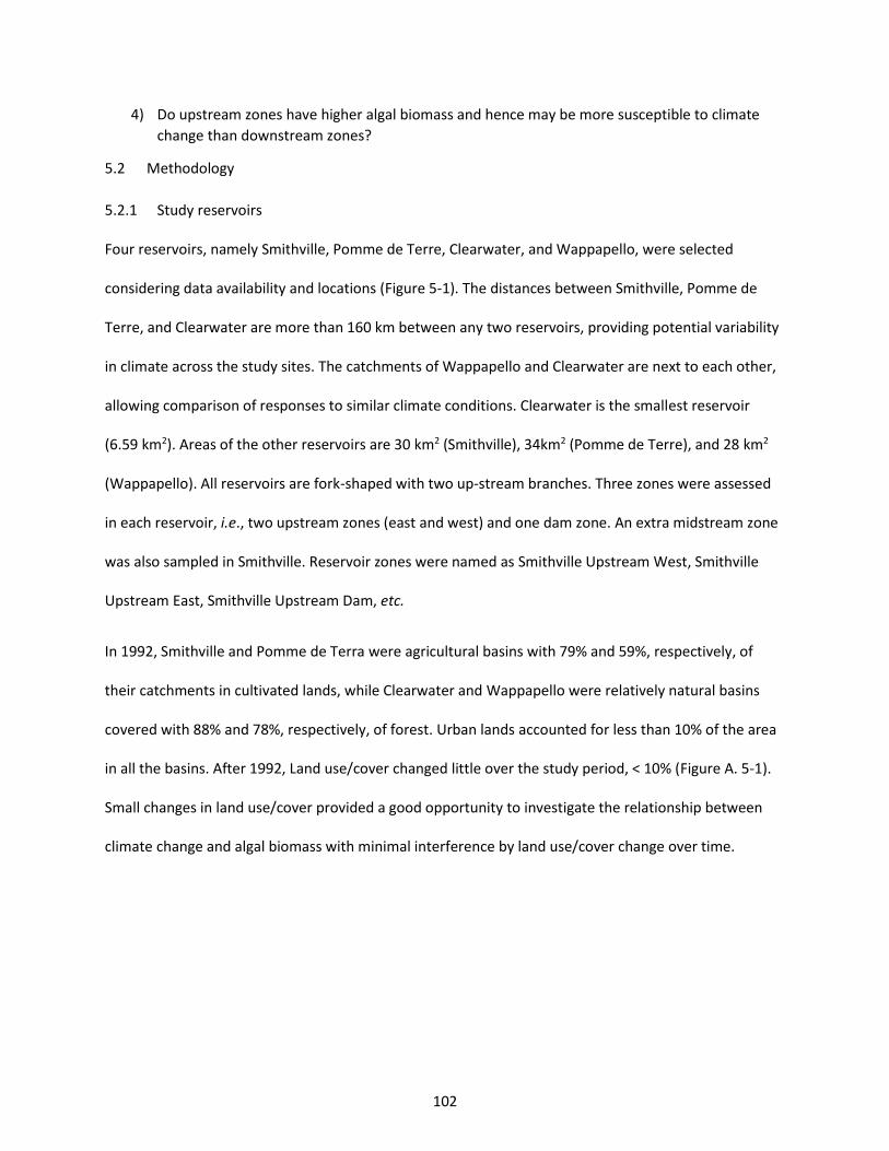
102
4) Do upstream zones have higher algal biomass and hence may be more susceptible to climate
change than downstream zones?
5.2 Methodology
5.2.1 Study reservoirs
Four reservoirs, namely Smithville, Pomme de Terre, Clearwater, and Wappapello, were selected
considering data availability and locations (Figure 5-1). The distances between Smithville, Pomme de
Terre, and Clearwater are more than 160 km between any two reservoirs, providing potential variability
in climate across the study sites. The catchments of Wappapello and Clearwater are next to each other,
allowing comparison of responses to similar climate conditions. Clearwater is the smallest reservoir
(6.59 km2). Areas of the other reservoirs are 30 km2 (Smithville), 34km2 (Pomme de Terre), and 28 km2
(Wappapello). All reservoirs are fork-shaped with two up-stream branches. Three zones were assessed
in each reservoir, i.e., two upstream zones (east and west) and one dam zone. An extra midstream zone
was also sampled in Smithville. Reservoir zones were named as Smithville Upstream West, Smithville
Upstream East, Smithville Upstream Dam, etc.
In 1992, Smithville and Pomme de Terra were agricultural basins with 79% and 59%, respectively, of
their catchments in cultivated lands, while Clearwater and Wappapello were relatively natural basins
covered with 88% and 78%, respectively, of forest. Urban lands accounted for less than 10% of the area
in all the basins. After 1992, Land use/cover changed little over the study period, < 10% (Figure A. 5-1).
Small changes in land use/cover provided a good opportunity to investigate the relationship between
climate change and algal biomass with minimal interference by land use/cover change over time.
103
Figure 5-1 Map of study reservoirs and associated catchment basins. Locations of basins are indicated by
middle maps. Polygons on reservoirs indicate study zones. Names of reservoirs are Smithville, Pomme
de Terre, Wappapello, and Clearwater (from West to East).
5.2.2 Data
Lake surface temperatures (1984-2011) were estimated using the thermal band (Band 6) of Landsat 5
Thematic Mapper (TM) (Google Earth Image ID: LANDSAT/LT5_L1T_TOA). Algal biomass (1984-2011)
was estimated as chlorophyll-a concentration (referred to as chlorophyll in the following text), which is a
pigment common to all algal species that is routinely used to measure algal biomass. Chlorophyll was
derived from Landsat 5 TM surface reflectance products (Google Earth Image ID: LEDAPS/LT5_L1T_SR)
using a random forest model. The chlorophyll random forest model was trained by ground-measured
chlorophyll (over 28 years and 39 reservoirs in Missouri). All bands and band ratios, except for the
thermal band (6), were used as model predictors. In the training dataset, ground-measured chlorophyll
was available for two to four dates during summers between 1989 and 2012. For each occasion, only
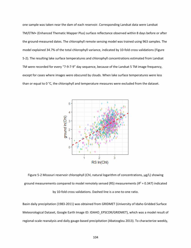
104
one sample was taken near the dam of each reservoir. Corresponding Landsat data were Landsat
TM/ETM+ (Enhanced Thematic Mapper Plus) surface reflectance observed within 8 days before or after
the ground-measured dates. The chlorophyll remote sensing model was trained using 963 samples. The
model explained 34.7% of the total chlorophyll variance, indicated by 10-fold cross validations (Figure
5-2). The resulting lake surface temperatures and chlorophyll concentrations estimated from Landsat
TM were recorded for every “7-9-7-9” day sequence, because of the Landsat 5 TM image frequency,
except for cases where images were obscured by clouds. When lake surface temperatures were less
than or equal to 0 °C, the chlorophyll and temperature measures were excluded from the dataset.
Figure 5-2 Missouri reservoir chlorophyll (Chl, natural logarithm of concentrations, µg/L) showing
ground measurements compared to model remotely sensed (RS) measurements (R2 = 0.347) indicated
by 10-fold cross validations. Dashed line is a one-to-one ratio.
Basin daily precipitation (1983-2011) was obtained from GRIDMET (University of Idaho Gridded Surface
Meteorological Dataset, Google Earth Image ID: IDAHO_EPSCOR/GRIDMET), which was a model result of
regional-scale reanalysis and daily gauge-based precipitation (Abatzoglou 2013). To characterize weekly,
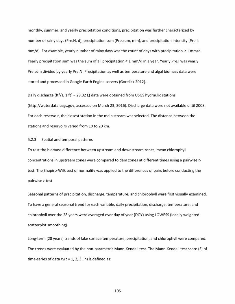
105
monthly, summer, and yearly precipitation conditions, precipitation was further characterized by
number of rainy days (Pre.N, d), precipitation sum (Pre.sum, mm), and precipitation intensity (Pre.I,
mm/d). For example, yearly number of rainy days was the count of days with precipitation ≥ 1 mm/d.
Yearly precipitation sum was the sum of all precipitation ≥ 1 mm/d in a year. Yearly Pre.I was yearly
Pre.sum divided by yearly Pre.N. Precipitation as well as temperature and algal biomass data were
stored and processed in Google Earth Engine servers (Gorelick 2012).
Daily discharge (ft3/s, 1 ft3 = 28.32 L) data were obtained from USGS hydraulic stations
(http://waterdata.usgs.gov, accessed on March 23, 2016). Discharge data were not available until 2008.
For each reservoir, the closest station in the main stream was selected. The distance between the
stations and reservoirs varied from 10 to 20 km.
5.2.3 Spatial and temporal patterns
To test the biomass difference between upstream and downstream zones, mean chlorophyll
concentrations in upstream zones were compared to dam zones at different times using a pairwise t-
test. The Shapiro-Wilk test of normality was applied to the differences of pairs before conducting the
pairwise t-test.
Seasonal patterns of precipitation, discharge, temperature, and chlorophyll were first visually examined.
To have a general seasonal trend for each variable, daily precipitation, discharge, temperature, and
chlorophyll over the 28 years were averaged over day of year (DOY) using LOWESS (locally weighted
scatterplot smoothing).
Long-term (28 years) trends of lake surface temperature, precipitation, and chlorophyll were compared.
The trends were evaluated by the non-parametric Mann-Kendall test. The Mann-Kendall test score (S) of
time-series of data xt (t = 1, 2, 3…n) is defined as:
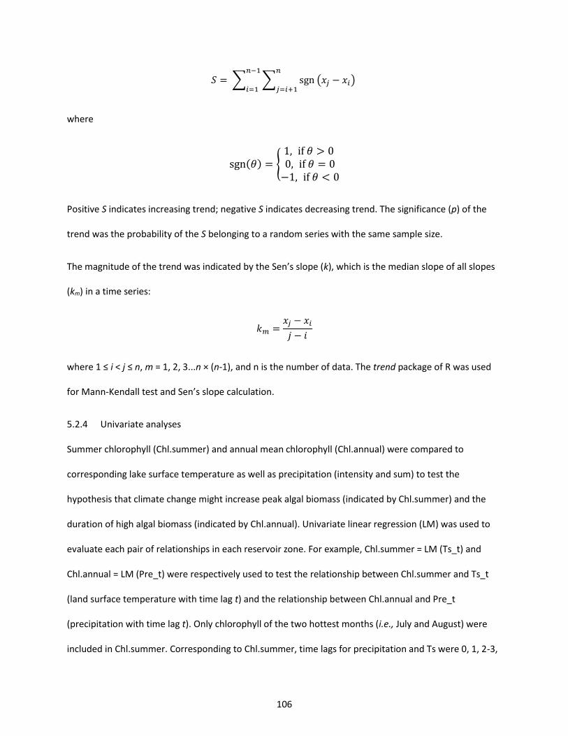
106
𝑆 = ∑ ∑ sgn (𝑥𝑗 − 𝑥𝑖)𝑛
𝑗=𝑖+1
𝑛−1
𝑖=1
where
sgn(𝜃) = {1, if 𝜃 > 0 0, if 𝜃 = 0
−1, if 𝜃 < 0
Positive S indicates increasing trend; negative S indicates decreasing trend. The significance (p) of the
trend was the probability of the S belonging to a random series with the same sample size.
The magnitude of the trend was indicated by the Sen’s slope (k), which is the median slope of all slopes
(km) in a time series:
𝑘𝑚 =𝑥𝑗 − 𝑥𝑖
𝑗 − 𝑖
where 1 ≤ i < j ≤ n, m = 1, 2, 3...n × (n-1), and n is the number of data. The trend package of R was used
for Mann-Kendall test and Sen’s slope calculation.
5.2.4 Univariate analyses
Summer chlorophyll (Chl.summer) and annual mean chlorophyll (Chl.annual) were compared to
corresponding lake surface temperature as well as precipitation (intensity and sum) to test the
hypothesis that climate change might increase peak algal biomass (indicated by Chl.summer) and the
duration of high algal biomass (indicated by Chl.annual). Univariate linear regression (LM) was used to
evaluate each pair of relationships in each reservoir zone. For example, Chl.summer = LM (Ts_t) and
Chl.annual = LM (Pre_t) were respectively used to test the relationship between Chl.summer and Ts_t
(land surface temperature with time lag t) and the relationship between Chl.annual and Pre_t
(precipitation with time lag t). Only chlorophyll of the two hottest months (i.e., July and August) were
included in Chl.summer. Corresponding to Chl.summer, time lags for precipitation and Ts were 0, 1, 2-3,
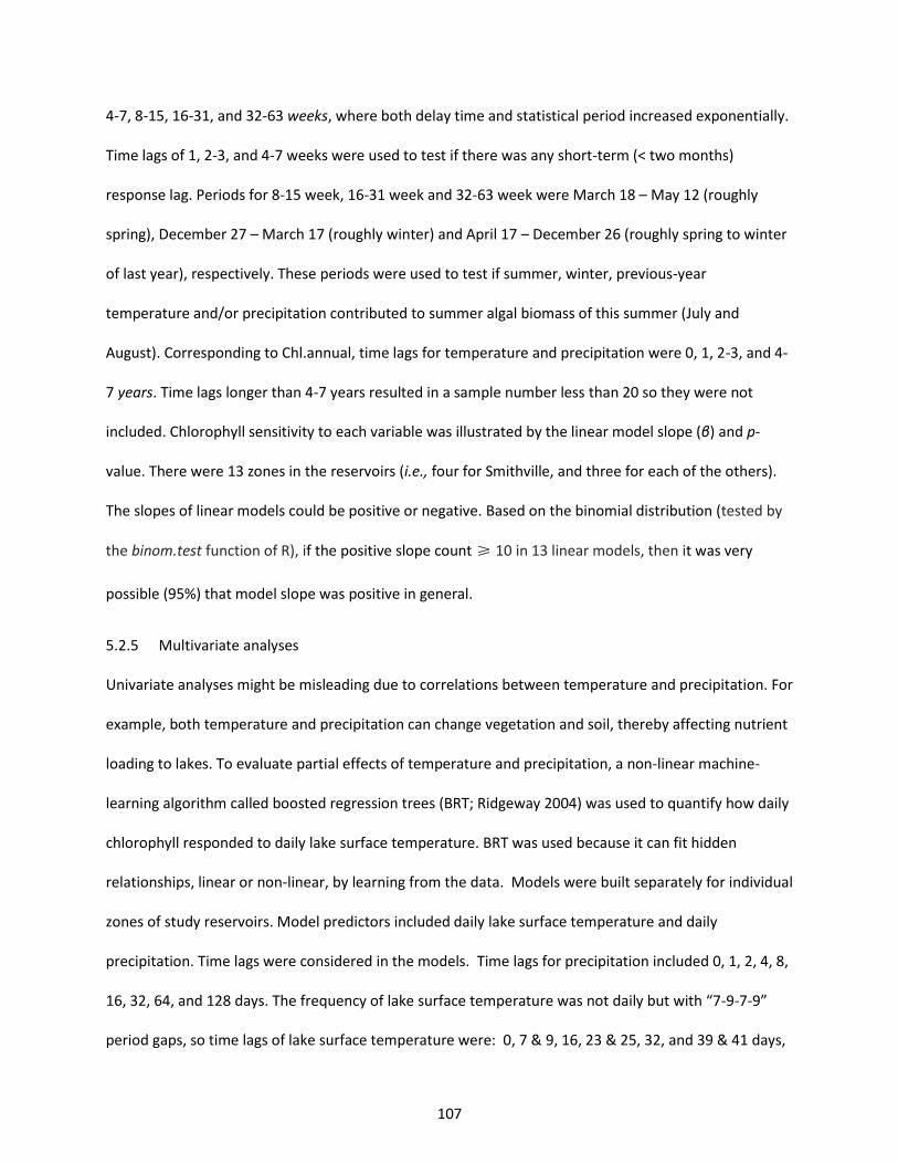
107
4-7, 8-15, 16-31, and 32-63 weeks, where both delay time and statistical period increased exponentially.
Time lags of 1, 2-3, and 4-7 weeks were used to test if there was any short-term (< two months)
response lag. Periods for 8-15 week, 16-31 week and 32-63 week were March 18 – May 12 (roughly
spring), December 27 – March 17 (roughly winter) and April 17 – December 26 (roughly spring to winter
of last year), respectively. These periods were used to test if summer, winter, previous-year
temperature and/or precipitation contributed to summer algal biomass of this summer (July and
August). Corresponding to Chl.annual, time lags for temperature and precipitation were 0, 1, 2-3, and 4-
7 years. Time lags longer than 4-7 years resulted in a sample number less than 20 so they were not
included. Chlorophyll sensitivity to each variable was illustrated by the linear model slope (β) and p-
value. There were 13 zones in the reservoirs (i.e., four for Smithville, and three for each of the others).
The slopes of linear models could be positive or negative. Based on the binomial distribution (tested by
the binom.test function of R), if the positive slope count ≥ 10 in 13 linear models, then it was very
possible (95%) that model slope was positive in general.
5.2.5 Multivariate analyses
Univariate analyses might be misleading due to correlations between temperature and precipitation. For
example, both temperature and precipitation can change vegetation and soil, thereby affecting nutrient
loading to lakes. To evaluate partial effects of temperature and precipitation, a non-linear machine-
learning algorithm called boosted regression trees (BRT; Ridgeway 2004) was used to quantify how daily
chlorophyll responded to daily lake surface temperature. BRT was used because it can fit hidden
relationships, linear or non-linear, by learning from the data. Models were built separately for individual
zones of study reservoirs. Model predictors included daily lake surface temperature and daily
precipitation. Time lags were considered in the models. Time lags for precipitation included 0, 1, 2, 4, 8,
16, 32, 64, and 128 days. The frequency of lake surface temperature was not daily but with “7-9-7-9”
period gaps, so time lags of lake surface temperature were: 0, 7 & 9, 16, 23 & 25, 32, and 39 & 41 days,
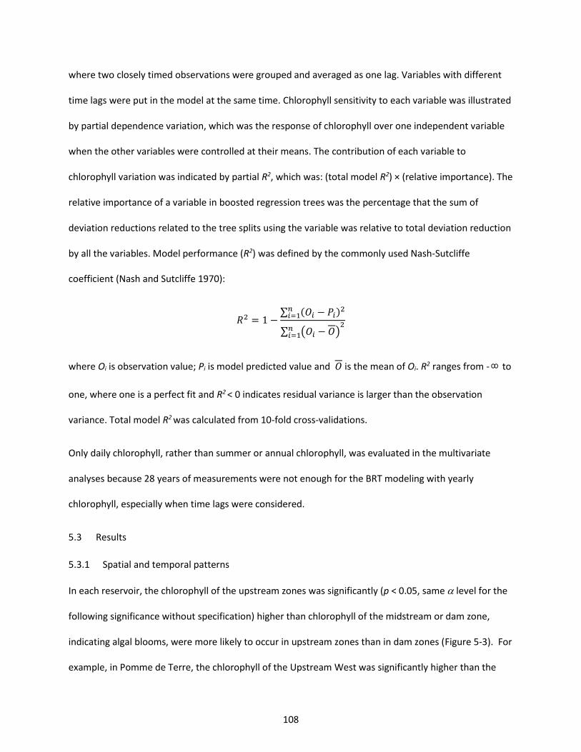
108
where two closely timed observations were grouped and averaged as one lag. Variables with different
time lags were put in the model at the same time. Chlorophyll sensitivity to each variable was illustrated
by partial dependence variation, which was the response of chlorophyll over one independent variable
when the other variables were controlled at their means. The contribution of each variable to
chlorophyll variation was indicated by partial R2, which was: (total model R2) × (relative importance). The
relative importance of a variable in boosted regression trees was the percentage that the sum of
deviation reductions related to the tree splits using the variable was relative to total deviation reduction
by all the variables. Model performance (R2) was defined by the commonly used Nash-Sutcliffe
coefficient (Nash and Sutcliffe 1970):
𝑅2 = 1 −∑ (𝑂𝑖 − 𝑃𝑖)2𝑛
𝑖=1
∑ (𝑂𝑖 − 𝑂)2𝑛
𝑖=1
where Oi is observation value; Pi is model predicted value and 𝑂 is the mean of Oi. R2 ranges from -∞ to
one, where one is a perfect fit and R2 < 0 indicates residual variance is larger than the observation
variance. Total model R2 was calculated from 10-fold cross-validations.
Only daily chlorophyll, rather than summer or annual chlorophyll, was evaluated in the multivariate
analyses because 28 years of measurements were not enough for the BRT modeling with yearly
chlorophyll, especially when time lags were considered.
5.3 Results
5.3.1 Spatial and temporal patterns
In each reservoir, the chlorophyll of the upstream zones was significantly (p < 0.05, same level for the
following significance without specification) higher than chlorophyll of the midstream or dam zone,
indicating algal blooms, were more likely to occur in upstream zones than in dam zones (Figure 5-3). For
example, in Pomme de Terre, the chlorophyll of the Upstream West was significantly higher than the
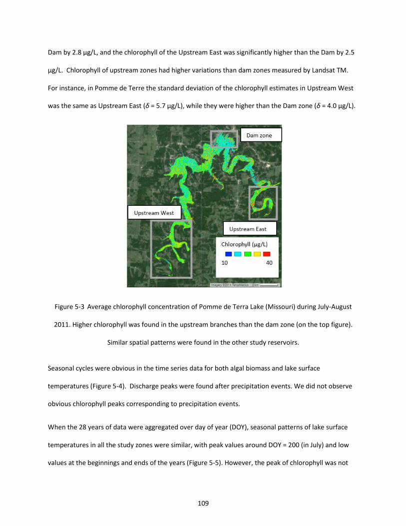
109
Dam by 2.8 µg/L, and the chlorophyll of the Upstream East was significantly higher than the Dam by 2.5
µg/L. Chlorophyll of upstream zones had higher variations than dam zones measured by Landsat TM.
For instance, in Pomme de Terre the standard deviation of the chlorophyll estimates in Upstream West
was the same as Upstream East (δ = 5.7 µg/L), while they were higher than the Dam zone (δ = 4.0 µg/L).
Figure 5-3 Average chlorophyll concentration of Pomme de Terra Lake (Missouri) during July-August
2011. Higher chlorophyll was found in the upstream branches than the dam zone (on the top figure).
Similar spatial patterns were found in the other study reservoirs.
Seasonal cycles were obvious in the time series data for both algal biomass and lake surface
temperatures (Figure 5-4). Discharge peaks were found after precipitation events. We did not observe
obvious chlorophyll peaks corresponding to precipitation events.
When the 28 years of data were aggregated over day of year (DOY), seasonal patterns of lake surface
temperatures in all the study zones were similar, with peak values around DOY = 200 (in July) and low
values at the beginnings and ends of the years (Figure 5-5). However, the peak of chlorophyll was not
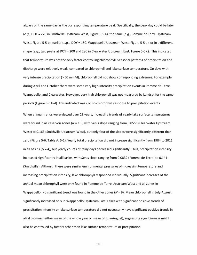
110
always on the same day as the corresponding temperature peak. Specifically, the peak day could be later
(e.g., DOY = 220 in Smithville Upstream West, Figure 5-5 a), the same (e.g., Pomme de Terre Upstream
West, Figure 5-5 b), earlier (e.g., DOY = 180, Wappapello Upstream West, Figure 5-5 d), or in a different
shape (e.g., two peaks at DOY = 200 and 280 in Clearwater Upstream East, Figure 5-5 c). This indicated
that temperature was not the only factor controlling chlorophyll. Seasonal patterns of precipitation and
discharge were relatively weak, compared to chlorophyll and lake surface temperature. On days with
very intense precipitation (> 50 mm/d), chlorophyll did not show corresponding extremes. For example,
during April and October there were some very high-intensity precipitation events in Pomme de Terre,
Wappapello, and Clearwater. However, very high chlorophyll was not measured by Landsat for the same
periods (Figure 5-5 b-d). This indicated weak or no chlorophyll response to precipitation events.
When annual trends were viewed over 28 years, increasing trends of yearly lake surface temperatures
were found in all reservoir zones (N = 13), with Sen’s slope ranging from 0.0556 (Clearwater Upstream
West) to 0.163 (Smithville Upstream West), but only four of the slopes were significantly different than
zero (Figure 5-6, Table A. 5-1). Yearly total precipitation did not increase significantly from 1984 to 2011
in all basins (N = 4), but yearly counts of rainy days decreased significantly. Thus, precipitation intensity
increased significantly in all basins, with Sen’s slope ranging from 0.0832 (Pomme de Terre) to 0.141
(Smithville). Although there were similar environmental pressures of increasing temperature and
increasing precipitation intensity, lake chlorophyll responded individually. Significant increases of the
annual mean chlorophyll were only found in Pomme de Terre Upstream West and all zones in
Wappapello. No significant trend was found in the other zones (N = 9). Mean chlorophyll in July-August
significantly increased only in Wappapello Upstream East. Lakes with significant positive trends of
precipitation intensity or lake surface temperature did not necessarily have significant positive trends in
algal biomass (either mean of the whole year or mean of July-August), suggesting algal biomass might
also be controlled by factors other than lake surface temperature or precipitation.
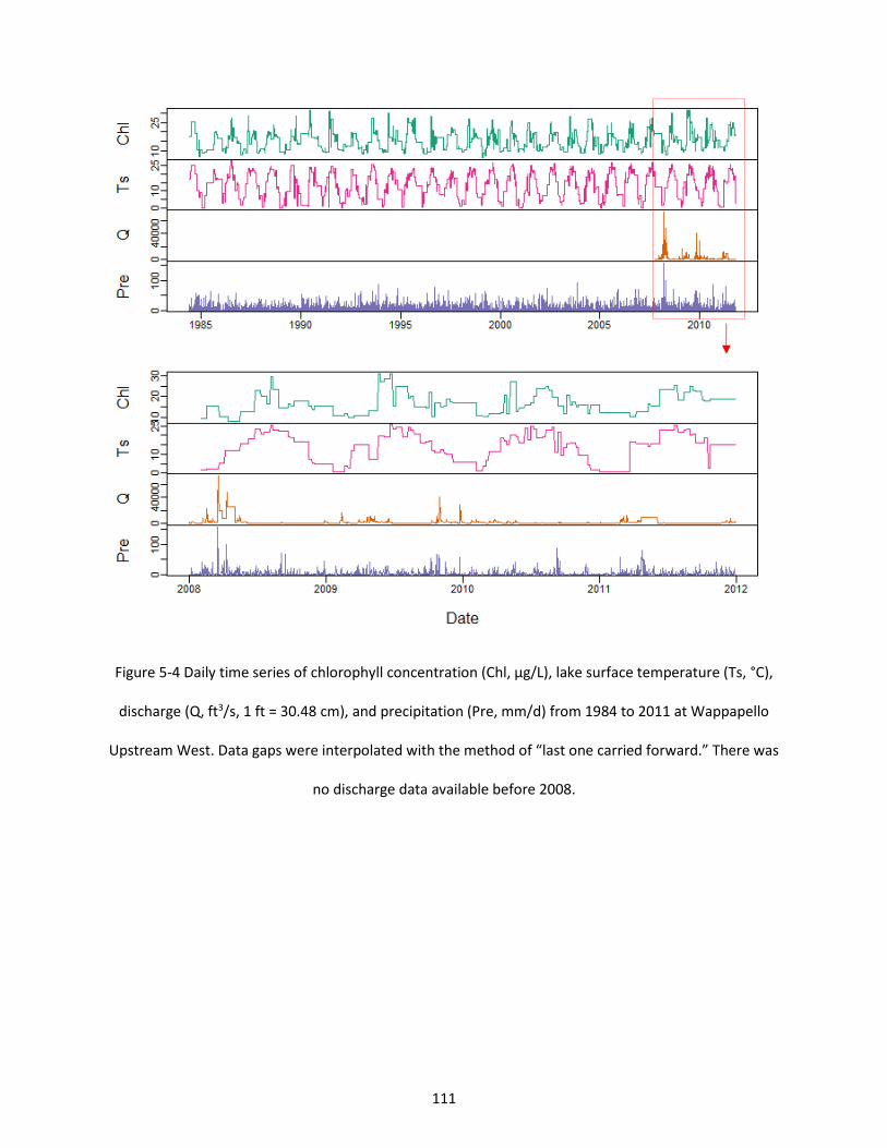
111
Figure 5-4 Daily time series of chlorophyll concentration (Chl, µg/L), lake surface temperature (Ts, °C),
discharge (Q, ft3/s, 1 ft = 30.48 cm), and precipitation (Pre, mm/d) from 1984 to 2011 at Wappapello
Upstream West. Data gaps were interpolated with the method of “last one carried forward.” There was
no discharge data available before 2008.
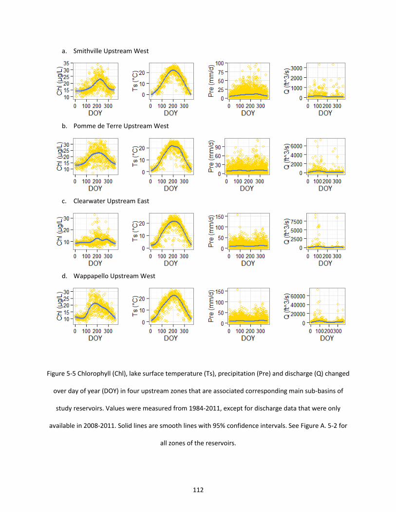
112
a. Smithville Upstream West
b. Pomme de Terre Upstream West
c. Clearwater Upstream East
d. Wappapello Upstream West
Figure 5-5 Chlorophyll (Chl), lake surface temperature (Ts), precipitation (Pre) and discharge (Q) changed
over day of year (DOY) in four upstream zones that are associated corresponding main sub-basins of
study reservoirs. Values were measured from 1984-2011, except for discharge data that were only
available in 2008-2011. Solid lines are smooth lines with 95% confidence intervals. See Figure A. 5-2 for
all zones of the reservoirs.
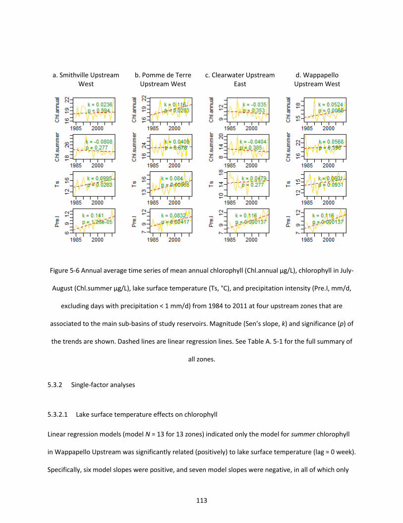
113
a. Smithville Upstream West
b. Pomme de Terre Upstream West
c. Clearwater Upstream East
d. Wappapello Upstream West
Figure 5-6 Annual average time series of mean annual chlorophyll (Chl.annual µg/L), chlorophyll in July-
August (Chl.summer µg/L), lake surface temperature (Ts, °C), and precipitation intensity (Pre.I, mm/d,
excluding days with precipitation < 1 mm/d) from 1984 to 2011 at four upstream zones that are
associated to the main sub-basins of study reservoirs. Magnitude (Sen’s slope, k) and significance (p) of
the trends are shown. Dashed lines are linear regression lines. See Table A. 5-1 for the full summary of
all zones.
5.3.2 Single-factor analyses
5.3.2.1 Lake surface temperature effects on chlorophyll
Linear regression models (model N = 13 for 13 zones) indicated only the model for summer chlorophyll
in Wappapello Upstream was significantly related (positively) to lake surface temperature (lag = 0 week).
Specifically, six model slopes were positive, and seven model slopes were negative, in all of which only
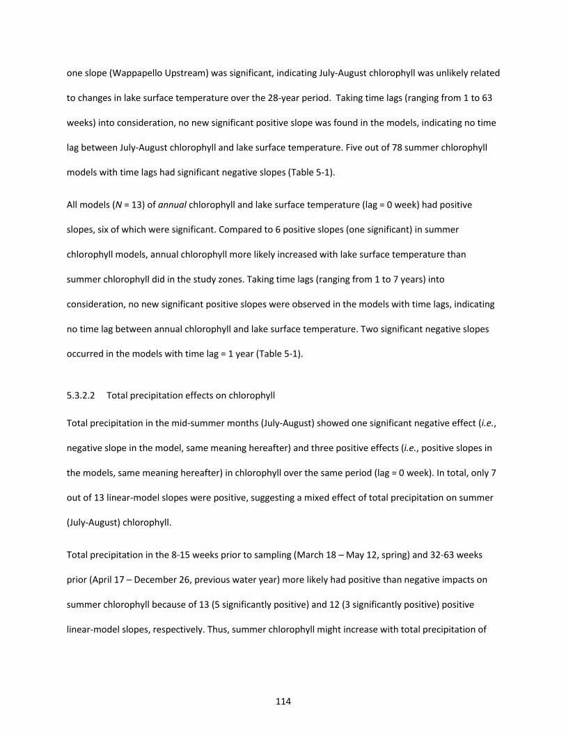
114
one slope (Wappapello Upstream) was significant, indicating July-August chlorophyll was unlikely related
to changes in lake surface temperature over the 28-year period. Taking time lags (ranging from 1 to 63
weeks) into consideration, no new significant positive slope was found in the models, indicating no time
lag between July-August chlorophyll and lake surface temperature. Five out of 78 summer chlorophyll
models with time lags had significant negative slopes (Table 5-1).
All models (N = 13) of annual chlorophyll and lake surface temperature (lag = 0 week) had positive
slopes, six of which were significant. Compared to 6 positive slopes (one significant) in summer
chlorophyll models, annual chlorophyll more likely increased with lake surface temperature than
summer chlorophyll did in the study zones. Taking time lags (ranging from 1 to 7 years) into
consideration, no new significant positive slopes were observed in the models with time lags, indicating
no time lag between annual chlorophyll and lake surface temperature. Two significant negative slopes
occurred in the models with time lag = 1 year (Table 5-1).
5.3.2.2 Total precipitation effects on chlorophyll
Total precipitation in the mid-summer months (July-August) showed one significant negative effect (i.e.,
negative slope in the model, same meaning hereafter) and three positive effects (i.e., positive slopes in
the models, same meaning hereafter) in chlorophyll over the same period (lag = 0 week). In total, only 7
out of 13 linear-model slopes were positive, suggesting a mixed effect of total precipitation on summer
(July-August) chlorophyll.
Total precipitation in the 8-15 weeks prior to sampling (March 18 – May 12, spring) and 32-63 weeks
prior (April 17 – December 26, previous water year) more likely had positive than negative impacts on
summer chlorophyll because of 13 (5 significantly positive) and 12 (3 significantly positive) positive
linear-model slopes, respectively. Thus, summer chlorophyll might increase with total precipitation of
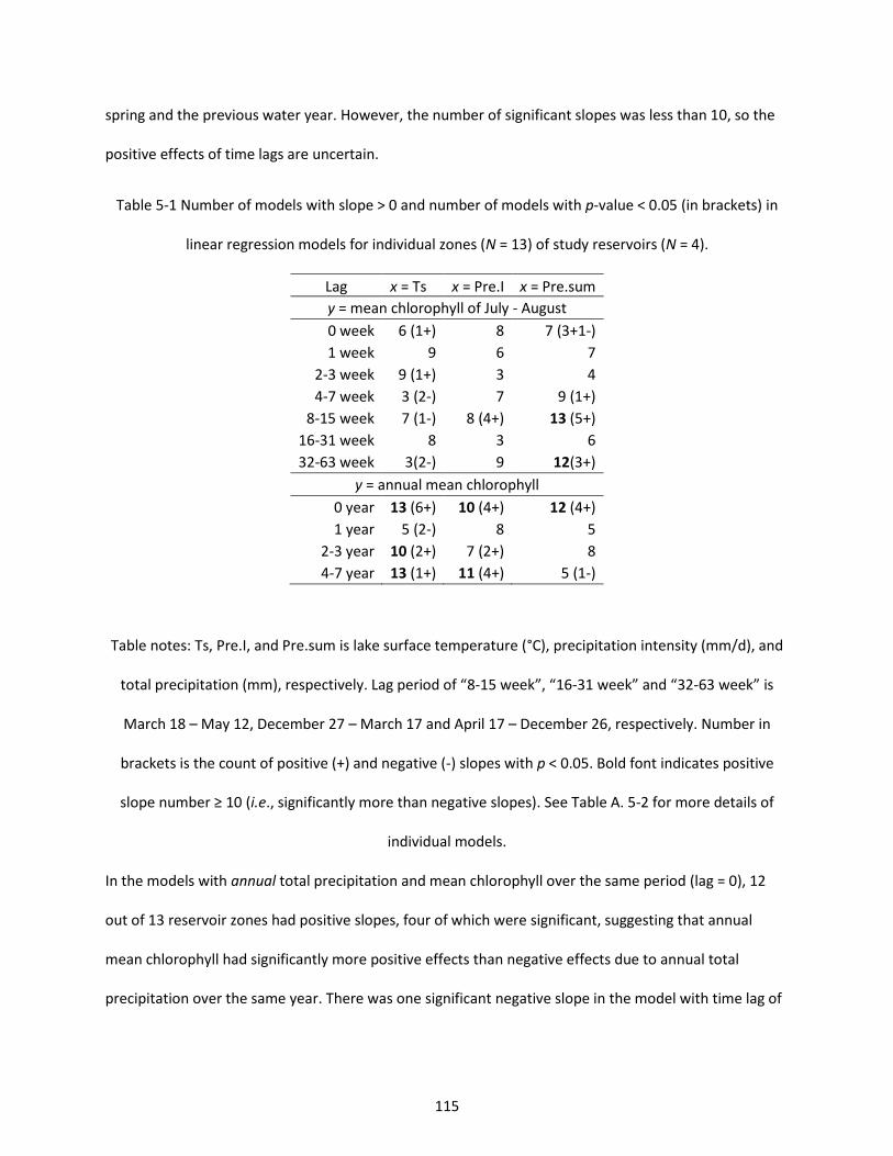
115
spring and the previous water year. However, the number of significant slopes was less than 10, so the
positive effects of time lags are uncertain.
Table 5-1 Number of models with slope > 0 and number of models with p-value < 0.05 (in brackets) in
linear regression models for individual zones (N = 13) of study reservoirs (N = 4).
Lag x = Ts x = Pre.I x = Pre.sum
y = mean chlorophyll of July - August
0 week 6 (1+) 8 7 (3+1-)
1 week 9 6 7
2-3 week 9 (1+) 3 4
4-7 week 3 (2-) 7 9 (1+)
8-15 week 7 (1-) 8 (4+) 13 (5+)
16-31 week 8 3 6
32-63 week 3(2-) 9 12(3+)
y = annual mean chlorophyll
0 year 13 (6+) 10 (4+) 12 (4+)
1 year 5 (2-) 8 5
2-3 year 10 (2+) 7 (2+) 8
4-7 year 13 (1+) 11 (4+) 5 (1-)
Table notes: Ts, Pre.I, and Pre.sum is lake surface temperature (°C), precipitation intensity (mm/d), and
total precipitation (mm), respectively. Lag period of “8-15 week”, “16-31 week” and “32-63 week” is
March 18 – May 12, December 27 – March 17 and April 17 – December 26, respectively. Number in
brackets is the count of positive (+) and negative (-) slopes with p < 0.05. Bold font indicates positive
slope number ≥ 10 (i.e., significantly more than negative slopes). See Table A. 5-2 for more details of
individual models.
In the models with annual total precipitation and mean chlorophyll over the same period (lag = 0), 12
out of 13 reservoir zones had positive slopes, four of which were significant, suggesting that annual
mean chlorophyll had significantly more positive effects than negative effects due to annual total
precipitation over the same year. There was one significant negative slope in the model with time lag of
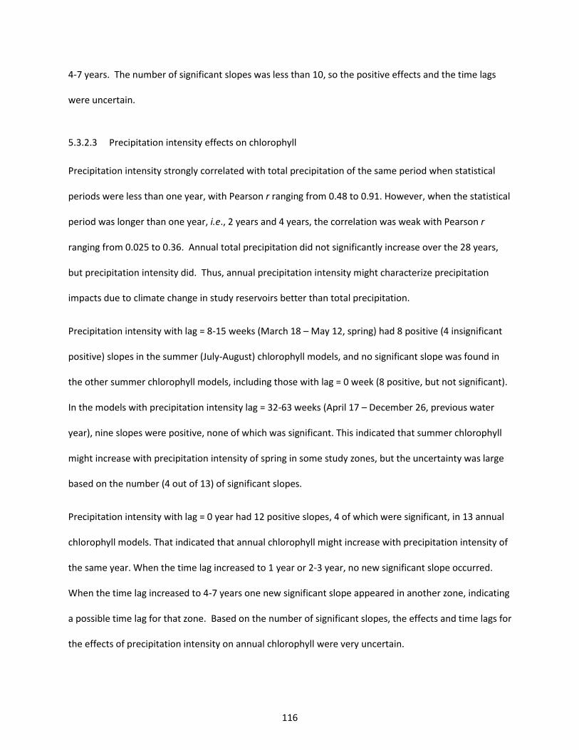
116
4-7 years. The number of significant slopes was less than 10, so the positive effects and the time lags
were uncertain.
5.3.2.3 Precipitation intensity effects on chlorophyll
Precipitation intensity strongly correlated with total precipitation of the same period when statistical
periods were less than one year, with Pearson r ranging from 0.48 to 0.91. However, when the statistical
period was longer than one year, i.e., 2 years and 4 years, the correlation was weak with Pearson r
ranging from 0.025 to 0.36. Annual total precipitation did not significantly increase over the 28 years,
but precipitation intensity did. Thus, annual precipitation intensity might characterize precipitation
impacts due to climate change in study reservoirs better than total precipitation.
Precipitation intensity with lag = 8-15 weeks (March 18 – May 12, spring) had 8 positive (4 insignificant
positive) slopes in the summer (July-August) chlorophyll models, and no significant slope was found in
the other summer chlorophyll models, including those with lag = 0 week (8 positive, but not significant).
In the models with precipitation intensity lag = 32-63 weeks (April 17 – December 26, previous water
year), nine slopes were positive, none of which was significant. This indicated that summer chlorophyll
might increase with precipitation intensity of spring in some study zones, but the uncertainty was large
based on the number (4 out of 13) of significant slopes.
Precipitation intensity with lag = 0 year had 12 positive slopes, 4 of which were significant, in 13 annual
chlorophyll models. That indicated that annual chlorophyll might increase with precipitation intensity of
the same year. When the time lag increased to 1 year or 2-3 year, no new significant slope occurred.
When the time lag increased to 4-7 years one new significant slope appeared in another zone, indicating
a possible time lag for that zone. Based on the number of significant slopes, the effects and time lags for
the effects of precipitation intensity on annual chlorophyll were very uncertain.
117
5.3.3 Multiple-factor analyses
Using models built with boosted regression trees to simulate relationships between daily chlorophyll
and daily weather (i.e., lake surface temperature and precipitation) with different time lags, model
performance indicated by 10-fold cross-validation R2 varied from -0.004 (Pomme de Terre Dam) to 0.506
(Wappapello Upstream East) (Figure 5-7, Table 5-2). That suggested that the daily variations of
chlorophyll in some zones such as Pomme de Terre could not be explained by temperature and
precipitation, but some others such as Wappapello Upstream East were correlated with temperature
and precipitation.
In models with 10-fold cross-validation R2 > 0.005, the model performance was mostly (> 50%) affected
by lake surface temperature (lag = 0 day). When the temperature (lag = 0 day) varied from 0 °C to 25 °C,
chlorophyll increased by 6-10 µg/L, varying with zones. Temperatures with time lags (i.e., 7 & 9, 16, 23 &
25, 32, and 39 & 41 days) had minor (< 10%) contributions in the models, indicating no time lag for
chlorophyll responding to lake surface temperature. Precipitations with different lags (i.e., 0, 1, 2, 4, 8,
16, 32, 64, and 128 days) had very small contributions in the models. All precipitation variables had less
than 10% of relative importance in total variance reduction of models, indicating chlorophyll was weakly
explained by precipitation, regardless of the time lags. Precipitation with time lags of 32 days or 64 days
had the highest relative importance, compared to the other precipitation variables, indicating possible
one- or two-month time lags for chlorophyll to respond to precipitation events. However, the evidence
was weak due to very small contribution (< 5%) of the precipitation variables in the models.
The model performances for the upstream zones were better than the mid-stream or dam zones.
Specifically, average R2 for eight upstream zones was 0.334, with maximum R2 = 0.506 (Wappapello
Upstream East), while average R2 for four dam zones was lower (0.138), with maximum R2 = 0.347
(Wappapello Dam) (Table 5-2).
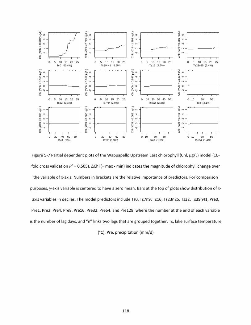
118
Figure 5-7 Partial dependent plots of the Wappapello Upstream East chlorophyll (Chl, µg/L) model (10-
fold cross validation R2 = 0.505). ΔChl (= max - min) indicates the magnitude of chlorophyll change over
the variable of x-axis. Numbers in brackets are the relative importance of predictors. For comparison
purposes, y-axis variable is centered to have a zero mean. Bars at the top of plots show distribution of x-
axis variables in deciles. The model predictors include Ts0, Ts7n9, Ts16, Ts23n25, Ts32, Ts39n41, Pre0,
Pre1, Pre2, Pre4, Pre8, Pre16, Pre32, Pre64, and Pre128, where the number at the end of each variable
is the number of lag days, and “n” links two lags that are grouped together. Ts, lake surface temperature
(°C); Pre, precipitation (mm/d)
0 5 10 15 20 25
-20
24
6
Ts0 (60.4%)
Chl (
Chl =
10.0
12
g/L
)
0 5 10 15 20 25
-20
24
6
Ts39n41 (8.5%)
Chl (
Chl =
2.6
25
g/L
)
0 5 10 15 20 25
-20
24
6
Ts16 (7.2%)
Chl (
Chl =
1.3
99
g/L
)
0 5 10 15 20 25
-20
24
6
Ts23n25 (3.4%)
Chl (
Chl =
0.8
85
g/L
)
0 5 10 15 20 25
-20
24
6
Ts32 (3.1%)
Chl (
Chl =
0.5
55
g/L
)
0 5 10 15 20 25
-20
24
6
Ts7n9 (2.9%)
Chl (
Chl =
0.6
12
g/L
)
0 10 20 30 40 50
-20
24
6
Pre32 (2.3%)
Chl (
Chl =
0.6
97
g/L
)
0 10 30 50
-20
24
6
Pre4 (2.1%)
Chl (
Chl =
0.5
33
g/L
)
0 20 40 60 80
-20
24
6
Pre1 (2%)
Chl (
Chl =
0.4
36
g/L
)
0 20 40 60 80
-20
24
6
Pre2 (1.9%)
Chl (
Chl =
0.3
60
g/L
)
0 10 30 50-2
02
46
Pre8 (1.5%)
Chl (
Chl =
0.0
69
g/L
)
0 10 30 50
-20
24
6
Pre64 (1.4%)
Chl (
Chl =
0.4
46
g/L
)
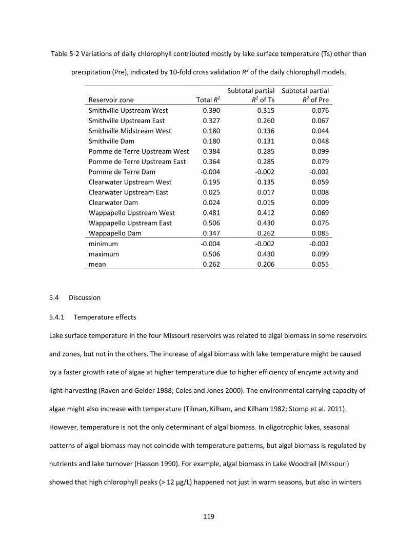
119
Table 5-2 Variations of daily chlorophyll contributed mostly by lake surface temperature (Ts) other than
precipitation (Pre), indicated by 10-fold cross validation R2 of the daily chlorophyll models.
Reservoir zone Total R2 Subtotal partial
R2 of Ts Subtotal partial
R2 of Pre
Smithville Upstream West 0.390 0.315 0.076
Smithville Upstream East 0.327 0.260 0.067
Smithville Midstream West 0.180 0.136 0.044
Smithville Dam 0.180 0.131 0.048
Pomme de Terre Upstream West 0.384 0.285 0.099
Pomme de Terre Upstream East 0.364 0.285 0.079
Pomme de Terre Dam -0.004 -0.002 -0.002
Clearwater Upstream West 0.195 0.135 0.059
Clearwater Upstream East 0.025 0.017 0.008
Clearwater Dam 0.024 0.015 0.009
Wappapello Upstream West 0.481 0.412 0.069
Wappapello Upstream East 0.506 0.430 0.076
Wappapello Dam 0.347 0.262 0.085
minimum -0.004 -0.002 -0.002
maximum 0.506 0.430 0.099
mean 0.262 0.206 0.055
5.4 Discussion
5.4.1 Temperature effects
Lake surface temperature in the four Missouri reservoirs was related to algal biomass in some reservoirs
and zones, but not in the others. The increase of algal biomass with lake temperature might be caused
by a faster growth rate of algae at higher temperature due to higher efficiency of enzyme activity and
light-harvesting (Raven and Geider 1988; Coles and Jones 2000). The environmental carrying capacity of
algae might also increase with temperature (Tilman, Kilham, and Kilham 1982; Stomp et al. 2011).
However, temperature is not the only determinant of algal biomass. In oligotrophic lakes, seasonal
patterns of algal biomass may not coincide with temperature patterns, but algal biomass is regulated by
nutrients and lake turnover (Hasson 1990). For example, algal biomass in Lake Woodrail (Missouri)
showed that high chlorophyll peaks (> 12 µg/L) happened not just in warm seasons, but also in winters
120
(Jones and Knowlton 2005). In Lake Erie, algal biomass has not correlated significantly with inter-annual
temperature differences in summer, but rather with nutrient loadings (Stumpf et al. 2012). In this study,
two chlorophyll peaks, instead of one, appeared in the chlorophyll-DOY relationship of Lake
Wappapello, where the average chlorophyll concentration was lower than the other reservoirs (Figure
5-5 c). These suggested that temperature impacts on algal biomass were also strongly mediated by
nutrients.
Algal biomass of the dam zones was significantly lower than associated upstream zones. Compared to
upstream zones, the variation in algal biomass in dam zones was explained less by lake surface
temperature in both one-factor models (Table A. 5-1) and multiple-factor models (Table 5-2). Dam areas
with lower nutrient levels might be subjected to stronger nutrient mediation than the upstream zones.
Both temperature and nutrients regulate algal biomass, and it would be interesting for future research
to investigate how the sensitivity of algal biomass to temperature changes with nutrient levels and N/P
ratios.
The results show that the temperature effect, indicated by the number of significant slopes in the
univariate linear models, was more likely found in annual chlorophyll than summer (July – August)
chlorophyll. The reason for that could be mathematical or ecological. Annual chlorophyll had lower
variance than summer chlorophyll, so annual models were more likely to be statistically significant than
summer models. On the other hand, algal biomass might be less sensitive and even saturated at high
temperature, so summer chlorophyll responded less to temperature than annual chlorophyll, which
included chlorophyll in cold months when algal biomass response to temperature was not saturated.
Lake surface temperatures in the study reservoirs varied from 16 °C to 30 °C. Growth rates of algae
might be stimulated at temperature > 25 °C (Lürling and De Senerpont Domis 2013).
121
5.4.2 Precipitation effects
5.4.2.1 Nutrient and light availability
Weak and mixed (positive and negative) correlations were found between precipitation (total
precipitation and precipitation intensity) and chlorophyll (annul and summer) in the studied Missouri
reservoirs. This might be due to complex hydrologic processes between precipitation events, nutrient
loading to lakes, and lake conditions. For instance, nutrients and light conditions might vary with
individual events and lakes. In Western Lake Superior after an extreme precipitation event on June 19–
20, 2012, both nutrients and turbidity (due to sediments and colored dissolved organic matter)
increased, then both returned to pre-event levels in two months; thus the temporal mismatch between
availability of nutrients and light resulted in no change in algal biomass over two months after the event
(Minor, Forsman, and Guildford 2014). However, if precipitation events bring more nutrients with less
turbidity, algal biomass might increase after the event. In our results, all four zones of Smithville Lake
had positive slopes in the July-August chlorophyll models (time lag = 0 week), three of which were
significant. That might be because Smithville Lake had a relatively high percentage of disturbed lands
(i.e., cultivated and urban lands) that might generate event flows from with higher nutrient
concentrations and potentially higher nutrient loading compared to other lands (Table 5-3). On the
other hand, one significantly negative slope was found in the Wappapello univariate models of July-
August chlorophyll. Wappapello watershed had a relatively low percentage of disturbed lands and
thereby potentially relatively low nutrient loads in the event flows. The negative correlation might be
due to the dilution effect of the low concentration flows. A predictable relationship between light and
the ratio of algal biomass to total phosphorus was shown in Lake Woodrail (Missouri) after precipitation
events, supporting the hypothesis of a mixed precipitation effect depending on nutrients and light
combination (Jones and Knowlton 2005).
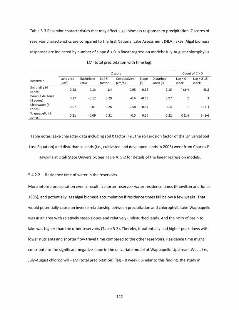
122
Table 5-3 Reservior characteristics that may affect algal biomass responses to precipitation. Z scores of
reservoir characteristics are compared to the first National Lake Assessment (NLA) lakes. Algal biomass
responses are indicated by number of slope β > 0 in linear regression models: July-August chlorophyll =
LM (total precipitation with time lag).
Z score Count of β > 0
Reservoir Lake area (km2)
Basin/lake ratio
Soil K factor
Conductivity (cm/h)
Slope (°)
Disturbed lands (%)
Lag = 0 week
Lag = 8-15 week
Smithville (4 zones)
0.23 -0.13 1.4 -0.95 -0.58 2.15 4 (3+) 4(1)
Pomme de Terre (3 zones)
0.27 -0.12 0.29 -0.6 -0.43 0.97 2 3
Clearwater (3 zones)
-0.07 -0.01 0.26 -0.58 0.57 -0.4 1 3 (3+)
Wappapello (3 zones)
0.21 -0.09 0.31 -0.5 0.16 -0.22 0 (1-) 3 (1+)
Table notes: Lake character data including soil K factor (i.e., the soil erosion factor of the Universal Soil
Loss Equation) and disturbance lands (i.e., cultivated and developed lands in 2005) were from Charles P.
Hawkins at Utah State University; See Table A. 5-2 for details of the linear regression models.
5.4.2.2 Residence time of water in the reservoirs
More intense precipitation events result in shorter reservoir water residence times (Knowlton and Jones
1995), and potentially less algal biomass accumulation if residence times fall below a few weeks. That
would potentially cause an inverse relationship between precipitation and chlorophyll. Lake Wappapello
was in an area with relatively steep slopes and relatively undisturbed lands. And the ratio of basin to
lake was higher than the other reservoirs (Table 5-3). Thereby, it potentially had higher peak flows with
lower nutrients and shorter flow travel time compared to the other reservoirs. Residence time might
contribute to the significant negative slope in the univariate model of Wappapello Upstream West, i.e.,
July-August chlorophyll = LM (total precipitation) (lag = 0 week). Similar to this finding, the study in
123
estuaries of North Carolina showed that algal biomass decreased after floods because of flushing and
shorter residence time (Paerl et al. 2014).
5.4.2.3 Time lags in algal biomass responses
The possibility of one- or two-month time lags was found in both univariate and multivariate models for
precipitation effects on chlorophyll. The lag might be the time for event flows to disperse and be mixed
in lakes, or/and the time for light to recover to a suitable level for algal biomass to catch up. For a
distance of 45 km between river outlet and dam in Mark Twain Lake (Missouri), it took about one month
for the turbid headwater to reach the dam in the 1990 flood event (Knowlton and Jones 1995). In
Western Lake Superior, it took about two months for turbidity to return to pre-event level (Minor,
Forsman, and Guildford 2014). The time periods of these observations were on a similar scale as the
time lags in this study (i.e., 1 and 2 months). Variation in time lags might be related to lake morphology
and events themselves. Time lags for algal biomass to respond to precipitation events have been
reported in the literature. For example, in Lake Erie where blooms consistently occurred in July-August,
average discharge during the March-June period was found exponentially related to annual algal
biomass (r2 = 0.97) during 2002 to 2011 (Stumpf et al. 2012). Extreme algal blooms in 2011 happened
after extreme springtime precipitation events in Lake Erie (Michalak et al. 2013).
5.4.2.4 Internal nutrient legacy sources
Internal nutrient sources may have more important effects on algal biomass than nutrient loading of the
same period caused by precipitation events. Nutrients deposited in lake bottoms could still influence
algal biomass far beyond the precipitation event periods, such as the next spring turnover time or even
years later. That might contribute to the weak correlations between precipitation and chlorophyll in
both univariate and multivariate models, and then there were additional complex effects of inflow
nutrients and light conditions.
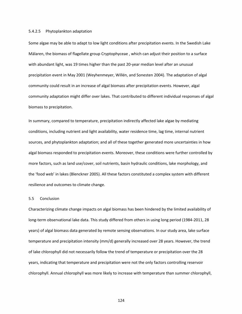
124
5.4.2.5 Phytoplankton adaptation
Some algae may be able to adapt to low light conditions after precipitation events. In the Swedish Lake
Mälaren, the biomass of flagellate group Cryptophyceae , which can adjust their position to a surface
with abundant light, was 19 times higher than the past 20-year median level after an unusual
precipitation event in May 2001 (Weyhenmeyer, Willén, and Sonesten 2004). The adaptation of algal
community could result in an increase of algal biomass after precipitation events. However, algal
community adaptation might differ over lakes. That contributed to different individual responses of algal
biomass to precipitation.
In summary, compared to temperature, precipitation indirectly affected lake algae by mediating
conditions, including nutrient and light availability, water residence time, lag time, internal nutrient
sources, and phytoplankton adaptation; and all of these together generated more uncertainties in how
algal biomass responded to precipitation events. Moreover, these conditions were further controlled by
more factors, such as land use/cover, soil nutrients, basin hydraulic conditions, lake morphology, and
the ‘food web’ in lakes (Blenckner 2005). All these factors constituted a complex system with different
resilience and outcomes to climate change.
5.5 Conclusion
Characterizing climate change impacts on algal biomass has been hindered by the limited availability of
long-term observational lake data. This study differed from others in using long period (1984-2011, 28
years) of algal biomass data generated by remote sensing observations. In our study area, lake surface
temperature and precipitation intensity (mm/d) generally increased over 28 years. However, the trend
of lake chlorophyll did not necessarily follow the trend of temperature or precipitation over the 28
years, indicating that temperature and precipitation were not the only factors controlling reservoir
chlorophyll. Annual chlorophyll was more likely to increase with temperature than summer chlorophyll,

125
suggesting that with global warming the algal growth period might expand while the peak biomass
during summer might saturate. More precipitation in spring as predicted by the climate models might
result in higher summer algal biomass. Annual chlorophyll might increase with higher total precipitation
or precipitation intensity without time lags. The uncertainty of the climate change impacts was high
since only a few of the univariate models were statistically significant. The multivariate models further
revealed that daily temperature and daily precipitation together explained as less zero and as high as
50.6% of the variance in daily chlorophyll. These findings are based on four Missouri reservoirs and may
not be applied to other lakes with different conditions of nutrients, turbidity (light), lake morphology,
soil hydraulic properties, soil nutrients, and land use/cover.
Acknowledgement
This work was supported by the U.S. Environmental Protection Agency (EPA) under EPA STAR Grant
#835203. The views and opinions expressed in this article are those of the authors and do not
necessarily reflect the official policy or position of U.S. EPA, or any other agency of the U.S. government.

126
APPENDIX
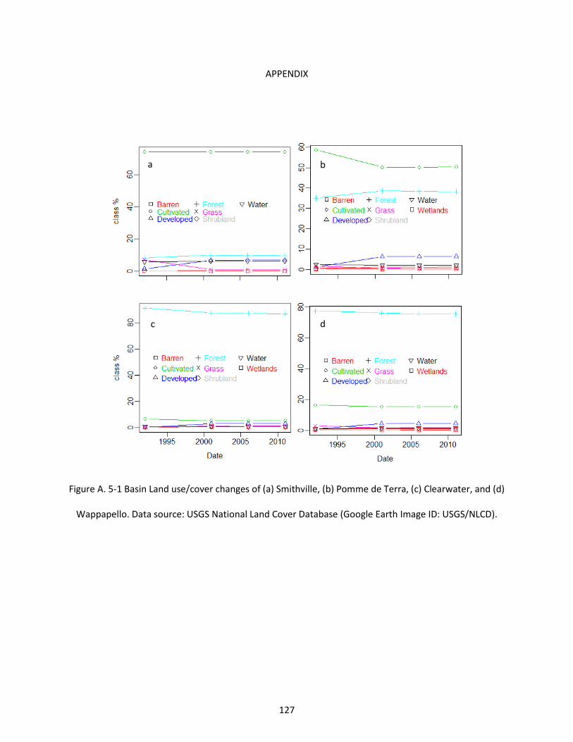
127
APPENDIX
Figure A. 5-1 Basin Land use/cover changes of (a) Smithville, (b) Pomme de Terra, (c) Clearwater, and (d)
Wappapello. Data source: USGS National Land Cover Database (Google Earth Image ID: USGS/NLCD).
a b
c d
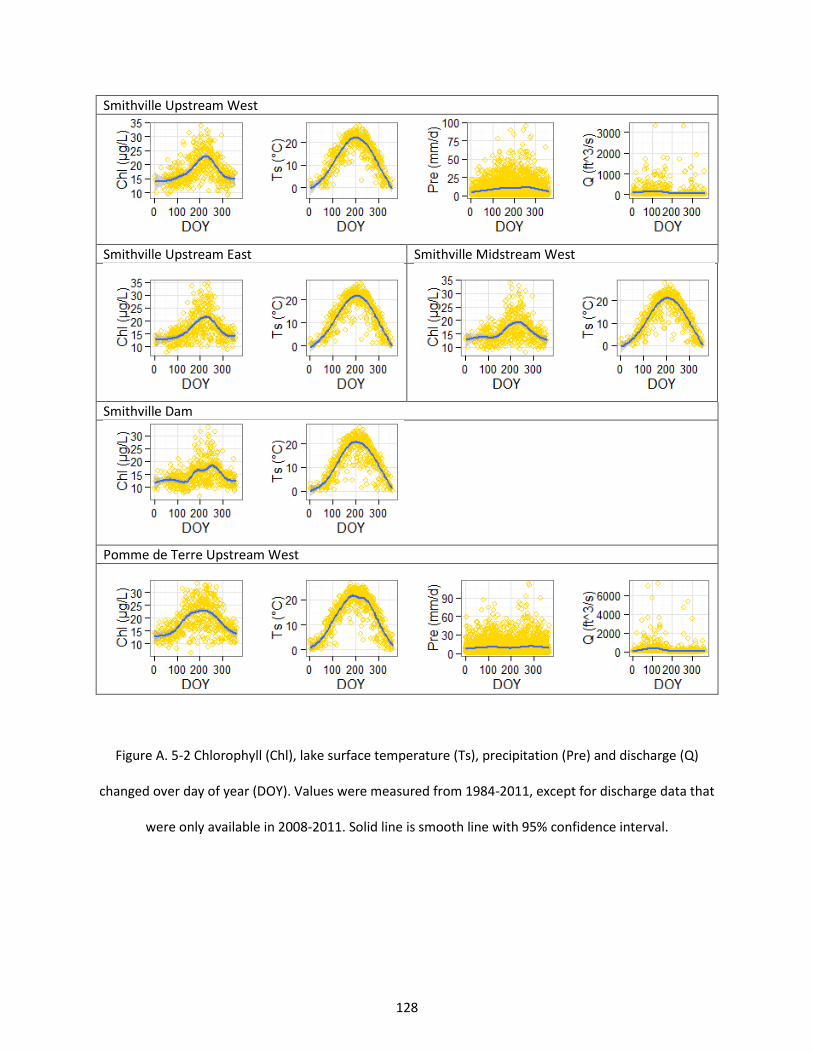
128
Smithville Upstream West
Smithville Upstream East Smithville Midstream West
Smithville Dam
Pomme de Terre Upstream West
Figure A. 5-2 Chlorophyll (Chl), lake surface temperature (Ts), precipitation (Pre) and discharge (Q)
changed over day of year (DOY). Values were measured from 1984-2011, except for discharge data that
were only available in 2008-2011. Solid line is smooth line with 95% confidence interval.
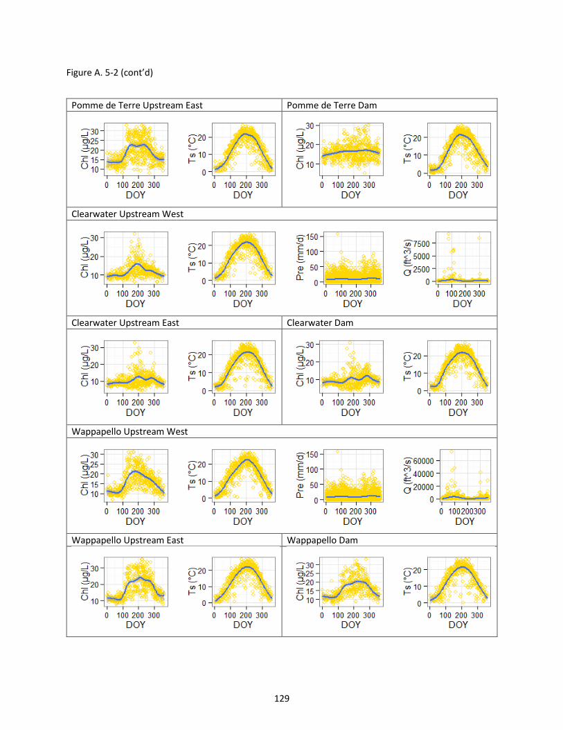
129
Figure A. 5-2 (cont’d)
Pomme de Terre Upstream East Pomme de Terre Dam
Clearwater Upstream West
Clearwater Upstream East Clearwater Dam
Wappapello Upstream West
Wappapello Upstream East Wappapello Dam
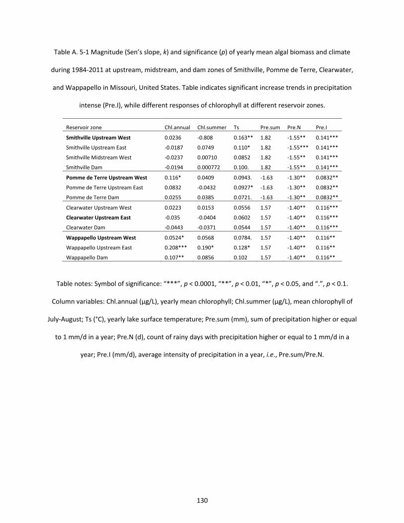
130
Table A. 5-1 Magnitude (Sen’s slope, k) and significance (p) of yearly mean algal biomass and climate
during 1984-2011 at upstream, midstream, and dam zones of Smithville, Pomme de Terre, Clearwater,
and Wappapello in Missouri, United States. Table indicates significant increase trends in precipitation
intense (Pre.I), while different responses of chlorophyll at different reservoir zones.
Reservoir zone Chl.annual Chl.summer Ts Pre.sum Pre.N Pre.I
Smithville Upstream West 0.0236 -0.808 0.163** 1.82 -1.55** 0.141***
Smithville Upstream East -0.0187 0.0749 0.110* 1.82 -1.55*** 0.141***
Smithville Midstream West -0.0237 0.00710 0.0852 1.82 -1.55** 0.141***
Smithville Dam -0.0194 0.000772 0.100. 1.82 -1.55** 0.141***
Pomme de Terre Upstream West 0.116* 0.0409 0.0943. -1.63 -1.30** 0.0832**
Pomme de Terre Upstream East 0.0832 -0.0432 0.0927* -1.63 -1.30** 0.0832**
Pomme de Terre Dam 0.0255 0.0385 0.0721. -1.63 -1.30** 0.0832**
Clearwater Upstream West 0.0223 0.0153 0.0556 1.57 -1.40** 0.116***
Clearwater Upstream East -0.035 -0.0404 0.0602 1.57 -1.40** 0.116***
Clearwater Dam -0.0443 -0.0371 0.0544 1.57 -1.40** 0.116***
Wappapello Upstream West 0.0524* 0.0568 0.0784. 1.57 -1.40** 0.116**
Wappapello Upstream East 0.208*** 0.190* 0.128* 1.57 -1.40** 0.116**
Wappapello Dam 0.107** 0.0856 0.102 1.57 -1.40** 0.116**
Table notes: Symbol of significance: “***”, p < 0.0001, “**”, p < 0.01, “*”, p < 0.05, and “.”, p < 0.1.
Column variables: Chl.annual (µg/L), yearly mean chlorophyll; Chl.summer (µg/L), mean chlorophyll of
July-August; Ts (°C), yearly lake surface temperature; Pre.sum (mm), sum of precipitation higher or equal
to 1 mm/d in a year; Pre.N (d), count of rainy days with precipitation higher or equal to 1 mm/d in a
year; Pre.I (mm/d), average intensity of precipitation in a year, i.e., Pre.sum/Pre.N.
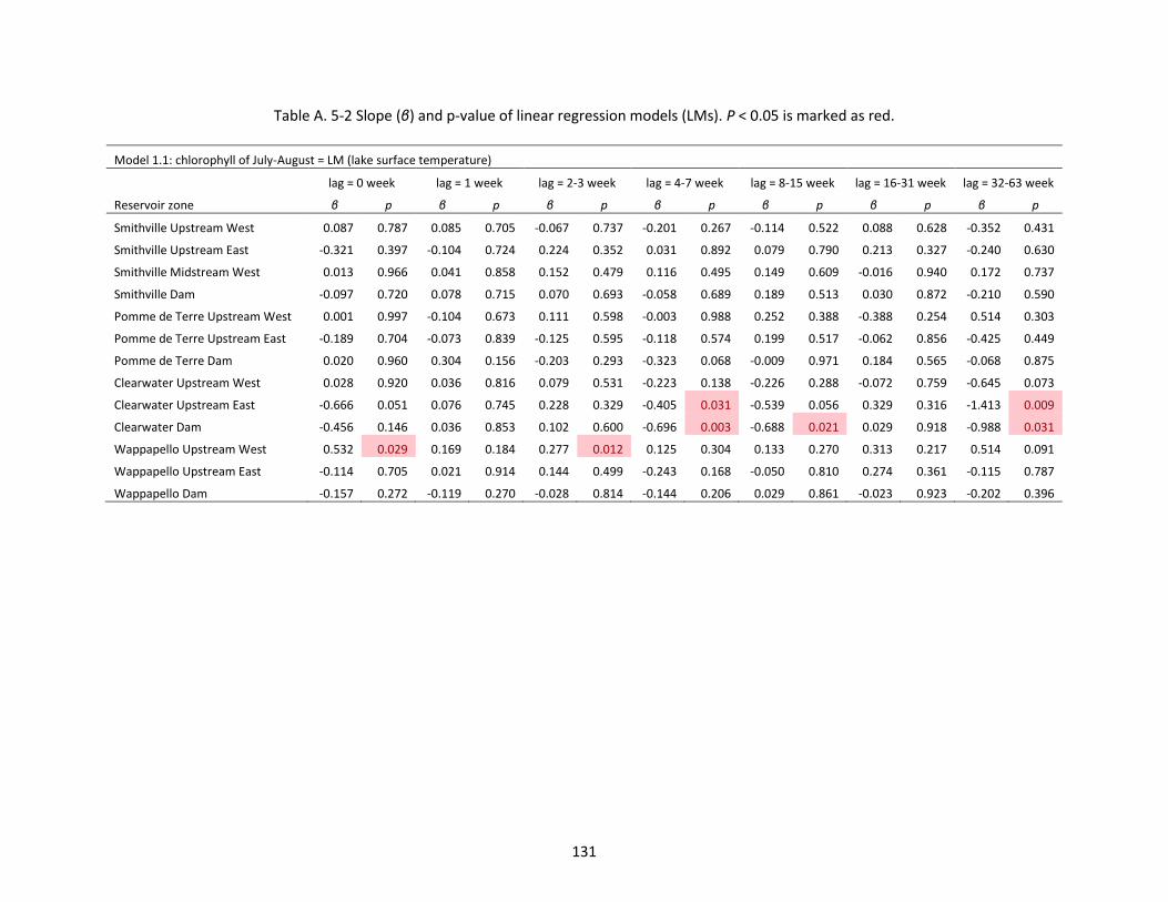
131
Table A. 5-2 Slope (β) and p-value of linear regression models (LMs). P < 0.05 is marked as red.
Model 1.1: chlorophyll of July-August = LM (lake surface temperature)
lag = 0 week lag = 1 week lag = 2-3 week lag = 4-7 week lag = 8-15 week lag = 16-31 week lag = 32-63 week
Reservoir zone β p β p β p β p β p β p β p
Smithville Upstream West 0.087 0.787 0.085 0.705 -0.067 0.737 -0.201 0.267 -0.114 0.522 0.088 0.628 -0.352 0.431
Smithville Upstream East -0.321 0.397 -0.104 0.724 0.224 0.352 0.031 0.892 0.079 0.790 0.213 0.327 -0.240 0.630
Smithville Midstream West 0.013 0.966 0.041 0.858 0.152 0.479 0.116 0.495 0.149 0.609 -0.016 0.940 0.172 0.737
Smithville Dam -0.097 0.720 0.078 0.715 0.070 0.693 -0.058 0.689 0.189 0.513 0.030 0.872 -0.210 0.590
Pomme de Terre Upstream West 0.001 0.997 -0.104 0.673 0.111 0.598 -0.003 0.988 0.252 0.388 -0.388 0.254 0.514 0.303
Pomme de Terre Upstream East -0.189 0.704 -0.073 0.839 -0.125 0.595 -0.118 0.574 0.199 0.517 -0.062 0.856 -0.425 0.449
Pomme de Terre Dam 0.020 0.960 0.304 0.156 -0.203 0.293 -0.323 0.068 -0.009 0.971 0.184 0.565 -0.068 0.875
Clearwater Upstream West 0.028 0.920 0.036 0.816 0.079 0.531 -0.223 0.138 -0.226 0.288 -0.072 0.759 -0.645 0.073
Clearwater Upstream East -0.666 0.051 0.076 0.745 0.228 0.329 -0.405 0.031 -0.539 0.056 0.329 0.316 -1.413 0.009
Clearwater Dam -0.456 0.146 0.036 0.853 0.102 0.600 -0.696 0.003 -0.688 0.021 0.029 0.918 -0.988 0.031
Wappapello Upstream West 0.532 0.029 0.169 0.184 0.277 0.012 0.125 0.304 0.133 0.270 0.313 0.217 0.514 0.091
Wappapello Upstream East -0.114 0.705 0.021 0.914 0.144 0.499 -0.243 0.168 -0.050 0.810 0.274 0.361 -0.115 0.787
Wappapello Dam -0.157 0.272 -0.119 0.270 -0.028 0.814 -0.144 0.206 0.029 0.861 -0.023 0.923 -0.202 0.396
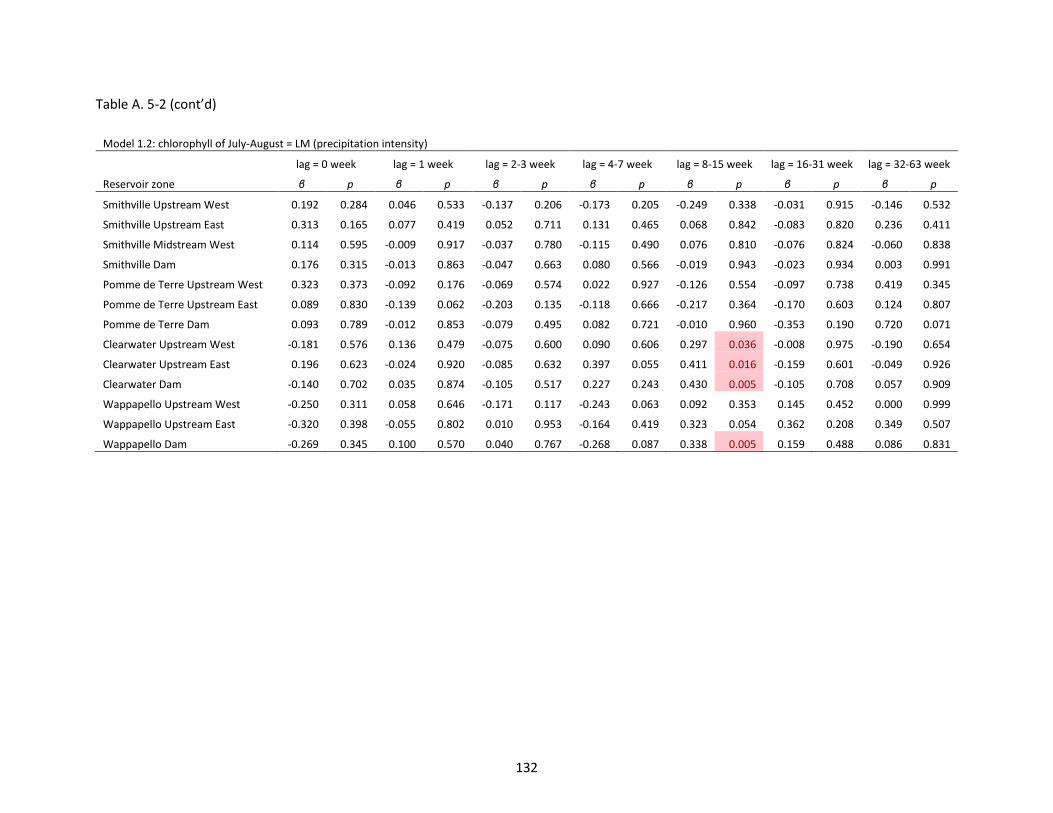
132
Table A. 5-2 (cont’d)
Model 1.2: chlorophyll of July-August = LM (precipitation intensity)
lag = 0 week lag = 1 week lag = 2-3 week lag = 4-7 week lag = 8-15 week lag = 16-31 week lag = 32-63 week
Reservoir zone β p β p β p β p β p β p β p
Smithville Upstream West 0.192 0.284 0.046 0.533 -0.137 0.206 -0.173 0.205 -0.249 0.338 -0.031 0.915 -0.146 0.532
Smithville Upstream East 0.313 0.165 0.077 0.419 0.052 0.711 0.131 0.465 0.068 0.842 -0.083 0.820 0.236 0.411
Smithville Midstream West 0.114 0.595 -0.009 0.917 -0.037 0.780 -0.115 0.490 0.076 0.810 -0.076 0.824 -0.060 0.838
Smithville Dam 0.176 0.315 -0.013 0.863 -0.047 0.663 0.080 0.566 -0.019 0.943 -0.023 0.934 0.003 0.991
Pomme de Terre Upstream West 0.323 0.373 -0.092 0.176 -0.069 0.574 0.022 0.927 -0.126 0.554 -0.097 0.738 0.419 0.345
Pomme de Terre Upstream East 0.089 0.830 -0.139 0.062 -0.203 0.135 -0.118 0.666 -0.217 0.364 -0.170 0.603 0.124 0.807
Pomme de Terre Dam 0.093 0.789 -0.012 0.853 -0.079 0.495 0.082 0.721 -0.010 0.960 -0.353 0.190 0.720 0.071
Clearwater Upstream West -0.181 0.576 0.136 0.479 -0.075 0.600 0.090 0.606 0.297 0.036 -0.008 0.975 -0.190 0.654
Clearwater Upstream East 0.196 0.623 -0.024 0.920 -0.085 0.632 0.397 0.055 0.411 0.016 -0.159 0.601 -0.049 0.926
Clearwater Dam -0.140 0.702 0.035 0.874 -0.105 0.517 0.227 0.243 0.430 0.005 -0.105 0.708 0.057 0.909
Wappapello Upstream West -0.250 0.311 0.058 0.646 -0.171 0.117 -0.243 0.063 0.092 0.353 0.145 0.452 0.000 0.999
Wappapello Upstream East -0.320 0.398 -0.055 0.802 0.010 0.953 -0.164 0.419 0.323 0.054 0.362 0.208 0.349 0.507
Wappapello Dam -0.269 0.345 0.100 0.570 0.040 0.767 -0.268 0.087 0.338 0.005 0.159 0.488 0.086 0.831
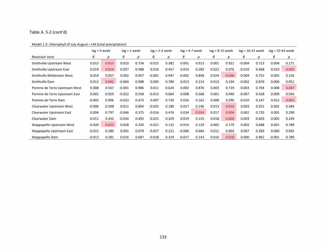
133
Table A. 5-2 (cont’d)
Model 1.3: chlorophyll of July-August = LM (total precipitation)
lag = 0 week lag = 1 week lag = 2-3 week lag = 4-7 week lag = 8-15 week lag = 16-31 week lag = 32-63 week
Reservoir zone β p β p β p β p β p β p β p
Smithville Upstream West 0.015 0.013 0.010 0.734 -0.015 0.382 0.001 0.913 0.001 0.921 -0.004 0.713 0.004 0.171
Smithville Upstream East 0.019 0.014 0.027 0.488 0.016 0.457 0.014 0.282 0.022 0.076 -0.010 0.468 0.010 0.005
Smithville Midstream West 0.014 0.057 0.002 0.957 -0.001 0.947 -0.002 0.858 0.024 0.036 -0.004 0.752 0.005 0.156
Smithville Dam 0.012 0.042 -0.004 0.908 0.005 0.780 0.013 0.214 0.013 0.194 -0.002 0.876 0.006 0.051
Pomme de Terre Upstream West 0.008 0.567 -0.001 0.986 0.011 0.624 0.002 0.876 0.003 0.719 -0.003 0.704 0.008 0.047
Pomme de Terre Upstream East 0.001 0.929 -0.022 0.558 -0.013 0.604 0.008 0.568 0.001 0.940 -0.007 0.428 0.009 0.056
Pomme de Terre Dam -0.002 0.906 -0.023 0.473 0.007 0.730 0.016 0.162 0.008 0.290 -0.010 0.147 0.012 0.001
Clearwater Upstream West -0.006 0.598 0.011 0.804 -0.025 0.180 0.017 0.146 0.013 0.010 0.003 0.551 0.002 0.584
Clearwater Upstream East 0.004 0.797 -0.046 0.375 -0.016 0.476 0.034 0.014 0.017 0.004 0.002 0.735 0.005 0.290
Clearwater Dam -0.011 0.432 -0.034 0.492 -0.021 0.329 0.019 0.155 0.018 0.000 0.003 0.603 0.005 0.249
Wappapello Upstream West -0.020 0.025 0.028 0.320 -0.021 0.132 -0.014 0.129 0.005 0.179 0.002 0.688 0.001 0.789
Wappapello Upstream East -0.015 0.280 0.001 0.979 -0.027 0.221 -0.006 0.684 0.011 0.064 0.007 0.283 0.000 0.945
Wappapello Dam -0.012 0.281 0.016 0.687 -0.018 0.319 -0.017 0.143 0.010 0.018 0.000 0.962 -0.001 0.780
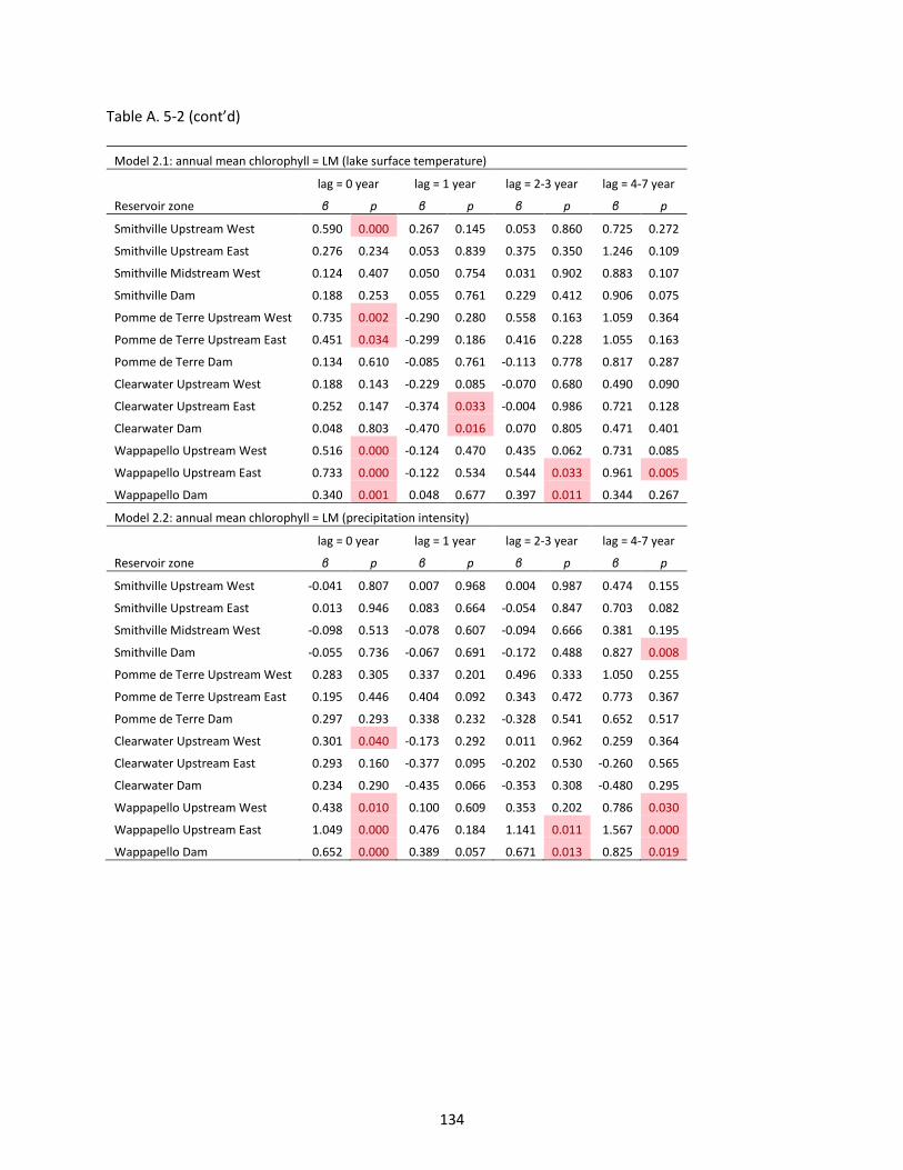
134
Table A. 5-2 (cont’d)
Model 2.1: annual mean chlorophyll = LM (lake surface temperature)
lag = 0 year lag = 1 year lag = 2-3 year lag = 4-7 year
Reservoir zone β p β p β p β p
Smithville Upstream West 0.590 0.000 0.267 0.145 0.053 0.860 0.725 0.272
Smithville Upstream East 0.276 0.234 0.053 0.839 0.375 0.350 1.246 0.109
Smithville Midstream West 0.124 0.407 0.050 0.754 0.031 0.902 0.883 0.107
Smithville Dam 0.188 0.253 0.055 0.761 0.229 0.412 0.906 0.075
Pomme de Terre Upstream West 0.735 0.002 -0.290 0.280 0.558 0.163 1.059 0.364
Pomme de Terre Upstream East 0.451 0.034 -0.299 0.186 0.416 0.228 1.055 0.163
Pomme de Terre Dam 0.134 0.610 -0.085 0.761 -0.113 0.778 0.817 0.287
Clearwater Upstream West 0.188 0.143 -0.229 0.085 -0.070 0.680 0.490 0.090
Clearwater Upstream East 0.252 0.147 -0.374 0.033 -0.004 0.986 0.721 0.128
Clearwater Dam 0.048 0.803 -0.470 0.016 0.070 0.805 0.471 0.401
Wappapello Upstream West 0.516 0.000 -0.124 0.470 0.435 0.062 0.731 0.085
Wappapello Upstream East 0.733 0.000 -0.122 0.534 0.544 0.033 0.961 0.005
Wappapello Dam 0.340 0.001 0.048 0.677 0.397 0.011 0.344 0.267
Model 2.2: annual mean chlorophyll = LM (precipitation intensity)
lag = 0 year lag = 1 year lag = 2-3 year lag = 4-7 year
Reservoir zone β p β p β p β p
Smithville Upstream West -0.041 0.807 0.007 0.968 0.004 0.987 0.474 0.155
Smithville Upstream East 0.013 0.946 0.083 0.664 -0.054 0.847 0.703 0.082
Smithville Midstream West -0.098 0.513 -0.078 0.607 -0.094 0.666 0.381 0.195
Smithville Dam -0.055 0.736 -0.067 0.691 -0.172 0.488 0.827 0.008
Pomme de Terre Upstream West 0.283 0.305 0.337 0.201 0.496 0.333 1.050 0.255
Pomme de Terre Upstream East 0.195 0.446 0.404 0.092 0.343 0.472 0.773 0.367
Pomme de Terre Dam 0.297 0.293 0.338 0.232 -0.328 0.541 0.652 0.517
Clearwater Upstream West 0.301 0.040 -0.173 0.292 0.011 0.962 0.259 0.364
Clearwater Upstream East 0.293 0.160 -0.377 0.095 -0.202 0.530 -0.260 0.565
Clearwater Dam 0.234 0.290 -0.435 0.066 -0.353 0.308 -0.480 0.295
Wappapello Upstream West 0.438 0.010 0.100 0.609 0.353 0.202 0.786 0.030
Wappapello Upstream East 1.049 0.000 0.476 0.184 1.141 0.011 1.567 0.000
Wappapello Dam 0.652 0.000 0.389 0.057 0.671 0.013 0.825 0.019
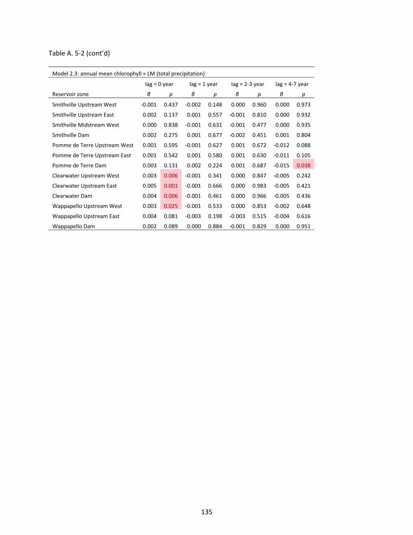
135
Table A. 5-2 (cont’d)
Model 2.3: annual mean chlorophyll = LM (total precipitation)
lag = 0 year lag = 1 year lag = 2-3 year lag = 4-7 year
Reservoir zone β p β p β p β p
Smithville Upstream West -0.001 0.437 -0.002 0.148 0.000 0.960 0.000 0.973
Smithville Upstream East 0.002 0.137 0.001 0.557 -0.001 0.810 0.000 0.932
Smithville Midstream West 0.000 0.838 -0.001 0.631 -0.001 0.477 0.000 0.935
Smithville Dam 0.002 0.275 0.001 0.677 -0.002 0.451 0.001 0.804
Pomme de Terre Upstream West 0.001 0.595 -0.001 0.627 0.001 0.672 -0.012 0.088
Pomme de Terre Upstream East 0.001 0.542 0.001 0.580 0.001 0.630 -0.011 0.105
Pomme de Terre Dam 0.003 0.131 0.002 0.224 0.001 0.687 -0.015 0.038
Clearwater Upstream West 0.003 0.006 -0.001 0.341 0.000 0.847 -0.005 0.242
Clearwater Upstream East 0.005 0.001 -0.001 0.666 0.000 0.983 -0.005 0.421
Clearwater Dam 0.004 0.006 -0.001 0.461 0.000 0.966 -0.005 0.436
Wappapello Upstream West 0.003 0.025 -0.001 0.533 0.000 0.853 -0.002 0.648
Wappapello Upstream East 0.004 0.081 -0.003 0.198 -0.003 0.515 -0.004 0.616
Wappapello Dam 0.002 0.089 0.000 0.884 -0.001 0.829 0.000 0.951

136
REFERENCES
137
REFERENCES
Abatzoglou, John T. 2013. “Development of Gridded Surface Meteorological Data for Ecological Applications and Modelling.” International Journal of Climatology 33 (1): 121–31. doi:10.1002/joc.3413.
Adrian, Rita, Norbert Walz, Thomas Hintze, Sigrid Hoeg, and Renate Rusche. 1999. “Effects of Ice Duration on Plankton Succession during Spring in a Shallow Polymictic Lake.” Freshwater Biology 41 (3): 621–34. doi:10.1046/j.1365-2427.1999.00411.x.
Adrian, Rita, Susann Wilhelm, and Dieter Gerten. 2006. “Life-History Traits of Lake Plankton Species May Govern Their Phenological Response to Climate Warming.” Global Change Biology 12 (4): 652–61. doi:10.1111/j.1365-2486.2006.01125.x.
Blenckner, Thorsten. 2005. “A Conceptual Model of Climate-Related Effects on Lake Ecosystems.” Hydrobiologia 533 (1–3): 1–14. doi:10.1007/s10750-004-1463-4.
Coles, James F., and R. Christian Jones. 2000. “Effect of Temperature on Photosynthesis-Light Response and Growth of Four Phytoplankton Species Isolated from a Tidal Freshwater River.” Journal of Phycology 36 (1): 7–16. doi:10.1046/j.1529-8817.2000.98219.x.
Dokulil, Martin T., and Katrin Teubner. 2000. “Cyanobacterial Dominance in Lakes.” Hydrobiologia 438 (1–3): 1–12. doi:10.1023/A:1004155810302.
George, D. Glen, M. Jarvinen, and Lauri Arvola. 2004. “The Influence of the North Atlantic Oscillation on the Winter Characteristics of Windermere (UK) and Paajarvi (Finland).” Boreal Environment Research 9: 389–400.
Gerten, Dieter, and Rita Adrian. 2001. “Differences in the Persistency of the North Atlantic Oscillation Signal among Lakes.” Limnology and Oceanography 46 (2): 448–55. doi:10.4319/lo.2001.46.2.0448.
Gorelick, Noel. 2012. “Google Earth Engine.” In AGU Fall Meeting Abstracts, 1:04. http://adsabs.harvard.edu/abs/2012AGUFM.U31A..04G.
Hasson, Lars-Anders. 1990. “Quantifying the Impact of Periphytic Algae on Nutrient Availability for Phytoplankton.” Freshwater Biology 24 (2): 265–273.
IPCC. 2014. “IPCC Fifth Assessment Report Climate Change 2014:Impacts, Adaptation, and Vulnerability.” IPCC-XXXVIII/DOC.4. (Intergovernmental Panel on Climate Change). http://www.ipcc.ch/.
Jones, John R., and Matthew F. Knowlton. 2005. “Chlorophyll Response to Nutrients and Non-Algal Seston in Missouri Reservoirs and Oxbow Lakes.” Lake and Reservoir Management 21 (3): 361–71. doi:10.1080/07438140509354441.
138
Knowlton, Matthew F., and John R. Jones. 1995. “Temporal and Spatial Dynamics of Suspended Sediment, Nutrients, and Algal Biomass in Mark Twain Lake, Missouri.” Archiv Fur Hydrobiologie 135: 145–178.
Lürling, Miquel, and Lisette N. De Senerpont Domis. 2013. “Predictability of Plankton Communities in an Unpredictable World.” Freshwater Biology 58 (3): 455–62. doi:10.1111/fwb.12092.
Marshall, Eric, and Timothy Randhir. 2008. “Effect of Climate Change on Watershed System: A Regional Analysis.” Climatic Change 89 (3–4): 263–80. doi:10.1007/s10584-007-9389-2.
McDonald, Michael E., Anne E. Hershey, and Michael C. Miller. 1996. “Global Warming Impacts on Lake Trout in Arctic Lakes.” Limnology and Oceanography 41: 1102–1108.
Michalak, Anna M., Eric J. Anderson, Dmitry Beletsky, Steven Boland, Nathan S. Bosch, Thomas B. Bridgeman, Justin D. Chaffin, et al. 2013. “Record-Setting Algal Bloom in Lake Erie Caused by Agricultural and Meteorological Trends Consistent with Expected Future Conditions.” Proceedings of the National Academy of Sciences 110 (16): 6448–52. doi:10.1073/pnas.1216006110.
Minor, Elizabeth C., Brandy Forsman, and Stephanie J. Guildford. 2014. “The Effect of a Flood Pulse on the Water Column of Western Lake Superior, USA.” Journal of Great Lakes Research 40 (2): 455–62. doi:10.1016/j.jglr.2014.03.015.
Nash, J. E., and J. V. Sutcliffe. 1970. “River Flow Forecasting through Conceptual Models Part I — A Discussion of Principles.” Journal of Hydrology 10 (3): 282–90. doi:10.1016/0022-1694(70)90255-6.
Paerl, Hans W., Nathan S. Hall, Benjamin L. Peierls, and Karen L. Rossignol. 2014. “Evolving Paradigms and Challenges in Estuarine and Coastal Eutrophication Dynamics in a Culturally and Climatically Stressed World.” Estuaries and Coasts 37 (2): 243–58. doi:10.1007/s12237-014-9773-x.
Paerl, Hans W., and Jef Huisman. 2008. “Blooms Like It Hot.” Science 320 (5872): 57–58. doi:10.1126/science.1155398.
Paerl, Hans W., and Valerie J. Paul. 2012. “Climate Change: Links to Global Expansion of Harmful Cyanobacteria.” Water Research, Cyanobacteria: Impacts of climate change on occurrence, toxicity and water quality management, 46 (5): 1349–63. doi:10.1016/j.watres.2011.08.002.
Pettersson, Kurt. 1990. “The Spring Development of Phytoplankton in Lake Erken: Species Composition, Biomass, Primary Production and Nutrient Conditions — a Review.” Hydrobiologia 191 (1): 9–14. doi:10.1007/BF00026033.
Praskievicz, Sarah, and Heejun Chang. 2011. “Impacts of Climate Change and Urban Development on Water Resources in the Tualatin River Basin, Oregon.” Annals of the Association of American Geographers 101 (2): 249–71. doi:10.1080/00045608.2010.544934.
139
Raven, John A., and Richard J. Geider. 1988. “Temperature and Algal Growth.” New Phytologist 110 (4): 441–61. doi:10.1111/j.1469-8137.1988.tb00282.x.
Ridgeway, Greg. 2004. “The Gbm Package.” R Foundation for Statistical Computing, Vienna, Austria. http://132.180.15.2/math/statlib/R/CRAN/doc/packages/gbm.pdf.
Robson, Barbara J., and David P. Hamilton. 2003. “Summer Flow Event Induces a Cyanobacterial Bloom in a Seasonal Western Australian Estuary.” Marine and Freshwater Research 54 (2): 139–51.
Schindler, David W. 2012. “The Dilemma of Controlling Cultural Eutrophication of Lakes.” Proc. R. Soc. B 279 (1746): 4322–33. doi:10.1098/rspb.2012.1032.
Slavik, K., B. J. Peterson, L. A. Deegan, W. B. Bowden, A. E. Hershey, and J. E. Hobbie. 2004. “Long-Term Responses of the Kuparuk River Ecosystem to Phosphorus Fertilization.” Ecology 85 (4): 939–54. doi:10.1890/02-4039.
Stomp, Maayke, Jef Huisman, Gary G. Mittelbach, Elena Litchman, and Christopher A. Klausmeier. 2011. “Large-Scale Biodiversity Patterns in Freshwater Phytoplankton.” Ecology 92 (11): 2096–2107.
Straile, D. 2000. “Meteorological Forcing of Plankton Dynamics in a Large and Deep Continental European Lake.” Oecologia 122 (1): 44–50. doi:10.1007/PL00008834.
Stumpf, Richard P., Timothy T. Wynne, David B. Baker, and Gary L. Fahnenstiel. 2012. “Interannual Variability of Cyanobacterial Blooms in Lake Erie.” PLoS ONE 7 (8): e42444. doi:10.1371/journal.pone.0042444.
Taner, Mehmet Ümit, James N. Carleton, and Marjorie Wellman. 2011. “Integrated Model Projections of Climate Change Impacts on a North American Lake.” Ecological Modelling 222 (18): 3380–93. doi:10.1016/j.ecolmodel.2011.07.015.
Tilman, David, Susan S. Kilham, and Peter Kilham. 1982. “Phytoplankton Community Ecology: The Role of Limiting Nutrients.” Annual Review of Ecology and Systematics 13: 349–72.
Weyhenmeyer, Gesa A., Eva Willén, and Lars Sonesten. 2004. “Effects of an Extreme Precipitation Event on Water Chemistry and Phytoplankton in the Swedish Lake Mälaren.” Boreal Environment Research 9 (5): 409–420.
140
6 ALGAL BIOMASS RESPONSES TO CLIMATE CHANGE IN LAKES ACROSS THE CONTINENTAL UNITED
STATES
Abstract
Climate change is expected to create conditions conducive to harmful algal blooms. However, in
complex watersheds and aquatic systems, it is not clear how algae in lakes respond to changes in
climate factors and nutrient loadings. It is even more challenging to predict climate change impacts on
lake algae that involve complex effects of climate change on interactions between watersheds and
aquatic systems. This study investigated relationships between algal biomass and climate change
utilizing a space-for-time substitution method with data from more than 1000 lakes across a large
gradient of climate in continental United States. Lake algal biomass was characterized using remote
sensing observations as well as in-lake measurements. Statistical models using boosted regression trees
indicated that (1) algal biomass increased with temperature; and (2) algal biomass increased with higher
precipitation intensity, but decreased with higher annual total precipitation. The climate scenario
analyses predicted that algal biomass would increase in the future climate. Specifically, algal biomass
would increase in all CO2 emission scenarios, and higher CO2 emission would result in higher algal
biomass increase.
Keywords: climate change, lakes, water quality, phytoplankton
Highlights
• Algal biomass increased with temperature.
• Algal biomass sensitivity to temperature increased with higher nutrient concentrations in lakes.
• Algal biomass decreased with total precipitation, but increased with precipitation intensity.
• Algal biomass sensitivity to precipitation intensity increased with soil erodibility.
• Algal biomass will increase more in the “high” CO2 emission scenario than the “low” one.
141
6.1 Introduction
An algal bloom is a rapid increase or accumulation of algae in water. Harmful algal blooms are significant
global and local threats to public health and aquatic ecosystems (Anderson 1989; Lopez et al. 2008).
Freshwater algal blooms are often dominated by cyanobacteria, some of which can release toxins and
cause sickness or death in the wildlife and humans who use the water for drinking or recreation
(Falconer, Beresford, and Runnegar 1983). The economic damages incurred from freshwater
eutrophication were conservatively estimated at 2.2 billion dollars per year in the United States,
considering recreational water usage, waterfront real estate, and recovery of biodiversity and drinking
water (Dodds et al. 2009). Predicted changes in climate may cause more algal blooms, especially harmful
cyanobacteria blooms, based on the following hypotheses (Paerl and Huisman 2008):
• Increased atmospheric CO2 enhances carbon availability for all phytoplankton species, especially
surface-dwelling cyanobacteria;
• Higher water temperatures, resulting in lower water viscosity and stronger thermal
stratification, facilitates buoyant cyanobacteria to out-compete other phytoplankton species;
• Higher temperatures accelerate growth of all phytoplankton species, especially cyanobacteria
that have a warmer temperature optimum than other algal groups;
• Higher hydrologic variability introduces more nutrients, especially particulate phosphorus (P),
which stimulates phytoplankton growth in inland lakes that are mostly P-limited.
Recently, some of these hypotheses have been questioned as being too simplistic to apply to the
complex conditions in lakes and their watersheds. Lürling et al. (2013) found that cyanobacteria did not
have significantly higher optimum temperatures than the other species, after taking more algal species
into consideration than Paerl and Paul (2012). Moreover, at optimum temperatures, cyanobacteria did
not grow significantly faster than the other species. Based on an extensive literature review, Reichwaldt
142
and Ghadouani (2012) found that harmful algae and total biomass of all species responded to rainfall
events variably on a case by case basis, not necessarily increasing with the changes of rainfall pattern.
Numerous laboratory experiments have supported some of the hypotheses, but natural ecosystems are
much more complicated than the incubation and mesocosm conditions of most experiments. Even
large-scale observations that include natural ecosystem complexities may not be long enough to
account for the hysteresis effect that nutrient legacies in lake sediments can have on algal production
(Schindler 2012).
Climate change impacts on algal biomass involve the complexity of algal responses to nutrient loading,
as well as the complexity of watershed-based nutrient loading that responds to climate change. Scholars
continue to debate how algal biomass responds to phosphorus and nitrogen control (Lewis and
Wurtsbaugh 2008; Conley et al. 2009; Schindler and Hecky 2009; Lewis, Wurtsbaugh, and Paerl 2011;
Schindler 2012). Above-ground vegetation and soil nutrients may shift to new regimes due to climate
change resulting in new combinations of CO2, temperature, and precipitation. Subsequently, inflow
nutrient quality and quantity may change. Additional processes in watersheds inevitably bring more
possible outcomes and uncertainties than solely considering in-lake processes and the
phosphorus/nitrogen control debate. Ultimately, despite a good deal of research, a consensus has not
yet been reached regarding sensitivity of algal blooms to climate change. This lack of consensus leaves
policy makers in a dilemma when planning for climate change, as they lack strong and consistent
scientific evidence for the impacts of climate change on eutrophication and harmful algal blooms
(Whitehead et al. 2009; Hudnell 2010).
The general goal of this study was to develop statistical relationships between climate variables and
algal biomass in lakes across a diversity of watersheds and climatic settings. Specifically, the present
study was designed to quantify the sensitivity of algal biomass to temperature and precipitation in lakes
across the United States. Chlorophyll-a (Chl) concentration was used as a proxy for algal biomass. Algal
143
biomass sensitivities to climate were assessed using a “space-for-time substitution” method (Pickett
1989; Blois et al. 2013) in which lake condition was assessed during one summer/year across the
continental United States, which includes a wide range of algal biomass and climatic conditions. We
assumed that the trajectories of algal biomass changes along temperature and precipitation gradients
over space would inform how the algal biomass would change in response to changes in the future
climate. The sensitivities to climate were evaluated by statistical models, i.e., boosted regression trees
(BRT), which are derived by non-linear machine-learning algorithms (Friedman 2001).The following
hypotheses were tested:
A. Chl (indicated by concentration) increases asymptotically with temperature until a maximum
positive effect of temperature is reached.
B. Temperature impacts on Chl are regulated by nutrient (e.g., phosphorus and nitrogen)
availability.
C. Chl increases with precipitation intensity due to soil erosion, but may decrease with total
precipitation (precipitation frequency) due to the dilution of inflow nutrients and algal
concentration.
D. Precipitation impacts on Chl are mediated by natural hydraulic conditions (e.g., watershed
slope, soil erodibility, and soil hydraulic conductivity). Specifically, Chl sensitivity to precipitation
increases with slope and soil erodibility for higher sediment loading to lakes, but decreases with
higher soil hydraulic conductivity because a greater proportion of precipitation infiltrates to
groundwater, resulting in less overland flow and consequent soil erosion.
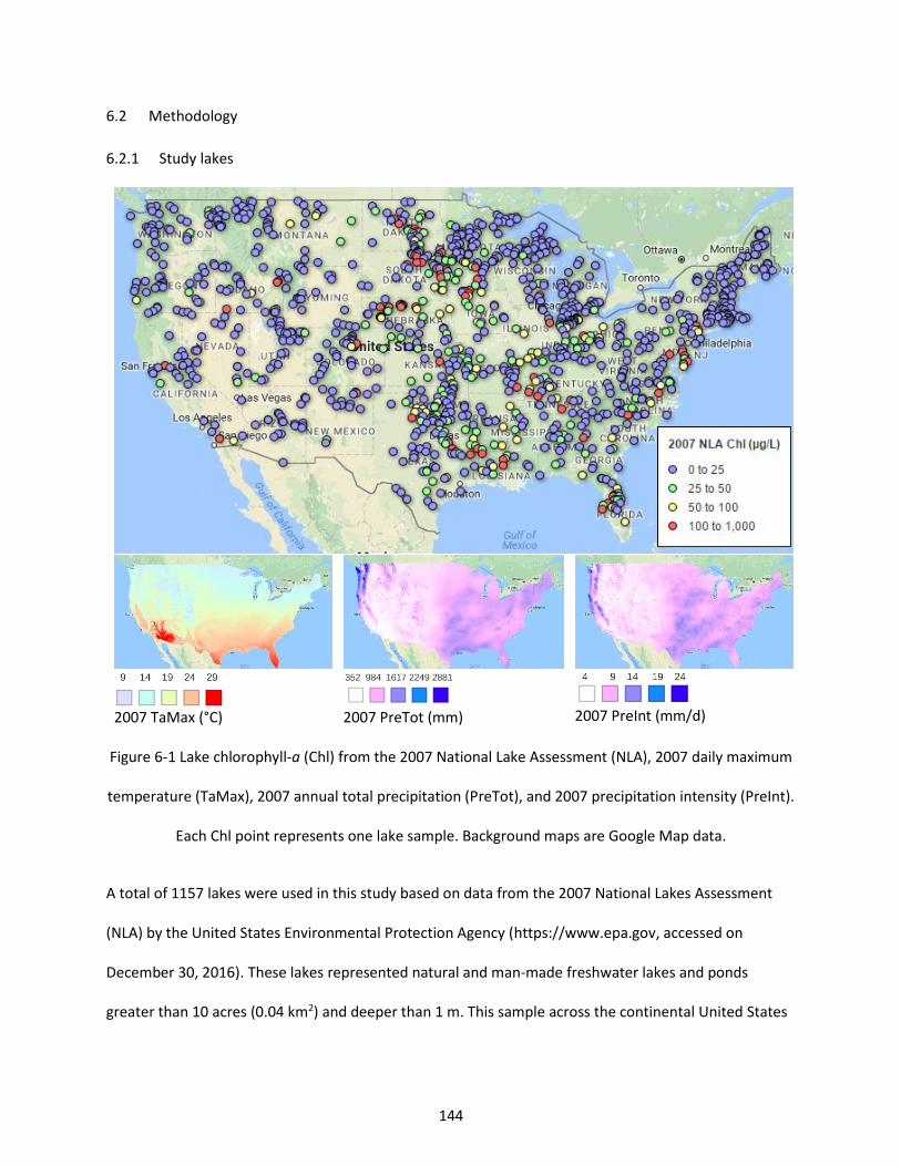
144
6.2 Methodology
6.2.1 Study lakes
2007 TaMax (°C)
2007 PreTot (mm)
2007 PreInt (mm/d)
Figure 6-1 Lake chlorophyll-a (Chl) from the 2007 National Lake Assessment (NLA), 2007 daily maximum
temperature (TaMax), 2007 annual total precipitation (PreTot), and 2007 precipitation intensity (PreInt).
Each Chl point represents one lake sample. Background maps are Google Map data.
A total of 1157 lakes were used in this study based on data from the 2007 National Lakes Assessment
(NLA) by the United States Environmental Protection Agency (https://www.epa.gov, accessed on
December 30, 2016). These lakes represented natural and man-made freshwater lakes and ponds
greater than 10 acres (0.04 km2) and deeper than 1 m. This sample across the continental United States
145
provided a wide range of algal biomass, temperature, precipitation, nutrient, and hydraulic conditions
(Figure 6-1).
6.2.2 Sensitivity and partial dependence analyses
Sensitivity of algal biomass (hereafter referred to as “Chl sensitivity”) was defined as the change in Chl
(dependent variable) along the gradient of an independent variable such as temperature and
precipitation. Boosted regression trees (BRT) were used to quantify algal biomass sensitivity to
temperature and precipitation. BRT models were calibrated with R codes adapted from Elith et al (2008).
The BRT algorithm core functions were from the gbm R package (Ridgeway 2004). Chl sensitivity was
evaluated by one-variable partial dependence analysis. Partial dependence of a predictor in a BRT model
was the response of Chl to the predictor when the other predictors were held at their means. One-
variable partial dependence analysis provided the trend and magnitude of Chl change along the gradient
of one independent variable. One-variable partial dependence analysis used the plot.gbm function from
the gbm R package. The contribution of each predictor in a BRT model was indicated by relative
importance. Relative importance of a predictor in a BRT model is the sum of deviation reduced by each
split using the predictor in the BRT trees, divided by the total deviation reduced by all predictors.
Relative importance was calculated with the summary.gbm function from the gbm R package. The
change of Chl sensitivity over the range of an independent variable, such as Chl sensitivity to
temperature changes over total phosphorus, was evaluated by two-variable partial dependence
analysis, i.e., how Chl sensitivity to one predictor changed with the other predictor when the remaining
predictors were held at their means. This was basically a two-way interaction analysis. In addition to the
range of Chl change, the magnitude of the two-way interaction was also indicated by the Friedman’s H-
statistic index (Friedman and Popescu 2008). The Friedman index ranges from zero to one (100%) with
higher values indicating stronger interactions. For instance, H = 10% indicates the interaction explained
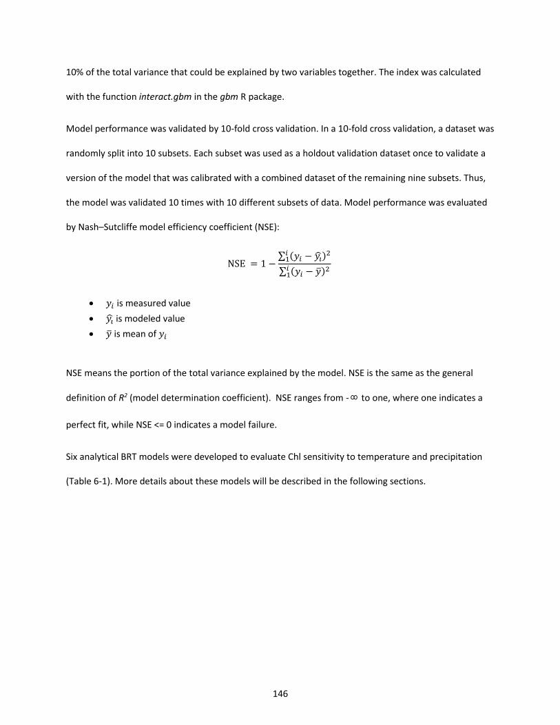
146
10% of the total variance that could be explained by two variables together. The index was calculated
with the function interact.gbm in the gbm R package.
Model performance was validated by 10-fold cross validation. In a 10-fold cross validation, a dataset was
randomly split into 10 subsets. Each subset was used as a holdout validation dataset once to validate a
version of the model that was calibrated with a combined dataset of the remaining nine subsets. Thus,
the model was validated 10 times with 10 different subsets of data. Model performance was evaluated
by Nash–Sutcliffe model efficiency coefficient (NSE):
NSE means the portion of the total variance explained by the model. NSE is the same as the general
definition of R2 (model determination coefficient). NSE ranges from -∞ to one, where one indicates a
perfect fit, while NSE <= 0 indicates a model failure.
Six analytical BRT models were developed to evaluate Chl sensitivity to temperature and precipitation
(Table 6-1). More details about these models will be described in the following sections.
NSE = 1 −∑ (𝑦𝑖 − 𝑦�̂�)
2𝑖1
∑ (𝑦𝑖 − �̅�)2𝑖1
• 𝑦𝑖 is measured value
• 𝑦�̂� is modeled value
• �̅� is mean of 𝑦𝑖
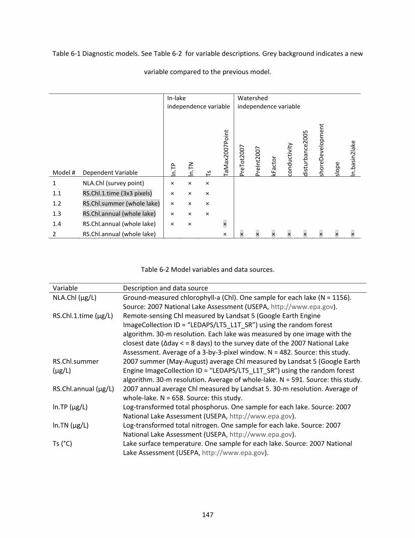
147
Table 6-1 Diagnostic models. See Table 6-2 for variable descriptions. Grey background indicates a new
variable compared to the previous model.
Model # Dependent Variable
In-lake independence variable
Watershed independence variable
ln.T
P
ln.T
N
Ts
TaM
ax2
00
7P
oin
t
Pre
Tot2
00
7
Pre
Int2
00
7
kFac
tor
con
du
ctiv
ity
dis
turb
ance
20
05
sho
reD
evel
op
men
t
slo
pe
ln.b
asin
2la
ke
1 NLA.Chl (survey point) × × ×
1.1 RS.Chl.1.time (3x3 pixels) × × ×
1.2 RS.Chl.summer (whole lake) × × ×
1.3 RS.Chl.annual (whole lake) × × ×
1.4 RS.Chl.annual (whole lake) × × ×
2 RS.Chl.annual (whole lake) × × × × × × × × ×
Table 6-2 Model variables and data sources.
Variable Description and data source
NLA.Chl (µg/L) Ground-measured chlorophyll-a (Chl). One sample for each lake (N = 1156). Source: 2007 National Lake Assessment (USEPA, http://www.epa.gov).
RS.Chl.1.time (µg/L) Remote-sensing Chl measured by Landsat 5 (Google Earth Engine ImageCollection ID = “LEDAPS/LT5_L1T_SR”) using the random forest algorithm. 30-m resolution. Each lake was measured by one image with the closest date (Δday < = 8 days) to the survey date of the 2007 National Lake Assessment. Average of a 3-by-3-pixel window. N = 482. Source: this study.
RS.Chl.summer (µg/L)
2007 summer (May-August) average Chl measured by Landsat 5 (Google Earth Engine ImageCollection ID = “LEDAPS/LT5_L1T_SR”) using the random forest algorithm. 30-m resolution. Average of whole-lake. N = 591. Source: this study.
RS.Chl.annual (µg/L) 2007 annual average Chl measured by Landsat 5. 30-m resolution. Average of whole-lake. N = 658. Source: this study.
ln.TP (µg/L) Log-transformed total phosphorus. One sample for each lake. Source: 2007 National Lake Assessment (USEPA, http://www.epa.gov).
ln.TN (µg/L) Log-transformed total nitrogen. One sample for each lake. Source: 2007 National Lake Assessment (USEPA, http://www.epa.gov).
Ts (°C) Lake surface temperature. One sample for each lake. Source: 2007 National Lake Assessment (USEPA, http://www.epa.gov).
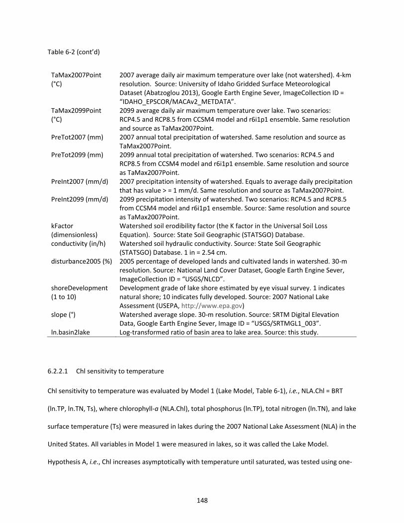
148
Table 6-2 (cont’d)
TaMax2007Point (°C)
2007 average daily air maximum temperature over lake (not watershed). 4-km resolution. Source: University of Idaho Gridded Surface Meteorological Dataset (Abatzoglou 2013), Google Earth Engine Sever, ImageCollection ID = “IDAHO_EPSCOR/MACAv2_METDATA”.
TaMax2099Point (°C)
2099 average daily air maximum temperature over lake. Two scenarios: RCP4.5 and RCP8.5 from CCSM4 model and r6i1p1 ensemble. Same resolution and source as TaMax2007Point.
PreTot2007 (mm) 2007 annual total precipitation of watershed. Same resolution and source as TaMax2007Point.
PreTot2099 (mm) 2099 annual total precipitation of watershed. Two scenarios: RCP4.5 and RCP8.5 from CCSM4 model and r6i1p1 ensemble. Same resolution and source as TaMax2007Point.
PreInt2007 (mm/d) 2007 precipitation intensity of watershed. Equals to average daily precipitation that has value > = 1 mm/d. Same resolution and source as TaMax2007Point.
PreInt2099 (mm/d) 2099 precipitation intensity of watershed. Two scenarios: RCP4.5 and RCP8.5 from CCSM4 model and r6i1p1 ensemble. Source: Same resolution and source as TaMax2007Point.
kFactor (dimensionless)
Watershed soil erodibility factor (the K factor in the Universal Soil Loss Equation). Source: State Soil Geographic (STATSGO) Database.
conductivity (in/h) Watershed soil hydraulic conductivity. Source: State Soil Geographic (STATSGO) Database. 1 in = 2.54 cm.
disturbance2005 (%) 2005 percentage of developed lands and cultivated lands in watershed. 30-m resolution. Source: National Land Cover Dataset, Google Earth Engine Sever, ImageCollection ID = “USGS/NLCD”.
shoreDevelopment (1 to 10)
Development grade of lake shore estimated by eye visual survey. 1 indicates natural shore; 10 indicates fully developed. Source: 2007 National Lake Assessment (USEPA, http://www.epa.gov)
slope (°) Watershed average slope. 30-m resolution. Source: SRTM Digital Elevation Data, Google Earth Engine Sever, Image ID = “USGS/SRTMGL1_003”.
ln.basin2lake Log-transformed ratio of basin area to lake area. Source: this study.
6.2.2.1 Chl sensitivity to temperature
Chl sensitivity to temperature was evaluated by Model 1 (Lake Model, Table 6-1), i.e., NLA.Chl = BRT
(ln.TP, ln.TN, Ts), where chlorophyll-a (NLA.Chl), total phosphorus (ln.TP), total nitrogen (ln.TN), and lake
surface temperature (Ts) were measured in lakes during the 2007 National Lake Assessment (NLA) in the
United States. All variables in Model 1 were measured in lakes, so it was called the Lake Model.
Hypothesis A, i.e., Chl increases asymptotically with temperature until saturated, was tested using one-
149
variable partial dependence analysis between NLA.Chl and Ts. Hypothesis B, i.e., Chl sensitivity to
temperature was regulated by nutrient availability, was tested using two-variable partial dependence
analyses between NLA.Chl, Ts, and each nutrient variable (ln.TP or ln.TN).
6.2.2.2 Chl sensitivity to precipitation
Chl sensitivity to precipitation was evaluated by Model 2 (Watershed Model, Table 6-1), i.e.,
RS.Chl.annual = BRT (TaMax2007Point, PreTot2007, PreInt2007, kFactor, conductivity, disturbance2005,
shoreDevelopment, slope, ln.basin2lake). The variables of this model will be explained in the following
paragraphs. Model 2 was an upscaled version of Model 1: the statistical period of the variables
increased from a summer (sampling duration) to a year; and lake nutrients were indirectly estimated by
precipitation and watershed characteristics. Thus, Model 2 was called the Watershed Model.
The measurement period was scaled up to a year in the Model 2 because precipitation effects on lake
Chl may have time lags that vary lake by lake and watershed by watershed (Chapter 5). Without knowing
the time lags for each specific lake in the study, it was impossible to select precipitation variables to
relate to lake Chl of a specific time. To address this problem, Model 2 used lake Chl and precipitation
conditions during a full year, assuming that annual average Chl was related by BRT to precipitation
conditions within the same year regardless of the time lags. The year of 2007 was picked for Model 2 so
it could be compared best to Model 1, which used 2007 NLA data.
NLA Chl was mostly measured only one time at one location in a lake during summer 2007 and therefore
could not be expected to represent the Chl of a whole year and over the whole lake. So, remote sensing
(RS) was used to estimate Chl. 2007 annual RS Chl (RS.Chl.annual) was derived using Landsat TM 5
(Google Earth Engine Image Collection ID = “LANDSAT/LT5_SR”) and a machine-learning algorithm,
random forest. Landsat images were Land Surface Reflectance with atmospheric correction (Masek et al.
2006). The random forest Chl model was trained with the ground-measured Chl from the 2007 NLA. The
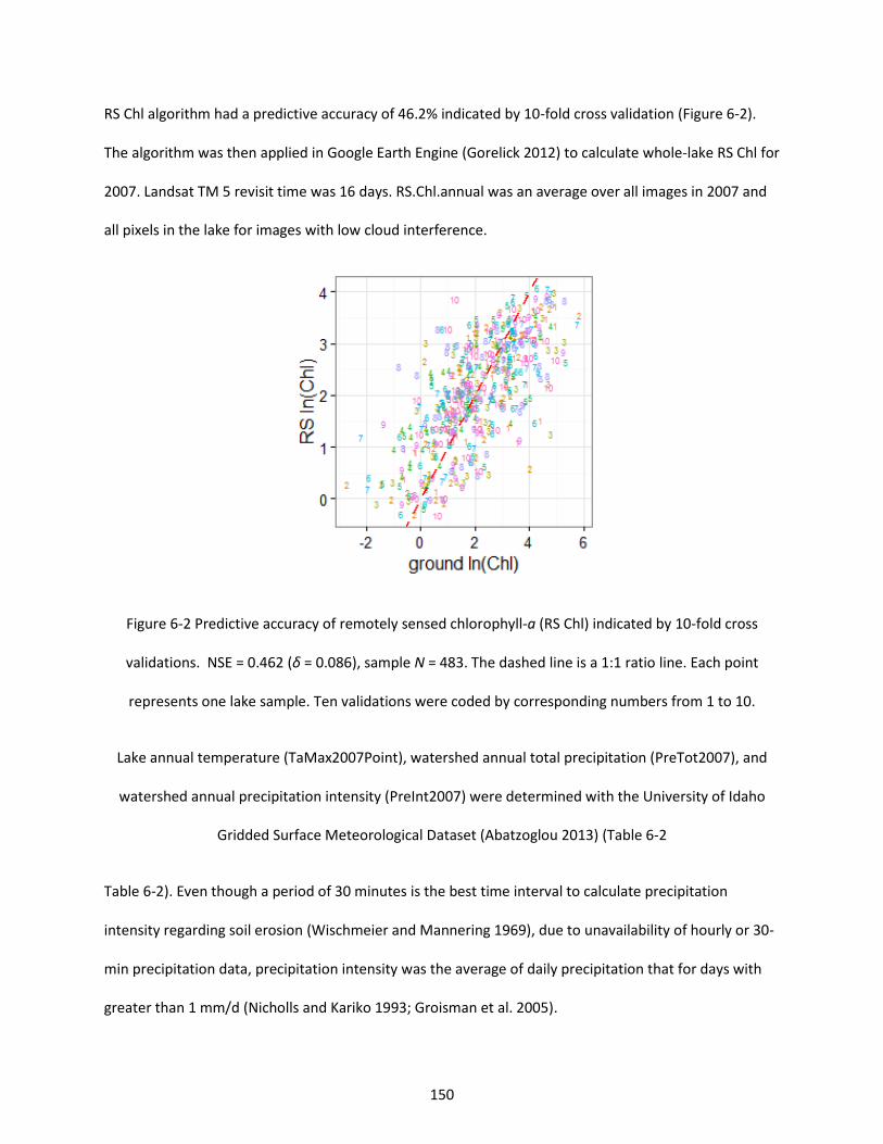
150
RS Chl algorithm had a predictive accuracy of 46.2% indicated by 10-fold cross validation (Figure 6-2).
The algorithm was then applied in Google Earth Engine (Gorelick 2012) to calculate whole-lake RS Chl for
2007. Landsat TM 5 revisit time was 16 days. RS.Chl.annual was an average over all images in 2007 and
all pixels in the lake for images with low cloud interference.
Figure 6-2 Predictive accuracy of remotely sensed chlorophyll-a (RS Chl) indicated by 10-fold cross
validations. NSE = 0.462 (δ = 0.086), sample N = 483. The dashed line is a 1:1 ratio line. Each point
represents one lake sample. Ten validations were coded by corresponding numbers from 1 to 10.
Lake annual temperature (TaMax2007Point), watershed annual total precipitation (PreTot2007), and
watershed annual precipitation intensity (PreInt2007) were determined with the University of Idaho
Gridded Surface Meteorological Dataset (Abatzoglou 2013) (Table 6-2
Table 6-2). Even though a period of 30 minutes is the best time interval to calculate precipitation
intensity regarding soil erosion (Wischmeier and Mannering 1969), due to unavailability of hourly or 30-
min precipitation data, precipitation intensity was the average of daily precipitation that for days with
greater than 1 mm/d (Nicholls and Kariko 1993; Groisman et al. 2005).
151
Nutrient conditions in Model 2 were estimated with precipitation and a set of watershed landscape
variables (Table 6-1). Those landscape variables were soil erodibility factor (kFactor), soil hydraulic
conductivity, percentage of developed and cultivated lands (disturbance2005), lake shore development
(shoreDevelopment), watershed slope (slope), and ratio of basin area to lake area (ln.basin2lake). These
variables were selected from a large variable pool (N = 68) of climate, soil, ecoregion, geology,
hydrology, watershed morphology, lake morphology, and land use/cover, which were similar to the
candidate variables in Olson and Hawkins (2013). Variables were selected by both forward and
backward selection. Redundant variables were eliminated from the nutrient condition model, and were
defined as variables resulting in changes in predictive deviation less than half of one standard error of
the predictive deviation of the full model.
Hypothesis C, i.e., Chl increases with precipitation intensity but decreases with total precipitation, was
tested using one-variable partial dependence analyses between RS.Chl.annual and each precipitation
variable (PreInt2007 or PreTot2007). Hypothesis D, i.e., Chl sensitivity to precipitation intensity was
mediated by natural hydraulic conditions, was tested using two-variable partial dependence analyses
between RS.Chl.annual, PreInt2007, and each natural hydraulic variable (kFactor, conductivity, or slope).
When upscaling the Lake Model to the Watershed Model for the analyses of Chl sensitivity to
precipitation, the model accuracy might be affected by (1) replacing NLA ground-measured Chl with RS
Chl, (2) replacing NLA ground-measured temperature (Ts) with annual air temperature (TaMax2007), or
(3) replacing NLA ground-measured nutrients with precipitation and landscape variables. To evaluate
the variable replacements, four intermediate models (Model 1.1, 1.2, 1.3 and 1.4 in Table 6-1) were built
to compare models in the stepwise transition from Model 1 and Model 2. Specifically:
152
1. Comparing NSE of Models 1 and 1.1 with ground-measured Chl (NLA.Chl) and RS Chl measured
one time (RS.Chl.1.time) being related to ground-measured water temperature, TP, and TN
provided a direct comparison of ground-measured Chl and RS Chl.
2. Comparing NSE of Models 1.1 and 1.2 with RS chl measure one time and RS Chl measured over
the summer (RS.Chl.summer) tested whether multiple measures of RS Chl during a season
provided better model performance than one measure.
3. Comparing NSE of Models 1.2 and 1.3 with RS summer Chl and RS annual Chl (RS.Chl.annual,
Table 6-2) tested whether annual Chl was similarly sensitive to temperature as summer Chl.
4. Comparing NSE of Models 1.3 and 1.4 with NLA ground-measured temperatures (Ts) and annual
air temperatures (TaMax2007) tested whether annual average temperature was better than the
one-time temperature measure.
5. Comparing NSE of Models 1.4 and 2 with in-lake nutrient measurements and watershed nutrient
proxies tested whether in-lake nutrients could be inferred by watershed proxies.
RS.Chl.1.time and RS.Chl.summer were estimated from Landsat 5 using the same algorithm as
RS.Chl.annual (Table 6-2). RS.Chl.1.time was RS Chl of 3×3 pixels with the same locations as NLA.Chl. The
dates of RS.Chl.1.time were the same or close (Δday <= 8 days) to NLA.Chl sampling dates.
RS.Chl.summer was the average of summer (May-Auguest, 2007) RS Chl. Some lakes did not have Chl
values due to cloud cover or no pure water pixels in the Landsat imagery. Most of those lakes were
small. 658, 591, and 482 lakes had RS.Chl.annual, RS.Chl.summer, and RS.Chl.1.time. The number and
identity of lakes was the same when calculating and comparing model performance using NSE.
6.2.3 Future scenario analyses
Future algal biomass was predicted using Model 2 and replacing the 2007 measures of temperature and
precipitation with predictions for 2099. The future temperature and precipitation were based upon two
CO2 emission scenarios, Representative Concentration Pathway (RCP) 4.5 (the “low” emission), and RCP
153
8.5 (the “high” emission). Both scenarios were produced under the fifth Coupled Model
Intercomparison Project (CMIP5) (Taylor, Stouffer, and Meehl 2012). The algal biomass difference
between 2007 and 2099 was evaluated by pairwise t-test, where the paired measurements were 2007
and 2099 Chl for each lake.
6.3 Results
6.3.1 Chl sensitivity to temperature
The Lake Model (Model 1) explained 40.6% (NSE = 0.406, σ = 0.325) of the total variance of ground
measured Chl, indicated by the 10-fold cross validation. Relative importance analyses of variables
showed that most of the model error was reduced by nutrients, i.e. total nitrogen (ln.TN, 64.1% of error
reduction) and total phosphorus (ln.TP, 26.4% of error reduction), while the remaining 9.5% of error
reduction was by lake surface temperature (Ts). One-variable partial independence analysis showed
that sample site Chl increased with Ts. Specifically, when Ts increased from 10 °C (minimum) to 34 °C
(maximum) and the nutrients were controlled at mean levels, Chl increased by 36.3 µg/L. In other
words, Chl sensitivity to Ts was 1.5 µg/(L °C) (Figure 6-3).
Chl sensitivity to Ts increased with total phosphorus and total nitrogen, according to two-variable partial
dependence analyses. Specifically, Chl sensitivity to Ts increased from 0.8 µg/(L °C) to 2.5 µg/(L °C) when
total phosphorus increased from 1 µg/L (minimum) to 479 µg/L (maximum). Chl sensitivity to Ts
increased from 0.8 µg/(L °C) to 4.2 µg/(L °C) when total nitrogen increased from 5 µg/L (minimum) to
26400 µg/L (maximum). Chl sensitivity to Ts did not continually increase with ln.TP or ln.TN at high
concentrations as it did at low concentrations. At high ln.TN, the sensitivity was slightly decreased
(Figure 6-4). Friedman's H-statistic in Model 1 showed that the interaction between Ts and ln.TP
accounted for 27.3% of the total variance explained by Ts and ln.TP, and the interaction between Ts and
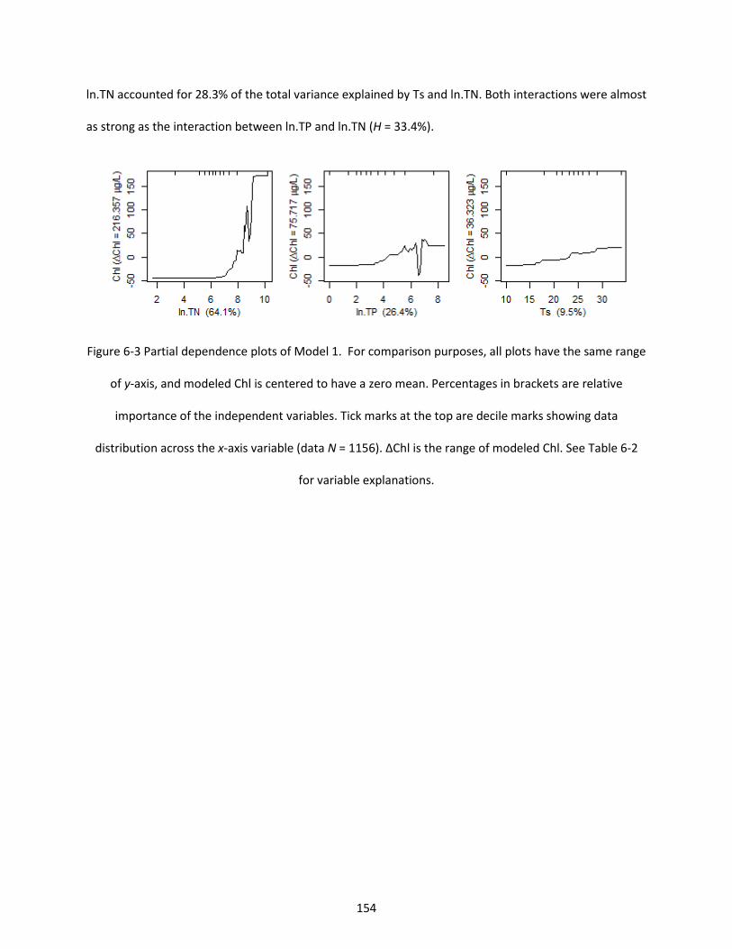
154
ln.TN accounted for 28.3% of the total variance explained by Ts and ln.TN. Both interactions were almost
as strong as the interaction between ln.TP and ln.TN (H = 33.4%).
Figure 6-3 Partial dependence plots of Model 1. For comparison purposes, all plots have the same range
of y-axis, and modeled Chl is centered to have a zero mean. Percentages in brackets are relative
importance of the independent variables. Tick marks at the top are decile marks showing data
distribution across the x-axis variable (data N = 1156). ∆Chl is the range of modeled Chl. See Table 6-2
for variable explanations.
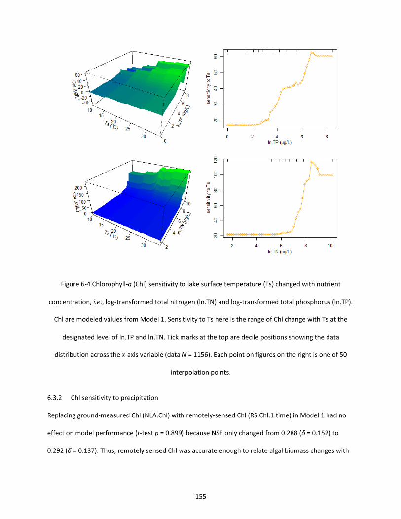
155
Figure 6-4 Chlorophyll-a (Chl) sensitivity to lake surface temperature (Ts) changed with nutrient
concentration, i.e., log-transformed total nitrogen (ln.TN) and log-transformed total phosphorus (ln.TP).
Chl are modeled values from Model 1. Sensitivity to Ts here is the range of Chl change with Ts at the
designated level of ln.TP and ln.TN. Tick marks at the top are decile positions showing the data
distribution across the x-axis variable (data N = 1156). Each point on figures on the right is one of 50
interpolation points.
6.3.2 Chl sensitivity to precipitation
Replacing ground-measured Chl (NLA.Chl) with remotely-sensed Chl (RS.Chl.1.time) in Model 1 had no
effect on model performance (t-test p = 0.899) because NSE only changed from 0.288 (δ = 0.152) to
0.292 (δ = 0.137). Thus, remotely sensed Chl was accurate enough to relate algal biomass changes with
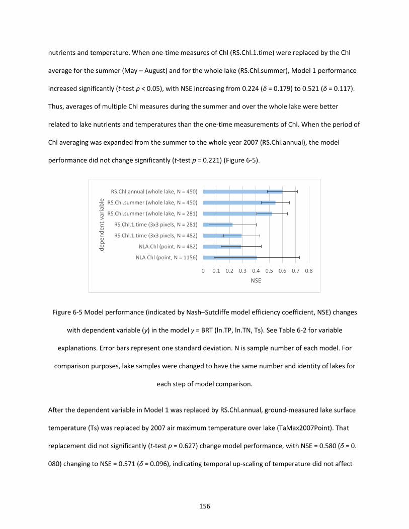
156
nutrients and temperature. When one-time measures of Chl (RS.Chl.1.time) were replaced by the Chl
average for the summer (May – August) and for the whole lake (RS.Chl.summer), Model 1 performance
increased significantly (t-test p < 0.05), with NSE increasing from 0.224 (δ = 0.179) to 0.521 (δ = 0.117).
Thus, averages of multiple Chl measures during the summer and over the whole lake were better
related to lake nutrients and temperatures than the one-time measurements of Chl. When the period of
Chl averaging was expanded from the summer to the whole year 2007 (RS.Chl.annual), the model
performance did not change significantly (t-test p = 0.221) (Figure 6-5).
Figure 6-5 Model performance (indicated by Nash–Sutcliffe model efficiency coefficient, NSE) changes
with dependent variable (y) in the model y = BRT (ln.TP, ln.TN, Ts). See Table 6-2 for variable
explanations. Error bars represent one standard deviation. N is sample number of each model. For
comparison purposes, lake samples were changed to have the same number and identity of lakes for
each step of model comparison.
After the dependent variable in Model 1 was replaced by RS.Chl.annual, ground-measured lake surface
temperature (Ts) was replaced by 2007 air maximum temperature over lake (TaMax2007Point). That
replacement did not significantly (t-test p = 0.627) change model performance, with NSE = 0.580 (δ = 0.
080) changing to NSE = 0.571 (δ = 0.096), indicating temporal up-scaling of temperature did not affect
0 0.1 0.2 0.3 0.4 0.5 0.6 0.7 0.8
NLA.Chl (point, N = 1156)
NLA.Chl (point, N = 482)
RS.Chl.1.time (3x3 pixels, N = 482)
RS.Chl.1.time (3x3 pixels, N = 281)
RS.Chl.summer (whole lake, N = 281)
RS.Chl.summer (whole lake, N = 450)
RS.Chl.annual (whole lake, N = 450)
NSE
dep
end
ent
vari
able
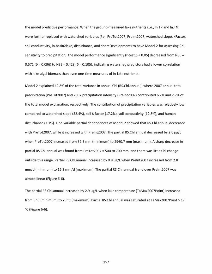
157
the model predictive performance. When the ground-measured lake nutrients (i.e., ln.TP and ln.TN)
were further replaced with watershed variables (i.e., PreTot2007, PreInt2007, watershed slope, kFactor,
soil conductivity, ln.basin2lake, disturbance, and shoreDevelopment) to have Model 2 for assessing Chl
sensitivity to precipitation, the model performance significantly (t-test p < 0.05) decreased from NSE =
0.571 (δ = 0.096) to NSE = 0.428 (δ = 0.105), indicating watershed predictors had a lower correlation
with lake algal biomass than even one-time measures of in-lake nutrients.
Model 2 explained 42.8% of the total variance in annual Chl (RS.Chl.annual), where 2007 annual total
precipitation (PreTot2007) and 2007 precipitation intensity (PreInt2007) contributed 6.7% and 2.7% of
the total model explanation, respectively. The contribution of precipitation variables was relatively low
compared to watershed slope (32.4%), soil K factor (17.2%), soil conductivity (12.8%), and human
disturbance (7.1%). One-variable partial dependences of Model 2 showed that RS.Chl.annual decreased
with PreTot2007, while it increased with PreInt2007. The partial RS.Chl.annual decreased by 2.0 µg/L
when PreTot2007 increased from 32.5 mm (minimum) to 2960.7 mm (maximum). A sharp decrease in
partial RS.Chl.annual was found from PreTot2007 = 500 to 700 mm, and there was little Chl change
outside this range. Partial RS.Chl.annual increased by 0.8 µg/L when PreInt2007 increased from 2.8
mm/d (minimum) to 16.3 mm/d (maximum). The partial RS.Chl.annual trend over PreInt2007 was
almost linear (Figure 6-6).
The partial RS.Chl.annual increased by 2.9 µg/L when lake temperature (TaMax2007Point) increased
from 5 °C (minimum) to 29 °C (maximum). Partial RS.Chl.annual was saturated at TaMax2007Point > 17
°C (Figure 6-6).
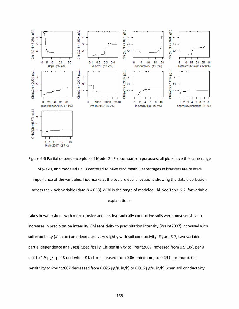
158
Figure 6-6 Partial dependence plots of Model 2. For comparison purposes, all plots have the same range
of y-axis, and modeled Chl is centered to have zero mean. Percentages in brackets are relative
importance of the variables. Tick marks at the top are decile locations showing the data distribution
across the x-axis variable (data N = 658). ∆Chl is the range of modeled Chl. See Table 6-2 for variable
explanations.
Lakes in watersheds with more erosive and less hydraulically conductive soils were most sensitive to
increases in precipitation intensity. Chl sensitivity to precipitation intensity (PreInt2007) increased with
soil erodibility (K factor) and decreased very slightly with soil conductivity (Figure 6-7, two-variable
partial dependence analyses). Specifically, Chl sensitivity to PreInt2007 increased from 0.9 µg/L per K
unit to 1.5 µg/L per K unit when K factor increased from 0.06 (minimum) to 0.49 (maximum). Chl
sensitivity to PreInt2007 decreased from 0.025 µg/(L in/h) to 0.016 µg/(L in/h) when soil conductivity
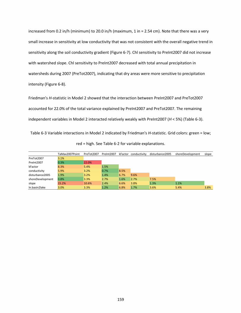
159
increased from 0.2 in/h (minimum) to 20.0 in/h (maximum, 1 in = 2.54 cm). Note that there was a very
small increase in sensitivity at low conductivity that was not consistent with the overall negative trend in
sensitivity along the soil conductivity gradient (Figure 6-7). Chl sensitivity to PreInt2007 did not increase
with watershed slope. Chl sensitivity to PreInt2007 decreased with total annual precipitation in
watersheds during 2007 (PreTot2007), indicating that dry areas were more sensitive to precipitation
intensity (Figure 6-8).
Friedman's H-statistic in Model 2 showed that the interaction between PreInt2007 and PreTot2007
accounted for 22.0% of the total variance explained by PreInt2007 and PreTot2007. The remaining
independent variables in Model 2 interacted relatively weakly with PreInt2007 (H < 5%) (Table 6-3).
Table 6-3 Variable interactions in Model 2 indicated by Friedman's H-statistic. Grid colors: green = low;
red = high. See Table 6-2 for variable explanations.
TaMax2007Point PreTot2007 PreInt2007 kFactor conductivity disturbance2005 shoreDevelopment slope
PreTot2007 3.1%
PreInt2007 0.3% 22.0%
kFactor 8.3% 5.4% 1.5%
conductivity 5.9% 3.2% 0.7% 8.5%
disturbance2005 1.9% 3.2% 1.4% 6.7% 9.6%
shoreDevelopment 0.8% 3.3% 2.7% 1.6% 2.7% 7.5%
slope 15.2% 10.6% 2.4% 6.6% 3.8% 1.3% 1.1%
ln.basin2lake 3.0% 3.3% 1.2% 6.8% 1.7% 3.6% 5.4% 3.8%
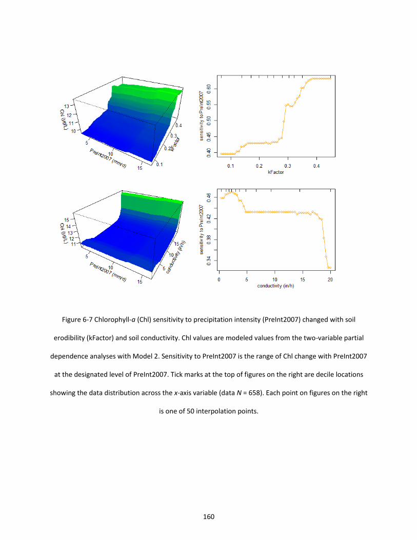
160
Figure 6-7 Chlorophyll-a (Chl) sensitivity to precipitation intensity (PreInt2007) changed with soil
erodibility (kFactor) and soil conductivity. Chl values are modeled values from the two-variable partial
dependence analyses with Model 2. Sensitivity to PreInt2007 is the range of Chl change with PreInt2007
at the designated level of PreInt2007. Tick marks at the top of figures on the right are decile locations
showing the data distribution across the x-axis variable (data N = 658). Each point on figures on the right
is one of 50 interpolation points.
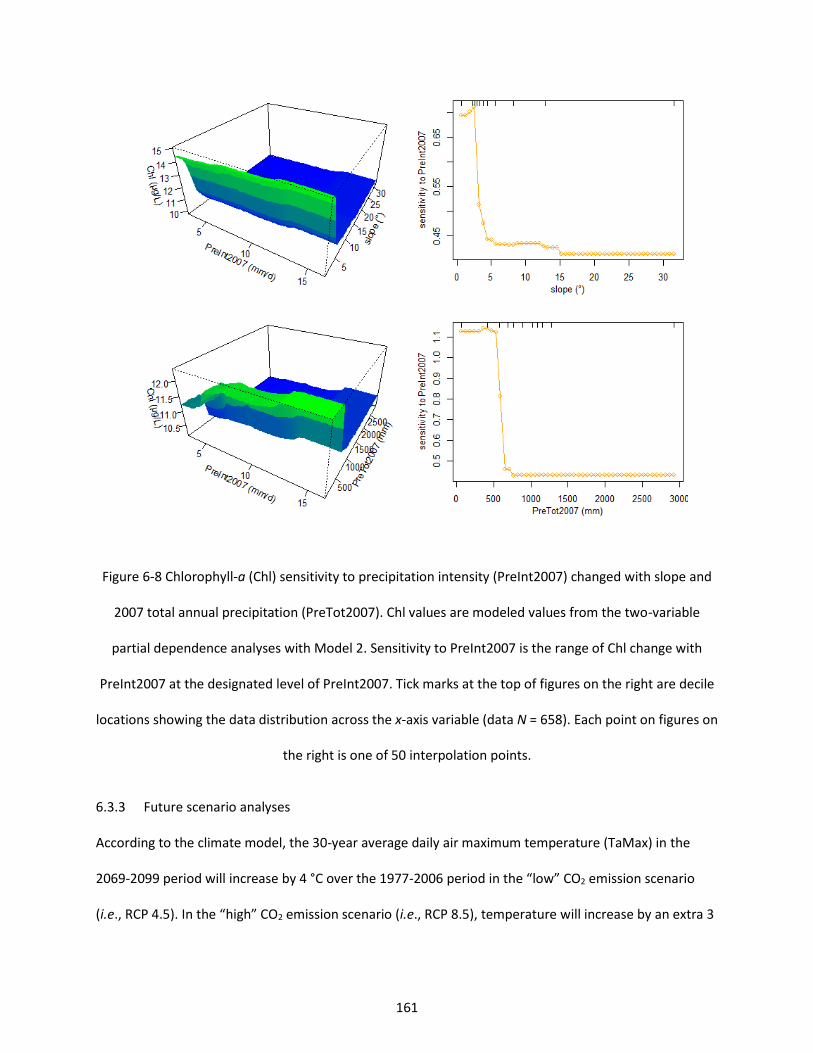
161
Figure 6-8 Chlorophyll-a (Chl) sensitivity to precipitation intensity (PreInt2007) changed with slope and
2007 total annual precipitation (PreTot2007). Chl values are modeled values from the two-variable
partial dependence analyses with Model 2. Sensitivity to PreInt2007 is the range of Chl change with
PreInt2007 at the designated level of PreInt2007. Tick marks at the top of figures on the right are decile
locations showing the data distribution across the x-axis variable (data N = 658). Each point on figures on
the right is one of 50 interpolation points.
6.3.3 Future scenario analyses
According to the climate model, the 30-year average daily air maximum temperature (TaMax) in the
2069-2099 period will increase by 4 °C over the 1977-2006 period in the “low” CO2 emission scenario
(i.e., RCP 4.5). In the “high” CO2 emission scenario (i.e., RCP 8.5), temperature will increase by an extra 3
162
°C on top of the “low” emission scenario. Annual total precipitation (PreTot) at the end of this century
(2069-2099) will increase by 20% over the 1977-2006 level in the “low” CO2 emission scenario. All
watersheds will get wetter, but the increase in wet areas is higher. In the “high” CO2 emission scenario,
the total precipitation will increase by an additional 18 mm on the top of the “low” emission scenario.
Precipitation intensity (PreInt) in 2069-2099 will increase by 10% over the 1977-2006 period in the “low”
CO2 emission scenario. In the “high” CO2 emission scenario, the precipitation intensity will increase by an
additional 10% on top of the “low” emission scenario, indicating more extreme precipitation conditions
in the future climate (Figure 6-9).
Using one year (2099) of future temperature and precipitation variables might not represent the future
climate indicated by 30-year averages due to interannual variability. TaMax in 2099 (RCP 4.5) was higher
than TaMax in 2007 by 3.5 °C; whereas, the 30-year (2069-2099) average TaMax was higher than TaMax
in 2007 by 4 °C. Total precipitation in 2099 (RCP 4.5) was higher than total precipitation in 2007 by 30%;
whereas total precipitation in 2069-2099 was higher than total precipitation in 2007 by 20%. No
significant change (pairwise t-test p = 0.258) was found between precipitation intensity of 2007 and
2099; whereas the change in the 30-year averages was 10%. The magnitudes of the yearly changes in
TaMax and total precipitation were similar to the 30-year average changes. However, the change of
yearly precipitation intensity had a different trend than the 30-year average trend (Figure 6-9).
However, the scenario analyses were based on 2099 annual predictions instead of 2069-2099 average,
because Model 2 was trained using annual variables. Replacing 2007 measured variables with the 2099
annual predictions (i.e., TaMax2099Point, PreTot2099, and PreInt2099) as the inputs of Model 2, 2099
lake Chl was significantly (pairwise t-test p < 0.05) greater than 2007 fitted Chl in both scenarios.
Specifically, in the “low” emission scenario, average lake Chl increased 0.8 µg/L, while in the “high”
emission scenario average lake Chl increased 1.2 µg/L. Chl in the “high” emission scenario was
significantly (pairwise t-test p < 0.05) higher than in the “low” emission scenario. The predicted Chl
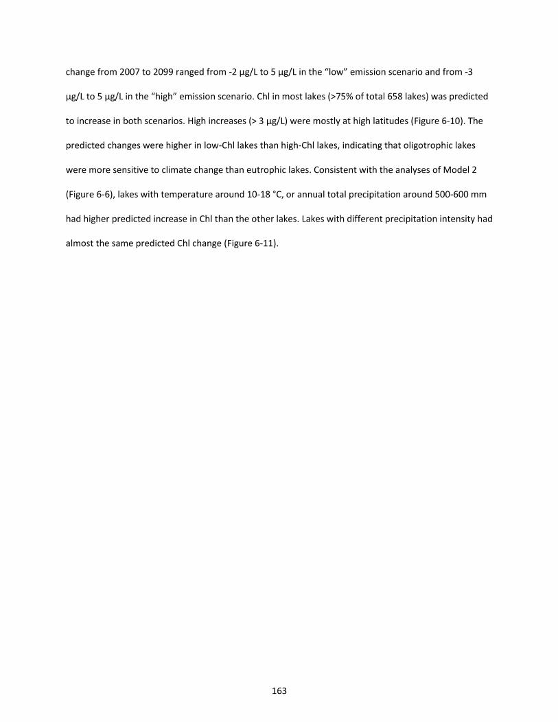
163
change from 2007 to 2099 ranged from -2 µg/L to 5 µg/L in the “low” emission scenario and from -3
µg/L to 5 µg/L in the “high” emission scenario. Chl in most lakes (>75% of total 658 lakes) was predicted
to increase in both scenarios. High increases (> 3 µg/L) were mostly at high latitudes (Figure 6-10). The
predicted changes were higher in low-Chl lakes than high-Chl lakes, indicating that oligotrophic lakes
were more sensitive to climate change than eutrophic lakes. Consistent with the analyses of Model 2
(Figure 6-6), lakes with temperature around 10-18 °C, or annual total precipitation around 500-600 mm
had higher predicted increase in Chl than the other lakes. Lakes with different precipitation intensity had
almost the same predicted Chl change (Figure 6-11).
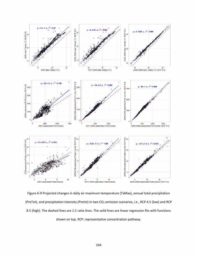
164
Figure 6-9 Projected changes in daily air maximum temperature (TaMax), annual total precipitation
(PreTot), and precipitation intensity (PreInt) in two CO2 emission scenarios, i.e., RCP 4.5 (low) and RCP
8.5 (high). The dashed lines are 1:1 ratio lines. The solid lines are linear regression fits with functions
shown on top. RCP: representative concentration pathway.
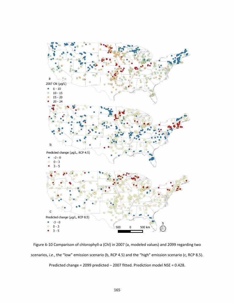
165
Figure 6-10 Comparison of chlorophyll-a (Chl) in 2007 (a, modeled values) and 2099 regarding two
scenarios, i.e., the “low” emission scenario (b, RCP 4.5) and the “high” emission scenario (c, RCP 8.5).
Predicted change = 2099 predicted – 2007 fitted. Prediction model NSE = 0.428.
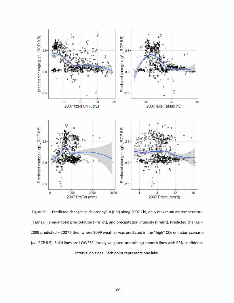
166
Figure 6-11 Predicted changes in chlorophyll-a (Chl) along 2007 Chl, daily maximum air temperature
(TaMax,), annual total precipitation (PreTot), and precipitation intensity (PreInt). Predicted change =
2099 predicted – 2007 fitted, where 2099 weather was predicted in the “high” CO2 emission scenario
(i.e. RCP 8.5). Solid lines are LOWESS (locally weighted smoothing) smooth lines with 95% confidence
interval on sides. Each point represents one lake.
167
6.4 Discussion
6.4.1 Chl increased with temperature but regulated by nutrients (Hypotheses A & B)
Algal growth follows Arrhenius and Michaelis–Menten enzymatic kinetics, where growth rate increases
with temperature and nutrients exponentially, but the rate of increase decreases with temperature and
nutrients (Gotham and Rhee 1981; Raven and Geider 1988). However, it gets more complicated when
applying the kinetics to algal biomass that treats all algal species as a whole. First, “enzyme”
concentration and spectrum are not constant any more, but change with algal species abundance and
composition. Second, temperature can change enzymatic properties (“temperature acclimation”), which
in turn change algal biomass sensitivities to temperature and nutrients (Davison 1991). Third,
“substrate” concentration is not constant. Nutrients are depleted when algal biomass increases and are
replenished by algal decomposition, which is also regulated by temperature and other substrate
concentrations (White et al. 1991). Although lab experiments have provided evidence supporting these
theories, they remain unclear in a wide range of complex aquatic systems with an almost infinite
number of possible combinations within/between algal species and involving nutrients, thermal
stratification, grazing, and decomposers. The findings of this paper have partly filled this knowledge gap.
The partial dependence analyses in Model 1 (Lake Model) and Model 2 (Watershed Model) illustrated
that Chl increased with temperature, and was saturated at high temperature, consistent with the
enzymatic kinetics responding to temperature, and Hypothesis A. More than half of Chl variation was
not explained in both Model 1 and Model 2 (NSE < 0.5). That might be due to the complex realities
mentioned above, e.g., temperature acclimation, and concentration variations in enzymes and
substrates. For nutrient regulation, the results confirmed Hypothesis B. Note that nutrient
concentrations themselves might not be the only regulation factors. Other factors include (1) nutrient
limitation, (2) grazing, and (3) light. Specifically: (1) When phosphorus availability is limited, Chl
sensitivity to temperature increases with total phosphorus (TP). When phosphorus is replete, Chl
168
sensitivity to temperature is not controlled by TP, but other factors, such as grazing and light. The same
rule applies to total nitrogen (TN). This might explain the results that Chl sensitivity to temperature did
not increase with increasing TN or TP concentration. (2) In addition to that, at higher nutrient levels,
algal production could be higher possibly resulting in a higher grazing rate, which offsets the increase in
Chl sensitivity with temperature (Carpenter, Kitchell, and Hodgson 1985). Moreover, higher TP may
favor accumulation of nitrogen-fixing cyanobacteria, which are more resistant to grazers than the other
species, while higher nitrogen does not give nitrogen-fixing cyanobacteria an advantage. Species
regulation of nutrient limitation might cause different nutrient regulation effects than were shown in
Model 1, where Chl sensitivity to temperature slightly decreased at high TN. (3) Light might be another
factor that co-varies with TN and TP and regulates Chl sensitivity to temperature. It is common that algal
growth is limited by light after precipitation events, which generate higher turbidity as well as nutrient
concentrations in inflows (Jones and Knowlton 2005). Higher turbidity could also reduce Chl sensitivity
to temperature at higher nutrient levels as was shown in Model 1.
In summary, Chl increased with temperature, but high variability is expected due to the complex
interactions among multiple abiotic and biotic factors. Chl sensitivity to temperature increased with
nutrients only when the nutrients were limiting. Chl sensitivity to temperature may not increase at high
nutrient levels due to grazing and light limitation, as well as nutrient saturation.
6.4.2 Chl sensitivity to precipitation (Hypothesis C) and its variations with natural hydraulic conditions
(Hypothesis D)
Rainfall-induced high stream flows usually have higher total nitrogen and phosphorus concentrations
than baseflow, and a few heavy rainfall events may carry most of nutrient loading to a lake over a year
(McDiffett et al. 1989; Coser 1989). However, as reviewed by Reichwaldt and Ghadouani (2012), algal
biomass could respond to precipitation in different ways. Algal biomass may increase after precipitation
events for higher nutrients and de-stratification (i.e., vertical mixing) (Kebede and Belay 1994; Nõges et
169
al. 2011). Opposite results may be seen for higher turbidity (including higher turbidity of inflows, and
turbidity caused by inflow turbulence in shallow lakes), or dilution (especially flushing effects in
reservoirs and estuaries) (Harris and Baxter 1996; Bouvy et al. 2003; Paerl et al. 2014). No change may
occur for a mismatch between nutrient availability and light availability (Minor, Forsman, and Guildford
2014). This study separated precipitation into total precipitation and precipitation intensity to study
precipitation impacts on algal biomass. The results from Model 2 were consistent with Hypothesis C, i.e.,
Chl increased with precipitation intensity but decreased with total precipitation. It was interesting that
Chl decreased with total precipitation when precipitation intensity was controlled as the mean. That
might be due to the dilution effect (nutrient concentration decrease) mentioned above, or a rinsing
effect (total nutrient loading decrease) related to a high frequency of precipitation events, i.e., the
nutrient generation in soils was slower than the nutrient loss due to frequent precipitation events. The
rinsing effect has also been hypothesized in a stream study using spatial statistical models similar to this
study (Olson and Hawkins 2013). It would be interesting to test whether nutrient loading to lakes
decreases with higher precipitation frequency in a time series in future studies.
Soil erosion increases with soil erodibility and decreases with soil hydraulic conductivity. Regarding soil
erodibility and conductivity, the results in the two-variable partial dependence analyses of Model 2 were
generally consistent with Hypothesis D, i.e., Chl sensitivity to precipitation intensity is regulated by
natural hydraulic conditions, except that Chl sensitivity to precipitation intensity did not always decrease
with higher soil hydraulic conductivity. There was a very small positive effect at low conductivity. The
small positive effect might be due to other factors that co-varied with soil hydraulic conductivity, such as
soil vegetation, which was not included in the model (Numata et al. 2003). An extra analysis showed
that watershed vegetation, indicated by normalized difference vegetation index (NDVI), decreased with
soil conductivity with a similar jump at low soil hydraulic conductivity (Figure 6-12). Adding NDVI in
Model 2, the magnitude of the positive effect at low conductivity decreased by half, further suggesting
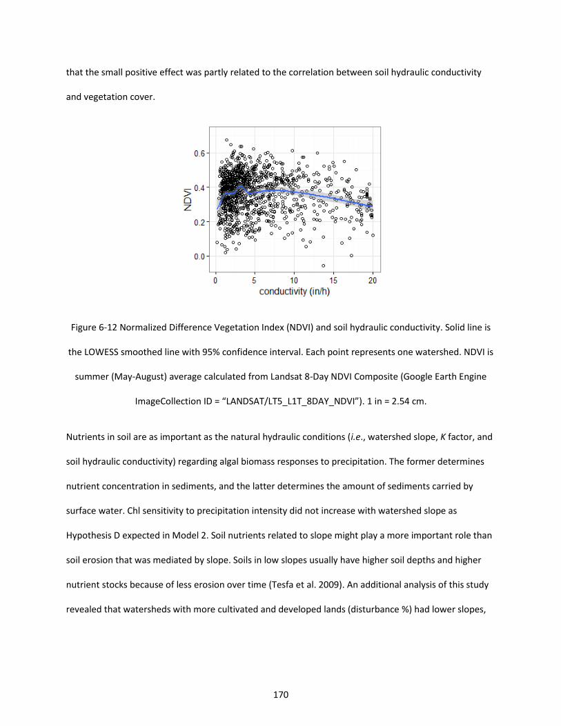
170
that the small positive effect was partly related to the correlation between soil hydraulic conductivity
and vegetation cover.
Figure 6-12 Normalized Difference Vegetation Index (NDVI) and soil hydraulic conductivity. Solid line is
the LOWESS smoothed line with 95% confidence interval. Each point represents one watershed. NDVI is
summer (May-August) average calculated from Landsat 8-Day NDVI Composite (Google Earth Engine
ImageCollection ID = “LANDSAT/LT5_L1T_8DAY_NDVI”). 1 in = 2.54 cm.
Nutrients in soil are as important as the natural hydraulic conditions (i.e., watershed slope, K factor, and
soil hydraulic conductivity) regarding algal biomass responses to precipitation. The former determines
nutrient concentration in sediments, and the latter determines the amount of sediments carried by
surface water. Chl sensitivity to precipitation intensity did not increase with watershed slope as
Hypothesis D expected in Model 2. Soil nutrients related to slope might play a more important role than
soil erosion that was mediated by slope. Soils in low slopes usually have higher soil depths and higher
nutrient stocks because of less erosion over time (Tesfa et al. 2009). An additional analysis of this study
revealed that watersheds with more cultivated and developed lands (disturbance %) had lower slopes,
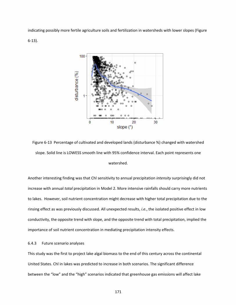
171
indicating possibly more fertile agriculture soils and fertilization in watersheds with lower slopes (Figure
6-13).
Figure 6-13 Percentage of cultivated and developed lands (disturbance %) changed with watershed
slope. Solid line is LOWESS smooth line with 95% confidence interval. Each point represents one
watershed.
Another interesting finding was that Chl sensitivity to annual precipitation intensity surprisingly did not
increase with annual total precipitation in Model 2. More intensive rainfalls should carry more nutrients
to lakes. However, soil nutrient concentration might decrease with higher total precipitation due to the
rinsing effect as was previously discussed. All unexpected results, i.e., the isolated positive effect in low
conductivity, the opposite trend with slope, and the opposite trend with total precipitation, implied the
importance of soil nutrient concentration in mediating precipitation intensity effects.
6.4.3 Future scenario analyses
This study was the first to project lake algal biomass to the end of this century across the continental
United States. Chl in lakes was predicted to increase in both scenarios. The significant difference
between the “low” and the “high” scenarios indicated that greenhouse gas emissions will affect lake
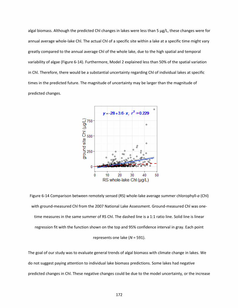
172
algal biomass. Although the predicted Chl changes in lakes were less than 5 µg/L, these changes were for
annual average whole-lake Chl. The actual Chl of a specific site within a lake at a specific time might vary
greatly compared to the annual average Chl of the whole lake, due to the high spatial and temporal
variability of algae (Figure 6-14). Furthermore, Model 2 explained less than 50% of the spatial variation
in Chl. Therefore, there would be a substantial uncertainty regarding Chl of individual lakes at specific
times in the predicted future. The magnitude of uncertainty may be larger than the magnitude of
predicted changes.
Figure 6-14 Comparison between remotely sensed (RS) whole-lake average summer chlorophyll-a (Chl)
with ground-measured Chl from the 2007 National Lake Assessment. Ground-measured Chl was one-
time measures in the same summer of RS Chl. The dashed line is a 1:1 ratio line. Solid line is linear
regression fit with the function shown on the top and 95% confidence interval in gray. Each point
represents one lake (N = 591).
The goal of our study was to evaluate general trends of algal biomass with climate change in lakes. We
do not suggest paying attention to individual lake biomass predictions. Some lakes had negative
predicted changes in Chl. These negative changes could be due to the model uncertainty, or the increase
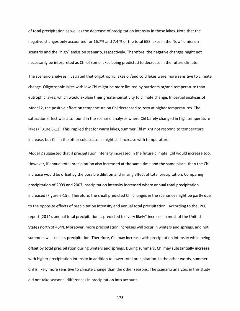
173
of total precipitation as well as the decrease of precipitation intensity in those lakes. Note that the
negative changes only accounted for 16.7% and 7.4 % of the total 658 lakes in the “low” emission
scenario and the “high” emission scenario, respectively. Therefore, the negative changes might not
necessarily be interpreted as Chl of some lakes being predicted to decrease in the future climate.
The scenario analyses illustrated that oligotrophic lakes or/and cold lakes were more sensitive to climate
change. Oligotrophic lakes with low Chl might be more limited by nutrients or/and temperature than
eutrophic lakes, which would explain their greater sensitivity to climate change. In partial analyses of
Model 2, the positive effect on temperature on Chl decreased to zero at higher temperatures. The
saturation effect was also found in the scenario analyses where Chl barely changed in high temperature
lakes (Figure 6-11). This implied that for warm lakes, summer Chl might not respond to temperature
increase, but Chl in the other cold seasons might still increase with temperature.
Model 2 suggested that if precipitation intensity increased in the future climate, Chl would increase too.
However, if annual total precipitation also increased at the same time and the same place, then the Chl
increase would be offset by the possible dilution and rinsing effect of total precipitation. Comparing
precipitation of 2099 and 2007, precipitation intensity increased where annual total precipitation
increased (Figure 6-15). Therefore, the small predicted Chl changes in the scenarios might be partly due
to the opposite effects of precipitation intensity and annual total precipitation. According to the IPCC
report (2014), annual total precipitation is predicted to “very likely” increase in most of the United
States north of 45°N. Moreover, more precipitation increases will occur in winters and springs, and hot
summers will see less precipitation. Therefore, Chl may increase with precipitation intensity while being
offset by total precipitation during winters and springs. During summers, Chl may substantially increase
with higher precipitation intensity in addition to lower total precipitation. In the other words, summer
Chl is likely more sensitive to climate change than the other seasons. The scenario analyses in this study
did not take seasonal differences in precipitation into account.
174
Figure 6-15 Predicted changes in precipitation intensity (PreInt change = Year 2099 – Year 2007), and
predicted changes in annual total precipitation (PreTot). 2099 precipitation projections are based on the
“high” emission scenario. Solid line is linear regression fit (r2 = 0.542) with 95% confidence interval in
gray.
6.4.4 Long-term temperature and precipitation effects
Algal biomass may increase with temperature due to higher growth rate of algae at higher temperatures
within a certain range (usually < 27 °C) (Lürling et al. 2013). But it is less recognized that temperature
may indirectly affect algal biomass by changing nutrient loading. Temperature may change nutrient
loading through its effects on watershed evapotranspiration, soil nutrients, and vegetation cover as
discussed below. (1) In six watersheds of Susquehanna River (USA), the future nutrient loadings were
predicted to decrease in summer for higher temperature using GWLF (Generalized Watershed Loading
Function) model, due to higher evapotranspiration and lower stream flow; but to increase during winter
for earlier snowmelt. Overall, annual nutrient loadings did not consistently increase or decrease in six
watersheds (Chang, Evans, and Easterling 2001). (2) It is still debated whether soil carbon (correlated
175
with soil nutrients) decreases or not with increasing temperature due to warming-induced acceleration
of decomposition and increases of plant nutrient assimilation (Davidson and Janssens 2006).
It is also not clear how soil organic matter changes may affect dissolved organic matter transport to
rivers and lakes (Kalbitz et al. 2000). If carbon decomposition does indeed increase more with
temperature than carbon assimilation does (Post et al. 1982), then organic nitrogen loadings may
decrease due to higher denitrification (Marshall and Randhir 2008). But on the other hand, lower soil pH
due to more active decomposition of anaerobic bacteria may provide more bioactive phosphorus
available to algae in rivers and lakes. Higher rates of ammonia nitrification especially in fertilized farms
with sufficient water may also reduce soil pH and provide more bioactive phosphorus (Stark and
Firestone 1995). (3) Vegetation cover may increase with temperature in wet areas (Kardol et al. 2010)
but decrease with warmer temperatures and drought in dry areas (Breshears et al. 2005). The former
may happen in winter and spring when temperature and precipitation are predicted to increase across
most of North America. The latter may happen in summer when temperature is predicted to increase
with unchanged or lower precipitation in the future climate according to IPCC (2014). The changes of
vegetation cover over space and season may cause changes in soil erosion and thereby lake algal
biomass. Inflow nutrient changes due to temperature are short-term processes. However, soil nutrients
and vegetation cover may take more than a year to show significant changes. Impacts of temperature
on nutrient loadings on a long-term scale are under-researched.
Compared to the short-term effects due to individual precipitation events, the long-term effects of
precipitation on algal biomass are also under-researched. The results in this study have revealed a
negative correlation between Chl and annual total precipitation. Continuous flushing of rainfall may
rinse nutrients from soils. On the other hand, at certain level of precipitation intensity, higher annual
total precipitation indicates more wet days, which favor vegetation growth (Ji and Peters 2003;
Donohue, McVICAR, and Roderick 2009) and thereby soil stabilization and nutrient accumulation
176
(Renard et al. 1991). It is unknown whether nutrient loading would increase due to vegetation growth,
or decrease due to soil stabilization and rinsing effect. Nonetheless, it may take years of precipitation
change to see significant vegetation changes and flushing effects.
Additionally, after nutrient loadings are changed by vegetation and soil nutrients, it may take years (e.g.,
10-15 years for total phosphorus, and < 5 years for total nitrogen based on a study of 35 cases) for lakes
to reach a new nutrient equilibrium, considering internal nutrient legacies (Jeppesen et al. 2005). The
internal nutrients might have caused the 2007 precipitation to have a lower contribution in Model 2
than slope and soil properties. Specifically, 2007 precipitation might be related more to 2007 nutrient
loadings while slope and soil properties might be more related to internal nutrients. A greater
importance of internal nutrient sources might cause more contributions of slope and soil properties in
Model 2. With all considerations of long-term terrestrial processes and in-lake nutrient legacies, the
time lag of temperature and precipitation effects on algal biomass may be longer than anticipated.
In Model 2, slope and soil properties explained much more annual Chl spatial variation than the 2007
precipitation. Slope and soil properties were the most important variables. Overall evidence suggested
that lake algal biomass might depend more on internal nutrients than yearly nutrient loadings. In other
words, short-term changes in precipitation patterns may not be as important as we think. This finding
agrees with some studies in individual lakes, which indicated that internal bioactive phosphorus was as
importance as new inputs (Auer et al. 1993; Nowlin, Evarts, and Vanni 2005).
In summary, climate change may affect algal biomass through both short-term or long-term
mechanisms, which were not discriminated in our models. This study used the method of space as
substitution of time, assuming each lake was in an equilibrium status under the influence of
temperature and precipitation. These levels could reflect long- or short-term responses depending on
local variations. Therefore, the sensitivity results only suggested how much algal biomass might change
177
with climate change, but did not provide information about how soon the change would happen after
climate change.
6.4.5 Climate change mitigation
From a climate change mitigation point of view, the Chl partial analyses in Model 2 (Figure 6-6) suggest
that reducing human disturbance (indicated by urban and agricultural lands) might offset Chl increases
due to temperature or precipitation. Chl decreased with less disturbance in Model 2. In Model 1, Chl
also decreased with TN and TP, which is related to human disturbance. How much change in human
disturbance would be enough to counterweight temperature rise? Taking 2 µg/L of annual average Chl
increase for example, it may require the percentage of urban and agricultural lands to decrease from
100% to 0% to neutralize the temperature effect (Figure 6-6). It seems impractical to solely rely on
controlling urbanization and agricultural activities to mitigate the risk of algal blooms due to climate
change.
6.5 Conclusion
Algal biomass in lakes across the US increases with temperature. Chl sensitivity to temperature increases
with increasing nutrient availability (i.e., TN and TP). Thus, the regulation of Chl sensitivity to
temperature by nutrients is most important when nutrients are limiting.
Algal biomass increases with higher precipitation intensity, but it decreases with higher annual total
precipitation (or precipitation frequency). Precipitation effects are mediated by soil properties including
soil erodibility, soil hydraulic conductivity, and perhaps soil nutrient content as well.
Algal biomass will increase with the future climate change. More Chl increase is expected in the “high”
CO2 emission scenario than the “low” scenario. Lakes with low Chl or/and low temperature are more
sensitive to climate change.

178
Acknowledgement
This work was supported by the U.S. Environmental Protection Agency (EPA) under Grant R835203. The
views and opinions expressed in this article are those of the authors and do not necessarily reflect the
official policy or position of U.S. EPA, or any other agency of the U.S. government.

179
REFERENCES
180
REFERENCES
Abatzoglou, John T. 2013. “Development of Gridded Surface Meteorological Data for Ecological Applications and Modelling.” International Journal of Climatology 33 (1): 121–31. doi:10.1002/joc.3413.
Anderson, Donald M. 1989. “Toxic Algal Blooms and Red Tides: A Global Perspective.” Red Tides: Biology, Environmental Science and Toxicology, 11–16.
Auer, Mt, Na Johnson, Mr Penn, and Sw Effler. 1993. “Measurement and Verification of Rates of Sediment Phosphorus Release for a Hypereutrophic Urban Lake.” Hydrobiologia 253 (1–3): 301–9. doi:10.1007/BF00050750.
Blois, Jessica L., John W. Williams, Matthew C. Fitzpatrick, Stephen T. Jackson, and Simon Ferrier. 2013. “Space Can Substitute for Time in Predicting Climate-Change Effects on Biodiversity.” Proceedings of the National Academy of Sciences 110 (23): 9374–79. doi:10.1073/pnas.1220228110.
Bouvy, Marc, Silvia M. Nascimento, Renato J. R. Molica, Andrea Ferreira, Vera Huszar, and Sandra M. F. O. Azevedo. 2003. “Limnological Features in Tapacurá Reservoir (Northeast Brazil) during a Severe Drought.” Hydrobiologia 493 (1–3): 115–30. doi:10.1023/A:1025405817350.
Breshears, David D., Neil S. Cobb, Paul M. Rich, Kevin P. Price, Craig D. Allen, Randy G. Balice, William H. Romme, et al. 2005. “Regional Vegetation Die-off in Response to Global-Change-Type Drought.” Proceedings of the National Academy of Sciences of the United States of America 102 (42): 15144–48. doi:10.1073/pnas.0505734102.
Carpenter, Stephen R., James F. Kitchell, and James R. Hodgson. 1985. “Cascading Trophic Interactions and Lake Productivity.” BioScience 35 (10): 634–39. doi:10.2307/1309989.
Chang, Heejun, Barry M. Evans, and David R. Easterling. 2001. “The Effects of Climate Change on Stream Flow and Nutrient Loading.” JAWRA Journal of the American Water Resources Association 37 (4): 973–85. doi:10.1111/j.1752-1688.2001.tb05526.x.
Conley, Daniel J., Hans W. Paerl, Robert W. Howarth, Donald F. Boesch, Sybil P. Seitzinger, Karl E. Havens, Christiane Lancelot, Gene E. Likens, and others. 2009. “Controlling Eutrophication: Nitrogen and Phosphorus.” Science 323 (5917): 1014–1015.
Coser, PR. 1989. “Nutrient Concentration-Flow Relationships and Loads in the South Pine River, South-Eastern Queensland. I. Phosphorus Loads.” Marine and Freshwater Research 40 (6): 613–30.
Davidson, Eric A., and Ivan A. Janssens. 2006. “Temperature Sensitivity of Soil Carbon Decomposition and Feedbacks to Climate Change.” Nature 440 (7081): 165–73. doi:10.1038/nature04514.
181
Davison, Ian R. 1991. “Environmental Effects on Algal Photosynthesis: Temperature.” Journal of Phycology 27 (1): 2–8. doi:10.1111/j.0022-3646.1991.00002.x.
Dodds, Walter K., Wes W. Bouska, Jeffrey L. Eitzmann, Tyler J. Pilger, Kristen L. Pitts, Alyssa J. Riley, Joshua T. Schloesser, and Darren J. Thornbrugh. 2009. “Eutrophication of U.S. Freshwaters: Analysis of Potential Economic Damages.” Environmental Science & Technology 43 (1): 12–19. doi:10.1021/es801217q.
Donohue, Randall J., Tim R. McVICAR, and Michael L. Roderick. 2009. “Climate-Related Trends in Australian Vegetation Cover as Inferred from Satellite Observations, 1981–2006.” Global Change Biology 15 (4): 1025–39. doi:10.1111/j.1365-2486.2008.01746.x.
Elith, J., J. R. Leathwick, and T. Hastie. 2008. “A Working Guide to Boosted Regression Trees.” Journal of Animal Ecology 77 (4): 802–13. doi:10.1111/j.1365-2656.2008.01390.x.
Falconer, I.R., A.M. Beresford, and M.T. Runnegar. 1983. “Evidence of Liver Damage by Toxin from a Bloom of the Blue-Green Alga, Microcystis Aeruginosa.” The Medical Journal of Australia 1 (11): 511–14.
Friedman, Jerome H. 2001. “Greedy Function Approximation: A Gradient Boosting Machine.” Annals of Statistics, 1189–1232.
Friedman, Jerome H., and Bogdan E. Popescu. 2008. “Predictive Learning via Rule Ensembles.” The Annals of Applied Statistics 2 (3): 916–54. doi:10.1214/07-AOAS148.
Gorelick, Noel. 2012. “Google Earth Engine.” In AGU Fall Meeting Abstracts, 1:4. http://adsabs.harvard.edu/abs/2012AGUFM.U31A..04G.
Gotham, Ivan J., and G-Yull Rhee. 1981. “Comparative Kinetic Studies of Phosphate-Limited Growth and Phosphate Uptake in Phytoplankton in Continuous Culture.” Journal of Phycology 17 (3): 257–65. doi:10.1111/j.1529-8817.1981.tb00848.x.
Groisman, P. Y., R. W. Knight, D. R. Easterling, T. R. Karl, G. C. Hegerl, and V. a. N. Razuvaev. 2005. “Trends in Intense Precipitation in the Climate Record.” Journal of Climate 18 (9): 1326–50. doi:10.1175/JCLI3339.1.
Harris, G.P., and G. Baxter. 1996. “Interannual Variability in Phytoplankton Biomass and Species Composition in a Subtropical Reservoir.” Freshwater Biology 35 (3): 545–60.
Hudnell, H. Kenneth. 2010. “The State of U.S. Freshwater Harmful Algal Blooms Assessments, Policy and Legislation.” Toxicon, Harmful Algal Blooms and Natural Toxins in Fresh and Marine Waters -- Exposure, occurrence, detection, toxicity, control, management and policy, 55 (5): 1024–34. doi:10.1016/j.toxicon.2009.07.021.
IPCC. 2014. “IPCC Fifth Assessment Report Climate Change 2014:Impacts, Adaptation, and Vulnerability.” IPCC-XXXVIII/DOC.4. (Intergovernmental Panel on Climate Change). http://www.ipcc.ch/.
182
Jeppesen, Erik, Martin Søndergaard, Jens Peder Jensen, Karl E. Havens, Orlane Anneville, Laurence Carvalho, Michael F. Coveney, et al. 2005. “Lake Responses to Reduced Nutrient Loading – an Analysis of Contemporary Long-Term Data from 35 Case Studies.” Freshwater Biology 50 (10): 1747–71. doi:10.1111/j.1365-2427.2005.01415.x.
Ji, Lei, and Albert J. Peters. 2003. “Assessing Vegetation Response to Drought in the Northern Great Plains Using Vegetation and Drought Indices.” Remote Sensing of Environment 87 (1): 85–98. doi:10.1016/S0034-4257(03)00174-3.
Jones, John R., and Matthew F. Knowlton. 2005. “Chlorophyll Response to Nutrients and Non-Algal Seston in Missouri Reservoirs and Oxbow Lakes.” Lake and Reservoir Management 21 (3): 361–71. doi:10.1080/07438140509354441.
Kalbitz, K., Stephen Solinger, J.-H. Park, B. Michalzik, and Egbert Matzner. 2000. “Controls on the Dynamics of Dissolved Organic Matter in Soils: A Review.” Soil Science 165 (4): 277–304.
Kardol, Paul, Courtney E. Campany, Lara Souza, Richard J. Norby, Jake F. Weltzin, and Aimee T. Classen. 2010. “Climate Change Effects on Plant Biomass Alter Dominance Patterns and Community Evenness in an Experimental Old-Field Ecosystem.” Global Change Biology 16 (10): 2676–87. doi:10.1111/j.1365-2486.2010.02162.x.
Kebede, Elizabeth, and Amha Belay. 1994. “Species Composition and Phytoplankton Biomass in a Tropical African Lake (Lake Awassa, Ethiopia).” Hydrobiologia 288 (1): 13–32. doi:10.1007/BF00006802.
Lewis, William M., and Wayne A. Wurtsbaugh. 2008. “Control of Lacustrine Phytoplankton by Nutrients: Erosion of the Phosphorus Paradigm.” International Review of Hydrobiology 93 (4–5): 446–65. doi:10.1002/iroh.200811065.
Lewis, William M., Wayne A. Wurtsbaugh, and Hans W. Paerl. 2011. “Rationale for Control of Anthropogenic Nitrogen and Phosphorus to Reduce Eutrophication of Inland Waters.” Environmental Science & Technology 45 (24): 10300–305. doi:10.1021/es202401p.
Lopez, C. B., E. B. Jewett, Q. Dortch, B. T. Walton, and H. K. Hudnell. 2008. “Scientific Assessment of Freshwater Harmful Algal Blooms.” Monograph or Serial Issue. http://www.cop.noaa.gov/stressors/extremeevents/hab/habhrca/FreshwaterReport_final_2008.pdf.
Lürling, Miquel, Fassil Eshetu, Elisabeth J. Faassen, Sarian Kosten, and Vera L. M. Huszar. 2013. “Comparison of Cyanobacterial and Green Algal Growth Rates at Different Temperatures.” Freshwater Biology 58 (3): 552–59. doi:10.1111/j.1365-2427.2012.02866.x.
Marshall, Eric, and Timothy Randhir. 2008. “Effect of Climate Change on Watershed System: A Regional Analysis.” Climatic Change 89 (3–4): 263–80. doi:10.1007/s10584-007-9389-2.
183
Masek, Jeffrey G., Eric F. Vermote, Nazmi E. Saleous, Robert Wolfe, Forrest G. Hall, Karl F. Huemmrich, Feng Gao, Jonathan Kutler, and Teng-Kui Lim. 2006. “A Landsat Surface Reflectance Dataset for North America, 1990-2000.” Geoscience and Remote Sensing Letters, IEEE 3 (1): 68–72.
McDiffett, Wayne F., Andrew W. Beidler, Thomas F. Dominick, and Kenneth D. McCrea. 1989. “Nutrient Concentration-Stream Discharge Relationships during Storm Events in a First-Order Stream.” Hydrobiologia 179 (2): 97–102. doi:10.1007/BF00007596.
Minor, Elizabeth C., Brandy Forsman, and Stephanie J. Guildford. 2014. “The Effect of a Flood Pulse on the Water Column of Western Lake Superior, USA.” Journal of Great Lakes Research 40 (2): 455–62. doi:10.1016/j.jglr.2014.03.015.
Nicholls, Neville, and Alex Kariko. 1993. “East Australian Rainfall Events: Interannual Variations, Trends, and Relationships with the Southern Oscillation.” Journal of Climate 6 (6): 1141–52. doi:10.1175/1520-0442(1993)006<1141:EAREIV>2.0.CO;2.
Nõges, Peeter, Tiina Nõges, Michela Ghiani, Fabrizio Sena, Roswitha Fresner, Maria Friedl, and Johanna Mildner. 2011. “Increased Nutrient Loading and Rapid Changes in Phytoplankton Expected with Climate Change in Stratified South European Lakes: Sensitivity of Lakes with Different Trophic State and Catchment Properties.” Hydrobiologia 667 (1): 255–70. doi:10.1007/s10750-011-0649-9.
Nowlin, Weston H., Jennifer L. Evarts, and Michael J. Vanni. 2005. “Release Rates and Potential Fates of Nitrogen and Phosphorus from Sediments in a Eutrophic Reservoir.” Freshwater Biology 50 (2): 301–22. doi:10.1111/j.1365-2427.2004.01316.x.
Numata, I., J. V. Soares, D. A. Roberts, F. C. Leonidas, O. A. Chadwick, and G. T. Batista. 2003. “Relationships among Soil Fertility Dynamics and Remotely Sensed Measures across Pasture Chronosequences in Rondônia, Brazil.” Remote Sensing of Environment, Large Scale Biosphere Atmosphere Experiment in Amazonia, 87 (4): 446–55. doi:10.1016/j.rse.2002.07.001.
Olson, John R., and Charles P. Hawkins. 2013. “Developing Site-Specific Nutrient Criteria from Empirical Models.” Freshwater Science 32 (3): 719–40. doi:10.1899/12-113.1.
Paerl, Hans W., Nathan S. Hall, Benjamin L. Peierls, and Karen L. Rossignol. 2014. “Evolving Paradigms and Challenges in Estuarine and Coastal Eutrophication Dynamics in a Culturally and Climatically Stressed World.” Estuaries and Coasts 37 (2): 243–58. doi:10.1007/s12237-014-9773-x.
Paerl, Hans W., and Jef Huisman. 2008. “Blooms Like It Hot.” Science 320 (5872): 57–58. doi:10.1126/science.1155398.
Paerl, Hans W., and Valerie J. Paul. 2012. “Climate Change: Links to Global Expansion of Harmful Cyanobacteria.” Water Research, Cyanobacteria: Impacts of climate change on occurrence, toxicity and water quality management, 46 (5): 1349–63. doi:10.1016/j.watres.2011.08.002.
184
Pickett, Steward T. A. 1989. “Space-for-Time Substitution as an Alternative to Long-Term Studies.” In Long-Term Studies in Ecology, edited by Gene E. Likens, 110–35. Springer New York. http://link.springer.com/chapter/10.1007/978-1-4615-7358-6_5.
Post, Wilfred M., William R. Emanuel, Paul J. Zinke, and Alan G. Stangenberger. 1982. “Soil Carbon Pools and World Life Zones.” Nature 298 (5870): 156–59. doi:10.1038/298156a0.
Raven, John A., and Richard J. Geider. 1988. “Temperature and Algal Growth.” New Phytologist 110 (4): 441–61. doi:10.1111/j.1469-8137.1988.tb00282.x.
Reichwaldt, Elke S., and Anas Ghadouani. 2012. “Effects of Rainfall Patterns on Toxic Cyanobacterial Blooms in a Changing Climate: Between Simplistic Scenarios and Complex Dynamics.” Water Research, Cyanobacteria: Impacts of climate change on occurrence, toxicity and water quality management, 46 (5): 1372–93. doi:10.1016/j.watres.2011.11.052.
Renard, Kenneth G., George R. Foster, Glenn A. Weesies, and Jeffrey P. Porter. 1991. “RUSLE: Revised Universal Soil Loss Equation.” Journal of Soil and Water Conservation 46 (1): 30–33.
Ridgeway, Greg. 2004. “The Gbm Package.” R Foundation for Statistical Computing, Vienna, Austria. http://132.180.15.2/math/statlib/R/CRAN/doc/packages/gbm.pdf.
Schindler, David W. 2012. “The Dilemma of Controlling Cultural Eutrophication of Lakes.” Proc. R. Soc. B 279 (1746): 4322–33. doi:10.1098/rspb.2012.1032.
Schindler, David W., and R. E. Hecky. 2009. “Eutrophication: More Nitrogen Data Needed.” Science 324: 721–722.
Stark, J. M., and M. K. Firestone. 1995. “Mechanisms for Soil Moisture Effects on Activity of Nitrifying Bacteria.” Applied and Environmental Microbiology 61 (1): 218–21.
Taylor, Karl E., Ronald J. Stouffer, and Gerald A. Meehl. 2012. “An Overview of Cmip5 and the Experiment Design.” Bulletin of the American Meteorological Society 93 (4): 485–98.
Tesfa, Teklu K., David G. Tarboton, David G. Chandler, and James P. McNamara. 2009. “Modeling Soil Depth from Topographic and Land Cover Attributes.” Water Resources Research 45 (10): W10438. doi:10.1029/2008WR007474.
White, Paul A., Jacob Kalff, Joseph B. Rasmussen, and Josep M. Gasol. 1991. “The Effect of Temperature and Algal Biomass on Bacterial Production and Specific Growth Rate in Freshwater and Marine Habitats.” Microbial Ecology 21 (1): 99–118. doi:10.1007/BF02539147.
Whitehead, P. G., R. L. Wilby, R. W. Battarbee, M. Kernan, and A. J. Wade. 2009. “A Review of the Potential Impacts of Climate Change on Surface Water Quality.” Hydrological Sciences Journal 54 (1): 101–23. doi:10.1623/hysj.54.1.101.
Wischmeier, Walter H., and J. V. Mannering. 1969. “Relation of Soil Properties to Its Erodibility.” Soil Science Society of America Journal 33 (1): 131–137.
185
7 SUMMARY
7.1 Dissertation summary
Harmful algal blooms are emerging hazards with a dramatic increase of public attention in recent years.
Climate change is projected to increase temperature, change seasonal distribution of precipitation,
increase frequency and intensity of droughts and floods, and increase annual precipitation in most areas
in the United States. The overarching goal of this dissertation research was to advance our knowledge of
the relationship between climate change and algal blooms. I hypothesized that the probability of algal
blooms will increase with climate change, because of rising temperature and higher nutrient loads to
lakes carried by runoff from more intense precipitation.
7.1.1 Model development
Historic satellite images can be used to derive long-term records of algal abundance, which provide
sufficient duration that they can be related to changes in climate. Most existing algorithms for
estimating chlorophyll-a in inland lakes using remote sensing imagery are based on linear regression and
are not accurate enough for long-term and large-scale assessment of algal biomass in lakes. Two mature
machine-learning algorithms—boosted regression trees (BRT) and random forest (RF)—were tested
using 383 Landsat TM/ETM+ images that covered 483 lakes across the continental United States. Both
algorithms showed significant improvements over traditional linear regression. Specifically, the BRT
model explained 46% of the total variance in ground-measured chlorophyll-a in lakes measured by 10-
fold cross validation, but the linear regression model only explained 40%. The RF model had similar
performance to the BRT model, explaining 45% of the total variance. Chlorophyll-a measures based on
the machine-learning algorithms were tested in western Lake Erie and the results indicated that these
measures are good enough to identify spatial distribution and temporal duration of the algal blooms.
Moreover, the correlation between remotely sensed chlorophyll-a and total phosphorus was as strong
as the correlation between ground-measured chlorophyll-a and total phosphorus, especially when
186
remote sensing chlorophyll-a was the average of multiple measures. These assessment results imply
that Landsat TM/ETM+ with machine-learning algorithms can be used to evaluate the historic conditions
of algal abundance in lakes across the continental United States, and relate those conditions to climate
change. The RF algorithm has been applied in Google Earth Engine—which has stored all Landsat data
and is fast in data processing by using cloud calculation—to automatically and rapidly produce long-term
whole-lake algal biomass for any lake of interest that is covered by Landsat TM/ETM+ images.
Applications outside the continental United States need to be further verified and lake areas measured
should be larger than one image pixel (30 m × 30 m) at least.
7.1.2 Interference from optically active agents in water
One of the greatest concerns about using remote sensing to measure chlorophyll-a in lakes is the
variable optical interference from combinations of algae, suspended sediments, and colored dissolved
organic matter (CDOM). Machine-learning algorithms are new in remote sensing of chlorophyll-a. The
effects of sediments and CDOM on chlorophyll-a in empirical models using remote sensing imagery in
inland waters have rarely been determined on a broad spatial and temporal scale, where sediments and
CDOM conditions greatly vary across lakes and seasons. The results based on a 24-year (1989-2012) in-
situ dataset in 39 reservoirs across Missouri (USA) showed that modeled chlorophyll-a based on BRT had
systematic bias related to sediments or CDOM. However, sediments and CDOM only explained
respectively 6.7% and 4.6% of the total residual variance. What’s more, the errors were unlikely caused
by sediments or CDOM, because the errors did not increase with higher concentrations of sediments or
CDOM as was expected in the theoretical simulations. There are two possible explanations for the
model insensitivity to sediments and CDOM. First, the machine-learning algorithm (i.e., BRT) may have
discriminated the sediments and CDOM effects on chlorophyll-a measurements by using band and band
ratios and considering the interactions between algae, sediments and CDOM. Second, the BRT model
explained 35% of the total variance in the measured chlorophyll-a, so the accuracy might not be high
187
enough to capture the effects of sediments or CDOM on the remote sensing signal. These results
indicate that sediments and CDOM should not introduce systematic bias in using remote sensing
chlorophyll-a to relate climate change to algal blooms.
7.1.3 Interference from the atmosphere
Another major concern about using remote sensing to measure chlorophyll-a in lakes is the interference
by atmospheric effects. The atmospheric signal may account for as much as 90% of at-sensor radiance
over waters, so the atmospheric interference on remote sensing of algal abundance is expected to be
substantial in lakes where atmospheric conditions greatly vary over time and space. Landsat surface
reflectance products corrected for atmospheric effects are new and have recently been made freely
available. The products are provisional and the atmospheric correction method was designed to meet
the needed accuracy for land (not water) surface reflectance. To test whether the atmospheric
corrections had improved the quality of Landsat TM/ETM+ images for remote sensing of inland water,
these products were examined by using ground-measured water samples during 1989-2012 in 39
reservoirs of Missouri (USA). Except for the thermal band (Band 6), all bands and band ratios were
investigated separately by using the model: Bi = RF (chlorophyll-a, sediments, and CDOM), where Bi is
the band or band ratio, RF is random forest, and the dependent variables are three optically active
agents in water. The model validation R2 for bands and band ratios without the correction ranged from 0
to 0.633 (mean = 0.271). The model validation R2 for bands and band ratios with the atmospheric
corrections ranged from 0 to 0.577 (mean = 0.226), which was not better than the models without the
atmospheric corrections, indicating the atmospheric corrections did not improve the imagery signals
related to chlorophyll-a, sediments, and CDOM. As a result, there was no significant difference in
estimates of chlorophyll-a, sediments, or CDOM concentrations using the corrected or uncorrected
Landsat TM/ETM+ images. Specifically, the optical agents—chlorophyll-a, sediments, and CDOM—were
measured by using the model: Optical agent = RF (bands, band ratios), where the agent is chlorophyll-a,
188
sediments, or CDOM. The model validation R2 was 0.312 (chlorophyll-a), 0.505 (sediments), and 0.731
(CDOM) with the uncorrected bands and band ratios. The model validation R2 was 0.329 (chlorophyll-a),
0.508 (sediments), and 0.733 (CDOM) with the corrected bands and band ratios. The atmospheric
correction method that was applied in the new Landsat TM/ETM+ products may be an improvement for
land applications but not for remote sensing of the optical characteristics of water, where radiance
signals are much weaker than those from land surfaces.
7.1.4 Time series analyses
The relationship between climate change and algal blooms was evaluated in four reservoirs in Missouri
(USA), where 28 years (1984-2011) of algal biomass data were generated from Landsat TM images. Both
changes in land use/cover and climate can affect algal biomass in lakes. Land use/cover barely changed
over the 28 years in the study watersheds, providing an opportunity to relate climate to algal biomass
given the minor effects from changes in land use/cover. Algal biomass was studied on four temporal
scales: 28-years, yearly, seasonal, and daily. Four of 13 reservoir zones had significant increases in
annual temperature (lake surface) during the 28 years, but only one of them (1/4) had significant
increases in annual algal biomass. All 13 reservoir zones had significant increases in annual precipitation
intensity (mm/d), but only four of them (4/13) had significant increases in annual algal biomass. Annual
total precipitation did not show significant increases or decreases over the years. The trend of annual
algal biomass did not necessarily agree with the trend of annual temperature or annual precipitation
(sum or intensity) during the 28 years, indicating that the trend of annual algal biomass was not
determined by only one factor, i.e., annual temperature, annual total precipitation, or annual
precipitation intensity. During the 28 years, algal biomass peaked usually in summers and was low in the
other cold months. Summer algal biomass significantly increased with summer temperature in only one
of 13 reservoir zones, indicated by univariate linear regression. However, annual algal biomass
significantly increased with annual temperature in six of 13 reservoir zones. It implies summer algal
189
biomass may saturate with rising temperature but the algal growth season may expand resulting in an
increase in mean annual algal biomass. Summer algal biomass had a mixed response (positive, negative,
or insignificant) to summer precipitation (sum and intensity). Summer algal biomass significantly
increased with spring precipitation intensity in four of 13 reservoir zones, and significantly increased
with spring total precipitation in five of 13 reservoir zones, indicating that summer algal biomass may
increase with climate change where more spring precipitation is predicted. Annual algal biomass
significantly increased with annual total precipitation in four of 13 reservoir zones, and significantly
increased with annual precipitation intensity in four of 13 reservoir zones, indicating that annual algal
biomass may increase with climate change where precipitation is predicted to be wetter and extremer.
These predicted changes of algal biomass related to climate impacts are based on univariate linear
regression, and the uncertainty is high since only 1-6, not all 13, of the models were statistically
significant. The multivariate models that considered both temperature and precipitation as well as their
time lags at the same time further revealed that daily temperature and daily precipitation together
explained 0-51% (varying with reservoir zones) of the total variance in daily chlorophyll-a during the 28
years. The daily temperature contributed more than 90% in the model performance, indicating that the
daily precipitation effects on daily algal biomass was relatively small after removing its correlation with
daily temperature. This study suggests that climate change impacts on algal biomass may vary with time
scale: daily, seasonal, annual, or longer-term. These findings are limited to four Missouri reservoirs and
may not be applied to other lakes with different conditions of nutrients, turbidity (light), lake
morphology, soil hydraulic condition, soil nutrients, and land use/cover.
7.1.5 Spatial Analyses
Impacts of climate change on algal blooms were evaluated in 1156 lakes in the continental United
States, using a space-for-time substitution method. This study assumed that the trajectories of algal
biomass changes along temperature and precipitation gradients over space would be the same as the
190
algal biomass changes with climate over time. Lake algal biomass was characterized by both ground-
measured and remotely-sensed algal biomass.
First, a lake model was built with boosted regression trees (BRT) and ground-measured variables:
chlorophyll-a = BRT (TP, TN, Ts), where TP, TN, and Ts are total phosphorus, total nitrogen, and lake
surface temperature, respectively. Each lake was measured once in summer 2007. The lake model
explained 41% of the total variance of chlorophyll-a. Within the 41% of the total variance, most (91%) of
it was explained by nutrients (i.e., TP and TN), and a small amount (9.5%) of it was explained by Ts. The
lake model indicated that the spatial variations in algal biomass in lakes were more related to in-lake
nutrients than Ts. The lake model showed that algal biomass increased with temperature at a rate of 1.5
µg/(L °C), and more increase occurred in lakes with more nutrients.
Second, a watershed model was built to evaluate the impacts of precipitation changes on algal biomass,
because precipitation affects algal biomass in lakes through watershed and in-lake processes with
possible time lags. The dependent variables of the watershed model were selected from a large variable
pool of climate, soil, ecoregion, geology, hydrology, watershed morphology, lake morphology, and land
use/cover. The statistical period of these variables was one year (2007), instead of a shorter period, to
consider possible time lags. Algal biomass was measured by using Landsat TM imagery. The watershed
model explained 43% of the total variance in annual chlorophyll-a. Within the 43% of the total variance,
most (72%) of it was explained by watershed slope, soil, and land use/cover, and a small part of it was
explained by annual temperature (13%), annual total precipitation (6.7%), and annual precipitation
intensity (mm/d, 2.7%). The watershed model indicated that watershed characteristics were more
important than climate in predicting the spatial variation of annual algal biomass. The watershed model
showed that mean annual algal biomass decreased with annual total precipitation, but increased with
annual precipitation intensity. Algal biomass sensitivity to precipitation intensity increased with soil
erodibility. The assessment of precipitation effects on algal biomass has a high uncertainty because the
191
precipitation variables explained a very small amount of the total algal biomass variance in the
watershed model. Finally, the watershed model predicted that algal biomass would increase in both the
“low” and the “high” CO2 emission scenarios, and the increase in the high scenario is more than the
increase in the low one. Note that the impacts of climate change on algal biomass are aggregated results
for all study lakes. The findings show general trends when all lakes were treated as a whole. Differences
in magnitude or even opposite effects are expected for some individual lakes.
7.2 Future directions
This research is the first attempt to quantify how algal abundance in lakes responds to rising
temperature and more extreme precipitation in future climate on a large continental scale. It was made
possible by the improvement in remote sensing of algal biomass in lakes with machine-learning
algorithms and Landsat TM/ETM+ imagery. Algal biomass in lakes across the continental United States
will generally increase with climate change. This conclusion is supported by the findings of this study.
However, to explain how climate change affects algal biomass in lakes requires more research.
Moreover, this study has not related algal biomass to harmful algal blooms that are dominated by
cyanobacteria and of more public interest. Below are some research needs based on the findings of this
study.
7.2.1 Impacts of temperature increase
The time series analyses in four Missouri reservoirs showed that summer algal did not respond to
increasing temperature in some reservoir zones, but annual algal biomass responded, suggesting that
algal biomass may be saturated in high summer temperature but increase with low temperature in
other cold seasons. Ecologically speaking, that could be true because algal growth is less likely limited by
temperature in summer than other seasons. However, it also could be just a mathematical
phenomenon, because the variance of summer algal biomass is larger than the variance in annual algal
biomass. Interestingly, the spatial analyses of a wide range of lakes showed that annual algal biomass
192
barely increased with high temperature. Therefore, the summer saturation could happen in both
summer and annual algal biomass. Algal seasonal succession is controlled not only by temperature, but
also other factors including food webs, thermal stratification, nutrients, and light. Will climate change
increase the peak algal biomass and expand the algal growth season? This question can be address by
analyzing time series of a number of lakes that represent different seasonal patterns of algal biomass.
The remote sensing tool developed in this study would be a great help in measuring long-term whole-
lake algal abundance.
7.2.2 Impacts of precipitation change
Will summer algal biomass increase with more spring precipitation that is predicted by the climate
change models? The univariate regression in four Missouri reservoirs showed that it was likely to be
true. However, the significance of the models varied reservoir by reservoir, and even varied between
zones in the same reservoir. Time lags may be related to traveling time of sediments that are brought by
precipitation events, and the mixing current characters that change with lake morphology. The first step
of future studies should be an analysis of lakes that may have time lags. Then a follow-up quantification
study should evaluate how much algal abundance will change due to more spring precipitation. The
assessment based on the watershed model in this study did not consider the seasonal changes of
precipitation. Therefore, the precipitation impacts may have been underestimated.
An interesting finding in the spatial analyses is annual algal biomass decreased with annual total
precipitation (“rinsing effect”). However, this effect was not found in the time series analyses in four
Missouri reservoirs, where annual algal biomass significantly increased with annual total precipitation in
four of 13 reservoir zones. There are at least two possible explanations for these controversial findings.
First, the rinsing effect may not exist, and the decrease of algal biomass in the watershed model was the
result of covariation with unexplained errors. The model only explained 42.8% of the total variance in
annual algal biomass in the watershed model. Second, the rinsing effect does exist in some lakes, but

193
not the others such as the study Missouri reservoirs. A time series inventory of lakes regarding this
effect is suggested for future research. The remote sensing tool developed in this study based on Google
Earth Engine has made future large-scale and long-term ecological studies practical, like the ones
suggested here.
7.2.3 Remote sensing of algal species
This study used chlorophyll-a as a proxy of algal biomass. Even though chlorophyll-a is a common
pigment of all algae, the pigment composition and the concentration of chlorophyll-a is different in
different algal species. That may introduce systematic bias in remote sensing of algal abundance. For
example, the spring blooms that are dominated by diatoms may be underestimated and summer
blooms that are dominated by green algae may be overestimated. The magnitude of this possible bias
should be the subject of future evaluation.
Can machine-learning algorithms discriminate cyanobacteria blooms from the blooms that are
dominated by other species? Since most harmful algal blooms in freshwater are cyanobacteria blooms,
answering this question if of great interest of the public. cyanobacteria blooms are usually featured with
accumulated surface algae and hence higher reflectance and land-vegetable-like spectrum characters.
Machine-learning algorithms may be sophisticated enough to discriminate cyanobacteria blooms from
the others. It is suggested to test this hypothesis in the National Lake Assessment data with algae
taxonomy measures. Finally, it may be possible to directly relate climate change to cyanobacteria
blooms after addressing the problems in remote sensing of algal species.