Biogeosciences, 4, 743–758, 2007www.biogeosciences.net/4/743/2007/© Author(s) 2007. This work is licensedunder a Creative Commons License.

Biogeosciences

Characterizing ecosystem-atmosphere interactions from short tointerannual time scales

M. D. Mahecha1, M. Reichstein1, H. Lange2, N. Carvalhais3, C. Bernhofer4, T. Gr unwald4, D. Papale5, and G. Seufert6

1Max-Planck-Institut fur Biogeochemie, P.O. Box 10 01 64, 07701 Jena, Germany2Norsk Institutt for Skog og Landskap, P.O. Box 115, 1431 Aas, Norway3Faculdade de Ciencias e Tecnologia, Universidade Nova de Lisboa, 2829-516 Caparica, Portugal4Institut fur Hydrologie und Meteorologie, Technische Universitat Dresden, 01062 Dresden, Germany5DISAFRI, Universita degli Studi della Tuscia, Via Camillo de Lellis, snc – 01100, Viterbo, Italy6Climate Change Unit, European Commission – Joint Research Centre, Via E. Fermi 1, 21020 Ispra, Italy

Received: 3 April 2007 – Published in Biogeosciences Discuss.: 2 May 2007Revised: 27 August 2007 – Accepted: 11 September 2007 – Published: 13 September 2007

Abstract. Characterizing ecosystem-atmosphere interac-tions in terms of carbon and water exchange on different timescales is considered a major challenge in terrestrial biogeo-chemical cycle research. The respective time series currentlycomprise an observation period of up to one decade. In thisstudy, we explored whether the observation period is alreadysufficient to detect cross-relationships between the variablesbeyond the annual cycle, as they are expected from compa-rable studies in climatology.

We investigated the potential of Singular System Analysis(SSA) to extract arbitrary kinds of oscillatory patterns. Themethod is completely data adaptive and performs an effectivesignal to noise separation.

We found that most observations (Net Ecosystem Ex-change,NEE, Gross Primary Productivity,GPP, EcosystemRespiration,Reco, Vapor Pressure Deficit,VPD, Latent Heat,LE, Sensible Heat,H, Wind Speed,u, and Precipitation,P)were influenced significantly by low-frequency components(interannual variability). Furthermore, we extracted a set ofnontrivial relationships and found clear seasonal hysteresiseffects except for the interrelation ofNEEwith Global Radi-ation (Rg).

SSA provides a new tool for the investigation of these phe-nomena explicitly on different time scales. Furthermore, weshowed that SSA has great potential for eddy covariance dataprocessing, since it can be applied as a novel gap filling ap-proach relying on the temporal correlation structure of thetime series structure only.

Correspondence to:M. D. Mahecha(miguel.mahecha@bgc-jena.mpg.de)

1 Introduction

Eddy covariance measurements at tower sites provide timeseries of CO2, H2O, and energy fluxes which can be usedto characterize the temporal development of ecosystem-atmosphere interactions (Aubinet et al., 2000; Baldocchi,2003). The data are collected globally within a variety ofinternational projects (e.g., CarboEuropeIP, Fluxnet-Canada,Ameriflux). Currently, many sites are close to producingcontinuous flux data records that are more than a decadein length, permitting ecosystem fluxes to be investigated ona variety of time scales beyond seasonal and annual cycles(Baldocchi, 2003; Saigusa et al., 2005; Wilson and Baldoc-chi, 2000). The observed fluxes can be regarded as eco-physiological responses to meteorological and climatologi-cal conditions but also to other types of external and intrinsicecosystem modifications (Baldocchi, 2003), and thus the ob-served flux variability can be attributed at least in part to thevariability of the driving variables (Law et al., 2002; Richard-son et al., 2007).

The time-scale dependencies of cross-relationships be-tween the variables are quite well understood for the shortterm (from hours to seasonal patterns) in a variety ofmicro-meteorological, ecophysiological, and statistical as-pects (Baldocchi, 2003). Moreover, it is well known thatsome of the driving variables (e.g., temperature and pre-cipitation) depict climate-induced low-frequency oscillationsand trends (Ghil and Vautard, 1991; Plaut and Vautard,1994; Palus and Novotna, 2006). A self-evident hypothe-sis is whether long-term temporal structures are detectablein existing flux data, given the current time series length.Consequently, much effort has been made since the initialeddy covariance measurement setups to investigate ecosys-tem flux variability beyond the annual cycle (e.g.,Gouldenet al., 1996), which is crucial for assessing ecosystems under

Published by Copernicus Publications on behalf of the European Geosciences Union.

744 M. D. Mahecha et al.: SSA of eddy covariance data

changing environmental conditions (Dunn et al., 2007). Inthis context, three main questions arise: (a) Can we identifyand provide accurate descriptions of flux variability on differ-ent temporal scales? (b) Is it possible to detect and describethe statistical properties of “interannual variability”; (c) are(possibly nonlinear) trends identifiable in the time series? Allof these are tied to the problem of identifying and separatingthe relevant time scales of the observed time series.

Related research fields have already provided a varietyof approaches for the investigation of time series on mul-tiple time scales including low-frequency oscillations andtrends (von Storch and Zwiers, 1999). One method for ex-tracting signals from time series is “Singular System Anal-ysis” (SSA), an approach originating in systems dynamics(Broomhead and King, 1986). The method is highly su-perior to the well-known Fourier analysis, since it is fullyphase- and amplitude-modulated (Allen and Smith, 1996)and suitable for analyzing short and nonstationary signals(Yiou et al., 2000). SSA had already been successfully ap-plied to problems in the fields of hydrometeorology (Shunand Duffy, 1999), hydrology (Lange and Bernhardt, 2004),climatology (Plaut and Vautard, 1995; Ghil et al., 2002), andoceanography (Jevrejeva et al., 2006). This study aims atexploring the potential of SSA within the context of eddycovariance flux data. The idea behind SSA is that each ob-served time series is a set of (linearly) superimposed sub-signals (Golyandina et al., 2001). In other words, we inves-tigated whether SSA could provide an option for the extrac-tion of components of ecosystem fluxes corresponding to dif-ferent time scales. Partitioning a time series into subsignalsis thought to separate long-term signals from the annual cy-cle and high-frequency components (Yiou et al., 2000; Ghilet al., 2002).

Our goal with this study is to provide a brief methodolog-ical introduction to SSA, including test statistics and the de-rived gap-filling strategy. The results and discussion focuson the variance allocation of different time scales in a setof fundamental observations. For characterizing ecosystem-atmosphere interactions, particular attention is given to netecosystem exchangeNEE, gross primary productivityGPP,ecosystem respirationReco, temperatureT, global radiationRg, precipitationP, vapor pressure deficitVPD, latent heatLE, sensible heatH, and wind speedu. Their temporal be-havior and cross-relationships are explored on a range fromintra- to interannual time scales. Finally, the methodolog-ical innovations for and limitations on future data adaptiveecosystem assessments and forecasts are highlighted.

2 Methods

2.1 Singular system analysis

The goal of SSA is to identify subsignals of a given time se-riesX(t), t=1, . . . , N and to project them to the correspond-

ing temporal scales. The time series (centered to zero mean)is subjected to SSA, which can be described as a two-stepprocedure consisting of a signal decomposition and a signalreconstruction (Golyandina et al., 2001). The decompositionaims at finding relevant orthogonal functions, which enablesthe partial or, if required, entire reconstruction of the timeseries.

The analysis first needs the a priori definition of an em-bedding dimension, which is a window of lengthP . Slidingthe window along the time series leads to a trajectory ma-trix consisting of the sequence ofK=N−P+1 time-laggedvectors of the original series. TheP dimensional vectors ofthe trajectory matrixZ are set up as described in Eq. (1),(Golyandina et al., 2001).

Zi = (X(i), . . . , X(i + P − 1))T 1 ≤ i ≤ K (1)

Based on the trajectory matrixZ a P×P covariance ma-trix C=

{ci,j

}is built, which according toVautard and Ghil

(1989) can be estimated directly from the data in form of aToeplitz matrix; see Eq. (2).

ci,j =1

N− | i − j |

N−|i−j |∑t=1

X(t)X(t+ | i − j |) (2)

The entries of the resultingP×P matrix represent the cap-tured covariance and depend on the lag| i−j | only, wherei, j=1, . . . , P . Based on this lag-covariance representation,one can determine the orthonormal basis by solving Eq. (3).

ET CE = 3 (3)

In this equation,E is aP ×P matrix containing the eigenvec-tors Ei , also called empirical orthogonal functions (EOFs)of C. The matrix 3 contains the respective eigenvaluesin the diagonal, sorted by convention in descending orderdiag(3)=(λ1, . . . , λP ), whereλ1 ≥ λ2 ≥, . . . ,≥ λP . Itcan be shown that due to the properties of covariance matrixC – preserving symmetry and being real valued and positivesemidefinite – all eigenvectors and eigenvalues are real val-ued, where the latter are nonnegative scalars. The eigenval-ues are proportional to the fraction of explained variance cor-responding to each EOF. In analogy to the well known Princi-pal Component Analysis, the decomposition allows the con-struction of principal components (PCs) as generated timeseries representing the extracted orthogonal modes (Eq.4).This is why SSA is often also called a “PCA in the time do-main.”

Aκ(t) =

P∑j=1

X(t + j − 1)Eκ(j), 1 ≤ κ ≤ P (4)

As it can be seen in Eq. (4), the principal components areobtained by simply projecting the time series onto the EOFs.This projection constructs a set ofP time series of lengthK.

The last step in SSA is the reconstruction of the time se-ries through the principal componentsAκ(t), see Eq. (5). The

Biogeosciences, 4, 743–758, 2007 www.biogeosciences.net/4/743/2007/

M. D. Mahecha et al.: SSA of eddy covariance data 745

original signal can be fully or partially reconstructed. This isa selective step, and the analyst has to decide whichAκ(t) arecombined so that one obtains an interpretable combinationof principal components. This enables signal-noise separa-tion and the reconstruction of specifically selected frequencycomponents, as illustrated by Eq. (5).

Rk(t) =1

Mt

∑κ∈K

Ut∑j=Lt

Aκ(t − j + 1)Eκ(j) (5)

In this reconstruction procedure,κ is an index set determin-ing the selection of modes used for the reconstruction,Mt

is a normalization factor, and the corresponding extensionfor the series boundaries are given byLt andUt (definitionsfor the boundary terms are given in Tab.1; a comprehensivederivation can be found inGhil et al., 2002).

The selective time series reconstruction creates the oppor-tunity of depicting the behavior of the series explicitly ondifferent temporal scales. The time scale of variation corre-sponding to an EOF or PC can be found by analyzing theirrespective power spectra. The individual modes usually havea very simple spectrum, being dominated by a single domi-nant frequency only.Vautard et al.(1992) pointed out that thesummation of the power spectra of the PCs preserves the fun-damental features of the power spectrum of the original se-ries. However, the “embedding dimension”P sets some lim-its: The lowest frequency recovered by the individual modeshas a period≤P (Ghil et al., 2002). Periodicities of lengthP either correspond to oscillations with period≤P or areinduced by (possibly nonlinear) trends (Yiou et al., 2000).

As the objective of this study is to also explore explicitlylong-range structures in the data, we searched for the greatestreliable value of the embedding dimension. The choice ofP

is a trade-off. On the one hand, maximizing the informationcontent of the analysis requires a large embedding windowP . On the other hand, it is crucial for optimizing the statisti-cal confidence of the decomposition to use a high number ofchannelsK. This balance is expressed by the ratioN

P, which

was minimized here because the investigated time series arequite short (N=8.5 yr) for the purpose of finding modes ofinterannual variability. We used the lowest ratio reported inthe literatureN

P=2.5 (Lange and Bernhardt, 2004), which is

equivalent toP=3.4 yr throughout the entire analysis.

2.2 Signal selection and separability

The finest temporal resolution for the selective time series re-construction can be determined by reconstructing the seriesindividually for each mode. However, a typical phenomenonin the decomposed representation of the time series is theappearance of two principal components of almost identicalstructure and period length but with opposite parity (phaseshift π/2). This can be explained by the fact that the repre-sentation of periodic modes requires at least two linear PCs(Hsieh and Wu, 2001). Thus the first step is to reconstruct

Table 1. The values of the normalization factorMt and of the lowerLt and upperUt bounds of summation.

Temporal locations Mt Lt Ut

for 1≤t≤P−1 t−1 1 t

for P≤t≤K P−1 1 P

for K+1≤t≤N (N−t+1)−1 t−N+P P

the analyzed time series based on identified correspondingoscillatory modes of equal dominant frequency. Whethertwo components set up as a quasi oscillatory pair has to bechecked manually for modes of similar dominant frequency.Golyandina et al.(2001) described this heuristic procedureas “Caterpillar SSA,” which is also beneficial for detectingunexpected oscillations. This is facilitated by reordering theeigenvalues according to the dominant frequency of the as-sociated EOF (Allen and Smith, 1996). After normalizingthe eigenvalues, this illustrates the variance allocation on theidentified dominant frequencies. This can be regarded as a“discretized power spectrum” (Shun and Duffy, 1999), whichis commonly called the “eigenspectrum” of a given series.

However, the eigenspectrum does not overcome the criti-cal point of finding a heuristic approach to signal selectionfor the subsequent interpretations. An useful alternative isto test the null hypothesis that the SSA output is compat-ible with a red noise assumption. The assumption of “rednoise” seems the most appropriate null hypothesis in geo-sciences, since many records (e.g., air and sea surface tem-perature, river runoff, climate indices) usually depict “red-dened” spectral properties (Ghil et al., 2002). In fact, thiscan also be shown forNEE time series from the eddy covari-ance measurements by investigating their specific autocorre-lation, which is nontrivial (Richardson et al., 2007b). Thiscan be regarded as statistical validation for the “red noise”null hypothesis. Several Monte Carlo SSA (MCSSA) ap-proaches were developed for testing whether the eigenspec-trum is compatible with an equivalent spectrum correspond-ing to a set of surrogate data generated through an autore-gressive process of the first order (AR(1); for different testvariants see, e.g.,Allen and Smith, 1996; Palus and Novotna,1998). Here, we followed an approach introduced byShunand Duffy (1999) that in terms of computation was muchmore effective and straightforward, and in which the analyticexpression for the red noise spectrum is fit to the eigenspec-trum:

φ(f ) =a

b + (2πf )2(6)

In this equation,a andb are process parameters, whereasf

represents the observed frequencies. The model is first fitto the overall eigenspectrum and a 95% confidence intervalis calculated. The fit is then repeated for the nonsignificant

www.biogeosciences.net/4/743/2007/ Biogeosciences, 4, 743–758, 2007

746 M. D. Mahecha et al.: SSA of eddy covariance data

fraction of the eigenspectrum only. This repetitive model fit-ting is stopped if no additional significant modes are identi-fied. This approach is not very common, therefore we ranseveral tests for the present study where the standard MC-SSA proposed byAllen and Smith(1996) based on more than300 iterations was shown to produce similar results than theabove model given byShun and Duffy(1999).

2.3 SSA for time series with missing values

The classic SSA variant presented is applicable to equidis-tant time series without missing values.Kondrashov andGhil (2006) introduced an iterative SSA gap-filling strategy,which allows (in the sense presented above) a time series re-construction feasible for fragmented time series. This can beinterpreted as an opportunity for applying SSA to fragmentedrecords or as a new tool for gap filling. The method consistsof a two-loop gap filling, which for the sake of simplicity isdescribed here in form of a “how to” recipe:

1. The first step is to remove the time series mean, wherethe mean is estimated from the present data only.

2. An inner-loop iteration starts as SSA of the zero-paddedtime series. The leading (highest eigenvalue) recon-structed component (RC) is used to fill the values inthe gaps. This allows a new estimate of the time seriesmean, which is used for recentering where the paddedvalues are set to their reconstructions. This procedure iscarried out based on the computed and recomputed RCsuntil a convergence criterion is met. Since the originalpublications did not specify the type and value of con-vergence, we used the correlation coefficient betweenthe subsequently filled time series and stopped the iter-ation whenr2>0.98.

3. After the first inner-loop iteration meets the conver-gence criterion, the method switches to an outer-loopiteration. This is the natural extension of the describedprocedure above, achieved by simply adding a second(third, etc.) newly reconstructed component to inner-loop iteration.

2.4 Eddy covariance data processing

The eddy covariance data were collected based on a 20Hzsampling frequency and subsequently aggregated to obtainthe half-hourly fluxes following the EUROFLUX methodol-ogy (Aubinet et al., 2000). The CO2 data were correctedfor canopy storage andu∗ filtered to avoid measurements ofinsufficient turbulence (Papale et al., 2006). A fundamen-tal problem of eddy covariance measurements is the intricatemeasurement setup, which leads to gaps of varying length,from hours to months (Richardson and Hollinger, 2007).

The primary gap filling of the half-hourly data is possiblethrough a variety of methods which do not lead to fundamen-tal differences (for a broad statistical comparison seeMoffat

et al., 2007). All gap-filling methods developed (or adapted)for processing eddy covariance data make use of empiricalknowledge on cross-relationships between the different vari-ables. The gap filling at this level works very well whengaps are rare and their distribution is random throughout thetime series. However, these gap-filling algorithms fail in thepresence of large gaps, where no secondary information, e.g.,on meteorological conditions, is available. The simultaneousoccurrences of instationarities in related meteorological vari-ables (e.g., during spring green-up) and large gaps induceadditional high ranges of uncertainties when conventionalgap-filling algorithms are applied (Richardson and Hollinger,2007). These findings provide some motivation for adoptingdifferent strategies to fill gaps based on the long-range auto-correlation structure of the time series.

The obvious approach would be to use SSA for gap fill-ing and further analyzing these half-hourly data. However,due to the high computational memory demand of SSA, thiswas not possible. In general, the SSA bottleneck construct-ing the lag-covariance matrix limits the application to timeseries with several thousands of observations. Furthermore,the goal of this study was to extract modes of variability fromintermediate to low frequencies. Hence, we adhered to a two-step gap-filling strategy: we first used the method providedby Reichstein et al.(2005, Appendix A), which is a locallydata-adaptive look-up table for filling missing values on ahalf-hourly basis. The data were subsequently averaged toobtain a daily sampling frequency. At this scale, the datareceived quality flags indicating the fraction of filled (half-hourly) data per day. An aggregated daily value was consid-ered missing if the amount of original observations fell below90%. These values were considered highly uncertain and re-estimated in a second gap-filling step by the univariate SSAstrategy introduced. The SSA and all related analyses wereperformed on these preprocessed daily flux data. The sametwo-step gap-filling and aggregation procedures were appliedto all analyzed time series. The complete procedure includ-ing data preprocessing and SSA is summarized in Fig. A1 asa flowchart-pseudocode.

2.5 Site description

The eddy covariance data were measured at the Anchor Sta-tion Tharandt (50◦57′49′′ N, 13◦34′01′′, 380 m a.s.l.), whichis ca. 25 km SW of Dresden, Germany, and corresponds to asuboceanic/subcontinental climate. Long-term meteorologi-cal records indicate a mean annual air temperature of 7.8◦Cand a mean annual precipitation sum of 823 mm. The dom-inant wind direction is SW. The area has been episodicallyaffected by summer droughts. The Anchor Station Tharandthas been a spruce stand (72%Picea abiesL. (Karst.)) since1887, interspersed with further coniferous evergreen (15%)and deciduous species (13%). A detailed description of theenvironmental conditions of the site, including descriptions

Biogeosciences, 4, 743–758, 2007 www.biogeosciences.net/4/743/2007/

M. D. Mahecha et al.: SSA of eddy covariance data 747

of the EC data recording and meteorological data, is providedby Grunwald and Bernhofer(2007).

3 Results and discussion

3.1 Significant frequencies and variance allocation

The eigenspectra for the analyzed ecosystem variables (NEE,GPP, Reco, VPD, P, T, Rg, LE, H, andu; Fig. 1) reveal aset of nontrivial patterns; a variety of significant frequencieswas found in the time series. The identified components aresummarized in Tab.2.

Analyzing the eigenspectra from the low- to the high-frequency domain shows that several variables are signifi-cantly driven by interannual variability (Tab.2). The derivedcarbon and energy fluxes,GPP, Reco, LE, andH depict sig-nificant modes at the very edge of their eigenspectra, indi-cating the presence of even longer-term structures than ef-fectively describable by the applied embedding procedure.These nonextractable subsignals from minimum frequencyEOFs can be either oscillations or trends, which cannot bedetermined at the given time series length. In the following,these patterns will be summarized as edge cycles. It is im-portant to note that similar components are also contained inmost of the other variables, but not on a significant level, sothat in the overall view we expect the signals to contain morelow-frequency modes.

Apart from the identified edge cycles, most time seriesdepict oscillations with periods of around 1.4, 1.7, 1.8, and2.3 yr., exceptT. The question remains whyT does not depictlow-frequency modes within the observation period whenevenReco (estimated fromNEE, T, and a reference respi-ratory component) does so. It is a well-known phenomenonin the northern hemisphere that temperature time series thatintegrate large geographical areas depict a set of oscilla-tory patterns and trends beyond the annual scale, (e.g.,Ghiland Vautard, 1991). Quasi biennial oscillations in the cli-mate system, for example, are visible in temperature recordsand can also be traced back to the NAO index (Palus andNovotna, 2006). The absence of similar observations couldbe either an artifact of the very short record or a local cli-matic property. Palus and Novotna (1998) already showedthat components of variability of space-replicated time seriesare highly dependent on their geographical location.

With respect to the annual cycle, it is obvious that it ex-plains most of the variance in all fluxes, except for precipi-tationP, which exhibits very peculiar behavior in the overalleigenspectrum. TheP-eigenspectrum indicates that one canassume that we are dealing with an almost entirely noise-dominated signal (97.5% of the signal is compatible with thered noise model), which is consistent with previous findingsin the literature (Shun and Duffy, 1999; Tessier et al., 1996)if the temporal resolution is not too small (e.g., daily). Onvery small time scales, however, rainfall also exhibits rather

intriguing multiscaling behavior.Peters et al.(2002), for ex-ample, uncovered a characteristic power law decay of rainevents as a function of their size when inferring precipitationat 1min intervals. The aggregation of the data to daily pre-cipitation integrals in this study eliminates such effects andprovides an explanation for why the precipitation eigenspec-trum appears much closer to noise than the other variables.

The highest frequency components detectable by SSA inthe present case lay within the range of intraannual variabil-ity. Noticeably, a semiannual component was found to becommon to most ecosystem variables where the exceptionsare againT andP. One has to take into account the relativeimportance of the different subsignals, as for some variablesthe significant high frequency components contribute a con-siderable fraction of variance to the entire time series (e.g.,NEE: 6.5%,GPP: 5.1%,VPD: 5.7%,LE: 12.5%,H: 9.8%,andu: 14%, see Table2). In the overall view, however, thevast majority of high-frequency components is not consid-ered to be significant (see Fig.1). The reconstruction of thetime series from subsignals within the range of the red noiseassumption is predominantly a high-frequency signal. Thisreconstruction could be of interest for further investigationsfocusing on short-term ecosystem-atmosphere relationships.

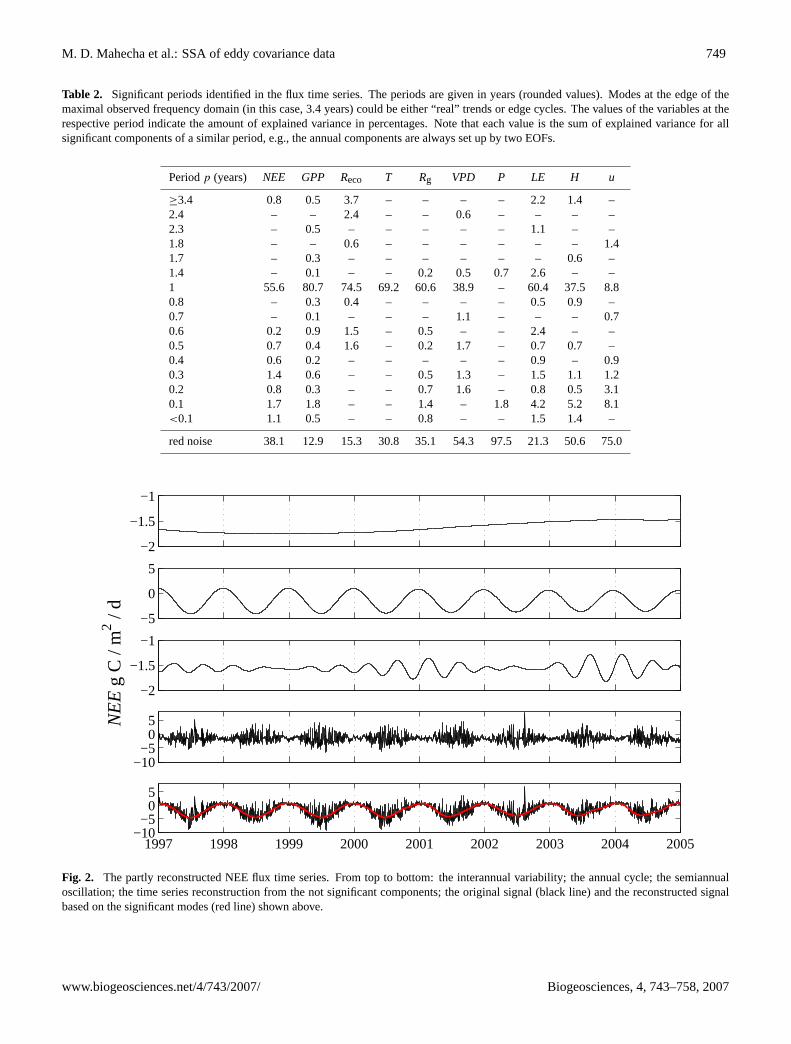
The results of the eigenspectra rely on the decompositionof the time series lag covariance structure as described inEq. (3). Yet only the subsequent time series reconstructionprovides insight into the effective behavior of the observationon the respective time scale. Figure2 presents an examplefor the reconstruction ofNEE. The figure also shows clearlythat it is not discernable whether the interannual variability isa sinusoidal oscillation or a (possibly nonlinear) trend. Fur-thermore, the semiannual component depicts a strong ampli-tude modulation, indicating that its importance in the timeseries structure is also time-dependent. It can also be seenhow a substantial part of the time series variance (38.1%) iscompatible with the red noise model according to the test ar-rangement. As indicated above, for the most part this signalis composed of high-frequency components. Finally, the bot-tom panel is an example for how the fundamental time evolu-tion of NEEwas reconstructed based on very few significantmodes.

3.2 Scale-dependentNEE-T relationships

As highlighted in Table2 and Fig.1, it was possible to re-veal that the different variables are dominated by a varietyof subsignals, which can be in part attributed to comparablefrequency classes. Thus it is possible to assess the cross-relationships of the data explicitly on the identified time scalerather than establishing empirical relationships from the en-tire observation space, as is the standard approach in mostclassic regression approaches.

Figure3 shows the relationship betweenNEEandT wheredifferent components are plotted in contrast with each other.The relationship between the pure annual components of

www.biogeosciences.net/4/743/2007/ Biogeosciences, 4, 743–758, 2007

748 M. D. Mahecha et al.: SSA of eddy covariance data

Fig. 1. The eigenspectra of the observed time series forNEE, Reco, GPP, VPD, LE, H, u, T, andP. The dots represent the dominantfrequencies of the time series at the respective normalized eigenvalue. The latter is equivalent to the amount of allocated variance. The redlines show the fitted red noise model. The gray areas are the corresponding 95% significance intervals.

both variables depicts a clear hysteresis effect (Fig.3, leftpanel). Adding the significant interannual component to theannual cycles has a remarkable effect on the observed hys-teresis (Fig.3, center panel). Although the interannual com-ponent accounts only for a small part of the data variability(Table2), the figure shows that this is sufficient to induce atrend in the summer fluxes toward decreased carbon uptake.On the contrary, the observed loss of carbon during the win-ter days found by the relationship of the annual componentsis neutralized by the interannual component (a more accuratedescription of the year-to-year anomalies is given in Sect.3.4and Fig.5). The total allocation of carbon which is due tothe interannual components is rather small. Despite this, wenow have to assert that the contribution of the interannualvariability could be essential for assessing the ecosystem un-der climate change conditions, given the observed forcing of

this component to the entire flux observations. Our findingscorroborate the assumption that interannual variability is amajor qualitative contribution required to describe the tem-poral behavior of the net carbon balance in terrestrial ecosys-tems. These empirical findings are of general importance formodeling purposes, since ecosystem models encounter limi-tations in the presence of interannual variability (Fujita et al.,2003; Hanson et al., 2004; Richardson et al., 2007; Siqueiraet al., 2006).

It has been shown that the seasonal and interannual com-ponents are not the only significant part of the time series.The intraannual component also plays a crucial role in theflux data, and their contribution induces complex variability(Fig. 3, right panel). These results provide a strong argu-ment for understanding cross-relationships in flux data as atemporal multilayer problem. In particular the components

Biogeosciences, 4, 743–758, 2007 www.biogeosciences.net/4/743/2007/

M. D. Mahecha et al.: SSA of eddy covariance data 749

Table 2. Significant periods identified in the flux time series. The periods are given in years (rounded values). Modes at the edge of themaximal observed frequency domain (in this case, 3.4 years) could be either “real” trends or edge cycles. The values of the variables at therespective period indicate the amount of explained variance in percentages. Note that each value is the sum of explained variance for allsignificant components of a similar period, e.g., the annual components are always set up by two EOFs.

Periodp (years) NEE GPP Reco T Rg VPD P LE H u

≥3.4 0.8 0.5 3.7 – – – – 2.2 1.4 –2.4 – – 2.4 – – 0.6 – – – –2.3 – 0.5 – – – – – 1.1 – –1.8 – – 0.6 – – – – – – 1.41.7 – 0.3 – – – – – – 0.6 –1.4 – 0.1 – – 0.2 0.5 0.7 2.6 – –1 55.6 80.7 74.5 69.2 60.6 38.9 – 60.4 37.5 8.80.8 – 0.3 0.4 – – – – 0.5 0.9 –0.7 – 0.1 – – – 1.1 – – – 0.70.6 0.2 0.9 1.5 – 0.5 – – 2.4 – –0.5 0.7 0.4 1.6 – 0.2 1.7 – 0.7 0.7 –0.4 0.6 0.2 – – – – – 0.9 – 0.90.3 1.4 0.6 – – 0.5 1.3 – 1.5 1.1 1.20.2 0.8 0.3 – – 0.7 1.6 – 0.8 0.5 3.10.1 1.7 1.8 – – 1.4 – 1.8 4.2 5.2 8.1<0.1 1.1 0.5 – – 0.8 – – 1.5 1.4 –

red noise 38.1 12.9 15.3 30.8 35.1 54.3 97.5 21.3 50.6 75.0

−2

−1.5

−1

−5

0

5

−2

−1.5

−1

NE

E g

C /

m2 / d

−10−5

05

1997 1998 1999 2000 2001 2002 2003 2004 2005−10−5

05

Fig. 2. The partly reconstructed NEE flux time series. From top to bottom: the interannual variability; the annual cycle; the semiannualoscillation; the time series reconstruction from the not significant components; the original signal (black line) and the reconstructed signalbased on the significant modes (red line) shown above.

www.biogeosciences.net/4/743/2007/ Biogeosciences, 4, 743–758, 2007

750 M. D. Mahecha et al.: SSA of eddy covariance data

Fig. 3. The cross-relationship of the partly reconstructedNEE and T time series. From left to right: The first panel shows the pureannual components of both variables where the color code permits tracing the temporal evolution. The black crosses show the respectivereconstructions form the non-significant components. The center panel time series reconstruction is based on the annual and interannualcomponents. The right panel shows a reconstruction, in which the significant intraannual components were also taken into consideration.

that contain most of the high-frequency variability and wereintegrated here into the “red noise” component (Fig.1) donot contain intuitive cross-relationships betweenNEEandT(Fig. 3). However, further investigation is needed to deter-mine whether short-term responses ofNEE to fluctuations inthe environment are extractable by means of SSA.

3.3 Hysteretic ecosystem-atmosphere relationships

There was evidence that similar hysteretic patterns as foundbetween the seasonalNEE andT components can be foundin the relationships ofNEE versusGPP, VPD, u, LE, or H.Figure4 shows how these variables are linked when inferredfrom a joint reconstruction of their annual and interannualcomponents. These hysteresis loops are particularly wellpronounced in terms ofNEE-VPD, NEE-u, andNEE-H de-pendencies. Less clear patters were found in theNEE-LEspace and the carbon cycle relationshipNEE-GPP.

The question that arises here is whether the hysteresisloops shown are indications for nonlinear cross-relationshipsin the observation space or if they might instead be dueto linear, yet time-lagged cross-relationship in ecosystem-atmosphere variables. Other open questions are whether non-linearity is induced at certain time scales, e.g., by the inter-annual variability, which was shown to be responsible fortransitions of the hysteresis loops in time. All these ques-tions need further investigations and require the applicationof information-theory-based test statistics (e.g.,Palus, 1996;Diks and Mudelsee, 2000), which is beyond the scope of thispaper.

Above all, it proved to be the case that a sole dependencyon annual time scales, which can apparently be well cap-tured by linear regression, was found when relatingNEEto Rg. Having observed that cross-relationships between

RCs originating from different variables can exhibit a widerange of dependencies, this occurrence of an apparently non-lagged linear relation is by no means trivial. Whether thisphenomenon is unique for the investigated site and relatedto the dominance of evergreen coniferous species (imply-ing low variations of the leaf area index) or a more generalphenomenon requires further investigation. This observationis in accordance with previous findings that showed thatRgprovides a good basis for modeling terrestrial carbon fluxes.

In the overall view, most cross-relationships between theecosystem variables contain more or less pronounced hys-teresis effects (Fig.4). There is a sound explanation in partic-ular for theNEE-T relationship: Owing to aRg-T hysteresis(not shown), theNEE-T dependence is an imparted effect.From an ecological point of view, this might appear trivialand can be understood as the time-varying ecosystem heatcapacity in the course of the seasonal cycle. Indeed, the ex-istence of hysteretic behavior of ecosystem-atmosphere in-teractions is well known, e.g.,Nakai et al.(2003) showedhystereticNEE-T relationships on short-time scales. Withrespect to the hysteresis on seasonal time scales, our resultsare in line with findings fromRichardson et al.(2006), whoshowed similar effects in the relationship between soil tem-perature and the sensitivity parameter of respiration to tem-perature (Q10).

As far as the magnitude of impact is concerned, the sea-sonal hysteresis might be of fundamental importance for fur-ther ecosystem modeling tasks. Apart from the “obvious”NEE-T example, the causes for the unexpected but equallywell-pronounced hysteresis effects, e.g., in theNEE-VPDre-lationships, remain unclear. This could lead to further ques-tions, for example regarding how to distinguish between thesimple coexistence of seasonal cycles and their mutual de-pendence. We presume that the extracted hysteresis loops

Biogeosciences, 4, 743–758, 2007 www.biogeosciences.net/4/743/2007/

M. D. Mahecha et al.: SSA of eddy covariance data 751

Fig. 4. The cross-relationships of the major variables withNEE. Black crosses show the respective red noise components. The color-codedreconstructed components comprise the annual and interannual components of the respective variables, where the color code permits tracingthe temporal evolution.

lead to more general problems in ecosystem theory. Ad-ditional research on hysteretic ecosystem-atmosphere ex-changes could, for example, contribute to a better under-standing of ecosystem memory. This is of relevance forthe quantification of lag effects in ecosystem responses toany type of recurrences on a variety of time scales, includ-ing summer droughts or winter anomalies (Seneviratne et al.,2006). An example is given here by theNEE-H relation-ship (Fig.4, lower central panel), where a clear deviation ofthe hysteretic behavior occurred precisely during the sum-mer heat wave in 2003 (cf.Ciais et al., 2005; Granier et al.,2007; Reichstein et al., 2007, for a comprehensive discussionof this climate anomaly).

Aside from the relationships of the annual-interannualRCs previously discussed, Fig.4 also shows the scatters ofthe red noise components for these variables. As discussedabove (shown in Fig.1 and Table2), the red noise frac-tion comprises most of the high-frequency components ofthe time series. When contrasting the cross-relationships ofthe non-significant and the annual-interannual components,we observed that there might be different types of relation-

ships acting on different time scales. This phenomenon ishighlighted, for example, in theNEE-GPPspace (Fig.4, up-per left panel). In this particular case, simple linear regres-sion analysis would lead to systematically varying parame-ters, depending on the time scale concerned. It is interestingto note that the red noiseNEE-Rg relationship appears similarto known light-use saturation effects. Overall, these resultscomprise intuitive examples for how the analysis of an en-tire signal might obscure the inherent cross-relationship on aseasonal time scale.

3.4 Deviations from mean annual-interannual components

One main advantage of SSA is that the partly reconstructedvariables can be further analyzed in analogy to existing ap-proaches that conventionally take the whole data series intoaccount. Figure5 supplies such a simple application exam-ple: Based on the annual-interannual components ofNEE,GPP, T, Rg, LE, H, andVPD, we estimated a mean seasonalcycle for each of them. In this respect, the capacity of SSAto extract phase- and amplitude-modulated signals allows the

www.biogeosciences.net/4/743/2007/ Biogeosciences, 4, 743–758, 2007

752 M. D. Mahecha et al.: SSA of eddy covariance data

Fig. 5. The deviations of the estimated mean reference componentof NEE, GPP, T, Rg, LE, H, andVPDbased on the joint reconstruc-tion of their respective annual and interannual components

calculation and visualization of the annual deviations of theRCs. This enables us, e.g., to investigate the effect of thesummer drought that affected the site in 2003, which is on-going with deviations in the investigated time series. A pos-itive deviation ofNEE, for example, turned out to be equallypronounced in the year 2004. By contrast,GPPseems to beaffected only during 2003, depicting decreased productivity.TheT record shows a smooth variation over the years, indi-cating a systematic amplitude shift, which can also be seen inRg. A more complicated pattern is found in the behavior ofLE, which is apparently not trivially related to the other vari-ables. From our results, the drought seem to have significantbearing on the deviations ofH andVPD. For an interpretationof these results, it is crucial to understand these deviationsagain in the context of the range of variation of the entiresignal and in terms of cross-relationships. We have to distin-guish, for example, between theVPD-deviations occurringon quantitatively very small scales (compared to the rangeof the seasonal-interannual variability; Fig.4) and the devi-ations ofH. The latter is the reason for the well-pronounceddeviation form theNEE-H hysteresis during 2003 (Fig.4,lower central panel).

Without going into a detailed discussion, this example il-lustrates one of the strengths and pitfalls of SSA: on the onehand, even simplistic approaches become powerful when thetime series are explored explicitly on the relevant tempo-ral scales only. On the other hand, events like the summerdrought of 2003 apparently influence the whole annual cy-cle of some flux time series, but they are not detectable in thetemperature cycle. This is suspicious, since especially a sum-mer heat wave was responsible for the anomaly in ecosystemproductivity (Ciais et al., 2005). One reason might be thatSSA allocates this effect on shorter time scales, of whichperiodicity matches the length of the heat wave. The openquestion requiring further investigation is which time scalesneed to be incorporated to achieve a sound representation oftime-localized anomalies.

3.5 Comparison of SSA with wavelet analysis

Singular System Analysis is an entirely data-driven method,and the achieved time series decomposition and projectionto different time scales can be seen as an “empirical vari-ance partitioning.” This is in contrast to methods using cer-tain functional classes (and usually parametric) as a fixedbasis. Of course, fundamental (quasi) oscillatory RCs asthe annual cycle can also be identified by a linear combi-nation of weighted sines and cosines as it is commonly ap-plied in terms of Fourier analysis. However, for phase- andamplitude-varying signals (e.g., as it was shown here veryclearly for the semiannual cycle ofNEE; Fig. 2), two EOFsare fully sufficient, whereas a Fourier type analysis would re-quire a large number of coefficients, in particular in the eventof sudden changes. Being able to decompose a signal into(possibly) nonharmonic or aperiodic subsignals is considered

Biogeosciences, 4, 743–758, 2007 www.biogeosciences.net/4/743/2007/

M. D. Mahecha et al.: SSA of eddy covariance data 753

one of SSA’s major strengths (Yiou et al., 2000). A furtheradvantage is the relative robustness of SSA to instationari-ties (not restricted to trends) of the signal mean and variance.This allows the analysis of nonstationary time series (Vau-tard et al., 1992) and is a major reason why using SSA canbe specifically advocated for environmental records such asecosystem-atmosphere fluxes.

Several recent studies investigating the temporal behav-ior of eddy covariance (and related) time series on varyingtime scales are based on wavelet analysis (e.g.,Katul et al.,2001; Braswell et al., 2005; Stoy et al., 2005; Richardsonet al., 2007). Indeed, wavelet analysis shares some impor-tant features with SSA, especially the ability to uncover theimpact of particular time scales on variation (Torrence andCompo, 1998). Wavelets use a (parametric) time-localizedshifting-window approach to extract the phase and amplitudeinformation of a time series. This leads to complex repre-sentations in the Fourier domain, but enableslocalizing theimportance of a given frequency scale in time: this is whywavelets can be seen as “mathematical microscopes” (Yiouet al., 2000) in time. The opposite is the case for SSA, whichis aglobal approach for the retrieval of the variation of sub-signals, as the shifting-window technique is solely exploitedto achieve statistical reliability. Wavelets and SSA can be ap-plied as complementary approaches.Jevrejeva et al.(2006),for example, used SSA for extracting nonlinear trends andvarying periodicities from sea-level records. In a subsequentstep, they used wavelet analysis as an independent tool forconfirming their results, gaining additional information fromboth algorithms.

Yiou et al. (2000) found that SSA and wavelet analysisshare fundamental features: they showed, e.g., that the EOFscan be interpreted in a way similar to mother wavelets, andthey provide further details (see alsoGhil et al., 2002). Fromthis perspective, a multiscale SSA (MS-SSA) was developed,extending the classical variant in analogy to wavelet analysis.The MS-SSA can be understood as the consecutive applica-tion of SSA to sliding windows. Roughly put, this is equiva-lent to applying SSA to each subvector in Eq. (1), where eachsubvectorZi is treated as an independent time seriesX(t) inSSA. Obviously, a local embedding dimensionP Zi needs tobe defined. With this they localized transitions in the SSAreconstructions on varying time scales in terms of waveletanalysis. When searching for low frequency components inthe available eddy covariance records, one is already operat-ing at the very limit with classic SSA. Thus at the moment,MS-SSA is not a feasible approach to the characterization ofecosystem-atmosphere interactions.

3.6 Limitations of SSA and potential extensions

The major problem is that SSA requires the heuristic settingof the embedding dimensionP (or P Zi ). Due to the lim-ited series length, we did not have much space for varyingthe parameter in this study and therefore opted for a ratio ofNP

= 2.5. Additional tests showed that the quality of sig-nal separability suffered by a further decrease of this ratio.Most extracted RCs were not well separable from each other,indicating a high degree of superimposition of signals (foran accurate definition of signal separability cf.Golyandinaet al., 2001). Increasing the ratioN

Palso did not lead to a bet-

ter signal separability and was not justified here. We foundthat the identified frequencies and their respective varianceallocations remain fairly stable over a certain range of em-bedding dimensions. Major shifts in the variance allocationsin the frequency domain occur mainly in the low-frequencymodes (f <1yr−1) due to the decrease of correlation strengthin the trajectory space. A less heuristic strategy could beto optimize the embedding dimension by means of more so-phisticated procedures (e.g.Cao, 1997), which were devel-oped for an optimal application of Takens’ embedding theo-rem (Takens, 1981).

Apart from these technical aspects of SSA performance,one has to consider the limitation of the method to linear fea-ture extraction. Recall that SSA is called a “PCA in the timedomain,” which holds true for the technical implementationof the decomposition as well as for the essential PCA out-come, which is to achieve a dimensionality reduction. Themain limitation of the presented SSA variant is its linear rep-resentation of the embedding space, which is inherited fromPCA. The question whether this is a suitable approach fordealing with real-world data is not trivial. E.g., it is wellknown that PCA is a suboptimal solution for dimensional-ity reduction in nonlinear systems and could be replaced bynonlinear dimensionality reduction (Kramer, 1991). In ac-cordance with these findings,Hsieh and Wu(2001); Hsiehand Hamilton(2001) andHsieh(2004) showed that the SSAresults can be nonlinearly generalized at different levels, e.g.,at the decomposition step or by generalizing the RCs withartificial neural networks. On the one hand, these featuresare principally challenging where the main advantage is thatoscillatory modes of arbitrary shape can be represented byone single nonlinear component (Hsieh, 2004). On the otherhand, such generalizations are fundamentally questionable;the critical point is that the neural network approaches men-tioned rely exclusively on previously linearly generated fea-tures, since the direct nonlinear feature extraction alwaysleads to a parameter space that exceeded the number of ob-servations. In this context, new developments of data explo-ration (e.g.Coifman et al., 2005; Tenenbaum et al., 2000)could provide alternative solutions for the next generation ofSSA.

www.biogeosciences.net/4/743/2007/ Biogeosciences, 4, 743–758, 2007

754 M. D. Mahecha et al.: SSA of eddy covariance data

3.7 Pattern extraction with missing data

In the context of eddy covariance measurements, missingdata and rejected values, e.g., due to unfavorable conditions,are unavoidable (Foken and Wichura, 1996). In terms of SSAapplications this is especially problematic where more than10% of data points were rejected and the method operatesat the very edge of a reasonable gap-filling procedure (Kon-drashov and Ghil, 2006).

Here, we applied SSA to a gappy time series, and the over-all results did not reveal fundamental problems. The SSAgap-filling strategy has the advantage that it interprets onlyavailable temporal correlation structures. This leads to a fur-ther analogy to wavelet analysis;Katul et al.(2001) showedthat missing data do not necessarily limit the investigation ofeddy covariance data in the frequency domain. They affirmbeing able to “remove the effect of missing values on spec-tral and co-spectral calculations.” All the same, this did notprovide a tool for filling large gaps in time series where SSAhas some potential. This potential needs further exploration,especially considering the multivariate SSA gap-filling strat-egy proposed byKondrashov and Ghil(2006). The latterwould make use of cross-correlations between ancillary vari-ables where available, and could switch to the univariate gapfilling presented above in the absence of secondary informa-tion.

The present study could not provide an in-depth qualityanalysis comparing the SSA-based gap filling with estab-lished techniques as they are currently used for eddy covari-ance data (Moffat et al., 2007). The introduction of SSA tothe analysis of eddy covariance data only hints at how avail-able gap-filling methods could be improved by incorporatingthe information lying on the temporal correlation structure. Ithas to be pointed out that the SSA gap-filling method is itselfnot in a fully mature stage of development (cf. the currentstate of the discussion:Kondrashov and Ghil, 2007; Schnei-der, 2007) and alternative approaches were recently formu-lated (Golyandina and Osipov, 2007). Despite these details,SSA gap filling is already a considerable step forward towarddealing with cases where, e.g., due to power outages none ofthe target variables or standard meteorological observationsare available (seeRichardson and Hollinger, 2007, for an indepth sensitivity analysis of data uncertainty in the presenceof long gaps).

3.8 Implications for future flux assessment and outlook

We have shown that SSA provides a new way for the par-titioning of ecosystem flux variability into different timescales. There is considerable research interest in such data-adaptive tools for assessing ecosystem-atmosphere carbon,water, and energy fluxes. The application of advanced timeseries techniques could reveal further unexpected patternsthat were previously hidden in the raw data. There are manypossible fields of application for SSA and related methods

in addition to the presented “variance partitioning,” e.g. ad-vanced flux-partitioning methods that separate the contri-butions of GPP and Reco to the net carbon flux. Com-parisons between different flux-partitioning methods showedthat there are essential differences between the different ap-proaches, but also that all known methods make compara-ble assumptions on underlying physiological kinetics (Stoyet al., 2006). The question is whether these models could berefined and validated on different time scales, as discoveredby applying SSA. With this we aim at stimulating furtherdiscussions on how future flux-partitioning algorithms couldwork, taking the different behavior of the variables on differ-ent time scales into account.

A further perspective relevant to the analysis of eddycovariance data is presented byGolyandina and Stepanov(2005). They showed how SSA could be expanded to a statis-tical time-series forecast. This problem is closely related tothe problem of gap-filling, where we showed the usefulnessof SSA.

This study highlighted a series of relevant applications ofSSA inferring ecosystem-atmosphere interactions from vary-ing time scales. Extending the observation period or realizingmulti-site analysis in future investigations is expected to pro-vide major insight into cross-relationships between ecosys-tem fluxes and both related meteorological and derived eco-physiological time series. This could improve our generalunderstanding of ecosystem-atmosphere relationships.

4 Conclusions

Ecosystem-atmosphere interactions inferred from eddy co-variance data now comprise a time window that allows in-vestigating flux behavior beyond annual cycles. This studyshowed that by applying advanced time-series analysis meth-ods, one can extract a wide range of significant modes rang-ing from the high-frequency domain to long-term compo-nents. One major innovation of the approach presented is thatit provides an integrated methodological framework compris-ing data analysis, including signal to noise enhancement andgap-filling.

SSA proved to be able to separate the inherent temporalscales of a time series. Here, we showed that this “variancepartitioning” could serve as the general basis of further data-adaptive or process-oriented modeling tasks. Based on thesemethodological advances, we were able to demonstrate thatthe eddy covariance observations are dominated to a nonneg-ligible extent by interannual variability. Overall, the investi-gation showed that the relationships between water, carbon,and energy fluxes are strongly determined by seasonal hys-teresis and vary fundamentally between different time-scales.

Biogeosciences, 4, 743–758, 2007 www.biogeosciences.net/4/743/2007/

M. D. Mahecha et al.: SSA of eddy covariance data 755

Appendix A

Fig. A1. The complete data processing and analysis of the study summarized as as a flowchart-pseudocode.

www.biogeosciences.net/4/743/2007/ Biogeosciences, 4, 743–758, 2007

756 M. D. Mahecha et al.: SSA of eddy covariance data

Acknowledgements.We gratefully acknowledge M. Palus,A. D. Richardson, S. I. Seneviratne, D. Kondrashov, and twoanonymous referees for their comments on the manuscript. Thecontinuous help of the technical staff in Tharandt, U. Eichelmann,H. Prasse, H. Hebentanz and U. Postel, is greatly acknowledged.This work is part of the integrated project “Carboeurope” (GOCE-CT2003-505572) of the European Union (EU). This research wasfunded in part by the Marie Curie European Reintegration Grant“GLUES” (MC MERG-CT-2005-031077). M. D. Mahecha andM. Reichstein would like to thank the Max Planck Society forsupporting the “Biogeochemical Model-Data Integration Group”as an Independent Junior Research Unit. N. Carvalhais thanksthe Portuguese Foundation for Science and Technology and theEU through the Operational Program “Science, Technology, andInnovation”, (PhD grant SFRH/BD/6517/2001).

Edited by: T. Laurila

References

Allen, M. R. and Smith, L. A.: Monte Carlo SSA: Detecting irreg-ular oscillations in the presence of coloured noise, J. Climate, 9,3373–3404, 1996.

Aubinet, M., Grelle, A., Ibrom, A., Rannik,U., Moncrieff, J., Fo-ken, T., Kowalski, A. S., Martin, P. H., Berbigier, P., Bernhofer,C., Clement, R., Elbers, J., Granier, A., Grunwald, T., Morgen-stern, K., Pilegaard, K., Rebmann, C., Snijders, W., Valentini,R., and Vesala, T.: Estimates of the annual net carbon and waterexchange of forests: the EUROFLUX methodology, Adv. Ecol.Res., 30, 113–175, 2000.

Baldocchi, D.: Assessing the eddy covariance technique for eval-uating carbon exchange rates of ecosystems: past, present andfuture, Global Change Biol., 9, 479–492, 2003.

Broomhead, D. S. and King, G. P.: Extracting qualitative dynamicsfrom experimental data, Physica D, 20, 217–236, 1986.

Braswell, B. H., Sacks, W. J., Linder, E. and Schimel, D. S.: Esti-mating diurnal to annual ecosystem parameters by synthesis of acarbon flux model with eddy covariance net ecosystem exchangeobservations, Global Change Biol., 11, 335–355, 2005.

Cao, L.: Practical method for determining the minimum embeddingdimension of a scalar time series, Physica D, 110, 43–50, 1997.

Ciais, P., Reichstein, M., Viovy, N., Granier, A., Ogee, J., Allard, V.,Buchmann, N., Aubinet, M., Bernhofer, C., Carrara, A., Cheval-lier, F., Noblet, N. D., Friend, A., Friedlingstein, P., Grunwald,T., Heinesch, B., Keronen, P., Knohl, A., Krinner, G., Loustau,D., Manca, G., Matteucci, G., Miglietta, F., Ourcival, J. M., Pi-legaard, K., Rambal, S., Seufert, G., Soussana, J. F., Sanz, M. J.,Schulze, E. D., Vesala, T., and Valentini, R.: Europe-wide reduc-tion in primary productivity caused by the heat and drought in2003, Nature, 437, 529–533, 2005.

Coifman, R. R., Lafon, S., Lee, A. B., Maggioni, M., Nadler, B.,Warner, F., and Zucker, S. W.: Geometric diffusions as a toolfor harmonic analysis and structure definition of data: Diffusionmaps, Proceedings of the National Academy of Sciences, 102,7426–7431, 2005.

Diks, C. and Mudelsee, M.: Redundancies in the Earth’s climato-logical time series, Phys. Lett. A, 275, 407–414, 2000.

Dunn, A. L., Barford, C. C., Wofsy, S. C., Goulden, M. L., andDaube, B. C.: A long-term record of carbon exchange in a boreal

black spruce forest: means, responses to interannual variability,and decadal trends, Global Change Biol., 13, 577–590, 2007.

Falge, E., Baldocchi, D., Olson, R. J., Anthoni, P., Aubinet, M.,Bernhofer, C., Burba, G., Ceulemans, R., Clement, R., Dolman,H., Granier, A., Gross, P., Grunwald, T., Hollinger, D., Jensen,N.-O., Katul, G., Keronen, P., Kowalski, A. nad Ta Lai, C., Law,B. E., Meyers, T., Moncrieff, J., Moors, E., Munger, J. W., Pi-legaard, K., Rannik,U., Rebmann, C., Suyker, A., Tenhunen, J.,Tu, K., Verma, S., Vesala, T., Wilson, K., and S., W.: Gap fill-ing strategies for long term energy flux data sets, Agric. ForestMeteorol., 107, 71–77, 2001.

Foken, T. and Wichura, B.: Tools for quality assessment of surface-based flux measurements, Agric. Forest Meteorol., 78, 83–105,1996.

Fujita, D., Ishizawa, M., Maksyutov, S., Thornton, P. E., Saeki, T.,Nakazawa, T..: Inter-annual variability of the atmospheric car-bon dioxide concentrations as simulated with global terrestrialbiosphere models and an atmospheric transport model, Tellus B,55, 530–546, 2003.

Ghil, M. and Vautard, R.: Interdecadal oscillations and the warmingtrend in global temperature time series, Nature, 350, 324–327,1991.

Ghil, M., Allen, M. R., Dettinger, M. D., Ide, K., Kondrashov, D.,Mann, M. E., Robertson, A. W., Saunders, A., Tian, Y., Varadi,F., and Yiou, P.: Advanced spectral methods for climatic timeseries, Rev. Geophys., 40, 1–25, 2002.

Golyandina, N., Osipov, E.: The “Caterpillar”-SSA method foranalysis of time series with missing values, J. Stat. Plan. Infer.,137, 2642–2653, 2007.

Golyandina, N. and Stepanov, D.: SSA-based approaches to analy-sis and forecast of multidimensional time series, in: Proceedingsof the 5th St. Petersburg Workshop on Simulation, pp. 293–298,St. Petersburg State University, St. Petersburg, 2005.

Golyandina, N., Nekrutkin, V., and Zhigljavsky, A.: Analysis ofTime Series Structure: SSA and related techniques, no. 90 inMonographs on Statistics and Applied Probability, Chapman &Hall/CRC, Boca Raton, 2001.

Goulden, M. L., Munger, J. W., Fan, S. M., Daube, B. C., andWofsy, S. C.: Exchange of Carbon Dioxide by a Deciduous For-est: Response to interannual Climate Variability, Science, 271,1576–1578, 1996.

Granier, A., Reichstein, M., Bredaa, N., Janssens, I. A., Falge, E.,Ciais, P., Grunwald, T., Aubinet, M., Berbigier, P., Bernhofer, C.,Buchmann, N., Facini, O., Grassi, G., Heinesch, B., Ilvesniemi,H., Keronen, P., Knohl, A., Kostner, B., Lagergren, F., Lindroth,A., Longdoz, B., Loustau, D., Mateus, J., Montagnani, L., Nyst,C., Moorsu, E., Papale, D., Peiffer, M., Pilegaard, K., Pita, G.,Pumpanen, J., Rambal, S., Rebmann, C., Rodrigues, A., Seufert,G., Tenhunen, J., Vesala, T., and Wang, Q.: Evidence for soilwater control on carbon and water dynamics in European forestsduring the extremely dry year: 2003, Agric. Forest Meteorol.,143, 123–145, 2007.

Grunwald, T. and Bernhofer, C.: A decade of carbon, water andenergy flux measurement of an old spruce forest at the AnchorStation Tharandt, Tellus B, 59, 387-396, 2007.

Hanson, P. J., Amthor, J. S., Wullschleger, S. D., Wilson, K. B.,Grant, R. E., Hartley, A., Hui, D., Hunt, E. R., Johnson, D. W.,Kimball, J. S., King, A. W., Luo, Y., McNulty, S. G., Sun,G., Thornton, P. E., Wang, S., Williams, M. Baldocchi, D. D.

Biogeosciences, 4, 743–758, 2007 www.biogeosciences.net/4/743/2007/

M. D. Mahecha et al.: SSA of eddy covariance data 757

and Cushman, R. M.: Oak forest carbon and water simula-tions: Model intercomparisons and evaluations against indepen-dent data, Ecol. Monogr., 74, 443–489, 2004.

Hsieh, W.: Nonlinear multivariate and time series analysis by neuralnetwork methods, Rev. Geophys., 42, 1–25, 2004.

Hsieh, W. and Hamilton, K.: Nonlinear singular spectrum analysisof the tropical stratospheric wind, Q. J. R. Meteorol. Soc., 129,2367–2382, 2001.

Hsieh, W. and Wu, A.: Nonlinear multichannel singular spec-trum analysis of the tropical Pacific climate variability usinga neural network approach, J. Geophys. Res., 107(C7), 3076,doi:10.1029/2001JC000957, 2001.

Jevrejeva, S., Grinsted, A., Moore, J. C., and Holgate, S.: Nonlineartrends and multiyear cycles in sea level records, J. Geophys. Res.,111, C09012, doi:10.1029/2005JC003229, 2006.

Katul, G., Lai, C.-T., Schafer, K., Vidakovic, B., J., A., Ellsworth,D., and Oren, R.: Multiscape analysis of vegetation surfacefluxes: from seconds to years, Adv. Water Resour., 24, 1119–1132, 2001.

Kondrashov, D. and Ghil, M.: Spatio-temporal filling of missingdata in geophysical data sets, Nonlin. Processes Geophys., 13,151–159, 2006,http://www.nonlin-processes-geophys.net/13/151/2006/.

Kondrashov, D. and Ghil, M.: Reply to T. Schneider’s commenton “Spatio-temporal filling of missing points in geophysical datasets”, Nonlin. Processes Geophys., 14, 3–4, 2007,http://www.nonlin-processes-geophys.net/14/3/2007/.

Kramer, M. A.: Nonlinear principal component analysis usingautoassociative neural networks, AIChE Journal, 37, 233–243,1991.

Lange, H. and Bernhardt, K.: Long-term components and regionalsynchronization of river runoffs, in: Hydrology: Science andPractice for the 21st Century, edited by Butler, A., British Hy-drological Society, London, 165–170, 2004.

Law, B. E., Falge, E., Gu, L., Baldocchi, D., Bakwin, P., Berbigier,P. Davis, K. J., Dolman, H., Falk, M., Fuentes, J., Goldstein,A. H., Granier, A., Grelle, A., Hollinger, D., Janssens, I., Jarvis,P., Jensen, N. O. Katul, G., Malhi, Y., Matteucci, G., Monson, R.,Munger, J., Oechel, W., Olson, R., Pilegaard, K., Paw, U. K. T.,Thorgeirsson, H., Valentini, R., Verma, S., Vesala, T., Wilson,K., and Wofsy, S.: Carbon dioxide and water vapor exchange ofterrestrial vegetation in response to environment, Agric. ForestMeteorol., 113, 97–120, 2002.

Moffat, A., Papale, D., Reichstein, M., Barr, A. G., Braswell, B. H.,Churkina, G., Desai, A. R., Falge, E., Gove, J. H., Heimann, M.,Hollinger, D. Y. Hui, D., Jarvis, A. J., Kattge, J., Noormets, A.,Richardson, A. D. Stauch, V. J.: Gap filling methods intercom-parison, Agric. Forest Meteorol., in press, 2007.

Nakai, Y., Kitamura, K., and Abe, S.: Year-long carbon dioxide ex-change above a broadleaf deciduous forest in Sapporo, NorthernJapan, Tellus B, 55, 305–312, 2003.

Palus, M.: Detecting nonlinearity in multivariate time series, Phys.Lett. A, 213, 138–147, 1996.

Palus, M. and Novotna, D.: Enhanced Monte Carlo SSA and thecase of climate oscillations, Phys. Lett. A, 248, 191–202, 1998.

Palus, M. and Novotna, D.: Quasi-biennial oscillations extractedfrom the monthly NAO index and temperature records are phase-synchronized, Nonlin. Processes Geophys., 13, 287–296, 2006,http://www.nonlin-processes-geophys.net/13/287/2006/.

Papale, D. and Valentini, R.: A new assessment of European forestscarbon exchanges by eddy fluxes and artificial neural networkspatialization, Global Change Biol., 9, 525–535, 2003.

Papale, D., Reichstein, M., Aubinet, M., Canfora, E., Bernhofer, C.,Kutsch, W., Longdoz, B., Rambal, S., Valentini, R., Vesala, T.,and Yakir, D.: Towards a standardized processing of Net Ecosys-tem Exchange measured with eddy covariance technique: algo-rithms and uncertainty estimation, Biogeosciences, 3, 571–583,2006,http://www.biogeosciences.net/3/571/2006/.

Peters, O., Hertlein, C., and Christensen, K.: A Complexity Viewof Rainfall, Physical Review Letters, 88, 018 701–1–018 701–4,2002.

Plaut, G. and Vautard, R.: Spells of low-frequency oscillations andweather regimes in the Northern Hemisphere, J. Atmos. Sci., 51,210–236, 1994.

Plaut, G. and Vautard, R.: interannual and interdecadal variability in335 years of Central England temperatures, Science, 268, 710–713, 1995.

Reichstein, M., Falge, E., Baldocchi, D., Papale, D., Valentini,R., Aubinet, M., Berbigier, P., Bernhofer, C., Buchmann, N.,Gilmanov, T., Granier, A., Grunwald, T., Havrnkov, K., Janous,D., Knohl, A., Laurila, T., Lohila, A., Loustau, D., Matteucci,G., Meyers, T., Miglietta, F., Ourcival, J.-M., Rambal, S., Roten-berg, E., Sanz, M., Seufert, G., Vaccari, F., Vesala, T., and Yakir,D.: On the separation of net ecosystem exchange into assimila-tion and ecosystem respiration: review and improved algorithm,Global Change Biol., 11, 1–16, 2005.

Reichstein, M., Ciais, P., Papale, D., Valentini, R., Running, S.,Viovy, N., Cramer, W., Granier, A., Oge, J., Allard, V., Aubi-net, M., Bernhofer, C., Buchmann, N., Carrara, A., Grunwald,T., Heinesch, B., Keronen, P., Knohl, A., Loustau, D., Manca,G., Matteucci, G., Miglietta, F., Ourcival, J. M., Pilegaard, K.,Rambal, S., Schaphoff, S., Seufert, G., Soussana, J.-F., Sanz,M.-J., Schulze, E. D., Vesala, T., and Heimann, M.: A combinededdy covariance, remote sensing and modeling view on the 2003European summer heatwave, Global Change Biol., 13, 634–651,2007.

Richardson, A. D., Braswell, B. H., Hollinger, D. Y., Burman, P.,Davidson, E. A., Evans, R. S., Flanagan, L. B., Munger, J. W.,Savage, K., Urbanski, S. P., and Wofsy, S. C.: Comparing sim-ple respiration models for eddy flux and dynamic chamber data,Agric. Forest Meteorol., 141, 219–234, 2006.

Richardson, A. D., Hollinger, D. Y., Aber, J. D., Ollinger, S. V., andBraswell, B. H.: Environmental variation is directly responsiblefor short- but not long-term variation in forest-atmosphere carbonexchange, Global Change Biol., 13, 788–803, 2007.

Richardson, A. D. and Hollinger, D. Y..: A method to estimatethe additional uncertainty in gap-filled NEE resulting from longgaps in the CO2 flux record, Agric. Forest Meteorol., in press,doi:10.1016/j.agrformet.2007.06.004, 2007a.

Richardson, A. D., Mahecha, M. D., Falge, E., Kattge, J., Moffat,A., Papale, D., Reichstein, M., Stauch, V. J., Braswell, B. H.,Churkina, G., Kruijt, B., and Hollinger, D. Y.: Statistical proper-ties of random CO2 flux measurement uncertainty inferred frommodel residuals, Agric. Forest Meteorol., in press, 2007b.

Saigusa, N., Yamamoto, S., Murayama, S., and Kondo, H.: Inter-annual variability of carbon budget components in an AsiaFluxforest site estimated by long-term flux measurements, Agric. For-

www.biogeosciences.net/4/743/2007/ Biogeosciences, 4, 743–758, 2007

758 M. D. Mahecha et al.: SSA of eddy covariance data

est Meteorol., 134, 4—16, 2005.Seneviratne, S. I., Koster, R. D., Guo, Z., Dirmeyer, P. A., Kowal-

czyk, E., Lawrence, D., Liu, P., Lu, C.-H., Mocko, D., Oleson,K. W., and Verseghy, D.: Soil Moisture Memory in AGCM Sim-ulations: Analysis of Global Land-Atmosphere Coupling Exper-iment (GLACE) Data. J. Hydrometeor., 7, 1090–1112, 2006.

Schneider, T.: Comment on “Spatio-temporal filling of missingpoints in geophysical data sets” by D. Kondrashov and M. Ghil,Nonlin. Processes Geophys., 13, 151–159, 2006, Nonlin. Pro-cesses Geophys., 14, 1–2, 2007,http://www.nonlin-processes-geophys.net/14/1/2007/.

Shun, T. and Duffy, C.: Low-frequency oscillations in precipita-tion, temperature, and runoff on a west facing mountain front: Ahydrogeologic interpretation, Water Resour. Res., 35, 191–201,1999.

Siqueira, M. B., G. G. Katul, D. A. Sampson, Stoy, P. C., Juang,J.-Y., McCarthy, H. R. and Oren, R.: Multi-scale model inter-comparisons of CO2 and H2O exchange rates in a maturingsoutheastern U.S. pine forest, Global Change Biol., 12, 1189–1207, 2006.

Stoy, P. C., Katul, G. G., Siqueira, M. B. S., Juang, J.-Y., McCarthy,H. R., Kim, H.-S.,Oishi, A. C., and Oren, R.: Variability in netecosystem exchange from hourly to inter-annual time scales atadjacent pine and hardwood forests: a wavelet analysis, TreePhysiol., 25, 887–902, 2005.

Stoy, P. C., Katul, G. G., Siqueira, M. B. S., Juang, J.-Y., Novick,K. A., Joshua, M., Uebelherr, and Oren, R.: An evaluation ofmodels for partitioning eddy covariance-measured net ecosystemexchange into photosynthesis and respiration, Agric. Forest Me-teorol., 141, 2–18, 2006.

Takens, F.: Detecting strange attractors in turbulence, in: LectureNotes in Dynamical Systems and Turbulence edited by Rand,D. A., and Young, L.-S., Lecture Notes in Mathematics, 898,366–381, Springer, 1981.

Tenenbaum, J. B., de Silva, V., and Langford, J. C.: A global ge-ometric framework for nonlinear dimensionality reduction, Sci-ence, 290, 2319–2323, 2000.

Tessier, Y., Lovejoy, S., Hubert, P., Schertzer, D., and Pecknold, S.:Multifractal analysis and modeling of rainfall and river flows andscaling, causal transfer functions, J. Geophys. Res., 101(D21),26 427–26 440, 1996.

Torrence, C., and Compo, G. P..: A Practical Guide to WaveletAnalysis, B. Am. Meteorol. Soc. 61–79, 1998.

Vautard, R. and Ghil, M.: Singular spectrum analysis in nonlineardynamics, with applications to paleoclimatic time series, PhysicaD, 35, 395–424, 1989.

Vautard R., Yiou P., and Ghil M.: Singular spectrum analysis: atoolkit for short noisy chaotic signals, Physica D, 58, 95–126,1992.

von Storch, H. and Zwiers, F.: Statistical Analysis in Climate Re-search, Cambridge University Press, Cambridge, 1999.

Wilson, K. and Baldocchi, D.: Seasonal and interannual variabilityof energy fluxes temperate deciduous forest in North America,Agric. Forest Meteorol., 100, 1–18, 2000.

Yiou P., Sornette, D., and Ghil M.: Data-adaptive wavelets andmulti-scale singular-spectrum analysis, Physica D, 142, 254–290, 2000.

Biogeosciences, 4, 743–758, 2007 www.biogeosciences.net/4/743/2007/