chapter 3 digital transmission fundamentals

Chapter 3 Digital Transmission

FundamentalsDigital Representation of Information

Why Digital Communications?Digital Representation of Analog Signals

Characterization of Communication ChannelsFundamental Limits in Digital Transmission

Line CodingModems and Digital Modulation

Properties of Media and Digital Transmission SystemsError Detection and Correction

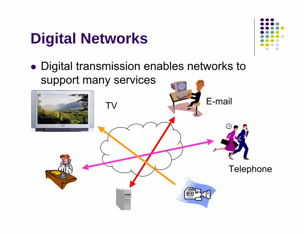
Digital Networks

Digital transmission enables networks to support many services

E-mail

Telephone

TV

Questions of InterestHow long will it take to transmit a message?

How many bits are in the message (text, image)?How fast does the network/system transfer information?

Can a network/system handle a voice (video) call?How many bits/second does voice/video require? At what quality?

How long will it take to transmit a message without errors?

How are errors introduced?How are errors detected and corrected?

What transmission speed is possible over radio, copper cables, fiber, infrared, …?

Chapter 3Digital Transmission

Fundamentals

Digital Representation of Information

Bits, numbers, informationBit: number with value 0 or 1

n bits: digital representation for 0, 1, … , 2n

Byte or Octet, n = 8Computer word, n = 16, 32, or 64

n bits allows enumeration of 2n possibilitiesn-bit field in a headern-bit representation of a voice sampleMessage consisting of n bits

The number of bits required to represent a message is a measure of its information content

More bits → More content

Block vs. Stream InformationBlock

Information that occurs in a single block

Text messageData fileJPEG imageMPEG file

Size = Bits / blockor bytes/block

1 kbyte = 210 bytes1 Mbyte = 220 bytes1 Gbyte = 230 bytes

StreamInformation that is produced & transmitted continuously

Real-time voiceStreaming video

Bit rate = bits / second1 kbps = 103 bps1 Mbps = 106 bps1 Gbps =109 bps

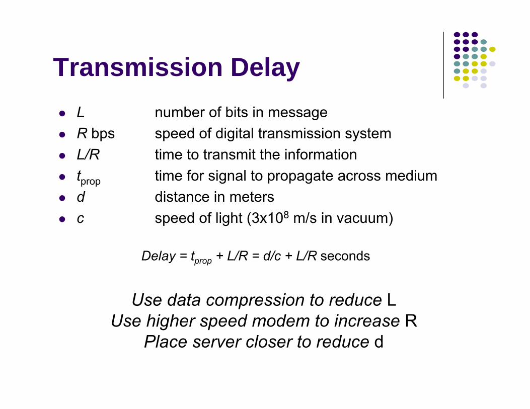
Transmission Delay

Use data compression to reduce LUse higher speed modem to increase R

Place server closer to reduce d

L number of bits in messageR bps speed of digital transmission systemL/R time to transmit the informationtprop time for signal to propagate across mediumd distance in metersc speed of light (3x108 m/s in vacuum)

Delay = tprop + L/R = d/c + L/R seconds

Compression

Information usually not represented efficientlyData compression algorithms

Represent the information using fewer bitsNoiseless: original information recovered exactly

E.g. zip, compress, GIF, fax

Noisy: recover information approximatelyJPEGTradeoff: # bits vs. quality

Compression Ratio#bits (original file) / #bits (compressed file)

H

W

= + +H

W

H

W

H

W

Color image

Red component

image

Green component

image

Blue component

image

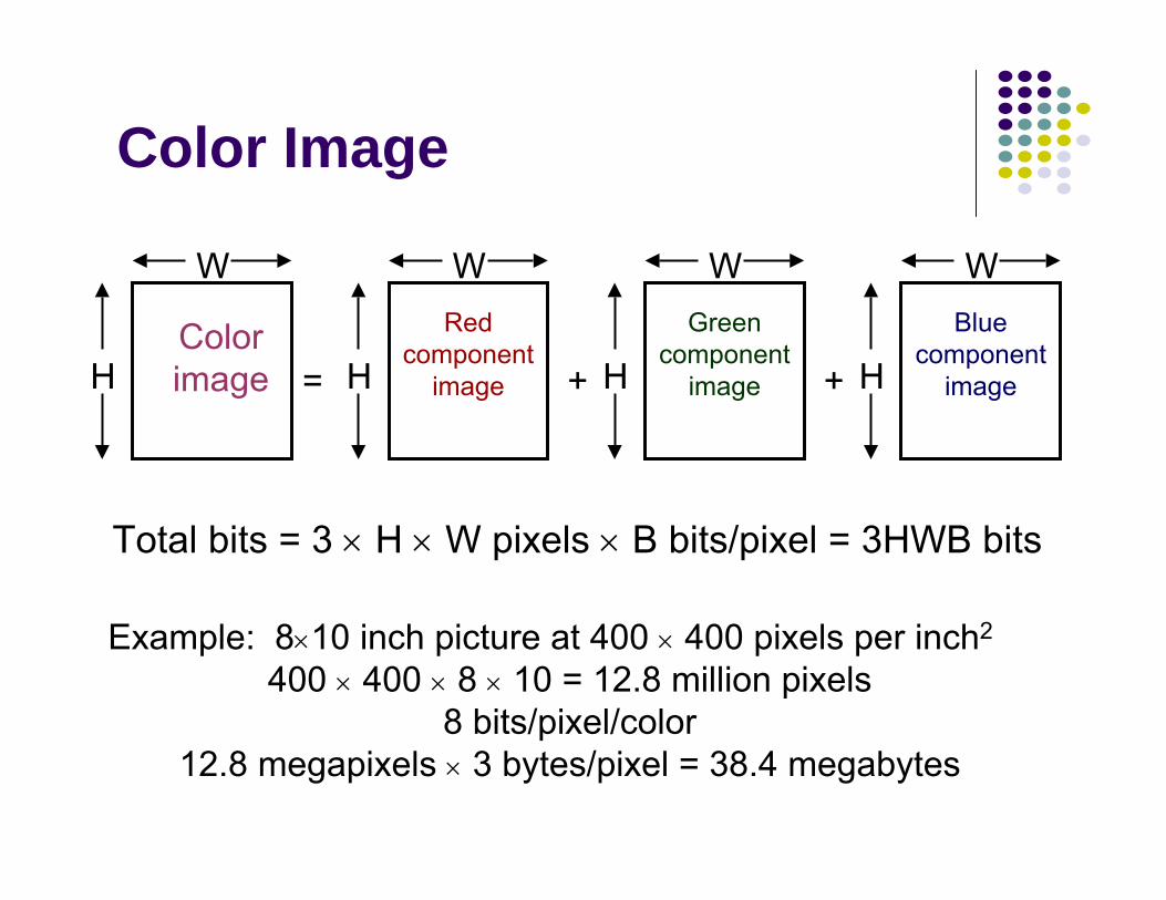
Total bits = 3 × H × W pixels × B bits/pixel = 3HWB bits

Example: 8×10 inch picture at 400 × 400 pixels per inch2

400 × 400 × 8 × 10 = 12.8 million pixels8 bits/pixel/color

12.8 megapixels × 3 bytes/pixel = 38.4 megabytes

Color Image

1-8 Mbytes (5-30)

38.4 Mbytes

8x10 in2 photo4002 pixels/in2

JPEGColor Image

5-54 kbytes(5-50)

256 kbytes

A4 page 200x100 pixels/in2

CCITT Group 3

Fax

(2-6)Kbytes-Mbytes

ASCIIZip, compress

Text

Compressed(Ratio)

OriginalFormatMethodType

Examples of Block Information

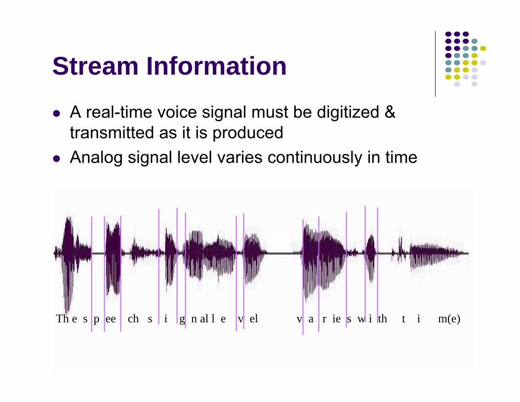
Th e s p ee ch s i g n al l e v el v a r ie s w i th t i m(e)

Stream InformationA real-time voice signal must be digitized & transmitted as it is producedAnalog signal level varies continuously in time

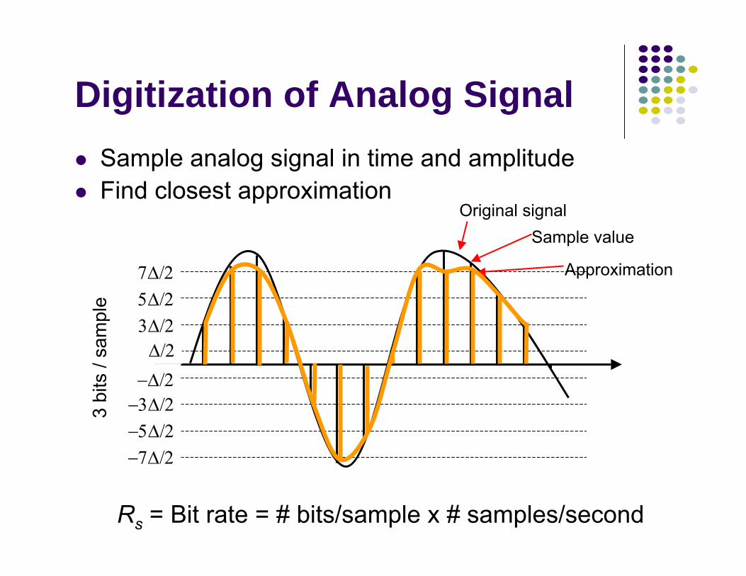
Digitization of Analog SignalSample analog signal in time and amplitudeFind closest approximation

Δ/23Δ/25Δ/27Δ/2

−Δ/2−3Δ/2−5Δ/2−7Δ/2

Original signalSample value

Approximation

Rs = Bit rate = # bits/sample x # samples/second

3 bi

ts /

sam

ple

Bit Rate of Digitized SignalBandwidth Ws Hertz: how fast the signal changes

Higher bandwidth → more frequent samplesMinimum sampling rate = 2 x Ws

Representation accuracy: range of approximation error

Higher accuracy→ smaller spacing between approximation values→ more bits per sample

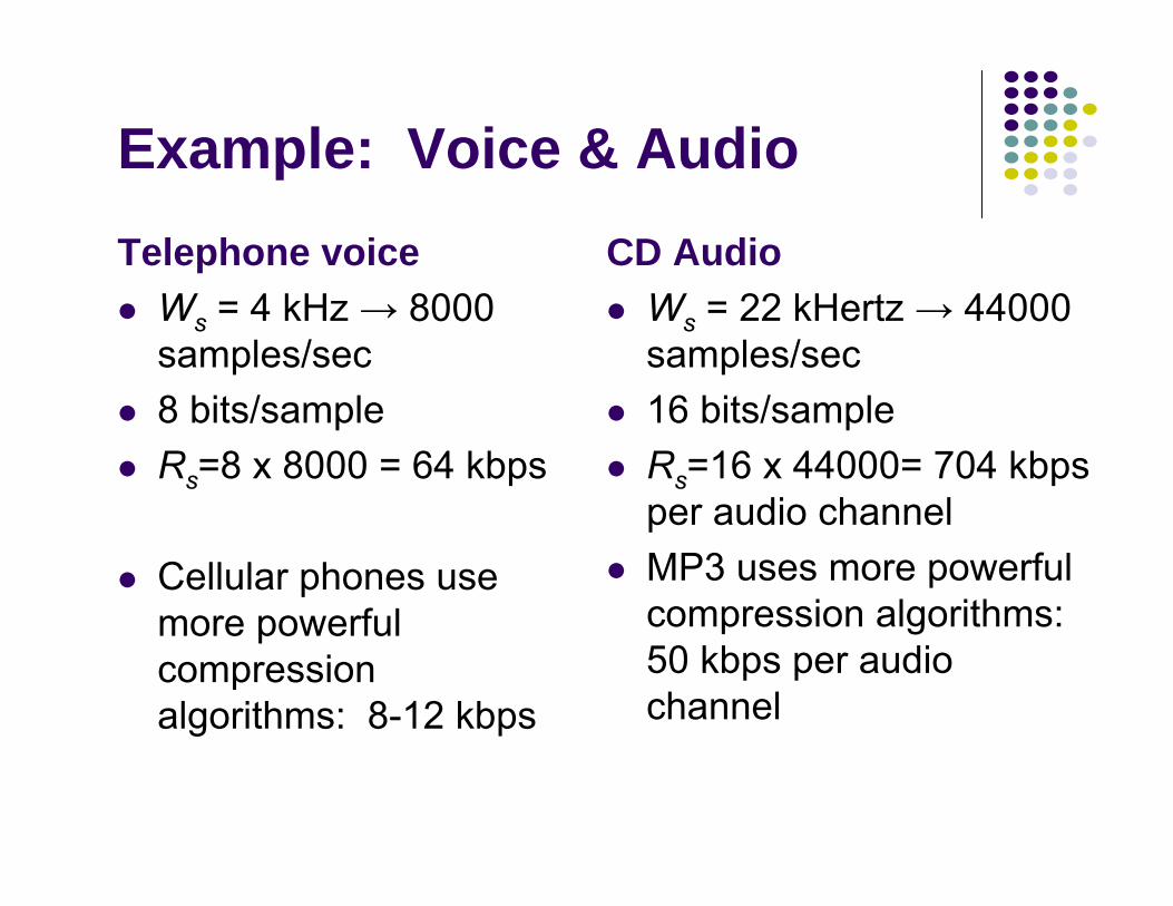
Example: Voice & AudioTelephone voice

Ws = 4 kHz → 8000 samples/sec8 bits/sampleRs=8 x 8000 = 64 kbps

Cellular phones use more powerful compression algorithms: 8-12 kbps

CD AudioWs = 22 kHertz → 44000 samples/sec16 bits/sampleRs=16 x 44000= 704 kbps per audio channelMP3 uses more powerful compression algorithms: 50 kbps per audio channel

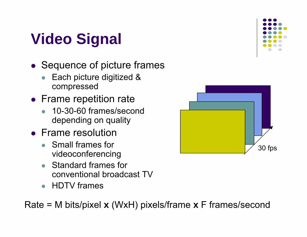
Video SignalSequence of picture frames

Each picture digitized & compressed

Frame repetition rate10-30-60 frames/second depending on quality

Frame resolutionSmall frames for videoconferencingStandard frames for conventional broadcast TVHDTV frames

30 fps

Rate = M bits/pixel x (WxH) pixels/frame x F frames/second

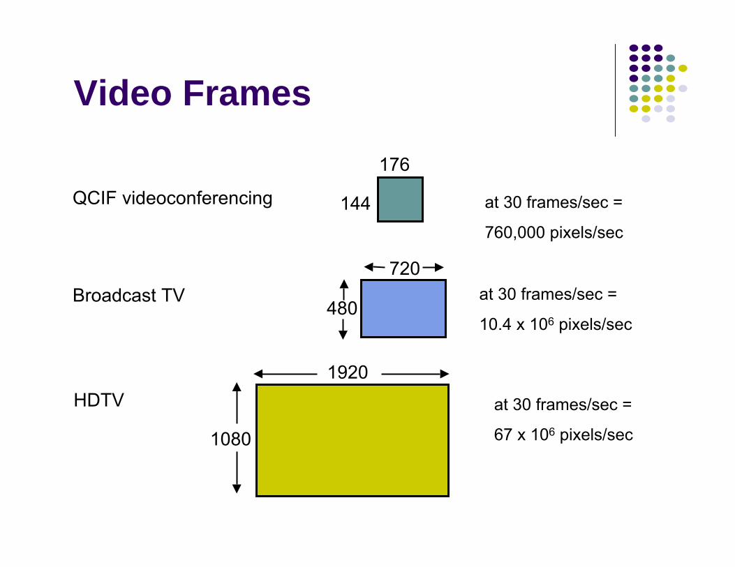
Video Frames

Broadcast TV at 30 frames/sec =

10.4 x 106 pixels/sec

720

480

HDTV at 30 frames/sec =

67 x 106 pixels/sec1080

1920

QCIF videoconferencing at 30 frames/sec =

760,000 pixels/sec

144

176

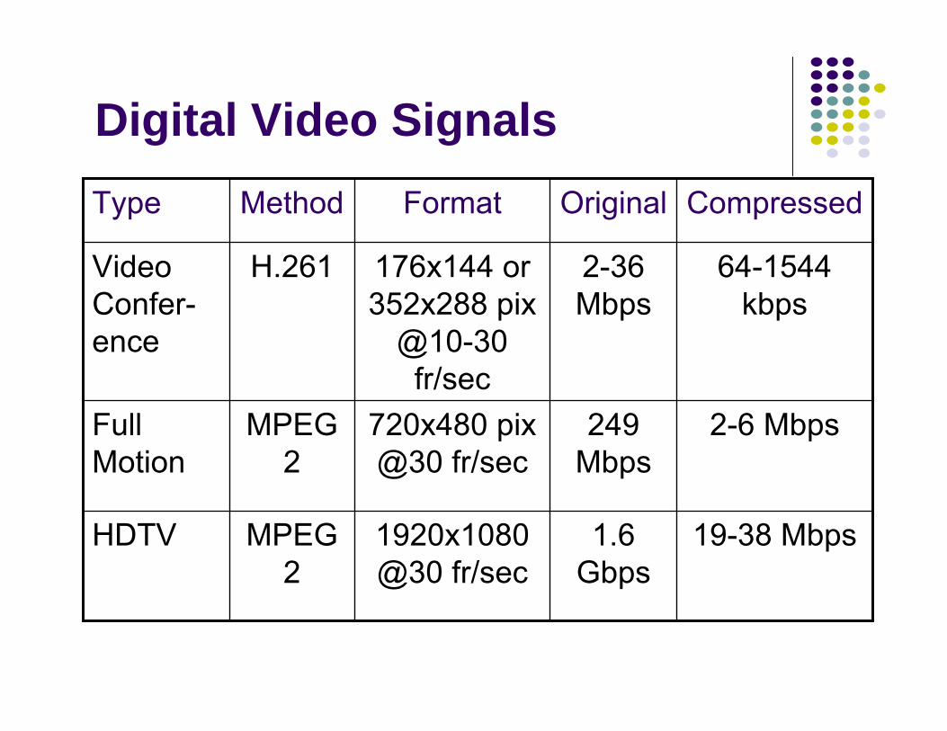
Digital Video Signals

19-38 Mbps1.6 Gbps

1920x1080 @30 fr/sec

MPEG2

HDTV

2-6 Mbps249 Mbps

720x480 pix @30 fr/sec

MPEG2

Full Motion

64-1544 kbps

2-36 Mbps

176x144 or 352x288 pix

@10-30 fr/sec

H.261Video Confer-ence

CompressedOriginalFormatMethodType

Transmission of Stream Information

Constant bit-rateSignals such as digitized telephone voice produce a steady stream: e.g. 64 kbpsNetwork must support steady transfer of signal, e.g. 64 kbps circuit

Variable bit-rateSignals such as digitized video produce a stream that varies in bit rate, e.g. according to motion and detail in a sceneNetwork must support variable transfer rate of signal, e.g. packet switching or rate-smoothing with constant bit-rate circuit

Stream Service Quality IssuesNetwork Transmission Impairments

Delay: Is information delivered in timely fashion?Jitter: Is information delivered in sufficiently smooth fashion?Loss: Is information delivered without loss? If loss occurs, is delivered signal quality acceptable?Applications & application layer protocols developed to deal with these impairments

Chapter 3Communication

Networks and Services

Why Digital Communications?

A Transmission System

TransmitterConverts information into signal suitable for transmissionInjects energy into communications medium or channel

Telephone converts voice into electric currentModem converts bits into tones

ReceiverReceives energy from mediumConverts received signal into form suitable for delivery to user

Telephone converts current into voiceModem converts tones into bits

Receiver

Communication channel

Transmitter

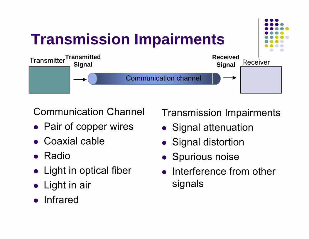
Transmission Impairments

Communication ChannelPair of copper wiresCoaxial cableRadio Light in optical fiberLight in airInfrared

Transmission ImpairmentsSignal attenuationSignal distortionSpurious noiseInterference from other signals

Transmitted Signal

Received Signal Receiver


Transmitter

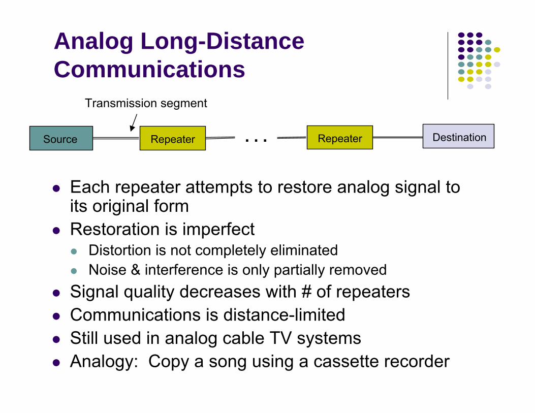
Analog Long-Distance Communications

Each repeater attempts to restore analog signal to its original formRestoration is imperfect

Distortion is not completely eliminatedNoise & interference is only partially removed

Signal quality decreases with # of repeatersCommunications is distance-limitedStill used in analog cable TV systemsAnalogy: Copy a song using a cassette recorder

Source DestinationRepeater

Transmission segment

Repeater. . .

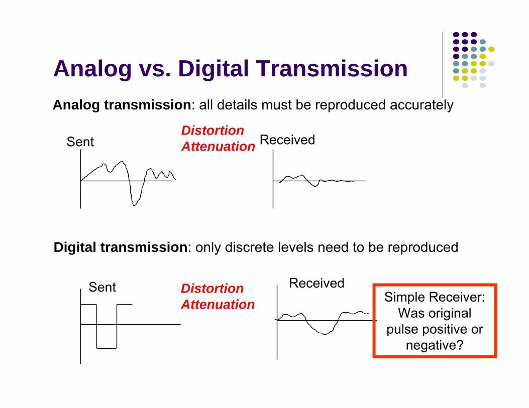
Analog vs. Digital TransmissionAnalog transmission: all details must be reproduced accurately

Sent

Sent

Received

Received

DistortionAttenuation

Digital transmission: only discrete levels need to be reproduced

DistortionAttenuation Simple Receiver:

Was original pulse positive or

negative?

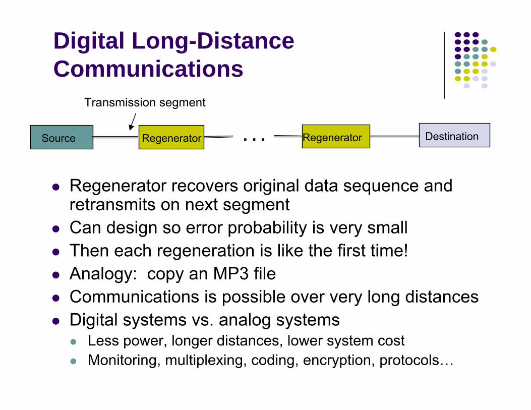
Digital Long-Distance Communications

Regenerator recovers original data sequence and retransmits on next segmentCan design so error probability is very smallThen each regeneration is like the first time!Analogy: copy an MP3 fileCommunications is possible over very long distancesDigital systems vs. analog systems

Less power, longer distances, lower system costMonitoring, multiplexing, coding, encryption, protocols…

Source DestinationRegenerator

Transmission segment

Regenerator. . .

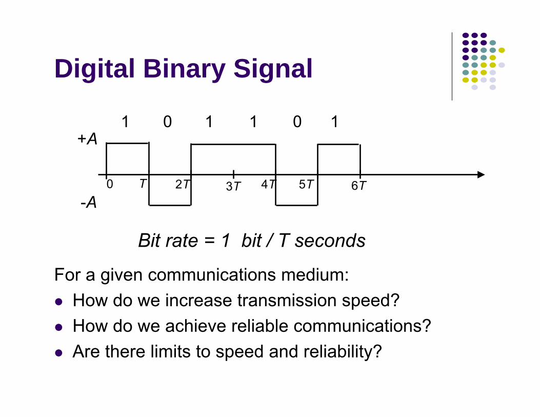
Digital Binary Signal

For a given communications medium:How do we increase transmission speed?How do we achieve reliable communications?Are there limits to speed and reliability?

+A

-A0 T 2T 3T 4T 5T 6T

1 1 1 10 0

Bit rate = 1 bit / T seconds

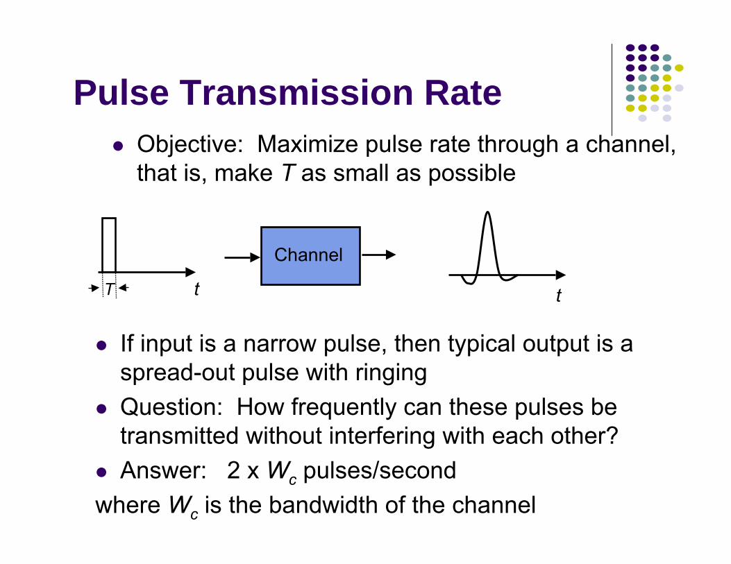
Pulse Transmission RateObjective: Maximize pulse rate through a channel, that is, make T as small as possible

Channel

t t

If input is a narrow pulse, then typical output is a spread-out pulse with ringingQuestion: How frequently can these pulses be transmitted without interfering with each other?Answer: 2 x Wc pulses/second

where Wc is the bandwidth of the channel

T

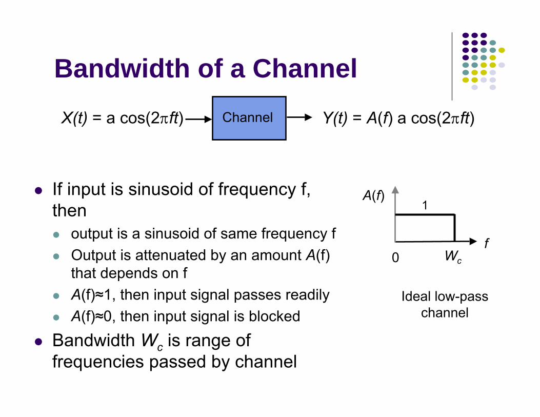
Bandwidth of a Channel

If input is sinusoid of frequency f, then

output is a sinusoid of same frequency fOutput is attenuated by an amount A(f) that depends on f A(f)≈1, then input signal passes readilyA(f)≈0, then input signal is blocked

Bandwidth Wc is range of frequencies passed by channel

ChannelX(t) = a cos(2πft) Y(t) = A(f) a cos(2πft)

Wc0f

A(f)1

Ideal low-pass channel

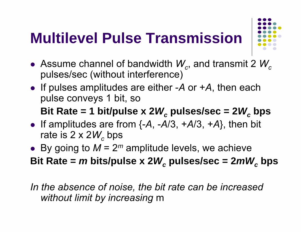
Multilevel Pulse TransmissionAssume channel of bandwidth Wc, and transmit 2 Wcpulses/sec (without interference)If pulses amplitudes are either -A or +A, then each pulse conveys 1 bit, so Bit Rate = 1 bit/pulse x 2Wc pulses/sec = 2Wc bpsIf amplitudes are from {-A, -A/3, +A/3, +A}, then bit rate is 2 x 2Wc bpsBy going to M = 2m amplitude levels, we achieve

Bit Rate = m bits/pulse x 2Wc pulses/sec = 2mWc bps

In the absence of noise, the bit rate can be increased without limit by increasing m

Noise & Reliable Communications

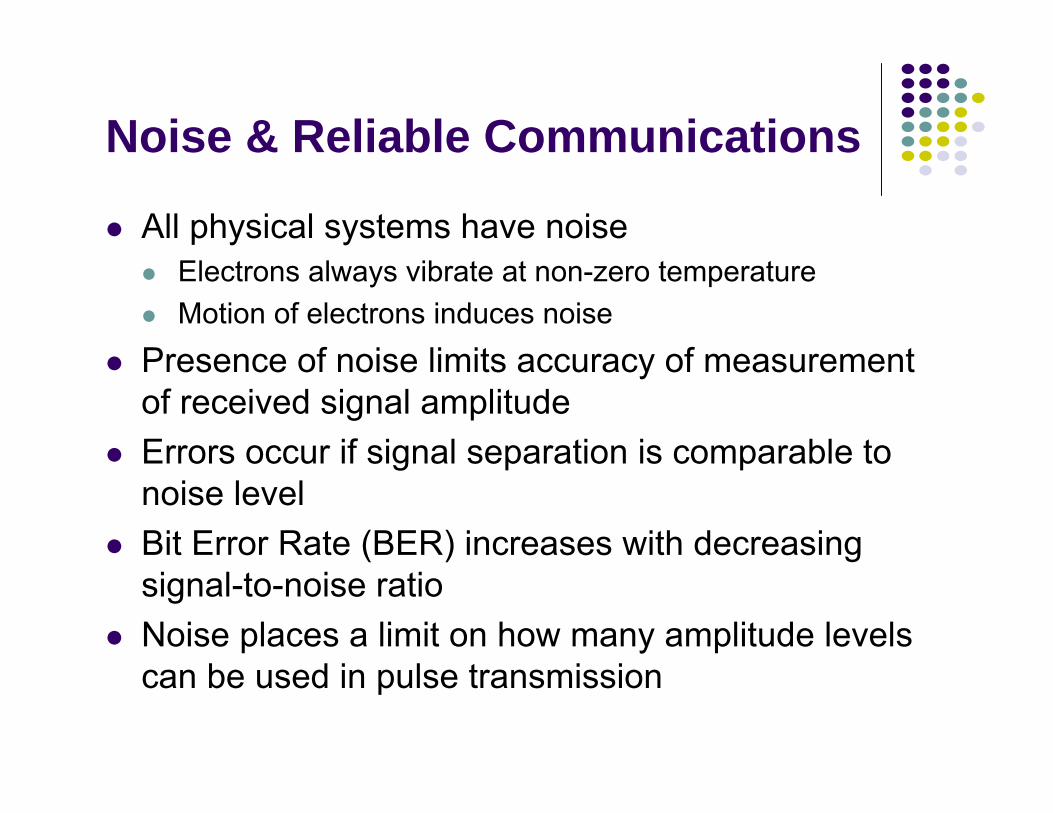
All physical systems have noiseElectrons always vibrate at non-zero temperatureMotion of electrons induces noise

Presence of noise limits accuracy of measurement of received signal amplitudeErrors occur if signal separation is comparable to noise levelBit Error Rate (BER) increases with decreasing signal-to-noise ratioNoise places a limit on how many amplitude levels can be used in pulse transmission

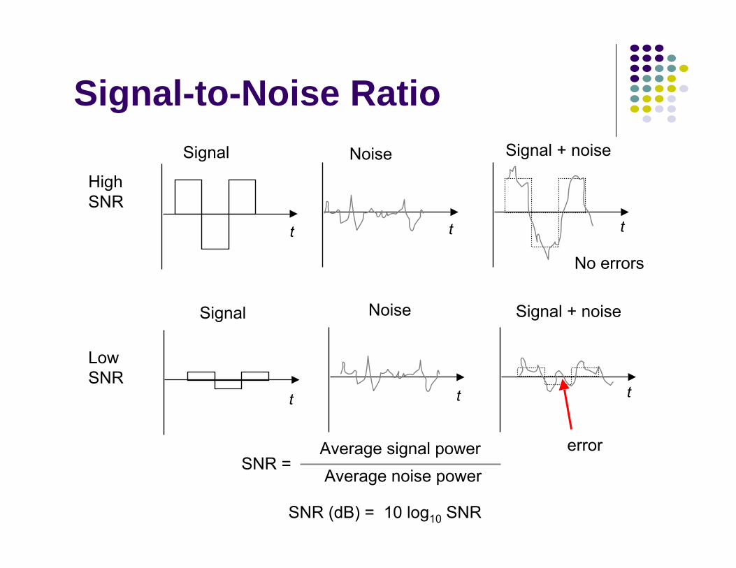
SNR = Average signal powerAverage noise power

SNR (dB) = 10 log10 SNR

Signal Noise Signal + noise

Signal Noise Signal + noise

HighSNR

LowSNR

t t t

t t t

Signal-to-Noise Ratio

error

No errors

Arbitrarily reliable communications is possible if the transmission rate R < C. If R > C, then arbitrarily reliable communications is not possible.

“Arbitrarily reliable” means the BER can be made arbitrarily small through sufficiently complex coding.C can be used as a measure of how close a system design is to the best achievable performance.Bandwidth Wc & SNR determine C

Shannon Channel Capacity

C = Wc log2 (1 + SNR) bps

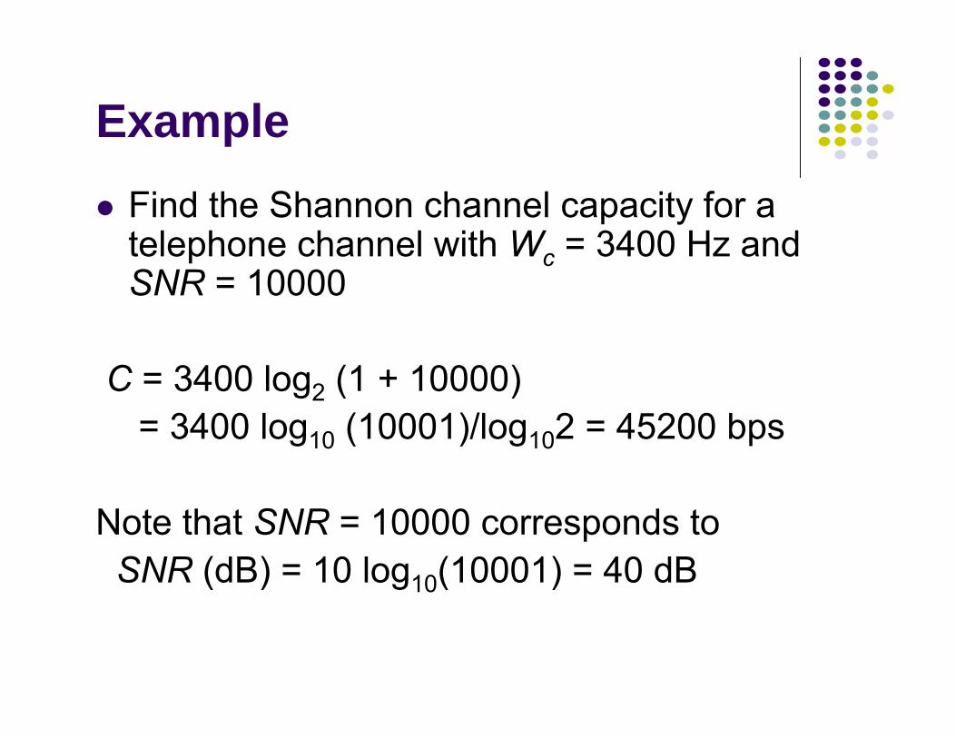
ExampleFind the Shannon channel capacity for a telephone channel with Wc = 3400 Hz and SNR = 10000

C = 3400 log2 (1 + 10000)= 3400 log10 (10001)/log102 = 45200 bps

Note that SNR = 10000 corresponds toSNR (dB) = 10 log10(10001) = 40 dB

Bit Rates of Digital Transmission Systems

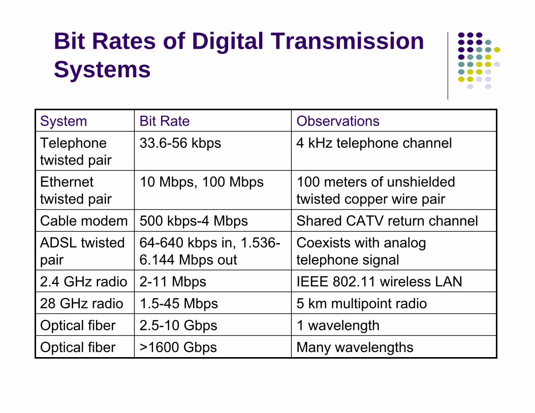
Many wavelengths>1600 GbpsOptical fiber1 wavelength2.5-10 GbpsOptical fiber 5 km multipoint radio1.5-45 Mbps28 GHz radio IEEE 802.11 wireless LAN2-11 Mbps2.4 GHz radio

Coexists with analog telephone signal

64-640 kbps in, 1.536-6.144 Mbps out

ADSL twisted pair

Shared CATV return channel500 kbps-4 MbpsCable modem

100 meters of unshielded twisted copper wire pair

10 Mbps, 100 MbpsEthernet twisted pair

4 kHz telephone channel33.6-56 kbpsTelephone twisted pair

ObservationsBit RateSystem

Examples of Channels

40 Gbps / wavelength

Many TeraHertzOptical fiber

54 Mbps / channel

300 MHz (11 channels)

5 GHz radio (IEEE 802.11)

30 Mbps/ channel

500 MHz (6 MHz channels)

Coaxial cable

1-6 Mbps1 MHzCopper pair

33 kbps3 kHzTelephone voice channel

Bit RatesBandwidthChannel


Fundamentals

Digital Representation of Analog Signals

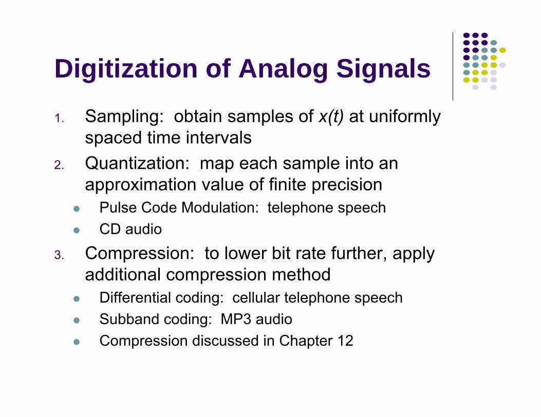
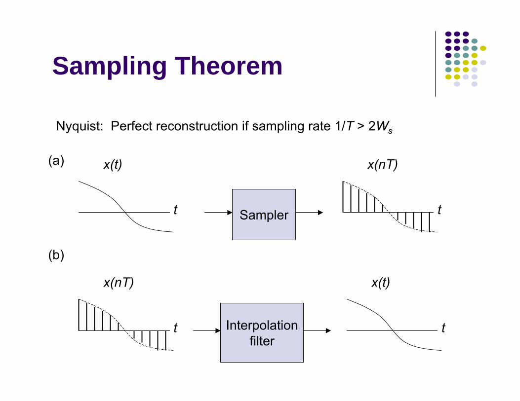
Digitization of Analog Signals1. Sampling: obtain samples of x(t) at uniformly

spaced time intervals2. Quantization: map each sample into an

approximation value of finite precisionPulse Code Modulation: telephone speechCD audio

3. Compression: to lower bit rate further, apply additional compression method

Differential coding: cellular telephone speechSubband coding: MP3 audioCompression discussed in Chapter 12

Sampling Rate and BandwidthA signal that varies faster needs to be sampled more frequentlyBandwidth measures how fast a signal varies

What is the bandwidth of a signal?How is bandwidth related to sampling rate?

1 ms

1 1 1 1 0 0 0 0

. . . . . .

t

x2(t)1 0 1 0 1 0 1 0

. . . . . .

t

1 ms

x1(t)

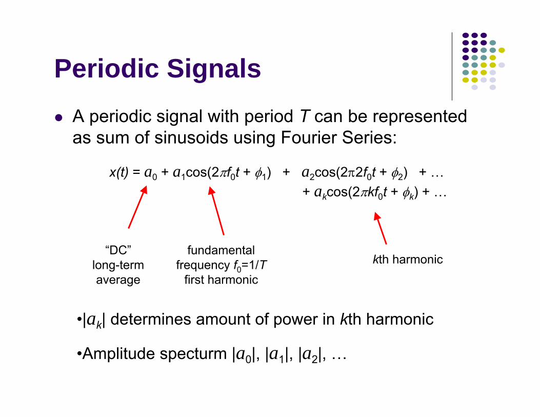
Periodic SignalsA periodic signal with period T can be represented as sum of sinusoids using Fourier Series:

“DC” long-term average

fundamental frequency f0=1/T

first harmonickth harmonic

x(t) = a0 + a1cos(2πf0t + φ1) + a2cos(2π2f0t + φ2) + … + akcos(2πkf0t + φk) + …

•|ak| determines amount of power in kth harmonic

•Amplitude specturm |a0|, |a1|, |a2|, …

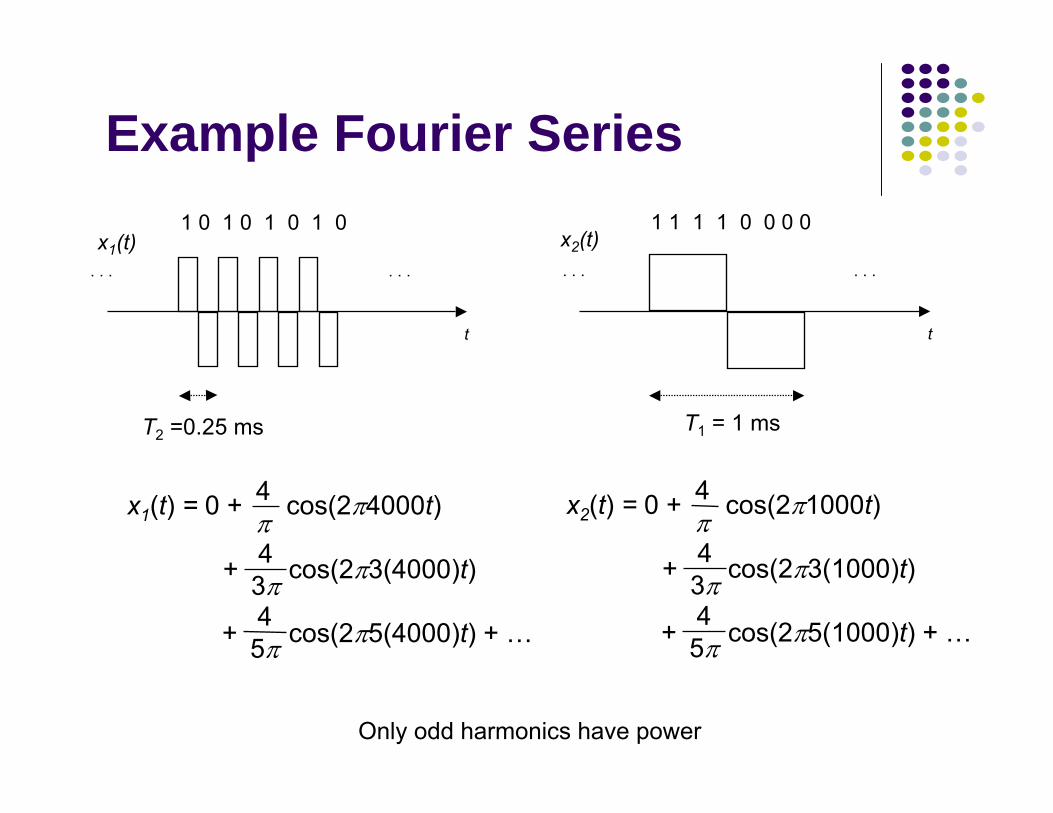
Example Fourier Series

T1 = 1 ms

1 1 1 1 0 0 0 0

. . . . . .

t

x2(t)1 0 1 0 1 0 1 0

. . . . . .

t

T2 =0.25 ms

x1(t)

Only odd harmonics have power

x1(t) = 0 + cos(2π4000t)

+ cos(2π3(4000)t)

+ cos(2π5(4000)t) + …

4 π

4 5π

4 3π

x2(t) = 0 + cos(2π1000t)

+ cos(2π3(1000)t)

+ cos(2π5(1000)t) + …

4 π

4 5π

4 3π

Spectra & BandwidthSpectrum of a signal: magnitude of amplitudes as a function of frequencyx1(t) varies faster in time & has more high frequency content than x2(t)Bandwidth Ws is defined as range of frequencies where a signal has non-negligible power, e.g. range of band that contains 99% of total signal power

0

0.2

0.4

0.6

0.8

1

1.2

0 3 6 9 12 15 18 21 24 27 30 33 36 39 42

frequency (kHz)

0

0.2

0.4

0.6

0.8

1

1.20 3 6 9 12 15 18 21 24 27 30 33 36 39 42

frequency (kHz)

Spectrum of x1(t)

Spectrum of x2(t)

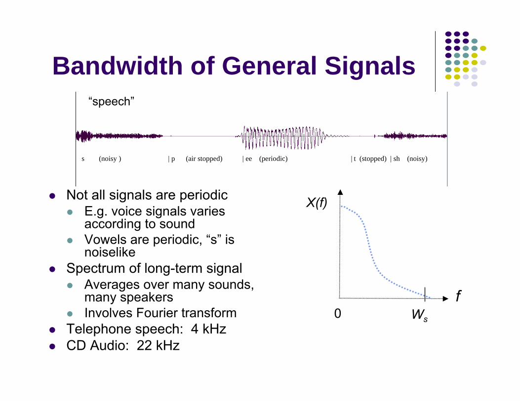
Bandwidth of General Signals

Not all signals are periodicE.g. voice signals varies according to soundVowels are periodic, “s” is noiselike

Spectrum of long-term signalAverages over many sounds, many speakersInvolves Fourier transform

Telephone speech: 4 kHzCD Audio: 22 kHz

s (noisy ) | p (air stopped) | ee (periodic) | t (stopped) | sh (noisy)

X(f)

f0 Ws

“speech”

Samplert

x(t)

t

x(nT)

Interpolationfilter

t

x(t)

t

x(nT)

(a)

(b)

Nyquist: Perfect reconstruction if sampling rate 1/T > 2Ws

Sampling Theorem

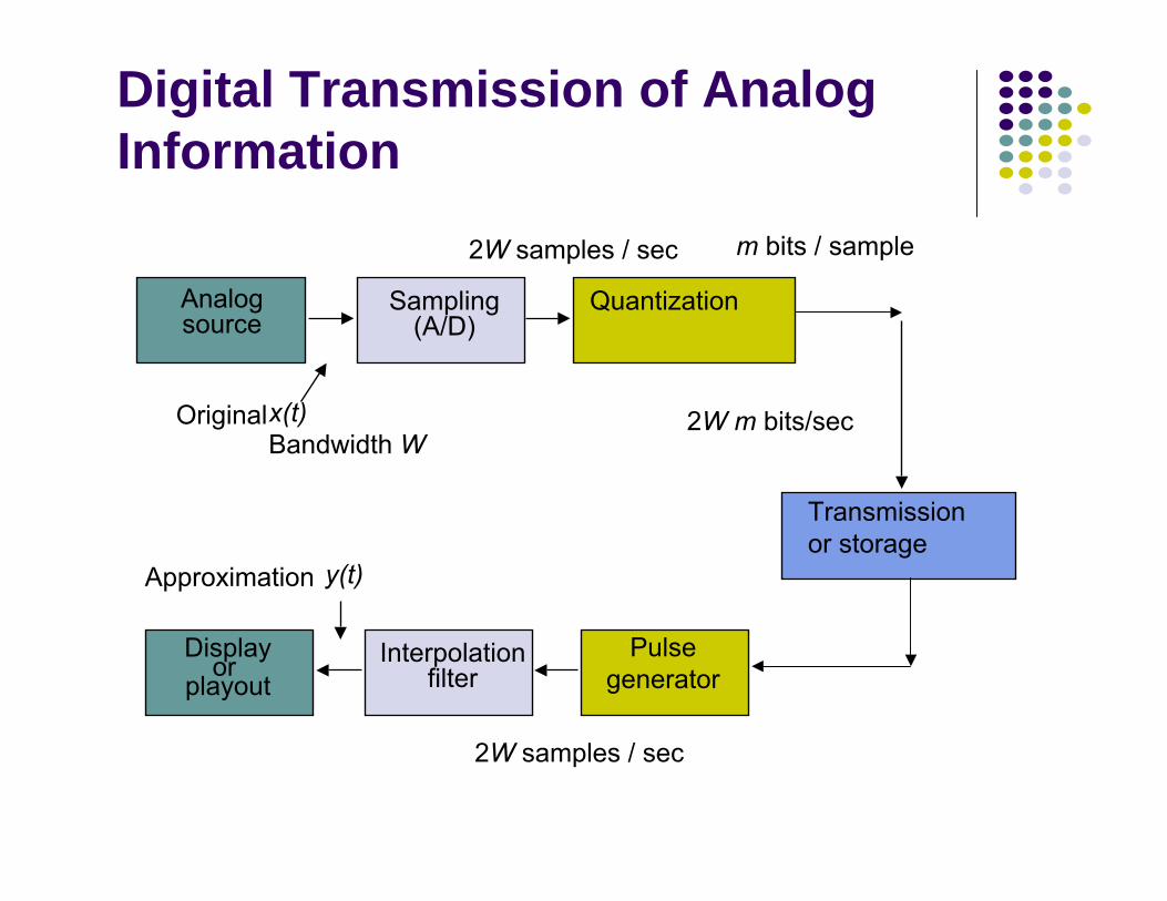
Digital Transmission of Analog Information

Interpolationfilter

Displayor

playout

2W samples / sec

2W m bits/secx(t)Bandwidth W

Sampling(A/D)

QuantizationAnalogsource

2W samples / sec m bits / sample

Pulsegenerator

y(t)

Original

Approximation

Transmissionor storage

input x(nT)

output y(nT)

0.5Δ1.5Δ

2.5Δ

3.5Δ

−0.5Δ

−1.5Δ−2.5Δ

−3.5Δ

Δ 2Δ 3Δ 4Δ

−Δ−2Δ−3Δ−4Δ

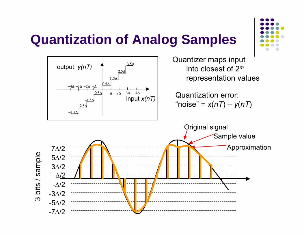
Quantization error:“noise” = x(nT) – y(nT)

Quantizer maps inputinto closest of 2m

representation values

Δ/23Δ/25Δ/27Δ/2

-Δ/2-3Δ/2-5Δ/2-7Δ/2

Original signalSample value

Approximation

3 bi

ts /

sam

ple

Quantization of Analog Samples

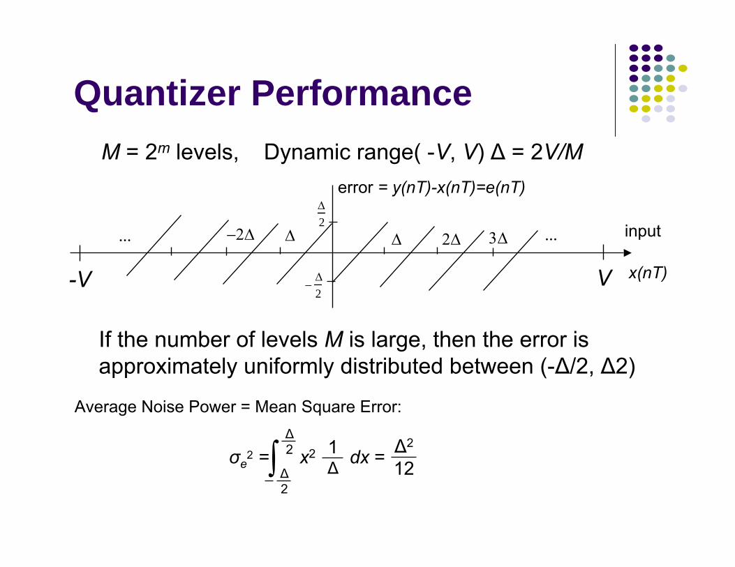
M = 2m levels, Dynamic range( -V, V) ∆ = 2V/M

Average Noise Power = Mean Square Error:

If the number of levels M is large, then the error isapproximately uniformly distributed between (-∆/2, ∆2)

Δ2

...

error = y(nT)-x(nT)=e(nT)

input...

−Δ2

3ΔΔ Δ−2Δ 2Δ

x(nT)V-V

Quantizer Performance

σe2 = x2 dx = ∆2

121 ∆∫

∆2

∆2

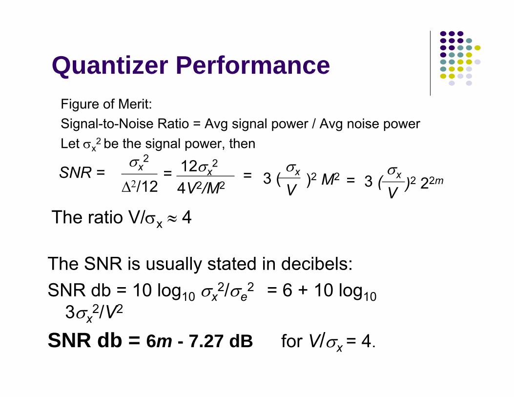
Figure of Merit: Signal-to-Noise Ratio = Avg signal power / Avg noise powerLet σx

2 be the signal power, thenσx

2

Δ2/12= 12σx

2

4V2/M2= σx3 (

V)2 M2 = 3 (

V )2 22mσxSNR =

The ratio V/σx ≈ 4

The SNR is usually stated in decibels:SNR db = 10 log10 σx

2/σe2� = 6 + 10 log10

3σx2/V2�

SNR db = 6m - 7.27 dB for V/σx = 4.

Quantizer Performance

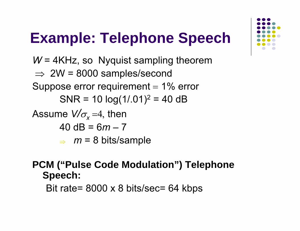
W = 4KHz, so Nyquist sampling theorem⇒ 2W = 8000 samples/secondSuppose error requirement = 1% error

SNR = 10 log(1/.01)2 = 40 dBAssume V/σx =4, then

40 dB = 6m – 7⇒ m = 8 bits/sample

PCM (“Pulse Code Modulation”) Telephone Speech:Bit rate= 8000 x 8 bits/sec= 64 kbps

Example: Telephone Speech


Fundamentals

Characterization of Communication Channels

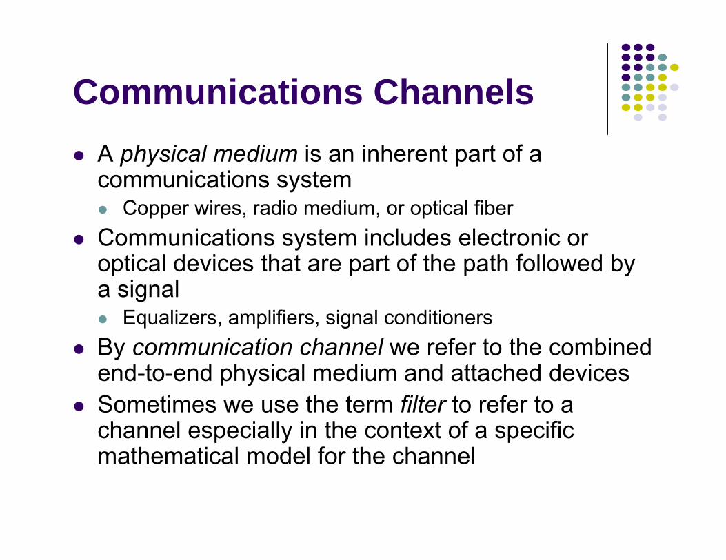
Communications ChannelsA physical medium is an inherent part of a communications system

Copper wires, radio medium, or optical fiberCommunications system includes electronic or optical devices that are part of the path followed by a signal

Equalizers, amplifiers, signal conditionersBy communication channel we refer to the combined end-to-end physical medium and attached devicesSometimes we use the term filter to refer to a channel especially in the context of a specific mathematical model for the channel

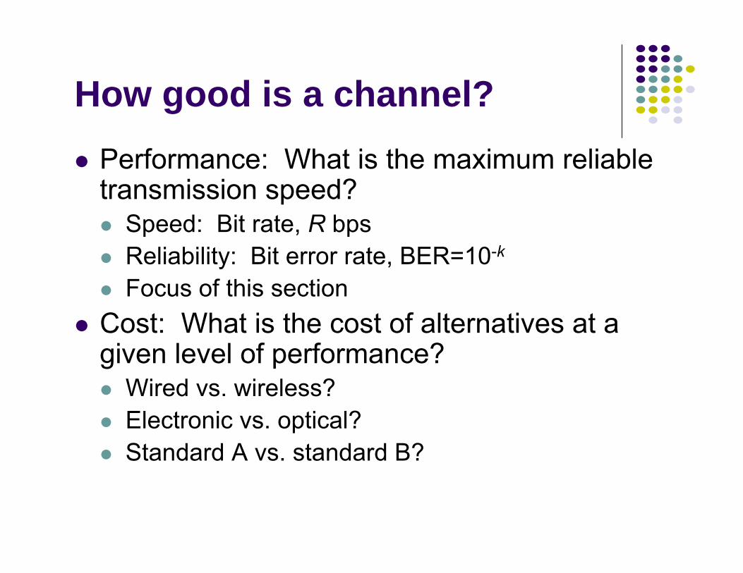
How good is a channel?Performance: What is the maximum reliable transmission speed?

Speed: Bit rate, R bpsReliability: Bit error rate, BER=10-k

Focus of this sectionCost: What is the cost of alternatives at a given level of performance?

Wired vs. wireless?Electronic vs. optical?Standard A vs. standard B?

Communications Channel

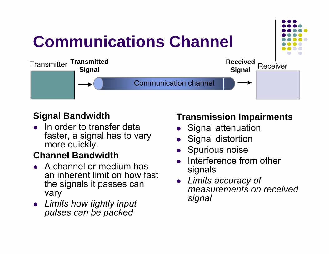
Signal BandwidthIn order to transfer data faster, a signal has to vary more quickly.

Channel BandwidthA channel or medium has an inherent limit on how fast the signals it passes can varyLimits how tightly input pulses can be packed

Transmission ImpairmentsSignal attenuationSignal distortionSpurious noiseInterference from other signalsLimits accuracy of measurements on received signal

Transmitted Signal

Received Signal Receiver


Transmitter

Channelt t

x(t)= Aincos 2πft y(t)=Aoutcos (2πft + ϕ(f))

AoutAin

A(f) =

Frequency Domain Channel Characterization

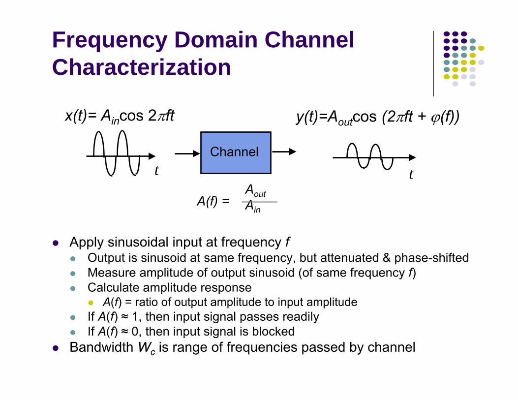
Apply sinusoidal input at frequency fOutput is sinusoid at same frequency, but attenuated & phase-shiftedMeasure amplitude of output sinusoid (of same frequency f)Calculate amplitude response

A(f) = ratio of output amplitude to input amplitudeIf A(f) ≈ 1, then input signal passes readilyIf A(f) ≈ 0, then input signal is blocked

Bandwidth Wc is range of frequencies passed by channel

Ideal Low-Pass FilterIdeal filter: all sinusoids with frequency f<Wc are passed without attenuation and delayed by τ seconds; sinusoids at other frequencies are blocked

Amplitude Response

f

1

f0

ϕ(f) = -2πft

1/ 2π

Phase Response

Wc

y(t)=Aincos (2πft - 2πfτ )= Aincos (2πf(t - τ )) = x(t-τ)

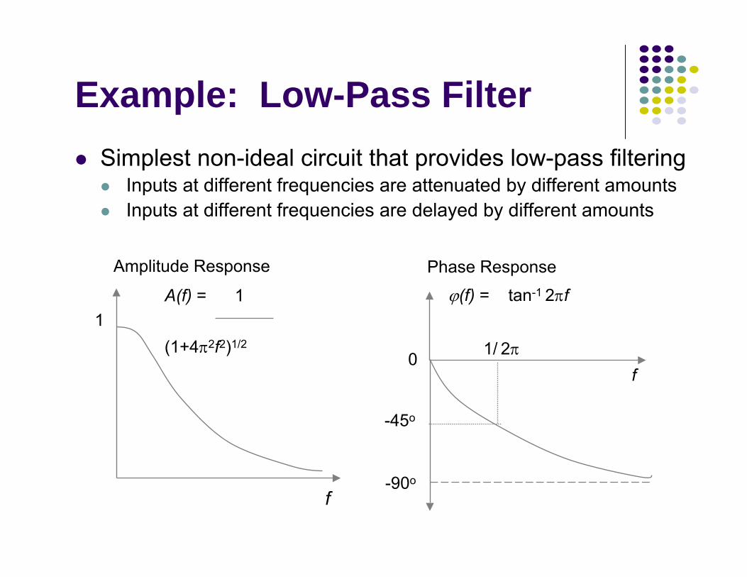
Example: Low-Pass FilterSimplest non-ideal circuit that provides low-pass filtering

Inputs at different frequencies are attenuated by different amountsInputs at different frequencies are delayed by different amounts

f

1A(f) = 1

(1+4π2f2)1/2

Amplitude Response

f0

ϕ(f) = tan-1 2πf

-45o

-90o

1/ 2π

Phase Response

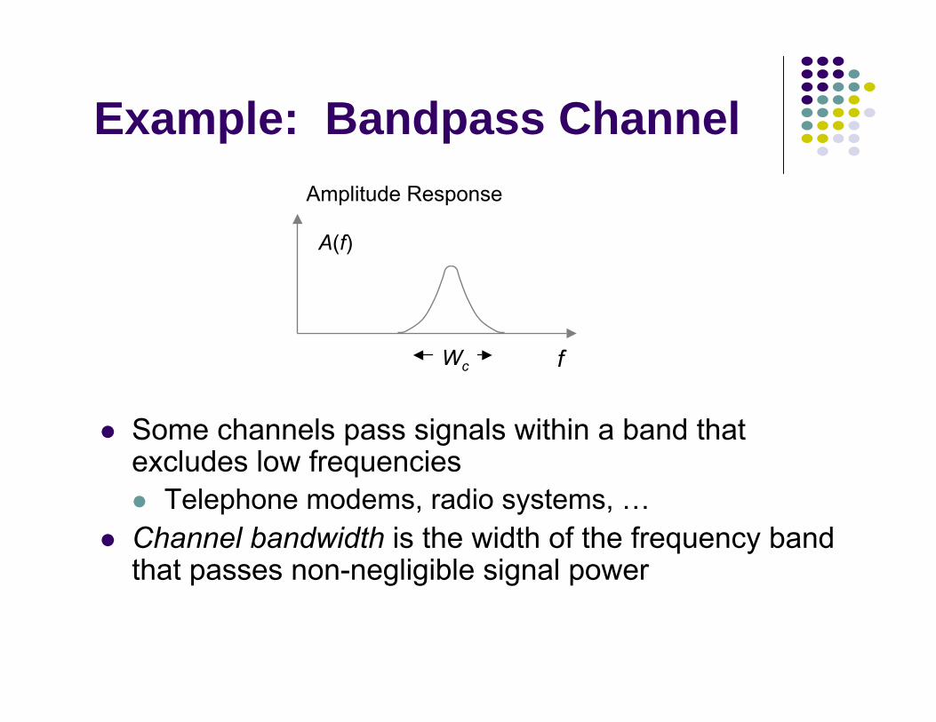
Example: Bandpass Channel

Some channels pass signals within a band that excludes low frequencies

Telephone modems, radio systems, …Channel bandwidth is the width of the frequency band that passes non-negligible signal power

f

Amplitude Response

A(f)

Wc

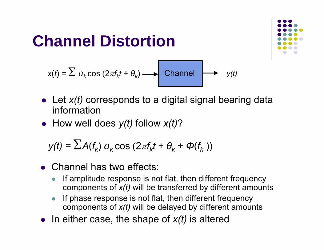
Channel Distortion

Channel has two effects:If amplitude response is not flat, then different frequency components of x(t) will be transferred by different amountsIf phase response is not flat, then different frequency components of x(t) will be delayed by different amounts

In either case, the shape of x(t) is altered

Let x(t) corresponds to a digital signal bearing data information How well does y(t) follow x(t)?

y(t) = ΣA(fk) ak cos (2πfkt + θk + Φ(fk ))

Channel y(t)x(t) = Σ ak cos (2πfkt + θk)

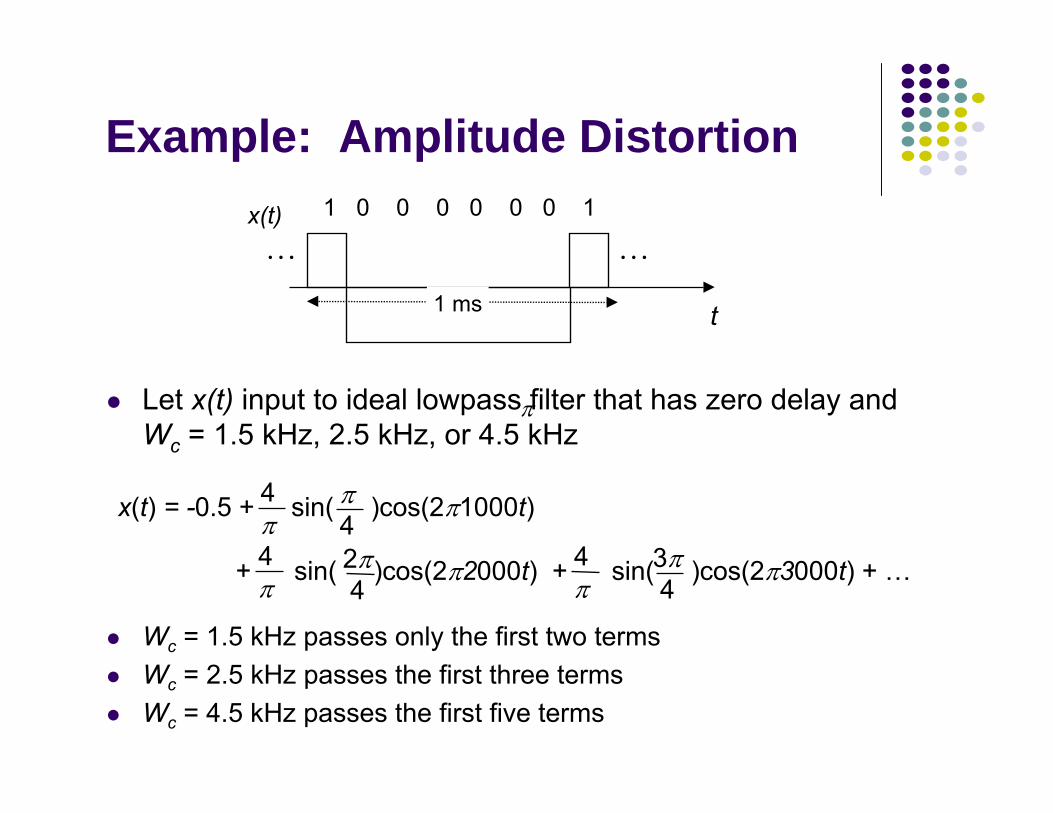
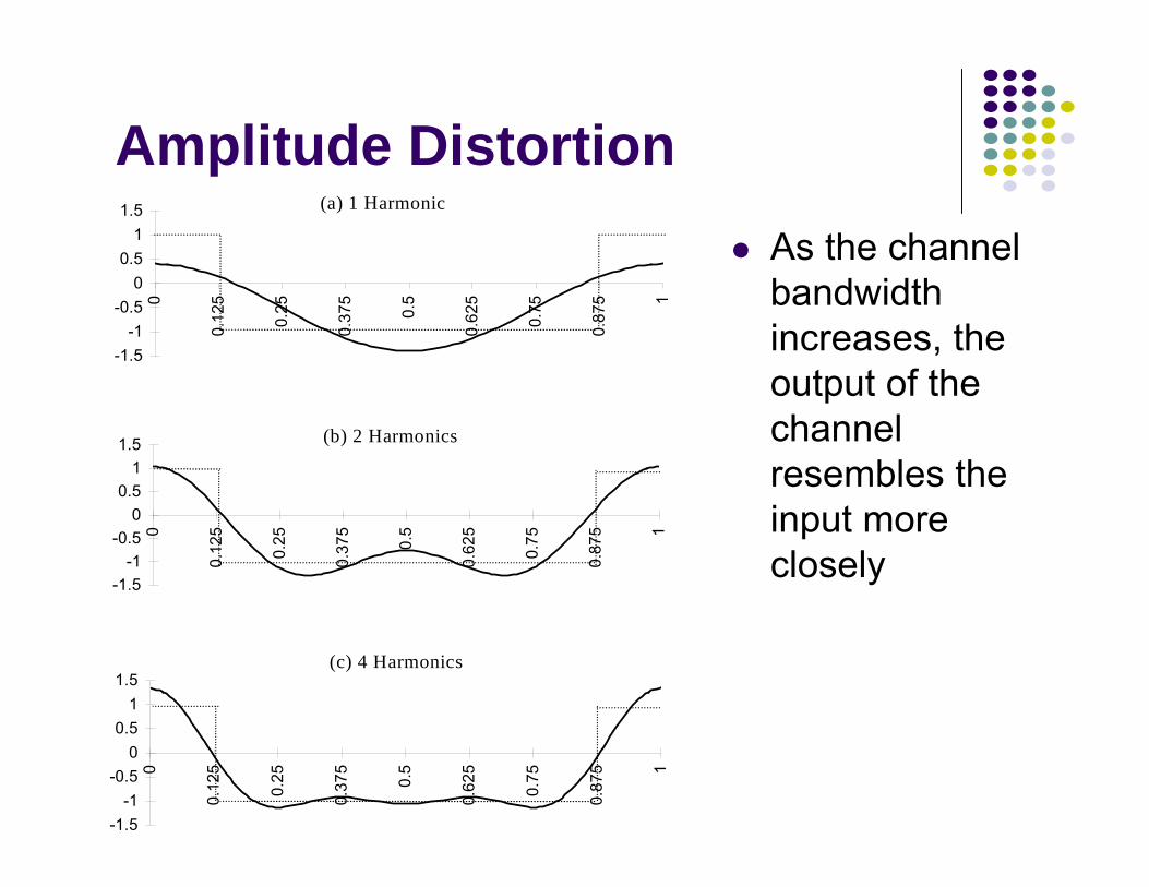
Example: Amplitude Distortion

Let x(t) input to ideal lowpass filter that has zero delay and Wc = 1.5 kHz, 2.5 kHz, or 4.5 kHz

1 0 0 0 0 0 0 1

. . . . . .

t1 ms

x(t)

Wc = 1.5 kHz passes only the first two termsWc = 2.5 kHz passes the first three termsWc = 4.5 kHz passes the first five terms

π

x(t) = -0.5 + sin( )cos(2π1000t)

+ sin( )cos(2π2000t) + sin( )cos(2π3000t) + …

4π

π4

4π

4π

2π4

3π4

-1.5-1

-0.50

0.51

1.5

0

0.12

5

0.25

0.37

5

0.5

0.62

5

0.75

0.87

5 1

-1.5-1

-0.50

0.51

1.5

0

0.12

5

0.25

0.37

5

0.5

0.62

5

0.75

0.87

5 1

-1.5-1

-0.50

0.51

1.5

0

0.12

5

0.25

0.37

5

0.5

0.62

5

0.75

0.87

5 1

(b) 2 Harmonics

(c) 4 Harmonics

(a) 1 Harmonic

Amplitude DistortionAs the channel bandwidth increases, the output of the channel resembles the input more closely

Channel

t0t

h(t)

td

Time-domain Characterization

Time-domain characterization of a channel requires finding the impulse response h(t)Apply a very narrow pulse to a channel and observe the channel output

h(t) typically a delayed pulse with ringingInterested in system designs with h(t) that can be packed closely without interfering with each other

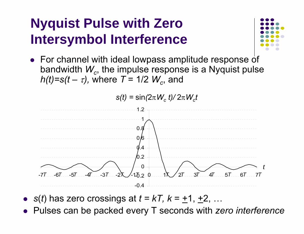
Nyquist Pulse with Zero Intersymbol Interference

For channel with ideal lowpass amplitude response of bandwidth Wc, the impulse response is a Nyquist pulse h(t)=s(t – τ), where T = 1/2 Wc, and

-0.4

-0.2

0

0.2

0.4

0.6

0.8

1

1.2

-7 -6 -5 -4 -3 -2 -1 0 1 2 3 4 5 6 7t

s(t) = sin(2πWc t)/ 2πWct

T T T T T T T T T T T T T T

s(t) has zero crossings at t = kT, k = +1, +2, …Pulses can be packed every T seconds with zero interference

-2

-1

0

1

2

-2 -1 0 1 2 3 4t

T T T T TT

-1

0

1

-2 -1 0 1 2 3 4t

T T T T TT

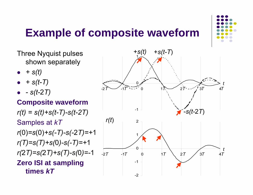
Example of composite waveformThree Nyquist pulses

shown separately+ s(t)+ s(t-T)- s(t-2T)

Composite waveformr(t) = s(t)+s(t-T)-s(t-2T)Samples at kTr(0)=s(0)+s(-T)-s(-2T)=+1r(T)=s(T)+s(0)-s(-T)=+1r(2T)=s(2T)+s(T)-s(0)=-1Zero ISI at sampling

times kT

r(t)

+s(t) +s(t-T)

-s(t-2T)

0f

A(f)

Nyquist pulse shapesIf channel is ideal low pass with Wc, then pulses maximum rate pulses can be transmitted without ISI is T = 1/2Wc sec.s(t) is one example of class of Nyquist pulses with zero ISI

Problem: sidelobes in s(t) decay as 1/t which add up quickly when there are slight errors in timing

Raised cosine pulse below has zero ISIRequires slightly more bandwidth than Wc

Sidelobes decay as 1/t3, so more robust to timing errors

1sin(πt/T)

πt/Tcos(παt/T)1 – (2αt/T)2

(1 – α)Wc Wc (1 + α)Wc


Fundamentals

Fundamental Limits in Digital Transmission

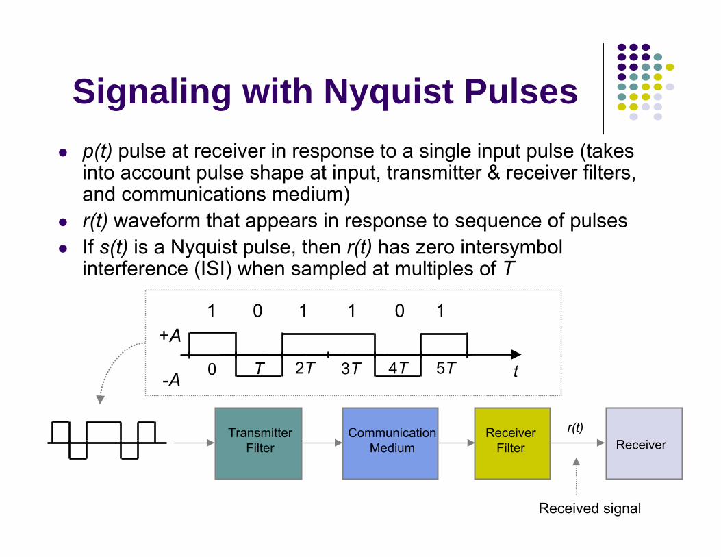
Transmitter Filter

Communication Medium

Receiver Filter Receiver

r(t)

Received signal

+A

-A 0 T 2T 3T 4T 5T

1 1 1 10 0

t

Signaling with Nyquist Pulsesp(t) pulse at receiver in response to a single input pulse (takes into account pulse shape at input, transmitter & receiver filters, and communications medium)r(t) waveform that appears in response to sequence of pulsesIf s(t) is a Nyquist pulse, then r(t) has zero intersymbolinterference (ISI) when sampled at multiples of T

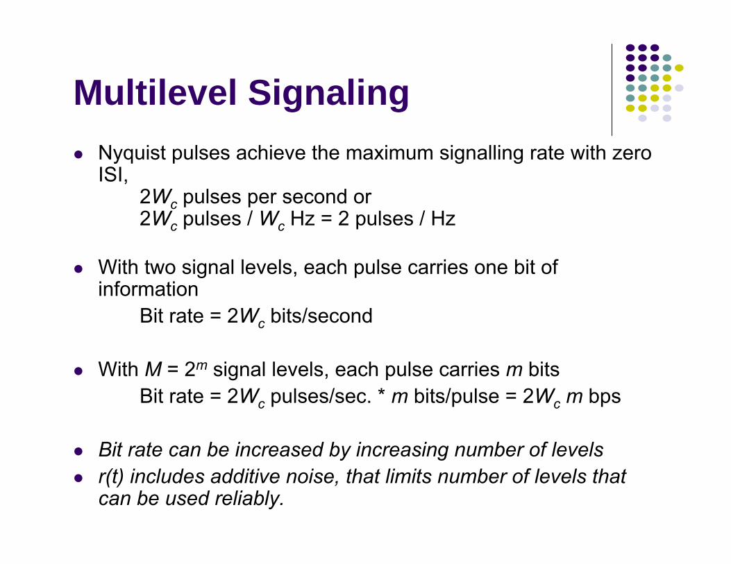
Multilevel SignalingNyquist pulses achieve the maximum signalling rate with zero ISI,

2Wc pulses per second or 2Wc pulses / Wc Hz = 2 pulses / Hz

With two signal levels, each pulse carries one bit of information

Bit rate = 2Wc bits/second

With M = 2m signal levels, each pulse carries m bitsBit rate = 2Wc pulses/sec. * m bits/pulse = 2Wc m bps

Bit rate can be increased by increasing number of levelsr(t) includes additive noise, that limits number of levels that can be used reliably.

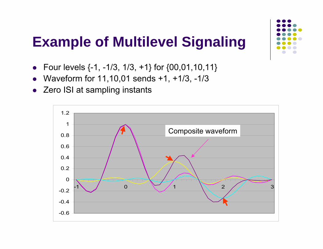
Example of Multilevel SignalingFour levels {-1, -1/3, 1/3, +1} for {00,01,10,11}Waveform for 11,10,01 sends +1, +1/3, -1/3Zero ISI at sampling instants

-0.6

-0.4

-0.2

0

0.2

0.4

0.6

0.8

1

1.2

-1 0 1 2 3

Composite waveform

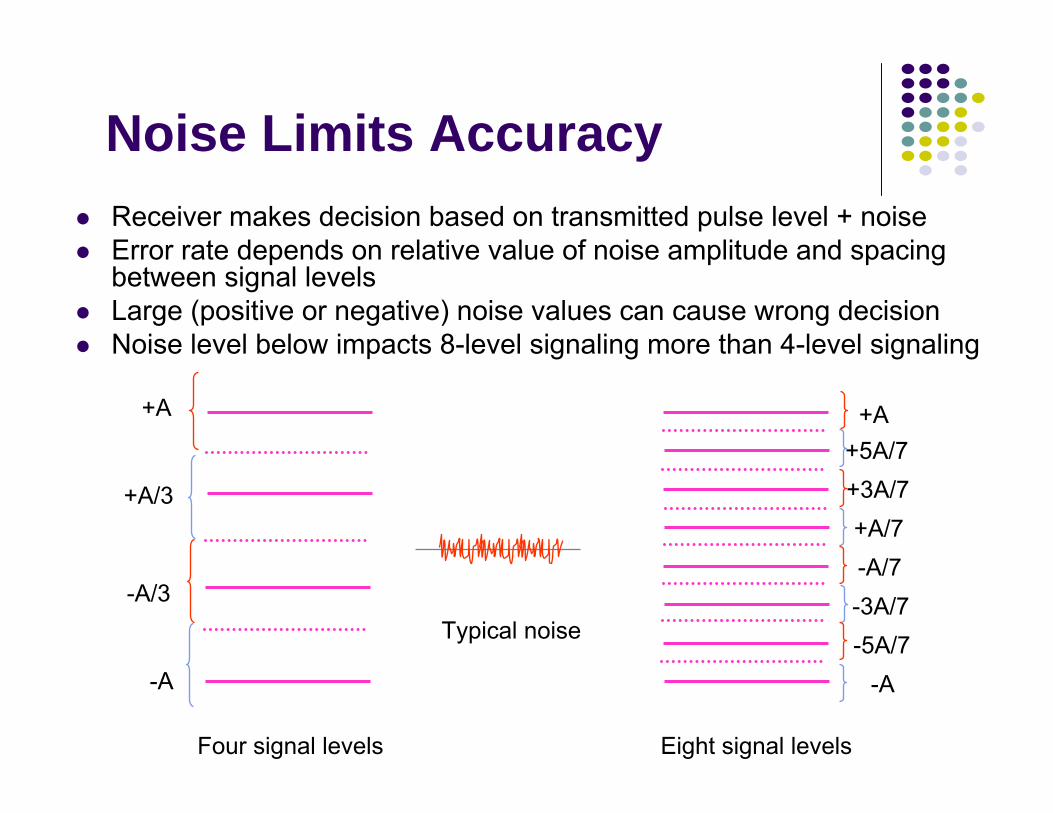
Four signal levels Eight signal levels

Typical noise

Noise Limits AccuracyReceiver makes decision based on transmitted pulse level + noiseError rate depends on relative value of noise amplitude and spacing between signal levels Large (positive or negative) noise values can cause wrong decisionNoise level below impacts 8-level signaling more than 4-level signaling

+A

+A/3

-A/3

-A

+A+5A/7+3A/7+A/7-A/7-3A/7-5A/7

-A

222

21 σ

σπxe−

x0

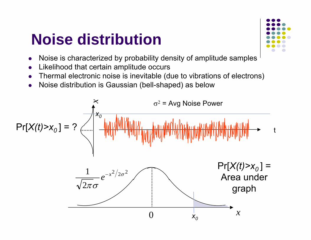
Noise distributionNoise is characterized by probability density of amplitude samplesLikelihood that certain amplitude occursThermal electronic noise is inevitable (due to vibrations of electrons)Noise distribution is Gaussian (bell-shaped) as below

t

x

Pr[X(t)>x0 ] = ?

Pr[X(t)>x0 ] =Area under

graph

x0

x0

σ2 = Avg Noise Power

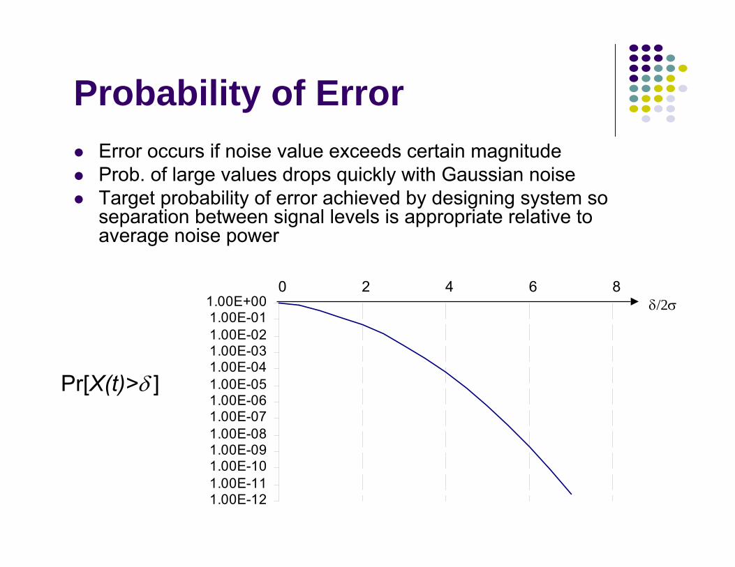
1.00E-121.00E-111.00E-101.00E-091.00E-081.00E-071.00E-061.00E-051.00E-041.00E-031.00E-021.00E-011.00E+00

0 2 4 6 8 δ/2σ

Probability of ErrorError occurs if noise value exceeds certain magnitudeProb. of large values drops quickly with Gaussian noiseTarget probability of error achieved by designing system so separation between signal levels is appropriate relative to average noise power

Pr[X(t)>δ ]

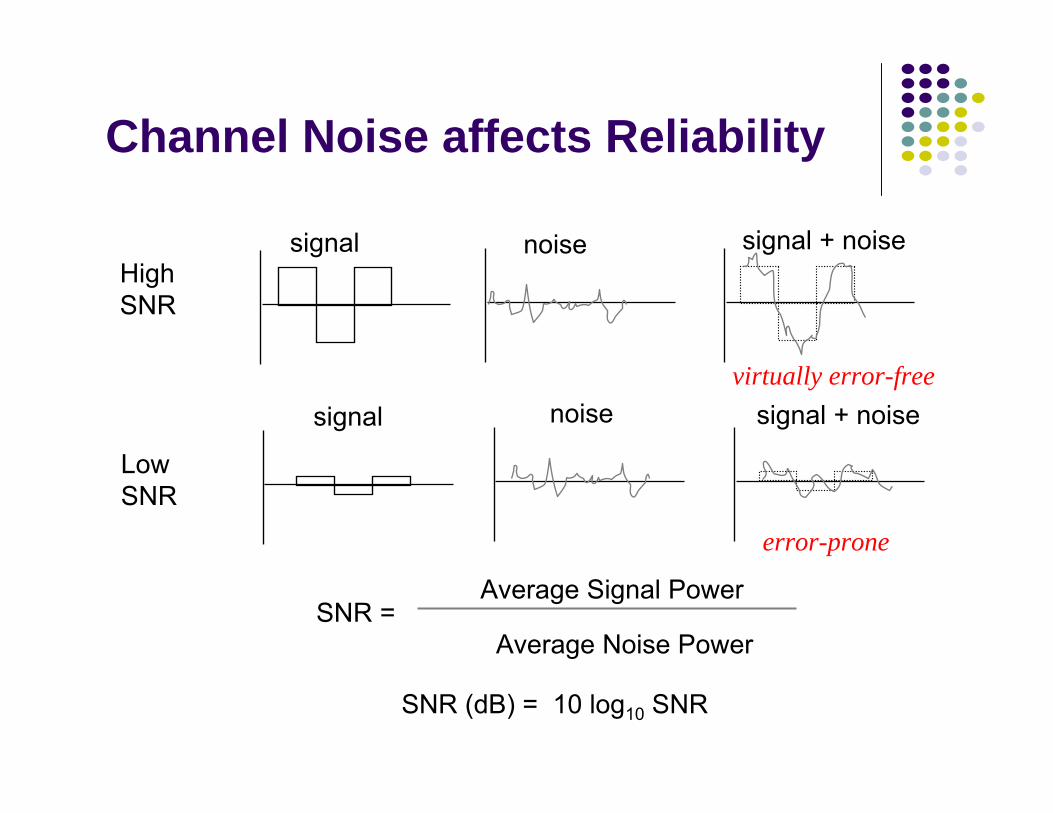
signal noise signal + noise

signal noise signal + noise

HighSNR

LowSNR

SNR = Average Signal Power

Average Noise Power

SNR (dB) = 10 log10 SNR

virtually error-free

error-prone

Channel Noise affects Reliability

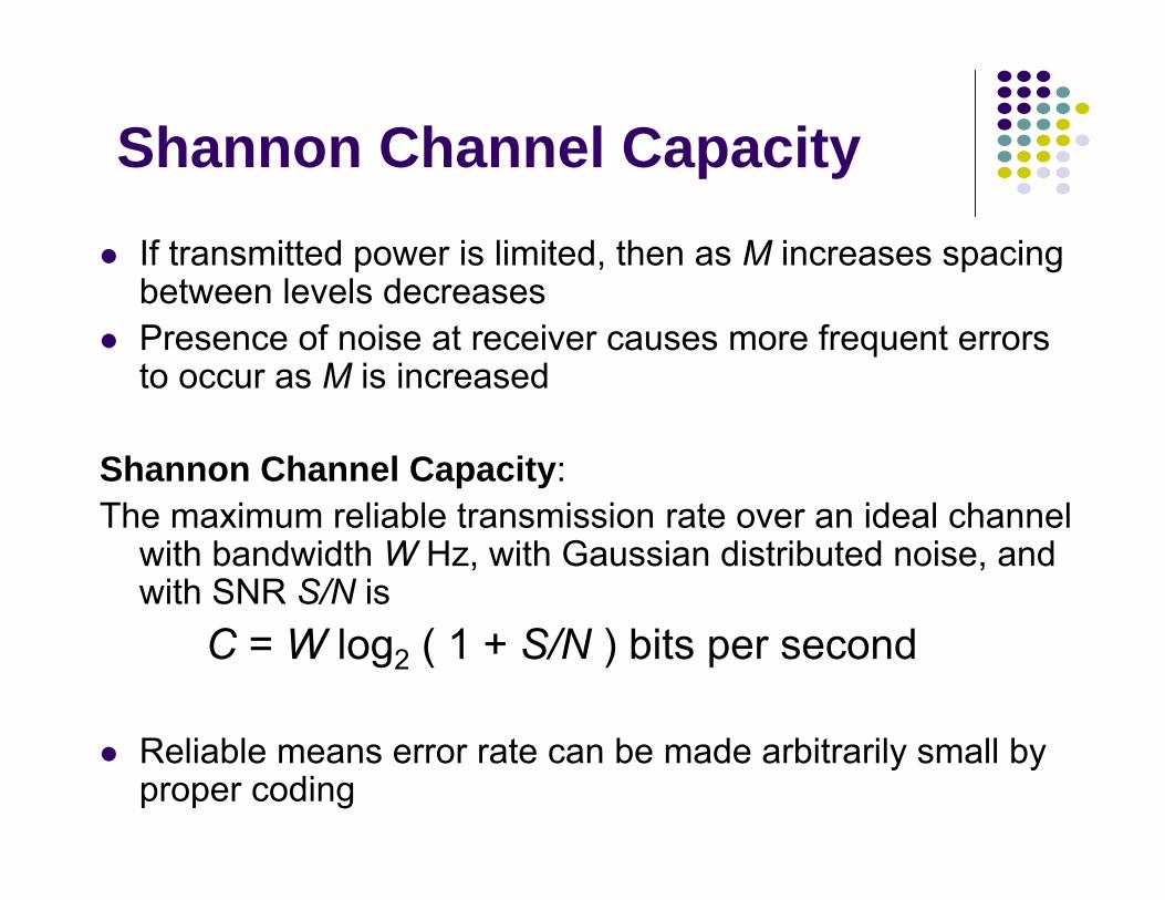
If transmitted power is limited, then as M increases spacing between levels decreasesPresence of noise at receiver causes more frequent errors to occur as M is increased

Shannon Channel Capacity:The maximum reliable transmission rate over an ideal channel

with bandwidth W Hz, with Gaussian distributed noise, and with SNR S/N is

C = W log2 ( 1 + S/N ) bits per second

Reliable means error rate can be made arbitrarily small by proper coding

Shannon Channel Capacity

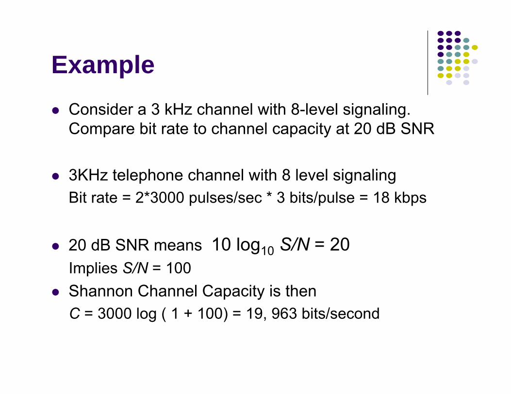
ExampleConsider a 3 kHz channel with 8-level signaling. Compare bit rate to channel capacity at 20 dB SNR

3KHz telephone channel with 8 level signalingBit rate = 2*3000 pulses/sec * 3 bits/pulse = 18 kbps

20 dB SNR means 10 log10 S/N = 20Implies S/N = 100Shannon Channel Capacity is thenC = 3000 log ( 1 + 100) = 19, 963 bits/second


Fundamentals

Line Coding

What is Line Coding?Mapping of binary information sequence into the digital signal that enters the channel

Ex. “1” maps to +A square pulse; “0” to –A pulseLine code selected to meet system requirements:

Transmitted power: Power consumption = $ Bit timing: Transitions in signal help timing recoveryBandwidth efficiency: Excessive transitions wastes bwLow frequency content: Some channels block low frequencies

long periods of +A or of –A causes signal to “droop”Waveform should not have low-frequency content

Error detection: Ability to detect errors helpsComplexity/cost: Is code implementable in chip at high speed?

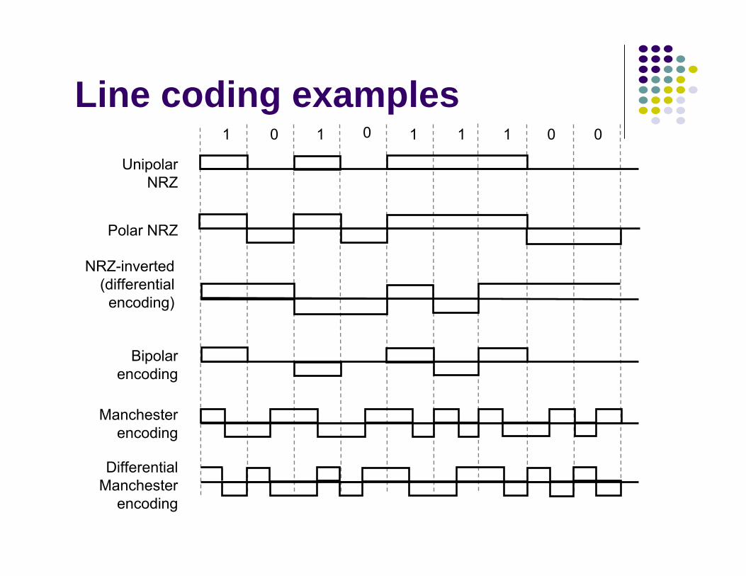
Line coding examples

NRZ-inverted(differential

encoding)

1 0 1 0 1 1 0 01

UnipolarNRZ

Bipolarencoding

Manchesterencoding

DifferentialManchester

encoding

Polar NRZ

-0.2

0

0.2

0.4

0.6

0.8

1

1.2

0

0.2

0.4

0.6

0.8 1

1.2

1.4

1.6

1.8 2

fT

pow

er d

ensi

ty

NRZ

Bipolar

Manchester

Spectrum of Line codesAssume 1s & 0s independent & equiprobable

NRZ has high content at low frequenciesBipolar tightly packed around T/2Manchester wasteful of bandwidth

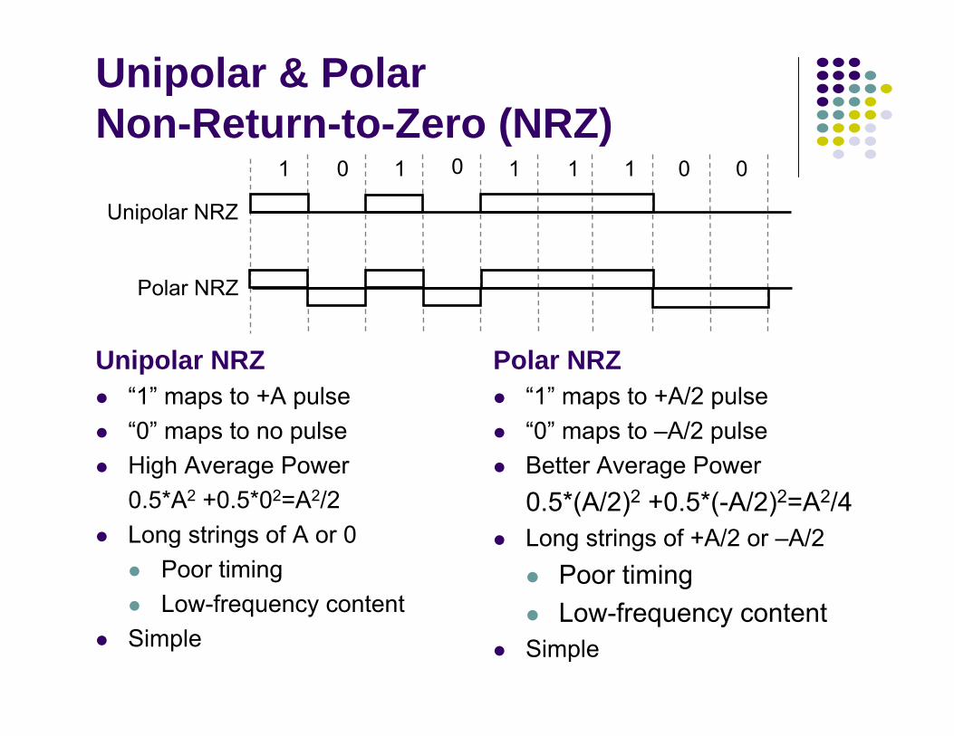
Unipolar & Polar Non-Return-to-Zero (NRZ)

Unipolar NRZ“1” maps to +A pulse“0” maps to no pulseHigh Average Power0.5*A2 +0.5*02=A2/2Long strings of A or 0

Poor timingLow-frequency content

Simple

Polar NRZ“1” maps to +A/2 pulse“0” maps to –A/2 pulseBetter Average Power0.5*(A/2)2 +0.5*(-A/2)2=A2/4Long strings of +A/2 or –A/2

Poor timing Low-frequency content

Simple

1 0 1 0 1 1 0 01

Unipolar NRZ

Polar NRZ

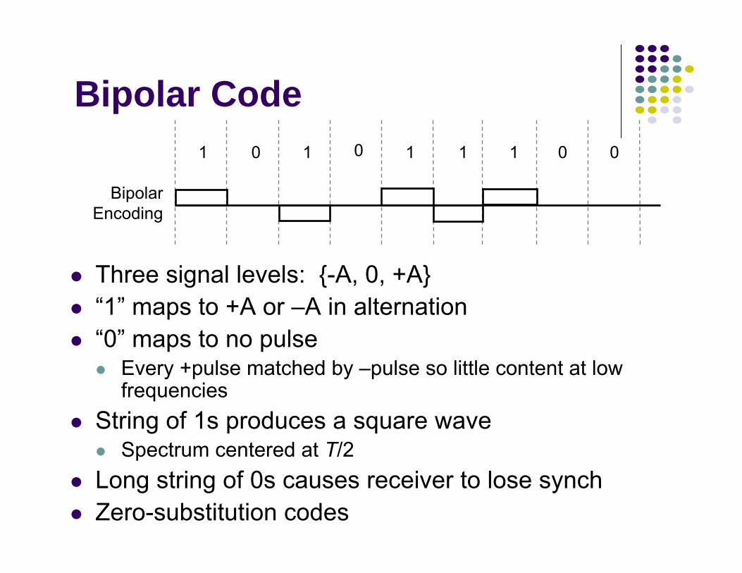
Bipolar Code

Three signal levels: {-A, 0, +A}“1” maps to +A or –A in alternation“0” maps to no pulse

Every +pulse matched by –pulse so little content at low frequencies

String of 1s produces a square waveSpectrum centered at T/2

Long string of 0s causes receiver to lose synchZero-substitution codes

1 0 1 0 1 1 0 01

Bipolar Encoding

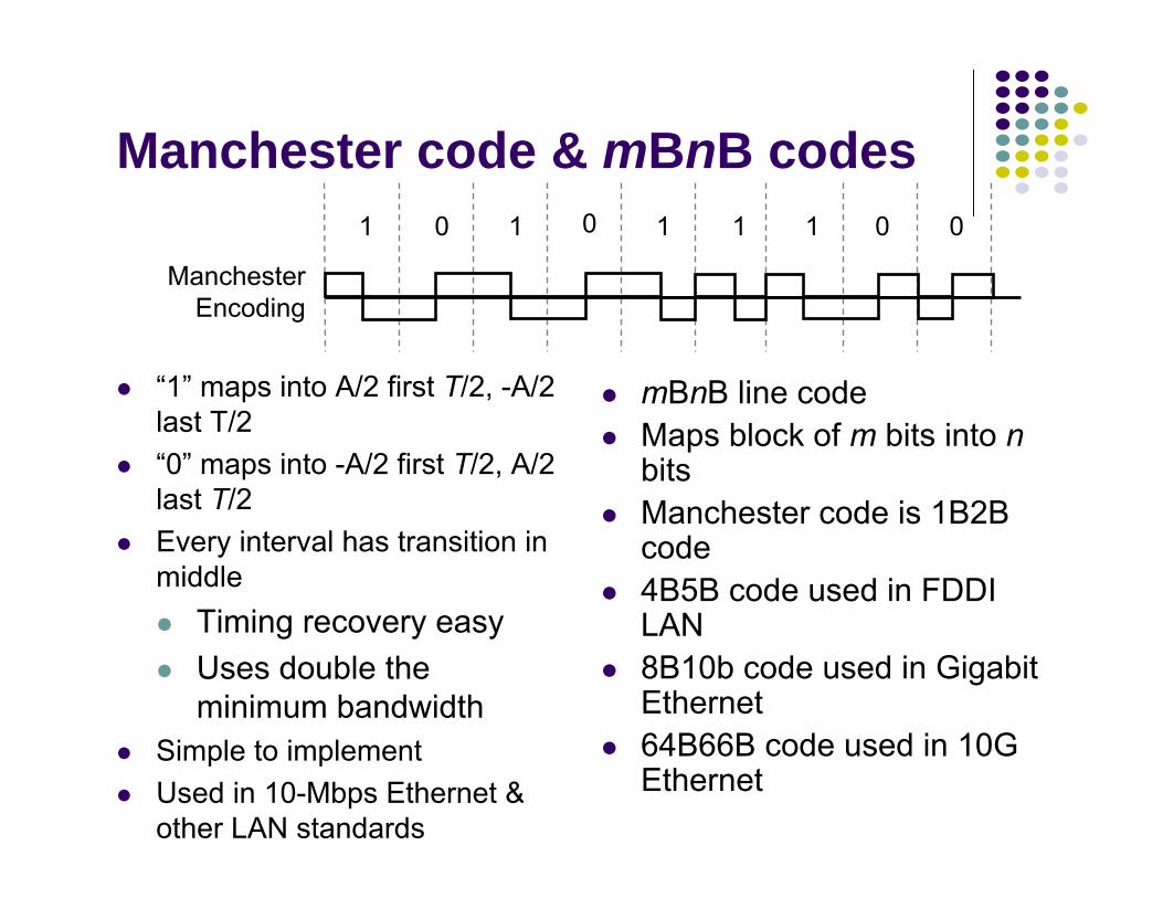
Manchester code & mBnB codes

“1” maps into A/2 first T/2, -A/2 last T/2“0” maps into -A/2 first T/2, A/2 last T/2Every interval has transition in middle

Timing recovery easyUses double the minimum bandwidth

Simple to implementUsed in 10-Mbps Ethernet & other LAN standards

mBnB line codeMaps block of m bits into nbitsManchester code is 1B2B code4B5B code used in FDDI LAN8B10b code used in Gigabit Ethernet64B66B code used in 10G Ethernet

1 0 1 0 1 1 0 01

Manchester Encoding

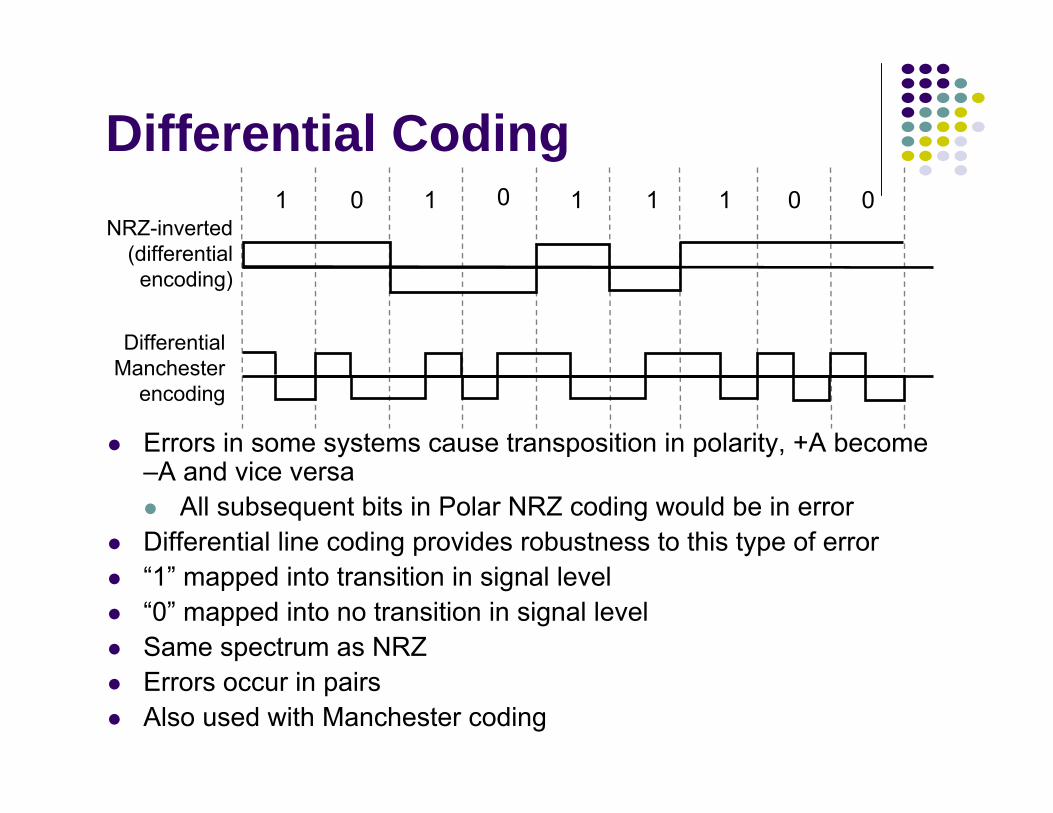
Differential Coding

Errors in some systems cause transposition in polarity, +A become –A and vice versa

All subsequent bits in Polar NRZ coding would be in errorDifferential line coding provides robustness to this type of error“1” mapped into transition in signal level“0” mapped into no transition in signal levelSame spectrum as NRZErrors occur in pairsAlso used with Manchester coding

NRZ-inverted(differential

encoding)

1 0 1 0 1 1 0 01

DifferentialManchester

encoding


Fundamentals

Modems and Digital Modulation

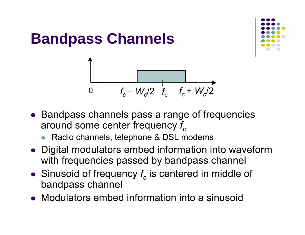
Bandpass Channels

Bandpass channels pass a range of frequencies around some center frequency fc

Radio channels, telephone & DSL modemsDigital modulators embed information into waveform with frequencies passed by bandpass channelSinusoid of frequency fc is centered in middle of bandpass channelModulators embed information into a sinusoid

fc – Wc/2 fc0 fc + Wc/2

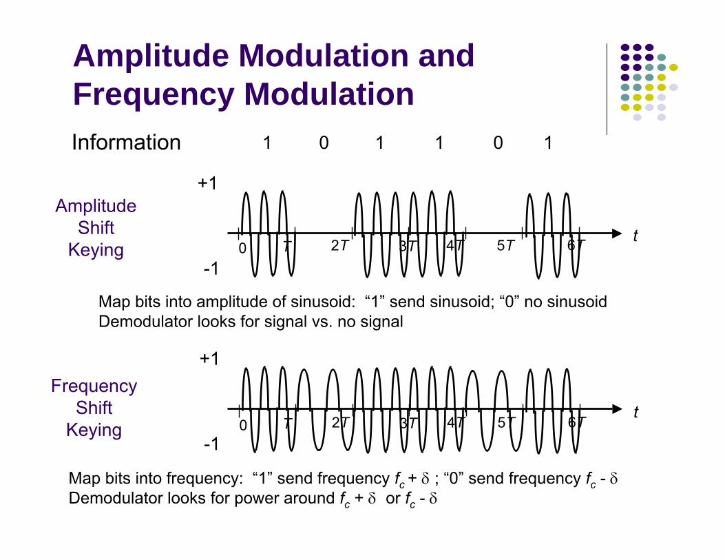
Information 1 1 1 10 0

+1

-10 T 2T 3T 4T 5T 6T

AmplitudeShift

Keying

+1

-1

FrequencyShift

Keying 0 T 2T 3T 4T 5T 6T

t

t

Amplitude Modulation and Frequency Modulation

Map bits into amplitude of sinusoid: “1” send sinusoid; “0” no sinusoidDemodulator looks for signal vs. no signal

Map bits into frequency: “1” send frequency fc + δ ; “0” send frequency fc - δDemodulator looks for power around fc + δ or fc - δ

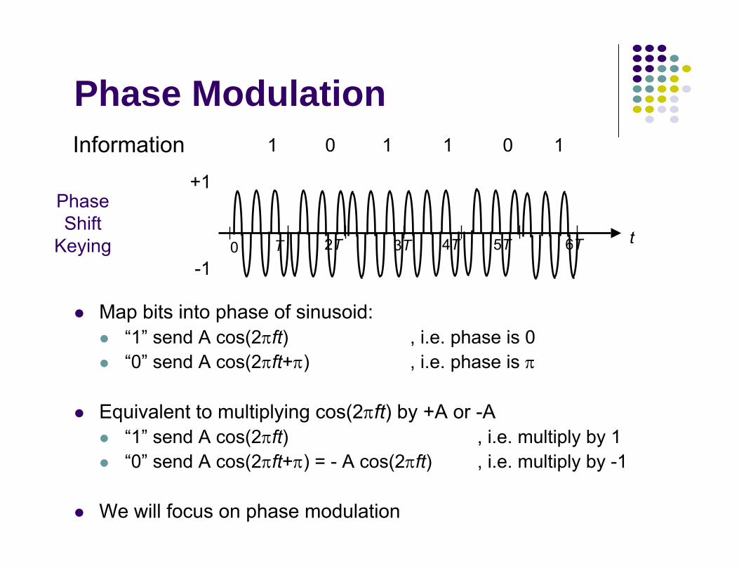
Phase Modulation

Map bits into phase of sinusoid:“1” send A cos(2πft) , i.e. phase is 0“0” send A cos(2πft+π) , i.e. phase is π

Equivalent to multiplying cos(2πft) by +A or -A“1” send A cos(2πft) , i.e. multiply by 1“0” send A cos(2πft+π) = - A cos(2πft) , i.e. multiply by -1

We will focus on phase modulation

+1

-1

PhaseShift

Keying 0 T 2T 3T 4T 5T 6T t

Information 1 1 1 10 0

Modulate cos(2πfct) by multiplying by Ak for T seconds:

Ak x

cos(2πfct)

Yi(t) = Ak cos(2πfct)

Transmitted signal during kth interval

Demodulate (recover Ak) by multiplying by 2cos(2πfct) for T seconds and lowpass filtering (smoothing):

x

2cos(2πfct)2Ak cos2(2πfct) = Ak {1 + cos(2π2fct)}

LowpassFilter

(Smoother)Xi(t)Yi(t) = Akcos(2πfct)

Received signal during kth interval

Modulator & Demodulator

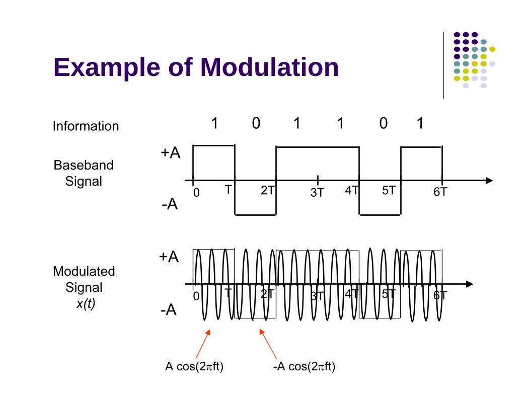
1 1 1 10 0

+A

-A0 T 2T 3T 4T 5T 6T

Information

BasebandSignal

ModulatedSignal

x(t)

+A

-A0 T 2T 3T 4T 5T 6T

Example of Modulation

A cos(2πft) -A cos(2πft)

1 1 1 10 0RecoveredInformation

Basebandsignal discernable

after smoothing

After multiplicationat receiver

x(t) cos(2πfct)

+A

-A0 T 2T 3T 4T 5T 6T

+A

-A0 T 2T 3T 4T 5T 6T

Example of DemodulationA {1 + cos(4πft)} -A {1 + cos(4πft)}

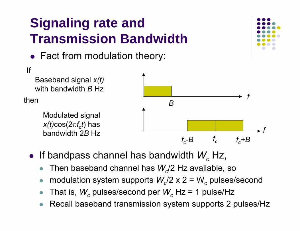
Signaling rate and Transmission Bandwidth

Fact from modulation theory:

Baseband signal x(t)with bandwidth B Hz

If

then B

fc+B

f

ffc-B fc

Modulated signal x(t)cos(2πfct) has bandwidth 2B Hz

If bandpass channel has bandwidth Wc Hz, Then baseband channel has Wc/2 Hz available, somodulation system supports Wc/2 x 2 = Wc pulses/secondThat is, Wc pulses/second per Wc Hz = 1 pulse/HzRecall baseband transmission system supports 2 pulses/Hz

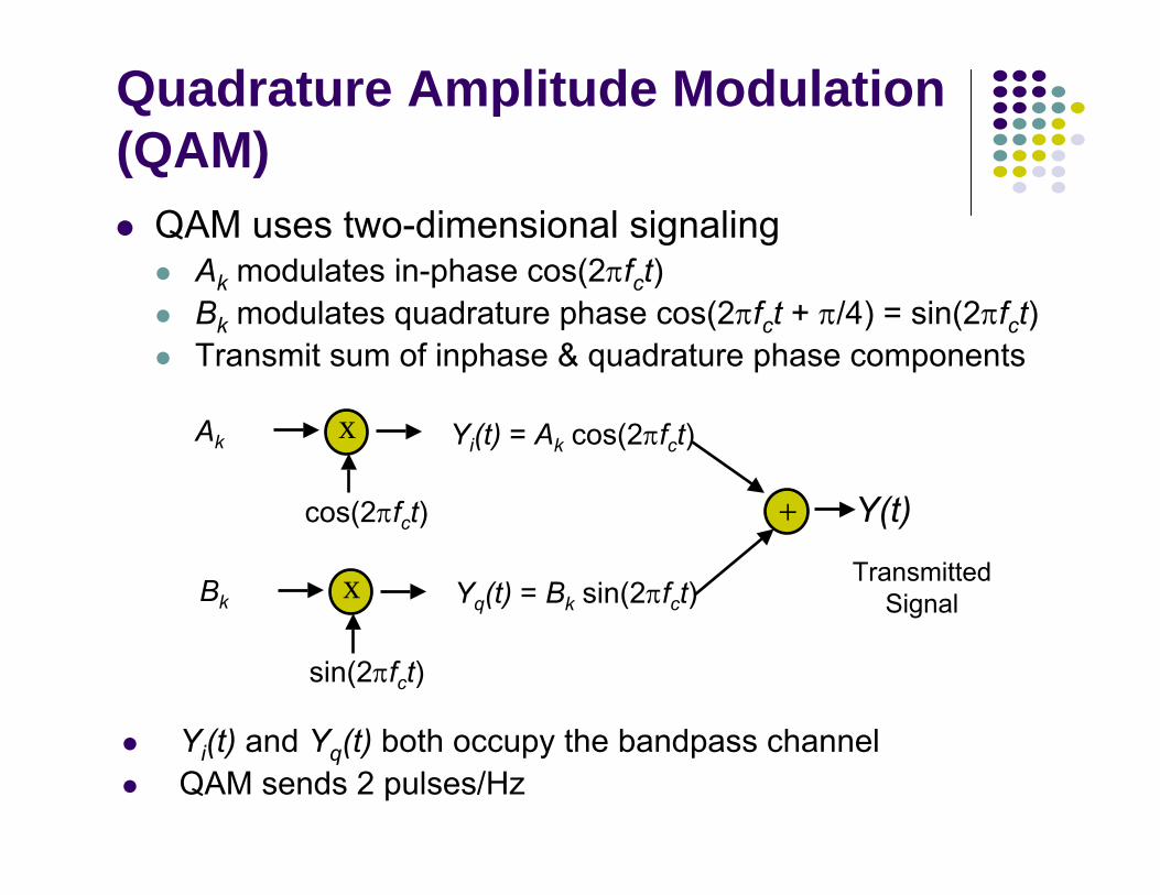
Ak x

cos(2πfct)

Yi(t) = Ak cos(2πfct)

Bk x

sin(2πfct)

Yq(t) = Bk sin(2πfct)

+ Y(t)

Yi(t) and Yq(t) both occupy the bandpass channelQAM sends 2 pulses/Hz

Quadrature Amplitude Modulation (QAM)

QAM uses two-dimensional signalingAk modulates in-phase cos(2πfct) Bk modulates quadrature phase cos(2πfct + π/4) = sin(2πfct)Transmit sum of inphase & quadrature phase components

TransmittedSignal

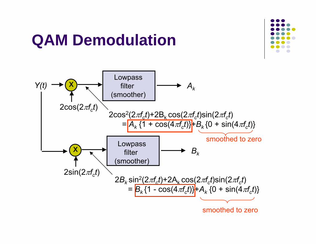
QAM Demodulation

Y(t) x

2cos(2πfct)2cos2(2πfct)+2Bk cos(2πfct)sin(2πfct)

= Ak {1 + cos(4πfct)}+Bk {0 + sin(4πfct)}

Lowpassfilter

(smoother)Ak

2Bk sin2(2πfct)+2Ak cos(2πfct)sin(2πfct)= Bk {1 - cos(4πfct)}+Ak {0 + sin(4πfct)}

x

2sin(2πfct)

Bk

Lowpassfilter

(smoother)

smoothed to zero

smoothed to zero

Signal Constellations

Each pair (Ak, Bk) defines a point in the planeSignal constellation set of signaling points

4 possible points per T sec.2 bits / pulse

Ak

Bk

16 possible points per T sec.4 bits / pulse

Ak

Bk

(A, A)

(A,-A)(-A,-A)

(-A,A)

Ak

Bk

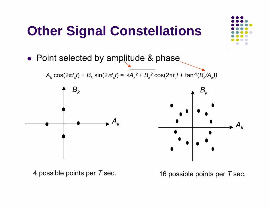
4 possible points per T sec.

Ak

Bk

16 possible points per T sec.

Other Signal Constellations

Point selected by amplitude & phase

Ak cos(2πfct) + Bk sin(2πfct) = √Ak2 + Bk

2 cos(2πfct + tan-1(Bk/Ak))

Telephone Modem StandardsTelephone Channel for modulation purposes has

Wc = 2400 Hz → 2400 pulses per second

Modem Standard V.32bisTrellis modulation maps m bits into one of 2m+1 constellation points14,400 bps Trellis 128 2400x69600 bps Trellis 32 2400x44800 bps QAM 4 2400x2

Modem Standard V.34 adjusts pulse rate to channel2400-33600 bps Trellis 960 2400-3429 pulses/sec


Fundamentals

Properties of Media and Digital Transmission Systems

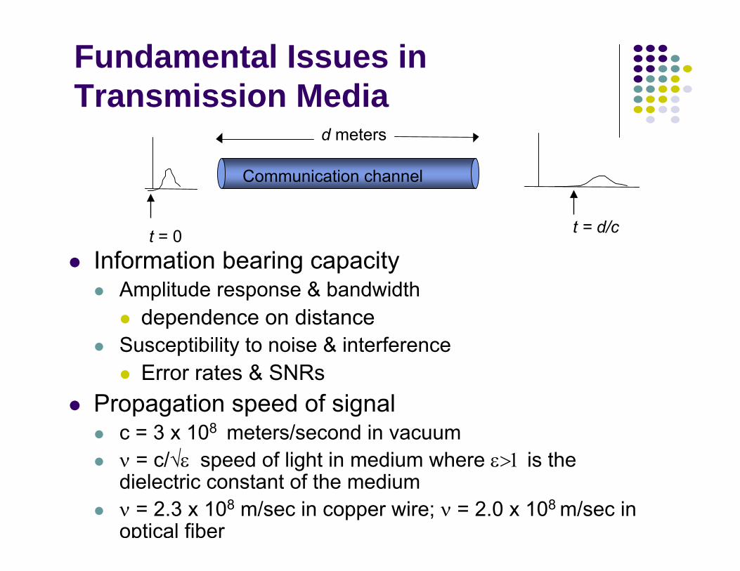
Fundamental Issues in Transmission Media

Information bearing capacityAmplitude response & bandwidth

dependence on distanceSusceptibility to noise & interference

Error rates & SNRsPropagation speed of signal

c = 3 x 108 meters/second in vacuumν = c/√ε speed of light in medium where ε>1 is the dielectric constant of the mediumν = 2.3 x 108 m/sec in copper wire; ν = 2.0 x 108 m/sec in optical fiber

t = 0 t = d/c


d meters

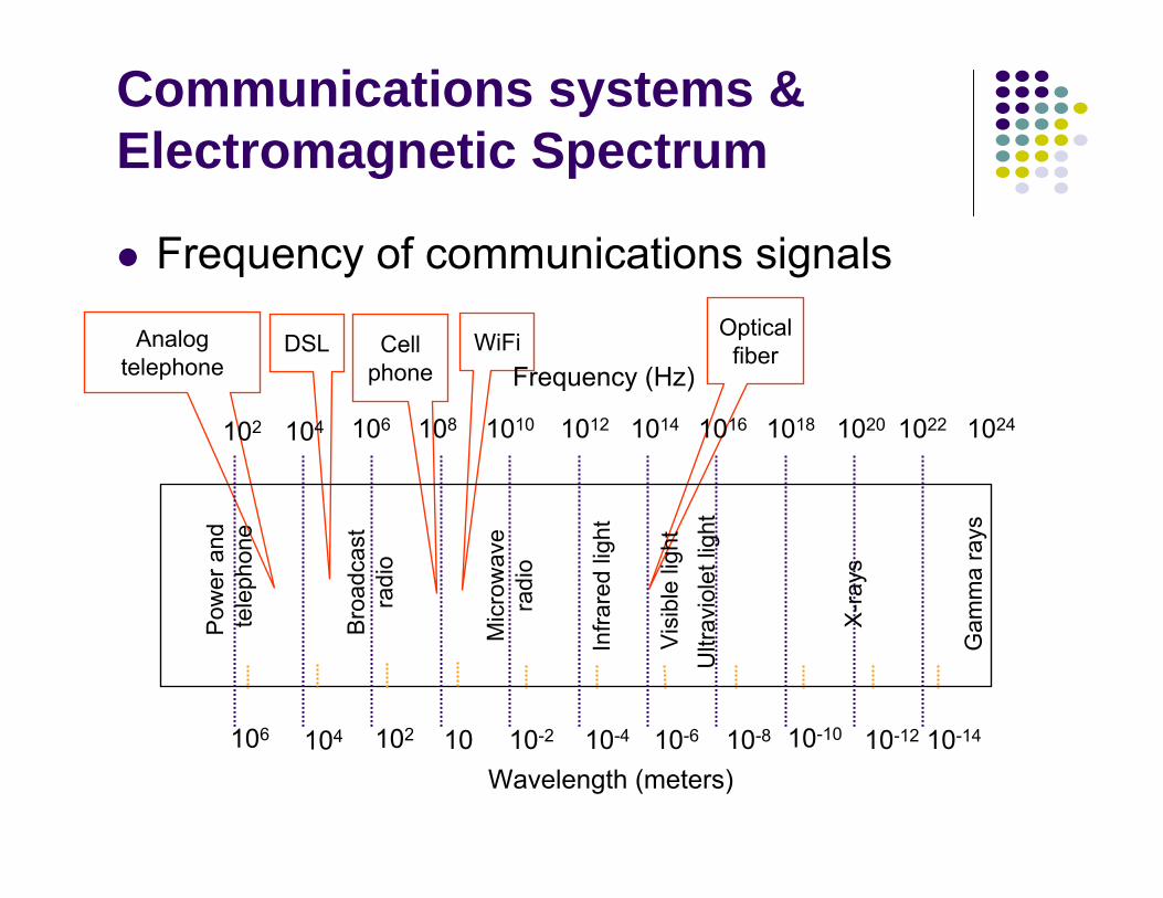
Communications systems & Electromagnetic Spectrum

Frequency of communications signals

Analog telephone

DSL Cell phone

WiFi Optical fiber

102 104 106 108 1010 1012 1014 1016 1018 1020 1022 1024

Frequency (Hz)

Wavelength (meters)106 104 102 10 10-2 10-4 10-6 10-8 10-10 10-12 10-14

Pow

er a

ndte

leph

one

Bro

adca

stra

dio

Mic

row

ave

radi

o

Infra

red

light

Visi

ble

light

Ultr

avio

let l

ight

X-r

ays

Gam

ma

rays

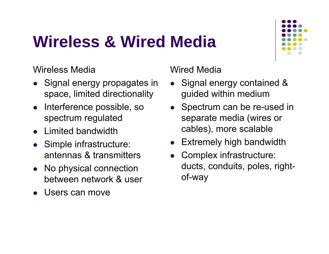
Wireless & Wired MediaWireless Media

Signal energy propagates in space, limited directionalityInterference possible, so spectrum regulatedLimited bandwidthSimple infrastructure: antennas & transmittersNo physical connection between network & userUsers can move

Wired MediaSignal energy contained & guided within mediumSpectrum can be re-used in separate media (wires or cables), more scalableExtremely high bandwidthComplex infrastructure: ducts, conduits, poles, right-of-way

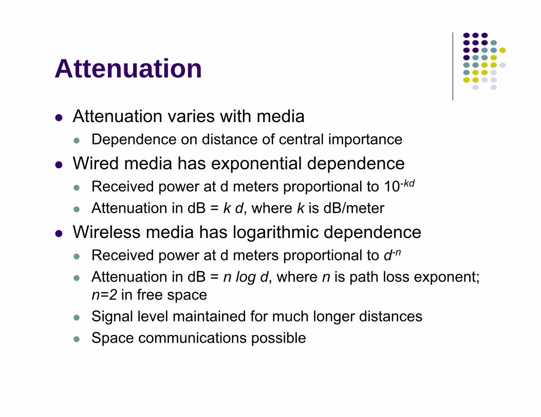
AttenuationAttenuation varies with media

Dependence on distance of central importanceWired media has exponential dependence

Received power at d meters proportional to 10-kd

Attenuation in dB = k d, where k is dB/meterWireless media has logarithmic dependence

Received power at d meters proportional to d-n

Attenuation in dB = n log d, where n is path loss exponent; n=2 in free spaceSignal level maintained for much longer distancesSpace communications possible

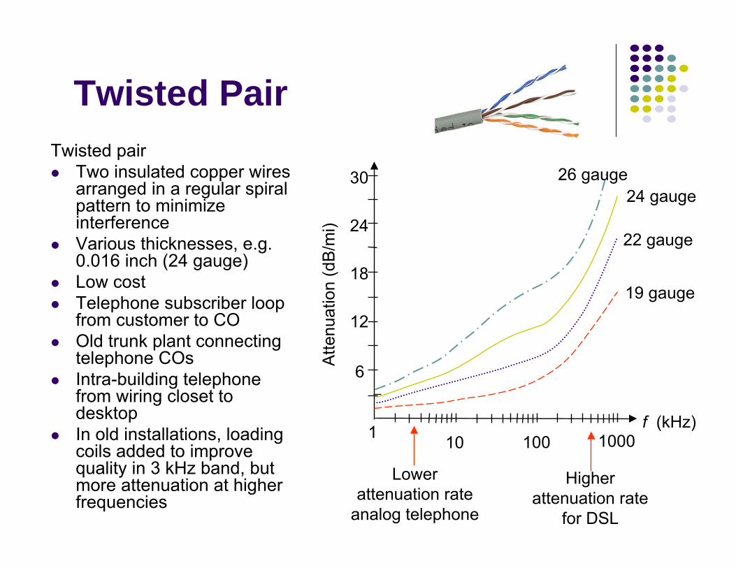
Twisted PairTwisted pair

Two insulated copper wires arranged in a regular spiral pattern to minimize interferenceVarious thicknesses, e.g. 0.016 inch (24 gauge)Low costTelephone subscriber loop from customer to COOld trunk plant connecting telephone COsIntra-building telephone from wiring closet to desktop In old installations, loading coils added to improve quality in 3 kHz band, but more attenuation at higher frequencies

Atte

nuat

ion

(dB

/mi)

f (kHz)

19 gauge

22 gauge

24 gauge26 gauge

6

12

18

24

30

1 10 100 1000

Lower attenuation rate

analog telephone

Higher attenuation rate

for DSL

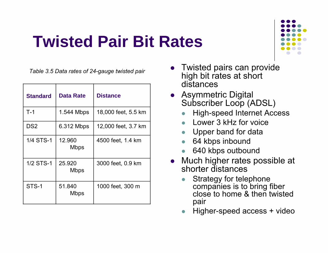
Twisted Pair Bit RatesTwisted pairs can provide high bit rates at short distancesAsymmetric Digital Subscriber Loop (ADSL)

High-speed Internet AccessLower 3 kHz for voiceUpper band for data64 kbps inbound640 kbps outbound

Much higher rates possible at shorter distances

Strategy for telephone companies is to bring fiber close to home & then twisted pairHigher-speed access + video

Table 3.5 Data rates of 24-gauge twisted pair

1000 feet, 300 m51.840 Mbps

STS-1

3000 feet, 0.9 km25.920 Mbps

1/2 STS-1

4500 feet, 1.4 km12.960 Mbps

1/4 STS-1

12,000 feet, 3.7 km6.312 MbpsDS2

18,000 feet, 5.5 km1.544 MbpsT-1

DistanceData RateStandard

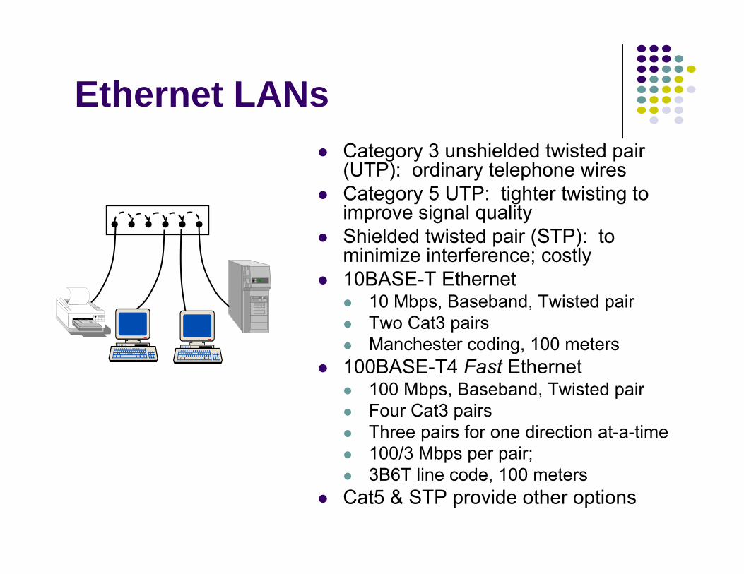
Ethernet LANsCategory 3 unshielded twisted pair (UTP): ordinary telephone wiresCategory 5 UTP: tighter twisting to improve signal qualityShielded twisted pair (STP): to minimize interference; costly10BASE-T Ethernet

10 Mbps, Baseband, Twisted pairTwo Cat3 pairsManchester coding, 100 meters

100BASE-T4 Fast Ethernet100 Mbps, Baseband, Twisted pairFour Cat3 pairsThree pairs for one direction at-a-time100/3 Mbps per pair; 3B6T line code, 100 meters

Cat5 & STP provide other options

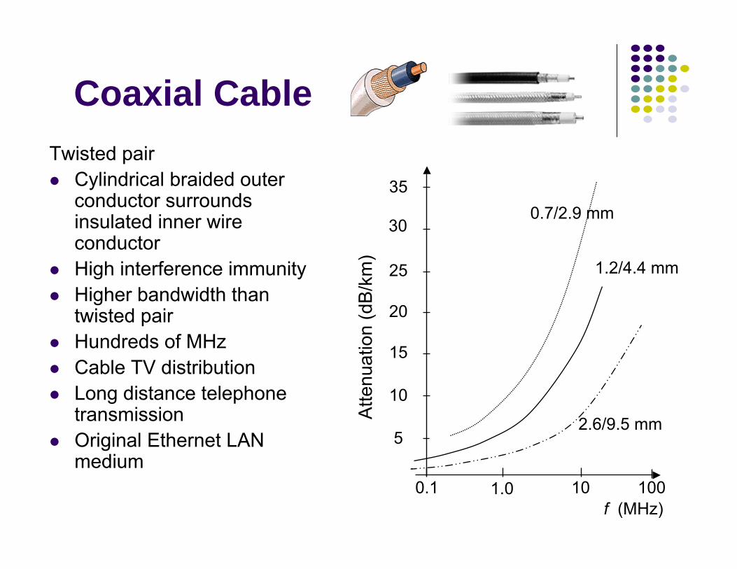
Coaxial CableTwisted pair

Cylindrical braided outer conductor surrounds insulated inner wire conductorHigh interference immunityHigher bandwidth than twisted pairHundreds of MHzCable TV distributionLong distance telephone transmissionOriginal Ethernet LAN medium

35

30

10

25

20

5

15A

ttenu

atio

n (d

B/k

m)

0.1 1.0 10 100f (MHz)

2.6/9.5 mm

1.2/4.4 mm

0.7/2.9 mm

UpstreamDownstream

5 MH

z

42 MH

z

54 MH

z

500 MH

z

550 MH

z

750 M

Hz

Downstream

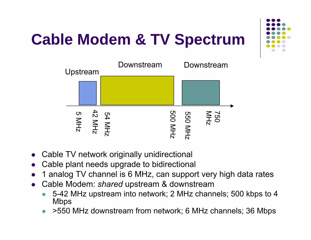
Cable Modem & TV Spectrum

Cable TV network originally unidirectionalCable plant needs upgrade to bidirectional1 analog TV channel is 6 MHz, can support very high data ratesCable Modem: shared upstream & downstream

5-42 MHz upstream into network; 2 MHz channels; 500 kbps to 4 Mbps>550 MHz downstream from network; 6 MHz channels; 36 Mbps

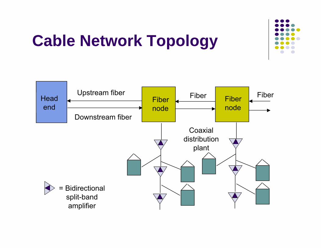
Cable Network Topology

Headend

Upstream fiber

Downstream fiber

Fibernode

Coaxialdistribution

plant

Fibernode

= Bidirectionalsplit-bandamplifier

Fiber Fiber

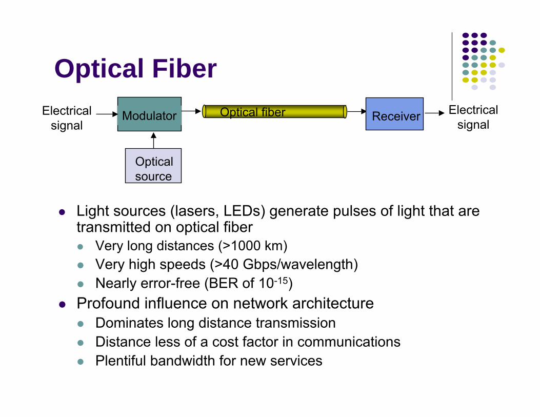
Optical Fiber

Light sources (lasers, LEDs) generate pulses of light that are transmitted on optical fiber

Very long distances (>1000 km)Very high speeds (>40 Gbps/wavelength)Nearly error-free (BER of 10-15)

Profound influence on network architectureDominates long distance transmissionDistance less of a cost factor in communicationsPlentiful bandwidth for new services

Optical fiber

Opticalsource

ModulatorElectricalsignal

Receiver Electricalsignal

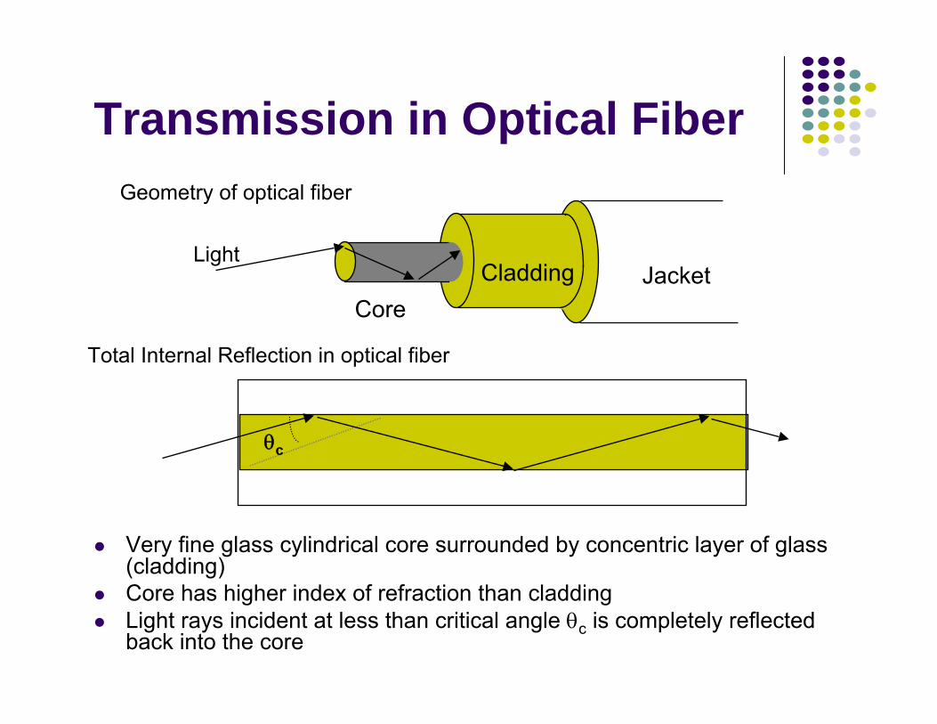
CoreCladding Jacket

Light

θc

Geometry of optical fiber

Total Internal Reflection in optical fiber

Transmission in Optical Fiber

Very fine glass cylindrical core surrounded by concentric layer of glass (cladding)Core has higher index of refraction than claddingLight rays incident at less than critical angle θc is completely reflected back into the core

Multimode: Thicker core, shorter reachRays on different paths interfere causing dispersion & limiting bit rate

Single mode: Very thin core supports only one mode (path)More expensive lasers, but achieves very high speeds

Multimode fiber: multiple rays follow different paths

Single-mode fiber: only direct path propagates in fiber

Direct path

Reflected path

Multimode & Single-mode Fiber

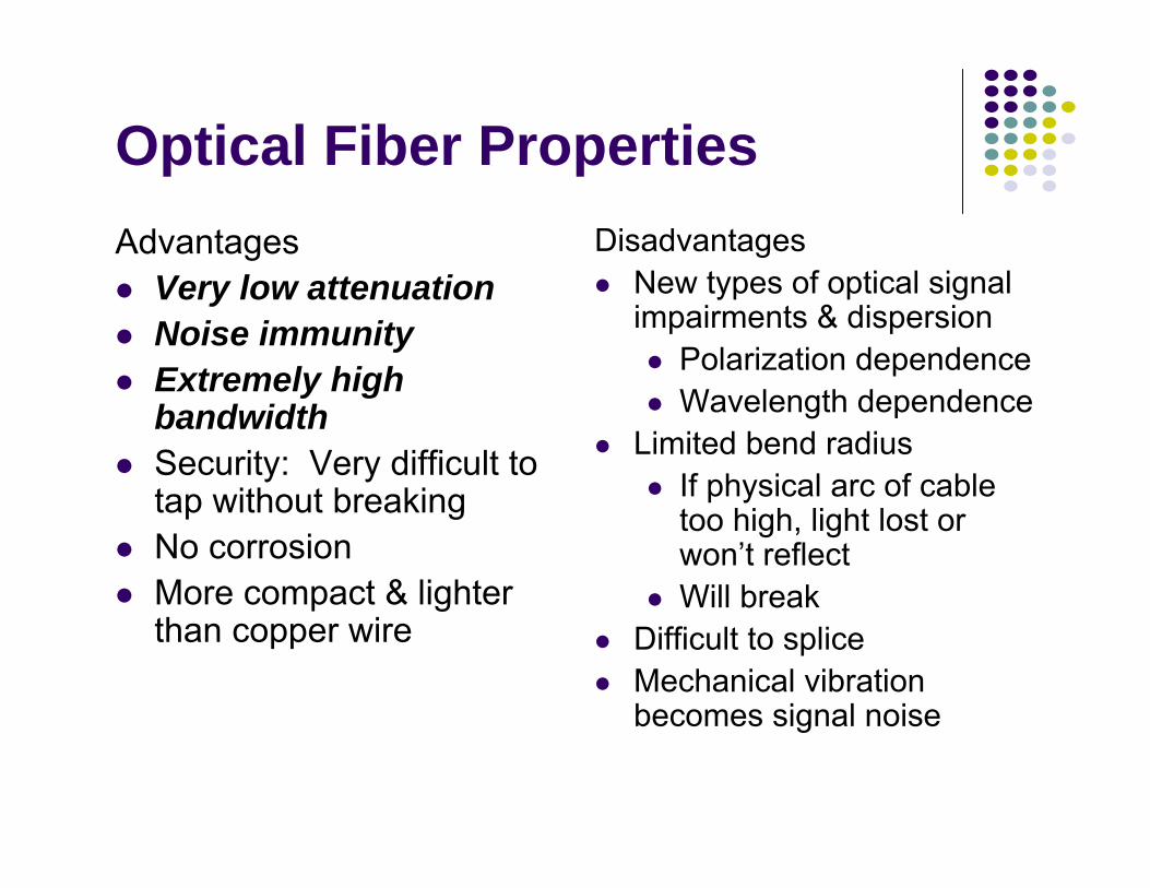
Optical Fiber PropertiesAdvantages

Very low attenuationNoise immunityExtremely high bandwidthSecurity: Very difficult to tap without breakingNo corrosionMore compact & lighter than copper wire

DisadvantagesNew types of optical signal impairments & dispersion

Polarization dependenceWavelength dependence

Limited bend radiusIf physical arc of cable too high, light lost or won’t reflectWill break

Difficult to spliceMechanical vibration becomes signal noise

100

50

10

5

1

0.5

0.1

0.05

0.010.8 1.0 1.2 1.4 1.6 1.8 Wavelength (μm)

Loss

(dB

/km

)

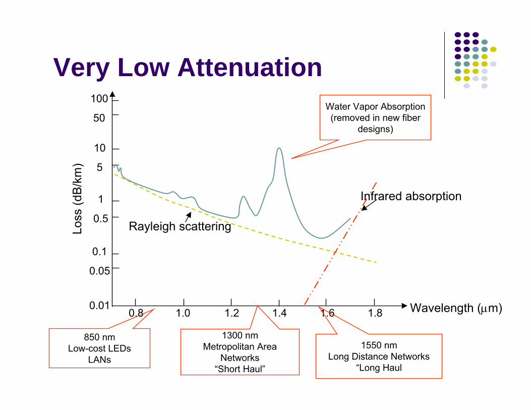
Infrared absorption

Rayleigh scattering

Very Low Attenuation

850 nmLow-cost LEDs

LANs

1300 nmMetropolitan Area

Networks“Short Haul”

1550 nmLong Distance Networks

“Long Haul

Water Vapor Absorption(removed in new fiber

designs)

100

50

10

5

1

0.5

0.1

0.8 1.0 1.2 1.4 1.6 1.8

Loss

(dB

/km

)

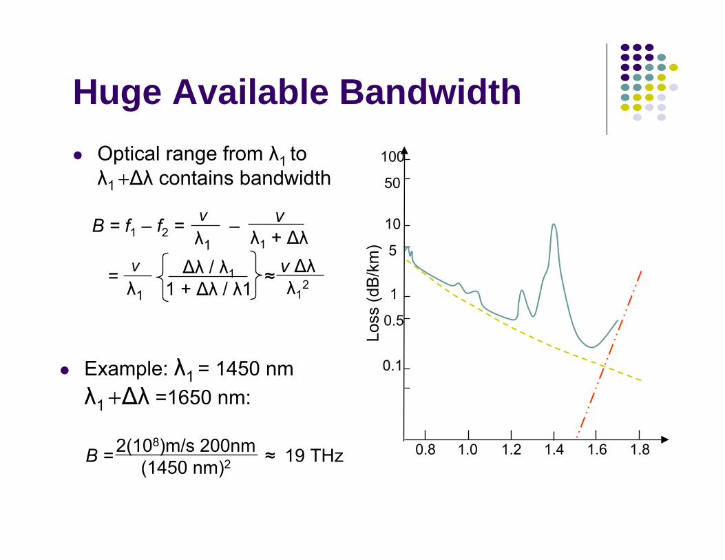
Huge Available BandwidthOptical range from λ1 to λ1 +∆λ contains bandwidth

Example: λ1 = 1450 nm λ1 +∆λ =1650 nm:

B = ≈ 19 THz

B = f1 – f2 = – vλ1 + ∆λ

vλ1

v ∆λλ1

2= ≈∆λ / λ11 + ∆λ / λ1

vλ1

2(108)m/s 200nm (1450 nm)2

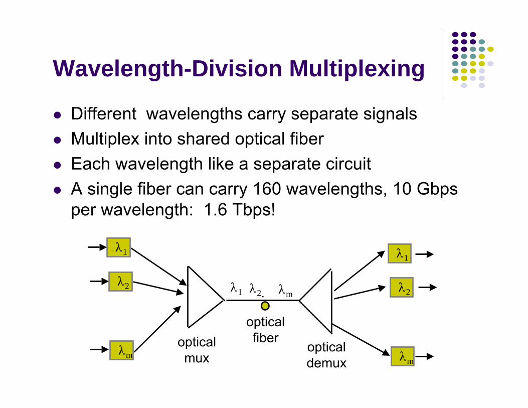
Wavelength-Division Multiplexing

Different wavelengths carry separate signalsMultiplex into shared optical fiberEach wavelength like a separate circuitA single fiber can carry 160 wavelengths, 10 Gbpsper wavelength: 1.6 Tbps!

λ1

λ2

λmopticalmux

λ1

λ2

λmopticaldemux

λ1 λ2. λm

opticalfiber

Coarse & Dense WDMCoarse WDM

Few wavelengths 4-8 with very wide spacingLow-cost, simple

Dense WDMMany tightly-packed wavelengthsITU Grid: 0.8 nm separation for 10Gbps signals0.4 nm for 2.5 Gbps

1550

1560

1540

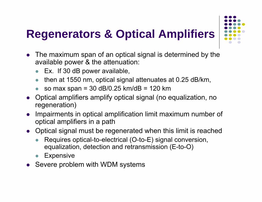
Regenerators & Optical AmplifiersThe maximum span of an optical signal is determined by the available power & the attenuation:

Ex. If 30 dB power available, then at 1550 nm, optical signal attenuates at 0.25 dB/km, so max span = 30 dB/0.25 km/dB = 120 km

Optical amplifiers amplify optical signal (no equalization, no regeneration)Impairments in optical amplification limit maximum number of optical amplifiers in a pathOptical signal must be regenerated when this limit is reached

Requires optical-to-electrical (O-to-E) signal conversion, equalization, detection and retransmission (E-to-O)Expensive

Severe problem with WDM systems

RegeneratorR R R R R R R R

DWDMmultiplexer

… …R

R

R

R

…R

R

R

R

…R

R

R

R

…R

R

R

R…

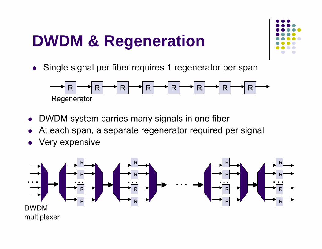
DWDM & RegenerationSingle signal per fiber requires 1 regenerator per span

DWDM system carries many signals in one fiberAt each span, a separate regenerator required per signalVery expensive

R

R

R

R

Opticalamplifier

… … …R

R

R

ROA OA OA OA… …

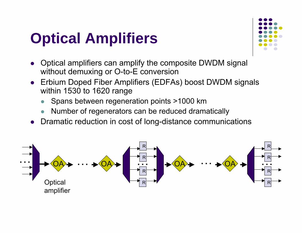
Optical AmplifiersOptical amplifiers can amplify the composite DWDM signal without demuxing or O-to-E conversionErbium Doped Fiber Amplifiers (EDFAs) boost DWDM signals within 1530 to 1620 range

Spans between regeneration points >1000 kmNumber of regenerators can be reduced dramatically

Dramatic reduction in cost of long-distance communications

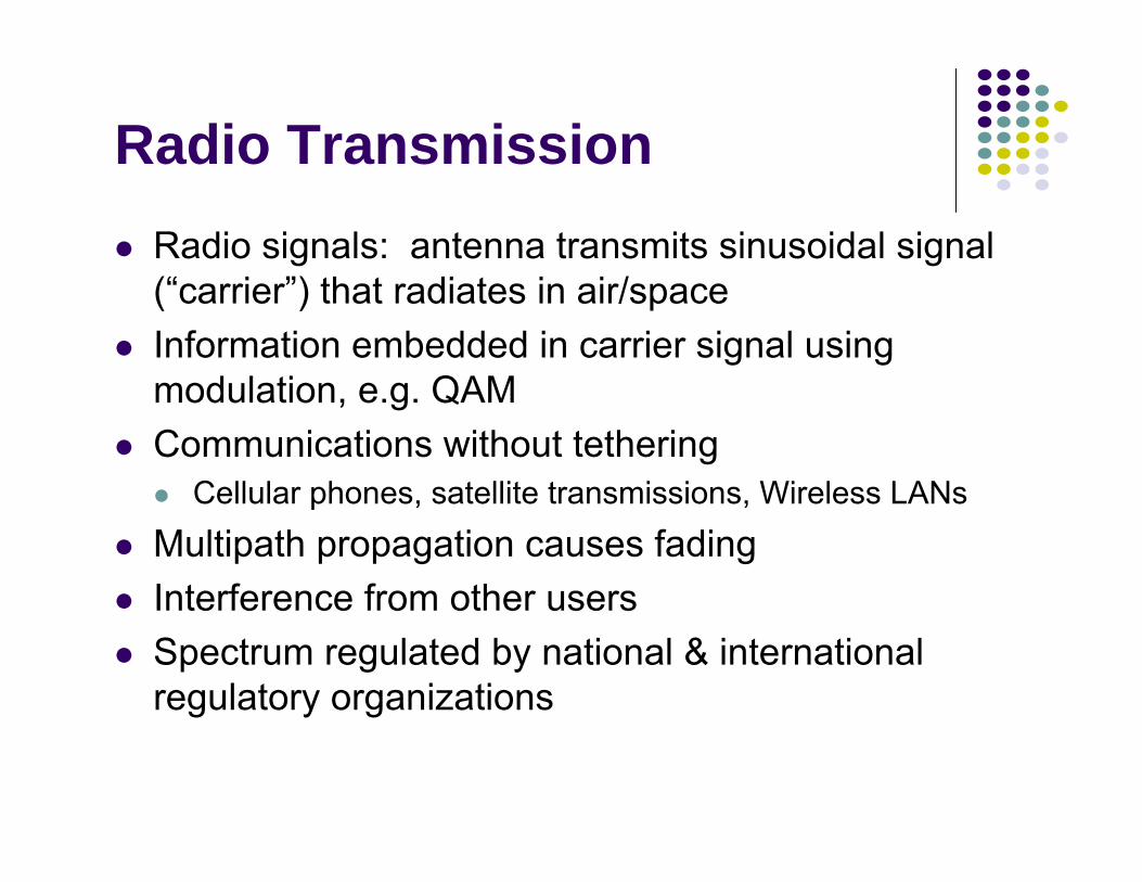
Radio TransmissionRadio signals: antenna transmits sinusoidal signal (“carrier”) that radiates in air/spaceInformation embedded in carrier signal using modulation, e.g. QAMCommunications without tethering

Cellular phones, satellite transmissions, Wireless LANsMultipath propagation causes fadingInterference from other usersSpectrum regulated by national & international regulatory organizations

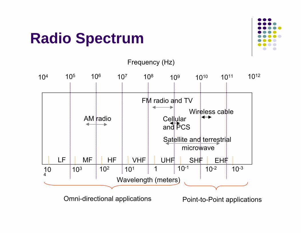
104 106 107 108 109 1010 1011 1012

Frequency (Hz)

Wavelength (meters)103 102 101 1 10-1 10-2 10-3

105

Satellite and terrestrialmicrowave

AM radio

FM radio and TV

LF MF HF VHF UHF SHF EHF104

Cellularand PCS

Wireless cable

Radio Spectrum

Omni-directional applications Point-to-Point applications

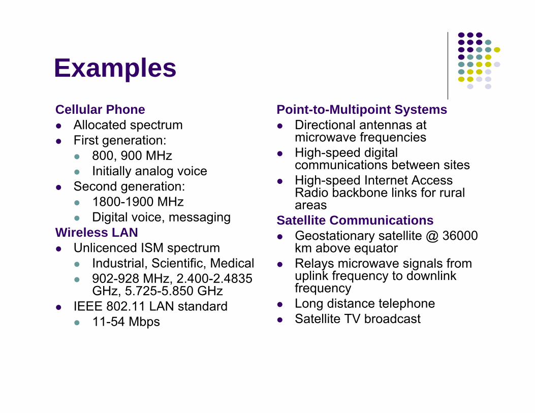
ExamplesCellular Phone

Allocated spectrumFirst generation:

800, 900 MHzInitially analog voice

Second generation:1800-1900 MHzDigital voice, messaging

Wireless LANUnlicenced ISM spectrum

Industrial, Scientific, Medical902-928 MHz, 2.400-2.4835 GHz, 5.725-5.850 GHz

IEEE 802.11 LAN standard11-54 Mbps

Point-to-Multipoint SystemsDirectional antennas at microwave frequenciesHigh-speed digital communications between sitesHigh-speed Internet Access Radio backbone links for rural areas

Satellite CommunicationsGeostationary satellite @ 36000 km above equatorRelays microwave signals from uplink frequency to downlink frequencyLong distance telephoneSatellite TV broadcast


Fundamentals

Error Detection and Correction

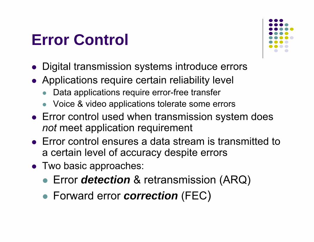
Error ControlDigital transmission systems introduce errorsApplications require certain reliability level

Data applications require error-free transferVoice & video applications tolerate some errors

Error control used when transmission system does not meet application requirementError control ensures a data stream is transmitted to a certain level of accuracy despite errors Two basic approaches:

Error detection & retransmission (ARQ)Forward error correction (FEC)

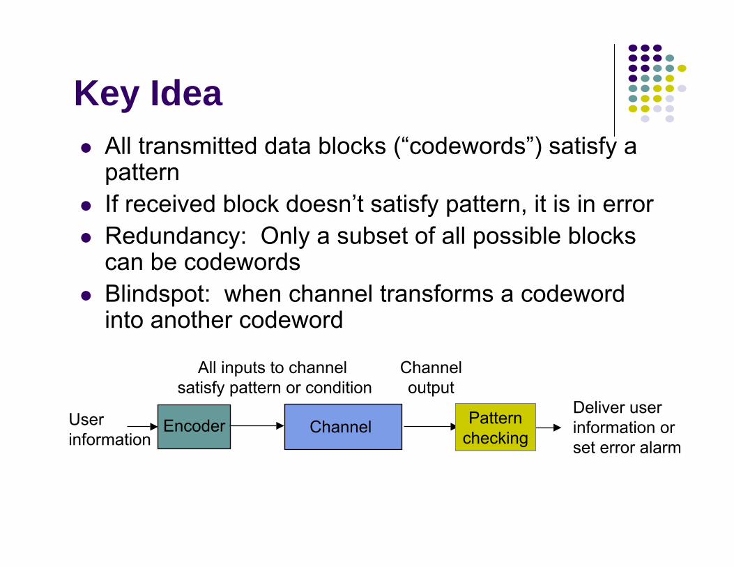
Key IdeaAll transmitted data blocks (“codewords”) satisfy a patternIf received block doesn’t satisfy pattern, it is in errorRedundancy: Only a subset of all possible blocks can be codewordsBlindspot: when channel transforms a codeword into another codeword

ChannelEncoderUserinformation

Patternchecking

All inputs to channelsatisfy pattern or condition

Channeloutput

Deliver user information orset error alarm

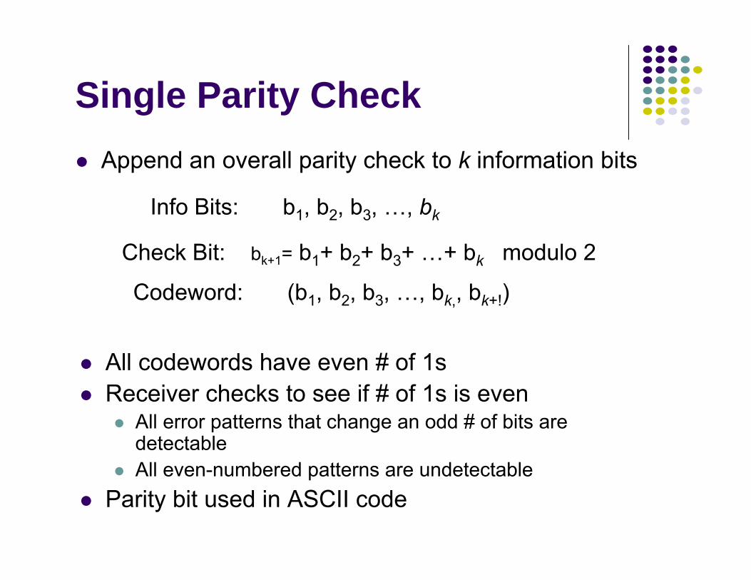
Single Parity CheckAppend an overall parity check to k information bits

Info Bits: b1, b2, b3, …, bk

Check Bit: bk+1= b1+ b2+ b3+ …+ bk modulo 2

Codeword: (b1, b2, b3, …, bk,, bk+!)

All codewords have even # of 1sReceiver checks to see if # of 1s is even

All error patterns that change an odd # of bits are detectableAll even-numbered patterns are undetectable

Parity bit used in ASCII code

Example of Single Parity CodeInformation (7 bits): (0, 1, 0, 1, 1, 0, 0)Parity Bit: b8 = 0 + 1 +0 + 1 +1 + 0 = 1Codeword (8 bits): (0, 1, 0, 1, 1, 0, 0, 1)

If single error in bit 3 : (0, 1, 1, 1, 1, 0, 0, 1)# of 1’s =5, oddError detected

If errors in bits 3 and 5: (0, 1, 1, 1, 0, 0, 0, 1)# of 1’s =4, evenError not detected

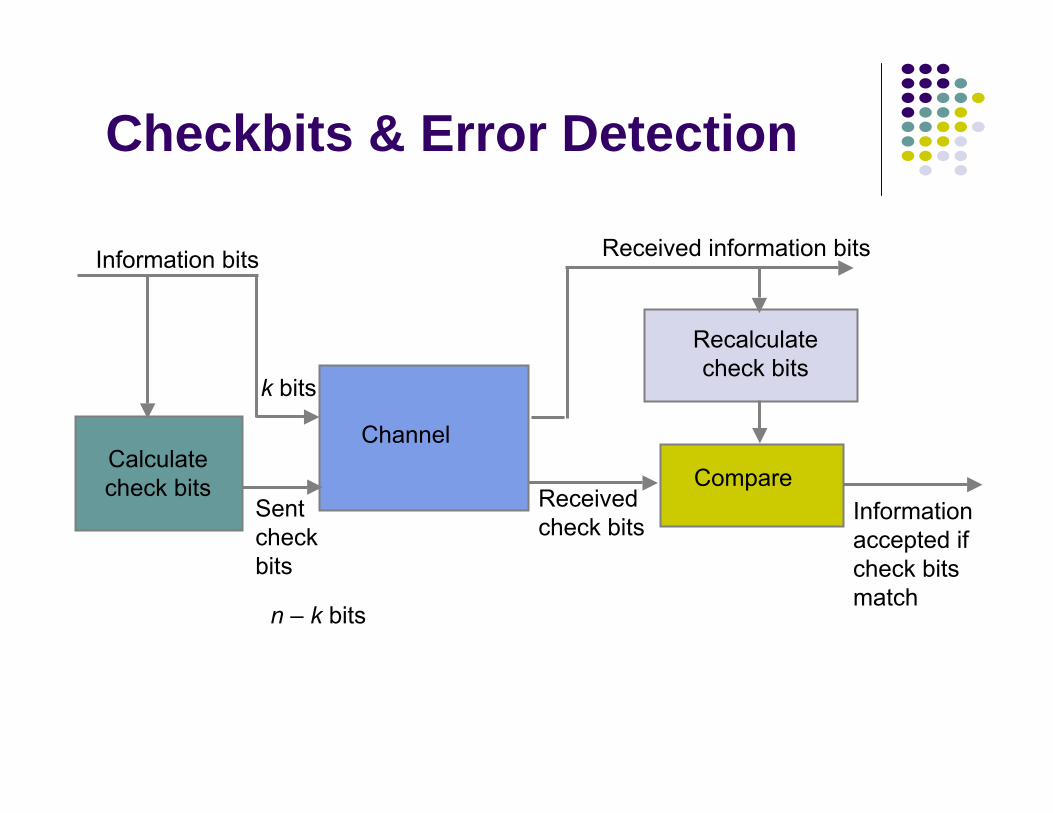
Checkbits & Error Detection

Calculate check bits

Channel

Recalculate check bits

Compare

Information bits Received information bits

Sent checkbits

Information accepted if check bits match

Received check bits

k bits

n – k bits

How good is the single parity check code?

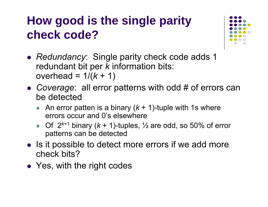
Redundancy: Single parity check code adds 1 redundant bit per k information bits: overhead = 1/(k + 1)Coverage: all error patterns with odd # of errors can be detected

An error patten is a binary (k + 1)-tuple with 1s where errors occur and 0’s elsewhereOf 2k+1 binary (k + 1)-tuples, ½ are odd, so 50% of error patterns can be detected

Is it possible to detect more errors if we add more check bits? Yes, with the right codes

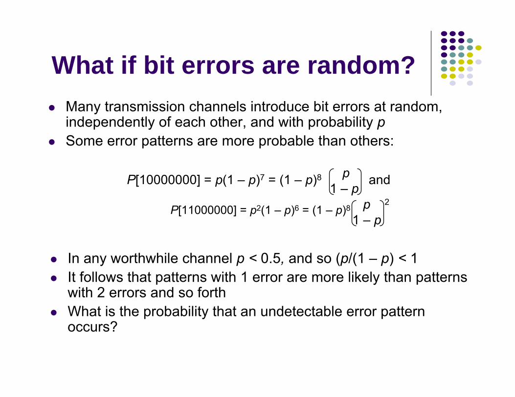
What if bit errors are random?Many transmission channels introduce bit errors at random, independently of each other, and with probability pSome error patterns are more probable than others:

In any worthwhile channel p < 0.5, and so (p/(1 – p) < 1It follows that patterns with 1 error are more likely than patterns with 2 errors and so forthWhat is the probability that an undetectable error pattern occurs?

P[10000000] = p(1 – p)7 = (1 – p)8 and

P[11000000] = p2(1 – p)6 = (1 – p)8

p1 – p

p 21 – p

Single parity check code with random bit errors

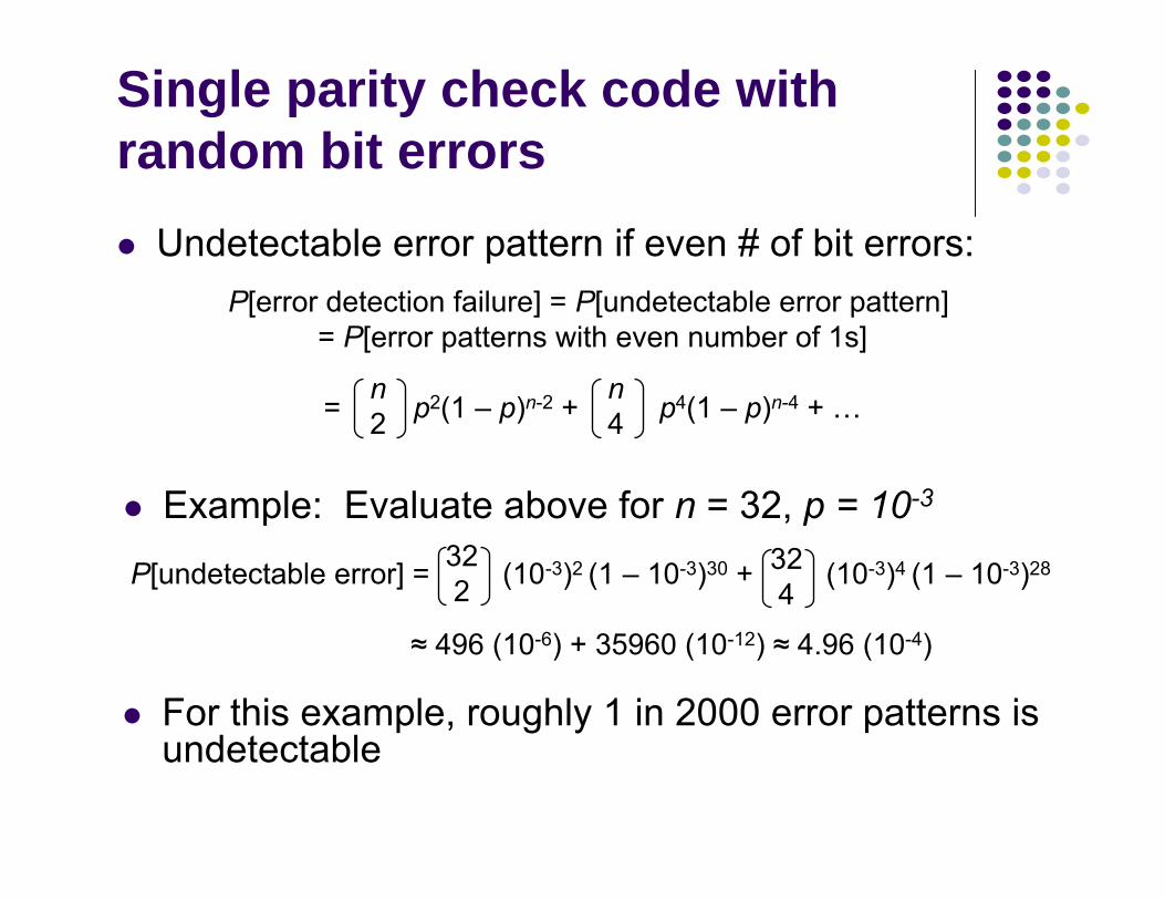
Undetectable error pattern if even # of bit errors:

Example: Evaluate above for n = 32, p = 10-3

For this example, roughly 1 in 2000 error patterns is undetectable

P[error detection failure] = P[undetectable error pattern] = P[error patterns with even number of 1s]

= p2(1 – p)n-2 + p4(1 – p)n-4 + …n2

n4

P[undetectable error] = (10-3)2 (1 – 10-3)30 + (10-3)4 (1 – 10-3)28

≈ 496 (10-6) + 35960 (10-12) ≈ 4.96 (10-4)

322

324

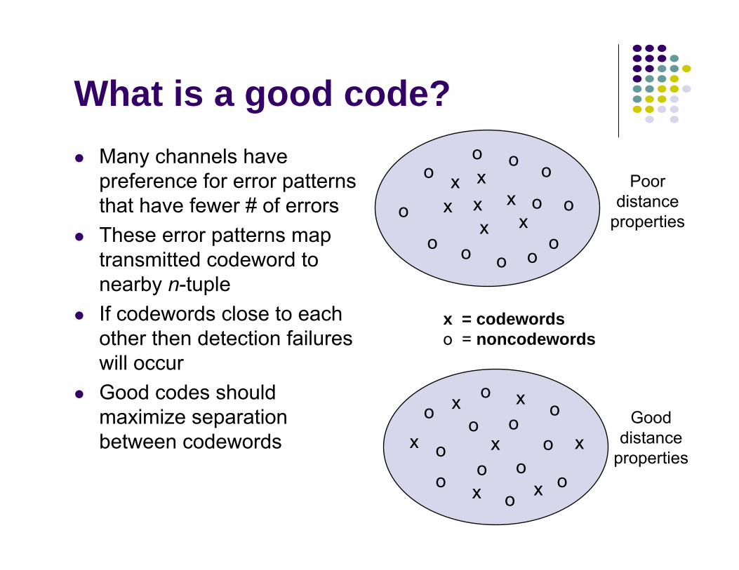
x = codewordso = noncodewords

x

x x

x

x

x

x

o

oo

oo

oo

ooo

o

o

ox

x xx

xx

x

o o

oo

ooooo

o

o Poordistance

properties

What is a good code?Many channels have preference for error patterns that have fewer # of errorsThese error patterns map transmitted codeword to nearby n-tupleIf codewords close to each other then detection failures will occurGood codes should maximize separation between codewords

Gooddistance

properties

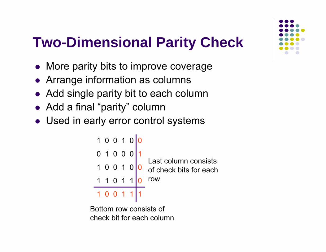
Two-Dimensional Parity Check

1 0 0 1 0 0

0 1 0 0 0 1

1 0 0 1 0 0

1 1 0 1 1 0

1 0 0 1 1 1

Bottom row consists of check bit for each column

Last column consists of check bits for each row

More parity bits to improve coverageArrange information as columnsAdd single parity bit to each columnAdd a final “parity” columnUsed in early error control systems

1 0 0 1 0 0

0 0 0 1 0 1

1 0 0 1 0 0

1 0 0 0 1 0

1 0 0 1 1 1

1 0 0 1 0 0

0 0 0 0 0 1

1 0 0 1 0 0

1 0 0 1 1 0

1 0 0 1 1 1

1 0 0 1 0 0

0 0 0 1 0 1

1 0 0 1 0 0

1 0 0 1 1 0

1 0 0 1 1 1

1 0 0 1 0 0

0 0 0 0 0 1

1 0 0 1 0 0

1 1 0 1 1 0

1 0 0 1 1 1

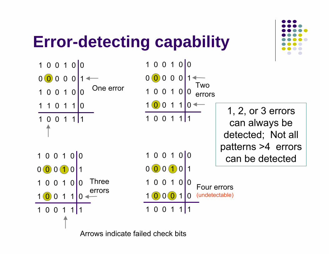
Arrows indicate failed check bits

Two errors

One error

Three errors Four errors

(undetectable)

Error-detecting capability

1, 2, or 3 errors can always be

detected; Not all patterns >4 errors can be detected

Other Error Detection CodesMany applications require very low error rateNeed codes that detect the vast majority of errorsSingle parity check codes do not detect enough errorsTwo-dimensional codes require too many check bitsThe following error detecting codes used in practice:

Internet Check SumsCRC Polynomial Codes

Internet ChecksumSeveral Internet protocols (e.g. IP, TCP, UDP) use check bits to detect errors in the IP header (or in the header and data for TCP/UDP)A checksum is calculated for header contents and included in a special field. Checksum recalculated at every router, so algorithm selected for ease of implementation in software Let header consist of L, 16-bit words, b0, b1, b2, ..., bL-1

The algorithm appends a 16-bit checksum bL

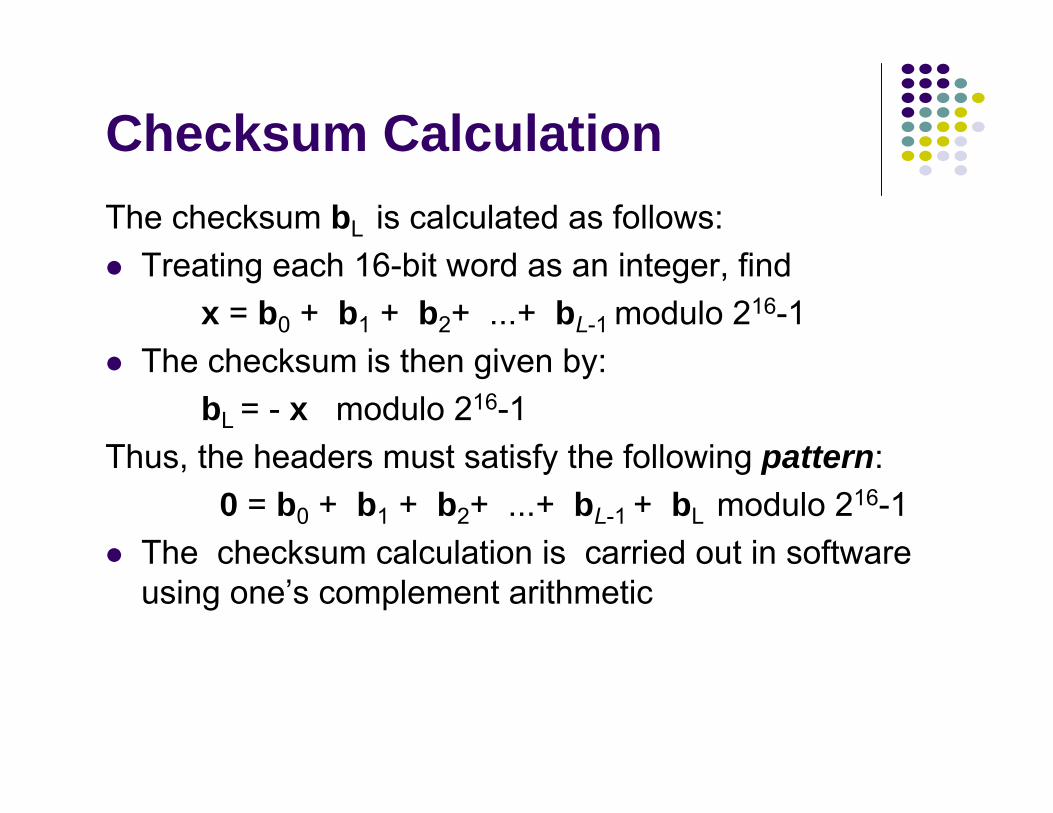
The checksum bL is calculated as follows:Treating each 16-bit word as an integer, find

x = b0 + b1 + b2+ ...+ bL-1 modulo 216-1The checksum is then given by:

bL = - x modulo 216-1Thus, the headers must satisfy the following pattern:

0 = b0 + b1 + b2+ ...+ bL-1 + bL modulo 216-1 The checksum calculation is carried out in software using one’s complement arithmetic

Checksum Calculation

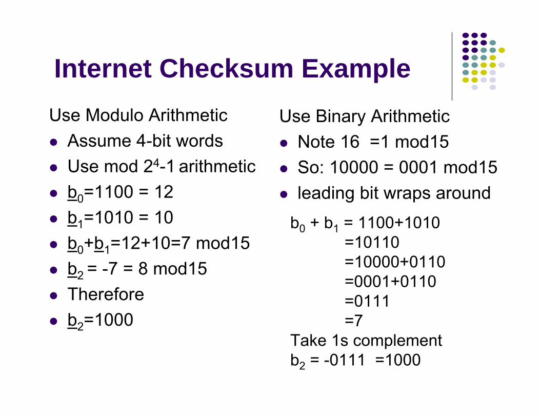
Internet Checksum ExampleUse Modulo Arithmetic

Assume 4-bit wordsUse mod 24-1 arithmeticb0=1100 = 12b1=1010 = 10b0+b1=12+10=7 mod15b2 = -7 = 8 mod15Thereforeb2=1000

Use Binary ArithmeticNote 16 =1 mod15So: 10000 = 0001 mod15leading bit wraps around

b0 + b1 = 1100+1010=10110=10000+0110=0001+0110=0111=7

Take 1s complementb2 = -0111 =1000

Polynomial Codes

Polynomials instead of vectors for codewordsPolynomial arithmetic instead of check sumsImplemented using shift-register circuitsAlso called cyclic redundancy check (CRC)codesMost data communications standards use polynomial codes for error detectionPolynomial codes also basis for powerful error-correction methods

Addition:

Multiplication:

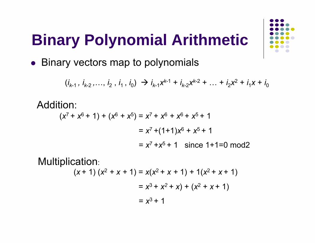
Binary Polynomial ArithmeticBinary vectors map to polynomials

(ik-1 , ik-2 ,…, i2 , i1 , i0) ik-1xk-1 + ik-2xk-2 + … + i2x2 + i1x + i0

(x7 + x6 + 1) + (x6 + x5) = x7 + x6 + x6 + x5 + 1

= x7 +(1+1)x6 + x5 + 1

= x7 +x5 + 1 since 1+1=0 mod2

(x + 1) (x2 + x + 1) = x(x2 + x + 1) + 1(x2 + x + 1)

= x3 + x2 + x) + (x2 + x + 1)

= x3 + 1

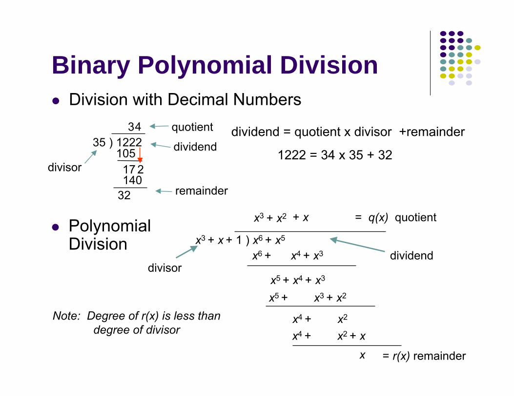
Binary Polynomial DivisionDivision with Decimal Numbers

32

35 ) 12223

10517 2

4

140divisor

quotient

remainder

dividend1222 = 34 x 35 + 32

dividend = quotient x divisor +remainder

Polynomial Division x3 + x + 1 ) x6 + x5

x6 + x4 + x3

x5 + x4 + x3

x5 + x3 + x2

x4 + x2

x4 + x2 + xx

= q(x) quotient

= r(x) remainder

divisordividend

+ x+ x2x3

Note: Degree of r(x) is less than degree of divisor

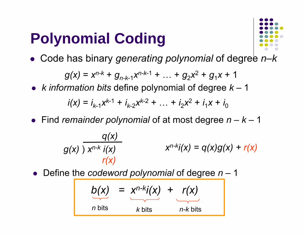
Polynomial CodingCode has binary generating polynomial of degree n–k

k information bits define polynomial of degree k – 1

Find remainder polynomial of at most degree n – k – 1

g(x) ) xn-k i(x)q(x)

r(x)xn-ki(x) = q(x)g(x) + r(x)

Define the codeword polynomial of degree n – 1

b(x) = xn-ki(x) + r(x)n bits k bits n-k bits

g(x) = xn-k + gn-k-1xn-k-1 + … + g2x2 + g1x + 1

i(x) = ik-1xk-1 + ik-2xk-2 + … + i2x2 + i1x + i0

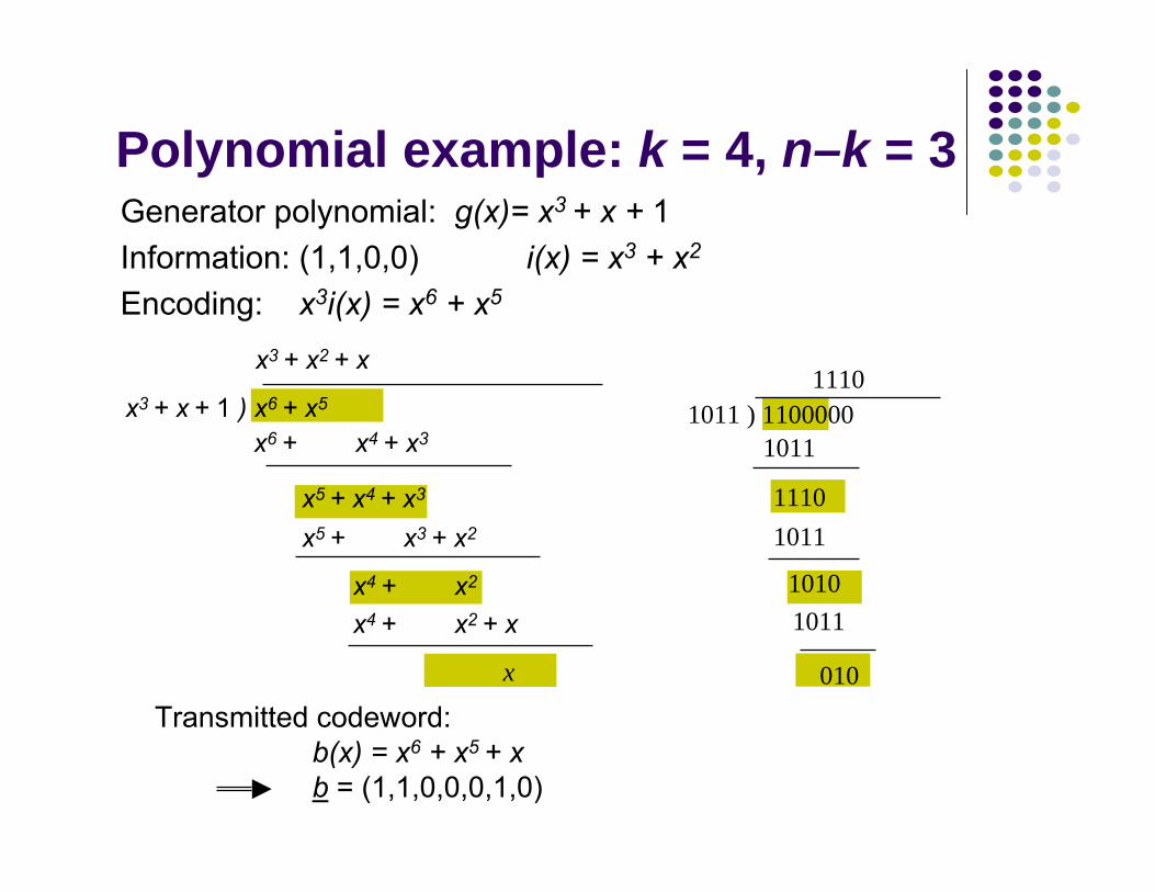
Transmitted codeword:b(x) = x6 + x5 + xb = (1,1,0,0,0,1,0)

1011 ) 11000001110

1011

11101011

10101011

010

x3 + x + 1 ) x6 + x5

x3 + x2 + x

x6 + x4 + x3

x5 + x4 + x3

x5 + x3 + x2

x4 + x2

x4 + x2 + x

x

Polynomial example: k = 4, n–k = 3Generator polynomial: g(x)= x3 + x + 1Information: (1,1,0,0) i(x) = x3 + x2

Encoding: x3i(x) = x6 + x5

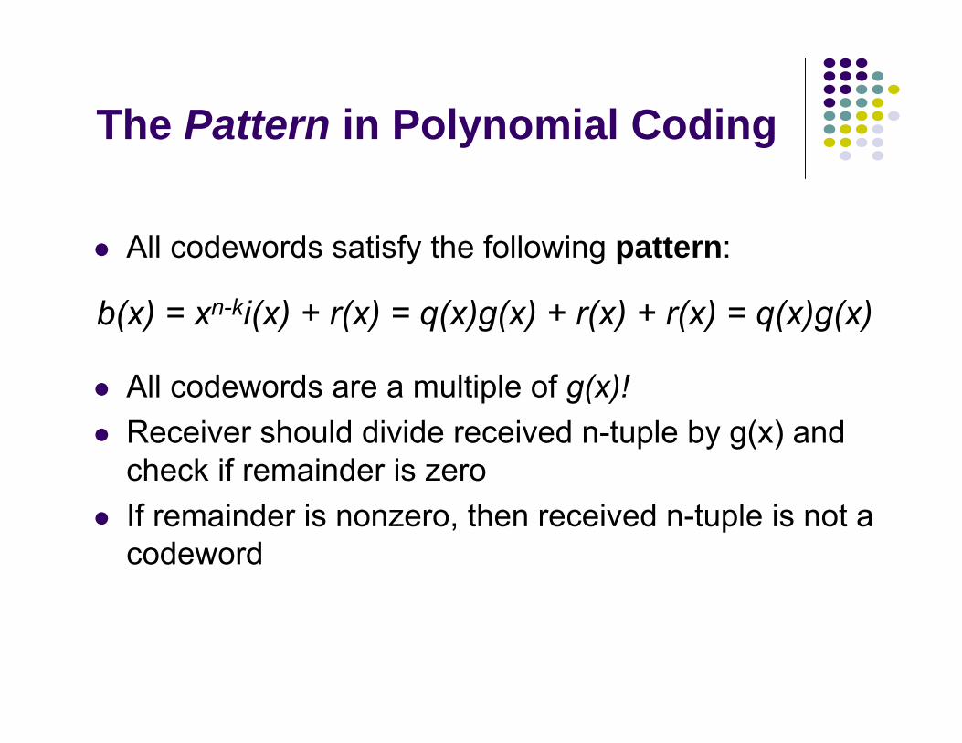
The Pattern in Polynomial Coding

All codewords satisfy the following pattern:

All codewords are a multiple of g(x)!Receiver should divide received n-tuple by g(x) and check if remainder is zeroIf remainder is nonzero, then received n-tuple is not a codeword

b(x) = xn-ki(x) + r(x) = q(x)g(x) + r(x) + r(x) = q(x)g(x)

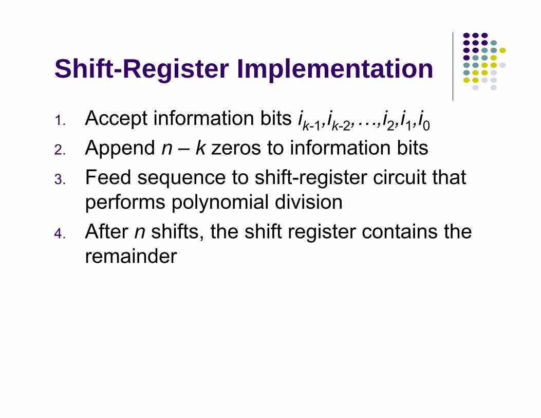
Shift-Register Implementation

1. Accept information bits ik-1,ik-2,…,i2,i1,i02. Append n – k zeros to information bits3. Feed sequence to shift-register circuit that

performs polynomial division4. After n shifts, the shift register contains the

remainder

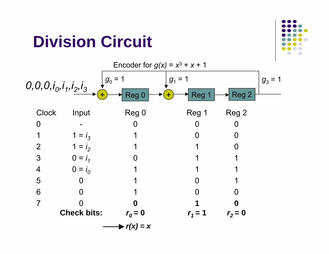
Clock Input Reg 0 Reg 1 Reg 20 - 0 0 01 1 = i3 1 0 02 1 = i2 1 1 03 0 = i1 0 1 14 0 = i0 1 1 15 0 1 0 16 0 1 0 07 0 0 1 0

Check bits: r0 = 0 r1 = 1 r2 = 0r(x) = x

Division Circuit

Reg 0 ++

Encoder for g(x) = x3 + x + 1

Reg 1 Reg 20,0,0,i0,i1,i2,i3

g0 = 1 g1 = 1 g3 = 1

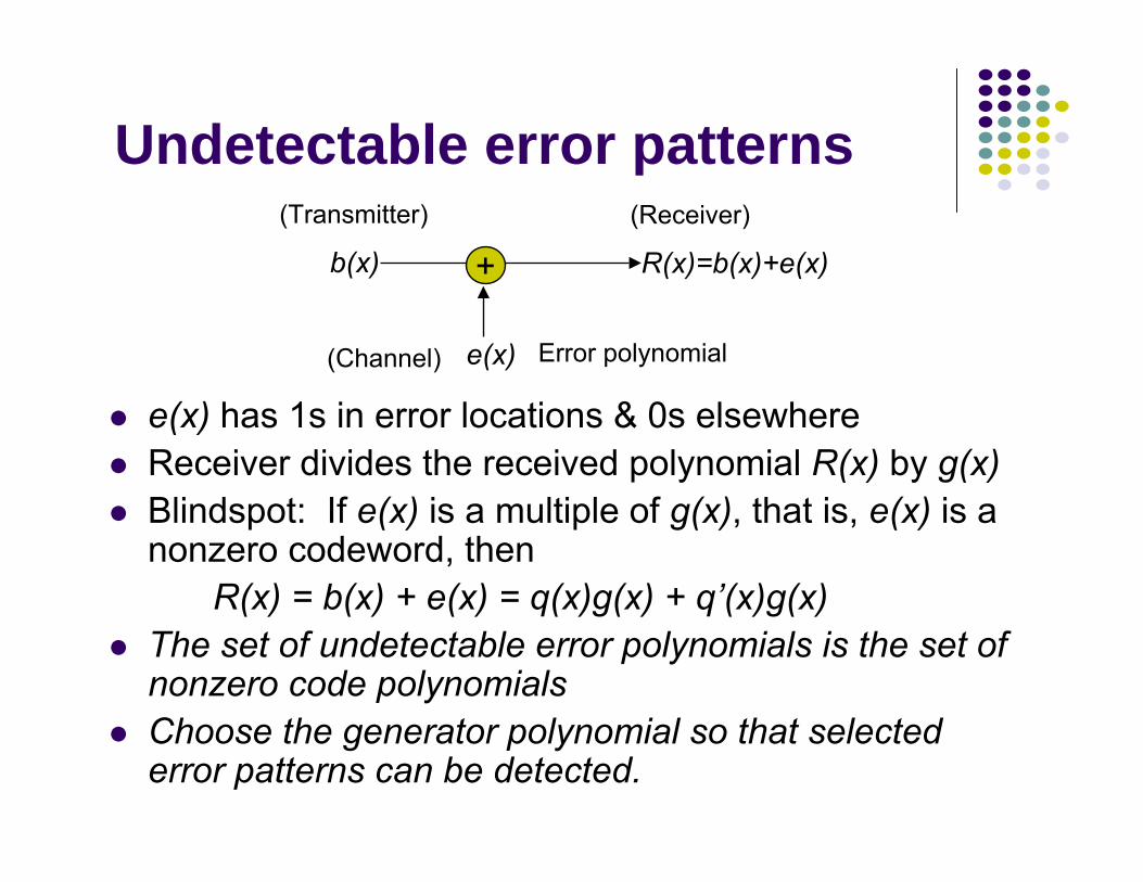
Undetectable error patterns

e(x) has 1s in error locations & 0s elsewhereReceiver divides the received polynomial R(x) by g(x)Blindspot: If e(x) is a multiple of g(x), that is, e(x) is a nonzero codeword, then

R(x) = b(x) + e(x) = q(x)g(x) + q’(x)g(x)The set of undetectable error polynomials is the set of nonzero code polynomialsChoose the generator polynomial so that selected error patterns can be detected.

b(x)

e(x)

R(x)=b(x)+e(x)+(Receiver)(Transmitter)

Error polynomial(Channel)

Designing good polynomial codes

Select generator polynomial so that likely error patterns are not multiples of g(x)Detecting Single Errors

e(x) = xi for error in location i + 1If g(x) has more than 1 term, it cannot divide xi

Detecting Double Errorse(x) = xi + xj = xi(xj-i+1) where j>i If g(x) has more than 1 term, it cannot divide xi

If g(x) is a primitive polynomial, it cannot divide xm+1 for all m<2n-k-1 (Need to keep codeword length less than 2n-k-1) Primitive polynomials can be found by consulting coding theory books

Designing good polynomial codes

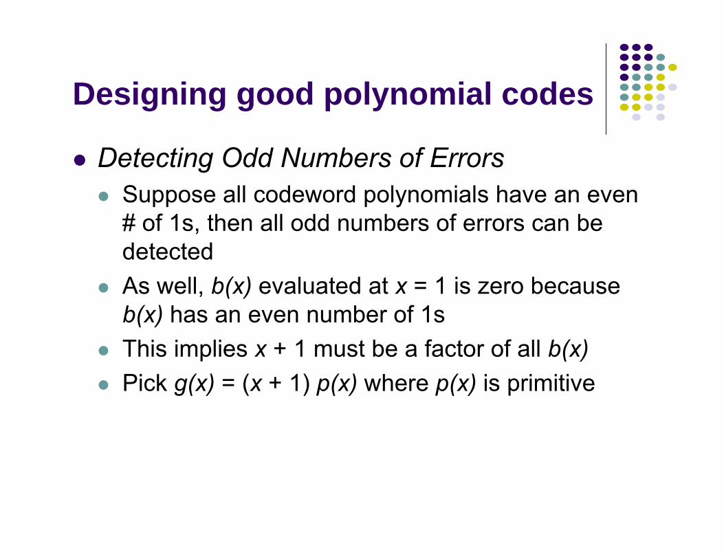
Detecting Odd Numbers of ErrorsSuppose all codeword polynomials have an even # of 1s, then all odd numbers of errors can be detectedAs well, b(x) evaluated at x = 1 is zero because b(x) has an even number of 1sThis implies x + 1 must be a factor of all b(x)Pick g(x) = (x + 1) p(x) where p(x) is primitive

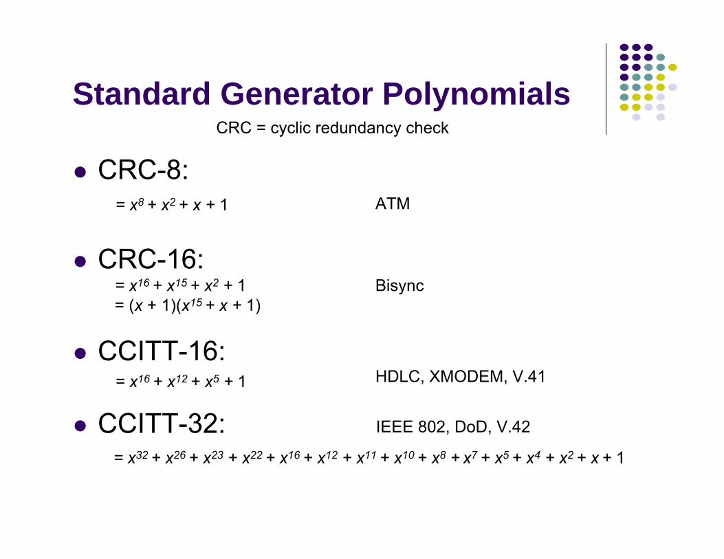
Standard Generator Polynomials

CRC-8:

CRC-16:

CCITT-16:

CCITT-32:

CRC = cyclic redundancy check

HDLC, XMODEM, V.41

IEEE 802, DoD, V.42

Bisync

ATM= x8 + x2 + x + 1

= x16 + x15 + x2 + 1= (x + 1)(x15 + x + 1)

= x16 + x12 + x5 + 1

= x32 + x26 + x23 + x22 + x16 + x12 + x11 + x10 + x8 + x7 + x5 + x4 + x2 + x + 1

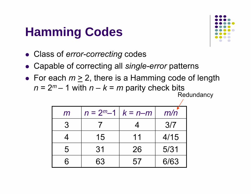
Hamming CodesClass of error-correcting codesCapable of correcting all single-error patternsFor each m > 2, there is a Hamming code of length n = 2m – 1 with n – k = m parity check bits

5726114

k = n–m

6/636365/313154/151543/773m/nn = 2m–1 m

Redundancy

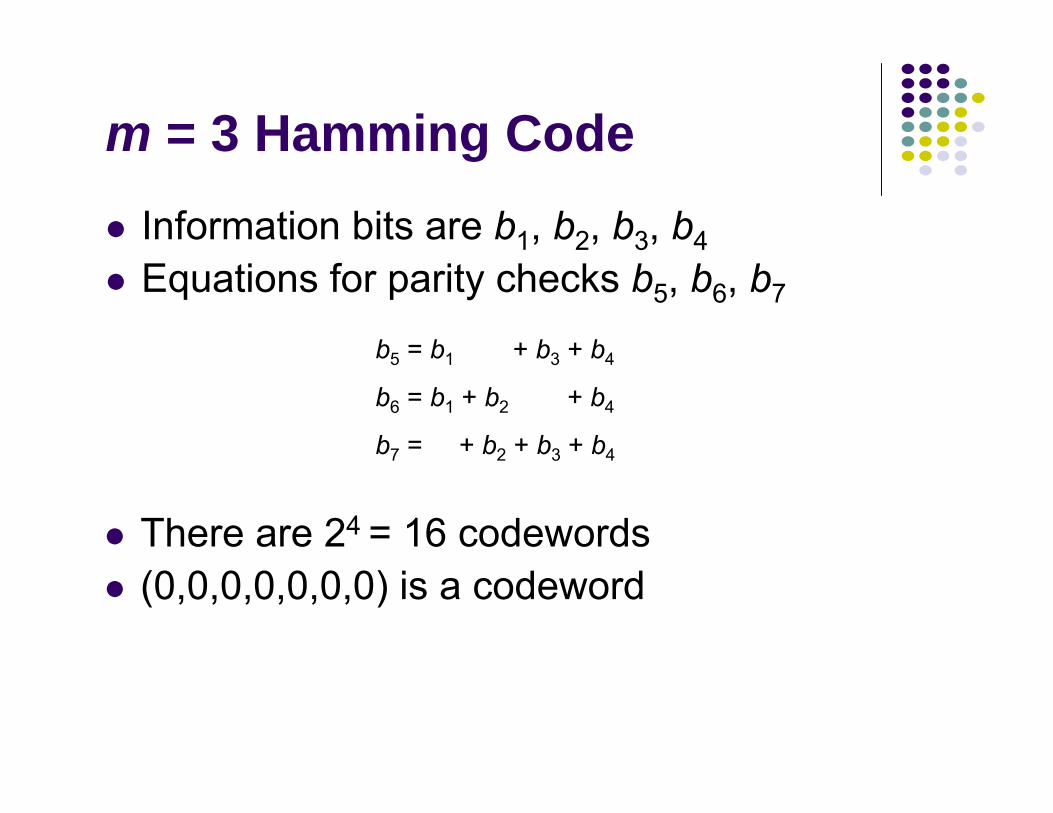
m = 3 Hamming CodeInformation bits are b1, b2, b3, b4Equations for parity checks b5, b6, b7

There are 24 = 16 codewords(0,0,0,0,0,0,0) is a codeword

b5 = b1 + b3 + b4

b6 = b1 + b2 + b4

b7 = + b2 + b3 + b4

Hamming (7,4) code

71 1 1 1 1 1 11 1 1 1

31 1 1 0 0 0 01 1 1 0

41 1 0 1 0 1 01 1 0 1

41 1 0 0 1 0 11 1 0 0

41 0 1 1 1 0 01 0 1 1

41 0 1 0 0 1 11 0 1 0

31 0 0 1 0 0 11 0 0 1

31 0 0 0 1 1 01 0 0 0

40 1 1 1 0 0 10 1 1 1

40 1 1 0 1 1 00 1 1 0

30 1 0 1 1 0 00 1 0 1

30 1 0 0 0 1 10 1 0 0

30 0 1 1 0 1 00 0 1 1

30 0 1 0 1 0 10 0 1 0

40 0 0 1 1 1 10 0 0 1

00 0 0 0 0 0 00 0 0 0

w(b)b1 b2 b3 b4 b5 b6 b7b1 b2 b3 b4

WeightCodewordInformation

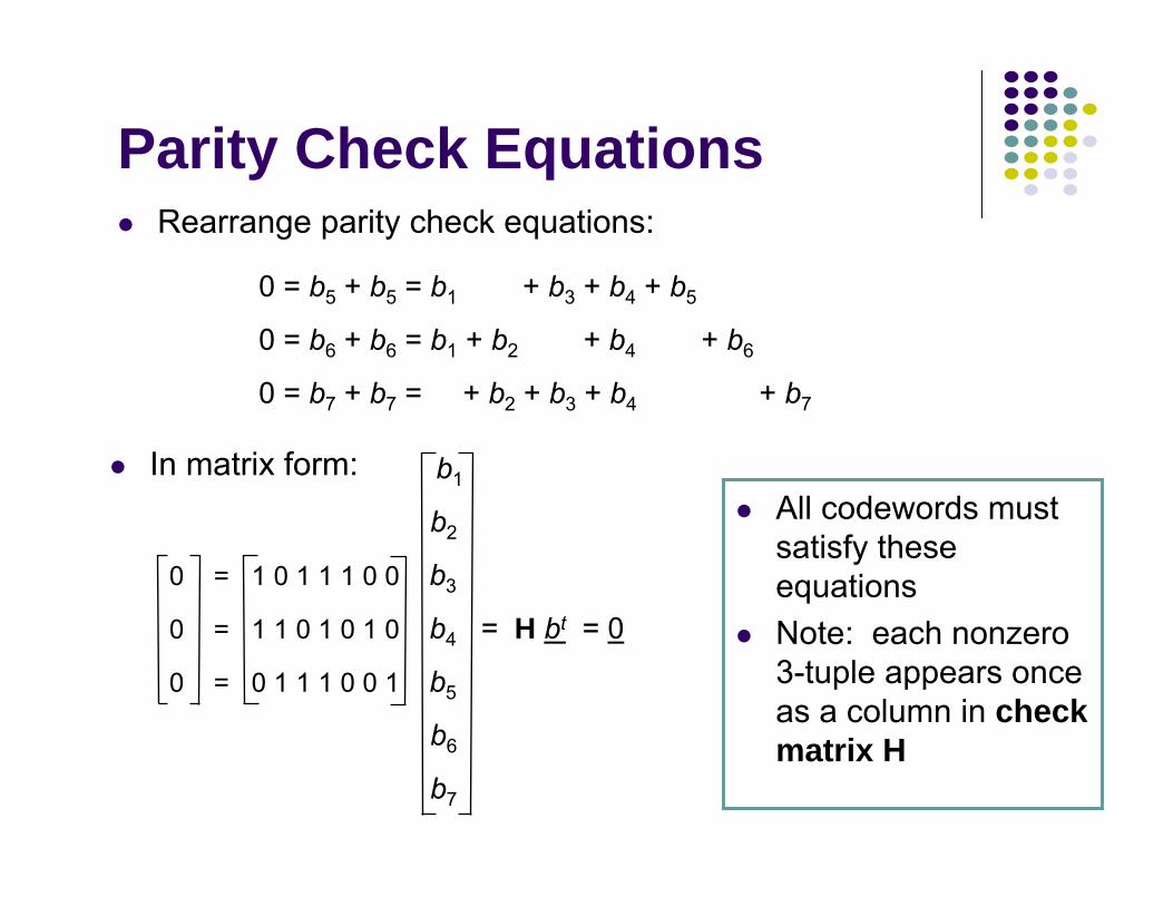
Parity Check EquationsRearrange parity check equations:

All codewords must satisfy these equationsNote: each nonzero 3-tuple appears once as a column in check matrix H

In matrix form:

0 = b5 + b5 = b1 + b3 + b4 + b5

0 = b6 + b6 = b1 + b2 + b4 + b6

0 = b7 + b7 = + b2 + b3 + b4 + b7

b1

b2

0 = 1 0 1 1 1 0 0 b3

0 = 1 1 0 1 0 1 0 b4 = H bt = 0

0 = 0 1 1 1 0 0 1 b5

b6

b7

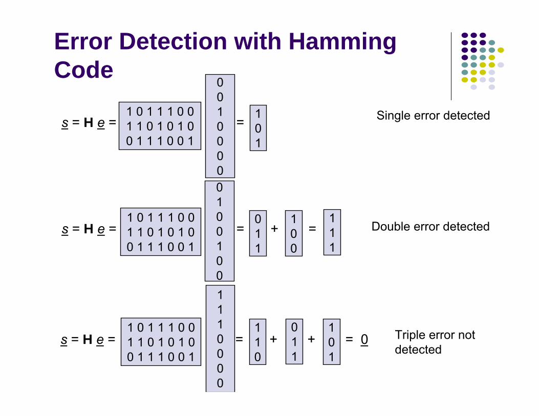
0010000

s = H e = =101

Single error detected

0100100

s = H e = = + =011

Double error detected100

1 0 1 1 1 0 01 1 0 1 0 1 00 1 1 1 0 0 1

1110000

s = H e = = + + = 0110

Triple error not detected

011

101

1 0 1 1 1 0 01 1 0 1 0 1 00 1 1 1 0 0 1

1 0 1 1 1 0 01 1 0 1 0 1 00 1 1 1 0 0 1

111

Error Detection with Hamming Code

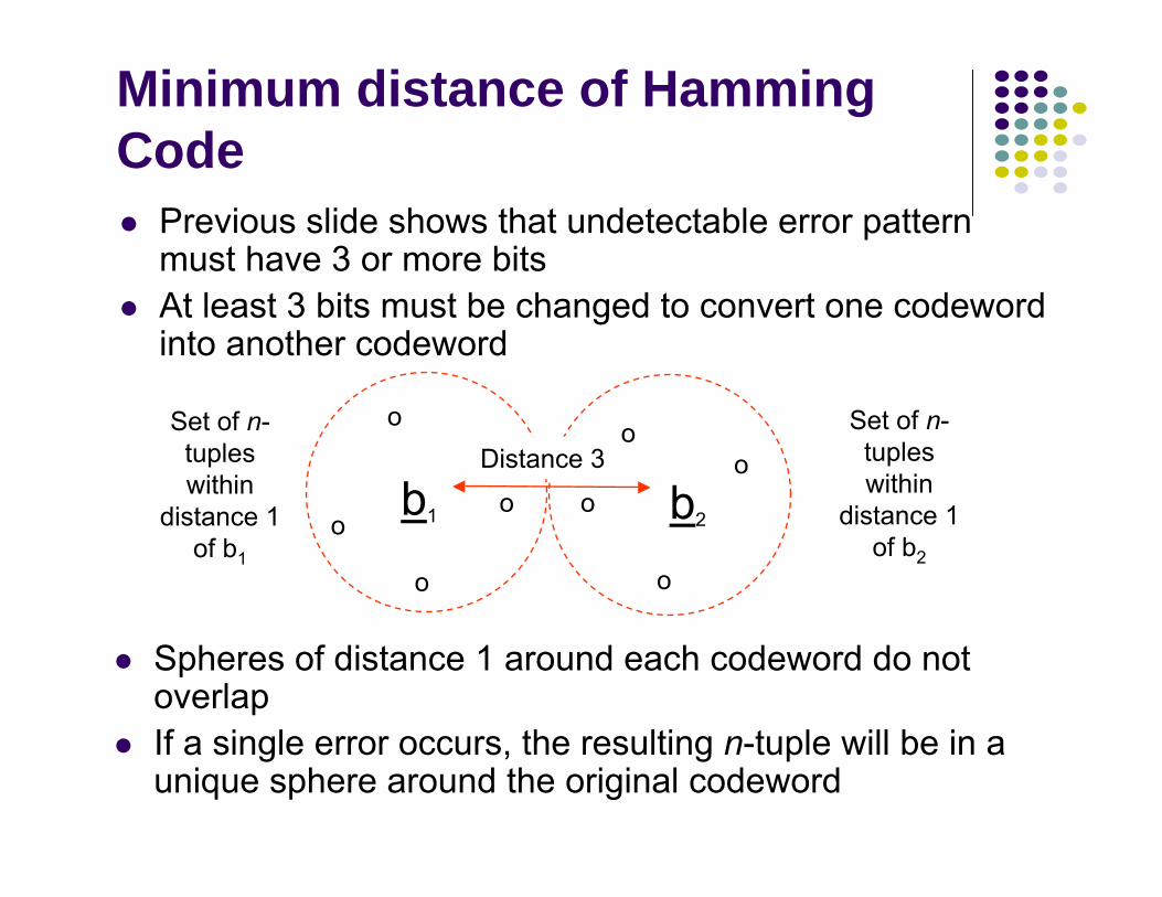
Minimum distance of Hamming Code

Previous slide shows that undetectable error pattern must have 3 or more bitsAt least 3 bits must be changed to convert one codeword into another codeword

b1 b2o o

o

o

o oo

o

Set of n-tupleswithin

distance 1 of b1

Set of n-tupleswithin

distance 1 of b2

Spheres of distance 1 around each codeword do not overlapIf a single error occurs, the resulting n-tuple will be in a unique sphere around the original codeword

Distance 3

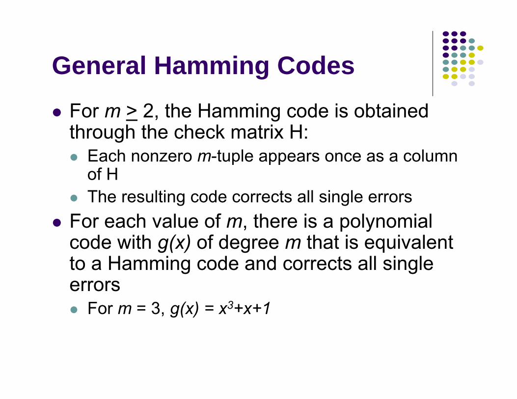
General Hamming CodesFor m > 2, the Hamming code is obtained through the check matrix H:

Each nonzero m-tuple appears once as a column of HThe resulting code corrects all single errors

For each value of m, there is a polynomial code with g(x) of degree m that is equivalent to a Hamming code and corrects all single errors

For m = 3, g(x) = x3+x+1

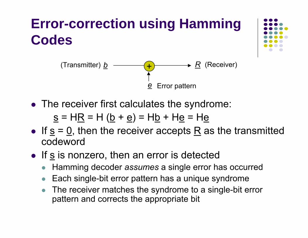
Error-correction using Hamming Codes

The receiver first calculates the syndrome:s = HR = H (b + e) = Hb + He = He

If s = 0, then the receiver accepts R as the transmitted codewordIf s is nonzero, then an error is detected

Hamming decoder assumes a single error has occurredEach single-bit error pattern has a unique syndromeThe receiver matches the syndrome to a single-bit error pattern and corrects the appropriate bit

b

e

R+ (Receiver)(Transmitter)

Error pattern

Performance of Hamming Error-Correcting Code

Assume bit errors occur independent of each other and with probability p

s = H R = He

s = 0 s = 0

No errors intransmission

Undetectableerrors

Correctableerrors

Uncorrectableerrors

(1–p)7 7p3

1–3p 3p

7p

7p(1–3p) 21p2


Fundamentals

RS-232 Asynchronous Data Transmission

Recommended Standard (RS) 232

Serial line interface between computer and modem or similar deviceData Terminal Equipment (DTE): computerData Communications Equipment (DCE): modemMechanical and Electrical specification

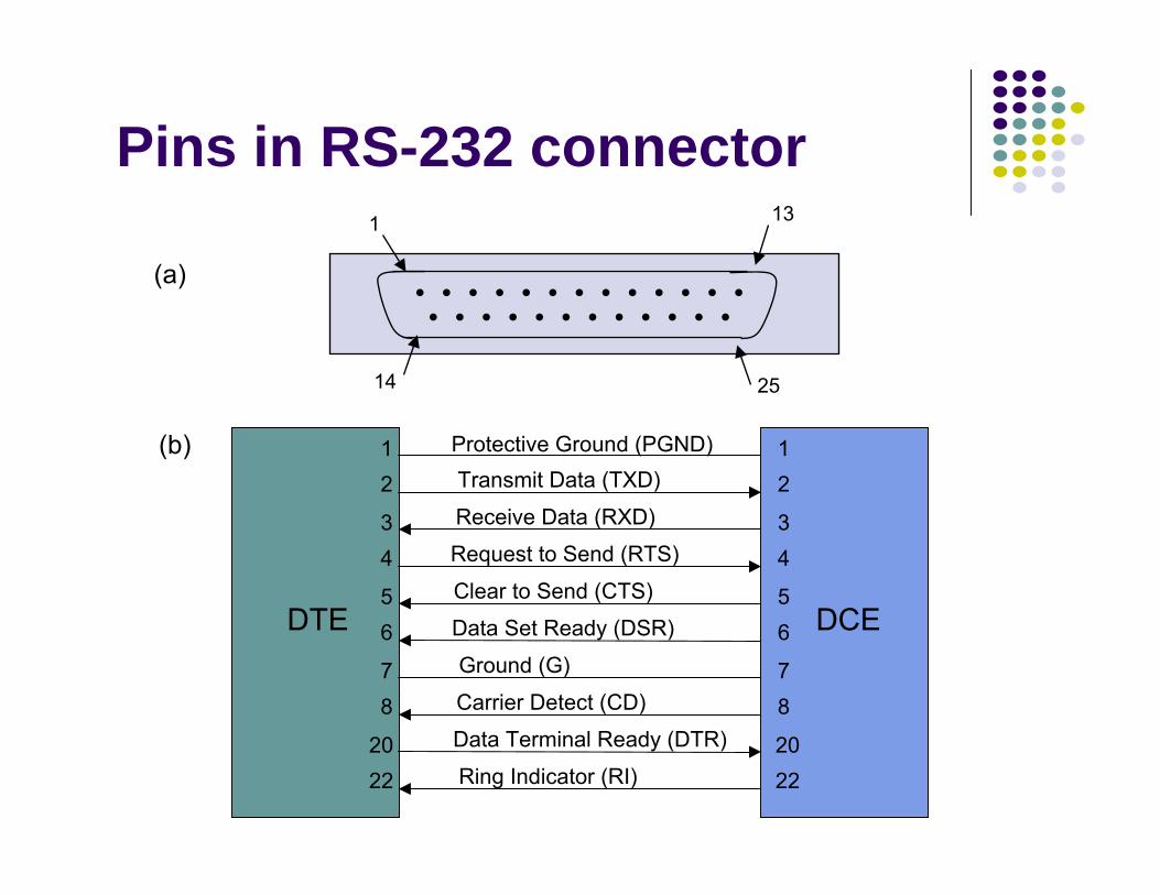
DTE DCE

Protective Ground (PGND)Transmit Data (TXD)

Receive Data (RXD)

Request to Send (RTS)

Clear to Send (CTS)

Data Set Ready (DSR)

Ground (G)

Carrier Detect (CD)

Data Terminal Ready (DTR)

Ring Indicator (RI)

12

34

56

78

2022

12

34

56

78

2022

(b)

13

(a)• • • • • • • • • • • • •

• • • • • • • • • • • •

1

2514

Pins in RS-232 connector

SynchronizationSynchronization of clocks in transmitters and receivers.

clock drift causes a loss of synchronization

Example: assume ‘1’ and ‘0’ are represented by V volts and 0 volts respectively

Correct receptionIncorrect reception due to incorrect clock (slower clock)

Clock

Data

S

T

1 0 1 1 0 1 0 0 1 0 0

Clock

Data

S’

T

1 0 1 1 1 0 0 1 0 0 0

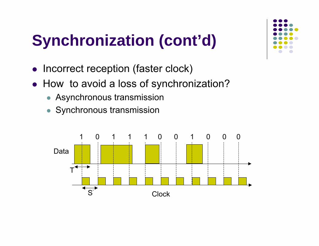
Synchronization (cont’d)Incorrect reception (faster clock)How to avoid a loss of synchronization?

Asynchronous transmissionSynchronous transmission

Clock

Data

S’

T

1 0 1 1 1 0 0 1 0 0 0

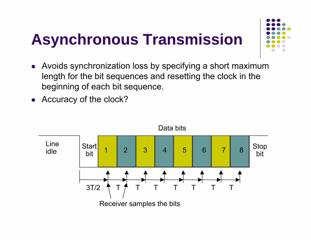
Asynchronous TransmissionAvoids synchronization loss by specifying a short maximum length for the bit sequences and resetting the clock in the beginning of each bit sequence. Accuracy of the clock?

Startbit

Stopbit1 2 3 4 5 6 7 8

Data bits

Lineidle

3T/2 T T T T T T T

Receiver samples the bits

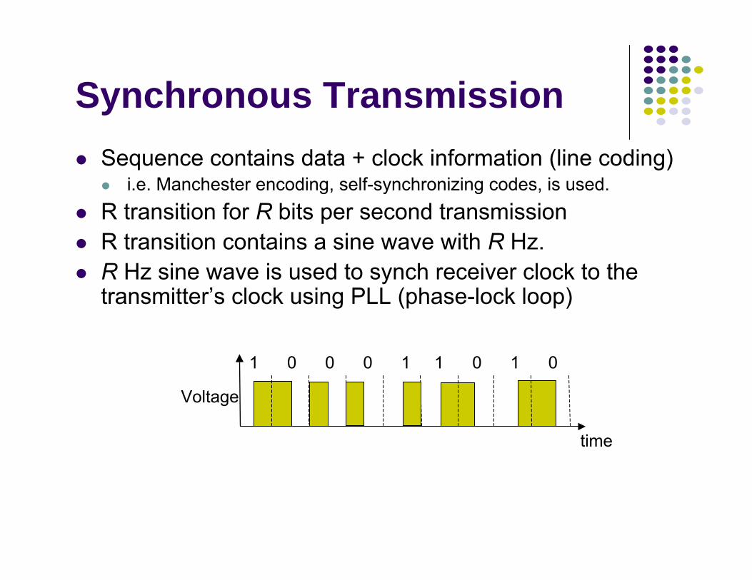
Synchronous Transmission

Voltage

1 0 0 0 1 1 0 1 0

time

Sequence contains data + clock information (line coding)i.e. Manchester encoding, self-synchronizing codes, is used.

R transition for R bits per second transmissionR transition contains a sine wave with R Hz.R Hz sine wave is used to synch receiver clock to the transmitter’s clock using PLL (phase-lock loop)

chapter 3 digital transmission fundamentals

Documents