chapter 1 magnetic skyrmions: theory and applications - arxiv

arX

iv:2

207.

0289

2v1

[co

nd-m

at.m

es-h

all]

6 J

ul 2

022 Chapter 1

Magnetic Skyrmions: Theory and

Applications

Lalla Btissam Drissi1,2,∗, El Hassan Saidi1,2, Mosto Bousmina2,3, Omar Fassi-Fehri2

1 LPHE, Modeling & Simulations, Faculty of Science, Mohammed V University in Rabat, Morocco.2 Hassan II Academy of Science and Technology, Rabat, Morocco.

3 Euromed Research Institute, Euro-Mediterranean University of Fes, Fes, Morocco.∗ Corresponding Author E-mails: [email protected], [email protected]

Abstract

Using the field theory method and coherent spin state approach, we investigate properties

of magnetic solitons in spacetime while focussing on 1D kinks, 2D and 3D skyrmions. We

also study the case of a rigid skyrmion dissolved in a magnetic background induced by the

electronic spins; and derive the effective rigid skyrmion equation of motion. We investigate

as well the interaction between an electron and a 3D skyrmion.

Keywords: Geometric phases, magnetic monopoles and topology, soliton and holonomy,

chiral magnets, skyrmion dynamics, numerical and experimental tests.

1

http://arxiv.org/abs/2207.02892v1

Contents

1 Magnetic Skyrmions: Theory and Applications 1

1.1 Introduction . . . . . . . . . . . . . . . . . . . . . . . . . . . . . . . . . . . . . 3

1.2 Quantum SU(2) spin dynamics . . . . . . . . . . . . . . . . . . . . . . . . . . . 5

1.2.1 Quantum spin 1/2 operator and beyond . . . . . . . . . . . . . . . . . . 5

1.2.2 Coherent spin states and semi-classical analysis . . . . . . . . . . . . . . 6

1.3 Magnetic solitons in lower dimensions . . . . . . . . . . . . . . . . . . . . . . . 8

1.3.1 One space dimensional solitons . . . . . . . . . . . . . . . . . . . . . . 9

1.3.2 Skyrmions in 2d space dimensions . . . . . . . . . . . . . . . . . . . . . 12

1.4 Three dimensional magnetic skyrmions . . . . . . . . . . . . . . . . . . . . . . 15

1.4.1 From 2d skyrmion to 3d homologue . . . . . . . . . . . . . . . . . . . . 15

1.4.2 Conserved topological current . . . . . . . . . . . . . . . . . . . . . . . 16

1.5 Effective dynamics of skyrmions . . . . . . . . . . . . . . . . . . . . . . . . . . 18

1.5.1 Equation of a rigid skyrmion . . . . . . . . . . . . . . . . . . . . . . . . 18

1.5.2 Implementing dissipation . . . . . . . . . . . . . . . . . . . . . . . . . . 20

1.6 Electron-skyrmion interaction . . . . . . . . . . . . . . . . . . . . . . . . . . . 22

1.6.1 Hund coupling . . . . . . . . . . . . . . . . . . . . . . . . . . . . . . . 22

1.6.2 Skyrmion with spin transfer torque . . . . . . . . . . . . . . . . . . . . . 25

1.7 Comments and perspectives . . . . . . . . . . . . . . . . . . . . . . . . . . . . . 27

1.1 Introduction

During the last two decades, the magnetic skyrmions and antiskyrmions have been subject to an

increasing interest in connection with the topological phase of matter [1, 2, 3, 4], the spin-tronics

[5, 6] and quantum computing [7, 8]; as well as in the search for advanced applications such as

racetrack memory, microwave oscillators and logic nanodevices making skyrmionic states very

promising candidates for future low power information technology devices [9, 10, 11, 12]. Ini-

tially proposed by T. Skyrme to describe hadrons in the theory of quantum chromodynamics

[13], skyrmions have however been observed in other fields of physics, including quantum Hall

systems [14, 15], Bose-Einstein condensates [16] and liquid crystals [17]. In quantum Hall (QH)

ferromagnets for example [18, 19], due to the exchange interaction; the electron spins sponta-

neously form a fully polarized ferromagnet close to the integer filling factor ν ≃ 1; slightly away,

other electrons organize into an intricate spin configuration because of a competitive interplay

between the Coulomb and Zeeman interactions [18]. Being quasiparticles, the skyrmions of

3

the QH system condense into a crystalline form leading to the crystallization of the skyrmions

[20, 21, 22, 23]; thus opening an important window on promising applications.

In order to overcome the lack of a prototype of a skyrmion-based spintronic devices for a

possible fabrication of nanodevices of data storage and logic technologies, intense research has

been carried out during the last few years [24, 25]. In this regard, several alternative nano-

objects have been identified to host stable skyrmions at room temperature. The first experimental

observation of crystalline skyrmionic states was in a three-dimensional metallic ferromagnet

MnSi with a B20 structure using small angle neutron scattering [26]. Then, real-space imag-

ing of the skyrmion has been reported using Lorentz transmission electron microscopy in non-

centrosymmetric magnetic compounds and in thin films with broken inversion symmetry, in-

cluding monosilicides, monogermanides, and their alloys, like Fe1−xCoxSi [27], FeGe [28], and

MnGe [29].

One of the key parameters in the formation of these topologically protected non-collinear spin

textures is the Dzyaloshinskii-Moriya Interaction (DMI) [30, 31]. Originating from the strong

spin-orbit coupling (SOC) at the interfaces, the DM exchange between atomic spins controls the

size and stability of the induced skyrmions. Depending on the symmetry of the crystal struc-

tures and the skyrmion windings number, the internal spins within a single skyrmion envelop a

sphere in different arrangements [32]. The in-plane component of the magnetization, in the Neel

skyrmion, is always pointed in the radial direction [33], while it is oriented perpendicularly with

respect to the position vector in the Bloch skyrmion [26]. Different from these two well-known

types of skyrmions are skyrmions with mixed Bloch-Neel topological spin textures observed in

Co/Pd multilayers [34]. Magnetic antiskyrmions, having a more complex boundary compared to

the chiral magnetic boundaries of skyrmions, exist above room temperature in tetragonal Heusler

materials [35]. Higher-order skyrmions should be stabilized in anisotropic frustrated magnet at

zero temperature [36] as well as in itinerant magnets with zero magnetic field [37].

In the quest to miniaturize magnetic storage devices, reduction of material’s dimensions as

well as preservation of the stability of magnetic nano-scale domains are necessary. One pos-

sible route to achieve this goal is the formation of topological protected skyrmions in certain

2D magnetic materials. To induce magnetic order and tune DMIs in 2D crystal structures,

their centrosymmetric should first be broken using some efficient ways such a (i) generate one-

atom thick hybrids where atoms are mixed in an alternating manner [38, 39, 40], (ii) apply bias

voltage or strain [41, 42, 43], (iii) insert adsorbents, impurities and defects [44, 45, 46]. In

graphene-like materials, fluorine chemisorption is an exothermic adsorption that gives rise to

stable 2D structures [47] and to long-range magnetism [48, 49]. In semi-fluorinated graphene, a

strong Dzyaloshinskii-Moriya interaction has been predicted with the presence of ferromagnetic

skyrmions [50]. The formation of a nanoskyrmion state in a Sn monolayer on a SiC(0001) sur-

face has been reported on the basis of a generalized Hubbard model [51]. Strong DMI between

the first nearest magnetic germanium neighbors in 2D semi-fluorinated germanene results in a

potential antiferromagnetic skyrmion [52].

In this bookchapter, we use the coherent spin states approach and the field theory method

(continuous limit of lattice magnetic models with DMI) to revisit some basic aspects and proper-

ties of magnetic solitons in spacetime while focusing on 1d kinks, 2d and 3d spatial skyrmions/antiskyrmions.

We also study the case of a rigid skyrmion dissolved in a magnetic background induced by the

Magnetic Skyrmions: Theory and Applications Magnetic Skyrmions: Theory and Applications

electronic spins of magnetic atoms like Mn; and derive the effective rigid skyrmion equation of

motion. In this regard, we describe the similarity between, on one hand, electrons in the electro-

magnetic background; and, on the other hand, rigid skyrmions bathing in a texture of magnetic

moments. We also investigate the interaction between electrons and skyrmions as well as the

effect of the spin transfer effect.

This bookchapter is organized as follows: In Section 2, we introduce some basic tools on

quantum SU(2) spins and review useful aspects of their dynamics. In Section 3, we investigate

the topological properties of kinks and 2d space solitons while describing in detail the under-

side of the topological structure of these low-dimensional solitons. In Section 4, we extend the

construction to approach topological properties to 3d skyrmions. In Section 5, we study the dy-

namics of rigid skyrmions without and with dissipation; and in Section 6, we use emergent gauge

potential fields to describe the effective dynamics of electrons interacting with the skyrmion in

the presence of a spin transfer torque. We end this study by making comments and describing

perspectives in the study of skyrmions.

1.2 Quantum SU(2) spin dynamics

In this section, we review some useful ingredients on the quantum SU(2) spin operator, its un-

derlying algebra and its time evolution while focussing on the interesting spin 1/2 states, con-

cerning electrons in materials; and on coherent spin states which are at the basis of the study of

skyrmions/antiskyrmions. First, we introduce rapidly the SU(2) spin operator S and the imple-

mentation of time dependence. Then, we investigate the non dissipative dynamics of the spin by

using semi-classical theory approach (coherent states). These tools can be also viewed as a first

step towards the topological study of spin induced 1D, 2D and 3D solitons undertaken in next

sections.

1.2.1 Quantum spin 1/2 operator and beyond

We begin by recalling that in non relativistic 3D quantum mechanics, the spin states |S z, S 〉of spinfull particles are characterised by two half integers (S z, S ), a positive S ≥ 0 and an S z

taking 2S + 1 values bounded as −S ≤ S z ≤ S with integral hoppings. For particles with

spin 1/2 like electrons, one distinguishes two basis vector states∣∣∣±1

2, 1

2

⟩that are eigenvalues

of the scaled Pauli matrix ~

2σz and the quadratic (Casimir) operator ~

2

4

∑3a=1 σ

2a, here the three

~

2σa with σa = ~σ.~ea are the three components of the spin 1/2 operator vector1 ~σ. From these

ingredients, we learn that the average < S z, S | ~2σz|S z, S >= ~S z (for short⟨~

2σz

⟩) is carried by

the z-direction since S z = ~S .~ez with ~ez = (0, 0, 1)T . For generic values of the SU(2) spin S ,

the spin operator reads as ~Ja where the three Ja’s are (2S + 1) × (2S + 1) generators of the

SU(2) group satisfying the usual commutation relations [Ja, Jb] = iεabcJc with εabc standing for

the completely antisymmetric Levi-Civita tensor with non zero value ε123 = 1; its inverse is

εcba with ε123 = −1. The time evolution of the spin 12

operator ~σa

2with dynamics governed

by a stationary Hamiltonian operator ( dH/dt = 0) is given by the Heisenberg representation

1 For convenience, we often refer to ~σ, ~ei, ~σ.~ei = σi respectively by bold symbols as σ, ei, σ.ei = σi.

of quantum mechanics. In this non dissipative description, the time dependence of the spin 12

operator S a (t) (the hat is to distinguish the operator S a from classical S a) is given by

S a = ei~

Ht

(~σa

2

)e−

i~

Ht (1.1)

where the Pauli matrices σa obey the usual commutation relations [σa, σb] = 2iεabcσc. For a

generic value of the SU(2) spin S , the above relation extends as S a = ei~

Ht (~Ja) e−i~

Ht. So, many

relations for the spin 1/2 may be straightforwardly generalised for generic values S of the SU(2)

spin. For example, for a spin value S 0, the (2S 0 + 1) states are given by |m, S 0〉 and are labeled

by −S 0 ≤ m ≤ S 0; one of these states namely |S 0, S 0〉 is very special; it is commonly known as

the highest weight state (HWS) as it corresponds to the biggest value m = S 0; from this state

one can generate all other spin states |m, S 0〉; this feature will be used when describing coherent

spin states. Because of the property σ2a = I, the square S 2

a =~

2

4I is time independent; and then

the time dynamics of S a (t) is rotational in the sense that dS a

dtis given by a commutator as follows

dS a

dt= i~(HS a − S aH). For the example where H is a linearly dependent function of S a like for

the Zeeman coupling, the Hamiltonian reads as HZ =∑

a ωaS a (for short ωaS a) with the ωa’s are

constants referring to the external source2; then the time evolution of S a reads, after using the

commutation relation [S a, S b] = i~εabcSc, as follows

dS a

dt= εabcω

bS c ⇔ dS

dt= ω ∧ S (1.2)

where appears the Levi-Civita εabc which, as we will see throughout this study, turns out to

play an important role in the study of topological field theory [53, 54] including solitons and

skyrmions we are interested in here [55, 56, 57, 58]. In this regards, notice that, along with this

εabc, we will encounter another completely antisymmetric Levi-Civita tensor namely ǫµ1...µD; it is

also due to DM interaction which in lattice description is given by (~S rµ2∧ ~S rµ1

).~dµ3...µD−2ǫµ1...µD;

and in continuous limit reads as εabcSbS c

µ1µ2daµ3...µD−2

ǫµ1...µD where, for convenience, we have set

S cµ1µ2= eµ1µ2

.∇S c with eµ1µ2= eµ2

− eµ1. To distinguish these two Levi-Civita tensors, we refer

to εabc as the target space Levi-Civita with SO(3)target symmetry; and to ǫµ1...µDas the spacetime

Levi-Civita with SO(1,D − 1) Lorentz symmetry containing as subsymmetry the usual space

rotation group SO(D − 1)space. Notice also that for the case where the Hamiltonian H(S ) is a

general function of the spin, the vector ωa is spin dependent and is given by the gradient ∂H

∂S a.

1.2.2 Coherent spin states and semi-classical analysis

To deal with the semi-classical dynamics of S (t) evolved by a Hamiltonian H(S), we use the

algebra [S a, S b] = i~εabcSc to think of the quantum spin in terms of a coherent spin state [59]

described by a (semi) classical vector ~S = ~S~n (no hat) of the Euclidean R3; see the Figure 1.1-

(a). This ”classical” 3-vector has an amplitude ~S and a direction ~n related to a given unit vector

~n0 as ~n = R (α, β, γ)~n0; and parameterised by α, β, γ. In the above relation, the ~n0 is thought of

as the north direction of a 2-sphere S2(n) given by the canonical vector (0, 0, 1)T ; it is invariant

2For an electron with Zeeman field Ba, we have ωa = −gqe

2meBa with g = 2 and qe = −e.


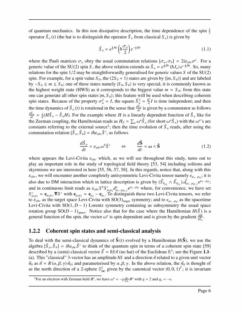
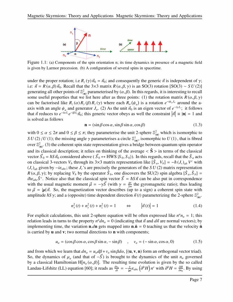
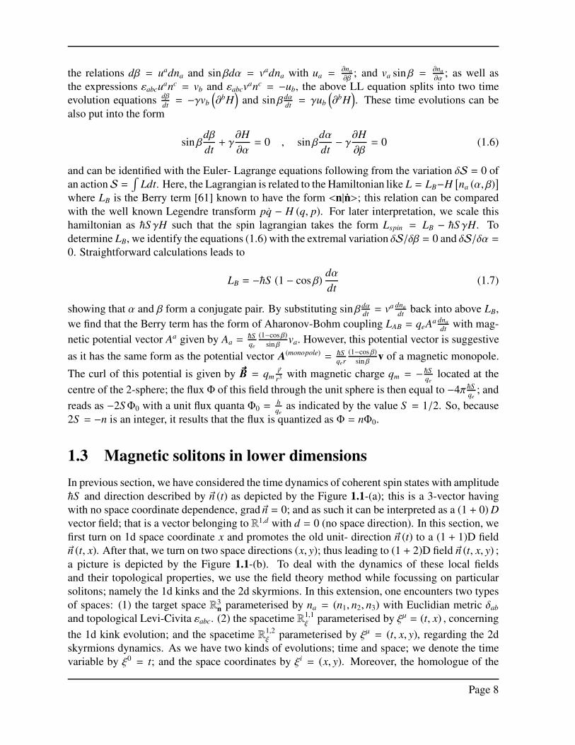
Figure 1.1: (a) Components of the spin orientation n; its time dynamics in presence of a magnetic field

is given by Larmor precession. (b) A configuration of several spins in spacetime.

under the proper rotation; i.e Rz (γ)~n0 = ~n0; and consequently the generic ~n is independent of γ;

i.e: ~n = R (α, β)~n0. Recall that the 3×3 matrix R (α, β, γ) is an SO(3) rotation [SO(3) ∼ S U (2)]

generating all other points of S2(n) parameterised by (α, β). In this regards, it is interesting to recall

some useful properties that we list here after as three points: (1) the rotation matrix R (α, β, γ)

can be factorised like Rz (α) Ry (β) Rz (γ) where each Ra

(ψa

)is a rotation e−iψaJa around the a-

axis with an angle ψa and generator Ja. (2) As the unit ~n0 is an eigen vector of e−iγJz ; it follows

that ~n reduces to e−iαJz e−iβJy~n0; this generic vector obeys as well the constraint∣∣∣~n∣∣∣ ≡ |n| = 1 and

is solved as follows

n = (sin β cosα, sin β sinα, cos β) (1.3)

with 0 ≤ α ≤ 2π and 0 ≤ β ≤ π; they parameterise the unit 2-sphere S2(n) which is isomorphic to

S U (2) /U (1); the missing angle γ parameterises a circle S1(n), isomorphic to U (1) , that is fibred

over S2(n)

. (3) the coherent spin state representation gives a bridge between quantum spin operator

and its classical description; it relies on thinking of the average < S > in terms of the classical

vector ~S 0 = ~S~n0 considered above ( ~S 0↔ HWS |S 0, S 0〉). In this regards, recall that the S a acts

on classical 3-vectors Vb through its 3×3 matrix representation like [S a,Vb] = −~ (Jc)ab Vc with

(Jc)ab given by −iεabc; these Jc’s are precisely the generators of the S U (2) matrix representation

R (α, β, γ); by replacing Vb by the operator S b, one discovers the SU(2) spin algebra [S a, S b] =

i~εabcSc. Notice also that the classical spin vector ~S = ~S~n can be also put in correspondence

with the usual magnetic moment ~µ = −γ~S (with γ =ge

2mthe gyromagnetic ratio); thus leading

to ~µ = |µ|~n. So, the magnetization vector describes (up to a sign) a coherent spin state with

amplitude ~S γ; and a (opposite) time dependent direction ~n (t) parameterizing the 2-sphere S2(n)

.

n2x (t) + n2

y (t) + n2z (t) = 1 ⇔

∣∣∣~n (t)∣∣∣ = 1 (1.4)

For explicit calculations, this unit 2-sphere equation will be often expressed like nana = 1; this

relation leads in turns to the property nadna = 0 (indicating that ~n and d~n are normal vectors); by

implementing time, the variation n.dn gets mapped into n.n = 0 teaching us that the velocity n

is carried by u and v; two normal directions to n with components;

ua = (cos β cosα, cos β sinα,− sin β) , va = (− sinα, cosα, 0) (1.5)

and from which we learn that dna = uadβ+va sin βdα, [(u, v, n) form an orthogonal vector triad).

So, the dynamics of µa (and that of −~S ) is brought to the dynamics of the unit na governed

by a classical Hamiltonian H[na (α, β)

]. The resulting time evolution is given by the so called

Landau-Lifshitz (LL) equation [60]; it reads as dna

dt= − γ

|µ|εabc

(∂bH

)nc with ∂bH = ∂H

∂nb. By using

the relations dβ = uadna and sin βdα = vadna with ua =∂na

∂β; and va sin β = ∂na

∂α; as well as

the expressions εabcuanc = vb and εabcv

anc = −ub, the above LL equation splits into two time

evolution equationsdβ

dt= −γvb

(∂bH

)and sin βdα

dt= γub

(∂bH

). These time evolutions can be

also put into the form

sin βdβ

dt+ γ

∂H

∂α= 0 , sin β

dα

dt− γ∂H

∂β= 0 (1.6)

and can be identified with the Euler- Lagrange equations following from the variation δS = 0 of

an actionS =∫

Ldt. Here, the Lagrangian is related to the Hamiltonian like L = LB−H[na (α, β)

]

where LB is the Berry term [61] known to have the form <n|n>; this relation can be compared

with the well known Legendre transform pq − H (q, p). For later interpretation, we scale this

hamiltonian as ~S γH such that the spin lagrangian takes the form Lspin = LB − ~S γH. To

determine LB, we identify the equations (1.6) with the extremal variation δS/δβ = 0 and δS/δα =0. Straightforward calculations leads to

LB = −~S (1 − cos β)dα

dt(1.7)

showing that α and β form a conjugate pair. By substituting sin βdαdt= va dna

dtback into above LB,

we find that the Berry term has the form of Aharonov-Bohm coupling LAB = qeAa dna

dtwith mag-

netic potential vector Aa given by Aa =~Sqe

(1−cos β)

sin βva. However, this potential vector is suggestive

as it has the same form as the potential vector A(monopole) = ~Sqer

(1−cos β)

sin βv of a magnetic monopole.

The curl of this potential is given by ~B = qm~rr3 with magnetic charge qm = −~Sqe

located at the

centre of the 2-sphere; the flux Φ of this field through the unit sphere is then equal to −4π~Sqe

; and

reads as −2SΦ0 with a unit flux quanta Φ0 =hqe

as indicated by the value S = 1/2. So, because

2S = −n is an integer, it results that the flux is quantized as Φ = nΦ0.

1.3 Magnetic solitons in lower dimensions

In previous section, we have considered the time dynamics of coherent spin states with amplitude

~S and direction described by ~n (t) as depicted by the Figure 1.1-(a); this is a 3-vector having

with no space coordinate dependence, grad~n = 0; and as such it can be interpreted as a (1 + 0) D

vector field; that is a vector belonging to R1,d with d = 0 (no space direction). In this section, we

first turn on 1d space coordinate x and promotes the old unit- direction ~n (t) to a (1 + 1)D field

~n (t, x). After that, we turn on two space directions (x, y); thus leading to (1 + 2)D field ~n (t, x, y) ;

a picture is depicted by the Figure 1.1-(b). To deal with the dynamics of these local fields

and their topological properties, we use the field theory method while focussing on particular

solitons; namely the 1d kinks and the 2d skyrmions. In this extension, one encounters two types

of spaces: (1) the target space R3n parameterised by na = (n1, n2, n3) with Euclidian metric δab

and topological Levi-Civita εabc. (2) the spacetime R1,1ξ parameterised by ξµ = (t, x) , concerning

the 1d kink evolution; and the spacetime R1,2ξ parameterised by ξµ = (t, x, y), regarding the 2d

skyrmions dynamics. As we have two kinds of evolutions; time and space; we denote the time

variable by ξ0 = t; and the space coordinates by ξi = (x, y). Moreover, the homologue of the


tensors δab and εabc are respectively given by the usual Lorentzian spacetime metric gµν, with

signature like gµνξµξν = x2 + y2 − t2, and the spacetime Levi-Civita ǫµνρ with ǫ012 = 1.

1.3.1 One space dimensional solitons

In (1 + 1)D spacetime, the local coordinates parameterising R1,1(ξ)

are given by ξµ = (t, x); so the

metric is restricted to gµνξµξν = x2 − t2. The field variable na (ξ) has in general three components

(n1, n2, n3) as described previously; but in what follows, we will simplify a little bit the picture

by setting n3 = 0; thus leading to a magnetic 1d soliton with two component field variable n =

(n1, n2) satisfying the constraint equation n.n = 1 at each point of spacetime. As this constraint

relation plays an important role in the construction, it is interesting to express it as nana = 1.

Before describing the topological properties of one space dimensional solitons (kinks), we think

it interesting to begin by giving first some useful features; in particular the three following ones.

(1) The constraint (n1)2 + (n2)2 = 1 is invariant S O (2)n rotations acting as n′a = Rabnb with

orthogonal rotation matrix

Rab =

(cosψ sinψ

− sinψ cosψ

), RTR = I (1.8)

The constraint nana = 1 can be also presented like NN = 1 with N standing for the complex

field n1 + in2 that reads also like eiα. In this complex notation, the symmetry of the constraint

is given by the phase change acting as N → UN with U = eiψ and corresponding to the shift

α→ α+ψ. Moreover the correspondence (n1, n2)↔ n1+ in2 describes precisely the well known

isomorphisms S O (2) ∼ U (1) ∼ S1(n)

where S1(n)

is a circle; it is precisely the equatorial circle

of the 2-sphere S2(n)

considered in previous section. (2) As for Eq(1.5), the constraint nana = 1

leads to nadna = 0; and so describes a rotational movement encoded in the relation dna = εabnb

where εab is the standard 2D antisymmetric tensor with ε21 = ε12 = 1; this εab is related to the

previous 3D Levi-Civita like εzab. Notice also that the constraint nana = 1 implies moreover

that dn2 = −nn

n2dn1; and consequently the area dn1 ∧ dn2, to be encountered later on, vanishes

identically. In this regards, recall that we have the following transformation

dn1 ∧ dn2 = Jdt ∧ dx , J = ǫµν∂µn1∂νn2 (1.9)

where ǫµν is the antisymmetric tensor in 1+1 spacetime, and J is the Jacobian of the transfor-

mation (t, x) → (n1, n2). (3) The condition nana = 1 can be dealt in two manners; either by

inserting it by help of a Lagrange multiplier; or by solving it in term of a free angular vari-

able like na = (cosα, sinα) from which we deduce the normal direction ua = dna

dαreading as

ua = (− sinα, cosα). In term of the complex field; we have N = eiα and NdN = idα. Though

interesting, the second way of doing hides an important property in which we are interested in

here namely the non linear dynamics and the topological symmetry.

Constrained dynamics

The classical spacetime dynamics of na (ξ) is described by a field action S =∫

dtL with La-

grangian L =∫

dxL and density L; this field density is given by −12

(∂µna

)(∂µna) − V (n) −

Λ (nana − 1) with ∂µ =∂∂ξµ

; it reads in terms of the Hamiltonian density as follows

L = πana −H (1.10)

where πa = ∂L∂na

. In the above Lagrangian density, the auxiliary field Λ (ξ) (no Kinetic term) is

a Lagrange multiplier carrying the constraint relation nana = 1. The V (n) is a potential energy

density which play an important role for describing 1d kinks with finite size. Notice also that the

variation δSδΛ= 0 gives precisely the constraint nana = 1 while the δS

δna = 0 gives the spacetime

dynamics of na described by the spacetime equation ∂µ∂µna − ∂V

∂na − Λna = 0. By substituting

na = (cosα, sinα), we obtain L = −12

(∂µα

)(∂µα) − V (α). If setting V (α) = 0, we end up

with the free field equation ∂µ∂µα = 0 that expands like

(∂2

x − ∂2t

)α = 0; it is invariant under

spacetime translations with conserved current symmetry ∂µTµν = 0 with Tµν standing for the

energy momentum tensor given by the 2×2 symmetric matrix ∂µα∂να+gµνL. The energy density

T00 is given by 12

(∂tα)2+ 1

2(∂xα)2 and the momentum density T10 reads as ∂xϕ∂xϕ. Focussing on

T00, the conserved energy E reads then as follows

E =1

2

∫ +∞

−∞dx

[(∂tα)2

+ (∂xα)2]≥ 0 (1.11)

with minimum corresponding to constant field (α = cte). Notice that general solutions of

∂µ∂µα = 0 are given by arbitrary functions f (x ± t); they include oscillating and non oscil-

lating functions. A typical non vibrating solution that is interesting for the present study is the

solitonic solution given (up to a constant c) by the following expression

ϕ (t, x) = π tanh

(x + t

λ

)(1.12)

where λ is a positive parameter representing the width where the soliton α (t, x) acquires a sig-

nificant variation. Notice that for a given t, the field varies from α (t,−∞) = −π to α (t,+∞) = π

regardless the value of λ. These limits are related to each other by a period 2π.

Topological current and charge

To start, notice that as far as conserved symmetries of (1.10) are concerned, there exists an exotic

invariance generated by a conserved Jµ (t, x) going beyond the spacetime translations generated

by the energy momentum tensor Tµν. The conserved spacetime current Jµ = (J0, J1) of this exotic

symmetry can be introduced in two different, but equivalent, manners; either by using the free

degree of freedom α; or by working with the constrained field na. In the first way, we think of the

charge density J0 like 12π∂1α and of the current density as J1 = − 1

2π∂0α. This conserved current

is a topological (1 + 1) D spacetime vector Jµ that is manifestly conserved; this feature follows

from the relation between Jµ and the antisymmetric ǫµν as follows [56],

Jµ =1

2πǫµν∂

να (1.13)

Because of the ǫµν; the continuity relation ∂µJµ =1

2πǫµν∂

µ∂να vanishes identically due to the

antisymmetry property of ǫµν. The particularity of the above conserved Jµ is its topological


nature; it is due to the constraint nana = 1 without recourse to the solution na = (cosα, sinα).

Indeed, Eq(1.13) can be derived by computing the Jacobian J = det(∂na

∂ξµ) of the mapping from

the 2d spacetime coordinates (t, x) to the target space fields (n1, n2). Recall that the spacetime

area dt ∧ dx can be written in terms of ǫµν like 12ǫµνdξ

µ ∧ dξν and, similarly, the target space area

dn1 ∧ dn2 can be expressed in terms of as εab follows 12εabdna ∧ dnb. The Jacobian J is precisely

given by (1.9); and can be presented into a covariant form like J = 12εµν∂µn

a∂νnbεab. This

expression of the Jacobian J captures important informations; in particular the three following

ones. (1) It can be expressed as a total divergence like ∂µ (πJµ) with spacetime vector

Jµ =1

2πεµνna∂νn

bεab (1.14)

and where 1π

is a normalisation; it is introduced for the interpretation of the topological charged as

just the usual winding number of the circle [encoded in the homotopy group relation π1

(S

1)= Z].

(2) Because of the constraint dn2 = −nn

n2dn1 following from nana = 1, the Jacobian J vanishes

identically; thus leading to the conservation law ∂µJµ = 0; i.e J = 0 and then ∂µJµ = 0. (3) The

conserved charge Q associated with the topological current is given by∫ +∞−∞ dxJ0 (t, x); it is time

independent despite the apparent t- variable in the integral (dQ/dt = 0). By using (1.13), this

charge reads also as 12π

∫ +∞−∞ dx∂xα (t, x) and after integration leads to

Q =1

2π[α (t,∞) − α (t,−∞)] (1.15)

Moreover, seen that α (t,∞) is an angular variable parameterising S1n; it may be subject to a

boundary condition like for instance the periodic α (t,∞) = α (t,−∞) + 2πN with N an integer;

this leads to an integral topological charge Q = N interpreted as the winding number of the

circle. In this regards, notice that: (i) the winding interpretation can be justified by observing

that under compactification of the space variable x, the infinite space line Rx = ]−∞,+∞[ gets

mapped into a circle S1(x) with angular coordinate −π ≤ ϕ ≤ π; so, the integral 1

2π

∫ +∞−∞ dx∂xα (t, x)

gets replaced by 12π

∫ +π−π dϕ∂α

∂ϕ; and then the mapping αt : ϕ → α (t, ϕ) is a mapping between two

circles namely S1(x) → S1

(n); the field α (t, ϕ) then describes a soliton (one space extended object)

wrapping the circle S1(x) N times; this propery is captured by πS1

(x)(S1

(n)) = Z, a homotopy group

property [62]. (ii) The charge Q is independent of the Lagrangian of the system as it follows

completely from the field constraint without any reference to the field action. (iii) Under a scale

transformation ξ′ = ξ/λ with a scaling parameter λ > 0, the topological charge of the field (1.12)

is invariant; but its total energy (1.11) get scaled as follows

Q′ = Q , E′ =1

λE (1.16)

This energy transformation shows that stable solitons with minimal energy correspond to λ→∞;

and then to a trivial soliton spreading along the real axis. However, one can have non trivial soli-

tonic configurations that are topologically protected and energetically stable with non diverging

λ. This can done by turning on an appropriate potential energy density V (n) in Eq(1.10). An

example of such potential is the one given byg

8

(n4

1+ n4

2− 1

), with positive g = M2, breaking

S O (2)n; by using the constraint n21 + n2

2 = 1, it can be putg

4n2

1n22. In terms of the angular field

α, it reads as V (α) =g

16(1 − cos 4α) leading to the well known sine-Gordon equation [63, 64]

namely ∂µ∂µα − g

4sin 4α = 0 with the symmetry property α → α + π

2. So, the solitonic solution

is periodic with period π2; that is the quarter of the old 2π period of the free field case. For static

field α (x), the sine Gordon equation reduces to d2αdx2 − M2

4sin 4α = 0; its solution for M > 0 is

given by arctan[exp Mx

]representing a sine- Gordon field evolving from 0 to π

2and describing a

kink with topological charge Q = 14. For M < 0, the soliton is an anti-kink evolving from π

2to 0

with charge Q = −14. Time dependent solutions can be obtained by help of boost transformations

x→ x±vt√1−v2

.

1.3.2 Skyrmions in 2d space dimensions

In this subsection, we investigate the topological properties of 2d Skyrmions by extending the

field theory study we have done above for 1d kinks to two space dimensions. For that, we

proceed as follows: First, we turn on the component n3 so that the skyrmion field n is a real

3-vector with three components (n1, n2, n3) constrained as in Eqs(1.4-1.5). Second, here we have

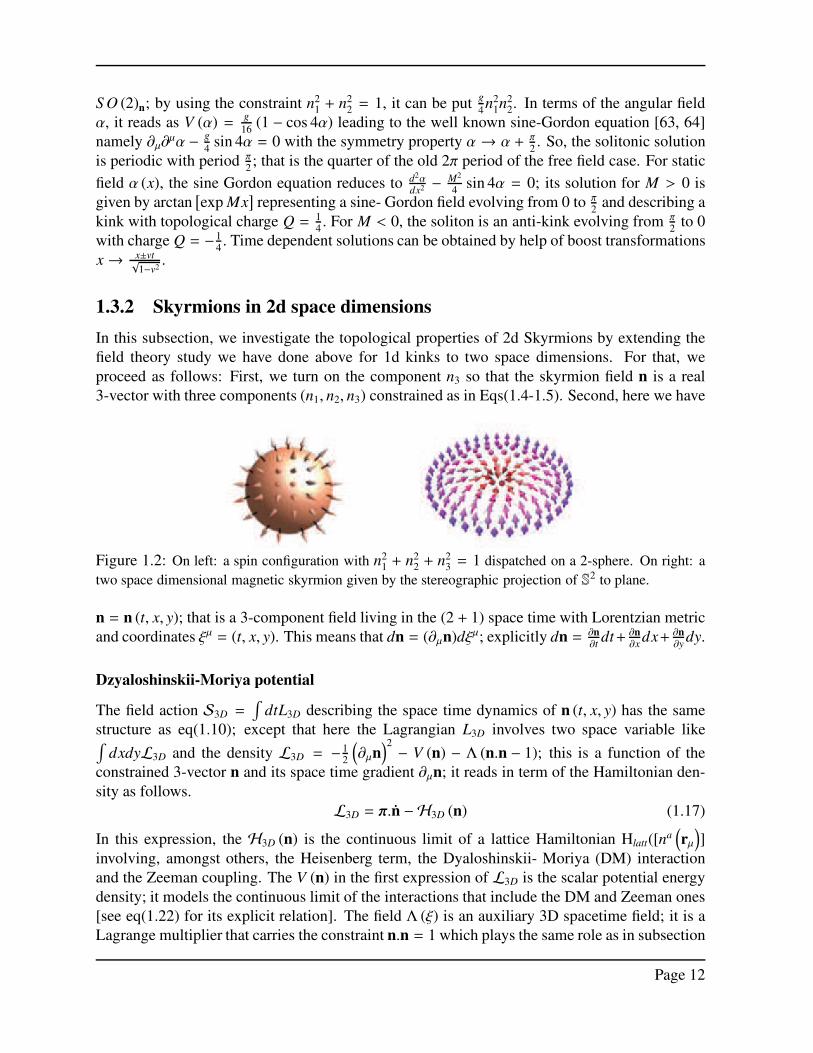
Figure 1.2: On left: a spin configuration with n21 + n2

2 + n23 = 1 dispatched on a 2-sphere. On right: a

two space dimensional magnetic skyrmion given by the stereographic projection of S2 to plane.

n = n (t, x, y); that is a 3-component field living in the (2 + 1) space time with Lorentzian metric

and coordinates ξµ = (t, x, y). This means that dn = (∂µn)dξµ; explicitly dn = ∂n∂t

dt+ ∂n∂x

dx+ ∂n∂y

dy.

Dzyaloshinskii-Moriya potential

The field action S3D =∫

dtL3D describing the space time dynamics of n (t, x, y) has the same

structure as eq(1.10); except that here the Lagrangian L3D involves two space variable like∫dxdyL3D and the density L3D = −1

2

(∂µn

)2− V (n) − Λ (n.n − 1); this is a function of the

constrained 3-vector n and its space time gradient ∂µn; it reads in term of the Hamiltonian den-

sity as follows.

L3D = π.n −H3D (n) (1.17)

In this expression, the H3D (n) is the continuous limit of a lattice Hamiltonian Hlatt([na(rµ

)]

involving, amongst others, the Heisenberg term, the Dyaloshinskii- Moriya (DM) interaction

and the Zeeman coupling. The V (n) in the first expression of L3D is the scalar potential energy

density; it models the continuous limit of the interactions that include the DM and Zeeman ones

[see eq(1.22) for its explicit relation]. The field Λ (ξ) is an auxiliary 3D spacetime field; it is a

Lagrange multiplier that carries the constraint n.n = 1 which plays the same role as in subsection


3.1. By variating this action with respect to the fields n andΛ; we get from δS3D

δΛ= 0 precisely the

field constraint n.n = 1; and from δS3D

δn= 0 the following Euler-Lagrange equation n = ∂V

∂n+Λn.

For later use, we express this field equation like

∂µ∂µna =∂V

∂na+ Λna (1.18)

The interest into this (1.18) is twice; first it can be put into the equivalent form ∂µ∂µna = εabcDbnc

where Db is an operator acting on nc to be derived later on [see eq(??)]; and second, it can be

used to give the relation between the scalar potential and the operator Db. To that purpose, we

start by noticing that there are two manners to deal with the field constraint nana = 1; either by

using the Lagrange multiplier Λ; or by solving it in terms of two angular field variables as given

by eq(1.5). In the second case, we have the triad na = (sin β cosα, sin β sinα, cos β) and

ua = (cos β cosα, cos β sinα,− sin β) , va = (− sinα, cosα, 0) (1.19)

but now β = β (t, x, y) and α = α (t, x, y) with 0 ≤ β ≤ π and 0 ≤ α ≤ 2π. Notice also that

the variation of the filed constraint leads to nadna = 0 teaching us interesting informations, in

particular the two following useful ones. (1) the movement of na in the target space is a rotational

movement; and so can be expressed like

dna = εabcωbnc ⇔ dn = ω ∧ n ⇔ ω ∼ n ∧ dn (1.20)

where the 1-form ωb is the rotation vector to be derived below. By substituting (1.20) back

into nadna, we obtain εbcaωbncna which vanishes identically due to the property εbcancna = 0. (2)

Having two degrees of freedom α and β, we can expand the differential dna like uadβ+va sinαdα

with the two vector fields ua =∂na

∂βand va =

∂na

∂αas given above. Notice that the three unit fields

(n, u, v) plays an important role in this study; they form a vector basis of the field space; they

obey the usual cross products namely n = u ∧ v and its homologue which given by cyclic

permutations; for example,

ua = εabcvbnc , va = −εabcu

bnc (1.21)

Putting these eqs(1.21) back into the expansion of dna in terms of dα, dβ; and comparing with

Eq(1.20), we end up with the explicit expression of the 1-form angular ”speed” vector ωb; it

reads as follows ωb = vbdβ − ub sinαdα. Notice that by using the space time coordinates ξ, we

can also express eq(1.20) like ∂µna = εabcωbµn

c withωbµ given by vb(∂µβ)−ub sinα(∂µα). From this

expression, we can compute the Laplacian ∂µ∂µna; which, by using the above relations; is equal

to εabc∂µ(ωbµn

c)

reading explicitly as εabc[(∂µωb

µ)nc + ωb

µ(∂µnc)] or equivalently like ∂µ∂µna =

εabcDbnc with operator Db = ωbµ∂

µ + (∂µωbµ). Notice that the above operator has an interesting

geometric interpretation; by factorising ωbµ, we can put it in the form ωd

µ (Dµ)bd where (Dµ)b

d

appears as a gauge covariant derivative (Dµ)bd = δ

bd∂

µ + (Aµ)bd with a non trivial gauge potential

(Aµ)bd given by ω

µ

d(∂νωb

ν). Comparing with (1.18) with ∂µ∂µna = εabcDbnc, we obtain ∂V∂na =

εabcDbnc −Λna; and then a scalar potential energy V given by∫εabc(dnaDbnc)−Λ

∫nadna. The

second term in this relation vanishes identically because nadna = 0; thus reducing to

V =

∫εabc(dnaDbnc) (1.22)

containing εabc(naDbnc) as a sub-term. In the end of this analysis, let us compare this sub-

term with the εabcnbnc

µ1µ2∆aµ1µ2 with ∆aµ1µ2 = da

µ3...µD−2ǫµ1...µD giving the general structure of the

DM coupling (see end of subsection 2.1). For (1 + 2)D spacetime, the general structure of DM

interaction reads εabcda0

(nb∇nc

).eµνǫ

0µν; by setting e0 = eµνǫ0µν and da = da

0e0 as well as Da =

da.∇, one brings it to the form εabc

(naDbnc

)which is the same as the one following from (1.22).

From kinks to 2d Skyrmions

Here, we study the topological properties of the 2d Skyrmion with dynamics governed by the

Lagrangian density (1.17). From the expression of the (1 + 1)D topological current (Jµ)2D dis-

cussed in subsection 2.1, which reads as 12πǫµνna∂νn

bεab, one can wonder the structure of the

(1 + 2)D topological current (Jµ)3D that is associated with the 2d Skyrmion described by the

3-vector field na (ξ). It is given by

(Jµ)3D =1

8πǫµνρna∂νn

b∂νncεabc (1.23)

where εabc is as before and where ǫµνρ is the completely antisymmetric Levi-Civita tensor in

the (1 + 2)D spacetime. The divergence ∂µ(Jµ)3D of the above spacetime vector vanishes iden-

tically; it has two remarkable properties that we want to comment before proceeding. (1) The

∂µ(Jµ)3D is nothing but the determinant of the 3 × 3 Jacobian matrix ∂na

∂ξµrelating the three field

variables na to the three spacetime coordinates ξµ; this Jacobian det(∂na

∂ξµ) is generally given by

13!ǫµνρ∂µn

a∂νnb∂νn

bεabc; it maps the spacetime volume d3ξ = dt ∧ dx ∧ dy into the target space

volume d3n = dn1∧dn2∧dn3. In this regards, recall that these two 3D volumes can be expressed

in covariant manners by using the completely antisymmetric tensors ǫµνρ and εabc introduced ear-

lier; and as noticed before play a central role in topology. The target space volume d3n can be

expressed like 13!εabcdna ∧ dnb ∧ dnc; and a similar relation can be also written down for the

spacetime volume d3ξ. Notice also that by substituting the differentials dna by their expansions

(∂na

∂ξµ)dξµ; and putting back into d3n, we obtain the relation d3n = J3Dd3ξ where J3D is pre-

cisely the Jacobian det(∂na

∂ξµ). (2) The conservation law ∂µ(Jµ)3D = 0 has a geometric origin; it

follows from the field constraint relation n21+ n2

2+ n2

3= 1 degenerating the volume of the 3D

target space down to a surface. This constraint relation describes a unit 2-sphere S2(n); and so a

vanishing volume d3n∣∣∣S

2(n)

= 0; thus leading to J3D = 0 and then to the above continuity equa-

tion. Having the explicit expression (1.23) of the topological current Jµ in terms of the magnetic

texture field n (ξ), we turn to determine the associated topological charge Q =∫

dxdyJ0 with

charge density J0 given by 18πεabcǫ

0i j(∂in

b∂ jnc)

na. Substituting ǫ0i jdx∧ dy by dξi ∧ dξ j, we have

J0dx ∧ dy = 18πεabcn

a(dnb ∧ dnc

). Moreover using the differentials dnb = ubdβ + vb sinαdα, we

can calculate the area dnb ∧ dnc in terms of the angles α and β; we find 2na(sinα)dβ ∧ dα where

we have used εabc

(ubvc − ucvb

)= 2na. So, the topological charge Q reads as 1

4π

∫S

2n

(sin β) dαdβ

which is equal to 1. In fact this value is just the unit charge; the general value is an integer Q = N

with N being the winding number π2(S2n); see below. Notice that J0 can be also presented like

J0 =εabc

8πna

(∂nb

∂x

∂nc

∂y− ∂nb

∂y

∂nc

∂x

)(1.24)


Replacing na by their expression in terms of the angles (sin β cosα, sin β sinα, cos β), we can

bring the above charge density J0 into two equivalent relations; first into the form likesin β

4π

(∂β

∂x∂α∂y− ∂β

∂y

∂β

∂x

);

and second as 14π

∂[α,cos β]∂[x,y]

which is nothing but the Jacobian of the transformation from the (x, y)

space to the unit 2-sphere with angular variables (α, β). The explicit expression of (n1, n2, n3) in

terms of the (x, y) space variables is given by

n1 =2x

x2 + y2 + 1, n2 =

2y

x2 + y2 + 1, n3 =

x2 + y2 − 1

x2 + y2 + 1(1.25)

but this is nothing but the stereographic projection of the 2-sphere S2ξ on the real plane. So, the

field na defines a mapping between S2ξ towards S2

n with topological charge given by the winding

number S2n around S2

n; this corresponds just to the homotopy property π2(S2n) = N.

1.4 Three dimensional magnetic skyrmions

In this section, we study the dynamics of the 3d skyrmion and its topological properties both

in target space R4n (with euclidian metric δAB) and in 4D spacetime R1,3

ξ parameterised by ξµ =

(t, x, y, z) (with Lorentzian metric gµν). The spacetime dynamics of the 3d skyrmion is described

by a four component field nA (ξ) obeying a constraint relation f (n) = 1; here the f (n) is given

by the quadratic form nAnA invariant under SO(4) transformations isomorphic to SU(2)×SU(2).

The structure of the topological current of the 3d skyrmion is encoded in two types of Levi-

Civita tensors namely the target space εABCD and the spacetime ǫµνρτ extending their homologue

concerning the kinks and 2d skyrmions.

1.4.1 From 2d skyrmion to 3d homologue

As for the 1d and 2d solitons considered previous section, the spacetime dynamics of the 3d

skyrmion in R1,3 is described by a field action S4D =∫

dtL4D with Lagrangian realized as the

space integral∫

dxdydzL4D. Generally, the Lagrangian density L4D is a function of the soliton

n (t, x, y, z) which is a real 4-component field [n = (n1, n2, n3, n4)] constrained like f[n (ξ)

]= 1.

For self ineracting field, the typical field expression of L4D is given by −12

(∂µn

)2− V (n) −

Λ[f (n) − 1

]where V (n) is a scalar potential; and where the auxiliary field Λ (ξ) is a Lagrange

multiplier carrying the field constraint. This density L4D reads in terms of the Hamiltonian as

Π.∂n∂t− H (n) . Below, we consider a 4-component skyrmionic field constrained as n.n = 1; and

focuss on a simple Lagrangian densityL = −12

(∂µn

)(∂µn)−Λ [n.n− 1] to describe the degrees

of freedom of n. Being a unit 4-component vector, we can solve the constraint n.n = 1 in terms

of three angular angles (α, β, γ) ; by setting

n = (m sin γ, cos γ) , m = (sin β cosα, sin β sinα, cos β) (1.26)

where m is a unit 3-vector parameterising the unit sphere S2[α]. Putting this field realisation back

intoL, we obtain− cos 2γ

2

(∂µγ

)2− 1−cos 2γ

4

(∂µm

)2−Λ [m.m − 1] . Notice that by restricting the 4D

spacetime R1,3 to the 3D hyperplane z=const; and by fixing the component field γ to π2, the above

Lagrangian density reduces to the one describing the spacetime dynamics of the 2d skyrmion.

Notice also that we can expand the differential dnA in terms of dγ, dβ, dα; we find the following

dna = ma cos γdγ + sin γ (uadβ + va sin βdα) , dn4 = − sin γdγ (1.27)

For convenience, we sometimes refer to the three (α, β, γ) collectively like αa = (α1, α2, α3) ; so

we have dnA = EAa dαb with EA

a =∂nA

∂αa .

1.4.2 Conserved topological current

First, we investigate the topological properties of the 3d skyrmion from the target space view;

that is without using the spacetine variables (t, x, y, z) = ξµ. Then, we turn to study the induced

topological properties of the 3d skyrmion viewed from the side of the 4D space time R1,3.

Topological current in target space

The 3d skyrmion field is described by a real four component vector nA subject to the constraint

relation nAnA = 1; so the soliton has SO(4) ∼ S O (3)1 × S O (3)2 symmetry leaving invariant

the condition nAnA = 1 that reads explicitly as (n1)2 + (n2)2 + (n3)2 + (n4)2 = 1. The algebraic

condition f [n] = 1 induces in turns the constraint equation d f = 0 leading to nAdnA = 0 and

showing that nA and dnA orthogonal 4-vectors in R4(n). From this constraint, we can construct(

nAdnB − nBdnA)/2 which is a 4×4 antisymmetric matrix Ω[AB] generating the SO(4) rotations;

this Ω[AB] contains 3+3 degrees of freedom generating the two S O (3)1 and S O (3)2 making

SO(4); the first three degrres are given by Ω[ab] with a, b = 1, 2, 3; and the other three concern

Ω[a4].Notice also that, from the view of the target space, the algebraic relation nAnA = 1 describes

a unit 3-sphere S3n sitting in R4

n; as such its volume 4-form d4n, which reads as 14!εABCDdnA ∧

dnB ∧ dnC ∧ dnD, vanishes identically when restricted to the 3-sphere; i.e: d4n∣∣∣S

3n= 0. This

vanishing property of d4n on S3n is a key ingredient in the derivation of the topological current J

of the 3D skyrmion and its conservation dJ = 0. Indeed, because of the property d2 = 0 (where

we have hidden the wedge product ∧), it follows that d4n can be expressed as dJ with the 3-form

J given by

J =1

4!εABCDnAdnBdnCdnD (1.28)

This 3-form describes precisely the topological current in the target space; this is because on

S3n, the 4-form d4n vanishes; and then dJ vanishes. By solving, the skyrmion field constraint

nAnA = 1 in terms of three angles αa as given by Eq(1.26); with these angular coordinates, we

have mapping f : R4n → S3

n with S3n ≃ S3

α. By expanding the differentials like dnA = EAa dαa with

EAa =

∂nA

∂αa ; then the conserved current on the 3-sphere S3α reads as follows

J =1

4!3!εABCD(nAEB

b ECc ED

d )εabcd3α (1.29)

where we have substituted the 3-form dαbdαcdαd on the 3-sphere S3α by the volume 3-form

εabcd3α. In this regards, recall that the volume of the 3-sphere is∫S

3(n)

d3α = π2

2.


Topological symmetry in spacetime

In the spacetime R1,3 with coordinates ξµ = (t, x, y, z), the 3d skyrmion is described by a four

component field nA (ξ) and is subject to the local constraint relation nAnA = 1. A typical static

configuration of the 3d skyrmion is obtained by solving the field sonctraint in terms of the space

coordinates; it is given by Eq(1.26) with the local space time fields m (ξ) and γ (ξ) thought of as

follows

m (ξ) =(

x

r,

y

r,

z

r

), γ (ξ) = arcsin

2rR

r2 + R2= arccos

r2 − R2

r2 + R2(1.30)

with r =√

x2 + y2 + z2, giving the radius of S2ξ , and R associated with the circle S1

ξ fibered over

S2ξ ; the value R = r corresponds to γ = π

2and R >> r to γ = π. Notice that γ (ξ) in eq(1.30)

has a spherical symmetry as it is a function only of r (no angles α, β, γ). Moreover, as this

configuration obeys sinγ (0) = 0 and sin γ (∞) = 0; we assume γ (0) = n0π and γ (∞) = n∞π.

Putting these relations back into (1.26), we obtain the following configuration

n =

(2xR

r2 + R2,

2yR

r2 + R2,

2zR

r2 + R2,

r2 − R2

r2 + R2

)(1.31)

describing a compactification of the space R3ξ into S3

ξ which is homotopic to S3n. From this view,

the n : ξ → n (ξ) is then a mapping from S3ξ into S3

n with topological charge given by the winding

number characterising the wrapping S3n on S3

ξ ; and for which we have the property π3(S3n) = Z. In

this regards, recall that 3-spheres S3 have a Hopf fibration given by a circle S1 sitting over S2 (for

short S3 ∼ S1⋉S

2); this non trivial fibration can be viewed from the relation S3 ∼ S U (2) and the

factorisation U (1)×S U (2) /U (1) with the coset S U (2) /U (1) identified with S2; and U (1) with

S1. Applying this fibration to S3

ξ and S3n, it follows that n : S3

ξ → S3n; and the same thing for the

bases S2ξ → S2

n and for the fibers S1ξ → S1

n. Returning to the topological current and the conserved

topological charge Q =∫R3 d3rJ0 (t, r), notice that in space time the differential dnA expands like(

∂µnA)

dξµ; then using the duality relation J[νρτ] = ǫµνρτJµ, we find, up to a normalisation by the

volume of the 3-sphere π2/2, the expression of the topological current Jµ (ξ) in terms of the 3D

skyrmion field

Jµ =1

12π2ǫµνρτna∂νn

b∂ρnc∂τn

cεabcd (1.32)

In terms of the angular variables, this current reads likeN∂να∂ρβ∂τγǫµνρτ withN = 12π2 (sin β) (sin γ)2.

From this current expression, we can determine the associated topological charge Q by space in-

tegration over the charge density

J0 (t, r) = −sin2 γ

2π2r2

dγ

dr(1.33)

Because of its spherical symmetry, the space volume d3r can be substituted by 4πr2dr; then

the charge Q reads as the integral − 4π2π2

∫ γ(∞)

γ(0)sin2 γdγ whose integration leads to the sum of

two terms coming from the integration of sin2 γ = 12− 1

2cos 2γ. The integral first reads as

1π

[γ (0) − γ (∞)

]; by substituting γ (0) = n0π, it contributes like Nπ. The integral of the second

tem gives 12π

[sin 2γ (0) − sin 2γ (∞)

]; it vanishes identically. So the topological charge is given

by

Q =γ (0) − γ (∞)

π= N (1.34)

1.5 Effective dynamics of skyrmions

In this section, we investigate the effective dynamics of a point- like skyrmion in a ferromagnetic

background field while focussing on the 2d configuration. First, we derive the effective equation

of a rigid skyrmion and comment on the underlying effective Lagrangian. We also describe the

similarity with the dynamics of an electron in a background electromagnetic field. Then, we

study the effect of dissipation on the skyrmion dynamics.

1.5.1 Equation of a rigid skyrmion

To get the effective equation of motion of a rigid skyrmion, we start by the spin (0 + 1) D action

Sspin =∫

dtLspin describing the time evolution of a coherent spin vector modeled by a rotating

magnetic moment n (t) with velocity n = dndt

; and make some accommodations. For that, recall

that the Lagrangian Lspin has the structure LB−~S γH where LB is the Berry term having the form

LB = qeA.n with geometric (Berry) potential A ∼ 〈n|n〉; and where H is the Hamiltonian of the

magnetic moment n (t) obeying the constraint n2 = 1. This magnetisation constraint is solved

by two free angles α (t) , β (t) ; they appear in the Berry term LB = −~S (1 − cos β) dαdt. Below, we

think of the above magnetisation as a ferromagnetic background n (r) filling the spatial region of

R1,dξ with coordinates ξ = (t, r); and of the skymion as a massive point- like particle R (t) moving

in this background.

Rigid skyrmion

We begin by introducing the variables describing the skyrmion in the magnetic background field

n (r). We denote by Ms the mass of the skyrmion, and by R and R its space position and its

velocity. For concreteness, we restrict the investigation to the spacetime R1,2ξ and refer to R by

the components Xi = (X, Y) and to r by the components xi = (x, y). Because of the Euclidean

metric δi j; we often we use both notations Xi and Xi = δi jXj without referring to δi j. Furthermore;

we limit the discussion to the interesting case where the only source of displacements in R1,2ξ is

due to the skyrmion R (t) (rigid skyrmion). In this picture, the description of the skyrmion R (t)

dissolved in the background magnet n (r) is given by

n (r, t) = n [r − R (t)] (1.35)

In this representation, the velocity n of the skyrmion dissolved in the background magnet can

be expressed into manners; either like −Xi ∂n∂Xi ; or as Xi ∂n

∂xi ; this is because ∂∂Xi = − ∂

∂xi . With

this parametrisation, the dynamics of the skyrmion is described by an action Ss =∫

dtLs with

Lagrangian given by a space integral Ls =~s

a2

∫d2rLs and spacetime density as follows

Ls = γ~SH − ~SLB (1.36)


In this relation, the density LB = − (1 − cos β) ∂α∂t

where now the angular variables are spacetime

fields β (t, r) and α (t, r). Similarly, the density H is the Hamiltonian density with arguments as

H[n, ∂µn, r

]and magnetic n as in Eq(1.35). In this field action Ss, the prefactor a−2 is required

by the continuum limit of lattice Hamiltonians Hlatt living on a square lattice with spacing pa-

rameter a. Recall that for these Hlatt’s, one generally has discrete sums like∑µ (...),

∑µ,ν (...) and

so on; in the limit where a is too small, these sums turn into 2D space integrals like a−2∫

d2r (...).

To fix ideas, we illustrate this limit on the typical hamiltonian HHDMZ , it describes the Heisenberg

model on the lattice Z2 augmented by the Dzyaloshinskii-Moriya and the Zeeman interactions

[65, 66]

HHDMZ = −J∑

〈µ,ν〉n(rµ

)n (rν) − D

∑

µ,ν,ρ

dµ.[n (rν) ∧ n

(rρ

)]ǫµνρ −

∑

µ

B.n(rµ

)(1.37)

with rν = rµ + aeνµ; that is eνµ = (rν − rµ)/a where a is the square lattice parameter. So,

the continuum limit H of this lattice Hamiltonian involves the target space metric δab and the

topological Levi-Civita tensor εabc of the target space R3n; it involves as well the metric gµν and

the completely antisymmetry ǫµνρ of the space time R1,2ξ . In terms of δab and εabc tensors, the

continuous hamiltonian density reads as follows

H = Ja2

2δab∂

ina∂inb + aεabcd

aµ

(nbDνρn

c)ǫµνρ − B.n (1.38)

with ∇νρ = eνµ.∇. Below, we set J=1 and, to factorise out the normalisation factor a2, scale the

parameters of the model like daµ = ad

aµ and B = a2B. For simplicity, we sometimes set as well

a= 1.

Skyrmion equation without dissipation

To get the effective field equation of motion of the point- like skyrmion without dissipation, we

calculate the vanishing condition of the functional variation of the action; that is δ(∫

dtd2rL) = 0.

General arguments indicate that the effective equation of the skyrmion with topological charge

qs in the background magnet has the form

MsXi = qsEi + qsǫ i jzXjBz (1.39)

from which one can wonder the effective Lagrangian describing the effective dynamics of the

skyrmion. It is given by

Ls =Ms

2δi jX

iX j − qsǫzi jBzXiX j − qsV (X) (1.40)

Notice that the right hand of equation (1.39) looks like the usual Lorentz force (qeE + qer ∧ B)

of a moving electron with qe in an external electromagnetic field (Ei, Bi) ; the corresponding La-

grangian is m2

r2 + qeB.(r ∧ r)−qeE.r. This similarity between the skyrmion and the electron in

background fields is because the skyrmion has a topological charge qs that can be put in cor-

respondence with qe; and, in the same way, the background field magnet Ei,Bi can be also put

in correspondence with the electromagnetic field (Ei, Bi). To rigourously derive the spacetime

eqs(1.39-1.40), we need to perform some manipulations relying on computing the effective ex-

pression of Ss = ~S∫

dt(∫

d2rLs) and its time variation δSs = 0. However, as Ls has two

terms like γ~SH − ~SLB, the calculations can be split in two stages; the first stage concerns the

block γ~S∫

d2rH with H[n, ∂µn, r

]which is a function of the magnetic texture (1.35); that is

n (r − R). The second stage regards the determination of the integral ~S∫

d2rLB. The compu-

tation of the first term is straightforwardly identified; by performing a space shift r → r + R,

the Hamiltonian density becomes H[n, ∂µn, r + R

]with n (r) and where the dependence in R

becomes explicit; thus allowing to think of the integral γ~S∫

d2rH as nothing but the scalar

energy potentialV (R) = ~S γ∫

d2rH (t, r,R) . So, we have

δ

δXa

(~S γ

∫d2rH

)=∂V∂Xa

(1.41)

Concerning the calculation of the ~S∫

d2rLB, the situation is somehow subtle; we do it in two

steps; first we calculate the (δ∫

d2rLB) because we know the variation δLB

δna which is equal to12εabcn

bnc. Then, we turn backward to determine ~S∫

d2rLB by integration. To that purpose,

recall also that the Berry term LB is given by − (1 − cos β) ∂α∂t

; and its variation δLB

δna∂na

∂X j∂X j is

equal to 12εabcn

bnc. To determine the time variation δLB = δ∫

d2rδLB, we first expand it like∫d2r δL

δna δna; and use δna = − ∂na

∂X j∂X j to put it into the form -∫

d2r δLB

δna∂na

∂X j∂X j. Then, substitutingδLB

δna by its expression 12εabcn

bnc with nc expanded like - ∂nc

∂Xi Xi, we end up with

δLB = 2~S

(∫d2r

1

2εabcn

b∂nc

∂xi

∂na

∂x j

)ǫ i j

(XδY − YδX

)(1.42)

Next, using the relation ǫ i jd2r = dxi ∧ dx j, the first factor becomes∫

12εabcn

adnb ∧ dnc gives pre-

cisely the skyrmion topological charge qs. So, the resulting δLB reduces to 2qs~S(XδY − YδX

)

that reads also like

δLB = −2qs~S ǫi jXiδX j (1.43)

This variation is very remarkable because it is contained in the variation of the effective coupling

LintB= −2qs~S ǫi jX

iX j which can be presented like LintB= −qsAiX

i where we have set Ai =

2~S ǫzi jXj; this vector can be interpreted as the vector potential of an effective magnetic field

Bz = 12ǫzi j∂iAi. By adding the kinetic term Ms

2XiXi, we end up with an effective Lagrangian LB

associated with the Berry term; it reads as follows LB =Ms

2δi jX

iX j − qsAiXi. So, the effective

Lagrangian Le f f describing the rigid 2d skyrmion in a ferromagnet is

Le f f =Ms

2R2 − qsA.R−V (R) (1.44)

From this Lagrangian, we learn the equation of the motion of the rigid skyrmion namely MsX j =

f j + 4qs~S ǫzi jXi; for the limit Ms = 0, it reduces to Xi = 1

4qs~Sǫz ji f j.

1.5.2 Implementing dissipation

So far we have considered magnetic moment obeying the constraint n2 = 1 with time evolution

given by the LL equation n = −γf ∧ n where the force f = −∂H∂n

. Using this equation, we deduce


the typical properties n.n = f.n = 0 from which we learn that the time variation dHdt

of the

Hamiltonian, which reads as ~S γ∫

d2r∂H∂na na, vanishes identically as explicitly exhibited below,

dH

dt= −~S γ

∫d2r (f.n) (1.45)

In presence of dissipation, we loose energy; and so one expects that dHdt< 0; indicating that the

rigid skyrmion has a damped dynamics. In what follows, we study the effect of dissipation in the

ferromagnet and derive the damped skyrmion equation.

Landau- Lifshitz- Gilbert equation

Due to dissipation, the force F acting on the rigid skyrmion R (t) has two terms, the old conser-

vative f = −∂H∂n

; and an extra force δf linearly dependent in magnetisation velocity n. Due to

this extra force δf = −αγn, the LL equation gets modified; its deformed expression is obtained by

shifting the old force f like F = f−αγn with α a positive damping parameter (Gilbert parameter).

As such, the previous LL relation gives the so called Landau-Lifschitz-Gilbert (LLG) equation

[67, 68]

n = −γf ∧ n + αn ∧ n (1.46)

where its both sides have n. From this generalised relation, we still have n.n = 0 (ensuring

n2 = 1); however f.n , 0 as it is equal to the Gilbert term namely −α (f ∧ n) .n. Notice that

eq(1.46) still describe a rotating magnetic moment in the target space (dn = 0); but with a

different angular velocity Ω which, in addition to f, depends moreover on the Gilbert parameter

and the magnetisation n. By factorising eq(1.46) like n = Ω ∧ n, we find

Ω =−γ

1 + α2[f + α(f ∧ n)] (1.47)

Notice that in presence of dissipation (α , 0), the variation of the hamiltonian dHdt

given by (1.45)

is no longer non vanishing; by first replacing f.n = − α (f ∧ n) .n and putting back in it, we get

dH

dt= α~S

∫d2rγ (f ∧ n) .n (1.48)

then, substituting γf ∧ n = αn ∧ n − n; we find that dHdt

is given by −α~s∫

d2r.n2 indicating thatdHdt< 0; and consequently a decreasing energy H (t) (loss of energy) while increasing time.

Damped skyrmion equation

To obtain the damped skyrmion equation due to the Gilbert term, we consider the rigid mag-

netic moment n [r − R (t)]; and compute the expression of the skyrmion velocity R in terms of

the conservative force f and the parameter α. To that purpose we start from eq(1.46) and mul-

tiply both equation sides by ∧dn while assuming f.n = 0 (the conservative force transverse to

magnetisation), we get n∧dn = −γ (f.dn) n + α (dn.n) n. Then, multiply scalarly by n, which

corresponds to a projection along the magnetisation, we obtain

n. (n∧dn) = −γ (f.dn) + α (dn.n) (1.49)

Substituting dn and n by their expansions dxi (∂in) and −Xi (∂in) , then multiplying by ∧dxl; we

end up with a relation involving dx j ∧ dxl (which reads as ǫz jld2r); so we have

Xl(4πJ0d2r

)= −γǫ0l j

(f.∂ jn

)d2r + αǫ0l jX j

(∂ jn

)2d2r (1.50)

where we have set J0 = 12πǫzi jn.

[(∂in)∧

(∂ jn

)], defining the magnetization density, and where

we have replaced(∂in.∂ jn

)by δi j (∂kn)2. By integrating over the 2d space while using

∫J0d2r =

4πqs and setting η j =1

4π

∫d2r

(∂ jn

)2≡ η, we arrive at the relation

4πqsXl = γǫ0l j

∫ (f.∂ jn

)d2r − 4πηαǫ0l jXl (1.51)

with ǫzxy = −ǫzxy = −1. The remaining step is to replace the conservative force f by −∂H∂n

and

proceeds in performing the integral over(f.∂ jn

). Because of the explicit dependence into r, the

f.∂ jn can be expressed like ∂exp

jH − ∂tot

jH ; the explicit derivation term ∂

exp

jH has been added

because the Hamiltonian density has an explicit dependence H[n, ∂µn, r

]. Recall that ∂tot

jH is

given by ∂exp

jH + ∂H

∂n.∂ jn which is equal to ∂

exp

jH − f.∂ jn. Notice also that the term ∂

exp

jH can

be also expressed like −∂H∂R

. Therefore, the integral(f.∂ jn

)d2r has two contributions namely the∫

(∂totjH)d2r which, being a total derivative, vanishes identically; and the term

∫(∂

exp

jH)d2r that

gives −∂V∂R. Putting this value back into (1.51), we end up with

4πqsXl = γǫzl j

(∂V∂X j+

4πηα

γXl

)(1.52)

Implementing the kinetic term of the skyrmion, we obtain the equation with dissipation MsR =

−∂V∂R+G

(z ∧ R − ηα

qsR)

where the constant G =4π~S qs

a2 stands for the gyrostropic constant.

1.6 Electron-skyrmion interaction

In this section, we investigate the interacting dynamics between electrons and skyrmions with

spin transfer torque (STT) [69]. The electron-skyrmion interaction is given by Hund coupling

JH(Ψ†σaΨ).na which leads to emergent S U (2) gauge potential that mediate the interaction be-

tween the spin texture n (t, r) and the two spin states (Ψ↑,Ψ↓) of the electron. We also study other

aspects of electron/skyrmion system like the limit of large Hund coupling; and the derivation of

the effective equation of motion of rigid skyrmions with STT.

1.6.1 Hund coupling

We start by recalling that a magnetic atom (like iron, manganese, ...) can be modeled by a

localized magnetic moment n (t, r) and mobile carriers represented by a two spin component field

Ψ (t, r); the components of the fields n andΨ are respectively given by na (t, r) with a=1,2,3; and

byΨα (t, r) with α =↑↓. Using the electronic vector density j(e) = Ψ†σΨ, the interaction between


localised and itinerant electrons of the magnetic atom are bound by the Hund coupling reading

as He−n = −JHn. j(e) with Hund parameter JH > 0 promoting alignment of n and j(e). So, the

dynamics of the interacting electron with the backround n is given by the Lagrangian density

Le = ~Ψ† i∂∂tΨ − He−n expanding as follows

Le [Ψ, n] = ~Ψ†i∂

∂tΨ −Ψ†

(P2

2m− JHσ.n

)Ψ (1.53)

where P =~i∇ and σ.n = σxnx + σ

yny + σznz.

Emergent gauge potential

Because of the ferromagnetic Hund coupling (JH > 0), the spin observable S ze =

~

2σz of the

conduction electron tends to align with the orientation σn = σ.n of the magnetisation n — with

angle θ = (ez, n)—; this alinement is accompanied by a local phase change of the electronic wave

function Ψ which becomes ψ = UΨ where U (t, r) = eiΘ(t,r) is a unitary S U (2) transformation

mapping σz into σn; that is σn = U†σzU. For later use, we refer to the new two components of

the electronic field like ψ+n, ψ−n (for short ψα with label α = ±) such that the gauge transforma-

tion reads as ψα = UααΨα; that is ψ± = U±↓Ψ↑ + U±↑Ψ↓. This local rotation of the electronic spin

wave induces a non abelian gauge potential with componentsAµ = −iU∂µU† mediating the in-

teraction between the electron and the magnetic texture. Indeed, putting the unitary change into

Le [Ψ, n], we end up with an equivalent Lagrangian density; but now with new field variables as

follows

Le

[ψ,Aµ

]= ~ψ†

(i∂0 − Aa

0σa

)ψ − ψ†

((P + ~Aaσa)2

2m− JHσ

z

)ψ (1.54)

Here, the vector potential matrix Aµ is valued in the S U (2) Lie algebra generated by the Pauli

matrices σa; so it can be expanded as Axµσ

x + Ayµσ

y + Azµσ

z with components Aaµ =

12Tr

(σaAµ

).

Notice that in going from the old Le [Ψ, n] to the new Le

[ψ,Aµ

], the spin texture n has disap-

peared; but not completely as it is manifested by an emergent non abelian gauge potentialAµ; so

everything is as if we have an electron interacting with an external field Aµ. To get the explicit

relation between the gauge potential and the magnetisation, we use the isomorphism S U (2) ∼ S3

and the Hopf fibration S1 × S2 to write the unitary matrix U as follows

U = eiγ

(cos θ

2e−iϕ sin θ

2

e+iϕ sin θ2− cos θ

2

), Aµ =

(Zµ W−

µ

W+µ −Zµ

)(1.55)

where the factor eiγ describes S1 and where, for later use, we have set W±µ = A1

µ ± iA2µ and

Zµ = A3µ. So, a specific realisation of the gauge transformation is given by fixing γ = cst ( say

γ = 0); it corresponds to restricting S3 down to S2 and SU(2) reduces down to SU(2)/U(1). In this

parametrisation, we can also express the unitary matrix U like m.σ with magnetic vector m =(sin θ

2cosϕ, sin θ

2sinϕ, cos θ

2

)obeying the property m2 = 1; the same constraint as before. By

putting back into Uσ.nU†, and using some algebraic relations like εabdεdce = δacδbe − δbcδae, we

obtain [2 (m.n) m − n] .σ. Then, substituting n by its expression (sin θ cos ϕ, sin θ sinϕ, cos θ),

we end up with the desired direction σz appearing in eq(1.54). On the other hand, by putting

U = m.σ back into −iU∂µU†, we obtain an explicit relation between the gauge potential and

the magnetic texture namely Aaµ = ε

abcmb∂µmc. From this expression, we learn the entries of the

potential matrixAµ of eq(1.55); the relation with the texture n is given in what follows seen that

m (θ)= n(θ/2).

Large Hund coupling limit

We start by noticing that the non abelian gauge potential Aaµ obtained above can be expressed in

a condensed form like εabcma∂µmb (for short m ∧ ∂µm); so it is normal to m; and then it can be

expanded as follows

Aaµ =

1

2ea∂µθ − fa sin

θ

2∂µϕ (1.56)

where we have used the local basis vectors m(θ), e(θ) and f(θ). This is an orthogonal triad which

turn out to be intimately related with the triad vectors given by eq(1.5); the relationships read

respectively like n(θ/2), u(θ/2) and v(θ/2) involving θ/2 angle instead of θ. Substituting these

basis vectors by their angular values, we obtain

A1µ

A2µ

A3µ

=1

2

− sinϕ

cos ϕ

0

∂µθ −1

2

sin θ cosϕ

sin θ sinϕ

cos θ − 1

∂µϕ (1.57)

from which we learn that the two first components combine in a complex gauge field W±µ =

A1µ ± iA2

µ which is equal to i2eiϕw±∂µn with w± = u ± iv; and the third component A3

µ has the re-

markable form 12

(1 − cos θ) ∂µϕ whose structure recalls the geometric Berry term (1.7). Below,

we set A3µ = Zµ as in eq(1.55); it contains the temporal component Z0 and the three spatial ones

Zi — denoted in section 2 respectively as a0 and ai—.

In the large Hund coupling (JH >> 1), the spin of the electron is quasi- aligned with the mag-

netisation n; so the electronic dynamics is mainly described by the chiral wave function(ψ+, 0

)

denoted below as χ = (χ, 0). Thus, the effective properties of the interaction between the electron

and the skyrmion can be obtained by restricting the above relations to the polarised electronic

spin wave χ. By setting ψ− = 0 into eq(1.54) and using χ†σxχ = χ†σyχ = 0 and χ†σzχ = χχ as

well as replacing(Axµσx

)2+

(A

yµσy

)2by 1

4

(∂µn

)2, the Lagrangian (1.54) reduces to the polarised

L(pol)e = Le

[χ, n,Zµ

]given by

L(pol)e = ~χ† (i∂0 − Z0σ

z)χ − χ†

(Pi + ~Z

aiσa

)2

2m+~

2

8m

(∂µn

)2− JHσ

z

χ (1.58)

where (Z0,Zi) define the four components of the emergent abelian gauge prepotential Zµ as-

sociated with the Pauli matrix σz; their explicit expressions are given by Z0 =12

(1 − cos θ) ϕ

and Zi =12

(1 − cos θ) ∂iϕ; their variation with respect to the magnetic texture are related to the

magnetisation field likeδZµδn= 1

2∂µn ∧ n.


1.6.2 Skyrmion with spin transfer torque

Here, we investigate the full dynamics of the electron/skyrmion system e−, n described by the

Lagrangian density Ltot containing the parts Ln + Le−n; the electronic Lagrangian Le−n is given

by eq(1.54). The Lagrangian Ln, describing the skyrmion dynamics, is as in eqs(??-1.7) namely

−~SZ0−Hn with Z0 =12

(1 − cos θ) ϕ. By setting Hn = Hn +~

2

8m

(∂µn

)2ψ†ψ, the full Lagrangian

density Ltot with can be then presented like L[ψ,Zµ

]− Hn like

L[ψ,Zµ

]= −~SZ0 + ~ψ

†(i∂

∂t− Z0σ

z

)ψ − ψ†

((Pi + ~Ziσ

z)2

2m

)ψ (1.59)

with (Pi + ~Ziσz)2 expanding as P2

i+~2

iZ2+~

(PiZ

i + ZiPi

)σz. The equations of motion of ψ and

n are obtained as usual by computing the extremisation of this Lagrangian density with respect to

the corresponding field variables. In general, we have δLtot = (δLtot/δn) .δn+(δLtot/δψ) .δψ+hc

which vanishes for δLtot/δn = 0 and δLtot/δψ† = 0.

Modified Landau- Lifshitz equation

Regarding the spin texture n, the associated field equation of motion is given by δLtot/δn = 0;

the contributions to this equation of motion come from the variations L and Hn with respect to

δn namely

δHδn− δLδZµ

δZµ

δn= 0 (1.60)

The variation δHn

δndepends on the structure of the skyrmion Hamiltonian density H ; its contri-

bution to the equation of motion can be presented like λ∂µ∂µn = F with some factor λ. How-

ever, the variation δLδZµ

δZµδn

describes skyrmion-electron interaction; and can be done explicitly

into two steps; the first step concerns the calculation of the time like component δLδZ0

δZ0

δn; it gives

−~2

[2S + ψ†σzψ

](n ∧ n); it is normal to n and to velocity n and involves the eletron spin density

ze = ψ

†σzψ.

The second step deals with the calculation of the space like component − δLδZi

δZi

δn; the factor δL

δZi

gives −~J i with a 3-component current vector density reading as follows

Ji =1

2m

(ψ†σzPiψ − Piψ

†σzψ)+~

m(ψ†ψ)Zi (1.61)

This vector two remarkable properties: (1) it is given by the sum of two contributions as it it

reads like J (+n)

i+J (−n)

iwith

J (+n)

l= ~

m(ψ+nψ+n)Zl +

12m

(ψ+n

~

i∂lψ+n − ~i ∂lψ+nψ+n

)

J (−n)

l= ~

m(ψ−nψ−n)Zl − ~

2im

(ψ−n

~

i∂lψ−n − ~i ∂lψ−nψ−n

) (1.62)

These vectors are respectively interpreted as two spin polarised currents; the J (+n)

iis associated

with the ψ+n wave function as it points in the same direction as n; theJ (−n)

iis however associated

with ψ−n pointing in the opposite direction of n. (2) Each one of the two J (+n) and J (−n) are in

turn given by the sum of two contributions as they can be respectively split like ~m

(ψ+nψ+n)Z+jψ+n

and ~

m(ψ−nψ−n)Z+ jψ−n

with vector density jψ standing for the usual current vector jψ =1

2mψ←→P ψ.

The contribution ~

m(ψψ)Z is proportional to the emergent gauge field Z; it defines a spin torque

transfert to the vector current density Ji.

Regarding the factor δZi

δn, it gives 1

2(∂in ∧ n); by substituting, the total contribution of δL

δZi

δZi

δnleads

to −~2(J i∂in)∧n that reads in a condensed form like −~

2(J .∇n)∧n. Putting back into eq(1.60),

we end up with the following modified LL equation

− ~2

[2S + ψ†σzψ

](n ∧ n) +

~

2(J .∇n)∧n − δHn

δn= 0 (1.63)

To compare this equation with the usual LL equation (~S n = δHn

δn∧ n) in absence of Hund

coupling (which corresponds to putting ψ to zero), we multiply eq(1.63) by ∧n in order to bring

it to a comparable relation with LL equation. By setting ze = ψ

†σzψ, describing the electronic

spin density |ψ+n|2 − |ψ−n|2; we find

− ~[

S

a−d+z

e

2

]n =

δHn

δn∧ n − ~ [(J .∇) n] (1.64)

where, due to n2 = 1, the space gradient J .∇n is normal to n; and so it can be set as Ω(e) ∧ n

with Ω(e) = J iω(e)

i. The above equation is a modified LL equation; it describes the dynamics of

the spin texture interacting with electrons through Hund coupling. Notice that for ψ → 0, this

equation reduces to ~ S

a−d n = ω(n) ∧ n showing that the vector n rotates with ω(n) = − δHn

δn. By

turning on ψ, we have n ∼ (ω(n) + Ω(e)) ∧ n indicating that the LL rotation is drifted by Ω(e)

coming from two sources: (i) the term ~ [(J .∇) n] which deforms LL vector ω(n) drifted by the

n ∧ (J .∇n); and (ii) the electronic spin density ze =

Ne

a−d ; this term adds to the density Sa−d of the

magnetic texture per unit volume; it involves the number Ne = N+ne − N−n

e with N±ne standing for

the filling factor of polarized conduction electrons. Moreover, if assuming n (t, r) = n (r − Vst)

with a uniform Vs, then the drift velocity na = − (∂ina) V i

s and(Ji

e∂i

)na = Ja

e . Putting back

into the modified LLG equation, we end up with the following relation between the Vs and ve

velocities (S + ne

2)va

s = nevae where we have set (∂in

a) V is = va

s and Jae = nev

ae .

Rigid skyrmion under spin transfer torque

Here, we investigate the dynamics of a 2D rigid skyrmion [n = n (r − R)] under a spin trans-

fer torque (STT) induced by itinerant electrons. For that, we apply the method, used in sub-

subsection 5.1.2 to derive Ls from the computation space integral of∫

d2rLs and eqs(1.36). To

begin, recall that in absence of the STT effect, the Lagrangian Ls of the 2D skyrmion’s point-

particle, with position R = (X, Y) and velocity R = (X, Y), is given by Ms

2R2− G

2z.(R∧ R)−V(R)

with effective scalar energy potential V(R) =∫

d2rH (r,R) and a constant G = 4π~a2 qsS . Under

STT induced by Hund coupling, the Lagrangian Ls gets deformed into Ls = Ls + ∆Ls, that is

Ls =Ms

2R2 − G

2z.(R ∧ R) − V(R) + ∆Ls (1.65)


To determine ∆Ls, we start from Ls =∫

d2rLtot with Lagrangian density as Ltot = L − Hn with

L given by eq(1.59). For convenience, we set L = −~SZ0 + Le−n and set

Le−n = ~ψ†(i∂

∂t− Z0σ

z

)ψ − ψ†

((Pi + ~Ziσ

z)2

2m

)ψ (1.66)

The deviation ∆Ls with respect to Ls in (1.65) comes from those terms in eq(1.66). Notice

that this expression involves the wave function ψ coupled to the emergent gauge potential field

Zµ = (Z0,Zi); that is −~∫

d2rψ†σzψZ0 and − 12m

∫d2rψ†[(Pi + ~Ziσ

z)2]ψ. Thus, to obtain ∆Ls,

we first calculate the variation δ(∆Ls)

δZµδZµ and put δZµ =

δZµδR.δR. Once, we have the explicit

expression of this variation, we turn backward to deduce the value of ∆Ls. To that purpose, we

proceed in two steps as follows: (i) We calculate the temporal contribution δ(∆Ls)

δZ0

δZ0

δR.δR; and (ii)

we compute the spatial δ(∆Ls)

δZi

δZi

δR.δR.Using the variation δZ0 =

12δn.

(n ∧ ∂ jn

)X j, the contribution

of the first term can be put as follows

δ (∆Ls)

δZ0

δZ0

δXlδXl= − ~

2J z

0ǫzi j

[XiδX j

](1.67)

where we have set z = ψ†σzψ and Jz0=

∫d2r

z

2ǫzkln. (∂kn∧∂ln) . Notice that the right hand side

in above relation can be also put into the form ~

2Jz

0ǫzi j

[δXiX j

]− δ

[~

2ǫzi j J

z0XiX j

]indicating that

∆Ls must contain the term ~

2ǫzi j J

z0XiX j which reads as well like ~

2J0z.

(R ∧ R

). Regarding the

spatial part δ(∆Ls)

δZi. δZi

δXlδXl, we have quite similar calculations allowing to put it in the following

formδ (∆Ls)

δZi

.δZi

δXlδXl = −~εzi j J

ziδX j (1.68)

where we have set Jzi (t) =∫

d2rJ zi (t, r) with J zi (t, r) given by eq(1.61). Here also notice

that the right hand of above equation can be put as well like δ[−~εzi j J

ziX j]

indicating that ∆Ls

contains in addition to ~2J0z.

(R ∧ R

), the term −~εzi j J

ziX j which reads also as −~z.J ∧ R with

two component vector J = (J zx, Jzy). Thus, we have the following modified skyrmion equation

Ls =Ms

2R2 − 1

2(G + ~J0) z.(R ∧ R) + ~z. (J ∧ R) − V(R) (1.69)

from which we determine the modified equation of motion of the rigid skyrmion in presence of

spin transfer torque.

1.7 Comments and perspectives

In this bookchapter, we have studied the basic aspects of the solitons dynamics in various (1 + d)

spacetime dimensions with d = 1, 2, 3; while emphasizing the analysis of their topological prop-

erties and their interaction with the environment. After having introduced the quantum SU(2)

spins, their coherent vector representation S = R (α, β, γ) S0 with S0 standing for the highest

weight spin state; and their link with the magnetic moments µ⋉S n, we have revisited the time

evolution of coherent spin states; and proceeded by investigating their spatial distribution while

focusing on kinks, 2d and 3d skyrmions. We have also considered the rigid skyrmions dissolved

in the magnetic texture without and with dissipation. Moreover, we explored the interaction be-

tween electrons and skyrmions and analyzed the effect of the spin transfer torque. In this regard,

we have refined the results concerning the modified LL equation for the rigid skyrmion in con-

nection with emergent non abelian SU(2) gauge fields. It is found that the magnetic skyrmions,

existing in a ferromagnetic (FM) medium, show interesting behaviors such as emergent elec-

trodynamics [70] and current-driven motion at low current densities [71, 72]. Consequently,

the attractive properties of ferromagnetic skyrmions make them promising candidates for high-

density and low-power spintronic technology. Besides, ferromagnetic skyrmions have the poten-

tial to encode bits in low-power magnetic storage devices. Therefore, alternative technology of

forming and controlling skyrmions is necessary for their use in device engineering. This investi-

gation was performed by using the field theory method based on coherent spin states described

by a constrained spacetime field captured by f (n) = 1. Such condition supports the topological

symmetry of magnetic solitons which is found to be characterised by integral topological charges

Q that are interpreted in terms of magnetic skyrmions and antiskyrmion; these topological states

can be imagined as (winding) quasiparticle excitations with Q > 0 and Q < 0 respectively.

Regarding these two skyrmionic configurations, it is interesting to notice that, unlike mag-

netic skyrmions, the missing rotational symmetry of antiskyrmions leads to anisotropic DMI,

which is highly relevant for racetrack applications. It follows that antiskyrmions exist in certain

Heusler materials having a particular type of DMI, including MnPtPdSn [35] and MnRhIrSn

[73]. It is then deduced that stabilized antiskyrmions can be observed in materials exhibiting D2d

symmetry such as layered systems with heavy metal atoms. Furthermore, the antiskyrmion show

some interesting features, namely long lifetimes at room temperature and a parallel motion to

the applied current [74]. Thus, antiskyrmions are easy to detect using conventional experimental

techniques and can be considered as the carriers of information in racetrack devices.

To lift the limitations associated with ferromagnetic skyrmions for low-power spintronic de-

vices, recent trends combine multiple subparticles in different magnetic surroundings. Stable

room-temperature antiferromagnetic skyrmions in synthetic Pt/Co/Ru antiferromagnets result

from the combination of two FM nano-objects coupled antiferromagnetically [75]. Compared

to their ferromagnetic analogs, antiferromagnetic skyrmions exhibit different dynamics and are

driven with several kilometers per second by currents. Coupling two subsystems with mutually

reversed spins, gives rise to ferrimagnetic skyrmions as detected in GdFeCo films using scan-

ning transmission X-ray microscopy [76]. At ambient temperature, these skyrmions move at a

speed of 50 m/s with a reduced skyrmion Hall angle of 20. Characterized by uncompensated

magnetization, the vanishing angular momentum line can be utilized as a self-focusing race-

track for skyrmions. Another technologically promising object is generated by the coexistence

of skyrmions and antiskyrmions in materials with D2d symmetry. The resulting spin textures

constitute information bits 0’ and ‘1’ generalizing the concept of racetrack device. Insensitive

to the repulsive interaction between the two distinct nano-objects, such emergent devices are

promising solution for racetrack storage applications.


Acknowledgement

L. B. Drissi would like to acknowledge ”Academie Hassan II des Sciences et Techniques-

Morocco”. She also acknowledges the Alexander von Humboldt Foundation for financial sup-

port via the George Forster Research Fellowship for experienced scientists (Ref 3.4 - MAR -

1202992).

Bibliography

[1] B. Gobel, I. Mertig, O. A. Tretiakov, Beyond skyrmions: Review and perspectives of alter-

native magnetic quasiparticles, Physics Reports 895, 1 (2021).

[2] N. Nagaosa, and Y. Tokura, 2013, “Topological properties and dynamics of magnetic

Skyrmions”, Nature Nanotechnol. 8, 899-911

[3] L. B. Drissi, E. H. Saidi, A signature index for third order topological insulators, J Phys

Condens Matter. (2020), 32(36): 365704.

[4] L. B. Drissi, E. H. Saidi, Domain walls in topological tri-hinge matter, Eur. Phys. J. Plus

(2021) 136: 68.

[5] J. Sampaio, V. Cros, S. Rohart, A. Thiaville, A. Fert, Nucleation, stability and current-

induced motion of isolated magnetic skyrmions in nanostructures, Nature Nanotechnology

8 (2013) 839.

[6] A. Fert, V. Cros, J. Sampaio, Skyrmions on the track, Nat. Nanotechnol. 8 (2013) 152–156.

[7] G. Yang, P. Stano, J. Klinovaja, D. Loss, Majorana bound states in magnetic skyrmions,

Physical Review B 93 (2016) 224505.

[8] K. M. Hals, M. Schecter, M. S. Rudner, Composite topological excitations in ferromagnet-

superconductor heterostructures, Physical Review Letters 117 (2016) 017001.

[9] G. Yu, P. Upadhyaya, Q. Shao, H. Wu, G. Yin, X. Li, C. He, W. Jiang, X. Han, P. K. Amiri,

et al., Room-temperature skyrmion shift device for memory application, Nano Letters 17

(2017) 261–268.

[10] I. L. Fernandes, J. Bouaziz, S. Blugel, S. Lounis, Universality of defect-skyrmion interac-

tion profiles, Nature Communications 9 (2018) 4395.

[11] G. Finocchio, F. Buttner, R. Tomasello, M Carpentieri, M. Klaui, (2016) “Magnetic

Skyrmions: from fundamental to applications”, J. Phys. D. Appl. Phys, 49, 423001.

[12] X. Zhang, Y. Zhou, M. Ezawa, G . P. Zhao, W. Zhao, (2015) “Magnetic Skyrmion transistor:

Skyrmion motion in a voltage-gated nanotrack”, Sc. Rep. 5, 11369.

[13] T. H. R. Skyrme, “A unified field theory of mesons and baryons”, Nucl. Phys. 31, (1962)

556-569.

31

[14] S. Sondhi, A. Karlhede, S. Kivelson, E. Rezayi, Skyrmions and the crossover from the

integer to fractional quantum Hall effect at small Zeeman energies, Physical Review B 47

(1993) 16419.

[15] Y. Ohuchi, et al. 2018, “Electric-field control of anomalous and topological Hall effects in

oxide bilayer thin films,” Nat. Commun. 9, 213

[16] U. Al Khawaja, H. Stoof, Skyrmions in a ferromagnetic Bose–Einstein condensate, Nature

411 (2001) 918.

[17] J. Fukuda, S. Zumer, Quasi-two-dimensional skyrmion lattices in a chiral nematic liquid

crystal, Nature Communications 2 (2011) 246.

[18] S. L. Sondhi, A. Karlhede, S. A. Kivelson, E. H. Rezayi, PRB. B47, 16419 (1993).

[19] S. E. Barrett, G. Dabbagh, L. N. Pfeiffer, K. W. West, R. Tycko, PRL 74, 5112 (1995).

[20] V. F. Mitrovic, M. Horvatic, C. Berthier, S. A. Lyon, M. Shayegan, PRB 76, 115335 (2007).

[21] L. Brey, H. A. Fertig, R. Cote, A. H. Mac Donald, PRL 75, 2562 (1995).

[22] Y. Gallais, J. Yan, A. Pinczuk, L. N. Pfeiffer, K. W. West, PRL 100, 086806 (2008).

[23] H. Zhu, G. Sambandamurthy, Y. P. Chen, P. Jiang, L. W. Engel, D. C. Tsui, L. N. Pfeiffer,

K. W. West, PRL 104, 226801 (2010).

[24] A. Fert, N. Reyren, and V. Cros, Nat. Rev. Mater. 2, 1 (2017).

[25] H. Vakili, Y. Xie, and A. W. Ghosh, Phys. Rev. B 102, 174420 (2020).

[26] S. Muhlbauer, B. Binz, F. Joinetz, C. Pfleiderer, A. Rosch, A. Neubauer, R. Georgii, and P.

Boni, Science 323, 915 (2009).

[27] X. Z. Yu, Y. Onose, N. Kanazawa, J. H. Park, J. H. Han, Y. Matsui, N. Nagaosa, and Y.

Tokura, Nature (London) 465, 901 (2010).

[28] X. Z. Yu, N. Kanazawa, Y. Onose, K. Kimoto, W. Z. Zhang, S. Ishiwata, Y. Matsui, and Y.

Tokura, Nat. Mater. 10, 106 (2010)

[29] T. Tanigaki, K. Shibata, N. Kanazawa, X. Yu, Y. Onose, H. S. Park, D. Shindo, and Y.

Tokura, Nano Lett. 15, 5438 (2015).

[30] I. Dzyaloshinsky, A thermodynamic theory of weak ferromagnetism of antiferromagnetics,

J. Phys. Chem. Sol. 4 (1958) 241–255.

T. Moriya, Anisotropic superexchange interaction and weak ferromagnetism, Phys. Rev.

120 (1960) 91.

[31] M. V. Mohammad and S. Satpathy, “Dzyaloshinskii-Moriya interaction in the presence of

Rashba and Dresselhaus spin-orbit coupling”, Phys. Rev. B, 97 (2018) 094419.


[32] N. Nagaosa and Y. Tokura, Nat. Nanotechnol. 8, 899 (2013).

[33] S. Heinze, K. Von Bergmann, M. Menzel, J. Brede, A. Kubetzka, R. Wiesendanger, G.

Bihlmayer, S. Blugel, Spontaneous atomic-scale magnetic skyrmion lattice in two dimen-

sions, Nature Physics 7 (2011) 713–718.

[34] J. A. Garlow, S. D. Pollard, M. Beleggia, T. Dutta, H. Yang, Y. Zhu, Physical Review

Letters 122 (2019) 237201.

[35] A. K. Nayak, V. Kumar, T. Ma, P. Werner, E. Pippel, R. Sahoo, F. Damay, U. K. Roßler, C.

Felser, S. S. Parkin, , Nature 548 (2017) 561.

[36] A. Leonov, M. Mostovoy, Multiply periodic states and isolated skyrmions in an anisotropic

frustrated magnet, Nat. Commun. 6 (2015) 8275.

[37] R. Ozawa, S. Hayami, Y. Motome, Zero-field skyrmions with a high topological number in

itinerant magnets, Physical Review Letters 118 (2017) 147205.

[38] C. Lee, J. L. Yang, et al., Monolayer honeycomb structures of group-IV elements and III-V

binary compounds: First-principles calculations. Physical Review B. 15 (2010) 155453.

[39] L. B. Drissi, E. H. Saidi, M. Bousmina, O. Fassi-Fehri, Journal of Physics: Condensed

Matter, 24(48), (2012) 485502

[40] L. B. Drissi, N. B. Kanga, S. Lounis, F. Djeffal, and S. Haddad, Electron-phonon dynamics

in 2D carbon based-hybrids XC (X= Si, Ge, Sn), Journal of Physics: Condensed Matter.

31 (2019) 135702.

[41] W. Yao, D. Xiao, and Q. Niu, Valley-dependent optoelectronics from inversion symmetry

breaking, Physical Review B. 77 (2019) 235406.

[42] J. Liu, M. Shi, J. Lu, and M. P. Anantram, Analysis of electrical-field-dependent

Dzyaloshinskii-Moriya interaction and magnetocrystalline anisotropy in a two-dimensional

ferromagnetic monolayer. Physical Review B. 97 (2019) 054416.

[43] L. B. Drissi, K. Sadki, M.H. Kourra, and M. Bousmina, Strain-engineering of Janus SiC

monolayer functionalized with H and F atoms. Physical Chemistry Chemical Physics. 123

(2018) 185106.

[44] Y. Mao, H. Xu, J. Yuan, and J. Zhong. Functionalization of the electronic and magnetic

properties of silicene by halogen atoms unilateral adsorption: a first-principles study. Jour-

nal of Physics: Condensed Matter 30 (2018) 365001.

[45] L. B. Drissi, F. Z. Ramadan, and S. Lounis. Halogenation of SiC for band-gap engineering

and excitonic Functionalization. Journal of Physics: Condensed Matter. 29 (2017) 455001.

[46] M. Sun, Q. Ren, Y. Zhao, J. P. Chou, J. Yu, and W. Tang, Electronic and magnetic proper-

ties of 4d series transition metal substituted graphene: a first-principles study. Carbon 120

(2017) 265-273.

[47] L. B. Drissi, F. Z. Ramadan, and N. B-J Kanga. Fluorination-control of electronic and

magnetic properties in GeC-hybrid. Chemical Physics Letters. 659 (2016) 148-153.

[48] E. J. Kan, H. J. Xiang, F. Wu, C. Tian, C. Lee, J. L. Yang,et al. Prediction for room-

temperature half-metallic ferromagnetism in the half-fluorinated single layers of BN and

ZnO. Applied Physics Letters.. 97 (2010) 122503.

[49] Y. Ma, Y. Dai, M. Guo, C. Niu, L. Yu, and B. Huang. Magnetic properties of the semifluori-

nated and semihydrogenated 2D sheets of group-IV and III-V binary compounds. Applied

Surface Science. 257 (2018) 7845-7850.

[50] A. N. Mazurenko, S. A. Rudenko, D. S. Nikolaev, A. Medvedeva, I. Lichtenstein, and M.

I. Katsnelson. Role of direct exchange and Dzyaloshinskii-Moriya interactions in magnetic

properties of graphene derivatives: C2F and C2H. Physical Review B. 94 (2016) 214411.

[51] D. I. Badrtdinov, S. A. Nikolaev, A. N. Rudenko, M. I. Katsnelson, and V. V. Mazurenko.

Nanoskyrmion engineering with s p-electron materials: Sn monolayer on a SiC (0001)

surface. Physical Review B. 98 (2018) 184425

[52] F. Z. Ramadan, F. J dos Santos, L. B. Drissi and S. Lounis, Complex magnetism of the

two-dimensional antiferromagnetic Ge2F: from a Neel spin-texture to a potential antiferro-

magnetic skyrmion, RCS (2021).

[53] R. Ahl Laamara, L. B. Drissi, E. H. Saidi, D-string fluid in conifold, I: Topological gauge

model, Nucl.Phys.B, 743, (2006), 333-353; D-string fluid in conifold: II. Matrix model for

D-droplets on S3, Nucl. Phys. B 749 (2006) 206-224.

[54] E. H. Saidi, Quantum line operators from Lax pairs, Jour of Math Physics 61, 063501

(2020); Gapped gravitinos, isospin 1/2 particles, and N=2 partial breaking, Progress of

Theoretical and Experimental Physics, 2019, 013B01, https://doi.org/10.1093/ptep/pty144.

[55] D. Finkelstein, J. Rubinstein, Connection between spin, statistics, and kinks, Journal of

Mathematical Physics 9 (1968) 1762–1779.

[56] G. S. Adkins, C. R. Nappi, E. Witten, Static properties of nucleons in the Skyrme model,

Nuclear Physics B 228 (1983) 552–566.

[57] J. Xia, X. Zhang, M. Ezawa, Z. Hou, W. Wang, X. Liu, Y. Zhou, Current-driven dynamics

of frustrated skyrmions in a synthetic antiferromagnetic bilayer, Physical Review Applied

11 (2019) 044046.

[58] M. Weißenhofer, U. Nowak, Orientation-dependent current-induced motion of skyrmions

with various topologies, Physical Review B 99 (2019) 224430

[59] J. H. Han, Skyrmions in CMP, Spinger Tracts in Modern Physics 278

[60] L. D. Landau, E.M Lifshitz, Theory of the dispersion of magnetic permeability in ferro-

magnetic bodies. Phys, Z. Sowietunion 8, 153 (1935).


[61] M. V. Berry; Quantal phase factors accompaying adiabatic changes. Proc. R. Soc. Lond. A

392, 45 (1984).

[62] A. Hatcher, (2002), Algebraic Topology, Cambridge University Press, ISBN 978-0-521-

79540-1, MR 1867354.

[63] S. Coleman, “The quantum sine-Gordon equation as the massive Thirring model”, Phys.

Rev.D 11, 2088 (1975).

[64] A. M. Kosevich, B. Ivanov, A. Kovalev, Magnetic solitons, Physics Reports 194 (1990)

117–238.

[65] S. Huang, C. Zhou, G. Chen, H. Shen, A. K. Schmid, K. Liu, Y. Wu, Stabilization and

current-induced motion of antiskyrmion in the presence of anisotropic Dzyaloshinskii-

Moriya interaction, Phys. Rev. B 96 (2017) 144412.

[66] K.-W. Kim, K.-W. Moon, N. Kerber, J. Nothhelfer, K. Everschor-Sitte, Asymmetric

skyrmion Hall effect in systems with a hybrid Dzyaloshinskii-Moriya interaction, Physi-

cal Review B 97 (2018) 224427.

[67] T. Gilbert, A Lagrangian formulation of the gyromagnetic equation of the magnetization

field, Physical Review 100 (1955) 1243.

[68] Y. Nakatani, Y. Uesake, and N. Hayashi, “Direct solution of the Landau-Lifshitz-

Gilbertequation for micromagnetics”, Jpn. J. Appl. Phys., Vol. 28, 1989, pp. 2485-2507.

[69] D. C. Ralph, M. D. Stiles, Spin Transfer Torques, J. Magn. Magn. Mater. 320, 1190-1216

(2008).

[70] P. Bruno, V. Dugaev, M. Taillefumier, Topological Hall effect and Berry phase in magnetic

nanostructures, Phys. Rev. Lett. 93 (2004) 096806.

[71] T. Dohi, S. DuttaGupta, S. Fukami, H. Ohno, Formation and current-induced motion of

synthetic antiferromagnetic skyrmion bubbles, Nature Communications 10 (2019) 5153.

[72] X. Yu, Y. Tokunaga, Y. Kaneko, W. Zhang, K. Kimoto, Y. Matsui, Y. Taguchi, Y. Tokura,

Biskyrmion states and their current-driven motion in a layered manganite, Nature Commu-

nications 5 (2014) 3198.

[73] J. Jena, R. Stinshoff, R. Saha, A. K. Srivastava, T. Ma, H. Deniz, P. Werner, C. Felser,

S. S. Parkin, Observation of magnetic antiskyrmions in the low magnetization ferrimagnet

Mn2Rh0.95Ir0.05Sn, Nano Letters 20 (2019) 59.

[74] M. Hoffmann, B. Zimmermann, G. P. Muller, D. Schurhoff, N. S. Kiselev, C. Melcher, S.

Blugel, Antiskyrmions stabilized at interfaces by anisotropic Dzyaloshinskii-Moriya inter-

actions, Nat. Commun. 8 (2017) 308.

[75] W. Legrand, D. Maccariello, F. Ajejas, S. Collin, A. Vecchiola, K. Bouzehouane, N.

Reyren, V. Cros, A. Fert, Room-temperature stabilization of antiferromagnetic skyrmions

in synthetic antiferromagnets, Nature Materials 19 (2020) 34.

[76] S. Woo, K. M. Song, X. Zhang, Y. Zhou, M. Ezawa, X. Liu, S. Finizio, J. Raabe, N. J.

Lee, S.-I. Kim, et al., Current-driven dynamics and inhibition of the skyrmion Hall effect

of ferrimagnetic skyrmions in GdFeCo films, Nature Communications 9 (2018) 959.

chapter 1 magnetic skyrmions: theory and applications - arxiv

Documents