c© 2012 by Olaseni Sode. All rights reserved.

A THEORETICAL STUDY OFMOLECULAR CRYSTALS

BY

OLASENI SODE

DISSERTATION

Submitted in partial fulfillment of the requirementsfor the degree of Doctor of Philosophy in Chemistry

in the Graduate College of theUniversity of Illinois at Urbana-Champaign, 2012

Urbana, Illinois

Doctoral Committee:

Professor So Hirata, ChairProfessor Peter AbbamonteProfessor Clifford DykstraProfessor Nancy Makri

All rights reserved

INFORMATION TO ALL USERSThe quality of this reproduction is dependent upon the quality of the copy submitted.

In the unlikely event that the author did not send a complete manuscriptand there are missing pages, these will be noted. Also, if material had to be removed,

a note will indicate the deletion.

Microform Edition © ProQuest LLC.All rights reserved. This work is protected against

unauthorized copying under Title 17, United States Code

ProQuest LLC.789 East Eisenhower Parkway

P.O. Box 1346Ann Arbor, MI 48106 - 1346

UMI 3633714

Published by ProQuest LLC (2014). Copyright in the Dissertation held by the Author.

UMI Number: 3633714

Abstract

A linear-scaling electron-correlation method based on a truncated, electrostatically embedded many-body expansion

of energies, named the binary-interaction method (BIM), has been proposed for molecular clusters and molecular

crystals. An infinitely extended, periodic, one-dimensional zigzag hydrogen fluoride chain was studied with this

method and the energies, structures, harmonic, and anharmonic frequencies of the infrared- and/or Raman-active

vibrations, phonon dispersions, and inelastic neutron scattering (INS) were calculated. A systematic hierarchy of

methods was applied from Hartree–Fock (HF) to coupled-cluster singles and doubles (CCSD), as well as combining

the aug-cc-pVDZ and aug-cc-pVTZ basis sets. Corrections of the basis-set superposition errors (BSSE) were made to

increase the accuracy, generating computed structural parameters that agreed very well with the observed parameters.

The anharmonic frequencies obtained by vibrational second-order Møller–Plesset (MP2) reproduced the observed

frequencies correctly.

In a three-dimensional framework of BIM, two configurations of solid hydrogen fluoride are explored. The en-

ergies, equilibrium atomic positions, lattice constants, and dipole moments of the two solid structures (polar and

nonpolar) were determined. The longer-range two-body Coulomb interactions were included to an infinite distance

by computing the Madelung constant. The MP2 method was used in conjunction with the Dunning basis sets to

account for electron-correlation, along with BSSE-corrections. The predicted relative energies showed that the non-

polar arrangement was considerably more stable than the polar one and the computed lattice constants of the nonpolar

configuration also agreed with the observed to within 0.3 Å.

A direct extension of BIM to solids under pressure was applied to the antiparallel structure of solid hydrogen

fluoride and deuterium fluoride under 0–20 GPa of ambient pressure. The optimized structures, including the lattice

parameters and molar volume, and phonon dispersion as well as phonon density of states (DOS), obtained at the MP2

level with aug-cc-pVDZ and aug-cc-pVTZ basis sets, were all determined at finite pressure. The non-coincidence of

the infrared and Raman mode pairs, explained as factor-group (Davydov) splitting, was in good agreement with the

observed and also largely justified previous vibrational band assignments based on one-dimensional chain models.

The hydrogen-amplitude-weighted phonon DOS at 0 GPa was compared to the one-dimensional analogue as well as

the observed INS spectra. All major observed peaks were straightforwardly assigned to the calculated peaks in the

ii

DOS.

The three-dimensional, proton-disordered phase of ice Ih at the MP2 level with an aug-cc-pVDZ basis set and

corrections to the BSSE was calculated. The structural and dynamical properties were explained, including the con-

troversial hypothesis of two distinct types of hydrogen bonds with strengths differing by a factor of two. The reason

for this explanation, two distinct hydrogen-bond-stretching peaks in the INS spectra, was investigated, and it was sug-

gested that directionality of the collective hydrogen-bond stretching vibrations lead to the observed spectral features.

Infrared and Raman spectra were computed for ice Ih, as well as the variation of INS with deuterium concentration.

Low-temperature heat capacities were also computed for the molecular crystal.

The solid-phase of carbon dioxide was treated with BIM using MP2 and the aug-cc-pVDZ and aug-cc-pVTZ basis

sets at finite pressure. The zero-pressure solid structure agreed to within 0.03 Å for the C–O bond length and to within

0.1 Å for the translational period of the cubic lattice. The infrared, Raman and INS spectra were calculated, and

the agreement with the observed is very accurate at nonzero pressures. Anharmonic frequencies were also obtained

and the Fermi resonance between of the bending overtone and symmetric stretching fundamental was observed for

the theoretical solid. The agreement with the experimental Fermi dyad peak was reproduced correctly at pressures

reaching 10 GPa.

An embedded fragmentation of vibrational energies was also studied. BIM and its counterpart the unary-interaction

method (UIM) were applied to the harmonic zero-point vibrational energies (ZPVE) of clusters and a crystal of hy-

drogen fluoride and water clusters. The ZPVE was reproduced accurately by both fragmentation schemes within a

few percent of the exact values or a few tenths of 1 kcal mol−1 per molecule. As well, both the monomer- and dimer-

based fragmentations were nearly equally accurate and useful for the absolute values of ZPVE, but the latter was more

reliable than the former in reproducing the relative ZPVE of cluster isomers of the same size. The embedding field,

which renders nonzero frequencies to the translational and rotational motions of monomers and dimers, is essential

as it mimics the pseudo-translational and librational motions of the entire clusters or crystals. Imaginary frequencies

were not ignored, and in fact, they were treated as estimates of the errors in the real part.

iii

To my family.

iv

Acknowledgments

I would like to first and foremost acknowledge my advisor, So Hirata, without whom this thesis would have been

impossible. His guidance and patience has been unbelievable throughout my graduate career. He has always been

encouraging and helpful, which says nothing of his scientific expertise. Upon joining his group I might have taken

this for granted, but I am now in full awe of it. Being able to learn from him has been an incredible experience.

My committee members were all very supportive as I wrapped up my Ph.D. thesis. I must thank Professor Nancy

Makri whose course was extremely informative and entertaining. I am grateful to have had the opportunity to learn

from her, even if only for a short period of time. The enthusiasm of Professor Clifford Dykstra showed towards my

thesis was very motivational. I cannot thank him enough for his willingness to be a part of my Ph.D. committee. I

must also acknowledge Professor Peter Abbamonte and thank him for joining my committee.

I would like to thank Alex Kutana, Yu-ya Ohnishi and Toru Shiozaki: three former members of the Hirata group

who were so helpful at teaching me everything from computer programming, to chemical bonding, to linear algebra.

Throughout my graduate career, Murat Keçeli has always been my big brother. When I first started, he spent hours

upon hours explaining the most basic things to me and for that I am now eternally grateful. When we moved to the

UIUC, he was one of the main reasons the transition was bearable. I thank him enormously.

It has been very enjoyable seeing the group grow larger and larger. When Kiyoshi Yagi first joined, I knew he

would provide a new kind of leadership and guidance, and he did just that. He has been nothing short of an inspiration

and role model to me. I have enjoyed having Matthew Hermes in the group and I look forward to truly great things

from him in the future. Xiao He was always there for me to confide in, and I thank him for all his kind and encouraging

words. To the newer group members, Kandis Gilliard, Sevnur Komurlu, Jinjin Li, Soohaeng Yoo Willow, Tomonori

Yamada, you have all made the group enjoyable and of the highest level. I know the group’s future is in more than

capable hands.

I began graduate school at the University of Florida and there are too many people there for me to acknowledge

individually. However, I must expressly thank Professors Rodney Bartlett, Philip Brucat, Hai-Ping Cheng, Yngve

Öhrn, and Daniel Talham, who were all very helpful. I would be remiss if I did not recognize my undergraduate

chemistry professor and mentor, Dr. James Brown. He always supported me, and I cannot thank him enough for all

v

the effort he has put into helping me achieve my goals.

Most importantly, I must thank my family and especially my mother and father. Everything that I have accom-

plished in life I owe to them, as they have always believed in me and have been completely supportive. Thank you.

vi

Table of Contents

1 Introduction . . . . . . . . . . . . . . . . . . . . . . . . . . . . . . . . . . . . . . . . . . . . . . . . . . 11.1 Outline . . . . . . . . . . . . . . . . . . . . . . . . . . . . . . . . . . . . . . . . . . . . . . . . . . 11.2 Molecular Hamiltonian . . . . . . . . . . . . . . . . . . . . . . . . . . . . . . . . . . . . . . . . . . 21.3 The Binary-Interaction Method . . . . . . . . . . . . . . . . . . . . . . . . . . . . . . . . . . . . . . 3

2 One-dimensional hydrogen fluoride . . . . . . . . . . . . . . . . . . . . . . . . . . . . . . . . . . . . . 52.1 Introduction . . . . . . . . . . . . . . . . . . . . . . . . . . . . . . . . . . . . . . . . . . . . . . . . 52.2 Computational Methods . . . . . . . . . . . . . . . . . . . . . . . . . . . . . . . . . . . . . . . . . . 72.3 Application: Solid Hydrogen Fluoride . . . . . . . . . . . . . . . . . . . . . . . . . . . . . . . . . . 9

2.3.1 Background . . . . . . . . . . . . . . . . . . . . . . . . . . . . . . . . . . . . . . . . . . . . 92.3.2 Structures . . . . . . . . . . . . . . . . . . . . . . . . . . . . . . . . . . . . . . . . . . . . . 102.3.3 Harmonic frequencies of the Infrared- and Raman-active phonons . . . . . . . . . . . . . . . 112.3.4 Anharmonic frequencies of the Infrared- and Raman-active phonons . . . . . . . . . . . . . . 122.3.5 Phonon dispersions and inelastic neutron scattering . . . . . . . . . . . . . . . . . . . . . . . 13

2.4 Conclusions . . . . . . . . . . . . . . . . . . . . . . . . . . . . . . . . . . . . . . . . . . . . . . . . 132.5 Tables . . . . . . . . . . . . . . . . . . . . . . . . . . . . . . . . . . . . . . . . . . . . . . . . . . . 142.6 Figures . . . . . . . . . . . . . . . . . . . . . . . . . . . . . . . . . . . . . . . . . . . . . . . . . . 20

3 Three-dimensional study of solid hydrogen fluoride . . . . . . . . . . . . . . . . . . . . . . . . . . . . 253.1 Introduction . . . . . . . . . . . . . . . . . . . . . . . . . . . . . . . . . . . . . . . . . . . . . . . . 253.2 Computational Methods . . . . . . . . . . . . . . . . . . . . . . . . . . . . . . . . . . . . . . . . . . 273.3 Application . . . . . . . . . . . . . . . . . . . . . . . . . . . . . . . . . . . . . . . . . . . . . . . . 29

3.3.1 Structures . . . . . . . . . . . . . . . . . . . . . . . . . . . . . . . . . . . . . . . . . . . . . 293.3.2 Dipole Moments . . . . . . . . . . . . . . . . . . . . . . . . . . . . . . . . . . . . . . . . . 30

3.4 Conclusion . . . . . . . . . . . . . . . . . . . . . . . . . . . . . . . . . . . . . . . . . . . . . . . . 313.5 Tables . . . . . . . . . . . . . . . . . . . . . . . . . . . . . . . . . . . . . . . . . . . . . . . . . . . 323.6 Figures . . . . . . . . . . . . . . . . . . . . . . . . . . . . . . . . . . . . . . . . . . . . . . . . . . 34

4 Finite pressure study of hydrogen fluoride . . . . . . . . . . . . . . . . . . . . . . . . . . . . . . . . . 374.1 Introduction . . . . . . . . . . . . . . . . . . . . . . . . . . . . . . . . . . . . . . . . . . . . . . . . 374.2 Theory and Computational Methods . . . . . . . . . . . . . . . . . . . . . . . . . . . . . . . . . . . 39

4.2.1 Internal Energy . . . . . . . . . . . . . . . . . . . . . . . . . . . . . . . . . . . . . . . . . . 394.3 Results and Discussion . . . . . . . . . . . . . . . . . . . . . . . . . . . . . . . . . . . . . . . . . . 42

4.3.1 Computational details . . . . . . . . . . . . . . . . . . . . . . . . . . . . . . . . . . . . . . 424.3.2 Zero-pressure structure . . . . . . . . . . . . . . . . . . . . . . . . . . . . . . . . . . . . . . 424.3.3 Pressure-dependence of structure . . . . . . . . . . . . . . . . . . . . . . . . . . . . . . . . 434.3.4 The k = 0 lattice vibrations at zero pressure . . . . . . . . . . . . . . . . . . . . . . . . . . . 454.3.5 Pressure dependence of the k = 0 lattice vibrations . . . . . . . . . . . . . . . . . . . . . . . 484.3.6 Phonon dispersions . . . . . . . . . . . . . . . . . . . . . . . . . . . . . . . . . . . . . . . . 50

4.4 Conclusion . . . . . . . . . . . . . . . . . . . . . . . . . . . . . . . . . . . . . . . . . . . . . . . . 514.5 Normal mode analysis in a crystal . . . . . . . . . . . . . . . . . . . . . . . . . . . . . . . . . . . . 534.6 Space group symmetry . . . . . . . . . . . . . . . . . . . . . . . . . . . . . . . . . . . . . . . . . . 54

vii

4.7 Tables . . . . . . . . . . . . . . . . . . . . . . . . . . . . . . . . . . . . . . . . . . . . . . . . . . . 554.8 Figures . . . . . . . . . . . . . . . . . . . . . . . . . . . . . . . . . . . . . . . . . . . . . . . . . . 63

5 Ab initio study of ice Ih . . . . . . . . . . . . . . . . . . . . . . . . . . . . . . . . . . . . . . . . . . . . 745.1 Introduction . . . . . . . . . . . . . . . . . . . . . . . . . . . . . . . . . . . . . . . . . . . . . . . . 745.2 Computational Methods . . . . . . . . . . . . . . . . . . . . . . . . . . . . . . . . . . . . . . . . . . 755.3 Results and Discussion . . . . . . . . . . . . . . . . . . . . . . . . . . . . . . . . . . . . . . . . . . 785.4 Conclusion . . . . . . . . . . . . . . . . . . . . . . . . . . . . . . . . . . . . . . . . . . . . . . . . 815.5 Tables . . . . . . . . . . . . . . . . . . . . . . . . . . . . . . . . . . . . . . . . . . . . . . . . . . . 825.6 Figures . . . . . . . . . . . . . . . . . . . . . . . . . . . . . . . . . . . . . . . . . . . . . . . . . . 83

6 Solid carbon dioxide . . . . . . . . . . . . . . . . . . . . . . . . . . . . . . . . . . . . . . . . . . . . . 896.1 Introduction . . . . . . . . . . . . . . . . . . . . . . . . . . . . . . . . . . . . . . . . . . . . . . . . 896.2 Computational Methods . . . . . . . . . . . . . . . . . . . . . . . . . . . . . . . . . . . . . . . . . . 906.3 Results and Discussion . . . . . . . . . . . . . . . . . . . . . . . . . . . . . . . . . . . . . . . . . . 926.4 Tables . . . . . . . . . . . . . . . . . . . . . . . . . . . . . . . . . . . . . . . . . . . . . . . . . . . 976.5 Figures . . . . . . . . . . . . . . . . . . . . . . . . . . . . . . . . . . . . . . . . . . . . . . . . . . 101

7 Zero-point vibrational energy . . . . . . . . . . . . . . . . . . . . . . . . . . . . . . . . . . . . . . . . 1107.1 Theory . . . . . . . . . . . . . . . . . . . . . . . . . . . . . . . . . . . . . . . . . . . . . . . . . . . 1117.2 Results and Discussion . . . . . . . . . . . . . . . . . . . . . . . . . . . . . . . . . . . . . . . . . . 113

7.2.1 Computational details . . . . . . . . . . . . . . . . . . . . . . . . . . . . . . . . . . . . . . 1137.2.2 Hydrogen fluoride clusters and crystal . . . . . . . . . . . . . . . . . . . . . . . . . . . . . . 1147.2.3 Water clusters . . . . . . . . . . . . . . . . . . . . . . . . . . . . . . . . . . . . . . . . . . . 115

7.3 Conclusion . . . . . . . . . . . . . . . . . . . . . . . . . . . . . . . . . . . . . . . . . . . . . . . . 1177.4 Tables . . . . . . . . . . . . . . . . . . . . . . . . . . . . . . . . . . . . . . . . . . . . . . . . . . . 1187.5 Figures . . . . . . . . . . . . . . . . . . . . . . . . . . . . . . . . . . . . . . . . . . . . . . . . . . 120

8 Conclusion . . . . . . . . . . . . . . . . . . . . . . . . . . . . . . . . . . . . . . . . . . . . . . . . . . . 123

9 References . . . . . . . . . . . . . . . . . . . . . . . . . . . . . . . . . . . . . . . . . . . . . . . . . . . 126

viii

1

Introduction

Chemical interactions which require theoretical interpretations exist in all phases of matter—gases, liquid, and solids.

However, due to computational limitations, less sophisticated models are applied the larger the systems. Thus the

degree of acheivable accuracy is strongly dependent on the size of system one is investigating. For small, gas-phase

molecules, modern electronic and vibrational structure theories have become unsurpassed in their ability to detail and

predict chemical properties and transformations. This is largely due to converging approximations to the Schrödinger

equation for small molecules combined with the presence of general computer progams which implement these ap-

proximations. For larger molecular systems including the liquid- and solid-phase, applicable theories have been

considerably limited as compared with gas-phase molecules.

Any theoretical method that plans to deal with large molecules, liquids and/or solids, must address the computa-

tional cost versus accuracy tradeoff and attempt to find a good balance between the two, while mitigating any adverse

effects. One such class of methods, density-functional theory (DFT), has long been the theory of choice for solid-state

physics. A fundamental drawback of approximations based on DFT is that there is no systematic way to overcome

the methods shortcomings. Thus any new method to address large molecular systems must at the least equal the

functionality of, but preferably go beyond, DFT.

This thesis will introduce such a method, which has proven to be extremely useful in treating molecules of all

sizes if not all types, from isolated gas-phase molecules, to molecular clusters, as well as most importantly molecular

crystals. It is based on the Gaussian-basis-set electronic-correlation methods that go beyond DFT, which have been

utilized to compute almost every type of chemical property in gas-phase molecules, not just energies.

1.1 Outline

A predicitive method for the treatment of weakly-interacting molecular clusters and crystals at the levels of many-body

perturbation and coupled-cluster theories is proposed in this thesis. In Chapter 2, the method is applied to an infinite,

one-dimensional chain of hydrogen fluoride. The geoemtry is optimized and the structural parameters and harmonic

and anharmonic frequencies are reported, to show the methods efficacy. Chapter 3 extends this one-dimensional ap-

1

proximation to three dimensions and applies it to three-dimensional, periodic, crystal of hydrogen fluoride. Using a

two-step optimization, exploiting the anisotropy of the hydrogen fluoride solid, the parallel and antiparallel configu-

rations are determined and the long-standing controversy concerning the structure of this solid was resolved. Chapter

4 explores again the three-dimensional structure of hydrogen fluoride, this time including the effects of finite pres-

sure. To do this, the enthalpy per unit cell is computed instead of the internal energy. In Chapter 5, the structural

and dynamical properties of the Ih phase of ice are reported. Here, compuational methods are introduced to calculate

infrared and Raman intensities. The lasting theory of two hydrogen-bond types with differing strengths is investi-

gated, along with infrared and Raman spectra, and variations of INS spectra with deuteration. Solid carbon dioxide

is investigated in Chapter 6 at finite pressures in the three-dimensional framework. The harmonic and anharmonic

frequencies, including Fermi resonance, are determined computationally, simulating the pressue dependence of Fermi

dyad frequency splitting and intensity ratio, which are used by geochemists as a spectroscopic geobarometer. Lastly

Chapter 7 extends the proposed embedded fragmentation method to vibrational energies, specifically zero-point vi-

brational energies, of molecular clusters and crystals. In the remainder of this chapter, the basic concepts and methods

used throughtout the thesis will be explained.

1.2 Molecular Hamiltonian

The essential task of quantum chemistry is solving the non-relativistic time-independent Schrödinger equation, where

the Hamiltonian in atomic units is defined as,

H =−N

∑I=1

12mI

∇2I +

N

∑I=1

N

∑J>I

ZIZJ

RIJ−

n

∑i=1

12

∇2i +

n

∑i=1

n

∑j>i

1ri j−

N

∑I=1

n

∑i=1

ZI

riI. (1.1)

In this equation, MI is the mass of nucleus I, ZI is the atomic number of nucleus I, riI and ri j are the distances from the

ith electron to the Ith nuclei and jth electron, respectively, and RIJ is the distance between the two nucluei I and J. The

kinetic energy operators for the nuclei and electrons are defined by the first and third terms in Eq. 1.1, respectively.

The remaining terms stand for Coulomb interactions between constituent particles.

Along with the molecular Hamiltonian, a fundamental concept of quantum chemistry is the Born–Oppenheimer

approximation. This approximation relies on the large mass of the nuclei compared to the electrons. As such, the

nuclear terms become constants and the electrons are considered as moving in a field of fixed nuclei, where only the

electronic portion of the Hamiltonian is used in the “electronic” Schrödinger equation:

He =−n

∑i=1

12

∇2i +

n

∑i=1

n

∑j>i

1ri j−

N

∑I=1

n

∑i=1

ZI

riI. (1.2)

2

The solution of this electronic Schrödinger is the electronic wavefunction and the corresponding electronic energy,

both of which depend explicitly on the electronic degrees of freedom but only parametrically on the nuclear coordi-

nates. The nuclear Hamiltonian in an average field of electrons then becomes,

HN =−N

∑I=1

12mI

∇2I +

N

∑I=1

N

∑J>I

ZIZJ

RIJ+Ee({RN}), (1.3)

where Ee({RN}) is the electronic energy as a function of nuclear coordinates RN, from which the total energy can be

determined. The total wave function is given in this approximation as,

Ψ = Ψe(re;RN)ΨN(RN). (1.4)

1.3 The Binary-Interaction Method

Hierarchies of systematic many-body methods are developed to solve electronic and nuclear (or more specifically,

vibrational) Schrödinger equations for small molecules. Yet, the high-dimensionality of the Schrödinger equations for

solid systems and even some moderately sized molecules forbids a direct application of current molecular electronic

or vibrational structure methods. The binary-interaction method deals with this by decomposing the total energy of

a certain class of large chemical systems, namely, molecular clusters and molecular crystals, into the energies of its

constituents. This relies on the weak interaction between subunits and is only proper for insulating molecular clusters

and crystals. For example, the total electronic energy of a molecular cluster is defined by the many-body expansion,

E = ∑i

Ei +∑i< j

(Ei j−Ei−E j)

+ ∑i< j<k

(Ei jk−Ei j−E jk +Ei +E j +Ek)+ · · · . (1.5)

Here Ei jk, Ei j and Ei are the energies of the trimer consisting of the ith, jth and kth monomers, dimer consisting of the

ith and jth monomers and the ith monomer, respectively. This formalism is exact, if the sum is not truncated, since

all the energies less than the n-body limit will cancel. Because the electronic Hamiltonian in Eq. 1.1 contains only

one-body and two-body terms, it is fitting to truncate the energy expansion at the two-body level. This results in the

binary-interaction method (BIM). Since the decay of the Coulomb interaction in molecular clusters and non-metallic

solids is slow, it is necessary to embed the monomers, dimers, trimers and so on in electrostatic potentials, representing

the remainder of the molecular environment, which must be determined self-consistently. The energy terms from Eq.

3

1.5 are obtained as eigenvalues of the Schrödinger equation

H̃i···kΨ̃i···k = Ei···kΨ̃i···k, (1.6)

where the effective Hamiltonian is defined as

H̃i···k = Hi···k + ∑M<(i,···k)

VM. (1.7)

Hi···k is the usual Hamiltonian of an isolated molecule or group of molecules, and VM is the embedding potential,

consisting of all the molecular subunits not in the i · · ·k cluster. The electrostatic interaction is thus accounted for to

the n-body, where n is the number of molecules in the cluster or crystal. Systematic many-body methods are then used

to solve Eq. 1.6.

The potential in Eq. 1.7, VM , must be determined self-consistently to account for polarizability or induction effects.

This ensures the correct electrostatic effects and can be created using dipole moments of the molecular fragments,

V dipoleM (r) = ∑

a∈M

za

|r− ra− d2 |− za

|r− ra +d2 |, (1.8)

or partial point charges on each atomic nucleus or some other fixed position,

V ESPM (r) = ∑

a∈M

za

|r− ra|, (1.9)

where za is the partial charge (not the nuclear charge) at some position ra. The differences between the two different

types of potentials tend to be minor. In some instances, however, use of the dipole moment potential can become too

crude, and it is necessary to use the partial charge potential. For instance, in the case of carbon dioxide, the molecular

dipole moment is zero, and it is necessary to include some partial charge potential to produce an embedding field. A

more detailed explanation of the BIM, its advantages, and drawbacks will be discussed in the later chapters, along

with an extension of the formalism to periodic systems.

4

2

One-dimensional hydrogen fluoride

2.1 Introduction

The inability of ab initio electron-correlation methods to treat (crystalline or amorphous) solids is one of the chief

shortcomings of modern electronic structure theory.1 The sheer high dimension of the equation of motion together

with the presence of many interaction types (covalent, ionic, hydrogen, van der Waals, etc.) in such systems makes

electron-correlation methods non-scalable with the system size and expensive to apply. A straightforward application

of electronic structure theory to periodic solids—crystalline orbital (CO) theory2–6—has been useful for polymers, but

calculations beyond Hartree–Fock (HF) or density-functional theoretical (DFT) levels have not been routine and the

corresponding methods (e.g., Ref. 7) are also tedious to implement even for polymers let alone for slabs and solids.

The most effective technique of reducing the dimension of partial differential equations is the (approximate) sepa-

ration of variables. When a solid or cluster is composed of weakly-interacting subunits, the total Hamiltonian and wave

function are approximately additively and multiplicatively separable, respectively, breaking down a high-dimensional

Schrödinger equation into several, low-dimensional equations, which are much easier to solve. Since the electronic

Hamiltonian consists of one- and two-body operators, the elementary unit of separation should be overlapping dimers

as well as monomers. Hence, the total energy of such systems can be approximated accurately by a many-body

expansion truncated after the two-body term:8, 9

E = ∑i

Ei +∑i< j

(Ei j−Ei−E j) , (2.1)

where Ei and Ei j are the energies of the ith monomer and of dimer consisting of the ith and jth monomers. Because the

longest-range chemical interaction between subunits in a non-metallic solid or cluster is of classical Coulomb (charge–

charge, dipole–dipole, etc.) type, these energies should be assessed in the framework of atomic partial charges9 or

molecular dipole moments8 that make up the electrostatic field of the rest of the solid or cluster constituents. Since this

field is affected by the dimer or monomer as much as the former affects the latter, self-consistency must be attained

for the field first before the quantum-mechanical terms are evaluated.

5

Previously,8–10 a fast method for evaluating molecular clusters and molecular crystals based on these ideas was de-

vised. The method, henceforth referred to as the binary-interaction method (BIM), first determines the self-consistent

atomic partial charges and/or self-consistent dipole moments of subunits (at the HF level) in an iterative algorithm.

It subsequently evaluates the energies of dimers and monomers in Eq. 2.1 in the field created by the other subunits’

charges or dipoles. This method has at least the following seven unique merits:

1 Achieves high accuracy at the lowest-order (i.e., binary-interaction) approximation, treating intramolecular

bonds of any type and intermolecular bonds of ionic, hydrogen-bond, and van der Waals types accurately;

2 Forms a systematic hierarchy of cost-accuracy trade-off, namely, binary-, ternary-, and quaternary-interaction

methods, etc.;

3 A low cost-scaling (quadratic scaling for small clusters and linear scaling for large clusters and solids);

4 Lends itself to straightforward function counterpoise basis-set superposition error (BSSE) corrections;

5 A low implementation cost (only a short script that executes an unmodified electronic structure code needs to

be written);

6 Yields size-extensive energies irrespective of the underlying electron-correlation treatments;

7 Readily extensible to (analytical) gradients and Hessians and other properties such as electronic excitations.

The applications of this method are, however, at present limited to clusters and crystals of molecules that are only

weakly-interacting through hydrogen bonds or van der Waals interactions. Furthermore, a tacit assumption is made

that each molecule is unambiguously assignable with an integer electron count. In this chapter, this method is ap-

plied to solid hydrogen fluoride, which is one of the most thoroughly characterized hydrogen-bonded crystals both

experimentally and theoretically and is, therefore, an ideal system to assess the performance of this new method. The

solid is known for its strong anisotropy caused by the one-dimensional hydrogen-bond network .11–13 It has therefore

been modeled in this chapter as a single zigzag chain of (HF)n and (DF)n with two molecules in a translational repeat

unit. We have combined the method with the periodic boundary conditions and examined the structures, energies,

and infrared- and/or Raman-active phonons and phonon dispersion curves as well as inelastic neutron scattering (INS)

from the solid. The ability to handle phonons with nonzero linear momenta as easily as zone-center phonons is an-

other advantage of the ‘energy-based’ method, which is only loosely coupled with the periodic boundary conditions,

in contrast to the CO theory. Methods including HF, second-order Møoller–Plesset perturbation (MP2), coupled-

cluster singles and doubles (CCSD), and CCSD with a noniterative triples correction [CCDS(T)] have been employed

with the inclusion, in some instances, of counterpoise BSSE corrections. These correlated treatments, along with the

6

long-range Coulomb lattice sums with self-consistent electrostatic fields, attempt to adequately capture the hydrogen-

bond cooperativity,14–20 which is essential to quantitatively describing molecular crystals. Furthermore, anharmonic

frequencies of the zone-center phonons have also been computed by vibrational MP2,21–23 taking account of the an-

harmonic couplings of up to two modes,24 and are compared with the frequencies of the observed infrared and/or

Raman bands.

2.2 Computational Methods

In the binary-interaction method,10 the energy per unit cell of a one-dimensional periodic system is approximated by

the following equation:

Ecell = ∑i

Ei(0)+∑i< j

(Ei(0) j(0)−Ei(0)−E j(0)

)+

12

S

∑n=−S

(1−δn0)∑i, j

(Ei(0) j(n)−Ei(0)−E j(n)

), (2.2)

where Ei(0) j(n) denotes the energy of the dimer consisting of the ith molecule in the central cell and jth molecule in the

nth cell, E j(n) the energy of the jth monomer in the nth cell, and δn0 is Kronecker’s delta. The integer parameters S,

M, and L determine the cutoff radii for the short-, mid-, and long-range interaction terms, respectively. The dimer and

monomer energies are obtained by an (unmodified) electronic structure program (such as Q-CHEM,25 NWCHEM,26 or

GAUSSIAN27). However, as mentioned earlier in the chapter, they are not calculated in vacuums but in the presence of

the electrostatic field surrounding them. Thus, the Hamiltonian of the dimers and monomers includes the potential,

V (r) =−M−1

∑m=−L

V LRm (r)+

M

∑m=−M

V MRm (r)+

L

∑m=M+1

V LRm (r), (2.3)

of which the mid-range (MR) part is expressed by

V LRm (r) = ∑

k∑γ

qkγ

|r− rk(m)γ |

, (2.4)

where qkγ represents the self-consistently determined partial charge of atom ‘γ’ in the kth molecule in the mth unit cell

centered at rk(m)γ . In the case where the atom is in the dimer being calculated, this value becomes zero. The long-range

(LR) part is a sum of the potentials created by the dipole moments of unit cells:

V MRm (r) =

q|r− rm + 1

2 d|− q|r− rm− 1

2 d|, (2.5)

where qd is the self-consistently determined dipole moment of a unit cell.

7

The energy gradients and Hessians can also be obtained approximately by

∂Ecell

∂x= ∑

i

∂Ei(0)

∂x+∑

i< j

(∂Ei(0) j(0)

∂x−

∂Ei(0)

∂x−

∂E j(0)

∂x

)

+12

S

∑n=−S

(1−δn0)∑i, j

(∂Ei(0) j(n)

∂x−

∂Ei(0)

∂x−

∂E j(n)

∂x

), (2.6)

∂ 2Ecell

∂x∂y= ∑

i

∂ 2Ei(0)

∂x∂y+∑

i< j

(∂ 2Ei(0) j(0)

∂x∂y−

∂ 2Ei(0)

∂x∂y−

∂ 2E j(0)

∂x∂y

)

+12

S

∑n=−S

(1−δn0)∑i, j

(∂ 2Ei(0) j(n)

∂x∂y−

∂ 2Ei(0)

∂x∂y−

∂ 2E j(n)

∂x∂y

), (2.7)

where x(y) is either an in-phase, collective coordinate of all atoms that are related by translational symmetry (including

the lattice constant) or an individual coordinate of an atom. The gradients and Hessians with respect to in-phase

coordinates are useful for geometry optimization and k = 0 phonons, while the Hessians with respect to individual

atomic coordinates are needed for computing phonon dispersions. Since the electrostatic field varies with atomic

coordinates, fully accurate gradients and Hessians would have to account for these variations; however, it has been

found that the effect of such variations is negligible and this approximation is sufficiently accurate.10, 28 The exception

is the gradients with respect to the lattice constant.29 With an increased lattice constant, the distance between the

outermost charges or dipoles and the central unit cell increases substantially, thus creating a large energy difference

with respect to a small displacement. The lattice gradient, therefore, includes a correction for this contribution as

follows:

∂Ecell

∂a=

12

S

∑n=−S

∑i, j

∑γ

n

{∂Ei(0) j(n)

∂x j(n)γ

−∂E j(n)

∂x j(n)γ

}+

∂EMR

∂a+

∂ELR

∂a, (2.8)

where a is the lattice vector which is parallel to the chain axis (say, x) and x j(n)γ is the x-coordinate of atom ‘γ’ of the

jth molecule in the nth cell and

EMR =12

M

∑m=−M

(1−δm0)∑i, j

∑γ,η

qiγ q j

η

|ri(0)γ − r j(m)

η |, (2.9)

ELR =12

−M−1

∑m=−L

ELRm +

12

L

∑m=M+1

ELRm , (2.10)

8

with

ELRm = q2 d ·d−3(d·r̂m)

2

r3m

, (2.11)

where rm = ma.

The Boys-Bernardi function counterpoise BSSE correction30 can be applied to energies, gradients, and Hessians

by replacing the energy expression in Eq. 2.1 by the following and similarly in Eqs. 2.6, 2.7, and 2.8:

(Ei(0) j(0)−Ei(0)−E j(0))− (Ei(0) jG(0)−Ei(0) jV (0))− (EiG(0) j(0)−EiV (0) j(0)), (2.12)

where Ei(0), Ei(0) jG(0), and Ei(0) jV (0) correspond to the dimers wherein the jth molecule in the central cell is replaced

by self-consistent atomic charges, a ghost molecule (no atoms, no atomic charges, but with basis sets), and a void (no

atoms, no atomic charges, and no basis sets), respectively.

This method is a simplification of Kitaura’s pair-interaction method31 in that the necessity of the self-consistent

electron density is eliminated in the former. For other related approaches, see Tschumper,32 Dahlke and Truhlar,33, 34

Li et al.,35 Jiang et al.,36 Stoll et al.,37 and Manby et al.38 Some other accurate calculations of molecular crystals

include Podeszwa et al.39 and Ringer and Sherrill.40

2.3 Application: Solid Hydrogen Fluoride

2.3.1 Background

The structures of solid hydrogen fluoride [(HF)n] and deuterium fluoride [(DF)n] have been well characterized ex-

perimentally. The X-ray diffraction study of Atoji and Lipscomb11 provided reliable bond lengths, bond angles, and

lattice constants of the orthorhombic crystal. Giguère and Zengin41 and Anderson et al.42 investigated the infrared

and Raman spectra of (HF)n. These studies indicated that the crystal had a highly anisotropic structure composed of

long zigzag chains with strong ‘cooperative behavior’ provided by the linear hydrogen-bond network. The chain is

known to belong to the factor group isomorphous to C2v and have four atoms (two molecules) in a translational repeat

unit. Additional studies of the vibrational spectra13, 43–46 and structures12, 47 have been performed. A consensus exists

on the assignments of the high-frequency stretching modes as well as of the pseudo-translational modes,43 but the

assignments of librational modes remain uncertain.48

Computational investigation of this solid is also quite vast. The CO calculations in the HF approximation by Beyer

and Karpfen49 and by Hirata and Iwata48 produced qualitatively correct results, but significantly underestimated the

hydrogen-bond cooperativity and were thus unable to provide a reliable basis of spectral band assignments. Some

9

DFT models were also combined with the CO technique and were found to describe the cooperativity more accurately

if a gradient-corrected exchange-correlation functional was used. On the basis of these calculations, assignments of

the observed infrared and Raman bands (the k = 0 phonons) were suggested by Hirata and Iwata,48 revising some

earlier assignments made by Anderson et al.,42 by Pinnick et al.,46 and by Kittelberger and Hornig.43 These CO

calculations were strongly based on the periodic boundary conditions and could probe only the k = 0 phonons, which

did not disrupt periodicity.

The so-called incremental scheme enabled Buth and Paulus50, 51 to apply CCSD to (HF)n. They obtained an

accurate binding energy of this solid in the complete-basis-set limit by extrapolation. Their method is similar to the

one proposed here in the sense that they both are based on truncated many-body expansions of correlation energies,

but they differ in several critical points. Buth and Paulus50, 51 solved the HF part of the problem using the CO method

and the subsequent correlation calculations employed localized (Wannier) functions. Because of this algorithmic

complexity, only single-point calculations were possible. To the authors’ knowledge, no geometry optimization and

vibrational analysis has been performed for (HF)n or (DF)n by an electron-correlation method.

2.3.2 Structures

The geometrical parameters of (HF)n were optimized at the HF, MP2, and CCSD levels with an additional BSSE

corrected calculation at the MP2 level (cp-MP2). The truncation radii of the short- (S), mid- (M) and long-range (L)

cutoffs were 50, 500, and 1000 bohrs.

Table 2.4 compares the calculated structural parameters with the observed values obtained by Atoji and Lip-

scomb,11 by Johnson et al.,12 and by Habuda et al.47 The H–F bond length with the electron correlation calculations

shows good agreement with the experimental results of 0.97±0.02 Å and 0.95±0.03 Å. The HF values of this bond

length are significantly shorter than the observed. Large errors with the opposite sign are observed in the H· · ·F and

the F· · ·F distances predicted by HF, which are overestimated by about 0.2 Å. The FHF angle observed by the neutron

diffraction studies of Johnson et al.12 is in agreement with all of the calculated angles. However, for the FFF angle, the

values seem to deviate somewhat from experiments (116 and 120.1 degrees), especially in the HF case (134 degrees).

At the MP2 level and above, the angles are greatly decreased. The HF values of the translational period (4.89 Å)

are much too large as compared with those obtained by Johnson et al. (4.26 Å)12 and by Atoji and Lipscomb (4.32

Å)11 because of the overestimations of the H· · ·F and the F· · ·F distances and FFF angle at this level. The reasonable

estimate of the observed values is reached at the cp-MP2/aug-cc-pVTZ level (4.48 Å).

The large disagreement at the HF level points to the fact that the theory is unsuitable at accurately predicting the

crystal structure of hydrogen-bonded systems and, in particular, the cooperative behavior of hydrogen bonds. The

work of Hirata and Iwata48 explained this point after similar discrepancies at the HF level were observed. Upon

10

inclusion of electron correlation, the structural parameters are significantly improved. The differences between CCSD

and MP2 and between aug-cc-pVDZ and aug-cc-pVTZ seem rather minor as compared with those between HF and

correlated results. The BSSE corrections are clearly not negligible (and they slightly weaken the hydrogen bonds)

and should be included in quantitative calculations. With the aug-cc-pVTZ basis set, the BSSE corrections provide

improved results over those without such corrections for all but a few parameters.

2.3.3 Harmonic frequencies of the Infrared- and Raman-active phonons

The calculated harmonic frequencies of the infrared- and/or Raman-active phonons of (HF)n and (DF)n are presented

in Tables 2.1 and 2.2, respectively. They are compared with the observed infrared band frequencies of the solid HF

and DF reported by Kittelberger and Hornig43 and the Raman band frequencies obtained by Anderson et al.42 The

normal modes are grouped into stretching (S), librational (L), and pseudo-translational (T) modes.

In the high-frequency stretching region, the two fundamental bands assignable to the S(A1) and S(B1) modes

are severely overestimated by HF. With the aug-cc-pVDZ basis set, the respective vibrational frequencies are 4202

and 4106 cm−1, and even with the enlarged basis (aug-cc-pVTZ), they do not much change (4206 and 4102 cm−1).

The large discrepancies of around 1000 cm−1 from the experimental values are attributed to the underestimation of

the hydrogen-bond cooperativity and vibrational anharmonicity (see below). At the MP2 level, therefore, part of the

discrepancies are removed, although not completely; the frequencies of the stretching modes are lowered, in this case,

by an average of 545 cm−1. With the BSSE correction, a slight increase (an average of 71 cm−1) in these frequencies

is observed, shifting away from the observed values, yet, still offering better experimental agreement than HF. CCSD

yields even higher frequencies than MP2 by about 150 cm−1 with the aug-cc-pVDZ basis set. The remaining errors of

several 100 cm−1 are the basis set and anharmonic effects. In the (DF)n case (Table 2.2), the same trends are observed

with less exaggerated frequency differences. This is only a superficial improvement, as the standard deviations for

(HF)n (1531 cm−1) and (DF)n (1100 cm−1) are roughly proportional to the respective stretching frequencies.

The pseudo-translational vibrations, T(A1) and T(B1), are found in the low-frequency region. Again the calculated

values obtained at the HF level do not agree with the observed frequencies. They are underestimated because they

exhibit hydrogen-bond stretching and this cooperativity is too small in the HF results. The frequencies of this region

calculated by MP2 and CCSD show excellent agreement with the corresponding observed data. The BSSE corrections

decrease these frequencies, as expected, and are significant, but the agreement is not necessarily improved because the

errors from other sources overshadow the corrections.

The librational region (1100–500 cm−1) houses the remaining four fundamental vibrational modes. The spectra in

this region are rather convoluted due to the breadth of the peaks. The HF calculations yield the frequencies of L(A1)

and L(A2) that agree well with the observed values. This may only be coincidence since the two higher-frequency

11

modes [L(B2) and L(B1)] are considerably underestimated. Again, MP2 predicts the frequencies of all four librational

modes in good overall agreement with the observed. Unlike the stretching modes (> 3000 cm−1), the calculated

frequencies of these modes tend to be lower than the observed, suggesting that they are associated with negative

anharmonicity.

2.3.4 Anharmonic frequencies of the Infrared- and Raman-active phonons

The calculated anharmonic frequencies of the infrared- and/or Raman-active phonons of (HF)n were computed with

the potential energy surfaces (PESs) in the one- (1MR) and two-mode coupling (2MR) approximations,24 respectively.

The PESs were expressed as numerical values on rectilinear Gauss–Hermite quadrature grids in an arbitrary set of

normal coordinates (11 grid points were used along each normal coordinate) and the vibrational MP221–23 method

as implemented in the SINDO program52 was used. These calculations took into account only k = 0 phonons by

scanning the PESs at geometries with in-phase nuclear displacements; in other words, the phonon dispersion was

ignored. The 1MR CCSD(T)/aug-cc-pVDZ calculations were carried out using the CCSD/aug-cc-pVDZ optimized

geometry, harmonic frequencies, and normal coordinates. In the 2MR CCSD(T)+MP2/aug-cc-pVDZ calculations,

the 1MR CCSD(T) and 2MR MP2 PESs were combined, both expressed in terms of the MP2/aug-cc-pVDZ geometry

and normal coordinates.

Table 2.3 lists the anharmonic frequencies in the 1MR approximation. The frequencies of the S(A1) and S(B1)

modes are affected differently by anharmonicity. The S(A1) mode is an in-phase H–F stretch and the potential energy

curve along this mode is strongly Morse-like. Consequently, there is a large decrease (by 300–350 cm−1) in the

frequency on going from a harmonic to anharmonic treatment. The benefits of anharmonicity on the S(B1) mode, an

out-of-phase H–F stretch, on the other hand, are somewhat less. Its anharmonic frequency is larger than the harmonic

counterpart (by 100–150 cm−1). The pseudo-translational modes are affected similarly as the H–F stretching modes.

The frequencies of T(A1), which can be viewed as an in-phase stretch of the hydrogen bonds, are lowered by the

inclusion of the anharmonicity, whereas the T(B1) frequencies (out-of-phase stretch) increase slightly (by about 10

cm−1). The librational modes increase their frequencies upon inclusion of anharmonicity in the direction of the

experimental values (the negative anhar-monicity). However, the increases tend to be too large and the anharmonic

frequencies are significantly overestimated. Consequently, the mean absolute deviation from the Raman measurements

(156 cm−1) of the highest-level calculation (cp-MP2/aug-cc-pVTZ) is slightly greater than the harmonic counterpart

(125 cm−1).

Table 2.5 attests to the dramatic improvements in the anharmonic frequencies brought to by the 2MR treatment.

The S(A1) frequencies are lowered by another 80–180 cm−1 relative to the 1MR results and become closer to the

experimental values. The S(B1) frequencies, which were hardly improved by the 1MR treatment, are now reduced

12

by as much as 600–730 cm−1. These shifts may be too large, but they nevertheless bring theory and experiment in

slightly better accord. The frequencies of T(B1) are raised by the 2MR somewhat, again improving the agreement.

The librational modes, for which the 1MR anharmonic calculations are most troublesome, undergo systematic and

noticeable improvements upon inclusion of the anharmonic mode-mode couplings at the 2MR. The best overall agree-

ment is obtained between the combined CCSD(T) and MP2 calculation and the Raman measurement with the mean

absolute deviation of 55 cm−1, which is 2–3 times as small as the corresponding harmonic and 1MR anharmonic

values. The results underscore the significance of anharmonic mode-mode coupling among phonons. They render a

further support to the aforementioned assignments of the librational modes.

2.3.5 Phonon dispersions and inelastic neutron scattering

The optical phonon dispersion curves of (HF)n are depicted in Figs. 1 and 2 and those of (DF)n in Figs. 3 and 4. The

infrared- and Raman-active vibrations occur at the edges of the curves. The calculations show a large dispersion in

the high-frequency stretching S(A1)–S(B1) branch as well as in the pseudo-translational T(A1)–T(B1) branch. Both

of these branches correspond to the motions along the chain axis. The librational region shows a large dispersion in

the L(A1)–L(B1) branch. This disagrees with the results of Tubino and Zerbi,53 which show only small dispersions

in the librational region. The work of Beyer and Karpfen,49 however, suggests that both dispersions in this region, the

L(A1)–L(B1) branch in particular, are rather large and this study supports this conclusion. A comparison between the

MP2 and HF branches indicates that electron correlation merely shifts the curves either upward or downward but the

shapes are almost unchanged.

The hydrogen-amplitude-weighted phonon density of states and simulated INS spectrum of (HF)n are displayed

in Fig. 5. The experimental INS spectrum of Boutin et al.54 shows two peaks at 53 and 539 cm−1 and a low intensity

shoulder at 216 cm−1. Axmann et al.55 observed a total of five peaks: two sharp ones at 57 and 605 cm−1 and three

more at 87, 133, and 223 cm−1. The predicted spectrum exhibits peaks clustering around 30 cm−1, another two peaks

centered at 240 cm−1, and some very intense peaks starting at 550 cm−1. Clearly, the observed peak at 53–57 cm−1

is assigned to the cluster at around 30 cm−1, which are due to acoustic phonons not shown in Fig. 1. A small peak

at 216 or 223 cm−1 corresponds to the T(A1) mode, giving rise to the infrared and Raman bands at about 200 cm−1.

The peaks at 550 to 605 cm−1 are contributed chiefly by L(A1) and by the L(A2)–L(B2) branch.

2.4 Conclusions

In this chapter, (HF)n and (DF)n were studied with BIM under periodic boundary conditions. The optimized structural

parameters and harmonic frequencies of the k = 0 phonons obtained by HF have large errors because of the inability

13

of the theory to describe the cooperative behavior of network hydrogen bonds. MP2 and CCSD yield the structural

properties and harmonic frequencies that agree with the experimental values considerably more accurately, although

some errors still remain that are probably due to basis set deficiencies. The anharmonic calculations in the 1MR

treatment, which includes only single-mode anharmonicity but no mode-mode coupling, do not improve the overall

agreement, while they certainly improve the S(A1) frequencies. The inclusion of anharmonic mode-mode couplings

at least in the 2MR dramatically reduces the errors in calculated frequencies, underscoring the significance of such

couplings among phonons. The phonon dispersion curves computed at the MP2 level supported the revised infrared

and Raman band assignments of Hirata and Iwata48 and the prediction of Beyer and Karfpen:49 the L(B1) mode having

the highest frequency among the librational modes and a large dispersion in the L(A1)–L(B1) branch. The simulated

INS spectrum reproduces the features of the observed spectra and their assignments. The ease of implementation

and use of this method in conjunction with any electron-correlation theory renders this proposed method with great

promise as a general ab initio tool for structure and property prediction of molecular crystals.

2.5 Tables

14

Tabl

e2.

1:T

heha

rmon

icfr

eque

ncie

s(i

ncm−

1 )oft

hein

frar

ed-a

nd/o

rRam

an-a

ctiv

evi

brat

ions

of(H

F)n.

Mod

eH

F/aD

Za

HF/

aTZ

aM

P2/a

DZ

acp

-MP2

/aD

Za

MP2

/aT

Za

cp-M

P2/a

TZ

aC

CSD

/aD

Za

Infr

ared

bR

aman

c

T(A

1)13

813

620

017

819

218

418

520

218

8

T(B

1)27

627

432

929

434

431

030

535

636

4

L(A

1)52

354

356

354

563

357

053

755

356

9

L(A

2)56

757

162

858

567

961

359

7in

activ

e68

7

L(B

2)58

759

568

163

168

366

065

579

274

2

L(B

1)76

978

510

0293

197

296

595

397

5–10

2594

3

S(A

1)41

0641

0235

3536

1035

3936

2236

8630

6730

45

S(B

1)42

0242

0636

5737

1737

0737

7138

0234

0633

86

a"a

XZ

"st

ands

fort

heau

g-cc

-pV

XZ

basi

sse

t.b

Ref

.43

cR

ef.4

2

15

Tabl

e2.

2:T

heha

rmon

icfr

eque

ncie

s(i

ncm−

1 )oft

hein

frar

ed-a

nd/o

rRam

an-a

ctiv

evi

brat

ions

of(D

F)n.

Mod

eH

F/aD

Za

HF/

aTZ

aM

P2/a

DZ

acp

-MP2

/aD

Za

MP2

/aT

Za

cp-M

P2/a

TZ

aC

CSD

/aD

Za

Infr

ared

bR

aman

c

T(A

1)13

713

519

817

619

018

318

321

019

0

T(B

1)26

926

832

228

833

630

329

935

535

9

L(A

1)37

238

740

038

945

040

638

340

341

7

L(A

2)40

240

644

541

648

243

442

3in

activ

e49

2

L(B

2)42

643

149

345

749

247

847

557

255

2

L(B

1)55

756

972

267

270

369

668

872

070

3

S(A

1)29

7729

7425

6426

1825

6726

2726

7322

9422

81

S(B

1)30

4630

5026

5326

9526

8927

3527

5725

3025

11

a"a

XZ

"st

ands

fort

heau

g-cc

-pV

XZ

basi

sse

t.b

Ref

.43

cR

ef.4

2

16

Tabl

e2.

3:T

hean

harm

onic

freq

uenc

ies

(in

cm−

1 )oft

hein

frar

ed-a

nd/o

rRam

an-a

ctiv

evi

brat

ions

of(H

F)n

obta

ined

byvi

brat

iona

lMP2

with

inth

e1M

RPE

Ss.

Mod

eH

F/aD

Za

HF/

aTZ

aM

P2/a

DZ

acp

-MP2

/aD

Za

MP2

/aT

Za

cp-M

P2/a

TZ

aC

CSD

/aD

Za

CC

SD(T

)/aD

Za

Infr

ared

bR

aman

c

T(A

1)12

712

518

716

917

217

417

017

120

218

8

T(B

1)28

728

534

030

635

531

934

334

335

636

4

L(A

1)75

376

474

772

979

275

475

373

255

356

9

L(A

2)77

778

278

275

284

077

878

876

9in

activ

e68

7

L(B

2)80

681

283

179

182

682

181

078

579

274

2

L(B

1)91

492

710

5810

0210

4210

3810

0198

197

5–10

2594

3

S(A

1)38

9638

9431

8433

4431

7232

9533

5032

7830

6730

45

S(B

1)43

1843

1838

1438

6638

1538

7339

0638

9934

0633

86

a"a

XZ

"st

ands

fort

heau

g-cc

-pV

XZ

basi

sse

t.b

Ref

.43

cR

ef.4

2

17

Table 2.4: The structural parameters of (HF)n in Å and degrees.

H–F bond

length

H· · ·F bond

length

F· · ·F bond

length

FHF angle FFF angle Translational

Period

HF/aDZa 0.913 1.75 2.66 177 134 4.89

MP2/aDZa 0.947 1.63 2.57 176 118 4.41

cp-MP2/aDZa 0.945 1.69 2.63 177 121 4.57

CCSD/aDZa 0.941 1.64 2.58 177 125 4.58

HF/aTZa 0.913 1.74 2.65 179 134 4.89

MP2/aTZa 0.947 1.60 2.54 178 125 4.51

cp-MP2/aTZa 0.943 1.64 2.58 175 120 4.48

Experimentb 0.97, 0.95 1.53 2.50, 2.49 176 116, 120.1 4.26, 4.32

a "aXZ" stands for the aug-cc-pVXZ basis set.

b Refs. 11, 12, 47

18

Table 2.5: The anharmonic frequencies (in cm−1) of the infrared- and/or Raman-active vibrations of (HF)n obtainedby vibrational MP2 within the 2MR PESs.

Mode HF/aDZa MP2/aDZa CCSD(T)+MP2/aDZb Infraredc Ramand

T(A1) 116 183 184 202 188

T(B1) 291 380 377 356 364

L(A1) 560 658 647 553 569

L(A2) 599 719 704 inactive 687

L(B2) 631 749 741 792 742

L(B1) 767 1012 1000 975–1025 943

S(A1) 3816 3007 3096 3067 3045

S(B1) 3718 3091 3166 3406 3386

a "aXZ" stands for the aug-cc-pVXZ basis set.

b The 1MR and 2MR parts of the PESs were obtained by CCSD(T)/aug-cc-pVDZ

and MP2/aug-cc-pVDZ, respectively.

c Ref. 43

d Ref. 42

19

2.6 Figures

Figure 2.1: The optical phonon dispersion curves (100–1100 cm−1) of (HF)n obtained by MP2 (solid curves) and HF(broken curves) with the aug-cc-pVDZ basis set. The abscissa is the phase difference between the two adjacent HFoscillators.

20

Figure 2.2: The optical phonon dispersion curves (3400–4400 cm−1) of (HF)n obtained by MP2 (solid curves) and HF(broken curves) with the aug-cc-pVDZ basis set. The abscissa is the phase difference between the two adjacent HFoscillators.

21

Figure 2.3: The optical phonon dispersion curves (0–800 cm−1) of (DF)n obtained by MP2 (solid curves) and HF(broken curves) with the aug-cc-pVDZ basis set. The abscissa is the phase difference between the two adjacent DFoscillators.

22

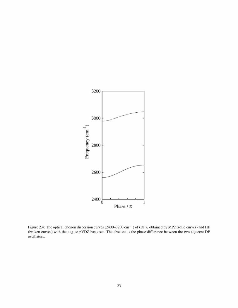
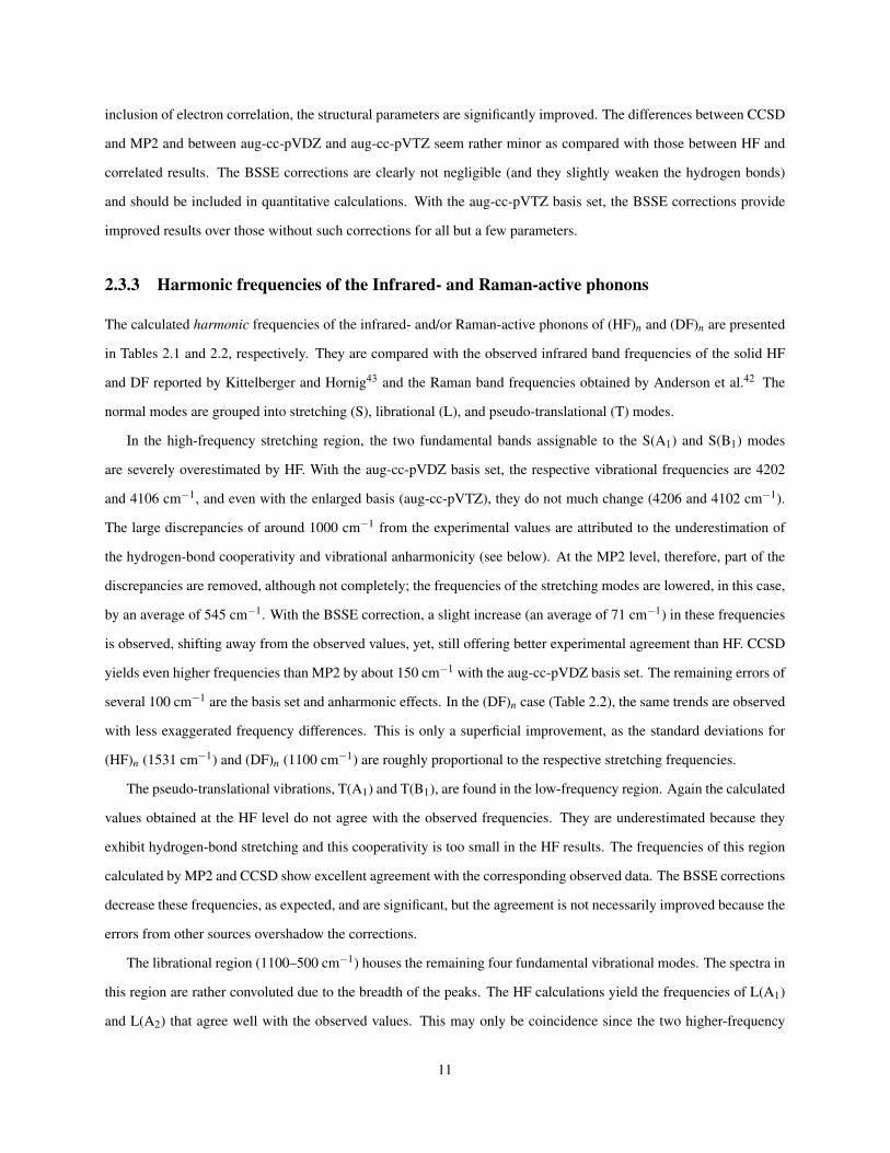
Figure 2.4: The optical phonon dispersion curves (2400–3200 cm−1) of (DF)n obtained by MP2 (solid curves) and HF(broken curves) with the aug-cc-pVDZ basis set. The abscissa is the phase difference between the two adjacent DFoscillators.

23

Figure 2.5: The hydrogen-amplitude-weighted density of states (the histogram) and its Gaussian convolution (with aFWHM of 40 cm−1) as a simulated INS spectrum of (HF)n.

24

3

Three-dimensional study of solid hydrogenfluoride

3.1 Introduction

The treatment of three-dimensional crystalline systems using ab initio electronic structure methods that go beyond

the usual Hartree–Fock (HF) and density-functional theory (DFT) approximations is the subject of recent research

efforts.56 The difficulty is caused by the high-dimensionality of the equation of motion for large or infinite number

of particles in the system and the non-scalability of ab initio electronic structure methods with system size. The vast

majority of studies of such systems have been undertaken using a reciprocal space framework, namely, the crystalline

orbital (CO) theory.3, 5, 7, 57–62 This approach employs a delocalized description under periodic boundary conditions, in

which the orbitals extend throughout the length of the system. It is particularly useful for calculating energy bands and

widely used for one-dimensional extended systems.5, 63, 64 Yet, applications to two- or three-dimensional systems can

be quite difficult. Furthermore, while implementations based on HF and DFT have been well established, those using

ab initio correlated methods are scarce and extremely tedious to develop.7, 61, 65, 66 Crystal defects, surface reactions

and adsorption, non-in-phase lattice vibrations and phonon dispersion, etc., where perfect periodic symmetry is lost,

prove to be challenging to study by CO theory.67, 68

In molecular and ionic crystals, electrons can be thought of as confined around the respective atoms or molecules,

such that only weak and/or classical intermolecular interactions become the primary concern in accurately reproducing

the total crystal energies. In such a system, a localized description of the electronic structure, namely, treating the

system as a collection of overlapping finite molecules becomes possible, breaking up the high-dimensional equation

of motion into many low-dimensional ones.9, 31–33 The finite molecules must be embedded in an electrostatic field

of the infinite system. This approach is presented in the literature10, 69 and in the preceding chapter for the one-

dimensional molecular crystal. BIM (see Chapter 2) realizes this description and approximates the energy by the sum

of the energies of monomers and overlapping dimers:

Ecell = ∑i

Ei(0)+∑i< j

(Ei(0) j(0)−Ei(0)−E j(0)

)+

12

S

∑n=−S

(1−δn0)∑i, j

(Ei(0) j(n)−Ei(0)−E j(n)

), (3.1)

25

where, as in Eq. 2.2, E j(n) and Ei(0) j(n) represent the energies of the jth monomer in the nth unit cell and the dimer

made up of the ith monomer in the central cell and jth monomer in the nth cell, respectively, and δn0 is Kronecker’s

delta. In the case of two- and three-dimensional crystals, the lattice sum cutoff radius (the integer parameter S)

must be severely restricted, owing to the sheer number of atoms within the radius, introducing fundamental errors,

especially of the Coulomb type. The neglect of the long-range Coulomb interactions, which decay as r−3, is inadvis-

able.70, 71 Accordingly, these two-body interactions must be supplemented outside the radius by adding the Madelung

constant to the energy per unit cell.72, 73 Three-body and higher-order Coulomb interactions (induction and hydrogen-

bond cooperativity) are also included via the embedding field, a lattice of self-consistently determined atomic partial

charges.67, 74 In this manner, a quantitative computational approach dealing with three-dimensional solids with long-

range interactions in the conceptually simpler direct-space algorithm can be developed relatively easily with existing

implementations of correlated methods for molecules.

As was mentioned in the previous chapter, solid hydrogen fluoride has been widely studied both experimentally

and theoretically and, in this sense, it may be considered one of the most fundamental hydrogen-bonded solids. How-

ever, some of the findings of experimental works are at least somewhat inconclusive. One aspect of dispute is the

assignment of the librational bands in the vibrational spectra, which has been addressed and resolved in Chapter 2.

Another controversy is the three-dimensional structure of the crystal, where discrepancies over the relative orienta-

tions of hydrogen fluoride chains point to three possible alignments:11, 75 polar, nonpolar, and disordered. The infrared

absorption studies of Kittelberger and Hornig43 and Giguère and Zengin41 advocated the disordered structure, while

Habuda and Gagarinsky47 used NMR spectroscopy to suggest that the nonpolar structure, in which adjacent zig-

zag hydrogen-bonded chains have opposite (antiparallel) directions, should be the most stable. However, a neutron

diffraction investigation of deuterium fluoride by Johnson et al.12 proposed the polar arrangement (i.e. parallel) as the

true crystal structure. Computational studies are also divided between the polar and nonpolar structures. Bacon and

Santry76 showed that the nonpolar structure is more stable, using a self-consistent field perturbation method within a

semi-empirical approximation to molecular integrals. The self-consistent Madelung potential (SCMP) approach pro-

posed by Ángyán and Silvi77 was applied to solid hydrogen fluoride, predicting the polar structure to be more stable.

Furthermore, the HF-based self-consistent crystal field method developed by Panas78 indicates a result congruent with

that of Bacon and Santry,76 supporting the nonpolar structure.

The present chapter investigates the three-dimensional structure of solid hydrogen fluoride, applying MP2 the-

ory with the aug-cc-pVDZ and aug-cc-pVTZ basis sets via the binary-interaction approximation under the periodic

boundary conditions. Although several calculations on infinite one-dimensional chains of hydrogen fluoride have been

reported,48, 50, 51, 58, 79, 80 there exist few three-dimensional simulations.81 Correctly accounting for the long-range two-

body Coulomb interactions becomes essential, and is achieved here by evaluating the Madelung constant. Three-body

26

and higher-order Coulomb interactions are also included as an embedding field in the way described above. The HF

method is also applied and compared with MP2 to quantify correlation effects. Furthermore, a counterpoise correction

is used to eliminate the BSSE. In this way, all types of interactions in the extended hydrogen-bonded network of the

solid can be characterized correctly, resolving the lack of consensus over its crystal structure. Quantitative predictions

of the lattice structure, binding energies, and dipole moments are made and compared to experimental values, where

available.

3.2 Computational Methods

The energy per unit cell (Ecell) of a three-dimensional crystal is a sum of the quantum-mechanical part (EQM) and the

classical-mechanical part (ECM):

Ecell = EQM +ECM (3.2)

where EQM is defined within the binary-interaction approximation as such:

EQM = ∑i

Ei(0,0,0)+∑i< j

(Ei(0,0,0) j(0,0,0)−Ei(0,0,0)−E j(0,0,0))

+12

Sx

∑l=−Sx

Sy

∑m=−Sy

Sz

∑n=−Sz

(1−δlmn)∑i, j(Ei(0,0,0) j(l,m,n)−Ei(0,0,0)−E j(l,m,n)). (3.3)

Here δlmn is Kronecker’s delta and is equal to unity only when l, m, and n all equal zero (otherwise it is zero),

Ei(0,0,0) j(l,m,n) represents the dimer energy of the ith molecule in the central cell and the jth molecule in the cell

labeled by the integer indexes, l, m, n, and Ei(0,0,0) refers to the monomer energy of the ith molecule within the

central cell. The integers Sx, Sy, and Sz are the short-range cutoffs in the x, y, and z directions beyond which only the

electrostatic energy is computed. The monomer and dimer energies were calculated using NWCHEM26 and QCHEM25

electronic structure programs, where the individual monomer and dimer Hamiltonians included the potential created

by a lattice of atomic charges determined self-consistently at the HF/aug-cc-pVDZ and HF/aug-cc-pVDZ levels. This

lattice represents the remainder of the crystal and includes all unit cells whose cell indexes satisfy |l| ≤Mx, |m| ≤My,

|n| ≤Mz, where integers Mx, My, Mz are the medium-range cutoffs.

Outside of this cutoff radius the long-range Coulomb interaction energy per unit cell is computed with the same

set of the self-consistent atomic charges as,

ECM = E(Lx,Ly,Lz)CM −2E(Mx,My,Mz)

CM +E(Sx,Sy,Sz)CM , (3.4)

27

and

E(Nx,Ny,Nz)CM =

12

Nx

∑l=−Nx

Ny

∑m=−Ny

Nz

∑n=−Nz

(1−δlmn)∑µ,ν

qµ qν

|rµ(0,0,0)− rν(l,m,n)|, (3.5)

where Lx, Ly, Lz are large integers, representing the long-range cutoffs, qµ is the atomic charge of the µth atom, and

rν(l,m,n) is the position of the ν th atom in the cell specified by the coordinates l, m, and n. To avoid over-counting, it

is necessary to subtract the electrostatic interactions within the medium-range cutoffs and beyond short-range cutoffs.

ECM, which is a partial Madelung constant, is evaluated as a real-space sum, although the Ewald summation82–84 and

its derivatives83, 84 are often employed in systems with large numbers of atoms in the unit cell.

A geometry optimization of the three-dimensional crystal is done in two steps. First, the infinite one-dimensional

zig-zag hydrogen-bonded chain is optimized with the one-dimensional analogue of this method. It utilizes the analyt-

ical gradients of energy with respect to in-phase Cartesian displacements as shown in the previous chapter,

∂Ecell

∂x= ∑

i

∂Ei(0)

∂x+∑

i< j

(∂Ei(0) j(0)

∂x−

∂Ei(0)

∂x−

∂E j(0)

∂x

)

+12

S

∑n=−S

(1−δn0)∑i, j

(∂Ei(0) j(n)

∂x−

∂Ei(0)

∂x−

∂E j(n)

∂x

), (3.6)

where again S is the short-range cutoff. Also, the gradient with respect to the lattice constant b can be obtained by

evaluating

∂Ecell

∂b=

12

S

∑n=−S

∑i, j

∑γ

n

{∂Ei(0) j(n)

∂y j(n)γ

−∂E j(n)

∂y j(n)γ

}+

∂ECM

∂b, (3.7)

where y j(n)γ is the y-coordinate of the µt atom of the jth monomer in the nth cell and ECM is the one-dimensional

analogue of Eq. 3.5, the precise definition of which can be found in the previous chapter, as well as in the literature.10, 69

The second optimization step involveds calculating the unit cell energy of the three-dimensional system from Eq. 3.2

by varying the lengths of the lattice vectors (a and c) perpendicular to the chain axis (b); the chain geometry is held

fixed, yielding a potential energy surface on a two-dimensional grid of a and c. This two-step optimization algorithm

neglects the coupled nature of the inter- and intra-chain interactions, which may, however, be expected to be weak.

The counterpoise BSSE correction developed by Boys and Bernardi30 is applied in each of the dimer calcuations in

both energy and gradient evaluation.

28

3.3 Application

3.3.1 Structures

The one-dimensional chain, was optimized69 using the HF and MP2 levels of theory with the aug-cc-pVDZ and aug-

cc-pVTZ basis sets. The cutoff radii for the short-, medium-, and long-range lattice sums in the one-dimensional calcu-

lations were respectively 50, 500, and 1000 bohrs.69 Optimization of the two (polar/parallel and nonpolar/antiparallel)

three-dimensional crystal configurations (Figure 3.1) was also done with the HF and MP2 methods with the aug-cc-

pVDZ and aug-cc-pVTZ basis sets, using Sx = Sz = 3 and Sy = 23, where the y component refers to the direction along

the chain length. The embedding field was a lattice of atomic charges self-consistently determined at the HF/aug-cc-

pVDZ and HF/aug-cc-pVTZ level with, Mx = Mz = 5 and My = 31. The cutoff radius of the Madelung constant was

extended to 1000 bohrs using the same atomic charges as the embedding field. At this radius, the convergence of the

Coulomb energy was achieved.

The unit cell of the three-dimensional solid hydrogen fluoride has four FH molecules or two hydrogen-bonded

chains, whereas in the one-dimensional scheme only two FH molecules (related to each other by glide reflection

symmetry) are in the unit cell. In the case of the polar structure,3329 where the chain orientation is parallel, the

two molecules in one chain can be translated along the perpendicular axes by half the respective lattice distances and

be superimposed on the other two molecules. The nonpolar (antiparallel) structure requires an additional reflection

of the hydrogen atoms with respect to the ac plane.12 These symmetries were imposed throughout the geometry

optimization.

The binding energies for the three-dimensional polar and nonpolar structures as well as for the one-dimensional

chain are shown in Table 3.1, where the positive values indicate a stabilization of the structure. In the one-dimensional

case, the calculated intra-chain binding results are compared to the basis-set extrapolated results of Buth and Paulus51

with and without correlation contributions. The agreement observed between the HF and MP2 results with the cor-

responding converged results demonstrates the effectiveness of the binary-interaction model at least within the one-

dimensional framework. In the three-dimensional case, The experimental values71 for lattice constants a and c were

used initially. The total HF energies differ by 6.5–6.6 kcal/mol between the two structures at the experimental lattice

constants, while the total MP2 lattice energies show a 6.9–8.8 kcal/mol difference there. Notably, the polar structure

has a large positive inter-chain binding energy in both the MP2 and HF approximations indicating a repulsive poten-

tial. This signifies that the nonpolar structure is not only substantially more stable than the polar structure, but also

the latter is unstable toward dissociation into individual chains in the vicinity of the observed lattice constants. In the

nonpolar structure, the inter-chain binding energies are small and become positive only when electron correlation ef-

fects are included. This suggests that dispersion interactions are essential in holding hydrogen-bonded chains together

29

in addition to favorable electrostatic interactions in the this configuration.

The present result contradicts Ángyán and Silvi,77 who used their SCMP approach and concluded that the polar

structure is more stable than the nonpolar one by 0.3 kcal/mol; however, it is in agreement with Bacon and Santry76

and with Panas,51 who have proposed the nonpolar structure to be more stable. Bacon and Santry76 have given a total

binding energy of +13.09 kcal/mol for the stable nonpolar structure, substantially larger than the calculated values

shown here at both MP2/aug-cc-pVDZ and MP2/aug-cc-pVTZ. This trend continues with Ángyán and Silvi who have

obtained a binding energy of about +15.1kcal/mol for their polar structure and +14.8 for the nonpolar one, but less

so with Panas of +9.88 kcal/mol.

Optimization of the two three-dimensional structures was attempted and the results further strengthens the case

for the antiparallel configuration. Figures 3.2 and 3.3 show the potential energy surfaces of the nonpolar and polar

structures, respectively, calculated at the MP2/aug-cc-pVDZ level. The potential surfaces obtained with the other

methods are qualitatively the same. The nonpolar structure shows as a potential minimum, whereas the polar potential

is completely repulsive in the domain plotted and no potential minimum was found elsewhere. The optimized lattice

constants, obtained only for the nonpolar structure, are given in Table 3.2 along with the experimental values. The

discrepancy between the experimental lattice constants and theory are as great as 20% for the HF/aug-cc-pVDZ

and HF/aug-cc-pVTZ approximations. The overestimation of the lattice constant b was discussed in the previous

chapter, where it was attributed to an inability of the HF approximation theory to fully recuperate the hydrogen-bond

cooperativity. The calculated value of b is greatly improved by the inclusion of electron correlation at the MP2 level.

Furthermore, the MP2 values of a and c are considerably smaller than the HF counterparts and are in much better

agreement with the observed lattice constants. The a and b parameters of MP2/aug-cc-pVDZ are overestimated only

by about 7%, while the c parameter is underestimated by less than 4%. The lattice constants found at the MP2/aug-

cc-pVTZ are in even closer agreement to the experimental data. Here, the calculated a and b parameters are no more

than 6% larger than the observed, and the c parameters correctly agree with each other. This improved agreement at

the correlated level must be traced to a more accurate description of electrostatic interactions and, to a lesser degree,

the inclusion of dispersion interactions by MP2.

3.3.2 Dipole Moments

Shown in Table 3.3 are the dipole moments of the hydrogen fluoride molecule in both crystal structures, compared to

the isolated gas-phase value. The dipole moments are computed with the atomic charges determined at the HF/aug-

cc-pVDZ and HF/aug-cc-pvTZ levels. The average dipole moment for the solid is 2.46 D (0.968 a.u.), exhibiting

roughly a 30% increase upon crystallization. The self-consistent determination of atomic charges in BIM is essen-

tial in reproducing this hydrogen-bond cooperativity effect, which may be lacking in other fixed charge schemes.34

30

Qualitatively similar results are proposed by the CO study from Beyer and Karpfen,49 where they report an average

dipole moment for the one-dimensional hydrogen fluoride chain to be 2.42 D (0.952 a.u.), a 15–20 % increase from

their isolated monomer value. The dipole moments obtained by the Mulliken scheme of Ángyán and Silvi77 found

that the dipole moments of the crystal were increased by 20 %. The reverse trend was observed in the results of an

SCF perturbative method,49 in which the magnitude of the dipole was only 1.86 D (0.731 a.u.), a decrease of 0.31 D

from their corresponding gas-phase dipole moment. Also, Ángyán and Silvi yielded values of 2.47 D (0.971 a.u.) and

2.48 D (0.974 a.u.) for the nonpolar and polar structures, respectively. These values are consistent with the current

results, where the nonpolar dipoles are somewhat smaller than their polar counterparts. However, this small difference

between the polar and nonpolar molecular dipole moments does not explain the large difference in binding energies

between the two. The dominant long-range Coulomb contribution to the total energy is thus primarily determined by

the overall cell dipole moment.

3.4 Conclusion

The study of one-dimensional of solid hydrogen fluoride from Chapter 2 has been extended to the three-dimensional

case, accounting for the long-range electrostatics to sufficiently large distances. The question over which of the

polar or nonpolar configurations is the most stable has been particularly addressed, along with equilibrium molecular

geometry, using BIM with a reasonable basis set and the BSSE correction. The binding energies of the nonpolar

structure are considerably greater than the polar ones, which is traced to repulsive inter-chain interactions in the latter.

Furthermore, the potential energy surface of the polar structure has been shown to be dissociative near the experimental

lattice constants, leading us to conclude that the nonpolar one is the actual crystal structure. This optimization scheme

allows for the prediction of all lattice parameters which agree reasonably well with the observed when MP2 is used.

Owing to its two-step nature, the scheme does not account for the coupling between intra- and inter-chain interactions.

One should expect this approximation to be partly responsible for the errors in the calculated lattice parameters,

although the coupling should be rather small because the system is anisotropic; the chains geometry should be largely

determined by intra-chain interactions alone. This is supported by the excellent agreement in geometry (Table 2.4)

and anharmonic phonon frequencies (Table 2.5) between experiments and calculations in the one-dimensional model.

31

3.5 Tables

Table 3.1: Optimized lattice constants (in Å) for the nonpolar configuration of solid hydrogen fluoride.

HF/aDZa HF/aTZa MP2/aDZa MP2/aTZa Expb

a 4.1 4.2 3.7 3.6 3.42

b 4.9 4.9 4.6 4.5 4.32

c 6.1 6.1 5.2 5.4 5.41

a "aXZ" stands for the aug-cc-pVXZ basis set.

b Ref. 11

Table 3.2: Total, inter-chain, and intra-chain binding energies (in kcal/mol) of solid hydrogen fluoride at experimentaland optimized geometries. Positive binding values indicate a stabilization energy.

Total Inter-chain Intra-chain

Polara Nonpolara Nonpolarb Polara Nonpolara Nonpolarb —

HF/aDZc −0.7 +5.8 +6.1 −7.0 −0.6 −0.2 +6.3

HF/aTZc −0.7 +5.9 +6.2 −6.9 −0.3 +0.0 +6.2

MP2/aDZc +1.0 +7.0 +7.1 −6.0 +0.2 +0.2 +6.8

MP2/aTZc +0.5 +9.3 +9.3 −7.0 +1.9 +1.9 +7.4

HF(∞)c,d · · · · · · · · · · · · · · · · · · +6.402

CCSD(∞)c,d · · · · · · · · · · · · · · · · · · +7.421

a Experimental lattice constants used for a and c.

b Optimized lattice constants used.

c "aXZ" stands for the aug-cc-pVXZ basis set.

d Ref. 51

32

Table 3.3: The molecular dipole moment (in Debye) of solid hydrogen fluoride at experimental and optimized geome-tries.

Molecule Solid

(Polar)b

Solid

(Nonpolar)b

Solid

(Nonpolar)c

HF/aDZa 1.90 2.42 2.41 2.41

HF/aTZa 1.89 2.44 2.43 2.42

MP2/aDZa 1.82 2.51 2.47 2.46

MP2/aTZa 1.81 2.56 2.54 2.54

a "aXZ" stands for the aug-cc-pVXZ basis set.

b Experimental lattice constants used for a and c.

c Optimized lattice constants used.

33

3.6 Figures

Figure 3.1: Lattice structures of the polar (parallel) and nonpolar (antiparallel) configurations of solid hydrogen fluo-ride.

34

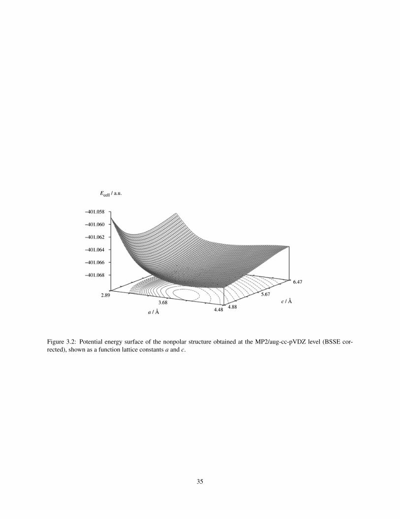
Figure 3.2: Potential energy surface of the nonpolar structure obtained at the MP2/aug-cc-pVDZ level (BSSE cor-rected), shown as a function lattice constants a and c.

35

Figure 3.3: Potential energy surface of the polar structure obtained at the MP2/aug-cc-pVDZ level (BSSE corrected),shown as a function lattice constants a and c.

36

4

Finite pressure study of hydrogen fluoride

4.1 Introduction

In the previous chapters as well as the literature, a linear-scaling, electron-correlation method for crystals, and even

large clusters, consisting of molecules that are only weakly-interacting with one another (through hydrogen bonds,

ionic bonds, or weaker) has been explained.8–10, 69, 85 It is based on a many-body expansion of the total energy into

the sum of the energies of monomers, overlapping dimers, overlapping trimers, etc., which are embedded in the

self-consistently determined electrostatic field of the rest of the cluster or crystal environment. The truncation after

the dimer (two-body) sum has been shown to lead to a model (BIM) which strikes an excellent balance between

cost and accuracy for a wide range of applications. BIM accounts for one- and two-body kinetic, Coulomb (i.e.,

classical electrostatic), exchange, and correlation interactions accurately by an electron-correlation method of choice

as well as three-body and all higher-order Coulomb interactions approximately but self-consistently, thus including

the polarization, induction, or hydrogen-bond cooperativity effect. BIM can, therefore, simultaneously describe all of

intramolecular covalent and ionic bonds and intermolecular ionic, hydrogen-bond, and dispersion interactions, whose

strengths span three orders of magnitude, both accurately and efficiently. Furthermore, BSSE, which tends to be a

substantial proportion of intermolecular interaction energies, can be easily corrected by the counterpoise (cp) method

applied to each dimer.

BIM is, therefore, a particularly simple and effective incarnation, but with limited applicability, of more general

fragment, local-basis, or divide-and-conquer technique, the area that has seen considerable interest and research ac-

tivities recently. a comprehensive review by Gordon et al.86 and a related article on crystals by Beran and Nanda87

have appeared recently and both provide an overview of the current research. The present method has been conceived

as a direct simplification of the pair-interaction method of Kitaura et al.,31 which is the predecessor of their fragment

molecular orbital (FMO) method.88

In this chapter, as the initial effort to integrate thermodynamics with quantum chemistry for solids, an extension

to BIM is reported. This allows for the calculation of enthalpy per unit cell of a crystalline solid and its gradients with

respect to atomic positions and lattice constants as well as Hessians with respect to atomic positions. By minimizing

37

the unit-cell enthalpy or equating its gradients to zero, the equilibrium structure of a solid is obtained under a static

ambient pressure. With Hessians, the calculate harmonic frequencies of the infrared- and/or Raman-active lattice

vibrations, phonon dispersion curves, phonon density of states (DOS), and inelastic neutron scattering cross sections

can be evaluated also as a function of pressure. A 3D treatment of a solid is essential in quantifying the pressure

effects even when the solid is highly anisotropic.

BIM and its extension are applied to 3D solid hydrogen fluoride (FH) and deuterium fluoride (FD) under a fi-

nite pressure. These are among the molecular crystals most extensively studied experimentally11–13, 41–43, 47, 75, 89 and

computationally.14, 49–51, 53, 58, 63, 65, 69, 76–78, 80, 81, 85, 90–103 They nonetheless remain poorly understood. Crystalline FH

and FD consist of strongly hydrogen-bonded zigzag polymer chains, but whether the sense of these chains is parallel,

antiparallel, or random has long been the subject of debate. A neutron diffraction study of solid FD by Johnson et al.12

has determined the structure to be parallel (C122v ) with the lattice constants: a = 3.31, b = 4.26, and c = 5.22 Å(with b

being parallel to the chain axes). However, an earlier X-ray study by Atoji and Lipscomb11 advocated random chain

orientations (D172h) with a = 3.42, b = 4.32, and c = 5.41 Å. An NMR study by Habuda and Gagarinsky,47 on the other

hand, advocated the antiparallel structure (D162h). Computational studies by Panas78 and by Bacon and Santry76 also

favored the antiparallel D162h structure, whereas another performed by Ángyán and Silvi predicted the parallel structure

to be the most stable. In Chapter 3, this issue was discussed after applying BIM at the MP2/aug-cc-pVTZ level with

a cp correction to the BSSE.85 This is believed to be the most accurate calculation performed thus far on 3D solid FH

and its conclusion suggested that solid FH has the antiparallel D162h structure at zero temperature and pressure.

Another uncertainty of solid FH and FD, which has some bearing on the aforementioned issue of the 3D structure,

is the interpretation of their vibrational spectra. On the basis of the coincidence of the observed infrared and Raman

band positions, Kittelberger and Hornig43 concluded that the structure is the disordered one (D172h) rather than the

antiparallel D162h structure that has a center of inversion and should obey the infrared-Raman exclusion rule. However,

the coincidence was observed only for H–F and D–F stretching modes whose bands were exceptionally broad. A

subsequent, improved measurement of Raman spectra by Anderson et al.42 revealed small, but meaningful differences

in the frequencies between infrared and Raman bands especially in the librational (400–1100 cm−1) and pseudo-

translational (0–400 cm−1) regions. These differences, which are factor-group (Davydov) splittings, may suggest

that the infrared-Raman exclusion rule can still be operative and the structure is antiparallel. Virtually all previous

attempts49, 53, 69, 80, 98, 101 to assign the infrared and Raman bands, either empirically or from the first principles, were

based on 1D (i.e., polymer) models and, though apparently successful in reproducing the observed band positions, had

no ability to quantify the effect of 3D crystalline environment on the band positions. Also, a doubt remains whether

the 1D model of solid FH and FD, which must still have relatively strong inter-chain ionic interactions, are entirely

justifiable and whether the most recent band assignments are correct.

38

It is possible experimentally to vary the strength of the crystal field and measure its influence on spectra. This

can be done by applying pressures on the solids. Pinnick et al.46 reported the Raman spectra of solid FH and FD

under pressures up to 12 GPa, showing that some bands increase in frequency while others decrease with increasing

pressure, providing valuable additional information for the band assignments. They also found some evidence of

a phase transition in solid FH (but not in solid FD) at about 6 GPa to a structure with symmetric H–F bonds. A

planewave density-functional theory (DFT) calculation was carried out by Zhang et al.102 to investigate this transition.

The calculation did predict such a transition but at a much higher pressure of 25 GPa, creating yet another controversy

to resolve.

In this chapter, both Hartree–Fock (HF) and MP2 with basis sets up to aug-cc-pVTZ and cp corrections to BSSE

were applied to the antiparallel structure of solid FH and FD under 0–20 GPa of pressure. The equilibrium structural

parameters, including lattice constants and molar volume, the frequencies of the infrared- and Raman-active vibrations,

phonon dispersion curves, and phonon DOS are computed as a function of pressure. The BIM calculations at the MP2

level account for two-body exchange and correlation (thus including dispersion) effects accurately and two-body and

all higher-order Coulomb interactions through the electrostatic embedding field. The embedding field is determined at

the HF level, but self-consistently, incorporating the induction effect, which must be significant in strongly hydrogen-

bonded networks in solid FH and FD. The BIM scheme is, however, fundamentally limited in allowing a phase

transition to the symmetric structure and the results at high pressures may not be as reliable. Nonetheless, these

computed results at lower pressures are perhaps the most accurate to date and provide a comprehensive and quantitative

theoretical description of three-dimensional solid FH and FD. The results are given below.

4.2 Theory and Computational Methods

4.2.1 Internal Energy

The internal energy per unit cell, U , of a molecular crystal within BIM is defined by

U = ∑i

Ei(0)+12 ∑

n∑i, j

′{Ei(0) j(n)−Ei(0)−E j(n)}

+ELR, (4.1)

where n represents the unit cell vector, (nx,ny,nz), Ei(0) is the energy of the ith molecule in the 0th unit cell, and

Ei(0) j(n) is the energy of the dimer consisting of the ith molecule in the 0th unit cell and the jth molecule in the nth

unit cell. The prime indicates that the spurious Ei(0)i(0) contributions are to be left out of the summation. The last

term is the long-range electrostatic contribution through an infinite distance or a part of the Madelung constant, the

39

precise definition of which can be found in the previous chapter. Crucial to the accuracy of BIM is the inclusion of an

electrostatic embedding field in the Hamiltonian of each of the monomer and dimer calculations. The embedding field

consists of atomic point charges determined self-consistently with one another at the HF level,9 thus accounting for

three-body and all higher-order electrostatic effects as well as polarization, induction, or hydrogen-bond cooperativity

effects. The self-consistent determination of the embedding field distinguishes BIM from other similar, but fixed-field

methods33, 34 that have limited or no ability to include polarization effects.

The energy gradients with respect to the atomic positions can be determined conveniently by

∂U∂x

= ∑i

∂Ei(0)

∂x+

12 ∑

n∑i, j

′{

∂Ei(0) j(n)

∂x−

∂Ei(0)

∂x−

∂E j(n)

∂x

}+

∂ELR

∂x, (4.2)

where ∂Ei(0)/∂x and ∂Ei(0) j(n)/∂x are gradients of the monomer and dimer energies that may be obtained analytically

from a molecular program. It has been found10, 28 that the derivatives of the embedding field (i.e., the atomic charge

and positions of the field) or the last term can be neglected without noticeable loss of accuracy, drastically simplifying

the implementation. The coordinate x is typically (but not necessarily) the collective one that specifies the positions

of all atoms that are related by periodic symmetry. Gradients with respect to such collective coordinates are most

convenient for a geometry optimization because in this process periodic symmetry is always maintained.

In a crystal, additional degrees of freedom of the lattice constants must be considered. The gradients with respect

to the lattice constant a (along the x axis) of an orthorhombic crystal is obtained by evaluating

∂U∂a

=12 ∑

n∑i, j

∑γ

nx

{∂Ei(0) j(n)

∂x j(n)γ

−∂E j(n)

∂x j(n)γ

}

+∂ELR

∂a, (4.3)

where x j(n)γ represents the x coordinate of the γth atom in the jth molecule of unit cell n. Unlike the atomic gradients

and Hessians (see below), where the derivatives of ELR can be ignored, the last term in the above equation is essential

and can indeed be a dominant contribution.10 See Ref. 10 for a programmable expression of this term (in the case of

the dipolar embedding field).

The second derivatives of the energy (the Hessians) with respect to the atomic positions are given by

∂ 2U∂x∂y

= ∑i

∂ 2Ei(0)

∂x∂y

+12 ∑

n∑i, j

′

{∂ 2Ei(0) j(n)

∂x∂y−

∂ 2Ei(0)

∂x∂y−

∂ 2E j(n)

∂x∂y

}

40

+∂ 2ELR

∂x∂y, (4.4)

of which, again, the last term and the derivatives of atomic point charges can be safely neglected. Here, x and y can

be the collective atomic coordinates, producing only the frequencies of phonons at the center of the Brillouin zone

(BZ). Since only these k = 0 phonons, which conform to the periodic symmetry, are infrared and/or Raman active,

the Hessian with respect to these collective coordinates is the most compact information one needs to obtain their

frequencies. It is also possible and equally easy to obtain the Hessian with respect to individual atomic coordinates

and the frequencies of phonons in the entire BZ, which lift periodic symmetry. The ability to obtain the energy of

a crystal at a geometry which no longer is periodic is another advantage of BIM and derives from the reliance on

the local basis. Section 4.5 documents the algorithm used to compute phonon dispersion and DOS in the harmonic

approximation.

To describe a solid under a finite pressure P, one must consider the enthalpy per unit cell, H, given by

H =U +PV, (4.5)

where U is the internal energy per unit cell defined above and V is the unit-cell volume. Since neither P nor V depends

on atomic positions, the gradients and Hessians of the enthalpy with respect to them are simply

∂H∂x

=∂U∂x

, (4.6)

and

∂ 2H∂x∂y

=∂ 2U∂x∂y

. (4.7)

The right-hand sides of these are already given. The gradients with respect to lattice constants again require special

consideration. Since V = abc in an orthorhombic unit cell, the lattice gradients become

∂H∂a

=∂U∂a

+Pbc, (4.8)

where the first term in the right-hand side is given by Eq. (4.3). These equations can be used to optimize crystal

geometries and frequencies of phonons under a static ambient pressure.

The number of dimers considered in Eqs. (4.1), (4.2), etc. can be substantial. Thus, an algorithm has been im-

plemented that exploits space group symmetry in addition to the periodic symmetry already used in the foregoing

41

formalism to minimize the computational cost. The details are given in Section 4.6.

4.3 Results and Discussion

4.3.1 Computational details

The BIM calculations were performed on the energies, structures, and phonons of the crystalline FH and FD at the

HF and frozen-core MP2 levels of theory with the aug-cc-pVDZ and aug-cc-pVTZ basis sets with and without the cp

correction of BSSE (henceforth the prefix “cp-” indicates the application of this correction). On the basis of the results

from the previous chapters, the antiparallel structure, drawn in Fig. 4.1, was assumed. The dimers in the rectangular

cuboid with dimensions of 3×3×3 unit cells (containing 108 molecules) were treated quantum mechanically using

the aforementioned methods. These dimers as well as monomers in the central unit cell were embedded in the lattice

of atomic point charges of the size 11× 11× 11 unit cells. These charges were determined at the HF level for

each monomer in the very embedding field and thus self-consistently with all the other monomers.9 The long-range

electrostatic contributions from the cuboid of 41× 41× 41 unit cells were added to the energies and lattice-constant

gradients.

The crystal structure of FH was determined under a pressure up to 20 GPa. From 0–6 GPa, an increment of one

GPa was applied, but beyond 6 GPa, the increment was increased to two GPa until 20 GPa was reached. The structure

of solid FD was taken to be the same. As shown in Fig. 4.1, the unit cell has four FH or FD molecules, which are all

symmetrically related by one another. This symmetry relation was enforced during the geometry optimization process.

The frequencies of the infrared- and Raman-active (i.e., k = 0) vibrational modes were obtained within the har-

monic approximation for solid FH and FD at each pressure and combination of theory and basis set except for (cp-

)MP2/aug-cc-pVTZ. The phonon dispersion curves were obtained along high-symmetry directions of the BZ with the

sampling rate of 100 k-points per direction. The phonon DOS and hydrogen-amplitude-weighted phonon DOS were

also calculated as histograms with the 1 cm−1 bins and the sampling rate of 213 k-points in the BZ. The hydrogen-

amplitude-weighted DOS were convoluted with a Gaussian function with a full-width-half-maximum of 40 cm−1.

To determine the atomic point charges, the NWCHEM program26 was used by the documented procedure,?, 9

whereas the Q-CHEM program25 was employed to compute energies, analytical gradients, and analytical Hessians

of the monomers and dimers.

4.3.2 Zero-pressure structure

The structural parameters and the molar volume of solid FH at zero pressure obtained at various combinations of HF,

cp-HF, MP2, and cp-MP2 with aug-cc-pVDZ, and aug-cc-pVTZ are presented in Table 4.1, where they are compared

42

with the diffraction data11, 12 obtained at 1 atm (0.0001 GPa) as well as with the results of previous calculations.69, 85

The results obtained in this work are listed in the table roughly in the order of increasing accuracy. Some con-

vergence can be observed as the theoretical level, basis set size, and cp treatment are raised. The values obtained at

the highest level used in this work, cp-MP2/aug-cc-pVTZ, are in excellent agreement with the diffraction data, while

those obtained at the HF level, in particular, show clear signs of deficiencies. As is well known,101 the HF theory fails

to fully capture the hydrogen-bond cooperativity and, as a result, the H–F and H· · ·F bonds are too short and too long,

respectively, generally underestimating the strength of a network of hydrogen bonds. The molar volume is, therefore,

overestimated excessively at this level of theory. Once the electron correlation is included at MP2, these large errors

are nearly completely erased. For instance, the lattice constants calculated by cp-MP2/aug-cc-pVTZ are 3.36, 4.46,

and 5.21 Å, which are in excellent agreement with the diffraction results: 3.31, 4.26, and 5.22 Å according to Johnson

et al.12 The agreement suggests both that the hydrogen-bond cooperativity is to a great extent an electron-correlation

effect and that MP2 is good enough for describing it.

The cp correction has a minor, but noticeable effect on the structure. As expected, it slightly weakens the hydrogen

bonds, making H· · ·F and F· · ·F bonds longer and the molar volume greater. Also as expected, this effect is greater

in the smaller basis set (aug-cc-pVDZ). For the lattice constants and molar volume, the cp correction appears to

accelerate the basis-set convergence as it should, but not necessarily for the H· · ·F and F· · ·F bonds.

Comparing 1D and 3D treatments of the solid, it is found that the structural parameters obtained by them to be in

surprisingly good agreement (within 0.02 Å), justifying the 1D treatment of this highly anisotropic solid and rendering

confidence to the conclusions drawn therefrom on spectral assignments, etc. This issue will be revisited for the infrared

and Raman band assignments, comparing directly the 1D and 3D vibrational analyses. It is important to note that

treating the system as an extended system, whether 1D or 3D, is essential to understanding this solid in quantitative

terms. The FH molecule in the gas-phase has the bond length of 0.917 Å, which is considerably shorter than the value

(0.947 Å according to cp-MP2/aug-cc-pVTZ) in the crystalline phase. Any type of intermolecular potentials with

fixed molecular geometry, no matter how accurate for a dimer in the gas-phase, will be unable to describe the solid

because the constituent molecular geometry and wave functions are altered strongly by the solid-state environment. A

3D treatment is mandatory once a pressure is applied, the effect of which is discussed next.

4.3.3 Pressure-dependence of structure

Figure 4.2 plots the calculated lattice constants as a function of pressure. The constants a and c, which are perpen-

dicular to the hydrogen-bonded chains, undergo nearly the same amount of compression. They both decrease more

rapidly at lower pressures (P ≤ 6 GPa) and less at higher pressures (P ≥ 6 GPa), indicating that, as the crystal is

compressed, it becomes stiffer as neighboring atoms begin to experience sharp repulsive parts of the nonbonded atom-

43

atom potentials. In other words, the potential energy curves of the crystal toward dissociation into separate individual

hydrogen-bonded chains are anharmonic and Morse-like. The constant b displays different pressure dependence from

a or c. It decreases at more or less a constant rate for the whole pressure range studied. This seems appropriate, given

the stronger hydrogen bonds being compressed in this direction, whose potentials are more harmonic and with more

constant compressibility for a wider range of pressure.

The molar volume is plotted as a function of pressure in Fig. 4.3. The solid at 0 GPa, with a volume of 11.8

cm3mol−1 according to cp-MP2/aug-cc-pVTZ, is initially softer, shrinking easily under pressure. With increasing

pressure, the solid becomes progressively stiffer, resisting compression. This is again explained by the fact that

atoms enter the repulsive parts of the nonbonded potentials. Since the repulsion is caused by the exchange interactions

described by HF, DFT, and MP2 equally well, the pressure dependence predicted by all three methods seem to converge

into one curve at high pressures. Conversely, at 0 GPa, the differences between different theories are much more

prominent, with the MP2 results distinctly closer to the measured molar volume than those of HF or DFT (Ref. 102).

The pressure dependence of the F· · ·F distance, drawn in Fig. 4.4, is similar to that of b as the latter is largely

determined by the former. At 0 GPa, the MP2 results are in the most accurate agreement with the observed, with HF

and DFT (Ref. 102) overestimating and underestimating the F· · ·F distance, respectively. The cp corrections are rather

insignificant as compared with the large differences between the different electronic structure levels.

Figure 4.5 presents the pressure dependence of the H–F and F· · ·H distances. As discussed above, at 0 GPa, MP2

predicts the most accurate bond lengths with HF exaggerating the difference between the two bond lengths. DFT,102

in contrast, predicts a much longer H–F bond and a much shorter F· · ·H bond. As the pressure is applied, the H–F and

F· · ·H bonds elongate and shrink, respectively, ultimately becoming one and the same type of bond in an equidistant

or symmetric hydrogen-bond structure.44, 104–106 Zhang et al.,102 using DFT which produced the data plotted in this

figure, predicted the pressure-induced transition to the symmetric structure at 25 GPa. In other words, the two broken

curves predicted by DFT will merge into one curve at that pressure. The present calculations, both HF and MP2,

are fragment-based and fundamentally incapable of describing the symmetric structure that has equally strong bonds

connecting the chains over their entire lengths. As a result, the H–F bond length shows only a modest extension even

up to 20 GPa according to HF or MP2. The F· · ·H bond length decreases at a much greater rate, but comes nowhere

near the other bond length or the symmetric structure. It is therefore expected that the BIM results even at the cp-

MP2/aug-cc-pVTZ level become less and less reliable as the pressure is increased because the BIM approximation

energetically penalizes the symmetric structure or the one closer to it.

The question is at which pressure BIM with MP2 becomes less reliable than DFT. The comparison with the

observed H–F and F· · ·H bond lengths indicates that DFT’s structure is already too symmetric at 0 GPa, yielding

the difference (0.37 Å) between the two bond lengths that is 35 % less than the experimental value (0.56 Å). MP2,

44

in contrast, overestimates this difference (0.67 Å) by a much smaller degree. Given the consistently more accurate

agreement with various experimental data at 0 GPa (see above), there seems little doubt that MP2 is more reliable than

DFT at low pressures. This, in combination with the expected failure of BIM at higher pressures, suggests that the

true pressure dependence curves to fall in between MP2 and DFT plots. Starting from the MP2 values and following

the trends predicted by DFT, the two curves do not seem to meet until the pressure reaches ca. 45 GPa.

The calculated pressure dependence of the bond angles shows that, although there is generally less variation in

these values, the FFF angle becomes slightly more acute, indicating more crooked chains, as the pressure is increased.

At 0 GPa, this angle is found to be 121◦ according to cp-MP2/aug-cc-pVTZ (in perfect agreement with the experi-

mental value12) and decreases monotonically toward 114◦ at 20 GPa. The FHF angle is found to be 180◦ at 0 GPa

and, with increasing pressure, it slowly decreases toward 176◦ at 20 GPa, producing less linear hydrogen bonds.

4.3.4 The k = 0 lattice vibrations at zero pressure

The previous calculation from Chapter 3 strongly favored the antiparallel (D162h) structure of solid FH and FD, which

has the center of inversion. The infrared- and Raman-active vibrations are, therefore, expected to be non-coincident,

with the gerade modes Raman active and the ungerade modes (except Au) infrared active. The cp-MP2/aug-cc-pVDZ

frequencies of the stretching (S) modes of solid FH and FD at 0 GPa are given in Tables 4.6 and 4.7, respectively, in

which the results of previous 1D calculations69, 101 and experiments42, 43, 46 are also shown. The corresponding data

in the librational (L) region are compiled in Tables 4.2 and 4.3. Those in the pseudo-translational (T ) region are in

Tables 4.4 and 4.5. The normal modes for solid FH are drawn schematically in Fig. 4.6. The focus of the discussion

here will be on the crystal-field (i.e., 3D) effect on the frequencies and its implication on the band assignments.

In the FH or FD stretching region of the spectra (Tables 4.6 and 4.7), four k = 0 modes are active and observed,

whose frequencies span nearly 400 cm−1. In the 1D chain model, only two k = 0 modes can exist in this frequency

region: S(A1) and S(B1). In S(A1), the two FH or FD molecules in the 1D unit cell stretch in phase; in S(B1), out of

phase. According to previous 1D studies,69, 101 the predicted frequencies of S(A1) are consistently lower than those of

S(B1) in both solid FH and FD. Hence, the infrared and Raman bands of solid FH at 3027–3067 cm−1 were assigned to

S(A1) and those at 3376–3406 cm−1 to S(B1). Similarly, the bands of solid FD at 2272–2294 cm−1 were attributed to

S(A1) and those at 2506–2530 cm−1 to S(B1). The B3LYP calculation101 seems to reproduce the frequency differences

between S(A1) and S(B1) more accurately than the cp-MP2 calculations, the latter underestimating them considerably.

However, from Chapter 2, much of the differences arise from the different anharmonic effect on these two modes. The

S(A1) mode, which is in phase and thus Morse-like, undergoes a large reduction in their calculated frequencies upon

inclusion of anharmonicity, while the S(B1) mode does much less because it is out of phase and more harmonic. In

other words, the more accurate agreement achieved by harmonic B3LYP is accidental, as is often the case with DFT.

45

The observed infrared and Raman band positions are not coincidental. The frequency differences on the order of

20 cm−1 can be seen between the infrared and Raman bands that are assigned to one and the same mode in a 1D

model. The differences are attributable as factor-group (Davydov) splittings. The current 3D calculation suggests that

the S(B1) mode in the 1D chain splits into two distinct modes, S(B1g) and S(B2u), in 3D with the latter being 10–14

cm−1 higher lying than the former. This agrees with the experimental findings that the infrared bands (which must

correspond to ungerade modes) are found at 19–30 cm−1 higher frequencies than the Raman bands (gerade modes).

The 3D cp-MP2/aug-cc-pVDZ frequencies for these modes are lower than the 1D cp-MP2/aug-cc-pVDZ frequencies

and are in much closer agreement with the observed values. The S(B1g) and S(B2u) modes differ from each other in

the phase of vibrations between adjacent hydrogen-bonded chains.

The current calculation predicts the splitting of S(A1) in 1D into S(B3u) and S(Ag) in 3D and the magnitudes

of splitting at 97 cm−1 in FH and 69 cm−1 in FD. The experiments find the splittings much smaller (ca. 20 cm−1)

and place the infrared bands at higher frequencies than the Raman bands, contrary to predictions. Furthermore, the

observed frequencies are 300–400 cm−1 lower than the calculated. These suggest strong anharmonic effects opera-

tional on these modes and the limitations of the harmonic approach in describing them. The previous 1D anharmonic

treatment (see Chapter 2) was unsatisfactory for these modes. It may thus be concluded that the crystal-field effect

on stretching vibrations is modest and that their 1D treatment is justified, whereas the harmonic treatment is not, in

particular, for S(A1).

Let us turn to the librational modes, which are listed in Tables 4.2 and 4.3. There are four such modes—L(A1),

L(A2), L(B2), and L(B1)—in the 1D model. The most accurate 1D calculations of their frequencies thus far were

performed by us69 using hybrid CCSD(T) and MP2 potential energy surfaces in anharmonic vibrational analyses.

They predicted the frequencies of these modes in FH at 647, 704, 741, and 1000 cm−1, supporting the previous band

assignments made by DFT.101 According to these assignments, the infrared band at 553 cm−1 and Raman band at

569 cm−1 are attributed to L(A1), the Raman band at 687 cm−1 to L(A2), the infrared band at 792 cm−1 and Raman

band at 742 cm−1 to L(B2), and the infrared bands in the range of 975–1025 cm−1 and Raman band at 943 cm−1

to L(B1). The 3D calculation largely supports these assignments except for two modes, for which the 3D treatment

seems essential and revised assignments have been proposed in this work. These issues will now be discussed.

The L(B1) mode in 1D splits into L(B2u) and L(B1g) in 3D. The magnitude of the splitting and the relative position

of the infrared and Raman bands are not correctly reproduced by 3D cp-MP2/aug-cc-pVDZ, but there seems little

doubt that the infrared bands at 975–1025 cm−1 and Raman band at 943 cm−1 correspond to L(B2u) and L(B1g),

respectively. Assuming that anharmonic and crystal-field effects on frequencies are decoupled and thus additive, the

anharmonic 3D frequency can be estimated for each librational mode of FH by adding the factor-group splitting from

1D and 3D cp-MP2 and the corresponding 1D anharmonic frequency.69 The anharmonic frequencies thus estimated

46

for L(B2u) and L(B1g) are 997 and 1072 cm−1, respectively. They are in reasonable agreement with the observed,

with the aforementioned limitations notwithstanding. The harmonic frequencies of these in FD are 669 and 727 cm−1,

which compare well with the experimental values, 720 and 703 cm−1, respectively.

The L(B2) mode in 1D, predicted to give rise to a band at 631 cm−1 according to 1D cp-MP2, turns into two modes,

L(B3g) at 601 cm−1 and L(B1u) at 669 cm−1, in 3D cp-MP2. The estimated anharmonic frequencies are 711 and 779

cm−1, respectively, which are in good agreement with the observed Raman (742 cm−1) and infrared (792 cm−1) band

positions. The corresponding harmonic frequencies in FD are 427 and 486 cm−1 as compared with the observed 552

and 572 cm−1. Remarkably, the infrared bands at 792 cm−1 in FH and at 572 cm−1 in FD almost completely disappear

if the FH or FD crystal films are deposited near−125◦C and subsequently cooled to−185◦C.43 They are intense when

the films are deposited directly at −185◦C. An explanation suggested by Kittelberger and Hornig is that the crystals

prepared at −125◦C, which is near the melting point, are more perfect and an infrared absorption due to transition

dipoles perpendicular to the films is hard to occur. Therefore, “one ought to consider the 792 cm−1 HF band as the

out-of-plane libration.”43 This is supported by the current calculated results and assignment; L(B1u) is an out-of-plane

libration (see Fig. 4.6) and the only such mode that is infrared active.

The L(A1) mode in 1D FH at 545 cm−1 (cp-MP2) becomes L(B3u) at 480 cm−1 and L(Ag) at 584 cm−1 in 3D

cp-MP2. The L(A2) mode in 1D at 585 cm−1 is split into L(B2g) at 510 cm−1 and L(Au) at 513 cm−1 in 3D. Unlike

the other modes, the band ordering of these modes is altered by the crystal-field effect; the 3D modes originating

from L(A2) have frequencies that are not necessarily higher than those arising from L(A1). Since the previous band

assignments were made primarily based on the band ordering, some of them concerning L(A1) and L(A2) may have

to be revised in view of this 3D calculation. The Raman band in FH observed at 569 cm−1 was previously grouped

together with the infrared band at 553 cm−1 and assigned to L(A1), whereas the Raman band at a higher frequency of

687 cm−1 was attributed to L(A2). The 3D calculation suggests that L(B2g), which corresponds to L(A2) in 1D, has

a lower frequency than L(Ag), which arises from L(A1). We, therefore, propose reassigning the Raman band at 569

cm−1 to L(B2g) and the 687 cm−1 band to L(A2), interchanging the previous assignments. The estimated anharmonic

frequencies are 629 and 686 cm−1, respectively, which agree well with the observed (569 and 687 cm−1, respectively).

The same applies to FD. The Raman band at 417 cm−1 should no longer be considered as a counterpart of the infrared

band at 403 cm−1. It is now assigned to L(B2g) with the harmonic frequency of 373 cm−1. The Raman band at 492

cm−1 is instead attributed to L(Ag) at the calculated frequency of 421 cm−1. One concern remains, however, to the

proposed assignments. They assign the most intense Raman bands to the B2g modes rather than the Ag modes.

There are two pseudo-translational modes in 1D and nine in 3D. The two 1D modes and the corresponding four 3D

modes are intermolecular vibrations, whereas the five additional modes in 3D are inter-chain vibrations, reducing to

the acoustic modes in 1D. Consequently, their frequencies are very low and hardly dependent on the hydrogen mass.

47

Therefore, the observed and calculated results for solid FH and FD in Tables 4.4 and 4.5 are almost identically similar

and can be discussed collectively. The T (B1) mode in 1D, predicted to occur at 294 (FH) or 288 (FD) cm−1, split into

the T (B2u) and T (B1g) modes in 3D. The factor-group splittings seem exaggerated by the current calculation (ca. 20

cm−1 versus a few cm−1 in the observed). The anharmonic effects, on the other hand, can be substantial, reaching

about 70 cm−1, and are reproduced reasonably well by the previous calculations. It should be noted that the anhar-

monic effects are positive on the pseudo-translational frequencies, suggesting that the potential energy curves along

these modes are more particle-in-a-box-like than Morse-like (which is reasonable for molecules or chains trapped by

weak bonds,107 but must be distinguished from the curves along dissociation coordinates discussed earlier). The T (A1)

mode in 1D becomes the T (Ag) and T (B3u) modes in 3D. Here, the factor-group splittings are observed to be 14–20

cm−1 with T (B3u) being higher, which agree with the calculated results, predicting a splitting of 34–37 cm−1 with the

band ordering, T (B3u)> T (Ag). The five additional modes in 3D correspond to individual chain translations and rota-

tions and are predicted to give rise to bands in the range of 44–129 cm−1. The Raman bands observed at 56–58 cm−1

in both FH and FD are assigned to T (B3g), whose calculated frequencies are 44 and 44 cm−1, respectively. Given the

positive anharmonic effects on the pseudo-translational frequencies,69 the assignment to T (B3g) is preferred, whose

harmonic frequencies are lower than the observed, as opposed to T (B2g), whose harmonic frequencies are higher.

4.3.5 Pressure dependence of the k = 0 lattice vibrations

The pressure dependence of Raman spectra of solid FH and FD was reported by Pinnick et al.,46 providing additional

information helpful for band assignments and for detecting the possible phase transition to the symmetric hydrogen-

bond structure.

Figures 4.7 and 4.8 plot the k = 0 frequencies of solid FH and FD as a function of pressure from 0 to 20 GPa. The

majority of the modes experience increases in frequency with pressure with the exception of the stretching and some

librational modes, whose frequencies decrease. The decrease in the stretching frequencies may be expected, however,

and has been observed previously in analogous systems.105, 108, 109 It can be explained as a precursor to the transition

to the symmetric structure; the pressure makes the F· · ·H bonds to become more H–F-bond-like and the H–F bonds

more F· · ·H-bond-like and thus have lower stretching frequencies.

The initial slopes (at 0 GPa) of the pressure dependence of the symmetric [S(Ag)] and antisymmetric [S(B1g)]

stretching frequencies of FH are −24 and −14 cm−1GPa−1, respectively. These can be compared with the observed

slopes of −54 and −32 cm−1GPa−1.46 Therefore, the calculation reproduces the fact that S(Ag) softens at ca. 70 %

greater a rate than S(B1g), which is expected because it is the former that leads to the symmetric hydrogen-bonded

structure and is hence more anharmonic (until the symmetrization is complete) than the latter. The BIM calculation’s

underestimation of the slopes as compared with the experiment46 should be ascribed to the BIM’s inability to describe

48

the symmetric structure. Essentially the same observation can be made to the pressure dependence of the S modes in

FD.

The observed Raman spectra of FD are much less congested than those of FH in the librational region. Three

peaks can be discerned somewhat clearly at some pressures and are labeled L1, L2, and L3 by Pinnick et al.46 in

Fig. 3 of their paper. The sharp and well separated L1 peak is linearly extrapolated to be 409±3 cm−1 at 0 GPa, but

seems to redshift slightly initially and then turn to blueshift as the pressure is further increased. This is assigned to the

L(B2g) mode with the cp-MP2 harmonic frequency of 373 cm−1. The calculation predicts a monotonic decrease in

frequency of this mode, which might explain the observed redshift at low pressures. The L2 and L3 peaks, on the other

hand, seem to increase their frequencies slowly with pressure, though their precise positions are hard to determine

especially at lower pressures. Their zero-pressure positions are extrapolated to be 515± 3 cm−1 (L2) and 564± 4

cm−1 (L3). They are assigned to L(Ag) and L(B3g), respectively, which have the calculated frequencies of 421 and

427 cm−1. Their frequencies also show either a slow increase or remain almost unchanged, which is consistent with

the experimental findings.

It is exceedingly difficult to understand the pressure-dependent Raman spectra of FH, which are complicated

partly due to the need to subtract the fluorescence background of the diamond anvil from the spectra.46 Broad, intense

features can be seen at around 950 cm−1 at pressures in the range of 1.8–3.4 GPa in Fig. 4 of Pinnick et al.46 They

may correspond to the Raman band at 943 cm−1 observed by Anderson et al.42 at 0 GPa. The broad features are

thus attributed to L(B1g), whose calculated frequencies increase with pressure. The observed pressure dependence is

unclear because of the broad band widths. Furthermore, the feature mysteriously disappears at 0.8 GPa, of which no

explanation was offered by Pinnick et al. The Raman features in the range of 500–800 cm−1 show complex pressure

dependence below 5 GPa: the peaks that are separated at low pressures tend to merge into one sharper band with

increasing pressure, which then becomes broad again but with multiple peaks as the pressure is increased further. This

may be consistent with the crossing seen between the pressure dependence curves of L(Ag) and L(B3g) at around the

same pressure range (below or around 5 GPa).

Pinnick et al.46 observed two Raman bands in the pseudo-translational region of the FD spectra: 58± 2 and

192±2 cm−1 at 0 GPa, having the linear pressure dependence of 4.8 and 6.0 cm−1GPa−1, respectively. These bands

are assigned to T (B3g) with the calculated frequency of 44 cm−1 and T (Ag) of 193 cm−1. The current calculations

predict the slopes of the pressure dependence to be, respectively, 4.6 and 6.4 cm−1 (averaged over 0–12 GPa in

accordance with the experiment), which agree accurately with the observed values. For FH, only the Raman band due

to T (Ag) is measured at 188±2 cm−1 at 0 GPa with the pressure dependence of 6.8 cm−1GPa−1. The corresponding

calculated values are 194 cm−1 (200 cm−1 with anharmonicity) and 6.4 cm−1GPa−1, again, in excellent agreement

with the observed.

49

4.3.6 Phonon dispersions

The phonon dispersion curves of solid FH and FD under zero and higher pressures have been calculated at the cp-

MP2/aug-cc-pVDZ level by the procedure described in Section 4.5. They are shown in Figs. 4.9 and 4.10 along various

high-symmetry directions in the BZ. The Γ point, at which infrared- and Raman-active modes occur, is found at the

leftmost edge of the figures and again towards the center. These figures illustrate the relative significance of intra- and

inter-chain interactions on different vibrational modes at various pressures.

The clean demarcation is immediately noticeable between the stretching and librational regions (at 1100 cm−1)

and between the librational and pseudo-translational regions (at 400 cm−1) in the zero-pressure phonon dispersion

curves in Fig. 4.9. This justifies such characterization of modes adopted here and by other researchers. It is also

important to note that the magnitude of dispersions differs greatly with directions in the BZ. The Γ—Y direction in

the BZ is along the chain length or the b lattice constant. The S—X, Z—T, and R—U directions also denote incidence

parallel to b. In these directions, the largest phonon dispersions are observed, reflecting the strong 1D anisotropy of

the interactions along the hydrogen-bonded chains.

In fact, the dispersion curves in the Γ—Y section closely resemble those obtained from the previous 1D calculation

(Fig. 2.1 of Chapter 2) when the right half of the figure is folded back onto the left half. In other words, it is basically

appropriate to interpret the vibrational spectra of this solid at 0 GPa in terms of a 1D model with the 3D effect being

treated perturbatively. There are also differences. Each folded 1D curve appears duplicated and becomes a pair in 3D,

the frequency differences between the counterparts corresponding to the factor-group splitting. The dispersions can be

seen along the axes perpendicular to the chains such as Y—S and X—Γ can be substantial especially in the librational

regions. Since the dispersions in these directions are null in an isolated chain,55, 103 they signal the breakdown of the

1D models. As already pointed out, the five additional optical branches emerge in the 3D treatment in the pseudo-

translational region, which do not exist in 1D.

Figure 4.10 shows that, unlike the dispersions at 0 GPa, a clear separation between the librational and pseudo-

translational regions no longer exists at 20 GPa. The curves become more convoluted and dispersions are large in

virtually any direction of the BZ. In other words, a 1D treatment of this solid is untenable at this high pressure. Al-

though the quantitative value of the BIM approximation may be in doubt at this pressure, strong qualitative agreement

can still be seen between the present phonon dispersion curves and those under an extremely high pressure (180 GPa)

obtained by Zhang et al.102 using DFT.

The same observations can be made to the phonon dispersion curves of solid FD at 0 and 20 GPa. Those in the

pseudo-translational region are indistinguishable from the corresponding curves of FH. The librational curves also

have the same overall shapes between FH and FD except that the dispersions are smaller and the frequencies are lower

in FD. All of these are expected and easily explained in terms of the difference in the hydrogen mass.

50

The hydrogen-amplitude-weighted phonon DOS at 0 GPa shown in Fig. 4.11 corroborates the inelastic neutron

scattering measurements made by Boutin et al.54 and Axmann et al.55 The observed spectra are generally broad, which

may be explained by the also broad and structureless DOS (even before the convolution) predicted by the calculation.

The DOS looks more like those from 3D solids than those from quasi-1D solids that are characterized by strong van

Hove singularities.

There are clear separations between the three broad features with highest peaks at 79, 210, and 546 cm−1 in the

convoluted DOS. The first arises from the acoustic and pseudo-translational modes. A similar peak was previously

reported69 as being purely associated with acoustic modes, yet from the present study it is apparent that this peak

not only contains acoustic modes but also low-frequency pseudo-translational modes. The second feature comes

from the pseudo-translational modes and the third and the broadest from the librational modes. Any more detailed

characterization seems difficult owing to both the congestion in the calculated DOS and the low resolution in the

observed spectra.54, 55 Nevertheless, the observed bands can be assigned to the peaks in the calculated DOS. Boutin et

al.54 reported bands at 53, 216, and 539 cm−1, which agree well with the calculated peak positions at 79, 210, and 546

cm−1. The peaks observed by Axmann et al.55 at 57, 87, and perhaps also 133 cm−1 are assignable to the first broad

feature with the 79 cm−1 peak. The peaks55 at 223 and 605 cm−1 correspond to those in the calculated DOS at 210

and 546 cm−1, respectively. Hence, the agreement between the calculated DOS at 0 GPa and the observed inelastic

neutron scattering spectra is generally good and quantitative.

Figure 4.11 also shows the pressure dependence of DOS, the most significant of which being the degradation

of peak definition at higher pressures. As was seen in the phonon dispersion curves, at increasing pressure, the gap

between librational and pseudo-translational modes is breached; the intensity of the pressurized librational frequencies

peaks decreases, as the entire low-frequency density of states are blueshifted. This behavior is also found in extreme

high pressures according to the DFT study of Zhang et al.102 below 750 cm−1 there is almost no density of states.

4.4 Conclusion

Presented in this chapter is a study of solid FH and FD under 0–20 GPa of pressure using the BIM scheme at the

HF and MP2 level with basis sets up to aug-cc-pVTZ and cp corrections to BSSE. The BIM has been extended to

compute enthalpy and internal energy per unit cell of a molecular crystal as well as their derivatives with respect

to atomic positions and lattice constants. The structural parameters, frequencies of the infrared- and Raman-active

(k = 0) vibrations, phonon dispersion curves, and phonon DOS have been determined as a function of pressure. The

findings can be summarized as follows:

(1) The observed structural parameters at 0 GPa have been reproduced by cp-MP2/aug-cc-pVTZ more accurately

51

than any previous ab initio calculations.

(2) The compression of the molar volume has been shown to occur at a similar rate as predicted in a previous DFT

study.102 As expected, compression is more difficult in the chain direction.

(3) The pressure dependence of lattice constants and molar volume predicted by various methods approach one

another at higher pressure because the interactions there become less due to correlation effects.

(4) While the MP2 results of H–F and F. . .H distances are in much more accurate agreement with the observed

at 0 GPa, they may be less so at higher pressures because of the intrinsic limitations of BIM. The DFT calculations

of Zhang et al.102 showed that these two bonds approach much more quickly toward the symmetric structure than the

present BIM MP2 calculation predicts, although DFT places the two bond distances too close with each other already

at 0 GPa as compared with experiments. The true pressure dependence (not observed) may, therefore, lie between

DFT and BIM MP2.

(5) The present 3D treatment of solid FH and FD has been able to explain the non-coincidence of infrared and

Raman band positions as the factor-group splitting. The signs and magnitudes of the splitting have been generally, but

not always correctly reproduced.

(6) The 3D treatment also has justified the previous 1D treatment of this highly anisotropic solid. In other words,

almost all the band assignments made on the basis of the 1D models have turned out to be supported by the present

3D calculation, with the exception of one pair of infrared and Raman bands in the librational region.

(7) The L(B1u) mode is the only out-of-plane infrared-active mode, which can explain the strong dependence of

the intensities of the corresponding infrared bands on the sample preparation conditions.

(8) Five additional pseudo-translational modes appear in the 3D treatment, which do not exist in 1D. The present

calculation has reproduced the observed frequencies of them accurately.

(9) The pressure dependence of the Raman bands in the stretching region (the redshift) has been explained quali-

tatively correctly by the present calculation. The blueshifting pressure dependence of the Raman bands in the pseudo-

translational region has been reproduced with quantitative accuracy.

(10) The present calculation has proved to be limited in explaining the complex pressure dependence of the libra-

tional modes.

(11) The present calculation has shown that the pressure dramatically increases the dispersions of pseudo-translational

and librational phonon branches, breaching the separation between them that clearly exists at 0 GPa.

(12) The hydrogen-amplitude-weighted phonon DOS at 0 GPa has explained all the observed major peaks in the

inelastic neutron scattering spectra. It also resembles the observed spectra more closely than do the DOS obtained

from the 1D calculations which tend to have sharper peaks.

(13) The phonon DOS at higher pressures have been predicted to be broad and structureless, suggesting that

52

information obtainable from inelastic neutron scattering from these solids at higher pressures may be limited.

4.5 Normal mode analysis in a crystal

The phonon dispersion curves or the frequencies of harmonic lattice vibrations as a function of wave vector k =

(kx,ky,kz) are obtained as the square-roots of the eigenvalues of the mass-weighted dynamical force-constant matrix,

D(k):

D(k)Li(k) = ω2i (k)Li(k), (4.9)

where Li(k) and ωi(k) are the mass-weighted normal-mode vector and frequency of the ith phonon branch with

wave vector k. The vectors, {Li(k)}, are an orthonormal set. The dynamical matrix is related to the mass-weighted

Cartesian force-constant matrix, F(n), by the discrete Fourier transform,

D(k) =Nx

∑nx=−Nx

Ny

∑ny=−Ny

Nz

∑nz=−Nz

F(n)

×exp(ikxnxa+ ikynyb+ ikznzc) , (4.10)

where again a,b and c are the lattice constants in the orthorhombic unit cell. An element of F(n) for the x coordinate

of the γth atom in the ith molecule and the y coordinate of the η th atom in the jth molecule, for example, is given by

Fxγ(i)yη( j)(n) = m−1/2γ m−1/2

η

∂ 2H

∂xi(0)γ ∂y j(n)

η

, (4.11)

where mγ is the mass of the γth atom.

Owing to the truncations of the (formally infinite) summations in Eq. (4.10), acoustic branches of the phonon

dispersion tend to suffer from some numerical errors, preventing them from converging smoothly toward zero at

the Γ point of the BZ. This problem is circumvented by projecting out the translational normal mode vectors from

the Cartesian force-constant matrices and thereby forcing the smooth convergence of acoustic branches. Thus, the

frequencies are obtained as the square-roots of the modified mass-weighted dynamical force-constant matrix, D′(k),

which is given by

D′(k) =Nx

∑nx=−Nx

Ny

∑ny=−Ny

Nz

∑nz=−Nz

F′(n)

×exp(ikxnxa+ ikynyb+ ikznzc) , (4.12)

53

with

F′(n) = F(n)+PD(0)P−D(0)

(2Nx +1)(2Ny +1)(2Nz +1). (4.13)

Here, P is the projector

P =(1−LxLT

x)(

1−LyLTy)(

1−LzLTz), (4.14)

where 1 is the identity matrix, Lx is the normalized, mass-weighted x-translational normal-mode vector and LTx is

its transpose (with Ly and Lz defined analogously). Unlike in the molecular case, where the rotational normal mode

vectors are also projected out, they constitute proper lattice vibrations in a crystal.

4.6 Space group symmetry

In the foregoing formulations of BIM, periodic symmetry is exploited to the fullest extent. Additionally, space group

symmetry can be used to identify many structurally equivalent dimers and to minimize the cost of the calculations;

only for the unique dimers, is it required to obtain energies and gradients (as well as Hessians, though space group

symmetry was not exploited for them here). A detection of equivalent dimers is achieved by the following simple

procedure:

1. Let D1 and D2 denote two dimers that are being tested for structural equivalence; D1 consists of monomers M1A

and M1B and D2 consists of M2A and M2B. Let r1 be the vector connecting from the center of mass of M1A to

that of M1B. Let r2 be the corresponding vector for D2.

2. Apply a symmetry operation (translation, rotation, inversion, etc.) on r1 to see if it superimposes r1 onto r2

within a preset numerical tolerance. If it does not, skip to Step 4. If it does, go to the next step.

3. Apply the symmetry operation to the Cartesian coordinates of atoms in D1 to find if they match those of D2

within a tolerance. If they do, D1 and D2 are said to be equivalent and the procedure terminates for this dimer

pair. If they do not, go to the next step.

4. Repeat Steps 2 and 3 after swapping labels M2A and M2B and thus inverting r2.

5. Repeat Steps 2 through 4 with a new symmetry operation until all operations are considered.

6. D1 and D2 are deemed inequivalent.

54

In this work, a tolerance of 0.001 Å was found to be appropriate. The set of symmetry operations considered need not

to be exhaustive.

4.7 Tables

55

Tabl

e4.

1:T

hest

ruct

ural

para

met

ers

ofso

lidFH

atze

ropr

essu

re.

The

bond

leng

ths

and

orth

orho

mbi

cla

ttice

cons

tant

s(a

,b,a

ndc)

inÅ

,the

bond

angl

esin

degr

ees,

and

the

mol

arvo

lum

e(V

)in

cm3 m

ol−

1 .

H–F

H···F

F···F

FHF

FFF

ab

cV

Neu

tron

diff

ract

iona

0.97±

0.02

1.53±

0.02

2.50±

0.01

176

116

3.31±

0.01

4.26±

0.01

5.22±

0.01

11.1

X-r

aydi

ffra

ctio

nb2.

49±

0.01

120.

13.

42±

0.01

4.32±

0.01

5.41±

0.01

12.0

1Dcp

-MP2

/aug

-cc-

pVT

Zc

0.94

31.

642.

5817

512

04.

48

3Dcp

-MP2

/aug

-cc-

pVT

Zd

0.94

31.

642.

5817

512

03.

64.

485.

814

.1

3DH

F/au

g-cc

-pV

TZ

e0.

913

1.76

2.67

177

130

3.76

4.84

5.63

15.4

3Dcp

-HF/

aug-

cc-p

VT

Ze

0.91

31.

762.

6817

712

83.

834.

825.

6915

.8

3DM

P2/a

ug-c

c-pV

DZ

e0.

948

1.62

2.57

179

118

3.20

4.40

4.99

10.6

3Dcp

-MP2

/aug

-cc-

pVD

Ze

0.94

81.

662.

6117

911

93.

374.

485.

1911

.8

3DM

P2/a

ug-c

c-pV

TZ

e0.

949

1.61

2.56

180

118

3.34

4.39

5.08

11.2

3Dcp

-MP2

/aug

-cc-

pVT

Ze

0.94

71.

622.

5618

012

13.

364.

465.

2111

.8

aJo

hnso

net

al.12

bA

toji

and

Lip

scom

b.11

cFr

omC

hapt

er2.

dFr

omC

hapt

er3.

eT

his

chap

ter.

56

Tabl

e4.

2:T

hefr

eque

ncie

s(i

ncm−

1 )oft

hek=

0la

ttice

vibr

atio

nsof

solid

FHin

the

libra

tiona

lreg

ion

atze

ropr

essu

re.

One

-dim

ensi

onal

mod

els

L(A

1)L(

A2)

L(B

2)L(

B1)

B3L

YP/

6-31

1++G

(d,p

)a66

872

279

510

93

cp-M

P2/a

ug-c

c-pV

DZ

b54

558

563

193

1

Anh

arm

onic

CC

SD(T

)/M

P2/a

ug-c

c-pV

DZ

b64

770

474

110

00

Thr

ee-d

imen

sion

alm

odel

sL(

B3u)

L(A

g)L(

B2g)

L(A

u)L(

B3g)

L(B

1u)

L(B

2u)

L(B

1g)

cp-M

P2/a

ug-c

c-pV

DZ

c48

058

451

051

360

166

992

810

03

Est

imat

edan

harm

onic

d58

268

662

963

271

177

999

710

72

Infr

ared

e55

3in

activ

ein

activ

ein

activ

ein

activ

e79

297

5–10

25in

activ

e

Ram

anf

inac

tive

687

569

inac

tive

742

inac

tive

inac

tive

943

Ram

ang

inac

tive

722±

156

6±

1in

activ

e77

6±

2in

activ

ein

activ

e···

aH

irat

aan

dIw

ata.

101

bFr

omC

hapt

er2.

cT

his

wor

k.d

The

sum

offa

ctor

-gro

upsp

littin

gsev

alua

ted

by1D

and

3Dcp

-MP2

/aug

-cc-

pVD

Zan

dth

ean

harm

onic

freq

uenc

ies

from

Ref

.69.

eK

ittel

berg

eran

dH

orni

g.43

fA

nder

son

etal

.42

gPi

nnic

ket

al.46

57

Tabl

e4.

3:T

hefr

eque

ncie

s(i

ncm−

1 )oft

hek=

0la

ttice

vibr

atio

nsof

solid

FDin

the

libra

tiona

lreg

ion

atze

ropr

essu

re.

One

-dim

ensi

onal

mod

els

L(A

1)L(

A2)

L(B

2)L(

B1)

B3L

YP/

6-31

1++G

(d,p

)a47

651

257

679

0

cp-M

P2/a

ug-c

c-pV

DZ

b45

048

249

270

3

Thr

ee-d

imen

sion

alm

odel

sL(

B3u)

L(A

g)L(

B2g)

L(A

u)L(

B3g)

L(B

1u)

L(B

2u)

L(B

1g)

cp-M

P2/a

ug-c

c-pV

DZ

c34

442

137

336

442

748

666

972

7

Infr

ared

d40

3in

activ

ein

activ

ein

activ

ein

activ

e57

272

0in

activ

e

Ram

ane

inac

tive

492

417

inac

tive

552

inac

tive

inac

tive

703

Ram

anf

inac

tive

515±

340

9±

3in

activ

e56

4±

4in

activ

ein

activ

e···

aH

irat

aan

dIw

ata.

101

bFr

omC

hapt

er2.

cT

his

chap

ter.

dK

ittel

berg

eran

dH

orni

g.43

eA

nder

son

etal

.42

fPi

nnic

ket

al.46

58

Tabl

e4.

4:T

hefr

eque

ncie

s(i

ncm−

1 )oft

hek=

0la

ttice

vibr

atio

nsof

solid

FHin

the

pseu

do-t

rans

latio

nalr

egio

nat

zero

pres

sure

.

One

-dim

ensi

onal

mod

els

acou

stic

acou

stic

acou

stic

acou

stic

acou

stic

T(A

1)T(B

1)

B3L

YP/

6-31

1++G

(d,p

)a0

00

00

198

409

cp-M

P2/a

ug-c

c-pV

DZ

b0

00

00

178

294

Anh

arm

onic

CC

SD(T

)/M

P2/a

ug-c

c-pV

DZ

c0

00

00

184

377

Thr

ee-d

imen

sion

alm

odel

sT(B

3g)

T(B

2g)

T(A

u)T(A

g)T(B

1g)

T(A

g)T(B

3u)

T(B

2u)

T(B

1g)

cp-M

P2/a

ug-c

c-pV

DZ

c44

7170

8512

919

423

129

732

2

Est

imat

edan

harm

onic

d44

7170

8512

920

023

738

040

5

Infr

ared

ein

activ

ein

activ

ein

activ

ein

activ

ein

activ

ein

activ

e20

236

6in

activ

e

Ram

anf

57···

inac

tive

···

157

188

inac

tive

inac

tive

364

Ram

ang

···

···

inac

tive

···

···

188±

2in

activ

ein

activ

e···

aH

irat

aan

dIw

ata.

101

bFr

omC

hapt

er2.

cT

his

chap

ter.

dT

hesu

mof

fact

or-g

roup

split

tings

eval

uate

dby

1Dan

d3D

cp-M

P2/a

ug-c

c-pV

DZ

and

the

anha

rmon

icfr

eque

ncie

sfr

omR

ef.6

9.e

Kitt

elbe

rger

and

Hor

nig.

43

fA

nder

son

etal

.42

gPi

nnic

ket

al.46

59

Tabl

e4.

5:T

hefr

eque

ncie

s(i

ncm−

1 )oft

hek=

0la

ttice

vibr

atio

nsof

solid

FDin

the

pseu

do-t

rans

latio

nalr

egio

nat

zero

pres

sure

.

One

-dim

ensi

onal

mod

els

acou

stic

acou

stic

acou

stic

acou

stic

acou

stic

T(A

1)T(B

1)

B3L

YP/

6-31

1++G

(d,p

)a0

00

00

196

400

cp-M

P2/a

ug-c

c-pV

DZ

b0

00

00

176

288

Thr

ee-d

imen

sion

alm

odel

sT(B

3g)

T(B

2g)

T(A

u)T(A

g)T(B

1g)

T(A

g)T(B

3u)

T(B

2u)

T(B

1g)

cp-M

P2/a

ug-c

c-pV

DZ

c44

6970

8212

619

322

729

231

5

Infr

ared

din

activ

ein

activ

ein

activ

ein

activ

ein

activ

ein

activ

e21

035

5in

activ

e

Ram

ane

56···

inac

tive

···

157

190

inac

tive

inac

tive

359

Ram

anf

58±

2···

inac

tive

···

···

192±

2in

activ

ein

activ

e···

aH

irat

aan

dIw

ata.

101

bFr

omC

hapt

er2.

cT

his

chap

ter.

dK

ittel

berg

eran

dH

orni

g.43

eA

nder

son

etal

.42

fPi

nnic

ket

al.46

60

Table 4.6: The frequencies (in cm−1) of the k = 0 lattice vibrations of solid FH in the stretching region at zero pressure.

One-dimensional models S(A1) S(B1)

B3LYP/6-311++G(d,p)a 3128 3521

cp-MP2/aug-cc-pVDZb 3610 3717

Three-dimensional models S(B3u) S(Ag) S(B1g) S(B2u)

cp-MP2/aug-cc-pVDZc 3458 3555 3570 3584

Infraredd 3067 inactive inactive 3406

Ramane inactive 3045 3386 inactive

Ramanf inactive 3027±6 3376±5 inactive

a Hirata and Iwata.101

b From Chapter 2.

c This chapter.

d Kittelberger and Hornig.43

e Anderson et al.42

f Pinnick et al.46

61

Table 4.7: The frequencies (in cm−1) of the k = 0 lattice vibrations of solid FD in the stretching region at zero pressure.

One-dimensional models S(A1) S(B1)

B3LYP/6-311++G(d,p)a 2272 2553

cp-MP2/aug-cc-pVDZb 2618 2695

Three-dimensional models S(B3u) S(Ag) S(B1g) S(B2u)

cp-MP2/aug-cc-pVDZc 2508 2577 2588 2598

Infraredd 2294 inactive inactive 2530

Ramane inactive 2281 2511 inactive

Ramanf inactive 2272±6 2506±4 inactive

a Hirata and Iwata.101

b From Chapter 2.

c This chapter.

d Kittelberger and Hornig.43

e Anderson et al.42

f Pinnick et al.46

62

4.8 Figures

Figure 4.1: The crystal structure of solid hydrogen fluoride (not to scale). The open circles represent fluorine atomsand the filled circles hydrogen atoms. The orthorhombic unit cell is outlined by the broken lines and the arrows thatcorrespond to the b and c lattice vectors. The a lattice vector is perpendicular to the page. The molecules drawn withthick lines are on the x =+a/2 plane.

63

Figure 4.2: The lattice constants calculated by cp-MP2/aug-cc-pVTZ as a function of pressure (P). The experimentalvalues were taken from Refs. 11 and 12.

64

Figure 4.3: The molar volume (V ) of solid FH as a function of pressure (P). The HF and MP2 results were obtained inthis study with the aug-cc-pVTZ basis set with and without the cp correction of BSSE. The experimental values weretaken from Refs. 11 and 12 and the DFT curve from Ref. 102.

65

Figure 4.4: The F· · ·F distance of solid FH as a function of pressure (P). The HF and MP2 results were obtained inthis study with the aug-cc-pVTZ basis set with and without the cp correction of BSSE. The experimental values weretaken from Refs. 11 and 12 and the DFT curve from Ref. 102.

66

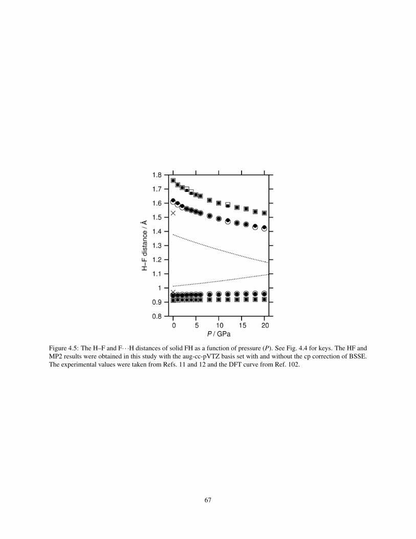
Figure 4.5: The H–F and F· · ·H distances of solid FH as a function of pressure (P). See Fig. 4.4 for keys. The HF andMP2 results were obtained in this study with the aug-cc-pVTZ basis set with and without the cp correction of BSSE.The experimental values were taken from Refs. 11 and 12 and the DFT curve from Ref. 102.

67

This journal is c the Owner Societies 2012 Phys. Chem. Chem. Phys., 2012, 14, 7765–7779 7773

L(B3g) at 601 cm!1 and L(B1u) at 669 cm!1, in 3D cp-MP2.The estimated anharmonic frequencies are 711 and 779 cm!1,respectively, which are in good agreement with the observedRaman (742 cm!1) and infrared (792 cm!1) band positions.The corresponding harmonic frequencies in FD are 427 and486 cm!1 as compared with the observed 552 and 572 cm!1.Remarkably, the infrared bands at 792 cm!1 in FH and at572 cm!1 in FD almost completely disappear if the FH or FDcrystal films are deposited near !125 1C and subsequentlycooled to !185 1C.12 They are intense when the films aredeposited directly at !185 1C. An explanation suggested byKittelberger and Hornig is that the crystals prepared at!125 1C,which is near the melting point, are more perfect and an infraredabsorption due to transition dipoles perpendicular to the films ishard to occur. Therefore, ‘‘one ought to consider the 792 cm!1

HF band as the out-of-plane libration.’’12 This is supported byour calculation and assignment; L(B1u) is an out-of-plane libra-tion (see Fig. 6) and the only such mode that is infrared active.The L(A1) mode in 1D FH at 545 cm!1 (cp-MP2) becomes

L(B3u) at 480 cm!1 and L(Ag) at 584 cm!1 in 3D cp-MP2. The

L(A2) mode in 1D at 585 cm!1 is split into L(B2g) at 510 cm!1

and L(Au) at 513 cm!1 in 3D. Unlike the other modes, theband ordering of these modes is altered by the crystal-fielde!ect; the 3D modes originating from L(A2) have frequenciesthat are not necessarily higher than those arising from L(A1).Since the previous band assignments were made primarilybased on the band ordering, some of them concerning L(A1)and L(A2) may have to be revised in view of this 3D calculation.The Raman band in FH observed at 569 cm!1 was previouslygrouped together with the infrared band at 553 cm!1 andassigned to L(A1), whereas the Raman band at a higherfrequency of 687 cm!1 was attributed to L(A2). The 3Dcalculation suggests that L(B2g), which corresponds to L(A2)in 1D, has a lower frequency than L(Ag), which arises fromL(A1). We, therefore, propose reassigning the Raman band at569 cm!1 to L(B2g) and the 687 cm!1 band to L(A2), inter-changing the previous assignments. The estimated anharmonicfrequencies are 629 and 686 cm!1, respectively, which agree wellwith the observed (569 and 687 cm!1, respectively). The sameapplies to FD. The Raman band at 417 cm!1 should no longer beconsidered as a counterpart of the infrared band at 403 cm!1. It isnow assigned to L(B2g) with the harmonic frequency of 373 cm!1.The Raman band at 492 cm!1 is instead attributed to L(Ag) at thecalculated frequency of 421 cm!1. One concern remains, however,to our proposed assignments. They assign themost intense Ramanbands to the B2g modes rather than the Ag modes.There are two pseudo-translational modes in 1D and nine in

3D. The two 1D modes and the corresponding four 3D modesare intermolecular vibrations, whereas the five additionalmodes in 3D are interchain vibrations, reducing to the acousticmodes in 1D. Consequently, their frequencies are very low andhardly dependent on the hydrogen mass. Therefore, theobserved and calculated results for solid FH and FD inTables 6 and 7 are almost identically similar and can bediscussed collectively. The T(B1) mode in 1D, predicted tooccur at 294 (FH) or 288 (FD) cm!1, splits into the T(B2u) andT(B1g) modes in 3D. The factor-group splittings seem exag-gerated by our calculation (ca. 20 cm!1 versus a few cm!1 inthe observed). The anharmonic e!ects, on the other hand, can

Fig. 6 Normal modes (not to scale) of the k = 0 lattice vibrations of

solid FH. The larger circles represent fluorine atoms and the smaller

the hydrogen atoms. Open circles denote that the atoms are on the

x = +a/2 plane, where the a lattice vector is perpendicular to the

page. The frequencies listed are obtained by the cp-MP2/aug-cc-pVDZ

calculations at 0 GPa.

Dow

nloa

ded

by U

nive

rsity

of I

llino

is - U

rban

a on

23

May

201

2Pu

blish

ed o

n 13

Mar

ch 2

012

on h

ttp://

pubs

.rsc.

org

| doi

:10.

1039

/C2C

P402

36J

View Online

Figure 4.6: Normal modes (not to scale) of the k = 0 lattice vibrations of solid FH. The larger circles represent fluorineatoms and the smaller the hydrogen atoms. Open circles denote that the atoms are on the x = +a/2 plane, wherethe a lattice vector is perpendicular to the page. The frequencies listed are obtained by the cp-MP2/aug-cc-pVDZcalculations at 0 GPa.

68

Figure 4.7: The frequencies of the k = 0 lattice vibrations in solid FH as a function of pressure (P) calculated atthe cp-MP2/aug-cc-pVDZ level. The calculated gerade and ungerade modes are plotted by solid and broken curves,respectively, and the observed Raman band positions46 by filled circles.

69

Figure 4.8: The frequencies of the k = 0 lattice vibrations in solid FD as a function of pressure (P) calculated atthe cp-MP2/aug-cc-pVDZ level. The calculated gerade and ungerade modes are plotted by solid and broken curves,respectively, and the observed Raman band positions46 by filled circles.

70

Figure 4.9: The phonon dispersion curves (0−−1100 cm−1) of solid FH in the first Brillouin zone at 0 GPa obtainedby cp-MP2/aug-cc-pVDZ.

71

Figure 4.10: The phonon dispersion curves (0−−1400 cm−1) of solid FH in the first Brillouin zone at 20 GPa obtainedby cp-MP2/aug-cc-pVDZ.

72

Figure 4.11: The hydrogen-amplitude-weighted phonon DOS (the histograms) and its Gaussian convolution with aFWHM of 40 cm−1 (the curves) of solid FH at 0, 10, and 20 GPa calculated by cp-MP2/aug-cc-pVDZ. The dashedand solid arrows indicate the positions of the peaks in inelastic neutron scattering spectra obtained by Boutin et al.54

and Axmann et al.,55 respectively.

73

5

Ab initio study of ice Ih

5.1 Introduction

Among the at least fifteen crystalline phases of ice, ice Ih is the most abundant on the Earth’s surface and arguably the

most important molecular crystal in nature.110–114 Ice Ih is hexagonal, proton disordered, and can easily be prepared

by freezing liquid water at 1 atm and 0◦C. Despite its structural simplicity and numerous spectroscopic113, 115–119 and

computational87, 120–127 studies, some aspects of the physical chemistry of ice Ih still remain not fully understood.

One of the controversies concerns with the unusually long O–H bond length of 1.000–1.008 Å in ice Ih reported by

a neutron diffraction study.128 The same bond lengths measured for ice II and IX were found to be much shorter (ca.

0.985 Å) and are likely to be more accurate because of the ordered proton positions in these phases. The proximity of

the frequencies of the O–H stretching vibrations and NMR parameters across the three phases 2 led Floriano et al.129

to reexamine the neutron scattering data and revise the O–H bond length of ice Ih to 0.985± 0.006 Å. This value is

now widely accepted, though it is yet to be confirmed independently by accurate theoretical calculations.

Another unresolved controversy involves the interpretation of the origin of the two peaks at 28.4 and 37.9 meV in

the hydrogen-bond-stretching region of the inelastic neutron scattering (INS) spectra of ice Ih.113, 114 Li and Ross, who

measured the spectra, hypothesized113, 114 the existence of “two types of hydrogen bonds” that differed in strength by

a factor of two and are randomly distributed throughout the lattice to account for the ratio of 1.3 between the two peak

positions. This hypothesis was met with much skepticism. Tse and Klug123 showed that it was possible to reproduce

the correct peak positions without the drastic hypothesis of Li and Ross; they used a force field that included long-

range electrostatic interactions that explained the two peaks. A definitive resolution of this issue, however, warrants

a first-principles spectral simulation with predictive power rather than an empirical model adjustable to experimental

results.

Both classical122, 123, 130–134 and quantum87, 121, 125, 127, 135 simulations have been previously performed on the struc-

tures and lattice vibrations of ice Ih. The former relied on empirical force fields such as TIP3P, TIP4P, TIP5P and

SPC/E, which were originally developed for liquid water and as such might not be suitable for ice.136 In fact, it has

been reported that some of these force fields fail to locate a stable structure of ferroelectric ice XI.137 Recently, a flexi-

74

ble, polarizable force field was suggested so as to reproduce both cluster energetics and some properties of ice Ih more

accurately.138, 139 There is, however, no general procedure to improve any of the existing force fields systematically.

The situation surrounding the quantum mechanical simulations of condensed matter has not been any brighter.

Density-functional theory (DFT) has been the standard in treating solids and liquids for its efficiency. However,

its accuracy depends on the choice of the density functional. A previous study125 has shown that DFT tends to

overestimate the O–H bond lengths in ice Ih. Another major drawback of most, if not all, functionals is their failure

to capture the dispersion interactions87, 140, 141 that are important in molecular crystals, although some attempts have

been made to correct this failure.142

As was mentioned in Chapter 2, the long-time Nature editor, Maddox,1 criticized this state of affairs as follows:

“One of the continuing scandals in the physical sciences is that it remains in general impossible to predict the struc-

ture of even the simplest crystalline solids from a knowledge of their chemical compositions. [. . . ] Solids such as

crystalline water (ice) are still thought to lie beyond mortals’ ken.”

With that in mind, the objective of this chapter is to demonstrate that there now exists a clear roadmap to predict the

structures and even dynamics of ice. These methods implement systematic series of diagrammatic many-body theories

in conjunction with also systematic basis sets, together converging towards the exact limits. MP2 theory—the simplest

of the series—is capable of describing covalent, ionic, hydrogen-bond, and dispersion interactions simultaneously and

from the first principles, all of which are important in ice and whose strengths span three orders of magnitude (100 to

0.1 kcal mol−1). In what follows, ab initio simulations at the MP2 level are demonstrated to offer reliable, quantitative

predictions of the structures and spectra of ice Ih and to help resolve some of the outstanding questions mentioned

above.

5.2 Computational Methods

It is the embedded-fragment method,86, 87, 143 BIM,8–10, 69, 85, 144 which allows for the MP2 routine to be applied to ice

Ih called the binary-interaction method (BIM). The scheme, summarized in the introduction of this thesis, is systematic

in that it is an example of the converging Bethe-Goldstone many-body expansion in a local basis, general in the choice

of electronic structure theory for monomers and dimers, and linear scaling in the computational cost with respect to

system size.

Owing to the additive nature of the energy, the energy derivatives with respect to atomic positions can also be

obtained as a sum of the corresponding derivatives for dimers and monomers in a linear-scaling algorithm. The first

and second derivatives with respect to atomic positions correspond to atomic forces and force constants, respectively,

which can be used to determine the crystal structures and phonons.10 Another unique advantage of this approach is

75

that one can obtain these derivatives with respect to individual atomic coordinates, unlike most methods for crystals

with which only the derivatives with respect to collective and in-phase atomic coordinates that preserve periodicity are

accessible. In consequence, one can calculate phonon dispersion and density of states (DOS) throughout the Brillouin

zone.

A new capability added to BIM is the linear-scaling calculations of infrared and Raman band intensities. In the

harmonic approximation, they are determined by the derivatives of dipole moments and polarizabilities with respect

to normal coordinates. On the basis of the ideas in Refs. 145–147 the following approximation to the dipole derivative

of a periodic solid are proposed:

∂ µp

∂xγ(0)= ∑

i

∂ µi(0)p

∂xγ(0)+∑

i< j

{∂ µ

i(0) j(0)p

∂xγ(0)− ∂ µ

i(0)p

∂xγ(0)− ∂ µ

j(0)p

∂xγ(0)

}

+12 ∑

n(1−δn0)∑

i, j

{∂ µ

i(0) j(n)p

∂xγ(0)− ∂ µ

i(0)p

∂xγ(0)− ∂ µ

j(n)p

∂xγ(0)

}, (5.1)

where xγ(0) is the x-coordinate of the γth atom in the 0th unit cell, µp is the p-axis component of the unit-cell dipole

moment (p = x,y, or z), µj(n)p is the p-component of the dipole moment of the jth monomer in the nth unit cell,

µi(0) j(n)p is the p-component of the dipole moment of the dimer consisting of the ith monomer in the 0th unit cell

and the jth monomer in the nth unit cell, and δn0 is Kronecker’s delta that is unity when n = 0 and zero otherwise.

The quantities in the right-hand side are calculable by efficient semi-analytical algorithms for molecules. While the

unit-cell dipole moment of a periodic solid is an ill-defined quantity,148 its derivatives and hence the IR intensities are

well defined.149, 150

Similarly, the polarizability derivatives of a periodic solid can be approximated by

∂αpq

∂xγ(0)= ∑

i

∂αi(0)pq

∂xγ(0)+∑

i< j

{∂α

i(0) j(0)pq

∂xγ(0)− ∂α

i(0)pq

∂xγ(0)− ∂α

j(0)pq

∂xγ(0)

}

+12 ∑

n(1−δn0)∑

i, j

{∂α

i(0) j(n)pq

∂xγ(0)− ∂α

i(0)pq

∂xγ(0)− ∂α

j(n)pq

∂xγ(0)

}, (5.2)

where αpq is the pq-component of the unit-cell polarizability tensor (p = x,y, or z and q = x,y, or z) and the cor-

responding monomer and dimer polarizabilities defined accordingly. A unit-cell polarizability of a periodic solid

is a non-trivial quantity to evaluate because of the difficulty of defining the dipole moment operator. Nevertheless,

Champagneet al.151–153 and Otto154 reported an analytical evaluation of the quantity under the periodic boundary

conditions. Bishop et al.155 also proposed an alternative definition, whereas Kudin and Scuseria156 devised a finite-

difference evaluation of the same. The definition given above is consistent with that for molecular clusters and is

most straightforward to understand and evaluate. The IR intensity, Ink, and Raman intensity, Rnk, for the fundamental

76

transition of the mode in the nth phonon branch with wave vector k are related to these derivatives as 57

Ink ∝

x,y,z

∑p

(∂~µp

∂Qnk

)2

, (5.3)

Rnk ∝32

(x,y,z

∑p

∂αpp

∂Qnk

)2

+212

x,y,z

∑p

x,y,z

∑q

(∂αpp

∂Qnk

)2

, (5.4)

where Qnk is the corresponding normal mode. Only the zone-center (k = 0) vibrations have nonzero intensities and

thus are IR- or Raman-active. The derivatives with respect to Qnk in the above expression are related to those with

respect to Cartesian coordinates by

∂ µp

∂Qnk=

Natom

∑γ=1

{∂ µp

∂ zγ(0)

∂ zγ(0)

∂Qnk+

∂ µp

∂ zγ(0)

∂ zγ(0)

∂Qnk+

∂ µp

∂ zγ(0)

∂ zγ(0)

∂Qnk

}, (5.5)

and by a similar expression for polarizability derivatives. Here, Natom is the number of atoms in the unit cell and the

second factor in each term should be readily available after the normal mode analysis.

BSSE-corrected HF and MP2 with the aug-cc-pVDZ basis set was applied to the three-dimensional, infinitely

extended ice Ih under the periodic boundary condition. Equilibrium lattice structures, IR and Raman band positions

and intensities, phonon dispersion, phonon DOS, hydrogen-amplitude-weighted phonon DOS, and heat capacity were

calculated for normal ice and its completely and/or partially deuterated species (if applicable).

The unit cell of ice Ih (see Figure 5.1) used consisted of a random arrangement of two non-ferroelectric unit cells

with P212121 and Pna21 symmetry groups.12, 19 It contained 64 water molecules with a quasi-random distribution of

protons that satisfied the Bernal–Fowler (ice) rules.3 The dimers with the water-water distance less than 8 Å and the

unique monomers within the unit cell were treated quantum mechanically at the BSSE-corrected HF or MP2 level with

the aug-cc-pVDZ basis set. The dimers and monomers were embedded in the electrostatic field of the supercell of size

3×3×3 (containing 1728 molecules). The long-range electrostatic interactions were summed in the supercell of size

21×21×21 (containing over a half million molecules). All molecular calculations were performed with GAUSSIAN.27

The unit cell geometry was determined by varying all atomic positions and lattice constants and minimizing

the maximum energy gradient below a 0.001 atomic units threshold. The vibrational analysis was performed in the

harmonic approximation by including force constants from the nearest neighbor unit cells. The frequencies of phonons

were determined on a 5×5×5 wave-vector grid in the reciprocal unit cell. The phonon DOS on the same wave-vector

grid were collected into a histogram with the bin size of 1 cm−1. The simulated INS spectrum is the product of the

hydrogen-amplitude-weighted DOS and the Debye–Waller factor. The latter is obtained in the isotropic approximation

with the mean square amplitude of hydrogen nuclei of 0.010 Å2. This value is reasonable as compared to the literature

values.2

77

The molar heat capacity was computed from the phonon DOS with the formula given in Ref. 59, which reads

Cν =R

Nmol.K

3Natom

∑n=1

∑k

(h̄ωnk

kBT

)2 e−h̄ωnk/kBT

1− e−h̄ωnk/kBT (5.6)

where R, kB and T are the gas constant, the Boltzmann constant and temperature, respectively, Nmol. is the number

of monomers in the unit cell, K is the number of wave vectors in the reciprocal unit cell, and ωnk stands for the

harmonic frequency of the mode in the nth phonon branch and wave vector k. The k-summation is taken on the

5×5×5 wave-vector grid in the reciprocal unit cell.

5.3 Results and Discussion

Table 5.1 compares the observed157 60 and predicted values of geometrical parameters of ice Ih. As expected,125, 158, 159

the HF theory, lacking dispersion and underestimating hydrogen-bond cooperativity,122, 135 underestimates the O–H

distances and overestimates the O· · ·O distances. Consequently, its predicted values of the lattice constants are notice-

ably in error. The MP2 theory, on the other hand, reproduces the experimental values accurately within 0.01 Å (bond

lengths) and 1 degree (bond angles). MP2, therefore, renders a clear, independent support for the now accepted bond

length of 0.985 Å, which is close to those found in ice II and IX. Though ice Ih is proton disordered and both the

calculated and observed O–H and O· · ·O distances in Table 5.1 are average values, the distributions are very narrow

with the standard deviations being less than 0.01 Å. This clearly contradicts the “two hydrogen bond” hypothesis of

Li and Ross; it is hard to contemplate a difference in the intermolecular force constants by a factor of two without

commensurate variations in bond lengths.

Figure 5.2 shows the simulated and observed IR, Raman, and INS spectra of ice Ih in the pseudo-translational

region (110–340 cm−1). The two peaks at 229 and 306 cm−1 (28.4 and 37.9 meV) in the observed INS spectrum,

which were at the center of controversy, are reproduced by MP2 without any assumption about different types of

hydrogen bonds. The calculated position (266 cm−1) of the lower-energy peak was, however, overestimated by 37

cm1, while the higher-energy peak positions are in good agreement between theory (313 cm−1) and experiment (306

cm−1). There are several possible causes for the discrepancy: the inherent errors in the MP2 theory, the size of the

aug-cc-pVDZ basis set, the embedded-fragmentation scheme, the quasi-periodicity of the proton positions (see the

Method section) and finally the lack of anharmonic effects. On the basis of anharmonic frequency calculations of

small water clusters in this part of the spectral region (see Table 2), the anharmonic effects are estimated to be mostly

responsible for these errors. Nevertheless, one can ascertain that the two peaks exist in the simulated INS spectrum and

correspond to the two in the observed one because the same two peaks can also be seen in the simulated and observed

Raman spectra. The calculated positions of the Raman bands are also blueshifted by 44 and 17 cm−1 relative to the

78

observed and the magnitudes of the shifts are comparable to the ones for the simulated INS peaks (37 and 7 cm−1).

The higher-energy peak can also be discerned in the calculated IR spectrum, but with much lower intensity. This is

consistent with the experimental spectrum, in which only a slow-decaying tail can be seen in the higher-frequency side

of the 229 cm−1 band. In summary, not only do the current results not support the two-hydrogen-bond-type hypothesis

of Li and Ross, they actually contradict it. This calculation suggests rather narrow distributions of the O–H and O· · ·O

distances and, at the same time, reproduce the two peaks in the simulated INS and Raman spectra.

Inspection into the normal modes reveals few distinctions in the patterns of the two peaks; the modes that contribute

to both INS peaks involve stretching motion of many hydrogen bonds. The calculated depolarization ratios of the two

corresponding Raman bands are 0.75, indicating that they are both non-totally symmetric. The polarization of the

IR transition dipole moments turned out to be most discerning. The higher-frequency band at around 313 cm−1

is mainly polarized along the b lattice constant, whereas the lower-frequency band at 266 cm−1 is c-polarized (the

observed broad IR band around 160 cm−1 and the shoulder at 190–210 cm−1 are assigned to the z-polarized 190 cm−1

and y-polarized 240 cm−1 bands, respectively). The two peaks are therefore both sensibly referred to as “hydrogen-

bond stretch,” but differ from each other in the polarization, namely, the directionality of the motion. The fact that

the directionality causes noticeable difference in frequencies may suggest the significance of anisotropic long-range

electrostatic effects, which is consistent with the explanation previously offered by Tse and Klug.123

The simulated IR, Raman, and INS spectra in the full range (0–3800 cm−1) are shown in Figure 5.3 and compared

with the observed. The latter consist of four well-separated manifolds of bands: pseudo-translational (0–400 cm−1);

librational (500–1100 cm−1); HOH bending (at around 1600 cm−1); O–H stretching (>3000 cm−1). Additionally,

one can see the feature at around 2200 cm−1 arising from the combination of bending and libration. All of these

features—both peak positions and intensities—are quantitatively (<3000 cm−1) and semi-quantitatively (>3000 cm−1)

reproduced by the current calculations. The differences between the calculated (harmonic) and observed frequencies

in the O–H stretching region (>3000 cm−1) can be to a great extent attributed to the effect of anharmonicity and to

a lesser extent to the basis set used. Indeed, the anharmonic frequency calculations for small water clusters in that

region (see Table 3) suggest that inclusion of anharmonicity, higher-rank electron correlation at the CCSD(T) level of

theory as well as larger basis sets will bring the calculated band origins in line with experiment.

The fidelity of the simulated INS spectra can be further confirmed by the computed spectra of normal, partially,

and fully deuterated ice Ih. Figures 5.4 and 5.5 compare the calculated hydrogen- or deuterium-amplitude-weighted

phonon DOS and observed INS spectra as a function of deuterium concentration. Figure 5.4 underscores the high

accuracy of phonon DOS predicted by MP2.

As more H2O are replaced by D2O in ice Ih, some peaks in the INS spectra disappear or emerge, while others

gradually shift their centers and shapes (see Figure 5.5). For instance, the peak at about 3300 cm−1, corresponding to

79

O–H stretch, disappears as the peak at about 2500 cm−1 due to O–D stretch appears. This has been reproduced by the

current calculations in which randomly chosen hydrogen atoms are replaced by deuterium atoms—not H2O replaced

by D2O. The appearance and disappearance of peaks are indicative of the non-overlap of phonon DOS between the

pure H2O and pure D2O crystals, which is the case with these stretching modes.

The features below 2000 cm−1 gradually change with D2O concentration. The current calculations again reproduce

these quite well and indicate different mechanisms of the spectral shape change between the features above and below

1000 cm−1. Below 1000 cm−1 the phonon DOS of H2O and D2O overlap and their shape changes gradually with the

deuterium concentration. On the other hand, above 1000 cm−1 three separate peaks that are close in energy (indicated

by arrows in the figure) appear and disappear with the D/H concentration change. They are due to the distinct bending

modes of D2O, HOD, and H2O in the order of increasing energy, which are not discerned spectroscopically. The

observed high peak intensity at the HOD bending frequency suggests the rapid D/H interchange in the mixed H2O/D2O

ice.

Figure 5.6 compares the calculated (constant-volume; Cν ) and observed (constant-pressure) molar heat capacities

of H2O and D2O ice. The differences between the constant-volume and constant-pressure values are negligible.

The calculated and observed Cν are in generally good agreement with one another, though they deviate at higher

temperatures owing to the lack of anharmonic effects in the current calculations.160 A more subtle issue that requires

explanation is the deviation of the low-temperature Cν from the T 3 behavior predicted by the Debye model (see the

inset in Figure 5.6) as observed by Flubacher et al.161 The current calculations reproduce this anomaly; the temperature

at which the deviation becomes the largest is well reproduced, if not the magnitude. The anomaly occurs because of

the peak in the phonon DOS centered around 60 cm−1 and extending to 100 cm−1 (as seen in Fig. 3), which is due

to soft acoustic lattice vibrations of hydrogen bonds. A numerical verification indicates that the anomaly disappears

when the DOS below 100 cm−1 is erased and the calculation of Cν is repeated.

A paper by Zhang et al.,162 recently reported planewave DFT calculations of the INS spectra of ice Ih. On this

basis, these authors including Li who originally proposed the “two-hydrogen-bond” hypothesis concluded that it was

not necessary to rely on this hypothesis to reproduce the two peaks in the INS spectra. Hence, the embedded-fragment

MP2 calculations and the DFT calculations of Zhang et al. are mutually consistent and in agreement on the key

conclusion about the origin of the two peaks. Apart from the very different computational methods Zhang et al. used,

which seem equally valid for this particular problem, it is important to note that the current calculations on IR and

Raman spectra give greater details of the two peaks. Whereas the DFT calculations by Zhang et al. were not very clear

about the distinct characteristics of the two peaks, the current MP2 calculations, especially those on the IR spectra,

showed that the two peaks have different directions of transition dipole moments.

80

5.4 Conclusion

A linear-scaling, embedded-fragment MP2 method has been applied to an infinitely extended, three-dimensional crys-

tal of ice Ih, predicting its structural parameters, IR, Raman, and INS spectra, as well as the heat capacity, all from the

first principles, i.e., without resorting to the use of density functionals or empirical potentials. The calculations predict

a narrow distribution of O–H bond lengths centered accurately at the experimental values for proton-ordered ice II and

IX and the two peaks in the hydrogen-bond-stretching region of INS spectra. They do not support and indeed disprove

the hypothesis of Li and Ross that there exist two types of hydrogen bonds with vastly different bond strengths. While

the two peaks are reasonably described as hydrogen-bond stretch, they do not originate from the difference in the force

constants associated with different nearest-neighbor local arrangements but rather from the different directionalities

of motion manifested in the distinct polarizations of absorbed photons. The calculations also shed light on the assign-

ments of individual IR, Raman, and INS peaks and their variation with deuterium concentration. They also elucidate

the cause of anomaly in the low-temperature heat capacity of ice.

81

5.5 Tables

Table 5.1: The geometrical parameters of ice Ih are shown with the standard deviations in parentheses. The bonddistances and lattice constants are given in Å and the HOH angle is in degrees.

HF/aug-cc-pVDZ MP2/aug-cc-pVDZ Experiment

O–H distance 0.955 (0.0008) 0.985 (0.0005) 0.985 ± 0.006 (Refs. 111, 129); 0.987 ± 0.005 (Ref. 60)

O· · ·O distance 2.796 (0.024) 2.757 (0.009) 2.750 (Ref. 112)

HOH angle 106.6 (0.3) 105.6 (0.2) 106.6 ± 1.5 (Ref. 111); 107 ± 1 (Ref. 60)

a 9.33 9.03 8.9938 (Ref. 157)

b 15.80 15.56 15.5777 (Ref. 157)

c 14.89 14.65 14.6422 (Ref. 157)

82

5.6 Figures

Figure 5.1: The unit cell (drawn in strong color and embedding field (drawn in faded color) of ice Ih.

83

Figure 5.2: Simulated (grey) and observed IR, Raman and INS spectra of ice Ih in the 110–340 cm−1 region.

84

Figure 5.3: Simulated (grey) and observed IR, Raman and INS spectra of ice Ih in the 0–3800 cm−1 region.

85

Figure 5.4: The INS spectra of normal and fully deuterated ice Ih in the low-energy region. The observed spectra ingrey; hydrogen and deuterium contributions in blue and red, respectively.

86

Figure 5.5: The INS spectra of normal, partially, and fully deuterated ice Ih. The observed spectra in grey; thehydrogen contributions in blue; the deuterium contributions in red, respectively. The red, purple, and blue arrowsindicate the peaks due to D2O, HOD, and H2O bending modes.

87

Figure 5.6: The constant-volume molar heat capacities of ice Ih in units of gas constant (R) as a function of tempera-ture.

88

6

Solid carbon dioxide

6.1 Introduction

The fundamental symmetric stretch (ν1) and the first bending overtone (2ν2) of CO2 have nearly coincident harmonic

frequencies and the same symmetry (Σ+g ), causing colossal resonance through anharmonic coupling (see Fig. 6.1).

Instead of just one peak (ν1) in the 1250–1450-cm−1 region of the Raman spectrum as the harmonic approximation

predicts, two peaks (ν+ and ν−) with substantial intensities appear, which are separated by more than 100 cm−1 in their

positions. This Fermi resonance163–183 in CO2—a textbook example of strong anharmonic mode-mode coupling—is

observed not only in the gas phase but also in the condensed phases184–200 under various pressures. Since the strength

of resonance is a sensitive function of the coincidence of the two harmonic frequencies, the different responses of

these frequencies to pressure can modulate the Fermi dyad splitting and intensity ratio.

Geochemists have utilized this property to develop one of the most accurate geobarometers for minerals with CO2

inclusions.201–205 The so-called residual pressure experienced by CO2 trapped in minerals carries a critical piece of

information in the study of mantle tectonics as it reports the depths at which these minerals were entrained by the host

magma. Previously, these depths were painstakingly determined by chemical analyses of the elemental compositions

of the minerals with unsatisfactory accuracy. With the spectroscopic geobarometer, the residual pressure can be

obtained directly from the noninvasive measurements of the Fermi dyad splitting and intensity ratio, greatly improving

geochemists’ ability to probe the formation history of minerals. For this geobarometer to work, the relationship

between the pressure and the Fermi resonance parameters must be thoroughly and quantitatively known.

Can this relationship for solid CO2 be determined from the first principles? The primary objective of this study is

to show that the answer is affirmative. The calculations are challenging as they must reproduce the relative positions of

the two harmonic frequencies (ν1 and 2ν2) and the cubic (k122) and other anharmonic force constants at high accuracy.

They must at the same time determine the pressure dependence of these quantities in the solid-state environment.

To achieve this, a hybrid approach was undertaken: an accurate quartic force field (QFF) of an isolated CO2

molecule was used, which reproduces the Fermi resonance quantitatively in the gas phase and has been determined in

a previous study181 using coupled-cluster singles and doubles with a noniterative triples [CCSD(T)] with the cc-pVTZ

89

basis set. In this present study, the pressure dependence of the quadratic force constants is determined accurately

with the embedded-fragment, linear-scaling method for solid CO2 under pressure at the second-order Møller–Plesset

perturbation (MP2) level with the aug-cc-pVDZ basis set. These two sets of information are used in combination with

the vibrational configuration-interaction (VCI) calculation that reproduces the Fermi dyad splitting quantitatively and

intensity ratio qualitatively as a function of pressure up to 10 GPa.

This agreement also sheds light on the long-standing issue concerning the order of the unperturbed (harmonic)

frequencies of ν1 and 2ν2. While the Fermi dyad splitting is insensitive to this order, the intensity ratio is not and

clearly favors the force field that places ν1 > 2ν2, potentially extinguishing any doubt about this correct order. In

addition to the Fermi resonance, the MP2 calculations reproduce the equilibrium structures, pressure dependence of

the molar volume and of other Raman band positions, and the zero-pressure infrared (IR) and Raman spectra in the

librational region of solid CO2. They can also explain the lifting of axial degeneracy of the bending mode in the

crystalline environment. The phonon density of states (DOS) in the librational region were also predicted, which may

be compared with inelastic neutron scattering from this solid, which is yet to be reported.

6.2 Computational Methods

The equilibrium lattice structures, phonon dispersions, phonon DOS, and their infrared and Raman intensities of a

three-dimensional, infinitely extended, periodic crystal of CO2 (phase I) as well as their pressure dependence have

been calculated by MP2 with the aug-cc-pVDZ (and sometimes also aug-cc-pVTZ) basis set. In this crystal, as in

most other molecular crystals, covalent, electrostatic (in this case, most importantly, quadrupole–quadrupole), and

dispersion interactions coexist with their strengths spanning three orders of magnitude (100 to 0.1 kcal mol−1). MP2

is perhaps the simplest electronic structure theory that can capture all these interactions from the first principles.

MP2 is an accurate but expensive computational procedure, the execution cost of which increases as the fifth

power of the number of energy bands and the third power of the number of wave vectors in the reciprocal space in

solid-state applications, which have thus been nearly unthinkable until recently. Such applications have been enabled

by exploiting the chemistry of the crystal, namely, the fact that the constituent molecules preserve their molecular

identities in this crystal even under high pressures. These molecules serve as a good localized basis with which to

break down the whole crystal into weakly interacting fragments that can be studied by molecular MP2 method as

implemented in GAUSSIAN.27

Specifically, the embedded-fragment method, BIM, was used which divides the internal energy per unit cell of

solid CO2 into the sum of the energies of monomers and overlapping dimers, which are embedded in the electrostatic

field of the rest of the crystalline environment. The embedding field is essential and, in the method, consists of self-

90

consistently determined atomic point charges at the Hartree–Fock level using NWCHEM.26 It allows us to recuperate

the dipole and quadrupole polarizability. The basis-set superposition errors (BSSE) have been corrected9 at each of

the dimer calculations by the function counterpoise method (the prefix “cp-” indicates this correction). The monomer

and dimer MP2 calculations have been executed in parallel in an algorithm that is (nearly) linear-scaling with respect

to both the system size and the number of processors.

A unit cell of CO2 (Fig. 6.2) consists of four molecules with their centers located at the face-centered positions

of the cubic lattice and aligned along the body-diagonal directions. The structure belongs to the Pa3 space group.

Symmetrically unique dimers in the 3×3×3 supercell, containing a total of 108 molecules, have been treated quantum

mechanically embedded in the field created by the 11× 11× 11 supercell of atomic point charges. Furthermore, the

long-range electrostatic interactions within the supercell of 41×41×41 containing over a quarter million molecules

has been taken into account in the internal energy calculation.

The molecular crystal can be placed under ambient pressure by simply applying BIM to the unit-cell enthalpy

instead of the unit-cell internal energy that differ from each other just by pressure times unit-cell volume as show

in Chapter 4. Furthermore, since the energy or enthalpy is approximated by a sum of monomer and dimer energies,

their derivatives with respect to atomic positions, lattice constants, external electric fields, etc. can also be obtained as

sums of respective molecular derivatives obtainable in a linear-scaling fashion from molecular methods implemented

in GAUSSIAN.27 These are essential in optimizing the crystal structure, calculating phonon dispersions and DOS, and

IR and Raman intensities as was explained in the previous chapter.

The equilibrium crystal structure has been determined by minimizing all energy (enthalpy) gradients to less than

4× 10−4 atomic units, while maintaining the Pa3 space-group symmetry of the unit cell as well as the D∞h point-

group symmetry of the molecules. The harmonic frequencies and normal modes have been obtained at each of the

21×21×21 wave vector grid points in the reciprocal space using the interaction force constants in the nearest neighbor

approximation. The phonon DOS has been collected as histograms in the 1-cm−1 bins. A pressure of up to 15 GPa has

been applied at the 1-GPa increment and the structure and phonon calculations have been repeated at each pressure.

The Fermi dyad frequencies and intensity ratios have been determined as a function of pressure as follows: First,

one can consider the crystal-field effects in solid CO2 at 1 atm (0.0001 GPa) to be sufficiently weak that its Fermi

resonance can be described by the accurate QFF obtained by CCSD(T)/cc-pVTZ in a previous study.181 A full VCI

calculation using this QFF gives the dyad frequencies of 1283 and 1392 cm−1 with the intensity ratio of 1.8 (with ν+

being more intense than ν−).181 The intensity ratio is calculated as |c+|2/|c−|2 where c± is the expansion coefficient

in the normalized VCI wave functions of ν±,

|ν±〉= c±|ν1〉+ c′±|2ν2〉+ . . . , (6.1)

91

with |ν1〉 and |2ν2〉 being the harmonic-oscillator basis functions of ν1 and 2ν2, respectively. At a higher pressure,

the dyad frequencies and intensity ratios were obtained by repeating VCI calculations on a CO2 molecule with its

diagonal quadratic force constants Fqq for mode q replaced by the following quantities that include the crystal-field

effects:

Fqq(P) = FCCSD(T)qq +FMP2

qq (P)−FMP2qq (0), (6.2)

where FCCSD(T)qq is the CCSD(T)/cc-pVTZ quadratic force constants of an isolated CO2 for mode q and FMP2

qq (P) is

the MP2/aug-cc-pVDZ quadratic force constants of solid CO2 under pressure P for mode q. The values of FMP2qq (P)

have been estimated from the average frequencies of four zone-center symmetric stretching modes (q = 1) and of eight

zone-center bending modes (q = 2).

6.3 Results and Discussion

First, the MP2 and experimental results are compared to assess the accuracy of the first-principle calculations for solid

CO2. It will be shown that the MP2 values of various observables of the solid and especially of their pressure depen-

dence are sufficiently accurate to be combined with the CCSD(T)/cc-pVTZ QFF of molecular CO2 in the simulation

of Fermi resonance of the solid under pressure.

Table 6.1 lists the C–O bond length, lattice constant, and molar volume of the solid CO2. The calculated C–O

bond lengths are in nearly exact agreement (within 0.01–0.02 Å) with the observed.206, 207 Furthermore, the agree-

ment improves with increasing the basis-set size, which is the hallmark of the ab initio methods. The predicted lattice

constants, which are determined by competitions between weaker attractive and repulsive interactions, are less accu-

rate, but they are still within 0.1–0.2 Å of the observed. Since the molar volumes are proportional to the cubic power

of the lattice constants, they show essentially the same trend as the lattice constants. Two important observations

can be made: First, the calculated lattice constants and hence molar volumes are smaller than the observed, which

foreshadows the overestimation of frequencies of lattice vibrations to be discussed later. Second, nearly half of the

underestimation of the lattice constants at the MP2 level seems ascribable to the BSSE as judged by the comparison

with cp-MP2. This, in turn, suggests that a significant portion of the attractive interactions in this solid is due to

dispersion.

The calculated pressure dependence of the solid’s structural parameters also shows reasonable agreement with the

observed.208–211 The molar volumes plotted in Fig. 6.3 are the best evidence of this. As mentioned, cp-MP2 yields the

volume that is in better agreement than MP2 at 0 GPa, but the difference diminishes with the pressure and virtually

vanishes at about 5 GPa. Convergence of the structural parameters obtained by various computational methods with

92

pressure is a universally observed phenomenon, reflecting the fact that at higher pressures exchange repulsion begins

to dominate intermolecular interactions, obscuring differences in theoretical treatments of other weaker interactions.

The curves predicted by both theoretical methods parallel (if not fall on) the observed, justifying the use of MP2/aug-

cc-pVDZ for simulating the pressure dependence especially at higher pressures. The C–O bond length (not shown) is

almost unchanged with pressure, shortening by only 0.07 Å at 15 GPa. The experimental data directly probing this

effect is vibrational frequencies of the C–O stretching modes, which will be discussed below.

In Table 6.2 are compared the frequencies and relative intensities of the lattice vibrations of solid CO2. As expected

from the underestimation of volume by the calculations (see above), they now overestimate the frequencies of these

intermolecular modes. The relative intensities are, however, surprisingly well reproduced, attesting to the fact that

MP2/aug-cc-pVDZ does describe the cohesive interactions in this solid with sufficiently high accuracy and from the

first principles.

Figure 6.4 compares the pressure dependence of the MP2 harmonic frequencies and of the observed positions

of the IR and Raman bands.212–214 While the predicted band positions are in error by as much as 50 cm−1 or more,

which can be ascribed to a variety of causes, the pressure dependence of all five (or six) modes, for which experimental

dependence is available, is extremely accurate. For example, MP2 predicts that ν3 (the antisymmetric stretching mode

appearing in 2300–2500 cm−1) increases with pressure at the average rate of 4.2 cm−1 GPa−1 (from 0.5 to 12.5 GPa),

which agrees exactly with the observed rate of 4.2 cm−1GPa−1 (in a similar pressure range).186

The frequencies of ν2 (between 600 and 700 cm−1) decrease with pressure. This is because, owing to the body-

diagonal arrangement of the CO2 molecules, the crystal becomes less crowded as the molecules bend, causing the

corresponding vibrations to have lower frequencies than in the gas phase. There are two distinct (IR-active) bending

modes with different frequencies in the solid phase. That is, the degeneracy of ν2 in an isolated CO2 molecule is lifted

due to the loss of axial symmetry caused by the crystal field, which is also observed experimentally; the crystal-field

splitting is 11 cm−1 computationally and 5 cm−1 experimentally.215, 216 The average slope of the two ν2 curves is

predicted to be −1.5 cm−1GPa−1 (from 0.5 to 12.5 GPa), which is again in excellent agreement with the observed

slope of −1.3 cm−1GPa−1.

The predicted pressure-dependence curves of the lattice vibrations (below 300 cm−1) nearly fall on the curves

observed at lower temperatures. Since the pressure dependence of the quadratic force constants of solid CO2 (not the

force constants themselves) was used in the simulations of Fermi resonance, the agreement in Fig. 6.4 is reassuring.

Further confidence to the MP2 calculation of solid CO2 is rendered by Fig. 6.5, where the calculated and observed

Raman spectra of the solid are compared in the librational region under pressure. While the predicted band positions

are blue-shifted by nearly a constant (see above), the calculated relative intensities and the overall appearance of the

simulated spectrum are in good agreement with the observed. Figure 6.6 records the phonon DOS in the librational

93

region, which is expected to have the similar predictive accuracy as Fig. 6.5 and may serve as a pilot simulation for a

future inelastic neutron scattering measurement of solid CO2.

The pressure dependence of the Fermi dyad splitting and intensity ratio is plotted in Fig. 6.7. At every pressure up

to 10 GPa, the calculated and experimental spectra186 agree accurately with each other. As the pressure is increased,

the splitting is predicted to increase monotonically from 109 (0 GPa) to 143 cm−1 (10 GPa), which compares well with

the experimental increase from 107 to 136 cm−1. The intensity ratio displays a more dramatic pressure dependence,

going from 2.1 at 0 GPa to 11 at 10 GPa experimentally. The calculation predicts the intensity ratio of 1.8 at 0 GPa

and of 5.1 at 10 GPa. These results indicate that higher pressures can gradually “turn off” the Fermi resonance. This

is caused by the increase and decrease, respectively, in the unperturbed frequencies of ν1 and ν2 with pressure (as

evidenced by the 1300–1400 and 600–700-cm−1 regions of Fig. 6.4) and the resulting noncoincidence of ν1 and 2ν2

at higher pressures.

Unlike the splitting, the intensity ratio depends more sensitively with the difference in the unperturbed (i.e., har-

monic) frequencies for ν1 and 2ν2 and with the cubic coupling k122. The discrepancy between theory and experiment

in the intensity ratio at higher pressures may, therefore, be partly ascribed to the neglect of pressure dependence of

k122 in the calculations.186, 188 Nonetheless, the agreement is striking.

The calculated frequencies of the dyad at 0 GPa are the same as those of isolated CO2 obtained at the CCSD(T)/cc-

pVTZ level.181 They show near exact agreement with the observed, but other QFF’s obtained at similar or higher levels

of theory exhibit the same degree of agreement for frequencies. They, however, differ greatly in the ability to even

qualitatively reproduce the intensity ratio (I+ ≈ 2.1I−) correctly. The CCSD(T)/cc-pVTZ level was chosen as it gives

the reasonably accurate intensity ratio for molecular CO2. The “best” QFF determined with the complete-basis-set

(CBS) extrapolation in Ref. 181, in contrast, yields qualitatively wrong intensity ratio (I+ < I−). The VCI calculations

with these various QFF’s indicate that the intensity ratio is correlated with the order of unperturbed ν1 and 2ν2: a

QFF with ν1 > 2ν2 yields I+ > I− and vice versa. While the Fermi dyad frequencies are insensitive to the order, the

intensity ratio is and even the “best” molecular calculation in 2007181 has proven not accurate enough to predict the

correct order and hence the intensity ratio. In other words, one aspect of the current calculation that is not entirely

first principles is that experimental knowledge I+ > I− was used to choose the QFF of isolated CO2. This finding,

however, sheds some light on the long-standing controversy about the order of unperturbed ν1 and 2ν2.

Table 6.3 compares the intramolecular vibrational frequencies of gaseous and solid CO2 as well as the respec-

tive observed frequencies. The harmonic frequencies for ν1 and 2ν2 are not meant to agree even qualitatively with the

observed frequencies of the corresponding bands, which undergo the Fermi resonance. Hence, the good agreement be-

tween MP2 and experiment for the 2ν2 frequencies of the solid is merely accidental; as a proof of this, the frequencies

of ν1 between theory and experiment differ by 65 cm−1. The VCI calculation using the QFF of CCSD(T)/cc-pVTZ,

94

on the other hand, reproduces the frequencies of ν2, ν−, and ν+ within 4 cm−1 and that of ν3 within 17 cm−1 of the

observed. This agreement is not accidental and reflects the intrinsic high accuracy of CCSD(T) and VCI as has been

just discussed.

Table I of Garrabos et al.192 summarizes more than a dozen studies published between 1945 and 1989 that con-

tributed to the controversy about the order of unperturbed ν1 and 2ν2 in gaseous, fluid, and solid phases (henceforth,

it should be understood that when discussing the order of ν1 and 2ν2, it is the unperturbed frequencies that are being

compared). One may be surprised to find that these studies are nearly evenly divided between ν1 > 2ν2 and ν1 < 2ν2,

although these two orders do not necessarily contradict with each other because they may be specific to a certain

phase. In the solid state at atmospheric pressure, ν1 > 2ν2 seems well established, whereas more researchers tend to

believe that ν1 < 2ν2 is the correct order in the gas phase despite the fact that it is reversed from the more established

solid-state order.

The harmonic MP2 calculation for isolated and solid CO2 apparently supports this view (though the conclusion

differs). In the gas phase, ν1 < 2ν2, but, in the solid phase, the frequency of the bending mode decreases significantly,

reversing the order to ν1 > 2ν2, according to MP2. This predicted redshift of ν2 by the crystalline environment is in

agreement with the experiment, though its magnitude is somewhat exaggerated by theory. It has already been shown

that ν2 continues to decrease with increasing crystal field, i.e., with increasing pressure and also that MP2 reproduces

the crystal-field splitting (11 cm−1), which is in fair agreement with the experiment (5 cm−1).

Despite the agreement between MP2 and the most widely held view of the frequency order, MP2 is not considered

to have high enough accuracy to place two frequencies in the correct order when the difference is only 9 cm−1 (in

the gas phase). In the solid phase, however, the difference is sufficiently large (at least 41 cm−1) that MP2 may be

said to support ν1 > 2ν2. A more accurate method, CCSD(T)/cc-pVTZ predicts the gas-phase order of ν1 > 2ν2

and the correct intensity ratio I+ > I−. What complicates the matter further is the fact that the even more accurate

CCSD(T)/CBS181 reverts back to ν1 < 2ν2, but it gives the qualitatively incorrect intensity ratio I+ < I−.

Given the fact that the only indisputable experimental evidence in this discussion is I+ > I− and the implication that

the order of unperturbed ν1 and 2ν2 in gas phase is hard to predict even with the most accurate theory, the conclusion

is that ν1 > 2ν2 in both the gas and solid phases, which invariably gives the correct intensity ratio. There is, therefore,

not a reversal of the order upon the crytal field at atmospheric pressure or higher pressures. The researchers who

have advocated ν1 < 2ν2 in the gas phase seem to dismiss the intensity ratio I+ ≈ 2.1I−, which clearly favors the

opposite order ν1 > 2ν2. They sometimes do so by casting doubt to the double harmonic approximation that underlies

this argument for ν1 > 2ν2, that is, the assumption that the Raman intensity of unperturbed 2ν2 is exactly zero.166

The calculations show that it is possible to reproduce the Fermi dyad intensity ratio from 0 to 6 GPa quantitatively

and 8 to 10 GPa semi-quantitatively with the double harmonic approximation in conjunction with VCI. This does

95

not necessarily refute the discounting of the intensity argument, but it renders support to the one consistent order of

ν1 > 2ν2 throughout various phases of CO2.

96

6.4 Tables

Table 6.1: The C–O bond length (rC−O), lattice constant (a), and molar volume (V ) of solid CO2 at 0 GPa.

rC−O / Å a / Å V / cm3 mol−1

MP2/aug-cc-pVDZ 1.18 5.40 23.7

cp-MP2/aug-cc-pVDZ 1.18 5.50 25.1

MP2/aug-cc-pVTZ 1.17 5.40 23.7

cp-MP2/aug-cc-pVTZ 1.17 5.46 24.5

Experimenta 1.16 5.62 26.8

a Reference 207.

97

Table 6.2: The harmonic frequencies (ν in cm−1) and relative IR or Raman intensities (I) of the lattice vibrations ofsolid CO2 at 0 GPa.212, 217–219 The intensities of the gerade modes are relative to that of the Eg mode and those of theungerade modes are relative to the higher-frequency Fu mode.

ν (exp.)∗ ν (calc.) I (exp.)† I (calc.)

Fg 134 164 10 34

Fg 93 111 24 30

Eg 75 83 100 100

Fu 118 156 100 100

Au 106 130 0 0

Eu 95 133 0 0

Fu 69 87 40 34

a References 212, 219.

b References 217, 218.

98

Table 6.3: The frequencies of gaseous and solid CO2 (in cm−1).

ν2 2ν2 or ν− ν1 or ν+ ν3

Gas

MP2/aug-cc-pVDZ/harmonic 657 1314 1305 2379

CCSD(T)/cc-pVTZ/harmonic 666 1331 1358 2413

CCSD(T)/cc-pVTZ/VCI 665 1283 1392 2366

Experiment∗ 667 1285 1388 2349

Solid

MP2/aug-cc-pVDZ/harmonic 628, 639 1251–1278 1319 2397

Experiment† 655, 660 1276 1384 2345

a References 165, 172.

b References 187, 189.

99

Table 6.4: The frequencies (in cm−1) of the zone-center vibrations of solid CO2 and its isotope-substituted counter-parts.

Eg Fu Fg Au Eu Fg Fu Eu Fu Fu Fg Ag Au Fu

CO2 83 87 111 130 133 156 164 626 628 639 1318 1319 2371 2397

13CO2 83 86 111 128 132 154 164 608 610 621 1318 1319 2303 2329

18O12C16O 80 85 108 127 130 151 159 621 623 634 1280 1281 2354 2380

C18O2 78 83 105 124 127 149 154 616 618 630 1243 1243 2336 2361

Experimenta 73 66 91 105 95 130 113 · · · 655 660 1384 1384 2344 2344

a Expirmental data on solid CO2 was taken from Falk,189 Ouillon et al.,187 and Olijnyk et al.194

100

6.5 Figures

ν12ν

2

ν2

Symmetric stretch

Bend

ν+

ν−

Figure 6.1: A schematic vibrational-energy-level diagram of CO2. The states drawn in black and grey are bright anddark states, respectively, of Raman spectroscopy.

101

Figure 6.2: The cubic (Pa3) structure of solid CO2-I. Drawn are 27 unit cells each containing four molecules in whichdimers are treated quantum mechanically.

102

0 2 4 6 8 10 12 14

Pressure / GPa

17

18

19

20

21

22

23

24

25

26

Volume / cm mol

Experiment

MP2/aug-cc-pVDZ

cp-MP2/aug-cc-pVTZ

-13

Figure 6.3: The pressure dependence of the volume of solid CO2. The experimental data are taken from Refs. 208,209.

103

0 2 4 6 8 10 12 14

Pressure / GPa

0

100

200

300

400

500

600

700

Experiment (20K)

Experiment (40K)

Experiment (80K)

Experiment (300K)

Theory

-1Frequency / cm

2300

2400

2500

1300

1400

Figure 6.4: The pressure dependence of the IR and Raman band positions. The calculations (blue) are based onMP2/aug-cc-pVDZ and experimental data (red, black, and grey) are taken from Refs. 186 and 190.

104

50 75 100 125 150 175 200 225 250

Frequency / cm

Raman Intensity

Experiment

Theory

-1

Figure 6.5: The calculated and observed Raman spectra of solid CO2 in the librational region. The calculated spectrum(blue) was obtained as the Gaussian convolution with a full width at half maxium (FWHM) of 8.3 cm−1 of thecalculated histogram (also blue) at 4.0 GPa, whereas the observed (red) from Ref. 186 was obtained at 4.5 GPa.

105

0 20 40 60 80 100 120 140 160 180

Frequency / cm

Phonon DOS

-1

Figure 6.6: The phonon DOS of solid CO2 in the librational region at 0 GPa.

106

1200 1250 1300 1350 1400 1450

Frequency / cm

Raman Intensity

Experiment

Theory

0 GPa

4 GPa

2 GPa

6 GPa

8 GPa

10 GPa

-1

v_ +

Figure 6.7: The pressure dependence of the Raman spectra of solid CO2 in the symmetric-stretching (Fermi-resonance)region. The experimental spectra (red) are the Gaussian convolution with a FWHM of 8.3 cm−1 of the peak positionsand intensities that have been interpolated from the raw experimental data taken from Ref. 186. The calculated spectra(blue) are also the Gaussian convolution with a FWHM of 8.3 cm−1.

107

XRM0

100

200

300

X

Freq

uenc

y / c

m-1

Figure 6.8: The phonon dispersion curves (0–300 cm−1) of solid CO2 in the first Brillouin zone at 0 GPa obtained byMP2/aug-cc-pVDZ.

108

XRM0

100

200

300

X

Freq

uenc

y / c

m-1

Figure 6.9: The phonon dispersion curves (0–300 cm−1) of solid CO2 in the first Brillouin zone at 10 GPa obtainedby MP2/aug-cc-pVDZ.

109

7

Zero-point vibrational energy

In the theories of molecular electronic structure, a number of methods have been developed that can calculate energies

at costs that are only linearly proportional to the molecular size. It has been argued that a higher-than-linear scaling of

cost is nonphysical because an electronic energy is extensive.220 The extensivity ensues from the short-range nature

of chemical interactions between two molecular fragments, allowing the sums of interactions to be truncated at some

radius.221–223 If the interactions are weak, as in molecular clusters and molecular crystals, one can devise particularly

efficient algorithms,8, 10, 31, 87 which may be collectively referred to as the embedded-fragment approach.86, 224 In the

other extreme exist metals, for which practical linear-scaling algorithms have yet to emerge, although they should be

possible because their energies are also extensive.222

Can zero-point vibrational energies (ZPVE) be evaluated at a linear-scaling cost? The answer should, in principle,

be affirmative, given that they are extensive because of the underlying extensive electronic energies. However, there

is also reason to suspect that it may be more difficult to fragment vibrations because all vibrational structures become

“metallic” in the bulk limit owing to the presence of acoustic vibrations that are accessible with infinitesimally small

energies. They include macroscopically-large-amplitude motions that may resist a localized description.

In this chapter, the objective is to answer this question by applying the previously developped embedded-fragment

methods8–10, 69, 85, 144 originally designed for electronic structures to the ZPVE of molecular clusters and a molecular

crystal and examining their accuracy within the harmonic approximation. The fragmentation of ZPVE into just the

sum of one-body contributions can already recover the exact value within ca. 2%, whereas the inclusion of two-body

contributions reduces the errors systematically down to ca. 0.8%, which is more than satisfactory for practical appli-

cations. An embedding field is essential because this causes the translational and rotational motions of fragments to

have nonzero frequencies, corresponding to the nonzero frequencies of pseudo-translational and librational vibrations

in clusters and crystals. As anticipated, however, these large-amplitude vibrations suffer from greater relative errors by

the fragmentation, so much so that some of their frequencies become imaginary. However, their effect on the overall

result is limited because their frequencies are small and their contribution to ZPVE is negligible. These imaginary

errors are found to be a reasonable estimate of errors in the real space and, in fact, more useful than harmful.

This study establishes the viability of the embedded fragmentation of ZPVE, making the cost of an entire electronic

110

and vibrational energy calculation linear (or no worse than quadratic) scaling with size and having no step involving

a global operation such as diagonalization of a matrix whose dimension grows with size. This work is closely re-

lated to, but distinct from other efforts geared toward describing intramolecular vibrations with fragment or localized

coordinates.225–228 While the present calculations are based on the harmonic approximation at zero temperature, the

conclusion should be transferable to anharmonic calculations and free energies at nonzero temperatures, which are

often important in determining the relative stability of isomers of molecular clusters and phases of molecular crystals.

7.1 Theory

In the harmonic approximation, ZPVE of a molecule consisting of n atoms is given by

EZPVE =3n

∑m=1

12

h̄ωm, (7.1)

where ωm represents the harmonic frequency of the mth vibrational mode obtained as the square root of the cor-

responding eigenvalue of the mass-weighted Hessian matrix. The five (in a linear molecule) or six (in a nonlinear

molecule) lowest-frequency modes that correspond to translational and rotational degrees of freedom and have zero

frequencies are included in the summation.

In a cluster that consists of N molecules, ZPVE can be written in a many-body expansion,

EZPVE =N

∑i=1

E(i)ZPVE

+N−1

∑i=1

N

∑j=i+1

{E(i, j)

ZPVE−E(i)ZPVE−E( j)

ZPVE

}+ . . . , (7.2)

where i and j label molecules and E(i)ZPVE and E(i, j)

ZPVE are one- and two-body ZPVE defined as,

E(i)ZPVE =

3ni

∑m=1

12

h̄ω(i)m , (7.3)

E(i, j)ZPVE =

3(ni+n j)

∑m=1

12

h̄ω(i, j)m . (7.4)

Here, ni is the number of atoms in the ith molecule and ω(i)m stands for the frequency of the mth vibrational mode of

the ith molecule and ω(i, j)m the mth frequency of the dimer consisting of the ith and jth molecules. Again, the modes

that correspond to translations and rotations are included in the summations.

The many-body expansion of Eq. (7.2) is formally exact when all possible molecular fragments are included,

111

i.e., up to the N-body sum. Truncating this expansion after the one-body sum constitutes the vibrational unary-

interaction method (UIM) and the truncation after the two-body sum the vibrational binary-interaction method (BIM).

For electronic structures, the interactions are of two-body type and BIM is effective, while UIM is not. For ZPVE, it

is not a priori obvious what the most appropriate order of truncation is. Both UIM and BIM will be applied to ZPVE.

Just like in electronic BIM, the monomers and dimers in the UIM and BIM for ZPVE are embedded in an electro-

static field of self-consistently determined point charges. This improves the convergence of the many-body expansion,

making the methods with low truncation orders viable. In the electronic BIM, these point charges allow three-body

and all higher-order Coulomb interactions to be included, while exchange and correlation interactions are treated at the

two-body level. In the vibrational BIM and UIM, not only does the embedding field account for the distortion of the

potential energy surfaces of the monomers and dimers by other constituent molecules, but it renders nonzero frequen-

cies to the translational and rotational motions of monomers and dimers. The motions constitute pseudo-translations

and librations, respectively, in the full cluster or crystal system and it is appropriate that they have nonzero frequencies.

This is why all 3n dynamical degrees of freedom are included where n is the number of atoms in the fragment in Eqs.

(7.3) and (7.4).

Some of these frequencies can be imaginary because individual monomers and dimers are not at their equilibrium

geometries even in the presence of the embedding field, which mimics their cluster and crystal environment. Therefore,

although ZPVE is of course real, the UIM, BIM, or other approximations yield complex ZPVE. Only when these

contributions comprise the full N-body sum are the UIM and BIM geometries guaranteed to cancel with one another

and vanish. Here, comparing the real part of UIM and BIM values with ZPVE is proposed, while using the imaginary

part as an estimate for the errors in real space.

In a three-dimensional crystal, ZPVE per unit cell in the harmonic approximation is obtained by evaluating,

EZPVE =V0

V

3n

∑m=1

∑k

12

h̄ωmk (7.5)

=V0

(2π)3

3n

∑m=1

∫ 12

h̄ωmkdk, (7.6)

where k is a wave vector in the reciprocal unit cell, ωmk is the frequency of the phonon in the mth branch with wave

vector k, and V and V0 are the volumes of the crystal and the reciprocal unit cell, respectively.

In a molecular crystal, the UIM and BIM approximations to ZPVE per unit cell are defined by the truncation after

the first term and the third term, respectively, of the formally exact expansion,

EZPVE =N

∑i=1

E(i0)ZPVE

112

+N−1

∑i=1

N

∑j=i+1

{E(i0, j0)

ZPVE −E(i0)ZPVE−E( j0)

ZPVE

}+

12 ∑

n

(1−δn0)N

∑i=1

N

∑j=1

{E(i0, jn)

ZPVE −E(i0)ZPVE−E( jn)

ZPVE

}+ . . . , (7.7)

where N here refers to the number of molecules in a unit cell, i and j label molecules in the unit cell, n run over all

unit cells with 0 being the central unit cell, and δn0 is Kronecker’s delta which is unity if n= 0 and zero otherwise.

The monomer energy, E(in)ZPVE, and the dimer energy, E(i0, jn)

ZPVE , are defined similarly as Eqs. (7.3) and (7.4):

E(in)ZPVE =

3ni

∑m=1

12

h̄ω(in)m , (7.8)

E(i0, jn)ZPVE =

3(ni+n j)

∑m=1

12

h̄ω(i0, jn)m , (7.9)

where ω(in)m is the frequency of the mth vibrational mode (no longer a phonon in this fragment picture) of the ith

molecule in the nth unit cell and ω(i0, jn)m the mth frequency of the dimer consisting of the ith molecule in the 0th

(central) unit cell and the jth molecule in the nth unit cell. The meanings of ni and n j are the same as before.

7.2 Results and Discussion

7.2.1 Computational details

The UIM and BIM calculations of ZPVE were performed on the clusters of hydrogen fluoride, (HF)n, with n = 2, 3,

and 6, the three-dimensional crystal of hydrogen fluoride, (HF)∞, the water clusters, (H2O)n, with n = 2, 3, 4, 6, 7, and

10. The equilibrium structures of (HF)n and (H2O)n were determined at the second-order Møller–Plesset perturbation

(MP2) theory in the frozen-core (FC) approximation with the aug-cc-pVDZ basis set using the GAUSSIAN electronic

structure program.27 Additionally, geometries of (H2O)6 were taken directly from the literature229 and compared their

ZPVE. The four isomers of (H2O)6 considered in this work are BAG, BK-1, CA, and PR in the notation of Temelso

et al.229 The harmonic frequencies of the monomers and dimers necessary to perform UIM and BIM calculations of

ZPVE were obtained analytically by GAUSSIAN at the MP2(FC)/aug-cc-pVDZ level.

The structure of (HF)∞ considered was antiparallel with D162h space-group symmetry. Four HF molecules constitute

the unit cell, and its geometry and lattice constants were determined by electronic version of BIM at the MP2(FC)/aug-

cc-pVDZ level in the previous chapter. Briefly, the monomers in the 0th unit cell and dimers originating in the 0th unit

cell but contained within the 3×3×3 supercell were treated by MP2, which were embedded in the electrostatic field of

113

atomic point charges in the 11×11×11 supercell. The long-range electrostatic contributions to the energy were taken

into account from the 41× 41× 41 supercell. The atomic point charges were determined at the Hartree–Fock level

using the NWCHEM electronic structure program.26 The frequency calculations of monomers and dimers were carried

out with GAUSSIAN at the MP2(FC)/aug-cc-pVDZ level. The subsequent vibrational UIM and BIM calculations used

the same cutoffs.

In the following, each ZPVE calculation is specified by the approximations used in electronic and vibrational

energies. The most complete calculation uses no fragmentation approach to either the electronic or vibrational part.

This is labelled “exact/exact” to indicate the conventional MP2 calculation of the Hessian of an entire cluster, followed

by the normal mode analysis in the full 3n−6 degrees of freedom, where n is the number of atoms in the whole cluster.

Label “BIM/exact” denotes the use of BIM for just the electronic structure part, while no fragmentation approximation

is invoked for ZPVE. Label “BIM/BIM” (“UIM/UIM”) indicates the use of BIM (UIM) for electronic structure and

BIM (UIM) for ZPVE. Note that the truncation rank of the many-body expansion of electronic energy cannot be

higher than that of vibrational energy. Comparison between “exact/exact” and “BIM/exact” reveals only the errors

associated with fragmentation of electronic structures as manifested in ZPVE. Comparison between “BIM/exact” and

“BIM/BIM” or “UIM/UIM” is more important in the current context as it quantifies the errors associated with the

fragmentation of ZPVE. The effect of fragmentation on ZPVE arising from the differences in geometries obtained

with and without the approximation for the electronic structure is not considered because it is presumably negligible.

7.2.2 Hydrogen fluoride clusters and crystal

The extensive hydrogen-bond network in (HF)n makes fragmenting ZPVE nontrivial. In Table 7.1, ZPVE obtained

by the exact/exact, BIM/exact, BIM/BIM, and UIM/UIM combinations of electronic and vibrational methods are

compared for the dimer, trimer, hexamer, and crystal of HF. The structures of the clusters are shown in Fig. 7.1.

The differences between exact/exact and BIM/exact merely reflect the errors caused by fragmentation of electronic

energies as manifested in ZPVE. They are generally small, not exceeding few tenths of 1 kcal mol−1 and are, there-

fore, similar in magnitude with the typical errors observed in the relative electronic energies between exact and BIM

calculations.8 The BIM/exact calculations are already plagued by small imaginary errors. This is because, in this

study, the geometries determined at the exact/exact level are used for all HF cluster calculations for consistency and

they differ slightly from those of BIM/exact.

The comparison between BIM/exact and BIM/BIM or UIM/UIM reveal the errors caused by the fragmentation

of ZPVE. For (HF)2, BIM/exact and BIM/BIM necessarily give the same result, while UIM/UIM overestimates the

BIM/exact ZPVE by 0.26 kcal mol−1, which is still tolerable. For (HF)3, the errors of BIM/BIM and UIM/UIM are

0.41 and 0.32 kcal mol−1, respectively; for (HF)6, they are 0.22 and 0.16 kcal mol−1. Although the errors in (HF)6

114

are found to be smaller than those in (HF)3, the agreement in the hexamer is somewhat fortuitous (see below). In

either case, both BIM/BIM and UIM/UIM levels have sufficiently small errors in all cases to be practically useful.

While normal mode analyses hardly pose a computational bottleneck, BIM and UIM, when combined with high-level

anharmonic treatments, may vastly broaden the applicability of accurate anharmonic analyses.

While the imaginary part of ZPVE is nonphysical, they help estimate the errors in the real part, which are oth-

erwise hard to quantify. These imaginary ZPVE increase monotonically with the cluster size in both BIM/BIM and

UIM/UIM. The imaginary ZPVE for (HF)6 are four times (in BIM) and twice (in UIM) as great as those for (HF)3,

suggesting that the better agreement in the real part of ZPVE for (HF)6 than for (HF)3 is the result of error cancellation.

Otherwise, the magnitudes of the imaginary part of ZPVE are in line with the errors in the real part, thus providing a

reasonable estimate of errors caused by fragmentation in the real part.

Crystalline HF exists as packed one-dimensional chains of rather strongly hydrogen-bonded molecules. The non-

additive behavior of the extended hydrogen-bond network and the sheer size of the system may make it particularly

challenging for fragmentation both at the electronic and vibrational level. Table 7.1 shows the errors in ZPVE per

unit cell (containing four HF molecules) obtained by BIM and UIM as being +0.47 kcal mol−1 and −0.75 kcal

mol−1, respectively. The error per molecule for (HF)∞ is slightly larger than in the molecular clusters, which may

be ascribed to the cooperativity in the extensive hydrogen-bonded chains and the existence of a large number of low-

frequency acoustic phonons, which are fundamentally delocalized. These, however, do not undermine the ability of

either BIM/BIM or UIM/UIM to recuperate ZPVE of (HF)∞ within 3% of the exact value or a few tenths of 1 kcal

mol−1 per molecule. The errors in (HF)∞ are expected to provide an upper limit, which is still smaller than the cor-

responding errors in electronic energies caused by fragmentation. Therefore, it is fair to conclude that UIM and BIM

approximations to ZPVE are quite useful.

7.2.3 Water clusters

The agreement in ZPVE between embedded-fragment methods and conventional brute-force is even more accurate for

(H2O)n (see Fig. 7.2 for structures). This may be ascribed to the fact that the hydrogen bonds in (H2O)n are weaker

than in (HF)n. As can be seen in Table 7.2, the deviations in the BIM/BIM values from the BIM/exact ones are quite

small and on the order of a few tenths of 1 kcal mol−1. They are also systematically smaller than the corresponding

errors in UIM/UIM. They increases with size until the maximum error per molecule is reached at (H2O)4, where it

is 0.50 kcal mol−1 or mere 0.8% of ZPVE. In the UIM/UIM approximation, the discrepancies from the BIM/exact

are systematically larger than BIM/BIM and they further increase with size (save for an irregularity in the trimer and

tetramer values), reaching nearly 2 kcal mol−1 for (H2O)7 and (H2O)10, which is nevertheless only 2% of ZPVE.

The imaginary part of the approximate ZPVE again help us have an order-of-magnitude estimate of errors in the

115

real part caused by the fragmentation. At both BIM/BIM and UIM/UIM levels, the imaginary errors increase mono-

tonically with size up to decamer, with the BIM/BIM values systematically smaller in magnitude than the UIM/UIM

counterparts. Given the linear growth of imaginary errors, the exceptionally accurate agreement between BIM/BIM

and BIM/exact for (H2O)7 and (H2O)10 is thought to be fortuitous, as for (HF)6.

The reason why BIM and UIM show improved agreement for larger clusters is unclear. For (H2O)n, BIM begins

to increasingly underestimate ZPVE with size, resulting in their errors turning from positive to negative between

n = 7 and 10. With UIM, the sign flip of errors occur much earlier: between n = 2 and 3. The overestimation of

ZPVE by BIM and UIM in smaller clusters is most likely due to the overestimation of the intramolecular vibrational

frequencies. The fragment or local treatment tends to exaggerate the true n-body effects on intramolecular vibrational

frequencies owing to the presence of partial atomic charges in the embedding field, which do not exhibit relaxation

during the vibrational motions and cause the vibrations to be stiffer. The underestimation of ZPVE by BIM and UIM in

larger clusters has to do with the underestimation or partial neglect (especially in UIM) of intermolecular vibrational

frequencies. The imaginary part of ZPVE reflects only the latter failure, while the real part may benefit from the

cancellation of errors between these two competing effects at certain cluster sizes. In other words, the absolute value

of the imaginary part of ZPVE may serve as an approximate upper bound for the error in the real part.

The next, more important question is, do the embedded-fragmentation schemes maintain the correct ordering of

ZPVE across isomers of the same size? In Table 7.3 are compared ZPVE of four isomers of (H2O)6 evaluated by

BIM/exact, BIM/BIM, and UIM/UIM. The structures of the hexamers are drawn in Fig. 7.3.

A highly accurate calculation by Temelso et al.229 shows that the prism structure (PR) has the highest ZPVE of

94.16 kcal mol−1, 0.20 kcal mol−1 higher than the next most energetic cage isomer (CA). The book (BK-1) and the

bag (BAG) have ZPVE that are lower still than that of CA by 0.37 and 0.58 kcal mol−1, respectively. These values of

energy differences are on the same order of magnitude as the inherent errors in BIM and UIM.

While BIM/exact systematically overestimate ZPVE as compared with Temelso et al.229 by 0.16–0.32 kcal mol−1,

it predicts the same ordering of the four isomers. Since BIM/exact is no longer an approximation to the more elaborate

and accurate method of Temelso et al., this agreement has less to do with the fidelity of electronic BIM approximation.

Comparing BIM/exact and BIM/BIM, the latter largely preserves the correct ordering, although it swaps the order

of the two most energetic isomers that differ in energy by only 0.12 kcal mol−1. The error between BIM/exact and

BIM/BIM is as large as 0.37 kcal mol−1 and is larger than some of the energy differences of adjacent isomers. Nev-

ertheless, they are found to have similar magnitudes and the same sign, cancelling with one another. This systematic

nature of errors enables BIM/BIM to almost reproduce the correct ordering.

The ordering and energetics predicted by UIM/UIM are much less accurate. The deviations from BIM/exact

reach nearly 2 kcal mol−1 in PR and, while they are still systematic, are too large to preserve the order predicted by

116

BIM/exact. UIM/UIM places BK-1 as the most energetic and PR the least. This is almost a complete inversion of the

correct ordering. We, therefore, conclude that, although BIM/BIM and UIM/UIM are equally useful in predicting the

absolute values of ZPVE, the former is distinctly more accurate than the latter in reproducing the relative energies of

the isomers of same size.

7.3 Conclusion

The embedded-fragment methods for electronic structures of molecular clusters and crystals constitute one of the most

rapidly growing class of electronic-structure methods86, 224 for their low development and execution costs, their high

and systematically improvable accuracy, and their flexibility in the use of underlying electron-correlation theories, an-

alytical derivative techniques, property evaluation modules, and BSSE corrections. The primary objective of this study

is to examine whether embedded fragmentation is valid for ZPVE, even though many vibrational modes are known to

be fundamentally delocalized and resist a localized description. This study has definitively shown that it is possible

to fragment ZPVE accurately, raising an immediate prospect of applying, e.g., accurate vibrational configuration-

interaction (VCI) calculation to a large molecular cluster or even to a molecular crystal. A VCI calculation for a

crystal is not only infeasible otherwise, but also nonsensical because VCI is not size-consistent.230

It has been found that both one-body (UIM) and two-body (BIM) truncations of the formally exact many-body

expansion of ZPVE are sufficiently accurate in reproducing the absolute values of ZPVE; UIM and BIM have errors

no greater than 2% and 0.8%, respectively, of the total ZPVE, which are on the order of a few tenths of 1 kcal mol−1.

The errors in (HF)∞ are found to be somewhat larger, but still less than 3%. The ability of UIM to recuperate ZPVE

so accurately indicates three facts: (1) that a large number of vibrational modes in molecular clusters and crystals are

well localized on individual molecules;228 (2) that these local intramolecular modes are the dominant contributions to

ZPVE; (3) that some intermolecular modes such as pseudo-translational and librational modes are approximately taken

into account by virtue of the embedding field even in UIM. BIM is generally an improvement over UIM for absolute

values of ZPVE. For relative ZPVE and energy ordering of isomers of the same size, BIM is distinctly superior to

UIM as the former can largely preserve the correct ordering while the latter seems unreliable.

One aspect of the proposed embedded-fragment methods that may appear disturbing initially is that the approx-

imate ZPVE are complex. The imaginary components arise because the individual fragments for which vibrational

analyses are performed are not at their equilibrium geometries even in the presence of the embedding field. They are

guaranteed to vanish in the exact limit of the many-body expansion, but remain at any earlier truncation. Because they

are entirely an error, it has been argued that their absolute values can be used as an approximate upper bound for the

error in the real part. This argument seems valid in light of the numerical data, supporting the usefulness of this extra

117

information in the imaginary space.

7.4 Tables

Table 7.1: The zero-point vibrational energies (in kcal mol−1) of hydrogen fluoride clusters and crystal. The value forthe crystal is per unit cell containing four molecules.

Electronic Vibrational (HF)2 (HF)3 (HF)6 (HF)∞

Exacta Exactb 13.51 22.52 46.08 · · ·

BIM Exactb 13.51+0.00i 22.60−0.05i 46.23−0.11i 30.81c

BIM BIM 13.51+0.00i 23.01+0.15i 46.39+0.59i 31.28+0.25i

UIM UIM 13.77+0.25i 22.28+0.67i 46.45+1.13i 30.06+0.66i

a The MP2(FC)/aug-cc-pVDZ calculation with no embedded-fragment approximation.

b The normal mode analysis with no embedded-fragment approximation.

c The geometry was optimized at the BIM level.85

Table 7.2: The zero-point vibrational energies (in kcal mol−1) of water clusters.

Electronic Vibrational (H2O)2 (H2O)3 (H2O)4 (H2O)7 (H2O)10

Exacta Exactb 28.90 45.50 61.78 110.18 159.41

BIM Exactb 28.90+0.00i 45.61−0.02i 61.93−0.02i 110.40−0.02i 159.79−0.02i

BIM BIM 28.90+0.00i 45.88+0.15i 62.43+0.85i 110.61+1.01i 159.65+1.38i

UIM UIM 29.08+0.27i 45.22+0.78i 61.56+1.01i 108.59+1.72i 157.83+2.46i

a The MP2(FC)/aug-cc-pVDZ calculation with no embedded-fragment approximation.

b The normal mode analysis with no embedded-fragment approximation.

118

Table 7.3: The zero-point vibrational energies (in kcal mol−1) of water hexamers.

Electronic Vibrational BAG BK-1 CA PR

BIM Exacta 93.59+0.02i 93.75+0.01i 94.28+0.01i 94.40+0.04i

BIM BIM 93.92+0.71i 94.12+0.61i 94.59+0.90i 94.56+1.22i

UIM UIM 92.96+1.42i 93.06+1.47i 92.65+1.47i 92.46+1.42i

Temelso et al.229 93.38 93.59 93.96 94.16

a The normal mode analysis with no embedded-fragment approximation. The imaginary

parts arise because the geometries were taken from Ref. 229 and not optimized at the

MP2(FC)/aug-cc-pVDZ level.

119

7.5 Figures

Figure 7.1: Hydrogen fluoride clusters.

120

Figure 7.2: Water clusters.

121

Figure 7.3: Water hexamers.

122

8

Conclusion

In Chapter 2, a linear-scaling electron-correlation method based on a truncated many-body expansion of the energies

of molecular crystals (BIM) was explained for the one-dimensional case. The energies, structures, harmonic, and

anharmonic frequencies of the infrared- and/or Raman-active vibrations, phonon dispersions, and inelastic neutron

scattering (INS) of the solid hydrogen fluoride were simulated employing an infinite, periodic, one-dimensional zigzag

hydrogen-bonded chain model. The Hartree–Fock, MP2, CCSD, and [CCSD(T)] methods were combined with the

aug-cc-pVDZ and aug-cc-pVTZ basis sets. In some instances, the BSSE corrections were instituted to increase the

accuracy. The computed structural parameters agreed with the observed parameters to within 0.1–0.2 Å and a few

degrees. The anharmonic frequencies obtained by vibrational MP2, allowing for two-phonon couplings, reproduced

the observed frequencies very correctly.

Chapter 3 again used BIM, in a reformulated three-dimensional framework, to evaluate the configuration of solid

hydrogen fluoride. The energies, equilibrium atomic positions, lattice constants, and dipole moments of the two

solid structures (polar and nonpolar) were determined, taking account of one- and two-body Coulomb (electrostatic),

exchange, and correlation interactions exactly and three-body and higher-order Coulomb interactions approximately

within certain truncation radii. The longer-range two-body Coulomb interactions were included to an infinite distance

by computing the Madelung constant. The MP2 method was used in conjunction with the aug-cc-pVDZ and aug-

cc-pVTZ basis sets for correlation, along with BSSE-corrections. The predicted relative energies showed that the

nonpolar arrangement was considerably more stable than the polar one, establishing the precise three-dimensional

structure of this crystal and finally resolving the structural controversy. The computed lattice constants of the nonpolar

configuration agreed with the observed to within 0.3 Å.

In Chapter 4, the three-dimensional formulation of BIM at the MP2 level and aug-cc-pVDZ and aug-cc-pVTZ

basis sets was applied to the antiparallel structure of solid hydrogen fluoride and deuterium fluoride under 0–20

GPa of ambient pressure. The optimized structures, including the lattice parameters and molar volume, and phonon

dispersion as well as phonon density of states (DOS), were all determined as a function of pressure. The structural

parameters at 0 GPa calculated by MP2 agreed accurately with the observed, making the predicted values at higher

pressures a useful pilot for future experiments. The corresponding values obtained by the Hartree–Fock method had

123

large, systematic errors. The MP2/aug-cc-pVDZ frequencies of the infrared- and Raman-active vibrations of the three-

dimensional solids were in good agreement with the observed and also justified previous vibrational analyses based

on one-dimensional chain models from Chapter 2; the non-coincidence of the infrared and Raman mode pairs can be

explained as factor-group (Davydov) splitting. The exceptions were one pair of modes in the librational region, for

which band assignments based on a one-dimensional chain model needed to be revised, as well as the five pseudo-

translational modes that existed only in a three-dimensional treatment. The observed pressure dependence of Raman

bands in the stretching region, which redshift with pressure, was accounted for by theory only qualitatively, while

that in the pseudo-translational region is reproduced with quantitative accuracy. The results of Chapter 4 appear to be

limited in explaining the complex pressure dependence of the librational modes. The hydrogen-amplitude-weighted

phonon DOS at 0 GPa was much less structured than the DOS obtained from one-dimensional models and may

have been more realistic in view of the also broad, structureless observed inelastic neutron scattering spectra. All

major observed peaks were straightforwardly assigned to the calculated peaks in the DOS. With increasing pressure,

MP2 predicted further broadening of bands and breaching of the demarcation between the pseudo-translational and

librational bands.

In Chapter 5, it was suggested that contrary to the current explanation, the two peaks in the hydrogen-bond-

stretching region of the INS spectra of ice Ih arise from the anisotropy of the collective hydrogen-bond stretching

vibrations and not due to two vastly different force constants. A BIM calculation of the structures and vibrational

spectra of the three-dimensional, proton-disordered phase of ice at the MP2 level with an aug-cc-pVDZ basis set

and BSSE-corrections was performed. Assignments of individual IR, Raman, and INS peaks and their variation with

deuterium concentration were explained, as well as the low-temperature heat capacity of ice.

In Chapter 6, the solid-phase of CO2, ‘dry-ice’, was studied. BIM was again used at the MP2 level with aug-cc-

pVDZ and aug-cc-pVTZ basis sets at finite pressure. The zero-pressure solid structure agreed to within 0.03 Å for the

C–O bond length and to within 0.1 Å for the translational period of the cubic lattice. The infrared, Raman and INS

spectra were calculated, and the agreement is very accurate even at nonzero pressures. Anharmonic frequencies were

also obtained and the Fermi resonance splitting of the bending overtone and symmetric stretching fundamental was

observed for the theoretical solid. The agreement with the experimental Fermi dyad peak was reproduced correctly at

pressures reaching 10 GPa, and the predicted intensity ratio of the two dyad peaks showed qualitative agreement with

experiment.

Lastly, in Chapter 7, BIM was extended to dealing with fragmentation of vibrational energies in molecular clusters

and crystals. The embedded monomer- and dimer-fragmentation methods were applied to the harmonic ZPVE of

clusters and a crystal of hydrogen fluoride and water clusters. In total, the ZPVE were reproduced accurately by both

fragmentation schemes within a few percent of exact values or a few tenths of 1 kcal mol−1 per molecule even for

124

crystalline hydrogen fluoride, which has acoustic phonons. As well, both the monomer- and dimer-based fragmenta-

tions were nearly equally accurate and useful for the absolute values of ZPVE, but the latter was more reliable than

the former in reproducing the relative ZPVE of cluster isomers of the same size. The embedding field is essential

as it renders nonzero frequencies to the translational and rotational motions of monomers and dimers, mimicking the

pseudo-translational and librational motions of the entire clusters or crystals. Some of these low-frequency modes of

fragments were calculated to have imaginary frequencies because the fragments were not at their equilibrium geome-

tries, causing ZPVE to be complex. The imaginary part of ZPVE, which is nonphysical and is guaranteed to vanish

in the exact limit of the many-body expansion, was nonetheless a useful estimate of errors in the real part, which are

otherwise hard to assess.

125

9

References

[1] J. Maddox. Nature 335, 201 (1988).

[2] G. Del Re, J. Ladik, and G. Biczó. Phys. Rev. 155, 997 (1967).

[3] J. M. André. J. Chem. Phys. 50, 1536 (1969).

[4] M. Kertész. In P.-O. Löwdin, editor, Advances in Quantum Chemistry, 161–214 (Academic Press, 1982).

[5] J. Ladik. Quantum theory of polymers as solids. Plenum Press, New York (1988).

[6] J.-Q. Sun and R. J. Bartlett. Vibrational spectroscopy of the hydrogen bond, volume 203 of Topics in CurrentChemistry (Springer Berlin Heidelberg, Berlin, Heidelberg, 1999).

[7] S. Hirata, R. Podeszwa, M. Tobita, and R. J. Bartlett. J. Chem. Phys. 120, 2581 (2004).

[8] S. Hirata, M. Valiev, M. Dupuis, S. S. Xantheas, S. Sugiki, and H. Sekino. Mol. Phys. 103, 2255 (2005).

[9] M. Kamiya, S. Hirata, and M. Valiev. J. Chem. Phys. 128, 074103 (2008).

[10] S. Hirata. J. Chem. Phys. 129, 204104 (2008).

[11] M. Atoji and W. N. Lipscomb. Acta Cryst 7, 173 (1954).

[12] M. W. Johnson, E. Sándor, and E. Arzi. Acta Crystallogr. B 31, 1998 (1975).

[13] M. L. N. Sastri and D. F. Hornig. J. Chem. Phys. 39, 3497 (1963).

[14] J. D. Bene and J. A. Pople. J. Chem. Phys. 52, 4858 (1970).

[15] J. E. D. Bene and J. A. Pople. J. Chem. Phys. 55, 2296 (1971).

[16] J. E. Del Bene and J. A. Pople. J. Chem. Phys. 58, 3605 (1973).

[17] P. Schuster, G. Zundel, and C. Sandorfy. The Hydrogen Bond. Recent Developments in Theory and Experiments(North-Holland, Amsterdam, 1976).

[18] G. A. Jeffrey, M. E. Gress, and S. Takagi. J. Am. Chem. Soc. 99, 609 (1977).

[19] Y. C. Tse and M. D. Newton. J. Am. Chem. Soc. 99, 611 (1977).

[20] G. A. Jeffrey and W. Saenger. Hydrogen bonding in biological structures (Springer-Verlag, Berlin, 1991).

[21] L. S. Norris, M. A. Ratner, A. E. Roitberg, and R. B. Gerber. J. Chem. Phys. 105, 11261 (1996).

[22] O. Christiansen. J. Chem. Phys. 119, 5773 (2003).

[23] K. Yagi, S. Hirata, and K. Hirao. J. Chem. Phys. 127, 034111 (2007).

[24] S. Carter, S. J. Culik, and J. M. Bowman. J. Chem. Phys. 107, 10458 (1997).

126

[25] Y. Shao, L. F. Molnar, Y. Jung, J. r. Kussmann, C. Ochsenfeld, S. T. Brown, A. T. B. Gilbert, L. V. Slipchenko,S. V. Levchenko, D. P. O Neill, R. A. DiStasio Jr, R. C. Lochan, T. Wang, G. J. O. Beran, N. A. Besley, J. M.Herbert, C. Yeh Lin, T. Van Voorhis, S. Hung Chien, A. Sodt, R. P. Steele, V. A. Rassolov, P. E. Maslen,P. P. Korambath, R. D. Adamson, B. Austin, J. Baker, E. F. C. Byrd, H. Dachsel, R. J. Doerksen, A. Dreuw,B. D. Dunietz, A. D. Dutoi, T. R. Furlani, S. R. Gwaltney, A. Heyden, S. Hirata, C.-P. Hsu, G. Kedziora,R. Z. Khalliulin, P. Klunzinger, A. M. Lee, M. S. Lee, W. Liang, I. Lotan, N. Nair, B. Peters, E. I. Proynov,P. A. Pieniazek, Y. Min Rhee, J. Ritchie, E. Rosta, C. David Sherrill, A. C. Simmonett, J. E. Subotnik, H. LeeWoodcock III, W. Zhang, A. T. Bell, A. K. Chakraborty, D. M. Chipman, F. J. Keil, A. Warshel, W. J. Hehre,H. F. Schaefer III, J. Kong, A. I. Krylov, P. M. W. Gill, and M. Head-Gordon. Phys. Chem. Chem. Phys. 8,3172 (2006).

[26] M. Valiev, E. J. Bylaska, N. Govind, K. Kowalski, T. P. Straatsma, H. J. J. Van Dam, D. Wang, J. Nieplocha,E. Apra, and T. L. Windus. Comput. Phys. Commun. 181, 1477 (2010).

[27] M. J. Frisch, G. W. Trucks, H. B. Schlegel, G. E. Scuseria, M. A. Robb, J. R. Cheeseman, G. Scalmani,V. Barone, B. Mennucci, G. A. Petersson, H. Nakatsuji, M. Caricato, X. Li, H. P. Hratchian, A. F. Iz-maylov, J. Bloino, G. Zheng, J. L. Sonnenberg, M. Hada, M. Ehara, K. Toyota, R. Fukuda, J. Hasegawa,M. Ishida, T. Nakajima, Y. Honda, O. Kitao, H. Nakai, T. Vreven, J. J. A. Montgomery, J. E. Peralta,F. Ogliaro, M. Bearpark, J. J. Heyd, E. Brothers, K. N. Kudin, V. N. Staroverov, R. Kobayashi, J. Normand,K. Raghavachari, A. Rendell, J. C. Burant, S. S. Iyengar, J. Tomasi, M. Cossi, N. Rega, J. M. Millam, M. Klene,J. E. Knox, J. B. Cross, V. Bakken, C. Adamo, J. Jaramillo, R. Gomperts, R. E. Stratmann, O. Yazyev, A. J.Austin, R. Cammi, C. Pomelli, J. W. Ochterski, R. L. Martin, K. Morokuma, V. G. Zakrzewski, G. A. Voth,P. Salvador, J. J. Dannenberg, S. Dapprich, A. D. Daniels, Ö. Farkas, J. B. Foresman, J. V. Or tiz, J. Cioslowski,and D. J. Fox. Gaussian 09 Revision B.01.

[28] K. Kitaura, S.-I. Sugiki, T. Nakano, Y. Komeiji, and M. Uebayasi. Chem. Phys. Lett. 336, 163 (2001).

[29] H. Teramae, T. Yamabe, and A. Imamura. J. Chem. Phys. 81, 3564 (1984).

[30] S. F. Boys and F. Bernardi. Mol. Phys. 19, 553 (1970).

[31] K. Kitaura, T. Sawai, T. Asada, T. Nakano, and M. Uebayasi. Chem. Phys. Lett. 312, 319 (1999).

[32] G. S. Tschumper. Chem. Phys. Lett. 427, 185 (2006).

[33] E. E. Dahlke and D. G. Truhlar. J. Chem. Theory Comput. 3, 46 (2007).

[34] E. E. Dahlke and D. G. Truhlar. J. Chem. Theory Comput. 3, 1342 (2007).

[35] S. Li, J. Shen, W. Li, and Y. Jiang. J. Chem. Phys. 125, 074109 (2006).

[36] N. Jiang, J. Ma, and Y. Jiang. J. Chem. Phys. 124, 114112 (2006).

[37] H. Stoll, B. Paulus, and P. Fulde. J. Chem. Phys. 123, 144108 (2005).

[38] F. R. Manby, D. Alfè, and M. J. Gillan. Phys. Chem. Chem. Phys. 8, 5178 (2006).

[39] R. Podeszwa, B. Rice, and K. Szalewicz. Phys. Rev. Lett. 101 (2008).

[40] A. L. Ringer and C. D. Sherrill. Chem. Eur. J. 14, 2542 (2008).

[41] P. A. Giguère and N. Zengin. Can. J. Chem. 36, 1013 (1958).

[42] A. Anderson, B. Torrie, and W. Tse. Chem. Phys. Lett. 70, 300 (1980).

[43] J. S. Kittelberger and D. F. Hornig. J. Chem. Phys. 46, 3099 (1967).

[44] R. Jansen, R. Bertoncini, D. Pinnick, A. Katz, R. C. Hanson, O. Sankey, and M. O’Keeffe. Phys. Rev. B 35,9830 (1987).

[45] S. Lee, D. Pinnick, S. Lindsay, and R. C. Hanson. Phys. Rev. B 34, 2799 (1986).

127

[46] D. Pinnick, A. Katz, and R. C. Hanson. Phys. Rev. B 39, 8677 (1989).

[47] S. P. Habuda and Y. V. Gagarinsky. Acta Crystallogr. B 27, 1677 (1971).

[48] S. Hirata and S. Iwata. J. Phys. Chem. A 102, 8426 (1998).

[49] A. Beyer and A. Karpfen. J. Chem. Phys. 64, 343 (1982).

[50] C. Buth and B. Paulus. Chem. Phys. Lett. 398, 44 (2004).

[51] C. Buth and B. Paulus. Phys. Rev. B 74, 045122 (2006).

[52] K. Yagi. University of Tokyo: Tokyo, Japan (2006).

[53] R. Tubino and Z. Giuseppe. J. Chem. Phys. 51, 4509 (1969).

[54] H. Boutin, G. J. Safford, and V. Brajovic. J. Chem. Phys. 39, 3135 (1963).

[55] A. Axmann, W. Biem, P. Borsch, F. Hoßfeld, and H. Stiller. Discuss. Faraday Soc. 48, 69 (1969).

[56] S. Hirata. Phys. Chem. Chem. Phys. 11, 8397 (2009).

[57] Reviews in Computational Chemistry 1, 1 (2005).

[58] M. Kertész, J. Koller, and A. Ažman. Chem. Phys. Lett. 36, 576 (1975).

[59] P. Y. Ayala, K. N. Kudin, and G. E. Scuseria. J. Chem. Phys. 115, 9698 (2001).

[60] M. Marsman, A. Grüneis, J. Paier, and G. Kresse. J. Chem. Phys. 130, 184103 (2009).

[61] M. Ferrero, M. Rérat, B. Kirtman, and R. Dovesi. J. Chem. Phys. 129, 244110 (2008).

[62] D. Jacquemin, B. Champagne, J. M. André, E. Deumens, and Y. Öhrn. J. Comput. Chem. 23, 1430 (2002).

[63] A. Karpfen. Chem. Phys. 47, 401 (1980).

[64] A. Pomogaeva, M. Springborg, B. Kirtman, F. L. Gu, and Y. Aoki. J. Chem. Phys. 130, 194106 (2009).

[65] C. Liegener and J. Ladik. Phys. Rev. B 35, 6403 (1987).

[66] L. Maschio, D. Usvyat, F. Manby, S. Casassa, C. Pisani, and M. Schütz. Phys. Rev. B 76, 075101 (2007).

[67] J. Sauer. Chem. Rev. 89, 199 (1989).

[68] J. M. Vail, A. H. Harker, J. H. Harding, and P. Saul. J. Phys. C Solid State 17, 3401 (2000).

[69] O. Sode, M. Keçeli, S. Hirata, and K. Yagi. Int. J. Quantum Chem. 109, 1928 (2009).

[70] D. M. York, T. A. Darden, and L. G. Pedersen. J. Chem. Phys. 99, 8345 (1993).

[71] D. M. Heyes. J. Chem. Phys. 74, 1924 (1981).

[72] C. Kittel. Introduction to Solid State Physics. Wiley, New York (1986).

[73] N. W. Ashcroft and N. D. Mermin. Solid State Physics (Thomson Learning, Toronto, 1976), 1 edition.

[74] N. W. Winter, R. M. Pitzer, and D. K. Temple. J. Chem. Phys. 86, 3549 (1987).

[75] S. H. Bauer, J. Y. Beach, and J. H. Simons. J. Am. Chem. Soc. 61, 19 (1939).

[76] J. Bacon and D. P. Santry. J. Chem. Phys. 56, 2011 (1972).

[77] J. G. Ángyán and B. Silvi. J. Chem. Phys. 86, 6957 (1987).

[78] I. Panas. Int. J. Quantum Chem. 46, 109 (1993).

128

[79] D. Jacquemin, J. M. André, and B. Champagne. J. Chem. Phys. 111, 5324 (1999).

[80] A. Karpfen and P. Schuster. Chem. Phys. Lett. 44, 459 (1976).

[81] P. Otto and E. Steinborn. Solid State Commun. 58, 281 (1986).

[82] P. P. Ewald. Ann. Phys. 369, 253 (1921).

[83] M. Deserno and C. Holm. J. Chem. Phys. 109, 7678 (1998).

[84] M. Deserno and C. Holm. J. Chem. Phys. 109, 7694 (1998).

[85] O. Sode and S. Hirata. J. Phys. Chem. A 114, 8873 (2010).

[86] M. S. Gordon, D. G. Fedorov, S. R. Pruitt, and L. V. Slipchenko. Chem. Rev. 112, 632 (2012).

[87] G. J. O. Beran and K. Nanda. J. Phys. Chem. Lett. 1, 3480 (2010).

[88] K. Kitaura, E. Ikeo, T. Asada, T. Nakano, and M. Uebayasi. Chem. Phys. Lett. 313, 701 (1999).

[89] A. Anderson, B. Torrie, and W. Tse. J. Raman Spectrosc. 10, 148 (1981).

[90] F. Bassani, L. Pietronero, and R. Resta. J. Phys. C Solid State 6, 2133 (1973).

[91] L. Pietronero. Chem. Phys. 6, 455 (1974).

[92] A. Zunger. J. Chem. Phys. 63, 1713 (1975).

[93] C. Merkel. Solid State Commun. 20, 755 (1976).

[94] A. Blumen and C. Merkel. Phys. Stat. Sol. (b) 83, 425 (1977).

[95] A. Karpfen, A. Beyer, and P. Schuster. Int. J. Quantum Chem. 19, 1113 (1981).

[96] W. Tse and A. Anderson. Chinese J. Phys. (1982).

[97] Y. J. I’haya, S. Narita, Y. Fujita, and H. Ujino. Int. J. Quantum Chem. 26, 153 (1984).

[98] J. F. Higgs, W. Y. Zeng, and A. Anderson. Phys. Stat. Sol. (b) 133, 475 (1986).

[99] M. Springborg. Phys. Rev. Lett. 59, 2287 (1987).

[100] M. Springborg. Phys. Rev. B 38, 1483 (1988).

[101] S. Hirata and S. Iwata. J. Chem. Phys. 108, 7901 (1998).

[102] L. Zhang, Y. Wang, X. Zhang, and M. Yanming. Phys. Rev. B 82, 014108 (2010).

[103] M. Krzystyniak. J. Chem. Phys. 133, 144505 (2010).

[104] K. Aoki, E. Katoh, H. Yamawaki, M. Sakashita, and H. Fujihisa. Physica B 265, 83 (1999).

[105] E. Katoh, H. Yamawaki, H. Fujihisa, M. Sakashita, and K. Aoki. Phys. Rev. B 59, 11244 (1999).

[106] E. Katoh, H. Yamawaki, H. Fujihisa, M. Sakashita, and K. Aoki. Phys. Rev. B 61, 119 (2000).

[107] S. Hirata, K. Yagi, S. A. Perera, S. Yamazaki, and K. Hirao. J. Chem. Phys. 128, 214305 (2008).

[108] P. Pruzan. J. Mol. Struct. 322, 279 (1994).

[109] P. G. Johannsen, W. Helle, and W. B. Holzapfel. J. Phys. Colloques 45, C8 (1984).

[110] C. G. Salzmann, P. G. Radaelli, B. Slater, and J. L. Finney. Phys. Chem. Chem. Phys. 13, 18468 (2011).

129

[111] V. F. Petrenko and R. W. Whitworth. Physics of Ice - Victor F. Petrenko, Robert W. Whitworth - Google Books(1999).

[112] N. H. Fletcher. The Chemical Physics of Ice. Cambridge Monographs on Physics. ISBN: 9780521112307 -1(2009).

[113] J. C. Li and D. K. Ross. Nature 365, 327 (1993).

[114] J. C. Li, S. M. Bennington, and D. K. Ross. Physics Letters A 192, 295 (1994).

[115] J. E. Bertie and E. Whalley. J. Chem. Phys. 46, 1271 (1967).

[116] J. E. Bertie, H. J. Labbe, and E. Whalley. J. Chem. Phys. 50, 4501 (1969).

[117] P. T. T. Wong and E. Whalley. J. Chem. Phys. 62, 2418 (1975).

[118] P. T. T. Wong and E. Whalley. J. Chem. Phys. 65, 829 (1976).

[119] J. C. Li. J. Chem. Phys. 105, 6733 (1996).

[120] J. S. Tse, M. L. Klein, and I. R. McDonald. J. Chem. Phys. 81, 6124 (1984).

[121] E. R. Davidson and K. Morokuma. J. Chem. Phys. 81, 3741 (1984).

[122] M. Marchi, J. S. Tse, and M. L. Klein. J. Chem. Phys. 85, 2414 (1986).

[123] J. S. Tse and D. D. Klug. Physics Letters A 198, 464 (1995).

[124] P. Wernet, D. Nordlund, U. Bergmann, M. Cavalleri, M. Odelius, H. Ogasawara, L. Å. Näslund, T. K. Hirsch,L. Ojamäe, P. Glatzel, L. G. M. Pettersson, and A. Nilsson. Science 304, 995 (2004).

[125] J.-L. Kuo, M. L. Klein, and W. F. Kuhs. J. Chem. Phys. 123, 134505 (2005).

[126] A. Erba, S. Casassa, R. Dovesi, L. Maschio, and C. Pisani. J. Chem. Phys. 130, 074505 (2009).

[127] X. Fan, D. Bing, J. Zhang, Z. Shen, and J.-L. Kuo. Computational Materials Science 49, S170 (2010).

[128] W. F. Kuhs and M. S. Lehmann. J. Phys. Chem. 87, 4312 (2012).

[129] M. A. Floriano, D. D. Klug, E. Whalley, E. C. Svensson, V. F. Sears, and E. D. Hallman. Nature 329, 821(1987).

[130] F. Li and J. L. Skinner. J. Chem. Phys. 132, 204505 (2010).

[131] F. Li and J. L. Skinner. J. Chem. Phys. 133, 244504 (2010).

[132] M. G. Sceats and S. A. Rice. J. Chem. Phys. 72, 3236 (1980).

[133] S. A. Rice, M. S. Bergren, A. C. Belch, and G. Nielsen. J. Phys. Chem. 87, 4295 (2012).

[134] F. Perakis, S. Widmer, and P. Hamm. J. Chem. Phys. 134, 204505 (2011).

[135] T. K. Hirsch and L. Ojamäe. J. Phys. Chem. B 108, 15856 (2004).

[136] J. L. F. Abascal, E. Sanz, R. García Fernández, and C. Vega. J. Chem. Phys. 122, 234511 (2005).

[137] V. Buch, P. Sandler, and J. Sadlej. J. Phys. Chem. B 102, 8641 (1998).

[138] C. J. Burnham and S. S. Xantheas. J. Chem. Phys. 116, 1500 (2002).

[139] S. Koßmann, J. Thar, B. Kirchner, P. A. Hunt, and T. Welton. J. Chem. Phys. 124, 174506 (2006).

[140] S. Kristyán and P. Pulay. Chem. Phys. Lett. 229, 175 (1994).

130

[141] L. F. Molnar, X. He, B. Wang, and K. M. Merz. J. Chem. Phys. 131, 065102 (2009).

[142] S. Grimme. J. Comput. Chem. 25, 1463 (2004).

[143] R. M. Richard and J. M. Herbert. J. Chem. Phys. 137, 064113 (2012).

[144] O. Sode and S. Hirata. Phys. Chem. Chem. Phys. 14, 7765 (2012).

[145] A. M. Gao, D. W. Zhang, J. Z. H. Zhang, and Y. Zhang. Chem. Phys. Lett. 394, 293 (2004).

[146] X. He and J. Z. H. Zhang. J. Chem. Phys. 122, 031103 (2005).

[147] W. Hua, T. Fang, W. Li, J.-G. Yu, and S. Li. J. Phys. Chem. A 112, 10864 (2008).

[148] R. Resta. Rev. Mod. Phys. 66, 899 (1994).

[149] D. Jacquemin, J. M. André, and B. Champagne. J. Chem. Phys. 118, 3956 (2003).

[150] A. Izmaylov and G. E. Scuseria. Phys. Rev. B 77, 165131 (2008).

[151] B. Champagne, J. G. Fripiat, and J. M. André. J. Chem. Phys. 96, 8330 (1992).

[152] B. Champagne and J. M. André. Int. J. Quantum Chem. 42, 1009 (1992).

[153] B. Champagne, D. H. Mosley, J. G. Fripiat, and J. M. André. Int. J. Quantum Chem. 46, 1 (1993).

[154] P. Otto. Phys. Rev. B 45, 10876 (1992).

[155] D. M. Bishop, F. L. Gu, and B. Kirtman. J. Chem. Phys. 114, 7633 (2001).

[156] K. N. Kudin and G. E. Scuseria. J. Chem. Phys. 113, 7779 (2000).

[157] K. Röttger, A. Endriss, J. Ihringer, S. Doyle, and W. F. Kuhs. Acta Crystallogr B Struct Sci 50, 644 (1994).

[158] S. S. Xantheas and T. H. Dunning. J. Chem. Phys. 99, 8774 (1993).

[159] C. Pisani, S. Casassa, and P. Ugliengo. Chem. Phys. Lett. 253, 201 (1996).

[160] D. D. Klug, E. Whalley, E. Svensson, J. Root, and V. Sears. Phys. Rev. B 44, 841 (1991).

[161] P. Flubacher, A. J. Leadbetter, and J. A. Morrison. J. Chem. Phys. 33, 1751 (1960).

[162] P. Zhang, L. Tian, Z. P. Zhang, G. Shao, and J. C. Li. J. Chem. Phys. 137, 044504 (2012).

[163] B. P. Stoicheff. Can. J. Phys. 36, 218 (1958).

[164] G. Amat and M. Pimbert. J. Mol. Spectrosc. 16, 278 (1965).

[165] H. R. Gordon and T. McCubbin Jr. J. Mol. Spectrosc. 19, 137 (1966).

[166] G. Amat. Pure Appl Chem 18, 383 (1969).

[167] Z. Cihla and A. Chedin. J. Mol. Spectrosc. 40, 337 (1971).

[168] H. E. Howard-Lock and B. P. Stoicheff. J. Mol. Spectrosc. 37, 321 (1971).

[169] J. L. Val. J. Mol. Spectrosc. 40, 367 (1971).

[170] R. Wright and C. Wang. J. Chem. Phys. 58, 2893 (1973).

[171] C. Wang and R. Wright. Chem. Phys. Lett. 23, 241 (1973).

[172] A. Chedin. J. Mol. Spectrosc. 76, 430 (1979).

[173] H. Finsterhölzl. Ber. Bunsen. Phys. Chem. 86, 797 (1982).

131

[174] J. Bertrán. Spectrochim. Acta A 39, 119 (1983).

[175] S. Montero. J. Chem. Phys. 79, 4091 (1983).

[176] N. Papineau and M. Péalat. J. Chem. Phys. 79, 5758 (1983).

[177] R. J. Hall and J. H. Stufflebeam. Appl. Opt. 23, 4319 (1984).

[178] F. Bogani and P. R. Salvi. J. Chem. Phys. 81, 4991 (1984).

[179] N. Papineau and M. Péalat. Appl. Opt. 24, 3002 (1985).

[180] J. K. G. Watson. J. Mol. Spectrosc. 132, 477 (1988).

[181] V. Rodriguez-Garcia, S. Hirata, K. Yagi, K. Hirao, T. Taketsugu, I. Schweigert, and M. Tasumi. J. Chem. Phys.126, 124303 (2007).

[182] K. Yagi, S. Hirata, and K. Hirao. Phys. Chem. Chem. Phys. 10, 1781 (2008).

[183] C. F. Windisch, V.-A. Glezakou, P. F. Martin, B. P. McGrail, and H. T. Schaef. Phys. Chem. Chem. Phys. 14,2560 (2012).

[184] Y. Garrabos, R. Tufeu, B. Le Neindre, G. Zalczer, and D. Beysens. J. Chem. Phys. 72, 4637 (1980).

[185] R. C. Hanson and K. Bachman. Chem. Phys. Lett. 73, 338 (1980).

[186] R. C. Hanson and L. H. Jones. J. Chem. Phys. 75, 1102 (1981).

[187] R. Ouillon, P. Ranson, and S. Califano. J. Chem. Phys. 83, 2162 (1985).

[188] K. D. Bier and H. J. Jodl. J. Chem. Phys. 86, 4406 (1987).

[189] M. Falk. J. Chem. Phys. 86, 560 (1987).

[190] H. Olijnyk, H. Däufer, H. J. Jodl, and H. D. Hochheimer. J. Chem. Phys. 88, 4204 (1988).

[191] Y. Garrabos, V. Chandrasekharan, M. Echargui, and F. Marsault-Herail. Chem. Phys. Lett. 160, 250 (1989).

[192] Y. Garrabos, M. Echargui, and F. Marsault-Herail. J. Chem. Phys. 91, 5869 (1989).

[193] K. M. Rosso and R. J. Bodnar. Geochim. Cosmochim. Ac. 59, 3961 (1995).

[194] H. Olijnyk and A. P. Jephcoat. Phys. Rev. B 57, 879 (1998).

[195] B. Holm, R. Ahuja, A. Belonoshko, and B. Johansson. Phys. Rev. Lett. 85, 1258 (2000).

[196] J. Yamamoto, H. Kagi, I. Kaneoka, Y. Lai, V. S. Prikhod’ko, and S. Arai. Earth Planet. Sc. Lett. 198, 511(2002).

[197] P. Ranson, R. Ouillon, and S. Califano. J. Raman Spectrosc. 17, 155 (2005).

[198] J. Yamamoto and H. Kagi. Chem. Lett. 35, 610 (2006).

[199] M. Arakawa, J. Yamamoto, and H. Kagi. Chem. Lett. 37, 280 (2008).

[200] X. Wang, I. M. Chou, W. Hu, R. C. Burruss, Q. Sun, and Y. Song. Geochim. Cosmochim. Ac. 75, 4080 (2011).

[201] E. Roedder. Earth Planet. Sc. Lett. 66, 369 (1983).

[202] O. Navon. Nature 353, 746 (1991).

[203] M. Schrauder and O. Navon. Nature 365, 42 (1993).

[204] Y. Kawakami, J. Yamamoto, and H. Kagi. Appl. Spectrosc. 57, 1333 (2003).

132

[205] M. L. Frezzotti, F. Tecce, and A. Casagli. J. Geochem. Explor. 112, 1 (2012).

[206] W. Keesom and J. Kohler. Physica 1, 167 (1934).

[207] A. Simon and K. Peters. Acta Crystallogr. B 36, 2750 (1980).

[208] L.-g. Liu. Earth Planet. Sc. Lett. 71, 104 (1984).

[209] B. Olinger. J. Chem. Phys. 77, 6255 (1982).

[210] K. Aoki, H. Yamawaki, M. Sakashita, Y. Gotoh, and K. Takemura. Science 263, 356 (1994).

[211] C.-S. Yoo, H. Cynn, F. Gygi, G. Galli, V. Iota, M. Nicol, S. Carlson, D. Häusermann, and C. Mailhiot. Phys.Rev. Lett. 83, 5527 (1999).

[212] J. W. Schmidt and W. B. Daniels. J. Chem. Phys. 73, 4848 (1980).

[213] V. Iota and C.-S. Yoo. Phys. Rev. Lett. 86, 5922 (2001).

[214] G. B. Hansen. Adv. Space Res. 20, 1613 (2003).

[215] S. A. Sandford and L. J. Allamandola. Astrophys. J. 355, 357 (1990).

[216] D. A. Dows and V. Schettino. J. Chem. Phys. 58, 5009 (1973).

[217] J. E. Cahill and G. E. Leroi. J. Chem. Phys. 51, 1324 (1969).

[218] A. Ron and O. Schnepp. J. Chem. Phys. 46, 3991 (1967).

[219] G. Cardini, P. Procacci, and R. Righini. Chem. Phys. 117, 355 (2003).

[220] M. Head-Gordon. J. Phys. Chem. 100, 13213 (2012).

[221] S. Hirata. Theor. Chem. Acc. 129, 727 (2011).

[222] S. Hirata and Y.-y. Ohnishi. Phys. Chem. Chem. Phys. 14, 7800 (2012).

[223] S. Hirata, M. Keçeli, Y.-y. Ohnishi, O. Sode, and K. Yagi. Annu. Rev. Phys. Chem. 63, 131 (2012).

[224] G. J. O. Beran and S. Hirata. Phys. Chem. Chem. Phys. 14, 7559 (2012).

[225] E. Kamarchik and J. M. Bowman. J. Phys. Chem. A 114, 12945 (2010).

[226] E. Kamarchik, Y. Wang, and J. M. Bowman. J. Chem. Phys. 134, 114311 (2011).

[227] Y. Wang and J. M. Bowman. J. Chem. Phys. 136, 144113 (2012).

[228] K. Yagi, M. Keçeli, and S. Hirata. in preparation (2012).

[229] B. Temelso, K. A. Archer, and G. C. Shields. J. Phys. Chem. A 115, 12034 (2011).

[230] S. Hirata, M. Keçeli, and K. Yagi. J. Chem. Phys. 133, 034109 (2010).

133