c 2016 by jialu liu. all rights reserved. - ideals @ illinois
TRANSCRIPT

c© 2016 by Jialu Liu. All rights reserved.
CONSTRUCTING AND MODELING TEXT-RICH INFORMATION NETWORKS:A PHRASE MINING-BASED APPROACH
BY
JIALU LIU
DISSERTATION
Submitted in partial fulfillment of the requirementsfor the degree of Doctor of Philosophy in Computer Science
in the Graduate College of theUniversity of Illinois at Urbana-Champaign, 2016
Urbana, Illinois
Doctoral Committee:
Professor Jiawei Han, ChairProfessor Chengxiang ZhaiProfessor Aditya ParameswaranDoctor Cong Yu, Google Research
Abstract
A lot of digital ink has been spilled on “big data” over the past few years, which is often
characterized by an explosion of information. Most of this surge owes its origin to the un-
structured data in the wild like words, images and video as comparing to the structured
information stored in fielded form in databases. The proliferation of text-heavy data is par-
ticularly overwhelming, reflected in everyone’s daily life in forms of web documents, business
reviews, news, social posts, etc. In the mean time, textual data and structured entities often
come in intertwined, such as authors/posters, document categories and tags, and document-
associated geo locations. With this background, a core research challenge presents itself
as how to turn massive, (semi-)unstructured data into structured knowledge. One promis-
ing paradigm studied in this dissertation is to integrate structured and unstructured data,
constructing an organized heterogeneous information network, and developing powerful
modeling mechanisms on such organized network. We name it text-rich information net-
work, since it is an integrated representation of both structured and unstructured textual
data.
To thoroughly develop the construction and modeling paradigm, this dissertation will
focus on forming a scalable data-driven framework and propose a new line of techniques
relying on the idea of phrase mining to bridge textual documents and structured entities.
We will first introduce the phrase mining method named SegPhrase+ to globally discover
semantically meaningful phrases from massive textual data, providing a high quality dictio-
nary for text structuralization. Clearly distinct from previous works that mostly focused on
ii
raw statistics of string matching, SegPhrase+ looks into the phrase context and effectively
rectifies raw statistics to significantly boost the performance.
Next, a novel algorithm based on latent keyphrases is developed and adopted to largely
eliminate irregularities in massive text via providing an consistent and interpretable docu-
ment representation. As a critical process in constructing the network, it uses the quality
phrases generated in the previous step as candidates. From them a set of keyphrases are
extracted to represent a particular document with inferred strength through a statistical
model. After this step, documents become more structured and are consistently represented
in the form of a bipartite network connecting documents with quality keyphrases. A more
heterogeneous text-rich information network can be constructed by incorporating different
types of document-associated entities as additional nodes.
Lastly, a general and scalable framework, Tensor2vec, are to be added to trational data
minining machanism, as the latter cannot readily solve the problem when the organized
heterogeneous network has nodes with different types. Tensor2vec is expected to elegantly
handle relevance search, entity classification, summarization and recommendation problems,
by making use of higher-order link information and projecting multi-typed nodes into a
shared low-dimensional vectorial space such that node proximity can be easily computed
and accurately predicted.
iii

To my parents and wife for all their love.
iv
Acknowledgments
I would like to thank all the people and agencies who give me tremendous support and help
to make this thesis happen.
First and foremost, I am greatly indebted to my advisor, Prof. Jiawei Han, one of the
nicest and most generous people I have met in my life. In the past five years, Prof. Han
has set up a great example of scientific researcher for me: his keen insights and vision, his
passion on research and life, his patience in mentoring students, and his diligence. Even
during his sabbatical, he spent most of the time on campus giving advice on our research. I
always feel lucky to have Prof. Han as my advisor, for all the insightful discussions, bright
ideas, earnest encouragements, and strongest supports in every means, which have turned
me into a qualified and mature researcher.
I would like to thank my thesis committee members, Prof. Chengxiang Zhai, Prof.
Aditya Parameswaran, and Dr. Cong Yu, for their great feedback and suggestions on my
Ph.D. research and thesis work. Prof. Zhai has been giving me invaluable support in many
aspects of my research and I have also benefited a lot from the discussions with him and his
Information Retrieval course. Prof. Parameswaran has given me many insightful comments
on this document, and help improve the content. I am grateful to Cong for not only sitting
on my dissertation committee, but also mentoring me through a wonderful intership at
Google Research, advising me through my job application process, and becoming my future
manager.
I have had the opportunity to work with numerous great mentors during the past summer
v
interships at IBM Research and Google. I want to thank Charu Aggarwal, Xiaoxin Yin, Don
Metzler for the opportunity to work with them on fascinating research problems, and for
their guidance.
During my Ph.D. study, it is my great honor to work with talented colleagues (also
friends) in the Data Mining group as well as the whole Database and Information System
(DAIS) group and Computer Science department at UIUC. I have benefited so much from
discussions and I owe sincere gratitude to them, especially, Mingcheng Chen, Jing Gao,
Quanquan Gu, Gui Huan, Meng Jiang, Brandon Novick, Meng Qu, Xiang Ren, Jingbo
Shang, Fangbo Tao, Chi Wang, Jingjing Wang, Yinan Zhang, Rongda Zhu (sorted alpha-
betically). I would also like to thank researchers from Army Research Lab during my visit to
Maryland, especially, Taylor Cassidy, Lance Kaplan and Clare Voss (sorted alphabetically).
Finally and above all, I owe my deepest gratitude to my parents and my wife. I want
to thank my parents for their endless and unreserved love, who have been encouraging and
supporting me all the time. I want to thank my wife, Xiaoxuan, for her love, understanding,
patience, and support at every moment. This thesis is dedicated to them.
vi
Table of Contents
Chapter 1 Introduction . . . . . . . . . . . . . . . . . . . . . . . . . . . . . 11.1 Background and Motivation . . . . . . . . . . . . . . . . . . . . . . . . . . . 11.2 Problem Formalization . . . . . . . . . . . . . . . . . . . . . . . . . . . . . . 31.3 Framework . . . . . . . . . . . . . . . . . . . . . . . . . . . . . . . . . . . . . 7
Chapter 2 Literature Review . . . . . . . . . . . . . . . . . . . . . . . . . . 122.1 Constructing Text-Rich Information Network . . . . . . . . . . . . . . . . . . 122.2 Modeling Text-Rich Information Network . . . . . . . . . . . . . . . . . . . . 132.3 Phrase Mining . . . . . . . . . . . . . . . . . . . . . . . . . . . . . . . . . . . 142.4 Document Representations . . . . . . . . . . . . . . . . . . . . . . . . . . . . 152.5 Keyphrase Extraction . . . . . . . . . . . . . . . . . . . . . . . . . . . . . . . 172.6 Network Embedding . . . . . . . . . . . . . . . . . . . . . . . . . . . . . . . 18
Chapter 3 A Data-Driven Approach for Phrase Mining . . . . . . . . . . 203.1 Phrase Quality and Phrasal Segmentation . . . . . . . . . . . . . . . . . . . 253.2 Phrase Mining Framework . . . . . . . . . . . . . . . . . . . . . . . . . . . . 28
3.2.1 Frequent Phrase Detection . . . . . . . . . . . . . . . . . . . . . . . . 293.2.2 Phrase Quality Estimation . . . . . . . . . . . . . . . . . . . . . . . . 303.2.3 Phrasal Segmentation . . . . . . . . . . . . . . . . . . . . . . . . . . . 333.2.4 Feedback as Segmentation Features . . . . . . . . . . . . . . . . . . . 383.2.5 Complexity Analysis . . . . . . . . . . . . . . . . . . . . . . . . . . . 40
3.3 Experimental Study . . . . . . . . . . . . . . . . . . . . . . . . . . . . . . . . 413.3.1 Quantitative Evaluation and Results . . . . . . . . . . . . . . . . . . 443.3.2 Model Selection . . . . . . . . . . . . . . . . . . . . . . . . . . . . . . 463.3.3 Efficiency Study . . . . . . . . . . . . . . . . . . . . . . . . . . . . . . 483.3.4 Case Study . . . . . . . . . . . . . . . . . . . . . . . . . . . . . . . . 50
Chapter 4 Latent Keyphrase Extraction for Semantic Information Mod-eling . . . . . . . . . . . . . . . . . . . . . . . . . . . . . . . . . . . . . . . . 534.1 Quality Phrase Silhouetting . . . . . . . . . . . . . . . . . . . . . . . . . . . 57
4.1.1 Model Learning . . . . . . . . . . . . . . . . . . . . . . . . . . . . . . 604.1.2 Model Initialization . . . . . . . . . . . . . . . . . . . . . . . . . . . . 62
4.2 Online Inference and Encoding . . . . . . . . . . . . . . . . . . . . . . . . . . 64
vii
4.2.1 Inexact Inference Using Gibbs Sampling . . . . . . . . . . . . . . . . 644.2.2 Search Space Reduction . . . . . . . . . . . . . . . . . . . . . . . . . 66
4.3 Experimental Study . . . . . . . . . . . . . . . . . . . . . . . . . . . . . . . . 674.3.1 Quantitative Evaluation and Results . . . . . . . . . . . . . . . . . . 694.3.2 Model Selection . . . . . . . . . . . . . . . . . . . . . . . . . . . . . . 754.3.3 Efficiency Study . . . . . . . . . . . . . . . . . . . . . . . . . . . . . . 774.3.4 Case Study . . . . . . . . . . . . . . . . . . . . . . . . . . . . . . . . 78
Chapter 5 Tensor-Based Large-Scale Network Embedding . . . . . . . . . 815.1 Network Schema and Entity Proximity . . . . . . . . . . . . . . . . . . . . . 855.2 Tensor2vec: The Network Embedding Framework . . . . . . . . . . . . . . . 88
5.2.1 Entity2vec . . . . . . . . . . . . . . . . . . . . . . . . . . . . . . . . . 885.2.2 Relation2vec . . . . . . . . . . . . . . . . . . . . . . . . . . . . . . . . 905.2.3 Multiple Relation Types . . . . . . . . . . . . . . . . . . . . . . . . . 91
5.3 Noise Pairwise Ranking . . . . . . . . . . . . . . . . . . . . . . . . . . . . . . 925.3.1 Objective Derivation . . . . . . . . . . . . . . . . . . . . . . . . . . . 925.3.2 Optimization for Entity2vec . . . . . . . . . . . . . . . . . . . . . . . 945.3.3 Optimization for Relation2vec . . . . . . . . . . . . . . . . . . . . . . 965.3.4 Unified Algorithm . . . . . . . . . . . . . . . . . . . . . . . . . . . . . 97
5.4 Experimental Study . . . . . . . . . . . . . . . . . . . . . . . . . . . . . . . . 975.4.1 Quantitative Evaluation and Results . . . . . . . . . . . . . . . . . . 1025.4.2 Robustness Study . . . . . . . . . . . . . . . . . . . . . . . . . . . . . 1035.4.3 Model Study . . . . . . . . . . . . . . . . . . . . . . . . . . . . . . . 1075.4.4 Efficiency Study . . . . . . . . . . . . . . . . . . . . . . . . . . . . . . 109
Chapter 6 Conclusion and Future Work . . . . . . . . . . . . . . . . . . . 1106.1 Conclusion . . . . . . . . . . . . . . . . . . . . . . . . . . . . . . . . . . . . . 1106.2 Impact . . . . . . . . . . . . . . . . . . . . . . . . . . . . . . . . . . . . . . . 1126.3 Research Frontiers . . . . . . . . . . . . . . . . . . . . . . . . . . . . . . . . 113
6.3.1 Enriching Text-Rich Information Networks . . . . . . . . . . . . . . . 1136.3.2 Refining Text-Rich Information Networks . . . . . . . . . . . . . . . . 1146.3.3 Modeling of Text-Rich Information Networks . . . . . . . . . . . . . . 114
References . . . . . . . . . . . . . . . . . . . . . . . . . . . . . . . . . . . . . . 116
viii
Chapter 1
Introduction
1.1 Background and Motivation
The past decade has witnessed the surge of interest in data mining which is broadly construed
to discover knowledge from all kinds of data, be it in academia, industry or daily life. The
information explosion brings the “big data” era to the light of the stage. This overwhelming
tide of information is largely composed of unstructured data like words, images and videos.
It is easy to distinguish them from structured data (e.g., relational data) in that the latter
can be readily stored in the fielded form in databases. A particularly prominent kind of
unstructured data comes in the form of text. Examples of such collections include scientific
publications, enterprise logs, news articles, social media and general Web pages.
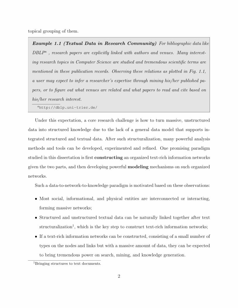
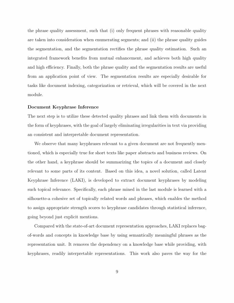
documents
Words:dbscan, methods, clustering, process, …
Topics:[k-means, clustering, clusters, dbscan, …]
[clusters, density, dbscan, clustering, …][machine, learning, knowledge, mining, …]
Knowledge base concepts:data mining: /m/0blvg
clustering analysis: /m/031f5pdbscan: /m/03cg_k1
Document
Representation
Others?
Document Keyphrase:dbscan: [dbscan, density, clustering, ...]
clustering: [clustering, clusters, partition, ...]data mining: [data mining, knowledge, ...]
authorvenue
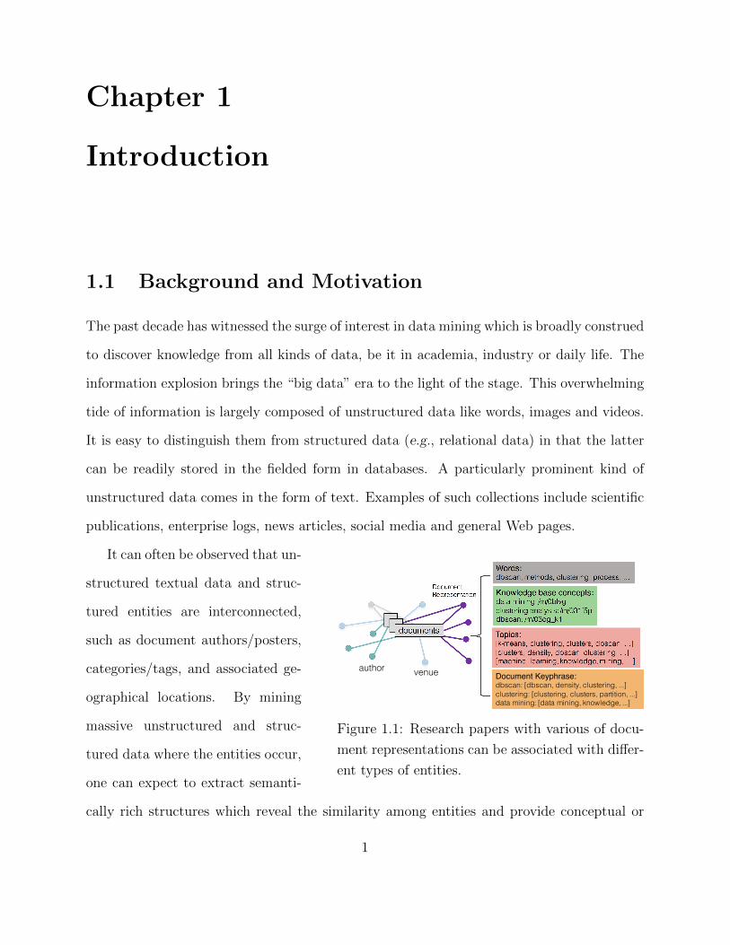
Figure 1.1: Research papers with various of docu-
ment representations can be associated with differ-
ent types of entities.
It can often be observed that un-
structured textual data and struc-
tured entities are interconnected,
such as document authors/posters,
categories/tags, and associated ge-
ographical locations. By mining
massive unstructured and struc-
tured data where the entities occur,
one can expect to extract semanti-
cally rich structures which reveal the similarity among entities and provide conceptual or
1
topical grouping of them.
Example 1.1 (Textual Data in Research Community) For bibliographic data like
DBLPa , research papers are explicitly linked with authors and venues. Many interest-
ing research topics in Computer Science are studied and tremendous scientific terms are
mentioned in these publication records. Observing these relations as plotted in Fig. 1.1,
a user may expect to infer a researcher’s expertise through mining his/her published pa-
pers, or to figure out what venues are related and what papers to read and cite based on
his/her research interest.
ahttp://dblp.uni-trier.de/
Under this expectation, a core research challenge is how to turn massive, unstructured
data into structured knowledge due to the lack of a general data model that supports in-
tegrated structured and textual data. After such structuralization, many powerful analysis
methods and tools can be developed, experimented and refined. One promising paradigm
studied in this dissertation is first constructing an organized text-rich information networks
given the two parts, and then developing powerful modeling mechanisms on such organized
networks.
Such a data-to-network-to-knowledge paradigm is motivated based on these observations:
• Most social, informational, and physical entities are interconnected or interacting,
forming massive networks;
• Structured and unstructured textual data can be naturally linked together after text
structuralization1, which is the key step to construct text-rich information networks;
• If a text-rich information networks can be constructed, consisting of a small number of
types on the nodes and links but with a massive amount of data, they can be expected
to bring tremendous power on search, mining, and knowledge generation.
1Bringing structures to text documents.
2
However, this paradigm poses significant challenges to the traditional text and network
mining techniques, including the following but not limited to
• The emerging big textual data, such as social media messages, can deviate from rigor-
ous language rules. Using various kinds of heavily trained linguistic processing makes
the method difficult to be applied.
• Document length and vocabulary may vary significantly across the corpus, e.g., web
pages. A good text structuralization approach needs to eliminate these obstacles and
generate compatible document representation.
• If a text-rich information networks can be constructed, it will be such a powerful tool
in data mining applications that we may predict it in no time to meet the requirements
of being extremely robust and scalable.
In this regard, we believe that the community would welcome and benefit from a set of
data-drive algorithms that work for large-scale datasets involving irregular textual data in
a robust way, while minimizing the human labeling cost. We are also convinced by various
study and experiments that our proposed methods embody enough novelty and contribution
to add solid building block, if not lay a sound base to the successive research.
1.2 Problem Formalization
We have developed a phrase mining algorithm en route of tackling the above mentioned chal-
lenge, which is one of our main contributions. This text structuraliation technique discovers
and utilizes semantically meaningful phrases from massive irregular text. Specifically,
3
Problem 1.1: Phrase Mining
Given a large in-domain document corpus D with specific focus on certain genres of
content, which can be any textual word sequences with arbitrary lengths, such as
articles, titles and queries, phrase mining tries to assign a value between 0 and 1 to
indicate the quality of each phrase, and provide a segmenter being able to partition a
text snippet into un-overlapped segments and identify phrase mentions. Phrases with
scores larger than 0.5 are viewed as quality phrases K = K1, · · · , KM.
Definition 1.1 (Quality Phrase) A quality phrase is a sequence of words that appear
contiguously in the text, and serves as a whole (non-composible) semantic unit in certain
context of the given documents.
There is no universally accepted definition of phrase quality. However, it is useful to
quantify phrase quality based on certain criteria, which will be discussed and defined in
Chapter 3. Note that within a particular domain, a phrase will likely have one meaning [36],
making the phrase relatively unambiguous and its quality estimation feasible. Moreover,
phrase quality is not contextual dependent. For example, both ‘knowledge discovery’ and
‘np hard’ are identified to be quality phrases from the bibliographic data in the computer
science domain. But in a specific paper published in the data mining conference, ‘knowledge
discovery’ should be considered to be more salient than ‘np hard’ even though they are
both mentioned in that paper. We call such salient phrases in the document as document
keyphrases, formally defined as
Definition 1.2 (Document Keyphrase) A document keyphrase is a quality phrase
that is relevant to a specific in-domain document, i.e., it serves as an informative word
or phrase to indicate the content of that specific document.
4
Different from typical way of defining keyphrase in the literature, we do not require their
number of mentions in a document to be significantly large. A supporting example is that: a
text mining paper may only mention ‘text mining’ once in its abstract, but this phrase is still
of great value since it is topically relevant to the rest of the content. This presents a brand
new challenge as well as brings great usefulness, especially for short texts. We formalize this
challenging problem as follows:
Problem 1.2: Document Keyphrase Extraction
Given a large collection of documents C and a set of high quality phrases K =
K1, · · · , KM, we aim to build a keyphrase extractor that can automatically iden-
tify document keyphrases given a new text query q, and infer strength scores
[P(q)1 , · · · , P (q)
M ]. Each entry in the vector quantifies relatedness between query and
a phrase in the range [0, 1]. Phrases with positive strength scores are considered to be
document keyphrases.
Compared with existing text mining approaches of modeling documents such as taking n-
grams, deriving noun phrases or using knowledge base concepts as demonstrated in Fig. 1.1,
we argue that high quality document keyphrases are naturally a better choice in the big
data scenario since they capture meaningful sequences of different lengths and can be easily
applied to emerging big corpora as a data-driven approach.
Meanwhile, documents become more structured and from the perspective of network, one
can think of bipartite relations between documents and keyphrases. On top of this simple
network, incorporating entities associated with the document extends the bipartite rela-
tions to higher-order relations, which is defined as a text-rich information network
throughout this dissertation.
5
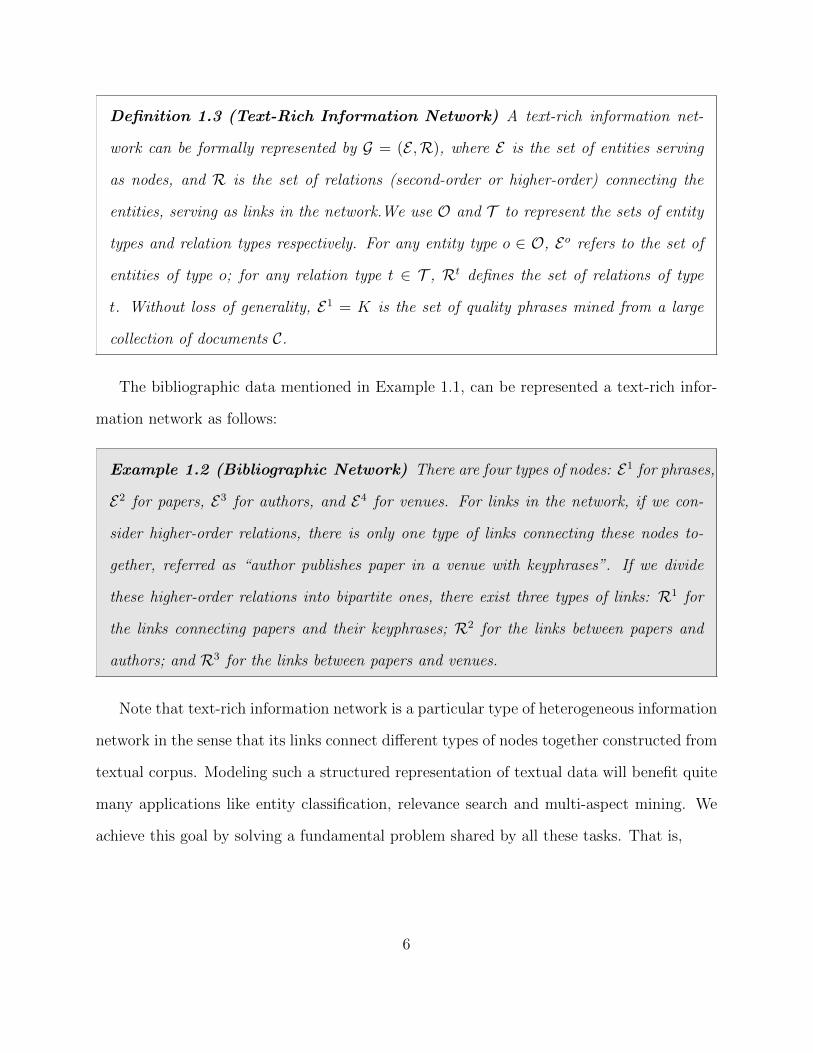
Definition 1.3 (Text-Rich Information Network) A text-rich information net-
work can be formally represented by G = (E ,R), where E is the set of entities serving
as nodes, and R is the set of relations (second-order or higher-order) connecting the
entities, serving as links in the network.We use O and T to represent the sets of entity
types and relation types respectively. For any entity type o ∈ O, Eo refers to the set of
entities of type o; for any relation type t ∈ T , Rt defines the set of relations of type
t. Without loss of generality, E1 = K is the set of quality phrases mined from a large
collection of documents C.
The bibliographic data mentioned in Example 1.1, can be represented a text-rich infor-
mation network as follows:
Example 1.2 (Bibliographic Network) There are four types of nodes: E1 for phrases,
E2 for papers, E3 for authors, and E4 for venues. For links in the network, if we con-
sider higher-order relations, there is only one type of links connecting these nodes to-
gether, referred as “author publishes paper in a venue with keyphrases”. If we divide
these higher-order relations into bipartite ones, there exist three types of links: R1 for
the links connecting papers and their keyphrases; R2 for the links between papers and
authors; and R3 for the links between papers and venues.
Note that text-rich information network is a particular type of heterogeneous information
network in the sense that its links connect different types of nodes together constructed from
textual corpus. Modeling such a structured representation of textual data will benefit quite
many applications like entity classification, relevance search and multi-aspect mining. We
achieve this goal by solving a fundamental problem shared by all these tasks. That is,
6
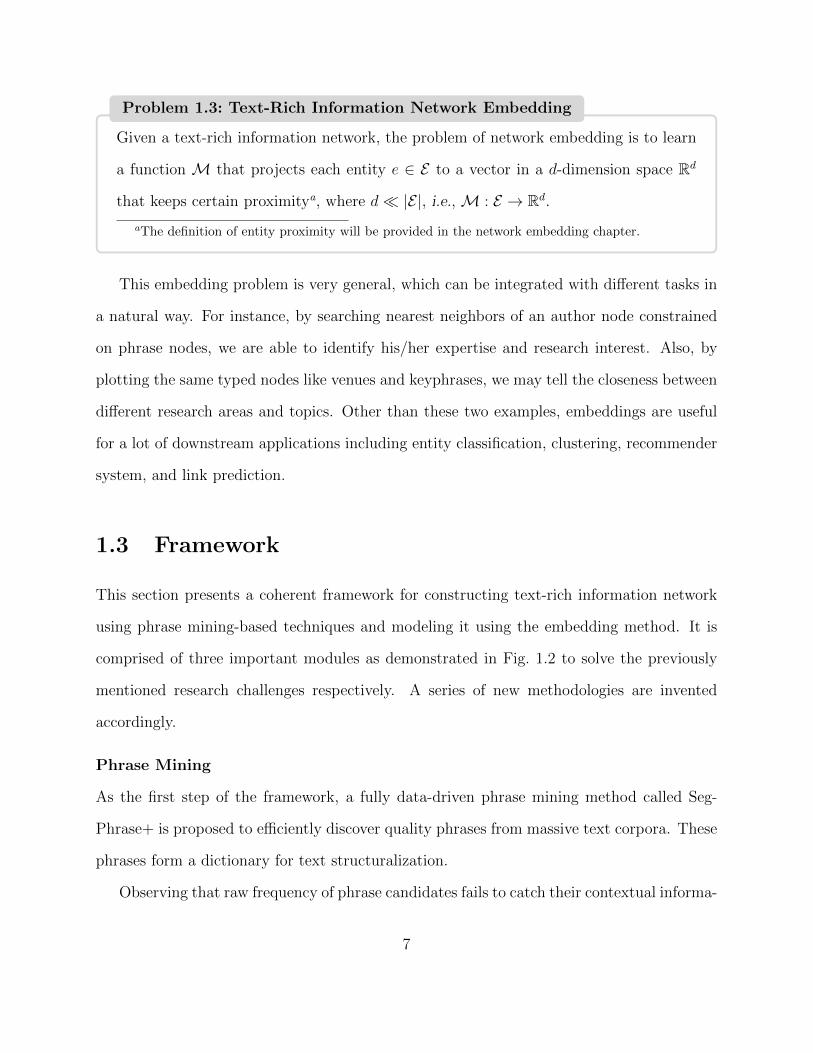
Problem 1.3: Text-Rich Information Network Embedding
Given a text-rich information network, the problem of network embedding is to learn
a function M that projects each entity e ∈ E to a vector in a d-dimension space Rd
that keeps certain proximitya, where d |E|, i.e., M : E → Rd.
aThe definition of entity proximity will be provided in the network embedding chapter.
This embedding problem is very general, which can be integrated with different tasks in
a natural way. For instance, by searching nearest neighbors of an author node constrained
on phrase nodes, we are able to identify his/her expertise and research interest. Also, by
plotting the same typed nodes like venues and keyphrases, we may tell the closeness between
different research areas and topics. Other than these two examples, embeddings are useful
for a lot of downstream applications including entity classification, clustering, recommender
system, and link prediction.
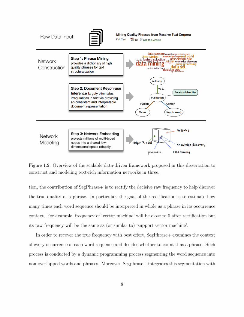
1.3 Framework
This section presents a coherent framework for constructing text-rich information network
using phrase mining-based techniques and modeling it using the embedding method. It is
comprised of three important modules as demonstrated in Fig. 1.2 to solve the previously
mentioned research challenges respectively. A series of new methodologies are invented
accordingly.
Phrase Mining
As the first step of the framework, a fully data-driven phrase mining method called Seg-
Phrase+ is proposed to efficiently discover quality phrases from massive text corpora. These
phrases form a dictionary for text structuralization.
Observing that raw frequency of phrase candidates fails to catch their contextual informa-
7
Step 2: Document Keyphrase
Inference!largely eliminates
irregularities in text via providing
an consistent and interpretable
document representation
Network
Construction
Network
Modeling
Raw Data Input:
!"#"$%&'&'(
)'*+,-.(-$.&/0*1-23
42"56&0/
7.("2$ 89$:*..
Step 1: Phrase Mining!provides a dictionary of high
quality phrases for text
structuralization
Step 3: Network Embedding!projects millions of multi-typed
nodes into a shared low-
dimensional space robustly.
Figure 1.2: Overview of the scalable data-driven framework proposed in this dissertation to
construct and modeling text-rich information networks in three.
tion, the contribution of SegPhrase+ is to rectify the decisive raw frequency to help discover
the true quality of a phrase. In particular, the goal of the rectification is to estimate how
many times each word sequence should be interpreted in whole as a phrase in its occurrence
context. For example, frequency of ‘vector machine’ will be close to 0 after rectification but
its raw frequency will be the same as (or similar to) ‘support vector machine’.
In order to recover the true frequency with best effort, SegPhrase+ examines the context
of every occurrence of each word sequence and decides whether to count it as a phrase. Such
process is conducted by a dynamic programming process segmenting the word sequence into
non-overlapped words and phrases. Moreover, Segphrase+ integrates this segmentation with
8
the phrase quality assessment, such that (i) only frequent phrases with reasonable quality
are taken into consideration when enumerating segments; and (ii) the phrase quality guides
the segmentation, and the segmentation rectifies the phrase quality estimation. Such an
integrated framework benefits from mutual enhancement, and achieves both high quality
and high efficiency. Finally, both the phrase quality and the segmentation results are useful
from an application point of view. The segmentation results are especially desirable for
tasks like document indexing, categorization or retrieval, which will be covered in the next
module.
Document Keyphrase Inference
The next step is to utilize these detected quality phrases and link them with documents in
the form of keyphrases, with the goal of largely eliminating irregularities in text via providing
an consistent and interpretable document representation.
We observe that many keyphrases relevant to a given document are not frequently men-
tioned, which is especially true for short texts like paper abstracts and business reviews. On
the other hand, a keyphrase should be summarizing the topics of a document and closely
relevant to some parts of its content. Based on this idea, a novel solution, called Latent
Keyphrase Inference (LAKI), is developed to extract document keyphrases by modeling
such topical relevance. Specifically, each phrase mined in the last module is learned with a
silhouette-a cohesive set of topically related words and phrases, which enables the method
to assign appropriate strength scores to keyphrase candidates through statistical inference,
going beyond just explicit mentions.
Compared with the state-of-art document representation approaches, LAKI replaces bag-
of-words and concepts in knowledge base by using semantically meaningful phrases as the
representation unit. It removes the dependency on a knowledge base while providing, with
keyphrases, readily interpretable representations. This work also paves the way for the
9
third module, i.e., finally constructing and modeling more complicated text-rich information
networks which involve in entities associated with the documents like authors, locations, etc.
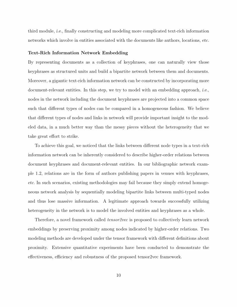
Text-Rich Information Network Embedding
By representing documents as a collection of keyphrases, one can naturally view those
keyphrases as structured units and build a bipartite network between them and documents.
Moreover, a gigantic text-rich information network can be constructed by incorporating more
document-relevant entities. In this step, we try to model with an embedding approach, i.e.,
nodes in the network including the document keyphrases are projected into a common space
such that different types of nodes can be compared in a homogeneous fashion. We believe
that different types of nodes and links in network will provide important insight to the mod-
eled data, in a much better way than the messy pieces without the heterogeneity that we
take great effort to strike.
To achieve this goal, we noticed that the links between different node types in a text-rich
information network can be inherently considered to describe higher-order relations between
document keyphrases and document-relevant entities. In our bibliographic network exam-
ple 1.2, relations are in the form of authors publishing papers in venues with keyphrases,
etc. In such scenarios, existing methodologies may fail because they simply extend homoge-
neous network analysis by sequentially modeling bipartite links between multi-typed nodes
and thus lose massive information. A legitimate approach towards successfully utilizing
heterogeneity in the network is to model the involved entities and keyphrases as a whole.
Therefore, a novel framework called tensor2vec is proposed to collectively learn network
embeddings by preserving proximity among nodes indicated by higher-order relations. Two
modeling methods are developed under the tensor framework with different definitions about
proximity. Extensive quantitative experiments have been conducted to demonstrate the
effectiveness, efficiency and robustness of the proposed tensor2vec framework.
10

We hope such an embedding approach can benefit a number of different data mining
tasks including relevance search, recommendation and classification.
The rest of the thesis is organized as follows. Chapter 2 reviews the literature. Then
the above modules are presented in Chapter 3 to 5. Chapter 6 concludes this thesis and
discusses the future work.
11
Chapter 2
Literature Review
In this chapter, an overview of the related work in constructing and modeling text-rich
information networks are first provided, followed by a detailed discussion about the literature
relevent to our proposed approaches.
2.1 Constructing Text-Rich Information Network
In order to construct high-quality information networks from textual data, information ex-
traction, natural language processing, and many other techniques should be integrated with
network construction. For textual data from general domain, entity linking techniques [90]
are developed to map from given entity mentions detected in text to entities in manually
curated knowledge bases like Freebase. For data in closed-domain where entity coverage in
public knowledge base is limited, mining quality phrases is a critical step. Similar to our
phrase mining work, [32] proposes a computationally efficient and effective model ToPMine,
which first executes an unsupervised phrase mining framework to segment a document into
single and multi-word phrases, and then employs a new topic model that operates on the
induced document partition. On top of that, entity typing techniques [84, 85] run data-
driven phrase mining to generate entity mention candidates and assign (fine-grained) types
(e.g., people, artist, actor) to mentions of entities in documents. Relationship extraction
is another important step to form links in network. Surface patterns between mentions of
entities in the text are grouped or categorized to serve as relations [106].
12
For the structured entities associated with textual data like relational database, it may
be easy to partially construct an information network from it with well-defined schema. But
they can still be noisy in real world. The first problem is ambiguity. That is, one entity in a
network may refer to multiple surface names, or different entities may correspond to the same
surface name in the input data. Realizing this problem, the goal of entity resolution [11, 62] is
to determine the mapping between entities and their mentions in the input structured data.
Secondly, relations among entities may not be explicitly given or not complete sometimes,
e.g., the advisor-advisee relationship in the academia network [109]. Link prediction [60] can
be employed to fill out the missing relations for comprehensive networks. Finally, links may
not be reliable or trustable, e.g., the inaccurate item information in an E-commerce website
and conflicting information of certain objects from multiple websites. Studies on this mainly
include truth discovery [58] and crowdsourcing [33].
2.2 Modeling Text-Rich Information Network
Once the text-rich information network is constructed, the modeling part is similar to the
existing literature regarding heterogeneous information network.
Compared to the widely-used homogeneous information network which models links be-
tween single-typed nodes, the heterogeneous information network can effectively fuse more
information and contain rich semantics in nodes and links, and thus it forms a new develop-
ment of data mining. More and more researchers have noticed the importance of heteroge-
neous information network analysis and many novel data mining tasks have been exploited
in such networks, such as similarity search [96], clustering [65, 97], classification [45], recom-
mendation [115] and information fusion [40]. More detailed literature review is introduced
in a recent survey [91].
Heterogeneous information network is a powerful tool to handle the variety of big data,
13
since it can flexibly and effectively integrate varied objects and heterogeneous information.
However, it is non-trivial work to build a real heterogeneous information network based
analysis system for huge, even dynamic data. So it usually cannot be contained in memory
and cannot be handled directly. Most of contemporary data mining tasks on heterogeneous
information network only work on small dataset, and fail to consider the quick and parallel
process on big data. But for our constructed text-rich information network, the scale is
really large considering millions of documents. There is an urge need for a scalable and
robust network mining technique that can solve very fundamental problem and serve the
results with other mining tasks.
2.3 Phrase Mining
Automatic extraction of quality phrases (i.e., multiword semantic units) from massive, dy-
namically growing corpora gains increasing attention due to its value in text analytics of
various domains. As the origin, the NLP community has conducted extensive studies
[111, 34, 79, 118, 5]. With pre-defined POS rules, one can generate noun phrases from
each document1. However, such rule-based methods usually suffer in domain adaptation.
Supervised noun phrase chunking techniques [81, 113, 20] leverage annotated documents
to automatically learn rules based on POS-tagged corpus. These supervised methods may
utilize more sophisticated NLP features such as dependency parser to further enhance the
precision [52, 69]. The various kinds of linguistic processing, domain-dependent language
rules, and expensive human labeling make it challenging to apply to emerging big corpora.
Another kind of approaches explore frequency statistics in document collections [28, 82,
78, 26, 32]. Most of them leverage a variety of statistical measures derived from a corpus to
estimate phrase quality. Therefore, they do not rely on linguistic feature generation, domain-
1http://www.nltk.org/howto/chunk.html
14
specific rules or large training sets, and can process massive corpora efficiently. In [78], several
indicators, including frequency and comparison to super/sub-sequences, were proposed to
extract n-grams that are not only popular but also concise as concepts. Deane [28] proposed
a heuristic metric over frequency distribution based on Zipfian ranks, to measure lexical
association for phrase candidates.
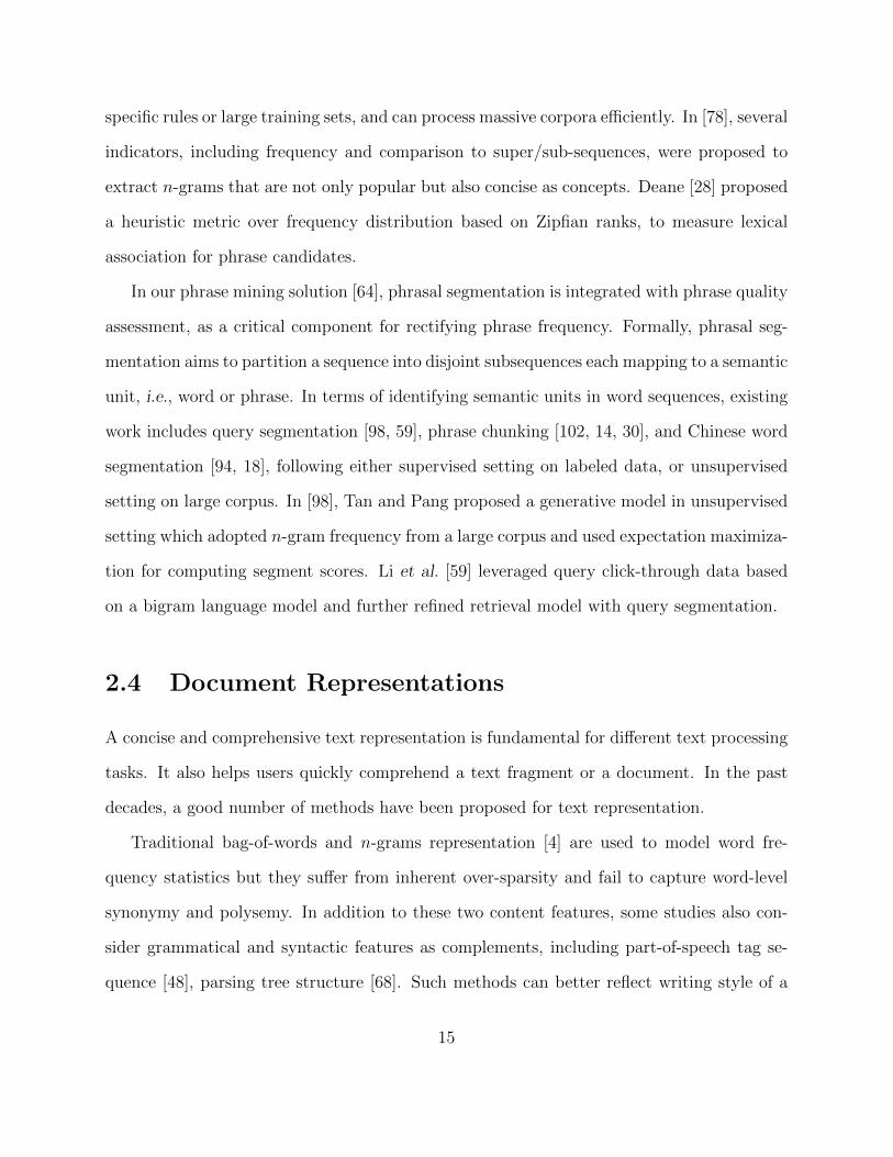
In our phrase mining solution [64], phrasal segmentation is integrated with phrase quality
assessment, as a critical component for rectifying phrase frequency. Formally, phrasal seg-
mentation aims to partition a sequence into disjoint subsequences each mapping to a semantic
unit, i.e., word or phrase. In terms of identifying semantic units in word sequences, existing
work includes query segmentation [98, 59], phrase chunking [102, 14, 30], and Chinese word
segmentation [94, 18], following either supervised setting on labeled data, or unsupervised
setting on large corpus. In [98], Tan and Pang proposed a generative model in unsupervised
setting which adopted n-gram frequency from a large corpus and used expectation maximiza-
tion for computing segment scores. Li et al. [59] leveraged query click-through data based
on a bigram language model and further refined retrieval model with query segmentation.
2.4 Document Representations
A concise and comprehensive text representation is fundamental for different text processing
tasks. It also helps users quickly comprehend a text fragment or a document. In the past
decades, a good number of methods have been proposed for text representation.
Traditional bag-of-words and n-grams representation [4] are used to model word fre-
quency statistics but they suffer from inherent over-sparsity and fail to capture word-level
synonymy and polysemy. In addition to these two content features, some studies also con-
sider grammatical and syntactic features as complements, including part-of-speech tag se-
quence [48], parsing tree structure [68]. Such methods can better reflect writing style of a
15
text fragment. But they rely on existing NLP tools and are heavily trained to be working
in a specific domain (usually open-domain).
On the other hand, neural network models are used to learn embeddings for each word in
a continuous space, e.g., distributed representation, which can encode not only attributional
similarity (i.e., words that appear in similar contexts will be close in the projected space),
but also the linguistic regularities (i.e., relational similarity between a pair of words) into
the learned vectors [8, 72]. However, aforementioned document representations are lack of
semantic interpretation—they do not have explicit semantic meaning and thus are hard to
be understood by users.
To provide an overview of the input text with richer semantics, a number of latent
topic-based methods are proposed [29, 15]. These methods leverage corpus-level word co-
occurrence statistics to discover different themes (i.e., latent topics) behind the input text,
and represent it using a vector where each dimension is a latent topic and each topic is a
distribution over words. Nevertheless, the interpretability of latent space for topic models is
still not straightforward and pursuing semantic meaning in inferred topics is difficult [17].
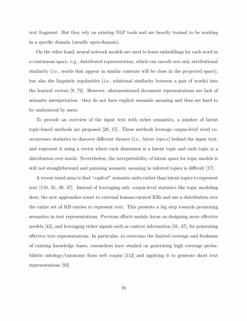
A recent trend aims to find “explicit” semantic units rather than latent topics to represent
text [110, 35, 39, 47]. Instead of leveraging only corpus-level statistics like topic modeling
does, the new approaches resort to external human-curated KBs and use a distribution over
the entire set of KB entries to represent text. This presents a big step towards promoting
semantics in text representations. Previous efforts mainly focus on designing more effective
models [43], and leveraging richer signals such as context information [31, 47], for generating
effective text representations. In particular, to overcome the limited coverage and freshness
of existing knowledge bases, researchers have studied on generating high coverage proba-
bilistic ontology/taxonomy from web corpus [112] and applying it to generate short text
representations [93].
16
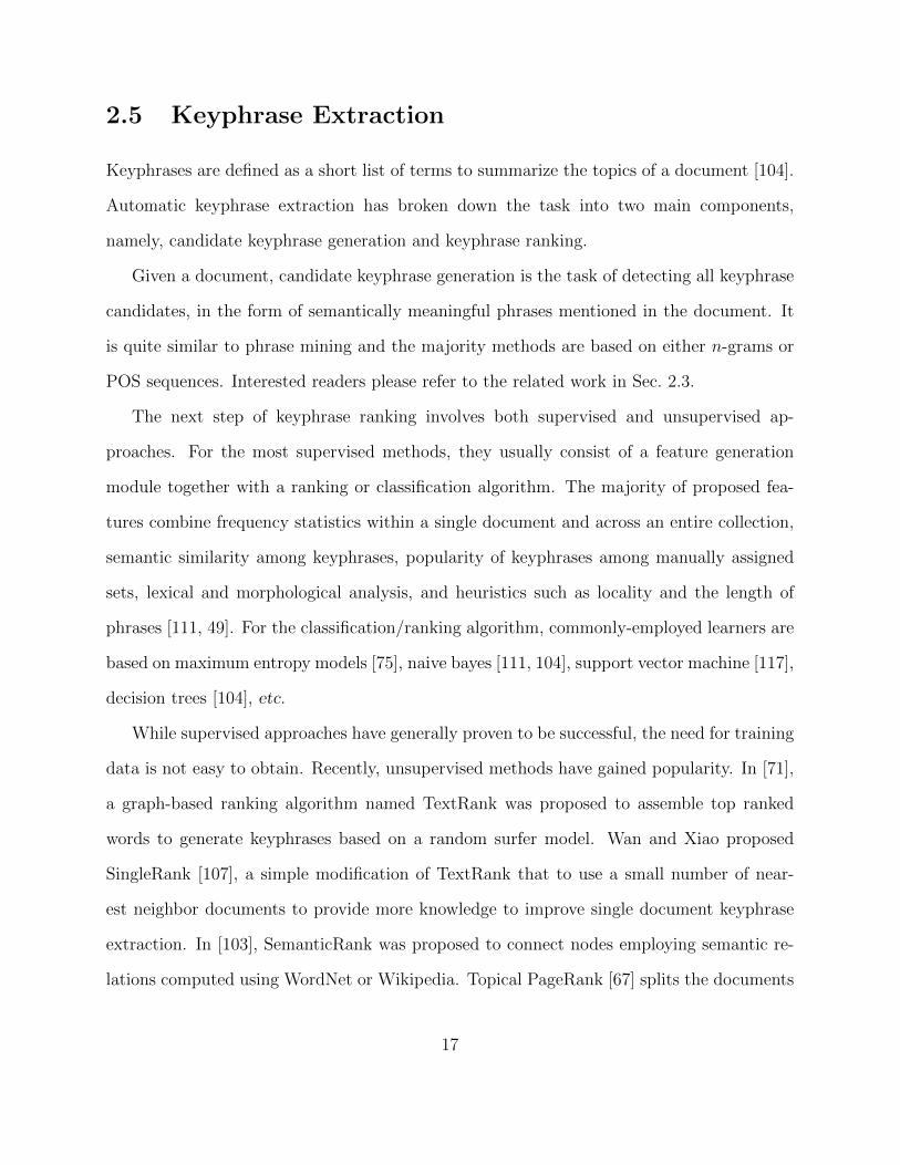
2.5 Keyphrase Extraction
Keyphrases are defined as a short list of terms to summarize the topics of a document [104].
Automatic keyphrase extraction has broken down the task into two main components,
namely, candidate keyphrase generation and keyphrase ranking.
Given a document, candidate keyphrase generation is the task of detecting all keyphrase
candidates, in the form of semantically meaningful phrases mentioned in the document. It
is quite similar to phrase mining and the majority methods are based on either n-grams or
POS sequences. Interested readers please refer to the related work in Sec. 2.3.
The next step of keyphrase ranking involves both supervised and unsupervised ap-
proaches. For the most supervised methods, they usually consist of a feature generation
module together with a ranking or classification algorithm. The majority of proposed fea-
tures combine frequency statistics within a single document and across an entire collection,
semantic similarity among keyphrases, popularity of keyphrases among manually assigned
sets, lexical and morphological analysis, and heuristics such as locality and the length of
phrases [111, 49]. For the classification/ranking algorithm, commonly-employed learners are
based on maximum entropy models [75], naive bayes [111, 104], support vector machine [117],
decision trees [104], etc.
While supervised approaches have generally proven to be successful, the need for training
data is not easy to obtain. Recently, unsupervised methods have gained popularity. In [71],
a graph-based ranking algorithm named TextRank was proposed to assemble top ranked
words to generate keyphrases based on a random surfer model. Wan and Xiao proposed
SingleRank [107], a simple modification of TextRank that to use a small number of near-
est neighbor documents to provide more knowledge to improve single document keyphrase
extraction. In [103], SemanticRank was proposed to connect nodes employing semantic re-
lations computed using WordNet or Wikipedia. Topical PageRank [67] splits the documents
17
into topics using a Latent Dirichlet Allocation model [15] and creates keyphrases from top
ranked topical words.
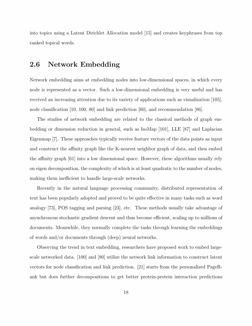
2.6 Network Embedding
Network embedding aims at embedding nodes into low-dimensional spaces, in which every
node is represented as a vector. Such a low-dimensional embedding is very useful and has
received an increasing attention due to its variety of applications such as visualization [105],
node classification [10, 100, 80] and link prediction [60], and recommendation [86].
The studies of network embedding are related to the classical methods of graph em-
bedding or dimension reduction in general, such as IsoMap [101], LLE [87] and Laplacian
Eigenmap [7]. These approaches typically receive feature vectors of the data points as input
and construct the affinity graph like the K-nearest neighbor graph of data, and then embed
the affinity graph [61] into a low dimensional space. However, these algorithms usually rely
on eigen decomposition, the complexity of which is at least quadratic to the number of nodes,
making them inefficient to handle large-scale networks.
Recently in the natural language processing community, distributed representation of
text has been popularly adopted and proved to be quite effective in many tasks such as word
analogy [73], POS tagging and parsing [23], etc. These methods usually take advantage of
asynchronous stochastic gradient descent and thus become efficient, scaling up to millions of
documents. Meanwhile, they normally complete the tasks through learning the embeddings
of words and/or documents through (deep) neural networks.
Observing the trend in text embedding, researchers have proposed work to embed large-
scale networked data. [100] and [80] utilize the network link information to construct latent
vectors for node classification and link prediction. [21] starts from the personalized PageR-
ank but does further decompositions to get better protein-protein interaction predictions
18
in biology networks. However, these “homogeneous” models cannot capture the extra node
type information and the information about relations across different typed nodes in hetero-
geneous information networks.
Heterogeneous information network is essentially an abstraction of higher-order rela-
tional data, where a higher-order relation is denoted as a hyper-link connecting more than
two nodes. It is worth noting that text-rich information network is a specific type of hetero-
geneous information newtork that is constructed from textual corpus and incorporate many
document-associated entities. There are also a few embedding algorithms developed for
such heterogeneous networks. But instead of modeling proximity among nodes co-occur in
each higher-order relation, both [99] and [19] decompose the high-order relation into several
pairwise interactions and then model them separately similar to the homogeneous setting
mentioned previously. Our model is substantially different since we directly model each
higher-order relation in heterogeneous information networks so that the proximity among
nodes can be better preserved.
In order to model the higher-order relations in the networks, we developed a tensor-based
framework. Studies of similar flavor of tensor modeling [50] have recently emerged for some
other mining tasks, such as recommender system [86], multi-relational learning [44], and
clustering [9]. In [86], a tensor factorization model is designed specifically for tag recommen-
dation; while we explore a more general framework for embedding from which two methods
are designed to model the entity-driven and relation-driven proximity respectively. [9] de-
fines higher-order network structures, such as cycles and feed-forward loops, and uses tensor
to model the higher-order relations. In sharp contrast, our framework is more general in
the sense that it allows a relatively large set of relation schema to describe networked data.
In addition, [9] only models the relation with one type of entity; while tensor2vec supports
multiple node types in multiple relations in a network.
19
Chapter 3
A Data-Driven Approach for PhraseMining
As the building block for text structuralization, phrase mining refers to the process of ex-
tracting quality phrases from a in-domain corpus. In large, dynamic collections of docu-
ments, analysts are often interested in variable-length phrases, including scientific concepts,
events, organizations, products, slogans and so on. Efficient extraction of quality phrases
enable a large body of applications to transform from word granularity to phrase granular-
ity. In the literature, examples of such applications include topic tracking [55], OLAP on
multi-dimensional text collections [116], and document categorization.
Though the study of this task originates from the natural language processing (NLP)
community, the challenge has been recognized of applying NLP tools in the emerging big data
that deviate from rigorous language rules. Query logs, social media messages, and textual
transaction records are just a few examples. Therefore, researchers have sought more general
data-driven approaches, primarily based on the frequent pattern mining principle [2, 92].
The early work focuses on efficiently retrieving recurring word sequences, but many such
sequences do not form meaningful phrases. More recent work filters or ranks them according
to frequency-based statistics. However, the raw frequency from the data tends to produce
misleading quality assessment, and the outcome is unsatisfactory, as the following example
demonstrates.
20
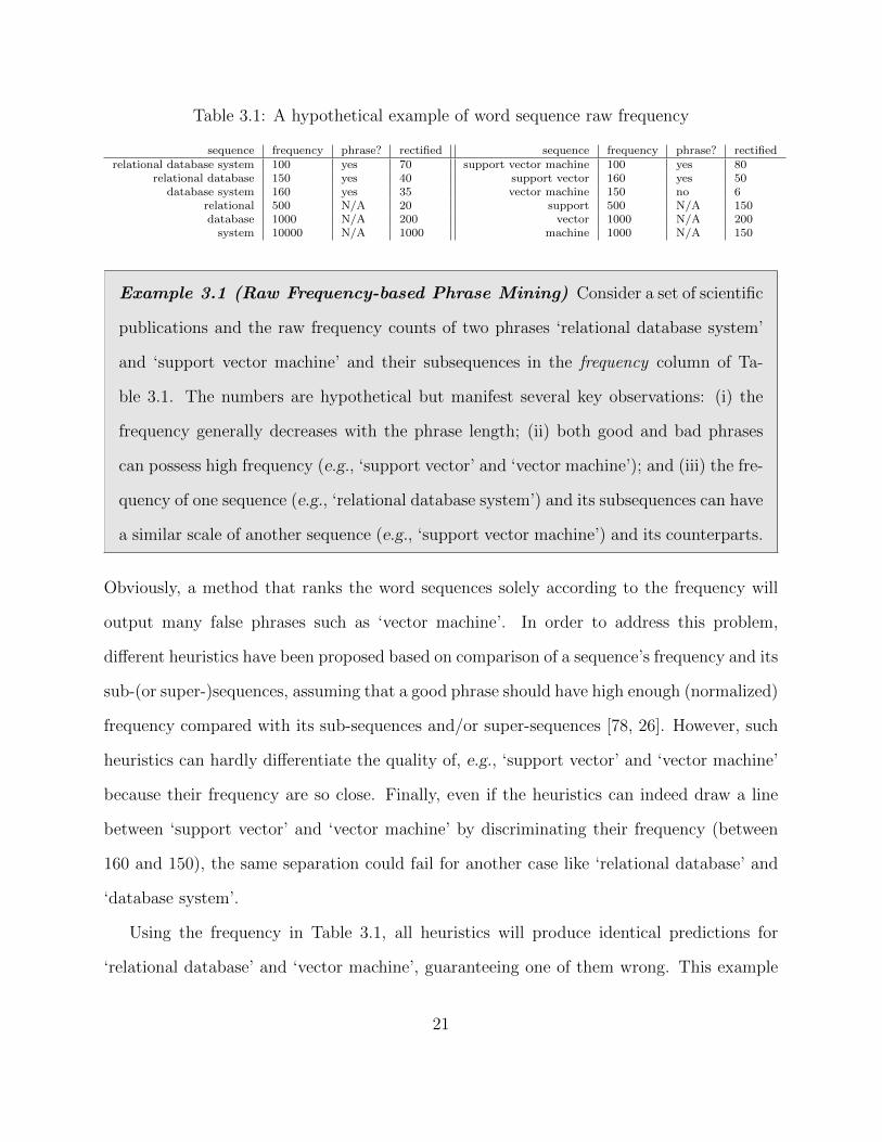
Table 3.1: A hypothetical example of word sequence raw frequency
sequence frequency phrase? rectified sequence frequency phrase? rectifiedrelational database system 100 yes 70 support vector machine 100 yes 80
relational database 150 yes 40 support vector 160 yes 50database system 160 yes 35 vector machine 150 no 6
relational 500 N/A 20 support 500 N/A 150database 1000 N/A 200 vector 1000 N/A 200
system 10000 N/A 1000 machine 1000 N/A 150
Example 3.1 (Raw Frequency-based Phrase Mining) Consider a set of scientific
publications and the raw frequency counts of two phrases ‘relational database system’
and ‘support vector machine’ and their subsequences in the frequency column of Ta-
ble 3.1. The numbers are hypothetical but manifest several key observations: (i) the
frequency generally decreases with the phrase length; (ii) both good and bad phrases
can possess high frequency (e.g., ‘support vector’ and ‘vector machine’); and (iii) the fre-
quency of one sequence (e.g., ‘relational database system’) and its subsequences can have
a similar scale of another sequence (e.g., ‘support vector machine’) and its counterparts.
Obviously, a method that ranks the word sequences solely according to the frequency will
output many false phrases such as ‘vector machine’. In order to address this problem,
different heuristics have been proposed based on comparison of a sequence’s frequency and its
sub-(or super-)sequences, assuming that a good phrase should have high enough (normalized)
frequency compared with its sub-sequences and/or super-sequences [78, 26]. However, such
heuristics can hardly differentiate the quality of, e.g., ‘support vector’ and ‘vector machine’
because their frequency are so close. Finally, even if the heuristics can indeed draw a line
between ‘support vector’ and ‘vector machine’ by discriminating their frequency (between
160 and 150), the same separation could fail for another case like ‘relational database’ and
‘database system’.
Using the frequency in Table 3.1, all heuristics will produce identical predictions for
‘relational database’ and ‘vector machine’, guaranteeing one of them wrong. This example
21

suggests the intrinsic limitations of using raw frequency counts, especially in judging whether
a sequence is too long (longer than a minimum semantic unit), too short (broken and not
informative), or right in length. It is a critical bottleneck for all frequency-based quality
assessment.
In this work [64], we address this bottleneck, proposing to rectify the decisive raw fre-
quency that hinders discovering the true quality of a phrase. The goal of the rectification is
to estimate how many times each word sequence should be interpreted in whole as a phrase
in its occurrence context. The following example illustrates this idea.
Example 3.2 (Rectification) Consider the following occurrences of the 6 multi-word
sequences listed in Table 3.1.
1. A drelational database systemc for images...
2. dDatabase systemc empowers everyone in your organization...
3. More formally, a dsupport vector machinec constructs a hyperplane...
4. The dsupport vectorc method is a new general method of dfunction estimationc...
5. A standard dfeature vectorc dmachine learningc setup is used to describe...
6. dRelevance vector machinec has an identical dfunctional formc to the dsupport
vector machinec...
7. The basic goal for dobject-oriented relational databasec is to dbridge the gapc be-
tween...
The first 4 instances should provide positive counts to these sequences, while the last three
instances should not provide positive counts to ‘vector machine’ or ‘relational database’
because they should not be interpreted as a whole phrase (instead, sequences like ‘feature
22
vector’ and ‘relevance vector machine’ can). Suppose one can correctly count true occur-
rences of the sequences, and collect rectified frequency as shown in the rectified column of
Table 3.1. The rectified frequency now clearly distinguishes ‘vector machine’ from the other
phrases, since ‘vector machine’ rarely occurs as a whole phrase.
The success of this approach relies on reasonably accurate rectification. Simple arith-
metics of the raw frequency, such as subtracting one sequence’s count with its quality super
sequence, are prone to error. First, which super sequences are quality phrases is a question
itself. Second, it is context-dependent to decide whether a sequence should be deemed a
whole phrase. For example, the fifth instance in Example 3.2 prefers ‘feature vector’ and
‘machine learning’ over ‘vector machine’, even though neither ‘feature vector machine’ nor
‘vector machine learning’ is a quality phrase. The context information is lost when we only
collect the frequency counts.
In order to recover the true frequency with best effort, we ought to examine the context
of every occurrence of each word sequence and decide whether to count it as a phrase. The
examination for one occurrence may involve enumeration of alternative possibilities, such as
extending the sequence or breaking the sequence, and comparison among them. The test
for word sequence occurrences could be expensive, losing the advantage in efficiency of the
frequent pattern mining approaches.
Facing the challenge of accuracy and efficiency, we propose a segmentation approach
named phrasal segmentation, and integrate it with the phrase quality assessment in a unified
framework with linear complexity (w.r.t the corpus size). First, the segmentation assigns
every word occurrence to only one phrase. In the first instance of Example 3.2, ‘relational
database system’ are bundled as a single phrase. Therefore, it automatically avoids double
counting ‘relational database’ and ‘database system’ within this instance. Similarly, the
segmentation of the fifth instance contributes to the count of ‘feature vector’ and ‘machine
learning’ instead of ‘feature’, ‘vector machine’ and ‘learning’. This strategy condenses the
23
individual tests for each word sequence and reduces the overall complexity while ensures
correctness. Second, though there are an exponential number of possible partitions of the
documents, we are concerned with those relevant to the phrase extraction task only. There-
fore, we can integrate the segmentation with the phrase quality assessment, such that (i)
only frequent phrases with reasonable quality are taken into consideration when enumerat-
ing partitions; and (ii) the phrase quality guides the segmentation, and the segmentation
rectifies the phrase quality estimation. Such an integrated framework benefits from mutual
enhancement, and achieves both high quality and high efficiency. Finally, both the phrase
quality and the segmentation results are useful from an application point of view. The seg-
mentation results are especially desirable for tasks like document indexing, categorization or
retrieval.
The main contributions lie in the following aspects:
• Realizing the limitation of raw frequency-based phrase mining, we propose a novel
segmentation-integrated framework to rectify the raw frequency. To the best of our
knowledge, it is the first work to integrate phrase extraction and phrasal segmentation
and mutually benefit each other.
• The proposed method is scalable: both computation time and required space grow
linearly as corpus size increases. It is easy to parallelize as well.
• Experimental results demonstrate that our method is efficient, generic, and highly ac-
curate. Case studies indicate that the proposed method significantly improves appli-
cations like interesting phrase mining [6, 37, 77] and relevant word/phrase search [73].
24
3.1 Phrase Quality and Phrasal Segmentation
Recall that phrase mining is a process of extracting quality phrases from an large in-domain
corpus. There is no universally accepted definition of phrase quality. But it is still useful to
quantify phrase quality based on certain criteria. We use a value between 0 and 1 to indicate
the quality of each phrase, and specify four requirements of a good phrase, which conform
with previous work.
• Popularity: Since many phrases are invented and adopted by people, it could change over
time or occasions whether a sequence of words should be regarded as a non-composible
semantic unit. When relational database was first introduced in 1970 [22], ‘data base’
was a simple composition of two words, and then with its gained popularity people even
invented a new word ‘database’, clearly as a whole semantic unit. ‘vector machine’ is not a
meaningful phrase in machine learning community, but it is a phrase in hardware design.
Quality phrases should occur with sufficient frequency in a given document collection.
• Concordance: Concordance refers to the collocation of tokens in such frequency that
is significantly higher than what is expected due to chance. A commonly-used example
of a phraseological-concordance is the two candidate phrases ‘strong tea’ and ‘powerful
tea’ [41]. One would assume that the two phrases appear in similar frequency, yet in the
English language, the phrase ‘strong tea’ is considered more proper and appears in much
higher frequency. Because a concordant phrase’s frequency deviates from what is expected,
we consider them belonging to a whole semantic unit.
• Informativeness: A phrase is informative if it is indicative of a specific topic. ‘This
paper’ is a popular and concordant phrase, but not informative in publication corpus.
• Completeness: Long frequent phrases and their subsets may both satisfy the above
criteria. A complete phrase should be interpreted as a whole semantic unit in certain
context. In the previous discussion of Example 3.2, the sequence ‘vector machine’ does not
25
appear as a complete phrase. Note that a phrase and its subphrase can both be valid in
appropriate context. For example, ‘relational database system’, ‘relational database’ and
‘database system’ can all be valid in certain context.
Efficiently and accurately extracting quality phrases is the main goal of this study. For
generality, we allow users to provide a few examples of quality phrases and inferior ones.
The estimated quality should therefore align with these labeled examples. Previous work
has overlooked some of the requirements and made assumptions against them. For example,
most work assumes a phrase candidate should either be included as a phrase, or excluded
entirely, without analyzing the context it appears. Parameswaran et al. [78] assumed that if
a phrase candidate with length n is a good phrase, its length n− 1 prefix and suffix cannot
be a good phrase simultaneously. We do not make such assumptions. Instead, we take a
context-dependent analysis approach – phrasal segmentation.
A phrasal segmentation defines a partition of a sequence into subsequences, such that
every subsequence corresponds to either a single word or a phrase. Example 3.2 shows
instances of such partitions, where all phrases with high quality are marked by brackets
dc. The phrasal segmentation is distinct from word, sentence or topic segmentation tasks
in natural language processing. It is also different from the syntactic or semantic parsing
which relies on grammar to decompose the sentences with rich structures like parse trees.
Phrasal segmentation provides the necessary granularity we need to extract quality phrases.
The total count for a phrase to appear in the segmented corpus is called rectified frequency.
It is beneficial to acknowledge that a sequence’s segmentation may not be unique, due
to two reasons. First, as we mentioned above, a word sequence may be regarded as a phrase
or not, depending on the adoption customs. Some phrases, like ‘bridge the gap’ in the last
instance of Example 3.2, are subject to a user’s requirement. Therefore, we seek for segmen-
tation that accommodates the phrase quality, which is learned from user-provided examples.
26
Second, a sequence could be ambiguous and have different interpretations. Nevertheless,
in most cases, it does not require perfect segmentation, no matter if such a segmentation
exists, to extract quality phrases. In a large document collection, the popularly adopted
phrases appear many times in a variety of context. Even with a few mistakes or debatable
partitions, a reasonably high quality segmentation (e.g., yielding no partition like ‘support
dvector machinec’) would retain sufficient support (i.e., rectified frequency) for these quality
phrases, albeit not for false phrases with high raw frequency.
With the above discussions, we have formalizations:
Definition 3.1 (Phrase Quality) Phrase quality is defined to be the possibility of a
multi-word sequence being a coherent semantic unit, according to the above four criteria.
Given a phrase v, phrase quality is:
Q(v) = p(dvc|v) ∈ [0, 1]
where dvc refers to the event that the words in v compose a phrase. For a single word
w, we define Q(w) = 1. For phrases, Q is to be learned from data.
For example, a good quality estimator is able to return Q(relational database system) ≈ 1
and Q(vector machine) ≈ 0.
Definition 3.2 (Phrasal Segmentation) Given a word sequence C = w1w2 . . . wn
of length n, a segmentation S = s1s2 . . . sm for C is induced by a boundary index sequence
B = b1, b2, . . . , bm+1 satisfying 1 = b1 < b2 < · · · < bm+1 = n+1, where a segment st =
wbtwbt+1 . . . wbt+|st|−1. Here |st| refers to the number of words in segment st. Since bt +
|st| = bt+1, for clearness we use w[bt,bt+1) to denote word sequence wbtwbt+1 · · ·wbt+|st|−1.
27
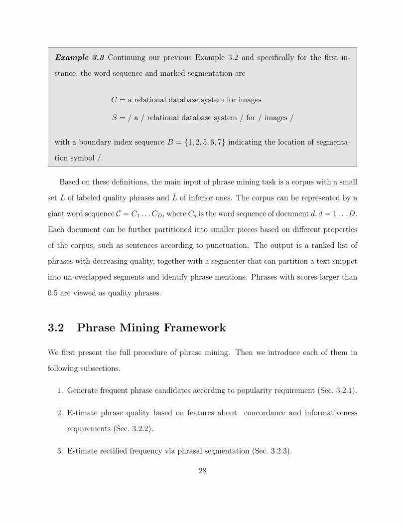
Example 3.3 Continuing our previous Example 3.2 and specifically for the first in-
stance, the word sequence and marked segmentation are
C = a relational database system for images
S = / a / relational database system / for / images /
with a boundary index sequence B = 1, 2, 5, 6, 7 indicating the location of segmenta-
tion symbol /.
Based on these definitions, the main input of phrase mining task is a corpus with a small
set L of labeled quality phrases and L of inferior ones. The corpus can be represented by a
giant word sequence C = C1 . . . CD, where Cd is the word sequence of document d, d = 1 . . . D.
Each document can be further partitioned into smaller pieces based on different properties
of the corpus, such as sentences according to punctuation. The output is a ranked list of
phrases with decreasing quality, together with a segmenter that can partition a text snippet
into un-overlapped segments and identify phrase mentions. Phrases with scores larger than
0.5 are viewed as quality phrases.
3.2 Phrase Mining Framework
We first present the full procedure of phrase mining. Then we introduce each of them in
following subsections.
1. Generate frequent phrase candidates according to popularity requirement (Sec. 3.2.1).
2. Estimate phrase quality based on features about concordance and informativeness
requirements (Sec. 3.2.2).
3. Estimate rectified frequency via phrasal segmentation (Sec. 3.2.3).
28
4. Add segmentation-based features derived from rectified frequency into the feature set
of phrase quality classifier (Sec. 3.2.4). Repeat step 2 and 3.
5. Filter phrases with low rectified frequencies to satisfy the completeness requirement
as post-processing step.
An complexity analysis for this framework is given at Sec 3.2.5 to show that both of its
computation time and required space grow linearly as the corpus size increases.
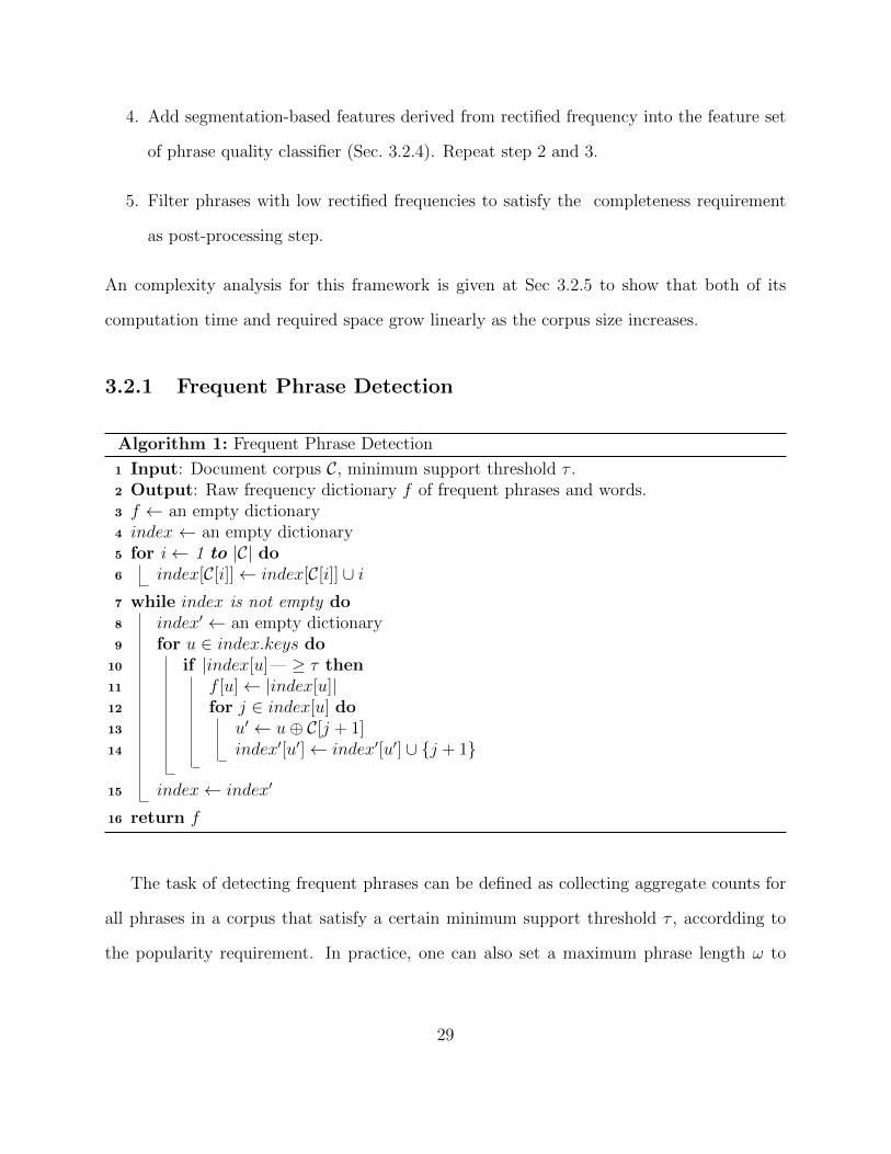
3.2.1 Frequent Phrase Detection
Algorithm 1: Frequent Phrase Detection
1 Input: Document corpus C, minimum support threshold τ .2 Output: Raw frequency dictionary f of frequent phrases and words.3 f ← an empty dictionary4 index ← an empty dictionary5 for i ← 1 to |C| do6 index[C[i]]← index[C[i]] ∪ i7 while index is not empty do8 index′ ← an empty dictionary9 for u ∈ index.keys do
10 if |index[u]— ≥ τ then11 f [u]← |index[u]|12 for j ∈ index[u] do13 u′ ← u⊕ C[j + 1]14 index′[u′]← index′[u′] ∪ j + 1
15 index← index′
16 return f
The task of detecting frequent phrases can be defined as collecting aggregate counts for
all phrases in a corpus that satisfy a certain minimum support threshold τ , accordding to
the popularity requirement. In practice, one can also set a maximum phrase length ω to
29
restrict the phrase length. Even if no explicit restriction is added, ω is typically a small
constant. For efficiently mining these frequent phrases, we draw upon two properties:
1. Downward Closure property: If a phrase is not frequent, then any its super-phrase is
guaranteed to be not frequent. Therefore, those longer phrases will be filtered and never
expanded.
2. Prefix property: If a phrase is frequent, any its prefix units should be frequent too. In
this way, all the frequent phrases can be generated by expanding their prefixes.
The algorithm for detecting frequent phrases is given in Alg. 1. We use C[·] to index a word
in the corpus string and |C| to denote the corpus size. The ⊕ operator is for concatecating
two words or phrases. Alg. 1 returns a key-value dictionary f . Its keys are vocabulary U
containing all frequent phrases P , and words U \ P . Its values are their raw frequency.
3.2.2 Phrase Quality Estimation
Estimating phrase quality from only a few training labels is challenging since a huge number
of phrase candidates might be generated from the first step and they are messy. Instead of
using one or two statistical measures [34, 79, 32], we choose to compute multiple features
for each candidate in P . A classifier is trained on these features to predict quality Q for all
unlabeled phrases. For phrases not in P , their quality is simply 0.
We divide the features into two categories according to concordance and informativeness
requirements in the following two subsections. Only representative features are introduced
for clearness. We then discuss about the classifier in Sec. 3.2.2.
Concordance Features
This set of features is designed to measure concordance among sub-units of a phrase. To
make phrases with different lengths comparable, we partition each phrase candidate into two
30
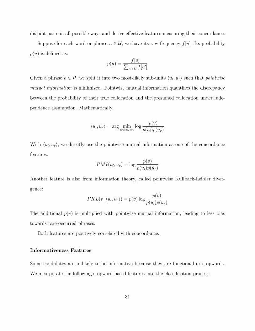
disjoint parts in all possible ways and derive effective features measuring their concordance.
Suppose for each word or phrase u ∈ U , we have its raw frequency f [u]. Its probability
p(u) is defined as:
p(u) =f [u]∑
u′∈U f [u′]
Given a phrase v ∈ P , we split it into two most-likely sub-units 〈ul, ur〉 such that pointwise
mutual information is minimized. Pointwise mutual information quantifies the discrepancy
between the probability of their true collocation and the presumed collocation under inde-
pendence assumption. Mathematically,
〈ul, ur〉 = arg minul⊕ur=v
logp(v)
p(ul)p(ur)
With 〈ul, ur〉, we directly use the pointwise mutual information as one of the concordance
features.
PMI(ul, ur) = logp(v)
p(ul)p(ur)
Another feature is also from information theory, called pointwise Kullback-Leibler diver-
gence:
PKL(v‖〈ul, ur〉) = p(v) logp(v)
p(ul)p(ur)
The additional p(v) is multiplied with pointwise mutual information, leading to less bias
towards rare-occurred phrases.
Both features are positively correlated with concordance.
Informativeness Features
Some candidates are unlikely to be informative because they are functional or stopwords.
We incorporate the following stopword-based features into the classification process:
31
• Whether stopwords are located at the beginning or the end of the phrase candidate;
which requires a dictionary of stopwords. Phrases that begin or end with stopwords, such
as ‘I am’, are often functional rather than informative.
A more generic feature is to measure the informativeness based on corpus statistics:
• Average inverse document frequency (IDF) computed over words;
where IDF for a word w is computed as
IDF(w) = log|C|
|d ∈ [D] : w ∈ Cd|
It is a traditional information retrieval measure of how much information a word provides
in order to retrieve a small subset of documents from a corpus. In general, quality phrases
are expected to have not too small average IDF.
In addition to word-based features, punctuation is frequently used in text to aid inter-
pretations of specific concept or idea. This information is helpful for our task. Specifically,
we adopt the following feature:
• Punctuation: probabilities of a phrase in quotes, brackets or capitalized;
higher probability usually indicates more likely a phrase is informative.
Besides these features, many other signals like knowledge-base entities and part-of-speech
tagging can be plugged into the feature set. They are less generic quality estimators and
require more training or external resources. It is easy to incorporate these features in our
framework when they are available.
Classifier
Our framework can work with arbitrary classifiers that can be effectively trained with small
labeled data and output a probabilistic score between 0 and 1. For instance, we can adopt
32
random forest [16] which is efficient to train with a small number of labels. The ratio
of positive predictions among all decision trees can be interpreted as a phrase’s quality
estimation. In experiments we will see that 200–300 labels are enough to train a satisfactory
classifier.
Just as we have mentioned, both quality phrases and inferior ones are required as labels
for training. To further reduce the labeling effort, some machine learning ideas like PU-
learning [57] can be applied to automatically retrieve negative labels. Active learning [89]
is another popular mechanism to substantially reduce the number of labels required via
iterative training. Moreover, it is possible to train a transferable model on one document
collection and adapt it to the target corpus. We plan to explore these directions in future
work.
3.2.3 Phrasal Segmentation
The discussion in Example 3.1 points out the limitations of using only raw frequency counts.
Instead, we ought to examine the context of every word sequence’s occurrence and decide
whether to count it as a phrase, as introduced in Example 3.2. The segmentation directly
addresses the completeness requirement, and indirectly helps with the concordance require-
ment via rectified frequency. Here we propose an efficient phrasal segmentation method to
compute rectified frequency of each phrase. We will see that combined with aforementioned
phrase quality estimation, bad phrases with high raw frequency get removed as their rectified
frequencies approach zero.
Furthermore, rectified phrase frequencies can be fed back to generate additional features
and improve the phrase quality estimation. This will be discussed in the next subsection.
We now propose the phrasal segmentation model integrated with the aforementioned
phrase quality Q. Given a word sequence C, and a segmentation S = s1 . . . sm induced by
33
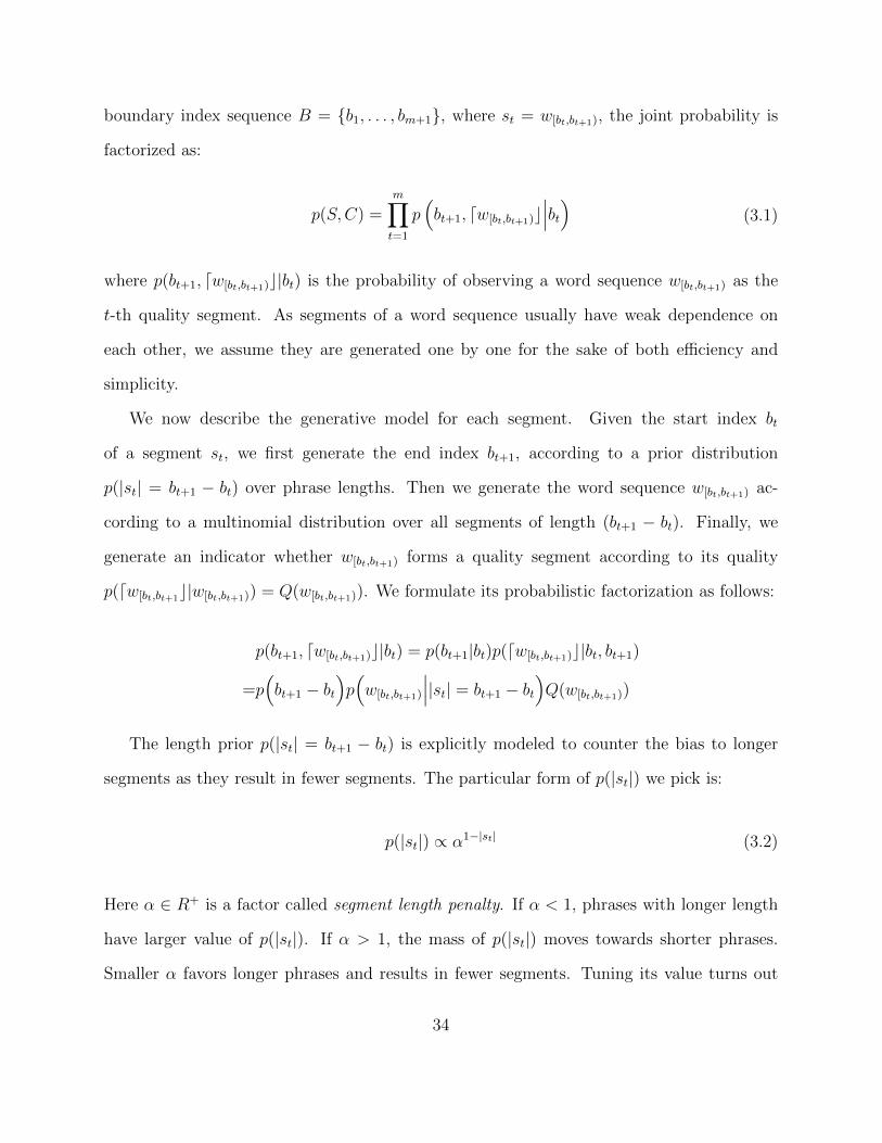
boundary index sequence B = b1, . . . , bm+1, where st = w[bt,bt+1), the joint probability is
factorized as:
p(S,C) =m∏t=1
p(bt+1, dw[bt,bt+1)c
∣∣∣bt) (3.1)
where p(bt+1, dw[bt,bt+1)c|bt) is the probability of observing a word sequence w[bt,bt+1) as the
t-th quality segment. As segments of a word sequence usually have weak dependence on
each other, we assume they are generated one by one for the sake of both efficiency and
simplicity.
We now describe the generative model for each segment. Given the start index bt
of a segment st, we first generate the end index bt+1, according to a prior distribution
p(|st| = bt+1 − bt) over phrase lengths. Then we generate the word sequence w[bt,bt+1) ac-
cording to a multinomial distribution over all segments of length (bt+1 − bt). Finally, we
generate an indicator whether w[bt,bt+1) forms a quality segment according to its quality
p(dw[bt,bt+1c|w[bt,bt+1)) = Q(w[bt,bt+1)). We formulate its probabilistic factorization as follows:
p(bt+1, dw[bt,bt+1)c|bt) = p(bt+1|bt)p(dw[bt,bt+1)c|bt, bt+1)
=p(bt+1 − bt
)p(w[bt,bt+1)
∣∣∣|st| = bt+1 − bt)Q(w[bt,bt+1))
The length prior p(|st| = bt+1 − bt) is explicitly modeled to counter the bias to longer
segments as they result in fewer segments. The particular form of p(|st|) we pick is:
p(|st|) ∝ α1−|st| (3.2)
Here α ∈ R+ is a factor called segment length penalty. If α < 1, phrases with longer length
have larger value of p(|st|). If α > 1, the mass of p(|st|) moves towards shorter phrases.
Smaller α favors longer phrases and results in fewer segments. Tuning its value turns out
34
to be a trade-off between precision and recall for recognizing quality phrases. At the end of
this subsection we will discuss how to estimate its value by reusing labels in Sec. 3.2.2. It is
worth mentioning that such segment length penalty is also discussed by Li et al. [59]. Our
formulation differs from theirs by posing a weaker penalty on long phrases.
We denote p(w[bt,bt+1)
∣∣∣|st|) with θw[bt,bt+1)for convenience. For a given corpus C with D
documents, we need to estimate θu = p(u∣∣∣|u|) for each frequent word and phrase u ∈ U ,
and infer segmentation S. We employ the maximum a posteriori principle and maximize the
joint probability of the corpus:
D∑d=1
log p(Sd, Cd) =D∑d=1
md∑t=1
log p(b
(d)t+1, dw
(d)[bt,bt+1
c∣∣∣b(d)t
)(3.3)
To find the best segmentation to maximize Eq. (3.3), one can use efficient dynamic
programming (DP) if θ is known. The algorithm is shown in Alg. 2.
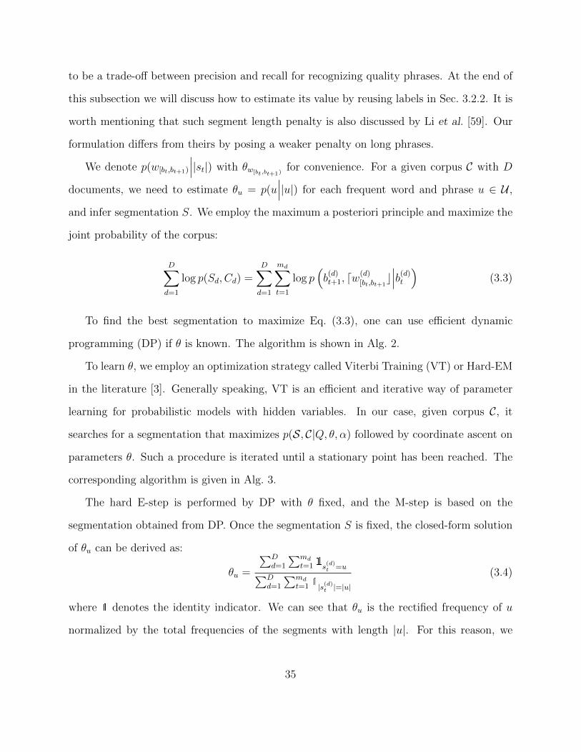
To learn θ, we employ an optimization strategy called Viterbi Training (VT) or Hard-EM
in the literature [3]. Generally speaking, VT is an efficient and iterative way of parameter
learning for probabilistic models with hidden variables. In our case, given corpus C, it
searches for a segmentation that maximizes p(S, C|Q, θ, α) followed by coordinate ascent on
parameters θ. Such a procedure is iterated until a stationary point has been reached. The
corresponding algorithm is given in Alg. 3.
The hard E-step is performed by DP with θ fixed, and the M-step is based on the
segmentation obtained from DP. Once the segmentation S is fixed, the closed-form solution
of θu can be derived as:
θu =
∑Dd=1
∑md
t=1 1s(d)t =u∑D
d=1
∑md
t=1 1|s(d)t |=|u|
(3.4)
where 1 denotes the identity indicator. We can see that θu is the rectified frequency of u
normalized by the total frequencies of the segments with length |u|. For this reason, we
35
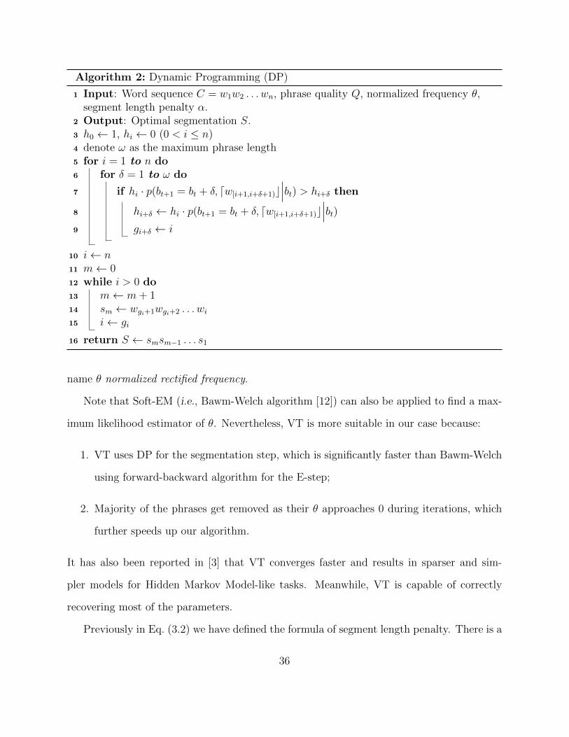
Algorithm 2: Dynamic Programming (DP)
1 Input: Word sequence C = w1w2 . . . wn, phrase quality Q, normalized frequency θ,segment length penalty α.
2 Output: Optimal segmentation S.3 h0 ← 1, hi ← 0 (0 < i ≤ n)4 denote ω as the maximum phrase length5 for i = 1 to n do6 for δ = 1 to ω do
7 if hi · p(bt+1 = bt + δ, dw[i+1,i+δ+1)c∣∣∣bt) > hi+δ then
8 hi+δ ← hi · p(bt+1 = bt + δ, dw[i+1,i+δ+1)c∣∣∣bt)
9 gi+δ ← i
10 i← n11 m← 012 while i > 0 do13 m← m+ 114 sm ← wgi+1wgi+2 . . . wi15 i← gi
16 return S ← smsm−1 . . . s1
name θ normalized rectified frequency.
Note that Soft-EM (i.e., Bawm-Welch algorithm [12]) can also be applied to find a max-
imum likelihood estimator of θ. Nevertheless, VT is more suitable in our case because:
1. VT uses DP for the segmentation step, which is significantly faster than Bawm-Welch
using forward-backward algorithm for the E-step;
2. Majority of the phrases get removed as their θ approaches 0 during iterations, which
further speeds up our algorithm.
It has also been reported in [3] that VT converges faster and results in sparser and sim-
pler models for Hidden Markov Model-like tasks. Meanwhile, VT is capable of correctly
recovering most of the parameters.
Previously in Eq. (3.2) we have defined the formula of segment length penalty. There is a
36
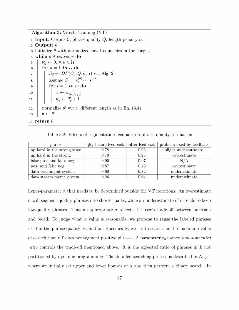
Algorithm 3: Viterbi Training (VT)
1 Input: Corpus C, phrase quality Q, length penalty α.2 Output: θ.3 initialize θ with normalized raw frequencies in the corpus4 while not converge do5 θ′u ← 0, ∀ u ∈ U6 for d = 1 to D do7 Sd ← DP (Cd, Q, θ, α) via Alg. 2
8 assume Sd = s(d)1 · · · s
(d)m
9 for t = 1 to m do
10 u← w(d)[bt,bt+1)
11 θ′u ← θ′u + 1
12 normalize θ′ w.r.t. different length as in Eq. (3.4)13 θ ← θ′
14 return θ
Table 3.2: Effects of segmentation feedback on phrase quality estimation
phrase qlty before feedback after feedback problem fixed by feedback
np hard in the strong sense 0.78 0.93 slight underestimatenp hard in the strong 0.70 0.23 overestimate
false pos. and false neg. 0.90 0.97 N/Apos. and false neg. 0.87 0.29 overestimate
data base mgmt system 0.60 0.82 underestimate
data stream mgmt system 0.26 0.64 underestimate
hyper-parameter α that needs to be determined outside the VT iterations. An overestimate
α will segment quality phrases into shorter parts, while an underestimate of α tends to keep
low-quality phrases. Thus an appropriate α reflects the user’s trade-off between precision
and recall. To judge what α value is reasonable, we propose to reuse the labeled phrases
used in the phrase quality estimation. Specifically, we try to search for the maximum value
of α such that VT does not segment positive phrases. A parameter r0 named non-segmented
ratio controls the trade-off mentioned above. It is the expected ratio of phrases in L not
partitioned by dynamic programming. The detailed searching process is described in Alg. 4
where we initially set upper and lower bounds of α and then perform a binary search. In
37
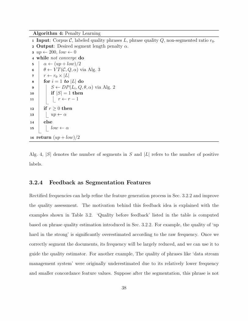
Algorithm 4: Penalty Learning
1 Input: Corpus C, labeled quality phrases L, phrase quality Q, non-segmented ratio r0.2 Output: Desired segment length penalty α.3 up← 200, low ← 04 while not converge do5 α← (up+ low)/26 θ ← V T (C, Q, α) via Alg. 37 r ← r0 × |L|8 for i = 1 to |L| do9 S ← DP (Li, Q, θ, α) via Alg. 2
10 if |S| = 1 then11 r ← r − 1
12 if r ≥ 0 then13 up← α
14 else15 low ← α
16 return (up+ low)/2
Alg. 4, |S| denotes the number of segments in S and |L| refers to the number of positive
labels.
3.2.4 Feedback as Segmentation Features
Rectified frequencies can help refine the feature generation process in Sec. 3.2.2 and improve
the quality assessment. The motivation behind this feedback idea is explained with the
examples shown in Table 3.2. ‘Quality before feedback’ listed in the table is computed
based on phrase quality estimation introduced in Sec. 3.2.2. For example, the quality of ‘np
hard in the strong’ is significantly overestimated according to the raw frequency. Once we
correctly segment the documents, its frequency will be largely reduced, and we can use it to
guide the quality estimator. For another example, The quality of phrases like ‘data stream
management system’ were originally underestimated due to its relatively lower frequency
and smaller concordance feature values. Suppose after the segmentation, this phrase is not
38
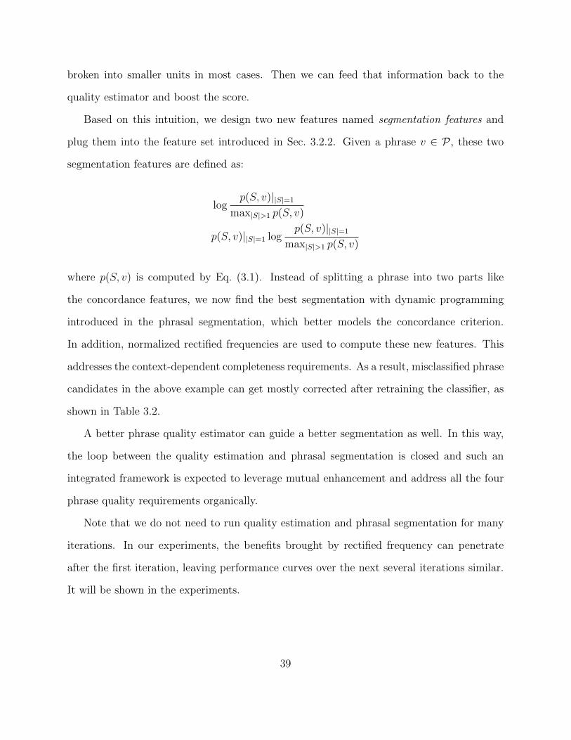
broken into smaller units in most cases. Then we can feed that information back to the
quality estimator and boost the score.
Based on this intuition, we design two new features named segmentation features and
plug them into the feature set introduced in Sec. 3.2.2. Given a phrase v ∈ P , these two
segmentation features are defined as:
logp(S, v)||S|=1
max|S|>1 p(S, v)
p(S, v)||S|=1 logp(S, v)||S|=1
max|S|>1 p(S, v)
where p(S, v) is computed by Eq. (3.1). Instead of splitting a phrase into two parts like
the concordance features, we now find the best segmentation with dynamic programming
introduced in the phrasal segmentation, which better models the concordance criterion.
In addition, normalized rectified frequencies are used to compute these new features. This
addresses the context-dependent completeness requirements. As a result, misclassified phrase
candidates in the above example can get mostly corrected after retraining the classifier, as
shown in Table 3.2.
A better phrase quality estimator can guide a better segmentation as well. In this way,
the loop between the quality estimation and phrasal segmentation is closed and such an
integrated framework is expected to leverage mutual enhancement and address all the four
phrase quality requirements organically.
Note that we do not need to run quality estimation and phrasal segmentation for many
iterations. In our experiments, the benefits brought by rectified frequency can penetrate
after the first iteration, leaving performance curves over the next several iterations similar.
It will be shown in the experiments.
39
3.2.5 Complexity Analysis
Frequent Phrases Detection: Since the operation of Hash table is O(1), both the time
and space complexities are O(ω|C|). ω is a small constant indicating the maximum phrase
length, so this step is linear to the size of corpus |C|.
Feature Extraction: When extracting features, the most challenging problem is how to
efficiently locate these phrase candidates in the original corpus, because the original texts
are crucial for finding the punctuation and capitalization information. Instead of using
some dictionaries to store all the occurrences, we take the advantage of the Aho-Corasick
Automaton algorithm and tailor it to find all the occurrences of phrase candidates. The time
complexity is O(|C|+ |P|) and space complexity O(|P|), where |P| refers to the total number
of frequent phrase candidates. As the length of each candidate is limited by a constant ω,
O(|P|) = O(|C|), so the complexity is O(|C|) in both time and space.
Phrase Quality Estimation: As we only labeled a very small set of phrase candidates,
as long as the number and depth of decision trees in the random forest are some constant,
the training time for the classifier is very small compared to other parts. For the prediction
stage, it is proportional to the size of phrase candidates and the dimensions of features.
Therefore, it could be O(|C|) in both time and space, although the actual magnitude might
be smaller.
Viterbi Training: It is easy to observe that Alg. 2 is O(nω), which is linear to the number
of words. ω is treated as a constant, and thus the VT process is also O(|C|) considering
Alg. 3 ususally finishes in a few iterations.
Penalty Learning: Suppose we only require a constant ε to check the convergence of the
binary search. Then after log2200ε
rounds, the algorithm converges. So the number of loops
could be treated as a constant. Because VT takes O(|C|) time, Penalty learning also takes
O(|C|) time.
40
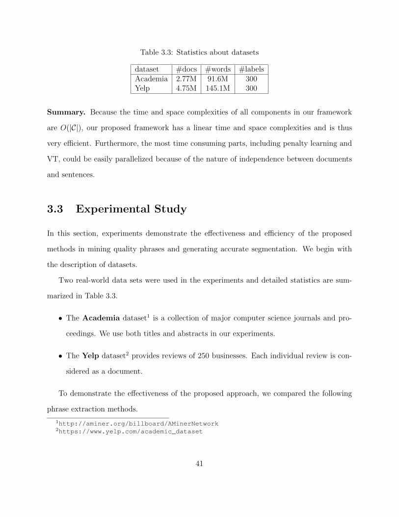
Table 3.3: Statistics about datasets
dataset #docs #words #labelsAcademia 2.77M 91.6M 300Yelp 4.75M 145.1M 300
Summary. Because the time and space complexities of all components in our framework
are O(|C|), our proposed framework has a linear time and space complexities and is thus
very efficient. Furthermore, the most time consuming parts, including penalty learning and
VT, could be easily parallelized because of the nature of independence between documents
and sentences.
3.3 Experimental Study
In this section, experiments demonstrate the effectiveness and efficiency of the proposed
methods in mining quality phrases and generating accurate segmentation. We begin with
the description of datasets.
Two real-world data sets were used in the experiments and detailed statistics are sum-
marized in Table 3.3.
• The Academia dataset1 is a collection of major computer science journals and pro-
ceedings. We use both titles and abstracts in our experiments.
• The Yelp dataset2 provides reviews of 250 businesses. Each individual review is con-
sidered as a document.
To demonstrate the effectiveness of the proposed approach, we compared the following
phrase extraction methods.
1http://aminer.org/billboard/AMinerNetwork2https://www.yelp.com/academic_dataset
41
• TF-IDF ranks phrases by the product of their raw frequencies and inverse document
frequencies;
• C-Value proposes a ranking measure based on frequencies of a phrase used as parts
of their super-phrases following a top-down scheme;
• ConExtr approaches phrase extraction as a market-baskets problem based on an
assumption about relationship between n-gram and prefix/suffix (n− 1)-gram;
• KEA3 is a supervised keyphrase extraction method for long documents. To apply this
method in our setting, we consider the whole corpus as a single document;
• TopMine4 is a topical phrase extraction method. We use its phrase mining module
for comparison;
• ClassPhrase ranks phrases based on their estimated qualities (removing step 3–5
from our framework);
• SegPhrase combines ClassPhrase with phrasal segmentation to filter overestimated
phrases based on normalized rectified frequency (removing step 4 from our framework);
• SegPhrase+ is similar to SegPhrase but adds segmentation features to refine quality
estimation. It contains the full procedures presented in Sec. 3.2.
The first two methods utilize NLP chunking to obtain phrase candidates. We use the
JATE5 implementation of the first two methods, i.e., TF-IDF and C-Value. Both of them
rely on OpenNLP6 as the linguistic processor to detect phrase candidates in the corpus. The
3https://code.google.com/p/kea-algorithm4http://web.engr.illinois.edu/˜elkishk2/5https://code.google.com/p/jatetoolkit6http://opennlp.apache.org
42
rest methods are all based on frequent n-grams and the runtime is dramatically reduced.
The last three methods are variations of our proposed method.
It is also worth mentioning that JATE contains several more implemented methods in-
cluding Weirdness [1]. They are not reported here due to their unsatisfactory performance
compared to the baselines listed above.
For the parameter setting, we set minimum phrase support τ as 30 and maximum phrase
length ω as 6, which are two parameters required by all methods. Other parameters required
by baselines were set according to the open source tools or the original papers.
For our proposed methods, training labels for phrases were collected by sampling repre-
sentative phrase candidates from groups of phrases pre-clustered on the normalized feature
space by k-means. We labeled research areas, tasks, algorithms and other scientific terms
in the Academia dataset as quality phrases. Some examples are ‘divide and conquer’, ‘np
complete’ and ‘relational database’. For the Yelp dataset, restaurants, dishes, cities and
other related concepts are labeled to be positive. In contrast, phrases like ‘under certain
assumptions’, ‘many restaurants’ and ‘last night’ were labeled as negative. We down-sample
low quality phrases because they are dominant over quality phrases. The number of train-
ing labels in our experiments are reported in Table 3.3. To automatically learn the value
of segment length penalty, we set the non-segmented ratio r0 in Alg. 4 as 1.0 for Academia
dataset and 0.95 for Yelp dataset. The selection of this parameter will be discussed in detail
later in this section.
To make outputs returned by different methods comparable, we converted all the phrase
candidates to lower case and merged plural with singular phrases. The phrase lists generated
by these methods have different size, and the tail of the lists are low quality. For the simplicity
of comparison, we discarded low-ranked phrases based on the minimum size among all phrase
lists except ConExtr. ConExtr returns all phrases without ranking. Thus we did not remove
its phrases. The remaining size of each list is still reasonably large (¿ 40,000).
43
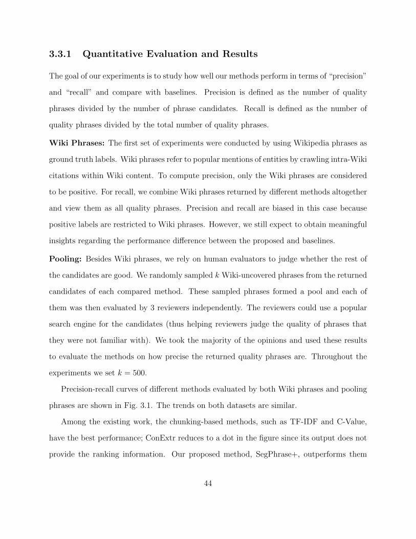
3.3.1 Quantitative Evaluation and Results
The goal of our experiments is to study how well our methods perform in terms of “precision”
and “recall” and compare with baselines. Precision is defined as the number of quality
phrases divided by the number of phrase candidates. Recall is defined as the number of
quality phrases divided by the total number of quality phrases.
Wiki Phrases: The first set of experiments were conducted by using Wikipedia phrases as
ground truth labels. Wiki phrases refer to popular mentions of entities by crawling intra-Wiki
citations within Wiki content. To compute precision, only the Wiki phrases are considered
to be positive. For recall, we combine Wiki phrases returned by different methods altogether
and view them as all quality phrases. Precision and recall are biased in this case because
positive labels are restricted to Wiki phrases. However, we still expect to obtain meaningful
insights regarding the performance difference between the proposed and baselines.
Pooling: Besides Wiki phrases, we rely on human evaluators to judge whether the rest of
the candidates are good. We randomly sampled k Wiki-uncovered phrases from the returned
candidates of each compared method. These sampled phrases formed a pool and each of
them was then evaluated by 3 reviewers independently. The reviewers could use a popular
search engine for the candidates (thus helping reviewers judge the quality of phrases that
they were not familiar with). We took the majority of the opinions and used these results
to evaluate the methods on how precise the returned quality phrases are. Throughout the
experiments we set k = 500.
Precision-recall curves of different methods evaluated by both Wiki phrases and pooling
phrases are shown in Fig. 3.1. The trends on both datasets are similar.
Among the existing work, the chunking-based methods, such as TF-IDF and C-Value,
have the best performance; ConExtr reduces to a dot in the figure since its output does not
provide the ranking information. Our proposed method, SegPhrase+, outperforms them
44
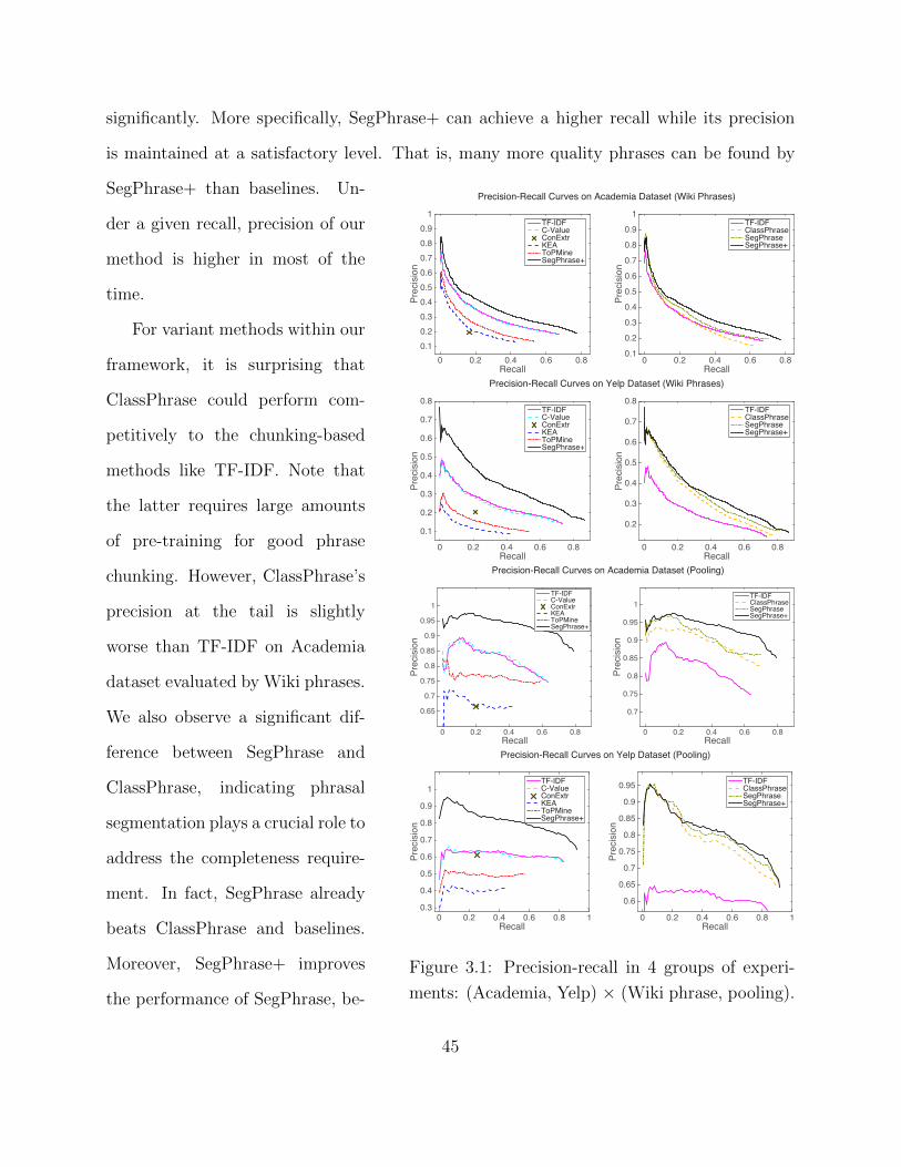
significantly. More specifically, SegPhrase+ can achieve a higher recall while its precision
is maintained at a satisfactory level. That is, many more quality phrases can be found by
Recall0 0.2 0.4 0.6 0.8
Pre
cis
ion
0.1
0.2
0.3
0.4
0.5
0.6
0.7
0.8
0.9
1TF-IDFC-ValueConExtrKEAToPMineSegPhrase+
Precision-Recall Curves on Academia Dataset (Wiki Phrases)
Recall0 0.2 0.4 0.6 0.8
Pre
cis
ion
0.1
0.2
0.3
0.4
0.5
0.6
0.7
0.8
0.9
1TF-IDFClassPhraseSegPhraseSegPhrase+
Recall0 0.2 0.4 0.6 0.8
Pre
cis
ion
0.1
0.2
0.3
0.4
0.5
0.6
0.7
0.8TF-IDFC-ValueConExtrKEAToPMineSegPhrase+
Precision-Recall Curves on Yelp Dataset (Wiki Phrases)
Recall0 0.2 0.4 0.6 0.8
Pre
cis
ion
0.2
0.3
0.4
0.5
0.6
0.7
0.8TF-IDFClassPhraseSegPhraseSegPhrase+
Recall0 0.2 0.4 0.6 0.8
Pre
cis
ion
0.65
0.7
0.75
0.8
0.85
0.9
0.95
1
TF-IDFC-ValueConExtrKEAToPMineSegPhrase+
Precision-Recall Curves on Academia Dataset (Pooling)
Recall0 0.2 0.4 0.6 0.8
Pre
cis
ion
0.7
0.75
0.8
0.85
0.9
0.95
1TF-IDFClassPhraseSegPhraseSegPhrase+
Recall0 0.2 0.4 0.6 0.8 1
Pre
cis
ion
0.3
0.4
0.5
0.6
0.7
0.8
0.9
1TF-IDFC-ValueConExtrKEAToPMineSegPhrase+
Precision-Recall Curves on Yelp Dataset (Pooling)
Recall0 0.2 0.4 0.6 0.8 1
Pre
cis
ion
0.6
0.65
0.7
0.75
0.8
0.85
0.9
0.95TF-IDFClassPhraseSegPhraseSegPhrase+
Figure 3.1: Precision-recall in 4 groups of experi-
ments: (Academia, Yelp) × (Wiki phrase, pooling).
SegPhrase+ than baselines. Un-
der a given recall, precision of our
method is higher in most of the
time.
For variant methods within our
framework, it is surprising that
ClassPhrase could perform com-
petitively to the chunking-based
methods like TF-IDF. Note that
the latter requires large amounts
of pre-training for good phrase
chunking. However, ClassPhrase’s
precision at the tail is slightly
worse than TF-IDF on Academia
dataset evaluated by Wiki phrases.
We also observe a significant dif-
ference between SegPhrase and
ClassPhrase, indicating phrasal
segmentation plays a crucial role to
address the completeness require-
ment. In fact, SegPhrase already
beats ClassPhrase and baselines.
Moreover, SegPhrase+ improves
the performance of SegPhrase, be-
45
cause of the use of phrasal segmen-
tation results as additional features.
An interesting observation is that the advantage of our method is more significant on
the pooling evaluations. The phrases in the pool are not covered by Wiki, indicating that
Wikipedia is not a complete source of quality phrases. However, our proposed methods,
including SegPhrase+, SegPhrase, and ClassPhrase, can mine out most of them (more than
80%) and keep a very high level of precision, especially on the Academia dataset. Therefore,
the evaluation results on the pooling phrases suggest that our methods not only detect the
well-known Wiki phrases, but also work properly for the long tail phrases which might occur
not so frequently.
From the result on Yelp dataset evaluated by pooling phrases, we notice that SegPhrase+
is a little weaker than SegPhrase at the head. As we know, SegPhrase+ has tried to utilize
phrasal segmentation results from SegPhrase to refine the phrase quality estimator. However,
segmentation features do not add new information for bigrams. If there are not many quality
phrases with more than two words, SegPhrase+ might not have significant improvement and
even can perform slightly worse due to the overfitting problem by reusing the same set of
labeled phrases. In fact, on Academia dataset, the ratios of quality phrases with more than
2 words are 24% among all Wiki phrases and 17% among pooling phrases. In contrast, these
statistics go down to to 13% and 10% on Yelp dataset, which verifies our conjecture and
explains why SegPhrase+ has slightly lower precision than SegPhrase at the head.
3.3.2 Model Selection
The goal of model selection is to study how well our methods perform in terms of “precision”
and “recall” on various candidate models with different parameters. We specifically want to
study two potentially interesting questions:
46
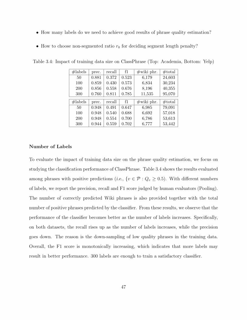
• How many labels do we need to achieve good results of phrase quality estimation?
• How to choose non-segmented ratio r0 for deciding segment length penalty?
Table 3.4: Impact of training data size on ClassPhrase (Top: Academia, Bottom: Yelp)
#labels prec. recall f1 #wiki phr. #total
50 0.881 0.372 0.523 6,179 24,603100 0.859 0.430 0.573 6,834 30,234200 0.856 0.558 0.676 8,196 40,355300 0.760 0.811 0.785 11,535 95,070
#labels prec. recall f1 #wiki phr. #total
50 0.948 0.491 0.647 6,985 79,091100 0.948 0.540 0.688 6,692 57,018200 0.948 0.554 0.700 6,786 53,613300 0.944 0.559 0.702 6,777 53,442
Number of Labels
To evaluate the impact of training data size on the phrase quality estimation, we focus on
studying the classification performance of ClassPhrase. Table 3.4 shows the results evaluated
among phrases with positive predictions (i.e., v ∈ P : Qv ≥ 0.5). With different numbers
of labels, we report the precision, recall and F1 score judged by human evaluators (Pooling).
The number of correctly predicted Wiki phrases is also provided together with the total
number of positive phrases predicted by the classifier. From these results, we observe that the
performance of the classifier becomes better as the number of labels increases. Specifically,
on both datasets, the recall rises up as the number of labels increases, while the precision
goes down. The reason is the down-sampling of low quality phrases in the training data.
Overall, the F1 score is monotonically increasing, which indicates that more labels may
result in better performance. 300 labels are enough to train a satisfactory classifier.
47
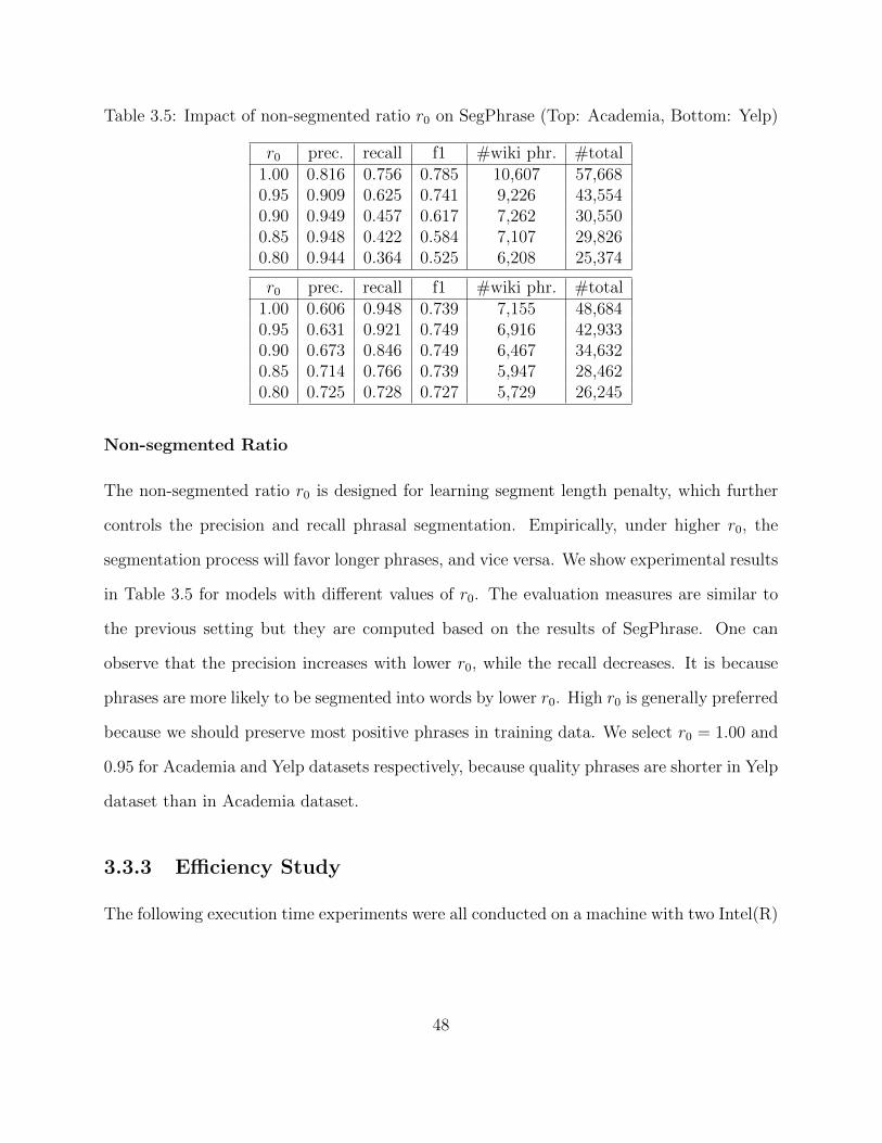
Table 3.5: Impact of non-segmented ratio r0 on SegPhrase (Top: Academia, Bottom: Yelp)
r0 prec. recall f1 #wiki phr. #total1.00 0.816 0.756 0.785 10,607 57,6680.95 0.909 0.625 0.741 9,226 43,5540.90 0.949 0.457 0.617 7,262 30,5500.85 0.948 0.422 0.584 7,107 29,8260.80 0.944 0.364 0.525 6,208 25,374
r0 prec. recall f1 #wiki phr. #total1.00 0.606 0.948 0.739 7,155 48,6840.95 0.631 0.921 0.749 6,916 42,9330.90 0.673 0.846 0.749 6,467 34,6320.85 0.714 0.766 0.739 5,947 28,4620.80 0.725 0.728 0.727 5,729 26,245
Non-segmented Ratio
The non-segmented ratio r0 is designed for learning segment length penalty, which further
controls the precision and recall phrasal segmentation. Empirically, under higher r0, the
segmentation process will favor longer phrases, and vice versa. We show experimental results
in Table 3.5 for models with different values of r0. The evaluation measures are similar to
the previous setting but they are computed based on the results of SegPhrase. One can
observe that the precision increases with lower r0, while the recall decreases. It is because
phrases are more likely to be segmented into words by lower r0. High r0 is generally preferred
because we should preserve most positive phrases in training data. We select r0 = 1.00 and
0.95 for Academia and Yelp datasets respectively, because quality phrases are shorter in Yelp
dataset than in Academia dataset.
3.3.3 Efficiency Study
The following execution time experiments were all conducted on a machine with two Intel(R)
48
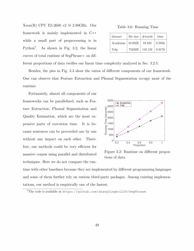
Table 3.6: Running Time
dataset file size #words time
Academia 613MB 91.6M 0.595h
Yelp 750MB 145.1M 0.917h
Xeon(R) CPU E5-2680 v2 @ 2.80GHz. Our
framework is mainly implemented in C++
while a small part of preprocessing is in
Python7. As shown in Fig. 3.2, the linear
curves of total runtime of SegPhrase+ on dif-
ferent proportions of data verifies our linear time complexity analyzed in Sec. 3.2.5.
Besides, the pies in Fig. 3.3 show the ratios of different components of our framework.
One can observe that Feature Extraction and Phrasal Segmentation occupy most of the
runtime.
Proportion0.2 0.4 0.6 0.8 1
Ru
nn
ing
Tim
e (
se
co
nd
s)
0
500
1000
1500
2000
2500
3000
3500Academia Yelp
Figure 3.2: Runtime on different propor-
tions of data
Fortunately, almost all components of our
frameworks can be parallelized, such as Fea-
ture Extraction, Phrasal Segmentation and
Quality Estimation, which are the most ex-
pensive parts of execution time. It is be-
cause sentences can be proceeded one by one
without any impact on each other. There-
fore, our methods could be very efficient for
massive corpus using parallel and distributed
techniques. Here we do not compare the run-
time with other baselines because they are implemented by different programming languages
and some of them further rely on various third-party packages. Among existing implemen-
tations, our method is empirically one of the fastest.
7The code is available at https://github.com/shangjingbo1226/SegPhrase.
49
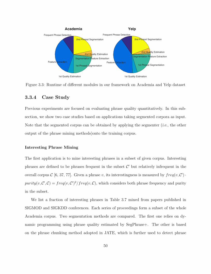
Frequent Phrase Detection
Feature Extraction
1st Quality Estimation
1st Phrasal Segmentation
Segmentation Feature Extraction
2nd Qualtiy Estimation
2nd Phrasal Segmentation
Academia
Frequent Phrase Detection
Feature Extraction
1st Quality Estimation
1st Phrasal Segmentation
Segmentation Feature Extraction
2nd Qualtiy Estimation
2nd Phrasal Segmentation
Yelp
Figure 3.3: Runtime of different modules in our framework on Academia and Yelp dataset
3.3.4 Case Study
Previous experiments are focused on evaluating phrase quality quantitatively. In this sub-
section, we show two case studies based on applications taking segmented corpora as input.
Note that the segmented corpus can be obtained by applying the segmenter (i.e., the other
output of the phrase mining methods)onto the training corpus.
Interesting Phrase Mining
The first application is to mine interesting phrases in a subset of given corpus. Interesting
phrases are defined to be phrases frequent in the subset C ′ but relatively infrequent in the
overall corpus C [6, 37, 77]. Given a phrase v, its interestingness is measured by freq(v, C ′) ·
purity(v, C ′, C) = freq(v, C ′)2/freq(v, C), which considers both phrase frequency and purity
in the subset.
We list a fraction of interesting phrases in Table 3.7 mined from papers published in
SIGMOD and SIGKDD conferences. Each series of proceedings form a subset of the whole
Academia corpus. Two segmentation methods are compared. The first one relies on dy-
namic programming using phrase quality estimated by SegPhrase+. The other is based
on the phrase chunking method adopted in JATE, which is further used to detect phrase
50
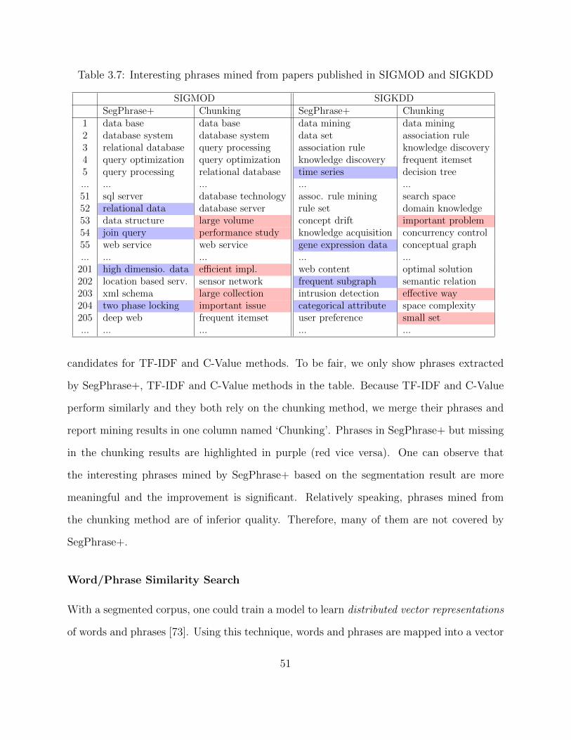
Table 3.7: Interesting phrases mined from papers published in SIGMOD and SIGKDD
SIGMOD SIGKDDSegPhrase+ Chunking SegPhrase+ Chunking
1 data base data base data mining data mining2 database system database system data set association rule3 relational database query processing association rule knowledge discovery4 query optimization query optimization knowledge discovery frequent itemset5 query processing relational database time series decision tree... ... ... ... ...51 sql server database technology assoc. rule mining search space52 relational data database server rule set domain knowledge53 data structure large volume concept drift important problem54 join query performance study knowledge acquisition concurrency control55 web service web service gene expression data conceptual graph... ... ... ... ...
201 high dimensio. data efficient impl. web content optimal solution202 location based serv. sensor network frequent subgraph semantic relation203 xml schema large collection intrusion detection effective way204 two phase locking important issue categorical attribute space complexity205 deep web frequent itemset user preference small set... ... ... ... ...
candidates for TF-IDF and C-Value methods. To be fair, we only show phrases extracted
by SegPhrase+, TF-IDF and C-Value methods in the table. Because TF-IDF and C-Value
perform similarly and they both rely on the chunking method, we merge their phrases and
report mining results in one column named ‘Chunking’. Phrases in SegPhrase+ but missing
in the chunking results are highlighted in purple (red vice versa). One can observe that
the interesting phrases mined by SegPhrase+ based on the segmentation result are more
meaningful and the improvement is significant. Relatively speaking, phrases mined from
the chunking method are of inferior quality. Therefore, many of them are not covered by
SegPhrase+.
Word/Phrase Similarity Search
With a segmented corpus, one could train a model to learn distributed vector representations
of words and phrases [73]. Using this technique, words and phrases are mapped into a vector
51
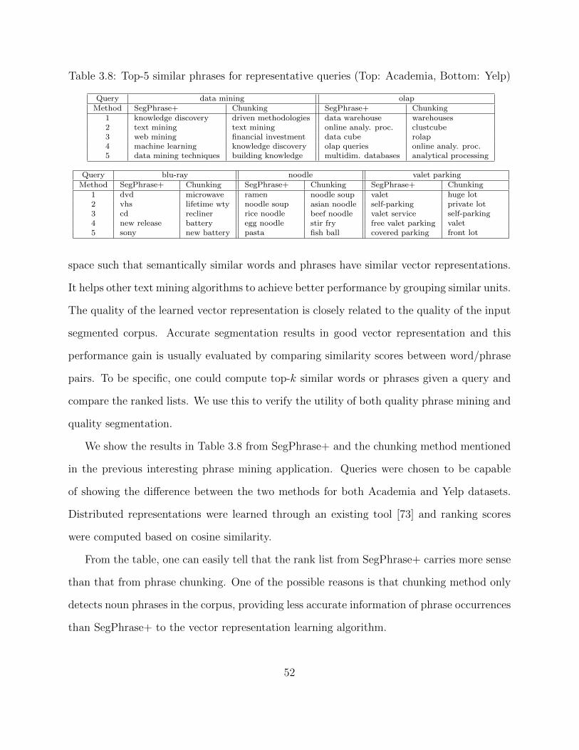
Table 3.8: Top-5 similar phrases for representative queries (Top: Academia, Bottom: Yelp)
Query data mining olapMethod SegPhrase+ Chunking SegPhrase+ Chunking
1 knowledge discovery driven methodologies data warehouse warehouses2 text mining text mining online analy. proc. clustcube3 web mining financial investment data cube rolap4 machine learning knowledge discovery olap queries online analy. proc.5 data mining techniques building knowledge multidim. databases analytical processing
Query blu-ray noodle valet parking
Method SegPhrase+ Chunking SegPhrase+ Chunking SegPhrase+ Chunking
1 dvd microwave ramen noodle soup valet huge lot2 vhs lifetime wty noodle soup asian noodle self-parking private lot3 cd recliner rice noodle beef noodle valet service self-parking4 new release battery egg noodle stir fry free valet parking valet5 sony new battery pasta fish ball covered parking front lot
space such that semantically similar words and phrases have similar vector representations.
It helps other text mining algorithms to achieve better performance by grouping similar units.
The quality of the learned vector representation is closely related to the quality of the input
segmented corpus. Accurate segmentation results in good vector representation and this
performance gain is usually evaluated by comparing similarity scores between word/phrase
pairs. To be specific, one could compute top-k similar words or phrases given a query and
compare the ranked lists. We use this to verify the utility of both quality phrase mining and
quality segmentation.
We show the results in Table 3.8 from SegPhrase+ and the chunking method mentioned
in the previous interesting phrase mining application. Queries were chosen to be capable
of showing the difference between the two methods for both Academia and Yelp datasets.
Distributed representations were learned through an existing tool [73] and ranking scores
were computed based on cosine similarity.
From the table, one can easily tell that the rank list from SegPhrase+ carries more sense
than that from phrase chunking. One of the possible reasons is that chunking method only
detects noun phrases in the corpus, providing less accurate information of phrase occurrences
than SegPhrase+ to the vector representation learning algorithm.
52
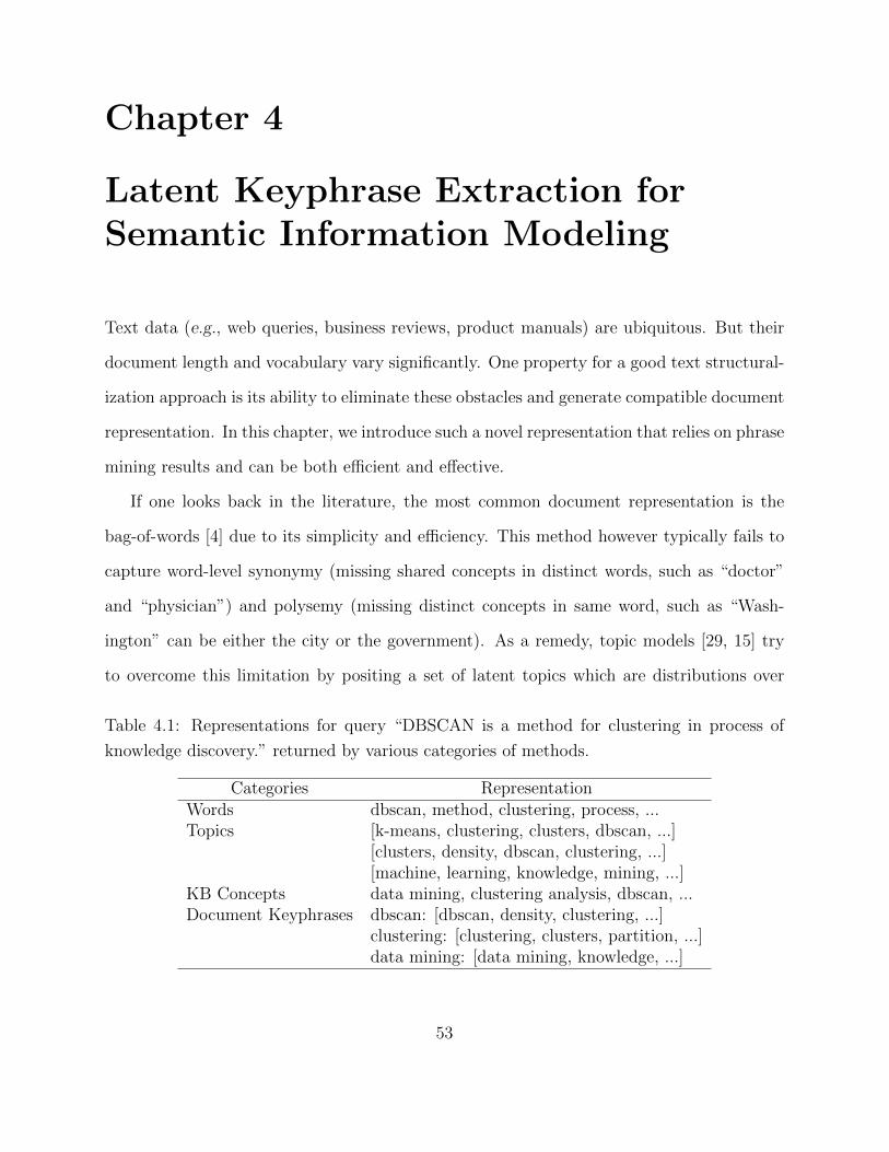
Chapter 4
Latent Keyphrase Extraction forSemantic Information Modeling
Text data (e.g., web queries, business reviews, product manuals) are ubiquitous. But their
document length and vocabulary vary significantly. One property for a good text structural-
ization approach is its ability to eliminate these obstacles and generate compatible document
representation. In this chapter, we introduce such a novel representation that relies on phrase
mining results and can be both efficient and effective.
If one looks back in the literature, the most common document representation is the
bag-of-words [4] due to its simplicity and efficiency. This method however typically fails to
capture word-level synonymy (missing shared concepts in distinct words, such as “doctor”
and “physician”) and polysemy (missing distinct concepts in same word, such as “Wash-
ington” can be either the city or the government). As a remedy, topic models [29, 15] try
to overcome this limitation by positing a set of latent topics which are distributions over
Table 4.1: Representations for query “DBSCAN is a method for clustering in process of
knowledge discovery.” returned by various categories of methods.
Categories RepresentationWords dbscan, method, clustering, process, ...Topics [k-means, clustering, clusters, dbscan, ...]
[clusters, density, dbscan, clustering, ...][machine, learning, knowledge, mining, ...]
KB Concepts data mining, clustering analysis, dbscan, ...Document Keyphrases dbscan: [dbscan, density, clustering, ...]
clustering: [clustering, clusters, partition, ...]data mining: [data mining, knowledge, ...]
53
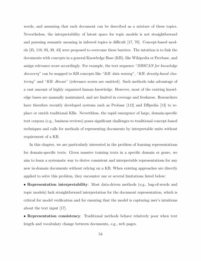
words, and assuming that each document can be described as a mixture of these topics.
Nevertheless, the interpretability of latent space for topic models is not straightforward
and pursuing semantic meaning in inferred topics is difficult [17, 70]. Concept-based mod-
els [35, 110, 93, 39, 43] were proposed to overcome these barriers. The intuition is to link the
documents with concepts in a general Knowledge Base (KB), like Wikipedia or Freebase, and
assign relevance score accordingly. For example, the text sequence “DBSCAN for knowledge
discovery” can be mapped to KB concepts like “KB: data mining”, “KB: density-based clus-
tering” and “KB: dbscan” (relevance scores are omitted). Such methods take advantage of
a vast amount of highly organized human knowledge. However, most of the existing knowl-
edge bases are manually maintained, and are limited in coverage and freshness. Researchers
have therefore recently developed systems such as Probase [112] and DBpedia [13] to re-
place or enrich traditional KBs. Neverthless, the rapid emergence of large, domain-specific
text corpora (e.g., business reviews) poses significant challenges to traditional concept-based
techniques and calls for methods of representing documents by interpretable units without
requirement of a KB.
In this chapter, we are particularly interested in the problem of learning representations
for domain-specific texts: Given massive training texts in a specific domain or genre, we
aim to learn a systematic way to derive consistent and interpretable representations for any
new in-domain documents without relying on a KB. When existing approaches are directly
applied to solve this problem, they encounter one or several limitations listed below:
• Representation interpretability: Most data-driven methods (e.g., bag-of-words and
topic models) lack straightforward interpretation for the document representation, which is
critical for model verification and for ensuring that the model is capturing user’s intuitions
about the text input [17].
• Representation consistency: Traditional methods behave relatively poor when text
length and vocabulary change between documents, e.g., web pages.
54
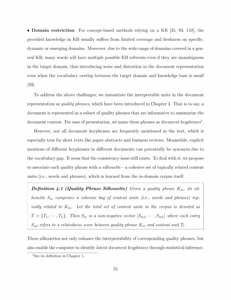
• Domain restriction: For concept-based methods relying on a KB [35, 93, 110], the
provided knowledge in KB usually suffers from limited coverage and freshness on specific,
dynamic or emerging domains. Moreover, due to the wide range of domains covered in a gen-
eral KB, many words will have multiple possible KB referents even if they are unambiguous
in the target domain, thus introducing noise and distortion in the document representation
even when the vocabulary overlap between the target domain and knowledge base is small
[39].
To address the above challenges, we instantiate the interpretable units in the document
representation as quality phrases, which have been introduced in Chapter 3. That is to say, a
document is represented as a subset of quality phrases that are informative to summarize the
document content. For ease of presentation, we name these phrases as document keyphrases1.
However, not all document keyphrases are frequently mentioned in the text, which is
especially true for short texts like paper abstracts and business reviews. Meanwhile, explicit
mentions of different keyphrases in different documents can potentially be synonym due to
the vocabulary gap. It seem that the consistency issue still exists. To deal with it, we propose
to associate each quality phrase with a silhouette—a cohesive set of topically related content
units (i.e., words and phrases), which is learned from the in-domain corpus itself.
Definition 4.1 (Quality Phrase Silhouette) Given a quality phrase Km, its sil-
houette Sm comprises a cohesive bag of content units (i.e., words and phrases) top-
ically related to Km. Let the total set of content units in the corpus is denoted as
T = T1, · · · , TL. Then Sm is a non-negative vector [Sm1, · · · , SmL] where each entry
Sml refers to a relatedness score between quality phrase Km and content unit Tl.
These silhouettes not only enhance the interpretability of corresponding quality phrases, but
also enable the computer to identify latent document keyphrases through statistical inference.
1See its definition in Chapter 1.
55
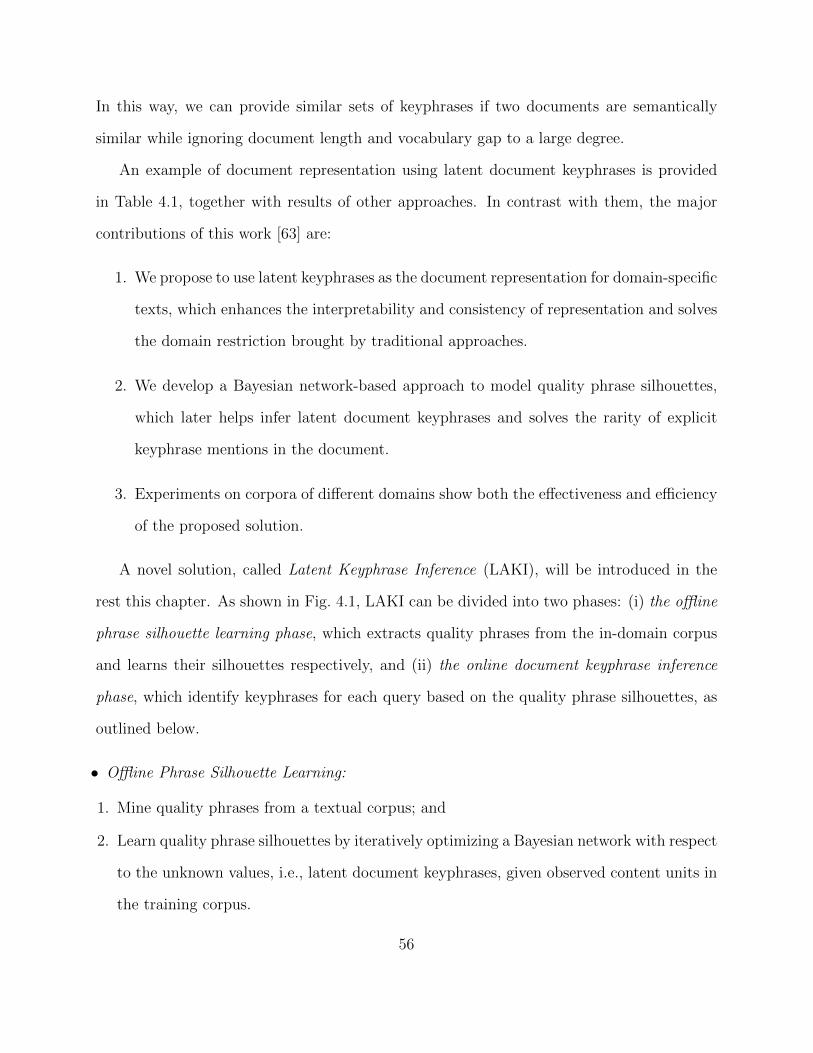
In this way, we can provide similar sets of keyphrases if two documents are semantically
similar while ignoring document length and vocabulary gap to a large degree.
An example of document representation using latent document keyphrases is provided
in Table 4.1, together with results of other approaches. In contrast with them, the major
contributions of this work [63] are:
1. We propose to use latent keyphrases as the document representation for domain-specific
texts, which enhances the interpretability and consistency of representation and solves
the domain restriction brought by traditional approaches.
2. We develop a Bayesian network-based approach to model quality phrase silhouettes,
which later helps infer latent document keyphrases and solves the rarity of explicit
keyphrase mentions in the document.
3. Experiments on corpora of different domains show both the effectiveness and efficiency
of the proposed solution.
A novel solution, called Latent Keyphrase Inference (LAKI), will be introduced in the
rest this chapter. As shown in Fig. 4.1, LAKI can be divided into two phases: (i) the offline
phrase silhouette learning phase, which extracts quality phrases from the in-domain corpus
and learns their silhouettes respectively, and (ii) the online document keyphrase inference
phase, which identify keyphrases for each query based on the quality phrase silhouettes, as
outlined below.
• Offline Phrase Silhouette Learning:
1. Mine quality phrases from a textual corpus; and
2. Learn quality phrase silhouettes by iteratively optimizing a Bayesian network with respect
to the unknown values, i.e., latent document keyphrases, given observed content units in
the training corpus.
56
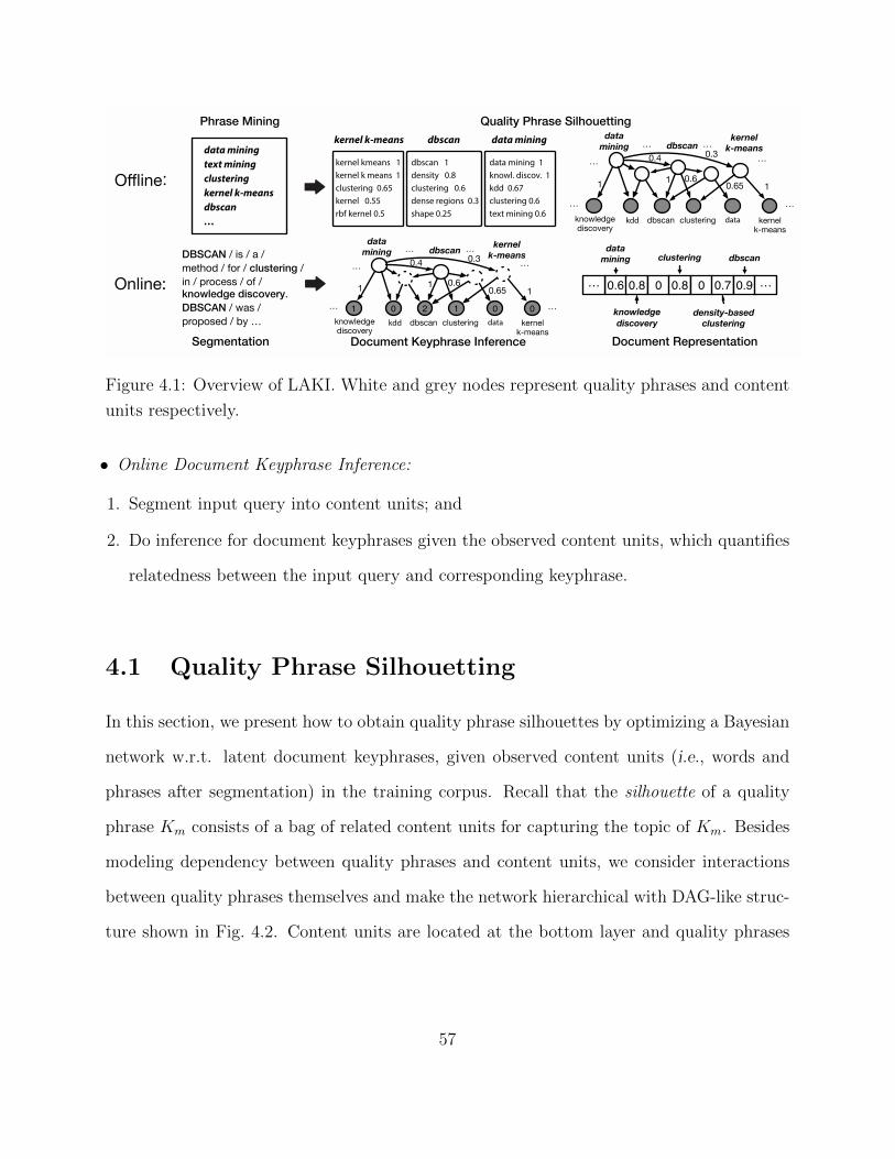
dbscan
kernel k-means dbscan data mining
0 01 0 2 1
knowledgediscovery
data
mining dbscankernel
k-means
clustering kernelk-means
…
……
dbscan
0.650.6
1 11
…
kdd
…
data
…
0.4 0.3
knowledgediscovery
data
mining dbscankernel
k-means
clustering kernelk-means
…
……
dbscan
0.650.6
1 11
…
kdd
…
data
…
0.4 0.3
Document Representation
DBSCAN / is / a /
method / for / clustering /
in / process / of / knowledge discovery.
DBSCAN / was /
proposed / by …
data mining
text mining
clustering
kernel k-means
dbscan
…
kernel kmeans 1
kernel k means 1
clustering 0.65
kernel 0.55
rbf kernel 0.5
dbscan 1
density 0.8
clustering 0.6
dense regions 0.3
shape 0.25
data mining 1
knowl. discov. 1
kdd 0.67
clustering 0.6
text mining 0.6
data
mining
0.6 0.8 0 0.8 0 0.7 0.9 ……
knowledge
discovery
density-based
clustering
Offline!
Online:
clustering
Phrase Mining
Segmentation
Quality Phrase Silhouetting
Document Keyphrase Inference
Figure 4.1: Overview of LAKI. White and grey nodes represent quality phrases and content
units respectively.
• Online Document Keyphrase Inference:
1. Segment input query into content units; and
2. Do inference for document keyphrases given the observed content units, which quantifies
relatedness between the input query and corresponding keyphrase.
4.1 Quality Phrase Silhouetting
In this section, we present how to obtain quality phrase silhouettes by optimizing a Bayesian
network w.r.t. latent document keyphrases, given observed content units (i.e., words and
phrases after segmentation) in the training corpus. Recall that the silhouette of a quality
phrase Km consists of a bag of related content units for capturing the topic of Km. Besides
modeling dependency between quality phrases and content units, we consider interactions
between quality phrases themselves and make the network hierarchical with DAG-like struc-
ture shown in Fig. 4.2. Content units are located at the bottom layer and quality phrases
57
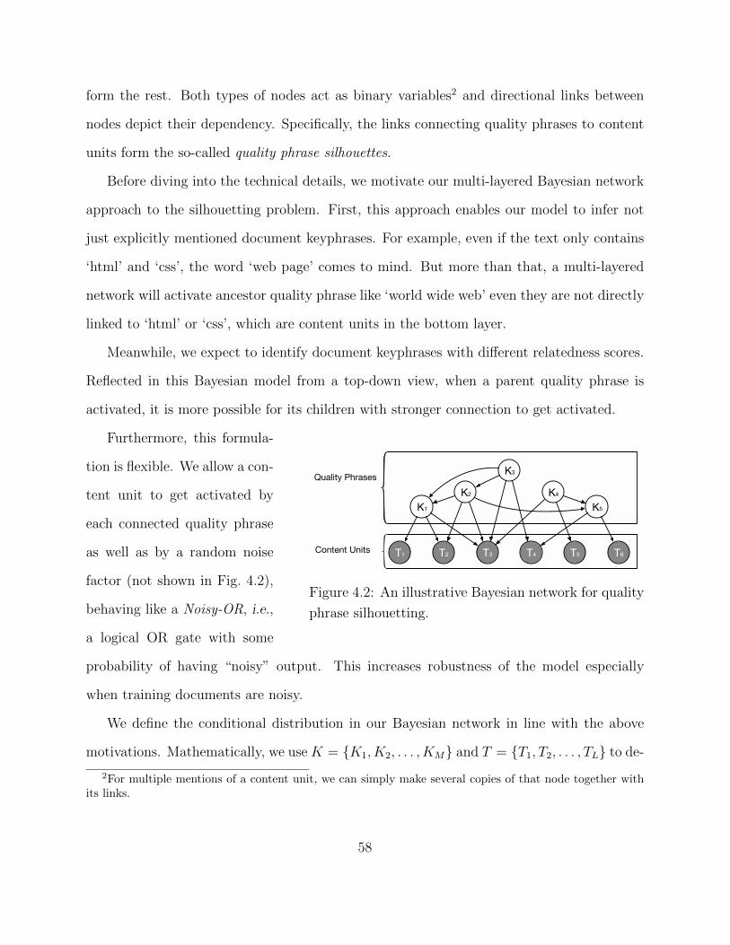
form the rest. Both types of nodes act as binary variables2 and directional links between
nodes depict their dependency. Specifically, the links connecting quality phrases to content
units form the so-called quality phrase silhouettes.
Before diving into the technical details, we motivate our multi-layered Bayesian network
approach to the silhouetting problem. First, this approach enables our model to infer not
just explicitly mentioned document keyphrases. For example, even if the text only contains
‘html’ and ‘css’, the word ‘web page’ comes to mind. But more than that, a multi-layered
network will activate ancestor quality phrase like ‘world wide web’ even they are not directly
linked to ‘html’ or ‘css’, which are content units in the bottom layer.
Meanwhile, we expect to identify document keyphrases with different relatedness scores.
Reflected in this Bayesian model from a top-down view, when a parent quality phrase is
activated, it is more possible for its children with stronger connection to get activated.
K5K1
K4K2
T5 T6T1 T2 T3 T4
K3
Quality Phrases
Content Units
Figure 4.2: An illustrative Bayesian network for quality
phrase silhouetting.
Furthermore, this formula-
tion is flexible. We allow a con-
tent unit to get activated by
each connected quality phrase
as well as by a random noise
factor (not shown in Fig. 4.2),
behaving like a Noisy-OR, i.e.,
a logical OR gate with some
probability of having “noisy” output. This increases robustness of the model especially
when training documents are noisy.
We define the conditional distribution in our Bayesian network in line with the above
motivations. Mathematically, we use K = K1, K2, . . . , KM and T = T1, T2, . . . , TL to de-
2For multiple mentions of a content unit, we can simply make several copies of that node together withits links.
58
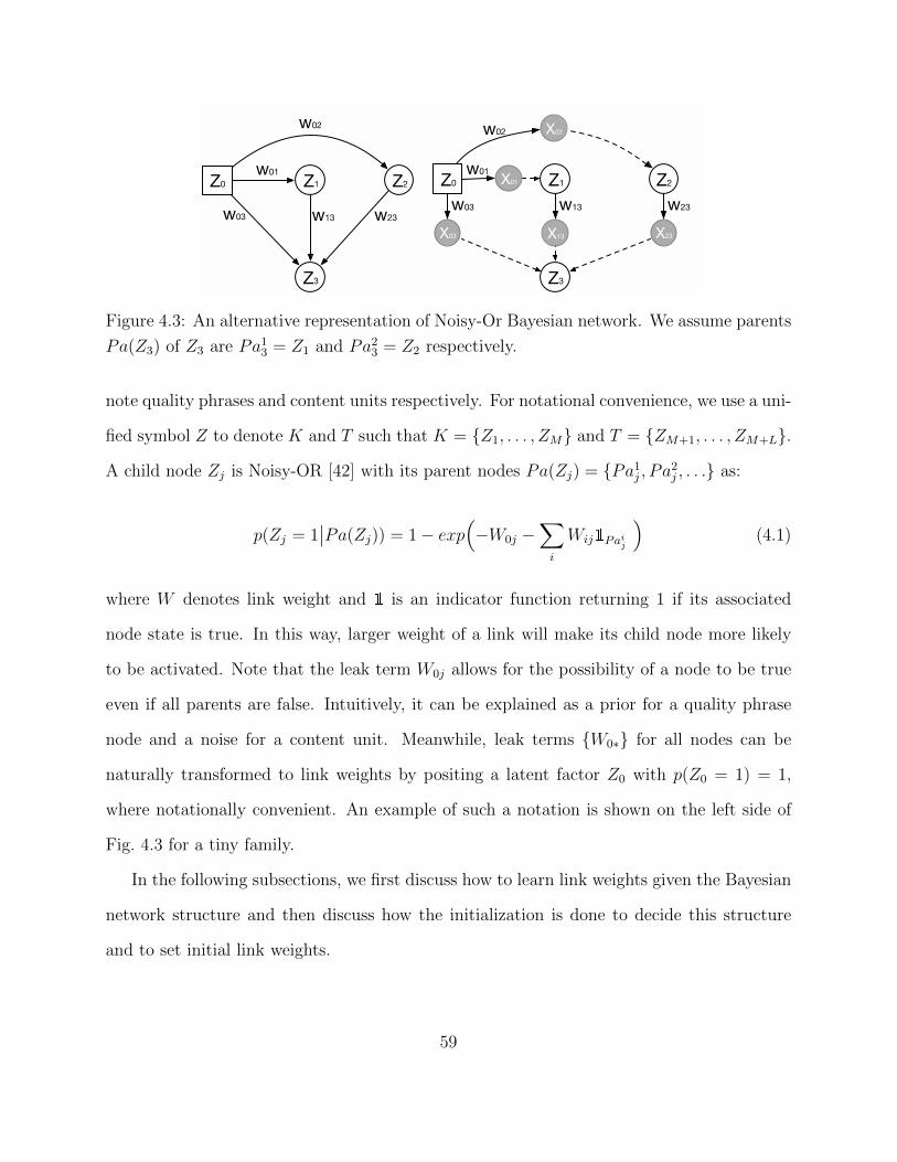
w03 w13 w23
w13w03 w23
Z3
Z0 Z1 Z2 Z0 Z1 Z2
Z3
X03 X13 X23
w01
w02X02
X01
w01
w02
Figure 4.3: An alternative representation of Noisy-Or Bayesian network. We assume parents
Pa(Z3) of Z3 are Pa13 = Z1 and Pa2
3 = Z2 respectively.
note quality phrases and content units respectively. For notational convenience, we use a uni-
fied symbol Z to denote K and T such that K = Z1, . . . , ZM and T = ZM+1, . . . , ZM+L.
A child node Zj is Noisy-OR [42] with its parent nodes Pa(Zj) = Pa1j , Pa
2j , . . . as:
p(Zj = 1∣∣Pa(Zj)) = 1− exp
(−W0j −
∑i
Wij1Paij
)(4.1)
where W denotes link weight and 1 is an indicator function returning 1 if its associated
node state is true. In this way, larger weight of a link will make its child node more likely
to be activated. Note that the leak term W0j allows for the possibility of a node to be true
even if all parents are false. Intuitively, it can be explained as a prior for a quality phrase
node and a noise for a content unit. Meanwhile, leak terms W0∗ for all nodes can be
naturally transformed to link weights by positing a latent factor Z0 with p(Z0 = 1) = 1,
where notationally convenient. An example of such a notation is shown on the left side of
Fig. 4.3 for a tiny family.
In the following subsections, we first discuss how to learn link weights given the Bayesian
network structure and then discuss how the initialization is done to decide this structure
and to set initial link weights.
59
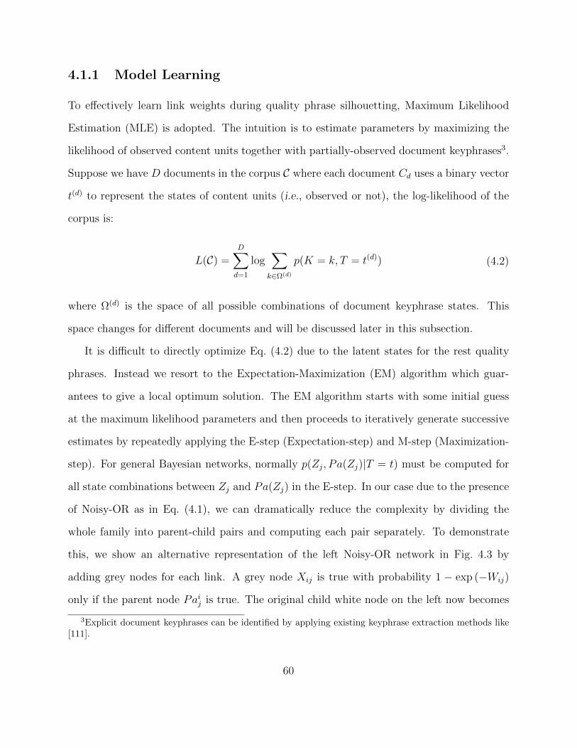
4.1.1 Model Learning
To effectively learn link weights during quality phrase silhouetting, Maximum Likelihood
Estimation (MLE) is adopted. The intuition is to estimate parameters by maximizing the
likelihood of observed content units together with partially-observed document keyphrases3.
Suppose we have D documents in the corpus C where each document Cd uses a binary vector
t(d) to represent the states of content units (i.e., observed or not), the log-likelihood of the
corpus is:
L(C) =D∑d=1
log∑k∈Ω(d)
p(K = k, T = t(d)) (4.2)
where Ω(d) is the space of all possible combinations of document keyphrase states. This
space changes for different documents and will be discussed later in this subsection.
It is difficult to directly optimize Eq. (4.2) due to the latent states for the rest quality
phrases. Instead we resort to the Expectation-Maximization (EM) algorithm which guar-
antees to give a local optimum solution. The EM algorithm starts with some initial guess
at the maximum likelihood parameters and then proceeds to iteratively generate successive
estimates by repeatedly applying the E-step (Expectation-step) and M-step (Maximization-
step). For general Bayesian networks, normally p(Zj, Pa(Zj)|T = t) must be computed for
all state combinations between Zj and Pa(Zj) in the E-step. In our case due to the presence
of Noisy-OR as in Eq. (4.1), we can dramatically reduce the complexity by dividing the
whole family into parent-child pairs and computing each pair separately. To demonstrate
this, we show an alternative representation of the left Noisy-OR network in Fig. 4.3 by
adding grey nodes for each link. A grey node Xij is true with probability 1 − exp (−Wij)
only if the parent node Paij is true. The original child white node on the left now becomes
3Explicit document keyphrases can be identified by applying existing keyphrase extraction methods like[111].
60
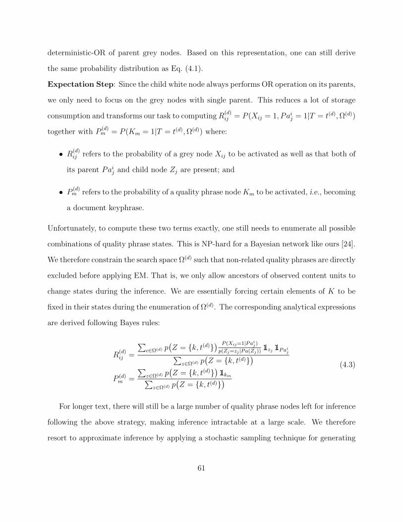
deterministic-OR of parent grey nodes. Based on this representation, one can still derive
the same probability distribution as Eq. (4.1).
Expectation Step: Since the child white node always performs OR operation on its parents,
we only need to focus on the grey nodes with single parent. This reduces a lot of storage
consumption and transforms our task to computingR(d)ij = P (Xij = 1, Paij = 1|T = t(d),Ω(d))
together with P(d)m = P (Km = 1|T = t(d),Ω(d)) where:
• R(d)ij refers to the probability of a grey node Xij to be activated as well as that both of
its parent Paij and child node Zj are present; and
• P (d)m refers to the probability of a quality phrase node Km to be activated, i.e., becoming
a document keyphrase.
Unfortunately, to compute these two terms exactly, one still needs to enumerate all possible
combinations of quality phrase states. This is NP-hard for a Bayesian network like ours [24].
We therefore constrain the search space Ω(d) such that non-related quality phrases are directly
excluded before applying EM. That is, we only allow ancestors of observed content units to
change states during the inference. We are essentially forcing certain elements of K to be
fixed in their states during the enumeration of Ω(d). The corresponding analytical expressions
are derived following Bayes rules:
R(d)ij =
∑c∈Ω(d) p
(Z = k, t(d)
) P (Xij=1|Paij)
p(Zj=zj |Pa(Zj))1zj 1Paij∑
z∈Ω(d) p(Z = k, t(d)
)P (d)m =
∑z∈Ω(d) p
(Z = k, t(d)
)1km∑
z∈Ω(d) p(Z = k, t(d)
) (4.3)
For longer text, there will still be a large number of quality phrase nodes left for inference
following the above strategy, making inference intractable at a large scale. We therefore
resort to approximate inference by applying a stochastic sampling technique for generating
61
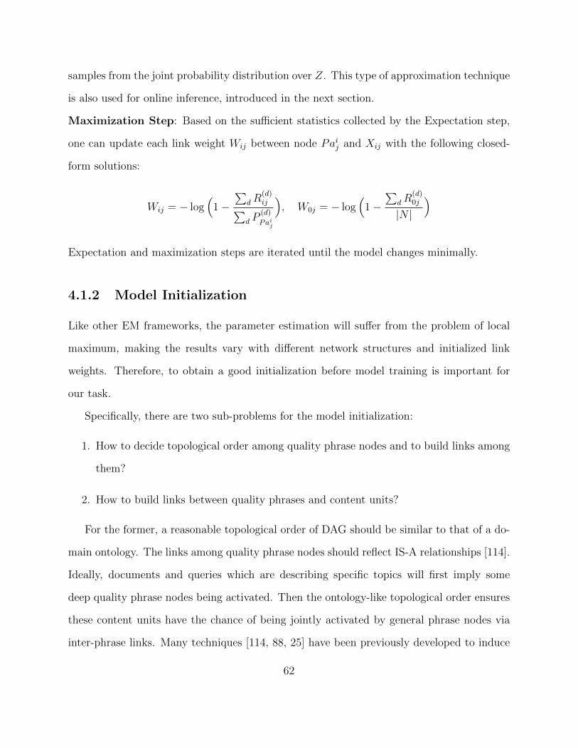
samples from the joint probability distribution over Z. This type of approximation technique
is also used for online inference, introduced in the next section.
Maximization Step: Based on the sufficient statistics collected by the Expectation step,
one can update each link weight Wij between node Paij and Xij with the following closed-
form solutions:
Wij = − log(
1−∑
dR(d)ij∑
d P(d)
Paij
), W0j = − log
(1−
∑dR
(d)0j
|N |
)
Expectation and maximization steps are iterated until the model changes minimally.
4.1.2 Model Initialization
Like other EM frameworks, the parameter estimation will suffer from the problem of local
maximum, making the results vary with different network structures and initialized link
weights. Therefore, to obtain a good initialization before model training is important for
our task.
Specifically, there are two sub-problems for the model initialization:
1. How to decide topological order among quality phrase nodes and to build links among
them?
2. How to build links between quality phrases and content units?
For the former, a reasonable topological order of DAG should be similar to that of a do-
main ontology. The links among quality phrase nodes should reflect IS-A relationships [114].
Ideally, documents and queries which are describing specific topics will first imply some
deep quality phrase nodes being activated. Then the ontology-like topological order ensures
these content units have the chance of being jointly activated by general phrase nodes via
inter-phrase links. Many techniques [114, 88, 25] have been previously developed to induce
62
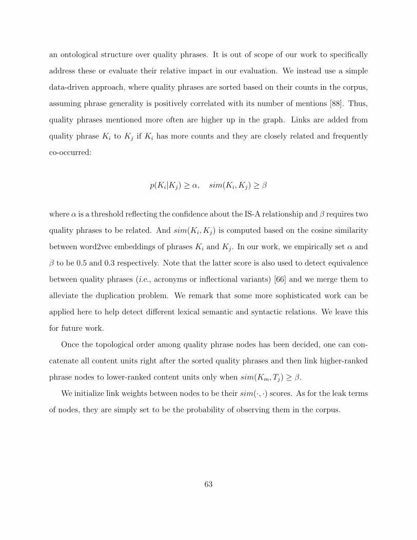
an ontological structure over quality phrases. It is out of scope of our work to specifically
address these or evaluate their relative impact in our evaluation. We instead use a simple
data-driven approach, where quality phrases are sorted based on their counts in the corpus,
assuming phrase generality is positively correlated with its number of mentions [88]. Thus,
quality phrases mentioned more often are higher up in the graph. Links are added from
quality phrase Ki to Kj if Ki has more counts and they are closely related and frequently
co-occurred:
p(Ki|Kj) ≥ α, sim(Ki, Kj) ≥ β
where α is a threshold reflecting the confidence about the IS-A relationship and β requires two
quality phrases to be related. And sim(Ki, Kj) is computed based on the cosine similarity
between word2vec embeddings of phrases Ki and Kj. In our work, we empirically set α and
β to be 0.5 and 0.3 respectively. Note that the latter score is also used to detect equivalence
between quality phrases (i.e., acronyms or inflectional variants) [66] and we merge them to
alleviate the duplication problem. We remark that some more sophisticated work can be
applied here to help detect different lexical semantic and syntactic relations. We leave this
for future work.
Once the topological order among quality phrase nodes has been decided, one can con-
catenate all content units right after the sorted quality phrases and then link higher-ranked
phrase nodes to lower-ranked content units only when sim(Km, Tj) ≥ β.
We initialize link weights between nodes to be their sim(·, ·) scores. As for the leak terms
of nodes, they are simply set to be the probability of observing them in the corpus.
63
4.2 Online Inference and Encoding
The online inference is designed to efficiently quantify the relatedness between the text query
and its potential document keyphrases. Inspired by the sufficient statistics collected in E-
step, we are particularly interested in computing P(q)m = p(Km|T = t(q)), i.e., the activation
probability for a certain keyphrase Km, as the non-negative relatedness score.
Notice that in the online inference phase, efficiency is usually a big challenge and the
inference previously mentioned for the E-step will be intractable if the document becomes
too long. In this regard, we resort to an approximate sampling approach. This technique
can be applied to compute both P(q)m and P
(d)m . At the same time, R
(d)ij = p(Xij, Pa
ij|T = t(d))
needed in the E-step can be benefited.
4.2.1 Inexact Inference Using Gibbs Sampling
In the last section, we discussed about the exact inference in E-step where enumeration over
document keyphrase states are necessary to help compute the above terms. In fact, they
can be more efficiently approximated by use of Monte Carlo sampling methods, which are
a set of computational techniques for generating samples from a target distribution like the
joint probability p(K,T = t) in our setting. Among the Monte Carlo family, we apply Gibbs
sampling in this work to sample quality phrase variables during each inference procedure.
Given content unit vector t representing a document Cd or query q, we proceed as follows:
1. Start with initial setting: only observed content units and explicit document keyphrases
are set to be true, denoted by k(0), t
2. For each s ∈ 1, . . . , S, sequentially sample all quality phrase nodes following condi-
tional distribution p(Km|K−m = k(s)1 , . . . , k
(s)m−1, k
(s−1)m+1 , . . . , k
(s−1)M , T = t), denoted as
k(s).
64
where
p(Km = 1|K−m = k−m, T = t) =p(Km = 1, K−m = k−m, T = t)∑1i=0 p(Km = i,K−m = k−m, T = t)
(4.4)
To compute Eq. (4.4) efficiently, for every quality phrase node, we maintain the following
probability ratio:
p(Km = 1, K−m = k−m, T = t)
p(Km = 0, K−m = k−m, T = t)(4.5)
where K−m refers to all the phrase nodes except Km. Given the above ratio, one can easily
compute Eq. (4.4) needed for sampling Km.
Now the problem becomes how to maintain Eq. (4.5) for each phrase node during the
sampling process. In fact, according to the chain rule in Bayesian network, we have
p(Km = 1, K−m = k−m, T = t)
p(Km = 0, K−m = k−m, T = t)=p(Km = 1|Pa(Km))
p(Km = 0|Pa(Km))
×∏
Zj∈Ch(Km)
p(Zj|Pa−Km(Zj), Km = 1)
p(Zj|Pa−Km(Zj), Km = 0)
where Ch(Km) refers Km’s children. From the above equation, one can conclude that
Eq. (4.5) for node Km should be updated whenever nodes in its Markov blanket4 change
states.
The above Gibbs sampling process ensures that samples approximate the joint probability
distribution between all phrase variables and content units. Such sampling is performed over
all the original nodes in the network but does not include the grey nodes (see Fig. 4.3) in the
alternative representation for the sake of sampling efficiency. One can easily compute the
probability distribution over each of the grey nodes given a quality phrase state combination.
4Markov blanket for a node in a Bayesian network composed of its parents, children and children’s otherparents.
65
By marginalizing over necessary quality phrase variables in the Bayesian network, the
following approximate equations can be derived:
Rij =
∑Ss=1
p(Xij=1|Paij)
p(Zj=z(s)j |Pa(Zj))
1z(s)j1Paij
S, Pm =
∑Ss=1 1k
(s)m
S
4.2.2 Search Space Reduction
To further improve the efficiency of Gibbs sampling, one can follow the idea of E-step to
reduce the number of sampled nodes. Intuitively, only a small portion of quality phrases are
related to the text query. There is no need to sample all phrase nodes since most of them do
not have chance to get activated. That is to say, we can skip majority of them based on a
reasonable relatedness prediction before conducting Gibbs sampling. Suppose content unit
vector T ′ = T ′1, · · · , T ′l ⊆ T contains only observed content units. We pick the following
scoring function:
p(T ′ = 1, · · · , 1|Zj = 1)
This score can be viewed as the probability of generating the observed content units when
quality phrase Zj is activated. Computing p(T ′ = 1, · · · , 1|Zj = 1) is still challenging
because quality phrases are connected and enumeration over state combinations of connected
quality phrases are unavoidable. Thus we adopt a local arborescence structure [108] to
approximate the probability by keeping the path from Zj to each content unit T ′r for which
the activation probability product along the path is maximum among all paths from Zj to
T ′r. In this way, the activation probability for each content unit is independent given Zj is
activated. The associate probability of the approximate link between quality phrase node
66
Zj and content unit Tr is denoted as p(T ′r = 1|Zj = 1). We then have:
p(T ′ = 1, · · · , 1|Zj = 1) ≈∏r
(1−(
1− p(T ′r = 1|Z0))×
(1− p(T ′r = 1|Zj = 1)
))
In addition, the score can be naturally and efficiently propagated from children to parents
in the network recursively:
p(T ′r = 1|Zj = 1) = maxi
p(T ′r = 1|Chij = 1) p(Chij = 1|Zj = 1)
where Chij refers to the ith child node of Zj. The above equation can be computed following
reverse topological order of quality phrase nodes. It is worth noting that in this stage
we are generating document keyphrase candidates for the sampling procedure in inference
step. Therefore, this pruning strategy is critical for model performance. A poor strategy
will incorporate irrelevant quality phrases and miss important ones, which further affects
sampling efficiency and undermines representation.
4.3 Experimental Study
In this section, experiments were conducted to demonstrate the effectiveness of the pro-
posed LAKI in generating high quality representations of text queries. We begin with the
description of datasets.
Two real-world data sets were used in the experiments and detailed statistics are sum-
marized in Table 4.2.
• The Academia dataset is a collection of major computer science publications. We use
both paper titles and abstracts in venues of database, data mining, machine learning,
67
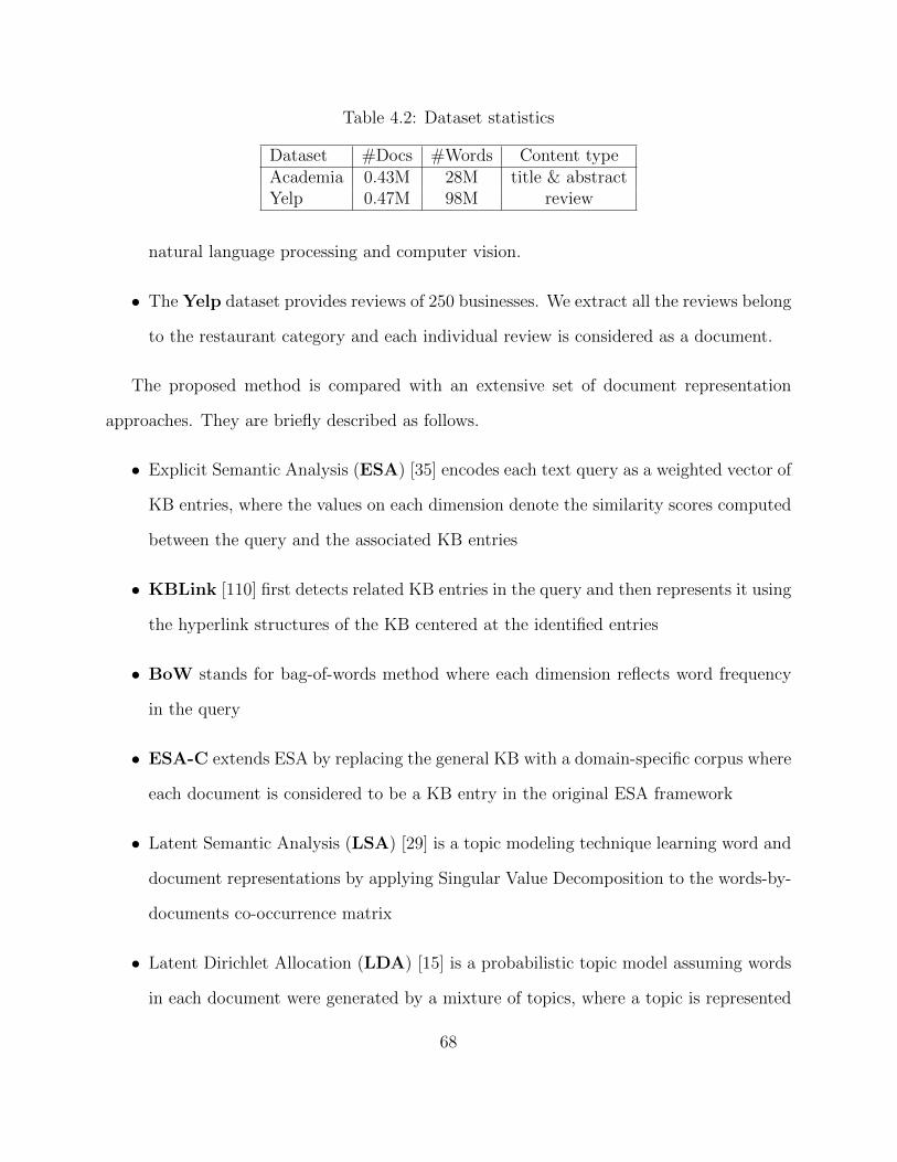
Table 4.2: Dataset statistics
Dataset #Docs #Words Content typeAcademia 0.43M 28M title & abstractYelp 0.47M 98M review
natural language processing and computer vision.
• The Yelp dataset provides reviews of 250 businesses. We extract all the reviews belong
to the restaurant category and each individual review is considered as a document.
The proposed method is compared with an extensive set of document representation
approaches. They are briefly described as follows.
• Explicit Semantic Analysis (ESA) [35] encodes each text query as a weighted vector of
KB entries, where the values on each dimension denote the similarity scores computed
between the query and the associated KB entries
• KBLink [110] first detects related KB entries in the query and then represents it using
the hyperlink structures of the KB centered at the identified entries
• BoW stands for bag-of-words method where each dimension reflects word frequency
in the query
• ESA-C extends ESA by replacing the general KB with a domain-specific corpus where
each document is considered to be a KB entry in the original ESA framework
• Latent Semantic Analysis (LSA) [29] is a topic modeling technique learning word and
document representations by applying Singular Value Decomposition to the words-by-
documents co-occurrence matrix
• Latent Dirichlet Allocation (LDA) [15] is a probabilistic topic model assuming words
in each document were generated by a mixture of topics, where a topic is represented
68
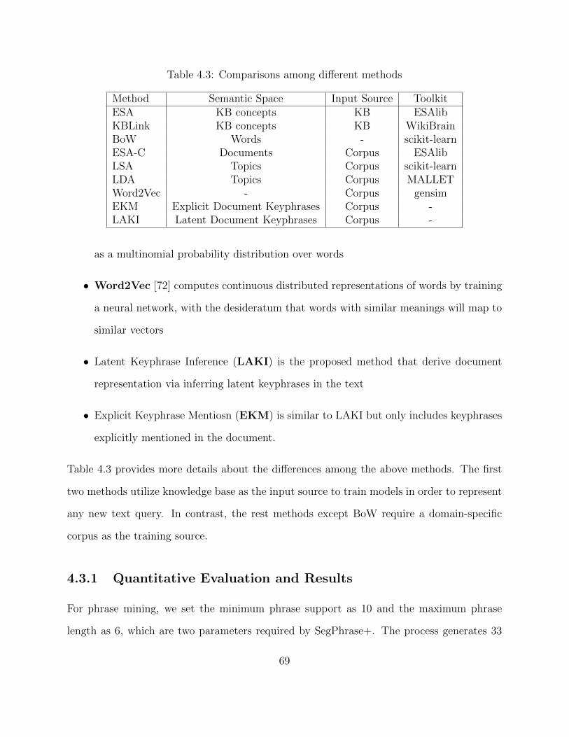
Table 4.3: Comparisons among different methods
Method Semantic Space Input Source ToolkitESA KB concepts KB ESAlibKBLink KB concepts KB WikiBrainBoW Words - scikit-learnESA-C Documents Corpus ESAlibLSA Topics Corpus scikit-learnLDA Topics Corpus MALLETWord2Vec - Corpus gensimEKM Explicit Document Keyphrases Corpus -LAKI Latent Document Keyphrases Corpus -
as a multinomial probability distribution over words
• Word2Vec [72] computes continuous distributed representations of words by training
a neural network, with the desideratum that words with similar meanings will map to
similar vectors
• Latent Keyphrase Inference (LAKI) is the proposed method that derive document
representation via inferring latent keyphrases in the text
• Explicit Keyphrase Mentiosn (EKM) is similar to LAKI but only includes keyphrases
explicitly mentioned in the document.
Table 4.3 provides more details about the differences among the above methods. The first
two methods utilize knowledge base as the input source to train models in order to represent
any new text query. In contrast, the rest methods except BoW require a domain-specific
corpus as the training source.
4.3.1 Quantitative Evaluation and Results
For phrase mining, we set the minimum phrase support as 10 and the maximum phrase
length as 6, which are two parameters required by SegPhrase+. The process generates 33
69
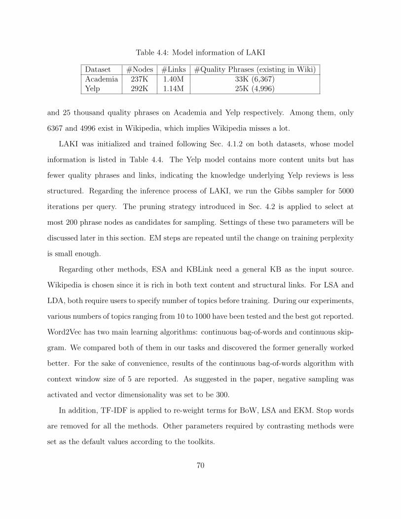
Table 4.4: Model information of LAKI
Dataset #Nodes #Links #Quality Phrases (existing in Wiki)Academia 237K 1.40M 33K (6,367)Yelp 292K 1.14M 25K (4,996)
and 25 thousand quality phrases on Academia and Yelp respectively. Among them, only
6367 and 4996 exist in Wikipedia, which implies Wikipedia misses a lot.
LAKI was initialized and trained following Sec. 4.1.2 on both datasets, whose model
information is listed in Table 4.4. The Yelp model contains more content units but has
fewer quality phrases and links, indicating the knowledge underlying Yelp reviews is less
structured. Regarding the inference process of LAKI, we run the Gibbs sampler for 5000
iterations per query. The pruning strategy introduced in Sec. 4.2 is applied to select at
most 200 phrase nodes as candidates for sampling. Settings of these two parameters will be
discussed later in this section. EM steps are repeated until the change on training perplexity
is small enough.
Regarding other methods, ESA and KBLink need a general KB as the input source.
Wikipedia is chosen since it is rich in both text content and structural links. For LSA and
LDA, both require users to specify number of topics before training. During our experiments,
various numbers of topics ranging from 10 to 1000 have been tested and the best got reported.
Word2Vec has two main learning algorithms: continuous bag-of-words and continuous skip-
gram. We compared both of them in our tasks and discovered the former generally worked
better. For the sake of convenience, results of the continuous bag-of-words algorithm with
context window size of 5 are reported. As suggested in the paper, negative sampling was
activated and vector dimensionality was set to be 300.
In addition, TF-IDF is applied to re-weight terms for BoW, LSA and EKM. Stop words
are removed for all the methods. Other parameters required by contrasting methods were
set as the default values according to the toolkits.
70
The goal of our experiments is to quantitatively evaluate how well our method performs
in generating documents representations of online queries. We introduce our empirical eval-
uation in two problem domains: phrase relatedness and document classification.
Phrase Relatedness: For a set of phrase pairs, method performance is evaluated by how
well the generated relatedness scores correlate with the gold scores. The gold score for each
phrase pair is based on human judgements of the pair’s semantic relatedness.
To create these phrase pairs, we first sampled 100 pairs of frequently co-occurred phrases
for each dataset respectively. Then we expanded the set by randomly combining phrases
from different pairs and the final evaluation set contains 300 pairs. Each pair was carefully
assigned a relatedness score from 0 to 3 where higher score indicates stronger similarity. We
used Pearson’s linear correlation coefficient to compare computed relatedness scores with
human judgements.
To compute semantic relatedness of a paired phrases, KBLink proposes to use a combined
relatedness measure inspired from TF-IDF and Google Distance. For other methods, cosine
metric is used to compare their vectorial representations.
Document Classification: In this classification task, we wish to classify a document
into several mutually exclusive classes. A challenging aspect of the document classification
problem is the choice of features. Considering document representations as features, we
expect the classification accuracy can well reflect the discriminative power of each method.
For each compared method, we first derived vectorial representations for all the training
and testing documents without reference to their true class label. Then a support vector
machine with both linear and radial basis function kernels was trained on the training set
(only the best was reported). Classification accuracy on the testing set is reported to measure
the performance of the method.
For the methods trained on the Academia dataset, we created a held-out set of 500
71
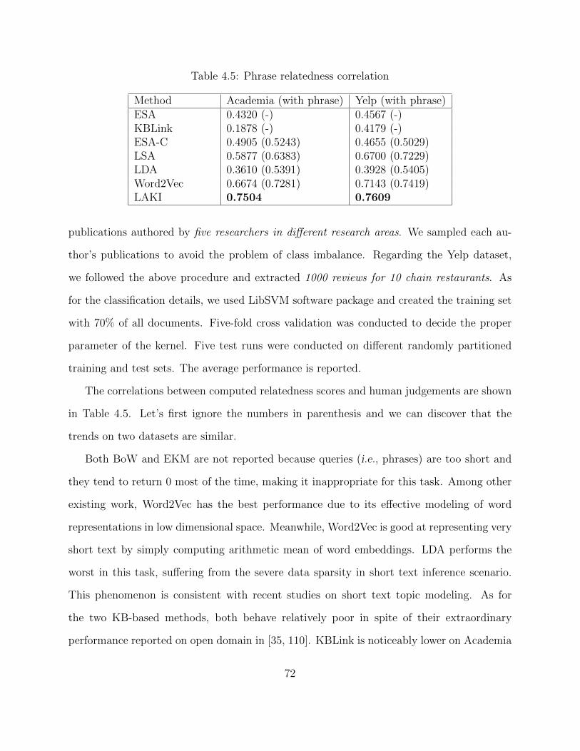
Table 4.5: Phrase relatedness correlation
Method Academia (with phrase) Yelp (with phrase)ESA 0.4320 (-) 0.4567 (-)KBLink 0.1878 (-) 0.4179 (-)ESA-C 0.4905 (0.5243) 0.4655 (0.5029)LSA 0.5877 (0.6383) 0.6700 (0.7229)LDA 0.3610 (0.5391) 0.3928 (0.5405)Word2Vec 0.6674 (0.7281) 0.7143 (0.7419)LAKI 0.7504 0.7609
publications authored by five researchers in different research areas. We sampled each au-
thor’s publications to avoid the problem of class imbalance. Regarding the Yelp dataset,
we followed the above procedure and extracted 1000 reviews for 10 chain restaurants. As
for the classification details, we used LibSVM software package and created the training set
with 70% of all documents. Five-fold cross validation was conducted to decide the proper
parameter of the kernel. Five test runs were conducted on different randomly partitioned
training and test sets. The average performance is reported.
The correlations between computed relatedness scores and human judgements are shown
in Table 4.5. Let’s first ignore the numbers in parenthesis and we can discover that the
trends on two datasets are similar.
Both BoW and EKM are not reported because queries (i.e., phrases) are too short and
they tend to return 0 most of the time, making it inappropriate for this task. Among other
existing work, Word2Vec has the best performance due to its effective modeling of word
representations in low dimensional space. Meanwhile, Word2Vec is good at representing very
short text by simply computing arithmetic mean of word embeddings. LDA performs the
worst in this task, suffering from the severe data sparsity in short text inference scenario.
This phenomenon is consistent with recent studies on short text topic modeling. As for
the two KB-based methods, both behave relatively poor in spite of their extraordinary
performance reported on open domain in [35, 110]. KBLink is noticeably lower on Academia
72
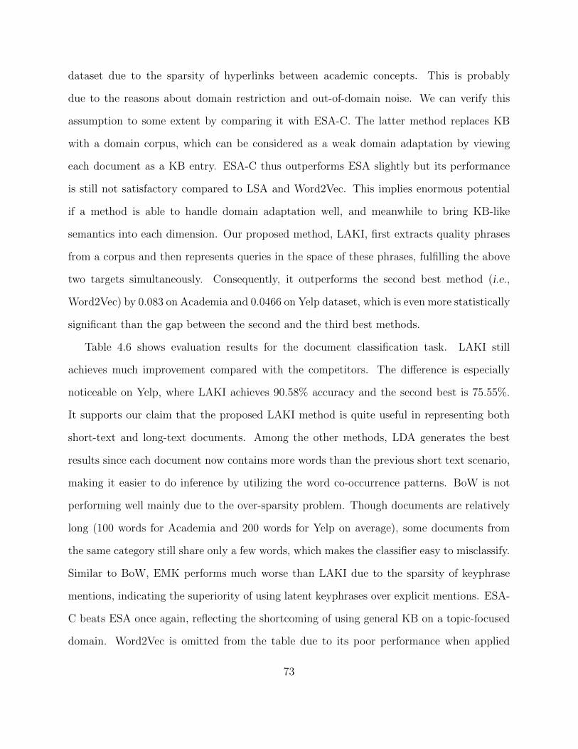
dataset due to the sparsity of hyperlinks between academic concepts. This is probably
due to the reasons about domain restriction and out-of-domain noise. We can verify this
assumption to some extent by comparing it with ESA-C. The latter method replaces KB
with a domain corpus, which can be considered as a weak domain adaptation by viewing
each document as a KB entry. ESA-C thus outperforms ESA slightly but its performance
is still not satisfactory compared to LSA and Word2Vec. This implies enormous potential
if a method is able to handle domain adaptation well, and meanwhile to bring KB-like
semantics into each dimension. Our proposed method, LAKI, first extracts quality phrases
from a corpus and then represents queries in the space of these phrases, fulfilling the above
two targets simultaneously. Consequently, it outperforms the second best method (i.e.,
Word2Vec) by 0.083 on Academia and 0.0466 on Yelp dataset, which is even more statistically
significant than the gap between the second and the third best methods.
Table 4.6 shows evaluation results for the document classification task. LAKI still
achieves much improvement compared with the competitors. The difference is especially
noticeable on Yelp, where LAKI achieves 90.58% accuracy and the second best is 75.55%.
It supports our claim that the proposed LAKI method is quite useful in representing both
short-text and long-text documents. Among the other methods, LDA generates the best
results since each document now contains more words than the previous short text scenario,
making it easier to do inference by utilizing the word co-occurrence patterns. BoW is not
performing well mainly due to the over-sparsity problem. Though documents are relatively
long (100 words for Academia and 200 words for Yelp on average), some documents from
the same category still share only a few words, which makes the classifier easy to misclassify.
Similar to BoW, EMK performs much worse than LAKI due to the sparsity of keyphrase
mentions, indicating the superiority of using latent keyphrases over explicit mentions. ESA-
C beats ESA once again, reflecting the shortcoming of using general KB on a topic-focused
domain. Word2Vec is omitted from the table due to its poor performance when applied
73
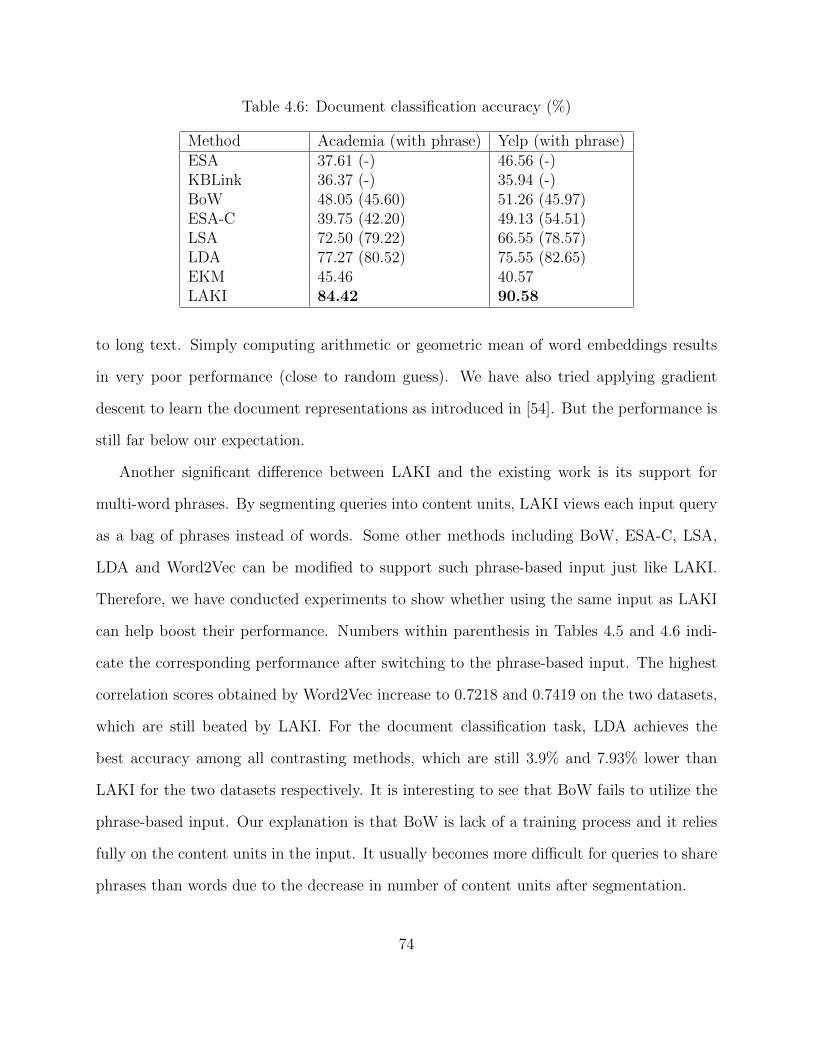
Table 4.6: Document classification accuracy (%)
Method Academia (with phrase) Yelp (with phrase)ESA 37.61 (-) 46.56 (-)KBLink 36.37 (-) 35.94 (-)BoW 48.05 (45.60) 51.26 (45.97)ESA-C 39.75 (42.20) 49.13 (54.51)LSA 72.50 (79.22) 66.55 (78.57)LDA 77.27 (80.52) 75.55 (82.65)EKM 45.46 40.57LAKI 84.42 90.58
to long text. Simply computing arithmetic or geometric mean of word embeddings results
in very poor performance (close to random guess). We have also tried applying gradient
descent to learn the document representations as introduced in [54]. But the performance is
still far below our expectation.
Another significant difference between LAKI and the existing work is its support for
multi-word phrases. By segmenting queries into content units, LAKI views each input query
as a bag of phrases instead of words. Some other methods including BoW, ESA-C, LSA,
LDA and Word2Vec can be modified to support such phrase-based input just like LAKI.
Therefore, we have conducted experiments to show whether using the same input as LAKI
can help boost their performance. Numbers within parenthesis in Tables 4.5 and 4.6 indi-
cate the corresponding performance after switching to the phrase-based input. The highest
correlation scores obtained by Word2Vec increase to 0.7218 and 0.7419 on the two datasets,
which are still beated by LAKI. For the document classification task, LDA achieves the
best accuracy among all contrasting methods, which are still 3.9% and 7.93% lower than
LAKI for the two datasets respectively. It is interesting to see that BoW fails to utilize the
phrase-based input. Our explanation is that BoW is lack of a training process and it relies
fully on the content units in the input. It usually becomes more difficult for queries to share
phrases than words due to the decrease in number of content units after segmentation.
74
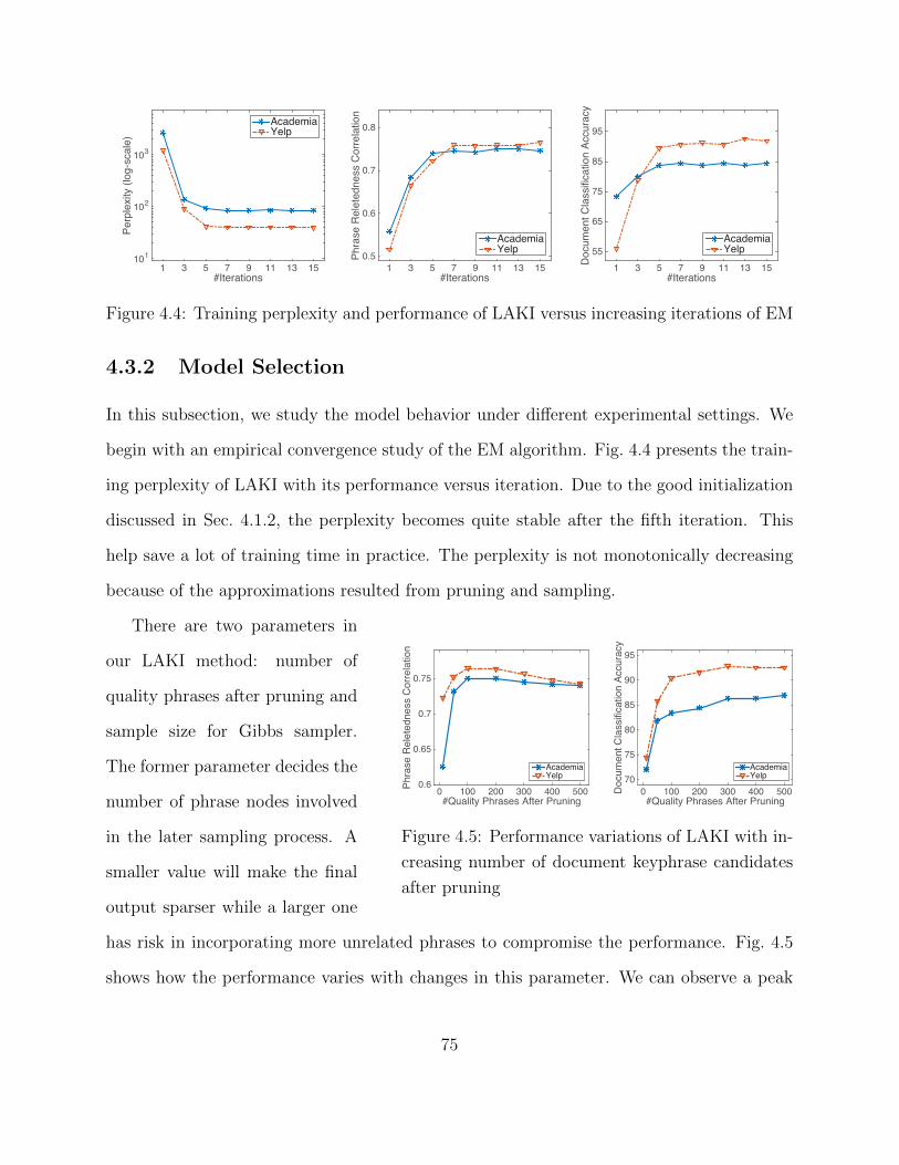
#Iterations1 3 5 7 9 11 13 15
Pe
rple
xity (
log
-sca
le)
101
102
103
AcademiaYelp
#Iterations1 3 5 7 9 11 13 15
Ph
rase
Re
lete
dn
ess C
orr
ela
tio
n
0.5
0.6
0.7
0.8
AcademiaYelp
#Iterations1 3 5 7 9 11 13 15
Do
cu
me
nt C
lassific
atio
n A
ccu
racy
55
65
75
85
95
AcademiaYelp
Figure 4.4: Training perplexity and performance of LAKI versus increasing iterations of EM
4.3.2 Model Selection
In this subsection, we study the model behavior under different experimental settings. We
begin with an empirical convergence study of the EM algorithm. Fig. 4.4 presents the train-
ing perplexity of LAKI with its performance versus iteration. Due to the good initialization
discussed in Sec. 4.1.2, the perplexity becomes quite stable after the fifth iteration. This
help save a lot of training time in practice. The perplexity is not monotonically decreasing
because of the approximations resulted from pruning and sampling.
#Quality Phrases After Pruning 0 100 200 300 400 500
Ph
rase
Re
lete
dn
ess C
orr
ela
tio
n
0.6
0.65
0.7
0.75
AcademiaYelp
#Quality Phrases After Pruning 0 100 200 300 400 500D
ocu
me
nt C
lassific
atio
n A
ccu
racy
70
75
80
85
90
95
AcademiaYelp
Figure 4.5: Performance variations of LAKI with in-
creasing number of document keyphrase candidates
after pruning
There are two parameters in
our LAKI method: number of
quality phrases after pruning and
sample size for Gibbs sampler.
The former parameter decides the
number of phrase nodes involved
in the later sampling process. A
smaller value will make the final
output sparser while a larger one
has risk in incorporating more unrelated phrases to compromise the performance. Fig. 4.5
shows how the performance varies with changes in this parameter. We can observe a peak
75
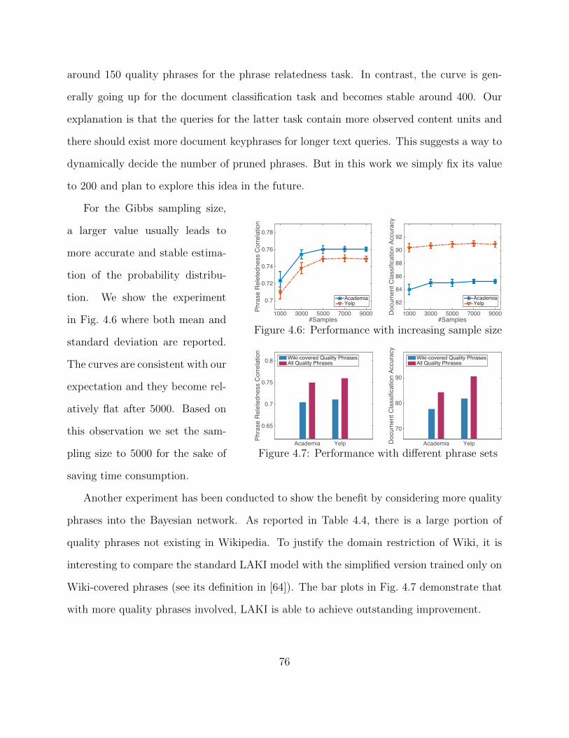
around 150 quality phrases for the phrase relatedness task. In contrast, the curve is gen-
erally going up for the document classification task and becomes stable around 400. Our
explanation is that the queries for the latter task contain more observed content units and
there should exist more document keyphrases for longer text queries. This suggests a way to
dynamically decide the number of pruned phrases. But in this work we simply fix its value
to 200 and plan to explore this idea in the future.
#Samples1000 3000 5000 7000 9000
Ph
rase
Re
lete
dn
ess C
orr
ela
tio
n
0.7
0.72
0.74
0.76
0.78
AcademiaYelp
#Samples1000 3000 5000 7000 9000D
ocu
me
nt C
lassific
atio
n A
ccu
racy
82
84
86
88
90
92
AcademiaYelp
Figure 4.6: Performance with increasing sample size
Academia Yelp
Ph
rase
Re
lete
dn
ess C
orr
ela
tio
n
0.65
0.7
0.75
0.8Wiki-covered Quality PhrasesAll Quality Phrases
Academia YelpDo
cu
me
nt C
lassific
atio
n A
ccu
racy
70
80
90
Wiki-covered Quality PhrasesAll Quality Phrases
Figure 4.7: Performance with different phrase sets
For the Gibbs sampling size,
a larger value usually leads to
more accurate and stable estima-
tion of the probability distribu-
tion. We show the experiment
in Fig. 4.6 where both mean and
standard deviation are reported.
The curves are consistent with our
expectation and they become rel-
atively flat after 5000. Based on
this observation we set the sam-
pling size to 5000 for the sake of
saving time consumption.
Another experiment has been conducted to show the benefit by considering more quality
phrases into the Bayesian network. As reported in Table 4.4, there is a large portion of
quality phrases not existing in Wikipedia. To justify the domain restriction of Wiki, it is
interesting to compare the standard LAKI model with the simplified version trained only on
Wiki-covered phrases (see its definition in [64]). The bar plots in Fig. 4.7 demonstrate that
with more quality phrases involved, LAKI is able to achieve outstanding improvement.
76
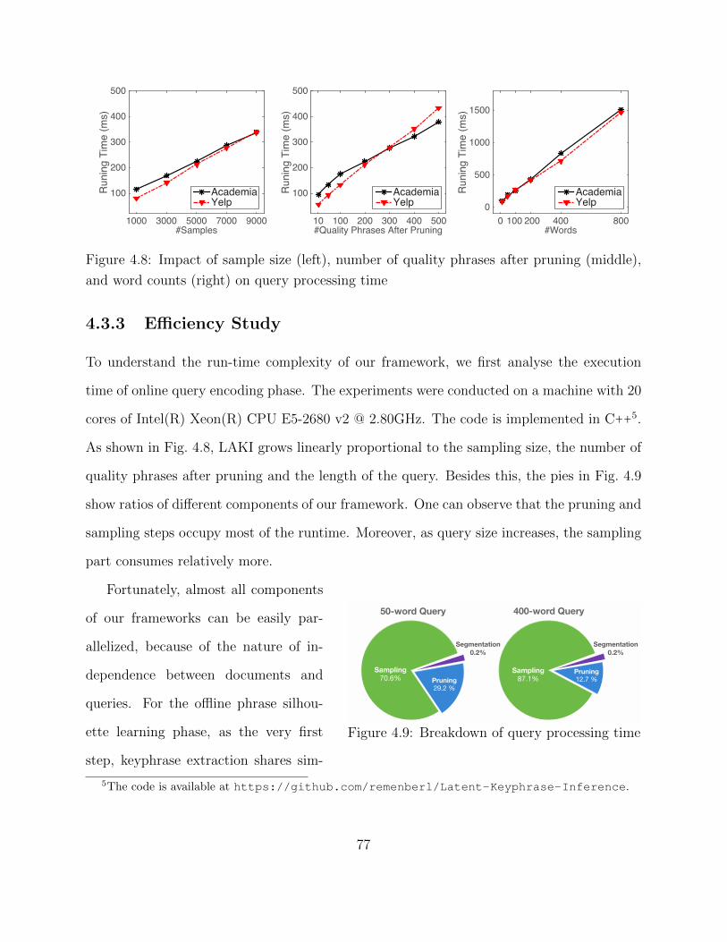
#Samples1000 3000 5000 7000 9000
Ru
nin
g T
ime
(m
s)
100
200
300
400
500
AcademiaYelp
#Quality Phrases After Pruning10 100 200 300 400 500
Ru
nin
g T
ime
(m
s)
100
200
300
400
500
AcademiaYelp
#Words0 100 200 400 800
Ru
nin
g T
ime
(m
s)
0
500
1000
1500
AcademiaYelp
Figure 4.8: Impact of sample size (left), number of quality phrases after pruning (middle),
and word counts (right) on query processing time
4.3.3 Efficiency Study
To understand the run-time complexity of our framework, we first analyse the execution
time of online query encoding phase. The experiments were conducted on a machine with 20
cores of Intel(R) Xeon(R) CPU E5-2680 v2 @ 2.80GHz. The code is implemented in C++5.
As shown in Fig. 4.8, LAKI grows linearly proportional to the sampling size, the number of
quality phrases after pruning and the length of the query. Besides this, the pies in Fig. 4.9
show ratios of different components of our framework. One can observe that the pruning and
sampling steps occupy most of the runtime. Moreover, as query size increases, the sampling
part consumes relatively more.
Sampling70.6% Pruning
29.2 %
Segmentation
0.2%
Sampling87.1%
Pruning12.7 %
Segmentation
0.2%
50-word Query 400-word Query
Figure 4.9: Breakdown of query processing time
Fortunately, almost all components
of our frameworks can be easily par-
allelized, because of the nature of in-
dependence between documents and
queries. For the offline phrase silhou-
ette learning phase, as the very first
step, keyphrase extraction shares sim-
5The code is available at https://github.com/remenberl/Latent-Keyphrase-Inference.
77
ilar time complexity as reported in [64]. The most time consuming part is quality phrase
silhouetting, which is an EM algorithm and each individual inference in E-step has similar
performance compared to Figs. 4.8 and 4.9. The only difference is the pruning time for
silhouetting because the search space is constrained as discussed in Sec. 4.1.1.
4.3.4 Case Study
Previous experiments are focused on evaluating representation quality and time complexity
quantitatively. In this subsection, we first present several queries with their top-ranked
document keyphrases in Table 4.7 generated from the online phase of LAKI. Overall we see
that LAKI can handle both short and long queries quite well. Most document keyphrases are
successfully identified in the list. Relatedness between keyphrase and queries generally drops
with ranking lowers down. Meanwhile, both general and specific document keyphrases exist
in the ranked list. This provides LAKI with more discriminative power when someone applies
it to text mining applications like document clustering and classification. Moreover, LAKI
has the ability to process ambiguous queries like ‘lda’ based on contextual words ‘topic’. We
attribute this to the well-modelled quality phrase silhouettes and we show some examples
of them in Table 4.8. As a quality phrase silhouette might contain many content units, we
only demonstrate ones with the most significant link weights. For ease of presentation, link
weights are omitted in the table.
78
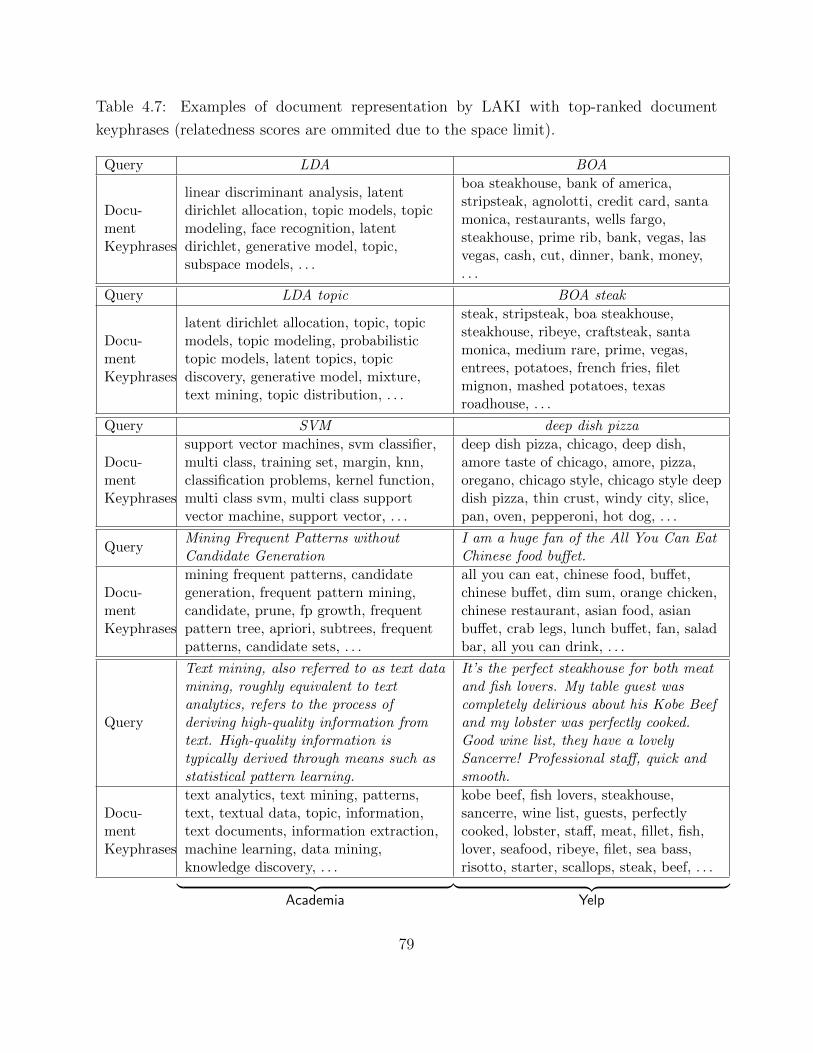
Table 4.7: Examples of document representation by LAKI with top-ranked document
keyphrases (relatedness scores are ommited due to the space limit).
Query LDA BOA
Docu-mentKeyphrases
linear discriminant analysis, latentdirichlet allocation, topic models, topicmodeling, face recognition, latentdirichlet, generative model, topic,subspace models, . . .
boa steakhouse, bank of america,stripsteak, agnolotti, credit card, santamonica, restaurants, wells fargo,steakhouse, prime rib, bank, vegas, lasvegas, cash, cut, dinner, bank, money,. . .
Query LDA topic BOA steak
Docu-mentKeyphrases
latent dirichlet allocation, topic, topicmodels, topic modeling, probabilistictopic models, latent topics, topicdiscovery, generative model, mixture,text mining, topic distribution, . . .
steak, stripsteak, boa steakhouse,steakhouse, ribeye, craftsteak, santamonica, medium rare, prime, vegas,entrees, potatoes, french fries, filetmignon, mashed potatoes, texasroadhouse, . . .
Query SVM deep dish pizza
Docu-mentKeyphrases
support vector machines, svm classifier,multi class, training set, margin, knn,classification problems, kernel function,multi class svm, multi class supportvector machine, support vector, . . .
deep dish pizza, chicago, deep dish,amore taste of chicago, amore, pizza,oregano, chicago style, chicago style deepdish pizza, thin crust, windy city, slice,pan, oven, pepperoni, hot dog, . . .
QueryMining Frequent Patterns withoutCandidate Generation
I am a huge fan of the All You Can EatChinese food buffet.
Docu-mentKeyphrases
mining frequent patterns, candidategeneration, frequent pattern mining,candidate, prune, fp growth, frequentpattern tree, apriori, subtrees, frequentpatterns, candidate sets, . . .
all you can eat, chinese food, buffet,chinese buffet, dim sum, orange chicken,chinese restaurant, asian food, asianbuffet, crab legs, lunch buffet, fan, saladbar, all you can drink, . . .
Query
Text mining, also referred to as text datamining, roughly equivalent to textanalytics, refers to the process ofderiving high-quality information fromtext. High-quality information istypically derived through means such asstatistical pattern learning.
It’s the perfect steakhouse for both meatand fish lovers. My table guest wascompletely delirious about his Kobe Beefand my lobster was perfectly cooked.Good wine list, they have a lovelySancerre! Professional staff, quick andsmooth.
Docu-mentKeyphrases
text analytics, text mining, patterns,text, textual data, topic, information,text documents, information extraction,machine learning, data mining,knowledge discovery, . . .
kobe beef, fish lovers, steakhouse,sancerre, wine list, guests, perfectlycooked, lobster, staff, meat, fillet, fish,lover, seafood, ribeye, filet, sea bass,risotto, starter, scallops, steak, beef, . . .︸ ︷︷ ︸︸ ︷︷ ︸
Academia Yelp
79
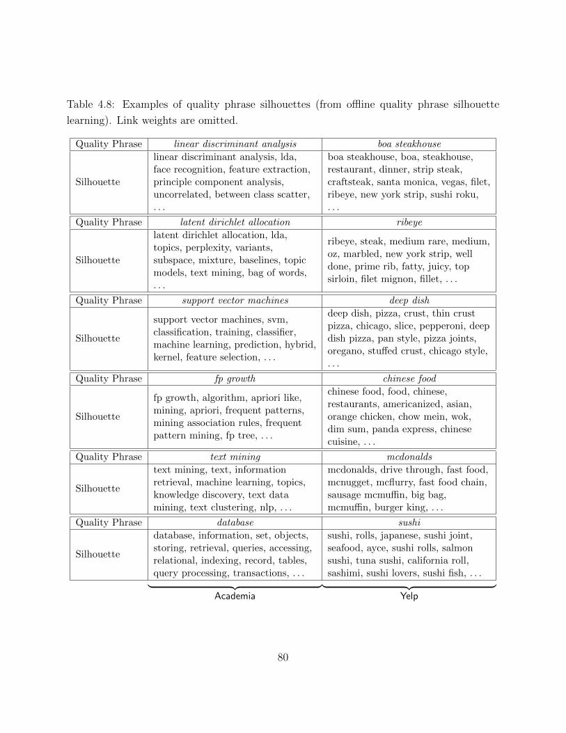
Table 4.8: Examples of quality phrase silhouettes (from offline quality phrase silhouette
learning). Link weights are omitted.
Quality Phrase linear discriminant analysis boa steakhouse
Silhouette
linear discriminant analysis, lda,face recognition, feature extraction,principle component analysis,uncorrelated, between class scatter,. . .
boa steakhouse, boa, steakhouse,restaurant, dinner, strip steak,craftsteak, santa monica, vegas, filet,ribeye, new york strip, sushi roku,. . .
Quality Phrase latent dirichlet allocation ribeye
Silhouette
latent dirichlet allocation, lda,topics, perplexity, variants,subspace, mixture, baselines, topicmodels, text mining, bag of words,. . .
ribeye, steak, medium rare, medium,oz, marbled, new york strip, welldone, prime rib, fatty, juicy, topsirloin, filet mignon, fillet, . . .
Quality Phrase support vector machines deep dish
Silhouette
support vector machines, svm,classification, training, classifier,machine learning, prediction, hybrid,kernel, feature selection, . . .
deep dish, pizza, crust, thin crustpizza, chicago, slice, pepperoni, deepdish pizza, pan style, pizza joints,oregano, stuffed crust, chicago style,. . .
Quality Phrase fp growth chinese food
Silhouette
fp growth, algorithm, apriori like,mining, apriori, frequent patterns,mining association rules, frequentpattern mining, fp tree, . . .
chinese food, food, chinese,restaurants, americanized, asian,orange chicken, chow mein, wok,dim sum, panda express, chinesecuisine, . . .
Quality Phrase text mining mcdonalds
Silhouette
text mining, text, informationretrieval, machine learning, topics,knowledge discovery, text datamining, text clustering, nlp, . . .
mcdonalds, drive through, fast food,mcnugget, mcflurry, fast food chain,sausage mcmuffin, big bag,mcmuffin, burger king, . . .
Quality Phrase database sushi
Silhouette
database, information, set, objects,storing, retrieval, queries, accessing,relational, indexing, record, tables,query processing, transactions, . . .
sushi, rolls, japanese, sushi joint,seafood, ayce, sushi rolls, salmonsushi, tuna sushi, california roll,sashimi, sushi lovers, sushi fish, . . .︸ ︷︷ ︸︸ ︷︷ ︸
Academia Yelp
80
Chapter 5
Tensor-Based Large-Scale NetworkEmbedding
The previous two chapters introduce how to bring structures into text. Besides analysing the
textual content, we notice that documents are naturally rich in structure in other aspects,
in which structures result from various relations between documents and their associated
entities.
In business reviews, there exist relations as users writing reviews for businesses. In
bibliographic data, relations are in the form of authors publishing papers in venues, etc. The
analysis of relational data containing documents is of great pragmatic interest, and has
attracted increasing attention in academia and industry [99, 26, 96, 46].
Prevalent mining approaches in the literature focus on “second-order” data in which a
bipartite network is built and analyzed between single-typed entities, e.g. authors, and doc-
ument content. However, many real-world data are more versatile in structure with regards
to more than two types involved. In such scenarios, existing methodologies may fail and a
legitimate approach towards such relations is to model the involved entities as a whole. In
particular, we define such relations involving more than two entity types (including docu-
ment content such as keyphrases) as higher-order relations. Accordingly, the collection of
higher-order relations is higher-order relational data. As discussed above, the bibliographical
data are an archetypal example, in which each publication relation involves four entity types:
author, paper, phrase, and venue. Due to the heterogeneity of the entities involved in each
relation, [45, 96] proposed to abstract such data as heterogeneous information networks [91],
where a network becomes heterogeneous if it contains more than two entity types, compared
81
to homogeneous or bipartite information networks containing one or two typed entities. Par-
ticularly, since the network is constructed and centered on documents, we name it Text-Rich
Information Network. Different from typical definition for links in the network which con-
nect two nodes, a link in text-rich information network in this chapter may associate with
more, in correspondence with a higher-order relation.
With the formulation of text-rich information network, this chapter studies the problem
of embedding nodes/entities in this type of network into a low-dimensional vector space, in
which every node/entity is represented by a vector. The learned embeddings should preserve
proximity in the network. Semantically, entities should have similar embeddings if they co-
occur with similar entities or they involve in similar relations. The similarity of relations are
further determined by the similarity of their constituent entities.
The learned embeddings are useful for various downstream applications including visu-
alization [105], entity classification [10], clustering [76], recommender system [53], and link
prediction [60]. Due to the broad applications of the entity embeddings and humongous scale
of real-world data, it is desirable to have an efficient framework for learning node embeddings
that scales in text-rich information network.
There have been some efforts en route to such embedding tasks, including [19, 99]. How-
ever, instead of directly analyzing the higher-order relational data by modeling every inter-
action among multiple entity types as a whole, [19, 99] opt to construct a set of bipartite
networks and model each of them separately.
In Fig. 5.1, a network schema (i.e., a generalized network explaining higher-order re-
lations) of the bibliographical data is depicted on the left. The publication relation is a
higher-order relation type, since entities of types author, venue and phrase are associated
with the relation identifier publication1. Existing methods, denoted as pairwise method
(shown on the bottom right of the figure), represent each higher-order relation as the union
1Different from Example 1.2, here entity “paper” is replaced with relation identifier “publication”.
82
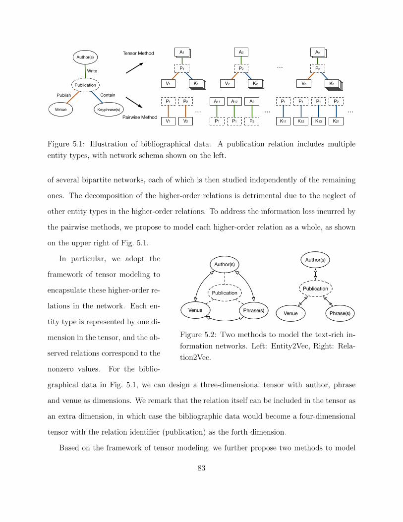
T1
Author(s)
Publication
Venue Keyphrase(s)
Write
Contain Publish
P1
V1
A11
P1
A12
P1
P2
V2
P1
V1
…
……Pairwise Method
Tensor Method A1A1
T1K1
P2
V2
A2
T1K2T1T1
Pn
Vn
A1An
T1Kn
A2
P2
P1
K11
P1
K12
P1
K13
P2
K21
…
Figure 5.1: Illustration of bibliographical data. A publication relation includes multiple
entity types, with network schema shown on the left.
of several bipartite networks, each of which is then studied independently of the remaining
ones. The decomposition of the higher-order relations is detrimental due to the neglect of
other entity types in the higher-order relations. To address the information loss incurred by
the pairwise methods, we propose to model each higher-order relation as a whole, as shown
on the upper right of Fig. 5.1.
Author(s)
Venue Phrase(s)
Publication
Author(s)
Publication
Venue Phrase(s)
Figure 5.2: Two methods to model the text-rich in-
formation networks. Left: Entity2Vec, Right: Rela-
tion2Vec.
In particular, we adopt the
framework of tensor modeling to
encapsulate these higher-order re-
lations in the network. Each en-
tity type is represented by one di-
mension in the tensor, and the ob-
served relations correspond to the
nonzero values. For the biblio-
graphical data in Fig. 5.1, we can design a three-dimensional tensor with author, phrase
and venue as dimensions. We remark that the relation itself can be included in the tensor as
an extra dimension, in which case the bibliographic data would become a four-dimensional
tensor with the relation identifier (publication) as the forth dimension.
Based on the framework of tensor modeling, we further propose two methods to model
83
the text-rich information networks, as depicted in Fig. 5.2. The entity-driven method (en-
tity2vec) models the proximity among entities that co-occur with similar constituent en-
tities in the higher-order relations; while the relation-driven method (relation2vec) models
the proximity among entities that oc-occur in similar higher-order relations. The arrows
indicate that information can be propagated in both directions.
In the pairwise methods, several bipartite relations are analyzed individually; in the
tensor-based framework, each higher-order relation becomes the basic unit. Therefore, the
tensor-based framework enables more efficient information propagation between the con-
stituent entities (and the relations for the relation2vec method). By comparison, in the
pairwise methods information can only be propagated between each pair of entities at one
time. Furthermore, with all entities considered in the tensor-based framework, it is more
robust to noisy entities. This is because informative entities may dominate tensor values,
which helps to control the negative effects of noisy entities. As for pairwise methods, noisy
entities would be modeled in absence of relevant entities due to the independent modeling
of each bipartite relation, resulting in perturbation of the learned model.
To summarize, we make the following contributions in this work2:
1. We propose the problem of learning embeddings for text-rich information networks. In
particular, we propose to model higher-order relations involving multiple entity types in
the network.
2. Under a novel framework of tensor2vec, we develop two methods to model higher-order
relations from different perspectives, entity-driven method entity2vec and relation-driven
method relation2vec, which enable more efficient information propagation between entities
and are more robust to noisy entities.
3. Extensive experiments are conducted to corroborate the efficacy of the tensor2vec frame-
work towards effective learning of network embeddings that preserve proximity.
2This work is in submission to KDD2016.
84
5.1 Network Schema and Entity Proximity
As we previously introduced, text-rich information network is essentially an abstraction for
higher-order relational data involving textual content. In this section, we first provide the
formal definition of relational data, followed by its network representation. Then we discuss
how to model entity proximity under such representation.
To begin with, we define relational data with its higher-order extension.
Definition 5.1 (Relational Data) By reusing the symbols in the definition of text-
rich information network, relational data are defined as D = (E ,R), where E = e1, . . . , en
is the set of entities and R is the set of relations (second-order or higher-order) among
the entities.
In conventional relational data, in which relations are mostly bipartite, i.e., R ⊆ E × E .
However, for higher-order relational data, there could be multiple entity types involved in
each relation type. Moreover, the number of relation types is not constrained and it is
possible to have multiple relation types among the same set of entity types.
We use O and T to represent the sets of entity types and relation types respectively. For
any entity type o ∈ O, Eo refers to the set of entities of type o; for any relation type t ∈ T ,
Rt defines the set of relations of type t. Moreover, the set of entity types involved in Rt is
defined as St, with the entity type of the jth component as Stj . Therefore, ∪t∈TRt = R and
∪t∈T St = O.
Definition 5.2 (Higher-order Relational Data) Higher-order relational data are
a collection of relations satisfying the condition that there exists t ∈ T for which |St| > 2.
A higher-order relational dataset can be naturally represented as a heterogeneous infor-
mation network, with its network schema defined as follows
85
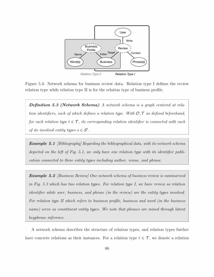
User
Review
Business Phrase(s)
Write
Contain Target
Word(s)
Name
Relation Type II Relation Type I
Business
Profile
Index
Figure 5.3: Network schema for business review data. Relation type I defines the review
relation type while relation type II is for the relation type of business profile.
Definition 5.3 (Network Schema) A network schema is a graph centered at rela-
tion identifiers, each of which defines a relation type. With O, T as defined beforehand,
for each relation type t ∈ T , its corresponding relation identifier is connected with each
of its involved entity types o ∈ St.
Example 5.1 [Bibliography] Regarding the bibliographical data, with its network schema
depicted on the left of Fig. 5.1, we only have one relation type with its identifier publi-
cation connected to three entity types including author, venue, and phrase.
Example 5.2 [Business Review] One network schema of business review is summarized
in Fig. 5.3 which has two relation types. For relation type I, we have review as relation
identifier while user, business, and phrase (in the review) are the entity types involved.
For relation type II which refers to business profile, business and word (in the business
name) serve as constituent entity types. We note that phrases are mined through latent
keyphrase inference.
A network schema describes the structure of relation types, and relation types further
have concrete relations as their instances. For a relation type t ∈ T , we denote a relation
86
as Rt =[Ht
1, . . . ,Ht|St|], where Ht
i (for i = 1, . . . , |St|) is a list of entities involved in the
relation instance. The entities in Hti are of the same entity type as Sti . The collection of
relations of type t is Rt = Rt.
Based on the bibliographical network schema described in Example 5.1, one of the most
cited KDD papers can be used as an example of a publication relation as follows.
T. Joachims. “Optimizing search engines using clickthrough data.” In KDD.
This bibliographic record provides a relation R with its elements Hvenue = [KDD];
Hauthor = [T. Joachims]; Hphrase = [search engines, clickthrough data, user query, . . .]3.
Given higher-order relational data and its network schema, we want to learn entity em-
beddings which represent each entity in a low-dimension space such that the proximity
between entities in the higher-order relational data can be well preserved. In particular, we
consider two approaches of modeling entity proximity, which relies on similarity propagation
through entity and relation respectively.
Definition 5.4 (Entity-Driven Proximity) The entity-driven proximity between
a pair of entities is the similarity between the entities they co-occurring with in the
relations.
In other words, two entities are close if they co-occur with similar entities in the higher-
order relations. Another approach learns proximity through relations.
Definition 5.5 (Relation-Driven Proximity) The relation-driven proximity between
a pair of entities is the similarity between their involving relations and the similarity be-
tween relations is further determined by proximity between their constituent entities.
3Superscript t is omitted for simplicity.
87
5.2 Tensor2vec: The Network Embedding Framework
In this section, we introduce the embedding framework, tensor2vec, for text-rich information
network.
For now, we assume that there is only one relation type in the network. The case
when there are multiple relation types will be discussed shortly. The relation Rt ∈ Rt can
be simplified as R with superscript t omitted. In addition, we define the concept of sub-
relation, which samples one entity from each entity list in R. For instance, given a relation
R =[H1, . . . ,H|S|
], a sub-relation is r =
[h1, . . . , h|S|
], such that hi ∈ Hi for i = 1, . . . , |S|.
Moreover, B = H1 × . . .×H|S| is the set of R’s sub-relations. |B| =∏|S|
i=1 |Hi| and r ∈ B.
Without loss of generality, we assume that each higher-order relation R has unit weight
in the network and each sub-relation r only appears once in B. When the number of entity
types |S| > 2, the higher-order relations D can be modeled in a tensor D. The index of each
element in the tensor is specified by the sub-relation r, with element value being the weight
of the sub-relation. Because each sub-relation may appear in multiple relations, the weight
of the sub-relation r is Dr =∑
R′∈R δ(r ∈ B′)/|B′|, where δ(·) is the indicator function, and
B′ is the set of sub-relations of R′.
Hence, the proposed framework on learning entity embeddings in higher-order relational
data is called tensor2vec.
Specifically, we propose two methods to model the higher-order relations in the network,
entity2vec and relation2vec, to model the entity-driven and relation-driven proximity, as
defined in Definition 5.4 and 5.5 respectively.
5.2.1 Entity2vec
For an observed relation, we first define the conditional probability of an entity co-occurring
with other constituent entities. More formally, given a relation R, we sample a sub-relation
88
r ∈ B. The probability of hj (target entity) co-occurring with r−j = [. . . , hj−1, hj+1, . . .]
(context entities) is defined as
P1(hj|r−j) =exp
(S(wj,W−j)
)∑e∈ESj exp
(S(we,W−j)
) , (5.1)
where ESj is the set of entities with the same entity type Sj, we is the embedding for
e ∈ ESj , W =[w1, . . . ,w|S|
]with wj ∈ Rd being the embedding vector for hj, and W−j
corresponds the list of embeddings for r−j. Moreover, S(·, ·) is a scoring function to measure
the proximity between target entity and context entities.
Particularly, we define the scoring function as follows:
S(x,Y) =∑n
i=1x>yi, (5.2)
where x,yi ∈ Rd for i = 1, . . . , n and Y = [y1, . . . ,yn].
Remark 5.1 It is worth noting the scoring function is a free parameter and orthogonal
to the proposed embedding framework. Other scoring functions can be adopted. For more
scoring functions, please refer to [50, 51, 86, 95].
As mentioned about, the entity2vec method is to model the entity-driven proximity.
Entities that co-occur with similar entities are similar. To preserve the entity-driven prox-
imity, we want to make the conditional probability be close to the empirical distribution of
P1(e|r−j) = D[r−j ,e]/Dr−j(∀e ∈ ESj), where Dr−j
=∑
e′∈ESj D[r−j ,e′] and [r−j, e′] = [. . . , hj−1,
e′, hj+1, . . .]. Therefore, with λr−j= Dr−j
being the importance of the context entities r−j,
we maximize the following objective function,
L1 = −∑|S|
j=1
∑r−j∈Aj
λr−j·KL
(P1(·|r−j),P1(·|r−j)
)=∑|S|
j=1
∑r−j∈Aj
∑e∈OSj D[r−j ,e] logP1(e|r−j),
89
where KL(·, ·) is the KL divergence, Aj = ∪R′∈RB′−j with B′−j = [r−j]r∈B′ , and the second
equality holds with constant terms omitted.
In addition, based on the definition of D, we obtain
∑r−j∈Aj
∑e∈OSj
D[r−j ,e] logP1(e|r−j)
=∑R∈R
1
|B|∑r∈B
logP1(hj|r−j).(5.3)
Substituting Eq. (5.3) into L1, it follows that
L1 =∑R∈R
1
|B|∑r∈B
|S|∑j=1
logP1(hj|r−j). (5.4)
5.2.2 Relation2vec
Since relation2vec method is to capture the relation-driven proximity, we first define the
conditional probability of a relation co-occurring with its constituent entities. We also inter-
pret it as given the list of constituent entities, how likely we can observe the corresponding
relation.
For a relation R, we sample a sub-relation r. We first extend the tensor D into |S| + 1
dimension and denote it as D, such that for an arbitrary relation R′, D[r,R′] = 1/|B′| if r ∈ B′
and 0 otherwise, where B′ is the set of sub-relations of R′. The conditional probability for
observing the relation R given r is
P2(R|r) =exp
(S(w,W)
)∑R′∈R exp
(S(w′,W)
) ,where w and w′ are the embeddings for the relations R and R′, and W is the list of
embeddings for all entities in r. S(·, ·) is the scoring function, as defined in Eq. (5.2).
As discussed above, the relation2vec model is to model the relation-driven proximity.
90
Entities are similar if they involve in similar relations. The similarity between relations is
determined by proximity between their constituent entities. To preserve the relation-driven
proximity, we optimize to minimize the KL-divergence of P2 and the empirical distribution
of P2(R′|r) = D[r,R′]/Dr. By defining λ′r as the importance of the sub-relation r, we have
that the objective function to be maximized is
L2 = −∑
r∈A λ′rKL
(P2(·|r),P2(·|r)
),
where A = ∪R∈RB. Therefore, A defines the set of sub-relations in the higher-order relational
data D.
Moreover, based on the definition of D, it holds that
∑r∈A
∑R′∈R
D[r,R′] logP2(R′|r)
=∑R∈R
1
|B|∑r∈B
logP2(R|r),(5.5)
Substituting Eq. (5.5) into L2 with λ′r = Dr and removing constant terms yields that
L2 =∑
R∈R
1
|B|∑
r∈BlogP2(R|r). (5.6)
5.2.3 Multiple Relation Types
Recall Example 5.2 that there could be multiple relation types associated with text-rich
information networks. In order to extend both methods to this case, we use L as a unified
notation for L1 and L2. Suppose there are |T | relation types, for t ∈ T , we denote the
objective as Lt. Thus, Lt = Lt1 for entity2vec, and Lt = Lt2 for relation2vec.
Therefore, considering all the relation types, we have the objective function as L∗ =∑t∈T Lt.
91
Remark 5.2 The number of entity types for the tth relation type is |St|. If |St| = 2 for
all t ∈ T , i.e., the higher-order relations reduce to bipartite, then the method of entity2vec
for the case with multiple relation types reduces to the prevailing pairwise method. In
other words, the existing models [19, 100] are special cases of our model.
5.3 Noise Pairwise Ranking
In this section, we propose a novel optimization framework from a pairwise ranking per-
spective, named as noise pairwise ranking. We first show its optimization procedures for
entity2vec and relation2vec given one relation type, i.e., |T | = 1, followed by the extension
to the case when there are multiple relation types.
5.3.1 Objective Derivation
Considering the objective function of entity2vec in Eq. (5.4), direct optimization of L1 is
intractable since the conditional probability Eq. (5.1) requires the summation over the entire
set of entities with certain type Sj. The same challenge exists for optimizing the objective
function of relation2vec in Eq. (5.6), which requires the summation over the entire set of
relations.
To address this challenge, noise contrastive estimation (NCE) [74] and negative sampling
(NEG) [73] are proposed. NCE reduces the problem of estimating the conditional proba-
bility into a probabilistic classification problem to distinguish samples from the empirical
distribution and a noise distribution. While negative sampling also learns the parameters as
a binary classification problem, it particularly formulates the objective as logistic regression,
which is shown to be effective in embedding learning [73, 80, 100].
As [38] shows, the hyperparameter of negative sampling value k [73] plays an important
92
role in obtaining the optimal embeddings. To get rid of the hyperparameter, we develop
a new optimization framework from a pairwise ranking perspective, noise pairwise ranking
(NPR). In comparison, NCE and NEG are discriminative models, while our model is a
generative model in optimizing the conditional probability. The developed NPR framework
is applicable to both entity2vec and relation2vec. To illustrate the underlying idea, the
conditional probability to be maximized can be abstracted as follows:
P(v|u) =exp
(S(wv,wu)
)∑v′∈V exp
(S(wv′ ,wu)
) , (5.7)
where V is the set of objects (which can be instantiated to entities or relations), with wv,wu
as the embeddings of the object v, u accordingly. Therefore, we have
P(v|u) =(
1 +∑v′ 6=v
exp(S(wv′ ,wu)− S(wv,wu)
))−1
, (5.8)
which follows from Eq. (5.7) via dividing the denominator and numerator by exp(S(wv,wu)
).
Instead of directly optimizing Eq. (5.8) over all v′ ∈ V \ v, we update Eq. (5.8) with respect
to a small set of noise samples in V \ v, where an individual sample is denoted as vn. With
σ(·) representing the sigmoid function that σ(x) = 1/(1+exp(−x)), we update the following
probability instead,
P(v > vn|u) = σ(− S(wvn ,wu) + S(wv,wu)
), (5.9)
which can be interpreted as maximizing the probability of observing the target v over the
noise vn, given the context u. Particularly, it can be easily verified that
P(v|u) >∏
vn 6=v P(v > vn|u),
which implies that optimizing P(v > vn|u) can be explained as optimizing the lower bound
93
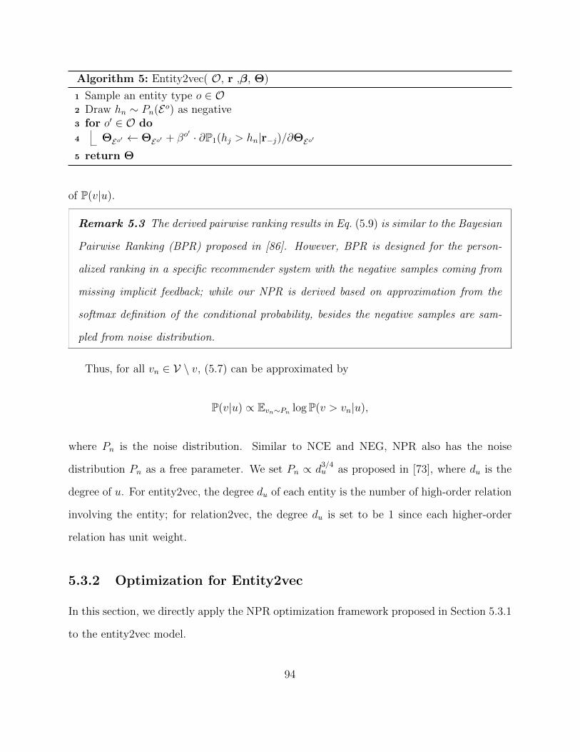
Algorithm 5: Entity2vec( O, r ,β, Θ)
1 Sample an entity type o ∈ O2 Draw hn ∼ Pn(Eo) as negative3 for o′ ∈ O do
4 ΘEo′ ← ΘEo′ + βo′ · ∂P1(hj > hn|r−j)/∂ΘEo′
5 return Θ
of P(v|u).
Remark 5.3 The derived pairwise ranking results in Eq. (5.9) is similar to the Bayesian
Pairwise Ranking (BPR) proposed in [86]. However, BPR is designed for the person-
alized ranking in a specific recommender system with the negative samples coming from
missing implicit feedback; while our NPR is derived based on approximation from the
softmax definition of the conditional probability, besides the negative samples are sam-
pled from noise distribution.
Thus, for all vn ∈ V \ v, (5.7) can be approximated by
P(v|u) ∝ Evn∼Pn logP(v > vn|u),
where Pn is the noise distribution. Similar to NCE and NEG, NPR also has the noise
distribution Pn as a free parameter. We set Pn ∝ d3/4u as proposed in [73], where du is the
degree of u. For entity2vec, the degree du of each entity is the number of high-order relation
involving the entity; for relation2vec, the degree du is set to be 1 since each higher-order
relation has unit weight.
5.3.2 Optimization for Entity2vec
In this section, we directly apply the NPR optimization framework proposed in Section 5.3.1
to the entity2vec model.
94
Based on the NPR optimization framework proposed in Section 5.3.1, we apply it to the
method of entity2vec. Recall that the objective of entity2vec is defined in Eq. (5.4) with the
conditional probability defined in Eq. (5.1). By applying the NPR optimization framework
to the conditional probability in Eq. (5.1), we have the new objective function as
L1 =∑
R∈R
1|B|∑r∈B
|S|∑j=1
Ehn∼Pn(Sj) logP1(hj > hn|r−j),
where hn is the sampled noise from Pn(Sj) and the latter is the noise distribution of entities
of type Sj. In addition
P1(hj > hn|r−j) = σ(− S(wn,W−j) + S(wj,W−j)
),
where wn is the embedding of hn.
To optimize L1, we use the asynchronous stochastic gradient algorithm (ASGD) [83] due
to the sparsity of the optimization problem, which means that most gradient updates only
modify a small portion of the variables. Define Θ = wee∈E as the parameters, we have
the gradient
∂L1∂Θ
=∑
R∈R1|B|∑
r∈B∑|S|
j=1 Ehn∼Pn(ESj )
∂ log P1(hj>hn|r−j)
∂Θ.
In specific,
∂ logP1(hj > hn|r−j)∂wj
= σ(S∆)∑l 6=j
wl;
∂ logP1(hj > hn|r−j)∂wn
= −σ(S∆)∑l 6=j
wl;
∂ logP1(hj > hn|r−j)∂wl
= σ(S∆)(wj −wn), ∀ l 6= j,
where S∆ = S(wn,W−j)− S(wj,W−j).
Note that entities with types of smaller size are updated more often due to the strategy of
sampling sub-relations. This inevitably makes some entity types better trained than others
95
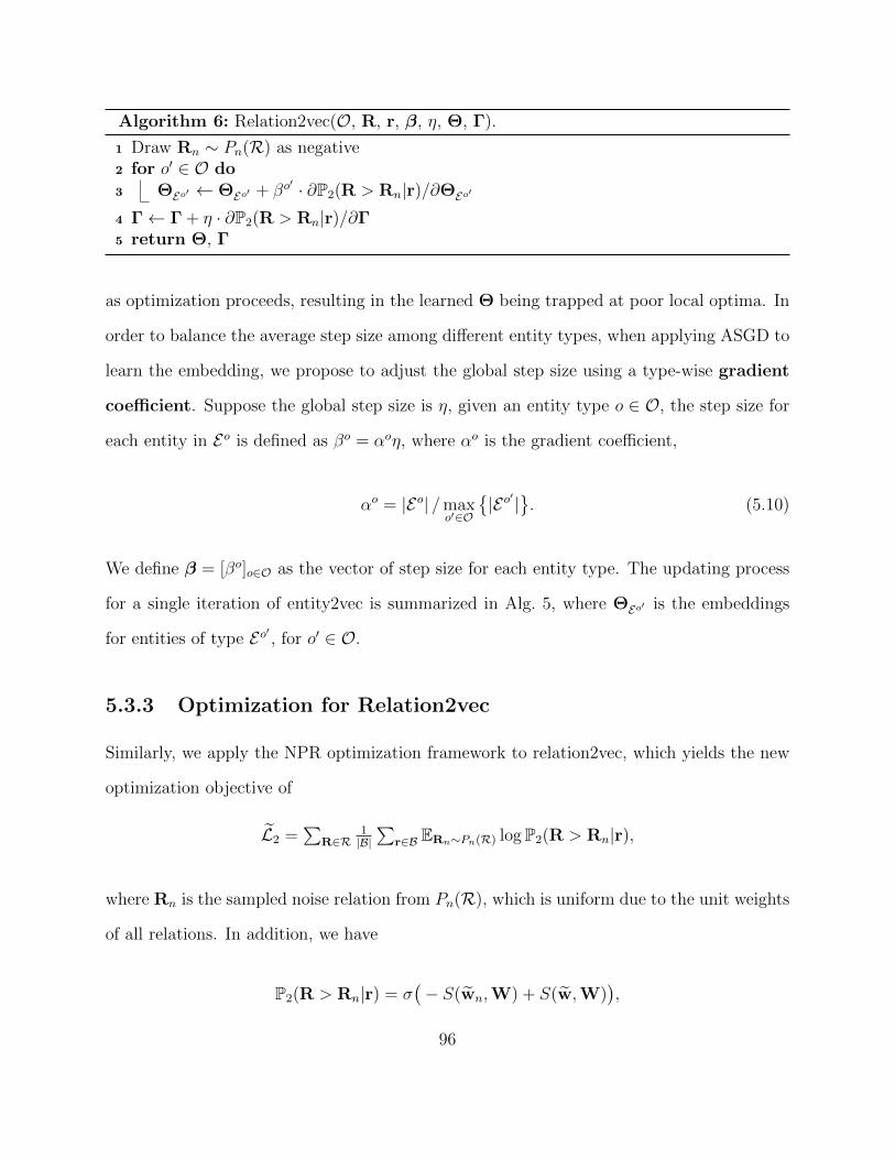
Algorithm 6: Relation2vec(O, R, r, β, η, Θ, Γ).
1 Draw Rn ∼ Pn(R) as negative2 for o′ ∈ O do3 ΘEo′ ← ΘEo′ + βo
′ · ∂P2(R > Rn|r)/∂ΘEo′
4 Γ← Γ + η · ∂P2(R > Rn|r)/∂Γ5 return Θ, Γ
as optimization proceeds, resulting in the learned Θ being trapped at poor local optima. In
order to balance the average step size among different entity types, when applying ASGD to
learn the embedding, we propose to adjust the global step size using a type-wise gradient
coefficient. Suppose the global step size is η, given an entity type o ∈ O, the step size for
each entity in Eo is defined as βo = αoη, where αo is the gradient coefficient,
αo = |Eo| /maxo′∈O
|Eo′|
. (5.10)
We define β = [βo]o∈O as the vector of step size for each entity type. The updating process
for a single iteration of entity2vec is summarized in Alg. 5, where ΘEo′ is the embeddings
for entities of type Eo′ , for o′ ∈ O.
5.3.3 Optimization for Relation2vec
Similarly, we apply the NPR optimization framework to relation2vec, which yields the new
optimization objective of
L2 =∑
R∈R1|B|∑
r∈B ERn∼Pn(R) logP2(R > Rn|r),
where Rn is the sampled noise relation from Pn(R), which is uniform due to the unit weights
of all relations. In addition, we have
P2(R > Rn|r) = σ(− S(wn,W) + S(w,W)
),
96
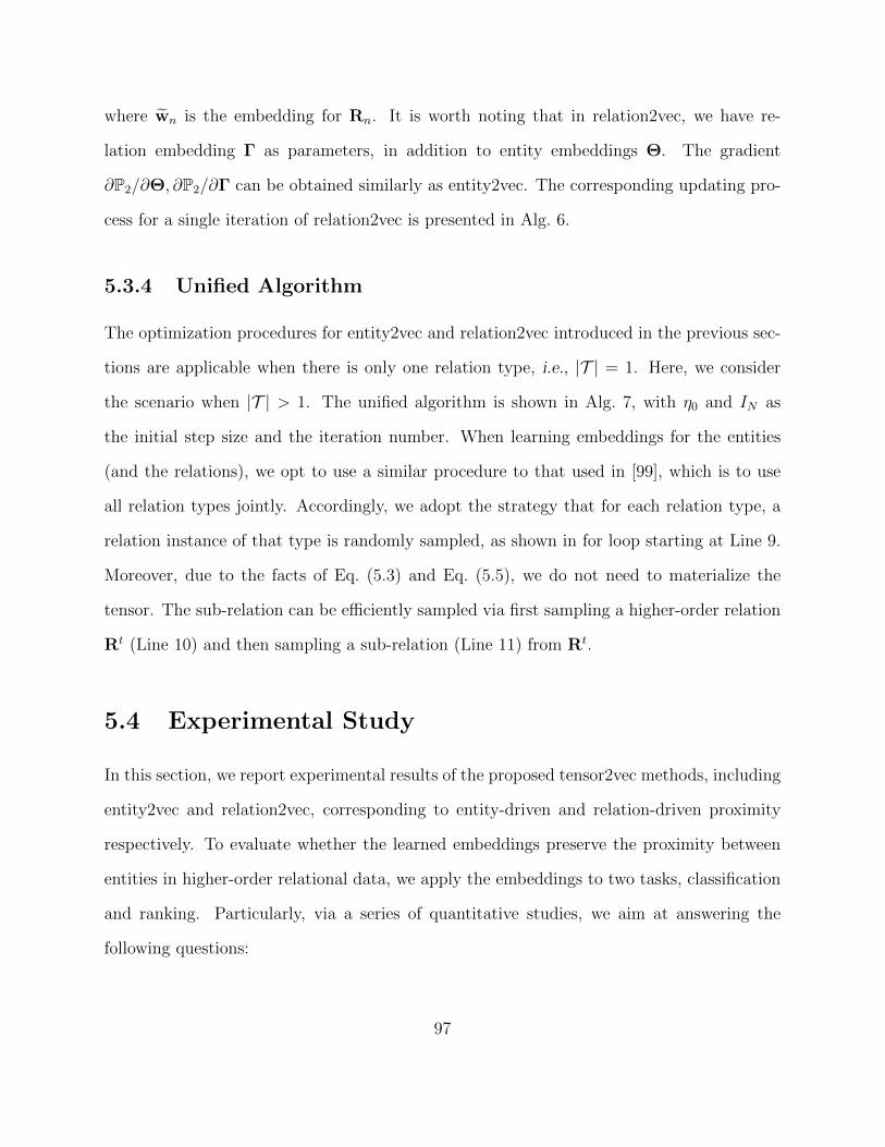
where wn is the embedding for Rn. It is worth noting that in relation2vec, we have re-
lation embedding Γ as parameters, in addition to entity embeddings Θ. The gradient
∂P2/∂Θ, ∂P2/∂Γ can be obtained similarly as entity2vec. The corresponding updating pro-
cess for a single iteration of relation2vec is presented in Alg. 6.
5.3.4 Unified Algorithm
The optimization procedures for entity2vec and relation2vec introduced in the previous sec-
tions are applicable when there is only one relation type, i.e., |T | = 1. Here, we consider
the scenario when |T | > 1. The unified algorithm is shown in Alg. 7, with η0 and IN as
the initial step size and the iteration number. When learning embeddings for the entities
(and the relations), we opt to use a similar procedure to that used in [99], which is to use
all relation types jointly. Accordingly, we adopt the strategy that for each relation type, a
relation instance of that type is randomly sampled, as shown in for loop starting at Line 9.
Moreover, due to the facts of Eq. (5.3) and Eq. (5.5), we do not need to materialize the
tensor. The sub-relation can be efficiently sampled via first sampling a higher-order relation
Rt (Line 10) and then sampling a sub-relation (Line 11) from Rt.
5.4 Experimental Study
In this section, we report experimental results of the proposed tensor2vec methods, including
entity2vec and relation2vec, corresponding to entity-driven and relation-driven proximity
respectively. To evaluate whether the learned embeddings preserve the proximity between
entities in higher-order relational data, we apply the embeddings to two tasks, classification
and ranking. Particularly, via a series of quantitative studies, we aim at answering the
following questions:
97
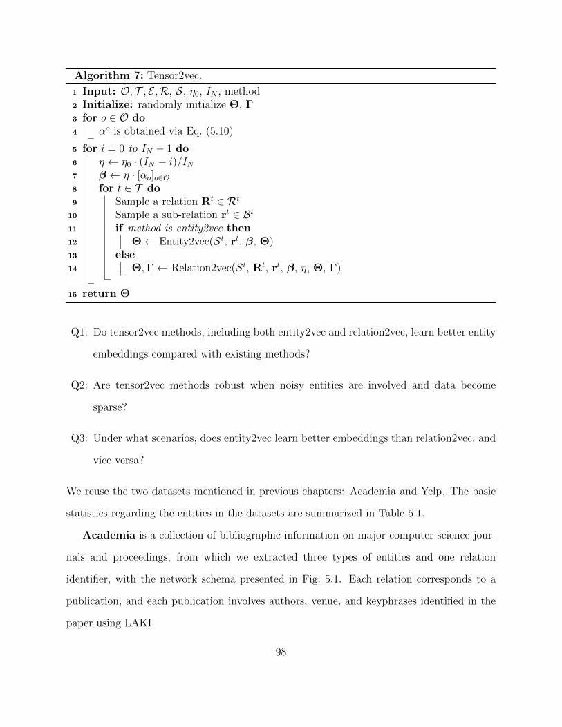
Algorithm 7: Tensor2vec.
1 Input: O, T , E ,R, S, η0, IN , method2 Initialize: randomly initialize Θ, Γ3 for o ∈ O do4 αo is obtained via Eq. (5.10)
5 for i = 0 to IN − 1 do6 η ← η0 · (IN − i)/IN7 β ← η · [αo]o∈O8 for t ∈ T do9 Sample a relation Rt ∈ Rt
10 Sample a sub-relation rt ∈ Bt11 if method is entity2vec then12 Θ← Entity2vec(St, rt, β, Θ)13 else14 Θ,Γ← Relation2vec(St, Rt, rt, β, η, Θ, Γ)
15 return Θ
Q1: Do tensor2vec methods, including both entity2vec and relation2vec, learn better entity
embeddings compared with existing methods?
Q2: Are tensor2vec methods robust when noisy entities are involved and data become
sparse?
Q3: Under what scenarios, does entity2vec learn better embeddings than relation2vec, and
vice versa?
We reuse the two datasets mentioned in previous chapters: Academia and Yelp. The basic
statistics regarding the entities in the datasets are summarized in Table 5.1.
Academia is a collection of bibliographic information on major computer science jour-
nals and proceedings, from which we extracted three types of entities and one relation
identifier, with the network schema presented in Fig. 5.1. Each relation corresponds to a
publication, and each publication involves authors, venue, and keyphrases identified in the
paper using LAKI.
98
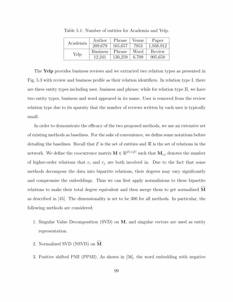
Table 5.1: Number of entities for Academia and Yelp.
AcademiaAuthor Phrase Venue Paper209,679 165,657 7953 1,938,912
YelpBusiness Phrase Word Review12,241 130,259 6,709 905,658
The Yelp provides business reviews and we extracted two relation types as presented in
Fig. 5.3 with review and business profile as their relation identifiers. In relation type I, there
are three entity types including user, business and phrase; while for relation type II, we have
two entity types, business and word appeared in its name. User is removed from the review
relation type due to its sparsity that the number of reviews written by each user is typically
small.
In order to demonstrate the efficacy of the two proposed methods, we use an extensive set
of existing methods as baselines. For the sake of convenience, we define some notations before
detailing the baselines. Recall that E is the set of entities and R is the set of relations in the
network. We define the coocurrence matrix M ∈ R|E|×|E| such that Mi,j denotes the number
of higher-order relations that ei and ej are both involved in. Due to the fact that some
methods decompose the data into bipartite relations, their degrees may vary significantly
and compromise the embeddings. Thus we can first apply normalizions to these bipartite
relations to make their total degree equivalent and then merge them to get normalized M
as described in [45]. The dimensionality is set to be 300 for all methods. In particular, the
following methods are considered:
1. Singular Value Decomposition (SVD) on M, and singular vectors are used as entity
representation.
2. Normalized SVD (NSVD) on M.
3. Positive shifted PMI (PPMI). As shown in [56], the word embedding with negative
99
sampling is equivalent to approximate the PPMI. Hence, we perform SVD on the
PPMI matrix of M .
4. Non-negative Matrix Factorization (NMF) on M, and matrix factor is used as entity
representation.
5. Normalized NMF (NNMF) on M.
6. LINE [100]: a second-order entity embedding approach. We ignore the higher-order
relations and apply LINE to the decomposed bipartite relations directly.
7. PTE [99]: an entity embedding approach that models each bipartite relation in a
round-robin fashion within every higher-order relation.4
The goal of our experiments is to quantitatively evaluate how well our methods perform
in generating proximity-preserved embeddings.
One way to evaluate the quality of the embeddings is through the proximity-related entity
classification task. After obtaining the embeddings of the entities, we feed these embeddings
into classifiers including linear SVM and logistic regression to perform classification with
five-fold cross validation. Supposing v ∈ E , we define l∗v as the true label of v while lv as the
predicted label of v. We report the classification metric accuracy (Acc.) which is defined as
Acc. =∑
v∈Elδ(lv = l∗v
)/|El|,
where El is the set of entities that have labels and δ(·) is the indicator function. Due to the
space limit, the higher accuracy between linear svm and logistic regression gets reported.
Classification relies on ground truth labels to learn mapping function between embeddings
and classes. It may not be able to exploit information underlying all dimensions. Therefore
4The labels are not provided during the training.
100
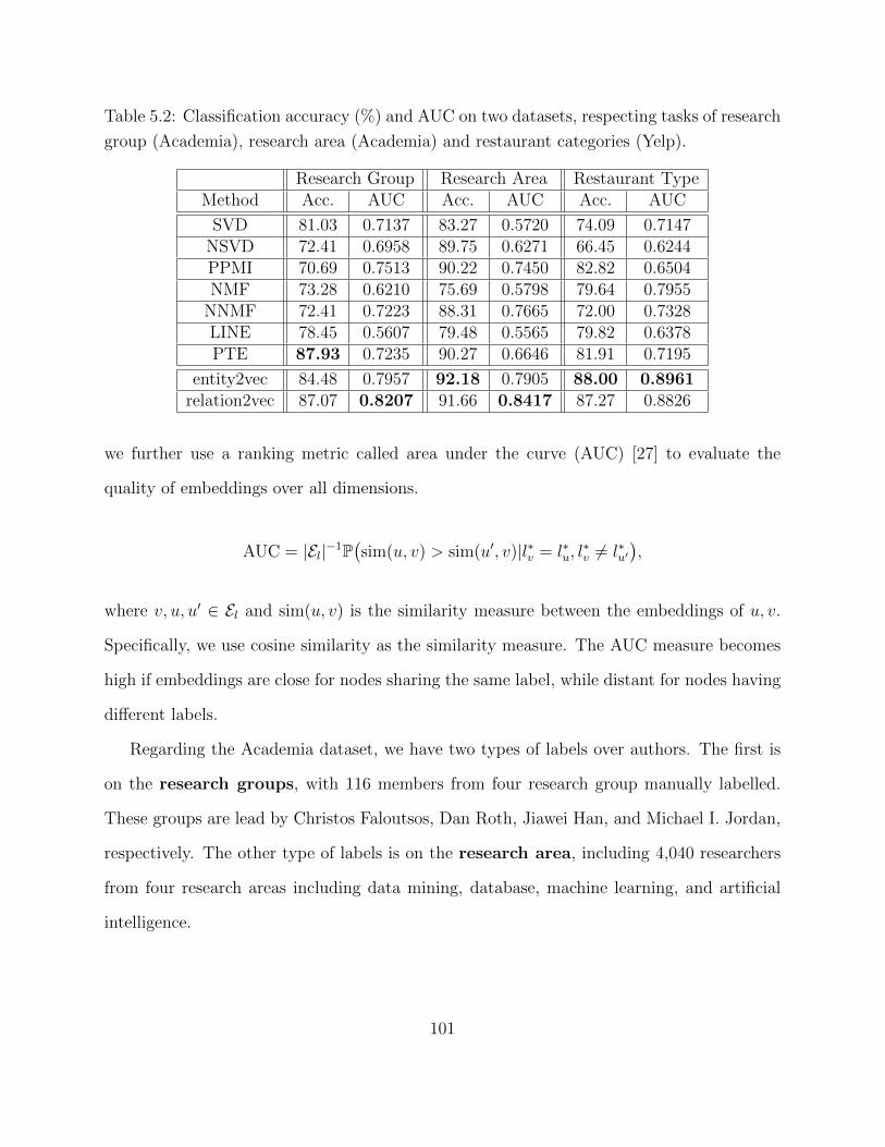
Table 5.2: Classification accuracy (%) and AUC on two datasets, respecting tasks of research
group (Academia), research area (Academia) and restaurant categories (Yelp).
Research Group Research Area Restaurant TypeMethod Acc. AUC Acc. AUC Acc. AUC
SVD 81.03 0.7137 83.27 0.5720 74.09 0.7147NSVD 72.41 0.6958 89.75 0.6271 66.45 0.6244PPMI 70.69 0.7513 90.22 0.7450 82.82 0.6504NMF 73.28 0.6210 75.69 0.5798 79.64 0.7955
NNMF 72.41 0.7223 88.31 0.7665 72.00 0.7328LINE 78.45 0.5607 79.48 0.5565 79.82 0.6378PTE 87.93 0.7235 90.27 0.6646 81.91 0.7195
entity2vec 84.48 0.7957 92.18 0.7905 88.00 0.8961relation2vec 87.07 0.8207 91.66 0.8417 87.27 0.8826
we further use a ranking metric called area under the curve (AUC) [27] to evaluate the
quality of embeddings over all dimensions.
AUC = |El|−1P(sim(u, v) > sim(u′, v)|l∗v = l∗u, l
∗v 6= l∗u′
),
where v, u, u′ ∈ El and sim(u, v) is the similarity measure between the embeddings of u, v.
Specifically, we use cosine similarity as the similarity measure. The AUC measure becomes
high if embeddings are close for nodes sharing the same label, while distant for nodes having
different labels.
Regarding the Academia dataset, we have two types of labels over authors. The first is
on the research groups, with 116 members from four research group manually labelled.
These groups are lead by Christos Faloutsos, Dan Roth, Jiawei Han, and Michael I. Jordan,
respectively. The other type of labels is on the research area, including 4,040 researchers
from four research areas including data mining, database, machine learning, and artificial
intelligence.
101
As for the Yelp dataset, we select eleven restaurant categories including Mexican,
Chinese, Italian, American (traditional), American (new), Mediterranean, Thai, French,
Japanese, Vietnamese and Indian as labels. For each category, we randomly select 100
restaurants that have at least 50 reviews. Restaurants with multiple labels are excluded.
5.4.1 Quantitative Evaluation and Results
Now we are ready to present the experimental results for the aforementioned tasks and try
to answer the three questions raised at the beginning of this section.
Table 5.2 summarizes the experimental results on classification (Acc.) and ranking (AUC)
in Academia and Yelp.
Considering the results for research group in Academia, we note that PTE and rela-
tion2vec achieve the best performance. PTE is slightly better than relation2vec on accuracy
but the latter outperforms the former on AUC by a large margin. Entity2vec narrowly loses
to relation2vec on both measures. It is interesting to see that the normalization strategy on
M has a big effect on the performance, but the trend is opposite between SVD and NMF.
For the task of research area in Academia, entity2vec attains the best performance on
classification accuracy and relation2vec has the highest AUC score. The results on research
area are better than the ones on research group for all methods, which means that the
research area task is easier than the former task. It’s worth noting that two tensor2vec
methods are better than baselines on both measures, confirming the their effectiveness of
capturing the proximity. We also observe that both NSVD and NNMF beat their unnor-
malized versions, implying that the normalization trick works at least for some tasks.
With respect to the Yelp dataset, on classifying the restaurant type, we observe that
both tensor2vec methods are significantly better than the baselines, for both measures. A
tentative explanation is that tensor2vec framework models both relation types explicitly, the
102
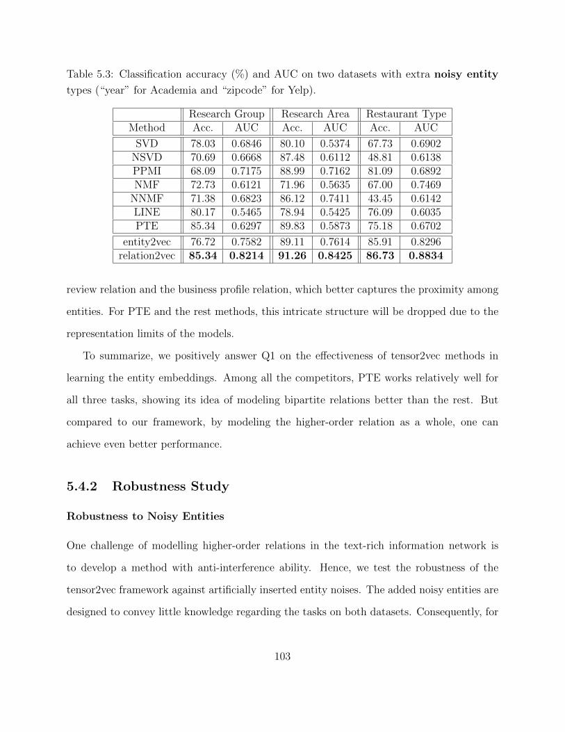
Table 5.3: Classification accuracy (%) and AUC on two datasets with extra noisy entity
types (“year” for Academia and “zipcode” for Yelp).
Research Group Research Area Restaurant TypeMethod Acc. AUC Acc. AUC Acc. AUC
SVD 78.03 0.6846 80.10 0.5374 67.73 0.6902NSVD 70.69 0.6668 87.48 0.6112 48.81 0.6138PPMI 68.09 0.7175 88.99 0.7162 81.09 0.6892NMF 72.73 0.6121 71.96 0.5635 67.00 0.7469
NNMF 71.38 0.6823 86.12 0.7411 43.45 0.6142LINE 80.17 0.5465 78.94 0.5425 76.09 0.6035PTE 85.34 0.6297 89.83 0.5873 75.18 0.6702
entity2vec 76.72 0.7582 89.11 0.7614 85.91 0.8296relation2vec 85.34 0.8214 91.26 0.8425 86.73 0.8834
review relation and the business profile relation, which better captures the proximity among
entities. For PTE and the rest methods, this intricate structure will be dropped due to the
representation limits of the models.
To summarize, we positively answer Q1 on the effectiveness of tensor2vec methods in
learning the entity embeddings. Among all the competitors, PTE works relatively well for
all three tasks, showing its idea of modeling bipartite relations better than the rest. But
compared to our framework, by modeling the higher-order relation as a whole, one can
achieve even better performance.
5.4.2 Robustness Study
Robustness to Noisy Entities
One challenge of modelling higher-order relations in the text-rich information network is
to develop a method with anti-interference ability. Hence, we test the robustness of the
tensor2vec framework against artificially inserted entity noises. The added noisy entities are
designed to convey little knowledge regarding the tasks on both datasets. Consequently, for
103
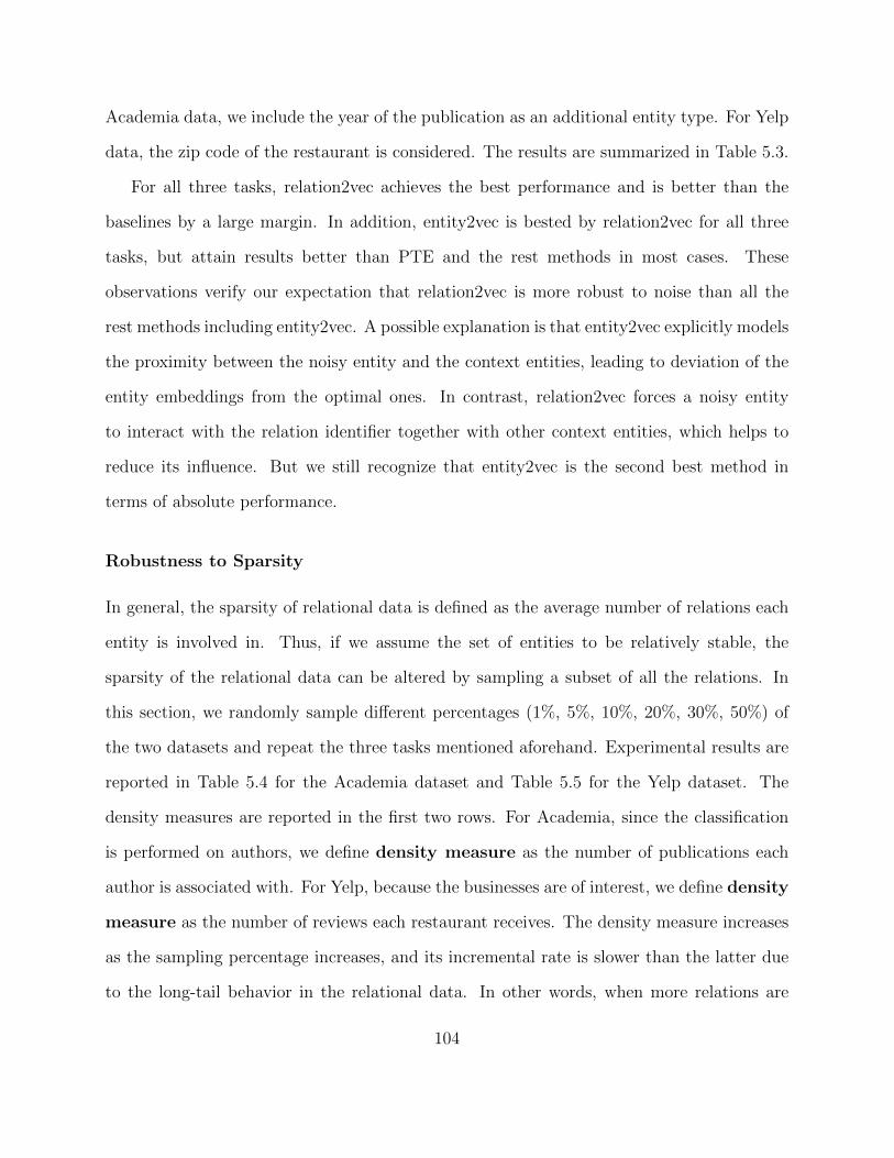
Academia data, we include the year of the publication as an additional entity type. For Yelp
data, the zip code of the restaurant is considered. The results are summarized in Table 5.3.
For all three tasks, relation2vec achieves the best performance and is better than the
baselines by a large margin. In addition, entity2vec is bested by relation2vec for all three
tasks, but attain results better than PTE and the rest methods in most cases. These
observations verify our expectation that relation2vec is more robust to noise than all the
rest methods including entity2vec. A possible explanation is that entity2vec explicitly models
the proximity between the noisy entity and the context entities, leading to deviation of the
entity embeddings from the optimal ones. In contrast, relation2vec forces a noisy entity
to interact with the relation identifier together with other context entities, which helps to
reduce its influence. But we still recognize that entity2vec is the second best method in
terms of absolute performance.
Robustness to Sparsity
In general, the sparsity of relational data is defined as the average number of relations each
entity is involved in. Thus, if we assume the set of entities to be relatively stable, the
sparsity of the relational data can be altered by sampling a subset of all the relations. In
this section, we randomly sample different percentages (1%, 5%, 10%, 20%, 30%, 50%) of
the two datasets and repeat the three tasks mentioned aforehand. Experimental results are
reported in Table 5.4 for the Academia dataset and Table 5.5 for the Yelp dataset. The
density measures are reported in the first two rows. For Academia, since the classification
is performed on authors, we define density measure as the number of publications each
author is associated with. For Yelp, because the businesses are of interest, we define density
measure as the number of reviews each restaurant receives. The density measure increases
as the sampling percentage increases, and its incremental rate is slower than the latter due
to the long-tail behavior in the relational data. In other words, when more relations are
104
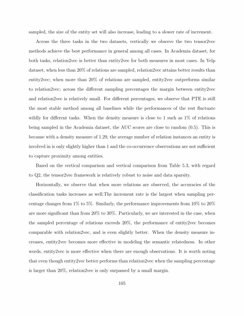
sampled, the size of the entity set will also increase, leading to a slower rate of increment.
Across the three tasks in the two datasets, vertically we observe the two tensor2vec
methods achieve the best performance in general among all cases. In Academia dataset, for
both tasks, relation2vec is better than entity2vec for both measures in most cases. In Yelp
dataset, when less than 20% of relations are sampled, relation2vec attains better results than
entity2vec; when more than 20% of relations are sampled, entity2vec outperforms similar
to relation2vec; across the different sampling percentages the margin between entity2vec
and relation2vec is relatively small. For different percentages, we observe that PTE is still
the most stable method among all baselines while the performances of the rest fluctuate
wildly for different tasks. When the density measure is close to 1 such as 1% of relations
being sampled in the Academia dataset, the AUC scores are close to random (0.5). This is
because with a density measure of 1.29, the average number of relation instances an entity is
involved in is only slightly higher than 1 and the co-occurrence observations are not sufficient
to capture proximity among entities.
Based on the vertical comparison and vertical comparison from Table 5.3, with regard
to Q2, the tensor2vec framework is relatively robust to noise and data sparsity.
Horizontally, we observe that when more relations are observed, the accuracies of the
classification tasks increases as well.The increment rate is the largest when sampling per-
centage changes from 1% to 5%. Similarly, the performance improvements from 10% to 20%
are more significant than from 20% to 30%. Particularly, we are interested in the case, when
the sampled percentage of relations exceeds 20%, the performance of entity2vec becomes
comparable with relation2vec, and is even slightly better. When the density measure in-
creases, entity2vec becomes more effective in modeling the semantic relatedness. In other
words, entity2vec is more effective when there are enough observations. It is worth noting
that even though entity2vec better performs than relation2vec when the sampling percentage
is larger than 20%, relation2vec is only surpassed by a small margin.
105
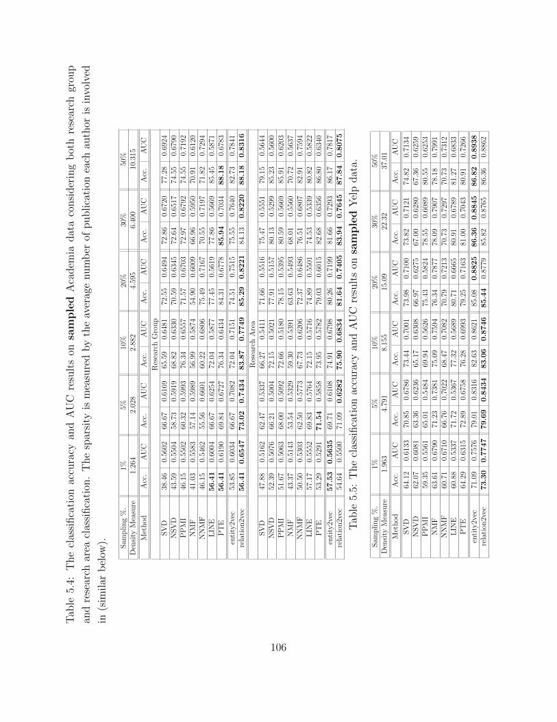
Tab
le5.
4:T
he
clas
sifica
tion
accu
racy
and
AU
Cre
sult
son
sam
ple
dA
cadem
iadat
aco
nsi
der
ing
bot
hre
sear
chgr
oup
and
rese
arch
area
clas
sifica
tion
.T
he
spar
sity
ism
easu
red
by
the
aver
age
num
ber
ofpublica
tion
each
auth
oris
invo
lved
in(s
imilar
bel
ow). Sam
pling
%.
1%5%
10%
20%
30%
50%
Den
sity
Mea
sure
1.26
42.
028
2.88
24.
595
6.40
010
.315
Met
hod
Acc
.A
UC
Acc
.A
UC
Acc
.A
UC
Acc
.A
UC
Acc
.A
UC
Acc
.A
UC
Res
earc
hG
roup
SV
D38
.46
0.56
0266
.67
0.61
6965
.59
0.64
8172
.55
0.64
9472
.86
0.67
2077
.28
0.69
24N
SV
D43
.59
0.55
0458
.73
0.59
1968
.82
0.63
3070
.59
0.63
4572
.64
0.65
1774
.55
0.67
90P
PM
I46
.15
0.55
0260
.32
0.59
9376
.34
0.65
5771
.57
0.67
0372
.97
0.67
9274
.55
0.71
92N
MF
41.0
30.
5583
57.1
40.
5989
56.9
90.
5874
54.9
00.
6009
66.9
60.
5950
70.9
10.
6120
NN
MF
46.1
50.
5462
55.5
60.
6601
60.2
20.
6806
75.4
90.
7167
70.5
50.
7197
71.8
20.
7294
LIN
E56.4
10.
6004
66.6
70.
6254
72.0
40.
5877
77.4
50.
5619
77.8
60.
5669
85.4
50.
5871
PT
E56.4
10.
6190
69.8
40.
6727
76.3
40.
6434
84.3
10.
6778
85.9
40.
7034
88.1
80.
6783
enti
ty2v
ec53
.85
0.60
3466
.67
0.70
8272
.04
0.71
5174
.51
0.75
1575
.55
0.76
4082
.73
0.78
41re
lati
on2v
ec56.4
10.6
547
73.0
20.7
434
83.8
70.7
749
85.2
90.8
221
84.1
30.8
220
88.1
80.8
316
Res
earc
hA
rea
SV
D47
.88
0.51
6262
.47
0.53
3766
.27
0.54
1171
.66
0.55
1675
.47
0.55
5179
.15
0.56
44N
SV
D52
.39
0.50
7666
.21
0.50
0472
.15
0.50
2177
.91
0.51
5780
.13
0.52
9985
.23
0.56
00P
PM
I51
.67
0.50
6368
.00
0.50
9272
.66
0.51
8078
.15
0.53
9580
.59
0.56
6985
.91
0.62
03N
MF
43.3
70.
5143
53.5
40.
5329
59.3
00.
5391
63.6
30.
5493
68.0
10.
5560
70.7
20.
5637
NN
MF
50.5
00.
5303
62.5
00.
5773
67.7
30.
6206
72.3
70.
6486
76.5
10.
6807
82.9
10.
7594
LIN
E57
.17
0.55
5269
.83
0.57
6472
.15
0.57
1674
.89
0.55
0174
.53
0.53
3980
.82
0.58
22P
TE
53.2
90.
5291
71.5
40.
5858
73.9
50.
5782
79.0
30.
6015
82.6
80.
6356
86.8
00.
6340
enti
ty2v
ec57.5
30.5
635
69.7
10.
6108
74.9
10.
6798
80.2
60.
7199
81.6
60.
7293
86.1
70.
7817
rela
tion
2vec
54.6
40.
5500
71.0
90.6
282
75.9
00.6
834
81.6
40.7
405
83.9
40.7
645
87.8
40.8
075
Tab
le5.
5:T
he
clas
sifica
tion
accu
racy
and
AU
Cre
sult
son
sam
ple
dY
elp
dat
a.
Sam
pling
%.
1%5%
10%
20%
30%
50%
Den
sity
Mea
sure
1.96
34.
791
8.15
515
.09
22.3
237
.01
Met
hod
Acc
.A
UC
Acc
.A
UC
Acc
.A
UC
Acc
.A
UC
Acc
.A
UC
Acc
.A
UC
SV
D64
.12
0.61
3370
.85
0.67
8673
.44
0.70
0173
.98
0.71
0073
.82
0.71
2174
.82
0.71
34N
SV
D62
.07
0.60
8163
.36
0.62
3665
.17
0.63
0866
.97
0.62
7567
.00
0.62
8067
.36
0.62
59P
PM
I59
.35
0.55
6165
.01
0.54
8469
.94
0.56
2675
.43
0.58
2478
.55
0.60
8980
.55
0.62
53N
MF
63.6
10.
6790
71.2
30.
7381
75.0
90.
7594
76.3
40.
7877
78.0
90.
7907
78.1
80.
7991
NN
MF
60.7
10.
6710
66.7
60.
7022
68.4
70.
7082
70.7
90.
7213
70.7
30.
7297
70.7
30.
7312
LIN
E60
.88
0.53
3771
.72
0.53
6777
.32
0.56
8980
.71
0.66
6580
.91
0.67
8981
.27
0.68
33P
TE
64.2
90.
6315
72.8
90.
6758
76.2
80.
6993
79.2
50.
7163
81.0
00.
7043
80.9
10.
7266
enti
ty2v
ec71
.09
0.75
7679
.01
0.83
1682
.63
0.86
2185
.08
0.8
825
86.3
60.8
845
86.8
20.8
938
rela
tion
2vec
73.3
00.7
747
79.6
90.8
434
83.0
60.8
746
85.4
40.
8779
85.8
20.
8765
86.3
60.
8862
106
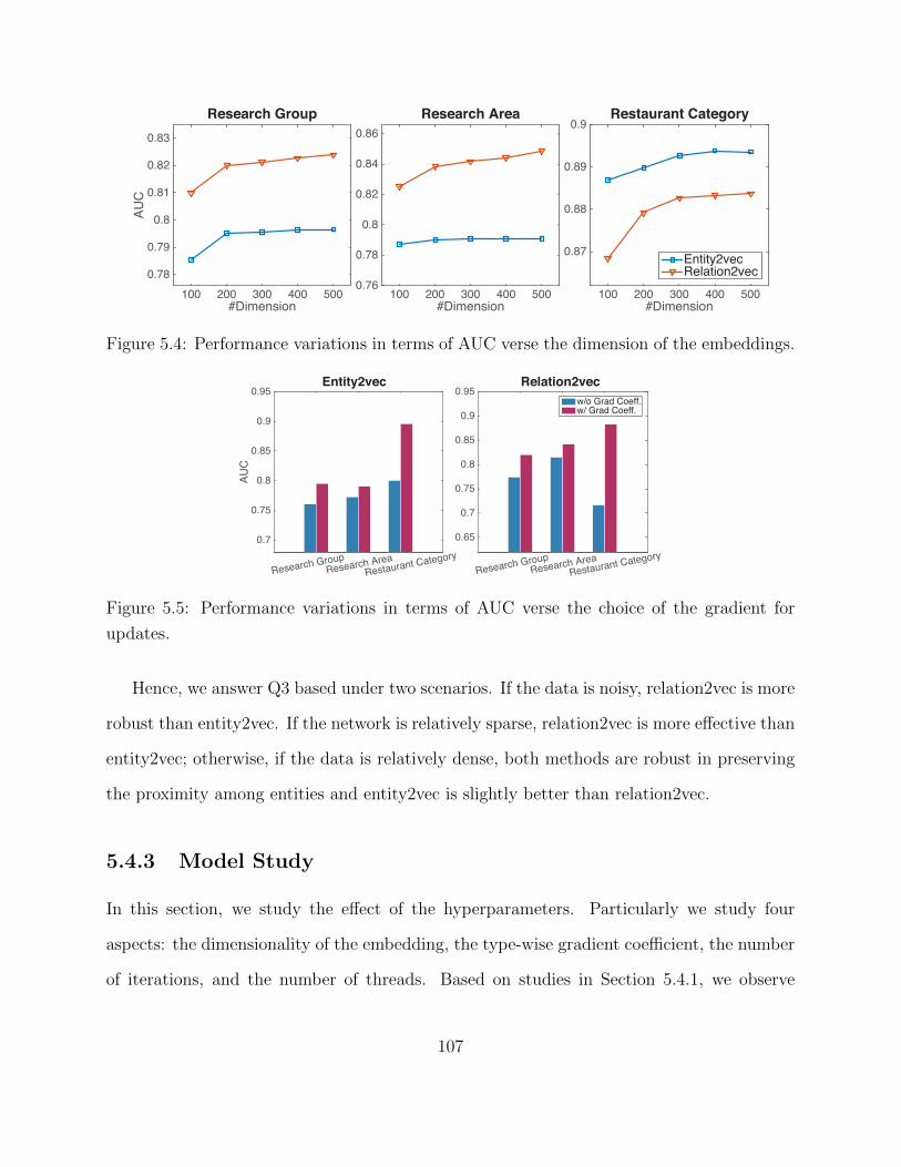
#Dimension100 200 300 400 500
AUC
0.78
0.79
0.8
0.81
0.82
0.83
Research Group
#Dimension100 200 300 400 500
0.76
0.78
0.8
0.82
0.84
0.86
Research Area
#Dimension100 200 300 400 500
0.87
0.88
0.89
0.9Restaurant Category
Entity2vecRelation2vec
Figure 5.4: Performance variations in terms of AUC verse the dimension of the embeddings.
Research Group
Research Area
Restaurant Category
AU
C
0.7
0.75
0.8
0.85
0.9
0.95Entity2vec
Research Group
Research Area
Restaurant Category
0.65
0.7
0.75
0.8
0.85
0.9
0.95Relation2vec
w/o Grad Coeff.w/ Grad Coeff.
Figure 5.5: Performance variations in terms of AUC verse the choice of the gradient for
updates.
Hence, we answer Q3 based under two scenarios. If the data is noisy, relation2vec is more
robust than entity2vec. If the network is relatively sparse, relation2vec is more effective than
entity2vec; otherwise, if the data is relatively dense, both methods are robust in preserving
the proximity among entities and entity2vec is slightly better than relation2vec.
5.4.3 Model Study
In this section, we study the effect of the hyperparameters. Particularly we study four
aspects: the dimensionality of the embedding, the type-wise gradient coefficient, the number
of iterations, and the number of threads. Based on studies in Section 5.4.1, we observe
107
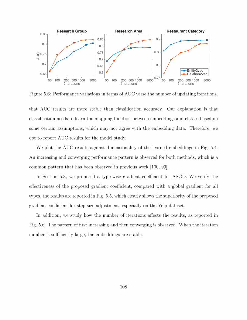
#Iterations50 100 250 500 1500 3000
AUC
0.65
0.7
0.75
0.8
0.85Research Group
#Iterations50 100 250 500 1500 3000
0.6
0.65
0.7
0.75
0.8
0.85
Research Area
#Iterations50 100 250 500 1500 3000
0.75
0.8
0.85
0.9
Restaurant Category
Entity2vecRelation2vec
Figure 5.6: Performance variations in terms of AUC verse the number of updating iterations.
that AUC results are more stable than classification accuracy. Our explanation is that
classification needs to learn the mapping function between embeddings and classes based on
some certain assumptions, which may not agree with the embedding data. Therefore, we
opt to report AUC results for the model study.
We plot the AUC results against dimensionality of the learned embeddings in Fig. 5.4.
An increasing and converging performance pattern is observed for both methods, which is a
common pattern that has been observed in previous work [100, 99].
In Section 5.3, we proposed a type-wise gradient coefficient for ASGD. We verify the
effectiveness of the proposed gradient coefficient, compared with a global gradient for all
types, the results are reported in Fig. 5.5, which clearly shows the superiority of the proposed
gradient coefficient for step size adjustment, especially on the Yelp dataset.
In addition, we study how the number of iterations affects the results, as reported in
Fig. 5.6. The pattern of first increasing and then converging is observed. When the iteration
number is sufficiently large, the embeddings are stable.
108
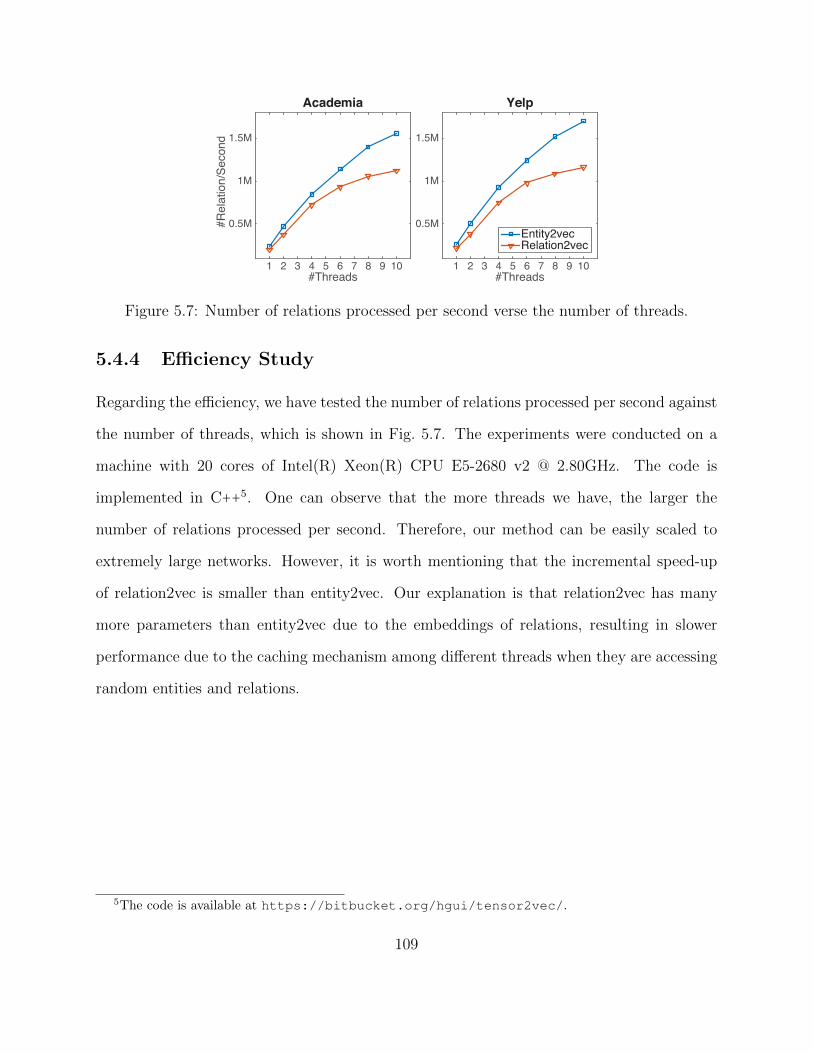
#Threads1 2 3 4 5 6 7 8 9 10
#Relation/Second
0.5M
1M
1.5M
Academia
#Threads1 2 3 4 5 6 7 8 9 10
0.5M
1M
1.5M
Yelp
Entity2vecRelation2vec
Figure 5.7: Number of relations processed per second verse the number of threads.
5.4.4 Efficiency Study
Regarding the efficiency, we have tested the number of relations processed per second against
the number of threads, which is shown in Fig. 5.7. The experiments were conducted on a
machine with 20 cores of Intel(R) Xeon(R) CPU E5-2680 v2 @ 2.80GHz. The code is
implemented in C++5. One can observe that the more threads we have, the larger the
number of relations processed per second. Therefore, our method can be easily scaled to
extremely large networks. However, it is worth mentioning that the incremental speed-up
of relation2vec is smaller than entity2vec. Our explanation is that relation2vec has many
more parameters than entity2vec due to the embeddings of relations, resulting in slower
performance due to the caching mechanism among different threads when they are accessing
random entities and relations.
5The code is available at https://bitbucket.org/hgui/tensor2vec/.
109
Chapter 6
Conclusion and Future Work
6.1 Conclusion
In this dissertation, we have taken several steps towards constructing and modeling text-rich
information networks, which follows the data-to-network-to-knowledge paradigm.
For phrase mining, we introduced a novel framework for extracting quality phrases from
text corpora focused on certain genres of content. The framework is data-driven and requires
only limited training to achieve outstanding performance. The key idea is to rectify the
raw frequency of phrases which misleads quality estimation. We develop a segmentation-
integrated approach for this purpose, which significantly boosts the final quality of extracted
phrases. It is the first work to explore the mutual benefit of phrase extraction and phrasal
segmentation. By intergrating them, this work addresses a fundamental limitation of phrase
mining and empowers widespread applications. Meanwhile, the method is scalable: both
computation time and required space grow linearly as corpus size increases.
A number of open problems need to be solved to allow further development of the pro-
posed phrase mining framework. One direction is to investigate reducing the number of
training labels. The current framework requires the model to be trained by 300 labeled
phrases. It would be preferable if a transferable model can be pretrained on general doc-
ument collection and adapt itself to the target corpus. An alternative is to use a domain-
independent phrase collection as the training source. Overlapped phrases are first identified
and then used to serve as the positive labels. Another direction is to replace Viterbi Training
110
by other parameter estimation approaches to further improve the phrasal segmentation. For
instance, one can find top-k best segmentations instead of one for each text snippet. This is
less deterministic than the current design but consumes more computational power.
For document keyphrase extraction, we introduced a new research problem of learning
representation for domain-specific texts using Latent Keyphrase Inference. It integrates
phrase mining and silhouetting to help infer latent document keyphrases and solves the
rarity of explicit keyphrase mentions in the query. The generated document representations
are shown to significantly boost performance in potential text mining tasks compared to
state-of-art methods. Meanwhile, document keyphrases are highly self-explanatory through
learned quality phrase silhouettes.
A number of open problems need to be solved to allow further development of LAKI. One
direction is to simultaneously model structured data such as meta information associated
with the documents, including named entity, authorship, publishers, etc.. An alternative
is to improve the model initialization by modeling more sophisticated relationship between
quality phrases and considering more robust structured learning method. Regarding the
scalability, it would be preferable if one can work out a more efficient inference algorithm.
For example, we can use a deterministic module like neural network and train it using
inference results from our current framework.
Lastly for text-rich information network embedding, we introduced the concept of net-
work schema to describe the structure of higher-order relations in the network. Moreover,
we proposed the tensor2vec framework, which models each higher-order relation as a whole,
resulting in more efficient information propagation. Two methods were presented to learn
proximity-preserved embeddings: entity2vec modeling the proximity among the constituent
entities, and relation2vec modeling proximity between the relation and the associated enti-
ties. Within the tensor2vec framework, we presented a ranking based method to efficiently
optimize the conditional probabilities via noise sampling. Extensive quantitative experi-
111
ments have been conducted to corroborate the efficacy of the proposed model in learning the
entity embeddings, particularly robustness towards noisy observations and data sparseness.
We identify some future work for the tensor2vec framework. Firstly, it is general and
could be adapted to many downstream applications, including recommender system and link
prediction. Secondly, this work focuses on learning embeddings in an unsupervised manner.
Exploring how to incorporate labels and generate predictive embeddings is a promising
direction. Finally, the text-rich information networks in this chapter is constructed by using
LAKI to extract structured units from text. An interesting extension is to consider linking
the networks with knowledge base.
6.2 Impact
The overarching theme of our research is developing large-scale data-driven methods that
can handle real-world text datasets in a robust way. It has broad impact on a variety of
text-related applications including document representation and indexing, relevance search,
entity classification, summarization and recommendation. It has been used in both academic
and industrial settings:
• Academia: Our works [64, 63] are being taught in data mining courses at UIUC
(CS512) and coursera. Several tutorials introduced and compared our works at top
computer science conferences including SIGMOD2016, WWW2016 and ACL2015.
• Industry:
– Our phrase mining work is used in Army Research Lab under the Network Science
Collaborative Technology Alliance (NSCTA) program.
– Since our works are open-sourced, they have been widely used among many com-
panies and independent researchers. A report from TripAdvisor is available on-
112
line1.
at Multiple Scales project (ADAMS) to detect insider threats and exfiltration in the
government and the military.
• Awards:
– SegPhrase [64] got the grand prize of Yelp Dataset Challenge, 2015
– The entity disambiguation work [62] won the 2nd place of KDD Cup: Author
Disambiguation Challenge, 2013
6.3 Research Frontiers
Mining textual data using network is a young and promising research field. There are many
unexplored territories and challenging research issues. Here we outline some of the research
directions stemming from our work.
6.3.1 Enriching Text-Rich Information Networks
Our study in most of the chapters assumes that a document is represented as a bag of
keyphrases and is associated with a set of entities. Algorithms developed using such net-
work schema can handle simple applications such as similarity search. To approach more
complicated tasks like answering questions ‘who are actively developing deep learning sys-
tems that can be deployed on distributed systems’, one needs to construct a richer network
involving more types of nodes and links. For example, phrases can be typed (i.e., phrases
like people name, job titles) by inferring their textual contexts. Attributes and hypernyms
are two link types that can be modeled between phrases. Meanwhile, link types among
1http://engineering.tripadvisor.com/using-nlp-to-find-interesting-collections-of-hotels/
113
document-associated entities can be more complicated by incorporating knowledge base re-
lations. Nevertheless, construction of a high-quality enriched text-rich information network
becomes increasingly more challenging when we move towards more structured knowledge
inferred from textual data.
6.3.2 Refining Text-Rich Information Networks
During the process of text structuralization, we typically use phrase mentions as the struc-
tured units. Our next challenge is to recognize concepts effectively for providing conceptual
summarization of unstructured data. Such refinement from phrase mentions to concepts
encounters two problems: (1) varietymany phrase mentions may refer to the same concept
(e.g., page rank and PageRank, cytosol and cytoplasm); and (2) ambiguitymultiple concepts
may share the same phrase mentions (e.g., PCR can refer to polymerase chain reaction
or principle component regression). Similar refinement can be applied to the document-
associated entities through entity resolution. But we notice that interconnected, structured
and unstructured data can mutually enhance each other in the process of refining since both
of them provide the context and imply similarity. By integrating the construction and refine-
ment of text-rich information network can greatly improve the network quality than doing
them in a sequential order.
6.3.3 Modeling of Text-Rich Information Networks
Network is the intermediate data representation between the raw data input and the discov-
ered knowledge output to users. Our previous studies on text-rich information networks as
well as existing studies on mining heterogeneous networks have shown that modeling data
as networks with multi-typed nodes often captures richer node/link semantics and generates
better results than their homogeneous or unstructured counterparts. But almost all these
114
works assume the network has only a few number of node types based on simple network
schema. As mentioned at the beginning of this section, network can become more com-
plicated with more node or link types, it brings new challenges and opportunities for more
powerful models to solve and explore. Besides the complication on node and link types, text-
rich information networks can also be huge, even dynamic, so it usually cannot be contained
in memory and cannot be handled directly. Once we know that the data is dynamically
updated or a user at a time could be only interested in a tiny portion of nodes and links,
we can model small networks “extracted”dynamically from some existing networks, based
on expected node/link behaviors or user-specified constraints.
115
References
[1] K. Ahmad, L. Gillam, and L. Tostevin. University of surrey participation in trec8:Weirdness indexing for logical document extrapolation and retrieval (wilder). In TheEighth Text REtrieval Conference.
[2] H. Ahonen. Knowledge discovery in documents by extracting frequent word sequences.Library Trends, 48(1), 1999.
[3] A. Allahverdyan and A. Galstyan. Comparative analysis of viterbi training and max-imum likelihood estimation for hmms. In Advances in Neural Information ProcessingSystems 24, pages 1674–1682, 2011.
[4] R. Baeza-Yates, B. Ribeiro-Neto, et al. Modern information retrieval. Addison-WesleyLongman Publishing Co., Inc., 1999.
[5] T. Baldwin and S. N. Kim. Multiword expressions. Handbook of Natural LanguageProcessing, second edition. Morgan and Claypool, 2010.
[6] S. Bedathur, K. Berberich, J. Dittrich, N. Mamoulis, and G. Weikum. Interesting-phrase mining for ad-hoc text analytics. Proceedings of the VLDB Endowment, 3(1-2):1348–1357, 2010.
[7] M. Belkin and P. Niyogi. Laplacian eigenmaps and spectral techniques for embeddingand clustering. In Advances in Neural Information Processing Systems 14, volume 14,pages 585–591, 2001.
[8] Y. Bengio, R. Ducharme, P. Vincent, and C. Janvin. A neural probabilistic languagemodel. Journal of Machine Learning Research, 3:1137–1155, 2003.
[9] A. R. Benson, D. F. Gleich, and J. Leskovec. Tensor spectral clustering for partition-ing higher-order network structures. In Proceedings of the 15th IEEE InternationalConference on Data Mining, pages 118–126, 2015.
[10] S. Bhagat, G. Cormode, and S. Muthukrishnan. Node classification in social networks.In Social network data analytics, pages 115–148. 2011.
[11] I. Bhattacharya and L. Getoor. Collective entity resolution in relational data. ACMTransactions on Knowledge Discovery from Data (TKDD), 1(1):5, 2007.
116
[12] C. M. Bishop. Pattern recognition and machine learning. Springer-Verlag New York,Inc., 2006.
[13] C. Bizer, J. Lehmann, G. Kobilarov, S. Auer, C. Becker, R. Cyganiak, and S. Hellmann.Dbpedia-a crystallization point for the web of data. Web Semantics: science, servicesand agents on the world wide web, 7(3):154–165, 2009.
[14] G. Blackwood, A. De Gispert, and W. Byrne. Phrasal segmentation models for statis-tical machine translation. In Coling 2008: Companion volume: Posters, pages 19–22,2008.
[15] D. M. Blei, A. Y. Ng, and M. I. Jordan. Latent dirichlet allocation. Journal of MachineLearning Research, 3:993–1022, 2003.
[16] L. Breiman. Random forests. Machine learning, 45(1):5–32, 2001.
[17] J. Chang, J. Boyd-Graber, C. Wang, S. Gerrish, and D. M. Blei. Reading tea leaves:How humans interpret topic models. pages 288–296, 2009.
[18] P.-C. Chang, M. Galley, and C. D. Manning. Optimizing chinese word segmentationfor machine translation performance. In Proceedings of the third workshop on statisticalmachine translation, pages 224–232, 2008.
[19] S. Chang, W. Han, J. Tang, G.-J. Qi, C. C. Aggarwal, and T. S. Huang. Hetero-geneous network embedding via deep architectures. In Proceedings of the 21st ACMSIGKDD international conference on Knowledge discovery and data mining, pages119–128, 2015.
[20] K.-h. Chen and H.-H. Chen. Extracting noun phrases from large-scale texts: A hybridapproach and its automatic evaluation. In Proceedings of the 32nd annual meeting onAssociation for Computational Linguistics, pages 234–241, 1994.
[21] H. Cho, B. Berger, and J. Peng. Diffusion component analysis: Unraveling functionaltopology in biological networks. In Research in Computational Molecular Biology,pages 62–64. Springer, 2015.
[22] E. F. Codd. A Relational Model for Large Shared Data Banks. Communications ofThe ACM, 13:377–387, 1970.
[23] R. Collobert, J. Weston, L. Bottou, M. Karlen, K. Kavukcuoglu, and P. Kuksa. Naturallanguage processing (almost) from scratch. The Journal of Machine Learning Research,12:2493–2537, 2011.
[24] G. F. Cooper. The computational complexity of probabilistic inference using bayesianbelief networks. Artificial intelligence, 42(2):393–405, 1990.
117
[25] M. Y. Dahab, H. A. Hassan, and A. Rafea. Textontoex: Automatic ontology construc-tion from natural english text. Expert Systems with Applications, 34(2):1474–1480,2008.
[26] M. Danilevsky, C. Wang, N. Desai, X. Ren, J. Guo, and J. Han. Automatic con-struction and ranking of topical keyphrases on collections of short documents. InProceedings of the 2014 SIAM International Conference on Data Mining, 2014.
[27] J. Davis and M. Goadrich. The relationship between precision-recall and roc curves. InProceedings of the 23rd international conference on Machine learning, pages 233–240,2006.
[28] P. Deane. A nonparametric method for extraction of candidate phrasal terms. InProceedings of the 43rd Annual Meeting on Association for Computational Linguistics,pages 605–613, 2005.
[29] S. C. Deerwester, S. T. Dumais, T. K. Landauer, G. W. Furnas, and R. A. Harshman.Indexing by latent semantic analysis. Journal of the American society for informationscience, 41(6):391–407, 1990.
[30] H. Echizen-ya and K. Araki. Automatic evaluation method for machine translationusing noun-phrase chunking. In Proceedings of the 48th Annual Meeting of the Asso-ciation for Computational Linguistics, pages 108–117, 2010.
[31] O. Egozi, S. Markovitch, and E. Gabrilovich. Concept-based information retrieval usingexplicit semantic analysis. ACM Transactions on Information Systems, 29(2):8:1–8:34,2011.
[32] A. El-Kishky, Y. Song, C. Wang, C. R. Voss, and J. Han. Scalable topical phrasemining from text corpora. Proceedings of the VLDB Endowment, 8(3), 2015.
[33] E. Estelles-Arolas and F. Gonzalez-Ladron-de Guevara. Towards an integrated crowd-sourcing definition. Journal of Information science, 38(2):189–200, 2012.
[34] K. Frantzi, S. Ananiadou, and H. Mima. Automatic recognition of multi-word terms:.the c-value/nc-value method. International Journal on Digital Libraries, 3(2):115–130,2000.
[35] E. Gabrilovich and S. Markovitch. Computing semantic relatedness using wikipedia-based explicit semantic analysis. In Proceedings of the 20th International Joint Con-ference on Artifical Intelligence, pages 1606–1611, 2007.
[36] W. A. Gale, K. W. Church, and D. Yarowsky. One sense per discourse. In Proceedingsof the workshop on Speech and Natural Language, pages 233–237, 1992.
118
[37] C. Gao and S. Michel. Top-k interesting phrase mining in ad-hoc collections usingsequence pattern indexing. In Proceedings of the 15th International Conference onExtending Database Technology, pages 264–275, 2012.
[38] Y. Goldberg and O. Levy. word2vec explained: deriving mikolov et al.’s negative-sampling word-embedding method. arXiv preprint arXiv:1402.3722, 2014.
[39] T. Gottron, M. Anderka, and B. Stein. Insights into explicit semantic analysis. InProceedings of the 20th ACM international conference on Information and knowledgemanagement, pages 1961–1964, 2011.
[40] H. Gui, Y. Sun, J. Han, and G. Brova. Modeling topic diffusion in multi-relationalbibliographic information networks. In Proceedings of the 23rd ACM InternationalConference on Conference on Information and Knowledge Management, pages 649–658, 2014.
[41] M. A. Halliday. Lexis as a linguistic level. In memory of JR Firth, pages 148–162,1966.
[42] Y. Halpern and D. Sontag. Unsupervised learning of noisy-or bayesian networks. InProceedings of the 29th Conference on Uncertainty in Artificial Intelligence, pages272–281, 2013.
[43] S. Hassan and R. Mihalcea. Semantic relatedness using salient semantic analysis.In Proceedings of the Twenty-Fifth AAAI Conference on Artificial Intelligence, pages884–889, 2011.
[44] R. Jenatton, N. L. Roux, A. Bordes, and G. R. Obozinski. A latent factor model forhighly multi-relational data. In Advances in Neural Information Processing Systems25, pages 3167–3175, 2012.
[45] M. Ji, J. Han, and M. Danilevsky. Ranking-based classification of heterogeneous infor-mation networks. In Proceedings of the 17th ACM SIGKDD international conferenceon Knowledge discovery and data mining, pages 1298–1306, 2011.
[46] T. Joachims. Optimizing search engines using clickthrough data. In SIGKDD, pages133–142. ACM, 2002.
[47] D. Kim, H. Wang, and A. Oh. Context-dependent conceptualization. In Proceedingsof the 23rd International Joint Conference on Artificial Intelligence, pages 2654–2661,2013.
[48] S. Kim, H. Kim, T. Weninger, J. Han, and H. D. Kim. Authorship classification: adiscriminative syntactic tree mining approach. In Proceedings of the 34th internationalACM SIGIR conference on Research and development in Information Retrieval, pages455–464, 2011.
119
[49] S. N. Kim, O. Medelyan, M.-Y. Kan, and T. Baldwin. Automatic keyphrase extractionfrom scientific articles. Language resources and evaluation, 47(3):723–742, 2013.
[50] T. G. Kolda and B. W. Bader. Tensor decompositions and applications. SIAM review,51(3):455–500, 2009.
[51] T. G. Kolda and J. Sun. Scalable tensor decompositions for multi-aspect data mining.In Proceedings of the 8th IEEE International Conference on Data Mining, pages 363–372, 2008.
[52] T. Koo, X. Carreras Perez, and M. Collins. Simple semi-supervised dependency pars-ing. pages 595–603, 2008.
[53] Y. Koren. The bellkor solution to the netflix grand prize. 2009.
[54] Q. Le and T. Mikolov. Distributed representations of sentences and documents. InProceedings of the 31st International Conference on Machine Learning, pages 1188–1196, 2014.
[55] J. Leskovec, L. Backstrom, and J. Kleinberg. Meme-tracking and the dynamics ofthe news cycle. In Proceedings of the 15th ACM SIGKDD international conference onKnowledge discovery and data mining, pages 497–506, 2009.
[56] O. Levy and Y. Goldberg. Neural word embedding as implicit matrix factorization.In Advances in Neural Information Processing Systems 27, pages 2177–2185, 2014.
[57] X. Li and B. Liu. Learning to classify texts using positive and unlabeled data. In Pro-ceedings of the 18th International Joint Conference on Artificial intelligence, volume 3,pages 587–592, 2003.
[58] Y. Li, J. Gao, C. Meng, Q. Li, L. Su, B. Zhao, W. Fan, and J. Han. A survey on truthdiscovery. ACM SIGKDD Explorations Newsletter, 17(2):1–16, 2016.
[59] Y. Li, B.-J. P. Hsu, C. Zhai, and K. Wang. Unsupervised query segmentation usingclickthrough for information retrieval. In Proceedings of the 34th international ACMSIGIR conference on Research and development in Information Retrieval, pages 285–294, 2011.
[60] D. Liben-Nowell and J. Kleinberg. The link-prediction problem for social networks.Journal of the American society for information science and technology, 58(7):1019–1031, 2007.
[61] J. Liu and J. Han. Spectral clustering. In C. Aggarwal and C. Reddy, editors, DataClustering: Algorithms and Applications. CRC Press, 2013.
120
[62] J. Liu, K. H. Lei, J. Y. Liu, C. Wang, and J. Han. Ranking-based name matchingfor author disambiguation in bibliographic data. In Proceedings of the 2013 KDD Cup2013 Workshop, page 8. ACM, 2013.
[63] J. Liu, X. Ren, J. Shang, T. Cassidy, C. R. Voss, and J. Han. Representing documentsvia latent keyphrase inference. In Proceedings of the 25th International Conference onWorld Wide Web, pages 1057–1067, 2016.
[64] J. Liu, J. Shang, C. Wang, X. Ren, and J. Han. Mining quality phrases from massivetext corpora. In Proceedings of the 2015 ACM SIGMOD International Conference onManagement of Data, pages 1729–1744, 2015.
[65] J. Liu, C. Wang, J. Gao, Q. Gu, C. Aggarwal, L. Kaplan, and J. Han. GIN: AClustering Model for Capturing Dual Heterogeneity in Networked Data, chapter 44,pages 388–396.
[66] Y. Liu, T. Ge, K. S. Mathews, H. Ji, and D. L. McGuinness. Exploiting task-orientedresources to learn word embeddings for clinical abbreviation expansion. ACL-IJCNLP2015, page 92, 2015.
[67] Z. Liu, W. Huang, Y. Zheng, and M. Sun. Automatic keyphrase extraction via topicdecomposition. In Proceedings of the 2010 Conference on Empirical Methods in NaturalLanguage Processing, pages 366–376, 2010.
[68] S. Massung, C. Zhai, and J. Hockenmaier. Structural parse tree features for textrepresentation. In Proceedings of the 2013 IEEE Seventh International Conference onSemantic Computing, pages 9–16, 2013.
[69] R. McDonald, F. Pereira, K. Ribarov, and J. Hajic. Non-projective dependency parsingusing spanning tree algorithms. In Proceedings of the conference on Human LanguageTechnology and Empirical Methods in Natural Language Processing, pages 523–530,2005.
[70] Q. Mei, X. Shen, and C. Zhai. Automatic labeling of multinomial topic models. In Pro-ceedings of the 13th ACM SIGKDD international conference on Knowledge discoveryand data mining, pages 490–499, 2007.
[71] R. Mihalcea and P. Tarau. Textrank: Bringing order into texts. In Proceedings of the2004 Conference on Empirical Methods in Natural Language Processing, 2004.
[72] T. Mikolov, K. Chen, G. Corrado, and J. Dean. Efficient estimation of word represen-tations in vector space. In Proceedings of Workshop at ICLR, 2013.
[73] T. Mikolov, I. Sutskever, K. Chen, G. S. Corrado, and J. Dean. Distributed repre-sentations of words and phrases and their compositionality. In Advances in NeuralInformation Processing Systems 26, pages 3111–3119, 2013.
121
[74] A. Mnih and Y. W. Teh. A fast and simple algorithm for training neural probabilisticlanguage models. In Proceedings of the 29th international conference on Machinelearning, pages 1751–1758, 2012.
[75] T. D. Nguyen and M.-Y. Kan. Keyphrase extraction in scientific publications. In AsianDigital Libraries. Looking Back 10 Years and Forging New Frontiers, pages 317–326.Springer, 2007.
[76] T. Opsahl and P. Panzarasa. Clustering in weighted networks. Social networks,31(2):155–163, 2009.
[77] D. P, A. Dey, and D. Majumdar. Fast mining of interesting phrases from subsets of textcorpora. In Proceedings of the 17th International Conference on Extending DatabaseTechnology, pages 193–204, 2014.
[78] A. Parameswaran, H. Garcia-Molina, and A. Rajaraman. Towards the web of concepts:Extracting concepts from large datasets. Proceedings of the VLDB Endowment, 3(1-2):566–577, 2010.
[79] Y. Park, R. J. Byrd, and B. K. Boguraev. Automatic glossary extraction: beyond ter-minology identification. In Proceedings of the 19th international conference on Com-putational linguistics - Volume 1, pages 1–7, 2002.
[80] B. Perozzi, R. Al-Rfou, and S. Skiena. Deepwalk: Online learning of social representa-tions. In Proceedings of the 20th ACM SIGKDD international conference on Knowledgediscovery and data mining, pages 701–710, 2014.
[81] V. Punyakanok and D. Roth. The use of classifiers in sequential inference. In Advancesin Neural Information Processing Systems 14, 2001.
[82] C. Ramisch, A. Villavicencio, and C. Boitet. Multiword expressions in the wild? themwetoolkit comes in handy. In Proceedings of the 23rd International Conference onComputational Linguistics: Demonstrations, pages 57–60, 2010.
[83] B. Recht, C. Re, S. Wright, and F. Niu. Hogwild: A lock-free approach to parallelizingstochastic gradient descent. In Advances in Neural Information Processing Systems24, pages 693–701, 2011.
[84] X. Ren, A. El-Kishky, C. Wang, F. Tao, C. R. Voss, and J. Han. Clustype: Effectiveentity recognition and typing by relation phrase-based clustering. In Proceedings ofthe 21st ACM SIGKDD international conference on Knowledge discovery and datamining, pages 995–1004, 2015.
[85] X. Ren, W. He, M. Qu, H. Ji, C. R. Voss, and J. Han. Label noise reduction in entitytyping by heterogeneous partial-label embeddings. In Proceedings of the 22nd ACMSIGKDD international conference on Knowledge discovery and data mining, 2016.
122
[86] S. Rendle and L. Schmidt-Thieme. Pairwise interaction tensor factorization for person-alized tag recommendation. In Proceedings of the third ACM international conferenceon Web search and data mining, pages 81–90, 2010.
[87] S. T. Roweis and L. K. Saul. Nonlinear dimensionality reduction by locally linearembedding. Science, 290(5500):2323–2326, 2000.
[88] M. Sanderson and B. Croft. Deriving concept hierarchies from text. In Proceedings ofthe 22nd annual international ACM SIGIR conference on Research and developmentin information retrieval, pages 206–213, 1999.
[89] B. Settles. Active Learning. Synthesis Lectures on Artificial Intelligence and MachineLearning. Morgan & Claypool Publishers, 2012.
[90] W. Shen, J. Wang, and J. Han. Entity linking with a knowledge base: Issues,techniques, and solutions. IEEE Transactions on Knowledge and Data Engineering,27(2):443–460, 2015.
[91] C. Shi, Y. Li, J. Zhang, Y. Sun, and P. S. Yu. A survey of heterogeneous informationnetwork analysis. CoRR, abs/1511.04854, 2015.
[92] A. Simitsis, A. Baid, Y. Sismanis, and B. Reinwald. Multidimensional content explo-ration. Proceedings of the VLDB Endowment, 1(1):660–671, 2008.
[93] Y. Song, H. Wang, Z. Wang, H. Li, and W. Chen. Short text conceptualization using aprobabilistic knowledgebase. In Proceedings of the 22nd International Joint Conferenceon Artificial Intelligence-Volume Volume Three, pages 2330–2336, 2011.
[94] R. Sproat, W. Gale, C. Shih, and N. Chang. A stochastic finite-state word-segmentation algorithm for chinese. Computational linguistics, 22(3):377–404, 1996.
[95] J. Sun, D. Tao, and C. Faloutsos. Beyond streams and graphs: dynamic tensor analy-sis. In Proceedings of the 12th ACM SIGKDD international conference on Knowledgediscovery and data mining, pages 374–383, 2006.
[96] Y. Sun, J. Han, X. Yan, P. S. Yu, and T. Wu. Pathsim: Meta path-based top-ksimilarity search in heterogeneous information networks. P‘, 4(11):992–1003, 2011.
[97] Y. Sun, Y. Yu, and J. Han. Ranking-based clustering of heterogeneous informationnetworks with star network schema. In Proceedings of the 15th ACM SIGKDD inter-national conference on Knowledge discovery and data mining, pages 797–806. ACM,2009.
[98] B. Tan and F. Peng. Unsupervised query segmentation using generative languagemodels and wikipedia. In Proceedings of the 17th international conference on WorldWide Web, pages 347–356, 2008.
123
[99] J. Tang, M. Qu, and Q. Mei. Pte: Predictive text embedding through large-scaleheterogeneous text networks. In Proceedings of the 21st ACM SIGKDD internationalconference on Knowledge discovery and data mining, pages 1165–1174, 2015.
[100] J. Tang, M. Qu, M. Wang, M. Zhang, J. Yan, and Q. Mei. Line: Large-scale infor-mation network embedding. In Proceedings of the 24th International Conference onWorld Wide Web, pages 1067–1077, 2015.
[101] J. B. Tenenbaum, V. De Silva, and J. C. Langford. A global geometric framework fornonlinear dimensionality reduction. Science, 290(5500):2319–2323, 2000.
[102] E. F. Tjong Kim Sang and S. Buchholz. Introduction to the conll-2000 shared task:Chunking. In Proceedings of the 2nd workshop on Learning language in logic and the4th conference on Computational natural language learning-Volume 7, pages 127–132,2000.
[103] G. Tsatsaronis, I. Varlamis, and K. Nørvag. Semanticrank: ranking keywords andsentences using semantic graphs. In Proceedings of the 23rd International Conferenceon Computational Linguistics, pages 1074–1082, 2010.
[104] P. Turney. Learning to extract keyphrases from text. Information Retrieval, 2:303–336,1999.
[105] L. Van der Maaten and G. Hinton. Visualizing data using t-sne. The Journal ofMachine Learning Research, 9(2579-2605):85, 2008.
[106] L. Vanderwende, H. D. III, and K. Kirchhoff, editors. Human Language Technolo-gies: Conference of the North American Chapter of the Association of ComputationalLinguistics, Proceedings, June 9-14, 2013, Westin Peachtree Plaza Hotel, Atlanta,Georgia, USA. The Association for Computational Linguistics, 2013.
[107] X. Wan and J. Xiao. Single document keyphrase extraction using neighborhood knowl-edge. In Proceedings of the 23rd National Conference on Artificial Intelligence, pages855–860, 2008.
[108] C. Wang, W. Chen, and Y. Wang. Scalable influence maximization for independentcascade model in large-scale social networks. Data Mining and Knowledge Discovery,25(3):545–576, 2012.
[109] C. Wang, J. Han, Y. Jia, J. Tang, D. Zhang, Y. Yu, and J. Guo. Mining advisor-advisee relationships from research publication networks. In Proceedings of the 16thACM SIGKDD international conference on Knowledge discovery and data mining,pages 203–212, 2010.
[110] I. Witten and D. Milne. An effective, low-cost measure of semantic relatedness obtainedfrom wikipedia links. In Proceedings of Workshop at AAAI, 2008.
124
[111] I. H. Witten, G. W. Paynter, E. Frank, C. Gutwin, and C. G. Nevill-Manning. Kea:Practical automatic keyphrase extraction. In Proceedings of the fourth ACM conferenceon Digital libraries, pages 254–255. ACM, 1999.
[112] W. Wu, H. Li, H. Wang, and K. Q. Zhu. Probase: A probabilistic taxonomy for textunderstanding. In Proceedings of the 2012 ACM SIGMOD International Conferenceon Management of Data, pages 481–492, 2012.
[113] E. Xun, C. Huang, and M. Zhou. A unified statistical model for the identificationof english basenp. In Proceedings of the 38th Annual Meeting on Association forComputational Linguistics, pages 109–116, 2000.
[114] X. Yin and S. Shah. Building taxonomy of web search intents for name entity queries.In Proceedings of the 19th international conference on World wide web, pages 1001–1010, 2010.
[115] X. Yu, X. Ren, Y. Sun, Q. Gu, B. Sturt, U. Khandelwal, B. Norick, and J. Han. Per-sonalized entity recommendation: A heterogeneous information network approach. InProceedings of the 7th ACM international conference on Web search and data mining,pages 283–292, 2014.
[116] D. Zhang, C. Zhai, and J. Han. Topic Cube: Topic Modeling for OLAP on Multidi-mensional Text Databases. In Proceedings of the 2009 SIAM International Conferenceon Data Mining, pages 1123–1134, 2009.
[117] K. Zhang, H. Xu, J. Tang, and J. Li. Keyword extraction using support vector machine.In Advances in Web-Age Information Management, pages 85–96. Springer, 2006.
[118] Z. Zhang, J. Iria, C. A. Brewster, and F. Ciravegna. A comparative evaluation of termrecognition algorithms. Proceedings of The sixth international conference on LanguageResources and Evaluation, 2008.
125