Page 1/23

CCST: Cell clustering for spatial transcriptomicsdata with graph neural networkJiachen Li 

Shanghai Jiao Tong University https://orcid.org/0000-0001-9137-6262Siheng Chen 

Shanghai Jiao Tong UniversityXiaoyong Pan 

Shanghai Jiao Tong University https://orcid.org/0000-0001-5010-464XYe Yuan  ( yuanye_auto@sjtu.edu.cn )

Shanghai Jiao Tong UniversityHong-bin Shen 

Shanghai Jiao Tong University

Article

Keywords:

Posted Date: December 8th, 2021

DOI: https://doi.org/10.21203/rs.3.rs-990495/v1

License: This work is licensed under a Creative Commons Attribution 4.0 International License.  Read Full License

Page 2/23

AbstractSpatial transcriptomics data can provide high-throughput gene expression pro�ling and spatial structureof tissues simultaneously. An essential question of its initial analysis is cell clustering. However, mostexisting studies rely on only gene expression information and cannot utilize spatial informatione�ciently. Taking advantages of two recent technical development, spatial transcriptomics and graphneural network, we thus introduce CCST, Cell Clustering for Spatial Transcriptomics data with graphneural network, an unsupervised cell clustering method based on graph convolutional network to improveab initio cell clustering and discovering of novel sub cell types based on curated cell category annotation.CCST is a general framework for dealing with various kinds of spatially resolved transcriptomics. Withapplication to �ve in vitro and in vivo spatial datasets, we show that CCST outperforms other spatialcluster approaches on spatial transcriptomics datasets, and can clearly identify all four cell cycle phasesfrom MERFISH data of cultured cells, and �nd novel functional sub cell types with different micro-environments from seqFISH+ data of brain, which are all validated experimentally, inspiring novelbiological hypotheses about the underlying interactions among cell state, cell type and micro-environment.

IntroductionA number of spatial transcriptomics technologies have been developed to achieve high-throughput geneexpression pro�ling and spatial structure of tissues simultaneously. Most of them are based on�uorescence in situ hybridization (FISH) approaches, such as osmFISH (1), MERFISH (2–5), seqFISH (6,7), seqFISH+ (5), and STARmap (8), which can quantify RNA transcripts of genes and their locations inthe sample. Integrated with image analysis, FISH enables single cell resolution high-throughput geneexpression quanti�cation and spatial location recording. FISH methods have been applied to differentspecies and tissues, such as lung (9), brain (1, 6, 8, 10), kidney (11), etc. These studies have provided newbiological insights on single cell location, neighborhood and interaction with in vivo tissue context.Alternative approaches include RNA-seq based technologies, like spatial transcriptomics (ST) (12), Slide-Seq (13), LCM-Seq (14), and etc. While these methods lead to whole transcriptomics pro�ling, mostcannot provide single cell resolution.

An essential question of singe cell gene expression data is cell state or type identi�cation, which isalways one of the key steps in any processing pipeline of the data, including lineage (15), cell cycle (5)and cell-cell interaction analysis (16, 17), etc. Now there have been several clustering approachesdeveloped for single cell RNA-seq data, which are mainly based on clustering of low dimensionrepresentation of gene expression of single cells (18–21). Most spatial data studies also rely on suchstrategies. For the MERFISH dataset of cultured U-2 OS cells (5), graph-based Louvain communitydetection (22, 23) is applied to top principal components of gene expression of single cells (24, 25).Integration of scRNA-seq is also adopted. For example, In the seqFISH study (26), a multiclass supportvector machine (SVM) classi�er is trained by cell type information from scRNA-seq data, and then appliedto map seqFISH cells to corresponding cell types.

Page 3/23

For spatial data, these expression-based methods cannot make full use of spatial location information,which is often coupled with cell identities. In vitro cultured cells in the same cell cycle phase are morelikely to resident together (5), and certain cell type of in vivo tissue is known to be spatially proximal toitself or to speci�c cell types (27). Spatial structure thus can be used as an informative feature to improvecell clustering. Giotto (28) is a package designed for processing spatial gene expression data as well.Recently, stLearn (29) has been developed. It �rstly utilizes the standard Louvain clustering procedure asused in scRNA-seq analysis to get a k-nearest neighbor (kNN) graph. Next the initial cluster is split intosub-clusters if its spots are spatially separated. sm�shHmrf (30) is another spatial clustering method thatstarts by the SVM classi�er trained using scRNA-seq data as mentioned above. It then updates cellclustering according to the principle that neighbor cells of the same identity have higher score.BayesSpace (31) is a fully Bayesian statistical clustering method designed for only spatialtranscriptomics (ST) data which encourages neighboring spots to belong to the same cluster. SpaGCN(32) utilizes a vanilla graph convolutional network (GCN) to integrate gene expression with spatiallocation and histology in ST. SEDR (33) uses a deep autoencoder to map the gene latent representation toa low-dimensional space. Most of spatial clustering approaches simply assume that the same cell groupis spatially close to each other and do not take into consideration the whole complex global cellinteractions across the tissue sample. Much work still needs to be investigated on this promising spatialrepresentation.

Here we develop a cell clustering method, Cell Clustering for Spatial Transcriptomics data (CCST), basedon graph convolutional networks (GCNs), which can simultaneously joint both gene expression andcomplex global spatial information of single cells from spatial gene expression data. A few years ago,GCN (34) was introduced to handle non-Euclidean relationship data, maintaining the power ofconvolutional neural network (CNN) (35, 36). The relationship data is encoded as graph with adjacentmatrix representing relationship among variables and node feature matrix representing variableobservations. GCN layer is designed to integrate graph (spatial structure in our case) and node feature(gene expression). For the cell clustering of spatial data, we �rst convert the data as graph, where noderepresents cell with gene expression pro�le as attributes and edge represents neighborhood relationshipbetween cells. Next a series of GCN layers is used to transfer graph and gene expression information ascell node embedding vectors, meanwhile the graph is corrupted to generate negative embeddings. Bylearning the discrimination task, the neural network (NN) model is trained to encode cell embedding fromspatial gene expression data, which is used for cell clustering.

CCST is tested on both FISH-based single cell transcriptomics and spot-based ST. CCST is also tested onboth in vitro and in vivo spatial datasets, with tasks of ab initio cell clustering and sub cell typediscovering based on manually curated cell category annotation. Our experimental results suggest CCSTcan greatly improve ab initio cell clustering upon prior methods in MERFISH dataset (5), by clearlyrecognizing cell groups of all four cell cycle phases of cultured cells of the same cell type. CCST can alsobe used to �nd novel sub cell types and their interactions with biological insights from seqFISH+ datasetsof mouse olfactory bulb (OB) and cortex tissues (10). In addition, to show superior to recently developedmethods, CCST is evaluated on two ST datasets and achieves better clustering results. All above results

Page 4/23

indicate that CCST can provide informative clues for better understanding cell identity, interaction, spatialorganization in tissues and organs.

The Ccst FrameworkWe extended the unsupervised node embedding method Deep Graph Infomax (DGI) (37), and developedCCST to discover novel cell subpopulation from spatial single cell expression data. As shown in Fig. 1,with both single cell location and gene expression information as inputs, CCST �rstly encodes the spatialdata into two matrices. One is hybrid adjacent matrix based on cell neighborhood where ahyperparameter λ(set as 0.8 by default on FISH and 0.2 on ST) is used for intracellular (gene) andextracellular (spatial) information balance (Methods), and the other one is gene expression pro�le matrixof single cell. Both matrices are fed into the DGI network to calculate embedding vector for each cell. DGIemploys a series of GCN layers that enables it to integrate both graph (cell location) and node attribute(gene expression) as node (single cell) embedding vectors. The edges in the graph are also permuted togenerate negative node embedding vectors that do not have any spatial structure information. By beingtrained how to discriminate the two embedding types, CCST learns to encode cell node embedding thatcontains both spatial structural information and gene expression. After dimension reduction by PrincipalComponent Analysis (PCA), k-means++ (38) was used for node clustering to �nd novel cell groups or cellsubpopulations.

Applying CCST to spatial gene expression data

While a number of spatial gene expression data have been created, here we focus on three FISH-baseddata that both contain thousands of genes with single cell resolution. The �rst one is MERFISH data (5)from in vitro cultured U-2 OS cells that provides 10,050 genes in 1,368 cells in three batches. This dataonly includes one cell type with different cell cycle phases. As the authors of the MERFISH papermentioned, they have discovered obvious spatial structures of cell cycle phase within this cell population,so it would be an ideal spatial dataset to test clustered cell groups since cell cycle can be used as groundtruth here. The second one is seqFISH+ data (10), consisting of 10,000 genes from 2,050 (913) cells inseparated �elds of view from mouse OB (cortex). Unlike the MERFISH data of only one cultured cell type,seqFISH+ data include several in vivo cell types and so it can be used to explore potential cellsubpopulations with complex biological molecular and spatial features. See Methods for dataset andpreprocessing details.

Although CCST is designed to �nd novel sub cell type and single cell interactions, CCST is also applied totwo more ST datasets here to test the generalization ability and extend potential application scope. Thesetwo ST datasets are human dorsolateral prefrontal cortex (DLPFC) and 10x Visium spatialtranscriptomics data of human breast cancer. The Adjust Rand Index (ARI) and local inverse Simpson’sindex (LISI) (39) are used for evaluating the performance of CCST and other approaches.

CCST identi�es spatial heterogeneity from MERFISH dataset

Page 5/23

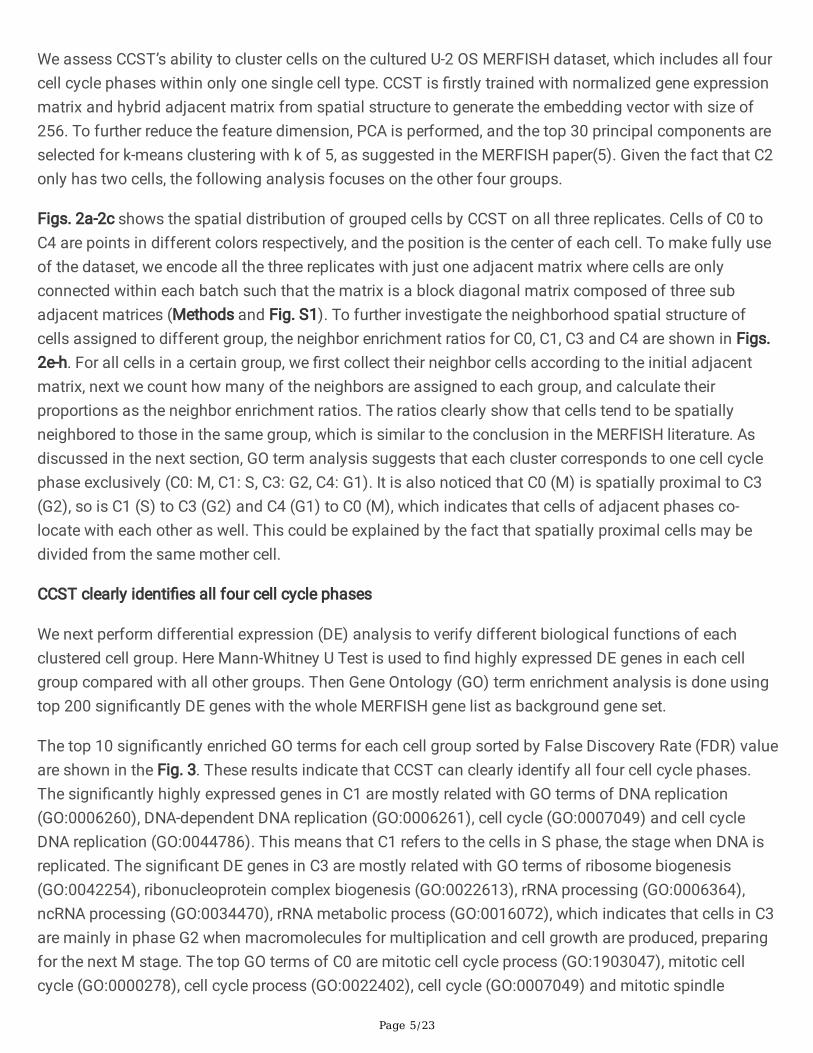
We assess CCST’s ability to cluster cells on the cultured U-2 OS MERFISH dataset, which includes all fourcell cycle phases within only one single cell type. CCST is �rstly trained with normalized gene expressionmatrix and hybrid adjacent matrix from spatial structure to generate the embedding vector with size of256. To further reduce the feature dimension, PCA is performed, and the top 30 principal components areselected for k-means clustering with k of 5, as suggested in the MERFISH paper(5). Given the fact that C2only has two cells, the following analysis focuses on the other four groups.

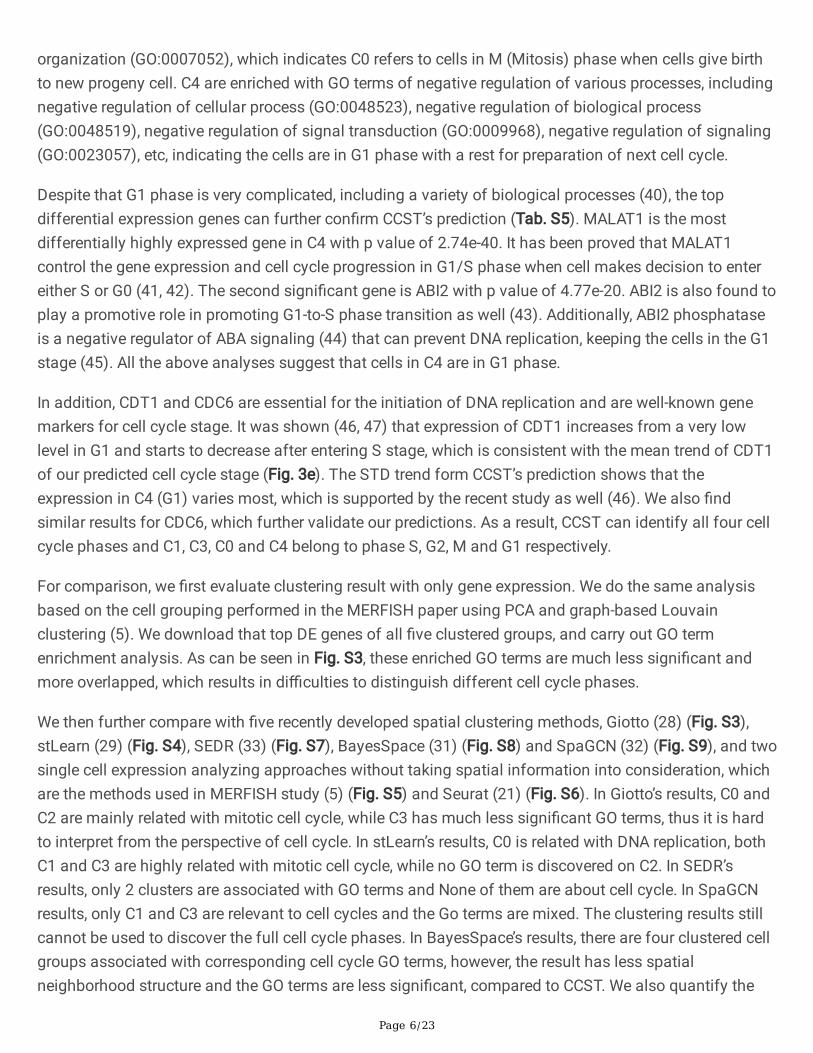
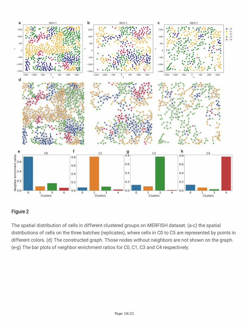
Figs. 2a-2c shows the spatial distribution of grouped cells by CCST on all three replicates. Cells of C0 toC4 are points in different colors respectively, and the position is the center of each cell. To make fully useof the dataset, we encode all the three replicates with just one adjacent matrix where cells are onlyconnected within each batch such that the matrix is a block diagonal matrix composed of three subadjacent matrices (Methods and Fig. S1). To further investigate the neighborhood spatial structure ofcells assigned to different group, the neighbor enrichment ratios for C0, C1, C3 and C4 are shown in Figs.2e-h. For all cells in a certain group, we �rst collect their neighbor cells according to the initial adjacentmatrix, next we count how many of the neighbors are assigned to each group, and calculate theirproportions as the neighbor enrichment ratios. The ratios clearly show that cells tend to be spatiallyneighbored to those in the same group, which is similar to the conclusion in the MERFISH literature. Asdiscussed in the next section, GO term analysis suggests that each cluster corresponds to one cell cyclephase exclusively (C0: M, C1: S, C3: G2, C4: G1). It is also noticed that C0 (M) is spatially proximal to C3(G2), so is C1 (S) to C3 (G2) and C4 (G1) to C0 (M), which indicates that cells of adjacent phases co-locate with each other as well. This could be explained by the fact that spatially proximal cells may bedivided from the same mother cell.

CCST clearly identi�es all four cell cycle phases 

We next perform differential expression (DE) analysis to verify different biological functions of eachclustered cell group. Here Mann-Whitney U Test is used to �nd highly expressed DE genes in each cellgroup compared with all other groups. Then Gene Ontology (GO) term enrichment analysis is done usingtop 200 signi�cantly DE genes with the whole MERFISH gene list as background gene set. 

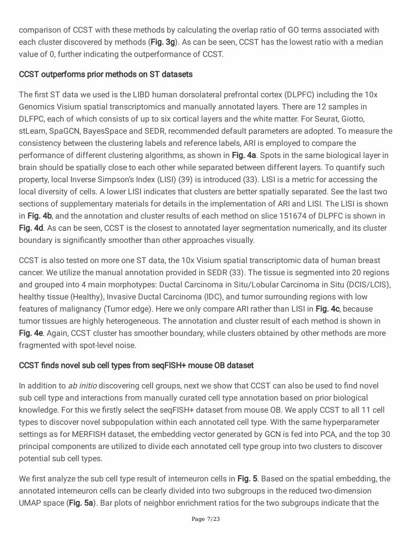
The top 10 signi�cantly enriched GO terms for each cell group sorted by False Discovery Rate (FDR) valueare shown in the Fig. 3. These results indicate that CCST can clearly identify all four cell cycle phases.The signi�cantly highly expressed genes in C1 are mostly related with GO terms of DNA replication(GO:0006260), DNA-dependent DNA replication (GO:0006261), cell cycle (GO:0007049) and cell cycleDNA replication (GO:0044786). This means that C1 refers to the cells in S phase, the stage when DNA isreplicated. The signi�cant DE genes in C3 are mostly related with GO terms of ribosome biogenesis(GO:0042254), ribonucleoprotein complex biogenesis (GO:0022613), rRNA processing (GO:0006364),ncRNA processing (GO:0034470), rRNA metabolic process (GO:0016072), which indicates that cells in C3are mainly in phase G2 when macromolecules for multiplication and cell growth are produced, preparingfor the next M stage. The top GO terms of C0 are mitotic cell cycle process (GO:1903047), mitotic cellcycle (GO:0000278), cell cycle process (GO:0022402), cell cycle (GO:0007049) and mitotic spindle

Page 6/23

organization (GO:0007052), which indicates C0 refers to cells in M (Mitosis) phase when cells give birthto new progeny cell. C4 are enriched with GO terms of negative regulation of various processes, includingnegative regulation of cellular process (GO:0048523), negative regulation of biological process(GO:0048519), negative regulation of signal transduction (GO:0009968), negative regulation of signaling(GO:0023057), etc, indicating the cells are in G1 phase with a rest for preparation of next cell cycle. 

Despite that G1 phase is very complicated, including a variety of biological processes (40), the topdifferential expression genes can further con�rm CCST’s prediction (Tab. S5). MALAT1 is the mostdifferentially highly expressed gene in C4 with p value of 2.74e-40. It has been proved that MALAT1control the gene expression and cell cycle progression in G1/S phase when cell makes decision to entereither S or G0 (41, 42). The second signi�cant gene is ABI2 with p value of 4.77e-20. ABI2 is also found toplay a promotive role in promoting G1-to-S phase transition as well (43). Additionally, ABI2 phosphataseis a negative regulator of ABA signaling (44) that can prevent DNA replication, keeping the cells in the G1stage (45). All the above analyses suggest that cells in C4 are in G1 phase. 

In addition, CDT1 and CDC6 are essential for the initiation of DNA replication and are well-known genemarkers for cell cycle stage. It was shown (46, 47) that expression of CDT1 increases from a very lowlevel in G1 and starts to decrease after entering S stage, which is consistent with the mean trend of CDT1of our predicted cell cycle stage (Fig. 3e). The STD trend form CCST’s prediction shows that theexpression in C4 (G1) varies most, which is supported by the recent study as well (46). We also �ndsimilar results for CDC6, which further validate our predictions. As a result, CCST can identify all four cellcycle phases and C1, C3, C0 and C4 belong to phase S, G2, M and G1 respectively.  

For comparison, we �rst evaluate clustering result with only gene expression. We do the same analysisbased on the cell grouping performed in the MERFISH paper using PCA and graph-based Louvainclustering (5). We download that top DE genes of all �ve clustered groups, and carry out GO termenrichment analysis. As can be seen in Fig. S3, these enriched GO terms are much less signi�cant andmore overlapped, which results in di�culties to distinguish different cell cycle phases. 

We then further compare with �ve recently developed spatial clustering methods, Giotto (28) (Fig. S3),stLearn (29) (Fig. S4), SEDR (33) (Fig. S7), BayesSpace (31) (Fig. S8) and SpaGCN (32) (Fig. S9), and twosingle cell expression analyzing approaches without taking spatial information into consideration, whichare the methods used in MERFISH study (5) (Fig. S5) and Seurat (21) (Fig. S6). In Giotto’s results, C0 andC2 are mainly related with mitotic cell cycle, while C3 has much less signi�cant GO terms, thus it is hardto interpret from the perspective of cell cycle. In stLearn’s results, C0 is related with DNA replication, bothC1 and C3 are highly related with mitotic cell cycle, while no GO term is discovered on C2. In SEDR’sresults, only 2 clusters are associated with GO terms and None of them are about cell cycle. In SpaGCNresults, only C1 and C3 are relevant to cell cycles and the Go terms are mixed. The clustering results stillcannot be used to discover the full cell cycle phases. In BayesSpace’s results, there are four clustered cellgroups associated with corresponding cell cycle GO terms, however, the result has less spatialneighborhood structure and the GO terms are less signi�cant, compared to CCST. We also quantify the

Page 7/23

comparison of CCST with these methods by calculating the overlap ratio of GO terms associated witheach cluster discovered by methods (Fig. 3g). As can be seen, CCST has the lowest ratio with a medianvalue of 0, further indicating the outperformance of CCST.

CCST outperforms prior methods on ST datasets

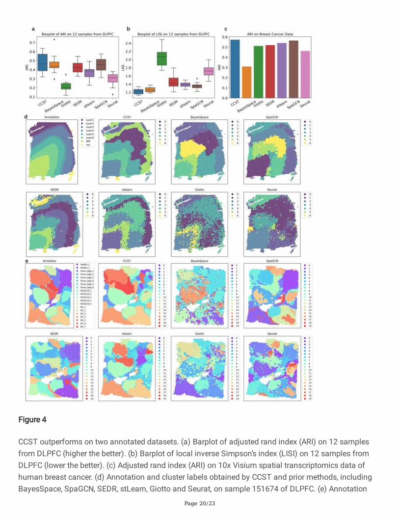
The �rst ST data we used is the LIBD human dorsolateral prefrontal cortex (DLPFC) including the 10xGenomics Visium spatial transcriptomics and manually annotated layers. There are 12 samples inDLFPC, each of which consists of up to six cortical layers and the white matter. For Seurat, Giotto,stLearn, SpaGCN, BayesSpace and SEDR, recommended default parameters are adopted. To measure theconsistency between the clustering labels and reference labels, ARI is employed to compare theperformance of different clustering algorithms, as shown in Fig. 4a. Spots in the same biological layer inbrain should be spatially close to each other while separated between different layers. To quantify suchproperty, local Inverse Simpson’s Index (LISI) (39) is introduced (33). LISI is a metric for accessing thelocal diversity of cells. A lower LISI indicates that clusters are better spatially separated. See the last twosections of supplementary materials for details in the implementation of ARI and LISI. The LISI is shownin Fig. 4b, and the annotation and cluster results of each method on slice 151674 of DLPFC is shown inFig. 4d. As can be seen, CCST is the closest to annotated layer segmentation numerically, and its clusterboundary is signi�cantly smoother than other approaches visually.

CCST is also tested on more one ST data, the 10x Visium spatial transcriptomic data of human breastcancer. We utilize the manual annotation provided in SEDR (33). The tissue is segmented into 20 regionsand grouped into 4 main morphotypes: Ductal Carcinoma in Situ/Lobular Carcinoma in Situ (DCIS/LCIS),healthy tissue (Healthy), Invasive Ductal Carcinoma (IDC), and tumor surrounding regions with lowfeatures of malignancy (Tumor edge). Here we only compare ARI rather than LISI in Fig. 4c, becausetumor tissues are highly heterogeneous. The annotation and cluster result of each method is shown inFig. 4e. Again, CCST cluster has smoother boundary, while clusters obtained by other methods are morefragmented with spot-level noise.

CCST �nds novel sub cell types from seqFISH+ mouse OB dataset

In addition to ab initio discovering cell groups, next we show that CCST can also be used to �nd novelsub cell type and interactions from manually curated cell type annotation based on prior biologicalknowledge. For this we �rstly select the seqFISH+ dataset from mouse OB. We apply CCST to all 11 celltypes to discover novel subpopulation within each annotated cell type. With the same hyperparametersettings as for MERFISH dataset, the embedding vector generated by GCN is fed into PCA, and the top 30principal components are utilized to divide each annotated cell type group into two clusters to discoverpotential sub cell types.

We �rst analyze the sub cell type result of interneuron cells in Fig. 5. Based on the spatial embedding, theannotated interneuron cells can be clearly divided into two subgroups in the reduced two-dimensionUMAP space (Fig. 5a). Bar plots of neighbor enrichment ratios for the two subgroups indicate that the

Page 8/23

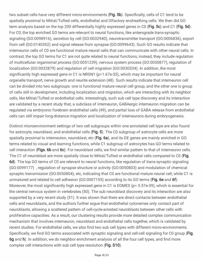
two subset cells have very different micro-environments (Fig. 5b). Speci�cally, cells of C1 tend to bespatially proximal to Mitral/Tufted cells, endothelial and Olfactory ensheathing cells. We then did GOterm analysis based on the top 200 differentially highly expressed genes in C0 (Fig. 5c) and C1 (Fig. 5d).For C0, the top enriched GO terms are relevant to neural functions, like anterograde trans-synapticsignaling (GO:0098916), secretion by cell (GO:0032940), neurotransmitter transport (GO:0006836), exportfrom cell (GO:0140352) and signal release from synapse (GO:0099643). Such GO results indicate thatinterneuron cells of C0 are functional mature neural cells that can communicate with other neural cells. Incontrast, the top GO terms for C1 are not quite related to neural functions, instead, they include regulationof multicellular organismal process (GO:0051239), nervous system process (GO:0050877), regulation oflocalization (GO:0032879) and regulation of cell migration (GO:0030334). In addition, the mostsigni�cantly high expressed gene in C1 is NRSN1 (p=1.67e-35), which may be important for neuralorganelle transport, nerve growth and neurite extension (48). Such results indicate that interneuron cellcan be divided into two subgroups: one is functional mature neural cell group, and the other one is groupof cells still in development, including localization and migration, which are interacting with its neighborcells, like Mitral/Tufted or endothelial cells. Interestingly, such sub cell type discovery and its interactionare validated by a recent study that, a subclass of interneuron, GABAergic interneuron migration can beregulated via embryonic forebrain endothelial cells (49), and partial loss of GABA release from endothelialcells can still impair long-distance migration and localization of interneurons during embryogenesis.

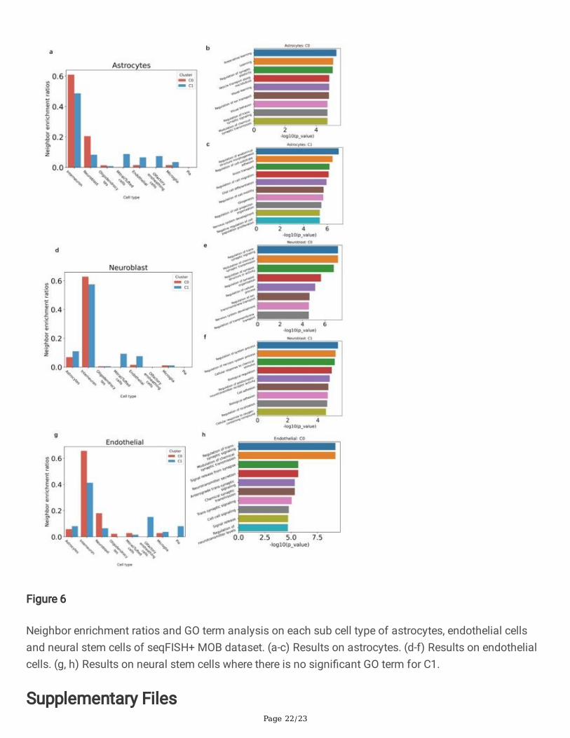
Distinct microenvironment settings of two cell subgroups within one annotated cell type are also foundfor astrocyte, neuroblast, and endothelial cells (Fig. 5). The C0 subgroup of astrocyte cells are morespatially proximal to interneuton, neuroblast, etc (Fig. 6a), and its DE genes are mainly enriched in GOterms related to visual and learning functions, while C1 subgroup of astrocytes has GO terms related tocell interaction (Figs. 6b and 6c). For neuroblast cells, we �nd similar pattern to that of interneuron cells.The C1 of neuroblast are more spatially close to Mitral/Tufted or endothelial cells compared to C0 (Fig.6d). The top GO terms of C0 are relevant to neural functions, like regulation of trans-synaptic signaling(GO:0099177)  , regulation of synapse structure or activity (GO:0050803) and modulation of chemicalsynaptic transmission (GO:0050804), etc, indicating that C0 are functional mature neural cell, while C1 isunmatured and related to cell adhesion (GO:0007155) according to its GO terms (Fig. 6e and 6f).Moreover, the most signi�cantly high expressed gene in C1 is EOMES (p= 5.57e-39), which is essential forthe central nervous system in vertebrates (50). The sub neuroblast discovery and its interaction are alsosupported by a very recent study (51). It was shown that there are direct contacts between endothelialcells and neuroblasts, and the authors further argue that endothelial cytonemes only contact part ofneuroblasts, allowing a scattered pattern of cell-cycle-arrested neuroblasts between other cells withproliferative capacities. As a result, our clustering results provide more detailed complex communicationmechanism that involves interneuron, neuroblast and endothelial cells together, which is validated byrecent studies. For endothelial cells, we also �nd two sub cell types with different micro-environments.Speci�cally, we �nd GO terms associated with synaptic signaling and cell-cell signaling for C0 group (Fig.6g and h). In addition, we do neighbor enrichment analysis of all the four cell types, and �nd morecomplex cell interactions with sub cell type resolution (Fig. S10). 

Page 9/23

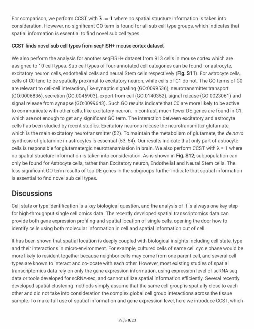
For comparison, we perform CCST with λ = 1 where no spatial structure information is taken intoconsideration. However, no signi�cant GO term is found for all sub cell type groups, which indicates thatspatial information is essential to �nd novel sub cell types.

CCST �nds novel sub cell types from seqFISH+ mouse cortex dataset

We also perform the analysis for another seqFISH+ dataset from 913 cells in mouse cortex which areassigned to 10 cell types. Sub cell types of four annotated cell categories can be found for astrocyte,excitatory neuron cells, endothelial cells and neural Stem cells respectively (Fig. S11). For astrocyte cells,cells of C0 tend to be spatially proximal to excitatory neuron, while cells of C1 do not. The GO terms of C0are relevant to cell-cell interaction, like synaptic signaling (GO:0099536), neurotransmitter transport(GO:0006836), secretion (GO:0046903), export from cell (GO:0140352), signal release (GO:0023061) andsignal release from synapse (GO:0099643). Such GO results indicate that C0 are more likely to be activeto communicate with other cells, like excitatory neuron. In contrast, much fewer DE genes are found in C1,which are not enough to get any signi�cant GO term. The interaction between excitatory and astrocytecells has been studied by recent studies. Excitatory neurons release the neurotransmitter glutamate,which is the main excitatory neurotransmitter (52). To maintain the metabolism of glutamate, the de novosynthesis of glutamine in astrocytes is essential (53, 54). Our results indicate that only part of astrocytecells is responsible for glutamatergic neurotransmission in brain. We also perform CCST with λ = 1 whereno spatial structure information is taken into consideration. As is shown in Fig. S12, subpopulation canonly be found for Astrocyte cells, rather than Excitatory neuron, Endothelial and Neural Stem cells. Theless signi�cant GO term results of top DE genes in the subgroups further indicate that spatial informationis essential to �nd novel sub cell types. 

DiscussionsCell state or type identi�cation is a key biological question, and the analysis of it is always one key stepfor high-throughput single cell omics data. The recently developed spatial transcriptomics data canprovide both gene expression pro�ling and spatial location of single cells, opening the door how toidentify cells using both molecular information in cell and spatial information out of cell.

It has been shown that spatial location is deeply coupled with biological insights including cell state, typeand their interactions in micro-environment. For example, cultured cells of same cell cycle phase would bemore likely to resident together because neighbor cells may come from one parent cell, and several celltypes are known to interact and co-locate with each other. However, most existing studies of spatialtranscriptomics data rely on only the gene expression information, using expression level of scRNA-seqdata or tools developed for scRNA-seq, and cannot utilize spatial information e�ciently. Several recentlydeveloped spatial clustering methods simply assume that the same cell group is spatially close to eachother and did not take into consideration the complex global cell group interactions across the tissuesample. To make full use of spatial information and gene expression level, here we introduce CCST, which

Page 10/23

uses unsupervised graph convolution network to learn cell embedding representation based on graphextracted from spatial transcriptomics data.

Results of different spatial transcriptomics datasets show CCST’s power. CCST can greatly improve abinitio cell clustering over existing methods from in vitro MERFISH dataset of cultured cell. Firstly, CCST’sprediction has more spatial structure. secondly, CCST can clearly recognize cell groups of all four cellcycle phases. Thirdly, it can �nd the spatial proximity between adjacent phases. In addition, for in vivodataset, CCST can also be used to �nd novel sub cell types with different biological functions and theirinteractions with biological insights from seqFISH+ datasets of mouse cortex and OB tissues, which issupported by DE gene analysis, GO term enrichment and other literatures. In the quantitative comparison,CCST obtained the highest ARI and lowest LISI on both ST datasets compared to all prior clusteringapproaches. So CCST can help understand cell identity, interaction and spatial organization from spatialdata.

CCST is implemented in Python. All the source code and spatial data can be downloaded from thesupporting website, https://github.com/xiaoyeye/CCST.

Methods1, Dataset 

Recently, with the cutting-edge technology in imaging the transcriptome in situ with highaccuracy, multiple high-throughput spatial expression datasets are available for analyzingcells based on both gene expression and spatial distribution. We take experiments on twobenchmark datasets. The first one is obtained by multiplexed error-robust fluorescence insitu hybridization (MERFISH) (5). consisting of the expression of 10,050 genes in 1,368human osteosarcoma cells from 3 batches (replicates). The second is obtained bysequential fluorescence in situ hybridization (seqFISH+) (10). The seqFISH+ dataset frommouse cortex contains the expression of 10,000 genes in 913 cells assigned to 10 cell types,and seqFISH+ dataset from MOB contains the expression of 10,000 genes in 2,050 cellsassigned to 11 cell types. Additionally, two ST datasets are utilized in our experiment,which are human dorsolateral prefrontal cortex (DLPFC) and 10x Visium spatialtranscriptomics data of human breast cancer. There are 12 samples in DLFPC, each ofwhich consists of up to six cortical layers and the white matter. In the annotation of humanbreast cancer provided by SEDR (33), the tissue is segmented to 20 areas.

2, Graph construction

A graph can be described by two matrices, an adjacent matrix for representing the graphstructure and a feature matrix for representing node attributes. To represent the spatialinformation among cells, an undirected graph is constructed for each field of view, wherecell is represented as node and edge connects pair of cells spatially close to each other. For

Page 11/23

this purpose, we firstly calculate the distance over each cell pair  , where   and   are theindices of two cells. Utilizing a proper threshold  , we can obtain the adjacent matrix 

where   is the number of cells,   if   and   otherwise. Theconstructed graph on MERFISH is illustrated in Fig. 2(d). To balance the weight betweenspatial information and the gene expression of an individual cell, we introduce ahyperparameter   to generate the hybrid adjacent matrix.

where   is an identity matrix. We conduct experiments with various   to better explorethe influence of spatial information.Similar to (5, 10), a series of preprocessing steps are introduced on the raw gene countdata to extract nodes features, including filtering out lowly expressed genes and lowlyvariable genes, normalizing the counts per cell, and batch correction if necessary.Here, we mainly follow the preprocessing strategy given by (5). Since the MERFISHdataset is collected from 3 replicates, batch correction is required. After removing thelowly expressed genes whose expression is fewer than 1 count per cell on average, weemploy Scanorama (55) to correct batch effect. Then we normalize the correctedexpressions following equation 2. Finally, the lowly variable genes whose variance ofnormalized expression is lower than 1 are dropped.

where   represents cell   and   represents gene  . On the seqFISH+ and two ST datasets, we adopt similar preprocessing steps without thebatch correction that is not needed.3, Node embedding and clusteringWith the recent progress in graph convolutional network (GCN), several approaches tolearn node representations from graph-structured data have been proposed. Here, weutilize an unsupervised graph embedding method, Deep Graph Infomax (DGI) (37). Different from previous approaches based on random walk, DGI relies on maximizingmutual information between local representations and global summaries of graphs. InGCN, nodes are embedded by repeatedly aggregating the features of neighbor nodes. Theextracted local feature contains the information of a subgraph centered on each individualnode. To better explore the high-level feature of the whole graph, DGI is designed to learnan encoder by maximizing mutual information over patches. This feature contains not onlylocal features, but also global features. The input to DGI is the hybrid adjacent matrix  and a set of node features,

, where  is the number of nodes,  represents the features of node  and  is the number of node features. In the vanilla DGI and majority applications of GCN, the

Page 12/23

adjacent matrix A is assumed to be filled with binary numbers, i.e.,  if there exists anedge between node  and  in the graph and  otherwise. Here we further apply DGI tothe weighted Graph constructed with hybrid adjacent matrix.The objective of DGI is learning an encoder  that maps input feature and adjacent matrixto embedding space: , where  represents high-levelrepresentations,  for each node  and  is the number of embedding features. Theencoder is composed of four graph convolutional layers for passing massage overneighbored nodes with a Parametric Rectified Linear Unit (PReLU) as the activationfunction. The  graph convolutional layer is:

where  and  are the input and output of the  graph convolutional layer,  is theweight matrix used for feature transformation.  is the adjacent matrix after being addedby self-loops,

The PReLU function is:

where  is a learnable parameter.The global representation  is obtained by mapping from the local representations with areadout function : and . With the local and global features, adiscriminator  is introduced to evaluate how much graph level information iscontained by a local patch. The higher  indicates, the patches are more likely to becontained within the summary. For training the discriminator, we generate negativesamples by a corruption function : , where the edges in the graph arereconstructed randomly. Then we obtain the local representations  for negative samplesas well. The full objective is:  

By maximizing the approximate representation of mutual information between  and , DGIoutputs the node embedding that contains structural information of the graph.PCA is performed on the obtained embedding vector for dimension reduction. Clusteringalgorithms UMAP is employed on top principal components to discover novel cell groups orcell subpopulations.4, Differential gene expression analysis

Page 13/23

To verify different biological functions of each clustered cell subpopulation, we finddifferentially expressed (DE) genes that are expressed highly in each subpopulation byMann-Whitney U Test for all cell types. With the top 200 DE genes and the whole gene list inthe corresponding dataset as the background, we carried out Gene Ontology (GO) termenrichment analysis for each subpopulation to construct a functional enrichment profile. We also take GO term analysis on the differential expressed genes of the five clustersdiscovered by (5). The results are shown in supplementary materials. the FDR values ofthose GO terms obtained in their approaches are not as low as those got by ours. Inaddition, the significantly related GO terms are mixed up in there 5 clusters.

DeclarationsAcknowledgments

This work was supported by the National Natural Science Foundation of China (No. 61725302,62073219, 61972251).

References1.         Codeluppi S, et al. (2018) Spatial organization of the somatosensory cortex revealed by osmFISH.Nature methods 15(11):932-935.

2.         Mo�tt JR & Zhuang X (2016) RNA imaging with multiplexed error-robust �uorescence in situhybridization (MERFISH). Methods in enzymology 572:1-49.

3.         Mo�tt JR, et al. (2016) High-throughput single-cell gene-expression pro�ling with multiplexederror-robust �uorescence in situ hybridization. Proceedings of the National Academy of Sciences113(39):11046-11051.

4.         Chen KH, Boettiger AN, Mo�tt JR, Wang S, & Zhuang X (2015) Spatially resolved, highlymultiplexed RNA pro�ling in single cells. Science 348(6233).

5.         Xia C, Fan J, Emanuel G, Hao J, & Zhuang X (2019) Spatial transcriptome pro�ling by MERFISHreveals subcellular RNA compartmentalization and cell cycle-dependent gene expression. Proceedings ofthe National Academy of Sciences 116(39):19490-19499.

6.         Eng C-HL, Shah S, Thomassie J, & Cai L (2017) Pro�ling the transcriptome with RNA SPOTs.Nature methods 14(12):1153-1155.

7.         Lubeck E, Coskun AF, Zhiyentayev T, Ahmad M, & Cai L (2014) Single-cell in situ RNA pro�ling bysequential hybridization. Nature methods 11(4):360-361.

Page 14/23

8.         Wang X, et al. (2018) Three-dimensional intact-tissue sequencing of single-cell transcriptionalstates. Science 361(6400).

9.         Schiller HB, et al. (2019) The human lung cell atlas: a high-resolution reference map of the humanlung in health and disease. American journal of respiratory cell and molecular biology 61(1):31-41.

10.        Eng C-HL, et al. (2019) Transcriptome-scale super-resolved imaging in tissues by RNA seqFISH+.Nature 568(7751):235-239.

11.        Park J, Liu CL, Kim J, & Susztak K (2019) Understanding the kidney one cell at a time. Kidneyinternational 96(4):862-870.

12.        Ståhl PL, et al. (2016) Visualization and analysis of gene expression in tissue sections by spatialtranscriptomics. Science 353(6294):78-82.

13.        Rodriques SG, et al. (2019) Slide-seq: A scalable technology for measuring genome-wideexpression at high spatial resolution. Science 363(6434):1463-1467.

14.        Nichterwitz S, et al. (2016) Laser capture microscopy coupled with Smart-seq2 for precise spatialtranscriptomic pro�ling. Nature communications 7(1):1-11.

15.        Pal B, et al. (2017) Construction of developmental lineage relationships in the mouse mammarygland by single-cell RNA pro�ling. Nature communications 8(1):1-14.

16.        Yuan Y & Bar-Joseph Z (2019) GCNG: Graph convolutional networks for inferring cell-cellinteractions. bioRxiv.

17.        Arnol D, Schapiro D, Bodenmiller B, Saez-Rodriguez J, & Stegle O (2019) Modeling cell-cellinteractions from spatial molecular data with spatial variance component analysis. Cell reports29(1):202-211. e206.

18.        Stuart T, et al. (2019) Comprehensive integration of single-cell data. Cell 177(7):1888-1902.e1821.

19.        Abdelaal T, et al. (2019) A comparison of automatic cell identi�cation methods for single-cell RNAsequencing data. Genome biology 20(1):1-19.

20.        Wolf FA, Angerer P, & Theis FJ (2018) SCANPY: large-scale single-cell gene expression dataanalysis. Genome biology 19(1):1-5.

21.        Hao Y, et al. (2021) Integrated analysis of multimodal single-cell data. Cell.

22.        Blondel VD, Guillaume J-L, Lambiotte R, & Lefebvre E (2008) Fast unfolding of communities inlarge networks. Journal of statistical mechanics: theory and experiment 2008(10):P10008.

Page 15/23

23.        Traag VA, Waltman L, & Van Eck NJ (2019) From Louvain to Leiden: guaranteeing well-connectedcommunities. Scienti�c reports 9(1):1-12.

24.        Shekhar K, et al. (2016) Comprehensive classi�cation of retinal bipolar neurons by single-celltranscriptomics. Cell 166(5):1308-1323. e1330.

25.        Pandey S, Shekhar K, Regev A, & Schier AF (2018) Comprehensive identi�cation and spatialmapping of habenular neuronal types using single-cell RNA-seq. Current Biology 28(7):1052-1065. e1057.

26.        Zhu Q, Shah S, Dries R, Cai L, & Yuan G-C (2018) Identi�cation of spatially associatedsubpopulations by combining scRNAseq and sequential �uorescence in situ hybridization data. Naturebiotechnology 36(12):1183-1190.

27.        Stoltzfus CR, et al. (2020) CytoMAP: a spatial analysis toolbox reveals features of myeloid cellorganization in lymphoid tissues. Cell reports 31(3):107523.

28.        Dries R, et al. (2021) Giotto: a toolbox for integrative analysis and visualization of spatialexpression data. Genome biology 22(1):1-31.

29.        Pham D, et al. (2020) stLearn: integrating spatial location, tissue morphology and geneexpression to �nd cell types, cell-cell interactions and spatial trajectories within undissociated tissues.bioRxiv.

30.        Teng H, Yuan Y, & Bar-Joseph Z (2021) Cell Type Assignments for Spatial Transcriptomics Data.bioRxiv.

31.        Zhao E, et al. (2021) Spatial transcriptomics at subspot resolution with BayesSpace. NatureBiotechnology:1-10.

32.        Hu J, et al. (2021) SpaGCN: Integrating gene expression, spatial location and histology to identifyspatial domains and spatially variable genes by graph convolutional network. Nature Methods:1-10.

33.        Fu H, Hang X, & Chen J (2021) Unsupervised Spatial Embedded Deep Representation of SpatialTranscriptomics. bioRxiv.

34.        Kipf TN & Welling M (2016) Semi-supervised classi�cation with graph convolutional networks.arXiv preprint arXiv:1609.02907.

35.        Krizhevsky A, Sutskever I, & Hinton GE (2012) Imagenet classi�cation with deep convolutionalneural networks. Advances in neural information processing systems 25:1097-1105.

36.        LeCun Y, Bottou L, Bengio Y, & Haffner P (1998) Gradient-based learning applied to documentrecognition. Proceedings of the IEEE 86(11):2278-2324.

37.        Veličković P, et al. (2018) Deep graph infomax. arXiv preprint arXiv:1809.10341.

Page 16/23

38.        Arthur D & Vassilvitskii S (2006) k-means++: The advantages of careful seeding.   (Stanford).

39.        Korsunsky I, et al. (2019) Fast, sensitive and accurate integration of single-cell data withHarmony. Nature methods 16(12):1289-1296.

40.        Donjerkovic D & Scott DW (2000) Regulation of the G1 phase of the mammalian cell cycle. Cellresearch 10(1):1-16.

41.        Tripathi V, et al. (2013) Long noncoding RNA MALAT1 controls cell cycle progression byregulating the expression of oncogenic transcription factor B-MYB. PLoS genetics 9(3):e1003368.

42.        Wang J, et al. (2014) MALAT1 promotes cell proliferation in gastric cancer by recruiting SF2/ASF.Biomedicine & Pharmacotherapy 68(5):557-564.

43.        Lu H, et al. (2020) miR‐25 expression is upregulated in pancreatic ductal adenocarcinoma andpromotes cell proliferation by targeting ABI2. Experimental and therapeutic medicine 19(5):3384-3390.

44.        Merlot S, Gosti F, Guerrier D, Vavasseur A, & Giraudat J (2001) The ABI1 and ABI2 proteinphosphatases 2C act in a negative feedback regulatory loop of the abscisic acid signalling pathway. ThePlant Journal 25(3):295-303.

45.        Swiatek A, Lenjou M, Van Bockstaele D, Inzé D, & Van Onckelen H (2002) Differential effect ofjasmonic acid and abscisic acid on cell cycle progression in tobacco BY-2 cells. Plant physiology128(1):201-211.

46.        Mahdessian D, et al. (2021) Spatiotemporal dissection of the cell cycle with single-cellproteogenomics. Nature 590(7847):649-654.

47.        Sakaue-Sawano A, et al. (2008) Visualizing spatiotemporal dynamics of multicellular cell-cycleprogression. Cell 132(3):487-498.

48.        Cheng C, et al. (2002) Cloning, expression and characterization of a novel human VMP gene.Molecular biology reports 29(3):281-286.

49.        Li S, et al. (2018) Endothelial cell-derived GABA signaling modulates neuronal migration andpostnatal behavior. Cell research 28(2):221-248.

50.        Russ AP, et al. (2000) Eomesodermin is required for mouse trophoblast development andmesoderm formation. Nature 404(6773):95-99.

51.        Taberner L, Bañón A, & Alsina B (2020) Sensory neuroblast quiescence depends on vascularcytoneme contacts and sensory neuronal differentiation requires initiation of blood �ow. Cell Reports32(2):107903.

52.        Bekkers JM (2011) Pyramidal neurons. Current biology 21(24):R975.

Page 17/23

53.        Parpura V, et al. (2017) Glutamate and ATP at the interface between signaling and metabolism inastroglia: examples from pathology. Neurochemical research 42(1):19-34.

54.        Schousboe A, Sca�di S, Bak LK, Waagepetersen HS, & McKenna MC (2014) Glutamatemetabolism in the brain focusing on astrocytes. Glutamate and ATP at the Interface of Metabolism andSignaling in the Brain,  (Springer), pp 13-30.

55.        Hie B, Bryson B, & Berger B (2019) E�cient integration of heterogeneous single-celltranscriptomes using Scanorama. Nature biotechnology 37(6):685-691.

Figures

Figure 1

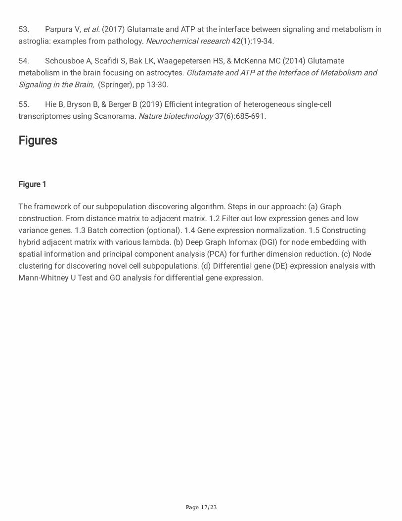
The framework of our subpopulation discovering algorithm. Steps in our approach: (a) Graphconstruction. From distance matrix to adjacent matrix. 1.2 Filter out low expression genes and lowvariance genes. 1.3 Batch correction (optional). 1.4 Gene expression normalization. 1.5 Constructinghybrid adjacent matrix with various lambda. (b) Deep Graph Infomax (DGI) for node embedding withspatial information and principal component analysis (PCA) for further dimension reduction. (c) Nodeclustering for discovering novel cell subpopulations. (d) Differential gene (DE) expression analysis withMann-Whitney U Test and GO analysis for differential gene expression.

Page 18/23

Figure 2

The spatial distribution of cells in different clustered groups on MERFISH dataset. (a-c) the spatialdistributions of cells on the three batches (replicates), where cells in C0 to C5 are represented by points indifferent colors. (d) The constructed graph. Those nodes without neighbors are not shown on the graph.(e-g) The bar plots of neighbor enrichment ratios for C0, C1, C3 and C4 respectively.

Page 19/23

Figure 3

CCST can identify four cell cycle phases clearly. (a-d) Top GO terms of clustered cell groups of C1, C3, C0and C4, corresponding to S, G2, M and G1 phase respectively. (e, f) The mean and standard deviation(std) of CDT1 and CDC6. (g) A GO result comparison of our CCST with prior methods, includingBayesSpace, Gitto, SpaGCN, Seurat and MERFISH pipeline. Stlearn and SEDR are not illustrated in the�gure, because only part of clusters given by them are associated with GO terms.

Page 20/23

Figure 4

CCST outperforms on two annotated datasets. (a) Barplot of adjusted rand index (ARI) on 12 samplesfrom DLPFC (higher the better). (b) Barplot of local inverse Simpson’s index (LISI) on 12 samples fromDLPFC (lower the better). (c) Adjusted rand index (ARI) on 10x Visium spatial transcriptomics data ofhuman breast cancer. (d) Annotation and cluster labels obtained by CCST and prior methods, includingBayesSpace, SpaGCN, SEDR, stLearn, Giotto and Seurat, on sample 151674 of DLPFC. (e) Annotation

Page 21/23

and cluster labels obtained by CCST and prior methods on 10x Visium spatial transcriptomics data ofhuman breast cancer.

Figure 5

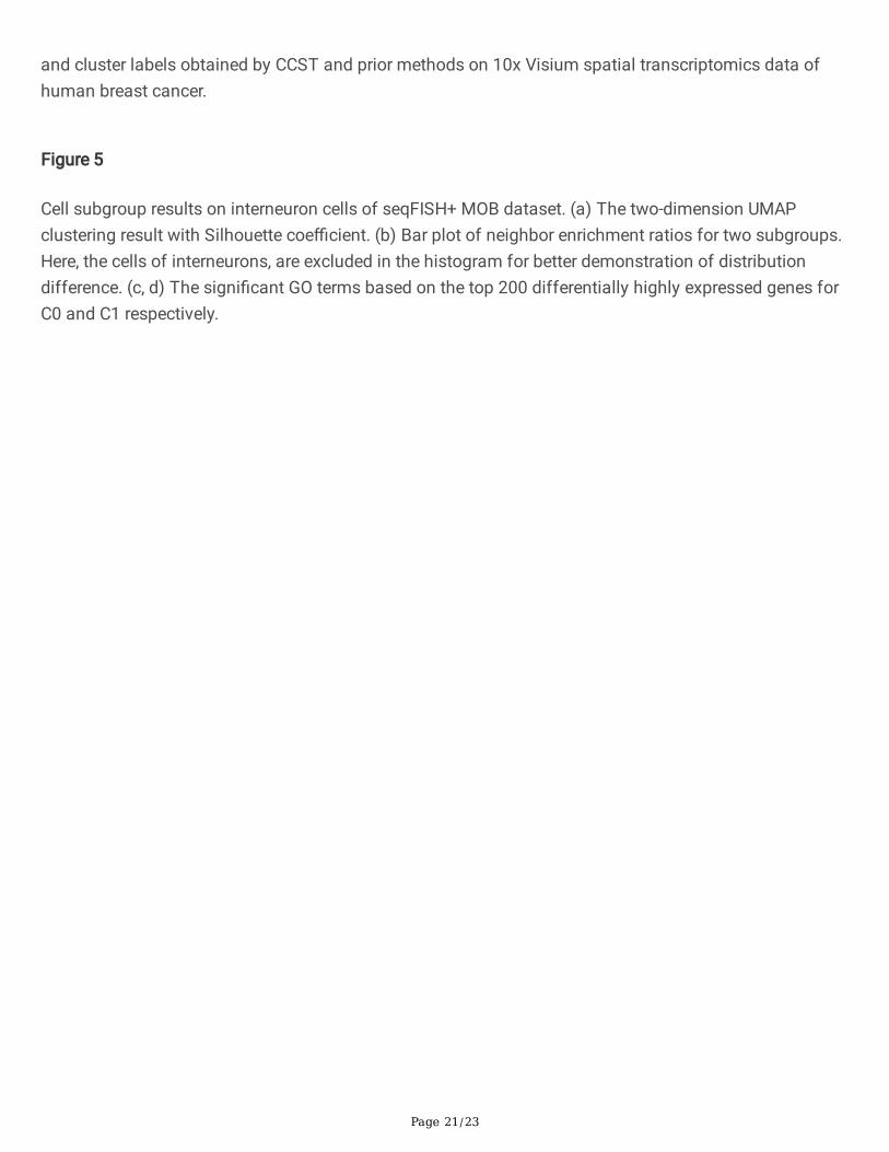
Cell subgroup results on interneuron cells of seqFISH+ MOB dataset. (a) The two-dimension UMAPclustering result with Silhouette coe�cient. (b) Bar plot of neighbor enrichment ratios for two subgroups.Here, the cells of interneurons, are excluded in the histogram for better demonstration of distributiondifference. (c, d) The signi�cant GO terms based on the top 200 differentially highly expressed genes forC0 and C1 respectively.

Page 22/23

Figure 6

Neighbor enrichment ratios and GO term analysis on each sub cell type of astrocytes, endothelial cellsand neural stem cells of seqFISH+ MOB dataset. (a-c) Results on astrocytes. (d-f) Results on endothelialcells. (g, h) Results on neural stem cells where there is no signi�cant GO term for C1.

Supplementary Files

Page 23/23

This is a list of supplementary �les associated with this preprint. Click to download.

supplementaryCCST.docx

YYuanCS�at.pdf

YYuanEPC�at.pdf