Canary Island Tomato Exports: A Structural Analysis of Seasonality

Gloria Martin Rodriguez

e-mail: gmartinr@ull.es Jose Juan Caceres Hernandez

e-mail: jcaceres@ull.es

Paper prepared for presentation at the Xth EAAE Congress ‘Exploring Diversity in the European Agri -Food System’,

Zaragoza (Spain), 28-31 August 2002

Copyright 2002 by Gloria Martín Rodríguez and José Juan Cáceres Hernández. All rights reserved. Readers may make verbatim copies of this document for noncommercial

purposes by any means, provided that this copyright notice appears on all such copies.

CANARY ISLAND TOMATO EXPORTS: A STRUCTURAL ANALYSIS OF SEASONALITY

Gloria Martín Rodríguez and José Juan Cáceres Hernández

Dpto. de Economía de las Instituciones, Estadística Económica y Econometría Facultad de Ciencias Económicas y Empresariales de la Universidad de La Laguna,

Camino la Hornera, s/n, 38071, La Laguna, Tenerife. gmartinr@ull.es, jcaceres@ull.es

Correspondence: José Juan Cáceres Hernández Department: Economía de las Instituciones, Estadística Económica y Econometría Postal Address: Facultad de Ciencias Económicas y Empresariales

Campus de Guajara; Camino La Hornera, s/n 38071 La Laguna Santa Cruz de Tenerife

Telephone: (922) 317035 Fax: (922) 317042 e-mail: jcaceres@ull.es

CANARY ISLAND TOMATO EXPORTS: A STRUCTURAL ANALYSIS OF SEASONALITY

SUMMARY

The European tomato market is characterised by a constant process of dynamic adjustment toward the equilibrium. Furthermore, Canary tomato exports cause a high seasonal impact on market prices in the winter period. In these circumstances, an adequate distribution of shipments throughout the campaign could contribute to maximize producers’ profits.

The goal of this paper is to analyse the seasonal pattern of Canary tomato exports to Europe throughout the first fourteen campaigns following Spanish integration into the European Union. These export levels show some degree of instability, clearly related to the changes in the European Union trade rules, and there is a long period, the summer, without exports. Moreover, we have opted by using weekly data. These factors should be taken into account in order to accurately capture the performance of exports and, specifically, the nature of their seasonal behaviour. Thus, this analysis is carried out inside the frame delimited by the structural approach to time series and the usefulness of spline functions as an alternative to standard seasonal variation models is shown. Key words: Canary tomato exports, weekly data, seasonality, structural models, splines. 1. INTRODUCTION

The cultivation of tomatoes for export in the Canary Islands has a long tradition. In the last decades of the 20th century, the participating agents in this activity have modernized cultivation, package and marketing techniques. The driving force behind this modernisation process has been national and international competition in the European markets. The strongest competitors of Canary suppliers are Morocco and, above all, Spain mainland. Canary shares in exports to Europe in the winter period were around 40% in the analysed campaigns. However the innovative effort of the producers will not be able to support the position of Canary tomatoes in the markets indefinitely. Furthermore, it is necessary to analyse precisely the appropriate moment for sending the quantity which every market demands. In those weeks in which the Canary export shares are the highest, the growth of these exports is usually accompanied by a fall in market prices. For this reason, Canary producers should plan their shipments in order to guarantee some profit margin. From this point of view, the study of the seasonal pattern of tomato exports from the Canary Islands is highly relevant to the marketing decision-making process. In this paper, the evolution of the weekly exports to Europe of Canary Islands tomatoes is analysed in the period following Spain’s entry in the European Union.

Before building an econometric model capturing the variations of this series, it is useful to point out some features of the tomato export activity in the Canary Islands. First, the seasonal pattern of Canary exports is characterised by concentration in winter and disappearance in summer. This pattern is a rational response guided by the search for profitability; there are no exports in summer because northern European countries and Canary supplies converge in this season, and so Canary tomato prices would be low. Second, the development of greenhouse technology in northern Europe, the increase in

Spain mainland supply and the third country supplies sharing the same export periods as Canary Islands product entry to the European market, have led to a growing overlap of the different supplies in spring and autumn. Finally, Spain’s full integration into the CAP has brought about the abolition of the mechanisms used by European producers as custom barriers against production from the Canary Islands1, and these changes have encouraged Canary producers to increase their exports, despite the fact that Moroccans have also benefitted from a significant reduction in these barriers2. From these remarks, it follows that the volumes of Canary tomatoes exported in the different weeks of the campaign have not kept stable throughout last years. In order to model the behaviour of exports, an important task is whether these alterations are located at specific times and can be captured through modifications in deterministic components, or whether they are more continuous and random changes that can be captured by ARMA models with or without unit roots. Moreover, if the classic definition of the components of a time series is relaxed, structural models appear to be a potentially appropriate tool for handling these instabilities. Structural analysis introduce a new conceptual framework which can lead to apparently different results although, nevertheless, equivalent to those obtained through alternative models, and the techniques used in this paper can be framed inside this approach. The use of the structural approach, the specific constraints which must be taken into account when weekly data are being studied and the existence of non-exporting periods of variable amplitude, are factors why this study can be interesting from an econometric point of view. The plan of the paper is as follows. In the next section, the data used are identified and some interesting features of their nature and preliminary processing are discussed. In case study, the properties of the series do not appear to remain the same over time. Then, structural models are an appropriate class of models to cope with this kind of situation. The basic statistical framework for handling such models is outlined in the third section. In section four, these procedures are applied to weekly series of Canary tomato exports. Section 5 presents the conclusions. 2. DATA This section is concerned with the series of weekly exports of Canary tomatoes (measured in 6 kg boxes) to European markets from the 1986/1987 harvest until the 1999/2000 harvest3. Each campaign is considered to start on week 27 of a year and

1 In practice, the reference price system did not allow Canary produce to enter European markets from the

month of April onwards of each year. This system was replaced by another, more flexible system of supply prices, introduced in July 1991. From the 1st January 1993, the abolition of supply price system meant a liberalisation of Canary exports to the European Community, with the exception of the maintenance of the complementary mechanism applied to exchanges, of very little impact. For a detailed explanation of these protection mechanisms, see Cáceres (2000: 292-305).

2 Since the signing of the Protocol between Morocco and the EU in 1988, and until the full integration of Spain in the CAP, Moroccan production entered European markets under similar conditions to Canary production. The 1994 GATT agreements constituted a hardening of the access conditions for Moroccan produce, but these conditions became null and void as a result of the EU-Morocco trade agreements of 1995 and 1996. See Cáceres (2000: 278-281, 308-312).

3 Export statistics have been obtained from weekly data published by the provincial exporter associations of Santa Cruz de Tenerife (ACETO) and of Las Palmas (FEDEX) in their export season reports. In the weeks where these sources did not register any data, they have been assigned a zero value.

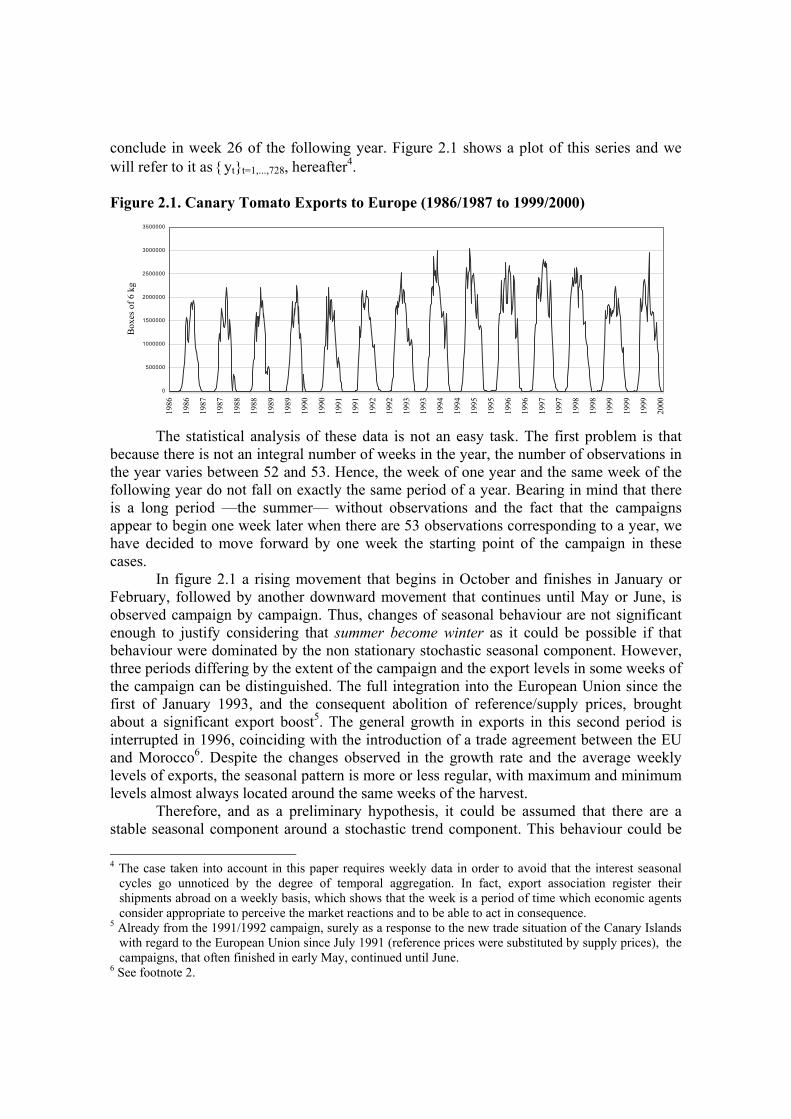
conclude in week 26 of the following year. Figure 2.1 shows a plot of this series and we will refer to it as {yt}t=1,...,728, hereafter4. Figure 2.1. Canary Tomato Exports to Europe (1986/1987 to 1999/2000)

0

500000

1000000

1500000

2000000

2500000

3000000

3500000

1986

1986

1987

1987

1988

1988

1989

1989

1990

1990

1991

1991

1992

1992

1993

1993

1994

1994

1995

1995

1996

1996

1997

1997

1998

1998

1999

1999

1999

2000

Box

es o

f 6 k

g

The statistical analysis of these data is not an easy task. The first problem is that

because there is not an integral number of weeks in the year, the number of observations in the year varies between 52 and 53. Hence, the week of one year and the same week of the following year do not fall on exactly the same period of a year. Bearing in mind that there is a long period —the summer— without observations and the fact that the campaigns appear to begin one week later when there are 53 observations corresponding to a year, we have decided to move forward by one week the starting point of the campaign in these cases. In figure 2.1 a rising movement that begins in October and finishes in January or February, followed by another downward movement that continues until May or June, is observed campaign by campaign. Thus, changes of seasonal behaviour are not significant enough to justify considering that summer become winter as it could be possible if that behaviour were dominated by the non stationary stochastic seasonal component. However, three periods differing by the extent of the campaign and the export levels in some weeks of the campaign can be distinguished. The full integration into the European Union since the first of January 1993, and the consequent abolition of reference/supply prices, brought about a significant export boost5. The general growth in exports in this second period is interrupted in 1996, coinciding with the introduction of a trade agreement between the EU and Morocco6. Despite the changes observed in the growth rate and the average weekly levels of exports, the seasonal pattern is more or less regular, with maximum and minimum levels almost always located around the same weeks of the harvest.

Therefore, and as a preliminary hypothesis, it could be assumed that there are a stable seasonal component around a stochastic trend component. This behaviour could be 4 The case taken into account in this paper requires weekly data in order to avoid that the interest seasonal

cycles go unnoticed by the degree of temporal aggregation. In fact, export association register their shipments abroad on a weekly basis, which shows that the week is a period of time which economic agents consider appropriate to perceive the market reactions and to be able to act in consequence.

5 Already from the 1991/1992 campaign, surely as a response to the new trade situation of the Canary Islands with regard to the European Union since July 1991 (reference prices were substituted by supply prices), the campaigns, that often finished in early May, continued until June.

6 See footnote 2.

modelled by a set of structural change assumptions in the deterministic components related to changes in trade rules. However, in this paper structural models are used as a tool which can capture the instabilities of the different components of the series through statistical criteria and without the researcher establishing, at least beforehand, such defined variation patterns. This methodology is briefly explained in the next section. 3. STRUCTURAL TIME SERIES MODELS

The analysis of time series is based on the stochastic process theory, originally built on the assumption of stationarity. However, few economic time series are stationary. Indeed, the greater availability of data in the last years and, especially, the possibility of constructing longer series with higher frequency of observations, make evident the difficulties in asserting as true the assumption of a fixed behaviour pattern over time. In this sense, it would be more appropriate to assume that the statistical properties of most of the socio-economic series show an evolutionary nature.

The traditional time series paradigm is one in which it is assumed that a series can be reduced to stationarity by differencing or detrending. However, modelling the stationary transformation is not the best way of identifying the salient features of a series. In a structural time series model, the source of non-stationarity is not eliminated and the aim is to present the stylised facts of a series in terms of a decomposition into stochastic components which have a direct interpretation7.

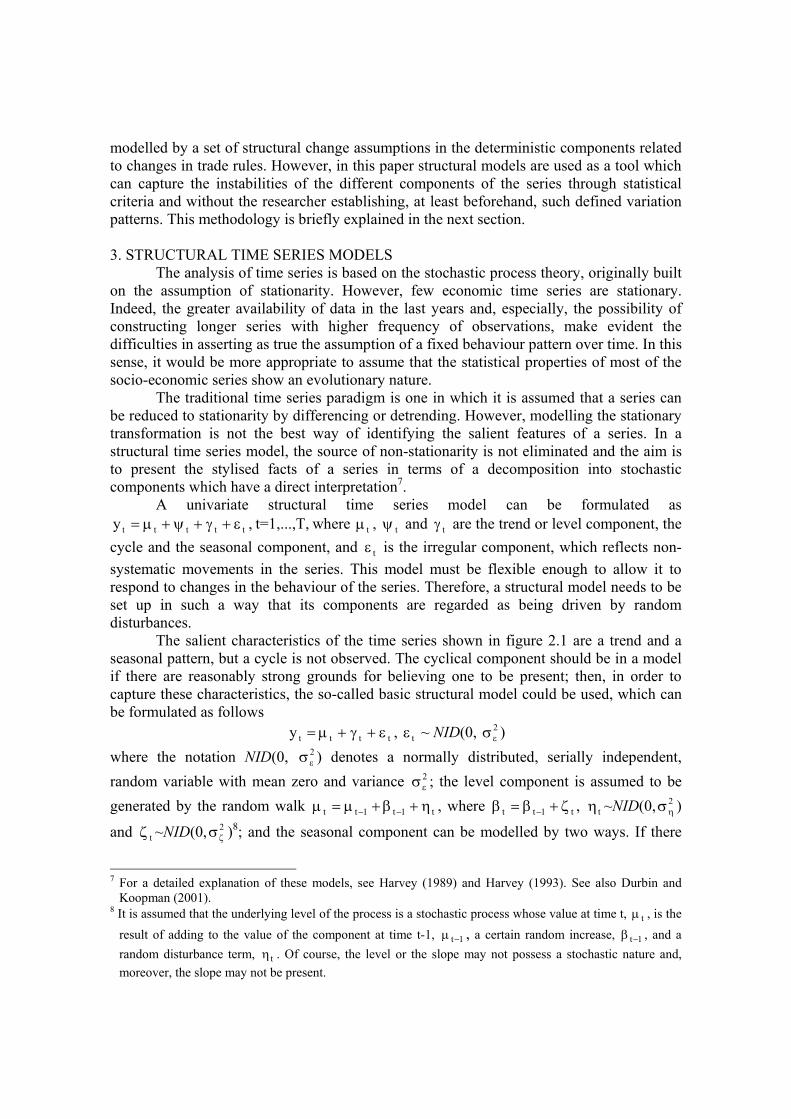
A univariate structural time series model can be formulated as ttttty ε+γ+ψ+µ= , t=1,...,T, where tµ , tψ and tγ are the trend or level component, the

cycle and the seasonal component, and tε is the irregular component, which reflects non-systematic movements in the series. This model must be flexible enough to allow it to respond to changes in the behaviour of the series. Therefore, a structural model needs to be set up in such a way that its components are regarded as being driven by random disturbances.

The salient characteristics of the time series shown in figure 2.1 are a trend and a seasonal pattern, but a cycle is not observed. The cyclical component should be in a model if there are reasonably strong grounds for believing one to be present; then, in order to capture these characteristics, the so-called basic structural model could be used, which can be formulated as follows

tttty ε+γ+µ= , tε ~ NID(0, 2εσ )

where the notation NID(0, 2εσ ) denotes a normally distributed, serially independent,

random variable with mean zero and variance 2εσ ; the level component is assumed to be

generated by the random walk t1t1tt η+β+µ=µ −− , where t1tt ζ+β=β − , tη ~NID(0, 2ησ )

and tζ ~NID(0, 2ζσ )8; and the seasonal component can be modelled by two ways. If there

7 For a detailed explanation of these models, see Harvey (1989) and Harvey (1993). See also Durbin and

Koopman (2001). 8 It is assumed that the underlying level of the process is a stochastic process whose value at time t, tµ , is the

result of adding to the value of the component at time t-1, 1t−µ , a certain random increase, 1t−β , and a random disturbance term, tη . Of course, the level or the slope may not possess a stochastic nature and, moreover, the slope may not be present.

are s seasons in the year, one way of achieving that the seasonal pattern evolves in time is to allow that the sum of the seasonal effects over any period of s consecutive seasons is not

strictly zero, but equal to a random disturbance term9; that is, t

1s

0jjt ω=γ∑

−

=

− , where ωt is

white noise with mean zero and variance 2ωσ . An alternative way of modelling such a

pattern is by a set of trigonometric terms at the seasonal frequencies, s/j2j π=λ ,

[ ]/2s1,...,j = ; then, the seasonal effect at time t is [ ]

∑=

γ=γ2/s

1jt,jt , where each tj,γ term is

constructed by a recursion formulae,

ωω

+

γγ

λλ−λλ

=

γγ

−

−*

tj,

tj,*

1tj,

1tj,

jj

jj*

tj,

tj,

cossensencos

, where

*tj,γ appears as a matter of construction, and tj,ω and *

tj,ω are zero mean white noise

processes which are uncorrelated with each other with a common variance 2ωσ . Note that

when s is even, the component at j=s/2 collapses to t/2,s1t/2,st/2,s ω+γ−=γ − . For the model to be identifiable, it must be assumed that the disturbances in all three components, level, seasonal and irregular, are mutually uncorrelated.

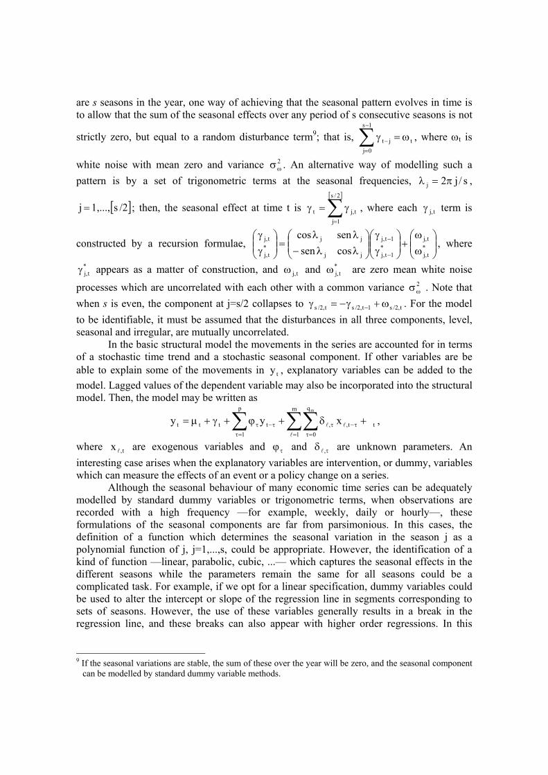
In the basic structural model the movements in the series are accounted for in terms of a stochastic time trend and a stochastic seasonal component. If other variables are be able to explain some of the movements in ty , explanatory variables can be added to the model. Lagged values of the dependent variable may also be incorporated into the structural model. Then, the model may be written as

t

m

1

q

0t,,

p

1tttt xyy

m

∑∑∑= =τ

τ−τ

=τ

τ−τ +δ+ϕ+γ+µ=l

ll ,

where t,x l are exogenous variables and τϕ and τδ ,l are unknown parameters. An interesting case arises when the explanatory variables are intervention, or dummy, variables which can measure the effects of an event or a policy change on a series. Although the seasonal behaviour of many economic time series can be adequately modelled by standard dummy variables or trigonometric terms, when observations are recorded with a high frequency —for example, weekly, daily or hourly—, these formulations of the seasonal components are far from parsimonious. In this cases, the definition of a function which determines the seasonal variation in the season j as a polynomial function of j, j=1,...,s, could be appropriate. However, the identification of a kind of function —linear, parabolic, cubic, ...— which captures the seasonal effects in the different seasons while the parameters remain the same for all seasons could be a complicated task. For example, if we opt for a linear specification, dummy variables could be used to alter the intercept or slope of the regression line in segments corresponding to sets of seasons. However, the use of these variables generally results in a break in the regression line, and these breaks can also appear with higher order regressions. In this

9 If the seasonal variations are stable, the sum of these over the year will be zero, and the seasonal component

can be modelled by standard dummy variable methods.

sense, spline functions are a tool to smooth the breaks and reconstruct the line segments in order to eliminate artificial and inappropriate jumps in the regression line10.

Splines are piecewise polynomial functions satisfying several conditions in order to allow transitions without breaks. The spline functions become increasingly smoother as the degree of the polynomial grows. In a formal sense, the g(t) spline is a function that approximates the ty values generated by the unknown function f(t) by means of several polynomials gi(t)=gi,0 + gi,1t + ... + gi,ptp, i= 1, ..., k; that is, g(t)=gi(t) in each of the intervals

1it − ≤ t≤ it , i= 1, ..., k. These polynomial functions are connected at joint points obeying continuity conditions. The set of pair values {( 0t , 0y ),...,( kt , ky )}, is referred to as the set of knots associated to the mesh { 0t , ..., kt }. The function g(t) is said to be a spline of degree p if g(t) is a polynomial of degree at most p in each of the intervals11 and its first p-1 derivatives vary continuously across the join points. The value of p can be interpreted as the smoothness degree, given that the greater the value of p, the smoother the spline function. In many applications, the choice of p=3 is advisable; this being the case, the spline function is defined as cubic12.

In addition to select the degree of polynomial in each interval, the specification of the spline requires the choice of the number and location of the points which delimit the intervals. Sometimes, the location of these join points is quite clear and it is incorporated into the model specification. In other cases, it is not possible to assume that the location of these points is known in advance and it must be estimated13. In any case, splines are an appropriate way of handling the periodical movements which change in a smooth manner and these functions can be added to a structural time series model as an additional unobservable component. If the seasonal pattern is fixed,

jt γ=γ , if the observation at time t corresponds to week j, j=1,...,s; then, this component could be modelled with a periodic cubic spline. That is, jj jg ε+=γ )( , where jε is a residual term associated to the adjustment and g(j) is a third degree piecewise polynomial function , gi(j)=gi,0 + gi,1j + gi,2j2 + gi,3j3, 1ij − ≤ j≤ ij , i=1,...,k, where 0j and kj are the first and last season, respectively. The continuity of the spline function, of its first derivative and of its second derivative are, respectively, enforced by the following conditions, ( ) ( )i1iii jgjg += , ( ) ( )i1iii jgjg +∇=∇ and ( ) ( )i1i

2ii

2 jgjg +∇=∇ , 1k,...,1i −= . The periodic nature of the spline is assured by means of the three following extra conditions:

( ) ( )01kk jg1jg =+ , ( ) ( )011kk jgjg ∇=∇ + and ( ) ( )012

1kk2 jgjg ∇=∇ + . This approach can be

10 Spline functions can also be used as a complementary tool to modelling seasonal effects by way of seasonal

dummy variables or trigonometric terms when there are simultaneous seasonal variations of different periods, as can be the case in series observed with a high frequency (see, for example, Harvey, Koopman and Riani, 1995).

11 Sometimes, it could be more appropriate to combine polynomials of different degrees in each of the intervals.

12 In comparison to the linear or quadratic case, the degree of a cubic spline is sufficiently high to give a smooth curve, and a higher degree can result in undesirable laxity. A mathematical analysis of splines functions is carried out by Nielsen (1998). See also Poirier (1973, 1976), Marsh (1983, 1986) and Marsh et al (1990). For a detailed account of cubic splines inside the frame of structural approach to time series, see Koopman (1992).

13 Marsh (1983, 1986) and Marsh et al (1990) have presented useful procedures for estimating the number and location of join points in spline regressions.

generalised to allow the seasonal pattern to evolve over time by letting spline be stochastic14.

Once the structural model has been formulated, the so-called Kalman filter15 allows the estimation of the different components of the series (state vector) at any point in the sample. Given the temporal dimension of state space variables, these estimates are usually compiled by plotting them directly against time and, in a more summarised form, by means of the estimation of the final state vector, which reflects the estimates of each component at the end of the sample. As has been mentioned, the components of the model are driven by their respective disturbance terms. Hence, the first step in this analysis is concerned with the estimation of the variance of these terms. This information can be expressed by means of the q ratios, defined as the ratios of each variance to the largest. Starting from these estimates, the conclusion could be reached that one of the variances of the disturbances is zero. If this is the case, it tells us that the corresponding component is fixed and, then, a standard regression type significance test can be carried out on the corresponding component in the final state16. If it is not significantly different from zero, it may be possible to simplify the model by eliminating that particular component. 4. STRUCTURAL MODELS FOR THE EXPORT SERIES In this section, the above described methodology is applied to the aforementioned export series. First, the basic structural model is estimated, and the conclusion is reached that the seasonal pattern has a deterministic nature, which is fairly captured using standard dummy models. Despite this, a spline function, which also captures the seasonal variations, is incorporated in order to show its usefulness as an alternative to the foregoing formulation. These two analyses are shown in detail in the following subsections.

4.1 Structural model with seasonal dummy variables

Notwithstanding the fact that the graph of the series under study does not allow us to deduce that the seasonal pattern is stochastic, it was decided to start model selection strategy with the basic structural model. The results of maximum likelihood estimation of this model indicates that both the slope and the seasonal pattern are constant17. The significance test of the slope in the final state vector suggests that the trend could be reduced to a random walk without drift. With regard to the seasonal component, despite the statistical non-significance of the parameters corresponding to some seasons, the joint test of the seasonal effects indicates the significance of this component18.

It was also clear from the graph of the estimated components for the previous model that the seasonal pattern and the slope remain the same throughout the period in question.

14 As will be seen in the next section, the export series shows a fixed seasonal pattern. Then, this section only

deals with non-stochastic spline functions. The incorporation of the stochastic nature is, nevertheless, necessary when there is random seasonal variations (see Koopman, 1992, and Harvey, Koopman and Riani, 1995).

15 See Kalman (1960) and Kalman and Bucy (1961) 16 If a component is fixed, the state information about this component is reduced to that provided by the final

state vector. 17 The smoothed option of the STAMP 6.0 program has been used (see Koopman et al, 2000). 18 The value of this statistic, which evaluates the joint statistical significance of the seasonal effects at the end

of the sample period, was 501.519. This statistic is asymptotically chi-square, χ2(51) in our case.

Bearing in mind these results, at first stage a model is proposed where the seasonal pattern is fixed, but level and slope remain their stochastic formulation; that is tttty ε+γ+µ= ,

with t1t1tt η+β+µ=µ −− , t1tt ς+β=β − and ∑=

γ=γ51

1jjt,jt z , t,jz , j=1, ..., 51, being equal to

1 if the observation corresponds to week j, -1 if the observation corresponds to week 52 and 0 in other cases19. Again, the estimation process leads to the conclusion that the variance of the disturbance term which drives the slope is zero, and the significance test of the slope in the final state vector indicates that it is not significantly different from zero.

In the face of these results, the following model was specified tttty ε+γ+µ= ,

with t1tt η+µ=µ − and ∑=

γ=γ51

1jjt,jt z . The estimates of hyperparameters confirm the

stochastic nature of the level component20. As regards the seasonal component, the significance tests in the final state vector show that there are statistically significant seasonal effects in the majority of weeks21.

It would therefore seem that the adequate model should include a stochastic level and a deterministic seasonal component. Nevertheless, in order to assess the adequacy of this model, it must be checked the behaviour of the innovations or prediction errors and the residuals of the two stochastic components. According to the appropriate test results, it can be assumed that the standardised innovations behave adequately as NID(0,1). However, it is clear from the plot of residuals against time that there are outliers such as the one detected in week 51 of 1990. Then, the model can not be regarded as being satisfactory and its specification must be changed as follows t

l,j,j,jttt Iy ε+λ+γ+µ= ∑ ll , with

t1tt η+µ=µ − and ∑=

γ=γ51

1jjt,jt z , l,jI being an intervention variable which takes value

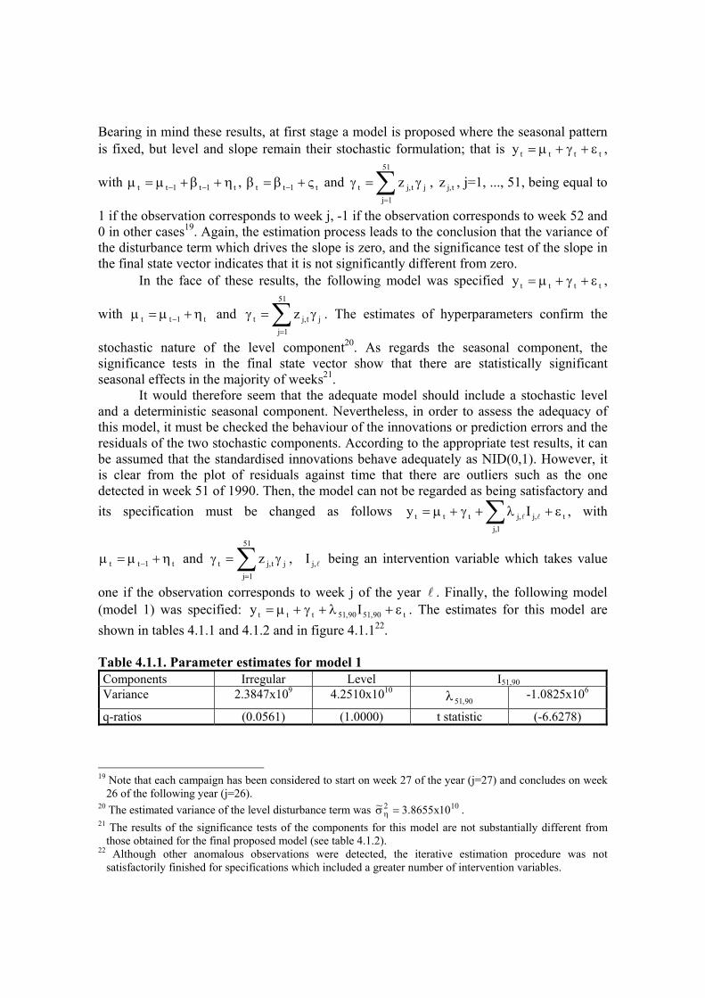
one if the observation corresponds to week j of the year l . Finally, the following model (model 1) was specified: t90,5190,51ttt Iy ε+λ+γ+µ= . The estimates for this model are shown in tables 4.1.1 and 4.1.2 and in figure 4.1.122.

Table 4.1.1. Parameter estimates for model 1 Components Irregular Level I51,90 Variance 2.3847x109 4.2510x1010

90,51λ -1.0825x106

q-ratios (0.0561) (1.0000) t statistic (-6.6278)

19 Note that each campaign has been considered to start on week 27 of the year (j=27) and concludes on week

26 of the following year (j=26). 20 The estimated variance of the level disturbance term was 102 10x8655.3~ =ση . 21 The results of the significance tests of the components for this model are not substantially different from

those obtained for the final proposed model (see table 4.1.2). 22 Although other anomalous observations were detected, the iterative estimation procedure was not

satisfactorily finished for specifications which included a greater number of intervention variables.

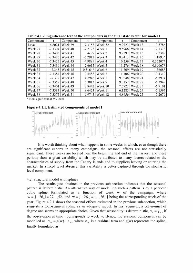
Table 4.1.2. Significance test of the components in the final state vector for model 1 Component t Component t Component t Component t Level 6.8021 Week 39 -7.3153 Week 52 9.9723 Week 13 3.5786Week 27 -7.3304 Week 40 -7.2175 Week 1 9.5966 Week 14 2.1378Week 28 -7.3403 Week 41 -6.99 Week 2 9.2297 Week 15 2.2389Week 29 -7.3416 Week 42 -6.2912 Week 3 8.7413 Week 16 1.1993*Week 30 -7.3427 Week 43 -4.9889 Week 4 10.259 Week 17 0.37207*Week 31 -7.3439 Week 44 -2.6615 Week 5 11.276 Week 18 -0.89067*Week 32 -7.345 Week 45 0.3164* Week 6 11.769 Week 19 -1.3668*Week 33 -7.3384 Week 46 2.5488 Week 7 11.106 Week 20 -3.4312Week 34 -7.332 Week 47 4.7945 Week 8 9.9648 Week 21 -5.3974Week 35 -7.3357 Week 48 6.3813 Week 9 9.3157 Week 22 -6.3949Week 36 -7.3401 Week 49 7.8442 Week 10 7.5722 Week 23 -6.9101Week 37 -7.3383 Week 50 8.6423 Week 11 6.1285 Week 24 -7.1597Week 38 -7.3375 Week 51 9.9745 Week 12 4.8656 Week 25 -7.2679

* Non significant at 5% level. Figure 4.1.1. Estimated components of model 1

1990 1995 2000

0

2.5e5

5e5

7.5e5

1e6

.25e6

1.5e6

.75e6

2e6

.25e6 Level component

1990 1995 2000

-7.5e5

-5e5

-2.5e5

0

2.5e5

5e5

7.5e5

1e6

1.25e6

1.5e6 Seasonal component

1990 1995 200060000

40000

20000

0

20000

40000

60000Irregular component

It is worth thinking about what happens in some weeks in which, even though there are significant exports in many campaigns, the seasonal effects are not statistically significant. These weeks are located near the beginning and end of the harvest, and these periods show a great variability which may be attributed to many factors related to the characteristics of supply from the Canary Islands and to suppliers leaving or entering the market. In a fixed level absence, this variability is better captured through the stochastic level component.

4.2. Structural model with splines

The results just obtained in the previous sub-section indicates that the seasonal pattern is deterministic. An alternative way of modelling such a pattern is by a periodic cubic spline formulated as a function of week w of the campaign, where

52,...,27j,26jw =−= , and 26,...,1j,26jw =+= , j being the corresponding week of the year. Figure 4.2.1 shows the seasonal effects estimated in the previous sub-section, which suggests a four-segment spline as an adequate model. In first segment, a polynomial of degree one seems an appropriate choice. Given that seasonality is deterministic, wt γ=γ , if the observation at time t corresponds to week w. Hence, the seasonal component can be modelled as ww )w(g ε+=γ , where wε is a residual term and g(w) represents the spline, finally formulated as:

≤≤+++≤≤+++≤≤+++≤≤+

=

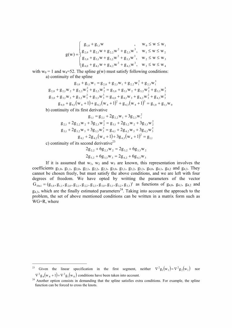
433

3,42

2,41,40,4

323

3,32

2,31,30,3

213

3,22

2,21,20,2

101,10,1

www,wgwgwggwww,wgwgwggwww,wgwgwggwww, wgg

)w(g

with w0 = 1 and w4=52. The spline g(w) must satisfy following conditions: a) continuity of the spline

( ) ( ) ( ) wgg1wg1wg1wgg wgwgwggwgwgwgg wgwgwggwgwgwgg

wgwgwgg wgg

01,10,13

43,42

42,441,40,4

333,4

232,431,40,4

333,3

232,331,30,3

323,3

222,321,30,3

323,2

222,221,20,2

313,2

212,211,20,211,10,1

+=+++++++++=++++++=+++

+++=+

b) continuity of its first derivative

( ) ( ) g1wg31wg2g wg3wg2gwg3wg2g wg3wg2gwg3wg2g

wg3wg2g g

1,12

43,442,41,4

233,432,41,4

233,332,31,3

223,322,31,3

223,222,21,2

213,212,21,21,1

=++++++=++++=++

++=

c) continuity of its second derivative23

33,42,433,32,3

23,32,323,22,2

wg6g2wg6g2wg6g2wg6g2

+=+

+=+

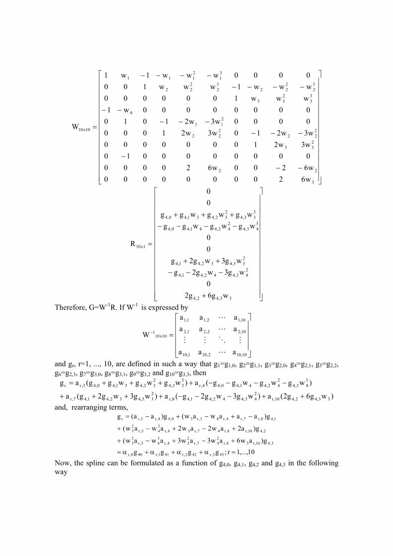
If it is assumed that w1, w2 and w3 are known, this representation involves the coefficients g1,0, g1,1, g2,0, g2,1, g2,2, g2,3, g3,0, g3,1, g3,2, g3,3, g4,0, g4,1, g4,2 and g4,3. They cannot be chosen freely, but must satisfy the above conditions, and we are left with four degrees of freedom. We have opted by writting the parameters of the vector

)'g ,g ,g ,g ,g ,g ,g ,g ,g ,(gG 3,33,23,13,02,32,22,12,01,11,010x1 = as functions of g4,0, g4,1, g4,2 and g4,3, which are the finally estimated parameters24. Taking into account the approach to the problem, the set of above mentioned conditions can be written in a matrix form such as WG=R, where

23 Given the linear specification in the first segment, neither ( ) ( )12

211

2 wgwg ∇=∇ nor

( ) ( )012

442 wg1wg ∇=+∇ conditions have been taken into account.

24 Another option consists in demanding that the spline satisfies extra conditions. For example, the spline function can be forced to cross the knots.

−−−

−−−−−−

−−

−−−−−−−−

=

3

22

233

222

222

211

0

33

233

32

222

32

222

31

2111

10x10

w6200000000w6200w6200000000000010w3w210000000w3w210w3w210000000w3w2101000000000w1

www1000000www1www1000000www1w1

W

+

−−−++

−−−−+++

=

33,42,4

243,442,41,4

233,432,41,4

343,4

242,441,40,4

333,4

232,431,40,4

1x10

wg6g20

wg3wg2gwg3wg2g

00

wgwgwggwgwgwgg

00

R

Therefore, G=W-1R. If W-1 is expressed by

=−

10,102,101,10

10,22,21,2

10,12,11,1

10x101

aaa

aaaaaa

W

L

MOMM

L

L

and gr, r=1, ..., 10, are defined in such a way that g1=g1,0, g2=g1,1, g3=g2,0, g4=g2,1, g5=g2,2, g6=g2,3, g7=g3,0, g8=g3,1, g9=g3,2 and g10=g3,3, then

)wg6g2(a)wg3wg2g(a)wg3wg2g(a

)wgwgwgg(a)wgwgwgg(ag

33,42,410,r243,442,41,48,r

233,432,41,47,r

343,4

242,441,40,44,r

333,4

232,431,40,43,rr

++−−−++++

−−−−++++=

and, rearranging terms,

10,...,1r;ggggg)aw6aw3aw3awaw(

g)a2aw2aw2awaw(

g)aaawaw(g)aa(g

433,r422,r411,r400,r

3,410,r38,r247,r

234,r

343,r

33

2,410,r8,r47,r34,r243,r

23

1,48,r7,r4,r43,r30,44,r3,rr

=α+α+α+α=

+−+−+

+−+−+

−+−+−=

Now, the spline can be formulated as a function of g4,0, g4,1, g4,2 and g4,3 in the following way

≤≤+++

≤≤α+α+α+α

+α+α+α+α

+α+α+α+α

+α+α+α+α≤≤α+α+α+α

+α+α+α+α

+α+α+α+α

+α+α+α+α≤≤α+α+α+α

+α+α+α+α

=

433

3,42

2,41,40,4

323

3,43,102,42,101,41,100,40,10

23,43,92,42,91,41,90,40,9

3,43,82,42,81,41,80,40,8

3,43,72,42,71,41,70,40,7

213

3,43,62,42,61,41,60,40,6

23,43,52,42,51,41,50,40,5

3,43,42,42,41,41,40,40,4

3,43,32,42,31,41,30,40,3

103,43,22,42,21,41,20,40,2

3,43,12,42,11,41,10,40,1

www si, wgwgwgg

www si ,w)gggg(

w)gggg(

w)gggg()gggg(

www si, w)gggg(

w)gggg(

w)gggg()gggg(

www si , w)gggg()gggg(

)w(g

that is, [ ]

[ ] w,43

3,42

2,41,40,4

w,3

33,43,102,42,101,41,100,40,10

23,43,92,42,91,41,90,40,93,43,82,42,81,41,80,40,8

3,43,72,42,71,41,70,40,7

w,2

33,43,62,42,61,41,60,40,6

23,43,52,42,51,41,50,40,53,43,42,42,41,41,40,40,4

3,43,32,42,31,41,30,40,3

w,13,43,22,42,21,41,20,40,23,43,12,42,11,41,10,40,1

Dwgwgwgg

D

w)gggg(

w)gggg(w)gggg(

)gggg(

D

w)gggg(

w)gggg(w)gggg(

)gggg(

Dw)gggg()gggg()w(g

++++

α+α+α+α+

α+α+α+α+α+α+α+α+

α+α+α+α

+

α+α+α+α+

α+α+α+α+α+α+α+α+

α+α+α+α

+

α+α+α+α+α+α+α+α=

where <≤

= −

caseother in ,0www,1

D i1iw,i , i=1,2,3, and

≤≤

=caseother in ,0

www,1D 43

w,4 , and rearranging

terms

w,33,4w,22,4w,11,4w,00,4

w,43

w,33

3,102

3,93,83,7

w,23

3,62

3,53,43,3w,13,23,13,4

w,42

w,33

2,102

2,92,82,7

w,23

2,62

2,52,42,3w,12,22,12,4

w,4w,33

1,102

1,91,81,7

w,23

1,62

1,51,41,3w,11,21,11,4

w,4w,33

0,102

0,90,80,7

w,23

0,62

0,50,40,3w,10,20,10,4

XgXgXgXg

DwD)www(

D)www(D)w(g

DwD)www(

D)www(D)w(g

wDD)www(

D)www(D)w(g

DD)www(

D)www(D)w(g)w(g

+++=

+α+α+α+α

α+α+α+α+α+α+

+α+α+α+α

α+α+α+α+α+α+

+α+α+α+α

α+α+α+α+α+α+

+α+α+α+α

α+α+α+α+α+α=

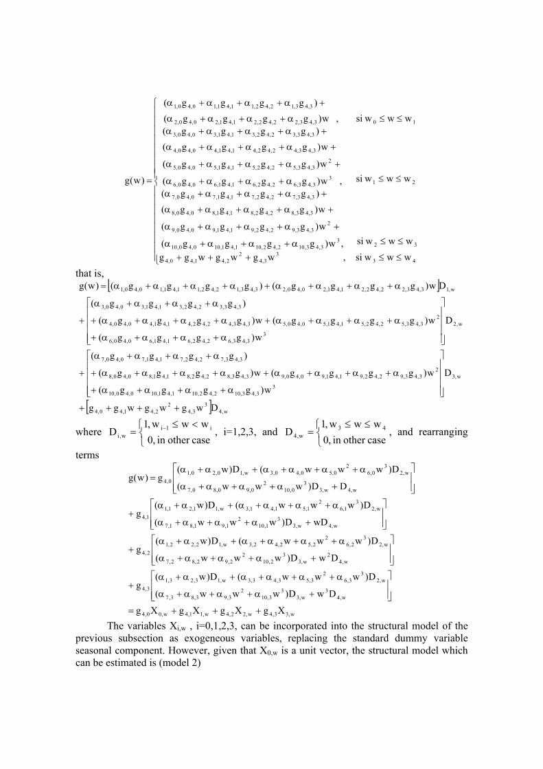
The variables Xi,w , i=0,1,2,3, can be incorporated into the structural model of the previous subsection as exogeneous variables, replacing the standard dummy variable seasonal component. However, given that X0,w is a unit vector, the structural model which can be estimated is (model 2)

t90,5190,51t,343t,242t,141tt IXgXgXgy ε+λ++++µ= where X1,t, X2,t and X3,t are column vectors of dimension 728x125 defined in such a way that Xi,t = Xi,w , i=1, 2, 3, if the observation at time t corresponds to week w of the campaign.

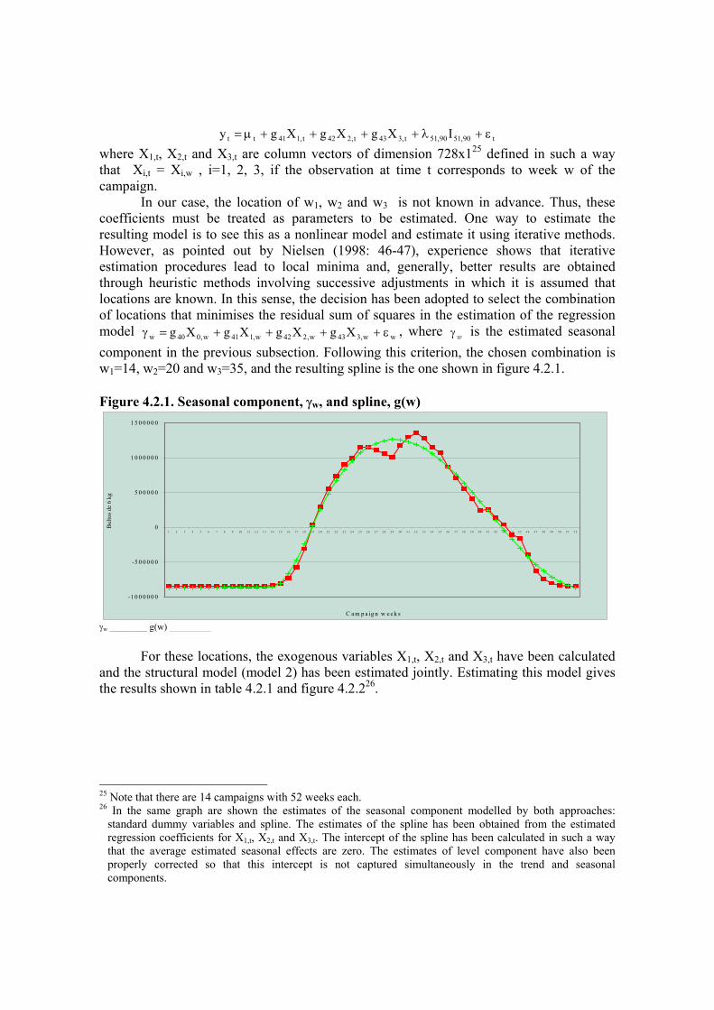
In our case, the location of w1, w2 and w3 is not known in advance. Thus, these coefficients must be treated as parameters to be estimated. One way to estimate the resulting model is to see this as a nonlinear model and estimate it using iterative methods. However, as pointed out by Nielsen (1998: 46-47), experience shows that iterative estimation procedures lead to local minima and, generally, better results are obtained through heuristic methods involving successive adjustments in which it is assumed that locations are known. In this sense, the decision has been adopted to select the combination of locations that minimises the residual sum of squares in the estimation of the regression model ww,343w,242w,141w,040w XgXgXgXg ε++++=γ , where wγ is the estimated seasonal component in the previous subsection. Following this criterion, the chosen combination is w1=14, w2=20 and w3=35, and the resulting spline is the one shown in figure 4.2.1.

Figure 4.2.1. Seasonal component, γw, and spline, g(w)

-1 0 0 0 0 0 0

-5 0 0 0 0 0

0

5 0 0 0 0 0

1 0 0 0 0 0 0

1 5 0 0 0 0 0

1 2 3 4 5 6 7 8 9 1 0 1 1 1 2 1 3 1 4 1 5 1 6 1 7 1 8 1 9 2 0 2 1 2 2 2 3 2 4 2 5 2 6 2 7 2 8 2 9 3 0 3 1 3 2 3 3 3 4 3 5 3 6 3 7 3 8 3 9 4 0 4 1 4 2 4 3 4 4 4 5 4 6 4 7 4 8 4 9 5 0 5 1 5 2

C a m p a ig n w e e k s

Bul

tos d

e 6

kg

γw ________ g(w) _________

For these locations, the exogenous variables X1,t, X2,t and X3,t have been calculated

and the structural model (model 2) has been estimated jointly. Estimating this model gives the results shown in table 4.2.1 and figure 4.2.226.

25 Note that there are 14 campaigns with 52 weeks each. 26 In the same graph are shown the estimates of the seasonal component modelled by both approaches:

standard dummy variables and spline. The estimates of the spline has been obtained from the estimated regression coefficients for X1,t, X2,t and X3,t. The intercept of the spline has been calculated in such a way that the average estimated seasonal effects are zero. The estimates of level component have also been properly corrected so that this intercept is not captured simultaneously in the trend and seasonal components.

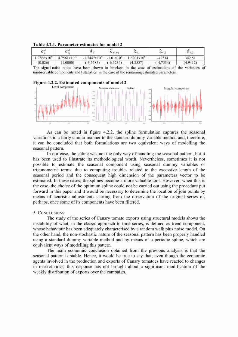
Table 4.2.1. Parameter estimates for model 2 2ˆ εσ 2ˆ ησ Tµ 90,51λ 1,4g 2,4g 3,4g

1.2566x108 4.7561x1010 -1.7447x107 -1.01x106 1.6201x106 -42514 342.51 (0.026) (1.0000) (-3.5585) (-6.5234) (4.3557) (-4.7534) (4.9412)

The signal-noise ratios have been shown in brackets in the case of estimations of the variances of unobservable components and t statistics in the case of the remaining estimated parameters. Figure 4.2.2. Estimated components of model 2

Level component

1990 1995 2000

0

5e5

1e6

1.5e6

2e6

Seasonal dummies Spline

1990 1995 2000

7.5e5

-5e5

2.5e5

0

2.5e5

5e5

7.5e5

1e6

.25e6

Irregular component

1990 1995 2000

-3000

-2000

-1000

0

1000

2000

3000

4000

As can be noted in figure 4.2.2, the spline formulation captures the seasonal

variations in a fairly similar manner to the standard dummy variable method and, therefore, it can be concluded that both formulations are two equivalent ways of modelling the seasonal pattern.

In our case, the spline was not the only way of handling the seasonal pattern, but it has been used to illustrate its methodological worth. Nevertheless, sometimes it is not possible to estimate the seasonal component using seasonal dummy variables or trigonometric terms, due to computing troubles related to the excessive length of the seasonal period and the consequent high dimension of the parameters vector to be estimated. In these cases, the splines become a more valuable tool. However, when this is the case, the choice of the optimum spline could not be carried out using the procedure put forward in this paper and it would be necessary to determine the location of join points by means of heuristic adjustments starting from the observation of the original series or, perhaps, once some of its components have been filtered. 5. CONCLUSIONS The study of the series of Canary tomato exports using structural models shows the instability of what, in the classic approach to time series, is defined as trend component, whose behaviour has been adequately characterised by a random walk plus noise model. On the other hand, the non-stochastic nature of the seasonal pattern has been properly handled using a standard dummy variable method and by means of a periodic spline, which are equivalent ways of modelling this pattern. The main economic conclusion obtained from the previous analysis is that the seasonal pattern is stable. Hence, it would be true to say that, even though the economic agents involved in the production and exports of Canary tomatoes have reacted to changes in market rules, this response has not brought about a significant modification of the weekly distribution of exports over the campaign.

6. BIBLIOGRAPHY Cáceres, J.J. (2000). La Exportación de Tomate en Canarias. Elementos para una estrategia competitiva. Ediciones Canarias. Durbin, J. and S.J. Koopman (2001). Time Series Analysis by State Space Methods. Oxford University Press. Harvey, A.C. (1989). Forecasting, structural time series models and the Kalman filter. Cambridge University Press. Harvey, A.C. (1993). Time series models. Harvester Wheatsheaf. Harvey, A.C., S.J. Koopman and M. Riani (1995) The modelling and seasonal adjustment of weekly observations, London School of Economics, Discussion paper nº EM/95/284. Kalman, R.E. (1960). «A new approach to linear filtering and prediction problems». Transactions ASME, Series D, Journal of Basic Engineering 82: 35-45. Kalman, R.E. and R.S. Bucy (1961). «New results in linear filtering and prediction theory». Transactions ASME, Series D, Journal of Basic Engineering 83: 95-108. Koopman, S.J. (1992) Diagnostic checking and intra-daily effects in time series models, Thesis Publishers, Tinbergen Institute Research Series, 27. Amsterdam. Koopman, S.J., A.C. Harvey, J.A. Doornik and N. Shephard (2000). STAMP: Structural time series analyser, modeller and predictor. Timberlake Consultants. Marsh, L. (1983) «On estimating spline regression», SUGI 8: 723-728. Marsh, L. (1986) «Estimating the number and location of knots in spline regression», Journal of Applied Business Research 3: 60-70. Marsh, L., M. Maudgal and J. Raman (1990) «Alternative methods of estimating piecewise linear and higher order regression models», SUGI 15: 523-527. Nielsen, H.B. (1998) Cubic Splines, IMM Department of Mathematical Modelling. Technical University of Denmark. Poirier, D.J. (1973) «Piecewise regression using cubic splines», Journal of the American Statistical Association 68: 515-524. Poirier, D.J. (1976) The econometric of structural change with special emphasis on spline functions, Amsterdam, North Holland.