business cycles in a small open economy

American Economic Association

Real Business Cycles in a Small Open EconomyAuthor(s): Enrique G. MendozaSource: The American Economic Review, Vol. 81, No. 4 (Sep., 1991), pp. 797-818Published by: American Economic AssociationStable URL: http://www.jstor.org/stable/2006643Accessed: 13/09/2009 21:42

Your use of the JSTOR archive indicates your acceptance of JSTOR's Terms and Conditions of Use, available athttp://www.jstor.org/page/info/about/policies/terms.jsp. JSTOR's Terms and Conditions of Use provides, in part, that unlessyou have obtained prior permission, you may not download an entire issue of a journal or multiple copies of articles, and youmay use content in the JSTOR archive only for your personal, non-commercial use.

Please contact the publisher regarding any further use of this work. Publisher contact information may be obtained athttp://www.jstor.org/action/showPublisher?publisherCode=aea.

Each copy of any part of a JSTOR transmission must contain the same copyright notice that appears on the screen or printedpage of such transmission.

JSTOR is a not-for-profit organization founded in 1995 to build trusted digital archives for scholarship. We work with thescholarly community to preserve their work and the materials they rely upon, and to build a common research platform thatpromotes the discovery and use of these resources. For more information about JSTOR, please contact [email protected].

American Economic Association is collaborating with JSTOR to digitize, preserve and extend access to TheAmerican Economic Review.

http://www.jstor.org

http://www.jstor.org/stable/2006643?origin=JSTOR-pdf

http://www.jstor.org/page/info/about/policies/terms.jsp

http://www.jstor.org/action/showPublisher?publisherCode=aea

Real Business Cycles in a Small Open Economy

By ENRIQUE G. MENDOZA*

This paper analyzes a real-business-cycle model of a small open economy. The model is parameterized, calibrated, and simulated to explore its ability to rationalize the observed pattern of postwar Canadian business fluctuations. The results show that the model mimics many of the stylized facts using moderate adjustment costs and minimal variability and persistence in the technological disturbances. In particular, the model is consistent with the observed positive correlation between savings and investment, even though financial capital is perfectly mobile, and with countercyclical fluctuations in external trade. (JEL E32, N12)

The "real business cycle" approach to economic fluctuations, which originated in the pioneering work of Finn Kydland and Edward Prescott (1982) and John Long and Charles Plosser (1983), has been the focus of attention of a significant portion of the research on dynamic macroeconomics during the last decade. Comprehensive reviews of this research by Bennett McCallum (1989) and Plosser (1989) have illustrated that, despite a number of important unresolved is- sues, the approach successfully explains some of the key empirical regularities that characterize economic fluctuations. In the basic real-business-cycle model, productivity disturbances motivate rational individuals to adjust savings and investment in order to smooth consumption, and to adjust employment in response to changes in the relative price of leisure and the productivity of labor. This behavior is consistent with some of the observed stylized facts because: (a) it generates procyclical fluctuations in con-

sumption, investment, and employment, (b) it causes investment to exhibit more variability than output or consumption, and (c) it produces positive persistence in all major macro-aggregates.

Most countries in the world economy exhibit well-defined empirical regularities not only in domestic indicators of economic activity, but also in key international indicators. The historical evidence on these international aspects of the business cycle is well documented by David Backus and Patrick Kehoe (1989). This evidence suggests that there are two significant stylized facts typical of modern open economies. First, national or domestic savings (S) and domestic investment (I) are positively correlated. Second, the current account and the balance of trade tend to move countercyclically.

The savings-investment correlation has been the subject of intense debate because of its alleged implications on the degree of international capital mobility. In a widely discussed paper, Martin Feldstein and Charles Horioka (1980) documented a strong cross-sectional correlation between S and I for a sample of OECD countries and interpreted this result as evidence against perfect capital mobility. Numerous subse- quent papers documented further evidence of the positive correlation between the two variables. As illustrated by Maurice Obst- feld (1986), Michael Dooley et al. (1987), and Linda Tesar (1991), the significantly

* Research Department, International Monetary Fund, Washington, DC 20431. This paper is based on my Ph.D. dissertation at the University of Western Ontario. I am indebted to Jeremy Greenwood, Gregory Huffman, Bruce Smith, and Zvi Hercowitz for supervis- ing my work and for many helpful discussions. Com- ments and suggestions by Dave Backus, Harold Cole, Mary Finn, Peter Howitt, Patrick Kehoe, David Lai- dler, Michael Parkin, Assaf Razin, Sergio Rebelo, Lars Svensson, and two anonymous referees are gratefully acknowledged. This paper reflects the author's views and not those of the International Monetary Fund.

797

798 THE AMERICAN ECONOMIC REVIEW SEPTEMBER 1991

positive savings-investment correlation has proved to be robust to virtually all alter- ations of the Feldstein-Horioka test and has been detected in time-series and cross-sectional samples of data for many countries.

Recent theoretical work has cast doubt on the inference of imperfect capital mobility drawn from the observed S-I correlations. Obstfeld (1986) has shown that a deterministic dynamic-equilibrium model with perfect capital mobility produces positive correlation between S and I as a result of persistent productivity changes or population growth. Subsequently, Mary Finn (1990) has illustrated that a two-country stochastic overlapping-generations model can recreate any kind of savings-investment correlation depending on the stochastic process of the underlying technological disturbances. Thus, theoretically, once stochastic elements are incorporated into an intertemporal-equilibrium framework, the correlation between S and I provides no clear indication of the degree of capital mobility.

The second observation, that the current account and the trade balance tend to move countercyclically, is also well established. Backus and Kehoe (1989) identify this pattern as common to the historical data of ten industrialized countries. Traditional models of the current account relied on a strong income effect on imports to explain this behavior. The intertemporal-equilibrium approach, in contrast, determines endoge- nously the relative strength of income and substitution effects and cannot predict un- ambiguously that the external accounts and output will be negatively correlated.' Sup- pose, for instance, that a positive productivity shock occurs. For the current account or the trade balance to be countercyclical, the pro-borrowing effect caused by an expected expansion of future output and the desire to increase investment must dominate the pro-saving effect induced by an increase in current output. Moreover, some empirical studies have shown that simple dynamic op-

timizing models cannot easily reproduce the weakly countercyclical fluctuations of external trade (see Shaghil Ahmed, 1986; Zvi Hercowitz, 1986b).

These two striking empirical regularities that emerge from the international data constitute important evidence against which real-business-cycle theory can be tested. In particular, the question that needs to be answered is: can a real-business-cycle model account for the positive savings-investment correlation and the countercyclical behavior of the balance of trade? Or, more generally, can a real-business-cycle model mimic the stylized facts typical of an actual open economy?

The objective of this paper is to address these questions by developing an extension of the real-business-cycle framework to the case of a small open economy. A dynamic stochastic model is used to explore the in- teraction of domestic physical capital and foreign financial assets as alternative vehicles for savings in an environment in which stochastic disturbances affect domestic productivity and the world's real interest rate. The novelty of this approach is that it ex- plores real business cycles in a framework in which trade in foreign assets finances trade imbalances and plays a crucial role in explaining the dynamics of savings and investment. The model is parameterized, simulated, and calibrated, using dynamic programming techniques, to determine its ability to mimic the stylized facts of an actual small open economy.

Contrary to the argument presented in Feldstein and Horioka (1980), the numerical analysis undertaken here finds that the correlation between savings and investment in a small open economy can be quite high even when there is perfect capital mobility. The results show not only that the persistence of productivity shocks is the key de- terminant of the savings-investment correlation, as Obstfeld (1986) and Finn (1990) have argued, but also that the shocks that rationalize postwar business cycles can explain the observed positive correlation between the two variables. In other notable research efforts, aimed at developing two- country open-economy real-business-cycle

'Jacob Frenkel and Assaf Razin (1987) illustrated this problem clearly.

VOL. 81 NO. 4 MENDOZA: REAL BUSINESS CYCLES 799

models, Backus et al. (1990) and Marianne Baxter and Mario Crucini (1990) also found that savings-investment correlations depend on the persistence of productivity disturbances.

Recent research also shows that investment reacts very differently to productivity shocks in open-economy real-business-cycle models than in closed-economy models. Ac- cess to foreign markets permits individuals to separate savings and investment by allow- ing them to finance a gap between the two with external resources. This separation produces disturbing results. For instance, Backus et al. (1990) find that unless time-to-build restrictions or international spillovers of technological disturbances are considered, a two-country model exaggerates the variability of investment. Similarly, the present paper shows that a model of a small open economy in which capital can be freely accumulated exaggerates the variability of investment and underestimates its correlation with savings. These two anomalies can be avoided by introducing moderate capital-adjustment costs, thus adopting the view that financial capital is more mobile than physical capital-a view previously explored by Dooley et al. (1987).

The model studied here also differs from the standard real-business-cycle prototype in its use of an endogenous rate of time preference to determine a well-defined stationary equilibrium for the holdings of foreign assets. This approach was introduced by Obstfeld (1981), following the principles formulated by Hirofumi Uzawa (1968), to analyze current-account dynamics in a deterministic model of a small open economy. In Obstfeld's model, the accumulation of external assets attains a stationary state when the rate of time preference reaches the level of the world's real interest rate, which is an exogenous variable for a small open economy. As Elhanan Helpman and Assaf Razin (1982) pointed out, as long as the rate of time preference is smaller (greater) than the rate of interest, individuals rationally choose to accumulate (de- plete) foreign assets in order to finance an increasing (decreasing) consumption stream. The constant-discount representation of

preferences cannot produce such well- defined dynamics. In this framework, either (a) there is no stationary equilibrium, if the interest rate and the rate of time preference are not preset to be equal, or (b) if the two are equal, the economy is always at a steady-state equilibrium that is consistent with any initial level of foreign asset holdings.

In contrast with Obstfeld's work, the endogenous rate of time preference is utilized in this paper to determine a stable stochastic steady state. This is done by introducing the stationary cardinal utility function (SCU) formulated by Larry Epstein (1983). Under a set of conditions to be described later, this utility function allows the use of dynamic programming techniques, guarantees the normality of consumption in all periods, and ensures the existence of a unique invariant limiting distribution of the state variables-all without causing a major deviation from the standard time-separable setup. A contribution of this paper is that it under- takes numerical simulations and solves for equilibrium stochastic processes using stationary cardinal utility.

The paper proceeds as follows. The next section describes the structure of the artificial economy and discusses the simulation method. Section II presents the results of simulation exercises for a benchmark model in which random shocks affect only domestic productivity and investment is not costly to adjust. Section III introduces random shocks that affect both domestic productivity and the world's real interest rate. Sec- tion IV considers costs of adjustment in the process of investment. Section V compares the performance of the artificial small open economy with some of the existing closed- economy real-business-cycle models, and some concluding remarks are presented in Section VI.

I. The Model and the Solution Technique

A. Structure of the Model

Production Technology and Financial Structure.-The economy produces an in- ternationally tradable composite commodity


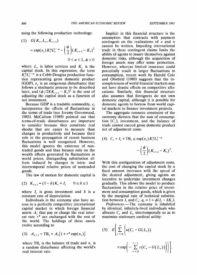
using the following production technology:

(1) G(K,,L,,K,+1)

= exp(e,)KaLla - (a 2)(K,+1 - K,)2

O<a<1,40>O

where L, is labor services and K, is the capital stock. In this expression, the term

aLl -a is a Cobb-Douglas production function representing gross domestic product (GDP), e, is an exogenous disturbance that follows a stochastic process to be described later, and (4/2XK,+1 - K,)2 is the cost of adjusting the capital stock as a function of net investment.

Because GDP is a tradable commodity, e, incorporates the effects of fluctuations in the terms of trade (see Jeremy Greenwood, 1983). McCallum (1989) pointed out that terms-of-trade disturbances are important to consider because they constitute real shocks that are easier to measure than changes in productivity and because their role in the propagation of recent business fluctuations is well recognized. However, this model ignores the existence of nontraded goods and thus focuses only on the wealth effects generated by fluctuations in world prices, disregarding substitution effects induced by changes in intra- and intertemporal relative prices of nontraded goods.

The law of motion for domestic capital is

(2) Kt+1=(1-3)Kt+It 0<a<1

where It is gross investment and 8 is a constant rate of depreciation.

Individuals in the economy also have access to a perfectly competitive international capital market in which foreign financial assets At that pay or charge the real interest rate r * are exchanged with the rest of the world. The holdings of these assets evolve according to

(3) At+i=TBt+At[1+r*exp(nt)]

where TBt is the balance of trade and nt is a random disturbance affecting the world's real interest rate.

Implicit in this financial structure is the assumption that contracts with payment contingent on the realizations of e and n cannot be written. Impeding international trade in these contingent claims limits the ability of agents to insure themselves against domestic risks, although the acquisition of foreign assets may offer some protection. However, whereas limited insurance could potentially result in larger fluctuations in consumption, recent work by Harold Cole and Obstfeld (1989) suggests that the in- completeness of world financial markets may not have drastic effects on competitive allo- cations. Similarly, this financial structure also assumes that foreigners do not own domestic capital, although it is possible for domestic agents to borrow from world capital markets to finance investment projects.

The aggregate resource constraint of the economy dictates that the sum of consumption (C,), investment, and the balance of trade cannot exceed gross domestic product net of adjustment costs:

(4) Ct + I, +TB, t exp(e,)KtLVt

- ( )(K,+1 - Kt) 2

With this configuration of adjustment costs, the cost of changing the capital stock by a fixed amount increases with the speed of the desired adjustment, giving agents an incentive to undertake investment changes gradually. This allows the model to produce fluctuations in the relative price of investment and consumption goods, which is given by the marginal rate of technical substitution between It and Ct: qt = 1 + O(It - MK).

Preferences. -The economy is inhabited by identical, infinitely-lived individuals who allocate C, and L, intertemporally so as to maximize stationary cardinal utility:

(5) E E {u(Ct-G(Lt)) t = 0

lt-1\


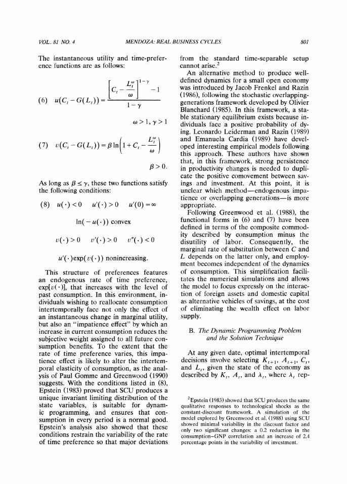
The instantaneous utility and time-preference functions are as follows:

Lt1-e

(6) u(Ct-G(Lt))= . 1- y

t > 1, y >

(7) v(Ct - G(Lt)) In pn1 + Ct -t

/3>0.

As long as /3 < y, these two functions satisfy the following conditions:

(8) u(.) < O u'(.) > O u'(O) =oo

ln( - u(.)) convex

v(() > O v'(.) > O v"(.) <O

u'(. )exp( v(.)) nonincreasing.

This structure of preferences features an endogenous rate of time preference, exp[v( )], that increases with the level of past consumption. In this environment, individuals wishing to reallocate consumption intertemporally face not only the effect of an instantaneous change in marginal utility, but also an "impatience effect" by which an increase in current consumption reduces the subjective weight assigned to all future consumption benefits. To the extent that the rate of time preference varies, this impatience effect is likely to alter the intertemporal elasticity of consumption, as the analysis of Paul Gomme and Greenwood (1990) suggests. With the conditions listed in (8), Epstein (1983) proved that SCU produces a unique invariant limiting distribution of the state variables, is suitable for dynamic programming, and ensures that consumption in every period is a normal good. Epstein's analysis also showed that these conditions restrain the variability of the rate of time preference so that major deviations

from the standard time-separable setup cannot arise.2

An alternative method to produce well- defined dynamics for a small open economy was introduced by Jacob Frenkel and Razin (1986), following the stochastic overlapping- generations framework developed by Olivier Blanchard (1985). In this framework, a stable stationary equilibrium exists because individuals face a positive probability of dy- ing. Leonardo Leiderman and Razin (1989) and Emanuela Cardia (1989) have developed interesting empirical models following this approach. These authors have shown that, in this framework, strong persistence in productivity changes is needed to duplicate the positive comovement between savings and investment. At this point, it is unclear which method-endogenous impatience or overlapping generations-is more appropriate.

Following Greenwood et al. (1988), the functional forms in (6) and (7) have been defined in terms of the composite commodity described by consumption minus the disutility of labor. Consequently, the marginal rate of substitution between C and L depends on the latter only, and employment becomes independent of the dynamics of consumption. This simplification facili- tates the numerical simulations and allows the model to focus expressly on the interac- tion of foreign assets and domestic capital as alternative vehicles of savings, at the cost of eliminating the wealth effect on labor supply.

B. The Dynamic Programming Problem and the Solution Technique

At any given date, optimal intertemporal decisions involve selecting K t+1, At+17 Ct, and Lt, given the state of the economy as described by Kt, At, and At, where At rep-

2Epstein (1983) showed that SCU produces the same qualitative responses to technological shocks as the constant-discount framework. A simulation of the model explored by Greenwood et al. (1988) using SCU showed minimal variability in the discount factor and only two significant changes: a 0.2 reduction in the consumption-GNP correlation and an increase of 2.4 percentage points in the variability of investment.


resents the realization of the state of nature with respect to the pair of disturbances (et, nt). These optimal choices must comply with the usual nonnegativity restrictions on C, K, and L and must also be consistent with intertemporal solvency. Long-run solvency is enforced by imposing an upper bound on foreign debt, At > / for all t, where A\ is a negative constant.3 This condition precludes individuals from running Ponzi-type schemes. By choosing /\ to be large enough in absolute value, the odds of approaching /\ in the stochastic steady state can be made infinitesimally small. This as- sertion will be verified numerically in the next section.

The time-recursive nature of the stationary cardinal utility, together with the simplified stochastic structure described later, im- plies that the optimal decision rules that characterize the equilibrium stochastic process of the economy can be obtained by solving the following functional-equation problem:4

(9) V( Kt, At, As)t

c LCt-- -1

=max{ ( )

+exp [-,1n(1+ Ct -1)]

x~~~~~~~~~~~~ 4l

X E vs,rV( Kt+1,,At+,,vAt+) 1 r=1l

with respect to Ct, Kt + 1, and A t + 1 and subject to

Ct exp(et)KKt L - 2 )(Kt+1-Kt

- Kt+ 1 + Kt(i 1-a)

+ [I+ r* exp(nt)] At -A,+

Lt= argmax(L)exP( et)KtLt - KJ L

At > A Kt>O, Lt >0 Ct >0.

The stochastic structure of the problem is simplified by assuming that the disturbances are Markov chains. Interest-rate and productivity shocks have two possible realizations each, so that in every period the small open economy experiences one of four possible states of nature At:

(10) A e A = ((e1,n1),(e1,n2),

(e2, n') , (e2, n2).

The probability of the current state As =

(nt, et) moving to state Ar+1 = (nx 1, et+ 1) next period is denoted as wsrr for x, i = 1,2 and s, r = 1, 4. These transition probabilities are given by the "simple persistence" rule:5

(11) Ts,r (1 0)r + OPs,r

In this formula, 0 is a parameter governing the persistence of e and n, Hr is the long- run probability of state Ar, and Ps, r = 1 if s = r and 0 otherwise. The transition probabilities must satisfy the usual properties that O < vsr < 1 and rsl + ws2 + wrs3 + 74 = 1 for s, r = 1,4.

This stochastic structure is simplified further by adopting the following symmetry conditions: FI(el, nl) = FI(e2, n2) = I, fl(e', n2) =F(e2, n1)=0.5-1-1, el =- 2 =

e, and nl = - n2= n. These conditions facil- itate the numerical analysis by restricting

3Gary Chamberlain and Chuck Wilson (1984) and Marilda Sotomayor (1984) have studied the complica- tions that may arise when weaker conditions are used to enforce intertemporal solvency.

4Following the analysis of Epstein (1983), I showed that the value function is concave in this case (Mendoza, 1988). A formal analysis of the properties and equilibrium conditions of the model is also presented in that paper.

5This rule is adopted from the work of Backus et al. (1989). In this case, the Kronecker delta has been defined as p to avoid confusion with the depreciation rate.


the set of free parameters to be specified and by relating these explicitly to the statistical moments that characterize the shocks. In particular, the asymptotic standard deviations of domestic and interest-rate shocks are given by o-e = e and o-n = n, respectively; their common first-order serial autocorrelation is Pe = Pn = p = 4f - 1; and their contemporaneous correlation coefficient is Pe,n = 6. Thus, the stochastic processes of the two disturbances are fully characterized by setting the values of the parameters e, n, HI, and 0.

Since this is a case in which the value function cannot be solved for analytically, a numerical procedure is used to study the equilibrium stochastic process of the artificial economy. The method employed here was formulated by Dimitri Bertsekas (1976) and introduced to dynamic macroeconomic models by Thomas Sargent (1980). Green- wood et al. (1988) used the same procedure to simulate a closed-economy real-business- cycle model with investment shocks and endogenous capacity utilization. The technique calculates the unique invariant joint limiting distribution of the state variables using an algorithm that solves the functional-equation problem (9) for a discrete version of the state space.

The first step in the solution procedure is to define two evenly spaced grids containing the values of domestic capital, K =

{K1 ... ., KN}, and foreign assets, A = {A1,.. .,AM). Thus, the state space of the artificial economy is defined by the set K xA x A of dimensions N X M X 4. These two grids are chosen to capture the ergodic set for the joint stationary distribution of K, A, and A and are refined until the covari- ances among the state variables converge. The grids are centered initially around the deterministic stationary equilibria of domestic capital and foreign assets, which are determined by a simultaneous equality between the rate of time preference, the net marginal productivity of capital, and the world's real interest rate.

The next step is to use an algorithm that solves the dynamic programming problem (9) by the method of successive approxima- tions. The algorithm, which is described in

detail by Greenwood et al. (1988), provides solutions for the relevant decision rules inside the set defined by KXAX A. The decision rules determine Kt+1 and At+1 given each possible combination of Kt, At, and A_. These decision rules, combined with the conditional probabilities -rsr, for s,r=1,4, define the one-step transition probabilities of moving from any initial triple of domestic capital, foreign assets, and the shocks to any other such triple in one period. The transition probabilities are condensed in a matrix P, of dimensions (4MN x 4MN), which is used to calculate limiting probabilities of each triple in the state space. The long-run probabilities are calculated by iterating the sequence x = x?P, where xo is an initial- guess vector of dimensions (1 x 4MN) and x1 is a vector of identical dimensions used as the new guess in the following iteration. These iterations eventually converge to a unique fixed point x*, which is the unique invariant joint limiting distribution of K, A, and A. This distribution produces what amounts to population moments of variability, comovement, and persistence of all variables in the model.6

C. Parameter Values and Calibration

To solve the model, values must be chosen for the parameters oe' Cl7 P, Pe,n7 a, r*v y, 3, w, /3, and b that characterize the stochastic disturbances, preferences, and technology. The model is parameterized so as to make it roughly consistent with some of the empirical regularities that reflect the structure of the Canadian economy. Canada is viewed as a typical small open economy because of the historical absence of capital controls and the high degree of integration of its financial markets with those of the United States. The data considered correspond to annual observations for the period 1946-1985, expressed in per capita terms of the population older than 14 years, trans- formed into logarithms and detrended with

6The numerical simulations were produced in an ETA-IOP supercomputer equipped with a vector-For- tran compiler.


a quadratic time trend. The statistical moments for the relevant macroeconomic time- series are reported in part I of Tables 1 and 6.

The values of the parameters o(e and p are set to mimic the variability and first- order serial autocorrelation of GDP, and o-,n and Pe,n are set to various different values in order to explore the model's sensitivity to domestic and international disturbances. An alternative approach, frequently employed in the real-business-cycle literature, is to determine values for these parameters using Solow residuals. However, as illustrated in the following sections, Solow residuals obtained from Canadian data exhibit too much variability and serial autocorrelation for the model to be consistent with the observed stylized facts. Moreover, as McCallum (1989) has explained, once adjustment costs and fluctuations in the terms of trade are taken into account, Solow residuals are not an accurate proxy for productivity shocks.7

The values of the parameters a (capital's share in output), r* (the world's real interest rate), y (the coefficient of relative risk aversion), 8 (the depreciation rate), w (1 plus the inverse of the intertemporal elasticity of substitution in labor supply), and /B (the consumption elasticity of the rate of time preference) are selected using actual data and the restrictions imposed by the structure of the model, and also by considering some estimates from the relevant empirical literature. These parameters are set as follows:

(12) a = 0.32 r* = 0.04 y = 1.001 or 2

=0.1 w =1.455 ,B=0.11.

The value of a is equal to 1 minus the average of the ratio of labor income to net national income at factor prices. The world's

interest rate, r*, is set to the value suggested by Kydland and Prescott (1982) and Prescott (1986) for the real interest rate in the U.S. economy. The parameter y takes two different values in an attempt to avoid the controversy surrounding point estimates, considering the indication of Prescott (1986) that y is not likely to be much larger than 1. The depreciation rate has the value commonly used in the real-business-cycle literature, and with it the model generates the same investment:output ratio observed in the data (22 percent).8 The value of w is in the range of the estimates that James Heckman and Thomas MaCurdy (1980) and MaCurdy (1981) obtained for the intertemporal elasticity of substitution in labor supply, and this value enables the model to mimic closely the percentage variability of hours.9 Given the other parameter values, ,B is determined by the steady-state condition that equates the rate of time preference with the world's real interest rate. This is done by imposing the restriction that the average ratio of net foreign interest payments to GDP is about 2 percent, as observed in Canadian postwar data.

The value of the adjustment-cost parameter, 0, depends on whether the correspond- ing simulation considers adjustment costs. Because adjustment costs are introduced to moderate the variability of capital accumulation, whenever 4 A 0 the parameter is set to mimic the percentage standard deviation of investment. This results in the range 0.023 < 0 < 0.028 for various simulation exercises. This range is consistent with the estimate of 0 obtained by Roger Craine (1975) for the U.S. economy. Using a ratio of price indexes to measure the relative price of capital goods, Craine estimated 0 at approximately 0.025. Moreover, this range of 0 values produces an average cost of

7Robert Hall (1988) has also questioned the use of Solow residuals as a proxy for productivity shocks because some empirical evidence does not support the assumptions of competition and constant returns. In particular, cyclical variations in hours are small compared with variations in output, and during periods of expansion, output sells for a price above marginal cost.

8Hercowitz (1986a) estimated 6 for Canada at 0.052 using the capital-evolution equation and the data on net capital stocks and gross investment. With this depreciation rate the model produces 43 percent standard deviation in investment and an average investment:output ratio of only 18 percent.

9Hercowitz (1986a) estimated values of w = 4.3 and 4.9 for the Canadian economy but found these estimates to be imprecise. In this model, w = 4.3 generates a standard deviation of hours of just 0.76 percent.


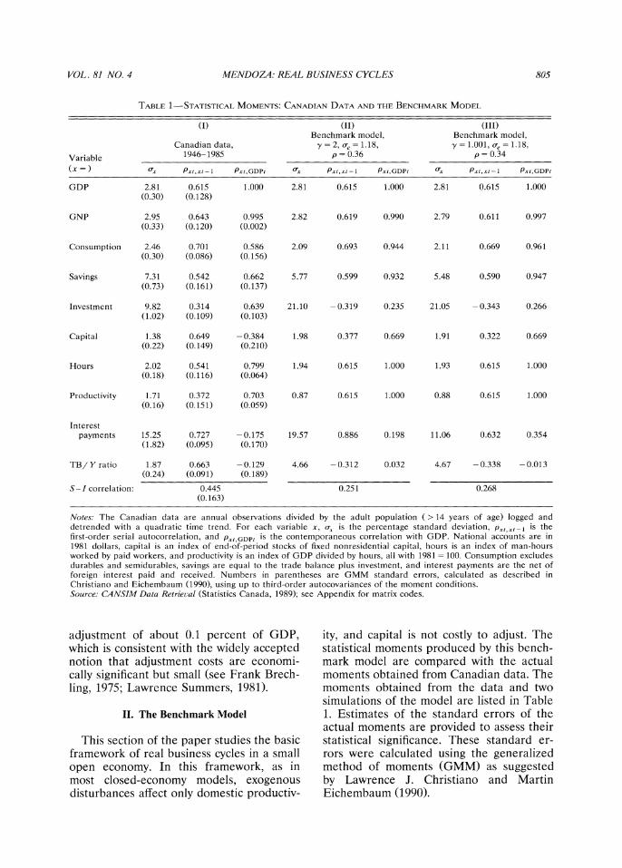
TABLE 1-STATISTICAL MOMENTS: CANADIAN DATA AND THE BENCHMARK MODEL

Benchmark model, Benchmark model, Canadian data, y = 2, a,e = 1.18, y 1.001, a,e = 1.18,

Variable 1946-1985 p = 0.36 p = 0.34 (x =) ox P Pxt,GDPt aIx Pxt,xt-I Pxt,GDPt aIx Pxt,xt-1 Pxt,GDPt

GDP 2.81 0.615 1.000 2.81 0.615 1.000 2.81 0.615 1.000 (0.30) (0.128)

GNP 2.95 0.643 0.995 2.82 0.619 0.990 2.79 0.611 0.997 (0.33) (0.120) (0.002)

Consumption 2.46 0.701 0.586 2.09 0.693 0.944 2.11 0.669 0.961 (0.30) (0.086) (0.156)

Savings 7.31 0.542 0.662 5.77 0.599 0.932 5.48 0.590 0.947 (0.73) (0.161) (0.137)

Investment 9.82 0.314 0.639 21.10 -0.319 0.235 21.05 -0.343 0.266 (1.02) (0.109) (0.103)

Capital 1.38 0.649 -0.384 1.98 0.377 0.669 1.91 0.322 0.669 (0.22) (0.149) (0.210)

Hours 2.02 0.541 0.799 1.94 0.615 1.000 1.93 0.615 1.000 (0.18) (0.116) (0.064)

Productivity 1.71 0.372 0.703 0.87 0.615 1.000 0.88 0.615 1.000 (0.16) (0.151) (0.059)

Interest payments 15.25 0.727 -0.175 19.57 0.886 0.198 11.06 0.632 0.354

(1.82) (0.095) (0.170)

TB/Y ratio 1.87 0.663 -0.129 4.66 -0.312 0.032 4.67 -0.338 -0.013 (0.24) (0.091) (0.189)

S-I correlation: 0.445 0.251 0.268 (0.163)

Notes: The Canadian data are annual observations divided by the adult population (> 14 years of age) logged and detrended with a quadratic time trend. For each variable x, a, is the percentage standard deviation, pxt xt-I is the first-order serial autocorrelation, and Pxt,GDPt is the contemporaneous correlation with GDP. National accounts are in 1981 dollars, capital is an index of end-of-period stocks of fixed nonresidential capital, hours is an index of man-hours worked by paid workers, and productivity is an index of GDP divided by hours, all with 1981 = 100. Consumption excludes durables and semidurables, savings are equal to the trade balance plus investment, and interest payments are the net of foreign interest paid and received. Numbers in parentheses are GMM standard errors, calculated as described in Christiano and Eichembaum (1990), using up to third-order autocovariances of the moment conditions. Source: CANSIM Data Retrieval (Statistics Canada, 1989); see Appendix for matrix codes.

adjustment of about 0.1 percent of GDP, which is consistent with the widely accepted notion that adjustment costs are economi- cally significant but small (see Frank Brech- ling, 1975; Lawrence Summers, 1981).

II. The Benchmark Model

This section of the paper studies the basic framework of real business cycles in a small open economy. In this framework, as in most closed-economy models, exogenous disturbances affect only domestic productiv-

ity, and capital is not costly to adjust. The statistical moments produced by this benchmark model are compared with the actual moments obtained from Canadian data. The moments obtained from the data and two simulations of the model are listed in Table 1. Estimates of the standard errors of the actual moments are provided to assess their statistical significance. These standard errors were calculated using the generalized method of moments (GMM) as suggested by Lawrence J. Christiano and Martin Eichembaum (1990).


PKA

0050

0033

0017

K 3 35 -092 A

3 25

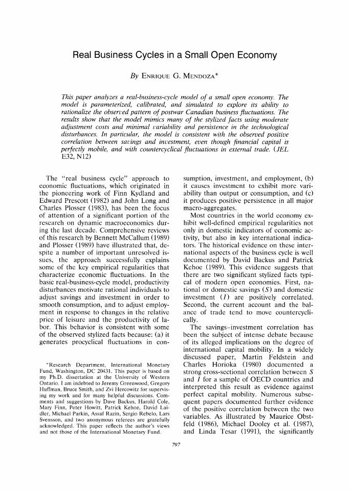
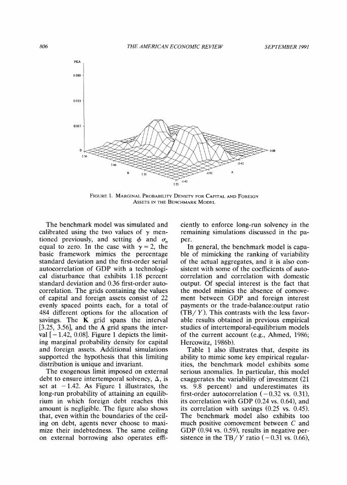
FIGURE 1. MARGINAL PROBABILITY DENSITY FOR CAPITAL AND FOREIGN

ASSETS IN THE BENCHMARK MODEL

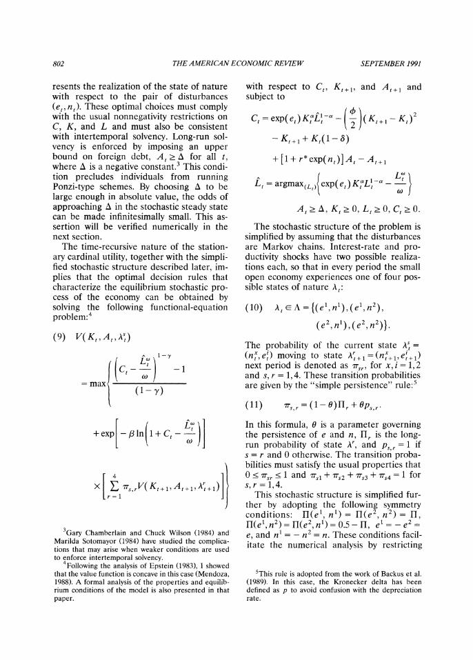
The benchmark model was simulated and calibrated using the two values of y mentioned previously, and setting 4 and o- equal to zero. In the case with y = 2, the basic framework mimics the percentage standard deviation and the first-order serial autocorrelation of GDP with a technological disturbance that exhibits 1.18 percent standard deviation and 0.36 first-order autocorrelation. The grids containing the values of capital and foreign assets consist of 22 evenly spaced points each, for a total of 484 different options for the allocation of savings. The K grid spans the interval [3.25, 3.56], and the A grid spans the interval [ - 1.42, 0.08]. Figure 1 depicts the limiting marginal probability density for capital and foreign assets. Additional simulations supported the hypothesis that this limiting distribution is unique and invariant.

The exogenous limit imposed on external debt to ensure intertemporal solvency, A, is set at - 1.42. As Figure 1 illustrates, the long-run probability of attaining an equilibrium in which foreign debt reaches this amount is negligible. The figure also shows that, even within the boundaries of the ceiling on debt, agents never choose to maximize their indebtedness. The same ceiling on external borrowing also operates effi-

ciently to enforce long-run solvency in the remaining simulations discussed in the paper.

In general, the benchmark model is capable of mimicking the ranking of variability of the actual aggregates, and it is also consistent with some of the coefficients of autocorrelation and correlation with domestic output. Of special interest is the fact that the model mimics the absence of comovement between GDP and foreign interest payments or the trade-balance:output ratio (TB/ Y). This contrasts with the less favor- able results obtained in previous empirical studies of intertemporal-equilibrium models of the current account (e.g., Ahmed, 1986; Hercowitz, 1986b).

Table 1 also illustrates that, despite its ability to mimic some key empirical regularities, the benchmark model exhibits some serious anomalies. In particular, this model exaggerates the variability of investment (21 vs. 9.8 percent) and underestimates its first-order autocorrelation (-0.32 vs. 0.31), its correlation with GDP (0.24 vs. 0.64), and its correlation with savings (0.25 vs. 0.45). The benchmark model also exhibits too much positive comovement between C and GDP (0.94 vs. 0.59), results in negative persistence in the TB/ Y ratio ( - 0.31 vs. 0.66),

VOL.81 NO. 4 MENDOZ2I: REAL BUSINESS CYCLES 807

and generates for L a stochastic process that shows perfect correlation with GDP. This last result is an unavoidable feature of the model that is implied by the structure of preferences and technology described in Section I.

The low correlation between S and I in the benchmark model is not related to the degree of international capital mobility. In- stead, it follows from the low degree of serial autocorrelation of the shocks used to calibrate the model. With p = 0.36, the productivity shocks are not persistent enough to cause sufficient divergence between the expected marginal productivity of capital and the world's real interest rate to produce a stronger correlation between S and I. If, for instance, p is increased to 0.99, the degree of correlation between savings and investment reaches 0.8. Thus, although the benchmark model cannot mimic simultane- ously the stylized facts of GDP and the correlation between savings and investment, it does support the argument presented by Obstfeld (1986) and Finn (1990), claiming that the intensity of the comovement between S and I in economies with perfect capital mobility depends on the degree of persistence of the underlying technological disturbances.

The benchmark model with y = 1.001 is calibrated by setting oSe and p to almost the same values as before, 1.18 percent and 0.34. This is an implication of the separation of savings and investment to be discussed next. The results show that a reduction in y affects mainly the behavior of foreign assets, because less risk-averse individuals attain optimal consumption without resorting as often to the insurance that these risk-free assets provide. Under these conditions, the degree of correlation between C and GDP appears to be independent of the degree of risk aversion. The model mimics poorly the behavior of investment and some of the other aggregates, as it did with y = 2.

The poor performance of the benchmark model is related to the separation of savings and investment that characterizes a small open economy, coupled with the absence of explicit adjustment costs. Investment is set to equalize the expected marginal returns,

in utility terms, of domestic capital and foreign assets. Savings, in contrast, are determined by equating the expected intertemporal marginal rate of substitution with the risk-free real rate of return on assets. When a productivity shock hits the economy, the capital stock is rapidly and freely adjusted to maintain the equality of expected returns. Incentives to smooth or substitute consumption intertemporally are irrelevant for investment decisions because the optimal adjustments in savings are achieved via changes in the current account. This behavior explains why the limiting distribution depicted in Figure 1 is bimodal. The two peaks reflect the ease with which individuals can adjust the capital stock to the productivity levels pertaining to high and low values of the productivity shock.

In closed-economy real-business-cycle models, investment is not as volatile, because savings and investment decisions are identical. Investment responds to the individuals' desire to smooth and substitute consumption across time, and it faces an increasing supply price. In contrast, in a small open economy consumption-smooth- ing operates via the current account, consumption-substitution does not occur (because the interest rate is determined exoge- nously), and the supply price of capital is fixed at r*.

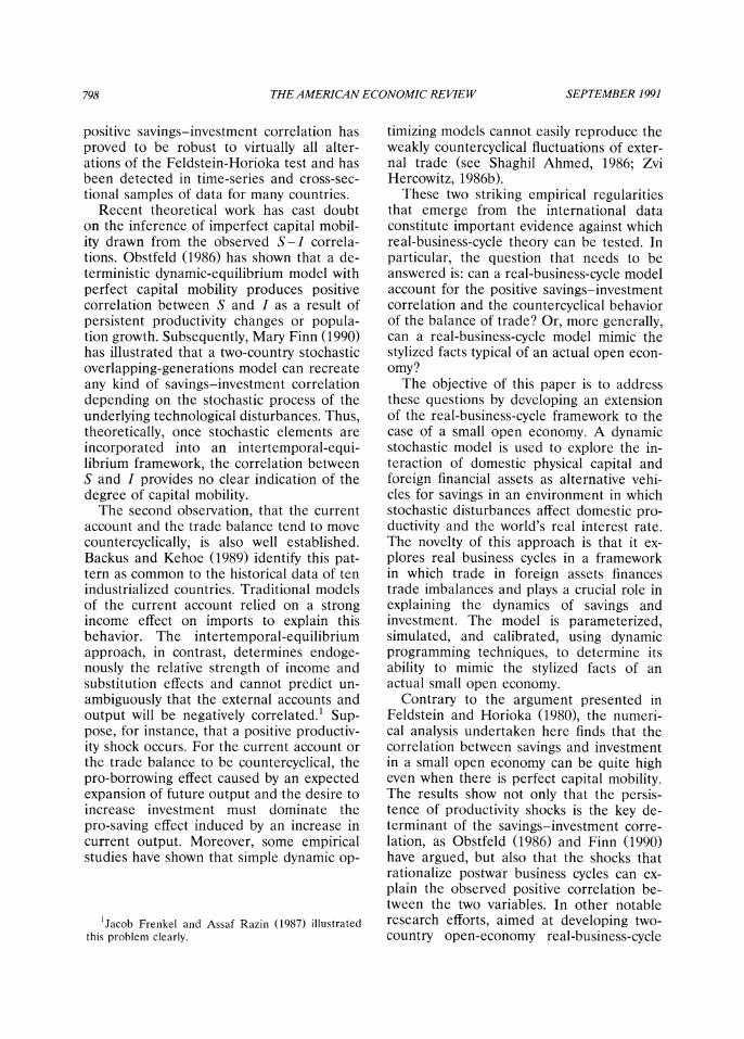
The analysis of the perfect-foresight version of the benchmark model, in which the evolution of the productivity disturbances is known with certainty, provides a clear illus- tration of the forces governing the behavior of investment. Without uncertainty, individuals invest optimally by equating the marginal returns paid on capital and foreign assets exactly each period:

(13) exp(et+?)FK(Kt+?,Lt+l)-8S=r*.

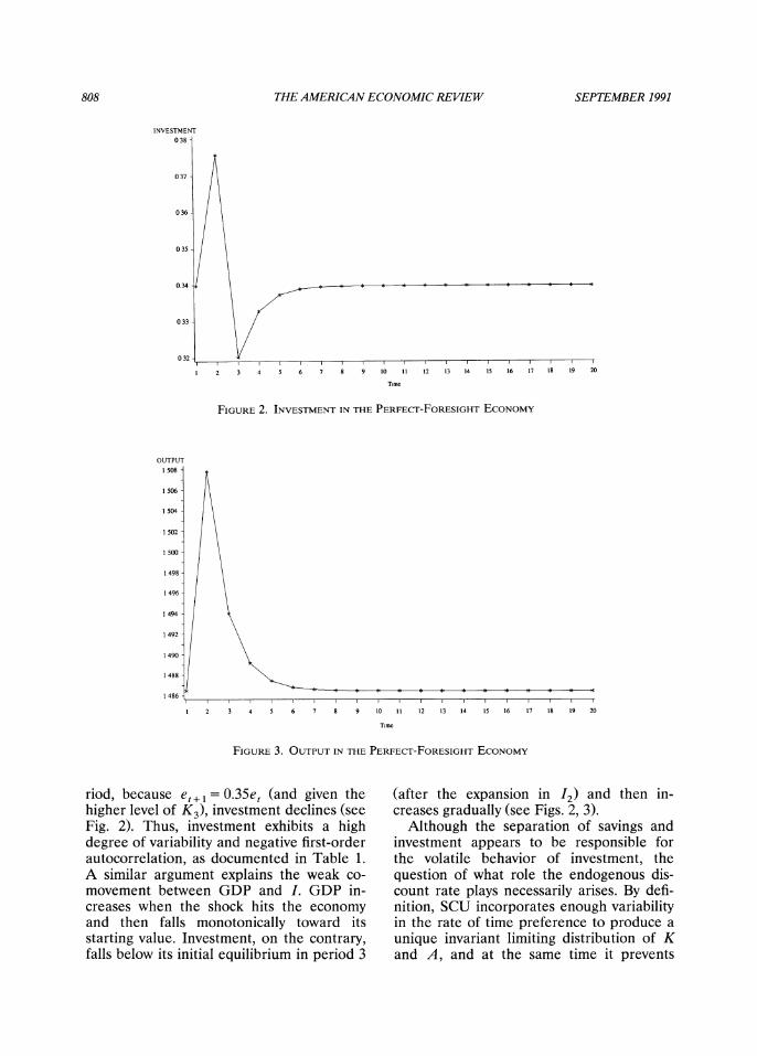
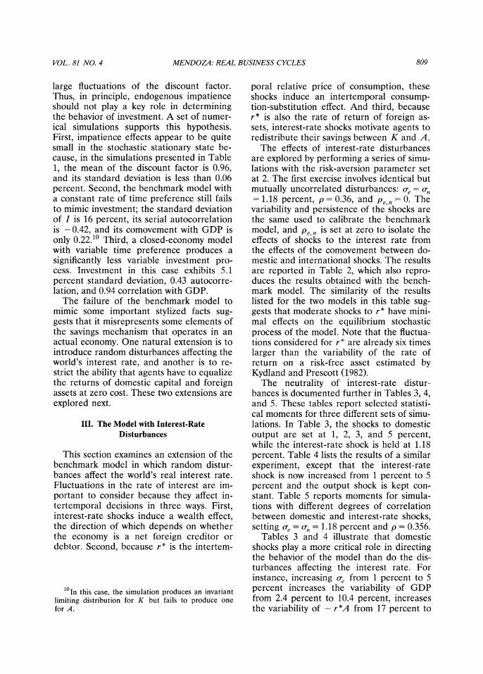
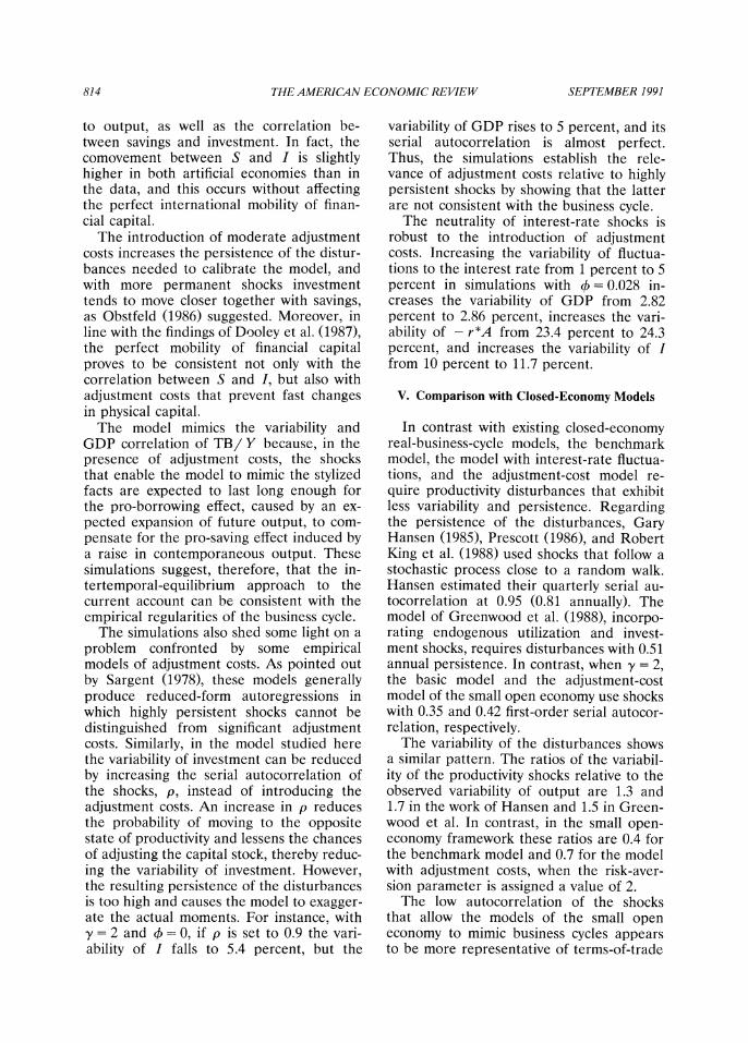
Figures 2 and 3 display the time profiles of investment and GDP resulting from this condition, assuming a 1.18-percent productivity shock that hits the economy at date 2, with a persistence parameter equal to 0.35. In period 2, investment is enlarged as K3 is adjusted upward to ensure that the equality in (13) is maintained. In the following pe-


INVESTMENT 038

037

036

035

0.34

0 33

0 32

1 2 3 4 5 6 7 8 9 10 11 12 13 14 15 16 17 18 19 20

Time

FIGURE 2. INVESTMENT IN THE PERFECT-FORESIGHT ECONOMY

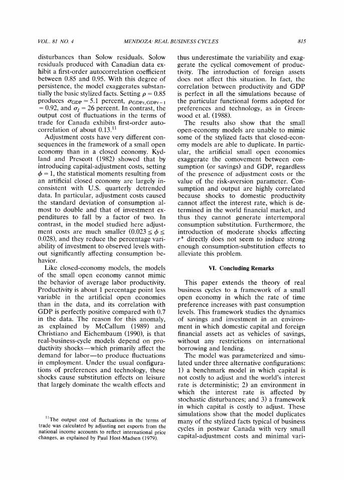
OUTPUT 1 508

1 506

1 504

1 502

1 500

1 498 -

1 496

1 494

1 492

1490

1 488

1 486

1 2 3 4 5 6 7 8 9 10 11 12 13 14 15 16 17 18 19 20

TLime

FIGURE 3. OUTPUT IN THE PERFECT-FORESIGHT ECONOMY

riod, because et+1 = 0.35et (and given the higher level of K3), investment declines (see Fig. 2). Thus, investment exhibits a high degree of variability and negative first-order autocorrelation, as documented in Table 1. A similar argument explains the weak comovement between GDP and I. GDP increases when the shock hits the economy and then falls monotonically toward its starting value. Investment, on the contrary, falls below its initial equilibrium in period 3

(after the expansion in I2) and then increases gradually (see Figs. 2, 3).

Although the separation of savings and investment appears to be responsible for the volatile behavior of investment, the question of what role the endogenous discount rate plays necessarily arises. By defi- nition, SCU incorporates enough variability in the rate of time preference to produce a unique invariant limiting distribution of K and A, and at the same time it prevents


large fluctuations of the discount factor. Thus, in principle, endogenous impatience should not play a key role in determining the behavior of investment. A set of numerical simulations supports this hypothesis. First, impatience effects appear to be quite small in the stochastic stationary state because, in the simulations presented in Table 1, the mean of the discount factor is 0.96, and its standard deviation is less than 0.06 percent. Second, the benchmark model with a constant rate of time preference still fails to mimic investment; the standard deviation of I is 16 percent, its serial autocorrelation is - 0.42, and its comovement with GDP is only 0.22.10 Third, a closed-economy model with variable time preference produces a significantly less variable investment process. Investment in this case exhibits 5.1 percent standard deviation, 0.43 autocorrelation, and 0.94 correlation with GDP.

The failure of the benchmark model to mimic some important stylized facts suggests that it misrepresents some elements of the savings mechanism that operates in an actual economy. One natural extension is to introduce random disturbances affecting the world's interest rate, and another is to re- strict the ability that agents have to equalize the returns of domestic capital and foreign assets at zero cost. These two extensions are explored next.

III. The Model with Interest-Rate Disturbances

This section examines an extension of the benchmark model in which random disturbances affect the world's real interest rate. Fluctuations in the rate of interest are important to consider because they affect intertemporal decisions in three ways. First, interest-rate shocks induce a wealth effect, the direction of which depends on whether the economy is a net foreign creditor or debtor. Second, because r* is the intertem-

poral relative price of consumption, these shocks induce an intertemporal consumption-substitution effect. And third, because r* is also the rate of return of foreign assets, interest-rate shocks motivate agents to redistribute their savings between K and A.

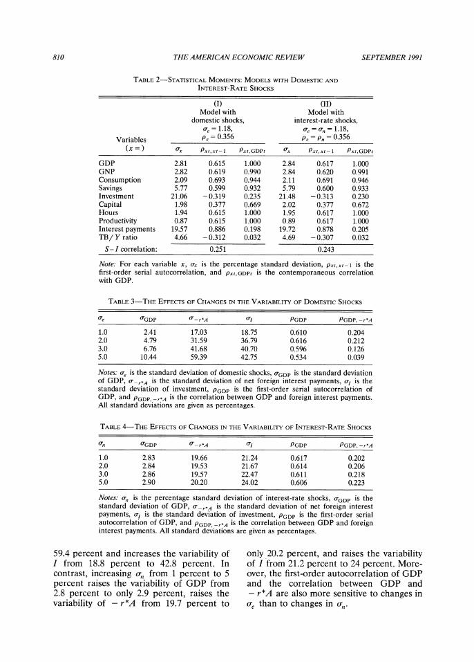
The effects of interest-rate disturbances are explored by performing a series of simulations with the risk-aversion parameter set at 2. The first exercise involves identical but mutually uncorrelated disturbances: o-e = on = 1.18 percent, p = 0.36, and Pe,n = 0. The variability and persistence of the shocks are the same used to calibrate the benchmark model, and Pe,n is set at zero to isolate the effects of shocks to the interest rate from the effects of the comovement between domestic and international shocks. The results are reported in Table 2, which also reproduces the results obtained with the benchmark model. The similarity of the results listed for the two models in this table suggests that moderate shocks to r* have minimal effects on the equilibrium stochastic process of the model. Note that the fluctuations considered for r* are already six times larger than the variability of the rate of return on a risk-free asset estimated by Kydland and Prescott (1982).

The neutrality of interest-rate disturbances is documented further in Tables 3, 4, and 5. These tables report selected statistical moments for three different sets of simulations. In Table 3, the shocks to domestic output are set at 1, 2, 3, and 5 percent, while the interest-rate shock is held at 1.18 percent. Table 4 lists the results of a similar experiment, except that the interest-rate shock is now increased from 1 percent to 5 percent and the output shock is kept constant. Table 5 reports moments for simulations with different degrees of correlation between domestic and interest-rate shocks, setting oe = o-, = 1.18 percent and p = 0.356.

Tables 3 and 4 illustrate that domestic shocks play a more critical role in directing the behavior of the model than do the disturbances affecting the interest rate. For instance, increasing o-e from 1 percent to 5 percent increases the variability of GDP from 2.4 percent to 10.4 percent, increases the variability of - r *A from 17 percent to

10In this case, the simulation produces an invariant limiting distribution for K but fails to produce one for A.


TABLE 2-STATISTICAL MOMENTS: MODELS WITH DOMESTIC AND

INTEREST-RATE SHOCKS

(I) (II) Model with Model with

domestic shocks, interest-rate shocks, ,e = 1.18, Ue = a, = 1.18,

Variables Pe = 0.356 Pe = Pn = 0.356 (x=) ax Pxt,xt-I Pxt,GDPt O'x Pxt,xt-I Pxt,GDPt

GDP 2.81 0.615 1.000 2.84 0.617 1.000 GNP 2.82 0.619 0.990 2.84 0.620 0.991 Consumption 2.09 0.693 0.944 2.11 0.691 0.946 Savings 5.77 0.599 0.932 5.79 0.600 0.933 Investment 21.06 -0.319 0.235 21.48 -0.313 0.230 Capital 1.98 0.377 0.669 2.02 0.377 0.672 Hours 1.94 0.615 1.000 1.95 0.617 1.000 Productivity 0.87 0.615 1.000 0.89 0.617 1.000 Interest payments 19.57 0.886 0.198 19.72 0.878 0.205 TB/ Y ratio 4.66 - 0.312 0.032 4.69 - 0.307 0.032

S-I correlation: 0.251 0.243

Note: For each variable x, Ox is the percentage standard deviation, pxt,xt-1 is the first-order serial autocorrelation, and Pxt,GDPt is the contemporaneous correlation with GDP.

TABLE 3-THE EFFECTS OF CHANGES IN THE VARIABILITY OF DOMESTIC SHOCKS

Ore 'TGDP O-r*A a, PGDP PGDP,-r*A

1.0 2.41 17.03 18.75 0.610 0.204 2.0 4.79 31.59 36.79 0.616 0.212 3.0 6.76 41.68 40.70 0.596 0.126 5.0 10.44 59.39 42.75 0.534 0.039

Notes: o-e is the standard deviation of domestic shocks, OGDP is the standard deviation of GDP, a_r*A is the standard deviation of net foreign interest payments, OI is the standard deviation of investment, PGDP is the first-order serial autocorrelation of GDP, and PGDP, -r*A is the correlation between GDP and foreign interest payments. All standard deviations are given as percentages.

TABLE 4-THE EFFECTS OF CHANGES IN THE VARIABILITY OF INTEREST-RATE SHOCKS

(Tn UGDP (f-r*A ?I PGDP PGDP, -r*A

1.0 2.83 19.66 21.24 0.617 0.202 2.0 2.84 19.53 21.67 0.614 0.206 3.0 2.86 19.57 22.47 0.611 0.218 5.0 2.90 20.20 24.02 0.606 0.223

Notes: o-n is the percentage standard deviation of interest-rate shocks, UGDP is the standard deviation of GDP, u-r*A is the standard deviation of net foreign interest payments, cr1 is the standard deviation of investment, PGDP is the first-order serial autocorrelation of GDP, and PGDP, -r*A is the correlation between GDP and foreign interest payments. All standard deviations are given as percentages.

59.4 percent and increases the variability of I from 18.8 percent to 42.8 percent. In contrast, increasing (fn from 1 percent to 5 percent raises the variability of GDP from 2.8 percent to only 2.9 percent, raises the variability of - r*A from 19.7 percent to

only 20.2 percent, and raises the variability of I from 21.2 percent to 24 percent. More- over, the first-order autocorrelation of GDP and the correlation between GDP and - r *A are also more sensitive to changes in ae than to changes in r,.


TABLE 5-THE EFFECTS OF CHANGES IN THE CORRELATION OF DOMESTIC AND

INTEREST-RATE SHOCKS

Pe,n OGDP 0f-r*A OI PGDP PGDP,-r*A

0.9 2.759 19.88 19.48 0.602 0.219 0.5 2.795 19.86 20.37 0.608 0.211 0.2 2.824 19.73 21.06 0.614 0.208 0.1 2.833 19.74 21.28 0.615 0.207 0 2.840 19.73 21.47 0.616 0.204

-0.1 2.849 19.69 21.69 0.618 0.203 -0.2 2.859 19.70 21.91 0.620 0.202 -0.5 2.884 19.67 22.52 0.625 0.199 -0.9 2.927 19.54 23.54 0.632 0.197

Notes: Pe n is the correlation between domestic and interest-rate shocks, 0-GDP is the standard deviation of GDP, ar-r*A is the standard deviation of net foreign interest payments, awi is the standard deviation of investment, PGDP is the first-order serial autocorrelation of GDP, and PGDP r*A is the correlation between GDP and foreign interest payments. All standard deviations are given as percentages.

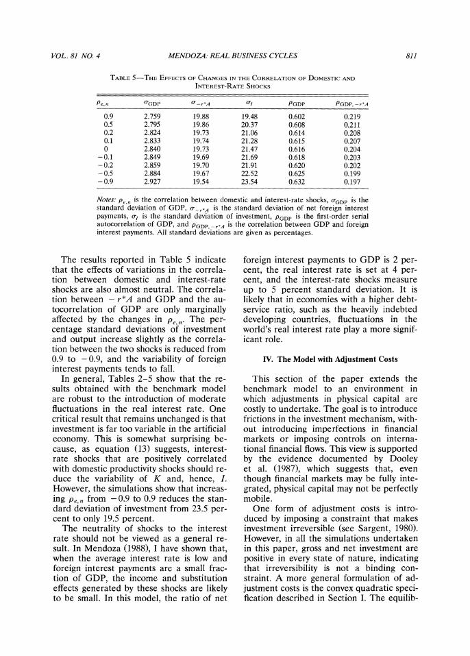
The results reported in Table 5 indicate that the effects of variations in the correlation between domestic and interest-rate shocks are also almost neutral. The correlation between - r *A and GDP and the autocorrelation of GDP are only marginally affected by the changes in pe,n. The percentage standard deviations of investment and output increase slightly as the correlation between the two shocks is reduced from 0.9 to -0.9, and the variability of foreign interest payments tends to fall.

In general, Tables 2-5 show that the results obtained with the benchmark model are robust to the introduction of moderate fluctuations in the real interest rate. One critical result that remains unchanged is that investment is far too variable in the artificial economy. This is somewhat surprising because, as equation (13) suggests, interest- rate shocks that are positively correlated with domestic productivity shocks should reduce the variability of K and, hence, I. However, the simulations show that increasing Pe,n from -0.9 to 0.9 reduces the standard deviation of investment from 23.5 percent to only 19.5 percent.

The neutrality of shocks to the interest rate should not be viewed as a general result. In Mendoza (1988), I have shown that, when the average interest rate is low and foreign interest payments are a small frac- tion of GDP, the income and substitution effects generated by these shocks are likely to be small. In this model, the ratio of net

foreign interest payments to GDP is 2 percent, the real interest rate is set at 4 percent, and the interest-rate shocks measure up to 5 percent standard deviation. It is likely that in economies with a higher debt- service ratio, such as the heavily indebted developing countries, fluctuations in the world's real interest rate play a more significant role.

IV. The Model with Adjustment Costs

This section of the paper extends the benchmark model to an environment in which adjustments in physical capital are costly to undertake. The goal is to introduce frictions in the investment mechanism, without introducing imperfections in financial markets or imposing controls on international financial flows. This view is supported by the evidence documented by Dooley et al. (1987), which suggests that, even though financial markets may be fully inte- grated, physical capital may not be perfectly mobile.

One form of adjustment costs is introduced by imposing a constraint that makes investment irreversible (see Sargent, 1980). However, in all the simulations undertaken in this paper, gross and net investment are positive in every state of nature, indicating that irreversibility is not a binding constraint. A more general formulation of adjustment costs is the convex quadratic speci- fication described in Section I. The equilib-


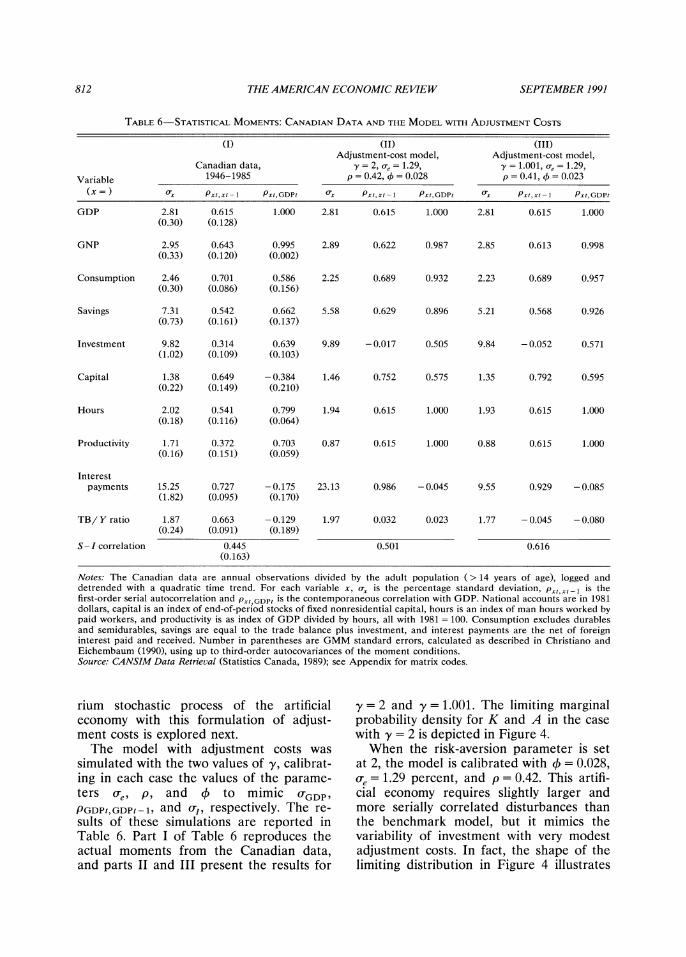
TABLE 6-STATISTICAL MOMENTS: CANADIAN DATA AND THE MODEL WITH ADJUSTMENT COSTS

Adjustment-cost model, Adjustment-cost model, Canadian data, -y = 2, ,e = 1.29, y = 1.001, a, = 1.29,

Variable 1946-1985 p = 0.42, ? = 0.028 p = 0.41, ? = 0.023

(x ) 0x Pxt,xt-1 Pxt,GDPt (Tx Pxt,xt-1 Pxt,GDPt (Tx Pxt,xt-i Pxt,GDPt

GDP 2.81 0.615 1.000 2.81 0.615 1.000 2.81 0.615 1.000 (0.30) (0.128)

GNP 2.95 0.643 0.995 2.89 0.622 0.987 2.85 0.613 0.998 (0.33) (0.120) (0.002)

Consumption 2.46 0.701 0.586 2.25 0.689 0.932 2.23 0.689 0.957 (0.30) (0.086) (0.156)

Savings 7.31 0.542 0.662 5.58 0.629 0.896 5.21 0.568 0.926 (0.73) (0.161) (0.137)

Investment 9.82 0.314 0.639 9.89 -0.017 0.505 9.84 -0.052 0.571 (1.02) (0.109) (0.103)

Capital 1.38 0.649 -0.384 1.46 0.752 0.575 1.35 0.792 0.595 (0.22) (0.149) (0.210)

Hours 2.02 0.541 0.799 1.94 0.615 1.000 1.93 0.615 1.000 (0.18) (0.116) (0.064)

Productivity 1.71 0.372 0.703 0.87 0.615 1.000 0.88 0.615 1.000 (0.16) (0.151) (0.059)

Interest payments 15.25 0.727 -0.175 23.13 0.986 -0.045 9.55 0.929 -0.085

(1.82) (0.095) (0.170)

TB/Y ratio 1.87 0.663 -0.129 1.97 0.032 0.023 1.77 -0.045 -0.080 (0.24) (0.091) (0.189)

S-I correlation 0.445 0.501 0.616 (0.163)

Notes: The Canadian data are annual observations divided by the adult population (> 14 years of age), logged and detrended with a quadratic time trend. For each variable x, ax is the percentage standard deviation, px x-1 is the first-order serial autocorrelation and Pxt,GDpt is the contemporaneous correlation with GDP. National accounts are in 1981 dollars, capital is an index of end-of-period stocks of fixed nonresidential capital, hours is an index of man hours worked by paid workers, and productivity is as index of GDP divided by hours, all with 1981 = 100. Consumption excludes durables and semidurables, savings are equal to the trade balance plus investment, and interest payments are the net of foreign interest paid and received. Number in parentheses are GMM standard errors, calculated as described in Christiano and Eichembaum (1990), using up to third-order autocovariances of the moment conditions. Source: CANSIM Data Retrieval (Statistics Canada, 1989); see Appendix for matrix codes.

rium stochastic process of the artificial economy with this formulation of adjustment costs is explored next.

The model with adjustment costs was simulated with the two values of y, calibrat- ing in each case the values of the parameters Se' p, and 0 to mimic 0(GDP'

PGDPt, GDPt -1, and o(-, respectively. The results of these simulations are reported in Table 6. Part I of Table 6 reproduces the actual moments from the Canadian data, and parts II and III present the results for

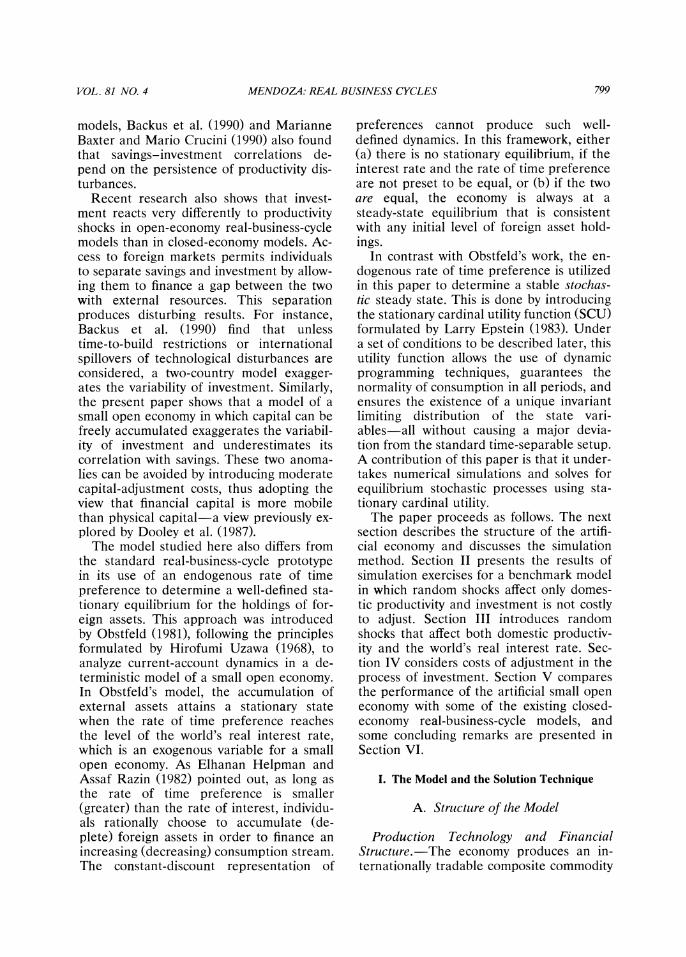
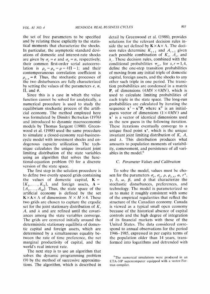
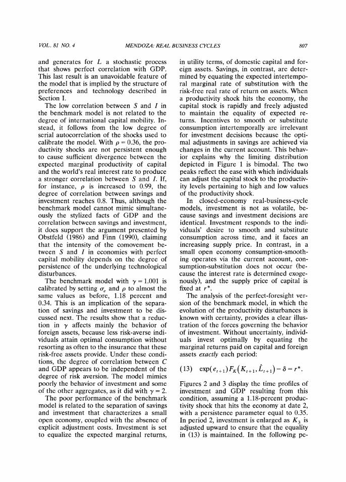
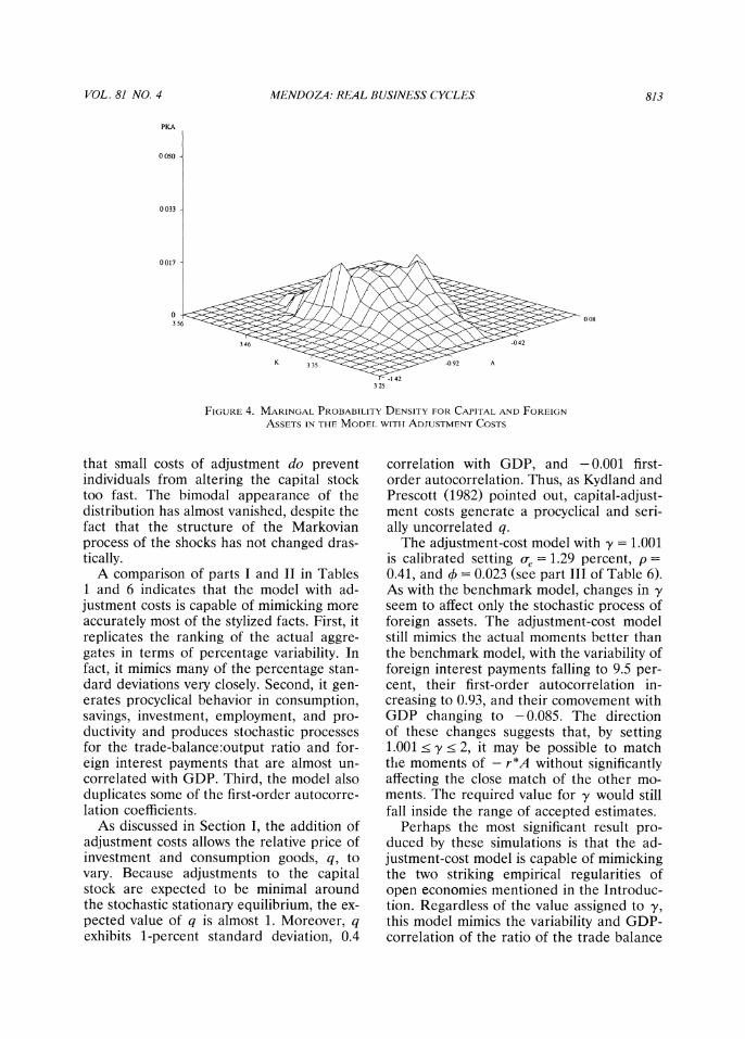
y = 2 and y = 1.001. The limiting marginal probability density for K and A in the case with y = 2 is depicted in Figure 4.

When the risk-aversion parameter is set at 2, the model is calibrated with 0 = 0.028, Se = 1.29 percent, and p = 0.42. This artificial economy requires slightly larger and more serially correlated disturbances than the benchmark model, but it mimics the variability of investment with very modest adjustment costs. In fact, the shape of the limiting distribution in Figure 4 illustrates


PKA

0 050

0033

0 017

0 008

3 25

FIGURE 4. MARINGAL PROBABILITY DENSITY FOR CAPITAL AND FOREIGN

ASSETS IN THE MODEL WITH ADJUSTMENT COSTS

that small costs of adjustment do prevent individuals from altering the capital stock too fast. The bimodal appearance of the distribution has almost vanished, despite the fact that the structure of the Markovian process of the shocks has not changed dras- tically.

A comparison of parts I and II in Tables 1 and 6 indicates that the model with adjustment costs is capable of mimicking more accurately most of the stylized facts. First, it replicates the ranking of the actual aggregates in terms of percentage variability. In fact, it mimics many of the percentage standard deviations very closely. Second, it generates procyclical behavior in consumption, savings, investment, employment, and productivity and produces stochastic processes for the trade-balance:output ratio and foreign interest payments that are almost uncorrelated with GDP. Third, the model also duplicates some of the first-order autocorrelation coefficients.

As discussed in Section I, the addition of adjustment costs allows the relative price of investment and consumption goods, q, to vary. Because adjustments to the capital stock are expected to be minimal around the stochastic stationary equilibrium, the expected value of q is almost 1. Moreover, q exhibits 1-percent standard deviation, 0.4

correlation with GDP, and - 0.001 first- order autocorrelation. Thus, as Kydland and Prescott (1982) pointed out, capital-adjustment costs generate a procyclical and serially uncorrelated q.

The adjustment-cost model with y = 1.001 is calibrated setting e- = 1.29 percent, p =

0.41, and 4 = 0.023 (see part III of Table 6). As with the benchmark model, changes in y seem to affect only the stochastic process of foreign assets. The adjustment-cost model still mimics the actual moments better than the benchmark model, with the variability of foreign interest payments falling to 9.5 percent, their first-order autocorrelation increasing to 0.93, and their comovement with GDP changing to - 0.085. The direction of these changes suggests that, by setting 1.001 < y < 2, it may be possible to match the moments of - r*A without significantly affecting the close match of the other moments. The required value for y would still fall inside the range of accepted estimates.

Perhaps the most significant result produced by these simulations is that the adjustment-cost model is capable of mimicking the two striking empirical regularities of open economies mentioned in the Introduc- tion. Regardless of the value assigned to y, this model mimics the variability and GDP- correlation of the ratio of the trade balance


to output, as well as the correlation between savings and investment. In fact, the comovement between S and I is slightly higher in both artificial economies than in the data, and this occurs without affecting the perfect international mobility of financial capital.

The introduction of moderate adjustment costs increases the persistence of the disturbances needed to calibrate the model, and with more permanent shocks investment tends to move closer together with savings, as Obstfeld (1986) suggested. Moreover, in line with the findings of Dooley et al. (1987), the perfect mobility of financial capital proves to be consistent not only with the correlation between S and I, but also with adjustment costs that prevent fast changes in physical capital.

The model mimics the variability and GDP correlation of TB/ Y because, in the presence of adjustment costs, the shocks that enable the model to mimic the stylized facts are expected to last long enough for the pro-borrowing effect, caused by an expected expansion of future output, to com- pensate for the pro-saving effect induced by a raise in contemporaneous output. These simulations suggest, therefore, that the intertemporal-equilibrium approach to the current account can be consistent with the empirical regularities of the business cycle.

The simulations also shed some light on a problem confronted by some empirical models of adjustment costs. As pointed out by Sargent (1978), these models generally produce reduced-form autoregressions in which highly persistent shocks cannot be distinguished from significant adjustment costs. Similarly, in the model studied here the variability of investment can be reduced by increasing the serial autocorrelation of the shocks, p, instead of introducing the adjustment costs. An increase in p reduces the probability of moving to the opposite state of productivity and lessens the chances of adjusting the capital stock, thereby reduc- ing the variability of investment. However, the resulting persistence of the disturbances is too high and causes the model to exaggerate the actual moments. For instance, with y = 2 and 4 = 0, if p is set to 0.9 the variability of I falls to 5.4 percent, but the

variability of GDP rises to 5 percent, and its serial autocorrelation is almost perfect. Thus, the simulations establish the rele- vance of adjustment costs relative to highly persistent shocks by showing that the latter are not consistent with the business cycle.

The neutrality of interest-rate shocks is robust to the introduction of adjustment costs. Increasing the variability of fluctuations to the interest rate from 1 percent to 5 percent in simulations with 4 = 0.028 increases the variability of GDP from 2.82 percent to 2.86 percent, increases the variability of - r*A from 23.4 percent to 24.3 percent, and increases the variability of I from 10 percent to 11.7 percent.

V. Comparison with Closed-Economy Models

In contrast with existing closed-economy real-business-cycle models, the benchmark model, the model with interest-rate fluctuations, and the adjustment-cost model re- quire productivity disturbances that exhibit less variability and persistence. Regarding the persistence of the disturbances, Gary Hansen (1985), Prescott (1986), and Robert King et al. (1988) used shocks that follow a stochastic process close to a random walk. Hansen estimated their quarterly serial autocorrelation at 0.95 (0.81 annually). The model of Greenwood et al. (1988), incorpo- rating endogenous utilization and investment shocks, requires disturbances with 0.51 annual persistence. In contrast, when y = 2, the basic model and the adjustment-cost model of the small open economy use shocks with 0.35 and 0.42 first-order serial autocorrelation, respectively.

The variability of the disturbances shows a similar pattern. The ratios of the variability of the productivity shocks relative to the observed variability of output are 1.3 and 1.7 in the work of Hansen and 1.5 in Green- wood et al. In contrast, in the small open- economy framework these ratios are 0.4 for the benchmark model and 0.7 for the model with adjustment costs, when the risk-aversion parameter is assigned a value of 2.

The low autocorrelation of the shocks that allow the models of the small open economy to mimic business cycles appears to be more representative of terms-of-trade


disturbances than Solow residuals. Solow residuals produced with Canadian data exhibit a first-order autocorrelation coefficient between 0.85 and 0.95. With this degree of persistence, the model exaggerates substan- tially the basic stylized facts. Setting p = 0.85 produces 0-GDP = 5.1 percent, PGDPt,GDPt-1 = 0.92, and o-I = 26 percent. In contrast, the output cost of fluctuations in the terms of trade for Canada exhibits first-order autocorrelation of about 0.13.11

Adjustment costs have very different con- sequences in the framework of a small open economy than in a closed economy. Kyd- land and Prescott (1982) showed that by introducing capital-adjustment costs, setting 0 = 1, the statistical moments resulting from an artificial closed economy are largely in- consistent with U.S. quarterly detrended data. In particular, adjustment costs caused the standard deviation of consumption almost to double and that of investment ex- penditures to fall by a factor of two. In contrast, in the model studied here adjustment costs are much smaller (0.023 < 4 < 0.028), and they reduce the percentage variability of investment to observed levels without significantly affecting consumption behavior.

Like closed-economy models, the models of the small open economy cannot mimic the behavior of average labor productivity. Productivity is about 1 percentage point less variable in the artificial open economies than in the data, and its correlation with GDP is perfectly positive compared with 0.7 in the data. The reason for this anomaly, as explained by McCallum (1989) and Christiano and Eichembaum (1990), is that real-business-cycle models depend on productivity shocks-which primarily affect the demand for labor-to produce fluctuations in employment. Under the usual configurations of preferences and technology, these shocks cause substitution effects on leisure that largely dominate the wealth effects and

thus underestimate the variability and exaggerate the cyclical comovement of productivity. The introduction of foreign assets does not affect this situation. In fact, the correlation between productivity and GDP is perfect in all the simulations because of the particular functional forms adopted for preferences and technology, as in Green- wood et al. (1988).

The results also show that the small open-economy models are unable to mimic some of the stylized facts that closed-economy models are able to duplicate. In particular, the artificial small open economies exaggerate the comovement between consumption (or savings) and GDP, regardless of the presence of adjustment costs or the value of the risk-aversion parameter. Con- sumption and output are highly correlated because shocks to domestic productivity cannot affect the interest rate, which is determined in the world financial market, and thus they cannot generate intertemporal consumption substitution. Furthermore, the introduction of moderate shocks affecting r* directly does not seem to induce strong enough consumption-substitution effects to alleviate this problem.

VI. Concluding Remarks

This paper extends the theory of real business cycles to a framework of a small open economy in which the rate of time preference increases with past consumption levels. This framework studies the dynamics of savings and investment in an environment in which domestic capital and foreign financial assets act as vehicles of savings, without any restrictions on international borrowing and lending.

The model was parameterized and simulated under three alternative configurations: 1) a benchmark model in which capital is not costly to adjust and the world's interest rate is deterministic; 2) an environment in which the interest rate is affected by stochastic disturbances; and 3) a framework in which capital is costly to adjust. These simulations show that the model duplicates many of the stylized facts typical of business cycles in postwar Canada with very small capital-adjustment costs and minimal vari-

1"The output cost of fluctuations in the terms of trade was calculated by adjusting net exports from the national income accounts to reflect international price changes, as explained by Paul Host-Madsen (1979).


ability and persistence in exogenous shocks. Exogenous shocks in this environment may follow from fluctuations in productivity or in the terms of trade. Without adjustment costs the model exaggerates the variability of investment because the separation of savings and investment, coupled with the absence of adjustment costs, allows physical capital to be altered too easily.

The simulations also illustrate that the model is consistent with two key empirical regularities typical of open economies. First, savings and investment are positively correlated despite the fact that financial capital is perfectly mobile across countries. Second, the trade balance and foreign assets tend to move against the business cycle. Neverthe- less, the model cannot duplicate some of the regularities observed in the data. In

particular, it exaggerates the procyclical behavior of productivity and consumption.

The appealing results obtained with the model suggest other topics for further research. The addition of nontradable com- modities would bring the model closer to reality and could help reduce the excessive consumption-output correlation. The model is also a natural framework for the study of business cycles arising as a result of terms- of-trade fluctuations in developing countries heavily dependent on exports of raw materials and imports of capital goods. Finally, the artificial economy and the numerical meth- ods employed here can be used to explore quantitatively the effects of economic policies such as tariffs and capital controls, which have been the subject of many interesting theoretical studies in recent years.

APPENDIX

CANSIM Data Retrieval Matrix Codes'2

Series title Matrix code

1) Gross national product at market prices 6630.1.1.1 2) Gross domestic product at market prices 6630.1.1.1.1 3) Investment income received from nonresidents 6630.1.1.1.2 4) Investment income paid to nonresidents 6630.1.1.1.3 5) Gross domestic product at 1981 prices 6629.1 6) Personal expenditure on goods and services at 1981 prices 6629.1.1 7) Business investment on fixed capital at 1981 prices 6629.1.5 8) Business inventory investment at 1981 prices 6629.1.6 9) Exports of goods and services at 1981 prices 6629.1.7

10) Imports of goods and services at 1981 prices 6629.1.8 11) Total male population 6968.1 12) Male population, ages 0-4 6968.1.1 13) Male population, ages 5-9 6968.1.2 14) Male population, ages 10-14 6968.1.3 15) Total female population 6968.2 16) Female population, ages 0-4 6968.2.1 17) Female population, ages 5-9 6968.2.2 18) Female population, ages 10-14 6968.2.3 19) Year-end net stock of fixed nonresidential capital in manufacturing

and nonmanufacturing industries 3487.2.7 20) Index of man-hours worked by paid workers 610.1 21) Net domestic income at factor cost 6627.1.1 22) Wages, salaries, and supplementary labor income 6627.1.1.1

12These data were retrieved in the spring of 1989. Due to frequent revisions made by Statistics Canada, the matrix code may not correspond to more recent updates of CANSIM or may appear as "terminated matrix." A listing of the data used in the paper is available from the author upon request.


REFERENCES

Ahmed, Shaghil, "Temporary and Permanent Government Spending in an Open Econ- omy: Some Evidence for the United Kingdom," Journal of Monetary Eco- nomics, June 1986, 17, 197-224.

Backus, David K., Gregory, Allan W. and Zin, Stanley E., "Risk Premiums in the Term Structure: Evidence from Artificial Economies," Journal of Monetary Eco- nomics, November 1989, 24, 371-400.

and Kehoe, Patrick J., "International Evidence on the Historical Properties of Business Cycles," Working Paper No. 402R, Federal Reserve Bank of Min- neapolis, Research Department, 1989. _ _ and Kydland, Finn E., "Inter- national Borrowing and World Business Cycles," Federal Reserve Bank of Min- neapolis, Research Department, Working Paper No. 426R, 1990.

Baxter, Marianne and Crucini, Mario J., "Ex- plaining Savings/Investment Correla- tions," Working Paper No. 224, Univer- sity of Rochester, Rochester Center for Economic Research, 1990.

Bertsekas, Dimitri P., Dynamic Programming and Stochastic Control, New York: Aca- demic Press, 1976.

Blanchard, Olivier J., "Debt, Deficits, and Finite Horizons," Journal of Political Economy, April 1985, 93, 223-47.

Brechling, Frank, Investment and Employ- ment Decisions, Totowa, NJ: Manchester University Press, 1975.

Cardia, Emanuela, "The Dynamics of Savings and Investment in Response to Monetary, Fiscal and Productivity Shocks," Working Paper No. 2088, University of Montreal, Department of Economics, 1989.

Chamberlain, Gary and Wilson, Chuck, "Opti- mal Intertemporal Consumption under Uncertainty," Workshop Series No. 8422, University of Wisconsin, Social Systems Research Institute, 1984.

Christiano, Lawrence J. and Eichembaum, Mar- tin, "Current Real Business Cycle Theo- ries and Aggregate Labor Fluctuations," Discussion Paper No. 24, Federal Re- serve Bank of Minneapolis, Institute for Empirical Macroeconomics, 1990.

Cole, Harold L. and Obstfeld, Maurice, "Com-

modity Trade and International Risk Sharing: How Much Do Financial Mar- kets Matter," NBER (Cambridge, MA) Working Paper No. 3027, 1989.

Craine, Roger, "Investment, Adjustment Costs, and Uncertainty," International Economic Review, August 1975, 16, 648- 61.

Dooley, Michael, Frankel, Jeffrey and Math- ieson, Donald J., "International Capital Mobility: What Do Savings-Investment Correlations Tell Us?," IMF Staff Papers, March 1987, 34, 503-29.

Epstein, Larry G., "Stationary Cardinal Util- ity and Optimal Growth under Uncer- tainty," Journal of Economic Theory, June 1983, 31, 133-52.

Feldstein, Martin and Horioka, Charles, "Domestic Savings and International Capital Flows," Economic Journal, June 1980, 90, 314-29.

Finn, Mary G., "On Savings and Investment Dynamics in a Small Open Economy," Journal of International Economics, Au- gust 1990, 29, 1-22.

Frenkel, Jacob A. and Razin, Assaf, "Fiscal Policies in the World Economy," Journal of Political Economy, June 1986, 94, 564-94.

and , Fiscal Policies and the World Economy, Cambridge, MA: MIT Press, 1987.

Gomme, Paul and Greenwood, Jeremy, "On the Cyclical Allocation of Risk," Working Pa- per No. 462, Federal Reserve Bank of Minneapolis, Research Department, 1990.

Greenwood, Jeremy, "Expectations, the Ex- change Rate, and the Current Account," Journal of Monetary Economics, Novem- ber 1983, 12, 543-69.

, Hercowitz, Zvi and Huffman, Gregory W., "Investment, Capacity Utilization, and the Real Business Cycle," American Eco- nomic Review, June 1988, 78, 402-17.

Hall, Robert E., "The Relation Between Price and Marginal Cost in U.S. Industry," Journal of Political Economy, October 1988, 96, 921-47.

Hansen, Gary D., "Indivisible Labor and the Business Cycle," Journal of Monetary Economics, November 1985, 16, 309-27.

Heckman, James J. and MaCurdy, Thomas, "A Life-Cycle Model of Female Labor Sup-

https://www.researchgate.net/publication/222630286_Risk_Premiums_in_the_Term_Structure_Evidence_from_Artificial_Economies?el=1_x_8&enrichId=rgreq-60e9943b4fb5f57810046cfa35c7989a-XXX&enrichSource=Y292ZXJQYWdlOzIyMjE3NDgzOTtBUzoxMDEyOTE3NjIxMjY4NDlAMTQwMTE2MTI0NjA1Nw==





https://www.researchgate.net/publication/223187907_Temporary_and_Permanent_Government_Spending_in_an_Open_Economy_Some_Evidence_for_the_United_Kingdom?el=1_x_8&enrichId=rgreq-60e9943b4fb5f57810046cfa35c7989a-XXX&enrichSource=Y292ZXJQYWdlOzIyMjE3NDgzOTtBUzoxMDEyOTE3NjIxMjY4NDlAMTQwMTE2MTI0NjA1Nw==






ply," Review of Economic Studies, January 1980, 47, 47-74; (Corrigendum, October 1982, 47, 659-60).

Helpman, Elhanan and Razin, Assaf, " Dy- namics of a Floating Exchange Rate Re- gime," Journal of Political Economy, Oct- ober 1982, 90, 728-54.

Hercowitz, Zvi, (1986a) "The Real Interest Rate and Aggregate Supply," Journal of Monetary Economics, September 1986, 18, 121-45.

, (1986b) "On the Determination of the Optimal External Debt: The Case of Israel," Journal of International Money and Finance, September 1986, 5, 315-34.

Host-Madsen, Paul, "Macroeconomic Ac- counts: An Overview," IMF Pamphlet Se- ries No. 29, International Monetary Fund, Washington, DC, 1979.

King, Robert G., Plosser, Charles I. and Rebelo, Sergio T., "Production, Growth, and Busi- ness Cycles. I. The Basic Neoclassical Model," Journal of Monetary Economics, March 1988, 21, 195-232.

Kydland, Finn E. and Prescott, Edward C., "Time to Build and Aggregate Fluctua- tions," Econometrica, November 1982, 50, 1345-70.

Leiderman, Leonardo and Razin, Assaf, "Cur- rent Account Dynamics: The Role of Real Shocks," IMF Working Paper No. WP/ 89/ 80, International Monetary Fund, Washington, DC, 1989.

Long, John B. and Plosser, Charles I., "Real Business Cycles," Journal of Political Economy, February 1983, 91, 39-59.

MaCurdy, Thomas, "An Empirical Investiga- tion of Labor Supply in a Life-Cycle Set- ting," Journal of Political Economy, De- cember 1981, 89, 1059-85.

McCallum, Bennett T., "Real Business Cycle Models," in R. J. Barro, ed., Modern Business Cycle Theory, Cambridge, MA: Harvard University Press, 1989, pp. 16-50.

Mendoza, Enrique G., "Real Business Cycles

and Optimal Foreign Asset Accumula- tion," unpublished manuscript, University of Western Ontario, Department of Eco- nomics, 1988.

Obstfeld, Maurice, "Macroeconomic Policy, Exchange-Rate Dynamics, and Optimal Asset Accumulation," Journal of Political Economy, December 1981, 89, 1142-61.

, "Capital Mobility in the World Economy: Theories and Measurement," Carnegie-Rochester Conference Series on Public Policy, Spring 1986, 24, 55-103.

Plosser, Charles I., "Understanding Real Business Cycles," Journal of Economic Perspectives, Summer 1989, 3, 51-77.

Prescott, Edward C., "Theory Ahead of Busi- ness Cycle Measurement," Carnegie- Rochester Conference Series on Public Pol- icy, Autumn 1986, 25, 11-44.

Sargent, Thomas J., "Estimation of Dynamic Labor Demand Equations under Rational Expectations," Journal of Political Econ- omy, December 1978, 25, 11-44.

,__ "Tobin's q and the Rate of Invest- ment in General Equilibrium," Carnegie- Rochester Conference Series on Public Pol- icy, Spring 1980, 12, 107-54.

Sotomayor, Marilda A. de 0., "On Income Fluctuations and Capital Gains," Journal of Economic Theory, June 1984, 32, 14-35.

Summers, Lawrence H., "Taxation and Corpo- rate Investment: A q-Theory Approach," Brookings Papers on Economic Activity, 1981, (1), 67-127.

Tesar, Linda, "Savings, Investment and In- ternational Capital Flows," Journal of In- ternational Economics, 1991, forthcoming.

Uzawa, Hirofumi, "Time Preference, the Consumption Function and Optimum As- set Holdings," in J. N. Wolfe, ed., Value, Capital and Growth: Papers in Honor of Sir John Hicks, Edinburgh: Edinburgh University Press, 1968, pp. 485-504.

Statistics Canada, CANSIM Data Retrieval, Ottawa, 1989, (magnetic tape).

https://www.researchgate.net/publication/4730734_Understanding_Real_Business_Cycles?el=1_x_8&enrichId=rgreq-60e9943b4fb5f57810046cfa35c7989a-XXX&enrichSource=Y292ZXJQYWdlOzIyMjE3NDgzOTtBUzoxMDEyOTE3NjIxMjY4NDlAMTQwMTE2MTI0NjA1Nw==



https://www.researchgate.net/publication/223632489_Production_Growth_and_Business_Cycles_I_The_Basic_Neo-Classical_Model?el=1_x_8&enrichId=rgreq-60e9943b4fb5f57810046cfa35c7989a-XXX&enrichSource=Y292ZXJQYWdlOzIyMjE3NDgzOTtBUzoxMDEyOTE3NjIxMjY4NDlAMTQwMTE2MTI0NjA1Nw==





https://www.researchgate.net/publication/24108199_Dynamics_of_a_Floating_Exchange_Rate_Regime?el=1_x_8&enrichId=rgreq-60e9943b4fb5f57810046cfa35c7989a-XXX&enrichSource=Y292ZXJQYWdlOzIyMjE3NDgzOTtBUzoxMDEyOTE3NjIxMjY4NDlAMTQwMTE2MTI0NjA1Nw==




https://www.researchgate.net/publication/4814826_'Time_To_Build_and_Aggregate_Fluctuations'?el=1_x_8&enrichId=rgreq-60e9943b4fb5f57810046cfa35c7989a-XXX&enrichSource=Y292ZXJQYWdlOzIyMjE3NDgzOTtBUzoxMDEyOTE3NjIxMjY4NDlAMTQwMTE2MTI0NjA1Nw==




https://www.researchgate.net/publication/248095591_Time_Preference_the_Consumption_Function_and_Optimum_Asset_Holdings?el=1_x_8&enrichId=rgreq-60e9943b4fb5f57810046cfa35c7989a-XXX&enrichSource=Y292ZXJQYWdlOzIyMjE3NDgzOTtBUzoxMDEyOTE3NjIxMjY4NDlAMTQwMTE2MTI0NjA1Nw==






https://www.researchgate.net/publication/24108238_Real_Business_Cycles?el=1_x_8&enrichId=rgreq-60e9943b4fb5f57810046cfa35c7989a-XXX&enrichSource=Y292ZXJQYWdlOzIyMjE3NDgzOTtBUzoxMDEyOTE3NjIxMjY4NDlAMTQwMTE2MTI0NjA1Nw==



https://www.researchgate.net/publication/222159175_Saving_Investment_and_International_Capital_Flows?el=1_x_8&enrichId=rgreq-60e9943b4fb5f57810046cfa35c7989a-XXX&enrichSource=Y292ZXJQYWdlOzIyMjE3NDgzOTtBUzoxMDEyOTE3NjIxMjY4NDlAMTQwMTE2MTI0NjA1Nw==



https://www.researchgate.net/publication/5049009_Theory_Ahead_of_Business_Cycle_Measurement?el=1_x_8&enrichId=rgreq-60e9943b4fb5f57810046cfa35c7989a-XXX&enrichSource=Y292ZXJQYWdlOzIyMjE3NDgzOTtBUzoxMDEyOTE3NjIxMjY4NDlAMTQwMTE2MTI0NjA1Nw==




https://www.researchgate.net/publication/4976230_On_income_fluctuations_and_capital_gains?el=1_x_8&enrichId=rgreq-60e9943b4fb5f57810046cfa35c7989a-XXX&enrichSource=Y292ZXJQYWdlOzIyMjE3NDgzOTtBUzoxMDEyOTE3NjIxMjY4NDlAMTQwMTE2MTI0NjA1Nw==




https://www.researchgate.net/publication/4729885_Taxation_and_Corporate_Investment_A_q-Theory_Approach?el=1_x_8&enrichId=rgreq-60e9943b4fb5f57810046cfa35c7989a-XXX&enrichSource=Y292ZXJQYWdlOzIyMjE3NDgzOTtBUzoxMDEyOTE3NjIxMjY4NDlAMTQwMTE2MTI0NjA1Nw==




https://www.researchgate.net/publication/5190455_Real_Business_Cycle_Models?el=1_x_8&enrichId=rgreq-60e9943b4fb5f57810046cfa35c7989a-XXX&enrichSource=Y292ZXJQYWdlOzIyMjE3NDgzOTtBUzoxMDEyOTE3NjIxMjY4NDlAMTQwMTE2MTI0NjA1Nw==





https://www.researchgate.net/publication/24108121_An_Empirical_Model_of_Labor_Supply_in_A_Life-Cycle_Setting?el=1_x_8&enrichId=rgreq-60e9943b4fb5f57810046cfa35c7989a-XXX&enrichSource=Y292ZXJQYWdlOzIyMjE3NDgzOTtBUzoxMDEyOTE3NjIxMjY4NDlAMTQwMTE2MTI0NjA1Nw==




https://www.researchgate.net/publication/239769498_Current_Account_DynamicsThe_Role_Of_Real_Shocks?el=1_x_8&enrichId=rgreq-60e9943b4fb5f57810046cfa35c7989a-XXX&enrichSource=Y292ZXJQYWdlOzIyMjE3NDgzOTtBUzoxMDEyOTE3NjIxMjY4NDlAMTQwMTE2MTI0NjA1Nw==





business cycles in a small open economy

Documents