NET Institute*

www.NETinst.org

Working Paper #07-15

September 2007

Bundling and Competition for Slots

Doh-Shin Jeon Universitat Pompeu Fabra

Domenico Menicucci

Università degli Studi di Firenze

* The Networks, Electronic Commerce, and Telecommunications (“NET”) Institute, http://www.NETinst.org, is a non-profit institution devoted to research on network industries, electronic commerce, telecommunications, the Internet, “virtual networks” comprised of computers that share the same technical standard or operating system, and on network issues in general.

Bundling and Competition for Slots¤

Doh-Shin Jeony and Domenico Menicucciz

September 29, 2007

Abstract

We study competition among upstream …rms when each of them sells a portfo-lio of distinct products and the downstream has a limited number of slots (or shelfspace). In this situation, we study how bundling a¤ects competition for slots. Whenthe downstream has k number of slots, social e¢ ciency requires that it purchases thebest k products among all upstream …rms’products. We …nd that under bundling,the outcome is always socially e¢ cient but under individual sale, the outcome is notnecessarily e¢ cient. Under individual sale, each upstream …rm faces a trade-o¤ be-tween quantity and rent extraction due to the coexistence of the internal competition(i.e. competition among its own products) and the external competition (i.e. com-petition from other …rms’products), which can create ine¢ ciency. On the contrary,bundling removes the internal competition and the external competition among bun-dles makes it optimal for each upstream …rm to sell only the products belonging tothe best k. This unambiguous welfare-enhancing e¤ect of bundling is novel.

Key words: Bundling, Competition among Portfolios, Limited Slots (or ShelfSpace)

JEL Code: D4, K21, L13, L41, L82

¤ This research was partially funded by the NET Institute (http://www.netinst.org/) whose …nancialsupport is gratefully acknowledged.

yUniversitat Pompeu Fabra and CREA. doh-shin.jeon@upf.eduzUniversità degli Studi di Firenze, Italy. domenico.menicucci@dmd.uni….it

1 Introduction

In vertical relations, very often each upstream firm sells a portfolio of distinct products

which compete for limited slots (or shelf space) of downstream firms. In this situation,

upstream firms may employ bundling as a strategy to win over the competition for the

limited slots. The practice of bundling has been a major antitrust issue and a subject

of intensive research in the past. However, to the best of our knowledge, the theoretical

Industrial Organization literature seems to have neglected competition among portfolios of

distinct products and, in particular, no paper has studied how bundling affects competition

for limited slots in this framework. In this paper, we attempt to provide a new perspective

on bundling by analyzing how it affects competition among portfolios of distinct products

for limited slots, and social welfare.

Examples of the situation we described above are abundant. For instance, in the movie

industry, each movie distributor has a portfolio of distinct movies and buyers (either movie

theaters or TV stations) have limited slots. More precisely, the number of movies that

can be projected in a season (or in a year) by a theater is constrained by time and the

number of rooms. Likewise, the number of movies that a TV station can show at prime

time during a year is also limited. Actually, allocation of slots in movie theaters has

been one of the main issues of the last presidential election in France regarding the movie

industry1. Furthermore, bundling in this industry (known as block booking2) was declared

illegal in two supreme court decisions in U.S.: Paramount Pictures, where blocks of films

were rented for theatrical exhibition, and Loew’s, where blocks of films were rented for

television exhibition. In addition, recently in MCA Television Ltd. v. Public Interest

Corp. (11th Circuit, April 1999), the court of appeals reaffirmed the per se illegal status

of block booking.

Another example we have in mind is that of manufacturers’ competition for a retailer’s

shelf space. Typically, each manufacturer produces a range of different products (for in-

stance, think about all the products sold under the brand name of Nestle) and manufac-

turers compete for a retailer’s limited shelf space. In this context, manufacturers having

a large portfolio of products may practice bundling (often called full-line forcing) for their

1Cahiers du Cinema (April, 2007) proposes to limits the number copies per film since certain movies bysaturating screens limits other films’ access to screens and asks the presidential candidates’ opinions aboutthe issue.

2Block booking refers to ”the practice of licensing, or offering for license, one feature or group offeatures on the condition that the exhibitor will also license another feature or group of features releasedby distributors during a given period” (Unites States v. Paramount Pictures, Inc., 334 U.S. 131, 156(1948)).

1

advantage and there has been antitrust cases related to this practice: Procter & Gamble /

Gillette3 and Societe des Caves de Roquefort.4

Moreover, since we consider a general model in which a firm can bundle any number

of products, our setup can be applied to bundling a large number of information goods, a

common practice in the Digital era (for instance, bundling of electronic academic journals).

In our model, we will assume away any asymmetric information or any uncertainty

about values of products. This will allow us to depart from the existing literature on block

booking or bundling (see the review of the related literature later on in this section) and

to identify what seems to us a first-order effect of bundling by focusing on the downstream

firm’s slot constraint. More precisely, we consider competition between two upstream firms

selling to a downstream firm who has k(> 0) number of slots. In our setting, a product

needs to occupy a slot to generate some value (i.e. a profit) to the downstream firm.

The upstream firms’ products are heterogenous in terms of the value that each of them

generates to the downstream firm. Therefore, social efficiency requires the downstream firm

to purchase and use the best k products among all products owned by the two upstream

firms. We focus on studying how bundling affects the set of the products that are purchased

and consumed by the downstream firm.

As the main result, we find that under bundling the outcome of competition is always

socially efficient, while this is not necessarily the case under individual sale. Under individ-

ual sale, each upstream firm faces a trade-off between quantity and rent extraction due to

the coexistence of the internal competition (i.e. competition among its own products) and

the external competition (i.e. competition from other firms’ products): as a firm increases

the number of products it induces the downstream firm to buy, it should abandon more

rent for each product it sells. This trade-off can make the outcome inefficient. On the

contrary, bundling removes the internal competition and the external competition among

bundles makes it optimal for each upstream firm to sell only his own products which belong

to the best k.

We think that this unambiguous welfare-enhancing effect of bundling is pretty novel.

Furthermore, we show that the efficiency property of bundling is very general in that it

holds regardless of whether we consider a sequential or simultaneous game or whether or

not we allow firms to contract directly on exclusive use of slots. The existing literature

analyzing bundling in a second-degree price discrimination framework often justifies the

rule of reason standard regarding bundling. Our result has strong policy implications that

go beyond the rule of reason.

3DG Competition case COMP/M.37324Conseil de la Concurrence, Decision 04-D-13, 8th April 2004.

2

There are only a few papers on block booking. The leverage theory, on which the

Supreme Court’s decisions were based, that block booking allows a distributor to extend

its monopoly power in a desirable movie to an undesirable one was criticized by Stigler since

the distributor is better off by selling only the desirable movie at a higher price. Instead

of the leverage theory, Stigler (1968) proposed a theory based on second-degree price dis-

crimination. However, Kenney and Klein (1983) point out that simple price discrimination

explanation since block booking is inconsistent with the facts of Paramount and Loew’s for

the prices of the blocks varied a great deal across markets and argue that block booking

mainly prevents exhibitors from oversearching, i.e. from rejecting films revealed ex post

to be of below-average value from an ex ante average-valued package. Their hypothesis is

empirically tested in a recent paper by Hanssen (2000) but the author finds little support

for the hypothesis5 and proposes that block booking was primarily intended to cheaply

provide films in quantity.

Most papers on bundling study bundling of two (physical) goods in the context of

second-degree price discrimination and focus on either surplus extraction (Schmalensee,

1984, McAfee et al. 1989, Salinger 1995 and Armstrong 1996, 1999) in a monopoly setting

or entry deterrence (Whinston 1990 and Nalebuff 2004) in a duopoly setting. Bakos and

Brynjolfsson (1999, 2000)’s papers are an exception, in that they study bundling of a large

number of information goods, but they maintain the second-degree price discrimination

framework. Their first paper shows that bundling allows a monopolist to extract more

surplus (since it reduces the variance of average valuations by the law of large numbers)

and thereby unambiguously increases social welfare;6 the second paper applies this insight

to entry deterrence (we do not address the entry deterrence issue). Since our novelty is

that we assume complete information and hence full surplus extraction is possible under

the monopoly setting, the rent extraction issue does not arise in our environment and there

is no use in applying the law of large number.

In Jeon-Menicucci (2006), we took a framework similar to the one in this paper to

study bundling electronic academic journals. More precisely, publishers owning portfolios

of distinct journals compete to sell them to a library who has a fixed budget to allocate

between journals and books. Publishers are assumed to have complete information about

the value that the library obtains from a journal and about the budget. We found that

bundling is a profitable strategy both in terms of surplus extraction and entry deterrence.

Conventional wisdom says that bundling has no effect in such a setting and this is true

without the budget constraint. However, when the budget constraint binds, we found that

5But Kenny and Klein (2000) do not agree with Hanseen’s analysis.6See also Armstrong (1999).

3

each firm has a strict incentive to adopt bundling but bundling reduces social welfare by

reducing the library’s consumption of journals and monographs. In this paper, instead of

focusing on the budget constraint of the buyer, we focus on his slot constraint. Another

difference is that Jeon-Menicucci (2006) focus on products (journals) of homogeneous value

while in this paper we consider products of heterogenous value. In spite of similarities of

the frameworks, the result we obtain here is contrary to the one in the previous paper since

we find that the allocation under bundling is socially efficient.

Finally, to our knowledge, Shaffer (1991) is the only paper that explicitly models the

downstream firm’s limited shelf space.7 He considers an upstream monopolist selling two

substitutable products with variable quantity. He finds that brand specific two-part tariffs

alone do not allow the monopolist to capture the maximum rent from the downstream firm

but full-line forcing (equivalent to bundling) does. We consider products of independent

values and hence the rent extraction issue Shaffer considers does not arise. In a general

setup of competition in which seller i has ni number of products and the buyer has k(<∑

i ni) number slots, we study how bundling affects the set of the products that occupy the

slots. Although products have independent values, competition arises because of the slot

constraint as long as there are at least two sellers.

In what follows, section 2 presents the model. Section 3 (4) characterizes the equilibrium

under individual sale (bundling). Section 5 compares individual sale with bundling in terms

of social welfare. Section 6 shows that when bundling is allowed, firms have an incentive

to bundle their products. Section 7 shows that the efficiency property of bundling is very

general. Section 8 concludes. Most proofs are gathered in the Appendix.

2 The setting

2.1 Model

There are two upstream firms, denoted by i = A,B, and a downstream firm, denoted by D.

Each firm i has a portfolio of ni(≥ 1) products for i = A,B, and all products are distinct;

let n ≡ nA + nB. Firm D has a limited number of slots (or shelf space) to distribute the

upstream firms’ products: the number of slots is given by k(≥ 1). Given (nA, nB, k), we

assume for simplicity that the cost of producing each product is zero for i = A,B and the

cost of distributing each product is zero for D.

D’s distribution of a product requires one unit of slot. Therefore, D can distribute at

most k number of products and we assume n > k. In this setup, we consider products of

7See also Verge (2001) who performs the social welfare analysis in the setup of Shaffer (1991).

4

heterogenous value and study how bundling affects the set of the products occupying the

limited slots. More precisely, we are interested in knowing when D distributes the best k

number of products. Let uji denote the gross profit that D obtains from distributing the

j-th best product of i; thus u1i ≥ u2

i ≥ ... ≥ unii > 0 for i = A,B. Let uj denote the gross

profit (or surplus) that D obtains from the j-th best product among all products owned

by both upstream firms, thus u1 ≥ u2 ≥ ... ≥ un. We assume uk > uk+1. Let m∗i denote

the number of i’s products in the set of the k best products among all products owned by

both upstream firms: by definition, m∗A + m∗

B = k. We assume m∗i ≥ 1 for i = A,B.8 In

this paper we study the case of nA ≥ k ≥ nB, but we can extend easily the analysis to the

case of nA < k or k < nB. Then, without loss of generality, we suppose nA = k.

Under individual sale, firm i chooses pji > 0 for its product with value uj

i , and we

define wji ≡ uj

i − pji as the net profit that D obtains from buying this product. Let

pi ≡ (p1i , p

2i , ..., p

nii ) and wi ≡ (w1

i , w2i , ..., w

nii ) denote the vectors of prices and of net profits

for the products of firm i, respectively. It is clear that there is a one-to-one correspondence

between pi and wi, and therefore we can equivalently express firm i’s decision problem in

terms of either pi or wi. However, when we use wi we need to recall that wji < uj

i for

i = A,B and j = 1, ..., ni. In particular, we will sometimes refer to the condition

w1A < u1

A, w2A < u2

A, ..., wkA < uk

A (1)

for firm A.

Under bundling, firm i sells a bundle Bi at a price Pi(> 0).

2.2 Nonexistence of equilibrium in a simultaneous game

Before presenting the timing of the sequential game that we study, we below illustrate that

equilibrium often does not exist in a simultaneous game under individual sale. Suppose

that A and B choose simultaneously pA and pB. As usual, we adopt as a tie-breaking

rule that if indifferent among different products, D buys the product which generates the

highest gross profit.

Suppose that A (B) has two (one) products and k = 2. Assume (u1A, u2

A, u1B) =

(3, 1, 2). Without loss of generality, we can assume that A chooses pA such that 3− p1A ≥

max {0, 1− p2A}: the net profit that D makes from buying A’s best product is positive

and larger than the one it makes from buying A’s second best product. Given pA sat-

isfying 3 − p1A ≥ max {0, 1− p2

A}, B’s best response is to choose p1B such that 2 − p1

B =

8The analysis of individual sale applies to m∗i = 0. m∗

i ≥ 1 simplifies the exposition of the analysis ofbundling.

5

max {0, 1− p2A}: B can find such a price since p2

A > 0 and hence max {0, 1− p2A} cannot be

larger than 1. Consider first the case in which 1 ≥ p2A > 0. In this case, B’s best response

is p1B = 1 + p2

A. However, then A can deviate by charging p2′A = p2

A − ε for ε(> 0) small

enough and sell both products. Consider now the case in which p2A > 1. In this case, B’s

best response is p1B = 2. However, then A can deviate by charging p2′

A = 1 − ε for ε(> 0)

small enough and sell both products. Therefore, there is no equilibrium (in pure strategy).9

The above example illustrates well the commitment issue that A faces. On the one

hand, if A can commit not to sell its second best product, then A and B can sell their best

products at the prices that extract D’s whole surplus. However, this outcome cannot be

an equilibrium since A has an incentive to deviate by undercutting B’s price (i.e. charging

p2′A = 1 − ε) to sell both products. On the other hand, there cannot be an equilibrium

in which D buys both products of A and does not buy B’s product. Therefore, in what

follows, we will consider a sequential game in which firm A can commit to its prices before

B chooses its prices.

2.3 Timing and tie-breaking rules

We consider the following sequential timing. When bundling is prohibited (i.e. under

individual sales),

Stage 1. A chooses pA;

Stage 2. after observing pA, B chooses pB;

Stage 3. D makes its purchase decision.

When bundling is allowed, at stage 1 (stage 2), A (B) decides whether or not to bundle

his products and pA or PA (pB or PB) accordingly: in addition, if firm i decides to bundle

his products, it also decides which products to include into the bundle.

In what follows we use the concept of subgame perfect Nash equilibrium (SPNE) to

determine the outcome of this game. Thus we start with D’s purchases at stage three. In

the case of individual sales, D chooses the k products yielding the highest non-negative net

profits. However, it is necessary to specify how D deals with ties, i.e. with products which

have the same net profit. Therefore we introduce the following tie-breaking rules.

T1: If D is indifferent between buying a product from A and a product from B (both

with non-negative net profits), and cannot buy both of them, then D buys B’s product.

9Even if we allow firms to charge zero price, the equilibrium does not exist. Suppose now p2A = 0: this

together with 3−p1A ≥ max

{0, 1− p2

A

}implies p1

A ≤ 2. In this case, B’s best response is p1B = 1. However,

then A can deviate by charging (p1′A, p2′

A) = (3, 2) for instance. Then, A sells only its best product but at ahigher price.

6

T1 is motivated by the fact that in our sequential game, given the price of A’s product

in question, B, as the follower, can always lower by ε > 0 its price to break D’s indifference.

Formally, in some cases B has no best reply without this assumption.

T2: If D is indifferent among different products offered by the same firm, and cannot

buy both of them, D buys the product that generates the highest gross value.

T2 is a standard tie-breaking rule.

Finally, we introduce the following tie-breaking rule for the upstream firms.

T3: Under bundling, if including a product into the bundle that i sells does not strictly

increase i’s profit, i prefers not to include the product into the bundle.

T3 makes a perfect sense when there is an infinitesimal cost of production. Although

we do not model any production cost for simplicity, T3 captures the essential effect that

would result from a positive production cost.

3 Individual sale

3.1 A preliminary result

Recall that we have set wji = uj

i−pji for i = A,B and j = 1, ..., ni, and wi = (w1

i , w2i , ..., w

nii )

for i = A,B. In wi ≡ (w(1)i , w

(2)i , ..., w

(ni)i ) we order instead the net profits in a decreasing

way, which means that w(1)i ≥ w

(2)i ≥ ... ≥ w

(ni)i . We now prove a simple and intuitive

result: there is no loss of generality in assuming that w(j)i = wj

i for all j.

Lemma 1 Without loss of generality, we can restrict our attention to the case in which

w1i ≥ w2

i ≥ ... ≥ wnii (i.e., wi = wi) for i=A,B.

In particular, lemma 1 implies the following monotonicity condition for firm A, which

we will use repeatedly in the remaining of the paper:

w1A ≥ w2

A ≥ ... ≥ wkA (2)

The lemma also implies that when firm i is selling mi number of products, i is actually

selling its products with the mi highest gross values.

7

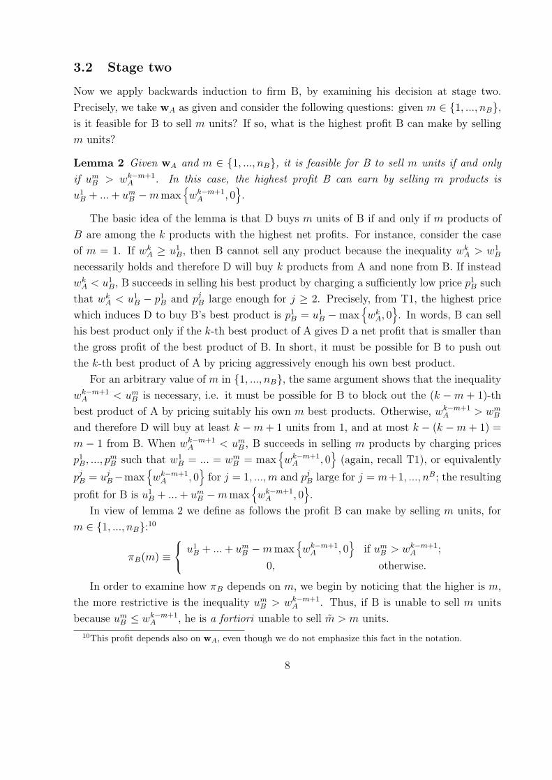
3.2 Stage two

Now we apply backwards induction to firm B, by examining his decision at stage two.

Precisely, we take wA as given and consider the following questions: given m ∈ {1, ..., nB},is it feasible for B to sell m units? If so, what is the highest profit B can make by selling

m units?

Lemma 2 Given wA and m ∈ {1, ..., nB}, it is feasible for B to sell m units if and only

if umB > wk−m+1

A . In this case, the highest profit B can earn by selling m products is

u1B + ... + um

B −m max{wk−m+1

A , 0}.

The basic idea of the lemma is that D buys m units of B if and only if m products of

B are among the k products with the highest net profits. For instance, consider the case

of m = 1. If wkA ≥ u1

B, then B cannot sell any product because the inequality wkA > w1

B

necessarily holds and therefore D will buy k products from A and none from B. If instead

wkA < u1

B, B succeeds in selling his best product by charging a sufficiently low price p1B such

that wkA < u1

B − p1B and pj

B large enough for j ≥ 2. Precisely, from T1, the highest price

which induces D to buy B’s best product is p1B = u1

B −max{wk

A, 0}. In words, B can sell

his best product only if the k-th best product of A gives D a net profit that is smaller than

the gross profit of the best product of B. In short, it must be possible for B to push out

the k-th best product of A by pricing aggressively enough his own best product.

For an arbitrary value of m in {1, ..., nB}, the same argument shows that the inequality

wk−m+1A < um

B is necessary, i.e. it must be possible for B to block out the (k −m + 1)-th

best product of A by pricing suitably his own m best products. Otherwise, wk−m+1A > wm

B

and therefore D will buy at least k −m + 1 units from 1, and at most k − (k −m + 1) =

m − 1 from B. When wk−m+1A < um

B , B succeeds in selling m products by charging prices

p1B, ..., pm

B such that w1B = ... = wm

B = max{wk−m+1

A , 0}

(again, recall T1), or equivalently

pjB = uj

B−max{wk−m+1

A , 0}

for j = 1, ..., m and pjB large for j = m+1, ..., nB; the resulting

profit for B is u1B + ... + um

B −m max{wk−m+1

A , 0}.

In view of lemma 2 we define as follows the profit B can make by selling m units, for

m ∈ {1, ..., nB}:10

πB(m) ≡

u1B + ... + um

B −m max{wk−m+1

A , 0}

if umB > wk−m+1

A ;

0, otherwise.

In order to examine how πB depends on m, we begin by noticing that the higher is m,

the more restrictive is the inequality umB > wk−m+1

A . Thus, if B is unable to sell m units

because umB ≤ wk−m+1

A , he is a fortiori unable to sell m > m units.

10This profit depends also on wA, even though we do not emphasize this fact in the notation.

8

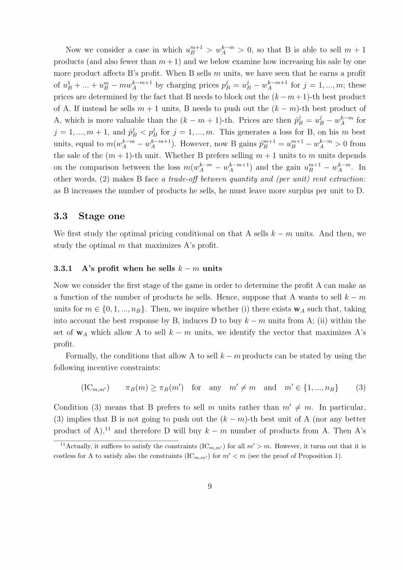
Now we consider a case in which um+1B > wk−m

A > 0, so that B is able to sell m + 1

products (and also fewer than m+1) and we below examine how increasing his sale by one

more product affects B’s profit. When B sells m units, we have seen that he earns a profit

of u1B + ... + um

B −mwk−m+1A by charging prices pj

B = ujB − wk−m+1

A for j = 1, ..., m; these

prices are determined by the fact that B needs to block out the (k−m+1)-th best product

of A. If instead he sells m + 1 units, B needs to push out the (k −m)-th best product of

A, which is more valuable than the (k −m + 1)-th. Prices are then pjB = uj

B − wk−mA for

j = 1, ..., m + 1, and pjB < pj

B for j = 1, ..., m. This generates a loss for B, on his m best

units, equal to m(wk−mA − wk−m+1

A ). However, now B gains pm+1B = um+1

B − wk−mA > 0 from

the sale of the (m + 1)-th unit. Whether B prefers selling m + 1 units to m units depends

on the comparison between the loss m(wk−mA − wk−m+1

A ) and the gain um+1B − wk−m

A . In

other words, (2) makes B face a trade-off between quantity and (per unit) rent extraction:

as B increases the number of products he sells, he must leave more surplus per unit to D.

3.3 Stage one

We first study the optimal pricing conditional on that A sells k −m units. And then, we

study the optimal m that maximizes A’s profit.

3.3.1 A’s profit when he sells k −m units

Now we consider the first stage of the game in order to determine the profit A can make as

a function of the number of products he sells. Hence, suppose that A wants to sell k −m

units for m ∈ {0, 1, ..., nB}. Then, we inquire whether (i) there exists wA such that, taking

into account the best response by B, induces D to buy k −m units from A; (ii) within the

set of wA which allow A to sell k − m units, we identify the vector that maximizes A’s

profit.

Formally, the conditions that allow A to sell k−m products can be stated by using the

following incentive constraints:

(ICm,m′) πB(m) ≥ πB(m′) for any m′ 6= m and m′ ∈ {1, ..., nB} (3)

Condition (3) means that B prefers to sell m units rather than m′ 6= m. In particular,

(3) implies that B is not going to push out the (k −m)-th best unit of A (nor any better

product of A),11 and therefore D will buy k − m number of products from A. Then A’s

11Actually, it suffices to satisfy the constraints (ICm,m′) for all m′ > m. However, it turns out that it iscostless for A to satisfy also the constraints (ICm,m′) for m′ < m (see the proof of Proposition 1).

9

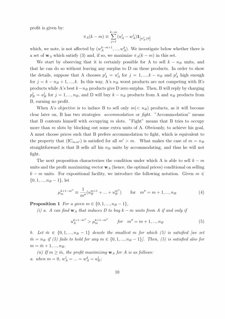
profit is given by:

πA(k −m) ≡k−m∑

j=1

(ujA − wj

A)1[wjA≥0]

which, we note, is not affected by (wk−m+1A , ..., wk

A). We investigate below whether there is

a set of wA which satisfy (3) and, if so, we maximize πA(k −m) in this set.

We start by observing that it is certainly possible for A to sell k − nB units, and

that he can do so without leaving any surplus to D on these products. In order to show

the details, suppose that A chooses pjA = uj

A for j = 1, ..., k − nB and pjA high enough

for j = k − nB + 1, ..., k. In this way, A’s nB worst products are not competing with B’s

products while A’s best k−nB products give D zero surplus. Then, B will reply by charging

pjB = uj

B for j = 1, ..., nB, and D will buy k − nB products from A and nB products from

B, earning no profit.

When A’s objective is to induce B to sell only m(< nB) products, as it will become

clear later on, B has two strategies: accommodation or fight. ”Accommodation” means

that B contents himself with occupying m slots. ”Fight” means that B tries to occupy

more than m slots by blocking out some extra units of A. Obviously, to achieve his goal,

A must choose prices such that B prefers accommodation to fight, which is equivalent to

the property that (ICm,m′) is satisfied for all m′ > m. What makes the case of m = nB

straightforward is that B sells all his nB units by accommodating, and thus he will not

fight.

The next proposition characterizes the condition under which A is able to sell k −m

units and the profit maximizing vector wA (hence, the optimal prices) conditional on selling

k − m units. For expositional facility, we introduce the following notation. Given m ∈{0, 1, ..., nB − 1}, let

µk+1−m′′m ≡ 1

m′′ (um+1B + ... + um′′

B ) for m′′ = m + 1, ..., nB (4)

Proposition 1 For a given m ∈ {0, 1, ..., nB − 1},(i) a. A can find wA that induces D to buy k −m units from A if and only if

uk+1−m′′A > µk+1−m′′

m for m′′ = m + 1, ..., nB (5)

b. Let m ∈ {0, 1, ..., nB − 1} denote the smallest m for which (5) is satisfied [we set

m = nB if (5) fails to hold for any m ∈ {0, 1, ..., nB − 1}]. Then, (5) is satisfied also for

m = m + 1, ..., nB.

(ii) If m ≥ m, the profit maximizing wA for A is as follows:

a. when m = 0, w1A = ... = wk

A = u1B;

10

b. when m ∈ {1, ..., nB − 1},

wk−m+1A = wk−m+2

A = ... = wkA = 0 (6)

wk−m′′+1A = max{wk−m′′+2

A , µk−m′′+1m } for m′′ = m + 1, ..., nB (7)

w1A = w2

A = ... = wk−nBA = wk−nB+1

A (8)

We below give the intuition of the results in Proposition 1; we focus on explaining the

profit maximizing wA conditional on selling k−m units for m ≥ 1, described in Proposition

1(ii)b.12 Given A’s objective to sell k −m units, A should structure his prices for the best

k−m products (the ones to sell) very differently from the prices for the m worst units (the

ones not to sell). On the one hand, regarding the m worst products, it is optimal to charge

very high prices (higher than their values) so that B does not face any competition from

them; precisely, (6) reveals that choosing wk−m+1A = wk−m+2

A = ... = wkA = 0 is optimal. The

reason is that this pricing maximizes B’s profit from accommodation and hence reduces B’s

temptation to fight. In fact, the pricing allows B to extract full surplus u1B + ... + um′

B from

his best m′ products if he wants to sell only m′ ≤ m products. Then, obviously, B strictly

prefers selling m units to selling less than m, and hence downward incentive constraints

(i.e. (ICm,m′) for m′ < m) are trivially satisfied. On the other hand, regarding the best

k −m units to sell, the prices should be competitive enough to make it unprofitable for B

to sell more than m units. In particular, A cannot extract full surplus from these products

since if he attempts to do that, B can sell all of his nB products by leaving no surplus per

product to D, given T1.

To explain the optimal pricing of the best k−m units, suppose that B wants to sell m+1

units instead of m units. Lemma 2 shows that B can sell m + 1 products only if wk−mA <

um+1B . In this case, B makes a profit equal to πB(m + 1) = u1

B + ... + um+1B − (m + 1)wk−m

A

and we have

πB(m + 1)− πB(m) = um+1B − (m + 1)wk−m

A

As we discussed after Lemma 2, um+1B − (m + 1)wk−m

A is composed of the loss −mwk−mA on

B’s best m units (with respect to selling them at full prices) plus the gain um+1B −wk−m

A from

selling the (m + 1)-th unit. Therefore, wk−mA ≥ um+1

B

m+1= µk−m

m allows to satisfy πB(m) ≥πB(m + 1): note that it is less restrictive than wk−m

A ≥ um+1B . Hence, the smallest value of

wk−mA satisfying (ICm,m+1) is wk−m

A = µk−mm , as described in (7). In order to deter B from

selling m + 2 units, we can argue as before. A sufficient condition is wk−m−1A ≥ um+2

B , but

12Proposition 1(ii)a is straightforward, as the best way for A to sell k products is to set w1A = ... = wk

A

equal to the value of B’s best product, u1B , provided that uk

A > u1B .

11

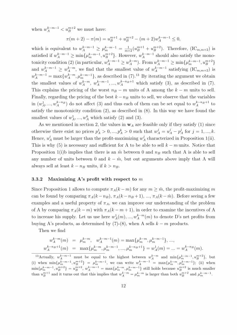
when wk−m−1A < um+2

B we must have:

π(m + 2)− π(m) = um+1B + um+2

B − (m + 2)wk−m−1A ≤ 0,

which is equivalent to wk−m−1A ≥ µk−m−1

m = 1m+2

(um+1B + um+2

B ). Therefore, (ICm,m+2) is

satisfied if wk−m−1A ≥ min{µk−m−1

m , um+2B }. However, wk−m−1

A should also satisfy the mono-

tonicity condition (2) (in particular, wk−m−1A ≥ wk−m

A ). From wk−m−1A ≥ min{µk−m−1

m , um+2B }

and wk−m−1A ≥ wk−m

A , we find that the smallest value of wk−m−1A satisfying (ICm,m+2) is

wk−m−1A = max{wk−m

A , µk−m−1m }, as described in (7).13 By iterating the argument we obtain

the smallest values of wk−mA , wk−m−1

A , ..., wk−nB+1A which satisfy (3), as described in (7).

This explains the pricing of the worst nB −m units of A among the k −m units to sell.

Finally, regarding the pricing of the best k−nB units to sell, we observe that the variables

in (w1A, ..., wk−nB

A ) do not affect (3) and thus each of them can be set equal to wk−nB+1A to

satisfy the monotonicity condition (2), as described in (8). In this way we have found the

smallest values of w1A, ..., wk

A which satisfy (2) and (3).

As we mentioned in section 2, the values in wA are feasible only if they satisfy (1) since

otherwise there exist no prices p1A > 0, ..., pk

A > 0 such that wjA = uj

A − pjA for j = 1, ..., k.

Hence, ujA must be larger than the profit-maximizing wj

A characterized in Proposition 1(ii).

This is why (5) is necessary and sufficient for A to be able to sell k −m units. Notice that

Proposition 1(i)b implies that there is an m between 0 and nB such that A is able to sell

any number of units between 0 and k − m, but out arguments above imply that A will

always sell at least k − nB units, if k > nB.

3.3.2 Maximizing A’s profit with respect to m

Since Proposition 1 allows to compute πA(k−m) for any m ≥ m, the profit-maximizing m

can be found by comparing πA(k−nB), πA(k−nB +1), ..., πA(k− m). Before seeing a few

examples and a useful property of πA, we can improve our understanding of the problem

of A by comparing πA(k−m) with πA(k−m + 1), in order to examine the incentives of A

to increase his supply. Let us use here w1A(m), ..., wk−m

A (m) to denote D’s net profits from

buying A’s products, as determined by (7)-(8), when A sells k −m products.

Then we find

wk−mA (m) = µk−m

m , wk−m−1A (m) = max{µk−m

m , µk−m−1m }, ...,

wk−nB+1A (m) = max{µk−m

m , µk−m−1m , ..., µk−nB+1

m } = w1A(m) = ... = wk−nB

A (m).

13Actually, wk−m−1A must be equal to the highest between wk−m

A and min{µk−m−1m , um+2

B }, but(i) when min{µk−m−1

m , um+2B } = µk−m−1

m , we can write wk−m−1A = max{µk−m

m , µk−m−1m }; (ii) when

min{µk−m−1m , um+2

B } = um+2B , wk−m−1

A = max{µk−mm , µk−m−1

m } still holds because um+2B is much smaller

than um+1B and it turns out that this implies that wk−m

A = µk−mm is larger than both um+2

B and µk−m−1m .

12

When instead A sells k −m + 1 products, we have:

wk−m+1A (m− 1) = µk−m+1

m−1 , wk−mA (m− 1) = max{µk−m+1

m−1 , µk−mm−1}, ...,

wk−nB+1A (m− 1) = max{µk−m+1

m−1 , µk−mm−1, ..., µ

k−nB+1m−1 } = w1

A(m− 1) = ... = wk−nBA (m− 1).

It is straightforward to see from (4) that µk+1−m′′m−1 > µk+1−m′′

m for any m′′ ∈ {m + 1, ..., nB},thus we have wk+1−m′′

A (m− 1) > wk+1−m′′A (m) for any m′′ ∈ {m + 1, ..., k}.

The latter inequality is very intuitive: in order to sell one extra unit, (i.e. k −m + 1

rather than k − m units). A must increase the rent it abandons to D for all the k − m

initial units. Thus, when we compare πA(k − m + 1) =∑k−m+1

j=1 (ujA − wj

A(m − 1)) with

πA(k−m) =∑k−m

j=1 (ujA −wj

A(m)), we see that πA(k−m + 1) contains the additional term

uk−m+1A − wk−m+1

A (m− 1) > 0, which is A’s profit on the (k −m + 1)-th unit sold, but A’s

profit on each of his first k −m units is reduced from ujA − wj

A(m) to ujA − wj

A(m− 1), as

we just proved that wjA(m− 1) > wj

A(m) for j ∈ {1, ..., k −m}. In words, as it is the case

with B, A also faces a trade off between quantity and rent extraction: as A sells more units,

it should leave more surplus per unit to D. Precisely, as A increases its sales from k−m to

k −m + 1, inducing B to accommodate becomes more difficult for two reasons. First, B’s

ability to fight is now stronger since he can use his m-th best unit, with value umB , which

was previously sold. Second, B has now less to lose by trying to push out a product of A,

since selling m − 1 products makes the profit from accommodation (described just after

Lemma 2) smaller than when selling m. Therefore, when A sells one extra unit, in order

to induce B not to fight, A should make his units more competitive by leaving D a higher

surplus for each unit.

We now present a result which simplifies the task of finding the optimal m. Precisely,

we prove a concavity-like property of πA which states that the marginal profit for A from

selling one extra unit is decreasing: the profit increase from selling k − m + 2 products

instead of k − m + 1 is smaller than the profit increase from selling k − m + 1 products

instead of k −m.

Proposition 2 (i) Suppose that it is feasible for A to sell k−m+2 units (i.e. m−2 ≥ m).

Then πA(k −m + 2)− πA(k −m + 1) ≤ πA(k −m + 1)− πA(k −m).

(ii) The optimal m for A, denoted by m∗∗A , is characterized as follows: πA(m∗∗

A ) ≥ max{πA(m∗∗A−

1), πA(m∗∗A +1)} if k−nB +1 ≤ m∗∗

A ≤ k− m− 1, πA(m∗∗A ) ≥ πA(m∗∗

A − 1) if m∗∗A = k− m,

πA(m∗∗A ) ≥ πA(m∗∗

A + 1) if m∗∗A = k − nB.

Notice that the concavity-like property of πA described in Proposition 2(i) implies im-

mediately Proposition 2(ii): in order to test the optimality of m∗∗A , it suffices to compare

the profit as the number of products to sell for A is decreased by one unit or increased by

one unit. In what follows, to give further insight, we study some specific settings.

13

3.3.3 When only the local incentive constraint (ICm,m+1) matters

Let us present first the simple case in which only the local incentive constraint (ICm,m+1)

matters. We saw that when A wants to sell k−m units, downward incentive constraint are

trivially satisfied but satisfying upward constraints requires A to abandon some surplus to

D. We below present a special case in which satisfying only (ICm,m+1) is sufficient to satisfy

(3), and this makes it straightforward to derive πA(k −m).

Corollary 1 Given m such that m ≤ m ≤ nB − 2, if um+2B ≤ 1

m+1um+1

B then (5) is

equivalent to uk−mA > 1

m+1um+1

B . When this condition is satisfied, (6)-(8) imply w1A = ... =

wk−mA = 1

m+1um+1

B > 0 = wk−m+1A = ... = wk

A; thus πA(k−m) = u1A + ...+uk−m

A − k−mm+1

um+1B .

Precisely, if um+2B is sufficiently smaller than um+1

B , it turns out that µk−mm ≥ µk−m−1

m ≥... ≥ µk−nB+1

m and then (5) is satisfied if and only if uk+1−m′′A > µk+1−m′′

m holds for m′′ = m+1,

or equivalently uk−mA > 1

m+1um+1

B . If this condition is satisfied, then the optimal prices for

A are such that the products he wants to sell give a constant net profit to D equal to1

m+1um+1

B , the profit satisfying (ICm,m+1) with equality. If the condition um+2B ≤ 1

m+1um+1

B

holds for every m ∈ {m, ..., nB − 2}, then we have

πA(k −m + 1)− πA(k −m) = uk−m+1A − 1

mum

B − (k −m)(1

mum

B −1

m + 1um+1

B ).

Note however that the conditions 1m+1

um+1B ≥ um+2

B , 1m+2

um+2B ≥ um+3

B , ..., 1nB−1

unB−1B ≥ unB

B

are somewhat restrictive, since they imply that the values of B’s products decrease quite

quickly. This also suggests that in general more than one upward incentive constraints

matter, as in the examples below.

3.3.4 Example 1: When nB = 3

Suppose that nB = 3. In order to sell k − 3 units, A sets

p1A = u1

A, p2A = u2

A, ..., pk−3A = uk−3

A , pk−2A ≥ uk−2

A , pk−1A ≥ uk−1

A , pkA ≥ uk

A.

and then B chooses p1B = u1

B, p2B = u2

B, p3B = u3

B. Hence, πA(k− 3) = u1A + u2

A + ... + uk−3A .

In order to find πA(k − 2) we have to consider (IC2,3), which is given by

(IC2,3) wk−2A ≥ 1

3u3

B.

Therefore, A chooses

p1A = u1

A −1

3u3

B, p2A = u2

A −1

3u3

B, ... , pk−2A = uk−2

A − 1

3u3

B, pk−1A ≥ uk−1

A , pkA ≥ uk

A.

14

which is feasible only if uk−2A > 1

3u3

B. Then, B plays p1B = u1

B, p2B = u2

B. Hence, πA(k−2) =

u1A + u2

A + ... + uk−2A − k−2

3u3

B.

In order to find πA(k− 1) we need to consider both (IC1,2) and (IC1,3), which are given by:

(IC1,2) wk−1A ≥ 1

2u2

B.

(IC1,3) wk−2A ≥ max{1

2u2

B,1

3(u2

B + u3B)}.

Hence, satisfying the incentive constraints is feasible if uk−1A > 1

2u2

B and uk−2A > max{1

2u2

B, 13(u2

B+

u3B)}. Then, A chooses

pjA = uj

A −max{1

2u2

B,1

3(u2

B + u3B)} for j = 1, ..., k − 2;

pk−1A = uk−1

A − 1

2u2

B, pkA ≥ uk

A.

Then πA(k − 1) = u1A + u2

A + ... + uk−2A + uk−1

A − (k − 2) max{12u2

B, 13(u2

B + u3B)} − 1

2u2

B.

Finally, A is able to sell k units if and only if ukA > ku1

B, and then πA(k) = u1A + u2

A +

... + uk−2A + uk−1

A + ukA − ku1

B.

In order to fix the ideas, suppose that u2B > 2u3

B, so that max{12u2

B, 13(u2

B +u3B)} = 1

2u2

B.

Then, from Proposition 2(ii), we see for instance that it is optimal for A to sell k − 2

products if πA(k − 2) ≥ max{πA(k − 1), πA(k − 3)}, which is equivalent to uk−2A ≥ k−2

3u3

B

and uk−1A ≤ k−2

2(u2

B−u3B)+ 1

2u2

B. The first inequality implies that the gain on the (k−2)-th

sold by A, uk−2A − 1

3u3

B, is larger than his loss on the k − 3 units, k−33

u3B, with respect to

selling them at full prices. The second inequality means that selling the (k − 1)-th unit

yields a profit of uk−1A − 1

2u2

B but results in a loss of k−22

(u2B − u3

B), which is larger than

uk−1A − 1

2u2

B.

3.3.5 Example 2: When all B’s products have the same value

Suppose that u1B = u2

B = ... = unBB ≡ uB > 0. In this case, for m(= 1, ..., nB − 1) and

m′′(= m + 1, ..., nB), we find that µk+1−m′′m = m′′−m

m′′ uB. Thus µk+1−m′′m is increasing in m′′.

Given m, the profit-maximizing w1A, ..., wk−m

A , determined by (7)-(8), are

wk−mA =

1

m + 1uB, wk−m−1

A =2

m + 2uB, ..., wk−nB+2

m =nB −m− 1

nB − 1uB,

wk−nB+1m =

nB −m

nB

uB = w1A = ... = wnB

A .

If m ≥ m, we have that πA(k−m) = u1A + ...+uk−m

A − [ 1m+1

+ 2m+2

+ ...+ nB−m−1nB−1

+ nB−mnB

(k−nB + 1)]uB.

15

In order to find the optimal m, we exploit lemma 2. Thus, m = nB is optimal if

πA(k − nB) ≥ πA(k − nB + 1), i.e. ifu

k−nB+1

A

uB≤ k−nB+1

nB. Finally, for m between 1 and

nB − 1, m is optimal if π(k −m)− π(k −m− 1) ≥ 0 and π(k −m + 1) ≤ π(k −m), i.e.

1

m+

1

m + 1+ ... +

1

nB − 1+

k − nB + 1

nB

≥ uk−m+1A

uB

and

uk−mA

uB

≥ 1

m + 1+

1

m + 2+ ... +

1

nB − 1+

k − nB + 1

nB

4 Bundling

In this section we initially assume that each firm practices bundling. Precisely, at stage

one firm A chooses qA of his products to include into his bundle BA, and a price PA for BA.

At stage two, after observing the move of A, B chooses qB of his products to include

into his bundle BB and a price PB for BB. In order to specify the value of a bundle for D,

it is not enough to specify the number of units it contains, but it is necessary to know the

precise products in the bundle. However, it is intuitive that if i inserts qi of his products

in Mi, it is optimal for him to choose the best qi products among the ones he can sell. For

i = A,B, let Ui(qi) denote the gross value of Mi for D if it includes the qi best products

of i: Ui(qi) =∑qi

j=1 uji . Let UAB(qA,qB) denote D’s gross profit from buying both bundles,

taking into account the capacity constraint of D; thus UAB(qA, qB) ≤ UA(qA) + UB(qB),

with equality if and only if qA + qB ≤ k. Therefore, the net profit of D from buying only

Mi is Ui(qi)− Pi, while D’s profit from buying BA and BB is UAB(qA, qB)− PA − PB.

As we did for the game with individual sales, we apply backwards induction starting

with stage three. Clearly, D determines his purchase by maximizing his own payoff. About

tie-breaking, we assume that D buys both bundles if UAB(qA, qB)−PA−PB ≥ max{UA(qA)−PA, UB(qB)−PB}, while he buys BB if UB(qB)−PB = UA(qA)−PA > UAB(qA, qB)−PA−PB

(this is consistent with T1).

At stage two, given (qA, PA), B wants to choose qB and (the maximal) PB such that D

decides to buy BB. In order to achieve this objective, B can choose between two strategies

as under individual sale: accommodation and fight. B can try to induce D to buy both

bundles or try to induce D to buy only BB (and block out BA). Recall from section 2

that m∗i is the number of firm i’s products of among the k best products overall, thus

m∗A + m∗

B = k. Before starting the analysis, it is useful to introduce the function

q(qA) =

min{nB, k − qA} if qA < m∗A

m∗B if qA ≥ m∗

A

16

The interpretation of q(qA) is as follows: if D has purchased BA which includes A’s best

qA units, then q(qA) is the maximal number of products of B which D would effectively

distribute under the slot constraint in case D buys BB as well. The next lemma characterizes

B’s optimal strategy at stage 2.

Lemma 3 At stage two, given a pair (qA, PA),

(i) B fights by choosing qB = nB and PB = UB(nB)− UA(qA) + PA if PA > UAB(qA, nB)−UB(nB);

(ii) B accommodates by choosing qB = q(qA) and PB = UAB[qA, q(qA)] − UA(qA) if PA ≤UAB(qA, nB)− UB(nB).

Not surprisingly, B ends up fighting (accommodating) when PA is large (small). Pre-

cisely, in order to fight, B includes all its products into BB since this decreases the relative

value to D of buying both bundles against buying only BB, and at the same times max-

imizes the value of BB. Then it is feasible for B to block BA out when D’s profit from

buying only BA is smaller than D’s profit from buying only BB, which is equivalent to

PA > UAB(qA, nB)− UB(nB).

Suppose now that B accommodates BA. Notice that for any qA, B finds it optimal to

induce D to buy and distribute at least his m∗B best units since q(qA) ≥ m∗

B. Furthermore,

if qA < m∗A, it is optimal for B to sell more than m∗

B units (if nB > m∗B) since his profit is

equal to UAB(qA, qB) − UA(qA). However, if qA ≥ m∗A, it is optimal for B to sell only m∗

B

units since including more than m∗B units does not affect his profit. Notice also that as long

as qA ≥ m∗A and B accommodates BA, D buys and distributes at least m∗

A best products

of A.

Corollary 2 Suppose that B accommodates BA. Then,

(i) For any qA, B can induce D to buy and distribute at least his m∗B best units; hence

A can never induce D to buy and distribute more than his m∗A best units.

(ii) Suppose qA ≥ m∗A. D always buys and distributes at least the m∗

A best units of A;

hence B can never induce D to buy and distribute more than his m∗B best units.

The next proposition describes the equilibrium under bundling and shows that each

firm i chooses qi = m∗i along the equilibrium path.

Proposition 3 When both firms practice bundling, there exists a unique SPNE and equi-

librium strategies are as follows:

(i) A chooses qA = m∗A and PA = UAB(m∗

A, nB)− UB(nB);

17

(ii) B plays as described by Lemma 3, and along the equilibrium path chooses qB = m∗B and

PB = UAB(m∗A,m∗

B)− UA(m∗A) = UB(m∗

B).

(iii) D buys both bundles and hence consumes the k best among both firms’ products.

Proof. At stage one, firm A will choose (qA, PA) in a way which induces B to accommodate

(otherwise A makes no profit), hence PA = UAB(qA, nB) − UB(nB) and qA is selected in

order to maximize UAB(qA, nB). Then it follows that qA = m∗A because qA < m∗

A implies

UAB(qA, nB) < UAB(m∗A, nB), while qA > m∗

A implies that some units are included in BB

but do not increase the profit of A. Given qA = m∗A and PA = UAB(m∗

A, nB) − UB(nB), B

will choose as described by Lemma 3(ii); thus qB = q(m∗A) = m∗

B and PB = UAB(m∗A,m∗

B)−UA(m∗

A) = UB(m∗B).

Given B’s best response described in Lemma 3, A chooses the largest PA which induces

B to accommodate (i.e. PA = UAB(qA, nB)−UB(nB)) and sets qA = m∗A, since UAB(qA, nB)

increases with qA up to qA = m∗A and then becomes constant. Then, the highest PB at

which B induces D to buy both bundles is PB = UAB(m∗A, qB)−UA(m∗

A), from Lemma 3(ii),

and this is maximized at qB = m∗B since UAB(m∗

A, qB) increases with qB up to qB = m∗B

and then becomes constant. Therefore, D ends up consuming the k best among both firms’

products.14

5 Social welfare comparison

In this section, we compare the outcome under individual sale and the one under bundling

in terms of the social welfare.

In our model, social welfare is equivalent to the gross profit of D and thus it is maximized

if D consumes the k best products among both firms’ products. In the previous section

we found that in the unique SPNE under bundling, D consumes precisely these products.

Therefore, under bundling, we always have the socially efficient outcome.

On the contrary, under individual sale, there is no particular reason for competition

to lead to the efficient outcome. The analysis in section 3 shows that each firm faces

a trade-off between quantity and rent extraction. In our sequential game, the profile of

products effectively consumed by D is determined by the first mover, firm A. However,

there is no reason that the trade-off for firm A induces him to sell m∗A number of products.

Although we completely characterized each firm’s strategy in equilibrium, having a general

characterization of the condition under which competition under individual sale leads to

the efficient outcome is messy since it depends on the vectors (u1A, ..., unA

A ) and (u1B, ..., unB

B ).

14A higher PB would make D buy only MA.

18

In order to provide the intuition for why the competition under individual sale does not

necessarily leads to the efficient allocation, we below provide two simple examples. Let m∗∗i

denote the number of products sold by firm i under individual sale. Obviously, we have

m∗∗A + m∗∗

B = k. In what follows, we give an example of m∗∗A < m∗

A and another example of

m∗∗A > m∗

A.

Example of m∗∗A < m∗

A

Suppose nB = 1 and ukA > u1

B, so that m∗B = 0. We have

πA(k − 1) = UA(k − 1);

πA(k) = UA(k − 1) + ukA − ku1

B.

Therefore,

πA(k − 1)− πA(k) > 0 if and only if ukA < ku1

B.

Hence, if ukA < ku1

B, we have m∗∗A = k−1 < m∗

A = k. The intuition for this result is simple.

If A sells only k − 1 = k − nB products, he can extract full surplus from his k − 1 best

products since B will not fight. However, if A chooses to sell all k products, it has to leave

D a net surplus equal to u1B for each of his product in order to block out B’s product. This

trade-off between quantity and rent extraction makes A sell only his k − 1 best products

when u1B is not too smaller than uk

A.

Example of m∗∗A > m∗

A

Consider the setting of example 2 in section 3: we have u1A > ... > u

m∗A

A > uB > um∗

A+1A >

... > ukA, u1

B = ... = um∗

BB = uB. Suppose m∗

B = nB. We have:

πA(k −m∗B) = UA(k −m∗

B);

πA(k −m∗B + 1) = UA(k −m∗

B) + um∗

A+1A − (k −m∗

B + 1)uB

m∗B + 1

.

Therefore,

πA(k −m∗B + 1)− πA(k −m∗

B) > 0 iff um∗

A+1A >

(k −m∗B + 1)

m∗B + 1

uB.

For instance, if um∗

A+1A is close to u1

B, we have πA(k−m∗B +1)−πA(k−m∗

B) > 0 if m∗B > k/2.

To sharpen the intuition, suppose m∗A = 0, m∗

B = k ≥ 2, u1A ' uB Then, πA(k−m∗

B) = 0.

Hence, A has to sell at least one product to generate a profit. Suppose that A charges

p1A = ε(> 0) very small and very high prices on the other products. If B accommodates

A’s product, B’s profit is (k − 1)uB. Instead, if B blocks A’s product out, B’s profit is

19

kuB − k(u1A − ε) ' kε. Therefore, B prefers accommodation and hence A can sell his

inferior product. This example is symmetric to the previous example: A takes advantage

of B’s trade-off between quantity and rent extraction in order to sell his inferior product.

The next proposition summarizes the main finding in terms of social welfare comparison:

Proposition 4 (social welfare) (i) Under bundling, the outcome is socially efficient: D

always consumes the k best products among both firms’ products.

(ii) Under individual sale, it is not necessarily the case: D can consume some products

which are not the k best either from A or from B.

(iii) Therefore, social welfare is higher under bundling than under individual sale.

The intuition for the result in Proposition 4 is that under individual sale, firm i faces not

only competition from firm j( 6= i)’s products but also competition among its own products

while under bundling there is no competition among its own products. This implies that

the trade-off between quantity and rent extraction which creates the inefficiency under

individual sale does not exist under bundling. Actually, the price that firm i can command

for its bundle weakly increases as it includes more products. Furthermore, this price strictly

increases as long as the additional product that is included into the bundle belongs to the

best k products among all products included in both firms’ bundles. This is why firm i

includes exactly his m∗B best products into the bundle and D consumes the k best products

by purchasing both bundles.

6 Incentives to bundle

We have examined above the two different regimes of no bundling and bundling. Now

we inquire which regime will endogenously emerge when each seller can choose between

bundling and no bundling. In short, we find that bundling is weakly dominant for firm B

and, given that B bundles, also for A it is weakly dominant to practice bundling.

Proposition 5 (i) If firm B can make a profit by pricing his products independently, then

B can make at least the same profit by bundling.

(ii) Given that B chooses to bundle, if firm A can make a profit by pricing his products

independently, then A can make at least the same profit by bundling.

While Proposition 5(i) suggests that B never loses from bundling Proposition 5(ii)

establishes the same result given that B bundles, as established by Proposition 5(i).

Thus, bundling emerges endogenously when it is not forbidden. In order to improve our

understanding of this fact, it might be useful to examine the benefits of B from bundling

20

when A uses individual sales. In the case in which B also uses individual sales and wants

to sell m products (this objective is attainable if and only if umB > wk−m+1

A ) we know from

Lemma 2 that his profit is u1B + ... + um

B −mwk−m+1A . On the other hand, we show in the

proof of Proposition 5 that he can make UB(m)−(wk−m+1A +wk−m+2

A + ...+wkA) by bundling.

Therefore, with individual sales he leaves D a net profit equal to wk−m+1A on each unit of

the m units he sells,15 for a combined value of mwk−m+1A . With bundling, instead, he needs

to leave to D the net value of the m worst products of A, wk−m+1A +wk−m+2

A + ...+wkA, which

is (weakly) smaller than mwk−m+1A . The reason for the result is that with individual sales,

D can replace each single product of B with the k −m + 1-th product of A if the product

of B yields D a profit smaller than wk−m+1A . On the other hand, D has less flexibility when

B bundles as he and can substitute BB only with the m worst units of A. This gives an

edge to B and allows him to extract a (weakly) higher price from D.

7 Robustness

In this section, we show that the efficiency property of bundling is robust in various settings.

7.1 Exclusive contracts

In all previous sections, after buying a number of products, D has the freedom to choose the

products to occupy the slots. In this subsection, we allow firms to sign exclusive contracts

on the use of slots such that if D buys qi number of products from firm i, i =A,B, D should

allocate exclusively qi number of slots on i’s products. Introducing exclusive contracts

does not affect the analysis of individual sale since under individual sale, D buys only

the products that he will effectively distribute. However, introducing exclusive contracts

might affect the analysis of bundling. For instance, we know from corollary 2 that without

exclusive contracts, firm i can never induce D to distribute more than m∗i units. However,

if firms can sign exclusive contracts, for instance, firm A can force D to distribute more

than m∗A units. Then, the question is to know whether it is profitable for A to do that.

The next proposition shows that the equilibrium outcome under bundling is the same

regardless of whether firms use exclusive contracts or not.16

Proposition 6 Under exclusive contracts, there exists a unique SPNE and equilibrium

strategies are as follows, in which qB(qA) ≡ min{k − qA, nB}:15wk−m+1

A is the value for D of the best product of A he does not purchase.16Notice however that B’s best response is different from the one described in lemma 3.

21

(i) A chooses qA = m∗A and PA = UAB(m∗

A, nB)− UB(nB);

(ii) Given a pair (qA, PA), B blocks BA out by playing qB = nB and PB = UB(nB) −UA(qA) + PA when PA > UA(qA) + UB[qB(qA)] − UB(nB); conversely, B accommodates by

playing qB = qB(qA) and PB = UAB[qA, qB(qA)] − UA(qA) = UB[qB(qA)] if PA ≤ UA(qA) +

UB[qB(qA)]− UB(nB).

(iii) Along the equilibrium path, (qA, PA, qB, PB) are like in the SPNE described in Propo-

sition 3, and thus D still buys both bundles and consumes the k best products among both

firms’ products.

In order to provide an intuition for our result, we consider what happens if A includes

m∗A + 1 units instead of m∗

A units into his bundle. Remember that without exclusive

contracts, this does not affect the set of the products that will be effectively distributed by

D, which implies that (i) this does affect B’s response and (ii) the price that A charges for

the bundle remains the same as well. Hence, under T3, A prefers including only m∗A units

into his bundle.

Consider now exclusive deals. Then, if A includes one more unit into his bundle, this

affects B’s choice between accommodation and flight since if B accommodates BA, B can

sell only m∗B − 1 units and obtains profit equal to UB(m∗

B − 1), which is smaller than

UB(m∗B). If B blocks BA out, he chooses qB = nB and PB such that

UB(nB)− PB ≥ UA(m∗A + 1)− PA.

This implies that in order to induce B to accommodate BA, A must choose PA such that

UB(m∗B − 1) ≥ UB(nB)− UA(m∗

A + 1) + PA.

Hence, A’s profit is UB(m∗B − 1) + UA(m∗

A + 1)− UB(nB), which is smaller than his profit

when A sells only m∗A units (UB(m∗

B) + UA(m∗A)−UB(nB)). It is interesting to notice that

the difference in A’s profits is exactly equal to

um∗

A+1A − u

m∗B

B < 0.

If A sells m∗A + 1 units through exclusive contracts, it induces D to replace the m∗

B-th

best product of B with the m∗A + 1-th best product of A, which is inferior to the former.

Hence, A should compensate D for the reduction in D’s surplus by reducing its price by

um∗

BB − u

m∗A+1

A . Therefore, A finds optimal to sell only m∗A units.

7.2 Simultaneous moves

We can prove that, under bundling, the outcome described by proposition 3 is unaltered if

the firms play simultaneously rather than sequentially. This makes more robust our result.

22

Proposition 7 Under bundling, if A and B choose (qA, PA) and (qB, PB) simultaneously

then the unique Nash equilibrium of the game is such that

(i) A plays qA = m∗A and PA = UAB(m∗

A, nB) − UB(nB), B plays qB = m∗B and PB =

UAB(nA,m∗B)− UA(nA).

(ii) D buys both bundles and consumes the k best among both firms’ products.

Proof. In order for (qA, PA), (qB, PB) to be an equilibrium it is necessary that both bundles

are purchased by D, otherwise a firm i which makes no profit could would deviate by

choosing qi = m∗i and Pi > 0 but close to zero. Hence, in view of Lemma 3(ii), it is

necessary that PA ≤ UAB(qA, nB) − UB(nB) and PB ≤ UAB(nA, qB) − UA(nA), otherwise

one firm can block the other firm’s bundle out. Then, in equilibrium the inequalities will

hold as equalities, and qi = m∗i for i = A,B since UAB(qA, nB)−UB(nB) is maximized with

respect to qA at qA = m∗A and UAB(nA, qB) − UA(nA) is maximized with respect to qB at

qB = m∗B.

It is interesting that in the game with simultaneous moves, A makes the same profit

as when moves are sequential, while B makes a lower profit. The reason is that, with

simultaneous moves, B’s bundle runs the risk of being pushed out by A if he chooses a too

high price, something which does not occur when B moves second.

We also notice that the outcome of the game with bundling remains the same as the

one described by propositions 3 and 7 also if we consider a sequential structure in which B

moves first and A moves second (in this case A’s profit is higher). In order to see why this

result obtains, it suffices to write Lemma 3 after swapping indexes and then repeating the

proof of Proposition 3.

8 Conclusion

We studied how bundling affects competition for limited slots in a general setting in which

each upstream firm owns a portfolio of distinct products. We found that the outcome

under bundling is socially efficient in that only the best products occupy the limited slots.

We also proved that this results is quite robust; the results holds regardless of whether we

consider a simultaneous or a sequential game, regardless of the order of the players if we

consider a sequential game, regardless of whether or not we allow firms to sign exclusive

contracts on the use of slots.

On the contrary, we showed that under individual sale, the outcome is not necessarily

efficient. Under simultaneous game, there is no equilibrium in pure strategy. Under se-

quential game, the number of products that each upstream firm sells is determined by a

23

trade-off between quantity and rent extraction such that there is no particular reason to

expect that this number coincides with the socially efficient one.

This unambiguous welfare-enhancing result under competing portfolios is quite novel

and has strong policy implications which go beyond the rule of reason standard based on

the existing literature on bundling.

9 Appendix

9.1 Proof of Lemma 1

What matters for D’s purchases (hence for A’s and B’s profits) are the vectors wA and

wB. Given (wA, wB), suppose that wB 6= wB and let mB denote the number of products

which D purchases from B; this means that D buys from B the products with net profits

w(1)B , w

(2)B , ..., w

(mB)B . Let u

(j)B represent D’s gross profit of the product with the net profit

w(j)B . Then, B’s profit is given by

πB =mB∑

j=1

[u

(j)B − w

(j)B

].

Now suppose that B choose prices pjB = uj

B − w(j)B for j = 1, ..., nB, and denote by wj

B

the resulting net profits for D. Then the same vector wB as before is obtained and w1B =

w(1)B ≥ w2

B = w(2)B ≥ ... ≥ wnB

B = w(nB)B . Thus, T1 and T2 imply that D will still purchase

mB number of products from B, and now B’s profit is

πB =mB∑

j=1

(ujB − wj

B)

By definition of ujB, πB is at least as large as πB and, in particular, πB > πB if

∑mBj=1 uj

B >∑mB

j=1 u(j)B , that is if the products sold initially by B are different from B’s mB products with

the highest net profits.

The above argument applies to firm B since it chooses pB after observing pA, and thus

can take wA as given. Conversely, firm A cannot take wB as given and the argument must

be slightly augmented as follows. If, given wA, it is optimal for B to choose prices such

that a certain wB is obtained, any pA which leaves unaltered wA leaves unaffected the

incentives for firm B, and also his best reply prices. This allows to argue as above for B:

in case that wA 6= wA, let A choose pjA = uj

A − w(j)A for j = 1, ..., k so that wj

B = w(j)B for

j = 1, ..., k and the same vector wA as before is obtained. Then, with respect to the initial

situation, (i) B will not change his reply; (ii) D will still buy mA products of A; (iii) A’s

profit will not decrease.

24

9.2 Proof of Proposition 1

Proof of (i)a There exists wA such that D will buy k − m units from A if and only if

there exists wA which satisfies (1), (2) and (3). Thus, since it is more likely that (1) is

satisfied the smaller are w1A, ..., wk

A, in order to prove (i)a we first find the smallest values

of w1A, ..., wk

A which satisfy (2) and (3), and then we show that these values satisfy (1) if

and only if (5) holds.

By Lemma 2, there exists pB such that D buys m′ units from B if and only if um′B >

wk−m′+1A . In particular, it is feasible for B to sell m ∈ {1, ..., nB − 1} units if and only if

umB > wk−m+1

A . If firm A chooses wk−m+1A such that wk−m+1

A ≥ umB , then it would actually

sell at least k −m + 1 units; thus it must be the case that umB > wk−m+1

A . This inequality

implies um′B > wk−m′+1

A for m′ = 1, ..., m− 1. Therefore, for m′ < m, (ICm,m′) is equivalent

to

πB(m)− πB(m′) = um′+1B + ... + um

B −m max{wk−m+1

A , 0}

+ m′ max{wk−m′+1

A , 0}≥ 0. (9)

For m′′ > m, instead, umB > wk−m+1

A does not imply um′′B > wk−m′′+1

A . In case that um′′B ≤

wk−m′′+1A , we have πB(m′′) = 0 and then (ICm,m′′) is trivially satisfied. In case that um′′

B >

wk−m′′+1A , then (ICm,m′′) is equivalent to

πB(m′′)−πB(m) = um+1B +...+um′′

B −m′′ max{wk−m′′+1

A , 0}+m max

{wk−m+1

A , 0}≤ 0. (10)

Therefore, (3) reduces to (9) for m′ = 1, ..., m− 1, and to um′′B ≤ wk−m′′+1

A and/or (10) for

m′′ = m + 1, ..., nB.

We first prove that it is convenient to choose wk−m+1A = wk−m+2

A = ... = wkA = 0. For

m′′ = m + 1, ..., nB, the value of wk−m+1A which most relaxes (10) is wk−m+1

A = 0, and

this [together with (2)], implies wk−m+2A = ... = wk

A = 0; these values of (wk−m+2A , ..., wk

A)

satisfy (9) for any m′ ∈ {1, ..., m− 1} and do not affect (ICm,m′′) for m′′ > m. Thus, with

wk−m+1A = wk−m+2

A = ... = wkA = 0 we have taken care of (9). We now turn our attention

to (10).

Given wk−m+1A = 0, (10) is equivalent to wk−m′′+1

A ≥ 1m′′ (u

m+1B + ...+um′′

B ). In particular,

for m′′ = m + 1 we find

wk−mA ≥ 1

m + 1um+1

B (11)

This condition is less restrictive than wk−mA ≥ um+1

B , the other way to satisfy (ICm,m+1),

and therefore (ICm,m+1) is satisfied if and only if (11) holds – notice that the right hand

side of (11) is µk−mm . For m′′ = m + 2, (ICm,m+2) is satisfied if and only if

wk−m−1A ≥ min

{1

m + 2(um+1

B + um+2B ), um+2

B

}(12)

25

and since um+1B ≥ um+2

B , either one can be the minimum in the right hand side of (12).

Likewise, for m′′ = m + 3, ..., nB, (ICm,m′′) is satisfied if and only if

wk−m′′+1A ≥ min

{1

m′′ (um+1B + ... + um′′

B ), um′′B

}= min{µk−m′′+1

m , um′′B }

In general, however, we cannot set wk−m′′+1A = min{µk−m′′+1

m , um′′B } for m′′ = m + 1, ..., nB

because (2) may be violated. The lowest values for wk−mA , wk−m−1

A , ..., wk−nB+1A which

satisfy (ICm,m′′) and (2) are given by wk−m′′+1A = max

{wk−m′′+2

A , min{µk−m′′+1m , um′′

B }}

for m′′ = m + 1, ..., nB, but we can actually prove that this is equivalent to setting

wk−m′′+1A = max{wk−m′′+2

A , µk−m′′+1m } for m′′ = m + 1, ..., nB, or equivalently wk−m′′+1

A =

max{µk−mm , ..., µk−m′′+1

m } for m′′ = m + 1, ..., nB. Precisely, if min{µk−m′′+1m , um′′

B } = um′′B

then max{wk−m′′+2

A , min{µk−m′′+1m , um′′

B }}

= wk−m′′+2A = max{wk−m′′+2

A , µk−m′′+1m }. In or-

der to see this fact, suppose that min{µk−m′′+1m , um′′

B } = um′′B for some m′′ ∈ {m + 2, m +

3, ..., nB}, and that this is the smallest m′′ with this property. Then um′′B ≤ 1

m′′ (um+1B +

... + um′′B ), or equivalently um′′

B ≤ 1m′′−1

(um+1B + ... + um′′−1

B ) = µk−m′′+2m . On the other

hand, min{µk−m′′+2m , um′′−1

B } = µk−m′′+2m by definition of m′′, thus wk−m′′+2

A ≥ µk−m′′+2m and

wk−m′′+1A = max{wk−m′′+2

A , um′′B } = wk−m′′+2

A . Furthermore µk−m′′+2m ≥ µk−m′′+1

m is true be-

cause it is equivalent to um′′B ≤ µk−m′′+2

m , which we know to be true. Thus, wk−m′′+1A can be

written as max{wk−m′′+2A , µk−m′′+1

m }, both when µk+1−m′′m < um′′

B (this is obvious) and when

µk+1−m′′m ≥ um′′

B (as we just proved).

Finally, we observe that no incentive constraint imposes any restriction on w1A, w2

A, ..., wk−nBA ;

thus we can pick w1A = w2

A = ... = wk−nBA = wk−nB+1

A to satisfy (2).

In this way we have identified the lowest values of w1A, ..., wk

A which satisfy (2) and (3),

and they are described by (6)-(8). However, these values are feasible if and only if they

satisfy (1). Clearly, the conditions wjA < uj

A for j ∈ {m + 1, ..., k} are satisfied given (6).

For j ∈ {k − nB + 1, ..., k − m} we have wjA = max{wj+1

A , µjm}, and thus wj

A < ujA for

j ∈ {k − nB + 1, ..., k −m} if and only if (5) is satisfied. Finally, from uk−nB+1A > wk−nB+1

A

it follows that ujA > wj

A = wk−nB+1A for j = 1, ..., k − nB. This establishes that A is able to

sell k −m units if and only if (5) is satisfied.

Proof of (i)b Now we suppose that (5) is satisfied for a certain m∗ ∈ {0, 1, ..., nB− 2},and show that (5) is satisfied also for m = m∗ + 1. If A wants to sell k − m∗ − 1 units,

(5) reduces to uk+1−m′′A > µk+1−m′′

m+1 for m′′ = m∗ + 2, ..., nB. This condition holds, as long

as (5) is satisfied, because it involves a subset of the inequalities which appear in (5) and

µk+1−m′′m+1 < µk+1−m′′

m for m′′ = m∗ + 2, ..., nB.

Proof of (ii) If we assume that (5) is satisfied for a certain m, then it is straightforward

to see that the values of w1A, ..., wk

A determined by (6)-(8) maximize the profit of A. Indeed,

(6)-(8) identify the smallest values of w1A, ..., wk

A which satisfy (2) and (3), and πA(k −m)

26

is decreasing in w1A, ..., wk

A.

9.3 Proof of Proposition 2

Since πA(k −m) =∑k−m

j=1 [ujA − wj

A(m)], we find

πA(k −m + 1)− πA(k −m) = uk−m+1A − wk−m+1

A (m− 1)−k−m∑

j=1

[wjA(m−1) − wj

A(m)]

= uk−m+1A − wk−m+1

A (m− 1)− [wk−mA (m− 1)− wk−m

A (m)]

−[wk−m−1A (m− 1)− wk−m−1

A (m)]− ...− [w1A(m− 1)− w1

A(m)]

and

πA(k −m + 2)− πA(k −m + 1) = uk−m+2A − wk−m+2

A (m− 2)−k−m+1∑

j=1

[wjA(m− 2)− wj

A(m− 1)]

= uk−m+2A − wk−m+2

A (m− 2)− [wk−m+1A (m− 2)− wk−m+1

A (m− 1)]

−[wk−mA (m− 2)− wk−m

A (m− 1)]

−[wk−m−1A (m− 2)− wk−m−1

A (m− 1)]− ...

−[w1A(m− 2)− w1

A(m− 1)]

In order to prove that πA(k −m + 2) − πA(k −m + 1) ≤ πA(k −m + 1) − πA(k −m) it

suffices to show that

wk−m+1A (m−1)+[wk−m

A (m−1)−wk−mA (m)]+[wk−m−1

A (m−1)−wk−m−1A (m)]+...+[w1

A(m−1)−w1A(m)]

is smaller (or equal) than

wk−m+2A (m− 2) + [wk−m+1

A (m− 2)− wk−m+1A (m− 1)] + [wk−m

A (m− 2)− wk−mA (m− 1)]

+[wk−m−1A (m− 2)− wk−m−1

A (m− 1)] + ... + [w1A(m− 2)− w1

A(m− 1)]

since uk−m+2A ≤ uk−m+1

A . In order to accomplish this task, we first prove that

wk−m+1A (m− 1) ≤ wk−m+2

A (m− 2) + wk−m+1A (m− 2)− wk−m+1

A (m− 1) (13)

and then we show that

wk+1−m′′A (m− 1)− wk+1−m′′

A (m) ≤ wk+1−m′′A (m− 2)− wk+1−m′′

A (m− 1) (14)

for m′′ = m + 1, ..., k.

We find from (4) and (7) that wk+1−mA (m − 1) = 1

mum

B , wk+2−mA (m − 2) = 1

m−1um−1

B

and wk+1−mA (m − 2) = max{ 1

m−1um−1

B , 1m

(um−1B + um

B )}. Thus (13) is equivalent to 2m

umB ≤

27

1m−1

um−1B + max{ 1

m−1um−1

B , 1m

(um−1B + um

B )}, and it is easy to see that this inequality holds

for either value of max{ 1m−1

um−1B , 1

m(um−1

B + umB )}.

About (14), we start by observing that if the inequalities µk−mm ≤ µk−m−1

m ≤ ... ≤µk−nB+1

m hold, then wk+1−m′′A (m) = µk+1−m′′

m for m′′ = m + 1, ..., nB. In the opposite case,

µk+1−m′′m > µk+1−(m′′+1)

m for some m′′ between m + 1 and nB − 1 and we use m′′(m) to

denote the smallest m′′ for which this inequality holds;17 notice that by using (4) we find

that µk+1−m′′m > µk+1−(m′′+1)

m is equivalent to µk+1−m′′m = 1

m′′ (um+1B + ... + um′′

B ) > um′′+1B .

Then it turns out that µk+1−m′′m > µk+1−(m′′+1)

m for m′′ = m′′(m) + 1, ..., nB − 1,18 and thus

wk+1−m′′A (m) = µk+1−m′′

m for m′′ = m+1, ..., m′′(m), and wk+1−m′′A (m) is constantly equal to

µk+1−m′′(m)m for m′′ = m′′(m) + 1, ..., nB.

Likewise, µk+1−m′′m−1 > µk+1−m′′−1

m−1 if and only if µk+1−m′′m−1 = 1

m′′ (umB +um+1

B +...+um′′B ) > um′′+1

B ,

and we let m′′(m−1) denote the smallest m′′ between m and nB−1 for which this inequality

holds. Notice that m′′(m− 1) ≤ m′′(m) because µk+1−m′′m−1 − µk+1−m′′

m = 1m′′u

mB > 0. Finally,

µk+1−m′′m−2 > µk+1−m′′−1

m−2 if and only if µk+1−m′′m−2 = 1

m′′ (um−1B + um

B + um+1B + ... + um′′

B ) > um′′+1B ,

and we let m′′(m−2) denote the smallest m′′ between m−1 and nB for which this inequality

is satisfied; we have m′′(m− 2) ≤ m′′(m− 1) because µk+1−m′′m−2 − µk+1−m′′

m−1 = 1m′′u

m−1B > 0.

Thus, as m′′ goes from m + 1 to nB, wk+1−m′′A (m− 2) may become constant at some point,

but not later than wk+1−m′′A (m−1), which in turn will not become constant (if it will) later

than wk+1−m′′A (m).

Now we prove that (14), or equivalently

2wk+1−m′′A (m− 1) ≤ wk+1−m′′

A (m− 2) + wk+1−m′′A (m), (15)

is satisfied for m′′ = m + 1, ..., k.

Step 1 The case of m + 1 ≤ m′′ < m′′(m − 2). Then wk+1−m′′A (m − 2) = 1

m′′ (um−1B +

umB + um+1

B + ... + um′′B ), wk+1−m′′

A (m− 1) = 1m′′ (u

mB + um+1

B + ... + um′′B ) and wk+1−m′′

A (m) =1

m′′ (um+1B +...+um′′

B ). As a consequence, (15) reduces to 2umB ≤ um−1

B +umB , which is satisfied.

Step 2 The case of m′′(m−2) ≤ m′′ < m′′(m−1). Then wk+1−m′′A (m−2) = 1

m′′(m−2)(um−1

B +

umB + um+1

B + ... + um′′(m−2)B ) > 1

m′′ (um−1B + um

B + um+1B + ... + um′′

B ), wk+1−m′′A (m − 1) =

1m′′ (u

mB + um+1

B + ... + um′′B ) and wk+1−m′′

A (m) = 1m′′ (u

m+1B + ... + um′′

B ). We know that (15)

would hold if wk+1−m′′A (m− 2) were equal to 1

m′′ (um−1B + um

B + um+1B + ... + um′′

B ), thus (15)

a fortiori holds since wk+1−m′′A (m− 2) > 1

m′′ (um−1B + um

B + um+1B + ... + um′′

B ).

17If µk−mm ≤ µk−m−1

m ≤ ... ≤ µk−nB+1m , then we set m′′(m) = nB . A similar remark applies to m′′(m−1)

and m′′(m− 2) defined below.18We know that µk+1−m′′

m > µk+1−(m′′+1)m is equivalent to um+1

B + ... + um′′B > m′′um′′+1

B , and whenthis inequality is satisfied at m′′ = m′′(m) we find that it is satisfied also at m′′ = m′′(m) + 1 sinceum′′+1

B ≥ um′′+2B .

28

Step 3 The case of m′′(m− 1) ≤ m′′ < m′′(m). Then wk+1−m′′A (m− 2) = 1

m′′(m−2)(um−1

B +

umB + um+1

B + ... + um′′(m−2)B ), wk+1−m′′

A (m − 1) = 1m′′(m−1)

(umB + um+1

B + ... + um′′(m−1)B ) >

1m′′ (u

mB + um+1

B + ... + um′′B ) and wk+1−m′′

A (m) = 1m′′ (u

m+1B + ... + um′′

B ). We know from step

2 that (15) holds at m′′ = m′′(m − 1) − 1. As m′′ increases to m′′(m − 1), and beyond,

wk+1−m′′A (m− 1) and wk+1−m′′

A (m− 2) remain constant while wk+1−m′′A (m) increases. Thus

(15) is still satisfied.

Step 4 The case of m′′(m) ≤ m′′ ≤ nB. Then wk+1−m′′A (m − 2) = 1

m′′(m−2)(um−1

B +

umB + um+1

B + ... + um′′(m−2)B ), wk+1−m′′

A (m − 1) = 1m′′(m−1)

(umB + um+1

B + ... + um′′(m−1)B )

and wk+1−m′′A (m) = 1

m′′(m)(um+1

B + ... + um′′(m)B ). We know from step 3 that (15) holds at

m′′ = m′′(m)− 1. As m′′ increases to m′′(m), and beyond, we have that wk+1−m′′A (m− 1),

wk+1−m′′A (m− 2) and wk+1−m′′

A (m) all remain constant; thus (15) still holds.19

Step 5 The case of m′′ = nB + 1, ..., k. From (8) we see that in this case (15) is reduced

to 2wk+1−nBA (m− 1) ≤ wk+1−nB

A (m− 2) + wk+1−nBA (m), and we have proved in step 4 that

this inequality is satisfied.

9.4 Proof of Corollary 1

We know from Proposition 1 that wk−mA = 1

m+1um+1

B and that wk+1−m′′A = max{ 1

m+1um+1

B , 1m+2

(um+1B +

um+2B ), ..., 1

m′′ (um+1B + ... + um′′

B )} (recall that µk+1−m′′m = 1

m′′ (um+1B + ... + um′′

B )) for m′′ =

m + 2, ..., nB. Given that 1m+1

um+1B ≥ um+2

B , we infer that 1m+1

um+1B ≥ um+3

B ≥ ... ≥ um′′B .

This implies that 1m′′ (u

m+1B +...+um′′

B ) ≤ 1m′′ [u

m+1B + 1

m+1um+1

B (m′′−m−1)] = 1m+1

um+1B . Thus,

max{ 1m+1

um+1B , 1

m+2(um+1

B + um+2B ), ..., 1

m′′ (um+1B + ... + um′′

B )} = 1m+1

um+1B and wk+1−m′′

A =1

m+1um+1

B for m′′ = m + 2, ..., nB.

9.5 Proof of Lemma 3

For B, it is possible to block BA out if and only if the following inequalities are satisfied:

UB(qB)− PB > UAB(qA, qB)− PA − PB (16)

UB(qB)− PB ≥ UA(qA)− PA (17)

Given (qA, PA), in order to relax (16) it is the best for B to choose qB = nB, as the left hand

side of (16) increases (weakly) more quickly with respect to qB than the right hand side;

at qB = nB, (16) reduces to PA > UAB(qA, nB) − UB(nB). Furthermore, the highest PB

19By invoking very similar argument to the ones used in steps 1-4 we can deal with the case in whichm′′(m − 2) = m′′(m − 1), or m′′(m − 1) = m′′(m), or m′′(m − 2) = m′′(m − 1) = m′′(m). We skip thedetails for the sake of brevity.

29

consistent with (17) is UB(qB)−UA(qA)+PA, and this is maximized at qB = nB. Therefore,

blocking out BA is feasible if and only if PA > UAB(qA, nB) − UB(nB), and in such a case

it yields B a payoff of UB(nB)− UA(qA) + PA.

Conversely, for B to accommodate BA, it is necessary and sufficient that (qB, PB) satisfies

UAB(qA, qB)− PA − PB ≥ max{UA(qA)− PA, UB(qB)− PB}, or equivalently

PB ≤ UAB(qA, qB)− UA(qA) (18)

PA ≤ UAB(qA, qB)− UB(qB) (19)

Hence, by accommodating BA, B can realize a profit of PB = UAB(qA, qB)− UA(qA)

Suppose now that PA > UAB(qA, nB)−UB(nB), so that it is feasible for B to block BA out.

Then it is easy to see that UB(nB) − UA(qA) + PA > UAB(qA, qB) − UA(qA), which means

that B gets a strictly larger profit by pushing BA out than by accommodating. Therefore,

B will block MA whenever this it feasible, i.e. when PA > UAB(qA, nB) − UB(nB); B will

instead accommodate when PA ≤ UAB(qA, nB)−UB(nB). In the latter case, it is profitable

for B to choose qB = q(qA) because this maximizes UAB(qA, qB) − UA(qA). We have thus

identified B’s strategy in any SPNE.

9.6 Proof of Proposition 5

(i) Suppose that B does not bundle, and let SB the set of products D buys from B, with

profit∑

j∈SBpj

B. Then, let B offer the bundle composed of the products in SB, at the

price∑

j∈SBpj

B. With respect to the previous setting, D has now less flexibility in his

purchases since he cannot buy only a few products in SB. However, he can still buy the

same products he was buying previously, and at the same aggregate price. Thus D will

buy the same products of A as before, and the bundle of B. This means that, by bundling

suitably a set of products, B can make at least the same profit as with individual sales.

(ii) Suppose that A does not practice bundling. Then, at stage two, B chooses qB and PB

after observing w1A, ..., wk

A. We start by finding B’s best reply. First notice that qB needs to

satisfy uqBB ≥ wk−qB+1

A , otherwise D will not distribute all products included in BB. Then,

in order to determine the optimal PB, we have that D’s payoff is UB(qB) − (wk−qB+1A +

wk−qB+2A + ...+wk

A) if he buys BB, while it is w1A + ...+wk

A otherwise. Thus, the optimal PB

is UB(qB)− (wk−qB+1A + wk−qB+2

A + ... + wkA), and the optimal qB is the largest value which

satisfies such that uqB ≥ wk−qB+1A .

In the case that A wants to sell k−m units, he needs to choose w1A = ... = wk−m

A = um+1B

(that requires uk−mA > um+1

B , or equivalently k−m ≤ m∗A) and, for instance, wk−m+1

A = ... =

wkA = 0. The profit A can make by selling k −m products with no bundling is therefore

30

u1A + ... + uk−m

A − (k −m)um+1B . In the case that A chooses to bundle, and still wants to

sell k −m ≤ m∗A units, we know from Lemma 3(ii) that the highest profit he can make is

UAB(k−m,nB)−UB(nB), which is equal to u1A + ...+uk−m

A − (um+1B + ...+unB

B ), the value of

the k−m best units of A minus the value of the nB−m worst units of B. In order to conclude

the proof, we show that u1A + ...+uk−m

A −(k−m)um+1B ≤ u1

A + ...+uk−mA −(um+1

B + ...+unBB ).

This inequality is equivalent to um+1B + ... + unB

B ≤ (k −m)um+1B , which is satisfied as (i)

the number of terms on the left hand side is nB −m ≤ k−m; (ii) each of the terms on the

left hand side is not larger than um+1B . In particular, equality holds if and only if k = nB

and um+1B = unB

B .

9.7 Proof of Proposition 6

As we know from the proof of Lemma 3, for B it is possible to push BA out if and only if

(16) and (17) are satisfied. Again, the highest PB which satisfies (17) is PB = UB(qB) −UA(qA) + PA, and it is maximized with respect to qB at qB = nB. About (16), it is still

true that it is most relaxed when qB = nB, but it is important to notice that D cannot

buy both BA and BB when qA + qB > k, since he cannot distribute all objects in both

bundles. Thus, (16) reduces to PA > UAB(qA, nB) − UB(nB) = UA(qA) when qA ≤ k − nB

and becomes irrelevant when qA > k − nB.20 In the latter case, B can block BA out if and

only if PA > UA(qA)− UB(nB), otherwise PB = UB(nB)− UA(qA) + PA ≤ 0.

If instead B wants to accommodate, then (qB, PB) needs to satisfy (18)-(19) and qB ≤ k−qA,

otherwise D cannot buy BA&BB; thus the right hand side of (19) is equal to UA(qA). In

order to maximize the right hand side of (18), B chooses qB(qA) = min{k − qA, nB} and

earns profit UB(qB), as long as PA ≤ UA(qA). Therefore, in the case of qA > k − nB and

UA(qA)− UB(nB) < PA ≤ UA(qA), B can choose between accommodating and pushing out

BA. By comparing the respective profits UB(k − qA) and UB(nB) − UA(qA) + PA, we see

that B pushes BA out when PA > UA(qA) + UB(k − qA)− UB(nB).

By using these results, at stage one A infers that he can earn UA(qA) by choosing qA ≤k − nB, while he can make UA(qA) + UB(k − qA)− UB(nB) if qA > k − nB. Since k ≥ nB,

we have that m∗A ≥ k − nB and thus 1’s profit is maximized at qA = m∗

A.

20In other words, when qA > k − nB , by choosing qB = nB firm B reduces the possible choices of D tobuying only MA or buying only MB .

31

10 References

References

[1] Armstrong, Mark (1999). “Price Discrimination by a Many-Product Firm.” Review of

Economic Studies, 66, 151-168.

[2] Bakos, Yannis and Eric Brynjolfsson (1999). “Bundling Information Goods: Pricing,

Profits and Efficiency.” Management Science, 45, 1613-1630.

[3] Bakos, Yannis and Eric Brynjolfsson (2000). “Bundling and Competition on the In-

ternet: Aggregation Strategies for Information Goods.” Marketing Science, 19, 63-82.

[4] Hanssen, F. Andrew (2000). ”The Block booking of Films Reexamined.” Journal of

Law and Economics, 43 (2): 395-426

[5] Jeon, Doh-Shin and Domenico Menicucci (2006). ”Bundling Electronic Journals and

Competition among Publishers.” Journal of the European Economic Association, vol.4

(5), September 2006, 1038-83

[6] Kenney, Roy W. and Klein, Benjamin (1983). ”The Economics of Block Booking.”

Journal of Law and Economics, 26 (3): 497-540

[7] Kenney, Roy W. and Klein, Benjamin (2000). ”How Block booking Facilitated Self-

Enforcing Films Contracts.” Journal of Law and Economics, 43 (2): 427-35

[8] McAfee, R. Preston, John McMillan, Michael D. Whinston (1989). “Multiproduct

Monopoly, Commodity Bundling, and Correlation of Values.” Quarterly Journal of

Economics, 114, 371-384.

[9] Nalebuff, Barry (2004). “Bundling as an Entry Barrier.” Quarterly Journal of Eco-

nomics, 119, 159-188.

[10] Salinger, Michael A. (1995). “A Graphical Analysis of Bundling.” Journal of Business,

68, 85-98.

[11] Schmalensee, Richard L. (1984). “Gaussian Demand and Commodity Bundling.” Jour-

nal of Business 57. S211-S230.

[12] Shaffer, Greg (1991). ”Capturing Strategic Rent: Full-Line Forcing, Brand Discounts,

Aggregate Rebates, and Maximum Resale Price Maintenance.” Journal of Industrial

Economics 39 (5): 557-575

32

[13] Stigler, George J. (1968). “A Note on Block Booking.” in The Organization of Industry,

edited by George J. Stigler. Homewood, Illinois: Richard D. Irwin.

[14] Verge, Thibaud (2001). ”Multi-product Monopolist and Full-line Forcing: The Effi-

ciency Argument Revisited.” Economics Bulletin, 12(4):.1-9.

[15] Whinston, Michael D. (1990). “Tying, Foreclosure and Exclusion.” American Eco-

nomic Review, 80, 837-59.

33