arX

iv:c

ond-

mat

/000

2051

v2 [

cond

-mat

.sup

r-co

n] 2

9 Ju

n 20

00

Bunching of fluxons by the Cherenkov radiation in Josephson multilayers

E. Goldobin∗

Institute of Thin Film and Ion Technology (ISI), Research Center Julich GmbH (FZJ)D-52425 Julich, Germany

B. A. Malomed†

Department of Interdisciplinary Studies, Faculty of EngineeringTel Aviv University, Tel Aviv 69978, Israel

A. V. UstinovPhysikalisches Institut III, Universitat Erlangen-Nurnberg, D-91054, Erlangen, Germany

(February 1, 2008)

A single magnetic fluxon moving at a high velocity in a Josephson multilayer (e.g., high-temperaturesuperconductor such as BSCCO) can emit electromagnetic waves (Cherenkov radiation), which leadsto formation of novel stable dynamic states consisting of several bunched fluxons. We find suchbunched states in numerical simulation in the simplest cases of two and three coupled junctions. Ata given driving current, several different bunched states are stable and move at velocities that arehigher than corresponding single-fluxon velocity. These and some of the more complex higher-orderbunched states and transitions between them are investigated in detail.

PACS: 74.50.+r, 74.80.Dm, 41.60.Bq,

I. INTRODUCTION

In the recent years, a great deal of attention was at-tracted to different kinds of solid state multilayered sys-tems, e.g., artificial Josephson and magnetic multilay-ers, high-temperature superconductors (HTS) and per-ovskites, to name just a few. Multilayers are attractivebecause it is often possible to multiply a physical effectachieved in one layer by N (and sometimes by N2), whereN is the number of layers. This can be exploited for fab-rication of novel solid-state devices. In addition, multi-layered solid state systems show a variety of new physicalphenomena which result from the interaction between in-dividual layers.

In this article we focus on Josephson multilayer, thesimplest example of which is a stack consisting of justtwo long Josephson junctions (LJJs). The results of ourconsideration can be applied to intrinsically layered HTSmaterials1, since the Josephson-stack model has provedto be appropriate for these structures2–4.

In earlier papers5–8 it was shown that, in some cases,a fluxon (Josephson vortex) moving in one of the layersof the stack may emit electromagnetic (plasma) waves bymeans of the Cherenkov mechanism. The fluxon togetherwith its Cherenkov radiation have a profile of a travelingwave, φ(x−ut), having an oscillating gradually decayingtail. Such a wave profile generates an effective potentialfor another fluxon which can be added into the system.If the second fluxon is trapped in one of the minima ofthis traveling potential, we can get a bunched state of twofluxons. In such a state, two fluxons can stably move ata small constant distance one from another, which is notpossible otherwise. Fluxons of the same polarity usually

repel each other, even being located in different layers.Similar bunched states were already found in a discrete

Josephson transmission lines9, as well as in long Joseph-son junctions with the so-called β-term due to the surfaceimpedance of the superconductor10–12. The dynamics ofconventional LJJ is described by the sine- Gordon equa-tion which does not allow the fluxon to move faster thanthe Swihart velocity and, therefore, the Cherenkov radi-ation never appears. In both cases mentioned above (thediscrete system or the system with the β-term), the per-turbation of the sine-Gordon equation results in a mod-ified dispersion relation for Josephson plasma waves andappearance of an oscillating tail. This tail, in turn, re-sults in an attractive interaction between fluxons, i.e.,bunching. Nevertheless, the mere presence of an oscillat-ing tail is not a sufficient condition for bunching.

In this paper, we investigate the problem of fluxonbunching in a system of two and three inductively cou-pled junctions with a primary state [1|0] (one fluxon inthe top junction and no fluxon in the bottom one) or[0|1|0] (a fluxon only in the middle junction of a 3-foldstack). We show that bunching is possible for some fluxonconfigurations and specific range of parameters of the sys-tem. In addition, it is found that the bunched states radi-ate less than single-fluxon states, and therefore can movewith a higher velocity. Section II presents the results ofnumerical simulations, in section III we discuss the ob-tained results and a feasibility of experimental observa-tion of bunched states. We also derive a simple analyticalexpression which show the possibility of the existence ofbunched states. Section IV concludes the work.

1

II. NUMERICAL SIMULATIONS

The system of equations which describes the dynamicsof Josephson phases φA,B in two coupled LJJA and LJJB

is13,14:

φAxx

1 − S2− φA

tt − sin φA −S

1 − S2φB

xx = αφAt − γ ; (1)

φBxx

1 − S2− φB

tt −sin φB

J−

S

1 − S2φA

xx = αφBt − γ , (2)

where S (−1 < S < 0) is a dimensionless coupling con-stant, J = jA

c /jBc is the ratio of the critical currents,

while α and γ = j/jAc are the damping coefficient and

normalized bias current, respectively, that are assumedto be the same in both LJJs. It is also assumed thatother parameters of the junctions, such as the effectivemagnetic thicknesses and capacitances, are the same. Ashas been shown earlier6,7, the Cherenkov radiation in atwo-fold stack may take place only if the fluxon is mov-ing in the junction with smaller jc. We suppose in thefollowing that the fluxon moves in LJJA, that impliesJ < 1.

In the case N = 3, we impose the symmetry conditionφA ≡ φC , which is natural when the fluxon moves in themiddle layer, and, thus, we can rewrite equations fromRef. [ 13] in the form

φAxx

1 − 2S2− φA

tt − sin φA −SφB

xx

1 − 2S2= αφA

t − γ ; (3)

φBxx

1 − 2S2− φB

tt − sin φB −2SφA

xx

1 − 2S2= αφB

t − γ . (4)

Note the factor 2 in the last term on the l.h.s. of Eq. (4).In the case of three coupled LJJs, we assume J = 1,since for more than two coupled junctions the Cherenkovradiation can be obtained for a uniform stack with equalcritical currents7

A. Numerical technique

The numerical procedure works as follows. For a givenset of the LJJs parameters, we compute the current-voltage characteristic (IVC) of the system, i.e., V A,B(γ).To calculate the voltages V A,B for fixed values of γ, wesimulate the dynamics of the phases φA,B(x, t) by solvingEqs. (1) and (2) for N = 2 or Eqs. (3) and (4) for N = 3,using the periodic boundary conditions:

φA,B(x = L) = φA,B(x = 0) + 2πNA,B; (5)

φA,Bx (x = L) = φA,B

x (x = 0), (6)

where NA,B is the number of fluxons trapped in LJJA,B.In order to simulate a quasi-infinite system, we have cho-sen annular geometry with the length (circumference) ofthe junction L = 100.

To solve the differential equations, we use an explicitmethod [expressing φA,B(t+∆t) as a function of φA,B(t)and φA,B(t−∆t)], treating φxx with a five-point, φtt witha three-point, and φt with a two-point symmetric finite-difference scheme. The spatial and time steps used forthe simulations were δx = 0.025, δt = 0.00625. After thesimulation of the phase dynamics for T = 10 time units,we calculate the average dc voltages V A,B for this timeinterval as

V A,B =1

T

∫ T

0

φA,Bt (t) dt =

φA,B(T ) − φA,B(0)

T. (7)

The dc voltage at point x can be defined as average num-ber of fluxons (the flux) passed through the junction atthis point. Since the average fluxon density is not sin-gular in any point of the junction (otherwise the energywill grow infinitely), we conclude that average dc voltageis the same for any point x. Therefore, for faster con-vergence of our averaging procedure, we can additionallyaverage the phases φA,B in (7) over the length of thestack.

After the values of V A,B were found as per Eq. (7),the evolution of the phases φA,B(x, t) is simulated furtherduring 1.1 T time units, the dc voltages V A,B are calcu-lated for this new time interval and compared with thepreviously calculated values. We repeat such iterationsfurther, increasing the time interval by a factor 1.1 untilthe difference in dc voltages |V (1.1n+1T )−V (1.1nT )| ob-tained in two subsequent iterations becomes less than anaccuracy δV = 10−4. The particular factor 1.1 was foundto be quite optimal and to provide for fast convergence,as well as more efficient averaging of low harmonics oneach subsequent step. Very small value of this factor,e.g., 1.01 (recall that only the values greater than 1 havemeaning), may result in a very slow convergence in thecase when φ(t) contains harmonics with the period ≥ T .Large values of the factor, e.g., ≥ 2, would consume a lotof CPU time already during the second or third iterationand, hence, are not good for practical use.

Once the voltage averaging for current γ is complete,the current γ is increased by a small amount δγ = 0.005to calculate the voltages at the next point of the IVC. Weuse a distribution of the phases (and their derivatives)achieved in the previous point of the IVC as the initialdistribution for the following point.

Further description of the software used for simulationcan be found in Ref. 15.

B. Two coupled junctions

For simulation we chose the following parameters ofthe system: S = −0.5 to be close to the limit of intrin-sically layered HTS, J = 0.5 to let the fluxon accelerateabove the c− and develop Cherenkov radiation tail. Thevelocity c− is the smallest of Swihart velocities of the

2

system. It characterizes the propagation of the out-of-phase mode of Josephson plasma waves. The value ofα = 0.04 is chosen somewhat higher than, e.g., in (Nb-Al-AlOx)N -Nb stacks. This choice is dictated by the needto keep the quasi-infinite approximation valid and satisfythe condition αL ≫ 1. Smaller α requires very large Land, therefore, unaffordably long simulation times. So,we made a compromise and chose the above α value.

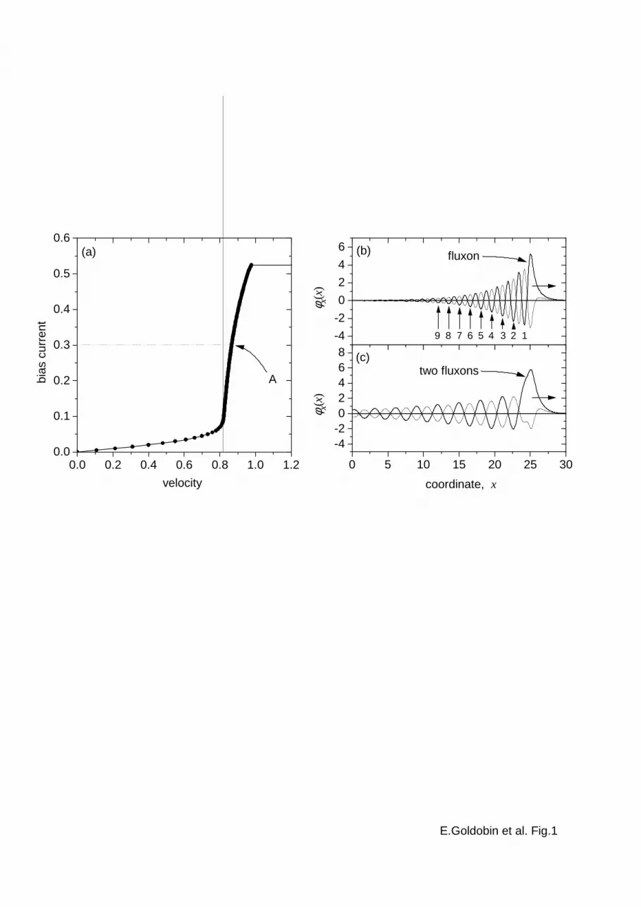
First, we simulated the IVC u(γ) in the [1|0] state, bysweeping γ from 0 up to 1 and making snapshots of phasegradients at every point of the IVC. This IVC is shownin Fig. 1(a), and the snapshot of the phase gradient atγ = 0.3 is presented in Fig. 1(b). As one can see, theCherenkov radiation tail, which is present for u > c−,has a sequence of minima where the second fluxon maybe trapped.

1. [1 + 1|0] state

In order to create a two-fluxon bunched state and checkits stability, we used the following “solution-engineering”procedure. By taking a snapshot of the phase profilesφA,B(x) at the bias value γ0 = 0.3, we constructed anansatz for the bunched solution in the form

φnewA,B(x) = φA,B(x) + φA,B(x + ∆x), (8)

where ∆x is chosen so that the center of the trailingfluxon is placed at one of the minima of the Cherenkovtail. For example, to trap the trailing fluxon in the first,second and third well, we used ∆x = 0.9, ∆x = 2.4and ∆x = 3.9, respectively. The phase distribution (andderivatives), constructed in this way, were used as theinitial condition for solving Eqs. (1) and (2) numerically.As the system relaxed to the desired state [1 + 1|0], wefurther traced u(γ) curve, varying γ0 down to 0 and upto 1.

We accomplished this procedure for a set of ∆x values,trying to trap the second fluxon in every well. Fig. 1(c)shows that a stable, tightly bunched state of two flux-ons is indeed possible. Actually, all the [1 + 1|0] statesobtained this way have been found to be stable, and wewere able to trace their IVCs up and down, starting fromthe initial value of the bias current γ = 0.3. For the casewhen the trailing fluxon is trapped in the first, secondand third minima, such IVCs are shown in Fig. 2.

The most interesting feature of these curves is thatthey correspond to the velocity of the bunched statethat is higher than that of the [1|0] state, at the samevalue of the bias current. Comparing solutions shownin Figs. 1(b) and 1(c), we see that the amplitude of thetrailing tail is smaller for the bunched state. This circum-stance suggests the following explanation to the fact thatthe observed velocity is higher in the state [1 + 1|0] thanin the single-fluxon one. Because the driving forces act-ing on two fluxons in the bunched and unbunched states

are the same, the difference in their velocities can be at-tributed only to the difference in the friction forces. Thefriction force acting on the fluxon in one junction is

Fα = α

∫ +∞

−∞

φxφt dx , (9)

and the same holds for the other junction. By just look-ing at Fig. 1(b) and (c) it is rather difficult to tell inwhich case the friction force is larger, but accurate cal-culations using Eq. (9) and profiles from Fig. 1(b) and (c)show that the friction force acting on two fluxons withthe tails shown in Fig. 1(b) is somewhat higher than thatfor Fig. 1(c). This result is not surprising if one recallsthat, to create the bunched state, we have shifted the[1|0] state by about half of the tail oscillation period rel-ative to the other single-fluxon state. Due to this, thetails of the two fluxons add up out of phase and partlycancel each other, making the tail’s amplitude behind thefluxon in the bunched state lower than that in the [1|0]state.

From Fig. 2 it is seen that every bunched state existsin a certain range of values of the bias current. If thecurrent is decreased below some threshold value, fluxonsdissociate and start moving apart, so that the interac-tion between them becomes exponentially small. Whenthe trailing fluxon sits in a minimum of the Cherenkovtail sufficiently far from the leading fluxon, the IVC cor-responding to this bunched state is almost undistinguish-able from that of the [1|0] state, as the two fluxons ap-proach the limit when they do not interact. We havefound that IVCs for M > 3, where M is the potentialwell’s number, is indeed almost identical to that of the[1|0] state. In contrast to bunching of fluxons in discreteLJJ9, the transitions from one bunched state to anotherwith different M do not take place in our system. Thus,we can say that the current range of a bunched state withsmaller M “eclipses” the bunched states with larger M .

The profiles of solutions found for various values ofthe bias current are shown in Fig. 3. We notice thatat the bottom of the step corresponding to the bunchedstate the radiation tail is much weaker and fluxons arebunched tighter. This is a direct consequence of the factthat at lower velocities the radiation wavelength and thedistance between minima becomes smaller, and so doesthe distance between the two fluxons. At a low bias cur-rent, the radiation wavelength and, hence, width of thepotential wells become very small and incommensurablewith the fluxon’s width. Therefore, the fluxon does notfit into the well and the bunched states virtually disap-pear.

2. [1|1] state

The initial condition for this state was constructed ina similar fashion to the [1 + 1|0] one, but now using across-sum of the shifted and unshifted solutions:

3

φnewA,B(x) = φA,B(x) + φB,A(x + ∆x). (10)

If for the [1 + 1|0] state, ∆x was ≈ (λ − 1

2)M , M =

1, 2 . . ., then in the [1|1] state we have to take ∆x ≈λM . We can also take M = 0 i.e., ∆x = 0, whichcorresponds to the degenerate case of the in-phase [1|1]state. The stability of this state was investigated in detailanalytically by Grønbech-Jensen and co-authors16, and isoutside the scope of this paper.

Our efforts to create a bound state [1|1] using the phasein the form (10) with M = 1, 2 . . . have not lead to anystable configuration of bunched fluxons with ∆x 6= 0.

3. Higher-order states

Looking at the phase gradient profiles shown in Fig. 3,one notes that these profiles are qualitatively very similarto the original profile of the soliton with a radiation tailbehind it [see Fig. 1(b)], with the only difference thatthere are two bunched solitons with a tail. So, we cantry to construct two pairs of bunched fluxons movingtogether, i.e., get a [2 + 2|0] bunched state. As before,the trapping of the trailing pair is possible in one of theminima of the tail generated by the leading pair. Toconstruct such a double-bunched state we employ theinitial conditions obtained using Eq. (8) at the bias pointγ0 = 0.3, using the steady phase distribution obtainedfor the [2|0] state at γ0 = 0.3. The shift ∆x was chosenin such a way that a pair of fluxons fits into one of theminima of the tail. We note that in this case we neededto vary ∆x a little bit before we have achieved trappingof the trailing pair in a desired well.

Simulations show that the obtained [2+2|0] states arestable and demonstrate an even higher velocity of thewhole four-fluxon aggregate. The corresponding IVCsand profiles are shown in Fig. 4(a) and (b), respectively.Note that at γ < 0.22 the bunched state [2 + 2|0] splitsfirst into [1 + 12 + 13 + 13|0] state (the subscripts denotethe well’s number M , counting from the previous fluxon),and at still lower bias current, γ < 0.2, they split intotwo independent [1 + 12|0] and [1 + 15|0] states. Thistwo states move with slightly different velocities and cancollide with each other due to the periodic nature of thesystem. As a result of collisions, these states ultimatelyundergo a transformation into two independent [1+15|0]states. As the bias decreases below ≈ 0.1, the velocity ubecomes smaller than c− and the Cherenkov radiationtails disappear. At this point, each of the [1 + 15|0]states smoothly transforms into two independent [1|0]states. The interaction between these states is exponen-tially small, with a characteristic length ∼ 1 (or, λJ inphysical units). We note that the interaction betweenkinks in the region u > c−, where they have tails, alsodecreases exponentially, but with a larger characteristiclength ∼ α−1.

The procedure of constructing higher-order bunchedstates can be performed using different states as “build-

ing blocks”. In particular, we also tried to form the[2 + 1|0] bunched state. Note that if two different statesare taken as building blocks, we need to match their ve-locities, and, hence, the wave lengths of the tail. Thus, wehave to combine two states at the same velocity, ratherthan at the same bias current. Since different states havetheir own velocity ranges, it is not always possible. Asan example, we have constructed a [2 + 1|0] state outof [2|0] state at γ = 0.15 and [1|0] state at γ = 0.45using an ansatz similar to (8). These states have ap-proximately the same velocity u ≈ 0.95 (see to Fig. 2).The constructed state was simulated, starting from thepoints γ = 0.3 and γ = 0.35, tracing IVC up and down asbefore. Depending on the bias current the system endsup in different states, namely in the state [1 + 11 + 12|0]for γ0 = 0.3, or in the state [1 + 11 + 11|0] = [3|0] forγ0 = 0.35. The IVCs of both states are shown in Fig. 4.The profiles of the phase gradients are shown in Fig. 4(c).

Our attempts to construct the states with a highernumber of bunched fluxons, e.g., [4+4|0], have failed sincefour fluxons do not fit into one well. We have concludedthat such states immediately get converted into one ofthe lower-order states.

C. Three coupled junctions

We have performed numerical simulation of Eqs. (3)and (4), using the same technique as described in theprevious section. Our intention here is to study the3-junction case in which the fluxon is put in the mid-dle junction ([0|1|0] state). All other parameters werethe same as in the case of the two-junction system, ex-cept for the ratio of the critical currents J , which wastaken equal to one. This simplest choice is made be-cause in a system of N > 2 coupled identical junctionsthe Cherenkov radiation appears in a [0| . . . |0|1|0| . . . |0]state for u > c− ≈ 0.765 (this pertains to S = −0.5).

Fig. 5 shows the IVCs of the original state [0|1|0],as well as IVCs of the bunched state [0|1 + 1|0] forM = 1, 2, 3. The profiles of the phase gradients atpoints A through D are shown in Fig. 6. Qualitatively,the bunching in the 3-fold system takes place in a sim-ilar fashion as that in the 2-fold system. Nevertheless,we did not succeed in creating a stable fluxon configura-tion with M = 3, although the stable states with otherM were obtained. We would like to mention, that whenthe second fluxon was put in the second minimum of thepotential to get the state with M = 2, the state withM = 1 has been finally established as a result of relax-ation. The same behavior was observed when we put thefluxon initially in the third minimum, the system endedup in the state [1 + 12|0]. For M ≥ 4, the behavior wasas usual. We tried to vary ∆x smoothly, so that the cen-ter of the trailing fluxon would correspond to differentpositions between the second and fourth well, but in thiscase we did not succeed to get [1 + 12|0] state.

4

Following the same way as for two coupled junctions,we tried to construct [0+1|1|0+1] states. As in the caseN = 2, these states were found unstable for any M > 0,e.g., they would split into [0|1 + 12|0] and [1| − 1|1]. Thestate [0|2+2|0] was not stable either for M = 1, 2, 3 andthe bias currents γ0 = 0.20, 0.30, 0.35.

The state [0|2 + 1|0] = [0|3|0], constructed by combin-ing the solutions for the [0|1|0] and [0|2|0] states movingwith equal velocities was found to be stable when start-ing at γ = 0.25 and sweeping bias current up and down.The dependence u(γ) is shown in Fig. 5. One may note,that for the states [0|2|0] and [0|3|0] the dependence isnot smooth. Indeed, for these states the Cherenkov radia-tion tail is so long (∼ L), that our annular system cannotsimulate an infinitely long system, resulting in Cherenkovresonances which inevitably appear in the system with afinite perimeter6,7.

III. ANALYSIS AND DISCUSSION

Because of the non-linear nature of the bunching prob-lem, it is hardly tractable analytically. Therefore, we herepresent an approach in which we analyze the asymptoticbehavior of the fluxon’s front and trailing tails in thelinear approximation. This technique is similar to thatemployed in Ref. 9. We assume that, at distances whichare large enough in comparison with the fluxon’s size, thefluxon’s profile is exponentially decaying,

φ(x, t) ∝ exp[p(x − ut)] , (11)

where p is a complex number which can be found bysubstituting this expression into Eqs. (1) and (2). As aresult we arrive at an equation∣

∣

∣

∣

∣

p2

1−S2 − p2u2 − 1 − αpu − Sp2

1−S2

− Sp2

1−S2

p2

1−S2 − p2u2 − 1

J− αpu

∣

∣

∣

∣

∣

= 0 ,

(12)

In general, this yields a 4-th order algebraic equationwhich always has 4 roots. If we want to describe a solitonmoving from left to right with a radiation tail behind it,we have to find the values p among the four roots whichadequately describe the front and rear parts of the soli-ton. Because the front (right) part of the soliton is notoscillating, it is described by Eq. (11) with real p < 0.The rear (left) part of the soliton is the oscillating tail,consequently it should be described by Eq. (11) with com-plex p having Re(p) > 0, the period of oscillations beingdetermined by the imaginary part of p. Analyzing the4-th order equation, we conclude that the two necessarytypes of the roots coexist only for u > c−, which is quitean obvious result.

To analyze the possibility of bunched state formation,we consider two fluxons situated at some distance fromeach other. We propose the following two conditions forthe two fluxons to form a bunched state:

1. Since non-oscillating tails result only in repulsionbetween fluxons, while the oscillating tail leads tomutual trapping, the condition

Re(pl) < |pr| , (13)

can be imposed to secure bunching. Here pl is theroot of Eq. (12) which describes the left (oscillat-ing) tail of the leading (right) fluxon, and pr is theroot of Eq. (12) which describes the right (non-oscillating) tail of the trailing (left) fluxon.

2. The relativistically contracted fluxon must fit intothe minimum of the tail, i.e.,

π

Im(p)>

√

u2

c2−

− 1 , (14)

where π/Im(p) is half of the wavelength of the tail-forming radiation (the well’s width), and the ex-pression on the r.h.s. of Eq. (14) approximatelycorresponds to the contraction of the fluxon at thetrans-Swihart velocities. Although our system isnot Lorentz invariant, numerical simulations showthat the fluxon indeed shrinks (not up to zero)when approaching the Swihart velocity c− fromboth sides.

Following this approach, we have found that the secondcondition (14) is always satisfied. The first condition (13)gives the following result. Bunching is possible at u >ub > c−. The value of ub can be calculated numericallyand for S = −0.5, J = 0.5, α = 0.04 it is ub = 0.837.Looking at Fig. 2, we see that this velocity corresponds tothe bias point where the [1 + 1M |0] states cease to exist.Thus, our crude approximation reasonably predicts thevelocity range where the bunching is possible.

IV. CONCLUSION

In this work we have shown by means of numericalsimulations that:

• The emission of the Cherenkov plasma waves by afluxon moving with high velocity creates an effec-tive potential with many wells, where other fluxonscan be trapped. This mechanism leads to bunchingbetween fluxons of the same polarity.

• We have proved numerically that in the system oftwo and three coupled junctions the bunched statesfor the fluxons in the same junction such as [1+1|0],[1 + 2|0], [2 + 2|0], [0|1 + 1|0] are stable. The stateswith fluxons in different junctions like [1|0+1] and[0+1|1|0+1] are numerically found unstable (exceptfor the degenerated case M = 0, when [1|1] is asimple in- phase state).

5

• Bunched fluxons propagate at a substantiallyhigher velocity than the corresponding free ones atthe same bias current, because of lower losses perfluxon.

• When decreasing the bias current, transitions be-tween the bunched states with different separationsbetween fluxons were not found. This behavior dif-fers from what is known for the bunched states in adiscrete system9. In addition, a splitting of multi-fluxon states into the states with smaller numbersof bunched fluxons is observed.

ACKNOWLEDGMENTS

This work was supported by a grant no. G0464-247.07/95 from the German-Israeli Foundation.

∗ e-mail: e.goldobin@fz-juelich.de , homepage: http://www.geocities.com/e goldobin

† e-mail: malomed@eng.tau.ac.il1 R. Kleiner, F. Steinmeyer, G. Kunkel, and P. Muller, Phys.Rev. Lett. 68, 2394 (1992);R. Kleiner and P. Muller, Phys. Rev. B 49, 1327 (1994).

2 R. Kleiner, P. Muller, H. Kohlstedt, N. F. Pedersen, andS. Sakai, Phys. Rev. B 73, 3942 (1994).

3 P. Muller, In: Festkorperprobleme Advances in Solid StatePhysics, vol. 34, ed. by Helbig (Vieweg, Braunschweig),p. 1 (1995).

4 A. V. Ustinov. In: Physics and Materials Science of VortexStates, Flux Pinning and Dynamics, NATO Science SeriesE, vol. 356, edited by R. Kossowsky et al., Kluwer Acad.Publ. (1999), pp. 465–488.

5 Yu. S. Kivshar and B. A. Malomed, Phys. Rev. B 37, 9325(1988).

6 E. Goldobin, A. Wallraff, N. Thyssen, and A. V. Ustinov,Phys. Rev. B 57, 130 (1998).

7 E. Goldobin, A. Wallraff, and A. V. Ustinov, accepted to J.Low Temp. Phys. (Nov 1999). see also cond-mat/9910234

8 G. Hechtfischer, R. Kleiner, A. V. Ustinov and P. Muller,Phys. Rev. Lett. 79, 1365 (1997).

9 A. V. Ustinov, B. A. Malomed, and S. Sakai, Phys. Rev. B57, 11691 (1998).

10 S. Sakai, Phys. Rev. B 36, 812 (1987).11 B. A. Malomed, Phys. Rev. B 47, 1111 (1993).12 I. V. Vernik, N. Lazarides, M. P. Sørensen, A. V. Ustinov,

N. F. Pedersen, and V. A. Oboznov, J. Appl. Phys. 79,7854 (1996).

13 S. Sakai, P. Bodin, and N. F. Pedersen. J. Appl. Phys. 73,2411 (1993).

14 E. Goldobin, A. Golubov, A. V. Ustinov, Czech. J. Phys.46, 663 (1996), LT-21 Suppl. S2

15 E. Goldobin, available online: http://www.geocities.com/SiliconValley/Heights/7318/StkJJ.htm (1999).

16 N. Grønbech-Jensen, D. Cai and M. R. Samuelsen, Phys.Rev. B 48, 16160 (1993).

FIG. 1. (a) The current-velocity characteristic u(γ) forthe fluxon moving in the [1|0] state (from left to right). (b)The profiles of the phase gradients φA,B

x (x) in the state [1|0] atγ = 0.3, corresponding to the bias point A shown in Fig. (a).The Cherenkov tail, present at u > c− ≈ 0.817, has a setof minima where the second fluxon can be trapped. (c) Theprofiles of φA,B

x (x) in the state [2|0] at the same value γ = 0.3as (b). Two fluxons shown in Fig. (c) are almost undistin-guishable.

FIG. 2. Current-velocity characteristics of differentbunched states [2|0]: the second fluxon is trapped in the firstminimum of the tail (state [1 + 11|0]), the second minimum(state [1 + 12|0]), and the third minimum (state [1 + 13|0]).The γ(u) curve for the [1|0] state is shown for comparison.The phase-gradient profiles corresponding to the bias pointsA through D are shown in Fig. 3.

FIG. 3. The profiles of the phase gradients φA,Bx (x) in the

[2|0] states at the bias points A through D marked in Fig. 2.

FIG. 4. (a) Current-velocity characteristics of thebunched states [4|0], [3|0], and [2 + 1|0]. Phase profiles of[4|0] state and [3|0] state at γ = 0.3 are shown in (b) and (c),respectively.

FIG. 5. Current-velocity characteristics of the state[0|1|0], bunched state [0|1 + 1M |0] for three different cases,M = 1, 2, 3, and the state [0|3|0]. The profiles of the Joseph-son phase gradients at the points A through D are shown inFig. 6

FIG. 6. The profiles of the Josephson phase gradientsφA,B

x (x) in [0|1 + 1M |0] states at the points A through Dmarked in Fig. 5.

6

0.0

0.1

0.2

0.3

0.4

0.5

0.6

0.0 0.2 0.4 0.6 0.8 1.0 1.2

(a)

A

velocity

bias

cur

rent

-4

-2

0

2

4

6

9 8 7 6 5 4 13 2

fluxon(b)

E.Goldobin et al. Fig.1

φ x(x)

0 5 10 15 20 25 30

-4-202468

two fluxons(c)

coordinate, x

φ x(x)

���

���

���

���

���

���

���

��� ��� ��� ��� ��� ���XEFB

>�_�@

>����_�@ >��� �_�@

>��� �_�

@

'

&

%

(�*ROGRELQ�HW�DO���)LJ���

$

YHORFLW\

ELDV�F

XUUHQ

W

-4

-2

0

2

4

6

two bunched fluxons

(a)

φ x(x)

-4

-2

0

2

4

6

two bunched fluxons

E.Goldobin et al. Fig. 3

(b)

φ x(x)

-4

-2

0

2

4

6 first fluxon

second fluxon

(c)

φ x(x)

0 10 20 30

-4

-2

0

2

4

6

second fluxonfirst fluxon(d)

φ x(x)

coordinate, x

���

���

���

���

���

���

���

��� ��� ��� ��� ��� ���

%

�D�

>�_�@�>�_�@

>��� ��

� �_�@

FB

>�_�@

$

>����������_�@

>�_�@

>�_�@

(�*ROGRELQ�HW�DO���)LJ���

�u>����_�@

YHORFLW\

ELDV�F

XUUHQW

��������

>�����������_�@ >�_�@

�E�

�I [�

[�

� �� �� ����������

>�������_�@ >�_�@

�F�I [�[�

FRRUGLQDWH���[

���

���

���

���

���

���

���

��� ��� ��� ��� ��� ���

>�_�_�@

F_

>�_����_�@

>�_����_�@

>�_��� �

_�@

'

&%

(�*ROGRELQ�HW�DO���)LJ���

$

YHORFLW\

ELDV�F

XUUHQ

W

��������

>�_����_�@�#�J� �����

�D�

�

I [�[ �

��������

>�_����_�@�#�J� �����

(�*ROGRELQ�HW�DO���)LJ���

�E�

I [�[ �

��������

>�_����_�@�#�J� �����

�F�

�

I [�[ �

� �� �� ����������

>�_����_�@�#�J� �����

�G�

I [�[ �

FRRUGLQDWH���[