building loss models - munich personal repec archive

Munich Personal RePEc Archive

Building Loss Models

Burnecki, Krzysztof and Janczura, Joanna and Weron, Rafal

Wrocław University of Technology, Poland

September 2010

Online at https://mpra.ub.uni-muenchen.de/25492/

MPRA Paper No. 25492, posted 28 Sep 2010 20:42 UTC

Building Loss Models1

Krzysztof Burnecki2, Joanna Janczura

2, and Rafał Weron

3

Abstract: This paper is intended as a guide to building insurance risk (loss)

models. A typical model for insurance risk, the so-called collective risk model,

treats the aggregate loss as having a compound distribution with two main

components: one characterizing the arrival of claims and another describing the

severity (or size) of loss resulting from the occurrence of a claim. In this paper we

first present efficient simulation algorithms for several classes of claim arrival

processes. Then we review a collection of loss distributions and present methods

that can be used to assess the goodness-of-fit of the claim size distribution. The

collective risk model is often used in health insurance and in general insurance,

whenever the main risk components are the number of insurance claims and the

amount of the claims. It can also be used for modeling other non-insurance

product risks, such as credit and operational risk.

Keywords: Insurance risk model; Loss distribution; Claim arrival process; Poisson

process; Renewal process; Random variable generation; Goodness-of-fit testing

JEL: C15, C46, C63, G22, G32

1 Chapter prepared for the 2

nd edition of Statistical Tools for Finance and Insurance, P.Cizek,

W.Härdle, R.Weron (eds.), Springer-Verlag, forthcoming in 2011.

2 Hugo Steinhaus Center, Wrocław University of Technology, Poland

3 Institute of Organization and Management, Wrocław University of Technology, Poland

1 Building Loss Models

Krzysztof Burnecki, Joanna Janczura, and Rafa l Weron

1.1 Introduction

A loss model or actuarial risk model is a parsimonious mathematical descrip-tion of the behavior of a collection of risks constituting an insurance portfolio.It is not intended to replace sound actuarial judgment. In fact, according toWillmot (2001), a well formulated model is consistent with and adds to intu-ition, but cannot and should not replace experience and insight. Moreover, aproperly constructed loss model should reflect a balance between simplicity andconformity to the data since overly complex models may be too complicated tobe useful.

A typical model for insurance risk, the so-called collective risk model, treats theaggregate loss as having a compound distribution with two main components:one characterizing the frequency (or incidence) of events and another describingthe severity (or size or amount) of gain or loss resulting from the occurrence ofan event (Kaas et al., 2008; Klugman, Panjer, and Willmot, 2008; Tse, 2009).The stochastic nature of both components is a fundamental assumption of arealistic risk model. In classical form it is defined as follows. If {Nt}t≥0 is aprocess counting claim occurrences and {Xk}∞k=1 is an independent sequenceof positive independent and identically distributed (i.i.d.) random variablesrepresenting claim sizes, then the risk process {Rt}t≥0 is given by

Rt = u+ c(t) −Nt∑

i=1

Xi. (1.1)

The non-negative constant u stands for the initial capital of the insurancecompany and the deterministic or stochastic function of time c(t) for the pre-

mium from sold insurance policies. The sum {∑Nt

i=1Xi} is the so-called ag-

2 1 Building Loss Models

gregate claim process, with the number of claims in the interval (0, t] beingmodeled by the counting process Nt. Recall, that the latter is defined asNt = max{n :

∑ni=1Wi ≤ t}, where {Wi}∞i=0 is a sequence of positive ran-

dom variables and∑0

i=1Wi ≡ 0. In the insurance risk context Nt is alsoreferred to as the claim arrival process.

The collective risk model is often used in health insurance and in general insur-ance, whenever the main risk components are the number of insurance claimsand the amount of the claims. It can also be used for modeling other non-insurance product risks, such as credit and operational risk (Chernobai, Rachev,and Fabozzi, 2007; Panjer, 2006). In the former, for example, the main riskcomponents are the number of credit events (either defaults or downgrades),and the amount lost as a result of the credit event.

The simplicity of the risk process defined in eqn. (1.1) is only illusionary. Inmost cases no analytical conclusions regarding the time evolution of the processcan be drawn. However, it is this evolution that is important for practitioners,who have to calculate functionals of the risk process like the expected time toruin and the ruin probability, see Chapter ??. The modeling of the aggregateclaim process consists of modeling the counting process {Nt} and the claim sizesequence {Xk}. Both processes are usually assumed to be independent, hencecan be treated independently of each other (Burnecki, Hardle, and Weron,2004). Modeling of the claim arrival process {Nt} is treated in Section 1.2,where we present efficient algorithms for four classes of processes. Modeling ofclaim severities and testing the goodness-of-fit is covered in Sections 1.3 and1.4, respectively. Finally, in Section 1.5 we build a model for the Danish firelosses dataset, which concerns major fire losses in profits that occurred between1980 and 2002 and were recorded by Copenhagen Re.

1.2 Claim Arrival Processes

In this section we focus on efficient simulation of the claim arrival process{Nt}. This process can be simulated either via the arrival times {Ti}, i.e. mo-ments when the ith claim occurs, or the inter-arrival times (or waiting times)Wi = Ti − Ti−1, i.e. the time periods between successive claims (Burnecki andWeron, 2005). Note that in terms of Wi’s the claim arrival process is given byNt =

∑∞

n=1 I(Tn ≤ t). In what follows we discuss four examples of {Nt},namely the classical (homogeneous) Poisson process, the non-homogeneousPoisson process, the mixed Poisson process and the renewal process.

1.2 Claim Arrival Processes 3

1.2.1 Homogeneous Poisson Process (HPP)

The most common and best known claim arrival process is the homogeneousPoisson process (HPP). It has stationary and independent increments and thenumber of claims in a given time interval is governed by the Poisson law. Whilethis process is normally appropriate in connection with life insurance modeling,it often suffers from the disadvantage of providing an inadequate fit to insurancedata in other coverages with substantial temporal variability.

Formally, a continuous-time stochastic process {Nt : t ≥ 0} is a (homogeneous)Poisson process with intensity (or rate) λ > 0 if (i) {Nt} is a counting process,and (ii) the waiting times Wi are independent and identically distributed andfollow an exponential law with intensity λ, i.e. with mean 1/λ (see Section1.3.2). This definition naturally leads to a simulation scheme for the successivearrival times Ti of the Poisson process on the interval (0, t]:

Algorithm HPP1 (Waiting times)

Step 1: set T0 = 0

Step 2: generate an exponential random variable E with intensity λ

Step 3: if Ti−1 + E < t then set Ti = Ti−1 + E and return to step 2 else stop

Sample trajectories of homogeneous (and non-homogeneous) Poisson processesare plotted in the top panels of Figure 1.1. The thin solid line is a HPP withintensity λ = 1 (left) and λ = 10 (right). Clearly the latter jumps more often.

Alternatively, the homogeneous Poisson process can be simulated by applyingthe following property (Rolski et al., 1999). Given that Nt = n, the n oc-currence times T1, T2, . . . , Tn have the same distribution as the order statisticscorresponding to n i.i.d. random variables uniformly distributed on the inter-val (0, t]. Hence, the arrival times of the HPP on the interval (0, t] can begenerated as follows:

Algorithm HPP2 (Conditional theorem)

Step 1: generate a Poisson random variable N with intensity λt

Step 2: generate N random variables Ui distributed uniformly on (0, 1), i.e.Ui ∼ U(0, 1), i = 1, 2, . . . , N

Step 3: set (T1, T2, . . . , TN) = t · sort{U1, U2, . . . , UN}


0 2 4 6 8 100

10

20

30

40

50

60

70

t

N(t

)

0 1 2 3 4 50

10

20

30

40

50

60

70

t

N(t

)

λ(t)=1+0⋅tλ(t)=1+0.1⋅tλ(t)=1+1⋅t

λ(t)=10+0⋅cos(2πt)

λ(t)=10+1⋅cos(2πt)

λ(t)=10+10⋅cos(2πt)

0 0.5 1 1.5 2 2.5 330

40

50

60

70

80

Time (years)

Nu

mb

er

of

eve

nts

pe

r d

ay

Claim intensity

November−December

Figure 1.1: Top left panel : Sample trajectories of a NHPP with linear intensityλ(t) = a+ b · t. Note that the first process (with b = 0) is in fact aHPP. Top right panel : Sample trajectories of a NHPP with periodicintensity λ(t) = a+ b · cos(2πt). Again, the first process is a HPP.Bottom panel : Intensity of car accident claims in Greater Wroc lawarea, Poland, in the period 1998-2000 (data from one of the majorinsurers in the region). Note, the larger number of accidents in lateFall/early Winter due to worse weather conditions.

STF2loss01.m

In general, this algorithm will run faster than HPP1 as it does not involve aloop. The only two inherent numerical difficulties involve generating a Poissonrandom variable and sorting a vector of occurrence times. Whereas the latterproblem can be solved, for instance, via the standard quicksort algorithm im-plemented in most statistical software packages (like sortrows.m in Matlab),the former requires more attention.


A straightforward algorithm to generate a Poisson random variable would take

N = min{n : U1 · . . . · Un < exp(−λ)} − 1, (1.2)

which is a consequence of the properties of the HPP (see above). However, forlarge λ, this method can become slow as the expected run time is proportionalto λ. Faster, but more complicated methods are available. Ahrens and Dieter(1982) suggested a generator which utilizes acceptance-complement with trun-cated normal variates for λ > 10 and reverts to table-aided inversion otherwise.Stadlober (1989) adapted the ratio of uniforms method for λ > 5 and classicalinversion for small λ’s. Hormann (1993) advocated the transformed rejectionmethod, which is a combination of the inversion and rejection algorithms. Sta-tistical software packages often use variants of these methods. For instance,Matlab’s poissrnd.m function uses the waiting time method (1.2) for λ < 15and Ahrens’ and Dieter’s method for larger values of λ.

Finally, since for the HPP the expected value of the process E(Nt) = λt, itis natural to define the premium function as c(t) = ct, where c = (1 + θ)µλand µ = E(Xk). The parameter θ > 0 is the relative safety loading which“guarantees” survival of the insurance company. With such a choice of thepremium function we obtain the classical form of the risk process:

Rt = u+ (1 + θ)µλt −Nt∑

i=1

Xi. (1.3)

1.2.2 Non-Homogeneous Poisson Process (NHPP)

The choice of a homogeneous Poisson process implies that the size of the port-folio cannot increase or decrease. In addition, it cannot describe situations,like in motor insurance, where claim occurrence epochs are likely to dependon the time of the year (worse weather conditions in Central Europe in lateFall/early Winter lead to more accidents, see the bottom panel in Figure 1.1)or of the week (heavier traffic occurs on Friday afternoons and before holidays).For modeling such phenomena the non-homogeneous Poisson process (NHPP)is much better. The NHPP can be thought of as a Poisson process with avariable (but predictable) intensity defined by the deterministic intensity (orrate) function λ(t). Note that the increments of a NHPP do not have to be sta-tionary. In the special case when the intensity takes a constant value λ(t) = λ,the NHPP reduces to the homogeneous Poisson process with intensity λ.


The simulation of the process in the non-homogeneous case is slightly morecomplicated than for the HPP. The first approach, known as the thinning orrejection method, is based on the following fact (Bratley, Fox, and Schrage,1987; Ross, 2002). Suppose that there exists a constant λ such that λ(t) ≤ λfor all t. Let T ∗

1 , T∗2 , T

∗3 , . . . be the successive arrival times of a homogeneous

Poisson process with intensity λ. If we accept the ith arrival time T ∗i with

probability λ(T ∗i )/λ, independently of all other arrivals, then the sequence

{Ti}∞i=0 of the accepted arrival times (in ascending order) forms a sequence ofthe arrival times of a non-homogeneous Poisson process with the rate functionλ(t). The resulting simulation algorithm on the interval (0, t] reads as follows:

Algorithm NHPP1 (Thinning)

Step 1: set T0 = 0 and T ∗ = 0

Step 2: generate an exponential random variable E with intensity λ

Step 3: if T ∗ + E < t then set T ∗ = T ∗ + E else stop

Step 4: generate a random variable U distributed uniformly on (0, 1)

Step 5: if U < λ(T ∗)/λ then set Ti = T ∗ (→ accept the arrival time)

Step 6: return to step 2

As mentioned in the previous section, the inter-arrival times of a homogeneousPoisson process have an exponential distribution. Therefore steps 2–3 gener-ate the next arrival time of a homogeneous Poisson process with intensity λ.Steps 4–5 amount to rejecting (hence the name of the method) or accepting aparticular arrival as part of the thinned process (hence the alternative name).Note, that in this algorithm we generate a HPP with intensity λ employing theHPP1 algorithm. We can also generate it using the HPP2 algorithm, which ingeneral is much faster.

The second approach is based on the observation that for a NHPP with ratefunction λ(t) the increment Nt − Ns, 0 < s < t, is distributed as a Poisson

random variable with intensity λ =∫ t

sλ(u)du (Grandell, 1991). Hence, the

cumulative distribution function Fs of the waiting time Ws is given by

Fs(t) = P(Ws ≤ t) = 1 − P(Ws > t) = 1 − P(Ns+t −Ns = 0) =

= 1 − exp

{−∫ s+t

s

λ(u)du

}= 1 − exp

{−∫ t

0

λ(s+ v)dv

}.


If the function λ(t) is such that we can find a formula for the inverse F−1s for

each s, we can generate a random quantity X with the distribution Fs by usingthe inverse transform method. The simulation algorithm on the interval (0, t],often called the integration method, can be summarized as follows:

Algorithm NHPP2 (Integration)

Step 1: set T0 = 0

Step 2: generate a random variable U distributed uniformly on (0, 1)

Step 3: if Ti−1 +F−1s (U) < t set Ti = Ti−1 +F−1

s (U) and return to step 2 elsestop

The third approach utilizes a generalization of the property used in the HPP2algorithm. Given that Nt = n, the n occurrence times T1, T2, . . . , Tn of thenon-homogeneous Poisson process have the same distributions as the orderstatistics corresponding to n independent random variables distributed on theinterval (0, t], each with the common density function f(v) = λ(v)/

∫ t

0λ(u)du,

where v ∈ (0, t]. Hence, the arrival times of the NHPP on the interval (0, t] canbe generated as follows:

Algorithm NHPP3 (Conditional theorem)

Step 1: generate a Poisson random variable N with intensity∫ t

0λ(u)du

Step 2: generate N random variables Vi, i = 1, 2, . . .N with density f(v) =

λ(v)/∫ t

0λ(u)du.

Step 3: set (T1, T2, . . . , TN) = sort{V1, V2, . . . , VN}.

The performance of the algorithm is highly dependent on the efficiency of thecomputer generator of random variables Vi. Simulation of Vi’s can be doneeither via the inverse transform method by integrating the density f(v) orvia the acceptance-rejection technique using the uniform distribution on theinterval (0, t) as the reference distribution. In a sense, the former approachleads to Algorithm NHPP2, whereas the latter one to Algorithm NHPP1.

Sample trajectories of non-homogeneous Poisson processes are plotted in thetop panels of Figure 1.1. In the top left panel realizations of a NHPP withlinear intensity λ(t) = a + b · t are presented for the same value of parameter


a. Note, that the higher the value of parameter b, the more pronounced is theincrease in the intensity of the process. In the top right panel realizations of aNHPP with periodic intensity λ(t) = a+ b · cos(2πt) are illustrated, again forthe same value of parameter a. This time, for high values of parameter b theevents exhibit a seasonal behavior. The process has periods of high activity(grouped around natural values of t) and periods of low activity, where almostno jumps take place. Such a process is much better suited to model the seasonalintensity of car accident claims (see the bottom panel in Figure 1.1) than theHPP.

Finally, we note that since in the non-homogeneous case the expected value ofthe process at time t is E(Nt) =

∫ t

0λ(s)ds, it is natural to define the premium

function as c(t) = (1 + θ)µ∫ t

0λ(s)ds. Then the risk process takes the form:

Rt = u+ (1 + θ)µ

∫ t

0

λ(s)ds−Nt∑

i=1

Xi. (1.4)

1.2.3 Mixed Poisson Process

In many situations the portfolio of an insurance company is diversified in thesense that the risks associated with different groups of policy holders are sig-nificantly different. For example, in motor insurance we might want to make adifference between male and female drivers or between drivers of different age.We would then assume that the claims come from a heterogeneous group ofclients, each one of them generating claims according to a Poisson distributionwith the intensity varying from one group to another.

Another practical reason for considering yet another generalization of the clas-sical Poisson process is the following. If we measure the volatility of risk pro-cesses, expressed in terms of the index of dispersion Var(Nt)/E(Nt), then oftenwe obtain estimates in excess of one – a value obtained for the homogeneousand the non-homogeneous cases. These empirical observations led to the intro-duction of the mixed Poisson process (MPP), see Rolski et al. (1999).

In the mixed Poisson process the distribution of {Nt} is given by a mixedPoisson distribution (Rolski et al., 1999). This means that, conditioning on anextrinsic random variable Λ (called a structure variable), the random variable{Nt} has a Poisson distribution. Typical examples for Λ are two-point, gammaand general inverse Gaussian distributions (Teugels and Vynckier, 1996). Since


for each t the claim numbers {Nt} up to time t are Poisson variates withintensity Λt, it is now reasonable to consider the premium function of the formc(t) = (1+θ)µΛt. This leads to the following representation of the risk process:

Rt = u+ (1 + θ)µΛt−Nt∑

i=1

Xi. (1.5)

The MPP can be generated using the uniformity property: given that Nt = n,the n occurrence times T1, T2, . . . , Tn have the same joint distribution as theorder statistics corresponding to n i.i.d. random variables uniformly distributedon the interval (0, t] (Albrecht, 1982). The procedure starts with the simulationof n as a realization ofNt for a given value of t. This can be done in the followingway: first a realization of a non-negative random variable Λ is generated and,conditioned upon its realization, Nt is simulated according to the Poisson lawwith parameter Λt. Then we simulate n uniform random numbers in (0, t).After rearrangement, these values yield the sample T1 ≤ . . . ≤ Tn of occurrencetimes. The algorithm is summarized below.

Algorithm MPP1 (Conditional theorem)

Step 1: generate a mixed Poisson random variable N with intensity Λt

Step 2: generate N random variables Ui distributed uniformly on (0, 1), i.e.Ui ∼ U(0, 1), i = 1, 2, . . . , N

Step 3: set (T1, T2, . . . , TN) = t · sort{U1, U2, . . . , UN}

1.2.4 Renewal Process

Generalizing the homogeneous Poisson process we come to the point whereinstead of making λ non-constant, we can make a variety of different distribu-tional assumptions on the sequence of waiting times {W1,W2, . . .} of the claimarrival process {Nt}. In some particular cases it might be useful to assume thatthe sequence is generated by a renewal process, i.e. the random variables Wi

are i.i.d., positive with a distribution function F . Note that the homogeneousPoisson process is a renewal process with exponentially distributed inter-arrivaltimes. This observation lets us write the following algorithm for the generationof the arrival times of a renewal process on the interval (0, t]:


Algorithm RP1 (Waiting times)

Step 1: set T0 = 0

Step 2: generate an F -distributed random variable X

Step 3: if Ti−1 +X < t then set Ti = Ti−1 +X and return to step 2 else stop

An important point in the previous generalizations of the Poisson process wasthe possibility to compensate risk and size fluctuations by the premiums. Thus,the premium rate had to be constantly adapted to the development of theclaims. For renewal claim arrival processes, a constant premium rate allowsfor a constant safety loading (Embrechts and Kluppelberg, 1993). Let {Nt}be a renewal process and assume that W1 has finite mean 1/λ. Then thepremium function is defined in a natural way as c(t) = (1 + θ)µλt, like for thehomogeneous Poisson process, which leads to the risk process of the form (1.3).

1.3 Loss Distributions

There are three basic approaches to deriving the loss distribution: empirical,analytical, and moment based. The empirical method, presented in Section1.3.1, can be used only when large data sets are available. In such cases asufficiently smooth and accurate estimate of the cumulative distribution func-tion (cdf) is obtained. Sometimes the application of curve fitting techniques –used to smooth the empirical distribution function – can be beneficial. If thecurve can be described by a function with a tractable analytical form, then thisapproach becomes computationally efficient and similar to the second method.

The analytical approach is probably the most often used in practice and cer-tainly the most frequently adopted in the actuarial literature. It reduces tofinding a suitable analytical expression which fits the observed data well andwhich is easy to handle. Basic characteristics and estimation issues for themost popular and useful loss distributions are discussed in Sections 1.3.2-1.3.8.Note, that sometimes it may be helpful to subdivide the range of the claimsize distribution into intervals for which different methods are employed. Forexample, the small and medium size claims could be described by the empiricalclaim size distribution, while the large claims – for which the scarcity of dataeliminates the use of the empirical approach – by an analytical loss distribution.

In some applications the exact shape of the loss distribution is not required.We may then use the moment based approach, which consists of estimating

1.3 Loss Distributions 11

only the lowest characteristics (moments) of the distribution, like the meanand variance. However, it should be kept in mind that even the lowest threeor four moments do not fully define the shape of a distribution, and thereforethe fit to the observed data may be poor. Further details on the moment basedapproach can be found e.g. in Daykin, Pentikainen, and Pesonen (1994).

Having a large collection of distributions to choose from, we need to narrowour selection to a single model and a unique parameter estimate. The type ofthe objective loss distribution can be easily selected by comparing the shapesof the empirical and theoretical mean excess functions. Goodness-of-fit canbe measured by tests based on the empirical distribution function. Finally,the hypothesis that the modeled random event is governed by a certain lossdistribution can be statistically tested. In Section 1.4 these statistical issuesare thoroughly discussed.

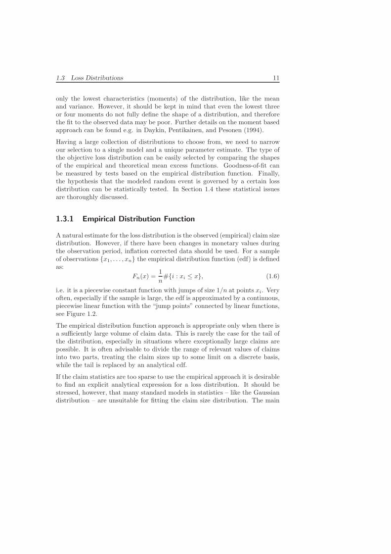
1.3.1 Empirical Distribution Function

A natural estimate for the loss distribution is the observed (empirical) claim sizedistribution. However, if there have been changes in monetary values duringthe observation period, inflation corrected data should be used. For a sampleof observations {x1, . . . , xn} the empirical distribution function (edf) is definedas:

Fn(x) =1

n#{i : xi ≤ x}, (1.6)

i.e. it is a piecewise constant function with jumps of size 1/n at points xi. Veryoften, especially if the sample is large, the edf is approximated by a continuous,piecewise linear function with the “jump points” connected by linear functions,see Figure 1.2.

The empirical distribution function approach is appropriate only when there isa sufficiently large volume of claim data. This is rarely the case for the tail ofthe distribution, especially in situations where exceptionally large claims arepossible. It is often advisable to divide the range of relevant values of claimsinto two parts, treating the claim sizes up to some limit on a discrete basis,while the tail is replaced by an analytical cdf.

If the claim statistics are too sparse to use the empirical approach it is desirableto find an explicit analytical expression for a loss distribution. It should bestressed, however, that many standard models in statistics – like the Gaussiandistribution – are unsuitable for fitting the claim size distribution. The main


0 1 2 3 4 50

0.2

0.4

0.6

0.8

1

x

cdf(

x)

0 1 2 3 4 50

0.2

0.4

0.6

0.8

1

x

cdf(

x)

Empirical df (edf)

Lognormal cdf

Approx. of the edf

Figure 1.2: Left panel : Empirical distribution function (edf) of a 10-elementlog-normally distributed sample with parameters µ = 0.5 andσ = 0.5, see Section 1.3.5. Right panel : Approximation of theedf by a continuous, piecewise linear function superimposed on thetheoretical distribution function.

STF2loss02.m

reason for this is the strongly skewed nature of loss distributions. The log-normal, Pareto, Burr, and Weibull distributions are typical candidates to beconsidered in applications. However, before we review these probability lawswe introduce two very versatile distributions – the exponential and gamma.

1.3.2 Exponential Distribution

Consider the random variable with the following density and distribution func-tions, respectively:

f(x) = βe−βx, x > 0, (1.7)

F (x) = 1 − e−βx, x > 0. (1.8)

This distribution is called the exponential distribution with parameter (or in-tensity) β > 0. The Laplace transform of (1.7) is

L(t)def=

∫ ∞

0

e−txf(x)dx =β

β + t, t > −β, (1.9)


yielding the general formula for the k-th raw moment

mkdef= (−1)k ∂

kL(t)

∂tk

∣∣∣t=0

=k!

βk. (1.10)

The mean and variance are thus β−1 and β−2, respectively. The maximumlikelihood estimator (equal to the method of moments estimator) for β is givenby:

β =1

m1, (1.11)

where

mk =1

n

n∑

i=1

xki , (1.12)

is the sample k-th raw moment.

To generate an exponential random variable X with intensity β we can usethe inverse transform (or inversion) method (Devroye, 1986; Ross, 2002). Themethod consists of taking a random number U distributed uniformly on theinterval (0, 1) and setting X = F−1(U), where F−1(x) = − 1

β log(1 − x) is the

inverse of the exponential cdf (1.8). In fact we can set X = − 1β logU since

(1 − U) has the same distribution as U .

The exponential distribution has many interesting features. As we have seenin Section 1.2.1, it arises as the inter-occurrence time of the events in a HPP. Ithas the memoryless property, i.e. P(X > x+ y|X > y) = P(X > x). Further,the n-th root of the Laplace transform (1.9) is

L(t) =

(β

β + t

) 1

n

, (1.13)

which is the Laplace transform of a gamma variate (see Section 1.3.4). Thusthe exponential distribution is infinitely divisible.

The exponential distribution is often used in developing models of insurancerisks. This usefulness stems in a large part from its many and varied tractablemathematical properties. However, a disadvantage of the exponential distri-bution is that its density is monotone decreasing (see Figure 1.3), a situationwhich may not be appropriate in some practical situations.


0 2 4 6 80

0.2

0.4

0.6

0.8

x

pd

f(x)

Exp(0.3)

Exp(1)

MixExp(0.5,0.3,1)

0 2 4 6 810

−2

10−1

100

x

pd

f(x)

Figure 1.3: Left panel: A probability density function (pdf) of a mixture of twoexponential distributions with mixing parameter a = 0.5 superim-posed on the pdfs of the component distributions. Right panel:

Semi-logarithmic plots of the pdfs displayed in the left panel. Theexponential pdfs are now straight lines with slopes −β. Note, thecurvature of the pdf of the mixture of two exponentials.

STF2loss03.m

1.3.3 Mixture of Exponential Distributions

Using the technique of mixing one can construct a wide class of distributions.The most commonly used in applications is a mixture of two exponentials, seeChapter ??. In Figure 1.3 a pdf of a mixture of two exponentials is plottedtogether with the pdfs of the mixing laws. Note, that the mixing procedurecan be applied to arbitrary distributions.

The construction goes as follows. Let a1, a2, . . . , an denote a series of non-negative weights satisfying

∑ni=1 ai = 1. Let F1(x), F2(x), . . . , Fn(x) denote an

arbitrary sequence of exponential distribution functions given by the parame-ters β1, β2, . . . , βn, respectively. Then, the distribution function:

F (x) =

n∑

i=1

aiFi(x) =

n∑

i=1

ai {1 − exp(−βix)} , (1.14)

is called a mixture of n exponential distributions (exponentials). The density


function of the constructed distribution is

f(x) =n∑

i=1

aifi(x) =n∑

i=1

aiβi exp(−βix), (1.15)

where f1(x), f2(x), . . . , fn(x) denote the density functions of the input expo-nential distributions. The Laplace transform of (1.15) is

L(t) =

n∑

i=1

aiβi

βi + t, t > − min

i=1...n{βi}, (1.16)

yielding the general formula for the k-th raw moment

mk =

n∑

i=1

aik!

βki

. (1.17)

The mean is thus∑n

i=1 aiβ−1i . The maximum likelihood and method of mo-

ments estimators for the mixture of n (n ≥ 2) exponential distributions canonly be evaluated numerically.

Simulation of variates defined by (1.14) can be performed using the compositionapproach (Ross, 2002). First generate a random variable I, equal to i withprobability ai, i = 1, ..., n. Then simulate an exponential variate with intensityβI . Note, that the method is general in the sense that it can be used for anyset of distributions Fi’s.

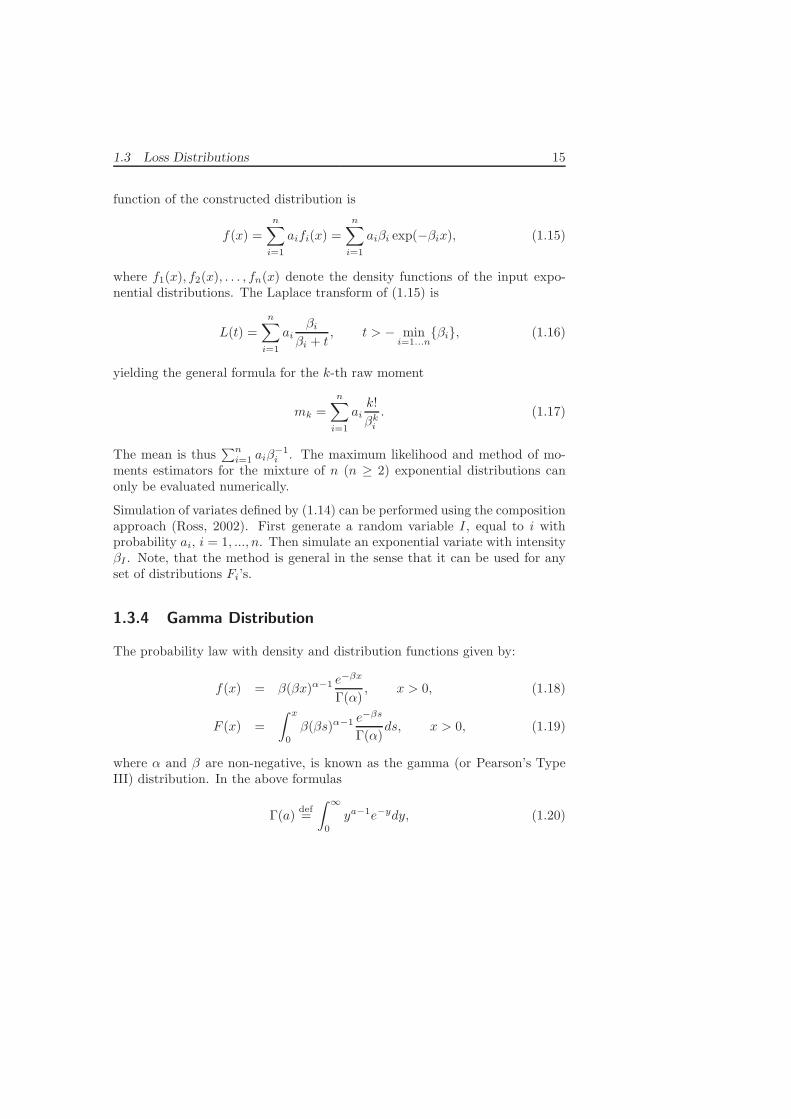
1.3.4 Gamma Distribution

The probability law with density and distribution functions given by:

f(x) = β(βx)α−1 e−βx

Γ(α), x > 0, (1.18)

F (x) =

∫ x

0

β(βs)α−1 e−βs

Γ(α)ds, x > 0, (1.19)

where α and β are non-negative, is known as the gamma (or Pearson’s TypeIII) distribution. In the above formulas

Γ(a)def=

∫ ∞

0

ya−1e−ydy, (1.20)


is the standard gamma function. Moreover, for β = 1 the integral in (1.19):

Γ(α, x)def=

1

Γ(α)

∫ x

0

sα−1e−sds, (1.21)

is called the incomplete gamma function. If the shape parameter α = 1, theexponential distribution results. If α is a positive integer, the distribution iscalled an Erlang law. If β = 1

2 and α = ν2 then it is called a chi-squared

(χ2) distribution with ν degrees of freedom, see the top panels in Figure 1.4.Moreover, a mixed Poisson distribution with gamma mixing distribution isnegative binomial.

The gamma distribution is closed under convolution, i.e. a sum of indepen-dent gamma variates with the same parameter β is again gamma distributedwith this β. Hence, it is infinitely divisible. Moreover, it is right-skewed andapproaches a normal distribution in the limit as α goes to infinity.

The Laplace transform of the gamma distribution is given by:

L(t) =

(β

β + t

)α

, t > −β. (1.22)

The k-th raw moment can be easily derived from the Laplace transform:

mk =Γ(α+ k)

Γ(α)βk. (1.23)

Hence, the mean and variance are

E(X) =α

β, (1.24)

Var(X) =α

β2. (1.25)

Finally, the method of moments estimators for the gamma distribution param-eters have closed form expressions:

α =m2

1

m2 − m21

, (1.26)

β =m1

m2 − m21

, (1.27)

but maximum likelihood estimators can only be evaluated numerically.


0 2 4 6 80

0.1

0.2

0.3

0.4

0.5

0.6

x

pd

f(x)

0 2 4 6 810

−3

10−2

10−1

100

xp

df(

x)

Gamma(1,2)

Gamma(2,1)

Gamma(3,0.5)

0 5 10 15 20 250

0.1

0.2

0.3

0.4

0.5

x

pd

f(x)

LogN(2,1)

LogN(2,0.1)

LogN(0.5,2)

0 5 10 15 20 2510

−3

10−2

10−1

100

x

pd

f(x)

Figure 1.4: Top panels: Three sample gamma pdfs, Gamma(α, β), on linearand semi-logarithmic plots. Note, that the first one (black solidline) is an exponential law, while the last one (dashed blue line)is a χ2 distribution with ν = 6 degrees of freedom. Bottom pan-

els: Three sample log-normal pdfs, LogN(µ, σ), on linear and semi-logarithmic plots. For small σ the log-normal distribution resemblesthe Gaussian.

STF2loss04.m

Unfortunately, simulation of gamma variates is not straightforward. For α < 1a simple but slow algorithm due to Johnk (1964) can be used, while for α > 1the rejection method is more optimal (Bratley, Fox, and Schrage, 1987; Devroye,1986). The gamma law is one of the most important distributions for modelingbecause it has very tractable mathematical properties. As we have seen aboveit is also very useful in creating other distributions, but by itself is rarely areasonable model for insurance claim sizes.


1.3.5 Log-Normal Distribution

Consider a random variable X which has the normal distribution with density

fN (x) =1√2πσ

exp

{−1

2

(x− µ)2

σ2

}, −∞ < x <∞. (1.28)

Let Y = eX so that X = logY . Then the probability density function of Y isgiven by:

f(y) = fN (log y)1

y=

1√2πσy

exp

{−1

2

(log y − µ)2

σ2

}, y > 0, (1.29)

where σ > 0 is the scale and −∞ < µ < ∞ is the location parameter. Thedistribution of Y is called log-normal; in econometrics it is also known as theCobb-Douglas law. The log-normal cdf is given by:

F (y) = Φ

(log y − µ

σ

), y > 0, (1.30)

where Φ(·) is the standard normal (with mean 0 and variance l) distributionfunction. The k-th raw moment mk of the log-normal variate can be easilyderived using results for normal random variables:

mk = E(Y k)

= E(ekX

)= MX(k) = exp

(µk +

σ2k2

2

), (1.31)

where MX(z) is the moment generating function of the normal distribution. Inparticular, the mean and variance are

E(X) = exp

(µ+

σ2

2

), (1.32)

Var(X) ={

exp(σ2)− 1}

exp(2µ+ σ2

), (1.33)

respectively. For both standard parameter estimation techniques the estimatorsare known in closed form. The method of moments estimators are given by:

µ = 2 log

(1

n

n∑

i=1

xi

)− 1

2log

(1

n

n∑

i=1

x2i

), (1.34)

σ2 = log

(1

n

n∑

i=1

x2i

)− 2 log

(1

n

n∑

i=1

xi

), (1.35)


while the maximum likelihood estimators by:

µ =1

n

n∑

i=1

log(xi), (1.36)

σ2 =1

n

n∑

i=1

{log(xi) − µ}2. (1.37)

Finally, the generation of a log-normal variate is straightforward. We simplyhave to take the exponent of a normal variate.

The log-normal distribution is very useful in modeling of claim sizes. For largeσ its tail is (semi-)heavy – heavier than the exponential but lighter than power-law, see the bottom panels in Figure 1.4. For small σ the log-normal resemblesa normal distribution, although this is not always desirable. It is infinitelydivisible and closed under scale and power transformations. However, it alsosuffers from some drawbacks. Most notably, the Laplace transform does nothave a closed form representation and the moment generating function doesnot exist.

1.3.6 Pareto Distribution

Suppose that a variate X has (conditional on β) an exponential distributionwith intensity β (i.e. with mean β−1, see Section 1.3.2). Further, supposethat β itself has a gamma distribution (see Section 1.3.4). The unconditionaldistribution of X is a mixture and is called the Pareto distribution. Moreover,it can be shown that if X is an exponential random variable and Y is a gammarandom variable, then X/Y is a Pareto random variable.

The density and distribution functions of a Pareto variate are given by:

f(x) =αλα

(λ+ x)α+1, x > 0, (1.38)

F (x) = 1 −(

λ

λ+ x

)α

, x > 0, (1.39)

respectively. Clearly, the shape parameter α and the scale parameter λ areboth positive. The k-th raw moment:

mk = λkk!Γ(α− k)

Γ(α), (1.40)


0 1 2 3 4 50

0.2

0.4

0.6

0.8

1

x

pdf(

x)

100

101

102

10−4

10−3

10−2

10−1

100

x

pdf(

x)

Par(0.5,2)

Par(2,0.5)

Par(2,1)

Figure 1.5: Three sample Pareto pdfs, Par(α, λ), on linear and double-logarithmic plots. The thick power-law tails of the Pareto distribu-tion (asymptotically linear in the log-log scale) are clearly visible.

STF2loss05.m

exists only for k < α. The mean and variance are thus:

E(X) =λ

α− 1, (1.41)

Var(X) =αλ2

(α − 1)2(α− 2), (1.42)

respectively. Note, that the mean exists only for α > 1 and the variance onlyfor α > 2. Hence, the Pareto distribution has very thick (or heavy) tails, seeFigure 1.5. The method of moments estimators are given by:

α = 2m2 − m2

1

m2 − 2m21

, (1.43)

λ =m1m2

m2 − 2m21

, (1.44)

where, as before, mk is the sample k-th raw moment (1.12). Note, that theestimators are well defined only when m2 − 2m2

1 > 0. Unfortunately, there areno closed form expressions for the maximum likelihood estimators and theycan only be evaluated numerically.

Like for many other distributions the simulation of a Pareto variate X canbe conducted via the inverse transform method. The inverse of the cdf (1.39)


has a simple analytical form F−1(x) = λ{

(1 − x)−1/α − 1}

. Hence, we can

set X = λ(U−1/α − 1

), where U is distributed uniformly on the unit interval.

We have to be cautious, however, when α is larger but very close to one. Thetheoretical mean exists, but the right tail is very heavy. The sample mean will,in general, be significantly lower than E(X).

The Pareto law is very useful in modeling claim sizes in insurance, due in largepart to its extremely thick tail. Its main drawback lies in its lack of mathe-matical tractability in some situations. Like for the log-normal distribution,the Laplace transform does not have a closed form representation and the mo-ment generating function does not exist. Moreover, like the exponential pdfthe Pareto density (1.38) is monotone decreasing, which may not be adequatein some practical situations.

1.3.7 Burr Distribution

Experience has shown that the Pareto formula is often an appropriate model forthe claim size distribution, particularly where exceptionally large claims mayoccur. However, there is sometimes a need to find heavy-tailed distributionswhich offer greater flexibility than the Pareto law, including a non-monotonepdf. Such flexibility is provided by the Burr distribution and its additionalshape parameter τ > 0. If Y has the Pareto distribution, then the distributionof X = Y 1/τ is known as the Burr distribution, see the top panels in Figure1.6. Its density and distribution functions are given by:

f(x) = ταλα xτ−1

(λ+ xτ )α+1, x > 0, (1.45)

F (x) = 1 −(

λ

λ+ xτ

)α

, x > 0, (1.46)

respectively. The k-th raw moment

mk =1

Γ(α)λk/τ Γ

(1 +

k

τ

)Γ

(α− k

τ

), (1.47)

exists only for k < τα. Naturally, the Laplace transform does not exist in aclosed form and the distribution has no moment generating function as it wasthe case with the Pareto distribution.


0 2 4 6 80

0.2

0.4

0.6

0.8

1

1.2

x

pdf(

x)

100

102

10−4

10−2

100

x

pdf(

x)

0 1 2 3 4 50

0.2

0.4

0.6

0.8

1

1.2

x

pdf(

x)

0 1 2 3 4 510

−4

10−2

100

x

pdf(

x)

Burr(0.5,2,1.5)

Burr(0.5,0.5,5)

Burr(2,1,0.5)

Weib(1,0.5)

Weib(1,2)

Weib(0.01,6)

Figure 1.6: Top panels: Three sample Burr pdfs, Burr(α, λ, τ), on linear anddouble-logarithmic plots. Note, the heavy, power-law tails. Bottom

panels: Three sample Weibull pdfs, Weib(β, τ), on linear and semi-logarithmic plots. We can see that for τ < 1 the tails are muchheavier and they look like power-law.

STF2loss06.m

The maximum likelihood and method of moments estimators for the Burr dis-tribution can only be evaluated numerically. A Burr variateX can be generatedusing the inverse transform method. The inverse of the cdf (1.46) has a sim-

ple analytical form F−1(x) =[λ{

(1 − x)−1/α − 1}]1/τ

. Hence, we can set

X ={λ(U−1/α − 1

)}1/τ, where U is distributed uniformly on the unit inter-

val. Like in the Pareto case, we have to be cautious when τα is larger but veryclose to one. The sample mean will generally be significantly lower than E(X).

1.4 Statistical Validation Techniques 23

1.3.8 Weibull Distribution

If V is an exponential variate, then the distribution of X = V 1/τ , τ > 0,is called the Weibull (or Frechet) distribution. Its density and distributionfunctions are given by:

f(x) = τβxτ−1e−βxτ

, x > 0, (1.48)

F (x) = 1 − e−βxτ

, x > 0, (1.49)

respectively. For τ = 2 it is known as the Rayleigh distribution. The Weibulllaw is roughly symmetrical for the shape parameter τ ≈ 3.6. When τ is smallerthe distribution is right-skewed, when τ is larger it is left-skewed, see the bottompanels in Figure 1.6. We can also observe that for τ < 1 the distributionbecomes heavy-tailed. In this case, like for the Pareto and Burr distributions,the moment generating function is infinite. The k-th raw moment can be shownto be

mk = β−k/τ Γ

(1 +

k

τ

). (1.50)

Like for the Burr distribution, the maximum likelihood and method of momentsestimators can only be evaluated numerically. Similarly, Weibull variates canbe generated using the inverse transform method.

1.4 Statistical Validation Techniques

Having a large collection of distributions to choose from we need to narrow ourselection to a single model and a unique parameter estimate. The type of theobjective loss distribution can be easily selected by comparing the shapes ofthe empirical and theoretical mean excess functions. The mean excess func-tion, presented in Section 1.4.1, is based on the idea of conditioning a randomvariable given that it exceeds a certain level.

Once the distribution class is selected and the parameters are estimated usingone of the available methods the goodness-of-fit has to be tested. A standardapproach consists of measuring the distance between the empirical and thefitted analytical distribution function. A group of statistics and tests based onthis idea is discussed in Section 1.4.2.


1.4.1 Mean Excess Function

For a claim amount random variable X , the mean excess function or meanresidual life function is the expected payment per claim on a policy with afixed amount deductible of x, where claims with amounts less than or equal tox are completely ignored:

e(x) = E(X − x|X > x) =

∫∞

x {1 − F (u)} du1 − F (x)

. (1.51)

In practice, the mean excess function e is estimated by en based on a represen-tative sample x1, . . . , xn:

en(x) =

∑xi>x xi

#{i : xi > x} − x. (1.52)

Note, that in a financial risk management context, switching from the right tailto the left tail, e(x) is referred to as the expected shortfall (Weron, 2004).

When considering the shapes of mean excess functions, the exponential dis-tribution plays a central role. It has the memoryless property, meaning thatwhether the information X > x is given or not, the expected value of X − xis the same as if one started at x = 0 and calculated E(X). The mean ex-cess function for the exponential distribution is therefore constant. One in facteasily calculates that for this case e(x) = 1/β for all x > 0.

If the distribution of X is heavier-tailed than the exponential distribution wefind that the mean excess function ultimately increases, when it is lighter-tailed e(x) ultimately decreases. Hence, the shape of e(x) provides importantinformation on the sub-exponential or super-exponential nature of the tail ofthe distribution at hand.

Mean excess functions for the distributions discussed in Section 1.3 are givenby the following formulas (and plotted in Figure 1.7):

• exponential:

e(x) =1

β;

• mixture of two exponentials:

e(x) =

aβ1

exp(−β1x) + 1−aβ2

exp(−β2x)

a exp(−β1x) + (1 − a) exp(−β2x);


0 5 10 15 20

50

100

150

e(x

)

x

0 5 10 15 20

50

100

150

e(x

)x

Log−normal

Gamma (α<1)

Gamma (α>1)

Mix−Exp

Pareto

Weibull (τ<1)

Weibull (τ>1)

Burr

Figure 1.7: Left panel: Shapes of the mean excess function e(x) for the log-normal, gamma (with α < 1 and α > 1) and a mixture of twoexponential distributions. Right panel: Shapes of the mean excessfunction e(x) for the Pareto, Weibull (with τ < 1 and τ > 1) andBurr distributions.

STF2loss07.m

• gamma:

e(x) =α

β· 1 − F (x, α+ 1, β)

1 − F (x, α, β)− x = β−1 {1 + o(1)} ,

where F (x, α, β) is the gamma distribution function (1.19);

• log-normal:

e(x) =exp

(µ+ σ2

2

){1 − Φ

(ln x−µ−σ2

σ

)}

{1 − Φ

(lnx−µ

σ

)} − x =

=σ2x

lnx− µ{1 + o(1)} ,

where o(1) stands for a term which tends to zero as u→ ∞;

• Pareto:

e(x) =λ+ x

α− 1, α > 1;


• Burr:

e(x) =λ1/τ Γ

(α− 1

τ

)Γ(1 + 1

τ

)

Γ(α)·(

λ

λ+ xτ

)−α

·

·{

1 − B

(1 +

1

τ, α− 1

τ,

xτ

λ+ xτ

)}− x =

=x

ατ − 1{1 + o(1)} , ατ > 1,

where Γ(·) is the standard gamma function (1.20) and

B(a, b, x)def=

Γ(a+ b)

Γ(a)Γ(b)

∫ x

0

ya−1(1 − y)b−1dy, (1.53)

is the beta function;

• Weibull:

e(x) =Γ (1 + 1/τ)

β1/τ

{1 − Γ

(1 +

1

τ, βxτ

)}exp (βxτ ) − x =

=x1−τ

βτ{1 + o(1)} ,

where Γ(·, ·) is the incomplete gamma function (1.21).

1.4.2 Tests Based on the Empirical Distribution Function

A statistics measuring the difference between the empirical Fn(x) and the fit-ted F (x) distribution function, called an edf statistic, is based on the verticaldifference between the distributions. This distance is usually measured eitherby a supremum or a quadratic norm (D’Agostino and Stephens, 1986).

The most popular supremum statistic:

D = supx

|Fn(x) − F (x)| , (1.54)

is known as the Kolmogorov or Kolmogorov-Smirnov statistic. It can also bewritten in terms of two supremum statistics:

D+ = supx

{Fn(x) − F (x)} and D− = supx

{F (x) − Fn(x)} ,


where the former is the largest vertical difference when Fn(x) is larger thanF (x) and the latter is the largest vertical difference when it is smaller. TheKolmogorov statistic is then given by D = max(D+, D−). A closely re-lated statistic proposed by Kuiper is simply a sum of the two differences, i.e.V = D+ +D−.

The second class of measures of discrepancy is given by the Cramer-von Misesfamily

Q = n

∞∫

−∞

{Fn(x) − F (x)}2ψ(x)dF (x), (1.55)

where ψ(x) is a suitable function which gives weights to the squared difference

{Fn(x) − F (x)}2. When ψ(x) = 1 we obtain the W 2 statistic of Cramer-vonMises. When ψ(x) = [F (x) {1 − F (x)}]−1 formula (1.55) yields the A2 statisticof Anderson and Darling. From the definitions of the statistics given above,suitable computing formulas must be found. This can be done by utilizing thetransformation Z = F (X). When F (x) is the true distribution function of X ,the random variable Z is uniformly distributed on the unit interval.

Suppose that a sample x1, . . . , xn gives values zi = F (xi), i = 1, . . . , n. It canbe easily shown that, for values z and x related by z = F (x), the correspondingvertical differences in the edf diagrams for X and for Z are equal. Consequently,edf statistics calculated from the empirical distribution function of the zi’scompared with the uniform distribution will take the same values as if theywere calculated from the empirical distribution function of the xi’s, comparedwith F (x). This leads to the following formulas given in terms of the orderstatistics z(1) < z(2) < · · · < z(n):

D+ = max1≤i≤n

{i

n− z(i)

}, (1.56)

D− = max1≤i≤n

{z(i) −

(i− 1)

n

}, (1.57)

D = max(D+, D−), (1.58)

V = D+ +D−, (1.59)

W 2 =

n∑

i=1

{z(i) −

(2i− 1)

2n

}2

+1

12n, (1.60)


A2 = −n− 1

n(2i− 1)

n∑

i=1

{log z(i) + log(1 − z(n+1−i))

}= (1.61)

= −n− 1

n

n∑

i=1

{(2i− 1) log z(i)+

+(2n+ 1 − 2i) log(1 − z(i))}. (1.62)

The general test of fit is structured as follows. The null hypothesis is that aspecific distribution is acceptable, whereas the alternative is that it is not:

H0 : Fn(x) = F (x; θ),

H1 : Fn(x) 6= F (x; θ),

where θ is a vector of known parameters. Small values of the test statistic Tare evidence in favor of the null hypothesis, large ones indicate its falsity. Tosee how unlikely such a large outcome would be if the null hypothesis was true,we calculate the p-value by:

p-value = P (T ≥ t), (1.63)

where t is the test value for a given sample. It is typical to reject the nullhypothesis when a small p-value is obtained.

However, we are in a situation where we want to test the hypothesis thatthe sample has a common distribution function F (x; θ) with unknown θ. Toemploy any of the edf tests we first need to estimate the parameters. It isimportant to recognize that when the parameters are estimated from the data,the critical values for the tests of the uniform distribution (or equivalently ofa fully specified distribution) must be reduced. In other words, if the valueof the test statistics T is d, then the p-value is overestimated by PU (T ≥ d).Here PU indicates that the probability is computed under the assumption of auniformly distributed sample. Hence, if PU (T ≥ d) is small, then the p-valuewill be even smaller and the hypothesis will be rejected. However, if it is largethen we have to obtain a more accurate estimate of the p-value.

Ross (2002) advocates the use of Monte Carlo simulations in this context.

First the parameter vector is estimated for a given sample of size n, yielding θ,and the edf test statistics is calculated assuming that the sample is distributedaccording to F (x; θ), returning a value of d. Next, a sample of size n of F (x; θ)-distributed variates is generated. The parameter vector is estimated for thissimulated sample, yielding θ1, and the edf test statistics is calculated assuming

1.5 Applications 29

that the sample is distributed according to F (x; θ1). The simulation is repeatedas many times as required to achieve a certain level of accuracy. The estimateof the p-value is obtained as the proportion of times that the test quantity isat least as large as d.

An alternative solution to the problem of unknown parameters was proposed byStephens (1978). The half-sample approach consists of using only half the datato estimate the parameters, but then using the entire data set to conduct thetest. In this case, the critical values for the uniform distribution can be applied,at least asymptotically. The quadratic edf tests seem to converge fairly rapidlyto their asymptotic distributions (D’Agostino and Stephens, 1986). Although,the method is much faster than the Monte Carlo approach it is not invariant –depending on the choice of the half-samples different test values will be obtainedand there is no way of increasing the accuracy.

As a side product, the edf tests supply us with a natural technique of esti-mating the parameter vector θ. We can simply find such θ∗ that minimizesa selected edf statistic. Out of the four presented statistics A2 is the mostpowerful when the fitted distribution departs from the true distribution in thetails (D’Agostino and Stephens, 1986). Since the fit in the tails is of crucialimportance in most actuarial applications A2 is the recommended statistic forthe estimation scheme.

1.5 Applications

In this section we illustrate some of the methods described earlier in the chapter.We conduct the analysis for the Danish fire losses dataset, which concerns majorfire losses in Danish Krone (DKK) that occurred between 1980 and 2002 andwere recorded by Copenhagen Re. Here we consider only losses in profits.The Danish fire losses dataset has been adjusted for inflation using the Danishconsumer price index.

1.5.1 Calibration of Loss Distributions

We first look for the appropriate shape of the distribution. To this end we plotthe empirical mean excess function for the analyzed data set, see Figure 1.8.Since the function represents an empirical mean above some threshold level, itsvalues for high x’s are not credible, and we do not include them in the plot.


0 2 4 6 8 10 12 14 16 180

2

4

6

8

10

12

en(x

) (D

KK

mill

ion)

x (DKK million)

Figure 1.8: The empirical mean excess function en(x) for the Danish fire data.

STF2loss08.m

Before we continue with calibration let us note, that in recent years outlier-resistant or so-called robust estimates of parameters are becoming more wide-spread in risk modeling. Such models – called robust (statistics) models –were introduced by P.J. Huber in 1981 and applied to robust regression anal-ysis (Huber, 2004). Under the robust approach the extreme data points areeliminated to avoid a situation when outliers drive future forecasts in an un-wanted (such as worst-case scenario) direction. One of the first applicationsof robust analysis to insurance claim data can be found in Chernobai et al.(2006). In that paper top 1% of the catastrophic losses were treated as outliersand excluded from the analysis. This procedure led to an improvement of theforecasting power of considered models. Also the resulting ruin probabilitieswere more optimistic than those predicted by the classical model. It is impor-tant to note, however, that neither of the two approaches – classical or robust– is preffered over the other. Rather, in the presence of outliers, the robustmodel can be used to complement to the classical one. Due to space limits, inthis chapter we will only present the results of the latter. The robust approachcan be easily conducted following the steps detailed in this Section.

The Danish fire losses show a super-exponential pattern suggesting a log-normal, Pareto or Burr distribution as the most adequate for modeling. Hence,in what follows we fit only these three distributions. We apply two estima-tion schemes: maximum likelihood and A2 statistics minimization. Out of thethree fitted distributions only the log-normal has closed form expressions for

1.5 Applications 31

Table 1.1: Parameter estimates obtained via the A2 minimization scheme andtest statistics for the fire loss amounts. The corresponding p-valuesbased on 1000 simulated samples are given in parentheses.

Distributions: log-normal Pareto BurrParameters: µ=12.525 α=1.3127 α=0.9844

σ=1.5384 λ=4.0588 · 105 λ=1.0585 · 106

τ=1.1096Tests: D 0.0180 0.0262 0.0266

(0.020) (<0.005) (<0.005)

V 0.0326 0.0516 0.0496(0.012) (<0.005) (<0.005)

W 2 0.0932 0.2322 0.2316(0.068) (<0.005) (<0.005)

A2 0.9851 2.6748 1.8894(0.005) (<0.005) (<0.005)

STF2loss08t.m

the maximum likelihood estimators. Parameter calibration for the remainingdistributions and the A2 minimization scheme is carried out via a simplex nu-merical optimization routine. A limited simulation study suggests that theA2 minimization scheme tends to return lower values of all edf test statisticsthan maximum likelihood estimation. Hence, it is exclusively used for furtheranalysis.

The results of parameter estimation and hypothesis testing for the Danish fireloss amounts are presented in Table 1.1. The log-normal distribution withparameters µ = 12.525 and σ = 1.5384 returns the best results. It is the onlydistribution that passes any of the four applied tests (D, V , W 2, and A2) at areasonable level. The Burr and Pareto laws yield worse fits as the tails of theedf are lighter than power-law tails. As expected, the remaining distributionsreturn even worse fits. Hence, we suggest to use the log-normal distribution asa model for the Danish fire loss amounts.


0 5 10 15 200

10

20

30

40

50

60

Time (years)

Nu

mb

er

of

eve

nts

0 5 10 15 200

500

1000

1500

2000

Time (years)

Ag

gre

ga

te n

um

be

r o

f lo

sse

s

Aggregate #losses

HPP fit

NHPP fit

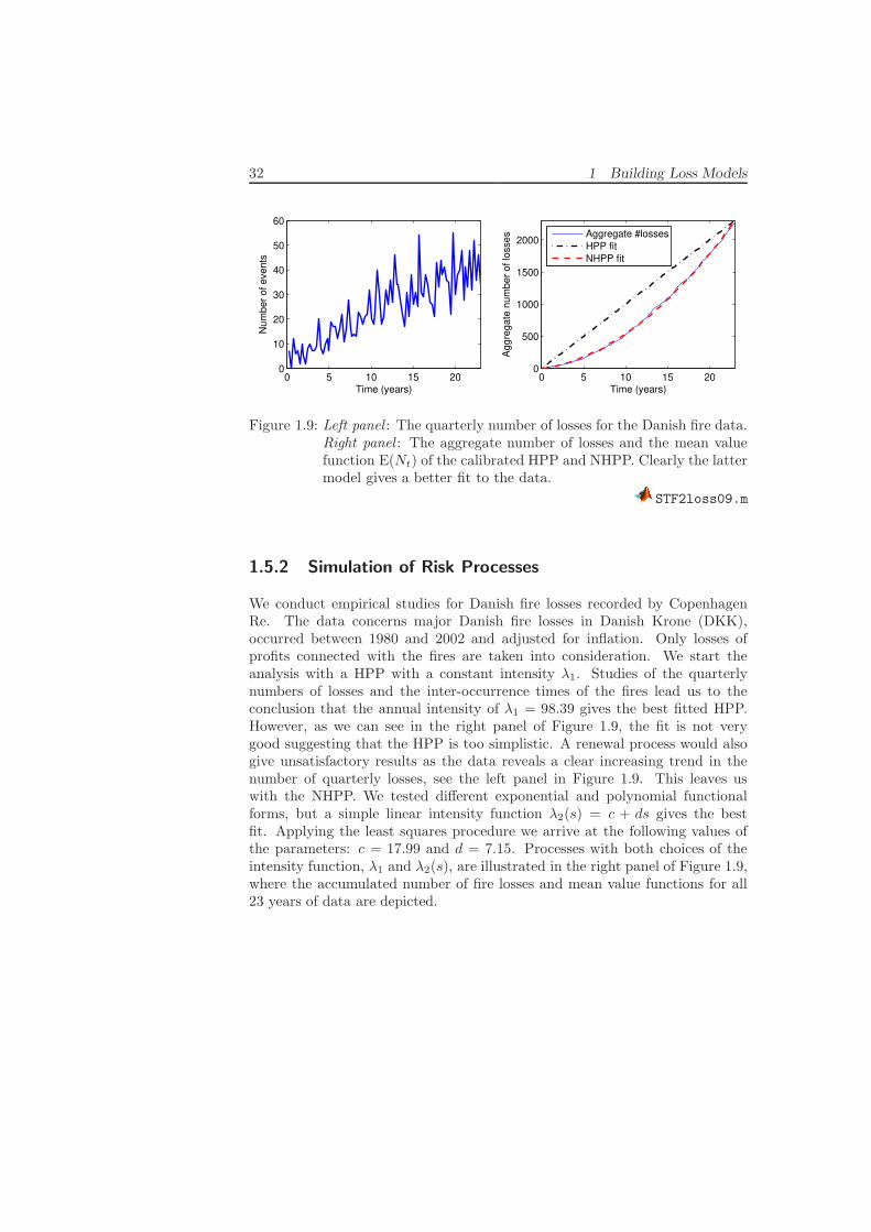
Figure 1.9: Left panel : The quarterly number of losses for the Danish fire data.Right panel : The aggregate number of losses and the mean valuefunction E(Nt) of the calibrated HPP and NHPP. Clearly the lattermodel gives a better fit to the data.

STF2loss09.m

1.5.2 Simulation of Risk Processes

We conduct empirical studies for Danish fire losses recorded by CopenhagenRe. The data concerns major Danish fire losses in Danish Krone (DKK),occurred between 1980 and 2002 and adjusted for inflation. Only losses ofprofits connected with the fires are taken into consideration. We start theanalysis with a HPP with a constant intensity λ1. Studies of the quarterlynumbers of losses and the inter-occurrence times of the fires lead us to theconclusion that the annual intensity of λ1 = 98.39 gives the best fitted HPP.However, as we can see in the right panel of Figure 1.9, the fit is not verygood suggesting that the HPP is too simplistic. A renewal process would alsogive unsatisfactory results as the data reveals a clear increasing trend in thenumber of quarterly losses, see the left panel in Figure 1.9. This leaves uswith the NHPP. We tested different exponential and polynomial functionalforms, but a simple linear intensity function λ2(s) = c + ds gives the bestfit. Applying the least squares procedure we arrive at the following values ofthe parameters: c = 17.99 and d = 7.15. Processes with both choices of theintensity function, λ1 and λ2(s), are illustrated in the right panel of Figure 1.9,where the accumulated number of fire losses and mean value functions for all23 years of data are depicted.

1.5 Applications 33

0 5 10 15 200

500

1000

1500

2000

2500

3000

Time (years)

Ca

pita

l (D

KK

mill

ion

)

0 5 10 15 200

500

1000

1500

2000

2500

3000

Time (years)C

ap

ita

l (D

KK

mill

ion

)

Figure 1.10: The Danish fire data simulation results for a NHPP with log-normal claim sizes (left panel) and a NHPP with Burr claim sizes(right panel). The dotted lines are the sample 0.001, 0.01, 0.05,0.25, 0.50, 0.75, 0.95, 0.99, 0.999-quantile lines based on 3000 tra-jectories of the risk process.

STF2loss10.m

After describing the claim arrival process we have to find an appropriate modelfor the loss amounts. In Section 1.5.1 a number of distributions were fittedto loss sizes. The log-normal distribution with parameters µ = 12.525 andσ = 1.5384 produced the best results. The Burr distribution with α = 0.9844,λ = 1.0585 · 106, and τ = 1.1096 overestimated the tails of the empiricaldistribution, nevertheless it gave the next best fit.

The simulation results are presented in Figure 1.10. We consider a hypotheticalscenario where the insurance company insures losses resulting from fire damage.The company’s initial capital is assumed to be u = 400 million DKK and therelative safety loading used is θ = 0.5. We choose two models of the riskprocess whose application is most justified by the statistical results describedabove: a NHPP with log-normal claim sizes and a NHPP with Burr claimsizes. In both panels the thick solid blue line is the “real” risk process, i.e.a trajectory constructed from the historical arrival times and values of thelosses. The different shapes of the “real” risk process in the two panels aredue to the different forms of the premium function c(t) which has to be chosenaccordingly to the type of the claim arrival process. The dashed red line is asample trajectory. The thin solid lines are the sample 0.001, 0.01, 0.05, 0.25,


0.50, 0.75, 0.95, 0.99, 0.999-quantile lines based on 3000 trajectories of the riskprocess. We assume that if the capital of the insurance company drops bellowzero, the company goes bankrupt, so the capital is set to zero and remains atthis level hereafter.

Comparing the log-normal and Burr claim size models, we can conclude that inthe latter model extreme events are more likely to happen. This is manifestedby wider quantile lines in the right panel of Figure 1.10. Since for log-normalclaim sizes the historical trajectory is above the 0.01-quantile line for most ofthe time, and taking into account that we have followed a non-robust estimationapproach of loss severities, we suggest to use this specification for further riskprocess modeling using the 1980-2002 Danish fire losses dataset.

Bibliography

Ahrens, J. H. and Dieter, U. (1982). Computer generation of Poisson deviatesfrom modified normal distributions, ACM Trans. Math. Soft. 8: 163–179.

Albrecht, P. (1982). On some statistical methods connected with the mixedPoisson process, Scandinavian Actuarial Journal: 1–14.

Bratley, P., Fox, B. L., and Schrage, L. E. (1987). A Guide to Simulation,Springer-Verlag, New York.

Burnecki, K., Hardle, W., and Weron, R. (2004). Simulation of Risk Processes,in J. Teugels, B. Sundt (eds.) Encyclopedia of Actuarial Science, Wiley,Chichester, 1564–1570.

Burnecki, K., Kukla, G., and Weron, R. (2000). Property insurance loss distri-butions, Physica A 287: 269-278.

K. Burnecki and R. Weron (2005). Modeling of the Risk Process, in P. Cizek,W. Hardle, R. Weron (eds.) Statistical Tools for Finance and Insurance,Springer-Verlag, Berlin, 319–339.

Chernobai, A., Burnecki, K., Rachev, S. T., Trueck, S. and Weron, R. (2006).Modelling catastrophe claims with left-truncated severity distributions,Computational Statistics 21: 537-555.

Chernobai, A.S., Rachev, S.T., and Fabozzi, F.J. (2007). Operational Risk: A

Guide to Basel II Capital Requirements, Models, and Analysis, Wiley.

D’Agostino, R. B. and Stephens, M. A. (1986). Goodness-of-Fit Techniques,Marcel Dekker, New York.

Daykin, C.D., Pentikainen, T., and Pesonen, M. (1994). Practical Risk Theory

for Actuaries, Chapman, London.

36 Bibliography

Devroye, L. (1986). Non-Uniform Random Variate Generation, Springer-Verlag, New York.

Embrechts, P. and Kluppelberg, C. (1993). Some aspects of insurance mathe-matics, Theory Probab. Appl. 38: 262–295.

Grandell, J. (1991). Aspects of Risk Theory, Springer, New York.

Hogg, R. and Klugman, S. A. (1984). Loss Distributions, Wiley, New York.

Hormann, W. (1993). The transformed rejection method for generating Poissonrandom variables, Insurance: Mathematics and Economics 12: 39–45.

Huber, P. J. (2004). Robust statistics, Wiley, Hoboken.

Johnk, M. D. (1964). Erzeugung von Betaverteilten und GammaverteiltenZufallszahlen, Metrika 8: 5-15.

Kaas, R., Goovaerts, M., Dhaene, J., and Denuit, M. (2008). Modern Actuarial

Risk Theory: Using R, Springer.

Klugman, S. A., Panjer, H.H., and Willmot, G.E. (2008). Loss Models: From

Data to Decisions (3rd ed.), Wiley, New York.

Panjer, H.H. (2006). Operational Risk : Modeling Analytics, Wiley.

Panjer, H.H. and Willmot, G.E. (1992). Insurance Risk Models, Society ofActuaries, Chicago.

Rolski, T., Schmidli, H., Schmidt, V., and Teugels, J. L. (1999). Stochastic

Processes for Insurance and Finance, Wiley, Chichester.

Ross, S. (2002). Simulation, Academic Press, San Diego.

Stadlober, E. (1989). Sampling from Poisson, binomial and hypergeometricdistributions: ratio of uniforms as a simple and fast alternative, Math.

Statist. Sektion 303, Forschungsgesellschaft Joanneum Graz.

Stephens, M. A. (1978). On the half-sample method for goodness-of-fit, Journal

of the Royal Statistical Society B 40: 64-70.

Teugels, J.L. and Vynckier, P. (1996). The structure distribution in a mixedPoisson process, J. Appl. Math. & Stoch. Anal. 9: 489–496.

Tse, Y.-K. (2009). Nonlife Actuarial Models: Theory, Methods and Evaluation,Cambridge University Press, Cambridge.

Bibliography 37

Weron, R. (2004). Computationally Intensive Value at Risk Calculations, in

J. E. Gentle, W. Hardle, Y. Mori (eds.) Handbook of Computational Statis-

tics, Springer, Berlin, 911–950.

Willmot, G. E. (2001). The nature of modelling insurance losses, The Munich

Re Inaugural Lecture, December 5, 2001, Toronto.

building loss models - munich personal repec archive

Documents