bounds on the tail probability and absolute difference between two distributions

This article was downloaded by: [Universita di Trento]On: 10 July 2013, At: 02:17Publisher: Taylor & FrancisInforma Ltd Registered in England and Wales Registered Number: 1072954 Registered office: Mortimer House,37-41 Mortimer Street, London W1T 3JH, UK

Communications in Statistics - Theory and MethodsPublication details, including instructions for authors and subscription information:http://www.tandfonline.com/loi/lsta20

Bounds on the Tail Probability and Absolute DifferenceBetween Two DistributionsM. N. Goria a & A. Tagliani aa Department of Computer and Management Sciences, Faculty of Economics, TrentoUniversity, Trento, ItalyPublished online: 02 Sep 2006.

To cite this article: M. N. Goria & A. Tagliani (2003) Bounds on the Tail Probability and Absolute Difference Between TwoDistributions, Communications in Statistics - Theory and Methods, 32:3, 519-532, DOI: 10.1081/STA-120018549

To link to this article: http://dx.doi.org/10.1081/STA-120018549

PLEASE SCROLL DOWN FOR ARTICLE

Taylor & Francis makes every effort to ensure the accuracy of all the information (the “Content”) containedin the publications on our platform. However, Taylor & Francis, our agents, and our licensors make norepresentations or warranties whatsoever as to the accuracy, completeness, or suitability for any purpose of theContent. Any opinions and views expressed in this publication are the opinions and views of the authors, andare not the views of or endorsed by Taylor & Francis. The accuracy of the Content should not be relied upon andshould be independently verified with primary sources of information. Taylor and Francis shall not be liable forany losses, actions, claims, proceedings, demands, costs, expenses, damages, and other liabilities whatsoeveror howsoever caused arising directly or indirectly in connection with, in relation to or arising out of the use ofthe Content.

This article may be used for research, teaching, and private study purposes. Any substantial or systematicreproduction, redistribution, reselling, loan, sub-licensing, systematic supply, or distribution in anyform to anyone is expressly forbidden. Terms & Conditions of access and use can be found at http://www.tandfonline.com/page/terms-and-conditions

http://www.tandfonline.com/loi/lsta20

http://www.tandfonline.com/action/showCitFormats?doi=10.1081/STA-120018549

http://dx.doi.org/10.1081/STA-120018549

http://www.tandfonline.com/page/terms-and-conditions

http://www.tandfonline.com/page/terms-and-conditions

©2003 Marcel Dekker, Inc. All rights reserved. This material may not be used or reproduced in any form without the express written permission of Marcel Dekker, Inc.

MARCEL DEKKER, INC. • 270 MADISON AVENUE • NEW YORK, NY 10016

COMMUNICATIONS IN STATISTICS

Theory and Methods

Vol. 32, No. 3, pp. 519–532, 2003

Bounds on the Tail Probability and Absolute

Difference Between Two Distributions

M. N. Goria* and A. Tagliani

Department of Computer and Management

Sciences, Faculty of Economics, Trento University,Trento, Italy

ABSTRACT

A fractional moment bound on the tail probabilities of a distributionis proposed and illustrated with examples. It is then combined with

the moment bound of Philips–Nelson, resulting in an improvementover the latter. Two bounds on the absolute difference between twodistributions, namely the fractional moment and entropy based

bounds are introduced. The first compares well with Lindsay–Basak’s window function while the second can be made as preciseas desired, according to the number of common moments assumed.

*Correspondence: M. N. Goria, Department of Computer and ManagementSciences, Faculty of Economics, Trento University, 38100 Trento, Italy; E-mail:[email protected].

519

DOI: 10.1081/STA-120018549 0361-0926 (Print); 1532-415X (Online)

Copyright & 2003 by Marcel Dekker, Inc. www.dekker.com

Dow

nloa

ded

by [

Uni

vers

ita d

i Tre

nto]

at 0

2:17

10

July

201

3



Key Words: Entropy; Fractional moments; Moments; Tail

probability.

1. INTRODUCTION

Bounds on probabilities in the central part and tails of a distribu-tion can be found in almost every text of probability and statistics.These are designed either to provide a rough estimate of the probabil-ity where the effective value is either difficult or unavailable for lackof information on the distribution function or exploited fruitfullyto establish theoretical results such as law of large number andcentral limit theorems. Among all bounds, Chernoff ’s bound is usedalmost exclusively, when a tight bound on the tail of distribution isrequired.

Recently Philips and Nelson (1995) proposed a new bound on thetails probabilities based on sequence of moments and showed that it issuperior to Chernoff ’s bound. Naveau (1997) reached the same conclu-sion for the discrete r.v using a sequence of factorial moments.

At first sight the result appears a bit surprizing since, underrestrictions, the moment generating function (Chernoff ’s bound) andsequence of moments (Philips–Nelson bound) are equivalent. The onlyplausible explanation seems that the moment generating functionprovides a global behavior of distribution, whereas the momentsdescribe its local characteristics, e.g., the concepts such as location,scale, symmetry and kurtosis, well familiar to the readers.

These bounds clearly exclude heavy tailed distributions such asPareto, Cauchy or more generally stable distributions. For these distri-butions however the fractional moments do exist (Goria, 1978) forCauchy distribution.

In Sec. 2 we first develop a bound based on a sequence of fractionalmoments and compute it for Cauchy and Pareto distributions inExample 1. Next we combine it with Philips–Nelson’s moment bound,leading to a new and more precise bound compared to the abovementioned one, as discussed in Example 2.

In Sec. 3 we propose two bounds on the absolute difference betweentwo distributions. The first is based on the fractional moments andmoments which compares well with the window bound of Lindsay andBasak (2001). The second, based on the entropy which can be made asprecise as desired, according to the number of common moments shearedby the two distributions.

520 Goria and Tagliani

Dow

nloa

ded

by [

Uni

vers

ita d

i Tre

nto]

at 0

2:17

10

July

201

3

https://www.researchgate.net/publication/241735479_Comparison_Between_the_Chernoff_and_Factorial_Moment_Bounds_for_Discrete_Random_Variables?el=1_x_8&enrichId=rgreq-2741c74c-675f-4962-be03-4421fd06e9f7&enrichSource=Y292ZXJQYWdlOzIzMzQ1Mjk1ODtBUzoxMDE5ODYyMTcyMzQ0NDFAMTQwMTMyNjgxODA1Ng==



2. FRACTIONAL MOMENTS BOUND ON THE TAIL

PROBABILITY OF DISTRIBUTION

Philips and Nelson (1995) consider a random variable X having anabsolutely continuous distribution function FX with support on the realline such that it has finite moments of all order and propose the followingbound on the tail of the distribution

PðX � tÞ � infk� 0

EðXþ=tÞk ¼ MðtÞ, t > 0,

where X þ is postive part of r.v X . They showed that this inequality iseven sharper than Chernoff ’s bound.

These bounds are not however applicable to heavy tailed distribu-tions, e.g., Cauchy and Pareto distributions, due to nonexistence of evenfirst moment but the fractional moments do exist for these distributions.Their exclusion from text books probably can be attributed to theirunclear meanings, unlike the first four moments.

Lin (1992) showed that the sequence of fractional moments underrestrictions uniquely determine their distribution, it follows thenthat the fractional moments like moments also do explain the variousfacits of a distribution. This result is particularly relevant to the heavytailed distributions, e.g., stable distributions. Consequently it seemsof interest to develope a bound based on fractional moments andfurther modify it appropriately in case certain number of momentsdo exist.

Let �1=k ¼ EðXþÞ1=k, k � 2 denote the kth order fractional moment,

then from Markov’s inequality, we have

PðX � tÞ � infk� 2

�1=k

t1=k¼ Mf ðtÞ

Note that the above bound is computable for any distribution particu-larly for those, not having even the mean finite. We illustrate it belowwith an example.

Example 1: Pareto and Cauchy Distributions

Consider the Pareto distribution with density

f ðxÞ ¼ �x��1, x � 1, � < 1:

Tail Probability Bounds 521

Dow

nloa

ded

by [

Uni

vers

ita d

i Tre

nto]

at 0

2:17

10

July

201

3

https://www.researchgate.net/publication/265314451_Characterizations_of_distributions_via_moments?el=1_x_8&enrichId=rgreq-2741c74c-675f-4962-be03-4421fd06e9f7&enrichSource=Y292ZXJQYWdlOzIzMzQ1Mjk1ODtBUzoxMDE5ODYyMTcyMzQ0NDFAMTQwMTMyNjgxODA1Ng==



If we let

gð�Þ ¼��

t�¼

1

t�ð1� �=�Þ, 0 � � < � < 1,

then we find that the function gð�Þ has minimum at

�0 ¼ð� log t� 1Þ

log t, t > eð1=aÞ:

We define k0, for �0 < 1=2 as

k0 ¼ ½1=�0 þ 1:1=�0 � ½1=�0 � 0:5

otherwise k0 ¼ ½1=�0. While for �0 � 1=2 we take k0 ¼ 2 and k0 ¼ 1,t � eð1=aÞ. As a result the fractional moment bound is

Mf ðtÞ ¼ gðk0Þ ¼1

t1=k0ð1� 1=ð�k0ÞÞ

We compared the exact probability with Mf ðtÞ for � ¼ 2=3, 3=4, 9=10.It turned out that the bound becomes sharper as � increases.

For Cauchy distribution with

gð� Þ ¼1

2t� cosð��=2Þ, � � 1=2

we find

k0 ¼ 1, t � 1, k0 ¼ 2, t � 4:81057

and with analogous procedure to above, �0 was found as

�0 ¼ ð2=�Þarc cosð�½�2þ 4ðlog tÞ2�1=2

Þ, t 2 ð1, 4:81057Þ,

from which k0 was determined.For both distributions, the bound Mf ðtÞ compared to exact prob-

ability was quite wide particularly for large t-values. This seems obviousas Mf ðtÞ tends to zero at the rate of t�1=2 compared to the exact valuewhich converge at the rate t�2, t�� respectively for Cauchy and Pareto


Dow

nloa

ded

by [

Uni

vers

ita d

i Tre

nto]

at 0

2:17

10

July

201

3



distribution. However if we do not insist on integer solution and considerinfimum over k > 1, the bound becomes better.

To rectify the above defect specially for large t-values we brought inthe mean of the Pareto distribution, i.e., we assumed 1 < � < 2 andconsidered the bound

M1ðtÞ ¼ infk� 1

�1=k

t1=k� Mf ðtÞ:

We compared M1ðtÞ with exact probability for � ¼ 1:5. This indeedshowed some improvement over Mf ðtÞ for large t-values.

From the above discussion it is clear how to modify the fractionalmoment bound in case the distribution has certain number of finitemoments. Next we compared Mf ðtÞ with very precise bounds ofChernoff and Philips–Nelson for the Normal and Gamma distributions.It turned out that the results are very similar in both cases, therefore weshall discuss Gamma distribution in details in the next example.

Example 2: Gamma Distribution

Consider Gamma distribution with density

f ðxÞ ¼x��1e�x

�ð�Þ, x � 0, � > 0:

From Philips–Nelson, we have

CðtÞ ¼ 1, t < �

¼ ðt=�Þ�eð��tÞ, t � �:

To evaluate Mf ðtÞ,MðtÞ, we consider

gð�Þ ¼ t�� ð�þ �Þ

�ð�Þ, � � 0

The function gð�Þ has minimum at �0 given by solution of the followingequation

1

�ð�þ �Þ

d �ð�þ �Þ

d�� log t ¼ 0

The exact solution �0 was determined numerically using Mathematica foreach fixed value of t and � ¼ 1=2, 1, 2, 3. It turned out that t� t0 <�0 < t� � and �0 < 0, t < t0. Further the numerical solution can beapproximated nicely as follows.


Dow

nloa

ded

by [

Uni

vers

ita d

i Tre

nto]

at 0

2:17

10

July

201

3



First for each � we determined tpð�Þ, p ¼ 0, 0:5, 1, the t-value corre-sponding to the solution �0 ¼ p, then divided the t-values into threedisjoint intervals ½t0, t0:5Þ, ½t0:5, t1Þ, t � t1 and finally found that �0 can bevery closely approximated by

�̂� ¼ t� t0 þ cið�Þð�� t0Þ, i ¼ 0, 0:5, 1,

where c0, c0:5 were determined at mid value of the interval and c1 at t1such that �̂� matches exactly with �0. The quantities ci are of small mag-nitude, in fact c0 < c0:5 < c1 with c1 � 0:0094.

The approximation has no impact on the value of MðtÞ but negligibleeffect for t � t1, where t is large. Like wise it has no effect on Mf ðtÞ fort � t0:5 but little effect for small values of t where k0 is very large.

For the bound MðtÞ, k0 ¼ 0, t � t0, otherwise found from �̂� as in thefirst example, whereas for Mf ðtÞ, k0 ¼ 1, t � t0 and for other t-valuesfrom 1=�̂�.

On comparison of Mf ðtÞ with MðtÞ and CðtÞ, it turned out that formoderate t-values, i.e., t � 1:09� and t < 1:6�, the fractional momentbound Mf ðtÞ is better than MðtÞ and CðtÞ respectively and thereafterboth CðtÞ and MðtÞ override Mf ðtÞ. This was to be expected as Mf ðtÞgoes to zero at t�1=2 rate.

From Example 1 it is clear that if we bring in the moments to modifyMf ðtÞ, the new bound

PðX > tÞ � infs�þs =t

s¼ M1ðtÞ,

where s 2 f. . . , 1=k, . . . , 1=2, 0, 1, . . . , k, . . .g will lead to an improvement,particularly for large t-values, as can be seen in the section of the graphbelow where we have presented M1ðtÞ,MðtÞ and CðtÞ for � ¼ 3.

From Fig. 1 it is clear that M1ðtÞ out performs Chernoff ’s boundand has an edge over MðtÞ for moderate values of t.

Figure 1. CðtÞ (continuous), MðtÞ (dashed), M1ðtÞ (dots).


Dow

nloa

ded

by [

Uni

vers

ita d

i Tre

nto]

at 0

2:17

10

July

201

3



Needless to say that the bound M1ðtÞ besides being preciser for allt > 0 than other bounds has the clear advantage over others of widerapplicability, i.e., it is usable even for the distribution with no finitemoment. Further with �̂� determined above, it was found that someimprovement still can be made over M1ðtÞ if we do not insist on integersolution.

3. BOUNDS ON THE ABSOLUTE DIFFERENCE

BETWEEN TWO DISTRIBUTION FUNCTIONS

We shall propose two bounds namely fractional moment–momentbound and an entropy based bound and discuss their relativeperformances

3.1. Fractional Moment–Moment Bound

Consider any two absolutely continuous distributions F and G suchthat both distributions have the same first k moments and fractionalmoments, i.e.,

�iðFÞþ¼ �iðGÞ

þ, i ¼ 1=k, . . . , 1, 2, . . . , k

of the positive part of r.vs. If we let

mkðtÞ ¼ minf1=k,..., 0, 1,..., kg

ð�iðFÞþ=tiÞ,

then we have the following inequality

jFðtÞ � GðtÞj ¼ j �FFðtÞ � �GGðtÞj � maxð �FFðtÞ, �GGðtÞÞ � mkðtÞ, t > 0:

ð3:1Þ

We compared the fractional moment–moment bound with the windowfunction of Lindsay and Basak, 2001, i.e.,

jFðtÞ � GðtÞj � kðtÞ ¼1

VkðtÞ0

MðkÞ�1VkðtÞ, t 2 R

þð3:2Þ

whereMðkÞ is a Hankel symmetric matrix defined by the first 2kmomentsand Vt ¼ ð1, t, t2, . . . , tkÞ, for Normal distribution with several values of k.


Dow

nloa

ded

by [

Uni

vers

ita d

i Tre

nto]

at 0

2:17

10

July

201

3

https://www.researchgate.net/publication/239832609_Moments_Determine_the_Tail_of_a_Distribution_But_Not_Much_Else?el=1_x_8&enrichId=rgreq-2741c74c-675f-4962-be03-4421fd06e9f7&enrichSource=Y292ZXJQYWdlOzIzMzQ1Mjk1ODtBUzoxMDE5ODYyMTcyMzQ0NDFAMTQwMTMyNjgxODA1Ng==



It turned out that the difference between two bound varies from aminimum of 1% to a maximum of 4% in favor of the window function.Needless to say that our bound has a computational advantage.

3.2. Entropy Bound

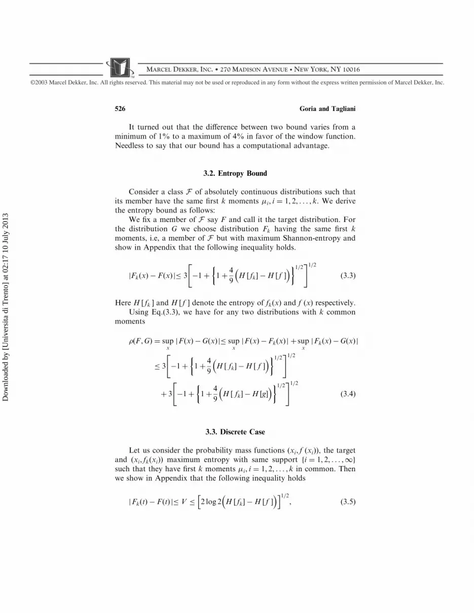
Consider a class F of absolutely continuous distributions such thatits member have the same first k moments �i, i ¼ 1, 2, . . . , k. We derivethe entropy bound as follows:

We fix a member of F say F and call it the target distribution. Forthe distribution G we choose distribution Fk having the same first kmoments, i.e, a member of F but with maximum Shannon-entropy andshow in Appendix that the following inequality holds.

jFkðxÞ � FðxÞ j� 3 �1þ 1þ4

9

�H ½ fk �H ½ f

�� 1=2" #1=2

ð3:3Þ

Here H ½ fk and H ½ f denote the entropy of fkðxÞ and f ðxÞ respectively.Using Eq.ð3:3Þ, we have for any two distributions with k common

moments

ðF ,GÞ ¼ supx

jFðxÞ �GðxÞ j� supx

jFðxÞ � FkðxÞ j þ supx

jFkðxÞ �GðxÞ j

� 3 �1þ 1þ4

9

�H ½ fk �H ½ f

�� 1=2" #1=2

þ 3 �1þ 1þ4

9

�H ½ fk �H ½g

�� 1=2" #1=2

ð3:4Þ

3.3. Discrete Case

Let us consider the probability mass functions ðxi, f ðxiÞÞ, the targetand ðxi, fkðxiÞÞ maximum entropy with same support fi ¼ 1, 2, . . . ,1g

such that they have first k moments �i, i ¼ 1, 2, . . . , k in common. Thenwe show in Appendix that the following inequality holds

jFkðtÞ � FðtÞ j� V �

h2 log 2

�H ½ fk �H ½ f

�i1=2, ð3:5Þ


Dow

nloa

ded

by [

Uni

vers

ita d

i Tre

nto]

at 0

2:17

10

July

201

3



where F ,Fk respectively denote the distribution function correspondingto f , fk:

In analogy with the continuous case, for each pair of distributions,we obtain the window estimate in discrete case as

ðF ,GÞ �h2 log 2

�H ½ fk �H ½ f

�i1=2þ

h2 log 2

�H ½ fk �H ½g

�i1=2:

ð3:6Þ

Remark

The inequalities (3.3) and (3.5) remain unaltered for the nonnegativevariable and further in such case we can consider distributions having anarbitrary number k of assigned moments (Tagliani, 2000).

Note that in the entropy bound, the two distributions involved donot play an equal role, in that the target distribution F has to be specifiedin advance. This disadvantage is overshadowed by the fact that the aboveinequalities can be made as precise as we like, by an appropriate choice ofk, i.e. the number of common moments.

3.4. Choice of k

In our previous discussion we assumed that the first k commonmoments of distributions F and G are preassigned. This may be justifiedin a theoretical work but in practice it is often necessary to decide howlarge k should be in given situation. To this end we restrict our attentiononly to those distributions having a determinate moment problem anddiscuss the choice of k.

Now for a class of distributions having a determinate momentproblem, we have a well defined sequence of entropies fH ½ fk, k ¼

1, 2, . . .1g. From Appendix, it is clear that the convergence in entropyentails convergence in divergence measure or equivalently in variationmeasure.

We know from a theorem Frontini and Tagliani (1997) that themonotonic decreasing sequence fH ½ fk, k ¼ 1, 2, . . .1g converges toH ½ f . To obtain an estimate of the error for large values of k, we shalluse Aitken �2-method.

For every distribution unlike the maximum entropy distribution,contents of information contained in it, are shared by the whole sequenceof moments and a further addition of a moment causes an entropydecrease. The size of decrease is not the same for every moment. Infact for most of the distributions met in practice, we find that the first


Dow

nloa

ded

by [

Uni

vers

ita d

i Tre

nto]

at 0

2:17

10

July

201

3



few moments generate a higher decrease than those later in the list.Consequently it seems reasonable to expect that the sequence of pointsð j,H ½ fjÞ, j ¼ 1, 2, . . . ,1 lie on a convex curve, i.e.,

D2H ½ fj ¼ H ½ fj � 2H ½ fð j�1Þ þH ½ fð j�2Þ > 0, j > 2

Next by Aitken’s �2-method, we define a new accelerated sequence as

H acc½ fj ¼ H ½ fj �

�H ½ fj �H ½ fðj�1Þ

�2D2H ½ fj

, j > 2

which converges faster to H ½ f than the initial sequence.If we take H ½ f ’ H acc

½ fk, for some k, we obtain the followingestimate of the error term

H ½ f �H acc½ fk ’

�H ½ fk �H ½ fðk�1Þ

�2D2H ½ fk

ð3:7Þ

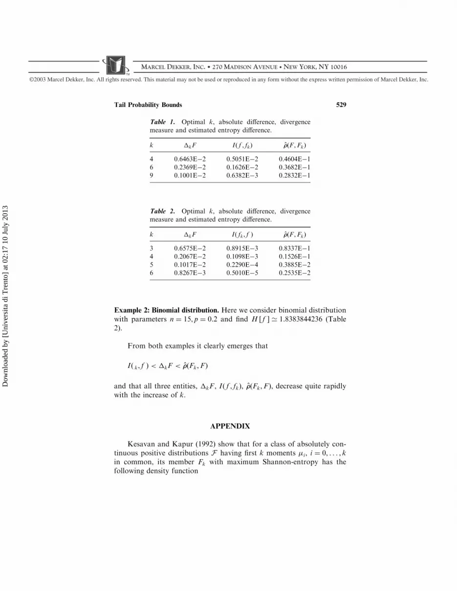
Using k found above in Eqs. ð3:4Þ and ð3:6Þ, we obtain an estimate ofðF ,GÞ which we denote by ̂ðF ,GÞ. Note that for any prefixed errorbound, we can determine an optimal value of k. We illustrate these resultswith two examples where in addition to the window estimate we alsoreport Ið fk, f Þ:

In both examples the determination of optimal value of k run in twosteps as follows: since F is known here, we first compute

�kF ¼:kFkðxÞ � FðxÞk1 ,

and Ið f k, f Þ for each k � 1, needed to evaluate window estimate. Nextwe find minimum value of k such that �kF � ̂ðF ,GÞ and declare it as anoptimal choice of k.

Example 1 (continuous case). To appreciate the size of entropy bound, wechoose F for illustrative purpose with the following density

f ðxÞ ¼�

2sinð�xÞ, x 2 ½0, 1

and zero elsewhere. Note that f ðxÞ has a determinate moment problem,with H ½ f ’ �0:144729886. The approximate density fkðxÞ, x 2 ½0,1Þ isgiven by Eq. (A.1). In Table 1 we report optimal value of k along withvarious quantities need for its determination.


Dow

nloa

ded

by [

Uni

vers

ita d

i Tre

nto]

at 0

2:17

10

July

201

3



Example 2: Binomial distribution. Here we consider binomial distributionwith parameters n ¼ 15, p ¼ 0:2 and find H ½ f ’ 1:8383844236 (Table2).

From both examples it clearly emerges that

Ið k, f Þ < �kF < ̂ðFk,FÞ

and that all three entities, �kF , Ið f , fkÞ, ̂ðFk,FÞ, decrease quite rapidlywith the increase of k.

APPENDIX

Kesavan and Kapur (1992) show that for a class of absolutely con-tinuous positive distributions F having first k moments �i, i ¼ 0, . . . , kin common, its member Fk with maximum Shannon-entropy has thefollowing density function

Table 1. Optimal k, absolute difference, divergence

measure and estimated entropy difference.

k �kF Ið f , fkÞ ̂ðF ,FkÞ

4 0.6463E�2 0.5051E�2 0.4604E�1

6 0.2369E�2 0.1626E�2 0.3682E�19 0.1001E�2 0.6382E�3 0.2832E�1

Table 2. Optimal k, absolute difference, divergencemeasure and estimated entropy difference.

k �kF Ið fk, f Þ ̂ðF ,FkÞ

3 0.6575E�2 0.8915E�3 0.8337E�14 0.2067E�2 0.1098E�3 0.1526E�1

5 0.1017E�2 0.2290E�4 0.3885E�26 0.8267E�3 0.5010E�5 0.2535E�2


Dow

nloa

ded

by [

Uni

vers

ita d

i Tre

nto]

at 0

2:17

10

July

201

3



fkðxÞ ¼ exp �Xkj¼0

jxj

!, x 2 ½0,1Þ, ðA:1Þ

and fkðxÞ ¼ 0 elsewhere. The i, i ¼ 0, 1, . . . , k are Lagrange’s multi-pliers, obtainable through �i and its Shannon-entropy H ½ fk is given by

H ½ fk ¼Xkj¼0

j�j

The main result on the absolute difference between the two distribu-tions is given in theorem below.

Theorem. For any member F 2 F with density f , the inequalities (3.3) and(3.5) hold.

Proof.

jFkðxÞ � FðxÞ j �

Z x

0

j fkðuÞ � f ðuÞ j du

�

Z þ1

0

j fkðuÞ � f ðuÞ j du ¼ V ðA:2Þ

and the above inequality remains valid for discrete case. It is straight-forward to see that the Kullback–Leibler’s divergence measure betweenfk, f is

Ið fk, f Þ ¼ �H ½ f þXkj¼0

j�j ¼ H ½ fk �H ½ f ðA:3Þ

and further for any other member G 2 F=F , the following holds

Iðg, f Þ � Ið fk, f Þ ¼ H ½ fk �H ½ f , G 2 F=F :

From Kullback (1967) we have its lower bound as

I �V 2

2þV 4

36:

Equivalently


Dow

nloa

ded

by [

Uni

vers

ita d

i Tre

nto]

at 0

2:17

10

July

201

3



V � 3 �1þ 1þ4

9I

� �1=2" #1=2

, ðA:4Þ

Substituting Eq. (A.4) and then Eq. (A.3) in Eq. (A.2), leads to Eq. (3.3).The proof of Eq. (3.5) is identical to Eq. (3.3) except that here we useCover (1991) lower bound

I �1

2 log 2V2

in place of Kullback’s bound.

Remark. Bound (3.1) may be sharpened further by taking into accountthe following inequality

I �V 2

2þV 4

36þ

V 6

288ðA:5Þ

as in Toussaint (1975) but this evidently leads to more complicatedinequality.

REFERENCES

Cover, T. M., Thomas, J. A. (1991). Elements of Information Theory.New York: John Wiley Sons, Inc.

Frontini, M., Tagliani, A. (1997). Entropy-convergence in Stiltjes andHamburger moment problem. Applied Math. and Computation88:39–51.

Goria, M. N. (1992). Fractional Absolute moments of the CauchyDistribution, Quaderni di Statistica e Matematica applicata allescienze Economico-Sociali 1:3–9. Trento University.

Kesavan, H. K., Kapur, J. N. (1992). Entropy Optimization Principleswith Applications. Academic Press.

Kullback, S. (1967). A lower bound for discrimination information interms of variation. IEEE Transaction on Information TheoryIT-13:126–127.

Lin, G. D. (1992). Characterizations of Distributions via moments.Sankhya: The Indian Journal of Statistics 54(Series A):128–132.

Lindsay, B. G., Basak, P. (2001 to appear). Moments determine the tailof a distribution (but not much else). The American Statistician.


Dow

nloa

ded

by [

Uni

vers

ita d

i Tre

nto]

at 0

2:17

10

July

201

3



Naveau, P. (1997). Comparison between the Chernoff and factorialmoment bounds for discrete random variables. The AmericanStatistician 51(1):40–41.

Philips, T. K., Nelson, R. (1995). The moment bound is tighter thanChernoff’s bound for positive tail probabilities. The AmericanStatistician 49(2):175–178.

Tagliani, A. (2000). Inverse Z transform and moment problem.Probability in Engineering and Informational Sciences 14:393–404.

Toussaint, G. T. (1975). Sharper lower bounds for discrimination infor-mation in terms of variation. IEEE Transaction on InformationTheory (Corresp.) IT-21:99–100.


Dow

nloa

ded

by [

Uni

vers

ita d

i Tre

nto]

at 0

2:17

10

July

201

3

bounds on the tail probability and absolute difference between two distributions

Documents