DISCUSSION PAPER SERIES

ABCD

www.cepr.org

Available online at: www.cepr.org/pubs/dps/DP6694.asp

www.ssrn.com/xxx/xxx/xxx

No. 6694

BOND SUPPLY AND EXCESS BOND RETURNS

Robin Greenwood and Dimitri Vayanos

FINANCIAL ECONOMICS

ISSN 0265-8003

BOND SUPPLY AND EXCESS BOND RETURNS

Robin Greenwood, Harvard Business School Dimitri Vayanos, London School of Economics (LSE), NBER and CEPR

Discussion Paper No. 6694

February 2008

Centre for Economic Policy Research 90–98 Goswell Rd, London EC1V 7RR, UK

Tel: (44 20) 7878 2900, Fax: (44 20) 7878 2999 Email: cepr@cepr.org, Website: www.cepr.org

This Discussion Paper is issued under the auspices of the Centre’s research programme in FINANCIAL ECONOMICS. Any opinions expressed here are those of the author(s) and not those of the Centre for Economic Policy Research. Research disseminated by CEPR may include views on policy, but the Centre itself takes no institutional policy positions.

The Centre for Economic Policy Research was established in 1983 as a private educational charity, to promote independent analysis and public discussion of open economies and the relations among them. It is pluralist and non-partisan, bringing economic research to bear on the analysis of medium- and long-run policy questions. Institutional (core) finance for the Centre has been provided through major grants from the Economic and Social Research Council, under which an ESRC Resource Centre operates within CEPR; the Esmée Fairbairn Charitable Trust; and the Bank of England. These organizations do not give prior review to the Centre’s publications, nor do they necessarily endorse the views expressed therein.

These Discussion Papers often represent preliminary or incomplete work, circulated to encourage discussion and comment. Citation and use of such a paper should take account of its provisional character.

Copyright: Robin Greenwood and Dimitri Vayanos

CEPR Discussion Paper No. 6694

February 2008

ABSTRACT

Bond Supply and Excess Bond Returns*

We examine empirically how the maturity structure of government debt affects bond yields and excess returns. Our analysis is based on a theoretical model of preferred habitat in which clienteles with strong preferences for specific maturities trade with arbitrageurs. Consistent with the model, we find that (i) the supply of long- relative to short-term bonds is positively related to the term spread, (ii) supply predicts positively long-term bonds' excess returns even after controlling for the term spread and the Cochrane-Piazzesi factor, (iii) the effects of supply are stronger for longer maturities, and (iv) following periods when arbitrageurs have lost money, both supply and the term spread are stronger predictors of excess returns.

JEL Classification: G1 and H6 Keywords: bond prices, limited arbitrage, preferred habitat and return predictability

Robin Greenwood Harvard Business School 44 Commonwealth, Unit 2 Boston MA 02163 USA Email: rgreenwood@hbs.edu For further Discussion Papers by this author see: www.cepr.org/pubs/new-dps/dplist.asp?authorid=158420

Dimitri Vayanos Department of Finance London School of Economics Houghton Street London WC2A 2AE Email: d.vayanos@lse.ac.uk For further Discussion Papers by this author see: www.cepr.org/pubs/new-dps/dplist.asp?authorid=116836

* We thank Malcolm Baker, Daniel Bergstresser, Ken Froot, Denis Gromb, Sam Hanson, Christian Julliard, Arvind Krishnamurthy, Anna Pavlova, Christopher Polk, Andrea Prat, Andrei Shleifer, Erik Stafford, Jeremy Stein, Otto Van Hemert, Michela Verardo, Jean-Luc Vila, Annette Vissing-Jorgensen and Jeff Wurgler for helpful discussions. Sonya Lai provided excellent research assistance. Financial support from the Paul Woolley Centre at the LSE is gratefully acknowledged.

Submitted 01 February 2008

1 Introduction

How does the maturity structure of government debt affect interest rates? If, for example,

the government raises the supply of long- relative to short-term bonds, would this impact the

spread between long and short rates (term spread)? According to standard representative-

agent models, there should be no effect because of Ricardian equivalence (Barro 1974).

Intuitively, the consumption of the representative agent, and hence interest rates, depend on

government spending but not on how spending is financed.

The irrelevance result is at odds with a view held by practitioners and emphasized in

early term-structure theories (e.g., Culbertson 1957, Modigliani and Sutch 1966). According

to that view, the term structure involves investor clienteles with preferences for specific

maturities. The yield for each maturity is influenced by the demand of the corresponding

clientele and the supply of bonds with that maturity. And while clienteles can substitute to

maturities away from their “preferred habitat,” such substitution is imperfect.

Determining whether or not maturity structure affects interest rates is relevant for public

policy and asset pricing. On the policy front, maturity structure could be used by the

government as a tool to reduce financing costs and raise aggregate welfare. On the asset-

pricing front, maturity structure could be a predictor of long-term bonds’ excess returns

relative to short-term bonds.

In this paper we examine empirically how maturity structure affects bond yields and

excess returns. We derive our predictions from a theoretical model of preferred habitat.

Drawing on Vayanos and Vila (2007), we assume that clienteles with strong preferences for

specific maturities trade with arbitrageurs. Absent arbitrageurs, the markets for different

maturities are segmented, and yields are determined by local demand and supply. Arbi-

trageurs integrate markets, rendering the term structure arbitrage-free. But because they

are risk averse, demand and supply affect prices. A basic prediction of the model is that

an increase in the relative supply of long-term bonds lowers their prices, thus raising their

yields and risk premia relative to short-term bonds. The model delivers further predictions

concerning how changes in supply affect the cross section of bond maturities, and how the

effects vary over time. For example, we link bond risk premia to arbitrageur risk aversion,

and identify times when risk aversion is likely to be high. The data support the model’s

predictions.

Our empirical approach is to construct, in every month starting from 1952, measures of

1

the maturity structure of promised payments on government bonds, including both interest

and principal. CRSP maintains a record of every bond issued since 1925, as well as its face

value outstanding at the end of each month. This allows for precise estimates of the maturity

structure of government debt. We relate these estimates to yield spreads, forward spreads,

and subsequent excess bond returns.

Our findings are as follows. First, the relative supply of long-term bonds is positively

related to the term spread. In general, this positive relationship can arise because high supply

predicts that short rates will increase, or because it predicts that long-term bonds will earn

high returns relative to short-term bonds. According to our model, the second explanation

is correct, and this is confirmed by the data: the relative supply of long-term bonds is

positively related to these bonds’ subsequent excess returns, while being weakly negatively

related to changes in short rates. The effects of supply on yield spreads and excess returns

are significant: a one standard deviation increase in the relative supply of long-term bonds is

associated with a 39 bps increase in the term spread and a 2.31 percent increase in long-term

bonds’ expected excess returns. Moreover, supply predicts returns even after controlling for

other well-known predictors, such as yield spreads or forward rate spreads (e.g., Fama and

Bliss 1987, Campbell and Shiller 1991) and the tent-shaped combination of forward rates

(Cochrane and Piazzesi 2005). In fact, supply becomes the dominant predictor when returns

are evaluated at horizons of three years or longer.

A third finding concerns the variation of the effects with bond maturity. Following an

increase in the relative supply of long-term bonds, our model predicts that arbitrageurs hold

more such bonds. Since long-term bonds are riskier than short-term bonds, arbitrageurs

bear more interest-rate risk. Therefore, they require larger expected returns from all bonds,

and especially so for longer maturities. Consistent with this prediction, we find that the

effects of supply on yield spreads and long-term bonds’ excess returns are stronger for longer

maturities.

A fourth finding concerns the variation of the effects with arbitrageur risk aversion. Our

model predicts that supply has stronger effects at times when arbitrageurs are more risk-

averse, because at those times they are less able to absorb demand or supply imbalances.

A related result concerns the predictive power of the term spread. In our model, the term

spread predicts positively long-term bonds’ excess returns: it is high, for example, when

long-term bonds are in large supply, which is also when excess returns are high. The positive

relationship between spread and excess returns is consistent with the evidence in Fama and

2

Bliss. But our model has the novel prediction that this relationship should be stronger at

times when arbitrageurs are more risk averse, because at those times they are less able to

arbitrage away the excess returns.

To measure arbitrageur risk aversion, we use a proxy implied by the model. Because

arbitrageurs absorb demand or supply imbalances across the term structure, they buy long-

term bonds when these are cheap relative to short-term bonds. This occurs, for example,

when long-term bonds are in large supply, and at those times the term structure slopes

up. Therefore, arbitrageurs lose money when an upward-sloping term structure is followed

by underperformance of long-term bonds relative to short-term bonds. Conversely, when

the term structure slopes down, arbitrageurs sell long-term bonds, and lose money if these

bonds subsequently outperform short-term bonds. If risk aversion increases following losses,

it can therefore be proxied by the product of term-structure slope times long-term bonds’

subsequent excess returns. Using this proxy, we confirm the implication of our model that

supply and the term spread are stronger predictors of excess returns when risk aversion is

high. These findings provide suggestive evidence for theories in which arbitrageur capital

influences asset returns.1

One concern with our analysis is that the maturity structure of government debt can be

endogenous, perhaps influenced by the level of interest rates or their past changes. Such

endogeneity could arise if the government chooses maturity structure to cater to clientele

demands. For example, an increase in the demand for long-term bonds could push long

rates down and induce the government to increase issuance at the long end.2 If catering

considerations were the main driver of maturity structure, the supply of long-term bonds

would be negatively related to the term spread, contrary to our findings. At the same time,

if catering does occur, the effects of supply would be larger than we find here.3

A number of papers examine the impact of maturity structure on interest rates in the

context of US Operation Twist. During 1962-1964, the US Treasury and Federal Reserve

1See, for example, Shleifer and Vishny (1997), Kyle and Xiong (2001), Xiong (2001), Gromb and Vayanos(2002, 2007), Gabaix, Krishnamurthy and Vigneron (2007), Brunnermeier and Pedersen (2007), and He andKrishnamurthy (2007).

2Guibaud, Nosbusch and Vayanos (2007) study issuance policy in the presence of incomplete markets andinvestor clienteles. They show that a welfare-maximizing government tailors the maturity structure to theclientele mix, e.g., issuing more long-term bonds if the fraction of long-horizon investors increases. A supplyresponse can also be generated by the private sector. Koijen, Van Hemert, and Van Nieuwerburgh (2007)show that households are more likely to take fixed-rate mortgages (effectively issuing long-term bonds) whenlong-term bonds are expensive relative to short-term bonds.

3Evidence pointing to large supply effects can be derived by identifying specific supply shocks. Forexample, in late October 2001 the US Treasury discontinued the 30-year bond. Upon announcement, theprice of the 30-year bond soared from 102.56 to 107.88, i.e., a yield drop of 34 bps.

3

tried to flatten the term structure by shortening the average maturity of government debt.

The program, known as Operation Twist (OT), had dual objectives. By increasing short-

term rates, the government hoped to improve the balance of payments. By lowering long-term

rates, the program was expected to stimulate economic growth via private investment. While

the papers evaluating OT (e.g., Modigliani and Sutch 1966, Ross 1966, Wallace 1967, Van

Horne and Bowers 1968, Holland 1969) reach different conclusions, none find strong evidence

that the operation was effective. Our analysis differs in both data and methodology. We

benefit from approximately forty more years of data, during which the average maturity of

government debt varied at a scale much larger than during OT. We also consider explicitly

the effect of supply on excess returns, while the previous literature considers only changes

in yields during a short period. The focus on excess returns is important because changes

in yields can be driven by expected future short rates. Finally, because we base our analysis

on a theoretical model, we can test for predictions beyond the mere existence of a supply

effect, e.g., how the effect depends on bond maturity and arbitrageur risk aversion.

Our findings are related to a number of recent papers documenting downward-sloping

demand curves in bond and options markets. In a similar spirit to our paper, Krishnamurthy

and Vissing-Jorgensen (2007) document a strong negative correlation between credit spreads

and the debt-to-gdp ratio, arguing that this reflects a downward-sloping demand for Treasury

debt. They also find larger effects for longer maturities, and interpret this as evidence that

the private sector can offer good substitutes for short-term government bonds but less so

for long-term ones. Fernald, Mosser and Keane (1994) and Kambhu and Mosser (2001)

describe incidents where interest-rate hedging by mortgage or options traders during the

1990s affected the term structure. Baker and Wurgler (2005) show that government bonds

comove more with large stocks with high earnings during “flights to quality,” reflecting

correlated demand for both types of securities. Garleanu, Pedersen and Poteshman (2007)

find evidence supporting downward-sloping demand curves for options. Baker, Greenwood,

and Wurgler (2003) find that firms are adept at timing their debt maturity decisions to take

advantage of predictability in bond excess returns.

The rest of this paper is organized as follows. Section 2 develops a theoretical model and

derives our main hypotheses. Section 3 describes the data and summarizes our measures of

maturity structure. Section 4 presents the results and Section 5 concludes.

4

2 Theoretical Predictions

A theoretical framework helps organize our empirical investigation of supply effects on the

term structure. The theory draws on the preferred-habitat model of Vayanos and Vila (2007),

in which investors with strong preferences for specific maturities trade with arbitrageurs.

In the absence of arbitrageurs, the markets for different maturities are segmented because

each maturity has its own clientele of investors. Arbitrageurs integrate markets, rendering

the term structure arbitrage-free. Because, however, arbitrageurs are risk averse, investor

demand has an effect.

We extend the Vayanos and Vila model to the case where government bonds are in positive

supply. We also allow for a general dependence of supply on maturity, which implies that in

the absence of arbitrageurs the term structure can have an arbitrary shape (determined by

local demand and supply). Using our model, we study the impact of supply on prices and

risk premia, and derive our empirical hypotheses.

2.1 Model

The model is set in continuous time. The term structure at time t consists of a continuum

of zero-coupon bonds with maturities in the interval (0, T ] and face value one. We denote

by P(τ)t the price of the bond with maturity τ at time t, and by y

(τ)t the bond’s yield (i.e.,

the spot rate for maturity τ). The yield is related to the price through

y(τ)t = − log P

(τ)t

τ. (1)

The short rate rt is the limit of y(τ)t when τ goes to zero. We take rt as exogenous and assume

that it follows the Ornstein-Uhlenbeck process

drt = κr(r − rt)dt + σrdBt, (2)

where (r, κr, σr) are constants and Bt is a Brownian motion. The short rate could be deter-

mined by the Central Bank and the macro-economic environment, but we do not model these

mechanisms. Instead, we examine how the bond prices P(τ)t are endogenously determined in

equilibrium given the short-rate process. The short rate is the only source of uncertainty in

5

the model.

There are three types of agents: the government, investors, and arbitrageurs. The gov-

ernment determines the supply of bonds through its issuance policy. We restrict attention

to policies where the supply of bonds with maturity τ can vary over time only in response

to changes in the corresponding yield y(τ)t .4

Investors have preferences for bonds of specific maturities. Examples are pension funds,

whose typical preferences are for maturities longer than fifteen years, life-insurance compa-

nies, with preferences for maturities around fifteen years, and asset managers and banks’

treasury departments, with preferences for maturities shorter than ten years. For simplicity,

we assume that preferences take an extreme form where each investor demands only a specific

maturity. Such preferences can arise when investors consume only once and are infinitely

risk averse.5 Precluding investors from substituting across maturities simplifies the analysis

without affecting the main intuitions. Indeed, if investors could tilt their portfolios towards

maturities with attractive yields, this would add to the arbitrageurs’ activity. Therefore,

the analysis would be qualitatively similar to assuming less risk-averse arbitrageurs. The

set of investors demanding maturity τ constitutes the clientele for the bond with the same

maturity. We assume that the demand of that clientele can vary over time only in response

to changes in the corresponding yield y(τ)t .

Taken together, the government and investors generate a net supply (government supply

minus investor demand) that we express in terms of time-t market value and denote by s(τ)t

for maturity τ . The net supply s(τ)t can depend only on y

(τ)t , and a natural assumption is that

it is a decreasing function. This is because of two effects operating in the same direction.

Since an increase in y(τ)t reduces the present value of bonds issued by the government, it

reduces gross supply. Moreover, if investors can substitute between bonds and other asset

classes (e.g., real estate), an increase in y(τ)t could raise their bond demand. For analytical

simplicity, we assume that s(τ)t depends linearly in y

(τ)t , i.e.,

s(τ)t = β(τ)− α(τ)τy

(τ)t , (3)

4For example, the government could maintain the face value for each maturity constant over time.5Besides simplifying the model, our assumed preferences have been documented in real-world bond mar-

kets, where they pose a problem for government buybacks (e.g., Informed Budgeteer 2001, Greenspan 2001).

6

where α(τ), β(τ) are general functions of τ such that α(τ) > 0.

Arbitrageurs can invest in all maturities, and choose a portfolio to trade off instantaneous

mean and variance. They solve the optimization problem

max{x(τ)

t }τ∈(0,T ]

[Et(dWt)− a

2V art(dWt)

], (4)

where Wt denotes the arbitrageurs’ time-t wealth, x(τ)t denotes their dollar investment in the

bond with maturity τ , and a is a risk-aversion coefficient. Arbitrageurs can be interpreted

as hedge funds or proprietary-trading desks, and their preferences over instantaneous mean

and variance could arise from short-term compensation. Intertemporal optimization under

logarithmic utility would also give rise to such preferences, but the risk-aversion coefficient

a would then depend on wealth. In taking a to be constant, we suppress wealth effects. We

appeal informally to wealth effects, however, when drawing some of the model’s empirical

implications.

2.2 Equilibrium Term Structure

In the absence of arbitrageurs, the equilibrium yield for maturity τ would be y(τ)t = β(τ)/[α(τ)τ ],

the value that renders the net supply s(τ)t in (3) equal to zero. Thus, the term structure could

have an arbitrary shape. Moreover, it would be constant over time and disconnected from

the time-varying short rate. Note that this term structure conforms to an extreme version

of the market-segmentation hypothesis (e.g., Culbertson (1957)): each maturity constitutes

a separate market, with yields being determined by local demand and supply.

Arbitrageurs bridge the disconnect between the constant term structure and the time-

varying short rate, incorporating information about expected short rates into bond prices.

Suppose, for example, that the short rate increases, becoming attractive relative to investing

in bonds. Investors do not take advantage of this opportunity because they prefer the safety

of the bond that matures at the time when they need to consume. But arbitrageurs do take

advantage by shorting bonds and investing at the short rate. Through this reverse-carry

trade, bond prices decrease, thus responding to the high short rate. Conversely, following a

negative shock to the short rate, arbitrageurs engage in a carry trade, borrowing short and

buying bonds.

7

In addition to bringing yields in line with expected short rates, arbitrageurs bring yields

in line with each other, smoothing local demand and supply pressures. Suppose, for example,

that supply is high at a particular maturity segment. In the absence of arbitrageurs, the

yield for that segment would be high but other segments would be unaffected. Arbitrageurs

exploit the difference in yields, buying that segment and shorting other segments to hedge

their risk exposure. This brings yields in line with each other, spreading the local effect of

supply over the entire term structure.

In imposing consistency between yields, arbitrageurs ensure that bonds are priced accord-

ing to a risk-neutral measure. Since the only risk factor is the short rate, the risk-neutral

measure is characterized by the market price λr of short-rate risk. Absence of arbitrage

imposes essentially no restrictions on λr. Instead, we determine λr through our equilibrium

analysis, and show that the properties of λr are central to our empirical implications.

We conjecture that bond yields in the presence of arbitrageurs are affine functions of the

short rate rt. Conjectured bond prices thus are

P(τ)t = e−[Ar(τ)rt+C(τ)] (5)

for two functions Ar(τ), C(τ) that depend on maturity τ . Proposition 1 determines Ar(τ), C(τ).

Proposition 1. The functions Ar(τ), C(τ) are given by

Ar(τ) =1− e−κ∗rτ

κ∗r, (6)

C(τ) = κ∗rr∗∫ τ

0

Ar(u)du− σ2r

2

∫ τ

0

Ar(u)2du, (7)

where

r∗ ≡ κrr + aσ2r

∫ T

0β(τ)Ar(τ)dτ + aσ4

r

2

∫ T

0α(τ)

[∫ τ

0Ar(u)2du

]Ar(τ)dτ

κ∗r[1 + aσ2

r

∫ T

0α(τ)

[∫ τ

0Ar(u)du

]Ar(τ)dτ

] (8)

and κ∗r is the unique solution to

κ∗r = κr + aσ2r

∫ T

0

α(τ)Ar(τ)2dτ. (9)

8

Eqs. (6) and (7) are the standard Vasicek (1977) formulas. These formulas hold in our

model because the dynamics of the short rate under the risk-neutral measure are Ornstein-

Uhlenbeck, as the true dynamics. Under the risk-neutral measure, the short rate reverts to

a mean r∗, given in (8), at a rate κ∗r, given in (9). The market price λr of short-rate risk is

the difference in the short rate’s drift under the risk-neutral and the true measure, i.e.,

λr = κ∗r(r∗ − rt)− κr(r − rt). (10)

Since (r, κr, r∗, κ∗r) are constants, λr is an affine function of rt. Bond risk premia are related

to λr through

1

dt

E(dP

(τ)t

)

P(τ)t

− rt = Ar(τ)λr. (11)

That is, the instantaneous expected excess return on the bond with maturity τ is equal to

the bond’s risk premium, derived by multiplying the bond’s sensitivity Ar(τ) to changes in

the short rate times the market price λr of short-rate risk.

The slope of λr is negative since (9) implies that κ∗r > κr. Therefore, λr is positive when

the short rate is low and negative when the short rate is high. Intuitively, when the short

rate is high, arbitrageurs are short bonds through the reverse-carry trade. Since arbitrageurs

are the marginal agents and are risk-averse, bonds earn negative risk premia. Conversely,

when the short rate is low, arbitrageurs are long bonds through the carry trade, and risk

premia are positive. Note that since the short rate is negatively related to the slope of the

term structure, premia are positively related to slope, consistent with the empirical findings

of Fama and Bliss (1987).

2.3 Effects of Debt Maturity Structure

Suppose that the government engages in a permanent change in maturity structure, issuing

long-term bonds and using the proceeds to buy back short-term bonds. We model this

transaction as a reduction of β(τ) for small τ and increase in β(τ) for large τ , i.e., a permanent

and constant reduction in the market value of short-term debt and same increase in the

market value of long-term debt. We assume that the integral∫ T

0β(τ)dτ remains constant so

9

that the government’s proceeds from issuing long-term bonds equal the cost of buying back

short-term bonds. Propositions 2, 3 and 4 examine how the increase in average maturity

affects bond prices and risk premia. These propositions generate our testable hypotheses.

Proposition 2. An increase in the relative supply of long-term bonds

• Raises bond yields, especially for long maturities.

• Raises bond risk premia, especially for long maturities.

The intuition is as follows. Absent arbitrageurs, markets are segmented and supply effects

are local: the increase in supply of long-term bonds raises long yields, while the decrease

in supply of short-term bonds lowers short yields. Arbitrageurs bring yields in line with

each other by buying long-term bonds and selling short-term bonds. Since long-term bonds

are more sensitive to short-rate risk, arbitrageurs’ overall risk increases. Since, in addition,

arbitrageurs are the marginal agents and are risk-averse, bond risk premia increase. The

increase in premia concerns all bonds but is more pronounced for long maturities because

these are more sensitive to short-rate risk. Since premia increase, bond prices decrease and

yields increase. The rise in yields is less pronounced for short-term bonds because risk premia

are less important for these bonds. Put differently, short-term bonds are close substitutes

to investing in the short rate, and arbitrageurs can tie their yields more closely to current

and expected future short rates. Similar to Greenwood (2005) and Garleanu, Pedersen and

Poteshman (2007), the pressure that supply shocks exert on prices depends on the degree of

substitutability of the assets whose supplies are being changed.

Formally, the increase in average maturity influences bond prices because it raises the

intercept of the market price λr of short-rate risk. Indeed, (9)-(10) imply that the intercept

of λr is increasing in∫ T

0β(τ)Ar(τ)dτ . This integral increases when β(τ) shifts weight to

long maturities because the function Ar(τ) is increasing in τ . It is because λr increases that

risk premia increase. Moreover, the increase in premia is larger for long maturities because

of (10). Proposition 2 generates the following testable hypotheses:

Hypothesis 1. The spread between the yield of a τ -year bond and a one-year bond is in-

creasing in the relative supply of long-term bonds.

Hypothesis 2. The expected return of a τ -year bond in excess of the one-year rate is in-

creasing in the relative supply of long-term bonds.

10

Hypothesis 3. The effects of supply on yields and expected excess returns are stronger for

larger τ .

Since changes in the relative supply of long-term bonds move yield spreads and risk

premia in the same direction, they tend to generate a positive relationship between the two

variables. Changes in the short rate also tend to generate a positive relationship because

yield spreads and risk premia are both decreasing in the short rate. This raises the question

whether regressions of excess returns on yield spreads, along the lines of Fama and Bliss,

capture the effects of both supply and the short rate. Yield spreads can subsume both

effects if supply and the short rate have the same relative effect on spreads as on premia.

Proposition 3 shows, however, that supply has a larger relative effect on premia.

Proposition 3. Consider an increase in the relative supply of long-term bonds and a decrease

in the short rate that both have the same effect on bond yield spreads. The increase in supply

has a larger effect on bond risk premia.

The intuition is that changes in the short rate affect yield spreads not only through risk

premia, but also through expectations of future short rates. By contrast, the effect of supply

on spreads is only through premia. Therefore, relative to the short rate, supply has a larger

effect on premia than on spreads. Proposition 3 leads to the following strengthening of

Hypothesis 2.

Hypothesis 2a. The expected return of a τ -year bond in excess of the one-year rate is

increasing in the relative supply of long-term bonds, even when yield spreads are held constant.

Our last hypothesis follows by considering the effects of arbitrageur risk aversion. Risk

aversion underlies two distinct phenomena in our model: the positive relationship between

the relative supply of long-term bonds and yields or risk premia, and the positive relationship

between premia and the slope of the term structure. Indeed, when arbitrageurs are risk-

neutral (a = 0), premia are zero and bond supply has no effect on yields. A natural conjecture

is that both positive relationships become stronger when arbitrageurs are more risk averse (a

increases). Proposition 4 confirms this conjecture, except possibly for the effects of supply.6

6The intuition why the effects of supply do not necessarily become stronger when a increases is as follows.When arbitrageurs are more risk-averse, they are less able to incorporate information about expected shortrates into bond prices. This reduces the sensitivity of long yields to the short rate. Since the short rate isthe only risk factor in our model, long-term bonds become less risky, and this can reduce the impact of anincrease in supply.

11

To characterize the relationship between premia and slope, we consider a regression in

the spirit of Fama and Bliss: the dependent variable is the instantaneous excess return

(expressed on an annual basis) on the bond with maturity τ , and the independent variable is

the difference between the instantaneous forward rate between maturities τ−dτ and τ and the

short rate. As in Vayanos and Vila, the coefficient in this regression is γp ≡ (κ∗r−κr)/κ∗r > 0.

Proposition 4. When arbitrageurs are more risk averse (a increases)

• The regression coefficient γp characterizing the positive relationship between bond risk

premia and term-structure slope is larger.

• An increase in the relative supply of long-term bonds has larger effects on bond yields

and risk premia, except possibly for large values of a.

Proposition 4 is a comparative-statics result because the parameter a is constant in

our model. Stepping outside of the model, however, we can interpret the proposition as

concerning the effects of time-variation in a. Indeed, if a is decreasing in arbitrageurs’

wealth, then it increases in periods when arbitrageurs lose money. Identifying such periods

requires a measure of arbitrageurs’ returns. Possible measures are the returns of hedge funds

or the profit-loss positions of proprietary-trading desks. But our model suggests an even more

direct measure (in the sense of requiring only term-structure data), derived from arbitrageurs’

trading strategies. For example, at times when the term structure is upward sloping, our

model predicts that arbitrageurs are engaged in the carry trade. Therefore, arbitrageurs’

wealth decreases when the carry trade loses money. Conversely, when the term structure

is downward sloping, arbitrageurs are engaged in the reverse-carry trade. Therefore, their

wealth decreases when the reverse-carry trade loses money. Adopting this interpretation of

Proposition 4, and ruling out large values of a, our model generates the following testable

hypothesis:

Hypothesis 4. Arbitrageurs lose money when the term structure slopes up and long-term

bonds subsequently underperform short-term bonds, or when the term structure slopes down

and long-term bonds subsequently outperform short-term bonds. Following such events:

• The relationship between expected excess return and the relative supply of long-term

bonds becomes stronger.

• The relationship between expected excess return and term-structure slope becomes stronger.

12

3 Data

We collect data on every U.S. government bond that was issued between 1940 and the present

from the CRSP historical bond database. CRSP collects data on bond characteristics (issue

date, coupon rate, maturity, callability features) as well as providing monthly observations

of face value outstanding. We break the stream of each bond’s cash flows into a series of

principal and coupon payments. On date t, the future payments are the sum of principal and

coupon payments from all bonds, bills, and notes that were issued on date t or before and

have not yet retired, all scaled by the face value outstanding at t. For example, consider the

7-year bond issued in February 1969 (CRSP ID 19760215.206250) with a coupon payment of

6.25 percent, and suppose that t denotes the last day of March 1972. On this day, investors

who held the bond were expecting eight more coupon payments of $3.125 per $100 of face

value, starting August 1972 and ending February 1976 (the maturity of the bond), with the

full principal to be repaid in February 1976. CRSP reports a total face value of $882 million

outstanding as of March 1972. Thus, as of this date, there are eight coupon payments of

$27.56 million and the principal payment of $882 million.

The face value of a bond can change throughout its traded life. This comes from the

Treasury issuing additional shares, or occasionally repurchasing all or some of the outstanding

value of the bond in an open market operation. In the example above, if the Treasury were

to repurchase the entire face value of the bond during April 1972, then at the end of April we

would register a remaining payment stream of zero. Despite generally complete data from

CRSP, we do find some reporting gaps in face values. Where these occur, we fill in missing

values with the face value outstanding at the end of the previous month.

In early sample years, face values are reported only occasionally. By the early 1950s,

face values are reported for over 95 percent of Treasury instruments, and so we start our

analysis there. This coincides with the beginning of the Fama-Bliss bond data, which starts

in June 1952. Thus, the majority of our tests rely on the sample period 1952-2005, with

excess returns measured into December 2006. Constraining our estimation to the 1964-2003

period studied in Cochrane and Piazzesi (2005) generally strengthens our results.

For a large fraction of securities, CRSP reports both face value and face value outstand-

ing held by the public. In principle, we would prefer to have the latter measure, as this

appropriately nets out Federal Reserve holdings and interagency holdings. However, we find

that face value held by the public is reported only sporadically for some bonds, and tends

13

to be missing for bills until quite recently. We follow the conservative approach and use the

entire face value outstanding, although we have experimented with adjustments for Federal

Reserve holdings, which we discuss in the robustness section.

3.1 Principal and Coupons

Total principal payments due τ years from date t are given by

PR(τ)t =

∑i

PR(τ)it ,

where i subscripts the individual bonds. To verify that we have captured all bonds outstand-

ing, we collect data from the back issues of the Bureau of Public Debt and match reported

totals to total principal payments at various points in time. In over 90 percent of months,

we are within 1 percent of the reported totals, suggesting that our methodology is sound.

Total coupon payments due τ years from date t are given by

C(τ)t =

∑i

C(τ)it ,

where coupons are one half the annual coupon rate times the face value. Total payments

due τ years from date t are the sum of principal and coupons

D(τ)t = PR

(τ)t + C

(τ)t .

Figure 1 shows expected future payments at a single point in time (June 1975). The figure

marks principal and coupon payments separately. Figure 1 is fairly typical in our time series

in that coupons constitute a fairly small fraction of total payments on a nominal basis (and

less on a present value basis). Coupon payments constitute a larger share of total payments

as the maturity lengthens, because bonds and notes pay coupons while bills do not.

Table I summarizes, and Panel A of Figure 2 shows, expected future payments at various

points in our sample. On average, about 41 percent of debt has a remaining maturity of less

than one year. Much of the remainder is still relatively short-term, with an average of 70

percent due within four years, and 74 percent due within five years. The table also shows

14

that there is significant variation throughout the time-series in the relative shares of debt at

various points in the maturity spectrum.

We denote total payments in all future years by

Dt =30∑

τ=1

D(τ)t

and total payments in T years or longer by

D(T+)t =

30∑τ=T

D(τ)t .

We construct two measures of debt maturity. The long-term debt share, D(10+)t /Dt, is defined

as total payments in ten years or longer, as a fraction of total payments in all future years.

An increase in this variable corresponds to a lengthening of debt maturity. An alternative

measure, highly correlated with the long-term debt share, is the dollar-weighted average

maturity Mt, shown in Panel B of Figure 2.

Figure 2 shows that debt maturity shortened between 1963 and 1973, lengthened through

the late 1980s, and then was flat for a period before falling again after 2000. While we do not

have bond-level data on Federal Reserve holdings, we collect their aggregate holdings of US

Treasuries, reported in manuals starting in the 1940s. Interestingly, simple measures of the

maturity of Federal Reserve holdings correlate strongly with our main debt maturity variable,

suggesting that the Federal Reserve does not take an active approach to managing the

maturity of its debt portfolio. Federal Reserve holdings, measured in dollar terms, increase

steadily throughout the sample period, during periods of considerable fluctuation in the debt-

to-gdp ratio. Thus, when debt-to-gdp is low, the Federal Reserve holds a disproportionately

large share of government debt.

3.2 Bond Prices and Returns

We use the Fama-Bliss discount bond database to calculate yields, forward rates, and excess

returns for two-, three-, four- and five-year bonds. For longer-dated instruments, we do not

have yields at each maturity, making it difficult to construct the entire forward-rate curve.

15

(For a formidable effort that constructs the curve starting in 1985, see Gurkaynak, Sack and

Wright 2006.) However, Ibbotson Associates supplies yields and returns on a bond with

approximately 20 years to maturity, and we use this to obtain a long-term yield and excess

return. We mainly focus on one-year excess returns, sampled monthly, but also consider

returns over longer horizons. Yields and returns are computed in logs. Yield spreads and

excess returns are constructed relative to the one-year bond.

4 Results

4.1 Supply and Bond Yields

We first study the relationship between yield spreads (and forward spreads) and debt matu-

rity. Figure 3 provides a first look at the data. We plot the 20-year yield spread at the end

of December of every year against our main measure of debt maturity, the long-term debt

share. The figure shows a strong positive correlation. Periods where debt is mostly short

term, such as the late 1960s, 1970s, and 2005, are associated with low spreads, while periods

where debt maturity is longer, such as the 1980s, 1990s, and early 2000s, are associated with

high spreads.

We estimate regressions of yield spreads on debt maturity measured at the end of every

month:

y(τ)t − y

(1)t = a + bD

(10+)t /Dt + εt.

These results are in Panel A of Table II. Debt maturity has a positive and significant effect

on yield spreads, consistent with Hypothesis 1. Moreover, consistent with Hypothesis 3, the

effect strengthens for longer-term spreads, both in terms of explanatory power and economic

significance. The coefficient on debt maturity increases from 0.016 for the 2-year spread to

0.077 for the 20-year spread. To put this coefficient in perspective, the standard deviation of

the long-term debt share is 5.04 percent (around a mean of 17 percent). Thus, a one standard

deviation change in the share is associated with a 39 basis point change in the 20-year spread.

Panel A shows similar results when debt maturity is measured by the dollar-weighted average

maturity Mt, rather than the long-term debt share.

Panel B of Table II shows the same regressions, substituting the τ -year forward-rate

16

spread for the yield spread. The results are somewhat stronger, consistent with the intuition

that the forward-rate spread is a direct measure of expected returns for a loan between

t + τ − 1 and t + τ , while the term spread is a blended measure of forward rates.

We also look at the relationship between debt maturity and the Cochrane-Piazzesi (2005)

factor. This factor is a linear combination of forward rates, and has considerable success

predicting excess returns of 2-, 3-, 4- and 5-year bonds. It is defined as follows:

γft = −0.00324− 2.14f(1)t + 0.81f

(2)t + 3.00f

(3)t + 0.80f

(4)t − 2.08f

(5)t .

The last column of Panel B shows a positive relationship between the Cochrane-Piazzesi

factor and our measures of debt maturity.

4.2 Supply and Bond Returns

Yield spreads can be positive because short rates are expected to increase or because long-

term bonds are expected to earn high returns relative to short-term bonds. In our model,

debt maturity is unrelated to short rates, and its effect on yield spreads is through the

expected excess returns of long-term bonds. Therefore, a sharper and more direct test of the

model is whether debt maturity is positively related to excess returns. We focus on excess

returns from now on.

Panel A of Figure 4 plots one-year excess returns of the 20-year bond at the end of

December of every year against the long-term debt share. The figure shows a strong positive

correlation. Periods where debt is mostly short term, such as the late 1960s and the 1970s,

are associated with low returns, while periods where debt maturity is longer, such as the

1980s, 1990s, and early 2000s, are associated with high returns.

We estimate regressions of one-year excess returns on debt maturity measured at the end

of every month:

r(τ)t+1 − y

(1)t = a + bD

(10+)t /Dt + εt+1.

The results are in Table III. We compute standard errors following Newey-West (1987),

allowing for 18 months of lags. (We increase the number of lags, relative to the yields

regressions, by 12 to account for the mechanical overlap of returns over the 12-month period.)

17

This procedure allows for an unspecified covariance between successive lags, with more weight

on more recent lags. We also calculate Hansen-Hodrick (1980) standard errors that explicitly

control for the overlapping observations, imposing equal weights on the first 12 lags. The

first row of t-statistics follows Newey-West and the second Hansen-Hodrick. The Newey-

West adjustment increases standard errors relative to OLS (not tabulated) by approximately

three-fold. The Hansen-Hodrick adjustment tends to produce standard errors comparable

to those computed using Newey-West.

Table III shows a positive and significant relationship between debt maturity and subse-

quent bond returns, consistent with Hypothesis 2. Moreover, consistent with Hypothesis 3,

the effect strengthens for longer-term bonds. The coefficient of debt maturity increases from

0.100 for the 2-year bond to 0.458 for the 20-year bond. Thus, if the government reduces the

share of bonds with maturity of 10 years or longer by one standard deviation (5.04 percent),

this lowers the expected excess return on the 20-year bond by 2.31 percent. The results are

similar when debt maturity is measured by the dollar-weighted average maturity Mt, rather

than the long-term debt share.

We next estimate multivariate regressions of bond returns on debt maturity and term-

structure control variables. Our preferred control is the Cochrane-Piazzesi (2005) factor, for

the sole reason that it has high explanatory power for future bond returns. We alternately

control for the τ -year yield spread (Fama and Bliss 1987, Campbell and Shiller 1991):

r(τ)t+1 − y

(1)t = a + bD

(10+)t /Dt + cγft + d(y

(τ)t − y

(1)t ) + εt+1.

Table IV shows the results. Compared to the univariate regressions, adding a term-structure

control greatly increases the explanatory power for subsequent excess returns. However,

coefficients on our two measures of debt maturity are not much affected. In particular,

consistent with Hypothesis 2a, debt maturity predicts returns beyond its role in determining

yield spreads. In untabulated regressions, we find similar results when controlling for the

forward-rate spread.

We next examine whether debt maturity forecasts bond returns at longer horizons. Since

our measure of debt maturity is quite persistent, we expect that forecastability remains

strong when the horizon increases.

Panel B of Figure 4 plots the three-year ahead cumulative excess return of the 20-year

bond, measured at the end of December of every year, against the long-term debt share.

18

The figure shows a strong positive correlation. This correlation is not driven by overlapping

data points: a similar correlation arises if we sample returns every three years.

Table V shows the results of our forecasting regressions estimated at longer horizons.

We replace the dependent variable with the excess return of the 20-year bond, six months,

12 months, 24 months, 36 months, and 60 months ahead. The table shows results from

both univariate and multivariate regressions, where the multivariate regressions control for

the Cochrane-Piazzesi factor. As the degree of return overlap increases, we adjust standard

errors accordingly.

Table V shows that debt maturity becomes a stronger predictor of bond returns when the

forecast horizon increases. The coefficient of debt maturity in the univariate regressions rises

from 0.458 for a one-year horizon to 2.713 for a five-year horizon (0.543 on an annualized

basis), and the R-squared rises from 6.8 percent to 42.8 percent. Furthermore, debt maturity

overtakes the Cochrane-Piazzesi factor in terms of predictive power for horizons of three

years or longer. Indeed, the univariate R-squared of debt maturity for three- and five-year

horizons is 26.4 and 42.8 percent, respectively, while the corresponding R-squared of the

Cochrane-Piazzesi factor (not shown in the table) is 15.3 and 18.0 percent.

4.3 Robustness Checks and Extensions

We subject our basic forecasting regressions to a series of robustness checks, most of which

are summarized in Table VI. For purposes of comparison, the first row of the table shows

the baseline results from Tables III and IV. Table VI reports results for the 20-year bond,

but results for other maturities have a similar flavor.

One immediate concern in any time-series regression is that our results might be driven

by a simple time trend. Table VI shows that this is not the case. Another concern relates to

the measurement of bond supply. Our main measures use the entire face value of each bond,

not adjusting for the fact that bonds held by Federal Reserve banks are not available to the

public. We can make an adjustment for Federal Reserve holdings as follows. Between 1941

and 1970, Banking and Monetary Statistics (various issues) report data on the maturity

structure of Federal Reserve holdings of government bonds. After 1970, these data are

available from issues of the Federal Reserve Bulletin. We recompute the long-term debt

share after netting out Federal Reserve holdings. The results are weaker in the univariate

specification but slightly stronger in the multivariate specification.

19

We next show results for a number of different subperiods. Cochrane and Piazzesi (2005)

study the period 1964-2003. Our results in that period remain significant, and become

stronger in the univariate specification. We then split the full sample in two: we find

significant forecastability in the second half but not in the first.

We next estimate our forecasting regressions annually, sampling the data at the end of

December of every year. We do this with returns at a one- and a three-year horizon. The

results are almost as strong as the baseline results, suggesting that we are not overstating

results by sampling the data at a monthly frequency.

The next specification recomputes debt maturity ignoring coupons. As coupons consti-

tute a meaningful fraction of bond payments, we expect the results to weaken. The results

indeed weaken in the univariate specification but are slightly stronger in the multivariate

specification.

The next two rows show estimates from GLS regressions following a Prais-Whinston

procedure that treats the error terms on both the left- and right-hand-side variables as

AR(1). This procedure amounts to a first-differenced version of our forecasting regression.

The results weaken in the univariate specification.

The last two rows show estimates from a regression where the dependent variable is the

excess return of the Ibbotson long-term (20-year) bond relative to the Ibbotson intermediate-

term bond. Extrapolating the logic of our model, we expect this return to be positively

related to the difference between the long-term and intermediate-term debt shares. Spec-

ification (1) confirms this conjecture. In Specification (2), we additionally control for the

long-term debt share from our baseline specification, to show that the result is not driven

by a mechanical correlation between the two shares. We are encouraged by these findings;

they suggest that the logic of our model may help explain richer patterns in bond returns.

We finally compute the small sample bias that arises when innovations in the forecasting

variables are correlated with innovations in returns (Mankiw and Shapiro 1986, Stambaugh

1986). The correlation in our data is small, and so is the bias. For the 20-year bond, for

example, the bias is approximately 0.02 (not tabulated), while the regression coefficients in

Tables III and IV range from 0.301 to 0.458.

20

4.4 Instrumental Variables Regressions

One concern with our analysis is that the maturity structure of government debt can be

endogenous, perhaps influenced by the level of interest rates or their past changes. For

example, the government could choose maturity structure to cater to clientele demands, or

to signal future policy decisions.7

Endogeneity could account for the positive relationship between yield spreads and debt

maturity, if a lengthening of debt maturity signals that short rates will increase. In unt-

abulated regressions, however, we find that debt maturity is weakly negatively related to

changes in future short rates.

To evaluate the impact of endogeneity on the excess-returns results, we use instrumental

variables. In Table VII, we estimate generalized method of moments instrumental variables

regressions of excess returns of the 20-year bond on the long-term debt share. For the purpose

of these regressions, we switch to annual sampling of the data; this avoids the complications

of estimating standard errors with overlapping returns observations.

We experiment with a variety of different instruments for the long-term debt share. We

start by using the lagged long-term debt share and controlling for the yield spread. The

long-term debt share is quite persistent, and thus lagged values forecast next year’s value

quite well. The second-stage results show that the instrumented value of the long-term debt

share is a stronger predictor of excess returns than in our baseline regressions: the regression

coefficient increases from the baseline value of 0.458 to 0.516. The remaining columns of

Table VII show similar results for different sets of instruments (including the debt/gdp

ratio) and longer forecast horizons. Thus, correcting for endogeneity tends to strengthen

our results relative to the baseline case. This is consistent with the government engaging in

some degree of catering to clientele demands, a possibility shown theoretically in Guibaud,

Nosbusch and Vayanos (2007).

4.5 Arbitrageur Wealth and Bond Returns

Our model predicts that if arbitrageurs are more risk-averse, debt maturity and yield spreads

are stronger predictors of excess returns. While this is derived as a comparative-statics

7The government could, for instance, shorten debt maturity during periods of high inflation, to signal acommitment to reducing inflation. Signaling could be effective because high inflation would raise the cost ofrefinancing short-term debt.

21

result, because risk aversion in the model is constant, we can explore time-series implications

under the assumption that risk aversion increases following losses. The model delivers sharp

predictions as to when arbitrageurs are likely to realize losses. Indeed, arbitrageurs buy

bonds following a decrease in the short rate or an increase in the relative supply of long-

term bonds, i.e., when the term structure slopes up. Therefore, they lose money when an

upward-sloping term structure is followed by underperformance of long-term bonds relative

to short-term bonds. Conversely, when the term structure slopes down, arbitrageurs sell

long-term bonds, and lose money if these bonds subsequently outperform short-term bonds.

Thus, the change in arbitrageurs’ wealth over year t can be proxied by

∆WArbt = (y

(τ)t−1 − y

(1)t−1) · (r(τ)

t − y(1)t−1), (12)

the product of the term spread at the end of year t− 1 times the excess return of long-term

bonds during year t.8

Table VIII shows results from time-series regressions of excess returns of the 20-year bond

on the term spread, debt maturity, lagged changes in arbitrageur wealth, and interactions of

lagged changes in wealth with the term spread and debt maturity:

r(τ)t+1 − y

(1)t = a + b(y

(τ)t − y

(1)t ) + cD

(10+)t /Dt + d∆WArb

t +

+e∆WArbt (y

(τ)t − y

(1)t ) + f∆WArb

t (D(10+)t /Dt) + εt+1.

Specification (1) uses the term spread, lagged changes in wealth, and their interaction.

According to Hypothesis 4, the interaction term should have a negative coefficient: the

spread predicts returns positively, and more so when wealth decreases. Specification (1)

8In untabulated regressions, we also consider the proxies

∆WArbt = sign(y(τ)

t−1 − y(1)t−1) · (r(τ)

t − y(1)t−1) (13)

and

∆WArbt = (D(10+)

t−1 /Dt−1) · (r(τ)t − y

(1)t−1). (14)

Proxy (13) is similar to (12), except that we use the sign of the term spread rather than the spread itself. Theresults are similar as for (12). Proxy (14) is based on the idea that arbitrageurs hold more long-term bondswhen these are in large supply. We expect proxies (12) and (13) to be more accurate than (14) becausethey capture trades that arbitrageurs are making in response to general changes in term-structure slope,whether these arise because of changes in supply, short rates, or investor demand. Regression results areindeed stronger for (12) and (13).

22

confirms this prediction, with a p-value of approximately 10 percent for the interaction

term. Specification (3) shows that the interaction term becomes very significant (p-value

0.1 percent) when changes in wealth are dropped. Specification (2) shows that changes in

wealth become significant when the interaction term is dropped. The stronger results of

Specifications (2) and (3) arise because of a multi-collinearity problem with Specification

(1): changes in wealth are highly correlated with the interaction term.

Specifications (4)-(6) are the counterparts of (1)-(3) with debt maturity replacing the

term spread. According to Hypothesis 4, the interaction term should have a negative coeffi-

cient: debt maturity predicts returns positively, and more so when wealth decreases. Speci-

fication (4) shows that the coefficient is indeed negative, with a p-value of approximately 15

percent. The multi-collinearity problem of Specification (1) applies also to Specification (4).

Indeed, Specification (6) shows that the interaction term becomes very significant (p-value

one percent) when changes in wealth are dropped. Specification (5) shows that changes in

wealth become significant when the interaction term is dropped.

Besides eliminating the multi-collinearity, Specifications (3) and (6) have an economic

rationale. Indeed, if debt maturity is zero, arbitrageurs play no role, and their risk aversion

is immaterial. Arbitrageurs also play no role if the term structure is flat. Therefore, changes

in arbitrageur wealth can matter only because of their interaction with debt maturity or the

term spread, consistent with Specifications (3) and (6). The results of these specifications

thus provide strong support for our Hypothesis 4.

Table VIII assumes that arbitrageur risk-aversion is influenced by trading performance

over a one-year horizon. The relevant horizon might be different, however, and is influenced

by the speed at which fresh capital can enter the arbitrage industry. Determining this horizon

can shed light into the speed of capital flows, and eventually contribute to the development

of calibrated models of limited arbitrage (e.g., He and Krishnamurthy 2007). We investigate

this issue in Table IX, where we proxy arbitrageur wealth by

∆WArbk,t =

k∑j=1

(y(τ)t−j − y

(1)t−j) · (r(τ)

t−j+1 − y(1)t−j),

i.e., the sum of wealth changes over the past k years, where the change in wealth over year t

is measured as in the baseline case (Eq. (12)). For example, the 24-month change in wealth is

the product of the 24-month lagged term spread times the excess return of long-term bonds

23

between months -24 and -12, plus the product of the 12-month lagged term spread times the

excess return between months -12 and 0. We report results for horizons of six, 12, 24, 36

and 60 months, and for Specifications (1) and (4), i.e., those generating the weakest results

in Table VIII.

Table IX shows that the interaction term in Specification (1) is least significant for the

one-year horizon, and becomes very significant for two-, three- and five-year horizons, with a

peak at three years. The interaction term in Specification (4) reaches its peak at two years.

The relevant horizon thus seems to be between two and three years.

5 Conclusion

During the past fifty years, the maturity of government debt has varied enormously, falling

from over 70 months in 1955 to 40 months in 1972, and then more than doubling through

the 1980s, before falling again in the 2000s. This paper investigates whether these shifts

in relative supply of long-term bonds affected bond prices and excess returns. In a simple

model, we derive several predictions concerning how supply affects bond prices and excess

returns, and how these relationships depend on bond maturity and the wealth of bond-market

arbitrageurs.

The evidence strongly supports our predictions. We emphasize four main findings. First,

the relative supply of long-term bonds is positively related to the term spread. Second, the

relative supply of long-term bonds predicts positively long-term bonds’ excess returns even

after controlling for the term spread and the Cochrane-Piazzesi factor. Third, the effects of

supply on the term spread and on excess returns are stronger for longer maturities. Finally,

following periods when arbitrageurs have lost money, both supply and the term spread are

stronger predictors of excess returns.

While our analysis concerns the term structure, our results can have broader implica-

tions. Our main variable, debt maturity, plays no role in standard representative-agent

models. That this variable has strong predictive power, emphasizes the importance of in-

vestor heterogeneity and clienteles. Our results also provide suggestive evidence for market

segmentation and arbitrageur wealth effects. If such effects are present in the government-

bond market, they are likely to be even stronger in less liquid markets.

24

A Proofs

Proof of Proposition 1: Applying Ito’s Lemma to (5) and using the dynamics (2) of the

short rate, we find that instantaneous bond returns are

dP(τ)t

P(τ)t

= µ(τ)t dt− Ar(τ)σrdBt, (15)

where

µ(τ)t ≡ A′

r(τ)rt + C ′(τ)− Ar(τ)κr(r − rt) +1

2Ar(τ)2σ2

r . (16)

Using (15), we write the arbitrageurs’ budget constraint as

dWt =

(Wt −

∫ T

0

x(τ)t

)rtdt +

∫ T

0

x(τ)t

dP(τ)t

P(τ)t

=

[Wtrt +

∫ T

0

x(τ)t (µ

(τ)t − rt)dτ

]dt−

[∫ T

0

x(τ)t Ar(τ)dτ

]σrdBt,

and the arbitrageurs’ optimization problem (4) as

max{x(τ)

t }τ∈(0,T ]

[∫ T

0

x(τ)t (µ

(τ)t − rt)dτ − aσ2

r

2

[∫ T

0

x(τ)t Ar(τ)dτ

]2]

.

The first-order condition is

µ(τ)t − rt = Ar(τ)λr, (17)

where

λr ≡ aσ2r

∫ T

0

x(τ)t Ar(τ)dτ. (18)

25

Market clearing implies that

x(τ)t = s

(τ)t = β(τ)− α(τ)τy

(τ)t = β(τ)− α(τ) [Ar(τ)rt + C(τ)] , (19)

where the second step follows from (3) and the third from (1) and (5). Substituting (16),

(18) and (19) into (17), we find

A′r(τ)rt + C ′(τ)− Ar(τ)κr(r − rt) +

1

2Ar(τ)2σ2

r − rt

= Ar(τ)aσ2r

∫ T

0

[β(τ)− α(τ) [Ar(τ)rt + C(τ)]] Ar(τ)dτ. (20)

This equation is affine in rt. Setting the linear terms to zero, we find the ODE

A′r(τ) + κrAr(τ)− 1 = −aσ2

rAr(τ)

∫ T

0

α(τ)Ar(τ)2dτ, (21)

and setting the constant terms to zero, we find the ODE

C ′(τ)− κrrAr(τ) +1

2σ2

rAr(τ)2 = aσ2rAr(τ)

∫ T

0

[β(τ)− α(τ)C(τ)] Ar(τ)dτ. (22)

These ODEs must be solved with the initial conditions Ar(0) = C(0) = 0. The solution to

(21) is (6), provided that κ∗r is a solution to (9). Eq. (9) has a unique solution because the

right-hand side is decreasing in κ∗r and is equal to zero for κ∗r = ∞. The solution to (22) is

C(τ) = z

∫ τ

0

Ar(u)du− σ2r

2

∫ τ

0

Ar(u)2du, (23)

where

z ≡ κrr + aσ2r

∫ T

0

[β(τ)− α(τ)C(τ)] Ar(τ)dτ. (24)

26

Substituting C(τ) from (23) into (24), we find

z = κrr + aσ2r

∫ T

0

β(τ)Ar(τ)dτ − aσ2rz

∫ T

0

α(τ)

[∫ τ

0

Ar(u)du

]Ar(τ)dτ

+aσ4

r

2

∫ T

0

α(τ)

[∫ τ

0

Ar(u)2du

]Ar(τ)dτ

⇒ z =κrr + aσ2

r

∫ T

0β(τ)Ar(τ)dτ + aσ4

r

2

∫ T

0α(τ)

[∫ τ

0Ar(u)2du

]Ar(τ)dτ

1 + aσ2r

∫ T

0α(τ)

[∫ τ

0Ar(u)du

]Ar(τ)dτ

.

Therefore, C(τ) is given by (7).

Proof of Proposition 2: An increase in the relative supply of long-term bonds corresponds

to a decrease of β(τ) for small τ and increase in β(τ) for large τ , holding∫ T

0β(τ)dτ constant.

Eqs. (6) and (9) imply that κ∗r and Ar(τ) remain unaffected. Eq. (8) implies that r∗ increases

since Ar(τ) is increasing in τ . Denoting by dr∗ the infinitesimal increase in r∗, (1), (5) and

(7) imply that the impact on bond yields is

∂

∂r∗

[Ar(τ)rt + C(τ)

τ

]dr∗ =

∂

∂r∗

[C(τ)

τ

]dr∗ =

κ∗r∫ τ

0Ar(u)du

τdr∗. (25)

This is positive and increasing in τ since Ar(τ) is increasing in τ . Eqs. (10) and (11) imply

that the impact on bond risk premia is

∂

∂r∗[Ar(τ)λr] dr∗ = Ar(τ)

∂λr

∂r∗dr∗ = κ∗rAr(τ)dr∗. (26)

This is positive and increasing in τ since Ar(τ) is increasing in τ .

Proof of Proposition 3: The impact of a short-rate change drt on yield spreads is

∂

∂rt

[Ar(τ)rt + C(τ)

τ− rt

]drt =

[Ar(τ)

τ− 1

]drt. (27)

27

The impact on risk premia is

∂

∂rt

[Ar(τ)λr] drt = Ar(τ)∂λr

∂rt

drt = (κr − κ∗r)Ar(τ)drt. (28)

Eqs. (25) and (27) imply that an increase in the relative supply of long-term bonds has the

same impact on yield spreads as a change in the short rate if

κ∗r∫ τ

0Ar(u)du

τdr∗ =

[Ar(τ)

τ− 1

]drt ⇔ dr∗ = −drt, (29)

where the second step follows from (21). Eqs. (26), (28), and (29) imply that the impact on

risk premia is larger under the increase in supply if

κ∗rAr(τ)dr∗ > (κr − κ∗r)Ar(τ)drt ⇔ κ∗r > κ∗r − κr.

The last inequality holds because the short rate is mean-reverting.

Proof of Proposition 4: The parameter γp is increasing in a if the same holds for κ∗r. To

show that κ∗r is increasing in a, we note that it is the unique solution of (9), whose right-hand

side is decreasing in κ∗r (because of (6)) and increasing in a.

To determine the supply effects, we assume that β(τ) changes to β(τ) + dβ(τ). Eq. (8)

implies that

dr∗ =aσ2

r

∫ T

0dβ(τ)Ar(τ)dτ

κ∗r[1 + aσ2

r

∫ T

0α(τ)

[∫ τ

0Ar(u)du

]Ar(τ)dτ

] .

Given dr∗, changes in yields and risk premia can be derived from (25) and (26). Since

κ∗rAr(τ) is increasing in κ∗r, the impact of supply on yields and risk premia is increasing in a

if the same holds for dr∗. Since dr∗ is increasing at a = 0, it is also increasing for small a.

28

References

Baker, M., R. Greenwood and J. Wurgler, 2003, “The Maturity of Debt Issues and

Predictable Variation in Bond Returns,” Journal of Financial Economics, 70, 261-291.

Baker, M. and J. Wurgler, 2005, “Comovement and Copredictability of Bonds and Bond-

Like Stocks,” working paper, Harvard University.

Barro, R., 1974, “Are Government Bonds Net Wealth?,” Journal of Political Economy, 82,

1095-1117.

Brunnermeier, M. and L. Pedersen, 2007, “Market Liquidity and Funding Liquidity,”

Review of Financial Studies, forthcoming.

Campbell, J. and R. Shiller, 1991, “Yield Spreads and Interest Rate Movements: A

Bird’s Eye View,” Review of Economic Studies, 58, 495-514.

Cochrane, J. and M. Piazzesi, 2005, “Bond Risk Premia,” American Economic Review,

95, 138-160.

Culbertson, J., 1957, “The Term Structure of Interest Rates,” Quarterly Journal of Eco-

nomics, 71, 485-517.

Fama, E. and R. Bliss, 1987, “The Information in Long-Maturity Forward Rates,” Amer-

ican Economic Review, 77, 680-692.

Fernald, J., P. Mosser and F. Keane, 1994, “Mortgage Security Hedging and the Yield

Curve,” Federal Reserve Bank of New York - Quarterly Review, Summer-Fall, 92-100.

Gabaix, X., A. Krishnamurthy, and O. Vigneron, 2007, “Limits of Arbitrage: The-

ory and Evidence from the Mortgage-Backed Securities Market,” Journal of Finance,

62, 557-595.

Garleanu, N., L. Pedersen and A. Poteshman, 2007, “Demand-Based Option Pricing,”

working paper, University of California Berkeley.

Greenspan, A., 2001, Testimony of Chairman Alan Greenspan before the Committee on

the Budget, US Senate.

29

Greenwood, R., 2005, “Short- and Long-Term Demand Curves for Stocks: Theory and

Evidence on the Dynamics of Arbitrage,” Journal of Financial Economics, 75, 607-

649.

Gromb, D. and D. Vayanos, 2002, “Equilibrium and Welfare in Markets with Finan-

cially Constrained Arbitrageurs,” Journal of Financial Economics, 66, 361-407.

Gromb, D. and D. Vayanos, 2007, “Financially Constrained Arbitrage and Cross-Market

Contagion,” working paper, London School of Economics.

Guibaud, S., Y. Nosbusch and D. Vayanos, 2007, “Preferred Habitat and the Opti-

mal Maturity Structure of Government Debt,” working paper, London School of Eco-

nomics.

Gurkaaynak, R., B. Sack and J. Wright, 2006, “The U.S. Treasury Yield Curve: 1961

to the Present,” Finance and Economics Discussion Series 2006-28, Board of Governors

of the Federal Reserve System.

Hansen, L. and R. Hodrick, 1980, “Forward Exchange Rates as Optimal Predictors of

Future Spot Rates: An Econometric Analysis,” Journal of Political Economy, 88, 829-

853.

He, Z. and A. Krishnamurthy, 2007, “Intermediary Asset Pricing,” working paper, North-

western University.

Holland, T, 1969, “‘Operation Twist’ and the Movement of Interest Rates and Related

Economic Time Series,” International Economic Review, 10, 260-265.

Informed Budgeteer, 2001, “Debt Limbo – How Low Can You Go?” 107th Congress, 1st

Session, No. 7. (Available at http://www.senate.gov/ budget/republican/analysis/2001/bb7-

01.pdf.)

Kambhu, J. and P. Mosser, 2001, “The Effect of Interest Rate Options Hedging on

Term-Structure Dynamics,” Federal Reserve Bank of New York Economic Policy Re-

view, 7, 51-70.

Koijen, R., Van Hemert, O., and S. Van Nieuwerburgh, 2007, “Mortgage timing,”

working paper, New York University.

30

Krishnamurthy, A. and A. Vissing-Jorgensen, 2007, “The Demand for Treasury Debt,”

working paper, Northwestern University.

Kyle, A. and W. Xiong, 2001, “Contagion as a Wealth Effect of Financial Intermedi-

aries,” Journal of Finance, 56, 1401-1440.

Mankiw, N. G., and M. Shapiro, 1986, “Do We Reject Too Often? Small Sample Prop-

erties of Tests of Rational Expectations Models,” Economics Letters, 20, 139-145.

Modigliani, F. and R. Sutch, 1966, “Innovations in Interest-Rate Policy,” American Eco-

nomic Review, 56, 178-197.

Newey, W. and K. West, 1987, “A Simple, Positive Semi-Definite, Heteroskedasticity

and Autocorrelation Consistent Covariance Matrix,” Econometrica, 55, 703-708.

Ross, M., 1966, “‘Operation Twist’: A Mistaken Policy?” Journal of Political Economy,

74, 195-199.

Shleifer, A., and R. Vishny, “The Limits of Arbitrage,” Journal of Finance, 52, 35-55.

Stambaugh, R., 1986, “Bias in Regressions with Lagged Stochastic Regressors,” Univer-

sity of Chicago working paper.

Van Horne, J. and D. Bowers, 1968, “The Liquidity Impact of Debt Management,” South-

ern Economic Journal, 34, 526-537.

Vasicek, O., 1977, “An Equilibrium Characterization of the Term Structure,” Journal of

Financial Economics, 5, 177-188.

Vayanos, D. and J.-L. Vila, 2007, “A Preferred-Habitat Model of the Term-Structure

of Interest Rates,” working paper, London School of Economics.

Wallace, N., 1966, “The Term Structure of Interest Rates and the Maturity Composition

of the Federal Debt,” Journal of Finance, 22, 301-312.

Xiong, W., 2001, “Convergence Trading with Wealth Effects,” Journal of Financial Eco-

nomics, 62, 247-292.

31

Figure 1 Principal and Coupon Payments

The maturity structure of marketable government debt as of June 1975, at which point the Treasury reported $315.6 billion of securities outstanding, including $128.6 billion of Treasury Bills, $150.3 billion of Notes, and $36.8 of Bonds. Including principal payments, total payments are $376 billion. The grey bars denote total principal payments, the solid bars denote total coupon payments, all sorted by month of maturity. For maturities of five years and longer, payments are aggregated at the yearly level.

0

500,000

1,000,000

1,500,000

2,000,000

2,500,000

3,000,000

3,500,000

1 2 3 4 5 6 7 8 9 10 11 12 13 14 15 16 17 18 19 20 21 22 23 24 25 26 27 28 29 30 31 32 33 34 35 36 37 38 39 40 41 42 43 44 45 46 47 48 49 50 51 52 53 54 55 56 57 58 59 6061

-72

73-8

485

-96

97-1

0810

9-12

012

1-13

213

3-14

414

5-15

615

7-16

816

9-18

018

1-19

219

3-20

420

5-21

621

7-22

822

9-24

024

1-25

225

3-26

426

5-27

627

7-28

828

9-30

030

1-31

231

3-32

432

5-33

633

7-34

834

9-36

0

Months until payment due

Paym

ent a

mou

nt

Figure 2 The maturity structure of government debt 1952-2005

Panel A shows the cumulative principal and coupon payments due within τ years, where both principal and coupon payments are expressed in face values. Panel B shows the dollar-weighted average maturity of principal and coupon payments. Panel A. Cumulative principal and coupon payments

0%

10%

20%

30%

40%

50%

60%

70%

80%

90%

100%

1952

1953

1954

1955

1956

1957

1958

1959

1960

1961

1962

1963

1964

1965

1966

1967

1968

1969

1970

1971

1972

1973

1974

1975

1976

1977

1978

1979

1980

1981

1982

1983

1984

1985

1986

1987

1988

1989

1990

1991

1992

1993

1994

1995

1996

1997

1998

1999

2000

2001

2002

2003

2004

2005

<1 year

<2 years

<3 years

<4 years

<5 years

<10 years<20 years

<25 years<30 years

Panel B. Dollar-weighted average maturity of principal and coupon payments (in months)

0

10

20

30

40

50

60

70

80

90

100

1952

1953

1954

1955

1956

1957

1958

1959

1960

1961

1962

1963

1964

1965

1966

1967

1968

1969

1970

1971

1972

1973

1974

1975

1976

1977

1978

1979

1980

1981

1982

1983

1984

1985

1986

1987

1988

1989

1990

1991

1992

1993

1994

1995

1996

1997

1998

1999

2000

2001

2002

2003

2004

2005

Figure 3 Term spread and government debt maturity

Scatterplot of term spread against debt maturity. Debt maturity is measured as the fraction of principal and coupon payments due in ten years or longer. The term spread is the difference in log yield between the 20-year bond and the one-year bond, and is measured in December each year. Yield on the 20-year bond is from Ibbotson; yield on the one-year bond is from Fama and Bliss.

19521953

1954

19551956

19571958

1959

196019611962

19631964

1965196619671968

1969

19701971

19721973

1974

19751976

1977

1978 19791980

1981

19821983

1984198519861987

19881989

1990

19911992

1993

199419951996

199719981999

2000

200120022003

2004

2005

-2.00%

-1.00%

0.00%

1.00%

2.00%

3.00%

4.00%

5.00%

0 0.05 0.1 0.15 0.2 0.25 0.3

Term

spre

ad

Fraction of Government Debt 10 yrs+

Figure 4 Bond returns and government debt maturity

Scatterplot of excess bond returns against debt maturity. Debt maturity is measured as the fraction of principal and coupon payments due in ten years or longer. In Panel A, excess bond returns are the difference between the one-year log return of the 20-year bond and the log yield of the one-year bond. In Panel B, excess bond returns are the three-year cumulation of one-year excess returns. Returns are measured in December each year. Panel A. One-year-ahead excess bond returns

1952

1953

1954

1955

1956

1957

1958

1959

1960

1961

1962196319641965

1966

1967

1968

1969

1970

1971

1972

1973

1974

1975

19761977

1978

1979

1980

1981

1982

1983

1984

1985

1986

1987

1988

1989

1990

1991

1992

1993

1994

1995

19961997

1998

1999

2000

2001

2002

20032004

2005

-20.00%

-15.00%

-10.00%

-5.00%

0.00%

5.00%

10.00%

15.00%

20.00%

25.00%

0.00 0.05 0.10 0.15 0.20 0.25 0.30Exce

ss B

ond

Ret

urns

Fraction of Government Debt 10 yrs+

Panel B. Three-year-ahead excess bond returns

1952

195319541955

19561957

1958

1959

19601961

19621963

19641965

1966

1967

1968

1969

1970

19711972

19731974

1975

1976

1977 1978

19791980

19811982

1983

1984

198519861987

19881989

1990

1991

1992

1993

1994

1995

19961997

1998

1999

2000

2001

20022003

-50.00%

-40.00%

-30.00%

-20.00%

-10.00%

0.00%

10.00%

20.00%

30.00%

40.00%

50.00%

0.00 0.05 0.10 0.15 0.20 0.25 0.30

Exce

ss B

ond

Ret

urns

Fraction of Government Debt 10 yrs+

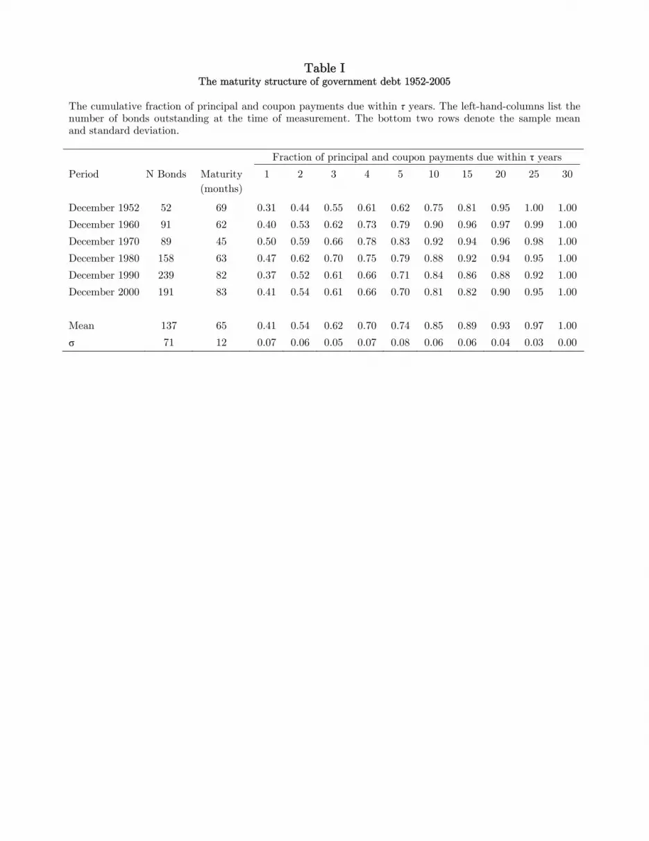
Table I The maturity structure of government debt 1952-2005

The cumulative fraction of principal and coupon payments due within τ years. The left-hand-columns list the number of bonds outstanding at the time of measurement. The bottom two rows denote the sample mean and standard deviation.

Fraction of principal and coupon payments due within τ years

Period N Bonds Maturity 1 2 3 4 5 10 15 20 25 30 (months) December 1952 52 69 0.31 0.44 0.55 0.61 0.62 0.75 0.81 0.95 1.00 1.00

December 1960 91 62 0.40 0.53 0.62 0.73 0.79 0.90 0.96 0.97 0.99 1.00

December 1970 89 45 0.50 0.59 0.66 0.78 0.83 0.92 0.94 0.96 0.98 1.00

December 1980 158 63 0.47 0.62 0.70 0.75 0.79 0.88 0.92 0.94 0.95 1.00

December 1990 239 82 0.37 0.52 0.61 0.66 0.71 0.84 0.86 0.88 0.92 1.00

December 2000 191 83 0.41 0.54 0.61 0.66 0.70 0.81 0.82 0.90 0.95 1.00

Mean 137 65 0.41 0.54 0.62 0.70 0.74 0.85 0.89 0.93 0.97 1.00

σ 71 12 0.07 0.06 0.05 0.07 0.08 0.06 0.06 0.04 0.03 0.00

Table II Bond yields and government debt maturity

The dependent variable is alternately the τ-year yield spread, the τ-year forward rate spread, or the Cochrane-Piazzesi (2005) factor, denoted by γft. The Cochrane-Piazzesi factor is calculated using the coefficients reported in Table 1 of their paper. The independent variable is alternately the fraction of principal and coupon payments due in ten years or longer, or the dollar-weighted average maturity of principal and coupon payments, Mt, expressed in months over 100. t-statistics, reported in brackets, follow Newey-West (1987), allowing up to six lags in the adjustment.

Panel A: Yield spreads ( ) (1)t ty yτ −

2-year 3-year 4-year 5-year 20-year (10 ) /t tD D+ 0.016 0.025 0.034 0.040 0.077

(2.593) (2.564) (2.742) (2.799) (3.677) Mt 0.006 0.010 0.013 0.015 0.028

(2.105) (2.246) (2.442) (2.384) (3.096)

R-squared 0.057 0.045 0.055 0.049 0.062 0.056 0.065 0.053 0.097 0.074

Panel B: Forward rate spreads ( ) (1)t tf yτ − and Cochrane-Piazzesi factor

2-year 3-year 4-year 5-year γft (10 ) /t tD D+ 0.033 0.043 0.061 0.063 0.059

(2.593) (2.478) (2.927) (2.836) (1.623) Mt 0.012 0.018 0.024 0.021 0.028

(2.105) (2.304) (2.674) (2.204) (2.018)

R-squared 0.057 0.045 0.049 0.047 0.066 0.060 0.061 0.041 0.015 0.021

Table III Bond returns and government debt maturity: Univariate tests

The dependent variable is the one-year log return of the τ-year bond minus the log yield of the one-year bond. The independent variable is alternately the fraction of principal and coupon payments due in ten years or longer, or the dollar-weighted average maturity of principal and coupon payments, Mt, expressed in months over 100. The first row of t-statistics, reported in brackets, follows Newey-West (1987), allowing up to 18 lags in the adjustment. The second row of t-statistics follows Hansen and Hodrick (1983), which accounts explicitly for the 12-months of overlap in return measurement. Excess return: 2-year bond 3-year bond 4-year bond 5-year bond 20-year bond

(10 ) /t tD D+ 0.100 0.168 0.231 0.274 0.458

NW, 18 lags (2.599) (2.566) (2.676) (2.685) (2.838)HH, 12 lags (2.273) (2.252) (2.358) (2.373) (2.528)

Mt 0.034 0.061 0.086 0.101 0.170

NW, 18 lags (1.924) (2.054) (2.189) (2.167) (2.313)HH, 12 lags (1.679) (1.799) (1.924) (1.908) (2.046)

R-squared 0.084 0.058 0.073 0.057 0.072 0.059 0.068 0.054 0.068 0.056

Table IV Bond returns and government debt maturity: Multivariate tests

The dependent variable is the one-year log return of the τ-year bond minus the log yield of the one-year bond. The independent variable is alternately the fraction of principal and coupon payments due in ten years or longer, or the dollar-weighted average maturity of principal and coupon payments, Mt, expressed in months over 100. Control variables include the τ-year yield spread and the Cochrane-Piazzesi (2005) factor. The first row of t-statistics, reported in brackets, follows Newey-West (1987), allowing up to 18 lags in the adjustment. The second row of t-statistics follows Hansen and Hodrick (1983), which accounts explicitly for the 12-months of overlap in return measurement. Excess

t2-year bond 3-year bond 4-year bond 5-year bond 20-year bond

(10 ) /t tD D+ 0.081 0.076 0.133 0.123 0.178 0.157 0.215 0.190 0.358 0.301 (2.298) (2.074) (2.228) (2.050) (2.366) (2.062) (2.395) (2.112) (2.622) (2.141) (2.017) (1.816) (1.962) (1.806) (2.094) (1.826) (2.126) (1.879) (2.362) (1.921)

Mt 0.025 0.044 0.061 0.072 0.122 (1.587) (1.703) (1.866) (1.888) (2.119) (1.389) (1.497) (1.648) (1.673) (1.897)

γft 0.310 0.313 0.603 0.605 0.883 0.885 1.004 1.007 1.677 1.680 (4.883) (4.523) (5.176) (4.872) (5.331) (5.053) (4.682) (4.457) (4.340) (4.181) (4.425) (4.070) (4.675) (4.380) (4.800) (4.532) (4.216) (3.999) (3.918) (3.763)

( ) (1)t ty yτ − 1.438 1.776 2.138 2.092 2.036

(3.178) (3.355) (3.549) (3.124) (2.768) (2.854) (2.982) (3.135) (2.782) (2.510)

R-squared 0.269 0.245 0.162 0.285 0.269 0.162 0.310 0.296 0.181 0.273 0.259 0.158 0.276 0.263 0.143

Table V Bond returns and government debt maturity: Various forecast horizons

The dependent variable is alternately the six-month log return of the 20-year bond minus the six-month log return of rolling over one-month T-bills, the one-year log return of the 20-year bond minus the log yield of the one-year bond, or the two, three, or five-year cumulation of one-year excess returns. The independent variable is the fraction of principal and coupon payments due in ten years or longer. The Cochrane-Piazzesi (2005) factor is used as a control. The first row of t-statistics, reported in brackets, follows Newey-West (1987), allowing up to n+6 lags in the adjustment, where n is the forecast horizon. The second row of t-statistics follows Hansen and Hodrick (1983), which accounts explicitly for the n-months of overlap in return measurement. Forecast horizon: 6-months 12-months 24-months 36-months 60-months

(10 ) /t tD D+ 0.219 0.166 0.458 0.358 1.003 0.891 1.574 1.453 2.713 2.543 (2.314) (2.070) (2.838) (2.622) (3.508) (3.431) (3.836) (3.803) (4.608) (4.847) (2.147) (1.876) (2.528) (2.362) (3.156) (3.153) (3.580) (3.768) (4.428) (5.216)

γft 0.903 1.677 1.981 2.146 3.078 (4.631) (4.340) (3.873) (4.565) (4.229) (4.349) (3.918) (4.175) (6.267) (4.395)

R-squared 0.030 0.143 0.068 0.276 0.164 0.309 0.264 0.375 0.428 0.552

Table VI Bond returns and government debt maturity: Robustness checks and extensions

Robustness checks and extensions of return-forecasting regressions. In each case, results are shown for both the univariate regression, as well as a multivariate regression that controls for the Cochrane-Piazzesi (2005) factor. In the baseline case, the dependent variable is the one-year log return of the 20-year bond minus the log yield of the one-year bond, and the independent variables is the fraction of principal and coupon payments due in ten years or longer. The robustness tests include: (a) adding a control for a time trend; (b) controlling for the maturity of debt that is held by Federal Reserve banks; (c) the 1964-2003 subperiod that is used in Cochrane and Piazzesi; (d) 1952-1977, the first half of the sample; (e) 1978-2004, the second half of the sample; (f) annual sampling of the data, leaving the dependent variable unchanged; (g) annual sampling of the data, replacing the dependent variable with 36-month returns; (h) ignoring coupons in the calculation of debt maturity; (i) GLS regressions following Prais-Whinston that adjust for AR(1) type persistence in both LHS and RHS variables; (j) GLS regressions with 36-month returns; (k) replacing the dependent variable with the return of long-term bonds minus that of intermediate-term bonds, and replacing the independent variable by the relative supply of long-term bonds minus that of intermediate-term bonds; (l) same as previous except controlling for the relative supply of long-term bonds (our baseline case variable). t-statistics, reported in brackets, follow Newey-West (1987), allowing up to 18 lags in the adjustment. Univariate Multivariate b (t) R2 b (t) R2

Baseline case 0.458 (2.838) 0.067 0.358 (2.622) 0.274Time trend control 0.320 (1.957) 0.095 0.334 (2.039) 0.277Fed holding control 0.331 (1.484) 0.022 0.512 (2.702) 0.2861964-2003 0.578 (3.018) 0.099 0.341 (2.304) 0.3781952-1977 -0.032 (-0.157) 0.001 0.097 (0.486) 0.0401978-2005 0.993 (2.365) 0.091 0.694 (2.017) 0.358Annual sampling, 12-month horizon 0.468 (2.567) 0.067 0.350 (2.344) 0.324Annual sampling, 36-month horizon 1.580 (3.499) 0.260 1.413 (3.731) 0.463Ignore Coupons 0.349 (1.788) 0.027 0.473 (2.792) 0.283GLS 12-month horizon (annual) 0.367 (1.717) 0.034 0.466 (2.686) 0.377GLS 36-month horizon (annual) 1.177 (1.663) 0.039 1.301 (2.081) 0.163Long-term over intermediate (1) 0.059 (3.504) 0.094 0.054 (3.471) 0.249Long-term over intermediate (2) 0.099 (3.179) 0.119 0.067 (2.475) 0.252

Table VII Bond returns and government debt maturity: GMM Instrumental Variables Regressions

Generalized method of moments instrumental variables regressions of excess bond returns on debt maturity. Debt maturity is measured as the fraction of principal and coupon payments due in ten years or longer. The first stage regression shows estimates from regressions of debt maturity on lagged values of itself, the term spread, the debt-to-gdp ratio, and a time trend. The second stage regression shows the slope coefficient of regressions of the one-year log return of the 20-year bond minus the log yield of the one-year bond, on instrumented values of debt maturity. t-statistics, reported in brackets, are computed using heteroskedasticity-robust standard errors are shown in parentheses.

Forecast horizon: 12-months 36-months

First stage Regression:

Dependent variable = (10 ) /t tD D+

Lagged (10 ) /t tD D+ 0.964 0.994 0.964 0.994 (29.084) (21.720) (29.084) (21.720)

( ) (1)t ty yτ − -0.204 -0.191 -0.204 -0.191

(-1.229) (-1.104) (-1.229) (-1.104)Debt/gdp 0.352 -0.027 0.352 -0.027 (9.710) (-1.096) (9.710) (-1.096)t 0.002 0.002 (6.415) (6.415)

First stage R-squared 0.917 0.692 0.919 0.917 0.692 0.919

Second stage regression:

Dependent variable = Excess bond returns

Forecast (10 ) /t tD D+ 0.516 0.665 0.552 1.779 1.953 2.154

(2.456) (2.069) (2.642) (4.576) (4.912) (5.875)

R-squared 0.06 0.06 0.06 0.26 0.26 0.25

Table VIII Bond returns, government debt maturity, and arbitrageur wealth

The dependent variable is the one-year log return of the 20-year bond minus the log yield of the one-year bond. The independent variables include the term spread, debt maturity, lagged changes in arbitrageur wealth, and interactions of lagged changes in arbitrageur wealth with the term spread and with debt maturity. Debt maturity is measured as the fraction of principal and coupon payments due in ten years or longer.

( ) (1) ( ) (1) (10 ) ( ) (1) (10 )1 1( ) / ( ) /( )t t t t t t t t t t t

Arb Arb Arbt t tr y a b y y cD D y y D Dd W e W f Wτ τ τ ε+ +

+ +− = + − + − ++ Δ + Δ + Δ

Arbitrageurs make money when the term structure is upward sloping and subsequent bond returns are high, thus changes in arbitrageur wealth are proxied by the term spread times subsequent excess bond returns. The first row of t-statistics, reported in brackets, follows Newey-West (1987), allowing up to 18 lags in the adjustment. The second row of t-statistics follows Hansen and Hodrick (1983), which accounts explicitly for the 12-months of overlap in return measurement. (1) (2) (3) (4) (5) (6)

( ) (1)t ty yτ − 3.222 2.822 3.367

(3.623) (3.682) (3.739) (3.219) (3.291) (3.337)

(10 ) /t tD D+

ArbtWΔ

( ) (1)( )t tArbt y yW τ −Δ

(10 ) /( )t tArbt

0.572 0.524 0.543

(3.282) (3.077) (3.175) (2.893) (2.719) (2.802)

-8.038 -14.571 25.857 -11.604

(-1.354) (-2.818) (1.004) (-2.359) (-1.189) (-2.614) (0.978) (-2.219)

-441.940 -721.280 -61.900

(-1.844) (-3.332) (-2.639) (-1.605) (-3.154) (-2.506)

D DW +Δ -189.270

(-1.488) (-1.463)

R-squared 0.183 0.173 0.175 0.117 0.107 0.113

Table IX The effects of arbitrageur wealth measured over different horizons

The dependent variable is the one-year log return of the 20-year bond minus the log yield of the one-year bond. The independent variables include the term spread, debt maturity, lagged changes in arbitrageur wealth, and interactions of lagged changes in arbitrageur wealth with the term spread and with debt maturity. Debt maturity is measured as the fraction of principal and coupon payments due in ten years or longer.

( ) (1) ( ) (1) (10 ) ( ) (1) (10 )1 1( ) / ( ) /( )t t t t t t t t t t t

Arb Arb Arbt t tr y a b y y cD D y y D Dd W e W f Wτ τ τ ε+ +

+ +− = + − + − ++ Δ + Δ + Δ

Arbitrageurs make money when the term structure is upward sloping and subsequent bond returns are high. We measure changes in arbitrageur wealth alternately over a 6, 12, 24, 36, or 60-month lookback period. For a lookback period of 24 months or longer, changes in arbitrageur wealth are measured as the sum of the product of term spreads times subsequent one-year-ahead excess bond returns, summed over the period. For more details, see the text. The first row of t-statistics, reported in brackets, follows Newey-West (1987), allowing up to 18 lags in the adjustment. The second row of t-statistics follows Hansen and Hodrick (1983), which accounts explicitly for the 12-months of overlap in return measurement. Return Forecasting Horizon: 12—month excess bond returns

Lookback period: 6-months 12-months 24-months 36-months 60-months

( ) (1)t ty yτ − 2.847 3.222 3.948 4.288 4.095

(3.633) (3.623) (4.106) (4.570) (3.789) (3.236) (3.219) (3.645) (4.099) (3.391)

(10 ) /t tD D+ 0.508 0.572 0.610 0.609 0.682

(3.055) (3.282) (3.279) (2.795) (2.427) (2.703) (2.893) (2.912) (2.479) (2.175)

ArbtWΔ 1.853 30.258 -8.038 25.857 1.305 34.346 6.381 17.670 5.683 9.062

(0.281) (0.971) (-1.354) (1.004) (0.257) (1.588) (1.397) (1.140) (1.751) (0.675) (0.318) (1.072) (-1.189) (0.978) (0.278) (1.519) (1.595) (1.141) (1.877) (0.649)

( ) (1)( )t tArbt y yW τ −Δ -523.860 -441.940 -701.800 -874.810 -687.750

(-2.255) (-1.844) (-2.725) (-3.346) (-2.709) (-2.834) (-1.605) (-2.706) (-3.378) (-2.620)

(10 ) /( )t tArbt D DW +Δ -164.990 -189.270 -198.850 -108.830 -66.832

(-1.010) (-1.488) (-1.882) (-1.265) (-0.803) (-1.099) (-1.463) (-1.822) (-1.242) (-0.761)

R-squared 0.132 0.077 0.183 0.117 0.189 0.097 0.211 0.086 0.177 0.093