block ywb offshore seismic campaign
TRANSCRIPT
Total E&P Myanmar
Block YWB Offshore Seismic Campaign
Initial Environmental Examination
Final Report
Rev 4 – February 2016
Artelia E&E – Branche Environnement – Unité RSE
Le First Part-Dieu – 2, avenue Lacassagne – 69425 Lyon Cedex 03 – France Tel/Fax: +33 (0)4 37 65 38 77 / +33 (0)4 37 65 38 01
Myanmar
Block YWB Offshore Seismic Campaign
Initial Environmental Examination
Revision 4
February 2016
Authors: Anne-Charlotte DUFAURE, Armeline DIMIER, Charles BOUHELIER, Christophe DERRIEN
Photos Credit: Total Exploration & Production
File: 8541128
ARTELIA E&E – BRANCHE ENVIRONNEMENT – UNITE RSE
Le First Part-Dieu – 2, avenue Lacassagne – 69425 Lyon Cedex 03 – France
Tel/Fax: +33 (0)4 37 65 38 77 / +33 (0)4 37 65 38 01
Quality form
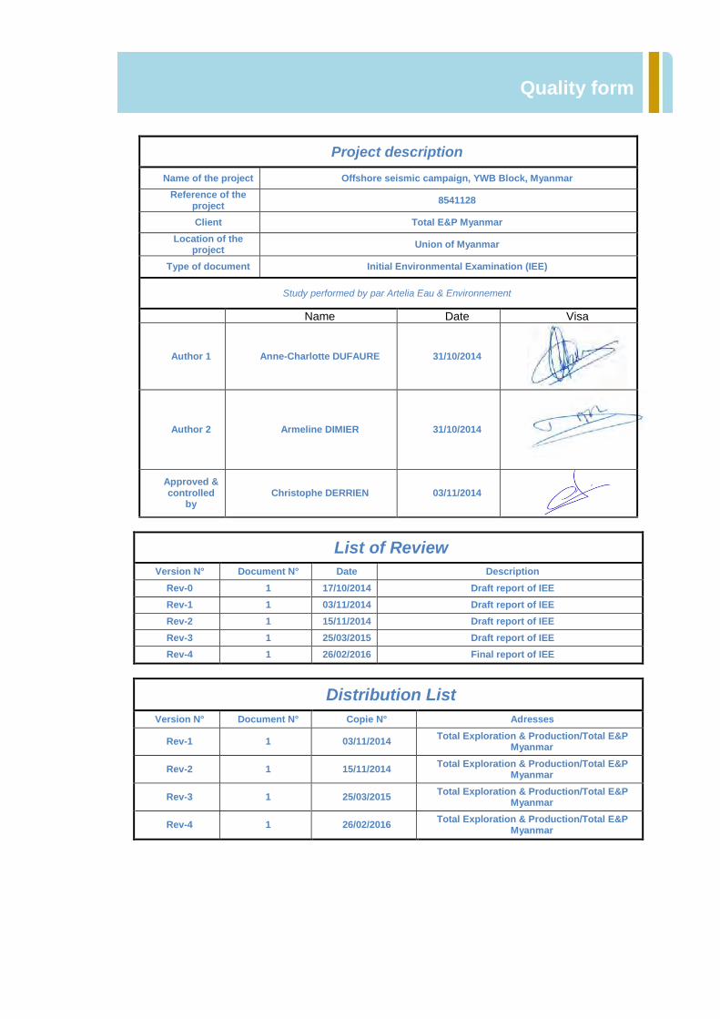
Project description
Name of the project Offshore seismic campaign, YWB Block, Myanmar
Reference of the project
8541128
Client Total E&P Myanmar
Location of the project
Union of Myanmar
Type of document Initial Environmental Examination (IEE)
Study performed by par Artelia Eau & Environnement
Name Date Visa
Author 1 Anne-Charlotte DUFAURE 31/10/2014
Author 2 Armeline DIMIER 31/10/2014
Approved & controlled
by Christophe DERRIEN 03/11/2014
List of Review
Version N° Document N° Date Description
Rev-0 1 17/10/2014 Draft report of IEE
Rev-1 1 03/11/2014 Draft report of IEE
Rev-2 1 15/11/2014 Draft report of IEE
Rev-3 1 25/03/2015 Draft report of IEE
Rev-4 1 26/02/2016 Final report of IEE
Distribution List Version N° Document N° Copie N° Adresses
Rev-1 1 03/11/2014 Total Exploration & Production/Total E&P
Myanmar
Rev-2 1 15/11/2014 Total Exploration & Production/Total E&P
Myanmar
Rev-3 1 25/03/2015 Total Exploration & Production/Total E&P
Myanmar
Rev-4 1 26/02/2016 Total Exploration & Production/Total E&P
Myanmar

Quality form
ARTELIA Eau & Environment Unité : Risque-Société-Environnement (RSE)
Immeuble Le First – 2, avenue Lacassagne
69 425 Lyon Cedex
Tel.: +33 (0)4 37 65 38 77
Fax: +33 (0)4 37 65 38 01

This page is intentionally left blank
TABLE OF CONTENTS
A
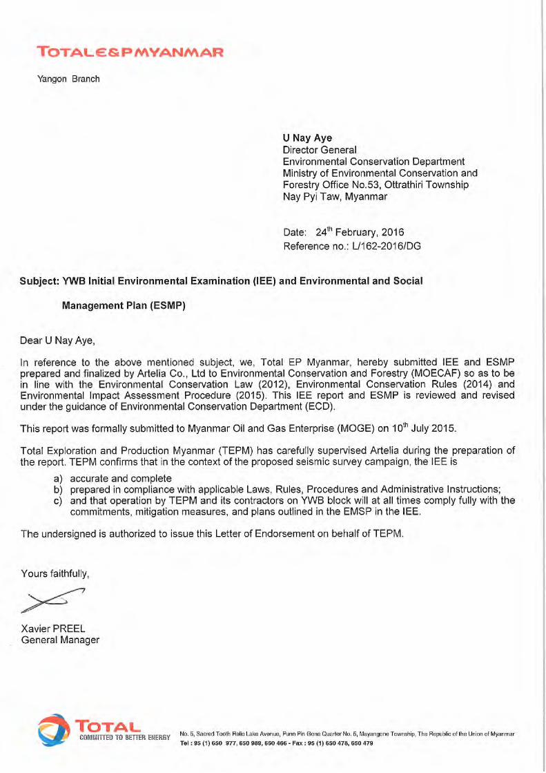
TEPM’s Letter of endorsement 1
SECTION 0. Executive summary 2
0.1 Myanmar language accurate summary 2
0.2 Introduction 3 0.2.1 Context 3 0.2.2 Description of the project 3 0.2.3 Timing of operation 5
0.3 Description of the proposed project 5 0.3.1 Seismic survey 5 0.3.2 Logistic aspects of the seismic campaign 7 0.3.3 Inventory of waste, discharges and emissions 7
0.4 Description of the existing environment 8 0.4.1 Physical environment 8 0.4.2 Biological environment 9 0.4.3 Socioeconomic environment 10
0.5 Environmental and social impact of the proposed project 10 0.5.1 Environmental impacts and associated measures 11 0.5.2 Socioeconomic impacts and associated measures 15
0.6 Environmental and social management plan 16
SECTION 1. Introduction 17
1.1 Context 17
1.2 Project location 19 1.2.1 3D survey location 19 1.2.2 2D seismic survey alternative location 20
1.3 Objectives of the IEE (Initial Environmental Evaluation) 22
SECTION 2. Description of the project 23
2.1 Seismic survey description 23 2.1.1 General description of marine seismic surveys 24 2.1.2 Description of 3D seismic surveys 26 2.1.3 Description of the alternative 2D seismic survey 27 2.1.4 YWB Block 28
2.2 Seismic acquisition Equipment 28
2.2.1 Master seismic vessel and chases/support vessels 28 2.2.2 Seismic source for seismic survey 31 2.2.3 Streamers 37
2.3 Timing of activity 40
2.4 Legal/policy control summary 41 2.4.1 International agreements and conventions 41 2.4.2 Myanmar environmental legislation in line with the Project 43 2.4.3 International guidelines and standards used for this IEE 47
2.5 Emission inventory 49 2.5.1 Acoustic emissions 49 2.5.2 Atmospheric emissions 50 2.5.3 Discharges 51 2.5.4 Hazardous and non hazardous waste 53
TABLE OF CONTENTS
B
SECTION 3. Project proponent details 54
3.1 TOtal E&P Myanmar and contact person 54
3.2 Institutional framework of the Project Proponent 56
3.2.1 Total E&P Myanmar 56 3.2.2 Seismic survey contractor : Polarcus 57
SECTION 4. Information on experts 58
SECTION 5. Description of the environment 59
5.1 Introduction 59
5.2 Geographical scope of the IEE 59
5.3 Meteorological environment 61 5.3.1 Temperature 62 5.3.2 Rainfall 62 5.3.3 Humidity 63 5.3.4 Wind 63 5.3.5 Vulnerability to natural disaster 63
5.4 Physical environment 65
5.4.1 Geomorphology and sismology 65 5.4.2 Regional oceanography 69 5.4.3 Water characteristics 74 5.4.4 Chlorophyll-a 75 5.4.5 Sediment quality 77
5.5 Biological environment 78 5.5.1 Offshore habitat and fauna 78 5.5.2 Coastal habitats and fauna 94 5.5.3 Protected areas 105
5.6 Socio-economic environment 111 5.6.1 Project study area 111 5.6.2 Coastal socio-economic environment 112 5.6.3 Marine socio-economic environment 120 5.6.4 Stakeholder identification 135 5.6.5 Total E&P Myanmar CSR Programs 140
5.7 Synthesis of environmental sensitivity 141 5.7.1 Methodology to access sensitivity 141 5.7.2 Sensitivity of the study area 142
SECTION 6. Environmental and social impact of the project 145
6.1 Methodology 145
6.2 Rating potential and residual impacts 145
6.3 Impact screening 148
6.4 Specific impact on marine mammals, turtles & fish 150
6.4.1 Underwater acoustic emissions 150 6.4.2 Potential impact on marine fauna 151 6.4.3 Conclusion of specific impacts on marine mammals, turtles and fish 155 6.4.4 Additional information 160
6.5 Others environmental and social impacts 161 6.5.1 Potential impact of airguns on benthic community, plankton and seabirds 161 6.5.2 Conclusion of underwater noise’s impacts on other marine fauna 163 6.5.3 Others environmental impacts 164
TABLE OF CONTENTS
C
6.5.4 Other socio-economic impacts 168
6.6 Ecosystem Evaluation 171
6.7 Cumulative impact assessment 172 6.7.1 General issues 172 6.7.2 Potential environmental impacts associated with seismic activities 172 6.7.3 Neighboring blocks seismic surveys schedule 173
6.8 2D seismic survey alternative 175
SECTION 7. Public consultation & disclosure 176
7.1 Initial stakeholder engagement 176
7.2 Public consultations 177 7.2.1 Public consultation in Myeik 178 7.2.2 Public consultation in Dawei 179
SECTION 8. Mitigation measures for the project 182
8.1 Specific mitigation measures for marine mammals, turtles and fishes 182
8.2 Commitment register with responsibilities 195
SECTION 9. Conclusion 199
SECTION 10. Environmental and social management plan 201
10.1 Introduction 201
10.2 Roles and responsibilities 201 10.2.1 RSES 201 10.2.2 Geophysical contractor role and responsibilities 202
10.3 Waste Management Plan 202 10.3.1 WMP key points 203 10.3.2 Wastewater 204
10.4 Oil Spill Contingency Plan (SOPEP) 205
10.5 Environmental monitoring program 205
10.5.1 Guiding principles 205 10.5.2 Marine mammals observation 205 10.5.3 Effluent discharge monitoring 209 10.5.4 Atmospheric emission monitoring 209
10.6 Training Program 210
10.7 Environmental Audit Program 210
10.8 Social Management Plan 211 10.8.1 Stakeholder engagement plan 211 10.8.2 Marine traffic safety plan 211
10.9 Emergency Response: cyclone and Tsunami Response Measures 212
SECTION 11. Responsible persons & costs for ESMP implementation 213
SECTION 12. References 214
12.1 Environmental References 214 12.1.1 Websites 214 12.1.2 Scientific articles 214 12.1.3 Reports 215 12.1.4 Convention 216
12.2 Socio-economic References 216

TABLE OF CONTENTS
D
12.2.1 Webistes 216 12.2.2 Socio-economic articles 216 12.2.3 Reports 216
12.3 Convention 218
SECTION 13. Appendices 219
LIST OF FIGURES
E
Figure 0-1 Project location, Bloc YWB 4 Figure 0-2 Possible 2D seismic survey path 4 Figure 0-3 Marine seismic data acquisition methodology 5 Figure 0-4 Typical seismic source 6 Figure 0-5 Typical seismic receiver cable 6 Figure 0-6 Fan mode geometry 6 Figure 0-7 Photograph of marine streamer vessel 7 Figure 0-8 Diagram of proposed shut-down and observation zones for YWB seismic survey 14 Figure 1-1 Myanmar Offshore Blocks 18 Figure 1-2 YWB Block location 19 Figure 1-3 2D seismic survey location 21 Figure 2-1 YWB Block location 23 Figure 2-2 Technique and example of data acquisition during a marine seismic survey 25 Figure 2-3 Racetrack shooting pattern for 3D seismic survey 26 Figure 2-4 Racetrack shooting pattern for the 2D seismic survey (Alternative) 27 Figure 2-5 Photographs of the marine streamer vessel 29 Figure 2-6 Photographs of support vessel (on the left) and chase vessels (on the right) 30 Figure 2-7 Typical air gun mechanics and example of typical air gun 31 Figure 2-8 Gun array layout 32 Figure 2-9 Pulsed sound from an air gun array expected to be generated during the project 34 Figure 2-10 Acoustic spectrum in water 35 Figure 2-11 Concept of spherical and cylindrical spreading 36 Figure 2-12 Graphical representation of airgun array acoustical spectrum in water 37 Figure 2-13 Typical seismic receiver cable 38 Figure 2-14 Fan mode geometry 39 Figure 2-15 Birds 39 Figure 2-16 Overall program of YWB 41 Figure 3-1 TEPM’s Organisation chart during seismic operation 56 Figure 3-2 Polarcus’ Organigram and connections with TEPM’s team 57 Figure 5-1 Calendar of the four seasons in the Union of Myanmar 61 Figure 5-2 Average temperature of Tavoy 62 Figure 5-3 Average rainfall of Tavoy 63 Figure 5-4 Natural hazard risks in Myanmar 64 Figure 5-5 Structural framework of the Andaman Sea 66 Figure 5-6 Characteristics of Martaban Canyon 67 Figure 5-7 Earthquakes in the study area 69 Figure 5-8 Bathymetry and topography within the YWB Block 70 Figure 5-9 Average wind and current within the project area (January to June) 71 Figure 5-10 Average wind and current within the project area between July to December 72 Figure 5-11 Surface water salinity of Andaman Sea (February to April 2007) 74 Figure 5-12 Chlorophyll-a sampling station in the Bay of Bengal 75 Figure 5-13 Concentration of chlorophyll-a (mg.m-3) in area C of the Bay of Bengal 76 Figure 5-14 Figure showing sediment distribution and dispersal pattern over the Ayeyarwady continental
shelf 77 Figure 5-15 Oceanic division 78 Figure 5-16 Plankton sampling program performed in the Bay of Bengal 80 Figure 5-17 Phytoplankton density (cells/liters) in the surface layer 81 Figure 5-18 Dominant phytoplankton species in the vicinity of the project location 82 Figure 5-19 Location of stations 93 Figure 5-20 Location of mangroves in Myanmar 95 Figure 5-21 Organisms likely to be encountered in the Myanmar’s seagrasses 96 Figure 5-22 Coral reef nearest the project area 99 Figure 5-23 Location of closest Important Bird Areas (IBAs) of the project area 100 Figure 5-24 Location of turtles nesting sites on the coast of Myanmar 103 Figure 5-25 Example of coastal marine mammals 105 Figure 5-26 Location of the nearest sensitive area of the project area 108 Figure 5-27 Moscos Island Wildlife Sanctuary 109 Figure 5-28 Lampi Island protected area 110 Figure 5-29 Map of Myanmar States and Regions 113 Figure 5-30 Population density by states 116 Figure 5-31 Ethnic groups distribution 118
LIST OF FIGURES
F
Figure 5-32 Myanmar offshore blocks and operators 122 Figure 5-33 Myanmar fishing zones as defined by Marine Fisheries law 125 Figure 5-34 Location of ports in Myanmar 133 Figure 5-35 Regional maritime routes and traffic density 134 Figure 5-36 Marine traffic of oil and gas operations 135 Figure 6-1 Screening of potential impacts 149 Figure 6-2 Listing of directs/indirect impacts caused by underwater acoustic emissions 150 Figure 6-3 Theoretical interrelationships of the source level and marine mammal response 151 Figure 6-4 Picture of a loggerhead sea turtle 153 Figure 6-5 Impacts of underwater sound levels on marine mammals generated by typical airguns 155 Figure 6-6 Listing of directs/indirect impacts cause by discharges into the environment 165 Figure 6-7 Example of direct and indirect impacts caused by the physical presence of the seismic
equipment 168 Figure 7-1 Picture of the public consultation in Myeik 179 Figure 7-2 Pictures of the public consultation in Dawei 180 Figure 8-1 M-Weighting curve (Southall et al., 2007) 184 Figure 8-2 Diagram of proposed shut-down and observation zones for YWB Block seismic survey 188 Figure 8-3 Soft start 190 Figure 8-4 Example of observation of marine mammals 192 Figure 8-5 Example of observation techniques of marine mammals 193 Figure 10-1 Waste segregation scheme 204
LIST OF TABLES
G
Table 2-1 Characteristics of vessels for the seismic campaign – generic characteristics 30 Table 2-2 Characteristics of airguns 32 Table 2-3 Characteristics of source signature intensity 34 Table 2-4 Characteristics of the streamers 38 Table 2-5 International agreements and convention in line with the project 41 Table 2-6 Myanmar environmental legislation in line with the project 43 Table 2-7 International guidelines and standards used for this IEE 47 Table 2-8 Hypothesis 50 Table 2-9 Summary of deck and bilge water 53 Table 2-10 Estimated wastes and emissions from seismic activities 53 Table 3-1 Local Total E&P Myanmar recent experience in seismic acquisition 54 Table 3-2 Detail Information about Project Proponent 54 Table 3-3 Detail Information about Project Proponent Organization 55 Table 5-1 Seamounts within the project area 68 Table 5-2 Cyclones recorded within the project area 73 Table 5-3 Pelagic fish present in Myanmar waters 84 Table 5-4 Commercially important fish in Myanmar 86 Table 5-5 Marine mammals occurring in Myanmar waters 87 Table 5-6 Seabirds IUCN threatened species in Myanmar 91 Table 5-7 Characteristics of Myanmar’s mangroves 95 Table 5-8 Distribution of seagrass along Myanmar coastal regions 97 Table 5-9 Location of coral reef in Myanmar 99 Table 5-10 Marine reptiles in the coastal waters of Myanmar 101 Table 5-11 Characteristics of the nearest sensitive areas (within the project location) 107 Table 5-12 Demographic data of the states in the study area 114 Table 5-13 Population at the coastal towns/ports in the study area 115 Table 5-14 Number of fishing vessels engaged in offshore fishery, 2013 129 Table 5-15 General principles for sensitivity scoring (Se) 141 Table 5-16 Synthesis of the description of the environment 142 Table 6-1 Rating impact severity 145 Table 6-2 Impact intensity 146 Table 6-3 Impact severity 147 Table 6-4 Impacts and mitigations on marine mammals, turtle and fish 156 Table 6-5 OCS collisions/spillage (2007-2012) 160 Table 6-6 Observed pathological effects associated with seismic noise 161 Table 6-7 Impacts and mitigations from underwater noise on other marine fauna 163 Table 6-8 Impacts and mitigations concerning others environmental impacts excluding the impacts of
airguns 165 Table 6-9 Socioeconomic impacts of YWB Seismic Project 170 Table 6-10 Increase of sound pressure level (SPL) corresponding to an increase of pressure 173 Table 7-1 Initial engagement with stakeholders 176 Table 7-2 List of participants to the public consultation in Myeik, December 16
th, 2014 178
Table 7-3 List of participants to the public consultation in Dawei, January 27th
, 2014 179 Table 8-1 Proposed injury criteria (Southall et al., 2007) 184 Table 8-2 Calculated distances to TTS and PTS thresholds for cetaceans 185 Table 8-3 Proposed exclusion for marine mammals occurring in Myanmar waters 187 Table 8-4 Commitment register 196 Table 10-1 Waste streams to be encountered during Total E&P Myanmar operations 203 Table 10-2 Synthesis of mitigation measures for underwater noise generated during seismic survey 207 Table 10-3 MMO Monitoring Form: Location and effort 208 Table 10-4 MMO MMO Monitoring Form: Record of operations 208 Table 10-5 MMO Monitoring Form: Record of sighting 208 Table 10-6 Seismic survey discharge monitoring program 209
LIST OF APPENDICES
H
APPENDIX A Policy, legal and administrative Framework 220 APPENDIX B JNCC Guidelines 221 APPENDIX C The Ecosystem-Based Management Fishery in the Bay of Bengal, 2008 222 APPENDIX D CV of Experts 223 APPENDIX E HSE Charter of TEPM 224 APPENDIX F Picture of marine species potentially present in the study area 225 APPENDIX G Attendance sheet for the public consultation organized in Myeik on December 16
th, 2014
(in Burmese language) 226 APPENDIX H MoM and attendance list for the public consultation organized in Dawei on January 27
th,
2015 (in Burmese language) 227 APPENDIX I Polarcus’ Garbage Management Plan 228 APPENDIX J Polarcus’ Oil Spill Procedure 229 APPENDIX K Polarcus’ Extreme Weather Procedure 230 APPENDIX L Polarcus’ Equipment 231
ABREVIATIONS
I
0-P Zero-to-peak AET Apparent Effect Threshold ALGAS Asia Least Cost Greenhouse gas Abatement Strategy DGPS Differential Global Positioning Systems EEZ Exclusive Economic Zones EIA Environmental Impact Assessment EMP Environmental Management Plan GHG Green House Gases IEE Initial Environmental Examination IFC International Finance Corporation
IMO International Maritime Organisation IPIECA International Petroleum Industry Environmental Conservation Association IUCN International Union for Conservation of Nature JNCC Joint Nature Conservation Committee LC Least Concern MARPOL 73/78
International Convention for Prevention of Pollution from Ships 1973/78
MEDEVAC MEDical EVACuation Mlf, Mmf, Mhf
Frequency weightings for cetaceans sensitive to low, middle and high frequencies
MMO Marine Mammal Observer MOE Ministry Of Energy MOGE Myanma Oil and Gas Entreprise NCEA National Commission for Environmental Affairs OCHA United Nation Office for the Coordination of Humanitarian Affairs OGP International Association of Oil and Gas Producers PAM Passive Acoustic Monitoring PSC Production Sharing Contract RMS Root Mean Square SEL Sound Exposure Level SELmp Sound Exposure Levels – multiple pulse SELop Sound Exposure Levels – single pulse SPL Sound Pressure Level TL Transmission Loss TSS Total Suspended Solids TTS Temporary Threshold Shift (refer to noise exposure limit of the marine mammal VU Vulnerable WHO World Health Organisation WMP Waste Management Plan

0
Offshore Seismic Campaign YWB Block Executive summary – 03/15
1231
TEPM’S LETTER OF ENDORSEMENT

0
Offshore Seismic Campaign YWB Block Executive summary – 03/15
2231
SECTION 0. EXECUTIVE SUMMARY
0.1 MYANMAR LANGUAGE ACCURATE SUMMARY
0
Offshore Seismic Campaign YWB Block Executive summary – 03/15
3231
0.2 INTRODUCTION
0.2.1 Context
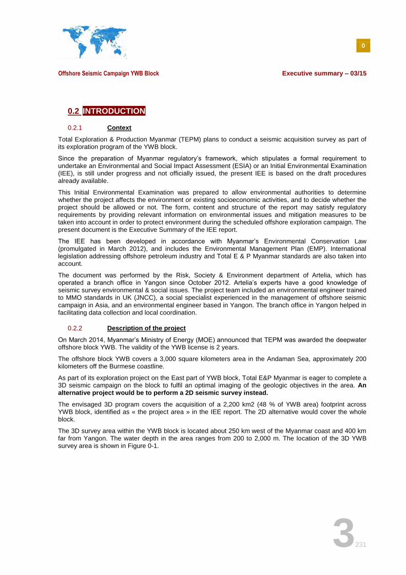
Total Exploration & Production Myanmar (TEPM) plans to conduct a seismic acquisition survey as part of its exploration program of the YWB block.
Since the preparation of Myanmar regulatory’s framework, which stipulates a formal requirement to undertake an Environmental and Social Impact Assessment (ESIA) or an Initial Environmental Examination (IEE), is still under progress and not officially issued, the present IEE is based on the draft procedures already available.
This Initial Environmental Examination was prepared to allow environmental authorities to determine whether the project affects the environment or existing socioeconomic activities, and to decide whether the project should be allowed or not. The form, content and structure of the report may satisfy regulatory requirements by providing relevant information on environmental issues and mitigation measures to be taken into account in order to protect environment during the scheduled offshore exploration campaign. The present document is the Executive Summary of the IEE report.
The IEE has been developed in accordance with Myanmar’s Environmental Conservation Law (promulgated in March 2012), and includes the Environmental Management Plan (EMP). International legislation addressing offshore petroleum industry and Total E & P Myanmar standards are also taken into account.
The document was performed by the Risk, Society & Environment department of Artelia, which has operated a branch office in Yangon since October 2012. Artelia’s experts have a good knowledge of seismic survey environmental & social issues. The project team included an environmental engineer trained to MMO standards in UK (JNCC), a social specialist experienced in the management of offshore seismic campaign in Asia, and an environmental engineer based in Yangon. The branch office in Yangon helped in facilitating data collection and local coordination.
0.2.2 Description of the project
On March 2014, Myanmar’s Ministry of Energy (MOE) announced that TEPM was awarded the deepwater offshore block YWB. The validity of the YWB license is 2 years.
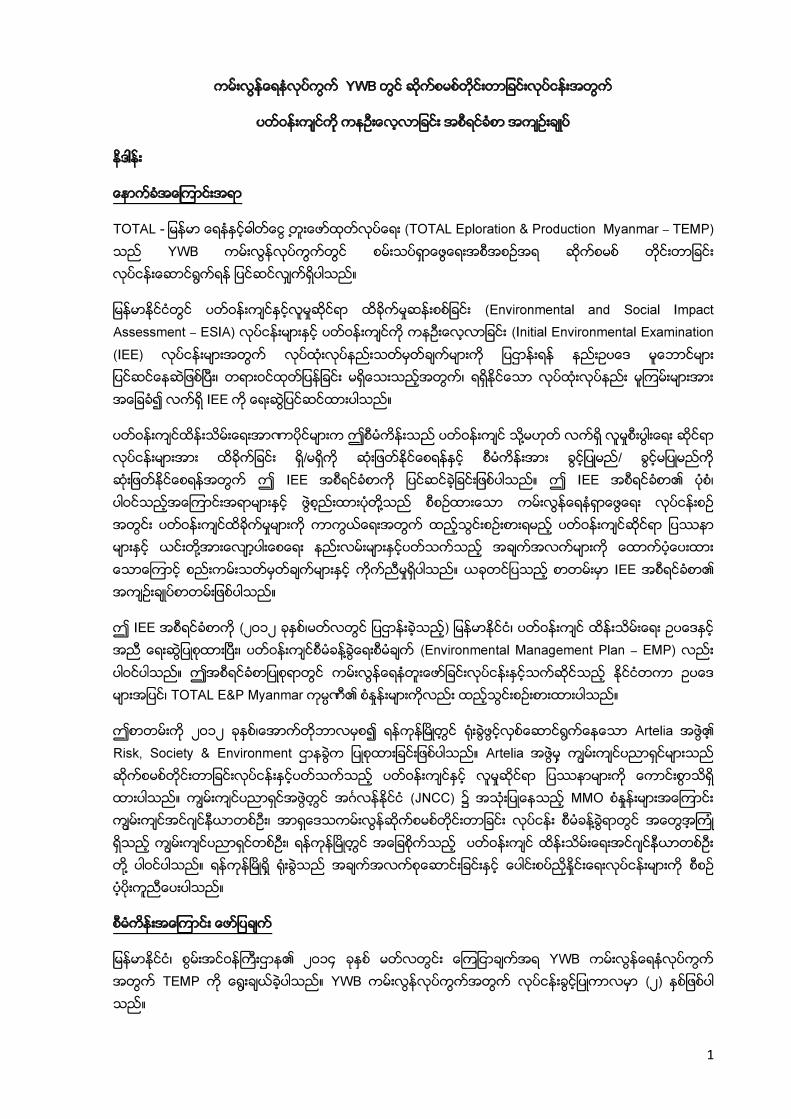
The offshore block YWB covers a 3,000 square kilometers area in the Andaman Sea, approximately 200 kilometers off the Burmese coastline.
As part of its exploration project on the East part of YWB block, Total E&P Myanmar is eager to complete a 3D seismic campaign on the block to fulfil an optimal imaging of the geologic objectives in the area. An alternative project would be to perform a 2D seismic survey instead.
The envisaged 3D program covers the acquisition of a 2,200 km2 (48 % of YWB area) footprint across YWB block, identified as « the project area » in the IEE report. The 2D alternative would cover the whole block.
The 3D survey area within the YWB block is located about 250 km west of the Myanmar coast and 400 km far from Yangon. The water depth in the area ranges from 200 to 2,000 m. The location of the 3D YWB survey area is shown in Figure 0-1.
0
Offshore Seismic Campaign YWB Block Executive summary – 03/15
4231
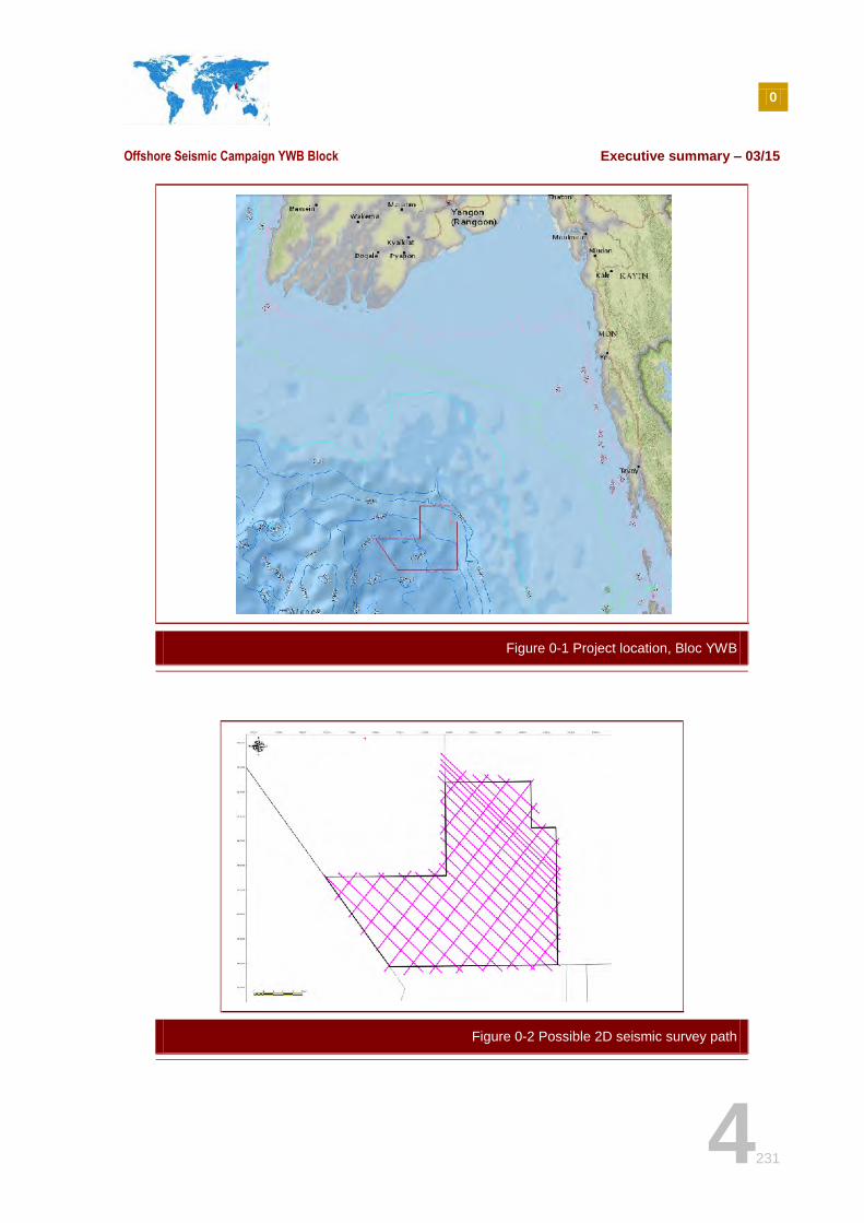
Figure 0-1 Project location, Bloc YWB
Figure 0-2 Possible 2D seismic survey path
0
Offshore Seismic Campaign YWB Block Executive summary – 03/15
5231
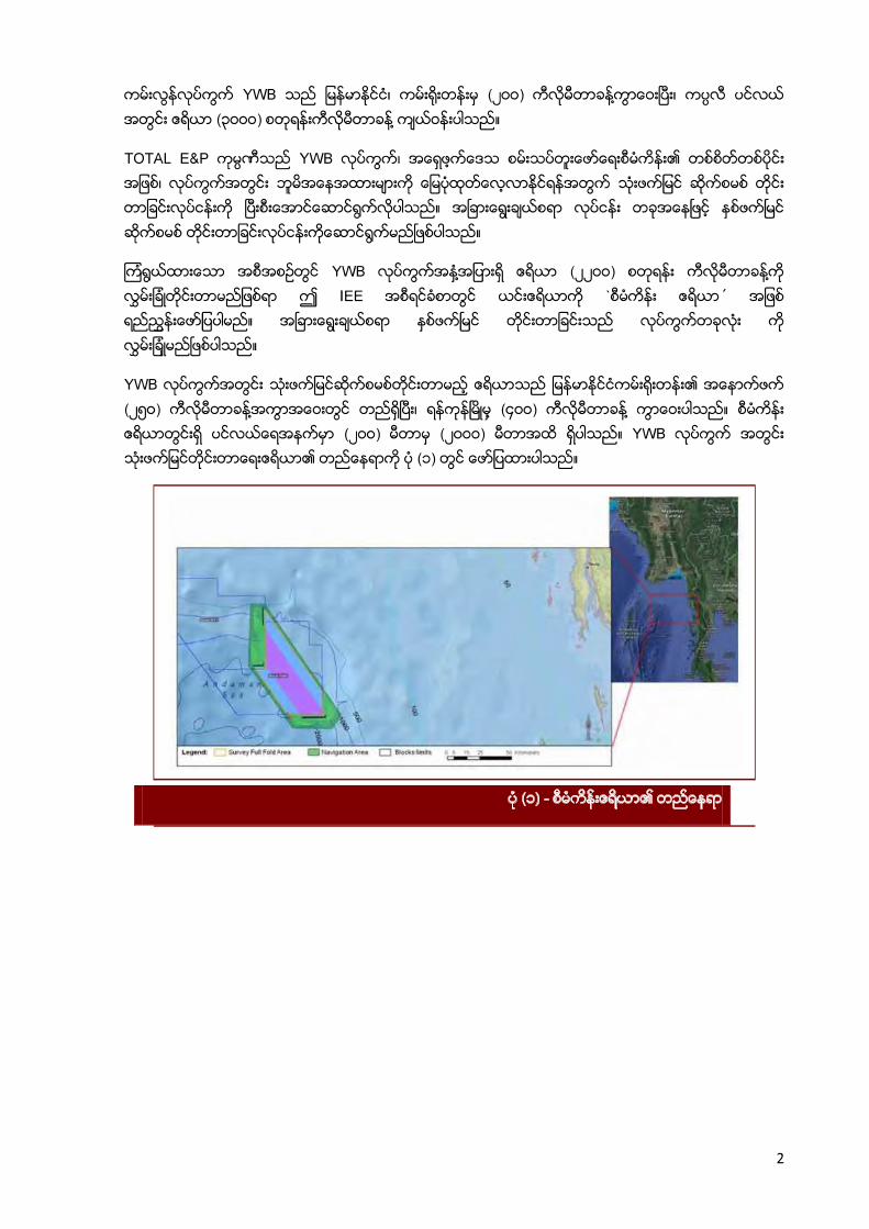
0.2.3 Timing of operation
The 3D seismic campaign is planned to begin on beginning of 2016 with the arrival of the seismic fleet on YWB block. Then, the seismic acquisition will last up to 3 months and the demobilisation of materials (retrieving seismic equipment from the sea) will last approximately 5 days. The alternative 2D seismic survey on the whole YWB block would last only one month because it covers a less dense grid with more space between the navigating lanes.
This project is part of a larger program, where exploration surveys lead to an exploration well in case of success.
0.3 DESCRIPTION OF THE PROPOSED PROJECT
0.3.1 Seismic survey
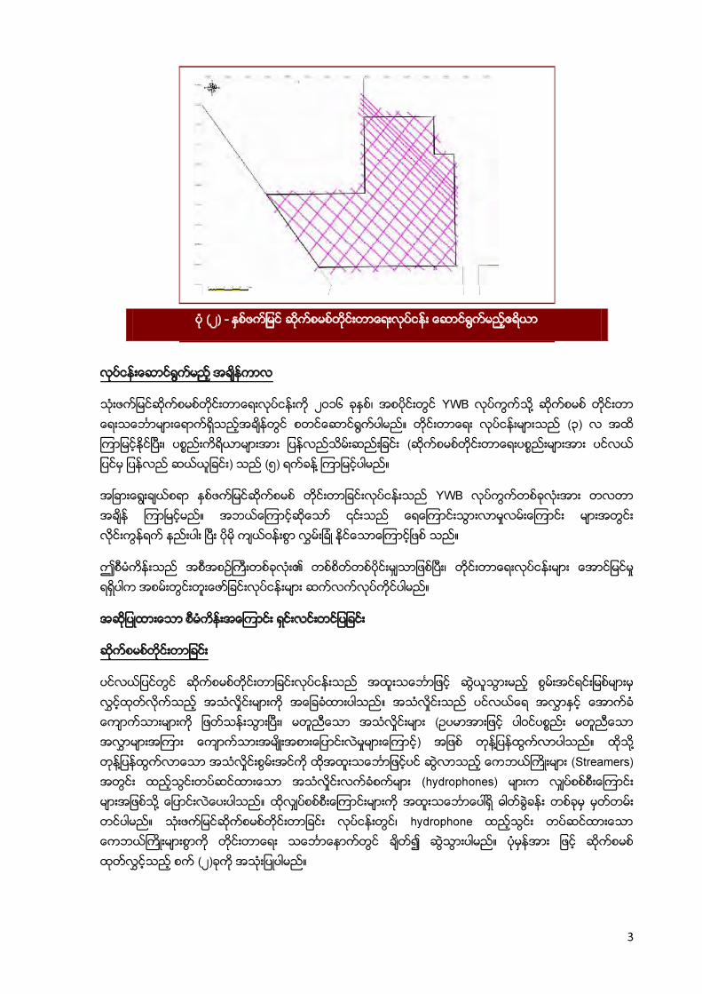
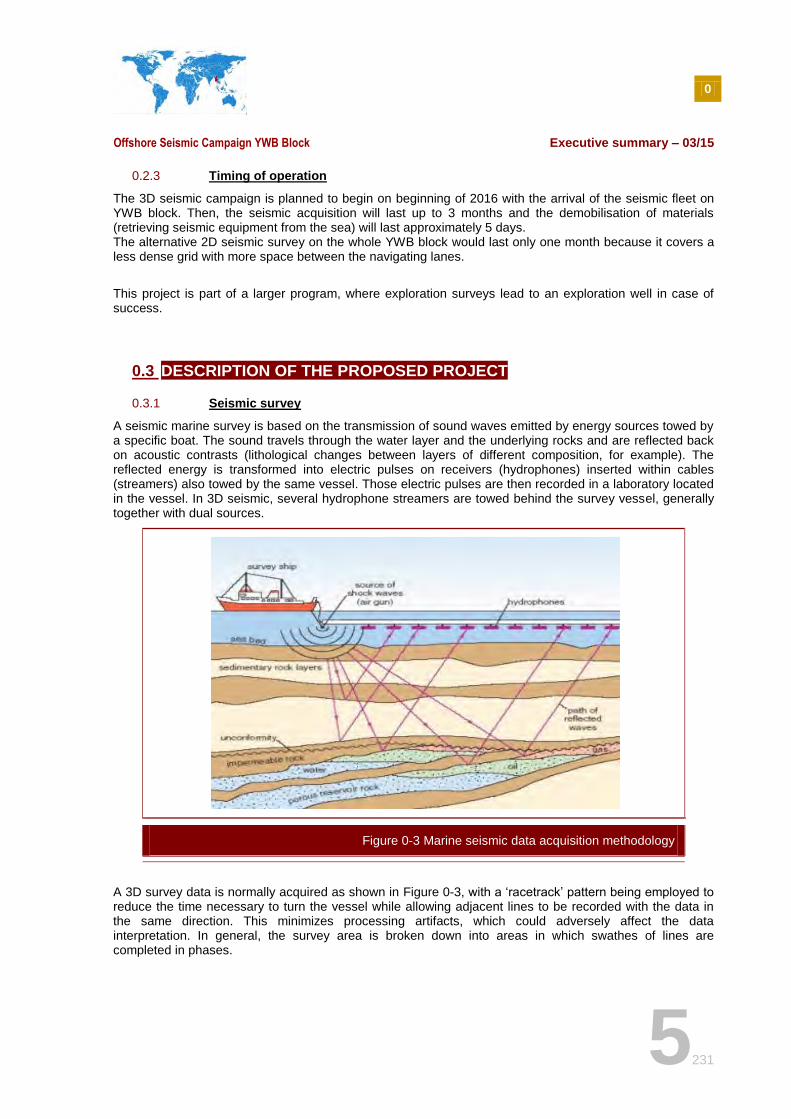
A seismic marine survey is based on the transmission of sound waves emitted by energy sources towed by a specific boat. The sound travels through the water layer and the underlying rocks and are reflected back on acoustic contrasts (lithological changes between layers of different composition, for example). The reflected energy is transformed into electric pulses on receivers (hydrophones) inserted within cables (streamers) also towed by the same vessel. Those electric pulses are then recorded in a laboratory located in the vessel. In 3D seismic, several hydrophone streamers are towed behind the survey vessel, generally together with dual sources.
A 3D survey data is normally acquired as shown in Figure 0-3, with a ‘racetrack’ pattern being employed to reduce the time necessary to turn the vessel while allowing adjacent lines to be recorded with the data in the same direction. This minimizes processing artifacts, which could adversely affect the data interpretation. In general, the survey area is broken down into areas in which swathes of lines are completed in phases.
Figure 0-3 Marine seismic data acquisition methodology
0
Offshore Seismic Campaign YWB Block Executive summary – 03/15
6231
Note: Seismic acquisition will only take place within YWB block. While the seismic vessel carries out its turn outside the YWB block, no airgun will be in activity.
(The Company has not yet selected the geophysical contractor that will carry out the operation; therefore, the description of the seismic equipment below is based on a generic pattern.)
An offshore seismic campaign uses the following devices:
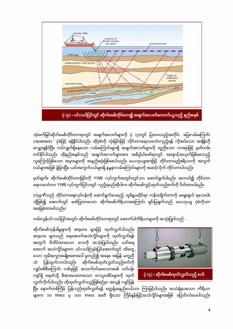
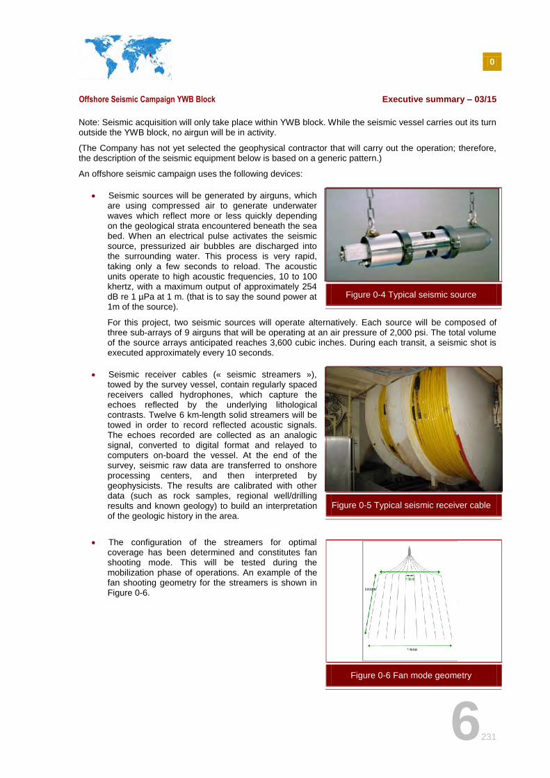
Seismic sources will be generated by airguns, which are using compressed air to generate underwater waves which reflect more or less quickly depending on the geological strata encountered beneath the sea bed. When an electrical pulse activates the seismic source, pressurized air bubbles are discharged into the surrounding water. This process is very rapid, taking only a few seconds to reload. The acoustic units operate to high acoustic frequencies, 10 to 100 khertz, with a maximum output of approximately 254 dB re 1 µPa at 1 m. (that is to say the sound power at 1m of the source).
For this project, two seismic sources will operate alternatively. Each source will be composed of three sub-arrays of 9 airguns that will be operating at an air pressure of 2,000 psi. The total volume of the source arrays anticipated reaches 3,600 cubic inches. During each transit, a seismic shot is executed approximately every 10 seconds.
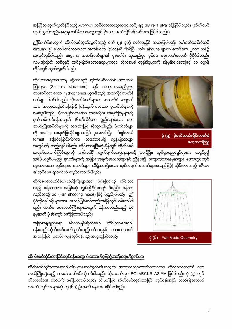
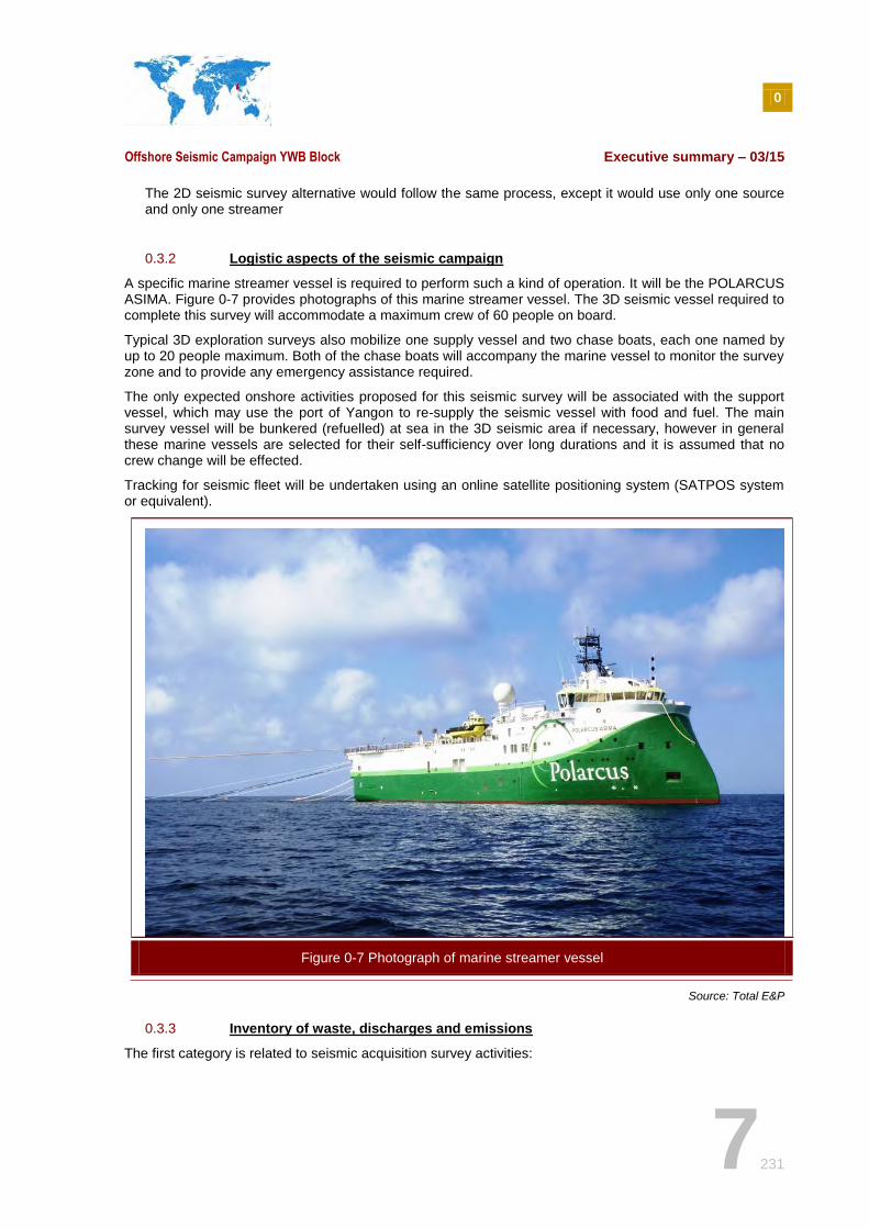
Seismic receiver cables (« seismic streamers »), towed by the survey vessel, contain regularly spaced receivers called hydrophones, which capture the echoes reflected by the underlying lithological contrasts. Twelve 6 km-length solid streamers will be towed in order to record reflected acoustic signals. The echoes recorded are collected as an analogic signal, converted to digital format and relayed to computers on-board the vessel. At the end of the survey, seismic raw data are transferred to onshore processing centers, and then interpreted by geophysicists. The results are calibrated with other data (such as rock samples, regional well/drilling results and known geology) to build an interpretation of the geologic history in the area.
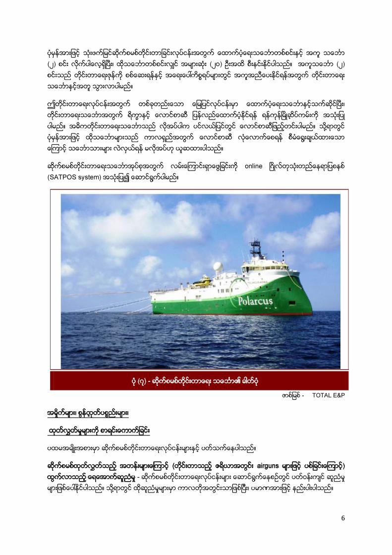
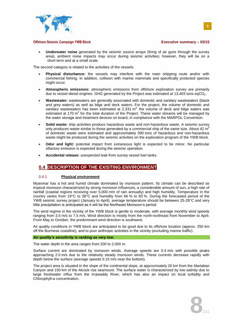
The configuration of the streamers for optimal coverage has been determined and constitutes fan shooting mode. This will be tested during the mobilization phase of operations. An example of the fan shooting geometry for the streamers is shown in Figure 0-6.
Figure 0-4 Typical seismic source
Figure 0-5 Typical seismic receiver cable
Figure 0-6 Fan mode geometry
0
Offshore Seismic Campaign YWB Block Executive summary – 03/15
7231
The 2D seismic survey alternative would follow the same process, except it would use only one source and only one streamer
0.3.2 Logistic aspects of the seismic campaign
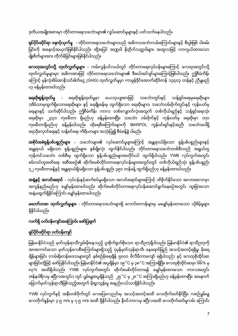
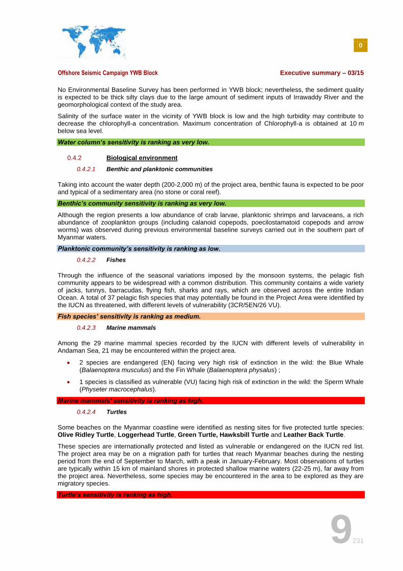
A specific marine streamer vessel is required to perform such a kind of operation. It will be the POLARCUS ASIMA. Figure 0-7 provides photographs of this marine streamer vessel. The 3D seismic vessel required to complete this survey will accommodate a maximum crew of 60 people on board.
Typical 3D exploration surveys also mobilize one supply vessel and two chase boats, each one named by up to 20 people maximum. Both of the chase boats will accompany the marine vessel to monitor the survey zone and to provide any emergency assistance required.
The only expected onshore activities proposed for this seismic survey will be associated with the support vessel, which may use the port of Yangon to re-supply the seismic vessel with food and fuel. The main survey vessel will be bunkered (refuelled) at sea in the 3D seismic area if necessary, however in general these marine vessels are selected for their self-sufficiency over long durations and it is assumed that no crew change will be effected.
Tracking for seismic fleet will be undertaken using an online satellite positioning system (SATPOS system or equivalent).
Figure 0-7 Photograph of marine streamer vessel
Source: Total E&P
0.3.3 Inventory of waste, discharges and emissions
The first category is related to seismic acquisition survey activities:
0
Offshore Seismic Campaign YWB Block Executive summary – 03/15
8231
Underwater noise generated by the seismic source arrays (firing of air guns through the survey area), ambient noise impacts may occur during seismic activities; however, they will be on a short term and at a small scale.
The second category is related to the activities of the vessels:
Physical disturbance: the vessels may interfere with the main shipping route and/or with
commercial fishing. In addition, collision with marine mammals and specifically protected species might occur.
Atmospheric emissions: atmospheric emissions from offshore exploration survey are primarily due to vessel diesel engines. GHG generated by the Project was estimated at 13,403 tons eqCO2.
Wastewater: wastewaters are generally associated with domestic and sanitary wastewaters (black and grey waters) as well as bilge and deck waters. For the project, the volume of domestic and sanitary wastewaters has been estimated at 2,331 m
3; the volume of deck and bilge waters was
estimated at 170 m3 for the total duration of the Project. These water streams will be managed by
the water storage and treatment devices on board, in compliance with the MARPOL Convention.
Solid waste: ship activities produce hazardous waste and non-hazardous waste. A seismic survey only produces waste similar to those generated by a commercial ship of the same size. About 42 m
3
of domestic waste were estimated and approximately 390 tons of hazardous and non-hazardous waste might be produced during the seismic activities on the exploration program of the YWB block.
Odor and light: potential impact from extraneous light is expected to be minor. No particular olfactory emission is expected during the seismic operation.
Accidental release: unexpected leak from survey vessel fuel tanks.
0.4 DESCRIPTION OF THE EXISTING ENVIRONMENT
0.4.1 Physical environment
Myanmar has a hot and humid climate dominated by monsoon pattern. Its climate can be described as tropical monsoon characterized by strong monsoon influences, a considerable amount of sun, a high rate of rainfall (coastal regions receiving over 5,000 mm of rain annually) and high humidity. Temperature in the country varies from 19°C to 38°C and humidity from 66 % to 83 %. During the forecasted period of the YWB seismic survey project (January to April), average temperature should be between 25-28°C and very little precipitation is anticipated as it will be the Northeast Monsoon’s period.
The wind regime in the vicinity of the YWB block is gentle to moderate, with average monthly wind speeds ranging from 3.5 m/s to 7.5 m/s. Wind direction is mostly from the north-northeast from November to April. From May to October, the predominant wind direction is southwest.
Air quality conditions in YWB block are anticipated to be good due to its offshore location (approx. 250 km off the Burmese coastline), and to poor anthropic activities in the vicinity (excluding marine traffic).
Air quality’s sensitivity is ranking as very low.
The water depth in the area ranges from 200 to 2,000 m.
Surface current are dominated by monsoon winds. Average speeds are 0.4 m/s with possible peaks approaching 2.0 m/s due to the relatively steady monsoon winds. These currents decrease rapidly with depth below the surface (average speeds 0.15 m/s near the bottom).
The project area is situated in the slope of the continental slope, at approximately 20 km from the Martaban Canyon and 150 km of the Alcock rise seamount. The surface water is characterized by low salinity due to large freshwater influx from the Irrawaddy River, which has also an impact on local turbidity and Chlorophyll-a concentration.
0
Offshore Seismic Campaign YWB Block Executive summary – 03/15
9231
No Environmental Baseline Survey has been performed in YWB block; nevertheless, the sediment quality is expected to be thick silty clays due to the large amount of sediment inputs of Irrawaddy River and the geomorphological context of the study area.
Salinity of the surface water in the vicinity of YWB block is low and the high turbidity may contribute to decrease the chlorophyll-a concentration. Maximum concentration of Chlorophyll-a is obtained at 10 m below sea level.
Water column’s sensitivity is ranking as very low.
0.4.2 Biological environment
0.4.2.1 Benthic and planktonic communities
Taking into account the water depth (200-2,000 m) of the project area, benthic fauna is expected to be poor and typical of a sedimentary area (no stone or coral reef).
Benthic’s community sensitivity is ranking as very low.
Although the region presents a low abundance of crab larvae, planktonic shrimps and larvaceans, a rich abundance of zooplankton groups (including calanoid copepods, poecilostamatoid copepods and arrow worms) was observed during previous environmental baseline surveys carried out in the southern part of Myanmar waters.
Planktonic community’s sensitivity is ranking as low.
0.4.2.2 Fishes
Through the influence of the seasonal variations imposed by the monsoon systems, the pelagic fish community appears to be widespread with a common distribution. This community contains a wide variety of jacks, tunnys, barracudas, flying fish, sharks and rays, which are observed across the entire Indian Ocean. A total of 37 pelagic fish species that may potentially be found in the Project Area were identified by the IUCN as threatened, with different levels of vulnerability (3CR/5EN/26 VU).
Fish species’ sensitivity is ranking as medium.
0.4.2.3 Marine mammals
Among the 29 marine mammal species recorded by the IUCN with different levels of vulnerability in Andaman Sea, 21 may be encountered within the project area.
2 species are endangered (EN) facing very high risk of extinction in the wild: the Blue Whale (Balaenoptera musculus) and the Fin Whale (Balaenoptera physalus) ;
1 species is classified as vulnerable (VU) facing high risk of extinction in the wild: the Sperm Whale (Physeter macrocephalus).
Marine mammals’ sensitivity is ranking as high.
0.4.2.4 Turtles
Some beaches on the Myanmar coastline were identified as nesting sites for five protected turtle species: Olive Ridley Turtle, Loggerhead Turtle, Green Turtle, Hawksbill Turtle and Leather Back Turtle.
These species are internationally protected and listed as vulnerable or endangered on the IUCN red list. The project area may be on a migration path for turtles that reach Myanmar beaches during the nesting period from the end of September to March, with a peak in January-February. Most observations of turtles are typically within 15 km of mainland shores in protected shallow marine waters (22-25 m), far away from the project area. Nevertheless, some species may be encountered in the area to be explored as they are migratory species.
Turtle’s sensitivity is ranking as high.
0
Offshore Seismic Campaign YWB Block Executive summary – 03/15
10231
0.4.2.5 Marine birds
A total of 20 seabird species are currently identified by the IUCN in Myanmar waters. Amongst these species, 4 species are identified as near threatened and 16 species are recorded as least concern.
Marine birds’sensitivity is ranking as low.
0.4.2.6 Coastal ecosystems, protected area and offshore flora
Myanmar has more than 2,000 kilometers of coastline on the Bay of Bengal. The land pattern in coastal areas consist of mangroves, coral reefs, sea-grass beds, evergreen forest, wetlands and various types of agricultural land. The closest coral reef is situated 158 km of the project area. The nearest Mangroves are at 250 km from the project area as seagrass beds.
Coastal ecosystem and flora’s sensitivity is ranking as medium.
No protected area is located close to the project. The closest is situated at 200 km of the project area (Moscos Island, Widelife sanctuary). The closest Important Bird Areas are Ayeyarwaddy Delta (250 km far from the project area) and Lampi National Park (350 km of the project area).
Protected area’s sensitivity is ranking as low.
0.4.3 Socioeconomic environment
The Project is located in the offshore fishery area, which represents more than 480,000 square kilometers and is only used by 2,000 domestic licensed vessels. However, interactions with fishermen are expected to be low due to the small number of fishermen authorized to fish in the offshore fishery area (2,000, against 30,000 in the inshore fishery area), the location of the block, out of identified fishing grounds, and a recent ban on foreign fishing in Myanmar waters that further reduces the likelihood to encounter fishermen (apart from illegal fishermen).
Fishing activities’ sensitivity is ranking as low.
The Project area is not located on major international shipping lanes. However, the eastern part of the YWB block is overlapping the domestic shipping lane (connecting Yangon to ports in the south of the country and to the Malacca Strait), meaning that commercial ships could be encountered in the Project area.
Marine traffic’s sensitivity is ranking as low.
0.5 ENVIRONMENTAL AND SOCIAL IMPACT OF THE PROPOSED PROJECT
The assessment was conducted in three distinct stages:
Identification of the impact source from the project description, and of the environment sensitivity from the description of its initial status;
Estimation of the potential impact of each source of impact on each sensitive environmental component ;
Identification of mitigation measures to reduce and control the potential impact, and estimation of the residual impact once these measures are implemented.
The study showed two main impacts on the environment and on the socioeconomic context:
The noise generated by marine seismic activities (airguns) may have consequences on the behavior of some species of on marine mammals, turtles and fishes.
At a very lower level, the impact of the presence of ships on commercial marine traffic and the offshore fishery sector.
The table below shows all the project residual impacts, i-e once the compensatory or mitigation measures are implemented. There are 7 impacts considered as « negligible » and 2 as « minor ».
0
Offshore Seismic Campaign YWB Block Executive summary – 03/15
11231
The original project is about a 3D seismic survey but TEPM could change and implement a 2D seismic survey instead. The 2D survey would use only source and one streamer, and it would cover less kilometers (and last only one month), therefore it is assumed that the environmental & social impacts of the 2D seismic campaign would be lighter than those from the 3D one. So, if the 2D alternative is chosen, the mitigation measures described for the 3D survey will be enough to cover efficiently these impacts.
0.5.1 Environmental impacts and associated measures
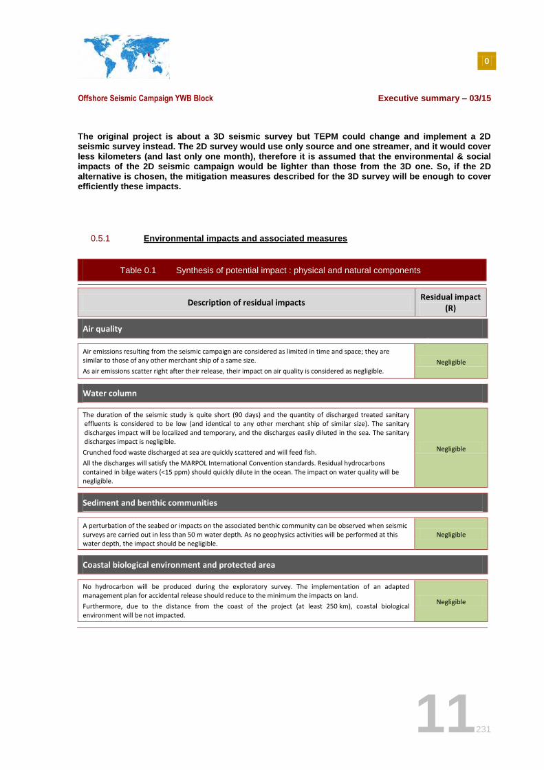
Table 0.1 Synthesis of potential impact : physical and natural components
Description of residual impacts Residual impact
(R)
Air quality
Air emissions resulting from the seismic campaign are considered as limited in time and space; they are similar to those of any other merchant ship of a same size.
As air emissions scatter right after their release, their impact on air quality is considered as negligible. Negligible
Water column
The duration of the seismic study is quite short (90 days) and the quantity of discharged treated sanitary effluents is considered to be low (and identical to any other merchant ship of similar size). The sanitary discharges impact will be localized and temporary, and the discharges easily diluted in the sea. The sanitary discharges impact is negligible.
Crunched food waste discharged at sea are quickly scattered and will feed fish.
All the discharges will satisfy the MARPOL International Convention standards. Residual hydrocarbons contained in bilge waters (<15 ppm) should quickly dilute in the ocean. The impact on water quality will be negligible.
Negligible
Sediment and benthic communities
A perturbation of the seabed or impacts on the associated benthic community can be observed when seismic surveys are carried out in less than 50 m water depth. As no geophysics activities will be performed at this water depth, the impact should be negligible.
Negligible
Coastal biological environment and protected area
No hydrocarbon will be produced during the exploratory survey. The implementation of an adapted management plan for accidental release should reduce to the minimum the impacts on land.
Furthermore, due to the distance from the coast of the project (at least 250 km), coastal biological environment will be not impacted.
Negligible
0
Offshore Seismic Campaign YWB Block Executive summary – 03/15
12231
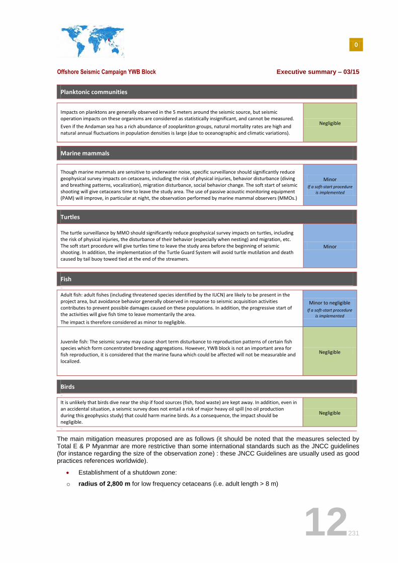
Planktonic communities
Impacts on planktons are generally observed in the 5 meters around the seismic source, but seismic operation impacts on these organisms are considered as statistically insignificant, and cannot be measured.
Even if the Andaman sea has a rich abundance of zooplankton groups, natural mortality rates are high and natural annual fluctuations in population densities is large (due to oceanographic and climatic variations).
Negligible
Marine mammals
Though marine mammals are sensitive to underwater noise, specific surveillance should significantly reduce geophysical survey impacts on cetaceans, including the risk of physical injuries, behavior disturbance (diving and breathing patterns, vocalization), migration disturbance, social behavior change. The soft start of seismic shooting will give cetaceans time to leave the study area. The use of passive acoustic monitoring equipment (PAM) will improve, in particular at night, the observation performed by marine mammal observers (MMOs.)
Minor
If a soft-start procedure is implemented
Turtles
The turtle surveillance by MMO should significantly reduce geophysical survey impacts on turtles, including the risk of physical injuries, the disturbance of their behavior (especially when nesting) and migration, etc. The soft start procedure will give turtles time to leave the study area before the beginning of seismic shooting. In addition, the implementation of the Turtle Guard System will avoid turtle mutilation and death caused by tail buoy towed tied at the end of the streamers.
Minor
Fish Turtles
Adult fish: adult fishes (including threatened species identified by the IUCN) are likely to be present in the project area, but avoidance behavior generally observed in response to seismic acquisition activities contributes to prevent possible damages caused on these populations. In addition, the progressive start of the activities will give fish time to leave momentarily the area.
The impact is therefore considered as minor to negligible.
Minor to negligible
If a soft-start procedure is implemented
Juvenile fish: The seismic survey may cause short term disturbance to reproduction patterns of certain fish species which form concentrated breeding aggregations. However, YWB block is not an important area for fish reproduction, it is considered that the marine fauna which could be affected will not be measurable and localized.
Negligible
Birds Turtles
It is unlikely that birds dive near the ship if food sources (fish, food waste) are kept away. In addition, even in an accidental situation, a seismic survey does not entail a risk of major heavy oil spill (no oil production during this geophysics study) that could harm marine birds. As a consequence, the impact should be negligible.
Negligible
Turtles
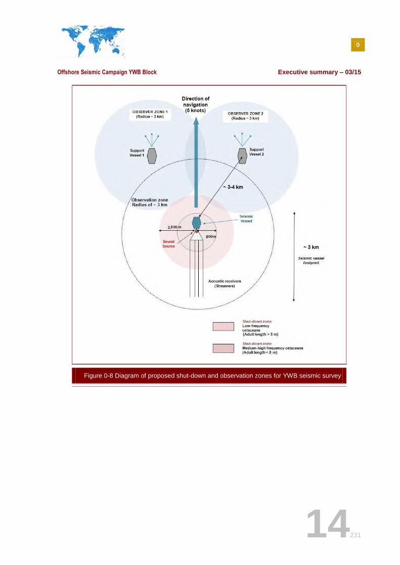
The main mitigation measures proposed are as follows (it should be noted that the measures selected by Total E & P Myanmar are more restrictive than some international standards such as the JNCC guidelines (for instance regarding the size of the observation zone) : these JNCC Guidelines are usually used as good practices references worldwide).
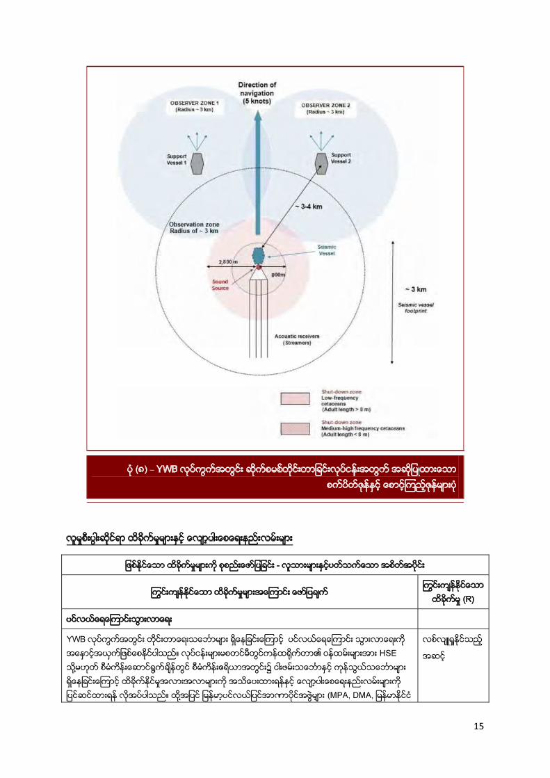
Establishment of a shutdown zone:
o radius of 2,800 m for low frequency cetaceans (i.e. adult length > 8 m)
0
Offshore Seismic Campaign YWB Block Executive summary – 03/15
13231
o radius of 800 m for medium/high frequency cetacean (i.e. adult length < 8 m)
Establishment of an observation zone (radius of 3 km) from the center of the seismic source array. Within this area, continuous visual monitoring will be undertaken by a qualified Marine Mammal Observer (MMO) on the seismic survey vessel, including continuous monitoring during a period of at least 60 minutes prior to airgun start-up (applicable to deep waters).
During the pre-shooting watch, the seismic survey will be stopped if a marine mammal is observed within this area. If a marine mammal enters the zone after operations have started, no mitigation actions are recommended by the JNCC.
1 observer on each of the 2 support vessels in addition to the MMO on seismic vessel. The observers will be members of the crew of each vessel trained by the MMO before the beginning of the survey. The Observers will be in charge of reporting any marine mammals approaching the area.
Establishment of a delay period of 20 minutes before the start-up (including soft start) after the last sighting of a marine mammal within the shutdown zone. Passive Acoustic Monitoring (PAM) will complement visual observation (with adapted devices that enable to detect animals when they vocalize, even when they dive for a long time) during night time and when visibility is too low to enable visual observations.
Implementation of a soft-start procedure. Prior to acquiring data on each seismic line and after each break in operations, power will increase slowly in the seismic array over a period of at least 20 minutes (no longer than 40 minutes) to allow sensitive marine fauna to leave/avoid the area.
An 800-m radius exclusion zone will be used as well for turtles. Moreover, tail buoys tied to streamers will be equipped with a protection system on their propellers (such as Turtle Guard) in order to prevent turtles from being injured.
Figure 0-8 illustrates the shut-down and observations zones proposed for the project to mitigate the impact on marine fauna.
0
Offshore Seismic Campaign YWB Block Executive summary – 03/15
14231
Figure 0-8 Diagram of proposed shut-down and observation zones for YWB seismic survey
0
Offshore Seismic Campaign YWB Block Executive summary – 03/15
15231
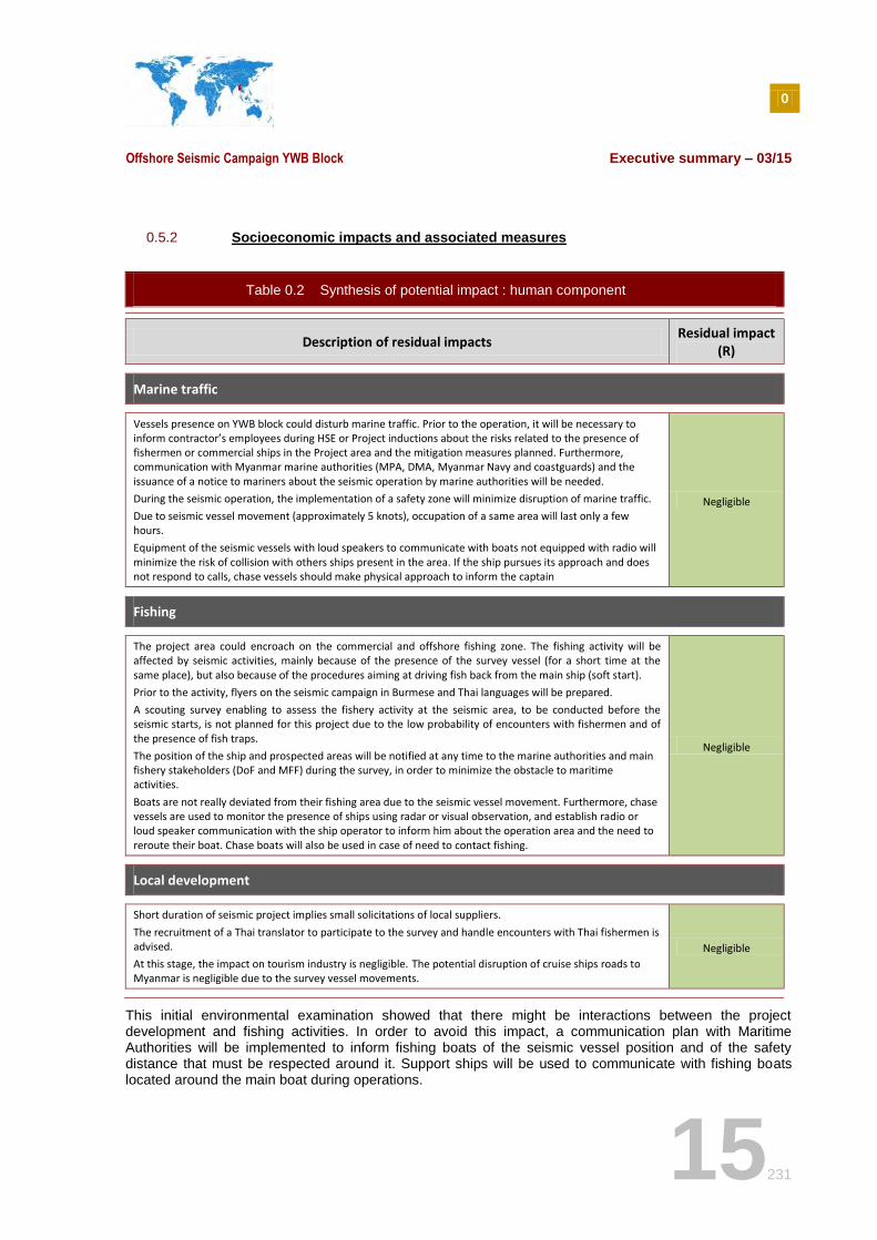
0.5.2 Socioeconomic impacts and associated measures
Table 0.2 Synthesis of potential impact : human component
Description of residual impacts Residual impact
(R)
Marine traffic
Vessels presence on YWB block could disturb marine traffic. Prior to the operation, it will be necessary to inform contractor’s employees during HSE or Project inductions about the risks related to the presence of fishermen or commercial ships in the Project area and the mitigation measures planned. Furthermore, communication with Myanmar marine authorities (MPA, DMA, Myanmar Navy and coastguards) and the issuance of a notice to mariners about the seismic operation by marine authorities will be needed.
During the seismic operation, the implementation of a safety zone will minimize disruption of marine traffic.
Due to seismic vessel movement (approximately 5 knots), occupation of a same area will last only a few hours.
Equipment of the seismic vessels with loud speakers to communicate with boats not equipped with radio will minimize the risk of collision with others ships present in the area. If the ship pursues its approach and does not respond to calls, chase vessels should make physical approach to inform the captain
Negligible
Fishing
The project area could encroach on the commercial and offshore fishing zone. The fishing activity will be affected by seismic activities, mainly because of the presence of the survey vessel (for a short time at the same place), but also because of the procedures aiming at driving fish back from the main ship (soft start).
Prior to the activity, flyers on the seismic campaign in Burmese and Thai languages will be prepared.
A scouting survey enabling to assess the fishery activity at the seismic area, to be conducted before the seismic starts, is not planned for this project due to the low probability of encounters with fishermen and of the presence of fish traps.
The position of the ship and prospected areas will be notified at any time to the marine authorities and main fishery stakeholders (DoF and MFF) during the survey, in order to minimize the obstacle to maritime activities.
Boats are not really deviated from their fishing area due to the seismic vessel movement. Furthermore, chase vessels are used to monitor the presence of ships using radar or visual observation, and establish radio or loud speaker communication with the ship operator to inform him about the operation area and the need to reroute their boat. Chase boats will also be used in case of need to contact fishing.
Negligible
Local development
Short duration of seismic project implies small solicitations of local suppliers.
The recruitment of a Thai translator to participate to the survey and handle encounters with Thai fishermen is advised.
At this stage, the impact on tourism industry is negligible. The potential disruption of cruise ships roads to Myanmar is negligible due to the survey vessel movements.
Negligible
This initial environmental examination showed that there might be interactions between the project development and fishing activities. In order to avoid this impact, a communication plan with Maritime Authorities will be implemented to inform fishing boats of the seismic vessel position and of the safety distance that must be respected around it. Support ships will be used to communicate with fishing boats located around the main boat during operations.
0
Offshore Seismic Campaign YWB Block Executive summary – 03/15
16231
To conclude, the impacts associated with these activities have a limited duration (90 days) and occur in a limited area (the vessels do not remain static). Thus, heavy and irreversible impacts are neither expected, nor long-term impacts significantly altering the environment or surrounding ecosystems.
0.6 ENVIRONMENTAL AND SOCIAL MANAGEMENT PLAN
The Environmental and Social Management Plan will ensure that all identified mitigation measures in the IEE are implemented, in an appropriate planning. It will include the following items:
Health, Safety and Environment policy;
Organization, resources and documentation;
Hazard identification and risk management;
Work procedures, change management and response in case of emergency situation;
Operation monitoring system: reporting, and research on corrective actions;
Waste management plan;
Discharge management plan;
Training program;
Environment monitoring plan ;
Socioeconomic program, including relationship with community, and navigation plan;
…
1
Offshore Seismic Campaign YWB Block Introduction – 11/14
17231
SECTION 1. INTRODUCTION
1.1 CONTEXT
Myanmar is one of the world's oldest oil producers, exporting its first barrel in 1853. Rangoon Oil Company, the first foreign oil company to drill in the country, was created in 1871. Between 1886 and 1963, the country's oil industry was dominated by Burmah Oil Company (BOC), which discovered the Yenangyaung field in 1887 and the Chauk field in 1902. Both are still in production.
Currently, in the offshore, Total E&P Myanmar, Petronas Carigali Myanmar, Daewoo, PTT-EP, China National Offshore Oil Corporation, China National Petrochemical Corporation, Essar, GAIL, Malaysia’s Rimbunam, India’s ONGC, Silver Wave Energy, Australia’s Danford Equities and Russia’s Sun Itera Oil & Gas are exploring and/or developing 31 blocks.
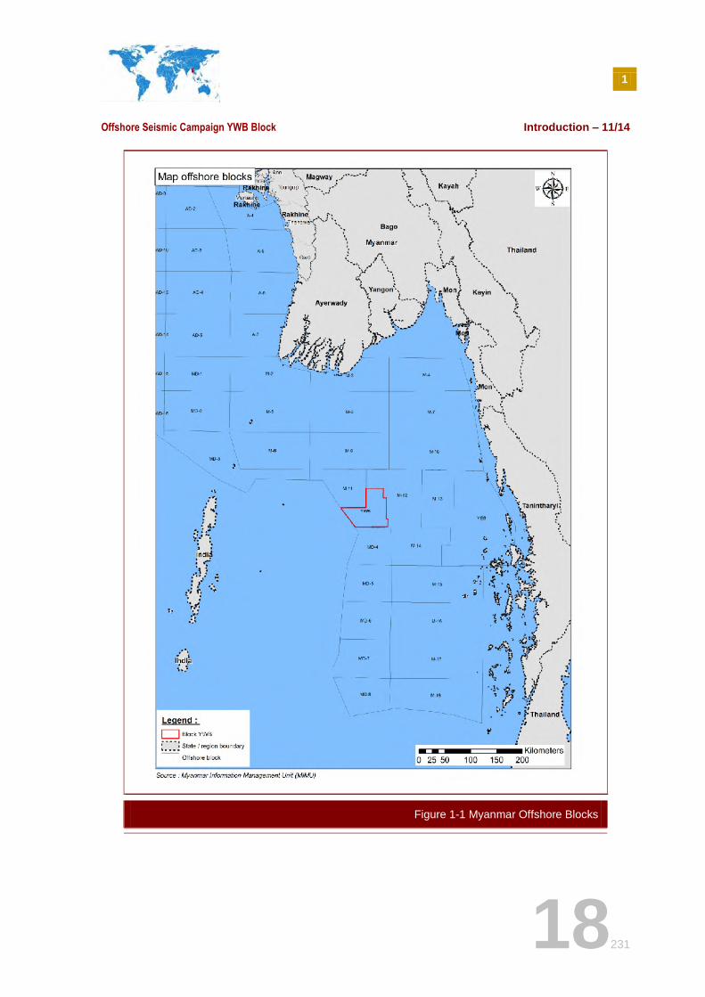
In this context, in March 2014, Myanmar’s Ministry of Energy (MOE) through its 100% state owned entity Myanmar Oil and Gas Enterprise (MOGE) has announced that Total E&P Myanmar was awarded the deepwater offshore block YWB (Cf. Figure 1-1). Total E&P Myanmar objectives are to evaluate the prospectivity of the East part of YWB Block, in particular to identify if there is an extension of the M11 anticlinorium; and the aim is to identify/obtain characteristics of potential hydrocarbons’ reservoirs. To achieve this, Total E&P Myanmar plans to complete a seismic campaign, object of the present Initial Environmental Examination. Total E&P Myanmar is 100% operator of YWB Block and the validity of the YWB license is 2 years.
The original project is about a 3D seismic survey but TEPM could change and implement a 2D seismic survey instead. The environmental & social impacts of a 2D seismic campaign being lighter than those from a 3D one, it is assumed that if the 2D alternative is chosen, the mitigation measures will have to be the same as described for the 3D.
1
Offshore Seismic Campaign YWB Block Introduction – 11/14
18231
Figure 1-1 Myanmar Offshore Blocks
1
Offshore Seismic Campaign YWB Block Introduction – 11/14
19231
Since the preparation of Myanmar regulatory’s framework, which stipulates a formal requirement to undertake an Environmental and Social Impact Assessment (ESIA) or an Initial Environmental Examination (IEE), is still under progress and not officially issued, Total E&P Myanmar performed the present IEE based on the Myanmar draft procedure available.
1.2 PROJECT LOCATION
1.2.1 3D survey location
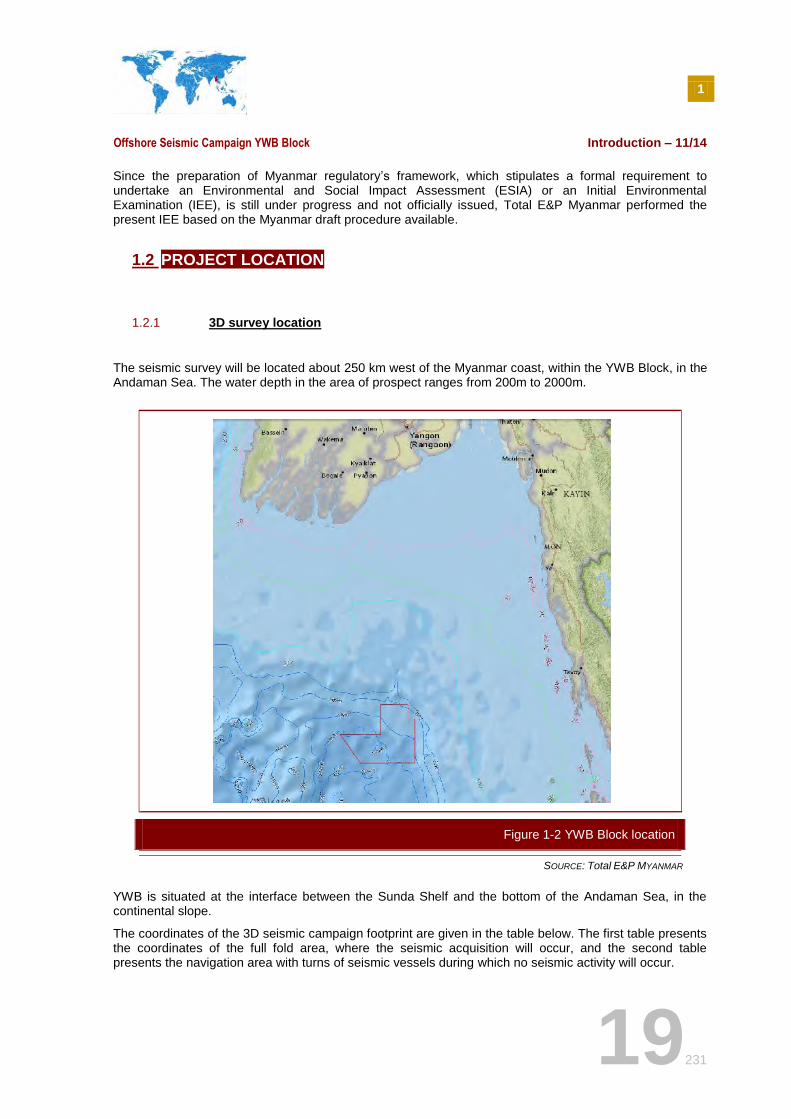
The seismic survey will be located about 250 km west of the Myanmar coast, within the YWB Block, in the Andaman Sea. The water depth in the area of prospect ranges from 200m to 2000m.
SOURCE: Total E&P MYANMAR
YWB is situated at the interface between the Sunda Shelf and the bottom of the Andaman Sea, in the continental slope.
The coordinates of the 3D seismic campaign footprint are given in the table below. The first table presents the coordinates of the full fold area, where the seismic acquisition will occur, and the second table presents the navigation area with turns of seismic vessels during which no seismic activity will occur.
Figure 1-2 YWB Block location
1
Offshore Seismic Campaign YWB Block Introduction – 11/14
20231
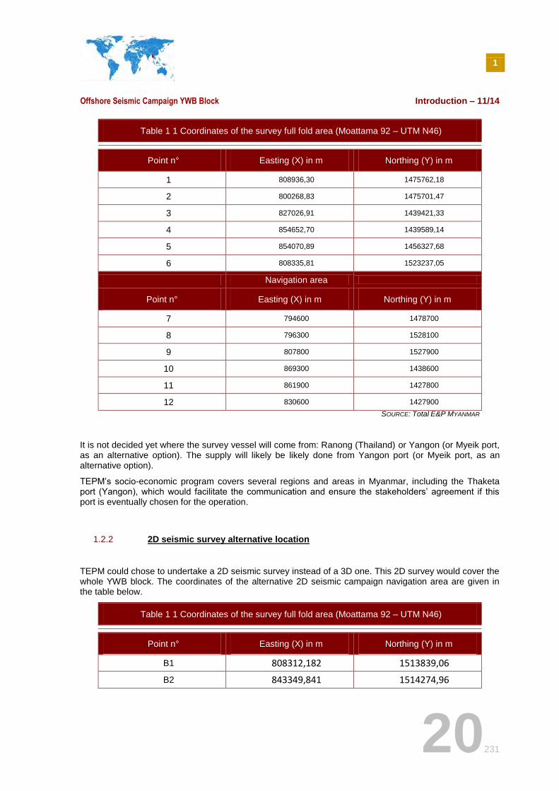
Table 1 1 Coordinates of the survey full fold area (Moattama 92 – UTM N46)
Point n° Easting (X) in m Northing (Y) in m
1 808936,30 1475762,18
2 800268,83 1475701,47
3 827026,91 1439421,33
4 854652,70 1439589,14
5 854070,89 1456327,68
6 808335,81 1523237,05
Navigation area
Point n° Easting (X) in m Northing (Y) in m
7 794600 1478700
8 796300 1528100
9 807800 1527900
10 869300 1438600
11 861900 1427800
12 830600 1427900
SOURCE: Total E&P MYANMAR
It is not decided yet where the survey vessel will come from: Ranong (Thailand) or Yangon (or Myeik port, as an alternative option). The supply will likely be likely done from Yangon port (or Myeik port, as an alternative option).
TEPM’s socio-economic program covers several regions and areas in Myanmar, including the Thaketa port (Yangon), which would facilitate the communication and ensure the stakeholders’ agreement if this port is eventually chosen for the operation.
1.2.2 2D seismic survey alternative location
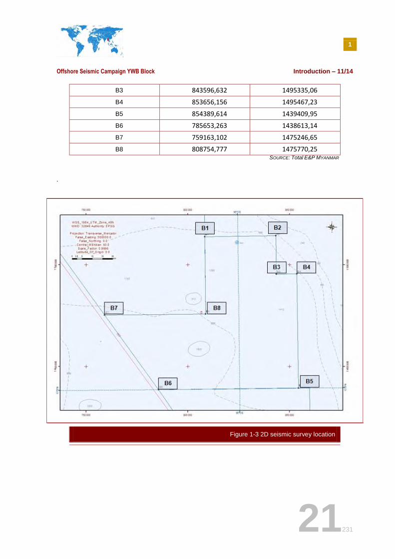
TEPM could chose to undertake a 2D seismic survey instead of a 3D one. This 2D survey would cover the whole YWB block. The coordinates of the alternative 2D seismic campaign navigation area are given in the table below.
Table 1 1 Coordinates of the survey full fold area (Moattama 92 – UTM N46)
Point n° Easting (X) in m Northing (Y) in m
B1 808312,182 1513839,06
B2 843349,841 1514274,96
1
Offshore Seismic Campaign YWB Block Introduction – 11/14
21231
B3 843596,632 1495335,06
B4 853656,156 1495467,23
B5 854389,614 1439409,95
B6 785653,263 1438613,14
B7 759163,102 1475246,65
B8 808754,777 1475770,25 SOURCE: Total E&P MYANMAR
.
Figure 1-3 2D seismic survey location
1
Offshore Seismic Campaign YWB Block Introduction – 11/14
22231
1.3 OBJECTIVES OF THE IEE (INITIAL ENVIRONMENTAL EVALUATION)
An Initial Environmental Evaluation is a report comprising an assessment of a proposed project that is prepared to aid environmental Authorities in determining whether the project affects the environment or existing socio-economic activities, and in deciding whether the project should be allowed or not. The form, content and structure of the report shall be in accordance with the Myanmar regulation (EIA Procedure), Total E&P Myanmar guidelines and international best practice, and include the Environmental Management Plan (EMP).
Box 1. Content of IEE Report The proposed IEE will comprise the following parts: a) Project description in reasonable detail together with overview and layout maps; b) Identification of the Project Proponent including the identification of the owners, directors (if any)
and day to day management and officers of the Project Proponent; c) Identification of the IEE experts, including which expert is responsible for which part of the IEE
Report; d) Description of the surrounding environmental conditions of the Project; e) Identification and assessment of potential Adverse Impacts; f) Results of the public consultation / public participation process and the Total E&P Myanmar's
written response to comments received during that process; g) The environmental protection measures of the Project; h) The conclusion of the IEE; i) The EMP; and j) The persons, organizations and budgets needed for implementation of the EMP.
2
Offshore Seismic Campaign YWB Block Description of the Project – 11/14
23231
SECTION 2. DESCRIPTION OF THE PROJECT
2.1 SEISMIC SURVEY DESCRIPTION
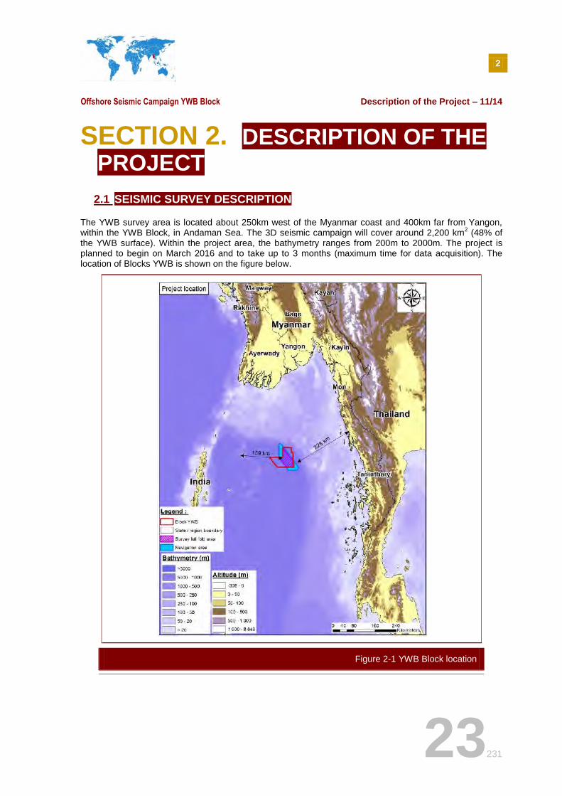
The YWB survey area is located about 250km west of the Myanmar coast and 400km far from Yangon, within the YWB Block, in Andaman Sea. The 3D seismic campaign will cover around 2,200 km
2 (48% of
the YWB surface). Within the project area, the bathymetry ranges from 200m to 2000m. The project is planned to begin on March 2016 and to take up to 3 months (maximum time for data acquisition). The location of Blocks YWB is shown on the figure below.
Figure 2-1 YWB Block location
2
Offshore Seismic Campaign YWB Block Description of the Project – 11/14
24231
2.1.1 General description of marine seismic surveys
Seismic surveys are carried out to allow the mapping of the subsurface geological formations and to allow the identification of potential hydrocarbon deposits.
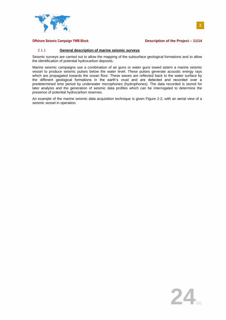
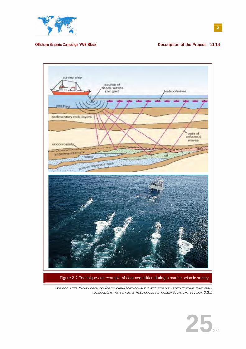
Marine seismic campaigns use a combination of air guns or water guns towed astern a marine seismic vessel to produce seismic pulses below the water level. These pulses generate acoustic energy rays which are propagated towards the ocean floor. These waves are reflected back to the water surface by the different geological formations in the earth’s crust and are detected and recorded over a predetermined time period by underwater microphones (hydrophones). The data recorded is stored for later analysis and the generation of seismic data profiles which can be interrogated to determine the presence of potential hydrocarbon reserves.
An example of the marine seismic data acquisition technique is given Figure 2-2, with an aerial view of a seismic vessel in operation.
2
Offshore Seismic Campaign YWB Block Description of the Project – 11/14
25231
SOURCE: HTTP://WWW.OPEN.EDU/OPENLEARN/SCIENCE-MATHS-TECHNOLOGY/SCIENCE/ENVIRONMENTAL-SCIENCE/EARTHS-PHYSICAL-RESOURCES-PETROLEUM/CONTENT-SECTION-3.2.1
Figure 2-2 Technique and example of data acquisition during a marine seismic survey
2
Offshore Seismic Campaign YWB Block Description of the Project – 11/14
26231
2.1.2 Description of 3D seismic surveys
In 3D surveys several hydrophone streamers are towed behind the survey vessel, together with generally dual sources. This technique is the one proposed for the exploration of the YWB Block.
Since seismic waves travel along expanding spherical wave fronts they have surface area. A truly representative image of the subsurface is only obtained when the entire wave field is sampled. A 3D seismic survey is more capable of accurately imaging reflected waves because it utilizes multiple points of observation. Multi streamer or multi source surveys allow for a range of different angles (azimuth) and distances (offset) to be sampled resulting in a volume, or cube, of seismic data.
This allows for a more detailed and accurate delineation of the boundaries and extent of the subsurface geological structures. Potential oil and gas reservoirs can be imaged in three dimensions allowing interpreters to view the data in cross-sections along 360° of azimuth, in depth slices parallel to the ground surface, and along planes that cut arbitrarily through the data volume. Information such as faulting and fracturing, bedding plane direction, the presence of pore fluids, complex geologic structure and detailed stratigraphy are now commonly interpreted from 3D seismic data sets.
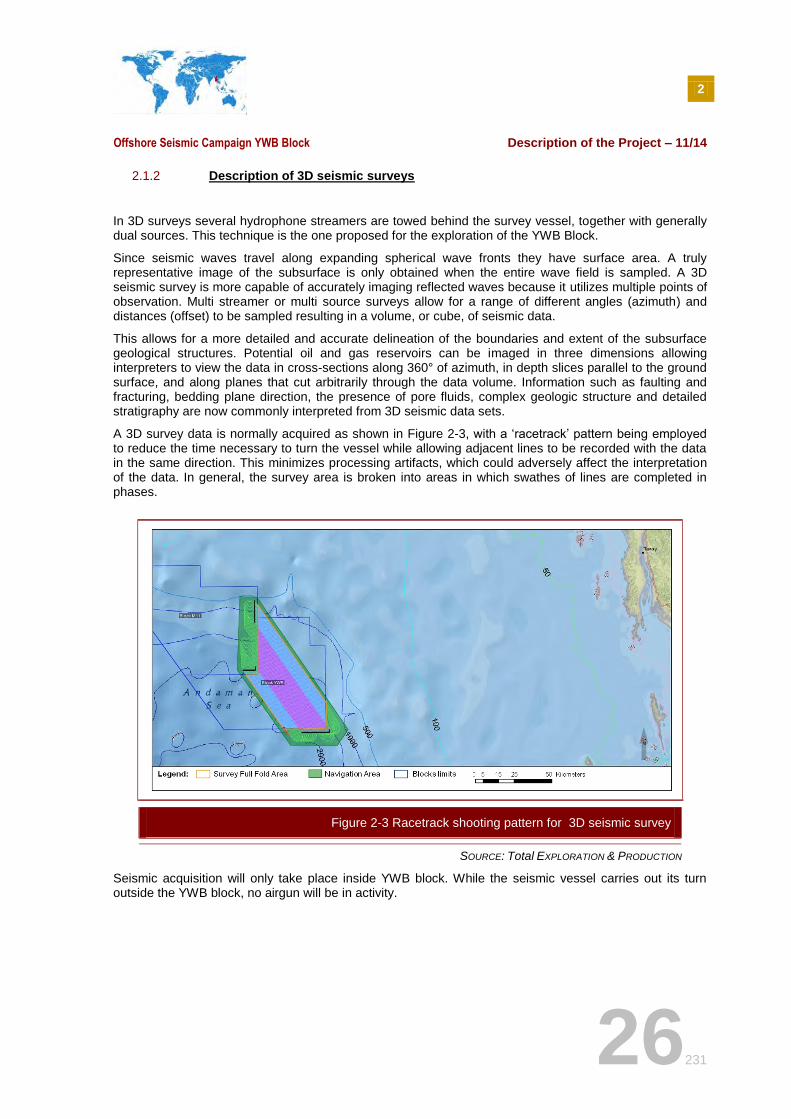
A 3D survey data is normally acquired as shown in Figure 2-3, with a ‘racetrack’ pattern being employed to reduce the time necessary to turn the vessel while allowing adjacent lines to be recorded with the data in the same direction. This minimizes processing artifacts, which could adversely affect the interpretation of the data. In general, the survey area is broken into areas in which swathes of lines are completed in phases.
SOURCE: Total EXPLORATION & PRODUCTION
Seismic acquisition will only take place inside YWB block. While the seismic vessel carries out its turn outside the YWB block, no airgun will be in activity.
Figure 2-3 Racetrack shooting pattern for 3D seismic survey
2
Offshore Seismic Campaign YWB Block Description of the Project – 11/14
27231
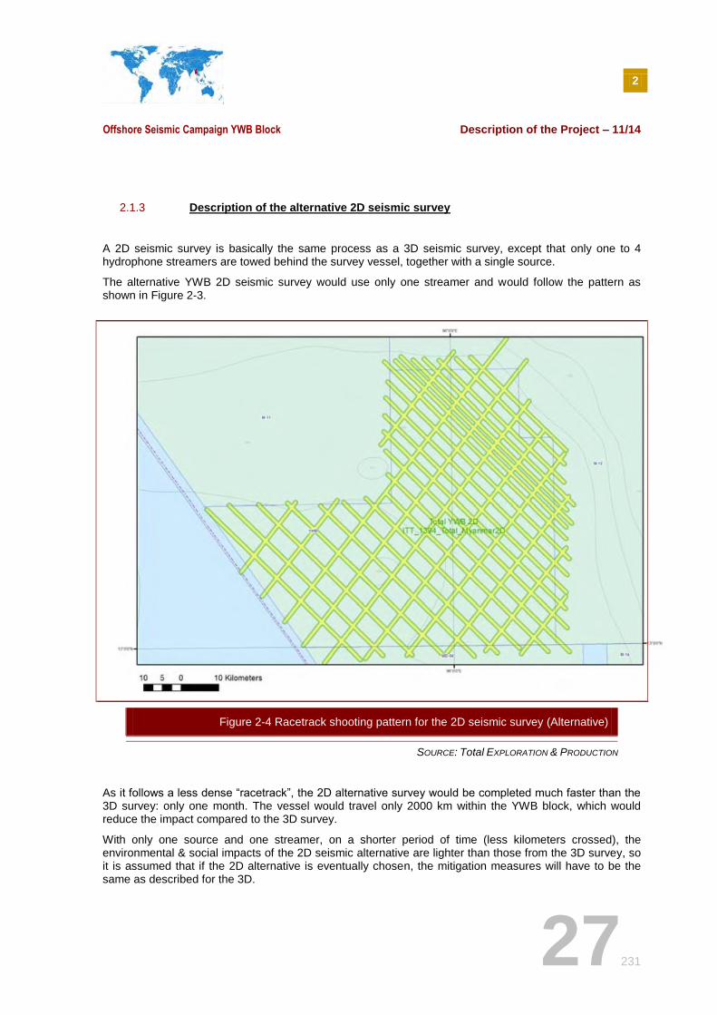
2.1.3 Description of the alternative 2D seismic survey
A 2D seismic survey is basically the same process as a 3D seismic survey, except that only one to 4 hydrophone streamers are towed behind the survey vessel, together with a single source.
The alternative YWB 2D seismic survey would use only one streamer and would follow the pattern as shown in Figure 2-3.
SOURCE: Total EXPLORATION & PRODUCTION
As it follows a less dense “racetrack”, the 2D alternative survey would be completed much faster than the 3D survey: only one month. The vessel would travel only 2000 km within the YWB block, which would reduce the impact compared to the 3D survey.
With only one source and one streamer, on a shorter period of time (less kilometers crossed), the environmental & social impacts of the 2D seismic alternative are lighter than those from the 3D survey, so it is assumed that if the 2D alternative is eventually chosen, the mitigation measures will have to be the same as described for the 3D.
Figure 2-4 Racetrack shooting pattern for the 2D seismic survey (Alternative)
2
Offshore Seismic Campaign YWB Block Description of the Project – 11/14
28231
2.1.4 YWB Block
The YWB SURVEY is located about 250 km west of the south-east Myanmar coast. Very few vintage 2D lines were acquired in the area during the 70s. The water depth ranges from 200 m to around 2000 m. The survey area will be approximately 2,000 km, coving the entirety of YWB Block. The targeted structure is the result of the rifting in the Andaman Sea and is consequently highly faulted. The aim of such an acquisition will be the detection of structural traps within the Plio-Pleistocene sequence. It is therefore essential to obtain a good structural image with a clear delineation of potential reservoirs. The YWB block is described in details in the section 5 “Description of the Environment”
2.2 SEISMIC ACQUISITION EQUIPMENT
A seismic survey system is mainly composed of the following equipment:
Seismic vessel and support vessels;
Seismic sources (airguns);
Seismic receiver cables (streamers).
The survey is completed in three steps: (i) deployment of the streamers (ii) initialization of the airgun firing sequence and carrying out of the seismic survey and (iii) recovery of the streamers.
2.2.1 Master seismic vessel and chases/support vessels
The marine streamer vessel will be manned by up to 60 personnel and the support vessels manned by up to 20 persons maximum each. There will be one supply vessel and one chase boat.
The vessels are equipped with accommodation and supplies’ quarters. The marine streamer vessel is equipped with a helipad that will serve for crew change and in case of medical evacuation necessity. The vessels are equipped with modern navigation equipment including radar, sonar, current meter, speed log, communication equipment and propulsion systems as well as independent energy production capabilities.
The streamer vessel will comprise an instrument’s room where the main seismic instrumentation is housed, including energy source firing.
The back deck serves the purpose of storing, retrieving and deploying seismic equipment. The energy source equipment (air guns) is generally located here as well as the air feed from seismic vessel compressors. The towing equipment is located here as well allowing for an accurate positioning behind the vessel and various operating conditions.
2
Offshore Seismic Campaign YWB Block Description of the Project – 11/14
29231
A compressor room contains the compressor engines and the compressors that supply high pressure air to the seismic sources. The compressor allows the continuous firing of seismic sources typically every ten seconds during data acquisition (12 to 24 hours/day).
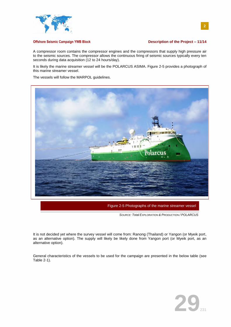
It is likely the marine streamer vessel will be the POLARCUS ASIMA. Figure 2-5 provides a photograph of this marine streamer vessel.
The vessels will follow the MARPOL guidelines.
SOURCE: Total EXPLORATION & PRODUCTION / POLARCUS
It is not decided yet where the survey vessel will come from: Ranong (Thailand) or Yangon (or Myeik port, as an alternative option). The supply will likely be likely done from Yangon port (or Myeik port, as an alternative option).
General characteristics of the vessels to be used for the campaign are presented in the below table (see Table 2-1).
Figure 2-5 Photographs of the marine streamer vessel
2
Offshore Seismic Campaign YWB Block Description of the Project – 11/14
30231
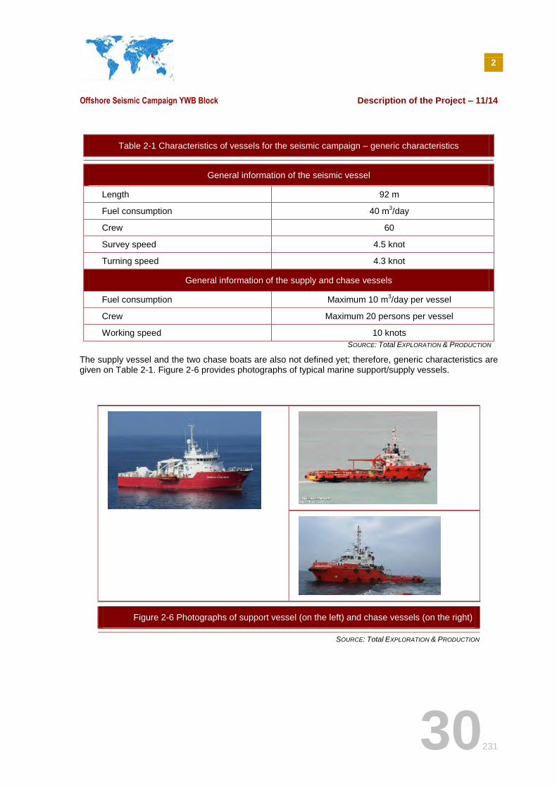
Table 2-1 Characteristics of vessels for the seismic campaign – generic characteristics
General information of the seismic vessel
Length 92 m
Fuel consumption 40 m3/day
Crew 60
Survey speed 4.5 knot
Turning speed 4.3 knot
General information of the supply and chase vessels
Fuel consumption Maximum 10 m3/day per vessel
Crew Maximum 20 persons per vessel
Working speed 10 knots
SOURCE: Total EXPLORATION & PRODUCTION
The supply vessel and the two chase boats are also not defined yet; therefore, generic characteristics are given on Table 2-1. Figure 2-6 provides photographs of typical marine support/supply vessels.
SOURCE: Total EXPLORATION & PRODUCTION
Figure 2-6 Photographs of support vessel (on the left) and chase vessels (on the right)
2
Offshore Seismic Campaign YWB Block Description of the Project – 11/14
31231
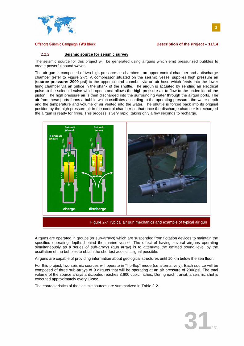
2.2.2 Seismic source for seismic survey
The seismic source for this project will be generated using airguns which emit pressurized bubbles to create powerful sound waves.
The air gun is composed of two high pressure air chambers; an upper control chamber and a discharge chamber (refer to Figure 2-7). A compressor situated on the seismic vessel supplies high pressure air (source pressure: 2000 psi) to the upper control chamber via an air hose which feeds into the lower firing chamber via an orifice in the shank of the shuttle. The airgun is actuated by sending an electrical pulse to the solenoid valve which opens and allows the high pressure air to flow to the underside of the piston. The high pressure air is then discharged into the surrounding water through the airgun ports. The air from these ports forms a bubble which oscillates according to the operating pressure, the water depth and the temperature and volume of air vented into the water. The shuttle is forced back into its original position by the high pressure air in the control chamber so that once the discharge chamber is recharged the airgun is ready for firing. This process is very rapid, taking only a few seconds to recharge.
Airguns are operated in groups (or sub-arrays) which are suspended from flotation devices to maintain the specified operating depths behind the marine vessel. The effect of having several airguns operating simultaneously as a series of sub-arrays (gun array) is to attenuate the emitted sound level by the oscillation of the bubbles to obtain the shortest acoustic signal possible.
Airguns are capable of providing information about geological structures until 10 km below the sea floor.
For this project, two seismic sources will operate in “flip-flop” mode (i.e alternatively). Each source will be composed of three sub-arrays of 9 airguns that will be operating at an air pressure of 2000psi. The total volume of the source arrays anticipated reaches 3,600 cubic inches. During each transit, a seismic shot is executed approximately every 10sec.
The characteristics of the seismic sources are summarized in Table 2-2.
Figure 2-7 Typical air gun mechanics and example of typical air gun
2
Offshore Seismic Campaign YWB Block Description of the Project – 11/14
32231
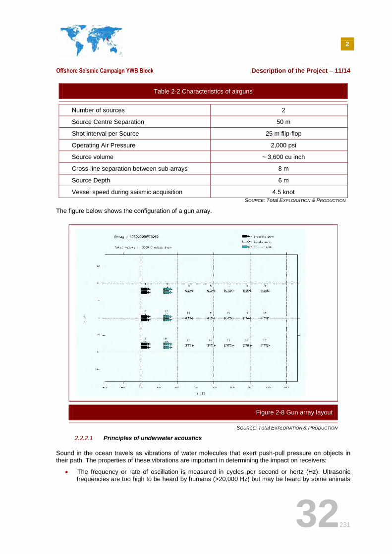
Table 2-2 Characteristics of airguns
Number of sources 2
Source Centre Separation 50 m
Shot interval per Source 25 m flip-flop
Operating Air Pressure 2,000 psi
Source volume ~ 3,600 cu inch
Cross-line separation between sub-arrays 8 m
Source Depth 6 m
Vessel speed during seismic acquisition 4.5 knot
SOURCE: Total EXPLORATION & PRODUCTION
The figure below shows the configuration of a gun array.
SOURCE: Total EXPLORATION & PRODUCTION
2.2.2.1 Principles of underwater acoustics
Sound in the ocean travels as vibrations of water molecules that exert push-pull pressure on objects in their path. The properties of these vibrations are important in determining the impact on receivers:
The frequency or rate of oscillation is measured in cycles per second or hertz (Hz). Ultrasonic frequencies are too high to be heard by humans (>20,000 Hz) but may be heard by some animals
Figure 2-8 Gun array layout
2
Offshore Seismic Campaign YWB Block Description of the Project – 11/14
33231
such as dolphins and bats. Infrasound is too low to be heard (<20 Hz) but can be heard by baleen whales (Richardson et al., 1995).
The wavelength is the length of the sound oscillation.
Sound pressure expressed in pressure units, microPascal (μPa), is the parameter measured by most instruments.
Acoustic intensity is the acoustic power per unit area in the direction of propagation (units: watts/m2). The
intensity, power and energy of an acoustic wave are proportional to the average of the pressure squared (mean square pressure).
The human ear responds in a logarithmic fashion to increases in sound intensity, therefore this scale has been adopted to reflect this response. The decibel scale is a logarithmic scale used to measure the intensity (power) of sound. It is defined as:
dB = 10 log10(I/I0), where I0 is a reference intensity.
However sound measuring devices usually respond to sound pressure (P) and the intensity of sound varies as the square of the pressure. Consequently, the level of sound intensity can be rewritten as:
dB = 20 log10(P/P0), where P0 is a reference pressure.
The reference pressure (P0) is chosen to indicate the limit of human hearing and is:
20 μPa in air;
1 μPa in water.
The logarithmic decibel scale allows a large range of values to be represented by smaller numbers. For example a doubling of the pressure represents approximately 3dB.
In water, the acoustic signals emitted by airguns generally have a sinusoidal form constituted by a peak and dip in pressure. The intensity is usually expressed in dB re 1 µPa-m, which represents the sound power at 1m of the source.
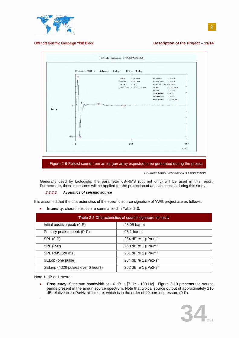
Figure 2-9 illustrates the waveform of an airgun which is a typical pulsed output. The sound can be characterized by the following parameters of the Sound Power Level (SPL):
Peak-to-peak (P-P) or Zero-to-peak pressure (0-P) (dB re 1 μPa-m): this considers the change in amplitude (pressure) of a sound wave, being respectively the maximum pressure of the rising part of the wave and the sum of the pressure of first peak plus the absolute value of the first trough.
RMS (Root Mean Square) (dB re 1 µPa-rms): measures the total sound intensity, and then, divides it by the length of the signal. In other words, it expresses the average peak pressure over the duration of the sound pulse. Acoustic power, intensity and energy are proportional to the mean squared pressure.
SEL (Sound Exposure level): measures the energy of a signal split up into one second. It involves a correction of the mean square calculation to account for the difficulty in determining signal duration. Behavioral response may be correlated with SEL, in particular for single pulse (SELop) and multi pulse (SELmp) sources. In the case of multiple pulse sources, like seismic sources (one pulse per 5 seconds), SELmp is the sum of the energy during the supposed contact between de sources and the receiver.
The noise level at a given frequency: usually the frequency at which the transmitted sound power is a maximum. In this case, the unit is "maximum amplitude" a µPa in dB/Hz.
2
Offshore Seismic Campaign YWB Block Description of the Project – 11/14
34231
SOURCE: Total EXPLORATION & PRODUCTION
Generally used by biologists, the parameter dB-RMS (but not only) will be used in this report. Furthermore, these measures will be applied for the protection of aquatic species during this study.
2.2.2.2 Acoustics of seismic source
It is assumed that the characteristics of the specific source signature of YWB project are as follows:
Intensity: characteristics are summarized in Table 2-3.
Table 2-3 Characteristics of source signature intensity
Initial positive peak (0-P) 48.05 bar.m
Primary peak to peak (P-P) 96.1 bar.m
SPL (0-P) 254 dB re 1 µPa-m1
SPL (P-P) 260 dB re 1 µPa-m1
SPL RMS (20 ms) 251 dB re 1 µPa-m1
SELop (one pulse) 234 dB re 1 µPa2-s1
SELmp (4320 pulses over 6 hours) 262 dB re 1 µPa2-s1
Note 1: dB at 1 metre
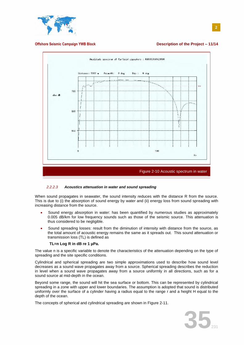
Frequency: Spectrum bandwidth at - 6 dB is [7 Hz - 100 Hz]. Figure 2-10 presents the source bands present in the airgun source spectrum. Note that typical source output of approximately 210 dB relative to 1 uPa/Hz at 1 metre, which is in the order of 40 bars of pressure (0-P).
Figure 2-9 Pulsed sound from an air gun array expected to be generated during the project
2
Offshore Seismic Campaign YWB Block Description of the Project – 11/14
35231
2.2.2.3 Acoustics attenuation in water and sound spreading
When sound propagates in seawater, the sound intensity reduces with the distance R from the source. This is due to (i) the absorption of sound energy by water and (ii) energy loss from sound spreading with increasing distance from the source.
Sound energy absorption in water: has been quantified by numerous studies as approximately 0.005 dB/km for low frequency sounds such as those of the seismic source. This attenuation is thus considered to be negligible.
Sound spreading losses: result from the diminution of intensity with distance from the source, as the total amount of acoustic energy remains the same as it spreads out. This sound attenuation or transmission loss (TL) is defined as
TL=n Log R in dB re 1 µPa.
The value n is a specific variable to denote the characteristics of the attenuation depending on the type of spreading and the site specific conditions.
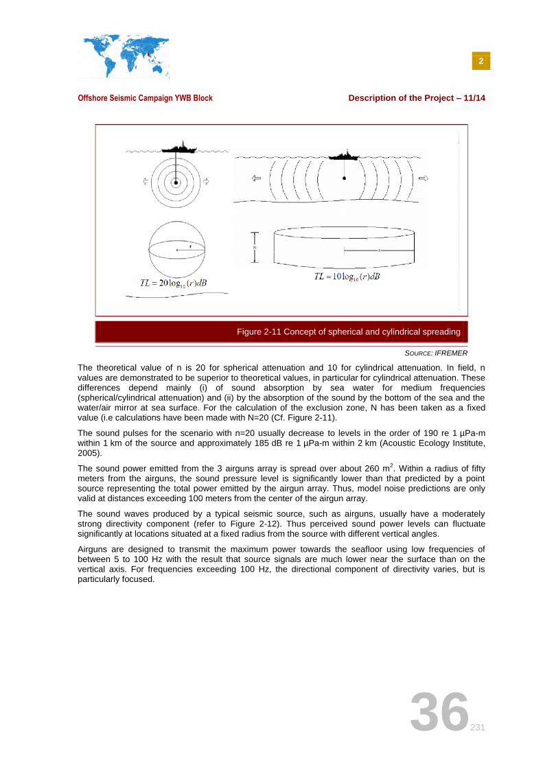
Cylindrical and spherical spreading are two simple approximations used to describe how sound level decreases as a sound wave propagates away from a source. Spherical spreading describes the reduction in level when a sound wave propagates away from a source uniformly in all directions, such as for a sound source at mid-depth in the ocean.
Beyond some range, the sound will hit the sea surface or bottom. This can be represented by cylindrical spreading in a zone with upper and lower boundaries. The assumption is adopted that sound is distributed uniformly over the surface of a cylinder having a radius equal to the range r and a height H equal to the depth of the ocean.
The concepts of spherical and cylindrical spreading are shown in Figure 2-11.
Figure 2-10 Acoustic spectrum in water
2
Offshore Seismic Campaign YWB Block Description of the Project – 11/14
36231
SOURCE: IFREMER
The theoretical value of n is 20 for spherical attenuation and 10 for cylindrical attenuation. In field, n values are demonstrated to be superior to theoretical values, in particular for cylindrical attenuation. These differences depend mainly (i) of sound absorption by sea water for medium frequencies (spherical/cylindrical attenuation) and (ii) by the absorption of the sound by the bottom of the sea and the water/air mirror at sea surface. For the calculation of the exclusion zone, N has been taken as a fixed value (i.e calculations have been made with N=20 (Cf. Figure 2-11).
The sound pulses for the scenario with n=20 usually decrease to levels in the order of 190 re 1 µPa-m within 1 km of the source and approximately 185 dB re 1 µPa-m within 2 km (Acoustic Ecology Institute, 2005).
The sound power emitted from the 3 airguns array is spread over about 260 m2. Within a radius of fifty
meters from the airguns, the sound pressure level is significantly lower than that predicted by a point source representing the total power emitted by the airgun array. Thus, model noise predictions are only valid at distances exceeding 100 meters from the center of the airgun array.
The sound waves produced by a typical seismic source, such as airguns, usually have a moderately strong directivity component (refer to Figure 2-12). Thus perceived sound power levels can fluctuate significantly at locations situated at a fixed radius from the source with different vertical angles.
Airguns are designed to transmit the maximum power towards the seafloor using low frequencies of between 5 to 100 Hz with the result that source signals are much lower near the surface than on the vertical axis. For frequencies exceeding 100 Hz, the directional component of directivity varies, but is particularly focused.
Figure 2-11 Concept of spherical and cylindrical spreading
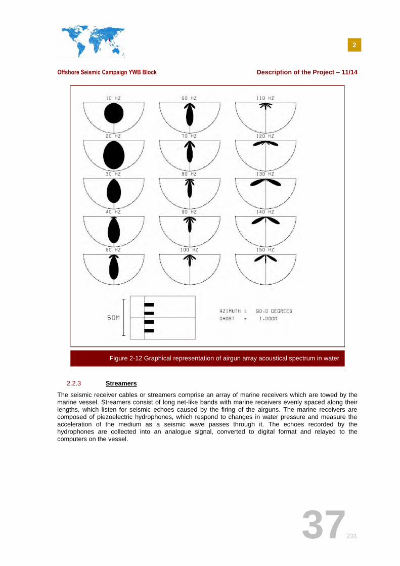
2
Offshore Seismic Campaign YWB Block Description of the Project – 11/14
37231
2.2.3 Streamers
The seismic receiver cables or streamers comprise an array of marine receivers which are towed by the marine vessel. Streamers consist of long net-like bands with marine receivers evenly spaced along their lengths, which listen for seismic echoes caused by the firing of the airguns. The marine receivers are composed of piezoelectric hydrophones, which respond to changes in water pressure and measure the acceleration of the medium as a seismic wave passes through it. The echoes recorded by the hydrophones are collected into an analogue signal, converted to digital format and relayed to the computers on the vessel.
Figure 2-12 Graphical representation of airgun array acoustical spectrum in water
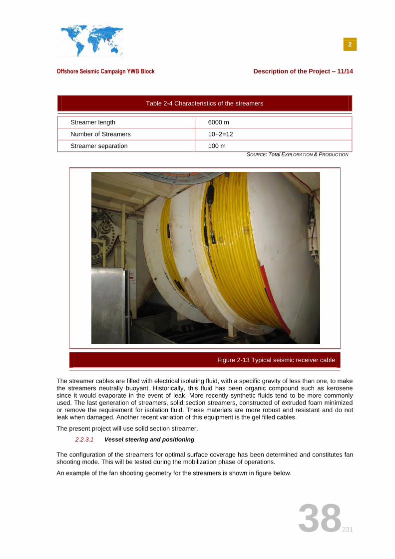
2
Offshore Seismic Campaign YWB Block Description of the Project – 11/14
38231
Table 2-4 Characteristics of the streamers
Streamer length 6000 m
Number of Streamers 10+2=12
Streamer separation 100 m
SOURCE: Total EXPLORATION & PRODUCTION
The streamer cables are filled with electrical isolating fluid, with a specific gravity of less than one, to make the streamers neutrally buoyant. Historically, this fluid has been organic compound such as kerosene since it would evaporate in the event of leak. More recently synthetic fluids tend to be more commonly used. The last generation of streamers, solid section streamers, constructed of extruded foam minimized or remove the requirement for isolation fluid. These materials are more robust and resistant and do not leak when damaged. Another recent variation of this equipment is the gel filled cables.
The present project will use solid section streamer.
2.2.3.1 Vessel steering and positioning
The configuration of the streamers for optimal surface coverage has been determined and constitutes fan shooting mode. This will be tested during the mobilization phase of operations.
An example of the fan shooting geometry for the streamers is shown in figure below.
Figure 2-13 Typical seismic receiver cable
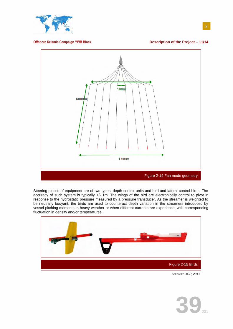
2
Offshore Seismic Campaign YWB Block Description of the Project – 11/14
39231
Steering pieces of equipment are of two types: depth control units and bird and lateral control birds. The accuracy of such system is typically +/- 1m. The wings of the bird are electronically control to pivot in response to the hydrostatic pressure measured by a pressure transducer. As the streamer is weighted to be neutrally buoyant, the birds are used to counteract depth variation in the streamers introduced by vessel pitching moments in heavy weather or when different currents are experience, with corresponding fluctuation in density and/or temperatures.
SOURCE: OGP, 2011
Figure 2-14 Fan mode geometry
Figure 2-15 Birds
2
Offshore Seismic Campaign YWB Block Description of the Project – 11/14
40231
2.2.3.2 Ancillary equipment and onshore support
Support vessels for this project will include 1 supply vessel, and 1 chase vessel which will accompany the marine vessel to monitor the survey zone and to provide any emergency assistance required (Cf. § 2.2.1 ).
The only expected onshore activities proposed for this seismic survey will be associated with the support vessel, which may visit the port Yangon to re-supply the seismic vessel with food and fuel. The main survey vessel will be bunkered (refueled) at sea in the 3D seismic area if necessary, however in general these marine vessels are selected for their self-sufficiency over long durations and it is assumed no crew changes will be effected.
The seismic vessel might originally come from Ranong (Thailand) or Yangon (Myeik could also be an alternative option).
Tracking for seismic fleet will be undertaken using an online satellite positioning system (SATPOS system or equivalent).
2.2.3.3 Positioning systems
Tail buoys will be used to position 2 independent dual frequency Differential Global Positioning (DGPS) systems. Calibration and validation of the positioning systems will be undertaken as part of the mobilization phase. These DGPS will record pitch, roll and heave at around 1 minute intervals; the height will be corrected from this data and these results will be GPS time stamped.
2.2.3.4 Additional equipment
It is critically important for the success of a seismic survey to know very precisely the location of sources and receivers. To achieve this compasses, which measure the deviation of the streamer relative to the magnetic North, are placed every 300m on the streamer. Acoustic ranging units are used to provide additional positional information. These are attached to the hull of the vessel, the source floats, the streamers themselves and the tailbuoys. The acoustic units operate to high acoustic frequencies, 10 to 100 khertz, with a maximum output SPL of approximately 195 dB re 1µPa at 1m. The provide range information up to approximately 1 km, after which distance the received sound pressure levels of these signals are attenuated to background levels.
Sea water temperature and salinity measurements shall be performed on regular basis throughout the survey and a current meter shall be available on-board the seismic vessel.
The equipment used by the contractor is described in detail in the APPENDIX L
2.3 TIMING OF ACTIVITY
The seismic campaign is planned to begin on the beginning of 2016 with the arrival of the seismic fleet on YWB block. Then, the seismic acquisition will last up to 1 month.
This project is part of a larger program, where exploration surveys lead to an exploration well in case of success. The expected overall YWB program is given in the figure below.
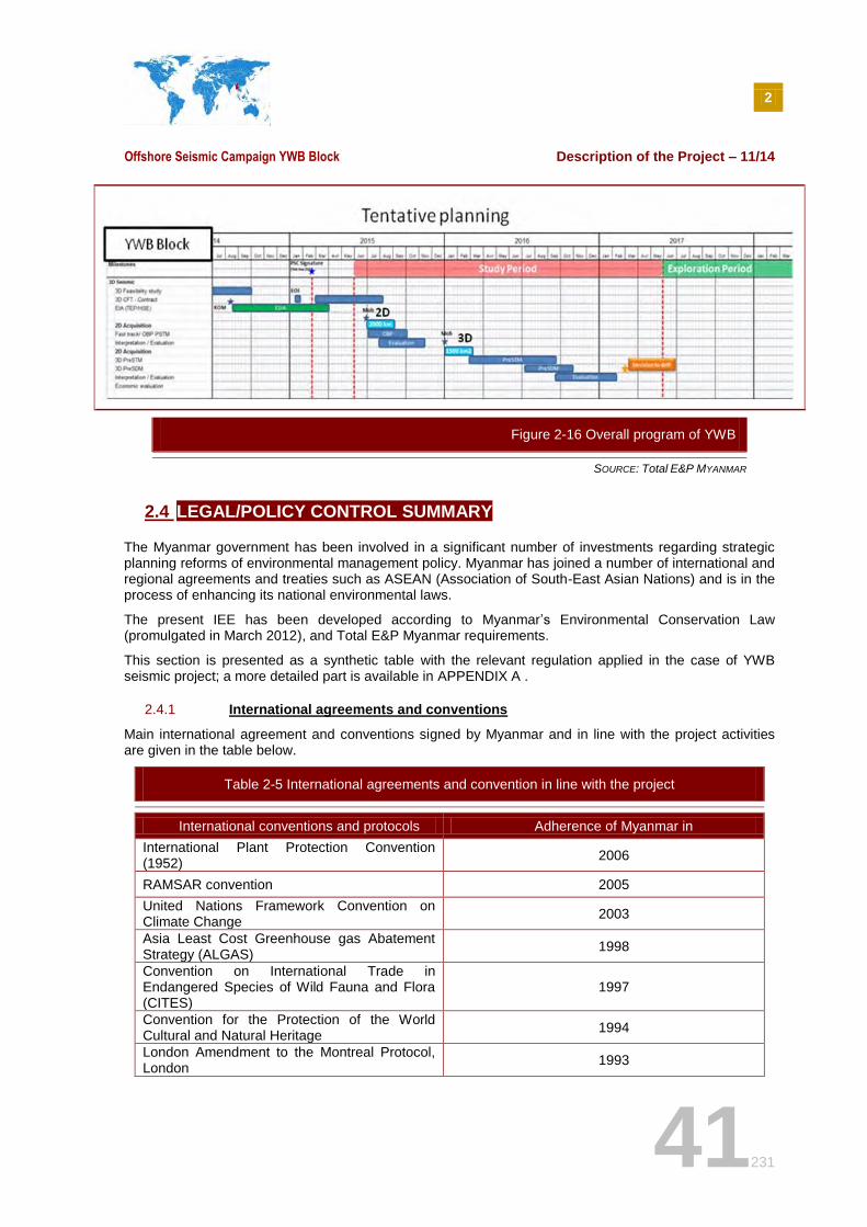
2
Offshore Seismic Campaign YWB Block Description of the Project – 11/14
41231
SOURCE: Total E&P MYANMAR
2.4 LEGAL/POLICY CONTROL SUMMARY
The Myanmar government has been involved in a significant number of investments regarding strategic planning reforms of environmental management policy. Myanmar has joined a number of international and regional agreements and treaties such as ASEAN (Association of South-East Asian Nations) and is in the process of enhancing its national environmental laws.
The present IEE has been developed according to Myanmar’s Environmental Conservation Law (promulgated in March 2012), and Total E&P Myanmar requirements.
This section is presented as a synthetic table with the relevant regulation applied in the case of YWB seismic project; a more detailed part is available in APPENDIX A .
2.4.1 International agreements and conventions
Main international agreement and conventions signed by Myanmar and in line with the project activities are given in the table below.
Table 2-5 International agreements and convention in line with the project
International conventions and protocols Adherence of Myanmar in
International Plant Protection Convention (1952)
2006
RAMSAR convention 2005
United Nations Framework Convention on Climate Change
2003
Asia Least Cost Greenhouse gas Abatement Strategy (ALGAS)
1998
Convention on International Trade in Endangered Species of Wild Fauna and Flora (CITES)
1997
Convention for the Protection of the World Cultural and Natural Heritage
1994
London Amendment to the Montreal Protocol, London
1993
Figure 2-16 Overall program of YWB
2
Offshore Seismic Campaign YWB Block Description of the Project – 11/14
42231
Table 2-5 International agreements and convention in line with the project
Convention on Biological Diversity, Rio de Janeiro
1992
Montreal Protocol on Substances that Deplete the Ozone Layer
1989
Vienna Convention for the protection of the Ozone Layer
1988
United Nations Convention on Law of the Sea 1986
International Convention on the Prevention of Pollution from Ships, 1973 as modified by the protocol of 1978 (MARPOL 73/78)
1988 Myanmar has only ratified annex I/II.
Nevertheless, we have applied recommendation of annex IV and V for this IEE
RIPAM or COLREG Convention 72 “collision regulation 72”
1987 The International Regulations for Preventing Collisions at Sea 1972 (Colregs) are published by the International Maritime Organization (IMO) and set out, among other things, the "rules of the road" or navigation rules to be followed by ships and other vessels at sea to prevent collisions between two or more vessels
SOLAS convention (Safety Of Life At Sea)
1987 International maritime safety treaty. It ensures that ships flagged by signatory States comply with minimum safety standards in construction, equipment and operation.
1948 Convention on the International Maritime Organization
1951
International Convention on Standards of Training, Certification and Watchkeeping for Seafarers, 1978 (STCW)
1988 This convention concerns the project particularly by its 2010 amendment which asks for new requirements for marine environment awareness training and training in leadership and teamwork; and new training guidance for personnel operating Dynamic Positioning Systems.
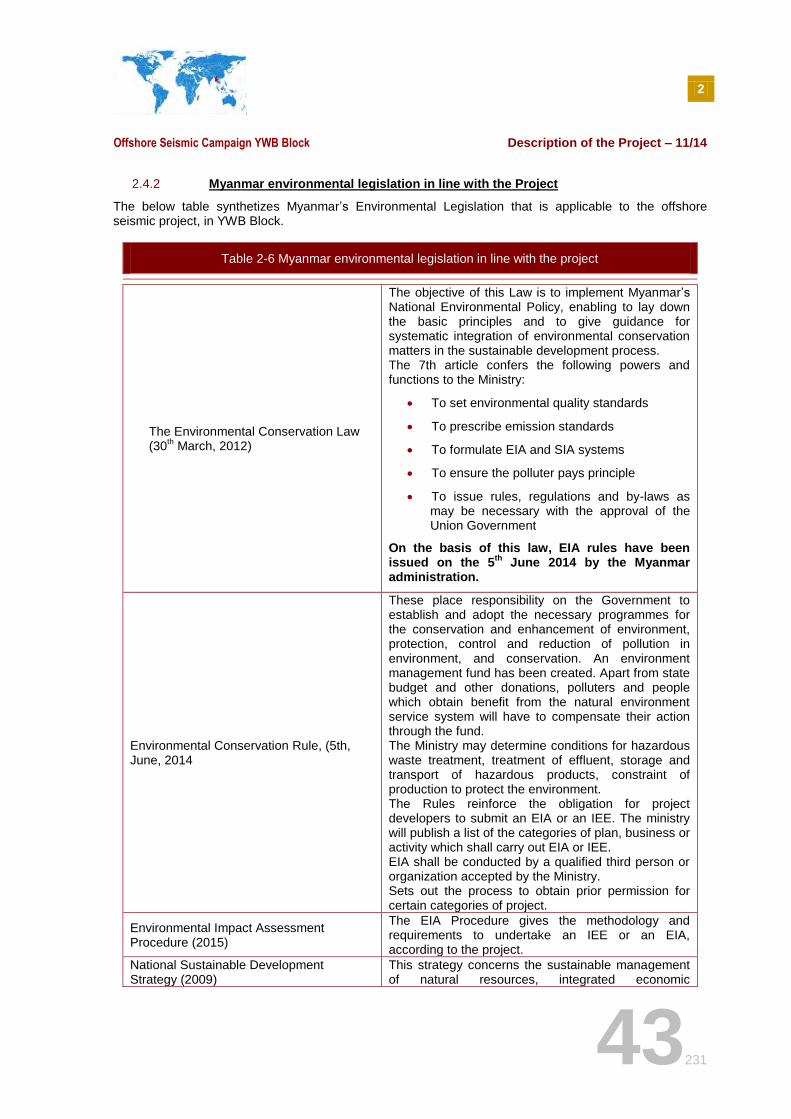
2
Offshore Seismic Campaign YWB Block Description of the Project – 11/14
43231
2.4.2 Myanmar environmental legislation in line with the Project
The below table synthetizes Myanmar’s Environmental Legislation that is applicable to the offshore seismic project, in YWB Block.
Table 2-6 Myanmar environmental legislation in line with the project
The Environmental Conservation Law (30
th March, 2012)
The objective of this Law is to implement Myanmar’s National Environmental Policy, enabling to lay down the basic principles and to give guidance for systematic integration of environmental conservation matters in the sustainable development process. The 7th article confers the following powers and functions to the Ministry:
To set environmental quality standards
To prescribe emission standards
To formulate EIA and SIA systems
To ensure the polluter pays principle
To issue rules, regulations and by-laws as may be necessary with the approval of the Union Government
On the basis of this law, EIA rules have been issued on the 5
th June 2014 by the Myanmar
administration.
Environmental Conservation Rule, (5th, June, 2014
These place responsibility on the Government to establish and adopt the necessary programmes for the conservation and enhancement of environment, protection, control and reduction of pollution in environment, and conservation. An environment management fund has been created. Apart from state budget and other donations, polluters and people which obtain benefit from the natural environment service system will have to compensate their action through the fund. The Ministry may determine conditions for hazardous waste treatment, treatment of effluent, storage and transport of hazardous products, constraint of production to protect the environment. The Rules reinforce the obligation for project developers to submit an EIA or an IEE. The ministry will publish a list of the categories of plan, business or activity which shall carry out EIA or IEE. EIA shall be conducted by a qualified third person or organization accepted by the Ministry. Sets out the process to obtain prior permission for certain categories of project.
Environmental Impact Assessment Procedure (2015)
The EIA Procedure gives the methodology and requirements to undertake an IEE or an EIA, according to the project.
National Sustainable Development Strategy (2009)
This strategy concerns the sustainable management of natural resources, integrated economic
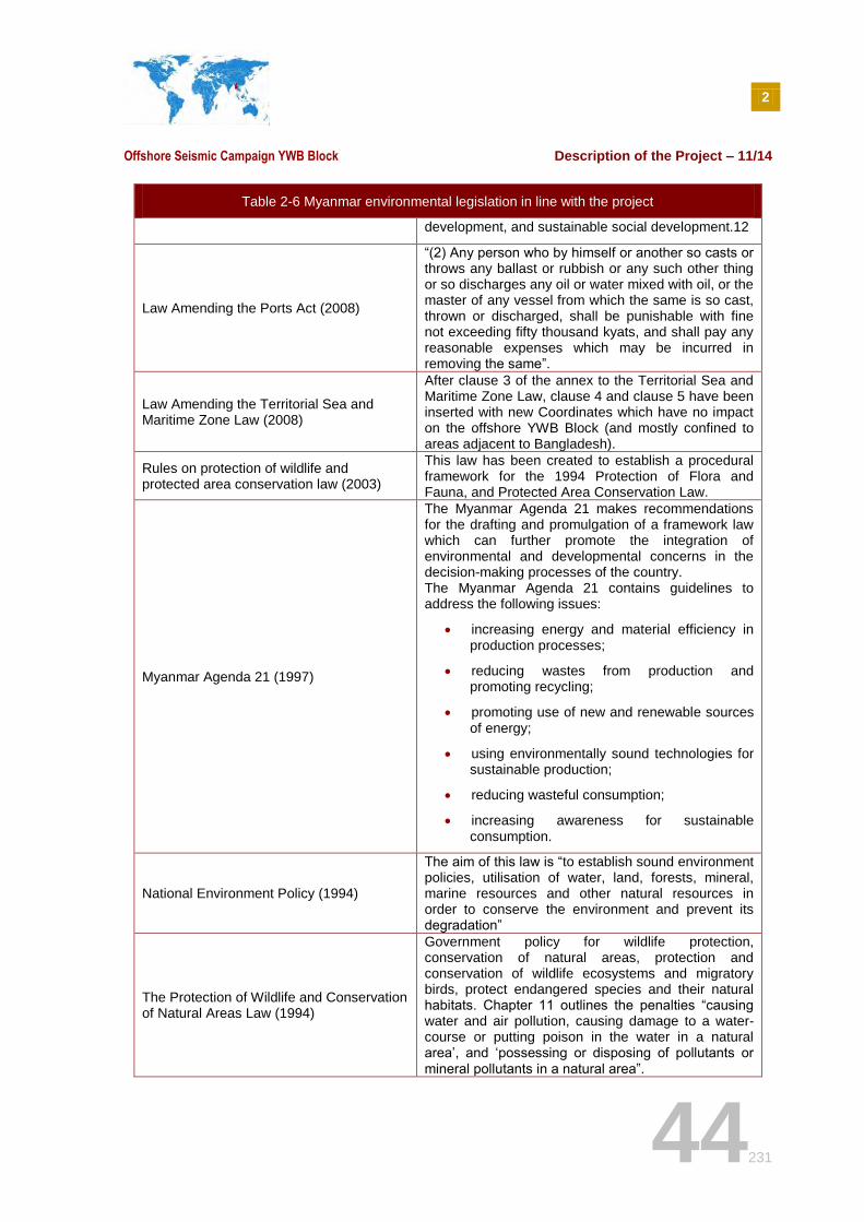
2
Offshore Seismic Campaign YWB Block Description of the Project – 11/14
44231
Table 2-6 Myanmar environmental legislation in line with the project
development, and sustainable social development.12
Law Amending the Ports Act (2008)
“(2) Any person who by himself or another so casts or throws any ballast or rubbish or any such other thing or so discharges any oil or water mixed with oil, or the master of any vessel from which the same is so cast, thrown or discharged, shall be punishable with fine not exceeding fifty thousand kyats, and shall pay any reasonable expenses which may be incurred in removing the same”.
Law Amending the Territorial Sea and Maritime Zone Law (2008)
After clause 3 of the annex to the Territorial Sea and Maritime Zone Law, clause 4 and clause 5 have been inserted with new Coordinates which have no impact on the offshore YWB Block (and mostly confined to areas adjacent to Bangladesh).
Rules on protection of wildlife and protected area conservation law (2003)
This law has been created to establish a procedural framework for the 1994 Protection of Flora and Fauna, and Protected Area Conservation Law.
Myanmar Agenda 21 (1997)
The Myanmar Agenda 21 makes recommendations for the drafting and promulgation of a framework law which can further promote the integration of environmental and developmental concerns in the decision-making processes of the country. The Myanmar Agenda 21 contains guidelines to address the following issues:
increasing energy and material efficiency in production processes;
reducing wastes from production and promoting recycling;
promoting use of new and renewable sources of energy;
using environmentally sound technologies for sustainable production;
reducing wasteful consumption;
increasing awareness for sustainable consumption.
National Environment Policy (1994)
The aim of this law is “to establish sound environment policies, utilisation of water, land, forests, mineral, marine resources and other natural resources in order to conserve the environment and prevent its degradation”
The Protection of Wildlife and Conservation of Natural Areas Law (1994)
Government policy for wildlife protection, conservation of natural areas, protection and conservation of wildlife ecosystems and migratory birds, protect endangered species and their natural habitats. Chapter 11 outlines the penalties “causing water and air pollution, causing damage to a water-course or putting poison in the water in a natural area’, and ‘possessing or disposing of pollutants or mineral pollutants in a natural area”.
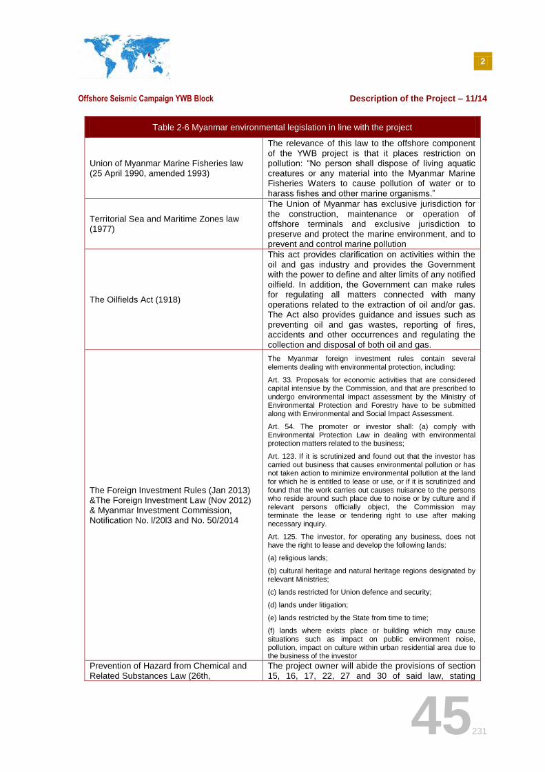
2
Offshore Seismic Campaign YWB Block Description of the Project – 11/14
45231
Table 2-6 Myanmar environmental legislation in line with the project
Union of Myanmar Marine Fisheries law (25 April 1990, amended 1993)
The relevance of this law to the offshore component of the YWB project is that it places restriction on pollution: “No person shall dispose of living aquatic creatures or any material into the Myanmar Marine Fisheries Waters to cause pollution of water or to harass fishes and other marine organisms.”
Territorial Sea and Maritime Zones law (1977)
The Union of Myanmar has exclusive jurisdiction for the construction, maintenance or operation of offshore terminals and exclusive jurisdiction to preserve and protect the marine environment, and to prevent and control marine pollution
The Oilfields Act (1918)
This act provides clarification on activities within the oil and gas industry and provides the Government with the power to define and alter limits of any notified oilfield. In addition, the Government can make rules for regulating all matters connected with many operations related to the extraction of oil and/or gas. The Act also provides guidance and issues such as preventing oil and gas wastes, reporting of fires, accidents and other occurrences and regulating the collection and disposal of both oil and gas.
The Foreign Investment Rules (Jan 2013) &The Foreign Investment Law (Nov 2012) & Myanmar Investment Commission, Notification No. l/20l3 and No. 50/2014
The Myanmar foreign investment rules contain several elements dealing with environmental protection, including:
Art. 33. Proposals for economic activities that are considered capital intensive by the Commission, and that are prescribed to undergo environmental impact assessment by the Ministry of Environmental Protection and Forestry have to be submitted along with Environmental and Social Impact Assessment.
Art. 54. The promoter or investor shall: (a) comply with Environmental Protection Law in dealing with environmental protection matters related to the business;
Art. 123. If it is scrutinized and found out that the investor has carried out business that causes environmental pollution or has not taken action to minimize environmental pollution at the land for which he is entitled to lease or use, or if it is scrutinized and found that the work carries out causes nuisance to the persons who reside around such place due to noise or by culture and if relevant persons officially object, the Commission may terminate the lease or tendering right to use after making necessary inquiry.
Art. 125. The investor, for operating any business, does not have the right to lease and develop the following lands:
(a) religious lands;
(b) cultural heritage and natural heritage regions designated by relevant Ministries;
(c) lands restricted for Union defence and security;
(d) lands under litigation;
(e) lands restricted by the State from time to time;
(f) lands where exists place or building which may cause situations such as impact on public environment noise, pollution, impact on culture within urban residential area due to the business of the investor
Prevention of Hazard from Chemical and Related Substances Law (26th,
The project owner will abide the provisions of section 15, 16, 17, 22, 27 and 30 of said law, stating
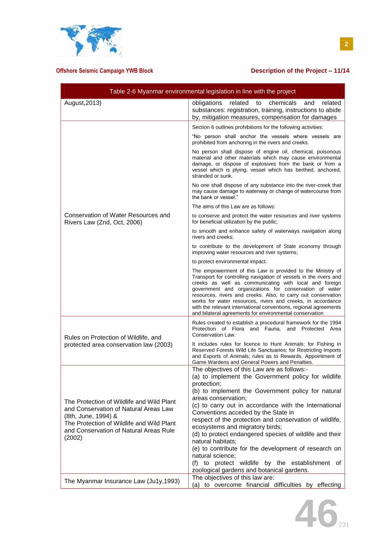
2
Offshore Seismic Campaign YWB Block Description of the Project – 11/14
46231
Table 2-6 Myanmar environmental legislation in line with the project
August,2013) obligations related to chemicals and related substances: registration, training, instructions to abide by, mitigation measures, compensation for damages
Conservation of Water Resources and Rivers Law (Znd, Oct, 2006)
Section 6 outlines prohibitions for the following activities:
“No person shall anchor the vessels where vessels are prohibited from anchoring in the rivers and creeks.
No person shall dispose of engine oil, chemical, poisonous material and other materials which may cause environmental damage, or dispose of explosives from the bank or from a vessel which is plying, vessel which has berthed, anchored, stranded or sunk.
No one shall dispose of any substance into the river-creek that may cause damage to waterway or change of watercourse from the bank or vessel.”
The aims of this Law are as follows:
to conserve and protect the water resources and river systems for beneficial utilization by the public;
to smooth and enhance safety of waterways navigation along rivers and creeks;
to contribute to the development of State economy through improving water resources and river systems;
to protect environmental impact.
The empowerment of this Law is provided to the Ministry of Transport for controlling navigation of vessels in the rivers and creeks as well as communicating with local and foreign government and organizations for conservation of water resources, rivers and creeks. Also, to carry out conservation works for water resources, rivers and creeks, in accordance with the relevant international conventions, regional agreements and bilateral agreements for environmental conservation
Rules on Protection of Wildlife, and protected area conservation law (2003)
Rules created to establish a procedural framework for the 1994 Protection of Flora and Fauna, and Protected Area Conservation Law.
It includes rules for licence to Hunt Animals; for Fishing in Reserved Forests Wild Life Sanctuaries; for Restricting Imports and Exports of Animals; rules as to Rewards, Appointment of Game Wardens and General Powers and Penalties.
The Protection of Wildlife and Wild Plant and Conservation of Natural Areas Law (8th, June, 1994) & The Protection of Wildlife and Wild Plant and Conservation of Natural Areas Rule (2002)
The objectives of this Law are as follows:- (a) to implement the Government policy for wildlife protection; (b) to implement the Government policy for natural areas conservation; (c) to carry out in accordance with the International Conventions acceded by the State in respect of the protection and conservation of wildlife, ecosystems and migratory birds; (d) to protect endangered species of wildlife and their natural habitats; (e) to contribute for the development of research on natural science; (f) to protect wildlife by the establishment of zoological gardens and botanical gardens.
The Myanmar Insurance Law (Ju1y,1993) The objectives of this law are: (a) to overcome financial difficulties by effecting
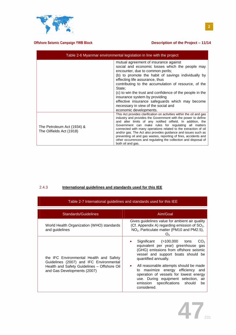
2
Offshore Seismic Campaign YWB Block Description of the Project – 11/14
47231
Table 2-6 Myanmar environmental legislation in line with the project
mutual agreement of insurance against social and economic losses which the people may encounter, due to common perils; (b) to promote the habit of savings individually by effecting life assurance, thus contributing to the accumulation of resource, of the State; (c) to win the trust and confidence of the people in the insurance system by providing effective insurance safeguards which may become necessary in view of the social and economic developments.
The Petroleum Act (1934) & The Oilfields Act (1918)
This Act provides clarification on activities within the oil and gas industry and provides the Government with the power to define and alter limits of any notified oilfield. In addition, the Government can make rules for regulating all matters connected with many operations related to the extraction of oil and/or gas. The Act also provides guidance and issues such as preventing oil and gas wastes, reporting of fires, accidents and other occurrences and regulating the collection and disposal of both oil and gas.
2.4.3 International guidelines and standards used for this IEE
Table 2-7 International guidelines and standards used for this IEE
Standards/Guidelines Aim/Goal
World Health Organization (WHO) standards and guidelines
Gives guidelines value for ambient air quality (Cf. Appendix A) regarding emission of SO2, NO2, Particulate matter (PM10 and PM2.5),
O3
the IFC Environmental Health and Safety Guidelines (2007) and IFC Environmental Health and Safety Guidelines – Offshore Oil and Gas Developments (2007)
Significant (>100,000 tons CO2 equivalent per year) greenhouse gas (GHG) emissions from offshore seismic vessel and support boats should be quantified annually.
All reasonable attempts should be made to maximize energy efficiency and operation of vessels for lowest energy use. During equipment selection, air emission specifications should be considered.
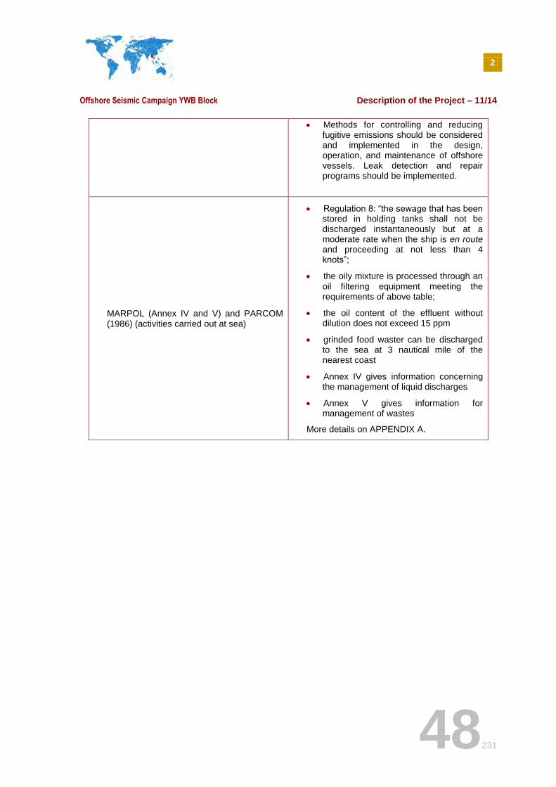
2
Offshore Seismic Campaign YWB Block Description of the Project – 11/14
48231
Methods for controlling and reducing fugitive emissions should be considered and implemented in the design, operation, and maintenance of offshore vessels. Leak detection and repair programs should be implemented.
MARPOL (Annex IV and V) and PARCOM (1986) (activities carried out at sea)
Regulation 8: “the sewage that has been stored in holding tanks shall not be discharged instantaneously but at a moderate rate when the ship is en route and proceeding at not less than 4 knots”;
the oily mixture is processed through an oil filtering equipment meeting the requirements of above table;
the oil content of the effluent without dilution does not exceed 15 ppm
grinded food waster can be discharged to the sea at 3 nautical mile of the nearest coast
Annex IV gives information concerning the management of liquid discharges
Annex V gives information for management of wastes
More details on APPENDIX A.
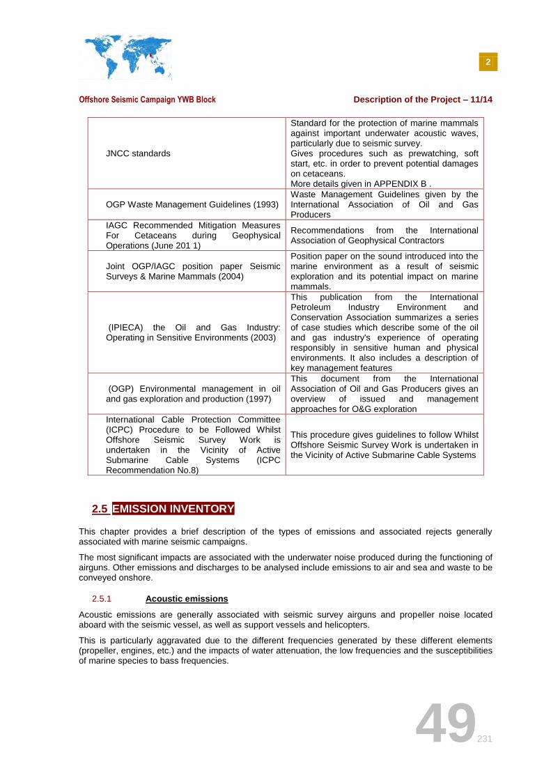
2
Offshore Seismic Campaign YWB Block Description of the Project – 11/14
49231
JNCC standards
Standard for the protection of marine mammals against important underwater acoustic waves, particularly due to seismic survey. Gives procedures such as prewatching, soft start, etc. in order to prevent potential damages on cetaceans. More details given in APPENDIX B .
OGP Waste Management Guidelines (1993) Waste Management Guidelines given by the International Association of Oil and Gas Producers
IAGC Recommended Mitigation Measures For Cetaceans during Geophysical Operations (June 201 1)
Recommendations from the International Association of Geophysical Contractors
Joint OGP/IAGC position paper Seismic Surveys & Marine Mammals (2004)
Position paper on the sound introduced into the marine environment as a result of seismic exploration and its potential impact on marine mammals.
(IPIECA) the Oil and Gas Industry: Operating in Sensitive Environments (2003)
This publication from the International Petroleum Industry Environment and Conservation Association summarizes a series of case studies which describe some of the oil and gas industry's experience of operating responsibly in sensitive human and physical environments. It also includes a description of key management features
(OGP) Environmental management in oil and gas exploration and production (1997)
This document from the International Association of Oil and Gas Producers gives an overview of issued and management approaches for O&G exploration
International Cable Protection Committee (ICPC) Procedure to be Followed Whilst Offshore Seismic Survey Work is undertaken in the Vicinity of Active Submarine Cable Systems (ICPC Recommendation No.8)
This procedure gives guidelines to follow Whilst Offshore Seismic Survey Work is undertaken in the Vicinity of Active Submarine Cable Systems
2.5 EMISSION INVENTORY
This chapter provides a brief description of the types of emissions and associated rejects generally associated with marine seismic campaigns.
The most significant impacts are associated with the underwater noise produced during the functioning of airguns. Other emissions and discharges to be analysed include emissions to air and sea and waste to be conveyed onshore.
2.5.1 Acoustic emissions
Acoustic emissions are generally associated with seismic survey airguns and propeller noise located aboard with the seismic vessel, as well as support vessels and helicopters.
This is particularly aggravated due to the different frequencies generated by these different elements (propeller, engines, etc.) and the impacts of water attenuation, the low frequencies and the susceptibilities of marine species to bass frequencies.
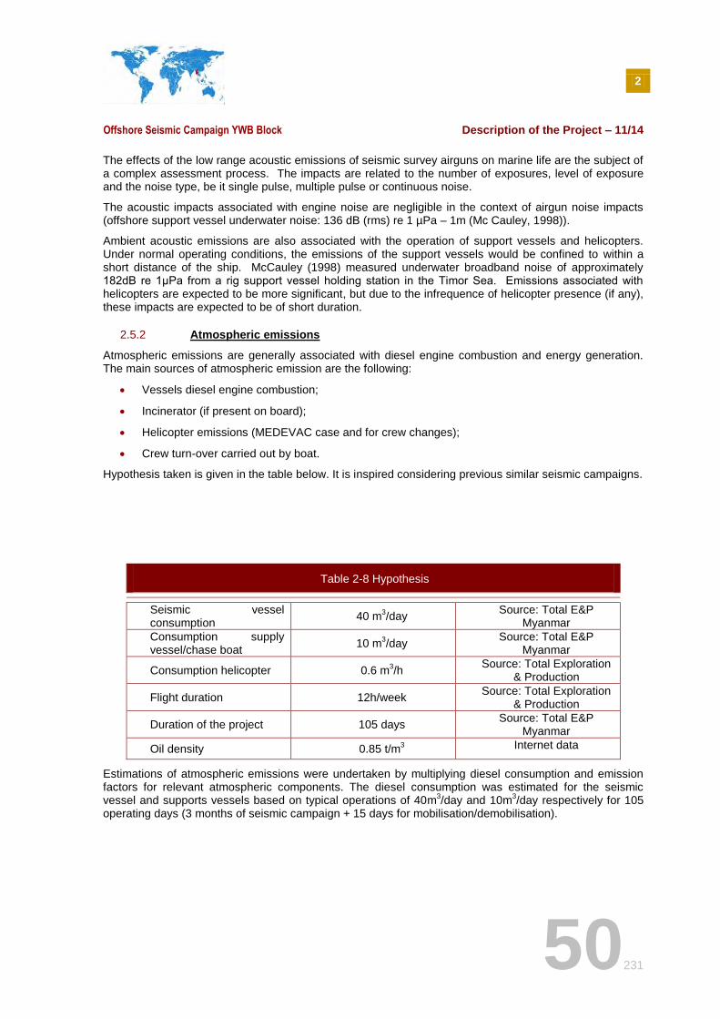
2
Offshore Seismic Campaign YWB Block Description of the Project – 11/14
50231
The effects of the low range acoustic emissions of seismic survey airguns on marine life are the subject of a complex assessment process. The impacts are related to the number of exposures, level of exposure and the noise type, be it single pulse, multiple pulse or continuous noise.
The acoustic impacts associated with engine noise are negligible in the context of airgun noise impacts (offshore support vessel underwater noise: 136 dB (rms) re 1 µPa – 1m (Mc Cauley, 1998)).
Ambient acoustic emissions are also associated with the operation of support vessels and helicopters. Under normal operating conditions, the emissions of the support vessels would be confined to within a short distance of the ship. McCauley (1998) measured underwater broadband noise of approximately 182dB re 1μPa from a rig support vessel holding station in the Timor Sea. Emissions associated with helicopters are expected to be more significant, but due to the infrequence of helicopter presence (if any), these impacts are expected to be of short duration.
2.5.2 Atmospheric emissions
Atmospheric emissions are generally associated with diesel engine combustion and energy generation. The main sources of atmospheric emission are the following:
Vessels diesel engine combustion;
Incinerator (if present on board);
Helicopter emissions (MEDEVAC case and for crew changes);
Crew turn-over carried out by boat.
Hypothesis taken is given in the table below. It is inspired considering previous similar seismic campaigns.
Table 2-8 Hypothesis
Seismic vessel consumption
40 m3/day
Source: Total E&P Myanmar
Consumption supply vessel/chase boat
10 m3/day
Source: Total E&P Myanmar
Consumption helicopter 0.6 m3/h
Source: Total Exploration & Production
Flight duration 12h/week Source: Total Exploration
& Production
Duration of the project 105 days Source: Total E&P
Myanmar
Oil density 0.85 t/m3 Internet data
Estimations of atmospheric emissions were undertaken by multiplying diesel consumption and emission factors for relevant atmospheric components. The diesel consumption was estimated for the seismic vessel and supports vessels based on typical operations of 40m
3/day and 10m
3/day respectively for 105
operating days (3 months of seismic campaign + 15 days for mobilisation/demobilisation).
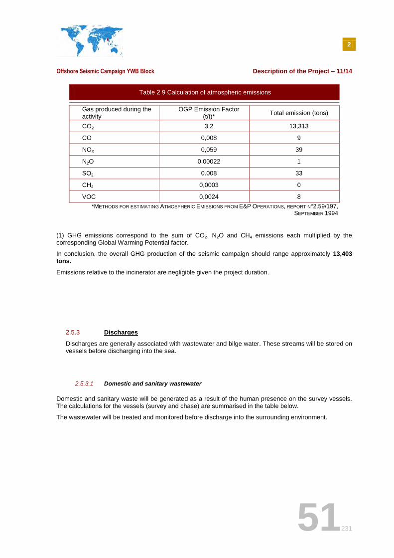
2
Offshore Seismic Campaign YWB Block Description of the Project – 11/14
51231
Table 2 9 Calculation of atmospheric emissions
Gas produced during the activity
OGP Emission Factor (t/t)*
Total emission (tons)
CO2 3,2 13,313
CO 0,008 9
NOX 0,059 39
N2O 0,00022 1
SO2 0.008 33
CH4 0,0003 0
VOC 0,0024 8
*METHODS FOR ESTIMATING ATMOSPHERIC EMISSIONS FROM E&P OPERATIONS, REPORT N°2.59/197, SEPTEMBER 1994
(1) GHG emissions correspond to the sum of CO2, N2O and CH4 emissions each multiplied by the corresponding Global Warming Potential factor.
In conclusion, the overall GHG production of the seismic campaign should range approximately 13,403 tons.
Emissions relative to the incinerator are negligible given the project duration.
2.5.3 Discharges
Discharges are generally associated with wastewater and bilge water. These streams will be stored on vessels before discharging into the sea.
2.5.3.1 Domestic and sanitary wastewater
Domestic and sanitary waste will be generated as a result of the human presence on the survey vessels. The calculations for the vessels (survey and chase) are summarised in the table below.
The wastewater will be treated and monitored before discharge into the surrounding environment.
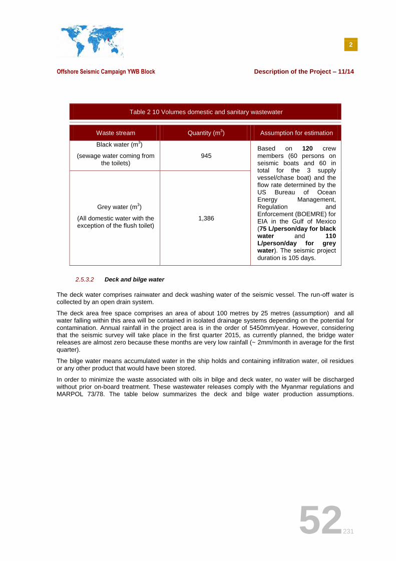
2
Offshore Seismic Campaign YWB Block Description of the Project – 11/14
52231
Table 2 10 Volumes domestic and sanitary wastewater
Waste stream Quantity (m3) Assumption for estimation
Black water (m3)
(sewage water coming from the toilets)
945 Based on 120 crew members (60 persons on seismic boats and 60 in total for the 3 supply vessel/chase boat) and the flow rate determined by the US Bureau of Ocean Energy Management, Regulation and Enforcement (BOEMRE) for EIA in the Gulf of Mexico (75 L/person/day for black water and 110 L/person/day for grey water). The seismic project duration is 105 days.
Grey water (m3)
(All domestic water with the exception of the flush toilet)
1,386
2.5.3.2 Deck and bilge water
The deck water comprises rainwater and deck washing water of the seismic vessel. The run-off water is collected by an open drain system.
The deck area free space comprises an area of about 100 metres by 25 metres (assumption) and all water falling within this area will be contained in isolated drainage systems depending on the potential for contamination. Annual rainfall in the project area is in the order of 5450mm/year. However, considering that the seismic survey will take place in the first quarter 2015, as currently planned, the bridge water releases are almost zero because these months are very low rainfall (~ 2mm/month in average for the first quarter).
The bilge water means accumulated water in the ship holds and containing infiltration water, oil residues or any other product that would have been stored.
In order to minimize the waste associated with oils in bilge and deck water, no water will be discharged without prior on-board treatment. These wastewater releases comply with the Myanmar regulations and MARPOL 73/78. The table below summarizes the deck and bilge water production assumptions.
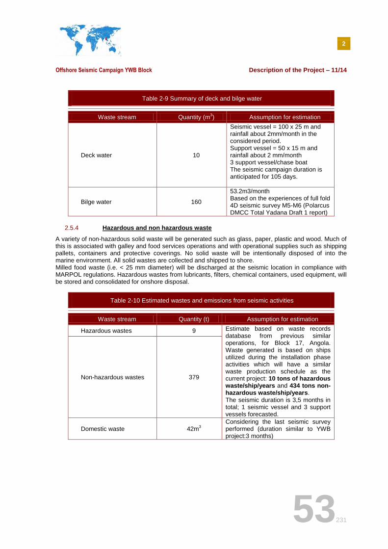
2
Offshore Seismic Campaign YWB Block Description of the Project – 11/14
53231
Table 2-9 Summary of deck and bilge water
Waste stream Quantity (m3) Assumption for estimation
Deck water 10
Seismic vessel = 100 x 25 m and rainfall about 2mm/month in the considered period. Support vessel = 50 x 15 m and rainfall about 2 mm/month 3 support vessel/chase boat The seismic campaign duration is anticipated for 105 days.
Bilge water 160
53.2m3/month Based on the experiences of full fold 4D seismic survey M5-M6 (Polarcus DMCC Total Yadana Draft 1 report)
2.5.4 Hazardous and non hazardous waste
A variety of non-hazardous solid waste will be generated such as glass, paper, plastic and wood. Much of this is associated with galley and food services operations and with operational supplies such as shipping pallets, containers and protective coverings. No solid waste will be intentionally disposed of into the marine environment. All solid wastes are collected and shipped to shore. Milled food waste (i.e. < 25 mm diameter) will be discharged at the seismic location in compliance with MARPOL regulations. Hazardous wastes from lubricants, filters, chemical containers, used equipment, will be stored and consolidated for onshore disposal.
Table 2-10 Estimated wastes and emissions from seismic activities
Waste stream Quantity (t) Assumption for estimation
Hazardous wastes 9 Estimate based on waste records database from previous similar operations, for Block 17, Angola. Waste generated is based on ships utilized during the installation phase activities which will have a similar waste production schedule as the current project: 10 tons of hazardous waste/ship/years and 434 tons non-hazardous waste/ship/years. The seismic duration is 3,5 months in total; 1 seismic vessel and 3 support vessels forecasted.
Non-hazardous wastes 379
Domestic waste 42m3
Considering the last seismic survey performed (duration similar to YWB project:3 months)
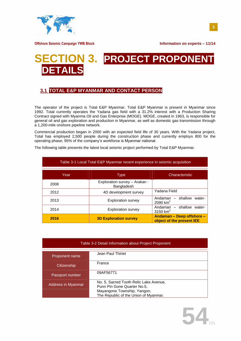
3
Offshore Seismic Campaign YWB Block Information on experts – 11/14
54231
SECTION 3. PROJECT PROPONENT DETAILS
3.1 TOTAL E&P MYANMAR AND CONTACT PERSON
The operator of the project is Total E&P Myanmar. Total E&P Myanmar is present in Myanmar since 1992. Total currently operates the Yadana gas field with a 31.2% interest with a Production Sharing Contract signed with Myanma Oil and Gas Enterprise (MOGE). MOGE, created in 1963, is responsible for general oil and gas exploration and production in Myanmar, as well as domestic gas transmission through a 1,200-mile onshore pipeline network.
Commercial production began in 2000 with an expected field life of 30 years. With the Yadana project, Total has employed 2,500 people during the construction phase and currently employs 800 for the operating phase; 95% of the company’s workforce is Myanmar national.
The following table presents the latest local seismic project performed by Total E&P Myanmar.
Table 3-1 Local Total E&P Myanmar recent experience in seismic acquisition
Year Type Characteristic
2008 Exploration survey – Arakan -
Bangladesh
2012 4D development survey Yadana Field
2013 Exploration survey Andaman – shallow water- 2090 km
2
2014 Exploration survey Andaman – shallow water- 3150 km
2
2016 3D Exploration survey Andaman – Deep offshore – object of the present IEE
Table 3-2 Detail Information about Project Proponent
Proponent name Jean Paul Thiriet
Citizenship France
Passport number 09AF56771
Address in Myanmar No. 5, Sacred Tooth Relic Lake Avenue, Punn Pin Gone Quarter No.5, Mayangone Township, Yangon, The Republic of the Union of Myanmar.
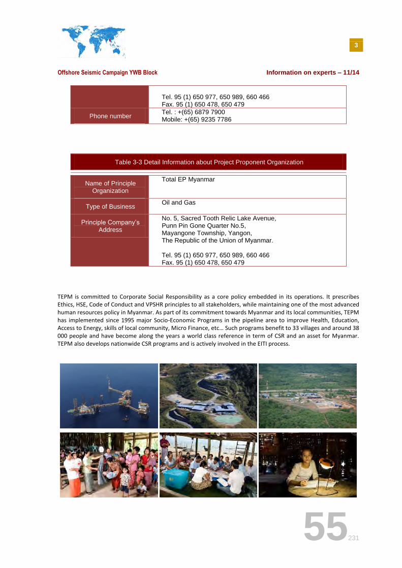
3
Offshore Seismic Campaign YWB Block Information on experts – 11/14
55231
Tel. 95 (1) 650 977, 650 989, 660 466 Fax. 95 (1) 650 478, 650 479
Phone number Tel. : +(65) 6879 7900 Mobile: +(65) 9235 7786
Table 3-3 Detail Information about Project Proponent Organization
Name of Principle Organization
Total EP Myanmar
Type of Business Oil and Gas
Principle Company’s Address
No. 5, Sacred Tooth Relic Lake Avenue, Punn Pin Gone Quarter No.5, Mayangone Township, Yangon, The Republic of the Union of Myanmar. Tel. 95 (1) 650 977, 650 989, 660 466 Fax. 95 (1) 650 478, 650 479
TEPM is committed to Corporate Social Responsibility as a core policy embedded in its operations. It prescribes Ethics, HSE, Code of Conduct and VPSHR principles to all stakeholders, while maintaining one of the most advanced human resources policy in Myanmar. As part of its commitment towards Myanmar and its local communities, TEPM has implemented since 1995 major Socio-Economic Programs in the pipeline area to improve Health, Education, Access to Energy, skills of local community, Micro Finance, etc… Such programs benefit to 33 villages and around 38 000 people and have become along the years a world class reference in term of CSR and an asset for Myanmar. TEPM also develops nationwide CSR programs and is actively involved in the EITI process.
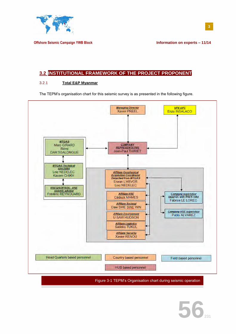
3
Offshore Seismic Campaign YWB Block Information on experts – 11/14
56231
3.2 INSTITUTIONAL FRAMEWORK OF THE PROJECT PROPONENT
3.2.1 Total E&P Myanmar
The TEPM’s organisation chart for this seismic survey is as presented in the following figure.
Figure 3-1 TEPM’s Organisation chart during seismic operation
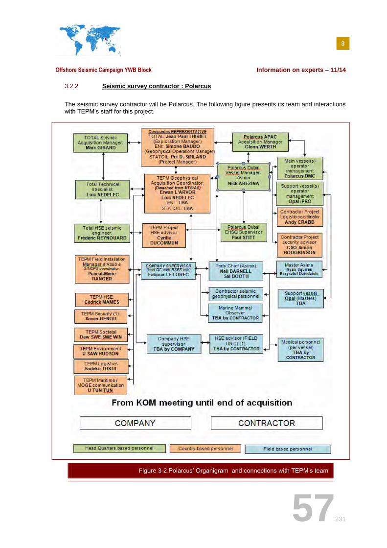
3
Offshore Seismic Campaign YWB Block Information on experts – 11/14
57231
3.2.2 Seismic survey contractor : Polarcus
The seismic survey contractor will be Polarcus. The following figure presents its team and interactions with TEPM’s staff for this project.
Figure 3-2 Polarcus’ Organigram and connections with TEPM’s team
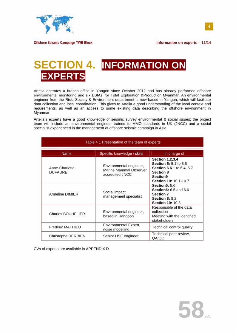
4
Offshore Seismic Campaign YWB Block Information on experts – 11/14
58231
SECTION 4. INFORMATION ON EXPERTS
Artelia operates a branch office in Yangon since October 2012 and has already performed offshore environmental monitoring and six ESIAs’ for Total Exploration &Production Myanmar. An environmental engineer from the Risk, Society & Environment department is now based in Yangon, which will facilitate data collection and local coordination. This gives to Artelia a good understanding of the local context and requirements, as well as an access to some existing data describing the offshore environment in Myanmar.
Artelia’s experts have a good knowledge of seismic survey environmental & social issues: the project team will include an environmental engineer trained to MMO standards in UK (JNCC) and a social specialist experienced in the management of offshore seismic campaign in Asia.
Table 4 1 Presentation of the team of experts
Name Specific knowledge / skills In charge of
Anne-Charlotte DUFAURE
Environmental engineer, Marine Mammal Observer accredited JNCC
Section 1,2,3,4 Section 5: 5.1 to 5.5 Section 6 6.1 to 6.4, 6.7 Section 8 Section9 Section 10: 10.1-10.7
Armeline DIMIER Social impact management specialist
Section5: 5.6 Section6: 6.5 and 6.6 Section 7 Section 8: 8.2 Section 10: 10.8
Charles BOUHELIER Environmental engineer, based in Rangoon
Responsible of the data collection Meeting with the identified stakeholders
Frederic MATHIEU Environmental Expert, noise modelling
Technical control quality
Christophe DERRIEN Senior HSE engineer Technical peer review, QA/QC
CVs of experts are available in APPENDIX D
5
Offshore Seismic Campaign YWB Block Description of the environment – 11/14
59231
SECTION 5. DESCRIPTION OF THE ENVIRONMENT
Note: The YWB seismic survey will be referred as “the Project” in the following sub-sections
5.1 INTRODUCTION
This section provides a description of the environmental conditions of the YWB block within the maritime jurisdiction of the Union of Myanmar (offshore) and its southern coastal areas.
The main environmental and social data for the project area has been obtained from a bibliographical research and previous environmental studies (including M5-M6 3 AA-3CA seismic project).
The study area covers all potential zones that may be impacted by the project activities, i.e the offshore area of the Project, the coastal areas, the natural environment (wetlands, rivers, national park, forest, deltas, etc...) and the socio-economical context.
5.2 GEOGRAPHICAL SCOPE OF THE IEE
The geographical scope of an impact evaluation process depends on the receiver’s environment, the involved activities, the direct or indirect nature of the impact and the existence of cumulative aspects.
In fact, the geographical scope of the analysis it is, in principal, not limited but is part of the potential impact analysis, which is per se a component of the impact scope. Therefore, it is legitimate to say that the intensity of an impact decreases with the distance and/or that the contribution of an impact has a direct or cumulated effect that dilutes in other contribution with the distance.
Then, the geographical scope of the IEE is the one for which a potential impact and their indirect effects were considered as existing. This IEE is focused on YWB block seismic project to determine the potential and residual impacts.
The typical geographical scopes are given in the table below to set the order of magnitudes.
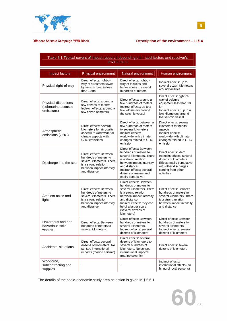
5
Offshore Seismic Campaign YWB Block Description of the environment – 11/14
60231
Table 5.1 Typical covers of impact research depending on impact factors and receiver’s environment
Impact factors Physical environment Natural environment Human environment
Physical right-of-way
Direct effects: right-of-way of streamers towed by seismic boat in less than 10km
Direct effects: right-of-way of facilities and buffer zones in several hundreds of meters
Indirect effects: up to several dozen kilometers around facilities
Physical disruptions (submarine acoustic emissions)
Direct effects: around a few dozens of meters Indirect effects: around a few dozen of meters
Direct effects: around a few hundreds of meters Indirect effects: up to a few kilometers around the seismic vessel
Direct effects: right-of-way of seismic equipment less than 10 km Indirect effects : up to a few kilometers around the seismic vessel
Atmospheric emissions (GHG)
Direct effects: several kilometers for air quality aspects to worldwide for climate aspects with GHG emissions
Direct effects: between a few hundreds of meters to several kilometers Indirect effects: worldwide with climate changes related to GHG emission
Direct effects: several kilometers for health aspects Indirect effects: worldwide with climate changes related to GHG emission
Discharge into the sea
Direct effects: Between hundreds of meters to several kilometers. There is a strong relation between impact intensity and distance.
Direct effects: Between hundreds of meters to several kilometers. There is a strong relation between impact intensity and distance. Indirect effects: several dozens of meters and easily cumulative
Direct effects: idem Indirects effects: several dozens of kilometers. Effects easily cumulative with other discharges coming from other activities
Ambient noise and light
Direct effects: Between hundreds of meters to several kilometers. There is a strong relation between impact intensity and distance.
Direct effects: Between hundreds of meters to several kilometers. There is a strong relation between impact intensity and distance. Indirect effects: they can be of a larger scale (several dozens of kilometers)
Direct effects: Between hundreds of meters to several kilometers. There is a strong relation between impact intensity and distance.
Hazardous and non-hazardous solid wastes
Direct effects: Between hundreds of meters to several kilometers.
Direct effects: Between hundreds of meters to several kilometers. Indirect effects: several dozens of kilometers
Direct effects: Between hundreds of meters to several kilometers. Indirect effects: several dozens of kilometers
Accidental situations
Direct effects: several dozens of kilometers. No sensed international impacts (marine seismic)
Direct effects: several dozens of kilometers to several hundreds of kilometers. No sensed international impacts (marine seismic)
Direct effects: several dozens of kilometers
Workforce, subcontracting and supplies
- - Indirect effects: international effects (no hiring of local persons)
The details of the socio-economic study area selection is given in § 5.6.1 .
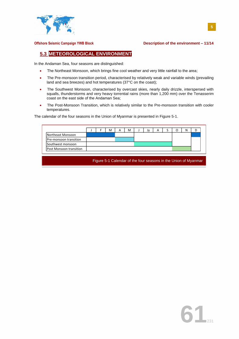
5
Offshore Seismic Campaign YWB Block Description of the environment – 11/14
61231
5.3 METEOROLOGICAL ENVIRONMENT
In the Andaman Sea, four seasons are distinguished:
The Northeast Monsoon, which brings fine cool weather and very little rainfall to the area;
The Pre-monsoon transition period, characterised by relatively weak and variable winds (prevailing land and sea breezes) and hot temperatures (37°C on the coast);
The Southwest Monsoon, characterised by overcast skies, nearly daily drizzle, interspersed with squalls, thunderstorms and very heavy torrential rains (more than 1,200 mm) over the Tenasserim coast on the east side of the Andaman Sea;
The Post-Monsoon Transition, which is relatively similar to the Pre-monsoon transition with cooler temperatures.
The calendar of the four seasons in the Union of Myanmar is presented in Figure 5-1.
J F M A M J Jy A S O N D
Northeast Monsoon
Pre-monsoon transition
Southwest monsoon
Post Monsoon transition
Figure 5-1 Calendar of the four seasons in the Union of Myanmar
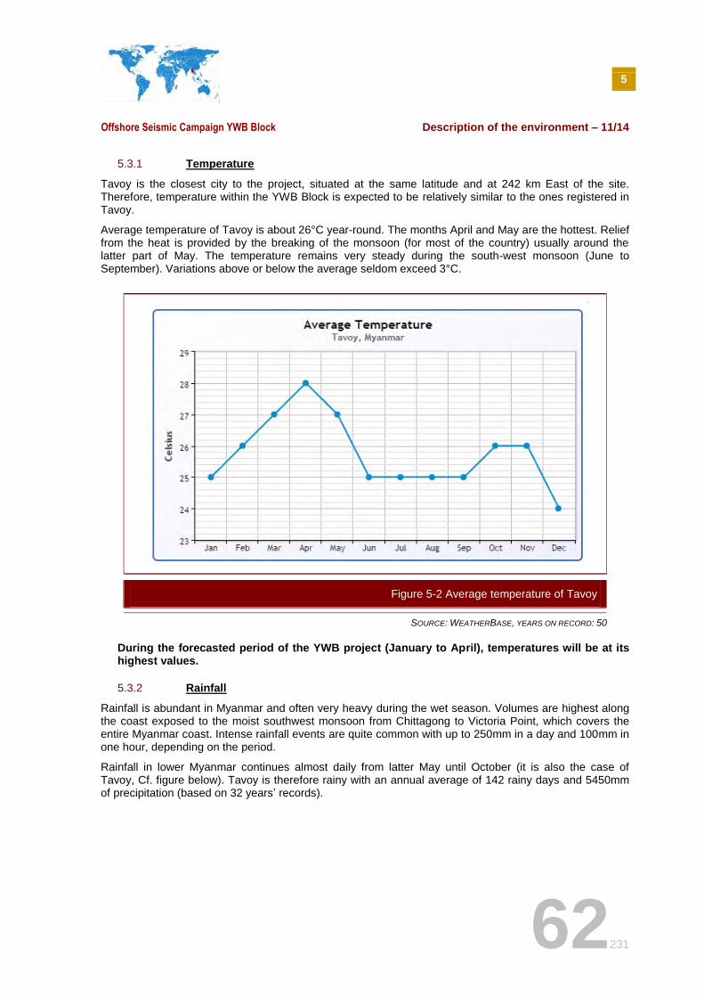
5
Offshore Seismic Campaign YWB Block Description of the environment – 11/14
62231
5.3.1 Temperature
Tavoy is the closest city to the project, situated at the same latitude and at 242 km East of the site. Therefore, temperature within the YWB Block is expected to be relatively similar to the ones registered in Tavoy.
Average temperature of Tavoy is about 26°C year-round. The months April and May are the hottest. Relief from the heat is provided by the breaking of the monsoon (for most of the country) usually around the latter part of May. The temperature remains very steady during the south-west monsoon (June to September). Variations above or below the average seldom exceed 3°C.
SOURCE: WEATHERBASE, YEARS ON RECORD: 50
During the forecasted period of the YWB project (January to April), temperatures will be at its highest values.
5.3.2 Rainfall
Rainfall is abundant in Myanmar and often very heavy during the wet season. Volumes are highest along the coast exposed to the moist southwest monsoon from Chittagong to Victoria Point, which covers the entire Myanmar coast. Intense rainfall events are quite common with up to 250mm in a day and 100mm in one hour, depending on the period.
Rainfall in lower Myanmar continues almost daily from latter May until October (it is also the case of Tavoy, Cf. figure below). Tavoy is therefore rainy with an annual average of 142 rainy days and 5450mm of precipitation (based on 32 years’ records).
Figure 5-2 Average temperature of Tavoy
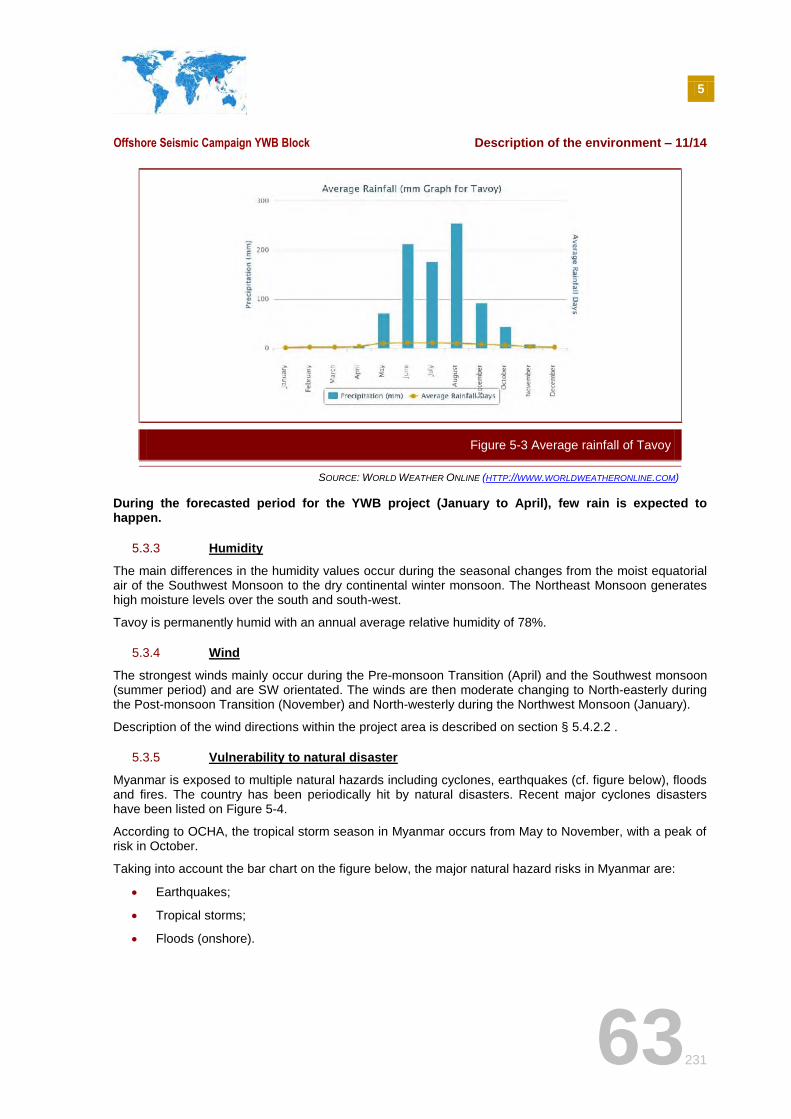
5
Offshore Seismic Campaign YWB Block Description of the environment – 11/14
63231
SOURCE: WORLD WEATHER ONLINE (HTTP://WWW.WORLDWEATHERONLINE.COM)
During the forecasted period for the YWB project (January to April), few rain is expected to happen.
5.3.3 Humidity
The main differences in the humidity values occur during the seasonal changes from the moist equatorial air of the Southwest Monsoon to the dry continental winter monsoon. The Northeast Monsoon generates high moisture levels over the south and south-west.
Tavoy is permanently humid with an annual average relative humidity of 78%.
5.3.4 Wind
The strongest winds mainly occur during the Pre-monsoon Transition (April) and the Southwest monsoon (summer period) and are SW orientated. The winds are then moderate changing to North-easterly during the Post-monsoon Transition (November) and North-westerly during the Northwest Monsoon (January).
Description of the wind directions within the project area is described on section § 5.4.2.2 .
5.3.5 Vulnerability to natural disaster
Myanmar is exposed to multiple natural hazards including cyclones, earthquakes (cf. figure below), floods and fires. The country has been periodically hit by natural disasters. Recent major cyclones disasters have been listed on Figure 5-4.
According to OCHA, the tropical storm season in Myanmar occurs from May to November, with a peak of risk in October.
Taking into account the bar chart on the figure below, the major natural hazard risks in Myanmar are:
Earthquakes;
Tropical storms;
Floods (onshore).
Figure 5-3 Average rainfall of Tavoy
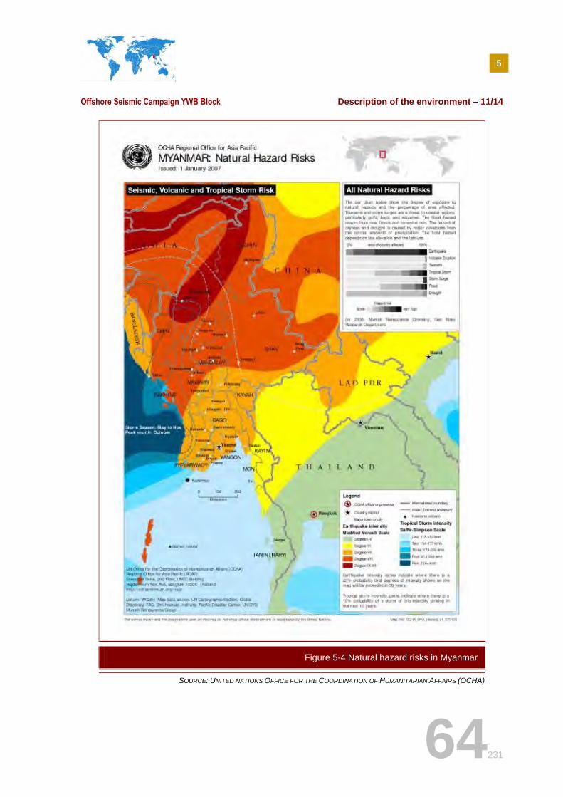
5
Offshore Seismic Campaign YWB Block Description of the environment – 11/14
64231
SOURCE: UNITED NATIONS OFFICE FOR THE COORDINATION OF HUMANITARIAN AFFAIRS (OCHA)
Figure 5-4 Natural hazard risks in Myanmar
5
Offshore Seismic Campaign YWB Block Description of the environment – 11/14
65231
The YWB block is potentially exposed to multiple natural hazards; the most worrying is the tropical storm. The most risky season occurs from May to November, with a risk higher in October (outside the forecasted project period).
5.4 PHYSICAL ENVIRONMENT
5.4.1 Geomorphology and sismology
5.4.1.1 Geomorphology
The project area is near the Andaman-Nicobar islands (cf. Figure 5-5) ~278km of the nearest YWB seismic project boundary.
At the Eastern/Northern sides of the project area, specific geological structures are present, namely: the Sagaing Fault system (SFS), the Martaban canyon (~20 km of the project location) and the Alcock rise seamount (~150 km of the project location).
The project is located within the continental slope (depth comprises between 200-2000m).
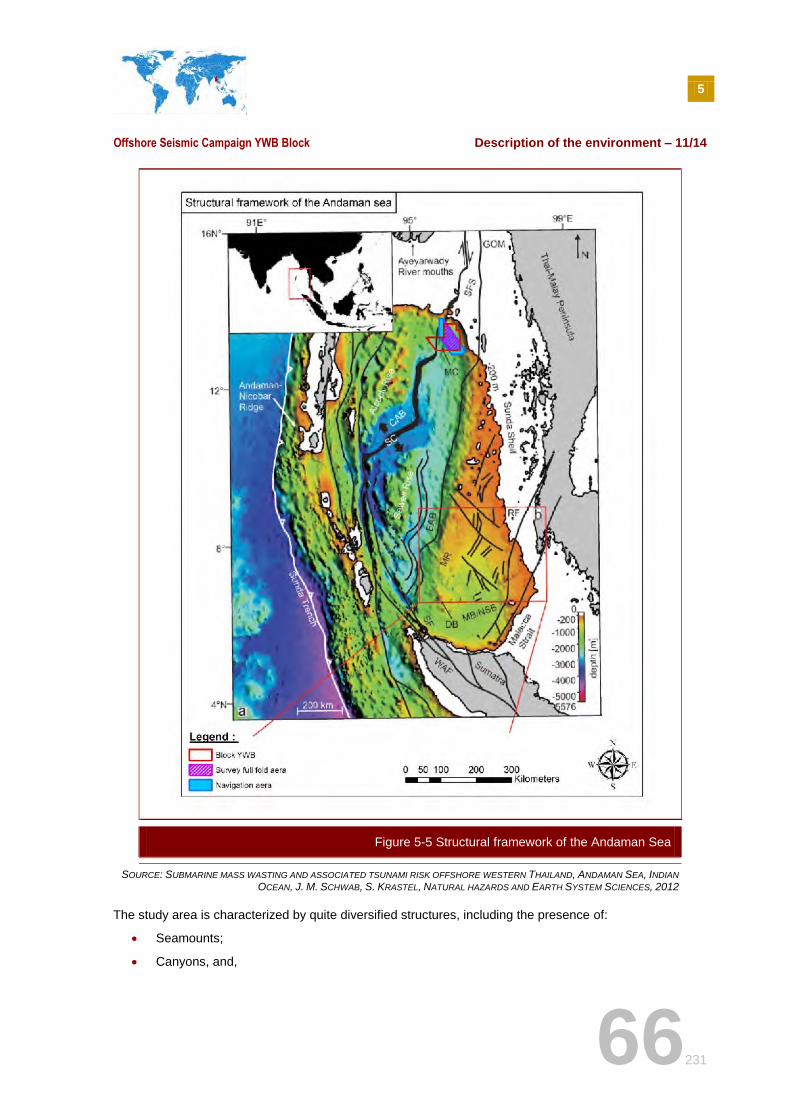
5
Offshore Seismic Campaign YWB Block Description of the environment – 11/14
66231
SOURCE: SUBMARINE MASS WASTING AND ASSOCIATED TSUNAMI RISK OFFSHORE WESTERN THAILAND, ANDAMAN SEA, INDIAN
OCEAN, J. M. SCHWAB, S. KRASTEL, NATURAL HAZARDS AND EARTH SYSTEM SCIENCES, 2012
The study area is characterized by quite diversified structures, including the presence of:
Seamounts;
Canyons, and,
Figure 5-5 Structural framework of the Andaman Sea
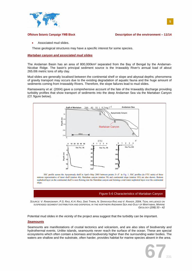
5
Offshore Seismic Campaign YWB Block Description of the environment – 11/14
67231
Associated mud slides.
These geological structures may have a specific interest for some species.
Martaban canyon and associated mud slides
The Andaman Basin has an area of 800,000km² separated from the Bay of Bengal by the Andaman-Nicobar Ridge. The basin's principal sediment source is the Irrawaddy River's annual load of about 265.l06 metric tons of silty clay.
Mud slides are generally localised between the continental shelf or slope and abyssal depths; phenomena of gravity transport may occurs due to the existing degradation of aquatic fauna and the huge amount of sediments coming from Irrawaddy Rivers. Therefore, the slope failures lead to mud slides.
Ramaswamy et al. (2004) gave a comprehensive account of the fate of the Irrawaddy discharge providing turbidity profiles that show transport of sediments into the deep Andaman Sea via the Martaban Canyon (Cf. figure below).
SOURCE: V. RAMASWAMY, P.S. RAO, K.H. RAO, SWE THWIN, N. SRINIVASA RAO AND V. RAIKER, 2004, TIDAL INFLUENCE ON
SUSPENDED SEDIMENT DISTRIBUTION AND DISPERSAL IN THE NORTHERN ANDAMAN SEA AND GULF OF MARTABAN, MARINE
GEOLOGY (208) 33 – 42
Potential mud slides in the vicinity of the project area suggest that the turbidity can be important.
Seamounts
Seamounts are manifestations of crustal tectonics and volcanism, and are also sites of biodiversity and hydrothermal events. Unlike islands, seamounts never reach the surface of the ocean. These are special ecosystems which often contain a biomass and biodiversity higher than the surrounding water bodies. The waters are shallow and the substrate, often harder, provides habitat for marine species absent in the area.
Figure 5-6 Characteristics of Martaban Canyon
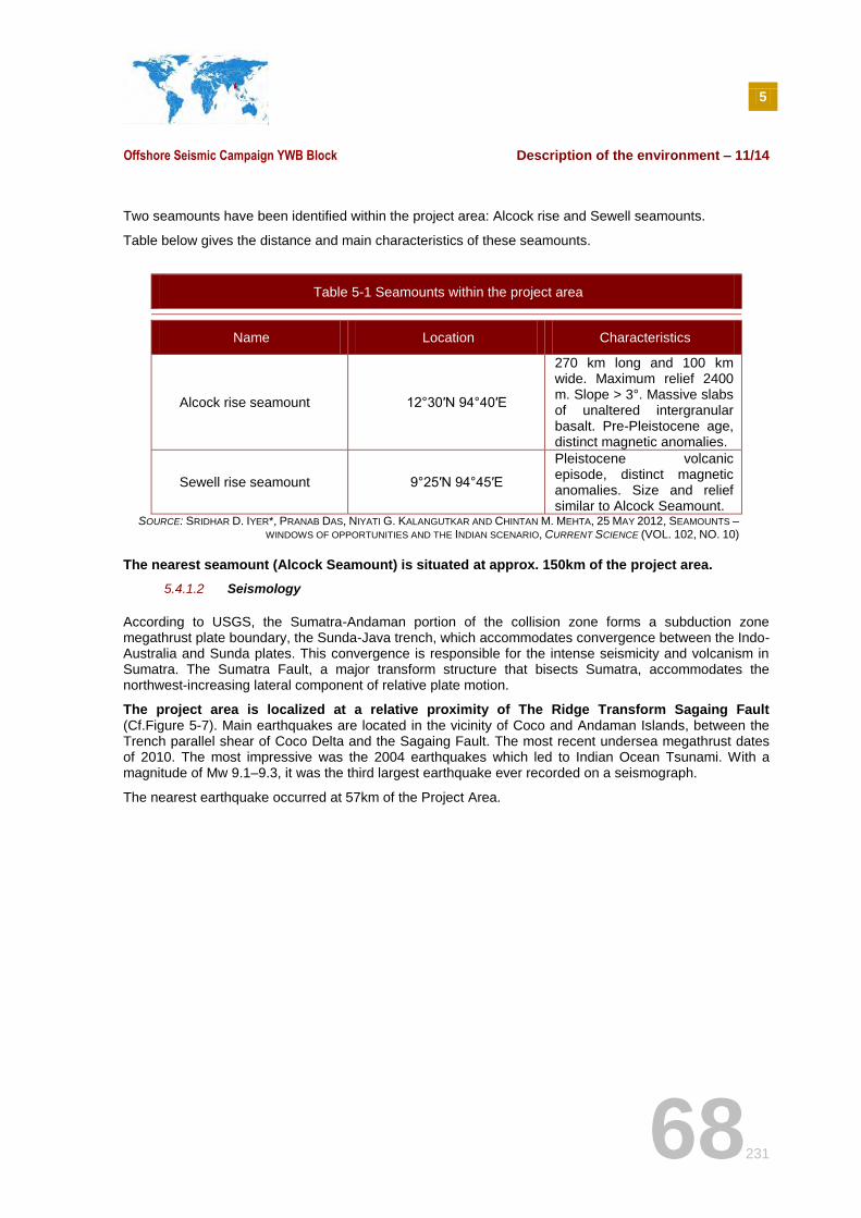
5
Offshore Seismic Campaign YWB Block Description of the environment – 11/14
68231
Two seamounts have been identified within the project area: Alcock rise and Sewell seamounts.
Table below gives the distance and main characteristics of these seamounts.
Table 5-1 Seamounts within the project area
Name Location Characteristics
Alcock rise seamount 12°30′N 94°40′E
270 km long and 100 km wide. Maximum relief 2400 m. Slope > 3°. Massive slabs of unaltered intergranular basalt. Pre-Pleistocene age, distinct magnetic anomalies.
Sewell rise seamount 9°25′N 94°45′E
Pleistocene volcanic episode, distinct magnetic anomalies. Size and relief similar to Alcock Seamount.
SOURCE: SRIDHAR D. IYER*, PRANAB DAS, NIYATI G. KALANGUTKAR AND CHINTAN M. MEHTA, 25 MAY 2012, SEAMOUNTS –
WINDOWS OF OPPORTUNITIES AND THE INDIAN SCENARIO, CURRENT SCIENCE (VOL. 102, NO. 10)
The nearest seamount (Alcock Seamount) is situated at approx. 150km of the project area.
5.4.1.2 Seismology
According to USGS, the Sumatra-Andaman portion of the collision zone forms a subduction zone megathrust plate boundary, the Sunda-Java trench, which accommodates convergence between the Indo-Australia and Sunda plates. This convergence is responsible for the intense seismicity and volcanism in Sumatra. The Sumatra Fault, a major transform structure that bisects Sumatra, accommodates the northwest-increasing lateral component of relative plate motion.
The project area is localized at a relative proximity of The Ridge Transform Sagaing Fault (Cf.Figure 5-7). Main earthquakes are located in the vicinity of Coco and Andaman Islands, between the Trench parallel shear of Coco Delta and the Sagaing Fault. The most recent undersea megathrust dates of 2010. The most impressive was the 2004 earthquakes which led to Indian Ocean Tsunami. With a magnitude of Mw 9.1–9.3, it was the third largest earthquake ever recorded on a seismograph.
The nearest earthquake occurred at 57km of the Project Area.
5
Offshore Seismic Campaign YWB Block Description of the environment – 11/14
69231
SOURCE: YU WANG, EARTHQUAKE GEOLOGY OF MYANMAR, CALIFORNIA INSTITUTE OF TECHNOLOGY, PASSADENA, 2013
5.4.2 Regional oceanography
5.4.2.1 Bathymetry
Bathymetry within the project area ranges from 200m to 2000m.
The YWB block is situated at the boundary of the continental shelf (Sunda Shelf) and mostly located on the continental slope.
Figure 5-7 Earthquakes in the study area
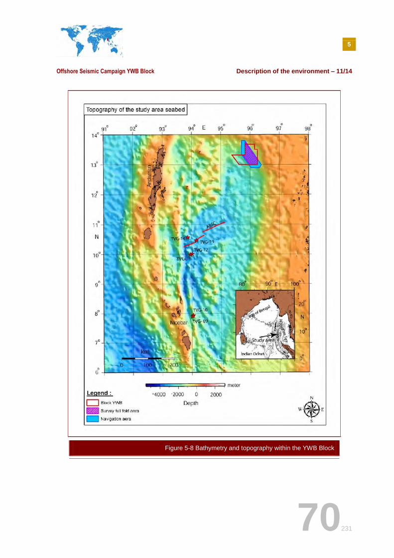
5
Offshore Seismic Campaign YWB Block Description of the environment – 11/14
70231
Figure 5-8 Bathymetry and topography within the YWB Block
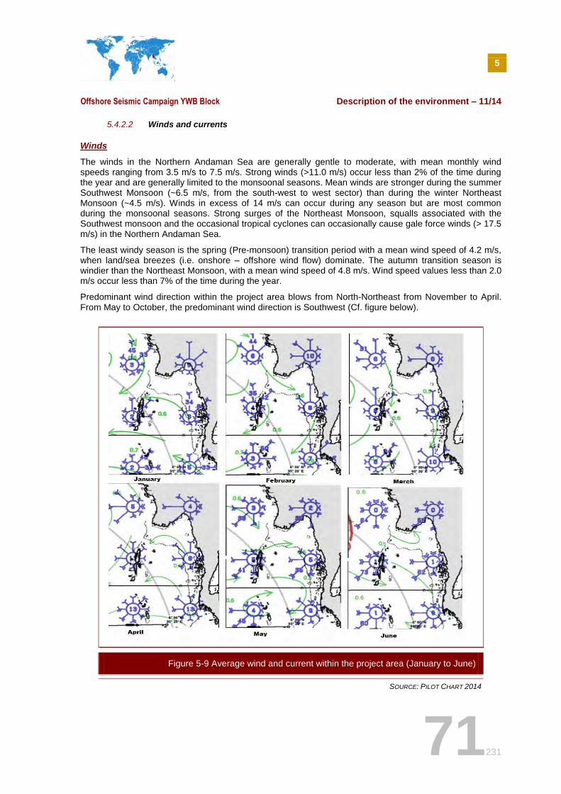
5
Offshore Seismic Campaign YWB Block Description of the environment – 11/14
71231
5.4.2.2 Winds and currents
Winds
The winds in the Northern Andaman Sea are generally gentle to moderate, with mean monthly wind speeds ranging from 3.5 m/s to 7.5 m/s. Strong winds (>11.0 m/s) occur less than 2% of the time during the year and are generally limited to the monsoonal seasons. Mean winds are stronger during the summer Southwest Monsoon (~6.5 m/s, from the south-west to west sector) than during the winter Northeast Monsoon (~4.5 m/s). Winds in excess of 14 m/s can occur during any season but are most common during the monsoonal seasons. Strong surges of the Northeast Monsoon, squalls associated with the Southwest monsoon and the occasional tropical cyclones can occasionally cause gale force winds (> 17.5 m/s) in the Northern Andaman Sea.
The least windy season is the spring (Pre-monsoon) transition period with a mean wind speed of 4.2 m/s, when land/sea breezes (i.e. onshore – offshore wind flow) dominate. The autumn transition season is windier than the Northeast Monsoon, with a mean wind speed of 4.8 m/s. Wind speed values less than 2.0 m/s occur less than 7% of the time during the year.
Predominant wind direction within the project area blows from North-Northeast from November to April. From May to October, the predominant wind direction is Southwest (Cf. figure below).
SOURCE: PILOT CHART 2014
Figure 5-9 Average wind and current within the project area (January to June)
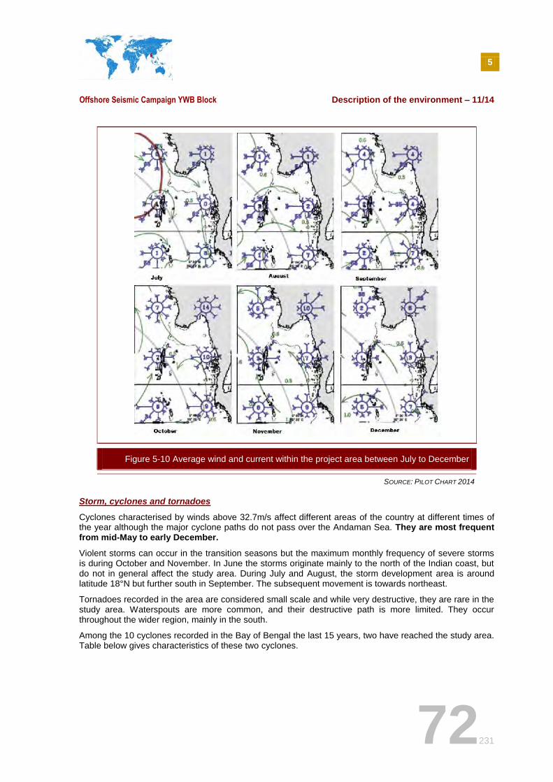
5
Offshore Seismic Campaign YWB Block Description of the environment – 11/14
72231
SOURCE: PILOT CHART 2014
Storm, cyclones and tornadoes
Cyclones characterised by winds above 32.7m/s affect different areas of the country at different times of the year although the major cyclone paths do not pass over the Andaman Sea. They are most frequent from mid-May to early December.
Violent storms can occur in the transition seasons but the maximum monthly frequency of severe storms is during October and November. In June the storms originate mainly to the north of the Indian coast, but do not in general affect the study area. During July and August, the storm development area is around latitude 18°N but further south in September. The subsequent movement is towards northeast.
Tornadoes recorded in the area are considered small scale and while very destructive, they are rare in the study area. Waterspouts are more common, and their destructive path is more limited. They occur throughout the wider region, mainly in the south.
Among the 10 cyclones recorded in the Bay of Bengal the last 15 years, two have reached the study area. Table below gives characteristics of these two cyclones.
Figure 5-10 Average wind and current within the project area between July to December
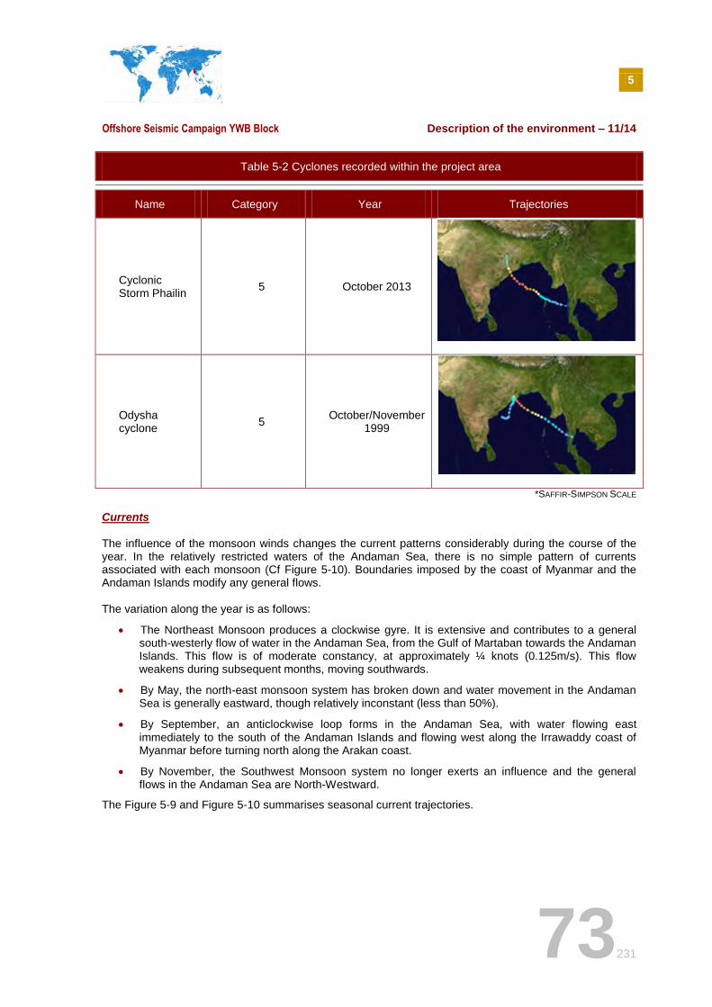
5
Offshore Seismic Campaign YWB Block Description of the environment – 11/14
73231
Table 5-2 Cyclones recorded within the project area
Name Category Year Trajectories
Cyclonic Storm Phailin
5 October 2013
Odysha cyclone
5 October/November
1999
*SAFFIR-SIMPSON SCALE
Currents
The influence of the monsoon winds changes the current patterns considerably during the course of the year. In the relatively restricted waters of the Andaman Sea, there is no simple pattern of currents associated with each monsoon (Cf Figure 5-10). Boundaries imposed by the coast of Myanmar and the Andaman Islands modify any general flows. The variation along the year is as follows:
The Northeast Monsoon produces a clockwise gyre. It is extensive and contributes to a general south-westerly flow of water in the Andaman Sea, from the Gulf of Martaban towards the Andaman Islands. This flow is of moderate constancy, at approximately ¼ knots (0.125m/s). This flow weakens during subsequent months, moving southwards.
By May, the north-east monsoon system has broken down and water movement in the Andaman Sea is generally eastward, though relatively inconstant (less than 50%).
By September, an anticlockwise loop forms in the Andaman Sea, with water flowing east immediately to the south of the Andaman Islands and flowing west along the Irrawaddy coast of Myanmar before turning north along the Arakan coast.
By November, the Southwest Monsoon system no longer exerts an influence and the general flows in the Andaman Sea are North-Westward.
The Figure 5-9 and Figure 5-10 summarises seasonal current trajectories.
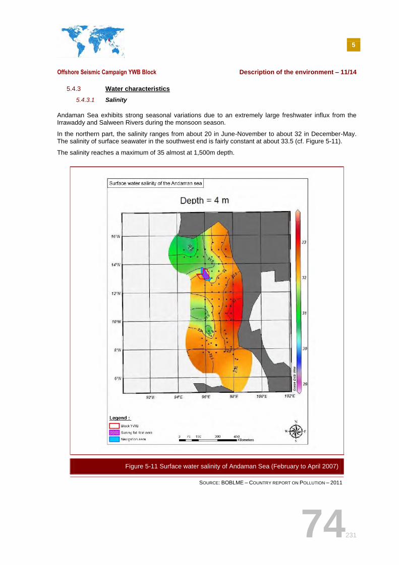
5
Offshore Seismic Campaign YWB Block Description of the environment – 11/14
74231
5.4.3 Water characteristics
5.4.3.1 Salinity
Andaman Sea exhibits strong seasonal variations due to an extremely large freshwater influx from the Irrawaddy and Salween Rivers during the monsoon season.
In the northern part, the salinity ranges from about 20 in June-November to about 32 in December-May. The salinity of surface seawater in the southwest end is fairly constant at about 33.5 (cf. Figure 5-11).
The salinity reaches a maximum of 35 almost at 1,500m depth.
SOURCE: BOBLME – COUNTRY REPORT ON POLLUTION – 2011
Figure 5-11 Surface water salinity of Andaman Sea (February to April 2007)
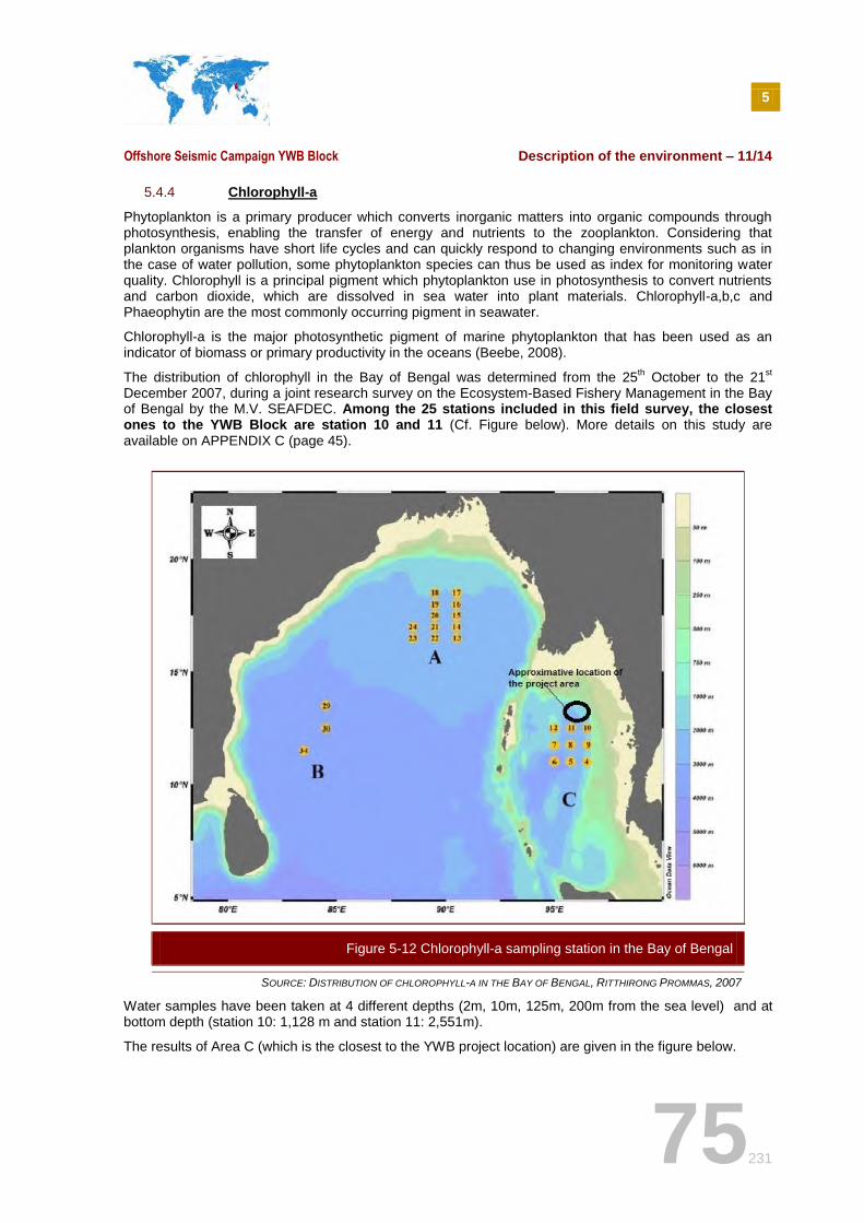
5
Offshore Seismic Campaign YWB Block Description of the environment – 11/14
75231
5.4.4 Chlorophyll-a
Phytoplankton is a primary producer which converts inorganic matters into organic compounds through photosynthesis, enabling the transfer of energy and nutrients to the zooplankton. Considering that plankton organisms have short life cycles and can quickly respond to changing environments such as in the case of water pollution, some phytoplankton species can thus be used as index for monitoring water quality. Chlorophyll is a principal pigment which phytoplankton use in photosynthesis to convert nutrients and carbon dioxide, which are dissolved in sea water into plant materials. Chlorophyll-a,b,c and Phaeophytin are the most commonly occurring pigment in seawater.
Chlorophyll-a is the major photosynthetic pigment of marine phytoplankton that has been used as an indicator of biomass or primary productivity in the oceans (Beebe, 2008).
The distribution of chlorophyll in the Bay of Bengal was determined from the 25th October to the 21
st
December 2007, during a joint research survey on the Ecosystem-Based Fishery Management in the Bay of Bengal by the M.V. SEAFDEC. Among the 25 stations included in this field survey, the closest ones to the YWB Block are station 10 and 11 (Cf. Figure below). More details on this study are available on APPENDIX C (page 45).
SOURCE: DISTRIBUTION OF CHLOROPHYLL-A IN THE BAY OF BENGAL, RITTHIRONG PROMMAS, 2007
Water samples have been taken at 4 different depths (2m, 10m, 125m, 200m from the sea level) and at bottom depth (station 10: 1,128 m and station 11: 2,551m).
The results of Area C (which is the closest to the YWB project location) are given in the figure below.
Figure 5-12 Chlorophyll-a sampling station in the Bay of Bengal
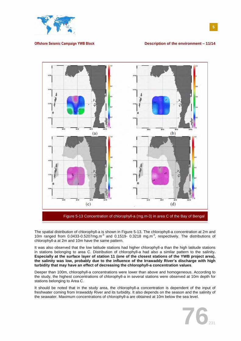
5
Offshore Seismic Campaign YWB Block Description of the environment – 11/14
76231
The spatial distribution of chlorophyll-a is shown in Figure 5-13. The chlorophyll-a concentration at 2m and 10m ranged from 0.0433-0.5207mg.m
-3 and 0.1519- 0.3218 mg.m
-3, respectively. The distributions of
chlorophyll-a at 2m and 10m have the same pattern.
It was also observed that the low latitude stations had higher chlorophyll-a than the high latitude stations in stations belonging to area C. Distribution of chlorophyll-a had also a similar pattern to the salinity. Especially at the surface layer of station 11 (one of the closest stations of the YWB project area), the salinity was low, probably due to the influence of the Irrawaddy River’s discharge with high turbidity that may have an effect of decreasing the chlorophyll-a concentration values.
Deeper than 100m, chlorophyll-a concentrations were lower than above and homogeneous. According to the study, the highest concentrations of chlorophyll-a in several stations were observed at 10m depth for stations belonging to Area C.
It should be noted that in the study area, the chlorophyll-a concentration is dependent of the input of freshwater coming from Irrawaddy River and its turbidity. It also depends on the season and the salinity of the seawater. Maximum concentrations of chlorophyll-a are obtained at 10m below the sea level.
Figure 5-13 Concentration of chlorophyll-a (mg.m-3) in area C of the Bay of Bengal
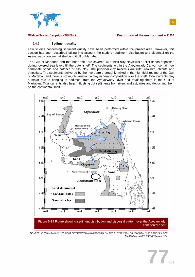
5
Offshore Seismic Campaign YWB Block Description of the environment – 11/14
77231
5.4.5 Sediment quality
Few studies concerning sediment quality have been performed within the project area. However, this section has been described taking into account the study of sediment distribution and dispersal on the Ayeyarwady continental shelf and Gulf of Martaban.
The Gulf of Martaban and the inner shelf are covered with thick silty clays while relict sands deposited during lowered sea levels fill the outer shelf. The sediments within the Ayeyarwady Canyon contain low carbonate sands and patches of silty clay. The principal clay minerals are illite, kaolinite, chlorite and smectites. The sediments delivered by the rivers are thoroughly mixed in the high tidal regime of the Gulf of Martaban and there is not much variation in clay mineral composition over the shelf. Tidal currents play a major role in bringing in sediment from the Ayeyarwady River and retaining them in the Gulf of Martaban. Tidal currents also help in flushing out sediments from rivers and estuaries and depositing them on the continental shelf.
SOURCE: V. RAMASWAMY, SEDIMENT DISTRIBUTION AND DISPERSAL ON THE AYEYARWADY CONTINENTAL SHELF AND GULF OF
MARTABAN, NORTHERN ANDAMAN SEA
Figure 5-14 Figure showing sediment distribution and dispersal pattern over the Ayeyarwady continental shelf
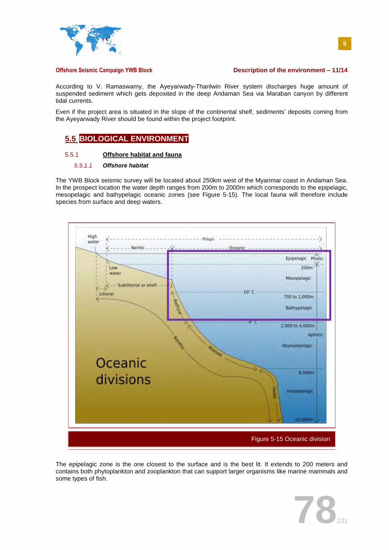
5
Offshore Seismic Campaign YWB Block Description of the environment – 11/14
78231
According to V. Ramaswamy, the Ayeyarwady-Thanlwin River system discharges huge amount of suspended sediment which gets deposited in the deep Andaman Sea via Maraban canyon by different tidal currents.
Even if the project area is situated in the slope of the continental shelf, sediments’ deposits coming from the Ayeyarwady River should be found within the project footprint.
5.5 BIOLOGICAL ENVIRONMENT
5.5.1 Offshore habitat and fauna
5.5.1.1 Offshore habitat
The YWB Block seismic survey will be located about 250km west of the Myanmar coast in Andaman Sea. In the prospect location the water depth ranges from 200m to 2000m which corresponds to the epipelagic, mesopelagic and bathypelagic oceanic zones (see Figure 5-15). The local fauna will therefore include species from surface and deep waters.
The epipelagic zone is the one closest to the surface and is the best lit. It extends to 200 meters and contains both phytoplankton and zooplankton that can support larger organisms like marine mammals and some types of fish.
Figure 5-15 Oceanic division
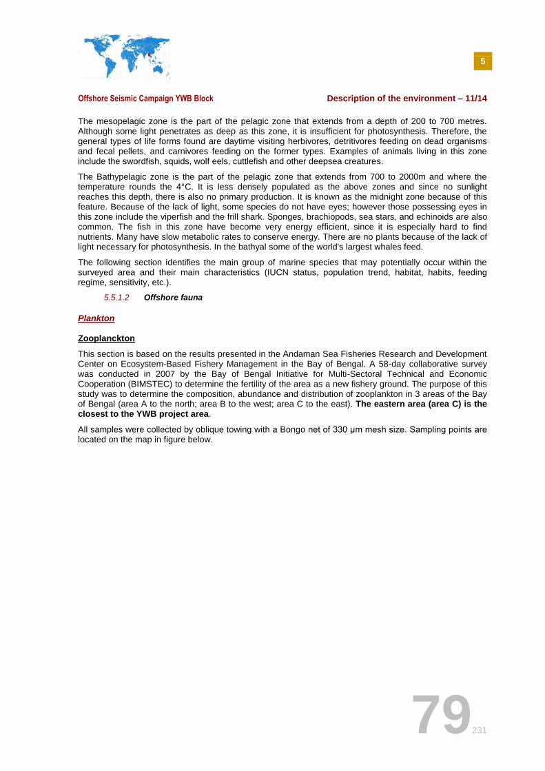
5
Offshore Seismic Campaign YWB Block Description of the environment – 11/14
79231
The mesopelagic zone is the part of the pelagic zone that extends from a depth of 200 to 700 metres. Although some light penetrates as deep as this zone, it is insufficient for photosynthesis. Therefore, the general types of life forms found are daytime visiting herbivores, detritivores feeding on dead organisms and fecal pellets, and carnivores feeding on the former types. Examples of animals living in this zone include the swordfish, squids, wolf eels, cuttlefish and other deepsea creatures.
The Bathypelagic zone is the part of the pelagic zone that extends from 700 to 2000m and where the temperature rounds the 4°C. It is less densely populated as the above zones and since no sunlight reaches this depth, there is also no primary production. It is known as the midnight zone because of this feature. Because of the lack of light, some species do not have eyes; however those possessing eyes in this zone include the viperfish and the frill shark. Sponges, brachiopods, sea stars, and echinoids are also common. The fish in this zone have become very energy efficient, since it is especially hard to find nutrients. Many have slow metabolic rates to conserve energy. There are no plants because of the lack of light necessary for photosynthesis. In the bathyal some of the world's largest whales feed.
The following section identifies the main group of marine species that may potentially occur within the surveyed area and their main characteristics (IUCN status, population trend, habitat, habits, feeding regime, sensitivity, etc.).
5.5.1.2 Offshore fauna
Plankton
Zooplanckton
This section is based on the results presented in the Andaman Sea Fisheries Research and Development Center on Ecosystem-Based Fishery Management in the Bay of Bengal. A 58-day collaborative survey was conducted in 2007 by the Bay of Bengal Initiative for Multi-Sectoral Technical and Economic Cooperation (BIMSTEC) to determine the fertility of the area as a new fishery ground. The purpose of this study was to determine the composition, abundance and distribution of zooplankton in 3 areas of the Bay of Bengal (area A to the north; area B to the west; area C to the east). The eastern area (area C) is the closest to the YWB project area.
All samples were collected by oblique towing with a Bongo net of 330 μm mesh size. Sampling points are located on the map in figure below.
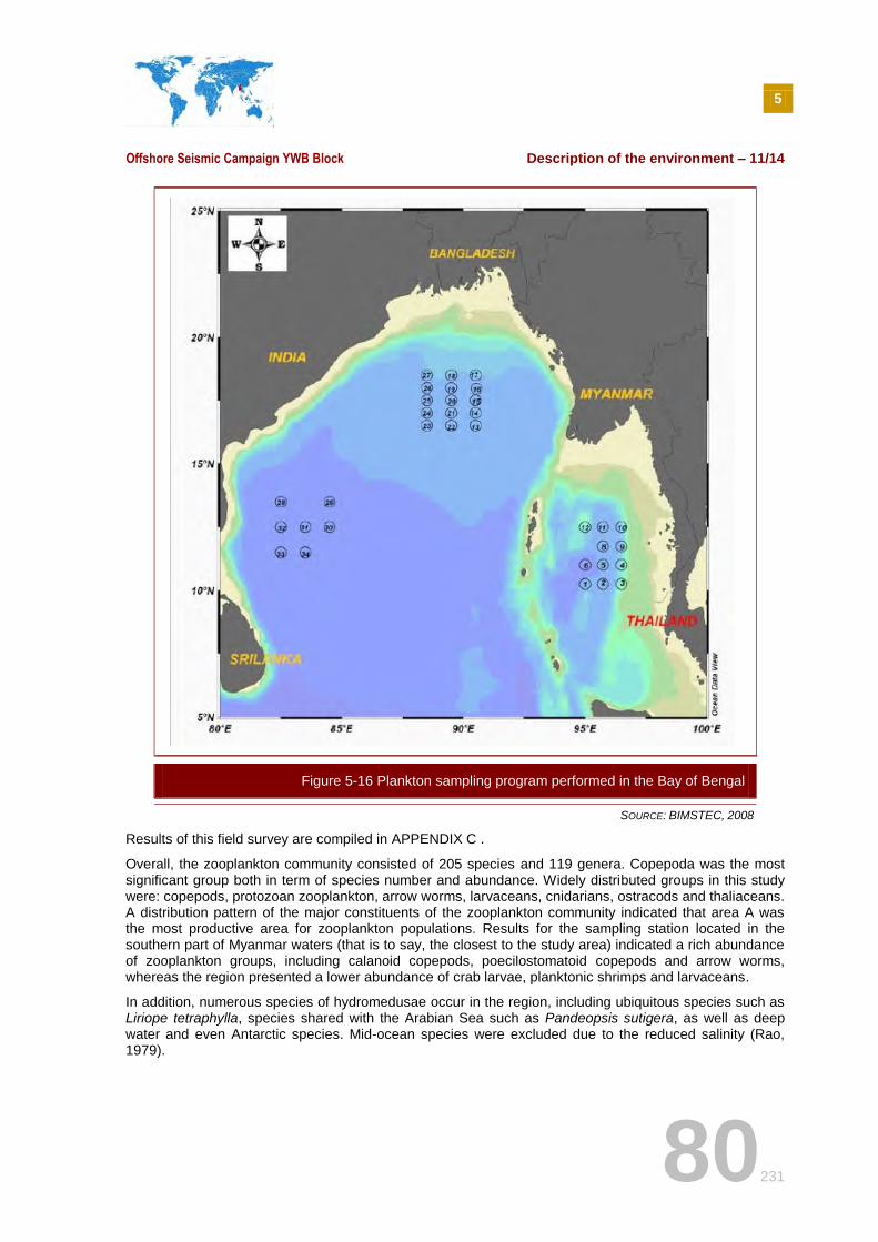
5
Offshore Seismic Campaign YWB Block Description of the environment – 11/14
80231
SOURCE: BIMSTEC, 2008
Results of this field survey are compiled in APPENDIX C .
Overall, the zooplankton community consisted of 205 species and 119 genera. Copepoda was the most significant group both in term of species number and abundance. Widely distributed groups in this study were: copepods, protozoan zooplankton, arrow worms, larvaceans, cnidarians, ostracods and thaliaceans. A distribution pattern of the major constituents of the zooplankton community indicated that area A was the most productive area for zooplankton populations. Results for the sampling station located in the southern part of Myanmar waters (that is to say, the closest to the study area) indicated a rich abundance of zooplankton groups, including calanoid copepods, poecilostomatoid copepods and arrow worms, whereas the region presented a lower abundance of crab larvae, planktonic shrimps and larvaceans.
In addition, numerous species of hydromedusae occur in the region, including ubiquitous species such as Liriope tetraphylla, species shared with the Arabian Sea such as Pandeopsis sutigera, as well as deep water and even Antarctic species. Mid-ocean species were excluded due to the reduced salinity (Rao, 1979).
Figure 5-16 Plankton sampling program performed in the Bay of Bengal
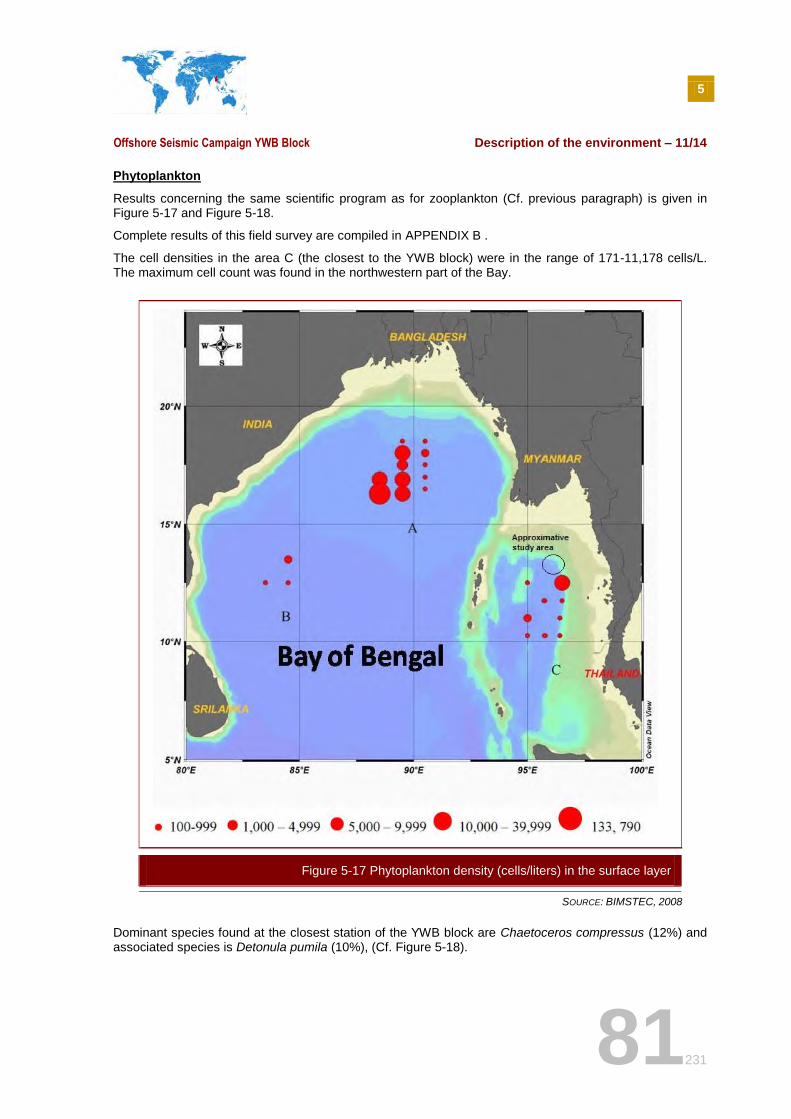
5
Offshore Seismic Campaign YWB Block Description of the environment – 11/14
81231
Phytoplankton
Results concerning the same scientific program as for zooplankton (Cf. previous paragraph) is given in Figure 5-17 and Figure 5-18.
Complete results of this field survey are compiled in APPENDIX B .
The cell densities in the area C (the closest to the YWB block) were in the range of 171-11,178 cells/L. The maximum cell count was found in the northwestern part of the Bay.
SOURCE: BIMSTEC, 2008
Dominant species found at the closest station of the YWB block are Chaetoceros compressus (12%) and associated species is Detonula pumila (10%), (Cf. Figure 5-18).
Figure 5-17 Phytoplankton density (cells/liters) in the surface layer
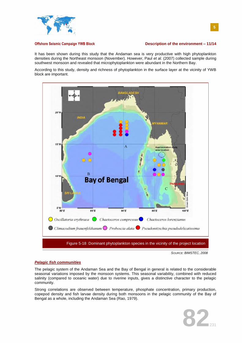
5
Offshore Seismic Campaign YWB Block Description of the environment – 11/14
82231
It has been shown during this study that the Andaman sea is very productive with high phytoplankton densities during the Northeast monsoon (November). However, Paul et al. (2007) collected sample during southwest monsoon and revealed that microphytoplankton were abundant in the Northern Bay.
According to this study, density and richness of phytoplankton in the surface layer at the vicinity of YWB block are important.
SOURCE: BIMSTEC, 2008
Pelagic fish communities
The pelagic system of the Andaman Sea and the Bay of Bengal in general is related to the considerable seasonal variations imposed by the monsoon systems. This seasonal variability, combined with reduced salinity (compared to oceanic water) due to riverine inputs, gives a distinctive character to the pelagic community.
Strong correlations are observed between temperature, phosphate concentration, primary production, copepod density and fish larvae density during both monsoons in the pelagic community of the Bay of Bengal as a whole, including the Andaman Sea (Rao, 1979).
Figure 5-18 Dominant phytoplankton species in the vicinity of the project location
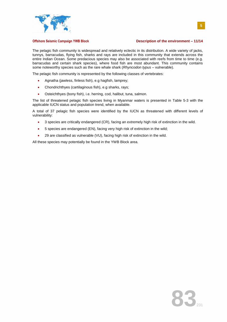
5
Offshore Seismic Campaign YWB Block Description of the environment – 11/14
83231
The pelagic fish community is widespread and relatively eclectic in its distribution. A wide variety of jacks, tunnys, barracudas, flying fish, sharks and rays are included in this community that extends across the entire Indian Ocean. Some predacious species may also be associated with reefs from time to time (e.g. barracudas and certain shark species), where food fish are most abundant. This community contains some noteworthy species such as the rare whale shark (Rhyncodon typus – vulnerable).
The pelagic fish community is represented by the following classes of vertebrates:
Agnatha (jawless, finless fish), e.g hagfish, lamprey;
Chondrichthyes (cartilaginous fish), e.g sharks, rays;
Osteichthyes (bony fish), i.e. herring, cod, halibut, tuna, salmon.
The list of threatened pelagic fish species living in Myanmar waters is presented in Table 5-3 with the applicable IUCN status and population trend, when available.
A total of 37 pelagic fish species were identified by the IUCN as threatened with different levels of vulnerability:
3 species are critically endangered (CR), facing an extremely high risk of extinction in the wild.
5 species are endangered (EN), facing very high risk of extinction in the wild;
29 are classified as vulnerable (VU), facing high risk of extinction in the wild.
All these species may potentially be found in the YWB Block area.
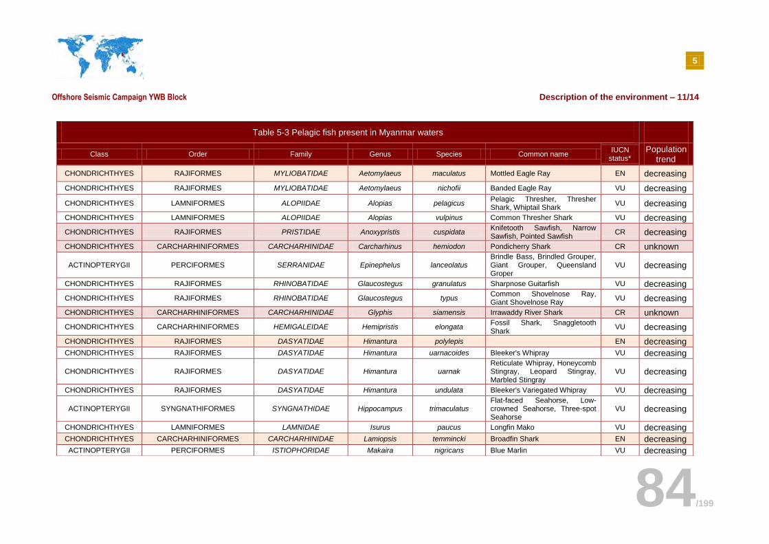
5
Offshore Seismic Campaign YWB Block Description of the environment – 11/14
84/199
Table 5-3 Pelagic fish present in Myanmar waters
Class Order Family Genus Species Common name IUCN
status* Population
trend
CHONDRICHTHYES RAJIFORMES MYLIOBATIDAE Aetomylaeus maculatus Mottled Eagle Ray EN decreasing
CHONDRICHTHYES RAJIFORMES MYLIOBATIDAE Aetomylaeus nichofii Banded Eagle Ray VU decreasing
CHONDRICHTHYES LAMNIFORMES ALOPIIDAE Alopias pelagicus Pelagic Thresher, Thresher Shark, Whiptail Shark
VU decreasing
CHONDRICHTHYES LAMNIFORMES ALOPIIDAE Alopias vulpinus Common Thresher Shark VU decreasing
CHONDRICHTHYES RAJIFORMES PRISTIDAE Anoxypristis cuspidata Knifetooth Sawfish, Narrow Sawfish, Pointed Sawfish
CR decreasing
CHONDRICHTHYES CARCHARHINIFORMES CARCHARHINIDAE Carcharhinus hemiodon Pondicherry Shark CR unknown
ACTINOPTERYGII PERCIFORMES SERRANIDAE Epinephelus lanceolatus Brindle Bass, Brindled Grouper, Giant Grouper, Queensland Groper
VU decreasing
CHONDRICHTHYES RAJIFORMES RHINOBATIDAE Glaucostegus granulatus Sharpnose Guitarfish VU decreasing
CHONDRICHTHYES RAJIFORMES RHINOBATIDAE Glaucostegus typus Common Shovelnose Ray, Giant Shovelnose Ray
VU decreasing
CHONDRICHTHYES CARCHARHINIFORMES CARCHARHINIDAE Glyphis siamensis Irrawaddy River Shark CR unknown
CHONDRICHTHYES CARCHARHINIFORMES HEMIGALEIDAE Hemipristis elongata Fossil Shark, Snaggletooth Shark
VU decreasing
CHONDRICHTHYES RAJIFORMES DASYATIDAE Himantura polylepis EN decreasing
CHONDRICHTHYES RAJIFORMES DASYATIDAE Himantura uarnacoides Bleeker's Whipray VU decreasing
CHONDRICHTHYES RAJIFORMES DASYATIDAE Himantura uarnak Reticulate Whipray, Honeycomb Stingray, Leopard Stingray, Marbled Stingray
VU decreasing
CHONDRICHTHYES RAJIFORMES DASYATIDAE Himantura undulata Bleeker's Variegated Whipray VU decreasing
ACTINOPTERYGII SYNGNATHIFORMES SYNGNATHIDAE Hippocampus trimaculatus Flat-faced Seahorse, Low-crowned Seahorse, Three-spot Seahorse
VU decreasing
CHONDRICHTHYES LAMNIFORMES LAMNIDAE Isurus paucus Longfin Mako VU decreasing
CHONDRICHTHYES CARCHARHINIFORMES CARCHARHINIDAE Lamiopsis temmincki Broadfin Shark EN decreasing
ACTINOPTERYGII PERCIFORMES ISTIOPHORIDAE Makaira nigricans Blue Marlin VU decreasing
5
Offshore Seismic Campaign YWB Block Description of the environment – 11/14
85/199
SOURCE: IUCN, 2014 – VU: VULNERABLE – EN: ENDANGERED – CR : CRITICALLY ENDANGERED
CHONDRICHTHYES RAJIFORMES MOBULIDAE Manta alfredi
Reef Manta Ray, Coastal Manta Ray, Inshore Manta Ray, Prince Alfred's Ray, Resident Manta Ray
VU decreasing
CHONDRICHTHYES RAJIFORMES MOBULIDAE Manta birostris
Giant Manta Ray, Chevron Manta Ray, Oceanic Manta Ray, Pacific Manta Ray, Pelagic Manta Ray
VU decreasing
CHONDRICHTHYES CARCHARHINIFORMES CARCHARHINIDAE Negaprion acutidens Sharptooth Lemon Shark VU decreasing
CHONDRICHTHYES RAJIFORMES RHINIDAE Rhina ancylostoma Bowmouth Guitarfish, Mud Skate, Shark Ray
VU decreasing
CHONDRICHTHYES ORECTOLOBIFORMES RHINCODONTIDAE Rhincodon typus Whale Shark VU decreasing
CHONDRICHTHYES RAJIFORMES RHINOBATIDAE Rhinobatos obtusus Widenose Guitarfish VU decreasing
CHONDRICHTHYES RAJIFORMES RHINOPTERIDAE Rhinoptera javanica Flapnose Ray, Javanese Cownose Ray
VU unknown
CHONDRICHTHYES CARCHARHINIFORMES SPHYRNIDAE Sphyrna lewini Scalloped Hammerhead EN unknown
CHONDRICHTHYES CARCHARHINIFORMES SPHYRNIDAE Sphyrna mokarran Great Hammerhead, Hammerhead Shark, Squat-headed Hammerhead Shark
EN decreasing
CHONDRICHTHYES RAJIFORMES DASYATIDAE Taeniurops meyeni
Black-blotched Stingray, Black-spotted Stingray, Blotched Fantail Ray, Fantail Stingray, Giant Reef Ray, Round Ribbontail Ray, Speckled Stingray
VU unknown
ACTINOPTERYGII PERCIFORMES SCOMBRIDAE Thunnus obesus Bigeye Tuna VU decreasing
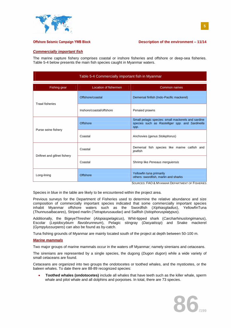
5
Offshore Seismic Campaign YWB Block Description of the environment – 11/14
86/199
Commercially important fish
The marine capture fishery comprises coastal or inshore fisheries and offshore or deep-sea fisheries. Table 5-4 below presents the main fish species caught in Myanmar waters.
Table 5-4 Commercially important fish in Myanmar
Fishing gear Location of fishermen Common names
Trawl fisheries
Offshore/coastal Demersal finfish (Indo-Pacific mackerel)
Inshore/coastal/offshore Penaied prawns
Purse seine fishery
Offshore Small pelagic species: small mackerels and sardine species such as Rastelliger spp. and Sardinella spp.
Coastal Anchovies (genus Stolephorus)
Driftnet and gillnet fishery
Coastal Demersal fish species like marine catfish and jewfish
Coastal Shrimp like Peneaus merguiensis
Long-lining Offshore Yellowfin tuna primarily others: swordfish, marlin and sharks
SOURCES: FAO & MYANMAR DEPARTMENT OF FISHERIES
Species in blue in the table are likely to be encountered within the project area.
Previous surveys for the Department of Fisheries used to determine the relative abundance and size composition of commercially important species indicated that some commercially important species inhabit Myanmar offshore waters such as the Swordfish (Xiphiasgladius), YellowfinTuna (Thunnusalbacares), Striped marlin (Tetrapturusaudax) and Sailfish (Istiophorusplatypus).
Additionally, the BigeyeThresher (Alopiaspelagicus), Whit-tipped shark (Carcharhinuslongimanus), Escolar (Lepidocybium flavobrunneum), Pelagic stingray (Dasyatissp) and Snake mackerel (Gympylussurpens) can also be found as by-catch.
Tuna fishing grounds of Myanmar are mainly located south of the project at depth between 50-100 m.
Marine mammals
Two major groups of marine mammals occur in the waters off Myanmar; namely sirenians and cetaceans.
The sirenians are represented by a single species, the dugong (Dugon dugon) while a wide variety of small cetaceans are found.
Cetaceans are organized into two groups the ondotocetes or toothed whales, and the mysticetes, or the baleen whales. To date there are 88-89 recognized species:
Toothed whales (ondotocetes) include all whales that have teeth such as the killer whale, sperm
whale and pilot whale and all dolphins and porpoises. In total, there are 73 species.
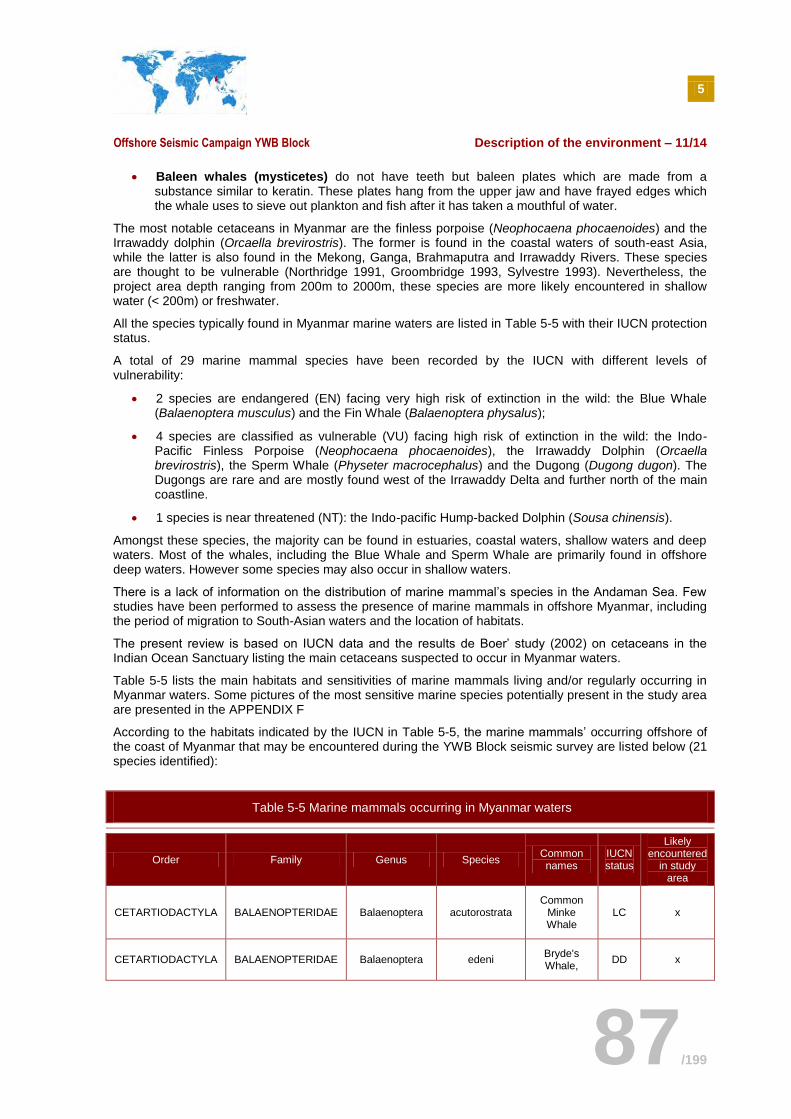
5
Offshore Seismic Campaign YWB Block Description of the environment – 11/14
87/199
Baleen whales (mysticetes) do not have teeth but baleen plates which are made from a substance similar to keratin. These plates hang from the upper jaw and have frayed edges which the whale uses to sieve out plankton and fish after it has taken a mouthful of water.
The most notable cetaceans in Myanmar are the finless porpoise (Neophocaena phocaenoides) and the Irrawaddy dolphin (Orcaella brevirostris). The former is found in the coastal waters of south-east Asia, while the latter is also found in the Mekong, Ganga, Brahmaputra and Irrawaddy Rivers. These species are thought to be vulnerable (Northridge 1991, Groombridge 1993, Sylvestre 1993). Nevertheless, the project area depth ranging from 200m to 2000m, these species are more likely encountered in shallow water (< 200m) or freshwater.
All the species typically found in Myanmar marine waters are listed in Table 5-5 with their IUCN protection status.
A total of 29 marine mammal species have been recorded by the IUCN with different levels of vulnerability:
2 species are endangered (EN) facing very high risk of extinction in the wild: the Blue Whale (Balaenoptera musculus) and the Fin Whale (Balaenoptera physalus);
4 species are classified as vulnerable (VU) facing high risk of extinction in the wild: the Indo-Pacific Finless Porpoise (Neophocaena phocaenoides), the Irrawaddy Dolphin (Orcaella brevirostris), the Sperm Whale (Physeter macrocephalus) and the Dugong (Dugong dugon). The Dugongs are rare and are mostly found west of the Irrawaddy Delta and further north of the main coastline.
1 species is near threatened (NT): the Indo-pacific Hump-backed Dolphin (Sousa chinensis).
Amongst these species, the majority can be found in estuaries, coastal waters, shallow waters and deep waters. Most of the whales, including the Blue Whale and Sperm Whale are primarily found in offshore deep waters. However some species may also occur in shallow waters.
There is a lack of information on the distribution of marine mammal’s species in the Andaman Sea. Few studies have been performed to assess the presence of marine mammals in offshore Myanmar, including the period of migration to South-Asian waters and the location of habitats.
The present review is based on IUCN data and the results de Boer’ study (2002) on cetaceans in the Indian Ocean Sanctuary listing the main cetaceans suspected to occur in Myanmar waters.
Table 5-5 lists the main habitats and sensitivities of marine mammals living and/or regularly occurring in Myanmar waters. Some pictures of the most sensitive marine species potentially present in the study area are presented in the APPENDIX F
According to the habitats indicated by the IUCN in Table 5-5, the marine mammals’ occurring offshore of the coast of Myanmar that may be encountered during the YWB Block seismic survey are listed below (21 species identified):
Table 5-5 Marine mammals occurring in Myanmar waters
Order Family Genus Species Common names
IUCN status
Likely encountered
in study area
CETARTIODACTYLA BALAENOPTERIDAE Balaenoptera acutorostrata Common
Minke Whale
LC x
CETARTIODACTYLA BALAENOPTERIDAE Balaenoptera edeni Bryde's Whale,
DD x
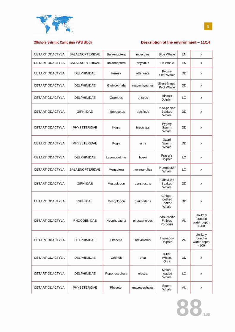
5
Offshore Seismic Campaign YWB Block Description of the environment – 11/14
88/199
CETARTIODACTYLA BALAENOPTERIDAE Balaenoptera musculus Blue Whale EN x
CETARTIODACTYLA BALAENOPTERIDAE Balaenoptera physalus Fin Whale EN x
CETARTIODACTYLA DELPHINIDAE Feresa attenuata Pygmy
Killer Whale DD x
CETARTIODACTYLA DELPHINIDAE Globicephala macrorhynchus Short-finned Pilot Whale
DD x
CETARTIODACTYLA DELPHINIDAE Grampus griseus Risso's Dolphin
LC x
CETARTIODACTYLA ZIPHIIDAE Indopacetus pacificus Indo-pacific
Beaked Whale
DD x
CETARTIODACTYLA PHYSETERIDAE Kogia breviceps Pygmy Sperm Whale
DD x
CETARTIODACTYLA PHYSETERIDAE Kogia sima Dwarf Sperm Whale
DD x
CETARTIODACTYLA DELPHINIDAE Lagenodelphis hosei Fraser's Dolphin
LC x
CETARTIODACTYLA BALAENOPTERIDAE Megaptera novaeangliae Humpback
Whale LC x
CETARTIODACTYLA ZIPHIIDAE Mesoplodon densirostris Blainville's
Beaked Whale
DD x
CETARTIODACTYLA ZIPHIIDAE Mesoplodon ginkgodens
Ginkgo-toothed Beaked Whale
DD x
CETARTIODACTYLA PHOCOENIDAE Neophocaena phocaenoides Indo-Pacific
Finless Porpoise
VU
Unlikely found in
water depth <200
CETARTIODACTYLA DELPHINIDAE Orcaella brevirostris Irrawaddy Dolphin
VU
Unlikely found in
water depth <200
CETARTIODACTYLA DELPHINIDAE Orcinus orca Killer
Whale, Orca
DD x
CETARTIODACTYLA DELPHINIDAE Peponocephala electra Melon-headed Whale
LC x
CETARTIODACTYLA PHYSETERIDAE Physeter macrocephalus Sperm Whale
VU x
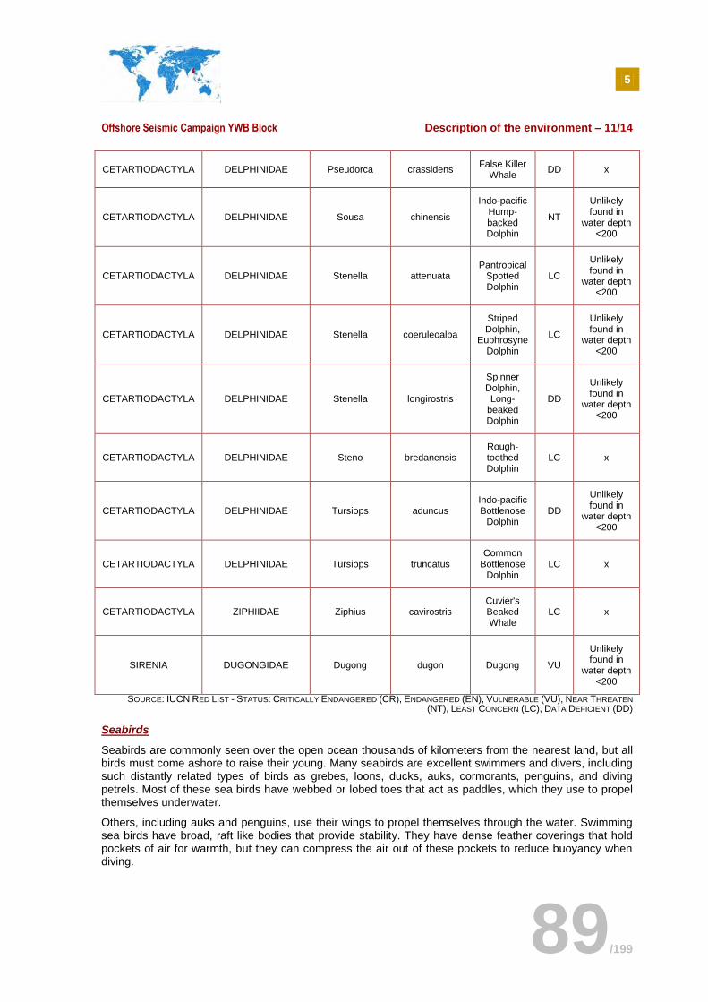
5
Offshore Seismic Campaign YWB Block Description of the environment – 11/14
89/199
CETARTIODACTYLA DELPHINIDAE Pseudorca crassidens False Killer
Whale DD x
CETARTIODACTYLA DELPHINIDAE Sousa chinensis
Indo-pacific Hump-backed Dolphin
NT
Unlikely found in
water depth <200
CETARTIODACTYLA DELPHINIDAE Stenella attenuata Pantropical
Spotted Dolphin
LC
Unlikely found in
water depth <200
CETARTIODACTYLA DELPHINIDAE Stenella coeruleoalba
Striped Dolphin,
Euphrosyne Dolphin
LC
Unlikely found in
water depth <200
CETARTIODACTYLA DELPHINIDAE Stenella longirostris
Spinner Dolphin, Long-
beaked Dolphin
DD
Unlikely found in
water depth <200
CETARTIODACTYLA DELPHINIDAE Steno bredanensis Rough-toothed Dolphin
LC x
CETARTIODACTYLA DELPHINIDAE Tursiops aduncus Indo-pacific Bottlenose
Dolphin DD
Unlikely found in
water depth <200
CETARTIODACTYLA DELPHINIDAE Tursiops truncatus Common
Bottlenose Dolphin
LC x
CETARTIODACTYLA ZIPHIIDAE Ziphius cavirostris Cuvier's Beaked Whale
LC x
SIRENIA DUGONGIDAE Dugong dugon Dugong VU
Unlikely found in
water depth <200
SOURCE: IUCN RED LIST - STATUS: CRITICALLY ENDANGERED (CR), ENDANGERED (EN), VULNERABLE (VU), NEAR THREATEN
(NT), LEAST CONCERN (LC), DATA DEFICIENT (DD)
Seabirds
Seabirds are commonly seen over the open ocean thousands of kilometers from the nearest land, but all birds must come ashore to raise their young. Many seabirds are excellent swimmers and divers, including such distantly related types of birds as grebes, loons, ducks, auks, cormorants, penguins, and diving petrels. Most of these sea birds have webbed or lobed toes that act as paddles, which they use to propel themselves underwater.
Others, including auks and penguins, use their wings to propel themselves through the water. Swimming sea birds have broad, raft like bodies that provide stability. They have dense feather coverings that hold pockets of air for warmth, but they can compress the air out of these pockets to reduce buoyancy when diving.

5
Offshore Seismic Campaign YWB Block Description of the environment – 11/14
90/199
All the seabird species typically found in Myanmar marine waters are listed in Table 5-6 with their IUCN protection status.
A total of 20 seabird species are currently identified by the IUCN in Myanmar waters. Amongst these species, 4 species are identified as near threatened and 16 species are recorded as least concern.
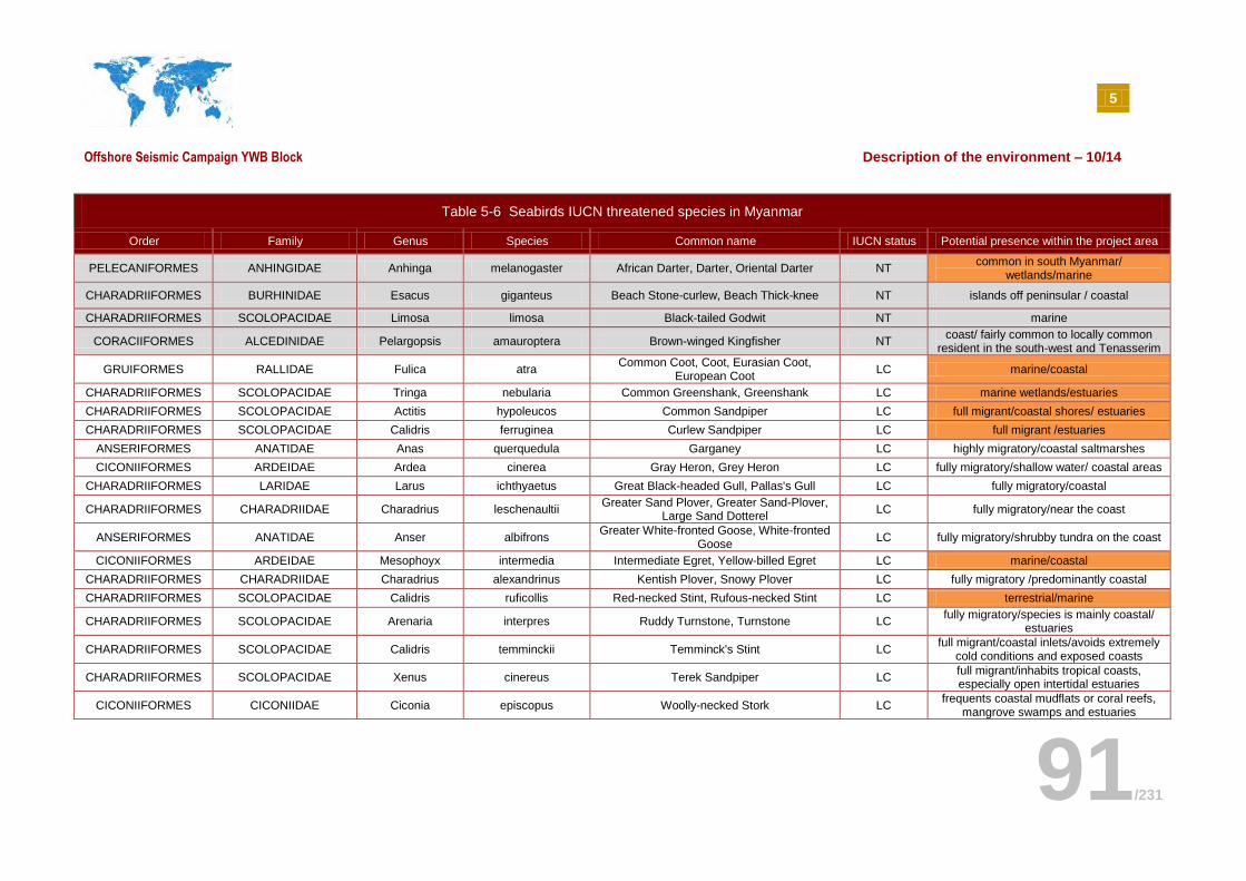
5
Offshore Seismic Campaign YWB Block Description of the environment – 10/14
91/231
Table 5-6 Seabirds IUCN threatened species in Myanmar
Order Family Genus Species Common name IUCN status Potential presence within the project area
PELECANIFORMES ANHINGIDAE Anhinga melanogaster African Darter, Darter, Oriental Darter NT common in south Myanmar/
wetlands/marine
CHARADRIIFORMES BURHINIDAE Esacus giganteus Beach Stone-curlew, Beach Thick-knee NT islands off peninsular / coastal
CHARADRIIFORMES SCOLOPACIDAE Limosa limosa Black-tailed Godwit NT marine
CORACIIFORMES ALCEDINIDAE Pelargopsis amauroptera Brown-winged Kingfisher NT coast/ fairly common to locally common
resident in the south-west and Tenasserim
GRUIFORMES RALLIDAE Fulica atra Common Coot, Coot, Eurasian Coot,
European Coot LC marine/coastal
CHARADRIIFORMES SCOLOPACIDAE Tringa nebularia Common Greenshank, Greenshank LC marine wetlands/estuaries
CHARADRIIFORMES SCOLOPACIDAE Actitis hypoleucos Common Sandpiper LC full migrant/coastal shores/ estuaries
CHARADRIIFORMES SCOLOPACIDAE Calidris ferruginea Curlew Sandpiper LC full migrant /estuaries
ANSERIFORMES ANATIDAE Anas querquedula Garganey LC highly migratory/coastal saltmarshes
CICONIIFORMES ARDEIDAE Ardea cinerea Gray Heron, Grey Heron LC fully migratory/shallow water/ coastal areas
CHARADRIIFORMES LARIDAE Larus ichthyaetus Great Black-headed Gull, Pallas's Gull LC fully migratory/coastal
CHARADRIIFORMES CHARADRIIDAE Charadrius leschenaultii Greater Sand Plover, Greater Sand-Plover,
Large Sand Dotterel LC fully migratory/near the coast
ANSERIFORMES ANATIDAE Anser albifrons Greater White-fronted Goose, White-fronted
Goose LC fully migratory/shrubby tundra on the coast
CICONIIFORMES ARDEIDAE Mesophoyx intermedia Intermediate Egret, Yellow-billed Egret LC marine/coastal
CHARADRIIFORMES CHARADRIIDAE Charadrius alexandrinus Kentish Plover, Snowy Plover LC fully migratory /predominantly coastal
CHARADRIIFORMES SCOLOPACIDAE Calidris ruficollis Red-necked Stint, Rufous-necked Stint LC terrestrial/marine
CHARADRIIFORMES SCOLOPACIDAE Arenaria interpres Ruddy Turnstone, Turnstone LC fully migratory/species is mainly coastal/
estuaries
CHARADRIIFORMES SCOLOPACIDAE Calidris temminckii Temminck's Stint LC full migrant/coastal inlets/avoids extremely
cold conditions and exposed coasts
CHARADRIIFORMES SCOLOPACIDAE Xenus cinereus Terek Sandpiper LC full migrant/inhabits tropical coasts, especially open intertidal estuaries
CICONIIFORMES CICONIIDAE Ciconia episcopus Woolly-necked Stork LC frequents coastal mudflats or coral reefs,
mangrove swamps and estuaries
5
Offshore Seismic Campaign YWB Block Description of the environment – 10/14
92/231
SOURCE: IUCN RED LIST - STATUS: CRITICALLY ENDANGERED (CR), ENDANGERED (EN), VULNERABLE (VU), NEAR THREATEN (NT), LEAST CONCERN (LC), DATA DEFICIENT (DD)
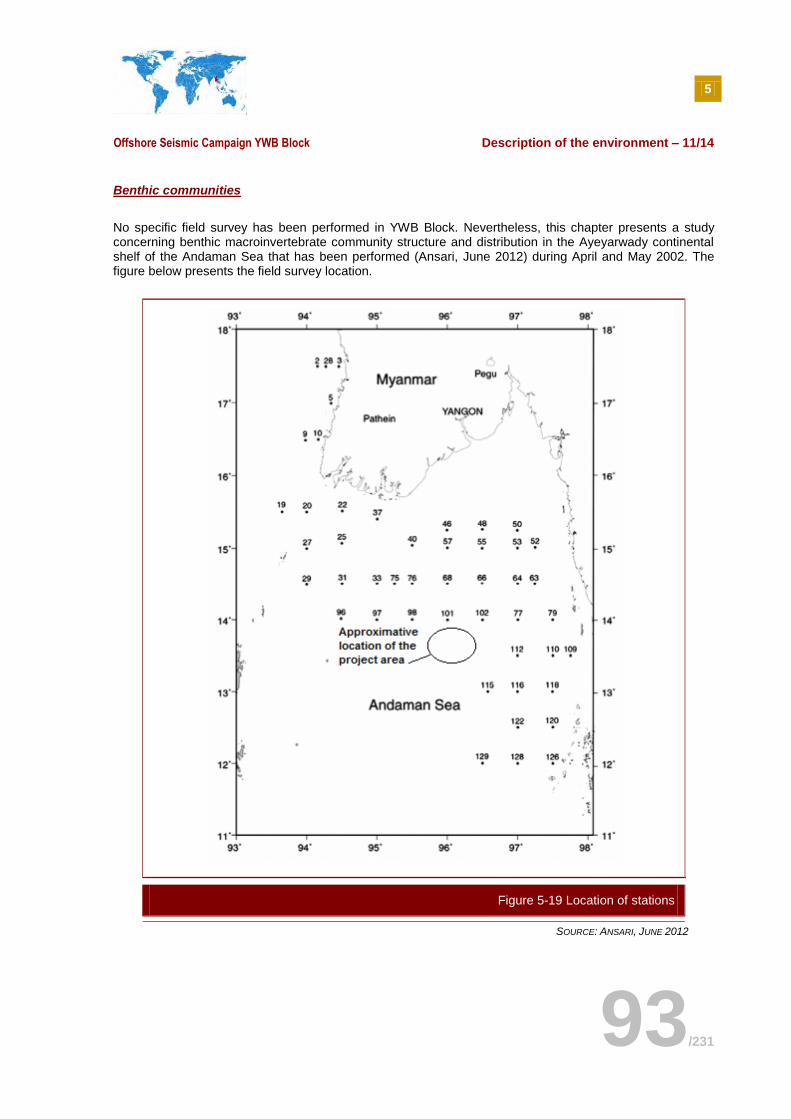
5
Offshore Seismic Campaign YWB Block Description of the environment – 11/14
93/231
Benthic communities
No specific field survey has been performed in YWB Block. Nevertheless, this chapter presents a study concerning benthic macroinvertebrate community structure and distribution in the Ayeyarwady continental shelf of the Andaman Sea that has been performed (Ansari, June 2012) during April and May 2002. The figure below presents the field survey location.
SOURCE: ANSARI, JUNE 2012
Figure 5-19 Location of stations
5
Offshore Seismic Campaign YWB Block Description of the environment – 11/14
94/231
Faunal composition differed in different depth. Forams were abundant in the shallow region (20-50m) while the polychaete showed no preference to water depth and were recorded regularly with high prevalence from all stations. Among crustaceans the amphipods, copepods, ostracods and macruran crabs were represented at different depth. About 24 taxa were recorded from 20-50m depth while the intermediate depth of 51-100m had the maximum taxa (27) and in the deepest zone 201-1000m there were only 11 taxa recorded. Between 500m and 1000m depth (which is the maximum depth of this field survey, and at the same time the closest to the project area), Polychaeta represented 52.7%, Crustacea 27.8%, Mollusca 6.9%, Echinodermata 0% and others 12.6%. The trends in the abundance of fauna reported in this scientific survey support the hypothesis that the quantity and species diversity of macrobenthos are higher in near shore than in offshore area with exception of specialized ecosystems.
Taking into account this information, and the water depth of the YWB project area (200-2000 m), the benthic community is expected to be not very abundant and diversified.
5.5.2 Coastal habitats and fauna
The following paragraph describes the Myanmar’s coastal environment which frames the study area, i.e., between the Ayeyarwady district and Tanintharyi but also Narcondam Island (situated at 158 km of the project area) and Mergui archipelago (situated at 250 km of the project area).
As it has been outlined previously, the project area is far away of the Myanmar coast. Even if some environmental and social sensitivities are highlighted in the following paragraph, it should be kept in mind that the project is at 250km far from the nearest Myanmar coast.
5.5.2.1 Coastal habitat
The land pattern in coastal areas in Myanmar consist of mangroves, coral reefs, sea-grass beds, evergreen forest, wetlands and various types of agricultural land.
Mangroves
With the exception of agriculture and wetlands the ecosystems contribute to maintain biological resources which are not only significant for the conservation of biological diversity but also of direct economic significance to Myanmar. Mangroves are found in all regions. The delta formation is the most extensive of Myanmar, which is situated at the southernmost portions in the Irrawaddy Delta. The other two formations are found along the sheltered coasts in the Rakhine and Tanintharyi region (the closest to the project area, but situated at 250km far from the project location). The original surface area covered of mangrove forest in Myanmar was 320,106 ha in early 1900.
The Rakhine mangroves are made up primarily of Rhizophora mucronata, R. candelria, Sonneratia spp., Kandelia rheedeii, Bruguiera spp., Xylocarpus granatum, X. moluccensis, Nipa fruticans, and Phoenix paludosa. The Irrawaddy mangroves consist of Rhizophora mucronata, R. conjugata, Bruguiera parviflora, B. gymnorhiza, B. cylindrica, Heritiera formes, Sonneratia apetala, S. griffithii, S. caseolaris, Xylocarpus granatum, X. molluccensis, Ceiops roxburghiana, C. mimosoides, Avicennia officinalis, Kanddelia rheedii, and Excoecaria agallocha. Finally, the Tanintharyi mangroves contain Rhizophora spp., Sonneratia caseolaris, Ceriops tegal, Xyloxarpus granatum, Avicennia officinalis, and Bruguiera spp.
The map in the figure below localizes the different Mangroves’ location in Myanmar.
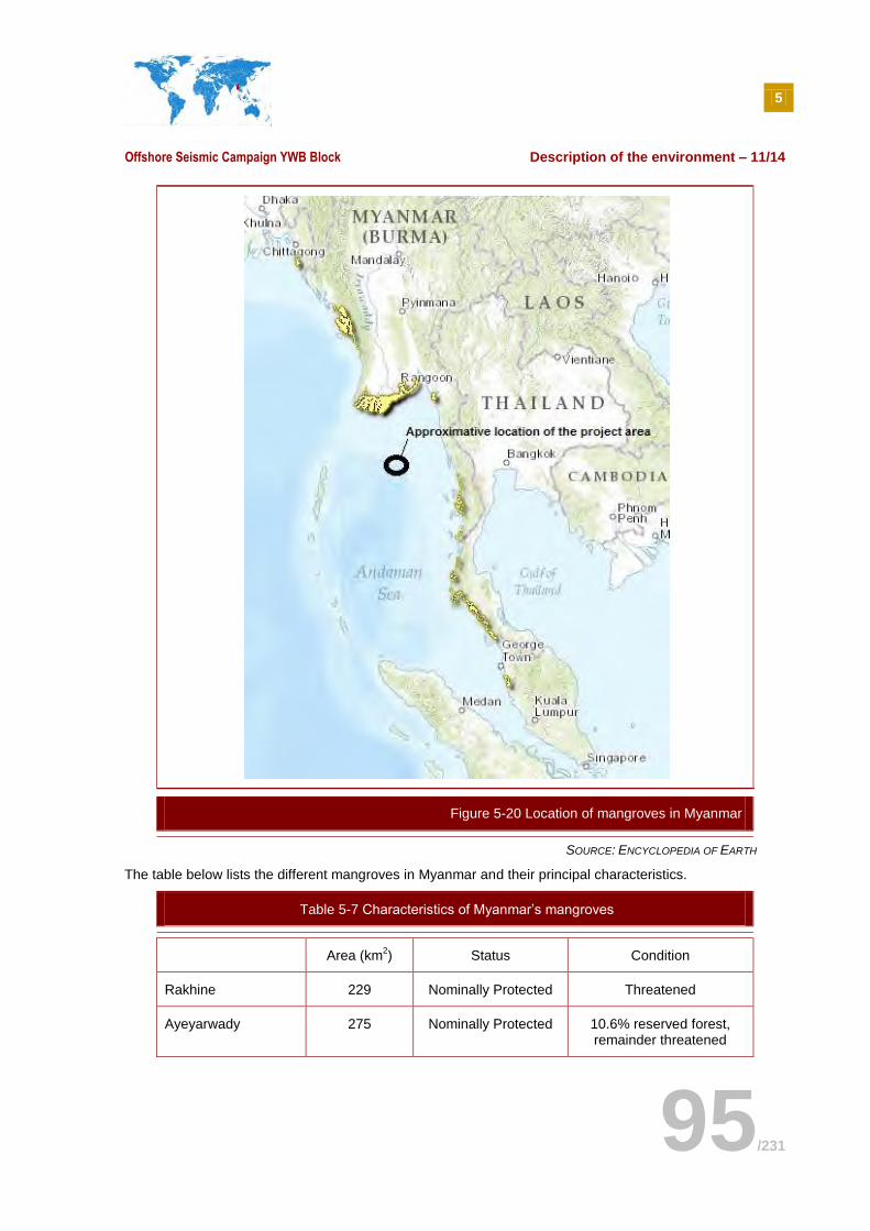
5
Offshore Seismic Campaign YWB Block Description of the environment – 11/14
95/231
SOURCE: ENCYCLOPEDIA OF EARTH
The table below lists the different mangroves in Myanmar and their principal characteristics.
Table 5-7 Characteristics of Myanmar’s mangroves
Area (km2) Status Condition
Rakhine 229 Nominally Protected Threatened
Ayeyarwady 275 Nominally Protected 10.6% reserved forest, remainder threatened
Figure 5-20 Location of mangroves in Myanmar
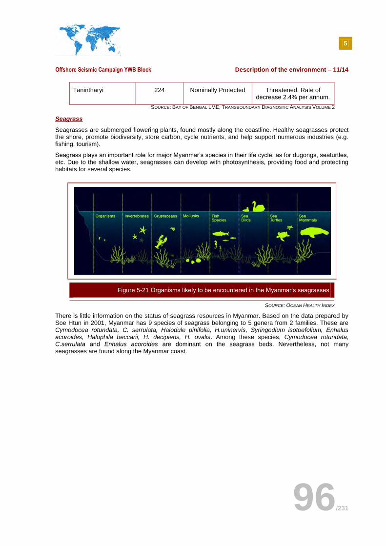
5
Offshore Seismic Campaign YWB Block Description of the environment – 11/14
96/231
Tanintharyi 224 Nominally Protected Threatened. Rate of decrease 2.4% per annum.
SOURCE: BAY OF BENGAL LME, TRANSBOUNDARY DIAGNOSTIC ANALYSIS VOLUME 2
Seagrass
Seagrasses are submerged flowering plants, found mostly along the coastline. Healthy seagrasses protect the shore, promote biodiversity, store carbon, cycle nutrients, and help support numerous industries (e.g. fishing, tourism).
Seagrass plays an important role for major Myanmar’s species in their life cycle, as for dugongs, seaturtles, etc. Due to the shallow water, seagrasses can develop with photosynthesis, providing food and protecting habitats for several species.
SOURCE: OCEAN HEALTH INDEX
There is little information on the status of seagrass resources in Myanmar. Based on the data prepared by Soe Htun in 2001, Myanmar has 9 species of seagrass belonging to 5 genera from 2 families. These are Cymodocea rotundata, C. serrulata, Halodule pinifolia, H.uninervis, Syringodium isotoefolium, Enhalus acoroides, Halophila beccarii, H. decipiens, H. ovalis. Among these species, Cymodocea rotundata, C.serrulata and Enhalus acoroides are dominant on the seagrass beds. Nevertheless, not many seagrasses are found along the Myanmar coast.
Figure 5-21 Organisms likely to be encountered in the Myanmar’s seagrasses
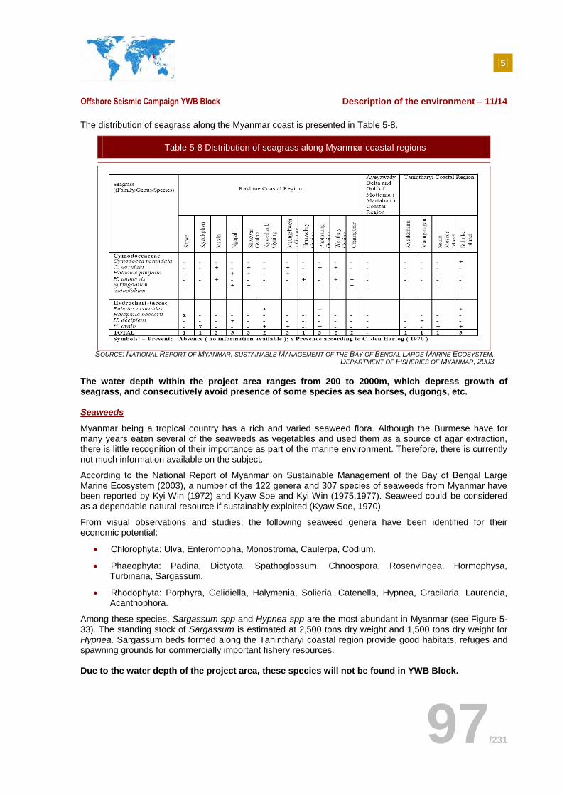
5
Offshore Seismic Campaign YWB Block Description of the environment – 11/14
97/231
The distribution of seagrass along the Myanmar coast is presented in Table 5-8.
Table 5-8 Distribution of seagrass along Myanmar coastal regions
SOURCE: NATIONAL REPORT OF MYANMAR, SUSTAINABLE MANAGEMENT OF THE BAY OF BENGAL LARGE MARINE ECOSYSTEM, DEPARTMENT OF FISHERIES OF MYANMAR, 2003
The water depth within the project area ranges from 200 to 2000m, which depress growth of seagrass, and consecutively avoid presence of some species as sea horses, dugongs, etc.
Seaweeds
Myanmar being a tropical country has a rich and varied seaweed flora. Although the Burmese have for many years eaten several of the seaweeds as vegetables and used them as a source of agar extraction, there is little recognition of their importance as part of the marine environment. Therefore, there is currently not much information available on the subject.
According to the National Report of Myanmar on Sustainable Management of the Bay of Bengal Large Marine Ecosystem (2003), a number of the 122 genera and 307 species of seaweeds from Myanmar have been reported by Kyi Win (1972) and Kyaw Soe and Kyi Win (1975,1977). Seaweed could be considered as a dependable natural resource if sustainably exploited (Kyaw Soe, 1970).
From visual observations and studies, the following seaweed genera have been identified for their economic potential:
Chlorophyta: Ulva, Enteromopha, Monostroma, Caulerpa, Codium.
Phaeophyta: Padina, Dictyota, Spathoglossum, Chnoospora, Rosenvingea, Hormophysa, Turbinaria, Sargassum.
Rhodophyta: Porphyra, Gelidiella, Halymenia, Solieria, Catenella, Hypnea, Gracilaria, Laurencia, Acanthophora.
Among these species, Sargassum spp and Hypnea spp are the most abundant in Myanmar (see Figure 5-33). The standing stock of Sargassum is estimated at 2,500 tons dry weight and 1,500 tons dry weight for Hypnea. Sargassum beds formed along the Tanintharyi coastal region provide good habitats, refuges and spawning grounds for commercially important fishery resources. Due to the water depth of the project area, these species will not be found in YWB Block.
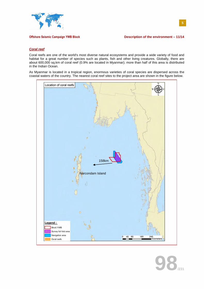
5
Offshore Seismic Campaign YWB Block Description of the environment – 11/14
98/231
Coral reef
Coral reefs are one of the world's most diverse natural ecosystems and provide a wide variety of food and habitat for a great number of species such as plants, fish and other living creatures. Globally, there are about 600,000 sq.km of coral reef (0.9% are located in Myanmar); more than half of this area is distributed in the Indian Ocean.
As Myanmar is located in a tropical region, enormous varieties of coral species are dispersed across the coastal waters of the country. The nearest coral reef sites to the project area are shown in the figure below.
158km
Narcondam Island
5
Offshore Seismic Campaign YWB Block Description of the environment – 11/14
99/231
SOURCE: HTTP://REEFGIS.REEFBASE.ORG/
A description of the coral reefs in Myanmar is given in the table below.
Table 5-9 Location of coral reef in Myanmar
Area (km2) % live coral cover Condition
Mergui Archipelago Fringing Unknown Blast fishing
Burma Banks 1,700 km2 Supposed to be good Tangled nets, blast
Rakhine area Barrier Fishing, coastal pollution
Tanintharyi Fringing unknown Poor fishing practices
SOURCE: BAY OF BENGAL LME, TRANSBOUNDARY DIAGNOSTIC ANALYSIS VOLUME 2
The nearest coral reef is located at 158 km of the project area.
5.5.2.2 Coastal fauna
Coastal birds
There are currently 55 Important Bird Areas (IBAs) recorded in Myanmar by the Birdlife International, which represent a total area of 54,364 km
2. 16 are protected, 3 partially protected and 36 are unprotected.
Myanmar’s IBAs cover 8% of the total land area of the country. There are several very large IBAs, reflecting the intact nature of natural habitats in some parts of the country.
According to the BirdLife association, the closest Important Bird Areas are:
Ayeyarwaddy Delta (approx. 250km far from the project area);
Lampi Island National Park (approx.350km of the project area).
Figure 5-22 Coral reef nearest the project area
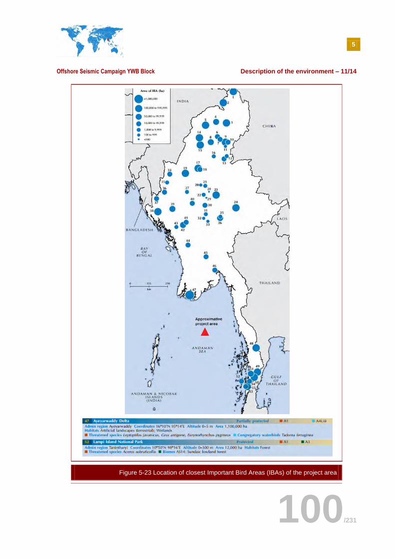
5
Offshore Seismic Campaign YWB Block Description of the environment – 11/14
100/231
Figure 5-23 Location of closest Important Bird Areas (IBAs) of the project area
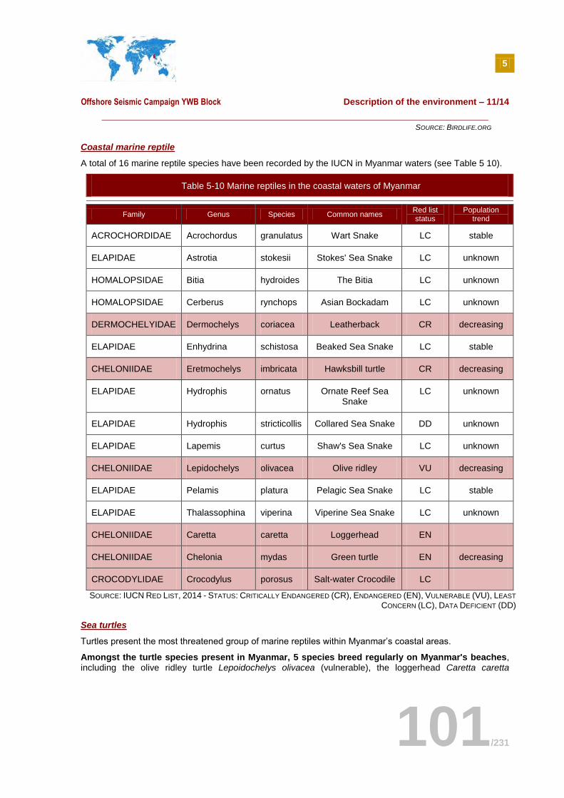
5
Offshore Seismic Campaign YWB Block Description of the environment – 11/14
101/231
SOURCE: BIRDLIFE.ORG
Coastal marine reptile
A total of 16 marine reptile species have been recorded by the IUCN in Myanmar waters (see Table 5 10).
Table 5-10 Marine reptiles in the coastal waters of Myanmar
Family Genus Species Common names Red list status
Population trend
ACROCHORDIDAE Acrochordus granulatus Wart Snake LC stable
ELAPIDAE Astrotia stokesii Stokes' Sea Snake LC unknown
HOMALOPSIDAE Bitia hydroides The Bitia LC unknown
HOMALOPSIDAE Cerberus rynchops Asian Bockadam LC unknown
DERMOCHELYIDAE Dermochelys coriacea Leatherback CR decreasing
ELAPIDAE Enhydrina schistosa Beaked Sea Snake LC stable
CHELONIIDAE Eretmochelys imbricata Hawksbill turtle CR decreasing
ELAPIDAE Hydrophis ornatus Ornate Reef Sea Snake
LC unknown
ELAPIDAE Hydrophis stricticollis Collared Sea Snake DD unknown
ELAPIDAE Lapemis curtus Shaw's Sea Snake LC unknown
CHELONIIDAE Lepidochelys olivacea Olive ridley VU decreasing
ELAPIDAE Pelamis platura Pelagic Sea Snake LC stable
ELAPIDAE Thalassophina viperina Viperine Sea Snake LC unknown
CHELONIIDAE Caretta caretta Loggerhead EN
CHELONIIDAE Chelonia mydas Green turtle EN decreasing
CROCODYLIDAE Crocodylus porosus Salt-water Crocodile LC
SOURCE: IUCN RED LIST, 2014 - STATUS: CRITICALLY ENDANGERED (CR), ENDANGERED (EN), VULNERABLE (VU), LEAST
CONCERN (LC), DATA DEFICIENT (DD)
Sea turtles
Turtles present the most threatened group of marine reptiles within Myanmar’s coastal areas.
Amongst the turtle species present in Myanmar, 5 species breed regularly on Myanmar's beaches, including the olive ridley turtle Lepoidochelys olivacea (vulnerable), the loggerhead Caretta caretta
5
Offshore Seismic Campaign YWB Block Description of the environment – 11/14
102/231
(endangered), the green turtle Chelonia mydas (endangered), the hawksbill turtle Eretmochelys imbricata (critically endangered), and leatherback Turtle Dermochelys coriacea (critically endangered).
Most observations of turtles are typically within 15 kilometers of mainland shores in protected, relatively shallow marine waters (22-55m). Each species of turtles live in different type of habitat:
Olive ridleys will occasionally occur in open waters. The multiple habitats and geographical localities used by this species vary throughout its life cycle;
Loggerhead sea turtles spend most of their lives in the open ocean and in shallow coastal waters.
They rarely come ashore, with the exception of the females' brief visits to construct nests and deposit eggs. Adults and juveniles live along the continental shelf, as well as in shallow coastal estuaries;
Green sea turtles move across three habitat types, depending on their life stage. They lay eggs on beaches. Mature turtles spend most of their time in shallow, coastal waters with lush seagrass beds. Adults frequent inshore bays, lagoons and shoals with lush seagrass meadows. Turtles spend most of their first five years in convergence zones within the open ocean. Upon leaving the nesting beach, it has been hypothesized for green turtles that hatchlings begin an oceanic phase (Carr 1987), perhaps floating passively in major current systems (gyres) that serve as open-ocean developmental grounds (Carr and Meylan 1980, Witham 1991). After a number of years in the oceanic zone, these turtles recruit to neritic developmental areas rich in seagrass and/or marine algae where they forage and grow until maturity (Musick and Limpus 1997). Upon attaining sexual maturity green turtles commence breeding migrations between foraging grounds and nesting areas that are undertaken every few years (Hirth 1997). Migrations are carried out by both males and females and may traverse oceanic zones, often spanning thousands of kilometers (Carr 1986, Mortimer and Portier 1989). During non-breeding periods adults reside at coastal neritic feeding areas that sometimes coincide with juvenile developmental habitats (e.g., Limpus et al. 1994, Seminoff et al. 2003).
Hawksbill sea turtles are rare in Myanmar. Adult hawksbill sea turtles are primarily found in tropical coral reefs. They are usually seen resting in caves and ledges in and around these reefs throughout the day. As a highly migratory species, they inhabit a wide range of habitats, from the open ocean to lagoons and even mangrove swamps in estuaries;
Leatherback turtles are also rare in Myanmar and can be found primarily in the open ocean. Its favored breeding beaches are mainland sites facing deep water and they seem to avoid those sites protected by coral reefs.
The hawksbill turtle and leatherback, which were occasionally reported by fishermen in some parts of Tanintharyi Coastal area, have totally disappeared from the Ayeyarwady Delta Coastal areas for example. All species have been abundant in the past.
The beaches of "Tha-mi-hla Kyune" (Diamonds island 15º 51' N 94º 17' E, at 319km of the Project area), an island at the mouth of the Pathein River, hosts the nesting green turtle and the loggerhead turtle. But "Kaing – Thaung – Kyune" (Kaing-Thaung Island) (15º 44' N 95º 04' E, at 272km of the project area) and "Taung-Ka-Done-Kyune"(Taung-Ka-Done Island) (15º 43' N 95º 18' E, at 262km of the project area), two small islands, which situated at the mouths of Ayeyarwady and Bogalay Rivers, respectively host the nesting olive ridley turtle and loggerhead turtle.
Most nesting is by olive ridley turtle (70%), followed by loggerhead turtle (20%) and green turtle (10%). The location of nesting sites of turtles in Myanmar’s beaches is presented in Figure 5-24.
Fisheries Department personnel walk the beaches at night during the nesting period (September-March, with a peak in January-February) and mark the location of all nests found. Nests low on the beach, which may be subjected to flooding, are transplanted to higher ground.
Figure 5-24 shows the distribution of nesting sites in the coastal areas of Myanmar. Sea turtles migration generally occurs from September to March.
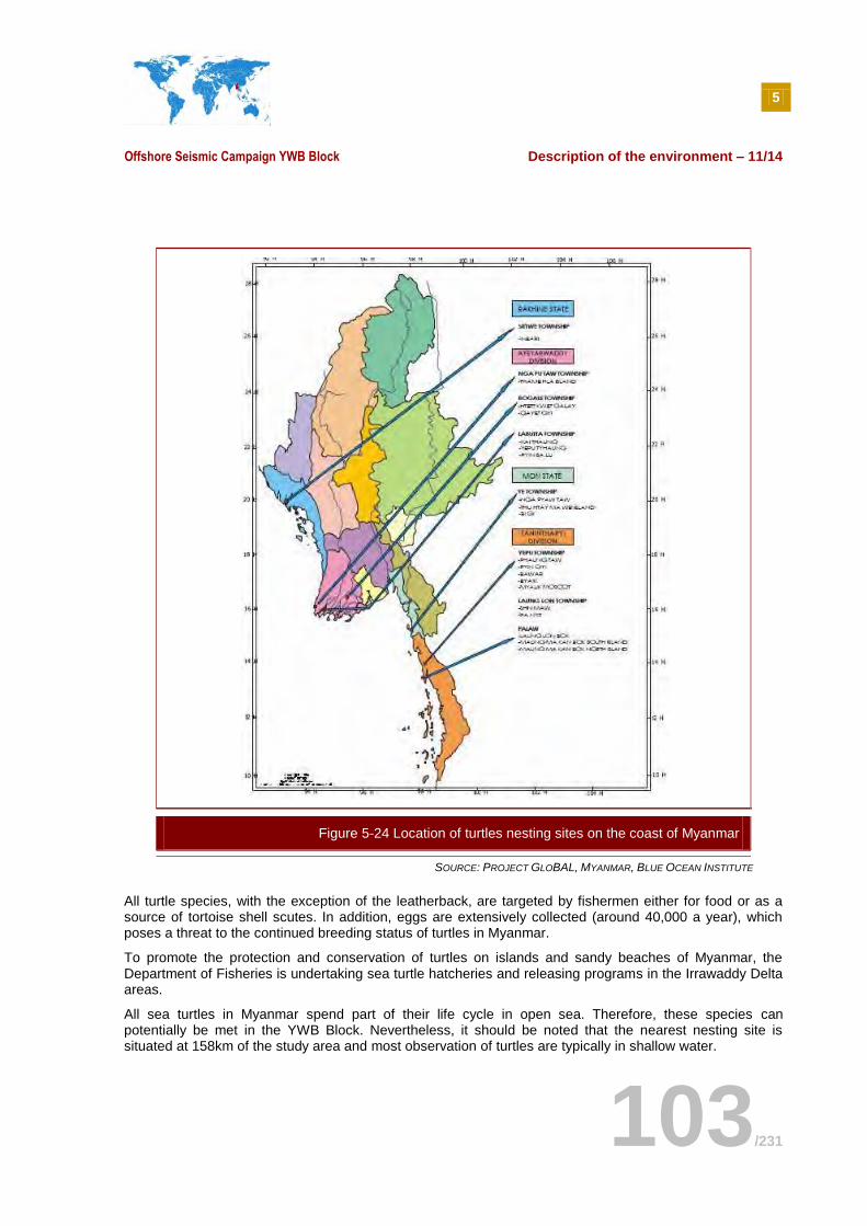
5
Offshore Seismic Campaign YWB Block Description of the environment – 11/14
103/231
SOURCE: PROJECT GLOBAL, MYANMAR, BLUE OCEAN INSTITUTE
All turtle species, with the exception of the leatherback, are targeted by fishermen either for food or as a source of tortoise shell scutes. In addition, eggs are extensively collected (around 40,000 a year), which poses a threat to the continued breeding status of turtles in Myanmar.
To promote the protection and conservation of turtles on islands and sandy beaches of Myanmar, the Department of Fisheries is undertaking sea turtle hatcheries and releasing programs in the Irrawaddy Delta areas.
All sea turtles in Myanmar spend part of their life cycle in open sea. Therefore, these species can potentially be met in the YWB Block. Nevertheless, it should be noted that the nearest nesting site is situated at 158km of the study area and most observation of turtles are typically in shallow water.
Figure 5-24 Location of turtles nesting sites on the coast of Myanmar
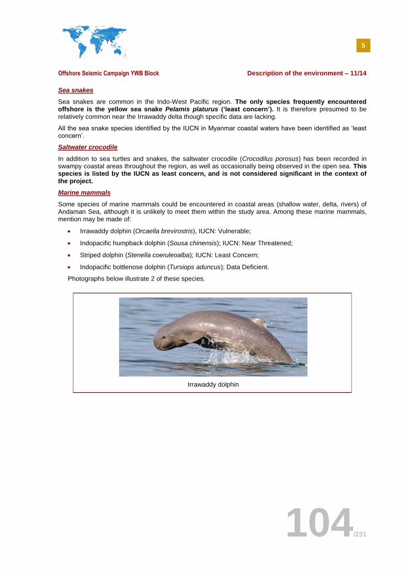
5
Offshore Seismic Campaign YWB Block Description of the environment – 11/14
104/231
Sea snakes
Sea snakes are common in the Indo-West Pacific region. The only species frequently encountered offshore is the yellow sea snake PeIamis platurus (‘least concern’). It is therefore presumed to be relatively common near the Irrawaddy delta though specific data are lacking.
All the sea snake species identified by the IUCN in Myanmar coastal waters have been identified as ‘least concern’.
Saltwater crocodile
In addition to sea turtles and snakes, the saltwater crocodile (Crocodilus porosus) has been recorded in swampy coastal areas throughout the region, as well as occasionally being observed in the open sea. This species is listed by the IUCN as least concern, and is not considered significant in the context of the project.
Marine mammals
Some species of marine mammals could be encountered in coastal areas (shallow water, delta, rivers) of Andaman Sea, although it is unlikely to meet them within the study area. Among these marine mammals, mention may be made of:
Irrawaddy dolphin (Orcaella brevirostris), IUCN: Vulnerable;
Indopacific humpback dolphin (Sousa chinensis); IUCN: Near Threatened;
Striped dolphin (Stenella coeruleoalba); IUCN: Least Concern;
Indopacific bottlenose dolphin (Tursiops aduncus); Data Deficient.
Photographs below illustrate 2 of these species.
Irrawaddy dolphin
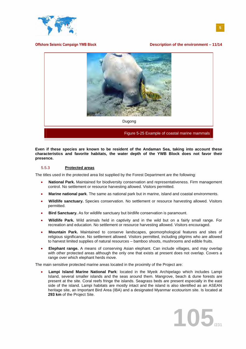
5
Offshore Seismic Campaign YWB Block Description of the environment – 11/14
105/231
Dugong
Even if these species are known to be resident of the Andaman Sea, taking into account these characteristics and favorite habitats, the water depth of the YWB Block does not favor their presence.
5.5.3 Protected areas
The titles used in the protected area list supplied by the Forest Department are the following:
National Park. Maintained for biodiversity conservation and representativeness. Firm management
control. No settlement or resource harvesting allowed. Visitors permitted.
Marine national park. The same as national park but in marine, island and coastal environments.
Wildlife sanctuary. Species conservation. No settlement or resource harvesting allowed. Visitors
permitted.
Bird Sanctuary. As for wildlife sanctuary but birdlife conservation is paramount.
Wildlife Park. Wild animals held in captivity and in the wild but on a fairly small range. For recreation and education. No settlement or resource harvesting allowed. Visitors encouraged.
Mountain Park. Maintained to conserve landscapes, geomorphological features and sites of
religious significance. No settlement allowed. Visitors permitted, including pilgrims who are allowed to harvest limited supplies of natural resources – bamboo shoots, mushrooms and edible fruits.
Elephant range. A means of conserving Asian elephant. Can include villages, and may overlap with other protected areas although the only one that exists at present does not overlap. Covers a range over which elephant herds move.
The main sensitive protected marine areas located in the proximity of the Project are:
Lampi Island Marine National Park: located in the Myeik Archipelago which includes Lampi
Island, several smaller islands and the seas around them. Mangrove, beach & dune forests are present at the site. Coral reefs fringe the islands. Seagrass beds are present especially in the east side of the island. Lampi habitats are mostly intact and the island is also identified as an ASEAN heritage site, an Important Bird Area (IBA) and a designated Myanmar ecotourism site. Is located at 293 km of the Project Site.
Figure 5-25 Example of coastal marine mammals
5
Offshore Seismic Campaign YWB Block Description of the environment – 11/14
106/231
Moscos Island Wildlife Sanctuary which comprises the south, middle and north Moscos group of islands in the northern part of the Andaman Sea. Except for some rocky islands, they are covered with evergreen forest. Although it is one of the four marine protected areas, mostly the terrestrial part of the islands is protected. Is located at 200km of the Project Site.
Ross Island Shark Protected Area. There is little information concerning this protection area. It is
situated at 215km of the project area.
These marine coastal sensitive areas are presented in more detail in the subsections below based on the Myanmar Protected Areas report from Istituto Oikos and banca, 2011.
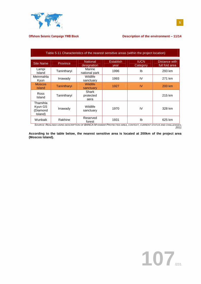
5
Offshore Seismic Campaign YWB Block Description of the environment – 11/14
107/231
Table 5-11 Characteristics of the nearest sensitive areas (within the project location)
Site Name Province National
designation Establish
year IUCN
Category Distance with full fold area
Lampi Island
Tanintharyi Marine
national park 1996 Ib 293 km
Meinmahla Kyun
Irrawady Wildlife
sanctuary 1993 IV 271 km
Moscos island
Tanintharyi Wildlife
sanctuary 1927 IV 200 km
Ross Island
Tanintharyi Shark
protected aera
215 km
Thamihla Kyun GS (Diamond
Island)
Irrawady Wildlife
sanctuary 1970 IV 328 km
Wunbaik Rakhine Reserved
forest 1931 Ib 625 km
SOURCE: REALISED USING DESCRIPTION OF BANCA MYANMAR PROTECTED AREA, CONTEXT, CURRENT STATUS AND CHALLENGES, 2011
According to the table below, the nearest sensitive area is located at 200km of the project area (Moscos Island).
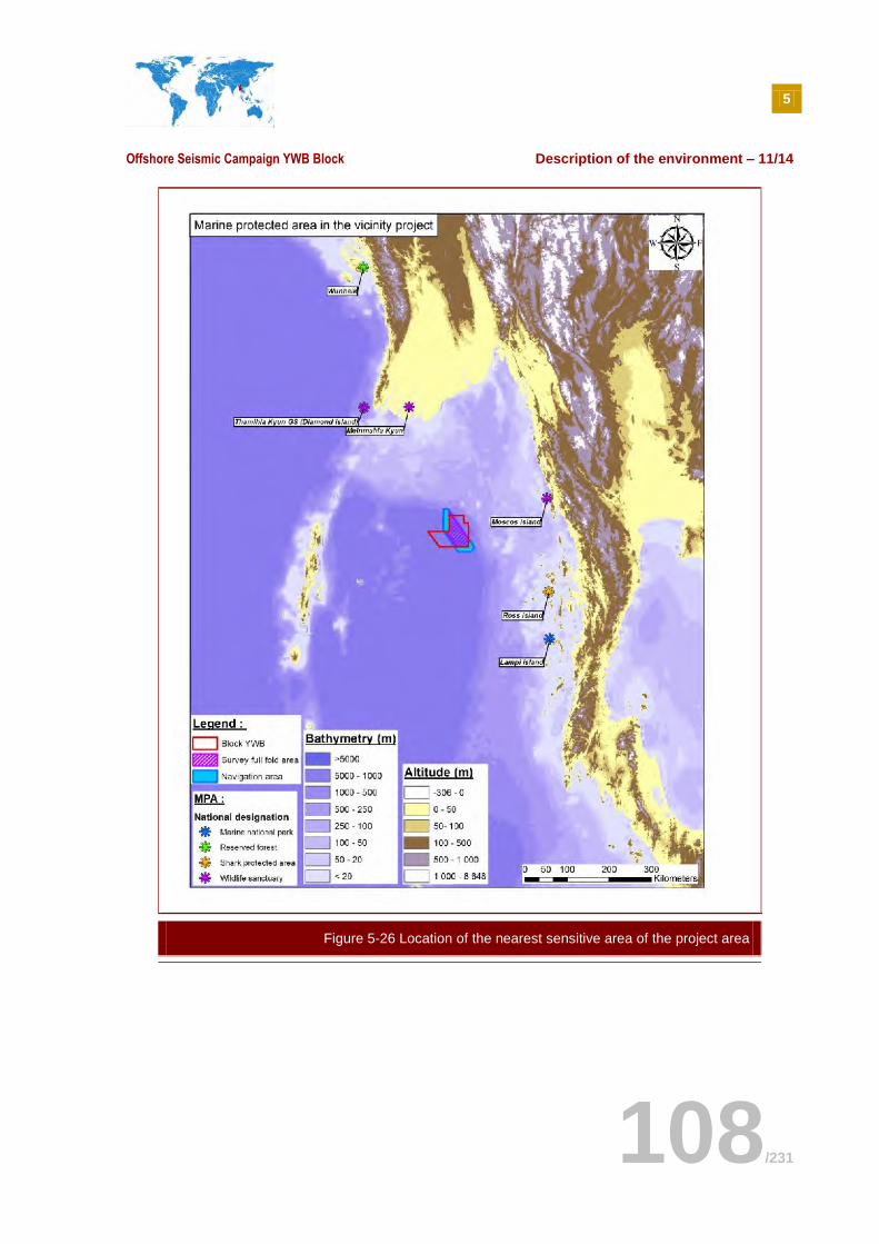
5
Offshore Seismic Campaign YWB Block Description of the environment – 11/14
108/231
Figure 5-26 Location of the nearest sensitive area of the project area
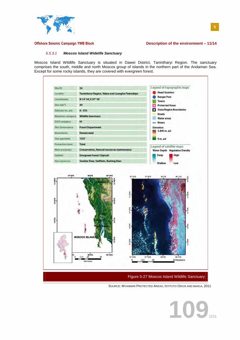
5
Offshore Seismic Campaign YWB Block Description of the environment – 11/14
109/231
5.5.3.1 Moscos Island Widelife Sanctuary
Moscos Island Wildlife Sanctuary is situated in Dawei District, Tanintharyi Region. The sanctuary comprises the south, middle and north Moscos group of islands in the northern part of the Andaman Sea. Except for some rocky islands, they are covered with evergreen forest.
SOURCE: MYANMAR PROTECTED AREAS, ISTITUTO OIKOS AND BANCA, 2011
Figure 5-27 Moscos Island Wildlife Sanctuary
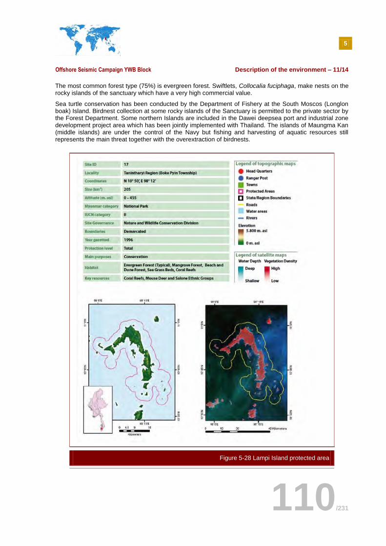
5
Offshore Seismic Campaign YWB Block Description of the environment – 11/14
110/231
The most common forest type (75%) is evergreen forest. Swiftlets, Collocalia fuciphaga, make nests on the rocky islands of the sanctuary which have a very high commercial value.
Sea turtle conservation has been conducted by the Department of Fishery at the South Moscos (Longlon boak) Island. Birdnest collection at some rocky islands of the Sanctuary is permitted to the private sector by the Forest Department. Some northern Islands are included in the Dawei deepsea port and industrial zone development project area which has been jointly implemented with Thailand. The islands of Maungma Kan (middle islands) are under the control of the Navy but fishing and harvesting of aquatic resources still represents the main threat together with the overextraction of birdnests.
Figure 5-28 Lampi Island protected area
5
Offshore Seismic Campaign YWB Block Description of the environment – 11/14
111/231
SOURCE: MYANMAR PROTECTED AREAS, ISTITUTO OIKOS AND BANCA, 2011
Lampi Island Marine National Park is located in Boke Pyin Township of Tanintharyi Region. The protected area was designated in 1996 to include an area extending two miles from the outer islands but there is no demarcation buoy or signal. Lampi Island is the biggest island and the core of the site. It is 205 km² and is oriented in a north-south direction, with a length of 48 km and a maximum width of about 6 km. It is generally hilly (150–270 m), presenting a rocky coast with presence of sandy beaches, bays and inlets. The sea depth between Island and the mainland is on average 12m and nowhere deeper than 24m. The protection level of the site is total. According to the notification no. 40/96, the boundaries of Lampi Island Marine National Park are as follows:
North boundary: two nautical miles north from the shoreline of Two Hill Island.
East Boundary: two nautical miles east from the shoreline of Pulo Gabon Island, Dolphin Islands (War Kyunn), Marble Island, Gregory Group Islands, Palo Taban Islands.
South Boundary: two nautical miles south from the shoreline of Pulo Tuhan Island which is south east of Lampi Island, Palo Nalo (Bo Cho) Island, Gu Gyi (Kyun) Island, Pulo Lobiaung Island.
West Boundary: two nautical miles west from the shoreline of Kanzagyi Island, Wa Ale Kyun Island, Ko Phawt Island, Pulo Tayu Island, Kular Island, Observation Island, Pulo Tu-ante Island, Pulo Lobiaung (Lin Shu) Island.
Lampi Island is covered by tropical lowland wet evergreen forest in the interior, mangrove forest along rivers and fresh-water sources, and beach and dune forest along the coast. Other important habitat types are coral reefs, seagrass, freshwater streams and swamps. The main island of Lampi has two major perennial rivers and many small seasonal streams. Fresh-water resources are abundant. The variety of habitats supports a high diversity of both terrestrial and marine resources.
The whole area is rich in coral reefs, seaweed and seagrass beds which serve as important habitats for molluscs, crustaceans, echinoderms and fishes, of which many species are of economic importance as food resources for local use and export. The seagrass meadows around Lampi Island also supports threatened species like the green turtle and the dugong that feed on seagrass, and a variety of birds that feed in the intertidal zone and sublittoral zone. Mangrove forests, found in the park in a very good conservation status, also provide an important habitat for many species of molluscs, crustaceans and fishes.
5.6 SOCIO-ECONOMIC ENVIRONMENT
5.6.1 Project study area
The YWB seismic campaign is located in offshore deep-sea waters off Myanmar coastline and is not expected to have significant interactions with the human environment and its economic activities, apart from offshore marine activities such as industrial fishing. Likelihoods that coastal human activities (artisanal fishing, aquaculture or tourism) are impacted by the project are also extremely limited, due to several reasons:
The first limiting factor is the distance of the block from the coast: around 250 km from the Ayeyarwady coast in the north, and 200 km from the Thanintharyi coast in the east. The distance and water depths are both factors deterring the presence of artisanal and small-scale fishermen in the area.
The second factor is the nature of the seismic operations, whose impacts are restricted to the location of the survey and do not extend further than a few kilometers (unlike drilling operations where accidental situations can lead to oil spills reaching the coast and impacting coastal communities).
5
Offshore Seismic Campaign YWB Block Description of the environment – 11/14
112/231
The last factor is the mobilization and demobilization of seismic vessels that will be done from Thailand and not from a port in Myanmar, entailing the absence of marine traffic from domestic ports by the Project that could generate impacts.
Consequently, this IEE focuses on analyzing marine economic activities (limited to commercial traffic and large-scale fishing) occurring in the Project area. However, since fish catches may be landed in coastal ports such as Pathein, Ahlon, Yangon, Mawlamyine, Myeik and Kawthoung, a general overview of the socio-economic conditions of coastal communities living in the four states where the ports are located (Ayeyarwady, Yangon, Mon and Thanintharyi) is also provided in the sections below. Bago State is not included in this study as no major port where fishermen could land their catch is located on its coast.
5.6.2 Coastal socio-economic environment
5.6.2.1 Administrative organization and sociodemographic characteristics
Administrative organization and governance
The Union of Myanmar is administratively divided into 7 States and 7 Regions. Each of them is headed by a Chief Minister who is appointed by the President, chosen among the regional and state legislature representatives. These States and Regions are divided into 63 Districts and a total of 324 Townships, further divided into wards and village tracts.
Six states have connections to the sea. Rakhine State borders the Bay of Bengal, while Yangon, Bago, Mon and Thanintharyi States border the Andaman Sea. Ayeyarwady State shares border with the two marine spaces. Figure 5-29 shows the location of these states as well as the YWB block. The closest states to the project location are Thanintharyi, followed by Ayeyarwady, Mon and Yangon.
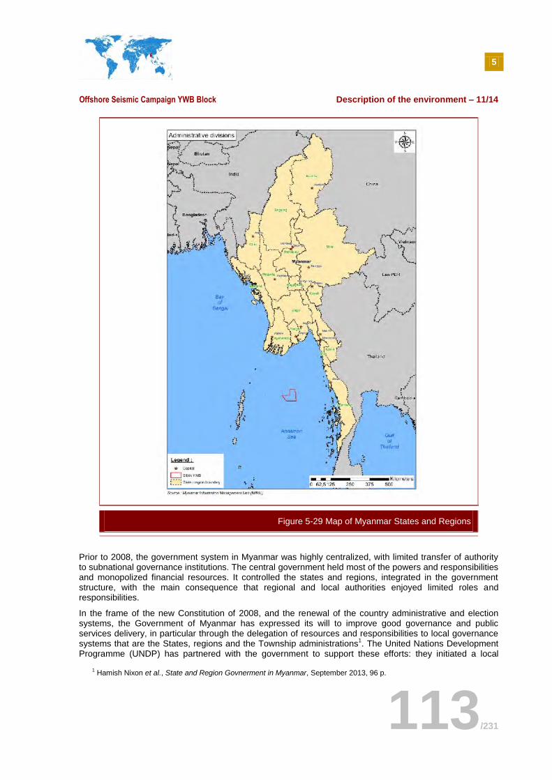
5
Offshore Seismic Campaign YWB Block Description of the environment – 11/14
113/231
Prior to 2008, the government system in Myanmar was highly centralized, with limited transfer of authority to subnational governance institutions. The central government held most of the powers and responsibilities and monopolized financial resources. It controlled the states and regions, integrated in the government structure, with the main consequence that regional and local authorities enjoyed limited roles and responsibilities.
In the frame of the new Constitution of 2008, and the renewal of the country administrative and election systems, the Government of Myanmar has expressed its will to improve good governance and public services delivery, in particular through the delegation of resources and responsibilities to local governance systems that are the States, regions and the Township administrations
1. The United Nations Development
Programme (UNDP) has partnered with the government to support these efforts: they initiated a local
1 Hamish Nixon et al., State and Region Govnerment in Myanmar, September 2013, 96 p.
Figure 5-29 Map of Myanmar States and Regions
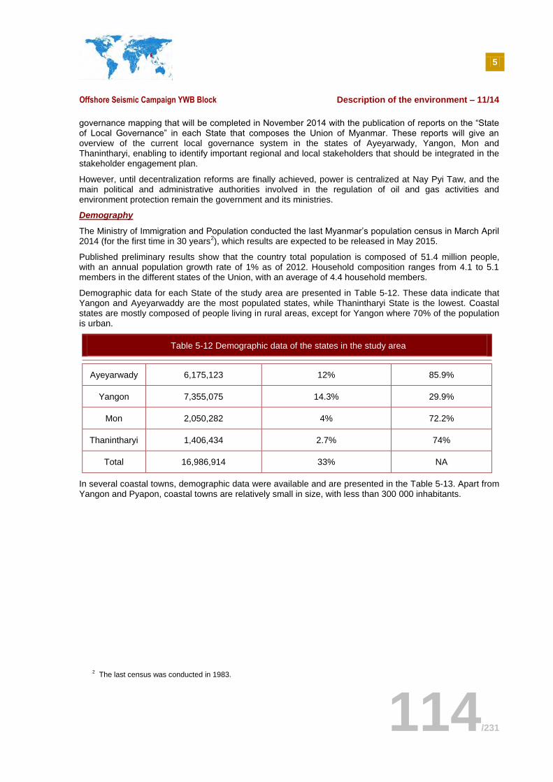
5
Offshore Seismic Campaign YWB Block Description of the environment – 11/14
114/231
governance mapping that will be completed in November 2014 with the publication of reports on the “State of Local Governance” in each State that composes the Union of Myanmar. These reports will give an overview of the current local governance system in the states of Ayeyarwady, Yangon, Mon and Thanintharyi, enabling to identify important regional and local stakeholders that should be integrated in the stakeholder engagement plan.
However, until decentralization reforms are finally achieved, power is centralized at Nay Pyi Taw, and the main political and administrative authorities involved in the regulation of oil and gas activities and environment protection remain the government and its ministries.
Demography
The Ministry of Immigration and Population conducted the last Myanmar’s population census in March April 2014 (for the first time in 30 years
2), which results are expected to be released in May 2015.
Published preliminary results show that the country total population is composed of 51.4 million people, with an annual population growth rate of 1% as of 2012. Household composition ranges from 4.1 to 5.1 members in the different states of the Union, with an average of 4.4 household members.
Demographic data for each State of the study area are presented in Table 5-12. These data indicate that Yangon and Ayeyarwaddy are the most populated states, while Thanintharyi State is the lowest. Coastal states are mostly composed of people living in rural areas, except for Yangon where 70% of the population is urban.
Table 5-12 Demographic data of the states in the study area
Ayeyarwady 6,175,123 12% 85.9%
Yangon 7,355,075 14.3% 29.9%
Mon 2,050,282 4% 72.2%
Thanintharyi 1,406,434 2.7% 74%
Total 16,986,914 33% NA
In several coastal towns, demographic data were available and are presented in the Table 5-13. Apart from Yangon and Pyapon, coastal towns are relatively small in size, with less than 300 000 inhabitants.
2 The last census was conducted in 1983.
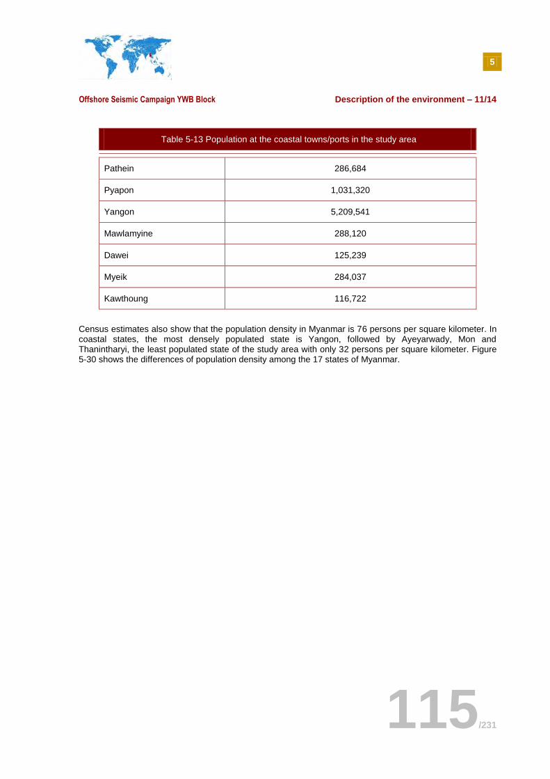
5
Offshore Seismic Campaign YWB Block Description of the environment – 11/14
115/231
Table 5-13 Population at the coastal towns/ports in the study area
Pathein 286,684
Pyapon 1,031,320
Yangon 5,209,541
Mawlamyine 288,120
Dawei 125,239
Myeik 284,037
Kawthoung 116,722
Census estimates also show that the population density in Myanmar is 76 persons per square kilometer. In coastal states, the most densely populated state is Yangon, followed by Ayeyarwady, Mon and Thanintharyi, the least populated state of the study area with only 32 persons per square kilometer. Figure 5-30 shows the differences of population density among the 17 states of Myanmar.
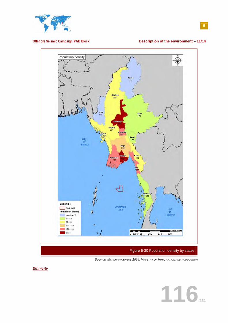
5
Offshore Seismic Campaign YWB Block Description of the environment – 11/14
116/231
SOURCE: MYANMAR CENSUS 2014, MINISTRY OF IMMIGRATION AND POPULATION
Ethnicity
Figure 5-30 Population density by states
5
Offshore Seismic Campaign YWB Block Description of the environment – 11/14
117/231
Myanmar is an ethnically diverse nation with more than a hundred distinct ethnic groups officially recognized by the Burmese government, each having a particular history, culture and language.
At the study area, coastal states are mostly inhabited by Bamar people (Ayeyarwady, Yangon and Tanintharyi states) while Mon State is populated by the Mon ethnic group. Figure 5-31 shows in more detail the ethnic distribution in the country and coastal states.
The Bamar are the dominant ethnic group in the country. They are 29 million people and inhabit mostly the central and upper plains of the country. This people from Sino-tibetan descent migrated from Yunnan, China, and settled in central Myanmar, progressively becoming the country prevailing group.
The Mon represents 8 million people, accounting for 15.6% of the total population. They are with the Pyu ethnic group the initial inhabitants of Myanmar Ayeyarwady valley, prior to the arrival of the Bamar people. They have been long time rulers over lower Myanmar, and supposedly brought Buddhism in the country. They have cultural particularities distinguishing them from the other ethnic groups of Myanmar, in the fields of language, arts (music, dances), clothes and architecture. However, their culture tends to fade away and assimilate with the Bamar culture, except in rural areas where Mon tradition still prevails.
South-east of the Project area, on the archipelago of Mergui in Thanintharyi State, live the Moken. They are a people referred to as sea gypsies, a denomination designating nomadic people living on the sea in several parts of Southeast Asia, such as Thailand, Malaysia, Philippines and Indonesia. In Myanmar, Moken people live essentially from sea-based sources of livelihoods, inhabiting their boat which is also their house. They are mobile by nature, but were progressively settled down in coastal villages, ending their migration-based living-patterns.
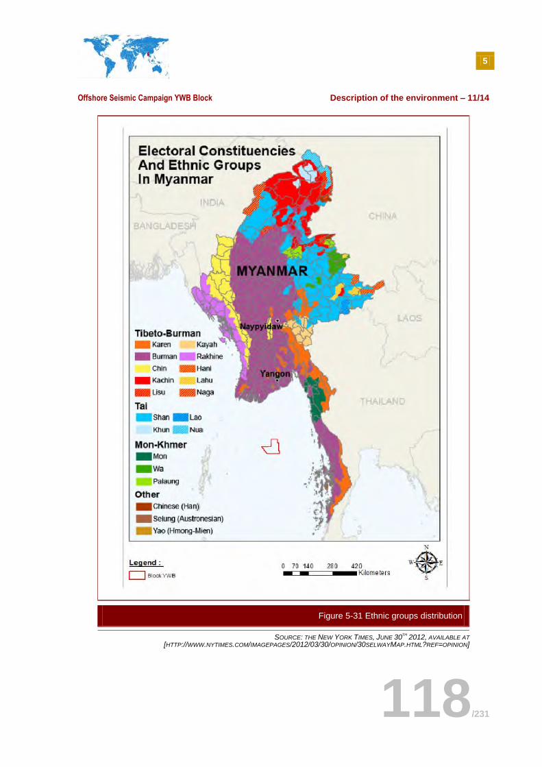
5
Offshore Seismic Campaign YWB Block Description of the environment – 11/14
118/231
SOURCE: THE NEW YORK TIMES, JUNE 30TH
2012, AVAILABLE AT
[HTTP://WWW.NYTIMES.COM/IMAGEPAGES/2012/03/30/OPINION/30SELWAYMAP.HTML?REF=OPINION]
Figure 5-31 Ethnic groups distribution
5
Offshore Seismic Campaign YWB Block Description of the environment – 11/14
119/231
Gender role
Myanmar used to be a matriarchal society, where women enjoyed independency, political power and rights over economic resources, despite Buddhism stereotypes on gender roles. The British rule and the subsequent establishment of a male military state relegated women’s rights behind those of men, the society accepting male rights prevalence as the norm.
Today, this heritage still delineates strong social roles between the two sexes. Despite a school enrolment being almost at parity between boys and girls, urban women increasing contribution to the household revenues, and despite sharing the same legal rights as those of men, gender equality is far from being achieved in the country
3. On the contrary, it varies greatly based on the living environment (urban or rural)
and the ethnic group belonging. Women still have a lower adult literacy rate as percentage of men’s and lower estimated incomes. Their role in the political sphere remains very limited, with only 5.7% of women holding seats at the Pyithu Hluttaw (lower house) of the national Union Parliament
4.
Although their social and political roles are still unequal to those of men, the contribution of women to economic activities in the country is high, with 75% of the total female population being economically active according to the International Labour Office (ILO). Women in the country are mostly engaged in the agricultural sector, especially in rural areas.
Religion
The main religion in Myanmar is Theravada Buddhism, practiced by around 90% of the population. Theravada Buddhism is the dominant religion for the Bamar, Shan, Arakanese and Mon ethnic groups. Other religions in the country are Islam and Christianity: Christianity is mostly present in the Kachin ethnic group, Chin and Naga; Islam is mostly practiced in Rakhine State by the Rohingya minority as well as in the south and center of the country (Yangon, Ayeyarwady, Magwe, and Mandalay). Other minorities practice their traditional religions, which is the case of the Chinese and some ethnic groups in the highland regions who practice animist believes.
Although the Constitution recognises freedom of religion, recent conflicts have opposed Buddhists and Muslims, undermining political stability in the country. Violent clashes started in 2013 in the city of Meiktila between Buddhist and Muslims groups, and led to a series of anti-Muslim riots throughout the country over the year. The support offered by a minority of the Buddhist clergy to anti-Muslim movements continued to fuel the conflicts, and recent clashes have occurred in July 2014
5.
However, no religious tensions have been observed in the coastal states of the study area, as they remain concentrated in the central part of the country.
5.6.2.2 Access to social services and infrastructure in the coastal areas
The country’s indicators on human development and access to basic social services have improved over the last years, but remain low according to international standards. Thus, Myanmar Human Development Index of 0.524 in 2013 ranks it 150 out of 187 countries, and is below the regional average of 0.703. Besides, 25.6% of its population lives below the national poverty line and has limited access to health, education, energy, water, or transportation infrastructures. The country also faces growing structural inequalities between states/regions, and urban/rural areas that are differently underserved in basic services and have therefore different levels of human development.
Health and education
With a life expectancy of 65.7 years in 2012, and the highest crude mortality rate of all Asia-Pacific countries (9 per 1000 people), health indicators in Myanmar reflect years of neglect and are distressing for a country that only recently opened to international health organizations assessments and interventions.
3 Than Than New, Gendered Spaces: Women in Burmese Society, Transformations, No. 6, February 2003.
4 Global Justice Center, The Gender Gap and Women’s Political Power in Myanmar, May 2013.
5 HUME Tim, Curfew imposed after deadly clashes between Buddhists, Muslims in Myanmar, CNN, 6
th July 2014.
5
Offshore Seismic Campaign YWB Block Description of the environment – 11/14
120/231
There have been an improvement in access to healthcare, with 81% of the population living in walking distance from a hospital (including township hospitals, public specialized hospitals and station hospitals) or health centre (including rural health centres, sub-rural health centres, maternal and child health centres). Besides, health expenditures by the Ministry of Health have more than doubled between 2007 and 2012.
However, basic health concerns continue to undermine the country human development. Maternal and child health is a major issue, along with HIV/AIDS, malaria and tuberculosis, which causes substantial mortality and morbidity. In 2012, HIV/AIDS prevalence rate represented 0.6% of the population. Malaria incidence was assessed at 2,743 cases for 100 000 people, while tuberculosis prevalence was estimated to 489 cases for 100 000 people
6.
Ongoing health issues in Myanmar are the major consequence of low government expenditures on health sector (2% of the GDP), low availability of medical care professionals and the poor condition or absence of health facilities. On average, Myanmar has only 1 physician per 2,188 people and 1 hospital bed per 1,667 people.
In the study area, Ayeyarwady and Mon states are disadvantaged compared to Yangon and Thanintahryi in terms of doctors’ distribution. Besides, Nargis cyclone in 2008 considerably decreased access to healthcare in Ayeyarwady State. Six years after, despite NGOs active role in post-disaster restoration, populations living in this State remain particularly vulnerable.
Government investment in primary education is more important than in the health sector, which is displayed by high indicators in the terms of literacy rate (93% of adults are literate) and gross primary school enrollment (114%). However, gross secondary school enrollment is low as compared to other regional neihgbours (50% of the children attend secondary school)
7.
Access to energy, water and sanitation
According to the International Energy Agency (IEA), Myanmar is in a condition of energy poverty. Its average electrification rate was about 28% in 2012. Urban areas have a better access than rural ones. Thus, Yangon City has the highest electrification rate (72%), followed by Nay Pyi Taw (65%), Kayar (42%), and Mandalay (35%), while rural areas are poorly electrified, with an average rural electrification rate of 16%.
Myanmar enjoys abundant water resources, and access to water is good at the national level with 70% of the population having access to drinkable water source in 2010. Access to improved water sources is higher in urban areas where 94.8% of people benefit from these sources, than in rural ones with 81.1% having access to them. Regional discrepancies are also observed, and states in the study have unequal access (44.6% in Ayeyarwady, 76.7% in Yangon). In terms of improved sanitation facilities,
79% of the
population has access to it, over 80% in the coastal area (including Ayeyarwady). This is the result of large investments in the sector from government and external sources, which have allowed tackling this issue efficiently.
5.6.3 Marine socio-economic environment
Myanmar economic development has accelerated over the last years, influenced by the democratization process initiated by the regime in 2010. Myanmar authorities have thus recently refurbished their laws and regulations to improve the ability of the domestic market to welcome foreign investments. They notably revised the 1988 Foreign Investment Law in 2012, to facilitate international companies’ investments in the country’s economy. Positive effects were felt rapidly, with an increase of foreign direct investment from USD 1.9 billion in 2012 to USD 2.7 billion in 2013, mostly in the energy, garment industry, information technologies and food and beverages. According to the World Bank, economic growth reached 6.5% in 2013, on the rise from 5.9% in 2012. The government notable efforts to improve the business environment and stakeholders’ interests in its market succeeded, and numerous foreign companies are now willing to invest in the country’s economy.
6 World Health Organization, Myanmar Health Profile 2012.
7 UNICEF statistics on Myanmar.
5
Offshore Seismic Campaign YWB Block Description of the environment – 11/14
121/231
Like for other sectors, marine economic activities represent a high potential of economic growth. Part of the Myanmar maritime space, they are regulated by the United Nations Convention on the Law of the
Sea (UNCLOS). This convention governs the States’ rights and responsibilities related to the oceans and
their resources. It establishes categories spatially demarcated such as the territorial waters, the contiguous zone and the Exclusive Economic Zone (EEZ). Each category represents rights and obligations for the signatory state: for instance, the EEZ status recognizes the right of a State to explore and exploit the
ocean’s resources8, but requires this State to guarantee free passage of foreign ships in its waters.
Myanmar is signatory State of this convention, and translated it in its Territorial Sea and Maritime Zones Law in 1977. The country already actively exploits its marine oil and gas resources, supported by several foreign companies. In parallel, the government sees an important potential of growth in the marine fishery sector. These sectors, along with the commercial shipping, use the same environment and their interests will probably overlap over the coming years, creating interactions and potential conflicts among them that need to be anticipated and whenever possible prevented.
5.6.3.1 Offshore oil and gas sector
Myanmar promising offshore oil and gas resources represent an important potential of growth for the country’s economy, attracting interest from the national and international oil and gas industry. In 2012, 34% of the Foreign Direct Investments in the country were directed at oil and gas exploration and production
9.
In a move to boost the increase of oil and gas activity in the country, the Ministry of Energy recently concluded the Myanmar Offshore Blocks Bidding Round 2013, attributing 20 offshore blocks to international companies
10. Ten deep-water blocks and ten shallow-water blocks were attributed to oil majors and
independent companies, such as Statoil, Eni, Shell, Total, ConocoPhillips, BG Group, and Woodside Energy.
YWB block was awarded to Total E&P Myanmar, and other blocks neighboring YWB were attributed to various companies, such as to Eni (block MD4). They can be localized in the Figure 5-32 and are for most of them in production:
The Yetagun field in M12, M13 and M14 produces since 2000 and is operated by a local subsidiary of Malaysian company Petronas.
The Zawtika, Kakonna and Gawthaka fields, located in blocks M9 and M11, started to produce in March 2014, and are operated by the Thai company Petroleum Authority of Thailand Exploration and Production International (PTTEP International).
Several other blocks are at the stage of 2-D or 3-D seismic campaigns.
This surge in offshore exploitation of oil and gas resources causes an increase in operational activities in the Andaman Sea, which could lead to negative cumulative impacts on the fishery sector and global marine traffic in the region.
8 UNITED NATIONS, The United Nations Convention on the Law of the Sea (A historical perspective), 1998, available at
[http://www.un.org/Depts/los/convention_agreements/convention_historical_perspective.htm#Exclusive Economic Zone] 9 OECD.
10 Offshore Energy Today, Myanmar awards new offshore blocks, March 26, 2014.
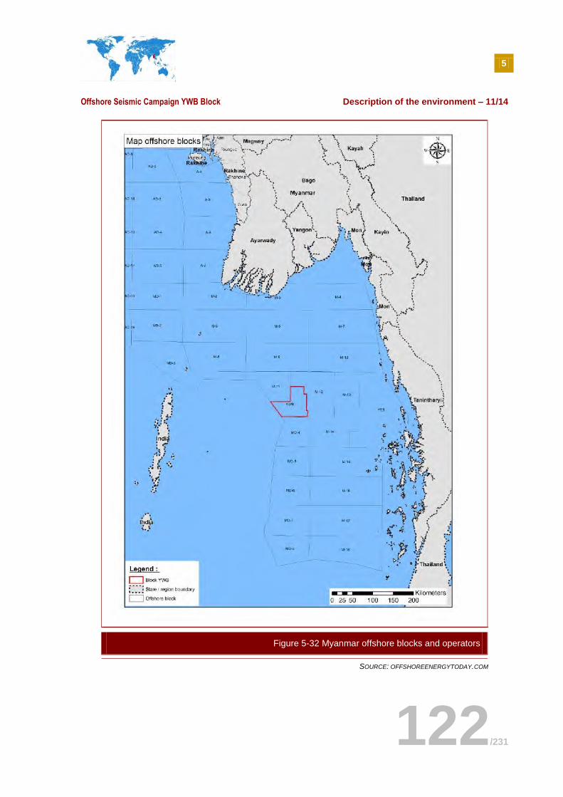
5
Offshore Seismic Campaign YWB Block Description of the environment – 11/14
122/231
SOURCE: OFFSHOREENERGYTODAY.COM
Figure 5-32 Myanmar offshore blocks and operators
5
Offshore Seismic Campaign YWB Block Description of the environment – 11/14
123/231
5.6.3.2 Marine fishery sector
Myanmar has a coastline of 2,280 kilometers, a marine water area of 486,000 square kilometers, and an
inland water area of 124,280 square kilometers11
. Generally, Myanmar fisheries are divided into two sub-sectors:
Inland fisheries, covering freshwater fisheries and aquaculture;
Marine fisheries, covering inshore and offshore fisheries.
The potential for development of fisheries in the country is considerable. This sector as a whole already represents the fourth most important export earning sector and generate with livestock 9.9% of the GDP
12. It employs an estimated number of 7,977,000 persons, among which 3,269,000 are active
fishermen13
. This represents 15% of the total country population, highlighting the evident importance of this sector for the economy. Besides, like in many Asian countries, fish and other products are important for the Myanmar people diet and for food security. In 2002, per capita consumption of fish amounted to 21.04 kg/yr and constituted 60 to 70% of the total protein intake for the population
14.
The YWB seismic project area is located in the marine fishery zone, more particularly in the offshore fishery zone as displayed on Figure 5-33.
Laws and regulations
Myanmar fishery sector was previously regulated by the Fisheries Act of 1905. Laws were upgraded in the 1990s to support the development of this sector, encompassing new topics such as artisanal and foreign fishing. Today, six laws are the basis for inland and marine fishery organization, management and control by the different government agencies in charge of this sector. These laws are listed below:
Law Relating to the Fishing Rights of Foreign Fishing Vessels - 1989
Law relating to Aquaculture - 1989
Myanmar Marine Fisheries Law - 1990
Freshwater Fisheries Law - 1991
Law Amending the Myanmar Marine Fisheries Law - 1993
Law Amending the Law Relating to the Fishing Rights of Foreign Fishing Vessels - 1993
Myanmar fishery sector is managed by the Ministry of Livestock, Fisheries and Rural Development, and more particularly by the Department of Fisheries (DoF), which takes care of both inland and marine fisheries. The most important mission of the DoF is to develop and implement sectorial policies aiming at promoting sustainable fishing practices and ensuring the preservation of marine resources. The DoF develops conservation efforts, promotes research and surveys on the current condition of marine resources in partnership with intergovernmental agencies, maintains statistics on fisheries, and supervises the fishery sector through delivery of licenses to national fishing vessels.
Marine fishery zones
Myanmar fishery zones are organized under the Marine Fisheries Law of 1990, which classifies the fishery sector into the inshore and offshore categories. Their main characteristics are detailed below:
11 Pe Myint, National Report of Myanmar on the Sustainable Management of The Bay of Bengal Large Marine Ecosystem, BOBLME, GCP/RAS/179/WBG, 2004
12According to the Institute of Marine Research figures, available at [http://www.imr.no/forskning/utviklingssamarbeid/surveys/myanmar_2013/en]
13 Bay of Bengal Large Marine Ecosystem - BOBLME
14 Pe Myint, National Report of Myanmar on the Sustainable Management of The Bay of Bengal Large Marine Ecosystem, BOBLME, GCP/RAS/179/WBG, 2004
5
Offshore Seismic Campaign YWB Block Description of the environment – 11/14
124/231
Inshore (or coastal) fishery: covers an area up to 5 miles from the shore for the Rakhine coast, and 10 nautical miles from the shore on the Ayeyarwady and Tanintharyi coasts. Boats entering this category should not be equipped with engine having more than 12 horsepower and length of the boat is limited to 30 feet.
Offshore fishery: covers the outer area of the inshore fishery zone up to the EEZ border. Boats
should have more than 12HP engine, and can use bottom trawl, purse seine, surrounding nets, drift nets and long lines
15.
As seen on Figure 5-33, the inshore zone is represented in deep blue and borders the coast, while the offshore zone spans from the inshore borders up to the EEZ borders, at water depths varying from 0 to over 200 meters. For administrative purposed, the Department of Fisheries has divided the offshore zone into 140 fishing grounds of 30X30 nautical miles block, using latitude and longitude lines. It has also designated 4 fishing areas, namely Rakhine (40 blocks), Ayeyarwady (44 blocks), Mon (14 blocks) and Taninthary (52 blocks). The Project area is located in the Thanintharyi offshore fishing zone. It is positioned at the edge of the EEZ, where water depths are higher than 200 meters.
15
FAO, The State of World Fisheries and Aquaculture, Opportunities and Challenges, 2014
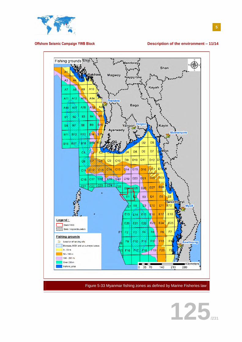
5
Offshore Seismic Campaign YWB Block Description of the environment – 11/14
125/231
Figure 5-33 Myanmar fishing zones as defined by Marine Fisheries law

5
Offshore Seismic Campaign YWB Block Description of the environment – 11/14
126/231
SOURCE: MYANMAR DEPARTMENT OF FISHERIES
5
Offshore Seismic Campaign YWB Block Description of the environment – 11/14
127/231
Marine fishery licensing system
The fishing vessel licensing system in Myanmar is framed by the Marine Fisheries Law and based on the nationality of the license requester. The national license system is divided into two sub-categories based on the fishing zones:
Inshore fishery zone license: the General Administration Department (GAD) is in charge of inshore fishing boats’ inspection. The Department of Fisheries proceeds with the issuance of fishing licenses upon recommendation of the GAD.
Offshore fishery zone license: the Department of Marine Administration (DMA) takes care of inspection and registration of the offshore fishing boats. Fishing licenses are delivered by the DoF only when DMA has issued its approval.
The Myanmar Fisheries Law encourages foreign fishing activity with the granting of fishing rights to foreign companies, but limits their activity to the EEZ. It is only under exceptional circumstances and expresses agreement of the related government agencies that foreign fishing vessels can conduct fishing activities in the country territorial waters. Foreign fishing companies can acquire licenses to operate in the Burmese waters from the Department of Fisheries, in exchange of a fee and upon approval of the Ministry of Livestock and Fisheries. In order to encourage empowerment of national fishing fleets and development of national capacities in the fishery sector, DoF will also grant licenses to the foreign companies that have formed a joint-venture with a state enterprise or a Burmese business partner.
Marine resources: surveys and estimations
The Myanmar fishery institutions do not have recent and reliable data informing on the marine resources available in their waters, as well as the size and composition of marine catches. This lack of knowledge is due to years of isolation, a focus of the previous fishery policies on inland resources (especially aquaculture) and a lack of means (in terms of budget, human resources and competencies) from the government agencies for collecting information and building expertise.
Without this knowledge, it is difficult for the Ministry of Livestock, Fisheries and Rural Development and the Department of Fisheries to draft a sustainable fishery policy which would preserve fishery resources while allowing for the commercial fishery sector to prosper.
Myanmar is member of several inter-governmental organizations specialized in fishery at the regional scale, such as the Southeast Asian Fisheries Development Centre (SEAFDEC), the Asia-Pacific Fisheries Commission (APFIC), and the Bay of Bengal Large Marine Ecosystem Program (BOBLME). Trying to build knowledge on the state of marine resources and fisheries, these organizations conducted several surveys in Myanmar waters under the leadership of the Food and Agriculture Organization (FAO).
These surveys enabled to draw estimations on fish stocks, but their results vary. According to the Institute of Marine Resources, fish stocks range between 1.3 and 1.8 million metric ton (mmt): 1 mmt for pelagic fish, and 0.8 mmt for demersal fish, respectively. But for the government of Myanmar, the potential maximum sustainable yield (MSY) of Myanmar waters is about 1.05 mmt per year (0.5 mmt of pelagic fish and 0.55 mmt of demersal fish)
16.
Conclusions of surveys conducted in 2004 and 2007 by the SEAFDEC on Myanmar marine fishery resources revealed that even if stocks were not known yet, Myanmar was rich in some commercially important big pelagic species such as sword fish (xiphias gladius), deep-sea lobster and deep-sea shrimp. Other commercially important species, such as yellowfin tuna (thunnus albacares), striped marlin (tetrapturus audax) and sailfish (istiophorus platypus) inhabit Myanmar offshore waters
17.
16
Tony J Pitcher, An Estimation of Compliance of the Fisheries of Myanmar with Article 7 (Fisheries Management) of the UN Code of Conduct for Responsible Fishing, 2007 17
Julius Kyaw, Department of Fisheries, Present Status of Off-shore Fishery Resources and Information on Tuna Fishery in Myanmar, Special Meeting on Improvement of Tuna Information and Data Collection in the Southeast Asia7-9 September, 2011. Songkhla Province, Thailand
5
Offshore Seismic Campaign YWB Block Description of the environment – 11/14
128/231
Recently, a large marine ecosystem survey was conducted in the frame of the EAF-Nansen project and the BOBLME
18. Piloted by the Institute of Marine Research, a Norwegian organization appointed by the
SEAFDEC, this study gathered a team of marine experts for a six-week field survey in November 2013, with the participation of the DoF. Due to large data the project has to process before being able to publish any report, it is unlikely that the results of the survey will be available by the end of the year, and therefore used in this study.
Waiting for these results, the data and information used by the Government to guide its decisions on fishery management are still out-of-date and inaccurate. Assertions are made by various stakeholders, such as the Myanmar Fishery Federation
19, on severe depletion of stocks and overfishing both for the offshore
and inshore fisheries20
. In the frame of the preparation of this IEE, discussions with NGOs specialized in marine ecosystem protection also tend to confirm this fact, despite a clear lack of data.
Fishing vessels and gears
Most recent estimates on the country total fishing fleet set the number of vessels at around 30 800 in 2011, among which half of it were non-motorized boats, and 1 600 were trawlers
21.
Myanmar fishery sector is mostly developed in the artisanal, small-scale inshore fishery zone (up to 10 miles from the coast), with 27 751 inshore fishing vessels registered by the DoF in 2012, a decrease compared to the 29 371 vessels the previous year. Among these, 55% are powered vessels, and the rest are non-motorised boats. They usually operates in waters less than 50-meter depth, due to a lack of technology, suitable fishing gears and equipment to process fisheries resources information (such as GPS or satellite devices).
The offshore fishery zone is mostly the domain of large national companies and foreign fishing vessels that have powerful boats, and concluded fishing agreements with the Ministry of Livestock, Fisheries and Rural Development.
Around 2450 national vessels were engaged in offshore fisheries in 2012. Additionally, 132 foreign vessels were reported having licenses to conduct offshore fishery
22. This number is in decrease compared to 2010
when 390 foreign fishing vessels had fishing licenses.
As presented in the Table 5-14 below, fleets operating offshore (encompassing foreign fishing vessels) mainly use active fishing gears, with trawling, driftnet and purse seine being the most commonly used. Static fishing techniques, fish traps or stow nets, are also used but less commonly in the offshore fishery zone.
18
The EAF-Nansen project, launched in 2006, is a multi-stakeholder project funded by the Norwegian Agency for Development Cooperation and managed by the FAO in partnership with the Institute of Marine Research (IMR). Its objective is to strengthen the knowledge base on fisheries and implement an ecosystem approach to marine fisheries in developing countries. The project conducts activities in the Bay of Bengal and in Myanmar, among other countries. More information at: [http://www.eaf-nansen.org/nansen/organization/17910/en] 19
The Irrawady, Burma Bans Foreign Fishing Boats from Its Waters, April 3, 2014 20
Source: UNDP, Myanmar Agricultural Sector Review and Investment Strategy, Volume 2: Agricultural Sector Investment Strategy, June 2004.
21BAY OF BENGAL LARGE MARINE ECOSYSTEM PROJECT (BOBLME), Transboundary Diagnostic Analaysis vol. 2, 2012.
22According to the Institute of Marine Research figures, available at
[http://www.imr.no/forskning/utviklingssamarbeid/surveys/myanmar_2013/en].
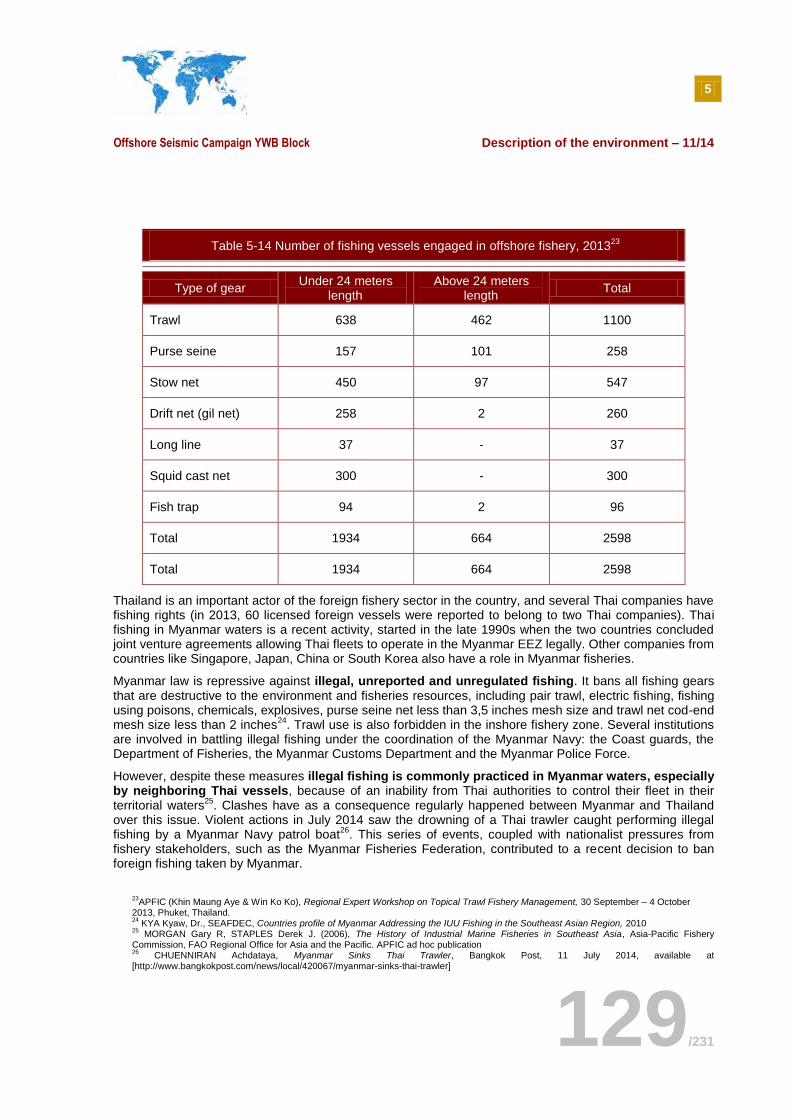
5
Offshore Seismic Campaign YWB Block Description of the environment – 11/14
129/231
Table 5-14 Number of fishing vessels engaged in offshore fishery, 201323
Type of gear Under 24 meters
length Above 24 meters
length Total
Trawl 638 462 1100
Purse seine 157 101 258
Stow net 450 97 547
Drift net (gil net) 258 2 260
Long line 37 - 37
Squid cast net 300 - 300
Fish trap 94 2 96
Total 1934 664 2598
Total 1934 664 2598
Thailand is an important actor of the foreign fishery sector in the country, and several Thai companies have fishing rights (in 2013, 60 licensed foreign vessels were reported to belong to two Thai companies). Thai fishing in Myanmar waters is a recent activity, started in the late 1990s when the two countries concluded joint venture agreements allowing Thai fleets to operate in the Myanmar EEZ legally. Other companies from countries like Singapore, Japan, China or South Korea also have a role in Myanmar fisheries.
Myanmar law is repressive against illegal, unreported and unregulated fishing. It bans all fishing gears that are destructive to the environment and fisheries resources, including pair trawl, electric fishing, fishing using poisons, chemicals, explosives, purse seine net less than 3,5 inches mesh size and trawl net cod-end mesh size less than 2 inches
24. Trawl use is also forbidden in the inshore fishery zone. Several institutions
are involved in battling illegal fishing under the coordination of the Myanmar Navy: the Coast guards, the Department of Fisheries, the Myanmar Customs Department and the Myanmar Police Force.
However, despite these measures illegal fishing is commonly practiced in Myanmar waters, especially by neighboring Thai vessels, because of an inability from Thai authorities to control their fleet in their territorial waters
25. Clashes have as a consequence regularly happened between Myanmar and Thailand
over this issue. Violent actions in July 2014 saw the drowning of a Thai trawler caught performing illegal fishing by a Myanmar Navy patrol boat
26. This series of events, coupled with nationalist pressures from
fishery stakeholders, such as the Myanmar Fisheries Federation, contributed to a recent decision to ban foreign fishing taken by Myanmar.
23
APFIC (Khin Maung Aye & Win Ko Ko), Regional Expert Workshop on Topical Trawl Fishery Management, 30 September – 4 October 2013, Phuket, Thailand. 24
KYA Kyaw, Dr., SEAFDEC, Countries profile of Myanmar Addressing the IUU Fishing in the Southeast Asian Region, 2010 25
MORGAN Gary R, STAPLES Derek J. (2006), The History of Industrial Marine Fisheries in Southeast Asia, Asia-Pacific Fishery Commission, FAO Regional Office for Asia and the Pacific. APFIC ad hoc publication 26
CHUENNIRAN Achdataya, Myanmar Sinks Thai Trawler, Bangkok Post, 11 July 2014, available at [http://www.bangkokpost.com/news/local/420067/myanmar-sinks-thai-trawler]
5
Offshore Seismic Campaign YWB Block Description of the environment – 11/14
130/231
Indeed, in April 2014, the Government of Myanmar decided the suspension of fishing rights and licensing for foreign vessels until further notice. This ban is justified by alleged fish resources depletion, due to overfishing and the use of destructive fishing gears by foreign companies whose activity has intensified over the last five years. It was welcomed by national fishing associations, since it was expected for a long time
27.
Fishing grounds, fish catches and exports
Commercially interesting species identified for the offshore fisheries, as described in the section on Marine resources: surveys and estimations, are pelagic fishes, with the tuna being in a privileged position for industrial development. Figure 5-33 shows the tuna fishing grounds (in blue circles on the map), and indicates that the YWB block is not located in these grounds. No data are available on fishing grounds for other species.
Myanmar is an important contributor to the regional fishery sector along with India. In terms of volume, total catches for all sectors (aquaculture, inland and marine capture fisheries) amounted to 4,464,419 tons in 2012. Among these, inland waters fisheries accounted for 1,246,460 tons and aquaculture for 0,885 tons.
The marine capture fisheries represented half of the total production, with 2,332,790 tons of catches in 2012, an increase of 7.5% from the previous year, and from 121% between 2003 and 2012. However, this figure is underestimated as it doesn’t take into account the production loss caused by illegal fishing, and by the landing of catches to foreign ports. Indeed, for fishing performed by foreign vessels, landing sites are usually not located in Myanmar but, according to the size of catches, to Phuket in Thailand, Penang in Malaysia or even in Japan. Foreign fleets have the modern equipment and powerful engines enabling them to easily transport their catch to international ports in a short time. These catches are therefore not reported in the country statistics.
Besides, the general composition of the marine catches landed in the country is also not known precisely28
. This lack of data prevents the country to identify overfishing by species, and therefore to adopt a sustainable fishery policy.
Main landing sites and wholesale fish markets are around Yangon, at Pazuntaung Nyaungdan and Annawa, with a fish market at San Pya in Alone township. Other major landing sites are found along the coast, at Thandwe, Mawlamyine, Myeik and Kawthoung cities. Capture fish landing there is sold through an auction system.
In terms of export, the best quality catches are exported to neighboring countries. 116 fishery processing factories are registered in Myanmar, and most of them export fish to the Chinese market. Only 20 of these factories have licenses to export to EU and United States markets. A recent project from the United Nations Industrial Development Organization will help upgrade eight other factories, increasing their standards to allow exports to these high profitability markets
29. However, exports to Europe and United States markets
remain limited at the time being.
Global marine products exports in 2013 amounted to 376,845 tons, generating revenues of USD 650 million. Excluding shrimps, fish products represented 70% of these exports (266,464 tons), and USD 380 million of revenues. During 2014 fiscal year, a decrease in fishery export was observed with only USD 550 million of revenues against the target set by the Myanmar government for marine products exports of USD 700 million. According to the Myanmar Fishery Products Processors and Exporters Association (MFPPEA), this decrease is mainly caused by a lack of competency in the fishery sector, preventing it to compete on international markets.
In regards to low quality catches, they are processed in Myanmar in the form of fish paste or fish meal for the chicken industry, or used fresh or chilled for direct consumption, with some fish being frozen or cured.
27
The Irrawady, Burma Bans Foreign Fishing Boats From Its Waters, April 3, 2014
29
ELEVEN MYANMAR, UNIDO to Upgrade Myanmar’s Fish Factories, 11 April 2014, available at [http://www.elevenmyanmar.com/index.php?option=com_content&view=article&id=5731:unido-to-upgrade-myanmar-s-fish-factories&catid=33:business&Itemid=356]
5
Offshore Seismic Campaign YWB Block Description of the environment – 11/14
131/231
Interactions between the fishery sector and the project
The Project area is located in the offshore fishery area (more specifically in the Thanintharyi fishery zone). In this area, representing around 480,000 square kilometers, fishing is performed by 2,600 licensed vessels. 2,450 are Myanmar nationals having offshore fishery permits. Others were foreign vessels that operated until a ban on foreign fishing was passed in April 2014. Fishermen in this area generally use large vessels and active fishing techniques to catch pelagic species, among them tuna. A passive fishing technique such as fixed fish traps is also practiced in the offshore fishery zone, although less commonly. Besides, illegal fishing is a real issue in the country and is frequently performed in the offshore fishery zone, mainly by Thai nationals.
Few fishing boats operating in Myanmar waters, or fish traps installed, are equipped with vessel monitoring system enabling to localize their area of activity. Therefore, it is not possible to prove with firm evidence that the Project area is popular with fishermen. However, due to the few number of vessels operating in the large offshore fishery zone, the location of the project area (200 km from the coast and in deep waters) and the recent ban on foreign fishing, interactions with fishermen are expected to be very limited during the seismic campaign, except with illegal fishing vessels.
According to the information collected during the public consultations, the YWB block is too far from the shore and the water is too deep to encounter any local fishing boats. Besides, as seen in Figure 5-33, the YWB block is out of the main long-line tuna fishing grounds, therefore it will be very unlikely to encounter any legal long-line tuna fishing boat. The only boats that could be encountered are maybe illegal ThaI fishing boats.
5.6.3.3 Port infrastructures and marine traffic
Port infrastructures
The Port of Yangon is the first international port of Myanmar. It has an annual traffic of more than 2,000 vessels, and 600,000 tons of goods transited there in 2013
30. Following the fast pace of economic
development in the country, marine traffic has increased over the last years, causing regular congestion at the port. This trend that is likely to continue in the future if additional infrastructures are not developed.
Yangon Port is placed under the management of the Myanmar Port Authority. This division of the Ministry of Transport also controls eight major ports along the coast (four on the west coast and four on the south-east coast). These ports receive international ships, but still have inadequate infrastructures and lack mechanised facilities that could increase their capacities. As shown in Figure 5-34, the main ports bordering the Project area are located in Pathein (Ayeyarwady State), Mawlamyine (Mon State), and in Dawei, Myeik and Kawthaung (Tanintharyi State).
Lacking the capacities and resources to develop its port infrastructures, Myanmar’s government supports private companies who wish to invest in this sector. Two projects are on the way, financed by foreign enterprises.
Located 25 km south of Yangon, the Myanmar International Terminals Thilawa (MITT) is a deep sea multi-purpose container port complementing the infrastructures of the Port of Yangon. It is operated by a private foreign company, Hutchison Port Holdings. Construction works will start in June 2015 according to the Myanmar Port Authority.
In the coastal city of Dawei, the development of a large deep-sea port has been planned for several years. This project is managed by the Dawei SEZ Development Co, a Thai-Burma consortium in charge of developing the port and a large Special Economic Zone. This deep-sea port will benefit
30
Interview with the Myanma Port Authority

5
Offshore Seismic Campaign YWB Block Description of the environment – 11/14
132/231
from domestic commercial traffic, but will also profit Thailand, who has had a significant increase in its business relationships with Myanmar over the last years. India could also take the advantage of this port as an alternative sea route to Southeast Asia, reducing its dependency from the congested Strait of Malacca.
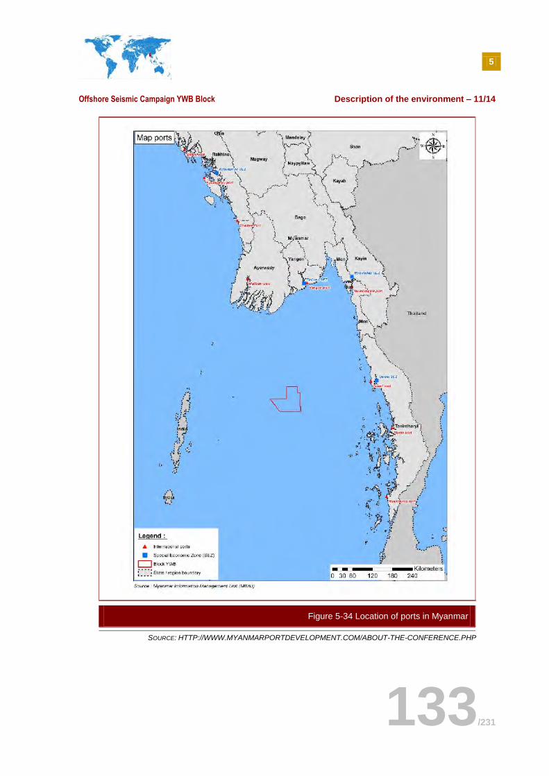
5
Offshore Seismic Campaign YWB Block Description of the environment – 11/14
133/231
SOURCE: HTTP://WWW.MYANMARPORTDEVELOPMENT.COM/ABOUT-THE-CONFERENCE.PHP
Figure 5-34 Location of ports in Myanmar
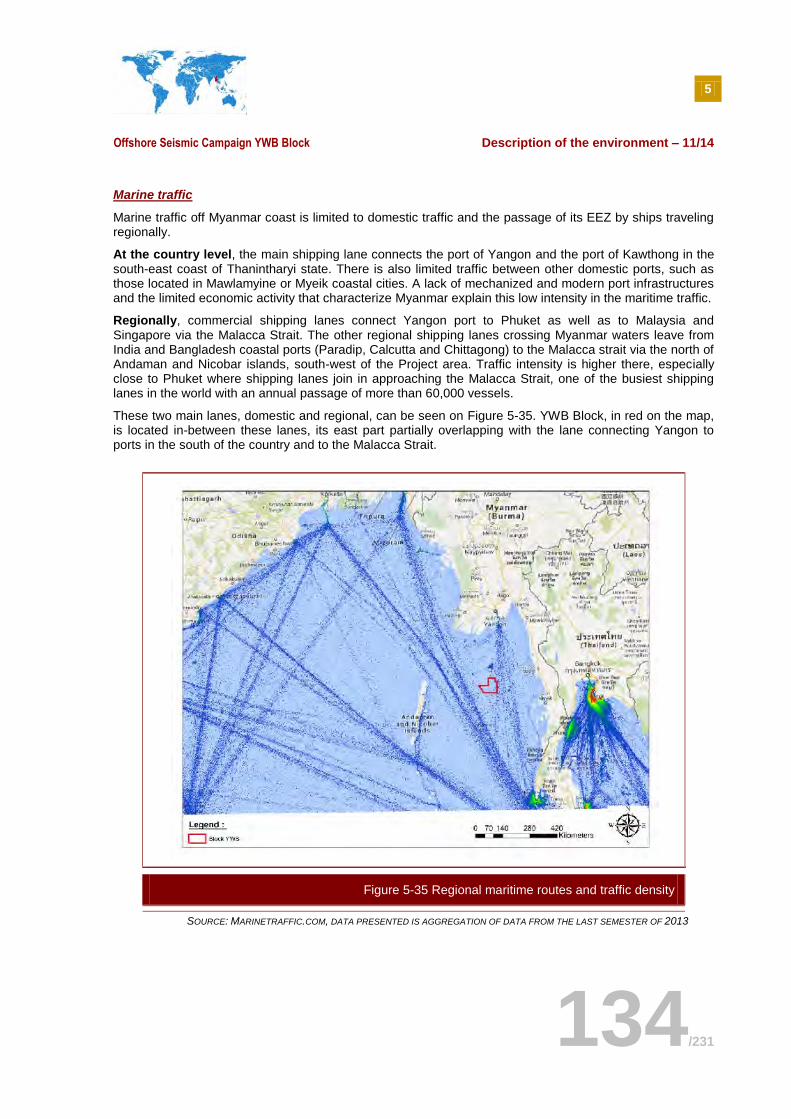
5
Offshore Seismic Campaign YWB Block Description of the environment – 11/14
134/231
Marine traffic
Marine traffic off Myanmar coast is limited to domestic traffic and the passage of its EEZ by ships traveling regionally.
At the country level, the main shipping lane connects the port of Yangon and the port of Kawthong in the south-east coast of Thanintharyi state. There is also limited traffic between other domestic ports, such as those located in Mawlamyine or Myeik coastal cities. A lack of mechanized and modern port infrastructures and the limited economic activity that characterize Myanmar explain this low intensity in the maritime traffic.
Regionally, commercial shipping lanes connect Yangon port to Phuket as well as to Malaysia and Singapore via the Malacca Strait. The other regional shipping lanes crossing Myanmar waters leave from India and Bangladesh coastal ports (Paradip, Calcutta and Chittagong) to the Malacca strait via the north of Andaman and Nicobar islands, south-west of the Project area. Traffic intensity is higher there, especially close to Phuket where shipping lanes join in approaching the Malacca Strait, one of the busiest shipping lanes in the world with an annual passage of more than 60,000 vessels.
These two main lanes, domestic and regional, can be seen on Figure 5-35. YWB Block, in red on the map, is located in-between these lanes, its east part partially overlapping with the lane connecting Yangon to ports in the south of the country and to the Malacca Strait.
SOURCE: MARINETRAFFIC.COM, DATA PRESENTED IS AGGREGATION OF DATA FROM THE LAST SEMESTER OF 2013
Figure 5-35 Regional maritime routes and traffic density
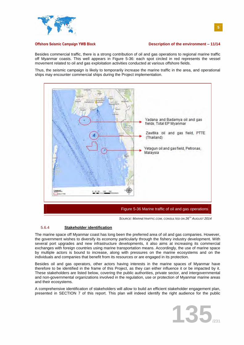
5
Offshore Seismic Campaign YWB Block Description of the environment – 11/14
135/231
Besides commercial traffic, there is a strong contribution of oil and gas operations to regional marine traffic off Myanmar coasts. This well appears in Figure 5-36: each spot circled in red represents the vessel movement related to oil and gas exploitation activities conducted at various offshore fields.
Thus, the seismic campaign is likely to temporarily increase the marine traffic in the area, and operational ships may encounter commercial ships during the Project implementation.
SOURCE: MARINETRAFFIC.COM, CONSULTED ON 26TH
AUGUST 2014
5.6.4 Stakeholder identification
The marine space off Myanmar coast has long been the preferred area of oil and gas companies. However, the government wishes to diversify its economy particularly through the fishery industry development. With several port upgrades and new infrastructure developments, it also aims at increasing its commercial exchanges with foreign countries using marine transportation means. Accordingly, the use of marine space by multiple actors is bound to increase, along with pressures on the marine ecosystems and on the individuals and companies that benefit from its resources or are engaged in its protection.
Besides oil and gas operators, other actors having interests in the marine spaces of Myanmar have therefore to be identified in the frame of this Project, as they can either influence it or be impacted by it. These stakeholders are listed below, covering the public authorities, private sector, and intergovernmental and non-governmental organizations involved in the regulation, use or protection of Myanmar marine areas and their ecosystems.
A comprehensive identification of stakeholders will allow to build an efficient stakeholder engagement plan, presented in SECTION 7 of this report. This plan will indeed identify the right audience for the public
Figure 5-36 Marine traffic of oil and gas operations
5
Offshore Seismic Campaign YWB Block Description of the environment – 11/14
136/231
consultations that will aim at gathering stakeholders’ perception on the impacts identified and the mitigation measures prepared in this report.
5.6.4.1 Public authorities
Public authorities grant the authorizations and permits needed by Total E & P Myanmar to perform the seismic campaign on YWB block. They also regulate the use of marine areas between various stakeholders, from commercial vessels to fishermen.
Ministries
Ministry of Energy (MoE): MoE is in charge of developing the oil and gas resources in the country.
It provides offshore and onshore blocks through bidding rounds to national and international companies for the purpose of exploration and/or exploitation.
Ministry of Environment Conservation and Forestry (MOECAF): MOECAF is in charge of developing the country environmental policy, in particular in the fields of water and marine resources conservation. It is also responsible for introducing a new environmental permitting system, which is in process of creation.
Ministry of Livestock, Fisheries and Rural Development (MLFRD): MLFRD is in charge of
developing, implementing and monitoring the country policies in the field of livestock, fishery and rural development, to ensure food security is achieved in the country, and prevent infectious diseases development that could endanger the national production.
o Department of Fisheries (DoF): Under the MLFRD, the DoF main mission is to guarantee the preservation of fish resources in order to ensure the sustainability of the fishery sector. The DoF develops conservation efforts, promotes research and surveys on the current condition of marine resources in partnership with intergovernmental agencies, maintains statistics on fisheries, and supervises the fishery sector through the delivery of licenses to fishing vessels.
Ministry of Transport (MoT): MoT is responsible for the organization of the country’s transport infrastructures, from air to marine transportation.
o Department of Marine Administration (DMA): DMA is placed under the management of the Ministry of Transport. It is responsible for the marine traffic safety (conformity of ships to national safety standards, improvement of rescue operations at sea) and human resources development in the maritime sector. It is in charge of the offshore fishing vessels inspection to determine if they meet safety standards, prior to the delivery of fishing licenses by the DoF.
o Myanma Port Authority (MPA): MPA is a government agency under the Ministry of Transport, founded in 1989 and located in Yangon. It is responsible for the regulation and administration of 8 coastal ports, among which Yangon Port. It is also in charge of developing and improving the port infrastructures, notably through the development of Special Economic Zones and their associated ports.
Myanmar Navy: Naval branch of the armed forces of Myanmar with 19,000 staff. The Myanmar Navy currently operates more than 122 vessels, and increased its activities over the last years to improve defence of its territorial waters in particular against illegal fishing.
Universities and research institutes
University of Mawlamyine (Mon State): it is one of the few universities in the country to offer a specialized degree in marine science, from Bachelor, Master to PhDs. It also has a Marine Science Laboratory in the coastal town of Setse, about 60 km south of Mawlamyine city. 900 students are registered across the various classes available.
5
Offshore Seismic Campaign YWB Block Description of the environment – 11/14
137/231
Institute of Fisheries Technology: Public institution established in Yangon in 1983 under the management of the Department of Fisheries. It provides training to fishermen on fishing techniques, fishing gears and fish processing, among others. Training courses can vary, from basic fishing technology to fish processing supervision.
Public enterprises
Myanmar Oil and Gas Enterprise (MOGE): MOGE is Myanmar oil and gas state-owned enterprise. Established in 1983, it is an operator in oil and gas exploration and production as well as domestic gas transport through pipeline networks. It is also partner of joint-ventures with foreign oil and gas companies such as Total, Chevron, etc.
5.6.4.2 Business associations
Union of Myanmar Federation of Chambers of Commerce and Industry (UMFCCI): UMFCCI is the largest not-for-profit business federation of the country. Its functions include human resources development and training, commercial courses, management and accounting, providing trade information and participation in international trade fairs. Almost every economic sector has its own federation under the umbrella of the UMFCCI. This is the case for the fishing industry, represented by the MFF.
Myanmar Fishery Federation (MFF): Non-profit association founded in 1989 with the objective to
encourage and promote fishing and fishery industries of Myanmar, through cooperation, training and knowledge sharing with other actors of the national fishery sector. The MFF counts 9 functional associations, and 13 regional fisheries associations under its umbrella. It has an important role in advocacy and opinion-making by regularly intervening in Myanmar media on issues of overfishing and depletion of the country marine resources.
Myanmar Marine Fisheries Association: Member of the MFF along with 8 other associations.
Myanmar Fishery Products Processors and Exporters Association (MFPPEA): Professional association in charge of supporting and promoting the processing and exporting companies in Myanmar.
5.6.4.3 Oil and gas companies
51 offshore blocks, among which 24 are located in deep water, have been awarded by the MoE to 7 companies. Directly surrounding the Project area, 3 companies have operations either at the exploration or exploitation stage. They are presented below.
Eni: Italian oil and gas company, operator of the block M4 neighboring YWB block.
PTTEP: Thai Oil and Gas Company, operator of the Zawtika gas field which covers several blocks
neighboring YWB.
PCML: Petronas Carigali Myanmar Ltd, a local branch of Petronas operating the Yetagun project neighbouring YWB block.
5.6.4.4 International organizations
Food and Agriculture Organization (FAO): FAO has a representation office in Myanmar since 1978, and is involved in a wide range of activities to support sectoral development, in particular fisheries, focusing mostly on aquaculture and coastal fisheries as a support to artisanal fishing communities.
5.6.4.5 Intergovernmental organizations
Intergovernmental organizations involved in the protection of marine spaces and/or the promotion of sustainable fisheries at the Southeast Asia regional level are numerous. They are particularly active in Myanmar, where the fishery sector is threatened by marine resources depletion.
5
Offshore Seismic Campaign YWB Block Description of the environment – 11/14
138/231
Asia Pacific Fishery Commission (APFIC): APFIC is a regional fishery body established by the FAO at the request of its members in 1948 during the organization of the Indo-Pacific Fisheries Council. Its Secretariat is provided and supported by the FAO. Its role is to promote full and proper utilization of living aquatic resources, by the development and management of fishing, processing and marketing activities. APFIC also aims at improving knowledge sharing, training and promotion of best practices in the fishery sector to encourage sustainable fisheries, in collaboration with other regional entities and the national fishery institutions of its members.
ASEAN Sectoral Working Group on Fisheries (ASWGFi): Under the leadership of the ASEAN,
ASWGFi is a regional working group gathering fisheries specialists during regular consultative forums which address issues such as registration of fishing vessels, census of marine resources, etc. Overall, the working group objective is to provide inputs for the creation of a common sustainable regional fishery policy among the ASEAN countries.
South East Asian Fisheries Development Center (SEAFDEC): SEAFDEC mission is to develop and manage the fisheries potential of the region, supporting the rational utilization of the resources through transfer of new technologies, research and information dissemination activities. SEAFDEC comprises 11 member countries: Brunei Darussalam, Cambodia, Indonesia, Japan, Lao PDR, Malaysia, Myanmar, Philippines, Singapore, Thailand, and Vietnam. Its central office is located in Thailand. The Marine Fisheries Research Department and the Marine Fishery Resources Development and Management Department are the two bodies working on assessing Myanmar marine resources and estimating potential for development of the fishery sector. The organization has also concluded an agreement with the ASEAN leading to the creation of a Fisheries Consultative Group.
Bay of Bengal Large Marine Ecosystem Project (BOBLME): BOBLME is a regional project whose objectives are to develop a coordinated policy on the management and protection of marine resources and environment in the large ecosystem of the Bay of Bengal. Its overall goal is to improve livelihoods of coastal communities depending on the BOB resources. Funded by international donors (Global Environmental Facility, Norway, Swedish Internal Development Agency), the project is piloted by the FAO in cooperation with respective Marine and/or Fisheries Ministries in each member country (Maldives, India, Sri Lanka, Bangladesh, Myanmar, Thailand, Indonesia and Malaysia).
5.6.4.6 International Non Governmental Organizations
The presence of international NGOs in the country has increased over the last 5 years due to a political opening which allows them to open branches and lead projects in various sectors, from community development projects aiming at reducing poverty to environment conservation initiatives targeting inland and marine ecosystems.
Fauna & Flora International (FFI): FFI works in Myanmar on various biodiversity and conservation projects. It currently leads a capacity-building program for marine conservation. Started in 2012, this program aims at identifying marine areas that should be protected, and support the management of already established protected areas. In partnership with Biodiversity and Nature Conservation Association (BANCA), a Myanmar national NGO, and the Forestry and Fisheries Departments, activities will consist in trainings on marine survey methods, community-based fisheries and marine protected areas establishment and management. One of the pilot areas for these activities is the Myeik archipelago off Thanintharyi State.
WWF: WWF has been very active in the greater Mekong region over the last decades, and has just recently opened an office in Myanmar. Its aim is to support Myanmar’s development ambitions with a focus on spatial planning and biodiversity conservation in parallel with ecosystem services protection and sustainable livelihoods.
Wildlife Conservation Society: International organization based in the USA, it is involved in the conservation of species with more than 500 projects in 60 countries. It started to operate in

5
Offshore Seismic Campaign YWB Block Description of the environment – 11/14
139/231
Myanmar in 1993, becoming the first international conservation organization to initiate a long-term program in the country. Their activities range from biological surveys, wildlife species population monitoring, to aid in the establishment of protected areas.
Human Rights Watch: Human Rights Watch regularly conduct human rights assessments in oil and gas projects, focusing on the pipelines connecting the offshore fields and the receiving countries than on offshore oil and gas platforms.
5.6.4.7 National Non Governmental Organizations
The economic strategy implemented by the government has succeeded in attracting international investors interests in various business sectors. Industrial developments are significant, increasingly threatening ecosystems that were preserved by years of isolation. To face these new environmental challenges, several national NGOs have been created over the last years to preserve and protect the wide range of natural ecosystems.
Myanmar Environmental Rehabilitation-conservation Network (MERN): MERN is a network of 20 local environmental NGOs created in 2009. It works for environmental rehabilitation and conservation activities in support of local communities, to help them improve their sources of livelihoods and food security. It has in particular a coastal livelihood and environmental restoration program in the state of Rakhine.
Biodiversity and Nature Conservation Association (BANCA): BANCA is a national NGO
registered since 2004 whose objectives are to support conservation of nature, biodiversity through advocacy, research, networking and capacity-building programs. It works with the FFI on a marine conservation project. It also worked on projects focusing on inland ecosystems with other international NGOs such as Birdlife International, the Royal Society for the Protection of Birds, Care, Arcona Cambridge, etc.
Marine Science Association, Myanmar (MSAM): MSAM is a national NGO whose objectives are to take part in the sustainable development activities in Myanmar using its marine science expertise to conduct marine and coastal research, conservation and development, and to raise awareness on marine environment preservation.
Community Development Association (CDA): CDA is a registered non-profit, local non-
government humanitarian organization established in Myanmar. Its mandates are to implement community developmental elementary interventions with effective involvement of existing support services and technical assistance. The Community Development Association has worked on various humanitarian assistance programs and has collaborated with Total E&P Myanmar.
Friends of Wildlife Myanmar: Run by a former forestry official and based in Yangon, Friends of Wildlife provides education and technical assistance to help local communities shift from slash-and-burn agriculture, hunting, and illegal logging to sustainable agriculture. It is also involved in sustainable fishery management promotion.
Burma Environmental Working Group (BEWG): BEWG gather Myanmar ethnic environmental
and social organizations, providing a forum for member organizations to collaborate on research, reporting, advocacy campaigns, capacity-building initiatives and policy formulation.
5.6.4.8 Media
Eleven Myanmar: Part of the Eleven Media Group funded in 2000, it has 5 weekly publications among which one is in English, and employs 250 staffs. Number of published copies is 450,000 in 2012.
The Myanmar Times: This newspaper has two versions, one in Burmese and one in English. It
counts more than 300 employees and has a circulation of around 25,000 copies.
5
Offshore Seismic Campaign YWB Block Description of the environment – 11/14
140/231
The Irrawaddy Magazine: Newsmagazine founded in 1992 by Burmese exiles living in Thailand. It is unaffiliated politically but supportive of democratic movements, and publishes news in English and in Burmese.
5.6.5 Total E&P Myanmar CSR Programs
Total E&P Myanmar has operated the Yadana gas field since 1992, in a consortium with Chevron (28.26%), Petroleum Authority of Thailand Exploration & Production (25.5%) and Myanma Oil and Gas Enterprise (15%).
Since 1995, it has implemented several socio-economic development programs at the onshore pipeline area, located in Thanintharyi State. In 1998, it extended its programs outside its operation areas to the national scale, focusing on public health and social welfare.
At the pipeline area, community development projects cover 33 villages. Major projects are detailed below:
Health (eye and dental care, medical staff training, provision of material and infrastructures);
Education (provision of infrastructures, scholarship and tuition program);
Community development and humanitarian assistance (flood relief assistance, road safety campaigns);
Microfinance (Village Bank Committees, capacity-building);
Support to agricultural activities and veterinary services (rubber, cocoa and paddy farmers, financial and technical trainings for farmers, support to the creation of local farmers associations, animal vaccination campaigns, etc.);
Infrastructures (roads, bridges, schools, health centers, water network, etc.);
Solar energy (launching of Total corporate TATS program);
Good stakeholder relations (communication with regional authorities, grievance mechanism).
At the national level, several programs were implemented in 2013 and are listed below:
Orphanages;
Blindness prevention program;
Integrated HIV Care program;
Support to Government doctors training;
Supports to Associate Medicale Franco–Asiatique (AMFA);
Supports to community in neighborhood;
“On Job training” facilities to CVT students (Center for Vocational Training);
Collaboration with Government Technical High School (Dawei).
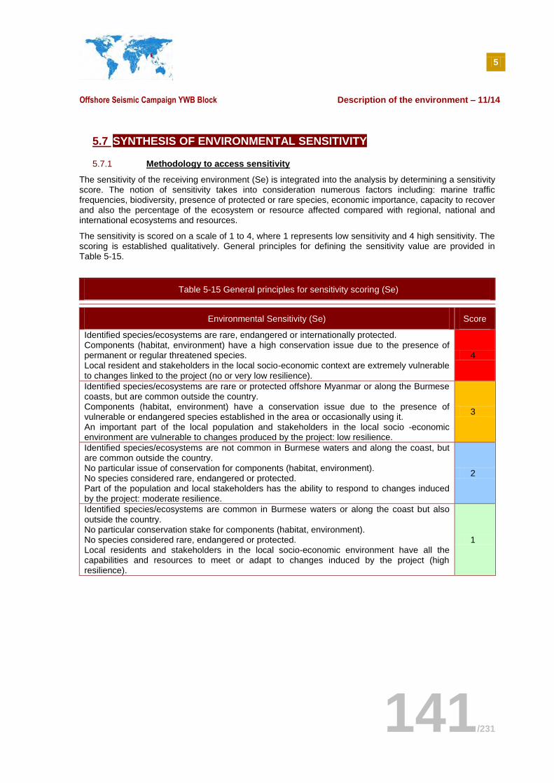
5
Offshore Seismic Campaign YWB Block Description of the environment – 11/14
141/231
5.7 SYNTHESIS OF ENVIRONMENTAL SENSITIVITY
5.7.1 Methodology to access sensitivity
The sensitivity of the receiving environment (Se) is integrated into the analysis by determining a sensitivity score. The notion of sensitivity takes into consideration numerous factors including: marine traffic frequencies, biodiversity, presence of protected or rare species, economic importance, capacity to recover and also the percentage of the ecosystem or resource affected compared with regional, national and international ecosystems and resources.
The sensitivity is scored on a scale of 1 to 4, where 1 represents low sensitivity and 4 high sensitivity. The scoring is established qualitatively. General principles for defining the sensitivity value are provided in Table 5-15.
Table 5-15 General principles for sensitivity scoring (Se)
Environmental Sensitivity (Se) Score
Identified species/ecosystems are rare, endangered or internationally protected. Components (habitat, environment) have a high conservation issue due to the presence of permanent or regular threatened species. Local resident and stakeholders in the local socio-economic context are extremely vulnerable to changes linked to the project (no or very low resilience).
4
Identified species/ecosystems are rare or protected offshore Myanmar or along the Burmese coasts, but are common outside the country. Components (habitat, environment) have a conservation issue due to the presence of vulnerable or endangered species established in the area or occasionally using it. An important part of the local population and stakeholders in the local socio -economic environment are vulnerable to changes produced by the project: low resilience.
3
Identified species/ecosystems are not common in Burmese waters and along the coast, but are common outside the country. No particular issue of conservation for components (habitat, environment). No species considered rare, endangered or protected. Part of the population and local stakeholders has the ability to respond to changes induced by the project: moderate resilience.
2
Identified species/ecosystems are common in Burmese waters or along the coast but also outside the country. No particular conservation stake for components (habitat, environment). No species considered rare, endangered or protected. Local residents and stakeholders in the local socio-economic environment have all the capabilities and resources to meet or adapt to changes induced by the project (high resilience).
1
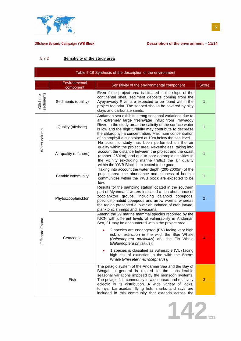
5
Offshore Seismic Campaign YWB Block Description of the environment – 11/14
142/231
5.7.2 Sensitivity of the study area
Table 5-16 Synthesis of the description of the environment
Environmental
component Sensitivity of the environmental component Score
Offshore
sedim
ents
Sediments (quality)
Even if the project area is situated in the slope of the continental shelf, sediment deposits coming from the Ayeyarwady River are expected to be found within the project footprint. The seabed should be covered by silty clays and carbonate sands.
1
Wate
r colu
mn Quality (offshore)
Andaman sea exhibits strong seasonal variations due to an extremely large freshwater influx from Irrawaddy River. In the study area, the salinity of the surface water is low and the high turbidity may contribute to decrease the chlorophyll-a concentration. Maximum concentration of chlorophyll-a is obtained at 10m below the sea level.
1
Air quality (offshore)
No scientific study has been performed on the air quality within the project area. Nevertheless, taking into account the distance between the project and the coast (approx. 250km), and due to poor anthropic activities in the vicinity (excluding marine traffic) the air quality within the YWB Block is expected to be good.
1
Offshore
Fauna
Benthic community
Taking into account the water depth (200-2000m) of the project area, the abundance and richness of benthic communities within the YWB block are expected to be low.
1
Phyto/Zooplanckton
Results for the sampling station located in the southern part of Myanmar’s waters indicated a rich abundance of zooplankton groups, including calanoid copepods, poecilostomatoid copepods and arrow worms, whereas the region presented a lower abundance of crab larvae, planktonic shrimps and larvaceans.
2
Cetaceans
Among the 29 marine mammal species recorded by the IUCN with different levels of vulnerability in Andaman Sea, 21 may be encountered within the project area:
2 species are endangered (EN) facing very high risk of extinction in the wild: the Blue Whale (Balaenoptera musculus) and the Fin Whale (Balaenoptera physalus);
1 species is classified as vulnerable (VU) facing high risk of extinction in the wild: the Sperm Whale (Physeter macrocephalus).
4
Fish
The pelagic system of the Andaman Sea and the Bay of Bengal in general is related to the considerable seasonal variations imposed by the monsoon systems. The pelagic fish community is widespread and relatively eclectic in its distribution. A wide variety of jacks, tunnys, barracudas, flying fish, sharks and rays are included in this community that extends across the
3
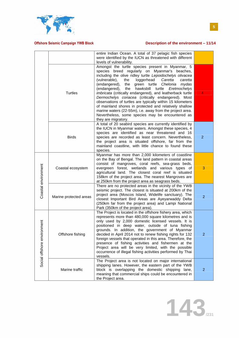
5
Offshore Seismic Campaign YWB Block Description of the environment – 11/14
143/231
entire Indian Ocean. A total of 37 pelagic fish species were identified by the IUCN as threatened with different levels of vulnerability.
Turtles
Amongst the turtle species present in Myanmar, 5 species breed regularly on Myanmar's beaches, including the olive ridley turtle Lepoidochelys olivacea (vulnerable), the loggerhead Caretta caretta (endangered), the green turtle Chelonia mydas (endangered), the hawksbill turtle Eretmochelys imbricata (critically endangered), and leatherback turtle Dermochelys coriacea (critically endangered). Most observations of turtles are typically within 15 kilometers of mainland shores in protected and relatively shallow marine waters (22-55m), i.e. away from the project area. Nevertheless, some species may be encountered as they are migratory.
4
Birds
A total of 20 seabird species are currently identified by the IUCN in Myanmar waters. Amongst these species, 4 species are identified as near threatened and 16 species are recorded as least concern. Nevertheless, the project area is situated offshore, far from the mainland coastline, with little chance to found these species.
2
Coasta
l environm
ent
Coastal ecosystem
Myanmar has more than 2,000 kilometers of coastline on the Bay of Bengal. The land pattern in coastal areas consist of mangroves, coral reefs, sea-grass beds, evergreen forest, wetlands and various types of agricultural land. The closest coral reef is situated 158km of the project area. The nearest Mangroves are at 250km from the project area as seagrass beds.
3
Marine protected areas
There are no protected areas in the vicinity of the YWB seismic project. The closest is situated at 200km of the project area (Moscos Island, Widelife sanctuary). The closest Important Bird Areas are Ayeyarwaddy Delta (250km far from the project area) and Lampi National Park (350km of the project area).
2
Socia
l offshore
environm
ent
Offshore fishing
The Project is located in the offshore fishery area, which represents more than 480,000 square kilometres and is only used by 2,000 domestic licensed vessels. It is positioned in deep water, outside of tuna fishing grounds. In addition, the government of Myanmar decided in April 2014 not to renew fishing rights for 132 foreign vessels that operated in this area. Therefore, the presence of fishing activities and fishermen at the Project area will be very limited, with the possible occurrence of illegal fishing activities performed by Thai vessels.
2
Marine traffic
The Project area is not located on major international shipping lanes. However, the eastern part of the YWB block is overlapping the domestic shipping lane, meaning that commercial ships could be encountered in the Project area.
2

5
Offshore Seismic Campaign YWB Block Description of the environment – 11/14
144/231
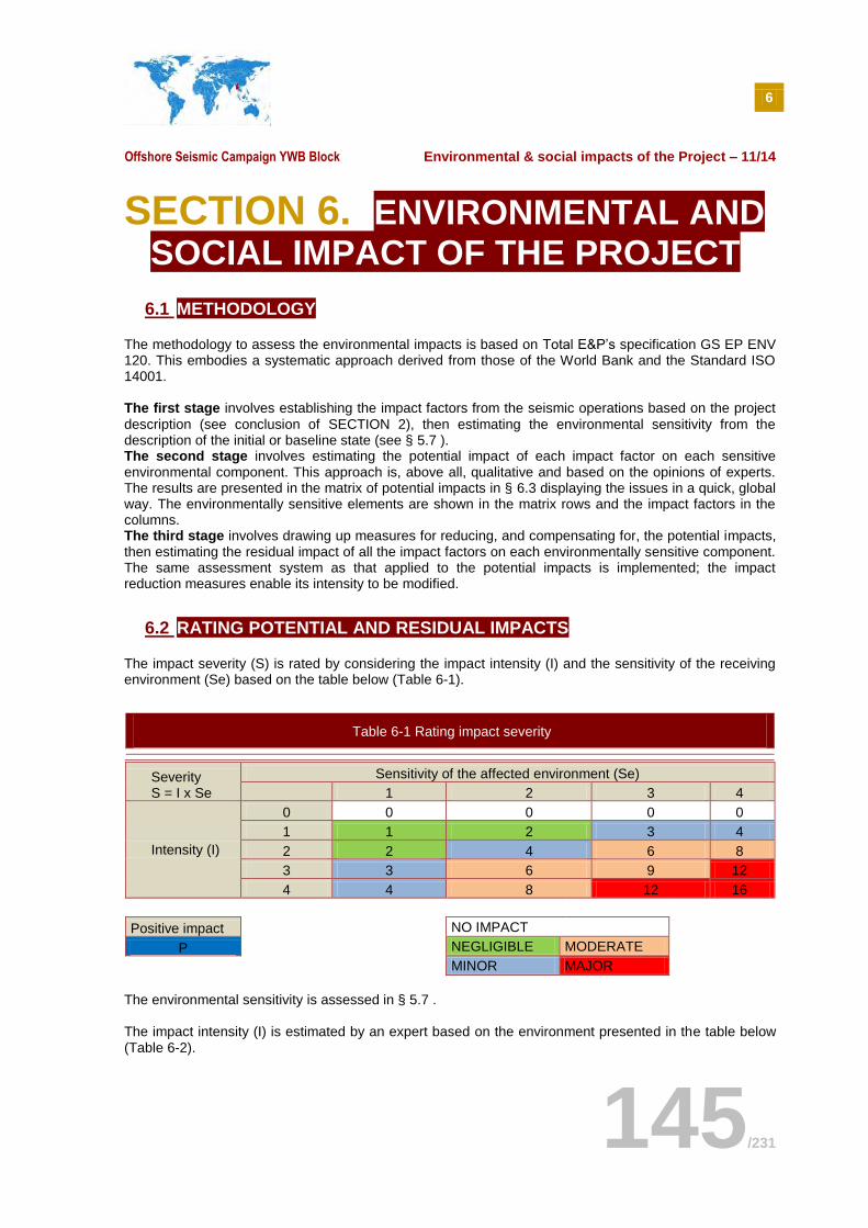
6
Offshore Seismic Campaign YWB Block Environmental & social impacts of the Project – 11/14
145/231
SECTION 6. ENVIRONMENTAL AND SOCIAL IMPACT OF THE PROJECT
6.1 METHODOLOGY
The methodology to assess the environmental impacts is based on Total E&P’s specification GS EP ENV 120. This embodies a systematic approach derived from those of the World Bank and the Standard ISO 14001. The first stage involves establishing the impact factors from the seismic operations based on the project
description (see conclusion of SECTION 2), then estimating the environmental sensitivity from the description of the initial or baseline state (see § 5.7 ). The second stage involves estimating the potential impact of each impact factor on each sensitive environmental component. This approach is, above all, qualitative and based on the opinions of experts. The results are presented in the matrix of potential impacts in § 6.3 displaying the issues in a quick, global way. The environmentally sensitive elements are shown in the matrix rows and the impact factors in the columns. The third stage involves drawing up measures for reducing, and compensating for, the potential impacts, then estimating the residual impact of all the impact factors on each environmentally sensitive component. The same assessment system as that applied to the potential impacts is implemented; the impact reduction measures enable its intensity to be modified.
6.2 RATING POTENTIAL AND RESIDUAL IMPACTS
The impact severity (S) is rated by considering the impact intensity (I) and the sensitivity of the receiving environment (Se) based on the table below (Table 6-1).
Table 6-1 Rating impact severity
Severity S = I x Se
Sensitivity of the affected environment (Se)
1 2 3 4
Intensity (I)
0 0 0 0 0
1 1 2 3 4
2 2 4 6 8
3 3 6 9 12
4 4 8 12 16
Positive impact
NO IMPACT
P
NEGLIGIBLE MODERATE
MINOR MAJOR
The environmental sensitivity is assessed in § 5.7 . The impact intensity (I) is estimated by an expert based on the environment presented in the table below (Table 6-2).
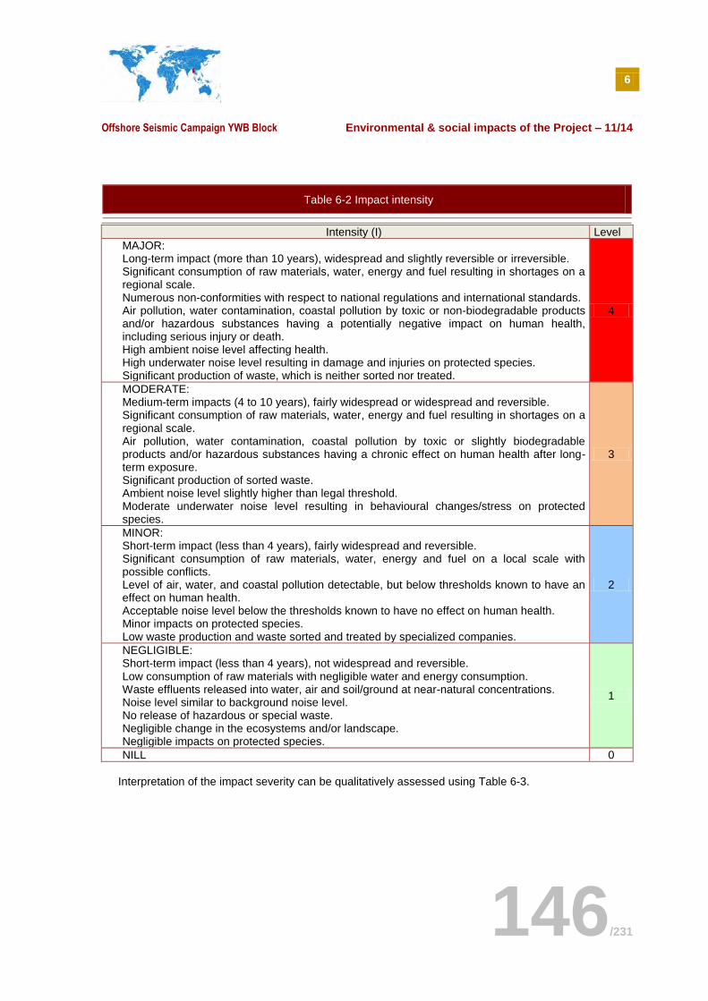
6
Offshore Seismic Campaign YWB Block Environmental & social impacts of the Project – 11/14
146/231
Table 6-2 Impact intensity
Intensity (I) Level
MAJOR: Long-term impact (more than 10 years), widespread and slightly reversible or irreversible. Significant consumption of raw materials, water, energy and fuel resulting in shortages on a regional scale. Numerous non-conformities with respect to national regulations and international standards. Air pollution, water contamination, coastal pollution by toxic or non-biodegradable products and/or hazardous substances having a potentially negative impact on human health, including serious injury or death. High ambient noise level affecting health. High underwater noise level resulting in damage and injuries on protected species. Significant production of waste, which is neither sorted nor treated.
4
MODERATE: Medium-term impacts (4 to 10 years), fairly widespread or widespread and reversible. Significant consumption of raw materials, water, energy and fuel resulting in shortages on a regional scale. Air pollution, water contamination, coastal pollution by toxic or slightly biodegradable products and/or hazardous substances having a chronic effect on human health after long-term exposure. Significant production of sorted waste. Ambient noise level slightly higher than legal threshold. Moderate underwater noise level resulting in behavioural changes/stress on protected species.
3
MINOR: Short-term impact (less than 4 years), fairly widespread and reversible. Significant consumption of raw materials, water, energy and fuel on a local scale with possible conflicts. Level of air, water, and coastal pollution detectable, but below thresholds known to have an effect on human health. Acceptable noise level below the thresholds known to have no effect on human health. Minor impacts on protected species. Low waste production and waste sorted and treated by specialized companies.
2
NEGLIGIBLE: Short-term impact (less than 4 years), not widespread and reversible. Low consumption of raw materials with negligible water and energy consumption. Waste effluents released into water, air and soil/ground at near-natural concentrations. Noise level similar to background noise level. No release of hazardous or special waste. Negligible change in the ecosystems and/or landscape. Negligible impacts on protected species.
1
NILL 0
Interpretation of the impact severity can be qualitatively assessed using Table 6-3.
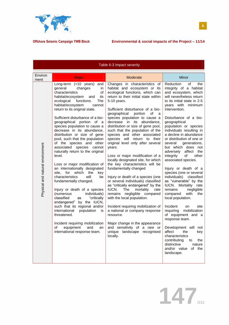
6
Offshore Seismic Campaign YWB Block Environmental & social impacts of the Project – 11/14
147/231
Table 6-3 Impact severity
Environment
Major Moderate Minor
Physic
al and
natu
ral environm
ent
Long-term (>10 years) and general changes in characteristics of habitat/ecosystem and its ecological functions. The habitat/ecosystem cannot return to its original state.
Sufficient disturbance of a bio-geographical portion of a species population to cause a decrease in its abundance, distribution or size of gene pool, such that the population of the species and other associated species cannot naturally return to the original level.
Loss or major modification of an internationally designated site, for which the key characteristics will be fundamentally changed.
Injury or death of a species (numerous individuals) classified as “critically endangered” by the IUCN, such that its regional and/or international population is threatened.
Incident requiring mobilization of equipment and an international response team.
Changes in characteristics of habitat and ecosystem or its ecological functions, which can return to their initial state within 5-10 years.
Sufficient disturbance of a bio-geographical portion of a species population to cause a decrease in its abundance, distribution or size of gene pool, such that the population of the species and other associated species will return to their original level only after several years.
Loss or major modification of a locally designated site, for which the key characteristics will be fundamentally changed
Injury or death of a species (one or several individuals) classified as “critically endangered” by the IUCN. The mortality rate remains negligible compared with the local population.
Incident requiring mobilization of a national or company response resource.
Major change in the appearance and sensitivity of a rare or unique landscape recognised locally.
Reduction of the integrity of a habitat and ecosystem, which will nevertheless return to its initial state in 2-5 years with minimum intervention.
Disturbance of a bio-geographical population or species individuals resulting in a decline in abundance or distribution of one or several generations, but which does not adversely affect the integrity of other associated species.
Injury or death of a species (one or several individuals) classified as “vulnerable” by the IUCN. Mortality rate remains negligible compared with the local population.
Incident on site requiring mobilization of equipment and a response team.
Development will not affect the key characteristics contributing to the distinctive nature and/or value of the landscape.
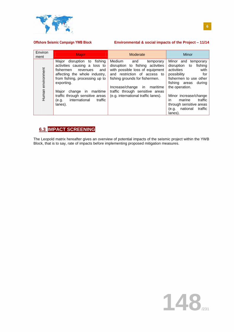
6
Offshore Seismic Campaign YWB Block Environmental & social impacts of the Project – 11/14
148/231
Environment
Major Moderate Minor
Hum
an e
nvironm
ent
Major disruption to fishing activities causing a loss to fishermen revenues and affecting the whole industry, from fishing, processing up to exporting.
Major change in maritime traffic through sensitive areas (e.g. international traffic lanes).
Medium and temporary disruption to fishing activities with possible loss of equipment and restriction of access to fishing grounds for fishermen.
Increase/change in maritime traffic through sensitive areas (e.g. international traffic lanes).
Minor and temporary disruption to fishing activities with possibility for fishermen to use other fishing areas during the operation. Minor increase/change in marine traffic through sensitive areas (e.g. national traffic lanes).
6.3 IMPACT SCREENING
The Leopold matrix hereafter gives an overview of potential impacts of the seismic project within the YWB Block, that is to say, rate of impacts before implementing proposed mitigation measures.
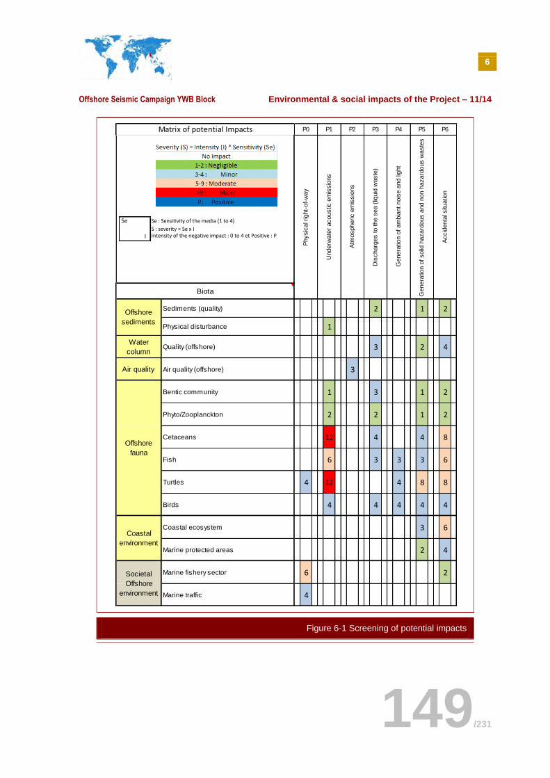
6
Offshore Seismic Campaign YWB Block Environmental & social impacts of the Project – 11/14
149/231
Sediments (quality) 0 0 0 2 0 1 2
Physical disturbance 0 1 0 0 0 0 0
Water
columnQuality (offshore) 0 0 0 3 0 2 4
Air quality Air quality (offshore) 0 0 3 0 0 0 0
Bentic community 0 1 0 3 0 1 2
Phyto/Zooplanckton 0 2 0 2 0 1 2
Cetaceans 0 12 0 4 0 4 8
Fish 0 6 0 3 3 3 6
Turtles 4 12 4 8 8
Birds 0 4 0 4 4 4 4
Coastal ecosystem 0 0 0 0 0 3 6
Marine protected areas 0 0 0 0 0 2 4
Marine fishery sector 6 0 0 0 0 0 2
Marine traffic 4 0 0 0 0 0 0
Accid
enta
l situ
atio
n
Biota
Offshore
sediments
Offshore
fauna
Coastal
environment
P1
Underw
ate
r acoustic
em
issio
ns
Societal
Offshore
environment
P5 P6
Physic
al r
ight-
of-
way
Atm
ospheric e
mis
sio
ns
Dis
charg
es to the s
ea (
liquid
waste
)
Genera
tion o
f am
bia
nt nois
e a
nd li
ght
Matrix of potential Impacts P0 P2 P3 P4
Genera
tion o
f solid
hazard
ous a
nd n
on h
azard
ous w
aste
s
Se Se : Sensitivity of the media (1 to 4)
S : severity = Se x I
I Intensity of the negative impact : 0 to 4 et Positive : P
Figure 6-1 Screening of potential impacts
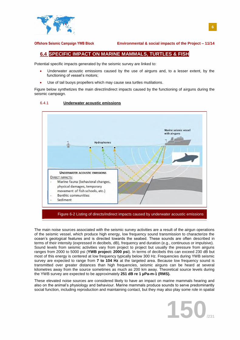
6
Offshore Seismic Campaign YWB Block Environmental & social impacts of the Project – 11/14
150/231
6.4 SPECIFIC IMPACT ON MARINE MAMMALS, TURTLES & FISH
Potential specific impacts generated by the seismic survey are linked to:
Underwater acoustic emissions caused by the use of airguns and, to a lesser extent, by the functioning of vessel’s motors;
Use of tail buoys propellers which may cause sea turtles mutilations.
Figure below synthetizes the main direct/indirect impacts caused by the functioning of airguns during the seismic campaign.
6.4.1 Underwater acoustic emissions
The main noise sources associated with the seismic survey activities are a result of the airgun operations of the seismic vessel, which produce high energy, low frequency sound transmission to characterize the ocean’s geological features and is directed towards the seabed. These sounds are often described in terms of their intensity (expressed in decibels, dB), frequency and duration (e.g., continuous or impulsive). Sound levels from seismic activities vary from project to project but usually the pressure from airguns ranges from 2000 to 5000 psi (YWB project: 2000 psi). In terms of decibels this can exceed 230 dB but most of this energy is centered at low frequency typically below 300 Hz. Frequencies during YWB seismic survey are expected to range from 7 to 104 Hz at the targeted area. Because low frequency sound is transmitted over greater distances than high frequencies, seismic airguns can be heard at several kilometres away from the source sometimes as much as 200 km away. Theoretical source levels during the YWB survey are expected to be approximately 251 dB re 1 µPa-m-1 (RMS).
These elevated noise sources are considered likely to have an impact on marine mammals hearing and also on the animal’s physiology and behaviour. Marine mammals produce sounds to serve predominantly social function, including reproduction and maintaining contact, but they may also play some role in spatial
Figure 6-2 Listing of directs/indirect impacts caused by underwater acoustic emissions
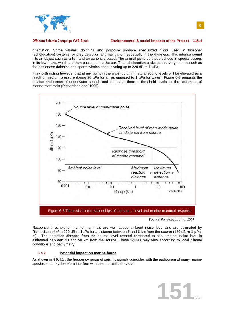
6
Offshore Seismic Campaign YWB Block Environmental & social impacts of the Project – 11/14
151/231
orientation. Some whales, dolphins and porpoise produce specialized clicks used in biosonar (echolocation) systems for prey detection and navigation, especially in the darkness. This intense sound hits an object such as a fish and an echo is created. The animal picks up these echoes in special tissues in its lower jaw, which are then passed on to the ear. The echolocation clicks can be very intense such as the bottlenose dolphins and sperm whales echo locating up to 220 dB re 1 µPa.
It is worth noting however that at any point in the water column, natural sound levels will be elevated as a result of medium pressure (being 20 µPa for air as opposed to 1 µPa for water). Figure 6-3 presents the relation and extent of underwater sounds and compares them to threshold levels for the responses of marine mammals (Richardson et al 1995).
SOURCE: RICHARDSON ET AL. 1995
Response threshold of marine mammals are well above ambient noise level and are estimated by Richardson et al at 120 dB re 1µPa for a distance between 5 and 6 km from the source (180 dB re 1 µPa-m) . The detection distance from the source level created compared to sea ambient noise level is estimated between 40 and 50 km from the source. These figures may vary according to local climate conditions and bathymetry.
6.4.2 Potential impact on marine fauna
As shown in § 6.4.1 , the frequency range of seismic signals coincides with the audiogram of many marine species and may therefore interfere with their normal behaviour.
Figure 6-3 Theoretical interrelationships of the source level and marine mammal response
6
Offshore Seismic Campaign YWB Block Environmental & social impacts of the Project – 11/14
152/231
Disturbance of marine organisms by sound emissions can generally be classified as physical or behavioural. It has been argued that the auditory system of marine mammals is sensitive to physical damage from sound pressure. Thus, mitigation measures have been developed with the aim of preventing from auditory damage against different forms of physical impacts (e.g. tissue damage) and behavioural disturbance (interfere with orientation, communication, feeding or migrating processes). The potential major acoustic impacts of anthropogenic noise sources on marine fauna include:
Death or physical injury as a result of exposure to excessive underwater noise such as air gun fire. These incidents are rare and are limited to an exposure range of several meters to a few hundred meters from the source. Temporary or permanent hearing losses are the most common injuries to mammals, even at low exposure levels for particularly sensitive species. Other observed responses include increased stress levels which may result in the compromise of immune, cardiovascular or reproductive systems of the animal. Changes in diving behaviour and respiration rates have also been noted.
Minor to severe behavioural changes as a result of exposure to anthropogenic noise. Noise exposure can also affect reproduction rates of marine species by causing interference with migratory routes, places of habitat, calving, reproduction and nurturing behaviour as a result of modification of routines to avoid noise exposure. These consequences are highly temporally dependent and can have significant impacts on species survival and abundance.
Masking of critical sounds such as those used for navigation, communication, detection of prey, fleeing from predators and potential mates (reproduction).
Indirect effects, such as changes in the abundance or behaviour of prey animals.
In consideration of these potential consequences it is necessary to determine the acoustic impacts and significance to marine fauna during the seismic acquisition survey. Further effects of nearby airgun operations on marine species have been the subject of numerous literature studies. Available research generally indicates that among the key elements of the ecosystem, including invertebrates, fish, marine mammals and sea turtles, physiological and behavioural effects vary greatly from one species to another and depend on the exposure level, i.e. the distance from the source. The main marine species living within the project area include (see § 5.5 ):
Phytoplankton (Cf. § 6.5.1 );
Benthic community (Cf. § 6.5.1 );
Pelagic fish;
Marine reptilian (turtles);
Marine mammals.
A brief description of the main effects on Fish, turtles, marine mammals for exposure levels are presented in the sub-sections below.
Fish species
Seismic surveys can have an impact on individual fish, fish populations and fisheries, either directly through harmful physiological effects or behavioral effects. Many fish species display a general ‘alarm’ response of increased speed at 156 - 161 dB re 1 µPa rms, which is included in the disturbance avoidance range of baleen whales (see Figure 6-3). Fish eggs, larvae and fry: the physiological effects will mainly affect younger stages of fish life such as eggs, larvae and fry. These are stages in fish development where the organisms have limited ability to escape from their habitual areas in the event of various influences. (DNV Energy, 2007).
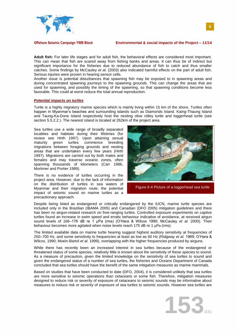
6
Offshore Seismic Campaign YWB Block Environmental & social impacts of the Project – 11/14
153/231
Adult fish: For later life stages and for adult fish, the behavioral effects are considered most important. This can mean that fish are scared away from fishing banks and areas. It can thus be of indirect but significant importance for the fisheries due to reduced abundance of fish to catch and thus smaller catches. Some findings by McCauley et al. (2003) also indicated harmful effects on the part of adult fish. Serious injuries were proven in hearing sensor cells. Another issue is potential disturbances that spawning fish may be exposed to in spawning areas and during concentrated spawning journeys to the spawning grounds. This can change the areas that are used for spawning, and possibly the timing of the spawning, so that spawning conditions become less favorable. This could at worst reduce the total annual reproduction.
Potential impacts on turtles
Turtle is a highly migratory marine species which is mainly living within 15 km of the shore. Turtles often happen in Myanmar’s beaches and surrounding islands such as Diamonds Island. Kaing-Thaung Island and Taung-Ka-Done Island respectively host the nesting olive ridley turtle and loggerhead turtle (see section 5.5.2.2 ). The nearest island is located at 262km of the project area.
Sea turtles use a wide range of broadly separated localities and habitats during their lifetimes (for review see Hirth 1997). Upon attaining sexual maturity green turtles commence breeding migrations between foraging grounds and nesting areas that are undertaken every few years (Hirth 1997). Migrations are carried out by both males and females and may traverse oceanic zones, often spanning thousands of kilometers (Carr 1986, Mortimer and Portier 1989).
There is no evidence of turtles occurring in the project area. However, due to the lack of information on the distribution of turtles in sea waters of Myanmar and their migration route, the potential impact of seismic sound on marine turtles as a precautionary approach.
Despite being listed as endangered or critically endangered by the IUCN, marine turtle species are included only in the Brazilian (IBAMA 2005) and Canadian (DFO 2005) mitigation guidelines and there has been no airgun-related research on free-ranging turtles. Controlled exposure experiments on captive turtles found an increase in swim speed and erratic behaviour indicative of avoidance, at received airgun sound levels of 166–176 dB re 1 μPa (rms) (O’Hara & Wilcox 1990; McCauley et al. 2000). Their behaviour becomes more agitated when noise levels reach 175 dB re 1 µPa (rms).
The limited available data on marine turtle hearing suggest highest auditory sensitivity at frequencies of 250–700 Hz, and some sensitivity to frequencies at least as low as 60 Hz (Ridgway et al. 1969; O’Hara & Wilcox, 1990; Moein-Bartol et al. 1999), overlapping with the higher frequencies produced by airguns.
While there has recently been an increased interest in sea turtles because of the endangered or threatened status of some species, relatively little is known about the sensitivity of these species to sound. As a measure of precaution, given the limited knowledge on the sensitivity of sea turtles to sound and given the endangered status of a number of sea turtles, the fisheries and Oceans Department of Canada concluded that sea turtles should have the benefit of the same mitigation measures as marine mammals.
Based on studies that have been conducted to date (DFO, 2004), it is considered unlikely that sea turtles are more sensitive to seismic operations than cetaceans or some fish. Therefore, mitigation measures designed to reduce risk or severity of exposure of cetaceans to seismic sounds may be informative about measures to reduce risk or severity of exposure of sea turtles to seismic sounds. However sea turtles are
Figure 6-4 Picture of a loggerhead sea turtle
6
Offshore Seismic Campaign YWB Block Environmental & social impacts of the Project – 11/14
154/231
harder to detect both visually and acoustically than are many species of cetaceans, so mitigation strategies based on sightings or acoustic detection of turtles, are expected to be less effective for turtles than for cetaceans.
6.4.2.1 Potential impact on marine mammal species
The study area is likely to be frequented by many species of marine mammal, in particular cetaceans, which are highly sensitive to the acoustic waves generated during seismic campaigns. Cetaceans are particularly susceptible to alterations in the acoustic environment as their sensory response system includes not only the ear but also the lower jaw and potentially the skin.
Two major groups of marine mammals occur in the waters off Myanmar; namely sirenians (dugong) and cetaceans organized into two groups the ondotocetes - toothed whales (killer whales, sperm whales, pilot whales and all dolphins and porpoises) and the mysticetes - baleen whales.
A total of 21 marine mammals species have been identified in section 5.5.2.2 to potentially occur within the survey area, including dolphins, porpoise, toothed whales and baleen whales.
Dolphins & porpoises
The dolphins and porpoises (ondocete cetaceans) produce sounds across some of the widest frequency bands that have been observed in animals. Their social sounds are generally in range audible to humans, from a few hundreds of Hz to several tens of kHz, but specialized clicks used in biosonar (echolocation) systems for prey detection and navigation extend well above 100 kHz (Southall et al. 2007).
Controlled studies on dolphins in tanks confirm that sensory reception is broadband (up to about 120-130 kHz) with a maximum sensitivity of between 5 and 100 kHz. The threshold of hearing is estimated at around 35-50 dB re 1m Pa at 1m for small and medium-sized odontocetes.
Striped dolphin (Stenella coeruleoalba), adopt avoidance behaviour when noise levels reach 150 - 160 dB re 1 µPa rms (McCauley et al, 2000).
Exposure to sufficiently high levels of noise can cause an upward shift in the threshold of hearing. These can be temporary threshold shifts (TTS) the severity of which is dependent on the level of sound and how long the exposure to this sound lasts. Bottlenose dolphins exposed to a single one second pulse of strong sound (192-201 dB) experienced mild TTS (Schlundt et al., 1999) However, hearing thresholds shifts were recoverable 12 hours after the last exposure. The TTS thresholds have not been quantified for repeated sounds such as seismic pulses.
Whales
Little practical information is available regarding the sensory responses of whales; however empirical studies indicate an aural sensitivity centered around the low and mid frequency ranges (1-20 kHz). The hearing threshold would be higher compared to dolphins, approximately 40-70 dB re 1m Pa at 1m relative to the much higher background noise in this spectrum range.
The large whales (mysticeste cetaceans) generally produced low-frequency sounds in the tens of Hz to the several kHz band, with a few signals extending above 10 kHz (Southall et al. 2007).
Physical damage includes tissues damage and hemorrhaging. There is some evidence that loud levels of sound can cause direct damage to the auditory apparatus. For eg. ear damage was reported during humpback whale post-mortem examinations from two individuals dead in the vicinity of Trinity Bay, NE Newfoundland, where industrial noises underwater drilling, blasting and dredging occurred at high sound levels, mainly between 20 – 400 Hz (Lien et al. 1995).
Concern has been expressed for deep diving species whose diving patterns may be disrupted by high levels of sound. These animals will be on a strict energy budget during deep dives and if startled may not have enough oxygen stored to flee from the noise source. Rapid swimming to the surface caused by startling the animals may also results in bends – a condition in which gas bubbles form in the blood and tissues as a result of surfacing too fast. Gas bubbles have been found in the tissues of cetaceans, in particular the liver, from animals that stranded after exposure to military sonar.
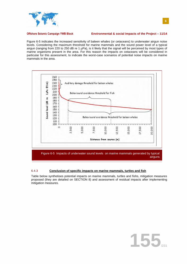
6
Offshore Seismic Campaign YWB Block Environmental & social impacts of the Project – 11/14
155/231
Figure 6-5 indicates the increased sensitivity of baleen whales (or cetaceans) to underwater airgun noise levels. Considering the maximum threshold for marine mammals and the sound power level of a typical airgun (ranging from 220 to 250 dB re 1 µPa), is it likely that the signal will be perceived by most types of marine organisms present in the area. For this reason the impacts on cetaceans will be considered in particular for this assessment, to indicate the worst-case scenarios of potential noise impacts on marine mammals in the area.
6.4.3 Conclusion of specific impacts on marine mammals, turtles and fish
Table below synthetises potential impacts on marine mammals, turtles and fishs, mitigation measures proposed (they are detailed on SECTION 8) and assessment of residual impacts after implementing mitigation measures.
Figure 6-5 Impacts of underwater sound levels on marine mammals generated by typical airguns
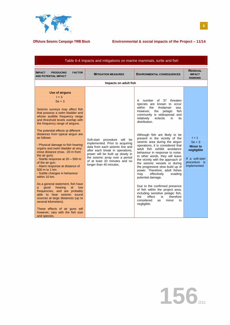
6
Offshore Seismic Campaign YWB Block Environmental & social impacts of the Project – 11/14
156/231
Table 6-4 Impacts and mitigations on marine mammals, turtle and fish
IMPACT PRODUCING FACTOR AND POTENTIAL IMPACT
MITIGATION MEASURES ENVIRONMENTAL CONSEQUENCES RESIDUAL
IMPACT
RANKING
Impacts on adult fish
Use of airguns
I = 3
Se = 3
Seismic surveys may affect fish that possess a swim bladder and whose audible frequency range and threshold levels overlap with the frequency range of airguns. The potential effects at different distances from typical airgun are as follows:
- Physical damage to fish hearing organs and swim bladder at very close distance (max. :20 m from the air gun); - Startle response at 20 – 500 m of the air gun; - Alarm response at distance of 500 m to 1 km - Subtle changes in behaviour within 10 km.
As a general statement, fish have a good hearing at low frequencies, and are probably able to hear seismic sound sources at large distances (up to several kilometers). These effects of air guns will however, vary with the fish size and species.
Soft-start procedure will be implemented. Prior to acquiring data from each seismic line and after each break in operations, power will be built up slowly in the seismic array over a period of at least 20 minutes and no longer than 40 minutes.
A number of 37 threaten species are known to occur within the Andaman sea. However, the pelagic fish community is widespread and relatively eclectic in its distribution.
Although fish are likely to be present in the vicinity of the seismic area during the airgun operations, it is considered that adult fish exhibit avoidance behaviour in response to noise. In other words, they will leave the vicinity with the approach of the seismic vessels or during the progressive slow build up of power. Therefore, adult fishes may effectively evading potential damage.
Due to the confirmed presence of fish within the project area, including sensitive pelagic fish, the effect is therefore considered as minor to negligible.
I = 1
Se = 3
Minor to negligible
If a soft-start procedure is implemented
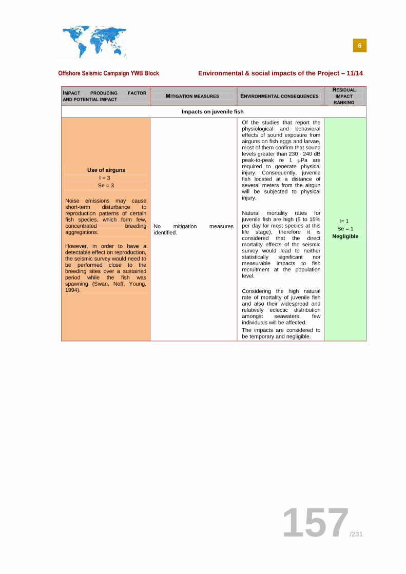
6
Offshore Seismic Campaign YWB Block Environmental & social impacts of the Project – 11/14
157/231
IMPACT PRODUCING FACTOR AND POTENTIAL IMPACT
MITIGATION MEASURES ENVIRONMENTAL CONSEQUENCES RESIDUAL
IMPACT
RANKING
Impacts on juvenile fish
Use of airguns
I = 3
Se = 3
Noise emissions may cause short-term disturbance to reproduction patterns of certain fish species, which form few, concentrated breeding aggregations.
However, in order to have a detectable effect on reproduction, the seismic survey would need to be performed close to the breeding sites over a sustained period while the fish was spawning (Swan, Neff, Young, 1994).
No mitigation measures identified.
Of the studies that report the physiological and behavioral effects of sound exposure from airguns on fish eggs and larvae, most of them confirm that sound levels greater than 230 - 240 dB peak-to-peak re 1 µPa are required to generate physical injury. Consequently, juvenile fish located at a distance of several meters from the airgun will be subjected to physical injury.
Natural mortality rates for juvenile fish are high (5 to 15% per day for most species at this life stage), therefore it is considered that the direct mortality effects of the seismic survey would lead to neither statistically significant nor measurable impacts to fish recruitment at the population level.
Considering the high natural rate of mortality of juvenile fish and also their widespread and relatively eclectic distribution amongst seawaters, few individuals will be affected.
The impacts are considered to be temporary and negligible.
I= 1
Se = 1
Negligible
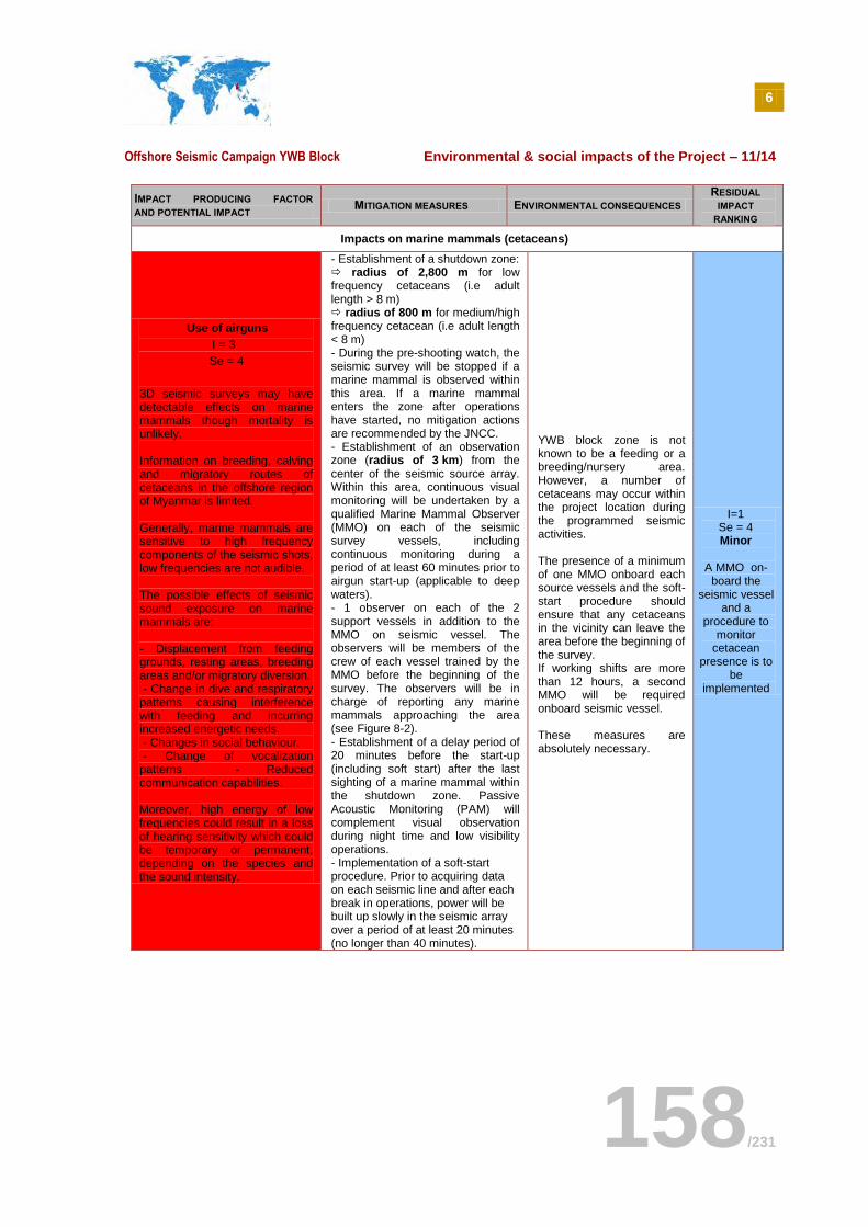
6
Offshore Seismic Campaign YWB Block Environmental & social impacts of the Project – 11/14
158/231
IMPACT PRODUCING FACTOR AND POTENTIAL IMPACT
MITIGATION MEASURES ENVIRONMENTAL CONSEQUENCES RESIDUAL
IMPACT
RANKING
Impacts on marine mammals (cetaceans)
Use of airguns
I = 3
Se = 4
3D seismic surveys may have detectable effects on marine mammals though mortality is unlikely. Information on breeding, calving and migratory routes of cetaceans in the offshore region of Myanmar is limited. Generally, marine mammals are sensitive to high frequency components of the seismic shots, low frequencies are not audible. The possible effects of seismic sound exposure on marine mammals are: - Displacement from feeding grounds, resting areas, breeding areas and/or migratory diversion. - Change in dive and respiratory patterns causing interference with feeding and incurring increased energetic needs. - Changes in social behaviour. - Change of vocalization patterns - Reduced communication capabilities.
Moreover, high energy of low frequencies could result in a loss of hearing sensitivity which could be temporary or permanent, depending on the species and the sound intensity.
- Establishment of a shutdown zone: radius of 2,800 m for low frequency cetaceans (i.e adult length > 8 m) radius of 800 m for medium/high frequency cetacean (i.e adult length < 8 m) - During the pre-shooting watch, the seismic survey will be stopped if a marine mammal is observed within this area. If a marine mammal enters the zone after operations have started, no mitigation actions are recommended by the JNCC. - Establishment of an observation zone (radius of 3 km) from the center of the seismic source array. Within this area, continuous visual monitoring will be undertaken by a qualified Marine Mammal Observer (MMO) on each of the seismic survey vessels, including continuous monitoring during a period of at least 60 minutes prior to airgun start-up (applicable to deep waters). - 1 observer on each of the 2 support vessels in addition to the MMO on seismic vessel. The observers will be members of the crew of each vessel trained by the MMO before the beginning of the survey. The observers will be in charge of reporting any marine mammals approaching the area (see Figure 8-2). - Establishment of a delay period of 20 minutes before the start-up (including soft start) after the last sighting of a marine mammal within the shutdown zone. Passive Acoustic Monitoring (PAM) will complement visual observation during night time and low visibility operations. - Implementation of a soft-start procedure. Prior to acquiring data on each seismic line and after each break in operations, power will be built up slowly in the seismic array over a period of at least 20 minutes (no longer than 40 minutes).
YWB block zone is not known to be a feeding or a breeding/nursery area. However, a number of cetaceans may occur within the project location during the programmed seismic activities. The presence of a minimum of one MMO onboard each source vessels and the soft-start procedure should ensure that any cetaceans in the vicinity can leave the area before the beginning of the survey. If working shifts are more than 12 hours, a second MMO will be required onboard seismic vessel. These measures are absolutely necessary.
I=1 Se = 4 Minor
A MMO on-
board the seismic vessel
and a procedure to
monitor cetacean
presence is to be
implemented
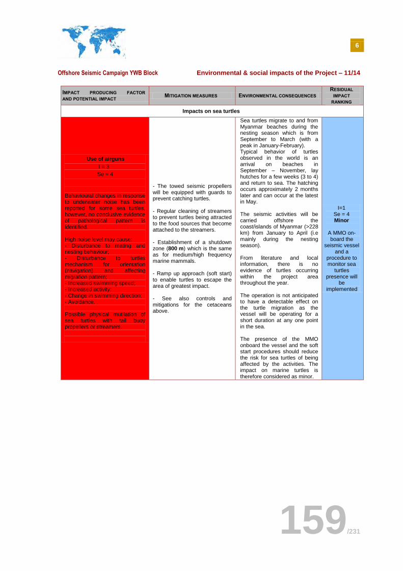
6
Offshore Seismic Campaign YWB Block Environmental & social impacts of the Project – 11/14
159/231
IMPACT PRODUCING FACTOR AND POTENTIAL IMPACT
MITIGATION MEASURES ENVIRONMENTAL CONSEQUENCES RESIDUAL
IMPACT
RANKING
Impacts on sea turtles
Use of airguns
I = 3
Se = 4
Behavioural changes in response to underwater noise has been reported for some sea turtles, however, no conclusive evidence of pathological pattern is identified. High noise level may cause: - Disturbance to mating and nesting behaviour; - Disturbance to turtles mechanism for orientation (navigation) and affecting migration pattern; - Increased swimming speed; - Increased activity; - Change in swimming direction; - Avoidance. Possible physical mutilation of sea turtles with tail buoy propellers or streamers.
- The towed seismic propellers will be equipped with guards to prevent catching turtles. - Regular cleaning of streamers to prevent turtles being attracted to the food sources that become attached to the streamers. - Establishment of a shutdown zone (800 m) which is the same as for medium/high frequency marine mammals. - Ramp up approach (soft start) to enable turtles to escape the area of greatest impact. - See also controls and mitigations for the cetaceans above.
Sea turtles migrate to and from Myanmar beaches during the nesting season which is from September to March (with a peak in January-February). Typical behavior of turtles observed in the world is an arrival on beaches in September – November, lay hutches for a few weeks (3 to 4) and return to sea. The hatching occurs approximately 2 months later and can occur at the latest in May. The seismic activities will be carried offshore the coast/islands of Myanmar (>228 km) from January to April (i.e mainly during the nesting season). From literature and local information, there is no evidence of turtles occurring within the project area throughout the year. The operation is not anticipated to have a detectable effect on the turtle migration as the vessel will be operating for a short duration at any one point in the sea. The presence of the MMO onboard the vessel and the soft start procedures should reduce the risk for sea turtles of being affected by the activities. The impact on marine turtles is therefore considered as minor.
I=1 Se = 4 Minor
A MMO on-board the
seismic vessel and a
procedure to monitor sea
turtles presence will
be implemented
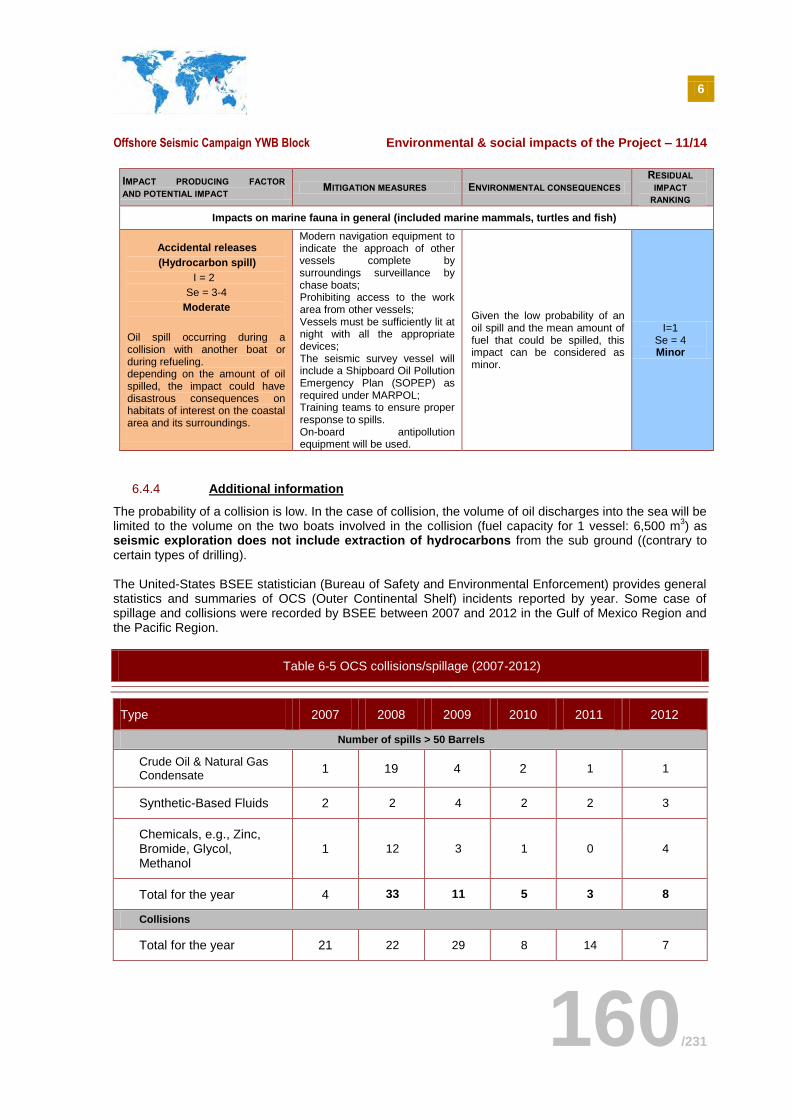
6
Offshore Seismic Campaign YWB Block Environmental & social impacts of the Project – 11/14
160/231
IMPACT PRODUCING FACTOR AND POTENTIAL IMPACT
MITIGATION MEASURES ENVIRONMENTAL CONSEQUENCES RESIDUAL
IMPACT
RANKING
Impacts on marine fauna in general (included marine mammals, turtles and fish)
Accidental releases
(Hydrocarbon spill)
I = 2
Se = 3-4
Moderate
Oil spill occurring during a collision with another boat or during refueling. depending on the amount of oil spilled, the impact could have disastrous consequences on habitats of interest on the coastal area and its surroundings.
Modern navigation equipment to indicate the approach of other vessels complete by surroundings surveillance by chase boats; Prohibiting access to the work area from other vessels; Vessels must be sufficiently lit at night with all the appropriate devices; The seismic survey vessel will include a Shipboard Oil Pollution Emergency Plan (SOPEP) as required under MARPOL; Training teams to ensure proper response to spills. On-board antipollution equipment will be used.
Given the low probability of an oil spill and the mean amount of fuel that could be spilled, this impact can be considered as minor.
I=1 Se = 4 Minor
6.4.4 Additional information
The probability of a collision is low. In the case of collision, the volume of oil discharges into the sea will be limited to the volume on the two boats involved in the collision (fuel capacity for 1 vessel: 6,500 m
3) as
seismic exploration does not include extraction of hydrocarbons from the sub ground ((contrary to certain types of drilling). The United-States BSEE statistician (Bureau of Safety and Environmental Enforcement) provides general statistics and summaries of OCS (Outer Continental Shelf) incidents reported by year. Some case of spillage and collisions were recorded by BSEE between 2007 and 2012 in the Gulf of Mexico Region and the Pacific Region.
Table 6-5 OCS collisions/spillage (2007-2012)
Type 2007 2008 2009 2010 2011 2012
Number of spills > 50 Barrels
Crude Oil & Natural Gas Condensate
1 19 4 2 1 1
Synthetic-Based Fluids 2 2 4 2 2 3
Chemicals, e.g., Zinc, Bromide, Glycol, Methanol
1 12 3 1 0 4
Total for the year 4 33 11 5 3 8
Collisions
Total for the year 21 22 29 8 14 7
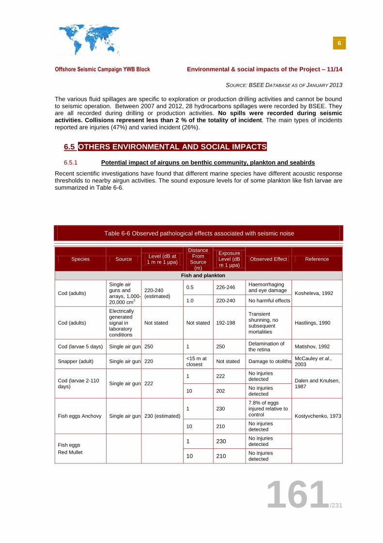
6
Offshore Seismic Campaign YWB Block Environmental & social impacts of the Project – 11/14
161/231
SOURCE: BSEE DATABASE AS OF JANUARY 2013
The various fluid spillages are specific to exploration or production drilling activities and cannot be bound to seismic operation. Between 2007 and 2012, 28 hydrocarbons spillages were recorded by BSEE. They are all recorded during drilling or production activities. No spills were recorded during seismic activities. Collisions represent less than 2 % of the totality of incident. The main types of incidents reported are injuries (47%) and varied incident (26%).
6.5 OTHERS ENVIRONMENTAL AND SOCIAL IMPACTS
6.5.1 Potential impact of airguns on benthic community, plankton and seabirds
Recent scientific investigations have found that different marine species have different acoustic response thresholds to nearby airgun activities. The sound exposure levels for of some plankton like fish larvae are summarized in Table 6-6.
Table 6-6 Observed pathological effects associated with seismic noise
Species Source Level (dB at
1 m re 1 µpa)
Distance From
Source (m)
Exposure Level (dB re 1 µpa)
Observed Effect Reference
Fish and plankton
Cod (adults)
Single air guns and arrays, 1,000-20,000 cm
3
220-240 (estimated)
0.5 226-246 Haemorrhaging and eye damage
Kosheleva, 1992
1.0 220-240 No harmful effects
Cod (adults)
Electrically generated signal in laboratory conditions
Not stated Not stated 192-198
Transient shunning, no subsequent mortalities
Hastlings, 1990
Cod (larvae 5 days) Single air gun 250 1 250 Delamination of the retina
Matishov, 1992
Snapper (adult) Single air gun 220 <15 m at closest
Not stated Damage to otoliths McCauley et al., 2003
Cod (larvae 2-110 days)
Single air gun 222
1 222 No injuries detected Dalen and Knulsen,
1987 10 202
No injuries detected
Fish eggs Anchovy Single air gun 230 (estimated)
1 230 7.8% of eggs injured relative to control Kostyvchenko, 1973
10 210 No injuries detected
Fish eggs
Red Mullet
1 230 No injuries detected
10 210 No injuries detected
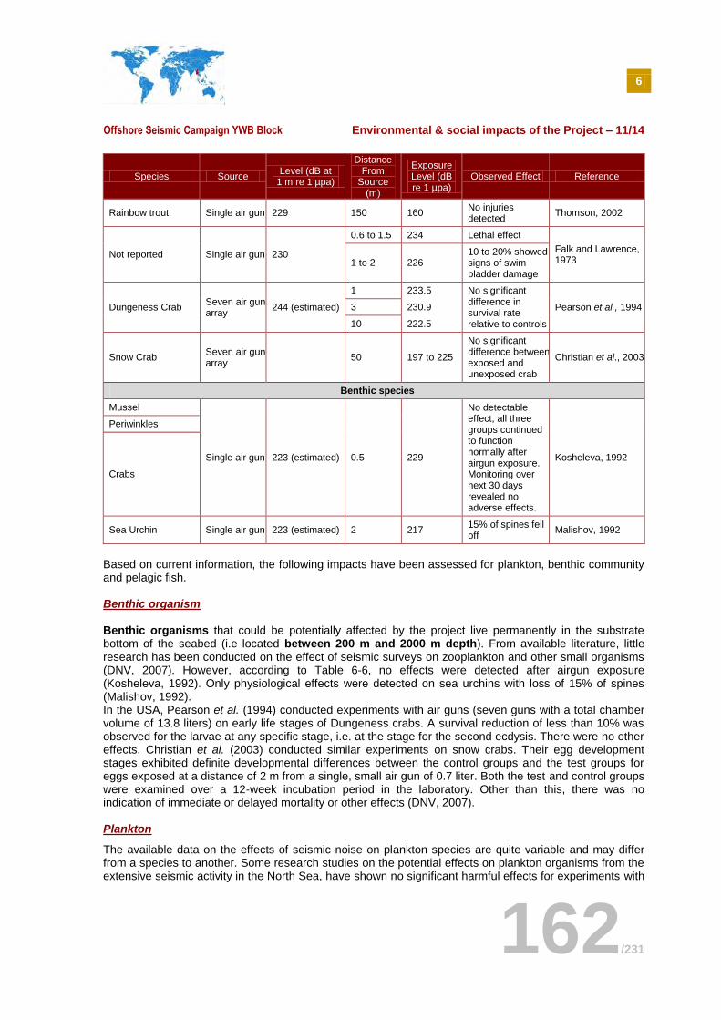
6
Offshore Seismic Campaign YWB Block Environmental & social impacts of the Project – 11/14
162/231
Species Source Level (dB at
1 m re 1 µpa)
Distance From
Source (m)
Exposure Level (dB re 1 µpa)
Observed Effect Reference
Rainbow trout Single air gun 229 150 160 No injuries detected
Thomson, 2002
Not reported Single air gun 230
0.6 to 1.5 234 Lethal effect
Falk and Lawrence, 1973 1 to 2 226
10 to 20% showed signs of swim bladder damage
Dungeness Crab Seven air gun array
244 (estimated)
1 233.5 No significant difference in survival rate relative to controls
Pearson et al., 1994 3 230.9
10 222.5
Snow Crab Seven air gun array
50 197 to 225
No significant difference between exposed and unexposed crab
Christian et al., 2003
Benthic species
Mussel
Single air gun 223 (estimated) 0.5 229
No detectable effect, all three groups continued to function normally after airgun exposure. Monitoring over next 30 days revealed no adverse effects.
Kosheleva, 1992
Periwinkles
Crabs
Sea Urchin Single air gun 223 (estimated) 2 217 15% of spines fell off
Malishov, 1992
Based on current information, the following impacts have been assessed for plankton, benthic community and pelagic fish.
Benthic organism
Benthic organisms that could be potentially affected by the project live permanently in the substrate bottom of the seabed (i.e located between 200 m and 2000 m depth). From available literature, little research has been conducted on the effect of seismic surveys on zooplankton and other small organisms (DNV, 2007). However, according to Table 6-6, no effects were detected after airgun exposure (Kosheleva, 1992). Only physiological effects were detected on sea urchins with loss of 15% of spines (Malishov, 1992). In the USA, Pearson et al. (1994) conducted experiments with air guns (seven guns with a total chamber volume of 13.8 liters) on early life stages of Dungeness crabs. A survival reduction of less than 10% was observed for the larvae at any specific stage, i.e. at the stage for the second ecdysis. There were no other effects. Christian et al. (2003) conducted similar experiments on snow crabs. Their egg development stages exhibited definite developmental differences between the control groups and the test groups for eggs exposed at a distance of 2 m from a single, small air gun of 0.7 liter. Both the test and control groups were examined over a 12-week incubation period in the laboratory. Other than this, there was no indication of immediate or delayed mortality or other effects (DNV, 2007).
Plankton
The available data on the effects of seismic noise on plankton species are quite variable and may differ from a species to another. Some research studies on the potential effects on plankton organisms from the extensive seismic activity in the North Sea, have shown no significant harmful effects for experiments with
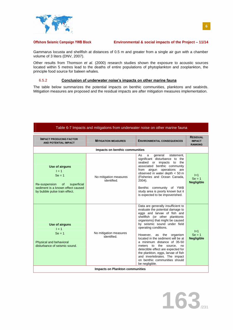
6
Offshore Seismic Campaign YWB Block Environmental & social impacts of the Project – 11/14
163/231
Gammarus locusta and shellfish at distances of 0.5 m and greater from a single air gun with a chamber volume of 3 liters (DNV, 2007).
Other results from Thomson et al. (2000) research studies shown the exposure to acoustic sources located within 5 metres lead to the deaths of entire populations of phytoplankton and zooplankton, the principle food source for baleen whales.
6.5.2 Conclusion of underwater noise’s impacts on other marine fauna
The table below summarizes the potential impacts on benthic communities, planktons and seabirds. Mitigation measures are proposed and the residual impacts are after mitigation measures implementation.
Table 6-7 Impacts and mitigations from underwater noise on other marine fauna
IMPACT PRODUCING FACTOR AND POTENTIAL IMPACT
MITIGATION MEASURES ENVIRONMENTAL CONSEQUENCES RESIDUAL
IMPACT
RANKING
Impacts on benthic communities
Use of airguns
I = 1
Se = 1
Re-suspension of superficial sediment is a known effect caused by bubble pulse train effect.
No mitigation measures identified.
As a general statement, significant disturbance to the seabed or impacts to the associated benthic community from airgun operations are observed in water depth < 50 m (Fisheries and Ocean Canada, 2004). Benthic community of YWB study area is poorly known but it is expected to be impoverished.
I=1 Se = 1
Negligible
Use of airguns
I = 1
Se = 1
Physical and behavioral disturbance of seismic sound.
No mitigation measures identified.
Data are generally insufficient to evaluate the potential damage to eggs and larvae of fish and shellfish (or other planktonic organisms) that might be caused by seismic sound under field operating conditions. However, as the organism located in the sediment will be at a minimum distance of 35-50 meters to the source, no detectible effect are expected for the plankton, eggs, larvae of fish and invertebrates. The impact on benthic communities should be negligible.
I=1 Se = 1
Negligible
Impacts on Plankton communities
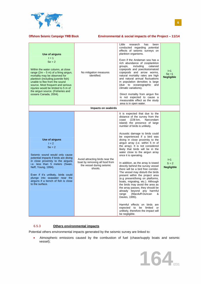
6
Offshore Seismic Campaign YWB Block Environmental & social impacts of the Project – 11/14
164/231
Use of airguns
I = 1
Se = 2
Within the water column, at close range (2m – 5 m) of a firing airgun, mortality may be observed for plankton (including juvenile fish) unable to flee from the sound source. Most frequent and serious injuries would be limited to 5 m of the airgun source. (Fisheries and oceans Canada, 2004).
No mitigation measures identified.
Little research has been conducted regarding potential effects of seismic surveys on plankton organisms. Even if the Andaman sea has a rich abundance of zooplankton groups, including calanoid copepods and poecilostomatoid copepods and arrow worms, natural mortality rates are high and natural annual fluctuations in population densities is large (due to oceanographic and climatic variations). Direct mortality from airgun fire is not expected to cause a measurable effect as the study area is in open water.
I=1 Se =1
Negligible
Impacts on seabirds
Use of airguns
I = 2
Se = 2
Seismic sound would only cause potential impacts if birds are diving in close proximity to the airguns i.e. less than 5 meters (Swan, Neff, Young, 1994).
Even if it’s unlikely, birds could plunge into seawater near the airguns if a bench of fish is close to the surface.
Avoid attracting birds near the boat by removing all food from
the vessel during seismic shoots.
It is expected that due to the distance of the survey from the coast (228 km, Narcondam island) the presence of large number of birds is unlikely.
Acoustic damage to birds could be experienced if a bird was diving in close proximity to the airgun array (i.e. within 5 m of the array). It is not considered likely that birds will be in the water close to the airgun array once it is operating.
In addition, as the array is towed directly behind the survey vessel there will be a bird free corridor. The vessel may disturb the birds present within the project area (e.g present/living on platforms, boats, migrating, etc.). Although the birds may avoid the area as the array passes, they should be already beyond any harmful range (Macduff-Duncan & Davies, 1995).
Harmful effects on birds are expected to be limited or unlikely, therefore the impact will be negligible.
I=1
S = 2
Negligible
6.5.3 Others environmental impacts
Potential others environmental impacts generated by the seismic survey are linked to:
Atmospheric emissions caused by the combustion of fuel (chase/supply boats and seismic vessel);
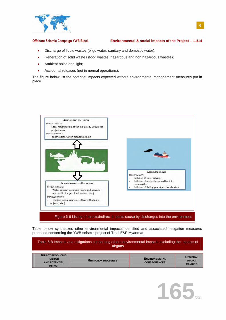
6
Offshore Seismic Campaign YWB Block Environmental & social impacts of the Project – 11/14
165/231
Discharge of liquid wastes (bilge water, sanitary and domestic water);
Generation of solid wastes (food wastes, hazardous and non hazardous wastes);
Ambient noise and light;
Accidental releases (not in normal operations).
The figure below list the potential impacts expected without environmental management measures put in place.
Table below synthetizes other environmental impacts identified and associated mitigation measures proposed concerning the YWB seismic project of Total E&P Myanmar.
Table 6-8 Impacts and mitigations concerning others environmental impacts excluding the impacts of airguns
IMPACT PRODUCING
FACTOR AND POTENTIAL
IMPACT
MITIGATION MEASURES ENVIRONMENTAL
CONSEQUENCES
RESIDUAL
IMPACT
RANKING
Figure 6-6 Listing of directs/indirect impacts cause by discharges into the environment
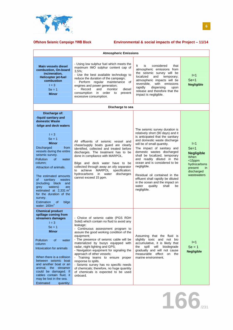
6
Offshore Seismic Campaign YWB Block Environmental & social impacts of the Project – 11/14
166/231
Atmospheric Emissions
Main vessels diesel combustion, On-board
incineration, Helicopter jet-fuel
combustion
I = 3
Se = 1
Minor
- - Using low sulphur fuel which meets the maximum IMO sulphur content cap of 3,5%;
- - Use the best available technology to reduce the duration of the campaign;
- - Perform regular maintenance of engines and power generation;
- - Record and monitor diesel consumption in order to prevent excessive consumption.
It is considered that atmospheric emissions from the seismic survey will be localized and temporary; atmospheric impacts will be reversible, with emissions rapidly dispersing upon release and therefore that the impact is negligible.
I=1
Se=1
Negligible
Discharge to sea
Discharge of:
-liquid sanitary and domestic Waste
-bilge and deck waters
I = 3
Se = 1
Minor
Discharged from vessels during the entire seismic survey.
Pollution of water column;
Attraction of animals.
The estimated amounts of sanitary wastes (including black and grey waters) are estimated at 2,331 m
3
for the duration of the survey.
Estimation of bilge water: 160m
3
All effluents of seismic vessel and chase/supply boats guard are clearly identified, collected and treated before discharges. The treatment has to be done in compliance with MARPOL. Bilge and deck water have to be collected through away an oily separator to achieve MARPOL specification: hydrocarbons in water discharges cannot exceed 15 ppm.
The seismic survey duration is relatively short (90 days) and it is anticipated that the sanitary and domestic waste discharge will be of small quantity.
The impact of sanitary and domestic wastes discharged shall be localized, temporary and readily diluted in the ocean and is considered to be negligible.
Residual oil contained in the effluent shall rapidly be diluted in the ocean and the impact on water quality shall be negligible.
I=1
Se=1
Negligible
When <15ppm hydrocarbons present in discharged wastewaters
Chemical product spillage coming from streamers damages
I = 3
Se = 1
Minor
Pollution of water column
Intoxication for animals
When there is a collision between seismic boat and another boat or an animal, the streamer could be damaged. If cables contain fluid, it may be lost in the sea.
Estimated quantity:
- - Choice of seismic cable (PGS RDH Solid) which contain no fluid to avoid any leakage;
- - Continuous assessment program to assure the good working condition of the equipment;
- - The presence of seismic cable will be materialized by buoys equipped with radar, night lighting and GPS;
- - Navigation equipment for signaling the approach of other vessels;
- - Training teams to ensure proper response to spills.
- - Seismic survey has no specific needs of chemicals; therefore, no huge quantity of chemicals is expected to be used onboard.
Assuming that the fluid is slightly toxic and not bio accumulative, it is likely that the spill will biodegrade gradually and will not cause measurable effect on the marine environment.
I=1
Se = 1
Negligible
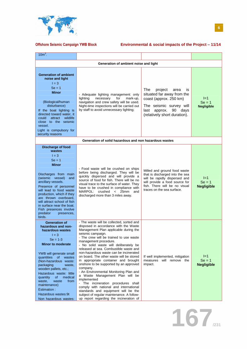
6
Offshore Seismic Campaign YWB Block Environmental & social impacts of the Project – 11/14
167/231
10m3.
Generation of ambient noise and light
Generation of ambient noise and light
I = 3
Se = 1
Minor
(Biological/human disturbance)
If the boat lighting is directed toward water, it could attract wildlife close to the seismic vessel.
Light is compulsory for security reasons
- - Adequate lighting management: only lighting necessary for mark-up, navigation and crew safety will be used. Night-time inspections will be carried out by staff to avoid unnecessary lighting;
The project area is situated far away from the coast (approx. 250 km)
The seismic survey will last approx. 90 days (relatively short duration).
I=1 Se = 1
Negligible
Generation of solid hazardous and non hazardous wastes
Discharge of food wastes
I = 3
Se = 1
Minor
Discharges from main (seismic vessel) and ancillary vessels.
Presence of personnel will lead to food waste production, which if they are thrown overboard, will attract school of fish in surface near the boat. Fish presences involve predator presences, birds.
- - Food waste will be crushed on ships before being discharged. They will be quickly dispersed and will provide a source of food for fish. There will be no visual trace to the surface of water. They have to be crushed in compliance with MARPOL: crushed < 25mm and discharged more than 3 miles away.
Milled and ground food waste that is discharged into the sea will be rapidly dispersed and will provide a food source for fish. There will be no visual traces on the sea surface.
I=1 Se = 1
Negligible
Generation of hazardous and non- hazardous wastes
I = 3
Se = 1-3
Minor to moderate
YWB will generate small quantities of wastes (Non-hazardous waste: packaging waste, wooden pallets, etc.;
Hazardous waste: little quantity of medical waste, waste from maintenance)
Estimation :
Hazardous wastes:9t
Non hazardous wastes:
- - The waste will be collected, sorted and disposed in accordance with the Waste Management Plan applicable during the seismic campaign.
- - The crew will be trained to use waste management procedure.
- - No solid waste will deliberately be released at sea. Combustible waste and non-hazardous waste can be incinerated on board. The other waste will be stored in appropriate container and brought onshore to be supported by an approved company.
- - An Environmental Monitoring Plan and a Waste Management Plan will be implemented
- - The incineration procedures shall comply with national and international standards and equipment will be the subject of regular maintenance. A follow-up report regarding the incineration of
If well implemented, mitigation measures will remove the impact.
I=1 Se = 1
Negligible
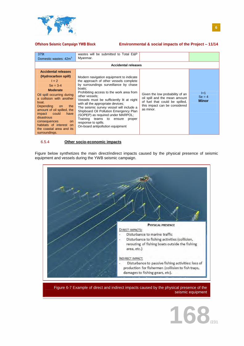
6
Offshore Seismic Campaign YWB Block Environmental & social impacts of the Project – 11/14
168/231
379t
Domestic wastes: 42m3
wastes will be submitted to Total E&P Myanmar.
Accidental releases
Accidental releases
(Hydrocarbon spill)
I = 2
Se = 3-4
Moderate
Oil spill occurring during a collision with another boat. Depending on the amount of oil spilled, the impact could have disastrous consequences on habitats of interest on the coastal area and its surroundings.
Modern navigation equipment to indicate the approach of other vessels complete by surroundings surveillance by chase boats; Prohibiting access to the work area from other vessels; Vessels must be sufficiently lit at night with all the appropriate devices; The seismic survey vessel will include a Shipboard Oil Pollution Emergency Plan (SOPEP) as required under MARPOL; Training teams to ensure proper response to spills. On-board antipollution equipment
Given the low probability of an oil spill and the mean amount of fuel that could be spilled, this impact can be considered as minor.
I=1 Se = 4
Minor
6.5.4 Other socio-economic impacts
Figure below synthetizes the main direct/indirect impacts caused by the physical presence of seismic equipment and vessels during the YWB seismic campaign.
Figure 6-7 Example of direct and indirect impacts caused by the physical presence of the seismic equipment
6
Offshore Seismic Campaign YWB Block Environmental & social impacts of the Project – 11/14
169/231
As shown in the analysis of sensitive components, the only two social components that will be impacted by the project are the commercial marine traffic and the offshore fishery sector.
6.5.4.1 Disturbances to marine traffic
During a seismic campaign, disturbances to commercial marine traffic are caused by the physical presence and movements of the survey vessel and the chase/supply boats. Indeed, their presence can cause collision with all kind of ships, including commercial ships. Unlike for fixed facilities, there are no requirements for a formal safety zone to be established around seismic vessels. Aside from applying the general maritime rules (in order to avoid collision between vessels), navigation restrictions will have to be implemented. Ships have to be excluded from the operational area of the seismic in order to limit the risks. This exclusion may cause a rerouting of the vessels that usually cross the seismic survey area to reach their port of destination.
6.5.4.2 Disturbance to fishing activities
As detailed in the part 6.4 , seismic operations can have direct impacts on fish populations evolving at the seismic location during the shooting. The underwater acoustic sound produced by airguns can affect fish and fish banks behaviors, causing them to either move down to the sea bottom or leave the seismic location temporarily. However, several studies proved that this impact’s effect on socio-economic activities cannot be assessed. A report, produced for the Norwegian Oil Industry Association in 2003 and gathering results of seismic impacts assessments on fish and fisheries concludes that although behavioral changes of fish are confirmed by scientific studies, there are no effects of seismic surveys on long term catch rates or on the size of fish stocks in general
31, as opposed to fishermen’s
general belief that seismic activities interfere with fisheries in a negative way. A more recent study commissioned by the Norwegian Petroleum Directorate and conducted by the Institute of Marine Research in 2009, confirmed that the sound produced by a 3D seismic survey performed in the Nordland temporarily influenced either positively or negatively the fish catches based on the type of species (it was observed that there were increases in fish catches for some endemic species, and reductions of catches for others
32.)
Another impact of seismic surveys on fisheries is the general disturbance to fishing activities induced by the physical presence of boats and cables, which can cause a loss of equipment or production for fishermen as described below:
Seismic vessels can collide with fishing boats;
Active fishing gears in the form of nets stretching behind fishing boats can be damaged by the seismic vessels or the streamers;
Passive fishing gears in the form of static fish traps or fish aggregating devices installed in the sea and marked by a buoy (or even unmarked) can also be damaged by vessel movements.
For safety reasons, and to avoid loss of seismic material during the survey performance, fishermen must be kept out from the operational area. This can cause a perturbation of their daily activities and a possible loss of production if they cannot perform fishing in another area. The table below synthetises the potential socio-economic impacts, the mitigation measures proposed and the assessment of residual impacts after implementation of the mitigation measures.
31
GAUSLAND Ingebret, Seismic Surveys Impacts on Fish and Fisheries, Report for Norwegian Oil Industry Association, March 2003. 32
http://www.imr.no/forskning/prosjekter/seismikk_gav_bade_okte_og_reduserte_fiskefangster/en.
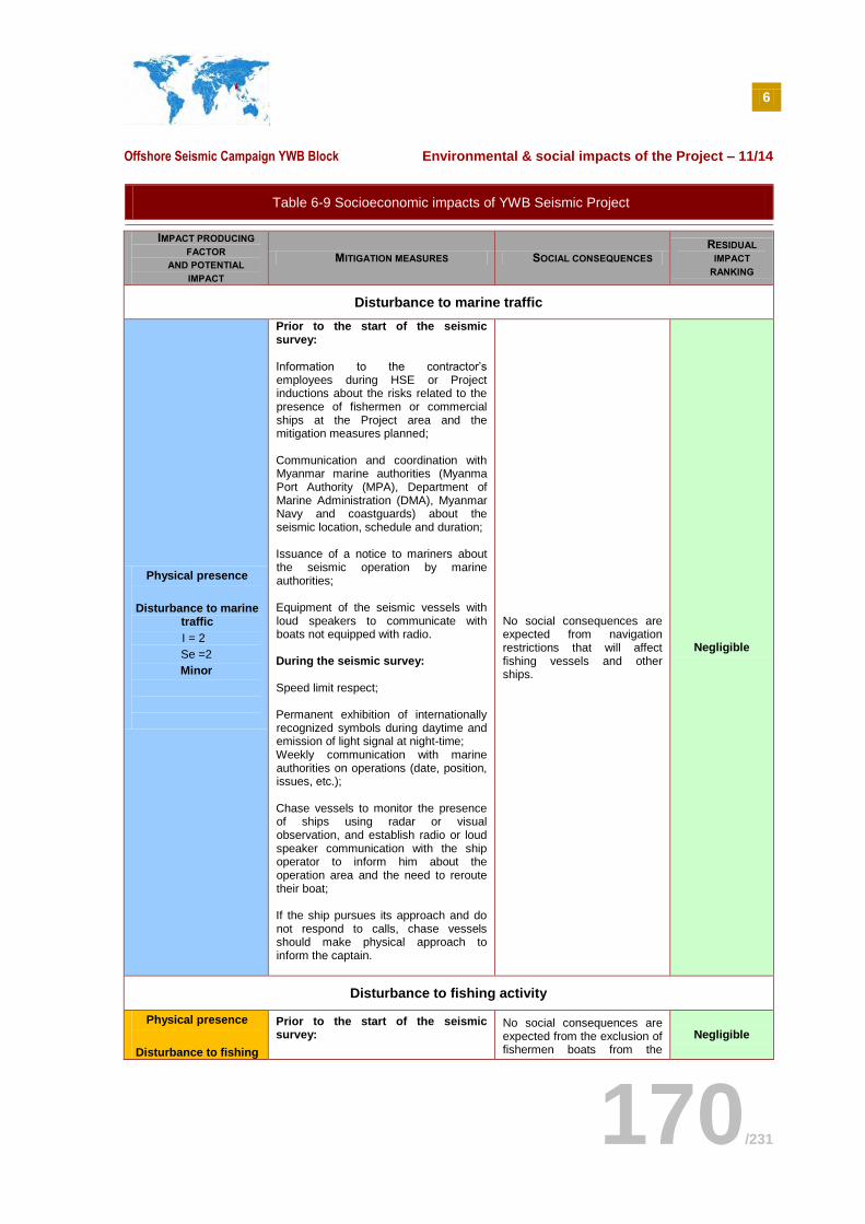
6
Offshore Seismic Campaign YWB Block Environmental & social impacts of the Project – 11/14
170/231
Table 6-9 Socioeconomic impacts of YWB Seismic Project
IMPACT PRODUCING
FACTOR AND POTENTIAL
IMPACT
MITIGATION MEASURES SOCIAL CONSEQUENCES RESIDUAL
IMPACT
RANKING
Disturbance to marine traffic
Physical presence
Disturbance to marine traffic
I = 2
Se =2
Minor
Prior to the start of the seismic survey:
- Information to the contractor’s
employees during HSE or Project inductions about the risks related to the presence of fishermen or commercial ships at the Project area and the mitigation measures planned;
- - Communication and coordination with
Myanmar marine authorities (Myanma Port Authority (MPA), Department of Marine Administration (DMA), Myanmar Navy and coastguards) about the seismic location, schedule and duration;
- - Issuance of a notice to mariners about
the seismic operation by marine authorities;
- - Equipment of the seismic vessels with
loud speakers to communicate with boats not equipped with radio.
During the seismic survey:
- - Speed limit respect; - - Permanent exhibition of internationally
recognized symbols during daytime and emission of light signal at night-time;
- Weekly communication with marine authorities on operations (date, position, issues, etc.);
- - Chase vessels to monitor the presence
of ships using radar or visual observation, and establish radio or loud speaker communication with the ship operator to inform him about the operation area and the need to reroute their boat;
- - If the ship pursues its approach and do
not respond to calls, chase vessels should make physical approach to inform the captain.
No social consequences are expected from navigation restrictions that will affect fishing vessels and other ships.
Negligible
Disturbance to fishing activity
Physical presence
Disturbance to fishing
Prior to the start of the seismic survey:
-
No social consequences are expected from the exclusion of fishermen boats from the
Negligible
6
Offshore Seismic Campaign YWB Block Environmental & social impacts of the Project – 11/14
171/231
activities
I = 3
Se = 2
Moderate
- Communication and coordination with marine authorities and main fishery stakeholders (DoF and MFF) about the seismic location, schedule and duration;
- - Preparation of flyers on the seismic
campaign in Burmese and Thai language;
- - Recruitment of a Fisheries Liaison
Officer able to speak Burmese and Thai languages that will participate to the survey and handle encounters with both Burmese and Thai fishermen, solving any issues that could arise between these fishermen and the project;
- A scouting survey enabling to assess the fishery activity at the seismic area (localize fishermen and interview them to determine their origin, spot and count the fish traps installed in the area) should be conducted before the seismic starts even if there is a low probability of encounters with fishermen and of the presence of fish traps. During the seismic survey: Chase vessels to monitor the presence of ships using radar or visual observation, and establish radio or loud speaker communication with the ship operator to inform him about the operation area and the need to reroute their boat; If the ship pursues its approach and do not respond to calls, chase vessels should make physical approach to inform the captain.
seismic survey area.
It is very unlikely that the project will create any jobs opportunity, especially in the Tanintharyi Region; this social impact is therefore neutral.
6.6 ECOSYSTEM EVALUATION
Myanmar fishery sector annually produces 4.464 million tons of seafood products, stemming from inland and marine fisheries and generates USD 650 million revenues in export for the country. Among these 4.464 million tons, half (2.332 million tons) is produced by the marine fisheries in an area of 480,000 square kilometers.
However, due to the Project’s far distance from the coast, its location in deepwater, its short campaign duration (3 months), added to the fact that it is not located on major tuna fishing grounds and that foreign fishing boats have been banned from the country’s waters since April 2014, it is extremely unlikely that the seismic survey has a decrease effect on the fish catches. Therefore, the operation will not impact the ecosystem in a way that would decrease its capacity to provide resources and revenues to individuals.
6
Offshore Seismic Campaign YWB Block Environmental & social impacts of the Project – 11/14
172/231
6.7 CUMULATIVE IMPACT ASSESSMENT
6.7.1 General issues
The environmental impacts associated with a project may be accumulated or intensified when considered in the context of existing operations in the area. The cumulative impacts on different environmental indicators may vary depending on the scale, intensity, and proximity of multiple operations, as well as the interactions of environmental ecosystems affected.
This assessment allows the consideration of deviations from baseline environmental conditions as a result of simultaneous marine activities, current and future, and accounts for the seeming insignificance of a single activity which may trigger, aggravate or in some other way worsen the impacts of a project when considered in collaboration with another.
The evaluation of cumulative impacts associated with seismic activities is extremely complex due to the transient nature of airgun fire, the continual displacement of the source and other diverse operational and environmental interactions.
In order to account for the complexity of cumulative impacts, this assessment was conducted in four phases:
Identification of environmental components which may be significantly adversely affected by the project;
Identification of projects or activities (mainly future) which may have a negative impact on the environmental components identified above;
Determination of the sensitivity of environmental components to cumulative impacts (be they over a short- or long-term period) when considered in parallel with other projects or activities identified in the area;
Determination of significance of cumulative impacts on the environmental components after consideration of proposed mitigation measures.
The potential impacts associated with the marine YWB seismic survey are considered in the context of other existing marine operations in the potentially affected area in the sections below.
6.7.2 Potential environmental impacts associated with seismic activities
The impact assessment indicated that the environmental components susceptible to be the most affected by the YWB seismic activities are the:
Acoustic environment and response mechanisms of marine mammals;
And in least extension, socio-economic environment as a result of disturbance to fishing and shipping traffic routes.
The cumulative effects on marine mammals and fishing/shipping traffic routes may appear if they are affected by other actions at the same time and in the same area.
It is possible that an operator from a nearby block shoot its seismic survey simultaneously with Total E&P Myanmar YWB Seismic project.
Environmental cumulative impacts are anticipated due to the significative increase of anthropogenic underwater sound generated by both seismic surveys which could have an impact on the marine fauna in general.
The logarithmic definition of the decibel scale implies that an increase of 10 times in the scale of sound pressure expressed in Pascal corresponds to a 20dB increase in the pressure level.
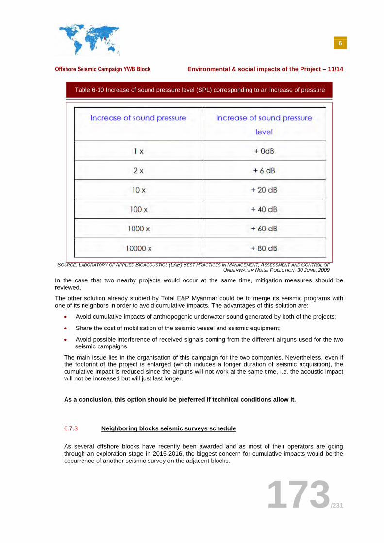
6
Offshore Seismic Campaign YWB Block Environmental & social impacts of the Project – 11/14
173/231
Table 6-10 Increase of sound pressure level (SPL) corresponding to an increase of pressure
SOURCE: LABORATORY OF APPLIED BIOACOUSTICS (LAB) BEST PRACTICES IN MANAGEMENT, ASSESSMENT AND CONTROL OF
UNDERWATER NOISE POLLUTION, 30 JUNE, 2009
In the case that two nearby projects would occur at the same time, mitigation measures should be reviewed.
The other solution already studied by Total E&P Myanmar could be to merge its seismic programs with one of its neighbors in order to avoid cumulative impacts. The advantages of this solution are:
Avoid cumulative impacts of anthropogenic underwater sound generated by both of the projects;
Share the cost of mobilisation of the seismic vessel and seismic equipment;
Avoid possible interference of received signals coming from the different airguns used for the two seismic campaigns.
The main issue lies in the organisation of this campaign for the two companies. Nevertheless, even if the footprint of the project is enlarged (which induces a longer duration of seismic acquisition), the cumulative impact is reduced since the airguns will not work at the same time, i.e. the acoustic impact will not be increased but will just last longer. As a conclusion, this option should be preferred if technical conditions allow it.
6.7.3 Neighboring blocks seismic surveys schedule
As several offshore blocks have recently been awarded and as most of their operators are going through an exploration stage in 2015-2016, the biggest concern for cumulative impacts would be the occurrence of another seismic survey on the adjacent blocks.
6
Offshore Seismic Campaign YWB Block Environmental & social impacts of the Project – 11/14
174/231
The adjacent blocks are as follows:
Block M11: PTTEP – a seismic survey is planned for early 2016 and will be perform with the same acquisition vessel as TEPM, just before the seismic survey on YWB. Therefore there won’t be any cumulative impacts because of this project as these surveys don’t occur at the same time.
Block M12: Petronas – Yetagun - no seismic survey planned at the time of the TEPM’s seismic campaign.
Block MD-4: ENI – no seismic survey planned in 2016 According to this schedule there won’t be any other seismic survey on the neighboring blocks at the same time. The fact that the same vessel is used for the seismic acquisition on different blocks enables to limit the cumulative impacts of these surveys in the Myanmar waters. It is noticeable that coordination meetings are organized between O&G actors on a regular basis, at both Managerial and HSE levels.
6
Offshore Seismic Campaign YWB Block Environmental & social impacts of the Project – 11/14
175/231
6.8 2D SEISMIC SURVEY ALTERNATIVE
The original project is about a 3D seismic survey but TEPM could change and implement a 2D seismic survey instead. The 2D survey would use only source and one streamer, and it would cover less kilometres (and last only one month), therefore it is assumed that the environmental & social impacts of the 2D seismic campaign would be lighter than those from the 3D one. So, if the 2D alternative is chosen, the mitigation measures described for the 3D survey will be enough to cover efficiently these impacts.
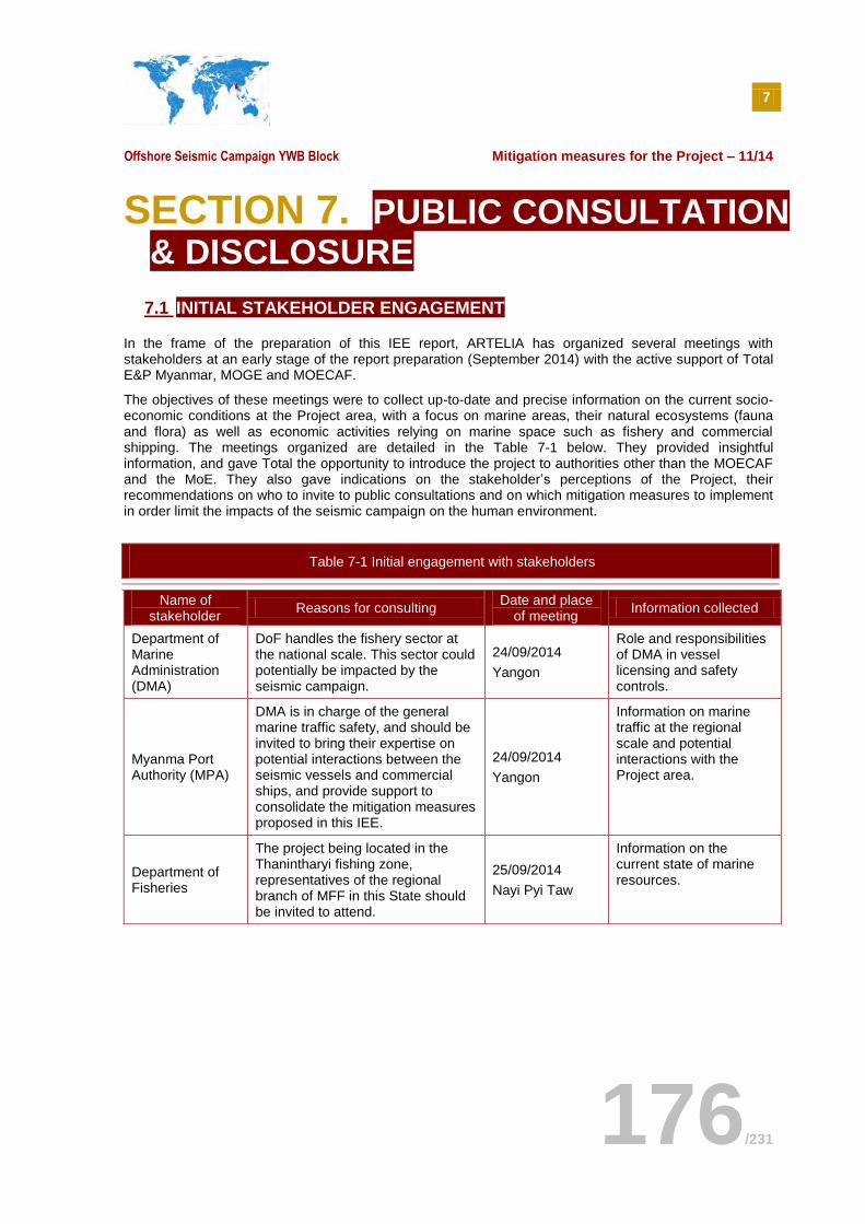
7
Offshore Seismic Campaign YWB Block Mitigation measures for the Project – 11/14
176/231
SECTION 7. PUBLIC CONSULTATION & DISCLOSURE
7.1 INITIAL STAKEHOLDER ENGAGEMENT
In the frame of the preparation of this IEE report, ARTELIA has organized several meetings with stakeholders at an early stage of the report preparation (September 2014) with the active support of Total E&P Myanmar, MOGE and MOECAF.
The objectives of these meetings were to collect up-to-date and precise information on the current socio-economic conditions at the Project area, with a focus on marine areas, their natural ecosystems (fauna and flora) as well as economic activities relying on marine space such as fishery and commercial shipping. The meetings organized are detailed in the Table 7-1 below. They provided insightful information, and gave Total the opportunity to introduce the project to authorities other than the MOECAF and the MoE. They also gave indications on the stakeholder’s perceptions of the Project, their recommendations on who to invite to public consultations and on which mitigation measures to implement in order limit the impacts of the seismic campaign on the human environment.
Table 7-1 Initial engagement with stakeholders
Name of stakeholder
Reasons for consulting Date and place
of meeting Information collected
Department of Marine Administration (DMA)
DoF handles the fishery sector at the national scale. This sector could potentially be impacted by the seismic campaign.
24/09/2014
Yangon
Role and responsibilities of DMA in vessel licensing and safety controls.
Myanma Port Authority (MPA)
DMA is in charge of the general marine traffic safety, and should be invited to bring their expertise on potential interactions between the seismic vessels and commercial ships, and provide support to consolidate the mitigation measures proposed in this IEE.
24/09/2014
Yangon
Information on marine traffic at the regional scale and potential interactions with the Project area.
Department of Fisheries
The project being located in the Thanintharyi fishing zone, representatives of the regional branch of MFF in this State should be invited to attend.
25/09/2014
Nayi Pyi Taw
Information on the current state of marine resources.
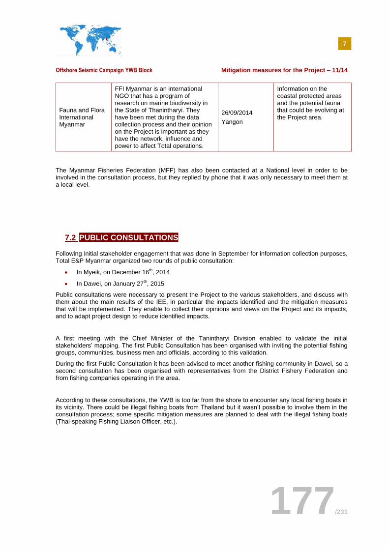
7
Offshore Seismic Campaign YWB Block Mitigation measures for the Project – 11/14
177/231
Fauna and Flora International Myanmar
FFI Myanmar is an international NGO that has a program of research on marine biodiversity in the State of Thanintharyi. They have been met during the data collection process and their opinion on the Project is important as they have the network, influence and power to affect Total operations.
26/09/2014
Yangon
Information on the coastal protected areas and the potential fauna that could be evolving at the Project area.
The Myanmar Fisheries Federation (MFF) has also been contacted at a National level in order to be involved in the consultation process, but they replied by phone that it was only necessary to meet them at a local level.
7.2 PUBLIC CONSULTATIONS
Following initial stakeholder engagement that was done in September for information collection purposes, Total E&P Myanmar organized two rounds of public consultation:
In Myeik, on December 16th, 2014
In Dawei, on January 27th, 2015
Public consultations were necessary to present the Project to the various stakeholders, and discuss with them about the main results of the IEE, in particular the impacts identified and the mitigation measures that will be implemented. They enable to collect their opinions and views on the Project and its impacts, and to adapt project design to reduce identified impacts.
A first meeting with the Chief Minister of the Tanintharyi Division enabled to validate the initial stakeholders’ mapping. The first Public Consultation has been organised with inviting the potential fishing groups, communities, business men and officials, according to this validation.
During the first Public Consultation it has been advised to meet another fishing community in Dawei, so a second consultation has been organised with representatives from the District Fishery Federation and from fishing companies operating in the area.
According to these consultations, the YWB is too far from the shore to encounter any local fishing boats in its vicinity. There could be illegal fishing boats from Thailand but it wasn’t possible to involve them in the consultation process; some specific mitigation measures are planned to deal with the illegal fishing boats (Thai-speaking Fishing Liaison Officer, etc.).
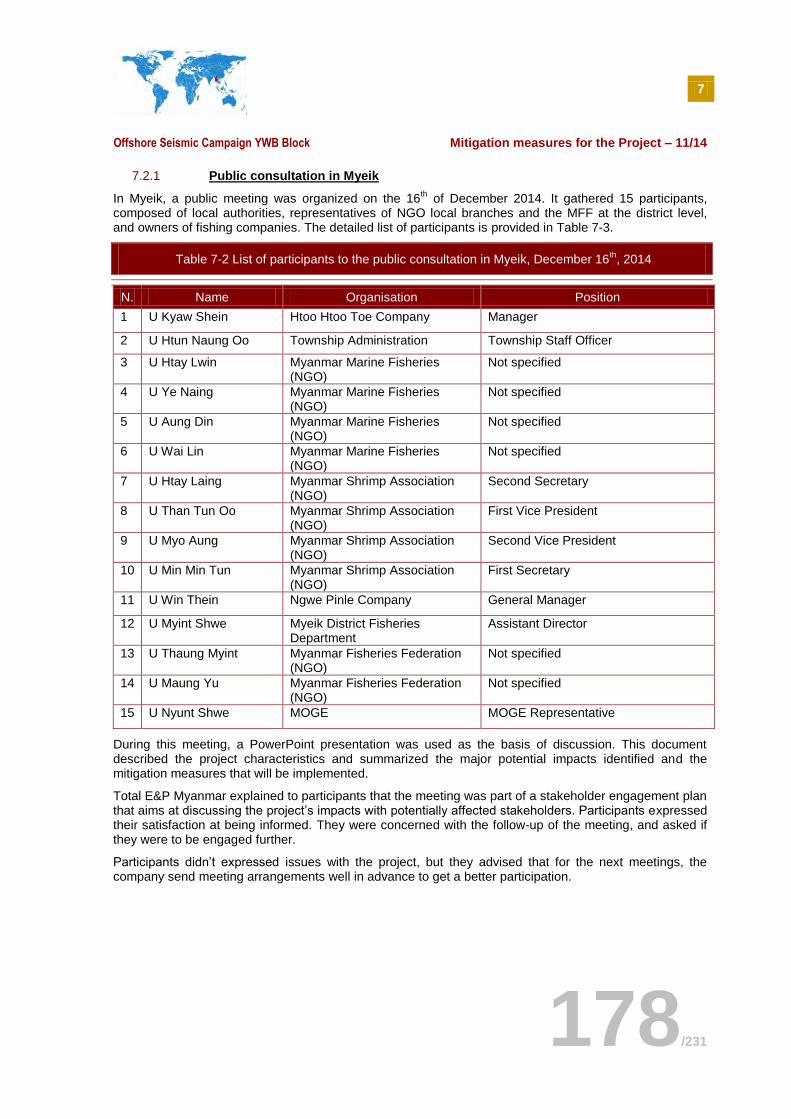
7
Offshore Seismic Campaign YWB Block Mitigation measures for the Project – 11/14
178/231
7.2.1 Public consultation in Myeik
In Myeik, a public meeting was organized on the 16th of December 2014. It gathered 15 participants,
composed of local authorities, representatives of NGO local branches and the MFF at the district level, and owners of fishing companies. The detailed list of participants is provided in Table 7-3.
Table 7-2 List of participants to the public consultation in Myeik, December 16th, 2014
N. Name Organisation Position
1 U Kyaw Shein Htoo Htoo Toe Company Manager
2 U Htun Naung Oo Township Administration Township Staff Officer
3 U Htay Lwin Myanmar Marine Fisheries (NGO)
Not specified
4 U Ye Naing Myanmar Marine Fisheries (NGO)
Not specified
5 U Aung Din Myanmar Marine Fisheries (NGO)
Not specified
6 U Wai Lin Myanmar Marine Fisheries (NGO)
Not specified
7 U Htay Laing Myanmar Shrimp Association (NGO)
Second Secretary
8 U Than Tun Oo Myanmar Shrimp Association (NGO)
First Vice President
9 U Myo Aung Myanmar Shrimp Association (NGO)
Second Vice President
10 U Min Min Tun Myanmar Shrimp Association (NGO)
First Secretary
11 U Win Thein Ngwe Pinle Company General Manager
12 U Myint Shwe Myeik District Fisheries Department
Assistant Director
13 U Thaung Myint Myanmar Fisheries Federation (NGO)
Not specified
14 U Maung Yu Myanmar Fisheries Federation (NGO)
Not specified
15 U Nyunt Shwe MOGE MOGE Representative
During this meeting, a PowerPoint presentation was used as the basis of discussion. This document described the project characteristics and summarized the major potential impacts identified and the mitigation measures that will be implemented.
Total E&P Myanmar explained to participants that the meeting was part of a stakeholder engagement plan that aims at discussing the project’s impacts with potentially affected stakeholders. Participants expressed their satisfaction at being informed. They were concerned with the follow-up of the meeting, and asked if they were to be engaged further.
Participants didn’t expressed issues with the project, but they advised that for the next meetings, the company send meeting arrangements well in advance to get a better participation.
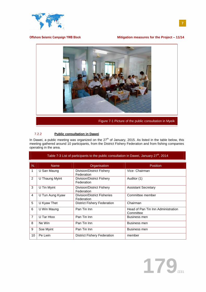
7
Offshore Seismic Campaign YWB Block Mitigation measures for the Project – 11/14
179/231
7.2.2 Public consultation in Dawei
In Dawei, a public meeting was organized on the 27th of January, 2015. As listed in the table below, this
meeting gathered around 10 participants, from the District Fishery Federation and from fishing companies operating in the area.
Table 7-3 List of participants to the public consultation in Dawei, January 27th, 2014
N. Name Organisation Position
1 U San Maung Division/District Fishery Federation
Vice- Chairman
2 U Thaung Myint Division/District Fishery Federation
Auditor (1)
3 U Tin Myint Division/District Fishery Federation
Assistant Secretary
4 U Tun Aung Kyaw Division/District Fisheries Federation
Committee member
5 U Kyaw Thet District Fishery Federation Chairman
6 U Win Maung Pan Tin Inn Head of Pan Tin Inn Administration Committee
7 U Tar Htoo Pan Tin Inn Business men
8 Ne Win Pan Tin Inn Business men
9 Soe Myint Pan Tin Inn Business men
10 Pe Lwin District Fishery Federation member
Figure 7-1 Picture of the public consultation in Myeik
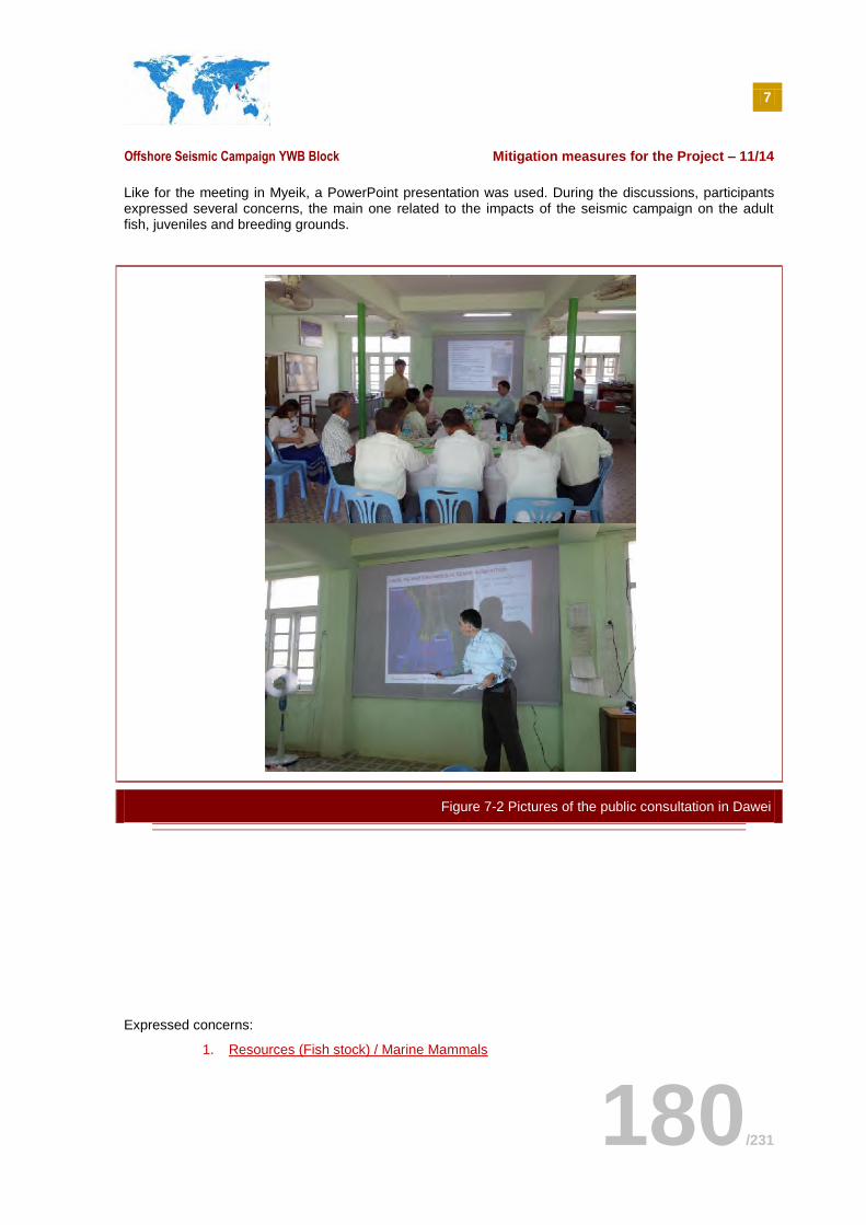
7
Offshore Seismic Campaign YWB Block Mitigation measures for the Project – 11/14
180/231
Like for the meeting in Myeik, a PowerPoint presentation was used. During the discussions, participants expressed several concerns, the main one related to the impacts of the seismic campaign on the adult fish, juveniles and breeding grounds.
Expressed concerns:
1. Resources (Fish stock) / Marine Mammals
Figure 7-2 Pictures of the public consultation in Dawei
7
Offshore Seismic Campaign YWB Block Mitigation measures for the Project – 11/14
181/231
Baseline
- Is there an important source / density of fish in this area?
→ According to the 2013 BOBLME study the biomass has been decreasing in Myanmar offshore waters during the last 30 years. Precise data are not available on YWB block.
Physical damage to fishes:
- Is there a risk of death / Injury for the fishes?
→ The residual impact on the fish is minor to negligible, no risk of death/injury
Disturbance in the breeding areas
- Is the survey going to damage to the Sea bed?
→ At this distance, the impact on the seabed is negligible.
- What are the impacts on fish’s reproduction?
→ There is no evidence of disturbance to reproduction patterns (no measurable effect).
- Is there a risk that fishes will permanently leave the area?
→ The fish will temporarily avoid the zone of seismic acquisition and will come back.
- How long will it take to recover a normal environment?
→Studies show that the short time period to attain normal fish catch rates following a survey, within the surveyed area, varies with season, locality, duration of shooting, etc.
→Minor / no impact is expected in the YWB block.
2. Impact on Fishing activity
What will be the duration of exclusion?
→This exclusion area is motivated by HSE concerns for the fishermen and is aiming at avoiding collision and/or damage to fishing gears
The duration of the full survey should be less than 3 months. Only the “active” portion of the survey will be restricted for fishing. Any particular area (active portion of the survey) should not be restricted for more than a few weeks.
Area of Exclusion
- What is the size of the exclusion area?
→The size of the restricted area should be about 500 km2 but will vary depending on the survey size.
8
Offshore Seismic Campaign YWB Block Mitigation measures for the Project – 11/14
182/231
SECTION 8. MITIGATION MEASURES FOR THE PROJECT
This section gives details on mitigation measures associated with potential underwater acoustic impacts of the YWB project on marine mammals, turtles and fish. Mitigations measures associated with others environmental and social potential impacts of the project have already been developed on § 6.5 .
At the end of this section, a commitment register will detail roles and responsibilities for each of the mitigation measures proposed in this IEE.
8.1 SPECIFIC MITIGATION MEASURES FOR MARINE MAMMALS, TURTLES AND FISHES
8.1.1.1 Mitigation actions and procedures
The methods recommended by the IAGC (International Association of Geophysical Organisation) and the JNCC (Joint Nature Conservation Committee, UK) to minimize the disturbance of marine mammals during the course of marine seismic activities will be implemented. The protocol will be adapted to account for the zones of exclusion determined necessary for the project (being 2,800 m and 800 m, cf. below). Marine mammal observers will accompany the vessel during the life of operations to ensure compliance with the intervention protocols.
A brief description of how the shutdown distances have been calculated and mitigation measures to be implemented are presented in § 8.1.1.2 . Additional mitigation measures to ensure the protection of marine mammals, fish and turtles are described on §8.1.1.3 .
8.1.1.2 Temporary and permanent threshold criteria for cetaceans- calculation of shutdown areas
National Marine Fisheries Services Criteria
The National Marine Fisheries Services (NMFS) proposes the adoption of physiological change thresholds by the definition of TTS ('Temporary Threshold Shift') and PTS ('Permanent Threshold Shift') criteria.
The TTS and PTS respectively define the upper exposure limit for the temporary and permanent loss of hearing ability.
These thresholds do not take into account either the exposure duration, which is implicitly considered as very short, or the level of loss, implicitly regarded as disability.
The NMFS proposes the adoption of thresholds for marine mammals based on a conservative approach using the results of TTS studies of many marine mammal species. This value defines the spatial limit (or exclusion zone) of seismic activities in order to comply with the following values:
180 dB re µPa (RMS) for cetaceans;
190 dB re µPa (RMS) for pinnipeds (not expected in the study area).
The NMFS also provides a criteria of "behavioural discomfort" of 160 dB re µPa (RMS) for all cetaceans species.
The exclusion zone is then determined by the characteristics of the source and depth of the zone.
Marine Animal Noise Exposure Criteria
8
Offshore Seismic Campaign YWB Block Mitigation measures for the Project – 11/14
183/231
A more recent and highly regarded study was conducted by Southall et al. (2007), which proposed criteria for injury for marine mammal groups and sound types. Noise exposure criteria for auditory injury have been based in the publication on exposures inducing PTS-onset i.e 40 dB-TTS.
Definition:
PTS-onset is an irreversible elevation of the hearing threshold (i.e loss in sensitivity) at a specific frequency. PTS is presumed to be likely if the threshold is over 40 dB above TTS. Noise-inducted PTS represents tissue injury, whereas TTS does not.
TTS-onset has been defined as being a temporary elevation of a hearing threshold by 6 dB (Southall and al). TTS involves reduced hearing sensitivity following exposure, it results primarily from the fatigue (as opposed to loss) of cochlear hair cells and is by definition reversible.
Criteria for injury were derived from measured or assumed TTS-onset thresholds for each marine mammal group plus TTS growth rate estimates. Available data for 2 mid-frequency cetacean species are used as a basis for estimating PTS-onset thresholds for all cetaceans.
The PTS-onset thresholds are used to define exclusion zones. This study was developed on the basis of an extensive industry related bibliography and considers many factors in the development of criteria:
The designation of sound response frequency weightings depending on mammal type, being
mammals sensitive to low, mid and high frequency acoustic sources. These mammal types have been designated with a specific weighting curve to represent their sonar response, ie to modify the sonar signal to represent the noise level perceived by the mammal. For instance, mammals with sensitivity to high frequency sounds (eg dolphins and porpoises) will be much less affected by low frequency airgun emissions than baleen whales, which are sensitive to low frequency sounds.
As such, each mammal type (of low, mid and high frequency sensitivities) has been designated with a specific weighting curve to represent sonar response, being Mlf, Mmf and Mhf respectively (refer to Figure 8-1). Thus, in the frequency range of 7 – 104 Hz of airgun firing, weightings of -2 and -15 dB respectively were adopted for mammals sensitive to low and middle frequencies in order to modify the emitted sound level to represent the perceived noise levels for marine mammals sensitive to low and middle frequencies.
Signal type, being single pulse, multi pulse and continuous. The seismic survey will be characterized by multiple pulses sound of 20 ms duration repeated every 10-15 seconds.
Indicator types, being the SPLo-p and the SEL. The sound energy level describes the energy
sum of each signal pulse. For a doubling in pulse (i.e. doubling of energy) the SEL doubles by 3 dB. The strictest indicator will be used to define the exclusion zone. For the calculation of the SEL, an exposure duration of 120 minutes has been adopted, a conservative assumption of the time required for the acoustic source to move away from the static cetacean or vice versa. Assuming a streamer vessel speed of 9 km/h, this would signify a significant reduction in received sound levels over the period calculated.
The sound response frequency weightings for different mammal species are shown in Figure 8-1 and values of PTS-onset are presented as an extract in Table 8-1).
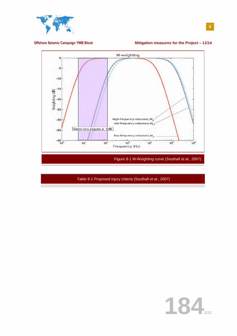
8
Offshore Seismic Campaign YWB Block Mitigation measures for the Project – 11/14
184/231
Table 8-1 Proposed injury criteria (Southall et al., 2007)
Figure 8-1 M-Weighting curve (Southall et al., 2007)
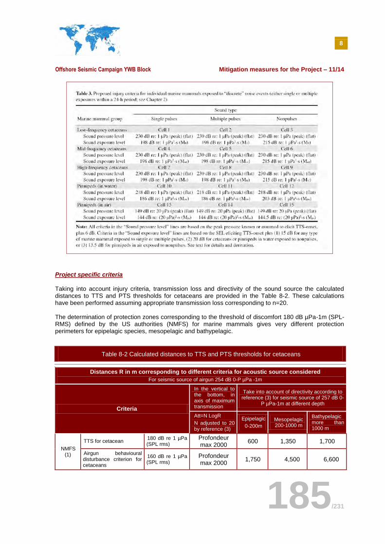
8
Offshore Seismic Campaign YWB Block Mitigation measures for the Project – 11/14
185/231
Project specific criteria
Taking into account injury criteria, transmission loss and directivity of the sound source the calculated distances to TTS and PTS thresholds for cetaceans are provided in the Table 8-2. These calculations have been performed assuming appropriate transmission loss corresponding to n=20. The determination of protection zones corresponding to the threshold of discomfort 180 dB µPa-1m (SPL-RMS) defined by the US authorities (NMFS) for marine mammals gives very different protection perimeters for epipelagic species, mesopelagic and bathypelagic.
Table 8-2 Calculated distances to TTS and PTS thresholds for cetaceans
Distances R in m corresponding to different criteria for acoustic source considered
For seismic source of airgun 254 dB 0-P µPa -1m
Criteria
In the vertical to the bottom, in axis of maximum transmission
Take into account of directivity according to reference (3) for seismic source of 257 dB 0-
P µPa-1m at different depth
Att=N LogR
N adjusted to 20 by reference (3)
Epipelagic
0-200m
Mesopelagic 200-1000 m
Bathypelagic more than 1000 m
NMFS (1)
TTS for cetacean 180 dB re 1 µPa (SPL rms)
Profondeur max 2000
600 1,350 1,700
Airgun behavioural disturbance criterion for cetaceans
160 dB re 1 µPa (SPL rms)
Profondeur max 2000
1,750 4,500 6,600
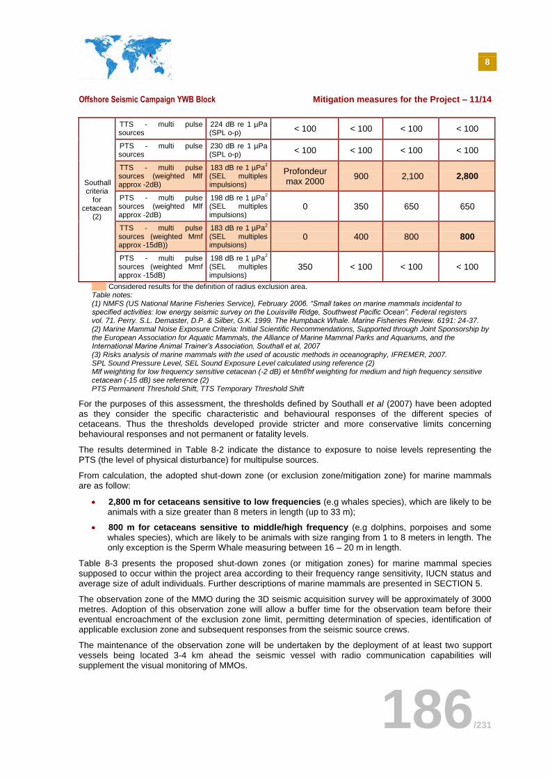
8
Offshore Seismic Campaign YWB Block Mitigation measures for the Project – 11/14
186/231
Southall criteria
for cetacean
(2)
TTS - multi pulse sources
224 dB re 1 µPa (SPL o-p)
< 100 < 100 < 100 < 100
PTS - multi pulse sources
230 dB re 1 µPa (SPL o-p)
< 100 < 100 < 100 < 100
TTS - multi pulse sources (weighted Mlf approx -2dB)
183 dB re 1 µPa2
(SEL multiples impulsions)
Profondeur max 2000
900 2,100 2,800
PTS - multi pulse sources (weighted Mlf approx -2dB)
198 dB re 1 µPa2
(SEL multiples impulsions)
0 350 650 650
TTS - multi pulse sources (weighted Mmf approx -15dB))
183 dB re 1 µPa2
(SEL multiples impulsions)
0 400 800 800
PTS - multi pulse sources (weighted Mmf approx -15dB)
198 dB re 1 µPa2
(SEL multiples impulsions)
350 < 100 < 100 < 100
XXX Considered results for the definition of radius exclusion area. Table notes: (1) NMFS (US National Marine Fisheries Service), February 2006. “Small takes on marine mammals incidental to specified activities: low energy seismic survey on the Louisville Ridge, Southwest Pacific Ocean”. Federal registers vol. 71. Perry. S.L. Demaster, D.P. & Silber, G.K. 1999. The Humpback Whale. Marine Fisheries Review. 6191: 24-37. (2) Marine Mammal Noise Exposure Criteria: Initial Scientific Recommendations, Supported through Joint Sponsorship by the European Association for Aquatic Mammals, the Alliance of Marine Mammal Parks and Aquariums, and the International Marine Animal Trainer’s Association, Southall et al, 2007 (3) Risks analysis of marine mammals with the used of acoustic methods in oceanography, IFREMER, 2007. SPL Sound Pressure Level, SEL Sound Exposure Level calculated using reference (2) Mlf weighting for low frequency sensitive cetacean (-2 dB) et Mmf/hf weighting for medium and high frequency sensitive cetacean (-15 dB) see reference (2) PTS Permanent Threshold Shift, TTS Temporary Threshold Shift
For the purposes of this assessment, the thresholds defined by Southall et al (2007) have been adopted as they consider the specific characteristic and behavioural responses of the different species of cetaceans. Thus the thresholds developed provide stricter and more conservative limits concerning behavioural responses and not permanent or fatality levels.
The results determined in Table 8-2 indicate the distance to exposure to noise levels representing the PTS (the level of physical disturbance) for multipulse sources.
From calculation, the adopted shut-down zone (or exclusion zone/mitigation zone) for marine mammals are as follow:
2,800 m for cetaceans sensitive to low frequencies (e.g whales species), which are likely to be animals with a size greater than 8 meters in length (up to 33 m);
800 m for cetaceans sensitive to middle/high frequency (e.g dolphins, porpoises and some whales species), which are likely to be animals with size ranging from 1 to 8 meters in length. The only exception is the Sperm Whale measuring between 16 – 20 m in length.
Table 8-3 presents the proposed shut-down zones (or mitigation zones) for marine mammal species supposed to occur within the project area according to their frequency range sensitivity, IUCN status and average size of adult individuals. Further descriptions of marine mammals are presented in SECTION 5.
The observation zone of the MMO during the 3D seismic acquisition survey will be approximately of 3000 metres. Adoption of this observation zone will allow a buffer time for the observation team before their eventual encroachment of the exclusion zone limit, permitting determination of species, identification of applicable exclusion zone and subsequent responses from the seismic source crews.
The maintenance of the observation zone will be undertaken by the deployment of at least two support vessels being located 3-4 km ahead the seismic vessel with radio communication capabilities will supplement the visual monitoring of MMOs.
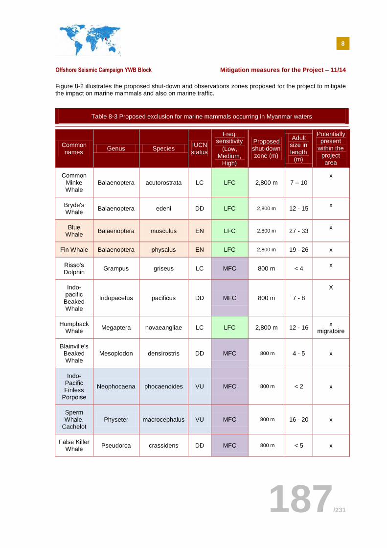
8
Offshore Seismic Campaign YWB Block Mitigation measures for the Project – 11/14
187/231
Figure 8-2 illustrates the proposed shut-down and observations zones proposed for the project to mitigate the impact on marine mammals and also on marine traffic.
Table 8-3 Proposed exclusion for marine mammals occurring in Myanmar waters
Common names
Genus Species IUCN status
Freq. sensitivity
(Low, Medium,
High)
Proposed shut-down zone (m)
Adult size in length
(m)
Potentially present
within the project area
Common Minke Whale
Balaenoptera acutorostrata LC LFC 2,800 m 7 – 10 x
Bryde's Whale
Balaenoptera edeni DD LFC 2,800 m 12 - 15 x
Blue Whale
Balaenoptera musculus EN LFC 2,800 m 27 - 33 x
Fin Whale Balaenoptera physalus EN LFC 2,800 m 19 - 26 x
Risso's Dolphin
Grampus griseus LC MFC 800 m < 4 x
Indo-pacific
Beaked Whale
Indopacetus pacificus DD MFC 800 m 7 - 8
X
Humpback Whale
Megaptera novaeangliae LC LFC 2,800 m 12 - 16 x
migratoire
Blainville's Beaked Whale
Mesoplodon densirostris DD MFC 800 m 4 - 5 x
Indo-Pacific Finless
Porpoise
Neophocaena phocaenoides VU MFC 800 m < 2 x
Sperm Whale,
Cachelot Physeter macrocephalus VU MFC 800 m 16 - 20 x
False Killer Whale
Pseudorca crassidens DD MFC 800 m < 5 x
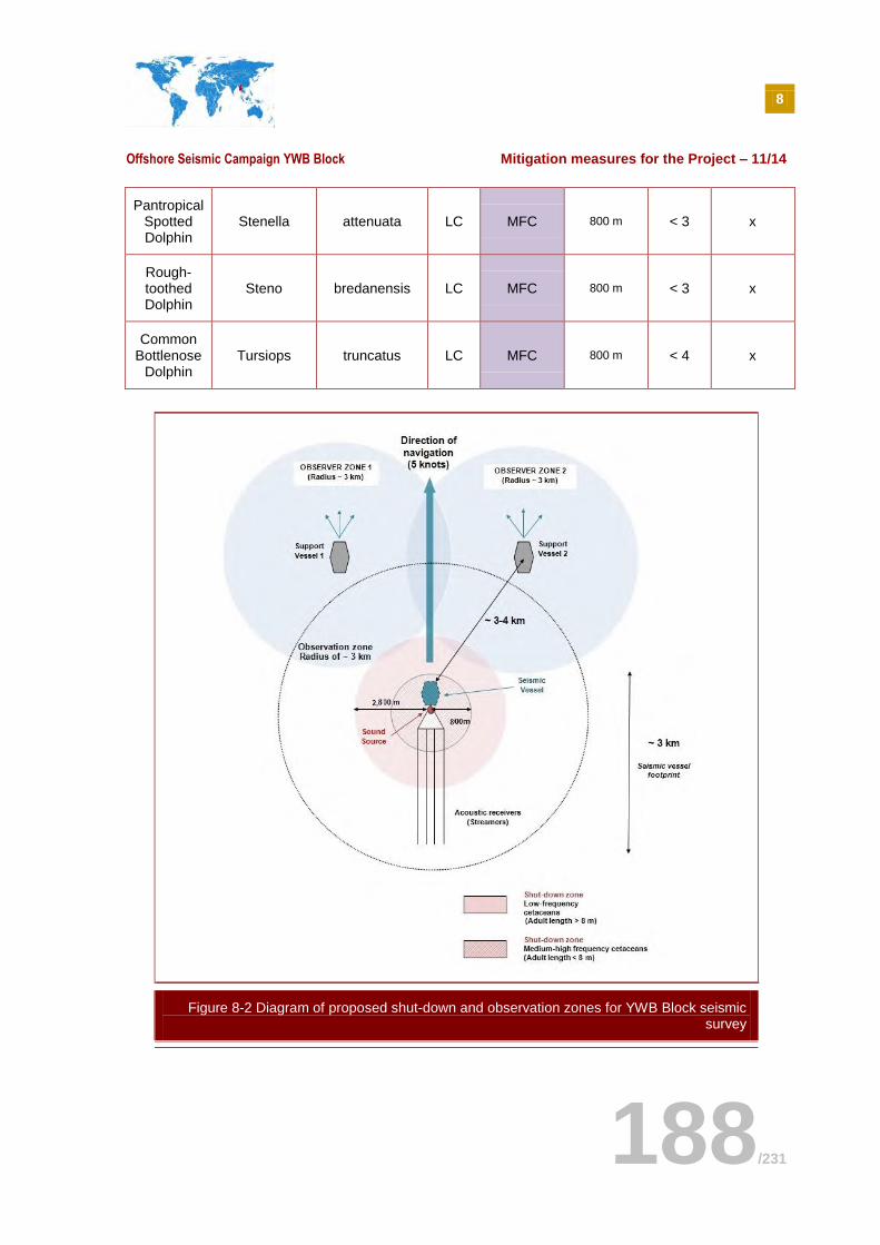
8
Offshore Seismic Campaign YWB Block Mitigation measures for the Project – 11/14
188/231
Pantropical Spotted Dolphin
Stenella attenuata LC MFC 800 m < 3 x
Rough-toothed Dolphin
Steno bredanensis LC MFC 800 m < 3 x
Common Bottlenose
Dolphin Tursiops truncatus LC MFC 800 m < 4 x
Figure 8-2 Diagram of proposed shut-down and observation zones for YWB Block seismic survey
8
Offshore Seismic Campaign YWB Block Mitigation measures for the Project – 11/14
189/231
Pre-shooting search
The pre-shooting search should normally be conducted over a period of 60 minutes before commencement of any use of the airguns (the YWB Block is situated in deepwater >200m depth). The MMO should make a visual assessment to determine if any marine mammals are within the mitigation/exclusion zone (i.e 800 metres or 2,800m of the centre of the airgun array).
If PAM is used in conjunction with visual monitoring, the PAM operator should ensure the system is deployed and being monitored for vocalisations during each designated pre-shooting period.
Delay if marine mammals are detected within the mitigation zone
Mitigation actions are taken by either the MMO or the PAM in the following cases scenario:
If marine mammals are detected by the MMO within the mitigation zone of the center of the airgun array during the pre-shooting search, the soft-start of the seismic sources should be delayed until their passage, or the transit of the vessel, results in the marine mammals being more than 800 or 2,800 meters away from the source.
In both cases, there should be a 20 minute delay from the time of the last sighting within the mitigation zone of the source to the commencement of the soft-start, in order to determine whether the animals have left the area.
If PAM is used, it is the responsibility of the PAM operatives to assess any acoustic detection and determine if there are likely to be marine mammals within the mitigation zone. If the PAM operatives consider marine mammals are present within that range then the start of the operation should be delayed as outlined above.
If marine mammals are detected within the mitigation zone whilst the airguns are firing, either during the soft-start procedure or whilst at full power, there is no requirement to stop firing the airguns.
Soft start procedure (ramp-ups)
The soft-start is defined as the time that airguns commence shooting till the time that full operational power is obtained. Soft-start procedures are based on precautionary practice of starting the sound source at low levels and then building these levels up gradually. The goal of a soft start is to give sufficient warning to marine mammals in the vicinity of the survey area of the increasing noise in their environment. The idea is to provide these animals with adequate time to move away from the survey area before the sound sources achieve the full energy output.
Soft starts involve using the equipment that produces the sound source during operations. Soft start procedures are carried out during seismic surveys by first firing the smallest volume airgun and then adding successively larger volume airguns to the firing pattern with each step. It is recommended that soft starts for seismic surveys should last at least 20 minutes and last no longer than 40 minutes.
A soft-start procedure is required every time the airguns are used or if there is any break in airgun activity day or night exceeding 10 minutes.
Soft start procedures on seismic surveys vessels are often automated on-board vessels to ensure consistency. An example of this is shown below.
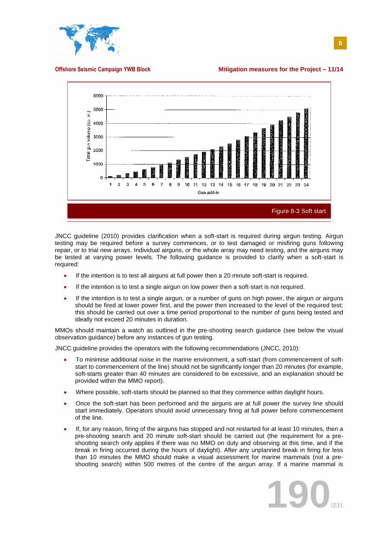
8
Offshore Seismic Campaign YWB Block Mitigation measures for the Project – 11/14
190/231
JNCC guideline (2010) provides clarification when a soft-start is required during airgun testing. Airgun testing may be required before a survey commences, or to test damaged or misfiring guns following repair, or to trial new arrays. Individual airguns, or the whole array may need testing, and the airguns may be tested at varying power levels. The following guidance is provided to clarify when a soft-start is required:
If the intention is to test all airguns at full power then a 20 minute soft-start is required.
If the intention is to test a single airgun on low power then a soft-start is not required.
If the intention is to test a single airgun, or a number of guns on high power, the airgun or airguns should be fired at lower power first, and the power then increased to the level of the required test; this should be carried out over a time period proportional to the number of guns being tested and ideally not exceed 20 minutes in duration.
MMOs should maintain a watch as outlined in the pre-shooting search guidance (see below the visual observation guidance) before any instances of gun testing.
JNCC guideline provides the operators with the following recommendations (JNCC, 2010):
To minimise additional noise in the marine environment, a soft-start (from commencement of soft-start to commencement of the line) should not be significantly longer than 20 minutes (for example, soft-starts greater than 40 minutes are considered to be excessive, and an explanation should be provided within the MMO report).
Where possible, soft-starts should be planned so that they commence within daylight hours.
Once the soft-start has been performed and the airguns are at full power the survey line should start immediately. Operators should avoid unnecessary firing at full power before commencement of the line.
If, for any reason, firing of the airguns has stopped and not restarted for at least 10 minutes, then a pre-shooting search and 20 minute soft-start should be carried out (the requirement for a pre-shooting search only applies if there was no MMO on duty and observing at this time, and if the break in firing occurred during the hours of daylight). After any unplanned break in firing for less than 10 minutes the MMO should make a visual assessment for marine mammals (not a pre-shooting search) within 500 metres of the centre of the airgun array. If a marine mammal is
Figure 8-3 Soft start
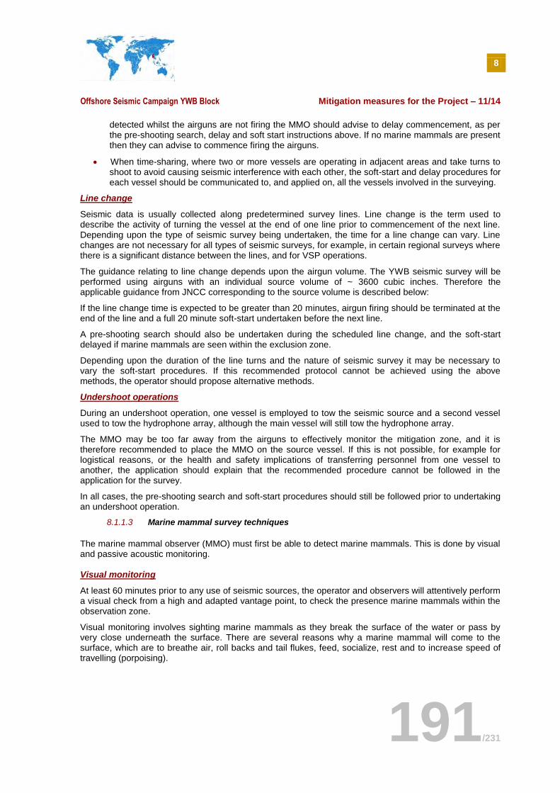
8
Offshore Seismic Campaign YWB Block Mitigation measures for the Project – 11/14
191/231
detected whilst the airguns are not firing the MMO should advise to delay commencement, as per the pre-shooting search, delay and soft start instructions above. If no marine mammals are present then they can advise to commence firing the airguns.
When time-sharing, where two or more vessels are operating in adjacent areas and take turns to shoot to avoid causing seismic interference with each other, the soft-start and delay procedures for each vessel should be communicated to, and applied on, all the vessels involved in the surveying.
Line change
Seismic data is usually collected along predetermined survey lines. Line change is the term used to describe the activity of turning the vessel at the end of one line prior to commencement of the next line. Depending upon the type of seismic survey being undertaken, the time for a line change can vary. Line changes are not necessary for all types of seismic surveys, for example, in certain regional surveys where there is a significant distance between the lines, and for VSP operations.
The guidance relating to line change depends upon the airgun volume. The YWB seismic survey will be performed using airguns with an individual source volume of ~ 3600 cubic inches. Therefore the applicable guidance from JNCC corresponding to the source volume is described below:
If the line change time is expected to be greater than 20 minutes, airgun firing should be terminated at the end of the line and a full 20 minute soft-start undertaken before the next line.
A pre-shooting search should also be undertaken during the scheduled line change, and the soft-start delayed if marine mammals are seen within the exclusion zone.
Depending upon the duration of the line turns and the nature of seismic survey it may be necessary to vary the soft-start procedures. If this recommended protocol cannot be achieved using the above methods, the operator should propose alternative methods.
Undershoot operations
During an undershoot operation, one vessel is employed to tow the seismic source and a second vessel used to tow the hydrophone array, although the main vessel will still tow the hydrophone array.
The MMO may be too far away from the airguns to effectively monitor the mitigation zone, and it is therefore recommended to place the MMO on the source vessel. If this is not possible, for example for logistical reasons, or the health and safety implications of transferring personnel from one vessel to another, the application should explain that the recommended procedure cannot be followed in the application for the survey.
In all cases, the pre-shooting search and soft-start procedures should still be followed prior to undertaking an undershoot operation.
8.1.1.3 Marine mammal survey techniques
The marine mammal observer (MMO) must first be able to detect marine mammals. This is done by visual and passive acoustic monitoring.
Visual monitoring
At least 60 minutes prior to any use of seismic sources, the operator and observers will attentively perform a visual check from a high and adapted vantage point, to check the presence marine mammals within the observation zone.
Visual monitoring involves sighting marine mammals as they break the surface of the water or pass by very close underneath the surface. There are several reasons why a marine mammal will come to the surface, which are to breathe air, roll backs and tail flukes, feed, socialize, rest and to increase speed of travelling (porpoising).
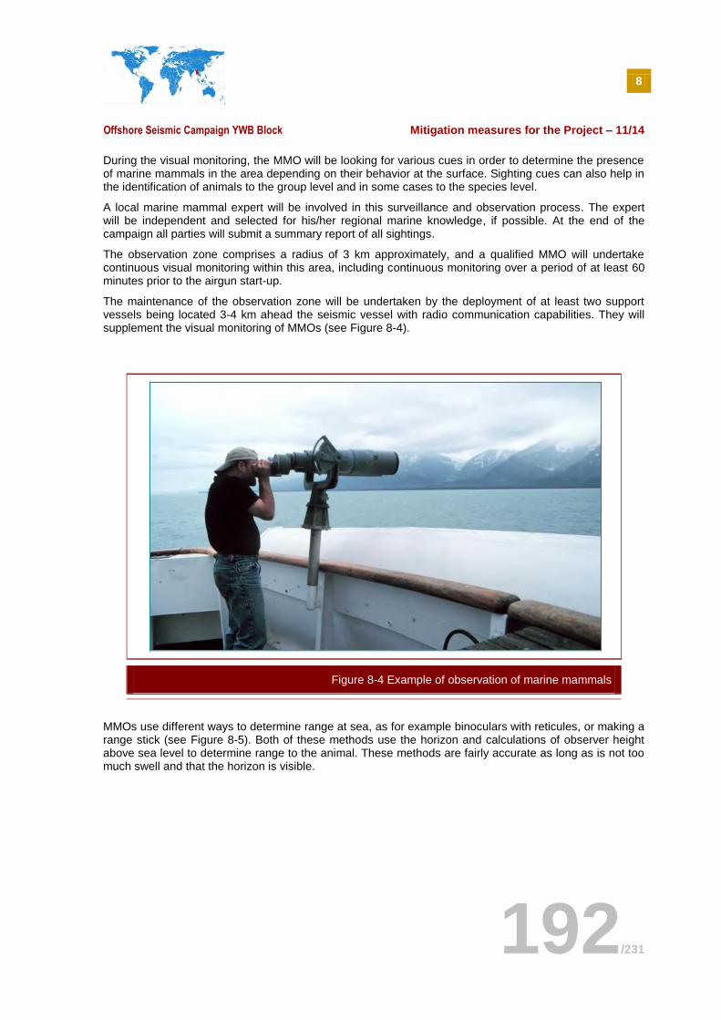
8
Offshore Seismic Campaign YWB Block Mitigation measures for the Project – 11/14
192/231
During the visual monitoring, the MMO will be looking for various cues in order to determine the presence of marine mammals in the area depending on their behavior at the surface. Sighting cues can also help in the identification of animals to the group level and in some cases to the species level.
A local marine mammal expert will be involved in this surveillance and observation process. The expert will be independent and selected for his/her regional marine knowledge, if possible. At the end of the campaign all parties will submit a summary report of all sightings.
The observation zone comprises a radius of 3 km approximately, and a qualified MMO will undertake continuous visual monitoring within this area, including continuous monitoring over a period of at least 60 minutes prior to the airgun start-up.
The maintenance of the observation zone will be undertaken by the deployment of at least two support vessels being located 3-4 km ahead the seismic vessel with radio communication capabilities. They will supplement the visual monitoring of MMOs (see Figure 8-4).
MMOs use different ways to determine range at sea, as for example binoculars with reticules, or making a range stick (see Figure 8-5). Both of these methods use the horizon and calculations of observer height above sea level to determine range to the animal. These methods are fairly accurate as long as is not too much swell and that the horizon is visible.
Figure 8-4 Example of observation of marine mammals
8
Offshore Seismic Campaign YWB Block Mitigation measures for the Project – 11/14
193/231
Binoculars
Binoculars
Sighting
SOURCE: JNCC
Passive acoustic monitoring
Visual observation is an ineffective mitigation tool during periods of darkness or poor visibility (such as fog), or during periods when the sea state is not conducive to visual mitigation, as it will not be possible to detect marine mammals in the vicinity of airgun sources. Under such conditions, PAM is considered to be the only currently available mitigation technique that can be used to detect marine mammals.
Passive acoustic monitoring may be a requirement for surveys that are conducted in particularly sensitive areas or for certain species, such as sperm whales. It is also helpful in detecting harbor porpoises within the 500 metres mitigation zone, although the systems have their limitations and can only be used to detect vocalising species of marine mammals.
Submerge cetacean are much more risk than those on the surface. According the JNCC, this makes it particularly important to use a hydrophone whenever possible to detect vocally active animals that may be invisible from the surface. The PAM system is therefore ideally used in conjunction with visual monitoring, to provide effective 24 hours mitigation for cetaceans.
PAM equipment – frequency range
PAM systems consist of hydrophones that are deployed into the water column, and the detected sounds are processed using specialized software. The equipment involves towing long lengths of cable (200-300 m) which ensures that the hydrophones elements are away from the engines. This system usually contains filters to eliminate some of the engine noise.
Current equipment for electronic detection of cetaceans can detect 5 to 8 times more cetaceans than previously (Gillespie & Chappell, 1998). Electronic detection systems passively record all frequencies up to 140 kHz (the waves used for seismic reach 200 kHz). Software will be used to assess frequencies anomalies corresponding to the potential presence of sound emitting marine mammals.
Conditions of use of PAM and limitations
The advantages that PAM has over visual monitoring are:
- Acoustic detection of cetaceans is less affected by weather conditions;
Figure 8-5 Example of observation techniques of marine mammals
8
Offshore Seismic Campaign YWB Block Mitigation measures for the Project – 11/14
194/231
- Acoustic detection range for many species superior than visual detection;
- Acoustic detection can be made of animals below the surface (as long as they are vocalizing) and therefore increases the likelihood of detecting deep diving species,
- Acoustic monitoring can be conducted 24 hrs a day;
- A complete and permanent record can be made of acoustic monitoring cues.
However, PAM does have the following limitations:
- Current PAM systems do not give accurate estimates of range. The accuracy can be estimated at +/-300 meters which means animals detected and calculated to be within 500 meters from the source could, in reality, be 500 + 300 = 800 meters, but their detection would still lead to a delay in the soft-start. Although, at present it is not possible to express the range accuracy of most PAM systems in numerical terms.
- PAM systems do not have a reliable range determination facility or can only calculate the range for some species. For e.g baleen whales vocalize at frequencies which are very difficult to detect using current PAM systems, whereas harbor porpoise utilize high frequencies (130 kHz) and thus has a very short acoustic detection range;
In such cases, the detection of a confirmed cetacean vocalization should still be used to initiate postponement of the soft-start if the PAM operator is able to make a judgment about the range of the animals from the airgun source, because of their experience gained in differentiating between distant and close vocalizations. In the absence of PAM systems capable of range determination, this expert judgment will constitute the basis for deciding whether an area is free from cetaceans prior to the soft-start.
Animals do not vocalize all of the time and may pass by undetected;
Interference with other maritime anthropogenic sound, such as boat nearby, engines, etc…
This last example serves to illustrate that it is in the operator’s best interests to use the most accurate system available and to check with the PAM provider if the frequency range covered are adapted to local marine mammals.
Requirements for MMOs and PAMs
The YWB blocks are located off the coast of Myanmar in the northern part of the Andaman Sea. The seismic campaign will be conducted within area located between latitudes 14ºN and 15ºN, and longitudes 95ºE and 97°E. The amount of daylight is more than 12 hours a day between March (13
th) and the end of
September.
Considering JNCC guidelines and the sensitivity of potential marine mammals that may occur within the project area:
One MMO should be appointed for the purpose of monitoring the implementation of the guidelines and undertaking visual observations to detect marine mammals during periods of seismic activity;
A second MMO should be appointed for the mitigation actions in the following cases:
- if the survey is carried out during the period of mid-March to end of September, being the migration period for sea turtles;
- if the observation time required is more than 12 hours working-shift.
One PAM system should be used to supplement visual observations.

8
Offshore Seismic Campaign YWB Block Mitigation measures for the Project – 11/14
195/231
8.2 COMMITMENT REGISTER WITH RESPONSIBILITIES
The impact mitigation measures regarding the seismic survey activities have been outlined in SECTION 8 and in paragraph 6.5 and are listed in the commitment register below.
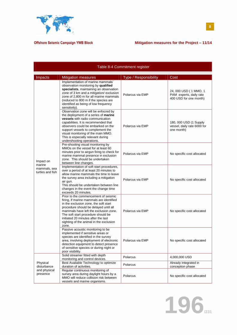
8
Offshore Seismic Campaign YWB Block Mitigation measures for the Project – 11/14
196/231
Table 8-4 Commitment register
Impacts Mitigation measures Type / Responsibility Cost
Impact on marine mammals, sea turtles and fish
Implementation of marine mammals’ observation monitoring by qualified specialists, maintaining an observation zone of 3 km and a mitigation/ exclusion zone of 2,800 m for all marine mammals (reduced to 800 m if the species are identified as being of low frequency sensitivity).
Polarcus via EMP 24, 000 USD ( 1 MMO, 1 PAM experts, daily rate 400 USD for one month)
Observation zone will be enfocred by the deployment of a series of marine vessels with radio communication capabilities. It is recommended that observers could be embarked on the support vessels to complement the visual monitoring of the main MMO. This is especially relevant during undershooting operations.
Polarcus via EMP 180, 000 USD (1 Supply vessel, daily rate 6000 for one month)
Pre-shooting visual monitoring by MMOs on the vessel for at least 60 minutes prior to airgun firing to check for marine mammal presence in exclusion zone. This should be undertaken between line changes.
Polarcus via EMP No specific cost allocated
Implementation of soft start procedures, over a period of at least 20 minutes to allow marine mammals the time to leave the survey area including a mitigation air gun. This should be undertaken between line changes in the event the change time exceeds 20 minutes.
Polarcus via EMP No specific cost allocated
Prior to the commencement of seismic firing, if marine mammals are identified in the exclusion zone, the soft start procedure should be delayed until all mammals have left the exclusion zone. The soft start procedure should be initiated 20 minutes after the last sighting of the animal in the exclusion zone.
Polarcus via EMP No specific cost allocated
Passive acoustic monitoring to be implemented if sensitive areas or species are identified in the survey area, involving deployment of electronic detection equipment to detect presence of sensitive species or during night or poor visibility.
Polarcus via EMP No specific cost allocated
Physical disturbance and physical presence
Solid streamer fitted with depth monitoring and control devices.
Polarcus 4,000,000 USD
Best Available Technology to optimize duration of activities.
Polarcus Already integrated in conception phase
Regular continuous monitoring of survey area during daylight hours by a MMO will reduce collision risk between vessels and marine organisms.
Polarcus No specific cost allocated
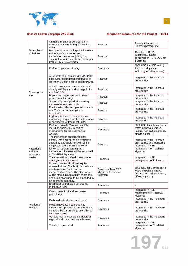
8
Offshore Seismic Campaign YWB Block Mitigation measures for the Project – 11/14
197/231
Atmospheric emissions
On-going maintenance program to ensure equipment is in good working order.
Polarcus Already integrated in Polarcus prerequisite
Best available technologies to increase efficiency of combustion and incineration processes (Using low sulphur fuel which meets the maximum IMO sulphur cap of 3.5%).
Polarcus
159,000 USD ( 20 cu.mtrs/day Diesel consumption – 265 USD for 1 cu.mtrs)
Discharge to sea
Perform regular monitoring. Polcarcus 4000 USD for HSE audit ( 1 Auditor, 2 days rate including travel expenses)
All vessels shall comply with MARPOL: bilge water segregated and treated to less than 15 mg/l prior to sea discharge.
Polarcus Integrated in the Polarcus prerequisite
Suitable sewage treatment units shall comply with Myanmar discharge limits and MARPOL.
Polarcus Integrated in the Polarcus prerequisite
Bilge water segregated and treated prior to sea discharge.
Polarcus Integrated in the Polarcus prerequisite
Survey ships equipped with sanitary wastewater treatment units.
Polarcus Integrated in the Polarcus prerequisite
Food waste milled and ground to a size of <25 mm in diameter prior to discharge.
Polarcus Integrated in the Polarcus prerequisite
Implementation of maintenance and monitoring program for the performance of sewage water treatment units.
Polarcus Integrated in the Polarcus prerequisite
Hazardous and non hazardous wastes
Perform a Waste Management Plan, including appropriate reporting mechanisms for the treatment of wastes.
Polcarcus
5000 USD for 2 times port’s waste disposal charges (includ. Port call, clearance, offloading etc…)
The incineration procedures shall comply with national and international standards and equipment will be the subject of regular maintenance. A follow-up report regarding the incineration of wastes will be submitted to Total E&P Myanmar.
Polarcus
Integrated in the Polarcus prerequisite and monitoring Integrated in HSE management of Total E&P Myanmar
The crew will be trained to use waste management procedures.
Polcarcus Integrated in HSE management of Polcarcus
No solid waste will deliberately be released at sea. Combustible waste and non-hazardous waste can be incinerated on board. The other waste will be stored in appropriate containers and brought onshore to be supported by an approved company.
Polarcus / Total E&P Myanmar for onshore treatment
5000 USD for 2 times port’s waste disposal charges (includ. Port call, clearance, offloading etc...)
Accidental releases
Shipboard Oil Pollution Emergency Plans (SOPEP).
Polcarcus -
Crew trained in oil spill response procedures.
Polcarcus Integrated in HSE management of Total E&P Myanmar
On-board antipollution equipment. Polcarcus Integrated in the Polcarcus prerequisite
Modern navigation equipment to indicate the approach of other vessels complete by surroundings surveillance by chase boats.
Polcarcus Integrated in the Polcarcus prerequisite
Vessels must be sufficiently visible at night with all the appropriate devices.
Polcarcus Integrated in the Polcarcus prerequisite
Training of personnel. Polcarcus Integrated in HSE management of Total E&P Myanmar
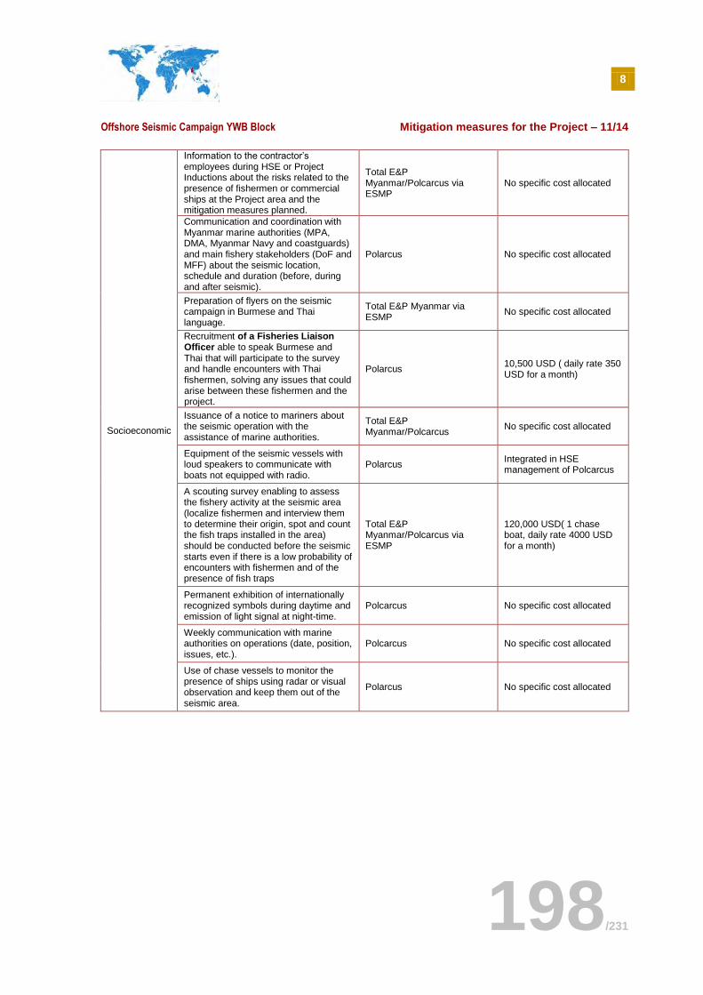
8
Offshore Seismic Campaign YWB Block Mitigation measures for the Project – 11/14
198/231
Socioeconomic
Information to the contractor’s employees during HSE or Project Inductions about the risks related to the presence of fishermen or commercial ships at the Project area and the mitigation measures planned.
Total E&P Myanmar/Polcarcus via ESMP
No specific cost allocated
Communication and coordination with Myanmar marine authorities (MPA, DMA, Myanmar Navy and coastguards) and main fishery stakeholders (DoF and MFF) about the seismic location, schedule and duration (before, during and after seismic).
Polarcus No specific cost allocated
Preparation of flyers on the seismic campaign in Burmese and Thai language.
Total E&P Myanmar via ESMP
No specific cost allocated
- Recruitment of a Fisheries Liaison Officer able to speak Burmese and Thai that will participate to the survey and handle encounters with Thai fishermen, solving any issues that could arise between these fishermen and the project.
Polarcus 10,500 USD ( daily rate 350 USD for a month)
Issuance of a notice to mariners about the seismic operation with the assistance of marine authorities.
Total E&P Myanmar/Polcarcus
No specific cost allocated
Equipment of the seismic vessels with loud speakers to communicate with boats not equipped with radio.
Polarcus Integrated in HSE management of Polcarcus
A scouting survey enabling to assess the fishery activity at the seismic area (localize fishermen and interview them to determine their origin, spot and count the fish traps installed in the area) should be conducted before the seismic starts even if there is a low probability of encounters with fishermen and of the presence of fish traps
Total E&P Myanmar/Polcarcus via ESMP
120,000 USD( 1 chase boat, daily rate 4000 USD for a month)
Permanent exhibition of internationally recognized symbols during daytime and emission of light signal at night-time.
Polcarcus No specific cost allocated
Weekly communication with marine authorities on operations (date, position, issues, etc.).
Polcarcus No specific cost allocated
Use of chase vessels to monitor the presence of ships using radar or visual observation and keep them out of the seismic area.
Polarcus No specific cost allocated
9
Offshore Seismic Campaign YWB Block Mitigation measures for the Project – 11/14
199/231
SECTION 9. CONCLUSION
The Total E&P Myanmar Project consists of a 3D seismic acquisition with a full fold area of 2,200km2 in
the YWB Block, situated at approx. 250km of the Myanmar coastline. The project is planned to begin on January 2015 and will last up to 3 months.
The principle of seismic acquisition is to use compressed air to generate underwater waves which reflect more or less quickly depending on the geological strata encountered beneath the sea. Processing of the reflected waves allows identifying potential sources of hydrocarbons in the subsoil. Total E&P Myanmar will use two seismic sources with an operating air pressure of 2,000psi (The total volume of source arrays anticipated reaches 3,600 cubic inches) towed by the seismic vessel. Twelve 6km-length solid streamers will be also towed in order to record reflected acoustic signals. The anticipated source pressure level (SPL, 0-P) will be 254 dB 1µPa.m
-1.
The seismic vessel will be supported by two chase boats to identify any possible embarrassment to the seismic survey (as floating objects, for example). One supply vessel will be used for logistical needs.
GHG generated by the Project has been estimated at 13,403 tons eqCO2. Volumes of domestic and sanitary wastewater were estimated at 2,331m
3. Deck and bilge waters were estimated at 170m
3 for the
total duration of the Project, domestic waste at 42m3 and hazardous and non hazardous waste at 390
tons.
During the forecasting period of the Project (January to April), average temperature should be between 25-28°C and very little precipitation is anticipated as it will be the Northeast Monsoon’s period. Predominant wind direction in YWB should be North/North-East from November to April.
The project area is located in the continental slope at approx. 20km from the Martaban Canyon and 150km of the Alcock rise seamount. The nearest coastline is the Narcondam Island (258km).
The surface water is characterised by low salinity due to large freshwater influx from the Irrawaddy River which has also an impact on the local turbidity and chlorophyll-a concentration. No Environmental Baseline Survey has been performed in YWB block; nevertheless, the sediment quality is expected to be thick silty clays due to the large amount of sediment inputs of Irrawaddy River and the geomorphological context of the study area.
Richness of zooplanckton in the study area is important with copepods, arrow worms, crab larvae, etc. According to the bibliographic research performed for this IEE, 34 pelagic fish species were identified by the IUCN as threatened (3 CR / 5 EN / 26 VU). All these species may potentially be found in the Project Area. Among the 29 marine mammals identified by IUCN in Myanmar’s waters, 21 may be encountered in YWB Block (2 EN / 1 VU). 20 seabird species have been identified in Myanmar’s waters. Even if most observation of sea turtles occurs in shallow waters, as the 5 main species are migrant they may be encountered in YWB Block.
Myanmar coastal environment has also been described in this IEE although the project area is located at approximately 250km off the Myanmar coastline.
It will therefore have limited relations with the human environment. The only socio-economic activities that may interact with the seismic operations are commercial marine traffic and large-scale fishery. However, interactions will be limited due to the low marine traffic density on the shipping lane that partially crosses the seismic area. Similarly, interactions with fishermen are expected to be low due to the small number of fishermen authorized to fish in the offshore fishery area (2,000, against 30,000 in the inshore fishery area), the location of the block, out of identified fishing grounds, and a recent ban on foreign fishing in Myanmar waters that further reduce the likelihood to encounter fishermen (apart from illegal fishermen).
The description of the environment has shown that cetaceans, fish and turtles are the most sensitive components of the project’s environment.
9
Offshore Seismic Campaign YWB Block Mitigation measures for the Project – 11/14
200/231
The main potential impacts of the project identified in this IEE are underwater noise generated by airguns on marine mammals and turtles. Other potential impacts identified are atmospheric emissions, generation of waste, liquid discharges into the sea, potential interaction with fishing activity and marine traffic. Impacts of the project on the human environment are expected to be of minor importance.
Mitigation measures are nevertheless planned in order to limit disturbances of marine users, in particular to decrease the risks of vessel collisions and damages to fishing gears. These measures range from information of various marine stakeholders on the project, to preparation of flyers to be distributed to fishermen encountered at sea during the operation and the preparation of the contractor’s team to handle vessels approaching the seismic location.
Mitigation measures have been proposed in accordance with specific standards, as JNCC guidelines for cetacean’s protection and MARPOL convention for the management of liquid discharges and waste.
Additional measures have been proposed in order to ensure the avoidance of impacts on marine mammals, taking into account their sensitivity to low and medium frequencies sound.
Finally, frameworks of the several Environmental and Social Management Plan have been proposed for the management and monitoring of proposed measures. A commitment register gives the role and responsibilities for the implementation of all the mitigation measures proposed in this IEE.
The impacts have been assessed and mitigation measures have allowed reducing, compensating or removing these potential impacts to make them acceptable.
10
Offshore Seismic Campaign YWB Block Environmental and social management plan – 11/14
201/231
SECTION 10. ENVIRONMENTAL AND SOCIAL MANAGEMENT PLAN
10.1 INTRODUCTION
An Environmental and Social Management Plan (ESMP) and its specific procedures will be prepared by Total E&P Myanmar and all relevant contractors for the seismic activities. This section briefly describes the Environmental and Social Management Plan (EMSP) relevant to the Total E&P Myanmar seismic acquisition project that will be prepared by Total E&P Myanmar and the seismic contractor, in accordance with the Environmental Management System and relevant (Health, Safety and Environment (HSE) specifications. It also incorporates the principles outlined in the General Specifications GS-EP-ENV 001 (Environmental Requirements for Project Design and E&P Activities), GS-EP-ENV-120 (Environmental Impact Assessment of E&P activities), and GS-EP-SDV 102 (Social Impact Assessment) issued by the Exploration & Production branch of TOTAL group. In compliance with these guidelines, this ESMP will include the following Management Plan:
Waste Management Plan;
Oil Spill Contingency Plan (SOPEP);
Environmental Monitoring Program;
Training Program;
Environmental Audit Program;
Social Management Plan, if relevant.
10.2 ROLES AND RESPONSIBILITIES
Environmental management will be supervised on board by a Company man representing Total E&P Myanmar. He will act as the RSES (Responsible Safety and Environment on Site) and will be nominated by TEPM General Manager. RSES works in collaboration with the HSE coordinator within the contracted company which carries out the campaign. He directly report to TEPM Seismic Operation Superintendent and to Geosciences Manager for all aspects of HSE.
10.2.1 RSES
His role consists in:
Ensuring the implementation of risk reduction and control of impacts procedures;
Checking compatibility and simultaneous activities coordination;
Imposing additional risk reduction measure more complete if the situation requires it;
Supporting emergency situations control.
10
Offshore Seismic Campaign YWB Block Environmental and social management plan – 11/14
202/231
10.2.2 Geophysical contractor role and responsibilities
The ESMP for the exploration campaign will be prepared by the seismic contractor, in accordance with the requirements of Myanmar’s regulation and TEPM. Particular attention falls on the following aspects:
Contractor selection in compliance with project standards;
Communication on the ESMP key points;
Sharing of information;
Specific training;
Method to assess and monitor environmental and social performance during operations.
The seismic contractor will designate an HSE coordinator within his teams. He/she will be in charge of all the environmental and social aspect; he/she will work in collaboration with the RSES. He/she will also be in charge of daily HSE organization and the implementation of the daily reporting to TEPM.
10.3 WASTE MANAGEMENT PLAN
The objectives of the Waste Management Plan (WMP) are to provide a framework to ensure that the disposal of produced waste is performed under conditions that prevent significant impacts on the environment. WMP will include the list of produced waste, the classification, sorting and recording system until final disposal in compliance with local and international regulation. The WMP will provide rules to collect, sort, classify, store and transport waste to a suitable disposal area. The main objectives of the WMP are to:
Minimize the generation of waste material by judicious use of raw materials and reuse or recycling of materials, when feasible;
Treat or dispose waste with a minimum impact on the surrounding environment, and;
Enhance awareness of the staff on-site about proper waste management procedures.
The WMP prepared by geophysical contractor will be approved by Total E&P Myanmar. Particular attention falls on the respect of national regulation and MARPOL (Appendix A). The Garbage Management Plan is requested by the MARPOL Convention. The Garbage Management Plan from Polarcus, the seismic survey operator chosen by TEPM, is presented in APPENDIX I . This Garbage Management Plan states: “In following this procedure we ensure our vessel follows the requirements of MARPOL 73/78 and amendments and ‘Our Commitment to the Environment’ to prevent:
Mishandling of shipboard garbage which could, o cause unsanitary conditions, o spread disease o attract rodent / insect infestation
Mishandling of shipboard garbage which could cause further damage / burdenthe ecosystem and environment in which we live.
Breach of the MARPOL Regulations, potentially threatening the company Explore Green agenda and Polarcus reputation.
Polarcus accepts the responsibility for tracking our generated waste through to its final destination.”
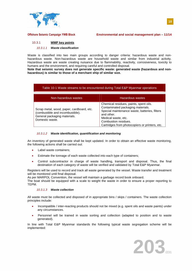
10
Offshore Seismic Campaign YWB Block Environmental and social management plan – 11/14
203/231
10.3.1 WMP key points
10.3.1.1 Waste classification
Waste is classified into two main groups according to danger criteria: hazardous waste and non-hazardous waste. Non-hazardous waste are household waste and similar from industrial activity. Hazardous waste are waste creating nuisance due to flammability, reactivity, corrosiveness, toxicity to humans and the environment, and requiring careful and controlled disposal. Note that seismic survey does not generate specific waste: generated waste (hazardous and non-hazardous) is similar to those of a merchant ship of similar size.
Table 10-1 Waste streams to be encountered during Total E&P Myanmar operations
Non-hazardous wastes Hazardous wastes
Scrap metal, wood, paper, cardboard, etc. (combustible and incombustible). General packaging materials. Domestic waste.
Chemical residues, paints, spent oils. Contaminated packaging materials. Special maintenance waste, batteries, filters and other. Medical waste, etc. Combustion residues. Cartridges from photocopiers or printers, etc.
10.3.1.2 Waste identification, quantification and monitoring
An inventory of generated waste shall be kept updated. In order to obtain an effective waste monitoring, the following actions shall be carried out:
Label waste containers;
Estimate the tonnage of each waste collected into each type of containers;
Control subcontractor in charge of waste handling, transport and disposal. Thus, the final destination of each category of waste will be verified and validated by Total E&P Myanmar.
Registers will be used to record and track all waste generated by the vessel. Waste transfer and treatment will be monitored until final disposal. As per MARPOL Convention, the vessel will maintain a garbage record book onboard. The boat should be equipped with a scale to weight the waste in order to ensure a proper reporting to TEPM.
10.3.1.3 Waste collection
All waste must be collected and disposed of in appropriate bins / skips / containers. The waste collection principles include:
Incompatible / inter-reacting products should not be mixed (e.g. spent oils and waste paints) under any circumstances.
Personnel will be trained in waste sorting and collection (adapted to position and to waste generated).
In line with Total E&P Myanmar standards the following typical waste segregation scheme will be implemented:
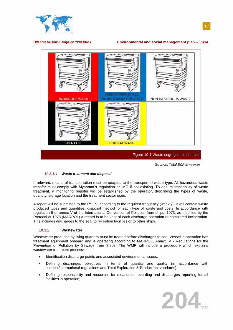
10
Offshore Seismic Campaign YWB Block Environmental and social management plan – 11/14
204/231
SOURCE: Total E&P MYANMAR
10.3.1.4 Waste treatment and disposal
If relevant, means of transportation must be adapted to the transported waste type. All hazardous waste transfer must comply with Myanmar’s regulation or IMO if not existing. To ensure traceability of waste treatment, a monitoring register will be established by the operator, describing the types of waste, quantity, storage location and the treatment sector used. A report will be submitted to the RSES, according to the required frequency (weekly). It will contain waste produced types and quantities, disposal method for each type of waste and costs. In accordance with regulation 9 of annex V of the International Convention of Pollution from ships, 1973, as modified by the Protocol of 1978 (MARPOL) a record is to be kept of each discharge operation or completed incineration. This includes discharges to the sea, to reception facilities or to other ships.
10.3.2 Wastewater
Wastewater produced by living quarters must be treated before discharges to sea. Vessel in operation has treatment equipment onboard and is operating according to MARPOL, Annex IV - Regulations for the Prevention of Pollution by Sewage from Ships. The WMP will include a procedure which explains wastewater treatment process:
Identification discharge points and associated environmental issues;
Defining discharges objectives in terms of quantity and quality (in accordance with national/international regulations and Total Exploration & Production standards);
Defining responsibility and resources for measures, recording and discharges reporting for all facilities in operation;
Figure 10-1 Waste segregation scheme
10
Offshore Seismic Campaign YWB Block Environmental and social management plan – 11/14
205/231
Defining material and procedures used for discharges treatment, in order to respect predefined threshold values.
10.4 OIL SPILL CONTINGENCY PLAN (SOPEP)
The contractor will submit to Total E&P Myanmar a plan for approval which includes procedures for the control of oil and chemicals spills. For vessels over 400 tons, the plan already exists under the name SOPEP: Ship Offshore Pollution Emergency Plan, in accordance with MARPOL. All Oil Spill Prevention measures that are listed in existing procedures are to be followed at any time to avoid Oil Spills. Particular attention is to be paid to the Oil Spill prevention measures mentioned in the procedures for refueling at sea. If an oil spill does occur, the approved SOPEP plan is to be followed and the reporting of any oil spill, regardless of quantity, is to be communicated to Total E&P Myanmar. Minor spills will be managed by cleaning instructions and absorbent products utilization to contain any accidental spillage (oil / chemicals). The Oil Spill Procedure from Polarcus, the seismic survey operator chosen by TEPM, is presented in APPENDIX J .
10.5 ENVIRONMENTAL MONITORING PROGRAM
The main concerns of this EMoP are the acoustic impacts of seismic activities on marine fauna, and the implementation of adequate monitoring procedures to minimize potential risks by the implementation of a marine mammal observation program.
10.5.1 Guiding principles
The main goals of the EMoP are as follows:
Manage and minimise the acoustic impacts to marine fauna via the implementation of appropriate management and monitoring procedures;
Check the overall effectiveness of design and operational procedures in protecting the environment;
Comply with regulations, standards, compliance programmes;
Detect sudden environmental changes;
Measure physical disturbance and subsequent recovery following the end of operations;
Assess impact and recovery following accidents and incidents;
Confirm that environmental equipment and procedures are effective and suitable; and
Compare observed impacts with those predicted in the IEE.
10.5.2 Marine mammals observation
A Marine Mammal Observer (MMO) program will be implemented according to best practice in the oil and gas industry during survey operations. One qualified Marine Mammal Observer (MMO) will be located on-board (one in the survey vessel and two others observers trained will be in the support vessels upstream the seismic vessel) and will monitor the presence of marine life within the following shutdown zones:
2,800 m for cetaceans sensitive to low frequencies (e.g. whales species), which are likely to be animals with a length greater than 8 meters (up to 33 m);
10
Offshore Seismic Campaign YWB Block Environmental and social management plan – 11/14
206/231
800 m for cetaceans sensitive to middle/high frequency (e.g. dolphins and some whales species), which are likely to be animals with length ranging from 1 to 8 meters.
It must be noted that the radius may be adapted if tests will be done in order to measure the sound pressure level. The monitoring procedure set up by Total E&P Myanmar will be developed on the basis of the recommendations of the Joint Nature Conservation Committee (JNCC and taking into account specific technical and biological research on the subject used in this IEE. An environmental monitoring register will list all observations of marine fauna (fish, turtles, birds, etc.) while the observation sessions on board. It will complement the logbook of marine mammal observers.
10.5.2.1 MMO capabilities
The MMO should be suitably qualified with:
Specific knowledge of identification of main species of marine mammals, sharks, marine birds and marine turtles;
Knowledge of good practices for MMO surveys in oil and gas activities;
General knowledge of marine mammal behaviour;
General knowledge of marine mammal and turtle sensitivity to sound;
General knowledge of the Environmental Management System of Total E&P Myanmar and other HSE procedures.
The implementation of this MMO program as a sustainable development strategy may present an opportunity to develop new proficiencies and capacities to transfer this knowledge from Total E&P Myanmar to local government agencies. In this capacity, the observation reports of marine mammals may be sent to the associations and the scientific community which might be interested.
10.5.2.2 Procedures
The observers - The observers must be able to carry out the task of detecting, tracking and identifying marine organisms. However, it is preferable that other workers involved in the survey and present on board each source vessel have some understanding of the process in order to support the implementation and the coordination of the observation procedure. The observer is to be located on an observational platform (the height depends on the vessel) and should be in direct communication with the MMO, party chief and if necessary client representative of the seismic survey. The observation - The activities of the MMO should occur throughout the day, from the departure of the vessels, so that the MMOs gain experience and increase identification capacities. Equipment for marine mammal observation should include marine binoculars, camera, laptop and identification keys of marine mammals. Before the start of seismic survey activities, the MMO/observers must observe the horizon within a radius of approximately 3 km (observation zone) of the source vessels to ensure the absence of marine mammals within a radius of 2,800 m (shutdown zone); this zone may be reduced to 800 meters if the MMO can identify that the species in question is sensitive to middle and high frequencies. If a marine mammal is sighted in the shutdown zone before the start of the shooting, the observer must delay the seismic activity until the marine mammal has left the shutdown zone. The observation will continue until the marine mammal is outside the established zone perimeter. Due to the potential severity of impacts on marine mammals, it is critical to incorporate the following components into seismic survey activities:
Use of "soft-start" procedures especially during bad weather or during night;
10
Offshore Seismic Campaign YWB Block Environmental and social management plan – 11/14
207/231
The constant watch for marine mammals before the start of activities;
The delay between seismic observation and shooting in the event that marine mammals are located in the vicinity of the vessel;
Use of vessel staff as supplementary marine mammal observers to support MMO (surveillance and communication purposes only).
The table below summarizes waiting time and specific mitigation measures proposed for Total E&P Myanmar seismic campaign.
Table 10-2 Synthesis of mitigation measures for underwater noise generated during seismic survey
Mitigation measures Seismic campaign recommendation
Marine mammal monitoring requirement
Day: observer(s) required; Passive Acoustic
Monitoring – PAM may be recommended;(1)
Night: Passive Acoustic Monitoring – PAM (1)
Duration of pre-operations monitoring period 60 minutes (1)
Shutdown zone (or « mitigation zone » or « exclusion
zone »)
2,800 m (2) for low-frequency sensitive
cetaceans (size 8 to 33 m);
800 m (2) for medium/high frequency sensitive
cetaceans (size 1 to 8 m).
Length of soft start At least 20 minutes and no longer than 40 minutes (1)
Delay of soft start after last detection of marine
mammal in mitigation zone 30 minutes (1)
Sources:
(1) Good practice recommended by English governmental organization - Joint Nature Conservation Committee’ (JNCC);
(2) Radius calculated from criteria developed by Southall work: Marine Mammal Noise Exposure Criteria: Initial Scientific Recommendations, Supported through Joint Sponsorship by the European Association for Aquatic Mammals, the Alliance of Marine Mammal Parks and Aquariums, and the International Marine Animal Trainer’s Association, Southall et al, 2007.
10.5.2.3 Reports
Daily reports should be completed in accordance with JNCC (2010) guidelines. A marine mammal observation monitoring form should be available to the MMO for inclusion in an observational report. The observations regarding marine mammals, sea turtles and birds are required by the JNCC (2010) include:
Location (latitude and longitude), distance from vessel;
Identification and determination of species, sex and size;
The behaviour of animals for each consecutive observation;
Meteorological data (weather conditions, state of the sea, winds) and coverage should be recorded during each period.
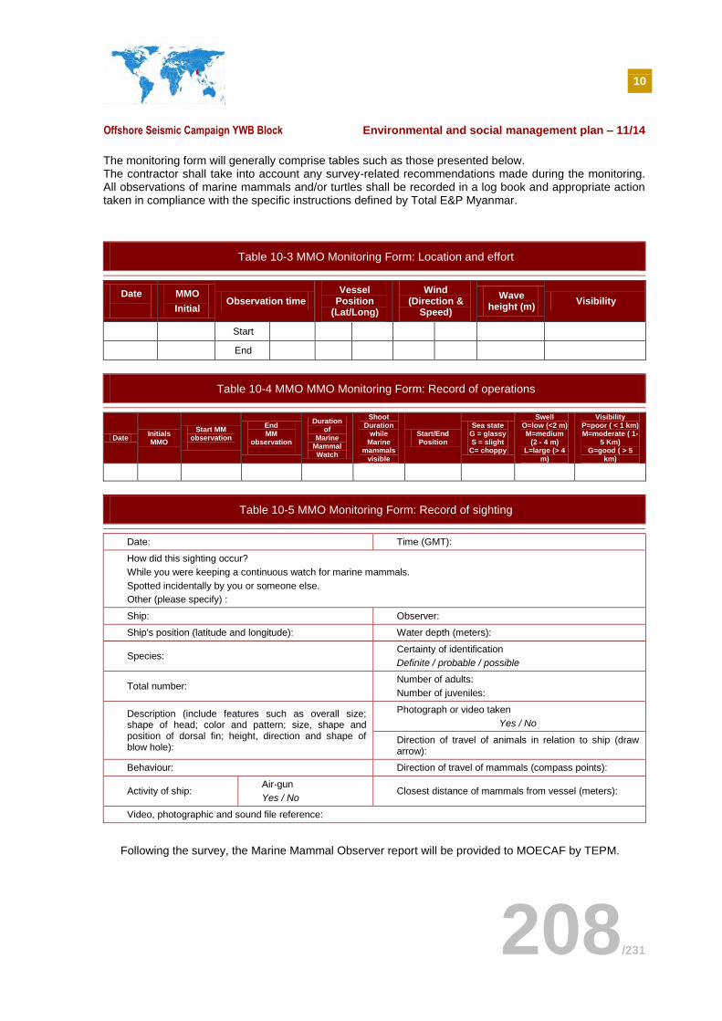
10
Offshore Seismic Campaign YWB Block Environmental and social management plan – 11/14
208/231
The monitoring form will generally comprise tables such as those presented below. The contractor shall take into account any survey-related recommendations made during the monitoring. All observations of marine mammals and/or turtles shall be recorded in a log book and appropriate action taken in compliance with the specific instructions defined by Total E&P Myanmar.
Table 10-3 MMO Monitoring Form: Location and effort
Date
MMO
Initial Observation time
Vessel Position
(Lat/Long)
Wind (Direction &
Speed)
Wave height (m)
Visibility
Start
End
Table 10-4 MMO MMO Monitoring Form: Record of operations
Date Initials MMO
Start MM observation
End MM
observation
Duration of
Marine Mammal Watch
Shoot Duration
while Marine
mammals visible
Start/End Position
Sea state G = glassy S = slight
C= choppy
Swell O=low (<2 m) M=medium
(2 - 4 m) L=large (> 4
m)
Visibility P=poor ( < 1 km) M=moderate ( 1-
5 Km) G=good ( > 5
km)
Table 10-5 MMO Monitoring Form: Record of sighting
Date: Time (GMT):
How did this sighting occur?
While you were keeping a continuous watch for marine mammals.
Spotted incidentally by you or someone else.
Other (please specify) :
Ship: Observer:
Ship's position (latitude and longitude): Water depth (meters):
Species: Certainty of identification
Definite / probable / possible
Total number: Number of adults:
Number of juveniles:
Description (include features such as overall size; shape of head; color and pattern; size, shape and position of dorsal fin; height, direction and shape of blow hole):
Photograph or video taken
Yes / No
Direction of travel of animals in relation to ship (draw arrow):
Behaviour: Direction of travel of mammals (compass points):
Activity of ship: Air-gun
Yes / No Closest distance of mammals from vessel (meters):
Video, photographic and sound file reference:
Following the survey, the Marine Mammal Observer report will be provided to MOECAF by TEPM.
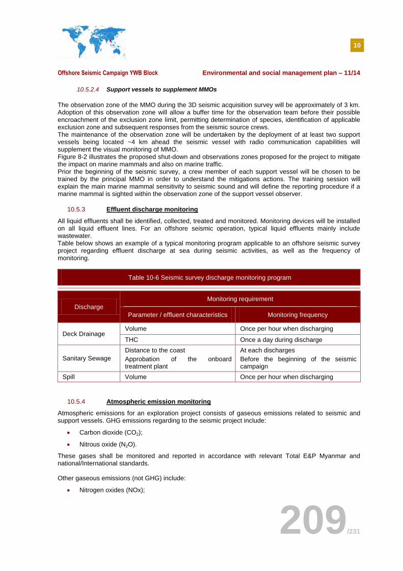
10
Offshore Seismic Campaign YWB Block Environmental and social management plan – 11/14
209/231
10.5.2.4 Support vessels to supplement MMOs
The observation zone of the MMO during the 3D seismic acquisition survey will be approximately of 3 km. Adoption of this observation zone will allow a buffer time for the observation team before their possible encroachment of the exclusion zone limit, permitting determination of species, identification of applicable exclusion zone and subsequent responses from the seismic source crews. The maintenance of the observation zone will be undertaken by the deployment of at least two support vessels being located ~4 km ahead the seismic vessel with radio communication capabilities will supplement the visual monitoring of MMO. Figure 8-2 illustrates the proposed shut-down and observations zones proposed for the project to mitigate the impact on marine mammals and also on marine traffic. Prior the beginning of the seismic survey, a crew member of each support vessel will be chosen to be trained by the principal MMO in order to understand the mitigations actions. The training session will explain the main marine mammal sensitivity to seismic sound and will define the reporting procedure if a marine mammal is sighted within the observation zone of the support vessel observer.
10.5.3 Effluent discharge monitoring
All liquid effluents shall be identified, collected, treated and monitored. Monitoring devices will be installed on all liquid effluent lines. For an offshore seismic operation, typical liquid effluents mainly include wastewater. Table below shows an example of a typical monitoring program applicable to an offshore seismic survey project regarding effluent discharge at sea during seismic activities, as well as the frequency of monitoring.
Table 10-6 Seismic survey discharge monitoring program
Discharge
Monitoring requirement
Parameter / effluent characteristics Monitoring frequency
Deck Drainage Volume Once per hour when discharging
THC Once a day during discharge
Sanitary Sewage
Distance to the coast
Approbation of the onboard treatment plant
At each discharges
Before the beginning of the seismic campaign
Spill Volume Once per hour when discharging
10.5.4 Atmospheric emission monitoring
Atmospheric emissions for an exploration project consists of gaseous emissions related to seismic and support vessels. GHG emissions regarding to the seismic project include:
Carbon dioxide (CO2);
Nitrous oxide (N2O).
These gases shall be monitored and reported in accordance with relevant Total E&P Myanmar and national/International standards.
Other gaseous emissions (not GHG) include:
Nitrogen oxides (NOx);
10
Offshore Seismic Campaign YWB Block Environmental and social management plan – 11/14
210/231
Sulphur oxides (SOx); and
Volatile Organic Compounds (VOCs).
In order to minimize the emission of these gases into the atmosphere, Total E&P Myanmar shall adopt the following strategies:
Choice of recent ships, equipped with powerful engines.
Selection of utility fuels with the lowest possible sulphur content.
10.6 TRAINING PROGRAM
Conscientious planning and good project design are not sufficient to ensure right environmental and social management if the staff on board does not apply environmental good practices. A training program for staff about respect of the various environmental procedures will be prepared by the contractor in charge of the seismic campaign and will be submitted to Total E&P for approval. It will be consistent with the significant environmental aspects and impacts associated with the proposed exploration activities. The training will take place on board, with the assistance of HSE supervisor. The training sessions may take the form of toolbox and will broach the following topics:
Environmental policy;
Waste management procedures;
Discharges (air and liquids) management;
Dangerous chemicals management, including SOPEP implementation in case of accidental spillage;
Regulatory and socio-economic aspect management;
Identification and treatment of non-compliance, etc.
10.7 ENVIRONMENTAL AUDIT PROGRAM
An Environmental audit program will be written in compliance with Total E&P Myanmar and will include:
Identification of deviations from regulatory standards and contractual requirements identified;
Evaluation of the various plans implementation efficiency, devices and mitigation measures identified in this study;
The Total E&P Myanmar Supervisor, with the seismic contractor HSE coordinator, will be responsible for the implementation of internal environmental audits on environmental good practices. He will be responsible for preparing environmental reports to the authorities, if any. Audits will be provided during the various exploration phases:
Before starting operation, an HSE marine seismic operation specialist mandated by Total E&P Myanmar will carry out an audit on the contracted vessels. This audit enables the specialist to review environmental procedure at the beginning of the project. The HSE specialist will be accompanied by the HSE coordinator and the quality controller (Total E&P Myanmar) in charge of the technical supervision of the seismic acquisition.
Regular audits (monthly for example) will be conducted by the HSE supervisor to ensure that the monitoring, control and intervention on board are in agreement with the recommendations of the ESMP.
Total E&P will inform the MOECAF an incident is observed.
10
Offshore Seismic Campaign YWB Block Environmental and social management plan – 11/14
211/231
10.8 SOCIAL MANAGEMENT PLAN
10.8.1 Stakeholder engagement plan
Total E&P Myanmar shall implement the stakeholder engagement plan prepared in SECTION 7 of this document. The purpose of this plan is to create an open and transparent dialogue and minimize any adverse impact of the project on these stakeholders. Total E&P Myanmar shall develop further this plan, integrating other stakeholders that the company may identify during the project implementation. The specific objectives and actions this plan shall follow are to:
Establish appropriate communication channels with authorities (MoE, MOECAF, DoF, MPA, DMA, etc.) and other stakeholders relevant to the Project (such as those having commercial or environmental interests in marine areas) prior to the beginning of the operation;
Maintain a positive relationship based on dialogue and transparency with all these stakeholders;
Prior to the beginning of the seismic campaign, inform them about the exact seismic location, schedule and duration through e-mails, phone calls or personal meetings;
Inform them during the seismic campaign and once it is completed about major socio-economic issues encountered, if any;
Develop a grievance mechanism based on Total E&P corporate policies (and especially GM_EP_SDV_202);
Record, report and solve grievances made by stakeholders related to any impact or incident occurring during the performance of the operations;
Offer to share valuable information acquired during the seismic (such as results of bathymetry surveys) with stakeholders who might have an interest in having them (NGOs involved in marine ecosystem protection, fishermen, government agency, etc.);
For the purpose of guaranteeing smooth operations and minimizing issues that could rise from encounter with fishermen or commercial ships at the Project location, additional measures are recommended to be implemented by Total E&P Myanmar and the Contractor:
Total E&P Myanmar shall prepare the Job Description of the Fisheries Liaison Officer and request he provides Total E&P Myanmar with regular (daily or weekly) reports;
Total E&P Myanmar shall prepare leaflets in Burmese and Thai languages explaining the seismic and its main hazards for fishermen, and the contractor shall distribute it to all fishermen encountered in the area during the Project implementation;
Total E&P Myanmar shall inform the contractor’s employees during HSE or Project Inductions about the risks related to the presence of fishermen or commercial ships at the Project area and the mitigation measures planned to limit these risks;
The Contractor shall recruit a Fisheries Liaison Officer speaking Burmese and Thai language. This Officer should stay on board during the operation in order to handle any issue that may arise with fishermen in the area, whether they are from Burmese or Thai nationality;
10.8.2 Marine traffic safety plan
Safety of marine users that may be affected by Total E&P Myanmar seismic operations shall be guaranteed by the application at all times of international marine safety standards established by the
International Maritime Organization (IMO) and in particular the International Convention for the Safety of Life at Sea (SOLAS). Total corporate marine safety policy shall also be applied by the
seismic contractor. Additional measures should be implemented by the contractor to limit the risks of vessel collisions, covering:
Speed limit respect;
Permanent exhibition of internationally recognized symbols during daytime and emission of light signal at night-time;
10
Offshore Seismic Campaign YWB Block Environmental and social management plan – 11/14
212/231
Equipment of the seismic vessels with loud speakers to communicate with boats not equipped with radio;
Weekly communication with marine authorities on operations (date, position, issues, etc.);
Defined procedures to be implemented in case of an accident where another marine user is affected (fishermen, cargoes, tankers, etc.).
10.9 EMERGENCY RESPONSE: CYCLONE AND TSUNAMI RESPONSE MEASURES
Tropical cyclones have the potential to cause damage to survey equipment, present a risk to the safety and health of survey personnel and have the potential to cause spills of hazardous materials into the environment from damaged vessels. The YWB Block 3D seismic survey is scheduled to commence in March 2016, with an expected duration of about 1 month. Therefore, the survey is supposed to be out of the cyclone season in this area (starting in May).
Polarcus has developed and implemented an “Extreme Weather Procedure” for all seismic surveys utilising its vessels. This procedure will be applied during the YWB Block seismic survey. During the survey, the procedure will be implemented in the event of an approaching cyclone. If a cyclone looks to be forming within the region of the survey, support and chase vessels will depart from the YWB Block location for safer waters. Depending on the situation, the survey vessel may also retrieve the towed seismic equipment (airgun arrays, vanes, streamers, tail buoys etc.) and in a worst case scenario proceed to the nearest port away from the expected track of the approaching cyclone.
The Polarcus’ “Extreme Weather Procedure” is available in APPENDIX K
Tsunamis do not represent a threat to vessels in offshore deep waters well away from inshore, shallow water, coastal areas and shorelines. In the deep ocean, destructive tsunamis can be small—often only a few feet or less in height—and cannot be seen nor can they be felt by ships. Tsunami wave energy extends from the surface to the seabed in the deepest waters, but, as the tsunami reaches shallower coastal waters, wave height can increase rapidly. As the tsunami reaches the coastline, the wave energy is compressed into a much shorter distance creating destructive, live-threatening waves.
11
Offshore Seismic Campaign YWB Block Responsible persons & costs for ESMP implementation – 11/14
213/231
SECTION 11. RESPONSIBLE PERSONS & COSTS FOR ESMP IMPLEMENTATION
The commitment register developed in Table 8-4 list the comprehensive measures proposed in this IEE and give the responsible for each measure to be monitored. When possible, an estimation of the cost/measure has been given.
12
Offshore Seismic Campaign YWB Block References – 11/14
214/231
SECTION 12. REFERENCES
12.1 ENVIRONMENTAL REFERENCES
12.1.1 Websites
Acousticecology website: http://www.acousticecology.org/
ASEAN Regional Centre for Biodiversity Conservation website: http://www.arcbc.org.ph/
Birdlife International website: http://www.birdlife.org/
Encyclopedia of the Nations website: http://www.nationsencyclopedia.com/
FAO website: http://www.fao.org/
Fish Base website: http://www.fishbase.org
Institute of Security Studies (ISS) website: hwww.iss.europa.eu/ttp://www.iss.co.za/
International Association of Geophysical Contractors (IAGC) website: http://www.iagc.org/
International Maritime Organization website http://www.imo.org/imo/convent/pollute.htm
JNCC website: http://jncc.defra.gov.uk/
Kessinger. W article on seismic data acquisition: http://walter.kessinger.com/work/seisx_acquisition.html
Lomont-Doherty Earth Observatory, Columbia University website : http://www.ldeo.columbia.edu/
Mekong River Commission (MRC) website: http://www.mekonginfo.org/
Ministry of Energy of Myanmar website: http://www.energy.gov.mm/
MMOA website: www.mmo-association.org
MPA Global website: http://www.mpaglobal.org/
Myanmar website: http://www.myanmars.net/
Nasa Earth Observatory website: http://earthobservatory.nasa.gov/
Protected planet website: http://www.protectedplanet.net/
Southeast Asian Fisheries Development Center (SEAFDEC) website: http:// http://map.seafdec.org/
Total E&P Myanmar website: burma.total.com/
US Department of State Website: http://www.state.gov/
US Energy Information Administration website: http://www.eia.doe.gov/
United Nations Environment Programme (UNEP) – World Conservation Monitoring Centre website: http://www.unep-wcmc.org/
Water Environment Partnership in Asia (WEPA) website: http://www.wepa-db.net/
Wild World (WWF) website: http://www.worldwildlife.org/
12.1.2 Scientific articles
R. M., 1981 (ed.) Atlas, Microbial Ecology Fundamentals and Applications. Addition–Wesley, Reading, Massachusette, 361 – 368
12
Offshore Seismic Campaign YWB Block References – 11/14
215/231
R. M. and Bartha, R. 1973, Atlas, Fate and Effects of polluting petroleum in the marine environment. Microbiological Review, 49 – 85
June 2012, Benthic Macroinvertebrate community structure and distribution in the Ayeyarwady continental shelf, Andaman Sea, Indian Journal of Geo Marine Sciences (vol 41(3)), 272-278
Caroline R. Weir, 2007, Observations of Marine Turtles in Relation to Seismic Airgun Sound off Angola, Marine Turtle Newsletter (116), 17-20
Haughton, P. D. W., 2001, The petroleum exploration of Ireland's offshore basins, Geological Society of London (No 188)
Hook, S.E., N.S. Fisher, 2001, Reproductive toxicity of metals in calanoid copepods, Marine Biology (138), 1131-1140.
Joseph Graber, 2011, Land-based Infrared Imagery for Marine Mammal Detection, Master of Science in Mechanical Engineering, University of Washington
Naing, Thet Zaw, 2006, Waterbirds survey in mouth of Yangon River and Ayeyarwaddy (Irrawaddy) delta. Indian Birds 2 (3), 65-71
Smith, B.D., Thant, H., Lwin, J.M. and Shaw, C.D., 1997, Preliminary investigation of cetaceans in the Ayeyarwady River and northern coastal waters of Myanmar. Asian Marine Biology (14), 173-194
Southall et al., 2007, Aquatic Mammals Marine Mammal Noise Exposure Criteria: Initial Scientific Recommendations (Volume 33, Number 4)
Velasquez, I.B., G.S. Jacinto, F.S. Valera, 2002, The speciation of dissolved copper, cadmium, and zinc in the Manila Bay, Philippines, Marine Pollution Bulletin (45), 210-217
12.1.3 Reports
De Boer, M.N. , R. Baldwin, C.L.K. Burton, E.L. Eyre, K.C.S. Jenner, M-N.M. Jenner, S.G. Keith, K.A.McCabe, E.C.M. Parsons, V.M. Peddemors, H.C. Rosenbaum, P. Rudolph and M. P. Simmonds (eds.), 2002, Cetaceans in the Indian Ocean Sanctuary: A Review. A Whale and Dolphin Conservation Society Science Report
DNV Energy. Effects of seismic surveys on fish, fish catches and sea mammals 2007-0512 rev 01, Cooperation group - Fishery Industry and Petroleum Industry
Multi Klient Invest As, April 28, 2011, Environmental Impact Assessment For Marine 2D Seismic Reflection Survey Baffin Bay And Davis Strait Offshore Eastern Canada By
Fisheries and Oceans Canada. Review of Scientific Information on Impacts of Seismic Sound on Fish, Invertebrates, Marine Turtles and Marine Mammals, Habitat Status Report 2004/002
Alberto Baldacci, Michael Carron and Nicola Portunato, December 2005, Infrared detection of marine mammals, NURC Technical Report SR-443
Lurton / Deruiter, November 2011, International Hydrographic Review, Sound Radiation of seafloor-mapping echosounders in the water column, in relation to the risk posed to marine mammals
Myanmar Protected Areas: Context, Current Status and Challenges, BANCA, 2011
Report of the Ad-hoc Group on the Impacts of Sonar on Cetaceans and Fish (AGISC) (2nd edition), ICES AGISC, 2005
S. Roussy, February 2008, External final report, Water, Sanitation & Hygiene Disaster Risk Reduction Assessment, Irrawaddy division
H. Sekha, May 2003, Toxicity of trace elements: truth or myth, Advanced Aquarist (Volume 2 issue 5)
The Ecosystem-Based Management Fishery in the Bay of Bengal, BIMSTEC, September 2008
12
Offshore Seismic Campaign YWB Block References – 11/14
216/231
Thein Aung. Presentation of the Status of biodiversity conservation in Myanmar, Nature Wildlife Conservation Division, Forest Department of Myanmar
UP-MSI, ABC, ARCBC, DENR, ASEAN, 2002. Marine Protected Areas in Southeast Asia. ASEAN Regional Centre for Biodiversity Conservation, Department of Environment and Natural Resources, Los Baños, Philippines. 142 pp, 10 maps
WHO, 1984, Guidelines for drinking water quality (Vol. 1. Recommendations)
World Bank Group, 1998, Pollution, Prevention and Abatement Handbook –Towards Cleaner Production
12.1.4 Convention
International Convention for the Prevention of Pollution from Ships (MARPOL), 1973/78
12.2 SOCIO-ECONOMIC REFERENCES
12.2.1 Webistes
US Department of State Website: http://www.state.gov/
US Energy Information Administration website: http://www.eia.doe.gov/
United Nations Environment Programme (UNEP) – World Conservation Monitoring Centre website: http://www.unep-wcmcg/
12.2.2 Socio-economic articles
Aung San Yamin, 3 April 2014, Burma Bans Foreign Fishing Boats from Its Waters, The Irrawady
Beech Hannah, 30 January 2009, A Closer Look at Burma's Ethnic Minorities, TIME
Chie Ikeya, 2005/2006, The 'Traditional' High Status of Women in Burma: A Historical Reconsideration, Journal of Burma Studies
Chuenniran Achdataya, 11 July 2014, Myanmar Sinks Thai Trawler, Bangkok Post
Eleven Myanmar, Sunday, 27 July 2014, Kyaukphyu fishermen see depleted fish stock due to Shwe project
Eleven Myanmar, 11 April 2014, UNIDO to Upgrade Myanmar’s Fish Factories, available at http://www.elevenmyanmar.com/index.php?option=com_content&view=article&id=5731:unido-to-upgrade-myanmar-s-fish-factories&catid=33:business&Itemid=356
International Business Times, 26 February 2014, Myanmar's Fish Exports Slump in 2013 As FDI Remains Low For Sector
Pitcher Tony J., 2007, An Estimation of Compliance of the Fisheries of Myanmar with Article 7 (Fisheries Management) of the UN Code of Conduct for Responsible Fishing
12.2.3 Reports
ADB, 2013, Framework of Inclusive Growth Indicators 2013, Myanmar
ADB, December 2012, Asian Development Bank and Myanmar, Factsheet
IHLCA Project Technical Unit, June 2011, Integrated Household Living Conditions Survey in Myanmar (2009-2010), Poverty Profile
ADB, August 2012, Myanmar in Transition: Opportunities and Challenges
Asia Foundation, September 2013, State and Region Government in Myanmar
12
Offshore Seismic Campaign YWB Block References – 11/14
217/231
APFIC, 2004, Status and potential of fisheries and aquaculture in Asia and the Pacific, Food and Agriculture Organization of the United Nations Regional Office for Asia and the Pacific Bangkok
APFIC/FAO Regional Consultative workshop,4–6 October 201, Strengthening assessment of fisheries and aquaculture in the Asia-Pacific region for policy development, Yangon, Myanmar
APFIC (Khin Maung Aye & Win Ko Ko), 30 September – 4 October 2013, Regional Expert Workshop on Topical Trawl Fishery Management, Phuket, Thailand
Bay of Bengal large marine ecosystem project (BOBLME), Transboundary Diagnostic Analysis vol. 1, 2012
Bay of Bengal large marine ecosystem project (BOBLME), Transboundary Diagnostic Analysis vol. 2, 2012
FAO, 5–9 October 2009, Report of the Second Workshop on the Assessment of Fishery Sector Status in South and Southeast Asia, Bangkok FAO, 2014, The State of World Fisheries and Aquaculture, Opportunities and Challenges FAO Corporate Document Repository, Coastal State requirements for foreign fishing, Myanmar, available at http://www.fao.org/docrep/v9982e/v9982e2w.htm Flewwelling Peter, Hosch Gilles, December 2003, Country review: Myanmar, Fishery Policy and Planning Division, Fisheries Department, http://www.fao.org/docrep/009/a0477e/a0477e0d.htm Gausland Ingebret, March 2003, Seismic Surveys Impacts on Fish and Fisheries, Report for Norwegian Oil Industry Association Global Justice Center, May 2013, The Gender Gap and Women’s Political Power in Myanmar
Hamish Nixon et al., September 2013, State and Region Government in Myanmar, 96 p
Hume Tim, 6 July 2014, Curfew imposed after deadly clashes between Buddhists, Muslims in Myanmar, CNN
IRIN, March 2012, What next for Myanmar?
Kyaw Julius, 7-9 September 2011, Department of Fisheries, Present Status of Off-shore Fishery Resources and Information on Tuna Fishery in Myanmar, Special Meeting on Improvement of Tuna Information and Data Collection in the Southeast Asia. Songkhla Province, Thailand Kya Kyaw, Dr., SEAFDEC, 2010, Countries profile of Myanmar Addressing the IUU Fishing in the Southeast Asian Region Ministry of Immigration and Population, August 2014, Census Report Volume 1 Morgan Gary R, Staples Derek J., 2006, The History of Industrial Marine Fisheries in Southeast Asia, Asia-Pacific Fishery Commission, FAO Regional Office for Asia and the Pacific. APFIC ad hoc publication New Than Than, February 2003, Gendered Spaces: Women in Burmese Society, Transformations, No. 6 Offshore Energy Today, March 26, 2014, Myanmar awards new offshore blocks
PE Myint, 2004, National Report of Myanmar on the Sustainable Management of the Bay of Bengal Large Marine Ecosystem, BOBLME, GCP/RAS/179/WBG
SEAFDEC Training Department, Report of the Expert Meeting on Deep-sea Fishing and Its Impact to Ecosystem, workshop from 31 August to 2 September 2010 at Jasmine City Hotel, Bangkok, Thailand
12
Offshore Seismic Campaign YWB Block References – 11/14
218/231
Staples D., 2009, Status and potential of offshore resources in South and Southeast Asia. Asia-Pacific Fishery Commission, FAO Regional Office for Asia and the Pacific
UNFPA, June 2010, Report on Situation Analysis of Population and Development, Reproductive Health and Gender in Myanmar
UNDP, June 2004, Myanmar Agricultural Sector Review and Investment Strategy, Volume 2: Agricultural Sector Investment Strategy
UNDP, 2013, Human Development Report 2013
UNDP, 2013, Annual Report 2013, Myanmar
World Health Organization, 2012, Myanmar Health Profile 2012
World Health Organization, 2012, OECD, Health at a Glance Asia/Pacific 2012
World Bank Group, October 2013, Myanmar Economic Monitor
12.3 CONVENTION
UNITED NATIONS, The United Nations Convention on the Law of the Sea (A historical perspective), 1998, available at [http://www.un.org/Depts/los/convention_agreements/convention_historical_perspective.htm#Exclusive Economic Zone]

13
Offshore Seismic Campaign YWB Block Appendices – 11/14
219/199
SECTION 13. APPENDICES

13
Offshore Seismic Campaign YWB Block Appendices – 11/14
220/199
APPENDIX A Policy, legal and administrative Framework
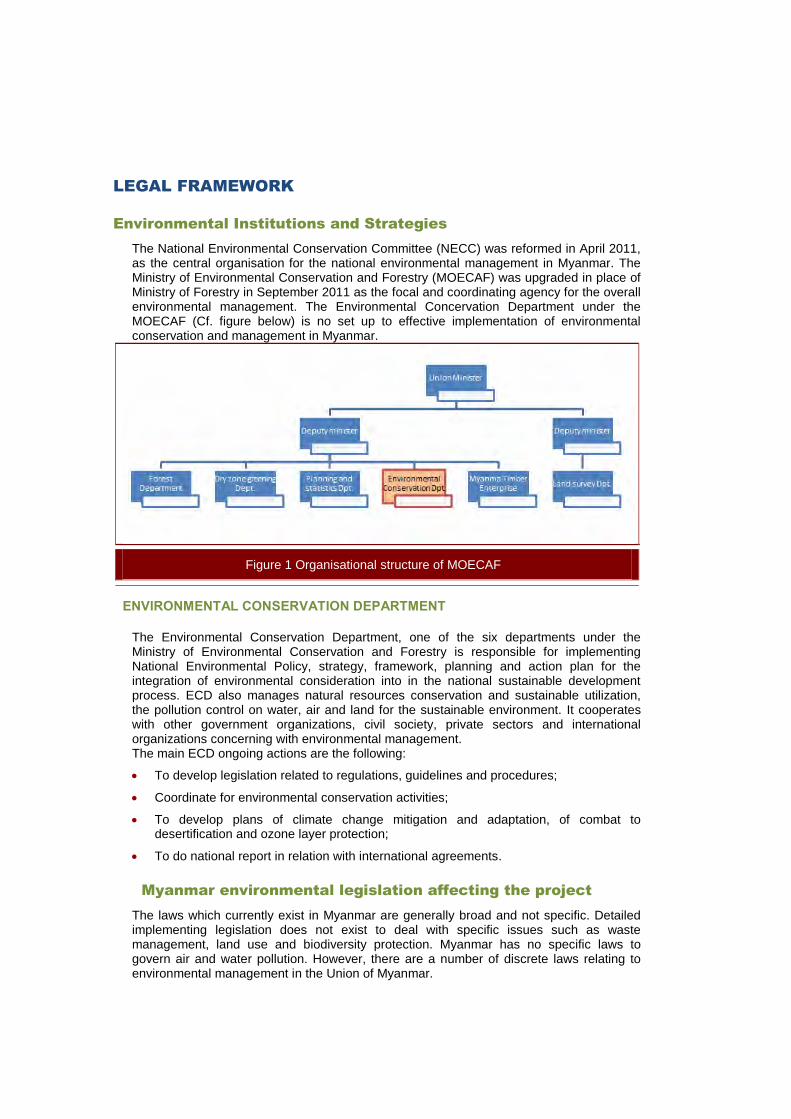
LEGAL FRAMEWORK
Environmental Institutions and Strategies
The National Environmental Conservation Committee (NECC) was reformed in April 2011, as the central organisation for the national environmental management in Myanmar. The Ministry of Environmental Conservation and Forestry (MOECAF) was upgraded in place of Ministry of Forestry in September 2011 as the focal and coordinating agency for the overall environmental management. The Environmental Concervation Department under the MOECAF (Cf. figure below) is no set up to effective implementation of environmental conservation and management in Myanmar.
Figure 1 Organisational structure of MOECAF
ENVIRONMENTAL CONSERVATION DEPARTMENT
The Environmental Conservation Department, one of the six departments under the Ministry of Environmental Conservation and Forestry is responsible for implementing National Environmental Policy, strategy, framework, planning and action plan for the integration of environmental consideration into in the national sustainable development process. ECD also manages natural resources conservation and sustainable utilization, the pollution control on water, air and land for the sustainable environment. It cooperates with other government organizations, civil society, private sectors and international organizations concerning with environmental management. The main ECD ongoing actions are the following:
To develop legislation related to regulations, guidelines and procedures;
Coordinate for environmental conservation activities;
To develop plans of climate change mitigation and adaptation, of combat to desertification and ozone layer protection;
To do national report in relation with international agreements.
Myanmar environmental legislation affecting the project
The laws which currently exist in Myanmar are generally broad and not specific. Detailed implementing legislation does not exist to deal with specific issues such as waste management, land use and biodiversity protection. Myanmar has no specific laws to govern air and water pollution. However, there are a number of discrete laws relating to environmental management in the Union of Myanmar.
THE ENVIRONMENTAL CONSERVATION LAW (30TH MARCH, 2012)
The objective of this Law is to implement the Myanmar National Environmental Policy, enabling to lay down the basic principles and to give guidance for systematic integration of environmental conservation matters in the sustainable development process. An Environmental Conservation Committee is formed. It requires the Ministry to cooperate and give technical advice for environmental conservation to the department managing natural resources. The committee and the ministry can take “necessary measures relating to an environmental emergency”. The 7th article confers the following powers and functions on the Ministry:
To set environmental quality standards
To prescribe emission standards
To formulate EIA and SIA systems
To ensure the polluter pays principle
To issue rules, regulations and by-laws as may be necessary with the approval of the Union Government
The purpose is to assess if a project to be undertaken causes a significant impact on the environment. The ministry may, with the approval of the Union Government, require obtaining the prior authorization to carry projects which may damage the environmental quality. On the basis of this law, EIA rules have been issued in draft by the Myanmar administration.
THE LAW AMENDING THE PROTECTION AND PRESERVATION OF CULTURAL HERITAGE REGIONS LAW (2009)
This amendment is concerned with revising fine for failure to abide by this law.
THE STATE SUPPLEMENTARY APPROPRIATION LAW (2009)
This law is concerned with sanctioned allotment and administration of supplementary expenditures and taking of loans for the respective persons mentioned in this law.
NATIONAL SUSTAINABLE DEVELOPMENT STRATEGY (2009)
This law is concerned with the sustainable management of natural resources, integrated economic development, and sustainable social development.
THE LAW AMENDING THE PORTS ACT (2008)
11. Sub-section 2 of section 21 of the Ports Act shall be substituted as follows: “ (2) Any person who by himself or another so casts or throws any ballast or rubbish or any such other thing or so discharges any oil or water mixed with oil, or the master of any vessel from which the same is so cast, thrown or discharged, shall be punishable with fine not exceeding fifty thousand kyats, and shall pay any reasonable expenses which may be incurred in removing the same.”
THE LAW AMENDING THE TERRITORIAL SEA AND MARITIME ZONE LAW (2008)
After clause 3 of the annex to the Territorial Sea and Maritime Zone Law, clause 4 and clause 5 have been inserted with new Coordinates which has no impact on the offshore installations of TEPM (and mostly confined to areas adjacent to Bangladesh).
CONSERVATION OF WATER RESOURCES AND RIVERS LAW (2006)
Section 6 outlines prohibitions for the following activities:
“No person shall anchor the vessels where vessels are prohibited from anchoring in the rivers and creeks.
No person shall dispose of engine oil, chemical, poisonous material and other materials which may cause environmental damage, or dispose of explosives from the bank or from a vessel which is plying, vessel which has berthed, anchored, stranded or sunk.
No one shall dispose of any substance into the river-creek that may cause damage to waterway or change of watercourse from the bank or vessel.”
The aims of this Law are as follows:
to conserve and protect the water resources and river systems for beneficial utilization by the public
to smooth and enhance safety of waterways navigation along rivers and creeks
to contribute to the development of State economy through improving water resources and river systems
to protect environmental impact.
The empowerment of this Law is provided to the Ministry of Transport for controlling navigation of vessels in the rivers and creeks as well as communicating with local and foreign government and organizations for conservation of water resources, rivers and creeks. Also, to carry out conservation works for water resources, rivers and creeks, in accordance with the relevant international conventions, regional agreements and bilateral agreements for environmental conservation.
RULES ON PROTECTION OF WILDLIFE, AND PROTECTED AREA CONSERVATION LAW (2003)
This law has been created to establish a procedural framework for the 1994 Protection of Flora and Fauna, and Protected Area Conservation Law.
MYANMAR AGENDA 21 (1997)
The Myanmar Agenda 21 encompasses a broad range of sectors and issues. Building on the National Environment Policy, the agenda takes into consideration the programme guidelines found in the global Agenda 21 and is aimed at strengthening and promoting systematic environmental management in the country. Most importantly, the Myanmar Agenda 21 makes recommendations for the drafting and promulgation of a framework law which can further promote the integration of environmental and developmental concerns in the decision-making processes of the country. The Myanmar Agenda 21 contains guidelines to address the following issues:
increasing energy and material efficiency in production processes;
reducing wastes from production and promoting recycling;
promoting use of new and renewable sources of energy;
using environmentally sound technologies for sustainable production;
reducing wasteful consumption;
increasing awareness for sustainable consumption.
NATIONAL ENVIRONMENT POLICY (1994)
The National Environment Policy is reproduced below: “To establish sound environment policies, utilisation of water, land, forests, mineral, marine resources and other natural resources in order to conserve the environment and prevent its degradation, the Government of the Union of Myanmar hereby adopts the following policy: The wealth of the nation is its people, its cultural heritage, its environment and its natural resources. The objective of Myanmar’s environmental policy is aimed at achieving
harmony and balance between these through the integration of environmental considerations into the development process to enhance the quality of the life of all its citizens. Every nation has the sovereign right to utilise its natural resources in accordance with its environmental policies; but great care must be taken not to exceed its jurisdiction or infringe upon the interests of other nations. It is the responsibility of the State and every citizen to preserve its natural resources in the interests of present and future generations. Environmental protection should always be the primary objective in seeking development.”
THE PROTECTION OF WILDLIFE AND CONSERVATION OF NATURAL AREAS LAW (1994)
Government policy for wildlife protection, conservation of natural areas, protection and conservation of wildlife ecosystems and migratory birds, protect endangered species and their natural habitats. Chapter 11 outlines the penalties “causing water and air pollution, causing damage to a water-course or putting poison in the water in a natural area’, and ‘possessing or disposing of pollutants or mineral pollutants in a natural area”.
UNION OF MYANMAR MARINE FISHERIES LAW (25 APRIL 1990, AMENDED 1993)
This law places restrictions on marine fisheries, including punishments for non-compliances. The relevance of this law to the offshore component of the Yadana project is that it places restriction on pollution: “No person shall dispose of living aquatic creatures or any material into the Myanmar Marine Fisheries Waters to cause pollution of water or to harass fishes and other marine organisms.”
TERRITORIAL SEA AND MARITIME ZONES LAW (1977)
The Union of Myanmar has exclusive jurisdiction for the construction, maintenance or operation of offshore terminals and exclusive jurisdiction to preserve and protect the marine environment, and to prevent and control marine pollution.
PUBLIC HEALTH LAW (1972)
Section 9 of this law empowers the Government to carry out measures relating to environmental health, such as garbage disposal, use of water for drinking and other purposes, radioactivity, protection of air from pollution, sanitation works and food and drug safety. However, detailed provisions do not exist to ensure more effective and comprehensive regulation of these areas.
PENAL CODE (1 MAY 1961, AND EXTENDED TO PUBLIC HEALTH LAW IN 1972)
The penal code is mainly concerned with public health; it is considered an offence to “voluntarily corrupt or foul the water of any public spring or reservoir so as to render it less fit for the purpose for which it is ordinarily used”, or to pollute the atmosphere arising from smoke, fumes, noxious odours, dust particles, noise and radioactive substances. The only control of water pollution in the country is through guidelines issued in June 1994 by the Myanmar Investment Commission. These guidelines require that new projects, from both foreign and private investments, have waste water treatment plants or systems.
THE PETROLEUM ACT (1934)
The Petroleum act is concerned with regulation of the production, storage and transport of oil so as not to cause pollution and fire.
THE OILFIELDS ACT (1918)
This act provides clarification on activities within the oil and gas industry, and provides the Government with the power to define and alter limits of any notified oilfield. In addition, the Government may make rules for regulating all matters connected with many operations
related to the extraction of oil and/or gas. The Act also provides guidance and issues such as preventing oil and gas wastes, reporting of fires, accidents and other occurrences and regulating the collection and disposal of both oil and gas.
Environmental and Social Impact Assessment Legislation
The objective of this Law is to implement the Myanmar National Environmental Policy, enabling to lay down the basic principles and to give guidance for systematic integration of environmental conservation matters in the sustainable development process. An Environmental Conservation Committee is formed. It requires the Ministry to cooperate and give technical advice for environmental conservation to the department managing natural resources. The committee and the ministry can take “necessary measures relating to an environmental emergency”. The 7th article confers the following powers and functions on the Ministry:
To set environmental quality standards
To prescribe emission standards
To formulate EIA and SIA systems
To ensure the polluter pays principle
To issue rules, regulations and by-laws as may be necessary with the approval of the Union Government
The Environmental Conservation Law lays down the basic principles and guidance for systematic integration of environmental conservation matters in the sustainable development process. The purpose is to assess if a project to be undertaken causes a significant impact on the environment. The ministry may, with the approval of the Union Government, require to obtain the prior authorization to carry projects which may damage the environmental quality. On the basis of this law, EIA rules are actually under construction by the Myanmar administration.
INTERNATIONAL AGREEMENTS AND CONVENTIONS
The Union of Myanmar is signatory to the following international conventions and protocols:
Asia Least Cost Greenhouse gas Abatement Strategy (ALGAS), 1998
Convention on Climate Change, 1992.
International Convention on the Prevention of Pollution from Ships, 1973 as modified by the protocol of 1978 (MARPOL 73/78) with the exceptions of Annex III (packaged substances), Annex IV (sewage) and Annex V (garbage).
Montreal Protocol on Substances that Deplete the Ozone Layer, 1989.
Vienna Convention for the protection of the Ozone Layer, 1988.
London Amendment to the Montreal Protocol, London 1990.
United Nations Convention on Law of the Sea, 1986.
Convention on Biological Diversity, Rio de Janeiro, 1992.
The domain of action of these conventions is summarised in Appendix C. The Myanmar government has not signed Annexes IV and V of the MARPOL convention which relate to garbage and sewage disposal. However these guidelines have been adopted as a standard for pollution control and are in line with international policy, which has already been adopted into TOTAL and TEPM design and operational procedures.
INTERNATIONAL ENVIRONMENTAL GUIDELINES AND
STANDARD
An increasing volume of environmental guidelines and principles has been issued by relevant international organisations over the last two decades. More recently, one trend of international law development is the increasing use of cross reference to complement working guidelines and standards developed by competent organisations. For instance, the reference to "generally accepted international standards" in the Law of the Sea Convention, and "guidelines and standards adopted by the competent international organisation" in the Barcelona Offshore Exploration Protocol.
International organizations
WORLD BANK AND IFC
Founded in 1944, the World Bank Group is one of the world's largest sources of development assistance. The Bank is now working in more than 100 developing economies, bringing a mix of finance and ideas to improve living standards and eliminate the worst forms of poverty. For each of its clients, the Bank works with government agencies, non-governmental organisations, and the private sector to formulate assistance strategies. The methodology of impact evaluation used in this report is inspired from the methodology developed by the World Bank. IFC (International Finance Corporation) is the private sector arm of the World Bank Group. IFC has 182 member countries (including Myanmar since December 1956).
UNITED NATIONS ENVIRONMENT PROGRAMME (UNEP)
An early example of the international guidelines on petroleum environmental regulation is the UNEP environmental law guidelines and principles on Offshore Mining and Drilling issued in 1982. The principal provisions of this document are summarised in the following points:
State should take preventive measures against, limit and reduce pollution and other adverse effect on the environment resulting from offshore exploration and exploitation of hydrocarbons and other minerals by adopting regulations and through international co-operations. National laws and regulations should not be less effective than international rules and standards.
The granting of an authorisation should be preceded by an environmental assessment. Authorisations should be refused if there are clear indications that significant adverse effects caused by such operations could not be avoided.
States have the responsibility to ensure that activities within their jurisdiction do not cause damage to the environment of other states or areas beyond the limits of national jurisdiction.
States should ensure that safety measures, contingency planning and implementation measures are undertaken for offshore operations; and appropriate measures are adopted for determining environmental liability and compensation for damages resulting from offshore operations.
INTERNATIONAL ASSOCIATION OF OIL AND GAS PRODUCERS (OGP)
The OGP is the worldwide association of Oil and Gas Companies involved in exploration and production. The members include private and state-owned oil and gas companies, national associations and petroleum institutes. OGP represent their members before international regulatory bodies, and has observer status as a non-governmental
organisation, with global and regional regulatory bodies that have an interest in marine environment protection. TOTAL is a member of OGP.
INTERNATIONAL PETROLEUM INDUSTRY ENVIRONMENTAL CONSERVATION ASSOCIATION (IPIECA)
IPIECA is a voluntary non-profit organization whose membership includes both petroleum companies and associations at the national, regional or international levels. It addresses global environmental and social issues related to the petroleum industry: oil spill preparedness and response, global climate change, biodiversity, social responsibility, fuel quality and vehicle emissions, and human health. IPIECA also helps members identify new global issues and assesses their potential impact on the oil industry. The Association represents the views of its members in public forums and provides an interface between the petroleum industry and the United Nations Agencies. IPIECA's goals are to promote good practices and industry consensus through arranging international workshops, publishing authoritative reports, providing a channel of communication with the UN, providing a forum for open dialogue, facilitating stakeholder engagement, promoting partnerships. TOTAL is a member of IPIECA.
INTERNATIONAL MARITIME ORGANIZATION (IMO)
The purposes of the Organization is "to provide machinery for cooperation among Governments in the field of governmental regulation and practices relating to technical matters of all kinds affecting shipping engaged in international trade; to encourage and facilitate the general adoption of the highest practicable standards in matters concerning maritime safety, efficiency of navigation and prevention and control of marine pollution from ships". The Organization is also empowered to deal with administrative and legal matters related to these purposes. The IMO developed and introduced international conventions dealing with safety at sea and prevention of marine pollution. One of the most important of all these measures was the International Convention for the Prevention of Pollution from Ships, 1973, as modified by the Protocol of 1978 relating thereto (MARPOL 73/78). IMO also developed a number of other legal conventions and around 40 conventions and protocols have been adopted by the Organization and most of them have been amended on several occasions to ensure that they are kept up to date with changes taking place in world shipping. IMO has introduced measures to improve the way legislation is implemented, by assisting flag States (the countries whose flag a ship flies) and by encouraging the establishment of regional port State control systems. When ships go to foreign ports they can be inspected to ensure that they meet IMO standards.
International standards and guidelines
The ESIA will adopt standards and guidelines from:
World Health Organization (WHO) standards and guidelines;
the IFC Environmental Health and Safety Guidelines (2007) and IFC Environmental Health and Safety Guidelines – Offshore Oil and Gas Developments (2007);
MARPOL and PARCOM (1986) (activities carried out at sea).
These environmental standards are described hereafter. The EHS Guidelines for Offshore Oil and Gas Development (IFC, 2007) include information relevant to seismic exploration, exploratory and production drilling, development and production activities, offshore pipeline operations, offshore transportation, tanker loading and unloading, ancillary and support operations, and decommissioning. The guidelines also address potential onshore impacts that may result from offshore oil and gas activities. Potential environmental issues associated with offshore oil and gas development projects include the following:
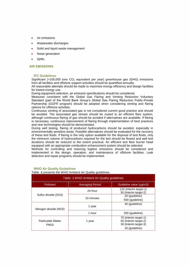
Air emissions
Wastewater discharges
Solid and liquid waste management
Noise generation
Spills.
AIR EMISSIONS
IFC Guidelines Significant (>100,000 tons CO2 equivalent per year) greenhouse gas (GHG) emissions from all facilities and offshore support activities should be quantified annually. All reasonable attempts should be made to maximize energy efficiency and design facilities for lowest energy use. During equipment selection, air emission specifications should be considered. Measures consistent with the Global Gas Flaring and Venting Reduction Voluntary Standard (part of the World Bank Group’s Global Gas Flaring Reduction Public-Private Partnership (GGFR program) should be adopted when considering venting and flaring options for offshore activities. Continuous venting of associated gas is not considered current good practice and should be avoided. The associated gas stream should be routed to an efficient flare system, although continuous flaring of gas should be avoided if alternatives are available. If flaring is necessary, continuous improvement of flaring through implementation of best practices and new technologies should be demonstrated. During well testing, flaring of produced hydrocarbons should be avoided, especially in environmentally sensitive areas. Feasible alternatives should be evaluated for the recovery of these test fluids. If flaring is the only option available for the disposal of test fluids, only the minimum volume of hydrocarbons required for the test should be flowed and well test durations should be reduced to the extent practical. An efficient test flare burner head equipped with an appropriate combustion enhancement system should be selected. Methods for controlling and reducing fugitive emissions should be considered and implemented in the design, operation, and maintenance of offshore facilities. Leak detection and repair programs should be implemented.
WHO Air Quality Guidelines Table -1 presents the WHO Ambient Air Quality guidelines.
Table -1 WHO Ambient Air Quality guidelines
Pollutant Averaging Period Guideline value (µg/m3)
Sulfur dioxide (SO2)
24-hour 125 (Interim target-1) 50 (Interim target-2)
10 minutes 20 (guideline)
500 (guideline)
Nitrogen dioxide (NO2) 1 year
40 (guideline)
1 hour 200 (guideline)
Particulate Matter
PM10
1 year
70 (Interim target-1) 50 (Interim target-2) 30 (Interim target-3)
20 (guideline)
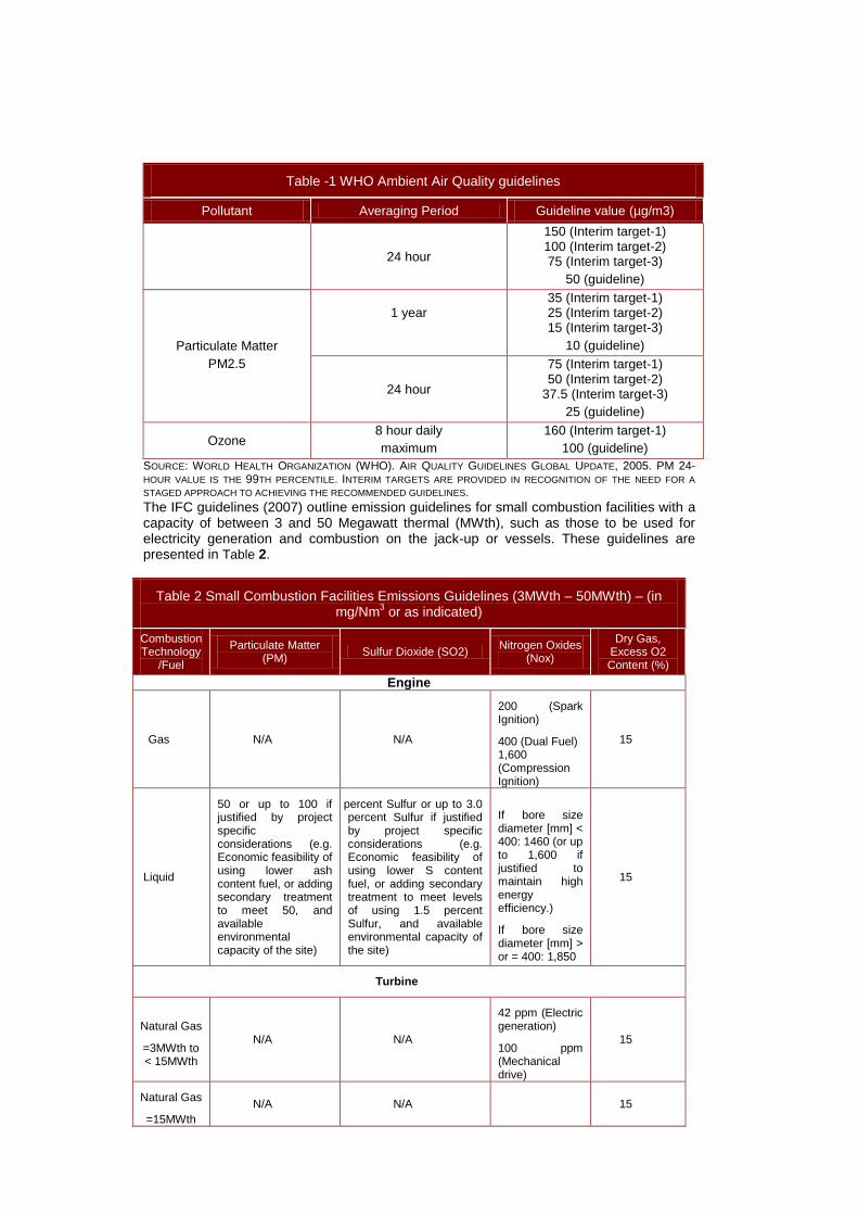
Table -1 WHO Ambient Air Quality guidelines
Pollutant Averaging Period Guideline value (µg/m3)
24 hour
150 (Interim target-1) 100 (Interim target-2) 75 (Interim target-3)
50 (guideline)
Particulate Matter
PM2.5
1 year
35 (Interim target-1) 25 (Interim target-2) 15 (Interim target-3)
10 (guideline)
24 hour
75 (Interim target-1) 50 (Interim target-2)
37.5 (Interim target-3)
25 (guideline)
Ozone 8 hour daily
maximum
160 (Interim target-1)
100 (guideline)
SOURCE: WORLD HEALTH ORGANIZATION (WHO). AIR QUALITY GUIDELINES GLOBAL UPDATE, 2005. PM 24-HOUR VALUE IS THE 99TH PERCENTILE. INTERIM TARGETS ARE PROVIDED IN RECOGNITION OF THE NEED FOR A
STAGED APPROACH TO ACHIEVING THE RECOMMENDED GUIDELINES.
The IFC guidelines (2007) outline emission guidelines for small combustion facilities with a capacity of between 3 and 50 Megawatt thermal (MWth), such as those to be used for electricity generation and combustion on the jack-up or vessels. These guidelines are presented in Table 2.
Table 2 Small Combustion Facilities Emissions Guidelines (3MWth – 50MWth) – (in mg/Nm
3 or as indicated)
Combustion Technology
/Fuel
Particulate Matter (PM)
Sulfur Dioxide (SO2) Nitrogen Oxides
(Nox)
Dry Gas, Excess O2 Content (%)
Engine
Gas N/A N/A
200 (Spark Ignition)
400 (Dual Fuel) 1,600 (Compression Ignition)
15
Liquid
50 or up to 100 if justified by project specific considerations (e.g. Economic feasibility of using lower ash content fuel, or adding secondary treatment to meet 50, and available environmental capacity of the site)
1.5 percent Sulfur or up to 3.0 percent Sulfur if justified by project specific considerations (e.g. Economic feasibility of using lower S content fuel, or adding secondary treatment to meet levels of using 1.5 percent Sulfur, and available environmental capacity of the site)
If bore size diameter [mm] < 400: 1460 (or up to 1,600 if justified to maintain high energy efficiency.)
If bore size diameter [mm] > or = 400: 1,850
15
Turbine
Natural Gas
=3MWth to < 15MWth
N/A N/A
42 ppm (Electric generation)
100 ppm (Mechanical drive)
15
Natural Gas
=15MWth
N/A N/A 15
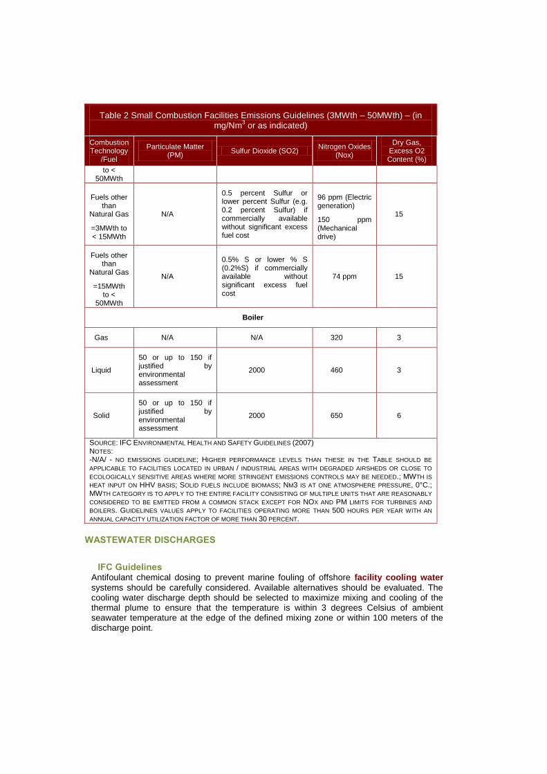
Table 2 Small Combustion Facilities Emissions Guidelines (3MWth – 50MWth) – (in mg/Nm
3 or as indicated)
Combustion Technology
/Fuel
Particulate Matter (PM)
Sulfur Dioxide (SO2) Nitrogen Oxides
(Nox)
Dry Gas, Excess O2 Content (%)
to < 50MWth
Fuels other than
Natural Gas
=3MWth to < 15MWth
N/A
0.5 percent Sulfur or lower percent Sulfur (e.g. 0.2 percent Sulfur) if commercially available without significant excess fuel cost
96 ppm (Electric generation)
150 ppm (Mechanical drive)
15
Fuels other than
Natural Gas
=15MWth to <
50MWth
N/A
0.5% S or lower % S (0.2%S) if commercially available without significant excess fuel cost
74 ppm 15
Boiler
Gas N/A N/A 320 3
Liquid
50 or up to 150 if justified by environmental assessment
2000 460 3
Solid
50 or up to 150 if justified by environmental assessment
2000 650 6
SOURCE: IFC ENVIRONMENTAL HEALTH AND SAFETY GUIDELINES (2007) NOTES: -N/A/ - NO EMISSIONS GUIDELINE; HIGHER PERFORMANCE LEVELS THAN THESE IN THE TABLE SHOULD BE
APPLICABLE TO FACILITIES LOCATED IN URBAN / INDUSTRIAL AREAS WITH DEGRADED AIRSHEDS OR CLOSE TO
ECOLOGICALLY SENSITIVE AREAS WHERE MORE STRINGENT EMISSIONS CONTROLS MAY BE NEEDED.; MWTH IS
HEAT INPUT ON HHV BASIS; SOLID FUELS INCLUDE BIOMASS; NM3 IS AT ONE ATMOSPHERE PRESSURE, 0°C.; MWTH CATEGORY IS TO APPLY TO THE ENTIRE FACILITY CONSISTING OF MULTIPLE UNITS THAT ARE REASONABLY
CONSIDERED TO BE EMITTED FROM A COMMON STACK EXCEPT FOR NOX AND PM LIMITS FOR TURBINES AND
BOILERS. GUIDELINES VALUES APPLY TO FACILITIES OPERATING MORE THAN 500 HOURS PER YEAR WITH AN
ANNUAL CAPACITY UTILIZATION FACTOR OF MORE THAN 30 PERCENT.
WASTEWATER DISCHARGES
IFC Guidelines Antifoulant chemical dosing to prevent marine fouling of offshore facility cooling water
systems should be carefully considered. Available alternatives should be evaluated. The cooling water discharge depth should be selected to maximize mixing and cooling of the thermal plume to ensure that the temperature is within 3 degrees Celsius of ambient seawater temperature at the edge of the defined mixing zone or within 100 meters of the discharge point.
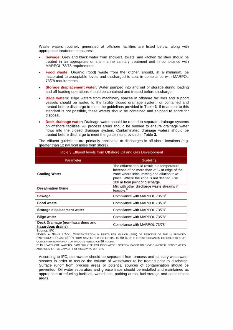
Waste waters routinely generated at offshore facilities are listed below, along with appropriate treatment measures:
Sewage: Grey and black water from showers, toilets, and kitchen facilities should be treated in an appropriate on-site marine sanitary treatment unit in compliance with MARPOL 73/78 requirements.
Food waste: Organic (food) waste from the kitchen should, at a minimum, be macerated to acceptable levels and discharged to sea, in compliance with MARPOL 73/78 requirements.
Storage displacement water: Water pumped into and out of storage during loading and off-loading operations should be contained and treated before discharge.
Bilge waters: Bilge waters from machinery spaces in offshore facilities and support vessels should be routed to the facility closed drainage system, or contained and treated before discharge to meet the guidelines provided in Table 3. If treatment to this standard is not possible, these waters should be contained and shipped to shore for disposal.
Deck drainage water: Drainage water should be routed to separate drainage systems
on offshore facilities. All process areas should be bunded to ensure drainage water flows into the closed drainage system. Contaminated drainage waters should be treated before discharge to meet the guidelines provided in Table 3.
The effluent guidelines are primarily applicable to discharges in off-shore locations (e.g. greater than 12 nautical miles from shore).
Table 3 Effluent levels from Offshore Oil and Gas Development
Parameter Guideline
Cooling Water
The effluent should result in a temperature increase of no more than 3° C at edge of the zone where initial mixing and dilution take place. Where the zone is not defined, use 100 m from point of discharge.
Desalination Brine Mix with other discharge waste streams if feasible.
b
Sewage Compliance with MARPOL 73/78b
Food waste Compliance with MARPOL 73/78b
Storage displacement water Compliance with MARPOL 73/78b
Bilge water Compliance with MARPOL 73/78b
Deck Drainage (non-hazardous and hazardous drains)
Compliance with MARPOL 73/78b
SOURCE: IFC NOTES: A: 96-HR LC-50: CONCENTRATION IN PARTS PER MILLION (PPM) OR PERCENT OF THE SUSPENDED
PARTICULATE PHASE (SPP) FROM SAMPLE THAT IS LETHAL TO 50 % OF THE TEST ORGANISM EXPOSED TO THAT
CONCENTRATION FOR A CONTINUOUS PERIOD OF 96 HOURS. B: IN NEARSHORE WATERS, CAREFULLY SELECT DISCHARGE LOCATION BASED ON ENVIRONMENTAL SENSITIVITIES
AND ASSIMILATIVE CAPACITY OF RECEIVING WATERS
According to IFC, stormwater should be separated from process and sanitary wastewater streams in order to reduce the volume of wastewater to be treated prior to discharge. Surface runoff from process areas or potential sources of contamination should be prevented. Oil water separators and grease traps should be installed and maintained as appropriate at refueling facilities, workshops, parking areas, fuel storage and containment areas.
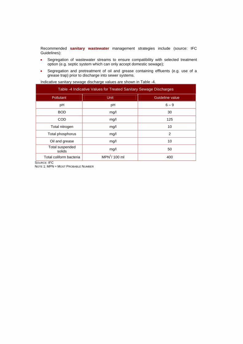
Recommended sanitary wastewater management strategies include (source: IFC Guidelines):
Segregation of wastewater streams to ensure compatibility with selected treatment option (e.g. septic system which can only accept domestic sewage);
Segregation and pretreatment of oil and grease containing effluents (e.g. use of a grease trap) prior to discharge into sewer systems.
Indicative sanitary sewage discharge values are shown in Table -4.
Table -4 Indicative Values for Treated Sanitary Sewage Discharges
Pollutant Unit Guideline value
pH pH 6 – 9
BOD mg/l 30
COD mg/l 125
Total nitrogen mg/l 10
Total phosphorus mg/l 2
Oil and grease mg/l 10
Total suspended solids
mg/l 50
Total coliform bacteria MPN1/ 100 ml 400
SOURCE: IFC NOTE 1: MPN = MOST PROBABLE NUMBER
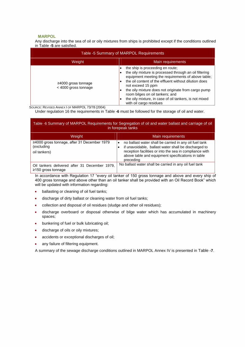
MARPOL Any discharge into the sea of oil or oily mixtures from ships is prohibited except if the conditions outlined in Table -5 are satisfied.
Table -5 Summary of MARPOL Requirements
Weight Main requirements
≥4000 gross tonnage < 4000 gross tonnage
the ship is proceeding en route;
the oily mixture is processed through an oil filtering equipment meeting the requirements of above table;
the oil content of the effluent without dilution does not exceed 15 ppm
the oily mixture does not originate from cargo pump room bilges on oil tankers; and
the oily mixture, in case of oil tankers, is not mixed with oil cargo residues
SOURCE: REVISED ANNEX I OF MARPOL 73/78 (2004)
Under regulation 16 the requirements in Table -6 must be followed for the storage of oil and water.
Table -6 Summary of MARPOL Requirements for Segregation of oil and water ballast and carriage of oil in forepeak tanks
Weight Main requirements
≥4000 gross tonnage, after 31 December 1979 (excluding
oil tankers)
no ballast water shall be carried in any oil fuel tank
if unavoidable, ballast water shall be discharged to reception facilities or into the sea in compliance with above table and equipment specifications in table preceding
Oil tankers delivered after 31 December 1979, ≥150 gross tonnage
No ballast water shall be carried in any oil fuel tank
In accordance with Regulation 17 “every oil tanker of 150 gross tonnage and above and every ship of 400 gross tonnage and above other than an oil tanker shall be provided with an Oil Record Book” which will be updated with information regarding:
ballasting or cleaning of oil fuel tanks;
discharge of dirty ballast or cleaning water from oil fuel tanks;
collection and disposal of oil residues (sludge and other oil residues);
discharge overboard or disposal otherwise of bilge water which has accumulated in machinery spaces;
bunkering of fuel or bulk lubricating oil;
discharge of oils or oily mixtures;
accidents or exceptional discharges of oil;
any failure of filtering equipment.
A summary of the sewage discharge conditions outlined in MARPOL Annex IV is presented in Table -7.
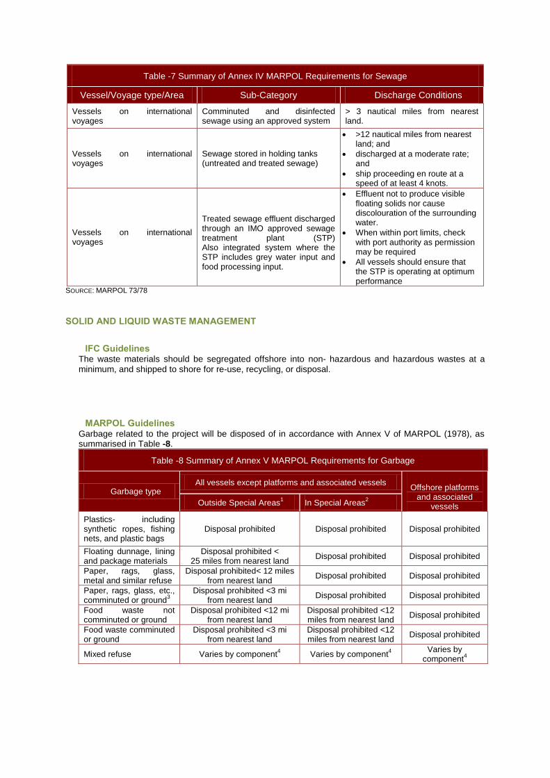
Table -7 Summary of Annex IV MARPOL Requirements for Sewage
Vessel/Voyage type/Area Sub-Category Discharge Conditions
Vessels on international voyages
Comminuted and disinfected sewage using an approved system
> 3 nautical miles from nearest land.
Vessels on international voyages
Sewage stored in holding tanks (untreated and treated sewage)
>12 nautical miles from nearest land; and
discharged at a moderate rate; and
ship proceeding en route at a speed of at least 4 knots.
Vessels on international voyages
Treated sewage effluent discharged through an IMO approved sewage treatment plant (STP) Also integrated system where the STP includes grey water input and food processing input.
Effluent not to produce visible floating solids nor cause discolouration of the surrounding water.
When within port limits, check with port authority as permission may be required
All vessels should ensure that the STP is operating at optimum performance
SOURCE: MARPOL 73/78
SOLID AND LIQUID WASTE MANAGEMENT
IFC Guidelines The waste materials should be segregated offshore into non- hazardous and hazardous wastes at a minimum, and shipped to shore for re-use, recycling, or disposal.
MARPOL Guidelines Garbage related to the project will be disposed of in accordance with Annex V of MARPOL (1978), as summarised in Table -8.
Table -8 Summary of Annex V MARPOL Requirements for Garbage
Garbage type All vessels except platforms and associated vessels
Offshore platforms and associated
vessels Outside Special Areas1 In Special Areas
2
Plastics- including synthetic ropes, fishing nets, and plastic bags
Disposal prohibited Disposal prohibited Disposal prohibited
Floating dunnage, lining and package materials
Disposal prohibited < 25 miles from nearest land
Disposal prohibited Disposal prohibited
Paper, rags, glass, metal and similar refuse
Disposal prohibited< 12 miles from nearest land
Disposal prohibited Disposal prohibited
Paper, rags, glass, etc., comminuted or ground
3 Disposal prohibited <3 mi
from nearest land Disposal prohibited Disposal prohibited
Food waste not comminuted or ground
Disposal prohibited <12 mi from nearest land
Disposal prohibited <12 miles from nearest land
Disposal prohibited
Food waste comminuted or ground
Disposal prohibited <3 mi from nearest land
Disposal prohibited <12 miles from nearest land
Disposal prohibited
Mixed refuse Varies by component4
Varies by component4
Varies by component
4
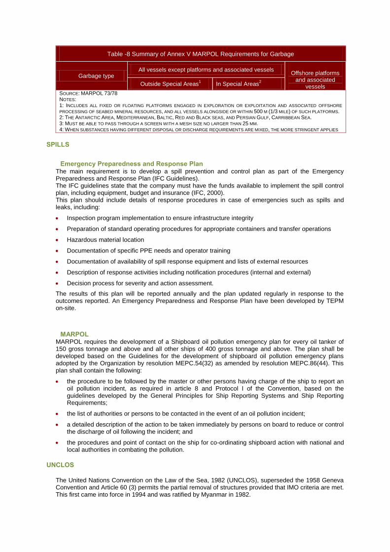
Table -8 Summary of Annex V MARPOL Requirements for Garbage
Garbage type All vessels except platforms and associated vessels
Offshore platforms and associated
vessels Outside Special Areas1 In Special Areas
2
SOURCE: MARPOL 73/78 NOTES: 1: INCLUDES ALL FIXED OR FLOATING PLATFORMS ENGAGED IN EXPLORATION OR EXPLOITATION AND ASSOCIATED OFFSHORE
PROCESSING OF SEABED MINERAL RESOURCES, AND ALL VESSELS ALONGSIDE OR WITHIN 500 M (1/3 MILE) OF SUCH PLATFORMS. 2: THE ANTARCTIC AREA, MEDITERRANEAN, BALTIC, RED AND BLACK SEAS, AND PERSIAN GULF, CARRIBBEAN SEA. 3: MUST BE ABLE TO PASS THROUGH A SCREEN WITH A MESH SIZE NO LARGER THAN 25 MM. 4: WHEN SUBSTANCES HAVING DIFFERENT DISPOSAL OR DISCHARGE REQUIREMENTS ARE MIXED, THE MORE STRINGENT APPLIES
SPILLS
Emergency Preparedness and Response Plan The main requirement is to develop a spill prevention and control plan as part of the Emergency Preparedness and Response Plan (IFC Guidelines). The IFC guidelines state that the company must have the funds available to implement the spill control plan, including equipment, budget and insurance (IFC, 2000). This plan should include details of response procedures in case of emergencies such as spills and leaks, including:
Inspection program implementation to ensure infrastructure integrity
Preparation of standard operating procedures for appropriate containers and transfer operations
Hazardous material location
Documentation of specific PPE needs and operator training
Documentation of availability of spill response equipment and lists of external resources
Description of response activities including notification procedures (internal and external)
Decision process for severity and action assessment.
The results of this plan will be reported annually and the plan updated regularly in response to the outcomes reported. An Emergency Preparedness and Response Plan have been developed by TEPM on-site.
MARPOL MARPOL requires the development of a Shipboard oil pollution emergency plan for every oil tanker of 150 gross tonnage and above and all other ships of 400 gross tonnage and above. The plan shall be developed based on the Guidelines for the development of shipboard oil pollution emergency plans adopted by the Organization by resolution MEPC.54(32) as amended by resolution MEPC.86(44). This plan shall contain the following:
the procedure to be followed by the master or other persons having charge of the ship to report an oil pollution incident, as required in article 8 and Protocol I of the Convention, based on the guidelines developed by the General Principles for Ship Reporting Systems and Ship Reporting Requirements;
the list of authorities or persons to be contacted in the event of an oil pollution incident;
a detailed description of the action to be taken immediately by persons on board to reduce or control the discharge of oil following the incident; and
the procedures and point of contact on the ship for co-ordinating shipboard action with national and local authorities in combating the pollution.
UNCLOS
The United Nations Convention on the Law of the Sea, 1982 (UNCLOS), superseded the 1958 Geneva Convention and Article 60 (3) permits the partial removal of structures provided that IMO criteria are met. This first came into force in 1994 and was ratified by Myanmar in 1982.

THE LONDON (DUMPING) CONVENTION, 1972
The 1972 London Convention (and the subsequent 1996 Protocol) made the provision of generic guidance for any wastes that can be dumped at sea. New guidelines were adopted in 2000, to specify different classes of waste, including platforms and other man-made waste.

13
Offshore Seismic Campaign YWB Block Appendices – 11/14
221/199
APPENDIX B JNCC Guidelines
JNCC guidelines for minimising the risk of injury and disturbance to marine mammals from seismic surveys
August 2010
To find out more about seismic surveys visit http://www.jncc.gov.uk/page-1534 To learn more about JNCC visit http://www.jncc.gov.uk/page=1729
JNCC, Marine Advice, Inverdee House, Baxter Street Aberdeen, AB11 9QA, United Kingdom Tel: +44(0)1224 266550 Email: [email protected]
JNCC guidelines for minimising the risk of injury and disturbance to marine mammals from seismic surveys
August 2010
Introduction The guidelines have been written for activities on the United Kingdom Continental Shelf (UKCS) and are aimed at reducing the risk of injury to negligible levels and can also potentially reduce the risk of disturbance from seismic surveys to marine mammals including seals, whales, dolphins and porpoises. Whilst there are no objections to these guidelines being used elsewhere JNCC would encourage all operators to determine if any special or local circumstances pertain, as we would not wish these guidelines to be used where a local management tool has already been adopted (for instance in the Gulf of Mexico OCS Region). In this context, JNCC notes that other protected fauna, for example turtles, will occur in waters where these guidelines may be used, and would suggest that, whilst the appropriate mitigation may require further investigation, the soft-start procedures for marine mammals would also be appropriate for marine turtles and basking sharksi. The guidelines require the use of trained Marine Mammal Observers (MMOs) whose role is to advise on the use of the guidelines and to conduct pre-shooting searches for marine mammals before commencement of any seismic activity. A further duty is to ensure that the JNCC reporting forms are completed for inclusion in the MMO report. In addition to the visual mitigation provided by MMOs, if seismic surveys are planned to start during hours of darkness or low visibility it is considered best practice to deploy Passive Acoustic Monitoring (PAM). The 2010 version of the JNCC seismic guidelines reflects amendments (2007 and 2009 amendments) to the Conservation (Natural Habitats &c.) Regulations 1994 (Habitat Regulations, HR) for England and Walesii and the Offshore Marine Conservation (Natural Habitats, &c.) Regulations 2007 (Offshore Marine Regulations, OMR, as amended in 2009 and 2010). Both regulations have revised the definition of deliberate disturbance of ‘European Protected Species’ (EPS), which now excludes
i Basking sharks are protected from intentional capture or disturbance in British waters (up to 12 miles offshore) under a 1998 listing on the Wildlife and Countryside Act (1981), Schedule 5. ii In 2010 a consolidated version of the regulations came into force: The Conservation of Habitats and
Species Regulations 2010.
trivial disturbance from the offence. Both regulations now also include the offence of deliberate injury. European Protected Species include cetaceans and turtles. It has been recognised that sound generated from seismic sources has the potential to cause injury and possibly also disturbance to marine mammals. Seismic surveys have therefore the potential to cause a deliberate injury offence as defined under regulations 41(1)(a) and 39(1)(a) and a deliberate disturbance offence as in 41(1)(b) and 39(1)(b) of the HR and OMR, respectively. The JNCC seismic guidelines reflect best practice for operators to follow during the planning, operational and reporting stages. It is considered that compliance with the recommendations in these guidelines will reduce the risk of injury to EPS to negligible levels. Please note that the mitigation measures recommended in the existing guidelines are more relevant to the prevention of injury rather than disturbance as defined in regulations 41(2) and 39(1A), of the HR and OMR, respectively. The onus should be on the entity responsible for the activity to assess whether a disturbance offence is likely to occur. Guidance on how to carry out such risk assessment is provided in the JNCC, NE and CCW document ‘The protection of marine European Protected Species from injury and disturbance’. In relation to oil and gas seismic surveys in the UKCS, it is a requirement of the consent issued under regulation 4 of the Petroleum Activities (Conservation of Habitats) Regulations 2001 (& 2007 Amendments) by the Department for Energy Climate Change (DECC), that the JNCC Seismic Guidelines must be followed, and the elements of the guidelines that are relevant to a particular survey are incorporated into the legally-binding condition of consent. It should be noted that it is the responsibility of the company issued consent by DECCiii, referred to in these guidelines as the ‘applicant’, to ensure that these guidelines are followed, and it is recommended that a copy of the JNCC guidelines are available onboard all vessels undertaking seismic activities in UK waters. Where relevant, when the survey is completed a MMO report must be submitted to the JNCC.
iii
Department of Energy and Climate Change was formerly known as Department for Business and Regulatory Reform (BERR)
Index Section 1 – Assessing and minimising the risk of injury
1.1 The planning stage Section 2 – Marine Mammal Observers (MMOs)
2.1 Role of the MMO 2.2 Training requirements for MMOs 2.3 MMO equipment and reporting forms 2.4 Reporting requirements – the MMO report
Section 3 – Guidance before and during seismic activity
3.1 Pre-shooting search 3.2 Delay if marine mammals are detected within the
mitigation zone (500 metres) 3.3 The soft-start 3.3.1 Soft-start requirements for site survey or Vertical Seismic
Profiling (VSP) 3.3.2. Soft-starts and airgun testing 3.4 Line change 3.4.1 Seismic surveys with an airgun volume of 500 cubic
inches or more 3.4.2 Seismic surveys with an airgun volume of 180 cubic
inches or less 3.5 Undershoot operations
Section 4 – Acoustic monitoring 4.1 Use of PAM as a mitigation tool
Section 5 – Requirements for MMOs and PAM Section 6 – Background Information
6.1. Existing protection to cetaceans
Section 7 – References and contacts
Terminology Marine European Protected Species: These are marine species in Annex IV(a) of the Habitats Directive that occur naturally in the waters of the United Kingdom. These consist of several species of cetaceans (whales, dolphins and porpoises), turtles, and the Atlantic Sturgeon. Marine Mammal Observer (MMO): Individual responsible for conducting visual watches for marine mammals. For some seismic surveys it may be requested that observers are trained, dedicated and / or experienced. The MMO may also be a PAM operative if trained.
Trained MMO: Has been on a JNCC recognised course
Dedicated MMO: Trained observer whose role on board is to conduct visual watches for marine mammals (although it could double up as a PAM operative)
Experienced MMO: Trained observer with 3 years of field experience observing for marine mammals, and practical experience of implementing the JNCC guidelines
PAM Operative: Person experienced in the use of PAM software and hardware and marine mammal acoustics
Mitigation Zone: The area where a Marine Mammal Observer keeps watch for marine mammals (and delays the start of activity should any marine mammals be detected). Passive Acoustic Monitoring (PAM): Software system that utilises hydrophones to detect the vocalisations of marine mammals. Seismic Survey: Any survey that uses airguns, including 2D/3D/4D and OBC (On-Bottom Cabling) surveys and any similar techniques that use airguns. Surveys using multibeam systems and sub-bottom profiling equipment such as boomers, pingers etc are not considered in these guidelines. However, the guidelines can be adapted and applied to the operation of such systems if considered appropriate. Shot Point Interval (SPI): Interval between firing of the airgun or airguns. Site Survey: Seismic survey of a limited area proposed for drilling, infrastructure emplacement etc (typically with source size of 180 cubic inches or less). Soft-Start: Turning on the airguns at low power and gradually and systematically increasing the output until full power is achieved (usually over a period of 20 minutes). The appropriate soft-start method is dependant upon the type of seismic survey and is discussed in section 3. United Kingdom Waters: Parts of the sea in or adjacent to the United Kingdom from the low water mark up to the limits of the United Kingdom Continental Shelf. Vertical Seismic Profiling (VSP) or Borehole Seismic: Seismic survey undertaken ‘down hole’ in connection with well operations (typically with a source size of 500 cubic inches).
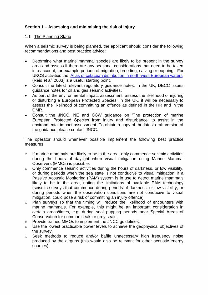
Section 1 – Assessing and minimising the risk of injury 1.1 The Planning Stage When a seismic survey is being planned, the applicant should consider the following recommendations and best practice advice:
Determine what marine mammal species are likely to be present in the survey area and assess if there are any seasonal considerations that need to be taken into account, for example periods of migration, breeding, calving or pupping. For UKCS activities the ‘Atlas of cetacean distribution in north-west European waters’ (Reid et al. 2003) is a useful starting point.
Consult the latest relevant regulatory guidance notes; in the UK, DECC issues guidance notes for oil and gas seismic activities.
As part of the environmental impact assessment, assess the likelihood of injuring or disturbing a European Protected Species. In the UK, it will be necessary to assess the likelihood of committing an offence as defined in the HR and in the OMR.
Consult the JNCC, NE and CCW guidance on ‘The protection of marine European Protected Species from injury and disturbance’ to assist in the environmental impact assessment. To obtain a copy of the latest draft version of the guidance please contact JNCC.
The operator should whenever possible implement the following best practice measures:
o If marine mammals are likely to be in the area, only commence seismic activities
during the hours of daylight when visual mitigation using Marine Mammal Observers (MMOs) is possible.
o Only commence seismic activities during the hours of darkness, or low visibility, or during periods when the sea state is not conducive to visual mitigation, if a Passive Acoustic Monitoring (PAM) system is in use to detect marine mammals likely to be in the area, noting the limitations of available PAM technology (seismic surveys that commence during periods of darkness, or low visibility, or during periods when the observation conditions are not conducive to visual mitigation, could pose a risk of committing an injury offence).
o Plan surveys so that the timing will reduce the likelihood of encounters with marine mammals. For example, this might be an important consideration in certain areas/times, e.g. during seal pupping periods near Special Areas of Conservation for common seals or grey seals.
o Provide trained MMOs to implement the JNCC guidelines. o Use the lowest practicable power levels to achieve the geophysical objectives of
the survey. o Seek methods to reduce and/or baffle unnecessary high frequency noise
produced by the airguns (this would also be relevant for other acoustic energy sources).
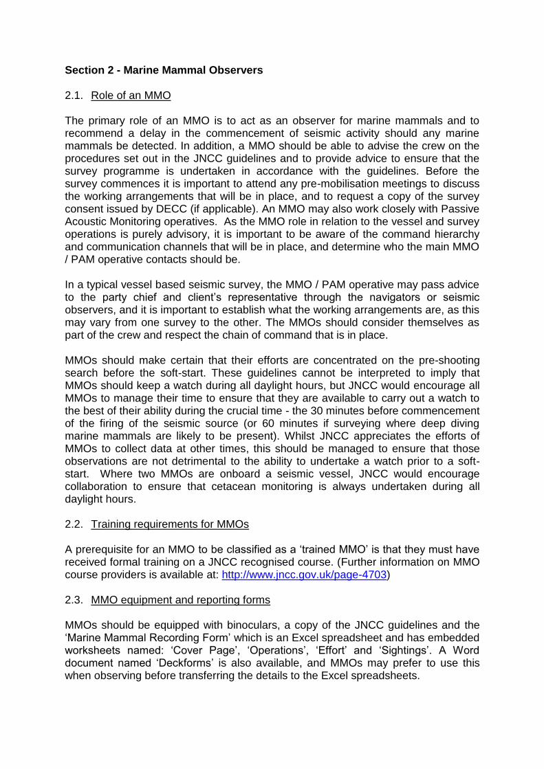
Section 2 - Marine Mammal Observers 2.1. Role of an MMO The primary role of an MMO is to act as an observer for marine mammals and to recommend a delay in the commencement of seismic activity should any marine mammals be detected. In addition, a MMO should be able to advise the crew on the procedures set out in the JNCC guidelines and to provide advice to ensure that the survey programme is undertaken in accordance with the guidelines. Before the survey commences it is important to attend any pre-mobilisation meetings to discuss the working arrangements that will be in place, and to request a copy of the survey consent issued by DECC (if applicable). An MMO may also work closely with Passive Acoustic Monitoring operatives. As the MMO role in relation to the vessel and survey operations is purely advisory, it is important to be aware of the command hierarchy and communication channels that will be in place, and determine who the main MMO / PAM operative contacts should be. In a typical vessel based seismic survey, the MMO / PAM operative may pass advice to the party chief and client’s representative through the navigators or seismic observers, and it is important to establish what the working arrangements are, as this may vary from one survey to the other. The MMOs should consider themselves as part of the crew and respect the chain of command that is in place. MMOs should make certain that their efforts are concentrated on the pre-shooting search before the soft-start. These guidelines cannot be interpreted to imply that MMOs should keep a watch during all daylight hours, but JNCC would encourage all MMOs to manage their time to ensure that they are available to carry out a watch to the best of their ability during the crucial time - the 30 minutes before commencement of the firing of the seismic source (or 60 minutes if surveying where deep diving marine mammals are likely to be present). Whilst JNCC appreciates the efforts of MMOs to collect data at other times, this should be managed to ensure that those observations are not detrimental to the ability to undertake a watch prior to a soft-start. Where two MMOs are onboard a seismic vessel, JNCC would encourage collaboration to ensure that cetacean monitoring is always undertaken during all daylight hours. 2.2. Training requirements for MMOs A prerequisite for an MMO to be classified as a ‘trained MMO’ is that they must have received formal training on a JNCC recognised course. (Further information on MMO course providers is available at: http://www.jncc.gov.uk/page-4703) 2.3. MMO equipment and reporting forms MMOs should be equipped with binoculars, a copy of the JNCC guidelines and the ‘Marine Mammal Recording Form’ which is an Excel spreadsheet and has embedded worksheets named: ‘Cover Page’, ‘Operations’, ‘Effort’ and ‘Sightings’. A Word document named ‘Deckforms’ is also available, and MMOs may prefer to use this when observing before transferring the details to the Excel spreadsheets.
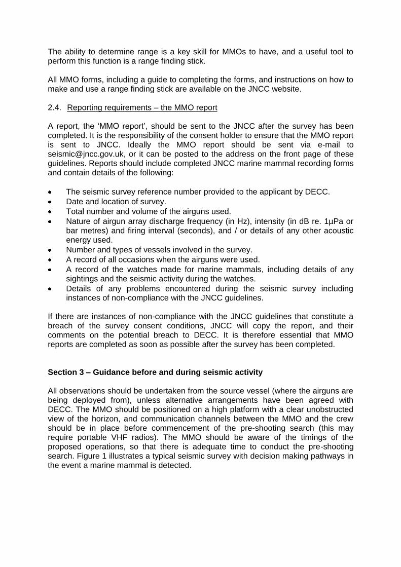
The ability to determine range is a key skill for MMOs to have, and a useful tool to perform this function is a range finding stick. All MMO forms, including a guide to completing the forms, and instructions on how to make and use a range finding stick are available on the JNCC website. 2.4. Reporting requirements – the MMO report A report, the ‘MMO report’, should be sent to the JNCC after the survey has been completed. It is the responsibility of the consent holder to ensure that the MMO report is sent to JNCC. Ideally the MMO report should be sent via e-mail to [email protected], or it can be posted to the address on the front page of these guidelines. Reports should include completed JNCC marine mammal recording forms and contain details of the following:
The seismic survey reference number provided to the applicant by DECC.
Date and location of survey.
Total number and volume of the airguns used.
Nature of airgun array discharge frequency (in Hz), intensity (in dB re. 1µPa or bar metres) and firing interval (seconds), and / or details of any other acoustic energy used.
Number and types of vessels involved in the survey.
A record of all occasions when the airguns were used.
A record of the watches made for marine mammals, including details of any sightings and the seismic activity during the watches.
Details of any problems encountered during the seismic survey including instances of non-compliance with the JNCC guidelines.
If there are instances of non-compliance with the JNCC guidelines that constitute a breach of the survey consent conditions, JNCC will copy the report, and their comments on the potential breach to DECC. It is therefore essential that MMO reports are completed as soon as possible after the survey has been completed. Section 3 – Guidance before and during seismic activity
All observations should be undertaken from the source vessel (where the airguns are being deployed from), unless alternative arrangements have been agreed with DECC. The MMO should be positioned on a high platform with a clear unobstructed view of the horizon, and communication channels between the MMO and the crew should be in place before commencement of the pre-shooting search (this may require portable VHF radios). The MMO should be aware of the timings of the proposed operations, so that there is adequate time to conduct the pre-shooting search. Figure 1 illustrates a typical seismic survey with decision making pathways in the event a marine mammal is detected.
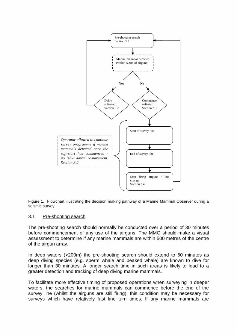
Figure 1. Flowchart illustrating the decision making pathway of a Marine Mammal Observer during a seismic survey.
3.1 Pre-shooting search The pre-shooting search should normally be conducted over a period of 30 minutes before commencement of any use of the airguns. The MMO should make a visual assessment to determine if any marine mammals are within 500 metres of the centre of the airgun array. In deep waters (>200m) the pre-shooting search should extend to 60 minutes as deep diving species (e.g. sperm whale and beaked whale) are known to dive for longer than 30 minutes. A longer search time in such areas is likely to lead to a greater detection and tracking of deep diving marine mammals. To facilitate more effective timing of proposed operations when surveying in deeper waters, the searches for marine mammals can commence before the end of the survey line (whilst the airguns are still firing); this condition may be necessary for surveys which have relatively fast line turn times. If any marine mammals are
Pre-shooting search
Section 3.1
Start of survey line
End of survey line
Marine mammal detected
(within 500m of airguns)
Delay
soft-start
Section 3.2
Operator allowed to continue
survey programme if marine
mammals detected once the
soft-start has commenced -
no ‘shut down’ requirement.
Section 3.2 Section ?
Commence
soft-start
Section 3.3
Yes No
Stop firing airguns / line change
Section 3.4
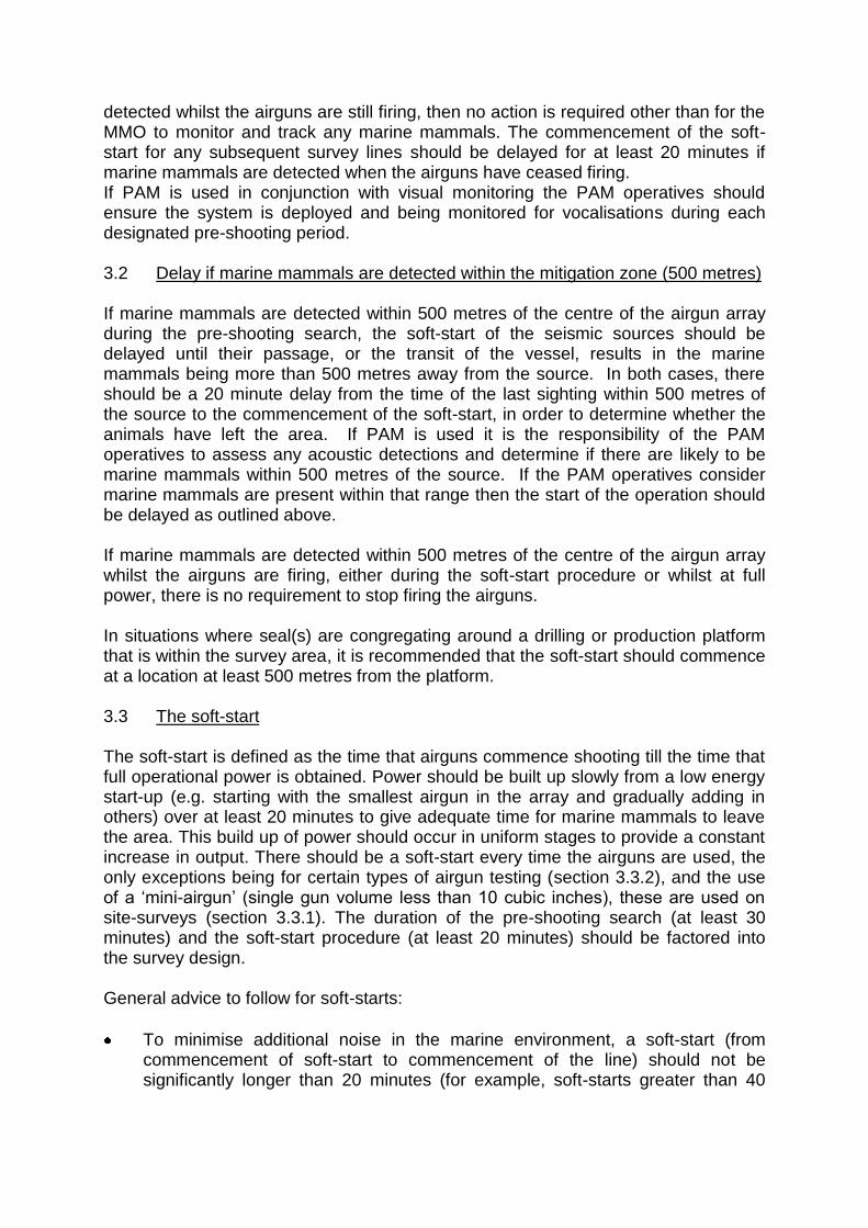
detected whilst the airguns are still firing, then no action is required other than for the MMO to monitor and track any marine mammals. The commencement of the soft-start for any subsequent survey lines should be delayed for at least 20 minutes if marine mammals are detected when the airguns have ceased firing. If PAM is used in conjunction with visual monitoring the PAM operatives should ensure the system is deployed and being monitored for vocalisations during each designated pre-shooting period. 3.2 Delay if marine mammals are detected within the mitigation zone (500 metres) If marine mammals are detected within 500 metres of the centre of the airgun array during the pre-shooting search, the soft-start of the seismic sources should be delayed until their passage, or the transit of the vessel, results in the marine mammals being more than 500 metres away from the source. In both cases, there should be a 20 minute delay from the time of the last sighting within 500 metres of the source to the commencement of the soft-start, in order to determine whether the animals have left the area. If PAM is used it is the responsibility of the PAM operatives to assess any acoustic detections and determine if there are likely to be marine mammals within 500 metres of the source. If the PAM operatives consider marine mammals are present within that range then the start of the operation should be delayed as outlined above. If marine mammals are detected within 500 metres of the centre of the airgun array whilst the airguns are firing, either during the soft-start procedure or whilst at full power, there is no requirement to stop firing the airguns.
In situations where seal(s) are congregating around a drilling or production platform that is within the survey area, it is recommended that the soft-start should commence at a location at least 500 metres from the platform. 3.3 The soft-start The soft-start is defined as the time that airguns commence shooting till the time that full operational power is obtained. Power should be built up slowly from a low energy start-up (e.g. starting with the smallest airgun in the array and gradually adding in others) over at least 20 minutes to give adequate time for marine mammals to leave the area. This build up of power should occur in uniform stages to provide a constant increase in output. There should be a soft-start every time the airguns are used, the only exceptions being for certain types of airgun testing (section 3.3.2), and the use of a ‘mini-airgun’ (single gun volume less than 10 cubic inches), these are used on site-surveys (section 3.3.1). The duration of the pre-shooting search (at least 30 minutes) and the soft-start procedure (at least 20 minutes) should be factored into the survey design. General advice to follow for soft-starts:
To minimise additional noise in the marine environment, a soft-start (from commencement of soft-start to commencement of the line) should not be significantly longer than 20 minutes (for example, soft-starts greater than 40
minutes are considered to be excessive, and an explanation should be provided within the MMO report).
Where possible, soft-starts should be planned so that they commence within daylight hours.
Once the soft-start has been performed and the airguns are at full power the survey line should start immediately. Operators should avoid unnecessary firing at full power before commencement of the line.
If, for any reason, firing of the airguns has stopped and not restarted for at least 10 minutes, then a pre-shooting search and 20 minute soft-start should be carried out (the requirement for a pre-shooting search only applies if there was no MMO on duty and observing at this time, and if the break in firing occurred during the hours of daylight). After any unplanned break in firing for less than 10 minutes the MMO should make a visual assessment for marine mammals (not a pre-shooting search) within 500 metres of the centre of the airgun array. If a marine mammal is detected whilst the airguns are not firing the MMO should advise to delay commencement, as per the pre-shooting search, delay and soft start instructions above. If no marine mammals are present then they can advise to commence firing the airguns.
When time-sharing, where two or more vessels are operating in adjacent areas and take turns to shoot to avoid causing seismic interference with each other, the soft-start and delay procedures for each vessel should be communicated to, and applied on, all the vessels involved in the surveying.
3.3.1 Soft-start requirements for site survey or Vertical Seismic Profiling (VSP) Surveys should be planned so that, whenever possible, the soft-start procedures for site surveys and Vertical Seismic Profiles (VSP’s) commence during daylight hours. Whilst it is appreciated that high resolution site surveys / VSP operations may produce lower acoustic output than 2D or 3D surveys it is still considered desirable to undertake a soft-start to allow for marine mammals to move away from the seismic source. For ultra high resolution site surveys that only use a ‘mini-airgun’ (single airgun with a volume of less than 10 cubic inches) there is no requirement to perform a soft-start, however, a pre-shooting search should still be conducted before its use. For site surveys and VSPs, a number of options are available to effect a soft-start.
The standard method, where power is built up slowly from a low energy start-up (e.g. starting with the smallest airgun in the array and gradually adding in others) over at least 20 minutes to give adequate time for marine mammals to leave the vicinity.
As the relationship between acoustic output and pressure of the air contained in the airgun is close to linear and most site surveys / VSP operations use only a small number of airguns and a soft-start can be achieved by slowly increasing the air pressure in 500 psi steps. From our understanding, the minimum air pressure which the airgun array can be set to will vary, as this is dependent on the make and model of the airgun being used. The time from initial airgun start up to full power should be at least 20 minutes.
Over a minimum time period of 20 minutes the airguns should be fired at an increasing frequency (by decreasing the Shot Point Interval (SPI)) until the desired firing frequency is reached.
3.3.2 Soft-starts and airgun testing Airgun tests may be required before a survey commences, or to test damaged or misfiring guns following repair, or to trial new arrays. Individual airguns, or the whole array may need testing, and the airguns may be tested at varying power levels. The following guidance is provided to clarify when a soft-start is required:
If the intention is to test all airguns at full power then a 20 minute soft-start is required.
If the intention is to test a single airgun on low power then a soft-start is not required.
If the intention is to test a single airgun, or a number of guns on high power, the airgun or airguns should be fired at lower power first, and the power then increased to the level of the required test; this should be carried out over a time period proportional to the number of guns being tested and ideally not exceed 20 minutes in duration.
MMOs should maintain a watch as outlined in the pre-shooting search guidance (section 3.1) before any instances of gun testing. 3.4 Line Change Seismic data is usually collected along predetermined survey lines. Line change is the term used to describe the activity of turning the vessel at the end of one line prior to commencement of the next line. Depending upon the type of seismic survey being undertaken, the time for a line change can vary. Line changes are not necessary for all types of seismic surveys, for example, in certain regional surveys where there is a significant distance between the lines, and for VSP operations. The guidance relating to line change depends upon the airgun volume. 3.4.1 Seismic surveys with an airgun volume of 500 cubic inches or more
If the line change time is expected to be greater than 20 minutes, airgun firing should be terminated at the end of the line and a full 20 minute soft-start undertaken before the next line. A pre-shooting search should also be undertaken during the scheduled line change, and the soft-start delayed if marine mammals are seen within 500 metres of the centre of the airgun array.
3.4.2 Seismic surveys with an airgun volume of 180 cubic inches or less (site
surveys)
If the line change time is expected to be greater than 40 minutes, airgun firing should be terminated at the end of the line and a full 20 minute soft-start undertaken before the next line. The pre-shooting search should also be
undertaken during the scheduled line change, and the soft-start delayed if marine mammals are seen within 500 metres of the centre of the airgun array.
If the line change time is expected to be less than 40 minutes, airgun firing can continue during the turn, but the Shot Point Interval (SPI) should be increased (longer duration between shots). Ideally, the SPI should not exceed 5 minutes during the turn.
Depending upon the duration of the line turns and the nature of seismic survey it may be necessary to vary the soft-start procedures. If an applicant determines that an effective line change can not be achieved using the above methods please contact JNCC at the earliest possible opportunity to discuss the proposed alternative, and include the details of the agreed procedure and the consultation with the JNCC in the application for survey consent. 3.5 Undershoot operations During an undershoot operation, one vessel is employed to tow the seismic source and a second vessel used to tow the hydrophone array, although the main vessel will still tow the hydrophone array. This procedure is used to facilitate shooting under platforms or other obstructions. The MMO may be too far away from the airguns to effectively monitor the mitigation zone, and it is therefore recommended to place the MMO on the source vessel. If this is not possible, for example for logistical reasons, or the health and safety implications of transferring personnel from one vessel to another, the application should explain that the recommended procedure cannot be followed in the application for the survey consent, or the application for a variation of that consent. Irrespective of the MMO location agreed with DECC, the pre-shooting search and soft-start procedures should still be followed prior to undertaking an undershoot operation. Section 4 - Acoustic Monitoring Visual observation is an ineffective mitigation tool during periods of darkness or poor visibility (such as fog), or during periods when the sea state is not conducive to visual mitigation, as it will not be possible to detect marine mammals in the vicinity of airgun sources. Under such conditions, PAM is considered to be the only currently available mitigation technique that can be used to detect marine mammals. Current PAM systems can be particularly helpful in detecting harbour porpoises within the 500 metre mitigation zone, although the systems have their limitations and can only be used to detect vocalising species of marine mammals. PAM systems consist of hydrophones that are deployed into the water column, and the detected sounds are processed using specialised software. PAM operatives are needed to set up and deploy the equipment and to interpret the detected sounds. 4.1 Use of PAM as a mitigation tool PAM can provide a useful supplement to visual observations undertaken by MMOs and JNCC may recommend that it is used as a mitigation tool when commenting on applications for survey consents. However, in many cases it is not as accurate as
visual observation for determining range, and this will mean that the mitigation zone will reflect the range accuracy of the system. For example, if the range accuracy of a system is estimated at +/-300 metres, animals detected and calculated to be within 500 metres from the source could, in reality, be 500 + 300 = 800 metres, but their detection would still lead to a delay in the soft-start. Although, at present it is not possible to express the range accuracy of most PAM systems in numerical terms, this example serves to illustrate that it is in the operator’s best interests to use the most accurate system available, and for the PAM operative to factor in a realistic estimate of the range accuracy. Some PAM systems do not have a reliable range determination facility or can only calculate the range for some species. In such cases, the detection of a confirmed cetacean vocalisation should still be used to initiate postponement of the soft-start if the PAM operator is able to make a judgement about the range of the animals from the airgun source, because of their experience gained in differentiating between distant and close vocalisations. In the absence of PAM systems capable of range determination, this expert judgement will constitute the basis for deciding whether an area is free from cetaceans prior to the soft-start. In all cases where PAM is employed, a brief description of the system and an explanation of how the applicant intends to deploy PAM to greatest effect should be included in the application for survey consent. In the last few years, software that processes and analyses cetacean sounds has been developed. An example of this is PAMGuard, an open source software that has been developed as part of the International Association of Oil and Gas Producers Joint Industry Project (JIP). JNCC recognises that PAMGuard is currently in a transition period between use as a research tool and widespread adoption as a monitoring technique. Moreover, JNCC recognises the need to balance proactive implementation of PAM with the need to further develop its capability, for example to include species recognition and baleen whale detection, and therefore encourages users of these systems to actively contribute to their development and refinement. Section 5 – Requirements for MMOs and PAM Any survey application or consultation received by JNCC will be considered on a case-by-case basis, and the mitigation measures advised to DECC will reflect the particulars of the survey and the importance of the survey area for marine mammals. The following paragraphs are provided as a guide to the advice applicants are likely to receive following submission of an application with JNCC. For areas that are currently considered particularly important for marine mammals, for example in the UK this includes areas West of Scotland, the Moray Firth and Cardigan Bay, JNCC may recommend that:
The MMOs should be experienced MMOs, and that PAM should be used.
The PAM system should be used to supplement visual observations, or as the main mitigation tool if the seismic survey activity commences during periods of
darkness or poor visibility, or during periods when the sea state is not conducive to visual mitigation.
JNCC will advise that two marine mammal observers should be used when daylight hours exceed approximately 12 hours per day (between 1st April and 1st October north of 57O latitude), or the survey is in an area considered particularly important for marine mammals. When a non-dedicated MMO is recommended by JNCC (e.g. for VSPs and certain site-surveys), and the recommendation is incorporated into the conditions of the survey consent, a member of the rig’s or vessels crew can perform the duties providing the crew member is a trained MMO. When a dedicated MMO is recommended and this is a condition of the survey consent, the MMO should be employed solely for the purpose of monitoring the implementation of the guidelines and undertaking visual observations to detect marine mammals during periods of seismic activity. When two dedicated MMOs are requested and this is a condition of the survey consent, both should be employed solely for the purposes of monitoring the implementation of the guidelines and undertaking visual observations, and the use of a crew member with other responsibilities as the second observer is not considered to be an adequate substitute for a dedicated MMO, or to be in compliance with the conditions of the survey consent. Section 6 - Background Information These guidelines were originally prepared by a Working Group convened by the Department of the Environment, and were developed from a draft prepared by the Sea Mammal Research Unit (SMRU). The guidelines have subsequently been reviewed three times by the Joint Nature Conservation Committee, following consultation with interested parties. 6.1. Existing protection to cetaceans
Section 9 of the Wildlife and Countryside Act 1981 (CRoW amended) prohibits the intentional or reckless killing, injuring or disturbance of any cetacean. The UK is also a signatory to the Agreement on the Conservation of Small Cetaceans of the Baltic and North Seas (ASCOBANS) and has applied its provisions in all UK waters. Amongst other actions required to conserve and manage populations of small cetaceans, ASCOBANS requires range states to "work towards...the prevention of ...disturbance, especially of an acoustic nature". Reflecting the requirements of the Convention on the Conservation of European Wildlife and Habitats (the Bern Convention) and Article 12 of the EC Habitats and Species Directive (92/43/EEC), the UK has the following legislation in place:
The Conservation of Habitats and Species Regulations 2010
The Conservation (Natural Habitats, &c.) Regulations 1995 (Northern Ireland) (and 2009 amendments)
The Conservation (Natural Habitats, &c.) Amendment (No. 2) Regulations 2008 (Scotland) (and 2009 amendments)
The Offshore Petroleum Activities (Conservation of Habitats) Regulations 2001 (and 2007 amendments),
The Offshore Marine Conservation (Natural Habitats, &c.) Regulations 2007 (and 2009 and 2010 amendments) (beyond 12 nautical miles UKCS)
Section 7 – References and contacts Further information on DECC’s survey consent procedure can be found at: http://www.og.decc.gov.uk/. A copy of these guidelines, the standard forms (electronic and hard copy) and further background information is available from the above address, or can be found on the JNCC website at: http://www.jncc.gov.uk/page-1534 Reid, J.B., Evans, P.G.H., & Northridge, S.P. (2003). ‘Atlas of cetacean distribution in north-west European waters’ (Online). http://www.jncc.gov.uk/page-2713 If you have any comments or questions relating to these guidelines, or suggestions on how they may be improved, please email [email protected]

13
Offshore Seismic Campaign YWB Block Appendices – 11/14
222/231
APPENDIX C The Ecosystem-Based Management Fishery in the Bay of Bengal, 2008
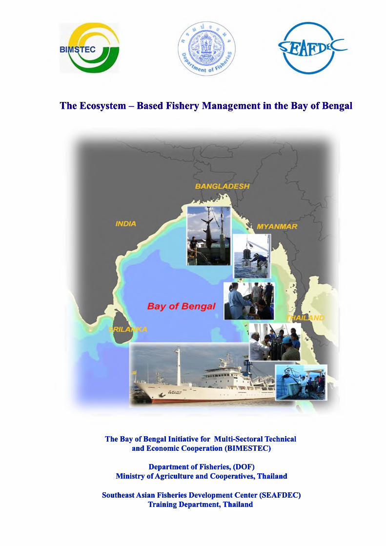
The Ecosystem-Based Management Fishery in the Bay of Bengal
Department of Fisheries, (DOF) Ministry of Agriculture and Cooperatives, Thailand
September, 2008
The Ecosystem-Based Fishery Management in the Bay of Bengal
i
The Ecosystem-Based Fishery Management in the Bay of Bengal
Executive Summary 1. Introduction
The Ecosystem-Based Fishery Management in the Bay of Bengal is a collaborative fishery research project conducted by members of the Multi-Sectoral Technical and Economic Cooperation (BIMSTEC). The BIMSTEC is an international economic cooperation of a group of countries comprising Bangladesh, India, Sri Lanka, Thailand, Myanmar, Bhutan and Nepal. The economic cooperation initiative was initially formulated Bangladesh, India, Sri Lanka and Thailand in their 6 June 1997 Agreement recognized as the “Bangladesh, India, Sri Lanka and Thailand Economic Cooperation” or BIST-EC. Myanmar attended the inaugural June Meeting as an observer and joined the organization as a full member at a Special Ministerial Meeting held in Bangkok on 22 December 1997, upon which the name of the grouping was changed to BIMST-EC. Nepal was granted observer status by the second Ministerial Meeting in Dhaka in December 1998. Subsequently, full membership has been granted to Nepal and Bhutan in 2004. In the first Summit on 31 July 2004, leaders of the group agreed that the name of the grouping should be known as BIMSTEC or the Bay of Bengal Initiative for Multi-Sectoral Technical and Economic Cooperation.
BIMSTEC has thirteen priority sectors cover all areas of cooperation. Six priority sectors of cooperation were identified at the 2nd Ministerial Meeting in Dhaka on 19 November 1998. They include the followings:
1. Trade and Investment, led by Bangladesh 2. Transport and Communication, led by India 3. Energy, led by Myanmar 4. Tourism, led by India 5. Technology, led by Sri Lanka 6. Fisheries, led by Thailand The BIMSTEC member countries recognize the role played by the fisheries
sector in food supply and food security for their peoples. The natural resource rents provided by the Bay of Bengal and other inland and coastal bodies of water should be properly managed. In the past decades, the overexploitation of the fishery resources and the overcapacity of fishing fleets are the results of rapid fishing technology development, the ever increasing demands for fish as dictated by population growth and export economic policies, and the open access management of the fisheries. A new and effective management is therefore needed to bail the sub-region out of this economic and technical dilemma.
Around the world, fishery managers are increasingly recognizing ecosystems as natural capital assets. Scientific understanding of ecosystem production functions is improving rapidly but remains a limiting factor in incorporating natural capital into decisions, via systems of national accounting and other mechanisms. It is clear that formal sharing of experience, and defining of priorities for future work, could greatly accelerate the rate of innovation and uptake of new approaches.
The Bay of Bengal is a large marine ecosystem where coastal countries have been fishing. Its geographical and hydrological characteristics support plenitude of a variety of fish and shrimps. Sardines, anchovies, and mackerels are commonly caught whilst yellowfin tuna, bigeye tuna, skipjack tuna and swordfish, other large and precious pelagic fish known in the world market are harvested here. The Bay of Bengal is thus known for the
The Ecosystem-Based Fishery Management in the Bay of Bengal
ii
source of employment in fishing and income enjoyed by a large number of people, as well as their countries in terms of foreign currency earning.
Three projects in the fisheries sectors have been approved by the 6th Ministerial Meeting in 2004. These are: 1) Ecosystem-based fisheries management in the Bay of Bengal (proposed by Thailand); 2) Impact of offshore oil and gas drilling on the marine fishery resources in the Bay of Bengal (proposed by Bangladesh); and 3) marine fish stock assessment, management and development of new fisheries in the Bay of Bengal (proposed by Bangladesh). Further discussion was made on these three projects during the BIMSTEC Technical Meeting in 2005. For the first project, the Technical Meeting suggested that a focus should be made on the straddling and highly migratory fish stocks and the survey of deep sea areas beyond the EEZ. 2. The Overall Objectives
The overall objectives of this project are as follows: 1) To understand the physical and chemical oceanographic and hydrological
conditions of the Bay of Bengal. 2) To investigate the biological data of economic fish in terms of species,
abundance, distribution, maturity size, feeding etc. 3) To assess the potential of fishery resources in the Bay of Bengal. 4) To strengthen capability in research work and knowledge exchange by training
on the job on board the Thai research vessel. 5) To improve understanding and collaboration among researchers of the member
countries during on board surveys. 3. The Project Output It is expected that the obtained scientific data and information from all sub-projects will be highly beneficial for States bordering the Bay of Bengal to eventually draft the policy on sustainable utilization of fishery resources and achieve the effective fisheries management in the Bay of Bengal.
4. The Findings
The project spent a total of 58 days (from 25 October to 21 December 2007) in the survey, using a SEAFDEC research vessel, in the following maritime areas:
Area A (latitude 16°N -19°N, longitude 88°E -91°E) Area B (latitude 09°N -14°N, longitude 82°E -85°E) Area C (latitude 09°N -13°N, longitude 95°E -97°E) Three types of fishing methods were used during the whole period of the surveys:
pelagic long line, drift gill net and automatic squid jigging. The results of the studies are summarized as follow:
4.1 The Oceanographic and Hydrobiological Conditions a) The Oceanographic Condition The oceanographic survey found the western side (area B) of the Bay with
higher salinity than the north (area A) and the eastern (area C) boundaries. The water circulation in the Bay, as exhibited by the surface salinity in three spatial areas, was density-driven. Two core cold eddies were observed in the north area of the Bay. The large volume of
The Ecosystem-Based Fishery Management in the Bay of Bengal
iii
freshwater discharge by the major rivers plays an important role in inducing lower salinity and higher temperature of the mixed layer (between 14 and 49 m) in the western and eastern areas of the Bay. Hypoxia (where dissolved oxygen was <0.5 ml/l) was found 200 m and deeper in the northern side of the Bay. Surface water shallower than 400 m was occupied by three water masses: Bay of Bengal water (salinity 32-34 psu), Andaman Sea water (salinity 31-33 psu), and Indian Central water (salinity more than 35 psu). The Indian central water occupied all deepest layers of all survey areas.
Distribution of nutrients: nitrite + nitrate, silicate and phosphate were found to correlate positively with depth at all sampling stations. The concentrations of nutrients in the mixed layer depth were low and undetectable in several sampling stations but distinctly high at western station (station 23) of the north of the Bay where chlorophyll-a concentration was also high. In the thermocline layer, a strong nutricline concentration was noticed to be rapidly increasing with depth. Until about 200-250 m the nutrient values were nearly constant or slightly changed. The differentiated pattern of depth profiles of both total phosphorus and total alkalinity together with the relationship between total alkalinity and total phosphorus indicate that sea water characteristic in the enclosed Andaman Sea is different from the entire Bay of Bengal.
Spatial distribution of chlorophyll-a displayed a pattern similar to that of salinity. Most of the low latitude stations exhibited somewhat higher chlorophyll-a concentrations than in those of high latitude stations.
b) Hydrobiological Conditions A total of 135 phytoplankton species identified belong to the groups of
cyanobacteria, diatom, dinoflagellates and silicoflagellates. The northern side of the Bay was inhabited by the highest phytoplankton densities due to the blooms of Pseudo-nitzschia pseudodelicatissima in the western part (station 23) of this area.
Similar to phytoplankton, a high concentration of zooplankton was found in the northern area of the Bay. The zooplankton community consisted of 205 species. Copepod was the most prevalent group both in terms of the number of species and biomass. Thirteen families of cephalopod paralarvae were found during the survey period. Family Ommastrephidae was widely distributed in the Bay.
Of the fifty-two families of fish larvae identified, those belong to Family Photichthyidae were the most abundant. The majority of these fishes belong to the inshore reef-fish and oceanic fish groups. In overall, the east of the Bay or the Andaman Sea harbours the richest ichthyodiversity and the highest biomass of fish larvae compared to other study areas.
4.2 The Fishery Resources From the fishery surveys with 3 types of fishing gear; drift gill net (DGN), pelagic longline (PLL) and automatic squid jigging machine (ASJ), DGN and PLL were satisfactorily effective in catching pelagic fishes and were ideally appropriate tools for sustainable exploitation of the pelagic fishery resources in the Bay of Bengal. It was low catch per unit of effort (CPUE) from ASJ. The overall CPUEs from each type of fishing gear operated in the entire survey areas were DGN 0.84 no/hr (1.27 kg/hr), PLL 1.23 no/100 hooks (27.96 kg/100 hooks) and ASJ 0.19 no/line/hr (0.03 kg/line/hr) In all fishing areas and with all types of fishing gear, the sum total of five most abundant species captured by number were in the following order: skipjack tuna (Katsuwonus pelamis, 22.94%), swordfish (Xiphias gladius, 12.94%), silky shark (Carcharhinus falsiformis, 8.82%), frigate tuna (Auxis thazard, 8.24%) and bigeye thresher shark (Alopias supersiliosus, 6.47%).
The Ecosystem-Based Fishery Management in the Bay of Bengal
iv
In terms of weight, the swordfish (34.82%) ranked first of the top-five species followed by bigeye thresher shark (33.88%), silky shark (8.21%) black marlin (Makaira indica 4.23%) and yellowfin tuna (Thunnus albacares, 3.98%), respectively.
Considering the fishing areas where fish were found in great abundance, the top-five pelagic species were mostly found in area A and C. It can be said that area A is a fertile fishing ground for DGN fishery targeting at tunas particularly skipjack tuna whereas area C is a good fishing ground for billfish fishing with PLL. Although DGN and PLL were operated successfully, their lower CPUEs were achieved when comparing to that of commercial fishing vessels. This could attribute to seasonal variation as the survey period may not fall into a high fishing season. Moreover, the fishing operations were not as intensive as those exerted by commercial fishing vessels.
It was found that the sizes of the fishes captured by these types of fishing gear were mostly sexually mature. The mean total lengths of skipjack tuna, frigate tuna, dolphinfish, swordfish, bigeye thresher shark and silky shark were 41.46, 35.14, 72.94, 211.00, 271.00 and 111.33 cm, respectively. Sex ratios of these species, except that of skipjack tuna, were approximately 1:1. The schools of skipjack tuna were male dominant. Although there were high percentages of sexually mature individuals of both sexes during the survey period, it still insufficient to determine the spawning ground and spawning season. It was considered that the survey duration was rather short, approximately 2 months, and so the acquired biological data concerned with reproductive cycle were insufficient to clarify such items.
Regarding the squids caught by automatic squid jigging machine, the total catches were represented by only one species of Ommastrephidae, purpleback flying squid (Sthenoteuthis oualaniensis) which was noticeable more concentrated in area C than in areas A and B. The mean length of the cephalopod was 104 mm for males and 169 mm for females. Sex ratio was 1 male to 4.57 females. At present purpleback flying squid is not regarded as a target species in commercial fishery because of its gristle and low quality for human consumption. 5. Heavy Metal Contamination The Bay of Bengal’s purpleback squid (Sthenoteuthis oualaniensis) contained mercury (Hg), lead (Pb) and Zinc (Zn) concentrations in both edible parts and visceral mass were within the safety limits. The mean copper (Cu) concentration in visceral (but not edible) tissues of the squid from every station was higher than the safety limit. The mean cadmium (Cd) concentrations in both edible part and visceral mass of the squid from every station are higher than those of the proposed safety limit. This concluded that Hg, Pb, Zn and Cu concentration in the edible body part of the purpleback squid from the Bay of Bengal are lower than safety limit except Cd. At the same time the study of Hg concentration in fish tissues caught from the same area were also carried out. Most fish analyzed still had Hg concentration in the tissue within the EU and CODEX limit of 0.5µg/g, particularly when fish size not exceeding approximately 15 kg in weight or 150 cm in length. The Hg burden in the tissue of both bigeye thresher shark and swordfish reported in this study were the highest. Swordfish which weighed more than 40 kg accumulated very high Hg content in their flesh exceeding 1 µg./g wet weight which was over the upper limit of the CODEX and EU guideline levels.
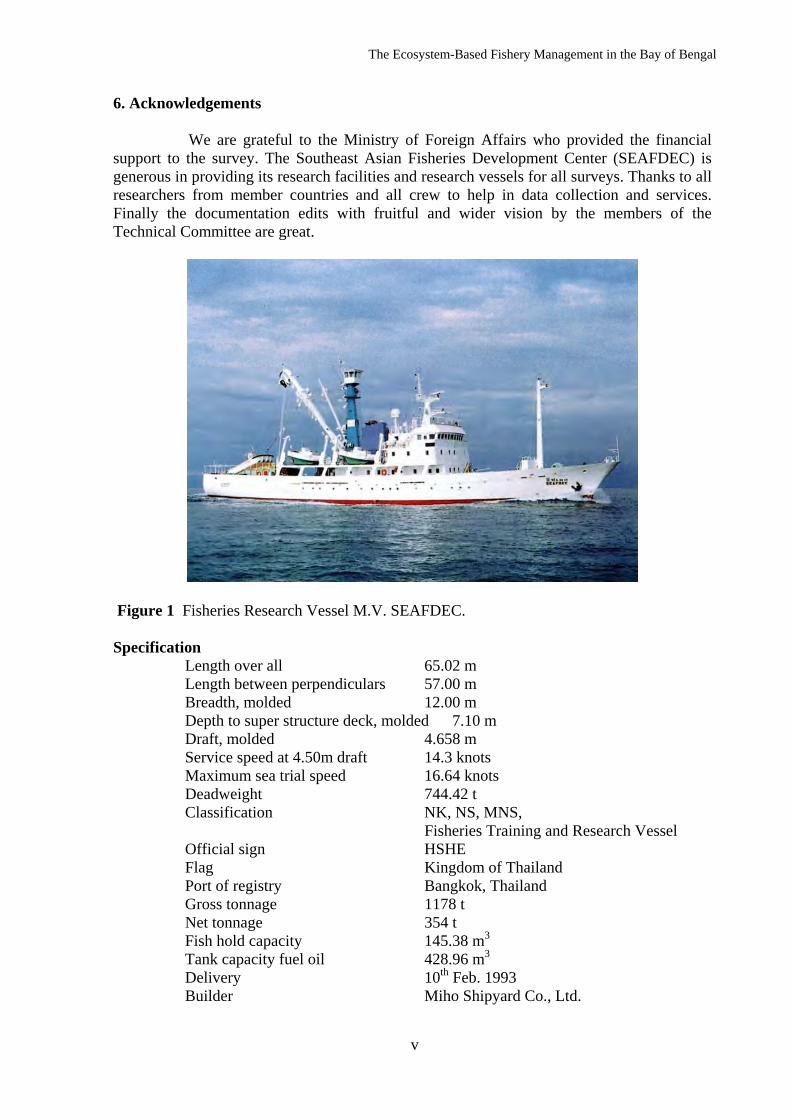
The Ecosystem-Based Fishery Management in the Bay of Bengal
v
6. Acknowledgements
We are grateful to the Ministry of Foreign Affairs who provided the financial support to the survey. The Southeast Asian Fisheries Development Center (SEAFDEC) is generous in providing its research facilities and research vessels for all surveys. Thanks to all researchers from member countries and all crew to help in data collection and services. Finally the documentation edits with fruitful and wider vision by the members of the Technical Committee are great.
Figure 1 Fisheries Research Vessel M.V. SEAFDEC. Specification
Length over all 65.02 m Length between perpendiculars 57.00 m Breadth, molded 12.00 m Depth to super structure deck, molded 7.10 m Draft, molded 4.658 m Service speed at 4.50m draft 14.3 knots Maximum sea trial speed 16.64 knots Deadweight 744.42 t Classification NK, NS, MNS, Fisheries Training and Research Vessel Official sign HSHE Flag Kingdom of Thailand Port of registry Bangkok, Thailand Gross tonnage 1178 t Net tonnage 354 t Fish hold capacity 145.38 m3
Tank capacity fuel oil 428.96 m3 Delivery 10th Feb. 1993 Builder Miho Shipyard Co., Ltd.
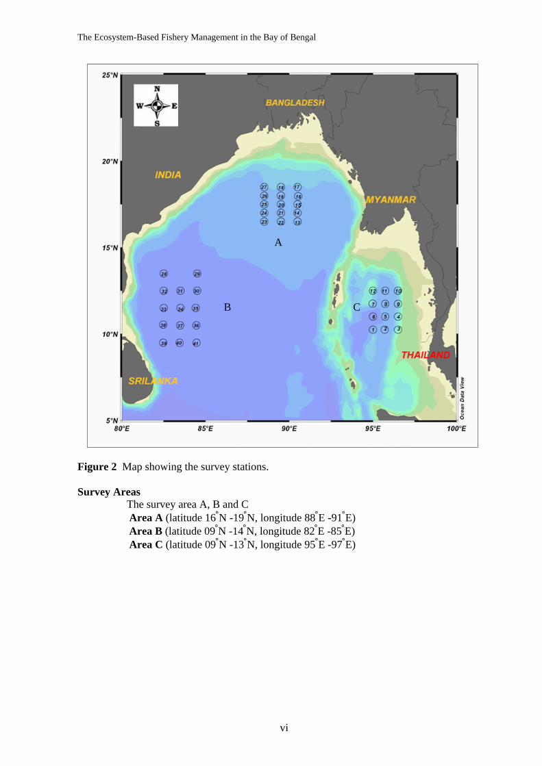
The Ecosystem-Based Fishery Management in the Bay of Bengal
vi
Figure 2 Map showing the survey stations. Survey Areas
The survey area A, B and C Area A (latitude 16°N -19°N, longitude 88°E -91°E) Area B (latitude 09°N -14°N, longitude 82°E -85°E) Area C (latitude 09°N -13°N, longitude 95°E -97°E)
A
B C
The Ecosystem-Based Fishery Management in the Bay of Bengal
vii
Table of Contents
Contents Page Executive Summary i Table of Contents vii The oceanographic condition
Oceanographic Condition of the Bay of Bengal During 1 November- December 2007
Comparison of Total Phosphorous Contents and Total Alkalinity 17 in Seawater of Different Area in the Bay of Bengal
Distribution of Nutrients in the Bay of Bengal 33 Distribution of Chorophyll-a in the Bay of Bengal 45
Hydrobiological conditions Species Composition, Abundance and Distribution of Phytoplankton 53
in the Bay of Bengal Composition , Abundance and Distribution of Zooplankton 65
in the Bay of Bengal Abundance, Composition and Distribution of Fish Larvae 93
in the Bay of Bengal Distribution and Abundance of Cephalopod Paralarvae 125
in the Bay of Bengal
The fishery resources Large Pelagic Fishery Resource Survey using Pelagic Longline 135
in the Bay of Bengal Marine Resource Surveys by Drift Gill Net in the Bay of Bengal 149 Efficiency of the Circle Hook in Comparison with J-Hook 167
in longline Fishery Biological Aspects of Economic Fishes in the Bay of Bengal 182 Elasmobranches Found in the Bay of Bengal from 190
Pelagic Longline and Drift Gill Net Fishing Age and Reproduction of Sthenoteuthis oualaniensis in the Bay of Bengal 195 Stomach Content of the Large Pelagic Fish in the Bay of Bengal 206
Heavy Metal Contamination An Assessment of Mercury Concentration in Fish Tissues Caught 221
from Three Compartments of the Bay of Bengal Heavy Metal Contents in Purpleback Squid (Sthenoteuthis oualaniensis) 233
from the Bay of Bengal Appendix 245
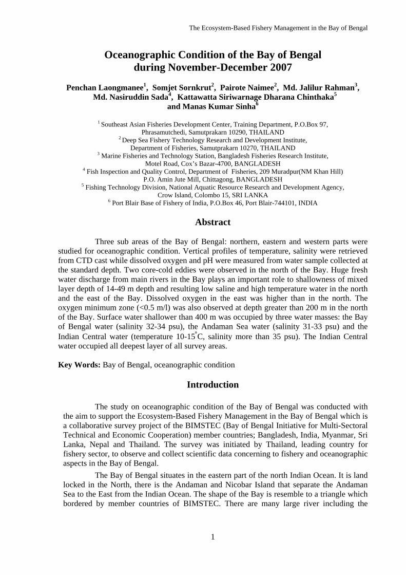
The Ecosystem-Based Fishery Management in the Bay of Bengal
1
Oceanographic Condition of the Bay of Bengal during November-December 2007
Penchan Laongmanee1, Somjet Sornkrut2, Pairote Naimee2, Md. Jalilur Rahman3,
Md. Nasiruddin Sada4, Kattawatta Siriwarnage Dharana Chinthaka5 and Manas Kumar Sinha6
1 Southeast Asian Fisheries Development Center, Training Department, P.O.Box 97,
Phrasamutchedi, Samutprakarn 10290, THAILAND 2 Deep Sea Fishery Technology Research and Development Institute,
Department of Fisheries, Samutprakarn 10270, THAILAND 3 Marine Fisheries and Technology Station, Bangladesh Fisheries Research Institute,
Motel Road, Cox’s Bazar-4700, BANGLADESH 4 Fish Inspection and Quality Control, Department of Fisheries, 209 Muradpur(NM Khan Hill)
P.O. Amin Jute Mill, Chittagong, BANGLADESH 5 Fishing Technology Division, National Aquatic Resource Research and Development Agency,
Crow Island, Colombo 15, SRI LANKA 6 Port Blair Base of Fishery of India, P.O.Box 46, Port Blair-744101, INDIA
Abstract
Three sub areas of the Bay of Bengal: northern, eastern and western parts were
studied for oceanographic condition. Vertical profiles of temperature, salinity were retrieved from CTD cast while dissolved oxygen and pH were measured from water sample collected at the standard depth. Two core-cold eddies were observed in the north of the Bay. Huge fresh water discharge from main rivers in the Bay plays an important role to shallowness of mixed layer depth of 14-49 m depth and resulting low saline and high temperature water in the north and the east of the Bay. Dissolved oxygen in the east was higher than in the north. The oxygen minimum zone (<0.5 m/l) was also observed at depth greater than 200 m in the north of the Bay. Surface water shallower than 400 m was occupied by three water masses: the Bay of Bengal water (salinity 32-34 psu), the Andaman Sea water (salinity 31-33 psu) and the Indian Central water (temperature 10-15°C, salinity more than 35 psu). The Indian Central water occupied all deepest layer of all survey areas. Key Words: Bay of Bengal, oceanographic condition
Introduction
The study on oceanographic condition of the Bay of Bengal was conducted with the aim to support the Ecosystem-Based Fishery Management in the Bay of Bengal which is a collaborative survey project of the BIMSTEC (Bay of Bengal Initiative for Multi-Sectoral Technical and Economic Cooperation) member countries; Bangladesh, India, Myanmar, Sri Lanka, Nepal and Thailand. The survey was initiated by Thailand, leading country for fishery sector, to observe and collect scientific data concerning to fishery and oceanographic aspects in the Bay of Bengal.
The Bay of Bengal situates in the eastern part of the north Indian Ocean. It is land locked in the North, there is the Andaman and Nicobar Island that separate the Andaman Sea to the East from the Indian Ocean. The shape of the Bay is resemble to a triangle which bordered by member countries of BIMSTEC. There are many large river including the
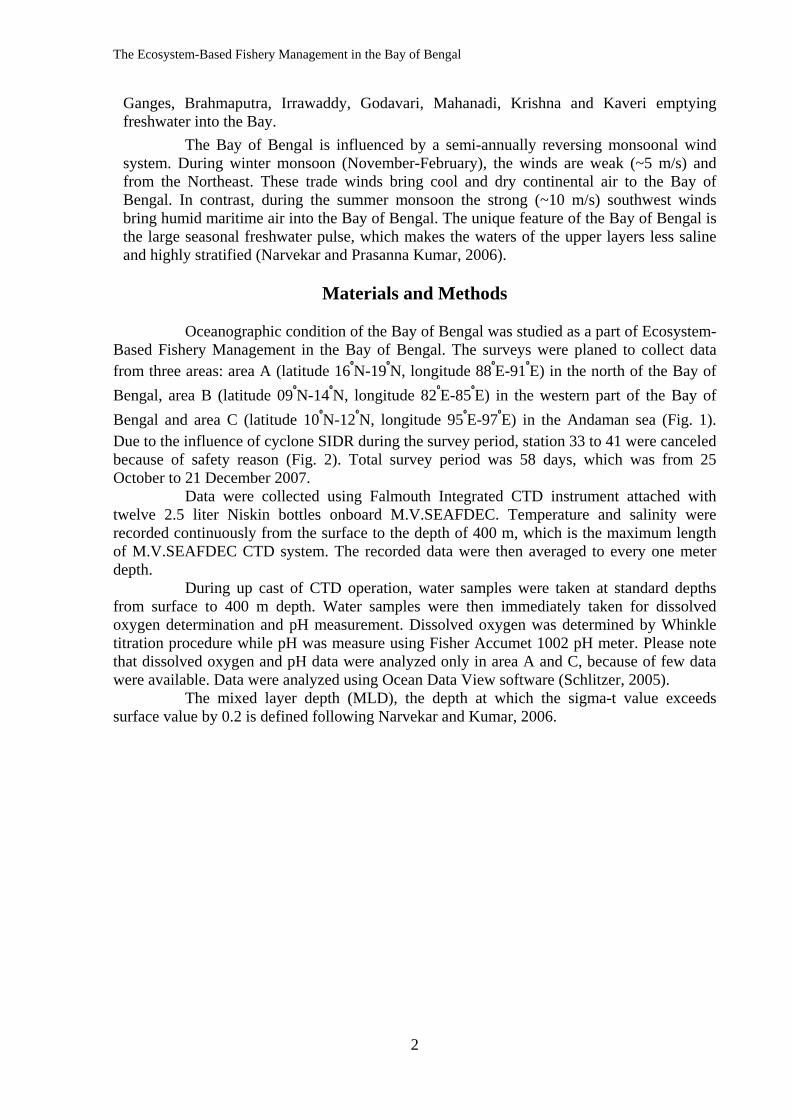
The Ecosystem-Based Fishery Management in the Bay of Bengal
2
Ganges, Brahmaputra, Irrawaddy, Godavari, Mahanadi, Krishna and Kaveri emptying freshwater into the Bay.
The Bay of Bengal is influenced by a semi-annually reversing monsoonal wind system. During winter monsoon (November-February), the winds are weak (~5 m/s) and from the Northeast. These trade winds bring cool and dry continental air to the Bay of Bengal. In contrast, during the summer monsoon the strong (~10 m/s) southwest winds bring humid maritime air into the Bay of Bengal. The unique feature of the Bay of Bengal is the large seasonal freshwater pulse, which makes the waters of the upper layers less saline and highly stratified (Narvekar and Prasanna Kumar, 2006).
Materials and Methods
Oceanographic condition of the Bay of Bengal was studied as a part of Ecosystem-
Based Fishery Management in the Bay of Bengal. The surveys were planed to collect data from three areas: area A (latitude 16ºN-19ºN, longitude 88ºE-91ºE) in the north of the Bay of Bengal, area B (latitude 09ºN-14ºN, longitude 82ºE-85ºE) in the western part of the Bay of Bengal and area C (latitude 10ºN-12ºN, longitude 95ºE-97ºE) in the Andaman sea (Fig. 1). Due to the influence of cyclone SIDR during the survey period, station 33 to 41 were canceled because of safety reason (Fig. 2). Total survey period was 58 days, which was from 25 October to 21 December 2007.
Data were collected using Falmouth Integrated CTD instrument attached with twelve 2.5 liter Niskin bottles onboard M.V.SEAFDEC. Temperature and salinity were recorded continuously from the surface to the depth of 400 m, which is the maximum length of M.V.SEAFDEC CTD system. The recorded data were then averaged to every one meter depth.
During up cast of CTD operation, water samples were taken at standard depths from surface to 400 m depth. Water samples were then immediately taken for dissolved oxygen determination and pH measurement. Dissolved oxygen was determined by Whinkle titration procedure while pH was measure using Fisher Accumet 1002 pH meter. Please note that dissolved oxygen and pH data were analyzed only in area A and C, because of few data were available. Data were analyzed using Ocean Data View software (Schlitzer, 2005).
The mixed layer depth (MLD), the depth at which the sigma-t value exceeds surface value by 0.2 is defined following Narvekar and Kumar, 2006.
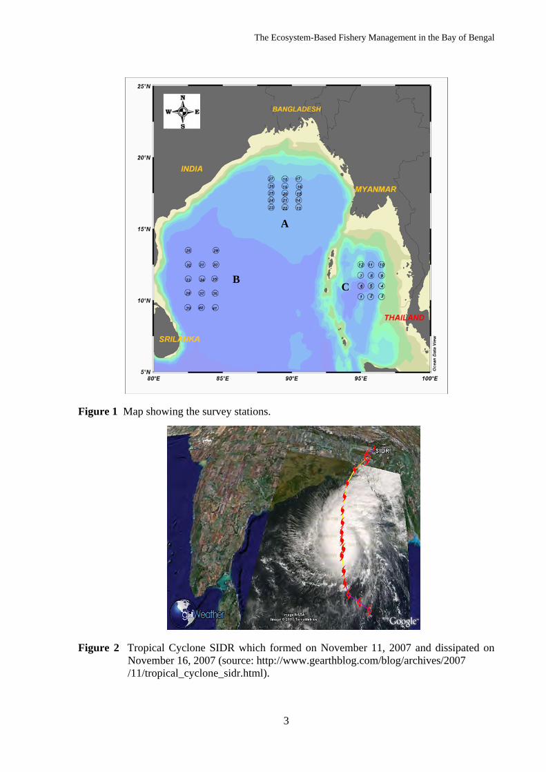
The Ecosystem-Based Fishery Management in the Bay of Bengal
3
Figure 1 Map showing the survey stations.
Figure 2 Tropical Cyclone SIDR which formed on November 11, 2007 and dissipated on
November 16, 2007 (source: http://www.gearthblog.com/blog/archives/2007 /11/tropical_cyclone_sidr.html).
A
B C
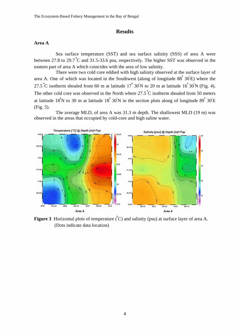
The Ecosystem-Based Fishery Management in the Bay of Bengal
4
Results
Area A
Sea surface temperature (SST) and sea surface salinity (SSS) of area A were between 27.8 to 29.7 ºC and 31.5-33.6 psu, respectively. The higher SST was observed in the eastern part of area A which coincides with the area of low salinity.
There were two cold core eddied with high salinity observed at the surface layer of area A. One of which was located in the Southwest (along of longitude 88º 30′E) where the 27.5 ºC isotherm shoaled from 60 m at latitude 17º 30′N to 20 m at latitude 16º 30′N (Fig. 4). The other cold core was observed in the North where 27.5 ºC isotherm shoaled from 50 meters at latitude 18ºN to 30 m at latitude 18º 30′N in the section plots along of longitude 89º 30′E (Fig. 5).
The average MLD, of area A was 31.3 m depth. The shallowest MLD (19 m) was observed in the areas that occupied by cold-core and high saline water.
Figure 3 Horizontal plots of temperature (ºC) and salinity (psu) at surface layer of area A. (Dots indicate data location)
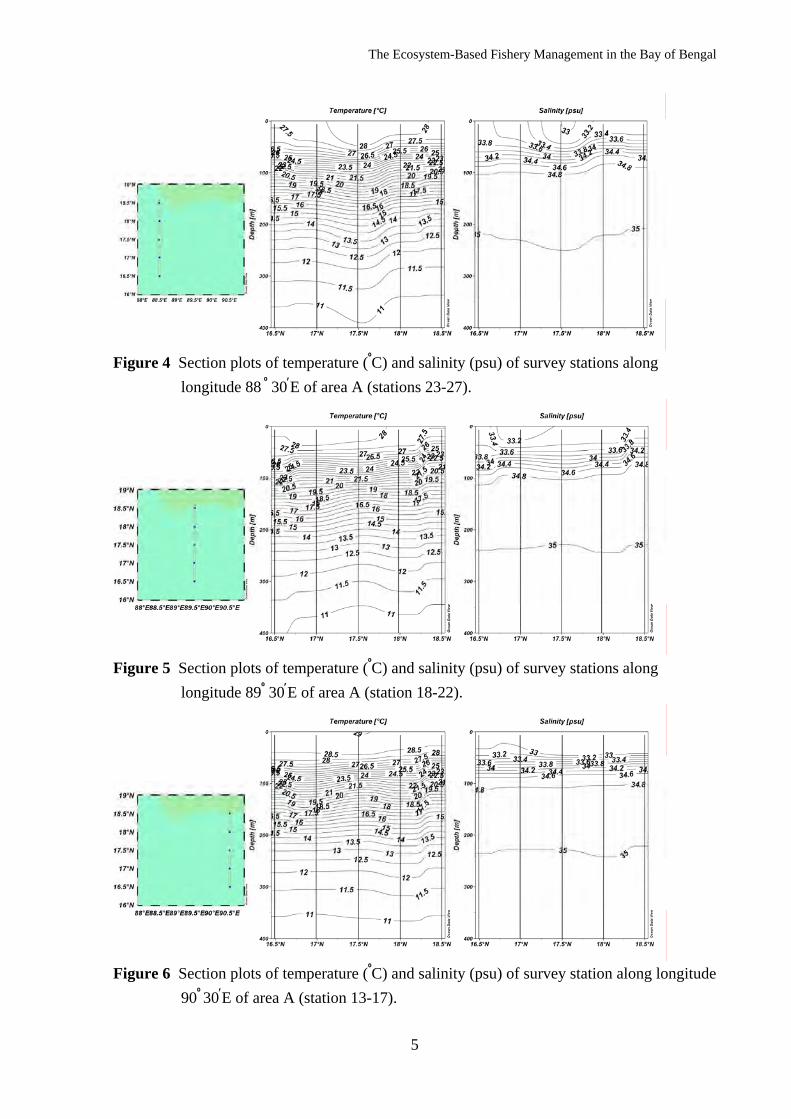
The Ecosystem-Based Fishery Management in the Bay of Bengal
5
Figure 4 Section plots of temperature (ºC) and salinity (psu) of survey stations along longitude 88 º 30′E of area A (stations 23-27).
Figure 5 Section plots of temperature (ºC) and salinity (psu) of survey stations along longitude 89º 30′E of area A (station 18-22).
Figure 6 Section plots of temperature (ºC) and salinity (psu) of survey station along longitude 90º 30′E of area A (station 13-17).
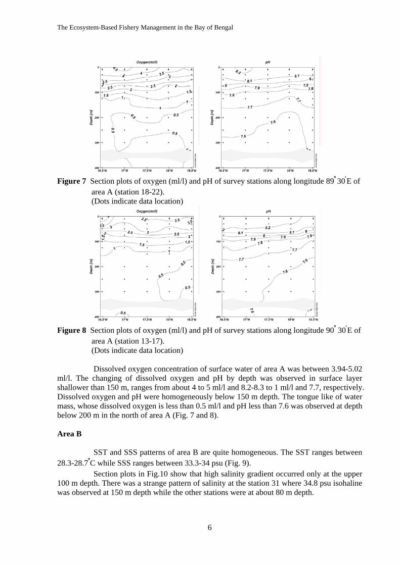
The Ecosystem-Based Fishery Management in the Bay of Bengal
6
Figure 7 Section plots of oxygen (ml/l) and pH of survey stations along longitude 89º 30′E of area A (station 18-22). (Dots indicate data location)
Figure 8 Section plots of oxygen (ml/l) and pH of survey stations along longitude 90º 30′E of area A (station 13-17). (Dots indicate data location)
Dissolved oxygen concentration of surface water of area A was between 3.94-5.02 ml/l. The changing of dissolved oxygen and pH by depth was observed in surface layer shallower than 150 m, ranges from about 4 to 5 ml/l and 8.2-8.3 to 1 ml/l and 7.7, respectively. Dissolved oxygen and pH were homogeneously below 150 m depth. The tongue like of water mass, whose dissolved oxygen is less than 0.5 ml/l and pH less than 7.6 was observed at depth below 200 m in the north of area A (Fig. 7 and 8). Area B
SST and SSS patterns of area B are quite homogeneous. The SST ranges between 28.3-28.7ºC while SSS ranges between 33.3-34 psu (Fig. 9).
Section plots in Fig.10 show that high salinity gradient occurred only at the upper 100 m depth. There was a strange pattern of salinity at the station 31 where 34.8 psu isohaline was observed at 150 m depth while the other stations were at about 80 m depth.
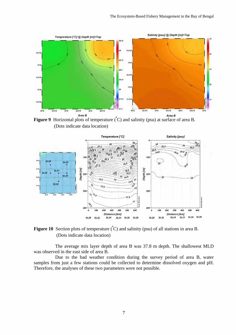
The Ecosystem-Based Fishery Management in the Bay of Bengal
7
Figure 9 Horizontal plots of temperature (ºC) and salinity (psu) at surface of area B. (Dots indicate data location)
Figure 10 Section plots of temperature (ºC) and salinity (psu) of all stations in area B. (Dots indicate data location)
The average mix layer depth of area B was 37.8 m depth. The shallowest MLD was observed in the east side of area B.
Due to the bad weather condition during the survey period of area B, water samples from just a few stations could be collected to determine dissolved oxygen and pH. Therefore, the analyses of these two parameters were not possible.
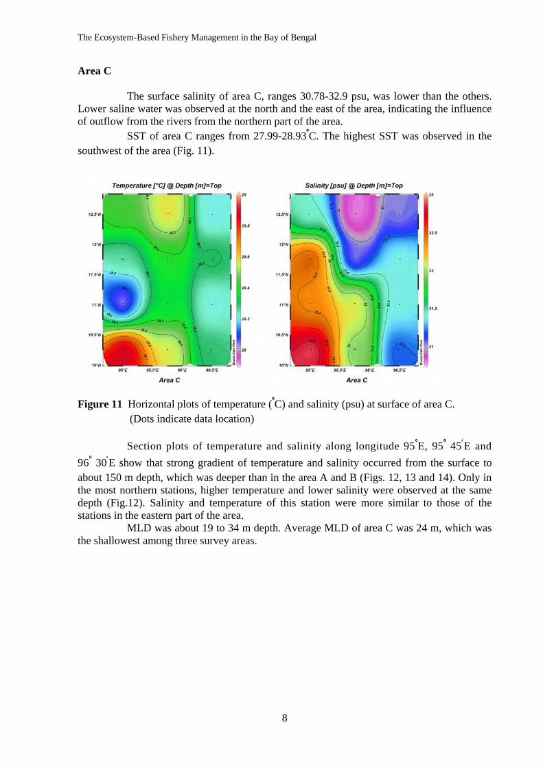
The Ecosystem-Based Fishery Management in the Bay of Bengal
8
Area C
The surface salinity of area C, ranges 30.78-32.9 psu, was lower than the others. Lower saline water was observed at the north and the east of the area, indicating the influence of outflow from the rivers from the northern part of the area.
SST of area C ranges from 27.99-28.93ºC. The highest SST was observed in the southwest of the area (Fig. 11).
Figure 11 Horizontal plots of temperature (ºC) and salinity (psu) at surface of area C. (Dots indicate data location)
Section plots of temperature and salinity along longitude 95ºE, 95º 45′E and 96º 30′E show that strong gradient of temperature and salinity occurred from the surface to about 150 m depth, which was deeper than in the area A and B (Figs. 12, 13 and 14). Only in the most northern stations, higher temperature and lower salinity were observed at the same depth (Fig.12). Salinity and temperature of this station were more similar to those of the stations in the eastern part of the area.
MLD was about 19 to 34 m depth. Average MLD of area C was 24 m, which was the shallowest among three survey areas.
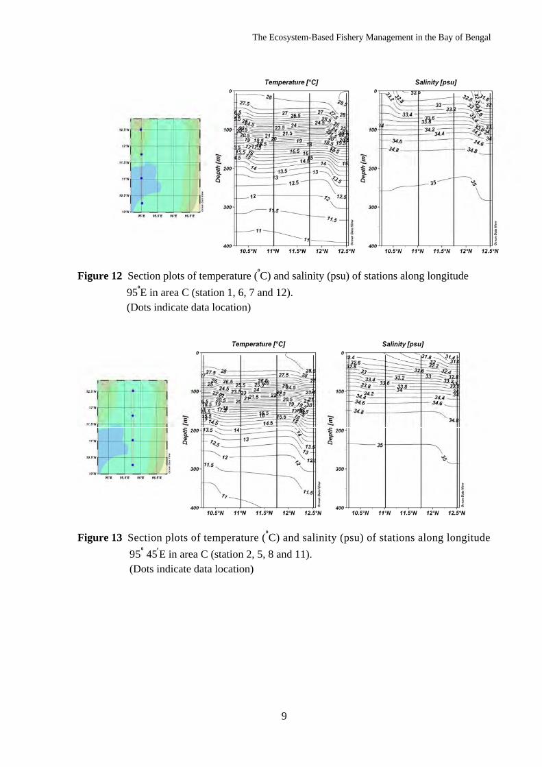
The Ecosystem-Based Fishery Management in the Bay of Bengal
9
Figure 12 Section plots of temperature (ºC) and salinity (psu) of stations along longitude 95ºE in area C (station 1, 6, 7 and 12). (Dots indicate data location)
Figure 13 Section plots of temperature (ºC) and salinity (psu) of stations along longitude 95º 45′E in area C (station 2, 5, 8 and 11). (Dots indicate data location)
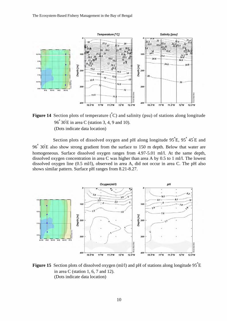
The Ecosystem-Based Fishery Management in the Bay of Bengal
10
Figure 14 Section plots of temperature (ºC) and salinity (psu) of stations along longitude 96º 30′E in area C (station 3, 4, 9 and 10). (Dots indicate data location)
Section plots of dissolved oxygen and pH along longitude 95ºE, 95º 45′E and 96º 30′E also show strong gradient from the surface to 150 m depth. Below that water are homogeneous. Surface dissolved oxygen ranges from 4.97-5.01 ml/l. At the same depth, dissolved oxygen concentration in area C was higher than area A by 0.5 to 1 ml/l. The lowest dissolved oxygen line (0.5 ml/l), observed in area A, did not occur in area C. The pH also shows similar pattern. Surface pH ranges from 8.21-8.27.
Figure 15 Section plots of dissolved oxygen (ml/l) and pH of stations along longitude 95ºE in area C (station 1, 6, 7 and 12). (Dots indicate data location)
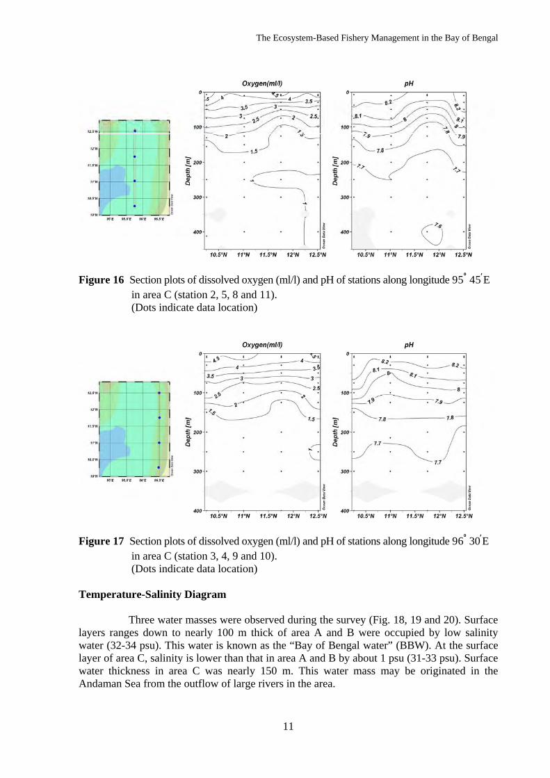
The Ecosystem-Based Fishery Management in the Bay of Bengal
11
Figure 16 Section plots of dissolved oxygen (ml/l) and pH of stations along longitude 95º 45′E in area C (station 2, 5, 8 and 11). (Dots indicate data location)
Figure 17 Section plots of dissolved oxygen (ml/l) and pH of stations along longitude 96º 30′E in area C (station 3, 4, 9 and 10). (Dots indicate data location) Temperature-Salinity Diagram
Three water masses were observed during the survey (Fig. 18, 19 and 20). Surface layers ranges down to nearly 100 m thick of area A and B were occupied by low salinity water (32-34 psu). This water is known as the “Bay of Bengal water” (BBW). At the surface layer of area C, salinity is lower than that in area A and B by about 1 psu (31-33 psu). Surface water thickness in area C was nearly 150 m. This water mass may be originated in the Andaman Sea from the outflow of large rivers in the area.
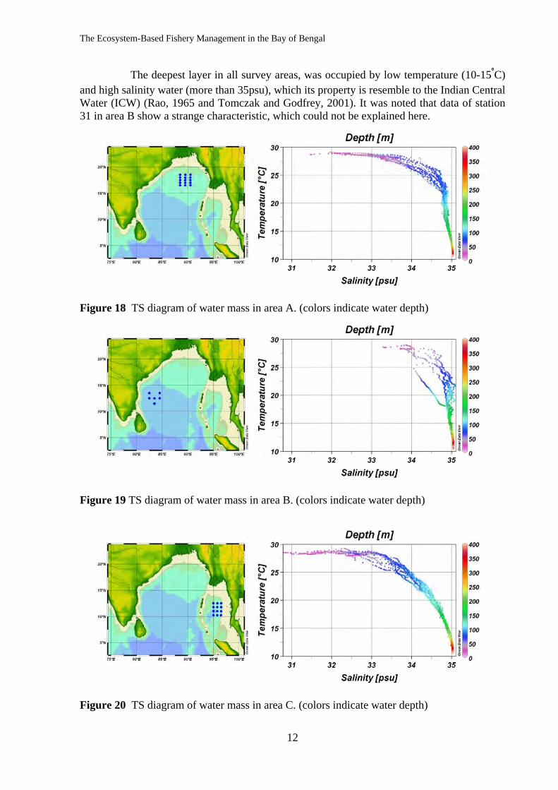
The Ecosystem-Based Fishery Management in the Bay of Bengal
12
The deepest layer in all survey areas, was occupied by low temperature (10-15ºC) and high salinity water (more than 35psu), which its property is resemble to the Indian Central Water (ICW) (Rao, 1965 and Tomczak and Godfrey, 2001). It was noted that data of station 31 in area B show a strange characteristic, which could not be explained here.
Figure 18 TS diagram of water mass in area A. (colors indicate water depth)
Figure 19 TS diagram of water mass in area B. (colors indicate water depth)
Figure 20 TS diagram of water mass in area C. (colors indicate water depth)
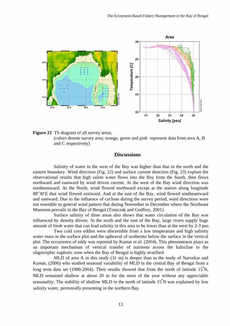
The Ecosystem-Based Fishery Management in the Bay of Bengal
13
Figure 21 TS diagram of all survey areas.
(colors denote survey area; orange, green and pink represent data from area A, B and C respectively)
Discussions
Salinity of water in the west of the Bay was higher than that in the north and the
eastern boundary. Wind direction (Fig. 22) and surface current direction (Fig. 23) explain the observational results that high saline water flows into the Bay from the South, then flows northward and eastward by wind driven current. At the west of the Bay wind direction was northeastward. At the North, wind flowed northward except at the station along longitude 88ο30′E that wind flowed eastward. And at the east of the Bay, wind flowed southeastward and eastward. Due to the influence of cyclone during the survey period, wind directions were not resemble to general wind pattern that during November to December where the Northeast Monsoon prevails in the Bay of Bengal (Tomczak and Godfrey, 2001).
Surface salinity of three areas also shows that water circulation of the Bay was influenced by density driven. At the north and the east of the Bay, large rivers supply huge amount of fresh water that can lead salinity in this area to be lower than at the west by 2-3 psu.
Two cold core eddies were discernible from a low temperature and high salinity water mass in the surface plot and the upheaval of isotherms below the surface in the vertical plot. The occurrence of eddy was reported by Kumar et al. (2004). This phenomenon plays as an important mechanism of vertical transfer of nutrients across the halocline to the oligotrophic euphotic zone when the Bay of Bengal is highly stratified.
MLD of area A in this study (31 m) is deeper than in the study of Narvekar and Kumar, (2006) who studied seasonal variability of MLD in the central Bay of Bengal from a long term data set (1900-2004). Their results showed that from the north of latitude 15ºN, MLD remained shallow at about 20 m for the most of the year without any appreciable seasonality. The stability of shallow MLD in the north of latitude 15ºN was explained by low salinity water, perennially presenting in the northern Bay.
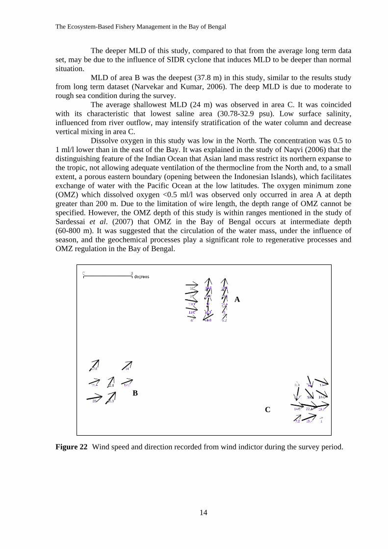
The Ecosystem-Based Fishery Management in the Bay of Bengal
14
The deeper MLD of this study, compared to that from the average long term data set, may be due to the influence of SIDR cyclone that induces MLD to be deeper than normal situation.
MLD of area B was the deepest (37.8 m) in this study, similar to the results study from long term dataset (Narvekar and Kumar, 2006). The deep MLD is due to moderate to rough sea condition during the survey.
The average shallowest MLD (24 m) was observed in area C. It was coincided with its characteristic that lowest saline area (30.78-32.9 psu). Low surface salinity, influenced from river outflow, may intensify stratification of the water column and decrease vertical mixing in area C.
Dissolve oxygen in this study was low in the North. The concentration was 0.5 to 1 ml/l lower than in the east of the Bay. It was explained in the study of Naqvi (2006) that the distinguishing feature of the Indian Ocean that Asian land mass restrict its northern expanse to the tropic, not allowing adequate ventilation of the thermocline from the North and, to a small extent, a porous eastern boundary (opening between the Indonesian Islands), which facilitates exchange of water with the Pacific Ocean at the low latitudes. The oxygen minimum zone (OMZ) which dissolved oxygen <0.5 ml/l was observed only occurred in area A at depth greater than 200 m. Due to the limitation of wire length, the depth range of OMZ cannot be specified. However, the OMZ depth of this study is within ranges mentioned in the study of Sardessai et al. (2007) that OMZ in the Bay of Bengal occurs at intermediate depth (60-800 m). It was suggested that the circulation of the water mass, under the influence of season, and the geochemical processes play a significant role to regenerative processes and OMZ regulation in the Bay of Bengal.
Figure 22 Wind speed and direction recorded from wind indictor during the survey period.
A
B
C
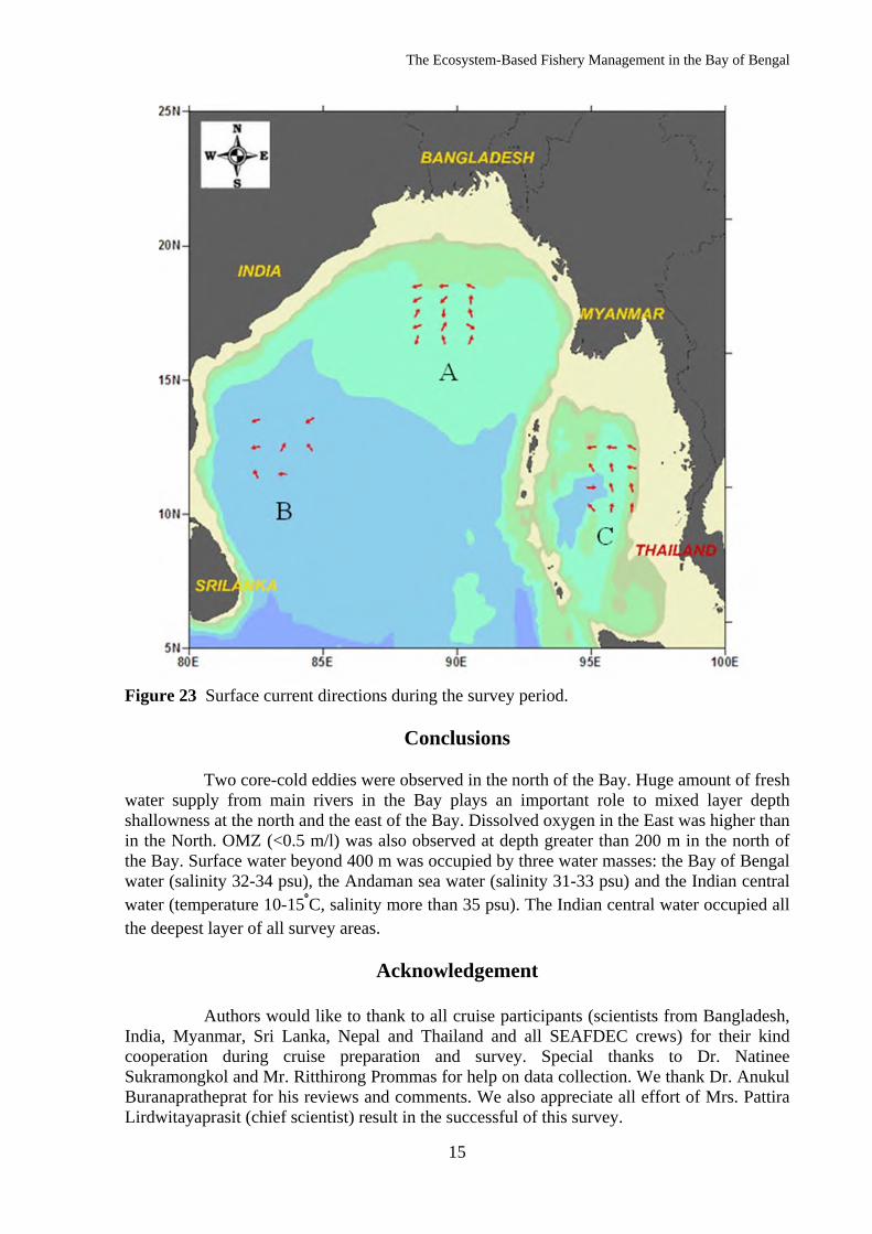
The Ecosystem-Based Fishery Management in the Bay of Bengal
15
Figure 23 Surface current directions during the survey period.
Conclusions
Two core-cold eddies were observed in the north of the Bay. Huge amount of fresh water supply from main rivers in the Bay plays an important role to mixed layer depth shallowness at the north and the east of the Bay. Dissolved oxygen in the East was higher than in the North. OMZ (<0.5 m/l) was also observed at depth greater than 200 m in the north of the Bay. Surface water beyond 400 m was occupied by three water masses: the Bay of Bengal water (salinity 32-34 psu), the Andaman sea water (salinity 31-33 psu) and the Indian central water (temperature 10-15ºC, salinity more than 35 psu). The Indian central water occupied all the deepest layer of all survey areas.
Acknowledgement
Authors would like to thank to all cruise participants (scientists from Bangladesh, India, Myanmar, Sri Lanka, Nepal and Thailand and all SEAFDEC crews) for their kind cooperation during cruise preparation and survey. Special thanks to Dr. Natinee Sukramongkol and Mr. Ritthirong Prommas for help on data collection. We thank Dr. Anukul Buranapratheprat for his reviews and comments. We also appreciate all effort of Mrs. Pattira Lirdwitayaprasit (chief scientist) result in the successful of this survey.
The Ecosystem-Based Fishery Management in the Bay of Bengal
16
References
Naqvi, S. W. A. 2006. Oxygen Deficiency in the North Indian Ocean. Gayana, Vol. 70. India. p. 53-58.
Narvekar, J. and S. P. Kumar. 2006. Seasonal variability of the mixed layer in the central Bay of Bengal and associated changes in nutrients and chlorophyll. Deep-Sea Research I 53:820-835. Kumar, S. P., M. Nuncio, J. Narvekar, A. Kumar, S. Sardesai, S. N. de Souza, M. Gauns, N. Ramaiah and M. Madhupratap. 2004. Are eddies nature’s trigger to enhance biological productivity in the Bay of Bengal. Geophys. Res. Lett. 31(7). Rao, T. C. S. 1965. Hydrographic feature of northern Indian Ocean. Def. Sci. J. 15:171-176. Sardessai S., N. Ramaiah, S. P. Kumar and S. N. de Sousa. 2007. Influence of environmental
forcings on the seasonality of dissolved oxygen and nutrients in the Bay of Bengal. Jurnal of Marine Science 65(2):275-300.
Schlitzer, R. 2006. Ocean Data View. Available Source: http://odv.awi.de, July 3, 2008. Tomczak, M. and J. S. Godfrey. 2001. Regional Oceanography: An Introduction, Chapter 12, Hydrology of the Indian Ocean. Available Soue: http://www.es.flinders.edu.au/~mattom/regoc/pdfverson.html, July 3, 2008.
The Ecosystem-Based Fishery Management in the Bay of Bengal
17
Comparison of Total Phosphorus Contents and Total Alkalinity in Seawater of Different Area in the Bay of Bengal
Penjai Sompongchaiyakul1, Saisiri Chaichana2,
Chanthip Bunluedaj3 and Natinee Sukramongkol4
1 Faculty of Environmental Management, Prince of Songkla University, Hat-Yai, Songkhla, THAILAND 2 Department of Environmental Science, Songkhla Rajabhat University, Songkhla, THAILAND
3 Deep Sea Fishery Technology Research and Development Institute, Department of Fisheries, Samutprakarn 10270, THAILAND
4 Southeast Asian Fisheries Development Center, Training Department, P.O.Box 97, Phrasamutchedi, Samutprakarn 10290, THAILAND
Abstract
Total phosphorus and total alkalinity at different depth throughout the water column (400 m depth, salinity ca. 34 psu) in three areas of the Bay of Bengal were investigated in order to compare their distribution in different areas of the Bay of Bengal. It was found that pattern of depth profile of both total phosphorus and total alkalinity in area C (the Andaman Sea) is different from the other two areas of the Bay of Bengal. Together with the relationship between total alkalinity and total phosphorus, it can be indicated that the characteristics of seawater in the enclosed Andaman Sea are different from the entire Bay of Bengal. In comparison with the other two areas, lower total alkalinity in the surface water and higher total alkalinity but lower total phosphorus in the deeper water was observed in the Andaman Sea. Key words: total phosphorus, total alkalinity, Bay of Bengal
Introduction Primary producer in the sea, phytoplankton, require dissolved inorganic nutrients for their growth. The free orthophosphate ion component is a vital nutrient for sustaining marine productivity (e.g., Codispoti, 1989; Tyrrell, 1999). It is well known as the limiting nutrient for primary productivity in marine systems. Regeneration of phosphorus from both particulate and dissolved forms of organic phosphorus is a potentially important source of bioavailable P for marine primary and secondary producers (Ammerman and Azam, 1985; Bjorkman and Karl, 1994; Jackson and Williams, 1985; Karl et al., 1993; Monaghan and Ruttenberg, 1999). Within pools of dissolved and particulate phosphorus or so-called total phosphorus, turnover rates of organic phosphorus are rapid and seasonal, enabling low inorganic phosphorus concentrations to support high primary productivity (Benitez-Nelson and Buesseler, 1999). Total alkalinity, a measurement of buffering capacity of the marine systems, is known to be a conservative parameter of water masses, therefore its measurements act as a water mass tracer (Schiettecatte et al., 2003, Watanabe et al., 2004). However, the oceans act as a natural reservoir for carbon dioxide (CO2). Atmospheric CO2 dissolves naturally in the ocean, forming carbonic acid (H2CO3), a weak acid. It is estimated that the world ocean is taking up 1.7 GtC per year, which is almost 30% of the CO2 released anthropogenically into the atmosphere (Prentice et al., 2001). The uptake of anthropogenic carbon since 1750 has led to the ocean becoming more acidic, with an average decrease in pH of 0.1 units (UNEP, 2008).
The Ecosystem-Based Fishery Management in the Bay of Bengal
18
Although the coastal ocean is only a small fraction (8%) of the total ocean area, several studies have suggested the importance of the CO2 dynamics in this area. Between 15% and 50% of the oceanic primary production is now attributed to coastal ocean (Walsh, 1991; Muller-Karger, 2000). Recent studies have concluded that some continental shelves, in general the zone shallower than 200 m, act as a sink for atmospheric CO2 (Tsunogai et al., 1999; Frankignoulle and Borges, 2001), of up to 0.6 GtC per year worldwide (Yool and Fasham, 2001), which is about 30% of the oceanic CO2 uptake. Another reason that we care about alkalinity is that when organisms build calcium carbonate skeletons, they effectively remove calcium and carbonate from the water column. Progressive acidification of the oceans due to increasing atmospheric CO2 is expected to reduce biocalcification of the shells; bones and skeletons most marine organisms possess (UNEP, 2008). In this study, total phosphorus and total alkalinity at different depth throughout the water column (400 m depth, salinity ca. 34 psu) in three areas of the Bay of Bengal were investigated in order to compare their distribution in different areas of the Bay of Bengal.
Material and Methods Sample collection was conducted onboard M.V. SEAFDEC from 25 October to 21 December 2007 under an Ecosystem-Based Fishery Management Project in the Bay of Bengal in collaborative among the BIMSTEC members (Bangladesh, India, Myanmar, Nepal, Sri Lanka, and Thailand). Seawater samples were collected at selected depth, using a iCTD system couple with Carousel water sample (Niskin Bottles), from 28 oceanographic stations in the Bay of Bengal 12 stations in area A (upper part of the Bay of Bengal covered international waters and the EEZ of Bangladesh and India), 4 stations in area B (western area of the Bay of Bengal, offshore of India and Sri Lanka waters) and 12 stations in area C (central part of the Andaman Sea covered the EEZ of Myanmar and the Andaman Island of India) (Fig. 1). Sea water samples for total phosphorus analysis were filled in pre-cleaned 60 ml plastic bottles and immediately kept frozen (-45ºC) until analyzed. Sea water samples for total alkalinity analysis were filled in 125 ml plastic bottles which pre-added a few drops of HgCl2 and then store at room temperature until analysis. Since total phosphorus defined as all forms of phosphorus, all bound fractions were liberated by persulfate oxidation prior the measurement of the orthophosphate form by ascorbic acid-colorimetric method (Menzel and Corwin, 1965; Grasshoff et al., 1983; Strickland and Parsons, 1972) The amount of total alkalinity in seawater was measured by carrying out a potentiometric titration of a known volume of sea water in a vessel which is sealed from the atmosphere. This is accomplished by adding precise amounts of 0.1 N HCl to the vessel in small increments, and measuring the change in the electromotive potential of the water caused by this addition. The data were used to calculate the total alkalinity by the modified Gran method.
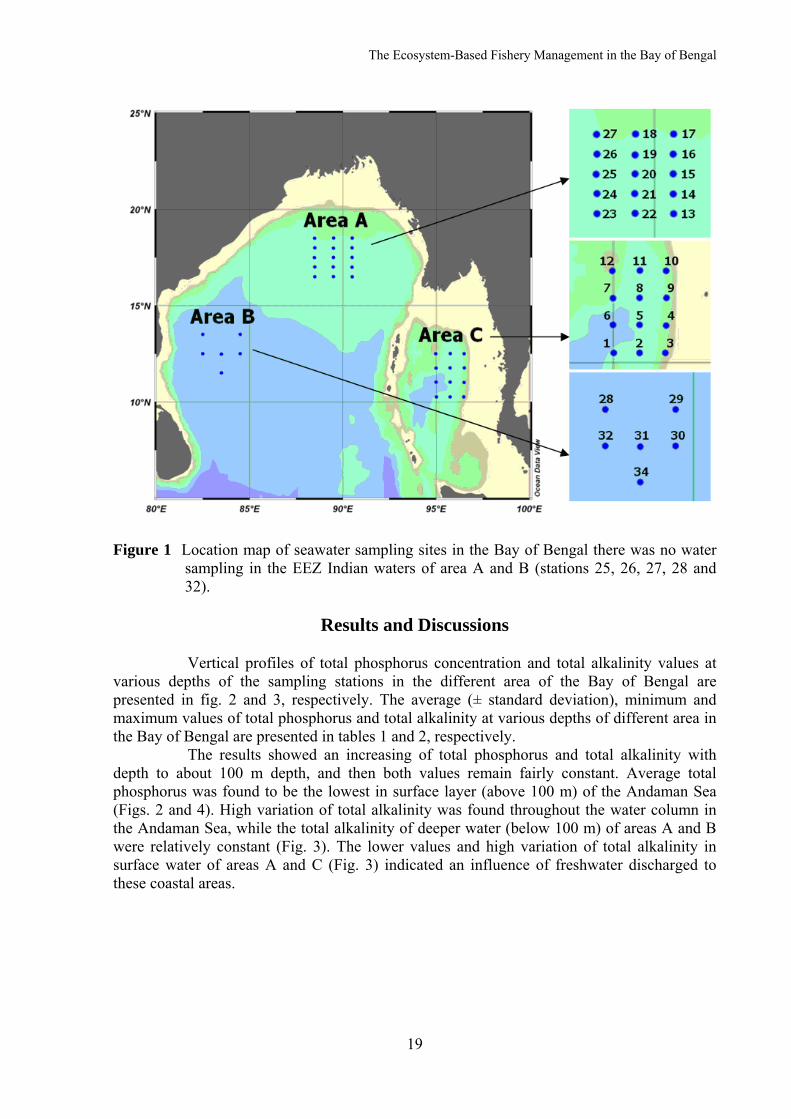
The Ecosystem-Based Fishery Management in the Bay of Bengal
19
Figure 1 Location map of seawater sampling sites in the Bay of Bengal there was no water
sampling in the EEZ Indian waters of area A and B (stations 25, 26, 27, 28 and 32).
Results and Discussions
Vertical profiles of total phosphorus concentration and total alkalinity values at various depths of the sampling stations in the different area of the Bay of Bengal are presented in fig. 2 and 3, respectively. The average (± standard deviation), minimum and maximum values of total phosphorus and total alkalinity at various depths of different area in the Bay of Bengal are presented in tables 1 and 2, respectively. The results showed an increasing of total phosphorus and total alkalinity with depth to about 100 m depth, and then both values remain fairly constant. Average total phosphorus was found to be the lowest in surface layer (above 100 m) of the Andaman Sea (Figs. 2 and 4). High variation of total alkalinity was found throughout the water column in the Andaman Sea, while the total alkalinity of deeper water (below 100 m) of areas A and B were relatively constant (Fig. 3). The lower values and high variation of total alkalinity in surface water of areas A and C (Fig. 3) indicated an influence of freshwater discharged to these coastal areas.
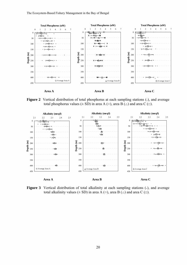
The Ecosystem-Based Fishery Management in the Bay of Bengal
20
0
50
100
150
200
250
300
350
400
450
0 1 2 3 4 5 6 7
Total Phosphorus (uM)D
epth
(m)
Average Area A
0
50
100
150
200
250
300
350
400
450
0 1 2 3 4 5 6 7
Total Phosphorus (uM)
Dep
th (m
)Average Area B
0
50
100
150
200
250
300
350
400
450
0 1 2 3 4 5 6 7
Total Phosphorus (uM)
Dep
th (m
)
Average Area C
Area A
Area B
Area C
Figure 2 Vertical distribution of total phosphorus at each sampling stations (●), and average
total phosphorus values (± SD) in area A (○), area B ( ) and area C (□).
0
50
100
150
200
250
300
350
400
450
2.1 2.2 2.3 2.4 2.5
Alkalinity (meq/l)
Dep
th (m
)
Average Area A
0
50
100
150
200
250
300
350
400
450
2.1 2.2 2.3 2.4 2.5
Alkalinity (meq/l)
Dep
th (m
)
Average Area B
0
50
100
150
200
250
300
350
400
450
2.1 2.2 2.3 2.4 2.5
Alkalinity (meq/l)
Dep
th (m
)
Average Area C
Area A
Area B
Area C
Figure 3 Vertical distribution of total alkalinity at each sampling stations (●), and average
total alkalinity values (± SD) in area A (○), area B ( ) and area C (□).
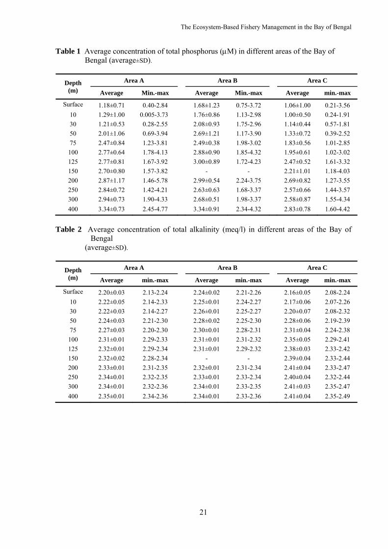
The Ecosystem-Based Fishery Management in the Bay of Bengal
21
Table 1 Average concentration of total phosphorus (μM) in different areas of the Bay of Bengal (average±SD).
Depth (m)
Area A Area B Area C
Average Min.-max Average Min.-max Average min.-max
Surface 1.18±0.71 0.40-2.84 1.68±1.23 0.75-3.72 1.06±1.00 0.21-3.56 10 1.29±1.00 0.005-3.73 1.76±0.86 1.13-2.98 1.00±0.50 0.24-1.91 30 1.21±0.53 0.28-2.55 2.08±0.93 1.75-2.96 1.14±0.44 0.57-1.81 50 2.01±1.06 0.69-3.94 2.69±1.21 1.17-3.90 1.33±0.72 0.39-2.52 75 2.47±0.84 1.23-3.81 2.49±0.38 1.98-3.02 1.83±0.56 1.01-2.85
100 2.77±0.64 1.78-4.13 2.88±0.90 1.85-4.32 1.95±0.61 1.02-3.02 125 2.77±0.81 1.67-3.92 3.00±0.89 1.72-4.23 2.47±0.52 1.61-3.32 150 2.70±0.80 1.57-3.82 - - 2.21±1.01 1.18-4.03 200 2.87±1.17 1.46-5.78 2.99±0.54 2.24-3.75 2.69±0.82 1.27-3.55 250 2.84±0.72 1.42-4.21 2.63±0.63 1.68-3.37 2.57±0.66 1.44-3.57 300 2.94±0.73 1.90-4.33 2.68±0.51 1.98-3.37 2.58±0.87 1.55-4.34 400 3.34±0.73 2.45-4.77 3.34±0.91 2.34-4.32 2.83±0.78 1.60-4.42
Table 2 Average concentration of total alkalinity (meq/l) in different areas of the Bay of
Bengal (average±SD).
Depth (m)
Area A Area B Area C
Average min.-max Average min.-max Average min.-max
Surface 2.20±0.03 2.13-2.24 2.24±0.02 2.21-2.26 2.16±0.05 2.08-2.24 10 2.22±0.05 2.14-2.33 2.25±0.01 2.24-2.27 2.17±0.06 2.07-2.26 30 2.22±0.03 2.14-2.27 2.26±0.01 2.25-2.27 2.20±0.07 2.08-2.32 50 2.24±0.03 2.21-2.30 2.28±0.02 2.25-2.30 2.28±0.06 2.19-2.39 75 2.27±0.03 2.20-2.30 2.30±0.01 2.28-2.31 2.31±0.04 2.24-2.38
100 2.31±0.01 2.29-2.33 2.31±0.01 2.31-2.32 2.35±0.05 2.29-2.41 125 2.32±0.01 2.29-2.34 2.31±0.01 2.29-2.32 2.38±0.03 2.33-2.42 150 2.32±0.02 2.28-2.34 - - 2.39±0.04 2.33-2.44 200 2.33±0.01 2.31-2.35 2.32±0.01 2.31-2.34 2.41±0.04 2.33-2.47 250 2.34±0.01 2.32-2.35 2.33±0.01 2.33-2.34 2.40±0.04 2.32-2.44 300 2.34±0.01 2.32-2.36 2.34±0.01 2.33-2.35 2.41±0.03 2.35-2.47 400 2.35±0.01 2.34-2.36 2.34±0.01 2.33-2.36 2.41±0.04 2.35-2.49
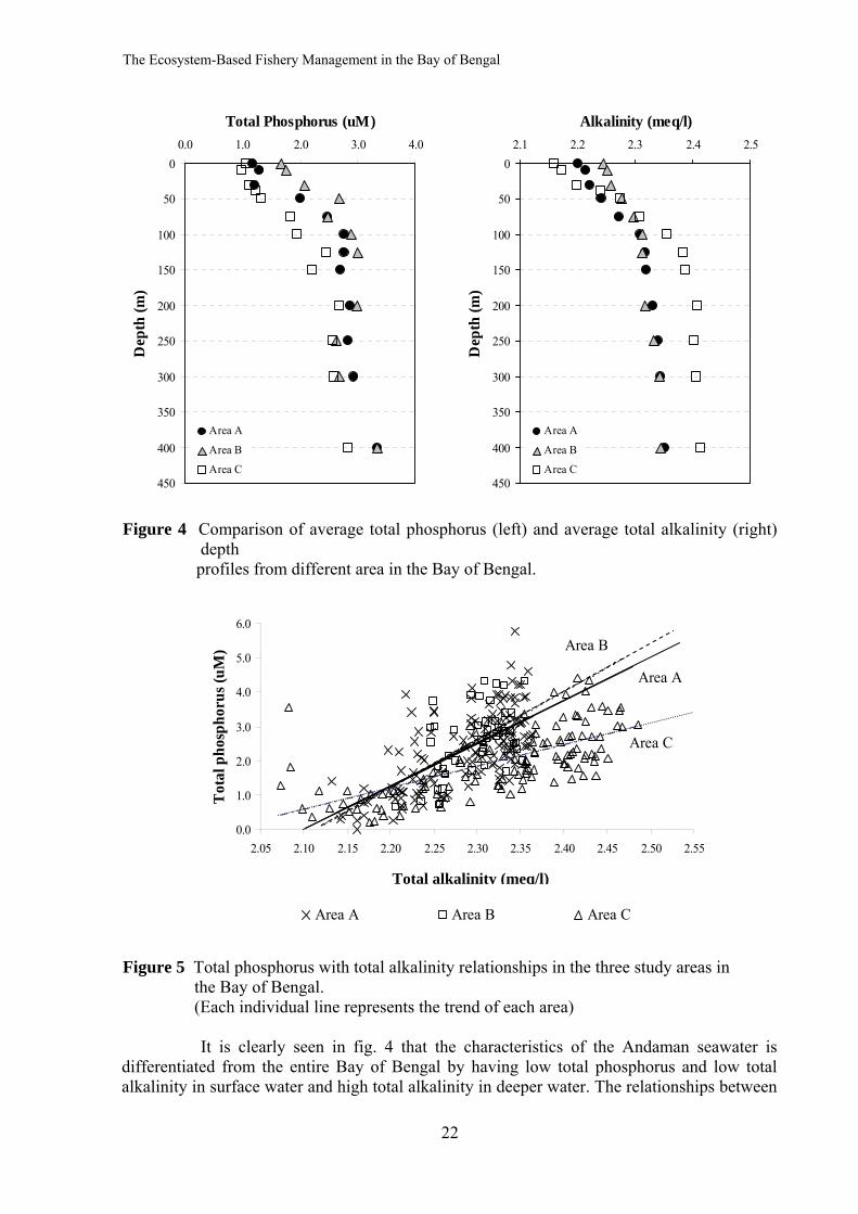
The Ecosystem-Based Fishery Management in the Bay of Bengal
22
0
50
100
150
200
250
300
350
400
450
0.0 1.0 2.0 3.0 4.0
Total Phosphorus (uM)D
epth
(m)
Area A
Area B
Area C
0
50
100
150
200
250
300
350
400
450
2.1 2.2 2.3 2.4 2.5
Alkalinity (meq/l)
Dep
th (m
)
Area A
Area B
Area C
Figure 4 Comparison of average total phosphorus (left) and average total alkalinity (right)
depth profiles from different area in the Bay of Bengal.
Figure 5 Total phosphorus with total alkalinity relationships in the three study areas in the Bay of Bengal. (Each individual line represents the trend of each area)
It is clearly seen in fig. 4 that the characteristics of the Andaman seawater is differentiated from the entire Bay of Bengal by having low total phosphorus and low total alkalinity in surface water and high total alkalinity in deeper water. The relationships between
0.0
1.0
2.0
3.0
4.0
5.0
6.0
2.05 2.10 2.15 2.20 2.25 2.30 2.35 2.40 2.45 2.50 2.55
Alkalinity (meq/l)
Tot
al p
hosp
horu
s (uM
)
Area A Area B Area C
Area A
Area B
Area C
Total alkalinity (meq/l)
The Ecosystem-Based Fishery Management in the Bay of Bengal
23
total phosphorus and total alkalinity of samples taken from area A and B give similar trend lines, whereas those from area C (the Andaman Sea) show a dissimilar trend (Fig. 5). High variation of total alkalinity values throughout the water column down to 400 m depth in the Andaman Sea may be affected from internal waves. It is believed that the internal waves in the Andaman Sea occur all year round (Jackson, 2004). The amplitudes of internal waves in the Andaman Sea may be up to 70-80 m and can propagate over several hundred kilometers, which lead to transport of water mass and induce turbulence and mixing in the water column (Osborne and Burch, 1980; Jackson, 2004). Fig. 6 and 7 illustrate horizontal distribution of total phosphorus and total alkalinity, respectively, at different depth. These two figures indicate that the eastern part of the Bay of Bengal is a low total phosphorus region. The distribution of total alkalinity and total phosphorus along north-south section in the area C (the Andaman Sea) and area A (the upper part of the Bay of Bengal) are illustrated in figs. 8 and 9, respectively, and the east-west section of area A is shown in fig. 10.
Conclusion The total alkalinity in surface water of area C (the Andaman Sea) is lower than those of areas A and B, however, but is higher at the depths below 100 down to 400 m. The vertical distribution of total phosphorus and total alkalinity in areas A and B of the Bay of Bengal are similar. The differentiated pattern of depth profiles of both total phosphorus and total alkalinity together with the relationship between total alkalinity and total phosphorus indicate that sea water characteristics in the enclosed Andaman Sea is different from the entire Bay of Bengal. Unfortunately, analyses of organic carbon and total nitrogen in these seawater samples are not yet finished. Total alkalinity coupled with pH and temperature data, amount of dissolved inorganic carbon (DIC) species and dissolved carbon dioxide gas (pCO2) in seawater can be calculated. Interpretation of this data set will provide clearer understanding of biogeochemical processes occurring in these three areas of the Bay of Bengal.
Acknowledgement We gratefully acknowledge Miss Sopana Boonyapiwat and Ms. Pattira Lirdwitayaprasit for their kind cooperation of this collaborative work. We would also like to thank the officers and crew of M.V. SEAFDEC for assisting in sample collection.
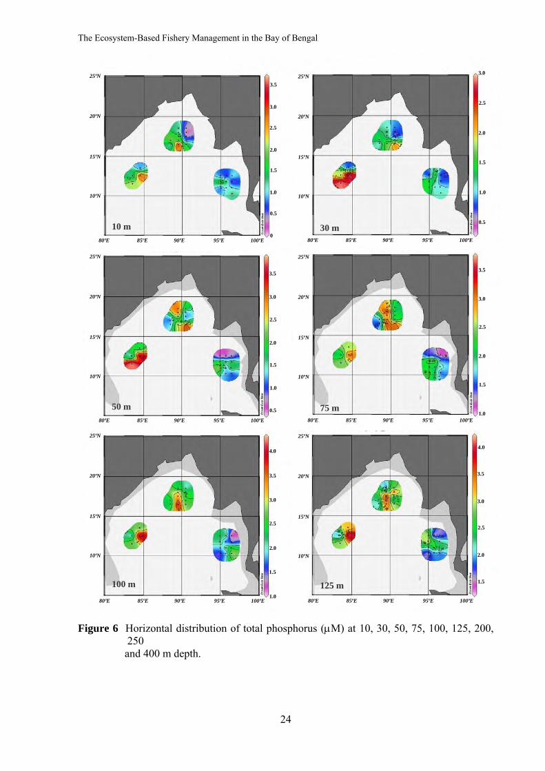
The Ecosystem-Based Fishery Management in the Bay of Bengal
24
Figure 6 Horizontal distribution of total phosphorus (μM) at 10, 30, 50, 75, 100, 125, 200,
250 and 400 m depth.
100 m 125 m
50 m 75 m
10 m 30 m80ºE 85ºE 90ºE 95ºE 100ºE 80ºE 85ºE 90ºE 95ºE 100ºE
80ºE 85ºE 90ºE 95ºE 100ºE 80ºE 85ºE 90ºE 95ºE 100ºE
80ºE 85ºE 90ºE 95ºE 100ºE 80ºE 85ºE 90ºE 95ºE 100ºE
25ºN
20ºN
15ºN
10ºN
25ºN
20ºN
15ºN
10ºN
25ºN
20ºN
15ºN
10ºN
25ºN
20ºN
15ºN
10ºN
25ºN
20ºN
15ºN
10ºN
25ºN
20ºN
15ºN
10ºN
3.5
3.0
2.5
2.0
1.5
1.0
0.5
0
3.0
2.5
2.0
1.5
1.0
0.5
3.5
2.5
2.0
1.5
1.0
0.5
3.0
3.5
2.5
2.0
1.5
1.0
3.0
3.5
2.5
2.0
1.5
1.0
4.0
3.0
3.5
2.5
2.0
1.5
4.0
3.0
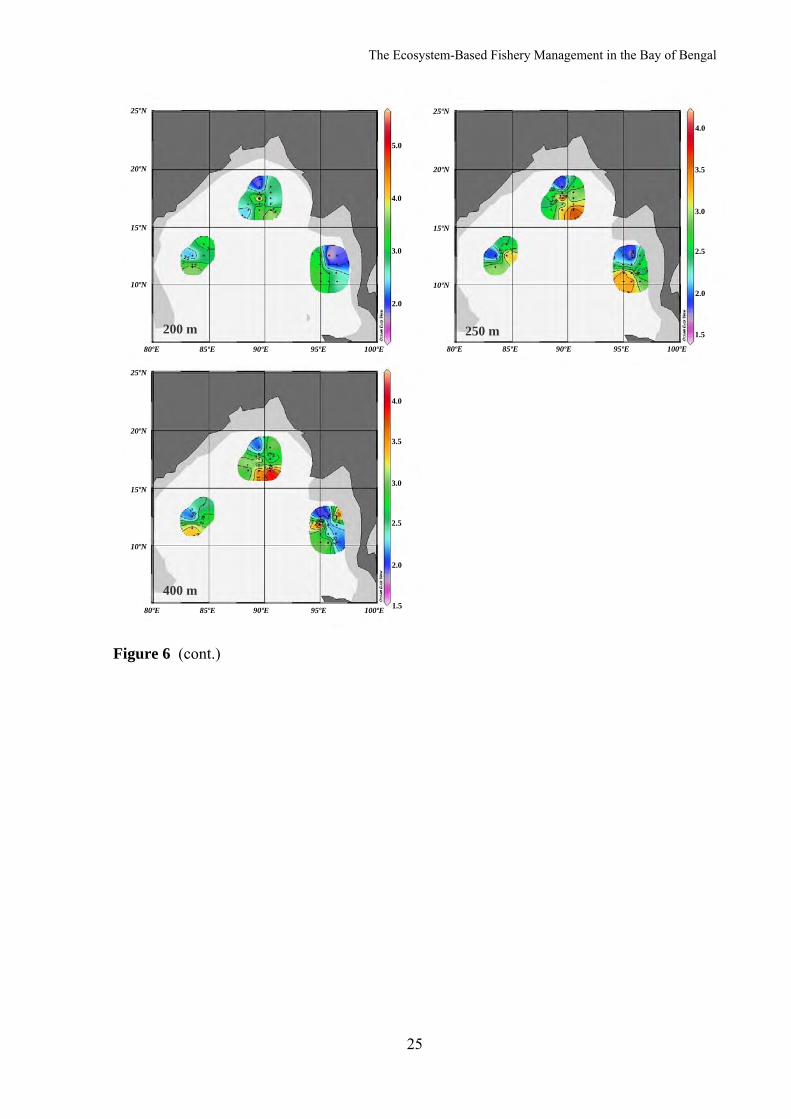
The Ecosystem-Based Fishery Management in the Bay of Bengal
25
Figure 6 (cont.)
400 m
200 m 250 m80ºE 85ºE 90ºE 95ºE 100ºE 80ºE 85ºE 90ºE 95ºE 100ºE
80ºE 85ºE 90ºE 95ºE 100ºE
25ºN
20ºN
15ºN
10ºN
25ºN
20ºN
15ºN
10ºN
25ºN
20ºN
15ºN
10ºN
3.0
2.0
5.0
4.0
3.5
2.5
2.0
1.5
4.0
3.0
3.5
2.5
2.0
1.5
4.0
3.0
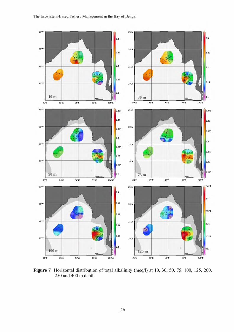
The Ecosystem-Based Fishery Management in the Bay of Bengal
26
Figure 7 Horizontal distribution of total alkalinity (meq/l) at 10, 30, 50, 75, 100, 125, 200,
250 and 400 m depth.
100 m 125 m
50 m 75 m
10 m 30 m80ºE 85ºE 90ºE 95ºE 100ºE 80ºE 85ºE 90ºE 95ºE 100ºE
80ºE 85ºE 90ºE 95ºE 100ºE 80ºE 85ºE 90ºE 95ºE 100ºE
80ºE 85ºE 90ºE 95ºE 100ºE 80ºE 85ºE 90ºE 95ºE 100ºE
25ºN
20ºN
15ºN
10ºN
25ºN
20ºN
15ºN
10ºN
25ºN
20ºN
15ºN
10ºN
25ºN
20ºN
15ºN
10ºN
25ºN
20ºN
15ºN
10ºN
25ºN
20ºN
15ºN
10ºN
2.3
2.25
2.2
2.15
2.1
2.3
2.25
2.2
2.15
2.1
2.35
2.325
2.275
2.25
2.2
2.375
2.3
2.225
2.35
2.325
2.275
2.25
2.375
2.3
2.225
2.4
2.38
2.34
2.32
2.36
2.3
2.4
2.375
2.325
2.425
2.35
2.3
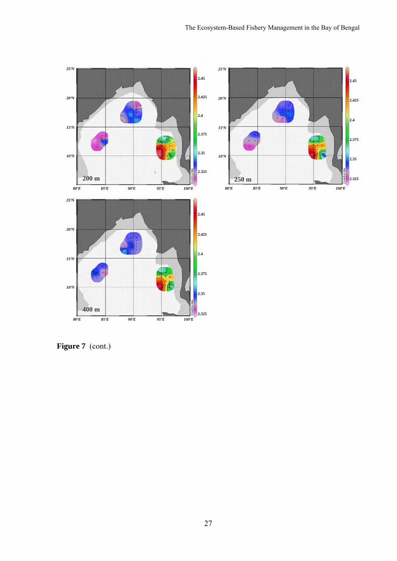
The Ecosystem-Based Fishery Management in the Bay of Bengal
27
Figure 7 (cont.)
400 m
200 m 250 m80ºE 85ºE 90ºE 95ºE 100ºE 80ºE 85ºE 90ºE 95ºE 100ºE
80ºE 85ºE 90ºE 95ºE 100ºE
25ºN
20ºN
15ºN
10ºN
25ºN
20ºN
15ºN
10ºN
25ºN
20ºN
15ºN
10ºN
2.425
2.4
2.35
2.45
2.375
2.325
2.425
2.4
2.35
2.45
2.375
2.325
2.425
2.4
2.35
2.45
2.375
2.325
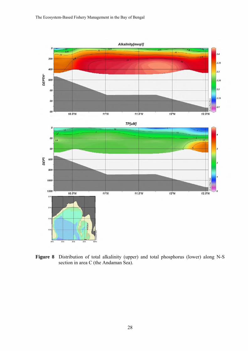
The Ecosystem-Based Fishery Management in the Bay of Bengal
28
Figure 8 Distribution of total alkalinity (upper) and total phosphorus (lower) along N-S
section in area C (the Andaman Sea).
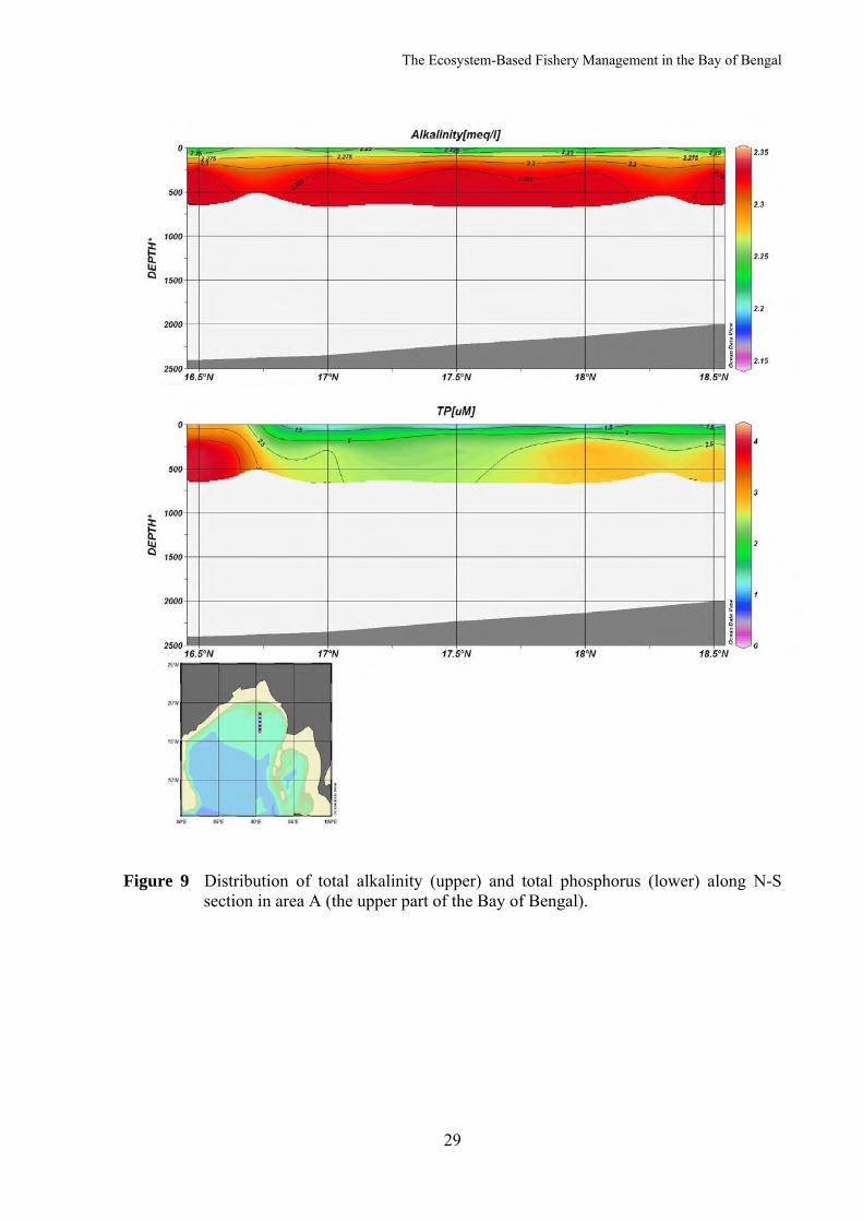
The Ecosystem-Based Fishery Management in the Bay of Bengal
29
Discussion
Figure 9 Distribution of total alkalinity (upper) and total phosphorus (lower) along N-S
section in area A (the upper part of the Bay of Bengal).
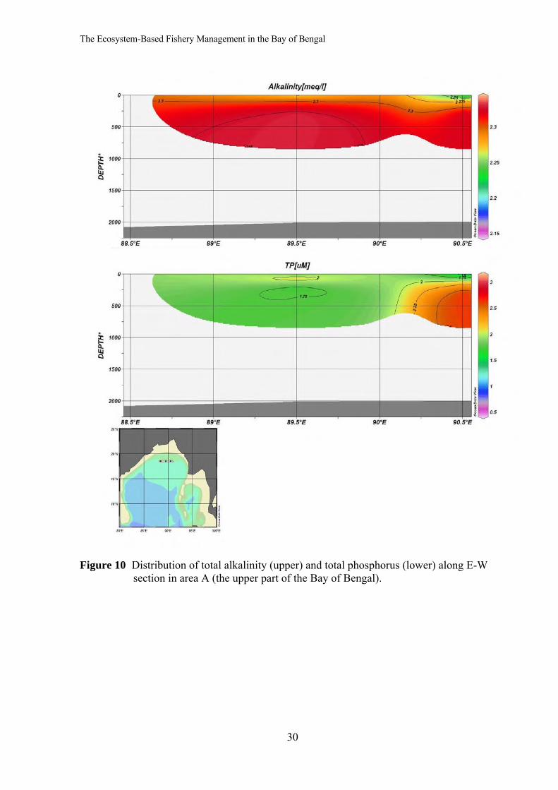
The Ecosystem-Based Fishery Management in the Bay of Bengal
30
Figure 10 Distribution of total alkalinity (upper) and total phosphorus (lower) along E-W section in area A (the upper part of the Bay of Bengal).
The Ecosystem-Based Fishery Management in the Bay of Bengal
31
References Ammerman, J. W. and F. Azam. 1985. Bacterial 5'-nucleotidase in aquatic ecosystems: a
novel mechanism of phosphorus regeneration. Science 227:1338-1340. Benitez-Nelson, C. R. and K. O. Buesseler. 1999. Variability of inorganic and organic
phosphorus turnover rates in the coastal ocean. Nature 398:502-505. Bjorkman, K. and D. M. Karl. 1994. Bioavailability of inorganic and organic phosphorus
compounds to natural assemblages of microorganisms. Mar. Ecol. Prog. Ser. 111:265-273.
Codispoti, L. A. 1989. Phosphorus vs. nitrogen limitations in new and export production. In: Berger, W. H., V. S. Smetacek and G. Wefer (eds.). Productivity of the Oceans: Present and Past. Wiley, New York. p. 377-394.
Frankignoulle, M., and A. V. Borges. 2001. European continental shelf as a significant sink for atmospheric carbon dioxide. Global Biogeochem. Cycles 15(3):569-576.
Grasshoff, K. M., K. Kremling and M. Ehrhardt. 1999. Methods of Seawater Analysis, 3rd edition. Weinheim: Wiley-VCH. 600 p.
Jackson, C. R. 2004. An Atlas of Internal Solitary-like Waves and their Properties, 2nd edition. Global Ocean Associates, Alexandria, VA 22310, USA. 560 p.
Jackson, G.A. and P.M. Williams 1985. Importance of dissolved organic nitrogen and phosphorus to biological nutrient cycling. Deep-Sea Res. 32:223-235.
Karl, D. M., G. Tien, J. Dore and C. D. Winn. 1993. Total dissolved nitrogen and phosphorus concentrations at US-JGOFS Station ALOHA: Redfield reconciliation. Mar. Chem. 41: 203-208.
Menzel, D. W. and N. Corwin. 1965. The measurement of total phosphorus in seawater based on the liberation of organically bound fractions by persulfate oxidation. Limnology and Oceanography 10(2):280-282.
Monaghan, E. J. and K. C. Ruttenberg. 1999. Dissolved organic phosphorus in the coastal ocean: reassessment of available methods and seasonal phosphorus profiles from the Eel River Shelf. Limnology and Oceanography. 44:1702-1714.
Muller-Karger, F. 2000. Carbon on the margins. Available Source: http://usjgofs.whoi.Edu/mzweb/margins_rpt. html.
Osborne, A. R. and T. L Burch. 1980. Internal solutions in the Andaman Sea. Science 208:451. Prentice, I.C. 2001. The carbon cycle and atmospheric carbondioxide. In: Houghton, J. T.,
Y. Ding, D. J. Griggs, M. Noguer, P. J. van der Linden, X. Dai, K. Maskell and C.A. Johnson (eds.). Climate Change 2001: the Scientific Basis, Cambridge University. Press, Cambridge. p. 183-237.
Schiettecatte, L. S., H. Thomas, A. Vieira Borges and M. Frankignoulle. 2003. Normalized total alkalinity as a tracer of the surface water masses of the North Sea. Geophysical Research Abstracts 5:1099-2003. Available Source: http://www.cosis.net/abstracts/EAE03/01099/EAE03-J-01099.pdf.
Strickland, J. D. H. and T. R. Parsons. 1972. A practical handbook of seawater analysis. Fisheries Research Board of Canada Bulletin 167:71-75.
Tsunogai, S., S. Watanabe and T. Sato. 1999. Is there a continental shelf pump for the absorption of atmospheric Co2 Tellus Ser. B. 51:701-712.
Tyrrell, T. 1999. The relative influences of nitrogen and phosphorus on oceanic primary production. Nature 400:525-531.
The Ecosystem-Based Fishery Management in the Bay of Bengal
32
UNEP. 2008. In dead water-merging of climate change with pollution, over-harvest, and infestations in the world’s fishing grounds: Rapid response assessment. Nellemann, C., Hain, S. and J. Alder. (eds.). United Nations Environment Programme (UNEP), February 2008, GRID-Arendal, Norway. 62 p.
Walsh, J. J. 1991. Importance of continental margins in the marine biogeochemical cycling of carbon and nitrogen. Nature 350:53-55.
Watanabea, A., H. Kayannea, K. Nozakic, K. Katoc, A. Negishic, S. Kudob, H. Kimotod, M. Tsudad and, A. G. Dickson. 2004. A rapid, precise potentiometric determination of total alkalinity in seawater by a newly developed flow-through analyzer designed for coastal regions. Marine Chemistry 85:75-87.
Yool, A. and M. J. R. Fasham. 2001. An examination of the continental shelf pump in an open ocean general circulation model. Global Biogeochemical Cycles 15(4):831-844.
The Ecosystem-Based Fishery Management in the Bay of Bengal
33
Distribution of Nutrients in the Bay of Bengal
Ritthirong Prommas1, Pirote Naimee2 and Natinee Sukramongkol1
1 Southeast Asian Fisheries Development Center, Training Department, P.O.Box 97, Phrasamutchedi, Samutprakarn 10290, THAILAND.
2 Deep Sea Fishery Technology Research and Development Institute, Department of Fisheries, Sumutprakarn 10270, THAILAND
Abstract
The spatial distribution of nutrients (nitrite + nitrate, silicate and phosphate) was
determined during the joint research survey on the Ecosystem-Based Fishery Management in the Bay of Bengal by M.V. SEAFDEC between 25 October to 21 December 2007. Water samples from twenty-eight stations were analyzed onboard by the Integral Futura Continuous Flow Automated Analysis. The detectable ranges of nitrite + nitrate, silicate and phosphate in the northern Bay of Bengal were 0.07-37.87, 0.01-48.56 and 0.10-3.13 µM; in the western Bay of Bengal 2.06-35.23, 2.89-46.03 and 0.15-3.16 µM; and in the eastern Bay of Bengal 0.35-36.63, 0.05-46.63 and 0.36-2.76 µM, respectively. The vertical section profiles indicated that the concentrations of nutrients in the mixed layer depth were very low and undetectable in several sampling stations. In the thermocline layer, a strong nutricline concentration was noticed to be rapidly increasing with depth but below 200-250 m, it tended to be constant. Furthermore, several near shore stations were observed to have higher concentrations of nutrients than the stations in the open sea. Key words: nutrient, nitrite + nitrate, silicate, phosphate, Bay of Bengal
Introduction
Nutrient is functionally involved in the process of living organisms. Traditionally,
in chemical oceanography the term has been applied almost exclusively to silicate, phosphate and inorganic nitrogen. The role of nutrients in the ocean is to support the ocean food chains. Phytoplanktons are primary food producers in the sea and through photosynthesis, they produce food for zooplanktons which are then consumed by organisms higher up in the food chain (Spencer, 1975).
Generally, nutrient is also present in sea water in very small amounts, but only minute quantities of these are required by living organisms. Nutrient is essential for phytoplankton growth as it is taken up by phytoplankton cells and built in as atoms in amino acids, proteins, nucleic acids, fats, etc. Among the nutrient elements, silicate is essential for diatoms to build up their skeletons which consist of biogenic silicate (Baretta-Bekker et al., 1998).
When phytoplankton, zooplankton or higher organisms are dead, these are decomposed by marine bacteria. This in turn takes a particle form of nutrient and in a dissolved form so that phytoplankton can use it more easily. Distribution of nutrients is useful for predicting the phytoplankton abundance and assemblages. Moreover, it could also be used as indicator of the status of nutrient loading or to predict productivity (De-Pauw and Naessens, 1991).
With the importance of nutrients as mentioned above, this study aimed to measure the nutrient level (nitrite + nitrate, silicate and phosphate) and to illustrate the nutrients distribution in the Bay of Bengal.
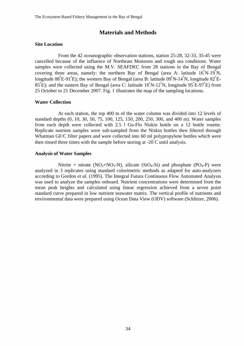
The Ecosystem-Based Fishery Management in the Bay of Bengal
34
Materials and Methods
Site Location
From the 42 oceanographic observation stations, station 25-28, 32-33, 35-45 were cancelled because of the influence of Northeast Monsoon and rough sea conditions. Water samples were collected using the M.V. SEAFDEC from 28 stations in the Bay of Bengal covering three areas, namely: the northern Bay of Bengal (area A: latitude 16°N-19°N, longitude 88°E-91°E); the western Bay of Bengal (area B: latitude 09°N-14°N, longitude 82°E-85°E); and the eastern Bay of Bengal (area C: latitude 10°N-12°N, longitude 95°E-97°E) from 25 October to 21 December 2007. Fig. 1 illustrates the map of the sampling locations. Water Collection
At each station, the top 400 m of the water column was divided into 12 levels of standard depths (0, 10, 30, 50, 75, 100, 125, 150, 200, 250, 300, and 400 m). Water samples from each depth were collected with 2.5 l Go-Flo Niskin bottle on a 12 bottle rosette. Replicate nutrient samples were sub-sampled from the Niskin bottles then filtered through Whatman GF/C filter papers and were collected into 60 ml polypropylene bottles which were then rinsed three times with the sample before storing at -20°C until analysis. Analysis of Water Samples
Nitrite + nitrate (NO2+NO3-N), silicate (SiO4-Si) and phosphate (PO4-P) were analyzed in 3 replicates using standard colorimetric methods as adapted for auto-analyzers according to Gordon et al. (1995). The Integral Futura Continuous Flow Automated Analysis was used to analyze the samples onboard. Nutrient concentrations were determined from the mean peak heights and calculated using linear regression achieved from a seven point standard curve prepared in low nutrient seawater matrix. The vertical profile of nutrients and environmental data were prepared using Ocean Data View (ODV) software (Schlitzer, 2006).
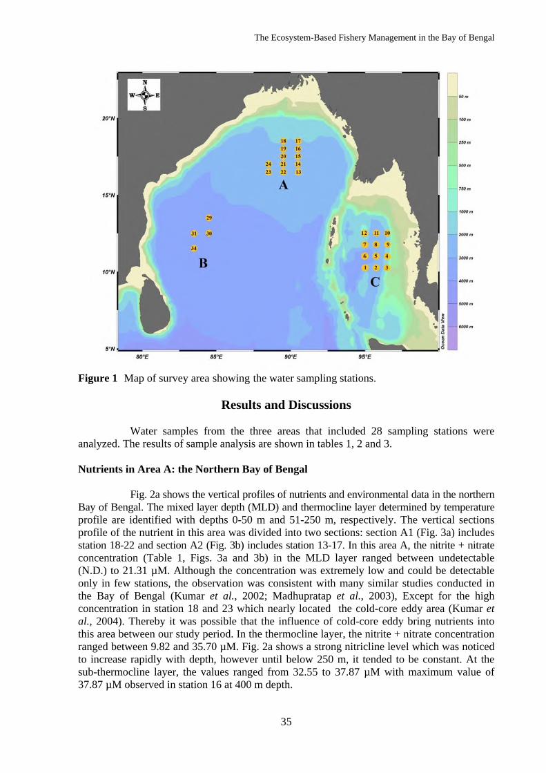
The Ecosystem-Based Fishery Management in the Bay of Bengal
35
Figure 1 Map of survey area showing the water sampling stations.
Results and Discussions
Water samples from the three areas that included 28 sampling stations were analyzed. The results of sample analysis are shown in tables 1, 2 and 3. Nutrients in Area A: the Northern Bay of Bengal
Fig. 2a shows the vertical profiles of nutrients and environmental data in the northern
Bay of Bengal. The mixed layer depth (MLD) and thermocline layer determined by temperature profile are identified with depths 0-50 m and 51-250 m, respectively. The vertical sections profile of the nutrient in this area was divided into two sections: section A1 (Fig. 3a) includes station 18-22 and section A2 (Fig. 3b) includes station 13-17. In this area A, the nitrite + nitrate concentration (Table 1, Figs. 3a and 3b) in the MLD layer ranged between undetectable (N.D.) to 21.31 µM. Although the concentration was extremely low and could be detectable only in few stations, the observation was consistent with many similar studies conducted in the Bay of Bengal (Kumar et al., 2002; Madhupratap et al., 2003), Except for the high concentration in station 18 and 23 which nearly located the cold-core eddy area (Kumar et al., 2004). Thereby it was possible that the influence of cold-core eddy bring nutrients into this area between our study period. In the thermocline layer, the nitrite + nitrate concentration ranged between 9.82 and 35.70 µM. Fig. 2a shows a strong nitricline level which was noticed to increase rapidly with depth, however until below 250 m, it tended to be constant. At the sub-thermocline layer, the values ranged from 32.55 to 37.87 µM with maximum value of 37.87 µM observed in station 16 at 400 m depth.
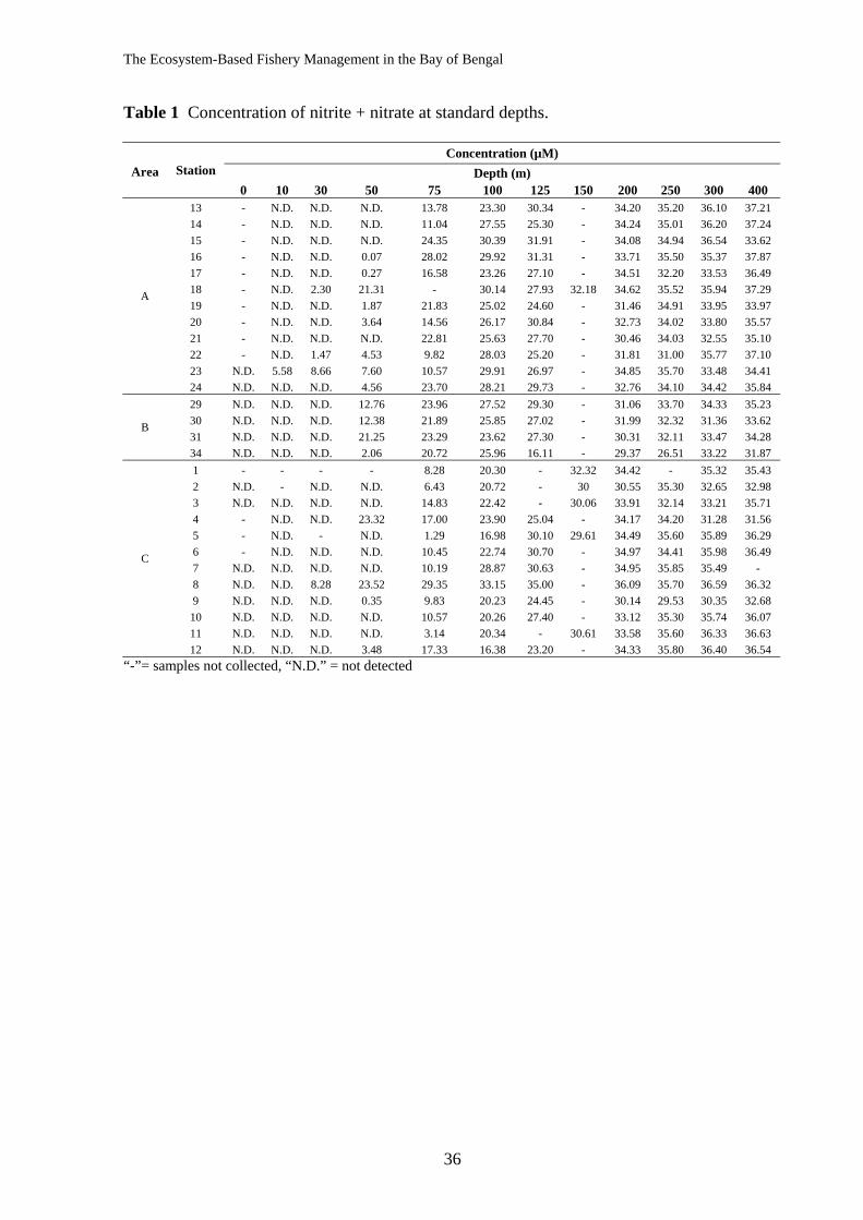
The Ecosystem-Based Fishery Management in the Bay of Bengal
36
Table 1 Concentration of nitrite + nitrate at standard depths.
Station Concentration (µM)
Area Depth (m) 0 10 30 50 75 100 125 150 200 250 300 400
A
13 - N.D. N.D. N.D. 13.78 23.30 30.34 - 34.20 35.20 36.10 37.21 14 - N.D. N.D. N.D. 11.04 27.55 25.30 - 34.24 35.01 36.20 37.24 15 - N.D. N.D. N.D. 24.35 30.39 31.91 - 34.08 34.94 36.54 33.62 16 - N.D. N.D. 0.07 28.02 29.92 31.31 - 33.71 35.50 35.37 37.87 17 - N.D. N.D. 0.27 16.58 23.26 27.10 - 34.51 32.20 33.53 36.49 18 - N.D. 2.30 21.31 - 30.14 27.93 32.18 34.62 35.52 35.94 37.29 19 - N.D. N.D. 1.87 21.83 25.02 24.60 - 31.46 34.91 33.95 33.97 20 - N.D. N.D. 3.64 14.56 26.17 30.84 - 32.73 34.02 33.80 35.57 21 - N.D. N.D. N.D. 22.81 25.63 27.70 - 30.46 34.03 32.55 35.10 22 - N.D. 1.47 4.53 9.82 28.03 25.20 - 31.81 31.00 35.77 37.10 23 N.D. 5.58 8.66 7.60 10.57 29.91 26.97 - 34.85 35.70 33.48 34.41 24 N.D. N.D. N.D. 4.56 23.70 28.21 29.73 - 32.76 34.10 34.42 35.84
B
29 N.D. N.D. N.D. 12.76 23.96 27.52 29.30 - 31.06 33.70 34.33 35.23 30 N.D. N.D. N.D. 12.38 21.89 25.85 27.02 - 31.99 32.32 31.36 33.62 31 N.D. N.D. N.D. 21.25 23.29 23.62 27.30 - 30.31 32.11 33.47 34.28 34 N.D. N.D. N.D. 2.06 20.72 25.96 16.11 - 29.37 26.51 33.22 31.87
C
1 - - - - 8.28 20.30 - 32.32 34.42 - 35.32 35.43 2 N.D. - N.D. N.D. 6.43 20.72 - 30 30.55 35.30 32.65 32.98 3 N.D. N.D. N.D. N.D. 14.83 22.42 - 30.06 33.91 32.14 33.21 35.71 4 - N.D. N.D. 23.32 17.00 23.90 25.04 - 34.17 34.20 31.28 31.56 5 - N.D. - N.D. 1.29 16.98 30.10 29.61 34.49 35.60 35.89 36.29 6 - N.D. N.D. N.D. 10.45 22.74 30.70 - 34.97 34.41 35.98 36.49 7 N.D. N.D. N.D. N.D. 10.19 28.87 30.63 - 34.95 35.85 35.49 - 8 N.D. N.D. 8.28 23.52 29.35 33.15 35.00 - 36.09 35.70 36.59 36.32 9 N.D. N.D. N.D. 0.35 9.83 20.23 24.45 - 30.14 29.53 30.35 32.68 10 N.D. N.D. N.D. N.D. 10.57 20.26 27.40 - 33.12 35.30 35.74 36.07 11 N.D. N.D. N.D. N.D. 3.14 20.34 - 30.61 33.58 35.60 36.33 36.63 12 N.D. N.D. N.D. 3.48 17.33 16.38 23.20 - 34.33 35.80 36.40 36.54
“-”= samples not collected, “N.D.” = not detected
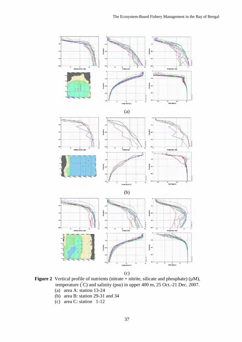
The Ecosystem-Based Fishery Management in the Bay of Bengal
37
(a)
(b)
(c)
Figure 2 Vertical profile of nutrients (nitrate + nitrite, silicate and phosphate) (µM), temperature (°C) and salinity (psu) in upper 400 m, 25 Oct.-21 Dec. 2007.
(a) area A: station 13-24 (b) area B: station 29-31 and 34 (c) area C: station 1-12
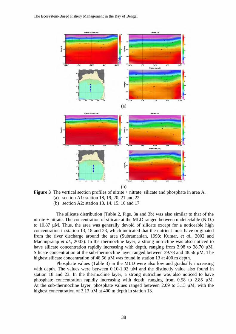
The Ecosystem-Based Fishery Management in the Bay of Bengal
38
(a)
(b)
Figure 3 The vertical section profiles of nitrite + nitrate, silicate and phosphate in area A. (a) section A1: station 18, 19, 20, 21 and 22 (b) section A2: station 13, 14, 15, 16 and 17
The silicate distribution (Table 2, Figs. 3a and 3b) was also similar to that of the
nitrite + nitrate. The concentration of silicate at the MLD ranged between undetectable (N.D.) to 10.87 µM. Thus, the area was generally devoid of silicate except for a noticeable high concentration in station 13, 18 and 23, which indicated that the nutrient must have originated from the river discharge around the area (Subramanian, 1993; Kumar, et al., 2002 and Madhupratap et al., 2003). In the thermocline layer, a strong nutricline was also noticed to have silicate concentration rapidly increasing with depth, ranging from 2.98 to 38.70 µM. Silicate concentration at the sub-thermocline layer ranged between 39.78 and 48.56 µM, The highest silicate concentration of 48.56 µM was found in station 13 at 400 m depth.
Phosphate values (Table 3) in the MLD were also low and gradually increasing with depth. The values were between 0.10-1.02 µM and the distinctly value also found in station 18 and 23. In the thermocline layer, a strong nutricline was also noticed to have phosphate concentration rapidly increasing with depth, ranging from 0.58 to 2.85 µM. At the sub-thermocline layer, phosphate values ranged between 2.09 to 3.13 µM, with the highest concentration of 3.13 µM at 400 m depth in station 13.
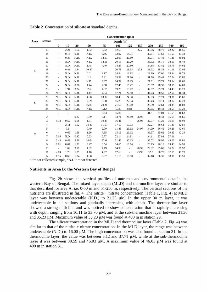
The Ecosystem-Based Fishery Management in the Bay of Bengal
39
Table 2 Concentration of silicate at standard depths.
station Concentration (µM)
Area Depth (m) 0 10 30 50 75 100 125 150 200 250 300 400
A
13 - 2.24 1.64 1.32 5.82 12.65 - 22.2 35.06 38.70 42.22 48.56 14 - 0.14 0.26 N.D. 3.46 12.92 14.91 - 33.81 37.63 41.55 47.42 15 - 0.38 N.D. N.D. 13.17 22.03 26.80 - 33.91 37.43 41.86 40.02 16 - N.D. N.D. N.D. 14.51 20.15 29.20 - 33.52 36.70 38.53 48.44 17 - N.D. N.D. 1.45 7.40 14.23 20.80 - 34.88 33.42 35.79 44.62 18 - 0.43 1.44 10.87 - 20.78 21.54 27.8 33.72 38.33 41.01 47.03 19 - N.D. N.D. 0.01 9.17 14.94 16.92 - 28.19 37.00 35.34 39.78 20 - N.D. N.D. 1.1 5.21 15.52 21.90 - 31.78 35.44 37.24 42.80 21 - N.D. N.D. N.D. 9.07 14.32 17.23 - 27.81 33.71 33.64 40.60 22 - N.D. 0.86 1.44 2.98 12.45 15.42 - 28.87 28.30 38.55 44.69 23 - 1.94 3.24 2.6 4.32 19.29 19.72 - 32.97 35.71 34.43 41.28 24 N.D. N.D. N.D. 1.17 7.94 17.21 27.80 - 34.73 38.50 42.57 46.34
B
29 N.D. N.D. N.D. 4.98 10.07 18.43 24.30 - 32.03 37.71 39.86 45.67 30 N.D. N.D. N.D. 2.89 8.58 15.23 22.34 - 30.43 33.11 33.17 42.23 31 N.D. N.D. N.D. 16.00 20.21 21.66 25.00 - 28.99 32.61 39.39 46.03 34 N.D. N.D. N.D. N.D. 5.12 9.35 8.81 - 20.65 19.44 30.59 33.28
C
1 - - - - 6.63 15.86 - - 31.81 37.04 41.59 46.63 2 - - 0.32 0.39 5.11 13.71 24.40 26.92 - 38.44 35.69 38.66 3 5.18 0.52 0.56 1.71 10.49 16.41 - 26.93 32.77 31.22 36.19 40.98 4 - 2.11 1.92 18.40 11.57 17.10 19.93 - 32.27 38.61 31.49 32.59 5 - 0.9 - 0.49 2.00 11.48 26.62 24.97 34.99 36.42 39.26 42.60 6 - 0.66 1.59 1.96 7.85 15.19 26.12 - 36.57 35.62 39.35 42.29 7 0.05 N.D. 0.42 0.63 6.77 22.14 24.91 - 34.11 37.81 37.01 - 8 0.43 0.49 5.86 14.64 22.6 31.42 35.13 - 38.52 38.94 43.26 40.81 9 0.61 0.67 1.22 3.47 6.54 14.65 18.74 - 26.15 26.10 29.43 34.93 10 - 1.69 3.19 1.32 7.79 14.93 - 20.93 29.82 35.60 36.72 39.92 11 2.03 1.73 1.29 1.10 4.67 12.69 - 23.95 32.2 36.72 37.15 41.78 12 1.15 0.69 1.24 1.38 9.97 11.15 16.80 - 32.18 36.30 38.08 43.51
“-”= not collected sample, “N.D.” = not detected Nutrients in Area B: the Western Bay of Bengal
Fig. 2b shows the vertical profiles of nutrients and environmental data in the western Bay of Bengal. The mixed layer depth (MLD) and thermocline layer are similar to that described for area A, i.e. 0-50 m and 51-250 m, respectively. The vertical sections of the nutrients are illustrated in fig. 4. The nitrite + nitrate concentration (Table 1, Fig. 4) at MLD layer was between undetectable (N.D.) to 21.25 µM. In the upper 30 m layer, it was undetectable in all stations and gradually increasing with depth. The thermocline layer showed a strong nitricline and was noticed to show concentration that is rapidly increasing with depth, ranging from 16.11 to 33.70 µM, and at the sub-thermocline layer between 31.36 and 35.23 µM. Maximum value of 35.23 µM was found at 400 m in station 29.
The silicate concentration in the MLD and thermocline layer (Table 2, Fig. 4) was similar to that of the nitrite + nitrate concentration. In the MLD layer, the range was between undetectable (N.D.) to 16.00 µM. The high concentration was also found at station 31. In the thermocline layer, the value was between 5.12 and 37.71 µM, while at the sub-thermocline layer it was between 30.59 and 46.03 µM. A maximum value of 46.03 µM was found at 400 m in station 31.
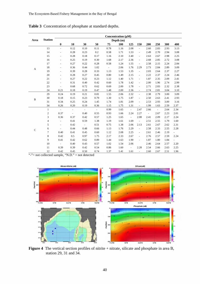
The Ecosystem-Based Fishery Management in the Bay of Bengal
40
Table 3 Concentration of phosphate at standard depths.
Station
Concentration (µM) Area Depth (m)
0 10 30 50 75 100 125 150 200 250 300 400
A
13 - 0.12 0.10 0.11 0.78 1.16 2.08 - 2.60 2.83 2.93 3.13 14 - 0.28 0.23 0.2 0.58 1.71 1.53 - 2.49 2.70 2.94 3.08 15 - 0.28 0.18 0.17 1.16 2.10 2.40 - 2.63 2.67 2.98 2.25 16 - 0.25 0.19 0.30 1.68 2.17 2.36 - 2.68 2.85 2.72 3.08 17 - 0.27 0.22 0.28 0.58 1.24 1.55 - 2.58 2.15 2.24 2.84 18 - 0.36 0.44 1.02 - 2.06 1.76 2.29 2.73 2.84 2.89 3.09 19 - 0.39 0.28 0.33 1.13 1.53 1.35 - 2.03 2.64 2.37 2.27 20 - 0.28 0.27 0.45 0.80 1.49 2.15 - 2.22 2.37 2.24 2.46 21 - 0.27 0.22 0.23 1.12 1.40 1.71 - 1.87 2.35 2.09 2.41 22 - 0.31 0.40 0.42 0.60 1.78 1.42 - 2.00 1.96 2.74 2.99 23 - 0.68 0.72 0.62 0.69 2.00 1.78 - 2.71 2.83 2.32 2.38 24 0.21 0.18 0.19 0.47 1.48 2.00 2.36 - 2.74 2.81 3.04 3.10
B
29 0.24 0.19 0.21 0.81 1.55 2.06 2.32 - 2.38 2.79 3.00 3.09 30 0.18 0.15 0.23 0.79 1.30 1.75 1.87 - 2.50 2.63 2.41 2.93 31 0.34 0.25 0.24 1.45 1.74 1.81 2.09 - 2.53 2.93 3.00 3.16 34 0.26 0.20 0.19 0.36 1.15 1.75 1.31 - 1.99 1.63 2.59 2.37
C
1 - - - - 0.99 1.65 - 2.47 2.66 - 2.64 2.34 2 0.37 - 0.40 0.55 0.93 1.66 2.24 2.27 - 2.67 2.23 2.01 3 0.36 0.37 0.42 0.57 1.25 1.65 - 2.08 2.41 2.09 2.17 2.24 4 - 0.41 0.59 1.38 1.19 1.61 1.69 - 2.51 2.55 1.79 1.60 5 - 0.42 - 0.51 0.75 1.38 2.06 2.13 2.61 2.67 2.62 2.31 6 - 0.44 0.48 0.66 1.13 1.76 2.29 - 2.58 2.33 2.55 2.28 7 0.40 0.41 0.45 0.60 1.12 2.08 2.25 - 2.61 2.46 2.19 - 8 0.42 0.5 0.97 1.75 2.17 2.33 2.67 - 2.76 2.57 2.59 2.24 9 0.41 0.42 0.62 0.89 1.44 1.63 1.90 - 1.87 1.80 1.84 - 10 - 0.40 0.43 0.57 1.02 1.54 2.06 2.46 2.64 2.57 2.20 11 0.39 0.39 0.42 0.54 0.86 1.60 - 2.28 2.54 2.66 2.63 2.25 12 0.42 0.45 0.50 0.74 1.37 1.41 1.61 - 2.60 2.67 2.51 1.96
“-”= not collected sample, “N.D.” = not detected
Figure 4 The vertical section profiles of nitrite + nitrate, silicate and phosphate in area B,
station 29, 31 and 34.
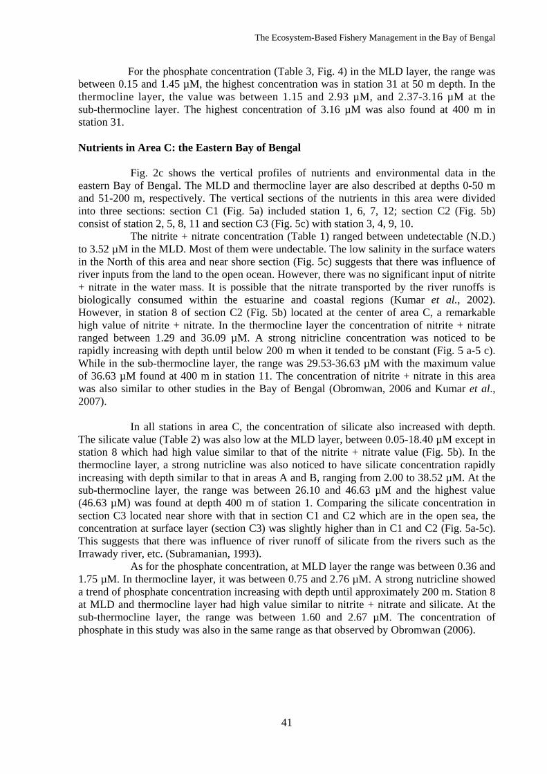
The Ecosystem-Based Fishery Management in the Bay of Bengal
41
For the phosphate concentration (Table 3, Fig. 4) in the MLD layer, the range was between 0.15 and 1.45 µM, the highest concentration was in station 31 at 50 m depth. In the thermocline layer, the value was between 1.15 and 2.93 µM, and 2.37-3.16 µM at the sub-thermocline layer. The highest concentration of 3.16 µM was also found at 400 m in station 31. Nutrients in Area C: the Eastern Bay of Bengal
Fig. 2c shows the vertical profiles of nutrients and environmental data in the eastern Bay of Bengal. The MLD and thermocline layer are also described at depths 0-50 m and 51-200 m, respectively. The vertical sections of the nutrients in this area were divided into three sections: section C1 (Fig. 5a) included station 1, 6, 7, 12; section C2 (Fig. 5b) consist of station 2, 5, 8, 11 and section C3 (Fig. 5c) with station 3, 4, 9, 10.
The nitrite + nitrate concentration (Table 1) ranged between undetectable (N.D.) to 3.52 µM in the MLD. Most of them were undectable. The low salinity in the surface waters in the North of this area and near shore section (Fig. 5c) suggests that there was influence of river inputs from the land to the open ocean. However, there was no significant input of nitrite + nitrate in the water mass. It is possible that the nitrate transported by the river runoffs is biologically consumed within the estuarine and coastal regions (Kumar et al., 2002). However, in station 8 of section C2 (Fig. 5b) located at the center of area C, a remarkable high value of nitrite + nitrate. In the thermocline layer the concentration of nitrite + nitrate ranged between 1.29 and 36.09 µM. A strong nitricline concentration was noticed to be rapidly increasing with depth until below 200 m when it tended to be constant (Fig. 5 a-5 c). While in the sub-thermocline layer, the range was 29.53-36.63 µM with the maximum value of 36.63 µM found at 400 m in station 11. The concentration of nitrite + nitrate in this area was also similar to other studies in the Bay of Bengal (Obromwan, 2006 and Kumar et al., 2007).
In all stations in area C, the concentration of silicate also increased with depth.
The silicate value (Table 2) was also low at the MLD layer, between 0.05-18.40 µM except in station 8 which had high value similar to that of the nitrite + nitrate value (Fig. 5b). In the thermocline layer, a strong nutricline was also noticed to have silicate concentration rapidly increasing with depth similar to that in areas A and B, ranging from 2.00 to 38.52 µM. At the sub-thermocline layer, the range was between 26.10 and 46.63 µM and the highest value (46.63 µM) was found at depth 400 m of station 1. Comparing the silicate concentration in section C3 located near shore with that in section C1 and C2 which are in the open sea, the concentration at surface layer (section C3) was slightly higher than in C1 and C2 (Fig. 5a-5c). This suggests that there was influence of river runoff of silicate from the rivers such as the Irrawady river, etc. (Subramanian, 1993).
As for the phosphate concentration, at MLD layer the range was between 0.36 and 1.75 µM. In thermocline layer, it was between 0.75 and 2.76 µM. A strong nutricline showed a trend of phosphate concentration increasing with depth until approximately 200 m. Station 8 at MLD and thermocline layer had high value similar to nitrite + nitrate and silicate. At the sub-thermocline layer, the range was between 1.60 and 2.67 µM. The concentration of phosphate in this study was also in the same range as that observed by Obromwan (2006).
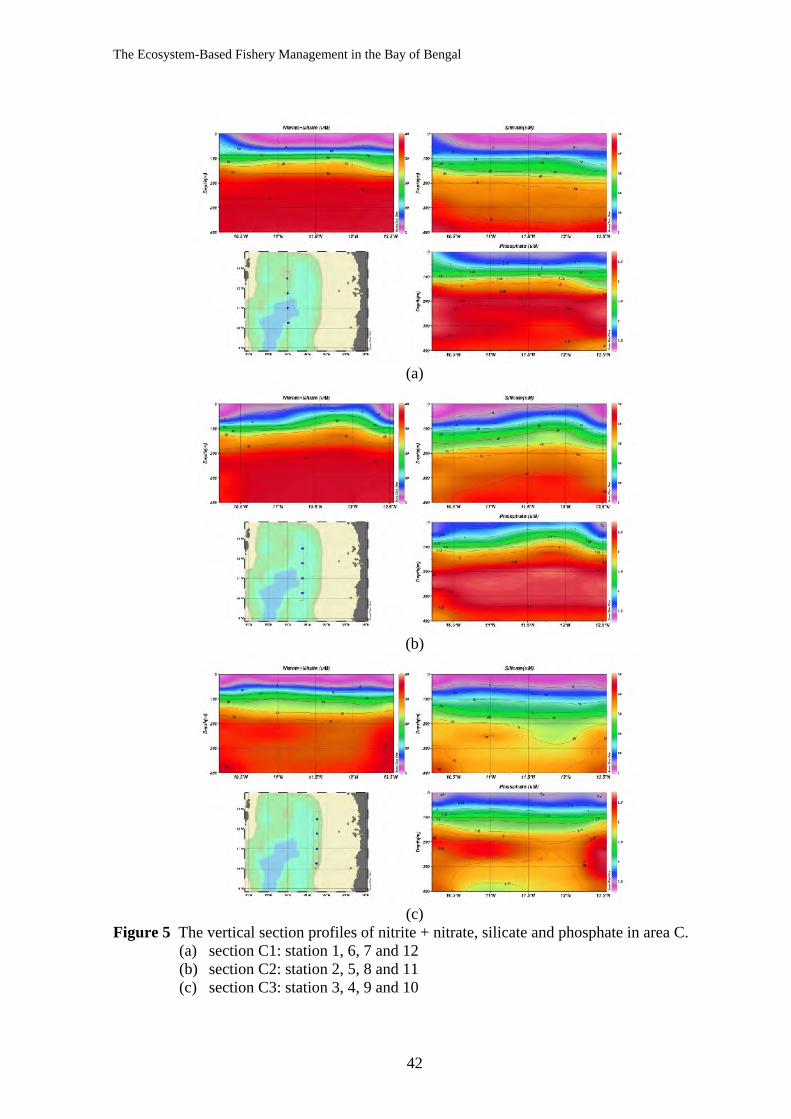
The Ecosystem-Based Fishery Management in the Bay of Bengal
42
(a)
(b)
(c)
Figure 5 The vertical section profiles of nitrite + nitrate, silicate and phosphate in area C. (a) section C1: station 1, 6, 7 and 12 (b) section C2: station 2, 5, 8 and 11 (c) section C3: station 3, 4, 9 and 10
The Ecosystem-Based Fishery Management in the Bay of Bengal
43
Conclusions
The result of this study showed that the distribution of the nutrients: nitrite + nitrate, silicate and phosphate uniformly increased with depth at all sampling stations. Generally, the MLD layer in the Bay of Bengal had very low nutrient concentrations or sometimes even undetectable. In addition, there were several near shore stations that had nutrient concentration higher than those in stations in the open sea. Nutricline concentration was noticed to be rapidly increasing with depth beyond 50 m. Until about 200-250 m, the nutrient values were nearly constant or slightly changed. Finally, spatial distribution of nutrient studies will certainly provide better scientific basis to understand the ecosystem of the Bay of Bengal.
Acknowledgement
The authors wish to express their sincere thanks to all the scientists from Bangladesh, India, Myanmar, Sri Lanka, Nepal and Thailand for their cooperation during the BIMSTEC project survey, 75-1/2007 cruise of the M.V. SEAFDEC. The successful completion of this project would have not been possible without the dedication also of the officers from the Department of Fisheries of Thailand; and the captain, the officers and crew of the M.V. SEAFDEC. Special thanks are also extended to Ms. Penchan Laongmanee and Virgilia T. Sulit (SEAFDEC), Ms. Puntip Wisespongpand (Department of Marine Science, Kasetsart University), Ms. Orapin Chanpongsaeng and Ms.Chamchoi Tanapong (Deep Sea Fishery Technology Research and Development Institute, Department of Fisheries) for their constructive and critical comments and suggestions.
References Baretta-Becker, J. G., E. K. Duursma and B. R. Kuipers. (eds.). 1998. Encyclopedia of
Marine Sciences. 2nd edition. Springer-Verlag Berlin Heidelberg, New York. 357 p. De-Pauw, N. and F. E. Naessens. 1991. Nutrient induced competition between species of
marine diatoms. Hydrobiological Bulletin 25:23-28. Gordon, L. I., J. C. Jennings, A. A. Ross and J. M. Krest. 1995. A Suggested Protocol for
Continuous Flow Automated Analysis of Seawater Nutrients (Phosphate, Nitrate, Nitrite and Silicic Acid) in the WOCE Hydrographic Program and the Joint Global Ocean Fluxes Study. WOCE Hydrographic Program Office, Methods Manual WHPO. 55 pp.
Kumar, S. P., P. M. Muraleedharan, T. G. Prasad, M. Gauns, N. Ramaiah, S. N. de Souza, S. Sardesai and M. Madhupratap. 2002. Why is the Bay of Bengal less productive during summer monsoon compared to the Arabian sea. Geophysical Research Letters 29(24):2238-2435.
Kumar, S. P., M. Nuncio, N. Ramaiah, S. Sardasai, J. Narvekar, V. Frenandes and J. T. Paul. 2007. Eddy-mediated biological productivity in the Bay of Bengal during fall and spring intermonsoons. J. dsr. 54:1619-1640.
Madhupratap, M., M. Gauns, N. Ramaiah, S. P. Kumar, P. M. Muraleedharan, S. N. de Soura, S. Sardessai and U. Muraleedharan. 2003. Biogeochemistry of the Bay of Bengal: physical, chemical and primary productivity characteristics of the central and western Bay of Bengal during summer monsoon 2001. Deep-sea Research II 50:88-896.
Obromwan, S. 2006. Spatial distribution of nutrient in the Andaman Sea. In: Preliminary Results on the Large Pelagic Fisheries Resources Survey in the Andaman Sea. TD/RES/99 SEAFDEC. p. 20-25.

The Ecosystem-Based Fishery Management in the Bay of Bengal
44
Spencer, C.P. 1975. The micronutrient elements. In: Riley, J. P. and G. Skirrow. (eds.). Chemical Oceanography. Vol.II 2nd edition. Academic Press Inc., London. p. 245-300.
Schlitzer, R. 2006. Ocean Data View. Available Source: http://odv.awi.de, July 3, 2008. Subramanian, V. 1993. Sediment load of Indian Rivers. Curr. Sci. 64:928-930.
The Ecosystem-Based Fishery Management in the Bay of Bengal
45
Distribution of Chlorophyll-a in the Bay of Bengal
Ritthirong Prommas1, Pirote Naimee2, Penchan Laongmanee1, Natinee Sukramongkol1 and Nawinee Khumthong1
1 Southeast Asian Fisheries Development Center, Training Department
P.O.Box 97, Phrasamutchedi, Samutprakarn 10290, THAILAND 2 Deep Sea Fishery Technology Research and Development Institute,
Department of Fisheries, Sumutprakarn 10270, THAILAND
Abstract
The distribution of chlorophyll in the Bay of Bengal was determined between 25 October to 21 December 2007, during the joint research survey on the Ecosystem-Based Fishery Management in the Bay of Bengal by the M.V. SEAFDEC. Chlorophyll-a from twenty-four stations in the study area were investigated using spectrophotometer. Results showed that the concentrations of chlorophyll-a in the eastern Bay of Bengal was 0.0375-0.5207 mg m-3. In the northern Bay of Bengal it was 0.0365-1.1162 mg m-3. While in the western Bay of Bengal the range was 0.0357-0.1839 mg m-3. The spatial distribution of chlorophyll-a was similar pattern to the salinity and the highest concentration mostly confined at 10 m. The surface layer taken at the low latitude stations had higher concentrations than at the high latitude stations. Furthermore, river discharge with high turbidity may impede photosynthesis activity of phytoplankton in this area. Key words: chlorophyll-a, primary productivity, Bay of Bengal
Introduction
Phytoplankton is a primary producer which converts inorganic matters into organic compounds through photosynthesis, enabling the transfer of energy and nutrients to the zooplankton. Considering that plankton organisms have short life cycles and can quickly respond to changing environments such as in the case of water pollution, some phytoplankton species can thus be used as index for monitoring water quality.
Chlorophyll is a principal pigment which phytoplankton use in photosynthesis to convert nutrients and carbon dioxide, which are dissolved in sea water into plant materials. Chlorophyll-a,b,c and Phaeophytin are the most commonly occurring pigment in seawater. Their concentrations showed wide fluctuation. Chlorophyll-a is the major photosynthetic pigment of marine phytoplankton that has been used as an indicator of biomass or primary productivity in the oceans (Beebe, 2008). The aim of this study is to collect information on the distribution of chlorophyll-a in the Bay of Bengal as they reflect the primary productivity.
Materials and Methods Site Location
From the 42 oceanographic observation stations, station 25-28, 32-33, 35-45 were cancelled because of the influence of the northeast monsoon and rough sea conditions. Furthermore, the samples extracted from station 1, 2, 3 and 31 had decomposed before these could be analyzed due to the repair of the spectrophotometer. In this study, the water samples were collected from 24 stations in the Bay of Bengal covering three areas, namely: in the
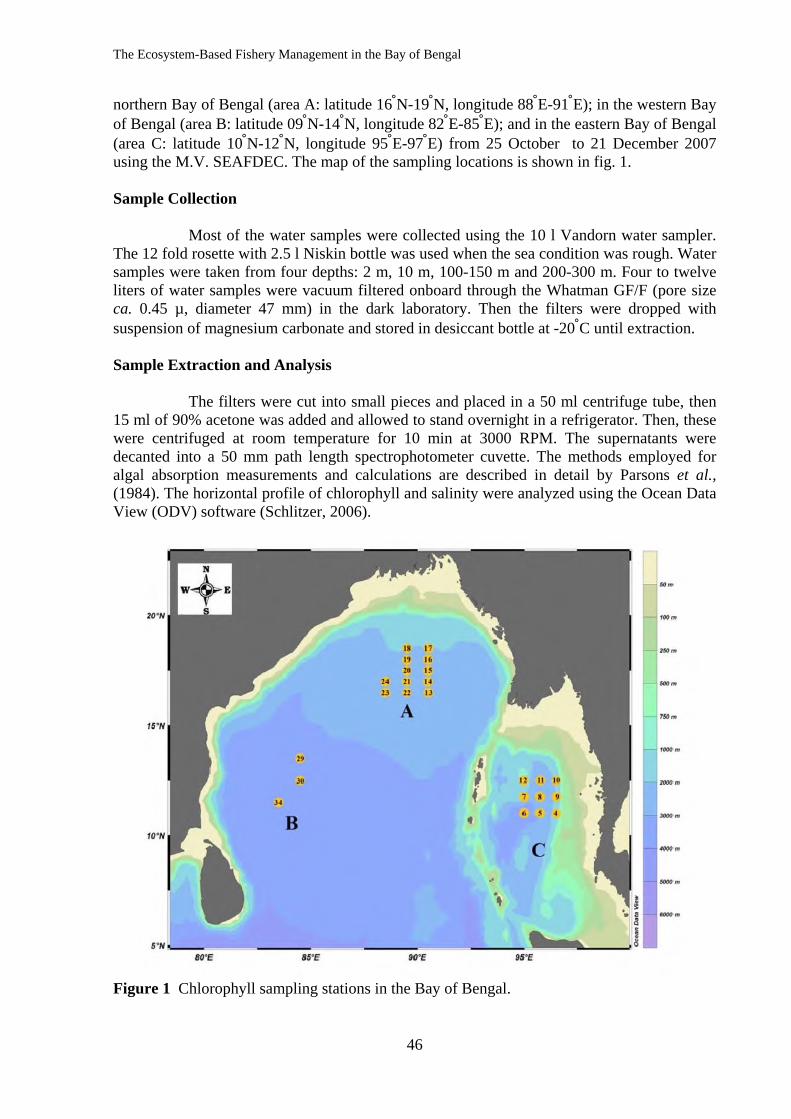
The Ecosystem-Based Fishery Management in the Bay of Bengal
46
northern Bay of Bengal (area A: latitude 16°N-19°N, longitude 88°E-91°E); in the western Bay of Bengal (area B: latitude 09°N-14°N, longitude 82°E-85°E); and in the eastern Bay of Bengal (area C: latitude 10°N-12°N, longitude 95°E-97°E) from 25 October to 21 December 2007 using the M.V. SEAFDEC. The map of the sampling locations is shown in fig. 1. Sample Collection
Most of the water samples were collected using the 10 l Vandorn water sampler. The 12 fold rosette with 2.5 l Niskin bottle was used when the sea condition was rough. Water samples were taken from four depths: 2 m, 10 m, 100-150 m and 200-300 m. Four to twelve liters of water samples were vacuum filtered onboard through the Whatman GF/F (pore size ca. 0.45 µ, diameter 47 mm) in the dark laboratory. Then the filters were dropped with suspension of magnesium carbonate and stored in desiccant bottle at -20°C until extraction. Sample Extraction and Analysis
The filters were cut into small pieces and placed in a 50 ml centrifuge tube, then 15 ml of 90% acetone was added and allowed to stand overnight in a refrigerator. Then, these were centrifuged at room temperature for 10 min at 3000 RPM. The supernatants were decanted into a 50 mm path length spectrophotometer cuvette. The methods employed for algal absorption measurements and calculations are described in detail by Parsons et al., (1984). The horizontal profile of chlorophyll and salinity were analyzed using the Ocean Data View (ODV) software (Schlitzer, 2006).
Figure 1 Chlorophyll sampling stations in the Bay of Bengal.
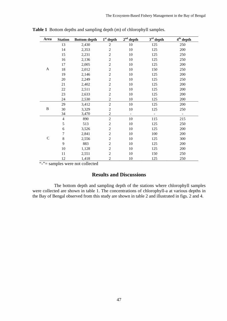
The Ecosystem-Based Fishery Management in the Bay of Bengal
47
Table 1 Bottom depths and sampling depth (m) of chlorophyll samples.
Area Station Bottom depth 1st depth 2nd depth 3rd depth 4th depth 13 2,430 2 10 125 250 14 2,353 2 10 125 200 15 2,231 2 10 125 250 16 2,136 2 10 125 250 17 2,005 2 10 125 200
A 18 2,012 2 10 150 250 19 2,146 2 10 125 200 20 2,249 2 10 125 250 21 2,402 2 10 125 200 22 2,511 2 10 125 200 23 2,633 2 10 125 200 24 2,530 2 10 125 200 29 3,412 2 10 125 200
B 30 3,329 2 10 125 250 34 3,470 2 - - - 4 890 2 10 115 215 5 513 2 10 125 250 6 3,526 2 10 125 200 7 2,841 2 10 100 200
C 8 2,556 2 10 125 300 9 883 2 10 125 200 10 1,128 2 10 125 200 11 2,551 2 10 150 250 12 1,418 2 10 125 250
“-”= samples were not collected
Results and Discussions
The bottom depth and sampling depth of the stations where chlorophyll samples were collected are shown in table 1. The concentrations of chlorophyll-a at various depths in the Bay of Bengal observed from this study are shown in table 2 and illustrated in figs. 2 and 4.
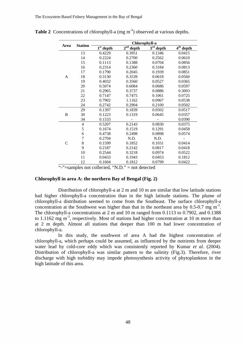
The Ecosystem-Based Fishery Management in the Bay of Bengal
48
Table 2 Concentrations of chlorophyll-a (mg m-3) observed at various depths.
Area Station Chlorophyll-a 1st depth 2nd depth 3rd depth 4th depth
13 0.4229 0.3951 0.1346 0.0415 14 0.2224 0.2700 0.2562 0.0610 15 0.1113 0.1388 0.0704 0.0856 16 0.2314 0.2360 0.3184 0.0813 17 0.1790 0.2045 0.1939 0.0851
A 18 0.3130 0.3539 0.0618 0.0560 19 0.4032 0.3560 0.0527 0.0365 20 0.5074 0.6084 0.0686 0.0597 21 0.2965 0.3737 0.0886 0.3003 22 0.7147 0.7475 0.1061 0.0725 23 0.7902 1.1162 0.0967 0.0538 24 0.2742 0.2904 0.2100 0.0502 29 0.1397 0.1839 0.0502 0.0517
B 30 0.1223 0.1319 0.0645 0.0357 34 0.1533 - - 0.0390 4 0.5207 0.2143 0.0830 0.0375 5 0.1674 0.1519 0.1291 0.0458 6 0.4738 0.2498 0.0898 0.0574 7 0.2704 N.D. N.D. -
C 8 0.1599 0.1852 0.1031 0.0414 9 0.2187 0.2142 0.0817 0.0418 10 0.2544 0.3218 0.0974 0.0522 11 0.0433 0.1943 0.0453 0.1812 12 0.1604 0.1812 0.0799 0.0422
“-”=samples not collected, “N.D.” = not detected Chlorophyll in area A: the northern Bay of Bengal (Fig. 2)
Distribution of chlorophyll-a at 2 m and 10 m are similar that low latitude stations had higher chlorophyll-a concentration than in the high latitude stations. The plume of chlorophyll-a distribution seemed to come from the Southeast. The surface chlorophyll-a concentration at the Southwest was higher than that in the northeast area by 0.5-0.7 mg m-3. The chlorophyll-a concentrations at 2 m and 10 m ranged from 0.1113 to 0.7902, and 0.1388 to 1.1162 mg m-3, respectively. Most of stations had higher concentration at 10 m more than at 2 m depth. Almost all stations that deeper than 100 m had lower concentration of chlorophyll-a.
In this study, the southwest of area A had the highest concentration of chlorophyll-a, which perhaps could be assumed, as influenced by the nutrients from deeper water lead by cold-core eddy which was consistently reported by Kumar et al. (2004). Distribution of chlorophyll-a was similar pattern to the salinity (Fig.3). Therefore, river discharge with high turbidity may impede photosynthesis activity of phytoplankton in the high latitude of this area.
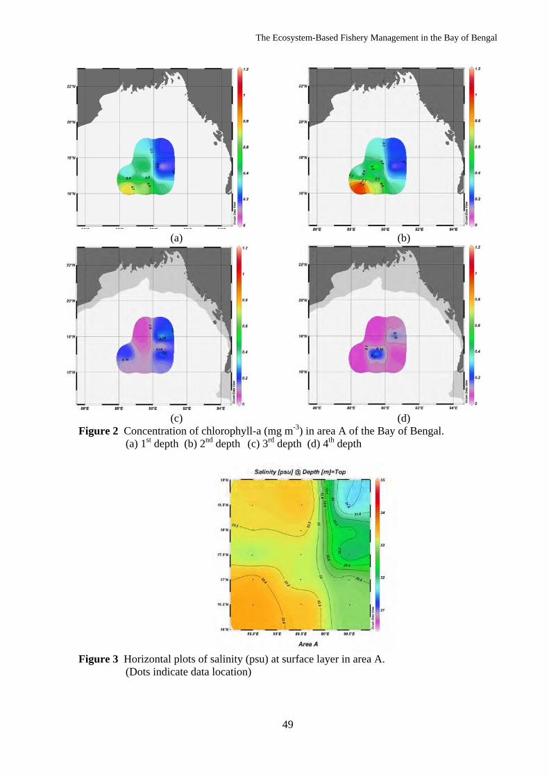
The Ecosystem-Based Fishery Management in the Bay of Bengal
49
(a) (b)
(c) (d) Figure 2 Concentration of chlorophyll-a (mg m-3) in area A of the Bay of Bengal.
(a) 1st depth (b) 2nd depth (c) 3rd depth (d) 4th depth
Figure 3 Horizontal plots of salinity (psu) at surface layer in area A. (Dots indicate data location)
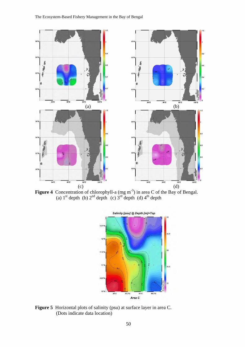
The Ecosystem-Based Fishery Management in the Bay of Bengal
50
(a) (b)
(c) (d) Figure 4 Concentration of chlorophyll-a (mg m-3) in area C of the Bay of Bengal.
(a) 1st depth (b) 2nd depth (c) 3rd depth (d) 4th depth
Figure 5 Horizontal plots of salinity (psu) at surface layer in area C. (Dots indicate data location)
The Ecosystem-Based Fishery Management in the Bay of Bengal
51
Chlorophyll in Area B: the Western Bay of Bengal
During the period when area B was surveyed, many of the survey stations were canceled because of the Northeast Monsoon and rough sea conditions. The data in area B were therefore not enough to make a conclusion. However, the chlorophyll-a concentrations observed from this area are indicated in table 2.
Chlorophyll in Area C: the Eastern Bay of Bengal (Fig. 4)
Spatial distribution of chlorophyll-a is shown in fig. 4. The chlorophyll-a concentrations at 2 m and 10 m ranged from 0.0433-0.5207 mg m-3 and 0.1519 to 0.3218 mg m-3, respectively. The distributions of chlorophyll-a at 2 m and 10 m are same pattern. It was also observed that the low latitude stations had higher chlorophyll-a than the high latitude stations, similar to that in area A. Distribution of chlorophyll-a was also similar pattern to the salinity (Fig.5). Especially at surface layer of station 11, the salinity was low, because influence of the Irrawadee river discharge with high turbidity may effect to decreasing of chlorophyll-a concentration. At deeper than 100 m, chlorophyll-a concentrations were lower than above and homogeneous.
The observed range of chlorophyll-a at 2 m ranged between 0.04-0.52 mg m-3, which were higher than in earlier reports by Wisespongpand et al. (2006) that the concentrations of chlorophyll-a in the Andaman Sea covering the waters of Thailand and Myanmar between 06° 45´N, 096° 15´E and 12° 45´N, 096° 45´E, were 0.03-0.11 mg m-3 . In this study, the highest concentrations of chlorophyll-a in several stations were observed at 10 m depth similar to area A.
Conclusions
It was observed during the survey that most of the low latitude stations in the Bay
of Bengal exhibited somewhat higher chlorophyll-a concentrations than in the high latitude stations. The highest chlorophyll concentration was mostly confined at 10 m of most of the survey stations. Distribution of chlorophyll-a was similar pattern to the salinity. Furthermore, river discharge with high turbidity may impede photosynthesis activity of phytoplankton.
Acknowledgements
The authors wish to express their sincere thanks to all the scientists from Bangladesh, India, Myanmar, Sri Lanka, Nepal and Thailand for their cooperation during the BIMSTEC project survey, 75-1/2007 cruise of the M.V. SEAFDEC. The successful completion of this project would have not also been possible without the dedication of the officers from the Department of Fisheries of Thailand as well as the captain, officers and crew of the M.V. SEAFDEC. Our special thanks are also extended to Ms. Suree Satapoomin (Phuket Marine Biological Center), Ms. Puntip Wisespongpand (Department of Marine Science, Kasetsart University) and Ms. Virgilia T. Sulit (SEAFDEC) for their constructive and critical comments and suggestions.
The Ecosystem-Based Fishery Management in the Bay of Bengal
52
References
Beebe, W. 2008. Production and life. In: Sverdrup, K. A. and E. V. Armbrust. (eds.). An Introduction to the World’s Oceans. McGraw-Hill, New York. p. 371-388.
Kumar, S. P., M. Nuncio, N. Jayu, K. Ajoy, S. Sardesai, S. N. Desouza, G. Mangesh, N. Ramaiah and M. Madhupratap. 2004. Are eddies nature’s trigger to enhance biological productivity in the Bay of Bengal. Geophys. Res. Lett. Vol. 31.
Parsons, T. R., Y. Maita and C. M. Lalli. 1984. A Manual of Chemical and Biological Methods for Seawater Analysis. Pergamon Press plc, Oxford. 173 p.
Schlitzer, R. 2006. Ocean Data View. Available Source: http://odv.awi.de July 3, 2008. Wisespongpand, P., S. Deetae, S. Patarajinda and R. Prommas. 2006. Sub-thermocline
chlorophyll maxima in the Andaman sea. In: Preliminary Results on the Large Pelagic Fisheries Resources Survey in the Andaman sea. TD/RES/99 SEAFDEC. p. 26-38.
The Ecosystem-Based Fishery Management in the Bay of Bengal
53
Species Composition, Abundance and Distribution of Phytoplankton in the Bay of Bengal
Sopana Booonyapiwat1, Md. Nasiruddin Sada2, Jay Kishore Mandal3
and Manas Kumar Sinha4
1Deep Sea Fishery Technology Research and Development Institute, Department of Fisheries, Kasetklang, Chatuchak, Bangkok 10900 THAILAND
2Fish Inspection and Quality Control, Department of Fisheries, 209 Muradpur(NM Khan Hill) P.O. Amin Jute Mill, Chittagong, BANGLADESH
3Fisheries Development Centre Dhangadhi, Geta, Dhangadhi, Kailali, NEPAL 4Port Blair Base of Fishery of India, P.O.Box 46, Port Blair-744101, INDIA
Abstract
Species composition, abundance and distribution of phytoplankton were studied
from water samples collected at surface layer of 24 stations in 3 areas (north, west and east) in the Bay of Bengal in November 2007. A total of 135 phytoplankton species belonging to 2 species of cyanobacteria, 78 species of diatoms, 53 species of dinoflagellates and 1 species of silicoflagellate were identified. The occurrence of species in each area was recorded. Oscillatoria erythraea and Proboscia alata were the dominant species in all areas. Pseudo-nitzschia pseudodelicatissima presented with high densities causing the blooms in the Northern Bay. The highest phytoplankton density was 133,790 cells/L. Dinoflagellate did not dominate phytoplankton population during this survey. Key words : phytoplankton, Bay of Bengal, species composition, abundance, distribution
Introduction
This study is a part of the project on “The Ecosystem-Based Fishery Management in the Bay of Bengal” which is a collaborative survey project of the BIMSTEC member countries.
The Bay of Bengal is characterized as a large marine ecosystem bounded by territory of many countries. It is a semi-enclosed tropical ocean basin under strong influence of tropical monsoons and receives large volume of freshwater from both river discharge and rainfall (Vinayachandran and Mathew, 2003).The northern part of the Bay of Bengal is an area where storm surges and cyclones frequently occur. These cyclones cause turbulence in coastal and nearshore areas (Dwivedi and Choubey, 1998).
The information on phytoplankton in the offshore waters of the Bay of Bengal is scanty and inadequate for understanding the dynamics of the Bay ecosystem. Most studies have been carried out in the coastal areas. The International Indian Ocean Expedition was the prominent survey conducted both in the coastal areas and open sea of the Indian Ocean including the Bay of Bengal in 1963. Dinoflagellate species collected during this survey were recorded by Taylor (1974). Except for this expedition, the present study is the first investigation of phytoplankton in the offshore areas around the Bay. The purpose of this study is to describe species composition, abundance and distribution in the surface layer in the Bay of Bengal. The results will benefit for marine fishery studies of the BIMSTEC member countries.
The Ecosystem-Based Fishery Management in the Bay of Bengal
54
Materials and Methods
Phytoplankton sampling was carried out on board M.V.SEAFDEC at 24 stations during November 2007. The study area was divided into three areas: area A or the Northern Bay, area B or the Western Bay and area C locates in the Eastern Bay of Bengal (Fig. 1). Seawater samples were collected by Van Dorn water sampler at 2-4 m below the sea surface. Forty to sixty liters of the water samples were filtered onto a 20 µm mesh phytoplankton net and preserved with 2% formalin/seawater mixture immediately. The samples were concentrated by sedimentation. Phytoplankton in the concentrated samples was count and identified by using a 0.5 ml counting slide, compound microscope fitted with a phase contrast device. Filamentous cyanobacteria was counted as one unit or filament.
Results
Identification
A total of 58 genera with 135 species were identified from the samples collected in the surface layer during this survey. The identified phytoplankton consisted of 2 genera with 2 species of cyanobacteria, 36 genera with 78 species of diatoms, 19 genera with 53 species of dinoflagellates and 1genus with 1 species of silicoflagellate. There were 52 genera with 103 species, 29 genera with 46 species and 48 genera with 95 species observed in the area A,B, and C, respectively. A taxonomic list and occurrence were recorded in Table1. Phytoplankton Abundance
Phytoplankton densities in 3 areas of the Bay of Bengal are shown in Fig.2 and Table 2. The cell densities in the area A, B and C were in the range of 261-133,790, 509-722 and 171-11,178 cells/L, respectively. The maximum cell count was found at station 23 which is located in the northwestern part of the Bay. The cell densities examined from 3 stations in the area B were rather low similar to most stations in the area C but high cell densities were observed near coastal area of Myanmar. Species Composition and Distribution
One species of cyanobacteria and 5 species of diatoms dominated phytoplankton population in the surface layer during the survey period in the Bay of Bengal. The composition of 6 dominant species and 15 associated species are shown in Table 2. Oscillatoria erythraea and Proboscia alata occurred as dominant species distributed in all areas (area A, B and C).
Phytoplankton population at 6 western stations of the area A were dominated by Pseudo-nitzscia pseudodelicatissima (Fig.3) and presented with highest percentage of abundance (68.12%) at station 20. The massive blooms of Pseudo-nitzsci pseudodelicatissima as dominant species and Chaetoceros messanensis as associated species, with of 27.67 % and 20.62 % contribution to total phytoplankton density, respectively, led to distinct phytoplankton bloom at station 23 in which total phytoplankton density reached 133,790 cells/l. Phytoplankton communities in 4 stations in area A were distinguished from other areas due to their lower abundance and the dominance (in term of percentage of abundance) of a cyanobacteria, Oscillatoria erythraea. There was no distinct bloom of phytoplankton in the area B and C. The dominant species and associated species of 3 stations in the area B occurred with low percentage of abundance of low total phytoplankton densities.
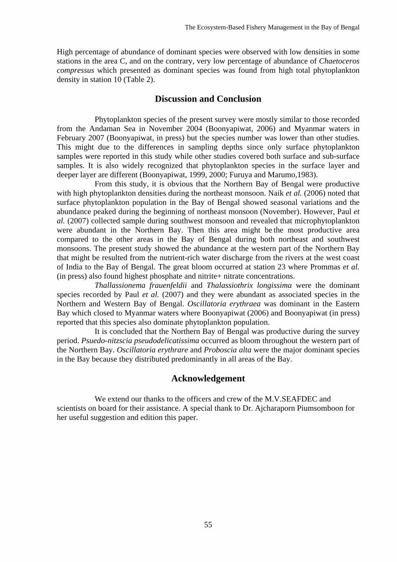
The Ecosystem-Based Fishery Management in the Bay of Bengal
55
High percentage of abundance of dominant species were observed with low densities in some stations in the area C, and on the contrary, very low percentage of abundance of Chaetoceros compressus which presented as dominant species was found from high total phytoplankton density in station 10 (Table 2).
Discussion and Conclusion
Phytoplankton species of the present survey were mostly similar to those recorded from the Andaman Sea in November 2004 (Boonyapiwat, 2006) and Myanmar waters in February 2007 (Boonyapiwat, in press) but the species number was lower than other studies. This might due to the differences in sampling depths since only surface phytoplankton samples were reported in this study while other studies covered both surface and sub-surface samples. It is also widely recognized that phytoplankton species in the surface layer and deeper layer are different (Boonyapiwat, 1999, 2000; Furuya and Marumo,1983).
From this study, it is obvious that the Northern Bay of Bengal were productive with high phytoplankton densities during the northeast monsoon. Naik et al. (2006) noted that surface phytoplankton population in the Bay of Bengal showed seasonal variations and the abundance peaked during the beginning of northeast monsoon (November). However, Paul et al. (2007) collected sample during southwest monsoon and revealed that microphytoplankton were abundant in the Northern Bay. Then this area might be the most productive area compared to the other areas in the Bay of Bengal during both northeast and southwest monsoons. The present study showed the abundance at the western part of the Northern Bay that might be resulted from the nutrient-rich water discharge from the rivers at the west coast of India to the Bay of Bengal. The great bloom occurred at station 23 where Prommas et al. (in press) also found highest phosphate and nitrite+ nitrate concentrations.
Thallassionema frauenfeldii and Thalassiothrix longissima were the dominant species recorded by Paul et al. (2007) and they were abundant as associated species in the Northern and Western Bay of Bengal. Oscillatoria erythraea was dominant in the Eastern Bay which closed to Myanmar waters where Boonyapiwat (2006) and Boonyapiwat (in press) reported that this species also dominate phytoplankton population.
It is concluded that the Northern Bay of Bengal was productive during the survey period. Psuedo-nitzscia pseudodelicatissima occurred as bloom throughout the western part of the Northern Bay. Oscillatoria erythrare and Proboscia alta were the major dominant species in the Bay because they distributed predominantly in all areas of the Bay.
Acknowledgement
We extend our thanks to the officers and crew of the M.V.SEAFDEC and scientists on board for their assistance. A special thank to Dr. Ajcharaporn Piumsomboon for her useful suggestion and edition this paper.
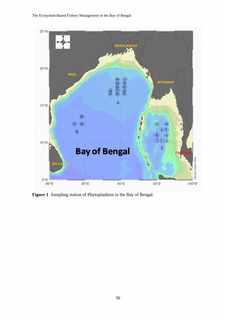
The Ecosystem-Based Fishery Management in the Bay of Bengal
56
Figure 1 Sampling station of Phytoplankton in the Bay of Bengal.
A
B
C
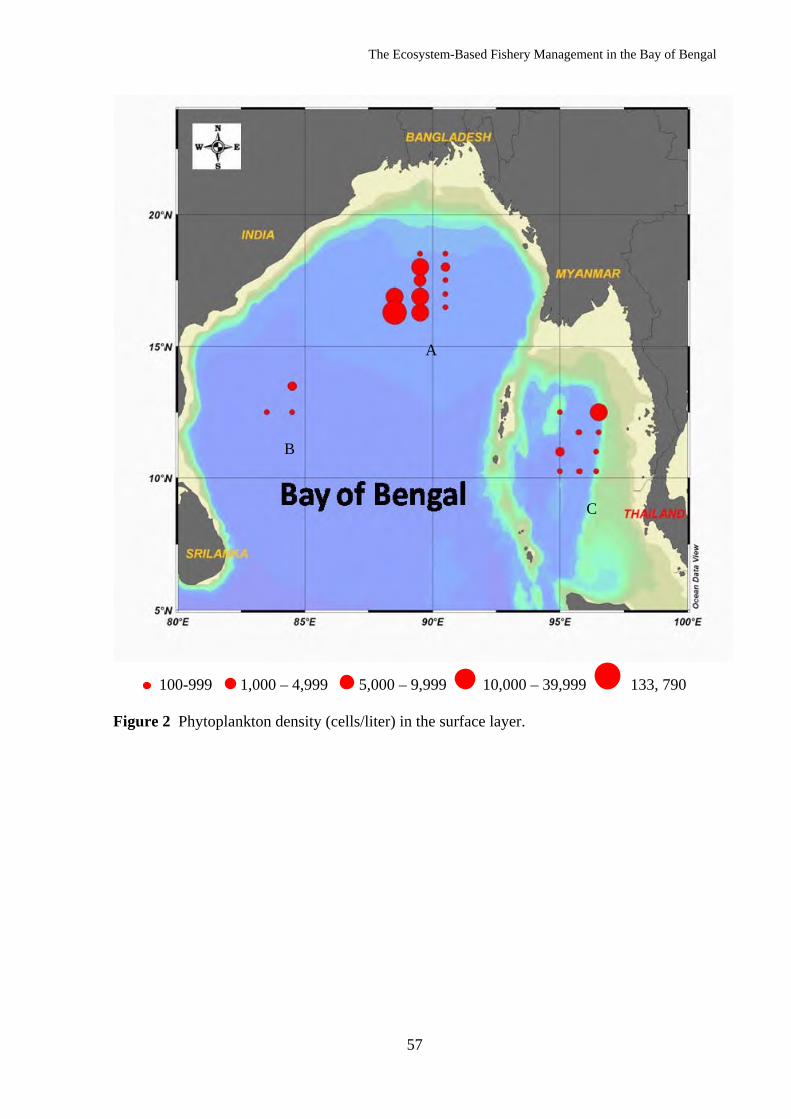
The Ecosystem-Based Fishery Management in the Bay of Bengal
57
100-999 1,000 – 4,999 5,000 – 9,999 10,000 – 39,999 133, 790 Figure 2 Phytoplankton density (cells/liter) in the surface layer.
A
B
C
The Ecosystem-Based Fishery Management in the Bay of Bengal
58
Oscillatoria erythraea Chaetoceros compressus Chaetoceros lorenzianus Climacodium frauenfeldianum Proboscia alata Pseudonitzschia pseudodelicatissima Figure 3 Dominant phytoplankton species in the Bay of Bengal.
A
B
C
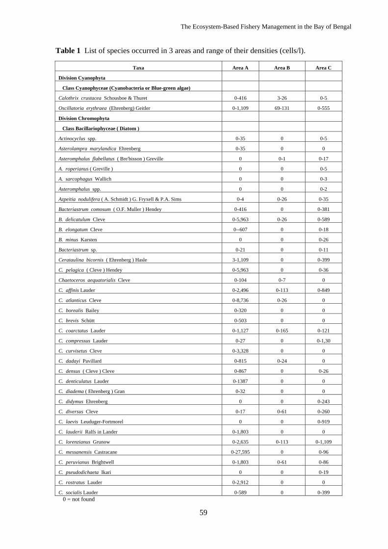
The Ecosystem-Based Fishery Management in the Bay of Bengal
59
Table 1 List of species occurred in 3 areas and range of their densities (cells/l).
Taxa Area A Area B Area C
Division Cyanophyta
Class Cyanophyceae (Cyanobacteria or Blue-green algae)
Calothrix crustacea Schousboe & Thuret 0-416 3-26 0-5
Oscillatoria erythraea (Ehrenberg) Geitler 0-1,109 69-131 0-555
Division Chromophyta
Class Bacillariophyceae ( Diatom )
Actinocyclus spp. 0-35 0 0-5
Asterolampra marylandica Ehrenberg 0-35 0 0
Asteromphalus flabellatus ( Bre'bisson ) Greville 0 0-1 0-17
A. roperianus ( Greville ) 0 0 0-5
A. sarcophagus Wallich 0 0 0-3
Asteromphalus spp. 0 0 0-2
Azpeitia nodulifera ( A. Schmidt ) G. Fryxell & P.A. Sims 0-4 0-26 0-35
Bacteriastrum comosum ( O.F. Muller ) Hendey 0-416 0 0-381
B. delicatulum Cleve 0-5,963 0-26 0-589
B. elongatum Cleve 0--607 0 0-18
B. minus Karsten 0 0 0-26
Bacteriastrum sp. 0-21 0 0-11
Cerataulina bicornis ( Ehrenberg ) Hasle 3-1,109 0 0-399
C. pelagica ( Cleve ) Hendey 0-5,963 0 0-36
Chaetoceros aequatorialis Cleve 0-104 0-7 0
C. affinis Lauder 0-2,496 0-113 0-849
C. atlanticus Cleve 0-8,736 0-26 0
C. borealis Bailey 0-320 0 0
C. brevis Schütt 0-503 0 0
C. coarctatus Lauder 0-1,127 0-165 0-121
C. compressus Lauder 0-27 0 0-1,30
C. curvisetus Cleve 0-3,328 0 0
C. dadayi Pavillard 0-815 0-24 0
C. densus ( Cleve ) Cleve 0-867 0 0-26
C. denticulatus Lauder 0-1387 0 0
C. diadema ( Ehrenberg ) Gran 0-32 0 0
C. didymus Ehrenberg 0 0 0-243
C. diversus Cleve 0-17 0-61 0-260
C. laevis Leuduger-Fortmorel 0 0 0-919
C. lauderii Ralfs in Lander 0-1,803 0 0
C. lorenzianus Grunow 0-2,635 0-113 0-1,109
C. messanensis Castracane 0-27,595 0 0-96
C. peruvianus Brightwell 0-1,803 0-61 0-86
C. pseudodichaeta Ikari 0 0 0-19
C. rostratus Lauder 0-2,912 0 0
C. socialis Lauder 0-589 0 0-399 0 = not found
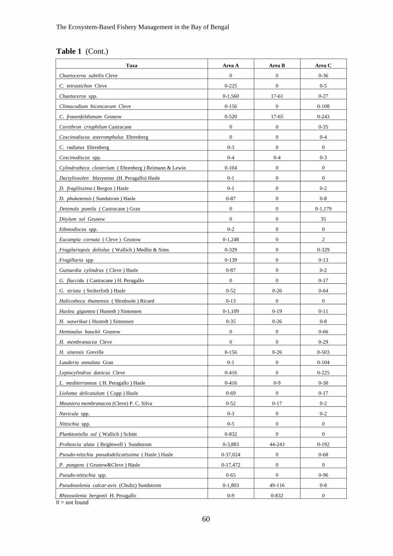
The Ecosystem-Based Fishery Management in the Bay of Bengal
60
Table 1 (Cont.)
Taxa Area A Area B Area C
Chaetoceros subtilis Cleve 0 0 0-36
C. tetrastichon Cleve 0-225 0 0-5
Chaetoceros spp. 0-1,560 17-61 0-27
Climacodium biconcavum Cleve 0-156 0 0-108
C. frauenfeldianum Grunow 0-520 17-65 0-243
Corethron criophilum Castracane 0 0 0-35
Coscinodiscus asteromphalus Ehrenberg 0 0 0-4
C. radiatus Ehrenberg 0-3 0 0
Coscinodiscus spp. 0-4 0-4 0-3
Cylindrotheca closterium ( Ehrenberg ) Reimann & Lewin 0-104 0 0
Dactyliosolen blavyanus (H. Peragallo) Hasle 0-1 0 0
D. fragilissima ( Bergon ) Hasle 0-1 0 0-2
D. phuketensis ( Sundstrom ) Hasle 0-87 0 0-8
Detonula pumila ( Castracane ) Gran 0 0 0-1,179
Ditylum sol Grunow 0 0 35
Ethmodiscus spp. 0-2 0 0
Eucampia cornuta ( Cleve ) Grunow 0-1,248 0 2
Fragilariopsis doliolus ( Wallich ) Medlin & Sims 0-329 0 0-329
Fragillaria spp. 0-139 0 0-13
Guinardia cylindrus ( Cleve ) Hasle 0-87 0 0-2
G. flaccida ( Castracane ) H. Peragallo 0 0 0-17
G. striata ( Stolterfoth ) Hasle 0-52 0-26 0-64
Halicotheca thamensis ( Shrubsole ) Ricard 0-13 0 0
Haslea gigantea ( Hustedt ) Simonsen 0-1,109 0-19 0-11
H. wawrikae ( Hustedt ) Simonsen 0-35 0-26 0-8
Hemiaulus hauckii Grunow 0 0 0-66
H. membranacea Cleve 0 0 0-29
H. sinensis Greville 0-156 0-26 0-503
Lauderia annulata Gran 0-1 0 0-104
Leptocylindrus danicus Cleve 0-416 0 0-225
L. mediterraneus ( H. Peragallo ) Hasle 0-416 0-9 0-30
Lioloma delicatulum ( Cupp ) Hasle 0-69 0 0-17
Meuniera membranacea (Cleve) P. C. Silva 0-52 0-17 0-2
Navicula spp. 0-3 0 0-2
Nitzschia spp. 0-5 0 0
Planktoniella sol ( Wallich ) Schütt 0-832 0 0
Proboscia alata ( Brightwell ) Sundstrom 0-3,883 44-243 0-192
Pseudo-nitzchia pseudodelicatissima ( Hasle ) Hasle 0-37,024 0 0-68
P. pungens ( Grunow&Cleve ) Hasle 0-17,472 0 0
Pseudo-nitzschia spp. 0-65 0 0-96
Pseudosolenia calcar-avis (Chultz) Sundstrom 0-1,803 49-116 0-8
Rhizosolenia bergonii H. Peragallo 0-9 0-832 0 0 = not found
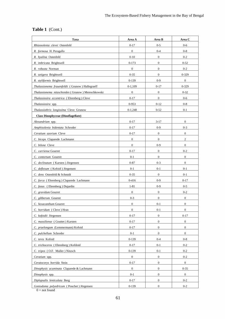
The Ecosystem-Based Fishery Management in the Bay of Bengal
61
Table 1 (Cont.)
Taxa Area A Area B Area C
Rhizosolenia clevei Ostenfeld 0-17 0-5 0-6
R. formosa H. Peragallo 0 0-4 0-8
R. hyalina Ostenfeld 0-10 0 0-2
R. imbricata Brightwell 0-173 0 0-52
R. robusta Norman 0 0 0-2
R. setigera Brightwell 0-35 0 0-329
R. styliformis Brightwell 0-139 0-9 0
Thalassionema frauenfeldii ( Grunow ) Hallegraeff 0-1,109 0-17 0-329
Thalassionema nitzschioides ( Grunow ) Mereschkowski 0 0 0-32
Thalassiosira eccentrica ( Ehrenberg ) Cleve 0-17 0 0-6
Thalassiosira spp. 0-953 0-12 0-8
Thalassiothrix longissima Cleve Grunow 0-1,248 0-52 0-1
Class Dinophyceae (Dinoflagellate)
Alexandrium spp. 0-17 3-17 0
Amphisolenia bidentata Schroder 0-17 0-9 0-3
Ceratium azorium Cleve 0-17 0 0
C. biceps Claparede Lachmann 0 0 2
C. bilone Cleve 0 0-9 0
C. carriense Gourret 0-17 0 0-2
C. contortum Gourret 0-1 0 0
C. declinatum ( Karsten ) Jörgensen 0-87 0-3 0
C. deflexum ( Kofoid ) Jörgensen 0-1 0-1 0-1
C. dens Ostenfeld & Schmidt 0-35 0 0-1
C. furca ( Ehrenberg ) Claparede Lachmann 0-416 0-9 0-17
C. fusus ( Ehrenberg ) Dujardin 1-81 0-9 0-5
C. gravidum Gourret 0 0 0-2
C. gibberum Gourret 0-3 0 0
C. hexacanthum Gourret 0 0-1 0
C. horridum ( Cleve ) Hran 0 0-1 0
C. kofoidii Jörgensen 0-17 0 0-17
C. massiliense ( Gouttet ) Karsten 0-17 0 0
C. praelongum (Lemmermann) Kofoid 0-17 0 0
C. pulchellum Schroder 0-1 0 0
C. teres Kofoid 0-139 0-4 0-8
C. trichoceros ( Ehrenberg ) Kofdoid 0-17 0-1 0-2
C. tripos ( O.F. Muller ) Nitzsch 0-139 0-1 0-2
Ceratium spp. 0 0 0-2
Ceratocorys horrida Stein 0-17 0 0
Dinophysis acuminata Claparede & Lachmann 0 0 0-35
Dinophysis spp. 0-1 0 0
Diplopsalis lenticulata Berg 0-17 0 0-2
Goniodoma polyedricum ( Pouchet ) Jörgensen 0-139 0 0-2 0 = not found
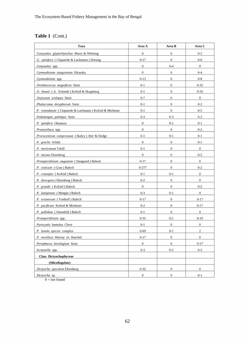
The Ecosystem-Based Fishery Management in the Bay of Bengal
62
Table 1 (Cont.)
Taxa Area A Area B Area C
Gonyaulax glyptorhynchus Murry & Whitting 0 0 0-2
G. spinifera ( Claparede & Lachmann ) Diesing 0-17 0 0-6
Gonyaulax spp. 0 0-4 0
Gymnodinium sanguineum Hirasaka 0 0 0-4
Gymnodinium spp. 0-13 0 0-8
Ornithocercus magnificus Stein 0-1 0 0-35
O. thumii ( A. Schmidt ) Kofoid & Skogsberg 0-1 0 0-35
Oxytoxum scolopax Stein 0-7 0 0
Phalacroma doryphorum Stein 0-1 0 0-2
P. rotundatum ( Claparede & Lachmann ) Kofoid & Michener 0-1 0 0-5
Podolampas palmipes Stein 0-3 0-3 0-2
P. spinifera Okamura 0 0-1 0-1
Pronoctiluca spp. 0 0 0-2
Prorocentrum compressum ( Bailey ) Abe' & Dodge 0-1 0-1 0-1
P. graclie Schütt 0 0 0-1
P. mexicanum Tafall 0-1 0 0
P. micans Ehrenberg 0 0 0-5
Protoperidinium angustum ( Dangeard ) Balech 0-17 0 0
P. conicum ( Gran ) Balech 0-277 0 0-2
P. crassipes ( Kofoid ) Balech 0-1 0-1 0
P. divergens ( Ehrenberg ) Balech 0-2 0 0
P. grande ( Kofoid ) Balech 0 0 0-2
P. latispinum ( Mangin ) Balech 0-3 0-1 0
P. oceanicum ( Vanhoff ) Balech 0-17 0 0-17
P. pacificum Kofoid & Michener 0-2 0 0-17
P. pallidum ( Ostenfeld ) Balech 0-1 0 0
Protoperidinium spp. 0-35 0-1 0-10
Pyrocystis hamulus Cleve 0-1 0 0
P. lunula species complex 0-69 0-1 2
P. noctiluca Murray ex Haeckel 0-17 0 0
Pyrophacus horologium Stein 0 0 0-17
Scripsiella spp. 0-3 0-5 0-5
Class Dictyochophyceae
(Silicoflagelate)
Dictyocha speculum Ehrenberg 0-35 0 0
Dictyocha sp. 0 0 0-1 0 = not found
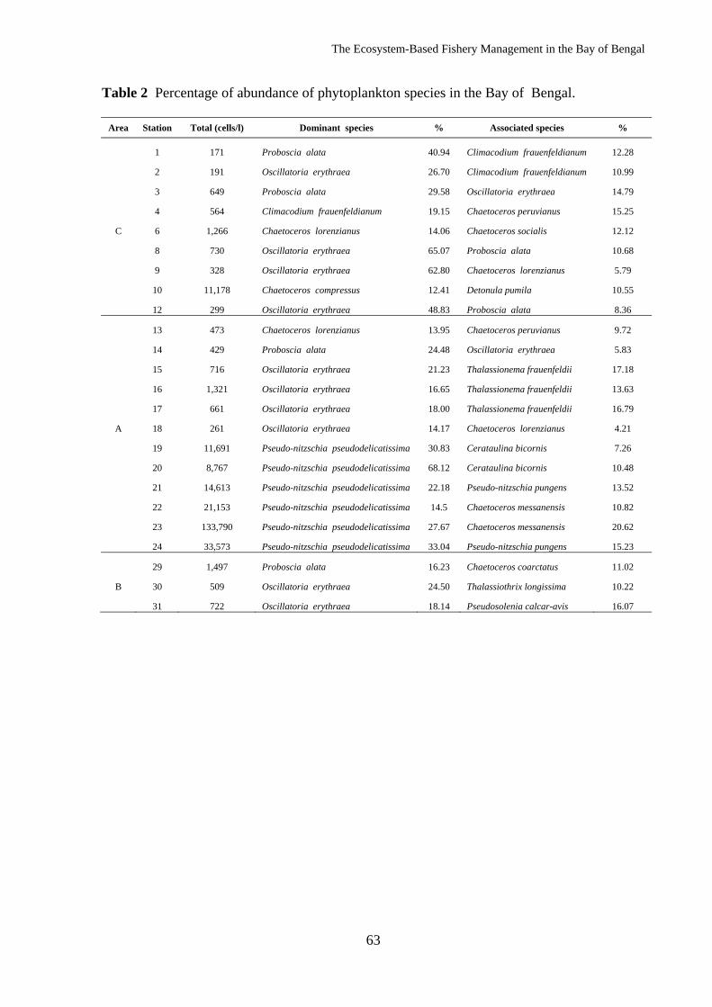
The Ecosystem-Based Fishery Management in the Bay of Bengal
63
Table 2 Percentage of abundance of phytoplankton species in the Bay of Bengal.
Area Station Total (cells/l) Dominant species % Associated species %
1 171 Proboscia alata 40.94 Climacodium frauenfeldianum 12.28
2 191 Oscillatoria erythraea 26.70 Climacodium frauenfeldianum 10.99
3 649 Proboscia alata 29.58 Oscillatoria erythraea 14.79
4 564 Climacodium frauenfeldianum 19.15 Chaetoceros peruvianus 15.25
C 6 1,266 Chaetoceros lorenzianus 14.06 Chaetoceros socialis 12.12
8 730 Oscillatoria erythraea 65.07 Proboscia alata 10.68
9 328 Oscillatoria erythraea 62.80 Chaetoceros lorenzianus 5.79
10 11,178 Chaetoceros compressus 12.41 Detonula pumila 10.55
12 299 Oscillatoria erythraea 48.83 Proboscia alata 8.36
13 473 Chaetoceros lorenzianus 13.95 Chaetoceros peruvianus 9.72
14 429 Proboscia alata 24.48 Oscillatoria erythraea 5.83
15 716 Oscillatoria erythraea 21.23 Thalassionema frauenfeldii 17.18
16 1,321 Oscillatoria erythraea 16.65 Thalassionema frauenfeldii 13.63
17 661 Oscillatoria erythraea 18.00 Thalassionema frauenfeldii 16.79
A 18 261 Oscillatoria erythraea 14.17 Chaetoceros lorenzianus 4.21
19 11,691 Pseudo-nitzschia pseudodelicatissima 30.83 Cerataulina bicornis 7.26
20 8,767 Pseudo-nitzschia pseudodelicatissima 68.12 Cerataulina bicornis 10.48
21 14,613 Pseudo-nitzschia pseudodelicatissima 22.18 Pseudo-nitzschia pungens 13.52
22 21,153 Pseudo-nitzschia pseudodelicatissima 14.5 Chaetoceros messanensis 10.82
23 133,790 Pseudo-nitzschia pseudodelicatissima 27.67 Chaetoceros messanensis 20.62
24 33,573 Pseudo-nitzschia pseudodelicatissima 33.04 Pseudo-nitzschia pungens 15.23
29 1,497 Proboscia alata 16.23 Chaetoceros coarctatus 11.02
B 30 509 Oscillatoria erythraea 24.50 Thalassiothrix longissima 10.22
31 722 Oscillatoria erythraea 18.14 Pseudosolenia calcar-avis 16.07
The Ecosystem-Based Fishery Management in the Bay of Bengal
64
References
Boonyapiwat, S. 1999. Distribution, Abundance and Species Composition of Phytoplankton in the South China Sea, Area II : Sabah, Sarawak and Brunei Darussalam, in Proceedings of the Second Technical Seminar on Marine Fishery Resources Survey in the South China Sea, Area II : West Coast of Sabah, Sarawak and Brunei Darussalam. Dec. 1998. Kuala Lampur, SEAFDEC. p 177-196.
Boonyapiwat, S. 2000. Species Composition, Abundance and Distribution of Phytoplankton in the Thermocline Layer in the South China Sea, Area III : Western Philippines, in
Proceedings of the Third Technical Seminar on Marine Fishery Resources Survey in the South China Sea , Area III : Western Philippines. Feb. 2000. SEAFDEC. p 197-216.
Boonyapiwat, S. 2006. Composition, abundance and distribution of phytoplankton in the Andaman Sea. Preliminary Results on the Large Pelagic Fisheries Resources Survey in the Andaman Sea. TD/RES/99 SEAFDEC p40-52.
Boonyapiwat, S., K. Tienpisuth and W. Ngowsakul. Abundance and distribution of phytoplankton in Myanmar waters. In Report on Fisheries Resources Survey in Myanmar Waters. SEAFDEC (in press).
Dwivedi, S. N. and A. K. Choubey. 1998. Indian Ocean Large Marine Ecosystems : Need for National and Regional Framework for Conservation and Sustainable Development. In
K. Sherman, E. N. Okemwa and M. J. Ntiba (Eds.) Large Marine Ecosystems of the Indian Ocean : Assessment, Sustainability, and Management. Blackwell Science, Inc. 361-367.
Furuya, K. and R. Marumo. 1983. The structure of the phytoplankton community in the subsurface chlorophyll maxima in the westernNorth Pacific Ocean. J. Plank. Res., 5: 393-406.
Naik, R., S. Hegde, A. C. Anil, K. Nisha and V. V. Gopalakrishna. 2006. Phytoplankton community structure in the Bay of Bengal : spatial and temporal variation. Poster Abstract in International Workshop on Sustained Indian Ocean Biogeochemical and Ecological Research. National Institute of Oceanography, Dona-Paula, Goa, India.
Paul, J. T., N. Ramaiah, M. Gauns and V. Fernandes. 2007. Preponderance of a few diatom species among the highly diverse microphytoplankton assemblages in the Bay of Bengal. Marine Biology. 152(1) : 63-75.
Prommas, R., P. Naimee and N. Sukramongkol. Spatial distribution of nutrients in the Bay of Bengal. Report on the Ecosystem-Based Fishery Management in the Bay of Bengal (in press).
Taylor, F. J. R. 1976. Dinoflagellates from the International Indian Ocean Expedition. E.Schweizerbart’sche Verlagbuchhandlung. 234 p.
Vinayachandran, P. N. and S. Mathew. 2003. Phytoplankton bloom in the Bay of Bengal during the northeast monsoon and its intensification by cyclones. Geophysical Research Letters. 30(11).
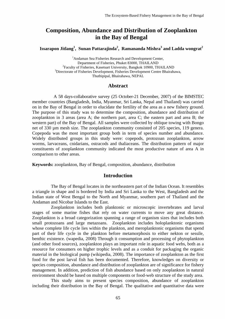
The Ecosystem-Based Fishery Management in the Bay of Bengal
65
Composition, Abundance and Distribution of Zooplankton in the Bay of Bengal
Issarapon Jitlang1, Sunan Pattarajinda2, Ramananda Mishra3 and Ladda wongrat2
1Andaman Sea Fisheries Research and Development Center,
Department of Fisheries, Phuket 83000, THAILAND
2Faculty of Fisheries, Kasetsart University, Bangkok 10900, THAILAND 3Directorate of Fisheries Development, Fisheries Development Centre Bhairahawa,
Thuthipipal, Bhairahawa, NEPAL
Abstract
A 58 days-collaborative survey (25 October-21 December, 2007) of the BIMSTEC member countries (Bangladesh, India, Myanmar, Sri Lanka, Nepal and Thailand) was carried on in the Bay of Bengal in order to elucidate the fertility of the area as a new fishery ground. The purpose of this study was to determine the composition, abundance and distribution of zooplankton in 3 areas (area A; the northern part, area C; the eastern part and area B; the western part) of the Bay of Bengal. All samples were collected by oblique towing with Bongo net of 330 µm mesh size. The zooplankton community consisted of 205 species, 119 genera. Copepoda was the most important group both in term of species number and abundance. Widely distributed groups in this study were: copepods, protozoan zooplankton, arrow worms, larvaceans, cnidarians, ostracods and thaliaceans. The distribution pattern of major constituents of zooplankton community indicated the most productive nature of area A in comparison to other areas. Keywords: zooplankton, Bay of Bengal, composition, abundance, distribution
Introduction
The Bay of Bengal locates in the northeastern part of the Indian Ocean. It resembles a triangle in shape and is bordered by India and Sri Lanka to the West, Bangladesh and the Indian state of West Bengal to the North and Myanmar, southern part of Thailand and the Andaman and Nicobar Islands to the East.
Zooplankton includes both planktonic or microscopic invertebrates and larval stages of some marine fishes that rely on water currents to move any great distance. Zooplankton is a broad categorization spanning a range of organism sizes that includes both small protozoans and large metazoans. Zooplankton includes holoplanktonic organisms whose complete life cycle lies within the plankton, and meroplanktonic organisms that spend part of their life cycle in the plankton before metamorphosis to either nekton or sessile, benthic existence. (wapedia, 2008) Through it consumption and processing of phytoplankton (and other food sources), zooplankton plays an important role in aquatic food webs, both as a resource for consumers on higher trophic levels and as a conduit for packaging the organic material in the biological pump (wikipedia, 2008). The importance of zooplankton as the first food for the post larval fish has been documented. Therefore, knowledges on diversity or species composition, abundance and distribution of zooplankton are of significance for fishery management. In addition, prediction of fish abundance based on only zooplankton in natural environment should be based on multiple components or food-web structure of the study area.
This study aims to present species composition, abundance of zooplankton including their distribution in the Bay of Bengal. The qualitative and quantitative data were
The Ecosystem-Based Fishery Management in the Bay of Bengal
66
analyzed from 33 samples taken from 3 areas in the Bay of Bengal. This is a collaborative survey project of the BIMSTEC member countries (Bangladesh, India, Myanmar, Sri Lanka, Nepal and Thailand). The main purpose of BIMSTEC is to manage fishery resources in the Bay of Bengal.
Material and Methods
Zooplankton samples were collected from 33 stations during the cruise of fisheries research vessel M.V. SEAFDEC between 25 October to 21 December 2007 (Table 1 and Fig. 1) in the Bay of Bengal. The sampling stations were divided into 3 areas: area A (latitude 16°N-19°N, longitude 88°E-91°E) covered 15 stations (station 13-27), area B (latitude 09°N-14°N, longitude 82°E-85°E) included 7 stations (station 13-27) and area C (latitude 10°N-12°N, longitude 95°E-97°E) included 11 stations (station 1-6 and 8-12).
Zooplankton samples were collected using a Bongo net, 45 cm. in diameter and 330 µm mesh size, equipped with a flow meter and obliquely towed at a vessel speed of 2 knots. The towing depth of each haul was 150 meters. The samples were immediately preserved in 5% buffered formaldehyde sea water for further analyses.
Zooplankton samples were counted for larger representatives such as cnidarians, decapods, euphausids, arrow worms, etc. using an open counting chamber of 80 mm X 50 mm X 2 mm size. Counting was made under a binocular dissecting microscope at proper magnification. The examination at a higher magnification under the compound microscope may be used to identify questionable organisms. For dense sample, zooplanktorn fraction of <200 µm were separated from the larger ones by filtration and sub-sampled with a Widebore pipet for an aliquot of 1-5 ml for counting with a Sedgwick-Rafter counting chamber under a compound microscope at 100X magnification.
Report zooplankton as number per cubic meter:
No. individuals/ m3 = Where C = number of organisms counted, V1 = volume of the concentrated sample (ml), V2 = volume of the sample counted (ml), V3 = volume of the filtered volume of water (m3)
C x V1 V2 x V3
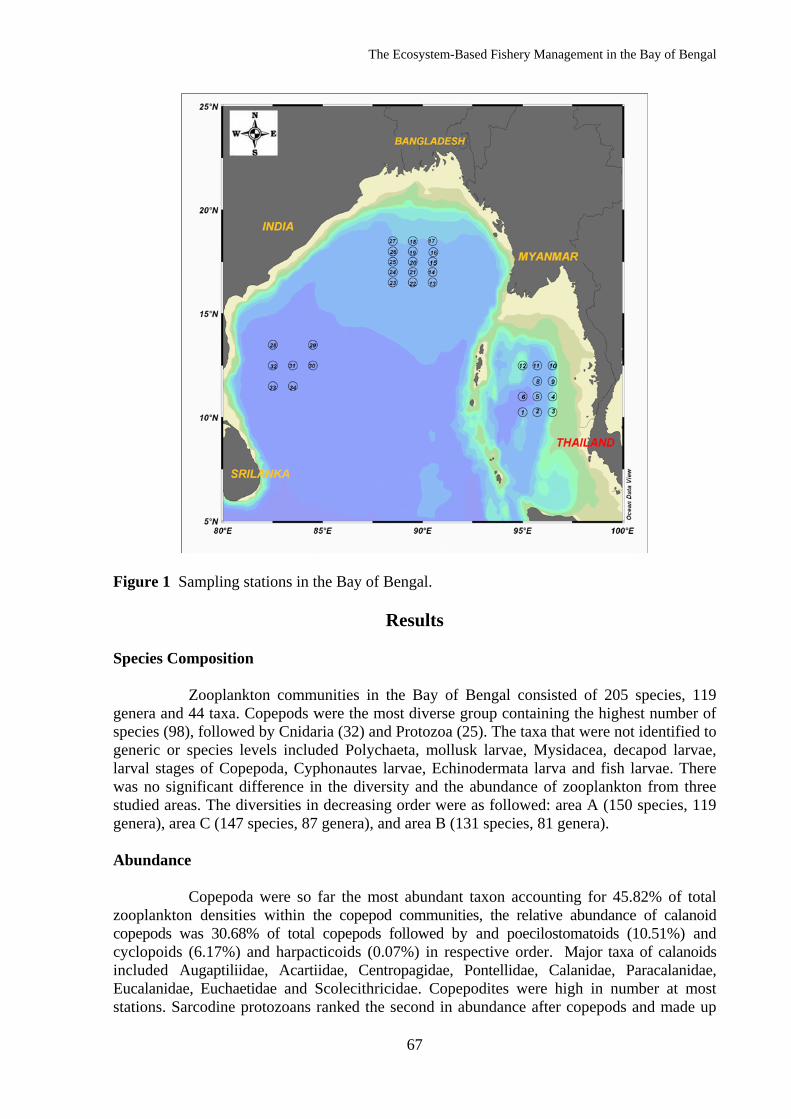
The Ecosystem-Based Fishery Management in the Bay of Bengal
67
Figure 1 Sampling stations in the Bay of Bengal.
Results Species Composition
Zooplankton communities in the Bay of Bengal consisted of 205 species, 119 genera and 44 taxa. Copepods were the most diverse group containing the highest number of species (98), followed by Cnidaria (32) and Protozoa (25). The taxa that were not identified to generic or species levels included Polychaeta, mollusk larvae, Mysidacea, decapod larvae, larval stages of Copepoda, Cyphonautes larvae, Echinodermata larva and fish larvae. There was no significant difference in the diversity and the abundance of zooplankton from three studied areas. The diversities in decreasing order were as followed: area A (150 species, 119 genera), area C (147 species, 87 genera), and area B (131 species, 81 genera). Abundance
Copepoda were so far the most abundant taxon accounting for 45.82% of total zooplankton densities within the copepod communities, the relative abundance of calanoid copepods was 30.68% of total copepods followed by and poecilostomatoids (10.51%) and cyclopoids (6.17%) and harpacticoids (0.07%) in respective order. Major taxa of calanoids included Augaptiliidae, Acartiidae, Centropagidae, Pontellidae, Calanidae, Paracalanidae, Eucalanidae, Euchaetidae and Scolecithricidae. Copepodites were high in number at most stations. Sarcodine protozoans ranked the second in abundance after copepods and made up
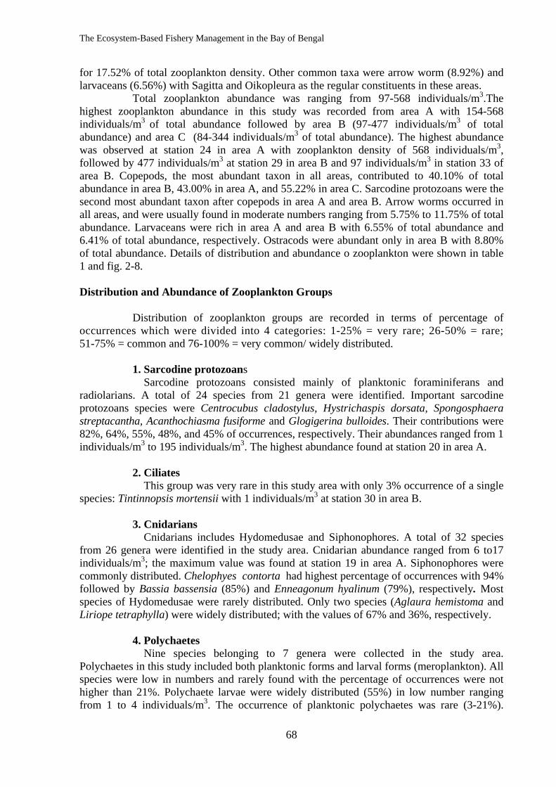
The Ecosystem-Based Fishery Management in the Bay of Bengal
68
for 17.52% of total zooplankton density. Other common taxa were arrow worm (8.92%) and larvaceans (6.56%) with Sagitta and Oikopleura as the regular constituents in these areas.
Total zooplankton abundance was ranging from 97-568 individuals/m3.The highest zooplankton abundance in this study was recorded from area A with 154-568 individuals/m3 of total abundance followed by area B (97-477 individuals/m3 of total abundance) and area C (84-344 individuals/m3 of total abundance). The highest abundance was observed at station 24 in area A with zooplankton density of 568 individuals/m3, followed by 477 individuals/m3 at station 29 in area B and 97 individuals/m3 in station 33 of area B. Copepods, the most abundant taxon in all areas, contributed to 40.10% of total abundance in area B, 43.00% in area A, and 55.22% in area C. Sarcodine protozoans were the second most abundant taxon after copepods in area A and area B. Arrow worms occurred in all areas, and were usually found in moderate numbers ranging from 5.75% to 11.75% of total abundance. Larvaceans were rich in area A and area B with 6.55% of total abundance and 6.41% of total abundance, respectively. Ostracods were abundant only in area B with 8.80% of total abundance. Details of distribution and abundance o zooplankton were shown in table 1 and fig. 2-8. Distribution and Abundance of Zooplankton Groups
Distribution of zooplankton groups are recorded in terms of percentage of occurrences which were divided into 4 categories: 1-25% = very rare; 26-50% = rare; 51-75% = common and 76-100% = very common/ widely distributed.
1. Sarcodine protozoans Sarcodine protozoans consisted mainly of planktonic foraminiferans and
radiolarians. A total of 24 species from 21 genera were identified. Important sarcodine protozoans species were Centrocubus cladostylus, Hystrichaspis dorsata, Spongosphaera streptacantha, Acanthochiasma fusiforme and Glogigerina bulloides. Their contributions were 82%, 64%, 55%, 48%, and 45% of occurrences, respectively. Their abundances ranged from 1 individuals/m3 to 195 individuals/m3. The highest abundance found at station 20 in area A.
2. Ciliates This group was very rare in this study area with only 3% occurrence of a single
species: Tintinnopsis mortensii with 1 individuals/m3 at station 30 in area B.
3. Cnidarians Cnidarians includes Hydomedusae and Siphonophores. A total of 32 species
from 26 genera were identified in the study area. Cnidarian abundance ranged from 6 to17 individuals/m3; the maximum value was found at station 19 in area A. Siphonophores were commonly distributed. Chelophyes contorta had highest percentage of occurrences with 94% followed by Bassia bassensia (85%) and Enneagonum hyalinum (79%), respectively. Most species of Hydomedusae were rarely distributed. Only two species (Aglaura hemistoma and Liriope tetraphylla) were widely distributed; with the values of 67% and 36%, respectively.
4. Polychaetes Nine species belonging to 7 genera were collected in the study area.
Polychaetes in this study included both planktonic forms and larval forms (meroplankton). All species were low in numbers and rarely found with the percentage of occurrences were not higher than 21%. Polychaete larvae were widely distributed (55%) in low number ranging from 1 to 4 individuals/m3. The occurrence of planktonic polychaetes was rare (3-21%).
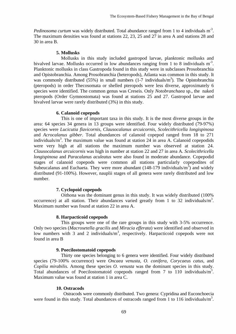
The Ecosystem-Based Fishery Management in the Bay of Bengal
69
Pedinosoma curtum was widely distributed. Total abundance ranged from 1 to 4 individuals m-3. The maximum densities was found at stations 22, 23, 25 and 27 in area A and stations 28 and 30 in area B.
5. Mollusks Mollusks in this study included gastropod larvae, planktonic mollusks and
bivalved larvae. Mollusks occurred in low abundances ranging from 1 to 8 individuals m-3. Planktonic mollusks in class Gastropoda found in this study were in subclasses Prosobranchia and Opistobranchia. Among Prosobranchia (heteropods), Atlanta was common in this study. It was commonly distributed (55%) in small numbers (1-7 individuals/m3). The Opistobranchia (pteropods) in order Thecosomata or shelled pteropods were less diverse, approximately 6 species were identified. The common genus was Creseis. Only Notobranchaea sp., the naked pteropods (Order Gymnostomata) was found at stations 25 and 27. Gastropod larvae and bivalved larvae were rarely distributed (3%) in this study.
6. Calanoid copepods This is one of important taxa in this study. It is the most diverse groups in the
area: 64 species 34 genera in 13 groups were identified. Four widely distributed (79-97%) species were Lucicutia flavicornis, Clausocalanus arcuicornis, Scolecithricella longispinosa and Acrocalanus gibber. Total abundances of calanoid copepod ranged from 18 to 271 individuals/m3. The maximum value was found at station 24 in area A. Calanoid copepodids were very high at all stations the maximum number was observed at station 24. Clausocalanus arcuicornis was high in number at station 22 and 27 in area A. Scolecithricella longispinosa and Paracalanus aculeatus were also found in moderate abundance. Copepodid stages of calanoid copepods were common all stations particularly copepodites of Subeucalanus and Euchaeta. They were more abundant (148-179 individuals/m3) and widely distributed (91-100%). However, nauplii stages of all genera were rarely distributed and low number.
7. Cyclopoid copepods Oithona was the dominant genus in this study. It was widely distributed (100%
occurrence) at all station. Their abundances varied greatly from 1 to 32 individuals/m3. Maximum number was found at station 22 in area A.
8. Harpacticoid copepods This groups were one of the rare groups in this study with 3-5% occurrence.
Only two species (Macrosetella gracilis and Miracia efferata) were identified and observed in low numbers with 3 and 2 individuals/m3, respectively. Harpacticoid copepods were not found in area B
9. Poecilostomatoid copepods Thirty one species belonging to 6 genera were identified. Four widely distributed
species (79-100% occurrence) were Oncaea venusta, O. conifera, Corycaeus catus, and Copilia mirabilis. Among these species O. venusta was the dominant species in this study. Total abundances of Poecilostomatoid copepods ranged from 7 to 110 individuals/m3. Maximum value was found at station 1 in area C.
10. Ostracods Ostracods were commonly distributed. Two genera: Cypridina and Euconchoecia
were found in this study. Total abundances of ostracods ranged from 1 to 116 individuals/m3.
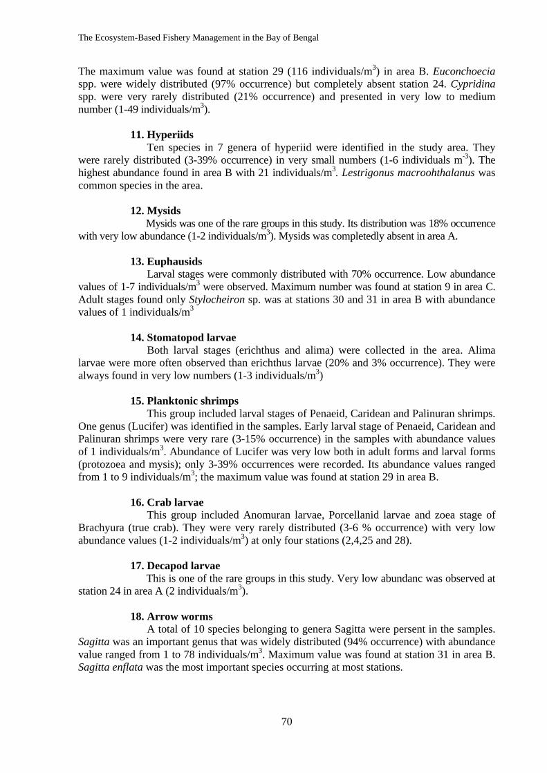
The Ecosystem-Based Fishery Management in the Bay of Bengal
70
The maximum value was found at station 29 (116 individuals/m3) in area B. Euconchoecia spp. were widely distributed (97% occurrence) but completely absent station 24. Cypridina spp. were very rarely distributed (21% occurrence) and presented in very low to medium number (1-49 individuals/m3).
11. Hyperiids Ten species in 7 genera of hyperiid were identified in the study area. They
were rarely distributed (3-39% occurrence) in very small numbers (1-6 individuals m-3). The highest abundance found in area B with 21 individuals/m3. Lestrigonus macroohthalanus was common species in the area.
12. Mysids Mysids was one of the rare groups in this study. Its distribution was 18% occurrence
with very low abundance (1-2 individuals/m3). Mysids was completedly absent in area A. 13. Euphausids Larval stages were commonly distributed with 70% occurrence. Low abundance
values of 1-7 individuals/m3 were observed. Maximum number was found at station 9 in area C. Adult stages found only Stylocheiron sp. was at stations 30 and 31 in area B with abundance values of 1 individuals/m3
14. Stomatopod larvae Both larval stages (erichthus and alima) were collected in the area. Alima
larvae were more often observed than erichthus larvae (20% and 3% occurrence). They were always found in very low numbers (1-3 individuals/m3)
15. Planktonic shrimps This group included larval stages of Penaeid, Caridean and Palinuran shrimps.
One genus (Lucifer) was identified in the samples. Early larval stage of Penaeid, Caridean and Palinuran shrimps were very rare (3-15% occurrence) in the samples with abundance values of 1 individuals/m3. Abundance of Lucifer was very low both in adult forms and larval forms (protozoea and mysis); only 3-39% occurrences were recorded. Its abundance values ranged from 1 to 9 individuals/m3; the maximum value was found at station 29 in area B.
16. Crab larvae This group included Anomuran larvae, Porcellanid larvae and zoea stage of
Brachyura (true crab). They were very rarely distributed (3-6 % occurrence) with very low abundance values (1-2 individuals/m3) at only four stations (2,4,25 and 28).
17. Decapod larvae This is one of the rare groups in this study. Very low abundanc was observed at
station 24 in area A (2 individuals/m3). 18. Arrow worms A total of 10 species belonging to genera Sagitta were persent in the samples.
Sagitta was an important genus that was widely distributed (94% occurrence) with abundance value ranged from 1 to 78 individuals/m3. Maximum value was found at station 31 in area B. Sagitta enflata was the most important species occurring at most stations.
The Ecosystem-Based Fishery Management in the Bay of Bengal
71
19. Bryozoans Cyphonautes larvae, the larval stage of phylum Ectoprocta were rarely
observed (9% occurrence) in this study. Very low abundances (1 individual/m3) were recorded at three stations (11, 17 and 25). Bryozoans wwas completely absent in Area B.
20. Echinodermata larvae This group consisted of bipinnaria larvae of class Asteroidea, auricularia
larvae of class Holothuroidea, echinopluteus larvae of class Echinoidea and ophiopluteus larvae of class Ophiuroidea. They were very rare in distribution (21%, 3%, 9% and 18% occurrence), respectively. Their abundances varied from 5 to 106 individuals/m3. Bipinnaria larvae and auricularia larvae were found only in area C. Echinopluteus larvae and Ophiopluteus larvae were found in area A and C. Echinodermata larvae was completely absent in area B.
21. Larvaceans Only one genus: Oikopleura was found in this study. They were regularly
found (18-94%) in the study area. Their abundances ranged from 1 individual/m3 to 39 individuals/m3. Two important species were: O. fusiformis and O. longicauda, and were widely distributed with 94% and 88% occurrences, respectively. The highest abundance found in area A (74 individuals/m3).
22. Thaliaceans Two groups of thaliaceans were rare and present in low number. Salps
consisted three genera: Pegea, Salpa and Thalia. Only one genus of doliolids (Doliolum) was identified. Doliolum spp. were common in distribution (80% occurrence), but occurred in low abundance values (1-7 individuals/m3). Maximum number of thaliaceans were found at station13 and 27 in area A. Salps were rarely distributed (15-24% occurrence) of low number ranging from 1-4 individuals/m3
23. Fish eggs and fish larvae The data recorded here was underestimated; accurate data will be published
elsewhere under ichthyoplankton. Fish eggs and fish larvae were separarely collected by a 500 µm plankton net. Eggs and larvae of fish rarely distributed (3-9% occurrence) in low numbers ranging from 1 to 2 individuals/m3. They were observed in three found only three samples collected from station 13, 23 and 32.
24. Cephalochordates Amphioxides sp. was only one species collected in the study area. This groups
was one of the rare groups in this study with 21% occurrence. Small number (1-4 individuals/m3) was observed at 7 stations. The maximum value was found at station 20 in area A. Cephalochordates was absent in area C.
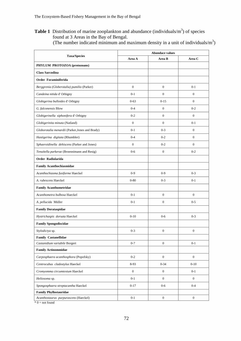
The Ecosystem-Based Fishery Management in the Bay of Bengal
72
Table 1 Distribution of marine zooplankton and abundance (individuals/m3) of species found at 3 Areas in the Bay of Bengal.
(The number indicated minimum and maximum density in a unit of individuals/m3)
Taxa/Species Abundace values
Area A Area B Area C
PHYLUM PROTOZOA (protozoans)
Class Sarcodina
Order Foraminiferida
Berggrenia (Globerotalia) pumilio (Parker) 0 0 0-1
Candeina nitida d' Orbigny 0-1 0 0
Globigerina bulloides d' Orbigny 0-63 0-15 0
G. falconensis Blow 0-4 0 0-2
Globigerinella siphonifera d' Orbigny 0-2 0 0
Globigerinita minuta (Natland) 0 0 0-1
Globorotalia menardii (Parker,Jones and Brady) 0-1 0-3 0
Hastigerina digitata (Rhumbler) 0-4 0-2 0
Sphaeroidinella dehiscens (Parker and Jones) 0 0-2 0
Tenuitella parkerae (Broennimann and Resig) 0-6 0 0-2
Order Radiolarida
Family Acanthochiasmidae
Acanthochiasma fusiforme Haeckel 0-9 0-9 0-3
A. rubescens Haeckel 0-80 0-3 0-1
Family Acanthometridae
Acanthometra bulbosa Haeckel 0-1 0 0
A. pellucida Müller 0-1 0 0-5
Family Dorataspidae
Hystrichaspis dorsata Haeckel 0-10 0-6 0-3
Family Spongodiscidae
Stylodictya sp. 0-3 0 0
Family Castanellidae
Castanidium variabile Borgert 0-7 0 0-1
Family Actinommidae
Carposphaera acanthosphora (Popofsky) 0-2 0 0
Centrocubus cladostylus Haeckel 8-93 0-34 0-10
Cromyomma circumtextum Haeckel 0 0 0-1
Heliosoma sp. 0-1 0 0
Spongosphaera streptacantha Haeckel 0-17 0-6 0-4
Family Phyllostauridae
Acanthostaurus purpurascens (Haeckel) 0-1 0 0 * 0 = not found
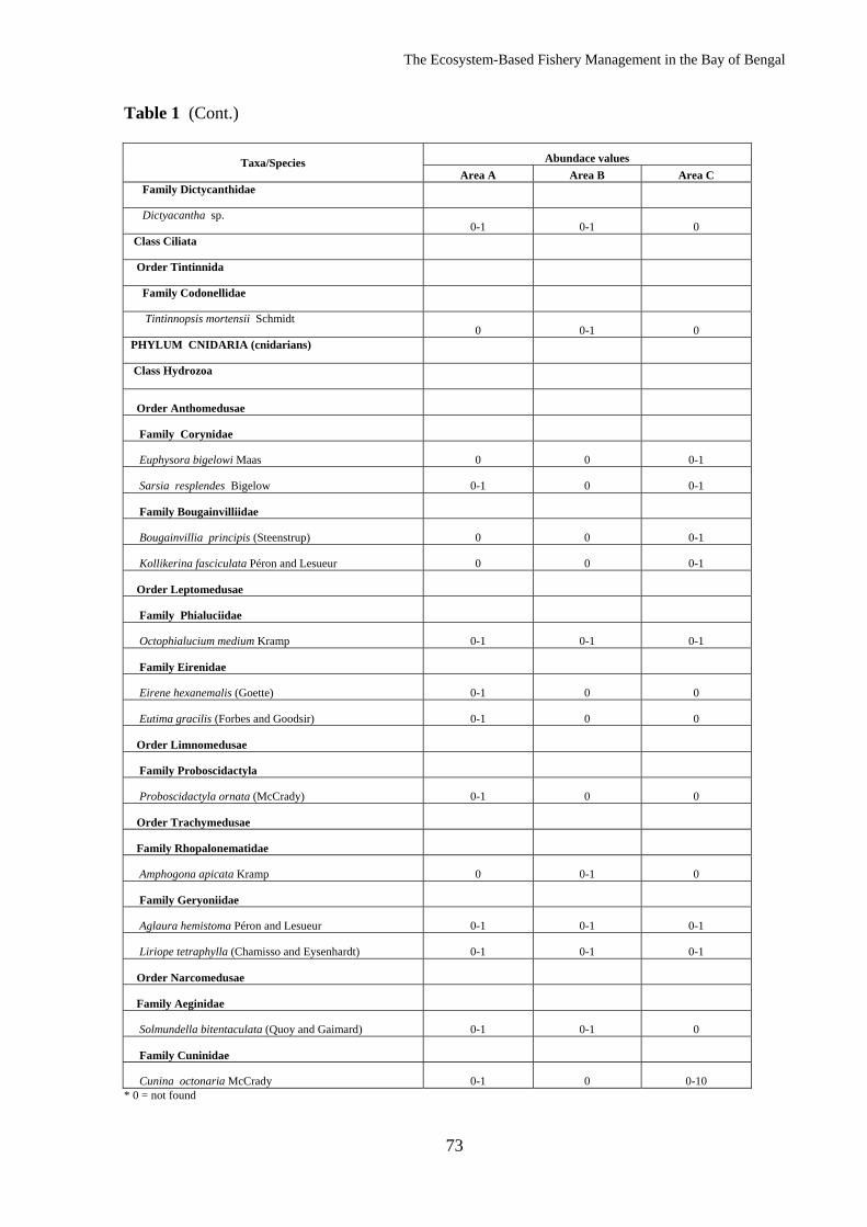
The Ecosystem-Based Fishery Management in the Bay of Bengal
73
Table 1 (Cont.)
Taxa/Species Abundace values Area A Area B Area C
Family Dictycanthidae
Dictyacantha sp. 0-1 0-1 0
Class Ciliata
Order Tintinnida
Family Codonellidae
Tintinnopsis mortensii Schmidt 0 0-1 0
PHYLUM CNIDARIA (cnidarians)
Class Hydrozoa
Order Anthomedusae
Family Corynidae
Euphysora bigelowi Maas 0 0 0-1
Sarsia resplendes Bigelow 0-1 0 0-1
Family Bougainvilliidae
Bougainvillia principis (Steenstrup) 0 0 0-1
Kollikerina fasciculata Péron and Lesueur 0 0 0-1
Order Leptomedusae
Family Phialuciidae
Octophialucium medium Kramp 0-1 0-1 0-1
Family Eirenidae
Eirene hexanemalis (Goette) 0-1 0 0
Eutima gracilis (Forbes and Goodsir) 0-1 0 0
Order Limnomedusae
Family Proboscidactyla
Proboscidactyla ornata (McCrady) 0-1 0 0
Order Trachymedusae
Family Rhopalonematidae
Amphogona apicata Kramp 0 0-1 0
Family Geryoniidae
Aglaura hemistoma Péron and Lesueur 0-1 0-1 0-1
Liriope tetraphylla (Chamisso and Eysenhardt) 0-1 0-1 0-1
Order Narcomedusae
Family Aeginidae
Solmundella bitentaculata (Quoy and Gaimard) 0-1 0-1 0
Family Cuninidae
Cunina octonaria McCrady 0-1 0 0-10 * 0 = not found
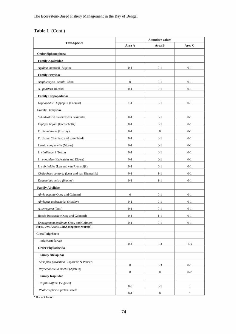
The Ecosystem-Based Fishery Management in the Bay of Bengal
74
Table 1 (Cont.)
Taxa/Species Abundace values
Area A Area B Area C
Order Siphonophora
Family Agalmidae
Agalma haeckeli Bigeloe 0-1 0-1 0-1
Family Prayidae
Amphicaryon acaule Chun 0 0-1 0-1
A. peltifera Haeckel 0-1 0-1 0-1
Family Hippopodiidae
Hippopodius hippopus (Forskal) 1-1 0-1 0-1
Family Diphyidae
Sulculeolaria quadrivalvis Blainville 0-1 0-1 0-1
Diphyes bojani (Eschscholtz) 0-1 0-1 0-1
D. chamissonis (Huxley) 0-1 0 0-1
D. dispar Chamisso and Eysenhardt 0-1 0-1 0-1
Lensia campanella (Moser) 0-1 0-1 0-1
L. challengeri Totton 0-1 0-1 0-1
L. conoidea (Keferstein and Ehlers) 0-1 0-1 0-1
L. subtiloides (Len and van Riemsdijk) 0-1 0-1 0-1
Chelophyes contorta (Lens and van Riemsdijk) 0-1 1-1 0-1
Eudoxoides mitra (Huxley) 0-1 1-1 0-1
Family Abylidae
Abyla trigona Quoy and Gaimard 0 0-1 0-1
Abylopsis eschscholtzi (Huxley) 0-1 0-1 0-1
A. tetragona (Otto) 0-1 0-1 0-1
Bassia bassensia (Quoy and Gaimard) 0-1 1-1 0-1
Enneagonum hyalinum Quoy and Gaimard 0-1 0-1 0-1 PHYLUM ANNELIDA (segment worms)
Class Polychaeta
Polychaete larvae
0-4 0-3 1-3 Order Phyllodocida
Family Alciopidae
Alciopina parasitica Clapare'de & Panceri
0 0-3 0-1 Rhynchonerella moebii (Apstein)
0 0 0-2 Family Iospilidae
Iospilus affinis (Viguier)
0-3 0-1 0 Phalacrophorus pictus Greeff
0-1 0 0 * 0 = not found
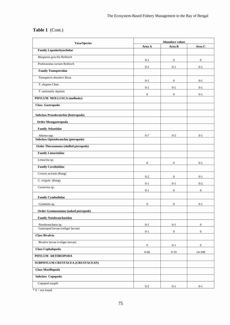
The Ecosystem-Based Fishery Management in the Bay of Bengal
75
Table 1 (Cont.)
Taxa/Species Abundace values Area A Area B Area C
Family Lopadorhynchidae
Maupasia gracilis Reibisch 0-1 0 0
Pedinosoma curtum Reibisch 0-2 0-1 0-1
Family Tomopteridae
Tomopteris dunckeri Rosa 0-1 0 0-1
T. elegans Chun 0-1 0-1 0-1
T. nationalis Apstein 0 0 0-1
PHYLUM MOLLUSCA (mollusks)
Class Gastropoda
Subclass Prosobranchia (heteropods)
Order Mesogastropoda
Family Atlantidae
Atlanta spp. 0-7 0-5 0-1 Subclass Opistobranchia (pteropods)
Order Thecosomata (shelled pteropods)
Family Limacinidae
Limacina sp.
0 0 0-1 Family Cavoliniidae
Creseis acicula (Rang)
0-2 0 0-1 C. virgula (Rang)
0-1 0-1 0-2 Cuvierina sp.
0-1 0 0
Family Cymbuliidae
Cymbulia sp. 0 0 0-1
Order Gymnosomata (naked pteropods)
Family Notobranchaeidae
Notobranchaea sp. 0-1 0-1 0 Gastropod larvae (veliger larvae)
0-1 0 0 Class Bivalvia
Bivalve larvae (veliger larvae)
0 0-1 0 Class Cephalopoda
0-66 0-35 14-108 PHYLUM ARTHROPODA
SUBPHYLUM CRUSTACEA (CRUSTACEAN)
Class Maxillopoda
Subclass Copepoda
Copepod nauplii
0-2 0-1 0-1 * 0 = not found
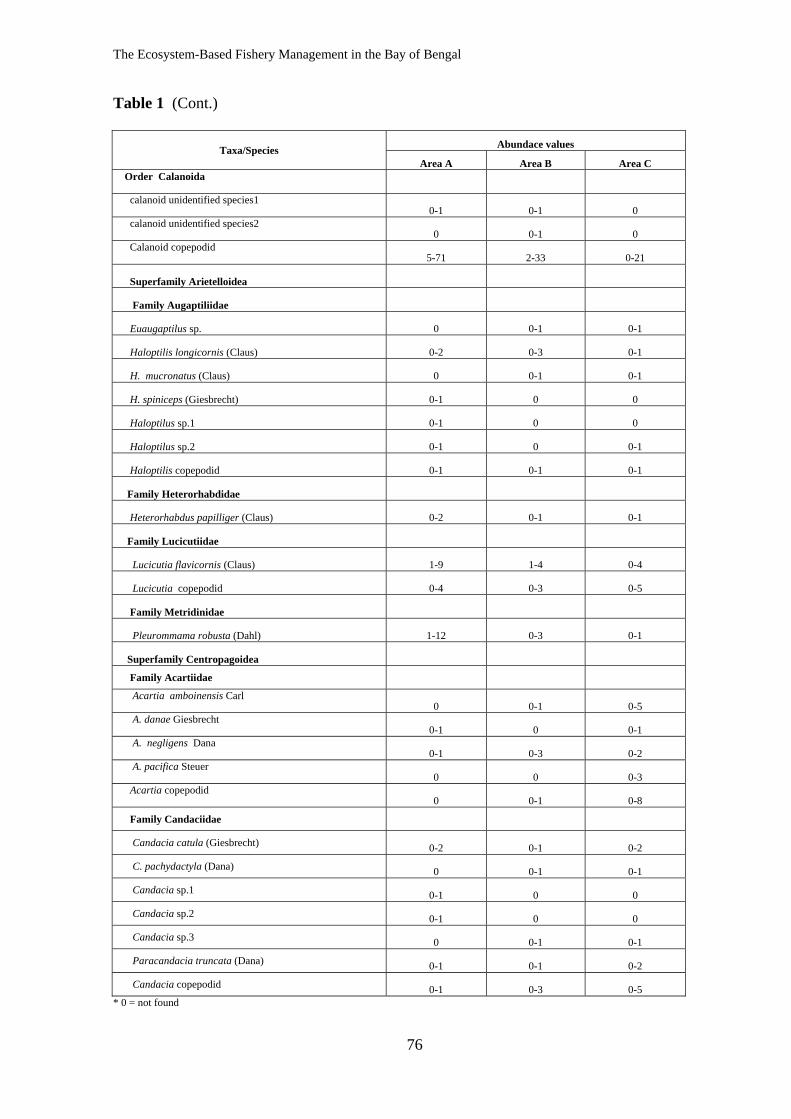
The Ecosystem-Based Fishery Management in the Bay of Bengal
76
Table 1 (Cont.)
Taxa/Species Abundace values
Area A Area B Area C Order Calanoida
calanoid unidentified species1
0-1 0-1 0 calanoid unidentified species2
0 0-1 0 Calanoid copepodid
5-71 2-33 0-21
Superfamily Arietelloidea
Family Augaptiliidae
Euaugaptilus sp. 0 0-1 0-1
Haloptilis longicornis (Claus) 0-2 0-3 0-1
H. mucronatus (Claus) 0 0-1 0-1
H. spiniceps (Giesbrecht) 0-1 0 0
Haloptilus sp.1 0-1 0 0
Haloptilus sp.2 0-1 0 0-1
Haloptilis copepodid 0-1 0-1 0-1
Family Heterorhabdidae
Heterorhabdus papilliger (Claus) 0-2 0-1 0-1
Family Lucicutiidae
Lucicutia flavicornis (Claus) 1-9 1-4 0-4
Lucicutia copepodid 0-4 0-3 0-5
Family Metridinidae
Pleurommama robusta (Dahl) 1-12 0-3 0-1
Superfamily Centropagoidea
Family Acartiidae Acartia amboinensis Carl
0 0-1 0-5 A. danae Giesbrecht
0-1 0 0-1 A. negligens Dana
0-1 0-3 0-2 A. pacifica Steuer
0 0 0-3 Acartia copepodid
0 0-1 0-8
Family Candaciidae
Candacia catula (Giesbrecht) 0-2 0-1 0-2
C. pachydactyla (Dana) 0 0-1 0-1
Candacia sp.1 0-1 0 0
Candacia sp.2 0-1 0 0
Candacia sp.3 0 0-1 0-1
Paracandacia truncata (Dana) 0-1 0-1 0-2
Candacia copepodid 0-1 0-3 0-5 * 0 = not found
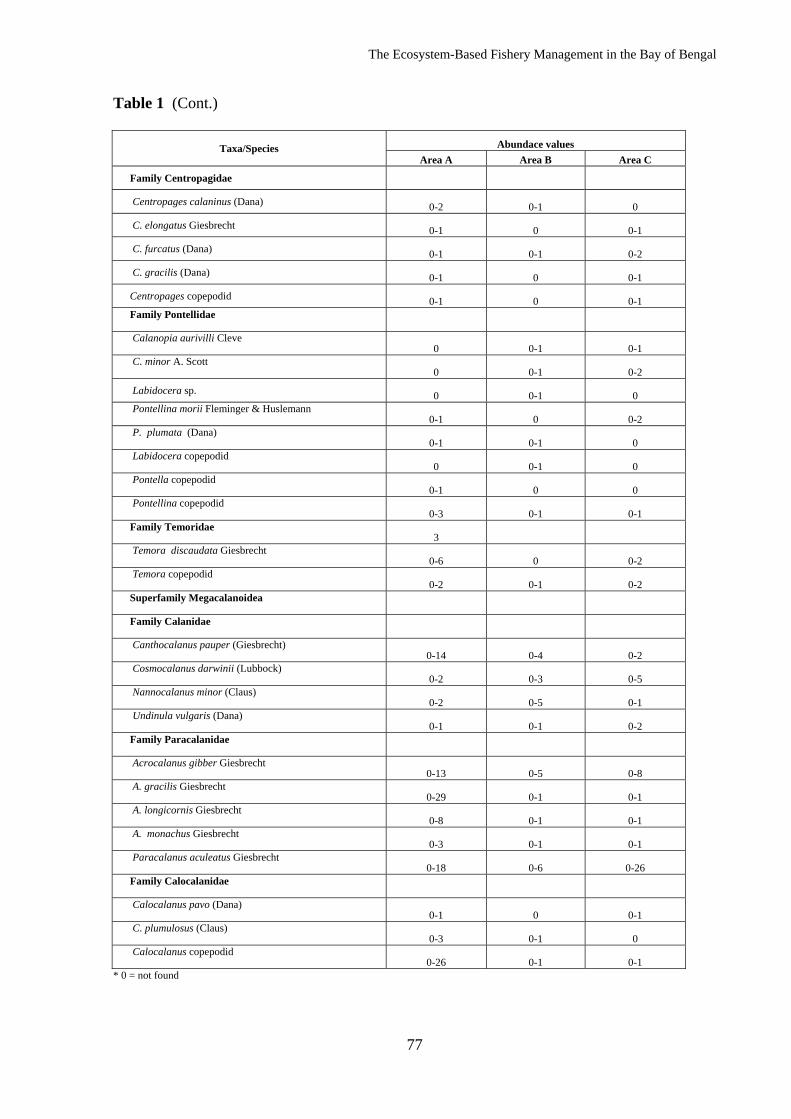
The Ecosystem-Based Fishery Management in the Bay of Bengal
77
Table 1 (Cont.)
Taxa/Species Abundace values Area A Area B Area C
Family Centropagidae
Centropages calaninus (Dana) 0-2 0-1 0
C. elongatus Giesbrecht 0-1 0 0-1
C. furcatus (Dana) 0-1 0-1 0-2
C. gracilis (Dana) 0-1 0 0-1
Centropages copepodid 0-1 0 0-1 Family Pontellidae
Calanopia aurivilli Cleve
0 0-1 0-1 C. minor A. Scott
0 0-1 0-2
Labidocera sp. 0 0-1 0 Pontellina morii Fleminger & Huslemann
0-1 0 0-2 P. plumata (Dana)
0-1 0-1 0 Labidocera copepodid
0 0-1 0 Pontella copepodid
0-1 0 0 Pontellina copepodid
0-3 0-1 0-1 Family Temoridae
3 Temora discaudata Giesbrecht
0-6 0 0-2 Temora copepodid
0-2 0-1 0-2 Superfamily Megacalanoidea
Family Calanidae
Canthocalanus pauper (Giesbrecht)
0-14 0-4 0-2 Cosmocalanus darwinii (Lubbock)
0-2 0-3 0-5 Nannocalanus minor (Claus)
0-2 0-5 0-1 Undinula vulgaris (Dana)
0-1 0-1 0-2 Family Paracalanidae
Acrocalanus gibber Giesbrecht
0-13 0-5 0-8 A. gracilis Giesbrecht
0-29 0-1 0-1 A. longicornis Giesbrecht
0-8 0-1 0-1 A. monachus Giesbrecht
0-3 0-1 0-1 Paracalanus aculeatus Giesbrecht
0-18 0-6 0-26 Family Calocalanidae
Calocalanus pavo (Dana)
0-1 0 0-1 C. plumulosus (Claus)
0-3 0-1 0 Calocalanus copepodid
0-26 0-1 0-1 * 0 = not found
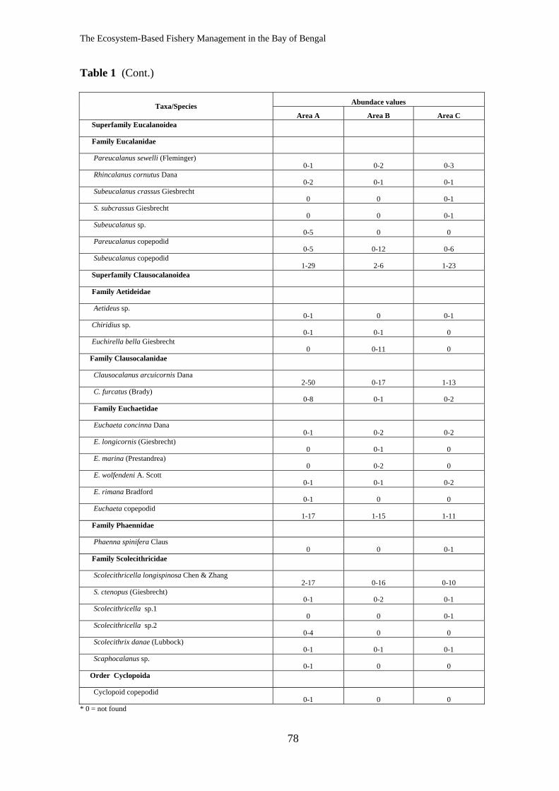
The Ecosystem-Based Fishery Management in the Bay of Bengal
78
Table 1 (Cont.)
Taxa/Species Abundace values
Area A Area B Area C Superfamily Eucalanoidea
Family Eucalanidae
Pareucalanus sewelli (Fleminger)
0-1 0-2 0-3 Rhincalanus cornutus Dana
0-2 0-1 0-1 Subeucalanus crassus Giesbrecht
0 0 0-1 S. subcrassus Giesbrecht
0 0 0-1 Subeucalanus sp.
0-5 0 0 Pareucalanus copepodid
0-5 0-12 0-6 Subeucalanus copepodid
1-29 2-6 1-23 Superfamily Clausocalanoidea
Family Aetideidae
Aetideus sp.
0-1 0 0-1 Chiridius sp.
0-1 0-1 0 Euchirella bella Giesbrecht
0 0-11 0 Family Clausocalanidae
Clausocalanus arcuicornis Dana
2-50 0-17 1-13 C. furcatus (Brady)
0-8 0-1 0-2 Family Euchaetidae
Euchaeta concinna Dana
0-1 0-2 0-2 E. longicornis (Giesbrecht)
0 0-1 0 E. marina (Prestandrea)
0 0-2 0 E. wolfendeni A. Scott
0-1 0-1 0-2 E. rimana Bradford
0-1 0 0 Euchaeta copepodid
1-17 1-15 1-11 Family Phaennidae
Phaenna spinifera Claus
0 0 0-1 Family Scolecithricidae
Scolecithricella longispinosa Chen & Zhang
2-17 0-16 0-10 S. ctenopus (Giesbrecht)
0-1 0-2 0-1 Scolecithricella sp.1
0 0 0-1 Scolecithricella sp.2
0-4 0 0 Scolecithrix danae (Lubbock)
0-1 0-1 0-1 Scaphocalanus sp.
0-1 0 0 Order Cyclopoida
Cyclopoid copepodid
0-1 0 0 * 0 = not found
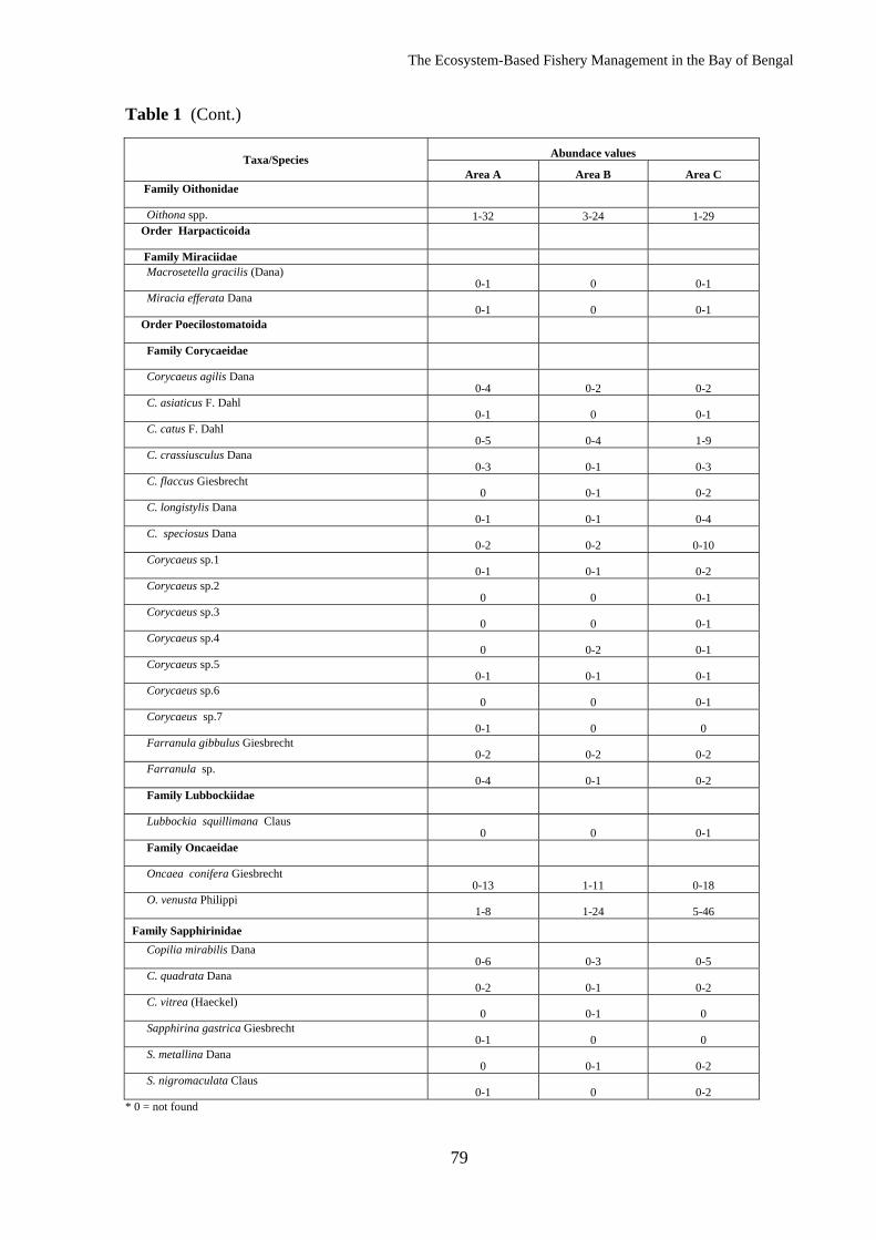
The Ecosystem-Based Fishery Management in the Bay of Bengal
79
Table 1 (Cont.)
Taxa/Species Abundace values
Area A Area B Area C Family Oithonidae
Oithona spp. 1-32 3-24 1-29 Order Harpacticoida
Family Miraciidae Macrosetella gracilis (Dana)
0-1 0 0-1 Miracia efferata Dana
0-1 0 0-1 Order Poecilostomatoida
Family Corycaeidae
Corycaeus agilis Dana
0-4 0-2 0-2 C. asiaticus F. Dahl
0-1 0 0-1 C. catus F. Dahl
0-5 0-4 1-9 C. crassiusculus Dana
0-3 0-1 0-3 C. flaccus Giesbrecht
0 0-1 0-2 C. longistylis Dana
0-1 0-1 0-4 C. speciosus Dana
0-2 0-2 0-10 Corycaeus sp.1
0-1 0-1 0-2 Corycaeus sp.2
0 0 0-1 Corycaeus sp.3
0 0 0-1 Corycaeus sp.4
0 0-2 0-1 Corycaeus sp.5
0-1 0-1 0-1 Corycaeus sp.6
0 0 0-1 Corycaeus sp.7
0-1 0 0 Farranula gibbulus Giesbrecht
0-2 0-2 0-2 Farranula sp.
0-4 0-1 0-2 Family Lubbockiidae
Lubbockia squillimana Claus
0 0 0-1 Family Oncaeidae
Oncaea conifera Giesbrecht
0-13 1-11 0-18 O. venusta Philippi
1-8 1-24 5-46 Family Sapphirinidae Copilia mirabilis Dana
0-6 0-3 0-5 C. quadrata Dana
0-2 0-1 0-2 C. vitrea (Haeckel)
0 0-1 0 Sapphirina gastrica Giesbrecht
0-1 0 0 S. metallina Dana
0 0-1 0-2 S. nigromaculata Claus
0-1 0 0-2 * 0 = not found
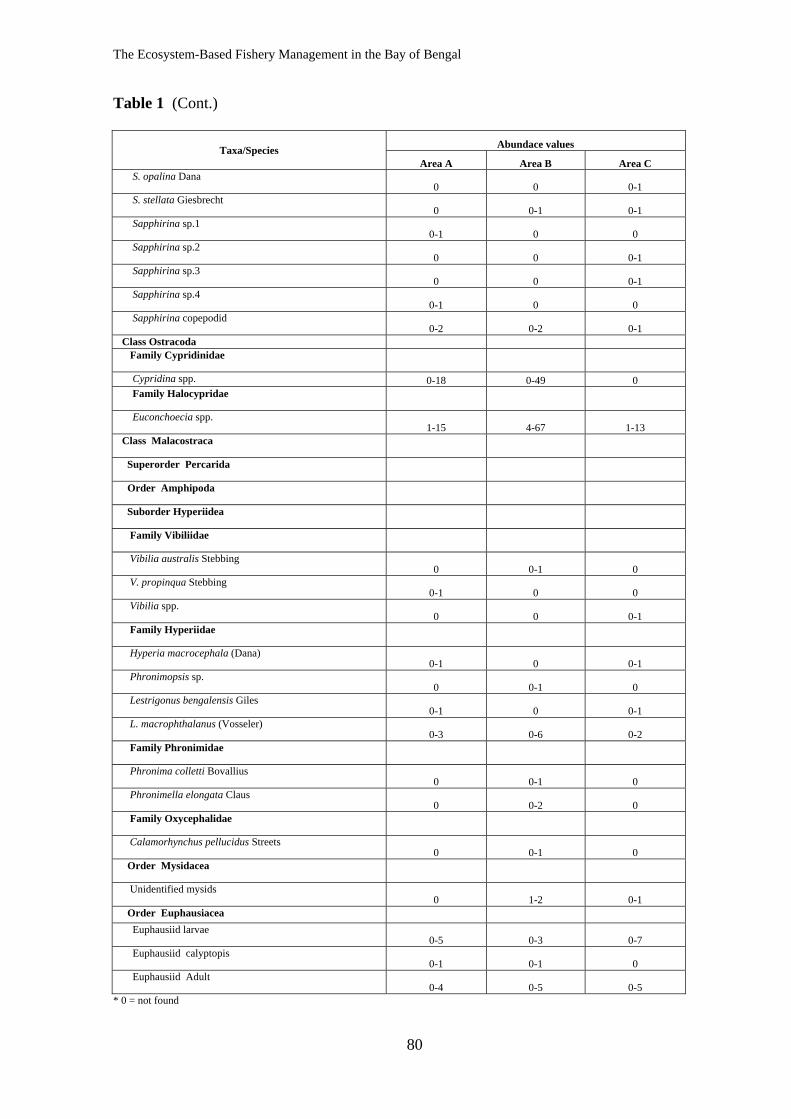
The Ecosystem-Based Fishery Management in the Bay of Bengal
80
Table 1 (Cont.)
Taxa/Species Abundace values
Area A Area B Area C S. opalina Dana
0 0 0-1 S. stellata Giesbrecht
0 0-1 0-1 Sapphirina sp.1
0-1 0 0 Sapphirina sp.2
0 0 0-1 Sapphirina sp.3
0 0 0-1 Sapphirina sp.4
0-1 0 0 Sapphirina copepodid
0-2 0-2 0-1 Class Ostracoda Family Cypridinidae
Cypridina spp. 0-18 0-49 0 Family Halocypridae
Euconchoecia spp.
1-15 4-67 1-13 Class Malacostraca
Superorder Percarida
Order Amphipoda
Suborder Hyperiidea
Family Vibiliidae
Vibilia australis Stebbing
0 0-1 0 V. propinqua Stebbing
0-1 0 0 Vibilia spp.
0 0 0-1 Family Hyperiidae
Hyperia macrocephala (Dana)
0-1 0 0-1 Phronimopsis sp.
0 0-1 0 Lestrigonus bengalensis Giles
0-1 0 0-1 L. macrophthalanus (Vosseler)
0-3 0-6 0-2 Family Phronimidae
Phronima colletti Bovallius
0 0-1 0 Phronimella elongata Claus
0 0-2 0 Family Oxycephalidae
Calamorhynchus pellucidus Streets
0 0-1 0 Order Mysidacea
Unidentified mysids
0 1-2 0-1 Order Euphausiacea Euphausiid larvae
0-5 0-3 0-7 Euphausiid calyptopis
0-1 0-1 0 Euphausiid Adult
0-4 0-5 0-5 * 0 = not found
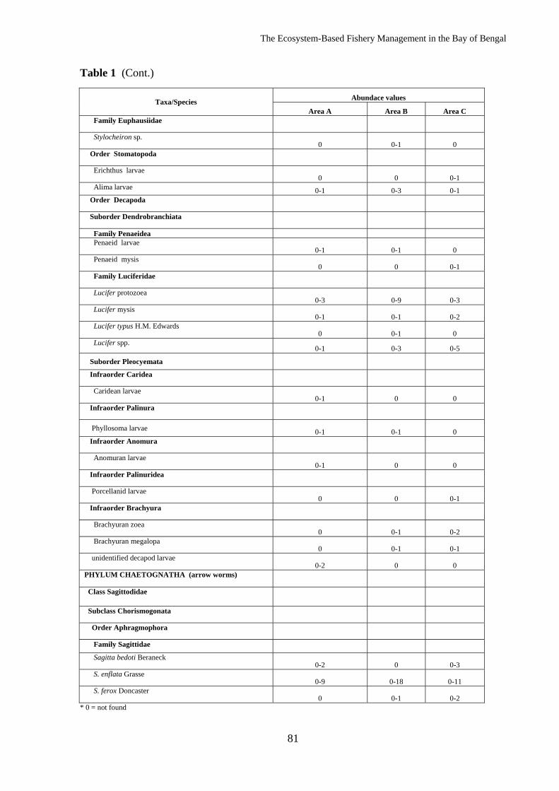
The Ecosystem-Based Fishery Management in the Bay of Bengal
81
Table 1 (Cont.)
Taxa/Species Abundace values
Area A Area B Area C Family Euphausiidae
Stylocheiron sp.
0 0-1 0 Order Stomatopoda
Erichthus larvae
0 0 0-1 Alima larvae 0-1 0-3 0-1 Order Decapoda
Suborder Dendrobranchiata
Family Penaeidea Penaeid larvae
0-1 0-1 0 Penaeid mysis
0 0 0-1 Family Luciferidae
Lucifer protozoea
0-3 0-9 0-3 Lucifer mysis
0-1 0-1 0-2 Lucifer typus H.M. Edwards
0 0-1 0 Lucifer spp.
0-1 0-3 0-5
Suborder Pleocyemata Infraorder Caridea
Caridean larvae
0-1 0 0 Infraorder Palinura
Phyllosoma larvae 0-1 0-1 0 Infraorder Anomura
Anomuran larvae
0-1 0 0 Infraorder Palinuridea
Porcellanid larvae
0 0 0-1 Infraorder Brachyura
Brachyuran zoea
0 0-1 0-2 Brachyuran megalopa
0 0-1 0-1 unidentified decapod larvae
0-2 0 0 PHYLUM CHAETOGNATHA (arrow worms)
Class Sagittodidae
Subclass Chorismogonata
Order Aphragmophora
Family Sagittidae Sagitta bedoti Beraneck
0-2 0 0-3 S. enflata Grasse
0-9 0-18 0-11 S. ferox Doncaster
0 0-1 0-2 * 0 = not found
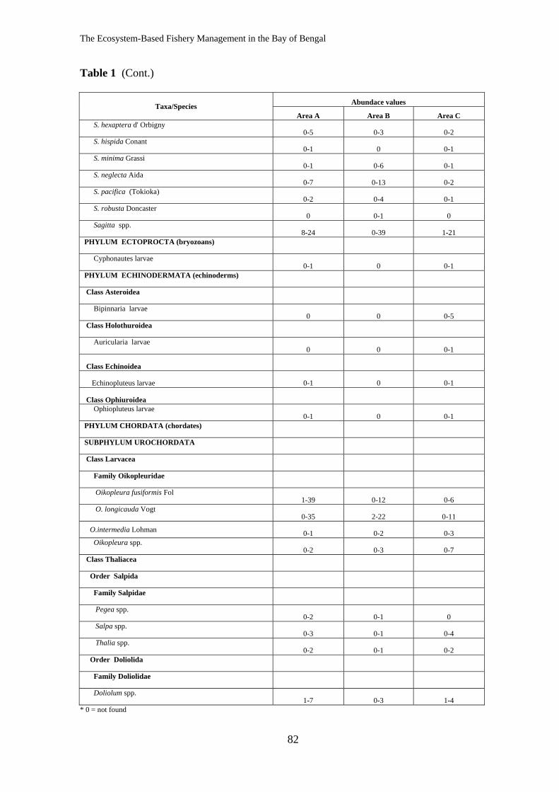
The Ecosystem-Based Fishery Management in the Bay of Bengal
82
Table 1 (Cont.)
Taxa/Species Abundace values
Area A Area B Area C S. hexaptera d' Orbigny
0-5 0-3 0-2 S. hispida Conant
0-1 0 0-1 S. minima Grassi
0-1 0-6 0-1 S. neglecta Aida
0-7 0-13 0-2 S. pacifica (Tokioka)
0-2 0-4 0-1 S. robusta Doncaster
0 0-1 0 Sagitta spp.
8-24 0-39 1-21 PHYLUM ECTOPROCTA (bryozoans)
Cyphonautes larvae
0-1 0 0-1 PHYLUM ECHINODERMATA (echinoderms)
Class Asteroidea
Bipinnaria larvae
0 0 0-5 Class Holothuroidea
Auricularia larvae
0 0 0-1
Class Echinoidea
Echinopluteus larvae 0-1 0 0-1
Class Ophiuroidea Ophiopluteus larvae
0-1 0 0-1 PHYLUM CHORDATA (chordates)
SUBPHYLUM UROCHORDATA
Class Larvacea
Family Oikopleuridae
Oikopleura fusiformis Fol
1-39 0-12 0-6 O. longicauda Vogt
0-35 2-22 0-11
O.intermedia Lohman 0-1 0-2 0-3 Oikopleura spp.
0-2 0-3 0-7 Class Thaliacea
Order Salpida
Family Salpidae
Pegea spp.
0-2 0-1 0 Salpa spp.
0-3 0-1 0-4 Thalia spp.
0-2 0-1 0-2 Order Doliolida
Family Doliolidae
Doliolum spp.
1-7 0-3 1-4 * 0 = not found
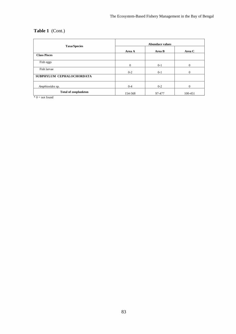
The Ecosystem-Based Fishery Management in the Bay of Bengal
83
Table 1 (Cont.)
Taxa/Species Abundace values
Area A Area B Area C Class Pisces
Fish eggs
0 0-1 0 Fish larvae
0-2 0-1 0 SUBPHYLUM CEPHALOCHORDATA
Amphioxides sp. 0-4 0-2 0
Total of zooplankton 154-568 97-477 100-451 * 0 = not found
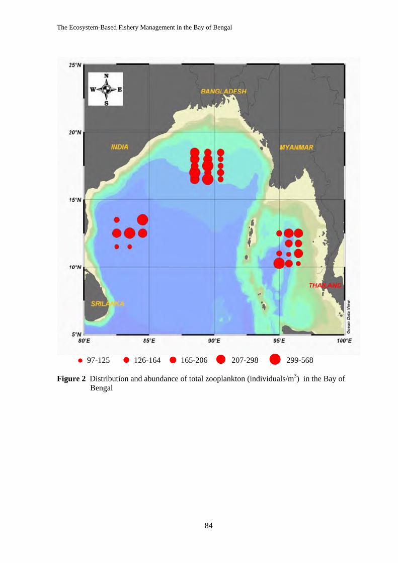
The Ecosystem-Based Fishery Management in the Bay of Bengal
84
97-125 126-164 165-206 207-298 299-568 Figure 2 Distribution and abundance of total zooplankton (individuals/m3) in the Bay of
Bengal
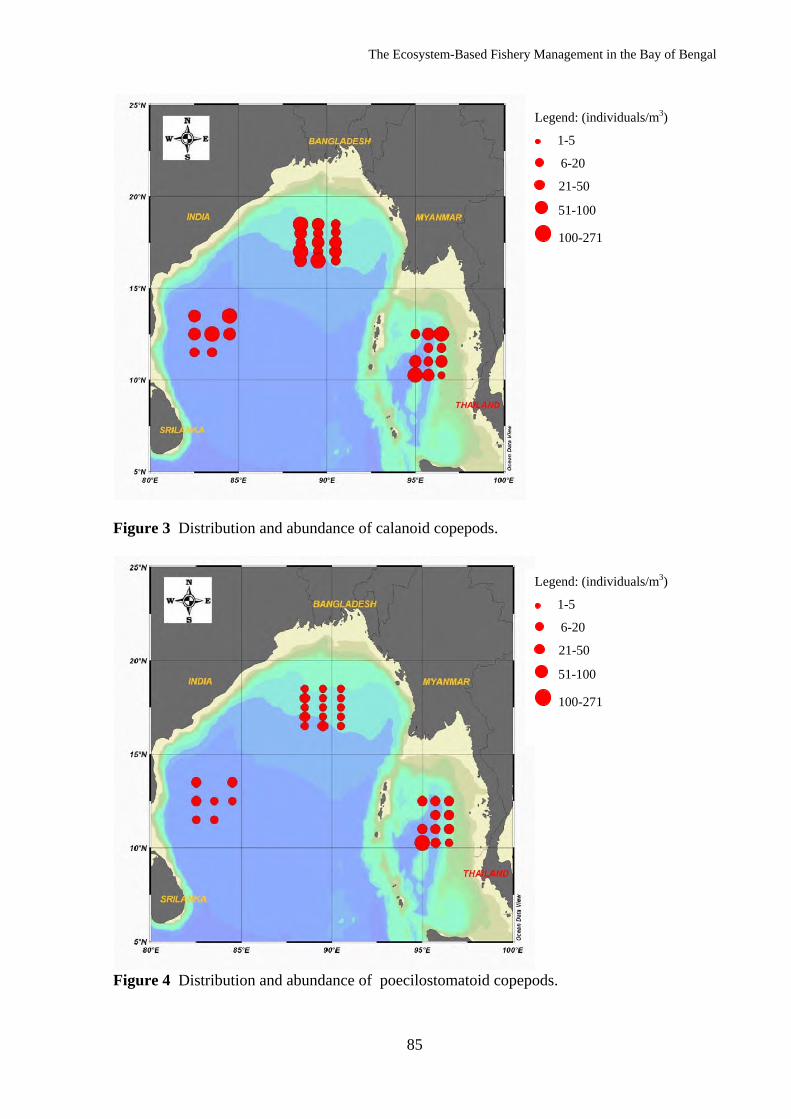
The Ecosystem-Based Fishery Management in the Bay of Bengal
85
Figure 3 Distribution and abundance of calanoid copepods.
Figure 4 Distribution and abundance of poecilostomatoid copepods.
Legend: (individuals/m3)
1-5
6-20
21-50
51-100
100-271
Legend: (individuals/m3)
1-5
6-20
21-50
51-100
100-271
The Ecosystem-Based Fishery Management in the Bay of Bengal
86
Figure 5 Distribution and abundance of planktonic shrimps.
Figure 6 Distribution and abundance of crab larvae.
Legend: (individuals/m3)
1-5
6-20
21-50
51-100
100-271
Legend: (individuals/m3)
1-5
6-20
21-50
51-100
100-271
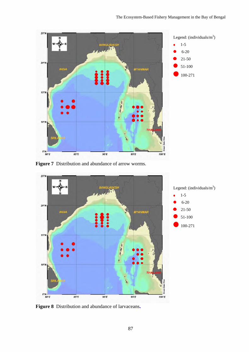
The Ecosystem-Based Fishery Management in the Bay of Bengal
87
Figure 7 Distribution and abundance of arrow worms.
Figure 8 Distribution and abundance of larvaceans.
Legend: (individuals/m3)
1-5
6-20
21-50
51-100
100-271
Legend: (individuals/m3)
1-5
6-20
21-50
51-100
100-271
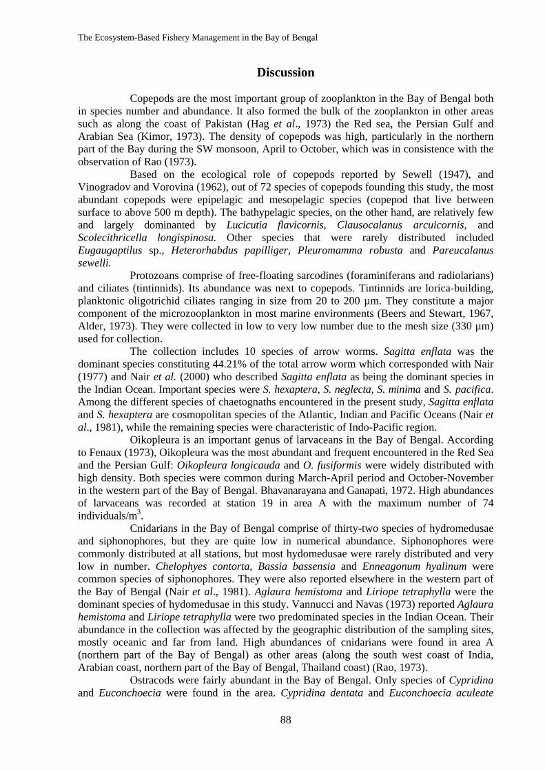
The Ecosystem-Based Fishery Management in the Bay of Bengal
88
Discussion
Copepods are the most important group of zooplankton in the Bay of Bengal both in species number and abundance. It also formed the bulk of the zooplankton in other areas such as along the coast of Pakistan (Hag et al., 1973) the Red sea, the Persian Gulf and Arabian Sea (Kimor, 1973). The density of copepods was high, particularly in the northern part of the Bay during the SW monsoon, April to October, which was in consistence with the observation of Rao (1973).
Based on the ecological role of copepods reported by Sewell (1947), and Vinogradov and Vorovina (1962), out of 72 species of copepods founding this study, the most abundant copepods were epipelagic and mesopelagic species (copepod that live between surface to above 500 m depth). The bathypelagic species, on the other hand, are relatively few and largely dominanted by Lucicutia flavicornis, Clausocalanus arcuicornis, and Scolecithricella longispinosa. Other species that were rarely distributed included Eugaugaptilus sp., Heterorhabdus papilliger, Pleuromamma robusta and Pareucalanus sewelli.
Protozoans comprise of free-floating sarcodines (foraminiferans and radiolarians) and ciliates (tintinnids). Its abundance was next to copepods. Tintinnids are lorica-building, planktonic oligotrichid ciliates ranging in size from 20 to 200 µm. They constitute a major component of the microzooplankton in most marine environments (Beers and Stewart, 1967, Alder, 1973). They were collected in low to very low number due to the mesh size (330 µm) used for collection.
The collection includes 10 species of arrow worms. Sagitta enflata was the dominant species constituting 44.21% of the total arrow worm which corresponded with Nair (1977) and Nair et al. (2000) who described Sagitta enflata as being the dominant species in the Indian Ocean. Important species were S. hexaptera, S. neglecta, S. minima and S. pacifica. Among the different species of chaetognaths encountered in the present study, Sagitta enflata and S. hexaptera are cosmopolitan species of the Atlantic, Indian and Pacific Oceans (Nair et al., 1981), while the remaining species were characteristic of Indo-Pacific region.
Oikopleura is an important genus of larvaceans in the Bay of Bengal. According to Fenaux (1973), Oikopleura was the most abundant and frequent encountered in the Red Sea and the Persian Gulf: Oikopleura longicauda and O. fusiformis were widely distributed with high density. Both species were common during March-April period and October-November in the western part of the Bay of Bengal. Bhavanarayana and Ganapati, 1972. High abundances of larvaceans was recorded at station 19 in area A with the maximum number of 74 individuals/m3.
Cnidarians in the Bay of Bengal comprise of thirty-two species of hydromedusae and siphonophores, but they are quite low in numerical abundance. Siphonophores were commonly distributed at all stations, but most hydomedusae were rarely distributed and very low in number. Chelophyes contorta, Bassia bassensia and Enneagonum hyalinum were common species of siphonophores. They were also reported elsewhere in the western part of the Bay of Bengal (Nair et al., 1981). Aglaura hemistoma and Liriope tetraphylla were the dominant species of hydomedusae in this study. Vannucci and Navas (1973) reported Aglaura hemistoma and Liriope tetraphylla were two predominated species in the Indian Ocean. Their abundance in the collection was affected by the geographic distribution of the sampling sites, mostly oceanic and far from land. High abundances of cnidarians were found in area A (northern part of the Bay of Bengal) as other areas (along the south west coast of India, Arabian coast, northern part of the Bay of Bengal, Thailand coast) (Rao, 1973).
Ostracods were fairly abundant in the Bay of Bengal. Only species of Cypridina and Euconchoecia were found in the area. Cypridina dentata and Euconchoecia aculeate
The Ecosystem-Based Fishery Management in the Bay of Bengal
89
found in neritic as well as ocenics waters. George and Nair (1980) Euconchoecia spp. was dominant at most stations in the Bay of Bengal (Nair et al., 1981) but they always presented in low number in this study. High abundances (116 individuals/m3) of ostracod was observed at station 29 in area B (western part of the Bay of Bengal).
Thaliaceans in the Bay of Bangal comprise of Salps (Pegea, Salpa and Thalia) and only one doliolid genus (Doliolum). Doliolum spp. were commonly distributed at all areas. According to Bhavanarayana and Ganapati (1972), they were common during March-April period and October-November in the western part of the Bay of Bengal. Salps were scarcely distributed in this study.
Regarding planktonic shrimps (included larval stages of Penaeid, Caridean and Palinuran shrimps and Lucifer), they were very rarely distributed with low values. Larval stages of euphausids were commonly distributed but in very low number. Only adult stages of Stylocheiron was found in area B (westhern part of the Bay of Bengal). Stylocheiron insulare , a coastal species, recurred in the Andaman Sea and south of Java. (Brinton and Gopolakrishnan, 1973). In the case of polycheaetes, there were both planktonic forms and larval forms (meroplankton). Larval forms were widely distributed with low number but planktonic forms occurrence were rarely distributed. Mollusks presented in the area included gastropod larvae, planktonic mollusks and bivalved larvae. Atlanta and Creseis were common in the Bay of Bengal with low number. Planktonic mollusks and bivalved larvae were sparse in this study. Lestrigonus macroohthalanus was the dominant species of hyperiid in the Bay of Bengal. Most hyperiids were rarely distributed in small numbers. Fairly high concentration of amphipods were noted towards the northern part of the Bay of Bengal (Nair et al.,1981). But the abundance of hyperiids of area B (western part of the Bay of Bengal) was higher thanthose of other areas. Echinoderm larvae, mysids, crab larvae, stomatopod larvae, decapod larva, bryozoans and cephalochordates yielded low abundance in all samples examined. Their detailed results will be published elsewhere.
Acknowledgements
The authors would like to thank Ms.Nittaya Wuttichareanmongkol, Ms.Natthawadee Phukham, and Ms. Supattra Rodniam who identified cnidarians and copepods.
Reference
Alda, V. A. 1973. Tintinnoinea. In: Zeitzschel, B. and S. Gerlach (eds.). The Biology of the Indian Ocean. Springer-Verlag, New York. p. 321-384.
Alvarino, A. 1967. The Chaetognatha of the NAGA Expedition (1959-1961) in the South China Sea and the Gulf of Thailand. NAGA Report, Vol.4, Part 2. 194 p.
Alder, V. A. 1999. Tintinnoinea. In: Boltovskoy, D. (ed.). South Atlantic Zooplankton. Vol.1. Backhuys Publishers, Leiden. p. 321-384.
Anderson, O. R. 1983. Radiolaria. Springer-Verlay, New York. 335 p. Anderson, O. R., M. Spindler, A. W. H. Bé and C. H. Hemleben. 1979. Trophic activity of
planktonic foraminifera. J. mar. biol. Assoc. UK. 59:791-799. Angel, M. V. 1999. Ostracoda. In: Boltovskoy, D. (ed.). South Atlantic Zooplankton.
Vol.2. Backhuys Publishers, Leiden. p. 815-868. Beers, J. R. and J. L. Stewart. 1967. Microplankton in the euphotic zone at five locations
across the California current. J. Fish Res. Bd. Canada, 24:203-2068. Bernstein, R., S. A. Kling and D. Boltovskoy. 1999. Acantharia. In: Boltovskoy, D. (ed.).
South Atlantic Zooplankton. Vol.1. Backhuys Publishers, Leiden. p. 75-148.
The Ecosystem-Based Fishery Management in the Bay of Bengal
90
Boltovskoy, D. 1999. Radiolaria Polycystina. In: Boltovskoy, D. (ed.). South Atlantic Zooplankton. Vol.1. Backhuys Publishers, Leiden. p. 149-212.
Bouillion, J. 1999. Hydromedusae. In: Boltovskoy, D. (ed.). South Atlantic Zooplankton. Vol.1. Backhuys Publishers, Leiden. p. 385-465.
Bradford-Grieve, J. M., E. L. Markhaseva, C. E. F. Rocha and B. Abiahy. 1999. Copepoda. In: Boltovskoy, D. (ed.). South Atlantic Zooplankton Vol. 2. Backhuys Publishers, Leiden. p. 869-1098.
Brinton, E. and K. Gopalakrishnan. 1973. The distribution of Indian Ocean Euphausiids. In : Zeitzschel, B. and S. Gerlach (eds.). The biology of the Indian Ocean. Springer-Verlag, New York. p. 257-328.
Daniel, R. 1985. Coelenterata: Hydrozoa, Siphonophora. The fauna of India and the adjacent countries zoological survey of India.
Casanova, J. P. 1999. Chaetognatha. In: Boltovskoy, D. (ed.). South Atlantic Zooplankton. Vol.2. Backhuys Publishers, Leiden. p. 1353-1374.
Chihara, M. and M. Murano. 1997. An Illustrated Guide to Marine Plankton in Japan. Tokai University Press. Shizuoka, Japan. p. 649-1000.
Conway, D. V. P., R. G. White, J. Hugues-Dit-Cile, C. P. Gallienne and D. B. Robins. 2003. Guid to the coastal and surface zooplankton of the south-western Indian ocean. Marine Biological Association of the United Kingdom Occasional Publication. 322 p.
Day, J. H. 1967. A Monograph on the Polychaeta of Southern Africa. Part I. Errantia, Part 2, Sedentaria. Trustees of the British Museum (Natural History), London.
Esnal, G. B. 1999. Appendicularia. In: Boltovskoy, D. (ed.). South Atlantic Zooplankton. Vol.2. Backhuys Publishers, Leiden. p. 1375-1400.
Esnal, G. B. 1999. Pyrosomatida. In: Boltovskoy, D. (ed.). South Atlantic Zooplankton. Vol.2. Backhuys Publishers, Leiden. p. 1401-1408.
Esnal, G. B. and M. C. Daponte. 1999. Doliolida. In: Boltovskoy, D. (ed.). South Atlantic Zooplankton. Vol.2. Backhuys Publishers, Leiden. p. 1409-1422.
Esnal, G. B. and M. C. Daponte. 1999. Salpida. In: Boltovskoy, D. (ed.). South Atlantic Zooplankton. Vol.2. Backhuys Publishers, Leiden. p. 1423-1444.
Fenaux, R. 1973. Appendicularians from the Indian Ocean, Red Sea and the Persian Gulf. In: Zeitchel, B. and S. A. Gerlach (eds). The biology of the Indian Ocean. 3:409-414.
George, J. and V. R. Nair. 1980. Planktonic ostracods of the northern Indian Ocean. Mahasager Bull. Natn. Inst. Oceanogr. 3:29-44.
Gibbons, M. J., V. A. Spiridonov and G. A. Tarling. 1999. Euphausiacea. In: Boltovskoy, D. (ed.). South Atlantic Zooplankton. Vol.2. Backhuys Publishers, Leiden. p. 1241-1280.
Halim, Y. 1969. Plankton of the Red Sea. Oceansar. Mar. Biol. Ann. Rev. 7: 231-275. Haq, S. M., J. A. Khan and S. Chugtai. 1973. The distribution and abundance of zooplankton
along the coast of Pakistan during postmonsoon and premonsoon periods. In: Zeitzschel, B. and S. Gerlach (eds.). The Biology of the Indian Ocean. Springer-Verlag, New York. p. 257-272.
Hemleben, C. H., M. Spindler, I. Breitinger and W. B. Deuser. 1985. Field and laboratory studies on the ontogony and ecology of some globorotalid species from the Sargasso sea off Bermuda. J. Foram. Res. 15:254-272.
Kasturirangan, L. R. 1963. A key for the identification of the more common plankton copepoda of Indian coastal waters. Council of Scientific and Industrial research, New Delhi. 87 p.
Kemle-von Mücke, S. and C. Hemleben. 1999. Foraminifera. In: Boltovskoy, D. (ed.). South Atlantic Zooplankton. Vol.1. Backhuys Publishers, Leiden. p. 43-74.
The Ecosystem-Based Fishery Management in the Bay of Bengal
91
Kimor, B. 1973. Plankton relations of the Red Sea, Persian Gulf and Arabian Sea. In: Zeitzschel, B. and S. Gerlach (eds.). The Biology of the Indian Ocean. Springer-Verlag, New York. p. 221-232.
Kling, S. A. and D. Boltovskoy. 1999. Radiolaria. In: Boltovskoy, D. (ed.). South Atlantic Zooplankton. Vol.1. Backhuys Publishers, Leiden. p. 213-264.
Kramp, P. L. 1968. The Hydromedusae of the Pacific and Indian Ocean. “DANA” No. 63. 162 p. Martin, J. W. and G. E. Davis. 2001. An Update Classification of the Recent Crustacea.
Science Series No. 39, Natural History Museum of Los Angeles County. p. 58-75. Minanzan, H. W. 1999. Ctenophora. In: Boltovskoy, D. (ed.). South Atlantic Zooplankton.
Vol.1. Backhuys Publishers, Leiden. p. 561-574. Mulyadi, M. D. 2002. The calanoid copepods family Pontellidae from Indonesian waters,
with notes on its species-groups. Treubia. 32(2):1-167. Mulyadi, M. D. 2004. Calanoid Copepods in Indonesian Waters. Research Center for
Biology, Indonesia institute of Sciencs Bogor, Indonesia. 195 p. Nair, K. K. C., P. G. Jacob and S. Kumaran. 1973. Distribution and abundance of planktonic
amphipods in the Indian Ocean. In: Zeitchel, B. and S. A. Gerlach (eds.). The biology of the Indian Ocean. Springer-Verlag, Berlin. p. 349-356.
Nair, V. R. 1977. Chaetognaths of Indian Ocean. Proc. Symp. Warmwater Zoopl. Spl. Publ. 168-195.
Nair, S. R. S., V. R. Nair, C. T. Achuthankutty and M. Madhupratap. 1981. Zooplankton composition and diversity in western Bay of Bengal. Journal of Plankton Research 3(4):493-508.
Nair, V. R., K. V. Jayalakshmy and M. Terazaki. 2000. Abundance and diversity of chaetognaths from the Rodriguez Triple Junction area of the Indian Ocean. Deccan Geography 38(1-2):41-51.
Onbé, T. 1999. Ctenopoda and Onychopoda (Cladocera). In: Boltovskoy, D. (ed.). South Atlantic Zooplankton. Vol.1. Backhuys Publishers, Leiden. p. 797-814
Owre, H. B. and M. Foyo. 1967. Fauna Caribaea Manuals for the Identification of the Fauna of the Tropical Western Atlantic. Fauna Caribeae Number 1 Crustacea, Part 1: Copepoda: Copepods of the Florida Current. Institute of Marine Science, University of Miami. 137 p.
Othman, B. H. R. and Toda, T. 2006. Pontellid copepods from Singapore. In: Coastal Marine Science Special Issue: The proceeding of the 2nd seminar of JSPS Multilateral Core University Program on Coastal Oceanography. Coastal Marine Science 30(1):305-319.
Pohle, G., A. Fransozo, M. L. Negreiros-Fransozo and F. L. M Mantelotto. 1999. Larval Decapoda (Brachyura). In: Boltovskoy, D. (ed.). South Atlantic Zooplankton. Vol.2. Backhuys Publishers, Leiden. p. 1281-1352.
Pugh, P. R. 1999. Siphonophorae. In: Boltovskoy, D. (ed.). South Atlantic Zooplankton. Vol.1. Backhuys Publishers, Leiden. p. 467-511.
Rao, T. S. S. 1973. Zooplankton studies in the Indian Ocean. In: Zeitzschel, B. and Gerlach, S. (eds.). The biology of the Indian Ocean. Springer-Verlag, New York. p. 243-255.
Richter, G. and R. R. Seapy. 1999. Heteropoda. In: Boltovskoy, D. (ed.). South Atlantic Zooplankton. Vol.1. Backhuys Publishers, Leiden. p. 621-648.
Russell, F. S. 1953. The Medudae of the British Isles. Anthomedusae, Leptomedusae, Trchymedusae, Narcomedusae. Cambridge at the University Press, London. The United Kingdom.
Sewell, R. B. S. 1947. The free swimming plangtonic copepoda. Systematic account. Sci. Rep. John Murray Exped. 8:1-303.
The Ecosystem-Based Fishery Management in the Bay of Bengal
92
Sullivan, D. O. 1982. A Guide of the Hydromedusae of the Southern Ocean and Adjacent Waters. A rare Research Notes 5. Antarctic Division, Department of Science and Technology. Australia.
Suwanrumpha, W. 1987. A Key for the Identification of Copepods Collected in the Gulf of Thailand Waters. Technical Paper No. 4. Marine Fisheries Laboratory Marine Fisheries Division, Bangkok. 147 p.
Theusen, E. and M. A. F. Alamo. 1999. Polychaeta. In: Boltovskoy, D. (ed.). South Atlantic Zooplankton. Vol.1. Backhuys Publishers, Leiden. p. 595-620.
Vannucci, M. and D. Navas. 1973. Distribution of hydromedusae in the Indian Ocean. in: Zeitchel, B. and S. A. Gerlach (eds.). The Biology of the Indian Ocean. Ecological Studies.Vol.3. p. 273-281.
Van Spoel, S. and J. R. Dadon. 1999. Pteropoda. In: Boltovskoy, D. (ed.). South Atlantic Zooplankton. Vol.1. Backhuys Publishers, Leiden. p. 649-706.
Vinogradov, G. 1999. Amphipoda. In: Boltovskoy, D. (ed.). South Atlantic Zooplankton. Vol.2. Backhuys Publishers, Leiden. p. 1141-1240.
Vinogradov, M. E. and N. M. Voronina. 1962. The distribution of different groups of plankton in accordane with their trophic level in the Indian Equatorial Current area. Rapp. P.-V. Requn. Cous. Inst. Exlor. Mer. 153:200-204.
Vinogradov, M. E., A. F. Volkov and T. N. Semenova. 1996. Hyperiid amphipods (Amphipoda, Hyperiidae) of the world oceans. Science Publishes, Inc., U.S.A. 632 p.
Win, K. 1977. A species list of the zooplankton from the coastal water of Burma. In: Proceedings of the Symposium on Warm Water Zooplankton, 14-19 October, 1977,
National Institute of Oceanography, Goa, India. p. 93-99. Wutticharoenmongkol, N. and L. Wongrat, L. 2004. Diversity and abundance of planktonic
hydrozoans, class hydrozoa in the upper Gulf of Thailand. J. Science Res. (Section T), 3(1):27-44. (In Thai, English abstract)
Wikipedia. Available Source: http://en.wikipedia.org/wiki/Zooplankton. July 14, 2008. Wapedia. Available Source: http://wapedia.mobi/en/Zooplankton. July 14, 2008.
The Ecosystem-Based Fishery Management in the Bay of Bengal
93
Composition, Abundance and Distribution of Fish Larvae in the Bay of Bengal
Pattira Lirdwitayaprasit1, Chirat Nuangsang1, Paitoon Puewkhao2 Md. Jalilur Rahman3, U Aung Htay Oo4, and U Aung Win Sien5
1 Deep Sea Fishery Technology Research and Development Institute,
Department of Fisheries, Samutprakarn 10270, THAILAND 2 Andaman Sea Fisheries Research and Development Center,
Department of Fisheries, Phuket 83000, THAILAND
3Marine Fisheries and Technology Station, Bangladesh Fisheries Research Institute, Motel Road, Cox’s Bazar-4700, BANGLADESH
4 Marine Fishery Resources Survey and Research Unit, Department of Fisheries, Yangon, MYANMAR 5Department of Fisheries, Insein Rd, West Gyoton, Insein Township, Yangon, MYANMAR
Abstract
The study on composition, abundance, and distribution of fish larvae was
conducted in the Bay of Bengal (BOB) with the aim to get more scientific data for fishery management in this area. Fish larvae samples were collected in the northern (area A), western (area B) and eastern part (area C) of the BOB during the period of 25 October to 6 December, 2007. Fifty-two families of fish larvae were identified of which Photichthyidae was the most abundance. Fifty one families could be found in area C while only nineteen and eighteen families were observed in area B and A. The highest average density of total fish larvae, 485 larvae/1,000 m3, was also obtained in area C. A total of twenty-four economic important fish larvae families were found in the studied areas. Almost all economic families were presented in area C while 8 and 7 families were found in area B and A. These results suggested that the Andaman Sea or area C was the richest diversity and most abundant of fish larvae in this study. Regarding to tuna larvae, a small number were recorded during this survey period. Six species of tuna larvae were found in area C, 3 species in area A and 2 species in area B. The relationships between environmental parameters and fish larvae abundance have not been analyzed statistically due to the small sample sizes in this study. However, the spatial changes in temperature indicating that at 75 m depth of three study areas the temperature was obviously fluctuated whereas at the surface and 150 m depth a slightly change was observed. As for the changes in salinity, the results showed the halocline layer of area C was deeper than those of area A and B indicating that these areas were influenced by the river runoff of which the huge nutrients were discharged. Although, this study provided some information about abundance and distribution of fish larvae in the BOB but there are still not enough to understand the clear pattern of fish larvae abundance and distribution of the whole area. The further study on temporal and spatial distribution of fish larvae in relation to oceanographic parameters was also recommended. Key words: composition, abundance, distribution, fish larvae, Bay of Bengal
Introduction
The Bay of Bengal (BOB) is one of the large marine ecosystem of the world
ocean that lacks of large scale seasonal upwelling and defined as moderately productive ecosystem (Madhupratap et al., 2003). BOB is land locked ocean in the north and influenced by seasonally reversing monsoon winds. Shankar et al. (2002) reported that the low sea surface salinities, particularly in the northern region of BOB were a result of the heavy
The Ecosystem-Based Fishery Management in the Bay of Bengal
94
monsoonal precipitation. The large freshwater are from the Ganga, Brahmaputra and Irrawaddy rivers (UNESCO, 1988). This excess water fluxes is a significant source of freshwater to BOB. The large riverine outflows generates highly stable stratification in the upper layers of the northern BOB and forms a strong “barrier layer” to the re-supply of nutrients from deeper waters during summer monsoon throughout the post-summer periods. The barrier layer in conjunction with hydrographic characteristics will have a profound influence on the biological productivity (Sprintall and Tomczak 1992, Vinayachandran et al., 2002)
Generally, BOB is considered to have a lower biological productivity than its western counterpart, the Arabian Sea. Although the rivers may bring nutrients, these are though to be removed in the deeper waters because of the narrow shelf (Qasim, 1970). Most previous biological studies in BOB focused mainly on the seasonal variation in primary production and on the composition and abundance of mesozooplankton (Nair et al., 1981; Achuthankutty et al., 1980; Madhupratap et al., 2003) but little is known about fish larvae abundance and its composition.
In this present work, the study of larvae is a part of the biological oceanographic survey incorporated in the project Ecosystem-Based Fishery Management in the Bay of Bengal (BOB) which is a collaborative survey project among member countries of BIMSTEC (Bangladesh, India, Myanmar, Sri Lanka, Nepal and Thailand) aimed for fishery management. The understanding of abundance and distribution of fish larvae in conjunction with ecological conditions could fill up the gap in the study of fish life history and be considered as an important information for fishery management. Generally, the larval stage is most vulnerable to ecological changes, any fluctuation either quality or quantity of the ecological conditions will be harmful to larval lives and may probably indicate the onward potential of recruitment (Leis and Rennis, 1983). Although, there was some information of fish larvae in some coastal areas of the Indian Ocean but little is known about the distribution and abundance of fish larvae in offshore areas of the BOB.
To provide more information of fish larvae for fishery management, the study on abundance and distribution of fish larvae in the eastern, northern and western part of the BOB was conducted. The results may be served as the basic information to evaluate the existing of fish stocks and may also be served as the preliminary information for the future investigations in relation to environmental parameters.
Objectives
1. To identify fish larvae composition. 2. To determine abundance and distribution of the total fish larvae and the top five
most abundant families. 3. To determine abundance and distribution of tuna larvae in the Bay of Bengal. 4. To compare fish larvae assemblages by stations.
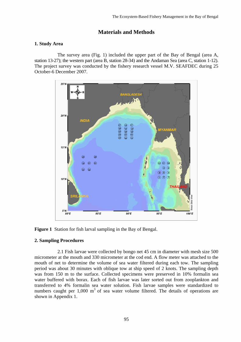
The Ecosystem-Based Fishery Management in the Bay of Bengal
95
Materials and Methods 1. Study Area
The survey area (Fig. 1) included the upper part of the Bay of Bengal (area A, station 13-27); the western part (area B, station 28-34) and the Andaman Sea (area C, station 1-12). The project survey was conducted by the fishery research vessel M.V. SEAFDEC during 25 October-6 December 2007.
Figure 1 Station for fish larval sampling in the Bay of Bengal. 2. Sampling Procedures
2.1 Fish larvae were collected by bongo net 45 cm in diameter with mesh size 500 micrometer at the mouth and 330 micrometer at the cod end. A flow meter was attached to the mouth of net to determine the volume of sea water filtered during each tow. The sampling period was about 30 minutes with oblique tow at ship speed of 2 knots. The sampling depth was from 150 m to the surface. Collected specimens were preserved in 10% formalin sea water buffered with borax. Each of fish larvae was later sorted out from zooplankton and transferred to 4% formalin sea water solution. Fish larvae samples were standardized to numbers caught per 1,000 m3 of sea water volume filtered. The details of operations are shown in Appendix 1.
The Ecosystem-Based Fishery Management in the Bay of Bengal
96
2.2 Environmental factors (temperature, salinity) at 3 levels (surface water, 75 m and 150 m) in each station were measured by CTD at the same time as fish larvae were collected. 3. Laboratory Method
Fish larvae were identified under stereo microscope to family level by using the descriptions of related taxa given in Leis and Rennis (1983), Ozawa (1986), Nishikawa and Rimmer (1987), Matsumoto (1958), Matsumoto (1972), Leis and Carson-Edwart (2000). Unidentified larvae were placed in “unknown” category due to the samples were too small to identify and damaged larvae were placed in “incomplete” category. 4. Data Analysis
The number of total fish larvae and the top five most abundant families which were standardized to number caught per 1,000 m3 of seawater volume filtered were mapped for spatial distribution.
Determination of the Constancy of Occurrence was based on the ecological index proposed by Dajoz (1983) cited by Schifino et. al., 2004:
C = P/Q x100
Where: C = Constancy of Occurrence of the family (%) P = Number of samples where the family occurred Q = Total number of samples
The families were then divided into three categories:
Constants (when C>50%) Accessories (when 25%≤C≤50%) Accidental (when C<25%)
Determination for the type of fish larvae which grouped into 5 categories based on
the adult habitat (Smith and Heemstra, 1986). Group 1: fresh water fish Group 2: neritic fish Group 3: inshore-reef fish Group 4: shallow to oceanic fish Group 5: oceanic fish
For comparing the community structures of fish larvae by station, a cluster
analysis was used as shown in the form of a dendrogram. The analysis used a squared Euclidean distance as a measurement of proximity and followed an unweighted pair group method-arithmetic average for linkage as described by Pielou (1984). The software used for cluster analysis was Statistica for Windows 6.0 version (Statsoft, Inc. 1984-2001).
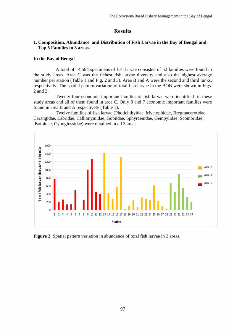
The Ecosystem-Based Fishery Management in the Bay of Bengal
97
Results 1. Composition, Abundance and Distribution of Fish Larvae in the Bay of Bengal and Top 5 Families in 3 areas. In the Bay of Bengal
A total of 14,584 specimens of fish larvae consisted of 52 families were found in the study areas. Area C was the richest fish larvae diversity and also the highest average number per station (Table 1 and Fig. 2 and 3). Area B and A were the second and third ranks, respectively. The spatial pattern variation of total fish larvae in the BOB were shown in Figs. 2 and 3.
Twenty-four economic important families of fish larvae were identified in these study areas and all of them found in area C. Only 8 and 7 economic important families were found in area B and A respectively (Table 1).
Twelve families of fish larvae (Photichthyidae, Myctophidae, Bregmacerotidae, Carangidae, Labridae, Callionymidae, Gobiidae, Sphyraenidae, Gempylidae, Scombridae, Bothidae, Cynoglossidae) were obtained in all 3 areas.
0
200
400
600
800
1000
1200
1400
1600
1 2 3 4 5 6 7 8 9 10 11 12 13 14 15 16 17 18 19 20 21 22 23 24 25 26 27 28 29 30 31 32 33 34
Station
Area A
Area B
Area C
Tot
al fi
sh la
rvae
(lar
vae/
1,0
00 m
3)
Figure 2 Spatial pattern variation in abundance of total fish larvae in 3 areas.
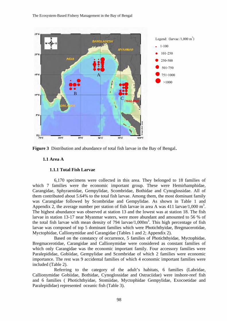
The Ecosystem-Based Fishery Management in the Bay of Bengal
98
Figure 3 Distribution and abundance of total fish larvae in the Bay of Bengal.
1.1 Area A 1.1.1 Total Fish Larvae
6,170 specimens were collected in this area. They belonged to 18 families of which 7 families were the economic important group. These were Hemirhamphidae, Carangidae, Sphyraenidae, Gempylidae, Scombridae, Bothidae and Cynoglossidae. All of them contributed about 5.64% to the total fish larvae. Among them, the most dominant family was Carangidae followed by Scombridae and Gempylidae. As shown in Table 1 and Appendix 2, the average number per station of fish larvae in area A was 411 larvae/1,000 m3. The highest abundance was observed at station 13 and the lowest was at station 18. The fish larvae in station 13-17 near Myanmar waters, were more abundant and amounted to 56 % of the total fish larvae with mean density of 794 larvae/1,000m3. This high percentage of fish larvae was composed of top 5 dominant families which were Photichthyidae, Bregmacerotidae, Myctophidae, Callionymidae and Carangidae (Tables 1 and 2; Appendix 2).
Based on the constancy of occurrence, 5 families of Photichthyidae, Myctophidae, Bregmacerotidae, Carangidae and Callionymidae were considered as constant families of which only Carangidae was the economic important family. Four accessory families were Paralepididae, Gobiidae, Gempylidae and Scombridae of which 2 families were economic importance. The rest was 9 accidental families of which 4 economic important families were included (Table 2).
Referring to the category of the adult’s habitats, 6 families (Labridae, Callionymidae Gobiidae, Bothidae, Cynoglossidae and Ostraciidae) were inshore-reef fish and 6 families ( Photichthyidae, Stomiidae, Myctophidae Gempylidae, Exocoetidae and Paralepididae) represented oceanic fish (Table 3).
Legend: (larvae /1,000 m3) 1-100 101-250 250-500 501-750 751-1000 >1000
A
B C
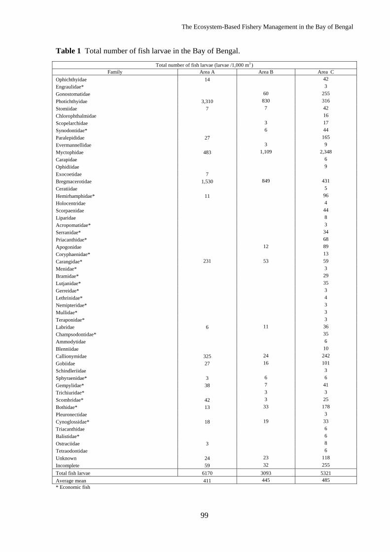
The Ecosystem-Based Fishery Management in the Bay of Bengal
99
Table 1 Total number of fish larvae in the Bay of Bengal.
Total number of fish larvae (larvae /1,000 m3 ) Family Area A Area B Area C
Ophichthyidae 14 42 Engraulidae* 3 Gonostomatidae 60 255 Photichthyidae 3,310 830 316 Stomiidae 7 7 42 Chlorophthalmidae 16 Scopelarchidae 3 17 Synodontidae* 6 44 Paralepididae 27 165 Evermannellidae 3 9 Myctophidae 483 1,109 2,348 Carapidae 6 Ophidiidae 9 Exocoetidae 7 Bregmacerotidae 1,530 849 431 Ceratiidae 5 Hemirhamphidae* 11 96 Holocentridae 4 Scorpaenidae 44 Liparidae 8 Acropomatidae* 3 Serranidae* 34 Priacanthidae* 68 Apogonidae 12 89 Coryphaenidae* 13 Carangidae* 231 53 59 Menidae* 3 Bramidae* 29 Lutjanidae* 35 Gerreidae* 3 Lethrinidae* 4 Nemipteridae* 3 Mullidae* 3 Teraponidae* 3 Labridae 6 11 36 Champsodontidae* 35 Ammodytidae 6 Blenniidae 10 Callionymidae 325 24 242 Gobiidae 27 16 101 Schindleriidae 3 Sphyraenidae* 3 6 6 Gempylidae* 38 7 41 Trichiuridae* 3 3 Scombridae* 42 3 25 Bothidae* 13 33 178 Pleuronectidae 3 Cynoglossidae* 18 19 33 Triacanthidae 6 Balistidae* 6 Ostraciidae 3 8 Tetraodontidae 6 Unknown 24 23 118 Incomplete 59 32 255 Total fish larvae 6170 3093 5321 Average mean 411 445 485 * Economic fish
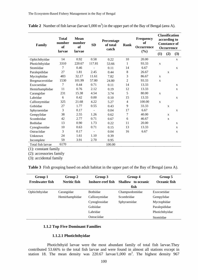
The Ecosystem-Based Fishery Management in the Bay of Bengal
100
Table 2 Number of fish larvae (larvae/1,000 m3) in the upper part of the Bay of Bengal (area A).
Family
Total number
of larvae
Mean number
of larvae
SD Percentage
of total catch
Rank
Frequency of
Occurrence (%)
Classification according to Constance of Occurrence
(1) (2) (3) Ophichthyidae 14 0.92 0.58 0.22 10 20.00 x Photichthyidae 3310 220.67 117.81 53.66 1 93.33 x Stomiidae 7 0.46 - 0.11 14 6.67 x Paralepididae 27 1.81 2.45 0.44 8 26.67 x Myctophidae 483 32.17 11.61 7.82 3 86.67 x Bregmacerotidae 1530 101.99 57.80 24.80 2 93.33 x Exocoetidae 7 0.44 0.71 0.11 14 13.33 x Hemirhamphidae 11 0.76 2.12 0.19 12 13.33 x Carangidae 231 15.38 4.54 3.74 5 80.00 x Labridae 6 0.42 0.00 0.10 15 13.33 x Callionymidae 325 21.68 4.22 5.27 4 100.00 x Gobiidae 27 1.77 0.55 0.43 9 33.33 x Sphyraenidae 3 0.17 - 0.04 17 6.67 x Gempylidae 38 2.55 1.26 0.62 7 40.00 x Scombridae 42 2.77 0.71 0.67 6 46.67 x Bothidae 13 0.90 1.73 0.22 11 20.00 x Cynoglossidae 10 0.63 0.71 0.15 13 13.33 x Ostraciidae 3 0.17 - 0.04 16 6.67 x Unknown 24 1.61 1.10 0.39 Incomplete 59 3.91 2.70 0.95 Total fish larvae 6170 100.00
(1): constant family (2): accessories family (3): accidental family Table 3 Fish grouping based on adult habitat in the upper part of the Bay of Bengal (area A).
Group 1 Group 2 Group 3 Group 4 Group 5 Freshwater fish Neritic fish Inshore-reef fish Shallow to oceanic Oceanic fish
fish Ophichthyidae Carangidae Bothidae Champsodontidae Exocoetidae Hemirhamphidae Callionymidae Scombridae Gempylidae
Cynoglossidae Sphyraenidae Myctophidae Gobiidae Paralepididae Labridae Photichthyidae Ostraciidae Stomiidae
1.1.2 Top Five Dominant Families 1.1.2.1 Photichthyidae
Photichthyid larvae were the most abundant family of total fish larvae.They contributed 53.66% to the total fish larvae and were found in almost all stations except in station 18. The mean density was 220.67 larvae/1,000 m3. The highest density 967
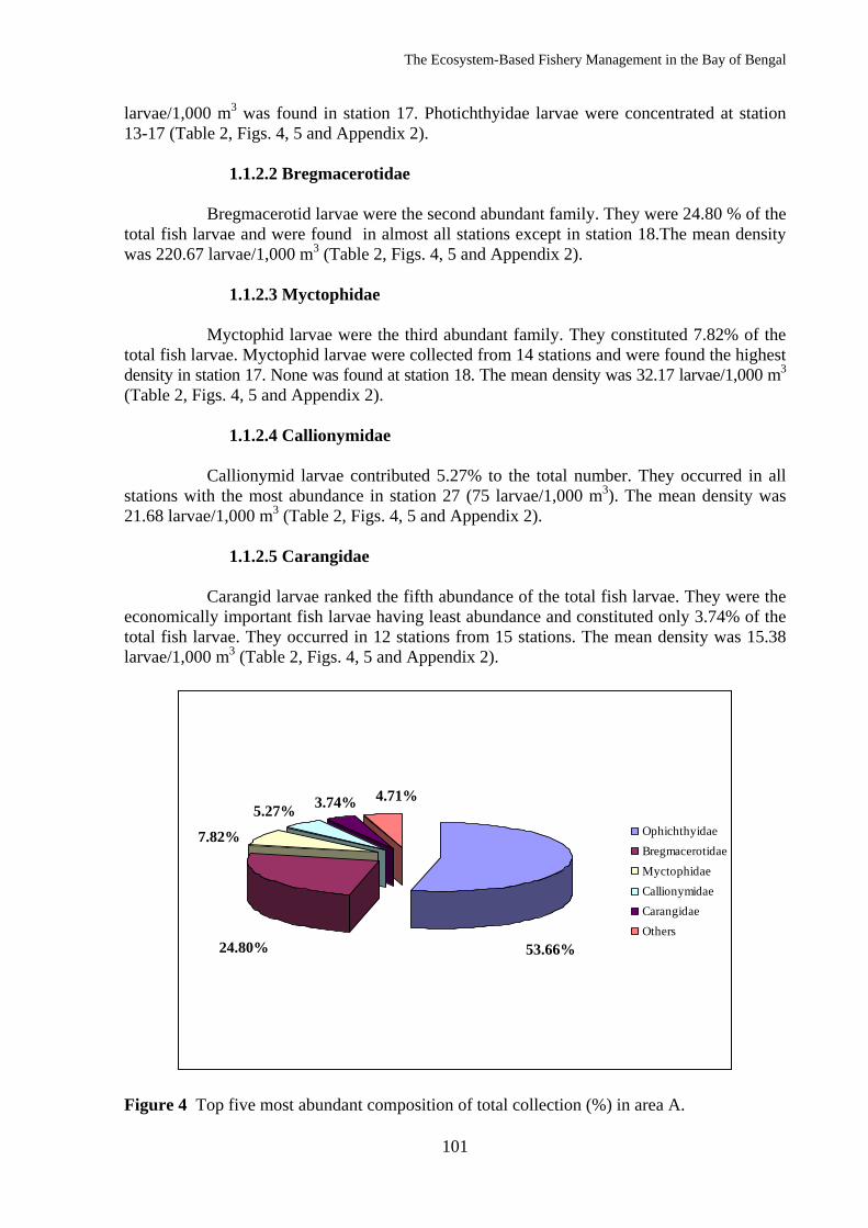
The Ecosystem-Based Fishery Management in the Bay of Bengal
101
larvae/1,000 m3 was found in station 17. Photichthyidae larvae were concentrated at station 13-17 (Table 2, Figs. 4, 5 and Appendix 2).
1.1.2.2 Bregmacerotidae
Bregmacerotid larvae were the second abundant family. They were 24.80 % of the total fish larvae and were found in almost all stations except in station 18.The mean density was 220.67 larvae/1,000 m3 (Table 2, Figs. 4, 5 and Appendix 2). 1.1.2.3 Myctophidae
Myctophid larvae were the third abundant family. They constituted 7.82% of the total fish larvae. Myctophid larvae were collected from 14 stations and were found the highest density in station 17. None was found at station 18. The mean density was 32.17 larvae/1,000 m3
(Table 2, Figs. 4, 5 and Appendix 2). 1.1.2.4 Callionymidae
Callionymid larvae contributed 5.27% to the total number. They occurred in all stations with the most abundance in station 27 (75 larvae/1,000 m3). The mean density was 21.68 larvae/1,000 m3 (Table 2, Figs. 4, 5 and Appendix 2). 1.1.2.5 Carangidae
Carangid larvae ranked the fifth abundance of the total fish larvae. They were the economically important fish larvae having least abundance and constituted only 3.74% of the total fish larvae. They occurred in 12 stations from 15 stations. The mean density was 15.38 larvae/1,000 m3 (Table 2, Figs. 4, 5 and Appendix 2).
24.80%
7.82%
5.27% 3.74% 4.71%
53.66%
OphichthyidaeBregmacerotidaeMyctophidaeCallionymidaeCarangidaeOthers
Figure 4 Top five most abundant composition of total collection (%) in area A.
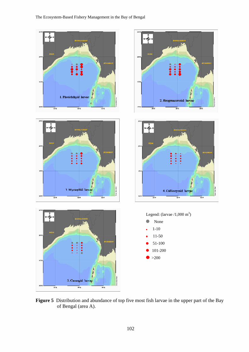
The Ecosystem-Based Fishery Management in the Bay of Bengal
102
Figure 5 Distribution and abundance of top five most fish larvae in the upper part of the Bay of Bengal (area A).
Legend: (larvae /1,000 m3)
None
1-10
11-50
51-100
101-200
>200
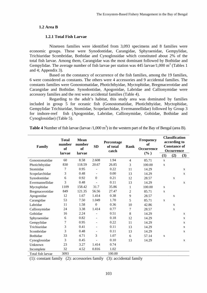
The Ecosystem-Based Fishery Management in the Bay of Bengal
103
1.2 Area B 1.2.1 Total Fish Larvae
Nineteen families were identified from 3,093 specimens and 8 families were economic groups. These were Synodontidae, Carangidae, Sphyraenidae, Gempylidae, Trichiuridae Scombridae, Bothidae and Cynoglossidae which constituted about 2% of the total fish larvae. Among them, Carangidae was the most dominant followed by Bothidae and Gempylidae. The average number of fish larvae per station was 445 larvae/1,000 m3 (Tables 1 and 4; Appendix 3).
Based on the constancy of occurrence of the fish families, among the 19 families, 6 were considered as constants. The others were 4 accessories and 9 accidental families. The constants families were Gonostomatidae, Photichthyidae, Myctophidae, Bregmacerotidae and Carangidae and Bothidae. Synodontidae, Apogonidae, Labridae and Callionymidae were accessory families and the rest were accidental families (Table 4).
Regarding to the adult’s habitat, this study area was dominated by families included in group 5 for oceanic fish (Gonostomatidae, Photichthyidae, Myctophidae, Gempylidae Trichiuridae, Stomiidae, Scopelarchidae, Evermannellidae) followed by Group 3 for inshore-reef fish (Apogonidae, Labridae, Callionymidae, Gobiidae, Bothidae and Cynoglossidae) (Table 5). Table 4 Number of fish larvae (larvae /1,000 m3) in the western part of the Bay of Bengal (area B).
Family
Total number
of larvae
Mean number
of larvae
SD Percentage
of total catch
Rank
Frequency of
Occurrence (% )
Classification according to Constance of Occurrence
(1) (2) (3) Gonostomatidae 60 8.58 2.608 1.94 4 85.71 x Photichthyidae 830 118.59 20.67 26.85 3 100.00 x Stomiidae 7 0.95 - 0.22 11 14.29 x Scopelarchidae 3 0.48 - 0.00 13 14.29 x Synodontidae 6 0.92 0 0.21 12 28.57 x Evermannellidae 3 0.48 - 0.11 13 14.29 x Myctophidae 1109 158.42 31.7 35.86 1 100.00 x Bregmacerotidae 849 121.35 56.56 27.47 2 85.71 x Apogonidae 12 1.67 1.414 0.38 9 28.57 x Carangidae 53 7.50 1.049 1.70 5 85.71 x Labridae 11 1.58 0 0.36 10 42.86 x Callionymidae 24 3.38 1.414 0.77 7 28.57 x Gobiidae 16 2.24 - 0.51 8 14.29 x Sphyraenidae 6 0.82 - 0.18 12 14.29 x Gempylidae 7 0.95 - 0.22 11 14.29 x Trichiuridae 3 0.41 - 0.11 13 14.29 x Scombridae 3 0.48 - 0.11 13 14.29 x Bothidae 33 4.71 3 1.07 6 57.14 x Cynoglossidae 3 0.45 - 0.10 13 14.29 x Unknown 23 3.27 1.414 0.74 Incomplete 32 4.52 0.816 1.02 Total fish larvae 3093 100.00 (1): constant family (2): accessories family (3): accidental family
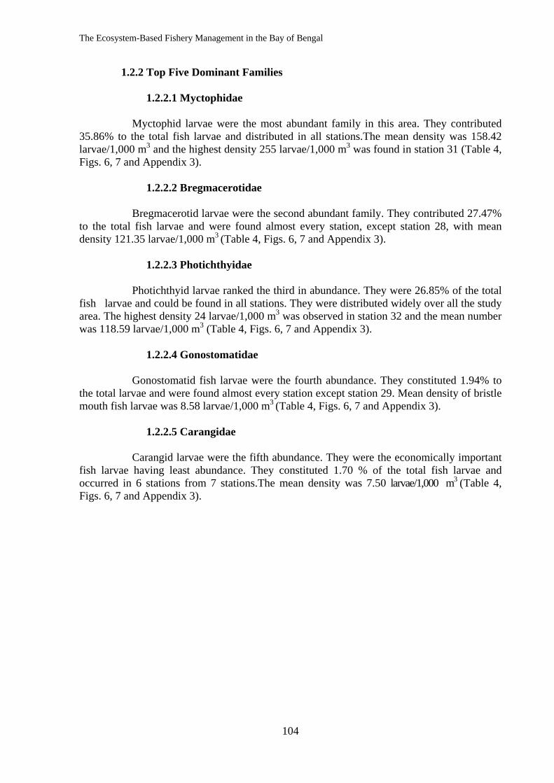
The Ecosystem-Based Fishery Management in the Bay of Bengal
104
1.2.2 Top Five Dominant Families 1.2.2.1 Myctophidae
Myctophid larvae were the most abundant family in this area. They contributed 35.86% to the total fish larvae and distributed in all stations.The mean density was 158.42 larvae/1,000 m3 and the highest density 255 larvae/1,000 m3 was found in station 31 (Table 4, Figs. 6, 7 and Appendix 3). 1.2.2.2 Bregmacerotidae
Bregmacerotid larvae were the second abundant family. They contributed 27.47% to the total fish larvae and were found almost every station, except station 28, with mean density 121.35 larvae/1,000 m3 (Table 4, Figs. 6, 7 and Appendix 3). 1.2.2.3 Photichthyidae
Photichthyid larvae ranked the third in abundance. They were 26.85% of the total fish larvae and could be found in all stations. They were distributed widely over all the study area. The highest density 24 larvae/1,000 m3 was observed in station 32 and the mean number was 118.59 larvae/1,000 m3 (Table 4, Figs. 6, 7 and Appendix 3). 1.2.2.4 Gonostomatidae
Gonostomatid fish larvae were the fourth abundance. They constituted 1.94% to the total larvae and were found almost every station except station 29. Mean density of bristle mouth fish larvae was 8.58 larvae/1,000 m3 (Table 4, Figs. 6, 7 and Appendix 3).
1.2.2.5 Carangidae
Carangid larvae were the fifth abundance. They were the economically important fish larvae having least abundance. They constituted 1.70 % of the total fish larvae and occurred in 6 stations from 7 stations.The mean density was 7.50 larvae/1,000 m3 (Table 4, Figs. 6, 7 and Appendix 3).
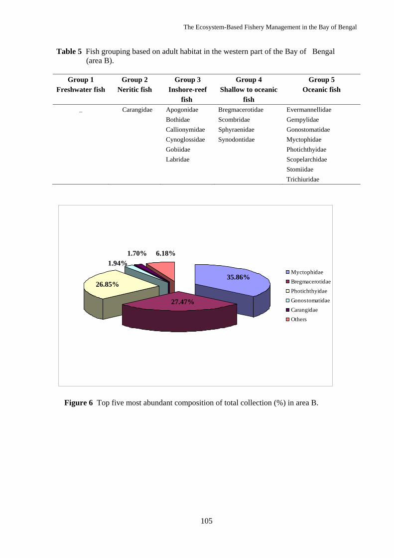
The Ecosystem-Based Fishery Management in the Bay of Bengal
105
Table 5 Fish grouping based on adult habitat in the western part of the Bay of Bengal (area B).
Group 1 Group 2 Group 3 Group 4 Group 5
Freshwater fish Neritic fish Inshore-reef Shallow to oceanic Oceanic fish fish fish _ Carangidae Apogonidae Bregmacerotidae Evermannellidae Bothidae Scombridae Gempylidae Callionymidae Sphyraenidae Gonostomatidae Cynoglossidae Synodontidae Myctophidae Gobiidae Photichthyidae Labridae Scopelarchidae Stomiidae Trichiuridae
1.70%1.94%
6.18%
26.85%
27.47%
35.86%MyctophidaeBregmacerotidaePhotichthyidaeGonostomatidaeCarangidaeOthers
Figure 6 Top five most abundant composition of total collection (%) in area B.
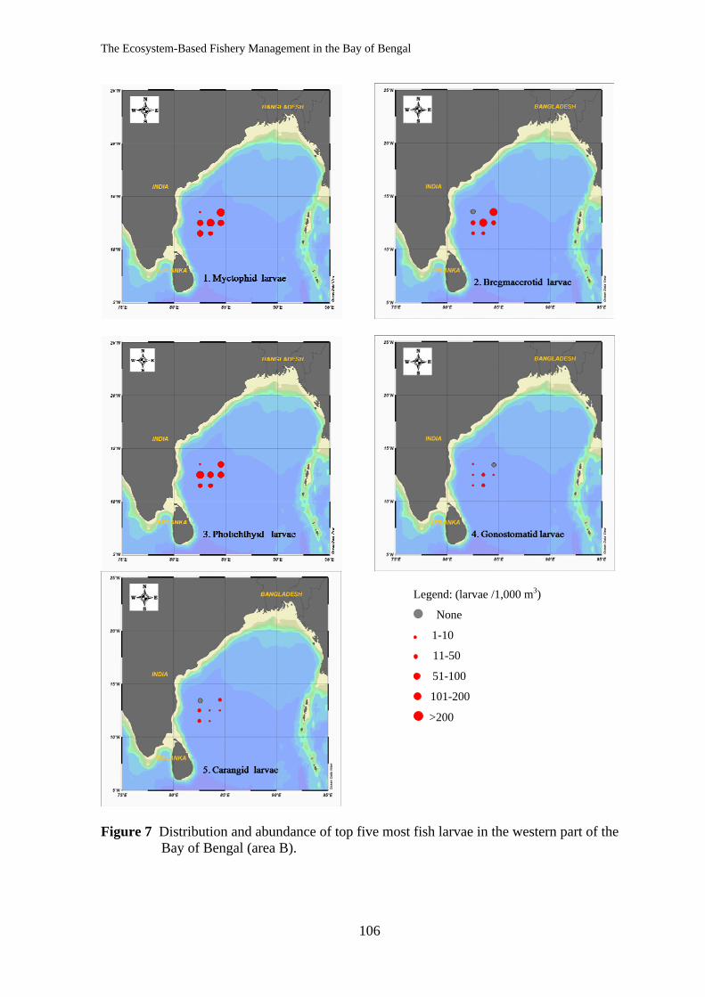
The Ecosystem-Based Fishery Management in the Bay of Bengal
106
Figure 7 Distribution and abundance of top five most fish larvae in the western part of the Bay of Bengal (area B).
Legend: (larvae /1,000 m3)
None
1-10
11-50
51-100
101-200
>200
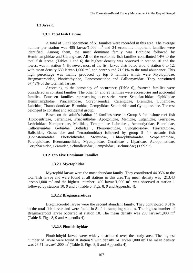
The Ecosystem-Based Fishery Management in the Bay of Bengal
107
1.3 Area C 1.3.1 Total Fish Larvae
A total of 5,321 specimens of 51 families were recorded in this area. The average number per station was 485 larvae/1,000 m3 and 24 economic important families were identified. Among them, the most dominant family was Bothidae followed by Hemirhamphidae and Carangidae. All of the economic fish families contributed 14% to the total fish larvae. (Tables 1 and 6) the highest density was observed in station 10 and the lowest was in station 4. However, most of the fish larvae distributed around station 6 to 12, with mean density 639 larvae/1,000 m3, and contributed 71.91% to the total abundance. This high percentage was mainly produced by top 5 families which were Myctophidae, Bregmacerotidae, Photichthyidae, Gonostomatidae and Callionymidae. They constituted 67.43% of the total fish larvae.
According to the constancy of occurrence (Table 6), fourteen families were considered as constant families. The other 14 and 23 families were accessories and accidental families. Fourteen families representing accessories were Scopelarchidae, Ophidiidae Hemirhamphidae, Priacanthidae, Coryphaenidae, Carangidae, Bramidae, Lutjanidae, Labridae, Chamsodontidae, Blennidae, Gempylidae, Scombridae and Cynoglossidae. The rest belonged to constant and accidental group.
Based on the adult’s habitat 22 families were in Group 3 for inshore-reef fish (Holocentridae, Serranidae, Priacanthidae, Apogonidae, Menidae, Lutjanidae, Gerreidae, Lethrinidae, Nemipteridae, Mullidae, Teraponidae Labridae , Ammodytidae, Blenniidae, Callionymidae, Gobiidae, Bothidae , Pleuronectidae, Cynoglossidae, Triacanthidae, Balistidae, Ostraciidae and Tetraodontidae) followed by group 5 for oceanic fish (Gonostomatidae, Photichthyidae, Stomiidae, Chlorophthalmidae, Scopelarchidae, Paralepididae, Evermannellidae, Myctophidae, Ceratiidae , Liparidae, Acropomatidae, Coryphaenidae, Bramidae, Schindleriidae, Gempylidae, Trichiuridae) (Table 7).
1.3.2 Top Five Dominant Families 1.3.2.1 Myctophidae
Myctophid larvae were the most abundant family. They contributed 44.05% to the total fish larvae and were found at all stations in this area.The mean density was 213.43 larvae/1,000 m3 and the highest number 490 larvae/1,000 m3 was observed at station 1 followed by stations 10, 9 and 6 (Table 6, Figs. 8, 9 and Appendix 4).
1.3.2.2 Bregmacerotidae
Bregmacerotid larvae were the second abundant family. They contributed 8.01% to the total fish larvae and were found in 8 of 11 sampling stations. The highest number of Bregmacerotid larvae occurred at station 10. The mean density was 208 larvae/1,000 m3
(Table 6, Figs. 8, 9 and Appendix 4).
1.3.2.3 Photichthyidae
Photichthyid larvae were widely distributed over the study area. The highest number of larvae were found at station 9 with density 74 larvae/1,000 m3.The mean density was 28.71 larvae/1,000 m3 (Table 6, Figs. 8, 9 and Appendix 4).
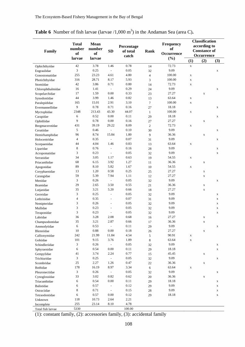
The Ecosystem-Based Fishery Management in the Bay of Bengal
108
Table 6 Number of fish larvae (larvae /1,000 m3) in the Andaman Sea (area C).
Family
Total number
of larvae
Mean number
of larvae
SD Percentage
of total catch
Rank
Frequency of
Occurrence (%)
Classification according to Constance of Occurrence
(1) (2) (3) Ophichthyidae 42 3.78 1.46 0.78 14 72.73 x Engraulidae 3 0.25 - 0.05 32 9.09 x Gonostomatidae 255 23.23 4.61 4.80 4 100.00 x Photichthyidae 316 28.71 8.17 5.93 3 100.00 x Stomiidae 42 3.86 0.71 0.80 14 72.73 x Chlorophthalmidae 16 1.41 - 0.29 24 9.09 x Scopelarchidae 17 1.59 0.00 0.33 23 27.27 x Synodontidae 44 3.99 1.46 0.82 13 63.64 x Paralepididae 165 15.01 2.91 3.10 7 100.00 x Evermannellidae 9 0.78 0.71 0.16 27 18.18 x Myctophidae 2348 213.43 43.30 44.07 1 100.00 x Carapidae 6 0.52 0.00 0.11 29 18.18 x Ophidiidae 9 0.78 0.00 0.16 27 27.27 x Bregmacerotidae 431 39.19 29.22 8.09 2 72.73 x Ceratiidae 5 0.46 - 0.10 30 9.09 x Hemirhamphidae 96 8.74 15.84 1.80 9 36.36 x Holocentridae 4 0.35 - 0.07 31 9.09 x Scorpaenidae 44 4.04 1.46 0.83 13 63.64 x Liparidae 8 0.76 - 0.16 28 9.09 x Acropomatidae 3 0.23 - 0.05 32 9.09 x Serranidae 34 3.05 1.17 0.63 19 54.55 x Priacanthidae 68 6.15 3.92 1.27 11 36.36 x Apogonidae 89 8.10 5.82 1.67 10 54.55 x Coryphaenidae 13 1.20 0.58 0.25 25 27.27 x Carangidae 59 5.39 7.94 1.11 12 27.27 x Menidae 3 0.26 - 0.05 32 9.09 x Bramidae 29 2.65 3.50 0.55 21 36.36 x Lutjanidae 35 3.21 5.20 0.66 18 27.27 x Gerreidae 3 0.25 - 0.05 32 9.09 x Lethrinidae 4 0.35 - 0.07 31 9.09 x Nemipteridae 3 0.26 - 0.05 32 9.09 x Mullidae 3 0.23 - 0.05 32 9.09 x Teraponidae 3 0.23 - 0.05 32 9.09 x Labridae 36 3.28 2.08 0.68 16 27.27 x Champsodontidae 35 3.21 2.87 0.66 17 36.36 x Ammodytidae 6 0.53 - 0.11 29 9.09 x Blenniidae 10 0.88 0.00 0.18 26 27.27 x Callionymidae 242 21.99 11.84 4.54 5 90.91 x Gobiidae 101 9.15 3.76 1.89 8 63.64 x Schindleriidae 3 0.26 - 0.05 32 9.09 x Sphyraenidae 6 0.54 0.00 0.11 29 18.18 x Gempylidae 41 3.74 2.24 0.77 15 45.45 x Trichiuridae 3 0.25 - 0.05 32 9.09 x Scombridae 25 2.27 1.26 0.47 22 36.36 x Bothidae 178 16.19 8.97 3.34 6 63.64 x Pleuronectidae 3 0.26 - 0.05 32 9.09 x Cynoglossidae 33 3.02 0.82 0.62 20 36.36 x Triacanthidae 6 0.54 0.00 0.11 29 18.18 x Balistidae 6 0.57 - 0.12 29 9.09 x Ostraciidae 8 0.71 - 0.15 28 9.09 x Tetraodontidae 6 0.57 0.00 0.12 29 18.18 x Unknown 118 10.73 2.64 2.21 Incomplete 255 23.14 8.10 4.78 Total fish larvae 5330 100.00
(1): constant family, (2): accessories family, (3): accidental family
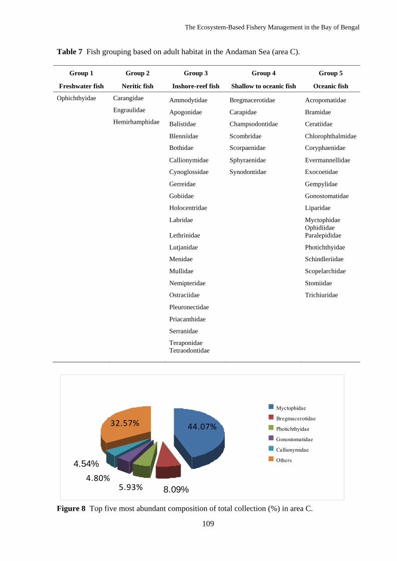
The Ecosystem-Based Fishery Management in the Bay of Bengal
109
Table 7 Fish grouping based on adult habitat in the Andaman Sea (area C).
Group 1 Group 2 Group 3 Group 4 Group 5
Freshwater fish Neritic fish Inshore-reef fish Shallow to oceanic fish Oceanic fish
Ophichthyidae Carangidae Ammodytidae Bregmacerotidae Acropomatidae Engraulidae Apogonidae Carapidae Bramidae Hemirhamphidae Balistidae Champsodontidae Ceratiidae Blenniidae Scombridae Chlorophthalmidae Bothidae Scorpaenidae Coryphaenidae Callionymidae Sphyraenidae Evermannellidae Cynoglossidae Synodontidae Exocoetidae Gerreidae Gempylidae Gobiidae Gonostomatidae Holocentridae Liparidae Labridae Myctophidae
Lethrinidae Ophidiidae Paralepididae
Lutjanidae Photichthyidae Menidae Schindleriidae Mullidae Scopelarchidae Nemipteridae Stomiidae Ostraciidae Trichiuridae Pleuronectidae Priacanthidae
Serranidae
Teraponidae
Tetraodontidae
44.07%
8.09%5.93%4.80%
4.54%
32.57%
MyctophidaeBregmacerotidaePhotichthyidaeGonostomatidaeCallionymidaeOthers
Figure 8 Top five most abundant composition of total collection (%) in area C.
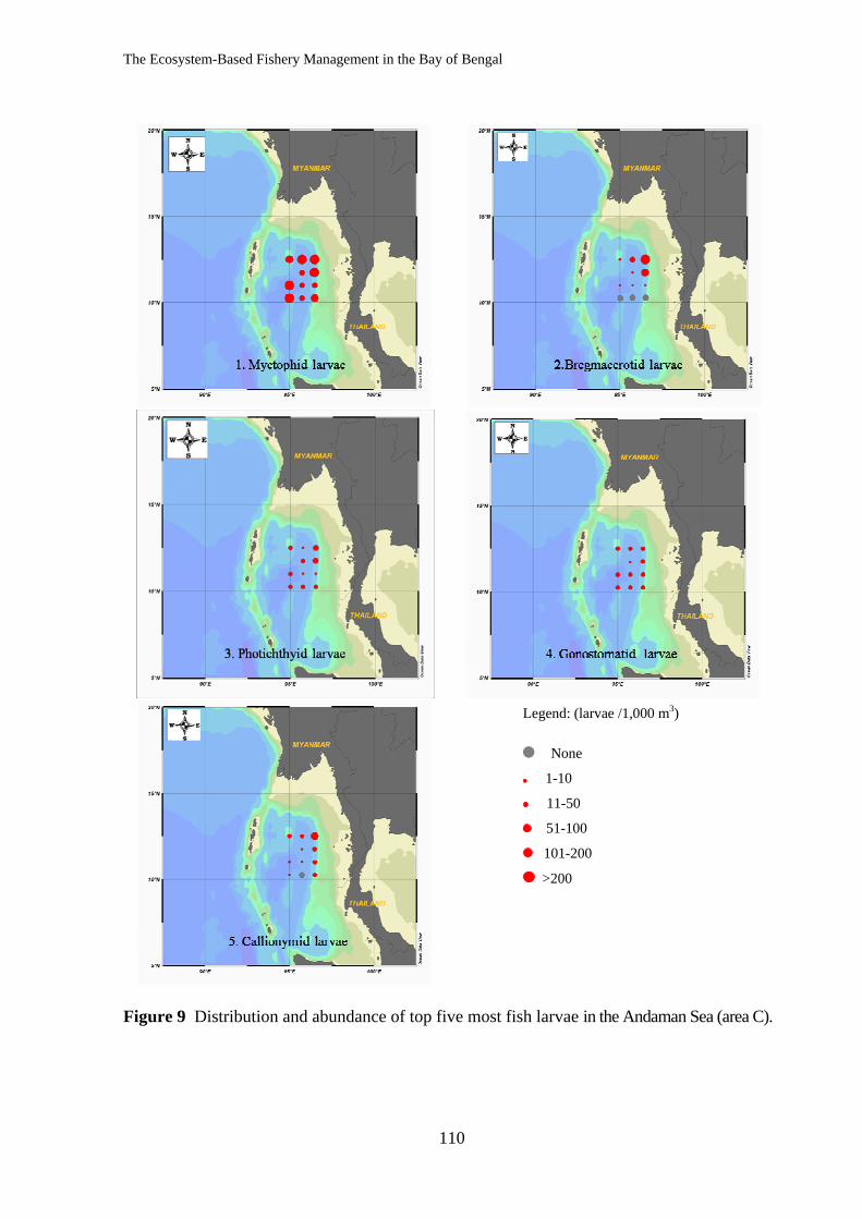
The Ecosystem-Based Fishery Management in the Bay of Bengal
110
Figure 9 Distribution and abundance of top five most fish larvae in the Andaman Sea (area C).
Legend: (larvae /1,000 m3)
None
1-10
11-50
51-100
101-200
>200
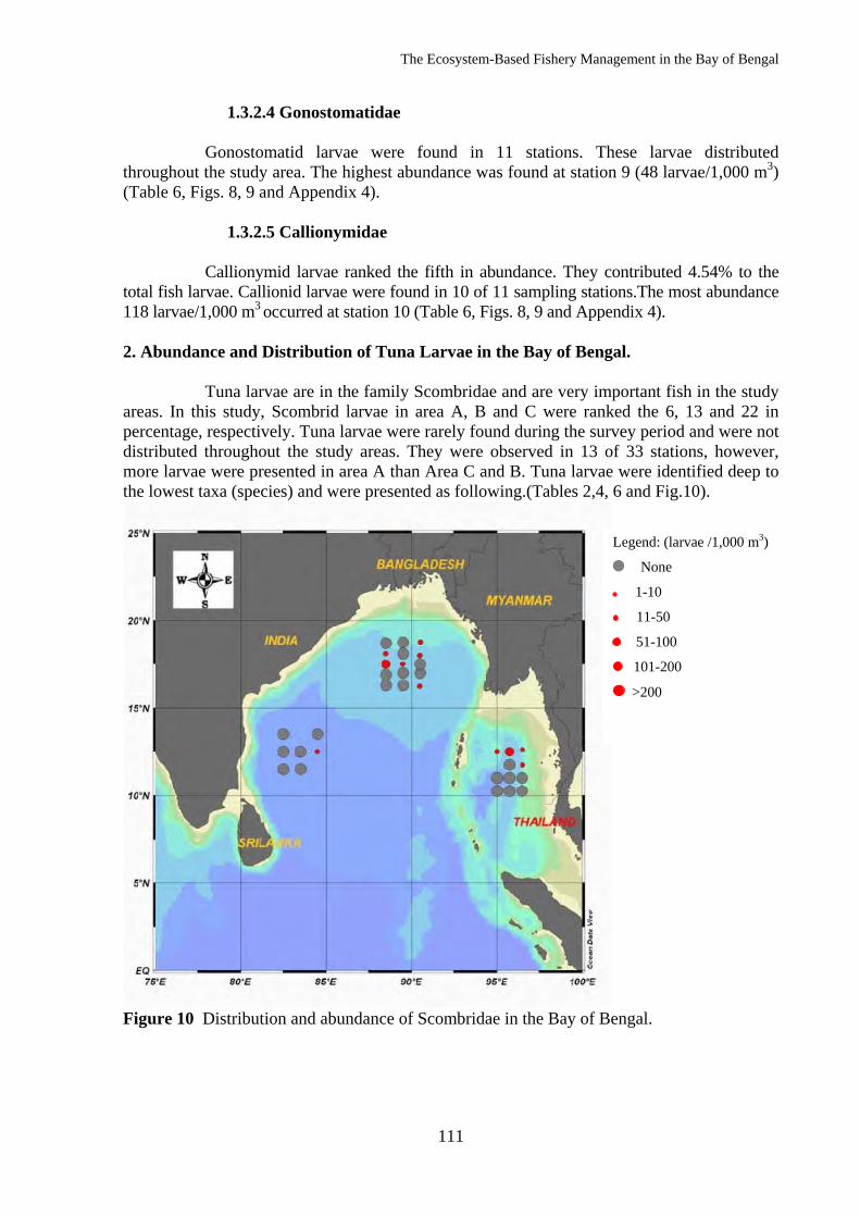
The Ecosystem-Based Fishery Management in the Bay of Bengal
111
1.3.2.4 Gonostomatidae
Gonostomatid larvae were found in 11 stations. These larvae distributed throughout the study area. The highest abundance was found at station 9 (48 larvae/1,000 m3) (Table 6, Figs. 8, 9 and Appendix 4).
1.3.2.5 Callionymidae
Callionymid larvae ranked the fifth in abundance. They contributed 4.54% to the total fish larvae. Callionid larvae were found in 10 of 11 sampling stations.The most abundance 118 larvae/1,000 m3 occurred at station 10 (Table 6, Figs. 8, 9 and Appendix 4). 2. Abundance and Distribution of Tuna Larvae in the Bay of Bengal.
Tuna larvae are in the family Scombridae and are very important fish in the study areas. In this study, Scombrid larvae in area A, B and C were ranked the 6, 13 and 22 in percentage, respectively. Tuna larvae were rarely found during the survey period and were not distributed throughout the study areas. They were observed in 13 of 33 stations, however, more larvae were presented in area A than Area C and B. Tuna larvae were identified deep to the lowest taxa (species) and were presented as following.(Tables 2,4, 6 and Fig.10).
Figure 10 Distribution and abundance of Scombridae in the Bay of Bengal.
Legend: (larvae /1,000 m3)
None
1-10
11-50
51-100
101-200
>200
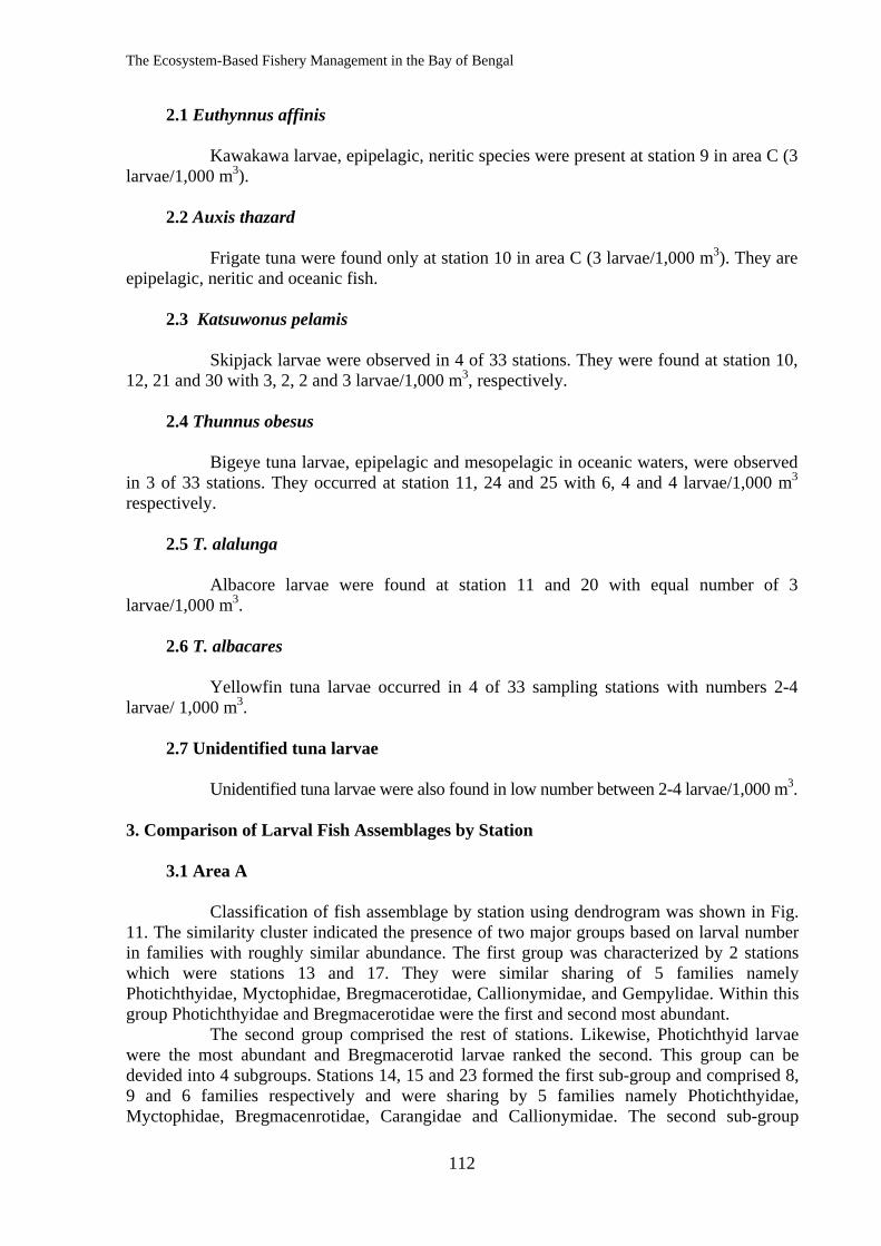
The Ecosystem-Based Fishery Management in the Bay of Bengal
112
2.1 Euthynnus affinis
Kawakawa larvae, epipelagic, neritic species were present at station 9 in area C (3 larvae/1,000 m3).
2.2 Auxis thazard
Frigate tuna were found only at station 10 in area C (3 larvae/1,000 m3). They are epipelagic, neritic and oceanic fish.
2.3 Katsuwonus pelamis
Skipjack larvae were observed in 4 of 33 stations. They were found at station 10, 12, 21 and 30 with 3, 2, 2 and 3 larvae/1,000 m3, respectively.
2.4 Thunnus obesus
Bigeye tuna larvae, epipelagic and mesopelagic in oceanic waters, were observed in 3 of 33 stations. They occurred at station 11, 24 and 25 with 6, 4 and 4 larvae/1,000 m3 respectively.
2.5 T. alalunga
Albacore larvae were found at station 11 and 20 with equal number of 3 larvae/1,000 m3.
2.6 T. albacares
Yellowfin tuna larvae occurred in 4 of 33 sampling stations with numbers 2-4 larvae/ 1,000 m3.
2.7 Unidentified tuna larvae
Unidentified tuna larvae were also found in low number between 2-4 larvae/1,000 m3. 3. Comparison of Larval Fish Assemblages by Station 3.1 Area A
Classification of fish assemblage by station using dendrogram was shown in Fig. 11. The similarity cluster indicated the presence of two major groups based on larval number in families with roughly similar abundance. The first group was characterized by 2 stations which were stations 13 and 17. They were similar sharing of 5 families namely Photichthyidae, Myctophidae, Bregmacerotidae, Callionymidae, and Gempylidae. Within this group Photichthyidae and Bregmacerotidae were the first and second most abundant.
The second group comprised the rest of stations. Likewise, Photichthyid larvae were the most abundant and Bregmacerotid larvae ranked the second. This group can be devided into 4 subgroups. Stations 14, 15 and 23 formed the first sub-group and comprised 8, 9 and 6 families respectively and were sharing by 5 families namely Photichthyidae, Myctophidae, Bregmacenrotidae, Carangidae and Callionymidae. The second sub-group
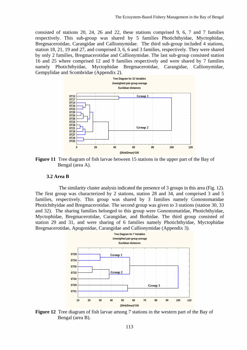
The Ecosystem-Based Fishery Management in the Bay of Bengal
113
consisted of stations 20, 24, 26 and 22, these stations comprised 9, 6, 7 and 7 families respectively. This sub-group was shared by 5 families Photichthyidae, Myctophidae, Bregmacerotidae, Carangidae and Calliomymidae. The third sub-group included 4 stations, station 18, 21, 19 and 27, and comprised 3, 6, 6 and 3 families, respectively. They were shared by only 2 families, Bregmacerotidae and Callionymidae. The last sub-group consisted station 16 and 25 where comprised 12 and 9 families respectively and were shared by 7 families namely Photichthyidae, Myctophidae Bregmacerotidae, Carangidae, Callionymidae, Gempylidae and Scombridae (Appendix 2).
Tree Diagram for 15 VariablesUnweighted pair-group average
Euclidean distances
(Dlink/Dmax)*100
ST25 ST16 ST27 ST19 ST21 ST18 ST22 ST26 ST24 ST20 ST23 ST15 ST14 ST17 ST13
0 20 40 60 80 100 120
Figure 11 Tree diagram of fish larvae between 15 stations in the upper part of the Bay of Bengal (area A). 3.2 Area B
The similarity cluster analysis indicated the presence of 3 groups in this area (Fig. 12). The first group was characterized by 2 stations, station 28 and 34, and comprised 3 and 5 families, respectively. This group was shared by 3 families namely Gonostomatidae Photichthyidae and Bregmacerotidae. The second group was given to 3 stations (station 30, 33 and 32). The sharing families belonged to this group were Gonostomatidae, Photichthyidae, Myctophidae, Bregmacerotidae, Carangidae, and Bothidae. The third group consisted of station 29 and 31, and were sharing of 6 families namely Photichthyidae, Myctophidae Bregmacerotidae, Apogonidae, Carangidae and Callionymidae (Appendix 3).
Tree Diagram for 7 VariablesUnweighted pair-group average
Euclidean distances
(Dlink/Dmax)*100
ST31
ST29
ST32
ST33
ST30
ST34
ST28
10 20 30 40 50 60 70 80 90 100 110
Figure 12 Tree diagram of fish larvae among 7 stations in the western part of the Bay of Bengal (area B).
Group 1
Group 2
Group 1
Group 2
Group 3
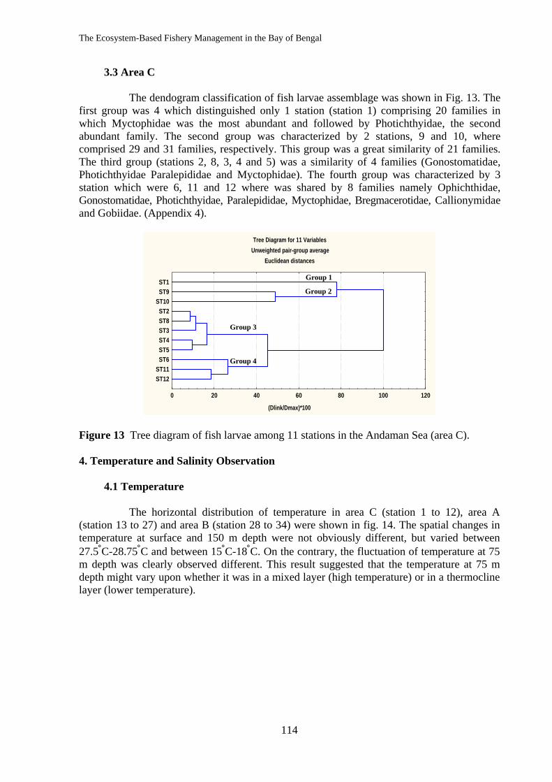
The Ecosystem-Based Fishery Management in the Bay of Bengal
114
3.3 Area C
The dendogram classification of fish larvae assemblage was shown in Fig. 13. The first group was 4 which distinguished only 1 station (station 1) comprising 20 families in which Myctophidae was the most abundant and followed by Photichthyidae, the second abundant family. The second group was characterized by 2 stations, 9 and 10, where comprised 29 and 31 families, respectively. This group was a great similarity of 21 families. The third group (stations 2, 8, 3, 4 and 5) was a similarity of 4 families (Gonostomatidae, Photichthyidae Paralepididae and Myctophidae). The fourth group was characterized by 3 station which were 6, 11 and 12 where was shared by 8 families namely Ophichthidae, Gonostomatidae, Photichthyidae, Paralepididae, Myctophidae, Bregmacerotidae, Callionymidae and Gobiidae. (Appendix 4).
Tree Diagram for 11 VariablesUnweighted pair-group average
Euclidean distances
(Dlink/Dmax)*100
ST12 ST11 ST6 ST5 ST4 ST3 ST8 ST2 ST10 ST9 ST1
0 20 40 60 80 100 120
Figure 13 Tree diagram of fish larvae among 11 stations in the Andaman Sea (area C). 4. Temperature and Salinity Observation 4.1 Temperature
The horizontal distribution of temperature in area C (station 1 to 12), area A (station 13 to 27) and area B (station 28 to 34) were shown in fig. 14. The spatial changes in temperature at surface and 150 m depth were not obviously different, but varied between 27.5°C-28.75°C and between 15°C-18°C. On the contrary, the fluctuation of temperature at 75 m depth was clearly observed different. This result suggested that the temperature at 75 m depth might vary upon whether it was in a mixed layer (high temperature) or in a thermocline layer (lower temperature).
Group 1
Group 2
Group 4
Group 3
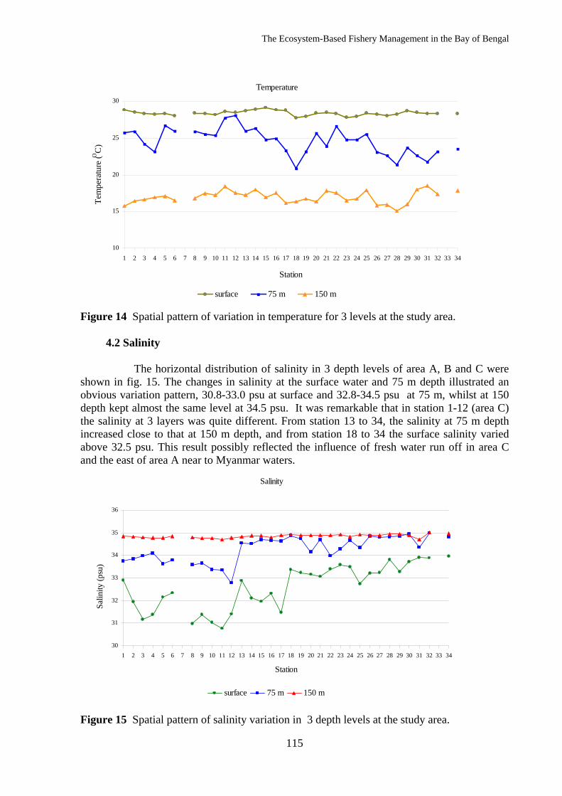
The Ecosystem-Based Fishery Management in the Bay of Bengal
115
Temperature
10
15
20
25
30
1 2 3 4 5 6 7 8 9 10 11 12 13 14 15 16 17 18 19 20 21 22 23 24 25 26 27 28 29 30 31 32 33 34
Station
Tem
pera
ture
(OC
)
surface 75 m 150 m
Figure 14 Spatial pattern of variation in temperature for 3 levels at the study area. 4.2 Salinity
The horizontal distribution of salinity in 3 depth levels of area A, B and C were shown in fig. 15. The changes in salinity at the surface water and 75 m depth illustrated an obvious variation pattern, 30.8-33.0 psu at surface and 32.8-34.5 psu at 75 m, whilst at 150 depth kept almost the same level at 34.5 psu. It was remarkable that in station 1-12 (area C) the salinity at 3 layers was quite different. From station 13 to 34, the salinity at 75 m depth increased close to that at 150 m depth, and from station 18 to 34 the surface salinity varied above 32.5 psu. This result possibly reflected the influence of fresh water run off in area C and the east of area A near to Myanmar waters.
Salinity
30
31
32
33
34
35
36
1 2 3 4 5 6 7 8 9 10 11 12 13 14 15 16 17 18 19 20 21 22 23 24 25 26 27 28 29 30 31 32 33 34
Station
surface 75 m 150 m
Salin
ity (p
su)
Figure 15 Spatial pattern of salinity variation in 3 depth levels at the study area.
The Ecosystem-Based Fishery Management in the Bay of Bengal
116
Discussion
The total fish larvae of 52 families found in this present study seem to be lower diversity than the former works that conducted in more productive area of the other part of the Indian Ocean. Nellen (1973) reported the total of 102 fish larval families in the northwest Indian Ocean (Red Sea, Arabian Sea and Persian Gulf). He found 44 families of the oceanic plus deep benthic fish larvae and 58 families of the shelf fish larvae. In southeast Indian Ocean (NW continental shelf, Australia), Young et al. (1986) found 103 families of which 36 and 67 families were oceanic and shelf fish larvae.
In this study, during post summer monsoon, area C was found to be the richest fish larvae diversity (51 families) followed by area B (19 families) and area A (18 families). Although, the highest average density of fish larvae was also found in area C (485 larvae/1,000m3) but it was not so much different comparing to 445 and 411 larvae/1,000m3 that found in area B and A. Considering area C which is in the upper part of the Andaman Sea both of hydrographic conditions and fisheries resource information are not available except a few information in the lower part along the west coast of Thailand. As for fish larvae composition and abundance, Janekarn (1988) reported the diversity of 55 and 62 families of fish larvae found from the west coast of Thailand in 1982 and 1983. He also estimated the aggregated number of 123 families of fish larvae in the west coast of Thailand based upon his and other studies (Janekarn, 1992). This information indicated that the Andaman Sea was an area of high diversity of fish larvae in the Indian Ocean. However, referring to Mc Gowan and Frauendorf (1966) the diversity value was influenced not only by area but also by depth of haul, time and type of net used.
Based on the constancy of occurrence, among the 18 families in area A, the percentages by families of constant:accessory:accidental families were 28:22:50; in area B (19 families) were 32:21:47 and in area C (51 families) were 27.5:27.5:45, respectively. This study was similar to Chamchang (2006) who reported a relative low number of constant families suggesting the system appeared not to be stable. From this reference, 62 families of fish larvae were found in the Andaman Sea along the west coast of Myanmar and Thailand between 6°44.47'N to 12°40.80'N and 95°51.20'E to 96°45.30'E. Half of the mentioned study site were located almost the same latitude as area C but the sampling stations were located in more shallow waters. Furthermore, in that survey the fish larvae samples were collected in November 2004 which was almost the same month as this survey. Thirty six families of that finding were shared by 15, 13 and 6 families belonging to group 3 (inshore-reef fish), group 5 (oceanic fish) and group 4 (shallow to oceanic fish). This result suggested that fish larvae of group 3 and 5 were widely distributed between inshore and offshore waters, implying that this area was very important for habitat of adult fish and their larvae. Similar to this study, the relative large numbers of inshore-reef families and oceanic families, particularly area C, may also indicate that the Bay of Bengal is the connected boundary of inshore and oceanic currents. In addition, the occurrence of many accidental families possibly reflects that the majority of the adult fish exiting in the Bay of Bengal are commonly inshore residents and their larvae are occasionally carried out offshore by currents.
In this study the most of the abundant families were Photichthyidae, Myctophidae, Bregmacerotidae, Gonostomatidae, Callionymidae, and Carangidae. Family Myctophidae is the largest family of oceanic fish with 500 species found around the world, they are an important constituent in the food chain of many local system being heavily preyed upon by cetaceans including whales and dolphins as well as large pelagic fish such as tuna and sharks (Nellen , 1973; Fish Base, 2004). Chamchang (2007) reported family Myctophidae was the most abundant contributing 30.41% to the total number of larvae followed by Stomiidae. Morliere et al. (1994) reported that Vinciguerria nimbaria (family Photichthyidae) must
The Ecosystem-Based Fishery Management in the Bay of Bengal
117
sustain the high concentration of small tuna and must be considered a major chain in the local food webs. Small tunas fed mainly on V. nimbaria for 40% by weight of tuna stomach content.
Larvae of the commercial important fish were not very high. Carangid larvae were common and abundant in area A and B which in addition appeared in considerable quantities at some stations in the Bay of Bengal. Very important to high sea fisheries, tuna larvae appeared more frequently in area A but their density was not remarkably high at any stations. Frigate tuna and kawakawa larvae were observed only one station in area C. The scantiness of tuna larvae may be attributed to the survey period that did not cover the spawning seasons of tunas. Yoshida (1979) reported frigate tuna’s spawning season in the Indian Ocean was occurred from January to April. Stequert and Marsac (1989) reported the greatest abundance of skipjack larvae in the eastern Indian Ocean in February.
Regarding to larval fish assemblage, based on a cluster analysis, it illustrated the patchy distribution of the majority of fish larvae because the stations appearing similarity in fish families and their abundance tended to be located adjacent to each other. This may be, in some extents, underline the influence of currents because larval lives are generally carried to elsewhere by currents.
Although, the relationships between environmental parameters and fish larvae abundance have not been analyzed statistically due to the small sample sizes in this study. Nevertheless, the linkage between oceanographic parameters and fish larvae abundance have been pointed out by a number of authors. Munk et. al., 2004 investigated linkages among physics, chemistry and plankton biology across the continental shelf and shelf slope of the Andaman Sea. They found that the abundant peak of both mesozooplankton and fish larvae were at mid-shelf (50 to 65 m bottom depth) coinciding with a hydrographic front generated. Other studies in the tropics have found strong cross- shelf gradients in abundance, but were unable to detect consistent patterns related to hydrography or other factors (Williams et. al., 1988, Leis, 1993). The study of mesopelagic fish larvae in the northern Arabian Sea during the intermonsoon period (March-June 1987) by Röpke (1993) showed that prey abundance and distribution in the water column were related to fish larval distribution. Most of the Myctophid and Photichthyid larvae avoided the upper mixed layer, which contained the highest concentrations of potential prey organisms, and their distribution was also not directly related to pycnocline depth. Below the mixed surface layer the abundance and vertical distribution of potential prey was more important in determining the vertical distribution of the larvae than the gradient of physical stratification. The results also indicted that larvae of mesopelagic moved downward during early development and adapted to their later life in the mesopelagic zone.
Like the tropical Asian Waters, the BOB was influenced by monsoons as well as by the river runoff. Area A in the north and area B in the west of the BOB were influenced by two great rivers (Ganga and Brahmaputra rivers) and some other smaller rivers. Area C was largely influenced by Salween and Irrawaddy rivers. These river systems carried huge quantities of nutrient-rich and freshwater mass into the bay during south-west monsoon. In addition, area C seems to be a basin enclosed by the Andaman and Nicobar Islands. This area is not only topographically different from the other two areas but also hydrological richer and more suitable than those areas. These favorable conditions probably supported the distribution and abundance of fish larvae as shown in Tables 2, 4 and 6. The richest in diversity of fish larvae in this area might due to the influence of nutrient-rich from two great rivers that discharged nutrients into the north of area C and also the reef areas around the enclosing islands. Further more, the investigation of large pelagic fisheries resources by pelagic long line (Nuangsang et al., 2008) conducted during same cruise as this present study showed that percentage of hooking rate was the highest in area C (2.17%) followed by area B (0.91%) and
The Ecosystem-Based Fishery Management in the Bay of Bengal
118
area A (0.78%). Desai and Bhargawa(1998) estimated he potential pelagic production in 4 exclusive economic zone of India which were along west coast, east coast, around the Andaman , Nicobar islands and Lakshadweep. He found that the average potential pelagic productions during monsoon (June-September) and postmonsoon (October-January) period in the Andaman and Nicobar area were higher than those along the east coast of India. These results suggested that Andaman and Nicobar area was the important fishery potential area in BOB. However, further study focused on the relationships of fish larvae and oceanographic parameters in different monsoon systems are needed for more understanding of the whole picture of fish larvae composition and abundance in the BOB.
Conclusion
A total of 52 families of fish larvae were identified and 24 families represented economically important group. Photichthyidae was the most abundant family in the survey area followed by Myctophidae, Bregmacerotidae, Callionymidae and Carangidae which was the most dominant of economic group. It was observed that not many families distributed widely in the Bay of Bengal whilst a large number accidentally occurred. In addition, most of the fish families were categorized inshore reef-fish and oceanic fish. In overall, area C appeared the richest diversity of fish families and also the highest average density of fish larvae compared to area A and B.
Acknowdedgement The authors would like to thank all researchers from BIMSTEC countries, SEAFDEC, DOF and crews from SEAFDEC for their appreciative during the survey. Special thanks to Mrs. Piyawan Hussadee and Miss Chantip bunluedaj for help on data analysis. Also thanks to Ms. Chamchoi Tanpong and Dr.Chongkolnee Chamchang for their comment and advice in correcting this report, Mr.Pirote Naimee for maps illustration.
References Achuthankutty, C. T., M. Madhupratap, V. R. Nair, S. R. S. Nair and T. S. S. Rao. 1980. Zooplankton biomass and composition in the western Bay of Bengal during late Southwest monsoon. Indian Journal of Marine Science 9:201-206. Chamchang, C. 2006. Composition, abundance and distribution of Ichthyoplankton in the Andaman Sea. In: Preliminary Rusults on the Large Pelagic Fisheries Resources
Survey in the Andaman Sea. TD/RES/99 SEAFDEC. p. 66-100. FishBase. 2004. Fish Species in the Indian Ocean. http://www.larvalbase.org/ Janekarn, V. 1988. Biogeography and environmental biology of fish larvae along the West coast of Thailand. A master degree dissertation. The University of Newcastle. 107 pp. Janekarn, V. 1992. Fish larvae in the vicinity of shelf front in the Andaman Sea.
In: Proceeding: The Seminar on Fisheries, 16-18 September 1992, Department of Fisheries, Bangkok, Thailand. p. 343-353.
Leis, J. M., and D. S. Rennis. 1983. The larvae of Indo- Pacific Coral Reef Fishes. New South Wales University Press. New South Wales, Australia. 269 pp. Lies, J. M. 1993. Larval fish assemblages near Indo- Pacific coral reefs. Bull. Mar. Sci. 53
(2):362-392.
The Ecosystem-Based Fishery Management in the Bay of Bengal
119
Leis, J. M. and B. M. Carson-Ewart. 2000. The Larvae of Indo- Pacific Coastal Fishes: An identification guide to marine fish larvae. Fauna Malesiana. Vol. 2. 850 pp. Matsumoto, W. M. 1958. Description and distribution of larvae of four species of tuna in Central Pacific Waters. Fishery Bulletin 128(58 ):72 pp. Matsumoto, W. M., E. H. Ahlstrom, S. Jones, W. L. Klawe, W. J. Richards and S. Ueyanagi. 1972. On the clarification of larvae identification particularly in genus Thunnus. Fisheries Bulletin 70(1):1-12. Mc. Gowan J. A. and V. S. Frauendorf. 1966. The relationship between size of net used and estimates of zooplankton diversity. Limnol. Oceanogr. 11:456-469. Madhu, N. V., P. A. Maheswaran, R. Jyothibabu, V. Sunil, C. Revichandran, T.
Balasubramanian,T. C. Gopalakrishnan and K. K. C. Nair. 2002. Enhanced biological production of Chennai triggered by October 1999 super cyclone (Orissa). Current Science 82:1472-1479.
Madhupratap, M., G. M. Ramaiaha, S. Prasanna, P. M. Muraleedharan, S. N. De Sousa, S. Sardessai and U. Muraleedharan. 2003. Biogeochemical of the Bay of Bengal:Physical, chemical and primary productivity characteristics of the central and western Bay of Bengal during summer monsoon 2001. Deep-Sea Research 50(2):881-896. Munk,P., P. K. Bjornsen, P. Boonruang, M. Fryd, P. J. Hansen, V. Janekarn, V.,Limtrakulvong, T. G. Nielsen, O. S. Hansen, S.,Satapoomin, S. Sawangarreruks, H. A. Thomson and J. B. Ostergaard. 2004. Assemblages of fish larvae and mesozooplankton across the continental shelf and shelf slope of the Andaman Sea (NE Indian Ocean ). Mar. Ecol. Prog. Ser. 274:87-97. Nair, S. R., V. R. Nair, C. T. Achunthankutty and M.Madhupratap. 1981. Zooplankton
composition and diversity in western Bay of Bengal. Journal of Plankton Research 34:493-508.
Nellen, W. 1973. Kinds and abundance of fish larvae in the Arabian Sea and the Persian Gulf. In: Zeitzschel, B. (ed.). The Biology of the Indian Ocean Springer-Verlag, New York. p. 415-430. Nishikawa, Y. and D. W. Rimmer. 1987. Identification of larval tunas, billfishes and other scombroid fishes (suborder Scombroidei): an illustrated guide. CSIRO Marine Laboratories Report 186. 20 pp. Nuangsang, C., S. Promjinda, O. Chamason, Md. J. Rahman, R. P. P. K. Jayasinghe, U. Aung
Htay Oo and M. K. Sinha. Large pelagic fishery resource survey using pelagic longline in the Bay of Bengal. (in press).
Ozawa, T. (ed.). 1986. Studies on the Oceanic Icthyoplankton in the Western North Pacific. Kyushu University Press, Kyushu. 430 pp. Pielou, E. C. 1984. The Interpretation of Ecological Data a Primer on Classification and Ordination. John Wiley&Sons Ltd., Worcester. 263 pp. Qasim, S. Z. 1977. Biological productivity of the Indian Ocean. Indian Journal of Marine Science 6:122-137. Schifino, L. C., C. B. Fialho and J. R. Verani. 2004. Fish community composition, seasonality and abundance in Fortaleza Lagoon, Cidreira. Braz Arch. Biol. Technol. 47(5):11 pp. Shetye, L. R., S. Shenoi, A. D. Gouevia, G. S. Michael and D. Sundar. 1991. Wind-driven Coastal upwelling along the western boundary of the Bay of Bengal during the
south west monsoon. Continental Shelf Research 11:1397-1408. Shankar, D., P. N. Vinayachandran and A. S. Unnikrishnan. 2002. The monsoon currents in the north Indian Ocean. Progress in Oceanograhphy 52:63-70.
The Ecosystem-Based Fishery Management in the Bay of Bengal
120
Smith M. M. and C. P. Heemstra. 1986. Smiths’ Sea Fishes. Smith Institute Ichthyology, Grahamstown Mac Millan. South Africa Johannesburg. 1047 pp. Sprintall, J. and M. Tomczak. 1992. Evidence of barrier layer in the surface layer of the tropics. Journal of Geophysical Research 97:7305-7316. Stequert, B. and F. Marsac. 1989. Tropical tuna surface fisheries in the Indian Ocean. FAO Fisheries Technical Paper no. 282. 238 p. UNESCO. 1988. River inputs into Ocean system: status and recommendation for research. UNESCO Technical papers in marine science, No. 55. Final report of SCOR Working Group 46, Paris. 25 pp. Vinayachandran, P. N., V. S. N. Murty and V. Rameshbabu. 2002. Observations of barrier layer formation in the Bay of Bengal during summer monsoon. Journal of Geophysical Research 107:15-25. Williams, D. M.; P. Dixon and S. English. 1988. Cross shelf distribution of copepods and fish larvae across the central Great Barrier Reef. Mar. Biol. 99:577-589. Yoshida, H. O. 1979. Synopsis of biological data on tunas of the genus Euthynnus. NOAA Tech. Rep. NMFS Circ. 429:57 pp.
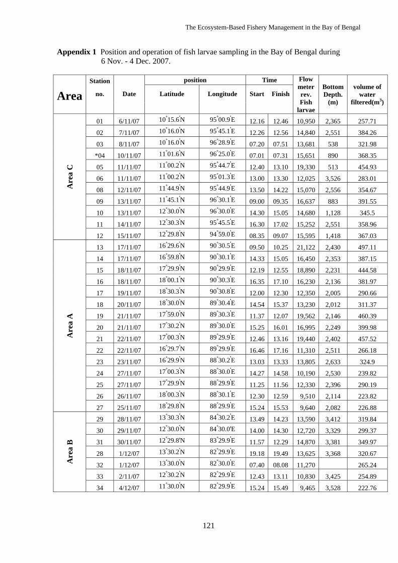
The Ecosystem-Based Fishery Management in the Bay of Bengal
121
Appendix 1 Position and operation of fish larvae sampling in the Bay of Bengal during 6 Nov. - 4 Dec. 2007. Station position Time Flow
meter rev. Fish
larvae
Bottom Depth.
(m)
volume of water
filtered(m3) Area no. Date Latitude Longitude Start Finish
Are
a C
01 6/11/07 10°15.6'N 95°00.9'E 12.16 12.46 10,950 2,365 257.71
02 7/11/07 10°16.0'N 95°45.1'E 12.26 12.56 14,840 2,551 384.26
03 8/11/07 10°16.0'N 96°28.9'E 07.20 07.51 13,681 538 321.98
*04 10/11/07 11°01.6'N 96°25.0'E 07.01 07.31 15,651 890 368.35
05 11/11/07 11°00.2'N 95°44.7'E 12.40 13.10 19,330 513 454.93
06 11/11/07 11°00.2'N 95°01.3'E 13.00 13.30 12,025 3,526 283.01
08 12/11/07 11°44.9'N 95°44.9'E 13.50 14.22 15,070 2,556 354.67
09 13/11/07 11°45.1'N 96°30.1'E 09.00 09.35 16,637 883 391.55
10 13/11/07 12°30.0'N 96°30.0'E 14.30 15.05 14,680 1,128 345.5
11 14/11/07 12°30.3'N 95°45.5'E 16.30 17.02 15,252 2,551 358.96
12 15/11/07 12°29.8'N 94°59.0'E 08.35 09.07 15,595 1,418 367.03
Are
a A
13 17/11/07 16°29.6'N 90°30.5'E 09.50 10.25 21,122 2,430 497.11
14 17/11/07 16°59.8'N 90°30.1'E 14.33 15.05 16,450 2,353 387.15
15 18/11/07 17°29.9'N 90°29.9'E 12.19 12.55 18,890 2,231 444.58
16 18/11/07 18°00.1'N 90°30.3'E 16.35 17.10 16,230 2,136 381.97
17 19/11/07 18°30.3'N 90°30.8'E 12.00 12.30 12,350 2,005 290.66
18 20/11/07 18°30.0'N 89°30.4'E 14.54 15.37 13,230 2,012 311.37
19 21/11/07 17°59.0'N 89°30.3'E 11.37 12.07 19,562 2,146 460.39
20 21/11/07 17°30.2'N 89°30.0'E 15.25 16.01 16,995 2,249 399.98
21 22/11/07 17°00.3'N 89°29.9'E 12.46 13.16 19,440 2,402 457.52
22 22/11/07 16°29.7'N 89°29.9'E 16.46 17.16 11,310 2,511 266.18
23 23/11/07 16°29.9'N 88°30.2'E 13.03 13.33 13,805 2,633 324.9
24 27/11/07 17°00.3'N 88°30.0'E 14.27 14.58 10,190 2,530 239.82
25 27/11/07 17°29.9'N 88°29.9'E 11.25 11.56 12,330 2,396 290.19
26 26/11/07 18°00.3'N 88°30.1'E 12.30 12.59 9,510 2,114 223.82
27 25/11/07 18°29.8'N 88°29.9'E 15.24 15.53 9,640 2,082 226.88
Are
a B
29 28/11/07 13°30.3'N 84°30.2'E 13.49 14.23 13,590 3,412 319.84
30 29/11/07 12°30.0'N 84°30.0'E 14.00 14.30 12,720 3,329 299.37
31 30/11/07 12°29.8'N 83°29.9'E 11.57 12.29 14,870 3,381 349.97
28 1/12/07 13°30.2'N 82°29.9'E 19.18 19.49 13,625 3,368 320.67
32 1/12/07 13°30.0'N 82°30.0'E 07.40 08.08 11,270 265.24
33 2/11/07 12°30.2'N 82°29.9'E 12.43 13.11 10,830 3,425 254.89
34 4/12/07 11°30.0'N 82°29.9'E 15.24 15.49 9,465 3,528 222.76
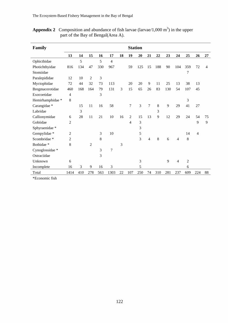
The Ecosystem-Based Fishery Management in the Bay of Bengal
122
Appendix 2 Composition and abundance of fish larvae (larvae/1,000 m3) in the upper part of the Bay of Bengal(Area A). Family Station 13 14 15 16 17 18 19 20 21 22 23 24 25 26 27 Ophicthidae 5 5 4 Photichthyidae 816 134 47 330 967 59 125 15 188 90 104 359 72 4 Stomiidae 7 Paralepididae 12 10 2 3 Myctophidae 72 44 32 73 113 20 20 9 11 25 13 38 13 Bregmacerotidae 460 168 164 79 131 3 15 65 26 83 130 54 107 45 Exocoetidae 4 3 Hemirhamphidae * 8 3 Carangidae * 15 11 16 58 7 3 7 8 9 29 41 27 Labridae 3 3 Callionymidae 6 28 11 21 10 16 2 15 13 9 12 29 24 54 75 Gobiidae 2 4 3 9 9 Sphyraenidae * 3 Gempylidae * 2 3 10 5 14 4 Scombridae * 2 8 3 4 8 6 4 8 Bothidae * 8 2 3 Cynoglossidae * 3 7 Ostraciidae 3 Unknown 6 3 9 4 2 Incomplete 16 3 9 16 3 5 6 Total 1414 410 278 563 1303 22 107 250 74 310 281 237 609 224 88 *Economic fish
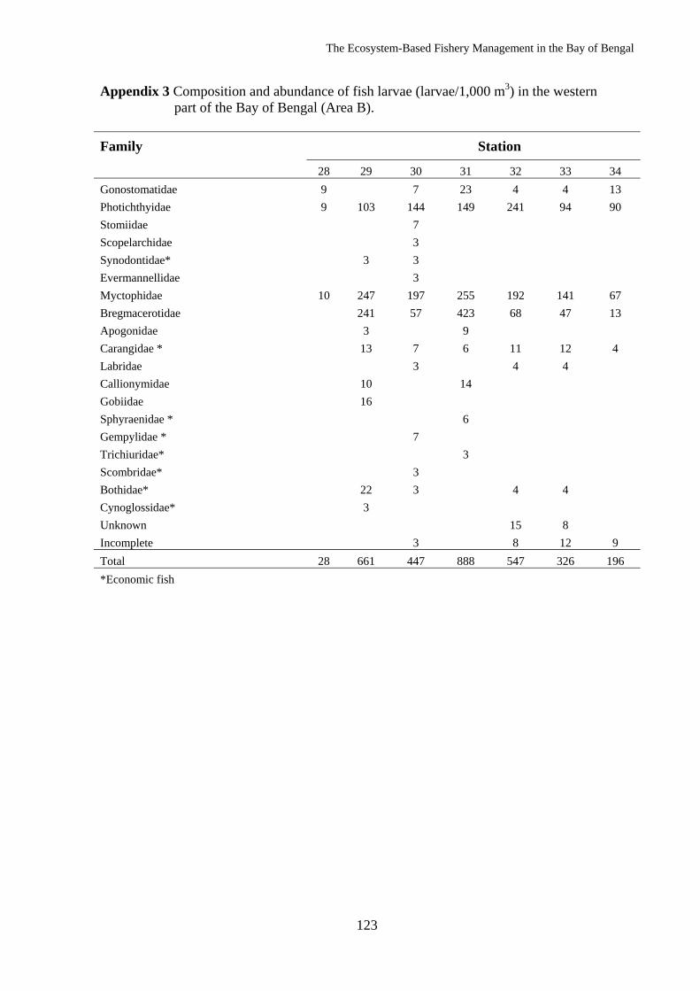
The Ecosystem-Based Fishery Management in the Bay of Bengal
123
Appendix 3 Composition and abundance of fish larvae (larvae/1,000 m3) in the western part of the Bay of Bengal (Area B). Family Station
28 29 30 31 32 33 34 Gonostomatidae 9 7 23 4 4 13 Photichthyidae 9 103 144 149 241 94 90 Stomiidae 7 Scopelarchidae 3 Synodontidae* 3 3 Evermannellidae 3 Myctophidae 10 247 197 255 192 141 67 Bregmacerotidae 241 57 423 68 47 13 Apogonidae 3 9 Carangidae * 13 7 6 11 12 4 Labridae 3 4 4 Callionymidae 10 14 Gobiidae 16 Sphyraenidae * 6 Gempylidae * 7 Trichiuridae* 3 Scombridae* 3 Bothidae* 22 3 4 4 Cynoglossidae* 3 Unknown 15 8 Incomplete 3 8 12 9 Total 28 661 447 888 547 326 196 *Economic fish
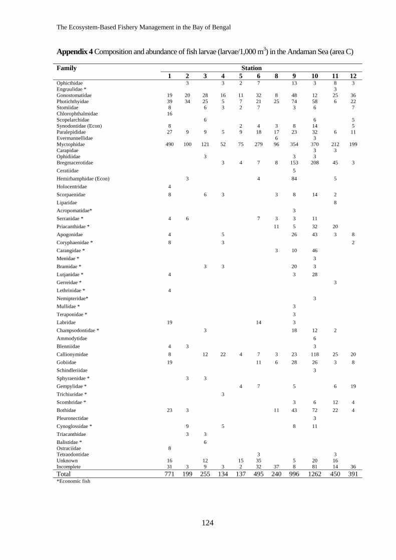
The Ecosystem-Based Fishery Management in the Bay of Bengal
124
Appendix 4 Composition and abundance of fish larvae (larvae/1,000 m3) in the Andaman Sea (area C) Family Station 1 2 3 4 5 6 8 9 10 11 12 Ophicthidae 3 3 2 7 13 3 8 3 Engraulidae * 3 Gonostomatidae 19 20 28 16 11 32 8 48 12 25 36 Photichthyidae 39 34 25 5 7 21 25 74 58 6 22 Stomiidae 8 6 3 2 7 3 6 7 Chlorophthalmidae 16 Scopelarchidae 6 6 5 Synodontidae (Econ) 8 2 4 3 8 14 5 Paralepididae 27 9 9 5 9 18 17 23 32 6 11 Evermannellidae 6 3 Myctophidae 490 100 121 52 75 279 96 354 370 212 199 Carapidae 3 3 Ophidiidae 3 3 3 Bregmacerotidae 3 4 7 8 153 208 45 3 Ceratiidae 5 Hemirhamphidae (Econ) 3 4 84 5 Holocentridae 4 Scorpaenidae 8 6 3 3 8 14 2 Liparidae 8 Acropomatidae* 3 Serranidae * 4 6 7 3 3 11 Priacanthidae * 11 5 32 20 Apogonidae 4 5 26 43 3 8 Coryphaenidae * 8 3 2 Carangidae * 3 10 46 Menidae * 3 Bramidae * 3 3 20 3 Lutjanidae * 4 3 28 Gerreidae * 3 Lethrinidae * 4 Nemipteridae* 3 Mullidae * 3 Teraponidae * 3 Labridae 19 14 3 Champsodontidae * 3 18 12 2 Ammodytidae 6 Blenniidae 4 3 3 Callionymidae 8 12 22 4 7 3 23 118 25 20 Gobiidae 19 11 6 28 26 3 8 Schindleriidae 3 Sphyraenidae * 3 3 Gempylidae * 4 7 5 6 19 Trichiuridae * 3 Scombridae * 3 6 12 4 Bothidae 23 3 11 43 72 22 4 Pleuronectidae 3 Cynoglossidae * 9 5 8 11 Triacanthidae 3 3 Balistidae * 6 Ostraciidae 8 Tetraodontidae 3 3 Unknown 16 12 15 35 5 20 16 Incomplete 31 3 9 3 2 32 37 8 81 14 36 Total 771 199 255 134 137 495 240 996 1262 450 391 *Economic fish
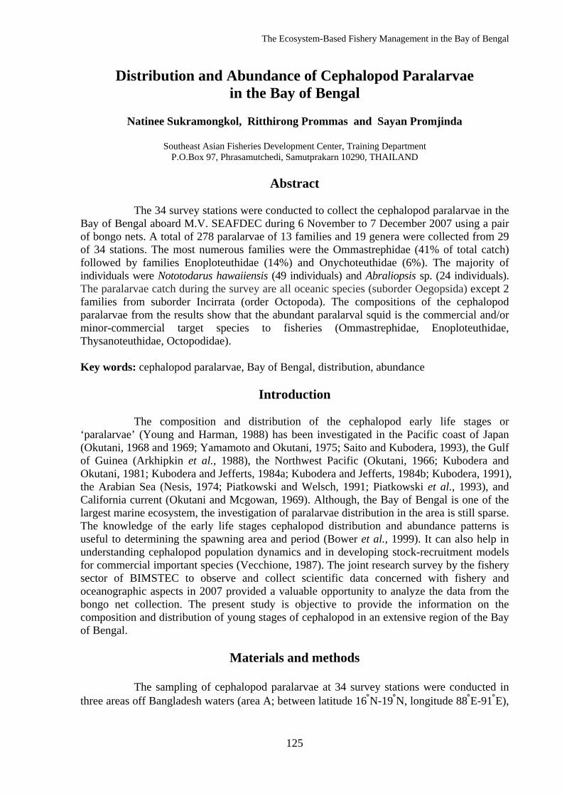
The Ecosystem-Based Fishery Management in the Bay of Bengal
125
Distribution and Abundance of Cephalopod Paralarvae in the Bay of Bengal
Natinee Sukramongkol, Ritthirong Prommas and Sayan Promjinda
Southeast Asian Fisheries Development Center, Training Department
P.O.Box 97, Phrasamutchedi, Samutprakarn 10290, THAILAND
Abstract
The 34 survey stations were conducted to collect the cephalopod paralarvae in the Bay of Bengal aboard M.V. SEAFDEC during 6 November to 7 December 2007 using a pair of bongo nets. A total of 278 paralarvae of 13 families and 19 genera were collected from 29 of 34 stations. The most numerous families were the Ommastrephidae (41% of total catch) followed by families Enoploteuthidae (14%) and Onychoteuthidae (6%). The majority of individuals were Nototodarus hawaiiensis (49 individuals) and Abraliopsis sp. (24 individuals). The paralarvae catch during the survey are all oceanic species (suborder Oegopsida) except 2 families from suborder Incirrata (order Octopoda). The compositions of the cephalopod paralarvae from the results show that the abundant paralarval squid is the commercial and/or minor-commercial target species to fisheries (Ommastrephidae, Enoploteuthidae, Thysanoteuthidae, Octopodidae). Key words: cephalopod paralarvae, Bay of Bengal, distribution, abundance
Introduction
The composition and distribution of the cephalopod early life stages or ‘paralarvae’ (Young and Harman, 1988) has been investigated in the Pacific coast of Japan (Okutani, 1968 and 1969; Yamamoto and Okutani, 1975; Saito and Kubodera, 1993), the Gulf of Guinea (Arkhipkin et al., 1988), the Northwest Pacific (Okutani, 1966; Kubodera and Okutani, 1981; Kubodera and Jefferts, 1984a; Kubodera and Jefferts, 1984b; Kubodera, 1991), the Arabian Sea (Nesis, 1974; Piatkowski and Welsch, 1991; Piatkowski et al., 1993), and California current (Okutani and Mcgowan, 1969). Although, the Bay of Bengal is one of the largest marine ecosystem, the investigation of paralarvae distribution in the area is still sparse. The knowledge of the early life stages cephalopod distribution and abundance patterns is useful to determining the spawning area and period (Bower et al., 1999). It can also help in understanding cephalopod population dynamics and in developing stock-recruitment models for commercial important species (Vecchione, 1987). The joint research survey by the fishery sector of BIMSTEC to observe and collect scientific data concerned with fishery and oceanographic aspects in 2007 provided a valuable opportunity to analyze the data from the bongo net collection. The present study is objective to provide the information on the composition and distribution of young stages of cephalopod in an extensive region of the Bay of Bengal.
Materials and methods
The sampling of cephalopod paralarvae at 34 survey stations were conducted in three areas off Bangladesh waters (area A; between latitude 16°N-19°N, longitude 88°E-91°E),
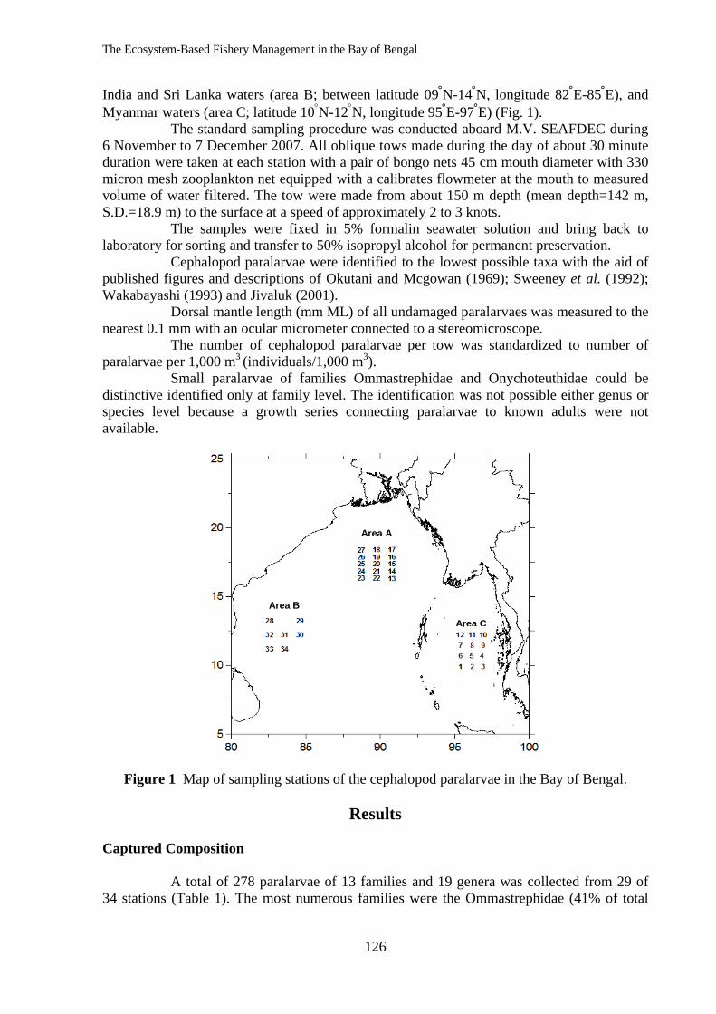
The Ecosystem-Based Fishery Management in the Bay of Bengal
126
India and Sri Lanka waters (area B; between latitude 09°N-14°N, longitude 82°E-85°E), and Myanmar waters (area C; latitude 10°N-12°N, longitude 95°E-97°E) (Fig. 1).
The standard sampling procedure was conducted aboard M.V. SEAFDEC during 6 November to 7 December 2007. All oblique tows made during the day of about 30 minute duration were taken at each station with a pair of bongo nets 45 cm mouth diameter with 330 micron mesh zooplankton net equipped with a calibrates flowmeter at the mouth to measured volume of water filtered. The tow were made from about 150 m depth (mean depth=142 m, S.D.=18.9 m) to the surface at a speed of approximately 2 to 3 knots.
The samples were fixed in 5% formalin seawater solution and bring back to laboratory for sorting and transfer to 50% isopropyl alcohol for permanent preservation.
Cephalopod paralarvae were identified to the lowest possible taxa with the aid of published figures and descriptions of Okutani and Mcgowan (1969); Sweeney et al. (1992); Wakabayashi (1993) and Jivaluk (2001).
Dorsal mantle length (mm ML) of all undamaged paralarvaes was measured to the nearest 0.1 mm with an ocular micrometer connected to a stereomicroscope.
The number of cephalopod paralarvae per tow was standardized to number of paralarvae per 1,000 m3 (individuals/1,000 m3).
Small paralarvae of families Ommastrephidae and Onychoteuthidae could be distinctive identified only at family level. The identification was not possible either genus or species level because a growth series connecting paralarvae to known adults were not available.
Figure 1 Map of sampling stations of the cephalopod paralarvae in the Bay of Bengal.
Results Captured Composition
A total of 278 paralarvae of 13 families and 19 genera was collected from 29 of 34 stations (Table 1). The most numerous families were the Ommastrephidae (41% of total
Area A
Area B
Area C
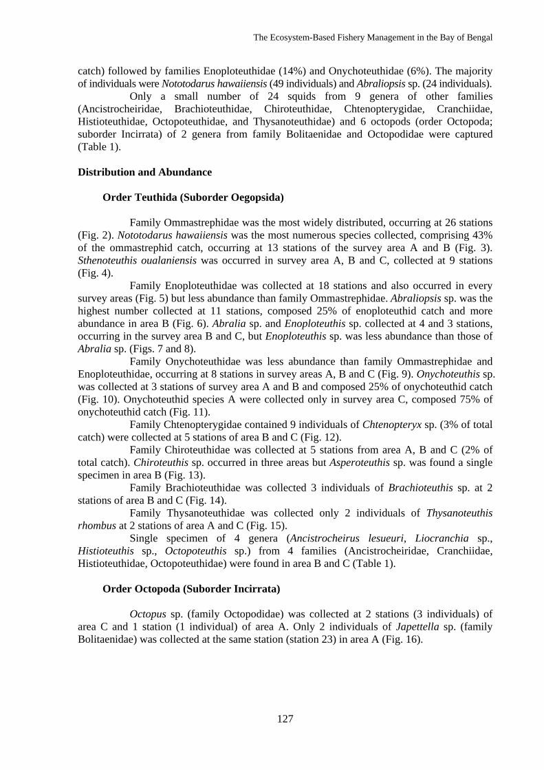
The Ecosystem-Based Fishery Management in the Bay of Bengal
127
catch) followed by families Enoploteuthidae (14%) and Onychoteuthidae (6%). The majority of individuals were Nototodarus hawaiiensis (49 individuals) and Abraliopsis sp. (24 individuals).
Only a small number of 24 squids from 9 genera of other families (Ancistrocheiridae, Brachioteuthidae, Chiroteuthidae, Chtenopterygidae, Cranchiidae, Histioteuthidae, Octopoteuthidae, and Thysanoteuthidae) and 6 octopods (order Octopoda; suborder Incirrata) of 2 genera from family Bolitaenidae and Octopodidae were captured (Table 1). Distribution and Abundance Order Teuthida (Suborder Oegopsida)
Family Ommastrephidae was the most widely distributed, occurring at 26 stations (Fig. 2). Nototodarus hawaiiensis was the most numerous species collected, comprising 43% of the ommastrephid catch, occurring at 13 stations of the survey area A and B (Fig. 3). Sthenoteuthis oualaniensis was occurred in survey area A, B and C, collected at 9 stations (Fig. 4).
Family Enoploteuthidae was collected at 18 stations and also occurred in every survey areas (Fig. 5) but less abundance than family Ommastrephidae. Abraliopsis sp. was the highest number collected at 11 stations, composed 25% of enoploteuthid catch and more abundance in area B (Fig. 6). Abralia sp. and Enoploteuthis sp. collected at 4 and 3 stations, occurring in the survey area B and C, but Enoploteuthis sp. was less abundance than those of Abralia sp. (Figs. 7 and 8).
Family Onychoteuthidae was less abundance than family Ommastrephidae and Enoploteuthidae, occurring at 8 stations in survey areas A, B and C (Fig. 9). Onychoteuthis sp. was collected at 3 stations of survey area A and B and composed 25% of onychoteuthid catch (Fig. 10). Onychoteuthid species A were collected only in survey area C, composed 75% of onychoteuthid catch (Fig. 11).
Family Chtenopterygidae contained 9 individuals of Chtenopteryx sp. (3% of total catch) were collected at 5 stations of area B and C (Fig. 12).
Family Chiroteuthidae was collected at 5 stations from area A, B and C (2% of total catch). Chiroteuthis sp. occurred in three areas but Asperoteuthis sp. was found a single specimen in area B (Fig. 13).
Family Brachioteuthidae was collected 3 individuals of Brachioteuthis sp. at 2 stations of area B and C (Fig. 14).
Family Thysanoteuthidae was collected only 2 individuals of Thysanoteuthis rhombus at 2 stations of area A and C (Fig. 15).
Single specimen of 4 genera (Ancistrocheirus lesueuri, Liocranchia sp., Histioteuthis sp., Octopoteuthis sp.) from 4 families (Ancistrocheiridae, Cranchiidae, Histioteuthidae, Octopoteuthidae) were found in area B and C (Table 1).
Order Octopoda (Suborder Incirrata)
Octopus sp. (family Octopodidae) was collected at 2 stations (3 individuals) of area C and 1 station (1 individual) of area A. Only 2 individuals of Japettella sp. (family Bolitaenidae) was collected at the same station (station 23) in area A (Fig. 16).

The Ecosystem-Based Fishery Management in the Bay of Bengal
128
Tab
le 1
Num
ber o
f spe
cies
and
indi
vidu
als o
f cep
halo
pod
para
larv
ae c
olle
cted
by
zoop
lank
ton
net d
urin
g th
e B
IMST
EC su
rvey
and
man
tle le
ngth
rang
e (m
m) o
f sam
ples
.
12
34
56
78
910
1112
1314
1516
1718
1920
2122
2324
2526
2728
2930
3132
3334
Ord
er O
ctop
oda
Fam
ily B
olita
enid
aeJa
pette
lla s
p.?
22
2.3
- 8.5
Fam
ily O
ctop
odid
aeO
ctop
us s
p.2
11
41.
7 - 3
.9
Ord
er T
euth
idae
Fam
ily A
ncis
troch
eirid
aeA
ncis
troch
eiru
s le
sueu
ri1
1
Fam
ily B
rach
iote
uthi
dae
Bra
chio
teut
his
sp.
21
33.
5 - 4
.2
Fam
ily C
hiro
teut
hida
eA
sper
oteu
this
sp.
11
Chi
rote
uthi
s s
p.1
11
25
3.9
- 6.9
Fam
ily C
hten
opte
rygi
dae
Cht
enop
tery
x s
p.1
21
41
90.
9 - 4
.5
Fam
ily C
ranc
hiid
aeLi
ocra
nchi
a s
p.1
1
Fam
ily E
nopl
oteu
thid
aeA
bral
ia s
p.3
22
31
111.
8 - 7
.2A
bral
iops
is s
p.3
11
12
11
71
42
241.
4 - 5
.6E
nopl
oteu
this
sp.
11
13
2.2
- 5.1
Fam
ily H
istio
teut
hida
eH
istio
teut
his
sp.
11
Fam
ily O
ctop
oteu
thid
aeO
ctop
oteu
this
sp.
11
Fam
ily O
mm
astre
phid
aeS
then
oteu
this
oua
lani
ensi
s1
21
13
27
12
202.
0 - 5
.1N
otot
odar
us h
awai
iens
is?
24
29
78
37
11
31
149
0.8
- 2.6
Om
mas
treph
id s
peci
es1
21
33
72
33
21
33
27
21
460.
4 - 2
.1
Fam
ily O
nych
oteu
thid
aeO
nych
oteu
this
sp.
11
24
2.4
- 7.4
Ony
chot
euth
id s
peci
es A
36
11
112
1.7
- 2.9
Fam
ily T
hysa
note
uthi
dae
Thys
anot
euth
is rh
ombu
s?1
12
Uni
dent
ified
126
112
16
115
52
11
14
37
179
0.5
- 10.
8
Tota
l cep
halo
pods
2717
617
06
016
189
95
02
24
71
80
1417
124
73
10
1810
1610
48
Area
CM
L ra
nge
(mm
)To
tal
Area
BAr
ea A
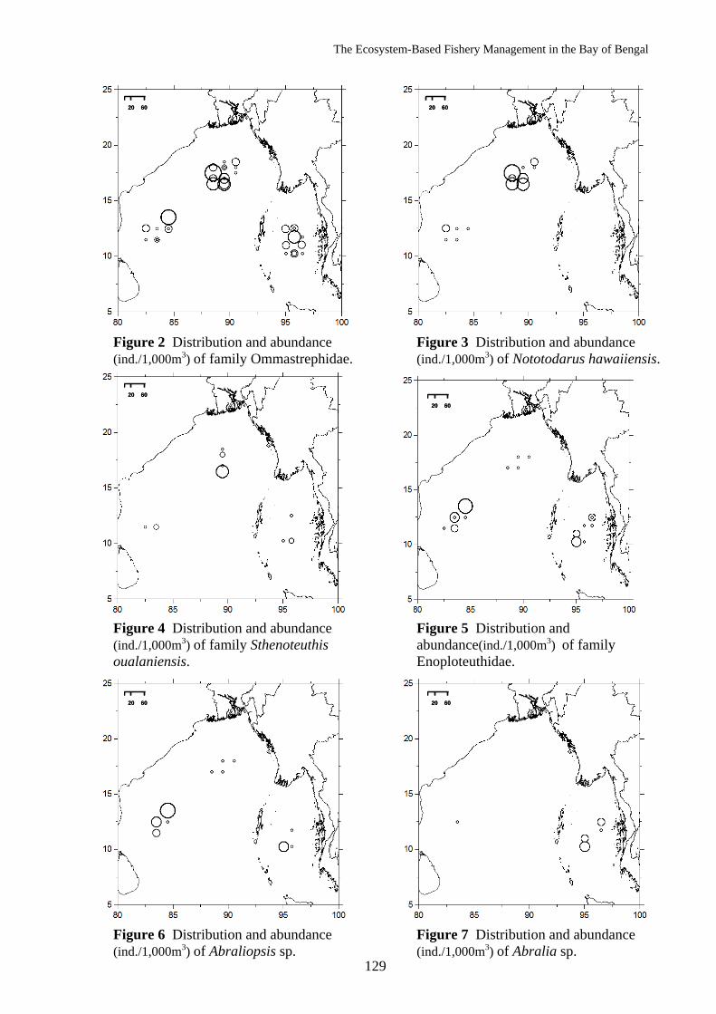
The Ecosystem-Based Fishery Management in the Bay of Bengal
129
Figure 2 Distribution and abundance (ind./1,000m3) of family Ommastrephidae.
Figure 3 Distribution and abundance (ind./1,000m3) of Nototodarus hawaiiensis.
Figure 4 Distribution and abundance (ind./1,000m3) of family Sthenoteuthis oualaniensis.
Figure 5 Distribution and abundance(ind./1,000m3) of family Enoploteuthidae.
Figure 6 Distribution and abundance (ind./1,000m3) of Abraliopsis sp.
Figure 7 Distribution and abundance (ind./1,000m3) of Abralia sp.
20 6020 60
20 6020 60 20 6020 60
20 6020 60
20 6020 6020 6020 60
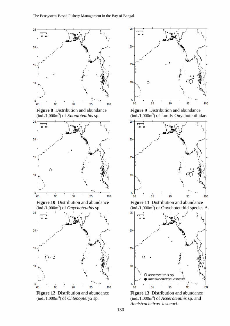
The Ecosystem-Based Fishery Management in the Bay of Bengal
130
Figure 8 Distribution and abundance (ind./1,000m3) of Enoploteuthis sp.
Figure 9 Distribution and abundance (ind./1,000m3) of family Onychoteuthidae.
Figure 10 Distribution and abundance (ind./1,000m3) of Onychoteuthis sp.
Figure 11 Distribution and abundance (ind./1,000m3) of Onychoteuthid species A.
Figure 12 Distribution and abundance (ind./1,000m3) of Chtenopteryx sp.
Figure 13 Distribution and abundance (ind./1,000m3) of Asperoteuthis sp. and Ancistrocheirus lesueuri.
Asperoteuthis sp. Ancistrocheirus lesueuri
20 6020 60
20 6020 6020 6020 60
20 6020 6020 6020 60
20 6020 60
The Ecosystem-Based Fishery Management in the Bay of Bengal
131
Figure 14 Distribution and abundance (ind./1,000m3) of Brachioteuthis sp.
Figure 15 Distribution and abundance (ind./1,000m3) of Thysanoteuthis rhombus.
Figure 16 Distribution and abundance (ind./1,000m3) of Octopus sp. and Japettella sp.
Octopus sp. Japettellas sp.
20 6020 60 20 6020 60
20 6020 60
The Ecosystem-Based Fishery Management in the Bay of Bengal
132
Discussion
The results of the present study showed that the paralarvae catch by zooplankton net during the survey are all oceanic species of various families of suborder Oegopsida (order Teuthida) except 2 families from suborder Incirrata (order Octopoda). The benthic adult octopods (Octopus sp.) were found occurred more than 200 km offshore of the Myanmar and Bangladesh waters. The results of the distribution found the assemblages of the pelagic adults in the continental slope and oceanic waters (Abralia sp., Abraliopsis sp., Enoploteuthis sp.), epi-mesopelagic adults (Sthenoteuthis oualaniensis, Nototodarus hawaiiensis, Onychoteuthis sp. Thysanoteuthis rhombus), mesopelagic adults (Asperoteuthis sp., Chiroteuthis sp., Histioteuthis sp.), and meso-bathypelagic adults (Chtenoteryx sp., Liocranchia sp., Octopoteuthis sp., Brachioteuthis sp.). A diverse community and the most numerous numbers of captured occurred in the survey area off Myanmar waters. Especially, the abundance of the small size of Ommastrephid species (<2 mm) suggesting the nearshore spawning in this area. Possibly the good feeding grounds influenced by surface water runoffs transporting nutrient-rich freshwater into the coastal areas (Sundström et al., 1987; Janecarn and Chullasorn, 1997; Limpsaichol et al., 1998) and/or upwelling conditions create by warm surface waters mixing the nutrient rich bottom (Dwivedi and Choubey, 1998). As the inshore-offshore spawning migrations is common in many cephalopod species (Nesis, 1993a; Mangold, 1987). Some Enoploteuthis species have also been reported to spawn only over the slopes or in nearshore oceanic regions (Nesis, 1993a and 1996). It is possible that spawning of ommastrephid squids may occur throughout the Bengal Bay. The composition from the results also show that the abundant paralarval squid is the commercial and/or minor-commercial target species to fisheries (Carpenter and Niem, 1998).
The results from the present study is useful for determining when and where adults spawn, particularly for species whose adults are difficult to catch (Bower et al., 1999). Further sampling survey in different monsoon season will help to provide a better understanding on life history of cephalopod species in these areas.
Acknowledgements
The authors wish to acknowledge the cooperation between the BIMSTEC member countries, Department of Fisheries of Thailand and SEAFDEC/TD. We would also like to thanks to the officers and crews of M.V. SEAFDEC for their helps during the surveys.
The Ecosystem-Based Fishery Management in the Bay of Bengal
133
References
Arkhipkin, A. I., Y. N. Zheronkin, Y. A. Loktionov and A. S. Schetinnikov. 1988. Fauna and distribution of pelagic cephalopods larvae in the Gulf of Guinea. Zool. Zh. 67(10):1459-1467. (in Russian, English abstract)
Bower, J. B., M. P. Seki, R. E. Young, K. A. Bigelow, J. Hirota and P. Flament. 1999. Cephalopod paralarvae assemblages in Hawaiian waters. Mar.Eco.Prog.Ser. 185:203-212.
Carpenter, K. E. and V. H. Niem. (eds.). 1998. FAO species identification guide for fishery purposes. The living marine resources of the Western Central Pacific, vol. 2, Cephalopods, crustacean, holothurians and sharks. FAO Publication, Rome. p. 764-780.
Dwivedi, S. N. and A. K. Choubey. 1998. Indian Ocean large marine ecosystems: need for national and regional framework for conservation and sustainable development. In: K Sherman, K., E. Okemwa and M. Ntiba. (eds.). Large Marine Ecosystems of the Indian Ocean: Assessment, Sustainability and Management. Blackwell Science.
Janekarn, V. and S. Chullasorn. 1997. Environmental impacts on coastal fisheries along the west coast of Thailand. In: Asia-Pacific Fishery Commission (APFIC): Environmental aspects of responsible fisheries. Proceedings of the APFIC Symposium Seoul, the Republic of Korea, 15-18 October 1996. FAO Bangkok. RAP Publication 32/1997. p. 222-233.
Jivaluk, J. 2001. Species, abundance and distribution of cephalopod paralarvae in the Gulf of Thailand in 1995 and 1996. Fish. Mus. Nat. Hist. Tech. Pap. No. 1/2001. 31 pp.
Kubodera, T. 1991. Distribution and abundance of the early life stages of octopus, Octopus dofleini Wulker 1910 in the North Pacific. Bull. Mar. Sci. 49(1-2):235-243.
Kubodera, T. and K. Jefferts. 1984a. Distribution and abundance of the early life stages of squid, primarily Gonatidae (Cephalopoda: Oegopsida) in the northern North Pacific (Part 1). Bull. Natl. Sci.Mus. Ser. A. (Zool). 10(3):91-106.
Kubodera, T. and K. Jefferts. 1984b. Distribution and abundance of the early life stages of squid, primarily Gonatidae (Cephalopoda: Oegopsida) in the northern North Pacific (Part 2). Bull. Natl. Sci.Mus. Ser. A. (Zool). 10(4):165-193.
Kubodera, T. and T. Okutani. 1981. The systematics and identification of larval cephalopods from the northern North Pacific. Res. Ins. N. Pac. Fish. Hokkaido Univ. Spec. p. 131-159.
Limpsaichol, P., S. Khokiattiwong, N. Bussarawit and P. Sojisuporn. 1998. Environmental factors influencing the health and productivity of the Phang-nga Bay. In: Community-based fisheries management in the Phang-nga Bay, Thailand. Proceedings of the National Workshop on Community-based Management organized by the Department of Fisheries of Thailand, FAO and the Bay of Bengal Programme, Phuket, Thailand, 14-16 February 1996. Phuket, Thailand. p. 85-120.
Mangold, K. 1987. Reproduction. In: Boyle PR. (ed). Cephalopod Life Cycles. Acadernic Press Inc, London. p. 157-200.
Nesis, K. N. 1974. Cephalopod larvae in the western Arabian Sea. Oceanoloqy 14(3): 441-445.
Nesis, K. N. 1993. Cephalopods of seamounts and submarinendges. In: Okutani, T., R. K. O'Dor and T. Kubodera, T. (eds.). Recent Advances in Cephalopod Fisheries Biology. Tokai University Press, Tokyo. p. 365-373.
Nesis, K. N. 1996. Mating, spawning and death in 0ceanic cephalopods: a review. Ruthenica 6(1):23-64.
Okutani, T. 1966. Studies on early life history of decapodan mollusca - II Planktonic larvae of decapodan cephalopods from the northern North Pacific in summer seasons during 1952-1959. Bull. Tokai. Reg. Fish .Res. Lab. 45:61-79.
The Ecosystem-Based Fishery Management in the Bay of Bengal
134
Okutani, T. 1968. Studies on early life history of decapodan mollusca-III. Systematics and distribution of larvae of decapod cephalopods collected from the sea surface on the Pacific coast of Japan 1960-1965. Bull. Tokai. Reg. Fish. Res. Lab. p. 559-57.
Okutani, T. 1969. Studies on early life history of decapodan Moliusca-IV. Bull. Tokai. Reg. Fish. Res. Lab. 58:83-96.
Okutani, T. and J. A. McGowan. 1969. Systematics, distribution, and abundance of the epiplanktonic squid (Cephalopoda: Decapoda) larvae of the California Current Aprd 1.954-March 1957. Bull. Scripps. Inst. Oceanogr. Univ. Calif. 14:1-90.
Piatkowski, U. and W. Welsch. 1991. On the distribution of pelagic cephalopods in the Arabian Sea. Bull. Mar. Sci. 49(1-2):186-198.
Piatkowski, U., W. Welsch and A. Ropke. 1993. Distribution patterns of the early life stages of pelagic cephalopods in three geographically different regions of the Arabian Sea. In: Okutani, T., R. K. O'Dor and T. Kubodera. (eds.). Recent Advances in Cephalopod Fisheries Biology. Tokai University Press, Tokyo. p. 417-431.
Saito. H. and T. Kubodera. 1993. Distribution of Ommastrephid rhynchoteuthion paralarvae (Mollusca: Cephalopoda) in the Kuroshio region. In: Okutani, T., R. K. O'Dor and T. Kubodera. (eds.). Recent Advances in Cephalopod Fisheries Biology. Tokai University Press, Tokyo. p. 457-466.
Sundström, B., V. Janekarn, J. Hylleberg and P. Boonruang. 1987. Annual pelagic primary production with notes on physical and chemical variables at Phuket, the Andaman Sea, Thailand. Res. Bull. Phuket Mar. Biol. Cent. 46:12 pp.
Sweeney, M. J., C. F. E Roper, K. M. Mangold, M. R. Clarke, and S. V. Boletzky. (eds.). 1992. Larval and Juvenile Cephalopods: A Manual for their Identification. Smithson. Contrib. Zool. 513:282 pp.
Vecchione, M. 1987. Juvenile ecology. In: Boyle, P. R. (ed.). Cephalopod Life Cycles, Vol. 2. Academic Press Inc, London. p. 61-84.
Wakabayashi, T. 1993. Species, distribution and abundance of cephalopod paralarvae in the western Australian waters. Master Thesis. Tokyo University of Fisheries, Tokyo. 120 pp.
Yamamoto, K. and T. Okutani. 1975. Studies on early life history of decapodan mollusca-V. Systematics and distribution of epipelagic larvae of decapod cephalopods in the southwestern waters of Japan during the summer in 1970. Bull. Tokai Reg Fish Res. Lab. 83:45-96.
Young, R. E. and R. F. Harman, R. F. 1988. Larvae, paralarvae and subadult in cephalopod terminology. Malacologia 29:201-207.
The Ecosystem-Based Fishery Management in the Bay of Bengal
135
Large Pelagic Fishery Resource Survey using Pelagic Longline in the Bay of Bengal
Chirat Nuangsang1, Sayan Promjinda2, Opas Chamason3, Md. Jalilur Rahman4,
Rankiri P.P. Krishantha Jayasinghe5, U Aung Htay Oo6 and Manas Kumar Sinha7
1 Deep Sea Fishery Technology Research and Development Institute,
Department of Fisheries, Samutprakarn 10270, THAILAND 2 Southeast Asian Fisheries Development Center, Training Department
P.O.Box 97, Phrasamutchedi, Samutprakarn 10290, THAILAND 3 Upper-Gulf Fisheries Research and Development Center,
Department of Fisheries, Samutprakarn 10130, THAILAND
4 Marine Fisheries and Technology Station, Bangladesh Fisheries Research Institute, Motel Road, Cox’s Bazar-4700, BANGLADESH
5 National Aquatic Resource Research and Development Agency, Crow Island, Colombo 15, SRI LANKA
6 Marine Fishery Resources Survey and Research Unit, Department of Fisheries, Yangon, MYANMAR 7 Port Blair Base of Fishery Survey of India, P.O.Box 46, Phoenix Bay, Port Blair, INDIA
Abstract
The fishery research vessel, M.V. SEAFDEC, of the Southeast Asian Fisheries Development Center (SEAFDEC) collaborated with the BIMSTEC member countries was conducted a survey using pelagic longline with thirteen fishing operations to investigate the potential of large pelagic fishery resources in the Bay of Bengal within 3 areas during 5 November to 4 December 2007. The mainline of pelagic longline was made from nylon monofilament in the reel system. Number of hook deployed in each station varied from 303-520, the hook operation depth was between 40-300 m. Shooting gear was done at dusk, baits using were round scads, milk fish and Indian mackerel then the gear was retrieved in the next morning. Total catch were weighing 1,754.65 kg and 77 numbers. Identified seventeen species belonged to 16 genera and 12 families were caught during the survey. Main catch, by weight and number, were swordfish (Xiphias gladius) 650.0 kg (37.044%), 21 individuals followed by bigeye thresher shark (Alopias superciliosus) 641.0 kg (36.531%), 11 individuals and yellowfin tuna (Thunnus albacares) 75.0 kg (4.274%), 3 individuals. The overall average catch rate was 1.23% (individuals/100 hooks). The highest catch rate 3.94% was found at station 12 at latitude 12°30′.30 N longitude 094°59′.70 E. The catch rate of swordfish was quite high comparing to commercial longline fleet. This suggests the prominent potential yield of swordfish in this surveyed area whilst the tuna is low. Keywords : Bay of Bengal, pelagic longline, large pelagic fishery
Introduction The Bay of Bengal is a bay that forms the northeastern part of the Indian Ocean. It occupies an area of 2,172,000 km², 2,090 km long and 1,600 km wide with an average depth of more than 2,600 m. It resembles a triangle in shape, and is bordered by India and Sri Lanka to the West, Bangladesh and the Indian state of west Bengal to the North (where the name comes from), and Myanmar, southern part of Thailand and the Andaman Sea and Nicobar Islands to the East. Its southern boundary extends as an imaginary line from Dondra Head at the southern end of Sri Lanka to the northern tip of Sumatra. The Bay of Bengal is
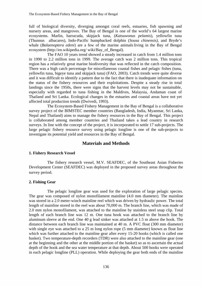
The Ecosystem-Based Fishery Management in the Bay of Bengal
136
full of biological diversity, diverging amongst coral reefs, estuaries, fish spawning and nursery areas, and mangroves. The Bay of Bengal is one of the world’s 64 largest marine ecosystems. Marlin, barracuda, skipjack tuna, (Katsuwonus pelamis), yellowfin tuna (Thunnus albacares), Indo-Pacific humpbacked dolphin (Sousa chinensis), and Bryde’s whale (Balaenoptera edeni) are a few of the marine animals living in the Bay of Bengal ecosystem (http://en.wikipedia.org/ wiki/Bay_of_Bengal). The FAO 10 years trend showed a steady increased in catch from 1.4 million tons in 1990 to 2.2 million tons in 1999. The average catch was 2 million tons. This tropical region has a relatively great marine biodiversity that was reflected in the catch composition. There was a high catch percentage for miscellaneous coastal fishes and pelagic fishes (tuna, yellowfin tuna, bigeye tuna and skipjack tuna) (FAO, 2003). Catch trends were quite diverse and it was difficult to identify a pattern due to the fact that there is inadequate information on the status of the fishery resources and their exploitations. Despite a steady rise in total landings since the 1950s, there were signs that the harvest levels may not be sustainable, especially with regarded to tuna fishing in the Maldives, Malaysia, Andaman coast of Thailand and Sri Lanka. Ecological changes in the estuaries and coastal areas have not yet affected total production trends (Dwivedi, 1993). The Ecosystem-Based Fishery Management in the Bay of Bengal is a collaborative survey project of the BIMSTEC member countries (Bangladesh, India, Myanmar, Sri Lanka, Nepal and Thailand) aims to manage the fishery resources in the Bay of Bengal. This project is collaborated among member countries and Thailand takes a lead country in research surveys. In line with the concept of the project, it is incorporated to settle 17 sub-projects. The large pelagic fishery resource survey using pelagic longline is one of the sub-projects to investigate its potential yield and resources in the Bay of Bengal.
Materials and Methods 1. Fishery Research Vessel The fishery research vessel, M.V. SEAFDEC, of the Southeast Asian Fisheries Development Center (SEAFDEC) was deployed in the proposed survey areas throughout the survey period. 2. Fishing Gear The pelagic longline gear was used for the exploration of large pelagic species. The gear was composed of nylon monofilament mainline (4.0 mm diameter). The mainline was stored in a 2.0 meter-winch mainline reel which was driven by hydraulic power. The total length of mainline stored in the reel was about 70,000 m. The branch line, which was made of 2.0 mm nylon monofilament, was attached to the mainline by stainless steel snap clip. Total length of each branch line was 12 m. One tuna hook was attached to the branch line by aluminum sleeve at the end. One 40 g lead sinker was attached at 1.5 m above the hook. The distance between each branch line was maintained at 40 m. A PVC float (300 mm diameter) with single eye was attached to a 25 m long nylon rope (5 mm diameter) known as float line which was further attached to the mainline gear after every 15-20 hooks (which is called one basket). Two temperature-depth recorders (TDR) were also attached to the mainline gear (one at the beginning and the other at the middle portion of the basket) so as to ascertain the actual depth of the hook and the sea water temperature at that depth. About 500 hooks were operated in each pelagic longline (PLL) operation. While deploying the gear both ends of the mainline
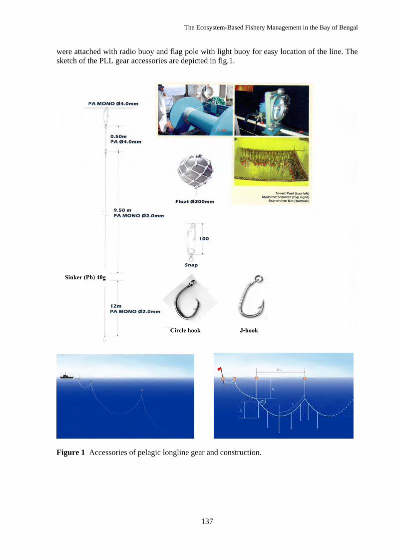
The Ecosystem-Based Fishery Management in the Bay of Bengal
137
were attached with radio buoy and flag pole with light buoy for easy location of the line. The sketch of the PLL gear accessories are depicted in fig.1.
Figure 1 Accessories of pelagic longline gear and construction.
Sinker (Pb) 40g
Circle hook J-hook
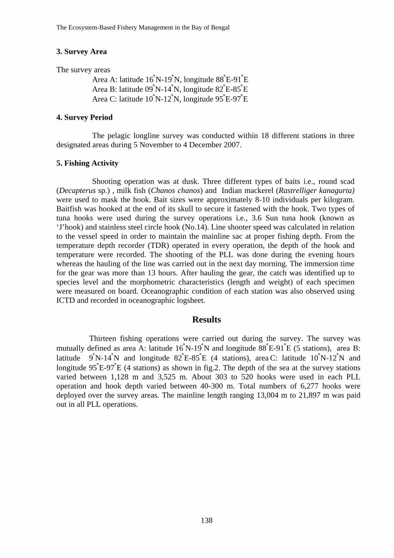
The Ecosystem-Based Fishery Management in the Bay of Bengal
138
3. Survey Area The survey areas
Area A: latitude 16°N-19°N, longitude 88°E-91°E Area B: latitude 09°N-14°N, longitude 82°E-85°E Area C: latitude 10°N-12°N, longitude 95°E-97°E
4. Survey Period The pelagic longline survey was conducted within 18 different stations in three designated areas during 5 November to 4 December 2007. 5. Fishing Activity Shooting operation was at dusk. Three different types of baits i.e., round scad (Decapterus sp.) , milk fish (Chanos chanos) and Indian mackerel (Rastrelliger kanagurta) were used to mask the hook. Bait sizes were approximately 8-10 individuals per kilogram. Baitfish was hooked at the end of its skull to secure it fastened with the hook. Two types of tuna hooks were used during the survey operations i.e., 3.6 Sun tuna hook (known as ‘J’hook) and stainless steel circle hook (No.14). Line shooter speed was calculated in relation to the vessel speed in order to maintain the mainline sac at proper fishing depth. From the temperature depth recorder (TDR) operated in every operation, the depth of the hook and temperature were recorded. The shooting of the PLL was done during the evening hours whereas the hauling of the line was carried out in the next day morning. The immersion time for the gear was more than 13 hours. After hauling the gear, the catch was identified up to species level and the morphometric characteristics (length and weight) of each specimen were measured on board. Oceanographic condition of each station was also observed using ICTD and recorded in oceanographic logsheet.
Results
Thirteen fishing operations were carried out during the survey. The survey was mutually defined as area A: latitude 16°N-19°N and longitude 88°E-91°E (5 stations), area B: latitude 9°N-14°N and longitude 82°E-85°E (4 stations), area C: latitude 10°N-12°N and longitude 95°E-97°E (4 stations) as shown in fig.2. The depth of the sea at the survey stations varied between 1,128 m and 3,525 m. About 303 to 520 hooks were used in each PLL operation and hook depth varied between 40-300 m. Total numbers of 6,277 hooks were deployed over the survey areas. The mainline length ranging 13,004 m to 21,897 m was paid out in all PLL operations.
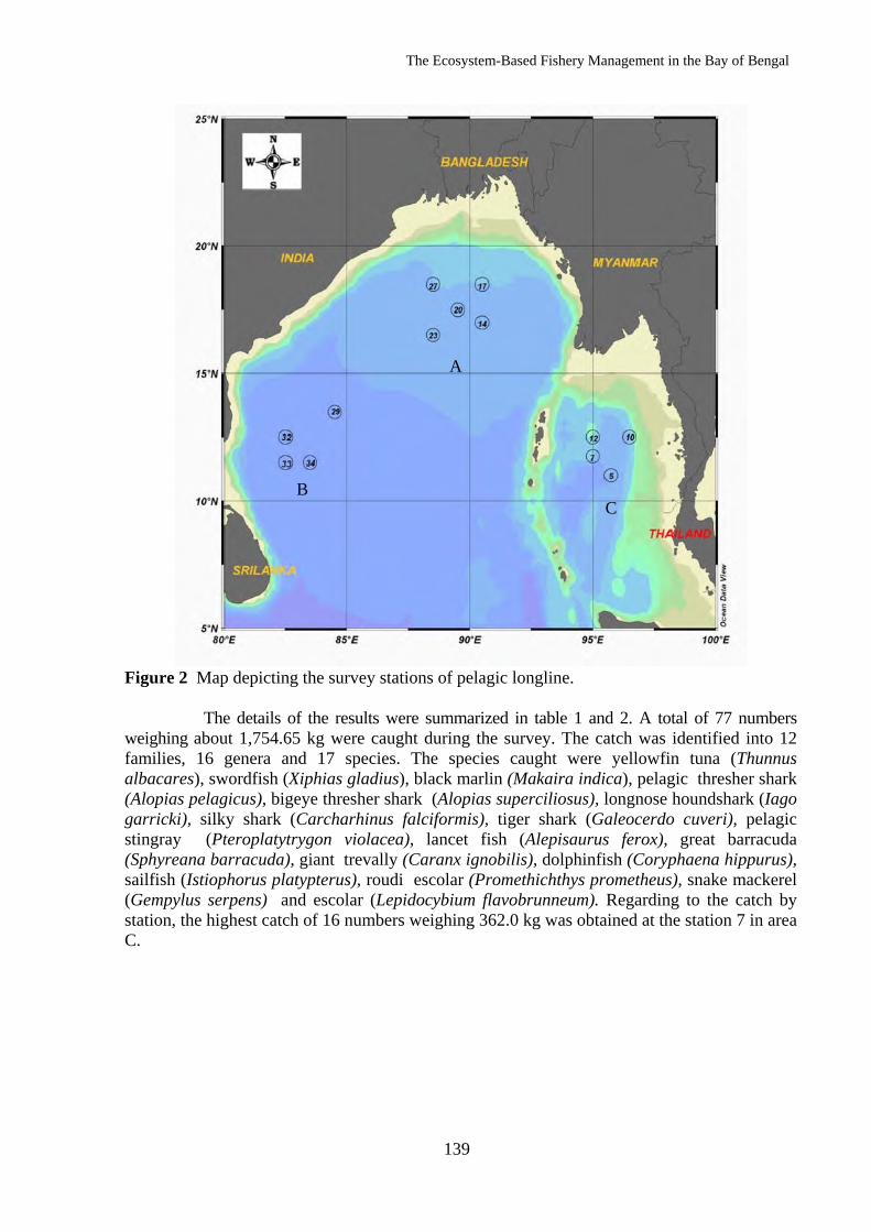
The Ecosystem-Based Fishery Management in the Bay of Bengal
139
Figure 2 Map depicting the survey stations of pelagic longline. The details of the results were summarized in table 1 and 2. A total of 77 numbers weighing about 1,754.65 kg were caught during the survey. The catch was identified into 12 families, 16 genera and 17 species. The species caught were yellowfin tuna (Thunnus albacares), swordfish (Xiphias gladius), black marlin (Makaira indica), pelagic thresher shark (Alopias pelagicus), bigeye thresher shark (Alopias superciliosus), longnose houndshark (Iago garricki), silky shark (Carcharhinus falciformis), tiger shark (Galeocerdo cuveri), pelagic stingray (Pteroplatytrygon violacea), lancet fish (Alepisaurus ferox), great barracuda (Sphyreana barracuda), giant trevally (Caranx ignobilis), dolphinfish (Coryphaena hippurus), sailfish (Istiophorus platypterus), roudi escolar (Promethichthys prometheus), snake mackerel (Gempylus serpens) and escolar (Lepidocybium flavobrunneum). Regarding to the catch by station, the highest catch of 16 numbers weighing 362.0 kg was obtained at the station 7 in area C.
A
B C
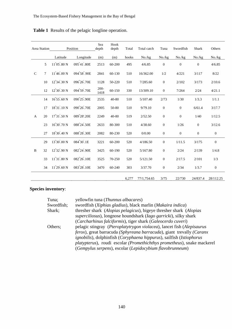
The Ecosystem-Based Fishery Management in the Bay of Bengal
140
Table 1 Results of the pelagic longline operation.
Species inventory:
Tuna; yellowfin tuna (Thunnus albacares) Swordfish; swordfish (Xiphias gladius), black marlin (Makaira indica) Shark; thresher shark (Alopias pelagicus), bigeye thresher shark (Alopias
superciliosus), longnose houndshark (Iago garricki), silky shark (Carcharhinus falciformis), tiger shark (Galeocerdo cuveri)
Others; pelagic stingray (Pteroplatytrygon violacea), lancet fish (Alepisaurus ferox), great barracuda (Sphyreana barracuda), giant trevally (Caranx ignobilis), dolphinfish (Coryphaena hippurus), sailfish (Istiophorus platypterus), roudi escolar (Promethichthys prometheus), snake mackerel (Gempylus serpens), escolar (Lepidocybium flavobrunneum)
Area Station Position Sea depth
Hook depth Total Total catch Tuna Swordfish Shark Others
Latitude Longitude (m) (m) hooks No./kg No./kg No./kg No./kg No./kg
5 11°05'.80 N 095°41'.80E 2513 60-200 495 4/6.85 0 0 0 4/6.85
C 7 11°46'.00 N 094°58''.90E 2841 60-130 510 16/362.00 1/2 4/221 3/117 8/22
10 12°34'.30 N 096°26'.70E 1128 50-220 510 7/285.60 0 2/102 3/173 2/10.6
12 12°30'.30 N 094°59'.70E 200-1418 60-150 330 13/309.10 0 7/264 2/24 4/21.1
14 16°55'.60 N 090°25'.90E 2535 40-80 510 5/107.40 2/73 1/30 1/3.3 1/1.1
17 18°31'.10 N 090°26'.70E 2005 50-80 510 9/79.10 0 0 6/61.4 3/17.7
A 20 17°31'.50 N 089°28'.20E 2249 40-80 519 2/52.50 0 0 1/40 1/12.5
23 16°30'.70 N 088°24'.50E 2633 80-300 510 4/38.60 0 1/26 0 3/12.6
27 18°30'.40 N 088°28'.30E 2082 80-230 520 0/0.00 0 0 0 0
29 13°30'.00 N 084°30'.1E 3221 60-200 520 4/186.50 0 1/11.5 3/175 0
B 32 12°32'.90 N 082°24'.90E 3425 60-190 520 5/167.80 0 2/24 2/139 1/4.8
33 11°31'.80 N 082°26'.10E 3525 70-250 520 5/121.50 0 2/17.5 2/101 1/3
34 11°29'.60 N 083°28'.10E 3470 60-240 303 3/37.70 0 2/34 1/3.7 0
6,277 77/1,754.65 3/75 22/730 24/837.4 28/112.25
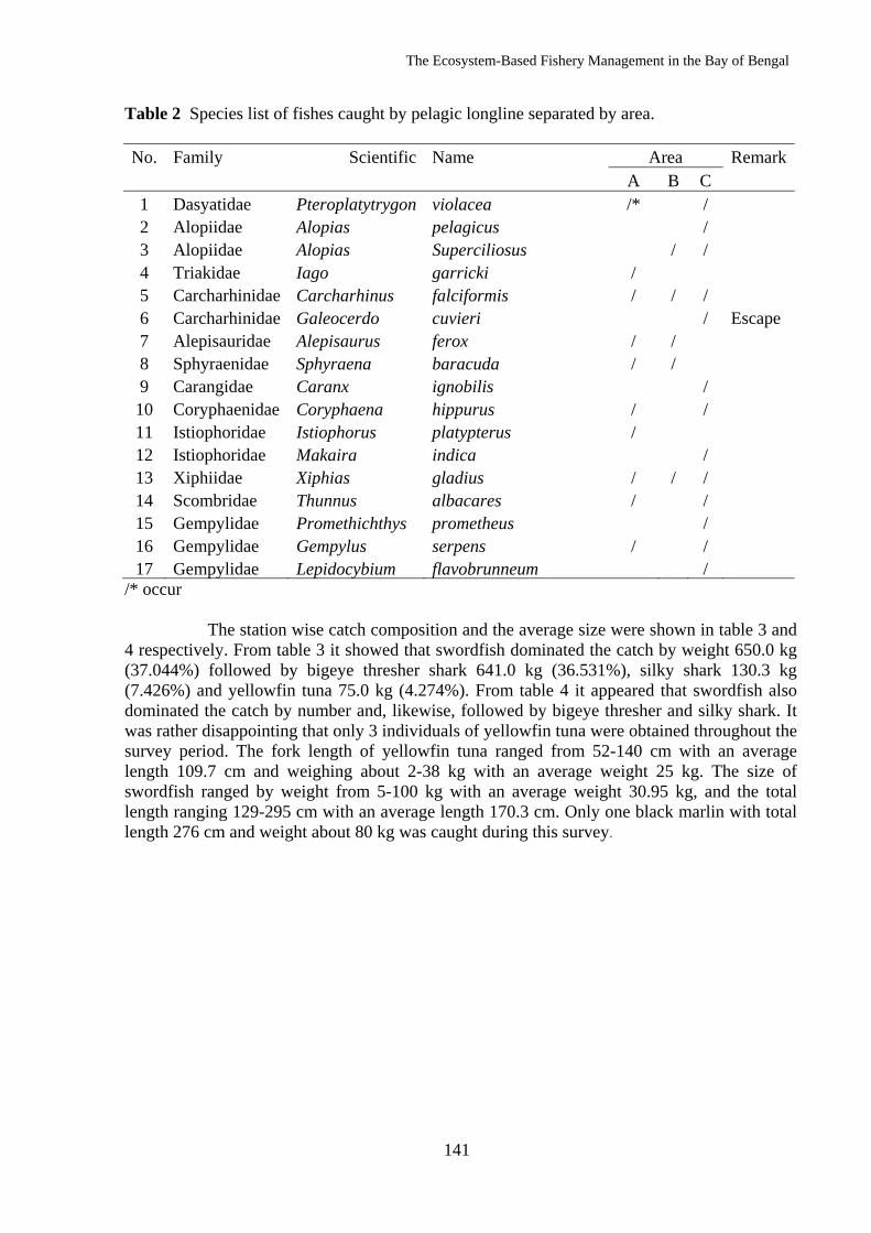
The Ecosystem-Based Fishery Management in the Bay of Bengal
141
Table 2 Species list of fishes caught by pelagic longline separated by area. No. Family Scientific Name Area Remark
A B C 1 Dasyatidae Pteroplatytrygon violacea /* / 2 Alopiidae Alopias pelagicus / 3 Alopiidae Alopias Superciliosus / / 4 Triakidae Iago garricki / 5 Carcharhinidae Carcharhinus falciformis / / / 6 Carcharhinidae Galeocerdo cuvieri / Escape 7 Alepisauridae Alepisaurus ferox / / 8 Sphyraenidae Sphyraena baracuda / / 9 Carangidae Caranx ignobilis /
10 Coryphaenidae Coryphaena hippurus / / 11 Istiophoridae Istiophorus platypterus / 12 Istiophoridae Makaira indica / 13 Xiphiidae Xiphias gladius / / / 14 Scombridae Thunnus albacares / / 15 Gempylidae Promethichthys prometheus / 16 Gempylidae Gempylus serpens / / 17 Gempylidae Lepidocybium flavobrunneum /
/* occur
The station wise catch composition and the average size were shown in table 3 and 4 respectively. From table 3 it showed that swordfish dominated the catch by weight 650.0 kg (37.044%) followed by bigeye thresher shark 641.0 kg (36.531%), silky shark 130.3 kg (7.426%) and yellowfin tuna 75.0 kg (4.274%). From table 4 it appeared that swordfish also dominated the catch by number and, likewise, followed by bigeye thresher and silky shark. It was rather disappointing that only 3 individuals of yellowfin tuna were obtained throughout the survey period. The fork length of yellowfin tuna ranged from 52-140 cm with an average length 109.7 cm and weighing about 2-38 kg with an average weight 25 kg. The size of swordfish ranged by weight from 5-100 kg with an average weight 30.95 kg, and the total length ranging 129-295 cm with an average length 170.3 cm. Only one black marlin with total length 276 cm and weight about 80 kg was caught during this survey.
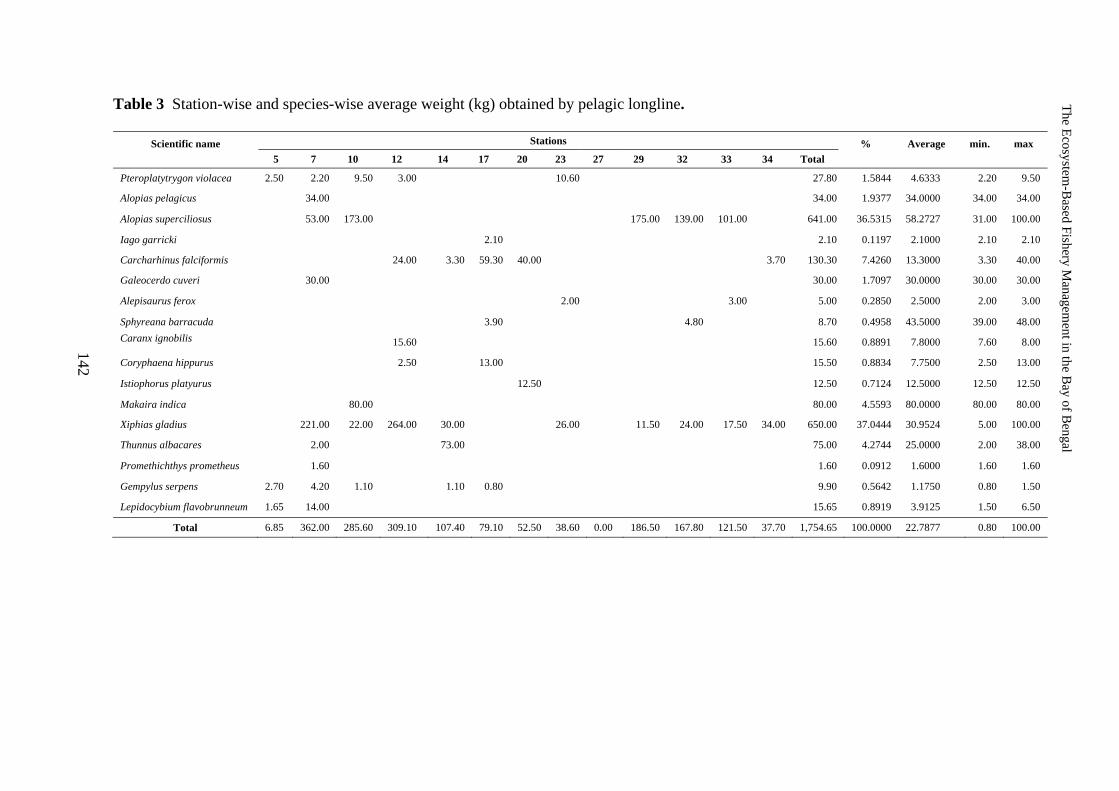
The Ecosystem-Based Fishery Management in the Bay of Bengal
142
Table 3 Station-wise and species-wise average weight (kg) obtained by pelagic longline.
Scientific name
Stations %
Average
min.
max 5 7 10 12 14 17 20 23 27 29 32 33 34 Total
Pteroplatytrygon violacea 2.50 2.20 9.50 3.00 10.60 27.80 1.5844 4.6333 2.20 9.50
Alopias pelagicus 34.00 34.00 1.9377 34.0000 34.00 34.00
Alopias superciliosus 53.00 173.00 175.00 139.00 101.00 641.00 36.5315 58.2727 31.00 100.00
Iago garricki 2.10 2.10 0.1197 2.1000 2.10 2.10
Carcharhinus falciformis 24.00 3.30 59.30 40.00 3.70 130.30 7.4260 13.3000 3.30 40.00
Galeocerdo cuveri 30.00 30.00 1.7097 30.0000 30.00 30.00
Alepisaurus ferox 2.00 3.00 5.00 0.2850 2.5000 2.00 3.00
Sphyreana barracuda 3.90 4.80 8.70 0.4958 43.5000 39.00 48.00 Caranx ignobilis 15.60 15.60 0.8891 7.8000 7.60 8.00
Coryphaena hippurus 2.50 13.00 15.50 0.8834 7.7500 2.50 13.00
Istiophorus platyurus 12.50 12.50 0.7124 12.5000 12.50 12.50
Makaira indica 80.00 80.00 4.5593 80.0000 80.00 80.00
Xiphias gladius 221.00 22.00 264.00 30.00 26.00 11.50 24.00 17.50 34.00 650.00 37.0444 30.9524 5.00 100.00
Thunnus albacares 2.00 73.00 75.00 4.2744 25.0000 2.00 38.00
Promethichthys prometheus 1.60 1.60 0.0912 1.6000 1.60 1.60
Gempylus serpens 2.70 4.20 1.10 1.10 0.80 9.90 0.5642 1.1750 0.80 1.50
Lepidocybium flavobrunneum 1.65 14.00 15.65 0.8919 3.9125 1.50 6.50
Total 6.85 362.00 285.60 309.10 107.40 79.10 52.50 38.60 0.00 186.50 167.80 121.50 37.70 1,754.65 100.0000 22.7877 0.80 100.00
142
The Ecosystem
-Based Fishery M
anagement in the B
ay of Bengal
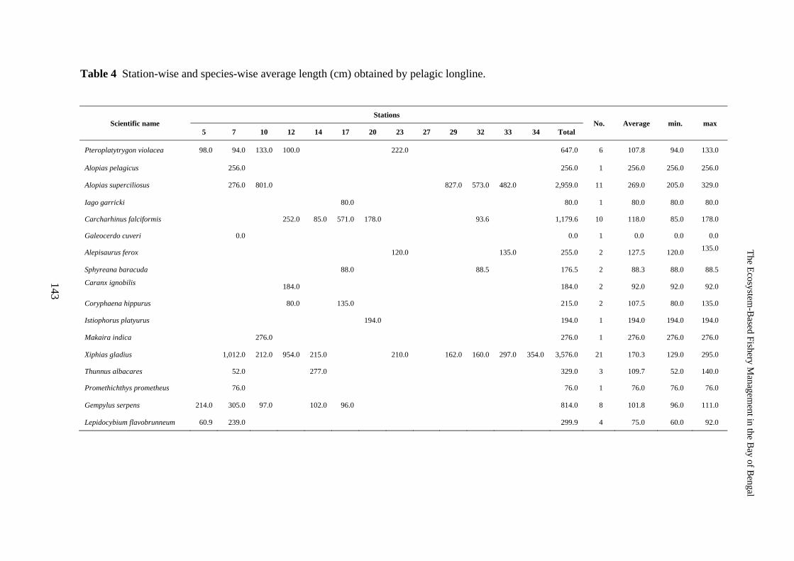
The Ecosystem-Based Fishery Management in the Bay of Bengal
143
Table 4 Station-wise and species-wise average length (cm) obtained by pelagic longline.
Scientific name Stations
No. Average min. max 5 7 10 12 14 17 20 23 27 29 32 33 34 Total
Pteroplatytrygon violacea 98.0 94.0 133.0 100.0 222.0 647.0 6 107.8 94.0 133.0
Alopias pelagicus 256.0 256.0 1 256.0 256.0 256.0
Alopias superciliosus 276.0 801.0 827.0 573.0 482.0 2,959.0 11 269.0 205.0 329.0
Iago garricki 80.0 80.0 1 80.0 80.0 80.0
Carcharhinus falciformis 252.0 85.0 571.0 178.0 93.6 1,179.6 10 118.0 85.0 178.0
Galeocerdo cuveri 0.0 0.0 1 0.0 0.0 0.0
Alepisaurus ferox 120.0 135.0 255.0 2 127.5 120.0 135.0
Sphyreana baracuda 88.0 88.5 176.5 2 88.3 88.0 88.5
Caranx ignobilis 184.0 184.0 2 92.0 92.0 92.0
Coryphaena hippurus 80.0 135.0 215.0 2 107.5 80.0 135.0
Istiophorus platyurus 194.0 194.0 1 194.0 194.0 194.0
Makaira indica 276.0 276.0 1 276.0 276.0 276.0
Xiphias gladius 1,012.0 212.0 954.0 215.0 210.0 162.0 160.0 297.0 354.0 3,576.0 21 170.3 129.0 295.0
Thunnus albacares 52.0 277.0 329.0 3 109.7 52.0 140.0
Promethichthys prometheus 76.0 76.0 1 76.0 76.0 76.0
Gempylus serpens 214.0 305.0 97.0 102.0 96.0 814.0 8 101.8 96.0 111.0
Lepidocybium flavobrunneum 60.9 239.0 299.9 4 75.0 60.0 92.0
143
The Ecosystem
-Based Fishery M
anagement in the B
ay of Bengal
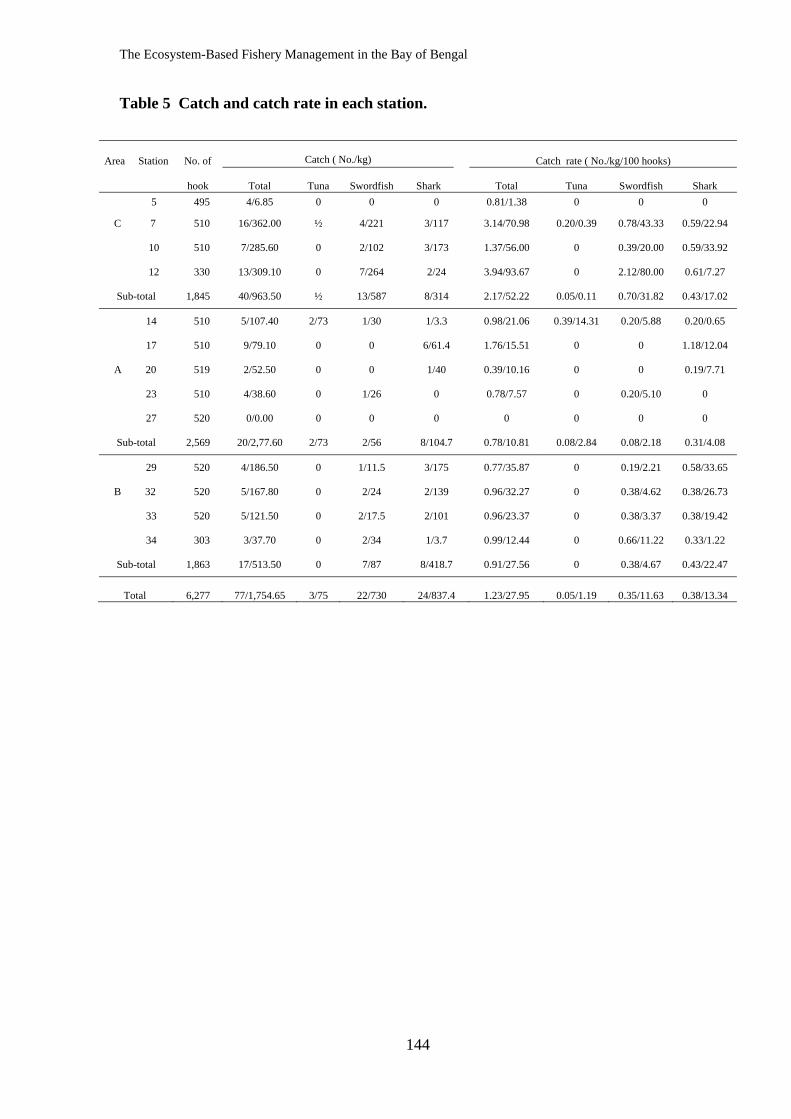
The Ecosystem-Based Fishery Management in the Bay of Bengal
144
Table 5 Catch and catch rate in each station.
Area Station No. of
Catch ( No./kg)
Catch rate ( No./kg/100 hooks)
hook Total Tuna Swordfish Shark Total Tuna Swordfish Shark 5 495 4/6.85 0 0 0 0.81/1.38 0 0 0
C 7 510 16/362.00 ½ 4/221 3/117 3.14/70.98 0.20/0.39 0.78/43.33 0.59/22.94
10 510 7/285.60 0 2/102 3/173 1.37/56.00 0 0.39/20.00 0.59/33.92
12 330 13/309.10 0 7/264 2/24 3.94/93.67 0 2.12/80.00 0.61/7.27
Sub-total 1,845 40/963.50 ½ 13/587 8/314 2.17/52.22 0.05/0.11 0.70/31.82 0.43/17.02
14 510 5/107.40 2/73 1/30 1/3.3 0.98/21.06 0.39/14.31 0.20/5.88 0.20/0.65
17 510 9/79.10 0 0 6/61.4 1.76/15.51 0 0 1.18/12.04
A 20 519 2/52.50 0 0 1/40 0.39/10.16 0 0 0.19/7.71
23 510 4/38.60 0 1/26 0 0.78/7.57 0 0.20/5.10 0
27 520 0/0.00 0 0 0 0 0 0 0
Sub-total 2,569 20/2,77.60 2/73 2/56 8/104.7 0.78/10.81 0.08/2.84 0.08/2.18 0.31/4.08
29 520 4/186.50 0 1/11.5 3/175 0.77/35.87 0 0.19/2.21 0.58/33.65
B 32 520 5/167.80 0 2/24 2/139 0.96/32.27 0 0.38/4.62 0.38/26.73
33 520 5/121.50 0 2/17.5 2/101 0.96/23.37 0 0.38/3.37 0.38/19.42
34 303 3/37.70 0 2/34 1/3.7 0.99/12.44 0 0.66/11.22 0.33/1.22
Sub-total 1,863 17/513.50 0 7/87 8/418.7 0.91/27.56 0 0.38/4.67 0.43/22.47
Total 6,277 77/1,754.65 3/75 22/730 24/837.4 1.23/27.95 0.05/1.19 0.35/11.63 0.38/13.34
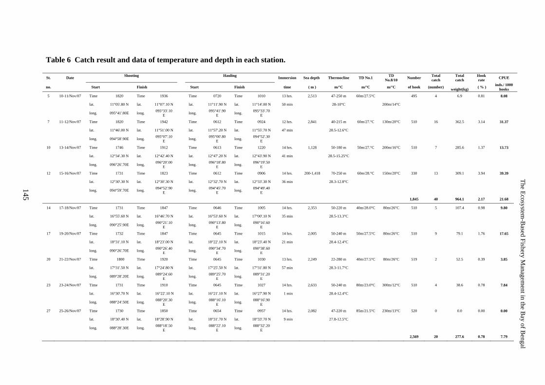
The Ecosystem-Based Fishery Management in the Bay of Bengal
145
Table 6 Catch result and data of temperature and depth in each station. St. Date Shooting
Hauling Immersion Sea depth Thermocline TD No.1 TD
No.8/10 Number Total catch
Total catch
Hook rate CPUE
no. Start Finish Start Finish time ( m ) m/°C m/°C m/°C of hook (number) weight(kg) ( % ) inds./ 1000
hooks
5 10-11/Nov/07 Time 1820 Time 1936 Time 0720 Time 1010 13 hrs. 2,513 47-250 m 60m/27.5°C 495 4 6.9 0.81 8.08
lat. 11°05'.80 N lat. 11°07'.10 N lat. 11°11'.90 N lat. 11°14'.00 N 50 min 28-10°C 200m/14°C
long. 095°41'.80E long. 095°33'.10 E long. 095°41'.90
E long. 095°33'.70 E
7 11-12/Nov/07 Time 1820 Time 1942 Time 0612 Time 0924 12 hrs. 2,841 40-215 m 60m/27.°C 130m/20°C 510 16 362.5 3.14 31.37
lat. 11°46'.00 N lat. 11°51'.00 N lat. 11°57'.20 N lat. 11°55'.70 N 47 min 28.5-12.6°C
long. 094°58'.90E long. 095°07'.10 E long. 095°00'.80
E long. 094°52'.30 E
10 13-14/Nov/07 Time 1746 Time 1912 Time 0613 Time 1220 14 hrs. 1,128 50-180 m 50m/27.°C 200m/16°C 510 7 285.6 1.37 13.73
lat. 12°34'.30 N lat. 12°42'.40 N lat. 12°47'.20 N lat. 12°43'.90 N 41 min 28.5-15.25°C
long. 096°26'.70E long, 096°20'.00 E long. 096°18'.80
E long. 096°19'.50 E
12 15-16/Nov/07 Time 1731 Time 1823 Time 0612 Time 0906 14 hrs. 200-1,418 70-250 m 60m/28.°C 150m/20°C 330 13 309.1 3.94 39.39
lat. 12°30'.30 N lat. 12°30'.30 N lat. 12°32'.70 N lat. 12°33'.30 N 36 min 28.3-12.8°C long. 094°59'.70E long. 094°52'.90
E long. 094°45'.70 E long. 094°49'.40
E
1,845 40 964.1 2.17 21.68
14 17-18/Nov/07 Time 1731 Time 1847 Time 0646 Time 1005 14 hrs. 2,353 50-220 m 40m/28.0°C 80m/26°C 510 5 107.4 0.98 9.80
lat. 16°55'.60 N lat. 16°46'.70 N lat. 16°53'.60 N lat. 17°00'.10 N 35 min 28.5-13.3°C
long. 090°25'.90E long. 090°21'.10 E long. 090°13'.80
E long. 090°16'.60 E
17 19-20/Nov/07 Time 1732 Time 1847 Time 0645 Time 1015 14 hrs. 2,005 50-240 m 50m/27.5°C 80m/26°C 510 9 79.1 1.76 17.65
lat. 18°31'.10 N lat. 18°23'.00 N lat. 18°22'.10 N lat. 18°23'.40 N 21 min 28.4-12.4°C
long. 090°26'.70E long. 090°26'.40 E long. 090°34'.70
E long. 090°38'.60 E
20 21-22/Nov/07 Time 1800 Time 1920 Time 0645 Time 1030 13 hrs. 2,249 22-280 m 40m/27.5°C 80m/26°C 519 2 52.5 0.39 3.85
lat. 17°31'.50 N lat. 17°24'.80 N lat. 17°25'.50 N lat. 17°31'.80 N 57 min 28.3-11.7°C
long. 089°28'.20E long. 089°24'.60 E long. 089°25'.70
E long. 089°31'.20 E
23 23-24/Nov/07 Time 1731 Time 1910 Time 0645 Time 1027 14 hrs. 2,633 50-240 m 80m/23.0°C 300m/12°C 510 4 38.6 0.78 7.84
lat. 16°30'.70 N lat. 16°22'.10 N lat. 16°21'.10 N lat. 16°27'.90 N 1 min 28.4-12.4°C
long. 088°24'.50E long. 088°20'.30 E long. 088°16'.10
E long. 088°16'.90 E
27 25-26/Nov/07 Time 1730 Time 1850 Time 0654 Time 0957 14 hrs. 2,082 47-220 m 85m/21.5°C 230m/13°C 520 0 0.0 0.00 0.00
lat. 18°30'.40 N lat. 18°28'.90 N lat. 18°31'.70 N lat. 18°33'.70 N 9 min 27.8-12.5°C
long. 088°28'.30E long. 088°18'.50 E long. 088°22'.10
E long. 088°32'.20 E
2,569 20 277.6 0.78 7.79
145
The Ecosystem
-Based Fishery M
anagement in the B
ay of Bengal
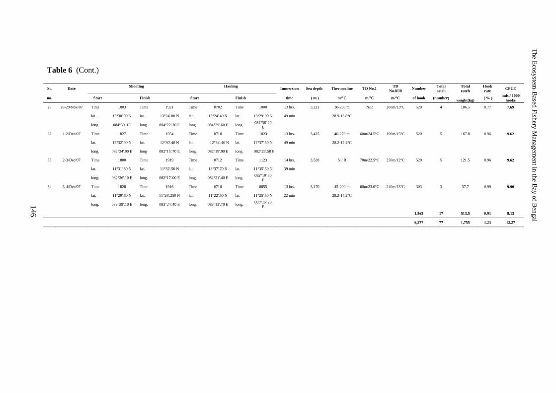
The Ecosystem-Based Fishery Management in the Bay of Bengal
146
Table 6 (Cont.) St. Date Shooting
Hauling
Immersion Sea depth Thermocline TD No.1 TD No.8/10 Number Total
catch Total catch
Hook rate CPUE
no. Start Finish Start Finish time ( m ) m/°C m/°C m/°C of hook (number) weight(kg) ( % ) inds./ 1000
hooks
29 28-29/Nov/07 Time 1803 Time 1921 Time 0702 Time 1000 13 hrs. 3,221 30-200 m N/R 200m/13°C 520 4 186.5 0.77 7.69
lat. 13°30'.00 N lat. 13°24'.80 N lat. 13°24'.40 N lat. 13°29'.00 N 49 min 28.9-13.8°C
long. 084°30'.1E long. 084°22'.20 E long. 084°29'.60 E long. 084°38'.20 E
32 1-2/Dec/07 Time 1827 Time 1954 Time 0718 Time 1023 13 hrs. 3,425 40-270 m 60m/24.5°C 190m/15°C 520 5 167.8 0.96 9.62
lat. 12°32'.90 N lat. 12°30'.40 N lat. 12°34'.40 N lat. 12°37'.50 N 49 min 28.2-12.4°C
long. 082°24'.90 E long 082°15'.70 E long. 082°19'.90 E long. 082°29'.50 E
33 2-3/Dec/07 Time 1800 Time 1919 Time 0712 Time 1123 14 hrs. 3,528 N / R 70m/22.5°C 250m/12°C 520 5 121.5 0.96 9.62
lat. 11°31'.80 N lat. 11°32'.50 N lat. 13°37'.70 N lat. 11°35'.50 N 39 min
long. 082°26'.10 E long. 082°17'.00 E long. 082°21'.40 E long. 082°19'.80 E
34 3-4/Dec/07 Time 1828 Time 1916 Time 0710 Time 0855 13 hrs. 3,470 45-200 m 60m/23.0°C 240m/13°C 303 3 37.7 0.99 9.90
lat. 11°29'.60 N lat. 11°26'.250 N lat. 11°22'.50 N lat. 11°25'.50 N 22 min 28.2-14.2°C
long. 083°28'.10 E long. 083°24'.40 E long. 083°13'.70 E long. 083°15'.20 E
1,863 17 513.5 0.91 9.13
6,277 77 1,755 1.23 12.27
146
The Ecosystem
-Based Fishery M
anagement in the B
ay of Bengal
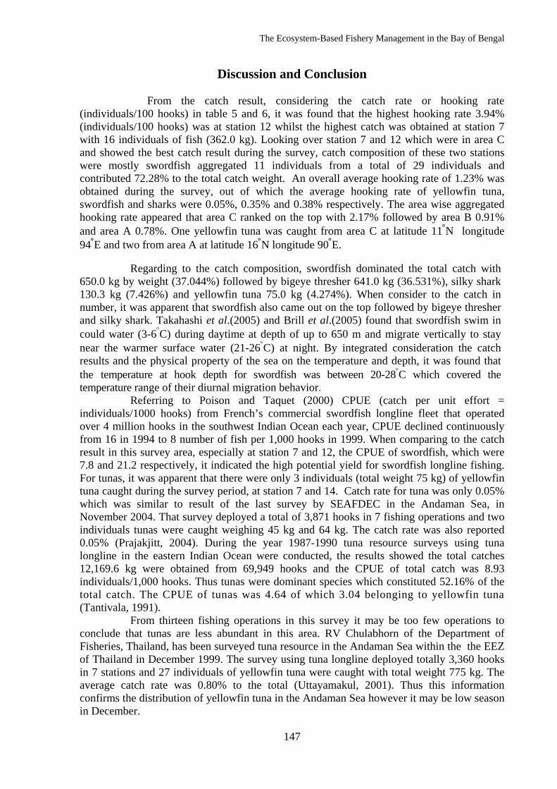
The Ecosystem-Based Fishery Management in the Bay of Bengal
147
Discussion and Conclusion
From the catch result, considering the catch rate or hooking rate (individuals/100 hooks) in table 5 and 6, it was found that the highest hooking rate 3.94% (individuals/100 hooks) was at station 12 whilst the highest catch was obtained at station 7 with 16 individuals of fish (362.0 kg). Looking over station 7 and 12 which were in area C and showed the best catch result during the survey, catch composition of these two stations were mostly swordfish aggregated 11 individuals from a total of 29 individuals and contributed 72.28% to the total catch weight. An overall average hooking rate of 1.23% was obtained during the survey, out of which the average hooking rate of yellowfin tuna, swordfish and sharks were 0.05%, 0.35% and 0.38% respectively. The area wise aggregated hooking rate appeared that area C ranked on the top with 2.17% followed by area B 0.91% and area A 0.78%. One yellowfin tuna was caught from area C at latitude 11°N longitude 94°E and two from area A at latitude 16°N longitude 90°E. Regarding to the catch composition, swordfish dominated the total catch with 650.0 kg by weight (37.044%) followed by bigeye thresher 641.0 kg (36.531%), silky shark 130.3 kg (7.426%) and yellowfin tuna 75.0 kg (4.274%). When consider to the catch in number, it was apparent that swordfish also came out on the top followed by bigeye thresher and silky shark. Takahashi et al.(2005) and Brill et al.(2005) found that swordfish swim in could water (3-6°C) during daytime at depth of up to 650 m and migrate vertically to stay near the warmer surface water (21-26°C) at night. By integrated consideration the catch results and the physical property of the sea on the temperature and depth, it was found that the temperature at hook depth for swordfish was between 20-28°C which covered the temperature range of their diurnal migration behavior. Referring to Poison and Taquet (2000) CPUE (catch per unit effort = individuals/1000 hooks) from French’s commercial swordfish longline fleet that operated over 4 million hooks in the southwest Indian Ocean each year, CPUE declined continuously from 16 in 1994 to 8 number of fish per 1,000 hooks in 1999. When comparing to the catch result in this survey area, especially at station 7 and 12, the CPUE of swordfish, which were 7.8 and 21.2 respectively, it indicated the high potential yield for swordfish longline fishing. For tunas, it was apparent that there were only 3 individuals (total weight 75 kg) of yellowfin tuna caught during the survey period, at station 7 and 14. Catch rate for tuna was only 0.05% which was similar to result of the last survey by SEAFDEC in the Andaman Sea, in November 2004. That survey deployed a total of 3,871 hooks in 7 fishing operations and two individuals tunas were caught weighing 45 kg and 64 kg. The catch rate was also reported 0.05% (Prajakjitt, 2004). During the year 1987-1990 tuna resource surveys using tuna longline in the eastern Indian Ocean were conducted, the results showed the total catches 12,169.6 kg were obtained from 69,949 hooks and the CPUE of total catch was 8.93 individuals/1,000 hooks. Thus tunas were dominant species which constituted 52.16% of the total catch. The CPUE of tunas was 4.64 of which 3.04 belonging to yellowfin tuna (Tantivala, 1991). From thirteen fishing operations in this survey it may be too few operations to conclude that tunas are less abundant in this area. RV Chulabhorn of the Department of Fisheries, Thailand, has been surveyed tuna resource in the Andaman Sea within the the EEZ of Thailand in December 1999. The survey using tuna longline deployed totally 3,360 hooks in 7 stations and 27 individuals of yellowfin tuna were caught with total weight 775 kg. The average catch rate was 0.80% to the total (Uttayamakul, 2001). Thus this information confirms the distribution of yellowfin tuna in the Andaman Sea however it may be low season in December.
The Ecosystem-Based Fishery Management in the Bay of Bengal
148
For further research survey, daytime fishing operation and increasing number of hook line per basket in order to cover wider range of fishing depth are suggested to ascertain about the abundance of tuna resource in the Bay of Bengal.
References
Brill, R. W., K. A. Bigelow, M. K. Musyl, K. A. Fritsches and E. J. Warrant. 2005. Bigeye
tuna (Thunnus obesus) behavior and physiology and their relevance to stock assessments and fishery biology. International Commission for the Conservation of Atlantic Tunas (ICCAT). Collective Volume of Scientific Papers ICCT. 57(2):142-161.
FAO. 2003. Trends in oceanic captures and clustering of large marine ecosystem - 2 studies based on the FAO capture database. FAO fisheries technical paper 435. FAO. 71 pp.
Dwivedi, S. W. 1993. Long-term variability in the food chains, biomass yield and oceanography of the Bay of Bengal ecosystem. In: Sherman, K., L. M. Alexander and B. D. Gold. (eds.). Large Marine Ecosystem: Stress, Mitigation and Sustainability. AAAS Press, Washington D. C., USA. p. 43-52.
Poison, F. and M. Toquet. 2000. French Swordfish Longline Fishery in Southwest Indian Ocean. In: Preliminary result from the PRR Program. WPB 00-06 IOTC Proceedings no.3. IOTC. p. 169-201.
Prajakjitt, P. 2004. Large pelagic fish survey in the Andaman Sea using pelagic longline. Preliminary results on the large pelagic fishery resources survey in the Andaman Sea. TD/RES/99 SEAFDEC. p. 102-112.
Takahashi, M., H. Okamura, K. Yokawa and M. Okazaki. 2005. Swimming behavior and migration of a swordfish recorded by archival tag. CSIRO Publishing Marine Freshwater Research. Australia. 54(4):527-534.
Tantivala, C. and T. Panniem. 1991. Tuna resources exploratory fishing survey by tuna longline in the Eastern Indian Ocean. Oceanic Fisheries Division, Department of Fisheries, Thailand. 32 pp.
Uttayamakul, W. 2001. Longline fishing: An alternative for responsible fishing in Andaman Sea. Oceanic Fisheries Division, Department of Fisheries, Bangkok, Thailand. 44 pp.
The Ecosystem-Based Fishery Management in the Bay of Bengal
149
Marine Resource Surveys by Drift Gill Net in the Bay of Bengal
Phithak Chaidee1, Narupon Darumas1, Opas Chamasont2, Md. Nasiruddin Sada3, Rankiri P. P. Krishantha Jayasinghe4,
Kattawatta Siriwarnage Dharana Chinthaka4, U Aung Win Sein5, Jagannath Nalla6 and Thanitha Thapanand-Chaidee7
1 Deep Sea Fishery Technology Research and Development Institute,
Department of Fisheries, Samutprakarn 10270, THAILAND 2 Upper-Gulf Fisheries Research and Development Center,
Department of Fisheries, Samutprakarn 10130, THAILAND
3 Fish Inspection and Quality Control, Department of Fisheries, 209 Muradpur(NM Khan Hill) P.O. Amin Jute Mill, Chittagong, BANGLADESH
4 National Aquatic Resource Research and Development Agency, Crow Island, Colombo 15, SRI LANKA
5 Department of Fisheries, Insein Rd, West Gyoton, Insein Township, Yangon, MYANMAR
6 Office of the Zonal Director, Visakhapatnam Base of Fishery Survey of India, Fishing Harbor, Beach Road, Vusakhapatnam-530001, INDIA
7 Department of Fishery Biology, Faculty of Fisheries, Kasetsart University, Bangkok 10900, THAILAND
Abstract
This paper presented the first time survey of marine resources in the Bay of Bengal in terms of catch composition; Catch per unit effort (CPUE) and catch per unit area (CPUA) by drift gill net (DGN). The survey was conducted in eight stations of three sub-areas during October–December 2007 under the mission of BIMSTEC collaborative project. The fishery research vessel, M.V. SEAFDEC (cruise No. 75-1/2007) was deployed in the proposed survey. A total catch of 137.60 kg from 108 fishing hours composed of 15 fish species (99.60% by weight) and one piece of diamondback squid (Thysanoteuthidae: Thysanoteuthis rhombus) was captured (0.40% by weight). The highest catch species of marine resources was skipjack tuna, Katsuwonus pelamis, (42.96% by weight). The CPUE was ranged from 0.15 to 2.08 kg h-1 and gave the average of 1.22 kg h-1. The CPUA was ranged from 1.297x10⁻⁴ to 1.651x10⁻³ kg m-2 of net area and gave the average of 8.809x10⁻⁴ kg m-2 of net area. Average catch was not shown significant different among the three survey areas. Skipjack tuna was also the most important economical species (66.72% IRI) and widely distributed in the survey area especially in area A. Silky shark (Carcharhinus falciformis), which was the second important (10.55% IRI), was distributed only in area C whereas frigate tuna (Auxis thazard thazard), which was the third important (7.47% IRI), was distributed only in area A. Key words: catch composition, marine resources, drift gill net, Bay of Bengal, BIMSTEC
Introduction Drift netting is a fishing technique where nets, called drift nets, are allowed to drift free in a sea or lake. Usually a drift net is a gill net with floats attached to a rope along the top of the net, and weights attached to another rope along the foot of the net. Drift net can range in length from 25 m to 2.5 miles. (http://en.wikipedia.org/wiki/Drift_net) The nomenclature of drift net or drift gill net depends on the target species. The common species are mackerel, flying fish, tuna and tuna-like, manta ray and other pelagic species. These fish species require different mesh and twin sizes as well as material to maximize catch. For mackerel, flying fish, sardines and other small pelagic species the nets are made of nylon monofilament of 0.20 mm
The Ecosystem-Based Fishery Management in the Bay of Bengal
150
to 0.40 mm diameter with mesh size from 25 mm to 90 mm. For tuna species, the material is nylon multifilament PA 210/12 to 210/18 in the main webbing whole iron rings and/or thicker multifilament nettings (210/30 to210/36) are used as weights. The mesh size ranges from 50 mm to 90 mm. There are 10 to 20 meshes of thicker netting acting as weights in the lower portion of the webbing. ( http://map.seafdec.org/Monograph project/gill_net_2.php ) Drift nets have been commonly used by many countries in the coastal waters. This type of net was heavily used by many Japanese, South Korean and Taiwanese fishing fleets on the high seas in the 1980s to target tunas. Generally, fish which are smaller than the meshes of the gill nets are able to pass through unhindered, while those which are too large to push their heads through the meshes as far as their gills are not retained. This gives a selectivity ogive which is skewed towards medium size fish, unlike active fishing gears such as trawl nets in which the proportion of fish entering the nets which are retained increases with length. Although highly selective with respect to size class of the fish captured, practically gill nets are blamed for the impact on non-target species particularly dolphins, turtles and seabirds. In 1993 gill nets were banned by the United Nations in international waters, although their use is still permitted within 200 nautical miles (400 km) of a coast. ( http://en.wikipedia.org/wiki/Gillnet ) However, in international waters which generally cover deep water areas, there are only a few types of fishing gear suitable for harvesting fishery resources. The important fishing gears suitable for fishing in deep water areas are purse-seine, pelagic longline and drift gill net (DGN). For pelagic fish commonly distribute in the upper layer, drift gill nets are widely deployed to catch these fishes because of the simplicity in operating. Thus, DGN is chosen to be one of the 3 types of fishing gear, besides pelagic longline and automatic squid jigging, for the survey and study of marine fishery resources in the Bay of Bengal and being the rationale of the sub-project on Marine Resource Surveys by Drift Gill Net in the Bay of Bengal. This sub-project aims to assess the potential of marine fishery resources captured by DGN in terms of species and catch composition, catch per unit effort (CPUE) and stock abundance in term of index of relative importance (IRI). The result from this research will support a useful background for effective fishery resource management in the Bay of Bengal. Furthermore, it will improve capabilities in fish stock assessment of the biologists and researchers in the member countries as well as to develop the academic ability in training the staff of the Faculty of Fisheries, Kasetsart University and establish a good collaboration among member countries in research and academic activities.
Materials and Methods Area of Fishing Operation The study was carried out in the Bay of Bengal during 25 October to 21 December 2007. Three sub-areas were defined namely area A: latitude 16°N-19°N and longitude 88°E-91°E (5 stations); area B: latitude 9°N-14°N and longitude 82°E-85°E (5 stations); and area C: latitude 10°N-12°N and longitude 95°E -97°E (5 stations) (Fig. 1). Fishing Gear The fishery research vessel, M.V. SEAFDEC, of the Southeast Asian Fisheries Development Center (SEAFDEC) was used in this study. Field sampling was conducted using two types of net materials for drift gill net (DGN), monofilament and multifilament nylon twines. Total length of monofilament DGN was 2,200 m with 100 mm of mesh size and 93 meshes at depth. Multifilament DGN was 2,500 m with 160 mm of mesh size and 100 meshes
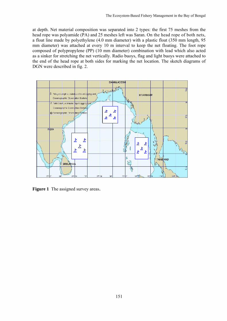
The Ecosystem-Based Fishery Management in the Bay of Bengal
151
at depth. Net material composition was separated into 2 types: the first 75 meshes from the head rope was polyamide (PA) and 25 meshes left was Saran. On the head rope of both nets, a float line made by polyethylene (4.0 mm diameter) with a plastic float (350 mm length, 95 mm diameter) was attached at every 10 m interval to keep the net floating. The foot rope composed of polypropylene (PP) (10 mm diameter) combination with lead which also acted as a sinker for stretching the net vertically. Radio buoys, flag and light buoys were attached to the end of the head rope at both sides for marking the net location. The sketch diagrams of DGN were described in fig. 2.
Figure 1 The assigned survey areas.
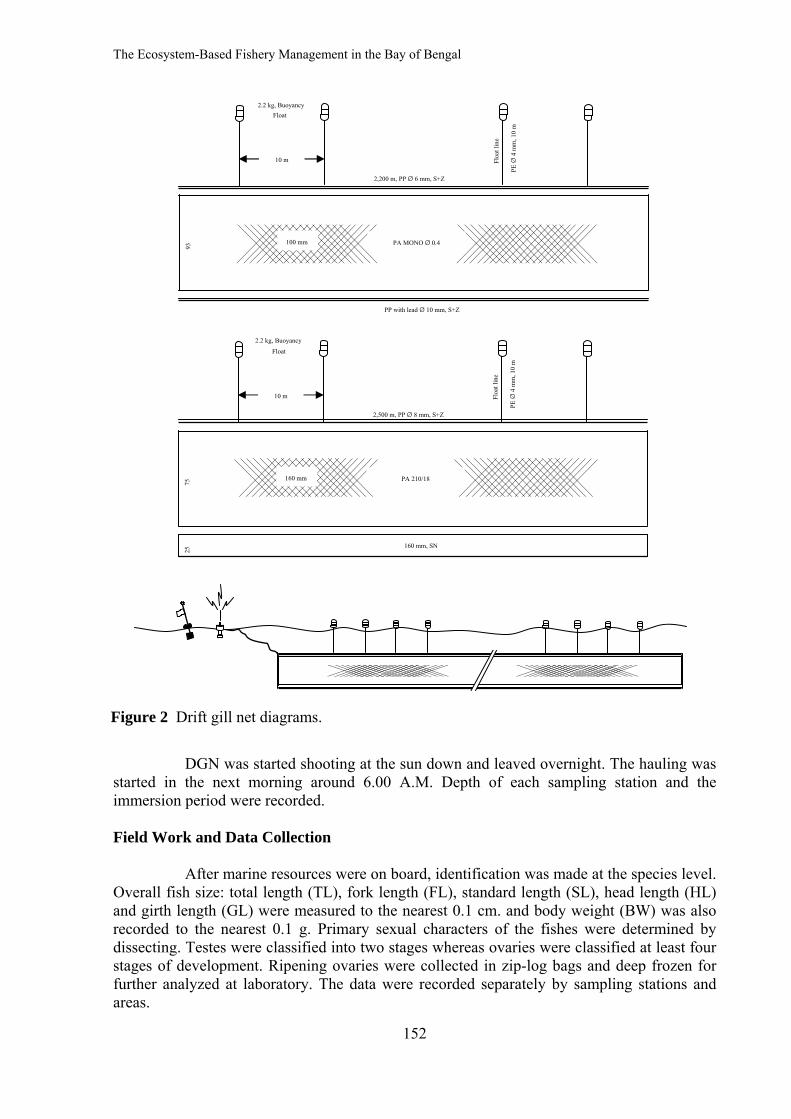
The Ecosystem-Based Fishery Management in the Bay of Bengal
152
DGN was started shooting at the sun down and leaved overnight. The hauling was started in the next morning around 6.00 A.M. Depth of each sampling station and the immersion period were recorded. Field Work and Data Collection After marine resources were on board, identification was made at the species level. Overall fish size: total length (TL), fork length (FL), standard length (SL), head length (HL) and girth length (GL) were measured to the nearest 0.1 cm. and body weight (BW) was also recorded to the nearest 0.1 g. Primary sexual characters of the fishes were determined by dissecting. Testes were classified into two stages whereas ovaries were classified at least four stages of development. Ripening ovaries were collected in zip-log bags and deep frozen for further analyzed at laboratory. The data were recorded separately by sampling stations and areas.
Figure 2 Drift gill net diagrams.
PA MONO Ø 0.4100 mm 93
PE Ø
4 mm
, 10 m
Float
line
Float 10 m
2,200 m, PP Ø 6 mm, S+Z
PP with lead Ø 10 mm, S+Z
2.2 kg, Buoyancy
160 mm, SN
PA 210/18160 mm 75
PE Ø
4 mm
, 10 m
Float
line
Float 10 m
2,500 m, PP Ø 8 mm, S+Z
25
2.2 kg, Buoyancy
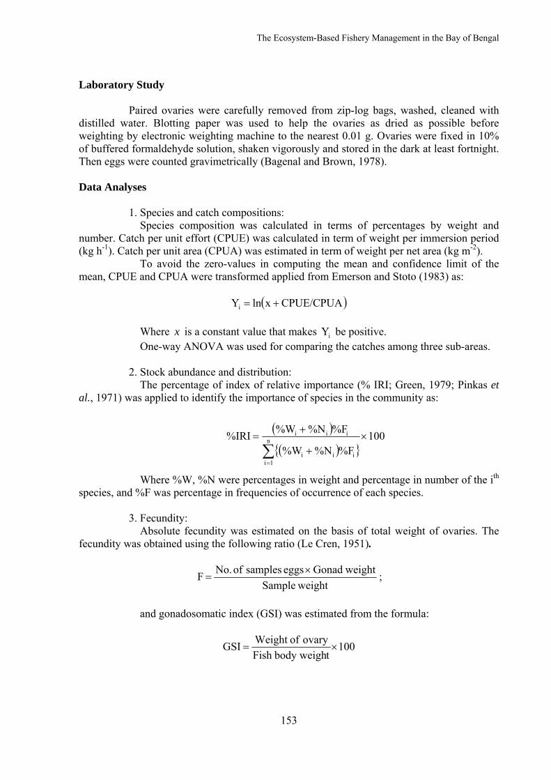
The Ecosystem-Based Fishery Management in the Bay of Bengal
153
Laboratory Study Paired ovaries were carefully removed from zip-log bags, washed, cleaned with distilled water. Blotting paper was used to help the ovaries as dried as possible before weighting by electronic weighting machine to the nearest 0.01 g. Ovaries were fixed in 10% of buffered formaldehyde solution, shaken vigorously and stored in the dark at least fortnight. Then eggs were counted gravimetrically (Bagenal and Brown, 1978). Data Analyses 1. Species and catch compositions: Species composition was calculated in terms of percentages by weight and number. Catch per unit effort (CPUE) was calculated in term of weight per immersion period (kg h-1). Catch per unit area (CPUA) was estimated in term of weight per net area (kg m-2). To avoid the zero-values in computing the mean and confidence limit of the mean, CPUE and CPUA were transformed applied from Emerson and Stoto (1983) as:
( )CPUE/CPUAxlnYi +=
Where x is a constant value that makes iY be positive. One-way ANOVA was used for comparing the catches among three sub-areas. 2. Stock abundance and distribution: The percentage of index of relative importance (% IRI; Green, 1979; Pinkas et al., 1971) was applied to identify the importance of species in the community as:
( )( ){ }
100%F%N%W
%F%N%W%IRI n
1iiii
iii ×+
+=
∑=
Where %W, %N were percentages in weight and percentage in number of the ith
species, and %F was percentage in frequencies of occurrence of each species. 3. Fecundity: Absolute fecundity was estimated on the basis of total weight of ovaries. The fecundity was obtained using the following ratio (Le Cren, 1951).
weightSample weightGonad eggs samples of No.F ×
= ;
and gonadosomatic index (GSI) was estimated from the formula:
100tbody weighFish
ovary ofWeight GSI ×=
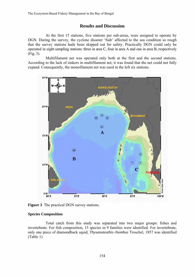
The Ecosystem-Based Fishery Management in the Bay of Bengal
154
Results and Discussion At the first 15 stations, five stations per sub-areas, were assigned to operate by DGN. During the survey, the cyclone disaster ‘Sidr’ affected to the sea condition so rough that the survey stations hade been skipped out for safety. Practically DGN could only be operated in eight sampling stations: three in area C, four in area A and one in area B, respectively (Fig. 3). Multifilament net was operated only both at the first and the second stations. According to the lack of sinkers in multifilament net, it was found that the net could not fully expand. Consequently, the monofilament net was used in the left six stations.
Figure 3 The practical DGN survey stations. Species Composition Total catch from this study was separated into two major groups: fishes and invertebrate. For fish composition, 15 species in 9 families were identified. For invertebrate, only one piece of diamondback squid, Thysanoteuthis rhombus Troschel, 1857 was identified (Table 1).
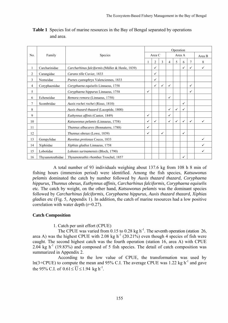
The Ecosystem-Based Fishery Management in the Bay of Bengal
155
Table 1 Species list of marine resources in the Bay of Bengal separated by operations and area.
No. Family Species Operation
Area C Area A Area B
1 2 3 4 5 6 7 8
1 Carcharinidae Carcharhinus falciformis (Müller & Henle, 1839)
2 Carangidae Caranx tille Cuvier, 1833
3 Nomeidae Psenes cyanophrys Valenciennes, 1833
4 Coryphaenidae Coryphaena equiselis Linnaeus, 1758
5 Coryphaena hippurus Linnaeus, 1758
6 Echeneidae Remora remora (Linnaeus, 1758)
7 Scombridae Auxis rochei rochei (Risso, 1810)
8 Auxis thazard thazard (Lacepède, 1800)
9 Euthynnus affinis (Cantor, 1849)
10 Katsuwonus pelamis (Linnaeus, 1758)
11 Thunnus albacares (Bonnaterre, 1788)
12 Thunnus obesus (Lowe, 1839)
13 Gempylidae Ruvettus pretiosus Cocco, 1833
14 Xiphiidae Xiphias gladius Linnaeus, 1758
15 Lobotidae Lobotes surinamensis (Bloch, 1790)
16 Thysanoteuthidae Thysanoteuthis rhombus Troschel, 1857
A total number of 93 individuals weighing about 137.6 kg from 108 h 8 min of fishing hours (immersion period) were identified. Among the fish species, Katsuwonus pelamis dominated the catch by number followed by Auxis thazard thazard, Coryphaena hippurus, Thunnus obesus, Euthynnus affinis, Carcharhinus falciformis, Coryphaena equiselis etc. The catch by weight, on the other hand, Katsuwonus pelamis was the dominant species followed by Carcharhinus falciformis, Coryphaena hippurus, Auxis thazard thazard, Xiphias gladias etc (Fig. 5, Appendix 1). In addition, the catch of marine resources had a low positive correlation with water depth (r=0.27). Catch Composition 1. Catch per unit effort (CPUE) The CPUE was varied from 0.15 to 0.28 kg h-1. The seventh operation (station 26, area A) was the highest CPUE with 2.08 kg h-1 (20.21%) even though 4 species of fish were caught. The second highest catch was the fourth operation (station 16, area A) with CPUE 2.04 kg h-1 (19.83%) and composed of 5 fish species. The detail of catch composition was summarized in Appendix 2. According to the low value of CPUE, the transformation was used by ln(3+CPUE) to compute the mean and 95% C.I. The average CPUE was 1.22 kg h-1 and gave the 95% C.I. of 94.1U61.0 ≤≤ kg h-1.
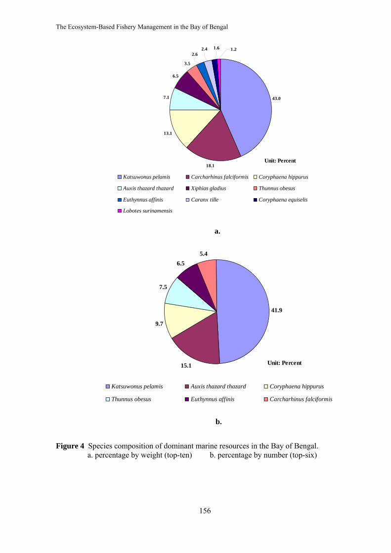
The Ecosystem-Based Fishery Management in the Bay of Bengal
156
Figure 4 Species composition of dominant marine resources in the Bay of Bengal. a. percentage by weight (top-ten) b. percentage by number (top-six)
43.0
18.1
13.1
7.1
6.5
3.5
2.62.4 1.6 1.2
Katsuwonus pelamis Carcharhinus falciformis Coryphaena hippurus
Auxis thazard thazard Xiphias gladius Thunnus obesus
Euthynnus affinis Caranx tille Coryphaena equiselis
Lobotes surinamensis
Unit: Percent
a.
41.9
15.1
9.7
7.5
6.55.4
Katsuwonus pelamis Auxis thazard thazard Coryphaena hippurus
Thunnus obesus Euthynnus affinis Carcharhinus falciformis
Unit: Percent
b.
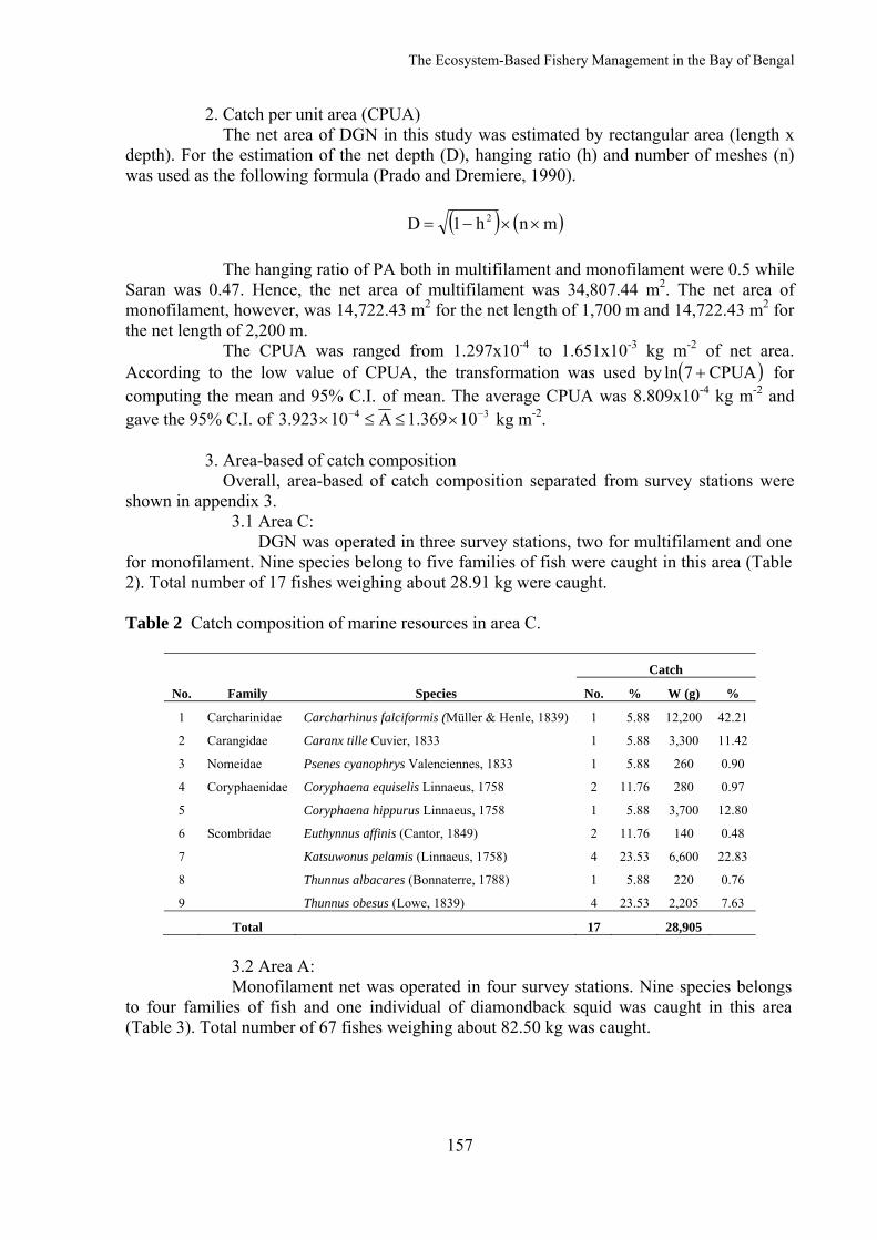
The Ecosystem-Based Fishery Management in the Bay of Bengal
157
2. Catch per unit area (CPUA) The net area of DGN in this study was estimated by rectangular area (length x depth). For the estimation of the net depth (D), hanging ratio (h) and number of meshes (n) was used as the following formula (Prado and Dremiere, 1990).
( ) ( )mnh1D 2 ××−=
The hanging ratio of PA both in multifilament and monofilament were 0.5 while Saran was 0.47. Hence, the net area of multifilament was 34,807.44 m2. The net area of monofilament, however, was 14,722.43 m2 for the net length of 1,700 m and 14,722.43 m2 for the net length of 2,200 m. The CPUA was ranged from 1.297x10⁻⁴ to 1.651x10⁻³ kg m-2 of net area. According to the low value of CPUA, the transformation was used by ( )CPUA7ln + for computing the mean and 95% C.I. of mean. The average CPUA was 8.809x10⁻⁴ kg m-2 and gave the 95% C.I. of 34 101.369A103.923 −− ×≤≤× kg m-2. 3. Area-based of catch composition Overall, area-based of catch composition separated from survey stations were shown in appendix 3.
3.1 Area C: DGN was operated in three survey stations, two for multifilament and one
for monofilament. Nine species belong to five families of fish were caught in this area (Table 2). Total number of 17 fishes weighing about 28.91 kg were caught.
Table 2 Catch composition of marine resources in area C.
No. Family Species
Catch
No. % W (g) %
1 Carcharinidae Carcharhinus falciformis (Müller & Henle, 1839) 1 5.88 12,200 42.21
2 Carangidae Caranx tille Cuvier, 1833 1 5.88 3,300 11.42
3 Nomeidae Psenes cyanophrys Valenciennes, 1833 1 5.88 260 0.90
4 Coryphaenidae Coryphaena equiselis Linnaeus, 1758 2 11.76 280 0.97
5 Coryphaena hippurus Linnaeus, 1758 1 5.88 3,700 12.80
6 Scombridae Euthynnus affinis (Cantor, 1849) 2 11.76 140 0.48
7 Katsuwonus pelamis (Linnaeus, 1758) 4 23.53 6,600 22.83
8 Thunnus albacares (Bonnaterre, 1788) 1 5.88 220 0.76
9 Thunnus obesus (Lowe, 1839) 4 23.53 2,205 7.63
Total 17 28,905 3.2 Area A: Monofilament net was operated in four survey stations. Nine species belongs to four families of fish and one individual of diamondback squid was caught in this area (Table 3). Total number of 67 fishes weighing about 82.50 kg was caught.
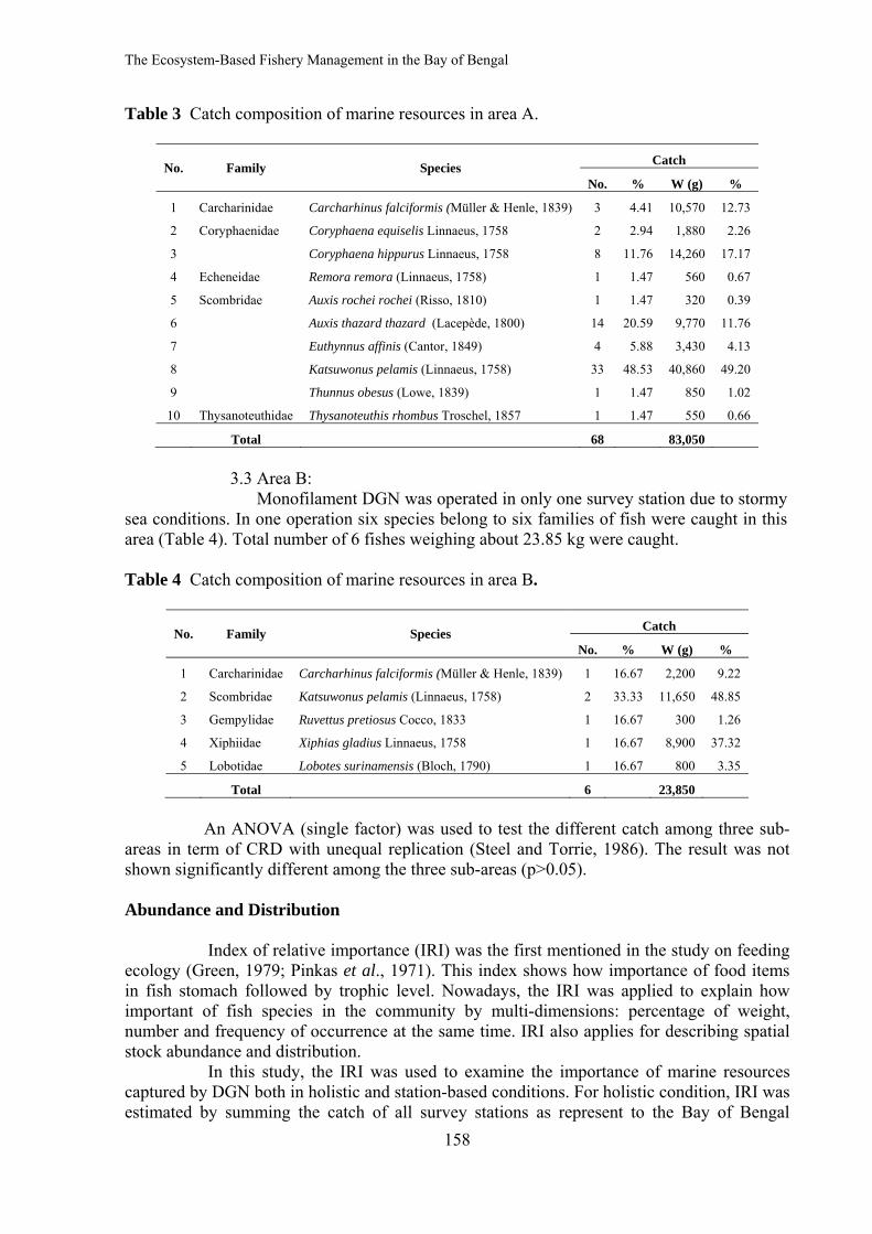
The Ecosystem-Based Fishery Management in the Bay of Bengal
158
Table 3 Catch composition of marine resources in area A.
No. Family Species Catch
No. % W (g) %
1 Carcharinidae Carcharhinus falciformis (Müller & Henle, 1839) 3 4.41 10,570 12.73
2 Coryphaenidae Coryphaena equiselis Linnaeus, 1758 2 2.94 1,880 2.26
3 Coryphaena hippurus Linnaeus, 1758 8 11.76 14,260 17.17
4 Echeneidae Remora remora (Linnaeus, 1758) 1 1.47 560 0.67
5 Scombridae Auxis rochei rochei (Risso, 1810) 1 1.47 320 0.39
6 Auxis thazard thazard (Lacepède, 1800) 14 20.59 9,770 11.76
7 Euthynnus affinis (Cantor, 1849) 4 5.88 3,430 4.13
8 Katsuwonus pelamis (Linnaeus, 1758) 33 48.53 40,860 49.20
9 Thunnus obesus (Lowe, 1839) 1 1.47 850 1.02
10 Thysanoteuthidae Thysanoteuthis rhombus Troschel, 1857 1 1.47 550 0.66
Total 68 83,050 3.3 Area B: Monofilament DGN was operated in only one survey station due to stormy
sea conditions. In one operation six species belong to six families of fish were caught in this area (Table 4). Total number of 6 fishes weighing about 23.85 kg were caught. Table 4 Catch composition of marine resources in area B.
No. Family Species Catch
No. % W (g) %
1 Carcharinidae Carcharhinus falciformis (Müller & Henle, 1839) 1 16.67 2,200 9.22
2 Scombridae Katsuwonus pelamis (Linnaeus, 1758) 2 33.33 11,650 48.85
3 Gempylidae Ruvettus pretiosus Cocco, 1833 1 16.67 300 1.26
4 Xiphiidae Xiphias gladius Linnaeus, 1758 1 16.67 8,900 37.32
5 Lobotidae Lobotes surinamensis (Bloch, 1790) 1 16.67 800 3.35
Total 6 23,850 An ANOVA (single factor) was used to test the different catch among three sub-areas in term of CRD with unequal replication (Steel and Torrie, 1986). The result was not shown significantly different among the three sub-areas (p>0.05).
Abundance and Distribution
Index of relative importance (IRI) was the first mentioned in the study on feeding ecology (Green, 1979; Pinkas et al., 1971). This index shows how importance of food items in fish stomach followed by trophic level. Nowadays, the IRI was applied to explain how important of fish species in the community by multi-dimensions: percentage of weight, number and frequency of occurrence at the same time. IRI also applies for describing spatial stock abundance and distribution.
In this study, the IRI was used to examine the importance of marine resources captured by DGN both in holistic and station-based conditions. For holistic condition, IRI was estimated by summing the catch of all survey stations as represent to the Bay of Bengal
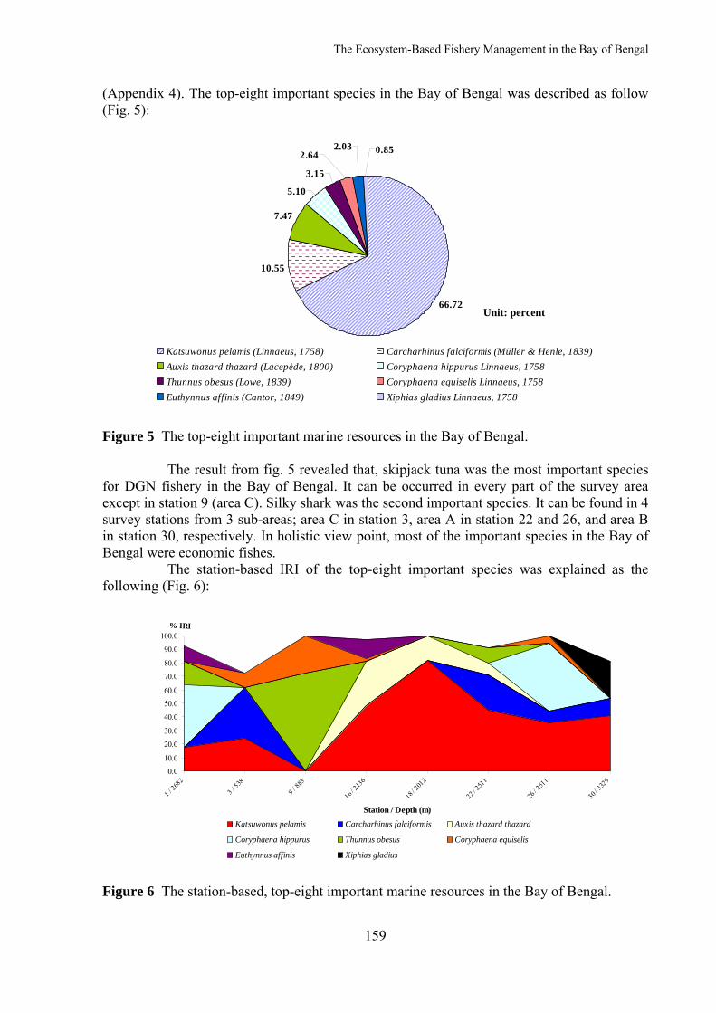
The Ecosystem-Based Fishery Management in the Bay of Bengal
159
(Appendix 4). The top-eight important species in the Bay of Bengal was described as follow (Fig. 5):
66.72
10.55
7.47
5.10
3.15
0.852.642.03
Katsuwonus pelamis (Linnaeus, 1758) Carcharhinus falciformis (Müller & Henle, 1839)Auxis thazard thazard (Lacepède, 1800) Coryphaena hippurus Linnaeus, 1758Thunnus obesus (Lowe, 1839) Coryphaena equiselis Linnaeus, 1758Euthynnus affinis (Cantor, 1849) Xiphias gladius Linnaeus, 1758
Figure 5 The top-eight important marine resources in the Bay of Bengal. The result from fig. 5 revealed that, skipjack tuna was the most important species for DGN fishery in the Bay of Bengal. It can be occurred in every part of the survey area except in station 9 (area C). Silky shark was the second important species. It can be found in 4 survey stations from 3 sub-areas; area C in station 3, area A in station 22 and 26, and area B in station 30, respectively. In holistic view point, most of the important species in the Bay of Bengal were economic fishes. The station-based IRI of the top-eight important species was explained as the following (Fig. 6):
0.0
10.0
20.0
30.0
40.0
50.0
60.0
70.0
80.0
90.0
100.0
1 / 268
2
3 / 538
9 / 883
16 / 21
36
18 / 2
012
22 / 25
11
26 / 2
511
30 / 332
9
Station / Depth (m)
% IRI
Katsuwonus pelamis Carcharhinus falciformis Auxis thazard thazard
Coryphaena hippurus Thunnus obesus Coryphaena equiselis
Euthynnus affinis Xiphias gladius
Figure 6 The station-based, top-eight important marine resources in the Bay of Bengal.
Unit: percent
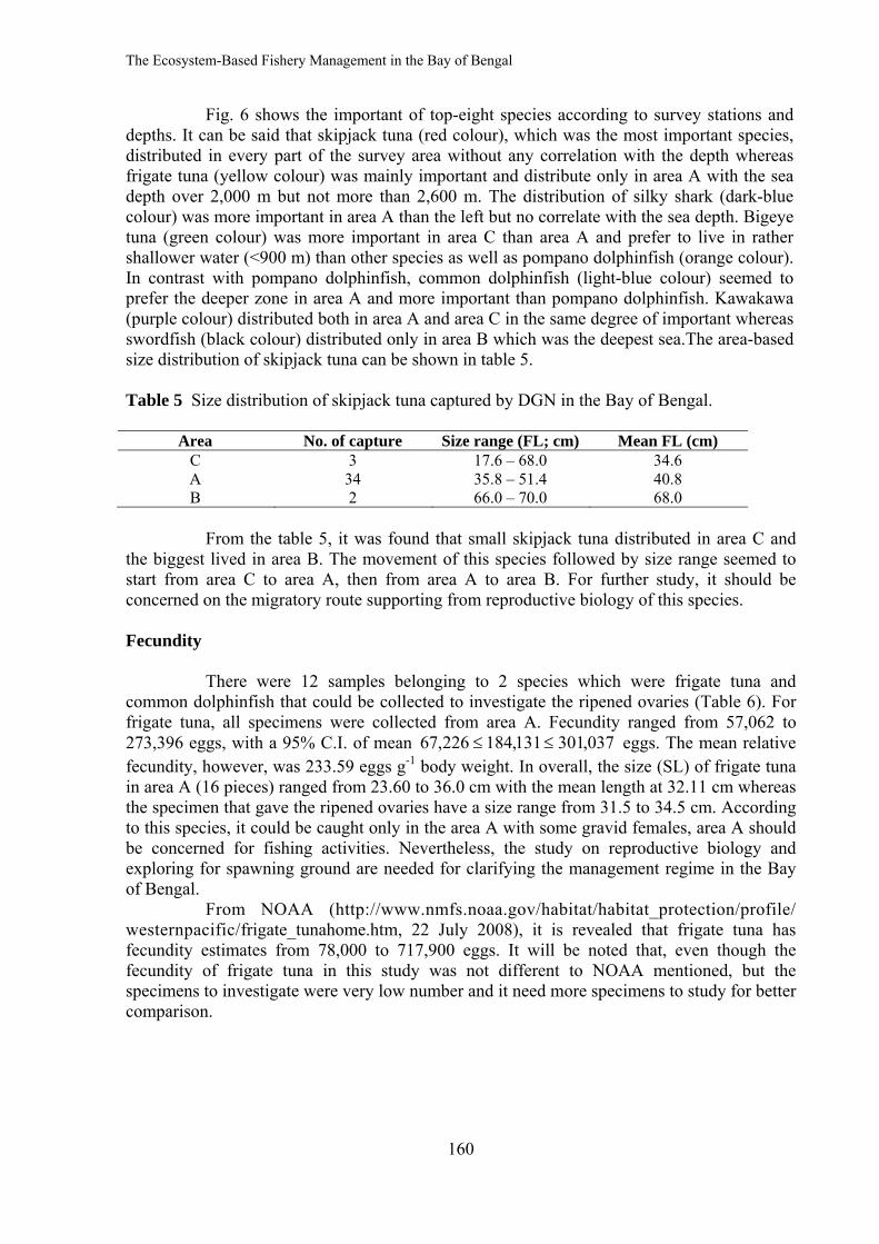
The Ecosystem-Based Fishery Management in the Bay of Bengal
160
Fig. 6 shows the important of top-eight species according to survey stations and depths. It can be said that skipjack tuna (red colour), which was the most important species, distributed in every part of the survey area without any correlation with the depth whereas frigate tuna (yellow colour) was mainly important and distribute only in area A with the sea depth over 2,000 m but not more than 2,600 m. The distribution of silky shark (dark-blue colour) was more important in area A than the left but no correlate with the sea depth. Bigeye tuna (green colour) was more important in area C than area A and prefer to live in rather shallower water (<900 m) than other species as well as pompano dolphinfish (orange colour). In contrast with pompano dolphinfish, common dolphinfish (light-blue colour) seemed to prefer the deeper zone in area A and more important than pompano dolphinfish. Kawakawa (purple colour) distributed both in area A and area C in the same degree of important whereas swordfish (black colour) distributed only in area B which was the deepest sea.The area-based size distribution of skipjack tuna can be shown in table 5. Table 5 Size distribution of skipjack tuna captured by DGN in the Bay of Bengal.
Area No. of capture Size range (FL; cm) Mean FL (cm) C 3 17.6 – 68.0 34.6 A 34 35.8 – 51.4 40.8 B 2 66.0 – 70.0 68.0
From the table 5, it was found that small skipjack tuna distributed in area C and the biggest lived in area B. The movement of this species followed by size range seemed to start from area C to area A, then from area A to area B. For further study, it should be concerned on the migratory route supporting from reproductive biology of this species. Fecundity There were 12 samples belonging to 2 species which were frigate tuna and common dolphinfish that could be collected to investigate the ripened ovaries (Table 6). For frigate tuna, all specimens were collected from area A. Fecundity ranged from 57,062 to 273,396 eggs, with a 95% C.I. of mean 037,301131,184226,67 ≤≤ eggs. The mean relative fecundity, however, was 233.59 eggs g-1 body weight. In overall, the size (SL) of frigate tuna in area A (16 pieces) ranged from 23.60 to 36.0 cm with the mean length at 32.11 cm whereas the specimen that gave the ripened ovaries have a size range from 31.5 to 34.5 cm. According to this species, it could be caught only in the area A with some gravid females, area A should be concerned for fishing activities. Nevertheless, the study on reproductive biology and exploring for spawning ground are needed for clarifying the management regime in the Bay of Bengal. From NOAA (http://www.nmfs.noaa.gov/habitat/habitat_protection/profile/ westernpacific/frigate_tunahome.htm, 22 July 2008), it is revealed that frigate tuna has fecundity estimates from 78,000 to 717,900 eggs. It will be noted that, even though the fecundity of frigate tuna in this study was not different to NOAA mentioned, but the specimens to investigate were very low number and it need more specimens to study for better comparison.
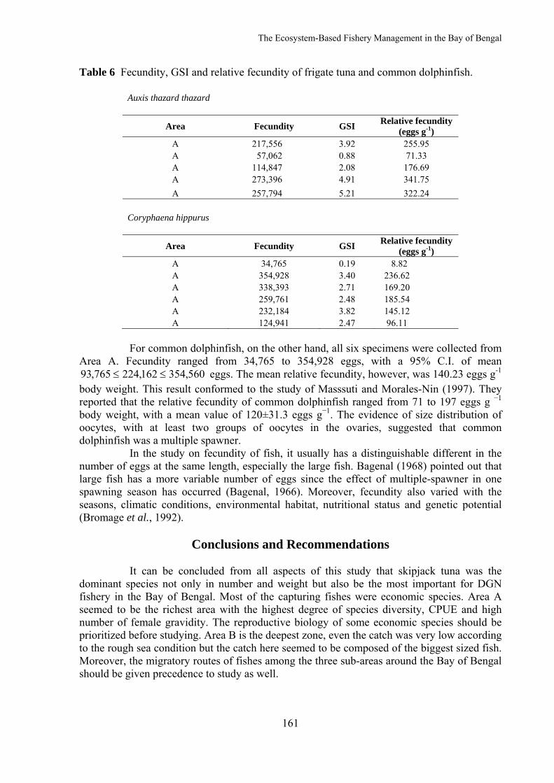
The Ecosystem-Based Fishery Management in the Bay of Bengal
161
Table 6 Fecundity, GSI and relative fecundity of frigate tuna and common dolphinfish.
Auxis thazard thazard
Area Fecundity GSI Relative fecundity (eggs g-1)
A 217,556 3.92 255.95 A 57,062 0.88 71.33 A 114,847 2.08 176.69 A 273,396 4.91 341.75 A 257,794 5.21 322.24
Coryphaena hippurus
Area Fecundity GSI Relative fecundity (eggs g-1)
A 34,765 0.19 8.82 A 354,928 3.40 236.62 A 338,393 2.71 169.20 A 259,761 2.48 185.54 A 232,184 3.82 145.12 A 124,941 2.47 96.11
For common dolphinfish, on the other hand, all six specimens were collected from Area A. Fecundity ranged from 34,765 to 354,928 eggs, with a 95% C.I. of mean
560,354162,224765,93 ≤≤ eggs. The mean relative fecundity, however, was 140.23 eggs g-1 body weight. This result conformed to the study of Masssuti and Morales-Nin (1997). They reported that the relative fecundity of common dolphinfish ranged from 71 to 197 eggs g −1 body weight, with a mean value of 120±31.3 eggs g−1. The evidence of size distribution of oocytes, with at least two groups of oocytes in the ovaries, suggested that common dolphinfish was a multiple spawner. In the study on fecundity of fish, it usually has a distinguishable different in the number of eggs at the same length, especially the large fish. Bagenal (1968) pointed out that large fish has a more variable number of eggs since the effect of multiple-spawner in one spawning season has occurred (Bagenal, 1966). Moreover, fecundity also varied with the seasons, climatic conditions, environmental habitat, nutritional status and genetic potential (Bromage et al., 1992).
Conclusions and Recommendations It can be concluded from all aspects of this study that skipjack tuna was the dominant species not only in number and weight but also be the most important for DGN fishery in the Bay of Bengal. Most of the capturing fishes were economic species. Area A seemed to be the richest area with the highest degree of species diversity, CPUE and high number of female gravidity. The reproductive biology of some economic species should be prioritized before studying. Area B is the deepest zone, even the catch was very low according to the rough sea condition but the catch here seemed to be composed of the biggest sized fish. Moreover, the migratory routes of fishes among the three sub-areas around the Bay of Bengal should be given precedence to study as well.
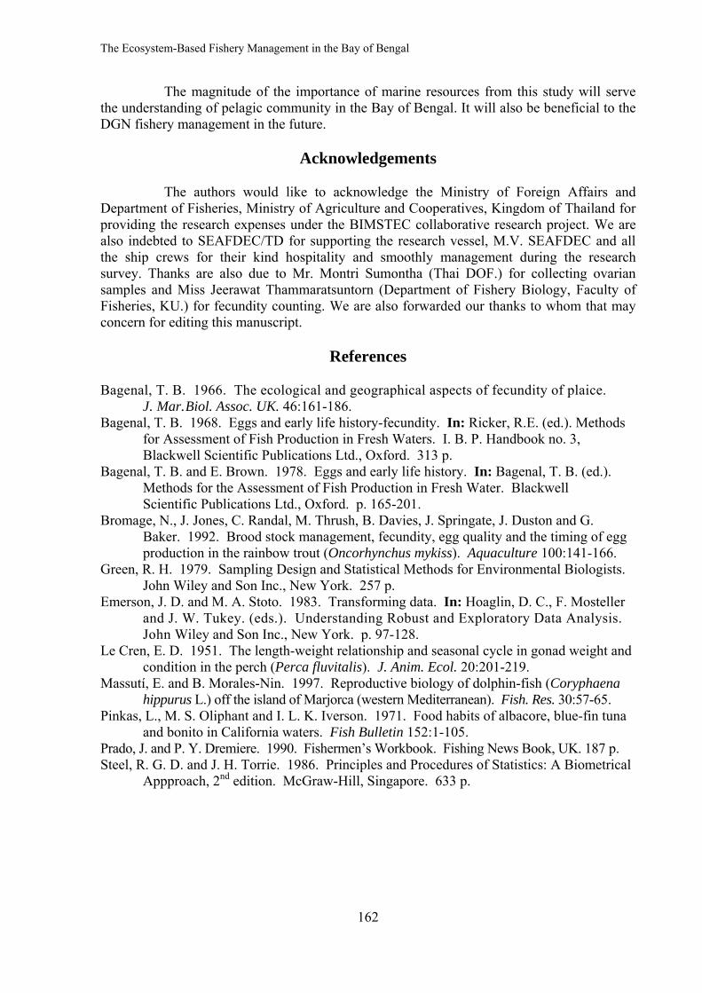
The Ecosystem-Based Fishery Management in the Bay of Bengal
162
The magnitude of the importance of marine resources from this study will serve the understanding of pelagic community in the Bay of Bengal. It will also be beneficial to the DGN fishery management in the future.
Acknowledgements The authors would like to acknowledge the Ministry of Foreign Affairs and Department of Fisheries, Ministry of Agriculture and Cooperatives, Kingdom of Thailand for providing the research expenses under the BIMSTEC collaborative research project. We are also indebted to SEAFDEC/TD for supporting the research vessel, M.V. SEAFDEC and all the ship crews for their kind hospitality and smoothly management during the research survey. Thanks are also due to Mr. Montri Sumontha (Thai DOF.) for collecting ovarian samples and Miss Jeerawat Thammaratsuntorn (Department of Fishery Biology, Faculty of Fisheries, KU.) for fecundity counting. We are also forwarded our thanks to whom that may concern for editing this manuscript.
References Bagenal, T. B. 1966. The ecological and geographical aspects of fecundity of plaice.
J. Mar. Biol. Assoc. UK. 46:161-186. Bagenal, T. B. 1968. Eggs and early life history-fecundity. In: Ricker, R.E. (ed.). Methods for Assessment of Fish Production in Fresh Waters. I. B. P. Handbook no. 3, Blackwell Scientific Publications Ltd., Oxford. 313 p. Bagenal, T. B. and E. Brown. 1978. Eggs and early life history. In: Bagenal, T. B. (ed.). Methods for the Assessment of Fish Production in Fresh Water. Blackwell Scientific Publications Ltd., Oxford. p. 165-201. Bromage, N., J. Jones, C. Randal, M. Thrush, B. Davies, J. Springate, J. Duston and G. Baker. 1992. Brood stock management, fecundity, egg quality and the timing of egg production in the rainbow trout (Oncorhynchus mykiss). Aquaculture 100:141-166. Green, R. H. 1979. Sampling Design and Statistical Methods for Environmental Biologists. John Wiley and Son Inc., New York. 257 p. Emerson, J. D. and M. A. Stoto. 1983. Transforming data. In: Hoaglin, D. C., F. Mosteller
and J. W. Tukey. (eds.). Understanding Robust and Exploratory Data Analysis. John Wiley and Son Inc., New York. p. 97-128.
Le Cren, E. D. 1951. The length-weight relationship and seasonal cycle in gonad weight and condition in the perch (Perca fluvitalis). J. Anim. Ecol. 20:201-219. Massutí, E. and B. Morales-Nin. 1997. Reproductive biology of dolphin-fish (Coryphaena hippurus L.) off the island of Marjorca (western Mediterranean). Fish. Res. 30:57-65. Pinkas, L., M. S. Oliphant and I. L. K. Iverson. 1971. Food habits of albacore, blue-fin tuna and bonito in California waters. Fish Bulletin 152:1-105. Prado, J. and P. Y. Dremiere. 1990. Fishermen’s Workbook. Fishing News Book, UK. 187 p. Steel, R. G. D. and J. H. Torrie. 1986. Principles and Procedures of Statistics: A Biometrical Appproach, 2nd edition. McGraw-Hill, Singapore. 633 p.
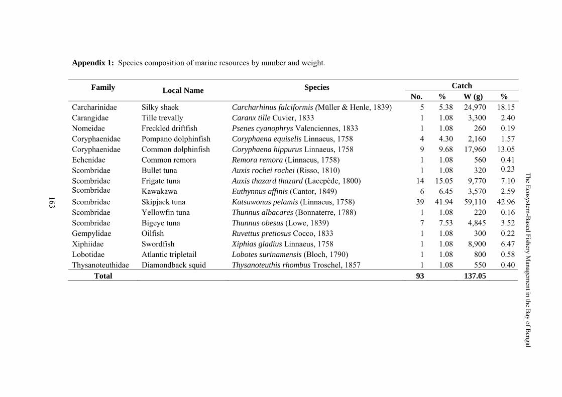
The Ecosystem-Based Fishery Management in the Bay of Bengal
163
Appendix 1: Species composition of marine resources by number and weight.
Family
Local Name Species
Catch No. % W (g) %
Carcharinidae Silky shaek Carcharhinus falciformis (Müller & Henle, 1839) 5 5.38 24,970 18.15 Carangidae Tille trevally Caranx tille Cuvier, 1833 1 1.08 3,300 2.40 Nomeidae Freckled driftfish Psenes cyanophrys Valenciennes, 1833 1 1.08 260 0.19 Coryphaenidae Pompano dolphinfish Coryphaena equiselis Linnaeus, 1758 4 4.30 2,160 1.57 Coryphaenidae Common dolphinfish Coryphaena hippurus Linnaeus, 1758 9 9.68 17,960 13.05 Echenidae Common remora Remora remora (Linnaeus, 1758) 1 1.08 560 0.41 Scombridae Bullet tuna Auxis rochei rochei (Risso, 1810) 1 1.08 320 0.23 Scombridae Frigate tuna Auxis thazard thazard (Lacepède, 1800) 14 15.05 9,770 7.10 Scombridae Kawakawa Euthynnus affinis (Cantor, 1849) 6 6.45 3,570 2.59 Scombridae Skipjack tuna Katsuwonus pelamis (Linnaeus, 1758) 39 41.94 59,110 42.96 Scombridae Yellowfin tuna Thunnus albacares (Bonnaterre, 1788) 1 1.08 220 0.16 Scombridae Bigeye tuna Thunnus obesus (Lowe, 1839) 7 7.53 4,845 3.52 Gempylidae Oilfish Ruvettus pretiosus Cocco, 1833 1 1.08 300 0.22 Xiphiidae Swordfish Xiphias gladius Linnaeus, 1758 1 1.08 8,900 6.47 Lobotidae Atlantic tripletail Lobotes surinamensis (Bloch, 1790) 1 1.08 800 0.58 Thysanoteuthidae Diamondback squid Thysanoteuthis rhombus Troschel, 1857 1 1.08 550 0.40
Total 93 137.05
163
The Ecosystem
-Based Fishery M
anagement in the B
ay of Bengal
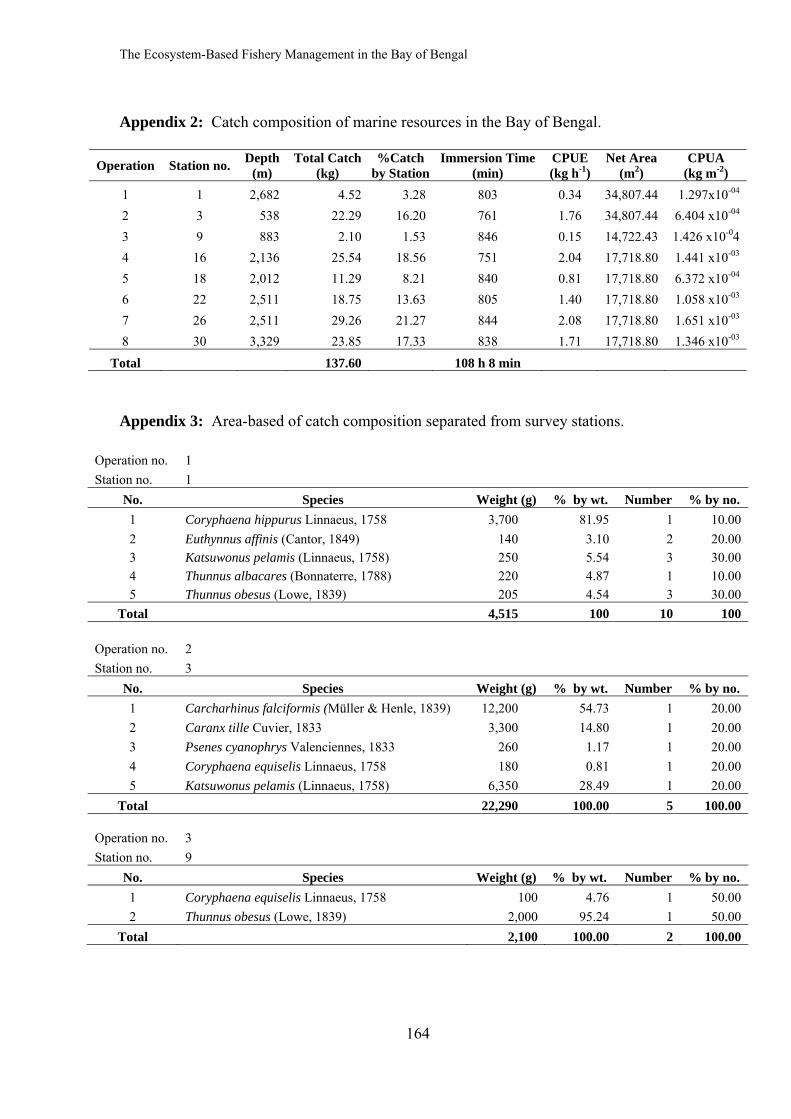
The Ecosystem-Based Fishery Management in the Bay of Bengal
164
Appendix 2: Catch composition of marine resources in the Bay of Bengal.
Operation Station no. Depth (m)
Total Catch (kg)
%Catch by Station
Immersion Time (min)
CPUE (kg h-1)
Net Area (m2)
CPUA (kg m-2)
1 1 2,682 4.52 3.28 803 0.34 34,807.44 1.297x10-04 2 3 538 22.29 16.20 761 1.76 34,807.44 6.404 x10-04 3 9 883 2.10 1.53 846 0.15 14,722.43 1.426 x10-04 4 16 2,136 25.54 18.56 751 2.04 17,718.80 1.441 x10-03 5 18 2,012 11.29 8.21 840 0.81 17,718.80 6.372 x10-04 6 22 2,511 18.75 13.63 805 1.40 17,718.80 1.058 x10-03 7 26 2,511 29.26 21.27 844 2.08 17,718.80 1.651 x10-03 8 30 3,329 23.85 17.33 838 1.71 17,718.80 1.346 x10-03
Total 137.60 108 h 8 min
Appendix 3: Area-based of catch composition separated from survey stations.
Operation no. 1 Station no. 1
No. Species Weight (g) % by wt. Number % by no. 1 Coryphaena hippurus Linnaeus, 1758 3,700 81.95 1 10.00 2 Euthynnus affinis (Cantor, 1849) 140 3.10 2 20.00 3 Katsuwonus pelamis (Linnaeus, 1758) 250 5.54 3 30.00 4 Thunnus albacares (Bonnaterre, 1788) 220 4.87 1 10.00 5 Thunnus obesus (Lowe, 1839) 205 4.54 3 30.00
Total 4,515 100 10 100
Operation no. 2 Station no. 3
No. Species Weight (g) % by wt. Number % by no. 1 Carcharhinus falciformis (Müller & Henle, 1839) 12,200 54.73 1 20.00 2 Caranx tille Cuvier, 1833 3,300 14.80 1 20.00 3 Psenes cyanophrys Valenciennes, 1833 260 1.17 1 20.00 4 Coryphaena equiselis Linnaeus, 1758 180 0.81 1 20.00 5 Katsuwonus pelamis (Linnaeus, 1758) 6,350 28.49 1 20.00
Total 22,290 100.00 5 100.00
Operation no. 3 Station no. 9
No. Species Weight (g) % by wt. Number % by no. 1 Coryphaena equiselis Linnaeus, 1758 100 4.76 1 50.00 2 Thunnus obesus (Lowe, 1839) 2,000 95.24 1 50.00
Total 2,100 100.00 2 100.00
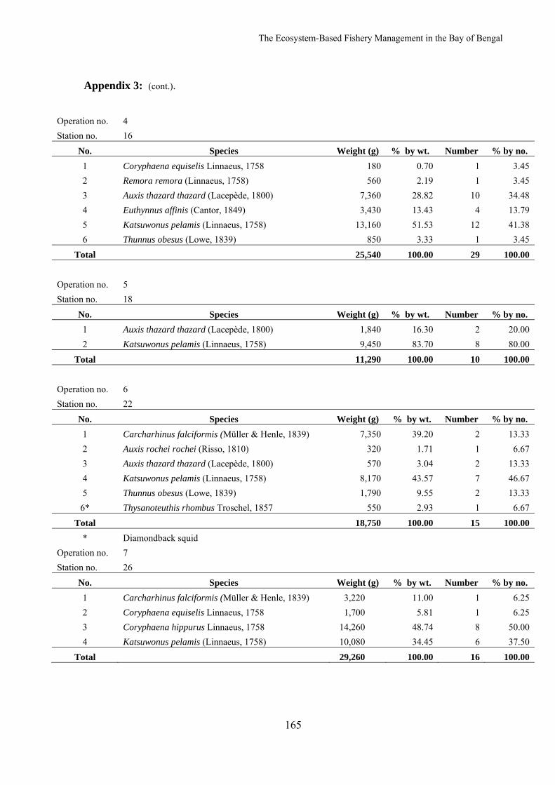
The Ecosystem-Based Fishery Management in the Bay of Bengal
165
Appendix 3: (cont.).
Operation no. 4 Station no. 16
No. Species Weight (g) % by wt. Number % by no. 1 Coryphaena equiselis Linnaeus, 1758 180 0.70 1 3.45 2 Remora remora (Linnaeus, 1758) 560 2.19 1 3.45 3 Auxis thazard thazard (Lacepède, 1800) 7,360 28.82 10 34.48 4 Euthynnus affinis (Cantor, 1849) 3,430 13.43 4 13.79 5 Katsuwonus pelamis (Linnaeus, 1758) 13,160 51.53 12 41.38 6 Thunnus obesus (Lowe, 1839) 850 3.33 1 3.45
Total 25,540 100.00 29 100.00
Operation no. 5 Station no. 18
No. Species Weight (g) % by wt. Number % by no. 1 Auxis thazard thazard (Lacepède, 1800) 1,840 16.30 2 20.00 2 Katsuwonus pelamis (Linnaeus, 1758) 9,450 83.70 8 80.00
Total 11,290 100.00 10 100.00
Operation no. 6 Station no. 22
No. Species Weight (g) % by wt. Number % by no. 1 Carcharhinus falciformis (Müller & Henle, 1839) 7,350 39.20 2 13.33 2 Auxis rochei rochei (Risso, 1810) 320 1.71 1 6.67 3 Auxis thazard thazard (Lacepède, 1800) 570 3.04 2 13.33 4 Katsuwonus pelamis (Linnaeus, 1758) 8,170 43.57 7 46.67 5 Thunnus obesus (Lowe, 1839) 1,790 9.55 2 13.33
6* Thysanoteuthis rhombus Troschel, 1857 550 2.93 1 6.67 Total 18,750 100.00 15 100.00
* Diamondback squid Operation no. 7 Station no. 26
No. Species Weight (g) % by wt. Number % by no. 1 Carcharhinus falciformis (Müller & Henle, 1839) 3,220 11.00 1 6.25 2 Coryphaena equiselis Linnaeus, 1758 1,700 5.81 1 6.25 3 Coryphaena hippurus Linnaeus, 1758 14,260 48.74 8 50.00 4 Katsuwonus pelamis (Linnaeus, 1758) 10,080 34.45 6 37.50
Total 29,260 100.00 16 100.00
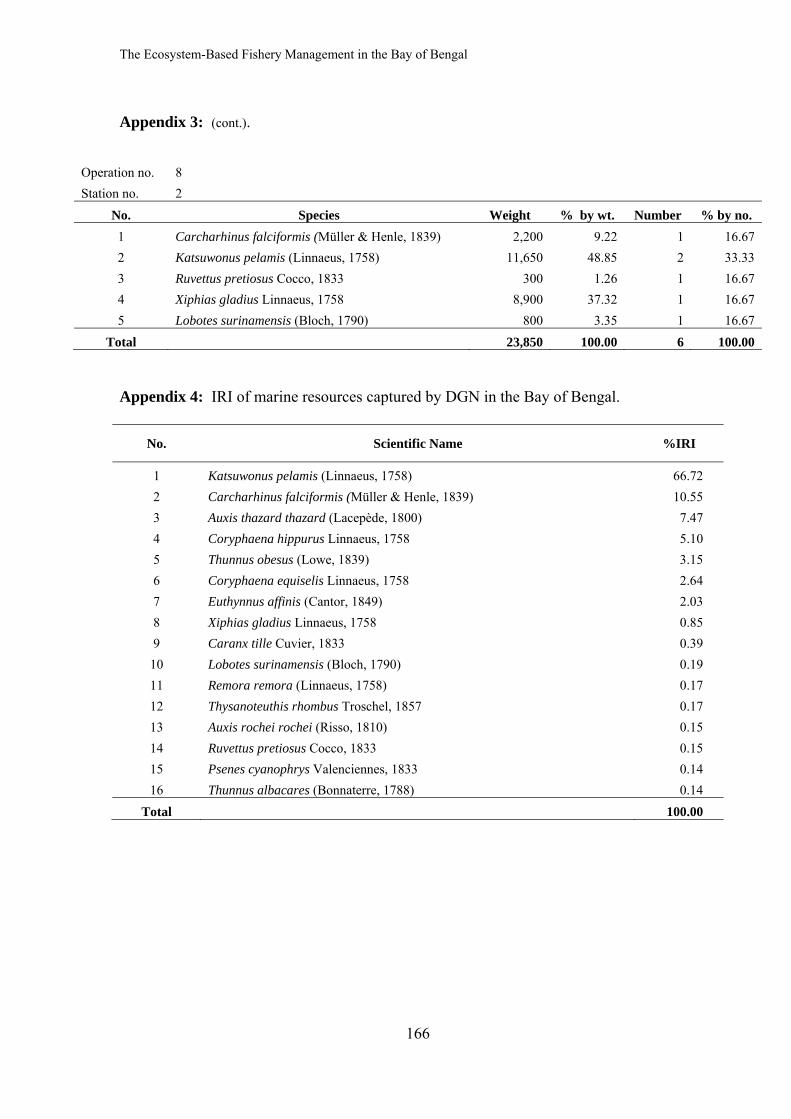
The Ecosystem-Based Fishery Management in the Bay of Bengal
166
Appendix 3: (cont.).
Operation no. 8 Station no. 2
No. Species Weight % by wt. Number % by no. 1 Carcharhinus falciformis (Müller & Henle, 1839) 2,200 9.22 1 16.67 2 Katsuwonus pelamis (Linnaeus, 1758) 11,650 48.85 2 33.33 3 Ruvettus pretiosus Cocco, 1833 300 1.26 1 16.67 4 Xiphias gladius Linnaeus, 1758 8,900 37.32 1 16.67 5 Lobotes surinamensis (Bloch, 1790) 800 3.35 1 16.67
Total 23,850 100.00 6 100.00
Appendix 4: IRI of marine resources captured by DGN in the Bay of Bengal.
No. Scientific Name %IRI
1 Katsuwonus pelamis (Linnaeus, 1758) 66.72 2 Carcharhinus falciformis (Müller & Henle, 1839) 10.55 3 Auxis thazard thazard (Lacepède, 1800) 7.47 4 Coryphaena hippurus Linnaeus, 1758 5.10 5 Thunnus obesus (Lowe, 1839) 3.15 6 Coryphaena equiselis Linnaeus, 1758 2.64 7 Euthynnus affinis (Cantor, 1849) 2.03 8 Xiphias gladius Linnaeus, 1758 0.85 9 Caranx tille Cuvier, 1833 0.39
10 Lobotes surinamensis (Bloch, 1790) 0.19 11 Remora remora (Linnaeus, 1758) 0.17 12 Thysanoteuthis rhombus Troschel, 1857 0.17 13 Auxis rochei rochei (Risso, 1810) 0.15 14 Ruvettus pretiosus Cocco, 1833 0.15 15 Psenes cyanophrys Valenciennes, 1833 0.14 16 Thunnus albacares (Bonnaterre, 1788) 0.14
Total 100.00
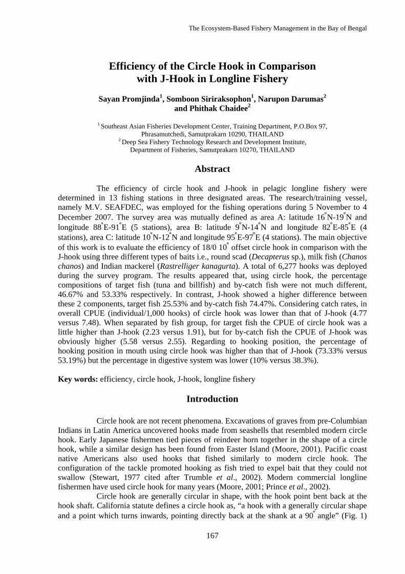
The Ecosystem-Based Fishery Management in the Bay of Bengal
167
Efficiency of the Circle Hook in Comparison with J-Hook in Longline Fishery
Sayan Promjinda1, Somboon Siriraksophon1, Narupon Darumas2
and Phithak Chaidee2
1 Southeast Asian Fisheries Development Center, Training Department, P.O.Box 97, Phrasamutchedi, Samutprakarn 10290, THAILAND
2 Deep Sea Fishery Technology Research and Development Institute, Department of Fisheries, Samutprakarn 10270, THAILAND
Abstract
The efficiency of circle hook and J-hook in pelagic longline fishery were
determined in 13 fishing stations in three designated areas. The research/training vessel, namely M.V. SEAFDEC, was employed for the fishing operations during 5 November to 4 December 2007. The survey area was mutually defined as area A: latitude 16°N-19°N and longitude 88°E-91°E (5 stations), area B: latitude 9°N-14°N and longitude 82°E-85°E (4 stations), area C: latitude 10°N-12°N and longitude 95°E-97°E (4 stations). The main objective of this work is to evaluate the efficiency of 18/0 10° offset circle hook in comparison with the J-hook using three different types of baits i.e., round scad (Decapterus sp.), milk fish (Chanos chanos) and Indian mackerel (Rastrelliger kanagurta). A total of 6,277 hooks was deployed during the survey program. The results appeared that, using circle hook, the percentage compositions of target fish (tuna and billfish) and by-catch fish were not much different, 46.67% and 53.33% respectively. In contrast, J-hook showed a higher difference between these 2 components, target fish 25.53% and by-catch fish 74.47%. Considering catch rates, in overall CPUE (individual/1,000 hooks) of circle hook was lower than that of J-hook (4.77 versus 7.48). When separated by fish group, for target fish the CPUE of circle hook was a little higher than J-hook (2.23 versus 1.91), but for by-catch fish the CPUE of J-hook was obviously higher (5.58 versus 2.55). Regarding to hooking position, the percentage of hooking position in mouth using circle hook was higher than that of J-hook (73.33% versus 53.19%) but the percentage in digestive system was lower (10% versus 38.3%). Key words: efficiency, circle hook, J-hook, longline fishery
Introduction
Circle hook are not recent phenomena. Excavations of graves from pre-Columbian Indians in Latin America uncovered hooks made from seashells that resembled modern circle hook. Early Japanese fishermen tied pieces of reindeer horn together in the shape of a circle hook, while a similar design has been found from Easter Island (Moore, 2001). Pacific coast native Americans also used hooks that fished similarly to modern circle hook. The configuration of the tackle promoted hooking as fish tried to expel bait that they could not swallow (Stewart, 1977 cited after Trumble et al., 2002). Modern commercial longline fishermen have used circle hook for many years (Moore, 2001; Prince et al., 2002).
Circle hook are generally circular in shape, with the hook point bent back at the hook shaft. California statute defines a circle hook as, “a hook with a generally circular shape and a point which turns inwards, pointing directly back at the shank at a 90° angle” (Fig. 1)
The Ecosystem-Based Fishery Management in the Bay of Bengal
168
Prince et al. (2002) defined a circle hook as “hook having a point that is perpendicular to the main hook shaft”, whereas J-hook is defined as hook having a point parallel to the hook shaft. When looking at the barb from behind the hook shank, the greater the “offset” angle, the more the barb is visible (the barb and the shank are not in the same plane). The amount of “offset” may be important for the evaluation of hooking location. However, Lukacovic (2001) detected no difference in deep hooking rates in striped bass between offset and non-offset hook.
Circle hook is designed to prevent the exposed barb point from puncturing internal organs if the hook is swallowed. Fish swallow the baited hook and begin to move away. This movement pulls the hook from the throat, decreasing the chance of gut hooking. As the hook shaft begins to exit the mouth, the shape of the hook causes the shaft to rotate towards the corner of the mouth and the barb embeds in the corner of the jaw (Florida Sea Grant College Program, 1999; Artmarina Fishing Fleet, 2002).
A comparison of efficiency between the circle hook and the J-hook in longline fishery is the sub-project under the Ecosystem-Based Fishery Management in the Bay of Bengal Project. The pelagic longline (PLL) operation was conducted in 13 different stations in three designated areas, during 5 November to 4 December 2007, in the Bay of Bengal.
Objectives To determine the efficiency of circle hook and J-hook with respect to:
- catch composition - catch rate - hooking position - length frequency distribution of some dominant fishes
Materials and Method
Survey Area
The survey area was mutually defined as area A: latitude 16°N-19°N and longitude 88°E-91°E (5 stations) area B: latitude 9°N-14°N and longitude 82°E-85°E (4 stations) and area C latitude 10°N-12°N and longitude 95°E-97°E (4 stations). The depth of the sea at the survey stations was varied between 1,128 m and 3,525 m. (Fig. 1).
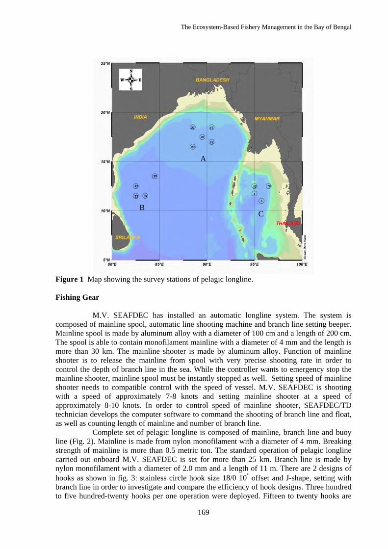
The Ecosystem-Based Fishery Management in the Bay of Bengal
169
Figure 1 Map showing the survey stations of pelagic longline. Fishing Gear
M.V. SEAFDEC has installed an automatic longline system. The system is composed of mainline spool, automatic line shooting machine and branch line setting beeper. Mainline spool is made by aluminum alloy with a diameter of 100 cm and a length of 200 cm. The spool is able to contain monofilament mainline with a diameter of 4 mm and the length is more than 30 km. The mainline shooter is made by aluminum alloy. Function of mainline shooter is to release the mainline from spool with very precise shooting rate in order to control the depth of branch line in the sea. While the controller wants to emergency stop the mainline shooter, mainline spool must be instantly stopped as well. Setting speed of mainline shooter needs to compatible control with the speed of vessel. M.V. SEAFDEC is shooting with a speed of approximately 7-8 knots and setting mainline shooter at a speed of approximately 8-10 knots. In order to control speed of mainline shooter, SEAFDEC/TD technician develops the computer software to command the shooting of branch line and float, as well as counting length of mainline and number of branch line.
Complete set of pelagic longline is composed of mainline, branch line and buoy line (Fig. 2). Mainline is made from nylon monofilament with a diameter of 4 mm. Breaking strength of mainline is more than 0.5 metric ton. The standard operation of pelagic longline carried out onboard M.V. SEAFDEC is set for more than 25 km. Branch line is made by nylon monofilament with a diameter of 2.0 mm and a length of 11 m. There are 2 designs of hooks as shown in fig. 3: stainless circle hook size 18/0 10° offset and J-shape, setting with branch line in order to investigate and compare the efficiency of hook designs. Three hundred to five hundred-twenty hooks per one operation were deployed. Fifteen to twenty hooks are
A
B C
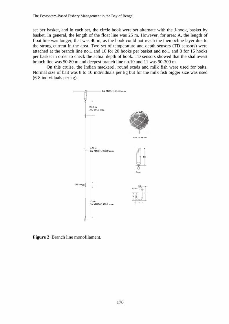
The Ecosystem-Based Fishery Management in the Bay of Bengal
170
set per basket, and in each set, the circle hook were set alternate with the J-hook, basket by basket. In general, the length of the float line was 25 m. However, for area: A, the length of float line was longer, that was 40 m, as the hook could not reach the themocline layer due to the strong current in the area. Two set of temperature and depth sensors (TD sensors) were attached at the branch line no.1 and 10 for 20 hooks per basket and no.1 and 8 for 15 hooks per basket in order to check the actual depth of hook. TD sensors showed that the shallowest branch line was 50-80 m and deepest branch line no.10 and 11 was 90-300 m.
On this cruise, the Indian mackerel, round scads and milk fish were used for baits. Normal size of bait was 8 to 10 individuals per kg but for the milk fish bigger size was used (6-8 individuals per kg). Figure 2 Branch line monofilament.
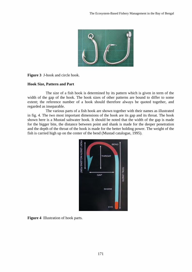
The Ecosystem-Based Fishery Management in the Bay of Bengal
171
Figure 3 J-hook and circle hook. Hook Size, Pattern and Part
The size of a fish hook is determined by its pattern which is given in term of the width of the gap of the hook. The hook sizes of other patterns are bound to differ to some extent; the reference number of a hook should therefore always be quoted together, and regarded as inseparable.
The various parts of a fish hook are shown together with their names as illustrated in fig. 4. The two most important dimensions of the hook are its gap and its throat. The hook shown here is a Mustad saltwater hook. It should be noted that the width of the gap is made for the bigger bite, the distance between point and shank is made for the deeper penetration and the depth of the throat of the hook is made for the better holding power. The weight of the fish is carried high up on the center of the bend (Mustad catalogue, 1995). Figure 4 Illustration of hook parts.
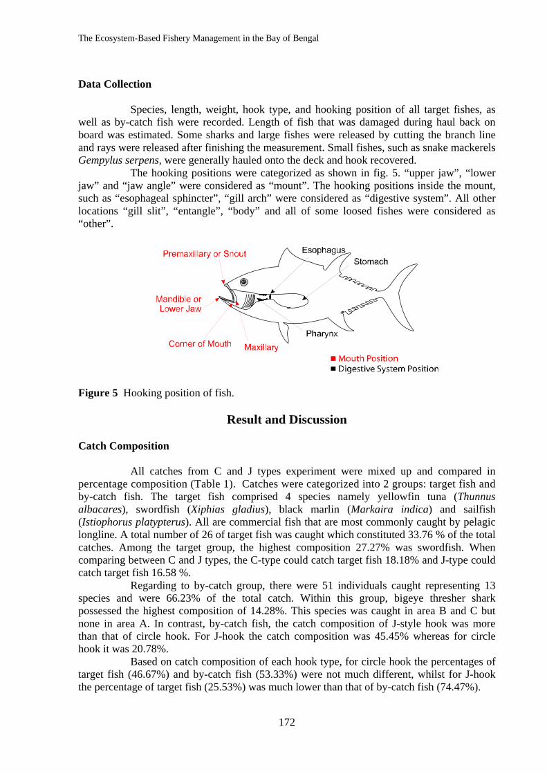
The Ecosystem-Based Fishery Management in the Bay of Bengal
172
Data Collection
Species, length, weight, hook type, and hooking position of all target fishes, as well as by-catch fish were recorded. Length of fish that was damaged during haul back on board was estimated. Some sharks and large fishes were released by cutting the branch line and rays were released after finishing the measurement. Small fishes, such as snake mackerels Gempylus serpens, were generally hauled onto the deck and hook recovered.
The hooking positions were categorized as shown in fig. 5. “upper jaw”, “lower jaw” and “jaw angle” were considered as “mount”. The hooking positions inside the mount, such as “esophageal sphincter”, “gill arch” were considered as “digestive system”. All other locations “gill slit”, “entangle”, “body” and all of some loosed fishes were considered as “other”.
Results
Figure 5 Hooking position of fish.
Result and Discussion Catch Composition
All catches from C and J types experiment were mixed up and compared in percentage composition (Table 1). Catches were categorized into 2 groups: target fish and by-catch fish. The target fish comprised 4 species namely yellowfin tuna (Thunnus albacares), swordfish (Xiphias gladius), black marlin (Markaira indica) and sailfish (Istiophorus platypterus). All are commercial fish that are most commonly caught by pelagic longline. A total number of 26 of target fish was caught which constituted 33.76 % of the total catches. Among the target group, the highest composition 27.27% was swordfish. When comparing between C and J types, the C-type could catch target fish 18.18% and J-type could catch target fish 16.58 %.
Regarding to by-catch group, there were 51 individuals caught representing 13 species and were 66.23% of the total catch. Within this group, bigeye thresher shark possessed the highest composition of 14.28%. This species was caught in area B and C but none in area A. In contrast, by-catch fish, the catch composition of J-style hook was more than that of circle hook. For J-hook the catch composition was 45.45% whereas for circle hook it was 20.78%.
Based on catch composition of each hook type, for circle hook the percentages of target fish (46.67%) and by-catch fish (53.33%) were not much different, whilst for J-hook the percentage of target fish (25.53%) was much lower than that of by-catch fish (74.47%).
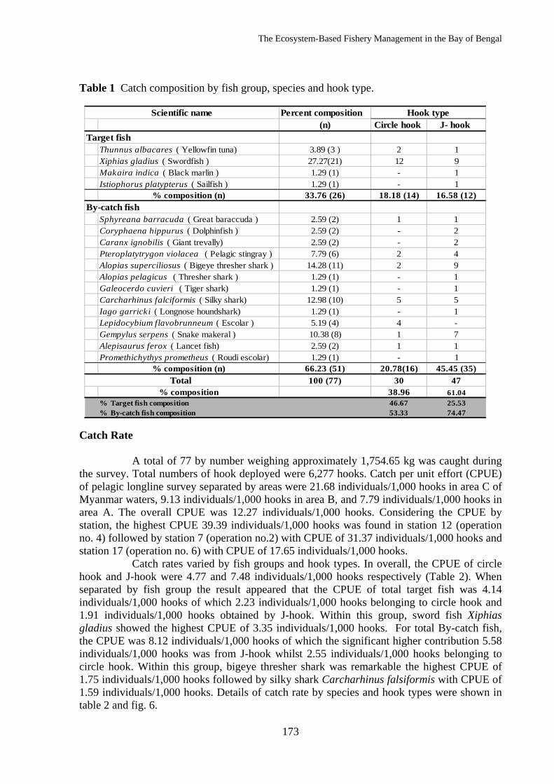
The Ecosystem-Based Fishery Management in the Bay of Bengal
173
Table 1 Catch composition by fish group, species and hook type. Catch Rate
A total of 77 by number weighing approximately 1,754.65 kg was caught during the survey. Total numbers of hook deployed were 6,277 hooks. Catch per unit effort (CPUE) of pelagic longline survey separated by areas were 21.68 individuals/1,000 hooks in area C of Myanmar waters, 9.13 individuals/1,000 hooks in area B, and 7.79 individuals/1,000 hooks in area A. The overall CPUE was 12.27 individuals/1,000 hooks. Considering the CPUE by station, the highest CPUE 39.39 individuals/1,000 hooks was found in station 12 (operation no. 4) followed by station 7 (operation no.2) with CPUE of 31.37 individuals/1,000 hooks and station 17 (operation no. 6) with CPUE of 17.65 individuals/1,000 hooks.
Catch rates varied by fish groups and hook types. In overall, the CPUE of circle hook and J-hook were 4.77 and 7.48 individuals/1,000 hooks respectively (Table 2). When separated by fish group the result appeared that the CPUE of total target fish was 4.14 individuals/1,000 hooks of which 2.23 individuals/1,000 hooks belonging to circle hook and 1.91 individuals/1,000 hooks obtained by J-hook. Within this group, sword fish Xiphias gladius showed the highest CPUE of 3.35 individuals/1,000 hooks. For total By-catch fish, the CPUE was 8.12 individuals/1,000 hooks of which the significant higher contribution 5.58 individuals/1,000 hooks was from J-hook whilst 2.55 individuals/1,000 hooks belonging to circle hook. Within this group, bigeye thresher shark was remarkable the highest CPUE of 1.75 individuals/1,000 hooks followed by silky shark Carcharhinus falsiformis with CPUE of 1.59 individuals/1,000 hooks. Details of catch rate by species and hook types were shown in table 2 and fig. 6.
Percent composition (n) Circle hook J- hook
Target fishThunnus albacares ( Yellowfin tuna) 3.89 (3 ) 2 1Xiphias gladius ( Swordfish ) 27.27(21) 12 9Makaira indica ( Black marlin ) 1.29 (1) - 1Istiophorus platypterus ( Sailfish ) 1.29 (1) - 1
% composition (n) 33.76 (26) 18.18 (14) 16.58 (12)By-catch fish
Sphyreana barracuda ( Great baraccuda ) 2.59 (2) 1 1Coryphaena hippurus ( Dolphinfish ) 2.59 (2) - 2Caranx ignobilis ( Giant trevally) 2.59 (2) - 2Pteroplatytrygon violacea ( Pelagic stingray ) 7.79 (6) 2 4Alopias superciliosus ( Bigeye thresher shark ) 14.28 (11) 2 9Alopias pelagicus ( Thresher shark ) 1.29 (1) - 1Galeocerdo cuvieri ( Tiger shark) 1.29 (1) - 1Carcharhinus falciformis ( Silky shark) 12.98 (10) 5 5Iago garricki ( Longnose houndshark) 1.29 (1) - 1Lepidocybium flavobrunneum ( Escolar ) 5.19 (4) 4 -Gempylus serpens ( Snake makeral ) 10.38 (8) 1 7Alepisaurus ferox ( Lancet fish) 2.59 (2) 1 1Promethichythys prometheus ( Roudi escolar) 1.29 (1) - 1
% composition (n) 66.23 (51) 20.78(16) 45.45 (35)100 (77) 30 47
% composition 38.96 61.04% Target fish composition 46.67 25.53% By-catch fish composition 53.33 74.47
Hook typeScientific name
Total
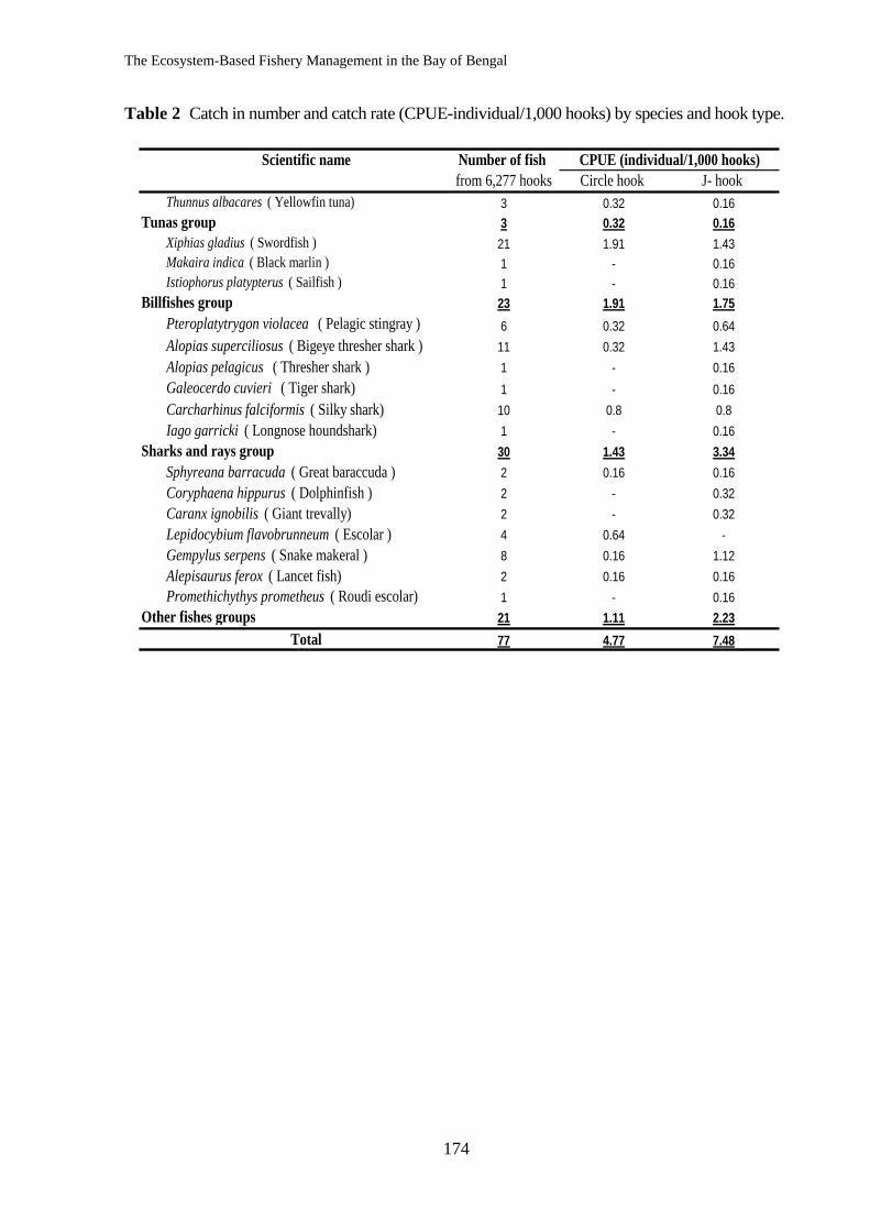
The Ecosystem-Based Fishery Management in the Bay of Bengal
174
Table 2 Catch in number and catch rate (CPUE-individual/1,000 hooks) by species and hook type.
Scientific name Number of fish from 6,277 hooks Circle hook J- hook
Thunnus albacares ( Yellowfin tuna) 3 0.32 0.16Tunas group 3 0.32 0.16
Xiphias gladius ( Swordfish ) 21 1.91 1.43Makaira indica ( Black marlin ) 1 - 0.16Istiophorus platypterus ( Sailfish ) 1 - 0.16
Billfishes group 23 1.91 1.75Pteroplatytrygon violacea ( Pelagic stingray ) 6 0.32 0.64Alopias superciliosus ( Bigeye thresher shark ) 11 0.32 1.43Alopias pelagicus ( Thresher shark ) 1 - 0.16Galeocerdo cuvieri ( Tiger shark) 1 - 0.16Carcharhinus falciformis ( Silky shark) 10 0.8 0.8Iago garricki ( Longnose houndshark) 1 - 0.16
Sharks and rays group 30 1.43 3.34Sphyreana barracuda ( Great baraccuda ) 2 0.16 0.16Coryphaena hippurus ( Dolphinfish ) 2 - 0.32Caranx ignobilis ( Giant trevally) 2 - 0.32Lepidocybium flavobrunneum ( Escolar ) 4 0.64 -Gempylus serpens ( Snake makeral ) 8 0.16 1.12Alepisaurus ferox ( Lancet fish) 2 0.16 0.16Promethichythys prometheus ( Roudi escolar) 1 - 0.16
Other fishes groups 21 1.11 2.23Total 77 4.77 7.48
CPUE (individual/1,000 hooks)
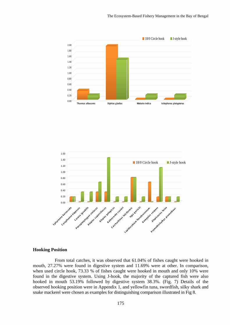
The Ecosystem-Based Fishery Management in the Bay of Bengal
175
Figure 6 Comparison of CPUE (individual/1,000 hooks) by species and hook type. Hooking Position
From total catches, it was observed that 61.04% of fishes caught were hooked in mouth, 27.27% were found in digestive system and 11.69% were at other. In comparison, when used circle hook, 73.33 % of fishes caught were hooked in mouth and only 10% were found in the digestive system. Using J-hook, the majority of the captured fish were also hooked in mouth 53.19% followed by digestive system 38.3%. (Fig. 7) Details of the observed hooking position were in Appendix 1, and yellowfin tuna, swordfish, silky shark and snake mackerel were chosen as examples for distinguishing comparison illustrated in Fig 8.
0.00
0.20
0.40
0.60
0.80
1.00
1.20
1.40
1.60
S phyreana b
arrac uda
C oryphaena hippurus
C aranx ignobilis
P teroplatytryg on v io
lacea
A lopias
s upercilio
s us
A lopias
pela
g ic us
G aleo
c erdo c uvie
ri
C archarhinus falc iformis
Iago g arric ki
L epidoc ybium
flavobrunneum
G empylus s
erpens
A lepis a
urus ferox
P rom
ethic hythys p
rometheus
18/0 Circle hook J-style hook
0.00
0.20
0.40
0.60
0.80
1.00
1.20
1.40
1.60
1.80
2.00
Thunnus albacares X iphias g ladius Makaira indic a Is tiophorus platypterus
18/0 Circle hook J-style hook
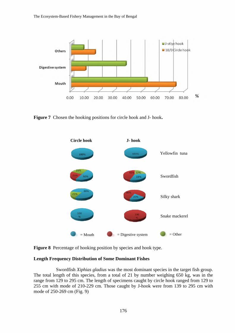
The Ecosystem-Based Fishery Management in the Bay of Bengal
176
Figure 7 Chosen the hooking positions for circle hook and J- hook.
Figure 8 Percentage of hooking position by species and hook type. Length Frequency Distribution of Some Dominant Fishes
Swordfish Xiphias gladius was the most dominant species in the target fish group. The total length of this species, from a total of 21 by number weighing 650 kg, was in the range from 129 to 295 cm. The length of specimens caught by circle hook ranged from 129 to 255 cm with mode of 210-229 cm. Those caught by J-hook were from 139 to 295 cm with mode of 250-269 cm (Fig. 9)
Circle hook J- hook
Yellowfin tuna
Swordfish
Silky shark
Snake mackerel
= Mouth = Digestive system = Other
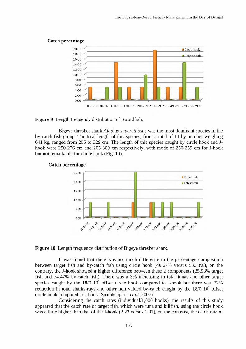
The Ecosystem-Based Fishery Management in the Bay of Bengal
177
Figure 9 Length frequency distribution of Swordfish.
Bigeye thresher shark Alopius superciliosus was the most dominant species in the by-catch fish group. The total length of this species, from a total of 11 by number weighing 641 kg, ranged from 205 to 329 cm. The length of this species caught by circle hook and J-hook were 250-276 cm and 205-309 cm respectively, with mode of 250-259 cm for J-hook but not remarkable for circle hook (Fig. 10).
Discussion and Conclusion
Figure 10 Length frequency distribution of Bigeye thresher shark.
It was found that there was not much difference in the percentage composition between target fish and by-catch fish using circle hook (46.67% versus 53.33%), on the contrary, the J-hook showed a higher difference between these 2 components (25.53% target fish and 74.47% by-catch fish). There was a 3% increasing in total tunas and other target species caught by the 18/0 10° offset circle hook compared to J-hook but there was 22% reduction in total sharks-rays and other non valued by-catch caught by the 18/0 10° offset circle hook compared to J-hook (Siriraksophon et al.,2007).
Considering the catch rates (individual/1,000 hooks), the results of this study appeared that the catch rate of target fish, which were tuna and billfish, using the circle hook was a little higher than that of the J-hook (2.23 versus 1.91), on the contrary, the catch rate of
Catch percentage
Catch percentage
The Ecosystem-Based Fishery Management in the Bay of Bengal
178
by-catch fish obtained by J-hook was approximately twofold of that belonging to circle hook (5.58 versus 2.55).Thus this result indicate that the catch-ability of circle hook and J-hook are almost equal for target fish but J-hook are more effective for by-catch fish. Furthermore, the effects of circle hook and J-hook on pelagic long line catch rate have been investigated with interesting results. One of the important by-catch fish from pelagic longline fishing is shark. In some areas sharks are non-target fish but in the western North Pacific they are the target fish (Simpfendorfer et al., 2005; Watson et al., 2005). When compared the blue shark catch rates (individual/1000 hooks) using 0° and 10° offset 18/0 circle hook with a combination of squid and mackerel baits to those using 25° offset 9/0 J-hook with squid bait. They used data collected by onboard observer during pelagic longline fishery in the west North Atlantic. Their results appeared that, compared to J-hook, catch rates significantly increased by 8-9% when circle hook were used with squid bait. However, Watson et al.(2005) discussed that circle hook might not actually catch more sharks than J-hook, they hypothesized that the results of J-hook might be erroneous because during haul back, sharks that were gut-hooked were more likely to bite off monofilament leaders and thus could escape from detention. In this study the difference in CPUE of bigeye thresher shark between J-hook and circle hook was obvious. The J-hook showed the higher CPUE than circle hook (1.43 versus 0.32). Only the silky shark Carcharhinus falciformis was observed a similar CPUE between J-hook and circle hook (0.8 individual/1,000 hooks).
Regarding to hooking position, the use of circle hook has been known to reduce the rate of deep hooking and increase mouth hooking in some pelagic fishes such as Atlantic bluefin tuna (Thunnus thynnus), yellowfin tuna (Thunnus albacares) and billfish (Prince et al., 2002; Skomal et al.,2002; Kerstetter and Graves, in press). Falterman and Graves (2002) reported that gut, foul and roof hooking events were seen with the J-hook but not with the circle hook. In this study hooking positions varied by hook type and fish species. From all species caught the circle hook were hooked in mouths with 61.04%. For yellowfin tuna both types of the hooks were recorded at 100% in mouths. For swordfish, the circle hook were hooked in mouth 50%, while the J-hook were found in digestive system 45%. Stillwell and Konler (1985) noted that many of the squid and mesopelagic fishes in swordfish gut contents showed an evidence of decapitation or slashing. This feeding behavior may explain the relatively high incidence of bill hooking. Silky sharks caught by the circle hook were hooked 80% in mouth but only 20% was observed from J-hook. In contrast, the hook type found most in digestive system was the J-hook (80%). These results are in good agreement with the observation from Kerstetter and Graves (in press). They reported that the circle hook caught fishes in the mouth more frequently than J-hook, whereas the J-hook hooked more often in the throat of gut. Although the differences in hooking position between hook types were not statistically significant, the yellowfin tuna in the fall fishery was over four times more likely to be hooked in the mouth with the circle hook than with the J-hook.
In considering the length frequency distribution of the 2 dominant species, both types of hooks are capable to detain a very large size of fish (over 100 cm). However, it was noticeable that the sizes caught of swordfish (Xiphias gladius) by J-hook were larger than those by circle hook. For bigeye thresher shark (Alopius superciliosus), the specimens caught by J-hook had length range wider than that obtained by circle hook.
From such results, it was recommended that for longline fishery, fishermen should use the C-type hook instead of J-type for higher catch of tuna target fish and at the same time the hook can reduce by-catch especially for those sharks and rays. Since shark and ray are distinguished as endanger species. Furthermore if the by-catch was caught, they will be released and still alive due to the hooking position that causes the fish less damage.
The Ecosystem-Based Fishery Management in the Bay of Bengal
179
Acknowledgement
The authors would like to express their appreciation for the time and patience of the
captain and all of the crews on M.V.SEAFDEC. This study would not have been possible without the staff and the biologists from Department of Fisheries, Thailand and participants from BIMSTEC member countries.
References
Artmarina Fishing Fleet, Guatemala. Available Source: http://www.artmarina.com/brazil/circle_of_life.html. August 20, 2008.
Falterman, B. and J. E. Graves. 2002. A preliminary comparison of the relative mortality and hooking efficiency of circle and straight shank (“J”) hooks used in the pelagic longline industry. Am. Fish. Soc. Symp. 30:80-87.
Florida Sea Grant College Program, December 1999. Fact Sheet SGEF-108. Available Source: http://www.edis.ifas.ufl.edu/BODY_SG042. August 20, 2008.
Kerstetter, D. W. and J. E. Graves. In press. Effects of circle versus J-style hooks on target and non-target species in a pelagic longline fishery. Fish. Res. 150 pp.
Lukacovic, R. 2001. An evaluation of deep hooking rates and relative hooking efficiency of several styles of circular configured hooks. In: Weinrich, D. R., P.G. Piavis, B. H. Pyle, A. A. Jarzynski, J. C. Walstrum, R. A. Sadzinski, E. J. Webb, H. W. Rickabaugh, E. Zlokovitz, J. P. Mower, R. Lukacovic and K. A. Whiteford (eds.). Stock assessment of selected resident and migratory recreational finfish species within Maryland=s Chesapeake Bay.Federal Aid Project F-54-R. Annual Report, Department of the Interior, Fish and Wildlife Service.
Moore, H. 2001. Circle Hooks for Saltwater Fly Fishing. Chesapeake Angler Magazine Online. Available Source: http://www.chesapeake-angler.com/july01hal.html. August 20, 2008.
Mustad, O. and A. S. Son. 1995. The international Fish Hook Catalogue. 3 pp. Prince, E. D., M. Ortiz and A. Venizelos. 2002. A comparison of circle hook and “J” hook
performance in recreational catch and release fisheries for billfish. Lucy, J.A. and A. L. Studholme. (eds.). Catch and release in marine recreational fisheries. American Fisheries Society, Symposium 30, Bethesda, Maryland. p. 66-79.
Simpfendorfer, C. A., R. D. Cavanagh, S. Tanaka and H. Ishihara. 2005. Chapter 7. Northwest Pacific, Regional Overviews. In: Fowler, S. L., R. D. Cavanagh, M. Camhi, G.H. Burgess, G. M. Cailliet, S. V. Fordham, C. A. Simpfendorfer and J. A. Musick. (eds.). Sharks, Rays and Chimaeras: The Status of the Chondrichthyan Fishes. IUCN-The World Conservation Union, Gland, Switzerland. p. 150-161.
Siriraksophon, S., C. Tantivala, J. D. Cohen, S. Promjinda and I. Chanrachkij. 2007. Mitigation of the Fishery Sea Turtles Interactions: Efficiency of the Circle Hook in Comparison with J-hook in Longline Fishery, Summary paper. Southeast Asian Fisheries Development Center/Training Department, Thailand. 10 pp.
Skomal, G. B., B. C Chase and E. D. Prince. 2002. A comparison of circle and straight hooks relative to hooking location, damage, and success while catch and release fishing for Atlantic bluefin tuna. Am. Fish. Soc. Symp. 30:57-65.
Stewart, H. 1977. Indian Fishing. Early Methods on the Northwest Coast. University of Washington Press, Washington. 230 pp.
Stillwell, C. E., and N. E. Kohler. 1985. Food and feeding ecology of the swordfish Xiphias

The Ecosystem-Based Fishery Management in the Bay of Bengal
180
gladius in the western North Atlantic Ocean with estimates of daily ration. Mar. Ecol. Prog. Ser. 22:239-247.
Watson, J. W., S. P. Epperly, A. K. Shah and D. G. Foster. 2005. Fishing methods to reduce sea turtle mortality associated with pelagic longlines. Can. J. Fish. Aquat. Sci. 62:965-981.
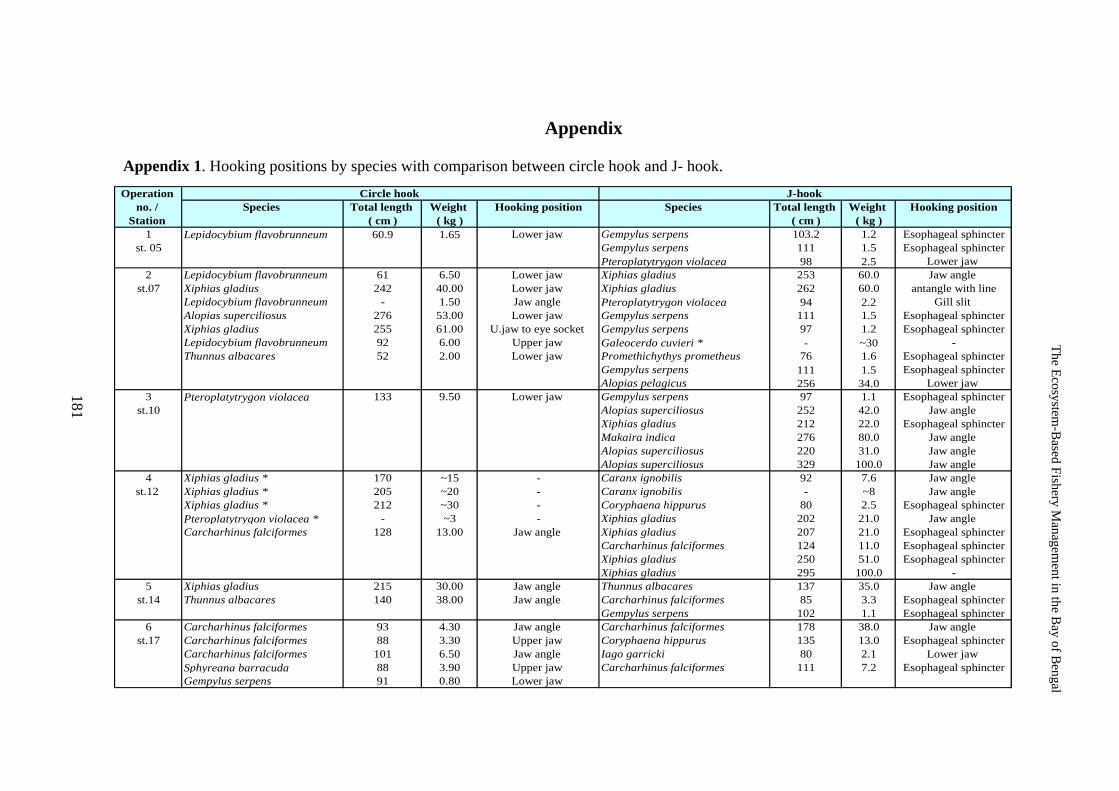
The Ecosystem-Based Fishery Management in the Bay of Bengal
181
Appendix
Appendix 1. Hooking positions by species with comparison between circle hook and J- hook.
Operation no. / Species Total length Weight Hooking position Species Total length Weight Hooking position
Station ( cm ) ( kg ) ( cm ) ( kg )1 Lepidocybium flavobrunneum 60.9 1.65 Lower jaw Gempylus serpens 103.2 1.2 Esophageal sphincter
st. 05 Gempylus serpens 111 1.5 Esophageal sphincterPteroplatytrygon violacea 98 2.5 Lower jaw
2 Lepidocybium flavobrunneum 61 6.50 Lower jaw Xiphias gladius 253 60.0 Jaw angle st.07 Xiphias gladius 242 40.00 Lower jaw Xiphias gladius 262 60.0 antangle with line
Lepidocybium flavobrunneum - 1.50 Jaw angle Pteroplatytrygon violacea 94 2.2 Gill slit Alopias superciliosus 276 53.00 Lower jaw Gempylus serpens 111 1.5 Esophageal sphincterXiphias gladius 255 61.00 U.jaw to eye socket Gempylus serpens 97 1.2 Esophageal sphincterLepidocybium flavobrunneum 92 6.00 Upper jaw Galeocerdo cuvieri * - ~30 -Thunnus albacares 52 2.00 Lower jaw Promethichythys prometheus 76 1.6 Esophageal sphincter
Gempylus serpens 111 1.5 Esophageal sphincterAlopias pelagicus 256 34.0 Lower jaw
3 Pteroplatytrygon violacea 133 9.50 Lower jaw Gempylus serpens 97 1.1 Esophageal sphincterst.10 Alopias superciliosus 252 42.0 Jaw angle
Xiphias gladius 212 22.0 Esophageal sphincterMakaira indica 276 80.0 Jaw angle Alopias superciliosus 220 31.0 Jaw angle Alopias superciliosus 329 100.0 Jaw angle
4 Xiphias gladius * 170 ~15 - Caranx ignobilis 92 7.6 Jaw angle st.12 Xiphias gladius * 205 ~20 - Caranx ignobilis - ~8 Jaw angle
Xiphias gladius * 212 ~30 - Coryphaena hippurus 80 2.5 Esophageal sphincterPteroplatytrygon violacea * - ~3 - Xiphias gladius 202 21.0 Jaw angle Carcharhinus falciformes 128 13.00 Jaw angle Xiphias gladius 207 21.0 Esophageal sphincter
Carcharhinus falciformes 124 11.0 Esophageal sphincterXiphias gladius 250 51.0 Esophageal sphincterXiphias gladius 295 100.0 -
5 Xiphias gladius 215 30.00 Jaw angle Thunnus albacares 137 35.0 Jaw angle st.14 Thunnus albacares 140 38.00 Jaw angle Carcharhinus falciformes 85 3.3 Esophageal sphincter
Gempylus serpens 102 1.1 Esophageal sphincter6 Carcharhinus falciformes 93 4.30 Jaw angle Carcharhinus falciformes 178 38.0 Jaw angle
st.17 Carcharhinus falciformes 88 3.30 Upper jaw Coryphaena hippurus 135 13.0 Esophageal sphincterCarcharhinus falciformes 101 6.50 Jaw angle Iago garricki 80 2.1 Lower jaw Sphyreana barracuda 88 3.90 Upper jaw Carcharhinus falciformes 111 7.2 Esophageal sphincterGempylus serpens 91 0.80 Lower jaw
Circle hook J-hook
181
The Ecosystem-B
ased Fishery Managem
ent in the Bay of B
engal
The Ecosystem-Based Fishery Management in the Bay of Bengal
182
Biological Aspects of Economic Fishes in the Bay of Bengal
Suma Rugpan1, Wilailux Premkit1, Chirdsak Chookong1, Montri Sumontha2 Md. Jalilur Rahman3 and Md. Nasiruddin Sada4
1 Deep Sea Fishery Technology Research and Development Institute,
Department of Fisheries, Samutprakarn 10270, THAILAND 2 Andaman Sea Fisheries Research and Development Center, Department of Fisheries,
Phuket 83000, THAILAND 3 Marine Fisheries and Technology Station, Bangladesh Fisheries Research Institute,
Motel Road, Cox’s Bazar-4700, BANDLADESH 4 Fish Inspection and Quality Control, Department of Fisheries, 209 Muradpur (NM Khan Hill)
P.O. Amin Jute Mill, BANGLADESH
Abstract Six dominant large sized fish species, Katsuwonus pelamis, Xiphias gladius, Auxis thazard, Alopias superciliosus, Carcharhinus falciformis and Coryphaena hippurus are economic important fishes in the Bay of Bengal which were chosen to study on biological aspect. The fish samples from 21 stations were obtained from drift gill net and pelagic long line operated by M.V. SEAFDEC during 25 October-21 December 2007 in the Bay of Bengal. The results showed that the average size of K. pelamis was 41± 10.19 cm whereas X. gladius, A. thazard, A. superciliosus, C. falciformis and C. hippurus were 211.00± 46.36, 35.14± 4.86, 271.00± 40.25, 111.33± 8.79 and 72.94± 12.58 cm respectively. The relationship between length and body weight showed high significant correlation in all respected species. There was significant difference in sex ratio of K. pelamis (p<0.05) but none in others species (p>0.05). The study of gonad development in this survey could not use to indicate the spawning season due to less specimens and the survey did not cover all year round. Key words: Bay of Bengal, economic fishes, sex ratio, gonad development
Introduction
The Bay of Bengal, a sea in the north-east arm of the Indian Ocean, is located between 5°N-22°N latitudes and 80°E-100°E longitudes. Fisheries are of major socioeconomic importance to all countries bordering the bay. The main commercial fish species are shrimp, tuna, yellowfin tuna, bigeye tuna and skipjack tuna. There is a high percentage catch for miscellaneous coastal fishes and pelagic fishes, however shrimp is the major export earner in this region. The Food and Agriculture Organization (FAO) 10 years trend showed a steady increased in catch from 1.4 million tons in 1990 to 2.2 million tons in 1999. An average catch was 2 million tons. Catch trends were quite diverse and it was difficult to identify a pattern due to the fact there was inadequate information on the status of the fishery resources and their exploitations. There were signs that the harvest levels may not be sustainable, especially with regard to tuna fishing in the Maldives, Malaysia, Andaman coast of Thailand and Sri Lanka. Furthermore, the most of countries surrounding the bay are weak in developing clear policies, appropriate strategies and the sustainable management of the fishery resources (NOAA. http.// na.nefsc.noaa.gov/lme/text/lme 34 htm; FAO, 2003). Therefore, the study on biological aspects (e.g. length and weight relationship, sex ration and maturation) is very useful and essential for fishery enhancement and management. It will support future fishery development with scientific data for not only conservation of the fishery resources but also appropriate fishery management for sustainable fishery in the Bay of Bengal.
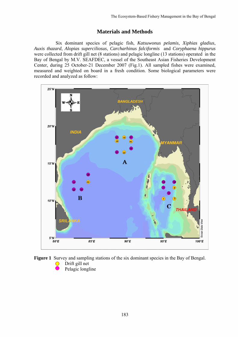
The Ecosystem-Based Fishery Management in the Bay of Bengal
183
Materials and Methods
Six dominant species of pelagic fish, Katsuwonus pelamis, Xiphias gladius, Auxis thazard, Alopias superciliosus, Carcharhinus falciformis and Coryphaena hippurus were collected from drift gill net (8 stations) and pelagic longline (13 stations) operated in the Bay of Bengal by M.V. SEAFDEC, a vessel of the Southeast Asian Fisheries Development Center, during 25 October-21 December 2007 (Fig.1). All sampled fishes were examined, measured and weighted on board in a fresh condition. Some biological parameters were recorded and analyzed as follow:
Figure 1 Survey and sampling stations of the six dominant species in the Bay of Bengal. Drift gill net Pelagic longline
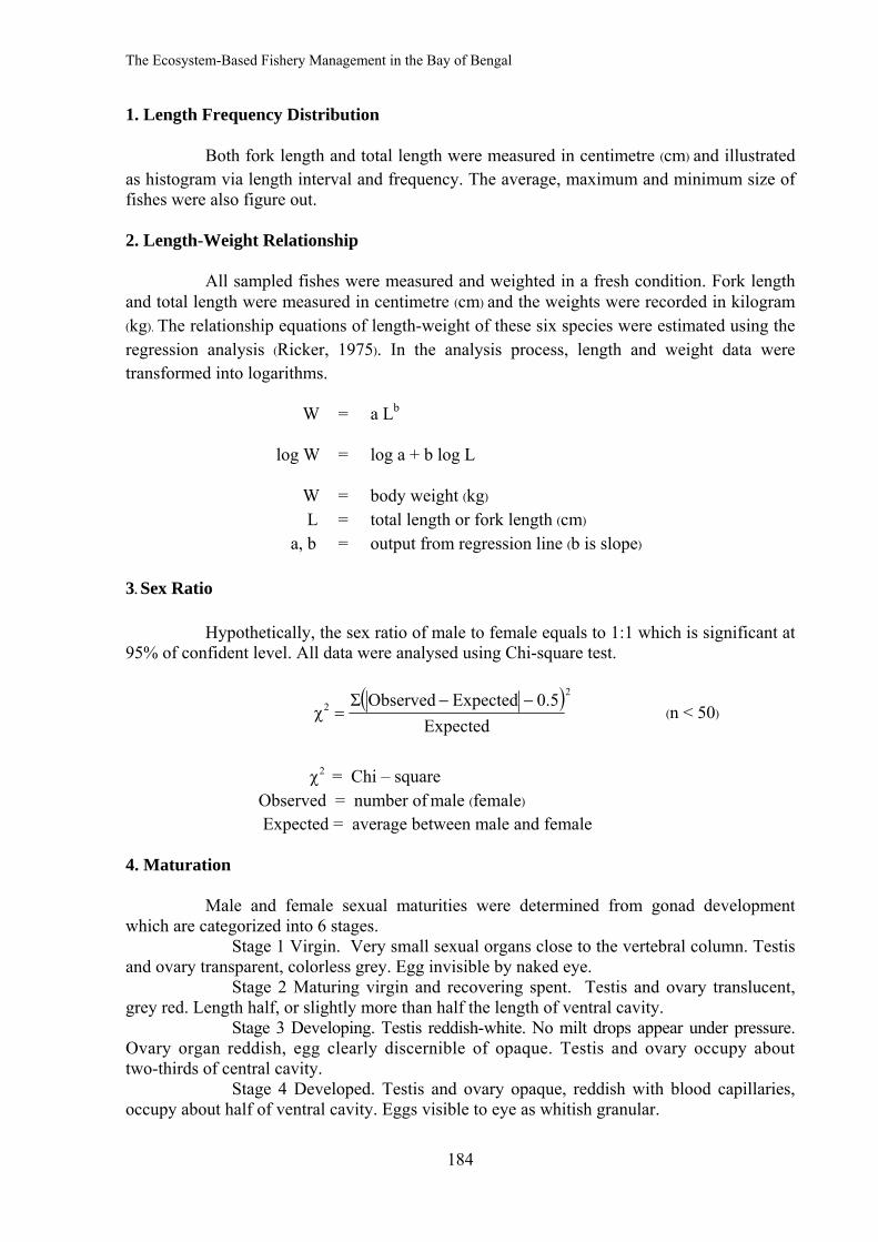
The Ecosystem-Based Fishery Management in the Bay of Bengal
184
1. Length Frequency Distribution Both fork length and total length were measured in centimetre (cm) and illustrated as histogram via length interval and frequency. The average, maximum and minimum size of fishes were also figure out. 2. Length-Weight Relationship All sampled fishes were measured and weighted in a fresh condition. Fork length and total length were measured in centimetre (cm) and the weights were recorded in kilogram (kg). The relationship equations of length-weight of these six species were estimated using the regression analysis (Ricker, 1975). In the analysis process, length and weight data were transformed into logarithms. W = a Lb log W = log a + b log L W = body weight (kg) L = total length or fork length (cm) a, b = output from regression line (b is slope) 3. Sex Ratio Hypothetically, the sex ratio of male to female equals to 1:1 which is significant at 95% of confident level. All data were analysed using Chi-square test.
( )2
2
Expected0.5ExpectedObservedΣ
χ−−
= (n < 50)
2χ = Chi – square Observed = number of male (female) Expected = average between male and female 4. Maturation Male and female sexual maturities were determined from gonad development which are categorized into 6 stages. Stage 1 Virgin. Very small sexual organs close to the vertebral column. Testis and ovary transparent, colorless grey. Egg invisible by naked eye. Stage 2 Maturing virgin and recovering spent. Testis and ovary translucent, grey red. Length half, or slightly more than half the length of ventral cavity. Stage 3 Developing. Testis reddish-white. No milt drops appear under pressure. Ovary organ reddish, egg clearly discernible of opaque. Testis and ovary occupy about two-thirds of central cavity. Stage 4 Developed. Testis and ovary opaque, reddish with blood capillaries, occupy about half of ventral cavity. Eggs visible to eye as whitish granular.
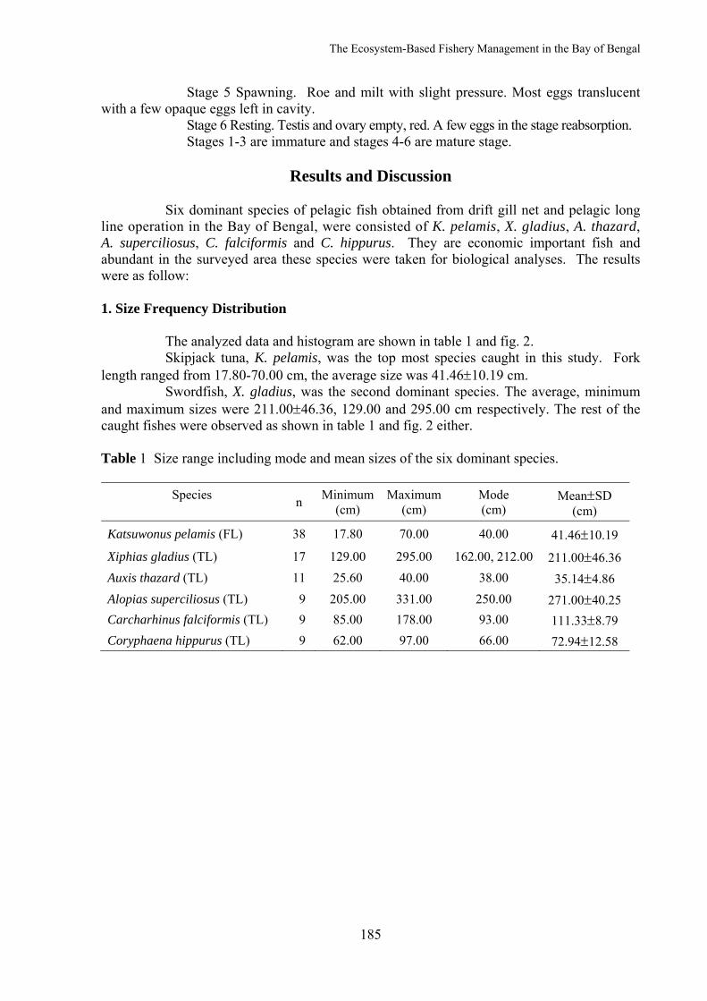
The Ecosystem-Based Fishery Management in the Bay of Bengal
185
Stage 5 Spawning. Roe and milt with slight pressure. Most eggs translucent with a few opaque eggs left in cavity. Stage 6 Resting. Testis and ovary empty, red. A few eggs in the stage reabsorption. Stages 1-3 are immature and stages 4-6 are mature stage.
Results and Discussion Six dominant species of pelagic fish obtained from drift gill net and pelagic long line operation in the Bay of Bengal, were consisted of K. pelamis, X. gladius, A. thazard, A. superciliosus, C. falciformis and C. hippurus. They are economic important fish and abundant in the surveyed area these species were taken for biological analyses. The results were as follow: 1. Size Frequency Distribution The analyzed data and histogram are shown in table 1 and fig. 2. Skipjack tuna, K. pelamis, was the top most species caught in this study. Fork length ranged from 17.80-70.00 cm, the average size was 41.46±10.19 cm. Swordfish, X. gladius, was the second dominant species. The average, minimum and maximum sizes were 211.00±46.36, 129.00 and 295.00 cm respectively. The rest of the caught fishes were observed as shown in table 1 and fig. 2 either. Table 1 Size range including mode and mean sizes of the six dominant species.
Species n Minimum
(cm) Maximum
(cm) Mode (cm)
Mean±SD (cm)
Katsuwonus pelamis (FL) 38 17.80 70.00 40.00 41.46±10.19
Xiphias gladius (TL) 17 129.00 295.00 162.00, 212.00 211.00±46.36 Auxis thazard (TL) 11 25.60 40.00 38.00 35.14±4.86 Alopias superciliosus (TL) 9 205.00 331.00 250.00 271.00±40.25 Carcharhinus falciformis (TL) 9 85.00 178.00 93.00 111.33±8.79 Coryphaena hippurus (TL) 9 62.00 97.00 66.00 72.94±12.58
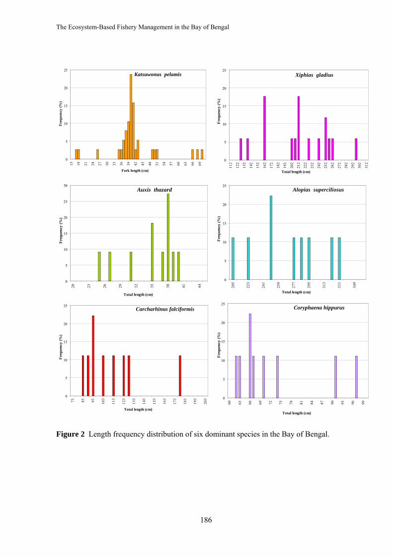
The Ecosystem-Based Fishery Management in the Bay of Bengal
186
0
5
10
15
20
2515 18 21 24 27 30 33 36 39 42 45 48 51 54 57 60 63 66 69
Fork length (cm)
Fre
quen
cy (%
)
Katsuwonus pelamis
0
5
10
15
20
25
112
122
132
142
152
162
172
182
192
202
212
222
232
242
252
262
272
282
292
302
312
Total length (cm)
Freq
uenc
y (%
)
Xiphias gladius
0
5
10
15
20
25
30
20 23 26 29 32 35 38 41 44
Total length (cm)
Freq
uenc
y (%
)
Auxis thazard
0
5
10
15
20
25
205
223
241
259
277
295
313
331
349
Total length (cm)
Freq
uenc
y (%
)
Alopias superciliosus
0
5
10
15
20
25
73 83 93 103
113
123
133
143
153
163
173
183
193
203
Total length (cm)
Freq
uenc
y (%
)
Carcharhinus falciformis
0
5
10
15
20
25
60 63 66 69 72 75 78 81 84 87 90 93 96 99
Total length (cm)
Freq
uenc
y (%
)
Coryphaena hippurus
Figure 2 Length frequency distribution of six dominant species in the Bay of Bengal.

The Ecosystem-Based Fishery Management in the Bay of Bengal
187
2. Length-Weight Relationship The relationship between length and weight of K. pelamis, X. gladius, A. thazard, A. superciliosus, C. falciformis and C. hippurus showed high coefficient of correlation (r2) which meant that weight absolutely increased with length. In addition they were allometric growth because the obtained b values were close to or bigger than 3 (Table 2 and Fig.3).
0
1
2
3
4
5
6
7
8
10 15 20 25 30 35 40 45 50 55 60 65 70
Fork length (cm)
Wei
ght (
kg)
Observed
Calculated
Katsuwonus pelamis
W = 0.00000899 FL3.1864
r2 = 0.9519n = 38
0
20
40
60
80
100
120
120 140 160 180 200 220 240 260 280 300 320
Total length (cm)W
eigh
t (kg
)
Observed
Calculated
Xiphias gladius
W = 0.00000013 TL3.5760
r2 = 0.9832n = 17
200
400
600
800
1,000
20 22 24 26 28 30 32 34 36 38 40
Total length (cm)
Wei
ght (
gm)
Observed
Calculated
Auxis thazard
W = 0.02078 TL2.9015
r2 = 0.9709n = 11
20
40
60
80
100
120
180 200 220 240 260 280 300 320 340
Total length (cm)
Wei
ght (
gm)
Observed
Calculated
Alopias superciliosus
W = 0.00001124 TL2.7574
r2 = 0.9153n = 9
0
10
20
30
40
75 100 125 150 175 200
Total length (cm)
Wei
ght (
gm)
Observed
Calculated
Carcharhinus falciformis
W = 0.000000827 TL3.4089
r2 = 0.9885n = 9
1,000
2,000
3,000
4,000
5,000
60 65 70 75 80 85 90 95 100
Total length (cm)
Wei
ght (
gm)
Observed
Calculated
Coryphaena hippurus
W = 0.01045 TL2.8187
r2 = 0.9872n = 9
Figure 3 The relationship between length and body weight of six dominant species.
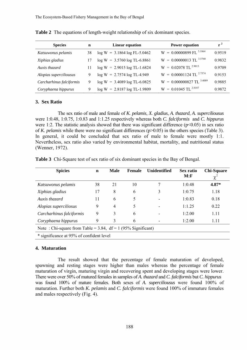
The Ecosystem-Based Fishery Management in the Bay of Bengal
188
Table 2 The equations of length-weight relationship of six dominant species.
Species n Linear equation Power equation r 2 Katsuwonus pelamis 38 log W = 3.1864 log FL-5.0462 W = 0.00000899 FL 3.1864 0.9519
Xiphias gladius 17 log W = 3.5760 log TL-6.8861 W = 0.00000013 TL 3.5760 0.9832
Auxis thazard 11 log W = 2.9015 log TL-1.6824 W = 0.02078 TL 2.9015 0.9709
Alopias superciliousus 9 log W = 2.7574 log TL-4.949 W = 0.00001124 TL 2.7574 0.9153
Carcharhinus falciformis 9 log W = 3.4089 log TL-6.0825 W = 0.000000827 TL 3.4089 0.9885
Coryphaena hippurus 9 log W = 2.8187 log TL-1.9809 W = 0.01045 TL 2.8187 0.9872
3. Sex Ratio The sex ratio of male and female of K. pelamis, X. gladius, A. thazard, A. superciliousus were 1:0.48, 1:0.75, 1:0.83 and 1:1.25 respectively whereas both C. falciformis and C. hippurus were 1:2. The statistic analysis showed that there was significant difference (p<0.05) in sex ratio of K. pelamis while there were no significant differences (p>0.05) in the others species (Table 3). In general, it could be concluded that sex ratio of male to female were mostly 1:1. Nevertheless, sex ratio also varied by environmental habitat, mortality, and nutritional status (Wenner, 1972). Table 3 Chi-Square test of sex ratio of six dominant species in the Bay of Bengal.
Spicies n Male Female Unidentified Sex ratio M:F
Chi-Square 2χ
Katsuwonus pelamis 38 21 10 7 1:0.48 4.87* Xiphias gladius 17 8 6 3 1:0.75 1.18 Auxis thazard 11 6 5 - 1:0.83 0.18 Alopias superciliosus 9 4 5 - 1:1.25 0.22 Carcharhinus falciformis 9 3 6 - 1:2.00 1.11 Coryphaena hippurus 9 3 6 - 1:2.00 1.11 Note : Chi-square from Table = 3.84, df = 1 (95% Significant) * significance at 95% of confident level
4. Maturation The result showed that the percentage of female maturation of developed, spawning and resting stages were higher than males whereas the percentage of female maturation of virgin, maturing virgin and recovering spent and developing stages were lower. There were over 50% of matured females in samples of A. thazard and C. falciformis but C. hippurus was found 100% of mature females. Both sexes of A. superciliousus were found 100% of maturation. Further both K. pelamis and C. falciformis were found 100% of immature females and males respectively (Fig. 4).
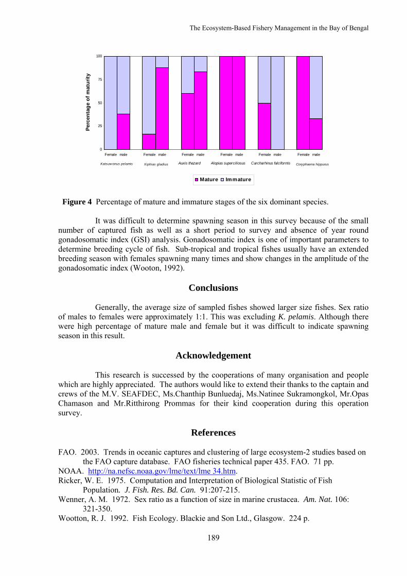
The Ecosystem-Based Fishery Management in the Bay of Bengal
189
0
25
50
75
100
Female male Female male Female male Female male Female male Female male
Perc
enta
ge o
f mat
urity
Mature Immature
Katsuwonus pelamis Xiphias gladius Auxis thazard Alopias superciliosus Carcharhinus falciformis Coryphaena hippurus
Figure 4 Percentage of mature and immature stages of the six dominant species. It was difficult to determine spawning season in this survey because of the small number of captured fish as well as a short period to survey and absence of year round gonadosomatic index (GSI) analysis. Gonadosomatic index is one of important parameters to determine breeding cycle of fish. Sub-tropical and tropical fishes usually have an extended breeding season with females spawning many times and show changes in the amplitude of the gonadosomatic index (Wooton, 1992).
Conclusions Generally, the average size of sampled fishes showed larger size fishes. Sex ratio of males to females were approximately 1:1. This was excluding K. pelamis. Although there were high percentage of mature male and female but it was difficult to indicate spawning season in this result.
Acknowledgement This research is successed by the cooperations of many organisation and people which are highly appreciated. The authors would like to extend their thanks to the captain and crews of the M.V. SEAFDEC, Ms.Chanthip Bunluedaj, Ms.Natinee Sukramongkol, Mr.Opas Chamason and Mr.Ritthirong Prommas for their kind cooperation during this operation survey.
References FAO. 2003. Trends in oceanic captures and clustering of large ecosystem-2 studies based on
the FAO capture database. FAO fisheries technical paper 435. FAO. 71 pp. NOAA. http://na.nefsc.noaa.gov/lme/text/lme 34.htm. Ricker, W. E. 1975. Computation and Interpretation of Biological Statistic of Fish
Population. J. Fish. Res. Bd. Can. 91:207-215. Wenner, A. M. 1972. Sex ratio as a function of size in marine crustacea. Am. Nat. 106:
321-350. Wootton, R. J. 1992. Fish Ecology. Blackie and Son Ltd., Glasgow. 224 p.
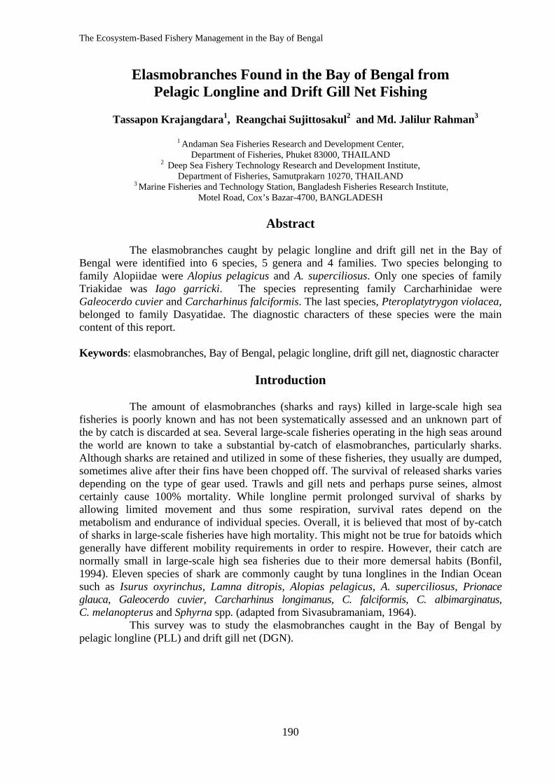
The Ecosystem-Based Fishery Management in the Bay of Bengal
190
Elasmobranches Found in the Bay of Bengal from Pelagic Longline and Drift Gill Net Fishing
Tassapon Krajangdara1, Reangchai Sujittosakul2 and Md. Jalilur Rahman3
1 Andaman Sea Fisheries Research and Development Center,
Department of Fisheries, Phuket 83000, THAILAND 2 Deep Sea Fishery Technology Research and Development Institute,
Department of Fisheries, Samutprakarn 10270, THAILAND 3 Marine Fisheries and Technology Station, Bangladesh Fisheries Research Institute,
Motel Road, Cox’s Bazar-4700, BANGLADESH
Abstract The elasmobranches caught by pelagic longline and drift gill net in the Bay of Bengal were identified into 6 species, 5 genera and 4 families. Two species belonging to family Alopiidae were Alopius pelagicus and A. superciliosus. Only one species of family Triakidae was Iago garricki. The species representing family Carcharhinidae were Galeocerdo cuvier and Carcharhinus falciformis. The last species, Pteroplatytrygon violacea, belonged to family Dasyatidae. The diagnostic characters of these species were the main content of this report. Keywords: elasmobranches, Bay of Bengal, pelagic longline, drift gill net, diagnostic character
Introduction The amount of elasmobranches (sharks and rays) killed in large-scale high sea fisheries is poorly known and has not been systematically assessed and an unknown part of the by catch is discarded at sea. Several large-scale fisheries operating in the high seas around the world are known to take a substantial by-catch of elasmobranches, particularly sharks. Although sharks are retained and utilized in some of these fisheries, they usually are dumped, sometimes alive after their fins have been chopped off. The survival of released sharks varies depending on the type of gear used. Trawls and gill nets and perhaps purse seines, almost certainly cause 100% mortality. While longline permit prolonged survival of sharks by allowing limited movement and thus some respiration, survival rates depend on the metabolism and endurance of individual species. Overall, it is believed that most of by-catch of sharks in large-scale fisheries have high mortality. This might not be true for batoids which generally have different mobility requirements in order to respire. However, their catch are normally small in large-scale high sea fisheries due to their more demersal habits (Bonfil, 1994). Eleven species of shark are commonly caught by tuna longlines in the Indian Ocean such as Isurus oxyrinchus, Lamna ditropis, Alopias pelagicus, A. superciliosus, Prionace glauca, Galeocerdo cuvier, Carcharhinus longimanus, C. falciformis, C. albimarginatus, C. melanopterus and Sphyrna spp. (adapted from Sivasubramaniam, 1964). This survey was to study the elasmobranches caught in the Bay of Bengal by pelagic longline (PLL) and drift gill net (DGN).
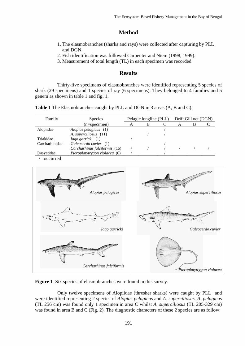
The Ecosystem-Based Fishery Management in the Bay of Bengal
191
Method
1. The elasmobranches (sharks and rays) were collected after capturing by PLL and DGN. 2. Fish identification was followed Carpenter and Niem (1998, 1999). 3. Measurement of total length (TL) in each specimen was recorded.
Results Thirty-five specimens of elasmobranches were identified representing 5 species of shark (29 specimens) and 1 species of ray (6 specimens). They belonged to 4 families and 5 genera as shown in table 1 and fig. 1. Table 1 The Elasmobranches caught by PLL and DGN in 3 areas (A, B and C).
Family Species Pelagic longline (PLL) Drift Gill net (DGN) (n=specimen) A B C A B C
Alopiidae Triakidae Carcharhinidae Dasyatidae
Alopias pelagicus (1) A. superciliosus (11) Iago garricki (1) Galeocerdo cuvier (1) Carcharhinus falciformis (15) Pteroplatytrygon violacea (6)
/ / /
/ /
/ / / / /
/
/
/
/ occurred
Figure 1 Six species of elasmobranches were found in this survey. Only twelve specimens of Alopiidae (thresher sharks) were caught by PLL and were identified representing 2 species of Alopias pelagicus and A. superciliosus. A. pelagicus (TL 256 cm) was found only 1 specimen in area C whilst A. superciliosus (TL 205-329 cm) was found in area B and C (Fig. 2). The diagnostic characters of these 2 species are as follow:
Alopias pelagicus Alopias superciliosus
Iago garricki Galeocerdo cuvier
Carcharhinus falciformisPteroplatytrygon violacea
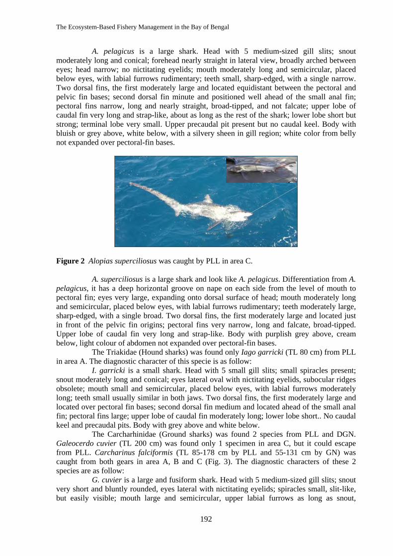
The Ecosystem-Based Fishery Management in the Bay of Bengal
192
A. pelagicus is a large shark. Head with 5 medium-sized gill slits; snout moderately long and conical; forehead nearly straight in lateral view, broadly arched between eyes; head narrow; no nictitating eyelids; mouth moderately long and semicircular, placed below eyes, with labial furrows rudimentary; teeth small, sharp-edged, with a single narrow. Two dorsal fins, the first moderately large and located equidistant between the pectoral and pelvic fin bases; second dorsal fin minute and positioned well ahead of the small anal fin; pectoral fins narrow, long and nearly straight, broad-tipped, and not falcate; upper lobe of caudal fin very long and strap-like, about as long as the rest of the shark; lower lobe short but strong; terminal lobe very small. Upper precaudal pit present but no caudal keel. Body with bluish or grey above, white below, with a silvery sheen in gill region; white color from belly not expanded over pectoral-fin bases.
Figure 2 Alopias superciliosus was caught by PLL in area C. A. superciliosus is a large shark and look like A. pelagicus. Differentiation from A. pelagicus, it has a deep horizontal groove on nape on each side from the level of mouth to pectoral fin; eyes very large, expanding onto dorsal surface of head; mouth moderately long and semicircular, placed below eyes, with labial furrows rudimentary; teeth moderately large, sharp-edged, with a single broad. Two dorsal fins, the first moderately large and located just in front of the pelvic fin origins; pectoral fins very narrow, long and falcate, broad-tipped. Upper lobe of caudal fin very long and strap-like. Body with purplish grey above, cream below, light colour of abdomen not expanded over pectoral-fin bases. The Triakidae (Hound sharks) was found only Iago garricki (TL 80 cm) from PLL in area A. The diagnostic character of this specie is as follow: I. garricki is a small shark. Head with 5 small gill slits; small spiracles present; snout moderately long and conical; eyes lateral oval with nictitating eyelids, subocular ridges obsolete; mouth small and semicircular, placed below eyes, with labial furrows moderately long; teeth small usually similar in both jaws. Two dorsal fins, the first moderately large and located over pectoral fin bases; second dorsal fin medium and located ahead of the small anal fin; pectoral fins large; upper lobe of caudal fin moderately long; lower lobe short.. No caudal keel and precaudal pits. Body with grey above and white below. The Carcharhinidae (Ground sharks) was found 2 species from PLL and DGN. Galeocerdo cuvier (TL 200 cm) was found only 1 specimen in area C, but it could escape from PLL. Carcharinus falciformis (TL 85-178 cm by PLL and 55-131 cm by GN) was caught from both gears in area A, B and C (Fig. 3). The diagnostic characters of these 2 species are as follow: G. cuvier is a large and fusiform shark. Head with 5 medium-sized gill slits; snout very short and bluntly rounded, eyes lateral with nictitating eyelids; spiracles small, slit-like, but easily visible; mouth large and semicircular, upper labial furrows as long as snout,
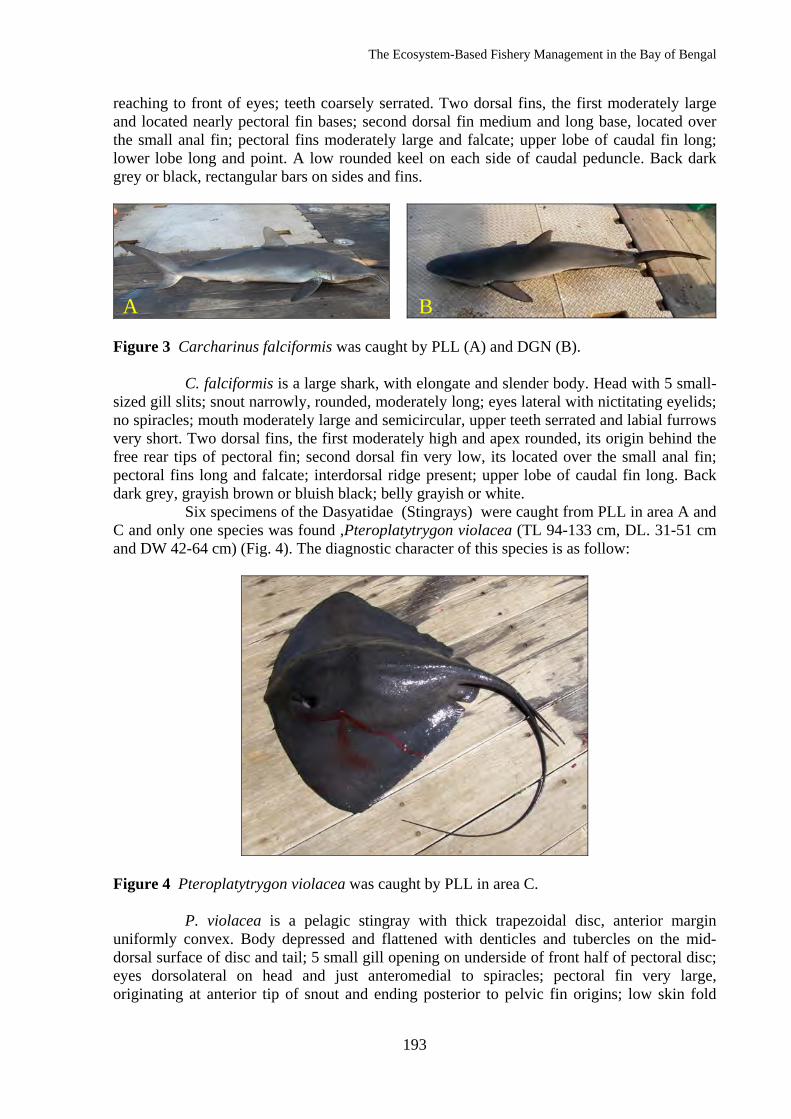
The Ecosystem-Based Fishery Management in the Bay of Bengal
193
reaching to front of eyes; teeth coarsely serrated. Two dorsal fins, the first moderately large and located nearly pectoral fin bases; second dorsal fin medium and long base, located over the small anal fin; pectoral fins moderately large and falcate; upper lobe of caudal fin long; lower lobe long and point. A low rounded keel on each side of caudal peduncle. Back dark grey or black, rectangular bars on sides and fins.
Figure 3 Carcharinus falciformis was caught by PLL (A) and DGN (B). C. falciformis is a large shark, with elongate and slender body. Head with 5 small-sized gill slits; snout narrowly, rounded, moderately long; eyes lateral with nictitating eyelids; no spiracles; mouth moderately large and semicircular, upper teeth serrated and labial furrows very short. Two dorsal fins, the first moderately high and apex rounded, its origin behind the free rear tips of pectoral fin; second dorsal fin very low, its located over the small anal fin; pectoral fins long and falcate; interdorsal ridge present; upper lobe of caudal fin long. Back dark grey, grayish brown or bluish black; belly grayish or white. Six specimens of the Dasyatidae (Stingrays) were caught from PLL in area A and C and only one species was found ,Pteroplatytrygon violacea (TL 94-133 cm, DL. 31-51 cm and DW 42-64 cm) (Fig. 4). The diagnostic character of this species is as follow:
Figure 4 Pteroplatytrygon violacea was caught by PLL in area C. P. violacea is a pelagic stingray with thick trapezoidal disc, anterior margin uniformly convex. Body depressed and flattened with denticles and tubercles on the mid-dorsal surface of disc and tail; 5 small gill opening on underside of front half of pectoral disc; eyes dorsolateral on head and just anteromedial to spiracles; pectoral fin very large, originating at anterior tip of snout and ending posterior to pelvic fin origins; low skin fold
A B
The Ecosystem-Based Fishery Management in the Bay of Bengal
194
present on undersurface of tail; whip-like tail longer than disc with large 2 stinging spine. Dark purple, black on both surfaces (ventral surface almost entirely dark).
Discussion and Conclusion The result of this survey appeared that only 6 species of elasmobranch were found. Most of them are epipelagic or mesopelagic fish. Catch of elasmobranches were not so many because the types of fishing gear used were selective fishing gear (PLL and GN).
References Bonfil, R. 1994. Overview of world elasmobranch fisheries. FAO Fisheries Technical Paper 341. FAO, Rome. 119 pp. Carpenter, K. E. and V. H. Niem. 1998. Sharks. In: FAO species identification guide for fishery purposes. The living marine resources of the Western Central Pacific. Vol.2.
FAO, Rome. p. 1193-1366. Carpenter, K. E. and V. H. Niem. 1999. Batoid fishes. In: FAO species identification guide
for fishery purposes. The living marine resources of the Western Central Pacific. Vol.3. FAO, Rome. p. 1397-1529.
Sivasubramaniam, K. 1964. Predation of tuna longline catches in the Indian Ocean, by killer whales and sharks. Bull. Fish. Res. Stn. Ceylon. 17(2):221-236.
The Ecosystem-Based Fishery Management in the Bay of Bengal
195
Age and Reproduction of Sthenoteuthis oualaniensis in the Bay of Bengal
Natinee Sukramongkol, Sayan Promjinda and Ritthirong Prommas
Southeast Asian Fisheries Development Center, Training Department, P.O.Box 97,
Phrasamutchedi, Samutprakarn 10290, THAILAND
Abstract
The specimens of Sthenoteuthis oualaniensis were caught by automatic squid jigging machines in the Bay of Bengal from 6 November to 7 December 2007. Fifteen fishing stations were conducted in three areas off Bangladesh waters, India and Sri Lanka waters, and Myanmar waters. Size distribution of S. oualaniensis ranged from 105 mm ML to 221 mm ML (169±30.8 mm ML in average and SD, n=32) for females and from 45 mm ML to 124 mm ML (104±28.2 mm ML in average and SD, n=7) for males, respectively. Statoliths from a total of 34 individuals (6 males, 28 females) of specimens (ML ranged from 45 to 221 mm) were used for the age estimation. Age of S. oualaniensis estimated from the counting of the statolith increments ranged from 63 days at 175 mm ML to 120 days at 199 mm ML for females and 40 days at 45 mm ML to 114 days at 124 mm ML for males, respectively. The mean age of females and males were 81.1 and 79.2 days old, respectively. The ML-BW relationships for S. oualaniensis was expressed as BW = 16.183ML4.1603 (r2 = 0.855, n = 32, 105-221 mm ML) and BW= 2.932ML1.4875 (r2 = 0.622, n = 7, 45-124 mm ML) for female and male, respectively. Based on the back calculation on the specimens collected from 6 to 30 November 2007, hatching date of the females S. oualaniensis was estimated to be from July to October 2007. There were different growth rates between sexes. Males those hatched in the same period with females grew with slower growth rates and captured in a smaller size than females.
Key words: Sthenoteuthis oualaniensis, age, reproduction, Bay of Bengal
Introduction
The purpleback flying squid Sthenoteuthis oualaniensis (family Ommastrephidae) is widely distributed in the tropical and subtropical areas of the Indo-Pacific and Indian Ocean (Nesis, 1977; Voss, 1973; Carpenter and Niem, 1998). The biomass of S. oualaniensis in the Indian Ocean was estimated to be about two million tons by the counting of the squid at the surface at night light stations (Zuev et al., 1985). Pinchukov (1989) and Zuev et al.(1985) had been reported the biomass of S. oualaniensis in the Indian Ocean was generally ranged from 50 to 75 kg per square km and high concentration from 4 to 42 ton per square km was mainly found in the Arabian Sea. The latest assessment of the total biomass of those squid throughout its range was about 8 to 11 million tons (Nigmatullin, 1990). Recent studies had been suggested that S. oualaniensis is probable under exploited resources and could sustain higher exploitation levels in the future (Dunning, 1998; Xinjun et al., 2007; Yatsu, 1997).
Since the statolith microstructure is useful for age determination of squids as otoliths in teleost fishes, the age and growth of S. oualaniensis are relying on the indirect validation studies, assuming the daily deposition of increments (Arkhipkin and Bizikov, 1991; Takagi et al., 2002). The squid was reported a short life span (1-1.5 years), high growth rates and complex population structure at least three main forms are distinguishable with and
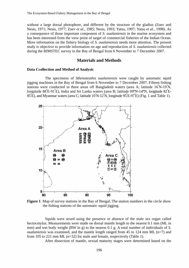
The Ecosystem-Based Fishery Management in the Bay of Bengal
196
without a large dorsal photophore, and different by the structure of the gladius (Zuev and Nesis, 1971; Nesis, 1977; Zuev et al., 1985; Nesis, 1993; Yatsu, 1997; Yatsu et al., 1998). As a consequence of those important component of S. oualaniensis in the marine ecosystem and has been interested from the view point of target of commercial fisheries of the Indian Ocean. More information on the fishery biology of S. oualaniensis needs more attention. The present study is objective to provide information on age and reproduction of S. oualaniensis collected during the BIMSTEC survey in the Bay of Bengal from 6 November to 7 December 2007.
Materials and Methods
Data Ccollection and Method of Analysis The specimens of Sthenoteuthis oualaniensis were caught by automatic squid
jigging machines in the Bay of Bengal from 6 November to 7 December 2007. Fifteen fishing stations were conducted in three areas off Bangladesh waters (area A; latitude 16ºN-19ºN, longitude 88ºE-91ºE), India and Sri Lanka waters (area B; latitude 09ºN-14ºN, longitude 82ºE-85ºE), and Myanmar waters (area C; latitude 10ºN-12ºN, longitude 95ºE-97ºE) (Fig. 1 and Table 1).
Figure 1 Map of survey stations in the Bay of Bengal. The station numbers in the circle show
the fishing stations of the automatic squid jigging.
Squids were sexed using the presence or absence of the male sex organ called hectocotylus. Measurements were made on dorsal mantle length to the nearest 0.1 mm (ML in mm) and wet body weight (BW in g) to the nearest 0.1 g. A total number of individuals of S. oualaniensis was examined, and the mantle length ranged from 45 to 124 mm ML (n=7) and from 105 to 221 mm ML (n=32) for male and female, respectively (Table 1).
After dissection of mantle, sexual maturity stages were determined based on the
Area A
Area CArea B
The Ecosystem-Based Fishery Management in the Bay of Bengal
197
definition of stages I to VI of Lipinski and Underhill (1995), stages I and II were defined as immature stage, stage III as maturing stage, stages IV and V as mature stage, and stage VI as spent in the present study. Statolith Handling and Ageing Technique
Paired statoliths were collected from specimens and stored in liquid paraffin until preparation following the method of Dawe and Natsukari (1991). The right statolith was used for counting increments. If the increment definition of the right statolith was poor, the left one was also examined. Anterior side of statolith was ground with 3M slim rubbing film sheet No. 4000-15000. Statolith increments were observed under an optical microscope (x400) (with digital camera attached). The image of increments were taken by digital camera and transferred to personal computer for counting on the number of growth increments. Counting of increments was made from the nucleus to the dorsal dome.
Statoliths from a total of 34 individuals (6 males, 28 females) of specimens (ML range from 45 to 221 mm) were readable and used for the age estimation. Size at Age and Ggrowth
Since the daily deposition of statolith increments had been validated in Ommastrephid squids (Todarodes pacificus, Illex argentinus, Ommastrephes bartramii, Sthenoteuthis oualaniensis, Dosidicus gigas), age in the present study was estimated relying on the assumption that the increments of S. oualaniensis statoliths were estimated as daily increment (Rodhouse and Hatfield, 1990; Arkhipkin and Bizikov, 1991; Jackson, 1994; Yatsu, 1997; Yatsu et al., 1998; Takagi et al., 2002).
Recently, the non-asymptotic growth models, included linear, exponential and power curves have been applied in many studies (I. lllecebrosus, Balch et al., 1988; S. oualaniensis, Arkhipkin and Bizikov, 1991; O. bartramii, Bower, 1996; D. gigas, Matsuda et al., 1998). In the present study, the linear regression was applied to the relationship between the estimated age (t in day) and mantle length (ML in mm) (Arkhipkin and Bizikov, 1991; Yatsu, 2000) as follows;
ML = MLo + at
Where MLo = 2.0 (since the smallest paralarvae of S. oualaniensis is 2.0 mm
in ML was collected during the survey); ML = Mantle length (in mm); t = estimated age (in day); a = least-squares linear regression coefficient.
The relationship between the mantle length (ML in mm) and total body weight (BW in g), expressed as BW = aMLb, were fitted by the least-squares linear regression of log transformed variables.
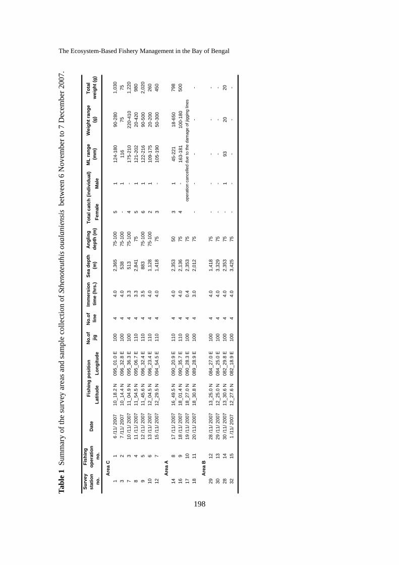
The Ecosystem-Based Fishery Management in the Bay of Bengal
198
Tabl
e 1
Sum
mar
y of
the
surv
ey a
reas
and
sam
ple
colle
ctio
n of
Sth
enot
euth
is o
uala
nien
sis
betw
een
6 N
ovem
ber t
o 7
Dec
embe
r 200
7.
Latit
ude
Long
itude
Fem
ale
Mal
e
11
6 /1
1/ 2
007
10_1
8.2
N09
5_01
.0 E
100
44.
02,
365
75-1
005
112
4-18
090
-280
1,03
03
27
/11/
200
710
_14.
4 N
096_
32.8
E10
04
4.0
538
75-1
00-
111
675
757
310
/11/
200
711
_04.
9 N
095_
36.3
E10
04
3.3
513
75-1
004
-17
5-21
022
0-41
01,
220
84
11 /1
1/ 2
007
11_5
4.5
N09
5_06
.7 E
110
43.
32,
841
755
112
1-20
220
-420
980
95
12 /1
1/ 2
007
11_4
5.6
N09
6_32
.4 E
110
43.
588
375
-100
61
122-
216
90-5
002,
020
106
13 /1
1/ 2
007
12_0
4.5
N09
6_23
.4 E
110
44.
01,
128
75-1
002
110
9-17
520
-200
260
127
15 /1
1/ 2
007
12_2
9.5
N09
4_54
.5 E
110
44.
01,
418
753
-10
5-19
050
-300
450
148
17 /1
1/ 2
007
16_4
9.5
N09
0_20
.9 E
110
44.
02,
353
503
145
-221
18-6
5079
816
918
/11/
200
718
_01.
4 N
090_
35.7
E11
04
4.0
2,13
675
4-
163-
181
100-
180
500
1710
19 /1
1/ 2
007
18_2
7.0
N09
0_28
.3 E
100
40.
42,
353
7518
1120
/11/
200
718
_30.
8 N
089_
28.9
E10
04
3.0
2,01
275
--
--
-
2912
28 /1
1/ 2
007
13_2
5.0
N08
4_27
.0 E
100
44.
01,
418
75-
--
--
3013
29 /1
1/ 2
007
12_2
5.0
N08
4_25
.0 E
100
44.
03,
329
75-
--
--
2814
30 /1
1/ 2
007
13_3
0.6
N08
2_29
.8 E
100
44.
02,
353
75-
193
2020
3215
1 /1
1/ 2
007
12_2
7.6
N08
2_18
.9 E
100
44.
03,
425
75-
--
--
Fish
ing
posi
tion
Surv
ey
stat
ion
no.
Fish
ing
oper
atio
n no
.D
ate
No.
of
jigN
o.of
lin
eIm
mer
sion
tim
e (h
rs.)
Sea
dept
h (m
)A
nglin
g de
pth
(m)
Tota
l w
eigh
t (g)
ML
rang
e (m
m)
Tota
l cat
ch (i
ndiv
idua
l)W
eigh
t ran
ge
(g)
oper
atio
n ca
ncel
led
due
to th
e da
mag
e of
jigg
ing
lines
Are
a C
Are
a A
Are
a B
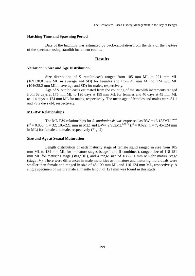
The Ecosystem-Based Fishery Management in the Bay of Bengal
199
Hatching Time and Spawning Period Date of the hatching was estimated by back-calculation from the data of the capture
of the specimen using statolith increment counts.
Results
Variation in Size and Age Distribution
Size distribution of S. oualaniensis ranged from 105 mm ML to 221 mm ML (169±30.8 mm ML in average and SD) for females and from 45 mm ML to 124 mm ML (104±28.2 mm ML in average and SD) for males, respectively.
Age of S. oualaniensis estimated from the counting of the statolith increments ranged from 63 days at 175 mm ML to 120 days at 199 mm ML for females and 40 days at 45 mm ML to 114 days at 124 mm ML for males, respectively. The mean age of females and males were 81.1 and 79.2 days old, respectively. ML-BW Relationships
The ML-BW relationships for S. oualaniensis was expressed as BW = 16.183ML4.1603 (r2 = 0.855, n = 32, 105-221 mm in ML) and BW= 2.932ML1.4875 (r2 = 0.622, n = 7, 45-124 mm in ML) for female and male, respectively (Fig. 2). Size and Age at Sexual Maturation
Length distribution of each maturity stage of female squid ranged in size from 105 mm ML to 134 mm ML for immature stages (stage I and II combined), ranged size of 118-181 mm ML for maturing stage (stage III), and a range size of 168-221 mm ML for mature stage (stage IV). There were differences in male maturities as immature and maturing individuals were smaller than female and ranged in size of 45-109 mm ML and 116-124 mm ML, respectively. A single specimen of mature male at mantle length of 121 mm was found in this study.
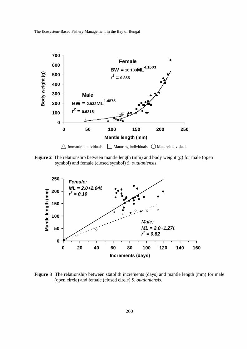
The Ecosystem-Based Fishery Management in the Bay of Bengal
200
Figure 2 The relationship between mantle length (mm) and body weight (g) for male (open
symbol) and female (closed symbol) S. oualaniensis. Figure 3 The relationship between statolith increments (days) and mantle length (mm) for male
(open circle) and female (closed circle) S. oualaniensis.
FemaleBW = 16.183ML4.1603
r2 = 0.855
MaleBW = 2.932ML1.4875
r2 = 0.6215
0
100
200
300
400
500
600
700
0 50 100 150 200 250
Mantle length (mm)
Bod
y w
eigh
t (g)
Maturing individuals Mature individuals Immature individuals
0
50
100
150
200
250
0 20 40 60 80 100 120 140 160Increments (days)
Man
tle le
ngth
(mm
)
Female; ML = 2.0+2.04t r2 = 0.10
Male; ML = 2.0+1.27t r2 = 0.82
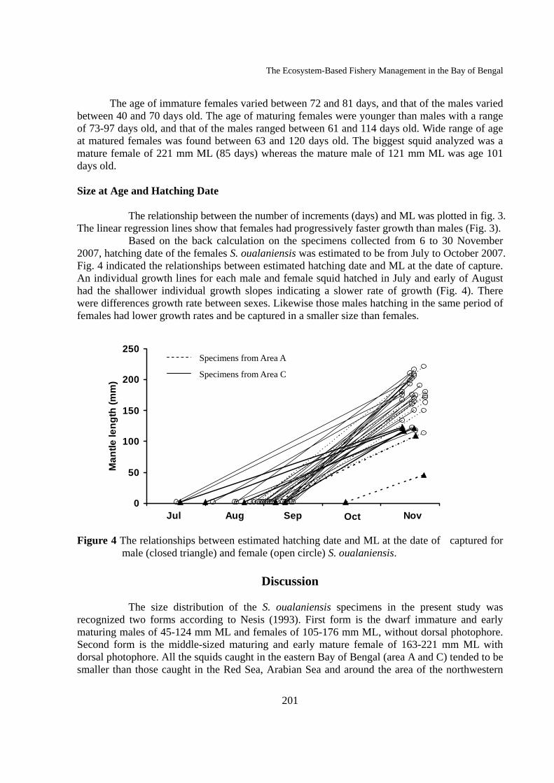
The Ecosystem-Based Fishery Management in the Bay of Bengal
201
The age of immature females varied between 72 and 81 days, and that of the males varied between 40 and 70 days old. The age of maturing females were younger than males with a range of 73-97 days old, and that of the males ranged between 61 and 114 days old. Wide range of age at matured females was found between 63 and 120 days old. The biggest squid analyzed was a mature female of 221 mm ML (85 days) whereas the mature male of 121 mm ML was age 101 days old. Size at Age and Hatching Date
The relationship between the number of increments (days) and ML was plotted in fig. 3. The linear regression lines show that females had progressively faster growth than males (Fig. 3).
Based on the back calculation on the specimens collected from 6 to 30 November 2007, hatching date of the females S. oualaniensis was estimated to be from July to October 2007. Fig. 4 indicated the relationships between estimated hatching date and ML at the date of capture. An individual growth lines for each male and female squid hatched in July and early of August had the shallower individual growth slopes indicating a slower rate of growth (Fig. 4). There were differences growth rate between sexes. Likewise those males hatching in the same period of females had lower growth rates and be captured in a smaller size than females.
Figure 4 The relationships between estimated hatching date and ML at the date of captured for
male (closed triangle) and female (open circle) S. oualaniensis.
Discussion
The size distribution of the S. oualaniensis specimens in the present study was recognized two forms according to Nesis (1993). First form is the dwarf immature and early maturing males of 45-124 mm ML and females of 105-176 mm ML, without dorsal photophore. Second form is the middle-sized maturing and early mature female of 163-221 mm ML with dorsal photophore. All the squids caught in the eastern Bay of Bengal (area A and C) tended to be smaller than those caught in the Red Sea, Arabian Sea and around the area of the northwestern
0
50
100
150
200
250
Man
tle le
ngth
(mm
)
Jul Aug Sep Oct Nov
Specimens from Area C
Specimens from Area A
The Ecosystem-Based Fishery Management in the Bay of Bengal
202
Indian Ocean (Nesis, 1977b, 1985, 1993; Yatsu, 1997; Xinjun et al., 2007). The S. oualaniensis specimens contain form 1 (Nesis, 1993) was also reported in the Andaman Sea of Thailand by Nateewathana (1997). These specimens were lack of dorsal photophores, but the females were much longer than 120 mm ML (the biggest specimen, PMBC no.11795, 323 mm ML; Nateewathana, 1997). The size distribution of S. oualaniensis in the present study is consistent with the previous results from the former USSR research in summer of the West Indian Ocean. The ML was mainly in the range of 90-180 mm ML, and 80-270 mm ML, and in the winter mainly ranged from 90 mm to 180 mm ML (Trotsenko and Pinchukov, 1994). The size ranged from 74 mm to 321 mm ML with the dominant group in the range of 110-250 mm ML was also reported as by-catch in the Chinese trawling boats (Yang, 2002).
The complex population of S. oualaniensis had been described three major and two minor forms by Nesis (1993). Those characters were important and attempt was made many times to describe as a separated species (Clarke, 1965 and Wormuth, 1976). The dwarf form was also suggested to be a separate species that could only be identified as an adult (Xinjun et al., 2007). Snyder (1998) suggested that the giant form resulted from a plastic phenotype in the species. A new study based on RADP DNA (Random Amplified Polymorphic DNA) analysis is being done in Marine Science and Technology of Shanghai Fisheries University, and preliminary findings suggest a large variation in biology among the groups (Xinjun et al., 2007).
The development of dorsal photophore and the structure of the hectocotylus were suggested to be affected by the combination of growth and maturation (Nesis, 1977b). The photophore is being to develop when squid reaches a ML of approximately 10 cm, but if maturation does not begin, the photophore development will be blocked. However, this hypothesis was cited but not verified (Nesis, 1993).
Many studies indicate that S. oualaniensis had its life span less than 1 year (Nesis, 1993; Dong, 1991; Trotsenko and Pinchukov, 1994). However, the result from age determination based on daily increments of statoliths which samplings were different both in locations and time. Yatsu (2000) determined growth curves for both sexes and reported a female of 120 mm ML at 51 days old which contrast to the data of Zaidi bin Zakaria (2000), which places a 115 mm ML female at an age of 95 days. This may suggests that environmental conditions such as temperature and food availability are the main factors influencing to growth rates, lifespan and fluctuations of relative gonad investment. Lastly the process to count the daily increment might suggest a bit different output since there has no verification from several counters in the same specimens.
S. oualaniensis has been subjected to commercial exploitation in the northwestern Indian Ocean by the Chinese squid jigging boats (Xinjun et al., 2007). The species also commercially fished off Okinawa, Taiwan and Hawaii as a tuna bait and human consumption (Okutani and Tung, 1978). Although this species is abundant in the South China Sea region but the fishery has never succeeded. It is low value for human consumption relatively to other squids and due to its toughness. A wide ecological amplitude character, complex intraspecific structure, high fecundity, short life cycle, high growth rate and significant production (Zuev and Nesis, 1971; Nesis, 1977; Zuev et al., 1985; Xinjun et al., 2007) make this species an interesting for further study on life history. However, the prior needs to the development of a commercial fishery for this species in the survey area especially in the eastern Bay of Bengal, are more data collection and information on distribution and fishery biology. At present this species has not been yet exploited in the Andaman Sea of Thailand.
The Ecosystem-Based Fishery Management in the Bay of Bengal
203
Acknowledgements
The authors wish to acknowledge the cooperation between the BIMSTEC member countries, Department of Fisheries of Thailand, and SEAFDEC/TD. We would also like to thanks to the officers and crews of the M.V. SEAFDEC for their help during the surveys.
References
Arkhipkin, A. I. and V. A. Bizikov. 1991. Comparative analysis of age and growth rates
estimation using statoliths and gladius in squids. In: Squid Age Determination Using
Statoliths, Proceedings of the International Workshop held in the Istituto di Technologia
della Pesca e del Pescato (ITPP–CNR). 1989. Mazara del Vallo, Italy. p. 19-37.
Balch, N., A. Sirois and G. V. Hurley. 1988. Growth increments in statoliths from paralarvae of
the Ommastrephid squid, Illex argentinu (Cephalopoda: Teuthoidae). Malacologia
29(1):103-112.
Bower, J. R. 1996. Estimated paralarval drift and inferred hatching sites for Ommastrephes
bartramii (Cephalopoda: Ommastrephidae) near the Hawaiian Archipelago. Fish. Bull.
94(3):398-411.
Carpenter, K. E. and V. H. Niem. (eds.). 1998. FAO species identification guide for fishery
purposes. The living marine resources of the Western Central Pacific, vol. 2,
Cephalopods, crustacean, holothurians and sharks. FAO Publication, Rome. p. 764-780.
Clarke, M. R. 1965. Large light organs on the dorsal surface of the squids Ommastrephes
pteropus, Symplectoteuthis oualaniensis and Dosidicus gigas. Proc.Malacol.Soc.
London. 36(5):319-321.
Dawe, E. and Y. Natsukari. 1991. Practical procedures of squid ageing using statoliths (Light
microscopy). In: Jereb, P., S. Ragonese and S. V. Boletzky. (eds.). Squid Ageing
Determination using Statoliths. NTR-ITPP Spec. Publ. Mazarra del Vallo. 1:83-95.
Dong, Z. Z. 1991. The Biology of Oceanic Economic Cephalopod in the World. Shangdong
Science Press, Jinan. p. 17-19. (in Chinese)
Dunning, M. C. 1998. A review of the systematic, distribution and biology of arrow squids of
the genus Nototodarus (Cephalopoda: Ommastrephidae). In: Voss, N.A., M. Vecchione,
R. B. Toll and M. J. Sweeney. (eds.). Systematics and Biogeography of Cephalopods.
Vol. 2 Smithsonian Institution Press, Washington D.C. p. 393-404.
The Ecosystem-Based Fishery Management in the Bay of Bengal
204
Lipinski, M. R. and L. G Underhill. 1995. Sexual maturation in squid: quantum or continuum.
S. Afr. J. Mar. Sci. 15:207-223.
Masuda, A., K. Yokawa, A. Yatsu and S. Kawahara. 1998. Growth and population structure of
Dosidicus gigas in the Southeastern Pacific In: Okutani, T. (ed.). Large Pelagic Squids.
Japan Marine Fishery Resources and Research Center, Tokyo, Japan.
p. 107-118.
Nateewathana, A. 1997. Two species of oceanic squids from the Andaman Sea Indian Ocean.
Phuket. Mar. Biol. Cent. Res. Bull. 17(1):453-464.
Nigmatullin, Ch. M. 1990. Resources and perspectives of the fisheries of nektonic epipelagic
squids in the World Ocean. Abstr. Commun. All-USSR Conf. on reserve food biological
resources of the open ocean and the USSR seas, Kaliningrad, March, 1990. Moscow. p.
11-13. (in Russian, English abstract).
Nesis, K. N. 1977. Population structure in the squid Sthenoteuthis oualaniensis (Lesson 1930)
(Ommastrephidae) in the Western tropical Pacific. In: Proceeding of the academy of
Science USSR, Shirsch Inst. Oceanol. 107:15-29.
Nesis, K. N. 1985. Oceanic cephalopods: Distribution, life forms, evolution. Moscow. Nauka.
287 pp. (in Russian, English abstract).
Nesis, K. N. 1993. Population structure of oceanic ommastrephids with particular reference to
Sthenoteuthis oualaniensis. In: Okutani, T., R. K. O'Dor and T. Kubodera. (eds.).
Recent Advances in Cephalopod Fisheries Biology. Tokai University. Press, Tokyo. p.
375-383.
NMFS. 2005. Final Environmental Impact Statement; Seabird Interaction Avoidance Methods
and Pelagic Squid Fishery Management. National Oceanic and Atmospheric
Administration. National Marine Fisheries Service. Pacific Islands Regional Office.
557 pp.
Okutani, T. and I. H. Tung. 1978. Review of biology of commercially important squids in
Japanese and adjacent waters. Symplectoteuthis oualaniensis (lesson). Veliger.
21(1):87-95.
Pinchukov, M. A. 1989. Oceanic Squids. In: Parin, N. V. and N. P. Novikov. (eds.). Biological
Resources of the Indian Ocean. Nauka. Moscow. p. 186-194. (in Russian, English abstract)
Rodhouse, P.G. and E. M. C. Hatfield. 1990. Age determination in squid using statolith growth
The Ecosystem-Based Fishery Management in the Bay of Bengal
205
increments. Fish. Res. 8:323-334.
Snyder, R. 1998. Aspects of the biology of the giant form of Sthenoteuthis oualaniensis
(Cephalopoda: Ommastrephidae) from the Arabian Sea. J. Mollus. Stud. 64:21-34.
Takagi, K., T. Kitahara, N. Suzuki, J. Mori and A.Yatsu. 2002. The age and growth of
Sthenoteuthis oualaniensis (Cephalopoda: Ommastrephidae) in the Pacific Ocean. Bull.
Mar. Sci. 71(2):1105-1108.
Trosenko, B. G., and M.A. Pinchukov. 1994. Mesoscale distribution features of the purpleback
flying squid Sthenoteuthis oualaniensis with reference to the structure of the upper quasi-
homogenous layer in the West India Ocean. Oceanol. 34(3):380-385.
Wormuth, J. H. 1976. The biogeography and numerical taxonomy of the Oegopsid squid family
Ommastrephidae in the Pacific Ocean. Bull. Scripps Inst. Oceanologr. 23:1-89.
Xinjun, C., L. Bilin, T. Siquan, Q. Weiguo and Z. Xiaohu. 2007. Fishery biology of purpleback
squid, Sthenoteuthis oualaniensis, in the northwest Indian Ocean. Fish. Res. 83:98-104.
Yang, D. K. 2002. The resources and it exploitation and utilization of two species of squid. J.
Shanghai Fisheries Univ. 11(2):176-179. (in Chinese, English abstract)
Yatsu, A. 1997. The biology of Sthenoteuthis oualaniensis and exploitation of the new squid
resources. Bull. Far-Sea Fishery 10:6-9 (in Japanese, English abstract).
Yatsu, A., F. Katto, F. Kakizoe, K. Yamanaka and K. Mizuno. 1998. Distribution and biology of
Sthenoteuthis oualaniensis in the Indian Ocean-preliminary results from the research
cruise of the R/V Shoyo-Maru in 1995. In: Okutani, T., R. K. O’Dor and T. Kubodera.
(eds.). Recent Advances in Cephalopod Fisheries Biology. Tokai University Press,
Tokyo. p. 145-153.
Yatsu, A. 2000. Age estimation of four oceanic squids, Ommastrephid bartramii, Dosidicus
gigas, Sthenoteuthis oualaniensis and Illex argentinus (Cephalopoda: Ommastrephidae)
based on statolith microstructure. Japan Int’. Res. Cent. Agr. Sci. 34(1):75-80.
Zuev, G. V. and K. N. Nesis. 1971. Kal’mary (Biologiya I Promysel) (squids [Biology and
Fishery]). Pishchevaya Promyshlennost, Moscow. 360 pp.
Zuev, G. V., Ch. M. Nigmatullin and V. N. Nikol’skii. 1985. Nektonnye Okeanicheskie kal’mary
(Nectonic Oceanic Squids). Agropromizdat, Moscow. 224 pp.
Zuev, G. V., C. Nigmatullin, M. Chesalin and K. N. Nesis. 2002. Main results of long-term worldwide studies on tropical nektonic oceanic squid genus Sthenoteuthis: an overview of the Soviet investigations. Bull. Mar. Sci. 71(2):1019-1060.

The Ecosystem-Based Fishery Management in the Bay of Bengal
206
Stomach Content of the Large Pelagic Fishes in the Bay of Bengal
Montri Sumontha1, Praulai Nootmorn1, Pornanan Keereerut1,
Rangkiri P.P. Krishantha Jayasinghe.2, Nalla Jagannath3 and Manas Kumar Sinha4
1 Andaman Sea Fisheries Research and Development Center,
Department of Fisheries, Phuket 83000, THAILAND 2 National Aquatic Resource Research and Development Agency,
Crow Island, Colombo 15, SRI LANKA 3 Office of the Zonal Director, Visakhapatnam Base of Fishery Survey of India,
Fishing Harbor, Beach Road, Vusakhapatnam-530001, INDIA 4 Port Blair Base of Fishery Survey of India, P.O.Box 46, Phoenix Bay, Port Blair, INDIA
Abstract
Investigation of stomach contents of apex predator; frigate tuna (Auxis thazard),
skipjack tuna (Kasuwonus pelamis), yellowfin tuna (Thunnus albacares), bigeye (Thunnus obesus) and swordfish (Xiphias gladius) were undertaken during November to December 2007. These fishes were caught in the Bay of Bengal with pelagic longline and drift gillnet from the survey cruise by MV. SEAFDEC.
Thirty five percent of 68 stomach samples of tuna and tuna-like species were found diet. The diet content were reported cephalopod (60.70% by weight and 44.83% by number), fish (38.85% by weight, 5.75% by number), and parasite (0.45% by weight, 49.42% by number). Prey fish composed of 3 families; Ostraciidae, Bramidae and Diretmidae, and 1 unidentified fish. Cephalopod was represented by Teuthoidea and Histioteuthis celetaria pacifica, Octopoda. Parasite was reported Nematode (black and white) and Digenea. Diet data were compared between surface and deep swimmer predators, the result showed higher the number of prey fish and parasite from deep swimmers (4.79 prey fish and 5.07 parasite per stomach) than that from surface swimmers (1.62 prey fish and 1.15 parasite per stomach).
Community of predator, prey and parasite was categorized into 3 assemblages upon species of such components and habitat (depth of water) of those species. It was found significant differences between groups. Groups B and C had the highest total number of taxon whilst the highest average number of parasite was found in group B, followed by groups C and A.
The preliminary structure of tuna trophic ecology in the Bay of Bengal was explained from the result of the present study. Future development on commercial deep-water fisheries and the taxonomy and field guide of deep-sea fishes and cephalopod beak have been suggested for the study in the Bay of Bengal.
Introduction
The predator-prey interactions play an important part in the structure and the
dynamics of multispecies communities. Facing the dramatic increase of the catches of tuna and related species in the Indian Ocean, especially the eastern Indian Ocean, it becomes necessary to assess the impact of the fisheries on the pelagic ecosystems. The implement of research activities leading to a better knowledge of trophic ecology of apex predators will provide such an ecosystem point of view that has to be considered nowadays in the high seas fisheries management.
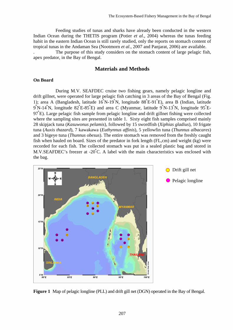
The Ecosystem-Based Fishery Management in the Bay of Bengal
207
Feeding studies of tunas and sharks have already been conducted in the western Indian Ocean during the THETIS program (Potier et al., 2004) whereas the tunas feeding habit in the eastern Indian Ocean is still rarely studied, only the reports on stomach content of tropical tunas in the Andaman Sea (Nootmorn et al., 2007 and Panjarat, 2006) are available. . The purpose of this study considers on the stomach content of large pelagic fish, apex predator, in the Bay of Bengal.
Materials and Methods On Board
During M.V. SEAFDEC cruise two fishing gears, namely pelagic longline and drift gillnet, were operated for large pelagic fish catching in 3 areas of the Bay of Bengal (Fig. 1); area A (Bangladesh, latitude 16°N-19°N, longitude 88°E-91°E), area B (Indian, latitude 9°N-14°N, longitude 82°E-85°E) and area C (Myanmar, latitude 9°N-13°N, longitude 95°E-97°E). Large pelagic fish sample from pelagic longline and drift gillnet fishing were collected where the sampling sites are presented in table 1. Sixty eight fish samples comprised mainly 28 skipjack tuna (Kasuwonus pelamis), followed by 15 swordfish (Xiphias gladius), 10 frigate tuna (Auxis thazard), 7 kawakawa (Euthynnus affinis), 5 yellowfin tuna (Thunnus albacares) and 3 bigeye tuna (Thunnus obesus). The entire stomach was removed from the freshly caught fish when hauled on board. Sizes of the predator in fork length (FL,cm) and weight (kg) were recorded for each fish. The collected stomach was put in a sealed plastic bag and stored in M.V.SEAFDEC’s freezer at -20°C. A label with the main characteristics was enclosed with the bag.
Figure 1 Map of pelagic longline (PLL) and drift gill net (DGN) operated in the Bay of Bengal.
Drift gill net Pelagic longline
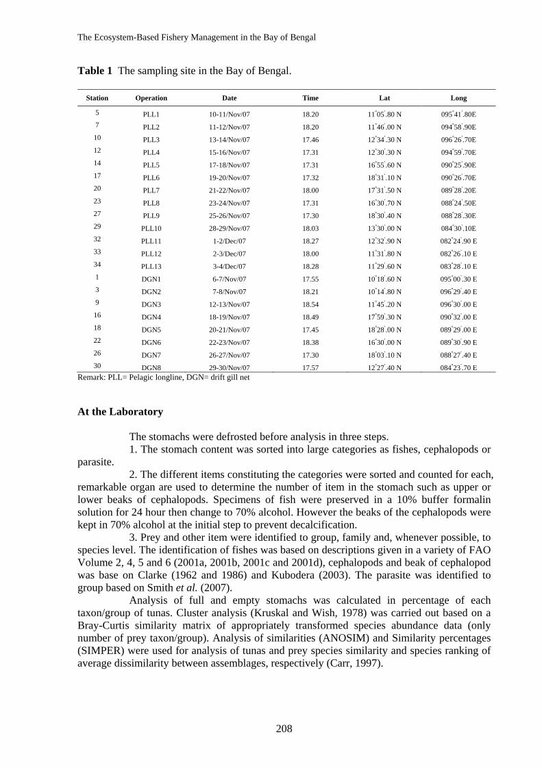
The Ecosystem-Based Fishery Management in the Bay of Bengal
208
Table 1 The sampling site in the Bay of Bengal.
Station Operation Date Time Lat Long
5 PLL1 10-11/Nov/07 18.20 11°05'.80 N 095°41'.80E 7 PLL2 11-12/Nov/07 18.20 11°46'.00 N 094°58'.90E 10 PLL3 13-14/Nov/07 17.46 12°34'.30 N 096°26'.70E 12 PLL4 15-16/Nov/07 17.31 12°30'.30 N 094°59'.70E 14 PLL5 17-18/Nov/07 17.31 16°55'.60 N 090°25'.90E 17 PLL6 19-20/Nov/07 17.32 18°31'.10 N 090°26'.70E 20 PLL7 21-22/Nov/07 18.00 17°31'.50 N 089°28'.20E 23 PLL8 23-24/Nov/07 17.31 16°30'.70 N 088°24'.50E 27 PLL9 25-26/Nov/07 17.30 18°30'.40 N 088°28'.30E 29 PLL10 28-29/Nov/07 18.03 13°30'.00 N 084°30'.10E 32 PLL11 1-2/Dec/07 18.27 12°32'.90 N 082°24'.90 E 33 PLL12 2-3/Dec/07 18.00 11°31'.80 N 082°26'.10 E 34 PLL13 3-4/Dec/07 18.28 11°29'.60 N 083°28'.10 E 1 DGN1 6-7/Nov/07 17.55 10°18'.60 N 095°00'.30 E 3 DGN2 7-8/Nov/07 18.21 10°14'.80 N 096°29'.40 E 9 DGN3 12-13/Nov/07 18.54 11°45'.20 N 096°30'.00 E 16 DGN4 18-19/Nov/07 18.49 17°59'.30 N 090°32'.00 E 18 DGN5 20-21/Nov/07 17.45 18°28'.00 N 089°29'.00 E 22 DGN6 22-23/Nov/07 18.38 16°30'.00 N 089°30'.90 E 26 DGN7 26-27/Nov/07 17.30 18°03'.10 N 088°27'.40 E 30 DGN8 29-30/Nov/07 17.57 12°27'.40 N 084°23'.70 E
Remark: PLL= Pelagic longline, DGN= drift gill net At the Laboratory
The stomachs were defrosted before analysis in three steps. 1. The stomach content was sorted into large categories as fishes, cephalopods or
parasite. 2. The different items constituting the categories were sorted and counted for each,
remarkable organ are used to determine the number of item in the stomach such as upper or lower beaks of cephalopods. Specimens of fish were preserved in a 10% buffer formalin solution for 24 hour then change to 70% alcohol. However the beaks of the cephalopods were kept in 70% alcohol at the initial step to prevent decalcification.
3. Prey and other item were identified to group, family and, whenever possible, to species level. The identification of fishes was based on descriptions given in a variety of FAO Volume 2, 4, 5 and 6 (2001a, 2001b, 2001c and 2001d), cephalopods and beak of cephalopod was base on Clarke (1962 and 1986) and Kubodera (2003). The parasite was identified to group based on Smith et al. (2007).
Analysis of full and empty stomachs was calculated in percentage of each taxon/group of tunas. Cluster analysis (Kruskal and Wish, 1978) was carried out based on a Bray-Curtis similarity matrix of appropriately transformed species abundance data (only number of prey taxon/group). Analysis of similarities (ANOSIM) and Similarity percentages (SIMPER) were used for analysis of tunas and prey species similarity and species ranking of average dissimilarity between assemblages, respectively (Carr, 1997).
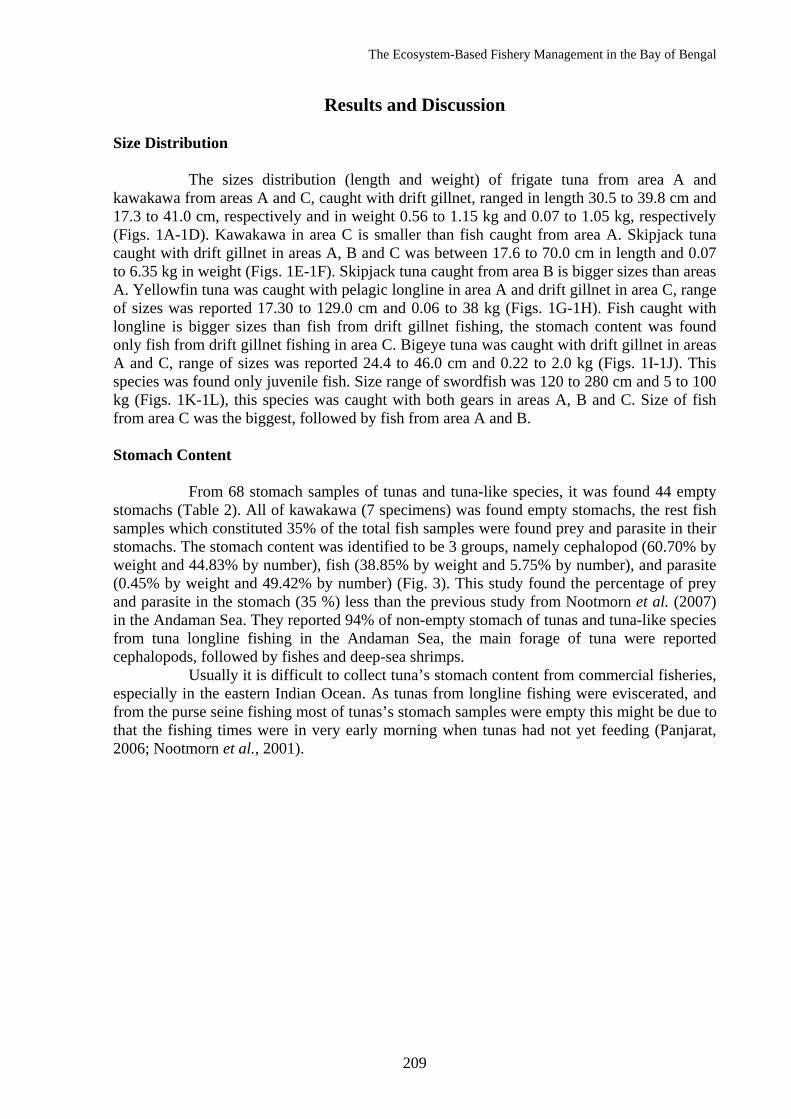
The Ecosystem-Based Fishery Management in the Bay of Bengal
209
Results and Discussion Size Distribution
The sizes distribution (length and weight) of frigate tuna from area A and kawakawa from areas A and C, caught with drift gillnet, ranged in length 30.5 to 39.8 cm and 17.3 to 41.0 cm, respectively and in weight 0.56 to 1.15 kg and 0.07 to 1.05 kg, respectively (Figs. 1A-1D). Kawakawa in area C is smaller than fish caught from area A. Skipjack tuna caught with drift gillnet in areas A, B and C was between 17.6 to 70.0 cm in length and 0.07 to 6.35 kg in weight (Figs. 1E-1F). Skipjack tuna caught from area B is bigger sizes than areas A. Yellowfin tuna was caught with pelagic longline in area A and drift gillnet in area C, range of sizes was reported 17.30 to 129.0 cm and 0.06 to 38 kg (Figs. 1G-1H). Fish caught with longline is bigger sizes than fish from drift gillnet fishing, the stomach content was found only fish from drift gillnet fishing in area C. Bigeye tuna was caught with drift gillnet in areas A and C, range of sizes was reported 24.4 to 46.0 cm and 0.22 to 2.0 kg (Figs. 1I-1J). This species was found only juvenile fish. Size range of swordfish was 120 to 280 cm and 5 to 100 kg (Figs. 1K-1L), this species was caught with both gears in areas A, B and C. Size of fish from area C was the biggest, followed by fish from area A and B. Stomach Content
From 68 stomach samples of tunas and tuna-like species, it was found 44 empty stomachs (Table 2). All of kawakawa (7 specimens) was found empty stomachs, the rest fish samples which constituted 35% of the total fish samples were found prey and parasite in their stomachs. The stomach content was identified to be 3 groups, namely cephalopod (60.70% by weight and 44.83% by number), fish (38.85% by weight and 5.75% by number), and parasite (0.45% by weight and 49.42% by number) (Fig. 3). This study found the percentage of prey and parasite in the stomach (35 %) less than the previous study from Nootmorn et al. (2007) in the Andaman Sea. They reported 94% of non-empty stomach of tunas and tuna-like species from tuna longline fishing in the Andaman Sea, the main forage of tuna were reported cephalopods, followed by fishes and deep-sea shrimps.
Usually it is difficult to collect tuna’s stomach content from commercial fisheries, especially in the eastern Indian Ocean. As tunas from longline fishing were eviscerated, and from the purse seine fishing most of tunas’s stomach samples were empty this might be due to that the fishing times were in very early morning when tunas had not yet feeding (Panjarat, 2006; Nootmorn et al., 2001).
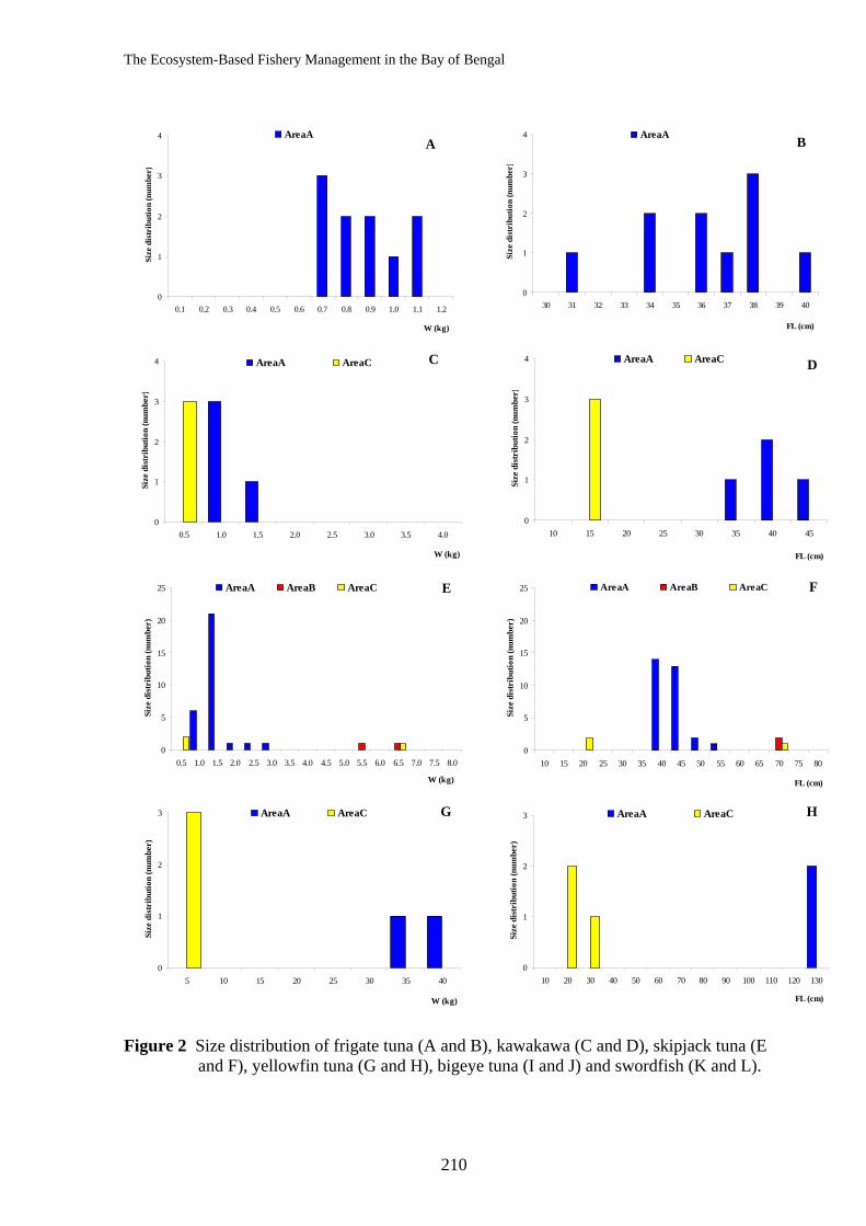
The Ecosystem-Based Fishery Management in the Bay of Bengal
210
0
1
2
3
4
0.1 0.2 0.3 0.4 0.5 0.6 0.7 0.8 0.9 1.0 1.1 1.2
W (kg)
Size
dis
trib
utio
n (n
umbe
r)AreaA
A
0
1
2
3
4
30 31 32 33 34 35 36 37 38 39 40
FL (cm)
Size
dis
trib
utio
n (n
umbe
r)
AreaA B
0
1
2
3
4
0.5 1.0 1.5 2.0 2.5 3.0 3.5 4.0
W (kg)
Size
dis
trib
utio
n (n
umbe
r)
AreaA AreaC C
0
1
2
3
4
10 15 20 25 30 35 40 45
FL (cm)
Size
dis
trib
utio
n (n
umbe
r)
AreaA AreaC D
0
5
10
15
20
25
0.5 1.0 1.5 2.0 2.5 3.0 3.5 4.0 4.5 5.0 5.5 6.0 6.5 7.0 7.5 8.0
W (kg)
Size
dis
trib
utio
n (n
umbe
r)
AreaA AreaB AreaC E
0
5
10
15
20
25
10 15 20 25 30 35 40 45 50 55 60 65 70 75 80
FL (cm)
Size
dis
trib
utio
n (n
umbe
r)
AreaA AreaB AreaC F
0
1
2
3
5 10 15 20 25 30 35 40
W (kg)
Size
dis
trib
utio
n (n
umbe
r)
AreaA AreaC G
0
1
2
3
10 20 30 40 50 60 70 80 90 100 110 120 130
FL (cm)
Size
dis
trib
utio
n (n
umbe
r)
AreaA AreaC H
Figure 2 Size distribution of frigate tuna (A and B), kawakawa (C and D), skipjack tuna (E and F), yellowfin tuna (G and H), bigeye tuna (I and J) and swordfish (K and L).
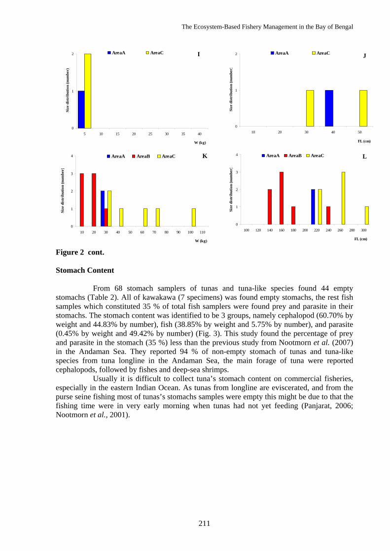
The Ecosystem-Based Fishery Management in the Bay of Bengal
211
0
1
2
5 10 15 20 25 30 35 40
W (kg)
Size
dis
trib
utio
n (n
umbe
r)
AreaA AreaC I
0
1
2
10 20 30 40 50
FL (cm)
Size
dis
trib
utio
n (n
umbe
r)
AreaA AreaC J
0
1
2
3
4
10 20 30 40 50 60 70 80 90 100 110
W (kg)
Size
dis
trib
utio
n (n
umbe
r)
AreaA AreaB AreaC K
0
1
2
3
4
100 120 140 160 180 200 220 240 260 280 300
FL (cm)
Size
dis
trib
utio
n (n
umbe
r)
AreaA AreaB AreaC L
Figure 2 cont. Stomach Content
From 68 stomach samplers of tunas and tuna-like species found 44 empty stomachs (Table 2). All of kawakawa (7 specimens) was found empty stomachs, the rest fish samples which constituted 35 % of total fish samplers were found prey and parasite in their stomachs. The stomach content was identified to be 3 groups, namely cephalopod (60.70% by weight and 44.83% by number), fish (38.85% by weight and 5.75% by number), and parasite (0.45% by weight and 49.42% by number) (Fig. 3). This study found the percentage of prey and parasite in the stomach (35 %) less than the previous study from Nootmorn et al. (2007) in the Andaman Sea. They reported 94 % of non-empty stomach of tunas and tuna-like species from tuna longline in the Andaman Sea, the main forage of tuna were reported cephalopods, followed by fishes and deep-sea shrimps.
Usually it is difficult to collect tuna’s stomach content on commercial fisheries, especially in the eastern Indian Ocean. As tunas from longline are eviscerated, and from the purse seine fishing most of tunas’s stomachs samples were empty this might be due to that the fishing time were in very early morning when tunas had not yet feeding (Panjarat, 2006; Nootmorn et al., 2001).
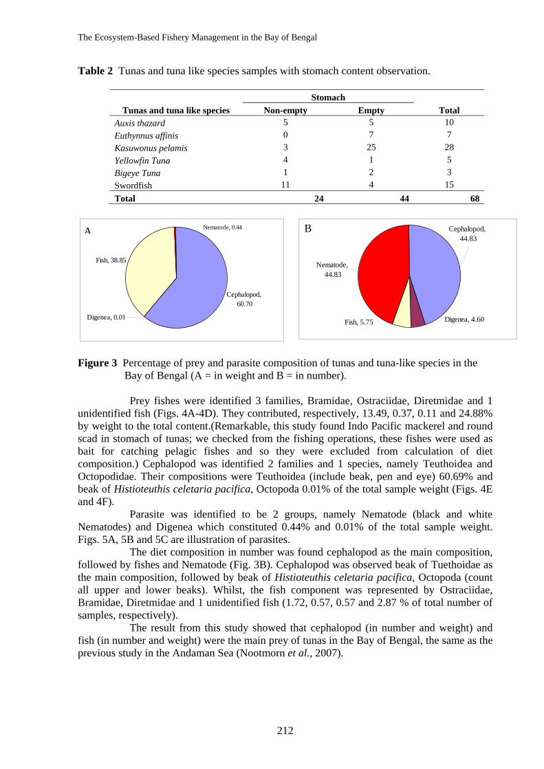
The Ecosystem-Based Fishery Management in the Bay of Bengal
212
Table 2 Tunas and tuna like species samples with stomach content observation.
Tunas and tuna like species Stomach
Total Non-empty Empty Auxis thazard 5 5 10 Euthynnus affinis 0 7 7 Kasuwonus pelamis 3 25 28 Yellowfin Tuna 4 1 5 Bigeye Tuna 1 2 3 Swordfish 11 4 15 Total 24 44 68
Cephalopod, 60.70
Fish, 38.85
Nematode, 0.44
Digenea, 0.01Fish, 5.75
Cephalopod, 44.83
Nematode, 44.83
Digenea, 4.60
Figure 3 Percentage of prey and parasite composition of tunas and tuna-like species in the
Bay of Bengal (A = in weight and B = in number).
Prey fishes were identified 3 families, Bramidae, Ostraciidae, Diretmidae and 1 unidentified fish (Figs. 4A-4D). They contributed, respectively, 13.49, 0.37, 0.11 and 24.88% by weight to the total content.(Remarkable, this study found Indo Pacific mackerel and round scad in stomach of tunas; we checked from the fishing operations, these fishes were used as bait for catching pelagic fishes and so they were excluded from calculation of diet composition.) Cephalopod was identified 2 families and 1 species, namely Teuthoidea and Octopodidae. Their compositions were Teuthoidea (include beak, pen and eye) 60.69% and beak of Histioteuthis celetaria pacifica, Octopoda 0.01% of the total sample weight (Figs. 4E and 4F).
Parasite was identified to be 2 groups, namely Nematode (black and white Nematodes) and Digenea which constituted 0.44% and 0.01% of the total sample weight. Figs. 5A, 5B and 5C are illustration of parasites.
The diet composition in number was found cephalopod as the main composition, followed by fishes and Nematode (Fig. 3B). Cephalopod was observed beak of Tuethoidae as the main composition, followed by beak of Histioteuthis celetaria pacifica, Octopoda (count all upper and lower beaks). Whilst, the fish component was represented by Ostraciidae, Bramidae, Diretmidae and 1 unidentified fish (1.72, 0.57, 0.57 and 2.87 % of total number of samples, respectively).
The result from this study showed that cephalopod (in number and weight) and fish (in number and weight) were the main prey of tunas in the Bay of Bengal, the same as the previous study in the Andaman Sea (Nootmorn et al., 2007).
A B
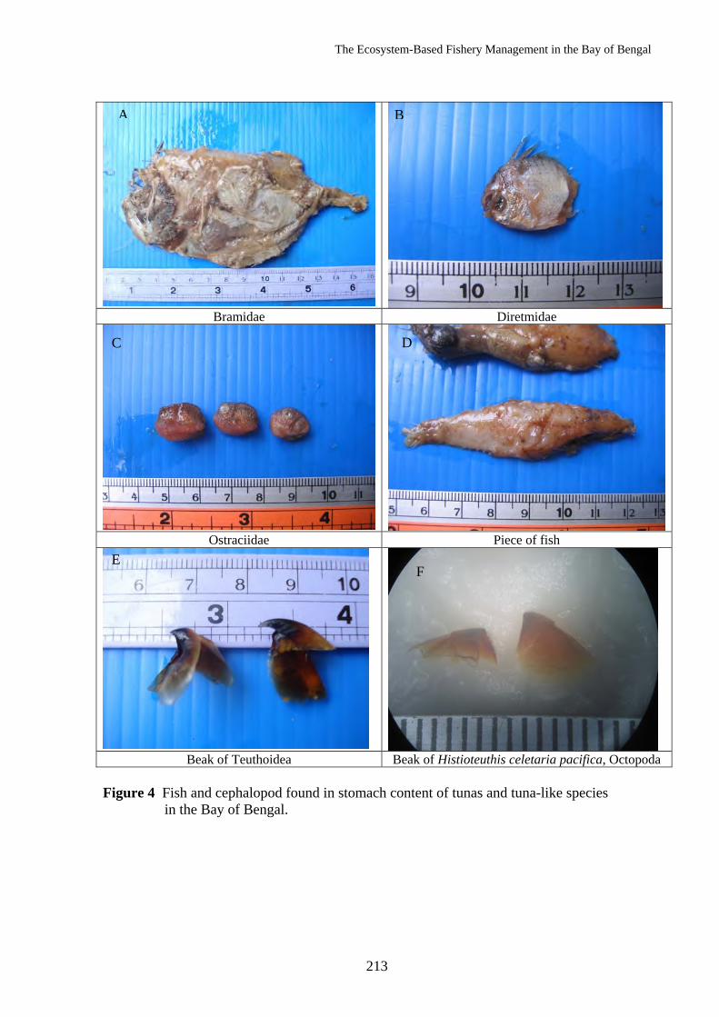
The Ecosystem-Based Fishery Management in the Bay of Bengal
213
Bramidae Diretmidae
Ostraciidae Piece of fish
Beak of Teuthoidea Beak of Histioteuthis celetaria pacifica, Octopoda Figure 4 Fish and cephalopod found in stomach content of tunas and tuna-like species
in the Bay of Bengal.
A B
FE
C D
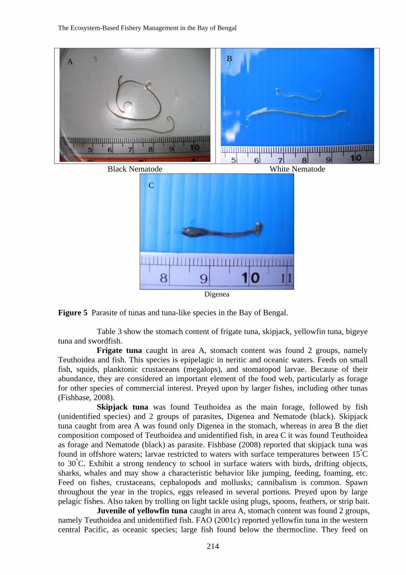
The Ecosystem-Based Fishery Management in the Bay of Bengal
214
Black Nematode White Nematode
Digenea
Figure 5 Parasite of tunas and tuna-like species in the Bay of Bengal.
Table 3 show the stomach content of frigate tuna, skipjack, yellowfin tuna, bigeye tuna and swordfish.
Frigate tuna caught in area A, stomach content was found 2 groups, namely Teuthoidea and fish. This species is epipelagic in neritic and oceanic waters. Feeds on small fish, squids, planktonic crustaceans (megalops), and stomatopod larvae. Because of their abundance, they are considered an important element of the food web, particularly as forage for other species of commercial interest. Preyed upon by larger fishes, including other tunas (Fishbase, 2008).
Skipjack tuna was found Teuthoidea as the main forage, followed by fish (unidentified species) and 2 groups of parasites, Digenea and Nematode (black). Skipjack tuna caught from area A was found only Digenea in the stomach, whereas in area B the diet composition composed of Teuthoidea and unidentified fish, in area C it was found Teuthoidea as forage and Nematode (black) as parasite. Fishbase (2008) reported that skipjack tuna was found in offshore waters; larvae restricted to waters with surface temperatures between 15°C to 30°C. Exhibit a strong tendency to school in surface waters with birds, drifting objects, sharks, whales and may show a characteristic behavior like jumping, feeding, foaming, etc. Feed on fishes, crustaceans, cephalopods and mollusks; cannibalism is common. Spawn throughout the year in the tropics, eggs released in several portions. Preyed upon by large pelagic fishes. Also taken by trolling on light tackle using plugs, spoons, feathers, or strip bait.
Juvenile of yellowfin tuna caught in area A, stomach content was found 2 groups, namely Teuthoidea and unidentified fish. FAO (2001c) reported yellowfin tuna in the western central Pacific, as oceanic species; large fish found below the thermocline. They feed on
C
A B
The Ecosystem-Based Fishery Management in the Bay of Bengal
215
many kinds of organisms, particularly fishes, squids and crustaceans. Nootmorn et al. (2007) reported this species were caught in the Andaman Sea at depth of water ranging from 41-80 m. Size of fish in length and weight was 120-138 cm and 20-31 kg. Stomach content was found fish (unidentified fish (1), Ostraciidae), cephalopod (Octopoda) and deep-sea shrimp (Aritridae). Panjarat (2006) reported the diet of this species, in the same area, composed of fishes (Tetraodontidae, Priacantidae, Balistidae and Syngnathidae) and cephalopod (Loliginidae and Teuthoidea). The previous studies reported high diversities of prey than this study because those fish samples were from pelagic longline fishing.
Juvenile of bigeye tuna caught in area C, the forage comprised of Teuthoidea, Ostracidae, Diretmidae and unidentified fish. Fishbase (2008) reported that this species occur in areas where water temperatures range from 13°-29°C, but the optimum is between 17° and 22°C. Variation in occurrence is closely related to seasonal and climatic changes in surface temperature and thermocline. Juveniles and small adults school at the surface in mono-species groups or mixed with other tunas, may be associated with floating objects. Adults stay in deeper waters. Feed on a wide variety of fishes, cephalopods and crustaceans during the day and at night.
Swordfish was found 6 groups in the stomach content; the main composition was Teuthoidea, followed by Bramidae, unidentified fish, Octopoda (Histioteuthis celetaria pacifica), Nematode (black) and Nematode (white) in all areas. In area A the stomach content was found 4 groups; Teuthoidea, Bramidae, unidentified fish and Nematode (black), area B found 4 groups; Teuthoidea, Octopoda, Nematode (black) and Nematode (white), whilst area C found 3 groups; Teuthoidea, Nematode (black) and Nematode (white). Swordfish are widely distribution throughout the study area at water depth range 10-132 m. Nootmorn et al. (2007) reported the diet of this species composed of cephalopod (Teuthoidea, Argonautidae and Octopoda), deep-sea shrimp (Aritridae) and fish (Thyrsiles atun, Cubiceps caeruleus, Gempylidae). Their study found higher diversity of prey however the groups of prey were the same as this study. FAO (2001c) reported that swordfish in the western central Pacific are an epi- and mesopelagic, oceanic species, usually found in surface waters until 550 m. Adults are opportunistic feeders, known to forage for their food from the surface to the bottom over a wide depth range. They feed on pelagic squids wherever abundant, that is same as this study.
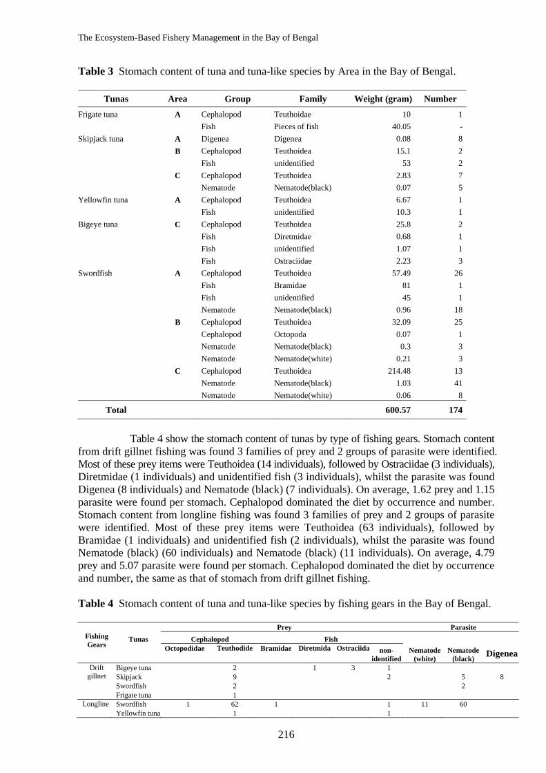
The Ecosystem-Based Fishery Management in the Bay of Bengal
216
Table 3 Stomach content of tuna and tuna-like species by Area in the Bay of Bengal.
Tunas Area Group Family Weight (gram) Number
Frigate tuna A Cephalopod Teuthoidae 10 1 Fish Pieces of fish 40.05 -Skipjack tuna A Digenea Digenea 0.08 8 B Cephalopod Teuthoidea 15.1 2 Fish unidentified 53 2 C Cephalopod Teuthoidea 2.83 7 Nematode Nematode(black) 0.07 5Yellowfin tuna A Cephalopod Teuthoidea 6.67 1 Fish unidentified 10.3 1Bigeye tuna C Cephalopod Teuthoidea 25.8 2 Fish Diretmidae 0.68 1 Fish unidentified 1.07 1 Fish Ostraciidae 2.23 3Swordfish A Cephalopod Teuthoidea 57.49 26 Fish Bramidae 81 1 Fish unidentified 45 1 Nematode Nematode(black) 0.96 18 B Cephalopod Teuthoidea 32.09 25 Cephalopod Octopoda 0.07 1 Nematode Nematode(black) 0.3 3 Nematode Nematode(white) 0.21 3 C Cephalopod Teuthoidea 214.48 13 Nematode Nematode(black) 1.03 41 Nematode Nematode(white) 0.06 8
Total 600.57 174
Table 4 show the stomach content of tunas by type of fishing gears. Stomach content
from drift gillnet fishing was found 3 families of prey and 2 groups of parasite were identified. Most of these prey items were Teuthoidea (14 individuals), followed by Ostraciidae (3 individuals), Diretmidae (1 individuals) and unidentified fish (3 individuals), whilst the parasite was found Digenea (8 individuals) and Nematode (black) (7 individuals). On average, 1.62 prey and 1.15 parasite were found per stomach. Cephalopod dominated the diet by occurrence and number. Stomach content from longline fishing was found 3 families of prey and 2 groups of parasite were identified. Most of these prey items were Teuthoidea (63 individuals), followed by Bramidae (1 individuals) and unidentified fish (2 individuals), whilst the parasite was found Nematode (black) (60 individuals) and Nematode (black) (11 individuals). On average, 4.79 prey and 5.07 parasite were found per stomach. Cephalopod dominated the diet by occurrence and number, the same as that of stomach from drift gillnet fishing. Table 4 Stomach content of tuna and tuna-like species by fishing gears in the Bay of Bengal.
Prey Parasite Fishing Gears
Tunas Cephalopod Fish Octopodidae Teuthodide Bramidae Diretmida Ostraciida non-
identified Nematode
(white) Nematode
(black) Digenea Drift
gillnet Bigeye tuna 2 1 3 1 Skipjack 9 2 5 8
Swordfish 2 2 Frigate tuna 1 Longline Swordfish 1 62 1 1 11 60 Yellowfin tuna 1 1
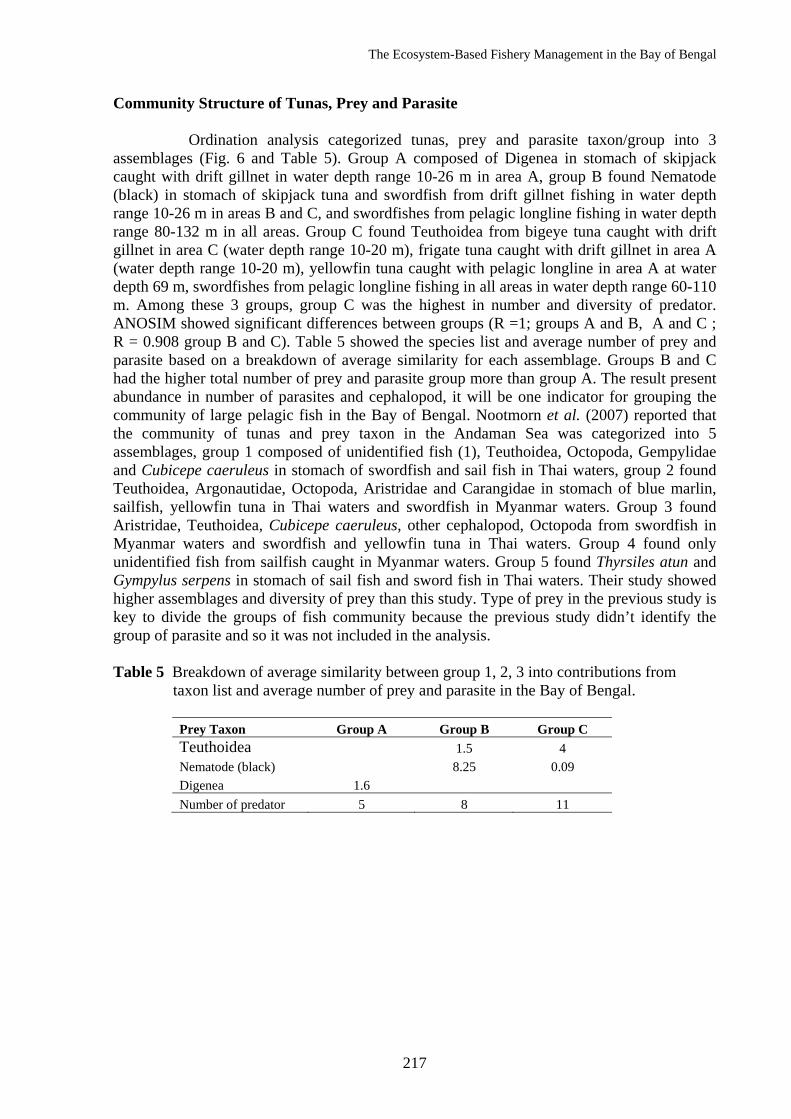
The Ecosystem-Based Fishery Management in the Bay of Bengal
217
Community Structure of Tunas, Prey and Parasite
Ordination analysis categorized tunas, prey and parasite taxon/group into 3 assemblages (Fig. 6 and Table 5). Group A composed of Digenea in stomach of skipjack caught with drift gillnet in water depth range 10-26 m in area A, group B found Nematode (black) in stomach of skipjack tuna and swordfish from drift gillnet fishing in water depth range 10-26 m in areas B and C, and swordfishes from pelagic longline fishing in water depth range 80-132 m in all areas. Group C found Teuthoidea from bigeye tuna caught with drift gillnet in area C (water depth range 10-20 m), frigate tuna caught with drift gillnet in area A (water depth range 10-20 m), yellowfin tuna caught with pelagic longline in area A at water depth 69 m, swordfishes from pelagic longline fishing in all areas in water depth range 60-110 m. Among these 3 groups, group C was the highest in number and diversity of predator. ANOSIM showed significant differences between groups (R =1; groups A and B, A and C ; R = 0.908 group B and C). Table 5 showed the species list and average number of prey and parasite based on a breakdown of average similarity for each assemblage. Groups B and C had the higher total number of prey and parasite group more than group A. The result present abundance in number of parasites and cephalopod, it will be one indicator for grouping the community of large pelagic fish in the Bay of Bengal. Nootmorn et al. (2007) reported that the community of tunas and prey taxon in the Andaman Sea was categorized into 5 assemblages, group 1 composed of unidentified fish (1), Teuthoidea, Octopoda, Gempylidae and Cubicepe caeruleus in stomach of swordfish and sail fish in Thai waters, group 2 found Teuthoidea, Argonautidae, Octopoda, Aristridae and Carangidae in stomach of blue marlin, sailfish, yellowfin tuna in Thai waters and swordfish in Myanmar waters. Group 3 found Aristridae, Teuthoidea, Cubicepe caeruleus, other cephalopod, Octopoda from swordfish in Myanmar waters and swordfish and yellowfin tuna in Thai waters. Group 4 found only unidentified fish from sailfish caught in Myanmar waters. Group 5 found Thyrsiles atun and Gympylus serpens in stomach of sail fish and sword fish in Thai waters. Their study showed higher assemblages and diversity of prey than this study. Type of prey in the previous study is key to divide the groups of fish community because the previous study didn’t identify the group of parasite and so it was not included in the analysis.
Table 5 Breakdown of average similarity between group 1, 2, 3 into contributions from
taxon list and average number of prey and parasite in the Bay of Bengal.
Prey Taxon Group A Group B Group C Teuthoidea 1.5 4 Nematode (black) 8.25 0.09 Digenea 1.6 Number of predator 5 8 11
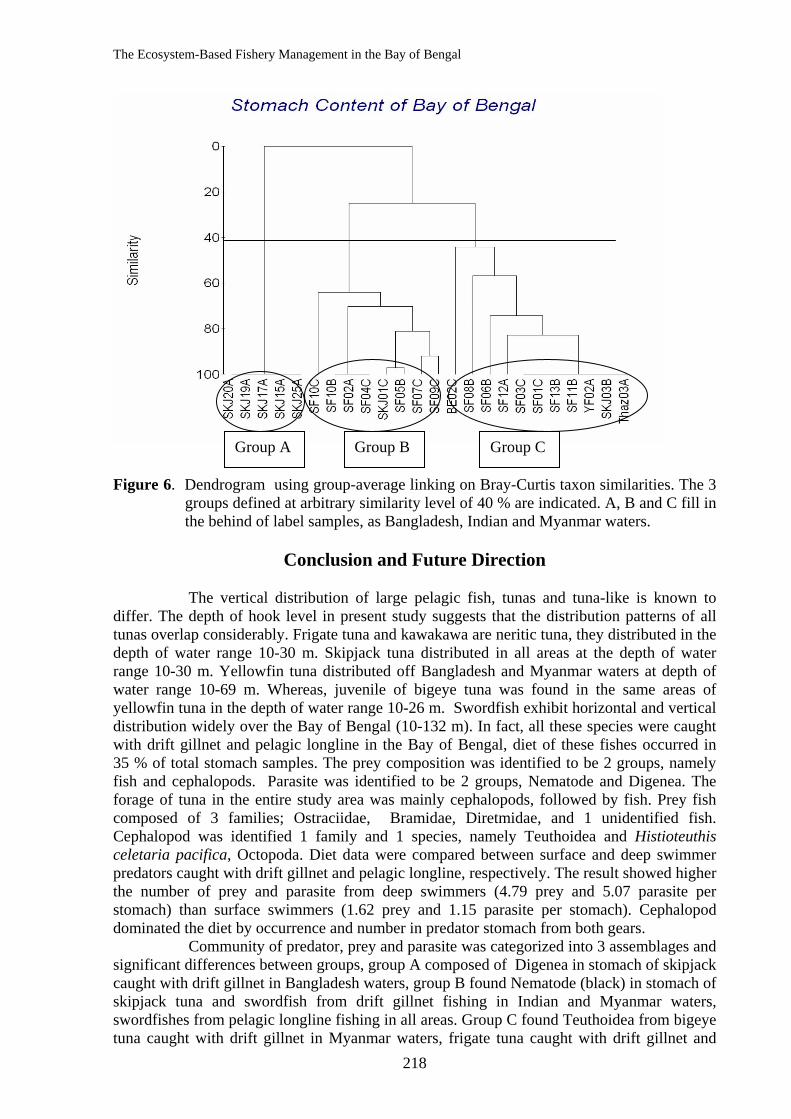
The Ecosystem-Based Fishery Management in the Bay of Bengal
218
Figure 6. Dendrogram using group-average linking on Bray-Curtis taxon similarities. The 3
groups defined at arbitrary similarity level of 40 % are indicated. A, B and C fill in the behind of label samples, as Bangladesh, Indian and Myanmar waters.
Conclusion and Future Direction
The vertical distribution of large pelagic fish, tunas and tuna-like is known to
differ. The depth of hook level in present study suggests that the distribution patterns of all tunas overlap considerably. Frigate tuna and kawakawa are neritic tuna, they distributed in the depth of water range 10-30 m. Skipjack tuna distributed in all areas at the depth of water range 10-30 m. Yellowfin tuna distributed off Bangladesh and Myanmar waters at depth of water range 10-69 m. Whereas, juvenile of bigeye tuna was found in the same areas of yellowfin tuna in the depth of water range 10-26 m. Swordfish exhibit horizontal and vertical distribution widely over the Bay of Bengal (10-132 m). In fact, all these species were caught with drift gillnet and pelagic longline in the Bay of Bengal, diet of these fishes occurred in 35 % of total stomach samples. The prey composition was identified to be 2 groups, namely fish and cephalopods. Parasite was identified to be 2 groups, Nematode and Digenea. The forage of tuna in the entire study area was mainly cephalopods, followed by fish. Prey fish composed of 3 families; Ostraciidae, Bramidae, Diretmidae, and 1 unidentified fish. Cephalopod was identified 1 family and 1 species, namely Teuthoidea and Histioteuthis celetaria pacifica, Octopoda. Diet data were compared between surface and deep swimmer predators caught with drift gillnet and pelagic longline, respectively. The result showed higher the number of prey and parasite from deep swimmers (4.79 prey and 5.07 parasite per stomach) than surface swimmers (1.62 prey and 1.15 parasite per stomach). Cephalopod dominated the diet by occurrence and number in predator stomach from both gears.
Community of predator, prey and parasite was categorized into 3 assemblages and significant differences between groups, group A composed of Digenea in stomach of skipjack caught with drift gillnet in Bangladesh waters, group B found Nematode (black) in stomach of skipjack tuna and swordfish from drift gillnet fishing in Indian and Myanmar waters, swordfishes from pelagic longline fishing in all areas. Group C found Teuthoidea from bigeye tuna caught with drift gillnet in Myanmar waters, frigate tuna caught with drift gillnet and
Group A Group B Group C
The Ecosystem-Based Fishery Management in the Bay of Bengal
219
yellowfin tuna caught with pelagic longline in Bangladesh waters, swordfishes from pelagic longline fishing in all areas. Groups B and C showed higher in total number and diversity of predator, prey and parasite groups than group A. The result from this study present abundance in number of parasites and cephalopod, it will be indicator to grouping the community of large pelagic fish in the Bay of Bengal.
The results of present study provide an example of interesting questions concerning tuna trophic ecology that may be answered. These data will provide a more complete picture of complex trophic dynamics of mixed-species tuna aggregation, as well as seasonal trends in feeding and aggregation behavior. The preliminary picture of pelagic fish ecology in the Bay of Bengal during November and December 2007 was investigated. Predator: frigate tuna is neritic species. The stomach content was found Teuthoidea and fish. Skipjack tuna was widely distributed throughout the study area at water depth range 10-30 m. This species was found Teuthoidea as the main forage, followed by fish (unidentified species), whereas 2 groups of parasites were recorded; Digenea and Nematode (black). Skipjack tuna caught from Bangladesh waters was found only Digenea in the stomach, in Indian waters found Teuthoidea and unidentified fish, in Myanmar waters found Teuthoidae as forage and Nematode (black) as parasite. Yellowfin tuna (juvenile fish) caught from Myanmar waters, prey was found Teuthoidea and unidentified. Juvenile of bigeye tuna caught in Myanmar waters at depth of water range 10-26 m, the forage comprised of Teuthoidea, Ostracidae, Diretmidae and unidentified fish. Swordfishes are widely distributed throughout the study area at water depth range 10-132 m. The diet was reported cephalopod (Teuthoidea and Octopoda) and fish (Bramidae and unidentified fish). Prey: pelagic squid, Teuthoidea was the main composition of cephalopod, it was high abundant and widely distributed in the water depth 10-120 m. Histioteuthis celetaria pacifica, Octopoda was distributed in water depth 60 m. Deep-sea fish: Ostraciidae showed the highest abundance in water depth range from 10-20 m in Myanmar waters, whilst Diretmidae was also found in same area as Ostraciidae. Bramidae was at water depth range 40 m in Bangladesh waters. Parasite: nematode (black) was the main composition, mostly found in stomach of swordfish caught with both gears at water depth range 10-132 m. Nematode (white) was found in stomach of swordfish caught from pelagic longline fishing at water depth range 60-120 m in Indian and Myanmar waters. Digenea was parasite of skipjack caught with drift gillnet at water depth range 10-20 m in Bangladesh waters.
The Bay of Bengal is recognized as one of the area where fisheries resources are under-exploited status. Lack of the field guide and taxonomy of deep-sea species, such as fishes, cephalopods (whole body and beak) is recognized in present study. The taxonomy key will be useful and support for study on the tropic dynamics of large pelagic fish in the Bay of Bengal. Up to date the knowledge of ecosystem to be based on for fisheries management is insufficient. The tropic dynamics of pelagic fish and prey will provide the information on quality of ecology. None/under-exploited tunas and pelagic squid in the Bay of Bengal are very interesting for commercial fishery because there is virtually no deep-sea fishery in the area. Nevertheless, the fact that some species reach a large size and are commonly taken on the basis of exploratory deep-water trawling, jigging and longline fishing suggests that they may have future commercial potential whenever the suitable deep-sea fishing gears are used in the area.
Acknowledgment
Authors would like to thank all SEAFDEC, DOF researchers and crews participated in the trip for great assistance to collect stomach samples of tunas and useful related information. Dr. Jaruwat Nabhitabhata (Prince of Somgkhla University) who helped to identify cephalopods from beaks in acknowledgement.
The Ecosystem-Based Fishery Management in the Bay of Bengal
220
Refferences
Carr, M. R., 1997. Primer user manual (Plymouth Routines in Multivariate Ecological
Research). Plymouth Marine Laboratory Natural Environment Research Council, UK, 42 pp.
Clarke, Malcolm R. 1962. The Identification of Cephalopod "Beak" and the Relationship Between Beak Size and Total Body Weight. Bulletin of the British Museum (Naural History) Zoology, 8(10): 421-480.
Clarke, Malcolm R. (ed.). 1986. A Handbook for the Identification of Cephalopod Beak. Oxford, Clarendon Press. 273 pp.
FAO. 2001a. The living marine resources of the Western Central Pacific. Vol. 2 Cephalopods, crustaceans, holothurians and sharks. Rome, FAO. pp687-1396.
FAO. 2001b. The living marine resources of the Western Central Pacific. Vol. 4 Bony fishes part 2 (Mugilidae to Carangidae). Rome, FAO. pp2069-2790.
FAO. 2001c. The living marine resources of the Western Central Pacific. Vol. 5 Bony fishes part 3 (Menidae to Pomacentridae). Rome, FAO. pp2791-3379.
FAO. 2001d. The living marine resources of the Western Central Pacific. Vol. 6 Bony fishes part 4 (Labridae to Latimeriidae), estuarine crocodiles, sea turtles, sea snakes and marine mammals. Rome, FAO. pp3381-4218.
Fishbase. 2008. http://www.fishbase.org/search.php. 4/8/2008. Kruskal, J. B. and Wish, M., 1978. Multidimensional scaling. Sage Publications, Beverley
Hills, California, USA. Kubodera, T. 2003. Manual for the identification of Cephalopod beaks in the NorthWestern
Pacific. http://research.kahaku.go.jp/Zoology/Beak/index.html. Nootmorn, P., S. Panjarat, S. Hoimuk, and W. Singtongyam. 2001. Thai tuna purse seine
fishery, Mukmanee, in the Indian Ocean, 1998 to 2000. Paper submitted at the Annual Meeting of Department of Fisheries, 18-20 September 2001, Bangkhaen, Bangkok, Thailand. 16 p. (in Thai).
Nootmorn, P., P. Keereerut and S. Hoimuk. 2007. Stomach content of tropical tunas from pelagic longline in the Andaman Sea. SEAFDEC TD/RES/-. 14 p. (unpublished)
Panjarat, S. 2006. Preliminary study on the stomach content of yellowfin tuna in the Andaman Sea. In Preliminary results on the large pelagic fisheries resources survey in the Andaman Sea. SEAFDEC TD/RES/99. pp 114-122.
Potier, M., F. Marsac, V. Lucas, R. Sabati, J-P Hallier, and F. Ménard. 2004. Feeding partitioning among tuna taken in surface and mid-xater layers: The case of yellowfin (Thunnus albacares) and bigeye (Thunnus obesus) in the western Tropical Indian Ocean. Western Indian Ocean J; Mar. Sci., 3 (1), 51-62.
Smith, P., B. Diggles, and S. Kim. 2007. Evaluation of parasite markers to access swordfish stock structure. Scientific Committee Third Regular Session, 13-24 August 2007, Honolulu, United States of America. WCPFC-SC3-BI SWG/IP-1. 13 p.
The Ecosystem-Based Fishery Management in the Bay of Bengal
221
An Assessment of Mercury Concentration in Fish Tissues Caught from Three Compartments of the Bay of Bengal
Penjai Sompongchaiyakul1, Jinnathum Hantow1, Somjet Sornkrut2,
Montri Sumontha3 and Rankiri P.P. Krishantha Jayasinghe4
1 Faculty of Environmental Management, Prince of Songkla University, Hat-Yai, Songkhla, THAILAND 2 Deep Sea Fishery Technology Research and Development Institute,
Department of Fisheries, Samutprakarn, 10270, THAILAND 3 Andaman Sea Fisheries Research and Development Center,
Department of Fisheries, Phuket 83000, THAILAND 4 National Aquatic Resource Research and Development Agency,
Crow Island, Colombo 15, SRI LANKA
Abstract
To assess mercury (Hg) contamination in fishery resources of the Bengal Bay, a
total of 78 specimens of 11 pelagic fish species were obtained during the joint survey of BIMSTEC member countries on Assessment and Management of Marine Resources, in November to December 2007. Individual specimen was coded, measured and weighed. The white flesh samples for Hg analyses were taken from the abdominal area of most fishes, and from the caudal area for sharks. Total Hg concentrations (expressed in ng/g wet weight) in the samples were as follow; 514±187 for bigeye thresher shark (Alopias superciliosus), 251±128 for copper shark (Carcharhinus brachyurus), 122±35 for silky shark (Carcharhinus falciformis), 48 for unidentified shark, 886±104 for tille travalley (Caranx tille), 64±62 for frigate tuna (Auxis thazard), 63±16 for kawakawa (Euthynnus affinis), 110±153 for skipjack tuna (Katsuwonus pelamis), 92±32 for yellowfin tuna (Thunnus albacares), 201 for bigeye tuna (Thunnus obesus), and 478 ± 416 for swordfish (Xiphias gladius). In general, the relationship between Hg levels in muscles and fish size was observed. Five of 8 bigeye thresher shark, only one tille travalley, 2 of 29 skipjack tuna and 5 of 16 swordfish had Hg concentrations in their fleshes exceeded the EU’s upper limit of 0.5 μg/g. Moreover, the swordfish that weighed over 40 kg contained Hg in their tissues higher than 1 μg/g. Key words: mercury, fish tissues, Bay of Bengal.
Introduction
Effect of mercury (Hg) and its compounds are currently well documented. Hg from either natural or anthropogenic sources enters the environment mainly as Hg vapor, is converted to organic form in aquatic environments by bacteria and phytoplankton (WHO, 1990 and 1991). It was found that total Hg found in fish tissue is chiefly present as methylmercury (MeHg) (Riisgard and Hansen 1990; Spry and Wiener, 1991; Bloom, 1992; Windom and Cranmer, 1998; Kehrig et al., 2002; Branco et al., 2007). MeHg is soluble, mobile, and quickly enters the aquatic food chain. It absorbed by fish when they eat smaller aquatic organisms and its binds to proteins in the fish tissue. MeHg then becomes biomagnified in the food chain through passage from bacteria, plankton, macroinvertebrates, herbivorous fish, piscivorous fish and finally, to humans (WHO, 1990 and 1991). The biomagnification of MeHg has been demonstrated by the elevated levels found in piscivorous fish compared with fish at lower levels of the food chain (Jackson 1991; Watras and Bloom
The Ecosystem-Based Fishery Management in the Bay of Bengal
222
1992; Porcella 1994). Hg levels in animals may end up being 10,000–100,000 times higher than the initial concentration in the water (WHO 1990 and 1991; ATSDR, 1999).
Fish appear to accumulate MeHg from both food sources and the water column as it passes over the gills during respiration. MeHg can also be produced within the fish’s gastrointestinal tract and on the external slime layer but the amount of MeHg contributed to tissue concentrations by these processes has not been quantified and is assumed to be insignificant. However, food was found to be the predominant source of Hg uptake in fish (Hall et al., 1997).
The consumption of fish is recommended because it is a good source of omega-3 fatty acids, which have been associated with health benefits due to its cardio-protective effects. However, the content of heavy metals, especially Hg, discovered in some fish makes it difficult to establish clearly the role of fish consumption on a healthy diet. Currently, dietary intake of fish and fish products is recognized as the most important route of non-occupational exposure to Hg, with fish and other seafood products being the dominant source of Hg in the diet (WHO, 1990 and 1991). Tissues of long-lived, slow-growing and highly migratory oceanic fishes, such as tunas, billfishes and pelagic sharks accumulate high concentrations of Hg, often exceeding the limit recommended for human consumption (Barber and Whaling, 1983; Adams, 2004; Branco et al., 2004).
Therefore, contamination of Hg in top predators of pelagic food webs and large fish are of widespread interest and concern. The accumulation of Hg in swordfish (Xiphias gladius), a piscovorous fish, is widely recognized (Monteiro and Lopes, 1990; Mendez et al., 2001; Storelli et al., 2005; Kojadinovic et al., 2006; Chien et al., 2007). The presence of Hg in swordfish seems to be a fact independent of human pollution, since values in the range 0.45 and 0.9 μg/g were found in museum specimens caught between 1878 and 1909, that is before industrial activities began to pollute the ambient sea (Miller et al., 1972).
To date, there have been very few published studies on Hg in fish from the Bay of Bengal. The objectives of this study were hence to analyze and interpret the total Hg content in the pelagic fish species collected from the Bay of Bengal during November to December 2007. This study will provide baseline data of Hg levels in the fleshy tissues of swordfish, tille trevally, 5 species of tunas (skipjack tuna, kawakawa, yellowfin tuna, frigate tuna and bigeye tuna) and 4 species of shark originating from 3 geographically area of the Bay of Bengal. Because Hg levels almost consistently increase with the size of the fish (Bloom, 1992; Windom and Cranmer, 1998; Gilmour and Riedel, 2000; Stafford and Haines, 2001), relationship between Hg levels and fish sizes (length and weight) was investigated. Hg burden in the same species caught in different area was also compared.
Material and Methods
Sample Collection
Seventy eight specimens of 11 predatory fish species, caught by pelagic longline and drift gill net, were obtained from the joint survey of BIMSTEC member countries on Assessment and Management of Marine Resources during November to December 2007 in 3 compartments of the Bay of Bengal (Fig. 1). Species identification and measuring of fish sizes (length and weight) were carried out on board of M.V. SEAFDEC.
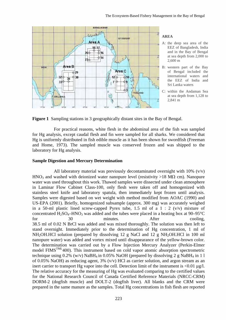
The Ecosystem-Based Fishery Management in the Bay of Bengal
223
Figure 1 Sampling stations in 3 geographically distant sites in the Bay of Bengal.
For practical reasons, white flesh in the abdominal area of the fish was sampled for Hg analysis, except caudal flesh and fin were sampled for all sharks. We considered that Hg is uniformly distributed in fish edible muscle as it has been shown for swordfish (Freeman and Home, 1973). The sampled muscle was conserved frozen and was shipped to the laboratory for Hg analysis. Sample Digestion and Mercury Determination
All laboratory material was previously decontaminated overnight with 10% (v/v) HNO3 and washed with deionized water nanopure level (resistivity >18 MΩ cm). Nanopure water was used throughout this work. Thawed samples were dissected under clean atmosphere in Laminar Flow Cabinet Class-100, only flesh were taken off and homogenized with stainless steel knife and laboratory spatula, then immediately kept frozen until analysis. Samples were digested based on wet weight with method modified from AOAC (1990) and US-EPA (2001). Briefly, homogenized subsample (approx. 300 mg) was accurately weighed in a 50-ml plastic lined screw-capped Pyrex tube, 1.5 ml of a 1 : 2 (v/v) mixture of concentrated H2SO4–HNO3 was added and the tubes were placed in a heating box at 90–95°C for 30 minutes. After cooling, 38.5 ml of 0.02 N BrCl was added and was mixed thoroughly. The solution was then left to stand overnight. Immediately prior to the determination of Hg concentration, 1 ml of NH2OH.HCl solution (prepared by dissolving 12 g NaCl and 12 g NH2OH.HCl in 100 ml nanopure water) was added and vortex mixed until disappearance of the yellow-brown color. The determination was carried out by a Flow Injection Mercury Analyzer (Perkin-Elmer model FIMSTML400). This instrument based on cold vapor atomic absorption spectrometric technique using 0.2% (w/v) NaBH4 in 0.05% NaOH (prepared by dissolving 2 g NaBH4 in 1 l of 0.05% NaOH) as reducing agent, 3% (v/v) HCl as carrier solution, and argon stream as an inert carrier to transport Hg vapor into the cell. Detection limit of the instrument is <0.01 µg/l. The relative accuracy for the measuring of Hg was evaluated comparing to the certified values for the National Research Council of Canada Certified Reference Materials (NRCC-CRM) DORM-2 (dogfish muscle) and DOLT-2 (dogfish liver). All blanks and the CRM were prepared in the same manure as the samples. Total Hg concentrations in fish flesh are reported
AREA
A: the deep sea area of the EEZ of Bangladesh, India and in the Bay of Bengal at sea depth from 2,000 to 2,600 m
B: western part of the Bay of Bengal included the international waters and the EEZ of India and Sri Lanka waters
C: within the Andaman Sea at sea depth from 1,128 to 2,841 m
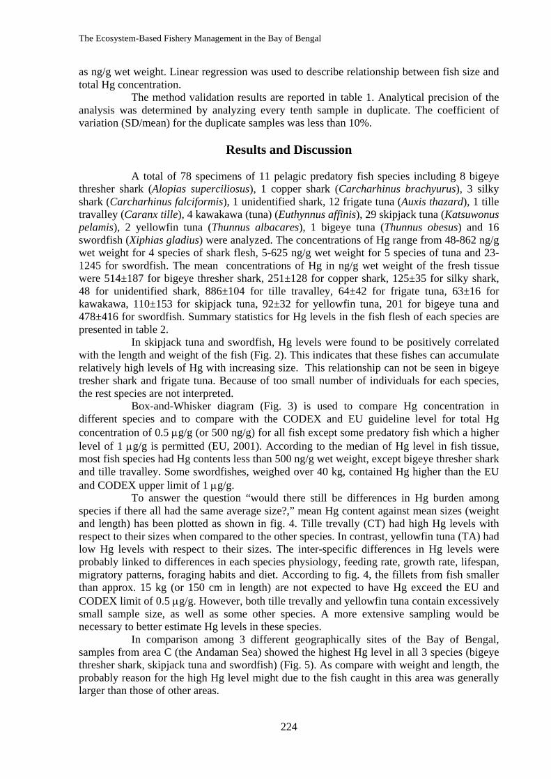
The Ecosystem-Based Fishery Management in the Bay of Bengal
224
as ng/g wet weight. Linear regression was used to describe relationship between fish size and total Hg concentration.
The method validation results are reported in table 1. Analytical precision of the analysis was determined by analyzing every tenth sample in duplicate. The coefficient of variation (SD/mean) for the duplicate samples was less than 10%.
Results and Discussion
A total of 78 specimens of 11 pelagic predatory fish species including 8 bigeye thresher shark (Alopias superciliosus), 1 copper shark (Carcharhinus brachyurus), 3 silky shark (Carcharhinus falciformis), 1 unidentified shark, 12 frigate tuna (Auxis thazard), 1 tille travalley (Caranx tille), 4 kawakawa (tuna) (Euthynnus affinis), 29 skipjack tuna (Katsuwonus pelamis), 2 yellowfin tuna (Thunnus albacares), 1 bigeye tuna (Thunnus obesus) and 16 swordfish (Xiphias gladius) were analyzed. The concentrations of Hg range from 48-862 ng/g wet weight for 4 species of shark flesh, 5-625 ng/g wet weight for 5 species of tuna and 23-1245 for swordfish. The mean concentrations of Hg in ng/g wet weight of the fresh tissue were 514±187 for bigeye thresher shark, 251±128 for copper shark, 125±35 for silky shark, 48 for unidentified shark, 886±104 for tille travalley, 64±42 for frigate tuna, 63±16 for kawakawa, 110±153 for skipjack tuna, 92±32 for yellowfin tuna, 201 for bigeye tuna and 478±416 for swordfish. Summary statistics for Hg levels in the fish flesh of each species are presented in table 2.
In skipjack tuna and swordfish, Hg levels were found to be positively correlated with the length and weight of the fish (Fig. 2). This indicates that these fishes can accumulate relatively high levels of Hg with increasing size. This relationship can not be seen in bigeye tresher shark and frigate tuna. Because of too small number of individuals for each species, the rest species are not interpreted.
Box-and-Whisker diagram (Fig. 3) is used to compare Hg concentration in different species and to compare with the CODEX and EU guideline level for total Hg concentration of 0.5 μg/g (or 500 ng/g) for all fish except some predatory fish which a higher level of 1 μg/g is permitted (EU, 2001). According to the median of Hg level in fish tissue, most fish species had Hg contents less than 500 ng/g wet weight, except bigeye thresher shark and tille travalley. Some swordfishes, weighed over 40 kg, contained Hg higher than the EU and CODEX upper limit of 1 μg/g.
To answer the question “would there still be differences in Hg burden among species if there all had the same average size?,” mean Hg content against mean sizes (weight and length) has been plotted as shown in fig. 4. Tille trevally (CT) had high Hg levels with respect to their sizes when compared to the other species. In contrast, yellowfin tuna (TA) had low Hg levels with respect to their sizes. The inter-specific differences in Hg levels were probably linked to differences in each species physiology, feeding rate, growth rate, lifespan, migratory patterns, foraging habits and diet. According to fig. 4, the fillets from fish smaller than approx. 15 kg (or 150 cm in length) are not expected to have Hg exceed the EU and CODEX limit of 0.5 μg/g. However, both tille trevally and yellowfin tuna contain excessively small sample size, as well as some other species. A more extensive sampling would be necessary to better estimate Hg levels in these species.
In comparison among 3 different geographically sites of the Bay of Bengal, samples from area C (the Andaman Sea) showed the highest Hg level in all 3 species (bigeye thresher shark, skipjack tuna and swordfish) (Fig. 5). As compare with weight and length, the probably reason for the high Hg level might due to the fish caught in this area was generally larger than those of other areas.
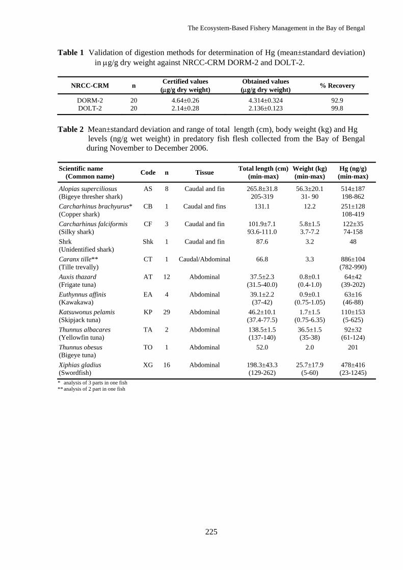
The Ecosystem-Based Fishery Management in the Bay of Bengal
225
Table 1 Validation of digestion methods for determination of Hg (mean±standard deviation) in μg/g dry weight against NRCC-CRM DORM-2 and DOLT-2.
NRCC-CRM n Certified values
(μg/g dry weight) Obtained values (μg/g dry weight) % Recovery
DORM-2 20 4.64±0.26 4.314±0.324 92.9 DOLT-2 20 2.14±0.28 2.136±0.123 99.8
Table 2 Mean±standard deviation and range of total length (cm), body weight (kg) and Hg levels (ng/g wet weight) in predatory fish flesh collected from the Bay of Bengal
during November to December 2006. Scientific name (Common name) Code n Tissue Total length (cm)
(min-max) Weight (kg) (min-max)
Hg (ng/g) (min-max)
Alopias superciliosus AS 8 Caudal and fin 265.8±31.8 56.3±20.1 514±187 (Bigeye thresher shark) 205-319 31- 90 198-862 Carcharhinus brachyurus* CB 1 Caudal and fins 131.1 12.2 251±128 (Copper shark) 108-419 Carcharhinus falciformis CF 3 Caudal and fin 101.9±7.1 5.8±1.5 122±35 (Silky shark) 93.6-111.0 3.7-7.2 74-158 Shrk Shk 1 Caudal and fin 87.6 3.2 48 (Unidentified shark) Caranx tille** CT 1 Caudal/Abdominal 66.8 3.3 886±104 (Tille trevally) (782-990) Auxis thazard AT 12 Abdominal 37.5±2.3 0.8±0.1 64±42 (Frigate tuna) (31.5-40.0) (0.4-1.0) (39-202) Euthynnus affinis EA 4 Abdominal 39.1±2.2 0.9±0.1 63±16 (Kawakawa) (37-42) (0.75-1.05) (46-88) Katsuwonus pelamis KP 29 Abdominal 46.2±10.1 1.7±1.5 110±153 (Skipjack tuna) (37.4-77.5) (0.75-6.35) (5-625) Thunnus albacares TA 2 Abdominal 138.5±1.5 36.5±1.5 92±32 (Yellowfin tuna) (137-140) (35-38) (61-124) Thunnus obesus TO 1 Abdominal 52.0 2.0 201 (Bigeye tuna) Xiphias gladius XG 16 Abdominal 198.3±43.3 25.7±17.9 478±416 (Swordfish) (129-262) (5-60) (23-1245) * analysis of 3 parts in one fish ** analysis of 2 part in one fish
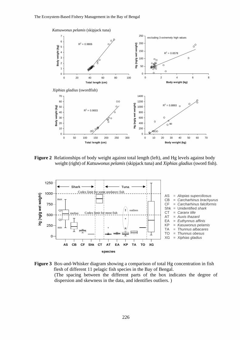
The Ecosystem-Based Fishery Management in the Bay of Bengal
226
Figure 2 Relationships of body weight against total length (left), and Hg levels against body weight (right) of Katsuwonus pelamis (skipjack tuna) and Xiphias gladius (sword fish). Figure 3 Box-and-Whisker diagram showing a comparison of total Hg concentration in fish flesh of different 11 pelagic fish species in the Bay of Bengal.
(The spacing between the different parts of the box indicates the degree of dispersion and skewness in the data, and identifies outliers. )
R2 = 0.9806
0
1
2
3
4
5
6
7
0 20 40 60 80 100
Total length (cm)
Body
wei
ght (
kg)
R2 = 0.6578
0
50
100
150
200
250
0 2 4 6 8
Body weight (kg)
Hg (n
g/g
wet
wei
ght)
excluding 3 extremely high values
Katsuwonus pelamis (skipjack tuna)
R2 = 0.9003
0
10
20
30
40
50
60
70
0 50 100 150 200 250 300
Total length (cm)
Body
wei
ght (
kg) R2 = 0.8893
0
200
400
600
800
1000
1200
1400
0 10 20 30 40 50 60 70
Body weight (kg)
Hg (n
g/g
wet
wei
ght)
Xiphias gladius (swordfish)
AS CB CF Shk CT AT EA KP TA TO XG
Shark Tuna
AS = Alopias superciliosus CB = Carcharhinus brachyurus CF = Carcharhinus falciformis Shk = Unidentified shark CT = Caranx tille AT = Auxis thazard EA = Euthynnus affinis KP = Kasuwonus pelamis TA = Thunnus albacares TO = Thunnus obesus XG = Xiphias gladius
max
min
Q1
Q3 median
outliers Codex limit for most fish
Codex limit for some predatory fish
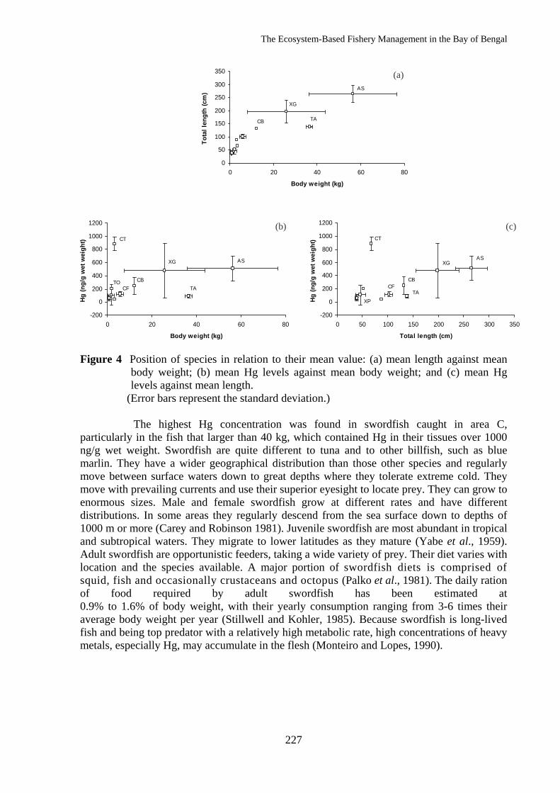
The Ecosystem-Based Fishery Management in the Bay of Bengal
227
Figure 4 Position of species in relation to their mean value: (a) mean length against mean
body weight; (b) mean Hg levels against mean body weight; and (c) mean Hg levels against mean length.
(Error bars represent the standard deviation.)
The highest Hg concentration was found in swordfish caught in area C, particularly in the fish that larger than 40 kg, which contained Hg in their tissues over 1000 ng/g wet weight. Swordfish are quite different to tuna and to other billfish, such as blue marlin. They have a wider geographical distribution than those other species and regularly move between surface waters down to great depths where they tolerate extreme cold. They move with prevailing currents and use their superior eyesight to locate prey. They can grow to enormous sizes. Male and female swordfish grow at different rates and have different distributions. In some areas they regularly descend from the sea surface down to depths of 1000 m or more (Carey and Robinson 1981). Juvenile swordfish are most abundant in tropical and subtropical waters. They migrate to lower latitudes as they mature (Yabe et al., 1959). Adult swordfish are opportunistic feeders, taking a wide variety of prey. Their diet varies with location and the species available. A major portion of swordfish diets is comprised of squid, fish and occasionally crustaceans and octopus (Palko et al., 1981). The daily ration of food required by adult swordfish has been estimated at 0.9% to 1.6% of body weight, with their yearly consumption ranging from 3-6 times their average body weight per year (Stillwell and Kohler, 1985). Because swordfish is long-lived fish and being top predator with a relatively high metabolic rate, high concentrations of heavy metals, especially Hg, may accumulate in the flesh (Monteiro and Lopes, 1990).
-200
0
200
400
600
800
1000
1200
0 50 100 150 200 250 300 350
Total length (cm)
Hg
(ng/
g w
et w
eigh
t)
AS XG
TA
CT
CB CF
XP
-200
0
200
400
600
800
1000
1200
0 20 40 60 80
Body weight (kg)
Hg
(ng/
g w
et w
eigh
t)
AS XG
TA
CT
CB CF
TO
0
50
100
150
200
250
300
350
0 20 40 60 80
Body weight (kg)
Tota
l len
gth
(cm
)
AS
TA
XG
CB
(b) (c)
(a)
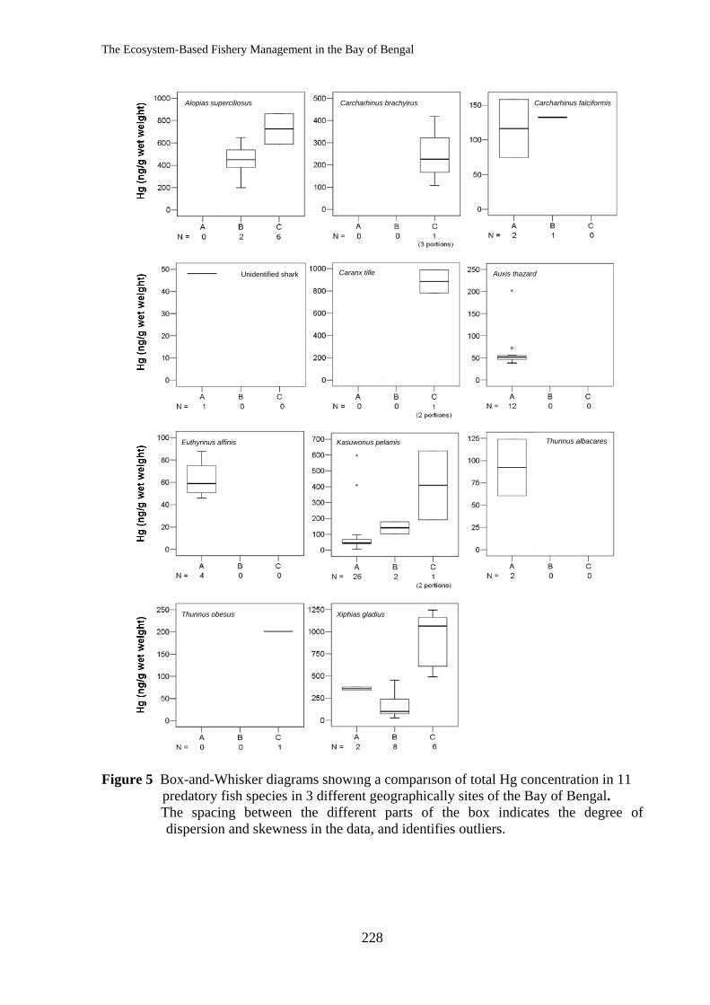
The Ecosystem-Based Fishery Management in the Bay of Bengal
228
Figure 5 Box-and-Whisker diagrams showing a comparison of total Hg concentration in 11 predatory fish species in 3 different geographically sites of the Bay of Bengal.
The spacing between the different parts of the box indicates the degree of dispersion and skewness in the data, and identifies outliers.
Alopias superciliosus Carcharhinus brachyirus Carcharhinus falciformis
Unidentified shark Caranx tille Auxis thazard
Thunnus albacares Euthynnus affinis Kasuwonus pelamis
Thunnus obesus Xiphias gladius
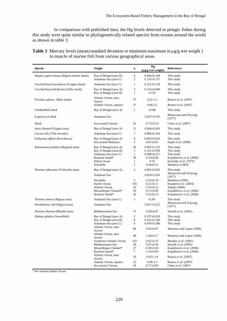
The Ecosystem-Based Fishery Management in the Bay of Bengal
229
In comparison with published data, the Hg levels detected in pelagic fishes during this study were quite similar to phylogenetically related species from oceans around the world as shown in table 3. Table 3 Mercury levels (mean±standard deviation or minimum-maximum in μg/g wet weight ) in muscle of marine fish from various geographical areas.
Species Origin n Hg (μg/g wet weight) References
Alopias superciliosus (Bigeye tresher shark) Bay of Bengal (area B) 6 0.444±0.144 This study Andaman Sea (area C) 2 0.726±0.137 This study
Carcharhinus brachyurus (Copper shark) Andaman Sea (area C) 1 0.251±0.128 This study
Carcharhinus falciformis (Silky shark) Bay of Bengal (area A) 2 0.116±0.040 This study Bay of Bengal (area B) 1 0.133 This study
Prionace glauca (Blue shark) Atlantic Ocean, near Azores 37 0.22-1.3 Branco et al. (2007)
Atlantic Ocean, equator 27 0.68-2.5 Branco et al. (2007)
Unidentified shark Bay of Bengal (area A) 1 0.048 This study
4 species of shark Andaman Sea 0.057-0.478 Menasveta and Siriyong (1977)
Shark Sea around Taiwan 41 0.73±0.54 Chien et al. (2007)
Auxis thazard (Frigate tuna) Bay of Bengal (area A) 12 0.064±0.042 This study
Caranx tille (Tille trevally) Andaman Sea (area C) 1 0.886±0.104 This study
Euthynnus affinis (Kawakawa) Bay of Bengal (area A) 4 0.063±0.016 This study Sea around Malaysia 5 0.01±0.01 Hajeb et al. (2009)
Katsuwonus pelamis (Skipjack tuna) Bay of Bengal (area A) 26 0.085±0.125 This study Bay of Bengal (area B) 2 0.141±0.038 This study Andaman Sea (area C) 1 0.408±0.217 This study Reunion Island* 39 0.19±0.66 Kojadinovic et al. (2006) Indian Ocean 1 0.53 Kureishy et al. (1979) Seuchells 5 0.34±0.11 Matthews (1983)
Thunnus albacares (Yellowfin tuna) Bay of Bengal (area A) 2 0.092±0.032 This study
Andaman Sea 0.026-0.234 Menasveta and Siriyong (1977)
Seychells 5 0.23±0.10 Matthews (1983) Pacific Ocean 105 0.21±0.11 Kraepiel et al. (2003) Atlantic Ocean 56 0.25±0.12 Adams (2004) Mozambique Channel* 20 0.13±0.09 Kojadinovic et al. (2006) Reunion Island* 19 0.21±0.15 Kojadinovic et al. (2006)
Thunnus obesus (Bigeye tuna) Andaman Sea (area C) 1 0.201 This study
Parathunnus sibi (Bigeye tuna) Andaman Sea 0.027-0.233 Menasveta and Siriyong (1977)
Thunnus thynnus (Bluefin tuna) Mediterranean Sea 73 0.20±0.07 Storelli et al. (2005)
Xiphias gladius (Swordfish) Bay of Bengal (area A) 2 0.357±0.018 This study Bay of Bengal (area B) 8 0.163±0.149 This study Andaman Sea (area C) 6 0.939±0.286 This study
Atlantic Ocean, near Azores 88 0.93±0.07 Monteiro and Lopes (1990)
Atlantic Ocean, near Azores 48 1.30±0.17 Monteiro and Lopes (1990)
Southwest Atlantic Ocean 192 0.62±0.35 Mendez et al. (2001) Mediterranean Sea 58 0.07±0.04 Storelli et al. (2005) Mozambique Channel* 37 0.38±0.26 Kojadinovic et al. (2006) Reunion Island* 7 1.24±0.83 Kojadinovic et al. (2006)
Atlantic Ocean, near Azores 29 0.031-2.4 Branco ei al. (2007)
Atlantic Ocean, equator 23 0.90-2.3 Branco ei al. (2007) Sea around Taiwan 58 0.77±0.83 Chien et al. (2007)
* the western Indian Ocean
The Ecosystem-Based Fishery Management in the Bay of Bengal
230
Conclusion
The study provided baseline data for Hg accumulated in fishery resources of the Bay of Bengal. Most fish analyzed in this study still had Hg concentration in the tissue within the EU and CODEX limit of 0.5 μg/g, particularly when fish size not exceeding approx. 15 kg in weight or 150 cm in length. As a predator fish of such longivity, bigeye thresher shark and swordfish are expected to bioaccumulate Hg. The Hg burden in the tissue of both fishes reported in this study was the highest. In addition, swordfish which weighed more than 40 kg accumulated very high Hg contents in their flesh exceeding 1 μg/g wet weight which over the upper limit of the CODEX and EU guideline levels. From the data of 3 species (bigeye thresher shark, skipjack tuna and swordfish) that distributed in all 3 different geographically areas of the Bay of Bengal, fishes caught in the Andaman Sea seems to have higher Hg concentration than those of other areas. The most likely reason might due to the age of fish caught in the Andaman Sea which may be older than those of other areas as compared with length and weight.
Acknowledgement
We gratefully acknowledge Miss Sopana Boonyapiwat for her kind cooperation of this collaborative work. We thank Miss Haruetai Apairat for her assistance during sample preparation and analysis. We would also like to thank the officers and crew of M.V. SEAFDEC for assisting in sample collection.
References Adams, D. 2004. Total mercury levels in tunas from offshore waters of the Florida Atlantic
coast. Mar. Poll. Bull. 49:659-667. ATSDR. 1999. Toxicological Profile for Mercury. Agency for Toxic Substances and
Disease Registry (ATSDR), U. S. Department of health and Human Services, Atlanta, Georgia. 676 pp. Available Source: http://www.atsdr.cdc.gov/toxprofiles/tp46.pdf; accessed. September 4, 2008.
AOAC. 1990. Association of official agricultural chemists. Mercury in fish. Method 977.15 (modified). In: Official Methods of Analysis of the Association of Official Analytical Chemists (AOAC), 15th editon. Arlington, VA, USA.
Barber, R. T. and P. J. Whaling. 1983. Mercury in marlin and sailfish. Mar. Poll. Bull. 14:395-396.
Bloom, N. S. 1992. On the chemical form of mercury in edible fish and marine invertebrate tissue. Can. J. Fish. Aquat. Sci. 49:1010-1017.
Branco, V., J. Canário, C. Vale, J. Raimundo and C. Reis. 2004. Total and organic mercury concentrations in muscle tissue of the blue shark (Prionace glauca L. 1758) from the Northeast Atlantic. Mar. Poll. Bull. 49:854-874.
Carey, F. G. and B. H. Robinson. 1981. Daily patterns in the activities of swordfish, Xiphias gladius, observed by acoustic telemetry. Fish. Bull. 79(2):277-292.
Chien, L. C., C. Y. Yeh, C. B. Jiang, C. S. Hsu and B. C. Han. 2007. Estimation of accepatable mercury intake from fish in Taiwan. Chemosphere 67:29-35.
EU. 2001. European Union (EU) Commission Regulation 466/2001 setting maximum levels for certain contaminants in foodstuffs (Consolidated version 2004). 26 pp.
Freeman, H. C. and D. A. Home. 1973. Sampling the edible muscle of the swordfish (Xiphias gladius) for the total mercury content. J. Fish. Res. Board Can. 30:1251-1252.
The Ecosystem-Based Fishery Management in the Bay of Bengal
231
Gilmour, C. C. and G. S. Riedel. 2000. A survey of size-specific mercury concentrations in game fish from Maryland fresh and estuarine waters. Arch. Environ. Contam. Toxicol. 39(1):53-9.
Hall, B. D., R. A. Bodaly, R. J. .P. Fudge, J. W. M. Rudd and D. M. Rosenberg. 1997. Food as the dominant pathway of methylmercury uptake by fish. Water Air Soil Pollut. 100(1-2):13-24.
Hajeb, P., S. Jinap, A. Ismail, A. B. Fatimah, B. Jamilah and M. A. Rahim. 2009. Assessment of mercury level in commonly consumed marine fishes in Malaysia. Food Control 20:79-84. Available Source: www.elsevier.com/locate/foodcont. September 1, 2008.
Jackson, T. A. 1991. Biological and environmental control of mercury accumulation by fish in lakes and reservoirs of northern Manitoba, Canada. Can. J. Fish. Aquat. Sci. 48(12): 2449-2470.
Kehrig, H. A., M. Costa, I. Moreira and O. Malm. 2002. Total and methylmercury in a Brazilian estuary, Rio de Janeiro. Mar. Poll. Bull. 44(10):1018-1023.
Kojadinovic, J., M. Potier, M. Le Corre, R. P. Cosson and P. Bustamante. 2006. Mercury content in commercial pelagic fish and its risk assessment in the Western Indian Ocean. Sci. Total Envi. 366:688-700.
Kraepiel, A. M. L, K. Keller, H. B. Chin, E. G. Malcolm and F. M. M. Morel. 2003. Sources and variations of mercury in tuna. Environ. Sci. Technol. 37:5551-5558.
Kureishy, T. W., M. D. George and R. S. Gupta. 1979. Total mercury content in some marine fish from the Indian Ocean. Mar. Poll. Bull. 10:357-360.
Matthews, A. D. 1983. Mercury content of commercial important fish of the Seychelles and their mercury levels of a selected part of the population. Environ. Res. 30:305-312.
Menasveta, P. and R. Siriyong. 1977. Mercury content of several predacious fish in the Andaman Sea. Mar. Poll. Bull. 8:200-204.
Mendez, E., H. Giudice, A. Pereira, G. Inocente and D. Medina. 2001. Total mercury content – fish weight relationship in swordfish (Xiphias gladius) caught in the Southwest Atlantic Ocean. J. Food Comp. Anal. 14:453-460.
Miller, E. E., P. M. Grant, R. Kishore, F. J. Steinkruger, F. S. Rowland and V. P. Guinn. 1972. Mercury concentrations in museum specimens of tuna and sword fish. New York. Science 175:1121-1122.
Monteiro, L. R. and H. D. Lopes. 1990. Mercury content of sword fish (Xiphias gladius) in relation to length, weight, age and sex. Mar. Pollut. Bull. 21:293-296.
Palko, B. J., G. L. Beardslay and W. J. Richards. 1981. Synopsis of the biology of the swordfish (Xiphias gladius) Linnaeus. United States Department of Commerce, NOAA Technical Report NMFS Circular 441 (FAO Fisheries Synopsis No. 127).
Porcella, D. B. 1994. Mercury in the environment: Biogeochemistry. In: Watras C. J. and J. W. Huckabee. (eds.). Mercury Pollution Integration and Synthesis. Boca Raton, Florida: Lewis Publishers. p. 3-19.
Riisgard, H. U. and S. Hansen. 1990. Biomagnification of mercury in a marine grazing food-chain: Algal cells Phaeodactylum tricornutum, mussels Mytilus edulis and flounders Platichthys flesus studied by means of a stepwise-reduction-CVAA method. Mar. Ecol. Prog. Ser. 62(3):259-270.
Spry, D. J. and J.G. Wiener. 1991. Metal bioavailability and toxicity to fish in low-alkalinity lakes: A critical review. Environ. Pollut. 71:243-304.
Stafford, C. P. and T. A. Haines. 2001. Mercury contamination and growth rate in two piscivore populations. Environ. Toxicol. Chem. 20:2099-2101.
The Ecosystem-Based Fishery Management in the Bay of Bengal
232
Stillwell, C. E. and N. E. Kohler. 1985. Food and feeding ecology of the swordfish Xiphias gladius in the western North Atlantic Ocean with estimates of daily ration. Mar. Ecol. Prog. Series 22:239-247.
Storelli, M. M., R. G. Stuffler, A. Storelli and G. O. Marcotrigiano. 2005. Accumulation of mercury, cadmium, lead and arsenic in swordfish and bluefin tuna from the Mediterranean Sea: A comparative study. Mar. Poll. Bull. 50:993-1018.
US-EPA. 2001. Appendix to Method 1631 Total Mercury in Tissue, Sludge, Sediment, and Soil by Acid Digestion and BrCl Oxidation. Based on a standard operating procedure provided by Frontier Geosciences, Inc.
Watras, C. J. and N. S. Bloom. 1992. Mercury and methylmercury in individual zooplankton: Implications for bioaccumulation. Limnol. Oceanogr. 37:1313-1318.
WHO. 1990. Methyl mercury. World Health Organization, International Programme on Chemical Safety. Geneva, Switzerland Vol.101.
WHO . 1991. Inorganic mercury. World Health Organization, International Programme on Chemical Safety. Geneva, Switzerland. Vol.118. 168 p.
Windom, H. L and G. Cranmer. 1998. Lack of observed impacts of gas production of Bongkot field, Thailand on Marine Biota. Mar. Poll. Bull. 36(10):799-807.
Yabe, H., S. Ueyanagi, S. Kikawa and H. Watanabe. 1959. Study on the life history of the sword-fish (Xiphias gladius) Linnaeus. Report of the Nankai Regional Fisheries Research Laboratories. 10:107-150.
The Ecosystem-Based Fishery Management in the Bay of Bengal
233
Heavy Metal Contents in Purpleback Squid (Sthenoteuthis oualaniensis) from the Bay of Bengal
Suwanna Panutrakul1, Rankiri P. P. Krishantha Jayasinghe2 and Chirdsak Chookong3
1 Department of Aquatic Science, Faculty of Science, Burapha University, Chonburi, THAILAND
2 National Aquatic Resource Research and Development Agency, Crow Island, Colombo 15, SRI LANKA
3 Deep Sea Fishery Technology Research and Development Institute, Department of Fisheries, Samutprakarn 10270, THAILAND
Abstract
Oceanic purpleback squid (Sthenoteuthis oualaniensis) were sampled at nine locations in the Bay of Bengal by the fishery research vessel M.V. SEAFDEC, of the Southeast Asian Fisheries Development Center (SEAFDEC). The squid were captured by jigging machines, and samples were kept frozen until analysis of heavy metal. Three individual squid were randomly chosen from each location and the edible parts of the squid (mantle, arm and tentacle) were separated from the visceral mass. The samples were homogenized and a portion from each individual was digested in a microwave digester. Hg concentration in the digested solution was determined by cold vapor atomic fluorescence spectrophotometer. Cd, Cu, Zn and Pb concentrations in the digested solution was determined by atomic absorption spectrophotometer. Results from this study show that purpleback squid from the Bay of Bengal accumulate high concentrations of Cd, Cu and Zn. Levels of heavy metals were similar across all sampling stations. These metals accumulate mainly in the visceral mass, which includes the ink sac, digestive gland, gills, and gonads, whereas accumulation in the edible part (mantle, arm and tentacle) is significantly lower. Cd was the only heavy metal in mantle tissue found to exceed safety standards. The concentrations of Cd and Cu in visceral mass were also higher than safety standards. The concentrations of Hg, Pb and Zn in both mantle and visceral mass were lower than safety standards. Our sampling indicates that purpleback squid is not safe for human consumption based on the degree of Cd contamination. Close monitoring is necessary in order to follow changes in Cd contamination. Further study to investigate sources of the heavy metals, especially Cd, may provide a better view on contaminant sources. Key words: heavy metal, purpleback squid, Sthenoteuthis oualaniensis, Bay of Bengal
Introduction
The Ecosystem-Based Fishery Management in the Bay of Bengal, a collaborative survey project of the BIMSTEC member countries (Bangladesh, India, Myanmar, Sri Lanka, Nepal and Thailand) carried out a 58-day survey trip in the Bay of Bengal from 25 October to 21 December 2007. The objectives were to assess the potential of fishery resources, collect biological data (species composition, distribution and catchability) of fishes and oceanic squids as well as study the physico-chemical and hydrological aspects of the survey area.
Purpleback squid (Sthenoteuthis oualaniensis) is an oceanic squid widely distributed in the equatorial and tropical waters of the Indo-Pacific Ocean. The squid is characterized by a wide ecological amplitude, complex intraspecific structure, high fecundity, short life cycle,
The Ecosystem-Based Fishery Management in the Bay of Bengal
234
high natural mortality, high growth rate and significant production (Nesis, 1977). It is very abundant and recognized as one of the main squid resources in the South China Sea and especially the northwestern Indian Ocean (Chesalin, 1997; Chesalin and Zuyev, 2002). Similar to all other squid, purpleback squid is carnivorous, feeding mainly on crustaceans, small fish, and other cephalopods (Collins et al., 1994; Collins and Pierce, 1996; Quetglas et al., 1999). Xinjun et al. (2007) found that stomach contents of purpleback squid from the northwestern Indian Ocean contained three major diet groups: fish, cephalopods and crustaceans, mainly Cypselurus spp. and S. oualaniensis. More than 60% of the stomachs of squid larger than 400 mm ML had evidence of cannibalism.
Squid are themselves important prey items for large fish, sea birds, and marine mammals (Pierce and Santos, 1996; Santos et al., 2001). Squid (and other cephalopods) are very efficient accumulators of various trace elements (Martin and Flegal, 1975; Miramand and Bentley, 1992; Bustamante et al., 2002). Toxic metals such as cadmium and mercury are bioaccumulated and retained in squid (Bustamante et al., 1998, 2006) and consequently passed on to predators, thus potentially increasing the contaminant load in higher trophic levels, including humans (Bustamante et al., 1998; Lahaye et al., 2005; Storelli et al., 2005, 2006).
The purpleback squid population in the Bay of Bengal has been recognized as a potential fishery resource for human consumption. Hence, information on heavy metal concentrations in this squid is important for future policy regarding exploitation of this species. The aims of this study were to determine and compare heavy metal concentrations in the edible portion (mantle, arm and tentacle) and visceral mass of purpleback squid (Sthenoteuthis oualaniensis) from nine sampling stations in the Bay of Bengal.
Materials and Methods
Samples of purpleback squid were caught by two Japanese automatic squid jigging
machines which were fixed and operated at the starboard side of the fishery research vessel M.V. SEAFDEC, of the Southeast Asian Fisheries Development Center (SEAFDEC). The squid were attracted by 500 kilowatt light from 15 halogen lamps fixed along the starboard side of the ship at a height of 10 m from the surface of water. The lights were switched on 60 minutes before the start of sampling. Collection occurred from 20.00-24.00 PM. for every sampling event. Seven of the sampling stations (1, 3, 7, 8, 9, 10 and 12) were located within area C, or the eastern part of the Bay of Bengal (Fig. 1). Two other sampling stations (14 and 16) were located at the northern part of the Bay (area A; Fig. 1). A list of sampling stations and their positions can be found in Table 1.
Mantle length and body weight of each individual caught were measured and recorded. Sex of the squids was determined by the presence or absence of a hectocotylus (modified ventral arm of the male). Each squid was placed in a plastic zip-log bag and kept frozen until analysis.
Prior to heavy metal analysis the samples of purpleback squid were thawed at room temperature. Three individuals from each sampling station were randomly chosen for the analysis, except for station 3, in which only one squid was available. The edible body parts (mantle, arm and tentacle) and visceral mass of each squid were separated. The samples were cut and homogenized in a blender. A 1.0-1.5 g portion of each homogenized sample was carefully weighed in a Teflon vessel. Hydrogen peroxide and sub-boiled distilled nitric acid was added to the vessels. The vessels were then closed tightly and placed in a microwave digester (CEM; Mar5x). Afterwards, the samples were cooled down and diluted with deionized water. Mercury (Hg) concentration in the digested sample was determined by Cold Vapor Atomic Fluorescence Spectrometer (PSAnalytical; Merlin) whereas Cd, Pb, and Cu were determined by Graphite Furnace Atomic Absorption Spectrophotometer (Unicam;
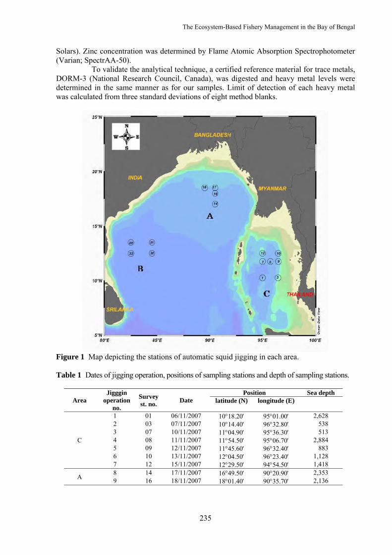
The Ecosystem-Based Fishery Management in the Bay of Bengal
235
Solars). Zinc concentration was determined by Flame Atomic Absorption Spectrophotometer (Varian; SpectrAA-50). To validate the analytical technique, a certified reference material for trace metals, DORM-3 (National Research Council, Canada), was digested and heavy metal levels were determined in the same manner as for our samples. Limit of detection of each heavy metal was calculated from three standard deviations of eight method blanks.
Figure 1 Map depicting the stations of automatic squid jigging in each area. Table 1 Dates of jigging operation, positions of sampling stations and depth of sampling stations.
Area Jigggin
operation no.
Survey st. no. Date
Position Sea depth latitude (N) longitude (E)
C
1 01 06/11/2007 10°18.20′ 95°01.00′ 2,628 2 03 07/11/2007 10°14.40′ 96°32.80′ 538 3 07 10/11/2007 11°04.90′ 95°36.30′ 513 4 08 11/11/2007 11°54.50′ 95°06.70′ 2,884 5 09 12/11/2007 11°45.60′ 96°32.40′ 883 6 10 13/11/2007 12°04.50′ 96°23.40′ 1,128 7 12 15/11/2007 12°29.50′ 94°54.50′ 1,418
A 8 14 17/11/2007 16°49.50′ 90°20.90′ 2,353 9 16 18/11/2007 18°01.40′ 90°35.70′ 2,136
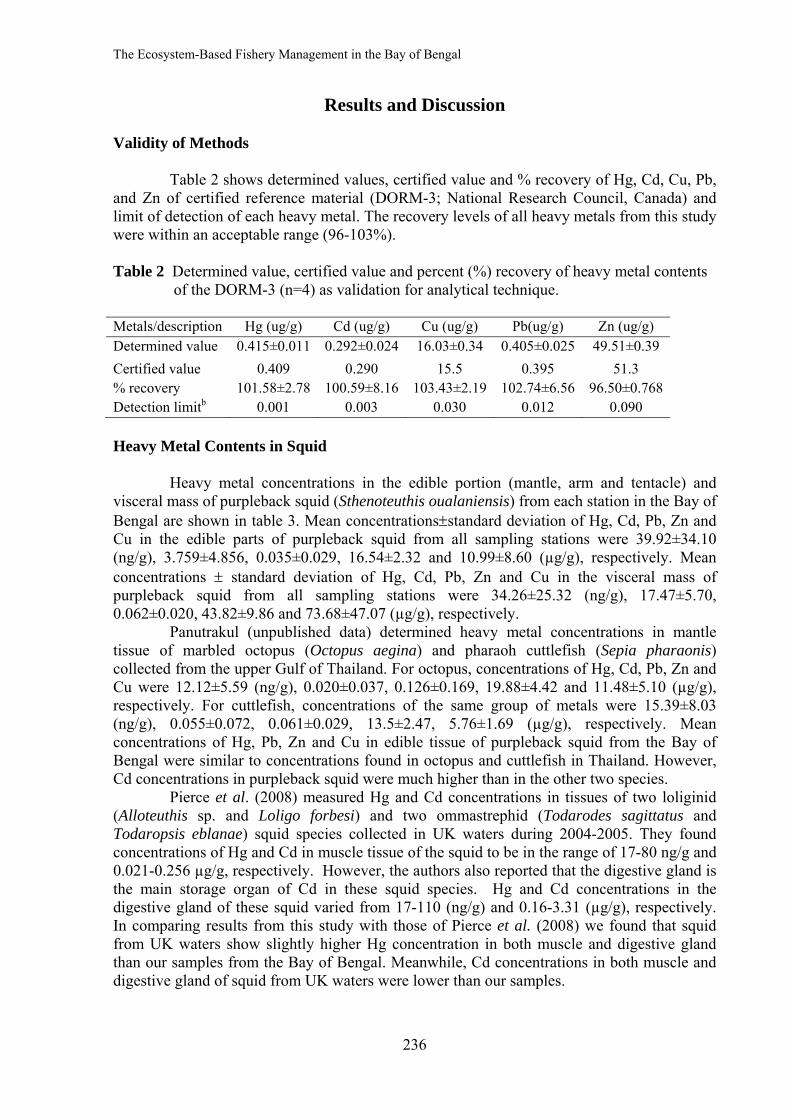
The Ecosystem-Based Fishery Management in the Bay of Bengal
236
Results and Discussion Validity of Methods
Table 2 shows determined values, certified value and % recovery of Hg, Cd, Cu, Pb, and Zn of certified reference material (DORM-3; National Research Council, Canada) and limit of detection of each heavy metal. The recovery levels of all heavy metals from this study were within an acceptable range (96-103%).
Table 2 Determined value, certified value and percent (%) recovery of heavy metal contents
of the DORM-3 (n=4) as validation for analytical technique. Metals/description Hg (ug/g) Cd (ug/g) Cu (ug/g) Pb(ug/g) Zn (ug/g) Determined value 0.415±0.011 0.292±0.024 16.03±0.34 0.405±0.025 49.51±0.39 Certified value 0.409 0.290 15.5 0.395 51.3 % recovery 101.58±2.78 100.59±8.16 103.43±2.19 102.74±6.56 96.50±0.768Detection limitb 0.001 0.003 0.030 0.012 0.090 Heavy Metal Contents in Squid
Heavy metal concentrations in the edible portion (mantle, arm and tentacle) and visceral mass of purpleback squid (Sthenoteuthis oualaniensis) from each station in the Bay of Bengal are shown in table 3. Mean concentrations±standard deviation of Hg, Cd, Pb, Zn and Cu in the edible parts of purpleback squid from all sampling stations were 39.92±34.10 (ng/g), 3.759±4.856, 0.035±0.029, 16.54±2.32 and 10.99±8.60 (µg/g), respectively. Mean concentrations ± standard deviation of Hg, Cd, Pb, Zn and Cu in the visceral mass of purpleback squid from all sampling stations were 34.26±25.32 (ng/g), 17.47±5.70, 0.062±0.020, 43.82±9.86 and 73.68±47.07 (µg/g), respectively.
Panutrakul (unpublished data) determined heavy metal concentrations in mantle tissue of marbled octopus (Octopus aegina) and pharaoh cuttlefish (Sepia pharaonis) collected from the upper Gulf of Thailand. For octopus, concentrations of Hg, Cd, Pb, Zn and Cu were 12.12±5.59 (ng/g), 0.020±0.037, 0.126±0.169, 19.88±4.42 and 11.48±5.10 (µg/g), respectively. For cuttlefish, concentrations of the same group of metals were 15.39±8.03 (ng/g), 0.055±0.072, 0.061±0.029, 13.5±2.47, 5.76±1.69 (µg/g), respectively. Mean concentrations of Hg, Pb, Zn and Cu in edible tissue of purpleback squid from the Bay of Bengal were similar to concentrations found in octopus and cuttlefish in Thailand. However, Cd concentrations in purpleback squid were much higher than in the other two species.
Pierce et al. (2008) measured Hg and Cd concentrations in tissues of two loliginid (Alloteuthis sp. and Loligo forbesi) and two ommastrephid (Todarodes sagittatus and Todaropsis eblanae) squid species collected in UK waters during 2004-2005. They found concentrations of Hg and Cd in muscle tissue of the squid to be in the range of 17-80 ng/g and 0.021-0.256 µg/g, respectively. However, the authors also reported that the digestive gland is the main storage organ of Cd in these squid species. Hg and Cd concentrations in the digestive gland of these squid varied from 17-110 (ng/g) and 0.16-3.31 (µg/g), respectively. In comparing results from this study with those of Pierce et al. (2008) we found that squid from UK waters show slightly higher Hg concentration in both muscle and digestive gland than our samples from the Bay of Bengal. Meanwhile, Cd concentrations in both muscle and digestive gland of squid from UK waters were lower than our samples.
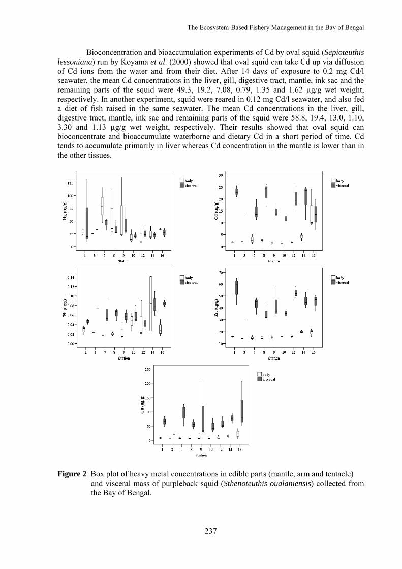
The Ecosystem-Based Fishery Management in the Bay of Bengal
237
Bioconcentration and bioaccumulation experiments of Cd by oval squid (Sepioteuthis lessoniana) run by Koyama et al. (2000) showed that oval squid can take Cd up via diffusion of Cd ions from the water and from their diet. After 14 days of exposure to 0.2 mg Cd/l seawater, the mean Cd concentrations in the liver, gill, digestive tract, mantle, ink sac and the remaining parts of the squid were 49.3, 19.2, 7.08, 0.79, 1.35 and 1.62 µg/g wet weight, respectively. In another experiment, squid were reared in 0.12 mg Cd/l seawater, and also fed a diet of fish raised in the same seawater. The mean Cd concentrations in the liver, gill, digestive tract, mantle, ink sac and remaining parts of the squid were 58.8, 19.4, 13.0, 1.10, 3.30 and 1.13 µg/g wet weight, respectively. Their results showed that oval squid can bioconcentrate and bioaccumulate waterborne and dietary Cd in a short period of time. Cd tends to accumulate primarily in liver whereas Cd concentration in the mantle is lower than in the other tissues.
Figure 2 Box plot of heavy metal concentrations in edible parts (mantle, arm and tentacle)
and visceral mass of purpleback squid (Sthenoteuthis oualaniensis) collected from the Bay of Bengal.
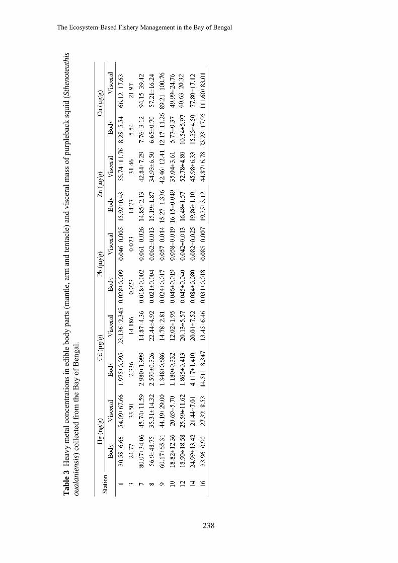
The Ecosystem-Based Fishery Management in the Bay of Bengal
238
Tab
le 3
Hea
vy m
etal
con
cent
ratio
ns in
edi
ble
body
par
ts (m
antle
, arm
and
tent
acle
) and
vis
cera
l mas
s of p
urpl
ebac
k sq
uid
(Sth
enot
euth
is
oual
anie
nsis
) col
lect
ed fr
om th
e B
ay o
f Ben
gal.
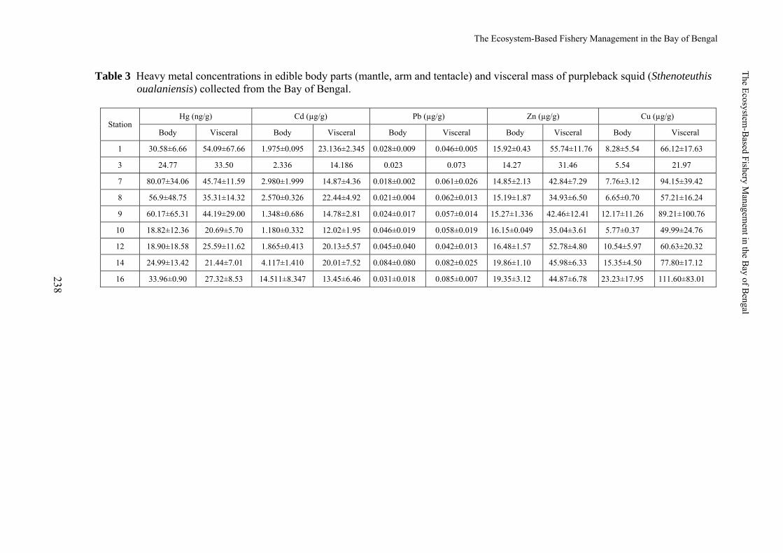
The Ecosystem-Based Fishery Management in the Bay of Bengal
239
Table 3 Heavy metal concentrations in edible body parts (mantle, arm and tentacle) and visceral mass of purpleback squid (Sthenoteuthis oualaniensis) collected from the Bay of Bengal.
Station Hg (ng/g) Cd (µg/g) Pb (µg/g) Zn (µg/g) Cu (µg/g)
Body Visceral Body Visceral Body Visceral Body Visceral Body Visceral
1 30.58±6.66 54.09±67.66 1.975±0.095 23.136±2.345 0.028±0.009 0.046±0.005 15.92±0.43 55.74±11.76 8.28±5.54 66.12±17.63
3 24.77 33.50 2.336 14.186 0.023 0.073 14.27 31.46 5.54 21.97
7 80.07±34.06 45.74±11.59 2.980±1.999 14.87±4.36 0.018±0.002 0.061±0.026 14.85±2.13 42.84±7.29 7.76±3.12 94.15±39.42
8 56.9±48.75 35.31±14.32 2.570±0.326 22.44±4.92 0.021±0.004 0.062±0.013 15.19±1.87 34.93±6.50 6.65±0.70 57.21±16.24
9 60.17±65.31 44.19±29.00 1.348±0.686 14.78±2.81 0.024±0.017 0.057±0.014 15.27±1.336 42.46±12.41 12.17±11.26 89.21±100.76
10 18.82±12.36 20.69±5.70 1.180±0.332 12.02±1.95 0.046±0.019 0.058±0.019 16.15±0.049 35.04±3.61 5.77±0.37 49.99±24.76
12 18.90±18.58 25.59±11.62 1.865±0.413 20.13±5.57 0.045±0.040 0.042±0.013 16.48±1.57 52.78±4.80 10.54±5.97 60.63±20.32
14 24.99±13.42 21.44±7.01 4.117±1.410 20.01±7.52 0.084±0.080 0.082±0.025 19.86±1.10 45.98±6.33 15.35±4.50 77.80±17.12
16 33.96±0.90 27.32±8.53 14.511±8.347 13.45±6.46 0.031±0.018 0.085±0.007 19.35±3.12 44.87±6.78 23.23±17.95 111.60±83.01
The Ecosystem-B
ased Fishery Managem
ent in the Bay of B
engal
238
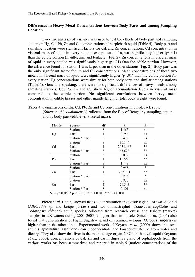
The Ecosystem-Based Fishery Management in the Bay of Bengal
240
Differences in Heavy Metal Concentrations between Body Parts and among Sampling Location
Two-way analysis of variance was used to test the effects of body part and sampling station on Hg, Cd, Pb, Zn and Cu concentrations of purpleback squid (Table 4). Body part and sampling location were significant factors for Cd, and Zn concentrations. Cd concentration in visceral mass of squid in every station, except station 16, was significantly higher (p<.01) than the edible portion (mantle, arm and tentacle) (Fig. 2). Zn concentrations in visceral mass of squid in every station was significantly higher (p<.01) than the edible portion. However, the difference found for station 1 was larger than in the other stations (Fig. 2). Body part was the only significant factor for Pb and Cu concentrations. Mean concentrations of these two metals in visceral mass of squid were significantly higher (p<.01) than the edible portion for every station. Hg concentrations were similar for both body parts and similar among stations (Table 4). Generally speaking, there were no significant differences of heavy metals among sampling stations. Cd, Pb, Zn and Cu show higher accumulation levels in visceral mass compared to the edible portion. No significant correlations between heavy metal concentration in edible tissues and either mantle length or total body weight were found. Table 4 Comparisons of Hg, Cd, Pb, Zn and Cu concentrations in purpleback squid
(Sthenoteuthis oualaniensis) collected from the Bay of Bengal by sampling station and by body part (edible vs. visceral mass).
Metals Source df F P Station 8 1.465 ns Hg Part 1 0.256 ns Station * Part 8 0.477 ns
Station 8 36.144 ns Cd Part 1 2034.466 ** Station * Part 8 65.623 ** Station 8 2.017 ns Pb Part 1 15.568 ** Station * Part 8 1.148 ns Station 8 2.958 * Zn Part 1 233.191 ** Station * Part 8 2.276 * Station 8 0.830 ns Cu Part 1 29.543 ** Station * Part 8 0.401 ns
Ns = p>0.05; * p < 0.05; ** p < 0.01; *** p < 0.001 Pierce et al. (2008) showed that Cd concentration in digestive gland of two loliginid
(Alloteuthis sp. and Loligo forbesi) and two ommastrephid (Todarodes sagittatus and Todaropsis eblanae) squid species collected from research cruise and fishery (market) samples in UK waters during 2004-2005 is higher than in muscle. Seixas et al. (2005) also found that concentration of Hg in digestive gland of common octopus (Octopus vulgaris) is higher than in the other tissue. Experimental work of Koyama et al. (2000) shows that oval squid (Sepioteuthis lessoniana) can bioconcentrate and bioaccumulate Cd from water and dietary. They also show that liver is the main storage organ for Cd in the oval squid (Koyama et al., 2000). Concentrations of Cd, Zn and Cu in digestive gland of cephalopods from the various works has been summarized and reported in table 5 (notice: concentrations of the
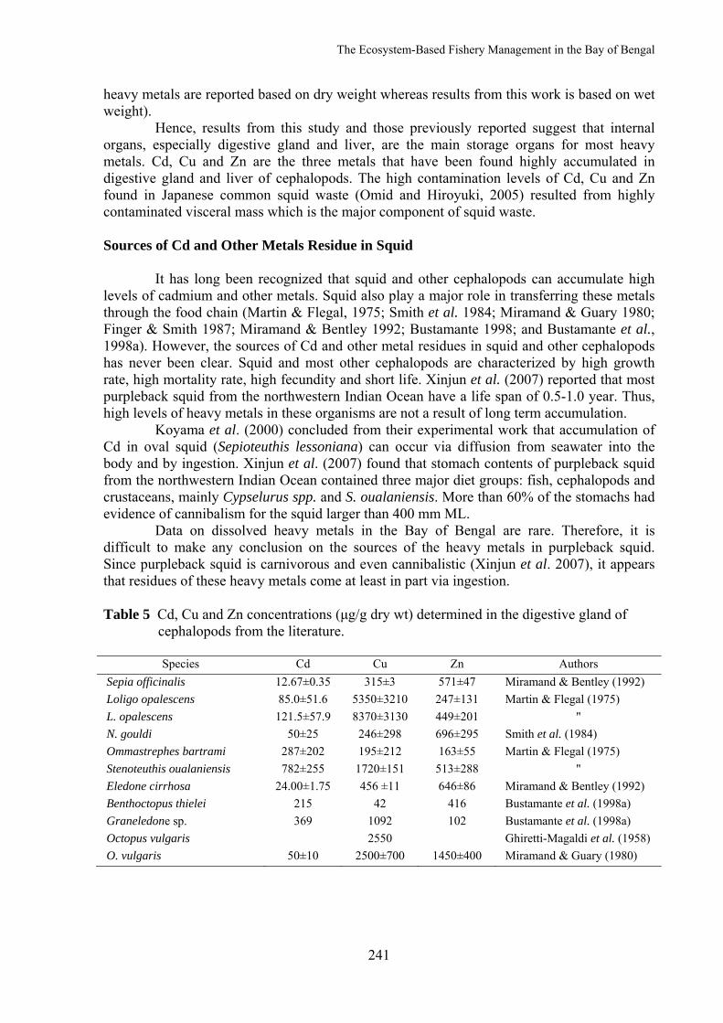
The Ecosystem-Based Fishery Management in the Bay of Bengal
241
heavy metals are reported based on dry weight whereas results from this work is based on wet weight).
Hence, results from this study and those previously reported suggest that internal organs, especially digestive gland and liver, are the main storage organs for most heavy metals. Cd, Cu and Zn are the three metals that have been found highly accumulated in digestive gland and liver of cephalopods. The high contamination levels of Cd, Cu and Zn found in Japanese common squid waste (Omid and Hiroyuki, 2005) resulted from highly contaminated visceral mass which is the major component of squid waste. Sources of Cd and Other Metals Residue in Squid
It has long been recognized that squid and other cephalopods can accumulate high levels of cadmium and other metals. Squid also play a major role in transferring these metals through the food chain (Martin & Flegal, 1975; Smith et al. 1984; Miramand & Guary 1980; Finger & Smith 1987; Miramand & Bentley 1992; Bustamante 1998; and Bustamante et al., 1998a). However, the sources of Cd and other metal residues in squid and other cephalopods has never been clear. Squid and most other cephalopods are characterized by high growth rate, high mortality rate, high fecundity and short life. Xinjun et al. (2007) reported that most purpleback squid from the northwestern Indian Ocean have a life span of 0.5-1.0 year. Thus, high levels of heavy metals in these organisms are not a result of long term accumulation.
Koyama et al. (2000) concluded from their experimental work that accumulation of Cd in oval squid (Sepioteuthis lessoniana) can occur via diffusion from seawater into the body and by ingestion. Xinjun et al. (2007) found that stomach contents of purpleback squid from the northwestern Indian Ocean contained three major diet groups: fish, cephalopods and crustaceans, mainly Cypselurus spp. and S. oualaniensis. More than 60% of the stomachs had evidence of cannibalism for the squid larger than 400 mm ML.
Data on dissolved heavy metals in the Bay of Bengal are rare. Therefore, it is difficult to make any conclusion on the sources of the heavy metals in purpleback squid. Since purpleback squid is carnivorous and even cannibalistic (Xinjun et al. 2007), it appears that residues of these heavy metals come at least in part via ingestion. Table 5 Cd, Cu and Zn concentrations (μg/g dry wt) determined in the digestive gland of
cephalopods from the literature.
Species Cd Cu Zn Authors Sepia officinalis 12.67±0.35 315±3 571±47 Miramand & Bentley (1992) Loligo opalescens 85.0±51.6 5350±3210 247±131 Martin & Flegal (1975) L. opalescens 121.5±57.9 8370±3130 449±201 " N. gouldi 50±25 246±298 696±295 Smith et al. (1984) Ommastrephes bartrami 287±202 195±212 163±55 Martin & Flegal (1975) Stenoteuthis oualaniensis 782±255 1720±151 513±288 " Eledone cirrhosa 24.00±1.75 456 ±11 646±86 Miramand & Bentley (1992) Benthoctopus thielei 215 42 416 Bustamante et al. (1998a) Graneledone sp. 369 1092 102 Bustamante et al. (1998a) Octopus vulgaris 2550 Ghiretti-Magaldi et al. (1958) O. vulgaris 50±10 2500±700 1450±400 Miramand & Guary (1980)
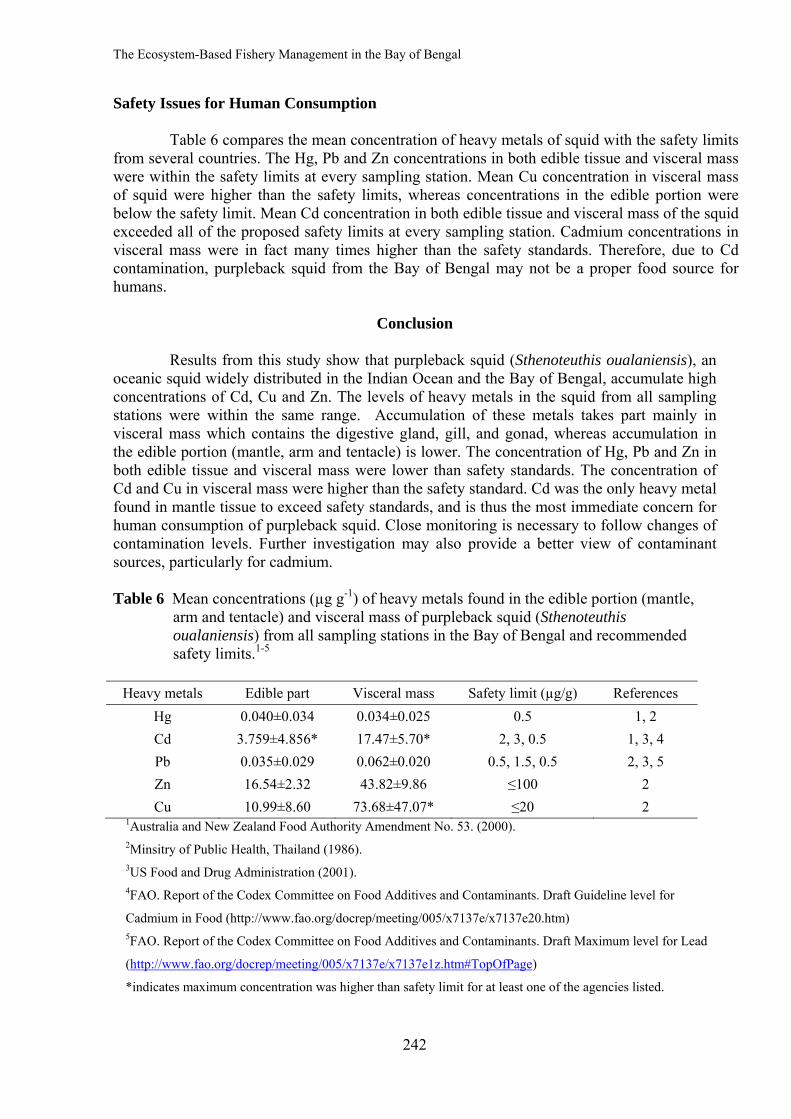
The Ecosystem-Based Fishery Management in the Bay of Bengal
242
Safety Issues for Human Consumption
Table 6 compares the mean concentration of heavy metals of squid with the safety limits from several countries. The Hg, Pb and Zn concentrations in both edible tissue and visceral mass were within the safety limits at every sampling station. Mean Cu concentration in visceral mass of squid were higher than the safety limits, whereas concentrations in the edible portion were below the safety limit. Mean Cd concentration in both edible tissue and visceral mass of the squid exceeded all of the proposed safety limits at every sampling station. Cadmium concentrations in visceral mass were in fact many times higher than the safety standards. Therefore, due to Cd contamination, purpleback squid from the Bay of Bengal may not be a proper food source for humans.
Conclusion
Results from this study show that purpleback squid (Sthenoteuthis oualaniensis), an oceanic squid widely distributed in the Indian Ocean and the Bay of Bengal, accumulate high concentrations of Cd, Cu and Zn. The levels of heavy metals in the squid from all sampling stations were within the same range. Accumulation of these metals takes part mainly in visceral mass which contains the digestive gland, gill, and gonad, whereas accumulation in the edible portion (mantle, arm and tentacle) is lower. The concentration of Hg, Pb and Zn in both edible tissue and visceral mass were lower than safety standards. The concentration of Cd and Cu in visceral mass were higher than the safety standard. Cd was the only heavy metal found in mantle tissue to exceed safety standards, and is thus the most immediate concern for human consumption of purpleback squid. Close monitoring is necessary to follow changes of contamination levels. Further investigation may also provide a better view of contaminant sources, particularly for cadmium. Table 6 Mean concentrations (µg g-1) of heavy metals found in the edible portion (mantle, arm and tentacle) and visceral mass of purpleback squid (Sthenoteuthis oualaniensis) from all sampling stations in the Bay of Bengal and recommended safety limits.1-5
Heavy metals Edible part Visceral mass Safety limit (µg/g) References Hg 0.040±0.034 0.034±0.025 0.5 1, 2 Cd 3.759±4.856* 17.47±5.70* 2, 3, 0.5 1, 3, 4 Pb 0.035±0.029 0.062±0.020 0.5, 1.5, 0.5 2, 3, 5 Zn 16.54±2.32 43.82±9.86 ≤100 2 Cu 10.99±8.60 73.68±47.07* ≤20 2
1Australia and New Zealand Food Authority Amendment No. 53. (2000). 2Minsitry of Public Health, Thailand (1986). 3US Food and Drug Administration (2001). 4FAO. Report of the Codex Committee on Food Additives and Contaminants. Draft Guideline level for
Cadmium in Food (http://www.fao.org/docrep/meeting/005/x7137e/x7137e20.htm) 5FAO. Report of the Codex Committee on Food Additives and Contaminants. Draft Maximum level for Lead
(http://www.fao.org/docrep/meeting/005/x7137e/x7137e1z.htm#TopOfPage)
*indicates maximum concentration was higher than safety limit for at least one of the agencies listed.
The Ecosystem-Based Fishery Management in the Bay of Bengal
243
References Australia and New Zealand Food Authority. 2000. Provisional Regulation Limitation of
Contamination in Food, Specifications and Standards for Foods, Food Additives, etc. Under The Food Sanitation Laws, April 2004, Standard 1.4.1, Contamination and Natural Toxicants, Maximum level of metal contaminates in food, Australia and New Zealand Food Authority Amendment no.53 to Food Standard Code, Commonwealth of Australia, 2000.
Bustamante, P., F. Caurant, S. W. Fowler and P. Miramand. 1998. Cephalopods as a vector for the transfer of cadmium to top marine predators in the north-east Atlantic Ocean. Sci. Total Environ. 220:71-80.
Bustamante, P., J. L. Teyssie, S. W. Fowler, O. Cotret, B. Danis, P. Miramand and M. Warnau. 2002. Biokinetics of zinc and cadmium accumulation and depuration at different stages in the life cycle of the cuttlefish Sepia officinalis. Mar. Ecol. Prog. Ser. 231:167-177.
Bustamante, P., V. Lahaye, C. Durnez, C. Churlaud and F. Caurant. 2006. Total and organic Hg concentrations in cephalopods from the North East Atlantic waters: influence of geographical origin and feeding ecology. Sci. Total Environ. 368:585-596.
Chesalin, M. V. 1994. Distribution and biology of the squid Sthenoteuthis oualaniensis in the Arabian Sea. Hydrobiol. J. 30(2):61-73.
Chesalin, M. V. and G. V. Zuyev. 2002. Pelagic cephalopods of the Arabian Sea with an emphasis on Sthenoteuthis oualaniensis. Bull. Mar. Sci. 71(1):209-221.
Collins, M. A. and G. J. Pierce. 1996. Size selectivity in the diet of Loligo forbesi (Cephalopoda: Loliginidae). J. Mar. Biol. Assoc. UK. 76:1081-1090.
FAO. Report of the Codex Committee on Food Additives and Contaminants. Draft Guideline level for Cadmium in Food . Available Source: http://www.fao.org/docrep/meeting/005/x7137e/x7137e20.htm.
FAO. Report of the Codex Committee on Food Additives and Contaminants. Draft Maximum level for Lead. Available Source: http://www.fao.org/docrep/meeting/005/x7137e/x7137e1z.htm.
FAO/WHO Codex Alimentarius Commission. 2005. Codex General Standard for Contaminants and Toxins in Food. Schedule 1. Maximum and Guideline Levels for Contaminants and Toxins in Food.
Ghiretti-Magaldi, A., A. Giuditta and F. Ghiretti. 1958. Pathways of terminal respiration in marine invertebrates. I. The respiratory system in cephalopods. J. Cell. Comp. Physiol. 52:389-429.
Koyama, J., N. Nanamori and S. Segawa. 2000. Bioaccumulation of waterborne and dietary Cadmium by Oval Squid, Sepioteuthis lessoniana and its distribution among organs. Marine Pollution Bulletin 40:961-967.
Lahaye, V., P. Bustamante, J. Spitz, K. Das, L. Meynier, V. Magnin, W. Dabin and F. Caurant. 2005. Long-term dietary preferences of common dolphins in the Bay of Biscay using a metallic tracer. Mar. Ecol. Prog. Ser. 305:275-285.
Martin, J. H. and A. R. Flegal. 1975. High copper concentrations in squid livers in association with elevated levels of silver, cadmium, and zinc. Mar. Biol. 30:51-55.
Ministry of Public Health. 1986. Notification No. 98. Standard Contamination Level in Food. Ministry of Public Health, Thailand.
Miramand, P. and D. Bentley. 1992. Concentration and distribution of heavy metals in tissues of two cephalopods, Eledone cirrhosa and Sepia officinalis, from the French coast of the English Channel. Mar. Biol. 114:407-414.
The Ecosystem-Based Fishery Management in the Bay of Bengal
244
Miramand, P. and J. C. Guary. 1980. High concentrations of some heavy metals in tissues of the Mediterranean octopus. Bull. Environ. Contam. Toxicol. 24:783-788.
Nesis, K. N. 1977. Population structure in the squid Sthenoteuthis oualanienses (Lessonn 1930) (Ommastrephidae) in theWestern Tropical Pacific. In: Proceedings of the Academy of Science USSR, Shirsch Inst. Oceanol. 107:15-29.
Omid, T. and Y. Hiroyuki. 2005. Effective recovery of harmful metal ions from squid waste using subcritical and supercritical water treatment. Environmental Science and Technology 39:2357-2363.
Panutrakul, S. (unpublished data). Heavy metal in Octopus and Cuttlefish from the Upper Gulf of Thailand.
Pierce, G. J. and M. B. Santos. 1996. Trophic interactions of squid Loligo forbesi in Scottish waters. In: Greenstreet, S. P. R. and M. L. Tasker. (eds.). Aquatic Predators and their Prey. Fishing News Books, Oxford. p. 58-64.
Pierce, G. J., G. Stowasser, L. C. Hastie and P. Bustamante. 2008. Geographic, seasonal and ontogenetic variation in cadmium and mercury concentrations in squid (Cephalopoda: Teuthoidea) from UK waters. Ecotoxicology and Environmental Safety 70:422-432.
Quetglas, A., F. Alemany, A. Carbonell, P. Merella and P. Sanchez. 1999. Diet of the European flying squid Todarodes sagittatus (Cephalopoda: Ommastrephidae) in the Balearic Sea (western Mediterranean). J. Mar. Biol. Assoc. UK. 79:479-486.
Santos, M. B., G. J. Pierce, J. Herman, A. Lopez, A. Guerra, E. Mente and M. R. Clarke. 2001. Feeding ecology of Cuvier’s beaked whale (Ziphius cavirostris): a review with new information on the diet of this species. J. Mar. Biol. Assoc. UK. 81:687-694.
Seixas, S., P. Bustamante and G. Pierce. 2005. Accumulation of mercury in the tissues of the common octopus Octopus vulgaris (L.) in two localities on the Portuguese coast. Science of the Total Environment 340:113-122.
Smith, J. D., L. Plues, M. Heyraud and R. D. Cherry. 1984. Concentrations of the elements Ag, Al, Ca, Cd, Cu, Fe, Mg, Pb and Zn, and the radionuclides 210Pb and 210Po in the digestive gland of the squid Nototodarus gouldi. Mar. Environ. Res. 13:55-68.
Storelli, M. M., G. Barone and G. O. Marcotrigiano. 2005. Cadmium in cephalopod molluscs: implications for public health. J. Food Prot. 68:577-580.
Storelli, M. M., R. Giacominelli-Stuffler, A. Storelli and G. O. Marcotrigiano. 2006. Cadmium and mercury in cephalopod molluscs: estimated weekly intake. Food Addit. Contam. 23:25-30.
US. Food and Drug Administration. 2001. Fish and Fisheries Products Hazards and Controls Guidance. 3rd edition. Appendix 5. FDA & EPA Safety Levels in Regulations and Guidance. Available Source: http://vm.cfsan.fda.gov/~comm/haccp4x5.html.
Xinjun, C., C. Bilin, T. Siquan, Q. Weiguo and Z. Xiaohu. 2007. Fishery biology of purpleback squid, Sthenoteuthis oualaniensis, in the northwest Indian Ocean. Fisheries Research 83:98-104.
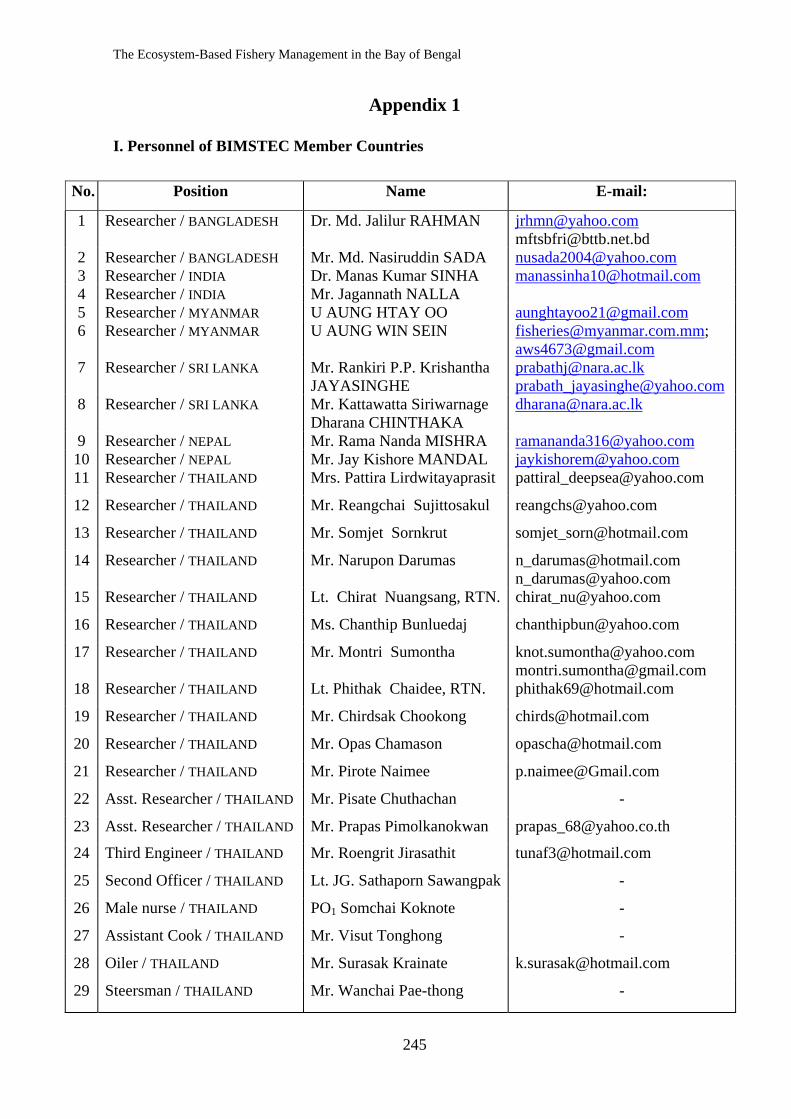
The Ecosystem-Based Fishery Management in the Bay of Bengal
245
Appendix 1
I. Personnel of BIMSTEC Member Countries
No. Position Name E-mail:
1 Researcher / BANGLADESH Dr. Md. Jalilur RAHMAN [email protected] [email protected]
2 Researcher / BANGLADESH Mr. Md. Nasiruddin SADA [email protected] 3 Researcher / INDIA Dr. Manas Kumar SINHA [email protected] 4 Researcher / INDIA Mr. Jagannath NALLA 5 Researcher / MYANMAR U AUNG HTAY OO [email protected] 6 Researcher / MYANMAR U AUNG WIN SEIN [email protected];
[email protected] 7 Researcher / SRI LANKA Mr. Rankiri P.P. Krishantha
JAYASINGHE [email protected] [email protected]
8 Researcher / SRI LANKA Mr. Kattawatta Siriwarnage Dharana CHINTHAKA
9 Researcher / NEPAL Mr. Rama Nanda MISHRA [email protected] 10 Researcher / NEPAL Mr. Jay Kishore MANDAL [email protected] 11 Researcher / THAILAND Mrs. Pattira Lirdwitayaprasit [email protected]
12 Researcher / THAILAND Mr. Reangchai Sujittosakul [email protected]
13 Researcher / THAILAND Mr. Somjet Sornkrut [email protected]
14 Researcher / THAILAND Mr. Narupon Darumas [email protected] [email protected]
15 Researcher / THAILAND Lt. Chirat Nuangsang, RTN. [email protected]
16 Researcher / THAILAND Ms. Chanthip Bunluedaj [email protected]
17 Researcher / THAILAND Mr. Montri Sumontha [email protected] [email protected]
18 Researcher / THAILAND Lt. Phithak Chaidee, RTN. [email protected]
19 Researcher / THAILAND Mr. Chirdsak Chookong [email protected]
20 Researcher / THAILAND Mr. Opas Chamason [email protected]
21 Researcher / THAILAND Mr. Pirote Naimee [email protected]
22 Asst. Researcher / THAILAND Mr. Pisate Chuthachan -
23 Asst. Researcher / THAILAND Mr. Prapas Pimolkanokwan [email protected]
24 Third Engineer / THAILAND Mr. Roengrit Jirasathit [email protected]
25 Second Officer / THAILAND Lt. JG. Sathaporn Sawangpak -
26 Male nurse / THAILAND PO1 Somchai Koknote -
27 Assistant Cook / THAILAND Mr. Visut Tonghong -
28 Oiler / THAILAND Mr. Surasak Krainate [email protected]
29 Steersman / THAILAND Mr. Wanchai Pae-thong -
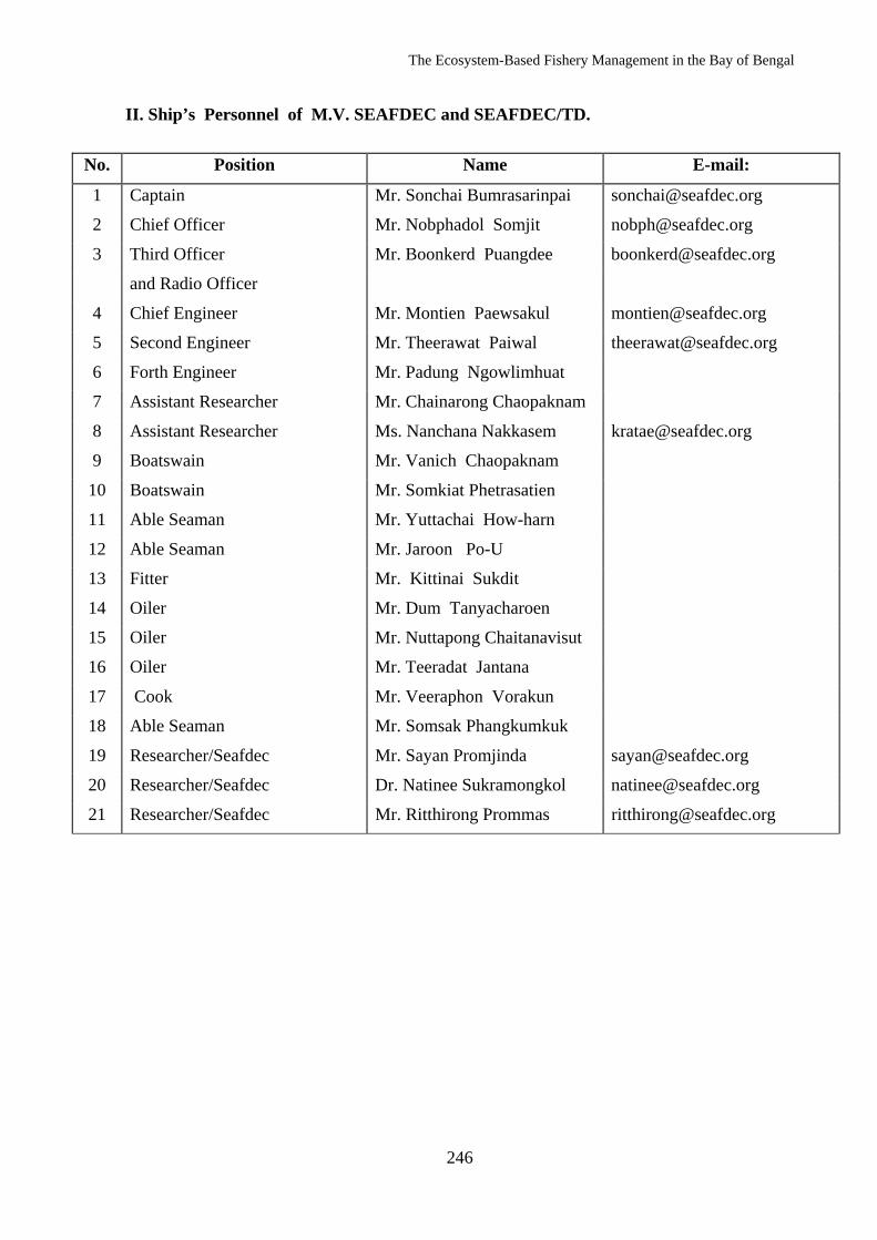
The Ecosystem-Based Fishery Management in the Bay of Bengal
246
II. Ship’s Personnel of M.V. SEAFDEC and SEAFDEC/TD.
No. Position Name E-mail:
1 Captain Mr. Sonchai Bumrasarinpai [email protected]
2 Chief Officer Mr. Nobphadol Somjit [email protected]
3 Third Officer Mr. Boonkerd Puangdee [email protected]
and Radio Officer
4 Chief Engineer Mr. Montien Paewsakul [email protected]
5 Second Engineer Mr. Theerawat Paiwal [email protected]
6 Forth Engineer Mr. Padung Ngowlimhuat
7 Assistant Researcher Mr. Chainarong Chaopaknam
8 Assistant Researcher Ms. Nanchana Nakkasem [email protected]
9 Boatswain Mr. Vanich Chaopaknam
10 Boatswain Mr. Somkiat Phetrasatien
11 Able Seaman Mr. Yuttachai How-harn
12 Able Seaman Mr. Jaroon Po-U
13 Fitter Mr. Kittinai Sukdit
14 Oiler Mr. Dum Tanyacharoen
15 Oiler Mr. Nuttapong Chaitanavisut
16 Oiler Mr. Teeradat Jantana
17 Cook Mr. Veeraphon Vorakun
18 Able Seaman Mr. Somsak Phangkumkuk
19 Researcher/Seafdec Mr. Sayan Promjinda [email protected]
20 Researcher/Seafdec Dr. Natinee Sukramongkol [email protected]
21 Researcher/Seafdec Mr. Ritthirong Prommas [email protected]
The Ecosystem-Based Fishery Management in the Bay of Bengal
247
Appendix 2 Opening ceremony of the Ecosystem-Based Fishery Management in the Bay of Bengal on 30 October 2007 in Phuket Province.
The Ecosystem-Based Fishery Management in the Bay of Bengal
248
Appendix 3 Oceanographic and drift gillnet operation on M.V. SEAFDEC
The Ecosystem-Based Fishery Management in the Bay of Bengal
249
Appendix 4 Pelagic longline operation
The Ecosystem-Based Fishery Management in the Bay of Bengal
250
Appendix 5 Closing ceremony of the Ecosystem-Based Fishery Management in the Bay of Bengal on 14 December 2007 in Phuket Province.

13
Offshore Seismic Campaign YWB Block Appendices – 11/14
223/231
APPENDIX D CV of Experts
| 06-14 CV Armeline Dimier Page 1
Armeline Dimier
Stakeholder Relationship and Social Impact Consultant
Water & Environment | RSE
Date of birth: December 12th 1985 Nationality: French Education:
- Master II in Geopolitics and International Relations, International Trade, International Law, Humanitarian Rights, Development Issues, Institut d'Etudes politiques de Toulouse, 2008
- Political Sciences Diploma (equivalent to a Master level), Politics and International Relations, Geopolitics, Institut d'Etudes Politiques de Grenoble and Sussex University in Brighton, 2007
Professional trainings: - Societal Management in Oil and Gas Operations, Total, February 2011 - Management of the relationships between NGOs and corporations, WWF Training Center, Paris, 2010
Languages: French (mother tongue), English (bilingual), Indonesian (bilingual), German (academic) Date of employment in Artelia: July 2014
CAREER SUMMARY | SKILLS
5-year experience in the field of corporate CSR strategy development in the oil & gas world, covering stakeholder mapping, consultation and engagement; social impact assessment, social management plan implementation and follow-up, community grievance management, and tools development. - Stakeholder mapping, consultation and engagement: mapping of stakeholders from the business,
authorities and civil society groups based on their interests and expectations, stakeholders’ priority ranking, development of consultation tools (interview questionnaire and guidelines), realization of consultations, development of engagement action plans in line with operational priorities.
- Social impact assessments and Social Management Plan implementation and follow-up: contribution to the realization of ESBS (Environmental and Social Baseline Assessment) and ESIA (Environmental and Social Impact Assessment) as well as Indonesian environmental and social studies (UKL-UPL and RKL-RPL), covering consultant identification, briefing, field survey preparation, quality control, and final hand-over. Development, implementation and follow-up of Social Management Plan.
- Community grievance management: development of claim registration database and claim handling
procedure.
- Tools development: integration of social data into GIS system, installation of societal management software (MOST).
| 06-14 CV Armeline Dimier Page 2
PROFESSIONAL EXPERIENCE
2014
MYANMAR Environmental and Social Impact Assessment for the Offshore Seismic Acquisition Campaign on the Block YWB - Coordination of the social impact assessment study realization with Artelia team in
Myanmar - Desk review of existing data and literature on the socio-economic context in which
the project takes place - Description of key socio-economic characteristics in the study area - Stakeholder mapping (business, authorities, civil society) - Analysis of stakeholders’ expectations and concerns - Assessment of social impacts - Development of appropriate mitigation measures and of the social management
plan Client: Total E & P Myanmar Position held: Social impact specialist
2014 SOUTH SUDAN
Environmental and Social Screening of 7 dam options for the Hydropower Expansion Plan and Regional Integration Plan of South Sudan into Regional Electricity Grid - Identification and selection of an appropriate set of criteria for measuring the
economic and social impacts (and performance) of each dam option - Desk review of existing data and literature on each criteria identified in order to
define current context and related sensitivities (example of criteria include land acquisition, physical displacement, health, food security, ethnic groups, public services, etc.)
- Assessment of potential impacts for each criteria and proposition of associated mitigation measures
- Ranking of impact importance for each criteria and each dam option - Final assessment of all the criteria for each dam option, in order to identify the most
performing option environmentally and socially Client: Nile Equatorial Lakes Subsidiary Action Program Position held: Social impact specialist
2014 BULGARIA
Preliminary Environmental and Social Impact Assessment for the offshore drilling of two exploration wells on Block 1-21 Han Asparuh - Coordination of the social impact assessment study realization with Artelia
Bulgarian team - Desk review of existing data and literature on the socio-economic context in which
the project takes place - Description of key socio-economic characteristics in the study area - Stakeholder mapping (business, authorities, civil society) - Analysis of stakeholders’ expectations and concerns - Assessment of social impacts
Development of appropriate mitigation measures and of the social management plan Client: Total E & P Bulgaria Position held: Social impact specialist
| 06-14 CV Armeline Dimier Page 3
2014 MAURITANIA
Environmental and Social Impact Assessment for the offshore drilling of one exploration well on Block C9 - Desk review of existing data and literature on the socio-economic context in which
the project takes place - Data collection of key socio-economic characteristics in the study area - Stakeholder mapping and analysis of stakeholders’ expectations and concerns - Assessment of social impacts - Development of appropriate mitigation measures and of the social management
plan Client: Total E & P Mauritanie Position held: Social impact specialist
PUBLICATIONS
“Re-engaging with Local Stakeholders in the Mature Oil and Gas Mahakam Block”, Technical paper presented during the Society of Petroleum Engineering (SPE) Conference on HSE in Long Beach, CA, on 20
th March 2014
PROFESSIONAL EXPERIENCE
2011 - 2014
Stakeholder Relationship and Social Impact Consultant, Total E&P Indonesie, Indonesia - East Kalimantan District operations:
- Stakeholder mapping and implementation of a consultation plan (interviews with 45 local and regional stakeholders); - Creation of a societal action plan, in line with company's requirements and stakeholders expectations in the fields of dialog, impact management, local content and community development projects; - Technical assistance for environmental and social baseline and impact studies: preparation of field work/surveys with the consultants, quality control and improvement of studies for Total Head Office and the Indonesian Ministry of Environment; - Improvement of internal societal procedures and standards in line with Head Office instructions: management of claim and grievances from local communities, mapping of social data using the company GIS - Implementation of mitigation measures for social impacts generated by specific operations (drilling, rig movement, seismic acquisition, etc.).
- West Papua District operations: stakeholder mapping, consultation preparation, including training of the field survey team. - Mentawai District operations: as a complementary study to the ESIA, stakeholder identification, mapping and ranking, Social Management Plan development and implementation, particularly related to control of contractors.
2010-2011
Societal Officer, Total Marketing France - Organizing cooperation between Total entities that have operations or projects in the region; - Preparing consultation of relevant external stakeholders, to identify how Total can contribute in achieving the region’s priorities in terms of economic and social development.
| 06-14 CV Armeline Dimier Page 4
FEB 2010 –
NOV 2010
Societal Coordination Officer, Total Supply & Marketing - Africa/Middle East Division, France - Realizing two annual surveys in the subsidiaries: AIDS Survey, aiming at assessing the progress of the policy of fight against AIDS and Societal Survey, aiming at collecting information on the CSR actions of the subsidiaries; - Improving the health policy (fight against AIDS and malaria) through awareness-raising campaigns; - Creating communication tools on the division CSR strategy, and particularly a brochure presenting the Division CSR strategy as well as subsidiaries projects in favor of social and economic local development.
SEPT 2008 –
MAY 2009
Societal Coordination Officer, Total Supply & Marketing - Africa/Middle East Division, France - Realizing two annual surveys in the subsidiaries: AIDS Survey, aiming at assessing the progress of the policy of fight against AIDS and Societal Survey, aiming at collecting information on the CSR actions of the subsidiaries; - Improving the health policy (fight against AIDS and malaria) through awareness-raising campaigns; - Organization of an annual internal sponsorship committee supporting initiatives from NGOs operating in our perimeter.
MAR 2008 –
AUG 2008
Public Fundraising Officer, Planet Finance - Monitoring of all the potential public donors and their related strategies/policies; - Research of public fundings: identification of donors and of their call for proposals; - Writing of proposals for big donors (EUROPEAID, USAID, IFC, Development Banks, etc); - Project management (logical framework, budget...); - Support to private fundraising team and contribution to the research of potential NGO and private companies partnerships.
| 07_2014 CV Frédéric Mathieu Page 1
Frédéric Mathieu
Project Manager
Water and Environment | Risks Society Environment Unit
Date of birth: 1966 Nationality: French Education and Training:
- Doctor in Ecology (Paris 7 University) : Chemical ecology of phytophagous insects, DEA Postgraduate Degree in Spectrochemistry and analytical organic chemistry (Paris 7 University),
- MST Degree in Management and Protection of the Environment (Paris 7 University). - Geographic Information System (ArcGis and 3D Analyst, ESRI 2001-2002) - Acoustics modeling (01dB Metravib: Mithra v5, 2001 and CadnaA, 2007-2010). - Hydraulic modeling (HEC RAS and River 2D) - GC-MS (Gas Chromatography and Mass Spectroscopy) (INRA, 1995-1997) - Health & Safety: First aid worker, CASC (firemen), 2008; - Health & Safety: Helicopter Underwater Escape Training (HUET), CETIS (Centre d’entraînement aux
Techniques Incendie et Survie des Marins-Pompiers de Marseille), 2008.
Languages: French (native language), English (medium), Spanish (basic) Date of employment in Artelia: 2007
CAREER SUMMARY | SKILLS
Frederic MATHIEU is a project manager with various environmental specializations: ecology, acoustic modeling, flooding area modeling, GIS (Geographical Information Systems), environmental discharges and insect control. His main responsibilities include performing environmental baseline surveys (EBS) and environmental impact assessments (EIA) in natural, urban or industrial contexts, acoustic modeling studies (often for inclusion in EIAs), GIS production and analysis, and natural area planning (tourism, education and preservation purposes).
He has experience in the following fields:
Management and project management
- Team management (up to 10 people), meeting facilitation, training, ... - Business Management: budget, technical responsibility, quality control, customer relationship
management, tendering, technical and commercial proposals ... - Supervision and carrying out technical studies, assistance in project management and
programming ... - Intervention for private and public sector in France, the TOM (French overseas territories) and
abroad (Algeria, French Polynesia, New Caledonia, Nigeria, Angola, Congo, Cameroon, Romania, Myanmar, Uganda ...)
Intervention areas: natural and industrial environments
- Baseline studies and field investigation (ecosystem / biodiversity, pollution, degradation of the environment, heritage, landscape, tourism potentials).
- Environmental Impact Assessment of industrial and development projects (subdivisions, roads, airports, tourist attractions, natural and urban areas...).
- Modelling the acoustic contribution of infrastructure and industrial projects. Sizing baffles, estimate overruns and isolation constraints.
- Creation of GIS (mapping and databases). - Flow modelling (1D and 2D) of streams for rehabilitation, flood risk and bank protection issues. - Calculation of supply and 2D hydraulic modelling applied to the design of artificial lagoons of big
hotels on the motu in Bora Bora.
| 07_2014 CV Frédéric Mathieu Page 2
- Development of natural environment and signalling. - Environmental management plan and environmental management system for industrial projects.
Tools: mapping, modelling, measurement and office softwares
- Acoustic Modelling: Mithra v5 CadnaA. Acoustic measurements: dBTrait frequency analyzer and sound level meters.
- ArcGIS Arc Map, Arc Catalog, 3D Analyst, Spatial Analyst and geodatabase in Access. - HEC RAS modelling and 2D River and all rules of thumb calculation (design flow, bank protection,
storm basin, thrust, and effluent dilution). - Sampling methods, probes and interpretation for many investigation settings of the natural and
industrial environment (surface water, groundwater, air and soil). Use of many national and international standards.
- Data analysis: STATISTIQUA: ANOVA, regression, factor analysis, parametric and nonparametric tests.
- Gas chromatography and mass spectrometry. - CAO: Microstation, PAO: Photoshop, GIMP, COREL suite, Office: Office and openoffice pack;
Database: Access.
PROFESSIONAL EXPERIENCE
MAIN ENVIRONMENTAL IMPACT ASSESSMENT AND ENVIRONMENTAL BASELINE STUDIES
INDUSTRIAL PROJECTS IN NATURAL ENVIRONMENTS
2013-ONGOING CAMEROON
Assessment of socio-economic and environmental conditions related to electricity and interconnection production options This study, conducted within the framework of the hydroelectricity expansion plan and the South Sudan regional integration plan in the regional electricity network, aims at: (i) carrying out an environmental assessment for the various projects and (ii) implementing a set of quantifiable environmental and social criteria/indicators helping to rank supply options. Client : NILE BASIN INITIATIVE / NELSAP (supported by the World Bank) Position : Project manager/environment expert
2013-ONGOING CAMEROON
Lom Pangar hydropower project, independent environmental and social technical audit The objective of this audit is to control independently the compliance of the implementation of the environmental and social obligations during the construction and the implementation phases. These obligations are mainly included in the project’s Environmental and Social Management Plan (ESMP), but other instructions can be established during the project, and the ESMP can be slightly modified. Client : EDC Position : Support expert for the impact assessment and building site follow-up
2014-ON GOING DRC
Environmental study of five oil fields in operation Field missions, control of water and environment quality, modelling framework of air quality (source terms and reference values) Client : Perenco Position : Environment expert for water and air contamination (including field mission)
| 07_2014 CV Frédéric Mathieu Page 3
2014 – ON GOING FRANCE
Risk assessment of ODC pipeline network Analysis of national reference documents (BSS, LISA, ADES, CARTHAGE, protected areas…) by geoprocessing to assess the environmental seriousness of the leak scenarios on the 1,300-km pipeline (in compliance with GESIP guide appendix 11). Client : TRAPIL Position : Project manager of the chapter concerning the environmental seriousness of the study
2013-2014 CAMEROON
Follow-up of sea turtles in Cameroon within the framework of CLNG project environmental assessment The preliminary ESIA of CLNG project underlines the potential cumulative impact on sea turtles of the projects related to Kribi port complex. Specific studies are required before the ESIA is conducted Activities: Implementing the study on site: choosing the team by taking into account methodological and social aspects, reinforcing the team skills with training session and selecting the sites. Client : GDF Suez Position : Project manager
2012-ONGOING DRC
Environmental and Social Impact Assessment (ESIA) for the Graben Albertine – Block III Seismic Project (Nord Kivu and Province Orientale) The Project comprises a 2D seismic survey in Easter Congo DRC. Block III of Graben Albertine extends over 3200 km2 and close to the Virunga national parc. Position held: Project Manager of the ESIA, Field mission, stakeholder consultation and village inquiry
Social field survey
ESIA/ESMP report
Public consultation
Management of the GPS mapping with a local NGO Client : Total Position : Project Manager of the ESIA, Field mission, stakeholder consultation and village inquiry
2013 CONGO
Environmental and Social Impact Assessment (ESIA) for Moho North and Phase 1 bis Oil and Gas exploitation Project Moho Nord and Moho Phase 1 bis are two oil and gas development project in deep offshore. Project includes: (i) drilling activities, (ii) construction/operation of the facilities such as Tension leg platform and Floating Production Unit, (iii) construction/operation of an export pipeline and (iv) on shore equipment in the existing oil treatment/export complex of Djéno.
Assessment of Best Available Technology
TDR of the project and associated stakeholders consultation
ESIA/ESMP of the two projects and public consultation activities
Health study Client : Total E&P Congo Position : Project manager of the TDR, ESIA/ESMP also involved in public consultation
2012-ONGOING CAMEROON
Environmental and Social Impact Assessment of CLNG project (Cameroon Liquefied Natural Gas) Conduct studies on the impact of assessment activities onsite, on the liquefaction plant and gas pipeline. The mission also includes carrying out field investigations and public consultation throughout the process. Client : GDF Suez Position : Senior Engineer, Head of field mission
| 07_2014 CV Frédéric Mathieu Page 4
2012-ONGOING CONGO DRC
Environmental and Social Impact Assessment and Resettlement Action Plan (RAP) for pilot industrial area project ESIA and RAP conducted according to World Bank processes. Client : World Bank Position : Responsible for scoping mission
2012 UGANDA
Environmental Impact Assessment for a drilling exploration campaign for TOTAL Quality control and knowledge transfer for local engineering office Client : Air Water Earth (AWE) Engineers Position : Field investigation supervision, review of reports and training
2009 – 2015 FRANCE
Baseline study and definition of an environmental monitoring program for CO2 geological storage of, site of Rousse Inventory of fauna and flora, monitoring of groundwater and surface water quality (chemical and biological). Phase 2: monitoring plan implementation (2010-2015) Client : TOTAL Position : Project manager
2011 OMAN
Baseline study for an incinerator and a hospital waste landfill site on a deserted site Field operation, sampling and results analysis (soil, air, noise) Client : Sogreah Oman Position : Environment expert
2010 FRANCE
Environmental statement to support permit application in 4 blocks (oil and gas) Environmental statement for onshore exploration drilling project and seismic acquisition survey of the shale gas reserves in four departments in northern France. The study was undertaken in compliance with French legislation. Development of a specific GIS database Client : Elixir Position : Project manager
2011 FRANCE
Environmental statement to support permit application in 3 blocks (oil and gas) Environmental statements undertaken in compliance with French legislation.. Client : Basgas Position : Project manager
2010 MYANMAR
Environmental monitoring survey of Yadana offshore TEPM platform Environmental survey of site and surrounding areas, including seawater and sediment analysis, and identification of benthic fauna species. The study is conducted in accordance with Total internal standards. Evaluation of potential impacts of Yadana platform activities on marine environment and comparison of the results with previous studies. Client : TOTAL Position : Project manager
2011 MYANMAR
EIA and Environmental Management Plan (EMP) of offshore seismic acquisition campaign of Yadana block Environmental baseline study of project area; Environmental Impact Assessment in accordance with client standards. Acoustical issues related to marine mammals Client : TOTAL Position : Project manager and acoustic expert
| 07_2014 CV Frédéric Mathieu Page 5
2012 MYANMAR
EIA and EMP of subsidence project of Yadana offshore TEPM platform Relocation of activities and quarters as a result of subsidence on the Yadana Complex offshore platform due to gas extraction.
- EIA for the decommissioning of existing facilities - Assessment for the installation of new infrastructure.
Client : TOTAL Position : Project manager and acoustic expert
2010 ALGERIA
EBS (Environmental Baseline Survey) for an exploration project in the Ahnet block Environmental Baseline Study (EBS) of Ahnet block, in particular future drilling sites. The study included:
- Evaluation of soil, groundwater and surface water contamination and air quality tests;
- Investigation of the biological environment (fauna-flora) and archaeology; - Meeting with stakeholders.
Client : TOTAL Position : Project manager
2010 ALGERIA
EIA for a drilling exploration project in the Ahnet block Environmental Impact Assessment performed in compliance with Algerian legislation based on the previous EBS. The study included:
- Baseline environmental assessment (landscape, fauna, flora); - Evaluation of environmental and social impacts; - Definition of mitigation measures; - Preparation of a Management Plan
Client : TOTAL Position : Project manager
2009-2010 ALGERIA
EBS (Environmental Baseline Survey) for exploration project in Rhourde Yacoub block Involved of an Environmental Baseline Study (EBS) including:
- Field survey: air quality measurement, water and soil quality analysis, flora and fauna investigation,
- Fauna and flora identification and archaeological inventory; - Satellite image analysis; - Assessment of environmentally sensitive elements; - Meeting with stakeholders.
Client : Ruhrgas Position : Project manager
2009-2010 ANGOLA
Pre-EIA for the implementation of a FPSO (Floating, Production, Storage and Offloading) for the CLOV development project in block 17 Preliminary Environmental Impact Assessment (pre-EIA) for the development of 4 fields on block 17. The CLOV project situation is offshore Angola in a water depth of approximately 1,100 m to 1,400 m, and includes: a FPSO (Floating, Production, Storage and Offloading), a Subsea Production System (SPS), and drilling of 34 wells. The tasks performed included:
- Environmental impact assessment; - Definition of mitigation measures; - Energy efficiency and greenhouse gases emissions assessment; - Preparation of an Environmental Management Plan.
Client : TOTAL Position : Project manager
| 07_2014 CV Frédéric Mathieu Page 6
2009 CONGO
EIA (Oil & Gas) 3D seismic acquisition survey in Block “Haute Mer” Preparation of Environmental Impact Assessment for exploration seismic survey in “Haute Mer” C block including:
- Preparation of the EIA in accordance with Congolese legislation - Recommendations for seismic survey methodology to minimize impact on
marine mammals. Client : TOTAL Position : Project manager
2010 NIGERIA
Preliminary Environmental Impact Assessment (PIAR) for the extension of the Amenam platform Preliminary Environmental Impact Assessment (PIAR) in accordance with Nigerian regulation and Total standards. The PIAR includes:
- Environment description; - Waste, discharge and emission inventory; - Evaluation of the impacts and mitigations measures; - Environmental Management Plan.
Client : TOTAL E&P Position : Project manager
2009-2012 ANGOLA
EIA and EMP for the offshore seismic acquisition campaign in block 32 (deep sea) - Description of the baseline environment - Preparation of the environmental impact assessment in compliance with
Angolan legislation Client : TOTAL Position : Project manager
2008 ALGERIA
Pre EIA and EMP for Timimoun licence development project The socio-economic baseline survey was carried out on 3 Daïras and 2 Wilayas around the Timimoun block. The aim was to understand the socio-economic context of human development within the project area, and improve local community involvement. The mission included: - A detailed description of the human, social, economic and cultural context; - A number of interviews of main stakeholders including local administrative authorities, associations, NGOs, religious and educational organizations, etc. - Stakeholder mapping; - Client support for the regulatory public consultation process with participation; - Impact assessment and definition of mitigation measures; - Social Management plan. Client : TOTAL Position : Project manager and acoustical expert
2010 ALGERIA
ESIA for 3D seismic acquisition survey in Timimoun Block - Description of the environmental baseline study - Preparation of the environmental impact assessment in compliance with the
Algerian laws Client : TOTAL Position : Project manager
2008-2011 NIGERIA
EIA (Oil & Gas industry) Pre- Environmental and Societal Impact Assessment (ESIA) for the EGINA field development project Client : TOTAL Position : Project manager
| 07_2014 CV Frédéric Mathieu Page 7
2008 ANGOLA
EIA and EMP for the 4D seismic acquisition campaign in block 32 (offshore) - Description of the environmental baseline study - Preparation of the environmental impact assessment in compliance with
Angolan legislation Client : TOTAL Position : Project manager
2008 ANGOLA
EIA and EMP for the 4D seismic and electromagnetic acquisition campaign for block 17 (offshore)
- Description of the environmental baseline study - Preparation of the environmental impact assessment in compliance with
Angolan legislation Client : TOTAL Position : Project manager
2009-2010 FRANCE
Pre EIA and EIA for the installation of a solar power plant Field surveys, EIA in compliance with French regulation. Issues: landscape and viticulture Client :Photowatt Position : Project manager
2009-2010 FRANCE
Pre EIA for the implementation of a solar power plant Field surveys, pre EIA in compliance with French regulations. Issues: landscape and flora Client :POWEO Position : Project manager
2010-2012 FRANCE
EIA for the wind farm installation project in the Forez Mountains Landscape, acoustic and faunal issues. Field survey organization, acoustic measures and modelling, landscape integration Client : ENR du Forez Position : Acoustic expert
2007 FRENCH
POLYNESIA TUAMOTU
EIA for the installation of a wind farm on Makemo Island Field baseline study, acoustic measures and modelling, landscape integration Client : Private Position : Project manager and acoustic expert
2003 FRENCH
POLYNESIA TAHITI
EIAs for Development of Faratea Harbour Field investigation, preparation and sampling of the environmental and social baseline study in compliance with Polynesian legislation Client : Établissement des Grands Travaux de Tahiti Position : Project manager
INDUSTRIAL PROJECTS IN INDUSTRIAL AND URBAN ENVIRONMENTS
| 07_2014 CV Frédéric Mathieu Page 8
2009-2010 ALGERIA
EIA, ESBS (Environmental and Social Baseline Survey), EMP for a Gas Liquefaction Plant in Arzew
- Environmental and Social Baseline Survey (ESBS); - Environmental Impact Assessment (EIA); - Noise Assessment; - Environmental Management Plan; - Risk assessment including HAZID review, calculation using PHAST software,
fault tree and event tree analysis, risk acceptability analysis. Client : Saipem-Sonatrach Position : Project manager
2007-2008 ALGERIA
EIAs and EMP for construction of thermal power plants Harbour of Algiers, Harbour of Annaba, Koudiet
- Environmental Impact Assessment (EIA), - Environmental Baseline Survey (EBS), - Risk Assessment, - Environmental Management and Monitoring Plan, - Waste Management Plan - Restoration Plan
Client : General Electric, Iberinco Position : Project manager and acoustic expert
2006 TAHITI
Environmental Studies for industrial and port development in Taravao Field study, sampling and preparation of the environmental and social baseline study in compliance with Polynesian legislation Client : Établissement des Grands Travaux de Tahiti Position : Project manager
2003 TAHITI
Identification of environment discharges and characterization studies of Papeete Harbour / Emissaries inventory Database development, GIS of physic-chemical and biological measures over a 20 year period. Analysis and interpretation of current-meter, physic-chemical and biological data. Analysis of main elements. Supervision of a diving mission to conduct the inventory and visit all the emissaries of the bay. Client : The Port Authority of Tahiti Position : Project manager and GIS expert
2008 FRANCE
Diagnosis of soil pollution, Paris airport Field operations, analysis interpretation and report Client : Veolia Position : Project manager and GIS expert
OTHER EIAS OF DEVELOPMENT PROJECTS IN URBAN CONTEXTS
2000-2007 FRENCH
POLYNESIA TAHITI
10 EIAs for the construction of housing estates 3 EIAs for the construction of commercial centers 2 EIAs for high school constructions 2 EIAs for the creation of commercial activity areas Client: Private and public sectors Position: Project manager, Study engineer and acoustic expert
| 07_2014 CV Frédéric Mathieu Page 9
EIAS OF DEVELOPMENT PROJECTS IN NATURAL CONTEXTS
2013-ONGOING MALI, BURKINA
FASO AND GHANA
West African Power Pool Interconnexion project of the electrical network of Ghana, Burkina and Mali Update of ESIAs and RAPs of the 3 countries taking into account comments of BAD (African Bank of development) and BEI (European Bank of Investment. Proposal of a shared ESIA and RAP background for the 3 countries to homogenise requirements and reports. ESIA and RAP of an extension of the main project in Ghana (section Ham Tumu and Ham Bolgatanga) Preliminary ESIA/RAP and TDR/Budget of the ESIA/RAP for a section of the electrical network in Mali. Client : Economic Community of West African States Position: Project Management and Environmental expert.
2013-ONGOING BURUNDI
Environmental and Social Impact Assessment (ESIA) and Resettlement Action Plan (RAP) for Jiji and Mulembwe Hydroelectric projects, including outgoing power line to Bujumbura and secondary networks connections surrounding urban centres. The project, named Jiji and Mulembwe Hydroelectric Complex”, comprises 3 components: the Mulembwe hydroelectric project (16,5 MW), the Jiji project (31,5MW), and the network of 220/110/33 kV transmission lines conveying the energy produced. (i) Policy framework of the population resettlement, (ii) ESIA/ESMP and RAP for each dam and HT power line projects and (iii) policy framework of the environmental and social management of the secondary electrification project. Involved in the ESIAs, ESMPs, RAPs completion and public consultations Client : Ministry of Energy and Mines – Régie de production et distribution d’eau et d’électricité (REGIDESCO) Position : ESIA expert
2012-ONGOING MALI
Hydroelectric project - Felou Monitoring of mitigation measures of impacts on the environment during the construction phase. Client : OMVS (Organisation for the Promotion of Rivers in Senegal) Position : Environmental expert
2011 CAMEROUN
EIA for Nachtigal dam project Organization and participation in the field survey (10 days, 12 people) for soil occupation, health, fishing and socio-economic aspects. Update of 2006 EIA report. Presentation of the impact study during public update meetings Client : ALUMINIUM PECHINEY (Rio Tinto Alcan) Position : Environmental expert
2006 FRENCH
POLYNESIA TAHITI
EBS for a dam construction project in endemic rain forest with a rich archeological importance - Papeiha Baseline study in an area of high biodiversity in French Polynesia Client : Projet privé Position : Environmental expert
| 07_2014 CV Frédéric Mathieu Page 10
2005 FRENCH
POLYNESIA NUKU HIVA
EIA for road construction in the endemic rainforests of Toovii Ridge Flora description in a forest of rich biodiversity in French Polynesia. The analysis resulted in the modification of the road layout Client : Direction of Urban planning Position : Project manager
2003 FRENCH
POLYNESIA TAHAA
EIA for the construction of the Dassin hotel Domain in Tahaa - Description of natural resources - Impact assessment - Suggestion for natural wealth enhancement and protection
Client : Private project Position : Environmental expert
2005 FRENCH
POLYNESIA BORA BORA
EIA for the construction of the Saint-Régis Bora Bora Resort hotel - Description of natural resources - Impact assessment - Suggestion for natural resources enhancement and protection - Development of a particular impact analysis methodology on landscape thanks
to a cartographical approach - Implementation of artificial reefs in the lagoon to develop coral colonies and
increase biomass Client : Private project Position : Project manager
2000 FRENCH
POLYNESIA BORA BORA
EIA for the construction of the Eden Garden hotel in Bora Bora - Description of natural resources - Impact assessment - Suggestion for landscape optimization to limit pesticide use in mosquito
treatments Client : Private project Position : Project manager
2002 FRENCH
POLYNESIA BORA BORA
EIA for the construction of the Bora Bora Nui Resort hotel - Description of natural resources - Impact assessment - Suggestion for natural resources enhancement and protection - Displacement of the coral colonies doomed to destruction to create submarine
landscapes - Implementation of artificial reefs to restore marine biomass
Client : Private project Position : Engineer
2007 FRENCH
POLYNESIA HUAHINE
EIA for hotel construction at Bali Hai Resort - Description of natural resources - Suggestions for the restoration of unsanitary lagoon
Client : Private Position : Project manager

| 07_2014 CV Frédéric Mathieu Page 11
1999-2005 TAHITI
EIAs for airfield construction on isolated islands such as Kahuehi, Rimatara and Atuona Islands
- Natural resource description - Impact assessment - Recommendations - Public consultation
Client : French Polynesian Ministry of Planning Position : Engineer
2004 FRENCH
POLYNESIA HUAHINE
EBS for a golf course in a region of rich archeological and natural importance - Natural resource description (biodiversity, landscape, historic sites) - Risk assessment related to facilities - Enhancement recommendations, suggestions
Client : Private project Position : Project manager
2000 FRENCH
POLYNESIA
Analysis of physic-chemical elements in Maeva Lake Bibliographical synthesis, specific solutions to take lagoon sediment samples and interpretation of further sediment analyses Client : Board of environment Position : Project manager
NATURAL AND URBAN AREAS PLANNING
2006 FRENCH
POLYNESIA
GIS design of the main biodiversity and cultural heritage spots of French Polynesia
- Collection of data : fauna, flora and ecosystems thanks to taxonomist experts - Information coding - Data base setup - GIS data formatting
Client : Board of the environment Position : Project manager
2006 FRENCH
POLYNESIA
Tetiaroa atoll Phase 1: synthesis and compilation of existing scientific documents Phase 2 : GIS organization, compilation and synthesis of the expertise mission (biodiversity, archaeology, landscape, coral ecosystem, fishing areas), multi-criteria analysis of ranked results and recommendations Client : Board of the environment Position : Project manager
2005 FRENCH
POLYNESIA
Participation in Papeete waterfront development architecture contest - Management of environmental aspects with the architecture - Environmental suggestions - Participation in the report presentation
Client : Établissement des Grands Travaux Position : Environment expert
| 07_2014 CV Frédéric Mathieu Page 12
2006 FRENCH
POLYNESIA
Design of the GIS geodatabase for the dead bodies development study in French Polynesian lagoons Development of the geodatabase and need survey interpretation Client : Board of the environment Position : GIS expert
2005 FRENCH
POLYNESIA
Feasibility study for the EcoParck implementation on Pearson domain site Eco Parck is the project of an association helped by the government for the implementation and promotion of sustainable development thanks to demonstrators in field such as energy, cultural practices, eco-construction, sorting and waste treatment.
- Natural resource description - Facilities environmental risks assessment - Suggestion for a project management structure - Sustainable development concept presentation
Client : Board of the environment Position : Project manager
2004-2005 FRENCH
POLYNESIA
Environmental Baseline Survey and planning proposal for 7 tourism spots Areas of interest concerning landscape, archeology, biodiversity and recreational activities
- Natural resource description - Suggestion for enhancement regarding historical, biological, legacy and
landscape constraints Client : Board of the environment Position : Project manager
2002-2008 FRENCH
POLYNESIA
Planning of Ane Ane land and creation of pedagogic paths - Natural resource description (biodiversity, landscape and historic sites) - Risk assessment related to facilities - Suggestions to enhance and use a natural area - Programming - Planning design and construction (paths, shelters, signage and panoramic
views) Phase 1: Baseline study Phase 2: Planning program Phase 3 : APS for the design and construction of an educational path Phase 4 : signage design (visual, educational content, selection of construction methods) Phase 5: project management, works ending in 2008 Client : City of Arue Position : Project manager
2003-2004 TAHITI
Re-creation of an urban square “le parc de Bougainville” with garden and landscape design Project management Client : City of Papeete Position : Project manager
| 07_2014 CV Frédéric Mathieu Page 13
2000-2004 FRENCH
POLYNESIA
Planning of Fautaua valley Archeological, geological, hydrogeological biodiversity and natural resources
- Natural resource description - Environmental and social assessment approach - Environmental hazards - Sustainable development policy
Phase 1: EDL Phase 2: planning program Phase 3: pilot study, content and GIS Client : Papeete Municipality Position : Project manager
ACOUSTIC MODELING MOST OF THE EIAS PERFORMED SINCE 2001 INVOLVE ACOUSTIC MODELING USING MITHRA (CSTB) OR CADNAA (DATAKUSTIK).
2012-ONGOING
REUNION ISLANDS Acoustic study for ZAC Renaissance project Initial state modeling (CadnaA), Project modeling (CadnaA), Assistance with the ground-plan optimization Client : Public institution in the Reunion Islands Position : Acoustic expert and project manager
2012 FRANCE
Acoustic study for an EIA: Bus of a high level of service between Place Castellane and the Luminy university Initial state modeling (CadnaA), Project modeling (CadnaA) Client : Public institution in Marseille Position : Acoustic expert and project manager
2011-2012 FRANCE
High Speed Line, PACA region Acoustic constraints study for PACA train line route selection (halos method) Client : RFF Position : Acoustic expert
2011 FRANCE
Noise black spot reduction - Baseline measurements - NF S31-085 measurements - Modelling of the selected option (using CadnaA) - Assistance with public presentation
Client : ASF Position : Project manager and acoustic expert
2011-2012 FRANCE
Noise study for ZAC Saclay project - Baseline measurements (NF S31-010) - Baseline modelling using CadnaA - Help with the ground plan optimization
Client : Public institution Paris-Saclay Position : Project manager and acoustic expert
2011 ALGERIA
Gas pipeline project from Algeria to Italy Noise study of the compression center within the framework of an EIA Client : Galsi Position : Acoustic expert
| 07_2014 CV Frédéric Mathieu Page 14
2011 FRANCE
Acoustic pre diagnosis for a windmill installation in Saint-Louis, Marie-Galante island Environmental initial measures and modelling Client : VAKUOENERGY Position : Acoustic expert
2011 FRANCE
Acoustic pre-diagnosis for a wind farm installation in Saint-Joseph, La Réunion Environmental initial measures and modelling Client : VAKUOENERGY Position : Acoustic expert
2011-2012 REUNION ISLANDS
Acoustic study for ZAC Saint-Paul project - Initial measures NF S31-010 - Initial state modelling (CadnaA) - Project modelling (CadnaA) - Assistance with the ground-plan optimization
Client : Artelia Position : Acoustic expert
2006-2008 FRENCH
POLYNESIA
Noise mapping of Papeete Methodology in accordance with the European directive EC/ 2002/49:
- Road noise and significant industrial contribution - Calibration with field measurements
Client : Papeete Position : Project manager and acoustic expert
2003 FRENCH
POLYNESIA
Acoustic modelling for a motocross training field - Baseline measurements NF S31-010 - Project modelling (Mithra) - Impacts on neighbouring houses
Client : Papeete Position : Project manager and acoustic expert
2001-2010 FRENCH
POLYNESIA
Acoustic measurements and modelling of rock crushing stations, treatment stations and cold rooms Client : Private client Position : Acoustic expert
DECONTAMINATION – HYDRAULIC – HYDROGEOLOGY
2007 NEW-CALEDONIA
Creek Liliane study - Field prospecting - 2D modelling - Remediation measure suggestions for the river damaged by mining activities.
Client : DAVAR Position : Project manager
2007 NEW-CALEDONIA
Swamp bridge construction Dimension hydrologic and hydraulic technic study Client : SLN Position : Project manager
| 07_2014 CV Frédéric Mathieu Page 15
2006 NEW-CALEDONIA
Hydrologic and hydraulic note regarding Potiaai housing building project 1D modelling (HAC RAS) Flooding hazards Bank protection Client : Teva I Uta town Position : Project manager
2006 NEW-CALEDONIA
Sizing of four storm basins for Pukalia Nui apartment complex construction Sizing of storm basins regarding EIA recommendations Client : Punaauia city Position : Project manager
2006 NEW-CALEDONIA
Paul Creek study - Field prospecting - 2D modelling - Remediation measure suggestions for the river damaged by mining activities.
Client : Le Nikel Position : Project manager
2006 FRENCH
POLYNESIA
Assessment of well watershed in Bora Bora Research setting up the watershed protection perimeters
- Environmental baseline study - Possible contamination pathways - Groundwater body flows - Suggested protection zones for the entire island - Identification of affected cadastral parcels
Client : Bora Bora city Position : Project manager
2006 ROMANIA
Supervision of a testing pump for the establishment of the capture of an industrial site Identification of the hydraulic characteristics of the well Client : Renault Position : Field engineer
2006 NEW-CALEDONIA
Hydrologic and hydraulic memo for Toofa housing project 1D modelling (HAC RAS) Flood hazards Bank protection Client : Renault Position : Field engineer
2004-2006 FRENCH
POLYNESIA
Hydraulic modelling (2D, river 2D and empiric method) to design artificial lagoons and beaches for the development of high luxury hotel in Bora-Bora Within the framework of an artificial lagoon design, the water carriage system is created according to a particular approach.
- Level study regarding the lagoon and the submarine plateau - System sizing according to renewal constraints related to artificial biotope
Client : Intercontinental hotel and Saint-Régis hotel Position : Field engineer
PUBLICATIONS

| 07_2014 CV Frédéric Mathieu Page 16
Seven publications in international research bulletins, eleven publications in international
conferences and other research on internal communications concerning ecological chemistry of insects: Semiochimic relationships inter and intra specific, orientation behavior, population dynamic, set up of emission/extraction devices (Dynamic and static head space, solid phase micro extraction,) and analysis of volatile and semi volatiles organic compounds emitted by plants and insects (GC-MS)
EMPLOYMENT RECORD
1998-2007 Environment project manager, SNC Pae Tai Pae Uta (French Polynesia).
Responsible for the development of new technical skills (GIS, hydraulics and acoustics)
1991-1997 Researcher in the chemical ecology of plant-eating insects, IRD and INRA
| 07 2012 CV Christophe DERRIEN Page 1
Christophe DERRIEN
HSE Project Director / Head of RSE department
Water & Environment | Risk, Society and Environment department (RSE)
Date of Birth : 20/05/1973 Nationality : French Education and Training:
MSC in Industrial Risks & Environment at the University of Lyon BSC in Environmental Engineering at the University of Lyon (with Honors) Helicopter Underwater Escape Training (HUET) valid until October 2013 Occupational Risk Prevention and Safety (INRS) Safety Management / ISRS (DNV) Environmental expert in chemical industries (UIC) HAZOP reviews (ARTHUR D. LITTLE) Environment and Quality internal Audit – ISO 14001 (APAVE) Safety Engineering (ENSPM FI)
Languages : French (mother tongue), English (fluent), Spanish (beginner) and Italian (intermediate) Start date in Artelia group : 2008
CAREER SUMMARY | SKILLS
- HSE management of industrial projects - HSE management : contingency plans, crisis management, management systems and audits
(SGS SEVESO 2 ; ISO 14001, OHSAS 18001 ; ISRS ; MASE ; ILO OHS 2001) - Risk and industrial environment assessment (SEVESO safety reports, environmental impact
assessments, pipeline assessment, permits and authorisations…) - Industrial risk analysis (APR, HAZID, AMDEC, …) - Occupational safety - Training conception and hosting, University teaching
PROFESSIONAL EXPERIENCE
INDUSTRIAL RISKS ASSESSMENT (ENVIRONMENT & SAFETY)
2012-2015 CAMEROON
Cameroon LNG project Environmental and social impact assessment (LNG plant, Offshore feed pipelines network), environmental and social management plan, offshore environmental, baseline survey, public consultations, biodiversity action plan, … Client : GDF Suez Position : Project director
2013 ALGERIA
GPL pumping station ELR-1, Hassi Messaoud Environmental and societal impact assessment, technological risk assessment (including HAZID and Fire & Explosion Risk Analysis) Client : ABB Spa Process & Automation pour SONATRACH TRC Position : Mission manager
| 07 2012 CV Christophe DERRIEN Page 2
2007-2014 GABON
Emergency management, Large Scale Exercises Organization of more than 5 Large scale exercises and training sessions on site (Cap Lopez, Atora, Mboumba, Anguille, and other off-shore sites,…) Client : TOTAL GABON Position : Project director
2013 CYPRUS
Offshore seismic campaign (block 11) Environmental and societal impact assessment Client : TOTAL E&P CYPRUS Position : Mission manager
2013 ALGERIA
Seismic campaign, exploration drilling, Hassi-Bir-Rekaiz block Environmental and societal impact assessment Client : PTTEP Position : Mission manager
2013 ALGERIA
Rhourde-Er-Rouni block Environmental baseline study, environmental liabilities study Client : CEPSA Position : Mission manager
2012-2014 CONGO
Moho Nord Project : submarine wells, FPU, TLP, integration N’Kossa, integration to Djeno terminal Environmental and societal impact assessment, health risk assessment Client : TOTAL E&P Congo Position : Mission manager
2013 MAURITANIA
Subsidiary Emergency Plan Development, organizing a full scale exercise Client : TOTAL EP MAURITANIE Position : Mission manager, HSE senior consultant
2012 MAURITANIA
Offshore oil exploration program on block C9 project (seismic, bathymetry, coring) Environmental & Social Baseline Survey Client : TOTAL E&P Mauritania Position : Project Director
2012 BRUNEI
DARUSSALAM
ML South project : platform well construction, drilling, sea line installation, and extension of the onshore gas treatment plant Environmental & Social Baseline Survey Client : TOTAL E&P Borneo Position : Project Director
2012 DRC
Maluku Special Economic Zone project Environmental & Social Baseline Survey, resettlement Action Plan (IFC standards and RDC regulations) Client : World Bank / IFC Position : Project Director
| 07 2012 CV Christophe DERRIEN Page 3
2011-2012 ALGERIA
GALSI Project : natural gas compression facility and underwater gas export pipeline Algeria-Sardinia-Italy Risk assessment, Site Contingency Plan, Atex survey, lightning assessment, environmental impact assessment, Environmental Management Plan Client: GALSI : SONATRACH – EDISON – ENEL Position : Project Director
2011 CHINA
Modified starch synthesis workshop Risk assessment, HAZID Client: ROQUETTE Position : Project Director
2011 ALGERIA
Rhourde Nouss Gas Treatment Facility Risk assessment of the 4th compression train Client: JGC / SONATRACH Position : Project Director
2010-2011 BAHREÏN
TATWEER project Production water treatment : HAZID, Fire Risk Review, HAZOP Client: VEOLIA WATER SOLUTIONS OIL & GAS Position : Project Director
2010 ALGERIA
Gassi Touil Production Center (CPF) Risk assessment Client: JGC / SONATRACH Position : Project Director
2009-2010 ALGERIA
Guellala and Haoud Berkaoui Production Center Revamping (CPF) Risk assessment Client: ABB / SONATRACH Position : Project Director
2009 ALGERIA
LPG-LDHP project in Hassi-Messaoud Environmental Impact Assessment Client: SAIPEM /SONATRACH Position : Project Director
2009 ALGERIA
GNL-3Z project Liquefaction, storage and offsite train at Arzew Risk assessment and Environmental Impact Assessment Client: SAIPEM-SNAMPROGETTI / SONATRACH Position : Project Director
2009 CONGO
HMC permit Offshore seismic survey on HMC permit Client: TOTAL E&P CONGO Position : Project Director
| 07 2012 CV Christophe DERRIEN Page 4
2008 ANGOLA
FPSO Dalia Environmental assessment on FPSO Dalia loading buoy incident Client: TOTAL E&P ANGOLA Position : Project Director
2009-2010 ANGOLA
FPSO CLOV project Environmental Impact Assessment Client: TOTAL E&P ANGOLA / CLOV PROJECT GROUP Position : Project Director
2009 France
Risk analysis of an industrial waste grouping facility Client: SITA SUEZ Position : Project Director
2009-2010 CONGO
Liambou industrial waste management facility Detailed fore project, Company consultation file, Risk assessment Client: TOTAL E&P CONGO Position : Project Director
HSE MANAGEMENT, CONTINGENCY MANAGEMENT & SITE CONTINGENCY PLAN PREPARATION
2012 ALGERIA
Groupement TFT Gas Treatment Facility Site Contingency Plan review according to new ARH canvas Client: Groupement TFT (SONATRACH – TOTAL – REPSOL) Position : Project Director
2011-2012 FRANCE AND
EUROPE
HSE Regulatory context study of the exploration-production of shale gas and intranet tool development: Client: Confidential Position : Project Director
2011 FRANCE
Risk Management Training to French site directors Client: NEXANS Position : Trainer
2011 ALGERIA
Rhourde Nouss Gas treatment facility Site Contingency Plan of the gas treatment facility Client: JGC / SONATRACH Position : Project Director
2011-2012 FRANCE
Rewriting of the antipollution development plan methodological guide Client: TOTAL/DGEP/HSE/ENV Position : Project Director
SINCE 2008 FRANCE
Training and tabletop exercise for the members of the Emergency Management Unit (4 missions) Client: TOTAL Exploration & Production, General Management Position : Project Director
| 07 2012 CV Christophe DERRIEN Page 5
SINCE 2006 WORLD
Emergency Management Unit training and organization of emergency simulation exercises Indonesia, USA, Russia (3 missions), Italy (5 missions), GTFT (Algeria, 5 missions), Congo (2 missions), Gabon (4 missions), Yemen, France (2 missions), Nigeria, Angola, … Client: TOTAL E&P Position : Project Director
2009 MALAYSIA
Subsidiary Emergency Plan Development Client: TOTAL E&P Malaysia Position : Project Director
2009 ALGERIA
Site Contingency Plan of the Gas Turbine Plant at the port in Alger Client: GENERAL ELECTRIC / SONELGAZ Position: Project Director
2009 ALGERIA
Site Contingency Plan of the Gas Turbine Plant in Annaba Client: GENERAL ELECTRIC / SONELGAZ Position : Project Director
INDUSTRIAL RISKS ASSESSMENT (ENVIRONMENT & SAFETY) – JANUARY 2000 TO JULY 2008
FRANCE Port-la-Nouvelle Oil Terminal Major risks assessment, pipeline and sea line risk assessments Client: TOTAL RM Position : Project Manager
FRANCE Ajaccio Oil Terminal Major risks assessment, safety engineering, pipeline risk and environmental impact assessment Client: TOTAL RM Position : Project Manager
FRANCE Nantes Oil Terminal Risk assessment Client: TOTAL RM Position : Project Manager
FRANCE Cournon-d’Auvergne Oil Terminal Environmental impact assessment, ICPE regulatory report Client: TOTAL RM Position : Project Manager
FRANCE Risk assessment of the perchloric acid production facilities Client: ATOFINA Position : Project Manager
FRANCE Risk assessment of the ammonia unloading and storage facilities Client: ATOFINA Position : Project Manager
| 07 2012 CV Christophe DERRIEN Page 6
FRANCE Safety report and Onsite risk assessment, HAZID review Client: TOTAL ACS Position : Project Manager
FRANCE Risk assessment of butadiene and styrene polymerization unit, HAZID review Client: MICHELIN Position : Project Manager
FRANCE Grandpuit Refinery Toxic dispersion modelling, risk analysis (UFIP methodology) of alkylation facilities, safety report Client: TOTAL RM Position : Project Manager
FRANCE KETEC Pediatric project, HAZOP review Client: SANOFI Position : Project Manager
FRANCE SEVESO Permit Industrial risks assessment (environment and safety) Client: RHODIA Position : Project Manager
FRANCE Brest port silos AMDEC, Risk assessment Client: CCI de Brest Position : Project Manager
EMERGENCY MANAGEMENT : TRAINING SESSIONS AND ASSISTANCE IN ORGANIZING FULL SCALE EXCERCISES
ALGERIA
2 missions Client: GROUPEMENT TFT SONATRACH-TOTAL-REPSOL Position : Project Manager
GABON, ITALY, RUSSIA, FRANCE
Client: TOTAL EXPLORATION PRODUCTION Position : Project Manager
FRANCE Client: BASF AGRO (agro-chemistry) Position : Project Manager
FRANCE Client: TOTAL ACS (special fuels and additives) Position : Project Manager
FRANCE Client: DISTILLERIES RYSSEN (alcohol distillation) Position : Trainer
FRANCE Pipeline contingency plan of the Montoir plant in Bretagne Client: DIESTER INDUSTRIE ATLANTIQUE Position : Project Manager
| 07 2012 CV Christophe DERRIEN Page 7
FRANCE Contingency plan of the slopes treatment plant of the Port of Brest Client: CCI BREST Position : Project Manager
FRANCE Contingency plan of the distillation units, the tank farm, and the off-site facilities Client: DISTILLERIES RYSSEN Position : Project Manager
FRANCE Contingency plan of the pipeline of Ajaccio terminal Client: TOTAL RM (oil storage)
Position : Project Manager
HSE MANAGEMENT SYSTEMS & AUDITS
FRANCE Assistance to the implementation of Safety Management Systems complying with the MASE standard in more than 200 critical contractors, design of a specific web site dedicated to the project Client: LAFARGE Ciments Position : Project Manager
WORLD
Preparation of the corporate environmental audit questionnaire (French & English) Client: ERAMET Position : Project Manager
FRANCE Implementation of a Security Management System (following Seveso regulation) Client: DISTILLERIES RYSSEN Position : Project Manager
FRANCE Oil Terminal, special fuels, additives and specialised chemistry Implementation of a SMS (following Seveso regulation and ISRS standard) Client: TOTAL ACS Position : Project Manager
FRANCE Implementation of a EMS following ISO 14001 standard Client: HOUGHTON Position : Project Manager
FRANCE 4 regulatory compliance audits on Gravelines and Genay plants Client: BASF Position : Project Manager
FRANCE 2 EMS ISO 14001 audits on Tavaux plant Client: SOLVAY Position : Project Manager
FRANCE ICPE regulatory compliance audit Client: MICHELIN Position : Project Manager
| 07 2012 CV Christophe DERRIEN Page 8
FRANCE 6 ISO 14001 audits, 1 OHSAS 18001 audit, 1 occupational safety audit Client: ALSTOM Transport Position : Project Manager
FRANCE EMS ISO 14001 audit Client: ALSTOM T&D Position : Project Manager
FRANCE Fire protection audit Client: ATMEL Position : HSE engineer
FRANCE Safety management system audit Client: SOLLAC Position : HSE engineer
FRANCE 3 EMS ISO 14001 and regulatory compliance audits Client: HOUGHTON SA Position : Project Manager
FRANCE EMS ISO 14001 audit and EMS internal audit training Client: SYGMAKALON Position : Project Manager
1997 FRANCE
Implementation of an Environmental Management System, HSE training for operators & engineers, HSE audits, Regulation follow-up Client: Elf Antar France – Port Pétrolier de Givors Position : HSE engineer
SAFETY ENGINEERING
2006 UNITED ARAB
EMIRATES
Management of the Central Complex firewater network optimization project, off-shore technical audit; technical specification and bid follow-up for a breathing “cascade system” Client: TOTAL ABK Position : HSE engineer
2002 FRANCE
HSE assistance on « Special Fuels » project design reviews Client: TOTAL ACS Position : HSE engineer
2004 FRANCE
Safety Concept Client: SHELL / BUREAU VERITAS Position : HSE engineer
2000 FRANCE
HSE general safety and environmental concept, fire protection engineering safety audit Client: ATMEL Position : HSE engineer
| 07 2012 CV Christophe DERRIEN Page 9
2002 FRANCE
Project management and safety engineering on petrochemical semi-industrial facilities Client: MICHELIN Position : HSE engineer
TRAINING CONCEPTION AND DEVELOPMENT
MASE standard: LlOYD’s REGISTER, FLOWTECH OHSAS 18001 : THALES HSE Management : TOTAL, ERAMET, HOUGHTON Trainers instruction : TOTAL Chemical risks : ALSTOM ISO 14001 internal audit : HOUGHTON, SYGMAKALON UNIVERSITY LYON I : in charge of teaching : French safety and environmental
regulations (ICPE), Occupational and Industrial safety regulations, risk assessment, seminar management
RISK ASSESSMENT, SAFETY ENGINEERING
1998 IRAN
Consequence analysis, fire and gas safety Client: TOTAL SOUTH PARS Position : HSE engineer
1999 POLAND
HAZOP reviews Client: PETROCHEMIA REFINERY Position : HSE engineer
1998 EGYPT
Environmental impact assessment review Client: MIDOR Position : HSE engineer
1999 QATAR
HAZOP reviews, reliability analysis on instrumentation, fire and gas protection Client: QATAR VINYL COMPANY Position : HSE engineer
PROFESSIONAL MEMBERSHIP
Member of the French Association for the Oil Technicians and Professionals (AFTP)
EMPLOYMENT RECORD
2005-2008 ODZ CONSULTANTS (Lyon, HSE consulting for process industry, assignments in
France and overseas) Operations Manager, project engineer: Management of 28 engineers and technicians, technical coordination and HSE consulting
2003-2005 ODZ CONSULTANTS (Lyon, HSE consulting for process industry, assignments in France and overseas) Business development Manager, project engineer : Marketing and sales management, Development of new services, assessment projects and HSE consulting

| 07 2012 CV Christophe DERRIEN Page 10
2000-2003 ODZ CONSULTANTS (Lyon, HSE consulting for process industry, assignments in France and overseas) HSE engineer, head of environmental consulting team : major hazards assessments, HSE management, HSE training, Safety engineering
1998-1999 TECHNIP (France and Italy, engineering for O&G industry) HSE engineer : process safety, Fire & Gas protection, accident modeling
1997 ELF ANTAR France (PPG, currently TOTAL ACS) HSE engineer, HSE System Management
| 07-2014 CV Anne-Charlotte DUFAURE Page 1
Anne-Charlotte DUFAURE
Project Engineer
Water & Environment | Risks, Society and Environment Unit (RSE)
Date of birth : 08/11/1986 Nationality : French Education : Water Engineer
- Master in Environmental Services Management and Engineering – 2012 - Polytech’Montpellier Engineering School - Water sciences and technologies – 2010 - University Diploma (2 years) in Life Science, major in marine biology – 2006
Languages: French (mother tongue), English, Spanish Date of employment in Artelia: 01/03/12
CAREER SUMMARY | SKILLS
Marine Mammal Observer (JNCC agreement - 2013)
Environmental Services
- Risk Management - Territory and sustainable governance - Performance monitoring and management - Development strategy of range of services - Thesis on Differentiated contract management
Water Sciences and Technologies
- Management and protection of the resource in water - Hydraulics - Hydrology - Processes’ Engineering and Water Treatment (sewage water/ drinking water) - Hydrobiology - Hydrogeology
Life Sciences – Marine biology
- marine ecology - coastal and benthic environment - oceanology/ oceanography - Plant and animal biology - Biochemistry - Joint approach of the littoral ecosystems
| 07-2014 CV Anne-Charlotte DUFAURE Page 2
PROFESSIONAL EXPERIENCE
2014
EUROPA ISLAND, FRANCE (TAAF)
Performance of a n Impact review for an exclusive 5-year-license to hydrocarbon exploration projects Development of an environmental and social impact assessment for offshore exploration projects Client : SAPETRO JDN SAS Position held : Project engineer
2014 BULGARIA
Impact Assessment for the drilling of an exploration well in the Black Sea Development of the environmental and social impact assessment for an offshore exploration drilling Client : Total E&P Bulgaria Position held : Project engineer
2014 MAURITANIA
Impact Assessment for the drilling of an ultra deep water exploration well (block C9) Development of the environmental and social impact assessment for an offshore exploration drilling Client : Total E&P Mauritania Position held : Project engineer
2014 ALGERIA
Environmental and social Impact Assessment for the construction and the operation of two combined cycle power plants (Jijel and Biskra) Participation in the environmental and social impact assessments for the implementation of two power plants in two different environments (urban/desert). Client : Hyundaï Engineering Co Ltd. Position held : Project engineer
2014 ALGERIA
Environmental and social Impact Assessment for a power plant in a desert environment (El Borma, Ouargla) Environmental and social impact assessment for the implementation of a new gas turbogenarator. Client : General Electric (GE) Position held : Project engineer
2014 MADAGASCAR
Environmental and social Impact Assessment for an offshore seismic acquisition project (block Amilobe) in Nosy Be Environmental and social impact assessment for a seismic acquisition project in a very tourist area and with major environmental issues. Client : Sterling Energy PLC Position held : Project engineer
2014 UNION OF
MYANMAR
Environmental Impact Assessment for Badamyar field development and Offshore Yadana infrastructure replacement in Burmese waters Environmental impact assessment for Badamyar offshore gas field development and the implementation of new oil facilities (jacket, pipeline, etc.) Client : Total E&P Myanmar Position held : Project engineer
| 07-2014 CV Anne-Charlotte DUFAURE Page 3
2014 FRANCE
Environmental Impact Assessment for reconstruction project of 30 manual dam of the Aisne and Meuse rivers Participation in the development of the water regulation file, the declaration of public utility and environmental impact assessment Client: Vinci Position held : Project engineer
2014 UNION OF
MYANMAR
Environmental Impact Assessment for an Offshore Seismic and Bathymetric Campaign (M5-M6 block) in Burmese waters Environmental impact assessment for the performance of an offshore seismic and bathymetric campaign Client : Total E&P Myanmar Position held : Project engineer
2013 CYPRUS
Environmental Impact Assessment for an Offshore Seismic Campaign in Cyprus waters Participation to an environmental impact assessment for the performance of a seismic campaign Client : Total E&P Cyprus Position held : Project engineer
2013 EGYPT
Environmental Impact Assessment for the drilling of an exploration well in Egypt Execution of the environmental impact assessment for the performance of an offshore exploration well Client : Total E&P Egypt Position held : Project engineer
2013 MADAGASCAR
Environmental and Social Impact Assessment concerning a seismic campaign in Madagascar Execution of the impact assessment for a seismic campaign in 4 study area (North, West, and South) in Madagascar Achieved 17 public consultations in Madagascar during 1 month; stakeholders: fishermen, mayors and regional representatives. Client : TGS Nopec Position held: Project engineer
2013 FRANCE
Environmental study concerning impacts of a wind farm decommissioning Regulatory synthesis, impacts methodology development, impacts identification and proposition of mitigation measures. Client : EDF Position held: Project engineer
2013 ALGERIA
Environmental and Social Impact Assessment concerning the implementation of LPG pumping station with electric line, gas conduit and road Execution of the impact assessment for the building of LPG pumping station Client : ABB SpA Position held: Project engineer
| 07-2014 CV Anne-Charlotte DUFAURE Page 4
2012 FRANCE
Environmental Impact Assessment and Water Legislation Act in regards to dike in Manosque, France Execution of the impact assessment and the Water Legislation Act for a dike rebuilding project close to an industrial zone. Client : Manosque district Position held: Project engineer
2012 FRANCE
Impact Survey for the drilling of an exploration well in Algeria Execution of part of the environmental and societal impact assessment for the creation of an exploration well Client : E On Ruhrgas Position held : Project engineer
2012 MAURITANIA
Impact Assessment for drilling exploration wells in Mauritania Realization of part of the ESIA for the construction of exploration wells Client : Total E&P Mauritania Position held : Project engineer
2012 FRANCE
Updating an impact statement for offshore seismic exploration Updating an impact statement on a 3D seismic exploration at sea Client : SAPETRO Position held : Project engineer
2012 FRANCE
Impact survey for a gas compressor station Assessment of the impact of the extension of a gas compressor station, Saint-Martin-de-Crau, in France Client : GRT Gaz Position held : Project engineer
2012 BURUNDI/RWANDA/ TANZANIA
Resumption of an impact assessment for a dam over water in Burundi / Rwanda / Tanzania - Rusumo Falls The project initially planned involved a large-scale dam, the choice of the project has evolved into a dam over water, a full resumption of the impact study was conducted. Client : NELSAP Position held : Project engineer
2010 ALGERIA
Environmental and societal impact survey Onshore gas and crude oil platform – Writing of the environmental and societal impact assessment report Client : Bir Seba Position held : Project engineer (internship)
EMPLOYMENT RECORD
04/10/10 –
31/12/11 FRANCE
Veolia Water Project Manager for planning and reporting activity set up of two agencies Project officer: set up activity reporting and planning tools. Change management – performance management

| 07-2014 CV Anne-Charlotte DUFAURE Page 5
15/06/09 –
15/09/09 SCOTLAND
Veolia Water Implementation of a thermophilic digester Internship : transition from a mesophilic to a thermophilic digester; Polymer optimisation ; Energy balance
2006-2007 FRANCE
JEPI : junior enterprise Polytech’Montpellier Biotic index (IBGN) survey Technician: Quality control and assessment of river water. Identification of the biological criteria distinctive of the quality of water in a river.

13
Offshore Seismic Campaign YWB Block Appendices – 11/14
224/231
APPENDIX E HSE Charter of TEPM
September 2009
Christophe de MargerieChairman and CEO
Safety HealtH environMent Quality CHarter
Total has based its policy in matters pertaining to safety, health, environment and quality on the following ten principles:
artiCle 1Total considers people safety and health protection, safety in regard to operations, respect for the environment, customer satisfaction and listening to stakeholders as paramount priorities.
artiCle 2Total strives to comply with applicable laws and regulations wherever it conducts its business and supplements them, when appropriate, with its own specific requirements.
artiCle 3Total promotes among its employees a shared culture whose core components are skills management, incident feedback, information and dialogue. This process is driven by the leadership and exemplary conduct of management.
artiCle 4Total favors the selection of its industrial and business partners on the basis of their ability to comply with its policy on safety, health, environment and quality.
artiCle 5Total implements, for all its operations, appropriate management policies regarding safety, health, environment and quality risks which are regularly assessed. No project development or product launch may be undertaken without a risk assessment covering the entire life of the project or product.
artiCle 6Appropriate safety, health, environment and quality management systems for each business undergo regular assessment involving measurement of performance, setting milestones, formulating relevant action plans and instituting suitable control procedures.
artiCle 7In order to respond effectively in the event of accidents, Total equips itself appropriately and establishes emergency procedures that are periodically reviewed and regularly tested during exercises.
artiCle 8Each person, at all levels, must be conscious in his or her job of his or her personal responsibility, giving due consideration to the prevention of risks of accident, harm to health, environmental damage or adverse impacts on product and service quality. Vigilance and professionalism in these fields are important criteria in evaluating the performance of each member of personnel, in particular for those in positions of responsibility.
artiCle 9In matters of safety, health, environment and quality, Total adopts a constructive attitude based on open dialogue with stakeholders and outside parties. Through its social commitment, It focuses on developing its activities in harmony with the neighbouring communities.
artiCle 10Total monitors and controls the Group’s energy consumption, greenhouse gas emissions, production of final waste and impact on biodiversity. The Group develops new processes, products and customer services in order to enhance energy efficiency and reduce environmental footprints. The Group is engaged in exploring for and developing additional energy resources. Total thus actively contributes to sustainable development.

APRIL 2011
ETHICS CHARTERTOTAL IS COMMITTED TO GROWING ITS BUSINESS BASED ON SHARED VALUES AND COMMON PRINCIPLES THAT CLEARLY ASSERT ITS ETHICAL STANDARDS AND ACCOUNTABILITY FOR ALL ITS BUSINESSES.
IN PARTICULAR, TOTAL IS ACCOUNTABLE TO:
n Its shareholders, with the objective of striving to ensure a good return on their investment and providing them complete and transparent information on a regular basis.
n Its customers, with the commitment to supplying quality products and services in strict compliance with accepted safety and environmental standards.
n Its employees, with attention to their professional development and the promotion of health and safety in the workplace. n Its suppliers and partners, in accordance with clear contract terms and conditions. The Group expects them to comply with the principles and behaviours described in its Code of Conduct.
n The civil society. Total contributes to the social and economic development of the countries in which it operates, in compliance with local legislation and regulation. It is committed to protecting the environment and respecting local cultures.
MORE GENERALLY, TOTAL STANDS FOR:
n The principles of the 1948 Universal Declaration of Human Rights. n The principles of the International Labour Organization. n The OECD guidelines for Multinational Enterprises. n The Principles of the United Nations Global Compact.
TOTAL RESPECTS THE PRINCIPLES OF FREE COMPETITION AND REJECTS ANY FORM OF CORRUPTION.
IT DOES NOT INTERVENE IN THE POLITICAL PROCESSES OF THE COUNTRIES IN WHICH IT OPERATES.
IT IS ACTIVELY INVOLVED IN ENVIRONMENTAL STEWARDSHIP AS PART OF ITS CLEAR-CUT COMMITMENT TO SUSTAINABLE DEVELOPMENT.
Total expects the Group’s employees to make a positive, contribution to the Group’s ethics policy, which they carry out in the course of their daily routine. It therefore requires the Group’s employees to adhere to the core values and principles expressed in the Code of Conduct. In particular, this involves:
n To strictly abide by all applicable legislation and regulation. n To diligently apply the health, safety and environment rules. n To build clear and honest relationships with customers, suppliers and associates. n To ensure confidentiality of business information. n To act with loyalty and integrity towards the Group by avoiding conflicts of interest and insider trading. n To refrain from intervening in the political arena of the countries in which they have no civil rights. n To contribute to a positive working team environment.
Christophe de MargerieChairman and CEO
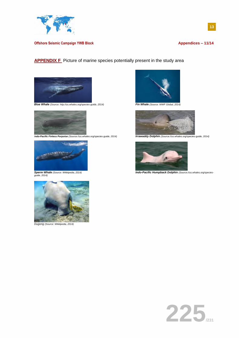
13
Offshore Seismic Campaign YWB Block Appendices – 11/14
225/231
APPENDIX F Picture of marine species potentially present in the study area
Blue Whale (Source: http://us.whales.org/species-guide, 2014) Fin Whale (Source: WWF Global, 2014)
Indo-Pacific Finless Porpoise (Source://us.whales.org/species-guide, 2014) Irrawaddy Dolphin (Source://us.whales.org/species-guide, 2014)
Sperm Whale (Source: Wkikipedia, 2014) Indo-Pacific Humpback Dolphin (Source://us.whales.org/species-
guide, 2014)
Dugong (Source: Wkikipedia, 2014)

13
Offshore Seismic Campaign YWB Block Appendices – 11/14
226/231
APPENDIX G Attendance sheet for the public consultation organized in Myeik on December 16th, 2014 (in Burmese language)
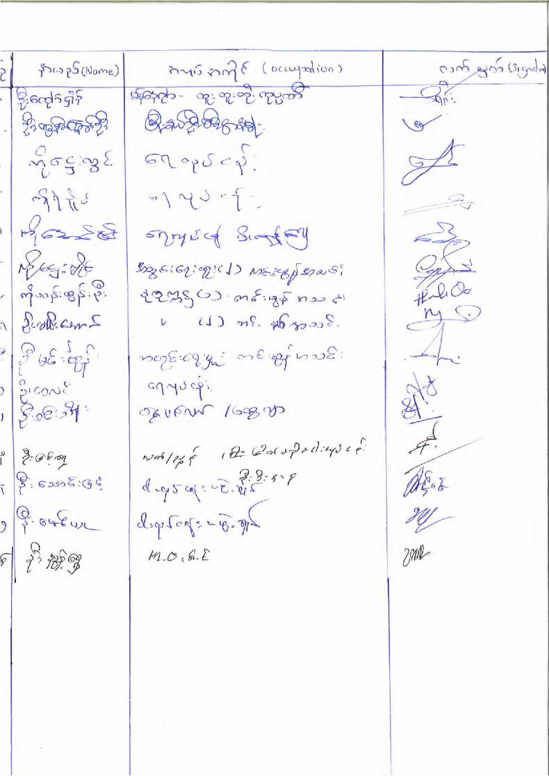

13
Offshore Seismic Campaign YWB Block Appendices – 11/14
227/231
APPENDIX H MoM and attendance list for the public consultation organized in Dawei on January 27th, 2015 (in Burmese language)
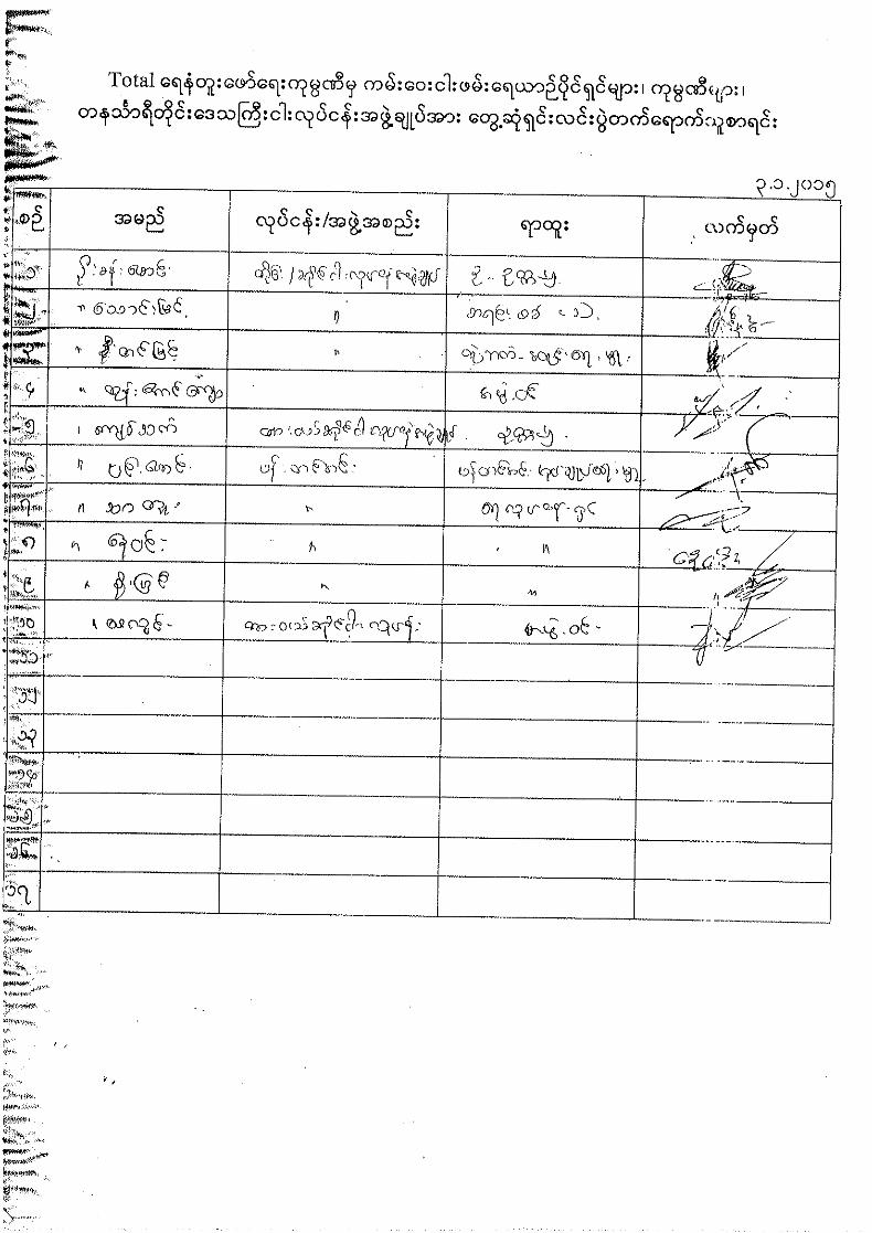
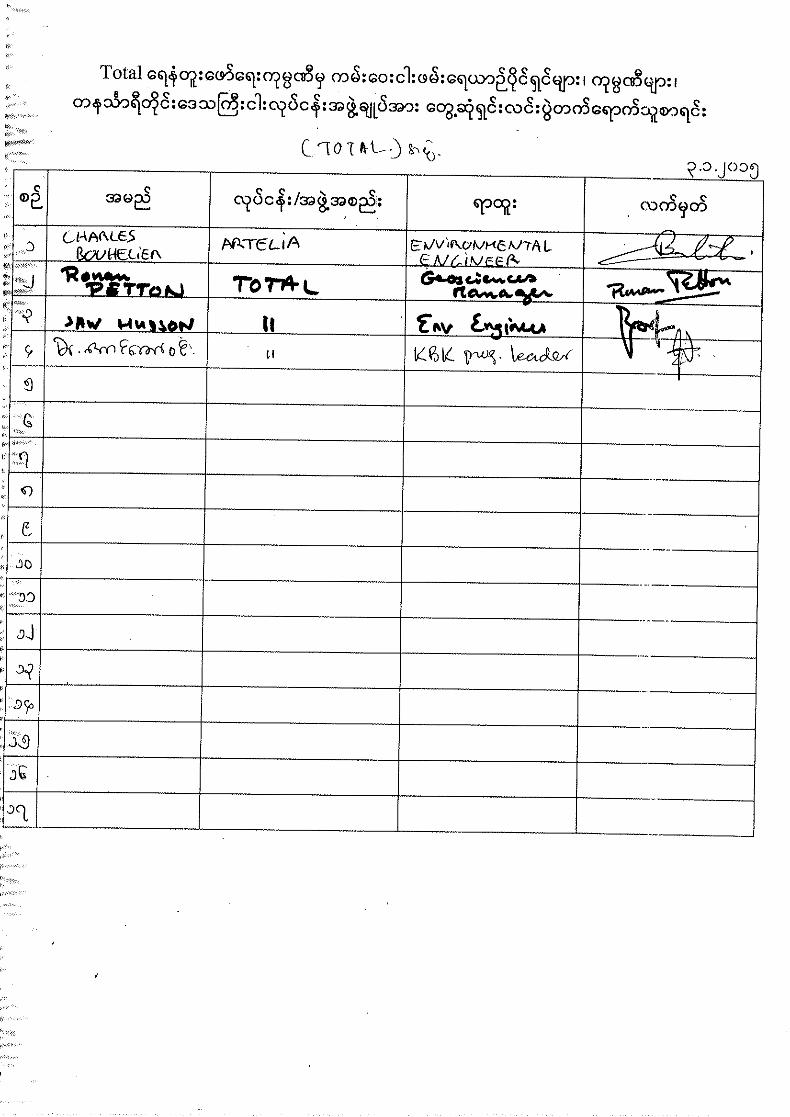

13
Offshore Seismic Campaign YWB Block Appendices – 11/14
228/231
APPENDIX I Polarcus’ Garbage Management Plan
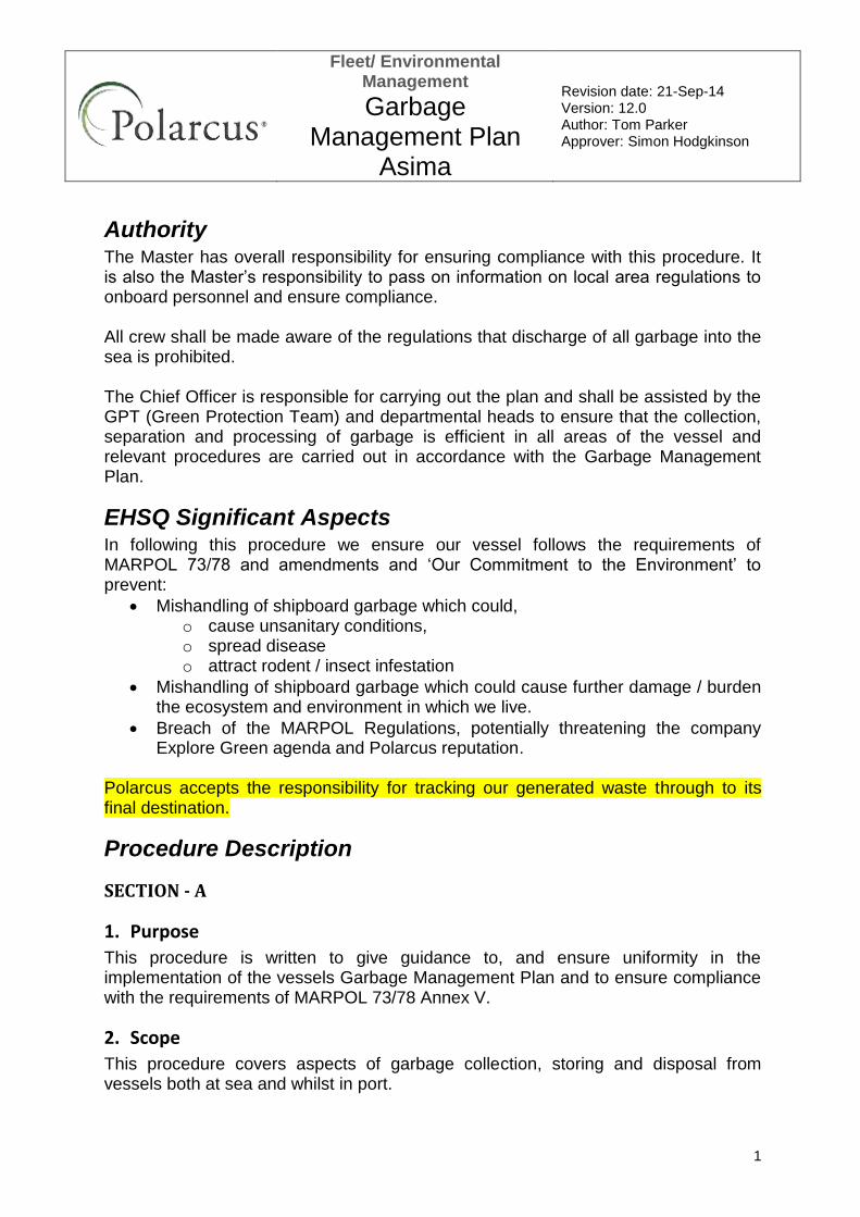
Fleet/ Environmental Management
Garbage Management Plan
Asima
Revision date: 21-Sep-14 Version: 12.0 Author: Tom Parker Approver: Simon Hodgkinson
1
Authority The Master has overall responsibility for ensuring compliance with this procedure. It is also the Master’s responsibility to pass on information on local area regulations to onboard personnel and ensure compliance. All crew shall be made aware of the regulations that discharge of all garbage into the sea is prohibited. The Chief Officer is responsible for carrying out the plan and shall be assisted by the GPT (Green Protection Team) and departmental heads to ensure that the collection, separation and processing of garbage is efficient in all areas of the vessel and relevant procedures are carried out in accordance with the Garbage Management Plan.
EHSQ Significant Aspects In following this procedure we ensure our vessel follows the requirements of MARPOL 73/78 and amendments and ‘Our Commitment to the Environment’ to prevent:
Mishandling of shipboard garbage which could, o cause unsanitary conditions, o spread disease o attract rodent / insect infestation
Mishandling of shipboard garbage which could cause further damage / burden the ecosystem and environment in which we live.
Breach of the MARPOL Regulations, potentially threatening the company Explore Green agenda and Polarcus reputation.
Polarcus accepts the responsibility for tracking our generated waste through to its final destination.
Procedure Description
SECTION - A
1. Purpose
This procedure is written to give guidance to, and ensure uniformity in the implementation of the vessels Garbage Management Plan and to ensure compliance with the requirements of MARPOL 73/78 Annex V.
2. Scope
This procedure covers aspects of garbage collection, storing and disposal from vessels both at sea and whilst in port.
Fleet/ Environmental Management
Garbage Management Plan
Asima
Revision date: 21-Sep-14 Version: 12.0 Author: Tom Parker Approver: Simon Hodgkinson
2
3. Management Commitments
Reference is made to Polarcus – Our Commitment to Environment.
4. Language
As required by the regulations this Garbage Management Plan is written in “English”, in the working language of the vessel.
5. Definitions
Cooking oil – any type of edible oil or animal fat used or intended to be used for the preparation or cooking of food, but does not include the food itself that is prepared using these oils. Food wastes – any spoiled or unspoiled food substances and includes fruits, vegetables, dairy products, poultry, meat products and food scraps generated aboard ship. GMP – Garbage Management Plan GPT – Green Protection Team Garbage – all kinds of food wastes, domestic wastes and operational wastes, all plastics, cargo residues, incinerator ashes, cooking oil, fishing gear, and animal carcasses generated during the normal operation of the ship and liable to be disposed of continuously or periodically except those substances which are defined or listed in other Annexes to the present Convention. Incinerator ashes – ash and clinkers resulting from shipboard incinerators used for the incineration of garbage. Operational wastes – all solid wastes (including slurries) not covered by other Annexes that are collected on board during normal maintenance or operations of a ship, or used for cargo stowage and handling. Operational wastes also includes cleaning agents and additives contained in cargo hold and external wash water. Operational wastes does not include grey water, bilge water, or other similar discharges essential to the operation of a ship, taking into account the guidelines developed by the Organization. Plastic – a solid material which contains as an essential ingredient one or more high molecular mass polymers and which is formed (shaped) during either manufacture of the polymer or the fabrication into a finished product by heat and/or pressure. Plastics have material properties ranging from hard and brittle to soft and elastic. For the purposes of this annex, "all plastics" means all garbage that consists of or includes plastic in any form, including synthetic ropes, synthetic fishing nets, plastic garbage bags and incinerator ashes from plastic products.
Fleet/ Environmental Management
Garbage Management Plan
Asima
Revision date: 21-Sep-14 Version: 12.0 Author: Tom Parker Approver: Simon Hodgkinson
3
Special area – a sea area where for recognized technical reasons in relation to its oceanographic and ecological condition and to the particular character of its traffic the adoption of special mandatory methods for the prevention of sea pollution by garbage is required. For the purposes of Annex V the special areas are the Mediterranean Sea area, the Baltic Sea area, the Black Sea area, the Red Sea area, the Gulfs area, the North Sea area, the Antarctic area and the Wider Caribbean Region, including the Gulf of Mexico.
6. Actions
6.1 Collecting garbage
Garbage collection points should be at appropriate sites around the vessel with separation into the waste streams indicated in this document. Various bins distinguished by color and/or name are placed around the vessel. Garbage is sorted by different categories and type. The following should be observed as a minimum:-
Food waste shall be collected in designated bins with cover. Black bins
Non combustibles – Plastics except food wrapping, Packaging Material, Metal, Glass etc. to be collected in designated bins for storage until discharging to an approved shore reception facility. Green bins
Alkaline Batteries Grey Bin
Combustible garbage i.e.; oily rags, shall be collected in fire proof designated bins. Red Steel Bins with cover.
Lithium batteries when discharged are to be stored in special storage containers and returned to the manufacturer – Lithium batteries do not form part of the vessel waste stream.
6.2 Storing of garbage
Garbage shall be stored in suitable means in designated places on board, and be sorted at least as follows:
Plastics and plastics mixed with non plastic garbage
Metals, aerosol cans, cans of unusable paints, chemicals and other solvents
Food waste including materials contaminated by such wastes
Other garbage which can be incinerated paper, wood and food waste.
Used lithium batteries (See procedure Lithium Battery Storage and Handling)
6.3 Onboard Processing of garbage
Garbage shall be stored in suitable means in designated places on board, and be sorted at least as follows: Overboard – macerated food waste.
Fleet/ Environmental Management
Garbage Management Plan
Asima
Revision date: 21-Sep-14 Version: 12.0 Author: Tom Parker Approver: Simon Hodgkinson
4
Incinerator – food waste, wood, paper, cardboard, plastic food wrapping (to reduce contamination), sludge. Disposal Ashore – All other items. Operation of the incinerator shall be limited to approved operators only and the list of approved operators shall be clearly displayed. Incineration - Please note that MARPOL 73/78 Annex VI (Air Pollution) also prohibits the incineration on board ship of certain products, such as contaminated packaging materials and polychlorinated biphenyls (PCBs). The use of the Incinerator onboard may at times be restricted due to national requirements which prohibit the use of shipboard incinerators. When operating from such countries all onboard incinerators must be tagged and locked out. The disposal of incinerator ashes at sea is prohibited. Incinerator Ash shall be retained on board to be:
Shipped via supply vessels ashore and then sent to an appropriate waste reception facility
Landed ashore during port calls and sent to an appropriate waste reception facility.
6.4 Disposing of garbage according to Marpol 73/78 Annex V and in relation to Polarcus operations
MARPOL 73/78 Annex V indicates the legal minimum standard for disposal of garbage at sea. The company requirements or local regulations may indicate a higher standard. The vessel will always operate to the highest standard or regulation in force. Special note outside of Marpol 73/78 requirements: One must take into consideration food waste disposed of overboard will attract sharks, which may result in shark bites on the streamers. Regulation 3 - General Prohibition on Discharge of Garbage into the Sea. States the following:
Discharge of all garbage into the sea is prohibited. Regulation 4 - Discharge of Garbage Outside Special Areas States the following: Discharge of the following garbage into the sea outside special areas shall only be permitted while the ship is en route and as far as practicable from the nearest land, but in any case not less than:
Fleet/ Environmental Management
Garbage Management Plan
Asima
Revision date: 21-Sep-14 Version: 12.0 Author: Tom Parker Approver: Simon Hodgkinson
5
3 nautical miles from the nearest land for food wastes which have been passed through a comminuter or grinder. Such comminuted or ground food wastes shall be capable of passing through a screen with openings no greater than 25 mm.
12 nautical miles from the nearest land for food wastes that have not been treated in accordance with subparagraph in bullet point above.
When garbage is mixed with or contaminated by other substances prohibited from discharge or having different discharge requirements, the more stringent requirements shall apply.
Regulation 6 – Discharge of Garbage within Special Areas States the following: Discharge of the following garbage into the sea within special areas shall only be permitted while the ship is en route and as follows
Discharge into the sea of food wastes as far as practicable from the nearest land, but not less than 12 nautical miles from the nearest land or the nearest ice shelf. Food wastes shall be comminuted or ground and shall be capable of passing through a screen with openings no greater than 25 mm. Food wastes shall not be contaminated by any other garbage type. Discharge of introduced avian products, including poultry and poultry parts, is not permitted in the Antarctic area unless it has been treated to be made sterile
Cleaning agents or additives contained in deck and external surfaces wash water may be discharged into the sea, but only if these substances are not harmful to the marine environment, taking into account guidelines developed by the Organization
The following rules (in addition to the rules in paragraph 1 of this regulation) apply with respect to the Antarctic area.
Each Party at whose ports ships depart en route to or arrive from the Antarctic area undertakes to ensure that as soon as practicable adequate facilities are provided for the reception of all garbage from all ships, without causing undue delay, and according to the needs of the ships using them.
Each Party shall ensure that all ships entitled to fly its flag, before entering the Antarctic area, have sufficient capacity on board for the retention of all garbage, while operating in the area and have concluded arrangements to discharge such garbage at a reception facility after leaving the area.
When garbage is mixed with or contaminated by other substances prohibited from discharge or having different discharge requirements, the more stringent requirements shall apply
Regulation 7 – Exceptions States the following: Regulations 3, 4, 5 and 6 of this Annex shall not apply to:
Fleet/ Environmental Management
Garbage Management Plan
Asima
Revision date: 21-Sep-14 Version: 12.0 Author: Tom Parker Approver: Simon Hodgkinson
6
The discharge of garbage from a ship necessary for the purpose of securing the safety of a ship and those on board or saving life at sea; or
The accidental loss of garbage resulting from damage to a ship or its equipment, provided that all reasonable precautions have been taken before and after the occurrence of the damage, to prevent or minimize the accidental loss.
Exception of en route
The en route requirements of regulations 4 and 6 shall not apply to the discharge of food wastes where it is clear the retention on board of these food wastes presents an imminent health risk to the people on board
7. Minimization efforts
Reference is made to - Procurement departments procedure where suppliers are asked to supply goods in Eco friendly packaging material to reduce pollution at source. When goods are received in port they are unpacked while vessel is in port – time permitting so that packaging material etc. are not carried out to sea. The company has made efforts to minimize waste through such endeavors as limiting the purchases of individual bottled waters and promoting the consumption of the vessel produced potable water. Bottled water is now supplied onboard as an emergency type supply versus the previous program of being the main source of drinking water. A reduction in approximately 500,000 plastic water bottles annually. Environmental awareness of the crew is raised on the vessel during EHSQ meetings and encouraged to adhere to GMP. Company has a reward recognition program for crew member’s effort to reduce garbage and suggesting new ideas for pollution prevention. The Company focuses on the use of the most environmentally friendly products to reduce pollution and emissions and also the minimization of waste.
8. Training
The Company commitment towards Environmental responsibility will be communicated to the crew. During the familiarization of the vessel a special mention is made of the Garbage Management Plan and an overview of the system given. Personnel are informed about garbage segregation and correct disposal techniques for various types of garbage on board. The vessel operates a “NOTHING OVERBOARD” policy in regards to waste other than the permissible wastes identified in MARPOL Regulations.
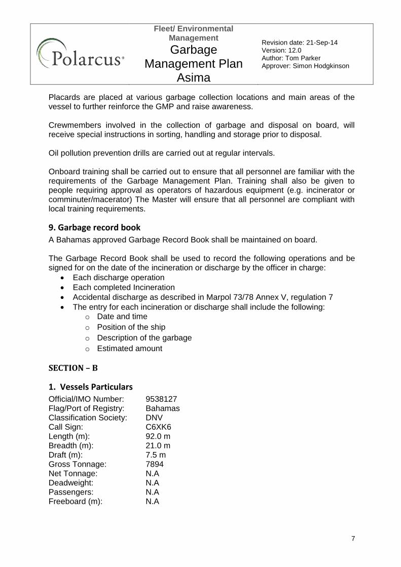
Fleet/ Environmental Management
Garbage Management Plan
Asima
Revision date: 21-Sep-14 Version: 12.0 Author: Tom Parker Approver: Simon Hodgkinson
7
Placards are placed at various garbage collection locations and main areas of the vessel to further reinforce the GMP and raise awareness. Crewmembers involved in the collection of garbage and disposal on board, will receive special instructions in sorting, handling and storage prior to disposal. Oil pollution prevention drills are carried out at regular intervals. Onboard training shall be carried out to ensure that all personnel are familiar with the requirements of the Garbage Management Plan. Training shall also be given to people requiring approval as operators of hazardous equipment (e.g. incinerator or comminuter/macerator) The Master will ensure that all personnel are compliant with local training requirements.
9. Garbage record book
A Bahamas approved Garbage Record Book shall be maintained on board. The Garbage Record Book shall be used to record the following operations and be signed for on the date of the incineration or discharge by the officer in charge:
Each discharge operation
Each completed Incineration
Accidental discharge as described in Marpol 73/78 Annex V, regulation 7
The entry for each incineration or discharge shall include the following: o Date and time
o Position of the ship
o Description of the garbage
o Estimated amount
SECTION – B
1. Vessels Particulars
Official/IMO Number: 9538127 Flag/Port of Registry: Bahamas Classification Society: DNV Call Sign: C6XK6 Length (m): 92.0 m Breadth (m): 21.0 m Draft (m): 7.5 m Gross Tonnage: 7894 Net Tonnage: N.A Deadweight: N.A Passengers: N.A Freeboard (m): N.A
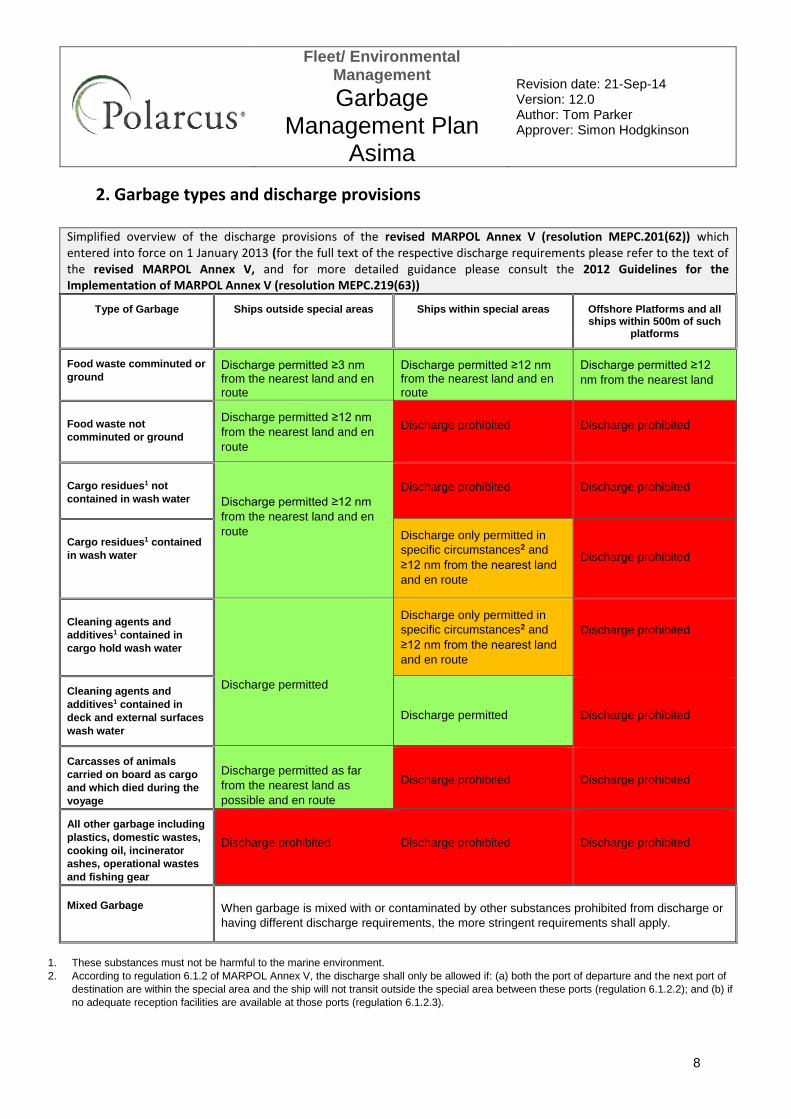
Fleet/ Environmental Management
Garbage Management Plan
Asima
Revision date: 21-Sep-14 Version: 12.0 Author: Tom Parker Approver: Simon Hodgkinson
8
2. Garbage types and discharge provisions
Simplified overview of the discharge provisions of the revised MARPOL Annex V (resolution MEPC.201(62)) which entered into force on 1 January 2013 (for the full text of the respective discharge requirements please refer to the text of the revised MARPOL Annex V, and for more detailed guidance please consult the 2012 Guidelines for the Implementation of MARPOL Annex V (resolution MEPC.219(63))
Type of Garbage Ships outside special areas Ships within special areas Offshore Platforms and all ships within 500m of such
platforms
Food waste comminuted or
ground Discharge permitted ≥3 nm from the nearest land and en route
Discharge permitted ≥12 nm from the nearest land and en route
Discharge permitted ≥12
nm from the nearest land
Food waste not
comminuted or ground
Discharge permitted ≥12 nm
from the nearest land and en
route
Discharge prohibited Discharge prohibited
Cargo residues1 not
contained in wash water
Discharge permitted ≥12 nm
from the nearest land and en
route
Discharge prohibited Discharge prohibited
Cargo residues1 contained
in wash water
Discharge only permitted in
specific circumstances2 and
≥12 nm from the nearest land
and en route
Discharge prohibited
Cleaning agents and
additives1 contained in
cargo hold wash water
Discharge permitted
Discharge only permitted in
specific circumstances2 and
≥12 nm from the nearest land
and en route
Discharge prohibited
Cleaning agents and
additives1 contained in
deck and external surfaces
wash water
Discharge permitted
Discharge prohibited
Carcasses of animals
carried on board as cargo
and which died during the
voyage
Discharge permitted as far
from the nearest land as
possible and en route
Discharge prohibited
Discharge prohibited
All other garbage including
plastics, domestic wastes,
cooking oil, incinerator
ashes, operational wastes
and fishing gear
Discharge prohibited
Discharge prohibited
Discharge prohibited
Mixed Garbage
When garbage is mixed with or contaminated by other substances prohibited from discharge or
having different discharge requirements, the more stringent requirements shall apply.
1. These substances must not be harmful to the marine environment.
2. According to regulation 6.1.2 of MARPOL Annex V, the discharge shall only be allowed if: (a) both the port of departure and the next port of
destination are within the special area and the ship will not transit outside the special area between these ports (regulation 6.1.2.2); and (b) if
no adequate reception facilities are available at those ports (regulation 6.1.2.3).
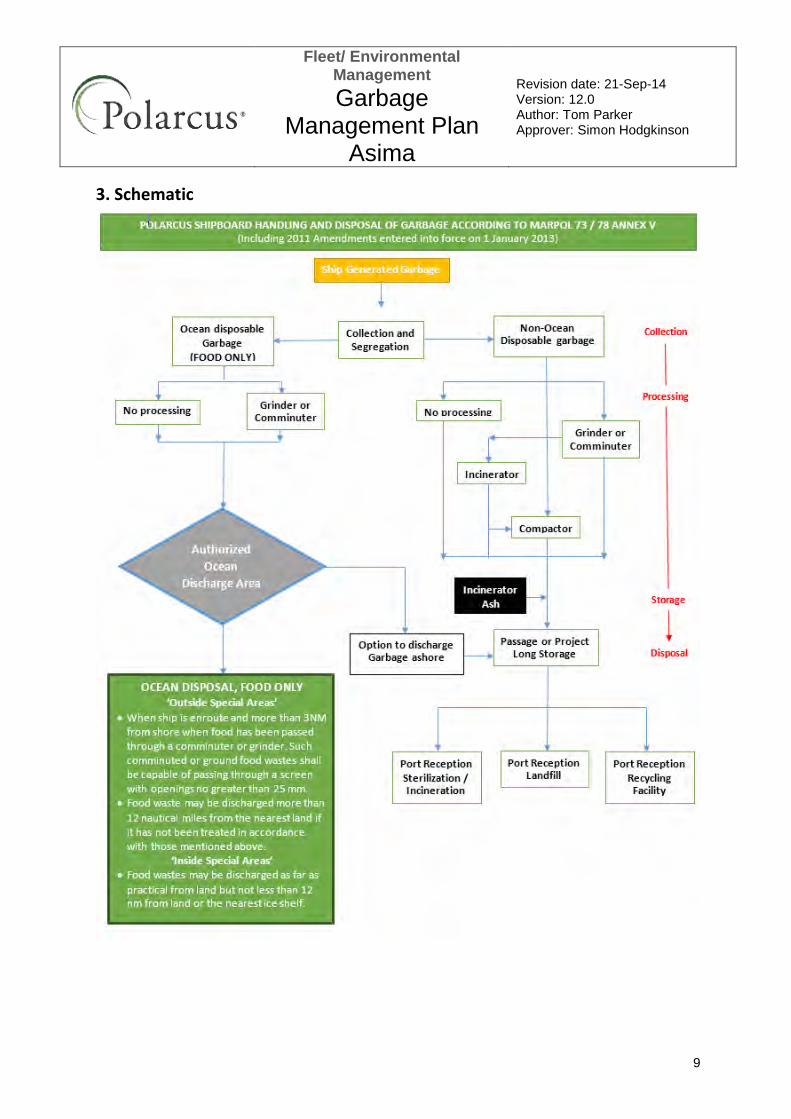
Fleet/ Environmental Management
Garbage Management Plan
Asima
Revision date: 21-Sep-14 Version: 12.0 Author: Tom Parker Approver: Simon Hodgkinson
9
3. Schematic
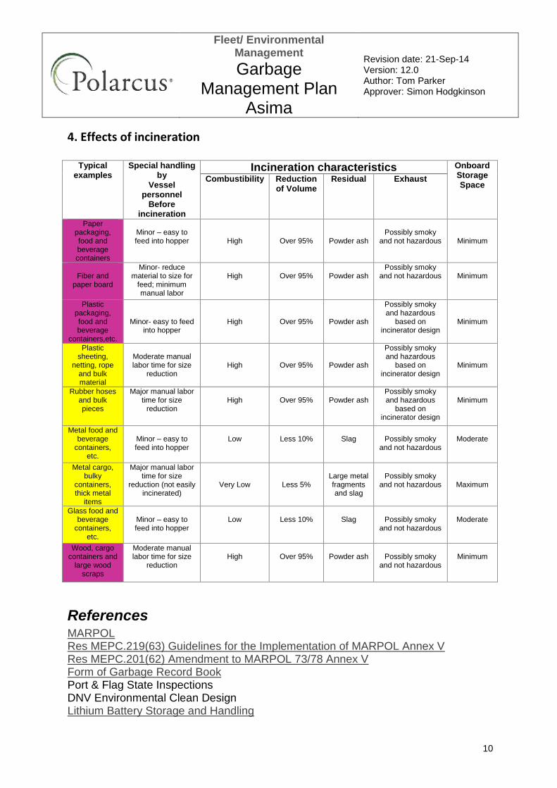
Fleet/ Environmental Management
Garbage Management Plan
Asima
Revision date: 21-Sep-14 Version: 12.0 Author: Tom Parker Approver: Simon Hodgkinson
10
4. Effects of incineration
Typical
examples Special handling
by Vessel
personnel Before
incineration
Incineration characteristics Onboard Storage Space
Combustibility Reduction of Volume
Residual Exhaust
Paper packaging, food and beverage containers
Minor – easy to feed into hopper
High
Over 95%
Powder ash
Possibly smoky
and not hazardous
Minimum
Fiber and
paper board
Minor- reduce material to size for
feed; minimum manual labor
High
Over 95%
Powder ash
Possibly smoky and not hazardous
Minimum
Plastic packaging, food and beverage
containers,etc.
Minor- easy to feed into hopper
High
Over 95%
Powder ash
Possibly smoky and hazardous
based on incinerator design
Minimum
Plastic sheeting,
netting, rope and bulk material
Moderate manual labor time for size
reduction
High
Over 95%
Powder ash
Possibly smoky and hazardous
based on incinerator design
Minimum
Rubber hoses and bulk pieces
Major manual labor time for size
reduction
High
Over 95%
Powder ash
Possibly smoky and hazardous
based on incinerator design
Minimum
Metal food and beverage
containers, etc.
Minor – easy to feed into hopper
Low
Less 10%
Slag
Possibly smoky
and not hazardous
Moderate
Metal cargo, bulky
containers, thick metal
items
Major manual labor time for size
reduction (not easily incinerated)
Very Low
Less 5%
Large metal fragments and slag
Possibly smoky
and not hazardous
Maximum
Glass food and beverage
containers, etc.
Minor – easy to feed into hopper
Low
Less 10%
Slag
Possibly smoky
and not hazardous
Moderate
Wood, cargo containers and
large wood scraps
Moderate manual labor time for size
reduction
High
Over 95%
Powder ash
Possibly smoky
and not hazardous
Minimum
References MARPOL Res MEPC.219(63) Guidelines for the Implementation of MARPOL Annex V Res MEPC.201(62) Amendment to MARPOL 73/78 Annex V Form of Garbage Record Book Port & Flag State Inspections DNV Environmental Clean Design Lithium Battery Storage and Handling
Fleet/ Environmental Management
Garbage Management Plan
Asima
Revision date: 21-Sep-14 Version: 12.0 Author: Tom Parker Approver: Simon Hodgkinson
11
Attachments ASIMA Waste Management International Pollution Regulations Placard Record of Garbage Discharge UMCC call Incinerator Waste Compactor
Table of Amendments
Rev Date Rev No. Amendments
21-Sep-14 12 Updated EHSQ Significant Aspects – About generated waste.

13
Offshore Seismic Campaign YWB Block Appendices – 11/14
229/231
APPENDIX J Polarcus’ Oil Spill Procedure
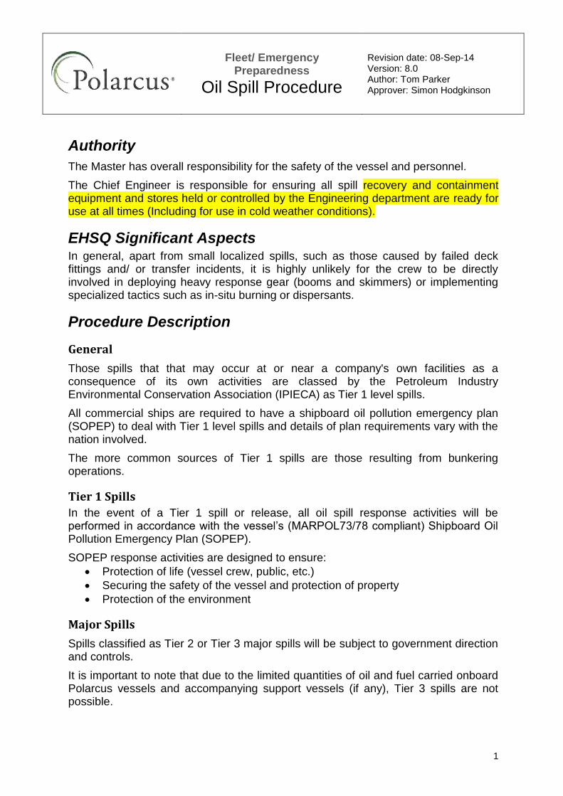
Fleet/ Emergency Preparedness
Oil Spill Procedure
Revision date: 08-Sep-14 Version: 8.0 Author: Tom Parker Approver: Simon Hodgkinson
1
Authority
The Master has overall responsibility for the safety of the vessel and personnel.
The Chief Engineer is responsible for ensuring all spill recovery and containment equipment and stores held or controlled by the Engineering department are ready for use at all times (Including for use in cold weather conditions).
EHSQ Significant Aspects In general, apart from small localized spills, such as those caused by failed deck fittings and/ or transfer incidents, it is highly unlikely for the crew to be directly involved in deploying heavy response gear (booms and skimmers) or implementing specialized tactics such as in-situ burning or dispersants.
Procedure Description
General
Those spills that that may occur at or near a company's own facilities as a consequence of its own activities are classed by the Petroleum Industry Environmental Conservation Association (IPIECA) as Tier 1 level spills.
All commercial ships are required to have a shipboard oil pollution emergency plan (SOPEP) to deal with Tier 1 level spills and details of plan requirements vary with the nation involved.
The more common sources of Tier 1 spills are those resulting from bunkering operations.
Tier 1 Spills
In the event of a Tier 1 spill or release, all oil spill response activities will be performed in accordance with the vessel’s (MARPOL73/78 compliant) Shipboard Oil Pollution Emergency Plan (SOPEP).
SOPEP response activities are designed to ensure:
Protection of life (vessel crew, public, etc.)
Securing the safety of the vessel and protection of property
Protection of the environment
Major Spills
Spills classified as Tier 2 or Tier 3 major spills will be subject to government direction and controls.
It is important to note that due to the limited quantities of oil and fuel carried onboard Polarcus vessels and accompanying support vessels (if any), Tier 3 spills are not possible.
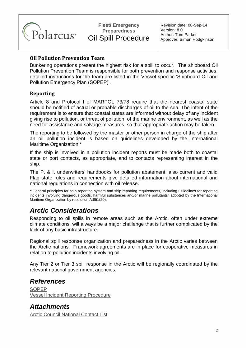
Fleet/ Emergency Preparedness
Oil Spill Procedure
Revision date: 08-Sep-14 Version: 8.0 Author: Tom Parker Approver: Simon Hodgkinson
2
Oil Pollution Prevention Team
Bunkering operations present the highest risk for a spill to occur. The shipboard Oil Pollution Prevention Team is responsible for both prevention and response activities, detailed instructions for the team are listed in the Vessel specific ‘Shipboard Oil and Pollution Emergency Plan (SOPEP)’.
Reporting
Article 8 and Protocol I of MARPOL 73/78 require that the nearest coastal state should be notified of actual or probable discharges of oil to the sea. The intent of the requirement is to ensure that coastal states are informed without delay of any incident giving rise to pollution, or threat of pollution, of the marine environment, as well as the need for assistance and salvage measures, so that appropriate action may be taken.
The reporting to be followed by the master or other person in charge of the ship after an oil pollution incident is based on guidelines developed by the International Maritime Organization.*
If the ship is involved in a pollution incident reports must be made both to coastal state or port contacts, as appropriate, and to contacts representing interest in the ship.
The P. & I. underwriters' handbooks for pollution abatement, also current and valid Flag state rules and requirements give detailed information about international and national regulations in connection with oil release.
*"General principles for ship reporting system and ship reporting requirements, including Guidelines for reporting incidents involving dangerous goods, harmful substances and/or marine pollutants" adopted by the International Maritime Organization by resolution A.851(20).
Arctic Considerations Responding to oil spills in remote areas such as the Arctic, often under extreme climate conditions, will always be a major challenge that is further complicated by the lack of any basic infrastructure. Regional spill response organization and preparedness in the Arctic varies between the Arctic nations. Framework agreements are in place for cooperative measures in relation to pollution incidents involving oil. Any Tier 2 or Tier 3 spill response in the Arctic will be regionally coordinated by the relevant national government agencies.
References SOPEP Vessel Incident Reporting Procedure
Attachments Arctic Council National Contact List

Fleet/ Emergency Preparedness
Oil Spill Procedure
Revision date: 08-Sep-14 Version: 8.0 Author: Tom Parker Approver: Simon Hodgkinson
3
Table of Amendments
Rev Date Rev No. Amendments
08-Sep-14 8 Changes made to “Authority” subheading

13
Offshore Seismic Campaign YWB Block Appendices – 11/14
230/231
APPENDIX K Polarcus’ Extreme Weather Procedure
Fleet/ Emergency Preparedness
Extreme Weather Procedure
Revision date: 21-Jan-15 Version: 7.0 Author: Chris Griffin Approver: Simon Hodgkinson
1
Authority The Master of the vessel will take whatever action he feels necessary to prevent the vessel from navigating through extreme weather conditions. The Master is responsible for all actions taken. The Party Manager is responsible for all seismic towed equipment and the decisions taken regarding it but this will never supersede the directions and decisions of the vessel Master when preparing for such extreme weather avoidance.
EHSQ Significant Aspects In following this Procedure we can ensure our vessels are prepared for extreme weather conditions when they occur and are managed safely in a way to;
Prevent fatalities, and life threatening injuries due to the hazards associated with extreme weather.
Prevent damage to our vessels and equipment during the periods of extreme weather.
Procedure Description Use the Extreme Weather Checklist for guidance
Weather Alert Levels
In determining a :
Green Alert: Hurricane, Typhoon or Cyclone confirmed, but more than 1000 nm
from location. No action necessary other than monitoring and plotting the storm movements.
Yellow Alert: Hurricane, Typhoon or Cyclone reported in or approaching location
and at a distance of 800 - 1000nm. Continue monitoring and plotting. Secure all loose items.
Orange Alert: Hurricane, Typhoon or Cyclone developing or entering within a radius
of 800 nm of location. Weather reports to be obtained at 3 hourly intervals. The vessel Master will prepare plans for evacuating the survey area.
Red Alert: Hurricane, Typhoon or Cyclone developing or entering within a radius of
500 nm of location. The Master will advise Polarcus Management of the situation and the plan for evacuation. (Decision or time line to pick up gear should be agreed upon at this stage since further delay could cause problems).
Hurricane, Typhoon or Cyclone Evacuation
If the Hurricane, Typhoon or Cyclone enters within 300nm of location, the vessel is to cease operations and prepare to leave area for shelter. If there are circumstances that may hamper evacuation, or the recovery of the seismic equipment, the evacuation should be initiated earlier. In such a situation, the Vessel Manager should be kept up to date with the position and status of the vessel.
Fleet/ Emergency Preparedness
Extreme Weather Procedure
Revision date: 21-Jan-15 Version: 7.0 Author: Chris Griffin Approver: Simon Hodgkinson
2
When the Hurricane, Typhoon or Cyclone has passed, a status report of the vessel and crew is to be made.
Standing by for weather in the Project Area
If it is necessary to stand by during periods of extreme weather when the in-sea seismic equipment is deployed the Master will identify an area considered safe for the vessel and in-sea equipment. This area shall be:
Identified within 24 hours of arrival on project.
Of adequate size for the vessel to maneuver freely in.
In close proximity to the project.
Free of surface and sub-sea obstructions which would potentially endanger the vessel or in-sea towed seismic equipment.
Away from charted sea lanes with minimal or no shipping traffic.
Of adequate water depth to provide sufficient clearance for the safety of the vessel and in-sea equipment while standing by and maneuvering during the periods of extreme weather.
References EHSQ Project Plan
Attachments Extreme Weather Checklist
Table of Amendments
Rev Date Rev No. Amendments
21-Jan-15 7.0 Reviewed with minor changes.

13
Offshore Seismic Campaign YWB Block Appendices – 11/14
231/231
APPENDIX L Polarcus’ Equipment
FUTURE CONTRACTOR 2D Marine Seismic Data Acquisition SERVICES EXHIBIT C – PERSONNEL AND EQUIPMENT FOR BLOCKS MD2, AD10 & YWB
Exhibit C
CONTRACTOR’s PERSONNEL and EQUIPMENT
THIS CONTRACT IS THE PROPERTY ENI MYANMAR B.V., STATOIL MYANAMAR PTE LTD AND TOTAL E&P MYANMAR AND SHALL NOT BE DISCLOSED TO THIRD PARTIES OR REPRODUCED IN ANY MANNER FOR ANY PURPOSE WHATSOEVER EXCEPT WITH COMPANIES WRITTEN CONSENT;
FUTURE CONTRACTOR 2D Marine Seismic Data Acquisition SERVICES EXHIBIT C – PERSONNEL AND EQUIPMENT FOR BLOCKS MD2, AD10 & YWB
PAGE - 2 - THIS CONTRACT IS THE PROPERTY ENI MYANMAR B.V., STATOIL MYANAMAR PTE LTD AND TOTAL E&P MYANMAR AND SHALL NOT BE DISCLOSED TO THIRD PARTIES OR REPRODUCED IN ANY MANNER FOR ANY PURPOSE WHATSOEVER EXCEPT WITH COMPANIES WRITTEN CONSENT.
TABLE OF CONTENTS
1 CONTRACTOR’s PERSONNEL ................................................................................................. 4 1.1. Seismic vessel(s) geophysical CONTRACTOR’s PERSONNEL .......................................................... 4 1.2. Seismic vessel(s) marine CONTRACTOR’s PERSONNEL ................................................................... 5 1.3. Support vessel(s) marine CONTRACTOR’s PERSONNEL ................................................................... 6 1.4. Onshore support CONTRACTOR’s PERSONNEL ................................................................................. 6 1.5. Additional and optional CONTRACTOR’s PERSONNEL ....................................................................... 8
2 Operational considerations ....................................................................................................... 8 3 Vessel(s) ..................................................................................................................................... 8 3.1. Seismic vessel(s) main characteristics .................................................................................................. 9 3.2. Seismic vessel(s) propulsion and power ............................................................................................. 10 3.3. Seismic vessel(s) navigation................................................................................................................. 10 3.4. Seismic vessel(s) helideck .................................................................................................................... 11 3.5. Seismic vessel(s) auxiliary boats ......................................................................................................... 11 3.6. Safety equipment .................................................................................................................................... 11 3.7. Support vessel(s) main characteristics ............................................................................................... 11 3.8. Support vessel(s) propulsion and power ............................................................................................. 12 3.9. Support vessel(s) communications ...................................................................................................... 12 3.10. Support vessel(s) navigation .............................................................................................................. 12 3.11. Support vessel safety equipment ....................................................................................................... 12 3.12. Pre-assessment of the vessel (documentation required) ................................................................ 12 3.13. Pre-assessment of the performance of the vessel ............................................................................ 14
4 Seismic source ........................................................................................................................ 15 4.1. Source characteristics ........................................................................................................................... 15 4.2. Compressor, sensor and peripheral equipment characteristics ....................................................... 16 4.3. Seismic source spare equipment .......................................................................................................... 16
5 Seismic recording system ....................................................................................................... 16 5.1. Seismic recorder characteristics .......................................................................................................... 17 5.2. Streamer characteristics........................................................................................................................ 17 5.3. Peripheral equipment characteristics .................................................................................................. 19 5.4. Seismic recording spare equipment ..................................................................................................... 19
6 Seismic data quality control ................................................................................................... 20 7 Source and receiver positioning ............................................................................................ 20 8 DGPS ........................................................................................................................................ 21 8.1. Primary DGPS ......................................................................................................................................... 21 8.2. Secondary DGPS .................................................................................................................................... 22 8.3. Tertiary DGPS .......................................................................................................................................... 24
9 RGPS ........................................................................................................................................ 25 10 Heading sensors .................................................................................................................... 26 10.1. Gyro-compass ....................................................................................................................................... 26 10.2. Back-up gyro-compass ......................................................................................................................... 26 10.3. GPS based heading and attitude sensor ............................................................................................ 26
11 Streamer compasses ............................................................................................................. 26 12 Bathymetry ............................................................................................................................. 27 12.1. Echo sounder ........................................................................................................................................ 27 12.2. Sea water speed of sound, temperature and salinity meter ............................................................ 27 12.3. Bathymetry data processing ................................................................................................................ 27
13 Integrated navigation system ................................................................................................ 27 13.1. Online integrated navigation system ................................................................................................. 27 13.2. Offline integrated navigation system .................................................................................................. 28
14 System timing ........................................................................................................................ 28 15 Seismic processing equipment and software ...................................................................... 28 16 Quality control attribute database ........................................................................................ 29 17 Gravimetry data acquisition equipment ............................................................................... 29 18 Magnetometry data acquisition equipment .......................................................................... 30 19 Additional and optional EQUIPMENT ................................................................................... 30
FUTURE CONTRACTOR 2D Marine Seismic Data Acquisition SERVICES EXHIBIT C – PERSONNEL AND EQUIPMENT FOR BLOCKS MD2, AD10 & YWB
19.1. Additional EQUIPMENT ........................................................................................................................ 30 19.2. Optional EQUIPMENT ........................................................................................................................... 30
List of figures Fig. 1 Fig. 2 Fig. 3 Fig. 4 Fig. 5 Fig. 6 Fig. 7 Fig. 8 Fig. 9 Fig. 10 Fig. 11 Fig. 12 Fig.13
- - - - - - - - - - - -
Seismic source configuration Individual sub-Array configuration Seismic Source Signature (modelled with standard parameters) Seismic Source Signature (modelled with SURVEY parameters) Timing Diagram of Shooting and Recording Sequence Amplitude and Phase Spectrum of the seismic recorder filters Vessel, source and streamer geometry Front Streamer Configuration Tail Streamer Configuration Streamer Active Section Configuration Seismic Trace Configuration Source directivity diagrams, in line and cross line Dropout specification for proposed source array
PAGE - 3 - THIS CONTRACT IS THE PROPERTY ENI MYANMAR B.V., STATOIL MYANAMAR PTE LTD AND TOTAL E&P MYANMAR AND SHALL NOT BE DISCLOSED TO THIRD PARTIES OR REPRODUCED IN ANY MANNER FOR ANY PURPOSE WHATSOEVER EXCEPT WITH COMPANIES WRITTEN CONSENT. Annexes
Annexe 1 Individual gun sub-array composition
Annexe 2 DGPS description
Annexe 3 DGPS reference and monitor station description
Annexe 4 RGPS description
Annexe 5 Gyro-compass description
Annexe 6 GPS heading sensor description
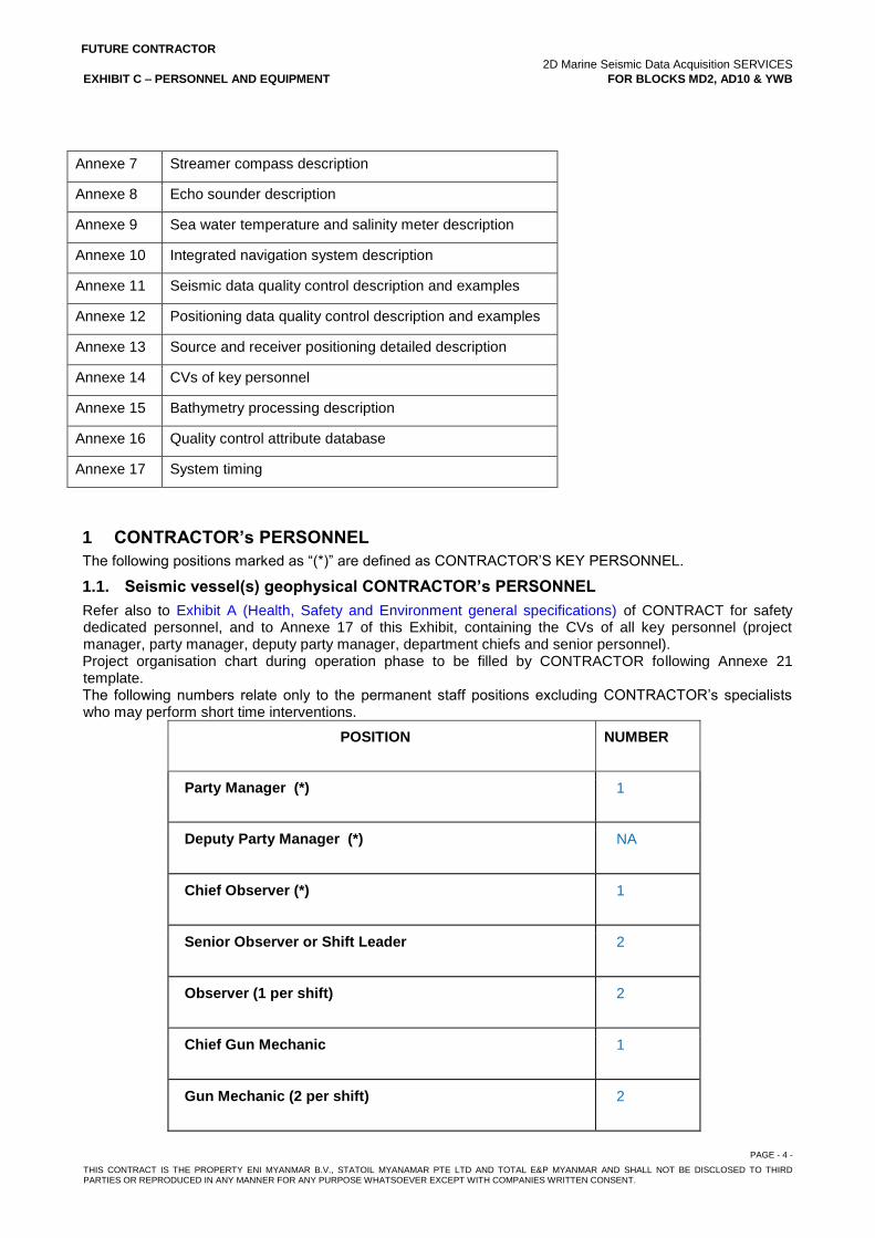
FUTURE CONTRACTOR 2D Marine Seismic Data Acquisition SERVICES EXHIBIT C – PERSONNEL AND EQUIPMENT FOR BLOCKS MD2, AD10 & YWB
PAGE - 4 - THIS CONTRACT IS THE PROPERTY ENI MYANMAR B.V., STATOIL MYANAMAR PTE LTD AND TOTAL E&P MYANMAR AND SHALL NOT BE DISCLOSED TO THIRD PARTIES OR REPRODUCED IN ANY MANNER FOR ANY PURPOSE WHATSOEVER EXCEPT WITH COMPANIES WRITTEN CONSENT.
Annexe 7 Streamer compass description
Annexe 8 Echo sounder description
Annexe 9 Sea water temperature and salinity meter description
Annexe 10 Integrated navigation system description
Annexe 11 Seismic data quality control description and examples
Annexe 12 Positioning data quality control description and examples
Annexe 13 Source and receiver positioning detailed description
Annexe 14 CVs of key personnel
Annexe 15 Bathymetry processing description
Annexe 16 Quality control attribute database
Annexe 17 System timing
1 CONTRACTOR’s PERSONNEL
The following positions marked as “(*)” are defined as CONTRACTOR’S KEY PERSONNEL.
1.1. Seismic vessel(s) geophysical CONTRACTOR’s PERSONNEL
Refer also to Exhibit A (Health, Safety and Environment general specifications) of CONTRACT for safety dedicated personnel, and to Annexe 17 of this Exhibit, containing the CVs of all key personnel (project manager, party manager, deputy party manager, department chiefs and senior personnel). Project organisation chart during operation phase to be filled by CONTRACTOR following Annexe 21 template. The following numbers relate only to the permanent staff positions excluding CONTRACTOR’s specialists who may perform short time interventions.
POSITION NUMBER
Party Manager (*) 1
Deputy Party Manager (*) NA
Chief Observer (*) 1
Senior Observer or Shift Leader 2
Observer (1 per shift) 2
Chief Gun Mechanic 1
Gun Mechanic (2 per shift) 2
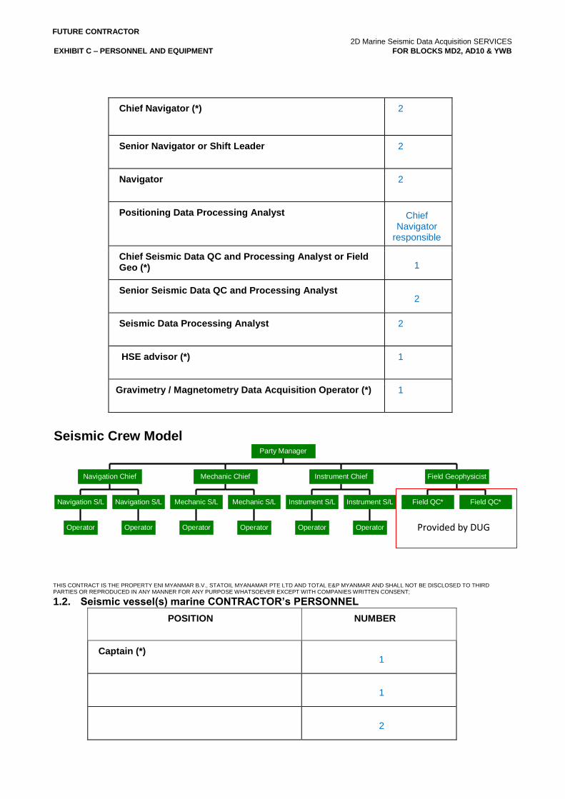
FUTURE CONTRACTOR 2D Marine Seismic Data Acquisition SERVICES EXHIBIT C – PERSONNEL AND EQUIPMENT FOR BLOCKS MD2, AD10 & YWB
Chief Navigator (*) 2
Senior Navigator or Shift Leader 2
Navigator 2
Positioning Data Processing Analyst Chief Navigator
responsible
Chief Seismic Data QC and Processing Analyst or Field Geo (*) 1
Senior Seismic Data QC and Processing Analyst 2
Seismic Data Processing Analyst 2
HSE advisor (*) 1
Gravimetry / Magnetometry Data Acquisition Operator (*) 1
Seismic Crew Model
Operator
Navigation S/L
Operator
Navigation S/L
Navigation Chief
Operator
Mechanic S/L
Operator
Mechanic S/L
Mechanic Chief
Operator
Instrument S/L
Operator
Instrument S/L
Instrument Chief
Field QC* Field QC*
Field Geophysicist
Party Manager
THIS CONTRACT IS THE PROPERTY ENI MYANMAR B.V., STATOIL MYANAMAR PTE LTD AND TOTAL E&P MYANMAR AND SHALL NOT BE DISCLOSED TO THIRD PARTIES OR REPRODUCED IN ANY MANNER FOR ANY PURPOSE WHATSOEVER EXCEPT WITH COMPANIES WRITTEN CONSENT; 1.2. Seismic vessel(s) marine CONTRACTOR’s PERSONNEL
POSITION NUMBER
Captain (*) 1
1
2
Provided by DUG
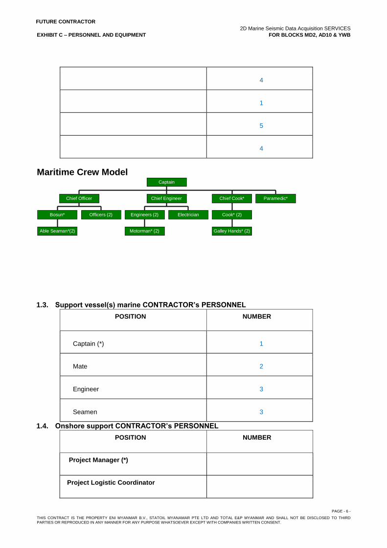
FUTURE CONTRACTOR 2D Marine Seismic Data Acquisition SERVICES EXHIBIT C – PERSONNEL AND EQUIPMENT FOR BLOCKS MD2, AD10 & YWB
PAGE - 6 - THIS CONTRACT IS THE PROPERTY ENI MYANMAR B.V., STATOIL MYANAMAR PTE LTD AND TOTAL E&P MYANMAR AND SHALL NOT BE DISCLOSED TO THIRD PARTIES OR REPRODUCED IN ANY MANNER FOR ANY PURPOSE WHATSOEVER EXCEPT WITH COMPANIES WRITTEN CONSENT.
4
1
5
4
Maritime Crew Model
Able Seaman*(2)
Bosun* Officers (2)
Chief Officer
Motorman* (2)
Engineers (2) Electrician
Chief Engineer
Galley Hands* (2)
Cook* (2)
Chief Cook* Paramedic*
Captain
1.3. Support vessel(s) marine CONTRACTOR’s PERSONNEL
POSITION NUMBER
Captain (*) 1
Mate 2
Engineer 3
Seamen 3
1.4. Onshore support CONTRACTOR’s PERSONNEL
POSITION NUMBER
Project Manager (*)
Project Logistic Coordinator

FUTURE CONTRACTOR 2D Marine Seismic Data Acquisition SERVICES EXHIBIT C – PERSONNEL AND EQUIPMENT FOR BLOCKS MD2, AD10 & YWB
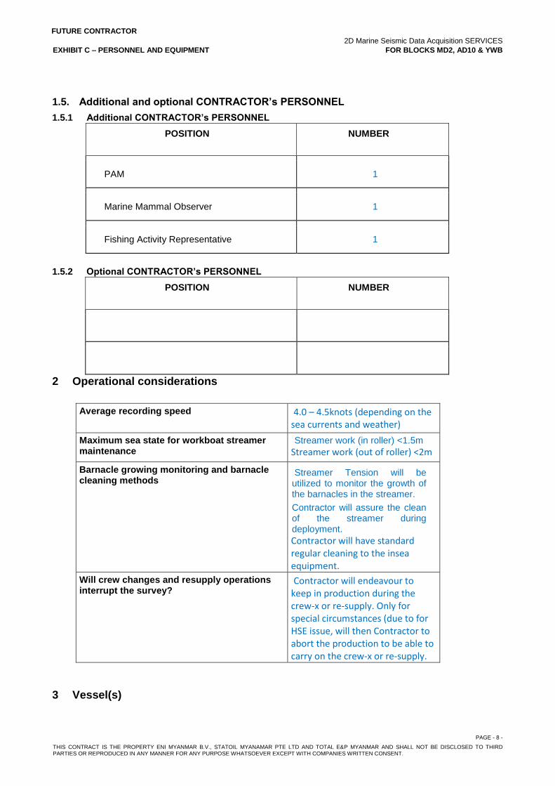
FUTURE CONTRACTOR 2D Marine Seismic Data Acquisition SERVICES EXHIBIT C – PERSONNEL AND EQUIPMENT FOR BLOCKS MD2, AD10 & YWB
PAGE - 8 - THIS CONTRACT IS THE PROPERTY ENI MYANMAR B.V., STATOIL MYANAMAR PTE LTD AND TOTAL E&P MYANMAR AND SHALL NOT BE DISCLOSED TO THIRD PARTIES OR REPRODUCED IN ANY MANNER FOR ANY PURPOSE WHATSOEVER EXCEPT WITH COMPANIES WRITTEN CONSENT.
1.5. Additional and optional CONTRACTOR’s PERSONNEL
1.5.1 Additional CONTRACTOR’s PERSONNEL
POSITION NUMBER
PAM 1
Marine Mammal Observer 1
Fishing Activity Representative 1
1.5.2 Optional CONTRACTOR’s PERSONNEL
POSITION NUMBER
2 Operational considerations
Average recording speed 4.0 – 4.5knots (depending on the sea currents and weather)
Maximum sea state for workboat streamer maintenance
Streamer work (in roller) <1.5m
Streamer work (out of roller) <2m
Barnacle growing monitoring and barnacle cleaning methods
Streamer Tension will be utilized to monitor the growth of the barnacles in the streamer.
Contractor will assure the clean of the streamer during deployment.
Contractor will have standard regular cleaning to the insea equipment.
Will crew changes and resupply operations interrupt the survey?
Contractor will endeavour to keep in production during the crew-x or re-supply. Only for special circumstances (due to for HSE issue, will then Contractor to abort the production to be able to carry on the crew-x or re-supply.
3 Vessel(s)
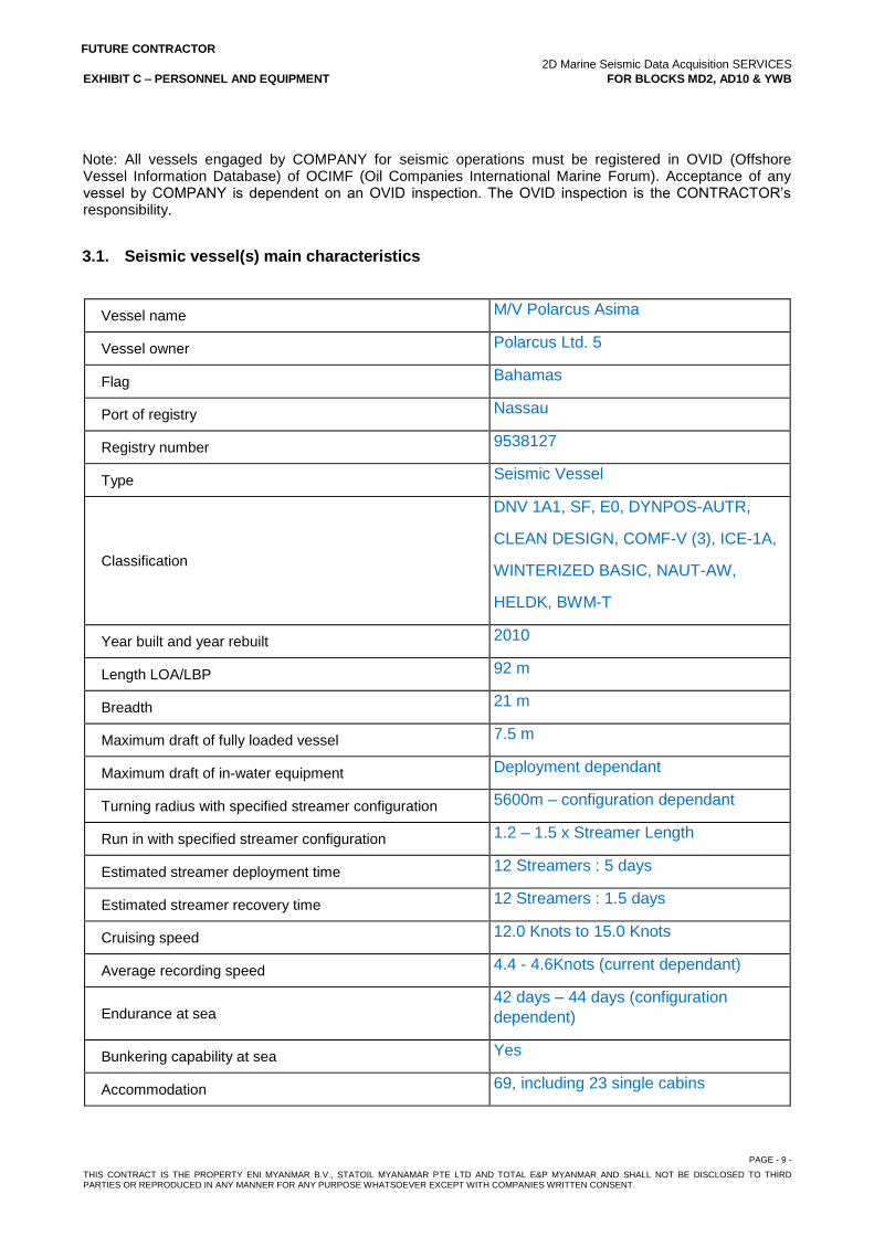
FUTURE CONTRACTOR 2D Marine Seismic Data Acquisition SERVICES EXHIBIT C – PERSONNEL AND EQUIPMENT FOR BLOCKS MD2, AD10 & YWB
PAGE - 9 - THIS CONTRACT IS THE PROPERTY ENI MYANMAR B.V., STATOIL MYANAMAR PTE LTD AND TOTAL E&P MYANMAR AND SHALL NOT BE DISCLOSED TO THIRD PARTIES OR REPRODUCED IN ANY MANNER FOR ANY PURPOSE WHATSOEVER EXCEPT WITH COMPANIES WRITTEN CONSENT.
Note: All vessels engaged by COMPANY for seismic operations must be registered in OVID (Offshore Vessel Information Database) of OCIMF (Oil Companies International Marine Forum). Acceptance of any vessel by COMPANY is dependent on an OVID inspection. The OVID inspection is the CONTRACTOR’s responsibility.
3.1. Seismic vessel(s) main characteristics
Vessel name M/V Polarcus Asima
Vessel owner Polarcus Ltd. 5
Flag Bahamas
Port of registry Nassau
Registry number 9538127
Type Seismic Vessel
Classification
DNV 1A1, SF, E0, DYNPOS-AUTR,
CLEAN DESIGN, COMF-V (3), ICE-1A,
WINTERIZED BASIC, NAUT-AW,
HELDK, BWM-T
Year built and year rebuilt 2010
Length LOA/LBP 92 m
Breadth 21 m
Maximum draft of fully loaded vessel 7.5 m
Maximum draft of in-water equipment Deployment dependant
Turning radius with specified streamer configuration 5600m – configuration dependant
Run in with specified streamer configuration 1.2 – 1.5 x Streamer Length
Estimated streamer deployment time 12 Streamers : 5 days
Estimated streamer recovery time 12 Streamers : 1.5 days
Cruising speed 12.0 Knots to 15.0 Knots
Average recording speed 4.4 - 4.6Knots (current dependant)
Endurance at sea 42 days – 44 days (configuration
dependent)
Bunkering capability at sea Yes
Accommodation 69, including 23 single cabins
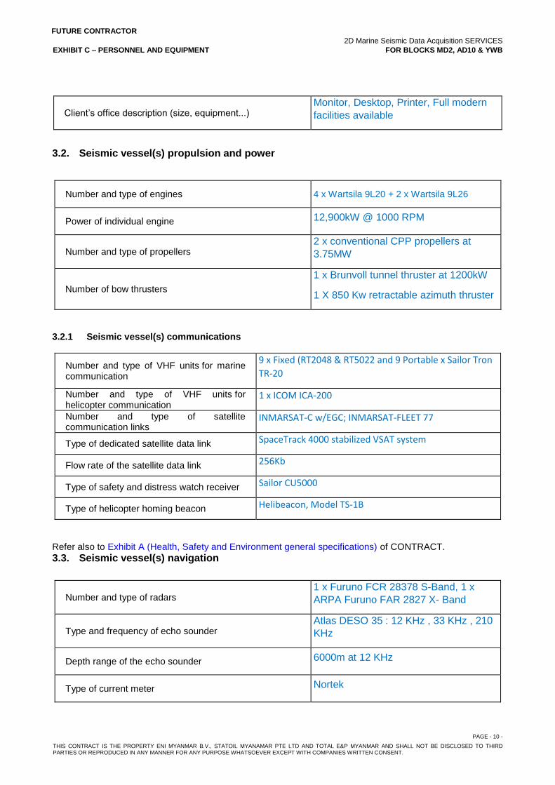
FUTURE CONTRACTOR 2D Marine Seismic Data Acquisition SERVICES EXHIBIT C – PERSONNEL AND EQUIPMENT FOR BLOCKS MD2, AD10 & YWB
PAGE - 10 - THIS CONTRACT IS THE PROPERTY ENI MYANMAR B.V., STATOIL MYANAMAR PTE LTD AND TOTAL E&P MYANMAR AND SHALL NOT BE DISCLOSED TO THIRD PARTIES OR REPRODUCED IN ANY MANNER FOR ANY PURPOSE WHATSOEVER EXCEPT WITH COMPANIES WRITTEN CONSENT.
Client’s office description (size, equipment...) Monitor, Desktop, Printer, Full modern
facilities available
3.2. Seismic vessel(s) propulsion and power
Number and type of engines 4 x Wartsila 9L20 + 2 x Wartsila 9L26
Power of individual engine 12,900kW @ 1000 RPM
Number and type of propellers 2 x conventional CPP propellers at
3.75MW
Number of bow thrusters
1 x Brunvoll tunnel thruster at 1200kW
1 X 850 Kw retractable azimuth thruster
3.2.1 Seismic vessel(s) communications
Number and type of VHF units for marine communication
9 x Fixed (RT2048 & RT5022 and 9 Portable x Sailor Tron
TR-20
Number and type of VHF units for helicopter communication
1 x ICOM ICA-200
Number and type of satellite communication links
INMARSAT-C w/EGC; INMARSAT-FLEET 77
Type of dedicated satellite data link SpaceTrack 4000 stabilized VSAT system
Flow rate of the satellite data link 256Kb
Type of safety and distress watch receiver Sailor CU5000
Type of helicopter homing beacon Helibeacon, Model TS-1B
Refer also to Exhibit A (Health, Safety and Environment general specifications) of CONTRACT. 3.3. Seismic vessel(s) navigation
Number and type of radars 1 x Furuno FCR 28378 S-Band, 1 x
ARPA Furuno FAR 2827 X- Band
Type and frequency of echo sounder Atlas DESO 35 : 12 KHz , 33 KHz , 210
KHz
Depth range of the echo sounder 6000m at 12 KHz
Type of current meter Nortek
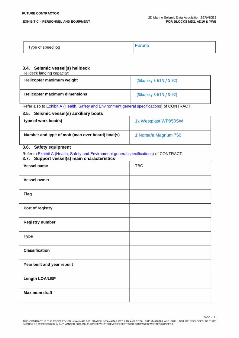
FUTURE CONTRACTOR 2D Marine Seismic Data Acquisition SERVICES EXHIBIT C – PERSONNEL AND EQUIPMENT FOR BLOCKS MD2, AD10 & YWB
PAGE - 11 - THIS CONTRACT IS THE PROPERTY ENI MYANMAR B.V., STATOIL MYANAMAR PTE LTD AND TOTAL E&P MYANMAR AND SHALL NOT BE DISCLOSED TO THIRD PARTIES OR REPRODUCED IN ANY MANNER FOR ANY PURPOSE WHATSOEVER EXCEPT WITH COMPANIES WRITTEN CONSENT.
Type of speed log Furuno
3.4. Seismic vessel(s) helideck Helideck landing capacity:
Helicopter maximum weight (Sikorsky S-61N / S-92)
Helicopter maximum dimensions (Sikorsky S-61N / S-92)
Refer also to Exhibit A (Health, Safety and Environment general specifications) of CONTRACT.
3.5. Seismic vessel(s) auxiliary boats
type of work boat(s) 1x Westplast WP950SW
Number and type of mob (man over board) boat(s) 1 Norsafe Magnum 750
3.6. Safety equipment
Refer to Exhibit A (Health, Safety and Environment general specifications) of CONTRACT. 3.7. Support vessel(s) main characteristics
Vessel name TBC
Vessel owner
Flag
Port of registry
Registry number
Type
Classification
Year built and year rebuilt
Length LOA/LBP
Maximum draft
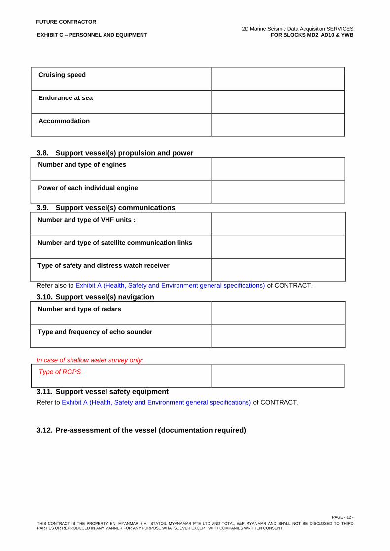
FUTURE CONTRACTOR 2D Marine Seismic Data Acquisition SERVICES EXHIBIT C – PERSONNEL AND EQUIPMENT FOR BLOCKS MD2, AD10 & YWB
PAGE - 12 - THIS CONTRACT IS THE PROPERTY ENI MYANMAR B.V., STATOIL MYANAMAR PTE LTD AND TOTAL E&P MYANMAR AND SHALL NOT BE DISCLOSED TO THIRD PARTIES OR REPRODUCED IN ANY MANNER FOR ANY PURPOSE WHATSOEVER EXCEPT WITH COMPANIES WRITTEN CONSENT.
Cruising speed
Endurance at sea
Accommodation
3.8. Support vessel(s) propulsion and power
Number and type of engines
Power of each individual engine
3.9. Support vessel(s) communications
Number and type of VHF units :
Number and type of satellite communication links
Type of safety and distress watch receiver
Refer also to Exhibit A (Health, Safety and Environment general specifications) of CONTRACT.
3.10. Support vessel(s) navigation
Number and type of radars
Type and frequency of echo sounder
In case of shallow water survey only:
Type of RGPS
3.11. Support vessel safety equipment
Refer to Exhibit A (Health, Safety and Environment general specifications) of CONTRACT.
3.12. Pre-assessment of the vessel (documentation required)
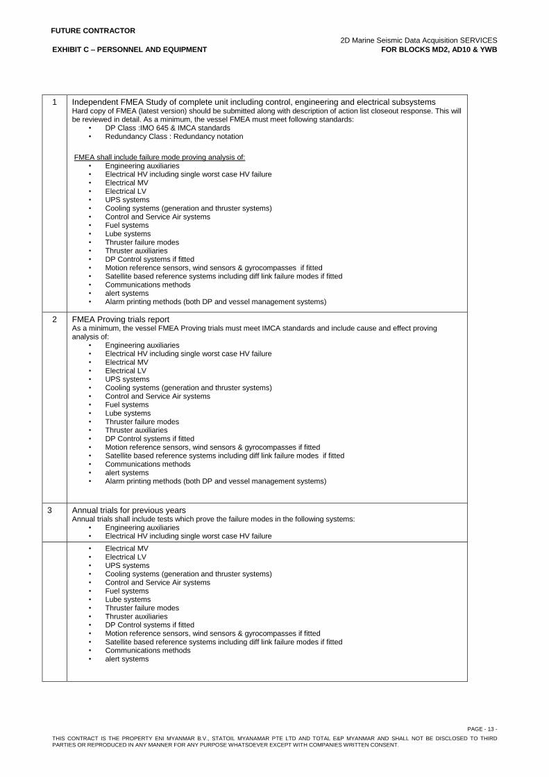
FUTURE CONTRACTOR 2D Marine Seismic Data Acquisition SERVICES EXHIBIT C – PERSONNEL AND EQUIPMENT FOR BLOCKS MD2, AD10 & YWB
PAGE - 13 - THIS CONTRACT IS THE PROPERTY ENI MYANMAR B.V., STATOIL MYANAMAR PTE LTD AND TOTAL E&P MYANMAR AND SHALL NOT BE DISCLOSED TO THIRD PARTIES OR REPRODUCED IN ANY MANNER FOR ANY PURPOSE WHATSOEVER EXCEPT WITH COMPANIES WRITTEN CONSENT.
1 Independent FMEA Study of complete unit including control, engineering and electrical subsystems Hard copy of FMEA (latest version) should be submitted along with description of action list closeout response. This will be reviewed in detail. As a minimum, the vessel FMEA must meet following standards:
• DP Class :IMO 645 & IMCA standards • Redundancy Class : Redundancy notation
FMEA shall include failure mode proving analysis of:
• Engineering auxiliaries • Electrical HV including single worst case HV failure • Electrical MV • Electrical LV • UPS systems • Cooling systems (generation and thruster systems) • Control and Service Air systems • Fuel systems • Lube systems • Thruster failure modes • Thruster auxiliaries • DP Control systems if fitted • Motion reference sensors, wind sensors & gyrocompasses if fitted • Satellite based reference systems including diff link failure modes if fitted • Communications methods • alert systems • Alarm printing methods (both DP and vessel management systems)
2 FMEA Proving trials report As a minimum, the vessel FMEA Proving trials must meet IMCA standards and include cause and effect proving analysis of:
• Engineering auxiliaries • Electrical HV including single worst case HV failure • Electrical MV • Electrical LV • UPS systems • Cooling systems (generation and thruster systems) • Control and Service Air systems • Fuel systems • Lube systems • Thruster failure modes • Thruster auxiliaries • DP Control systems if fitted • Motion reference sensors, wind sensors & gyrocompasses if fitted • Satellite based reference systems including diff link failure modes if fitted • Communications methods • alert systems • Alarm printing methods (both DP and vessel management systems)
3 Annual trials for previous years Annual trials shall include tests which prove the failure modes in the following systems:
• Engineering auxiliaries • Electrical HV including single worst case HV failure
• Electrical MV • Electrical LV • UPS systems • Cooling systems (generation and thruster systems) • Control and Service Air systems • Fuel systems • Lube systems • Thruster failure modes • Thruster auxiliaries • DP Control systems if fitted • Motion reference sensors, wind sensors & gyrocompasses if fitted • Satellite based reference systems including diff link failure modes if fitted • Communications methods • alert systems
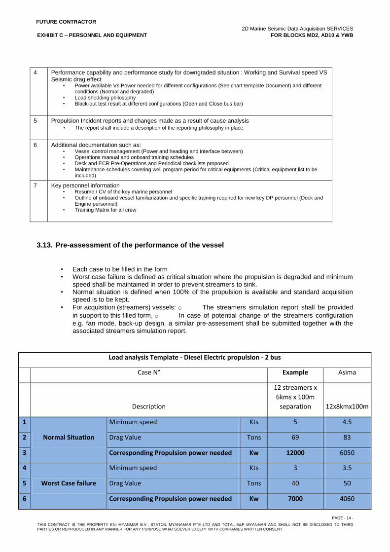
FUTURE CONTRACTOR 2D Marine Seismic Data Acquisition SERVICES EXHIBIT C – PERSONNEL AND EQUIPMENT FOR BLOCKS MD2, AD10 & YWB
PAGE - 14 - THIS CONTRACT IS THE PROPERTY ENI MYANMAR B.V., STATOIL MYANAMAR PTE LTD AND TOTAL E&P MYANMAR AND SHALL NOT BE DISCLOSED TO THIRD PARTIES OR REPRODUCED IN ANY MANNER FOR ANY PURPOSE WHATSOEVER EXCEPT WITH COMPANIES WRITTEN CONSENT.
4 Performance capability and performance study for downgraded situation : Working and Survival speed VS Seismic drag effect
• Power available Vs Power needed for different configurations (See chart template Document) and different conditions (Normal and degraded)
• Load shedding philosophy • Black-out test result at different configurations (Open and Close bus bar)
5 Propulsion Incident reports and changes made as a result of cause analysis • The report shall include a description of the reporting philosophy in place.
6 Additional documentation such as: • Vessel control management (Power and heading and interface between) • Operations manual and onboard training schedules • Deck and ECR Pre-Operations and Periodical checklists proposed • Maintenance schedules covering well program period for critical equipments (Critical equipment list to be
included)
7 Key personnel information • Resume / CV of the key marine personnel • Outline of onboard vessel familiarization and specific training required for new key DP personnel (Deck and
Engine personnel) • Training Matrix for all crew
3.13. Pre-assessment of the performance of the vessel
• Each case to be filled in the form • Worst case failure is defined as critical situation where the propulsion is degraded and minimum
speed shall be maintained in order to prevent streamers to sink. • Normal situation is defined when 100% of the propulsion is available and standard acquisition
speed is to be kept. • For acquisition (streamers) vessels: o The streamers simulation report shall be provided
in support to this filled form, o In case of potential change of the streamers configuration
e.g. fan mode, back-up design, a similar pre-assessment shall be submitted together with the associated streamers simulation report.
Load analysis Template - Diesel Electric propulsion - 2 bus
Case N° Example Asima
Description
12 streamers x
6kms x 100m
separation 12x8kmx100m
1
Normal Situation
Minimum speed Kts 5 4.5
2 Drag Value Tons 69 83
3 Corresponding Propulsion power needed Kw 12000 6050
4
Worst Case failure
Minimum speed Kts 3 3.5
5 Drag Value Tons 40 50
6 Corresponding Propulsion power needed Kw 7000 4060
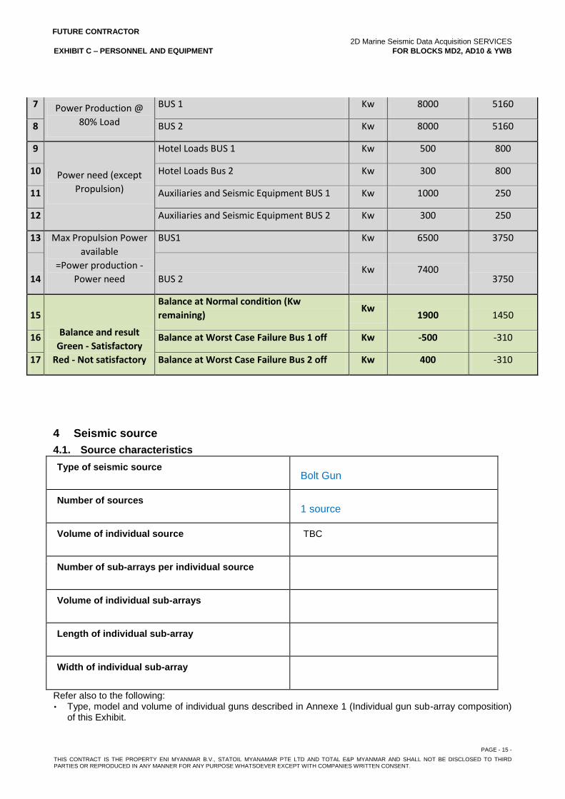
FUTURE CONTRACTOR 2D Marine Seismic Data Acquisition SERVICES EXHIBIT C – PERSONNEL AND EQUIPMENT FOR BLOCKS MD2, AD10 & YWB
PAGE - 15 - THIS CONTRACT IS THE PROPERTY ENI MYANMAR B.V., STATOIL MYANAMAR PTE LTD AND TOTAL E&P MYANMAR AND SHALL NOT BE DISCLOSED TO THIRD PARTIES OR REPRODUCED IN ANY MANNER FOR ANY PURPOSE WHATSOEVER EXCEPT WITH COMPANIES WRITTEN CONSENT.
7 Power Production @
80% Load
BUS 1 Kw 8000 5160
8 BUS 2 Kw 8000 5160
9
Power need (except
Propulsion)
Hotel Loads BUS 1 Kw 500 800
10 Hotel Loads Bus 2 Kw 300 800
11 Auxiliaries and Seismic Equipment BUS 1 Kw 1000 250
12 Auxiliaries and Seismic Equipment BUS 2 Kw 300 250
13 Max Propulsion Power
available
=Power production -
Power need
BUS1 Kw 6500 3750
14 BUS 2 Kw 7400
3750
15
Balance and result
Green - Satisfactory
Red - Not satisfactory
Balance at Normal condition (Kw
remaining) Kw
1900 1450
16 Balance at Worst Case Failure Bus 1 off Kw -500 -310
17 Balance at Worst Case Failure Bus 2 off Kw 400 -310
4 Seismic source
4.1. Source characteristics
Type of seismic source Bolt Gun
Number of sources 1 source
Volume of individual source TBC
Number of sub-arrays per individual source
Volume of individual sub-arrays
Length of individual sub-array
Width of individual sub-array
Refer also to the following: • Type, model and volume of individual guns described in Annexe 1 (Individual gun sub-array composition)
of this Exhibit.
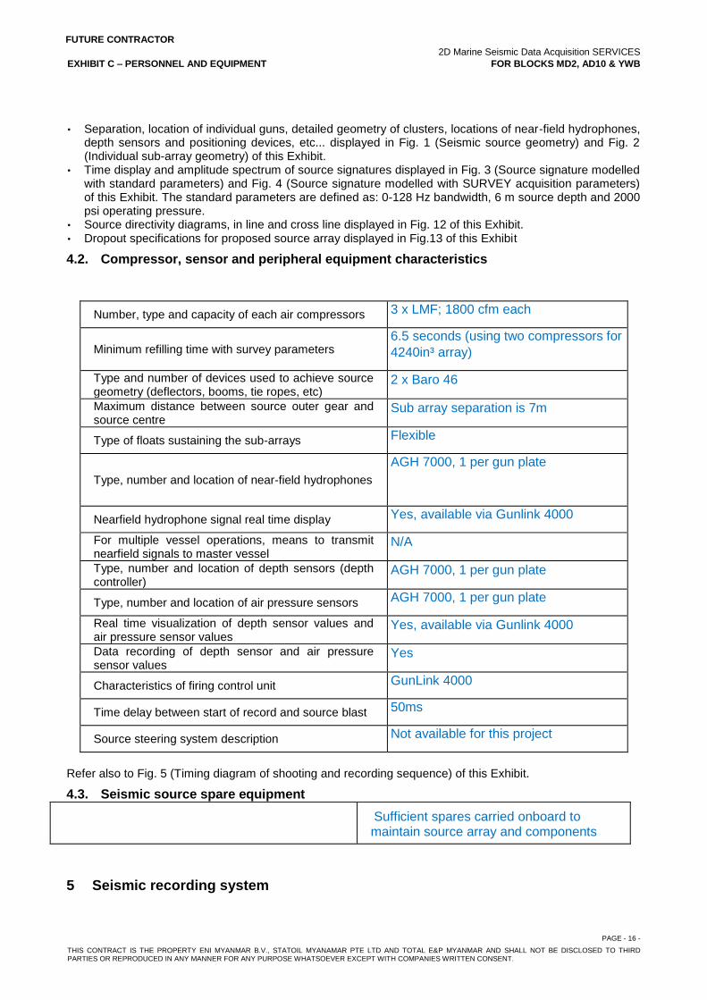
FUTURE CONTRACTOR 2D Marine Seismic Data Acquisition SERVICES EXHIBIT C – PERSONNEL AND EQUIPMENT FOR BLOCKS MD2, AD10 & YWB
PAGE - 16 - THIS CONTRACT IS THE PROPERTY ENI MYANMAR B.V., STATOIL MYANAMAR PTE LTD AND TOTAL E&P MYANMAR AND SHALL NOT BE DISCLOSED TO THIRD PARTIES OR REPRODUCED IN ANY MANNER FOR ANY PURPOSE WHATSOEVER EXCEPT WITH COMPANIES WRITTEN CONSENT.
• Separation, location of individual guns, detailed geometry of clusters, locations of near-field hydrophones, depth sensors and positioning devices, etc... displayed in Fig. 1 (Seismic source geometry) and Fig. 2 (Individual sub-array geometry) of this Exhibit.
• Time display and amplitude spectrum of source signatures displayed in Fig. 3 (Source signature modelled with standard parameters) and Fig. 4 (Source signature modelled with SURVEY acquisition parameters) of this Exhibit. The standard parameters are defined as: 0-128 Hz bandwidth, 6 m source depth and 2000 psi operating pressure.
• Source directivity diagrams, in line and cross line displayed in Fig. 12 of this Exhibit. • Dropout specifications for proposed source array displayed in Fig.13 of this Exhibit
4.2. Compressor, sensor and peripheral equipment characteristics
Number, type and capacity of each air compressors 3 x LMF; 1800 cfm each
Minimum refilling time with survey parameters 6.5 seconds (using two compressors for
4240in³ array)
Type and number of devices used to achieve source geometry (deflectors, booms, tie ropes, etc)
2 x Baro 46
Maximum distance between source outer gear and source centre
Sub array separation is 7m
Type of floats sustaining the sub-arrays Flexible
Type, number and location of near-field hydrophones
AGH 7000, 1 per gun plate
Nearfield hydrophone signal real time display Yes, available via Gunlink 4000
For multiple vessel operations, means to transmit nearfield signals to master vessel
N/A
Type, number and location of depth sensors (depth controller)
AGH 7000, 1 per gun plate
Type, number and location of air pressure sensors AGH 7000, 1 per gun plate
Real time visualization of depth sensor values and air pressure sensor values
Yes, available via Gunlink 4000
Data recording of depth sensor and air pressure sensor values
Yes
Characteristics of firing control unit GunLink 4000
Time delay between start of record and source blast 50ms
Source steering system description Not available for this project
Refer also to Fig. 5 (Timing diagram of shooting and recording sequence) of this Exhibit.
4.3. Seismic source spare equipment
Sufficient spares carried onboard to maintain source array and components
5 Seismic recording system
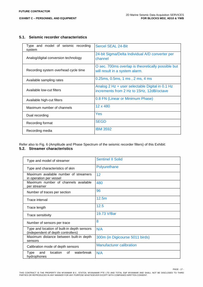
FUTURE CONTRACTOR 2D Marine Seismic Data Acquisition SERVICES EXHIBIT C – PERSONNEL AND EQUIPMENT FOR BLOCKS MD2, AD10 & YWB
PAGE - 17 - THIS CONTRACT IS THE PROPERTY ENI MYANMAR B.V., STATOIL MYANAMAR PTE LTD AND TOTAL E&P MYANMAR AND SHALL NOT BE DISCLOSED TO THIRD PARTIES OR REPRODUCED IN ANY MANNER FOR ANY PURPOSE WHATSOEVER EXCEPT WITH COMPANIES WRITTEN CONSENT.
5.1. Seismic recorder characteristics
Type and model of seismic recording system
Sercel SEAL 24-Bit
Analog/digital conversion technology 24-bit Sigma/Delta Individual A/D converter per
channel
Recording system overhead cycle time O sec. 700ms overlap is theoretically possible but
will result in a system alarm.
Available sampling rates 0.25ms, 0.5ms, 1 ms , 2 ms, 4 ms
Available low-cut filters Analog 2 Hz + user selectable Digital in 0.1 Hz
increments from 2 Hz to 15Hz, 12dB/octave
Available high-cut filters 0.8 FN (Linear or Minimum Phase)
Maximum number of channels 12 x 480
Dual recording Yes
Recording format SEGD
Recording media IBM 3592
Refer also to Fig. 6 (Amplitude and Phase Spectrum of the seismic recorder filters) of this Exhibit: 5.2. Streamer characteristics
Type and model of streamer Sentinel II Solid
Type and characteristics of skin Polyurethane
Maximum available number of streamers in operation per vessel
12
Maximum number of channels available per streamer
480
Number of traces per section 96
Trace interval 12.5m
Trace length 12.5
Trace sensitivity 19.73 V/Bar
Number of sensors per trace 8
Type and location of built-in depth sensors (independent of depth controllers)
N/A
Maximum distance between built-in depth sensors
300m (in Digicourse 5011 birds)
Calibration mode of depth sensors Manufacturer calibration
Type and location of waterbreak hydrophones
N/A
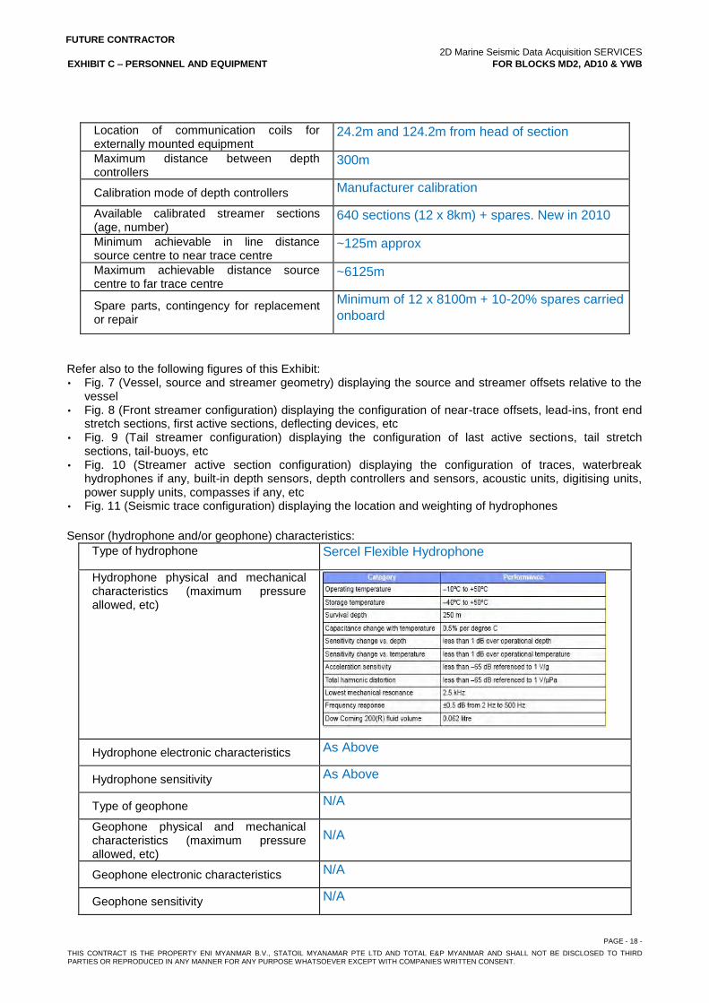
FUTURE CONTRACTOR 2D Marine Seismic Data Acquisition SERVICES EXHIBIT C – PERSONNEL AND EQUIPMENT FOR BLOCKS MD2, AD10 & YWB
PAGE - 18 - THIS CONTRACT IS THE PROPERTY ENI MYANMAR B.V., STATOIL MYANAMAR PTE LTD AND TOTAL E&P MYANMAR AND SHALL NOT BE DISCLOSED TO THIRD PARTIES OR REPRODUCED IN ANY MANNER FOR ANY PURPOSE WHATSOEVER EXCEPT WITH COMPANIES WRITTEN CONSENT.
Location of communication coils for externally mounted equipment
24.2m and 124.2m from head of section
Maximum distance between depth controllers
300m
Calibration mode of depth controllers Manufacturer calibration
Available calibrated streamer sections (age, number)
640 sections (12 x 8km) + spares. New in 2010
Minimum achievable in line distance source centre to near trace centre
~125m approx
Maximum achievable distance source centre to far trace centre
~6125m
Spare parts, contingency for replacement or repair
Minimum of 12 x 8100m + 10-20% spares carried
onboard
Refer also to the following figures of this Exhibit: • Fig. 7 (Vessel, source and streamer geometry) displaying the source and streamer offsets relative to the
vessel • Fig. 8 (Front streamer configuration) displaying the configuration of near-trace offsets, lead-ins, front end
stretch sections, first active sections, deflecting devices, etc • Fig. 9 (Tail streamer configuration) displaying the configuration of last active sections, tail stretch
sections, tail-buoys, etc • Fig. 10 (Streamer active section configuration) displaying the configuration of traces, waterbreak
hydrophones if any, built-in depth sensors, depth controllers and sensors, acoustic units, digitising units, power supply units, compasses if any, etc
• Fig. 11 (Seismic trace configuration) displaying the location and weighting of hydrophones Sensor (hydrophone and/or geophone) characteristics:
Type of hydrophone Sercel Flexible Hydrophone
Hydrophone physical and mechanical characteristics (maximum pressure allowed, etc)
Hydrophone electronic characteristics As Above
Hydrophone sensitivity As Above
Type of geophone N/A
Geophone physical and mechanical characteristics (maximum pressure allowed, etc)
N/A
Geophone electronic characteristics N/A
Geophone sensitivity N/A
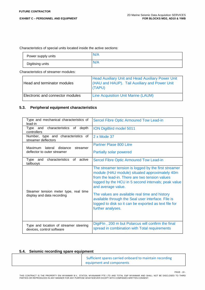
FUTURE CONTRACTOR 2D Marine Seismic Data Acquisition SERVICES EXHIBIT C – PERSONNEL AND EQUIPMENT FOR BLOCKS MD2, AD10 & YWB
PAGE - 19 - THIS CONTRACT IS THE PROPERTY ENI MYANMAR B.V., STATOIL MYANAMAR PTE LTD AND TOTAL E&P MYANMAR AND SHALL NOT BE DISCLOSED TO THIRD PARTIES OR REPRODUCED IN ANY MANNER FOR ANY PURPOSE WHATSOEVER EXCEPT WITH COMPANIES WRITTEN CONSENT.
Characteristics of special units located inside the active sections:
Power supply units N/A
Digitising units N/A
Characteristics of streamer modules:
Head and terminator modules
Head Auxiliary Unit and Head Auxiliary Power Unit
(HAU and HAUP). Tail Auxiliary and Power Unit
(TAPU)
Electronic and connector modules Line Acquisition Unit Marine (LAUM)
5.3. Peripheral equipment characteristics
Type and mechanical characteristics of lead-in
Sercel Fibre Optic Armoured Tow Lead-in
Type and characteristics of depth controllers
ION DigiBird model 5011
Number, type and characteristics of streamer deflectors
2 x Mode 37
Maximum lateral distance streamer deflector to outer streamer
Partner Plase 800 Litre
Partially solar powered
Type and characteristics of active tailbuoys
Sercel Fibre Optic Armoured Tow Lead-in
Steamer tension meter type, real time display and data recording
The streamer tension is logged by the first streamer
module (HAU module) situated approximately 40m
from the lead-in. There are two tension values
logged by the HCU in 5 second intervals; peak value
and average value.
The values are available real time and history
available through the Seal user interface. File is
logged to disk so it can be exported as text file for
further analyses.
Type and location of streamer steering devices, control software
DigiFIn , 200 m but Polarcus will confirm the final
spread in combination with Total requirements
5.4. Seismic recording spare equipment
Sufficient spares carried onboard to maintain recording equipment and components
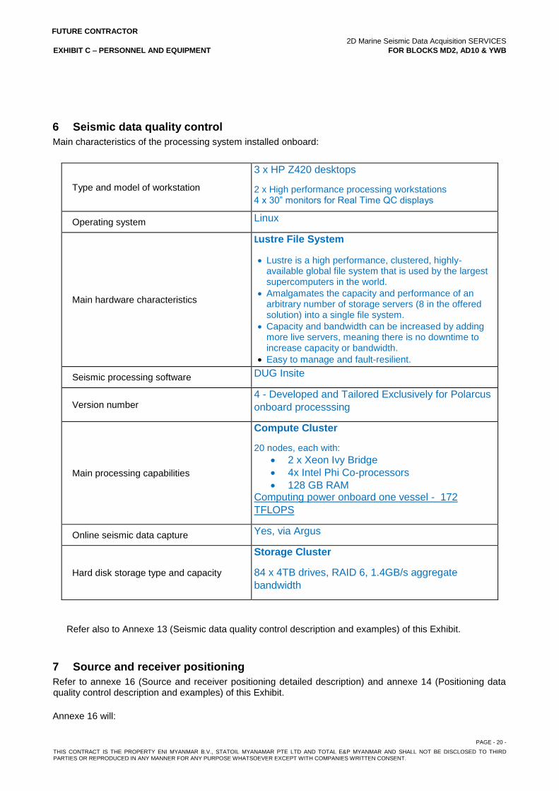
FUTURE CONTRACTOR 2D Marine Seismic Data Acquisition SERVICES EXHIBIT C – PERSONNEL AND EQUIPMENT FOR BLOCKS MD2, AD10 & YWB
PAGE - 20 - THIS CONTRACT IS THE PROPERTY ENI MYANMAR B.V., STATOIL MYANAMAR PTE LTD AND TOTAL E&P MYANMAR AND SHALL NOT BE DISCLOSED TO THIRD PARTIES OR REPRODUCED IN ANY MANNER FOR ANY PURPOSE WHATSOEVER EXCEPT WITH COMPANIES WRITTEN CONSENT.
6 Seismic data quality control
Main characteristics of the processing system installed onboard:
Type and model of workstation
3 x HP Z420 desktops
2 x High performance processing workstations 4 x 30” monitors for Real Time QC displays
Operating system Linux
Main hardware characteristics
Lustre File System
Lustre is a high performance, clustered, highly-available global file system that is used by the largest supercomputers in the world.
Amalgamates the capacity and performance of an arbitrary number of storage servers (8 in the offered solution) into a single file system.
Capacity and bandwidth can be increased by adding more live servers, meaning there is no downtime to increase capacity or bandwidth.
Easy to manage and fault-resilient.
Seismic processing software DUG Insite
Version number 4 - Developed and Tailored Exclusively for Polarcus
onboard processsing
Main processing capabilities
Compute Cluster
20 nodes, each with:
2 x Xeon Ivy Bridge
4x Intel Phi Co-processors
128 GB RAM Computing power onboard one vessel - 172
TFLOPS
Online seismic data capture Yes, via Argus
Hard disk storage type and capacity
Storage Cluster
84 x 4TB drives, RAID 6, 1.4GB/s aggregate
bandwidth
Refer also to Annexe 13 (Seismic data quality control description and examples) of this Exhibit.
7 Source and receiver positioning
Refer to annexe 16 (Source and receiver positioning detailed description) and annexe 14 (Positioning data quality control description and examples) of this Exhibit. Annexe 16 will:
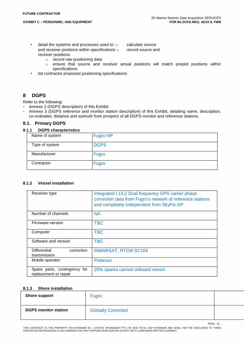
FUTURE CONTRACTOR 2D Marine Seismic Data Acquisition SERVICES EXHIBIT C – PERSONNEL AND EQUIPMENT FOR BLOCKS MD2, AD10 & YWB
PAGE - 21 - THIS CONTRACT IS THE PROPERTY ENI MYANMAR B.V., STATOIL MYANAMAR PTE LTD AND TOTAL E&P MYANMAR AND SHALL NOT BE DISCLOSED TO THIRD PARTIES OR REPRODUCED IN ANY MANNER FOR ANY PURPOSE WHATSOEVER EXCEPT WITH COMPANIES WRITTEN CONSENT.
• detail the systems and processes used to: o calculate source
and receiver positions within specifications o record source and
receiver positions o record raw positioning data o ensure that source and receiver actual positions will match preplot positions within
specifications • list contractor proposed positioning specifications
8 DGPS
Refer to the following: • Annexe 2 (DGPS description) of this Exhibit. • Annexe 3 (DGPS reference and monitor station description) of this Exhibit, detailing name, description,
co-ordinates, distance and azimuth from prospect of all DGPS monitor and reference stations.
8.1. Primary DGPS
8.1.1 DGPS characteristics Name of system Fugro HP
Type of system DGPS
Manufacturer Fugro
Contractor Fugro
8.1.2 Vessel installation
Receiver type Integrated L1/L2 Dual frequency GPS carrier phase
correction data from Fugro's network of reference stations
and completely independent from SkyFix-XP
Number of channels NA
Firmware version TBC
Computer TBC
Software and version TBC
Differential correction transmission
INMARSAT, RTCM SC104
Mobile operator Polarcus
Spare parts, contingency for replacement or repair
20% spares carried onboard vessel
8.1.3 Shore installation
Shore support Fugro
DGPS monitor station Globally Corrected
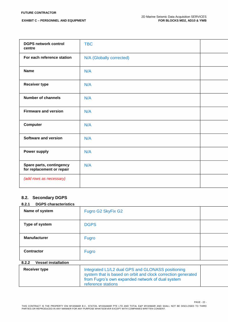
FUTURE CONTRACTOR 2D Marine Seismic Data Acquisition SERVICES EXHIBIT C – PERSONNEL AND EQUIPMENT FOR BLOCKS MD2, AD10 & YWB
PAGE - 22 - THIS CONTRACT IS THE PROPERTY ENI MYANMAR B.V., STATOIL MYANAMAR PTE LTD AND TOTAL E&P MYANMAR AND SHALL NOT BE DISCLOSED TO THIRD PARTIES OR REPRODUCED IN ANY MANNER FOR ANY PURPOSE WHATSOEVER EXCEPT WITH COMPANIES WRITTEN CONSENT.
DGPS network control centre
TBC
For each reference station N/A (Globally corrected)
Name N/A
Receiver type N/A
Number of channels N/A
Firmware and version N/A
Computer N/A
Software and version N/A
Power supply N/A
Spare parts, contingency for replacement or repair
N/A
(add rows as necessary)
8.2. Secondary DGPS
8.2.1 DGPS characteristics
Name of system Fugro G2 SkyFix G2
Type of system DGPS
Manufacturer Fugro
Contractor Fugro
8.2.2 Vessel installation
Receiver type Integrated L1/L2 dual GPS and GLONASS positioning system that is based on orbit and clock correction generated from Fugro’s own expanded network of dual system reference stations
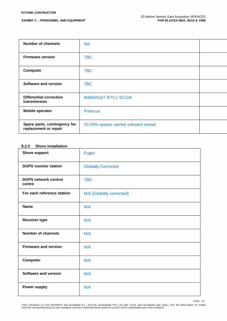
FUTURE CONTRACTOR 2D Marine Seismic Data Acquisition SERVICES EXHIBIT C – PERSONNEL AND EQUIPMENT FOR BLOCKS MD2, AD10 & YWB
PAGE - 23 - THIS CONTRACT IS THE PROPERTY ENI MYANMAR B.V., STATOIL MYANAMAR PTE LTD AND TOTAL E&P MYANMAR AND SHALL NOT BE DISCLOSED TO THIRD PARTIES OR REPRODUCED IN ANY MANNER FOR ANY PURPOSE WHATSOEVER EXCEPT WITH COMPANIES WRITTEN CONSENT.
Number of channels NA
Firmware version TBC
Computer TBC
Software and version TBC
Differential correction transmission
INMARSAT RTC< SC104
Mobile operator Polarcus
Spare parts, contingency for replacement or repair
10-20% spares carried onboard vessel
8.2.3 Shore installation
Shore support Fugro
DGPS monitor station Globally Corrected
DGPS network control centre
TBC
For each reference station N/A (Globally corrected)
Name N/A
Receiver type N/A
Number of channels N/A
Firmware and version N/A
Computer N/A
Software and version N/A
Power supply N/A
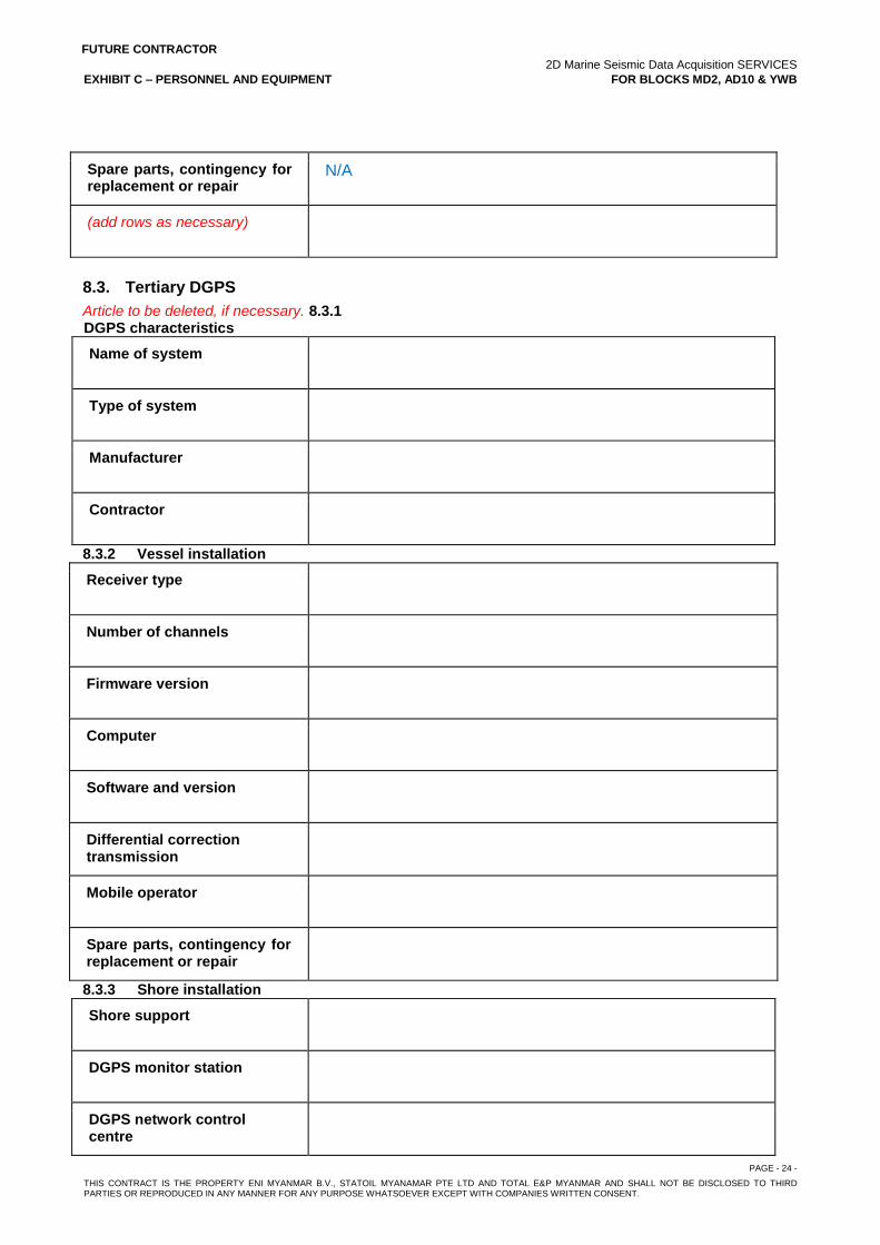
FUTURE CONTRACTOR 2D Marine Seismic Data Acquisition SERVICES EXHIBIT C – PERSONNEL AND EQUIPMENT FOR BLOCKS MD2, AD10 & YWB
PAGE - 24 - THIS CONTRACT IS THE PROPERTY ENI MYANMAR B.V., STATOIL MYANAMAR PTE LTD AND TOTAL E&P MYANMAR AND SHALL NOT BE DISCLOSED TO THIRD PARTIES OR REPRODUCED IN ANY MANNER FOR ANY PURPOSE WHATSOEVER EXCEPT WITH COMPANIES WRITTEN CONSENT.
Spare parts, contingency for replacement or repair
N/A
(add rows as necessary)
8.3. Tertiary DGPS
Article to be deleted, if necessary. 8.3.1 DGPS characteristics
Name of system
Type of system
Manufacturer
Contractor
8.3.2 Vessel installation
Receiver type
Number of channels
Firmware version
Computer
Software and version
Differential correction transmission
Mobile operator
Spare parts, contingency for replacement or repair
8.3.3 Shore installation
Shore support
DGPS monitor station
DGPS network control centre
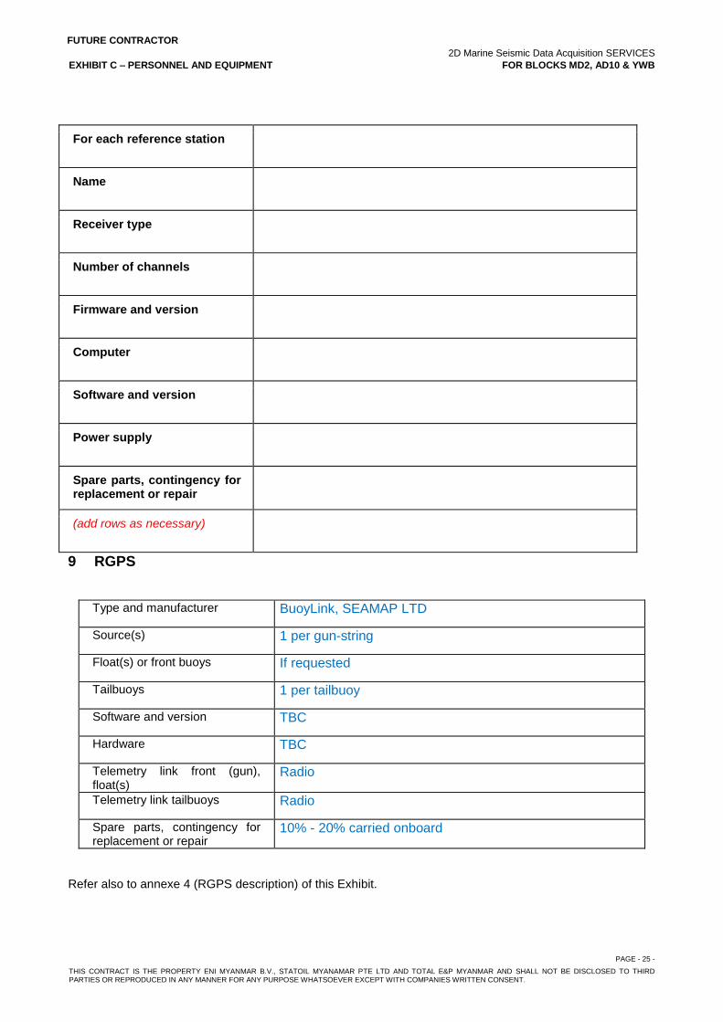
FUTURE CONTRACTOR 2D Marine Seismic Data Acquisition SERVICES EXHIBIT C – PERSONNEL AND EQUIPMENT FOR BLOCKS MD2, AD10 & YWB
PAGE - 25 - THIS CONTRACT IS THE PROPERTY ENI MYANMAR B.V., STATOIL MYANAMAR PTE LTD AND TOTAL E&P MYANMAR AND SHALL NOT BE DISCLOSED TO THIRD PARTIES OR REPRODUCED IN ANY MANNER FOR ANY PURPOSE WHATSOEVER EXCEPT WITH COMPANIES WRITTEN CONSENT.
For each reference station
Name
Receiver type
Number of channels
Firmware and version
Computer
Software and version
Power supply
Spare parts, contingency for replacement or repair
(add rows as necessary)
9 RGPS
Type and manufacturer BuoyLink, SEAMAP LTD
Source(s) 1 per gun-string
Float(s) or front buoys If requested
Tailbuoys 1 per tailbuoy
Software and version TBC
Hardware TBC
Telemetry link front (gun), float(s)
Radio
Telemetry link tailbuoys Radio
Spare parts, contingency for replacement or repair
10% - 20% carried onboard
Refer also to annexe 4 (RGPS description) of this Exhibit.
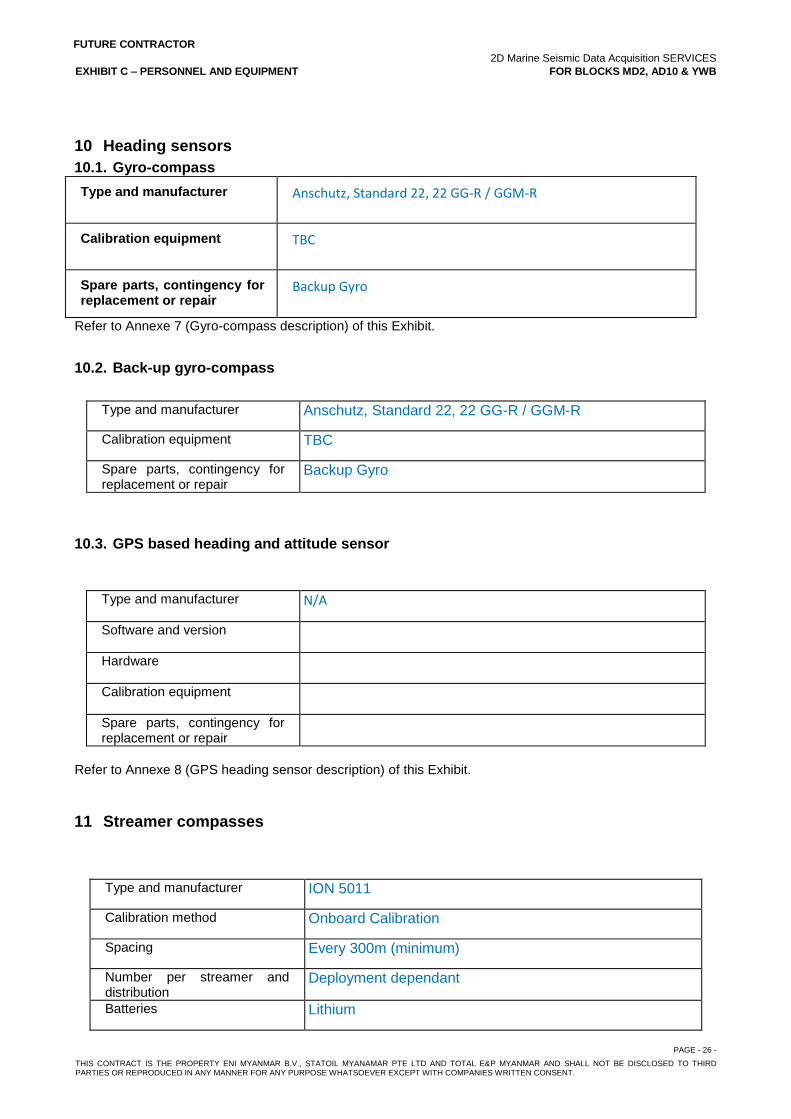
FUTURE CONTRACTOR 2D Marine Seismic Data Acquisition SERVICES EXHIBIT C – PERSONNEL AND EQUIPMENT FOR BLOCKS MD2, AD10 & YWB
PAGE - 26 - THIS CONTRACT IS THE PROPERTY ENI MYANMAR B.V., STATOIL MYANAMAR PTE LTD AND TOTAL E&P MYANMAR AND SHALL NOT BE DISCLOSED TO THIRD PARTIES OR REPRODUCED IN ANY MANNER FOR ANY PURPOSE WHATSOEVER EXCEPT WITH COMPANIES WRITTEN CONSENT.
10 Heading sensors
10.1. Gyro-compass
Type and manufacturer Anschutz, Standard 22, 22 GG-R / GGM-R
Calibration equipment TBC
Spare parts, contingency for replacement or repair
Backup Gyro
Refer to Annexe 7 (Gyro-compass description) of this Exhibit.
10.2. Back-up gyro-compass
Type and manufacturer Anschutz, Standard 22, 22 GG-R / GGM-R
Calibration equipment TBC
Spare parts, contingency for replacement or repair
Backup Gyro
10.3. GPS based heading and attitude sensor
Type and manufacturer N/A
Software and version
Hardware
Calibration equipment
Spare parts, contingency for replacement or repair
Refer to Annexe 8 (GPS heading sensor description) of this Exhibit.
11 Streamer compasses
Type and manufacturer ION 5011
Calibration method Onboard Calibration
Spacing Every 300m (minimum)
Number per streamer and distribution
Deployment dependant
Batteries Lithium
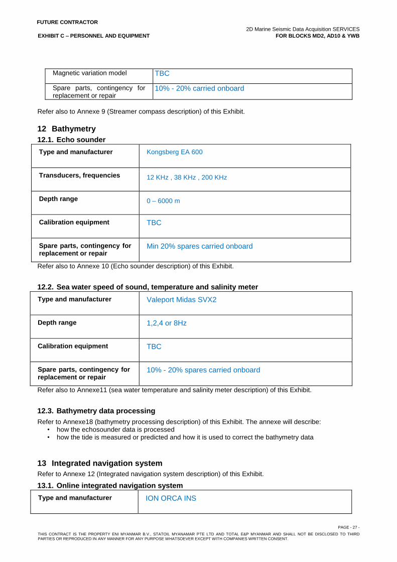
FUTURE CONTRACTOR 2D Marine Seismic Data Acquisition SERVICES EXHIBIT C – PERSONNEL AND EQUIPMENT FOR BLOCKS MD2, AD10 & YWB
PAGE - 27 - THIS CONTRACT IS THE PROPERTY ENI MYANMAR B.V., STATOIL MYANAMAR PTE LTD AND TOTAL E&P MYANMAR AND SHALL NOT BE DISCLOSED TO THIRD PARTIES OR REPRODUCED IN ANY MANNER FOR ANY PURPOSE WHATSOEVER EXCEPT WITH COMPANIES WRITTEN CONSENT.
Magnetic variation model TBC
Spare parts, contingency for replacement or repair
10% - 20% carried onboard
Refer also to Annexe 9 (Streamer compass description) of this Exhibit.
12 Bathymetry
12.1. Echo sounder
Type and manufacturer Kongsberg EA 600
Transducers, frequencies 12 KHz , 38 KHz , 200 KHz
Depth range 0 – 6000 m
Calibration equipment TBC
Spare parts, contingency for replacement or repair
Min 20% spares carried onboard
Refer also to Annexe 10 (Echo sounder description) of this Exhibit.
12.2. Sea water speed of sound, temperature and salinity meter
Type and manufacturer Valeport Midas SVX2
Depth range 1,2,4 or 8Hz
Calibration equipment TBC
Spare parts, contingency for replacement or repair
10% - 20% spares carried onboard
Refer also to Annexe11 (sea water temperature and salinity meter description) of this Exhibit.
12.3. Bathymetry data processing
Refer to Annexe18 (bathymetry processing description) of this Exhibit. The annexe will describe: • how the echosounder data is processed • how the tide is measured or predicted and how it is used to correct the bathymetry data
13 Integrated navigation system
Refer to Annexe 12 (Integrated navigation system description) of this Exhibit.
13.1. Online integrated navigation system
Type and manufacturer ION ORCA INS
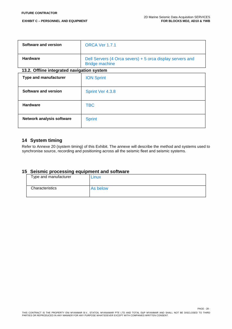
FUTURE CONTRACTOR 2D Marine Seismic Data Acquisition SERVICES EXHIBIT C – PERSONNEL AND EQUIPMENT FOR BLOCKS MD2, AD10 & YWB
PAGE - 28 - THIS CONTRACT IS THE PROPERTY ENI MYANMAR B.V., STATOIL MYANAMAR PTE LTD AND TOTAL E&P MYANMAR AND SHALL NOT BE DISCLOSED TO THIRD PARTIES OR REPRODUCED IN ANY MANNER FOR ANY PURPOSE WHATSOEVER EXCEPT WITH COMPANIES WRITTEN CONSENT.
Software and version ORCA Ver 1.7.1
Hardware Dell Servers (4 Orca severs) + 5 orca display servers and Bridge machine
13.2. Offline integrated navigation system
Type and manufacturer ION Sprint
Software and version Sprint Ver 4.3.8
Hardware TBC
Network analysis software Sprint
14 System timing
Refer to Annexe 20 (system timing) of this Exhibit. The annexe will describe the method and systems used to synchronise source, recording and positioning across all the seismic fleet and seismic systems.
15 Seismic processing equipment and software Type and manufacturer Linux
Characteristics As below
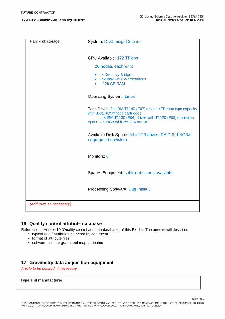
FUTURE CONTRACTOR 2D Marine Seismic Data Acquisition SERVICES EXHIBIT C – PERSONNEL AND EQUIPMENT FOR BLOCKS MD2, AD10 & YWB
PAGE - 29 - THIS CONTRACT IS THE PROPERTY ENI MYANMAR B.V., STATOIL MYANAMAR PTE LTD AND TOTAL E&P MYANMAR AND SHALL NOT BE DISCLOSED TO THIRD PARTIES OR REPRODUCED IN ANY MANNER FOR ANY PURPOSE WHATSOEVER EXCEPT WITH COMPANIES WRITTEN CONSENT.
Hard disk storage System: DUG Insight 3 Linux
CPU Available: 172 TFlops
20 nodes, each with:
x Xeon Ivy Bridge
4x Intel Phi Co-processors
128 GB RAM
Operating System: Linux
Tape Drives: 2 x IBM T1140 (E07) drives, 4TB max tape capacity with 3592 JC/JY tape cartridges 4 x IBM T1130 (E06) drives with T1120 (E05) emulation option – 500GB with 3592JA media.
Available Disk Space: 84 x 4TB drives, RAID 6, 1.4GB/s
aggregate bandwidth
Monitors: 6
Spares Equipment: sufficient spares available
Processing Software: Dug Insite 3
(add rows as necessary)
16 Quality control attribute database
Refer also to Annexe19 (Quality control attribute database) of this Exhibit. The annexe will describe: • typical list of attributes gathered by contractor • format of attribute files • software used to graph and map attributes
17 Gravimetry data acquisition equipment
Article to be deleted, if necessary.
Type and manufacturer
FUTURE CONTRACTOR 2D Marine Seismic Data Acquisition SERVICES EXHIBIT C – PERSONNEL AND EQUIPMENT FOR BLOCKS MD2, AD10 & YWB
PAGE - 30 - THIS CONTRACT IS THE PROPERTY ENI MYANMAR B.V., STATOIL MYANAMAR PTE LTD AND TOTAL E&P MYANMAR AND SHALL NOT BE DISCLOSED TO THIRD PARTIES OR REPRODUCED IN ANY MANNER FOR ANY PURPOSE WHATSOEVER EXCEPT WITH COMPANIES WRITTEN CONSENT.
Characteristics
(add rows as necessary)
18 Magnetometry data acquisition equipment
Article to be deleted, if necessary.
Type and manufacturer
Characteristics
(add rows as necessary)
19 Additional and optional EQUIPMENT
Article to be deleted, if necessary.
19.1. Additional EQUIPMENT
Type and manufacturer
Characteristics
(add rows as necessary)
19.2. Optional EQUIPMENT
Type and manufacturer
Characteristics
(add rows as necessary)
Figures Fig. 1 Seismic source configuration Fig. 2 - Individual sub-Array configuration
Fig. 3 - Seismic Source Signature (modelled with standard parameters)
Fig. 4 - Seismic Source Signature (modelled with SURVEY parameters)
FUTURE CONTRACTOR 2D Marine Seismic Data Acquisition SERVICES EXHIBIT C – PERSONNEL AND EQUIPMENT FOR BLOCKS MD2, AD10 & YWB
PAGE - 31 - THIS CONTRACT IS THE PROPERTY ENI MYANMAR B.V., STATOIL MYANAMAR PTE LTD AND TOTAL E&P MYANMAR AND SHALL NOT BE DISCLOSED TO THIRD PARTIES OR REPRODUCED IN ANY MANNER FOR ANY PURPOSE WHATSOEVER EXCEPT WITH COMPANIES WRITTEN CONSENT.
Fig. 5 - Timing Diagram of Shooting and Recording Sequence
Fig. 6 - Amplitude and Phase Spectrum of the seismic recorder filters
Fig. 7 - Vessel, source and streamer geometry
Fig. 8 - Front Streamer Configuration
Fig. 9 - Tail Streamer Configuration
Fig. 10 - Streamer Active Section Configuration
Fig. 11 - Seismic Trace Configuration
Fig. 12 Source directivity diagrams, in line and cross line
Fig.13 - Dropout specification for proposed source array Annexes
Annexe 1 Individual gun sub-array composition
Annexe 2 DGPS description
Annexe 3 DGPS reference and monitor station description
Annexe 4 RGPS description
Annexe 5 Gyro-compass description
Annexe 6 GPS heading sensor description
Annexe 7 Streamer compass description
Annexe 8 Echo sounder description
Annexe 9 Sea water temperature and salinity meter description
Annexe 10 Integrated navigation system description
Annexe 11 Seismic data quality control description and examples
Annexe 12 Positioning data quality control description and examples
Annexe 13 Source and receiver positioning detailed description
Annexe 14 CVs of key personnel
Annexe 15 Bathymetry processing description
Annexe 16 Quality control attribute database
Annexe 17 System timing