blind audiovisual source separation based on sparse redundant representations

358 IEEE TRANSACTIONS ON MULTIMEDIA, VOL. 12, NO. 5, AUGUST 2010

Blind Audiovisual Source Separation Basedon Sparse Redundant Representations

Anna Llagostera Casanovas, Gianluca Monaci, Pierre Vandergheynst, Senior Member, IEEE, andRémi Gribonval, Senior Member, IEEE

Abstract—In this paper, we propose a novel method which isable to detect and separate audiovisual sources present in a scene.Our method exploits the correlation between the video signalcaptured with a camera and a synchronously recorded one-mi-crophone audio track. In a first stage, audio and video modalitiesare decomposed into relevant basic structures using redundantrepresentations. Next, synchrony between relevant events in audioand video modalities is quantified. Based on this co-occurrencemeasure, audiovisual sources are counted and located in the imageusing a robust clustering algorithm that groups video structuresexhibiting strong correlations with the audio. Next periods whereeach source is active alone are determined and used to buildspectral Gaussian mixture models (GMMs) characterizing thesources acoustic behavior. Finally, these models are used to sep-arate the audio signal in periods during which several sourcesare mixed. The proposed approach has been extensively testedon synthetic and natural sequences composed of speakers andmusic instruments. Results show that the proposed method is ableto successfully detect, localize, separate, and reconstruct presentaudiovisual sources.

Index Terms—Audiovisual processing, blind source separation,Gaussian mixture models, sparse signal representation.

I. INTRODUCTION

I T is well known from everyday experience that visualinformation strongly contributes to the interpretation of

acoustic stimuli. This is particularly evident if we think aboutspeech: speaker lips movements are correlated with the pro-duced sound and the listener can exploit this correspondence tobetter understand speech, especially in adverse environments[1], [2]. The multimodal nature of speech is exploited since atleast two decades to design speech enhancement [3]–[5] andspeech recognition algorithms [6], [7] in noisy environments.Lately, this paradigm has been adopted also in the speech

Manuscript received May 25, 2009; revised October 22, 2009 and January22, 2010; accepted March 03, 2010. Date of publication May 18, 2010; date ofcurrent version July 16, 2010. This work was supported in part by the SwissNFS under grant number 200021-117884 and in part by the EU Framework 7FET-Open project FP7-ICT-225913-SMALL: Sparse Models, Algorithms andLearning for Large-Scale data. The associate editor coordinating the review ofthis manuscript and approving it for publication was Dr. Alex C. Kot.

A. Llagostera Casanovas and P. Vandergheynst are with the SignalProcessing Laboratory 2, EPFL, Lausanne 1015, Switzerland (e-mail:[email protected]; [email protected]).

G. Monaci was with the Signal Processing Laboratory 2, EPFL, Switzerland,and is now with the Video and Image Processing Group, Philips Research, Eind-hoven, The Netherlands (e-mail: [email protected]).

R. Gribonval is with the Centre de Recherche INRIA Rennes—Bretagne At-lantique, Rennes, France (e-mail: [email protected]).

Digital Object Identifier 10.1109/TMM.2010.2050650

Fig. 1. Example of a sequence considered in this work. The sample frame (left)shows the two speakers; as highlighted on the audio spectrogram (right), in thefirst part of the clip, the girl on the left speaks alone, then the boy on the rightstarts to speak as well, and finally the girl stops speaking and the boy speaksalone.

separation field to increase the performances of audio-onlymethods [8]–[12].

Audiovisual analysis is receiving increasing attention fromthe signal processing and computer vision communities, as itis at the basis of a broad range of applications, from automaticspeech/speaker recognition to robotics or indexing and segmen-tation of multimedia data [13]–[16]. Let us consider the exampleof a meeting. The scene is composed of several people speakingin turns or, sometimes, having parallel conversations. Detectingthe current speaker/speakers and associating to each one of themthe correct audio portions is extremely useful. For example, onecould select one person and obtain the corresponding speech andimage without the interference of other speakers. It can then bepossible to index the whole meeting by using a speech-to-text al-gorithm. In this way, one can search through amounts of indexeddata by keywords and recover the target scene (or the personor exact date where the word appeared, for example). The coreof all these applications is the audiovisual source separation. Inthis paper, we present a new algorithm which is able to automat-ically detect and separate the audiovisual sources that composea scene.

One typical sequence that we consider in this work, takenfrom the groups section of the CUAVE database [17], is shownin Fig. 1. It involves two speakers arranged as in the left sideof Fig. 1 that utter digits in English. As highlighted in the rightside of Fig. 1, in the first part of the clip, the girl on the leftspeaks alone, then the boy on the right starts to speak as well,and finally the girl stops speaking and the boy speaks alone.In this case, one audiovisual source is composed of the imageof one speaker and the sounds that she/he produces. However,we must not associate to this source a part of the image (orsoundtrack) belonging to the other speaker. What we want todo here is to detect and separate these audiovisual sources.

In a first stage towards a complete audiovisual source sepa-ration, several methods exploited synchrony between audio and

1520-9210/$26.00 © 2010 IEEE

LLAGOSTERA CASANOVAS et al.: BLIND AUDIOVISUAL SOURCE SEPARATION 359

video channels to improve the results in the audio source sep-aration domain when two microphones are available [8]–[12].In [10], the audio activity for each source (speaker) is assessedby computing the amount of motion in a previously detectedmouth region. Then, the sources activity is used to improve theaudio separation results when important noise is present. Thismethod can only be used in speech mixtures recorded with morethan one microphone. Approaches described in [8], [9], [11],and [12] first build audiovisual models for each source and thenthey use them to separate a given audio mixture. For those lastmethods, the sources in the mixture and the video part of eachone of them need to be known in advance, and the audiovisualsource model is also built offline.

Only two methods attempt a complete audiovisual source sep-aration using a video signal and the corresponding one-micro-phone soundtrack [18], [19]. Barzelay and Schechner propose in[18] to assess the temporal correlation between audio and videoonsets, which are, respectively, the beginning of a sound and asignificant change on the speed or direction of a video struc-ture. Audiovisual objects (AVO) are assumed to be composedof the video structures whose onsets match a majority of audioonsets and the audio signal associated to those audio onsets. Theaudio part of each AVO is computed by tracking the frequencyformants that follow the presence of its audio onsets. In [19], asimilar approach using canonical correlation analysis for findingcorrelated components in audio and video is presented. This ap-proach uses trajectories of “interest” points in the same way asin [18] and it adds an implementation using microphone arrays.The main differences between those approaches and our methodare the following.

1) The objective of the proposed method is to separate andreconstruct audiovisual sources. We want to stress that oursources are audiovisual, not only audio or video. Existingmethods do that only partially: they locate the video struc-tures more correlated with the audio and separate the audio(in [19], there is no evidence, however). Both methods donot attempt to reconstruct the video part of the sources.Concerning the audio, in [18], the separated soundtracksare recovered with an important energy loss due to the for-mants tracking, while in [19], no separated soundtracks areshown or analyzed.

2) We separate audiovisual sources using a simple and veryimportant observation: it is very unlikely that sources aremixed all the time. Thus, we detect periods during whichaudiovisual sources are active alone and periods duringwhich they are mixed. This is a very important step becauseonce one has this information, any one microphone audiosource separation technique can be used. Thus, we do notneed to know in advance the characteristics of the sourcescomposing the mixture (offline training is not needed any-more), since acoustic models for the sources can be learntin periods where they are active alone.

In this research work, the robust separation of audiovisualsources is achieved by solving four consecutive tasks. First, weestimate the number of audiovisual sources present in the se-quence (i.e., one silent person cannot be considered as a source).Second, the visual part of these sources is localized in the image.Third, we detect the temporal periods during which each audio-

visual source is active alone. Finally, these time slots are usedto build audio models for the sources and separate the originalsoundtrack when several sources are active at the same time.From a purely audio point of view, the video information en-sures the blindness of the one microphone audio source separa-tion explained in Section VI-B. The number of sources in thesequence and their characteristics are determined by combingaudio and video signals. As a result, our algorithm does not needany previous information or offline training to separate the audiomixture and accomplish the whole audiovisual source separa-tion task.

The paper has the following structure: in Section II, we de-scribe the blind audiovisual source separation (BAVSS) algo-rithm, while Section III details the audio and video features usedto represent both modalities. Section IV presents the methodemployed to assess and quantify the synchrony between audioand video relevant events: a key-point in our algorithm. Next,in Sections V and VI, the methodology used for the video andaudio separation, respectively, is explained in depth. Section VIIintroduces the performance measures that are used in the evalua-tion of our method. Section VIII presents the separation resultsobtained on real and synthesized audiovisual clips. Finally, inSection IX, achievements and future research directions are dis-cussed.

II. BLIND AUDIOVISUAL SOURCE SEPARATION (BAVSS)

Fig. 2 schematically illustrates the whole BAVSS process. Weobserve audiovisual sources, each one composed of its visualpart and its audio part. Thus, the soundtrack can be expressedas a set of audio sources ,and the video signal as a set of video sources

. Audio andvideo signals are decomposed using redundant representationsinto audio atoms and video atoms ,respectively, as explained in Section III. Audio and video atomsdescribe meaningful features of each modality in a compactway: an audio atom indicates the presence of a sound and eachvideo atom represents a part of the image and its evolutionthrough time.

In the next block, the fusion between audio and video modal-ities is performed at the atom level by assessing the temporalsynchrony between the presence of a sound and an oscillatorymovement of a video structure as explained in Section IV. Theresult is a set of correlation scores that associate each audioatom to each video atom according to their synchrony.

Next audiovisual sources are counted and localized usinga clustering algorithm that spatially groups video structureswhose movement is synchronous with the presence of soundsin the audio channel (Section V-A). These initial steps arethe most important ones for the BAVSS process since theyassess the relationships between audio and video structuresand determine the number of present audiovisual sources.Thus, in order to recover an estimate of the video part of eachsource, we only need to assign the video atoms to the sourcestaking into account their positions in the image (the procedureis detailed in Section V-B).

Then, each audio atom is assigned to one source according tothe classification of the associated video atoms. However, this


Fig. 2. Block diagram of the proposed audiovisual source separation algorithm.Audio and video channels are decomposed using redundant representations.Temporal correlation between relevant events in both modalities is assessed andquantified in the fusion stage, giving as a result the correlation scores � be-tween audio and video atoms. Next, video atoms that present strong correlationswith the whole soundtrack are grouped together using a clustering algorithmthat determines the number of audiovisual sources � in the scene and locatesthem on the image. Then, video atoms are assigned to the corresponding sourcesusing a proximity criterion, which provides an estimation of the video part ofthe sources. At this point, audio atoms are classified into the sources taking intoaccount their correlation with the labelled video atoms. The activity of eachsource (represented by activity vectors in the diagram) is determined accordingto the audio atoms classification. Finally, spectral GMMs for the sources arebuilt in temporal periods where the sources are active alone and these modelsare used to separate sources when they are mixed. In this way, the audio part ofthe sources is also estimated and the process is completed.

labelling of the audio atoms is not sufficient to clearly separatethe audio sources. This is due to the fact that until this point, ourmethod only assesses the temporal synchrony between audioand video structures, and thus, it is not discriminant when sev-eral sources are mixed. Thus, we use the audio atoms classifica-tion to detect the temporal periods of activity of each source asexplained in Section VI-A. The audio mixture is separated ac-cording to the spectral Gaussian mixture models that are builtin time slots during which each source is active alone (Sec-tion VI-B). In this final step, we obtain the estimates for theaudio part of the sources and the complete audiovisual separa-tion is achieved. The choice of the GMMs for the audio sepa-ration is motivated by their simplicity and the fact that GMMscan effectively represent the variety of sounds structures [20].However, once the periods of activity of the sources are deter-mined, any one microphone audio source separation algorithmcan be used.

Two main assumptions are made on the type of sequencesthat we can analyze. First, we assume that for each detectedvideo source, there is one and only one associated source in theaudio mixture. This means that if there is an audio “distracter” inthe sequence (e.g., a person speaking out of the camera’s fieldof view), it is considered as noise and its contribution to thesoundtrack is associated to the sources found in the video. Thisassumption simplifies the analysis, since we know in advance

that a one-to-one relationship between audio and video entitiesexists. The relaxation of this assumption will be the object offuture investigation. Moreover, we consider the video sourcesapproximately static globally, i.e., their location over the imageplane do not change too much (sources never switch their posi-tions for example). Again, this second assumption is made forsimplicity and it can be removed by using a 3-D clustering ofthe video atoms (using also the temporal dimension) instead ofa 2-D clustering. The video decomposition gives the position ofthe atom at each time instant, and thus, we can group togetheratoms that stay close through time to the video atoms most cor-related to the soundtrack.

III. AUDIO AND VIDEO REPRESENTATIONS

The effectiveness of the proposed algorithm is basically dueto the representations used for describing audio and video sig-nals. These representations decompose the signals according totheir salient structures, whose variations in characteristics suchas dimensions or position represent a relevant change in thewhole signal. For example, a variation in one pixel value maymean movement or not, but a position change of one full struc-ture will probably have this meaning. Sections III-A and B de-scribe representation techniques used for audio and video sig-nals.

A. Audio Representation

The audio signal is decomposed using the Matching Pur-suit algorithm (MP) [21] over a dictionary of Gabor atoms ,where a single window function, , generates all the atomsthat compose the dictionary. Each atom is builtby applying a transformation to the mother function .The possible transformations are scaling by , translationin time by and modulation in frequency by . Then, indicatingwith an index the set of transformations , an atom canbe represented as

(1)

where the value makes unitary. According to thisdefinition, each audio atom represents a sound and, more con-cisely, a concentration of acoustic energy around time and fre-quency .

Thus, an audio signal can be approximated usingatoms as

(2)

where corresponds to the coefficient for every atomfrom dictionary .

MP decomposition provides a sparse representation of theaudio energy distribution in the time-frequency plane, high-lighting the frequency components evolution. Moreover, MPperforms a denoising of the input signal, pointing out the mostrelevant structures [21].


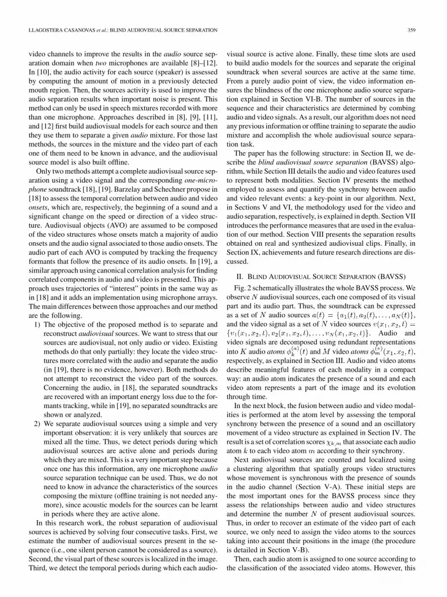
Fig. 3. Generating function � �� expressed by (4).

B. Video Representation

The video signal is represented using the 3D-MP algorithmproposed by Divorra and Vandergheynst in [22]. The videosignal is decomposed into a set of video atoms representingsalient video components and their temporal transformations(i.e., changes in their position, size, and orientation). Unlike thecase of simple pixel-based representations, when consideringimage structures that evolve in time, we deal with dynamic fea-tures that have a true geometrical meaning. Furthermore, sparsegeometric video decompositions provide compact representa-tions of information, allowing a considerable dimensionalityreduction of the input signals.

First of all, the first frame of the video signal, , isapproximated with a linear combination of atoms retrieved froma redundant dictionary of 2-D atoms as

(3)

where is the coefficient corresponding to each 2-D videoatom and is the subset of selected atom indexesfrom dictionary . As in the audio case, the dictionary is builtby varying the parameters of a mother function, an edge detectoratom with odd symmetry, that is a Gaussian along one axis andthe first derivative of a Gaussian along the perpendicular one(see Fig. 3). The generating function is thus expressed as

(4)

Then, these 2-D atoms are tracked from frame to frame usinga modified MP approach based on a Bayesian decision criteriaas explained in [22]. The possible transformations applied to

to build the video atoms are: translations over the imageplane , scaling to adapt the atom to theconsidered image structure, and rotations to locally orient thefunction along the edge.

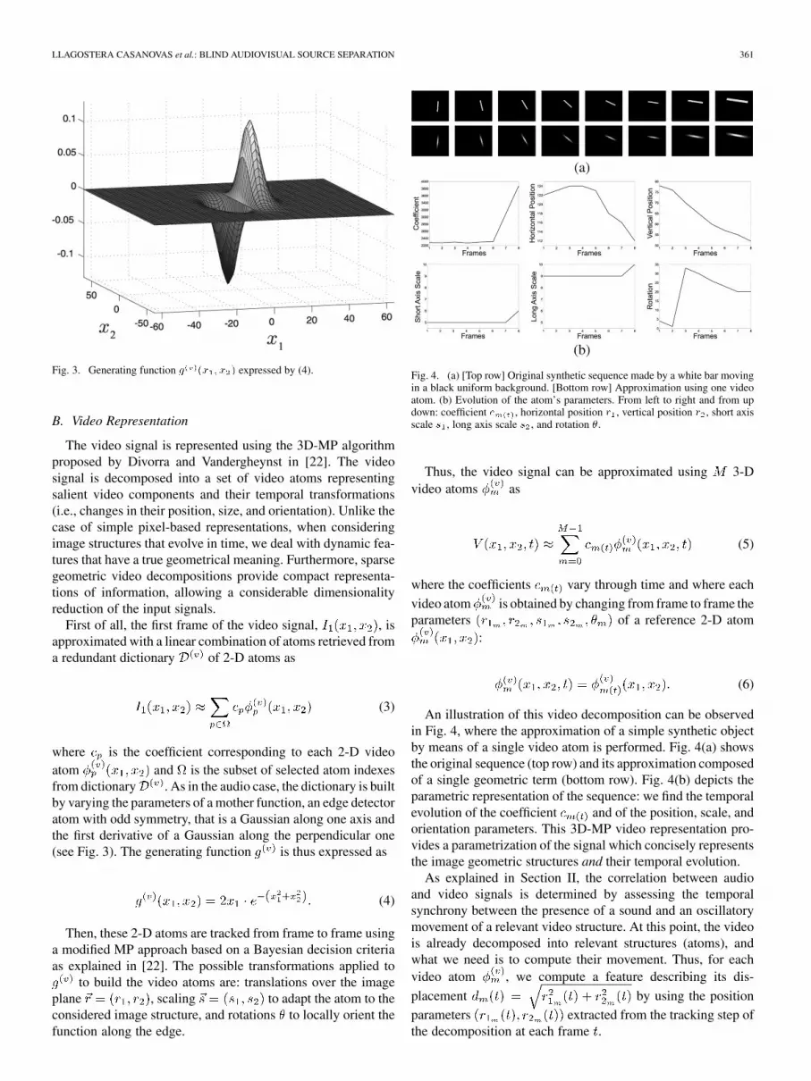
Fig. 4. (a) [Top row] Original synthetic sequence made by a white bar movingin a black uniform background. [Bottom row] Approximation using one videoatom. (b) Evolution of the atom’s parameters. From left to right and from updown: coefficient � , horizontal position � , vertical position � , short axisscale � , long axis scale � , and rotation �.

Thus, the video signal can be approximated using 3-Dvideo atoms as

(5)

where the coefficients vary through time and where each

video atom is obtained by changing from frame to frame theparameters of a reference 2-D atom

:

(6)

An illustration of this video decomposition can be observedin Fig. 4, where the approximation of a simple synthetic objectby means of a single video atom is performed. Fig. 4(a) showsthe original sequence (top row) and its approximation composedof a single geometric term (bottom row). Fig. 4(b) depicts theparametric representation of the sequence: we find the temporalevolution of the coefficient and of the position, scale, andorientation parameters. This 3D-MP video representation pro-vides a parametrization of the signal which concisely representsthe image geometric structures and their temporal evolution.

As explained in Section II, the correlation between audioand video signals is determined by assessing the temporalsynchrony between the presence of a sound and an oscillatorymovement of a relevant video structure. At this point, the videois already decomposed into relevant structures (atoms), andwhat we need is to compute their movement. Thus, for eachvideo atom , we compute a feature describing its dis-

placement by using the positionparameters extracted from the tracking step ofthe decomposition at each frame .


Fig. 5. (a) Audio feature �� and (b) displacement function � �� with cor-responding activation vector �� obtained for a video atom.

IV. AUDIO-VIDEO ATOMIC FUSION

Quantifying the relationships between audio and video struc-tures is the most important part in the whole process. All theaudiovisual information that is used in the next steps of the algo-rithm is extracted here. Thus, the fusion method that we choosein order to assess the correlation between audio and video de-termines the performance of the proposed method.

As explained before, approaches in audiovisual analysis arebased in an assumption of synchrony between related eventsin audio and video channels, i.e., when a person is speaking,his/her lips movements are temporally correlated to the speech.According to this observation, correlation scores are com-puted between each audio atom and each video atom .These scores measure the degree of synchrony between relevantevents in both modalities: the presence of an audio atom (energyin the time-frequency plane) and a peak in the video atom dis-placement (oscillation from an equilibrium position).

Audio feature: The feature that we consider is theenergy distribution of each audio atom projected over thetime axis. In the case of Gabor atoms, it is a Gaussian func-tion whose position and variance depend on the atoms pa-rameters and , respectively [Fig. 5(a)].Video feature: An activation vector [23] is built foreach atom displacement function by detecting thepeaks locations as shown in Fig. 5(b). The activation vectorpeaks are filtered by a window of width samplesin order to model delays and uncertainty.

There are two important remarks to be done concerning the fea-tures that we use. First of all, it is important to clarify that thepeaks on the displacement function represent an oscilla-tory movement of the atom . Thus, the activation vectordoes not depend on the original or relative position of the videoatom in the image. Notice that the peaks are situated at thetime instant where a change in the direction of the movementappears. That can be interpreted as a change in the sign of theacceleration of the atom or, what is the same, an oscillation onthe movement of that atom. The second remark concerns thechoice of the parameter that models delays between audio andvideo relevant events. Here samples corresponds to0.45 s, a time delay between a movement and the presence ofthe corresponding sound that appears to be appropriate. Frominformal tests, the setting of results not to be critical as itsvalue can be changed within a range of several samples withoutaffecting significantly the algorithm performance.

Finally, a scalar product is computed between audio and videofeatures in order to obtain the correlation scores:

(7)

This value is high when the audio atom and a peak in the videoatom’s displacement overlap in time or, what is the same, whena sound (audio energy) occurs more or less at the same time thanthe video structure is moving. Thus, a high correlation scoremeans high probability for a video structure of having generatedthe sound.

V. VIDEO SEPARATION

A. Spatial Clustering of Video Atoms

The idea now is to spatially group all the structures belongingto the same source in order to estimate the source position in theimage. We define the empirical confidence value of the thvideo atom as the sum of the MP coefficients of all the audioatoms associated to it in the whole sequence, , with

such that . This value is a measure of the numberof audio atoms related to this video structure and their weightin the MP decomposition of the audio track. Thus, a video atom

whose motion presents a high synchrony with sounds in theaudio channel will have a high confidence value , since alarge number of important audio atoms in the sequence will beassociated to this video atom in the audio-video atomic fusionstep (Section IV). In contrast, low values for correspond tovideo atoms whose motion is occasionally (and not continually)synchronous to the sounds.

Typically, the video part of each source is composed of groupsof atoms presenting high confidence values (and thus highcoherence with the audio signal), which are concentrated in asmall region in the image plane. Thus, a spatial clustering be-comes a natural way to count the sources in the sequence and es-timate their position in the image. Let each video atom be char-acterized by its position over the image plane and its confidencevalue, i.e., . In this work, we cluster the videoatoms correlated with the audio signal (i.e., with ) fol-lowing these three steps.

1) Clusters Creation: The algorithm creates clusters, by iteratively selecting the video atoms with

highest confidence value (and thus highest coherence withthe audio track) and adding to them video atoms closerthan a cluster size defined in pixels. Video atoms be-longing to a cluster cannot be the center of a new cluster.Thus, each new cluster is generated by the video atomwith highest confidence value from those which have notbeen classified yet.

2) Centroids Estimation: The center of mass of each clusteris computed taking the confidence value of every atom asthe mass. The resulting centroids are the coordinates in theimage where the algorithm locates the audiovisual sources.

3) Unreliable Clusters Elimination: We define the clusterconfidence value as the sum of the confidence values

of the atoms belonging to the cluster , i.e.,


Fig. 6. Example of the video sources reconstruction. On the left picture, theleft person is speaking, while on the right picture, the right person is speaking.

. Based on this measure, unreliable clusters, i.e.,clusters with small confidence value are removed, ob-taining the final set of clusters, , withcentroids . In this step, we remove cluster if

(8)

Further details about this clustering algorithm can be found in[24]. At this stage, a good localization of sources in the imageis achieved. The number of sources does not have to be spec-ified in advance since a confidence measure is introduced to au-tomatically eliminate unreliable clusters. In [24], we show thatthe results are not significantly affected by the cluster parame-ters choice. For ranging between 40 and 90 pixels, the pro-posed clustering algorithm has been proved to detect the correctnumber of sources (in all experiments, image dimensions are120 176 pixels). In fact, when we decrease the cluster sizemore possible sources appear ( increases), but all these clus-ters are far from the mouth and present a small correlation withthe audio signal. Thus, step 3 of the algorithm easily removesclusters that do not represent an audiovisual source as their con-fidence is much smaller.

B. Video Atoms Classification

This step classifies all video atoms closer than the cluster sizeto a centroid into the corresponding source. Notice that only

video atoms moving coherently with sounds are con-sidered for the video localization in Section V-A. Each suchgroup of video atoms describes the video modality of an au-diovisual source, achieving thus the video separation objective.Then, an estimate of the video part of the th source, , canbe computed simply as

(9)

Fig. 6 shows an example of the reconstruction of the currentspeaker detected by the algorithm. Only video atoms close to thesources estimated by the presented technique are considered.Thus, to carry out the reconstruction, the algorithm adds theirenergy and the effect is a highlight of the speaker’s face. In bothframes, the correct speaker is detected.

VI. AUDIO SEPARATION

A. Audio Atoms Classification

For every audio atom, we take into account all related videoatoms, their correlation scores, and their classification into asource. Accordingly, an audio atom should be assigned to thesource gathering most video atoms. Since we also want to re-ward synchrony, the assignation of each audio entity is per-formed in the following way.

1) Take all the video atoms correlated with the audioatom , i.e., for which .

2) Each of these video atoms is associated to an audiovisualsource ; for each source , compute a value thatis the sum of the correlation scores between the audio atom

and the video atoms s.t. :

(10)

Thus, this step rewards sources whose video atoms presenta high synchrony with the considered audio atom.

3) Classify the audio atom into the source if the valueis “big enough”: here we require to be twice as bigas any other value for the other sources. Thus, weattribute to if

(11)

If this condition is not fulfilled (this is typically the casewhen several sources are simultaneously active), this audioatom can belong to several sources and further processingis required. This decision bound is not a very critical pa-rameter since it only affects the classification of the audioatoms in time slots with several active sources. In periodswith only one source, the difference between the score forthe considered source and the others is enormous, andit is thus easy to classify the atom into the correct source.

Using the labels of audio atoms, time periods during whichonly one source is active are clearly determined. This is doneusing a very simple criterion: if in a continuous time slot longerthan seconds, all audio atoms are assigned to source , thenduring this period, only source is active. In all experiments,the value of is set to 1 s. The choice of this parameter hasbeen done according to the length of the analyzed sequences(around 20 s). This value has to be small enough to ensure that ina period, there is only one source active. At the same time, it hasto be big enough to allow the presence of periods where to trainthe source audio models. Thus, could be set automaticallyaccording to the length of the analyzed clip, e.g., one tenth ofthe sequence length.

When several sources are present, temporal informationalone is not sufficient to discriminate different audio sources inthe mixture. To overcome this limitation, in these ambiguoustime slots, a time-frequency analysis is performed, which ispresented in detail in Section VII.


B. GMM-Based Audio Source Separation

As explained in Section II, the choice of the spectral GMMsas our method for the separation of the audio part of the sourceshas been motivated by two main reasons. In spite of its sim-plicity, we can achieve good audio separation since GMMs areable to model multiple power spectral densities or, what is thesame, several frequency behaviors for the same source. This isa very interesting property given the diverse nature of sounds.Thus, GMMs have the capacity of modeling nonstationary sig-nals contrary to classical Wiener filters [20].

Here, we perform a one microphone GMM-based audiosource separation inspired by the supervised approach in [25]but introducing the video information. The method in [25]needs to know in advance the sources that compose the mixtureand their characteristics: the audio model for each source isbuilt offline. Here the information extracted from the videosignal through previous steps of our algorithm allows theapplication of the method without any offline training. Thus,the separation that we perform is completely blind since noprevious information about the sources is required.

The idea is to model the short time Fourier spectra of thesources by GMMs learned from training sequences .Using these models, the audio source separation is performedapplying time-frequency masking on the short time Fouriertransform (STFT) domain. We will first explain our model forthe sources, next the process we use to learn these models, andfinally the separation part.

Given an audio signal , we denote the STFT of this signaland the short time Fourier spec-

trum of the signal at time . The short time Fourier spectra ofthe signal, , are modeled with a GMM, i.e., the probabilitydensity function of is given by

(12)

with

(13)

Here is the complex value of the short time Fourierspectrum at frequency and , representing the localpower spectral density (PSD) at frequency in the state ofthe GMM, is the diagonal element of the diagonal covariancematrix . This spectral GMM is denoted

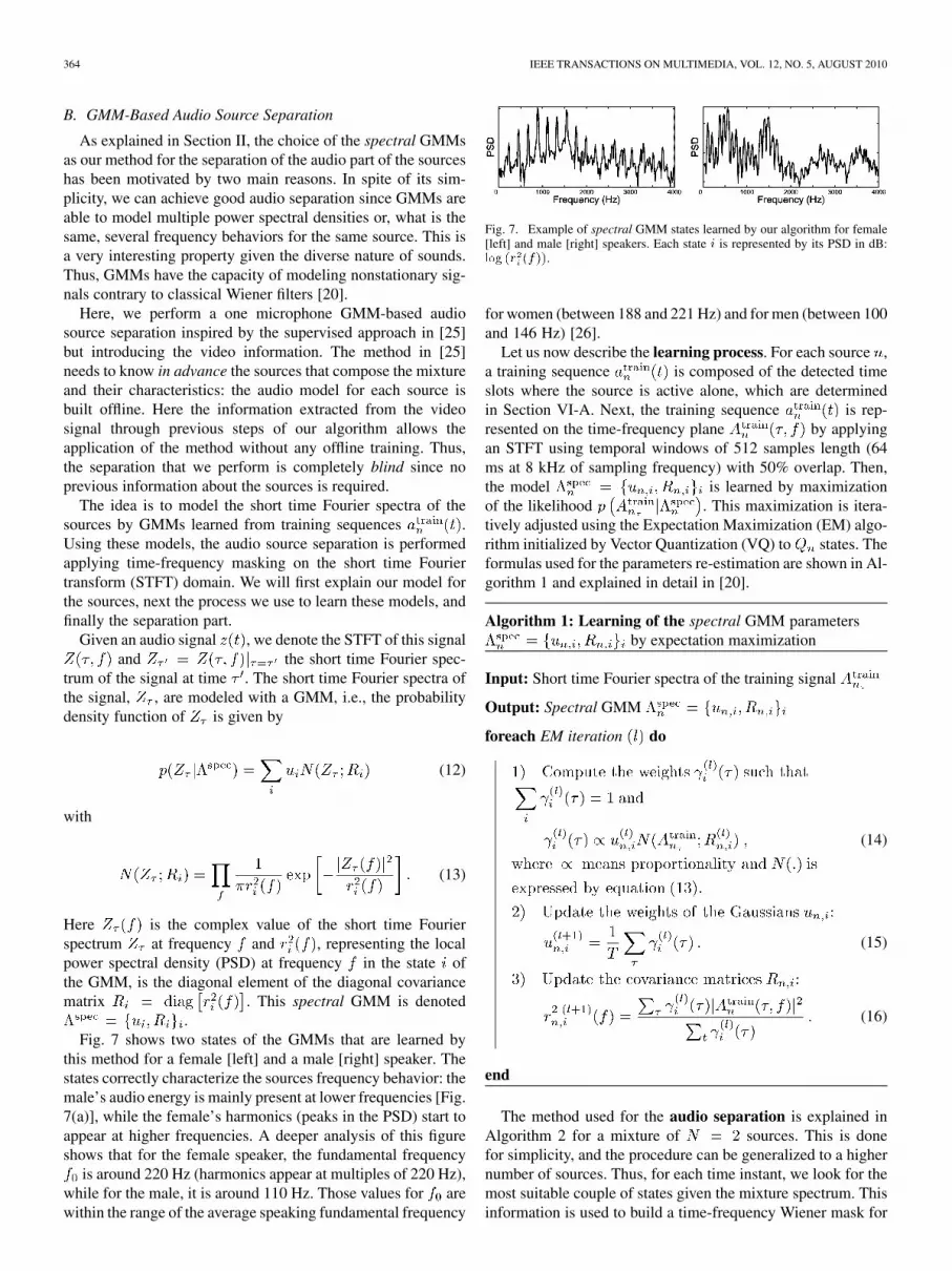
.Fig. 7 shows two states of the GMMs that are learned by

this method for a female [left] and a male [right] speaker. Thestates correctly characterize the sources frequency behavior: themale’s audio energy is mainly present at lower frequencies [Fig.7(a)], while the female’s harmonics (peaks in the PSD) start toappear at higher frequencies. A deeper analysis of this figureshows that for the female speaker, the fundamental frequency

is around 220 Hz (harmonics appear at multiples of 220 Hz),while for the male, it is around 110 Hz. Those values for arewithin the range of the average speaking fundamental frequency

Fig. 7. Example of spectral GMM states learned by our algorithm for female[left] and male [right] speakers. Each state � is represented by its PSD in dB:�� .

for women (between 188 and 221 Hz) and for men (between 100and 146 Hz) [26].

Let us now describe the learning process. For each source ,a training sequence is composed of the detected timeslots where the source is active alone, which are determinedin Section VI-A. Next, the training sequence is rep-resented on the time-frequency plane by applyingan STFT using temporal windows of 512 samples length (64ms at 8 kHz of sampling frequency) with 50% overlap. Then,the model is learned by maximizationof the likelihood . This maximization is itera-tively adjusted using the Expectation Maximization (EM) algo-rithm initialized by Vector Quantization (VQ) to states. Theformulas used for the parameters re-estimation are shown in Al-gorithm 1 and explained in detail in [20].

Algorithm 1: Learning of the spectral GMM parametersby expectation maximization

Input: Short time Fourier spectra of the training signal

Output: Spectral GMM

foreach EM iteration do

(14)

(15)

(16)

end

The method used for the audio separation is explained inAlgorithm 2 for a mixture of sources. This is donefor simplicity, and the procedure can be generalized to a highernumber of sources. Thus, for each time instant, we look for themost suitable couple of states given the mixture spectrum. Thisinformation is used to build a time-frequency Wiener mask for


each source (19) by combining the spectral PSDs in the cor-responding states with the knowledge aboutthe sources activity . When only one source is active, thisweight assigns all the soundtrack to this speaker. Otherwise,

and the analysis takes into account only the audioGMMs. In a further implementation, we could assign interme-diate values to that account for the degree of correlation be-tween audio and video. However, such cross-modal correlationhas to be accurately estimated to avoid the introduction of sep-aration errors.

Algorithm 2: Single-channel audio source separation usingknowledge about the sources activity

Input: Mixture , spectral GMMs , andactivity vectors for the sources

Output: Estimation of the sources audio part and

A) Compute the STFT of the mixture from thetemporal signal .

foreach do

(17)

(18)

(19)

(20)

end

B) Reconstruct estimations of the sources audio part in thetemporal domain from the STFT estimations .

VII. BAVSS PERFORMANCE MEASURES

A. Sources Activity Detection

The performance of the proposed method is highly related tothe accuracy in the estimation of the temporal periods in whicheach source is active alone. For our method, it is not funda-mental to detect all the time instants during which sources areactive alone, provided that the length of the detected period islong enough to train the source audio models. In fact, errors

occur only when our algorithm estimates that one source is ac-tive alone while in fact some of the other sources are active,too. In these error frames, our algorithm will learn an audiomodel for source that represents the frequency behavior ofseveral sources mixed, and that will cause errors in the sepa-ration. Two measures assess the performance of our method inthis domain: the activity-error-rate (ERR) and the activity-effi-ciency-rate (EFF).

Let be the number of audiovisual sources and be thenumber of video frames. For any fixed time and source , wedefine

“ ” (21)

“ ” (22)

Let with be the set of sources differentfrom . Then, we define

(23)

(24)

is the event where all sources different from are inac-tive and is the complementary event where one or more ofthe sources different from source are active.

The ERR for source is defined as

(25)

where is a function that returns the number of frameswhere our algorithm estimates that the event has place andthe ground truth soundtracks indicate that the current event is .Thus, the ERR represents the percentage of time during whichthe algorithm makes an important error since it decides thatsource is the only source active and it is not true (one or moreof the other sources are active, too).

The EFF for source is defined as

(26)

where is the number of frames where source is the onlysource active. Thus, the EFF represents the percentage of time inwhich a source is active alone that our method is able to detect.This parameter is very important parameter given the short du-ration of the analyzed sequences: the higher the EFF, the longerthe period during which we learn the source audio models and,consequently, we can expect to obtain better results on the audioseparation part.

B. Audio Source Separation

The BSS Evaluation Toolbox is used to evaluate the perfor-mance of the proposed method in the audio separation part.The estimated audio part of the sources is decomposed into:

, as described in [27].


is the target audio part of the source and and are,respectively, the interferences and artifacts error terms. Thesethree terms should represent the part of perceived as comingfrom the wanted source , from other unwanted sources

, and from other causes. Two quantities are computedusing this toolbox, the source-to-interferences ratio (SIR), andthe sources-to-artifacts ratio (SAR), defined as

(27)

(28)

Thus, the SIR measures the performance of our method in the re-jection of the interferences and the SAR quantifies the presenceof distortions and “burbling” artifacts on the separated audiosources. By combining SIR and SAR, one can be sure of elim-inating the interfering source without introducing too many ar-tifacts in the separated soundtracks.

For a given mixture and using the knowledge about the orig-inal audio part of the sources , oracle estimators for single-channel source separation by time-frequency masking are com-puted using the BSS Oracle Toolbox. These oracle estimatorsare computed using the ground truth waveforms in order to re-sult in the smallest possible distortion. As a result, and

establish the upper bounds for the proposed perfor-mance measures. For further details about the oracles estima-tion, please refer to [28].

Finally, in order to compare our results to those obtained in[18], we compute the preserved-signal-ratio (PSR) for sourceusing the method described in [29] as

(29)

where is the STFT of the original audio signal corre-sponding to source and is the time-frequency maskestimated using equation (19) and used in the audio demixingprocess. Thus, this measure represents the amount of acousticenergy that is preserved after the separation process.

VIII. EXPERIMENTS

In a first set of experiments (Section VIII-A), the proposedBAVSS algorithm is evaluated on synthesized audiovisual mix-tures composed of two persons speaking in front of a camera.These sequences present an artificial mixture generated by tem-porally shifting the audio and video signals corresponding toone of the speakers so that it overlaps with the speech of theother person. The performance of the proposed method in iden-tifying the number of sources in the scene, locating them theimage, and determining the activity periods of each one of themis assessed. Furthermore, a quantitative evaluation of the algo-rithm’s results in terms of audio separation is performed sincethe original soundtracks (ground truth) of each speaker sepa-rately are available for these sequences.

As explained before, at present, only two other methods haveattempted a complete audiovisual source separation [18], [19].The method presented in [19] does not provide any qualitativeor quantitative result in terms of audio separation. In fact, thispaper is mostly concentrated in the localization of the sourcesin the image and the only reference to the audio separation partstates that the quality of the separated soundtracks is not good.Regarding the method presented in [18], two measures are usedto evaluate quantitatively its performance in the audio separationpart: the improvement of the SIR and the PSR. In the last partof Section VIII-A, these two quantities are used to compare ourresults to those obtained by the approach in [18] when analyzingsequences composed of two speakers.

In Section VIII-B, we present a second set of experimentsin which speakers and music instruments are mixed. The com-plexity of the sequences is higher given the more realistic back-ground and the presence of distracting motion. These sequencesare real audiovisual mixtures where both sources are recordedat the same time. Thus, it is not possible to obtain a quantitativeevaluation of the algorithm’s performances as in Section VIII-Asince the audio ground truth is not available in this case. Themain objective of Section VIII-B is to demonstrate qualitativelythat our BAVSS method can deal successfully with complexreal-world sequences involving speech and music instruments.

Videos showing all the experiments and the estimated audio-visual sources after applying our method are available online athttp://lts2www.epfl.ch/~llagoste/BAVSSresults.htm.

A. CUAVE Database: Quantitative Results

Sequences are synthesized using clips taken from the groupspartition of the CUAVE database [17] with two speakers ut-tering sequences of digits alternatively. A typical sequences isshown in Fig. 1. The video data is sampled at 29.97 frames persecond with a resolution of 480 720 pixels, and the audio at44 kHz. The video has been resized to a 120 176 pixels, whilethe audio has been sub-sampled to 8 kHz. The video signal isdecomposed into video atoms and the soundtrack isdecomposed into atoms. The number of atoms ex-tracted from the decomposition does not need to be set a priori.It can be automatically chosen setting a threshold on the recon-struction quality.

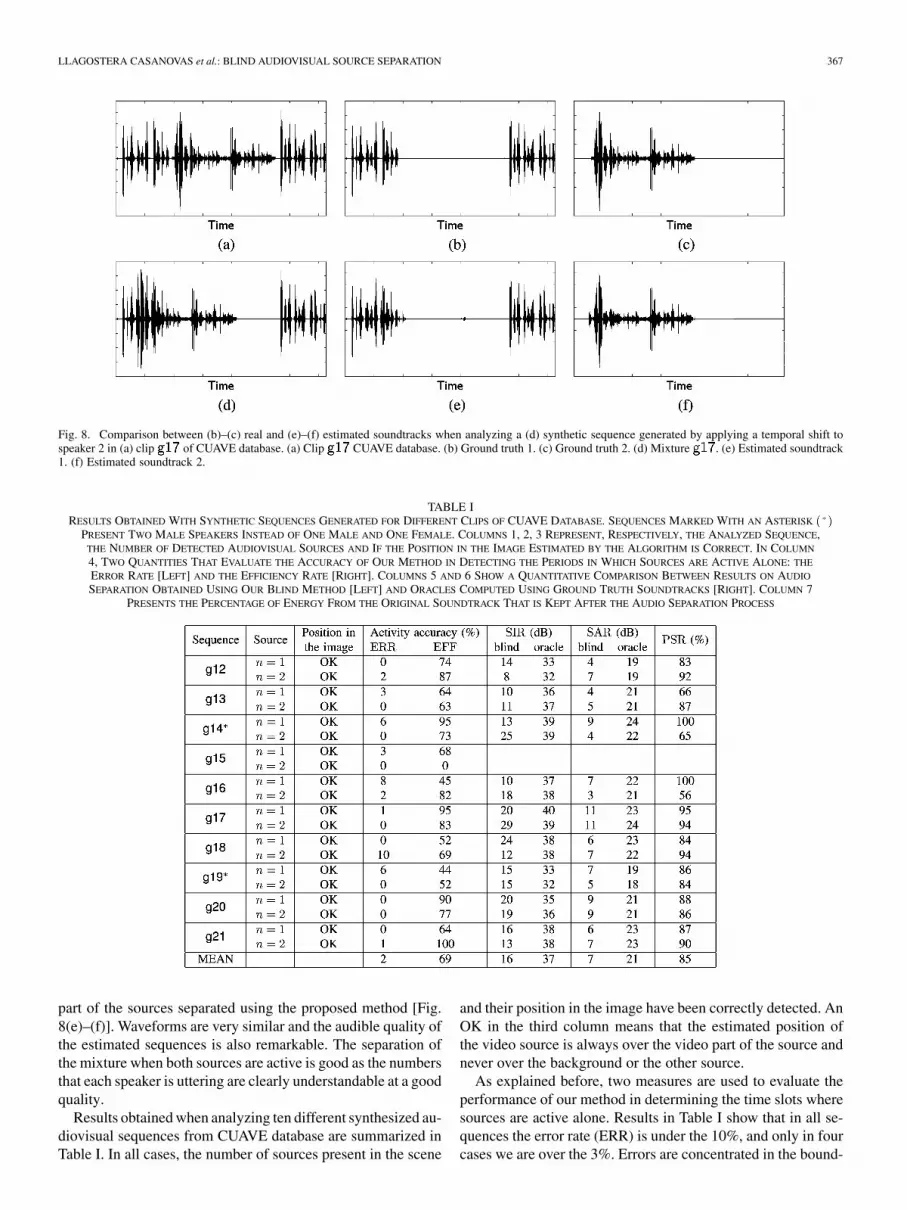
Ground truth mixtures are obtained by temporally shiftingaudio and video signals of one speaker in order to obtain timeslots with both speakers active simultaneously. In the resultingsynthetic clips, four cases are represented: both persons speakat the same time, only the boy or the girl speaks, or silence. Forfurther details on the procedure adopted to build the syntheticsequences, the reader is referred to [24]. An example of thisprocedure on the audio part is shown in Fig. 8. In Fig. 8(a),the figure shows the original clip of CUAVE database, inFig. 8(b), the ground truth for source 1 (which is the periodduring which speaker 1 is uttering numbers), and in Fig. 8(c),the ground truth for source 2 which is obtained by shifting itsaudio part. In Fig. 8(d), we can see the input to our algorithm, amixture built by adding ground truth waveforms 1 and 2.

Fig. 8 also gives a first qualitative evaluation of our method.It is possible to compare the ground truth to the estimated audio


Fig. 8. Comparison between (b)–(c) real and (e)–(f) estimated soundtracks when analyzing a (d) synthetic sequence generated by applying a temporal shift tospeaker 2 in (a) clip of CUAVE database. (a) Clip CUAVE database. (b) Ground truth 1. (c) Ground truth 2. (d) Mixture . (e) Estimated soundtrack1. (f) Estimated soundtrack 2.

TABLE IRESULTS OBTAINED WITH SYNTHETIC SEQUENCES GENERATED FOR DIFFERENT CLIPS OF CUAVE DATABASE. SEQUENCES MARKED WITH AN ASTERISK � �

PRESENT TWO MALE SPEAKERS INSTEAD OF ONE MALE AND ONE FEMALE. COLUMNS 1, 2, 3 REPRESENT, RESPECTIVELY, THE ANALYZED SEQUENCE,THE NUMBER OF DETECTED AUDIOVISUAL SOURCES AND IF THE POSITION IN THE IMAGE ESTIMATED BY THE ALGORITHM IS CORRECT. IN COLUMN

4, TWO QUANTITIES THAT EVALUATE THE ACCURACY OF OUR METHOD IN DETECTING THE PERIODS IN WHICH SOURCES ARE ACTIVE ALONE: THE

ERROR RATE [LEFT] AND THE EFFICIENCY RATE [RIGHT]. COLUMNS 5 AND 6 SHOW A QUANTITATIVE COMPARISON BETWEEN RESULTS ON AUDIO

SEPARATION OBTAINED USING OUR BLIND METHOD [LEFT] AND ORACLES COMPUTED USING GROUND TRUTH SOUNDTRACKS [RIGHT]. COLUMN 7PRESENTS THE PERCENTAGE OF ENERGY FROM THE ORIGINAL SOUNDTRACK THAT IS KEPT AFTER THE AUDIO SEPARATION PROCESS

part of the sources separated using the proposed method [Fig.8(e)–(f)]. Waveforms are very similar and the audible quality ofthe estimated sequences is also remarkable. The separation ofthe mixture when both sources are active is good as the numbersthat each speaker is uttering are clearly understandable at a goodquality.

Results obtained when analyzing ten different synthesized au-diovisual sequences from CUAVE database are summarized inTable I. In all cases, the number of sources present in the scene

and their position in the image have been correctly detected. AnOK in the third column means that the estimated position ofthe video source is always over the video part of the source andnever over the background or the other source.

As explained before, two measures are used to evaluate theperformance of our method in determining the time slots wheresources are active alone. Results in Table I show that in all se-quences the error rate (ERR) is under the 10%, and only in fourcases we are over the 3%. Errors are concentrated in the bound-


aries of the source activity, that is just before the person startsto speak or after he/she stops, because in general, motion in thevideo signal is not completely synchronous with sounds in theaudio channel. Concerning our method’s efficiency (EFF), onlyin three cases, we are able to detect less than 50% of periodswhere sources are alone, and we average a 69%, which is a highpercentage if we think about longer sequences. Low values forEFF are caused by the presence of video motion correlated to theaudio on the source that is not active. In fact, it is difficult to de-tect the complete periods when sources are active alone withoutintroducing errors, since there is a trade-off between them. If wechoose to detect all the periods (EFF increases), more false pos-itives will appear (ERR increases, too) and, as explained before,the models for each source will not be correct. Here we preferto have a high confidence when we decide that only one sourceis active, even if then the efficiency decreases.

A 100% on EFF means that periods in which the source isactive alone are perfectly detected. In this case, blind resultsfor SIR and SAR are the best results that we can achieve usingthe GMM-based audio separation method in Section VI-B sincethe training sequences are as long as possible. Consequently,the upper bounds for the performance in the blind separation ofthe audio track are clearly conditioned by the duration of thetraining sequences and the algorithm we use for the one micro-phone audio separation. While in some sequences the GMM-based separation seems suitable with performances up to 29 dBof SIR (sequence ), for some speakers, this does not seemto be the case (8 dB of SIR in sequence even if the com-bined EFF for both speakers is 81%). However, taking into ac-count the short duration of the analyzed sequences (20–30 s)and the training sequences (less than 8 s), results are satisfac-tory. Remember that the oracles in Table I represent the bestresults that we can obtain through any audio source separationmethod based on frequency masking if we know in advance theground truth soundtracks. In fact, oracles guarantee the min-imum distortion by computing the optimal time-frequency maskgiven the original separated soundtracks. The average SIR thatwe obtain (16 dB) is slightly better than the state-of-the-art onsingle-channel audio separation [20] and, unlike this method,we do it without any kind of supervision. As explained be-fore, the combination between audio and video signals in ourapproach eliminates the necessity of knowing in advance thesources in the mixture and its acoustic characteristics, which istypical in one microphone audio separation methods. Further-more, in all the resulting separated soundtracks here, even theones that present worse SIR, the numbers that each speaker ut-ters can be well understood.

In sequence , we can observe a major problem: there isno detected period when speaker 2 is active alone (see EFF inTable I). Consequently, it is not possible to train a model ofthat source and our separation method cannot be applied. Thishappens because there is video motion correlated to the audioon source 1 (which is inactive) all over the duration of the pe-riod during which only source 2 is active. However, we can ex-pect that with longer sequences (and longer time slots with eachsource active alone), this problem does not appear anymore,since in that case, it is unlikely that correlated video motion ispresent on the inactive source all the time.

The audio separation task is extremely challenging for se-quences and , where the mixture is composed by twomale speakers. The fundamental frequencies of the speakers areextremely close and, as a result, their formants energy is highlyoverlapped in the spectrogram. Even in this difficult context,quantitative results (with an average SIR of 17 dB) are close tothose obtained when analyzing sequences with a male-femalecombination.

The comparison between our method and the approach in[18] presents some difficulties. First, the test set in [18] is com-posed of three very short sequences (duration ranging between5 and 10 s), and only one of those sequences contains a mix-ture composed of speakers. Furthermore, distracting motion isavoided by locating the camera close to the speakers faces, i.e.,we can only observe the lips in the video corresponding to themale speaker. Although the differences are considerable, herewe compare the results in the speakers sequence in [18] withthe mean results through all the sequences that we have ana-lyzed. In [18], they report an improvement in the SIR of 14 dBand a PSR of 57.5% (those values represent the mean betweenthe male and female results). Here we obtain an average SIRof 16 dB and an average PSR of 85%. Thus, our approach com-pares especially favorable in terms of PSR, that is the amount ofacoustic energy that is preserved after the separation process. Infact, when demixing the audio part of the sources, our methodkeeps the 85% of the energy in the original audio signal, whilein [18], more than the 40% of this energy is lost. These resultsare related to the audio separation method used in each case: ourGMM-based separation seems more suitable than the frequencytracking used in [18] when we consider the PSR.

B. LTS Database: Qualitative Resultsin a Challenging Environment

More challenging sequences including speakers and musicinstruments have been recorded in order to qualitatively testthe performance of the proposed method when dealing withcomplex situations. The original video data are sampled at 30frames per second with a resolution of 240 320 pixels, andthe audio at 44 kHz. For its analysis, the video has been resizedto a 120 160 pixels, while the audio has been sub-sampledto 8 kHz. The length of the sequences is close to 1 min in thiscase. The video signal is decomposed into atoms andthe soundtrack is decomposed into atoms. As ex-plained before, a quantitative evaluation cannot be performed inthis case since in this section, we consider real mixtures whereboth sources are recorded at the same time.

In the first experiment (movie1), we analyze an audiovisualsequence where two persons are playing music instruments infront of a camera. A frame of this movie is shown in Fig. 9.In some temporal periods, they play at the same time, whilein others, they do a solo. A first difficulty is given by the factthat the video decomposition has to reflect the movement ofthe present structures, which is not an easy task when tryingto model the drumsticks and their trajectory. Thus, while thehand that is playing the guitar moves in a smooth way, drum-sticks movement is much more fast and abrupt. Another chal-lenge is caused by other movements correlated with the sound,especially those of the guitarist’s leg, and the proximity of the


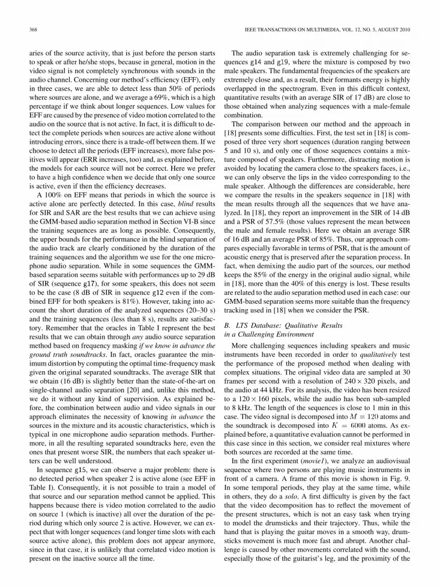
Fig. 9. Challenging audiovisual sequence where one person is playing a guitarand another one is hitting two drumsticks in a complex background. A frameof this movie [left] and the corresponding audio spectrogram [right] are repre-sented. Drumsticks are active in the beginning of the sequence, then the guitariststarts to play, and finally both instruments are mixed.

Fig. 10. Video sources reconstruction for movie1. The atoms that are high-lighted in the images are those that characterize the left source [left] and theright source [right], respectively. Background is composed of the residual en-ergy after the 3D-MP video decomposition and provides an easier visualizationof the reconstructed sources. Finally, crosses mark the position in the imagewhere our algorithm locates the sources.

sources. If we compare this sequence with the ones presented inthe literature, we can see that, in those cases, either the sourcesare much more separated in the image [19] or distracting motionis avoided by visually zooming into the sources [18]. Further-more, other methods are always tested on flat, or almost flat,backgrounds. Here the complex background (see Fig. 9) makesthe video decomposition task more complicated since a consid-erable part of the video atoms has to be used to represent it.

When analyzing movie1 with the proposed BAVSS method,the number of sources and its position in the image are perfectlydetected (see crosses on Fig. 10). A reconstruction of the imageusing the atoms assigned to each source is shown in Fig. 10. Inthe left picture, it is possible to see how the stick is successfullyrepresented by one video atom, and in the right one, the atomsthat surround the guitar are highlighted. In this sequence, theactivity periods of each source are also detected. A good char-acterization of the sources in the frequency domain is achieved,which leads to a satisfactory audio separation of the sources.Fig. 11 shows the spectrograms that we obtain. We can see thatdrumsticks sounds [left] are much more sharp in the spectro-gram (well-localized in time, broad range in frequency) whilethe guitar spectrogram [right] has much more energy and it iscomposed by several harmonic sounds. Concerning the audiblequality of the estimated soundtracks, the audio part of the drum-sticks is perfectly reconstructed at the beginning and it onlypresents some distortion at the end, where they are mixed withthe guitar sounds. In addition, it is almost impossible to hear theguitar in the drumsticks soundtrack. Finally, the quality of theguitar reconstruction is good even though there are some atten-uated drumstick sounds in the last part.

Fig. 11. Estimated spectrograms for drumsticks [left] and guitar [right] inmovie1. Drumsticks are silent in the middle of the sequence and the guitarat the beginning. Spectrograms show that the sources behavior is correctlydetected by the proposed method.

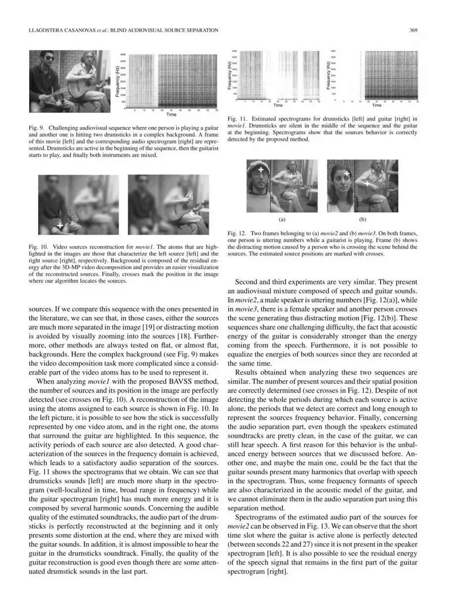
Fig. 12. Two frames belonging to (a) movie2 and (b) movie3. On both frames,one person is uttering numbers while a guitarist is playing. Frame (b) showsthe distracting motion caused by a person who is crossing the scene behind thesources. The estimated source positions are marked with crosses.

Second and third experiments are very similar. They presentan audiovisual mixture composed of speech and guitar sounds.In movie2, a male speaker is uttering numbers [Fig. 12(a)], whilein movie3, there is a female speaker and another person crossesthe scene generating thus distracting motion [Fig. 12(b)]. Thesesequences share one challenging difficulty, the fact that acousticenergy of the guitar is considerably stronger than the energycoming from the speech. Furthermore, it is not possible toequalize the energies of both sources since they are recorded atthe same time.

Results obtained when analyzing these two sequences aresimilar. The number of present sources and their spatial positionare correctly determined (see crosses in Fig. 12). Despite of notdetecting the whole periods during which each source is activealone, the periods that we detect are correct and long enough torepresent the sources frequency behavior. Finally, concerningthe audio separation part, even though the speakers estimatedsoundtracks are pretty clean, in the case of the guitar, we canstill hear speech. A first reason for this behavior is the unbal-anced energy between sources that we discussed before. An-other one, and maybe the main one, could be the fact that theguitar sounds present many harmonics that overlap with speechin the spectrogram. Thus, some frequency formants of speechare also characterized in the acoustic model of the guitar, andwe cannot eliminate them in the audio separation part using thisseparation method.

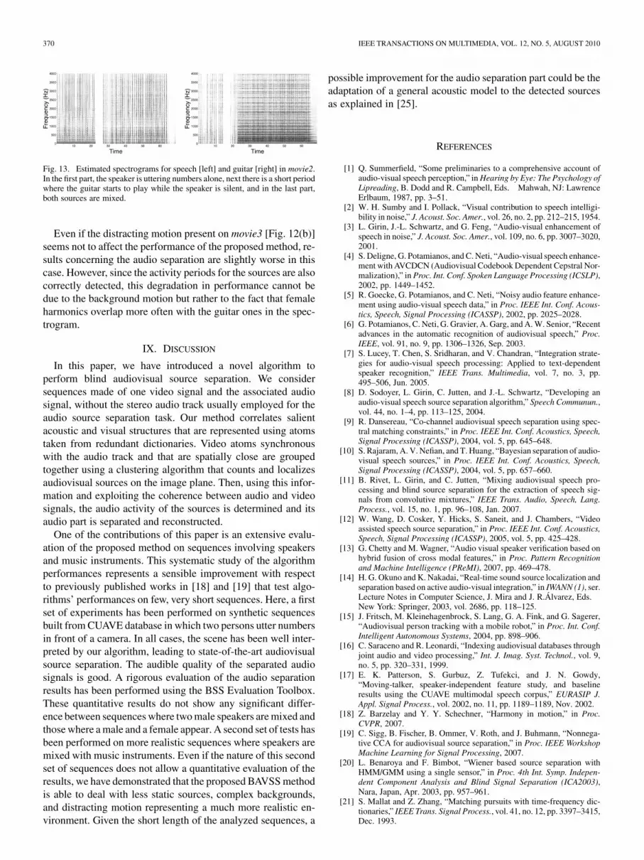
Spectrograms of the estimated audio part of the sources formovie2 can be observed in Fig. 13. We can observe that the shorttime slot where the guitar is active alone is perfectly detected(between seconds 22 and 27) since it is not present in the speakerspectrogram [left]. It is also possible to see the residual energyof the speech signal that remains in the first part of the guitarspectrogram [right].


Fig. 13. Estimated spectrograms for speech [left] and guitar [right] in movie2.In the first part, the speaker is uttering numbers alone, next there is a short periodwhere the guitar starts to play while the speaker is silent, and in the last part,both sources are mixed.

Even if the distracting motion present on movie3 [Fig. 12(b)]seems not to affect the performance of the proposed method, re-sults concerning the audio separation are slightly worse in thiscase. However, since the activity periods for the sources are alsocorrectly detected, this degradation in performance cannot bedue to the background motion but rather to the fact that femaleharmonics overlap more often with the guitar ones in the spec-trogram.

IX. DISCUSSION

In this paper, we have introduced a novel algorithm toperform blind audiovisual source separation. We considersequences made of one video signal and the associated audiosignal, without the stereo audio track usually employed for theaudio source separation task. Our method correlates salientacoustic and visual structures that are represented using atomstaken from redundant dictionaries. Video atoms synchronouswith the audio track and that are spatially close are groupedtogether using a clustering algorithm that counts and localizesaudiovisual sources on the image plane. Then, using this infor-mation and exploiting the coherence between audio and videosignals, the audio activity of the sources is determined and itsaudio part is separated and reconstructed.

One of the contributions of this paper is an extensive evalu-ation of the proposed method on sequences involving speakersand music instruments. This systematic study of the algorithmperformances represents a sensible improvement with respectto previously published works in [18] and [19] that test algo-rithms’ performances on few, very short sequences. Here, a firstset of experiments has been performed on synthetic sequencesbuilt from CUAVE database in which two persons utter numbersin front of a camera. In all cases, the scene has been well inter-preted by our algorithm, leading to state-of-the-art audiovisualsource separation. The audible quality of the separated audiosignals is good. A rigorous evaluation of the audio separationresults has been performed using the BSS Evaluation Toolbox.These quantitative results do not show any significant differ-ence between sequences where two male speakers are mixed andthose where a male and a female appear. A second set of tests hasbeen performed on more realistic sequences where speakers aremixed with music instruments. Even if the nature of this secondset of sequences does not allow a quantitative evaluation of theresults, we have demonstrated that the proposed BAVSS methodis able to deal with less static sources, complex backgrounds,and distracting motion representing a much more realistic en-vironment. Given the short length of the analyzed sequences, a

possible improvement for the audio separation part could be theadaptation of a general acoustic model to the detected sourcesas explained in [25].

REFERENCES

[1] Q. Summerfield, “Some preliminaries to a comprehensive account ofaudio-visual speech perception,” in Hearing by Eye: The Psychology ofLipreading, B. Dodd and R. Campbell, Eds. Mahwah, NJ: LawrenceErlbaum, 1987, pp. 3–51.

[2] W. H. Sumby and I. Pollack, “Visual contribution to speech intelligi-bility in noise,” J. Acoust. Soc. Amer., vol. 26, no. 2, pp. 212–215, 1954.

[3] L. Girin, J.-L. Schwartz, and G. Feng, “Audio-visual enhancement ofspeech in noise,” J. Acoust. Soc. Amer., vol. 109, no. 6, pp. 3007–3020,2001.

[4] S. Deligne, G. Potamianos, and C. Neti, “Audio-visual speech enhance-ment with AVCDCN (Audiovisual Codebook Dependent Cepstral Nor-malization),” in Proc. Int. Conf. Spoken Language Processing (ICSLP),2002, pp. 1449–1452.

[5] R. Goecke, G. Potamianos, and C. Neti, “Noisy audio feature enhance-ment using audio-visual speech data,” in Proc. IEEE Int. Conf. Acous-tics, Speech, Signal Processing (ICASSP), 2002, pp. 2025–2028.

[6] G. Potamianos, C. Neti, G. Gravier, A. Garg, and A. W. Senior, “Recentadvances in the automatic recognition of audiovisual speech,” Proc.IEEE, vol. 91, no. 9, pp. 1306–1326, Sep. 2003.

[7] S. Lucey, T. Chen, S. Sridharan, and V. Chandran, “Integration strate-gies for audio-visual speech processing: Applied to text-dependentspeaker recognition,” IEEE Trans. Multimedia, vol. 7, no. 3, pp.495–506, Jun. 2005.

[8] D. Sodoyer, L. Girin, C. Jutten, and J.-L. Schwartz, “Developing anaudio-visual speech source separation algorithm,” Speech Communun.,vol. 44, no. 1–4, pp. 113–125, 2004.

[9] R. Dansereau, “Co-channel audiovisual speech separation using spec-tral matching constraints,” in Proc. IEEE Int. Conf. Acoustics, Speech,Signal Processing (ICASSP), 2004, vol. 5, pp. 645–648.

[10] S. Rajaram, A. V. Nefian, and T. Huang, “Bayesian separation of audio-visual speech sources,” in Proc. IEEE Int. Conf. Acoustics, Speech,Signal Processing (ICASSP), 2004, vol. 5, pp. 657–660.

[11] B. Rivet, L. Girin, and C. Jutten, “Mixing audiovisual speech pro-cessing and blind source separation for the extraction of speech sig-nals from convolutive mixtures,” IEEE Trans. Audio, Speech, Lang.Process., vol. 15, no. 1, pp. 96–108, Jan. 2007.

[12] W. Wang, D. Cosker, Y. Hicks, S. Saneit, and J. Chambers, “Videoassisted speech source separation,” in Proc. IEEE Int. Conf. Acoustics,Speech, Signal Processing (ICASSP), 2005, vol. 5, pp. 425–428.

[13] G. Chetty and M. Wagner, “Audio visual speaker verification based onhybrid fusion of cross modal features,” in Proc. Pattern Recognitionand Machine Intelligence (PReMI), 2007, pp. 469–478.

[14] H. G. Okuno and K. Nakadai, “Real-time sound source localization andseparation based on active audio-visual integration,” in IWANN (1), ser.Lecture Notes in Computer Science, J. Mira and J. R.Álvarez, Eds.New York: Springer, 2003, vol. 2686, pp. 118–125.

[15] J. Fritsch, M. Kleinehagenbrock, S. Lang, G. A. Fink, and G. Sagerer,“Audiovisual person tracking with a mobile robot,” in Proc. Int. Conf.Intelligent Autonomous Systems, 2004, pp. 898–906.

[16] C. Saraceno and R. Leonardi, “Indexing audiovisual databases throughjoint audio and video processing,” Int. J. Imag. Syst. Technol., vol. 9,no. 5, pp. 320–331, 1999.

[17] E. K. Patterson, S. Gurbuz, Z. Tufekci, and J. N. Gowdy,“Moving-talker, speaker-independent feature study, and baselineresults using the CUAVE multimodal speech corpus,” EURASIP J.Appl. Signal Process., vol. 2002, no. 11, pp. 1189–1189, Nov. 2002.

[18] Z. Barzelay and Y. Y. Schechner, “Harmony in motion,” in Proc.CVPR, 2007.

[19] C. Sigg, B. Fischer, B. Ommer, V. Roth, and J. Buhmann, “Nonnega-tive CCA for audiovisual source separation,” in Proc. IEEE WorkshopMachine Learning for Signal Processing, 2007.

[20] L. Benaroya and F. Bimbot, “Wiener based source separation withHMM/GMM using a single sensor,” in Proc. 4th Int. Symp. Indepen-dent Component Analysis and Blind Signal Separation (ICA2003),Nara, Japan, Apr. 2003, pp. 957–961.

[21] S. Mallat and Z. Zhang, “Matching pursuits with time-frequency dic-tionaries,” IEEE Trans. Signal Process., vol. 41, no. 12, pp. 3397–3415,Dec. 1993.


[22] O. Divorra Escoda, G. Monaci, R. Figueras i Ventura, P. Van-dergheynst, and M. Bierlaire, “Geometric video approximation usingweighted matching pursuit,” IEEE Trans. Image Process., vol. 18, no.8, pp. 1703–1716, Aug. 2009.

[23] G. Monaci, O. Divorra, and P. Vandergheynst, “Analysis of multimodalsequences using geometric video representations,” Signal Process., vol.86, no. 12, pp. 3534–3548, 2006.

[24] A. Llagostera Casanovas, G. Monaci, and P. Vandergheynst,Blind Audiovisual Source Separation Using Sparse RedundantRepresentations, EPFL, 2007. [Online]. Available: http://infos-cience.epfl.ch/record/99671/files/.

[25] A. Ozerov, P. Philippe, F. Bimbot, and R. Gribonval, “Adaptation ofBayesian models for single channel source separation and its applica-tion to voice/music separation in popular music,” IEEE Trans. Audio,Speech, Lang. Process., vol. 15, no. 5, pp. 1564–1578, Jul., 2007.

[26] R. Baken and R. Orlikoff, Clinical Measurement of Speech and Voice,2nd ed. San Diego, CA: Singular/Thomson Learning, 2000.

[27] E. Vincent, C. Fevotte, and R. Gribonval, “Performance measurementin blind audio source separation,” IEEE Trans. Audio, Speech, Lang.Process., vol. 14, no. 4, pp. 1462–1469, Jul. 2006.

[28] E. Vincent, R. Gribonval, and M. D. Plumbley, “Oracle estimators forthe benchmarking of source separation algorithms,” Signal Process.,vol. 87, no. 8, pp. 1933–1950, 2007.

[29] O. Yilmaz and S. Rickard, “Blind separation of speech mixtures viatime-frequency masking,” IEEE Trans. Signal Process., vol. 52, no. 7,pp. 1830–1847, Jul. 2004.

Anna Llagostera Casanovas received the M.S.degree in electrical engineering from the UniversitatPolitècnica de Catalunya (UPC), Barcelona, Spain,in 2006. She is currently pursing the Ph.D. in signaland image processing at the Signal ProcessingLaboratory (LTS2), Swiss Federal Institute of Tech-nology (EPFL), Lausanne, Switzerland, under thesupervision of Prof. P. Vandergheynst.

Her current research interests include image andvideo processing, source separation, anisotropic dif-fusion, segmentation, and computer vision with ap-

plications to audiovisual data.

Gianluca Monaci received the degree in telecommu-nication engineering from the University of Siena,Siena, Italy, in 2002 and the Ph.D. degree in signaland image processing from the Swiss Federal Insti-tute of Technology (EPFL), Lausanne, Switzerland,in 2007.

He was a Postdoctoral Researcher with the SignalProcessing Laboratory 2 at EPFL. From 2007 to2008, he was a Postdoctoral Researcher with theRedwood Center for Theoretical Neuroscienceat the University of California, Berkeley. Since

December 2008, he has been a Senior Research Scientist in the Video andImage Processing Group at Philips Research, Eindhoven, The Netherlands. Hisresearch interests include image, video and multimodal signal representationand processing, source separation, machine learning, and computer vision withapplications to video and audiovisual data analysis.

For his work on multimodal signal analysis, Dr. Monaci received the IBMStudent Paper Award at the 2005 IEEE ICIP Conference. He was awarded theProspective Researcher fellowship in 2007 and the Advanced Researcher fel-lowship in 2008, both from the Swiss National Science Foundation.

Pierre Vandergheynst (SM’08) received the M.S.degree in physics and the Ph.D. degree in mathemat-ical physics from the Université catholique de Lou-vain, Louvain-la-Neuve, Belgium, in 1995 and 1998,respectively.

From 1998 to 2001, he was a Postdoctoral Re-searcher with the Signal Processing Laboratory,Swiss Federal Institute of Technology (EPFL), Lau-sanne, Switzerland. He was an Assistant Professorat EPFL (2002–2007), where he is now an Asso-ciate Professor. His research focuses on harmonic

analysis, sparse approximations, and mathematical image processing withapplications to higher dimensional, complex data processing. He is author orcoauthor of more than 50 journal papers, one monograph, and several bookchapters.

Dr. Vandergheynst was co-Editor-in-Chief of Signal Processing (2002–2006)and is an Associate Editor of the IEEE TRANSACTIONS ON SIGNAL PROCESSING

(2007–present). He has been on the Technical Committee of various conferencesand was Co-General Chairman of the EUSIPCO 2008 conference. He is a lau-reate of the Apple ARTS award and holds seven patents.

Rémi Gribonval (SM’08) graduated from ÉcoleNormale Supérieure, Paris, France in 1997. Hereceived the Ph.D. degree in applied mathematicsfrom the University of Paris-IX Dauphine, Paris,France, in 1999, and the Habilitation à Dirigerdes Recherches in applied mathematics from theUniversity of Rennes I, Rennes, France, in 2007.

From 1999 until 2001, he was a visiting scholar atthe Industrial Mathematics Institute (IMI) in the De-partment of Mathematics, University of South Car-olina, Columbia. He is now a Senior Research Scien-

tist (Directeur de Recherche) with INRIA (the French National Center for Com-puter Science and Control) at IRISA, Rennes, France, in the METISS group.His research focuses on sparse approximation, mathematical signal processing,and applications to multichannel audio signal processing, with a particular em-phasis in blind audio source separation and compressed sensing. Since 2002, hehas been the coordinator of several national, bilateral, and European researchprojects.

Dr. Gribonval was elected as a member of the steering committee for theinternational conference ICA on independent component analysis and sourceseparation in 2008.

blind audiovisual source separation based on sparse redundant representations

Documents