arX

iv:h

ep-p

h/99

0140

4v2

19

Apr

199

9

INFNFE-17-98BARI-TH/323-98

OUTP-98-94-P

Big bang nucleosynthesis limit on Nν

E. Lisi a∗, S. Sarkar b† and F.L. Villante c‡

aDipartimento di Fisica and Sezione INFN di Bari, Via Amendola 173, I-70126 Bari, ItalybTheoretical Physics, University of Oxford, 1 Keble Road, Oxford OX1 3NP, UK

cDipartimento di Fisica and Sezione INFN di Ferrara, Via del Paradiso 12, I-44100 Ferrara, Italy

(February 1, 2008)

Abstract

Recently we presented a simple method for determining the correlated un-

certainties of the light element abundances expected from big bang nucle-

osynthesis, which avoids the need for lengthy Monte Carlo simulations. We

now extend this approach to consider departures from the Standard Model,

in particular to constrain any new light degrees of freedom present in the

thermal plasma during nucleosynthesis. Since the observational situation re-

garding the inferred primordial abundances has not yet stabilized, we present

illustrative bounds on the equivalent number of neutrino species Nν for var-

ious combinations of individual abundance determinations. Our 95% C.L.

bounds on Nν range between 2 and 4, and can easily be reevaluated using the

technique provided when the abundances are known more accurately.

26.35.+c, 98.80.Ft, 14.60.St

Typeset using REVTEX

∗Eligio.Lisi@ba.infn.it

†S.Sarkar@physics.ox.ac.uk

‡Villante@fe.infn.it

1

I. INTRODUCTION

The Standard Model (SM) contains only Nν = 3 weakly interacting massless neutrinos.However the recent experimental evidence for neutrino oscillations [1] may require it to beextended to include new superweakly interacting massless (or very light) particles such assinglet neutrinos or Majorons. These do not couple to the Z0 vector boson and are thereforenot constrained by the precision studies of Z0 decays which establish the number of SU(2)L

doublet neutrino species to be [2]

Nν = 2.993 ± 0.011. (1)

However, as was emphasized some time ago [3], such particles would boost the relativisticenergy density, hence the expansion rate, during big bang nucleosynthesis (BBN), thusincreasing the yield of 4He. This argument was quantified for new types of neutrinos andnew superweakly interacting particles [4] in terms of a bound on the equivalent number of

massless neutrinos present during nucleosynthesis:

Nν = 3 + fB,F

∑

i

gi

2

(

Ti

Tν

)4

, (2)

where gi is the number of (interacting) helicity states, fB = 8/7 (bosons) and fF = 1(fermions), and the ratio Ti/Tν depends on the thermal history of the particle under consid-eration [5]. For example, Ti/Tν ≤ 0.465 for a particle which decouples above the electroweakscale such as a singlet Majoron or a sterile neutrino. However the situation may be morecomplicated, e.g. if the sterile neutrino has large mixing with a left-handed doublet species,it can be brought into equilibrium through (matter-enhanced) oscillations in the early uni-verse, making Ti/Tν ≃ 1 [6]. Moreover such oscillations can generate an asymmetry betweenνe and νe, thus directly affecting neutron-proton interconversions and the resultant yield of4He [7]. This can be quantified in terms of the effective value of Nν parametrizing the expan-sion rate during BBN, which may well be below 3! Similarly, non-trivial changes in Nν canbe induced by the decays [8] or annihilations [9] of massive neutrinos (into e.g. Majorons),so it is clear that it is a sensitive probe of new physics.

The precise bound on Nν from nucleosynthesis depends on the adopted primordial ele-mental abundances as well as uncertainties in the predicted values. Although the theoreticalcalculation of the primordial 4He abundance is now believed to be accurate to within ±0.4%[10], its observationally inferred value as reported by different groups [11,12] differs by asmuch as ≈ 4%. Furthermore, a bound on Nν can only be derived if the nucleon-to-photonratio η ≡ nN/nγ (or its lower bound) is known, since the effect of a faster expansion ratecan be compensated for by the effect of a smaller nucleon density. This involves comparisonof the expected and observed abundances of other elements such as D, 3He and 7Li whichare much more poorly determined, both observationally and theoretically. The most crucialelement in this context is deuterium which is supposedly always destroyed and never cre-ated by astrophysical processes following the big bang [13]. Until relatively recently [14,15],its primordial abundance could not be directly measured and only an indirect upper limitcould be derived based on models of galactic chemical evolution. As reviewed in ref. [16], theimplied lower bound to η was then used to set increasingly stringent upper bounds on Nν

2

ranging from 4 downwards [17], culminating in one below 3 which precipitated the so-called“crisis” for standard BBN [18], and was interpreted as requiring new physics.

However as cautioned before [19], there are large systematic uncertainties in such con-straints on Nν which are sensitive to our limited understanding of galactic chemical evolu-tion. Moreover it was emphasized [20] that the procedure used earlier [17] to bound Nν wasstatistically inconsistent since, e.g., correlations between the different elemental abundanceswere not taken into account. A Monte Carlo (MC) method was developed for estimationof the correlated uncertainties in the abundances of the synthesized elements [21,22], andincorporated into the standard BBN computer code [23], thus permitting reliable determi-nation of the bound on Nν from estimates of the primordial elemental abundances. Usingthis method, it was shown [24] that the conservative observational limits on the primordialabundances of D, 4He and 7Li allowed Nν ≤ 4.53 (95% C.L.), significantly less restrictivethan earlier estimates. Similar conclusions followed from studies using maximum likelihood(ML) methods [25–27]. However the use of the Monte Carlo method is computationallyexpensive and moreover the calculations need to be repeated whenever any of the inputparameters — either reaction rates or inferred primordial abundances — are updated.

In a previous paper [28] we presented a simple method for estimation of the BBN abun-dance uncertainties and their correlations, based on linear error propagation. To illustrateits advantages over the MC+ML method, we used simple χ2 statistics to obtain the best-fitvalue of the nucleon-to-photon ratio in the standard BBN model with Nν = 3 and indi-cated the relative importance of different nuclear reactions in determining the synthesizedabundances. In this work we extend this approach to consider departures from Nν = 3. Wehave checked that our results are consistent with those obtained independently [29] usingthe MC+ML method [29,30] where comparison is possible.

The essential advantage of our method is that the correlated constraints on Nν and ηcan be easily reevaluated using just a pocket calculator and the numerical tables provided,when the input nuclear reaction cross-sections or inferred abundances are known better. Wehave in fact embedded the calculations in a compact Fortran code, which is available uponrequest from the authors, or from a website [31]. Thus observers will be able to readily assessthe impact of new elemental abundance determinations on an important probe of physicsbeyond the standard model.

II. THE METHOD

In this section we recapitulate the basics of our method [28] and outline its extension tothe case Nν 6= 3.

A. Basic Ingredients

The method has both experimental and theoretical ingredients. The experimental in-gredients are: (a) the inferred values of the primordial abundances, Yi ± σi; and (b) thenuclear reaction rates, Rk ± ∆ Rk. We normalize [28] all the rates to a “default” set ofvalues (Rk ≡ 1), namely, to the values compiled in Ref. [22], except for the neutron decayrate, which is updated to its current value [2].

3

The theoretical ingredients are: (a) the calculated abundances Yi; and (b) the logarithmicderivatives λik = ∂ ln Yi/∂ ln Rk. Such functions have to be calculated for generic values ofNν and of x ≡ log10(η10), where η10 = η/10−10. Note that the fraction of the critical densityin nucleons is given by ΩNh2 ≃ η10/273, where h ∼ 0.7±0.1 is the present Hubble parameterin units of 100 km s−1 Mpc−1, and the present temperature of the relic radiation backgroundis T0 = 2.728 ± 0.002 K [2].

The logarithmic derivatives λik can be used to to propagate possible changes or updatesof the input reaction rates (Rk → Rk + δRk) to the theoretical abundances (Yi → Yi +YiλikδRk/Rk). Moreover, they enter in the calculation of the theoretical error matrix forthe abundances, σ2

ij = Yi Yj∑

k λikλjk(∆ Rk/Rk)2. This matrix, summed to the experimental

error matrix σ2ij = δijσiσj and then inverted [28], defines the covariance matrix of a simple χ2

statistical estimator. Contours of equal χ2 can then be used to set bounds on the parameters(x, Nν) at selected confidence levels.

In Ref. [28] we gave polynomial fits for the functions Yi(x, Nν) and λik(x, Nν) for x ∈ [0, 1]and Nν = 3. The extension of our method to the case Nν 6= 3 (say, 1 ≤ Nν ≤ 5) is, inprinciple, straightforward, since it simply requires recalculation of the functions Yi andλik at the chosen value of Nν . However, it would not be practical to present, or to use,extensive tables of polynomial coefficients for many different values of Nν . Therefore, wehave devised some formulae which, to good accuracy, relate the calculations for arbitraryvalues of Nν to the standard case Nν = 3, thus reducing the numerical task dramatically.Such approximations are discussed in the next subsection.

B. Useful Approximations

As is known from previous work [32], the synthesized elemental abundances D/H, 3He/H,and 7Li/H (i.e., Y2, Y3, and Y7 in our notation) are given to a good approximation by thequasi-fixed points of the corresponding rate equations, which formally read

dYi

dt∝ η

∑

+,−

Y × Y × 〈σv〉T , (3)

where the sum runs over the relevant source (+) and sink (−) terms, and 〈σv〉T isthe thermally-averaged reaction cross section. Since the temperature of the universeevolves as dT/dt ∝ −T 3√g⋆, with the number of relativistic degrees of freedom, g⋆ =2 + (7/4)(4/11)4/3Nν (following e+e− annihilation), the above equation can be rewritten as

dYi

dT∝ − η

g1/2⋆

T−3∑

+,−

Y × Y × 〈σv〉T , (4)

which shows that Y2, Y3, and Y7 depend on η and Nν essentially through the combina-tion η/g

1/2⋆ . Thus the calculated abundances Y2, Y3, and Y7 (as well as their logarithmic

derivatives λik) should be approximately constant for

log η − 1

2log g⋆ = const , (5)

as we have verified numerically.

4

Equation (5), linearized, suggests that the values of Yi and of λik for Nν = 3 + ∆Nν canbe related to the case Nν = 3 through an appropriate shift in x:

Yi(x, 3 + ∆Nν) ≃ Yi(x + ci∆Nν , 3) , (6)

λik(x, 3 + ∆Nν) ≃ λik(x + ci∆Nν , 3) , (7)

where the coefficient ci is estimated to be ∼ −0.03 from Eq. (5) (at least for small ∆Nν). Inorder to obtain a satisfactory accuracy in the whole range (x, Nν) ∈ [0, 1] × [1, 5], we allowupto a second-order variation in ∆Nν , and for a rescaling factor of the Yi’s:

Yi(x, 3 + ∆Nν) = (1 + ai∆Nν + bi∆Nν2) Yi(x + ci∆Nν + di∆Nν

2, 3) , (8)

λik(x, 3 + ∆Nν) = λik(x + ci∆Nν + di∆Nν2, 3) . (9)

We have checked that the above formulae (with coefficients determined through a numericalbest-fit) link the cases Nν 6= 3 to the standard case Nν = 3 with very good accuracy.

As regards the 4He abundance (Y4 in our notation), a semi-analytical approximation alsosuggests a relation between x and Nν similar to Eq. (5), although with different coefficients[33]. Indeed, functional relations of the kind (8,9) work well also in this case. However, inorder to achieve higher accuracy and, in particular, to match the result of the recent precisioncalculation of Y4 which includes all finite temperature and finite density corrections [10], wealso allow for a rescaling factor for the λ4k’s.

We wish to emphasize that the validity of our prescription [28] for the evaluation of theBBN uncertainties and for the χ2 statistical analysis does not depend on the approximationsdiscussed above. The semi-empirical relations (8,9) are only used to enable us to provide theinterested reader with a simple and compact numerical code [31]. This allows easy extractionof joint fits to x and Nν for a given set of elemental abundances, without having to run thefull BBN code, and with no significant loss in accuracy.

III. PRIMORDIAL LIGHT ELEMENT ABUNDANCES

The abundances of the light elements synthesized in the big bang have been subsequentlymodified through chemical evolution of the astrophysical environments where they are mea-sured [34]. The observational strategy then is to identify sites which have undergone as littlechemical processing as possible and rely on empirical methods to infer the primordial abun-dance. For example, measurements of deuterium (D) can now be made in quasar absorptionline systems (QAS) at high red shift; if there is a “ceiling” to the abundance in differentQAS then it can be assumed to be the primordial value. The helium (4He) abundance ismeasured in H II regions in blue compact galaxies (BCGs) which have undergone very lit-tle star formation; its primordial value is inferred either by using the associated nitrogenor oxygen abundance to track the stellar production of helium, or by simply observing themost metal-poor objects [35]. (We do not consider 3He which can undergo both creation anddestruction in stars [34] and is thus unreliable for use as a cosmological probe.) Closer tohome, the observed uniform abundance of lithium (7Li) in the hottest and most metal-poorPop II stars in our Galaxy is believed to reflect its primordial value [36].

However as observational methods have become more sophisticated, the situation hasbecome more, instead of less, uncertain. Large discrepancies, of a systematic nature, have

5

emerged between different observers who report, e.g., relatively ‘high’ [14,37,38] or ‘low’[15,39,40] values of deuterium in different QAS, and ‘low’ [11,41] or ‘high’ [12,42] valuesof helium in BCG, using different data reduction methods. It has been argued that thePop II lithium abundance [43–45] may in fact have been significantly depleted down fromits primordial value [46,47], with observers arguing to the contrary [48]. We do not wish totake sides in this matter and instead consider several combinations of observational deter-minations, which cover a wide range of possibilities, in order to demonstrate our methodand obtain illustrative best-fits for η and Nν . The reader is invited to use the programmewe have provided [31] to analyse other possible combinations of observational data.

A. Data Sets

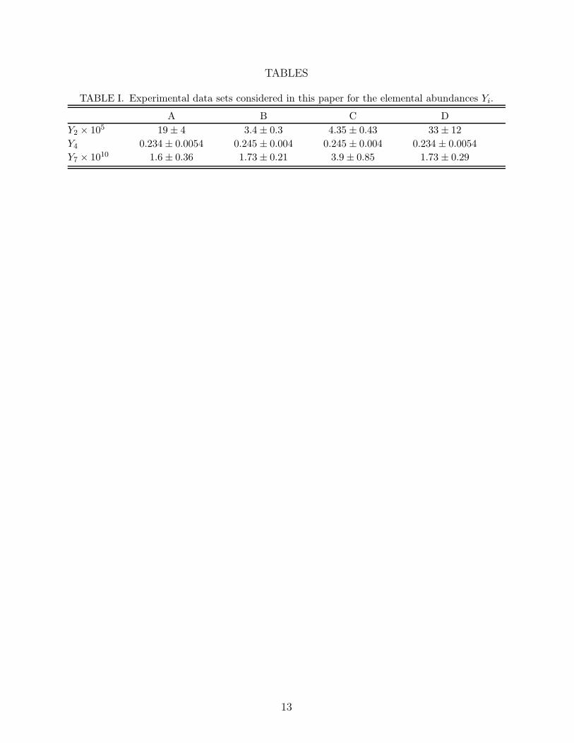
The data sets we consider are tabulated in Table I. Below we comment in detail on ourchoices.

• Data Set A: This is taken from Ref. [29] who performed the first detailed MC+MLanalysis to determine η and Nν and is chosen essentially for comparison with ourmethod, as in our previous paper [28].

Their adopted value of the primordial deuterium abundance, Y2 = 1.9±0.4×10−4, wasbased on early observations of a QAS at redshift z = 3.32 towards Q0014+813 whichsuggested a relatively ‘high’ value [14], and was consistent with limits set in otherQAS, but in conflict with the much lower abundance found in a QAS at z = 3.572towards Q1937-1009 [15]. More recently, observations of a QAS at z = 0.701 towardsQ1718+4807 have also yielded a high abundance [37,38] as we discuss later.

The primordial helium abundance was taken to be Y4 = 0.234±0.002±0.005 from linearregression to zero metallicity in a set of 62 BCGs [41], based largely on observationswhich gave a relatively ‘low’ value [11].

Finally the primordial lithium abundance Y7 = 1.6± 0.36× 10−10 was taken from thePop II observations of Ref. [44], assuming no depletion.

• Data Set B: This corresponds to the alternative combination of ‘low’ deuterium and‘high’ helium, as considered in our previous work [28], with some small changes.

The primordial deuterium abundance, Y2 = 3.4±0.3×10−5, adopted here is the averageof the ‘low’ values found in two well-observed QAS, at z = 3.572 towards Q1937-1009[39], and at z = 2.504 towards Q1009+2956 [40].

The primordial helium abundance, Y4 = 0.245 ± 0.004, is taken to be the average ofthe values found in the two most metal-poor BCGs, I Zw 18 and SBS 0335-052, from anew analysis which uses the helium lines themselves to self-consistently determine thephysical conditions in the H II region, and specifically excludes those regions which arebelieved to be affected by underlying stellar absorption [42]. For example these authorsdemonstrate that there is strong underlying stellar absorption in the NW componentof I Zw 18, which has been included in earlier analyses [11].

6

The primordial lithium abundance Y7 = 1.73 ± 0.21 × 10−10 is from Ref. [45], againassuming no depletion. (Note that the uncertainty was incorrectly reported as ±0.12×10−10 in Ref. [36], as used in our previous work [28].)

• Data Set C: It has been suggested [49] that the discordance between the ‘high’ and‘low’ values of the deuterium abundance reported in QAS may be considerably re-duced if the analysis of the H+D profiles accounts for the correlated velocity field ofbulk motion, i.e. mesoturbulence, rather than being based on multi-component mi-croturbulent models. It is then found [49] that a value of Y2 = (3.5 − 5.2) × 10−5 iscompatible simultaneously (at 95% C.L.) with observations of the QAS at z = 0.701towards Q1718+4807 (in which a ‘high’ value was reported [37,38]), and observationsof the QAS at z = 3.572 towards Q1937-1009 and at z = 2.504 towards Q1009+2956(in which a ‘low’ value was reported [39,40]). We adopt this value, along with thesame helium abundance as in Set B.

It has also been argued that the lithium abundance observed in Pop II stars hasbeen depleted down from a primordial value of Y7 = 3.9 ± 0.85 × 10−10 [50], thelower end of the range being set by the presence of highly overdepleted halo starsand consistency with the 7Li abundance in the Sun and in open clusters, while theupper end of the range is set by the observed dispersion of the Pop II abundance“plateau” and the 6Li/7Li depletion ratio. We adopt this value, noting that a somewhatsmaller depletion is suggested by other workers [47] who find a primordial abundanceof Y7 = 2.3 ± 0.5 × 10−10.

• Data Set D: Recently, a ‘high’ value of the deuterium abundance, Y2 = 3.3±1.2×10−4,has been reported from observations of a QAS at z = 0.701 towards Q1718+4807 [38],in confirmation of an earlier claim [37]. We adopt this value along with the samehelium abundance as in set A.

For the lithium abundance, we adopt the same value [45] as in Set B but increase thesystematic error by 0.02 dex to allow for the uncertainty in the oscillator strengths ofthe lithium lines [51].

B. Qualitative Implications on Nν and η

Different choices for the input data sets (A–D) lead to different implications for η andNν , that can be qualitatively understood through Figs. 1–4.

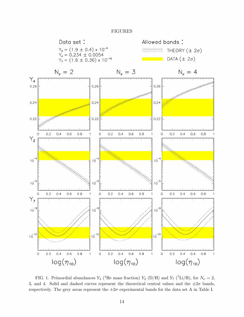
Figure 1 shows the BBN primordial abundances Yi (solid lines) and their ±2σ bands(dashed lines), as functions of x ≡ log(η/10−10), for Nν = 2, 3, and 4. The grey areasrepresent the ±2σ bands allowed by the data set A (see Table I). There is global consistencybetween theory and data for x ∼ 0.2 − 0.4 and Nν = 3, while for Nν = 2 (Nν = 4) the Y2

data prefer values of x lower (higher) than the Y4 data. Therefore, we expect that a globalfit will favor values of (x, Nν) close to (0.3, 3).

Figure 2 is analogous, but for the data set B. In this case, there is still consistencybetween theory and data at Nν = 3, although for values of x higher than for the data setA. For Nν = 2 (Nν = 4) the combination of Y2 and Y7 data prefer values of x lower (higher)than Y4. The best fit is thus expected to be around (x, Nν) ∼ (0.7, 3).

7

Similarly, Figure 3 shows the abundances for the data set C. The situation is similar todata set B (Fig. 2), but one can envisage a best fit at a slightly lower value of x, due to thehigher value of Y2, partly opposed by the increase in Y7.

Finally, Fig. 4 refers to the data set D. In this case, data and theory are not consistentfor Nν = 2, since Y2 and Y4 pull x in different directions, and no “compromise” is possiblesince intermediate values of x are disfavored by Y7. However, for Nν = 3 there is relativelygood agreement between data and theory at low x. Therefore, we expect a best fit around(x, Nν) ∼ (0.2, 3).

The qualitative indications discussed here are confirmed by a more accurate analysis,whose results are reported in the next section.

IV. DETERMINING Nν

We now present the results of fits to the data sets A–D in the (x, Nν) variables, using ourmethod to estimate the correlated theoretical uncertainties, and adopting χ2 statistics toinclude both theoretical and experimental errors. We have used the theoretical Yi’s obtainedby the standard (updated) BBN evolution code [23], and checked that using the polynomialfits given in Sec. II B induce negligible changes which would not be noticeable on the plots.

In the analysis, we optionally take into account a further constraint on η (independent onNν) coming from a recent analysis of the Lyα-“forest” absorption lines in quasar spectra. Theobserved mean opacity of the lines requires some minimum amount of neutral hydrogen inthe high redshift intergalactic medium, given a lower bound to the flux of ionizing radiation.Taking the latter from a conservative estimate of the integrated UV background due toquasars, Ref. [52] finds the constraint η ≥ 3.4 × 10−10. This bound is not well-definedstatistically but, for the sake of illustration, we have parametrized it through a penaltyfunction quadratic in η:

χ2Lyα(η) = 2.7 ×

(

3.4 × 10−10

η

)2

, (10)

to be eventually added to the χ2(η, Nν) derived from our fit to the elemental abundances.The above function excludes values of η smaller than 3.4×10−10 at 90% C.L. (for one degreeof freedom, η).

Figure 5 shows the results of joints fits to x = log(η10) and Nν using the abundances ofdata set A. The abundances Y2, Y4, and Y7 are used separately (upper panels), in combina-tions of two (middle panels), and all together, without and with the Lyα-forest constrainton η (lower panels). In this way the relative weight of each piece of data in the global fit canbe understood at glance. The three C.L. curves (solid, thick solid, and dashed) are definedby χ2 − χ2

min = 2.3, 6.2, and 11.8, respectively, corresponding to 68.3%, 95.4%, and 99.7%C.L. for two degrees of freedom (η and Nν), i.e., to the probability intervals often designatedas 1, 2, and 3 standard deviation limits. The χ2 is minimized for each combination of Yi,but the actual value of χ2

min (and the best-fit point) is shown only for the relevant globalcombination Y2 + Y4 + Y7(+Lyα).

The results shown in Fig. 5 for the combinations Y4+Y7 and Y2+Y4+Y7 are consistent withthose obtained in ref. [29] by using the same input data but a completely different analysis

8

method (namely Monte Carlo simulation plus maximum likelihood). The consistency isreassuring and confirms the validity of our method. For this data set, the helium anddeuterium abundances dominate the fit, as it can be seen by comparing the combinationsY2 + Y4 and Y2 + Y4 + Y7. The preferred values of x are relatively low, and the preferredvalues of Nν range between 2 and 4. Although the fit is excellent, the low value of x is inconflict with the Lyα-forest constraint on η, as indicated by the increase of χ2

min from 0.02to 8.89.

Figure 6 is analogous, but for the data set B which favors high values of x because ofthe ‘low’ deuterium abundance. The combination of Y2 + Y7 isolates, at high x, a narrowstrip which depends mildly on Nν . The inclusion of Y4 selects the central part of such strip,corresponding to Nν between 2 and 4. As in Fig. 5, the combination Y4 +Y7 does not appearto be very constraining. The overall fit to Y2 + Y4 + Y7 is acceptable but not particularlygood, mainly because Y2 and Y7 are only marginally compatible at high x. On the otherhand, the Y2 + Y4 + Y7 bounds are quite consistent with the Lyα-forest constraint.

In data set C, the deuterium abundance has increased further. Moreover the lithiumabundance is no longer at the minimum of the theoretical curve as before, so stronglydisfavors “intermediate” values of x. The overall effect, as shown in Figure 7, is that χ2

min

decreases a bit with respect to Set B, and the best fit value of x moves slightly lower. Theallowed value of Nν ranges between 2 and 4. Note that had we retained the same Y7 as inSet B, then χ2

min would have dropped to 0.91 (2.55) for the combination Y2 + Y4 + Y7 (+Lyα-forest constraint).

Finally, Fig. 8 refers to data set D which, like Data Set A, has the ‘high’ deuteriumabundance but with larger uncertainties. So although a low value of x is still picked out, ahigh x region is still possible at the 2σ level (in the Y2 + Y4 + Y7 panel) and is even favoredwhen the Lyα-forest bound is included (although with an unacceptably high χ2

min). Notethat had the lithium abundance been taken to be the same as in data set C (i.e. allowingfor depletion), the χ2

min would have been 0.07 (7.42) for the combination Y2 + Y4 + Y7 (+Lyα-forest constraint).

Of course one can also consider orthogonal combinations to those above, e.g. ‘high’ deu-terium and ‘high’ helium, or ‘low’ deuterium and ‘low’ helium [30]. The latter combinationimplies Nν ∼ 2, thus creating the so-called “crisis” for standard nucleosynthesis [18]. Con-versely, the former combination suggests Nν ∼ 4, which would also constitute evidence fornew physics. Allowing for depletion of the primordial lithium abundance to its Pop II value,relaxes the upper bound on Nν further, as noted earlier [24].

V. CONCLUSIONS

The results discussed above demonstrate that the present observational data on theprimordial elemental abundances are not as yet sufficiently stable to derive firm bounds onη and Nν . Different and arguably equally acceptable choices for the input data sets leadto very different predictions for η, and to relatively loose constraints on Nν in the range2 to 4 at the 95% C.L. Thus it may be premature to quote restrictive bounds based onsome particular combination of the observations, until the discrepancies between differentestimates are satisfactorily resolved. Our method of analysis provides the reader with an

9

easy-to-use technique [31] to recalculate the best-fit values as the observational situationevolves further.

However one might ask what would happen if these discrepancies remain? We havealready noted the importance of an independent constraint on η (from the Lyα-forest) indiscriminating between different options. However, given the many assumptions which gointo the argument [52], this constraint is rather uncertain at present. Fortunately it shouldbe possible in the near future to independently determine η to within ∼ 5% through mea-surements of the angular anisotropy of the cosmic microwave background (CMB) on smallangular scales [53], in particular with data from the all-sky surveyors MAP and PLANCK[54]. Such observations will also provide a precision measure of the relativistic particlecontent of the primordial plasma. Hopefully the primordial abundance of 4He would havestabilized by then, thus providing, in conjunction with the above measurements. a reliableprobe of a wide variety of new physics which can affect nucleosynthesis.

ACKNOWLEDGMENTS

We thank G. Fiorentini for useful discussions and for earlier collaboration on the subjectof this paper.

10

REFERENCES

[1] For a recent review, see J. Conrad, hep-ex/9811009, plenary talk at the Intern. Conf.on High Energy Physics, Vancouver (1998).

[2] C. Caso et al. (Particle Data Group), Eur. J. Phys. C 3, 1 (1998).[3] F. Hoyle and R.J. Tayler, Nature 203, 1108 (1964); P.J.E. Peebles, Phys. Rev. Lett. 16,

411 (1966); V.F. Shvartsman, Pis’ma Zh. Eksp. Teor. Fiz. 9, 315 (1969) [JETP Lett. 9,184 (1969)].

[4] G. Steigman, D.N. Schramm, and J. Gunn, Phys. Lett. 66B, 202 (1977); G. Steigman,K.A. Olive, and D.N. Schramm, Phys. Rev. Lett. 43, 239 (1979).

[5] K.A. Olive, D.N. Schramm, and G. Steigman, Nucl. Phys. B 180, 497 (1981).[6] K. Enqvist, K. Kainulainen and M. Thomson, Nucl. Phys. B 373, 498 (1992).[7] D.P. Kirilova and M.V. Chizhov, Nucl. Phys. B 534, 447 (1998); R. Foot and R.R.

Volkas, Phys. Rev. D 55, 5147 (1997).[8] A.D. Dolgov, S.H. Hansen, S. Pastor, and D.V. Semikoz, hep-ph/9809598; S. Hannestad,

Phys. Rev. D 57, 2213 (1998); M. Kawasaki, K. Kohri and K. Sato, Phys. Lett. B 430,132 (1998).

[9] A.D. Dolgov, S. Pastor, J.C. Romao, and J.W.F. Valle, Nucl. Phys. B 496, 24 (1997).[10] R. Lopez and M.S. Turner, astro-ph/9807279, to appear in Phys. Rev D.[11] B.E.J. Pagel, E.A. Simonson, R.J. Terlevich, and M.G. Edmunds, Mon. Not. R. Astr.

Soc. 255, 325 (1992); K.A. Olive and G. Steigman, Astrophys. J. Suppl. 97, 49 (1995).[12] Y.I. Izotov, T.X. Thuan, and V. A. Lipovetsky, Astrophys. J. 435, 647 (1994), Astro-

phys. J. Suppl. 108, 1 (1997).[13] R. Epstein, J. Lattimer, and D.N. Schramm, Nature 263, 198 (1976).[14] A. Songaila, L.L. Cowie, C.J. Hogan and M. Rugers, Nature 368, 599 (1994); R.F.

Carswell, M. Rauch, R.J. Weymann, A.J. Cooke, and J.K. Webb, Mon. Not. R. Astr.Soc. 268, L1 (1994); M. Rugers and C.J. Hogan, Astrophys. J. Lett. 459, L1 (1996),Astron. J. 111, 2135 (1996).

[15] D. Tytler, X-M. Fan, and S. Burles, Nature 381, 207 (1996); S. Burles and D. Tytler,Astron. J. 114, 1330 (1997).

[16] S. Sarkar, Rep. Prog. Phys. 59, 1493 (1996).[17] J. Yang, M.S. Turner, G. Steigman, D.N. Schramm, and K.A. Olive, Astrophys. J. 281,

493 (1984); G. Steigman, K.A. Olive, D.N. Schramm, and M.S. Turner, Phys. Lett. B176, 33 (1986); K.A. Olive, D.N. Schramm, G. Steigman, and T.P Walker, Phys. Lett.B 236, 454 (1990); T.P Walker, G. Steigman, D.N. Schramm, K.A. Olive, and H.-S.Kang, Astrophys. J. 376, 51 (1991).

[18] N. Hata, R.J. Scherrer, G. Steigman, D. Thomas, T.P. Walker, S. Bludman and P.Langacker, Phys. Rev. Lett. 75, 3977 (1995).

[19] J. Ellis, K. Enqvist, D.V. Nanopoulos, and S. Sarkar, Phys. Lett. B 167, 457 (1986).[20] P.J. Kernan and L.M. Krauss, Phys. Rev. Lett. 72, 3309 (1994); L.M. Krauss and P.J.

Kernan, Astrophys. J. Lett. 432, L79 (1994), Phys. Lett. B 347, 347 (1995).[21] L.M. Krauss and P. Romanelli, Astrophys. J. 358, 47 (1990);[22] M.S. Smith, L.H. Kawano, and R. A. Malaney, Astrophys. J. Suppl. 85, 219 (1993).[23] R.V. Wagoner, Astrophys. J. 179, 343 (1973); L. Kawano, Report No. Fermilab-Pub-

88/34-A, 1988 (unpublished), Report No. Fermilab-Pub-92/04-A, 1992 (unpublished).[24] P.J. Kernan and S. Sarkar, Phys. Rev. D54, R3681 (1996).

11

[25] C.J. Copi, D.N. Schramm, and M.S. Turner, Phys. Rev. D55, 3389 (1997).[26] B.D. Fields and K.A. Olive, Phys. Lett. B 368, 103 (1996); B.D. Fields, K. Kainulainen,

K.A. Olive, and D. Thomas, New Astron. 1, 77 (1996).[27] N. Hata, G. Steigman, S. Bludman, and P. Langacker, Phys. Rev. D55, 540 (1997).[28] G. Fiorentini, E. Lisi, S. Sarkar, and F.L. Villante, Phys. Rev. D58, 063506 (1998).[29] K.A. Olive and D. Thomas, Astropart. Phys. 7 (1997) 27.[30] E. Holtman, M. Kawasaki, K. Kohri, and T. Moroi, hep-ph/9805405.[31] See: http://www-thphys.physics.ox.ac.uk/users/SubirSarkar/bbn.html[32] R. Esmailzadeh, G.D. Starkman, and S. Dimopoulos, Astrophys. J. 378, 504 (1991).[33] J.A. Bernstein, L.S. Brown, and G. Feinberg, Rev. Mod. Phys. 61, 25 (1989).[34] B.E.J. Pagel, Nucleosynthesis and the Chemical Evolution of Galaxies (Cambridge Uni-

versity Press, Cambridge, 1997).[35] C. Hogan, Sp. Sci. Rev. 84, 127 (1998).[36] P. Molaro, in From Quantum Fluctuations to Cosmological Structures, edited by D.

Valls-Gabaud et al., ASP Conf. Ser. 126, 103 (1997).[37] J.K. Webb, R.F. Carswell, K.M. Lanzetta, R. Ferlet, M. Lemoine, and A. Vidal-Madjar,

Nature 388, 250 (1997).[38] D. Tytler, S. Burles, L. Lu, X-M. Fan, A. Wolfe and B.D. Savage, astro-ph/9810217, to

appear in Astron. J.[39] S. Burles and D. Tytler, Astrophys. J. 499, 699 (1998).[40] S. Burles and D. Tytler, Astrophys. J. 507, 732 (1998); Sp. Sci. Rev. 84, 65 (1998).[41] K.A. Olive, G. Steigman, and E.D. Skillman, Astrophys. J. 483, 788 (1997).[42] Y.I. Izotov and T.X. Thuan, Astrophys. J. 497, 227 (1998); 500, 188 (1998).[43] S.G. Ryan, T.C. Beers, C.P. Deliyannis, and J. Thorburn, Astrophys. J. 458, 543 (1996).[44] P. Molaro, F. Primas, and P. Bonifacio, Astron. Astrophys. 295, L47 (1995).[45] P. Bonifacio and P. Molaro, Mon. Not. Roy. Astron. Soc. 285, 847 (1997).[46] M.H. Pinsonneault, C.P. Deliyannis, and P. Demarque, Astrophys. J. Suppl. 78, 179

(1992).[47] S. Vauclair and C. Charbonnel, Astron. Astrophys. 295, 715 (1995); astro-ph/9802315,

to appear in Astrophys. J.[48] P. Bonifacio and P. Molaro, Astrophys. J. Lett. 500, L175 (1998).[49] S.A. Levshakov, W.H. Kegel, and F. Takahara, Astrophys. J. 499, L1 (1998); Astron.

and Astrophys. 336, L29 (1998); S.A. Levshakov, D. Tytler, and S. Burles, astro-ph/9812114.

[50] M.H. Pinsonneault, T.P. Walker, G. Steigman, and V.K. Naranyanan, astro-ph/9803073.

[51] P. Molaro, private communication.[52] D.H. Weinberg, J. Miralda-Escude, L. Hernquist, and N. Katz, Astrophys. J. 490, 564

(1997).[53] For a review, see, D.N. Spergel, Proc. Nobel Symp.: Particle Physics and the Universe,

Enkoping, Sweden, August 20-25, 1998, to be published in Phys. Scripta.[54] MAP: http://map.gsfc.nasa.gov/;

PLANCK: http://astro.estec.esa.nl/SA-general/Projects/Planck/

12

TABLES

TABLE I. Experimental data sets considered in this paper for the elemental abundances Yi.

A B C D

Y2 × 105 19 ± 4 3.4 ± 0.3 4.35 ± 0.43 33 ± 12

Y4 0.234 ± 0.0054 0.245 ± 0.004 0.245 ± 0.004 0.234 ± 0.0054

Y7 × 1010 1.6 ± 0.36 1.73 ± 0.21 3.9 ± 0.85 1.73 ± 0.29

13

FIGURES

FIG. 1. Primordial abundances Y4 (4He mass fraction) Y2 (D/H) and Y7 (7Li/H), for Nν = 2,

3, and 4. Solid and dashed curves represent the theoretical central values and the ±2σ bands,

respectively. The grey areas represent the ±2σ experimental bands for the data set A in Table I.

14

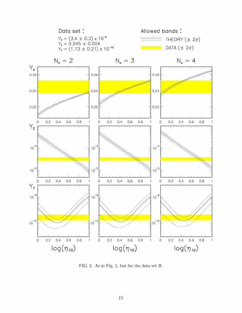
FIG. 2. As in Fig. 1, but for the data set B.

15

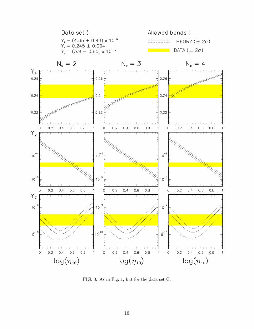
FIG. 3. As in Fig. 1, but for the data set C.

16

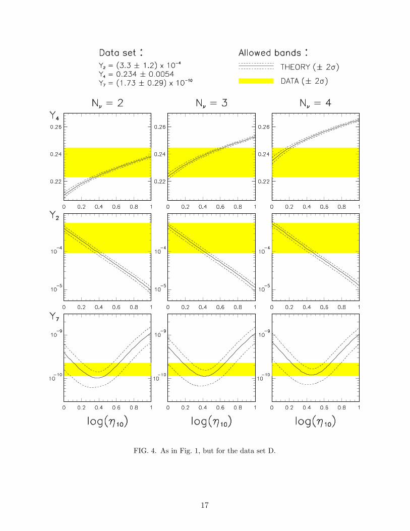
FIG. 4. As in Fig. 1, but for the data set D.

17

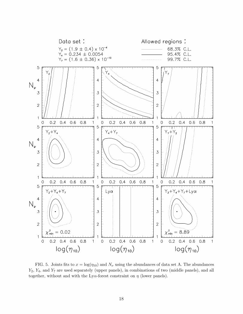
FIG. 5. Joints fits to x = log(η10) and Nν using the abundances of data set A. The abundances

Y2, Y4, and Y7 are used separately (upper panels), in combinations of two (middle panels), and all

together, without and with the Lyα-forest constraint on η (lower panels).

18

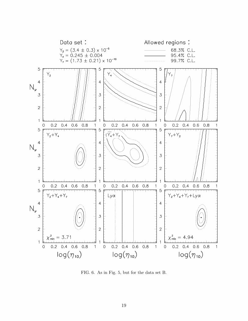
FIG. 6. As in Fig. 5, but for the data set B.

19

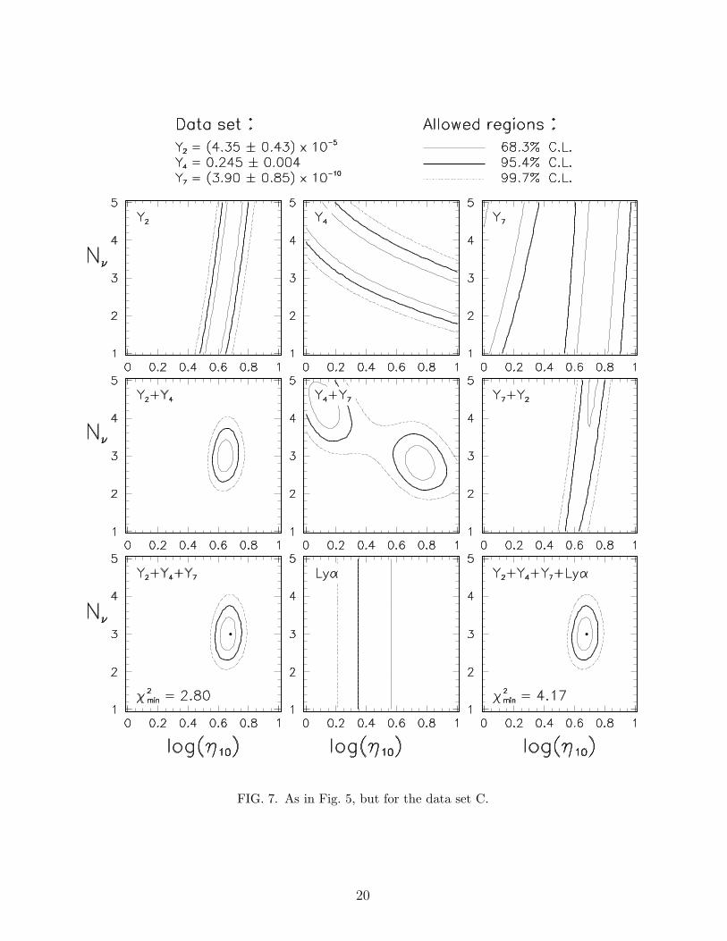
FIG. 7. As in Fig. 5, but for the data set C.

20

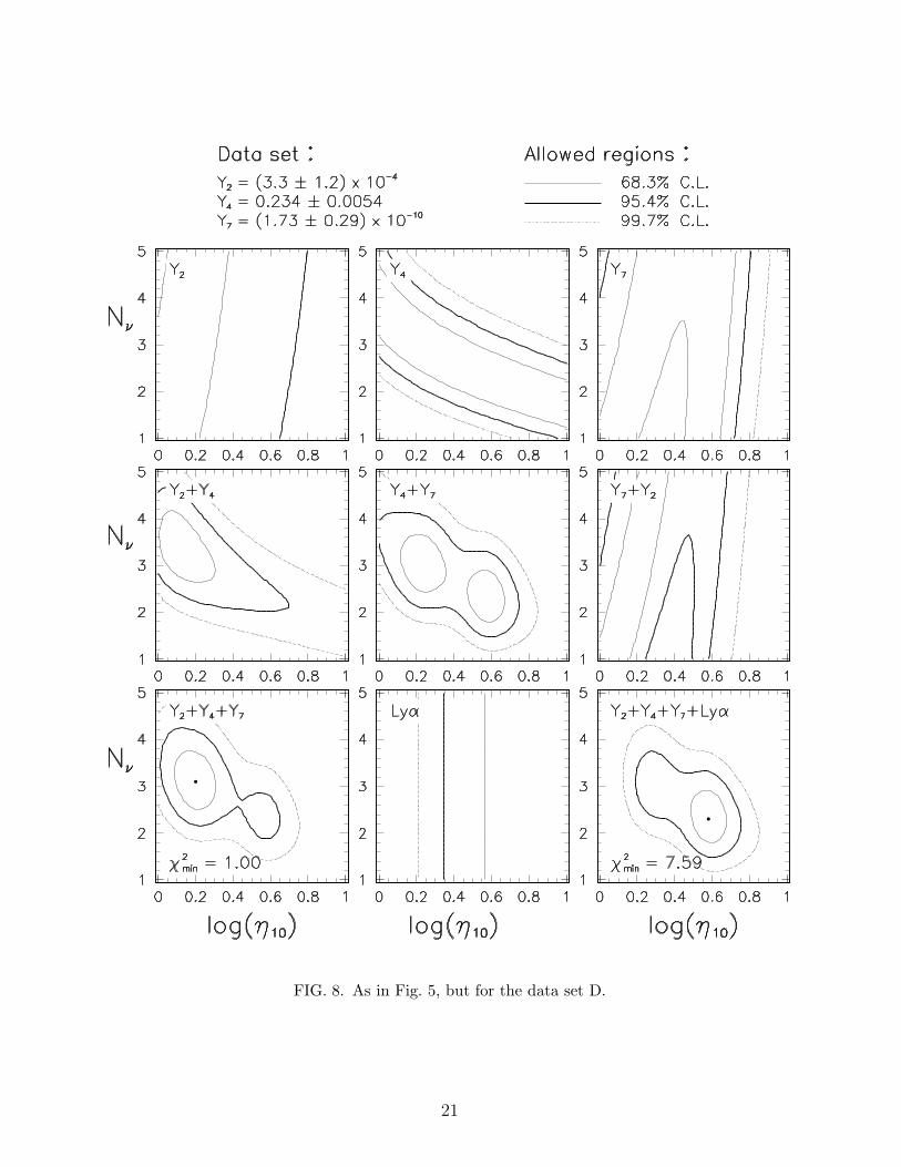
FIG. 8. As in Fig. 5, but for the data set D.

21