best practices in measuring vowel merger

Proceedings of Meetings on Acoustics

Volume 20, 2013 http://acousticalsociety.org/

166th Meeting of the Acoustical Society of America

San Francisco, California

2 - 6 December 2013

Session 4pSCa: Speech Communication

4pSCa1. Best practices in measuring vowel mergerJennifer Nycz* and Lauren Hall-Lew

*Corresponding author's address: Linguistics, Georgetown University, 1437 37th St. NW, Washington, DC 20057, [email protected] Vowel mergers are some of the most well-studied sound change phenomena. Yet the methods for assessing and characterizing an individual speaker'sparticipation in an ongoing merger (or split) vary widely, especially among researchers analyzing naturalistic corpora. We consider four methodologicalapproaches to representing and assessing vowel difference: Euclidean distances, mixed effects regression modeling (Nycz 2013), the Pillai-Bartlett trace(Hay, Warren, & Drager 2006), and the spectral overlap assessment metric (Wassink 2006). We discuss the strengths and weaknesses of each method andcompare them by applying all of them to three different data sets, each of which contains low vowel data from speakers whose status with respect to avowel contrast may not be clear-cut: realizations of COT and CAUGHT in San Francisco, California; COT and CAUGHT among Canadians in the NewYork City region; and TRAP and BATH among Scots who work in Southern England. We conclude with some practical recommendations.

Published by the Acoustical Society of America through the American Institute of Physics

J. Nycz and L. Hall-Lew

© 2014 Acoustical Society of America [DOI: 10.1121/1.4894063]Received 10 Jul 2014; published 15 Aug 2014Proceedings of Meetings on Acoustics, Vol. 20, 060008 (2014)

Redistribution subject to ASA license or copyright; see http://acousticalsociety.org/content/terms. Download to IP: 66.44.126.16 On: Mon, 18 Aug 2014 21:06:08

1. INTRODUCTION

Vowel mergers are some of the most frequently studied sound changes. Their realization in the speech of individualsas well as their spread through a community raise a number of interesting questions for sociolinguists, dialectologists,phoneticians, and phonologists [1]. Despite the long-standing interest in vowel merger (and its inverse, vowel split),the methods for assessing and quantifying differences in the realizations of word classes implicated in merger varywidely across studies, especially in research which draws its data from naturalistic speech corpora. These methodsalso vary with respect to the type of information they yield. Ideally, a method for assessing vowel difference would doall of the following:

1. Capture the distance between word classes in acoustic space. It is possible to determine a central tendency fora given word class in multidimensional acoustic space (typically, the two dimensional vowel space defined by F1 andF2). In most cases, we want to quantify the distance between these central tendencies. We would also like to identifywhich specific dimension(s) account for most of the difference, as this information can illuminate the changes leadingto merger or split (for example, if one vowel is backing or raising towards the other, possibly due to other changesoccurring in the wider system). Finally, we want to know whether such distances are statistically significant, or likelyto occur by chance even if there is no underlying difference.

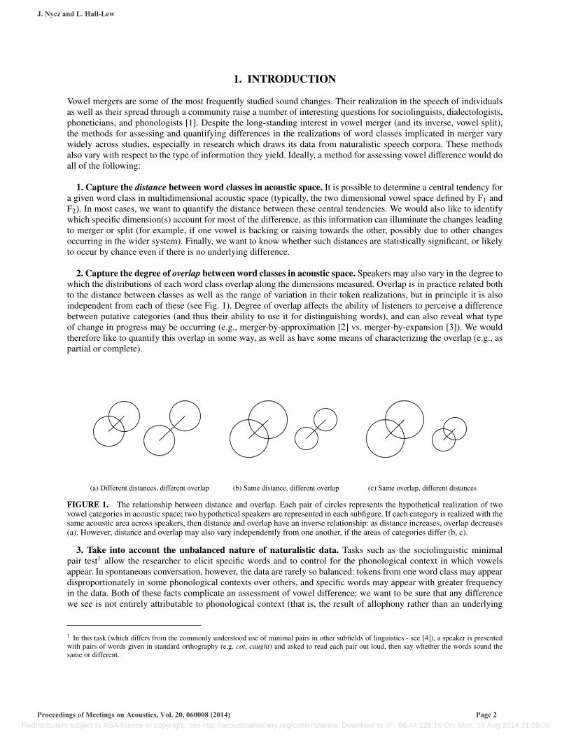
2. Capture the degree of overlap between word classes in acoustic space. Speakers may also vary in the degree towhich the distributions of each word class overlap along the dimensions measured. Overlap is in practice related bothto the distance between classes as well as the range of variation in their token realizations, but in principle it is alsoindependent from each of these (see Fig. 1). Degree of overlap affects the ability of listeners to perceive a differencebetween putative categories (and thus their ability to use it for distinguishing words), and can also reveal what typeof change in progress may be occurring (e.g., merger-by-approximation [2] vs. merger-by-expansion [3]). We wouldtherefore like to quantify this overlap in some way, as well as have some means of characterizing the overlap (e.g., aspartial or complete).

(a) Different distances, different overlap (b) Same distance, different overlap (c) Same overlap, different distances

FIGURE 1. The relationship between distance and overlap. Each pair of circles represents the hypothetical realization of twovowel categories in acoustic space; two hypothetical speakers are represented in each subfigure. If each category is realized with thesame acoustic area across speakers, then distance and overlap have an inverse relationship: as distance increases, overlap decreases(a). However, distance and overlap may also vary independently from one another, if the areas of categories differ (b, c).

3. Take into account the unbalanced nature of naturalistic data. Tasks such as the sociolinguistic minimalpair test1 allow the researcher to elicit specific words and to control for the phonological context in which vowelsappear. In spontaneous conversation, however, the data are rarely so balanced: tokens from one word class may appeardisproportionately in some phonological contexts over others, and specific words may appear with greater frequencyin the data. Both of these facts complicate an assessment of vowel difference: we want to be sure that any differencewe see is not entirely attributable to phonological context (that is, the result of allophony rather than an underlying

1 In this task (which differs from the commonly understood use of minimal pairs in other subfields of linguistics - see [4]), a speaker is presentedwith pairs of words given in standard orthography (e.g. cot, caught) and asked to read each pair out loud, then say whether the words sound thesame or different.


Proceedings of Meetings on Acoustics, Vol. 20, 060008 (2014) Redistribution subject to ASA license or copyright; see http://acousticalsociety.org/content/terms. Download to IP: 66.44.126.16 On: Mon, 18 Aug 2014 21:06:08

contrast) or the idiosyncratic patterning of particular words which are especially frequent in the data.

4. Enable a comparison between speakers in a corpus with respect to their degree of participation in a mergeror split in progress. Often, researchers are interested in the extent to which variation in the degree of word classdifference can be predicted by social factors such as age or attitude. In such cases, we need a measure of differencewhich can serve as a dependent variable in a statistical analysis, which requires that this measure be comparableacross all speakers in a corpus.

In this paper we review four methods for quantifying the acoustic correlates of merger, each of which has beenused in recent sociophonetic work. We discuss how each does or does not meet these desiderata, and then apply eachmethod to data2 from fifteen speakers: five individuals from each of three different data sets of spontaneous speech.These data sets represent word classes which are undergoing merger or split for some group of English speakers: COTand CAUGHT3 among San Franciscans and mobile Canadians, and TRAP and BATH among Scots. We discuss how thedifferent methods agree or disagree in their assessment of speakers within each data set as well as probable reasonsfor the disagreements, and end with practical recommendations.

2. THE FOUR METHODS

2.1. Euclidean distance

One way to quantify the difference between two putative vowel categories is to calculate their Euclidean distance4

(see, e.g., Baranowski [7], Irons [8], Dinkin [6] for use of this method in quantifying degree of low back merger.).The distance between vowels is modeled as the hypotenuse of a right triangle, with the other two sides of the triangledefined by distances along the F1 and F2 dimensions. The Pythagorean theorem is used to find the length of thehypotenuse; the smaller that value, the closer the vowels are in the two-dimensional vowel space. Euclidean distance istypically calculated using the mean F1 and F2 values for each category, but this method can also be used for individualtoken pairs when the members of each pair occur in the same phonological environment, such as in minimal pair data.

Euclidean distance obviously provides a measure of distance between categories, partially fulfilling one of ourrequirements from the previous section. If the distance is calculated for normalized vowel data, then the Euclideandistances can also be compared across speakers in a corpus and serve as a dependent variable in a statistical analysis.The main practical advantage to using Euclidean distance is ease: one does not need advanced statistical softwareto calculate this value, which can be determined using a simple formula within a spreadsheet program (or by handwith pencil and paper). Moreover, the resulting distance is given in units of measurement (such as Hertz) that aretransparent to linguists, and is easily visualized on the two-dimensional vowel space as a straight line between twopoints.

However, the method also has several disadvantages. First, it does not itself indicate whether the calculated distanceis in fact a statistically significant one; additional tests for differences in central tendency such as t tests must becarried out, and each test can only indicate a difference along one dimension (i.e. F1 or F2, but not the Euclideandistance itself). Second, Euclidean distance does not capture the amount of overlap between categories, nor anythingabout the distribution of the tokens within each category, information which is likely relevant to assessing both thetype and the degree of participation in a change in progress. Third, this method offers no way of controlling for the

2 Each method will be compared only with respect to F1 and F2 values, which are given in Hz.3 We use keyword labels rather than IPA symbols for two reasons. The first is phonological: we do not want to assume the presence or absence ofa contrast between two lexical sets, as the use of either two symbols (such as /O/ and /A/) or one for a given pair of sets would imply. The secondis phonetic: the realization of each lexical set’s vowels in all of the data we examine is variable, and may range over a region of the vowel spacethat could be labelled with several IPA symbols. We also use different keyword conventions for the US English and UK English datasets. TRAP andBATH are used in the British context because Wells’ sets are based on Received Pronunciation (RP), and RP is taken to be the dominant variety ofthe community under study, the Parliament of the United Kingdom. In contrast, COT and CAUGHT are used in the American contexts because therelevant (non-RP) vowel contrasts encompass multiple Wells’ sets [5] (COT includes LOT and PALM; CAUGHT includes CLOTH and THOUGHT).4 This measure is also sometimes referred to as Cartesian distance (e.g. Dinkin [6]).



allophonic contexts in which tokens appear. For example, /l/ tends to lower the F1 and F2 of preceding vowels; ifmany of the CAUGHT tokens in a data set appear before /l/ while only a few COT tokens appear in this context (acommon occurrence in many data sets), the Euclidean distance will overestimate the overall difference between theCAUGHT and COT categories. Controlling for such allophonic effects must be done manually, for instance by removingnon-common phonological contexts and then calculating distances on a subset of the data. Finally, this method cannottake into account word-specific effects on vowel realization: if a category’s overall distribution is substantially skewedby a particular lexical item, this information will be lost when all values are averaged together for that category.These disadvantages are of particular concern for researchers who draw their data from naturalistic speech, in whichcategory overlap and lack of control over both allophonic context and specific lexical items represented is the norm.

Another concern with Euclidean distance as it is typically used is the appropriateness of relying on the meanformant values for the determination of distance. The mean F1 or F2 will often not be the best indication of avowel’s central tendency, especially in the cases of variation and change which are of particular interest to manysociophoneticians: ongoing vowel shifts may result in token spreads that are not normally distributed, and tokens withextreme realizations may shift the mean in such a way as to misrepresent the central tendency of the overall tokencluster. One way to address this issue is to instead calculate Euclidean distance based on median F1 and F2 , which arerelatively unaffected by skewed distributions and extreme values. In the analyses that follow, we will report Euclideandistances calculated with medians (henceforth ED-Median) as well as those calculated with means (ED-Mean) anddiscuss any differences that arise.

2.2. Mixed Effects Regression & Adjusted Euclidean distance

Nycz [9], [4] used mixed effects regression to estimate the difference between word classes. This method exploitstwo key features of mixed effects models. First, such models can contain multiple fixed effects, meaning that termsrepresenting features of the phonological environment which may condition vowel realization can be included alongwith a term for WORD CLASS. Second, these models include random effects which reflect variation between randomlyselected individuals in a population: this means that the potentially idiosyncratic patterning of specific WORDs whichhappen to have appeared in a corpus can be taken into account when estimating the fixed effects of primary interest.Moreover, this helps to correct for WORD token number imbalances.

To estimate the difference between two word classes along the height dimension, two models are created withF1 as the outcome variable. The first model contains various fixed effects reflecting phonological environment5 anda random effect of WORD. The second model contains the same phonological fixed effects, the random effect ofWORD, and an additional fixed effect of WORD CLASS. The two models are then compared, and if the second modelis found to be significantly better than the first – that is, if WORD CLASS membership accounts for a significantamount of variation in F1 even when phonological context and word effects are taken into account – then this canbe interpreted as indicating that there is a significant difference between the two word classes along the heightdimension.6 Moreover, the effect size associated with WORD CLASS in the second model represents the distancebetween these two categories once phonological context and word effects are controlled for. The same procedure isfollowed to estimate the difference between word classes along the F2 dimension. The estimated differences in F1 andF2 can then be used to calculate an Adjusted Euclidean distance (ED-Adjusted).

This method improves upon the simpler Euclidean distance measures described in the previous section in a fewways. It overcomes (or at least greatly mitigates) the skewing effects of both allophony and word-specific effects in

5 Phonological environment was represented by four factors in the analyses described here: following and preceding segment voice/manner(VOICELESS OBSTRUENT, VOICED OBSTRUENT, NASAL, LATERAL, RHOTIC, PAUSE) and following and preceding segment place (APICAL,DORSAL, NOT LINGUAL).6 It is important to note that while the presence of a significant difference suggests that the speaker does not have vowel merger (in production), theabsence of significance cannot be taken as evidence that the speaker is underlyingly merged. Like any statistical model of acoustic data (includingthe MANOVA model discussed below), statistical significance is based on only those dependent acoustic variables entered into the model, and thestatus of merger versus near-merger or distinction is phonological, at the level of representations rather than acoustic outputs.



calculating the distances between two categories. Moreover, it produces a significance value associated with WORDCLASS that also takes into account these other factors.

However, the method shares a few disadvantages with Euclidean distance as described in the previous section. First,the significance assessments produced reflect the effect of WORD CLASS on each of F1 and F2 separately; it does notindicate whether the calculated ED-Adjusted itself is significant. Second, there is no explicit quantification of overlapbetween word classes in the model output.

2.3. Pillai-Bartlett Trace

Hay et al. [10] introduced a method for estimating the extent of overlap between vowel categories which theyreferred to as the ‘Pillai score’ (Pillai). Hay et al. [10] used this method in their analysis of NEAR and SQUARE inNew Zealand English; Kennedy [11] subsequently used it to examine CAUGHT and FOOT before /l/ in New ZealandEnglish, and Hall-Lew [12] and Wong and Hall-Lew [13] used it for analyzing COT and CAUGHT in San Franciscoand New York City. The Pillai score, formally known as the Pillai-Bartlett trace, is simply a statistic that is part ofthe output of a MANOVA model (see also Hall-Lew [14]). Multivariate analysis of variance (MANOVA) is a type ofANOVA that models variation with respect to more than one dependent variable simultaneously, such as both F1 andF2.7 The higher the value of the Pillai statistic, the greater the difference between the two distributions with respect tothese dependent variables. Each model also provides a measure of statistical significance, with a p value generated foreach Pillai statistic that indicates whether the difference between clusters is significant.

Another way to think of the MANOVA model is as a multivariate regression, so as to highlight the similaritybetween this method and the mixed effect regressions. The ‘Pillai score’ shares the advantage of ED-Adjusted inbeing the result of a model that can build in allophonic effects. However, the output of these two approaches differ,in that the Pillai does not represent distance so much as a more abstracted difference: Pillai score values range from0 to 1 in all cases, with 0 indicating no difference between two clusters and 1 indicating no similarity. As withmixed effect regression, including phonological context in the MANOVA allows for a calculation of difference thattakes into account possible imbalances between the clusters with respect to their representation in different contexts.This may result in smaller difference scores for a pair of clusters compared to those calculated on simple means ormedians, if context imbalances artificially increase the distance between those central tendencies. It is also possible,though probably less likely, that doing so may increase difference scores (two token distributions which differ inthe phonological contexts represented among them will yield a non-zero Pillai score even in the case where thedistributions have identical means and take up identical areas of acoustic space).

In contrast to ED-Adjusted (but similar to the Spectral Overlap method, discussed below), the Pillai score is directlydrawn from a procedure that models F1 and F2 variation simultaneously - a feature which may be desirable or not, aswe discuss further below. In addition, unlike the mixed effects regression, MANOVA (as currently implemented in Rand other statistical environments) cannot account for random effects, and therefore cannot correct for skew in a givendistribution that is due to a particular lexical effect. Furthermore, although the set range of Pillai scores from 0 to 1 isuseful for comparison across speakers (within a corpus), the Pillai values are not expressed in units that are easy tointerpret. Linguists are more likely to prefer measures that represent the difference between two acoustic categories inperceptually meaningful terms, such as Hertz.

2.4. Spectral Overlap

Wassink [16], [17] proposes one method for capturing the degree of overlap between two vowels. In the SpectralOverlap Assessment Metric (SOAM) method, normalized scatter for two vowel distributions is modeled as two

7 Note that other acoustic variables that contribute to vowel distinction may also be entered into the model (e.g., Di Paolo [15]).



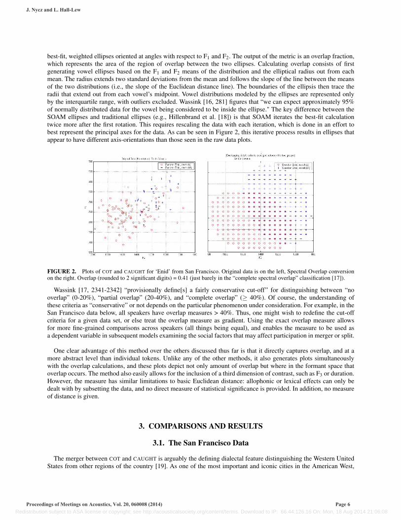
best-fit, weighted ellipses oriented at angles with respect to F1 and F2. The output of the metric is an overlap fraction,which represents the area of the region of overlap between the two ellipses. Calculating overlap consists of firstgenerating vowel ellipses based on the F1 and F2 means of the distribution and the elliptical radius out from eachmean. The radius extends two standard deviations from the mean and follows the slope of the line between the meansof the two distributions (i.e., the slope of the Euclidean distance line). The boundaries of the ellipsis then trace theradii that extend out from each vowel’s midpoint. Vowel distributions modeled by the ellipses are represented onlyby the interquartile range, with outliers excluded. Wassink [16, 281] figures that “we can expect approximately 95%of normally distributed data for the vowel being considered to be inside the ellipse." The key difference between theSOAM ellipses and traditional ellipses (e.g., Hillenbrand et al. [18]) is that SOAM iterates the best-fit calculationtwice more after the first rotation. This requires rescaling the data with each iteration, which is done in an effort tobest represent the principal axes for the data. As can be seen in Figure 2, this iterative process results in ellipses thatappear to have different axis-orientations than those seen in the raw data plots.

FIGURE 2. Plots of COT and CAUGHT for ‘Enid’ from San Francisco. Original data is on the left, Spectral Overlap conversionon the right. Overlap (rounded to 2 significant digits) = 0.41 (just barely in the “complete spectral overlap” classification [17]).

Wassink [17, 2341-2342] “provisionally define[s] a fairly conservative cut-off” for distinguishing between “nooverlap” (0-20%), “partial overlap” (20-40%), and “complete overlap” (≥ 40%). Of course, the understanding ofthese criteria as “conservative” or not depends on the particular phenomenon under consideration. For example, in theSan Francisco data below, all speakers have overlap measures > 40%. Thus, one might wish to redefine the cut-offcriteria for a given data set, or else treat the overlap measure as gradient. Using the exact overlap measure allowsfor more fine-grained comparisons across speakers (all things being equal), and enables the measure to be used asa dependent variable in subsequent models examining the social factors that may affect participation in merger or split.

One clear advantage of this method over the others discussed thus far is that it directly captures overlap, and at amore abstract level than individual tokens. Unlike any of the other methods, it also generates plots simultaneouslywith the overlap calculations, and these plots depict not only amount of overlap but where in the formant space thatoverlap occurs. The method also easily allows for the inclusion of a third dimension of contrast, such as F3 or duration.However, the measure has similar limitations to basic Euclidean distance: allophonic or lexical effects can only bedealt with by subsetting the data, and no direct measure of statistical significance is provided. In addition, no measureof distance is given.

3. COMPARISONS AND RESULTS

3.1. The San Francisco Data

The merger between COT and CAUGHT is arguably the defining dialectal feature distinguishing the Western UnitedStates from other regions of the country [19]. As one of the most important and iconic cities in the American West,



San Francisco might be expected to show the complete acoustic and perceptual merger that has been observed inall other cities across the region, but data presented in the Atlas of North American English (ANAE) show that SanFrancisco is a clear outlier in this respect, with the low back vowels still in a state of transition despite the widespreadregional pattern [19, 168]. This is particularly interesting in light of a study conducted in San Francisco around thetime of the ANAE’s data collection that found that younger speakers were clearly moving towards merger [20].

Recent work by Hall-Lew [12], [21] investigated the realization of low back vowels in San Francisco and thereasons behind the city’s outlier status with respect to these vowels. Thus the ability to compare relative degree ofmerger across speakers in the corpus, so as to relate this variation to social factors such as age, was of particularimportance in this study. Vowel tokens were drawn from sociolinguistic interviews, with no cap placed on the numberof tokens taken for particular words. As such, the data are not balanced with respect to phonological context nornumber of tokens per word.

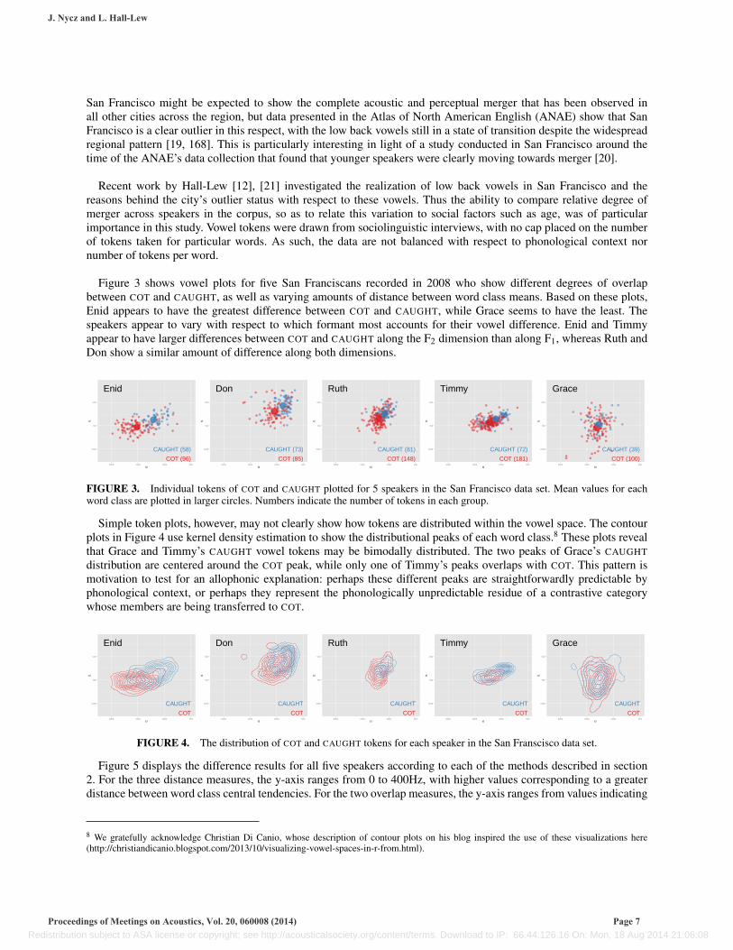
Figure 3 shows vowel plots for five San Franciscans recorded in 2008 who show different degrees of overlapbetween COT and CAUGHT, as well as varying amounts of distance between word class means. Based on these plots,Enid appears to have the greatest difference between COT and CAUGHT, while Grace seems to have the least. Thespeakers appear to vary with respect to which formant most accounts for their vowel difference. Enid and Timmyappear to have larger differences between COT and CAUGHT along the F2 dimension than along F1, whereas Ruth andDon show a similar amount of difference along both dimensions.

Enid

COT (96)

CAUGHT (58)

500

750

1000

500100015002000f2

f1

Don

COT (85)

CAUGHT (73)

500

750

1000

500100015002000f2

f1

Ruth

COT (148)

CAUGHT (81)

500

750

1000

500100015002000f2

f1

Timmy

COT (181)

CAUGHT (72)

500

750

1000

500100015002000f2

f1

Grace

COT (100)

CAUGHT (39)

500

750

1000

500100015002000f2

f1

FIGURE 3. Individual tokens of COT and CAUGHT plotted for 5 speakers in the San Francisco data set. Mean values for eachword class are plotted in larger circles. Numbers indicate the number of tokens in each group.

Simple token plots, however, may not clearly show how tokens are distributed within the vowel space. The contourplots in Figure 4 use kernel density estimation to show the distributional peaks of each word class.8 These plots revealthat Grace and Timmy’s CAUGHT vowel tokens may be bimodally distributed. The two peaks of Grace’s CAUGHTdistribution are centered around the COT peak, while only one of Timmy’s peaks overlaps with COT. This pattern ismotivation to test for an allophonic explanation: perhaps these different peaks are straightforwardly predictable byphonological context, or perhaps they represent the phonologically unpredictable residue of a contrastive categorywhose members are being transferred to COT.

Enid

COT

CAUGHT

500

750

1000

500100015002000f2

f1

Don

COT

CAUGHT

500

750

1000

500100015002000f2

f1

Ruth

COT

CAUGHT

500

750

1000

500100015002000f2

f1

Timmy

COT

CAUGHT

500

750

1000

500100015002000f2

f1

Grace

COT

CAUGHT

500

750

1000

500100015002000f2

f1

FIGURE 4. The distribution of COT and CAUGHT tokens for each speaker in the San Franscisco data set.

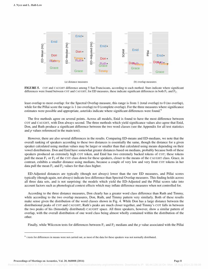
Figure 5 displays the difference results for all five speakers according to each of the methods described in section2. For the three distance measures, the y-axis ranges from 0 to 400Hz, with higher values corresponding to a greaterdistance between word class central tendencies. For the two overlap measures, the y-axis ranges from values indicating

8 We gratefully acknowledge Christian Di Canio, whose description of contour plots on his blog inspired the use of these visualizations here(http://christiandicanio.blogspot.com/2013/10/visualizing-vowel-spaces-in-r-from.html).



Don

Enid

Grace

Ruth Timmy

0

100

200

300

400

ED

−M

ean

(Hz)

Don

Enid

Grace

Ruth Timmy

*

*

**

0

100

200

300

400

−6 −3 0 3 6

ED

−M

edia

n (H

z)

Don

Enid

Grace Ruth

Timmy

*

*

*

0

100

200

300

400

−6 −3 0 3 6

ED

−A

djus

ted

(Hz)

(a) distance measures

Don

Enid

Grace

Ruth Timmy

0.00

0.25

0.50

0.75

1.00

−6 −3 0 3 6

SO

AM

Don

Enid

Grace

Ruth Timmy *

*

* *

0.00

0.25

0.50

0.75

1.00

−6 −3 0 3 6

Pill

ai

(b) overlap measures

FIGURE 5. COT and CAUGHT difference among 5 San Franciscans, according to each method. Stars indicate where significantdifferences were found between COT and CAUGHT; for ED measures, these indicate significant differences in both F1 and F2.

least overlap to most overlap: for the Spectral Overlap measure, this range is from 1 (total overlap) to 0 (no overlap),while for the Pillai score the range is 1 (no overlap) to 0 (complete overlap). For the three measures where significanceestimates were possible and appropriate, asterisks indicate where significant differences were found.9

The five methods agree on several points. Across all models, Enid is found to have the most difference betweenCOT and CAUGHT, with Don always second. The three methods which yield significance values also agree that Enid,Don, and Ruth produce a significant difference between the two word classes (see the Appendix for all test statisticsand p values referenced in the main text).

However, there are also several differences in the results. Comparing ED-means and ED-medians, we note that theoverall ranking of speakers according to these two distances is essentially the same, though the distance for a givenspeaker calculated using median values may be larger or smaller than that calculated using means depending on theirvowel distributions. Don and Enid have somewhat greater distances based on medians, probably because both of thesespeakers produced an extremely high COT token, and Enid has two extremely backed tokens of COT; these tokenspull the mean F1 or F2 of the COT class down for these speakers, closer to the means of the CAUGHT class. Grace, incontrast, exhibits a smaller distance using medians, because a couple of very low and very front COT tokens in herdata pull the mean F1 and F2 values for that class higher.

ED-Adjusted distances are typically (though not always) lower than the raw ED measures, and Pillai scorestypically (though again, not always) indicate less difference than Spectral Overlap measures. This finding holds acrossall three data sets, and is not surprising: the models which yield the ED-Adjusted and the Pillai scores take intoaccount factors such as phonological context effects which may inflate difference measures when not controlled for.

According to the three distance measures, Don clearly has a greater word class difference than Ruth and Timmy,while according to the two overlap measures, Don, Ruth, and Timmy pattern very similarly. Both of these resultsmake sense given the distribution of the word classes shown in Fig. 4. While Don has a large distance between thedistributional peaks of COT and CAUGHT, Ruth’s peaks are much closer together, and Timmy’s COT falls in betweenthe two peaks of his (bimodally distributed) CAUGHT space. All three speakers, however, show a similar pattern ofoverlap, with the overall distribution of one word class being almost wholly contained within the distribution of theother.

Finally, while Wilcoxon tests for differences between F1 and F2 medians and the p value associated with the Pillai

9 t tests for differences in means were not carried out, as most of the data for these speakers was not normally distributed.



score indicate that Timmy produces a significant difference between COT and CAUGHT, the mixed models methodfinds that the distance between these word classes is not significant along either dimension. The most likely reason forthis disagreement is that including a random effect of WORD makes an important difference for Timmy’s data. To testthis, we calculated an ED-Adjusted based on coefficients drawn from models containing fixed effects of phonologicalcontext and WORD CLASS only. This resulted in a statistically significant effect of WORD CLASS for F1. For Timmy,we can say that the lack of a word-specific factor (in the Wilcoxon and MANOVA models) directly results in anoverestimation of word class difference.

3.2. The Canadians-in-New-York Data

In comparison to vowel merger, vowel split - the appearance of a distinction where one was not previously present- has received relatively little attention. This is largely because mergers tend to spread at the expense of distinctions[22], so nascent splits are rarer in the community contexts that sociolinguists usually study. However, splits raisesimilar theoretical issues to mergers, and present similar practical issues in terms of their analysis.

Nycz [9, 4] investigated low back vowel production in a sample of expatriate Canadians living in and aroundNew York City. These individuals are native speakers of Canadian English, a dialect long characterized by a mergerbetween the COT and CAUGHT classes [23]. In contrast, New York City and surrounding communities maintain arobust low back vowel distinction [19]. Nycz wanted to determine whether these speakers showed any evidence ofhaving acquired a distinction between the COT and CAUGHT classes. Vowel tokens were drawn from sociolinguisticinterviews with no cap on the number of tokens per word, and indeed no cap on the number of tokens per speaker.

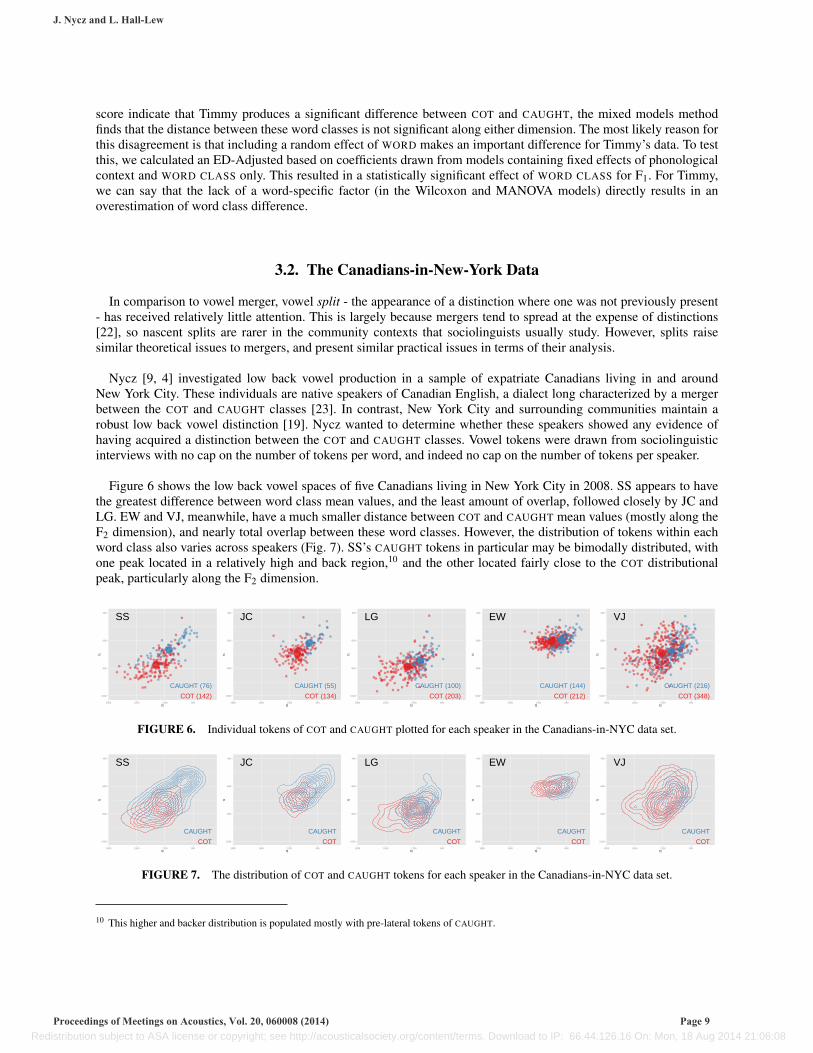
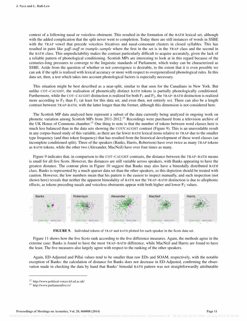
Figure 6 shows the low back vowel spaces of five Canadians living in New York City in 2008. SS appears to havethe greatest difference between word class mean values, and the least amount of overlap, followed closely by JC andLG. EW and VJ, meanwhile, have a much smaller distance between COT and CAUGHT mean values (mostly along theF2 dimension), and nearly total overlap between these word classes. However, the distribution of tokens within eachword class also varies across speakers (Fig. 7). SS’s CAUGHT tokens in particular may be bimodally distributed, withone peak located in a relatively high and back region,10 and the other located fairly close to the COT distributionalpeak, particularly along the F2 dimension.

SS

COT (142)

CAUGHT (76)

400

600

800

1000

900120015001800f2

f1

JC

COT (134)

CAUGHT (55)

400

600

800

1000

900120015001800f2

f1

LG

COT (203)

CAUGHT (100)

400

600

800

1000

900120015001800f2

f1

EW

COT (212)

CAUGHT (144)

400

600

800

1000

900120015001800f2

f1

VJ

COT (348)

CAUGHT (216)

400

600

800

1000

900120015001800f2

f1

FIGURE 6. Individual tokens of COT and CAUGHT plotted for each speaker in the Canadians-in-NYC data set.

SS

COT

CAUGHT

400

600

800

1000

900120015001800f2

f1

JC

COT

CAUGHT

400

600

800

1000

900120015001800f2

f1

LG

COT

CAUGHT

400

600

800

1000

900120015001800f2

f1

EW

COT

CAUGHT

400

600

800

1000

900120015001800f2

f1

VJ

COT

CAUGHT

400

600

800

1000

900120015001800f2

f1

FIGURE 7. The distribution of COT and CAUGHT tokens for each speaker in the Canadians-in-NYC data set.

10 This higher and backer distribution is populated mostly with pre-lateral tokens of CAUGHT.



Figure. 8 shows the results of the methods comparison for this data set. Again, the five measures largely agree withrespect to the extremes. SS is always found to have the most difference between COT and CAUGHT, while VJ is foundto have the least (or nearly the least) difference.

EW

JC LG

SS

VJ

0

50

100

150

200

ED

−M

ean

(Hz)

EW

JC LG

SS

VJ *

**

*

*F2 onlyF2 onlyF2 onlyF2 onlyF2 only

0

50

100

150

200

−6 −3 0 3 6

ED

−M

edia

n (H

z)

EW JC LG

SS

VJ

***

*

F2 onlyF2 onlyF2 onlyF2 onlyF2 onlyF1 onlyF1 onlyF1 onlyF1 onlyF1 only

0

50

100

150

200

−6 −3 0 3 6

ED

−A

djus

ted

(Hz)


EW JC

LG

SS

VJ

0.00

0.25

0.50

0.75

1.00

−6 −3 0 3 6

SO

AM

EW JC LG SS

VJ ** *

*

0.00

0.25

0.50

0.75

1.00

−6 −3 0 3 6

Pill

ai


FIGURE 8. COT and CAUGHT difference among 5 Canadians in NYC, according to each method. Stars indicate where significantdifferences were found between COT and CAUGHT; for ED measures, these indicate significant differences in both F1 and F2 unlessotherwise indicated.

As with the previous dataset, there are minor differences between ED-Mean and ED-Median for these speakers,though the overall ranking in the same. And again, we see that the two methods whose models include terms forphonological context (ED-Adjusted and Pillai) consistently estimate a smaller difference between word classes thantheir comparable methods which do not (ED and SOAM, respectively).

There is some disagreement with respect to the three speakers in the middle, reflecting differences in the distributionof tokens between speakers. For example, the three distance methods find that LG has more of a difference betweenword classes than EW, while the two overlap methods rank these speakers in the opposite way, demonstrating theindependence of distance and overlap as difference measures.

Wilcoxon tests indicate that all five speakers in this dataset produce a significant difference between COT andCAUGHT for at least one formant. The difference for one speaker (VJ) is not significant in models where factors otherthan word class are included. Adjusted Euclidean distance and Pillai both find that all speakers except for VJ havea significant difference between COT and CAUGHT, with the difference for SS greater than that for EW. The twomethods differ, however, in the specificity of their significance results. Because MANOVA determines the significanceof terms with respect to both F1 and F2 together, these results do not reveal whether these four speakers distinguishthe two word classes along both dimensions or just one. The mixed effects model approach, in contrast, shows thatwhile SS and LG has a significant difference between COT and CAUGHT along both the F1 and F2 dimensions, JCdistinguishes these classes only in F1

11 while EW distinguishes them only in F2.

3.3. The Scottish MP Data

Our final data set includes five Scottish Members of the UK Parliament (MPs), who have subtle but varyingdegrees of distance between what Wells [5] calls the TRAP and BATH lexical sets. Scottish Standard English (ScSE)is typically characterized by a single low vowel (which is more fronted or backed based on the particular regionalvariety). In contrast, the low front vowel in Southern Standard British English (SSBE), TRAP, underwent a splitsometime between the mid-18th and early 20th centuries where the vowel variably backed and/or lengthened in the

11 This despite an apparent difference in F2 according to the vowel plots, which disappears once phonological context is taken into account.



context of a following nasal or voiceless obstruent. This resulted in the formation of the BATH lexical set, althoughwith the added complication that the split never went to completion. Today there are still instances of words in SSBEwith the TRAP vowel that precede voiceless fricatives and nasal-consonant clusters in closed syllables. This hasresulted in pairs like gaff–staff or trample–sample where the first in the set is in the TRAP class and the second inthe BATH class. This unpredictability makes the contrast particularly difficult to acquire accurately, given the lack ofa reliable pattern of phonological conditioning. Scottish MPs are interesting to look at in this regard because of thecenturies-long pressures to converge to the linguistic standards of Parliament, which today can be characterized asSSBE. Aside from the question of whether or not convergence is desirable, to the extent that it is even possible wecan ask if the split is realized with lexical accuracy or more with respect to overgeneralized phonological rules. In thisdata set, then, a test which takes into account phonological factors is especially necessary.

This situation might be best described as a near-split, similar to that seen for the Canadians in New York. Butunlike COT–CAUGHT, the realisation of phonetically distinct BATH tokens is partially phonologically conditioned.Furthermore, while the COT–CAUGHT distinction is realized for both F1 and F2, the TRAP–BATH distinction is realizedmore according to F2 than F1 (at least for this data set, and even then, not entirely so). There can also be a lengthcontrast between TRAP-BATH, with the latter longer than the former, although this dimension is not considered here.

The Scottish MP data analyzed here represent a subset of the data currently being analyzed in ongoing work onphonetic variation among Scottish MPs from 2011-2012.12 Recordings were purchased from a television archive ofthe UK House of Commons chamber.13 One thing to note is that the number of tokens between word classes here ismuch less balanced than in the data sets showing the COT/CAUGHT contrast (Figure 9). This is an unavoidable resultin any corpus-based study of this variable, as there are far fewer BATH lexical items relative to TRAP due to the smallertype frequency (and thus token frequency) that has resulted from the historical development of these word classes (anincomplete conditioned split). Three of the speakers (Banks, Harris, Robertson) have over twice as many TRAP tokensas BATH tokens, while the other two (Alexander, MacNeil) have over four times as many.

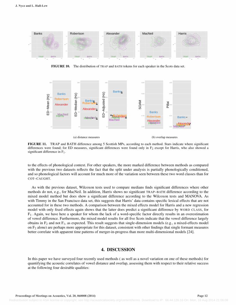
Figure 9 indicates that, in comparison to the COT–CAUGHT contrasts, the distance between the TRAP–BATH meansis small for all five Scots. However, the distances are still variable across speakers, with Banks appearing to have thegreatest distance. The contour plots in Figure 10 suggest that Banks may also have a bimodally distributed BATHclass. Banks is represented by a much sparser data set than the other speakers, so this depiction should be treated withcaution. However, the low numbers mean that his pattern is the easiest to inspect manually, and such inspection (notshown here) reveals that neither the apparent bimodality of BATH nor the TRAP–BATH distinction is due to allophoniceffects, as tokens preceding nasals and voiceless obstruents appear with both higher and lower F2 values.

Banks

TRAP (36) BATH (13)

600

800

1000

1000120014001600f2

f1

Robertson

TRAP (223) BATH (91)

600

800

1000

1000120014001600f2

f1

Alexander


600

800

1000

1000120014001600f2

f1

MacNeil


600

800

1000

1000120014001600f2

f1

Harris


600

800

1000

1000120014001600f2

f1

FIGURE 9. Individual tokens of TRAP and BATH plotted for each speaker in the Scots data set.

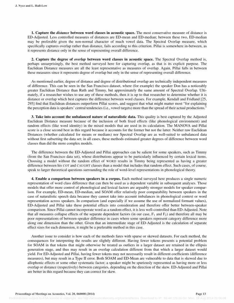
Figure 11 shows how the five Scots rank according to the five difference measures. Again, the methods agree in theextreme case: Banks is found to have the most TRAP–BATH difference, while MacNeil and Harris are found to havethe least. The five measures also largely agree with respect to the ranking of the other speakers.

Again, ED-Adjusted and Pillai values tend to be smaller than raw EDs and SOAM, respectively, with the notableexception of Banks: the calculation of distance for Banks does not decrease in ED-Adjusted, confirming the obser-vation made in checking the data by hand that Banks’ bimodal BATH pattern was not straightforwardly attributable

12 http://www.political-voices.lel.ed.ac.uk/13 http://www.parliamentlive.tv/



Banks

TRAP BATH

600

800

1000

1000120014001600f2

f1

Robertson

TRAP BATH

600

800

1000

1000120014001600f2

f1

Alexander

TRAP BATH

600

800

1000

1000120014001600f2

f1

MacNeil

TRAP BATH

600

800

1000

1000120014001600f2

f1

Harris

TRAP BATH

600

800

1000

1000120014001600f2

f1

FIGURE 10. The distribution of TRAP and BATH tokens for each speaker in the Scots data set.

Alexander

Banks

Harris MacNeil

Robertson

0

50

100

150

ED

−M

ean

(Hz)

Alexander

Banks

Harris MacNeil

Robertson

*

*

* *

*

F2F2F2F2F2

F2F2F2F2F2

F2F2F2F2F2

F2F2F2F2F2

0

50

100

150

−6 −3 0 3 6

ED

−M

edia

n (H

z)

Alexander

Banks

Harris MacNeil

Robertson *

*

*F2F2F2F2F2

F2F2F2F2F2

F2F2F2F2F2

0

50

100

150

−6 −3 0 3 6

ED

−A

djus

ted

(Hz)


Alexander

Banks

Harris MacNeil

Robertson

0.00

0.25

0.50

0.75

1.00

−6 −3 0 3 6

SO

AM

Alexander

Banks

Harris MacNeil Robertson *

*

* *0.00

0.25

0.50

0.75

1.00

−6 −3 0 3 6

Pill

ai


FIGURE 11. TRAP and BATH difference among 5 Scottish MPs, according to each method. Stars indicate where significantdifferences were found; for ED measures, significant differences were found only in F2 except for Harris, who also showed asignificant difference in F1.

to the effects of phonological context. For other speakers, the more marked difference between methods as comparedwith the previous two datasets reflects the fact that the split under analysis is partially phonologically conditioned,and so phonological factors will account for much more of the variation seen between these two word classes than forCOT–CAUGHT.

As with the previous dataset, Wilcoxon tests used to compare medians finds significant differences where othermethods do not, e.g., for MacNeil. In addition, Harris shows no significant TRAP–BATH difference according to themixed model method but does show a significant difference according to the Wilcoxon tests and MANOVA. Aswith Timmy in the San Francisco data set, this suggests that Harris’ data contains specific lexical effects that are notaccounted for in these two methods. A comparison between the mixed effects model for Harris and a new regressionmodel with only fixed effects again shows that the latter does predict a significant difference by WORD CLASS, forF1. Again, we have here a speaker for whom the lack of a word-specific factor directly results in an overestimationof vowel difference. Furthermore, the mixed model results for all five Scots indicate that the vowel difference largelyobtains in F2 and not F1, as expected. This result suggests that single-dimension models (e.g., a mixed-effects modelon F2 alone) are perhaps more appropriate for this dataset, consistent with other findings that single formant measuresbetter correlate with apparent time patterns of merger-in-progress than more multi-dimensional models [24].

4. DISCUSSION

In this paper we have surveyed four recently used methods ( as well as a novel variation on one of these methods) forquantifying the acoustic correlates of vowel distance and overlap, assessing them with respect to their relative successat the following four desirable qualities:



1. Capture the distance between word classes in acoustic space. The most conservative measure of distance isED-Adjusted. Less controlled measures of distances are ED-mean and ED-median; between these two, ED-medianmay be preferable given the non-normal character of much vowel data. The Spectral Overlap measure, whichspecifically captures overlap rather than distance, fails according to this criterion. Pillai is somewhere in-between, asit represents distance only in the sense of representing overall difference.

2. Capture the degree of overlap between word classes in acoustic space. The Spectral Overlap method is,perhaps unsurprisingly, the best method surveyed here for capturing overlap, as that is its explicit purpose. TheEuclidean Distance measures are all the least representative as measures of overlap. Again, Pillai falls in betweenthese measures since it represents degree of overlap but only in the sense of representing overall difference.

As mentioned earlier, degree of distance and degree of distributional overlap are technically independent measuresof difference. This can be seen in the San Francisco dataset, where (for example) the speaker Don has a noticeablygreater Euclidean Distance than Ruth and Timmy, but approximately the same amount of Spectral Overlap. Ulti-mately, if a researcher wishes to use any of these methods, then it is up to that researcher to determine whether it isdistance or overlap which best captures the difference between word classes. For example, Kendall and Fridland [25,295] find that Euclidean distances outperform Pillai scores, and suggest that what might matter most “for explainingthe perception data is speakers’ central tendencies (i.e., vowel targets) more than the spread of their actual productions.”

3. Take into account the unbalanced nature of naturalistic data. This quality is best captured by the AdjustedEuclidean Distance measure because of the inclusion of both fixed effects (like phonological environment) andrandom effects (like word identity) in the mixed models that are used in its calculation. The MANOVA and Pillaiscore is a close second best in this regard because it accounts for the former but not the latter. Neither raw EuclideanDistances (whether calculated for means or medians) nor Spectral Overlap are as well-suited to unbalanced datawithout first subsetting the data set; in all cases, these methods estimated greater degrees of difference between wordclasses than did the more complex models.

The difference between the ED-Adjusted and Pillai approaches can be salient for some speakers, such as Timmy(from the San Francisco data set), whose distributions appear to be particularly influenced by certain lexical items.Choosing a model without the random effect of WORD results in Timmy being represented as having a greaterdifference between his COT and CAUGHT classes than a model that includes that random effect. Such cases, of course.speak to larger theoretical questions surrounding the role of word-level representations in phonological theory.

4. Enable a comparison between speakers in a corpus. Each method surveyed here produces a single numericrepresentation of word class difference that can then be used as a dependent variable in subsequent analyses. Thosemodels that offer more control of phonological and lexical factors are arguably stronger models for speaker compar-ison. For example, ED-mean, ED-median, and SOAM offer relatively poor comparability between speakers in thecase of naturalistic speech data because they cannot take into account imbalances in phonological context or wordrepresentation across speakers. In comparison (and especially if we assume the use of normalized formant values),ED-Adjusted and Pillai take these potential effects into consideration and therefore offer better between-speakercomparison. Since Pillai cannot incorporate word as a random effect, it is less well-controlled than ED-Adjusted. Notethat all measures collapse effects of the separate dependent factors (in our case, F1 and F2) and therefore all may bepoor representations of between-speaker difference in cases where some speakers represent category difference morealong one dimension than the other. Given that an intermediate stage of ED-Adjusted is the calculation of separateeffect sizes for each dimension, it might be a preferable method in this case.

Another issue to consider is how each of the methods fares with sparse or skewed datasets. For each method, theconsequences for interpreting the results are slightly different. Having fewer tokens presents a potential problemfor SOAM in that tokens that might otherwise be treated as outliers in a larger dataset are retained in the ellipsisgeneration stage, and thus may result in an overlap calculation different from that which a larger dataset wouldyield. For ED-Adjusted and Pillai, having fewer tokens may not necessarily result in different coefficients (differencemeasures), but may result in a Type II error. Both SOAM and ED-Mean are vulnerable to data that is skewed due toallophonic effects or some other systematic factor; a speaker might be spuriously represented as having more or lessoverlap or distance (respectively) between categories, depending on the direction of the skew. ED-Adjusted and Pillaiare better in this regard because they can correct for skew.



However, it is important to keep in mind that these more sophisticated methods of analysis bring with them certainassumptions which may not hold in cases of change in progress, such as normal distribution of the residuals andhomogeneity of variance. Minor violations of these assumptions may not be a problem for a particular analysis (e.g.the Pillai statistic in particular is reasonably robust to such violations ([26, 719])), however, it is up to the researcherto determine how serious such violations are and take their resulting analysis with an appropriately-sized grain of salt.

What all methods share in terms of how they have been implemented in this paper is a comparison of word classesbased on midpoint F1 and F2 values alone. All of the methods described in this paper can in principle be extendedto include additional acoustic parameters; what we cannot fully address here is the question of the ideal numberof acoustic dimensions which ought to be considered in any assessment of difference. Other work (e.g. [15], [27])has found that additional parameters beyond F1 and F2 may contribute to a vowel contrast, indicating the need toinclude these in assessments of difference. On the other hand, the Scots data set discussed here suggest that somevowel contrasts may be best represented by one dimension rather than two. In all likelihood there is no universallyappropriate number of parameters; the researcher must determine for each individual data set which measures arelikely to be relevant, and develop statistical hypotheses and designs accordingly.

Overall, our results show that the methods tested here generally agree with one another with respect to thosespeakers at the extremes who show the most and least amounts of vowel difference in the data set. When speakersare ranked differently between method A and method B, the ranking for B usually indicates a switch between twospeakers adjacent in their ranking according to method A, rather than totally different re-orderings. However, themethods do differ in important ways.

Two of the methods - mixed modeling and MANOVA - consider phonological environment in the differencecalculation, a necessity given the large effect that phonological context has on vowel realization and the typicallyunbalanced nature of spontaneous speech data with respect to context. However, it is difficult to decide between thesetwo approaches, since they differ from each other in two crucial ways. The mixed effects regression allows one toconsider lexical effects, but requires separate models for each acoustic dimension under consideration. MANOVAmodels differences in terms of all acoustic dimensions simultaneously, but does not allow for inclusion of randomeffects. As noted in Section 2.3, this limitation of MANOVA is a practical one: while mixed MANOVAs are in theorypossible, they have not yet been implemented in a statistical environment accessible to most sociophoneticians. Shouldthe necessary package materialize, it will be possible to isolate the impact of univariate vs. multivariate statistics andthat of mixed effects modeling vs. fixed effects modeling.

What this points to in practical terms is the importance of understanding one’s data before making any calculations.Researchers ought to explore their data using both cross-tabulations of factors and data visualizations such as tokenplots and contour plots to identify unexpected distributional patterns and ascertain the reasons behind them. Forexample, if lexical items differ greatly in their frequency of occurrence for a particular speaker, then including arandom effect to account for possible lexical variation is important. If plots indicate that degree of overlap plays a keyrole in how a merger is progressing in a particular community, then a method which reflects degree of overlap in itscalculation of difference may be preferred. If multiple acoustic dimensions seem to contribute to difference, perhapsin synergistic ways, then a multivariate approach may be the best choice.

One of the next steps in this project is to gain a better understanding of the reasons for all the differences seen here,with the aim of accounting for exactly how the differences between methods interact with the differences between datasets. As we work towards that goal we are also considering additional methods that have been used in the literatureto quantify vowel overlap or category similarity more generally. These include but are not limited to mixture modelsor clustering models, Mahalanobis Distances [28], and d(a). D(a) is “a measure of sensitivity in the theory of signaldetection” [29, 1184], a calculation of “the between-category distance (the Euclidean distance ... ) divided by thewithin-category variance” [30, 921]. Cristia and Seidl [30] compare d(a) values to Euclidean distances, making it agood candidate to add to the comparisons considered here.

In the future, we hope to expand the method comparison to focus on those methods that can incorporate additionalacoustic variables besides single-point measurements of F1 and F2, such as vowel trajectory [31], F3, vowel duration,and voice quality [15]. Finally, we can approach these research questions from an entirely different angle by examining



how simulated data sets with pre-specified characteristics are assessed by various methods.

5. CONCLUSIONS

This exploratory study finds reassuring similarities as well as crucial differences between several measures ofcalculating vowel difference. While the results do not suggest a single ‘best’ metric above all others, researcherswho are interested in the acoustic representation of near-mergers and near-splits are encouraged to choose a methodof quantification based on known linguistic and representational facts about their data sets. One recommendation atpresent is for anyone studying mergers or splits to consider at least two different ways of operationalizing categorydistinction in the exploratory stages of their analysis.

ACKNOWLEDGMENTS

We would like to thank Daniel Ezra Johnson for helpful comments on a draft of this paper, as well as the followingpeople for useful discussions in its preparation: Katie Drager, Josef Fruehwald, Robert J. Podesva, Alicia BeckfordWassink, and audience members at the 166th Meeting of the Acoustical Society of America. All errors are our own.



REFERENCES

1. L. Clark, K. Watson, and W. Maguire, English Language and Linguistics 17, 229–390 (2013).2. P. Trudgill, and T. Foxcroft, “On the sociolinguistics of vocalic mergers: Transfer and approximation in East Anglia,” in

Sociolinguistic patterns in British English, edited by P. Trudgill, University Park Press, Baltimore, 1978, pp. 69–79.3. R. Herold, Language Variation and Change 9, 165–189 (1997).4. J. Nycz, English Language and Linguistics 17, 325–357 (2013).5. J. C. Wells, Accents of English, Cambridge University Press, Cambridge, UK, 1982.6. A. Dinkin, Dialect Boundaries and Phonological Change in Upstate New York, Ph.D. thesis, University of Pennsylvania

(2009).7. M. Baranowski, Phonological Variation and Change in the dialect of Charleston, South Carolina, vol. 92 of Publication of

the American Dialect Society, Duke University Press, 2007.8. T. L. Irons, Language Variation and Change 19, 137–180 (2007).9. J. Nycz, Second Dialect Acquisition: Implications for Theories of Phonological Representation, Ph.D. thesis, New York

University (2011).10. J. Hay, P. Warren, and K. Drager, Journal of Phonetics 34, 458–484 (2006).11. M. Kennedy, Variation in the Pronunciation of English by New Zealand school children, Master’s thesis, Victoria University

of Wellington (2006).12. L. Hall-Lew, Ethnicity and Phonetic Variation in a San Francisco Neighborhood, Ph.D. thesis, Stanford University (2009).13. A. Wong, and L. Hall-Lew, Language and Communication 35, 27–42 (2014).14. L. Hall-Lew, Proceedings of Meetings on Acoustics (POMA) 9,

http://scitation.aip.org/content/asa/journal/poma/9/1/10.1121/1.3460625 (2010).15. M. Di Paolo, Language and Communication 12, 267–292 (1992).16. A. B. Wassink, A Sociophonetic Analysis of Jamaican Vowels, Ph.D. thesis, The University of Michigan, Ann Arbor, MI

(1999).17. A. B. Wassink, Journal of the Acoustical Society of America 19, 2334–2350 (2006).18. J. Hillenbrand, L. A. Getty, M. J. Clark, and K. Wheeler, Journal of the Acoustical Society of America 97, 3099–3111 (1995).19. W. Labov, S. Ash, and C. Boberg, The Atlas of North American English: Phonetics, phonology, and sound change, Mouton de

Gruyter, New York/Berlin, 2006.20. B. Moonwomon, Sound Change in San Francisco English, Ph.D. thesis, University of California, Berkeley, Berkeley, CA

(1992).21. L. Hall-Lew, English Language and Linguistics 17, 359–390 (2013).22. W. Labov, Principles of Linguistic Change: Internal Factors, vol. 20 of Language and Society, Blackwell Publishing, Ltd.,

Oxford, UK, 1994.23. C. Boberg, “English in Canada: Phonology,” in Varieties of English, edited by E. W. Schneider, Mouton de Gruyter, 2008,

vol. 2, pp. 144–160.24. R. Podesva, J. Grieser, M. Howard, S. Kajino, J. Lee, and S. Lee, The PIN-PEN merger in Washington, DC: Historical effects

on the maintenance of racial differentiation (Forthcoming).25. T. Kendall, and V. Fridland, Journal of Phonetics 40, 289–306 (2012).26. A. Field, J. Miles, and Z. Field, Discovering Statistics Using R, Sage, 2012.27. V. Fridland, T. Kendall, and C. Farrington, Journal of the Acoustical Society of America 136, 341–349 (2014).28. P. C. Mahalanobis, Proceedings of the National Institute of Sciences of India 2, 49–55 (1936).29. R. S. Newman, S. A. Clouse, and J. Burnham, Journal of the Acoustical Society of America 109, 1181–96 (2001).30. A. Cristia, and A. Seidl, Journal of Child Language 41, 913–934 (2014).31. M. Scanlon, and A. B. Wassink, University of Pennsylvania Working Papers in Linguistics (Selected papers from NWAV 38)

16, 159–164 (2010).



APPENDIX

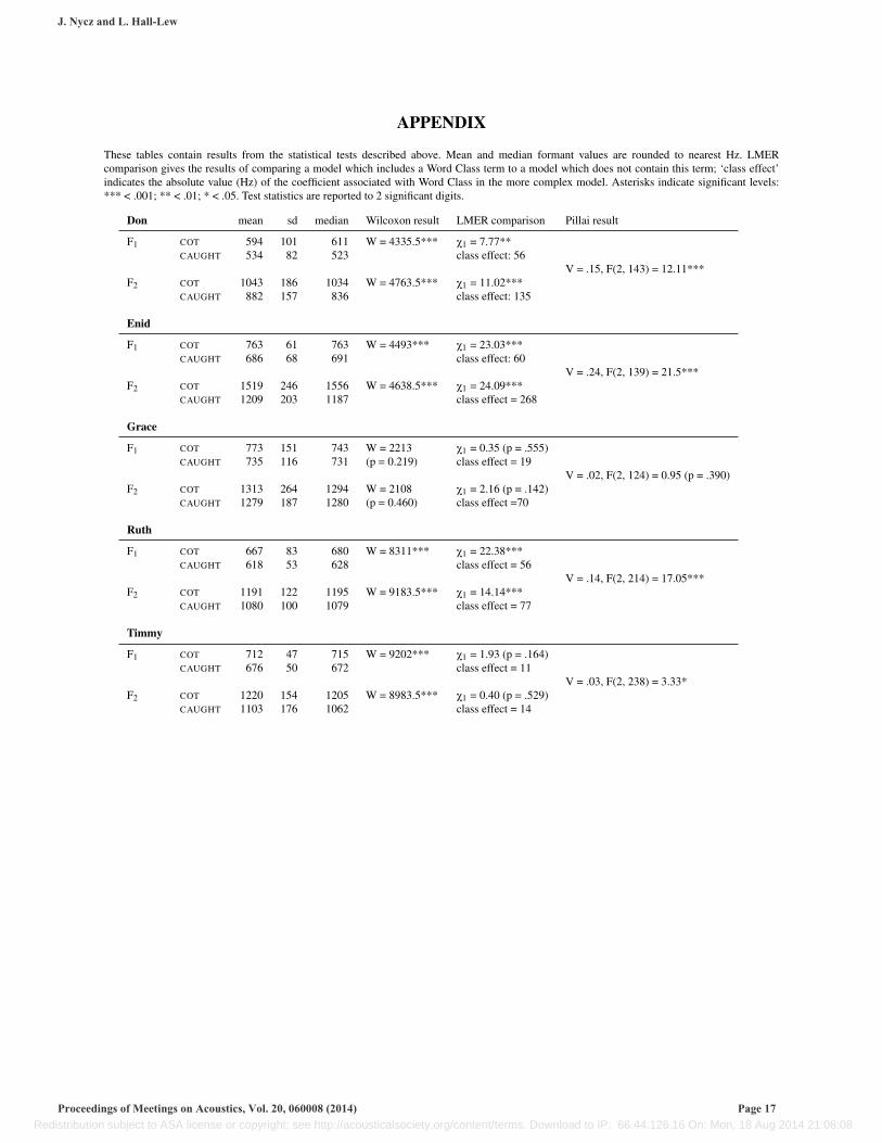
These tables contain results from the statistical tests described above. Mean and median formant values are rounded to nearest Hz. LMERcomparison gives the results of comparing a model which includes a Word Class term to a model which does not contain this term; ‘class effect’indicates the absolute value (Hz) of the coefficient associated with Word Class in the more complex model. Asterisks indicate significant levels:*** < .001; ** < .01; * < .05. Test statistics are reported to 2 significant digits.

Don mean sd median Wilcoxon result LMER comparison Pillai result

F1 COT 594 101 611 W = 4335.5*** X1 = 7.77**

V = .15, F(2, 143) = 12.11***CAUGHT 534 82 523 class effect: 56

F2 COT 1043 186 1034 W = 4763.5*** X1 = 11.02***CAUGHT 882 157 836 class effect: 135

Enid

F1 COT 763 61 763 W = 4493*** X1 = 23.03***

V = .24, F(2, 139) = 21.5***CAUGHT 686 68 691 class effect: 60

F2 COT 1519 246 1556 W = 4638.5*** X1 = 24.09***CAUGHT 1209 203 1187 class effect = 268

Grace

F1 COT 773 151 743 W = 2213 X1 = 0.35 (p = .555)

V = .02, F(2, 124) = 0.95 (p = .390)CAUGHT 735 116 731 (p = 0.219) class effect = 19

F2 COT 1313 264 1294 W = 2108 X1 = 2.16 (p = .142)CAUGHT 1279 187 1280 (p = 0.460) class effect =70

Ruth

F1 COT 667 83 680 W = 8311*** X1 = 22.38***

V = .14, F(2, 214) = 17.05***CAUGHT 618 53 628 class effect = 56

F2 COT 1191 122 1195 W = 9183.5*** X1 = 14.14***CAUGHT 1080 100 1079 class effect = 77

Timmy

F1 COT 712 47 715 W = 9202*** X1 = 1.93 (p = .164)

V = .03, F(2, 238) = 3.33*CAUGHT 676 50 672 class effect = 11

F2 COT 1220 154 1205 W = 8983.5*** X1 = 0.40 (p = .529)CAUGHT 1103 176 1062 class effect = 14



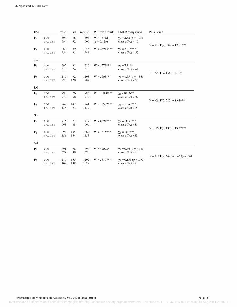
EW mean sd median Wilcoxon result LMER comparison Pillai result

F1 COT 604 38 608 W = 16712 X1 = 2.62 (p = .105)

V = .08, F(2, 334) = 13.91***CAUGHT 594 52 600 (p = 0.129) class effect = 10

F2 COT 1060 99 1056 W = 23913*** X1 = 21.15***CAUGHT 954 91 949 class effect = 53

JC

F1 COT 692 61 686 W = 5773*** X1 = 7.31**

V = .04, F(2, 168) = 3.70*CAUGHT 618 74 618 class effect = 42

F2 COT 1116 92 1108 W = 5908*** X1 = 1.75 (p = .186)CAUGHT 990 120 987 class effect =32

LG

F1 COT 790 76 786 W = 13970*** X1 - 10.56**

V = .06, F(2, 282) = 8.61***CAUGHT 742 68 742 class effect =36

F2 COT 1267 147 1241 W = 15572*** X1 = 11.63***CAUGHT 1135 93 1132 class effect =65

SS

F1 COT 775 77 777 W = 8894*** X1 = 16.39***

V = .16, F(2, 197) = 18.47***CAUGHT 668 88 666 class effect =81

F2 COT 1294 155 1264 W = 7815*** X1 = 10.76**CAUGHT 1156 164 1155 class effect =83

VJ

F1 COT 691 98 696 W = 42078* X1 = 0.56 (p = .454)

V = .00, F(2, 542) = 0.45 (p = .64)CAUGHT 674 88 678 class effect =8

F2 COT 1216 155 1202 W = 53157*** X1 = 0.159 (p = .690)CAUGHT 1108 138 1089 class effect =9



Alexander mean sd median Wilcoxon result LMER comparison Pillai result

F1 TRAP 721 97 708 W = 24603.5*** X1 = 0.68 (p = .410)

V = .08, F(2, 478) = 20.02***BATH 737 104 721 class effect = 12

F2 TRAP 1350 113 1333 W = 16258 X1 = 6.16*BATH 1276 80 1273 (p = 0.222) class effect = 33

Banks

F1 TRAP 782 98 786 W = 277 X1 = 0.00 (p = 1)

V = .22, F(2, 37) = 5.20*BATH 756 80 786 (p = 0.336) class effect = 34

F2 TRAP 1381 88 1365 W = 405.5*** X1 = 9.98*BATH 1272 78 1275 class effect = 116

Harris

F1 TRAP 736 69 744 W = 7300.5* X1 = 3.22 (p = .072)

V = .03, F(2, 243) = 3.22*BATH 711 87 730 (p = 0.047) class effect = 25

F2 TRAP 1372 95 1382 W = 7401* X1 = 1.48 (p = .223)BATH 1345 90 1355 class effect =20

MacNeil

F1 TRAP 746 69 748 W = 5933 X1 = 2.93 (p = .087)

V = .01, F(2, 267) = 1.40 (p = .248)BATH 735 80 730 (p = 0.367) class effect = 22

F2 TRAP 1312 84 1297 W = 6851.5** X1 = 0.60 (p = .440)BATH 1272 73 1272 class effect = 10

Robertson

F1 TRAP 773 82 767 W = 9612.5 X1 = 0.48 (p = .490)

V = .05, F(2, 301) = 8.24***BATH 782 81 771 (p = 0.465) class effect = 10

F2 TRAP 1446 104 1435 W = 15614.5*** X1 = 9.65*BATH 1351 87 1354 class effect = 38



best practices in measuring vowel merger

Documents