benefit generosity and the income effect on labor supply: quasi-experimental evidence
TRANSCRIPT
econstor www.econstor.eu
Der Open-Access-Publikationsserver der ZBW – Leibniz-Informationszentrum WirtschaftThe Open Access Publication Server of the ZBW – Leibniz Information Centre for Economics
Nutzungsbedingungen:Die ZBW räumt Ihnen als Nutzerin/Nutzer das unentgeltliche,räumlich unbeschränkte und zeitlich auf die Dauer des Schutzrechtsbeschränkte einfache Recht ein, das ausgewählte Werk im Rahmender unter→ http://www.econstor.eu/dspace/Nutzungsbedingungennachzulesenden vollständigen Nutzungsbedingungen zuvervielfältigen, mit denen die Nutzerin/der Nutzer sich durch dieerste Nutzung einverstanden erklärt.
Terms of use:The ZBW grants you, the user, the non-exclusive right to usethe selected work free of charge, territorially unrestricted andwithin the time limit of the term of the property rights accordingto the terms specified at→ http://www.econstor.eu/dspace/NutzungsbedingungenBy the first use of the selected work the user agrees anddeclares to comply with these terms of use.
zbw Leibniz-Informationszentrum WirtschaftLeibniz Information Centre for Economics
Danzer, Alexander M.
Conference Paper
Benefit Generosity and the Income Effect on LaborSupply: Quasi-Experimental Evidence
Proceedings of the German Development Economics Conference, Berlin 2011, No. 23
Provided in Cooperation with:Research Committee on Development Economics (AEL), GermanEconomic Association
Suggested Citation: Danzer, Alexander M. (2011) : Benefit Generosity and the Income Effecton Labor Supply: Quasi-Experimental Evidence, Proceedings of the German DevelopmentEconomics Conference, Berlin 2011, No. 23
This Version is available at:http://hdl.handle.net/10419/48326

1
Benefit Generosity and the Income Effect on Labor Supply:
Quasi-Experimental Evidence
Alexander M. Danzer a,b,c
a Royal Holloway College, University of London, Department of Economics, Egham, Surrey, TW20 0EX, UK
b Ludwig-Maximilians-University Munich, Department of Economics, Geschwister-Scholl-Platz 1, 80539 München, Germany. E-Mail: [email protected] Telephone: +49-89-2180-2224
c IZA Bonn, Schaumburg-Lippe-Straße 5-9, 53113 Bonn, Germany
Abstract
This paper uses an unanticipated, exogenous doubling of the legal minimum pension in Ukraine as a unique quasi-experiment to evaluate the income effect on various aspects of labor supply among the elderly. In contrast to previous studies, the unusually simple pension eligibility rule allows estimating a pure causal income effect. Applying difference-in-differences and regression discontinuity methods on two nationally representative data sets yields a retirement elasticity of 0.3. Men and women respond at different margins of labor supply but with similar overall effect. Despite retirement incentives being disproportionally large for low income earners old-age poverty declined significantly.
Keywords
pure income effect, benefit generosity, labor supply, retirement, poverty, wage effect
Acknowledgment
The author is grateful for valuable comments and suggestions by Peter Dolton, Christina Gathmann, Lars Handrich, Timothy Hatton, Victor Lavy, Melanie Lührmann, Omer Moav, Robert Moffitt, Robert Poppe, Sarah Smith, Kenneth Troske, Jonathan Wadsworth, Natalia Weisshaar, as well as seminar and conference participants in Bristol, Buch, Essex, London, Mannheim, Perth, Regensburg, and Shanghai. The ULMS data were kindly made available by the ESCIRRU consortium. All remaining errors are mine.
Financial support from a Thomas Holloway Research Scholarship is gratefully acknowledged.
2
Benefit Generosity and the Income Effect on Labor Supply: Quasi-Experimental
Evidence
1 Introduction
Most industrialized countries offer at least some social benefits which secure the basic
needs for the working age population and the elderly. As the fiscal sustainability of these
social insurance systems is being challenged by population ageing and adverse demographic
developments, governments have been reconsidering the generosity of benefits. Most lower-
middle income countries, on the contrary, are only starting to build up or expand social
security systems for their citizens. The population size, demographic development and rising
demand for broader social development in countries such as China, India, Indonesia, and
Russia will necessitate enormous policy reforms in the future.
The question how the generosity of universal benefits affects labor supply incentives
and retirement decisions has attracted substantial research, not least because it is concerned
with one of the fundamental aspects of consumer theory: whether individuals choose to
consume more goods or leisure when facing an increase in income. Empirical assessments,
however, have been facing serious challenges in quantifying pure income effects of benefit
generosity on labor supply. An ideal experiment to identify such an income effect has to
satisfy two conditions: First, a truly exogenous and unanticipated change in benefit levels and,
second, a benefit design in which labor supply decisions are not affected by selection,
substitution and option value effects.
The following investigation is based on a unique quasi-experiment which meets both
of these requirements and which changed the generosity of old-age benefits in a lower-middle
income country. In 2003, the Ukrainian government initiated a comprehensive pension reform
in order to reduce the fiscal burden of the pension system, which has been characterized by

3
full coverage of the population and low pension ages since Soviet times. Surprisingly, in
September 2004, the policy objectives were changed towards poverty reduction leading to the
implementation of a massive relative pension increase: Virtually overnight, all pensioners in
Ukraine experienced more than a doubling in the legal minimum pension, resulting in an
almost universal flat benefit level for all elderly. This jump to benefit levels of roughly 65
USD per month (corresponding to 225 international 2005 PPP Dollars) provides the necessary
exogenous income variation for this study.
The second condition is satisfied owing to several particular features of the Ukrainian
pension system:1 Old-age pension benefits are neither means-tested nor conditional on actual
retirement—and are thus, for instance, comparable to the Basic State Pension in the UK or
any other universal benefit (e.g., survivor benefits). Since benefits can be received
irrespectively of individual wealth and without the need to stop working, there are no self-
selection and substitution effects.2 Furthermore, as the Ukrainian old-age pension system does
not reward postponing retirement (i.e., benefit deferral does not increase pension wealth
accruals), the analysis is not confounded by option value effects.3 In this distinctive
institutional setting, the rise in benefit levels induces a pure income effect enabling
individuals above the statutory pension age to afford more leisure (assuming that leisure is a
normal good). These labor supply and retirement responses have a causal interpretation. A
literature search does not reveal any other study on old-age pensions that can estimate the
pure income effect without suffering from confounding factors like endogeneity, selection,
substitution or option value effects.
1 On the advantage of analysing simple financial incentive rules in retirement studies see Asch, Haider and Zissimopoulos (2005). 2 The substitution effect arises if employees who receive benefits have to sacrifice their labor earnings. 3 Subsequently, changes were made in order to introduce additional pension accruals for deferred pensions, see below. These changes, however, did not affect the time period under consideration here.

4
A virtue of the Ukrainian system is that it specifically allows studying the retirement
effect of women, an important subgroup which has been neglected for practical reasons in
almost all previous studies: In most countries, women’s labor force participation decisions
entail strong selection effects and their work histories are characterized by accumulated spells
of temporary absence from the labor market as well as part-time and non-standard forms of
employment. In contrast, women close to the pension age in modern Ukraine have very
different work histories: Due to the Soviet full employment policy the labor force
participation of women was almost as high as that of men. Comprehensive child and health
care facilities were provided at the work place. Furthermore, as part-time employment was
virtually non-existent, working 40 hours per week was the norm for men as well as for
women. Consequently, almost all women are entitled to a full individual pension. Hence,
retirement responses of women can be estimated thereby generating rare empirical insights for
the many countries, in which female labor force participation rates are rising.
This paper estimates the income effect with respect to the labor force participation
decision (at the extensive margin) as well as with respect to work intensity (at the intensive
margin). Comparing different effects for different measures of labor supply allows an
interpretation of how the rigidity of labor market institutions interacts with the pension
increase. Those parts of the labor market that are still predominantly governed by the strict
Labor Code from Soviet times show little labor supply effects with respect to work intensity
as employees are often constrained in their choice of working hours.
The empirical analysis is based on two independent, nationally representative data
sets, the Ukrainian Household Budget Survey and the Ukrainian Longitudinal Monitoring
Survey. The data sets contain a wealth of information including detailed pension take-up,
individual health status, information on working years, household wealth and composition. In
addition, one survey offers a retrospective labor market history until the Soviet era.
5
The analysis delivers the following key results: First, higher pension incomes have
strong disincentive effects on the labor force participation of people around the pension age.
The estimated income elasticity of retirement (0.32) is somewhat lower than in the previous
literature. Second, the income effect of retirement is slightly smaller for women than for men
at the extensive margin. The effect from the new pension policy induces a 37 to 47 percent
increase in retirement probability at the statutory pension age for men and a 30 to 39 percent
increase for women. Third, consistent with heterogeneous retirement incentives the estimated
labor supply reductions are disproportionally large for the less educated—and are zero at the
top of the educational distribution. This reflects the comparatively lower opportunity costs of
foregone earnings caused by immediate retirement among the less educated. Fourth, labor
supply effects at the intensive margin are weak on average and are only significant for
specific population subgroups, namely women and the less educated who are concentrated in
service sector occupations. Pension-eligible women who remain in the workforce after the
pension increase reduce their yearly working hours by 17 percent, while the results are
insignificant for men. The explanation for the generally weak adjustment at the intensive
margin is the strict legal regulation of weekly working time. Fifth, from a welfare perspective,
the pension increase has significantly reduced the likelihood of falling into poverty among the
elderly and has improved the old generation’s relative welfare position compared to the
working age population.
This paper builds on the large literature investigating the disincentive effects of old-
age pensions on the labor supply of older people (e.g. Burtless, 1986; Moffitt, 1987; Krueger
and Pischke, 1992; Blundell and Johnson, 1998; Blundell, Meghir and Smith, 2002; for an
international overview see Blöndal and Scarpetta, 1999; Gruber and Wise, 1999 and 2004).
Although economic theory suggests that financial incentives should have a causal effect on
retirement, the size and significance of the empirical estimates vary greatly. This is partly

6
driven by differences in empirical strategies: Neither cross-sectional nor panel data can
correct the endogeneity bias of pension accruals. One way to overcome this problem is by
exploiting natural experiments created by unexpected institutional changes that generate an
exogenous variation in pension benefits. However, suitable reforms are scarce. Moffitt (1987)
pioneers the evaluation of US Social Security changes by analyzing the effect of consecutive
benefit rises in an aggregated macro time-series framework (in which confounding micro-
economic behavioral effects remain uncontrolled for). Krueger and Pischke (1992) exploit a
purely exogenous downward adjustment of prospective pension entitlements for the so-called
Notch cohorts through the 1977 amendment to the US Social Security Act. Surprisingly, the
authors find little evidence that Social Security wealth affects retirement which might be due
to uncontrolled endogenous behavioral adjustments.
Given that Ukraine is a lower-middle income country, the present study also adds to
the scarce evidence on retirement decisions in developing and emerging countries. Although a
number of emerging countries have successfully introduced non-contributory pensions with
broad coverage (Willmore, 2007; Barr and Diamond, 2008) and despite the growing
importance of population aging around the globe, very little is known about the labor market
and retirement effects of pension systems in the developing world.4 However, since many
poor countries use their pension system as a key tool in the fight against poverty, estimates of
(unintended) retirement and labor supply effects from pension income are particularly
relevant to policy makers (cp. Holzmann and Hinz, 2005; Barr and Diamond, 2008). Among
this group of countries, South Africa is the one in which questions regarding old-age pensions
have been studied most intensively. The availability of good cross-sectional and panel data
4 The small retirement literature contrasts with an increasing literature on the effect of labor market regulations in developing and emerging countries (e.g. Harrison and Leamer, 1997). On institutional grounds, Freeman (2009) reviews some recent evidence on the pass-through of pension contribution rules on labor costs and labor demand in a number of developing countries. Barr and Diamond (2008) discuss some pension and retirement features of developing countries like relatively low pension ages and replacement rates, poor administrative capacities, widespread early retirement and the coverage problem of the informal sector.
7
has enabled research on various aspects of labor supply and income pooling of the old-age
social pension (Bertrand, Mullainathan and Miller, 2003; Duflo, 2003; Ardington, Case and
Hosegood, 2009); yet, this literature focuses exclusively on labor supply responses of adults
in working-age. McKee (2008) instead does analyze old-age labor supply in Indonesia in
response to family transfers which, however, are potentially endogenous. Vélez-Grajales
(2008) estimates a structural dynamic model to study the effect of changes in the pension
system on contribution behavior in Chile. She finds strong incentives to contribute to the
system when minimum pensions are increased; however, her labor market participation
analysis focuses on younger persons. The only paper with direct evidence on retirement
responses to social security receipt is by de Carvalho Filho (2008) who evaluates a multi-
faceted change in the pension eligibility rule for the subgroup of rural male workers in Brazil.
A simultaneous change in several pension features—among others a change in eligibility
criteria and a doubling in minimum benefits—reduced male labor force participation in the
relevant age groups by 38 percentage points. The concurrence of changes in various pension
elements and the Brazilian data set, which does not allow determining the type of pension
benefits (old-age, disability, social assistance) accurately, complicate the clear interpretation
of the retirement effects. Fortunately, the Ukrainian data are much more detailed in this
respect. Costa (1995) provides evidence on a pure income effect from the turn-of-the-century
Union Army Veteran Pension which was available to recruits whose health conditions had
deteriorated due to the military service, irrespectively of their labor market status. Unlike a
general old-age pension, benefit receipt was based on the examination of individual health
status and thus restricted to a highly selected subgroup of the population. Recipients of Union
Army Veteran pensions reduced their labor force participation strongly implying an income
elasticity of retirement of 0.7.
This paper offers three novel contributions: First, it carefully identifies the pure
8
income effect on labor supply at the extensive and intensive margin. The analysis adopts a
quasi-experimental approach exploiting a substantial increase in old-age pension income.
Owing to the unique features of the pension system, the estimates reflect a short-run labor
supply response that is not confounded by selection, substitution or option value effects. The
results are robust across two independent data sets, different estimation methods such as the
Difference-in-Difference as well as the Difference-in-Regression-Discontinuity designs and a
number of sensitivity tests. A discussion of potential general equilibrium effects clearly
indicates that labor demand explanations cannot account for the observed retirement patterns.
Second, unlike the previous literature this paper addresses the heterogeneity of labor supply
effects across different subgroups. Retirement decisions of both, men and women, are
analyzed. After the dissolution of the Soviet Union, labor force participation rates of women
remained high, thus facilitating a test of whether men and women respond differently to
changes in benefits. Furthermore, the simple benefit and incentive structure also allows a
consistent comparison of effects across the educational distribution. Third, remaining in the
workforce even at very old age is not uncommon in many poor countries that lack social
security systems. This paper also provides evidence on both poverty and labor supply effects
from an existing old-age security system for a lower-middle income country. The policy
challenges in these populous countries require sound empirical evidence.
The remainder of this paper is organized as follows: Section 2 describes the main
features of the Ukrainian pension system and the natural experiment. Section 3 provides details
on the incentive structure of benefit generosity. Section 4 discusses the identification strategy
and data used in this paper and presents the main retirement and labor supply results with
several robustness tests. Results on absolute and relative poverty of the elderly are given in
Section 5. This is followed by a brief discussion of potential general equilibrium effects of the
reform in Section 6. Section 7 concludes with some implications for public policy.

9
2 The Unexpected Legal Minimum Pension Increase in Ukraine
This paper exploits the exogenous income variation generated by a sudden and major
increase of old-age pensions in Ukraine in September 2004. Ukraine is a lower middle income
country with a GDP of 5,300 USD per capita PPP in 2003 (comparable to Peru and China),
which at that time corresponded to 14 percent of the US level. After a dramatic collapse of the
economic system and hyperinflation during the transition process in the 1990s, the Russian
financial crisis of 1998/9 finally depleted household savings. In the early 2000s the economy
experienced strong recovery with average annual growth rates of 7-8 percent and substantial
real wage increases. Inflation rates were on average 7 percent during the same period.
Ukraine has a mandatory defined benefit state pension system which is de facto
exclusively based on qualification by age. As in several other emerging countries, the
statutory state pension age is low with women qualifying from age of 55 and men from age of
60.5 Pensions are in practice linked to inflation. Apart from age, the second de jure eligibility
criterion is the fulfillment of a minimal number of working years (20 years for women and 25
years for men). Since the cohorts that approach the statutory pension age in the 2000s have
accumulated most of their employment histories during the Soviet era in a labor market with
full employment, the second criterion is fulfilled by more than 98 percent of men and women.
In the year 2003, the Ukrainian pension system was characterized by a high level of benefit
compression. Although the generosity of old-age pension benefits has been linked to
contribution payments, the level of benefit inequality remained limited due to the compressed
wage distribution during Soviet times. This inherited compression used to be further
reinforced by a cap on pension benefits at the amount of three times the legal minimum wage
(plus minor additions). At the same time the state pension scheme offered a minimum pension
guarantee (benefit floor) creating a bimodal pension distribution (Noel, Kantur, Prigozhina,
5 There are few hazardous occupations in which the normal pension age is even lower, e.g., in mining.
10
Rutledge and Fursova, 2006). These pension features imply de facto a non-contributory
pension scheme with universal coverage.
Despite modest replacement rates, the low pension ages in connection with a rapidly
aging population put fiscal pressure on the state budget which led the government to discuss
and ratify a comprehensive pension reform which came into force in January 2003.6 The
predominant reform objectives concerned better incentives for postponing retirement (by
introducing rather modest additions for pension deferral of 1 percent per year) and for
compliance in contribution payments of high-income earners (by removing the pension cap).
In September 2004, the Cabinet of Ministers surprisingly deviated from the reform
path. The government issued a decree according to which the minimum pension level was to
be increased in an attempt to reduce poverty among the elderly.7 In real terms, the guaranteed
floor rose from around 100 Ukrainian Hryvnia (UAH) per month to 250 UAH (roughly 65
USD) in early 2005. Figure 1 illustrates the substantial jump in the legal minimum pension
that will serve as the identifying variation in the following labor supply and poverty analyses.
The sharp rise in the minimum pension shifted the level of the pension floor and
increased its bite: Average wage earners with a complete working history were now entitled
to benefits that equaled the new minimum pension, and consequently 88 percent (!) of the
13.3 million pensioners in Ukraine received a flat benefit rate (World Bank, 2005). Although
at a higher absolute level, overall benefit compression had further increased. Figure 2
compares the distribution of pension benefits in the years 2003 and 2005. The figure clearly
depicts the bimodal structure of pension benefits before the pension increase of
6 The new pension system was designed to rest on three pillars, with the first one resembling a mandatory pay-as-you-go state pension system, the second one being a mandatory individual pension and the third one being private pension insurance. The second pillar was scheduled to start after 2007, while the other two pillars were scheduled for 2003 (for details see Handrich and Betliy, 2006). Contributions for the social security system (including PAYG system) are made by employees (1-2 percent) and employers (32 percent). Fiscal imbalances are smoothed out by budget subsidies. 7 CM Decree on Improving the Pension Provision Level, No.1215.

11
Figure 1: The legal monthly minimum pension over time
Note: The reported values are deflated 2002 Ukrainian Hryvnia (UAH). In September 2004, the Cabinet of Ministers decided to raise the legal minimum pension guarantee to the subsistence minimum. It was only in April 2005 that the government also amended the State Budget Law and implemented the new Pension Law which codified the higher pension rights. Pensions are in practice indexed to inflation. Source: Cabinet of Ministers, Ukraine, own calculations.
2004. The distribution is squeezed in between a low minimum pension floor (left vertical line)
and the pension cap. Quite differently, the benefit distribution of 2005 (dashed distribution) is
strongly shifted to the right and becomes unimodal. The previously binding benefit cap has
been removed by then.
The sharp increase in the pension level came as a surprise not only to the public but
also to the national pension fund, which had to administer the policy change.8 The sudden
change was implemented without obeying the ordinary legislative procedures. Indeed, the
government codified the higher pension rights only ex-post in April 2005 by amending
Article 28 on the ‘Minimum old-age pension’ of the State Pension Law.9 The abruptness of
8 In the months prior to the change, the fund had already quarrelled with the government over funding from the State Budget and threatened to reduce instalments in the event that the financial situation did not improve. The government managed to provide sufficient funding for the 2004 benefit increase. 9 The amendment reads as follows: “From 12 January 2005, in accordance with an earlier implemented change to Article 28 of the Ukrainian Law ‘On Mandatory State Pensions Insurance’, the provision of the minimal old-age pension, which applies from a minimum of 25 service years for men and 20 service years for women, will be

12
the pension rise is well documented (Kotusenko, 2004; World Bank, 2005; Góra, 2008) and
most observers immediately expressed concern about the deviation from the government’s
initial reform attempts, as exemplified in the following phrase:
“The sudden and large increase in minimum pension level, initiated in September 2004, [...] changed the Pay as You Go (PAYG) pension system into one with a strong fiscal and social disequilibrium.” (World Bank, 2005: 1)
Figure 2: Distribution of average monthly pension payments, 2003 and 2005
0.0
1.0
2.0
3.0
4.0
5K
erne
l den
sity
0 100 200 300 400Monthly pension payment, CPI deflated
Note: The superimposed full vertical lines mark the average monthly legal minimum pension for 2003 (left) and 2005 (right). The monthly legal minimum standard is computed as weighted average of the preceding 12 months. In 2005, the legal minimum pension rose slightly between January and April; however, pensioners were supposed to be ex-post compensated by the government, so that the nominal pension level should have been the same for all months in 2005. Failure to provide this compensation might be responsible for the fact that some pensioners were paid slightly below the minimum wage. Pension incomes are reported in Ukrainian Hryvnia (UAH) and are deflated by national CPI to December 2002. Source: UHBS, own calculations.
Total expenditures on the pension system increased from 9 to 15 percent of GDP
between 2003 and 2005 (Góra, 2008: 34). The respective figure for the OECD average in
2005 was 7.2 percent of GDP and around 10 percent even for countries with very mature
adjusted to the subsistence minimum which applies for persons who have lost their income generating capacity (332 UAH).” (Ministry of Labor and Social Policy, 2006: 36)
2003
2005

13
pension systems like Germany (OECD, 2009). Only by using massive revenues from
privatization the government was able to keep the looming budget deficit below 2 percent
(Góra, Rohozynsky and Sinyavskaya, 2010).
The timing of the pension increase just few months before the general elections to be
held in December 2004 generated rumors about the government having identified pensioners
as a powerful electorate (Handrich and Betliy, 2006). In August 2004, the presidential
campaign of contender Viktor Yushchenko announced to increase pensions in case of winning
the election. As the campaign of incumbent Viktor Yanukovych had not contained any
promises concerning pension generosity, the government anticipated this challenge with a
quick pension rise (cp. Copsey, 2006). In order not to scare other population groups off, the
new generosity was not financed through increases in taxes or pension contribution rates.
Pensioners have often been seen as the losers of the post-Socialist transition process
(for evidence to the contrary see Brück, Danzer, Muravyev and Weisshaar, 2010). In
comparison to Western economies, the shares of working pensioners were high in Ukraine
before the pension increase. Two years after statutory pension age (i.e., at 62 and 57 years of
age), roughly 40 percent of men and women had regular employment, and that share halved
for those three years older (i.e., at 65 and 60 years of age). Traditionally, the phenomenon of
working pensioners has been attributed to the insufficient pension entitlements of many
elderly, as evidenced for Russia (Kolev and Pascal, 2002). If poverty was the motivation
behind the elderly staying at work, a significant non-anticipated pension increase like the one
in 2004 should allow more pension-aged to afford retirement without falling into poverty.
While this paper also evaluates the public policy objective of poverty reduction, the pension
rise creates a unique opportunity to study labor supply responses as unintended side-effects of
a welfare policy. Any behavioral reaction would require that the elderly expect the shift in

14
pension income to persist. If Ukrainian citizens were unconfident about the permanency of the
reform the labor supply responses will be underestimated.
3 Benefit Generosity and Retirement Incentives
The generous pension increase depicted in Figure 1 affects the labor supply decision
of utility maximizing employees by reducing the cost associated with immediate retirement.
Apart from this general insight from standard consumer theory it is possible to hypothesize
about the strength of retirement incentives across different subgroups. Basically, the
equalization of benefits after the increase suggests that retirement incentives are stronger for
low income earners who gain disproportionally (also Noel et al., 2006). At closer inspection,
however, two opposing effects determine the relative retirement incentives. While higher
income levels are associated with higher opportunity costs of giving up labor income
(implying that high income earners are relatively less likely to retire), they are also associated
with lower marginal utility of income (implying that high income earners are relatively more
likely to retire). In total, the effect is theoretically ambiguous.
Consider the retirement decision as a discrete choice at every point in time; the
economic rationale whether or not to retreat from the labor market depends on the comparison
of costs and benefits of prospective lifetime income flows under different retirement regimes.
From an actuarial perspective, there exists one (or several) optimal point(s) in time at which
the income flow will be maximized (cp. Stock and Wise, 1991). Instead of picking the
individual optimal retirement date, the following approach compares retirement choices
before and after the pension increase. It computes net present values (NPV) of lifetime
income that representative individuals would face upon reaching the pension age using UHBS
data (for data details see below). The lifetime wealth at t can be computed as the sum of the
social security wealth and the wealth from working beyond pension age:

15
NPV = ( ) ( )( )( ) ( ) ( )
( )( )tr
R
trts
T
ts
tYs
tBs −=−= +
++ ∑∑ δ
πδ
π11
(1)
This formula reflects that an individual can choose to continue working and earn a
yearly income Y in addition to the yearly pension benefits B up to the real retirement age R,
after which B is the sole source of income.10 The probability to live until period s is indicated
by π(s).11 Assume that a person reaching statutory pension age has to decide whether to keep
on working or to retire immediately. For this decision, the entire lifelong wealth accumulation
is relevant. To illustrate the incentive structure in Ukraine, two scenarios are presented: one in
which the individual retires immediately upon reaching the pension age (R=0 and s=t) and
one in which the individual works three more years before retiring.
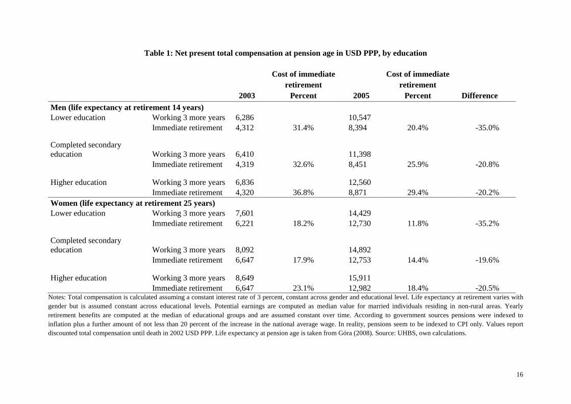
Table 1 compares the lifetime wealth for three broad educational groups of men and
women in the respective scenarios and reports the cost attached to immediate retirement.
Owing to differences in life expectancies the penalty for instantaneous retirement is lower for
women. For both sexes, the results for 2003 show substantial variation between educational
groups, with better educated individuals incurring higher costs for immediate retirement of up
to 37 percent. Given the substantial pension compression this is not surprising. Comparing the
wealth levels across years makes a general welfare improvement obvious. While the overall
cost pattern remains the same (better educated incurring higher costs), the reduction in the
retirement penalty is disproportionally large for the lower educational group. The pension
increase reduces the cost of immediate retirement for a low educated worker by 35 percent,
but only by one fifth for the better educated. In sum, labor supply responses should be
stronger among population groups that benefit disproportionally from the benefit rise.
10 As Ukraine is characterized by a high degree of benefit compression and therefore a low correlation between lifetime earnings and pension benefits, B can actually be treated as an education specific constant. 11 To compute the NPV, one has to make assumptions about life expectancy at pension age and about time preferences (discount rates δ). Life expectancy values at pension age are taken from Góra (2008). The discount rate is 3 percent (as we are comparing very narrowly defined scenarios here, the simulations are not very sensitive to the choice of the discount rate). For computational details see the Note of Table 1.
16
Table 1: Net present total compensation at pension age in USD PPP, by education
Cost of immediate
retirement Cost of immediate
retirement Difference 2003 Percent 2005 Percent
Men (life expectancy at retirement 14 years) Lower education Working 3 more years 6,286 10,547 Immediate retirement 4,312 31.4% 8,394 20.4% -35.0% Completed secondary education Working 3 more years 6,410 11,398 Immediate retirement 4,319 32.6% 8,451 25.9% -20.8% Higher education Working 3 more years 6,836 12,560 Immediate retirement 4,320 36.8% 8,871 29.4% -20.2% Women (life expectancy at retirement 25 years) Lower education Working 3 more years 7,601 14,429 Immediate retirement 6,221 18.2% 12,730 11.8% -35.2% Completed secondary education Working 3 more years 8,092 14,892 Immediate retirement 6,647 17.9% 12,753 14.4% -19.6% Higher education Working 3 more years 8,649 15,911 Immediate retirement 6,647 23.1% 12,982 18.4% -20.5%
Notes: Total compensation is calculated assuming a constant interest rate of 3 percent, constant across gender and educational level. Life expectancy at retirement varies with gender but is assumed constant across educational levels. Potential earnings are computed as median value for married individuals residing in non-rural areas. Yearly retirement benefits are computed at the median of educational groups and are assumed constant over time. According to government sources pensions were indexed to inflation plus a further amount of not less than 20 percent of the increase in the national average wage. In reality, pensions seem to be indexed to CPI only. Values report discounted total compensation until death in 2002 USD PPP. Life expectancy at pension age is taken from Góra (2008). Source: UHBS, own calculations.
17
4 Retirement and Labor Supply Responses to the Pension Increase
4.1 Data
The empirical analysis is based on several cross sections (2002-2006) of the nationally
representative Ukrainian Household Budget Survey (UHBS) which interviews 25,000
individuals and their households on an annual basis. Since data collection is performed by the
State Statistics Committee of Ukraine each December, the data set comprises two years prior,
two years after the pension increase as well as the year of the change itself. The 2004 wave
could not be used for the main analysis, since the pension rise from late 2004 was fully
reflected only in the annual pension income of 2005. To prevent from other potentially
confounding factors, the analysis is cleanest when performed on two cross-sections before
(2002/2003) and one after the pension increase (2005).12 The UHBS includes a rich set of
individual and household characteristics, including information on employment, annual
incomes, household assets and health. The available information on total completed working
years is crucial for testing the importance of the pension eligibility criterion that requires
minimum working years. As expected, only a minor fraction of those cohorts reaching
pension age has worked fewer than 20/25 years as a consequence of the Soviet full-
employment policy (1.9 percent of women and 2.0 percent of men).13
Since the UHBS does not contain information on working hours, a complementary
analysis is performed using the Ukrainian Longitudinal Monitoring Survey (ULMS). This is a
high quality panel data set providing comparable, but much more detailed labor market
information than its earlier established and well-known Russian counterpart (RLMS). The
12 As data further beyond the initial reform date are included into the analysis, the implicit phase-in of another reform will work against the retirement effect: Pensioners working beyond the statutory pension age see their monthly benefits grow by 1% per additional year of work. This effect is still negligible in 2005, but grows with each year thereafter that is added to the analysis. Thus, the option value effect of postponing retirement arises. 13 Actually a measure of years with pension contributions would be preferable. Although informal sector employment might be substantial in current Ukraine, the largest fraction of those close to the pension age has reached the minimum year requirement already during Soviet times. For instance, men born in 1944 who had started working in 1964 had already 28 years of working experience when the Soviet Union broke apart in 1991.

18
nationally representative ULMS has been collected by the Kiev International Institute of
Sociology in collaboration with an international network of economists in three years 2003,
2004 and 2007 (Lehmann and Terrell, 2006). The unique feature of the ULMS is a large
retrospective section providing detailed information on individual work histories since Soviet
times. The survey covers individuals aged 15 to 72 with an initial sample size of more than
6,000 respondents. As the vast majority of data collection took place in early summer (May to
July), the panel comprises two waves prior to and one wave after the pension increase.
The main dependent variable in the analysis is the retirement status measured
according to an activity-benefit-based definition. A person is classified as retired if not
working in the reference week, receiving old-age pension benefits and subjectively self-
categorizing him- or herself as retiree. Labor supply intensity is measured in hours per year,
weeks per year and hours per week.14 Among the independent variables, the main interest
rests on the indicator of pension eligibility, which is based exclusively on the age criterion in
the main analysis. Important control variables include individual characteristics (age, marital
status, years of schooling, years of work experience), health status (a composite indicator for
suffering from one of seven chronic diseases), household characteristics (household size, the
presence of children up to age seventeen, the presence of a person with invalidity status,
income generated from all other non-pension eligible household members and assets). Assets
are proxied by an indicator generated from detailed information on housing and durables
14 It should be noted that the persistent structural inflexibility of the Ukrainian labor market allows little choice at the intensive margin of labor supply. Most workers are contracted full-time with 40 hours per week. More than sixty (fifty) percent of employees worked exactly 40 hours in an average (the reference) working week and the concentration on full time employment is even more pronounced for those working beyond pension age (Figure A1 in the Appendix). A Kolmogorov-Smirnov test reveals that the hours distributions of working age and pension age employees are not significantly different at conventional levels of working hours (up to 55 hours). The working time pattern is similar for men and women and there is no significant change in working hours between 2003 and 2007. The share of those working between 15 and 25 hours is higher among working age women (7 percent) than among working age men (3 percent) and higher among pension aged women (12 percent) than among pension aged men (8 percent).

19
through the use of factor analysis.15 Finally, settlement location (place and region) and the
sub-regional structure of the labor market (unemployment rate, share of employees in mining,
share of employees in agriculture and share of state employment) are added as controls. A
detailed description of variable definitions is provided in the Appendix (Table A1).
4.2 Identification Strategy
The identification strategy of this paper exploits the exogenous variation in Ukrainian
pension benefits in September 2004. In order to prevent the results from being confounded by
two potential selection effects, the analyses adopt a conservative approach that may translate
into lower bounds estimates: First, the analysis uses pension eligibility instead of actual
benefit receipt to circumvent the endogeneity of the pension claim decision. Consistent across
both data sets and all years, 1 to 2 percent of those of pensionable age do not draw an old-age
benefit. Non-take-up concerns mainly eligible individuals who kept working and were not
officially registered at their current place of residence.16 Second, pension eligibility is
exclusively conditioned on an individual’s age. Although eligibility is de jure also based on
the minimum working years requirement, the fulfillment of this second criterion depends on various
decisions taken throughout the life, thus potentially introducing endogeneity bias. Both corrections
affect only very small groups of the sample. Robustness checks classifying those with below
20/25 years of work experience as ineligible or using actual benefit receipt confirm that the
true effect is economically and statistically slightly bigger (see Table A2 and Table A3).
15 Initially, factor analysis is performed on a wide range of wealth indicators and assets including house ownership, number of rooms, total living space per capita, eleven housing facilities (e.g., sewerage, type of heating, hot water etc.) and ten durables (e.g., refrigerator, computer, and car). As monetary values are not reported in the UHBS, ‘values’ are assigned according to age, condition at purchase and origin of product. From the factor analysis, the first factor is used as a household specific asset indicator. 16 As enrolment into the State Pension scheme is automatic, the difference should not be due to informational deficits (cp. Duflo and Saez, 2003).
20
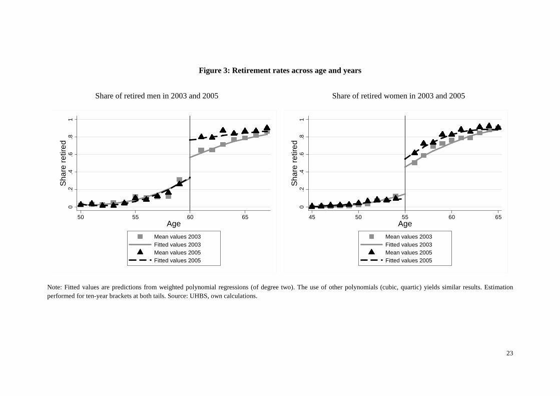
Figure 3 and Figure A2 show age-specific retirement rates for the year prior to the
pension rise (2003, displayed by dots) and the year after the pension increase (2005, displayed
by triangles) for men and women. The vertical line marks the gender-specific pension age on
the x-axis. The graphs are based on fitted values from weighted polynomial regressions. Early
retirement rates, which can be observed for men and women to the left of the retirement
discontinuity, differ very modestly over time. Above pension age, however, there is an
apparent upward shift in retirement rates after the benefit increase of 2004. The discontinuity
at the pension age has widened significantly between 2003 and 2005. This gap (and not the
one from entering pension age) is the retirement response of the minimum pension increase of
2004. The following econometric estimation of this effect uses Difference-in-Differences and
Difference-in-Regression-Discontinuity approaches.
4.3 Difference-in-Difference Estimation
The Difference-in-Differences (DiD) estimator exploits the discontinuity in pension
eligibility at pension age to compare changes over time in outcomes between those eligible
(treatment group) and those highly comparable but not yet eligible (control group) for an old-
age pension. The universal and exogenous change in pension generosity permits the
estimation of causal labor supply and retirement responses by comparing outcomes across
these two groups before and after the pension increase (the treatment). As a pure before-after
comparison of outcomes in the treatment group may be affected by time specific factors that
are common to all workers in Ukraine, the control group is used to difference away general
economic trends, e.g., changing macroeconomics conditions and aggregate labor demand.
Keeping in mind that the analysis is based on pension eligibility rather than actual benefit
receipt, the presented results have to be understood as lower bound estimates.
21
4.3.1 Main Results
Table 2 illustrates the identification strategy by mean comparisons in two-by-two
matrices. Women exhibit lower retirement rates than men across all cells as indicated in the
upper panel. Also, the behavioral response to reaching pension age is stronger for men (47
percentage points) than for women (44 percentage points). The time trend for those below
pension age is (insignificantly) negative, reflecting the increasing labor force participation
during the growth period of the mid 2000s in Ukraine. However, for those above pension age,
the time trend runs in the opposite direction, leading to a treatment effect of 17.6 percentage
points for men and 13.3 percentage points for women. Retirement rates rose by 37 and 30
percent as a result of the pension increase.
The lower panels report results from two falsification exercises, the first one
simulating an artificial pension age at 58 (for men) and 53 (for women) and the second
simulating the pension increase between the years 2002 and 2003. The first control
experiment indicates that early retirement rates increased with age but remained fairly stable
over time. The negative time trend at younger ages reconfirms the general positive
employment trend. Control experiment two shows that changes between 2002 and 2003 were
modest and insignificantly different from zero. The only puzzling effect is the (almost weakly
significant) increase in early retirement between 2002 and 2003 for men. However, this effect
is driven by compositional changes of the relatively small male sample.17 The remainder of
this section investigates the treatment effects in greater detail.
17 The density of the comparison groups around the discontinuity threshold is unequal between years as birth cohorts differ in size. This effect is obviously not caused by sorting around the threshold but by relatively small birth cohorts during WWII. The change in densities over time is especially pronounced for men (Figure A3): Between 2003 and 2005, the war-related smaller birth cohorts move across the discontinuity, resulting in less precise estimates below pension age in 2003 and above pension age in 2005.
22
The simple mean estimates can be generalized in a regression framework in order to
test the robustness of the results:18
y = β0 + β1P + β2T + β3P*T + β‘X + u (2)
with y being the dependent variable (retirement or labor supply intensity), P being an
indicator for pension eligibility (as compared to the non-eligibility N), T being an indicator for
the post-treatment period (i.e. the year 2005 for UHBS as well as 2007 for ULMS) and P*T
being an interaction effect of P and T. X is a vector of the before mentioned individual,
household and regional controls. If the pension increase was truly exogenous and non-
anticipated, the inclusion of covariates should lead to only modest changes of the results
presented so far. General differences in retirement rates between pension eligible and non-
eligible individuals are captured by β1. For males, it compares retirement rates among workers
aged 58 and 59 with those among workers aged 61 and 62, while it compares women aged 53
and 54 with women slightly above pension age, 56 and 57 years old.19 The β2 coefficient
captures changes over time which are common to treatment and control group as well as
independent of the scheduled policy. Hence, the approach relies on the assumption that no
general labor market shock affects the two groups differently. The coefficient of interest is the
difference-in-difference estimator β3 which reports the average treatment effect on those who
are eligible for the treatment:
18 Subscripts are ignored in the equation for expositional reasons. The equation is estimated by linear probability models. As a robustness check a Probit formulation of the model is applied, which yields slightly larger marginal fixed effects (Table A2). Recent advances in the econometric literature have suggested the use of bounded estimation for discrete DiD as counterfactual values might potentially become negative in the binary case (Athey and Imbens, 2006). In the current analysis, this concern is of less relevance as retirement levels of an appropriate control group are not expected to change radically over time. 19 As exact birth dates were not made available in the UHBS, all those with age exactly at the retirement threshold are excluded from the sample. Generally, it would be desirable to observe the same individuals over time. This can be done using the ULMS whereby the general results are confirmed (Table A4); however, the smaller sample size requires a broader choice of comparison age groups (three years). A drawback of the ULMS data is the gap in the observation period. The first post-reform observation is in 2007 and thus already two and a half years after the reforms took place. On the one hand this gives an indication of the persistence of the effect; on the other hand, it becomes harder to interpret the size of the treatment effect.
23
Figure 3: Retirement rates across age and years
Share of retired men in 2003 and 2005 Share of retired women in 2003 and 2005
0.2
.4.6
.81
Sha
re r
etire
d
50 55 60 65Age
Mean values 2003Fitted values 2003Mean values 2005Fitted values 2005
0.2
.4.6
.81
Sha
re r
etire
d
45 50 55 60 65Age
Mean values 2003Fitted values 2003Mean values 2005Fitted values 2005
Note: Fitted values are predictions from weighted polynomial regressions (of degree two). The use of other polynomials (cubic, quartic) yields similar results. Estimation performed for ten-year brackets at both tails. Source: UHBS, own calculations.

24
( ) ( )1,2,1,2,3 NNPP yyyy −−−=β (3)
If the treatment after 2004 is associated with increased retirement rates, this coefficient
should be positive and significantly different from zero. As higher benefits are paid to all
claimants without means or retirement testing, the treatment effect can be interpreted as a pure
income effect of the pension increase. A comprehensive way of controlling for various
composition effects is by estimating equation (2) while including sets of covariates in a
stepwise fashion. Table 3 reports results from this DiD estimation and confirms that pension
eligible individuals had higher retirement rates after the pension increase.20 While the
inclusion of covariates substantially improves the fit of the regressions, the size of the
coefficient of interest decreases only very modestly. The inclusion of health controls in
Column (4) clearly indicates that the observed retirement pattern is not driven by a
deteriorating health situation of the population, although Ukraine has indeed experienced a
severe health crisis during the transition process (Brainerd and Cutler, 2005). Given the
general improvement of the welfare situation of Ukrainian households during the 2000s, one
might argue that the results reflect welfare gains stemming from other household members.
However, income sources generated by younger co-residing adults as well as household asset
holdings are controlled for in Columns (5) and (6). Additionally, when restricting the sample
to households without co-residing working age adults the findings are robust.21
20 Robustness checks comparing the years 2002/3 and 2004/5 as well as 2002 and 2005 are found in Table A5. 21 The treatment effect for men increases to 0.183 in the full control case, while the treatment for women remains stable (0.109). Although it may seem desirable to present all results for households without cohabiting working age members, most households in Ukraine comprise two or more generations. Forty six percent of women aged 55 cohabit with at least one adult aged below 52. For men aged 60, the respective number is 39 percent. Also, only a minor fraction of the elderly live alone (12 percent of women and 15 percent of men). Overall, these cohabitation patterns lead to relatively small sample sizes.

25
Table 2: Retirement rates before and after the pension increase—extensive margin
Experiment of Interest: Year of benefit increase 2004, pension age at 60 (men) and 55 (women)
Panel A. Men 2002-2003 2005 Panel B. Women 2002-2003 2005 N=1097 Pre-increase Post-increase Difference N=1845 Pre-increase Post-increase Difference Age 58-59 0.215 0.166 -0.049 Age 53-54 0.111 0.078 -0.034 (0.027) (0.032) (0.042) (0.015) (0.015) (0.021) Age 61-62 0.689 0.816 0.127 Age 56-57 0.552 0.651 0.099 (0.022) (0.034) (0.041) (0.023) (0.026) (0.035) Difference 0.474 0.649 0.176 Difference 0.440 0.573 0.133 (0.035) (0.047) (0.059) (0.028) (0.030) (0.041) Control experiment 1: Artificial pension age at 58 (men) and 53 (women) Panel A. Men 2002-2003 2005 Panel B. Women 2002-2003 2005 N=685 Pre-increase Post-increase Difference N=1334 Pre-increase Post-increase Difference Age 57 0.171 0.159 -0.012 Age 52 0.078 0.062 -0.016 (0.034) (0.037) (0.051) (0.016) (0.022) (0.027) Age 58-59 0.215 0.166 -0.049 Age 53-54 0.111 0.078 -0.034 (0.027) (0.032) (0.042) (0.015) (0.015) (0.021) Difference 0.044 0.008 -0.037 Difference 0.033 0.015 -0.018 (0.044) (0.049) (0.066) (0.022) (0.027) (0.034) Control experiment 2: Artificial increase in benefit generosity between 2002 and 2003 Panel A. Men 2002 2003 Panel B. Women 2002 2003 N=757 Pre-increase Post-increase Difference N=1106 Pre-increase Post-increase Difference Age 58-59 0.163 0.266 0.103 Age 53-54 0.129 0.094 -0.034 (0.032) (0.043) (0.054) (0.022) (0.019) (0.028) Age 61-62 0.692 0.685 -0.006 Age 56-57 0.536 0.564 0.028 (0.032) (0.032) (0.045) (0.034) (0.032) (0.047) Difference 0.529 0.420 -0.110 Difference 0.408 0.470 0.062 (0.045) (0.054) (0.070) (0.041) (0.037) (0.055)
Note: Reported values are age and gender specific retirement rates. Robust standard errors in parentheses. Source: UHBS, own calculations.
26
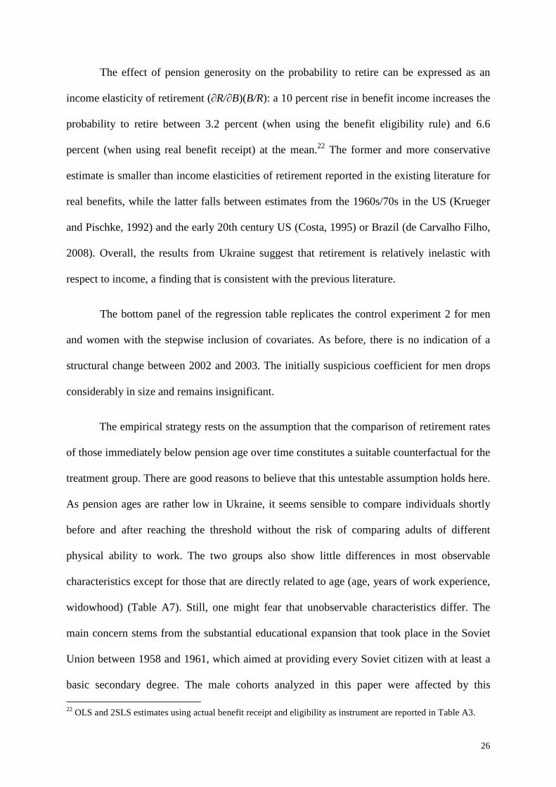
The effect of pension generosity on the probability to retire can be expressed as an
income elasticity of retirement (∂R/∂B)(B/R): a 10 percent rise in benefit income increases the
probability to retire between 3.2 percent (when using the benefit eligibility rule) and 6.6
percent (when using real benefit receipt) at the mean.22 The former and more conservative
estimate is smaller than income elasticities of retirement reported in the existing literature for
real benefits, while the latter falls between estimates from the 1960s/70s in the US (Krueger
and Pischke, 1992) and the early 20th century US (Costa, 1995) or Brazil (de Carvalho Filho,
2008). Overall, the results from Ukraine suggest that retirement is relatively inelastic with
respect to income, a finding that is consistent with the previous literature.
The bottom panel of the regression table replicates the control experiment 2 for men
and women with the stepwise inclusion of covariates. As before, there is no indication of a
structural change between 2002 and 2003. The initially suspicious coefficient for men drops
considerably in size and remains insignificant.
The empirical strategy rests on the assumption that the comparison of retirement rates
of those immediately below pension age over time constitutes a suitable counterfactual for the
treatment group. There are good reasons to believe that this untestable assumption holds here.
As pension ages are rather low in Ukraine, it seems sensible to compare individuals shortly
before and after reaching the threshold without the risk of comparing adults of different
physical ability to work. The two groups also show little differences in most observable
characteristics except for those that are directly related to age (age, years of work experience,
widowhood) (Table A7). Still, one might fear that unobservable characteristics differ. The
main concern stems from the substantial educational expansion that took place in the Soviet
Union between 1958 and 1961, which aimed at providing every Soviet citizen with at least a
basic secondary degree. The male cohorts analyzed in this paper were affected by this
22 OLS and 2SLS estimates using actual benefit receipt and eligibility as instrument are reported in Table A3.

27
expansion and a rising share of secondary educational degrees can be detected among the
respective male cohorts between the years 2002 and 2006. The share of older men with
secondary education increases by more than 12 percentage points within only five survey
years (see Table A8).23 As better educated individuals retire later in Ukraine—a consistent
finding across data sets and waves—the compositional change directly impacts retirement
rates. Controlling for educational attainments does not convincingly solve this problem as
some highly able youth might have been left without secondary degree in older cohorts due to
the lack of educational facilities while their younger fellows were better educated. However,
the potential bias introduced by the educational expansion will lead to underestimating the
retirement effect of the pension increase as better educated younger cohorts should exhibit
retirement rates that are lower than they would have been under the educational composition
of slightly older cohorts. Consequently, estimates for men are downward biased.
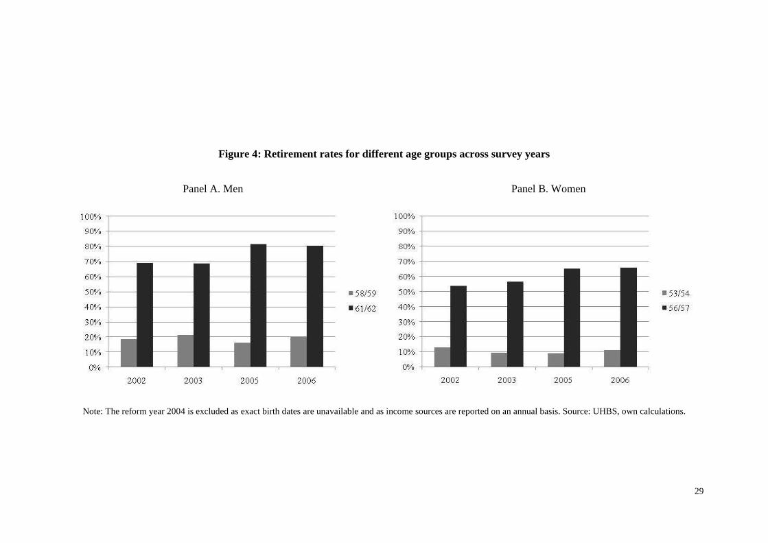
If the negative labor supply effect was truly induced by the pension increase, the
retirement rates of those slightly above pension age should exhibit a structural break over
time, while those of the control group should remain even. Figure 4 suggests that the labor
supply of those below pension age remained indeed roughly constant between 2002 and 2006.
In contrast, the share of retirees (up to two years after the statutory pension age) increased
between 2003 and 2005 by a fraction comparable to the DiD estimates. More formally, while
retirement rates for the treatment groups in 2005 and 2006 are significantly different from the
base year 2002, the T-statistics for differences of annual retirement rates of the control groups
below pension age remain well below two (Table A9). As there were no others policies in
place which could have changed retirement incentives,24 the reduced labor supply can be
causally attributed to the increase in the legal minimum pension guarantee.
23 Women of the affected birth cohorts were already older than the treatment group. 24 Most importantly, there were no changes in taxes in order to finance the pension expenditures.
28
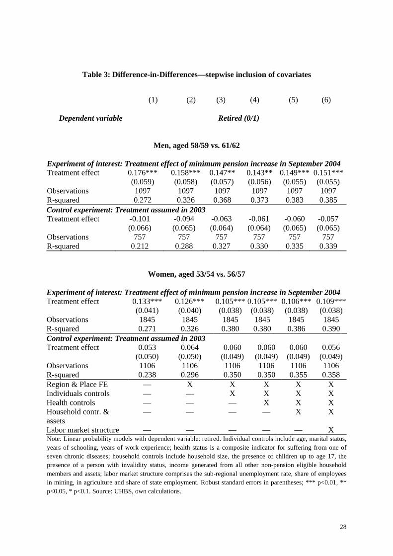
Table 3: Difference-in-Differences—stepwise inclusion of covariates
(1) (2) (3) (4) (5) (6)
Dependent variable Retired (0/1)
Men, aged 58/59 vs. 61/62
Experiment of interest: Treatment effect of minimum pension increase in September 2004 Treatment effect 0.176*** 0.158*** 0.147** 0.143** 0.149*** 0.151*** (0.059) (0.058) (0.057) (0.056) (0.055) (0.055) Observations 1097 1097 1097 1097 1097 1097 R-squared 0.272 0.326 0.368 0.373 0.383 0.385 Control experiment: Treatment assumed in 2003 Treatment effect -0.101 -0.094 -0.063 -0.061 -0.060 -0.057 (0.066) (0.065) (0.064) (0.064) (0.065) (0.065) Observations 757 757 757 757 757 757 R-squared 0.212 0.288 0.327 0.330 0.335 0.339
Women, aged 53/54 vs. 56/57
Experiment of interest: Treatment effect of minimum pension increase in September 2004 Treatment effect 0.133*** 0.126*** 0.105*** 0.105*** 0.106*** 0.109*** (0.041) (0.040) (0.038) (0.038) (0.038) (0.038) Observations 1845 1845 1845 1845 1845 1845 R-squared 0.271 0.326 0.380 0.380 0.386 0.390 Control experiment: Treatment assumed in 2003 Treatment effect 0.053 0.064 0.060 0.060 0.060 0.056 (0.050) (0.050) (0.049) (0.049) (0.049) (0.049) Observations 1106 1106 1106 1106 1106 1106 R-squared 0.238 0.296 0.350 0.350 0.355 0.358 Region & Place FE — X X X X X Individuals controls — — X X X X Health controls — — — X X X Household contr. & assets
— — — — X X
Labor market structure — — — — — X Note: Linear probability models with dependent variable: retired. Individual controls include age, marital status, years of schooling, years of work experience; health status is a composite indicator for suffering from one of seven chronic diseases; household controls include household size, the presence of children up to age 17, the presence of a person with invalidity status, income generated from all other non-pension eligible household members and assets; labor market structure comprises the sub-regional unemployment rate, share of employees in mining, in agriculture and share of state employment. Robust standard errors in parentheses; *** p<0.01, ** p<0.05, * p<0.1. Source: UHBS, own calculations.
29
Figure 4: Retirement rates for different age groups across survey years
Panel A. Men Panel B. Women
Note: The reform year 2004 is excluded as exact birth dates are unavailable and as income sources are reported on an annual basis. Source: UHBS, own calculations.
30
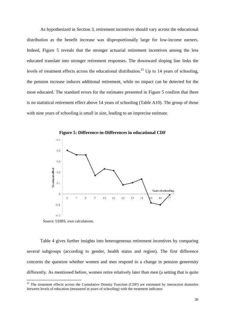
As hypothesized in Section 3, retirement incentives should vary across the educational
distribution as the benefit increase was disproportionally large for low-income earners.
Indeed, Figure 5 reveals that the stronger actuarial retirement incentives among the less
educated translate into stronger retirement responses. The downward sloping line links the
levels of treatment effects across the educational distribution.25 Up to 14 years of schooling,
the pension increase induces additional retirement, while no impact can be detected for the
most educated. The standard errors for the estimates presented in Figure 5 confirm that there
is no statistical retirement effect above 14 years of schooling (Table A10). The group of those
with nine years of schooling is small in size, leading to an imprecise estimate.
Figure 5: Difference-in-Differences in educational CDF
Source: UHBS, own calculations.
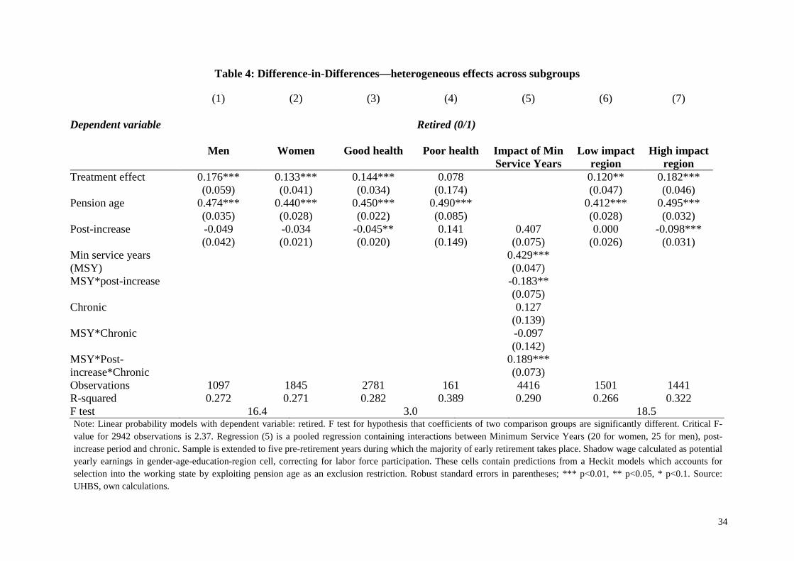
Table 4 gives further insights into heterogeneous retirement incentives by comparing
several subgroups (according to gender, health status and region). The first difference
concerns the question whether women and men respond to a change in pension generosity
differently. As mentioned before, women retire relatively later than men (a setting that is quite
25 The treatment effects across the Cumulative Density Function (CDF) are estimated by interaction dummies between levels of education (measured in years of schooling) with the treatment indicator.

31
unusual for most countries of the world but related to the especially severe health crisis of
men; Brainerd and Cutler, 2005), but given their relatively lower labor incomes they might
incur stronger retirement incentives from the equalizing pension increase. The first two
columns replicate the basic result for men and women. As reported above, the corresponding
marginal effects of these treatment effects are 37 percent and 30 percent and the income
elasticities of retirement are minus 0.35 and minus 0.32, respectively. The bottom line reports
the F statistics of a Chow test and clearly rejects the equality of the coefficients, so that
β3,female < β3,male. This result stands in contrast to the labor supply literature on the working age
population that normally finds stronger responses among women (Blundell and MaCurdy,
1999). However, the case might be different for individuals close to pension age.
Theoretically, the argument relating to women’s comparative advantage in household
production is of less relevance after the children have left. Also, in joint retirement decisions
(a topic briefly addressed below) women are often the second mover. Finally, women are
more likely to be employed in occupations that allow a gradual retreat from the labor market.
The section covering labor supply responses at the intensive margin will show that women,
unlike men, reduce yearly working hours. Taking into account the response at the intensive
margin, women’s overall response seems comparable to that of men.
Second, one can use the exogenous pension increase to study the relationship between
health status and retirement. Individuals with health conditions that result in the inability to
perform work are by definition excluded from the current analysis. The question remains
whether those with reduced working capacities respond differently than those without any
impediments. Research investigating the impact of health status on retirement is complicated
by reporting bias and the potential endogeneity of health status. Health at older ages is—
among other determinants—a consequence of individual decisions taken throughout life.
Empirical evidence suggests that chronically ill persons retire earlier as a result of lower labor

32
market returns and higher disutility from working (Currie and Madrian, 1999). Given that
chronically ill persons will be more likely to retire early, they should be less responsive to
retirement incentives at older ages. In the parlance of the evaluation literature, chronically ill
persons resemble ‘always takers’, for whom the treatment effect at the retirement threshold
would not be identified. As columns (3) and (4) suggest, this is indeed the case. Upon
reaching pension age, more than 80 percent of the chronically ill are already out of the labor
force and the treatment coefficient remains insignificant.
Despite the small sample size, the Chow test again rejects the equality of the
coefficients. This suggests that the measurement of the income effect at normal pension age
has little explanatory power for the chronically ill. Thus, column (5) tests whether chronically
ill people react at the minimum service year threshold for early retirement (20 years for
women, 25 years for men). Therefore, interactions between dummies indicating service time
above the minimum threshold, chronic disease and the post-increase period are included in a
pooled regression. The coefficient of interest is the triple interaction between the three
dummies: reaching the minimum threshold as a chronically ill person after the pension
increase induces 19 percentage points of additional retirement.
Finally, poorer regions should benefit more from the pension increase since the
pension increase leveled (the modest) regional variation in pension benefits that existed until
2003. Due to the substantial geographic variation in Ukraine’s economic structure as well as
wage and pension levels, a regional comparison is useful. After the pension increase, a flat
benefit rate applied for virtually every pensioner thus producing variation in the magnitude of
the pension gain. Columns (6) and (7) of Table 4 confirm that the retirement effect from the
pension increase was stronger in regions which had an above median pension level growth
between 2003 and 2005 and the difference between the two coefficients is significant.
33
Ukraine is characterized by an economic gradient between urban and rural areas that is
typical for many emerging countries. Urban and rural residents respond in a statistically
significant different manner to the benefit change. However, differences between urban and
rural population can be entirely explained by composition effects: when adding the full set of
controls, the coefficients converge closely to 0.119 for urban and 0.124 for rural residents.
4.3.2 Discussion and Robustness Checks
The basic identifying assumptions have been presented above. This section provides
further support for the methodological approach by addressing four potential caveats. First,
identification might not only be jeopardized if treatment and control group differed
structurally, but also if the pension increase affected the control group, i.e. those below
pension age and their incentives for retirement. The pension policy might increase prospective
old-age benefits and net present wealth levels for those below pension age, and subsequently
induce early retirement if people possessed private savings and the freedom to choose early
retirement. The loss of household savings during the 1990s—a fact that is reflected in the low
coverage of modern saving technologies26—makes such a shift among the control group
rather unlikely. The control experiment 1 of Table 2 confirms a reduction rather than increase
in early retirement. However, if early retirement incentives were reduced simultaneously with
the rise in pension benefits, the findings could simply reflect a change in early retirement
behavior or in occupational early retirement rules.27 Early retirement is indeed of some
importance in Ukraine, as workers in hazardous occupations (e.g. miners) have been entitled
to earlier retirement since Soviet times; however, the empirical evidence has remained scant.
26 According to the ULMS, only 8.9 percent of households held a savings bank account in 2007, 4.4 percent a life insurance, and 2 percent securities. Data for the earlier period are unavailable but were certainly lower. 27 The official rules for early retirement were unchanged during the observation period. Also, unlike in many industrialized countries, labor force exits from unemployment into retirement are rather unusual. Only 2 percent of current pensioners left the labor force directly from an unemployment spell into retirement.
34
Table 4: Difference-in-Differences—heterogeneous effects across subgroups (1) (2) (3) (4) (5) (6) (7) Dependent variable Retired (0/1)
Men Women Good health Poor health Impact of Min
Service Years Low impact
region High impact
region Treatment effect 0.176*** 0.133*** 0.144*** 0.078 0.120** 0.182*** (0.059) (0.041) (0.034) (0.174) (0.047) (0.046) Pension age 0.474*** 0.440*** 0.450*** 0.490*** 0.412*** 0.495*** (0.035) (0.028) (0.022) (0.085) (0.028) (0.032) Post-increase -0.049 -0.034 -0.045** 0.141 0.407 0.000 -0.098*** (0.042) (0.021) (0.020) (0.149) (0.075) (0.026) (0.031) Min service years (MSY)
0.429*** (0.047)
MSY*post-increase -0.183** (0.075) Chronic 0.127
(0.139)
MSY*Chronic -0.097 (0.142)
MSY*Post-increase*Chronic
0.189*** (0.073)
Observations 1097 1845 2781 161 4416 1501 1441 R-squared 0.272 0.271 0.282 0.389 0.290 0.266 0.322 F test 16.4 3.0 18.5 Note: Linear probability models with dependent variable: retired. F test for hypothesis that coefficients of two comparison groups are significantly different. Critical F-value for 2942 observations is 2.37. Regression (5) is a pooled regression containing interactions between Minimum Service Years (20 for women, 25 for men), post-increase period and chronic. Sample is extended to five pre-retirement years during which the majority of early retirement takes place. Shadow wage calculated as potential yearly earnings in gender-age-education-region cell, correcting for labor force participation. These cells contain predictions from a Heckit models which accounts for selection into the working state by exploiting pension age as an exclusion restriction. Robust standard errors in parentheses; *** p<0.01, ** p<0.05, * p<0.1. Source: UHBS, own calculations.
35
Luckily, the ULMS permits shedding some light on the issue, as all job changes and
job quits are recorded retrospectively to the year 1986. Of the entire 2003 sample, 18.9
percent (1,633 respondents) retired between 1986 and 2003 and of those 8.0 percent retired
through an early retirement scheme.28 However, these numbers mask some variation over
time: While early retirement schemes were quite common at the end of the Soviet period (14
percent of all retirees in 1986) they were later substantially reduced. During the period under
consideration (2003 to 2005) early retirement exits account for 5 to 6 percent of the total.
Respondents from hazardous occupations might not consider their retirement early though if
the normal pension age in these occupations is below the statutory pension age. Therefore an
indicator is constructed for those claiming to retire regularly but below the national normal
pension age. It turns out that the share of those in early normal retirement is slightly above 20
percent of all retirees per year and this value has been unchanged since 1996. Early normal
retirement is common in some specific occupations and predominantly in the mining sector.
As the mining industry is geographically concentrated in Ukraine’s Donetsk and Lugansk
regions excluding these from the analysis captures the majority of early normal retirees. This
exercise suggests no change to the previous results (see Table A11).
Second, the validity of the DiD estimates may be potentially impaired if household
composition responded to the availability of financial resources (Edmonds, Mammen and
Miller, 2005; Engelhardt, Gruber and Perry, 2005). Under the assumption that household
members at least partially pool their resources, changes in their relative contribution might
introduce incentives to split or unite households. To test for endogeneity in household
composition, models similar to (2) are estimated which employ household size and the
number of working age household members as dependent variables. If households were
significantly larger or smaller after the pension rise, we could not reject the hypothesis that 28 Early retirement is self-reported and coded from a multiple answer question. To check consistency of the responses, the answers were compared with the computed individual age at retirement.

36
household composition is responsible for the observed labor supply patterns. However, for
both measures of household composition, the ‘treatment’ effect from the pension increase is
zero (Table A12). Additional support comes from the ULMS panel data, which can be
restricted to households that do not change their composition after 2004. The results based on
this subsample confirm the previous findings. Hence, endogenous household formation
cannot explain the observed retirement patterns (Table A13).
Third, closely related to household composition is the fact that partners may take
retirement decisions jointly. As Ukraine has a traditionally high rate of female labor force
participation joint retirement decisions will play a role in this context; however, the full
complexity of the topic remains beyond the scope of this paper. From a theoretical
perspective, partners wish to customize retirement dates for reasons like complementarities in
their utility functions, shared tastes or similar economic environment and wealth (Hurd,
1990). According to some descriptive evidence on the joint retirement decision of couples,
wives seem to become more likely to retire immediately upon reaching their (young) pension
age (Table A14 and Table A15). Nevertheless, joint retirement seems to have increased
within the joint retirement frontier (the shaded area of Table A15) suggesting that the
additional income allows couples to synchronize retirement where it was not feasible before.
Finally, the presented DiD estimates might be sensitive to the bandwidth choice for
the comparison groups around the pension age. The treatment effect decreases in regressions
based on broader comparison groups (see Table A16 for a wide range of bandwidth choices).
This seems reasonable as we include ever-older age groups in our data aggregate which had
already higher pre-reform retirement rates. In other words, the additional retirement effect of
the pension increase decreases with age as already evidenced graphically in Figure 3. The fact
that the basic results and the precision of the estimates are preserved in a wide range of
settings confirms their robustness.
37
4.3.3 Intensive Margin of Labor Supply
The research on retirement decisions typically distinguishes between labor supply
responses at the extensive and the intensive margin. In the latter case, persons retire gradually
and reduce the number of working hours or working weeks rather than fully retreating from
the labor market. In a setting with unconstrained working hours choices, labor supply theory
suggests that individuals reduce their work effort continuously when pension benefits are
raised. In practice, however, the choice set of hours is likely to be discrete and limited such
that people with strong preference for leisure will retire completely, while people with strong
preferences for consumption will stay in work and presumably work more hours than desired.
As briefly mentioned before, labor relations in Post-Soviet Ukraine remain strongly regulated
by the state as the Labor Code prescribes an average working week of 40 hours. Regulated
exemptions apply in hazardous occupations and, for instance, for teachers. Enterprises do
generally not promote more flexibility in working time rules as compensation for overtime
work is costly. Part-time work was very untypical during Soviet times and employment with
reduced working hours is only emerging slowly.29 Instead, working time is more often
adjusted through weeks per year rather than hours per week. This is facilitated by the fact that
the Labor Code allows flexibility in annual vacation between 24 and 69 days.
The analysis of the effect at the intensive margin is based on the ULMS and focuses
on three dependent variables: yearly working hours, weeks worked per year and weekly
working hours. The longitudinal nature of the data allows controlling for unobserved
heterogeneity and thus ensures that the results are not confounded by changing educational
quality of treatment and control group across years.
29 The questionnaire of the ULMS asks individuals for their working hours and whether they normally work 40 hours; if not, respondents can chose from a list of reasons, most of which are related to exogenous shocks, like ‘material shortage’ or ‘sickness’. Almost half of those working below forty hours per week report that their working time is considered full-time in their occupation (e.g., teachers). Only 15 percent of respondents want to work deliberately less than full time, and this ratio was unchanged between 2003 and 2007.
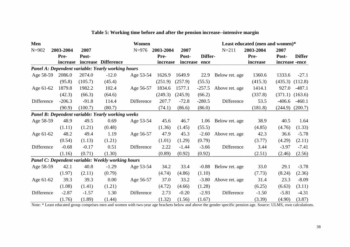
38
Table 5: Working time before and after the pension increase--intensive margin
Men Women Least educated (men and women)* N=902 2003-2004 2007 N=976 2003-2004 2007 N=211 2003-2004 2007
Pre- increase
Post- increase Difference
Pre- increase
Post-increase
Differ-ence
Pre- increase
Post- increase
Differ-ence
Panel A: Dependent variable: Yearly working hours Age 58-59 2086.0 2074.0 -12.0 Age 53-54 1626.9 1649.9 22.9 Below ret. age 1360.6 1333.6 -27.1
(95.8) (105.7) (45.4) (251.9) (257.9) (55.5) (415.3) (435.3) (112.8) Age 61-62 1879.8 1982.2 102.4 Age 56-57 1834.6 1577.1 -257.5 Above ret. age 1414.1 927.0 -487.1
(42.3) (66.3) (64.6) (249.3) (245.9) (66.2) (337.8) (371.1) (163.6) Difference -206.3 -91.8 114.4 Difference 207.7 -72.8 -280.5 Difference 53.5 -406.6 -460.1
(90.9) (100.7) (80.7) (74.1) (86.6) (86.0) (181.8) (244.9) (200.7) Panel B: Dependent variable: Yearly working weeks Age 58-59 48.9 49.5 0.69 Age 53-54 45.6 46.7 1.06 Below ret. age 38.9 40.5 1.64
(1.11) (1.21) (0.48) (1.36) (1.45) (55.5) (4.85) (4.76) (1.33) Age 61-62 48.2 49.4 1.19 Age 56-57 47.9 45.3 -2.60 Above ret. age 42.3 36.6 -5.78
(0.54) (1.13) (1.21) (1.01) (1.29) (0.79) (3.77) (4.29) (2.11) Difference -0.68 -0.17 0.51 Difference 2.22 -1.44 -3.66 Difference 3.44 -3.97 -7.41
(1.16) (0.71) (1.30) (0.89) (0.92) (0.92) (2.51) (2.46) (2.56) Panel C: Dependent variable: Weekly working hours Age 58-59 42.1 40.8 -1.29 Age 53-54 34.2 33.4 -0.88 Below ret. age 33.0 29.1 -3.78
(1.97) (2.11) (0.79) (4.74) (4.86) (1.10) (7.73) (8.24) (2.36) Age 61-62 39.3 39.3 0.00 Age 56-57 37.0 33.2 -3.80 Above ret. age 31.4 23.3 -8.09
(1.08) (1.41) (1.21) (4.72) (4.66) (1.28) (6.25) (6.63) (3.11) Difference -2.87 -1.57 1.30 Difference 2.73 -0.20 -2.93 Difference -1.50 -5.81 -4.31
(1.76) (1.89) (1.44) (1.32) (1.56) (1.67) (3.39) (4.90) (3.87) Note: * Least educated group comprises men and women with two-year age brackets below and above the gender specific pension age. Source: ULMS, own calculations.

39
Against the aforementioned institutional background it is not surprising that the share
of workers who reduce their working hours at the intensive margin is low, and the vast
majority is concentrated in low skilled service sector occupations (with teachers being the
only numerous exception). As Table 5 shows, women reduce their yearly labor supply by 281
hours or on average 17 percent (implying an income elasticity of working hours of minus
0.19). However, the effect is strongest for the least educated women and men. Workers in the
lowest educational group (primary or unfinished secondary education) reduce their yearly
working time by 460 hours, which is a substantial reduction of 34 percent (implying an
income elasticity of working hours of minus 0.48). These results hold also in the regression
set-up and are robust to the stepwise inclusion of various control variables (Table A17 to
Table A20) as well as individual fixed effects. The coefficient from the random effects
estimation (which is preferred over the fixed effects model on efficiency grounds) is less
precisely estimated, but even larger for the low educated (Table A21).
The results deliver two interesting insights: First, labor supply adjustments at the
intensive margin are predominantly realized through the number of working weeks rather than
weekly working hours. This suggests that workers adjust labor supply differently when they
are constrained in their hours choice set as is the case in Ukraine. Second, due to the gender
specific occupational structure there are no labor supply effects at the intensive margin for the
male sample. Reducing working hours is only possible in few (with the exception of teachers
mostly low skilled) service occupations. Women who reduced their yearly or weekly working
time by at least ten percent are employed in elementary service and sales occupations or
teachers. Male teachers, drivers, mobile plant operators as well as craft and trade operators
were most likely to reduce working weeks and hours by more than ten percent.30
30 Today’s labor supply choice might be partly correlated with the past occupational choice. When controlling for the occupation held in 1986 (which can be considered exogenous to recent retirement decisions) the results
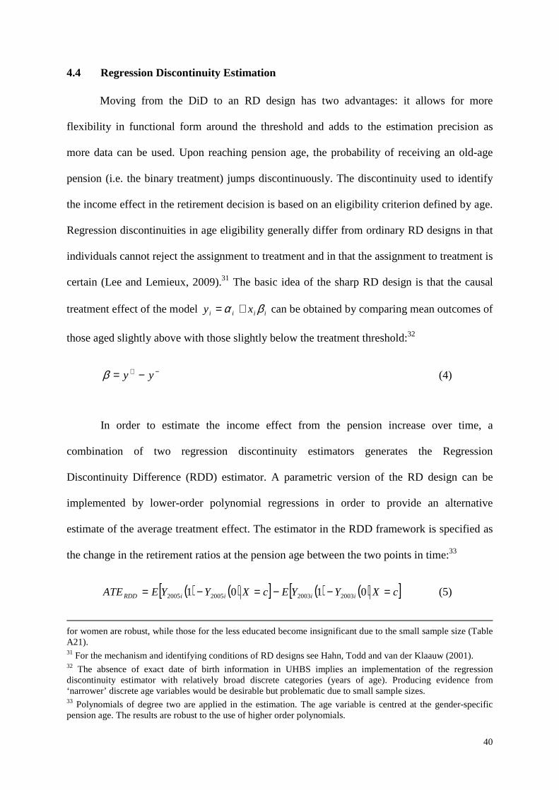
40
4.4 Regression Discontinuity Estimation
Moving from the DiD to an RD design has two advantages: it allows for more
flexibility in functional form around the threshold and adds to the estimation precision as
more data can be used. Upon reaching pension age, the probability of receiving an old-age
pension (i.e. the binary treatment) jumps discontinuously. The discontinuity used to identify
the income effect in the retirement decision is based on an eligibility criterion defined by age.
Regression discontinuities in age eligibility generally differ from ordinary RD designs in that
individuals cannot reject the assignment to treatment and in that the assignment to treatment is
certain (Lee and Lemieux, 2009).31 The basic idea of the sharp RD design is that the causal
treatment effect of the model iiii xy βα += can be obtained by comparing mean outcomes of
those aged slightly above with those slightly below the treatment threshold:32
−+ −= yyβ (4)
In order to estimate the income effect from the pension increase over time, a
combination of two regression discontinuity estimators generates the Regression
Discontinuity Difference (RDD) estimator. A parametric version of the RD design can be
implemented by lower-order polynomial regressions in order to provide an alternative
estimate of the average treatment effect. The estimator in the RDD framework is specified as
the change in the retirement ratios at the pension age between the two points in time:33
( ) ( )[ ] ( ) ( )[ ]cXYYEcXYYEATE iiiiRDD =−−=−= 0101 2003200320052005 (5)
for women are robust, while those for the less educated become insignificant due to the small sample size (Table A21). 31 For the mechanism and identifying conditions of RD designs see Hahn, Todd and van der Klaauw (2001). 32 The absence of exact date of birth information in UHBS implies an implementation of the regression discontinuity estimator with relatively broad discrete categories (years of age). Producing evidence from ‘narrower’ discrete age variables would be desirable but problematic due to small sample sizes. 33 Polynomials of degree two are applied in the estimation. The age variable is centred at the gender-specific pension age. The results are robust to the use of higher order polynomials.
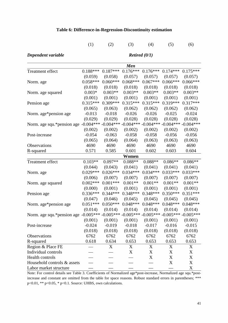
41
Table 6: Difference-in-Regression-Discontinuity estimation
(1) (2) (3) (4) (5) (6) Dependent variable Retired (0/1)
Men Treatment effect 0.188*** 0.187*** 0.176*** 0.176*** 0.174*** 0.175*** (0.059) (0.058) (0.057) (0.057) (0.057) (0.057) Norm. age 0.058*** 0.060*** 0.068*** 0.067*** 0.066*** 0.066*** (0.018) (0.018) (0.018) (0.018) (0.018) (0.018) Norm. age squared 0.003* 0.003** 0.003** 0.003** 0.003** 0.003** (0.001) (0.001) (0.001) (0.001) (0.001) (0.001) Pension age 0.315*** 0.309*** 0.315*** 0.315*** 0.319*** 0.317*** (0.065) (0.063) (0.062) (0.062) (0.062) (0.062) Norm. age*pension age -0.013 -0.018 -0.026 -0.026 -0.025 -0.024 (0.029) (0.029) (0.028) (0.028) (0.028) (0.028) Norm. age squ.*pension age -0.004*** -0.004*** -0.004*** -0.004*** -0.004*** -0.004***
(0.002) (0.002) (0.002) (0.002) (0.002) (0.002) Post-increase -0.054 -0.063 -0.058 -0.058 -0.056 -0.056 (0.065) (0.064) (0.064) (0.063) (0.063) (0.063) Observations 4690 4690 4690 4690 4690 4690 R-squared 0.571 0.585 0.601 0.602 0.603 0.604 Women Treatment effect 0.103** 0.097** 0.088** 0.088** 0.086** 0.086** (0.044) (0.043) (0.041) (0.041) (0.041) (0.041) Norm. age 0.029*** 0.026*** 0.034*** 0.034*** 0.033*** 0.033*** (0.006) (0.007) (0.007) (0.007) (0.007) (0.007) Norm. age squared 0.002*** 0.001*** 0.001** 0.001** 0.001** 0.001** (0.000) (0.001) (0.001) (0.001) (0.001) (0.001) Pension age 0.336*** 0.344*** 0.348*** 0.348*** 0.350*** 0.351*** (0.047) (0.046) (0.045) (0.045) (0.045) (0.045) Norm. age*pension age 0.051*** 0.050*** 0.048*** 0.048*** 0.048*** 0.048*** (0.014) (0.014) (0.014) (0.014) (0.014) (0.014) Norm. age squ.*pension age -0.005*** -0.005*** -0.005*** -0.005*** -0.005*** -0.005***
(0.001) (0.001) (0.001) (0.001) (0.001) (0.001) Post-increase -0.024 -0.019 -0.018 -0.017 -0.016 -0.015 (0.018) (0.018) (0.018) (0.018) (0.018) (0.018) Observations 6762 6762 6762 6762 6762 6762 R-squared 0.618 0.634 0.653 0.653 0.653 0.653 Region & Place FE — X X X X X Individual controls — — X X X X Health controls — — — X X X Household controls & assets — — — — X X Labor market structure — — — — — X Note: For control details see Table 3. Coefficients of Normalized age*post-increase, Normalized age squ.*post-increase and constant are omitted from the table for space reasons. Robust standard errors in parentheses; *** p<0.01, ** p<0.05, * p<0.1. Source: UHBS, own calculations.

42
As noted in Lee and Lemieux (2009), the validity of the RD design can be tested by
including covariates, which should neither change the estimates of interest nor their standard
errors. Table 6 shows that the retirement effect of the pension increase for men and women is
significantly positive and very stable when adding covariates in a stepwise fashion. Thus, the
data confirm the theoretical irrelevance of covariates for the pure income effect (cp. Lee and
Lemieux, 2009). The RDD estimates compare quite well to the DiD results but seem slightly
larger for men and slightly smaller for women. Both, DiD and RDD estimates report the
treatment effect of the pension increase for compliers, however, the RDD estimator is only
identified for those exactly at the pension age discontinuity. As such, the correct comparison
must be made with DiD results using very narrow comparison groups. The one year
bandwidth DiD treatment effect is 0.223 for men and 0.101 for women (Table A15) which is
indeed close to the RDD results. Men seem to respond strongest immediately after reaching
pension age while women respond within the first two years, indicating their higher flexibility
in joint retirement decisions.
5 Pension Generosity and Old-Age Poverty Reduction
The proclaimed public policy objective of the sudden increase in old-age pension
benefits was to reduce old-age poverty. But did the policy actually succeed in meeting its
objective? To evaluate its effect, this section presents evidence based on an individual annual
disposable income measure, which combines all yearly income sources regardless of whether
they were received in cash or in kind (including net labor incomes from all available jobs,
state transfers and benefits, gross personal transfers, interest and dividends reported in the
individual questionnaire).34 Total income is assessed against a country specific absolute
34 While it might seem preferable to measure poverty in terms of consumption, substantial difficulties stem from the pooling of household resources and the lack of individual level consumption data (for a comparison and methodological discussion of income and consumption poverty in Ukraine, see Brück et al., 2010).

43
poverty line from the World Bank (2007). The line of 187 UAH per capita per month (37
USD in 2005 terms) represents a basket that satisfies minimal needs in the form of food
purchases, non-food goods and services. According to this measure, poverty in 2003 was
lower among those above pension age (45.4 percent) than among to those just below pension
age (46.5 percent). In 2005, the share of the poor declined to 2.0 percent and 21.9 percent
respectively, indicating the eradication of income poverty among those in pension age. This is
not surprising as the minimum pension was set close to the World Bank line. When
benchmarking poverty in terms of a more generous poverty line defined by the Ukrainian
parliament35 (which is thought of as the level of socially acceptable minimum consumption),
poverty is reduced from 74.7 percent to 49.1 percent among those below pension age and
from 69.5 percent to 45.3 percent among recent retirees. Although this is a notable success it
is uncertain whether the reduction is attributable to the pension policy. The overall success
may be driven by a common trend mirrored in Ukraine’s substantial annual GDP growth of 7-
8 percent throughout the early 2000s with corresponding wage growth.
To estimate the impact of the pension increase on poverty, the same DiD approach is
used as before. The actual distance to the World Bank poverty line and the gender specific
relative position to the average disposable income (of the working aged between 45 years and
the pension age) are more informative metrics of poverty than the headcount. The monetary
gain from the pension change amounts to roughly 50 percent of the poverty line for the
average pensioner, while the advancement in the relative position lies between 23 percent and
25 percent (Table 7). These effects are robust to controlling for demographic and other
characteristics. Due to the concurrent wage growth, pensioners’ relative improvement is less
pronounced than their absolute gain. The estimates make clear that the government’s
minimum pension increase has met the policy objective of improving pensioners’ absolute
35 This line is located at 328 UAH (in 2005 terms).
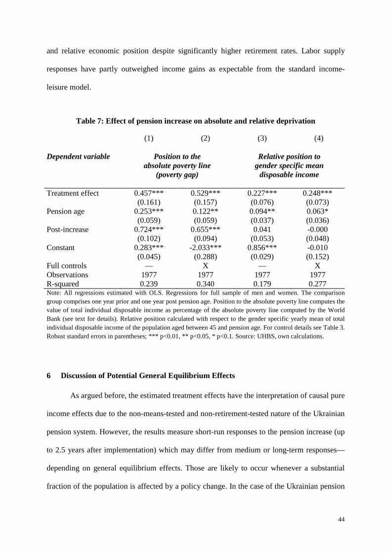
44
and relative economic position despite significantly higher retirement rates. Labor supply
responses have partly outweighed income gains as expectable from the standard income-
leisure model.
Table 7: Effect of pension increase on absolute and relative deprivation
(1) (2) (3) (4) Dependent variable Position to the
absolute poverty line (poverty gap)
Relative position to gender specific mean
disposable income
Treatment effect 0.457*** 0.529*** 0.227*** 0.248*** (0.161) (0.157) (0.076) (0.073) Pension age 0.253*** 0.122** 0.094** 0.063* (0.059) (0.059) (0.037) (0.036) Post-increase 0.724*** 0.655*** 0.041 -0.000 (0.102) (0.094) (0.053) (0.048) Constant 0.283*** -2.033*** 0.856*** -0.010 (0.045) (0.288) (0.029) (0.152) Full controls — X — X Observations 1977 1977 1977 1977 R-squared 0.239 0.340 0.179 0.277 Note: All regressions estimated with OLS. Regressions for full sample of men and women. The comparison group comprises one year prior and one year post pension age. Position to the absolute poverty line computes the value of total individual disposable income as percentage of the absolute poverty line computed by the World Bank (see text for details). Relative position calculated with respect to the gender specific yearly mean of total individual disposable income of the population aged between 45 and pension age. For control details see Table 3. Robust standard errors in parentheses; *** p<0.01, ** p<0.05, * p<0.1. Source: UHBS, own calculations.
6 Discussion of Potential General Equilibrium Effects
As argued before, the estimated treatment effects have the interpretation of causal pure
income effects due to the non-means-tested and non-retirement-tested nature of the Ukrainian
pension system. However, the results measure short-run responses to the pension increase (up
to 2.5 years after implementation) which may differ from medium or long-term responses—
depending on general equilibrium effects. Those are likely to occur whenever a substantial
fraction of the population is affected by a policy change. In the case of the Ukrainian pension
45
reform, the higher disposable income of the elderly may induce indirect and direct wage
effects thus altering the opportunity costs of retirement. Indirectly, the reform can affect
wages if additional consumption of the pensioners alters the overall demand and price
structure of the economy. This may have knock-on effects on the labor market. A direct effect
on wages could occur through additional retirement, i.e. reduced aggregate labor supply. A
back-of-the-envelope calculation reveals that additionally induced retirement amounts to
roughly 413,000 persons or 2.4 percent of the pre-2004 labor force. Indeed, the trend in real
wage growth changes after the implementation of the pension rise (Figure A4). After 2004,
the annual real wage growth exceeds the expected path by 5.6 percent. If the higher wage
growth was merely a compositional phenomenon (because workers with mainly Soviet era
skills left the labor force) the opportunity costs of individuals in pension age should not be
affected. If, however, this rapid wage growth was caused by labor supply shortages, shadow
wages of pensioners would increase and thereby reduce retirement incentives. By computing
real wage growth rates for different age groups it is possible to show that employees above
the pension age threshold enjoyed larger wage increases than the control groups (Figure A5).
Especially, the manpower of pension aged men was in high demand after the pension rise.
These wage patterns also indicate that potential demand explanations for the observed labor
supply patterns do not apply.
7 Conclusions and Policy Implications
This paper provides unique econometric evidence on the pure income effect on labor
supply. The exogenous and universal increase in old-age pension benefits in Ukraine in 2004
increased the probability of retiring at the statutory pension age by 30 to 47 percent (extensive
margin of labor supply). Corresponding to the incentive structure the retirement effect is
strongest for the less educated. Unlike in industrialized countries, adjustments of individual

46
labor supply at the intensive margin are only modest since workers are restricted in their
choices of working hours. The analysis reveals that only women and the least educated
workers adapt their yearly working time, mainly through reductions of yearly working weeks.
Although men react stronger at the extensive and women at the intensive margin of labor
supply the overall effect is roughly comparable across gender. From a welfare perspective, the
benefit increase lifts the majority of pensioners out of poverty, even though the reduction in
labor supply attenuates the pure welfare effect of the pension increase.
Although pension systems and economic circumstances differ across countries, the
behavioral results are informative about the existence of labor supply effects that arise from
universal benefit policies in general. Furthermore, the empirical results provide rare insights
for many developing or emerging countries facing similar challenges. Like Ukraine several
countries currently introduce or reform their pension systems (e.g., for Brazil see de Carvalho
Filho, 2008). This is especially true for (formerly) Socialist countries, as they share a common
labor market legacy and similarly structured pension systems, including full coverage, low
pension ages and low correlation between contributions and benefits. More specifically,
Ukraine’s quasi-pension experiment delivers the following policy conclusions:
First, an optimal policy design should take into account potential spill-over effects on
the labor market, i.e. through reduced aggregate labor supply. Second, changes in labor
market incentives caused by minimum pension guarantees or flat social benefits differ across
subgroups of the labor force depending on opportunity costs and the marginal utility of
wealth. Third, large scale pension policies may induce direct and indirect wage effects which
mitigate retirement incentives. Fourth, a generous full-coverage pension system is able to
achieve welfare objectives (reduce old-age poverty) although the success of such a policy has
to be contrasted with its labor supply effects, fiscal costs and the intergenerational burden.
Combating poverty with the help of untargeted old-age benefits is fiscally costly. The

47
effectiveness of welfare policies might be weakened by reduced labor market participation of
benefit recipients.
References
Angrist, Joshua D., and Alan B. Krueger. 1999. “Empirical Strategies in Labor
Economics.” In Handbook of Labor Economics, ed. Orley Ashenfelter, and David
Card, 1463-1555.
Ardington, Cally, Anne Case, and Victoria Hosegood. 2009. “Labor Supply Responses to
Large Social Transfers: Longitudinal Evidence from South Africa.” American
Economic Journal: Applied Economics, 1(1): 22-48.
Asch, Beth, Stephen J. Haider, and Julie Zissimopoulos. 2005. “Financial Incentives and
Retirement: Evidence from Federal Civil Service Workers.” Journal of Public
Economics, 89(2-3): 427-440.
Athey, Susan, and Guido W. Imbens. 2006. “Identification and Inference in Non-Linear
Difference-in-Differences Models.” Econometrica, 74(2): 431–497.
Barr, Nicholas, and Peter Diamond. 2008. Reforming Pensions. Principles and Policy
Choices. Oxford, New York: Oxford University Press.
Bertrand, Marianne, Sendhil Mullainathan, and Douglas Miller. 2003. “Public Policy and
Extended Families: Evidence from Pensions in South Africa.” The World Bank
Economic Review, 17(1): 27-50.
Blank, Rebecca M. 2002. “Evaluating Welfare Reforms in the United States.” Journal of
Economic Literature, 40(4): 1105-1166.
Blöndal, Sveinbjörn, and Stefano Scarpetta. 1999. “The Retirement Decision in OECD
Countries.” OECD Economics Department Working Papers 202.
Blundell, Richard, and Paul Johnson. 1998. “Pensions and Labor-Market Participation in
the United Kingdom.” American Economic Review, 88(2): 168-172.

48
Blundell, Richard, Costas Meghir, and Sarah Smith. 2002. “Pension incentives and the
pattern of early retirement.” Economic Journal, 112: C153-C170
Brainerd, Elizabeth, and David M. Cutler. 2005. “Autopsy on an Empire: Understanding
Mortality in Russia and the Former Soviet Union.” Journal of Economic Perspectives,
19(1): 107-130.
Brück, Tilman, Alexander M. Danzer, Alexander Muravyev, and Natalia Weisshaar.
2010. “Poverty during Transition: Household Survey Evidence from Ukraine.” Journal
of Comparative Economics, 38(2): 123-145.
Burtless, Gary. 1986. “Social Security, Unanticipated Benefit Increases, and the Timing of
Retirement.” The Review of Economic Studies, 53(5): 781-805.
Copsey, Nathaniel. 2006. “Europe and the Ukrainian Presidential Elections of 2004.”
EPERN Election Briefing No. 16. University of Sussex.
Costa, Dora. 1995. “Pensions and Retirement: Evidence from Union Army Veterans.” The
Quarterly Journal of Economics, 110(2): 297-319.
Currie, Janet, and Brigitte C. Madrian. 1999. “Health, Health Insurance and the Labor
Market.” in Handbook of Labor Economics Volume 3C, ed. Orley C. Ashenfelter and
David Card, Ch. 50. Amsterdam: Elsevier Science Publishers BV.
De Carvalho Filho, Irineu E. 2008. “Old-Age Benefits and Retirement Decisions of Rural
Elderly in Brazil.” Journal of Development Economics, 86: 129-146.
Duflo, Esther. 2003. “Grandmothers and Granddaughters. Old-Age Pensions and Intra-
household Allocation in South Africa.” The World Bank Economic Review, 17(1): 1-25.
Duflo, Esther, and Emmanuel Saez. 2003. “The Role of Information and Social Interactions
in Retirement Plan Decisions: Evidence from a Randomized Experiment.” The
Quarterly Journal of Economics, 118(3): 815-842.
Edmonds, Eric V., Kristin Mammen, and Douglas L. Miller. 2005. “Rearranging the
Family? Income Support and Elderly Living Arrangements in a Low-Income Country.”
The Journal of Human Resources, 40(1): 186-207.
Engelhardt, Gary V., Jonathan Gruber, and Cynthia D. Perry. 2005. “Social Security and
Elderly Living Arrangements: Evidence from the Social Security Notch.” The Journal
of Human Resources, 40(2): 354-372.

49
Freeman, Richard B. 2009. “Labor Regulations, Unions, and Social Protection in
Developing Countries: Market Distortion or Efficient Institutions.” in Handbook of
Development Economics, ed. Dani Rodrik and Mark R. Rosenzweig, Ch. 70. North
Holland: Elsevier.
Friedberg, Leora, and Anthony Webb. 2005. “Retirement and the Evolution of Pension
Structure.” Journal of Human Resources, 40(2): 281-308.
Góra, Marek. 2008. “Pension Reform. Challenge for Ukraine.” UNDP Blue Ribbon
Analytical and Advisory Centre, Kiev.
Góra, Marek, Rohozynsky, Oleksandr, and Oxana Sinyavskaya. 2010. “Pension reform
options for Russia and Ukraine: A critical analysis of available options and their
expected outcomes.” ESCIRRU Working Paper No. 25. Berlin.
Gruber, Jonathan, and David A. Wise. 1999. “Social Security Programs and Retirement
Around the World.” Research in Labor Economics, 18: 1-40.
Gruber, Jonathan, and David A. Wise. 2004. “Introduction and Summary.” in Social
Security Programs and Retirement Around the World: Micro Estimation, ed. Jonathan
Gruber and David A. Wise, 1-40. Chicago: University of Chicago Press.
Gustman, Alan L., and Thomas L. Steinmeier. 1986. “A structural retirement model.”
Econometrica, 54(3): 555-584.
Gustman, Alan L., Olivia S. Mitchell, Andrew A. Samwick, and Thomas L. Steinmeier.
2000. “Evaluating Pension Entitlements.” In Forecasting Retirement Needs and
Retirement Wealth, ed. Olivia S. Mitchell, P. Brett Hammond and Anna M.
Rappaport. Philadelphia: University of Pennsylvania Press.
Hahn, Jinyong, Petra Todd, and Wilbert Van der Klaauw. 2001. “Identification and
Estimation of Treatment Effects with a Regression-Discontinuity Design.”
Econometrica, 69(1): 201-209.
Handrich, Lars, and Oleksandra Betliy. 2006. “The Pension System Derailed: Proposals
how to get Back on the Reform Track.” Institute for Economic Research and Policy
Consulting in Ukraine, Policy Paper V9, Kiev.
Harrison, Ann, and Edward Leamer. 1997. “Labor Markets in Developing Countries: An
Agenda for Research.” Journal of Labor Economics, 15(3): 1-19.
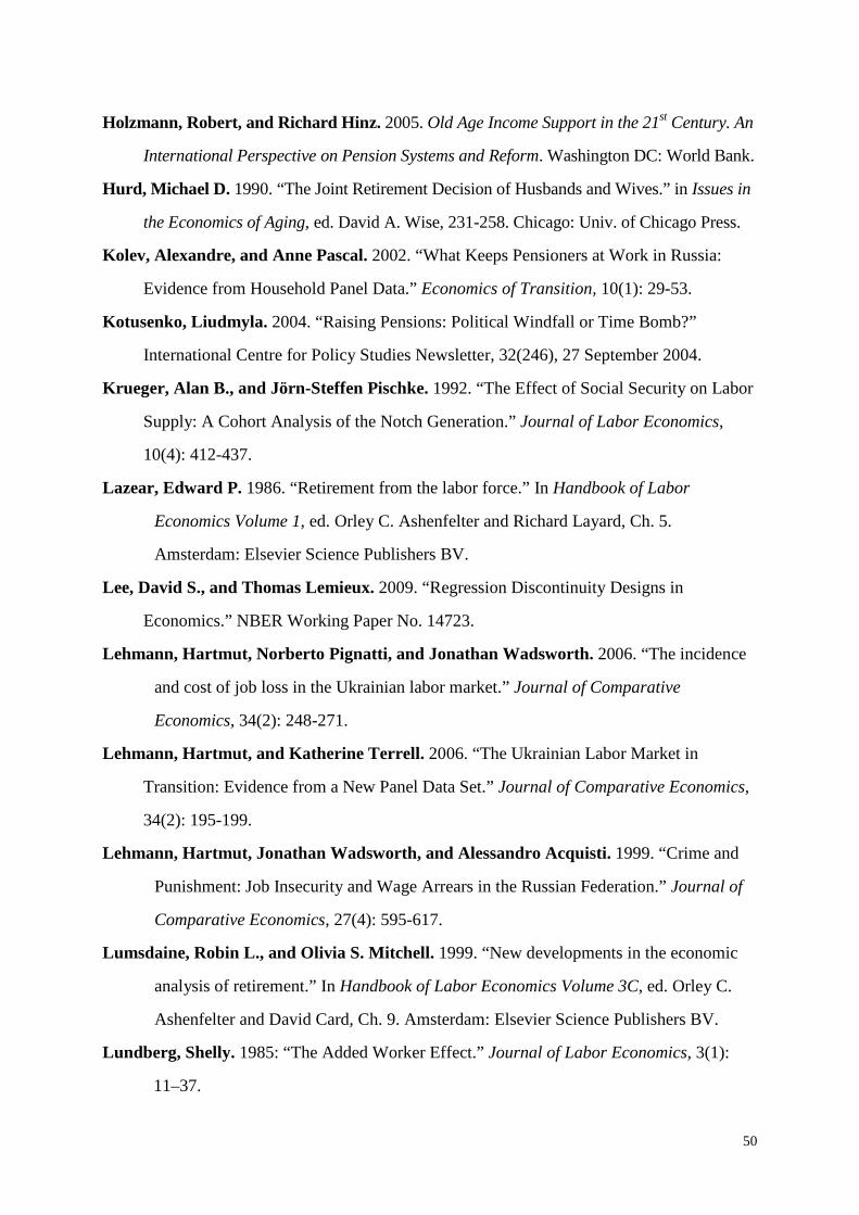
50
Holzmann, Robert, and Richard Hinz. 2005. Old Age Income Support in the 21st Century. An
International Perspective on Pension Systems and Reform. Washington DC: World Bank.
Hurd, Michael D. 1990. “The Joint Retirement Decision of Husbands and Wives.” in Issues in
the Economics of Aging, ed. David A. Wise, 231-258. Chicago: Univ. of Chicago Press.
Kolev, Alexandre, and Anne Pascal. 2002. “What Keeps Pensioners at Work in Russia:
Evidence from Household Panel Data.” Economics of Transition, 10(1): 29-53.
Kotusenko, Liudmyla. 2004. “Raising Pensions: Political Windfall or Time Bomb?”
International Centre for Policy Studies Newsletter, 32(246), 27 September 2004.
Krueger, Alan B., and Jörn-Steffen Pischke. 1992. “The Effect of Social Security on Labor
Supply: A Cohort Analysis of the Notch Generation.” Journal of Labor Economics,
10(4): 412-437.
Lazear, Edward P. 1986. “Retirement from the labor force.” In Handbook of Labor
Economics Volume 1, ed. Orley C. Ashenfelter and Richard Layard, Ch. 5.
Amsterdam: Elsevier Science Publishers BV.
Lee, David S., and Thomas Lemieux. 2009. “Regression Discontinuity Designs in
Economics.” NBER Working Paper No. 14723.
Lehmann, Hartmut, Norberto Pignatti, and Jonathan Wadsworth. 2006. “The incidence
and cost of job loss in the Ukrainian labor market.” Journal of Comparative
Economics, 34(2): 248-271.
Lehmann, Hartmut, and Katherine Terrell. 2006. “The Ukrainian Labor Market in
Transition: Evidence from a New Panel Data Set.” Journal of Comparative Economics,
34(2): 195-199.
Lehmann, Hartmut, Jonathan Wadsworth, and Alessandro Acquisti. 1999. “Crime and
Punishment: Job Insecurity and Wage Arrears in the Russian Federation.” Journal of
Comparative Economics, 27(4): 595-617.
Lumsdaine, Robin L., and Olivia S. Mitchell. 1999. “New developments in the economic
analysis of retirement.” In Handbook of Labor Economics Volume 3C, ed. Orley C.
Ashenfelter and David Card, Ch. 9. Amsterdam: Elsevier Science Publishers BV.
Lundberg, Shelly. 1985: “The Added Worker Effect.” Journal of Labor Economics, 3(1):
11–37.

51
McKee, Douglas. 2008. “Forward Thinking and Family Support: Explaining Retirement and
Old Age Labor Supply in Indonesia.” Mimeo.
Ministry of Labor and Social Policy of Ukraine. 2006: “On the Compulsory State Social
Insurance and Pension Provision.” [in Ukrainian] Kiev.
Mitchell, Olivia S. 1982. “Fringe benefits and labor mobility.” Journal of Human Resources,
17(2): 286-298.
Moffitt, Robert A. 1987. “Life Cycle Labor Supply and the Effect of the Social Security
System: A Time-Series Analysis.” In Work, Health, and Income Among the Elderly, ed.
Gary Burtless, 183-220. Washington DC: Brookings Institution.
Noel, Michel, Zeynep Kantur, Angela Prigozhina, Sue Rutledge, and Olena Fursova.
2006. “The Development of Non-Bank Financial Institutions in Ukraine. Policy Reform
Strategy and Action Plan.” World Bank Working Paper No. 81.
OECD. 2009. Pensions at a Glance—2009. Paris: OECD.
Palacios, Robert, and Edward Whitehouse. 2006. “Civil-service Pension Schemes Around
the World.” Social Protection Discussion Paper No. 0602, The World Bank.
Paxson, Christina H., and Nachum Sicherman. 1996. “The dynamics of dual job holding
and job mobility.” Journal of Labor Economics, 14(3): 357-393.
Stock, James H., and David A. Wise. 1990. “Pensions, the Option Value of Work, and
Retirement.” Econometrica, 58(5): 1151-1180.
Vélez-Grajales, Viviana. 2008. “Reforms to an Individual Account Pension System and their
Effects on work and Contribution Decisions: The Case of Chile.” Pension Research
Council Working Paper 2008-15. University of Pennsylvania.
Willmore, Larry. 2007. “Universal Pensions for Developing Countries.” World
Development, 35(1): 24-51.
World Bank. 2005. “Pension Reform in Ukraine. Remedies to Recent Fiscal and Structural
Challenges.” Mimeo.
World Bank. 2007. “Ukraine: Poverty Update.” Report No. 39887. Washington DC: World Bank.

52
Appendix of Figures and Tables – not intended for publication

53
Figure A1: Working hours of working age vs. pension age individuals
0.2
.4.6
0 50 100 0 50 100
Working age Pension age
Den
sity
Working hours, last weekGraphs by age
Note: Depicted are actual working hours; however, the distributions for contractual working hours look similar, except for the spike at zero hours. Source: ULMS, own calculations.
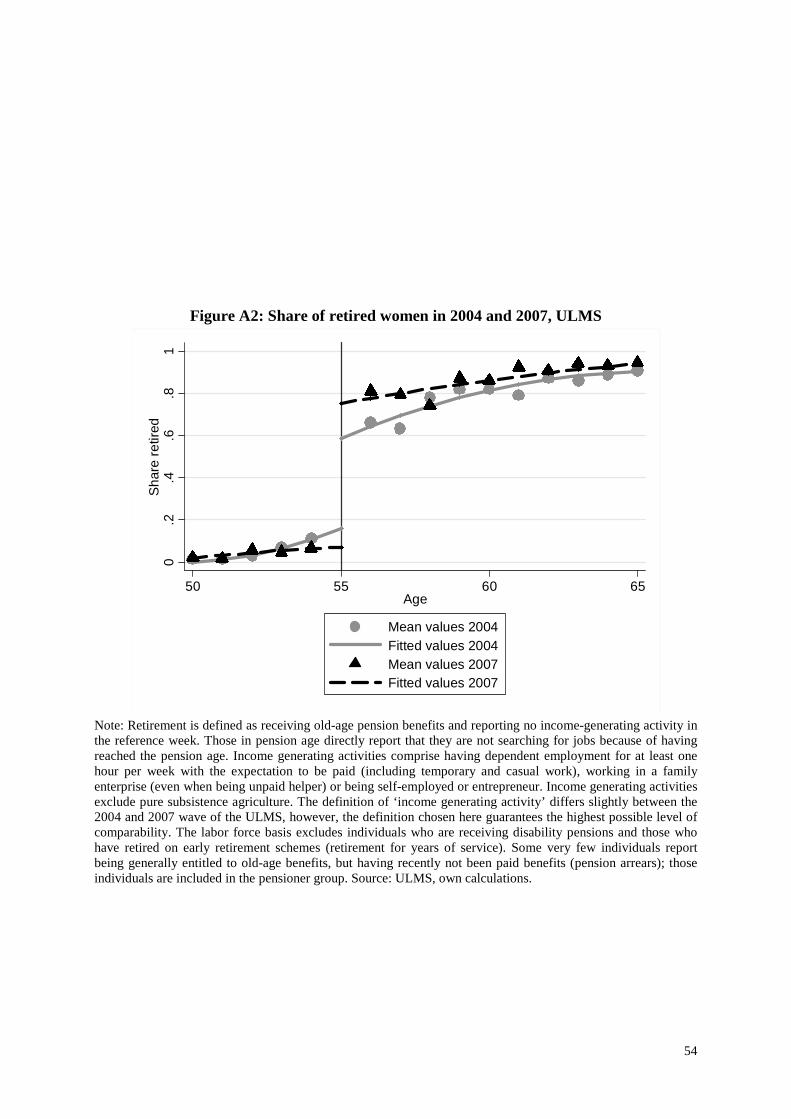
54
Figure A2: Share of retired women in 2004 and 2007, ULMS
0.2
.4.6
.81
Sha
re r
etire
d
50 55 60 65Age
Mean values 2004Fitted values 2004Mean values 2007Fitted values 2007
Note: Retirement is defined as receiving old-age pension benefits and reporting no income-generating activity in the reference week. Those in pension age directly report that they are not searching for jobs because of having reached the pension age. Income generating activities comprise having dependent employment for at least one hour per week with the expectation to be paid (including temporary and casual work), working in a family enterprise (even when being unpaid helper) or being self-employed or entrepreneur. Income generating activities exclude pure subsistence agriculture. The definition of ‘income generating activity’ differs slightly between the 2004 and 2007 wave of the ULMS, however, the definition chosen here guarantees the highest possible level of comparability. The labor force basis excludes individuals who are receiving disability pensions and those who have retired on early retirement schemes (retirement for years of service). Some very few individuals report being generally entitled to old-age benefits, but having recently not been paid benefits (pension arrears); those individuals are included in the pensioner group. Source: ULMS, own calculations.
55
Figure A3: Observational densities around the pension age threshold, by survey year
Men Women
0.0
2.0
4.0
6.0
8
50 55 60 65 50 55 60 65
2003 2005
Den
sity
AgeGraphs by UHBS wave
0.0
2.0
4.0
6.0
8
50 55 60 65 50 55 60 65
2003 2005
Den
sity
AgeGraphs by UHBS wave
Note: The vertical lines indicate the relevant pension age for state pensions. The differences in densities do obviously not reflect sorting around the threshold, but reflect different sizes of birth cohorts of the Ukrainian population. For men, the threshold ‘moves’ through the years of the WWII birth cohorts, producing low densities below (2003) or above (2005) pension age. Source: UHBS 2003 and 2005, own calculations.
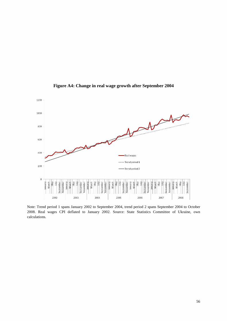
56
Figure A4: Change in real wage growth after September 2004
Note: Trend period 1 spans January 2002 to September 2004, trend period 2 spans September 2004 to October 2008. Real wages CPI deflated to January 2002. Source: State Statistics Committee of Ukraine, own calculations.

57
Figure A5: Real median wage growth for different age groups
Men Women
0%
20%
40%
60%
80%
100%
120%
140%
160%
2002 2003 2004 2005 2006
60-64 55-59 50-54 40-44 30-34
0%
20%
40%
60%
80%
100%
120%
140%
160%
2002 2003 2004 2005 2006
60-64 55-59 50-54 40-44 30-34
Source: UHBS data; author’s calculations.
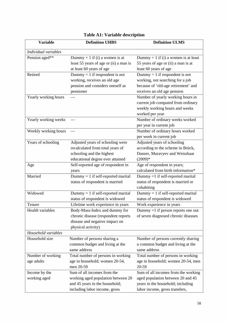
58
Table A1: Variable description
Variable Definition UHBS Definition ULMS
Individual variables Pension aged** Dummy = 1 if (i) a women is at
least 55 years of age or (ii) a man is at least 60 years of age
Dummy = 1 if (i) a women is at least 55 years of age or (ii) a man is at least 60 years of age
Retired Dummy = 1 if respondent is not working, receives an old age pension and considers oneself as pensioner
Dummy = 1 if respondent is not working, not searching for a job because of ‘old-age retirement’ and receives an old age pension
Yearly working hours — Number of yearly working hours in current job computed from ordinary weekly working hours and weeks worked per year
Yearly working weeks — Number of ordinary weeks worked per year in current job
Weekly working hours — Number of ordinary hours worked per week in current job
Years of schooling Adjusted years of schooling were recalculated from total years of schooling and the highest educational degree ever attained
Adjusted years of schooling according to the scheme in Brück, Danzer, Muravyev and Weisshaar (2009)*
Age Self-reported age of respondent in years
Age of respondent in years; calculated from birth information*
Married Dummy = 1 if self-reported marital status of respondent is married
Dummy =1 if self-reported marital status of respondent is married or cohabiting
Widowed Dummy = 1 if self-reported marital status of respondent is widowed
Dummy = 1 if self-reported marital status of respondent is widowed
Tenure Lifetime work experience in years Work experience in years Health variables Body-Mass-Index and dummy for
chronic disease (respondent reports disease and negative impact on physical activity)
Dummy =1 if person reports one out of seven diagnosed chronic diseases
Household variables Household size Number of persons sharing a
common budget and living at the same address
Number of persons currently sharing a common budget and living at the same address
Number of working age adults
Total number of persons in working age in household; women 20-54, men 20-59
Total number of persons in working age in household; women 20-54, men 20-59
Income by the working aged
Sum of all incomes from the working aged population between 20 and 45 years in the household; including labor income, gross
Sum of all incomes from the working aged population between 20 and 45 years in the household; including labor income, gross transfers,

59
transfers, dividends and capital income, state benefits; calculated from individual questionnaires
dividends and capital income, state benefits; calculated from individual questionnaires
Assets Asset indicator generated from factor analysis comprising information on home ownership, number of rooms, living space per capita, eleven housing facilities (e.g., sewerage, type of heating, hot water etc.) and ten durables (e.g., refrigerator, computer, and car). As monetary values are not reported, ‘values’ are assigned according to age, condition at purchase and origin of product. The first factor from the factor analysis is used as a household specific asset indicator.
Asset indicator generated from factor analysis comprising information on home ownership, number of rooms, living space per capita, eleven housing facilities (e.g., sewerage, type of heating, hot water etc.) and ten durables (e.g., refrigerator, computer, and car). As monetary values are not reported, ‘values’ are assigned according to age and condition at purchase (if bought in the last 12 months). The first factor from the factor analysis is used as a household specific asset indicator.
Invalid person in HH Dummy = 1 if household has member with invalidity status
—
Children up to age 17 in HH
Dummy = 1 if household contains children up to age 17
Dummy = 1 if household contains children up to age 17
City, Town, Village Dummies = 1 if respondent lives in urban settlement of big size, smaller size or in rural settlement
Dummies = 1 if respondent lives in urban settlement from 100,000 inhabitants, settlement up to 99,999 inhabitants or rural settlement
Oblast Dummies for oblasts (26 regions) Dummies for oblasts (26 reg.) Interview year Dummies for all interview years
2002-2006. Interviews were taken in December.
Dummies for all interview years 2003, 2004, 2007. Interviews were predominantly taken between May and July.
Labor market variables Regional share of employment in mining
Share of regional employment of the workforce in mining sector, computed for 78 regional clusters
—
Regional share of employment in agriculture
Share of regional employment of the workforce in agriculture, computed for 78 regional clusters
—
Regional share of employment in state sector
Share of regional employment of the workforce in the state sector, computed for 78 regional clusters
—
Unemployment rate Unemployment rate, computed for 78 regional clusters
—
Note: * These variables were cleaned to generate consistency across panel waves. ** For further robustness a variable was created that additionally requires a minimum of 20 years of work experience for women and 25 years of work experience for men.

60
Table A2: Robustness checks 1 & 2
(1) (2) (3) (4) (5) (6) Dependent variable Retired (0/1)
Robustness check 1: Probit specification, marginal effects reported Men Treatment effect 0.226*** 0.213*** 0.209** 0.206** 0.223*** 0.225*** (0.076) (0.079) (0.083) (0.083) (0.081) (0.081) Observations 1097 1097 1097 1097 1097 1097 Pseudo R-squared 0.209 0.263 0.310 0.316 0.325 0.328 Women
Treatment effect 0.170*** 0.173*** 0.147** 0.147** 0.151** 0.152** (0.061) (0.063) (0.064) (0.064) (0.064) (0.065) Observations 1845 1845 1845 1845 1845 1845 Pseudo R-squared 0.226 0.285 0.347 0.347 0.348 0.352
Robustness check 2: Omission of those below minimum working year threshold Men Treatment effect 0.180*** 0.160*** 0.162*** 0.157*** 0.163*** 0.163*** (0.061) (0.060) (0.058) (0.058) (0.056) (0.056) Constant 0.226*** 0.174** -56.762* -54.972* -56.023* -56.862* (0.028) (0.078) (32.678) (32.540) (32.414) (32.392) Observations 1063 1063 1063 1063 1063 1063 R-squared 0.260 0.317 0.372 0.376 0.386 0.388 Women
Treatment effect 0.137*** 0.125*** 0.098** 0.097** 0.100*** 0.103*** (0.041) (0.040) (0.038) (0.038) (0.038) (0.039) Constant 0.115*** 0.057 25.209 25.069 25.774 23.858 (0.015) (0.061) (18.700) (18.724) (18.707) (18.620) Observations 1806 1806 1806 1806 1806 1806 R-squared 0.266 0.321 0.388 0.388 0.389 0.392 Region & Place FE — X X X X X Individual controls — — X X X X Health controls — — — X X X Household controls — — — — X X Labor market structure — — — — — X
Note: Linear probability models with dependent variable: retired. Individual controls include age, marital status, years of schooling, years of work experience; health status is a composite indicator for suffering from one of seven chronic diseases; household controls include household size, the presence of children up to age 17, the presence of a person with invalidity status, income generated from all other non-pension eligible household members and assets; labor market structure comprises the sub-regional unemployment rate, share of employees in mining, in agriculture and share of state employment. Robust standard errors in parentheses; *** p<0.01, ** p<0.05, * p<0.1. Source: UHBS, own calculations.

61
Table A3: OLS and IV estimation of the effect of pension receipt on retirement
(1) (2) (3) (4) (5) (6) (7) (8) (9)
Dependent variable Retired (0/1)
Full sample Men Women
OLS 2SLS First stage OLS 2SLS First stage OLS 2SLS First stage Pension Receiver 0.359*** 0.427*** 0.412*** 0.644*** 0.363*** 0.439** (0.020) (0.041) (0.031) (0.073) (0.038) (0.176) Pension eligible*post-increase 0.679*** 0.665*** 0.223*** (0.024) (0.046) (0.026) Constant -0.749*** -0.488* -2.976*** 1.319*** 1.297*** 0.253 -1.039 0.000 -12.30*** (0.225) (0.266) (0.179) (0.200) (0.200) (0.189) (0.661) (2.443) (0.307) Observations 2942 2942 2942 1097 1097 1097 1845 1845 1845 F-stat 77.9 209.9 71.5 R-squared Partial R-squared
0.325 0.321 0.212
0.314 0.274 0.166
0.338 0.336 0.038
Note: Dependent variable: retired. All regressions control for full set of controls (see Table 3). Robust standard errors in parentheses; *** p<0.01, ** p<0.05, * p<0.1. Source: UHBS, own calculations.
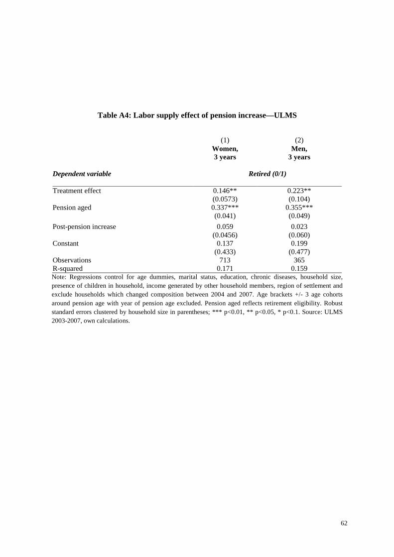
62
Table A4: Labor supply effect of pension increase—ULMS
(1) (2) Women,
3 years Men,
3 years
Dependent variable Retired (0/1) Treatment effect 0.146** 0.223** (0.0573) (0.104) Pension aged 0.337*** 0.355*** (0.041) (0.049)
Post-pension increase 0.059 0.023 (0.0456) (0.060) Constant 0.137 0.199 (0.433) (0.477) Observations 713 365 R-squared 0.171 0.159 Note: Regressions control for age dummies, marital status, education, chronic diseases, household size, presence of children in household, income generated by other household members, region of settlement and exclude households which changed composition between 2004 and 2007. Age brackets +/- 3 age cohorts around pension age with year of pension age excluded. Pension aged reflects retirement eligibility. Robust standard errors clustered by household size in parentheses; *** p<0.01, ** p<0.05, * p<0.1. Source: ULMS 2003-2007, own calculations.
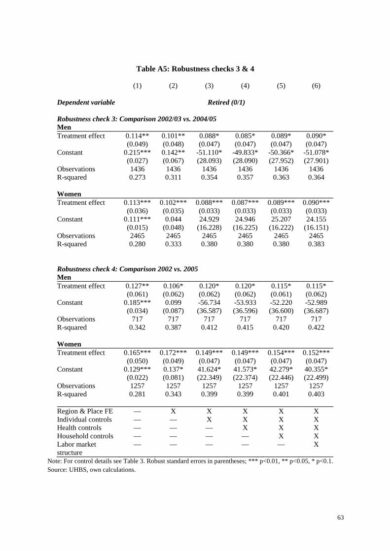
63
Table A5: Robustness checks 3 & 4 (1) (2) (3) (4) (5) (6)
Dependent variable Retired (0/1) Robustness check 3: Comparison 2002/03 vs. 2004/05 Men Treatment effect 0.114** 0.101** 0.088* 0.085* 0.089* 0.090* (0.049) (0.048) (0.047) (0.047) (0.047) (0.047) Constant 0.215*** 0.142** -51.110* -49.833* -50.366* -51.078* (0.027) (0.067) (28.093) (28.090) (27.952) (27.901) Observations 1436 1436 1436 1436 1436 1436 R-squared 0.273 0.311 0.354 0.357 0.363 0.364 Women
Treatment effect 0.113*** 0.102*** 0.088*** 0.087*** 0.089*** 0.090*** (0.036) (0.035) (0.033) (0.033) (0.033) (0.033) Constant 0.111*** 0.044 24.929 24.946 25.207 24.155 (0.015) (0.048) (16.228) (16.225) (16.222) (16.151) Observations 2465 2465 2465 2465 2465 2465 R-squared 0.280 0.333 0.380 0.380 0.380 0.383 Robustness check 4: Comparison 2002 vs. 2005 Men Treatment effect 0.127** 0.106* 0.120* 0.120* 0.115* 0.115* (0.061) (0.062) (0.062) (0.062) (0.061) (0.062) Constant 0.185*** 0.099 -56.734 -53.933 -52.220 -52.989 (0.034) (0.087) (36.587) (36.596) (36.600) (36.687) Observations 717 717 717 717 717 717 R-squared 0.342 0.387 0.412 0.415 0.420 0.422 Women
Treatment effect 0.165*** 0.172*** 0.149*** 0.149*** 0.154*** 0.152*** (0.050) (0.049) (0.047) (0.047) (0.047) (0.047) Constant 0.129*** 0.137* 41.624* 41.573* 42.279* 40.355* (0.022) (0.081) (22.349) (22.374) (22.446) (22.499) Observations 1257 1257 1257 1257 1257 1257 R-squared 0.281 0.343 0.399 0.399 0.401 0.403 Region & Place FE — X X X X X Individual controls — — X X X X Health controls — — — X X X Household controls — — — — X X Labor market structure
— — — — — X
Note: For control details see Table 3. Robust standard errors in parentheses; *** p<0.01, ** p<0.05, * p<0.1. Source: UHBS, own calculations.
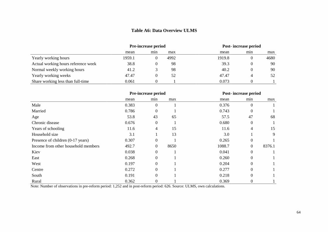
64
Table A6: Data Overview ULMS
Pre-increase period Post- increase period mean min max mean min max
Yearly working hours 1959.1 0 4992 1919.8 0 4680 Actual working hours reference week 38.8 0 98 39.3 0 90 Normal weekly working hours 41.2 3 98 40.2 0 90 Yearly working weeks 47.47 0 52 47.47 4 52 Share working less than full-time 0.061 0 1 0.073 0 1
Pre-increase period Post- increase period
mean min max mean min max
Male 0.383 0 1 0.376 0 1 Married 0.786 0 1 0.743 0 1 Age 53.8 43 65 57.5 47 68 Chronic disease 0.676 0 1 0.680 0 1 Years of schooling 11.6 4 15 11.6 4 15 Household size 3.1 1 13 3.0 1 9 Presence of children (0-17 years) 0.307 0 1 0.265 0 1 Income from other household members 492.7 0 8650 1088.7 0 8376.1 Kiev 0.038 0 1 0.041 0 1 East 0.268 0 1 0.260 0 1 West 0.197 0 1 0.204 0 1 Centre 0.272 0 1 0.277 0 1 South 0.191 0 1 0.218 0 1 Rural 0.362 0 1 0.369 0 1
Note: Number of observations in pre-reform period: 1,252 and in post-reform period: 626. Source: ULMS, own calculations.

65
Table A7: Mean comparison—before and after pension increase, control and treatment group
Women Before
increase After
increase
Below Retirement
age
Above Retirement
age Mean s.e. Mean s.e. Diff. s.e. Mean s.e. Mean s.e. Diff. s.e. Retired 0.334 (0.014) 0.409 (0.018) 0.075 (0.023) 0.100 (0.010) 0.607 (0.016) 0.506 (0.019)
Age 54.94 (0.047) 55.19 (0.056) 0.243 (0.073) 53.52 (0.017) 56.44 (0.016) 2.922 (0.023)
Married 0.655 (0.014) 0.654 (0.018) -0.001 (0.023) 0.670 (0.016) 0.639 (0.016) -0.031 (0.022)
Widowed 0.149 (0.011) 0.172 (0.014) 0.023 (0.018) 0.130 (0.011) 0.185 (0.013) 0.055 (0.017)
Years worked 31.52 (0.154) 31.10 (0.172) -0.428 (0.235) 30.29 (0.152) 32.33 (0.165) 2.038 (0.226)
Years of schooling 11.79 (0.080) 12.00 (0.088) 0.208 (0.121) 11.99 (0.081) 11.77 (0.087) -0.214 (0.119)
At least 12 yrs of schooling 0.495 (0.015) 0.574 (0.018) 0.079 (0.024) 0.541 (0.017) 0.513 (0.016) -0.028 (0.023)
At least 14 yrs of schooling 0.233 (0.013) 0.222 (0.015) -0.011 (0.020) 0.221 (0.014) 0.236 (0.014) 0.014 (0.020)
Household size 2.591 (0.038) 2.620 (0.047) 0.028 (0.061) 2.649 (0.042) 2.560 (0.041) -0.089 (0.059)
Children up to 17 in household 0.213 (0.012) 0.218 (0.015) 0.004 (0.020) 0.217 (0.014) 0.214 (0.013) -0.003 (0.019)
Person with invalidity status in HH 0.056 (0.007) 0.074 (0.010) 0.018 (0.012) 0.070 (0.009) 0.057 (0.008) -0.013 (0.011)
Total income of other HH members 945.6 (64.6) 1574.0 (123.5) 628.5 (128.3) 1318.8 (98.8) 1085.1 (80.3) -233.7 (126.5)
Body Mass Index 27.48 (0.129) 27.60 (0.148) 0.118 (0.199) 27.37 (0.141) 27.68 (0.134) 0.313 (0.195)
Reduced physical activity 0.362 (0.016) 0.307 (0.019) -0.054 (0.025) 0.317 (0.018) 0.361 (0.017) 0.044 (0.025)
Chronic disease 0.061 (0.007) 0.055 (0.008) -0.006 (0.011) 0.051 (0.007) 0.067 (0.008) 0.016 (0.011)
Medical treatment 0.099 (0.009) 0.106 (0.011) 0.007 (0.014) 0.095 (0.010) 0.108 (0.010) 0.012 (0.014)
Regular physical activity (sport) 0.129 (0.010) 0.111 (0.012) -0.018 (0.016) 0.117 (0.011) 0.126 (0.011) 0.009 (0.015)
Village 0.289 (0.014) 0.348 (0.018) 0.058 (0.022) 0.292 (0.015) 0.332 (0.015) 0.039 (0.022)
Town 0.296 (0.014) 0.268 (0.016) -0.028 (0.021) 0.283 (0.015) 0.286 (0.015) 0.002 (0.021)
City 0.415 (0.015) 0.384 (0.018) -0.031 (0.023) 0.424 (0.017) 0.383 (0.016) -0.042 (0.023)
Region 39.30 (0.732) 40.48 (0.864) 1.176 (1.141) 40.31 (0.801) 39.28 (0.780) -1.036 (0.559) (cont.)
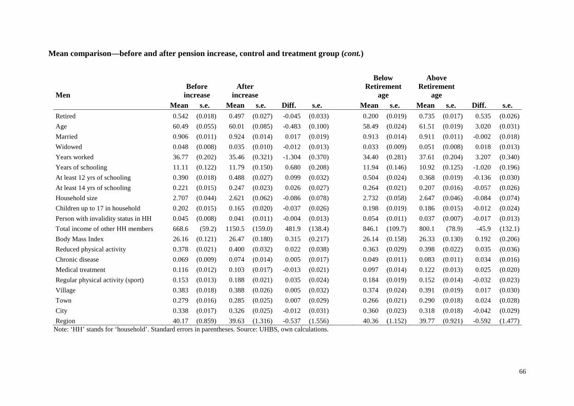
66
Mean comparison—before and after pension increase, control and treatment group (cont.)
Men Before
increase After
increase
Below Retirement
age
Above Retirement
age Mean s.e. Mean s.e. Diff. s.e. Mean s.e. Mean s.e. Diff. s.e. Retired 0.542 (0.018) 0.497 (0.027) -0.045 (0.033) 0.200 (0.019) 0.735 (0.017) 0.535 (0.026)
Age 60.49 (0.055) 60.01 (0.085) -0.483 (0.100) 58.49 (0.024) 61.51 (0.019) 3.020 (0.031)
Married 0.906 (0.011) 0.924 (0.014) 0.017 (0.019) 0.913 (0.014) 0.911 (0.011) -0.002 (0.018)
Widowed 0.048 (0.008) 0.035 (0.010) -0.012 (0.013) 0.033 (0.009) 0.051 (0.008) 0.018 (0.013)
Years worked 36.77 (0.202) 35.46 (0.321) -1.304 (0.370) 34.40 (0.281) 37.61 (0.204) 3.207 (0.340)
Years of schooling 11.11 (0.122) 11.79 (0.150) 0.680 (0.208) 11.94 (0.146) 10.92 (0.125) -1.020 (0.196)
At least 12 yrs of schooling 0.390 (0.018) 0.488 (0.027) 0.099 (0.032) 0.504 (0.024) 0.368 (0.019) -0.136 (0.030)
At least 14 yrs of schooling 0.221 (0.015) 0.247 (0.023) 0.026 (0.027) 0.264 (0.021) 0.207 (0.016) -0.057 (0.026)
Household size 2.707 (0.044) 2.621 (0.062) -0.086 (0.078) 2.732 (0.058) 2.647 (0.046) -0.084 (0.074)
Children up to 17 in household 0.202 (0.015) 0.165 (0.020) -0.037 (0.026) 0.198 (0.019) 0.186 (0.015) -0.012 (0.024)
Person with invalidity status in HH 0.045 (0.008) 0.041 (0.011) -0.004 (0.013) 0.054 (0.011) 0.037 (0.007) -0.017 (0.013)
Total income of other HH members 668.6 (59.2) 1150.5 (159.0) 481.9 (138.4) 846.1 (109.7) 800.1 (78.9) -45.9 (132.1)
Body Mass Index 26.16 (0.121) 26.47 (0.180) 0.315 (0.217) 26.14 (0.158) 26.33 (0.130) 0.192 (0.206)
Reduced physical activity 0.378 (0.021) 0.400 (0.032) 0.022 (0.038) 0.363 (0.029) 0.398 (0.022) 0.035 (0.036)
Chronic disease 0.069 (0.009) 0.074 (0.014) 0.005 (0.017) 0.049 (0.011) 0.083 (0.011) 0.034 (0.016)
Medical treatment 0.116 (0.012) 0.103 (0.017) -0.013 (0.021) 0.097 (0.014) 0.122 (0.013) 0.025 (0.020)
Regular physical activity (sport) 0.153 (0.013) 0.188 (0.021) 0.035 (0.024) 0.184 (0.019) 0.152 (0.014) -0.032 (0.023)
Village 0.383 (0.018) 0.388 (0.026) 0.005 (0.032) 0.374 (0.024) 0.391 (0.019) 0.017 (0.030)
Town 0.279 (0.016) 0.285 (0.025) 0.007 (0.029) 0.266 (0.021) 0.290 (0.018) 0.024 (0.028)
City 0.338 (0.017) 0.326 (0.025) -0.012 (0.031) 0.360 (0.023) 0.318 (0.018) -0.042 (0.029)
Region 40.17 (0.859) 39.63 (1.316) -0.537 (1.556) 40.36 (1.152) 39.77 (0.921) -0.592 (1.477) Note: ‘HH’ stands for ‘household’. Standard errors in parentheses. Source: UHBS, own calculations.
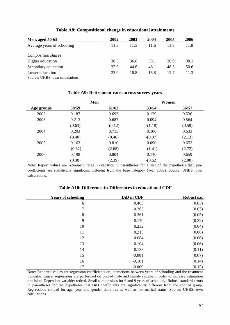
67
Table A8: Compositional change in educational attainments
Men, aged 50-65 2002 2003 2004 2005 2006 Average years of schooling 11.3 11.5 11.6 11.8 11.8
Composition shares Higher education 38.3 36.6 38.1 38.9 38.1 Secondary education 37.9 44.6 46.1 48.5 50.6 Lower education 23.9 18.8 15.8 12.7 11.3 Source: UHBS, own calculations.
Table A9: Retirement rates across survey years
Men Women Age groups 58/59 61/62 53/54 56/57
2002 0.187 0.692 0.129 0.536 2003 0.213 0.687 0.094 0.564
(0.63) -(0.12) -(1.18) (0.59) 2004 0.203 0.715 0.100 0.633
(0.40) (0.46) -(0.97) (2.13) 2005 0.163 0.816 0.090 0.652
-(0.62) (2.68) -(1.41) (2.72) 2006 0.198 0.804 0.110 0.659
(0.30) (2.39) -(0.62) (2.90) Note: Report values are retirement rates. T-statistics in parentheses for a test of the hypothesis that year coefficients are statistically significant different from the base category (year 2002). Source: UHBS, own calculations.
Table A10: Difference-in-Differences in educational CDF
Years of schooling DiD in CDF Robust s.e. 6 0.403 (0.03) 7 0.363 (0.03) 8 0.361 (0.05) 9 0.170 (0.22)
10 0.232 (0.04) 11 0.215 (0.06) 12 0.084 (0.06) 13 0.104 (0.06) 14 0.138 (0.11) 15 -0.081 (0.07) 16 -0.101 (0.14) 17 -0.009 (0.15)
Note: Reported values are regression coefficients on interactions between years of schooling and the treatment indicator. Linear regressions are performed on pooled male and female sample in order to increase estimation precision. Dependent variable: retired. Small sample sizes for 6 and 9 years of schooling. Robust standard errors in parentheses for the hypotheses that DiD coefficients are significantly different from the control group. Regressions control for age, year and gender dummies as well as for marital status. Source: UHBS, own calculations.
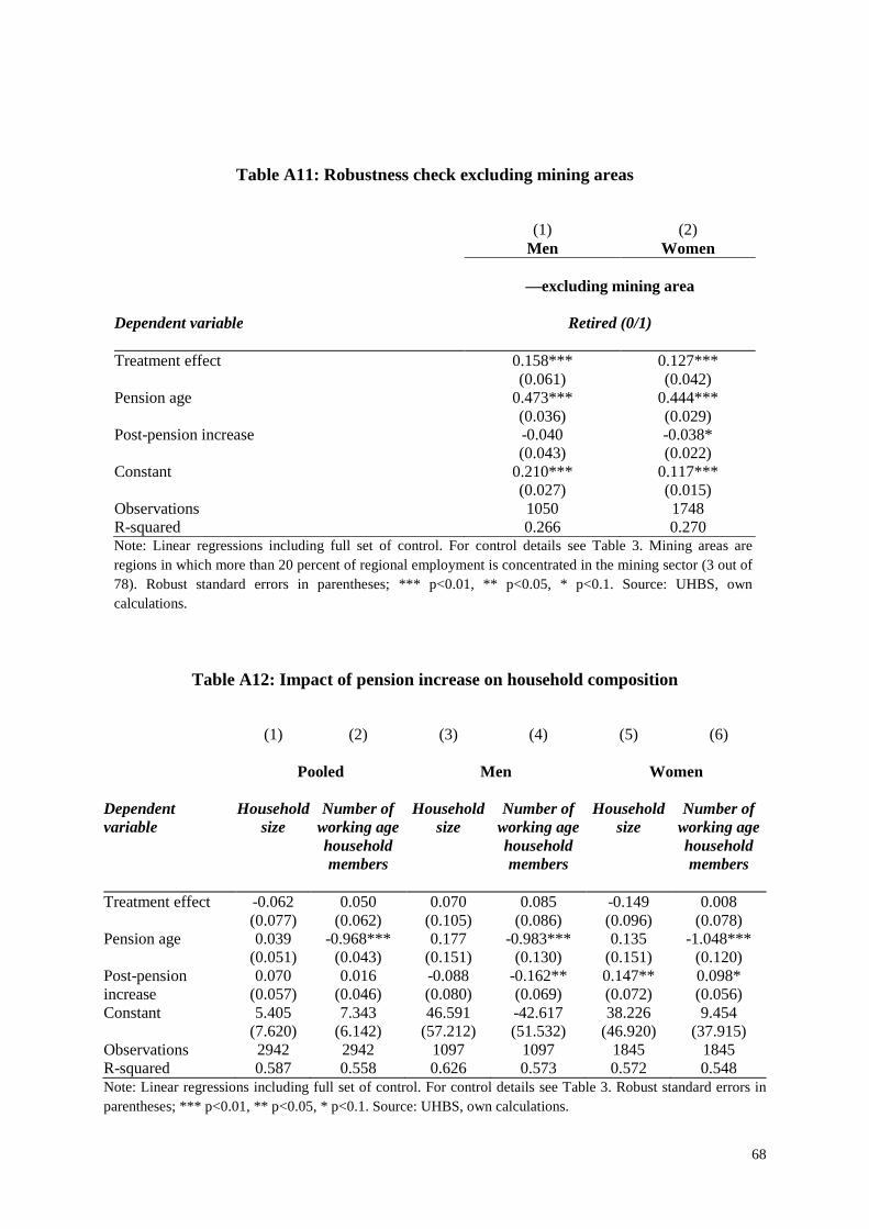
68
Table A11: Robustness check excluding mining areas
(1) (2) Men Women
—excluding mining area
Dependent variable Retired (0/1) Treatment effect 0.158*** 0.127*** (0.061) (0.042) Pension age 0.473*** 0.444*** (0.036) (0.029) Post-pension increase -0.040 -0.038* (0.043) (0.022) Constant 0.210*** 0.117*** (0.027) (0.015) Observations 1050 1748 R-squared 0.266 0.270 Note: Linear regressions including full set of control. For control details see Table 3. Mining areas are regions in which more than 20 percent of regional employment is concentrated in the mining sector (3 out of 78). Robust standard errors in parentheses; *** p<0.01, ** p<0.05, * p<0.1. Source: UHBS, own calculations.
Table A12: Impact of pension increase on household composition
(1) (2) (3) (4) (5) (6)
Pooled Men Women Dependent variable
Household size
Number of working age household members
Household size
Number of working age household members
Household size
Number of working age household members
Treatment effect -0.062 0.050 0.070 0.085 -0.149 0.008 (0.077) (0.062) (0.105) (0.086) (0.096) (0.078) Pension age 0.039 -0.968*** 0.177 -0.983*** 0.135 -1.048*** (0.051) (0.043) (0.151) (0.130) (0.151) (0.120) Post-pension increase
0.070 0.016 -0.088 -0.162** 0.147** 0.098* (0.057) (0.046) (0.080) (0.069) (0.072) (0.056)
Constant 5.405 7.343 46.591 -42.617 38.226 9.454 (7.620) (6.142) (57.212) (51.532) (46.920) (37.915) Observations 2942 2942 1097 1097 1845 1845 R-squared 0.587 0.558 0.626 0.573 0.572 0.548 Note: Linear regressions including full set of control. For control details see Table 3. Robust standard errors in parentheses; *** p<0.01, ** p<0.05, * p<0.1. Source: UHBS, own calculations.

69
Table A13: Labor supply effect of pension increase
(1) (2) Pooled, no household
re-formation Pooled, with household
re-formation
Dependent variable Retired (0/1)
Treatment effect 0.150*** 0.139*** (0.045) (0.041) Pension age 0.344*** 0.332*** (0.029) (0.024)
Post-pension increase 0.045 0.041 (0.036) (0.033) Constant 0.156 0.150 (0.323) (0.281) Observations 1078 1339 R-squared 0.156 0.168 Note: Regressions control for age dummies, gender, marital status, education, chronic diseases, household size, presence of children in household, income generated by other household members, region of settlement. Age brackets +/- 3 age cohorts around pension age with year of pension age excluded. Retirement defined by eligibility. Column (1) excludes households which changed composition between 2004 and 2007. Robust standard errors clustered by household size in parentheses; *** p<0.01, ** p<0.05, * p<0.1. Source: ULMS 2003-2007, own calculations.
Table A14: Retirement and eligibility of couples
Age of Husband Age of Wife 50-54 55-59 60-64 65-69 70-74
50-54 2003 7.4% 16.7% 59.6% a a 2005 9.6% 13.0% 50.0% 73.7% a sig. * ** *
55-59 2003 41.0% 46.6% 76.5% 88.5% a 2005 42.0% 54.8% 81.9% 86.7% a sig. ** **
60-64 2003 a 82.6% 88.9% 93.8% 100% 2005 a 81.3% 89.2% 92.9% 100% sig.
65-69 2003 a a 92.1% 95.6% 97.6% 2005 a a 96.2% 96.6% 95.3% sig. * *
70-74 2003 a a a 97.1% 99.1% 2005 a a a 100% 100% sig. *
Note: a. Less than 30 obs. in cell. Framed numbers contain between 30 and 40 observations. Cells report share of couples with at least one partner retired. Shaded area marks retirement eligibility of at least one
partner. *** p<0.01, ** p<0.05, * p<0.1. Source: UHBS, own calculations.

70
Table A15: Share of jointly retired couples
Age of Husband Age of Wife 50-54 55-59 60-64 65-69 70-74
50-54 2003 14.3% 17.6% 9.7% a a 2005 10.3% 12.9% 5.9% a a sig.
55-59 2003 0.0% 16.2% 53.8% 72.2% a 2005 4.8% 11.4% 65.6% 75.0% a sig. * ***
60-64 2003 a 21.1% 75.0% 76.4% 83.0%
2005 a 11.5% 77.4% 79.8% 81.5% sig.
65-69 2003 a a 75.9% 77.7% 88.4% 2005 a a 76.5% 83.2% 88.8% sig. **
70-74 2003 a a a 93.9% 91.8% 2005 a a a 88.6% 93.8% sig.
Note: a. Less than 30 obs. in cell. Framed numbers contain between 30 and 40 observations. Cells report share of jointly retired couples in all couples with at least one partner retired. Shaded area marks age of joint normal pension age. *** p<0.01, ** p<0.05, * p<0.1. Source: UHBS, own calculations.

71
Table A16: Difference-in-Differences—choice of comparison bandwidth
(1) (2) (3) (4) (5) Dependent variable Retired (0/1)
1 year 2 years 3 years 4 years 5 years
Men Treatment effect 0.223*** 0.176*** 0.146*** 0.118*** 0.105*** (0.086) (0.059) (0.045) (0.037) (0.031) Constant 0.297*** 0.215*** 0.199*** 0.184*** 0.166*** (0.044) (0.027) (0.021) (0.018) (0.014) Observations 538 1097 1729 2472 3226 R-squared 0.194 0.272 0.311 0.340 0.381
Women Treatment effect 0.101* 0.133*** 0.091*** 0.077*** 0.057** (0.057) (0.041) (0.033) (0.028) (0.025) Constant 0.124*** 0.111*** 0.099*** 0.084*** 0.073*** (0.021) (0.015) (0.011) (0.009) (0.007) Observations 996 1845 2675 3555 4398 R-squared 0.216 0.271 0.318 0.372 0.414 Note: Linear regressions including full set of control. For control details see Table 3. Robust standard errors in parentheses; *** p<0.01, ** p<0.05, * p<0.1. Source: UHBS, own calculations.

72
Table A17: Difference-in-Differences—yearly working hours
(1) (2) (3) (4) Full sample Men Women Educational
category 1
Dependent variable Yearly working hours Without Controls
Treatment effect -94.95 114.41 -280.46*** -460.05** (59.63) (80.65) (86.01) (200.69) Constant 1,722.59*** 2,086.04*** 1,626.93*** 1,360.62*** (122.95) (95.83) (251.90) (415.32) Goodness of fit (ρ²) 0.178 0.169 0.109 0.041 Observations 1877 902 976 211 Number of truncated observations 2794 999 1795 872 Full controls
Treatment effect -119.99** 50.90 -281.12*** -449.02** (60.88) (81.48) (84.86) (226.29) Constant 1,924.74* 2,799.48** 917.38 1,868.49 (1,084.40) (1,374.40) (798.14) (1,802.27) Goodness of fit (ρ²) 0.049 0.058 0. 045 0.061 Observations 1740 833 906 192 Number of truncated observations 2623 941 1682 815 Note: Table reports estimates from a truncated linear regression, truncation at zero. Regressions with no controls include a gender dummy and year of birth fixed effects. Full controls include region and settlement type fixed effects, age, years of schooling, marital status (married, widowed, single or separated), a dummy for one out of seven chronic diseases, children up to age 17 present in household, household size, total income of other household members. Robust standard errors in parentheses, clustered by id; *** p<0.01, ** p<0.05, * p<0.1. Source: ULMS, own calculations.
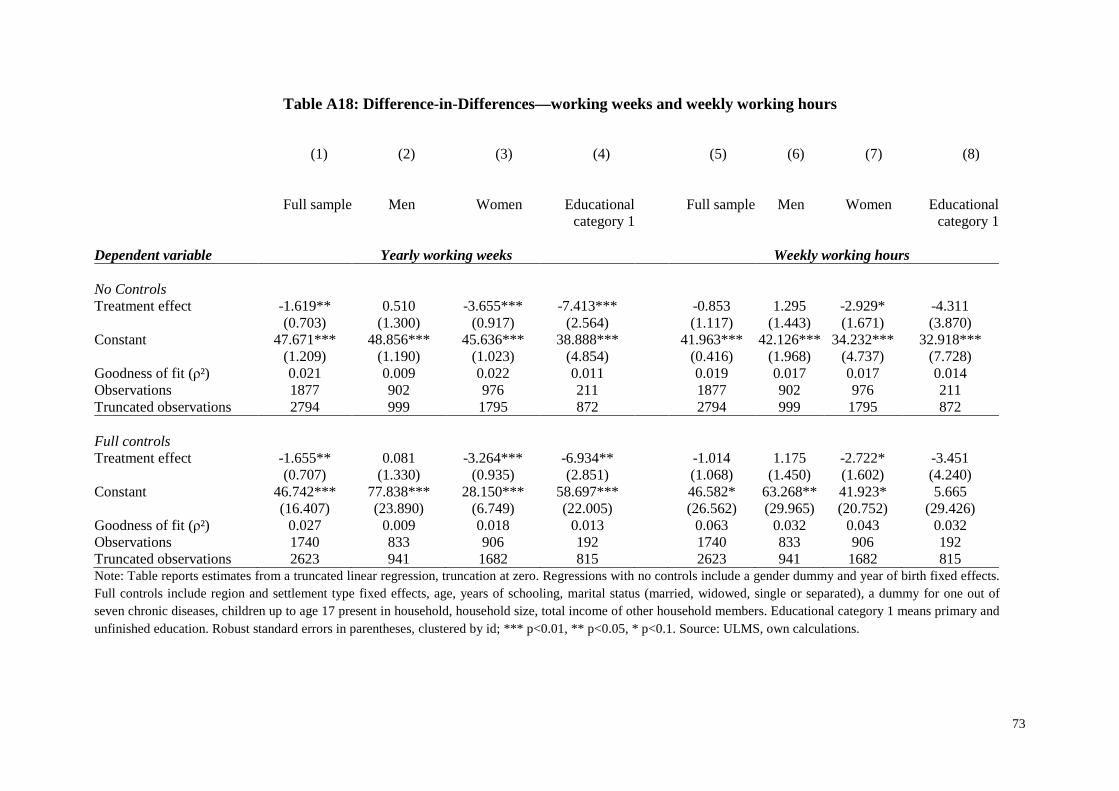
73
Table A18: Difference-in-Differences—working weeks and weekly working hours
(1) (2) (3) (4) (5) (6) (7) (8)
Full sample Men Women Educational category 1
Full sample Men Women Educational category 1
Dependent variable Yearly working weeks Weekly working hours
No Controls Treatment effect -1.619** 0.510 -3.655*** -7.413*** -0.853 1.295 -2.929* -4.311 (0.703) (1.300) (0.917) (2.564) (1.117) (1.443) (1.671) (3.870) Constant 47.671*** 48.856*** 45.636*** 38.888*** 41.963*** 42.126*** 34.232*** 32.918*** (1.209) (1.190) (1.023) (4.854) (0.416) (1.968) (4.737) (7.728) Goodness of fit (ρ²) 0.021 0.009 0.022 0.011 0.019 0.017 0.017 0.014 Observations 1877 902 976 211 1877 902 976 211 Truncated observations 2794 999 1795 872 2794 999 1795 872 Full controls
Treatment effect -1.655** 0.081 -3.264*** -6.934** -1.014 1.175 -2.722* -3.451 (0.707) (1.330) (0.935) (2.851) (1.068) (1.450) (1.602) (4.240) Constant 46.742*** 77.838*** 28.150*** 58.697*** 46.582* 63.268** 41.923* 5.665 (16.407) (23.890) (6.749) (22.005) (26.562) (29.965) (20.752) (29.426) Goodness of fit (ρ²) 0.027 0.009 0.018 0.013 0.063 0.032 0.043 0.032 Observations 1740 833 906 192 1740 833 906 192 Truncated observations 2623 941 1682 815 2623 941 1682 815 Note: Table reports estimates from a truncated linear regression, truncation at zero. Regressions with no controls include a gender dummy and year of birth fixed effects. Full controls include region and settlement type fixed effects, age, years of schooling, marital status (married, widowed, single or separated), a dummy for one out of seven chronic diseases, children up to age 17 present in household, household size, total income of other household members. Educational category 1 means primary and unfinished education. Robust standard errors in parentheses, clustered by id; *** p<0.01, ** p<0.05, * p<0.1. Source: ULMS, own calculations.
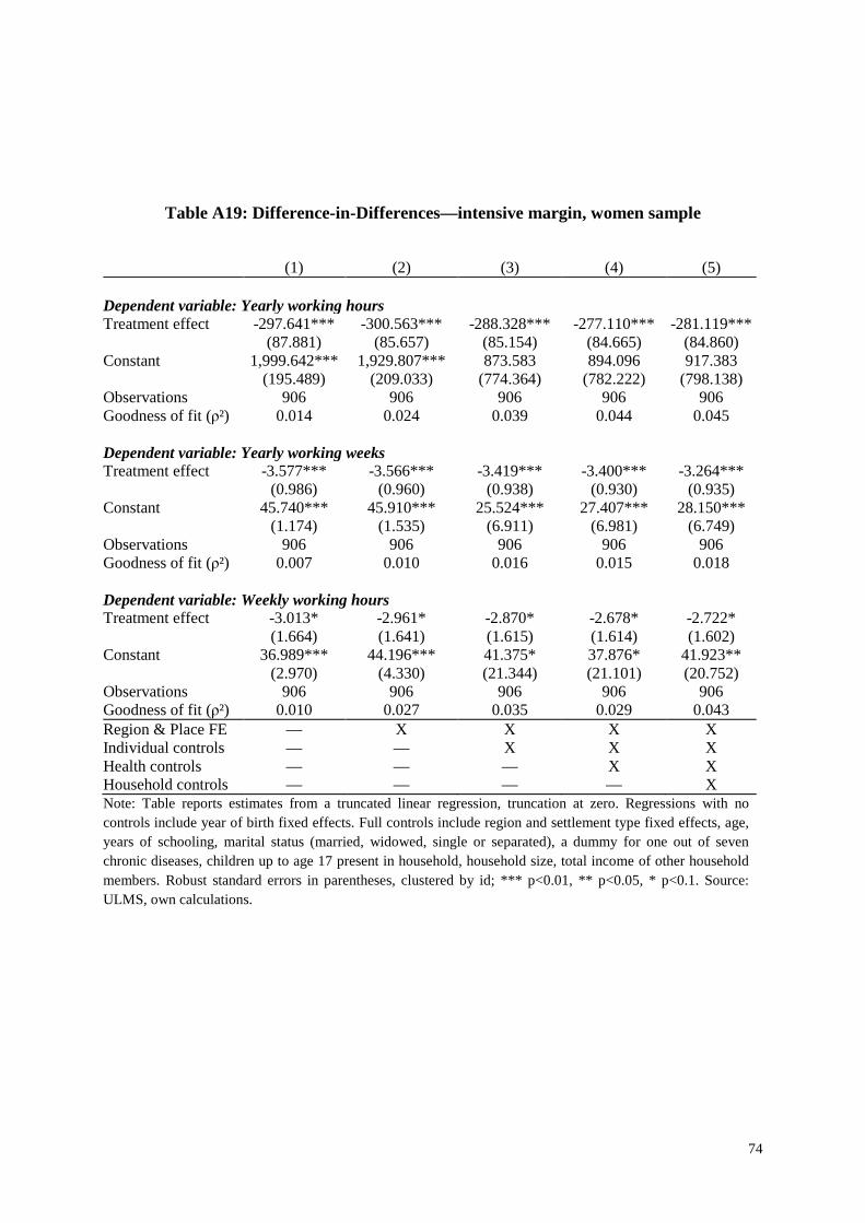
74
Table A19: Difference-in-Differences—intensive margin, women sample
(1) (2) (3) (4) (5) Dependent variable: Yearly working hours Treatment effect -297.641*** -300.563*** -288.328*** -277.110*** -281.119*** (87.881) (85.657) (85.154) (84.665) (84.860) Constant 1,999.642*** 1,929.807*** 873.583 894.096 917.383 (195.489) (209.033) (774.364) (782.222) (798.138) Observations 906 906 906 906 906 Goodness of fit (ρ²) 0.014 0.024 0.039 0.044 0.045 Dependent variable: Yearly working weeks Treatment effect -3.577*** -3.566*** -3.419*** -3.400*** -3.264*** (0.986) (0.960) (0.938) (0.930) (0.935) Constant 45.740*** 45.910*** 25.524*** 27.407*** 28.150*** (1.174) (1.535) (6.911) (6.981) (6.749) Observations 906 906 906 906 906 Goodness of fit (ρ²) 0.007 0.010 0.016 0.015 0.018 Dependent variable: Weekly working hours Treatment effect -3.013* -2.961* -2.870* -2.678* -2.722* (1.664) (1.641) (1.615) (1.614) (1.602) Constant 36.989*** 44.196*** 41.375* 37.876* 41.923** (2.970) (4.330) (21.344) (21.101) (20.752) Observations 906 906 906 906 906 Goodness of fit (ρ²) 0.010 0.027 0.035 0.029 0.043 Region & Place FE — X X X X Individual controls — — X X X Health controls — — — X X Household controls — — — — X Note: Table reports estimates from a truncated linear regression, truncation at zero. Regressions with no controls include year of birth fixed effects. Full controls include region and settlement type fixed effects, age, years of schooling, marital status (married, widowed, single or separated), a dummy for one out of seven chronic diseases, children up to age 17 present in household, household size, total income of other household members. Robust standard errors in parentheses, clustered by id; *** p<0.01, ** p<0.05, * p<0.1. Source: ULMS, own calculations.
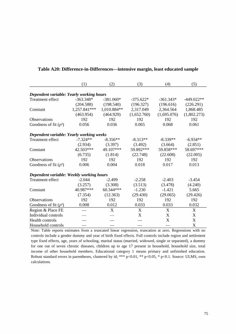
75
Table A20: Difference-in-Differences—intensive margin, least educated sample
(1) (2) (3) (4) (5) Dependent variable: Yearly working hours Treatment effect -363.348* -381.060* -375.622* -361.343* -449.022** (204.588) (198.540) (196.327) (196.616) (226.291) Constant 1,257.841*** 1,010.884** 2,317.049 2,364.564 1,868.485 (463.954) (464.929) (1,652.760) (1,695.076) (1,802.273) Observations 192 192 192 192 192 Goodness of fit (ρ²) 0.056 0.036 0.065 0.068 0.061 Dependent variable: Yearly working weeks Treatment effect -7.324** -8.356** -8.313** -8.339** -6.934** (2.934) (3.397) (3.492) (3.664) (2.851) Constant 42.503*** 49.107*** 59.892*** 59.858*** 58.697*** (6.735) (1.814) (22.748) (22.608) (22.005) Observations 192 192 192 192 192 Goodness of fit (ρ²) 0.006 0.004 0.018 0.017 0.013 Dependent variable: Weekly working hours Treatment effect -2.044 -2.499 -2.258 -2.403 -3.454 (3.257) (3.308) (3.513) (3.478) (4.240) Constant 40.987*** 60.344*** -1.230 -1.421 5.665 (7.354) (12.363) (29.430) (29.065) (29.426) Observations 192 192 192 192 192 Goodness of fit (ρ²) 0.008 0.012 0.033 0.033 0.032 Region & Place FE — X X X X Individual controls — — X X X Health controls — — — X X Household controls — — — — X Note: Table reports estimates from a truncated linear regression, truncation at zero. Regressions with no controls include a gender dummy and year of birth fixed effects. Full controls include region and settlement type fixed effects, age, years of schooling, marital status (married, widowed, single or separated), a dummy for one out of seven chronic diseases, children up to age 17 present in household, household size, total income of other household members. Educational category 1 means primary and unfinished education. Robust standard errors in parentheses, clustered by id; *** p<0.01, ** p<0.05, * p<0.1. Source: ULMS, own calculations.

76
Table A21: Robustness checks for labor supply responses at intensive margin
(1) (2) (3) (4)
(5) (6)
Full sample Sub sample of (1)
Baseline Random effects
Controlling for
occupation 1986
Chronic=0 Chronic=1 Only households
without change in
composition Dependent variable Yearly working hours Women Treatment effect -265.7*** -228.8*** -260.3*** 36.4 -354.4*** -244.1*** (84.1) (77.0) (89.8) (179.8) (89.0) (91.3) Constant 1,267.3 1,536.9 2,315.8* 225.9 954.5 (942.8) (1,055.3) (1,395.2) (1,160.7) (1,064.7) Observations 906 906 832 249 657 713
R-squared 0.003 0.132 0.000 0.000 0.018 0.013 Hausman test Prob>chi2
0.18
Least educated Treatment effect -449.0** -459.7* -375.52 -831.2* -201.1 -457.5** (226.3) (256.3) (259.69) (425.0) (225.7) (221.7) Constant 1,868.5 1,523.7 -7,446.1*** 1,401.7 3,341.0* (1,802.3) (1,493.4) (2,782.3) (2,422.3) (1,744.6) Observations 192 192 173 60 132 156
R-squared 0.061 0.282 0.046 0.021 0.054 0.076 Hausman test Prob>chi2
0.99
Note: All regressions include full set of controls (see Table 3). Regressions (1) and (3)-(6) are truncated linear regressions. Standard error clustered by id. Regression (2) is a random effects panel regression. The Hausman statistics tests the null hypothesis that there are no systematic differences in coefficients from random effects vs. fixed effects model (the latter not shown). *** p<0.01, ** p<0.05, * p<0.1. Source ULMS, own calculations.