The Study and Shielding of Electromagnetic Radiation from SuperKEKB Electron andPositron Beam Interactions

by

Alexandre BeaulieuBEng, Universite de Sherbrooke, 2009MASc, Universite de Sherbrooke, 2011

MSc, University of Victoria, 2013

A Dissertation submitted in partial fulfilment of therequirements for the degree of

Doctor of Philosophy

in the Department of Physics and Astronomy

© Alexandre Beaulieu, 2019University of Victoria

All rights reserved. This dissertation may not be reproduced in whole or in part, byphotocopy or other means, without the permission of the author.

Supervisory Committee

The Study and Shielding of Electromagnetic Radiation from SuperKEKB Electron andPositron Beam Interactions

by

Alexandre BeaulieuBEng, Universite de Sherbrooke, 2009MASc, Universite de Sherbrooke, 2011

MSc, University of Victoria, 2013

Supervisory Committee

Dr. J. M. Roney, Supervisor(Department of Physics and Astronomy)

Dr. M. Pospelov, Department Member(Department of Physics and Astronomy)

Dr. C. Bradley, Outside Member(Department of Mechanical Engineering)

ii

Abstract

This project contributes to the research and development studies towards successful com-missioning of the SuperKEKB electron-positron collider. This accelerator and storage ringscomplex aims at delivering the high-luminosity collisions of beams of electrons and posi-trons needed for the Belle II experiment. Such beams produce parasitic radiation — called“machine-induced backgrounds”, or simply “beam backgrounds” — that have detrimen-tal effects on the experimental apparatus performance and durability. The Beast II effort isdedicated to measuring the beam backgrounds, and aims at testing the predictive powerof the background models that were used in various phases of the Belle II design. A sec-ond objective is to ensure that the environment is safe for the detector prior to installing itaround the beam lines.

A major component of beam backgrounds consists of electromagnetic radiation. Thisstudy focusses on measuring this radiation at the location of the Belle II electromagneticcalorimeter. The measurements were achieved by placing scintillator crystals at positionsrepresentative of the Belle II calorimeter crystals that are the closest to the beam lines, andcomparing the data with predictions for different operating parameters of the accelerator.

Different phenomena related to machine backgrounds were observed: vacuum scrubbing,the electron-cloud effect, injection-related noise, beam-gas scattering and Touschek losses.Studies on the positron ring showed average background levels 13.5± 3.5 times larger thansimulation, whereas that ratio reachedO (102 − 103) for the electron ring. In the latter, thelarge uncertainty on the pressure measurements and the gas constituents limit the predic-tive power of the measurements. Radiation shields were also designed, fabricated, deliv-ered and installed in the detector to protect the electromagnetic calorimeter from radiationcoming from the beam lines.

iii

Contents

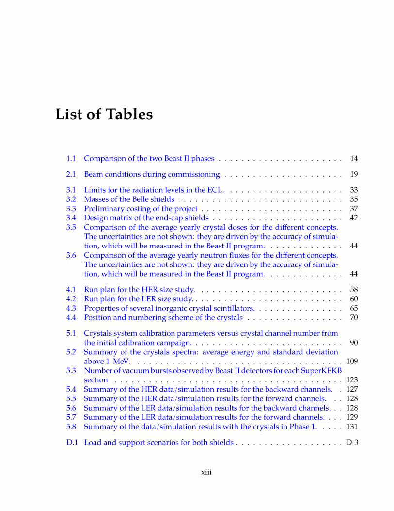
Supervisory Committee . . . . . . . . . . . . . . . . . . . . . . . . . . . . . . iiAbstract . . . . . . . . . . . . . . . . . . . . . . . . . . . . . . . . . . . . . . . iiiContents . . . . . . . . . . . . . . . . . . . . . . . . . . . . . . . . . . . . . . . ivList of Figures . . . . . . . . . . . . . . . . . . . . . . . . . . . . . . . . . . . . viiiList of Tables . . . . . . . . . . . . . . . . . . . . . . . . . . . . . . . . . . . . . xiiiAcknowledgements . . . . . . . . . . . . . . . . . . . . . . . . . . . . . . . . . xvDedication . . . . . . . . . . . . . . . . . . . . . . . . . . . . . . . . . . . . . . xviPersonal contributions to Belle II . . . . . . . . . . . . . . . . . . . . . . . . . xvii

1 Introduction 11.1 The Belle II experiment . . . . . . . . . . . . . . . . . . . . . . . . . . . . . . . 1

1.1.1 The Physics program . . . . . . . . . . . . . . . . . . . . . . . . . . . . 21.1.2 The accelerator: SuperKEKB . . . . . . . . . . . . . . . . . . . . . . . 51.1.3 The detector: Belle II . . . . . . . . . . . . . . . . . . . . . . . . . . . . 8

1.2 Beam-induced background and measurement . . . . . . . . . . . . . . . . . 121.2.1 Overview . . . . . . . . . . . . . . . . . . . . . . . . . . . . . . . . . . 121.2.2 Beast II, the accelerator commissioning detector . . . . . . . . . . . . 13

1.3 The research question . . . . . . . . . . . . . . . . . . . . . . . . . . . . . . . . 131.4 Goals of the project . . . . . . . . . . . . . . . . . . . . . . . . . . . . . . . . . 13

1.4.1 General goal . . . . . . . . . . . . . . . . . . . . . . . . . . . . . . . . . 131.4.2 Specific goals . . . . . . . . . . . . . . . . . . . . . . . . . . . . . . . . 15

1.5 Dissertation outline . . . . . . . . . . . . . . . . . . . . . . . . . . . . . . . . . 15

2 Source of accelerator-induced background at Belle II and their mitigation 172.1 The beams circulating at SuperKEKB . . . . . . . . . . . . . . . . . . . . . . . 17

2.1.1 Electron production . . . . . . . . . . . . . . . . . . . . . . . . . . . . 172.1.2 Positron production . . . . . . . . . . . . . . . . . . . . . . . . . . . . 182.1.3 Storage and beam structure . . . . . . . . . . . . . . . . . . . . . . . . 182.1.4 Beam conditions during commissioning . . . . . . . . . . . . . . . . . 18

2.2 Main background sources at Belle II . . . . . . . . . . . . . . . . . . . . . . . 182.2.1 Touschek radiation . . . . . . . . . . . . . . . . . . . . . . . . . . . . . 202.2.2 Beam-gas interactions . . . . . . . . . . . . . . . . . . . . . . . . . . . 212.2.3 Injection particle losses . . . . . . . . . . . . . . . . . . . . . . . . . . . 22

iv

2.2.4 Electron cloud effect . . . . . . . . . . . . . . . . . . . . . . . . . . . . 242.2.5 Beam-dust events . . . . . . . . . . . . . . . . . . . . . . . . . . . . . . 24

2.3 Background mitigation measures present at Belle II . . . . . . . . . . . . . . 252.3.1 Vacuum chamber design . . . . . . . . . . . . . . . . . . . . . . . . . . 252.3.2 Collimators . . . . . . . . . . . . . . . . . . . . . . . . . . . . . . . . . 272.3.3 ECL shields . . . . . . . . . . . . . . . . . . . . . . . . . . . . . . . . . 27

3 Design and construction of ECL radiation shields 303.1 Project definition: context, requirements, and deliverables . . . . . . . . . . 31

3.1.1 The end users . . . . . . . . . . . . . . . . . . . . . . . . . . . . . . . . 313.1.2 Performance goals . . . . . . . . . . . . . . . . . . . . . . . . . . . . . 323.1.3 Design constraints . . . . . . . . . . . . . . . . . . . . . . . . . . . . . 333.1.4 Deliverables . . . . . . . . . . . . . . . . . . . . . . . . . . . . . . . . . 36

3.2 Conceptual design . . . . . . . . . . . . . . . . . . . . . . . . . . . . . . . . . 383.2.1 Methodology . . . . . . . . . . . . . . . . . . . . . . . . . . . . . . . . 383.2.2 Concepts studied . . . . . . . . . . . . . . . . . . . . . . . . . . . . . . 413.2.3 Results . . . . . . . . . . . . . . . . . . . . . . . . . . . . . . . . . . . . 433.2.4 Discussion and recommendations . . . . . . . . . . . . . . . . . . . . 46

3.3 Technical design . . . . . . . . . . . . . . . . . . . . . . . . . . . . . . . . . . . 493.3.1 General design of the shields . . . . . . . . . . . . . . . . . . . . . . . 493.3.2 Structural analyses . . . . . . . . . . . . . . . . . . . . . . . . . . . . . 503.3.3 Final detailed designs . . . . . . . . . . . . . . . . . . . . . . . . . . . 523.3.4 Commissioning . . . . . . . . . . . . . . . . . . . . . . . . . . . . . . . 53

4 Experimental methodology for measuring single-beam-induced electromagneticradiation 564.1 Background studies in the first phase of beam commissioning . . . . . . . . 56

4.1.1 Influence of pressure . . . . . . . . . . . . . . . . . . . . . . . . . . . . 574.1.2 Influence of beam size . . . . . . . . . . . . . . . . . . . . . . . . . . . 584.1.3 Influence of injection efficiency . . . . . . . . . . . . . . . . . . . . . . 61

4.2 Analysis of residual gas constituents . . . . . . . . . . . . . . . . . . . . . . . 624.2.1 Gas model . . . . . . . . . . . . . . . . . . . . . . . . . . . . . . . . . . 624.2.2 Calculation of the proportion of each gas . . . . . . . . . . . . . . . . 634.2.3 Calculation of an effective Z for this gas mixture . . . . . . . . . . . . 634.2.4 Propagation of uncertainties . . . . . . . . . . . . . . . . . . . . . . . 63

4.3 Detectors and technology overview . . . . . . . . . . . . . . . . . . . . . . . . 644.3.1 CsI(Tl), CsI(pure) and LYSO crystal scintillators . . . . . . . . . . . . 644.3.2 Photo-detectors . . . . . . . . . . . . . . . . . . . . . . . . . . . . . . . 664.3.3 Mechanical integration . . . . . . . . . . . . . . . . . . . . . . . . . . . 684.3.4 Signal chain and data acquisition . . . . . . . . . . . . . . . . . . . . . 71

4.4 Calibration . . . . . . . . . . . . . . . . . . . . . . . . . . . . . . . . . . . . . . 724.4.1 Dedicated campaign . . . . . . . . . . . . . . . . . . . . . . . . . . . . 72

v

4.4.2 Time-dependence of the gain . . . . . . . . . . . . . . . . . . . . . . . 744.5 Comparisons between data and simulation . . . . . . . . . . . . . . . . . . . 75

4.5.1 Heuristic description of background measurements . . . . . . . . . . 754.5.2 Re-weighting procedure for simulated data . . . . . . . . . . . . . . . 774.5.3 Hypotheses related with the vacuum chamber pressure and gas con-

stituents . . . . . . . . . . . . . . . . . . . . . . . . . . . . . . . . . . . 784.5.4 The data-to-simulation ratio . . . . . . . . . . . . . . . . . . . . . . . . 794.5.5 Statistical uncertainty . . . . . . . . . . . . . . . . . . . . . . . . . . . 794.5.6 Systematic uncertainties . . . . . . . . . . . . . . . . . . . . . . . . . . 79

4.6 Beam-gas interactions and beam conditions evolution in Phase 1 . . . . . . . 844.6.1 Vacuum scrubbing . . . . . . . . . . . . . . . . . . . . . . . . . . . . . 844.6.2 Analysis of transient “beam-dust” events . . . . . . . . . . . . . . . . 87

5 Results and simulation 895.1 Specific results from the CsI(Tl), CsI(pure) and LYSO system . . . . . . . . 89

5.1.1 Calibration and time-dependence of the gain . . . . . . . . . . . . . . 895.1.2 Energy spectra for different conditions . . . . . . . . . . . . . . . . . . 91

5.2 Beam-gas interactions and beam conditions evolution in Phase 1 . . . . . . . 1105.2.1 Effect of gas mixture on beam backgrounds . . . . . . . . . . . . . . . 1105.2.2 Time series of pressures, background and effective atomic number

in pressure bump experiments . . . . . . . . . . . . . . . . . . . . . . 1125.2.3 Uncertainty on Ze . . . . . . . . . . . . . . . . . . . . . . . . . . . . . . 1135.2.4 Vacuum scrubbing and dynamic pressure . . . . . . . . . . . . . . . . 1155.2.5 Transient “beam-dust” events . . . . . . . . . . . . . . . . . . . . . . . 118

5.3 Quantitative comparison of data and simulation . . . . . . . . . . . . . . . . 1255.4 Extrapolation to commissioning phases 2 and 3 . . . . . . . . . . . . . . . . . 131

5.4.1 Phase 2 of commissioning: L = 5.4× 1033 cm−2s−1 . . . . . . . . . . 1335.4.2 Early physics operation: L = 5× 1034 cm−2s−1 . . . . . . . . . . . . . 1345.4.3 Full design luminosity: L = 8× 1035 cm−2s−1 . . . . . . . . . . . . . 136

6 Concluding remarks 1416.1 Aims . . . . . . . . . . . . . . . . . . . . . . . . . . . . . . . . . . . . . . . . . 1416.2 Findings . . . . . . . . . . . . . . . . . . . . . . . . . . . . . . . . . . . . . . . 142

6.2.1 Energy distributions . . . . . . . . . . . . . . . . . . . . . . . . . . . . 1426.2.2 Evolution of beam conditions in Phase 1 . . . . . . . . . . . . . . . . . 1426.2.3 Agreement between data and simulation . . . . . . . . . . . . . . . . 143

6.3 Implications . . . . . . . . . . . . . . . . . . . . . . . . . . . . . . . . . . . . . 1446.3.1 For Belle II . . . . . . . . . . . . . . . . . . . . . . . . . . . . . . . . . . 1446.3.2 For future e+e− colliders . . . . . . . . . . . . . . . . . . . . . . . . . . 144

6.4 Recommendations . . . . . . . . . . . . . . . . . . . . . . . . . . . . . . . . . 1456.4.1 Background measurement methodologies . . . . . . . . . . . . . . . 1456.4.2 Background models . . . . . . . . . . . . . . . . . . . . . . . . . . . . 146

vi

6.4.3 Background management . . . . . . . . . . . . . . . . . . . . . . . . . 1476.5 Final remarks . . . . . . . . . . . . . . . . . . . . . . . . . . . . . . . . . . . . 149

Appendices

A Detailed calibration results A-1A.1 Initial calibration campaign . . . . . . . . . . . . . . . . . . . . . . . . . . . . A-2A.2 Gain degradation as a function of beam dose . . . . . . . . . . . . . . . . . . A-6

B Mechanical Drawings B-1B.1 Belle-II Top View 41.5-R14 . . . . . . . . . . . . . . . . . . . . . . . . . . . . . B-2B.2 ECL Endcap Shields Envelopes ECL-SHLDS-000 . . . . . . . . . . . . . . . . B-3

C Results of the ECL shields conceptual design studies C-1C.1 Without shields . . . . . . . . . . . . . . . . . . . . . . . . . . . . . . . . . . . C-2C.2 Concepts 0 . . . . . . . . . . . . . . . . . . . . . . . . . . . . . . . . . . . . . . C-4C.3 Concepts A1 . . . . . . . . . . . . . . . . . . . . . . . . . . . . . . . . . . . . . C-6C.4 Concepts A2 . . . . . . . . . . . . . . . . . . . . . . . . . . . . . . . . . . . . . C-8C.5 Concepts B1 . . . . . . . . . . . . . . . . . . . . . . . . . . . . . . . . . . . . . C-10C.6 Concepts B2 . . . . . . . . . . . . . . . . . . . . . . . . . . . . . . . . . . . . . C-12C.7 Concepts C1 . . . . . . . . . . . . . . . . . . . . . . . . . . . . . . . . . . . . . C-14C.8 Concepts C2 . . . . . . . . . . . . . . . . . . . . . . . . . . . . . . . . . . . . . C-16

D Detail of the ECL shields technical design D-1D.1 General design of the shields . . . . . . . . . . . . . . . . . . . . . . . . . . . D-1

D.1.1 System of reference . . . . . . . . . . . . . . . . . . . . . . . . . . . . . D-1D.1.2 Applied loads and design safety factor . . . . . . . . . . . . . . . . . D-2

D.2 Design of the backward shield . . . . . . . . . . . . . . . . . . . . . . . . . . . D-9D.2.1 Shell . . . . . . . . . . . . . . . . . . . . . . . . . . . . . . . . . . . . . D-9D.2.2 Electromagnetic radiation shield . . . . . . . . . . . . . . . . . . . . . D-11D.2.3 Neutron shield . . . . . . . . . . . . . . . . . . . . . . . . . . . . . . . D-12D.2.4 Mounting points for transport and installation . . . . . . . . . . . . . D-15D.2.5 Attachments to end-cap . . . . . . . . . . . . . . . . . . . . . . . . . . D-18

D.3 Design of the forward shield . . . . . . . . . . . . . . . . . . . . . . . . . . . . D-23D.3.1 Shell . . . . . . . . . . . . . . . . . . . . . . . . . . . . . . . . . . . . . D-23D.3.2 Electromagnetic Radiation Shield . . . . . . . . . . . . . . . . . . . . . D-27D.3.3 Neutron Shield . . . . . . . . . . . . . . . . . . . . . . . . . . . . . . . D-28D.3.4 Mounting points for transport and installation . . . . . . . . . . . . . D-30D.3.5 Attachments to end-cap . . . . . . . . . . . . . . . . . . . . . . . . . . D-36

D.4 Summary of structural analyses . . . . . . . . . . . . . . . . . . . . . . . . . . D-40D.5 Fabrication and commissioning . . . . . . . . . . . . . . . . . . . . . . . . . . D-42

D.5.1 Vendor . . . . . . . . . . . . . . . . . . . . . . . . . . . . . . . . . . . . D-42D.5.2 Modifications from design drawings . . . . . . . . . . . . . . . . . . . D-42

vii

List of Figures

1.1 Belle II projected luminosity Profile . . . . . . . . . . . . . . . . . . . . . . . . 31.2 Schematic representation of SuperKEKB . . . . . . . . . . . . . . . . . . . . . 61.3 Technical drawing of the SuperKEKB storage rings . . . . . . . . . . . . . . . 71.4 Schematic of the Belle II detector . . . . . . . . . . . . . . . . . . . . . . . . . 81.5 Schematic side-view of TOP counter and internal reflecting Cherenkov pho-

tons . . . . . . . . . . . . . . . . . . . . . . . . . . . . . . . . . . . . . . . . . . 10

2.1 Plot of D (ξ) . . . . . . . . . . . . . . . . . . . . . . . . . . . . . . . . . . . . . 212.2 Background processes from beam-gas scattering . . . . . . . . . . . . . . . . 222.3 Trigger time distributions for LER injection . . . . . . . . . . . . . . . . . . . 232.4 Photograph of the antechamber design of the SuperKEKB vacuum chamber 262.5 Photograph of the permanent magnets around the LER . . . . . . . . . . . . 272.6 Cut-away view of a horizontal collimator system . . . . . . . . . . . . . . . . 282.7 Top view of the Belle-II detector showing the location of the ECL shields . . 29

3.1 Photograph of the forward ECL shield in the first Belle detector. . . . . . . . 313.2 Organisational Chart of the Belle-II Collaboration . . . . . . . . . . . . . . . 323.3 Envelopes available for the ECL end-cap shields represented as cross-sectional

views of axisymmetric volumes. . . . . . . . . . . . . . . . . . . . . . . . . . . 343.4 The photon mass attenuation length (or mean free path) λ = 1/(µ/ρ) . . . 383.5 Hot spot in the forward end-cap from the HER radiative Bhabha sample . . 413.6 Effect of varying the lead thickness on the radiation level safety factor . . . . 453.7 Effect of varying the relative thickness of the neutron absorber on the neu-

tron flux safety factor . . . . . . . . . . . . . . . . . . . . . . . . . . . . . . . . 463.8 1 MeV equivalent neutron flux in the second innermost row of forward crys-

tals for different boron concentrations in the HDPE layer. . . . . . . . . . . . 473.9 Conceptual representation of the ECL end-cap shields, with the main di-

mensions in mm . . . . . . . . . . . . . . . . . . . . . . . . . . . . . . . . . . . 483.10 Configuration of the shields: example for the backward shield . . . . . . . . 503.11 Complete design of the backward shield . . . . . . . . . . . . . . . . . . . . . 523.12 Complete design of the forward shield . . . . . . . . . . . . . . . . . . . . . . 533.13 Photographs of the ECL shields at various stages during the manufacturing

process. . . . . . . . . . . . . . . . . . . . . . . . . . . . . . . . . . . . . . . . . 54

viii

3.14 Photographs of the shields taken during the installation tests at KEK. . . . . 55

4.1 Schematic representation of the pressure bump studies run plan . . . . . . . 574.2 Photograph of the PMT and base assembly from the ZEUS experiment. . . . 664.3 Specifications of the Hamamatsu R580 photomultiplier tube. . . . . . . . . . 674.4 Distribution of the voltage supplied to each electrode of the PMT by the

ZEUS base . . . . . . . . . . . . . . . . . . . . . . . . . . . . . . . . . . . . . . 674.5 One calorimeter unit in Beast II . . . . . . . . . . . . . . . . . . . . . . . . . . 684.6 Integration of the calorimeters in Beast II . . . . . . . . . . . . . . . . . . . . 694.7 Disposition, naming scheme and coordinate system of the crystal calorime-

ter units . . . . . . . . . . . . . . . . . . . . . . . . . . . . . . . . . . . . . . . . 694.8 Signal chain based on the use of the CAEN DPP-PSD firmware . . . . . . . . 714.9 Photograph of a crystal dark box with a calibration source . . . . . . . . . . 734.10 Example of the charge distribution of cosmic ray muon signals in CsI(Tl)

used for calibrations . . . . . . . . . . . . . . . . . . . . . . . . . . . . . . . . 744.11 Relative calibration uncertainty of the crystal calorimeter units. . . . . . . . 824.12 Three examples of DAQ livetime distributions. . . . . . . . . . . . . . . . . . 834.13 Example of P-I curves on a full day . . . . . . . . . . . . . . . . . . . . . . . . 86

5.1 Relative gain curves for the three different crystal types. . . . . . . . . . . . . 915.2 Simulated pile-up effects in CsI(Tl) and LYSO crystals under different as-

sumptions for the background rates. . . . . . . . . . . . . . . . . . . . . . . . 935.3 Representative spectra from an early HER run . . . . . . . . . . . . . . . . . 955.4 Representative spectra from an early LER run . . . . . . . . . . . . . . . . . . 965.5 Representative spectra from a Beast II nominal HER run . . . . . . . . . . . 975.6 Representative spectra from a Beast II nominal LER run . . . . . . . . . . . . 995.7 Representative spectra from a Touschek-diminished LER run . . . . . . . . . 1015.8 Representative spectra from a Touschek-enhanced LER run . . . . . . . . . . 1025.9 Representative spectra from a Touschek-diminished HER run . . . . . . . . 1035.10 Representative spectra from a Touschek-enhanced HER run . . . . . . . . . 1045.11 Representative spectra from a beam-gas enhanced LER run . . . . . . . . . . 1055.12 Representative spectra from a beam-gas enhanced HER run . . . . . . . . . 1065.13 Example spectra for typical injection conditions. . . . . . . . . . . . . . . . . 1085.14 Gas contents off-line panel. . . . . . . . . . . . . . . . . . . . . . . . . . . . . 1115.15 Time series of a pressure bump experiment and results . . . . . . . . . . . . 1125.16 Confidence intervals around the Z2

e time series . . . . . . . . . . . . . . . . . 1135.17 Example probability distribution of Z2

e . . . . . . . . . . . . . . . . . . . . . . 1145.18 Confidence intervals around Z2

e as a function of Z2e . . . . . . . . . . . . . . . 114

5.19 Base pressure measured as a function of date . . . . . . . . . . . . . . . . . . 1155.20 Comparison of two methods used to estimate the dynamic pressure . . . . . 1165.21 Measured Touschek-subtracted HER beam-induced background as a func-

tion of delivered current. . . . . . . . . . . . . . . . . . . . . . . . . . . . . . . 117

ix

5.22 Measured Touschek-subtracted LER beam-induced background as a func-tion of delivered current. . . . . . . . . . . . . . . . . . . . . . . . . . . . . . . 118

5.23 Example of beam-dust events and peak identification . . . . . . . . . . . . . 1195.24 Comparison of the time structure of beam-dust events between SuperKEKB

and Beast II data . . . . . . . . . . . . . . . . . . . . . . . . . . . . . . . . . . . 1205.25 Scatter-plot of the beam-dust events 48-hour rate of from the SuperKEKB

and Beast II lists. . . . . . . . . . . . . . . . . . . . . . . . . . . . . . . . . . . . 1205.26 Cross-correlation between the beam-dust events from SuperKEKB and Beast II

datasets. . . . . . . . . . . . . . . . . . . . . . . . . . . . . . . . . . . . . . . . 1215.27 Example of beam dust events and corresponding pressure readings . . . . . 1225.28 Probability distributions of the beam-dust events amplitude . . . . . . . . . 1245.29 Examples of observed and simulated background rates in the Beast II dedi-

cated studies . . . . . . . . . . . . . . . . . . . . . . . . . . . . . . . . . . . . . 1255.30 Data to simulation ratio for the crystals detectors. . . . . . . . . . . . . . . . 1265.31 Uncertainty budget examples: LYSO crystal in position F2. . . . . . . . . . . 1305.32 Mapping of the angular index θID in the ECL. . . . . . . . . . . . . . . . . . . 1335.33 Total radiation dose projections for Phase 2 assuming the optimistic data/si-

mulation scaling. . . . . . . . . . . . . . . . . . . . . . . . . . . . . . . . . . . 1345.34 Total radiation dose projections for Phase 2 assuming the pessimistic da-

ta/simulation scaling. . . . . . . . . . . . . . . . . . . . . . . . . . . . . . . . . 1345.35 Total radiation dose projections for early Phase 3 conditions assuming the

optimistic data/simulation scaling. . . . . . . . . . . . . . . . . . . . . . . . . 1355.36 Total radiation dose projections for early Phase 3 conditions assuming the

pessimistic data/simulation scaling. . . . . . . . . . . . . . . . . . . . . . . . 1365.37 Total radiation dose projections for nominal Phase 3 conditions assuming

the optimistic data/simulation scaling. . . . . . . . . . . . . . . . . . . . . . . 1375.38 Total radiation dose projections for nominal Phase 3 conditions assuming

the pessimistic data/simulation scaling. . . . . . . . . . . . . . . . . . . . . . 1385.39 Relative light yield projection for nominal Phase 3 conditions assuming the

optimistic data/simulation scaling. . . . . . . . . . . . . . . . . . . . . . . . . 1395.40 Relative light yield projection for nominal Phase 3 conditions assuming the

pessimistic data/simulation scaling. . . . . . . . . . . . . . . . . . . . . . . . 139

A.1 Calibration curves for the six CsI(Tl) channels . . . . . . . . . . . . . . . . . A-2A.2 Measured energy resolution for the six CsI(Tl) channels. . . . . . . . . . . . A-3A.3 Calibration curves for the six CsI(pure) channels . . . . . . . . . . . . . . . . A-4A.4 Calibration curves for the six LYSO channels . . . . . . . . . . . . . . . . . . A-5A.5 Relative gain curves for the six CsI(Tl) channels . . . . . . . . . . . . . . . . A-6A.6 Relative gain curves for the six CsI(pure) channels . . . . . . . . . . . . . . . A-7A.7 Relative gain curves for the six LYSO channels . . . . . . . . . . . . . . . . . A-8

C.1 Material scan without shields . . . . . . . . . . . . . . . . . . . . . . . . . . . C-2C.2 Map of the does (in log scale) deposited in the ECL without shields . . . . . C-2

x

C.3 Radiation dose as a function for crystal row index without shields . . . . . . C-3C.4 Neutron flux as a function for crystal row index without shields . . . . . . . C-3C.5 Material scan of concepts 0 . . . . . . . . . . . . . . . . . . . . . . . . . . . . . C-4C.6 Map of the dose (in log scale) deposited in the ECL with concepts 0 . . . . . C-4C.7 Radiation dose as a function for crystal row index for concepts 0 . . . . . . . C-5C.8 Neutron flux as a function for crystal row index for concepts 0 . . . . . . . . C-5C.9 Material scan of concepts A1 . . . . . . . . . . . . . . . . . . . . . . . . . . . . C-6C.10 Map of the dose (in log scale) deposited in the ECL with concepts A1 . . . . C-6C.11 Radiation dose as a function for crystal row index for concepts A1 . . . . . . C-7C.12 Neutron flux as a function for crystal row index for concepts A1 . . . . . . . C-7C.13 Material scan of concepts A2 . . . . . . . . . . . . . . . . . . . . . . . . . . . . C-8C.14 Map of the dose (in log scale) deposited in the ECL with concepts A2 . . . . C-8C.15 Radiation dose as a function for crystal row index for concepts A2 . . . . . . C-9C.16 Neutron flux as a function for crystal row index for concepts A2 . . . . . . . C-9C.17 Material scan of concepts B1 . . . . . . . . . . . . . . . . . . . . . . . . . . . . C-10C.18 Map of the dose (in log scale) deposited in the ECL with concepts B1 . . . . C-10C.19 Radiation dose as a function for crystal row index for concepts B1 . . . . . . C-11C.20 Neutron flux as a function for crystal row index for concepts B1 . . . . . . . C-11C.21 Material scan of concepts B2 . . . . . . . . . . . . . . . . . . . . . . . . . . . . C-12C.22 Map of the dose (in log scale) deposited in the ECL with concepts B2 . . . . C-12C.23 Radiation dose as a function for crystal row index for concepts B2 . . . . . . C-13C.24 Neutron flux as a function for crystal row index for concepts B2 . . . . . . . C-13C.25 Material scan of concepts C1 . . . . . . . . . . . . . . . . . . . . . . . . . . . . C-14C.26 Map of the dose (in log scale) deposited in the ECL with concepts C1 . . . . C-14C.27 Radiation dose as a function for crystal row index for concepts C1 . . . . . . C-15C.28 Neutron flux as a function for crystal row index for concepts C1 . . . . . . . C-15C.29 Material scan of concepts C2 . . . . . . . . . . . . . . . . . . . . . . . . . . . . C-16C.30 Map of the dose (in log scale) deposited in the ECL with concepts C2 . . . . C-16C.31 Radiation dose as a function for crystal row index for concepts C2 . . . . . . C-17C.32 Neutron flux as a function for crystal row index for concepts C2 . . . . . . . C-17

D.1 System of reference for the load cases . . . . . . . . . . . . . . . . . . . . . . D-2D.2 Load and support scenarios . . . . . . . . . . . . . . . . . . . . . . . . . . . . D-4D.3 Example of meshed model . . . . . . . . . . . . . . . . . . . . . . . . . . . . . D-8D.4 Geometry of the shells of the backward shield . . . . . . . . . . . . . . . . . D-10D.5 Method of connecting the two backward shield halves together . . . . . . . D-10D.6 Geometry of the backward electromagnetic radiation shield . . . . . . . . . D-11D.7 Layout of the backward neutron radiation shield system . . . . . . . . . . . D-13D.8 Geometry of a backward neutron absorber sub-assembly . . . . . . . . . . . D-13D.9 Exploded view showing the assembly method of the backward neutron ab-

sorber . . . . . . . . . . . . . . . . . . . . . . . . . . . . . . . . . . . . . . . . . D-14D.10 Details of the backward neutron absorber cover . . . . . . . . . . . . . . . . . D-15

xi

D.11 Components of the backward shield during crane operation . . . . . . . . . D-16D.12 Layout of the mounting points to fix the backward jig adapter . . . . . . . . D-17D.13 Geometry of a mounting point for the backward jig adapter . . . . . . . . . D-17D.14 Mounting points for backward lifting support . . . . . . . . . . . . . . . . . D-18D.15 Equivalent stress distribution of the backward shield during loading case 5 D-19D.16 Equivalent stress distribution of the backward shield during loading case 8 D-20D.17 Geometry of the attachments to backward ECL end-cap . . . . . . . . . . . . D-21D.18 Equivalent stress distribution in the backward shield during loading case #13.D-23D.19 Details of the equivalent stress distribution in the backward shield end-cap

attachment during loading case #13. . . . . . . . . . . . . . . . . . . . . . . . D-24D.20 Convergence study for the equivalent stress on the backward ECL attach-

ment plate in loading case #13 . . . . . . . . . . . . . . . . . . . . . . . . . . . D-25D.21 Geometry of the shell of the forward shield . . . . . . . . . . . . . . . . . . . D-26D.22 Method of connecting the two forward shield halves together . . . . . . . . D-26D.23 Geometry of the forward electromagnetic radiation shield . . . . . . . . . . D-27D.24 Geometry of a forward neutron absorber sub-assembly . . . . . . . . . . . . D-28D.25 Section view showing the assembly method of the forward neutron absorber D-29D.26 Components of the forward shield during crane operation . . . . . . . . . . D-30D.27 Layout of the mounting points to fix the forward jig adapter . . . . . . . . . D-32D.28 Geometry of a mounting point for the forward jig adapter . . . . . . . . . . D-32D.29 Mounging points for lifting supports . . . . . . . . . . . . . . . . . . . . . . . D-33D.30 Equivalent stress distribution of the forward shield during loading case 8 . D-35D.31 Geometry of the attachments to forward ECL end-cap . . . . . . . . . . . . . D-36D.32 Equivalent stress distribution in the forward shield during loading case #13. D-38D.33 Details of the equivalent stress distribution in the forward shield end-cap

attachment during loading case #13. . . . . . . . . . . . . . . . . . . . . . . . D-39D.34 Convergence study for the equivalent stress on the forward ECL attachment

plate in loading case #13 . . . . . . . . . . . . . . . . . . . . . . . . . . . . . . D-39D.35 Example picture of the forward shield bushing welds (as built) . . . . . . . D-43D.36 As-built geometry of the loaded weld beads on the forward shield bushings D-44D.37 Failure plane in a fillet weld . . . . . . . . . . . . . . . . . . . . . . . . . . . . D-44D.38 As-built backward end-cap attachment plate. . . . . . . . . . . . . . . . . . . D-47

xii

List of Tables

1.1 Comparison of the two Beast II phases . . . . . . . . . . . . . . . . . . . . . . 14

2.1 Beam conditions during commissioning. . . . . . . . . . . . . . . . . . . . . . 19

3.1 Limits for the radiation levels in the ECL. . . . . . . . . . . . . . . . . . . . . 333.2 Masses of the Belle shields . . . . . . . . . . . . . . . . . . . . . . . . . . . . . 353.3 Preliminary costing of the project . . . . . . . . . . . . . . . . . . . . . . . . . 373.4 Design matrix of the end-cap shields . . . . . . . . . . . . . . . . . . . . . . . 423.5 Comparison of the average yearly crystal doses for the different concepts.

The uncertainties are not shown: they are driven by the accuracy of simula-tion, which will be measured in the Beast II program. . . . . . . . . . . . . . 44

3.6 Comparison of the average yearly neutron fluxes for the different concepts.The uncertainties are not shown: they are driven by the accuracy of simula-tion, which will be measured in the Beast II program. . . . . . . . . . . . . . 44

4.1 Run plan for the HER size study. . . . . . . . . . . . . . . . . . . . . . . . . . 584.2 Run plan for the LER size study. . . . . . . . . . . . . . . . . . . . . . . . . . . 604.3 Properties of several inorganic crystal scintillators. . . . . . . . . . . . . . . . 654.4 Position and numbering scheme of the crystals . . . . . . . . . . . . . . . . . 70

5.1 Crystals system calibration parameters versus crystal channel number fromthe initial calibration campaign. . . . . . . . . . . . . . . . . . . . . . . . . . . 90

5.2 Summary of the crystals spectra: average energy and standard deviationabove 1 MeV. . . . . . . . . . . . . . . . . . . . . . . . . . . . . . . . . . . . . 109

5.3 Number of vacuum bursts observed by Beast II detectors for each SuperKEKBsection . . . . . . . . . . . . . . . . . . . . . . . . . . . . . . . . . . . . . . . . 123

5.4 Summary of the HER data/simulation results for the backward channels. . 1275.5 Summary of the HER data/simulation results for the forward channels. . . 1285.6 Summary of the LER data/simulation results for the backward channels. . . 1285.7 Summary of the LER data/simulation results for the forward channels. . . . 1295.8 Summary of the data/simulation results with the crystals in Phase 1. . . . . 131

D.1 Load and support scenarios for both shields . . . . . . . . . . . . . . . . . . . D-3

xiii

D.2 Convergence study results for the equivalent stresses on the backward ECLfront cover during loading case 5 . . . . . . . . . . . . . . . . . . . . . . . . . D-21

D.3 Convergence study results for the equivalent stresses on the backward ECLassembly jig bushing during loading case 8 . . . . . . . . . . . . . . . . . . . D-21

D.4 Convergence study results for the equivalent stresses on the backward ECLassembly jig bushing during loading case 8 . . . . . . . . . . . . . . . . . . . D-34

D.5 Summary of the results of the Finite Element Analysis for structural resistanceD-41

xiv

Acknowledgements

I would like to thank:

My partner, Audrey, for her constant love and indefectible support, even when my in-volvement in research and constant travel meant difficult compromises. Je t’aime.

My family, for providing me with invaluable role models that pushed me, by both theirgood words and their good example, to reach my goals and ambitions.

Dr. J. Michael Roney, for his mentoring, much appreciated teaching skills and patience.

The Belle II Collaboration, for the positive feedback on my analysis and for providingone of the best learning environments I could think of. Special mentions to Dr. PeterLewis who developed high-quality tools essential to my work, and to Dr. MichaelHedges for the moral and social support, as well as the progress we made togethertowards our respective goals.

My fellow colleagues and office mates (and friends, in some cases ), for making theusually lonely life of a graduate student much more pleasurable and gratifying. It’sbeen an honour to work in your company.

NSERC and the University of Victoria, for funding my work with and allowing me tofocus on the scientific aspects of the project.

xv

Dedication

A mon pere, Romain.

xvi

Personal contributions to Belle II

A. Beaulieu’s personal contributions to the Belle II experiment are categorized in threedifferent topics: the Belle II detector hardware, the Beast II effort and the Belle II analysissoftware framework (BASF2).

Contributions to the Belle II detector hardwareThe candidate was responsible for the calorimeter radiation shield design and commis-sioning work described in Chapter 3. He took charge of the project from the beginning,starting with the definition of performance goals and design constraints. He then under-took a beam-background simulation driven conceptual study to select the best layout andmaterials, followed by a complete technical design with fabrication and assembly draw-ings. The candidate then collaborated with the University of Victoria purchasing serviceto select a manufacturer for the devices, and provided assistance during fabrication and de-sign revisions where required. Finally, he helped the final installation in 2017. A. Beaulieuauthored three internal notes describing the progress of the work.

Contributions to the Beast II effortA. Beaulieu contributed to the Beast II effort by providing the hardware integration of thePhase 1 crystals systems, assisted the installation of the Beast II detectors, helped withcalibration work and conducted measurements for the geometrical description of the ex-periment in the simulation framework. The candidate also delivered Phase 1 data analy-ses, including comparisons with simulation, that are focussed on the crystals systems dataand on the evolution of machine conditions during the experiment. He contributed to thedevelopment of the residual gas model and the framework to interpret the gas analyzerreadings. The Beast II effort forms the core of this Dissertation, and the material has nowbeen published [1], with the exception of the discussion on extrapolation of Phase 1 datato future beam conditions. He also produced 3D drawings of the Belle II area where manyBeast II Phase 2 systems were installed.

xvii

Contributions to BASF2

A. Beaulieu acted as the librarian of the structure package between September 2015 andMay 2017. He was thus in charge of the code quality, participated to the review processfor new functionalities and contributed to providing and updating documentation.

xviii

Chapter 1

Introduction

1.1 The Belle II experiment

Belle II is an asymmetric e+e− collider experiment nominally operating at the Υ(4S) res-onance with a centre-of-mass (CM) energy of √s = 10.58 GeV. As such, it is optimizedto study CP-violation in the B-meson sector, yet the general purpose detector is excellentto probe a broad range of physics including τ and c flavour physics and precision tests ofthe Standard Model (SM). Because of the high luminosity — an integrated 50 ab−1 is ex-pected — and the clean e+e− initial state, such a B-Factory provides an ideal environmentto conduct these tests and measurements. It also offers an ideal environment to conductsearches for exotic phenomena, otherwise known as Physics beyond the Standard Model(BSM).

Belle II is the successor to the Belle and BABAR experiments, which collected respectively1040 fb−1 and 514 fb−1 of data [2, 3]. Most of these data were recorded at the Υ(4S) reso-nance centre-of-mass energy, just above the BB threshold, but smaller data sets were alsotaken at other Υ(nS) (n = 1,2,3,5 for Belle, n = 2,3 for BABAR). The scientific program ofthese B-Factories was successful with scientific highlights such as

� the discovery of CP violation in the B system [4, 5], which was necessary for andcited in the awarding of the 2008 Nobel Prize in physics [6, 7, 8];

� the precision measurement of the CKM matrix elements [9]; or

1

� the observation of new particles (i.e. the X(3872) [10]) .

However the precision of many measurements was still limited by the statistical power ofthe data, therefore a high-luminosity B-Factory is prescribed to pursue the quest for theobservation of BSM phenomena. The next section provides more detail about the physicsprogram of Belle II, and the hardware developed for this experiment: the SuperKEKB e+e−

accelerator-collider and the Belle II particle detector.

1.1.1 The Physics program

The Belle II Physics program has been explored in depth by the Belle II Theory InterfacePlatform (B2TiP). The work consisted of a series of workshops started in 2014, and the re-sults are presented in the Belle II Physics Book, in preparation [11]. The primary goals ofthe experiment are to search for BSM Physics in the flavour sector, and increase the preci-sion of the Standard Model (SM) parameter measurements. These two are interconnected,since a significant deviation in a SM parameter could be an indication of a new physicalphenomenon whose description lies beyond the SM.

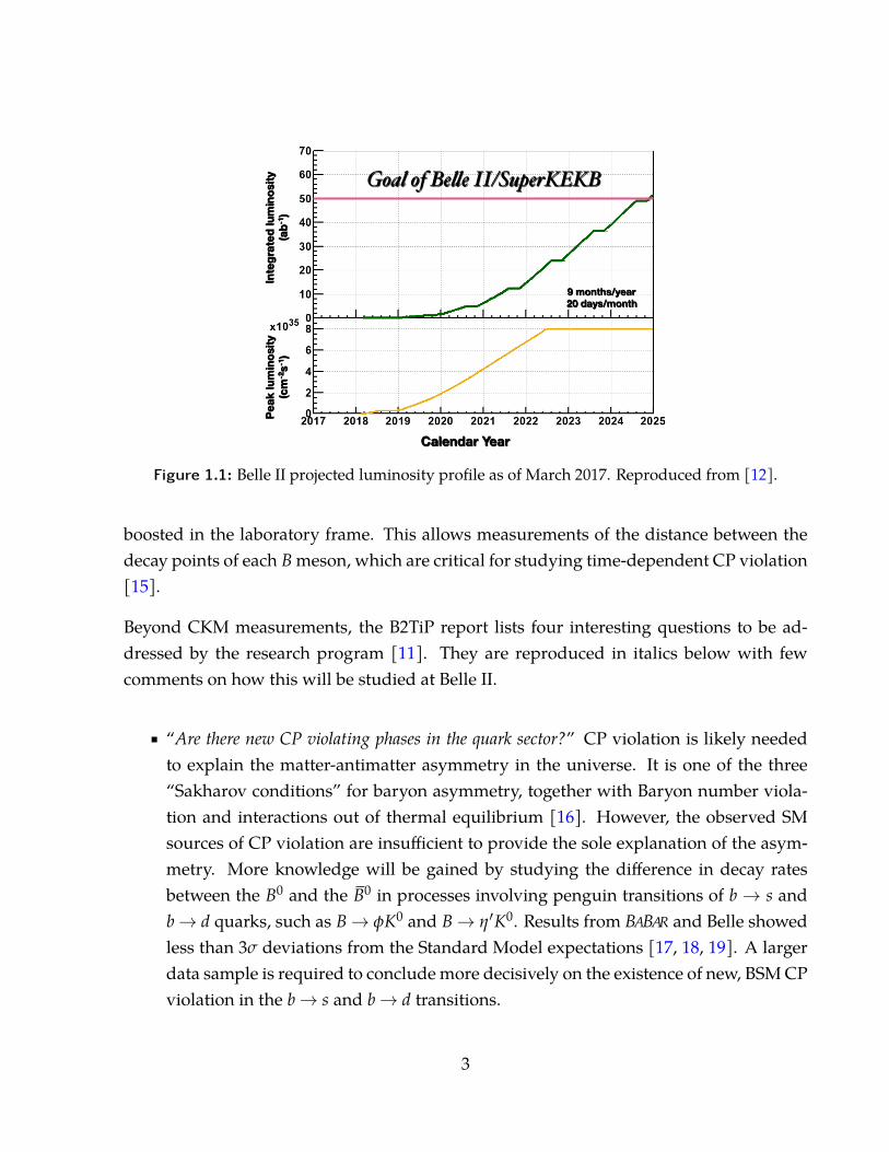
The main advantage of the Belle II experiment (with its large sample of e+e− collisions)over hadron colliders is that the initial state is a well-defined collision of fundamental par-ticles. A well known initial state with fewer background processes that contaminate thesignals is typically what is meant by a clean environment. The large number of collisionper unit time provides statistical power to the data set, and is referred to as a high lumi-nosity environment. The expected luminosity profile is reported in Figure 1.1. The peakinstantaneous luminosity is expected to be achieved in the middle of 2022, and data tak-ing will continue until 2025 to reach 50 ab−1 corresponding to over 4.1× 109 delivered BBpairs. This clean and high-statistics environment will enable data analysis techniques em-ploying fully reconstructed B meson decays to improve the precision on the CKM matrixelements by a factor of at least two [13], and reduce the limits of any BSM contribution tothe CP-violating phases by a factor of five [14].

Moreover, the Belle II experiment is studying collisions from an asymmetric collider. Thismeans that the electron and positron beams are each circulating at a different energy, whichis often tuned to provide 10.58 GeV in the centre of mass frame. Electron and positroncollisions at this energy produce Υ(4S) mesons, which then decay into BB pairs that are

2

SuperKEKB luminosity projection

Goal of Belle II/SuperKEKB

9 months/year 20 days/month

Inte

grat

ed lu

min

osity

(a

b-1)

Peak

lum

inos

ity

(cm

-2s-1

)

Calendar Year

Figure 1.1: Belle II projected luminosity profile as of March 2017. Reproduced from [12].

boosted in the laboratory frame. This allows measurements of the distance between thedecay points of each B meson, which are critical for studying time-dependent CP violation[15].

Beyond CKM measurements, the B2TiP report lists four interesting questions to be ad-dressed by the research program [11]. They are reproduced in italics below with fewcomments on how this will be studied at Belle II.

� “Are there new CP violating phases in the quark sector?” CP violation is likely neededto explain the matter-antimatter asymmetry in the universe. It is one of the three“Sakharov conditions” for baryon asymmetry, together with Baryon number viola-tion and interactions out of thermal equilibrium [16]. However, the observed SMsources of CP violation are insufficient to provide the sole explanation of the asym-metry. More knowledge will be gained by studying the difference in decay ratesbetween the B0 and the B0 in processes involving penguin transitions of b→ s andb→ d quarks, such as B→ φK0 and B→ η′K0. Results from BABAR and Belle showedless than 3σ deviations from the Standard Model expectations [17, 18, 19]. A largerdata sample is required to conclude more decisively on the existence of new, BSM CPviolation in the b→ s and b→ d transitions.

3

� “Does nature have multiple Higgs bosons?” New charged Higgs bosons, in addition tothe SM Higgs, are predicted by many models of new physics. Such charged Higgsescould manifest themselves in processes involving heavy flavour transitions, such asB→ τν and B→ D(∗)τν. The first process is in fact considered a golden decay modefor the observation of a contribution form a charged Higgs [20]. BABAR already ob-served a discrepancy greater than 3σ in these [21, 22], which was pushed beyond 4σ

with the addition of Belle and LHCb data [23], so further study will of this topic iswarranted.

� “Are there sources of lepton flavour violation (LFV) beyond the SM?” The only leptonflavour violating phenomena observed so far are the neutrino oscillations. Findingevidence for processes such as τ→ µγ in Belle II would provide crucial informationto solve the neutrino mass generation problem, for example by discriminating be-tween different Majorana neutrino mass models [24]. Moreover, such direct leptonflavour violation is highly suppressed in the SM with branching fractions on order of10−54 [25]. Unexpectedly large rates for this process — some models predict branch-ing fractions around 10−7 – 10−10 — would be a strong indication of BSM physics[20]. However, latest B-Factory results from BABAR and Belle showed no evidence ofsignals for this process [26, 27].

Moreover, the Belle II experiment can leverage the general-purpose detector, the clean en-vironment and the high statistical power of the data set to address questions not directlyrelated to flavour physics. The B2TiP report [11] lists two of these fundamental questions.

� “Is there a dark sector of particle physics at the same mass scale as ordinary matter?” Directsearches for dark matter candidates will be conducted using missing energy decays.Belle II has sensitivity to new particles at the MeV to GeV scale such as weakly in-teracting massive particles. Some models predict a vast hidden sector that wouldcouple to the Standard Model via new gauge symmetries [28]. B factories are a goodenvironment to search for such objects [29][30], and the single photon trigger linesof Belle II would provide a path to search for such hidden-sector particles includingdark matter candidates and gauge bosons.

� “What is the nature of the strong force in binding hadrons?” Exotic quarkonium stateswere recently observed in B factories and hadron colliders such as the LHC. The

4

Belle II program will contribute to this research topic by scanning the beam energiesand exploiting initial-state radiation processes to study a range of collision energies.Moreover, with its near 4π coverage and good particle identification performance,the detector will be enable the characterization of these newly discovered quarkoniastates and continue the study of QCD in the low-energy regime.

1.1.2 The accelerator: SuperKEKB

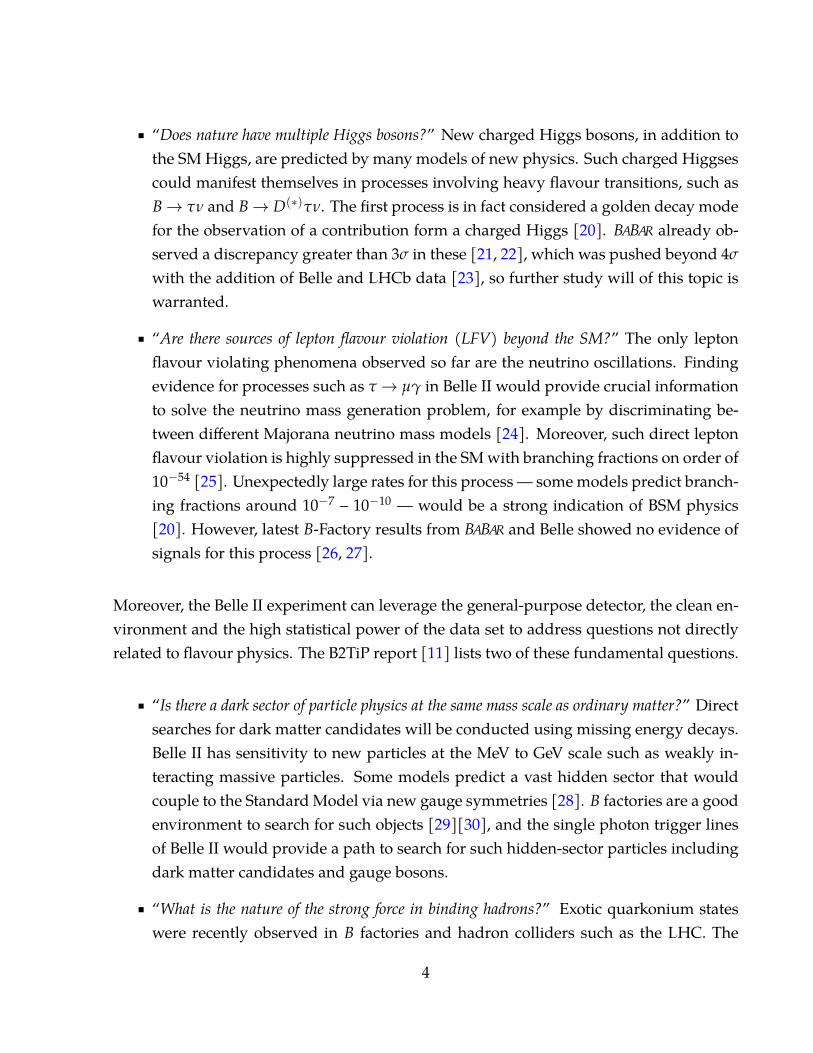
The SuperKEKB accelerator represented in Figure 1.2 is a major upgrade to KEKB, andaims to deliver more than 40 times the integrated luminosity of its predecessor. The lumi-nosity is a key factor in determining the performance of an experiment, since the produc-tion rate of a particle is the product of the delivered luminosity and its production crosssection. It is given by

L =f ne+ne−

4π√

εxβ∗xεyβ∗yF (1.1)

where f is the frequency of the bunch crossings, ne+, ne− are the number of electronsper bunch, and ε{x,y} are the emittances of the bunches in the transverse directions (xand y), and β∗{x,y} are the transverse amplitude functions β in the interaction region. Theasterisk in β∗ denotes an evaluation at the vicinity of the interaction point. The extra factorF < 1 is an efficiency term taking into account imperfections such as the non-zero crossingangle [9]. It is interesting to note that the product of bunch crossing frequency and thenumber of particles per bunches is directly proportional to the beam currents. Moreover,the emittance is the area in phase space of an ellipse containing the particles. The emittanceis defined, in each transverse direction i, with respect to the local rms size of the bunch andthe β function:

εi ≡σ2

iβi

. (1.2)

It is the envelope of the motion of the particles. The 40-fold increase in luminosity expectedfor SuperKEKB will be achieved by acting on all fronts: a factor 2 is gained by increasingthe beam currents, and the remaining 20-fold increase is obtained by focussing the beamsmore tightly in the interaction region (IR).

The main technological improvements required for the upgrade are indicated in Figure 1.2and consist of new

5

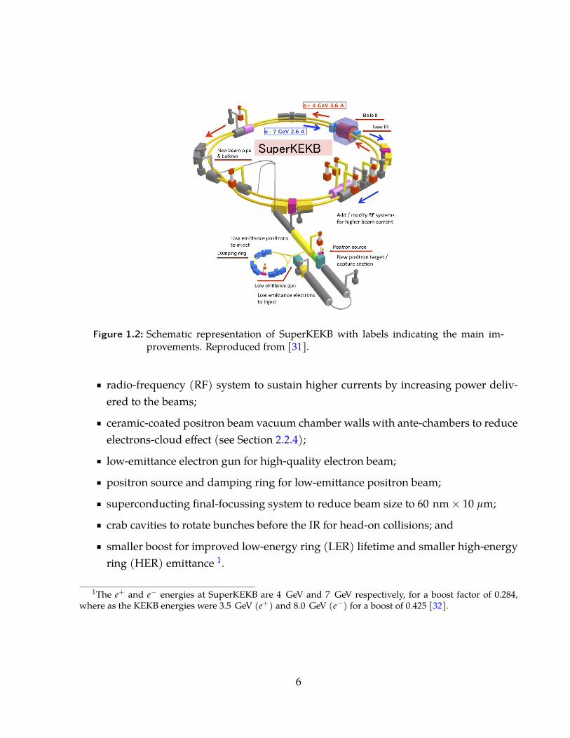
Figure 1.2: Schematic representation of SuperKEKB with labels indicating the main im-provements. Reproduced from [31].

� radio-frequency (RF) system to sustain higher currents by increasing power deliv-ered to the beams;

� ceramic-coated positron beam vacuum chamber walls with ante-chambers to reduceelectrons-cloud effect (see Section 2.2.4);

� low-emittance electron gun for high-quality electron beam;� positron source and damping ring for low-emittance positron beam;� superconducting final-focussing system to reduce beam size to 60 nm× 10 µm;� crab cavities to rotate bunches before the IR for head-on collisions; and� smaller boost for improved low-energy ring (LER) lifetime and smaller high-energy

ring (HER) emittance 1.

1The e+ and e− energies at SuperKEKB are 4 GeV and 7 GeV respectively, for a boost factor of 0.284,where as the KEKB energies were 3.5 GeV (e+) and 8.0 GeV (e−) for a boost of 0.425 [32].

6

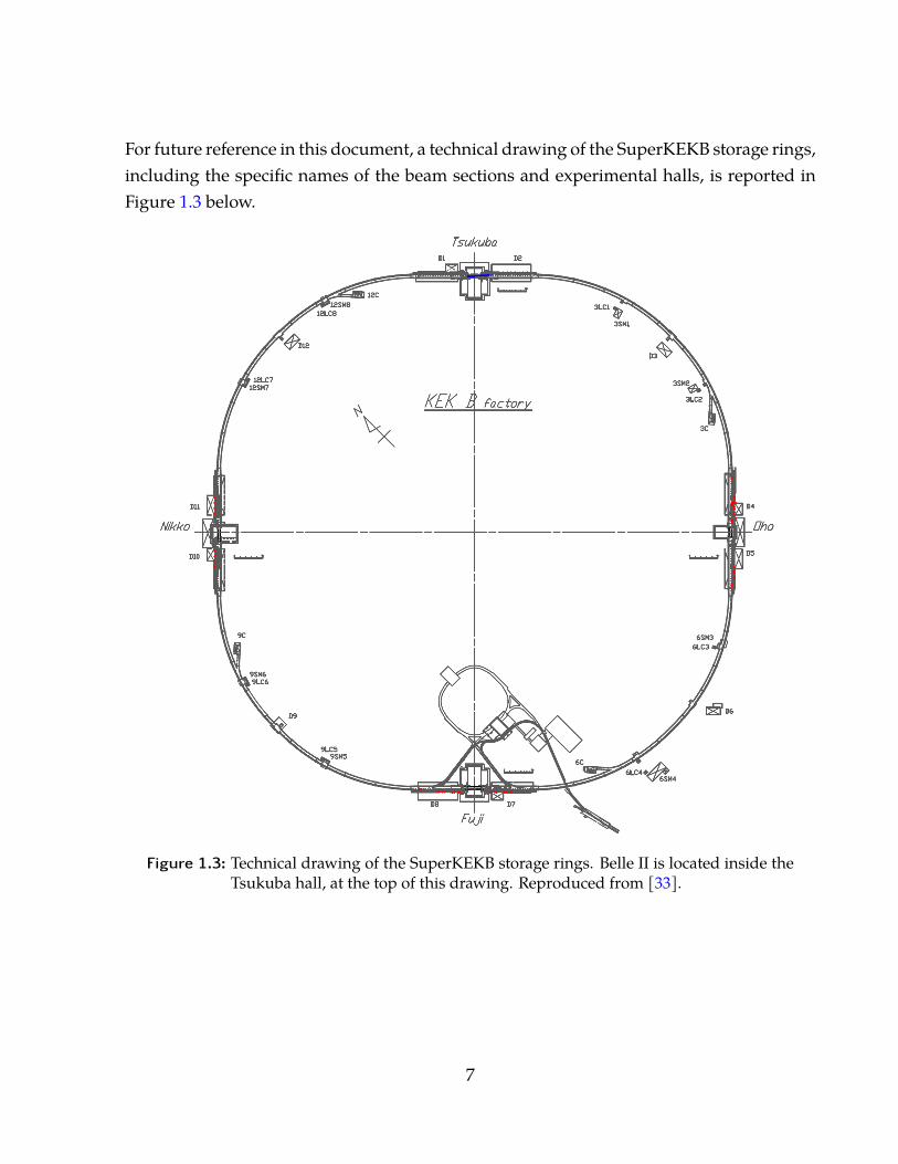
For future reference in this document, a technical drawing of the SuperKEKB storage rings,including the specific names of the beam sections and experimental halls, is reported inFigure 1.3 below.

Figure 1.3: Technical drawing of the SuperKEKB storage rings. Belle II is located inside theTsukuba hall, at the top of this drawing. Reproduced from [33].

7

1.1.3 The detector: Belle II

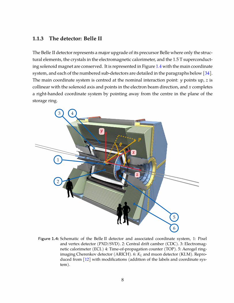
The Belle II detector represents a major upgrade of its precursor Belle where only the struc-tural elements, the crystals in the electromagnetic calorimeter, and the 1.5 T superconduct-ing solenoid magnet are conserved. It is represented in Figure 1.4 with the main coordinatesystem, and each of the numbered sub-detectors are detailed in the paragraphs below [34].The main coordinate system is centred at the nominal interaction point: y points up, z iscollinear with the solenoid axis and points in the electron beam direction, and x completesa right-handed coordinate system by pointing away from the centre in the plane of thestorage ring.

1

2

3 4

5

6

xxx

yyy

zzz

PPPφφφ

θθθ

Figure 1.4: Schematic of the Belle II detector and associated coordinate system, 1: Pixeland vertex detector (PXD/SVD). 2: Central drift camber (CDC). 3: Electromag-netic calorimeter (ECL) 4: Time-of-propagation counter (TOP). 5: Aerogel ring-imaging Cherenkov detector (ARICH). 6: KL and muon detector (KLM). Repro-duced from [12] with modifications (addition of the labels and coordinate sys-tem).

8

Pixel and vertex detector (VXD) The role of the innermost system of the Belle II detectoris to measure the decay vertices of the B- and D-mesons, and the τ-leptons and con-nect them to the tracks reconstructed in the central drift chamber. It is composed oftwo layers of silicon pixel detector and four layers of double-sided silicon strip de-tectors. The layers are located at radii between r = 14 mm and r = 140 mm, with alayout that is hermetic in φ, and the polar acceptance ranges from θ = 17◦ to θ = 150◦.The design performance specification is an impact parameter resolution σz0 ∼ 20 µm.

Central drift chamber (CDC) The drift chamber is used to reconstruct tracks and mea-sure the momentum of charged particles, contribute to particle identification (PID)by measuring energy losses (dE/dx), and provide a trigger signal for charged par-ticles. When a charged particle travels through the gas, it leaves a track of ionizedmolecules with the liberated electrons drifting towards the positively biased sensewires. At the sense wires, the electrons initiate an avalanche that ultimately pro-duces a measurable signal. There are 14,336 sense wires in the CDC and the locationof ionization associated with the signal on each sense wire is determined by mea-suring the drift times of electrons produced in the ionization. Pre-amplifiers andfront-end-digitizer boards are attached directly to these wires to provide the signalconditioning for data extraction, and the fast logic necessary for triggering. Thereare also 42,240 field wires that shape the electric field within the CDC for a moreuniform drift velocity. The Belle II CDC is an entirely new detector that extends toa larger radius from the beam pipe that did the Belle drift chamber. The other im-provements for Belle II are faster electronics and a higher cell density, especially atsmaller radii. As with the inner detectors, the CDC is hermetic in φ, and the polaracceptance ranges from 17◦ to 150◦. The expected transverse momentum resolutionis given as a function of the velocity of the particle β, and component of momentumtransverse to the solenoidal magnetic field, pt:

σpt /pt =

√(0.2%pt)

2 + (0.3%β)2 (1.3)

Time-of-propagation counter (TOP) The time-of-propagation counter is a PID device aim-ing at better pion/kaon separation using a novel technology. As depicted schemati-cally in Figure 1.5, the TOP consists of rectangular quartz radiators coupled to micro-channel plate photo-multiplier tubes (MCP-PMT). Charged particles travelling throughthe quartz bars faster than the speed of light in that medium emit a light cone —

9

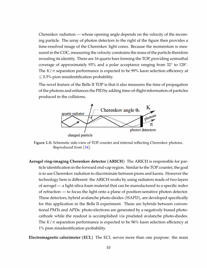
Cherenkov radiation — whose opening angle depends on the velocity of the incom-ing particle. The array of photon detectors to the right of the figure then provides atime-resolved image of the Cherenkov light cones. Because the momentum is mea-sured in the CDC, measuring the velocity constrains the mass of the particle thereforerevealing its identity. There are 16 quartz bars forming the TOP, providing azimuthalcoverage of approximately 93% and a polar acceptance ranging from 32◦ to 128◦.The K/π separation performance is expected to be 99% kaon selection efficiency at≤ 0.5% pion misidentification probability.The novel feature of the Belle II TOP is that it also measures the time of propagationof the photons and enhances the PID by adding time-of-flight information of particlesproduced in the collisions.

Figure 1.5: Schematic side-view of TOP counter and internal reflecting Cherenkov photons.Reproduced from [34].

Aerogel ring-imaging Cherenkov detector (ARICH) The ARICH is responsible for par-ticle identification in the forward end-cap region. Similar to the TOP counter, the goalis to use Cherenkov radiation to discriminate between pions and kaons. However thetechnology here is different: the ARICH works by using radiators made of two layersof aerogel — a light silica foam material that can be manufactured to a specific indexof refraction — to focus the light onto a plane of position-sensitive photon detector.These detectors, hybrid avalanche photo-diodes (HAPD), are developed specificallyfor this application in the Belle II experiment. These are hybrids between conven-tional PMTs and APDs: photo-electrons are generated by a negatively biased photo-cathode while the readout is accomplished via pixelated avalanche photo-diodes.The K/π separation performance is expected to be 96% kaon selection efficiency at1% pion misidentification probability.

Electromagnetic calorimeter (ECL) The ECL serves more than one purpose: the main

10

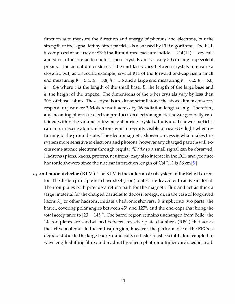
function is to measure the direction and energy of photons and electrons, but thestrength of the signal left by other particles is also used by PID algorithms. The ECLis composed of an array of 8736 thallium-doped caesium iodide — CsI(Tl) — crystalsaimed near the interaction point. These crystals are typically 30 cm long trapezoidalprisms. The actual dimensions of the end faces vary between crystals to ensure aclose fit, but, as a specific example, crystal #14 of the forward end-cap has a smallend measuring b = 5.4, B = 5.8, h = 5.6 and a large end measuring b = 6.2, B = 6.6,h = 6.4 where b is the length of the small base, B, the length of the large base andh, the height of the trapeze. The dimensions of the other crystals vary by less than30% of those values. These crystals are dense scintillators: the above dimensions cor-respond to just over 3 Moliere radii across by 16 radiation lengths long. Therefore,any incoming photon or electron produces an electromagnetic shower generally con-tained within the volume of few neighbouring crystals. Individual shower particlescan in turn excite atomic electrons which re-emits visible or near-UV light when re-turning to the ground state. The electromagnetic shower process is what makes thissystem more sensitive to electrons and photons, however any charged particle will ex-cite some atomic electrons through regular dE/dx so a small signal can be observed.Hadrons (pions, kaons, protons, neutrons) may also interact in the ECL and producehadronic showers since the nuclear interaction length of CsI(Tl) is 38 cm[9].

KL and muon detector (KLM) The KLM is the outermost subsystem of the Belle II detec-tor. The design principle is to have steel (iron) plates interleaved with active material.The iron plates both provide a return path for the magnetic flux and act as thick atarget material for the charged particles to deposit energy, or, in the case of long-livedkaons KL or other hadrons, initiate a hadronic showers. It is split into two parts: thebarrel, covering polar angles between 45◦ and 125◦, and the end-caps that bring thetotal acceptance to [20− 145]◦. The barrel region remains unchanged from Belle: the14 iron plates are sandwiched between resistive plate chambers (RPC) that act asthe active material. In the end-cap region, however, the performance of the RPCs isdegraded due to the large background rate, so faster plastic scintillators coupled towavelength-shifting fibres and readout by silicon photo-multipliers are used instead.

11

1.2 Beam-induced background and measurement

1.2.1 Overview

One challenge of commissioning a new collider experiment is to understand the differentsources of beam-induced background and keep them under control. The typical contribu-tions to detector backgrounds at e+e− collision experiments are the following: [35]

1. Beam-gas interactions

2. Intra-beam interactions

3. Synchrotron radiation

4. ”Physics” backgrounds such as Bhabha scattering

5. Interaction with thermal photons

6. Operational particle losses (e.g. beam injections losses and electron-cloud effect)

The first three components are independent of luminosity such that they are relevant tothe first accelerator commissioning phase as discussed below. There will be no focussingof the beams during that period, so sources that require collisions between the e+ and e−

beam particles are expected to be negligible. Furthermore, beam losses due to elastic scat-tering off thermal photons — the infra-red photons coming from black-body radiation ofthe vacuum chamber walls at room temperature — are only important at high energy e+e−

colliders such as LEP and LEP2 (where the centre-of-mass energy ranged from 45 GeV tonearly 100 GeV).

Continuous injection is an interesting feature of the SuperKEKB accelerator, although pre-dictions of the related background time structure are notoriously difficult [35]. One has torely on experimental methods to assess it, such as part of the project being presented.

A more detailed description of the different sources of machine-induced background rel-evant to the proposed project are reported in Section 2.2.

12

1.2.2 Beast II, the accelerator commissioning detector

The Beast II project (for Beam Exorcism for a Stable Experiment) aimed at studying theaccelerator-induced background before taking so-called “Physics” data. It was separatedin two distinct phases as presented in Table 1.1.

The research project that is the subject of this Dissertation pertains only to the first of thesephases, Phase 1. In summary, this initial phase provided a first insight into the reliabilityof background estimates coming from simulation during first operation of the SuperKEKBaccelerator. Certain types of background were enhanced due to the higher vacuum cham-ber pressure, while all luminosity-dependent sources were strongly suppressed becausethere wasn’t any final focussing of the beams. Even though these conditions were far fromwhat is expected during physics data taking, Beast II Phase 1 represented a unique oppor-tunity to measure exclusively the luminosity-independent background sources.

The second phase, Phase 2, involved using the Belle II detector without its vertex detector.The goal was to measure the background in more realistic conditions, and also determinewhen the radiation levels were safe for the vertex system to be added.

1.3 The research question

The research question is formulated as follows:

What are the quantitative characteristics of the beam-induced back-ground radiation associated with single beams in Phase 1 of Su-perKEKB operations under different beam configurations, and howprecisely are these modelled in simulations of the accelerator?

1.4 Goals of the project

1.4.1 General goal

The general goal of this project was to measure the machine-induced background near theintended position of the ECL end-cap of the Belle II detector, and to use these measure-ments to correct predictions from simulations of the accelerator and assess an uncertainty

13

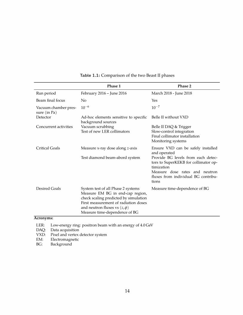
Table 1.1: Comparison of the two Beast II phases

Phase 1 Phase 2

Run period February 2016 – June 2016 March 2018 - June 2018Beam final focus No YesVacuum chamber pres-sure (in Pa)

10−6 10−7

Detector Ad-hoc elements sensitive to specificbackground sources

Belle II without VXD

Concurrent activities Vacuum scrubbing Belle II DAQ & TriggerTest of new LER collimators Slow-control integration

Final collimator installationMonitoring systems

Critical Goals Measure x-ray dose along z-axis Ensure VXD can be safely installedand operated

Test diamond beam-abord system Provide BG levels from each detec-tors to SuperKEKB for collimator op-timizationMeasure dose rates and neutronfluxes from individual BG contribu-tions

Desired Goals System test of all Phase 2 systems Measure time-dependence of BGMeasure EM BG in end-cap region,check scaling predicted by simulationFirst measurement of radiation dosesand neutron fluxes vs (z,φ)Measure time-dependence of BG

Acronyms:

LER: Low-energy ring: positron beam with an energy of 4.0 GeVDAQ: Data acquisitionVXD: Pixel and vertex detector systemEM: ElectromagneticBG: Background

14

on those predictions. In addition, this work mitigated the impact of the predicted machine-induced background through the provision of a radiation shield for the ECL.

1.4.2 Specific goals

The specific goals of this project were the following:

� Use tools developed by the Belle II Collaboration and SuperKEKB team to simulateoperating conditions during Phase 1, and predict impact on observed background inthe forward and backward calorimeter regions.

� Design and assemble the measurement apparatus, and integrate with the other Beast IIsub-detectors.

� Measure the relationship between the observed background and the pressure in thevacuum chamber, and follow its evolution during commissioning

� Measure the relationship between observed background levels and the size, currentand time-structure of bunches that comprise the beam, as described in Chapter 2.

� Measure the time-structure of background during beam injection.

� Combine the information to make predictions about the background level through-out the Belle II lifetime.

1.5 Dissertation outline

This Dissertation is organized as follows.

Chapter 2 provides more information about the context and the physics motivation for theresearch question which relates to accelerator-induced background and the quality of ourunderstanding of these phenomena.

Chapter 3 details the author’s personal contribution to the construction of the Belle II de-tector: the design, overseeing construction, and the commissioning of a pair of radiation

15

shields. The purpose of these shield is to protect a region of the calorimeter against elec-tromagnetic and neutron radiation arising from machine background, and their design isbased of the same simulation we aim to improve by the current measurement project.

Chapter 4 describes the experimental apparatus and the methodology employed to con-duct the background characterization. Chapter 5 presents the experimental results in com-parison with the simulation, as well as projections to future operating conditions.

***

16

Chapter 2

Source of accelerator-inducedbackground at Belle II and theirmitigation

2.1 The beams circulating at SuperKEKB

This description about accelerator-induced background starts with how beams are pro-duced and stored.

2.1.1 Electron production

Electrons are generated by a photocathode RF gun (or “electron gun”) specifically de-signed to deliver large charge and low emittance beams to SuperKEKB [36]. The pulsedlaser of the RF gun is directed to a photocathode that liberates two 10 nC bunches of elec-trons. These are accelerated, first by cavities within the gun itself, then by linear accelera-tor cavities, up to 3.3 GeV. At this point, the electron bunches can then be directed to thepositron source 3.5 mm away from the beamline in order to produce positrons for the LER,or they can pass through and be further accelerated up to 7 GeV before being delivered tothe HER [37, 38].

17

2.1.2 Positron production

In the positron mode, 3.3 GeV electron bunches collide with a 14 mm thick (4 X0) tung-sten target where they create an electromagnetic cascade, thus generating lower energypositrons and electrons. Positrons are captured in the positron-capture section with a fluxconcentrator, large aperture accelerating structures, and solenoid focusing coils. Approxi-mately 1 positron is retrieved for 10 incoming electrons [39]. The positrons are then accel-erated to 1.1 GeV, directed into the damping ring to reduce the emittance of the bunches,and finally accelerated to 4 GeV before delivery into the storage rings [37, 38].

2.1.3 Storage and beam structure

The storage rings store the beams in two 3 km circumference vacuum chambers. Theseare in fact squares with rounded corners (four straight section and four arc sections), as isvisible in Figure 1.3. The straight sections also contain RF cavities that compensate energylosses.

The beams are structured in trains of bunches. The design values for physics operation are2503 bunches per train for either species, with an average bunch current of 1.04 mA/bunchfor electrons and 1.44 mA/bunch for positrons [34]. As described in Section 1.1.2, the vol-ume of these bunches in phase space determines the emittance. A low emittance is desir-able to increase instantaneous luminosity, however a large amount of charge confined to asmall volume enhances beam losses via the Touschek effect, as discussed in Section 2.2.1.

2.1.4 Beam conditions during commissioning

Table 2.1 lists the conditions observed in Phases 1 and 2, and those expected in Phase 3.

2.2 Main background sources at Belle II

Three main sources of beam background are expected during the first phase of SuperKEKBcommissioning experiment: particles resulting from intra-bunch Touschek losses, interac-tions between beam particles and residual gas atoms in the beam pipe, and particle losses

18

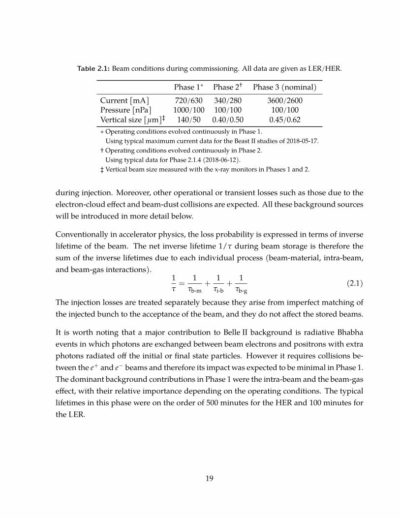
Table 2.1: Beam conditions during commissioning. All data are given as LER/HER.

Phase 1∗ Phase 2† Phase 3 (nominal)Current [mA] 720/630 340/280 3600/2600Pressure [nPa] 1000/100 100/100 100/100Vertical size [µm]‡ 140/50 0.40/0.50 0.45/0.62∗ Operating conditions evolved continuously in Phase 1.

Using typical maximum current data for the Beast II studies of 2018-05-17.† Operating conditions evolved continuously in Phase 2.

Using typical data for Phase 2.1.4 (2018-06-12).‡ Vertical beam size measured with the x-ray monitors in Phases 1 and 2.

during injection. Moreover, other operational or transient losses such as those due to theelectron-cloud effect and beam-dust collisions are expected. All these background sourceswill be introduced in more detail below.

Conventionally in accelerator physics, the loss probability is expressed in terms of inverselifetime of the beam. The net inverse lifetime 1/τ during beam storage is therefore thesum of the inverse lifetimes due to each individual process (beam-material, intra-beam,and beam-gas interactions).

1τ=

1τb-m

+1

τi-b+

1τb-g

(2.1)

The injection losses are treated separately because they arise from imperfect matching ofthe injected bunch to the acceptance of the beam, and they do not affect the stored beams.

It is worth noting that a major contribution to Belle II background is radiative Bhabhaevents in which photons are exchanged between beam electrons and positrons with extraphotons radiated off the initial or final state particles. However it requires collisions be-tween the e+ and e− beams and therefore its impact was expected to be minimal in Phase 1.The dominant background contributions in Phase 1 were the intra-beam and the beam-gaseffect, with their relative importance depending on the operating conditions. The typicallifetimes in this phase were on the order of 500 minutes for the HER and 100 minutes forthe LER.

19

2.2.1 Touschek radiation

The Touschek effect is the scattering of particles of the same species within a beam bunchof those particles. Such scattering induces an interchange between the transverse and lon-gitudinal momentum components of a pair of particles. These off-momentum particlesfall out of the stable orbit of the synchrotron and are deflected towards the walls of thevacuum chamber, producing electromagnetic showers.

This effect was first demonstrated in a paper by Bernardini and colleagues [40] in 1963,then described in more details by various authors [41, 42, 43]. It is expected to be thedominant intra-beam interaction contributing to the beam lifetime between injections. TheTouschek lifetime τTous. is:

1τTous.

=Nre

2c8πσxσyσz

λ3

γ2 D(ε,σp

), (2.2)

where N is the number of electrons or positrons in a bunch of volume σxσyσz, and re isthe electron classical radius (re ≈ 2.82× 10−15 m). The beam parameters are γ the beamlab-frame energy in units of particle mass (the Lorentz factor for a beam particle), σp theroot mean squared value of the individual particle momenta, and ε the accelerator limitingacceptance (either RF, momentum or geometric). The parameter λ is the relative accep-tance:

λ−1 =∆EE

=ε

γm0c. (2.3)

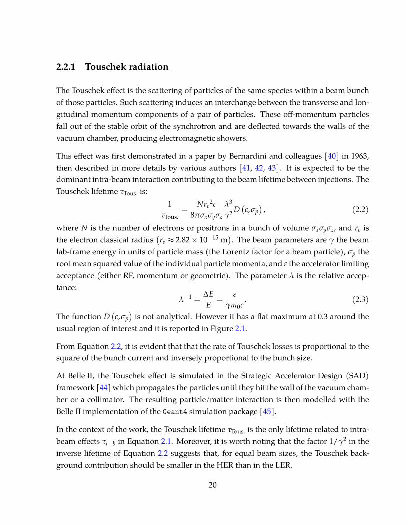
The function D(ε,σp

) is not analytical. However it has a flat maximum at 0.3 around theusual region of interest and it is reported in Figure 2.1.

From Equation 2.2, it is evident that that the rate of Touschek losses is proportional to thesquare of the bunch current and inversely proportional to the bunch size.

At Belle II, the Touschek effect is simulated in the Strategic Accelerator Design (SAD)framework [44] which propagates the particles until they hit the wall of the vacuum cham-ber or a collimator. The resulting particle/matter interaction is then modelled with theBelle II implementation of the Geant4 simulation package [45].

In the context of the work, the Touschek lifetime τTous. is the only lifetime related to intra-beam effects τi−b in Equation 2.1. Moreover, it is worth noting that the factor 1/γ2 in theinverse lifetime of Equation 2.2 suggests that, for equal beam sizes, the Touschek back-ground contribution should be smaller in the HER than in the LER.

20

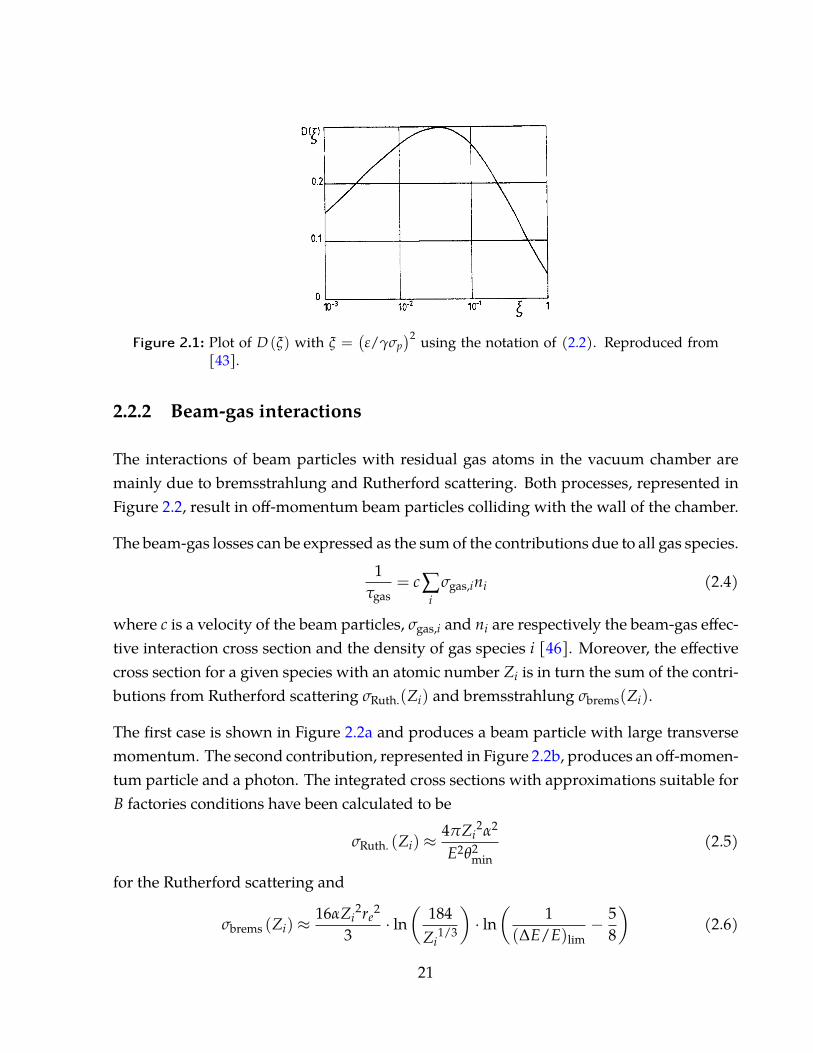
Figure 2.1: Plot of D (ξ) with ξ =(ε/γσp

)2 using the notation of (2.2). Reproduced from[43].

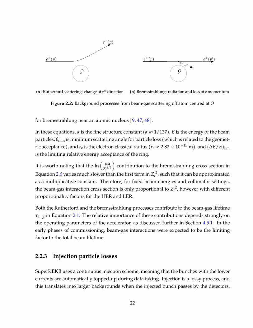
2.2.2 Beam-gas interactions

The interactions of beam particles with residual gas atoms in the vacuum chamber aremainly due to bremsstrahlung and Rutherford scattering. Both processes, represented inFigure 2.2, result in off-momentum beam particles colliding with the wall of the chamber.

The beam-gas losses can be expressed as the sum of the contributions due to all gas species.1

τgas= c∑

iσgas,ini (2.4)

where c is a velocity of the beam particles, σgas,i and ni are respectively the beam-gas effec-tive interaction cross section and the density of gas species i [46]. Moreover, the effectivecross section for a given species with an atomic number Zi is in turn the sum of the contri-butions from Rutherford scattering σRuth.(Zi) and bremsstrahlung σbrems(Zi).

The first case is shown in Figure 2.2a and produces a beam particle with large transversemomentum. The second contribution, represented in Figure 2.2b, produces an off-momen-tum particle and a photon. The integrated cross sections with approximations suitable forB factories conditions have been calculated to be

σRuth. (Zi) ≈4πZi

2α2

E2θ2min

(2.5)

for the Rutherford scattering and

σbrems (Zi) ≈16αZi

2re2

3· ln(

184Zi

1/3

)· ln(

1(∆E/E)lim

− 58

)(2.6)

21

O

e±(p)

e±(p)

(a) Rutherford scattering: change of e± direction

O

e±(p) e±(p′)

(b) Bremsstrahlung: radiation and loss of e momentum

Figure 2.2: Background processes from beam-gas scattering off atom centred at O

for bremsstrahlung near an atomic nucleus [9, 47, 48].

In these equations, α is the fine structure constant (α ≈ 1/137), E is the energy of the beamparticles, θmin is minimum scattering angle for particle loss (which is related to the geomet-ric acceptance), and re is the electron classical radius (re ≈ 2.82× 10−15 m), and (∆E/E)limis the limiting relative energy acceptance of the ring.

It is worth noting that the ln(

184Zi

1/3

)contribution to the bremsstrahlung cross section in

Equation 2.6 varies much slower than the first term in Zi2, such that it can be approximated

as a multiplicative constant. Therefore, for fixed beam energies and collimator settings,the beam-gas interaction cross section is only proportional to Zi

2, however with differentproportionality factors for the HER and LER.

Both the Rutherford and the bremsstrahlung processes contribute to the beam-gas lifetimeτb−g in Equation 2.1. The relative importance of these contributions depends strongly onthe operating parameters of the accelerator, as discussed further in Section 4.5.1. In theearly phases of commissioning, beam-gas interactions were expected to be the limitingfactor to the total beam lifetime.

2.2.3 Injection particle losses

SuperKEKB uses a continuous injection scheme, meaning that the bunches with the lowercurrents are automatically topped-up during data taking. Injection is a lossy process, andthis translates into larger backgrounds when the injected bunch passes by the detectors.

22

In Belle, the DAQ was vetoed for 4 ms after each injections to avoid recording data thatwould be flooded with noise hits. However at an injection rate of 50 Hz in Belle II thiswould correspond to a dead time of 20% [34].

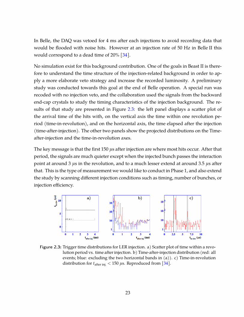
No simulation exist for this background contribution. One of the goals in Beast II is there-fore to understand the time structure of the injection-related background in order to ap-ply a more elaborate veto strategy and increase the recorded luminosity. A preliminarystudy was conducted towards this goal at the end of Belle operation. A special run wasrecoded with no injection veto, and the collaboration used the signals from the backwardend-cap crystals to study the timing characteristics of the injection background. The re-sults of that study are presented in Figure 2.3: the left panel displays a scatter plot ofthe arrival time of the hits with, on the vertical axis the time within one revolution pe-riod (time-in-revolution), and on the horizontal axis, the time elapsed after the injection(time-after-injection). The other two panels show the projected distributions on the Time-after-injection and the time-in-revolution axes.

The key message is that the first 150 µs after injection are where most hits occur. After thatperiod, the signals are much quieter except when the injected bunch passes the interactionpoint at around 3 µs in the revolution, and to a much lesser extend at around 3.5 µs afterthat. This is the type of measurement we would like to conduct in Phase 1, and also extendthe study by scanning different injection conditions such as timing, number of bunches, orinjection efficiency.

Figure 2.3: Trigger time distributions for LER injection. a) Scatter plot of time within a revo-lution period vs. time after injection. b) Time-after-injection distribution (red: allevents; blue: excluding the two horizontal bands in (a)). c) Time-in-revolutiondistribution for tafter inj. < 150 µs. Reproduced from [34].

23

2.2.4 Electron cloud effect

The electron cloud effect is typically a consequence of synchrotron radiation photons hit-ting the material of the vacuum chamber of the beam pipe and ejecting electrons via thephoto-electric effect. These primary photo-electrons are then accelerated by successivebunch crossings and often collide with the chamber material with a broad energy spec-trum, generating more secondary electron emissions. Such amplification processes are of-ten what determines the strength of the electron cloud effect, and factors of ten in gain canbe reached. The electron cloud effect occurs predominantly in positively-charged beamssince these attract the electrons. Other factors include beam currents, energy and bunchspacing, as well as vacuum chamber geometry, pressure, and the electronic properties ofthe surface material. Because of the many parameters involved, a numerical model is usu-ally required for any quantitative prediction of this effect, however in modern positron orproton beams the average density of electrons can reach 1010 m−3 to 1012 m−3 [49].

2.2.5 Beam-dust events1

During commissioning of the accelerator, one concern was the observation of localizedpressure bursts and accompanying background spikes. The prevalent hypothesis for theseobservations are collisions between the beam electrons and positrons, and small particlessuch as dust coming off the vacuum chamber material [50, 51, 52, 53]. These events willtherefore be referred to as “beam-dust” events in this dissertation.

Such beam-dust events are important during commissioning and running of an accelera-tor, since the corresponding increase in observed background often results in beam abortsand loss of operation time. The SuperKEKB group monitors these events by measuringpressure peaks around the beam pipe. The questions addressed in the present disserta-tion are

� What is the time structure of these beam-dust events during Phase 1 of SuperKEKB,and does it change as vacuum scrubbing progresses?

� Do the pressure bursts measured by SuperKEKB correspond to background peaksseen in the Beast II detectors?

1Written by the author of this dissertation, this subsection is also included textually in [1].

24

� Could the radiation resulting from these events be damaging to the detectors?

2.3 Background mitigation measures present at Belle II

Accelerator-induced background is almost exclusively the result of “lost” off-momentumparticles hitting interaction region (IR) material and generating showers of debris. Suchbackgrounds can reduce the lifetime of detector components through radiation damageand also introduce spurious noise in the detectors that interfere with the extraction of gen-uine physics signals from particles produced in the collisions. Three important measuresto mitigate these processes are: vacuum chamber design features (which include low op-erating pressures, the antechamber geometry, surface treatment and permanent magnetsthat help to control the electron-cloud effect), collimators upstream of the interaction re-gion (IR), and shielding near the IR with dense material [54].

2.3.1 Vacuum chamber design

Vacuum levels

The design value for cavity pressure is 10−7 Pa and the residual gas is mainly composedof H2 and CO. However since the cross sections for beam-gas interactions increase withA and Z, the partial pressure of dihydrogen is a negligible parameter when modellingbeam-gas backgrounds. The vacuum chambers of the LER are instrumented with massspectrometers so the dependence on the gas species can be verified experimentally. Thepressure in the cavity is expected to be comparable in SuperKEKB to what is was in KEKB:around 10−7 Pa.

The relevant quantity to monitor the quality of the vacuum is the so-called ”dynamic”pressure: we model the total pressure as the sum of the base pressure Pbase and a dynamicterm that is proportional to beam current [50]:

P = Pbase +dPdI

I. (2.7)

During commissioning, the second contribution, which is expected to track the gas des-orption rate from the walls of the vacuum chamber, is vastly dominating.

25

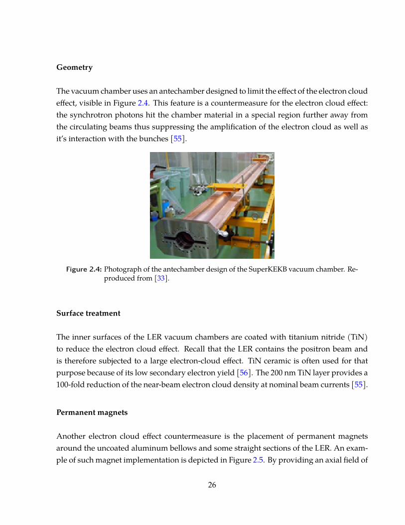
Geometry

The vacuum chamber uses an antechamber designed to limit the effect of the electron cloudeffect, visible in Figure 2.4. This feature is a countermeasure for the electron cloud effect:the synchrotron photons hit the chamber material in a special region further away fromthe circulating beams thus suppressing the amplification of the electron cloud as well asit’s interaction with the bunches [55].

Figure 2.4: Photograph of the antechamber design of the SuperKEKB vacuum chamber. Re-produced from [33].

Surface treatment

The inner surfaces of the LER vacuum chambers are coated with titanium nitride (TiN)to reduce the electron cloud effect. Recall that the LER contains the positron beam andis therefore subjected to a large electron-cloud effect. TiN ceramic is often used for thatpurpose because of its low secondary electron yield [56]. The 200 nm TiN layer provides a100-fold reduction of the near-beam electron cloud density at nominal beam currents [55].

Permanent magnets

Another electron cloud effect countermeasure is the placement of permanent magnetsaround the uncoated aluminum bellows and some straight sections of the LER. An exam-ple of such magnet implementation is depicted in Figure 2.5. By providing an axial field of

26

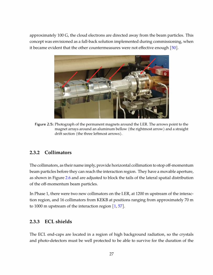
approximately 100 G, the cloud electrons are directed away from the beam particles. Thisconcept was envisioned as a fall-back solution implemented during commissioning, whenit became evident that the other countermeasures were not effective enough [50].

Figure 2.5: Photograph of the permanent magnets around the LER. The arrows point to themagnet arrays around an aluminum bellow (the rightmost arrow) and a straightdrift section (the three leftmost arrows).

2.3.2 Collimators

The collimators, as their name imply, provide horizontal collimation to stop off-momentumbeam particles before they can reach the interaction region. They have a movable aperture,as shown in Figure 2.6 and are adjusted to block the tails of the lateral spatial distributionof the off-momentum beam particles.

In Phase 1, there were two new collimators on the LER, at 1200 m upstream of the interac-tion region, and 16 collimators from KEKB at positions ranging from approximately 70 mto 1000 m upstream of the interaction region [1, 57].

2.3.3 ECL shields

The ECL end-caps are located in a region of high background radiation, so the crystalsand photo-detectors must be well protected to be able to survive for the duration of the

27

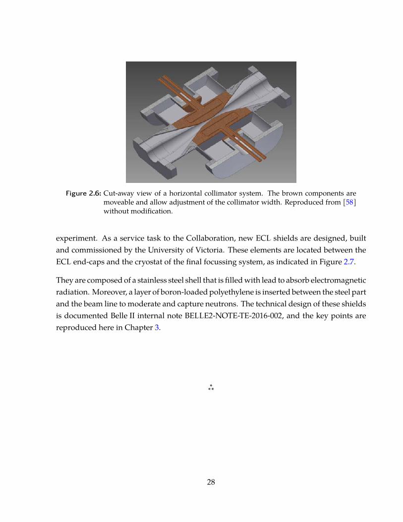
Figure 2.6: Cut-away view of a horizontal collimator system. The brown components aremoveable and allow adjustment of the collimator width. Reproduced from [58]without modification.

experiment. As a service task to the Collaboration, new ECL shields are designed, builtand commissioned by the University of Victoria. These elements are located between theECL end-caps and the cryostat of the final focussing system, as indicated in Figure 2.7.

They are composed of a stainless steel shell that is filled with lead to absorb electromagneticradiation. Moreover, a layer of boron-loaded polyethylene is inserted between the steel partand the beam line to moderate and capture neutrons. The technical design of these shieldsis documented Belle II internal note BELLE2-NOTE-TE-2016-002, and the key points arereproduced here in Chapter 3.

***

28

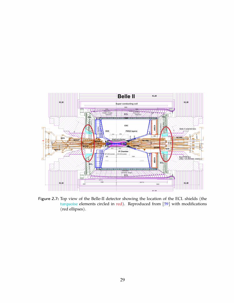
2.3777°

Belle-llTopview±41.5.vwx

1

1

2

2

3

3

4

4

5

5

6

6

7

7

8

8

9

9

10

10

11

11

12

12

A A

B B

C C

D D

E E

F F

G G

H H

Takashi Kohriki20100215

Takashi Kohriki20100215

R12A1

Belle II

1/10

Belle-ll(Nano beam)IR=±41.5 mrad.(Top view A)

KEK

DESIGNED DRAWN

of

ORIGINAL SCALEFINISH

DRAWING NO.

MECHANICAL ENGINEERING GROUPINSTITUTE FOR PARTICLE AND NUCLEAR STUDIES

HIGH ENERGY ACCELERATOR RESEARCH ORGANIZATIONOHO 1-1, TSUKUBA, IBARAKI 305-0801, JAPAN

TITLE

PROJECT

SIZE SHEET REV.

PROJECTION

CHECKED

CLEAN & DEGREASEREMOVE ALL BURRS

R16

0 280570

R11

45(A

RIC

H)

TOP VIEW

CDC

Small cell chamber

633.5(Cryostat)627.25(Cryostat)

QCS

30ｼ

17ｼ

R11

67(C

DC

IDS

)

ECL

Super conducting coil

ECL

ECL

ECL

ECL

ECL

2325(CDC)

R12

50(B

EC

L)

KLM

KLM

KLM

KLMKLM

KLM

BarrelBackward Forward

e+

e-

2.37

79°

4.7555°

TOP

20140213 R1220130318 R1120120720 R1020120418 R920120327 R820120302 R720120111 R620110701 R520100808 R420100519 R320100330 R220100310 R1

R11

37.5

(BP

ID in

ner m

ost R

.)R

1130

(CD

C-S

C o

uter

mos

t R.)

R45

2

R41

0

R15

5

410 525

Pre

-am

p

PXD(2 layers)

0.48

70°

Beam line axis(After +25.95mrad. rotation )

Belle II solenoid axisSVD

IP Chamber

310

1650(CDC)

10201930(ECL flange)

940(ECL flange)735(CDC) 1590(CDC)

19602980

QCS

QC2RE

QC2LE

QC2LP

QC1LE QC1RP

QC1RE

QC2RP

QC1LP

Belle II

2870(ECL flange)

1200

(TO

P)

AR

ICH

AR

ICH

20140213 R12 -QCS20131203 -CDC covers -B&FWD new pole pieces

3351 3920

ｿ54

0

ｿ73

4

1490 2417.5

ｿ58

1

ｿ50

0

928 1544

ｿ87

3

1000(CDC)2020

ｿ34

8ｿ11

00

ｿ69

4

ｿ88

6

1477.5

Figure 2.7: Top view of the Belle-II detector showing the location of the ECL shields (theturquoise elements circled in red). Reproduced from [59] with modifications(red ellipses).

29

Chapter 3

Design and construction of ECL radiationshields

In the forward and backward regions of the Belle II detector’s electromagnetic calorime-ter (ECL), a high level of radiation is undergone by the crystals and the avalanche photo-diodes (APD)1. To reduce the level of beam-induced background in the forward and back-ward end-caps — the “lids” on either side of the barrel of the ECL — heavy metal shieldswere placed between these end-caps and the final focusing system (QCS). In Belle, suchshields were made of a wedge of lead cast in a stainless steel shell. To give a better ideaof these devices, the shield in place in the forward region of the Belle detector is depictedin Figure 3.1. Engineering drawings of the forward and backward shields are reported inthe “Belle Forward ECL End-cap Shield KB-01785” and the “Belle Backward ECL End-capShield KB-01786” drawings, available within the KEK network.

The Belle shields have been discarded, so a new design study must be conducted account-ing for the 20-fold increase in luminosity. Early simulation studies indicated that, withoutsuch shields, both the crystal radiation dose and the neutron flux in the photodiodes wereexpected to lie above tolerance [61]2. The new shield designs will need to bring those levelsas low as possible, yet respect the mass and volume constraints.

The purpose of this chapter is to document the design work related to these radiation1An APD is a special category of photodiodes designed to be operated with large reverse bias voltages

(on the order of 100 V) such that a charged particle travelling through them triggers an avalanche ionisationprocess that amplifies the signal. Thus, APDs generally provide a larger gain than regular photodiodes.

2Later simulation with different QCS shielding showed this is not always the case.

30

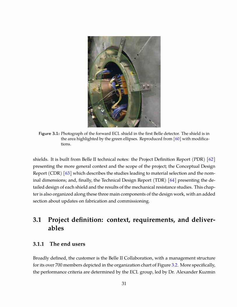
Figure 3.1: Photograph of the forward ECL shield in the first Belle detector. The shield is inthe area highlighted by the green ellipses. Reproduced from [60] with modifica-tions.

shields. It is built from Belle II technical notes: the Project Definition Report (PDR) [62]presenting the more general context and the scope of the project; the Conceptual DesignReport (CDR) [63] which describes the studies leading to material selection and the nom-inal dimensions; and, finally, the Technical Design Report (TDR) [64] presenting the de-tailed design of each shield and the results of the mechanical resistance studies. This chap-ter is also organized along these three main components of the design work, with an addedsection about updates on fabrication and commissioning.

3.1 Project definition: context, requirements, and deliver-ables

3.1.1 The end users

Broadly defined, the customer is the Belle II Collaboration, with a management structurefor its over 700 members depicted in the organization chart of Figure 3.2. More specifically,the performance criteria are determined by the ECL group, led by Dr. Alexander Kuzmin

31

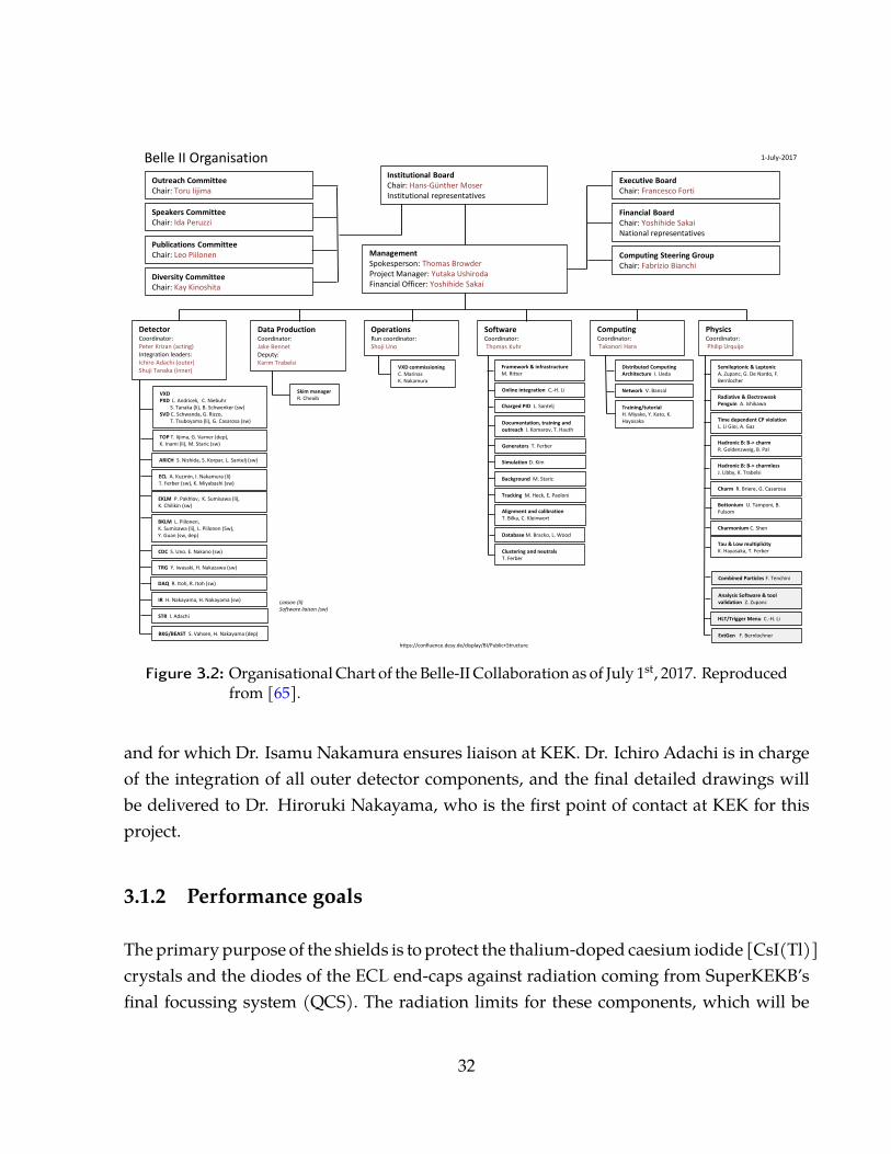
Belle II Organisation Institutional Board Chair: Hans-Günther Moser Institutional representatives

Outreach Committee Chair: Toru Iijima

Speakers Committee Chair: Ida Peruzzi

Publications Committee Chair: Leo Piilonen

Diversity Committee Chair: Kay Kinoshita

Management Spokesperson: Thomas Browder Project Manager: Yutaka Ushiroda Financial Officer: Yoshihide Sakai

Skim manager R. Cheaib

VXD commissioning C. Marinas K. Nakamura

Framework & infrastructure M. Ritter

Charged PID L. Santelj

Online integration C.-H. Li

Documentation, training and outreach I. Komarov, T. Hauth

Simulation D. Kim

Generators T. Ferber

Tracking M. Heck, E. Paoloni

Background M. Staric

Alignment and calibration T. Bilka, C. Kleinwort

Database M. Bracko, L. Wood

Clustering and neutrals T. Ferber

Executive Board Chair: Francesco Forti

Financial Board Chair: Yoshihide Sakai National representatives

Computing Steering Group Chair: Fabrizio Bianchi

Data Production Coordinator: Jake Bennet Deputy: Karim Trabelsi

VXD PXD L. Andricek, C. Niebuhr S. Tanaka (li), B. Schwenker (sw) SVD C. Schwanda, G. Rizzo, T. Tsuboyama (li), G. Casarosa (sw)

TOP T. Iijima, G. Varner (dep), K. Inami (li), M. Staric (sw)

ARICH S. Nishida, S. Korpar, L. Santelj (sw)

ECL A. Kuzmin, I. Nakamura (li) T. Ferber (sw), K. Miyabashi (sw)

EKLM P. Pakhlov, K. Sumisawa (li), K. Chilikin (sw)

BKLM L. Piilonen, K. Sumisawa (li), L. Piilonen (Sw), Y. Guan (sw, dep)

CDC S. Uno. E. Nakano (sw)

TRG Y. Iwasaki, H. Nakazawa (sw)

IR H. Nakayama, H. Nakayama (sw)

STR I. Adachi

BKG/BEAST S. Vahsen, H. Nakayama (dep)

DAQ R. Itoh, R. Itoh (sw)

Detector Coordinator: Peter Krizan (acting) Integration leaders: Ichiro Adachi (outer) Shuji Tanaka (inner)

Operations Run coordinator: Shoji Uno

Software Coordinator: Thomas Kuhr

Distributed Computing Architecture I. Ueda

Network V. Bansal

Training/tutorial H. Miyake, Y. Kato, K. Hayasaka

Liaison (li) Software liaison (sw)

Semileptonic & Leptonic A. Zupanc, G. De Nardo, F. Bernlocher

Time dependent CP violation L. Li Gioi, A. Gaz

Radiative & Electroweak Penguin A. Ishikawa

Hadronic B: B-> charm R. Goldenzweig, B. Pal

Charm R. Briere, G. Casarosa

Hadronic B: B-> charmless J. Libby, K. Trabelsi

Charmonium C. Shen

Bottonium U. Tamponi, B. Fulsom

Tau & Low multiplicity K. Hayasaka, T. Ferber

Physics Coordinator: Philip Urquijo

Combined Particles F. Tenchini

Analysis Software & tool validation Z. Zupanc

HLT/Trigger Menu C.-H. Li

EvtGen F. Bernlochner

Computing Coordinator: Takanori Hara

1-July-2017

https://confluence.desy.de/display/BI/Public+Structure

Figure 3.2: Organisational Chart of the Belle-II Collaboration as of July 1st, 2017. Reproducedfrom [65].

and for which Dr. Isamu Nakamura ensures liaison at KEK. Dr. Ichiro Adachi is in chargeof the integration of all outer detector components, and the final detailed drawings willbe delivered to Dr. Hiroruki Nakayama, who is the first point of contact at KEK for thisproject.

3.1.2 Performance goals

The primary purpose of the shields is to protect the thalium-doped caesium iodide [CsI(Tl)]crystals and the diodes of the ECL end-caps against radiation coming from SuperKEKB’sfinal focussing system (QCS). The radiation limits for these components, which will be

32

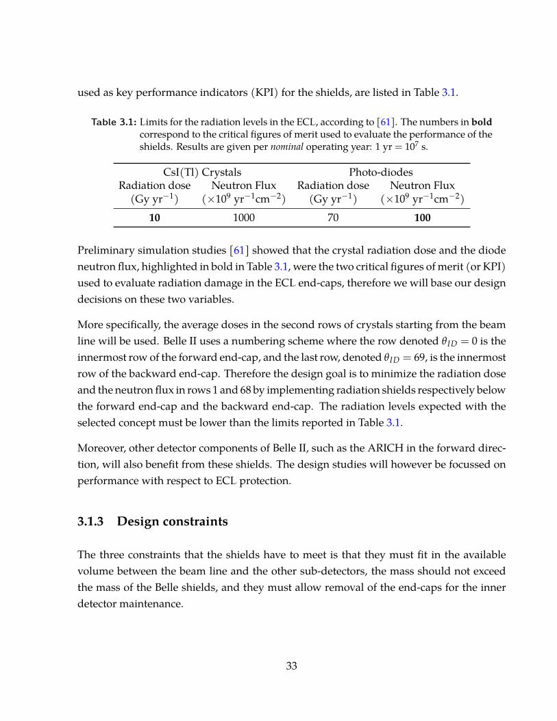
used as key performance indicators (KPI) for the shields, are listed in Table 3.1.

Table 3.1: Limits for the radiation levels in the ECL, according to [61]. The numbers in boldcorrespond to the critical figures of merit used to evaluate the performance of theshields. Results are given per nominal operating year: 1 yr = 107 s.

CsI(Tl) Crystals Photo-diodesRadiation dose Neutron Flux Radiation dose Neutron Flux

(Gy yr−1) (×109 yr−1cm−2) (Gy yr−1) (×109 yr−1cm−2)10 1000 70 100

Preliminary simulation studies [61] showed that the crystal radiation dose and the diodeneutron flux, highlighted in bold in Table 3.1, were the two critical figures of merit (or KPI)used to evaluate radiation damage in the ECL end-caps, therefore we will base our designdecisions on these two variables.

More specifically, the average doses in the second rows of crystals starting from the beamline will be used. Belle II uses a numbering scheme where the row denoted θID = 0 is theinnermost row of the forward end-cap, and the last row, denoted θID = 69, is the innermostrow of the backward end-cap. Therefore the design goal is to minimize the radiation doseand the neutron flux in rows 1 and 68 by implementing radiation shields respectively belowthe forward end-cap and the backward end-cap. The radiation levels expected with theselected concept must be lower than the limits reported in Table 3.1.

Moreover, other detector components of Belle II, such as the ARICH in the forward direc-tion, will also benefit from these shields. The design studies will however be focussed onperformance with respect to ECL protection.

3.1.3 Design constraints

The three constraints that the shields have to meet is that they must fit in the availablevolume between the beam line and the other sub-detectors, the mass should not exceedthe mass of the Belle shields, and they must allow removal of the end-caps for the innerdetector maintenance.

33

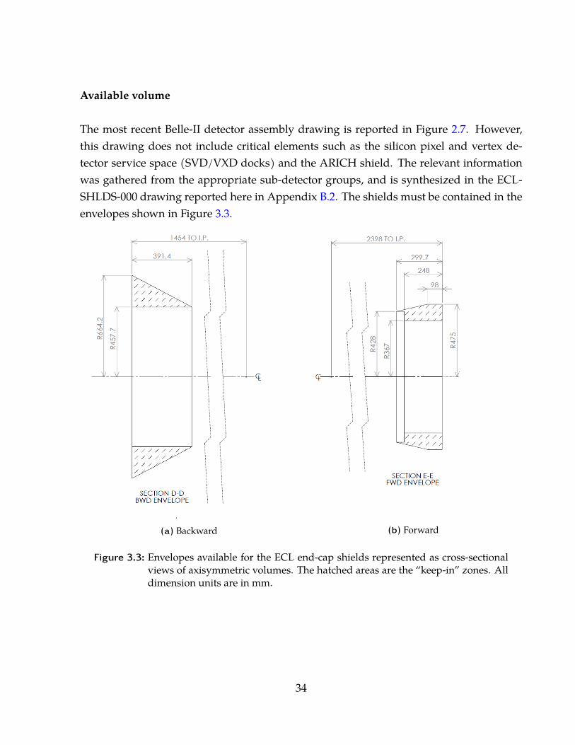
Available volume

The most recent Belle-II detector assembly drawing is reported in Figure 2.7. However,this drawing does not include critical elements such as the silicon pixel and vertex de-tector service space (SVD/VXD docks) and the ARICH shield. The relevant informationwas gathered from the appropriate sub-detector groups, and is synthesized in the ECL-SHLDS-000 drawing reported here in Appendix B.2. The shields must be contained in theenvelopes shown in Figure 3.3.

(a) Backward (b) Forward

Figure 3.3: Envelopes available for the ECL end-cap shields represented as cross-sectionalviews of axisymmetric volumes. The hatched areas are the “keep-in” zones. Alldimension units are in mm.

34

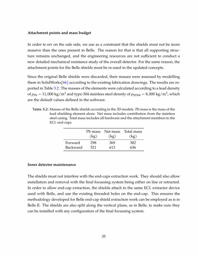
Attachment points and mass budget

In order to err on the safe side, we use as a constraint that the shields must not be moremassive than the ones present in Belle. The reason for that is that all supporting struc-ture remains unchanged, and the engineering resources are not sufficient to conduct anew detailed mechanical resistance study of the overall detector. For the same reason, theattachment points for the Belle shields must be re-used in the updated concepts.

Since the original Belle shields were discarded, their masses were assessed by modellingthem in SolidWorks[66] according to the existing fabrication drawings. The results are re-ported in Table 3.2. The masses of the elements were calculated according to a lead densityof ρPb = 11,000 kg/m3 and type-304 stainless steel density of ρSS304 = 8,000 kg/m3, whichare the default values defined in the software.

Table 3.2: Masses of the Belle shields according to the 3D models. Pb mass is the mass of thelead shielding element alone. Net mass includes contribution from the stainlesssteel casing. Total mass includes all hardware and the attachment members to theECL end-caps.

Pb mass Net mass Total mass(kg) (kg) (kg)

Forward 298 369 382Backward 521 613 636

Inner detector maintenance

The shields must not interfere with the end-caps extraction work. They should also allowinstallation and removal with the final focussing system being either on line or retracted.In order to allow end-cap extraction, the shields attach to the same ECL extractor deviceused with Belle, and use the existing threaded holes on the end-cap. This ensures themethodology developed for Belle end-cap shield extraction work can be employed as is inBelle II. The shields are also split along the vertical plane, as in Belle, to make sure theycan be installed with any configuration of the final focussing system.

35

3.1.4 Deliverables

Items delivered as part of the Canadian contribution to the ECL shields

The Canadian group is responsible for the following components:

� one backward shield assembly composed of two half-rings,

� one forward shield assembly composed of two half-rings,

� all brackets and fasteners needed to complete each assembly, and

� all brackets and fasteners needed to attach the assemblies to the ECL end-caps.

Other required items outside the scope of the shield design project

Other parts are needed to successfully install the shields on the ECL end-caps. These partsare either already at KEK from the Belle experiment, or will be purchased by KEK prior toinstallation.

� Installation jigs to hold the shield in the vertical orientation and move them in theaxial direction towards the end-caps. The assembly is represented in drawings KC-05036 and KC-05037, available within the KEK network.

� Forward and backward installation attachment to fix the shield to the above-mentionedjig during installation. These are represented by drawings KB-05030 and KB-05028,available within the KEK network.

Overall schedule and revisions

The original end date of the project was scheduled to be December 1st, 2016 since theshields were to be installed on the Belle-II detector in April 2017 or May 2017. Unfor-tunately, commissioning of Belle II suffered delays so the installation of the shields werere-scheduled to September and October, 2017.

36

The design and fabrication work of the shield themselves was also delayed. Delivery atKEK was originally scheduled in December 2016, at the latest. Instead, the actual deliverydate was May 14th, 2017. Since this is well ahead of the installation date, the delays indesign and fabrication of the shields will not have any impact on the experiment.

Preliminary cost estimates

Budgetary prices were requested in December 2014 with a preliminary concept of the back-ward shield in order to set the order of magnitude of the cost of the diverse components.The neutron shield design was not ready at the time of these budgetary quote requests.Table 3.3 contains the gathered information. There is a large variation between estimates,likely resulting from the fact this the project was considered “exotic” by some vendors. Todistil this down to one budgetary price, we used the estimate from the company that isthe most experienced in radiation shielding, MarShield, and added 25% contingency forthe uncertainties on the project in this preliminary phase. Our early cost estimate for thecomplete project was $45,000.

Table 3.3: Preliminary costing of the project. Prices (in CAD) are for a single shield, andwere obtained between January 2015 and June 2015.

Supplier Price per shieldSteel assembly Lead casting Neutron shield Shipping

Ramsay Group Ltd† 29,950 - - -Altech Machnining 14,000 - - -MarShield 9,250 3,100 - 1,800Ultraray - 8,000 - -Our estimate‡ - - 3,000 -†: This company is not in business anymore‡: Our estimate is based on raw material prices and $100/hr shop rate

37

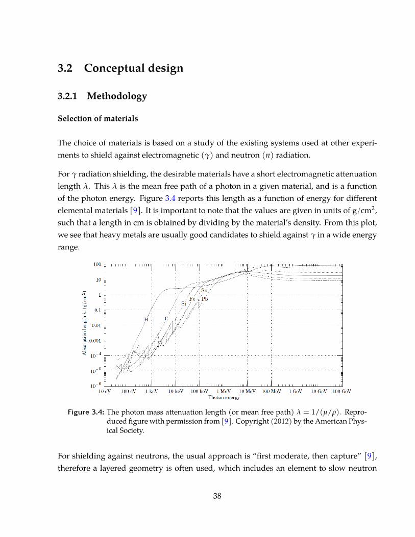
3.2 Conceptual design

3.2.1 Methodology

Selection of materials

The choice of materials is based on a study of the existing systems used at other experi-ments to shield against electromagnetic (γ) and neutron (n) radiation.

For γ radiation shielding, the desirable materials have a short electromagnetic attenuationlength λ. This λ is the mean free path of a photon in a given material, and is a functionof the photon energy. Figure 3.4 reports this length as a function of energy for differentelemental materials [9]. It is important to note that the values are given in units of g/cm2,such that a length in cm is obtained by dividing by the material’s density. From this plot,we see that heavy metals are usually good candidates to shield against γ in a wide energyrange.

Figure 3.4: The photon mass attenuation length (or mean free path) λ = 1/(µ/ρ). Repro-duced figure with permission from [9]. Copyright (2012) by the American Phys-ical Society.

For shielding against neutrons, the usual approach is “first moderate, then capture” [9],therefore a layered geometry is often used, which includes an element to slow neutron

38

down to thermal energies, an element with high neutron absorption cross section, andfinally a layer of dense material to block photon emitted by the neutron capture reactions.

Below is a list of commonly used materials for neutron shielding in high-energy physics(HEP) experiments.

� Low-cost materials

� Water [67]� Concrete [68]

� Hydrocarbons

� Paraffin [69]� Polyethylene [70, 71]

� Metals

� Iron (and steel) [70, 71, 72]� Aluminum [72]� Copper [73]� Lead [69, 70, 71]

� Other high neutron-absorption cross section elements

� Boron [69, 70, 71, 72, 74]� Lithium [69, 72]

Because the volume, mass and price budgets are all similar to the Belle shields, we fo-cused our selection to similar materials: lead cast into stainless steel casings, but with ex-tra components made of neutron-flux mitigating material. The latter is most efficiently ahydrogen-rich compound and may be loaded with elements having a high neutron ab-sorption cross-section such as boron or lithium.

While the nature of the electromagnetic shielding material is already defined, the exact for-mulation of the neutron absorption element will be determined in the design optimization

39

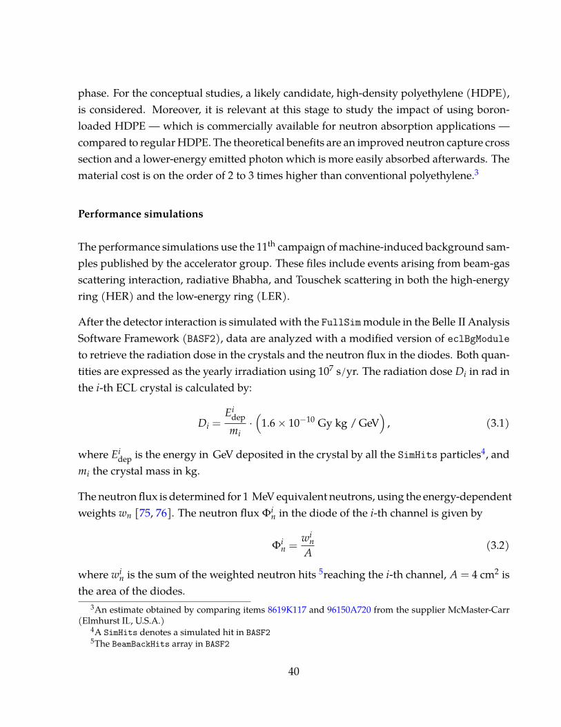
phase. For the conceptual studies, a likely candidate, high-density polyethylene (HDPE),is considered. Moreover, it is relevant at this stage to study the impact of using boron-loaded HDPE — which is commercially available for neutron absorption applications —compared to regular HDPE. The theoretical benefits are an improved neutron capture crosssection and a lower-energy emitted photon which is more easily absorbed afterwards. Thematerial cost is on the order of 2 to 3 times higher than conventional polyethylene.3

Performance simulations

The performance simulations use the 11th campaign of machine-induced background sam-ples published by the accelerator group. These files include events arising from beam-gasscattering interaction, radiative Bhabha, and Touschek scattering in both the high-energyring (HER) and the low-energy ring (LER).

After the detector interaction is simulated with the FullSimmodule in the Belle II AnalysisSoftware Framework (BASF2), data are analyzed with a modified version of eclBgModuleto retrieve the radiation dose in the crystals and the neutron flux in the diodes. Both quan-tities are expressed as the yearly irradiation using 107 s/yr. The radiation dose Di in rad inthe i-th ECL crystal is calculated by:

Di =Ei

depmi·(

1.6× 10−10 Gy kg / GeV)

, (3.1)

where Eidep is the energy in GeV deposited in the crystal by all the SimHits particles4, and

mi the crystal mass in kg.

The neutron flux is determined for 1 MeV equivalent neutrons, using the energy-dependentweights wn [75, 76]. The neutron flux Φi

n in the diode of the i-th channel is given by

Φin =

win

A(3.2)

where win is the sum of the weighted neutron hits 5reaching the i-th channel, A = 4 cm2 is

the area of the diodes.3An estimate obtained by comparing items 8619K117 and 96150A720 from the supplier McMaster-Carr

(Elmhurst IL, U.S.A.)4A SimHits denotes a simulated hit in BASF25The BeamBackHits array in BASF2

40

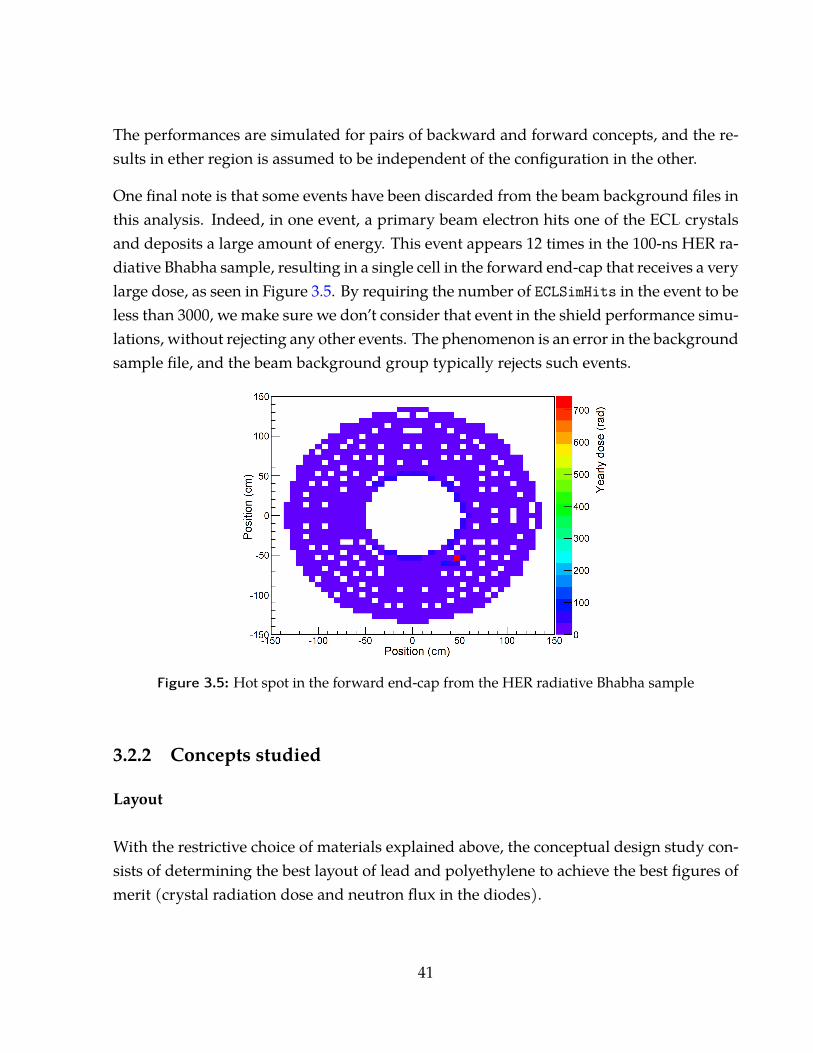
The performances are simulated for pairs of backward and forward concepts, and the re-sults in ether region is assumed to be independent of the configuration in the other.

One final note is that some events have been discarded from the beam background files inthis analysis. Indeed, in one event, a primary beam electron hits one of the ECL crystalsand deposits a large amount of energy. This event appears 12 times in the 100-ns HER ra-diative Bhabha sample, resulting in a single cell in the forward end-cap that receives a verylarge dose, as seen in Figure 3.5. By requiring the number of ECLSimHits in the event to beless than 3000, we make sure we don’t consider that event in the shield performance simu-lations, without rejecting any other events. The phenomenon is an error in the backgroundsample file, and the beam background group typically rejects such events.

Figure 3.5: Hot spot in the forward end-cap from the HER radiative Bhabha sample

3.2.2 Concepts studied

Layout

With the restrictive choice of materials explained above, the conceptual design study con-sists of determining the best layout of lead and polyethylene to achieve the best figures ofmerit (crystal radiation dose and neutron flux in the diodes).

41

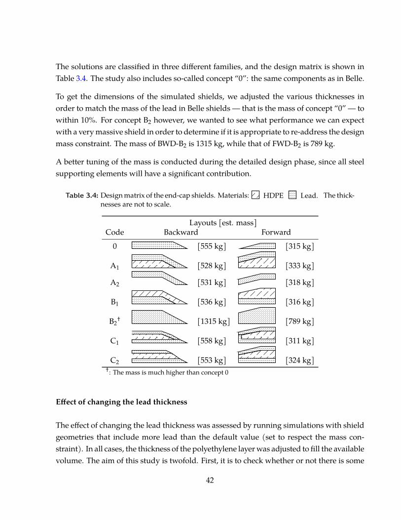
The solutions are classified in three different families, and the design matrix is shown inTable 3.4. The study also includes so-called concept “0”: the same components as in Belle.

To get the dimensions of the simulated shields, we adjusted the various thicknesses inorder to match the mass of the lead in Belle shields — that is the mass of concept “0” — towithin 10%. For concept B2 however, we wanted to see what performance we can expectwith a very massive shield in order to determine if it is appropriate to re-address the designmass constraint. The mass of BWD-B2 is 1315 kg, while that of FWD-B2 is 789 kg.

A better tuning of the mass is conducted during the detailed design phase, since all steelsupporting elements will have a significant contribution.

Table 3.4: Design matrix of the end-cap shields. Materials: HDPE Lead. The thick-nesses are not to scale.

Layouts [est. mass]Code Backward Forward

0 [555 kg] [315 kg]

A1 [528 kg] [333 kg]

A2 [531 kg] [318 kg]

B1 [536 kg] [316 kg]

B2† [1315 kg] [789 kg]

C1 [558 kg] [311 kg]

C2 [553 kg] [324 kg]†: The mass is much higher than concept 0

Effect of changing the lead thickness

The effect of changing the lead thickness was assessed by running simulations with shieldgeometries that include more lead than the default value (set to respect the mass con-straint). In all cases, the thickness of the polyethylene layer was adjusted to fill the availablevolume. The aim of this study is twofold. First, it is to check whether or not there is some

42

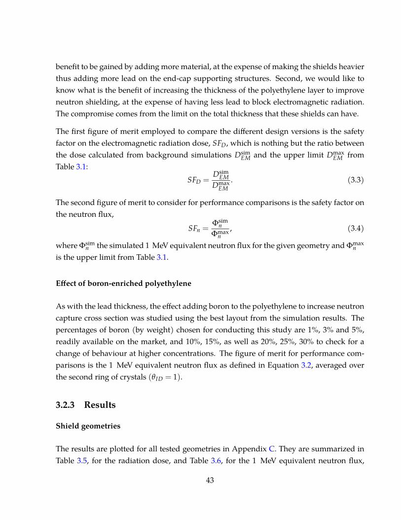
benefit to be gained by adding more material, at the expense of making the shields heavierthus adding more lead on the end-cap supporting structures. Second, we would like toknow what is the benefit of increasing the thickness of the polyethylene layer to improveneutron shielding, at the expense of having less lead to block electromagnetic radiation.The compromise comes from the limit on the total thickness that these shields can have.

The first figure of merit employed to compare the different design versions is the safetyfactor on the electromagnetic radiation dose, SFD, which is nothing but the ratio betweenthe dose calculated from background simulations Dsim

EM and the upper limit DmaxEM from

Table 3.1:SFD =

DsimEM

DmaxEM

. (3.3)

The second figure of merit to consider for performance comparisons is the safety factor onthe neutron flux,

SFn =Φsim

nΦmax

n, (3.4)

where Φsimn the simulated 1 MeV equivalent neutron flux for the given geometry and Φmax

n

is the upper limit from Table 3.1.

Effect of boron-enriched polyethylene

As with the lead thickness, the effect adding boron to the polyethylene to increase neutroncapture cross section was studied using the best layout from the simulation results. Thepercentages of boron (by weight) chosen for conducting this study are 1%, 3% and 5%,readily available on the market, and 10%, 15%, as well as 20%, 25%, 30% to check for achange of behaviour at higher concentrations. The figure of merit for performance com-parisons is the 1 MeV equivalent neutron flux as defined in Equation 3.2, averaged overthe second ring of crystals (θID = 1).

3.2.3 Results

Shield geometries

The results are plotted for all tested geometries in Appendix C. They are summarized inTable 3.5, for the radiation dose, and Table 3.6, for the 1 MeV equivalent neutron flux,

43

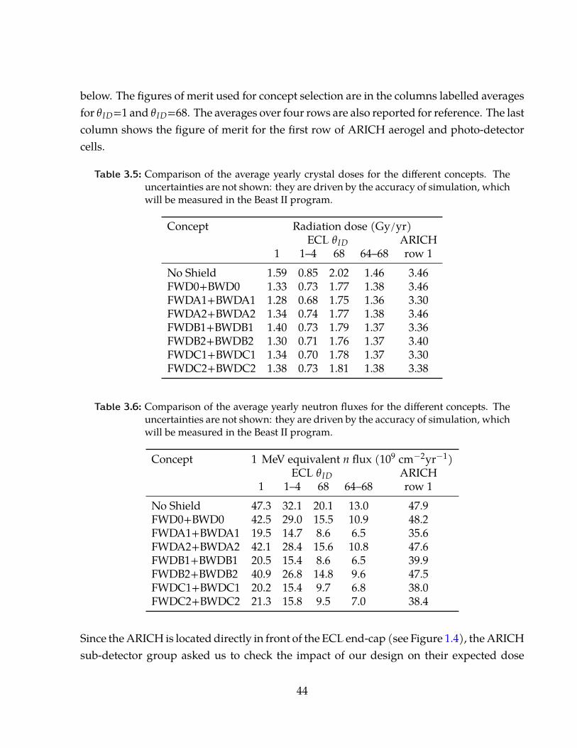
below. The figures of merit used for concept selection are in the columns labelled averagesfor θID=1 and θID=68. The averages over four rows are also reported for reference. The lastcolumn shows the figure of merit for the first row of ARICH aerogel and photo-detectorcells.

Table 3.5: Comparison of the average yearly crystal doses for the different concepts. Theuncertainties are not shown: they are driven by the accuracy of simulation, whichwill be measured in the Beast II program.

Concept Radiation dose (Gy/yr)ECL θID ARICH

1 1–4 68 64–68 row 1No Shield 1.59 0.85 2.02 1.46 3.46FWD0+BWD0 1.33 0.73 1.77 1.38 3.46FWDA1+BWDA1 1.28 0.68 1.75 1.36 3.30FWDA2+BWDA2 1.34 0.74 1.77 1.38 3.46FWDB1+BWDB1 1.40 0.73 1.79 1.37 3.36FWDB2+BWDB2 1.30 0.71 1.76 1.37 3.40FWDC1+BWDC1 1.34 0.70 1.78 1.37 3.30FWDC2+BWDC2 1.38 0.73 1.81 1.38 3.38

Table 3.6: Comparison of the average yearly neutron fluxes for the different concepts. Theuncertainties are not shown: they are driven by the accuracy of simulation, whichwill be measured in the Beast II program.

Concept 1 MeV equivalent n flux (109 cm−2yr−1)ECL θID ARICH

1 1–4 68 64–68 row 1No Shield 47.3 32.1 20.1 13.0 47.9FWD0+BWD0 42.5 29.0 15.5 10.9 48.2FWDA1+BWDA1 19.5 14.7 8.6 6.5 35.6FWDA2+BWDA2 42.1 28.4 15.6 10.8 47.6FWDB1+BWDB1 20.5 15.4 8.6 6.5 39.9FWDB2+BWDB2 40.9 26.8 14.8 9.6 47.5FWDC1+BWDC1 20.2 15.4 9.7 6.8 38.0FWDC2+BWDC2 21.3 15.8 9.5 7.0 38.4

Since the ARICH is located directly in front of the ECL end-cap (see Figure 1.4), the ARICHsub-detector group asked us to check the impact of our design on their expected dose

44

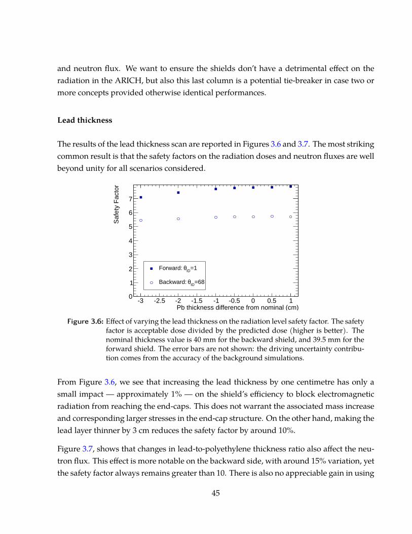
and neutron flux. We want to ensure the shields don’t have a detrimental effect on theradiation in the ARICH, but also this last column is a potential tie-breaker in case two ormore concepts provided otherwise identical performances.

Lead thickness

The results of the lead thickness scan are reported in Figures 3.6 and 3.7. The most strikingcommon result is that the safety factors on the radiation doses and neutron fluxes are wellbeyond unity for all scenarios considered.

Pb thickness difference from nominal (cm)-3 -2.5 -2 -1.5 -1 -0.5 0 0.5 1

Saf

ety

Fac

tor

0

1

2

3

4

5

6

7

Effect of varying thickness on radiation dose

=1IDθForward:

=68IDθBackward:

Figure 3.6: Effect of varying the lead thickness on the radiation level safety factor. The safetyfactor is acceptable dose divided by the predicted dose (higher is better). Thenominal thickness value is 40 mm for the backward shield, and 39.5 mm for theforward shield. The error bars are not shown: the driving uncertainty contribu-tion comes from the accuracy of the background simulations.

From Figure 3.6, we see that increasing the lead thickness by one centimetre has only asmall impact — approximately 1% — on the shield’s efficiency to block electromagneticradiation from reaching the end-caps. This does not warrant the associated mass increaseand corresponding larger stresses in the end-cap structure. On the other hand, making thelead layer thinner by 3 cm reduces the safety factor by around 10%.

Figure 3.7, shows that changes in lead-to-polyethylene thickness ratio also affect the neu-tron flux. This effect is more notable on the backward side, with around 15% variation, yetthe safety factor always remains greater than 10. There is also no appreciable gain in using

45

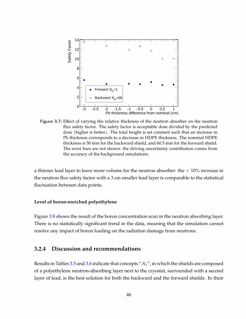
Pb thickness difference from nominal (cm)-3 -2.5 -2 -1.5 -1 -0.5 0 0.5 1

Saf

ety

Fac

tor

0

2

4

6

8

10

12

14

Effect of varying thickness on neutron flux

=1IDθForward:

=68IDθBackward:

Figure 3.7: Effect of varying the relative thickness of the neutron absorber on the neutronflux safety factor. The safety factor is acceptable dose divided by the predicteddose (higher is better). The total height is set constant such that an increase inPb thickness corresponds to a decrease in HDPE thickness. The nominal HDPEthickness is 50 mm for the backward shield, and 60.5 mm for the forward shield.The error bars are not shown: the driving uncertainty contribution comes fromthe accuracy of the background simulations.

a thinner lead layer to leave more volume for the neutron absorber: the < 10% increase inthe neutron flux safety factor with a 3 cm smaller lead layer is comparable to the statisticalfluctuation between data points.

Level of boron-enriched polyethylene

Figure 3.8 shows the result of the boron concentration scan in the neutron absorbing layer.There is no statistically significant trend in the data, meaning that the simulation cannotresolve any impact of boron loading on the radiation damage from neutrons.

3.2.4 Discussion and recommendations

Results in Tables 3.5 and 3.6 indicate that concepts “A1”, in which the shields are composedof a polyethylene neutron-absorbing layer next to the cryostat, surrounded with a secondlayer of lead, is the best solution for both the backward and the forward shields. In their

46

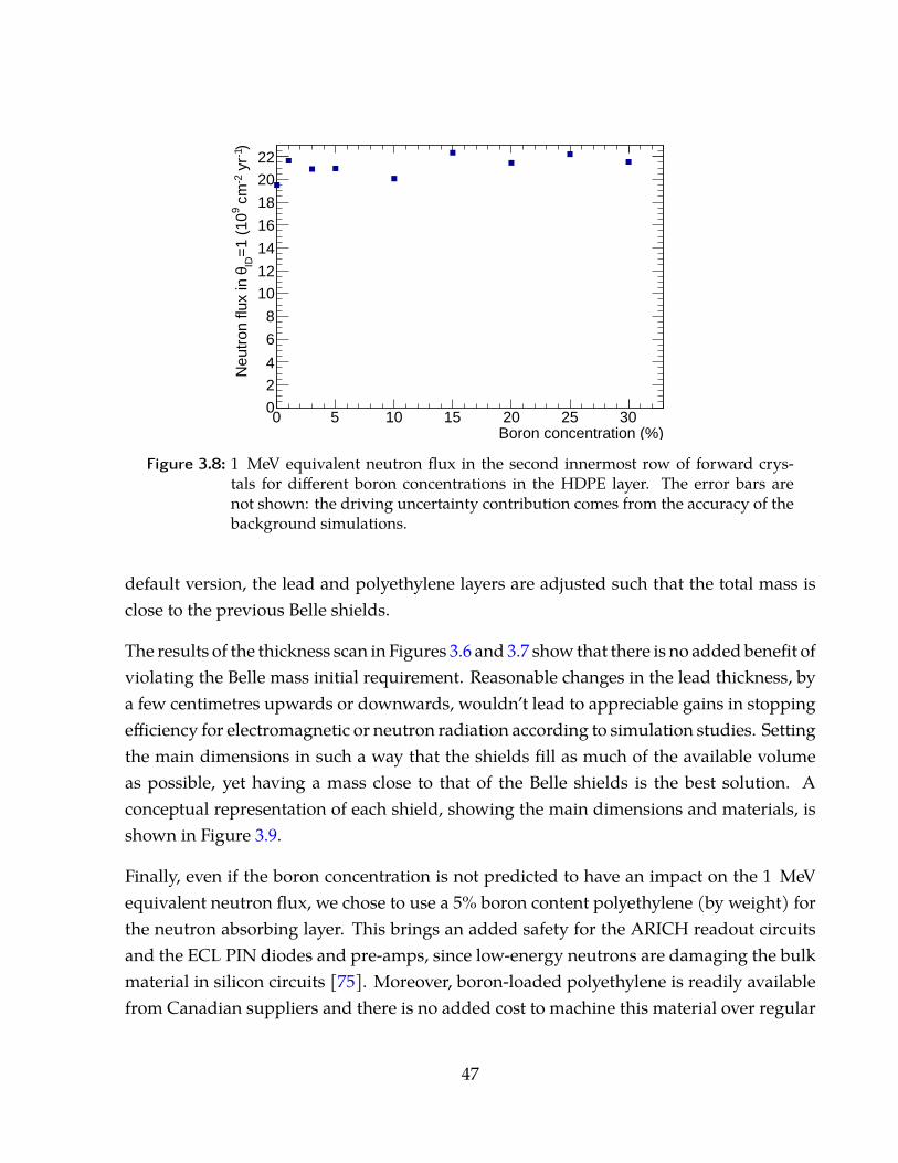
Boron concentration (%)0 5 10 15 20 25 30

)-1

yr

-2 c

m9

=1

(10

IDθN

eutr

on fl

ux in

0

2

4

6

8

10

12

14

16

18

20

22

Effect of Borated PE on fluxesEffect of Borated PE on fluxes

Figure 3.8: 1 MeV equivalent neutron flux in the second innermost row of forward crys-tals for different boron concentrations in the HDPE layer. The error bars arenot shown: the driving uncertainty contribution comes from the accuracy of thebackground simulations.

default version, the lead and polyethylene layers are adjusted such that the total mass isclose to the previous Belle shields.

The results of the thickness scan in Figures 3.6 and 3.7 show that there is no added benefit ofviolating the Belle mass initial requirement. Reasonable changes in the lead thickness, bya few centimetres upwards or downwards, wouldn’t lead to appreciable gains in stoppingefficiency for electromagnetic or neutron radiation according to simulation studies. Settingthe main dimensions in such a way that the shields fill as much of the available volumeas possible, yet having a mass close to that of the Belle shields is the best solution. Aconceptual representation of each shield, showing the main dimensions and materials, isshown in Figure 3.9.

Finally, even if the boron concentration is not predicted to have an impact on the 1 MeVequivalent neutron flux, we chose to use a 5% boron content polyethylene (by weight) forthe neutron absorbing layer. This brings an added safety for the ARICH readout circuitsand the ECL PIN diodes and pre-amps, since low-energy neutrons are damaging the bulkmaterial in silicon circuits [75]. Moreover, boron-loaded polyethylene is readily availablefrom Canadian suppliers and there is no added cost to machine this material over regular

47

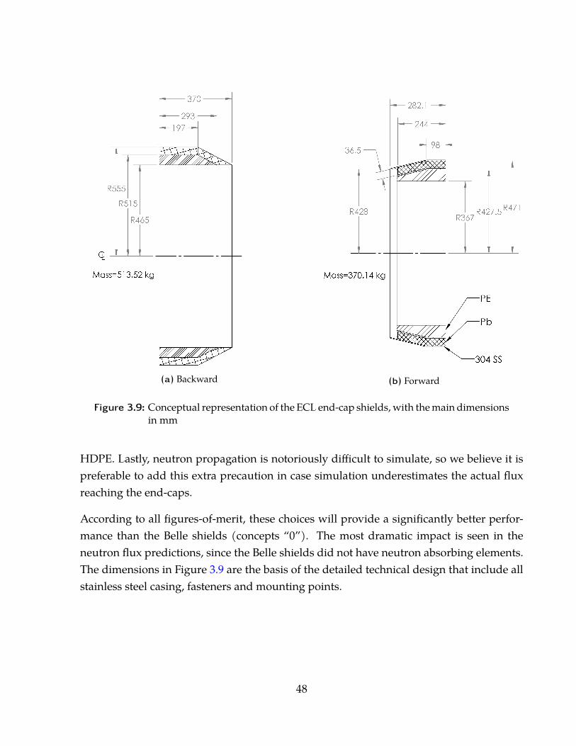
(a) Backward (b) Forward

Figure 3.9: Conceptual representation of the ECL end-cap shields, with the main dimensionsin mm

HDPE. Lastly, neutron propagation is notoriously difficult to simulate, so we believe it ispreferable to add this extra precaution in case simulation underestimates the actual fluxreaching the end-caps.

According to all figures-of-merit, these choices will provide a significantly better perfor-mance than the Belle shields (concepts “0”). The most dramatic impact is seen in theneutron flux predictions, since the Belle shields did not have neutron absorbing elements.The dimensions in Figure 3.9 are the basis of the detailed technical design that include allstainless steel casing, fasteners and mounting points.

48

3.3 Technical design

3.3.1 General design of the shields

Sub-systems and naming scheme

The project is part of the electromagnetic calorimeter (ECL) detector, and comprises twoproducts, the forward shield (ECL-100-000) and the backward shield (ECL-200-000). Eachshield is broken down into five (5) sub-systems with corresponding assembly numbers:

� the shell: ECL-X00-100,

� the electromagnetic radiation shield: ECL-X00-200,

� the neutron radiation shield: ECL-X00-300,

� the mounting points for transport and installation: ECL-X00-400,

� the attachments to the end-caps: ECL-X00-500,

where X = 1 for forward, and X = 2 for backward.

Configuration

The configuration, or layout of the different sub-systems in the products was studied inthe Conceptual Design Report (CDR)[63] and summarized in section 3.2. The generalconcepts of the Belle shield were re-used, and each product is made of two symmetricalhalves, split along the vertical plane. The enclosures used to contain the electromagneticradiation shields and attach the two halves together — also referred to as the “shells” —are made of 304 stainless steel. The neutron radiation shield is attached below the electro-magnetic radiation shield, i.e. at a smaller radius. The mounting points for transport arelocated at the same coordinates as the Belle shields, and the attachment to the end-capsare the same parts as what was used in Belle, for compatibility reasons. The configurationis represented in Figure 3.10. It is given for the example of the backward shield, but isidentical in both assemblies.

49

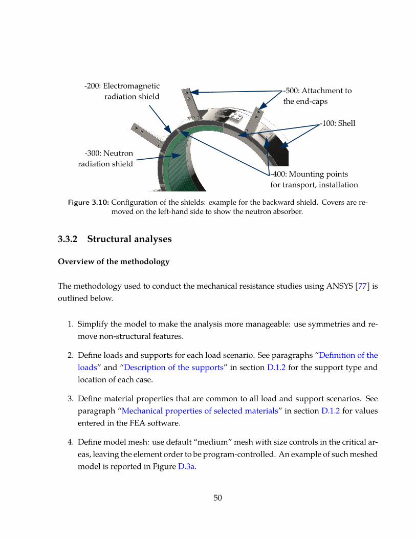
-100: Shell

-200: Electromagnetic radiation shield

-300: Neutron radiation shield

-400: Mounting points for transport, installation

-500: Attachment to the end-caps

Figure 3.10: Configuration of the shields: example for the backward shield. Covers are re-moved on the left-hand side to show the neutron absorber.

3.3.2 Structural analyses

Overview of the methodology

The methodology used to conduct the mechanical resistance studies using ANSYS [77] isoutlined below.

1. Simplify the model to make the analysis more manageable: use symmetries and re-move non-structural features.

2. Define loads and supports for each load scenario. See paragraphs “Definition of theloads” and “Description of the supports” in section D.1.2 for the support type andlocation of each case.

3. Define material properties that are common to all load and support scenarios. Seeparagraph “Mechanical properties of selected materials” in section D.1.2 for valuesentered in the FEA software.

4. Define model mesh: use default “medium” mesh with size controls in the critical ar-eas, leaving the element order to be program-controlled. An example of such meshedmodel is reported in Figure D.3a.

50

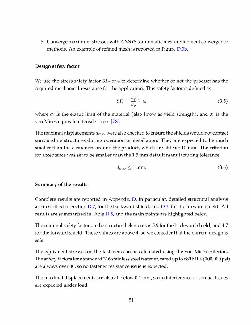
5. Converge maximum stresses with ANSYS’s automatic mesh-refinement convergencemethods. An example of refined mesh is reported in Figure D.3b.

Design safety factor

We use the stress safety factor SFσ of 4 to determine whether or not the product has therequired mechanical resistance for the application. This safety factor is defined as

SFσ =σy

σv≥ 4, (3.5)

where σy is the elastic limit of the material (also know as yield strength), and σv is thevon Mises equivalent tensile stress [78].

The maximal displacements dmax were also checked to ensure the shields would not contactsurrounding structures during operation or installation. They are expected to be muchsmaller than the clearances around the product, which are at least 10 mm. The criterionfor acceptance was set to be smaller than the 1.5 mm default manufacturing tolerance:

dmax ≤ 1 mm. (3.6)

Summary of the results

Complete results are reported in Appendix D. In particular, detailed structural analysisare described in Section D.2, for the backward shield, and D.3, for the forward shield. Allresults are summarized in Table D.5, and the main points are highlighted below.

The minimal safety factor on the structural elements is 5.9 for the backward shield, and 4.7for the forward shield. These values are above 4, so we consider that the current design issafe.

The equivalent stresses on the fasteners can be calculated using the von Mises criterion.The safety factors for a standard 316 stainless steel fastener, rated up to 689 MPa (100,000 psi),are always over 30, so no fastener resistance issue is expected.

The maximal displacements are also all below 0.1 mm, so no interference or contact issuesare expected under load.

51

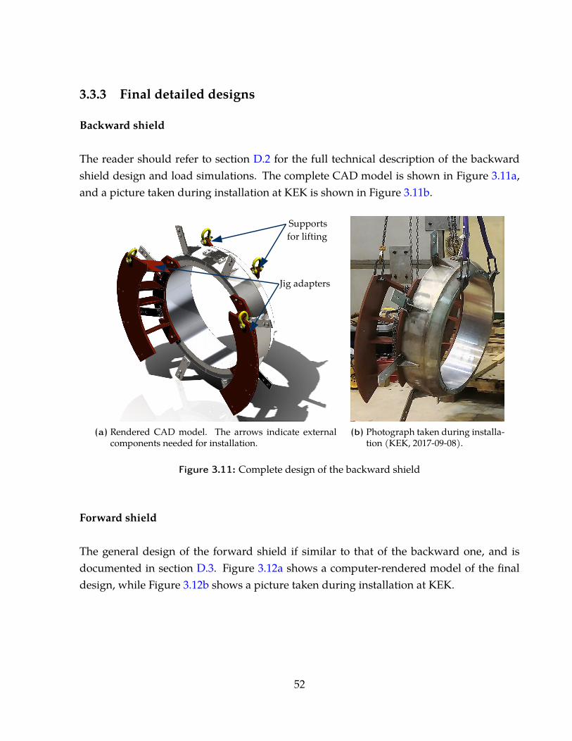
3.3.3 Final detailed designs

Backward shield

The reader should refer to section D.2 for the full technical description of the backwardshield design and load simulations. The complete CAD model is shown in Figure 3.11a,and a picture taken during installation at KEK is shown in Figure 3.11b.

Jig adapters

Supports for lifting

(a) Rendered CAD model. The arrows indicate externalcomponents needed for installation.

(b) Photograph taken during installa-tion (KEK, 2017-09-08).

Figure 3.11: Complete design of the backward shield

Forward shield

The general design of the forward shield if similar to that of the backward one, and isdocumented in section D.3. Figure 3.12a shows a computer-rendered model of the finaldesign, while Figure 3.12b shows a picture taken during installation at KEK.

52

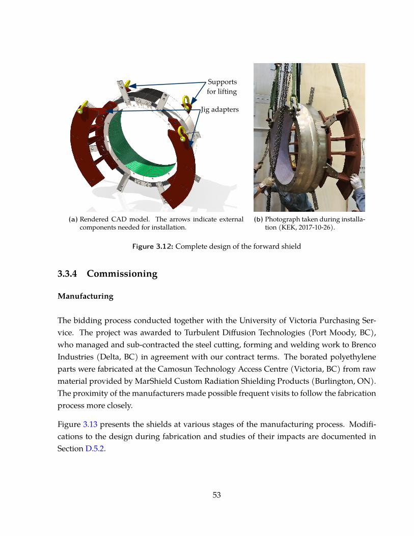
Jig adapters

Supports for lifting

(a) Rendered CAD model. The arrows indicate externalcomponents needed for installation.

(b) Photograph taken during installa-tion (KEK, 2017-10-26).

Figure 3.12: Complete design of the forward shield

3.3.4 Commissioning

Manufacturing

The bidding process conducted together with the University of Victoria Purchasing Ser-vice. The project was awarded to Turbulent Diffusion Technologies (Port Moody, BC),who managed and sub-contracted the steel cutting, forming and welding work to BrencoIndustries (Delta, BC) in agreement with our contract terms. The borated polyethyleneparts were fabricated at the Camosun Technology Access Centre (Victoria, BC) from rawmaterial provided by MarShield Custom Radiation Shielding Products (Burlington, ON).The proximity of the manufacturers made possible frequent visits to follow the fabricationprocess more closely.

Figure 3.13 presents the shields at various stages of the manufacturing process. Modifi-cations to the design during fabrication and studies of their impacts are documented inSection D.5.2.

53

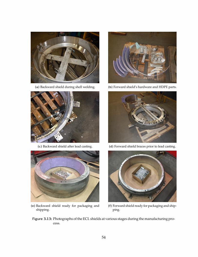
(a) Backward shield during shell welding. (b) Forward shield’s hardware and HDPE parts.

(c) Backward shield after lead casting. (d) Forward shield braces prior to lead casting.

(e) Backward shield ready for packaging andshipping.

(f) Forward shield ready for packaging and ship-ping.

Figure 3.13: Photographs of the ECL shields at various stages during the manufacturing pro-cess.

54

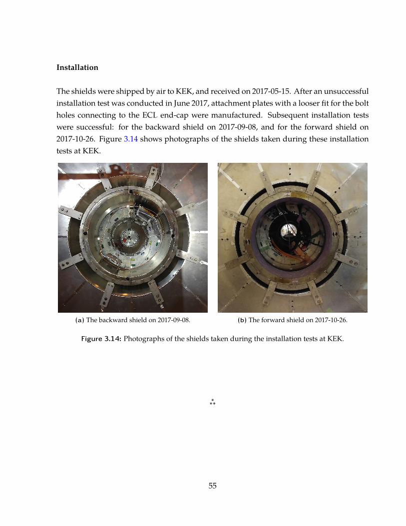
Installation

The shields were shipped by air to KEK, and received on 2017-05-15. After an unsuccessfulinstallation test was conducted in June 2017, attachment plates with a looser fit for the boltholes connecting to the ECL end-cap were manufactured. Subsequent installation testswere successful: for the backward shield on 2017-09-08, and for the forward shield on2017-10-26. Figure 3.14 shows photographs of the shields taken during these installationtests at KEK.

(a) The backward shield on 2017-09-08. (b) The forward shield on 2017-10-26.

Figure 3.14: Photographs of the shields taken during the installation tests at KEK.

***

55

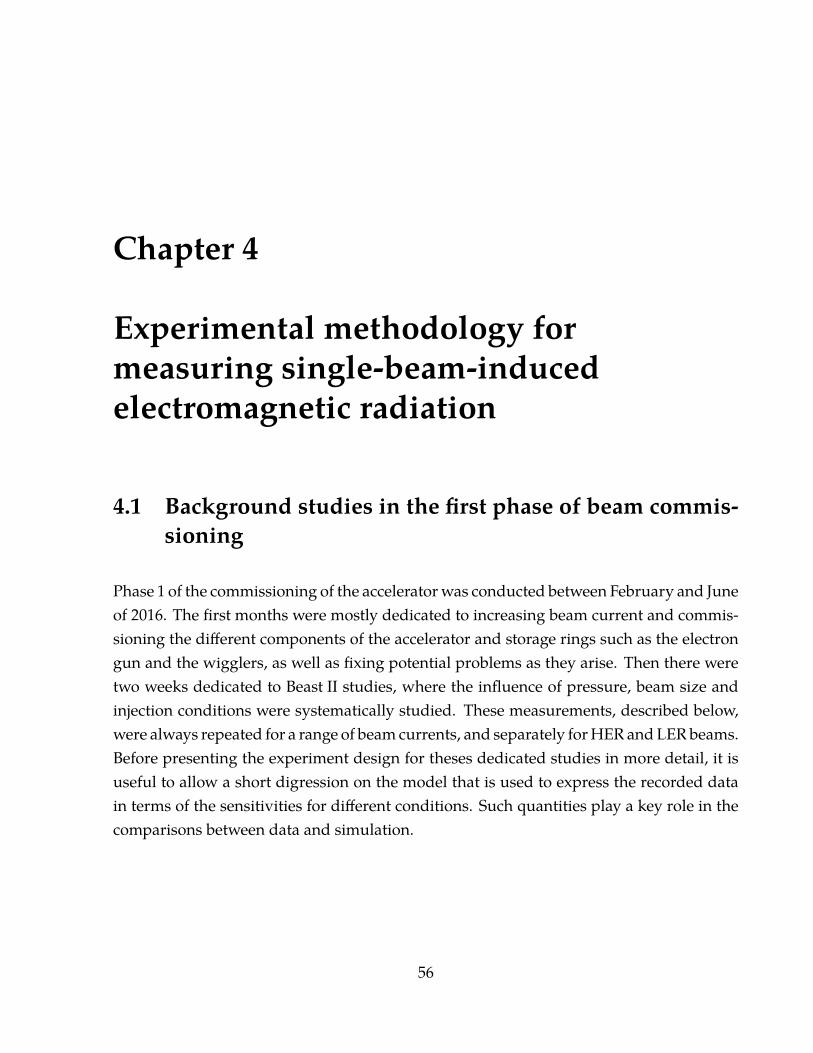
Chapter 4

Experimental methodology formeasuring single-beam-inducedelectromagnetic radiation

4.1 Background studies in the first phase of beam commis-sioning

Phase 1 of the commissioning of the accelerator was conducted between February and Juneof 2016. The first months were mostly dedicated to increasing beam current and commis-sioning the different components of the accelerator and storage rings such as the electrongun and the wigglers, as well as fixing potential problems as they arise. Then there weretwo weeks dedicated to Beast II studies, where the influence of pressure, beam size andinjection conditions were systematically studied. These measurements, described below,were always repeated for a range of beam currents, and separately for HER and LER beams.Before presenting the experiment design for theses dedicated studies in more detail, it isuseful to allow a short digression on the model that is used to express the recorded datain terms of the sensitivities for different conditions. Such quantities play a key role in thecomparisons between data and simulation.

56

4.1.1 Influence of pressure

Vacuum bump experiments are conducted by heating the non-evaporable getters1 (NEG)at various locations in the tunnel, far and near the Beast II region to release gas moleculesinto the vacuum chamber. The target is to heat the NEGs enough to increase the pressure bya factor∼ 100. We measured the pressure-dependence of the background rates versus thelocation of the vacuum bump. Moreover, the low-energy ring is equipped with a residualgas analyzer so a more refined analysis is possible by studying the effect of gas composition.The run plan is schematically represented in Figure 4.1.

Figure 4.1: Schematic representation of the pressure bump studies run plan. The arrowspoint to the location where the pressure bump was applied, with the associatedrun number in each box. The colours indicate which ring was studied: blue,the 6000 series, means the high-enery ring; while red, the 5000 series, means thelow-energy ring. Reproduced from [33] with modiciations (addition of labels).

1NEGs are used used in conjunction with vacuum pumps to bring the pressures down to the design valuesof 1× 10−7 Pa.

57

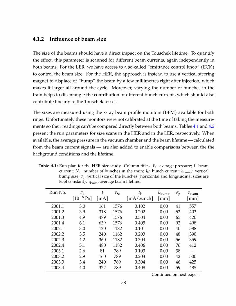
4.1.2 Influence of beam size

The size of the beams should have a direct impact on the Touschek lifetime. To quantifythe effect, this parameter is scanned for different beam currents, again independently inboth beams. For the LER, we have access to a so-called ”emittance control knob” (ECK)to control the beam size. For the HER, the approach is instead to use a vertical steeringmagnet to displace or ”bump” the beam by a few millimetres right after injection, whichmakes it larger all around the cycle. Moreover, varying the number of bunches in thetrain helps to disentangle the contribution of different bunch currents which should alsocontribute linearly to the Touschek losses.

The sizes are measured using the x-ray beam profile monitors (BPM) available for bothrings. Unfortunately these monitors were not calibrated at the time of taking the measure-ments so their readings can’t be compared directly between both beams. Tables 4.1 and 4.2present the run parameters for size scans in the HER and in the LER, respectively. Whenavailable, the average pressure in the vacuum chamber and the beam lifetime — calculatedfrom the beam current signals — are also added to enable comparisons between the thebackground conditions and the lifetime.

Table 4.1: Run plan for the HER size study. Column titles: Pe: average pressure; I: beamcurrent; Nb: number of bunches in the train; Ib: bunch current; hbump: verticalbump size; σy: vertical size of the bunches (horizontal and longitudinal sizes arekept constant); τbeam; average beam lifetime.

Run No. Pe I Nb Ib hbump σy τbeam[10−8 Pa] [mA] [mA/bunch] [mm] [min]

2001.1 3.0 161 1576 0.102 0.00 41 5572001.2 3.9 318 1576 0.202 0.00 52 4032001.3 4.9 479 1576 0.304 0.00 65 4202001.4 6.1 639 1576 0.405 0.00 92 4982002.1 3.0 120 1182 0.101 0.00 40 5882002.2 3.5 240 1182 0.203 0.00 48 3902002.3 4.2 360 1182 0.304 0.00 56 3592002.4 5.1 480 1182 0.406 0.00 76 4122003.1 2.6 81 789 0.103 0.00 38 -2003.2 2.9 160 789 0.203 0.00 42 5002003.3 3.4 240 789 0.304 0.00 46 4252003.4 4.0 322 789 0.408 0.00 59 485

Continued on next page...58

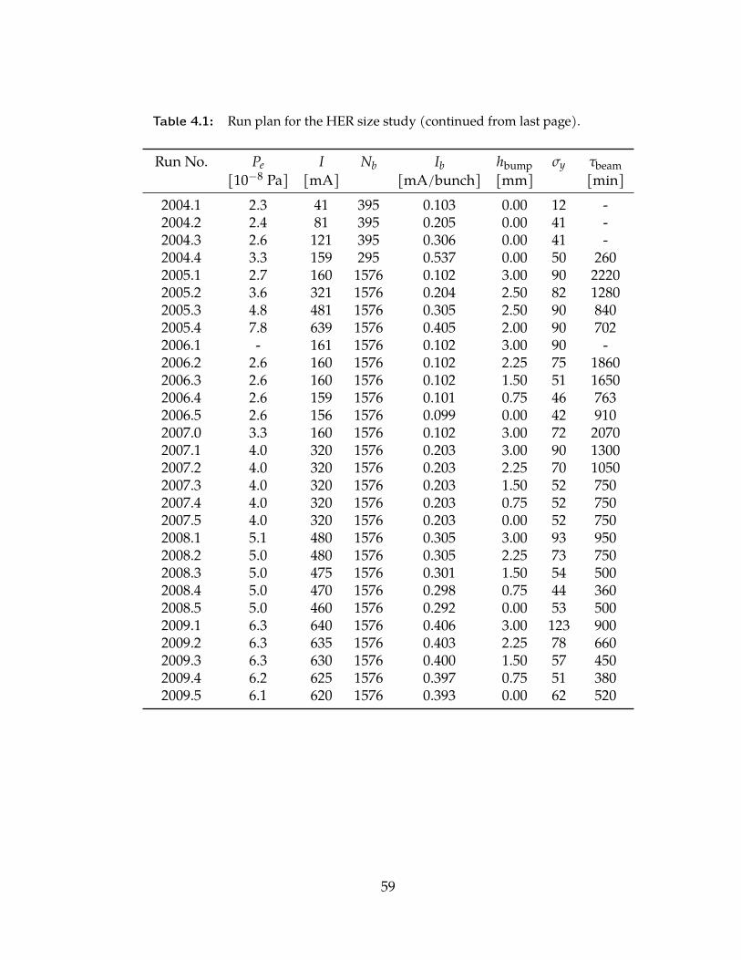
Table 4.1: Run plan for the HER size study (continued from last page).

Run No. Pe I Nb Ib hbump σy τbeam[10−8 Pa] [mA] [mA/bunch] [mm] [min]

2004.1 2.3 41 395 0.103 0.00 12 -2004.2 2.4 81 395 0.205 0.00 41 -2004.3 2.6 121 395 0.306 0.00 41 -2004.4 3.3 159 295 0.537 0.00 50 2602005.1 2.7 160 1576 0.102 3.00 90 22202005.2 3.6 321 1576 0.204 2.50 82 12802005.3 4.8 481 1576 0.305 2.50 90 8402005.4 7.8 639 1576 0.405 2.00 90 7022006.1 - 161 1576 0.102 3.00 90 -2006.2 2.6 160 1576 0.102 2.25 75 18602006.3 2.6 160 1576 0.102 1.50 51 16502006.4 2.6 159 1576 0.101 0.75 46 7632006.5 2.6 156 1576 0.099 0.00 42 9102007.0 3.3 160 1576 0.102 3.00 72 20702007.1 4.0 320 1576 0.203 3.00 90 13002007.2 4.0 320 1576 0.203 2.25 70 10502007.3 4.0 320 1576 0.203 1.50 52 7502007.4 4.0 320 1576 0.203 0.75 52 7502007.5 4.0 320 1576 0.203 0.00 52 7502008.1 5.1 480 1576 0.305 3.00 93 9502008.2 5.0 480 1576 0.305 2.25 73 7502008.3 5.0 475 1576 0.301 1.50 54 5002008.4 5.0 470 1576 0.298 0.75 44 3602008.5 5.0 460 1576 0.292 0.00 53 5002009.1 6.3 640 1576 0.406 3.00 123 9002009.2 6.3 635 1576 0.403 2.25 78 6602009.3 6.3 630 1576 0.400 1.50 57 4502009.4 6.2 625 1576 0.397 0.75 51 3802009.5 6.1 620 1576 0.393 0.00 62 520

59

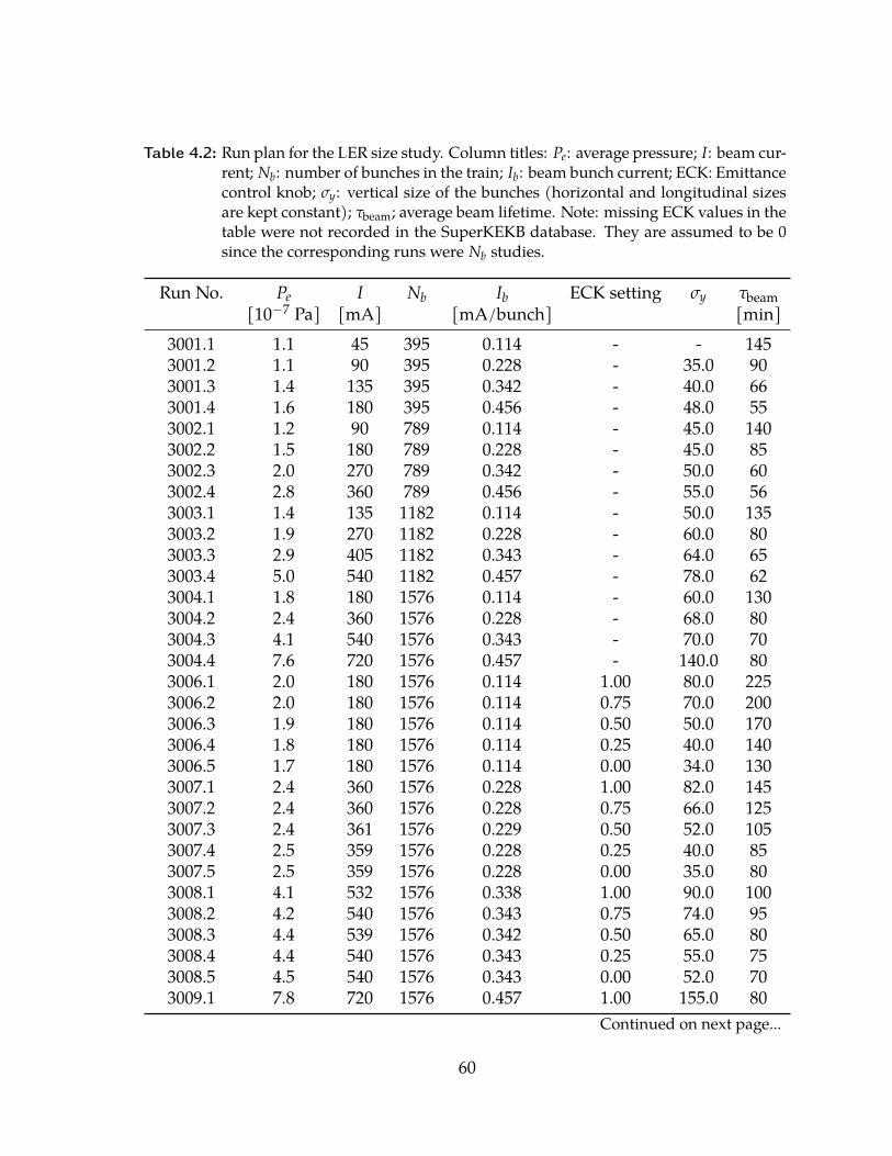
Table 4.2: Run plan for the LER size study. Column titles: Pe: average pressure; I: beam cur-rent; Nb: number of bunches in the train; Ib: beam bunch current; ECK: Emittancecontrol knob; σy: vertical size of the bunches (horizontal and longitudinal sizesare kept constant); τbeam; average beam lifetime. Note: missing ECK values in thetable were not recorded in the SuperKEKB database. They are assumed to be 0since the corresponding runs were Nb studies.

Run No. Pe I Nb Ib ECK setting σy τbeam[10−7 Pa] [mA] [mA/bunch] [min]

3001.1 1.1 45 395 0.114 - - 1453001.2 1.1 90 395 0.228 - 35.0 903001.3 1.4 135 395 0.342 - 40.0 663001.4 1.6 180 395 0.456 - 48.0 553002.1 1.2 90 789 0.114 - 45.0 1403002.2 1.5 180 789 0.228 - 45.0 853002.3 2.0 270 789 0.342 - 50.0 603002.4 2.8 360 789 0.456 - 55.0 563003.1 1.4 135 1182 0.114 - 50.0 1353003.2 1.9 270 1182 0.228 - 60.0 803003.3 2.9 405 1182 0.343 - 64.0 653003.4 5.0 540 1182 0.457 - 78.0 623004.1 1.8 180 1576 0.114 - 60.0 1303004.2 2.4 360 1576 0.228 - 68.0 803004.3 4.1 540 1576 0.343 - 70.0 703004.4 7.6 720 1576 0.457 - 140.0 803006.1 2.0 180 1576 0.114 1.00 80.0 2253006.2 2.0 180 1576 0.114 0.75 70.0 2003006.3 1.9 180 1576 0.114 0.50 50.0 1703006.4 1.8 180 1576 0.114 0.25 40.0 1403006.5 1.7 180 1576 0.114 0.00 34.0 1303007.1 2.4 360 1576 0.228 1.00 82.0 1453007.2 2.4 360 1576 0.228 0.75 66.0 1253007.3 2.4 361 1576 0.229 0.50 52.0 1053007.4 2.5 359 1576 0.228 0.25 40.0 853007.5 2.5 359 1576 0.228 0.00 35.0 803008.1 4.1 532 1576 0.338 1.00 90.0 1003008.2 4.2 540 1576 0.343 0.75 74.0 953008.3 4.4 539 1576 0.342 0.50 65.0 803008.4 4.4 540 1576 0.343 0.25 55.0 753008.5 4.5 540 1576 0.343 0.00 52.0 703009.1 7.8 720 1576 0.457 1.00 155.0 80

Continued on next page...

60

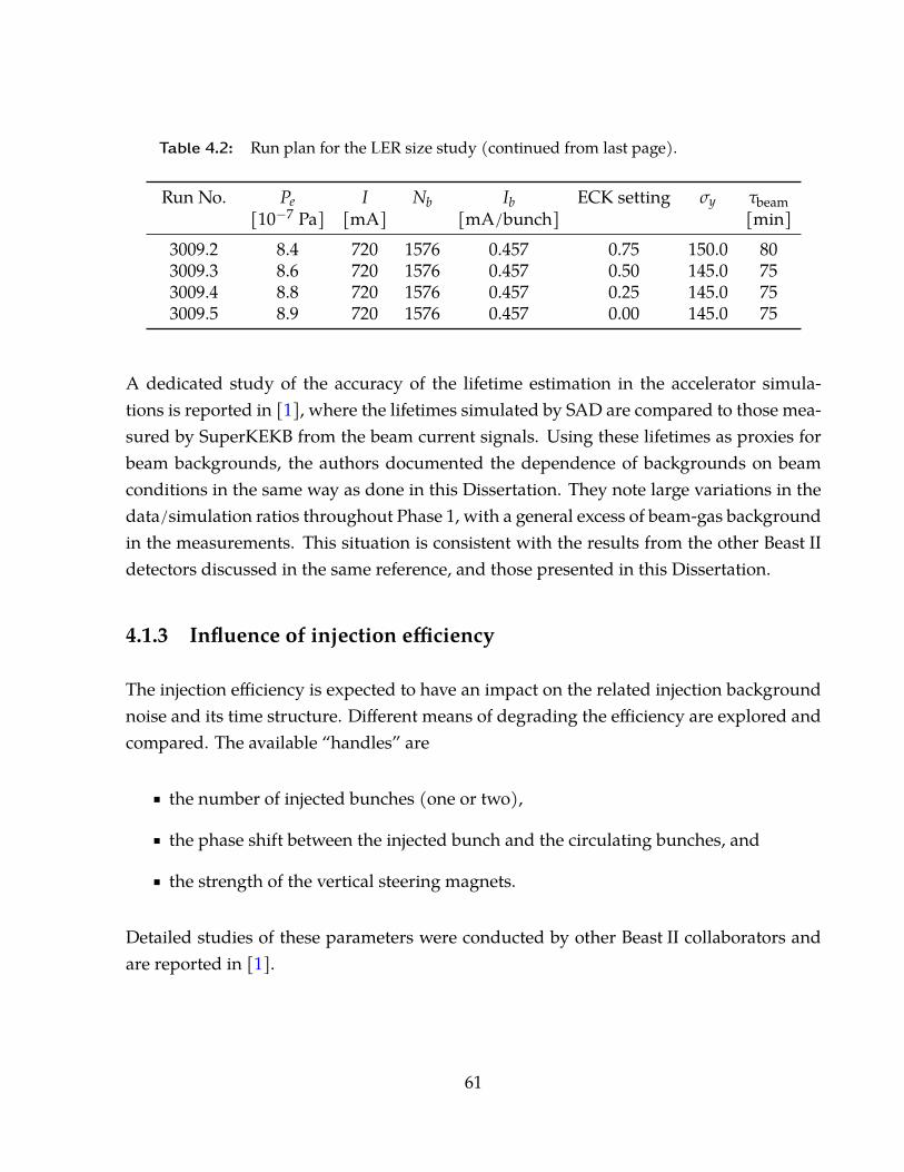
Table 4.2: Run plan for the LER size study (continued from last page).

Run No. Pe I Nb Ib ECK setting σy τbeam[10−7 Pa] [mA] [mA/bunch] [min]

3009.2 8.4 720 1576 0.457 0.75 150.0 803009.3 8.6 720 1576 0.457 0.50 145.0 753009.4 8.8 720 1576 0.457 0.25 145.0 753009.5 8.9 720 1576 0.457 0.00 145.0 75

A dedicated study of the accuracy of the lifetime estimation in the accelerator simula-tions is reported in [1], where the lifetimes simulated by SAD are compared to those mea-sured by SuperKEKB from the beam current signals. Using these lifetimes as proxies forbeam backgrounds, the authors documented the dependence of backgrounds on beamconditions in the same way as done in this Dissertation. They note large variations in thedata/simulation ratios throughout Phase 1, with a general excess of beam-gas backgroundin the measurements. This situation is consistent with the results from the other Beast IIdetectors discussed in the same reference, and those presented in this Dissertation.

4.1.3 Influence of injection efficiency

The injection efficiency is expected to have an impact on the related injection backgroundnoise and its time structure. Different means of degrading the efficiency are explored andcompared. The available “handles” are

� the number of injected bunches (one or two),

� the phase shift between the injected bunch and the circulating bunches, and

� the strength of the vertical steering magnets.

Detailed studies of these parameters were conducted by other Beast II collaborators andare reported in [1].

61

4.2 Analysis of residual gas constituents

The gas contents in the vacuum chambers have a large impact on the beam-gas backgroundbecause their rate depends on Zi

2. However, the simplest model of beam-gas interactionsassumes that the losses, hence the recorded background rate, are proportional to the prod-uct of the average pressure and beam current. The following section decribes the method-ology used to exploit the information coming from the residual gas analyzers (RGA) atSuperKEKB in order to improve our description of beam-gas interactions. The work wasdone in collaboration with Dr. Samuel R. de Jong [79] and the discussion below followsthat in the published Beast II report [1].

The SuperKEKB accelerator is instrumented with two RGAs: one near the Beast II detectoron the positron storage ring, and the other — approximately diametrically opposite in thestorage ring — near the positron injection site. These RGAs are in fact mass spectrometersproviding the partial pressure for gas fragment mass-to-charge ratios m/z between 1 and50. In order to compare measurements with the simulations generated assuming a puregas of atomic number Z = 7, we need to extract information of the relative importanceof each gas constituent, and calculate an effective Z for this gas, noted Ze. The analysismethod can be broken down in three steps: definition of the gas model, calculation of theproportion of each gas constituent, and calculation of the corresponding Ze.

4.2.1 Gas model

Because mass spectrometers only give distributions of the m/z for the different gas ionfragments, any further effort to interpret these as gas molecule abundances already in-volves an act of interpretation [80]. Some early assumption about the nature of the gasare therefore required. Di-hydrogen and air constituents are first added to the list of gasesas the default hypothesis: H2, H2O, N2, O2, CO, CO2, Ar. Then, light hydrocarbons areadded progressively starting from CH4 until all peaks in the spectra could be accountedfor: CH4, C2H6, C2H4, C3H4, C3H6, C3H8.

62

4.2.2 Calculation of the proportion of each gas

The proportion of each gas species in the residual gas is then found by calculating the op-timal proportions to explain the measured spectra in the least-squares sense. The problemis expressed as solving

argminx‖Ax− y‖2 , x ≥ 0 (4.1)

where y is a column vector of the observed relative abundances for each m/z peak, Ais a matrix whose columns each correspond to the standard spectrum for a gas modelconstituents, and x is a column vector of the relative proportion (in number of molecules)of each gas in the mix. The vector of the optimal proportions of each gas, x, is therefore

x =(

ATA)−1

ATy. (4.2)

4.2.3 Calculation of an effective Z for this gas mixture

The gas proportions xi, together with their molecular formulae, are then used to calculatethe number bj of atoms of element Zj by simply multiplying each xi by the number ofatoms of Zj in the gas molecules. Assuming that the probability of interaction between abeam electron and an atom Zj is proportional to Z2

j — this follows the typical cross sectionequations for Coulomb scattering and bremsstrahlung off atomic nuclei — the so-calledeffective Z, Ze, is expressed as a weighted average of Z2

j .⟨Z2⟩

=∑j Z2

j bj

∑j bj(4.3)

Ze =√〈Z2〉 (4.4)

It is “effective” in the sense that this Ze is the atomic number of a pure gas that would pro-duce the same level of beam-gas interactions as the gas mix found in the vacuum chamber.This number can then readily be used to scale the simulation that has been generated witha single value of Z = 7.

4.2.4 Propagation of uncertainties

The RGA used in Phase 1 was not calibrated for the gases present in the vacuum chamber.As such, the SuperKEKB vacuum group reported that we can reasonably expect a factor

63

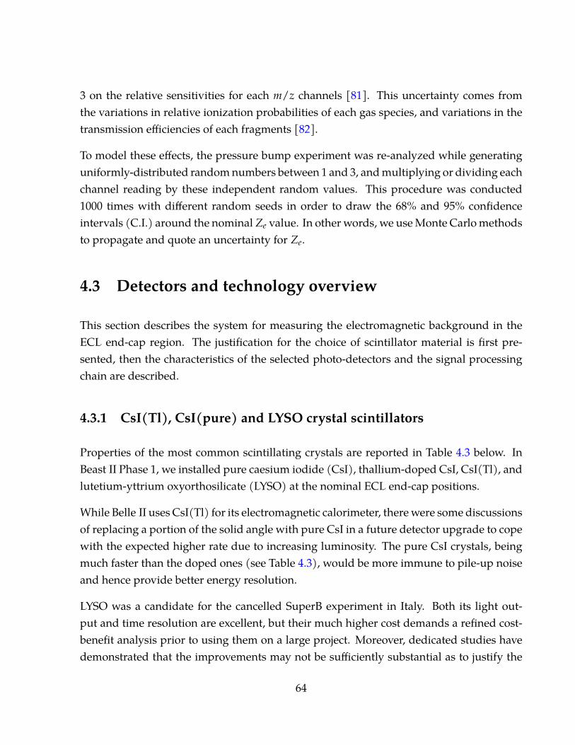
3 on the relative sensitivities for each m/z channels [81]. This uncertainty comes fromthe variations in relative ionization probabilities of each gas species, and variations in thetransmission efficiencies of each fragments [82].

To model these effects, the pressure bump experiment was re-analyzed while generatinguniformly-distributed random numbers between 1 and 3, and multiplying or dividing eachchannel reading by these independent random values. This procedure was conducted1000 times with different random seeds in order to draw the 68% and 95% confidenceintervals (C.I.) around the nominal Ze value. In other words, we use Monte Carlo methodsto propagate and quote an uncertainty for Ze.

4.3 Detectors and technology overview

This section describes the system for measuring the electromagnetic background in theECL end-cap region. The justification for the choice of scintillator material is first pre-sented, then the characteristics of the selected photo-detectors and the signal processingchain are described.

4.3.1 CsI(Tl), CsI(pure) and LYSO crystal scintillators

Properties of the most common scintillating crystals are reported in Table 4.3 below. InBeast II Phase 1, we installed pure caesium iodide (CsI), thallium-doped CsI, CsI(Tl), andlutetium-yttrium oxyorthosilicate (LYSO) at the nominal ECL end-cap positions.

While Belle II uses CsI(Tl) for its electromagnetic calorimeter, there were some discussionsof replacing a portion of the solid angle with pure CsI in a future detector upgrade to copewith the expected higher rate due to increasing luminosity. The pure CsI crystals, beingmuch faster than the doped ones (see Table 4.3), would be more immune to pile-up noiseand hence provide better energy resolution.

LYSO was a candidate for the cancelled SuperB experiment in Italy. Both its light out-put and time resolution are excellent, but their much higher cost demands a refined cost-benefit analysis prior to using them on a large project. Moreover, dedicated studies havedemonstrated that the improvements may not be sufficiently substantial as to justify the

64

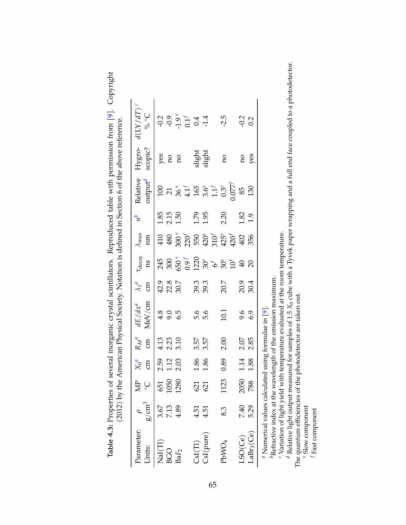
Table

4.3:

Prop

ertie

sofs

ever

alin

orga

nicc

rysta

lscin

tillat

ors.

Repr

oduc

edta

ble

with

perm

issio

nfro

m[9

].Co

pyrig

ht(2

012)

byth

eAm

erica

nPh

ysica

lSoc

iety.

Nota

tion

isde

fined

inSe

ction

6oft

heab

over

efere

nce.

Para

mete

r:ρ

MP

X0a

RM

adE

/dx

aλ

Iaτ d

ecay

λm

axnb

Relat

iveH

ygro

-d(

LY/

dT)

c

Units

:g/

cm3

◦ Ccm

cmM

eV/c

mcm

nsnm

outp

utd

scop

ic?%◦ C

NaI(T

l)3.6

765

12.5

94.1

34.8

42.9

245

410

1.85

100

yes

-0.2

BGO

7.13

1050

1.12

2.23

9.022

.830

048

02.1

521

no-0

.9Ba

F 24.8

912

802.0

33.1

06.5

30.7

650s

300s

1.50

36s

no-1

.9s

0.9f

220f

4.1f

0.1f

CsI(T

l)4.5

162

11.8

63.5

75.6

39.3

1220

550

1.79

165

sligh

t0.4

CsI(p

ure)

4.51

621

1.86

3.57

5.639

.330

s42

0s1.9

53.6

ssli

ght

-1.4

6f31

0f1.1

f

PbW

O 48.3

1123

0.89

2.00

10.1

20.7

30s

425s

2.20

0.3s

no-2

.510

f42

0f0.0

77f

LSO(

Ce)

7.40

2050

1.14

2.07

9.620

.940

402

1.82

85no

-0.2

LaBr

3(Ce

)5.2

978

81.8

82.8

56.9

30.4

2035

61.9

130

yes

0.2a

Num

erica

lvalu

esca

lculat

edus

ingf

orm

ulae

in[9

].b R

efrac

tivei

ndex

atth

ewav

eleng

thof

thee

miss

ion

max

imum

.c

Varia

tion

oflig

htyi

eldw

ithtem

pera

ture

evalu

ated

atth

eroo

mtem

pera

ture

.d

Relat

ivelig

htou

tput

mea

sure

dfo

rsam

ples

of1.5

X0

cube

with

aTyv

ekpa

perw

rapp

inga

ndaf

ulle

ndfa

ceco

upled

toap

hoto

detec

tor.

Theq

uant

umeffi

cienc

iesof

thep

hoto

detec

tora

reta

ken

out.

sSl

owco

mpo

nent

f Fas

tcom

pone

nt

65

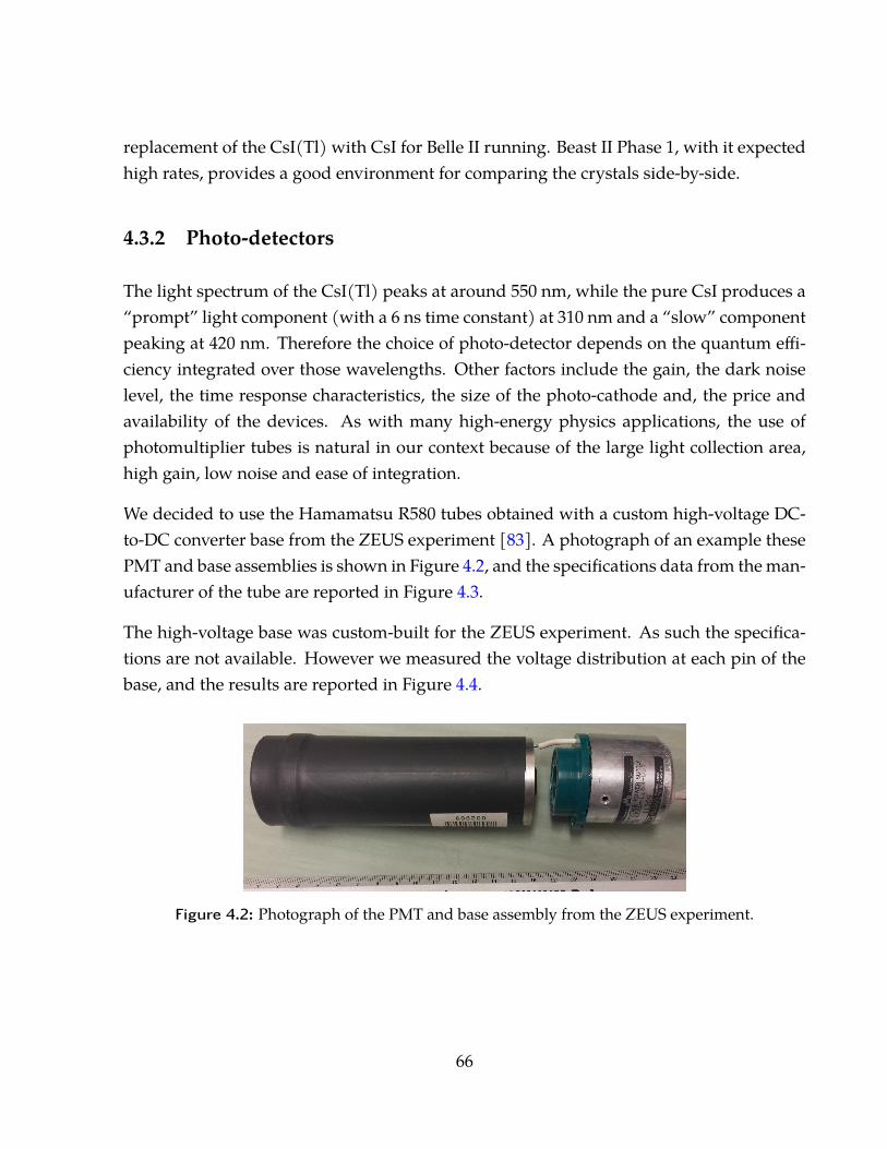
replacement of the CsI(Tl) with CsI for Belle II running. Beast II Phase 1, with it expectedhigh rates, provides a good environment for comparing the crystals side-by-side.

4.3.2 Photo-detectors

The light spectrum of the CsI(Tl) peaks at around 550 nm, while the pure CsI produces a“prompt” light component (with a 6 ns time constant) at 310 nm and a “slow” componentpeaking at 420 nm. Therefore the choice of photo-detector depends on the quantum effi-ciency integrated over those wavelengths. Other factors include the gain, the dark noiselevel, the time response characteristics, the size of the photo-cathode and, the price andavailability of the devices. As with many high-energy physics applications, the use ofphotomultiplier tubes is natural in our context because of the large light collection area,high gain, low noise and ease of integration.

We decided to use the Hamamatsu R580 tubes obtained with a custom high-voltage DC-to-DC converter base from the ZEUS experiment [83]. A photograph of an example thesePMT and base assemblies is shown in Figure 4.2, and the specifications data from the man-ufacturer of the tube are reported in Figure 4.3.

The high-voltage base was custom-built for the ZEUS experiment. As such the specifica-tions are not available. However we measured the voltage distribution at each pin of thebase, and the results are reported in Figure 4.4.

Figure 4.2: Photograph of the PMT and base assembly from the ZEUS experiment.

66

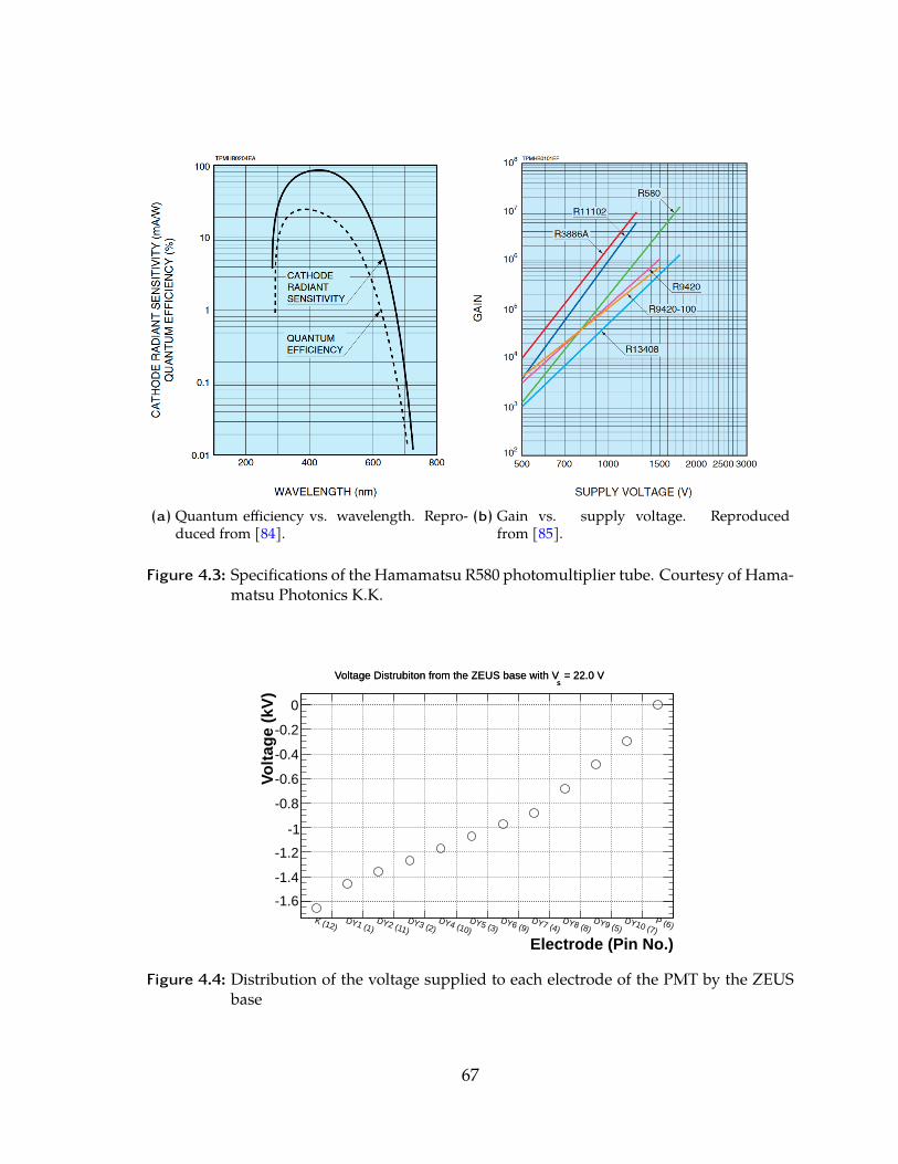
(a) Quantum efficiency vs. wavelength. Repro-duced from [84].

(b) Gain vs. supply voltage. Reproducedfrom [85].

Figure 4.3: Specifications of the Hamamatsu R580 photomultiplier tube. Courtesy of Hama-matsu Photonics K.K.

Electrode (Pin No.)

K (12)DY1 (1)

DY2 (11)DY3 (2)

DY4 (10)DY5 (3)

DY6 (9)DY7 (4)

DY8 (8)DY9 (5)

DY10 (7)P (6)

Vo

ltag

e (k

V)

-1.6

-1.4

-1.2

-1

-0.8

-0.6

-0.4

-0.2

0

= 22.0 Vs

Voltage Distrubiton from the ZEUS base with V = 22.0 Vs

Voltage Distrubiton from the ZEUS base with V

Figure 4.4: Distribution of the voltage supplied to each electrode of the PMT by the ZEUSbase

67

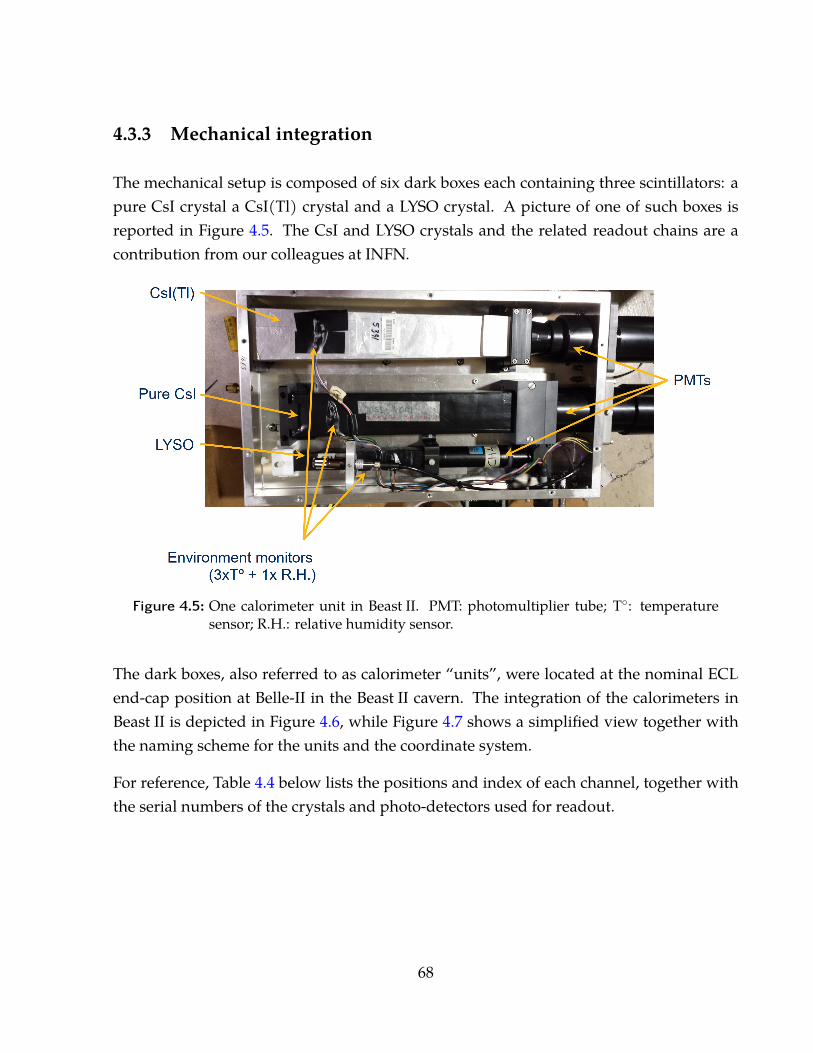
4.3.3 Mechanical integration

The mechanical setup is composed of six dark boxes each containing three scintillators: apure CsI crystal a CsI(Tl) crystal and a LYSO crystal. A picture of one of such boxes isreported in Figure 4.5. The CsI and LYSO crystals and the related readout chains are acontribution from our colleagues at INFN.

Figure 4.5: One calorimeter unit in Beast II. PMT: photomultiplier tube; T◦: temperaturesensor; R.H.: relative humidity sensor.

The dark boxes, also referred to as calorimeter “units”, were located at the nominal ECLend-cap position at Belle-II in the Beast II cavern. The integration of the calorimeters inBeast II is depicted in Figure 4.6, while Figure 4.7 shows a simplified view together withthe naming scheme for the units and the coordinate system.

For reference, Table 4.4 below lists the positions and index of each channel, together withthe serial numbers of the crystals and photo-detectors used for readout.

68

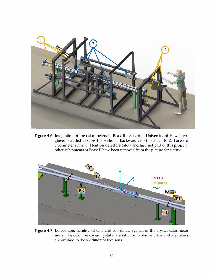
1

23

Figure 4.6: Integration of the calorimeters in Beast II. A typical University of Hawaii en-gineer is added to show the scale. 1. Backward calorimeter units; 2. Forwardcalorimeter units; 3. Neutron detectors (slow and fast, not part of this project);other subsystems of Beast II have been removed from the picture for clarity.

Figure 4.7: Disposition, naming scheme and coordinate system of the crystal calorimeterunits. The colour encodes crystal material information, and the unit identifiersare overlaid to the six different locations.

69

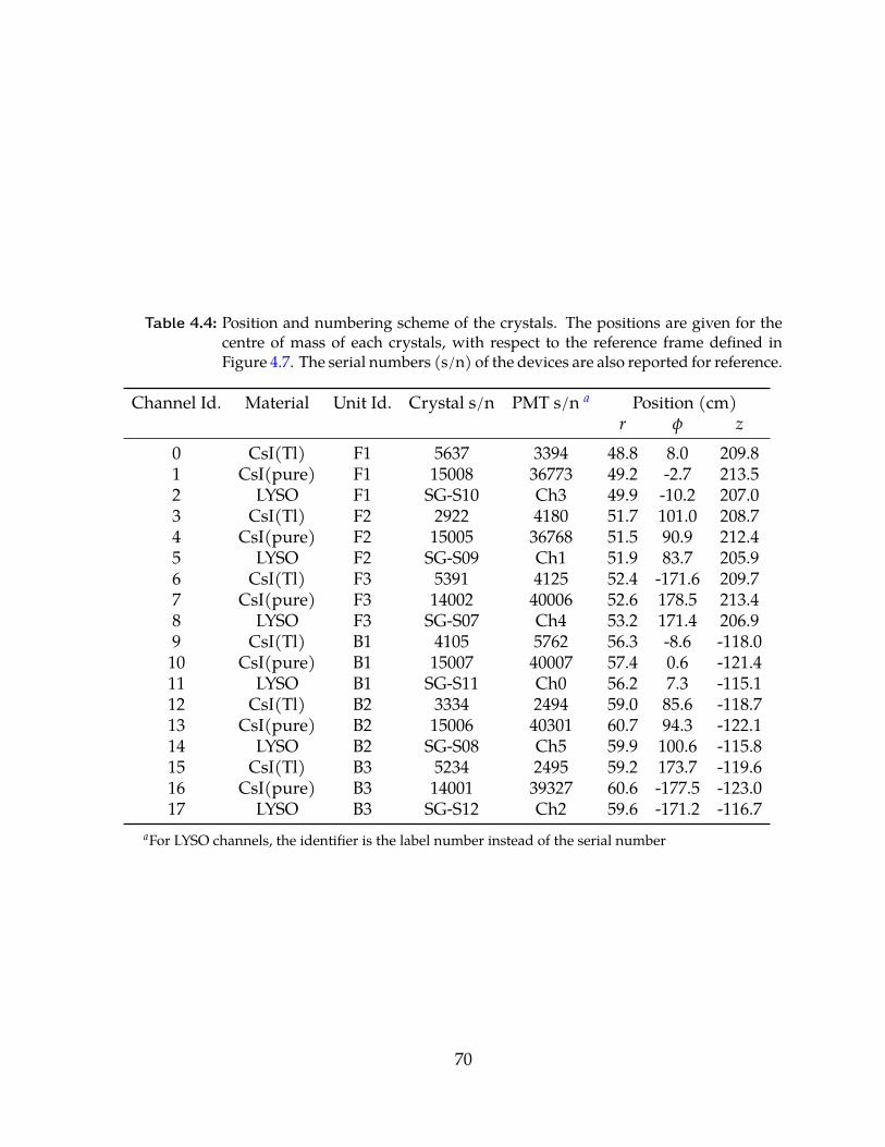
Table 4.4: Position and numbering scheme of the crystals. The positions are given for thecentre of mass of each crystals, with respect to the reference frame defined inFigure 4.7. The serial numbers (s/n) of the devices are also reported for reference.

Channel Id. Material Unit Id. Crystal s/n PMT s/n a Position (cm)r φ z

0 CsI(Tl) F1 5637 3394 48.8 8.0 209.81 CsI(pure) F1 15008 36773 49.2 -2.7 213.52 LYSO F1 SG-S10 Ch3 49.9 -10.2 207.03 CsI(Tl) F2 2922 4180 51.7 101.0 208.74 CsI(pure) F2 15005 36768 51.5 90.9 212.45 LYSO F2 SG-S09 Ch1 51.9 83.7 205.96 CsI(Tl) F3 5391 4125 52.4 -171.6 209.77 CsI(pure) F3 14002 40006 52.6 178.5 213.48 LYSO F3 SG-S07 Ch4 53.2 171.4 206.99 CsI(Tl) B1 4105 5762 56.3 -8.6 -118.010 CsI(pure) B1 15007 40007 57.4 0.6 -121.411 LYSO B1 SG-S11 Ch0 56.2 7.3 -115.112 CsI(Tl) B2 3334 2494 59.0 85.6 -118.713 CsI(pure) B2 15006 40301 60.7 94.3 -122.114 LYSO B2 SG-S08 Ch5 59.9 100.6 -115.815 CsI(Tl) B3 5234 2495 59.2 173.7 -119.616 CsI(pure) B3 14001 39327 60.6 -177.5 -123.017 LYSO B3 SG-S12 Ch2 59.6 -171.2 -116.7

aFor LYSO channels, the identifier is the label number instead of the serial number

70

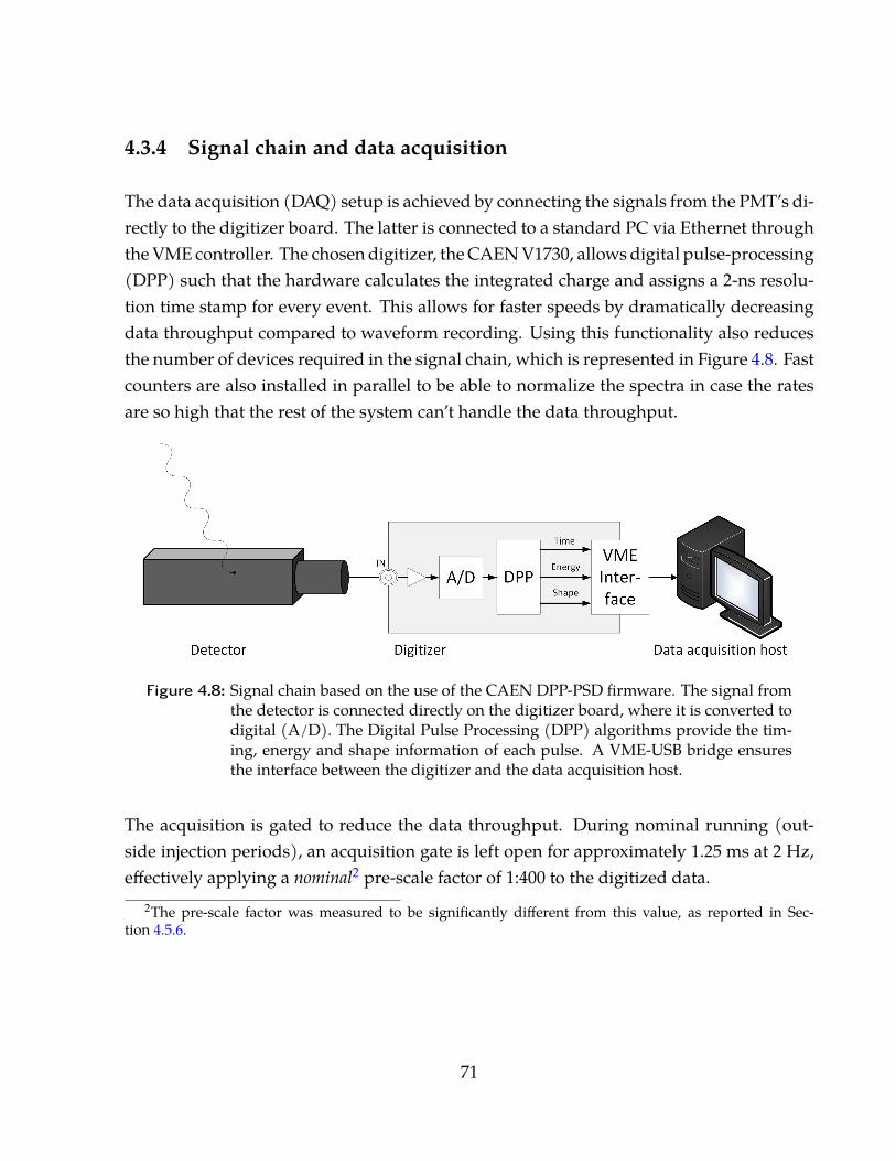
4.3.4 Signal chain and data acquisition

The data acquisition (DAQ) setup is achieved by connecting the signals from the PMT’s di-rectly to the digitizer board. The latter is connected to a standard PC via Ethernet throughthe VME controller. The chosen digitizer, the CAEN V1730, allows digital pulse-processing(DPP) such that the hardware calculates the integrated charge and assigns a 2-ns resolu-tion time stamp for every event. This allows for faster speeds by dramatically decreasingdata throughput compared to waveform recording. Using this functionality also reducesthe number of devices required in the signal chain, which is represented in Figure 4.8. Fastcounters are also installed in parallel to be able to normalize the spectra in case the ratesare so high that the rest of the system can’t handle the data throughput.

Figure 4.8: Signal chain based on the use of the CAEN DPP-PSD firmware. The signal fromthe detector is connected directly on the digitizer board, where it is converted todigital (A/D). The Digital Pulse Processing (DPP) algorithms provide the tim-ing, energy and shape information of each pulse. A VME-USB bridge ensuresthe interface between the digitizer and the data acquisition host.

The acquisition is gated to reduce the data throughput. During nominal running (out-side injection periods), an acquisition gate is left open for approximately 1.25 ms at 2 Hz,effectively applying a nominal2 pre-scale factor of 1:400 to the digitized data.

2The pre-scale factor was measured to be significantly different from this value, as reported in Sec-tion 4.5.6.

71

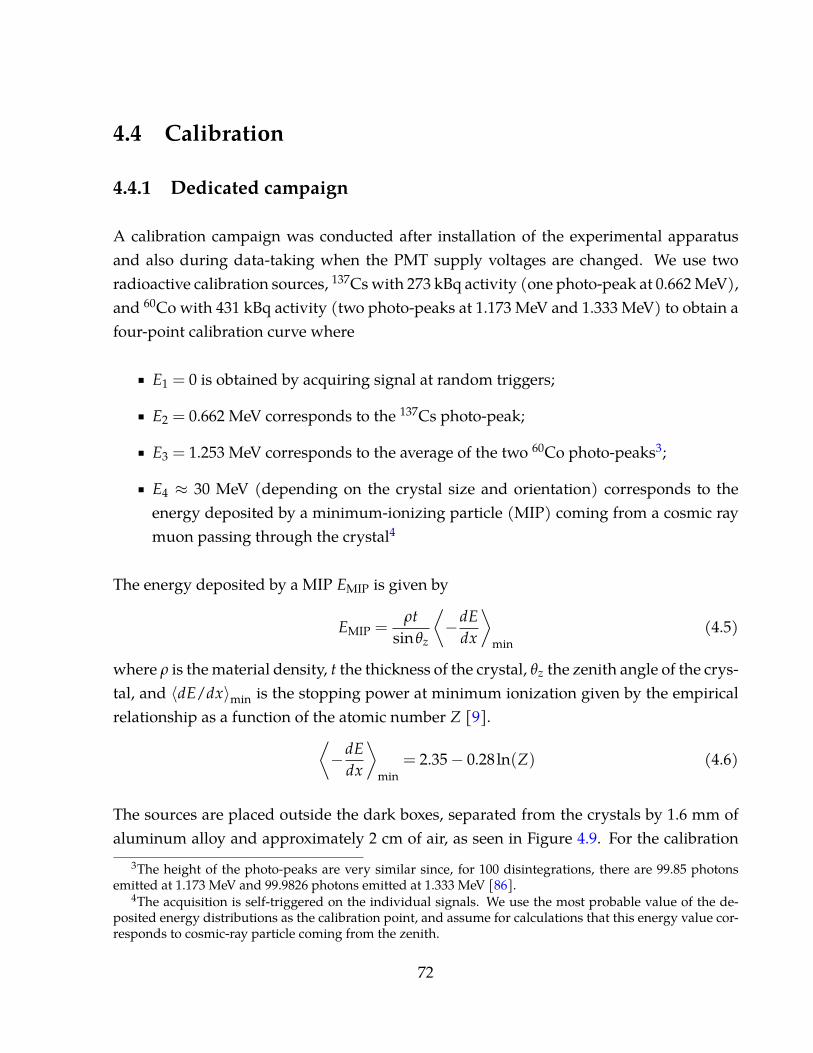
4.4 Calibration

4.4.1 Dedicated campaign

A calibration campaign was conducted after installation of the experimental apparatusand also during data-taking when the PMT supply voltages are changed. We use tworadioactive calibration sources, 137Cs with 273 kBq activity (one photo-peak at 0.662 MeV),and 60Co with 431 kBq activity (two photo-peaks at 1.173 MeV and 1.333 MeV) to obtain afour-point calibration curve where

� E1 = 0 is obtained by acquiring signal at random triggers;

� E2 = 0.662 MeV corresponds to the 137Cs photo-peak;

� E3 = 1.253 MeV corresponds to the average of the two 60Co photo-peaks3;

� E4 ≈ 30 MeV (depending on the crystal size and orientation) corresponds to theenergy deposited by a minimum-ionizing particle (MIP) coming from a cosmic raymuon passing through the crystal4

The energy deposited by a MIP EMIP is given by

EMIP =ρt

sinθz

⟨−dE

dx

⟩min

(4.5)

where ρ is the material density, t the thickness of the crystal, θz the zenith angle of the crys-tal, and 〈dE/dx〉min is the stopping power at minimum ionization given by the empiricalrelationship as a function of the atomic number Z [9].⟨

−dEdx

⟩min

= 2.35− 0.28ln(Z) (4.6)

The sources are placed outside the dark boxes, separated from the crystals by 1.6 mm ofaluminum alloy and approximately 2 cm of air, as seen in Figure 4.9. For the calibration

3The height of the photo-peaks are very similar since, for 100 disintegrations, there are 99.85 photonsemitted at 1.173 MeV and 99.9826 photons emitted at 1.333 MeV [86].

4The acquisition is self-triggered on the individual signals. We use the most probable value of the de-posited energy distributions as the calibration point, and assume for calculations that this energy value cor-responds to cosmic-ray particle coming from the zenith.

72

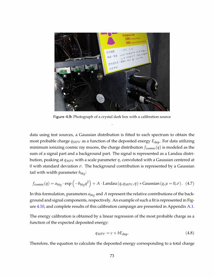
Figure 4.9: Photograph of a crystal dark box with a calibration source.

data using test sources, a Gaussian distribution is fitted to each spectrum to obtain themost probable charge qMPV as a function of the deposited energy Edep. For data utilizingminimum ionizing cosmic ray muons, the charge distribution fcosmic(q) is modeled as thesum of a signal part and a background part. The signal is represented as a Landau distri-bution, peaking at qMPV with a scale parameter η, convoluted with a Gaussian centered at0 with standard deviation σ. The background contribution is represented by a Gaussiantail with width parameter bbkg:

fcosmic(q) = abkg · exp(−bbkgq2

)+ A · Landau (q,qMPV ,η) ∗Gaussian (q,µ = 0,σ) . (4.7)

In this formulation, parameters abkg and A represent the relative contributions of the back-ground and signal components, respectively. An example of such a fit is represented in Fig-ure 4.10, and complete results of this calibration campaign are presented in Appendix A.1.

The energy calibration is obtained by a linear regression of the most probable charge as afunction of the expected deposited energy:

qMPV = c + bEdep. (4.8)

Therefore, the equation to calculate the deposited energy corresponding to a total charge

73

2000 4000 6000 8000 10000 [pC]

0

1

2

3

4

Rate

[Hz /

1.28

pC]

Figure 4.10: Example of the charge distribution of cosmic ray muon signals in CsI(Tl)used for energy calibration. Uncertainties on the bin contents are sta-tistical only. The optimal parameters of Equation 4.7 for this distribu-tion are abkg = (2.98± 0.12) Hz/pC, bbkg =

(1.31× 10−6 ± 2.9× 10−8) pC−2,

qMPV =(2.62× 103 ± 77

) pC, η = (208± 9) pC, σ = (226± 30) pC, A =(2.9± 0.1) Hz/pC with a fit χ2/ndf = 21.8/34. The dashed line represents thecontribution of the Gaussian-tail background only. Reproduced from [1].

Qlong read out from the digitizers is

E [MeV] =a ·Qlong − c

b(4.9)

where the parameter a comes from the setting of the DSP algorithm in the digitizers, pa-rameters b and c are obtained from a linear fit to the energy points described above.

4.4.2 Time-dependence of the gain

Unfortunately, due to radiation damage, the calibration changed during the Phase 1 oper-ating period. The gain of all channels was degraded, sometimes significantly, by a combi-nation of damage to the crystals themselves — most likely for the CsI(Tl) channels — andto the PMTs.

74

In order to recover from this, data points recorded when neither beam was circulatingare used to measure the position of the MIP peak. On a daily basis, these “beam-off”events are used to populate histograms such as presented in Figure 4.10, and identicalparameter estimation is attempted. Successful results, defined based on a list of criteriasuch as convergence of the algorithm, estimated parameters away from boundaries andadequate signal-to-noise ratio, are then used to measure the shift of the peak’s positionas a function of total integrated current, referred here as “beam dose”. It is compared tothe value recorded during the initial calibration period. We call the resulting quantity the“relative gain” of the channel.

The relative gain is modeled as a linear function of log10 of the total beam dose, and there-fore equation 4.9 is modified to include this term:

E(Qlong, Iint

)[MeV] =

a ·Qlong − cb

1p0 + p1 log10 Iint

(4.10)

where Iint is the sum of the integrated beam currents in both beams, and p0,p1 are theparameters adjusted to data, specific to each channel but constant throughout the experi-ment.

4.5 Comparisons between data and simulation

4.5.1 Heuristic description of background measurements

As described in Section 2.2, the main sources of background expected in Phase 1 are theTouschek effect, the beam-gas interactions, and the injections losses. The electron-cloudeffect is left out of the most simplistic picture since it is suppressed by hardware counter-measures and is not expected to play a major role during normal operation and dedicatedbackground studies. In order to conduct the data-to-simulation comparisons, we need toexpress the observed background rate in terms of the contributions from the first threeunderlying processes.

The cross section for both Rutherford scattering and bremsstrahlung is taken to be propor-tional to Zi

2 (see Section 2.2.2). Beam-gas scattering is akin to a fixed-target experimenttherefore we can define a luminosity as the product of the gas density, the incoming parti-cle flux and a characteristic length such as the storage ring circumference. Then, absorbing

75

all constants into a single multiplicative factor, we write the beam-gas contribution to thebackground rate as

OG = SG · IPeZe2, (4.11)

where SG is the beam-gas sensitivity, I is the beam current, Pe is an effective pressure of thevacuum chamber, and Ze is an effective atomic number for the residual gas in the chamber(see Section 4.2). The SG parameter is unique to each channel and stable when collimatorsare fixed, with independent LER and HER values [1].

Equation 2.2 shows that the Touschek lifetime is inversely proportional to the density ofparticles in a bunch N/σy. The loss rate is therefore proportional to the beam particle ratemultiplied by the inverse lifetime. Again, absorbing all constants into a single multiplica-tive factor5, we have the Touschek contribution to the observed background rate

OT = ST ·I

Nb

Iσy

, (4.12)

where ST is the Touschek sensitivity, analogue to the beam-gas sensitivity although withdifferent units. Moreover, Nb is the number of bunches in the train so the term I

Nbis the

“bunch current” — a measure of the charge in each bunch — which is proportional to N.

Inefficiencies in the continuous injection scheme produce enhanced background duringthis process. Similarly to the beam-gas and Touschek cases, we also define the injectionloss observable

Oinj = Sinj(1− εinj

)Ninj (4.13)

where εinj is the injection efficiency, Ninj is the number of injected particles per bunch andSinj is the injection loss sensitivity.

Each contribution is independent of the other, so the total observable rate is

O = SG · IPeZ2e + ST ·

I2

σy+ Sinj ·

(1− εinj

)Ninj. (4.14)

The sensitivities SG, ST and Sinj are unique to each channel and should be stable whencollimators and bunch fill patterns are fixed, and have independent LER and HER val-ues. They contain the various geometrical and (fixed) energy parameters, as well as the

5Here, both the particle density and the particle flux are proportionally related to the beam current for agiven bunch fill pattern.

76

propagation efficiency of the emitted background particle to the detector cell and the de-tection efficiency of the full signal chain [1]. In practice, Sinj is irrelevant in the dedicatedbackground studies since these are taken outside the injection periods, and the other twoparameters are neglected during the injection studies since the injection noise dominatesthe signals. In equations (4.11) to (4.14), the observableO can be either the hit rate or doserate, depending on the sub-detector of interest.

With this functional model in hand, we can discuss how each of these contributions arecompared to simulation, and validate our understanding of the driving machine back-ground mechanisms and their scaling.

4.5.2 Re-weighting procedure for simulated data

The simulation is generated with arbitrary beam conditions Is, Ps, Zse , σs

y and Nsb , which

are respectively the beam current, the average vacuum chamber pressure, the effectiveatomic number of the residual gas, the vertical beam size and the number of bunches in thetrain. The subscripts l, h indicate whether these conditions pertain to the LER or the HER.The simulated output, or observable, is denoted Os

X where X can be C for the Coulombprocess, B for the Bremsstrahlung process, or T for the Touschek process. As discussed inSection 2.2.2, the beam-gas backgrounds are the sum of the Coulomb and bremstrahlungcontributions such that

OsG =Os

C +OsB. (4.15)

In all the above the superscript s indicates that these are the “simulated” conditions andobservables, as opposed to superscript d that would indicate experimental, or “data” con-ditions and observables.

In this notation, the simulated background rates re-weighted to experimental conditionsare given by

Os =OsT

((Id)2

σdy Nd

b

)(σs

yNsb(

Is)2

)+

12

∑iD=1

Id · Pd[iD] ·(Zd

e)2

Is · Ps ·(Zs

e)2

(Os

C[iD] +OsB[iD]

), (4.16)

where the tilde denotes a re-weighted quantity and the index [iD] indicates the number ofthe “D section” of SuperKEKB (see Figure 1.3).

77

4.5.3 Hypotheses related with the vacuum chamber pressure and gasconstituents

One of the difficulties arising from modelling the observed backgrounds with Eq. (4.14)is that the pressure readings from SuperKEKB cold-cathode gauges (CCGs) has a largeuncertainty, estimated to be about 50%. On the top of this, we know the gas constituents atonly two specific locations in the positron storage ring, namely D02 and D06, and nowherein the electron storage ring.

Our best knowledge of the actual pressures in the chamber comes from discussions withthe SuperKEKB accelerator group, and consists of multiplying the CCG pressure readoutby a scale factor [81]

αP = 3.0± 1.5. (4.17)This factor is assumed to be identical between the HER and the LER, since it is thought toarise from calibration and placement of the pressure sensors.

Furthermore, devoid of any information of the contrary, we can only assume that the gasmixture is the same in the HER and in the LER. This particular hypothesis is rather weakbecause the residual gas constituents are mostly impurities desorbed from the vacuumchamber surfaces. However, the material of the two chambers is different so the contami-nation due to manufacturing process is expected to be different. Most of the HER sectionswere also re-used from KEKB, while the effect of 11 years of operation on the surface andcontamination conditions has been shown to be significant, even after extended periods ofstorage [50].

Therefore, we only have a limited knowledge of the actual gas conditions in the vacuumchambers, which are important inputs to the simulation. The high-energy ring results willbe the most difficult to interpret for two reasons:

1. there are no data to test any hypothesis on the gas constituents, and

2. the beam-gas background is expected to be a significant, if not the most significant,contribution to the overall background.

The last statement is justified by the dependence of Touschek lifetime on the square ofthe beam particle energy, as expressed in Eq (2.2). A larger beam energy translates into a

78

longer Touschek lifetime (and hence less Touschek background).

4.5.4 The data-to-simulation ratio

The comparisons between data and simulation are conducted using the simulated observ-ables re-weighted as shown in Equation (4.16), however using αPPd[iD] instead of Pd[iD]

to account for our limited knowledge of the actual vacuum chamber pressure. The data-to-simulation ratio Rds, measured by channel iCh, is the average on all valid data pointsof the ratio of the data observable over the re-weighted simulated observable.

Rds[iCh] =1

nRuns

nRuns

∑iRun=0

Od[iCh,iRun]

Os[iCh,iRun](4.18)

In the above, the index iRun corresponds to a specific sub-run of Tables 4.1 and 4.2. Thedata-to-simulation calculation study was conducted on runs 200[7-9] and 300[7-9], andtherefore

nRuns = 15.

4.5.5 Statistical uncertainty

The statistical uncertainty onRds is assessed by summing the standard errors on the meanobservable in a given sub-run in quadrature, then propagating the result onto the ratio in(4.18). Hence, a noisy channel, a brief sub-run or background readings that vary greatlyin the same sub-run would all translate into a large statistical uncertainty for the measure-ment and affect the uncertainty on the data-to-simulation ratio accordingly. The statisticaluncertainty is added in quadrature with the systematic uncertainty contributions detailedbelow to provide an estimate of the global uncertainty on the measurements.

4.5.6 Systematic uncertainties

The systematic contributions to the data/simulation ratio uncertainty are listed below.Comparisons of the hit rates, as recorded by the scaler on LYSO and CsI(pure) channels,are affected by three of these contributions, namely the uncertainty on the calculated αP

79

factor, the uncertainty on the beam size measurements, and the uncertainty on the beamcurrent measurements.

Comparisons of the dose rate, as recorded by the digitizers on CsI(Tl) and LYSO channels,are subject the the first three components named above, in addition to the uncertainty onthe DAQ livetime and that on the energy calibration, and the uncertainty on the energythreshold.

αP value

As mentionned in Section 4.5.3, the uncertainty on the pressure scale factor δ (αP) is pro-vided by the SuperKEKB group. It is taken to be half the pressure correction. [81]

Beam size

The beam size uncertainty is also given to us by the SuperKEKB group. The values are

δ(σy,HER

)= 0.0371µm

andδ(σy,LER

)= 0.0137µm.

Beam current

The beam current uncertainty is also given to us by the SuperKEKB group. The values are

δ (IHER) = δ (ILER) = 0.03 mA

Energy calibration

The uncertainty on the energy calibration is given by propagating the uncertainty of allparameters entering into the calibration equation:

δ(E)2 =

(∂E∂b

δb)2

+

(∂E∂c

δc)2

+

(∂E∂p0

δp0

)2

+

(∂E∂p1

δp1

)2

, (4.19)

80

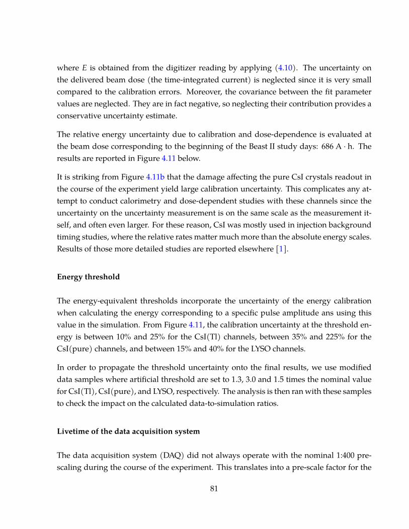
where E is obtained from the digitizer reading by applying (4.10). The uncertainty onthe delivered beam dose (the time-integrated current) is neglected since it is very smallcompared to the calibration errors. Moreover, the covariance between the fit parametervalues are neglected. They are in fact negative, so neglecting their contribution provides aconservative uncertainty estimate.

The relative energy uncertainty due to calibration and dose-dependence is evaluated atthe beam dose corresponding to the beginning of the Beast II study days: 686 A · h. Theresults are reported in Figure 4.11 below.

It is striking from Figure 4.11b that the damage affecting the pure CsI crystals readout inthe course of the experiment yield large calibration uncertainty. This complicates any at-tempt to conduct calorimetry and dose-dependent studies with these channels since theuncertainty on the uncertainty measurement is on the same scale as the measurement it-self, and often even larger. For these reason, CsI was mostly used in injection backgroundtiming studies, where the relative rates matter much more than the absolute energy scales.Results of those more detailed studies are reported elsewhere [1].

Energy threshold

The energy-equivalent thresholds incorporate the uncertainty of the energy calibrationwhen calculating the energy corresponding to a specific pulse amplitude ans using thisvalue in the simulation. From Figure 4.11, the calibration uncertainty at the threshold en-ergy is between 10% and 25% for the CsI(Tl) channels, between 35% and 225% for theCsI(pure) channels, and between 15% and 40% for the LYSO channels.

In order to propagate the threshold uncertainty onto the final results, we use modifieddata samples where artificial threshold are set to 1.3, 3.0 and 1.5 times the nominal valuefor CsI(Tl), CsI(pure), and LYSO, respectively. The analysis is then ran with these samplesto check the impact on the calculated data-to-simulation ratios.

Livetime of the data acquisition system

The data acquisition system (DAQ) did not always operate with the nominal 1:400 pre-scaling during the course of the experiment. This translates into a pre-scale factor for the

81

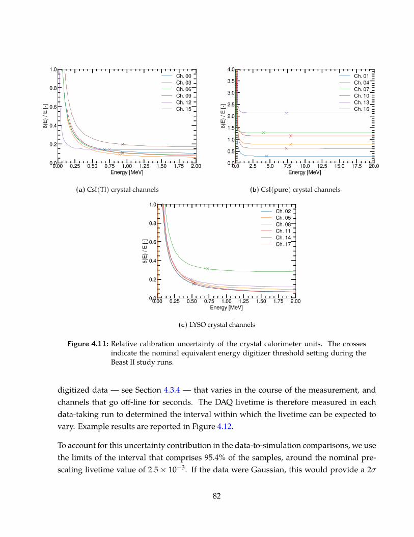
0.00 0.25 0.50 0.75 1.00 1.25 1.50 1.75 2.00Energy [MeV]

0.0

0.2

0.4

0.6

0.8

1.0

(E) /

E [-

]

Ch. 00Ch. 03Ch. 06Ch. 09Ch. 12Ch. 15

(a) CsI(Tl) crystal channels

0.0 2.5 5.0 7.5 10.0 12.5 15.0 17.5 20.0Energy [MeV]

0.0

0.5

1.0

1.5

2.0

2.5

3.0

3.5

4.0

(E) /

E [-

]

Ch. 01Ch. 04Ch. 07Ch. 10Ch. 13Ch. 16

(b) CsI(pure) crystal channels

0.00 0.25 0.50 0.75 1.00 1.25 1.50 1.75 2.00Energy [MeV]

0.0

0.2

0.4

0.6

0.8

1.0

(E) /

E [-

]

Ch. 02Ch. 05Ch. 08Ch. 11Ch. 14Ch. 17

(c) LYSO crystal channels

Figure 4.11: Relative calibration uncertainty of the crystal calorimeter units. The crossesindicate the nominal equivalent energy digitizer threshold setting during theBeast II study runs.

digitized data — see Section 4.3.4 — that varies in the course of the measurement, andchannels that go off-line for seconds. The DAQ livetime is therefore measured in eachdata-taking run to determined the interval within which the livetime can be expected tovary. Example results are reported in Figure 4.12.

To account for this uncertainty contribution in the data-to-simulation comparisons, we usethe limits of the interval that comprises 95.4% of the samples, around the nominal pre-scaling livetime value of 2.5× 10−3. If the data were Gaussian, this would provide a 2σ

82

0.000 0.001 0.002 0.003 0.004Live time [-]

0

250

500

750

1000

1250

1500

Entrie

s / .

× bi

n

:/ = /. % = [ . ; . ] ×

(a) Narrow livetime distribution

0.000 0.001 0.002 0.003 0.004Live time [-]

0

100

200

300

400

Entrie

s / .

× bi

n

:/ = /. % = [ . ; . ] ×

(b) Average livetime distribution

0.000 0.001 0.002 0.003 0.004Live time [-]

0

50

100

150

200

250

Entrie

s / .

× bi

n

:/ = /. % = [ . ; . ] ×

(c) Wide livetime distribution

Figure 4.12: Three examples of DAQ livetime distributions. Most distributions are similarto panel 4.12b, however two extreme examples are shown for completeness in4.12a and 4.12c. N/Nsam indicates the ratio of selected samples: those with alivetime value inconsistent with either a busy channel or with data recordedduring an injection period. The interval that covers 95.4% of the selected sam-ples is denoted 95.4% CI, and is used as an indicator of the livetime uncertainty.

interval around the nominal value. It is assumed that the measured dose rate is directlyproportional to the DAQ livetime. As such, the limits of the 95.4% coverage interval, rel-ative to the nominal value, are used as scaling factors for the dose rates in the systematicuncertainty studies.

83

4.6 Beam-gas interactions and beam conditions evolutionin Phase 1

The Beast II experiment is also valuable to study long-term performance improvementsof the accelerator as the commissioning program is undergoing. Two aspects are particu-larly useful for the experimentalist: the vacuum scrubbing process and the time structureof so-called “beam-dust” events, both contributing to background seen in Beast II and ex-pected in Belle II. Vacuum scrubbing is the general term used to describe out gassing ofthe vacuum chamber impurities induced by beam circulating in the accelerator. Beam-dustevents, on the other hand, correspond to rapid increases in few local pressure readings andmay trigger beam aborts. Thought to be the result of beam particle vaporizing microscopicor macroscopic particles, they were previously observed and studied at many acceleratorlaboratories such as KEK [87, 53], CERN [52, 51] and DESY [88].

In both cases, we are interested in the long-term behaviour of these quantities, and seehow they are related to operating conditions such as instantaneous and integrated cur-rents. The latter is also known as the “beam dose” and is a measure of progress of theaccelerator commissioning. The following section describes the approaches taken by theBeast II group to characterize these phenomena as well as their respective results.

4.6.1 Vacuum scrubbing

Phenomenology

In the particular context of particle accelerators, the typical thermal out gassing processis augmented by radiation-induced effects called electron-induced desorption (ESD) andphoton-induced desorption (PSD). While the former is more typical of electron-positroncolliders such as SuperKEKB, and can arise from machine-induced electron multipacting[89], the latter is the result of sychrotron photons from the accelerated charged beams —whose energy can be as high as few MeV — irradiating the vacuum chamber material [90].

With both phenomena, the desorption rate is a function of the integrated radiation dose onthe vacuum chamber material and follow the same behaviour [91]. After an initial electronor photon dose D0, the out-gassing rate η follows a power-law dependence with respect to

84

the integrated beam dose D:

η = η0

(DD0

)β

(4.20)

where η0 is the desorption rate at the initial dose D0, and the coefficient β is a functionof the irradiation energy spectrum, the material characteristics, and the physical process(ESD or PSD) behind the scrubbing.

Because such scrubbing releases gas molecules into the vacuum chamber, it should be di-rectly observable in terms of a dynamic pressure dP/dI component. Moreover, the beam-gas interactions between the impurities and the charged beams produce increased parti-cle losses around the accelerator. Such losses are observed with the Beast II systems asincreased radiation levels. These two techniques are used to assess the rate of vacuumscrubbing, and provide a statement on the adequacy of the vacuum expected for Belle IIoperation.

Dynamic pressure measurement

The dynamic pressure is a measurement of the rate of gas released from the material perunit current circulated in the beam pipe. Therefore it is expected to track the desorptionrate:

dPdI∼ η (4.21)

This dynamic pressure is the fundamental quantity used by the SuperKEKB group to quan-tify the rate of vacuum scrubbing [50]. However powerful, using a single dP/dI value fora given set of beam parameters remains an approximation. This fact is illustrated in Fig-ure 4.13. This example shows that the residual gas pressure is not a function of the currentalone. More importantly it also shows that dP/dI depends on other quantities such as theactual operating current — the relationship is not linear between 300 mA and 500 mA —and the time after the last injection. The data points at the far right, where currents are thehighest, were taken immediately after an injection period and exhibit short-term pressureincrease for decreasing currents (negative dP/dI).

With these warnings in mind, it is nonetheless useful to estimate this dynamical pres-sure term on a continuous basis. One approach is to neglect the base pressure inside thechamber — the equilibrium pressure when no beam is circulating — and assume linear-ity between pressures and currents. Examining only currents above 60% of the maximum

85

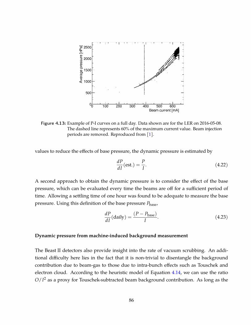
Figure 4.13: Example of P-I curves on a full day. Data shown are for the LER on 2016-05-08.The dashed line represents 60% of the maximum current value. Beam injectionperiods are removed. Reproduced from [1].

values to reduce the effects of base pressure, the dynamic pressure is estimated by

dPdI

(est.) = PI

. (4.22)

A second approach to obtain the dynamic pressure is to consider the effect of the basepressure, which can be evaluated every time the beams are off for a sufficient period oftime. Allowing a settling time of one hour was found to be adequate to measure the basepressure. Using this definition of the base pressure Pbase,

dPdI

(daily) = (P− Pbase)I

. (4.23)

Dynamic pressure from machine-induced background measurement

The Beast II detectors also provide insight into the rate of vacuum scrubbing. An addi-tional difficulty here lies in the fact that it is non-trivial to disentangle the backgroundcontribution due to beam-gas to those due to intra-bunch effects such as Touschek andelectron cloud. According to the heuristic model of Equation 4.14, we can use the ratioO/I2 as a proxy for Touschek-subtracted beam background contribution. As long as the

86

beam-gas contribution dominates the overall background radiation,

OI2 ∼ η, (4.24)

can be used to study the vacuum process. In Equation 4.24 the observable O is a dose rateor hit rate, depending on the sub-detector of interest.

4.6.2 Analysis of transient “beam-dust” events

General description and motivation

During commissioning of the accelerator, one concern was the observation of localizedpressure bursts and accompanying background spikes. The prevalent hypothesis for theseobservations are collisions between the beam electrons and positrons, and small particlessuch as dust coming off the vacuum chamber material [52, 51, 50]. These events will there-fore be referred to as “beam-dust” events in this document.

Such beam-dust events are important during commissioning and running of an accelera-tor, since the corresponding increase in observed background often results in beam abortsand loss of operation time. The SuperKEKB group monitors these events by measuringpressure peaks around the beam pipe. The questions addressed in the present study are

� What is the time structure of these beam-dust events during Phase 1 of SuperKEKB,and does it change as vacuum scrubbing progresses?

� Do the pressure bursts measured by SuperKEKB correspond to background peaksseen in the Beast II detectors?

� Could the radiation resulting from these events be damaging to the detectors?

Analysis methodology

Qualitatively, beam-dusts events present sharp peaks in Beast II detectors observables, forexample the deposited energy rate in the BGO, or the hit rate in the CsI crystals. Thesepeaks are much higher than the typical signal, and last less than 2 seconds.

87

The analysis therefore consists of finding peaks that are at least six standard deviationsabove the mean signal, calculated using 60 seconds running time windows. To furtherexclude electronic noise peaks in the count, we require such peaks to be seen in at leastfour channels and in at least two different detector systems. The coincidence time windowis set to 3 seconds since Beast II data coming from different sub-detectors is not perfectlyaligned in time. These requirements were adjusted on a small sample of clearly identifiablepeaks, then extended to the complete Phase 1 data set.

The results are compared to the list coming from the SuperKEKB accelerator group, whodefine beam-dust events as pressure bursts where any cold cathode pressure gauge valueis 15% larger than the previous 1-second average. From this list, only burst events locatedin regions D01 and D02 — the straight subsections on either side of the Beast II detector, seeFigure 1.3 — are considered. This amounts to 338 distinct burst events. The other regionswere excluded since vacuum bump experiments outside this range showed no correspond-ing increase of the Beast II observables, and therefore these events would be impossible tocorrelate with Beast II data.

The time resolution of the events provided by SuperKEKB is one minute so we use oneminute intervals also for the Beast II events. We calculate the cross correlation betweenthe two lists to ensure there are no time misalignment between the two datasets. A peakat lag=0 indicates the correct time alignment, and the cross-correlation value outside thepeak correspond to the number of accidental coincidences due to the finite time resolution.

Finally, we aim to provide a statement on the dose resulting from such events. To achievethis, we compare the peak level dose to the running average of the previous 60 seconds,and multiply by the probability of occurrence of such a peak for the given sub-detectorthat recorded it.

***

88

Chapter 5

Results and simulation

5.1 Specific results from the CsI(Tl), CsI(pure) and LYSOsystem

5.1.1 Calibration and time-dependence of the gain

The measured parameters from the initial calibration campaign are reported in Table 5.1below. Refer to Appendix A.1 for the detailed results and calibration curves, as well as theplots for the CsI(pure) and LYSO channels, produced by collaborators.

These calibration constants were technically only valid before beams started circulating.The methodology used to characterize of the gain degradation as a function of beam doseis described in Section 4.4.2. Figure 5.1 shows typical relative gain results for each crystaltype, and the complete results are reported in Appendix A.2. For some of the CsI(pure)channels, the PMT supply voltage settings were changed during the course of the exper-iment to reduce the gain by half, thus reducing the hit rates and and help preserving thePMTs. Nevertheless, the CsI(pure) channels showed a notable gain degradation, presum-ably from the sustained large currents in the tubes. We suspect that the gain degradationcome from the tubes themselves since CsI crystals have been shown have a good radiationhardness, with only 20% gain degradation at doses as high as 143 Gy [92]. Moreover, thePMTs on the CsI(pure) channels shave a 48 mm diameter active window which meanstheir active area is twice as large as the tubes on the CsI(Tl) channels. This makes themmore susceptible to damage from a larger light intensity, thus larger currents. Because

89

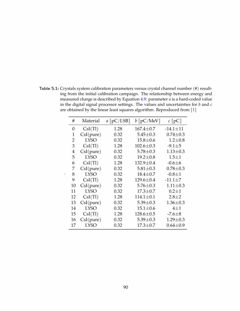
Table 5.1: Crystals system calibration parameters versus crystal channel number (#) result-ing from the initial calibration campaign. The relationship between energy andmeasured charge is described by Equation 4.9: parameter a is a hard-coded valuein the digital signal processor settings. The values and uncertainties for b and care obtained by the linear least squares algorithm. Reproduced from [1]

.

# Material a [pC/LSB] b [pC/MeV] c [pC]0 CsI(Tl) 1.28 167.4±0.7 -14.1±111 CsI(pure) 0.32 5.45±0.3 0.74±0.32 LYSO 0.32 15.8±0.6 1.2±0.83 CsI(Tl) 1.28 102.6±0.3 -9.1±54 CsI(pure) 0.32 5.78±0.3 1.13±0.35 LYSO 0.32 19.2±0.8 1.5±16 CsI(Tl) 1.28 132.9±0.4 -0.6±67 CsI(pure) 0.32 5.81±0.3 0.78±0.38 LYSO 0.32 18.4±0.7 -0.8±19 CsI(Tl) 1.28 129.6±0.4 -11.1±710 CsI(pure) 0.32 5.76±0.3 1.11±0.311 LYSO 0.32 17.3±0.7 0.2±112 CsI(Tl) 1.28 114.1±0.1 2.8±213 CsI(pure) 0.32 5.39±0.3 1.36±0.314 LYSO 0.32 15.1±0.6 4±115 CsI(Tl) 1.28 128.6±0.5 -7.6±816 CsI(pure) 0.32 5.39±0.3 1.29±0.317 LYSO 0.32 17.3±0.7 0.64±0.9

90

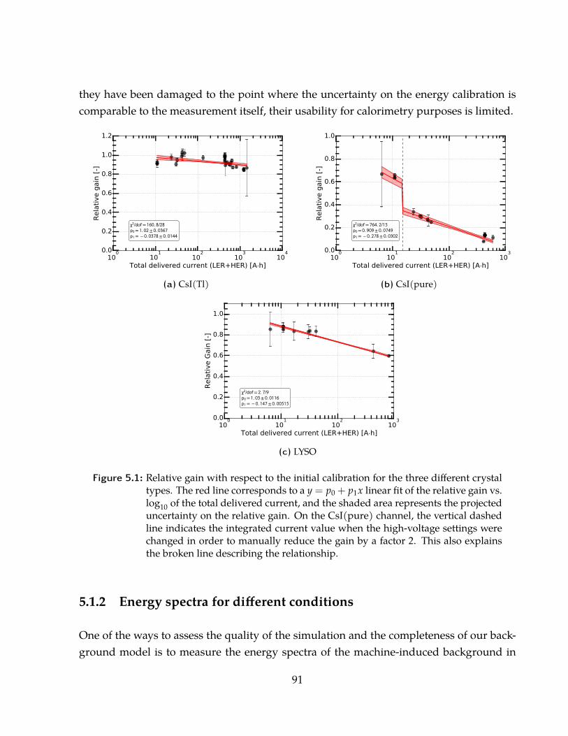
they have been damaged to the point where the uncertainty on the energy calibration iscomparable to the measurement itself, their usability for calorimetry purposes is limited.

100

101

102

103

104

Total delivered current (LER+HER) [A h]

0.0

0.2

0.4

0.6

0.8

1.0

1.2

Rela

tive g

ain

[-]

/ = . /= . ± .= . ± .

(a) CsI(Tl)

100

101

102

103

Total delivered current (LER+HER) [A h]

0.0

0.2

0.4

0.6

0.8

1.0

Rela

tive g

ain

[-]

/ = . /= . ± .= . ± .

(b) CsI(pure)

100

101

102

103

Total delivered current (LER+HER) [A h]

0.0

0.2

0.4

0.6

0.8

1.0

Rela

tive G

ain

[-]

/ = . /= . ± .= . ± .

(c) LYSO

Figure 5.1: Relative gain with respect to the initial calibration for the three different crystaltypes. The red line corresponds to a y = p0 + p1x linear fit of the relative gain vs.log10 of the total delivered current, and the shaded area represents the projecteduncertainty on the relative gain. On the CsI(pure) channel, the vertical dashedline indicates the integrated current value when the high-voltage settings werechanged in order to manually reduce the gain by a factor 2. This also explainsthe broken line describing the relationship.

5.1.2 Energy spectra for different conditions

One of the ways to assess the quality of the simulation and the completeness of our back-ground model is to measure the energy spectra of the machine-induced background in

91

different operating conditions. The next paragraphs present such spectra for nominal op-eration at the beginning and at the end of Phase 1, operation with deliberately larger beamsize to study the Touschek effect, and operation with larger vacuum chamber pressure tostudy beam-gas interactions.

The injection periods are all removed from these studies since designing a model for theinjection noise would be outside the scope of this project. An example spectrum takenduring injection is nonetheless presented to provide a sense of the impact of injections onthe overall backgrounds.

Before presenting the spectra for these all these different conditions, a short digression onthe pile-up effects visible in the CsI(Tl) channels is warranted.

Pile-up effects in CsI(Tl) crystals

One recurrent feature in CsI(Tl) spectra is that the tails of the measured distributions arelonger than those of the simulated ones. This is notable, for instance, in Figures 5.5a and5.6c. A likely explanation for this is pile-up of low-energy hits within one charge integra-tion gate. Since the time structure of the background is not known accurately for all beamconditions, such pile-up effects are not included in the simulated samples.

We set up a toy Monte Carlo experiment to determine, for different background rates, whatthe impacts on the spectra would be. To each simulated hit, we add a number of “parasitic”hits with the expected number of hits from each energy bin given by the input distributionshape and the assumed background rate. Then, for each simulated hit, the actual numberof hits to be added from each energy bin is taken from a Poisson distribution centred at theexpected value. The results fro CsI(Tl) are shown in Figure 5.2a.

We see that pile-up of low-energy hits effectively smears the distributions, and enhancesthe tails while depleting the lower energy bins. Furthermore, the impact becomes notice-able for hit rates greater than 25 kHz. However, none of the shapes shown in Figure 5.2amatches what is measured e.g. in Figures 5.5a and 5.6c. It is likely that the time struc-ture of the background is richer than the above models, and contains contributions fromdifferent frequencies. In the future, more elaborate description of pile-up effect could in-volve time structure information from measurement based on faster crystals. As of theBelle II software release current at the time of this study (release-01-00-02), there is no

92

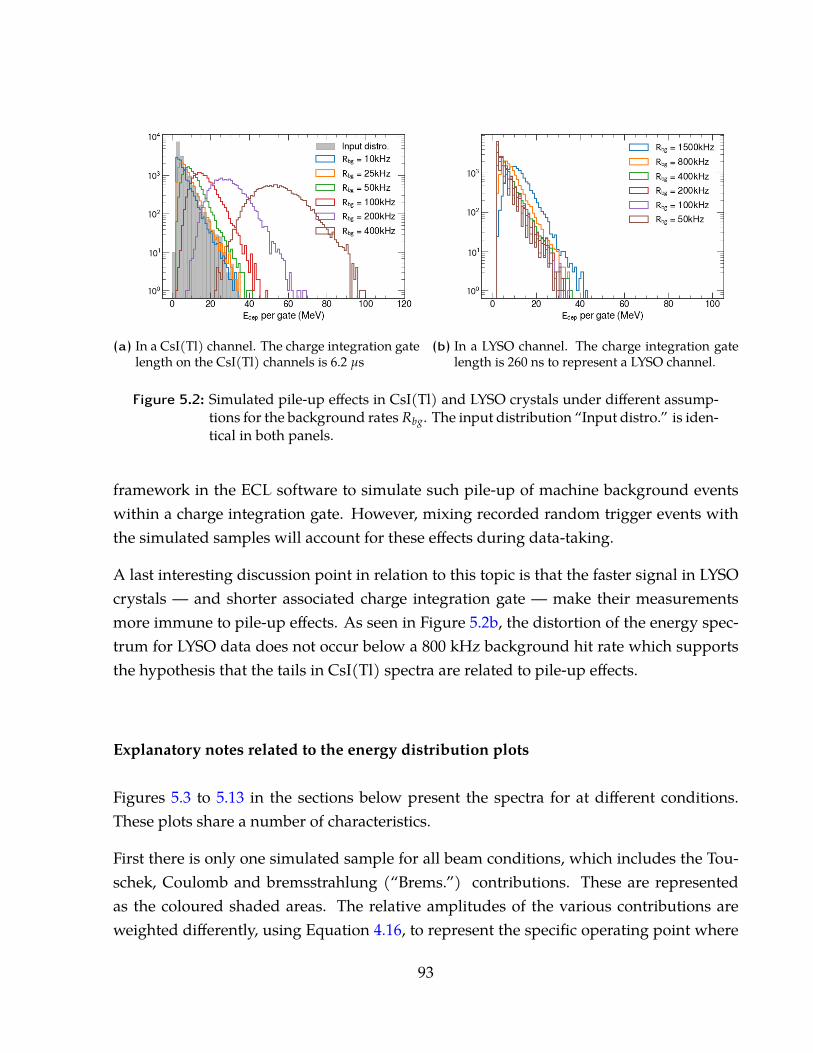
(a) In a CsI(Tl) channel. The charge integration gatelength on the CsI(Tl) channels is 6.2 µs

(b) In a LYSO channel. The charge integration gatelength is 260 ns to represent a LYSO channel.

Figure 5.2: Simulated pile-up effects in CsI(Tl) and LYSO crystals under different assump-tions for the background rates Rbg. The input distribution “Input distro.” is iden-tical in both panels.

framework in the ECL software to simulate such pile-up of machine background eventswithin a charge integration gate. However, mixing recorded random trigger events withthe simulated samples will account for these effects during data-taking.

A last interesting discussion point in relation to this topic is that the faster signal in LYSOcrystals — and shorter associated charge integration gate — make their measurementsmore immune to pile-up effects. As seen in Figure 5.2b, the distortion of the energy spec-trum for LYSO data does not occur below a 800 kHz background hit rate which supportsthe hypothesis that the tails in CsI(Tl) spectra are related to pile-up effects.

Explanatory notes related to the energy distribution plots

Figures 5.3 to 5.13 in the sections below present the spectra for at different conditions.These plots share a number of characteristics.

First there is only one simulated sample for all beam conditions, which includes the Tou-schek, Coulomb and bremsstrahlung (“Brems.”) contributions. These are representedas the coloured shaded areas. The relative amplitudes of the various contributions areweighted differently, using Equation 4.16, to represent the specific operating point where

93

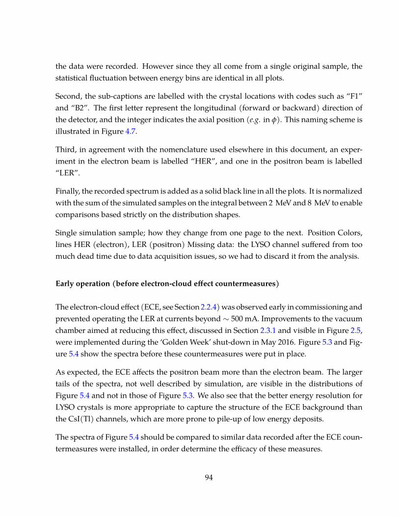
the data were recorded. However since they all come from a single original sample, thestatistical fluctuation between energy bins are identical in all plots.

Second, the sub-captions are labelled with the crystal locations with codes such as “F1”and “B2”. The first letter represent the longitudinal (forward or backward) direction ofthe detector, and the integer indicates the axial position (e.g. in φ). This naming scheme isillustrated in Figure 4.7.

Third, in agreement with the nomenclature used elsewhere in this document, an exper-iment in the electron beam is labelled “HER”, and one in the positron beam is labelled“LER”.

Finally, the recorded spectrum is added as a solid black line in all the plots. It is normalizedwith the sum of the simulated samples on the integral between 2 MeV and 8 MeV to enablecomparisons based strictly on the distribution shapes.

Single simulation sample; how they change from one page to the next. Position Colors,lines HER (electron), LER (positron) Missing data: the LYSO channel suffered from toomuch dead time due to data acquisition issues, so we had to discard it from the analysis.

Early operation (before electron-cloud effect countermeasures)

The electron-cloud effect (ECE, see Section 2.2.4) was observed early in commissioning andprevented operating the LER at currents beyond ∼ 500 mA. Improvements to the vacuumchamber aimed at reducing this effect, discussed in Section 2.3.1 and visible in Figure 2.5,were implemented during the ‘Golden Week’ shut-down in May 2016. Figure 5.3 and Fig-ure 5.4 show the spectra before these countermeasures were put in place.

As expected, the ECE affects the positron beam more than the electron beam. The largertails of the spectra, not well described by simulation, are visible in the distributions ofFigure 5.4 and not in those of Figure 5.3. We also see that the better energy resolution forLYSO crystals is more appropriate to capture the structure of the ECE background thanthe CsI(Tl) channels, which are more prone to pile-up of low energy deposits.

The spectra of Figure 5.4 should be compared to similar data recorded after the ECE coun-termeasures were installed, in order determine the efficacy of these measures.

94

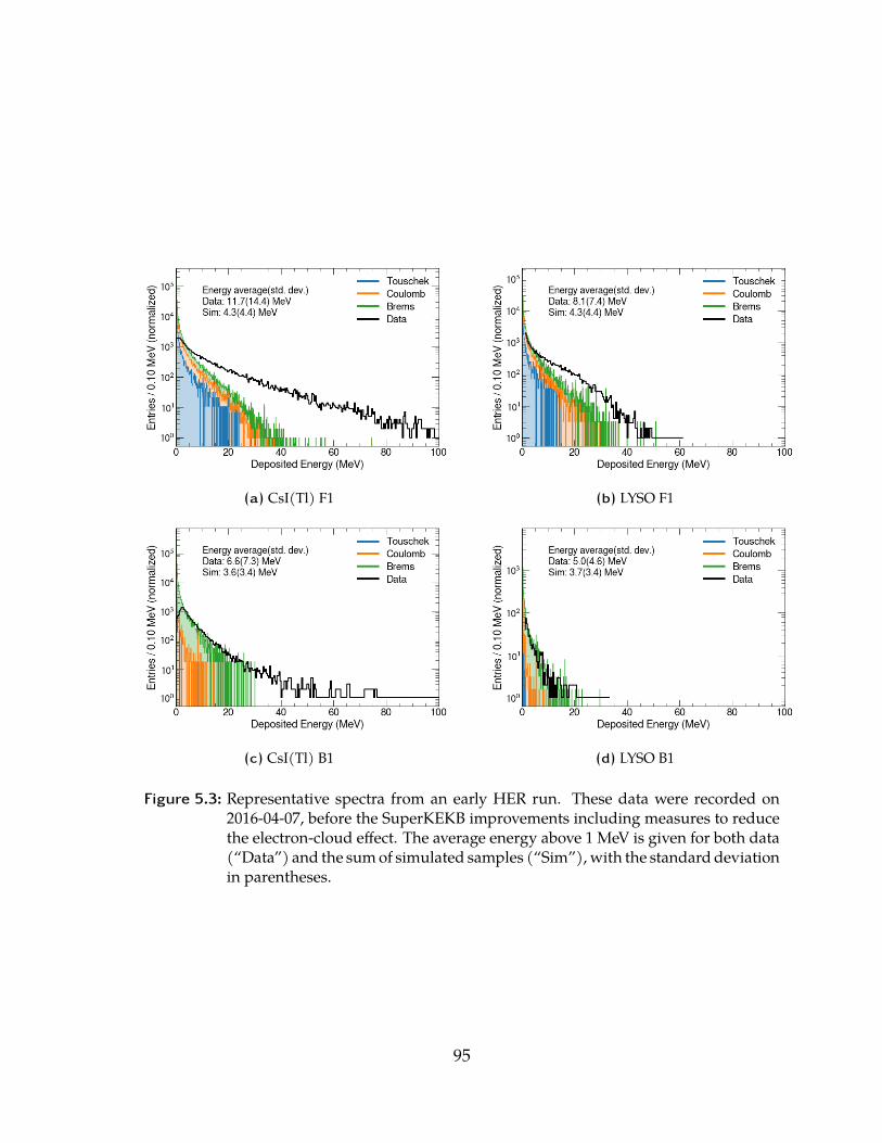
(a) CsI(Tl) F1 (b) LYSO F1

(c) CsI(Tl) B1 (d) LYSO B1

Figure 5.3: Representative spectra from an early HER run. These data were recorded on2016-04-07, before the SuperKEKB improvements including measures to reducethe electron-cloud effect. The average energy above 1 MeV is given for both data(“Data”) and the sum of simulated samples (“Sim”), with the standard deviationin parentheses.

95

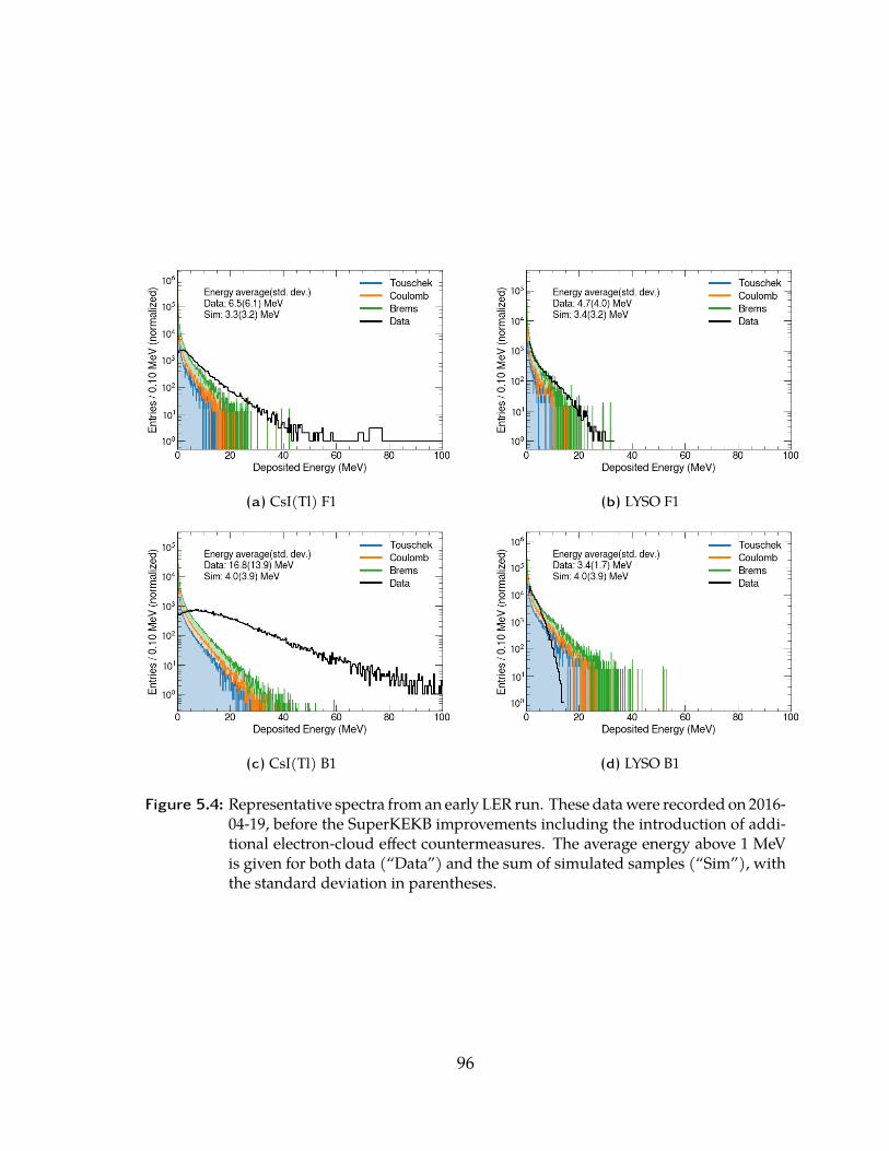
(a) CsI(Tl) F1 (b) LYSO F1

(c) CsI(Tl) B1 (d) LYSO B1

Figure 5.4: Representative spectra from an early LER run. These data were recorded on 2016-04-19, before the SuperKEKB improvements including the introduction of addi-tional electron-cloud effect countermeasures. The average energy above 1 MeVis given for both data (“Data”) and the sum of simulated samples (“Sim”), withthe standard deviation in parentheses.

96

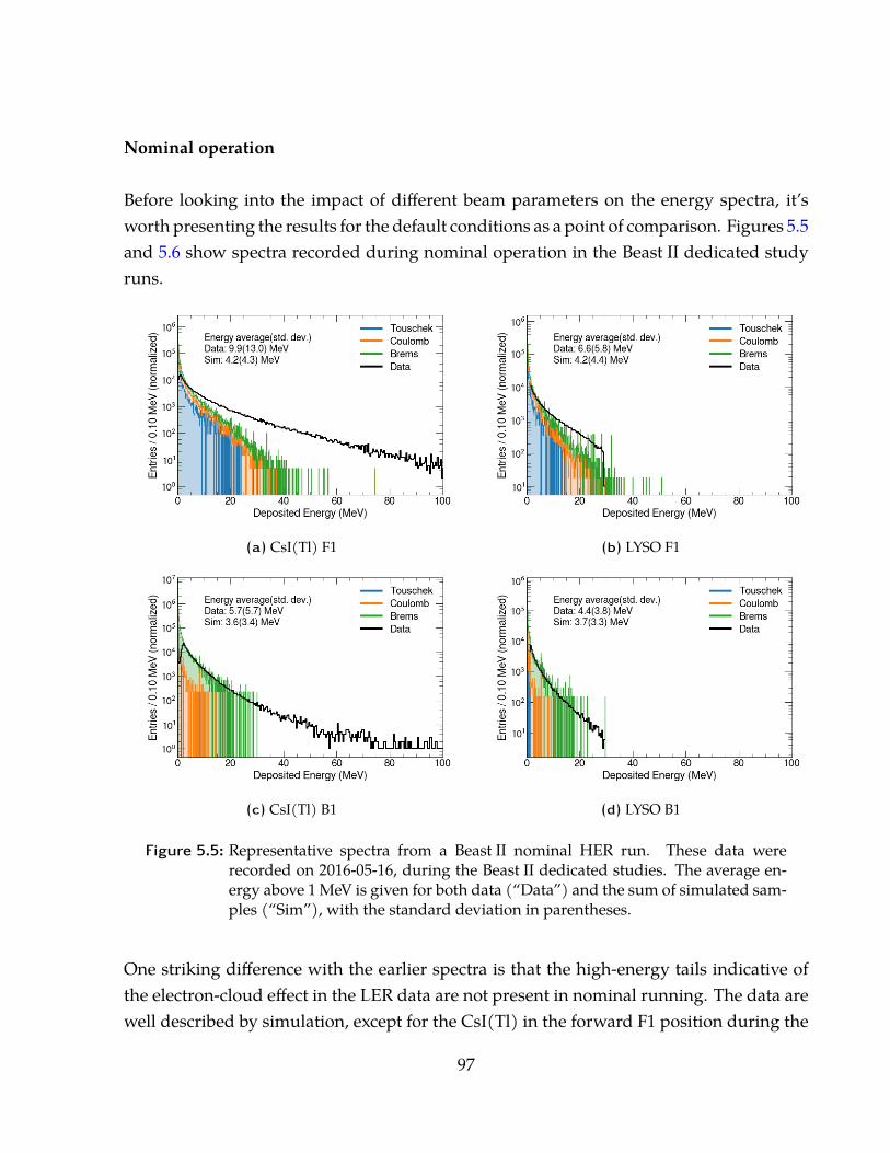
Nominal operation

Before looking into the impact of different beam parameters on the energy spectra, it’sworth presenting the results for the default conditions as a point of comparison. Figures 5.5and 5.6 show spectra recorded during nominal operation in the Beast II dedicated studyruns.

(a) CsI(Tl) F1 (b) LYSO F1

(c) CsI(Tl) B1 (d) LYSO B1

Figure 5.5: Representative spectra from a Beast II nominal HER run. These data wererecorded on 2016-05-16, during the Beast II dedicated studies. The average en-ergy above 1 MeV is given for both data (“Data”) and the sum of simulated sam-ples (“Sim”), with the standard deviation in parentheses.

One striking difference with the earlier spectra is that the high-energy tails indicative ofthe electron-cloud effect in the LER data are not present in nominal running. The data arewell described by simulation, except for the CsI(Tl) in the forward F1 position during the

97

HER runs (Figure 5.5a), and the CsI(Tl) in the backward B1 position in the LER runs (Fig-ure 5.6c). In both cases, the channel corresponds to the detector positioned immediatelydownstream from the interaction region, in the direction of the beam.

98

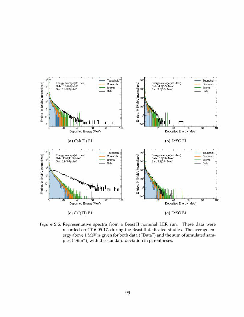
(a) CsI(Tl) F1 (b) LYSO F1

(c) CsI(Tl) B1 (d) LYSO B1

Figure 5.6: Representative spectra from a Beast II nominal LER run. These data wererecorded on 2016-05-17, during the Beast II dedicated studies. The average en-ergy above 1 MeV is given for both data (“Data”) and the sum of simulated sam-ples (“Sim”), with the standard deviation in parentheses.

99

Touschek effect study

A qualitative study of the Touschek effect on the spectra is conducted by comparing Fig-ure 5.7 with Figure 5.8 for the LER (37% more Touschek), and Figure 5.9 with Figure 5.10for the HER (240% more Touschek).

From the LER runs of Figures 5.7 and 5.8, we see that the backward CsI(Tl) channel (bothpanels (c)) exhibits a larger tail in the Touschek-enhanced than in the Touschek-diminishedrun. This tail represents part of the background that is not well modelled by our heuristicmodel of Eq. 4.14. On the forward channels of panels (a) and (b), however, there is noappreciable impact of beam size on the shape of spectra (beyond what is explained by ourbackground model). Again, for the LER, the “backward” channels are downstream fromthe interaction region.

For the HER Touschek study, there is no clear impact of increasing the beam size by afactor of approximately 2.4. This can be seen by comparing Figures 5.9 and 5.10: eventhough the Touschek contributions are different, the shapes of the measured distributionsare indistinguishable, so the part not explained by our background model (Eq. 4.14) isconsistent in the two cases.

Note that for one of the sub-runs shown in panel 5.10b, the LYSO channel suffered from toomuch deadtime due to data acquisition issues, so we had to discard it from the analysis.

100

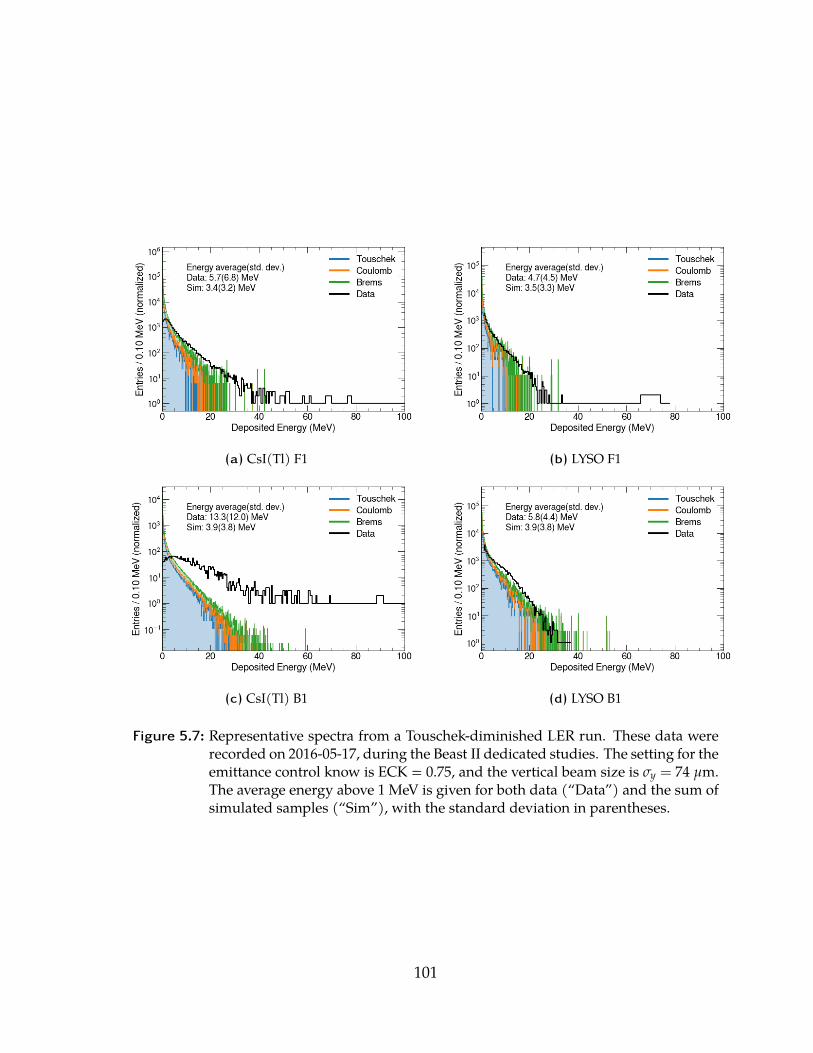
(a) CsI(Tl) F1 (b) LYSO F1

(c) CsI(Tl) B1 (d) LYSO B1

Figure 5.7: Representative spectra from a Touschek-diminished LER run. These data wererecorded on 2016-05-17, during the Beast II dedicated studies. The setting for theemittance control know is ECK = 0.75, and the vertical beam size is σy = 74 µm.The average energy above 1 MeV is given for both data (“Data”) and the sum ofsimulated samples (“Sim”), with the standard deviation in parentheses.

101

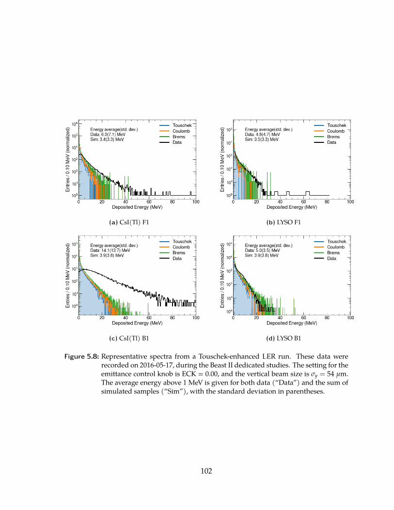
(a) CsI(Tl) F1 (b) LYSO F1

(c) CsI(Tl) B1 (d) LYSO B1

Figure 5.8: Representative spectra from a Touschek-enhanced LER run. These data wererecorded on 2016-05-17, during the Beast II dedicated studies. The setting for theemittance control knob is ECK = 0.00, and the vertical beam size is σy = 54 µm.The average energy above 1 MeV is given for both data (“Data”) and the sum ofsimulated samples (“Sim”), with the standard deviation in parentheses.

102

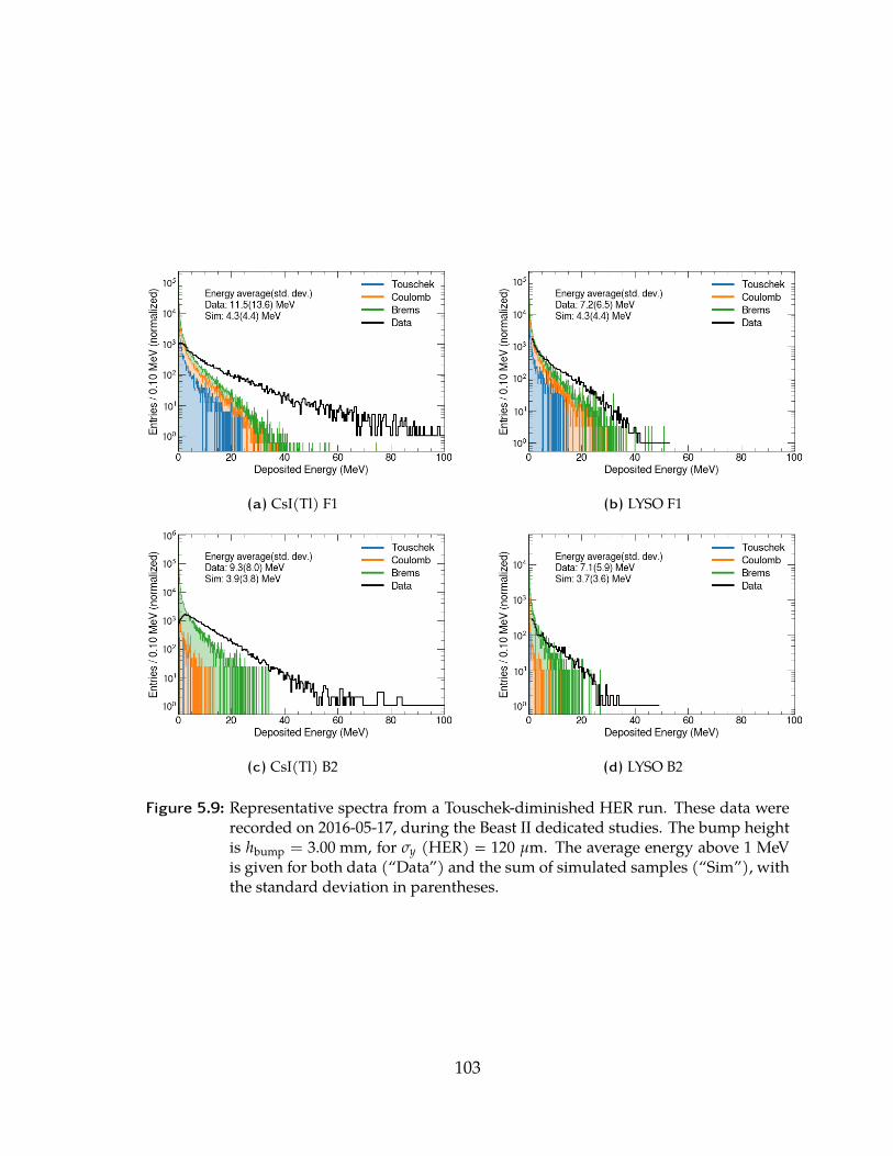
(a) CsI(Tl) F1 (b) LYSO F1

(c) CsI(Tl) B2 (d) LYSO B2

Figure 5.9: Representative spectra from a Touschek-diminished HER run. These data wererecorded on 2016-05-17, during the Beast II dedicated studies. The bump heightis hbump = 3.00 mm, for σy (HER) = 120 µm. The average energy above 1 MeVis given for both data (“Data”) and the sum of simulated samples (“Sim”), withthe standard deviation in parentheses.

103

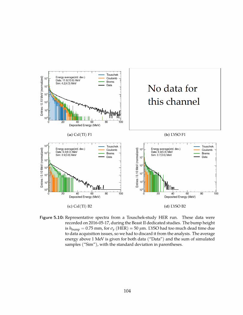
(a) CsI(Tl) F1 (b) LYSO F1

(c) CsI(Tl) B2 (d) LYSO B2

Figure 5.10: Representative spectra from a Touschek-study HER run. These data wererecorded on 2016-05-17, during the Beast II dedicated studies. The bump heightis hbump = 0.75 mm, for σy (HER) = 50 µm. LYSO had too much dead time dueto data acquisition issues, so we had to discard it from the analysis. The averageenergy above 1 MeV is given for both data (“Data”) and the sum of simulatedsamples (“Sim”), with the standard deviation in parentheses.

104

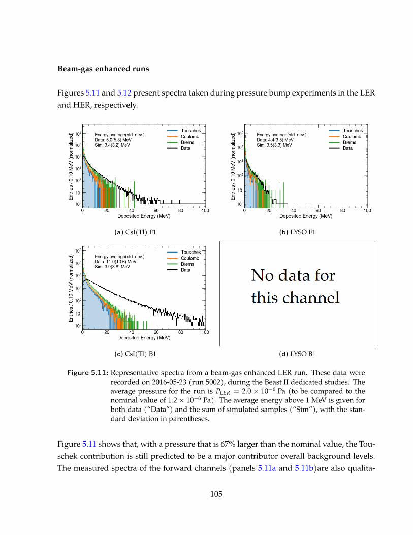
Beam-gas enhanced runs

Figures 5.11 and 5.12 present spectra taken during pressure bump experiments in the LERand HER, respectively.

(a) CsI(Tl) F1 (b) LYSO F1

(c) CsI(Tl) B1 (d) LYSO B1

Figure 5.11: Representative spectra from a beam-gas enhanced LER run. These data wererecorded on 2016-05-23 (run 5002), during the Beast II dedicated studies. Theaverage pressure for the run is PLER = 2.0 × 10−6 Pa (to be compared to thenominal value of 1.2× 10−6 Pa). The average energy above 1 MeV is given forboth data (“Data”) and the sum of simulated samples (“Sim”), with the stan-dard deviation in parentheses.

Figure 5.11 shows that, with a pressure that is 67% larger than the nominal value, the Tou-schek contribution is still predicted to be a major contributor overall background levels.The measured spectra of the forward channels (panels 5.11a and 5.11b)are also qualita-

105

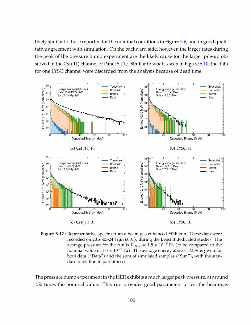
tively similar to those reported for the nominal conditions in Figure 5.6, and in good quali-tative agreement with simulation. On the backward side, however, the larger rates duringthe peak of the pressure bump experiment are the likely cause for the larger pile-up ob-served in the CsI(Tl) channel of Panel 5.11c. Similar to what is seen in Figure 5.10, the datafor one LYSO channel were discarded from the analysis because of dead time.

(a) CsI(Tl) F1 (b) LYSO F1

(c) CsI(Tl) B1 (d) LYSO B1

Figure 5.12: Representative spectra from a beam-gas enhanced HER run. These data wererecorded on 2016-05-24 (run 6001), during the Beast II dedicated studies. Theaverage pressure for the run is PHER = 1.5 × 10−5 Pa (to be compared to thenominal value of 1.0× 10−7 Pa). The average energy above 1 MeV is given forboth data (“Data”) and the sum of simulated samples (“Sim”), with the stan-dard deviation in parentheses.

The pressure bump experiment in the HER exhibits a much larger peak pressure, at around150 times the nominal value. This run provides good parameters to test the beam-gas

106

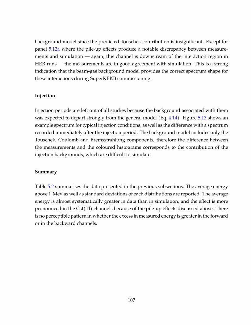
background model since the predicted Touschek contribution is insignificant. Except forpanel 5.12a where the pile-up effects produce a notable discrepancy between measure-ments and simulation — again, this channel is downstream of the interaction region inHER runs — the measurements are in good agreement with simulation. This is a strongindication that the beam-gas background model provides the correct spectrum shape forthese interactions during SuperKEKB commissioning.

Injection

Injection periods are left out of all studies because the background associated with themwas expected to depart strongly from the general model (Eq. 4.14). Figure 5.13 shows anexample spectrum for typical injection conditions, as well as the difference with a spectrumrecorded immediately after the injection period. The background model includes only theTouschek, Coulomb and Bremsstrahlung components, therefore the difference betweenthe measurements and the coloured histograms corresponds to the contribution of theinjection backgrounds, which are difficult to simulate.

Summary

Table 5.2 summarises the data presented in the previous subsections. The average energyabove 1 MeV as well as standard deviations of each distributions are reported. The averageenergy is almost systematically greater in data than in simulation, and the effect is morepronounced in the CsI(Tl) channels because of the pile-up effects discussed above. Thereis no perceptible pattern in whether the excess in measured energy is greater in the forwardor in the backward channels.

107

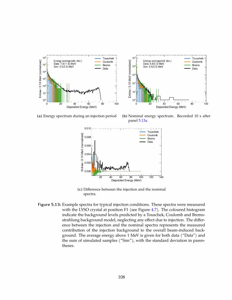
(a) Energy spectrum during an injection period (b) Nominal energy spectrum. Recorded 10 s afterpanel 5.13a.

(c) Difference between the injection and the nominalspectra.

Figure 5.13: Example spectra for typical injection conditions. These spectra were measuredwith the LYSO crystal at position F1 (see Figure 4.7). The coloured histogramindicate the background levels predicted by a Touschek, Coulomb and Brems-strahlung background model, neglecting any effect due to injection. The differ-ence between the injection and the nominal spectra represents the measuredcontribution of the injection background to the overall beam-induced back-ground. The average energy above 1 MeV is given for both data (“Data”) andthe sum of simulated samples (“Sim”), with the standard deviation in paren-theses.

108

Table

5.2:

Sum

mar

yof

the

crys

tals

spec

tra:a

vera

geen

ergy

and

stand

ard

devi

atio

nab

ove

1M

eV,w

here

the

stand

ard

devi

atio

nis

then

umbe

rin

brac

kets.

Then

umbe

rin

squa

rebr

acke

tsin

thefi

rstco

lum

ncr

oss-r

efere

nces

the

figur

enum

berw

here

thed

ataa

ppea

r. CsI(T

l)-F1

LYSO

-F1

CsI(T

l)-B1

LYSO

-B1

CsI(T

l)-B2

LYSO

-B2

Run

Type

HER

:Tou

sche

ksca

nat

σy=

120µ

m[5

.9]da

ta11

.5(13

.6)7.2

(6.5)

6.2(5

.4)-

9.3(8

.0)7.1

(5.9)

sim4.3

(4.4)

4.3(4

.4)3.6

(3.4)

-3.9

(3.8)

3.7(3

.6)H

ER:T

ousc

heks

can

atσ

y=

50µ

m[5

.10]

data

11.6(

13.6)

-6.2

(6.0)

-9.2

(8.0)

6.9(5

.8)sim

4.2(4

.3)-

3.6(3

.4)-

3.9(3

.8)3.7

(3.6)

HER

:Befo

reEC

Efix

es[5

.3]da

ta11

.7(14

.4)8.1

(7.4)

6.6(7

.3)5.0

(4.6)

9.5(8

.6)8.0

(7.2)

sim4.3

(4.4)

4.3(4

.4)3.6

(3.4)

3.7(3

.4)3.9

(3.8)

3.7(3

.6)H

ER:N

omin

al[5

.5]da

ta9.9

(13.0

)6.6

(5.8)

5.7(5

.7)4.4

(3.8)

7.5(7

.0)-

sim4.2

(4.3)

4.2(4

.4)3.6

(3.4)

3.7(3

.3)3.9

(3.8)

-H

ER:P

ress

ureb

ump

[5.12

]da

ta10

.6(13

.2)7.1

(6.7)

5.9(5

.7)4.5

(4.0)

7.9(7

.1)6.4

(5.4)

sim4.4

(4.6)

4.4(4

.5)3.6

(3.4)

3.7(3

.4)3.9

(3.8)

3.7(3

.6)LE

R:Be

fore

ECE

fixes

[5.4]

data

6.5(6

.1)4.7

(4.0)

16.8(

13.9)

3.4(1

.7)18

.5(23

.4)4.3

(2.9)

sim3.3

(3.2)

3.4(3

.2)4.0

(3.9)

4.0(3

.9)3.9

(3.9)

4.0(4

.1)LE

R:To

usch

eksc

anat

σy=

54µ

m[5

.8]da

ta6.0

(7.1)

4.8(4

.7)14

.1(13

.7)5.0

(3.5)

-7.2

(6.5)

sim3.4

(3.3)

3.5(3

.3)3.9

(3.8)

3.9(3

.8)-

4.0(4

.0)LE

R:To

usch

eksc

anat

σy=

74µ

m[5

.7]da

ta5.7

(6.8)

4.7(4

.5)13

.3(12

.0)5.8

(4.4)

-7.8

(7.5)

sim3.4

(3.2)

3.5(3

.3)3.9

(3.8)

3.9(3

.8)-

4.0(4

.0)LE

R:In

jectio

n[5

.13]

data

8.5(2

1.2)

7.0(1

1.6)

14.1(

13.7)

6.3(6

.0)18

.2(33

.5)11

.4(12

.8)sim

3.4(3

.3)3.5

(3.3)

3.9(3

.8)3.9

(3.8)

3.8(3

.7)4.0

(4.0)

LER:

Nom

inal

[5.6]

data

5.8(6

.6)4.9

(5.3)

13.6(

11.9)

5.3(3

.9)15

.3(21

.3)7.9

(8.0)

sim3.4

(3.3)

3.5(3

.3)3.9

(3.8)

3.9(3

.8)3.8

(3.8)

4.0(4

.0)LE

R:Pr

essu

rebu

mp

[5.11

]da

ta5.0

(5.3)

4.4(3

.5)11

.0(10

.6)2.8

(1.4)

11.1(

16.2)

4.6(5

.1)sim

3.4(3

.2)3.5

(3.3)

3.9(3

.8)3.9

(3.8)

3.8(3

.8)4.0

(4.0)

109

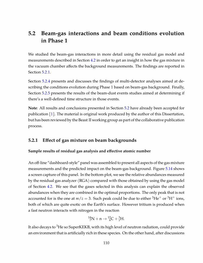
5.2 Beam-gas interactions and beam conditions evolutionin Phase 1

We studied the beam-gas interactions in more detail using the residual gas model andmeasurements described in Section 4.2 in order to get an insight in how the gas mixture inthe vacuum chamber affects the background measurements. The findings are reported inSection 5.2.1.

Section 5.2.4 presents and discusses the findings of multi-detector analyses aimed at de-scribing the conditions evolution during Phase 1 based on beam-gas background. Finally,Section 5.2.5 presents the results of the beam-dust events studies aimed at determining ifthere’s a well-defined time structure in those events.

Note: All results and conclusions presented in Section 5.2 have already been accepted forpublication [1]. The material is original work produced by the author of this Dissertation,but has been reviewed by the Beast II working group as part of the collaborative publicationprocess.

5.2.1 Effect of gas mixture on beam backgrounds

Sample results of residual gas analysis and effective atomic number

An off-line “dashboard-style” panel was assembled to present all aspects of the gas mixturemeasurements and the predicted impact on the beam-gas background. Figure 5.14 showsa screen capture of this panel. In the bottom plot, we see the relative abundances measuredby the residual gas analyzer (RGA) compared with those obtained by using the gas modelof Section 4.2. We see that the gases selected in this analysis can explain the observedabundances when they are combined in the optimal proportions. The only peak that is notaccounted for is the one at m/z = 3. Such peak could be due to either 3He+ or 3H+ ions,both of which are quite exotic on the Earth’s surface. However tritium is produced whena fast neutron interacts with nitrogen in the reaction

147N + n→ 12

6C + 31H.

It also decays to 3He so SuperKEKB, with its high level of neutron radiation, could providean environment that is artificially rich in these species. On the other hand, after discussions

110

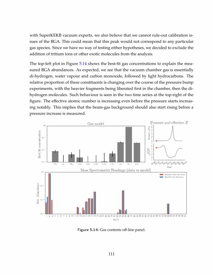
with SuperKEKB vacuum experts, we also believe that we cannot rule-out calibration is-sues of the RGA. This could mean that this peak would not correspond to any particulargas species. Since we have no way of testing either hypotheses, we decided to exclude theaddition of tritium ions or other exotic molecules from the analysis.

The top-left plot in Figure 5.14 shows the best-fit gas concentrations to explain the mea-sured RGA abundances. As expected, we see that the vacuum chamber gas is essentiallydi-hydrogen, water vapour and carbon monoxide, followed by light hydrocarbons. Therelative proportion of these constituents is changing over the course of the pressure bumpexperiments, with the heavier fragments being liberated first in the chamber, then the di-hydrogen molecules. Such behaviour is seen in the two time series at the top-right of thefigure. The effective atomic number is increasing even before the pressure starts increas-ing notably. This implies that the beam-gas background should also start rising before apressure increase is measured.

Figure 5.14: Gas contents off-line panel.

111

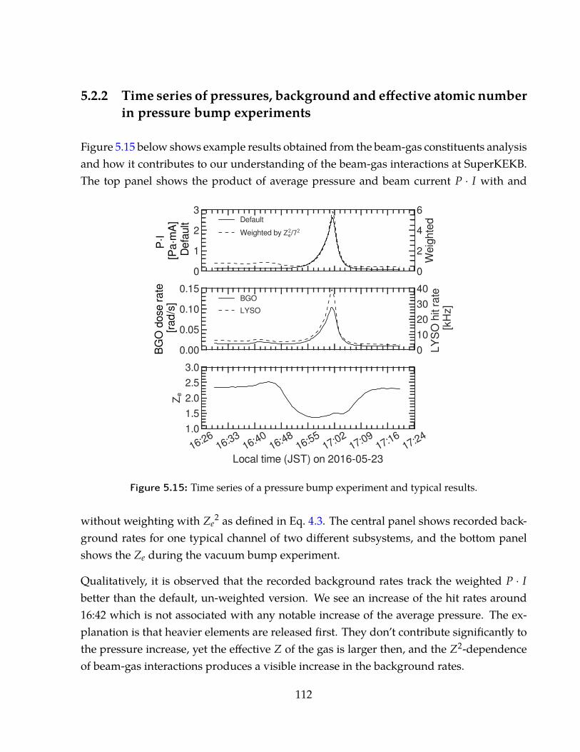
5.2.2 Time series of pressures, background and effective atomic numberin pressure bump experiments

Figure 5.15 below shows example results obtained from the beam-gas constituents analysisand how it contributes to our understanding of the beam-gas interactions at SuperKEKB.The top panel shows the product of average pressure and beam current P · I with and

0123

PI

[Pam

A]

Defa

ult

Default

0246

Weig

hted

Weighted by /

0.000.050.100.15

BGO

dose

rate

[rad

/s]

BGO

010203040

LYSO

hit r

ate

[kHz

]LYSO

16:2616:33

16:4016:48

16:5517:02

17:0917:16

17:24

Local time (JST) on 2016-05-23

1.01.52.02.53.0

Figure 5.15: Time series of a pressure bump experiment and typical results.

without weighting with Ze2 as defined in Eq. 4.3. The central panel shows recorded back-

ground rates for one typical channel of two different subsystems, and the bottom panelshows the Ze during the vacuum bump experiment.

Qualitatively, it is observed that the recorded background rates track the weighted P · Ibetter than the default, un-weighted version. We see an increase of the hit rates around16:42 which is not associated with any notable increase of the average pressure. The ex-planation is that heavier elements are released first. They don’t contribute significantly tothe pressure increase, yet the effective Z of the gas is larger then, and the Z2-dependenceof beam-gas interactions produces a visible increase in the background rates.

112

5.2.3 Uncertainty on Ze

The procedure used to calculate the uncertainty on Ze is descried in Section 4.2.4, andFigure 5.16 shows the results. In this section, the variable of interest is the square of Ze sincethe beam-gas cross sections, hence the background rates, are proportional to Z2

e . On topof the relative magnitude of the confidence intervals, it is worth noting that the confidenceintervals are not symmetrical around the nominal value.

Figure 5.16: Confidence intervals around the Z2e time series for the 2016-05-23 pressure

bump experiment. The shaded area represents the 1000 different Monte Carlopseudo-experiments overlayed with each other. Lines labeled 68% C.I. and95% C.I. are the limits of confidence intervals around the nominal value.

This asymmetry arises from the non-linearities present in the Ze calculations, and can bebetter observed by looking at a slice of the time series of Figure 5.16. Such a slice is pre-sented in Figure 5.17, where we see the nominal Z2

e value at a specific time sample, as wellas the PDF estimated by Monte Carlo methods. This PDF is asymmetric, therefore using itto produce confidence intervals for the nominal value will yield ranges that aren’t symmet-rically distributed around the nominal value. One way to summarize this study is to lookat the confidence intervals as a function of Z2

e , as represented in Figure 5.18. This plot canbe used to asses the uncertainty arising from Z2

e values when used to scale the simulationto experimental conditions.

113

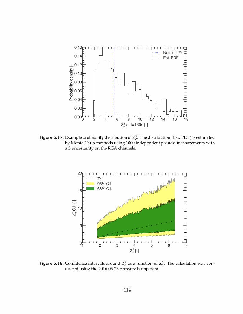
0 2 4 6 8 10 12 14 16 18 at t=160s [-]

0.00

0.02

0.04

0.06

0.08

0.10

0.12

0.14

0.16

Prob

abilit

y den

sity [

-]

Nominal Est. PDF

Figure 5.17: Example probability distribution of Z2e . The distribution (Est. PDF) is estimated

by Monte Carlo methods using 1000 independent pseudo-measurements witha 3 uncertainty on the RGA channels.

1 2 3 4 5 6 7 [-]

0

5

10

15

20

C.I.

[-]

95% C.I.68% C.I.

Figure 5.18: Confidence intervals around Z2e as a function of Z2

e . The calculation was con-ducted using the 2016-05-23 pressure bump data.

114

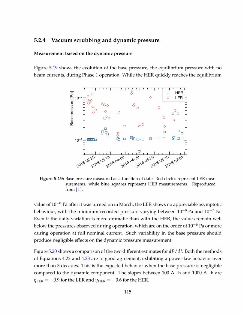
5.2.4 Vacuum scrubbing and dynamic pressure

Measurement based on the dynamic pressure

Figure 5.19 shows the evolution of the base pressure, the equilibrium pressure with nobeam currents, during Phase 1 operation. While the HER quickly reaches the equilibrium

2016-02-26

2016-03-18

2016-04-08

2016-04-29

2016-05-20

2016-06-10

2016-07-01

Base

pres

sure

[Pa] HER

LER

Figure 5.19: Base pressure measured as a function of date. Red circles represent LER mea-surements, while blue squares represent HER measurements. Reproducedfrom [1].

value of 10−8 Pa after it was turned on in March, the LER shows no appreciable asymptoticbehaviour, with the minimum recorded pressure varying between 10−8 Pa and 10−7 Pa.Even if the daily variation is more dramatic than with the HER, the values remain wellbelow the pressures observed during operation, which are on the order of 10−6 Pa or moreduring operation at full nominal current. Such variability in the base pressure shouldproduce negligible effects on the dynamic pressure measurement.

Figure 5.20 shows a comparison of the two different estimates for dP/dI. Both the methodsof Equations 4.22 and 4.23 are in good agreement, exhibiting a power-law behavior overmore than 3 decades. This is the expected behavior when the base pressure is negligiblecompared to the dynamic component. The slopes between 100 A · h and 1000 A · h areηLER = −0.9 for the LER and ηHER = −0.6 for the HER.

115

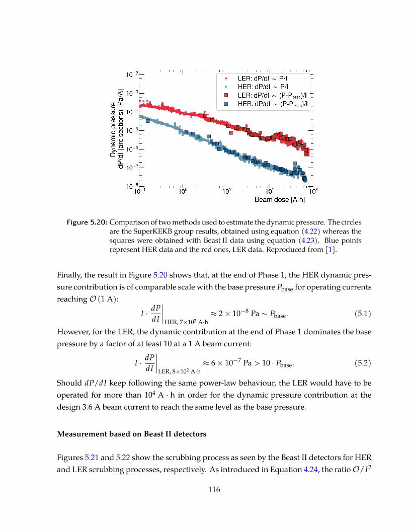
Figure 5.20: Comparison of two methods used to estimate the dynamic pressure. The circlesare the SuperKEKB group results, obtained using equation (4.22) whereas thesquares were obtained with Beast II data using equation (4.23). Blue pointsrepresent HER data and the red ones, LER data. Reproduced from [1].

Finally, the result in Figure 5.20 shows that, at the end of Phase 1, the HER dynamic pres-sure contribution is of comparable scale with the base pressure Pbase for operating currentsreaching O (1 A):

I · dPdI

∣∣∣∣HER, 7×102 A·h

≈ 2× 10−8 Pa∼ Pbase. (5.1)

However, for the LER, the dynamic contribution at the end of Phase 1 dominates the basepressure by a factor of at least 10 at a 1 A beam current:

I · dPdI

∣∣∣∣LER, 8×102 A·h

≈ 6× 10−7 Pa > 10 · Pbase. (5.2)

Should dP/dI keep following the same power-law behaviour, the LER would have to beoperated for more than 104 A · h in order for the dynamic pressure contribution at thedesign 3.6 A beam current to reach the same level as the base pressure.

Measurement based on Beast II detectors

Figures 5.21 and 5.22 show the scrubbing process as seen by the Beast II detectors for HERand LER scrubbing processes, respectively. As introduced in Equation 4.24, the ratioO/I2

116

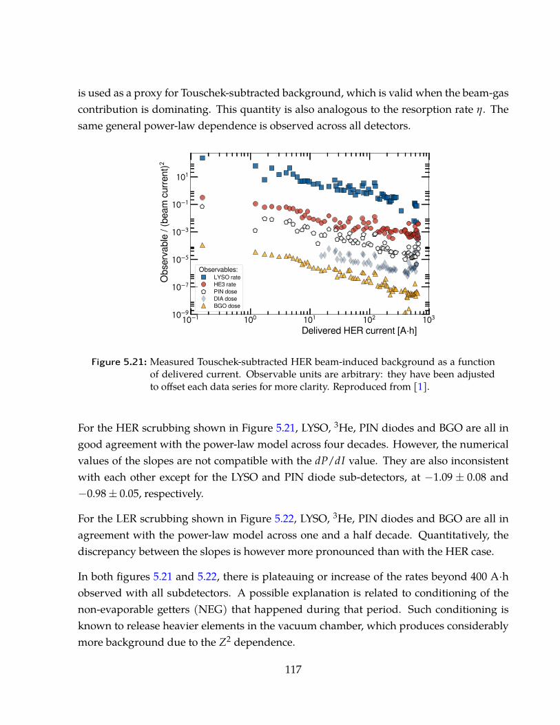
is used as a proxy for Touschek-subtracted background, which is valid when the beam-gascontribution is dominating. This quantity is also analogous to the resorption rate η. Thesame general power-law dependence is observed across all detectors.

Delivered HER current [A h]

Obse

rvable

/ (be

am cu

rrent)

Observables: LYSO rateHE3 ratePIN doseDIA doseBGO dose

Figure 5.21: Measured Touschek-subtracted HER beam-induced background as a functionof delivered current. Observable units are arbitrary: they have been adjustedto offset each data series for more clarity. Reproduced from [1].

For the HER scrubbing shown in Figure 5.21, LYSO, 3He, PIN diodes and BGO are all ingood agreement with the power-law model across four decades. However, the numericalvalues of the slopes are not compatible with the dP/dI value. They are also inconsistentwith each other except for the LYSO and PIN diode sub-detectors, at −1.09 ± 0.08 and−0.98± 0.05, respectively.

For the LER scrubbing shown in Figure 5.22, LYSO, 3He, PIN diodes and BGO are all inagreement with the power-law model across one and a half decade. Quantitatively, thediscrepancy between the slopes is however more pronounced than with the HER case.

In both figures 5.21 and 5.22, there is plateauing or increase of the rates beyond 400 A·hobserved with all subdetectors. A possible explanation is related to conditioning of thenon-evaporable getters (NEG) that happened during that period. Such conditioning isknown to release heavier elements in the vacuum chamber, which produces considerablymore background due to the Z2 dependence.

117

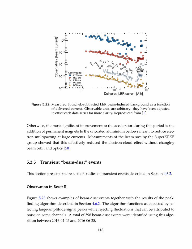
Delivered LER current [A h]

Obse

rvable

/ (be

am cu

rrent)

Observables: LYSO rateHE3 ratePIN doseDIA doseBGO dose

Figure 5.22: Measured Touschek-subtracted LER beam-induced background as a functionof delivered current. Observable units are arbitrary: they have been adjustedto offset each data series for more clarity. Reproduced from [1].

Otherwise, the most significant improvement to the accelerator during this period is theaddition of permanent magnets to the uncoated aluminium bellows meant to reduce elec-tron multipacting at large currents. Measurements of the beam size by the SuperKEKBgroup showed that this effectively reduced the electron-cloud effect without changingbeam orbit and optics [50].

5.2.5 Transient “beam-dust” events

This section presents the results of studies on transient events described in Section 4.6.2.

Observation in Beast II

Figure 5.23 shows examples of beam-dust events together with the results of the peak-finding algorithm described in Section 4.6.2. The algorithm functions as expected by se-lecting large-amplitude signal peaks while rejecting fluctuations that can be attributed tonoise on some channels. A total of 598 beam-dust events were identified using this algo-rithm between 2016-04-05 and 2016-06-28.

118

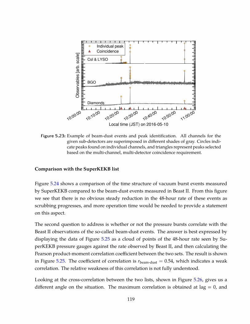
CsI & LYSO

Individual peakCoincidence

Obse

rvable

s [ar

b. sc

ale]

BGO

10:00:0010:10:00

10:20:0010:30:00

10:40:0010:50:00

11:00:00

Local time (JST) on 2016-05-10

Diamonds

Figure 5.23: Example of beam-dust events and peak identification. All channels for thegiven sub-detectors are superimposed in different shades of gray. Circles indi-cate peaks found on individual channels, and triangles represent peaks selectedbased on the multi-channel, multi-detector coincidence requirement.

Comparison with the SuperKEKB list

Figure 5.24 shows a comparison of the time structure of vacuum burst events measuredby SuperKEKB compared to the beam-dust events measured in Beast II. From this figurewe see that there is no obvious steady reduction in the 48-hour rate of these events asscrubbing progresses, and more operation time would be needed to provide a statementon this aspect.

The second question to address is whether or not the pressure bursts correlate with theBeast II observations of the so-called beam-dust events. The answer is best expressed bydisplaying the data of Figure 5.25 as a cloud of points of the 48-hour rate seen by Su-perKEKB pressure gauges against the rate observed by Beast II, and then calculating thePearson product-moment correlation coefficient between the two sets. The result is shownin Figure 5.25. The coefficient of correlation is rbeam-dust = 0.54, which indicates a weakcorrelation. The relative weakness of this correlation is not fully understood.

Looking at the cross-correlation between the two lists, shown in Figure 5.26, gives us adifferent angle on the situation. The maximum correlation is obtained at lag = 0, and

119

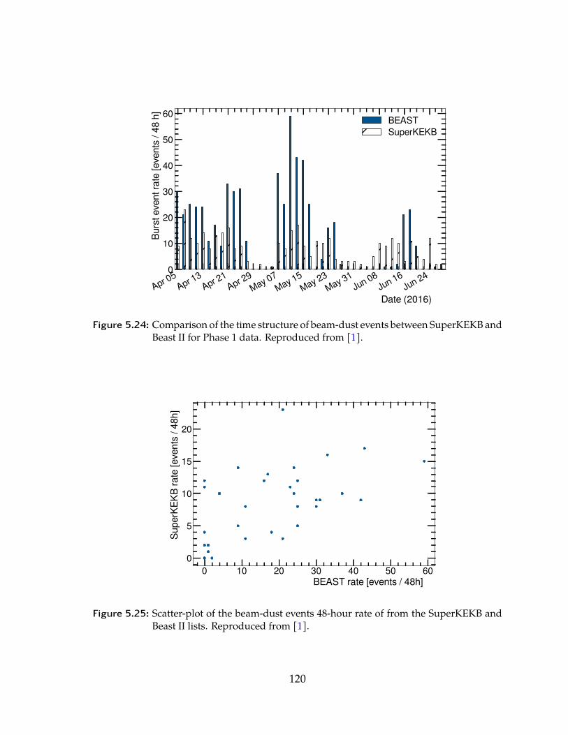
Apr 05Apr 13

Apr 21Apr 29

May 07May 15

May 23May 31

Jun 08Jun 16

Jun 24

Date (2016)

0

10

20

30

40

50

60

Burst

even

t rate

[eve

nts / 4

8 h]

BEASTSuperKEKB

Figure 5.24: Comparison of the time structure of beam-dust events between SuperKEKB andBeast II for Phase 1 data. Reproduced from [1].

0 10 20 30 40 50 60BEAST rate [events / 48h]

0

5

10

15

20

Supe

rKEK

B ra

te [ev

ents

/ 48h

]

Figure 5.25: Scatter-plot of the beam-dust events 48-hour rate of from the SuperKEKB andBeast II lists. Reproduced from [1].

120

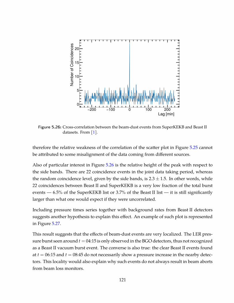
200 100 0 100 200Lag [min]

0

5

10

15

20

Numb

er of

Coin

ciden

ces

Figure 5.26: Cross-correlation between the beam-dust events from SuperKEKB and Beast IIdatasets. From [1].

therefore the relative weakness of the correlation of the scatter plot in Figure 5.25 cannotbe attributed to some misalignment of the data coming from different sources.

Also of particular interest in Figure 5.26 is the relative height of the peak with respect tothe side bands. There are 22 coincidence events in the joint data taking period, whereasthe random coincidence level, given by the side bands, is 2.3± 1.5. In other words, while22 coincidences between Beast II and SuperKEKB is a very low fraction of the total burstevents — 6.5% of the SuperKEKB list or 3.7% of the Beast II list — it is still significantlylarger than what one would expect if they were uncorrelated.

Including pressure times series together with background rates from Beast II detectorssuggests another hypothesis to explain this effect. An example of such plot is representedin Figure 5.27.

This result suggests that the effects of beam-dust events are very localized. The LER pres-sure burst seen around t = 04:15 is only observed in the BGO detectors, thus not recognizedas a Beast II vacuum burst event. The converse is also true: the clear Beast II events foundat t = 06:15 and t = 08:45 do not necessarily show a pressure increase in the nearby detec-tors. This locality would also explain why such events do not always result in beam abortsfrom beam loss monitors.

121

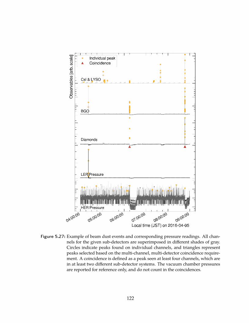
Figure 5.27: Example of beam dust events and corresponding pressure readings. All chan-nels for the given sub-detectors are superimposed in different shades of gray.Circles indicate peaks found on individual channels, and triangles representpeaks selected based on the multi-channel, multi-detector coincidence require-ment. A coincidence is defined as a peak seen at least four channels, which arein at least two different sub-detector systems. The vacuum chamber pressuresare reported for reference only, and do not count in the coincidences.

122

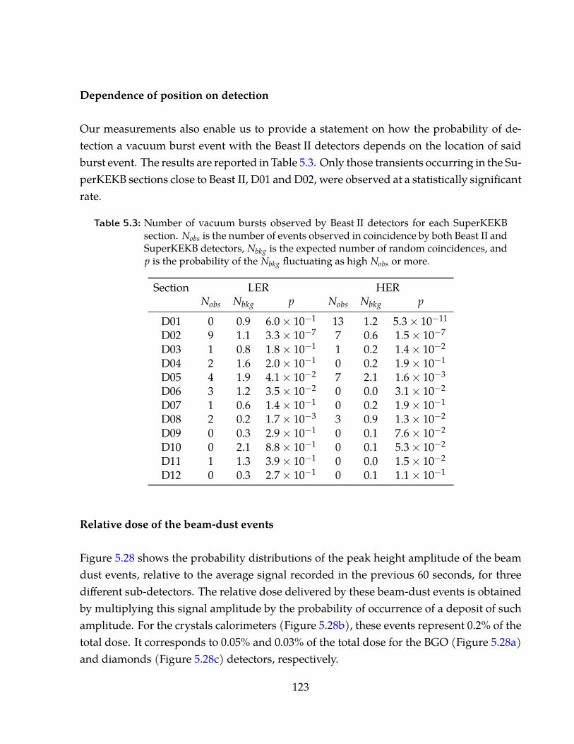
Dependence of position on detection

Our measurements also enable us to provide a statement on how the probability of de-tection a vacuum burst event with the Beast II detectors depends on the location of saidburst event. The results are reported in Table 5.3. Only those transients occurring in the Su-perKEKB sections close to Beast II, D01 and D02, were observed at a statistically significantrate.

Table 5.3: Number of vacuum bursts observed by Beast II detectors for each SuperKEKBsection. Nobs is the number of events observed in coincidence by both Beast II andSuperKEKB detectors, Nbkg is the expected number of random coincidences, andp is the probability of the Nbkg fluctuating as high Nobs or more.

Section LER HERNobs Nbkg p Nobs Nbkg p

D01 0 0.9 6.0× 10−1 13 1.2 5.3× 10−11

D02 9 1.1 3.3× 10−7 7 0.6 1.5× 10−7

D03 1 0.8 1.8× 10−1 1 0.2 1.4× 10−2

D04 2 1.6 2.0× 10−1 0 0.2 1.9× 10−1

D05 4 1.9 4.1× 10−2 7 2.1 1.6× 10−3

D06 3 1.2 3.5× 10−2 0 0.0 3.1× 10−2

D07 1 0.6 1.4× 10−1 0 0.2 1.9× 10−1

D08 2 0.2 1.7× 10−3 3 0.9 1.3× 10−2

D09 0 0.3 2.9× 10−1 0 0.1 7.6× 10−2

D10 0 2.1 8.8× 10−1 0 0.1 5.3× 10−2

D11 1 1.3 3.9× 10−1 0 0.0 1.5× 10−2

D12 0 0.3 2.7× 10−1 0 0.1 1.1× 10−1

Relative dose of the beam-dust events

Figure 5.28 shows the probability distributions of the peak height amplitude of the beamdust events, relative to the average signal recorded in the previous 60 seconds, for threedifferent sub-detectors. The relative dose delivered by these beam-dust events is obtainedby multiplying this signal amplitude by the probability of occurrence of a deposit of suchamplitude. For the crystals calorimeters (Figure 5.28b), these events represent 0.2% of thetotal dose. It corresponds to 0.05% and 0.03% of the total dose for the BGO (Figure 5.28a)and diamonds (Figure 5.28c) detectors, respectively.

123

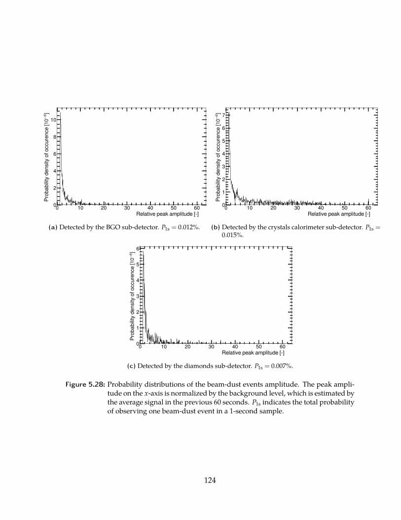
0 10 20 30 40 50 60Relative peak amplitude [-]

0

2

4

6

8

10

Prob

abilit

y den

sity o

f occ

uren

ce [

]

(a) Detected by the BGO sub-detector. P1s = 0.012%.

0 10 20 30 40 50 60Relative peak amplitude [-]

0

1

2

3

4

5

6

7

Prob

abilit

y den

sity o

f occ

uren

ce [

](b) Detected by the crystals calorimeter sub-detector. P1s =

0.015%.

0 10 20 30 40 50 60Relative peak amplitude [-]

0

1

2

3

4

5

6

Prob

abilit

y den

sity o

f occ

uren

ce [

]

(c) Detected by the diamonds sub-detector. P1s = 0.007%.

Figure 5.28: Probability distributions of the beam-dust events amplitude. The peak ampli-tude on the x-axis is normalized by the background level, which is estimated bythe average signal in the previous 60 seconds. P1s indicates the total probabilityof observing one beam-dust event in a 1-second sample.

124

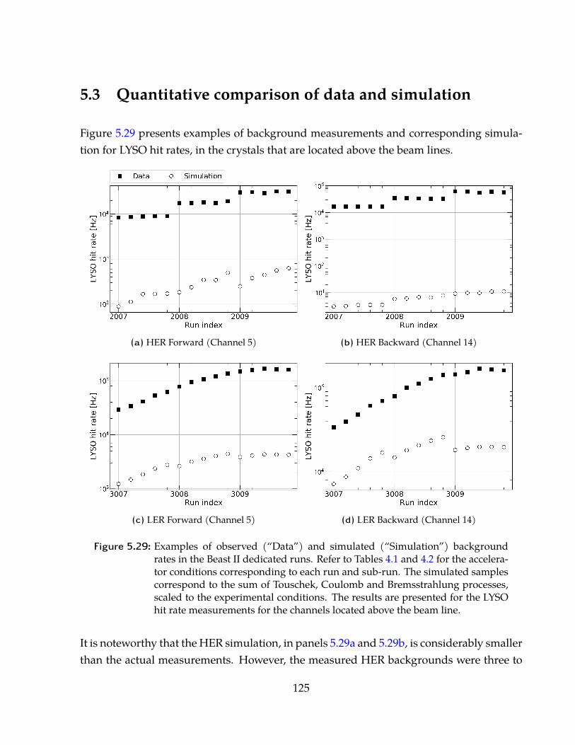
5.3 Quantitative comparison of data and simulation

Figure 5.29 presents examples of background measurements and corresponding simula-tion for LYSO hit rates, in the crystals that are located above the beam lines.

(a) HER Forward (Channel 5) (b) HER Backward (Channel 14)

(c) LER Forward (Channel 5) (d) LER Backward (Channel 14)

Figure 5.29: Examples of observed (“Data”) and simulated (“Simulation”) backgroundrates in the Beast II dedicated runs. Refer to Tables 4.1 and 4.2 for the accelera-tor conditions corresponding to each run and sub-run. The simulated samplescorrespond to the sum of Touschek, Coulomb and Bremsstrahlung processes,scaled to the experimental conditions. The results are presented for the LYSOhit rate measurements for the channels located above the beam line.

It is noteworthy that the HER simulation, in panels 5.29a and 5.29b, is considerably smallerthan the actual measurements. However, the measured HER backgrounds were three to

125

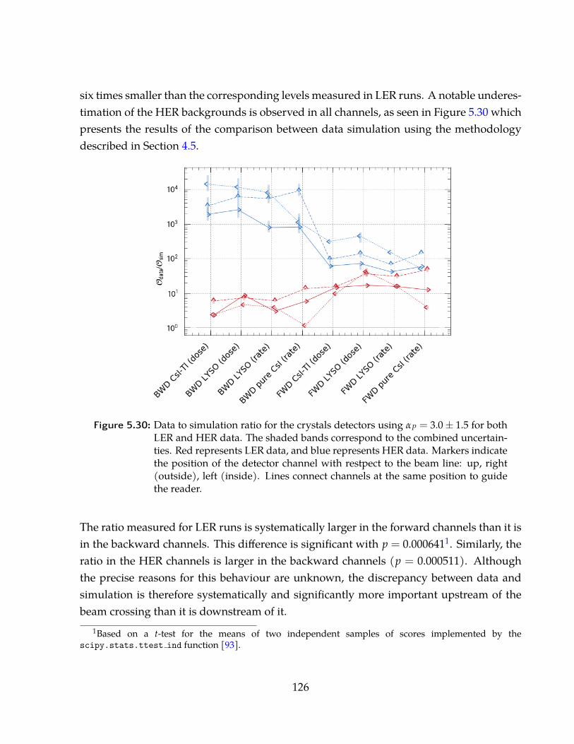
six times smaller than the corresponding levels measured in LER runs. A notable underes-timation of the HER backgrounds is observed in all channels, as seen in Figure 5.30 whichpresents the results of the comparison between data simulation using the methodologydescribed in Section 4.5.

Figure 5.30: Data to simulation ratio for the crystals detectors using αP = 3.0± 1.5 for bothLER and HER data. The shaded bands correspond to the combined uncertain-ties. Red represents LER data, and blue represents HER data. Markers indicatethe position of the detector channel with restpect to the beam line: up, right(outside), left (inside). Lines connect channels at the same position to guidethe reader.

The ratio measured for LER runs is systematically larger in the forward channels than it isin the backward channels. This difference is significant with p = 0.0006411. Similarly, theratio in the HER channels is larger in the backward channels (p = 0.000511). Althoughthe precise reasons for this behaviour are unknown, the discrepancy between data andsimulation is therefore systematically and significantly more important upstream of thebeam crossing than it is downstream of it.

1Based on a t-test for the means of two independent samples of scores implemented by thescipy.stats.ttest ind function [93].

126

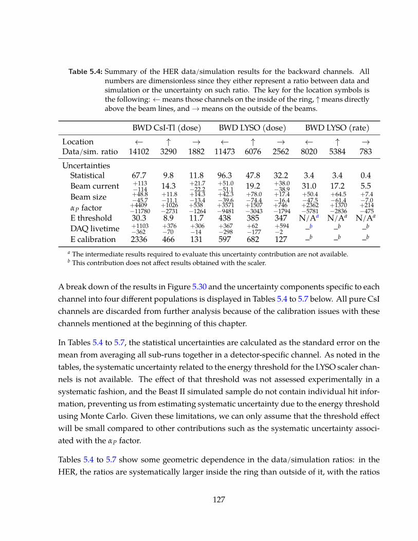
Table 5.4: Summary of the HER data/simulation results for the backward channels. Allnumbers are dimensionless since they either represent a ratio between data andsimulation or the uncertainty on such ratio. The key for the location symbols isthe following: ←means those channels on the inside of the ring, ↑means directlyabove the beam lines, and→means on the outside of the beams.

BWD CsI-Tl (dose) BWD LYSO (dose) BWD LYSO (rate)Location ← ↑ → ← ↑ → ← ↑ →Data/sim. ratio 14102 3290 1882 11473 6076 2562 8020 5384 783Uncertainties

Statistical 67.7 9.8 11.8 96.3 47.8 32.2 3.4 3.4 0.4Beam current +113

−114 14.3 +21.7−22.2

+51.0−51.1 19.2 +38.0

−38.9 31.0 17.2 5.5Beam size +48.8

−45.7+11.8−11.1

+14.3−13.4

+42.3−39.6

+78.0−74.4

+17.4−16.4

+50.4−47.5

+64.5−61.4

+7.4−7.0

αP factor +4409−11780

+1026−2731

+538−1264

+3571−9481

+1507−3043

+746−1794

+2362−5781

+1370−2836

+214−475

E threshold 30.3 8.9 11.7 438 385 347 N/Aa N/Aa N/Aa

DAQ livetime +1103−362

+376−70

+306−14

+367−298

+62−177

+594−2 –b –b –b

E calibration 2336 466 131 597 682 127 –b –b –b

a The intermediate results required to evaluate this uncertainty contribution are not available.b This contribution does not affect results obtained with the scaler.

A break down of the results in Figure 5.30 and the uncertainty components specific to eachchannel into four different populations is displayed in Tables 5.4 to 5.7 below. All pure CsIchannels are discarded from further analysis because of the calibration issues with thesechannels mentioned at the beginning of this chapter.

In Tables 5.4 to 5.7, the statistical uncertainties are calculated as the standard error on themean from averaging all sub-runs together in a detector-specific channel. As noted in thetables, the systematic uncertainty related to the energy threshold for the LYSO scaler chan-nels is not available. The effect of that threshold was not assessed experimentally in asystematic fashion, and the Beast II simulated sample do not contain individual hit infor-mation, preventing us from estimating systematic uncertainty due to the energy thresholdusing Monte Carlo. Given these limitations, we can only assume that the threshold effectwill be small compared to other contributions such as the systematic uncertainty associ-ated with the αP factor.

Tables 5.4 to 5.7 show some geometric dependence in the data/simulation ratios: in theHER, the ratios are systematically larger inside the ring than outside of it, with the ratios

127

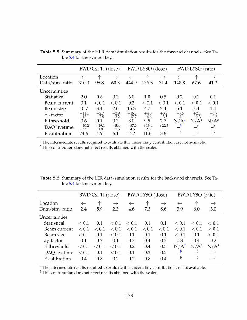
Table 5.5: Summary of the HER data/simulation results for the forward channels. See Ta-ble 5.4 for the symbol key.

FWD CsI-Tl (dose) FWD LYSO (dose) FWD LYSO (rate)Location ← ↑ → ← ↑ → ← ↑ →Data/sim. ratio 310.0 95.8 60.8 444.9 136.5 71.4 148.8 67.6 41.2Uncertainties

Statistical 2.0 0.6 0.3 6.0 1.0 0.5 0.2 0.1 0.1Beam current 0.1 < 0.1 < 0.1 0.2 < 0.1 < 0.1 < 0.1 < 0.1 < 0.1Beam size 10.7 3.4 2.0 15.3 4.7 2.4 5.1 2.4 1.4αP factor +11.1

−12.1+2.7−2.8

+2.9−3.2

+16.3−17.7

+4.3−4.6

+3.2−3.5

+5.5−6.1

+2.1−2.3

+1.7−1.8

E threshold 0.6 0.1 0.3 8.0 9.5 2.7 N/Aa N/Aa N/Aa

DAQ livetime +10.2−6.7

+19.1−1.8

+5.4−1.5

+87.0−4.5

+19.4−2.5

+22.3−1.3 –b –b –b

E calibration 24.6 4.9 6.1 122 11.6 3.6 –b –b –b

a The intermediate results required to evaluate this uncertainty contribution are not available.b This contribution does not affect results obtained with the scaler.

Table 5.6: Summary of the LER data/simulation results for the backward channels. See Ta-ble 5.4 for the symbol key.

BWD CsI-Tl (dose) BWD LYSO (dose) BWD LYSO (rate)Location ← ↑ → ← ↑ → ← ↑ →Data/sim. ratio 2.4 5.9 2.3 4.6 7.3 8.6 3.9 6.0 3.0Uncertainties

Statistical < 0.1 0.1 < 0.1 < 0.1 0.1 0.1 < 0.1 < 0.1 < 0.1Beam current < 0.1 < 0.1 < 0.1 < 0.1 < 0.1 < 0.1 < 0.1 < 0.1 < 0.1Beam size < 0.1 0.1 < 0.1 0.1 0.1 0.1 < 0.1 0.1 < 0.1αP factor 0.1 0.2 0.1 0.2 0.4 0.2 0.3 0.4 0.2E threshold < 0.1 < 0.1 < 0.1 0.2 0.4 0.3 N/Aa N/Aa N/Aa

DAQ livetime < 0.1 0.1 < 0.1 0.1 0.2 0.2 –b –b –b

E calibration 0.4 0.8 0.2 0.2 0.8 0.4 –b –b –b

a The intermediate results required to evaluate this uncertainty contribution are not available.b This contribution does not affect results obtained with the scaler.

128

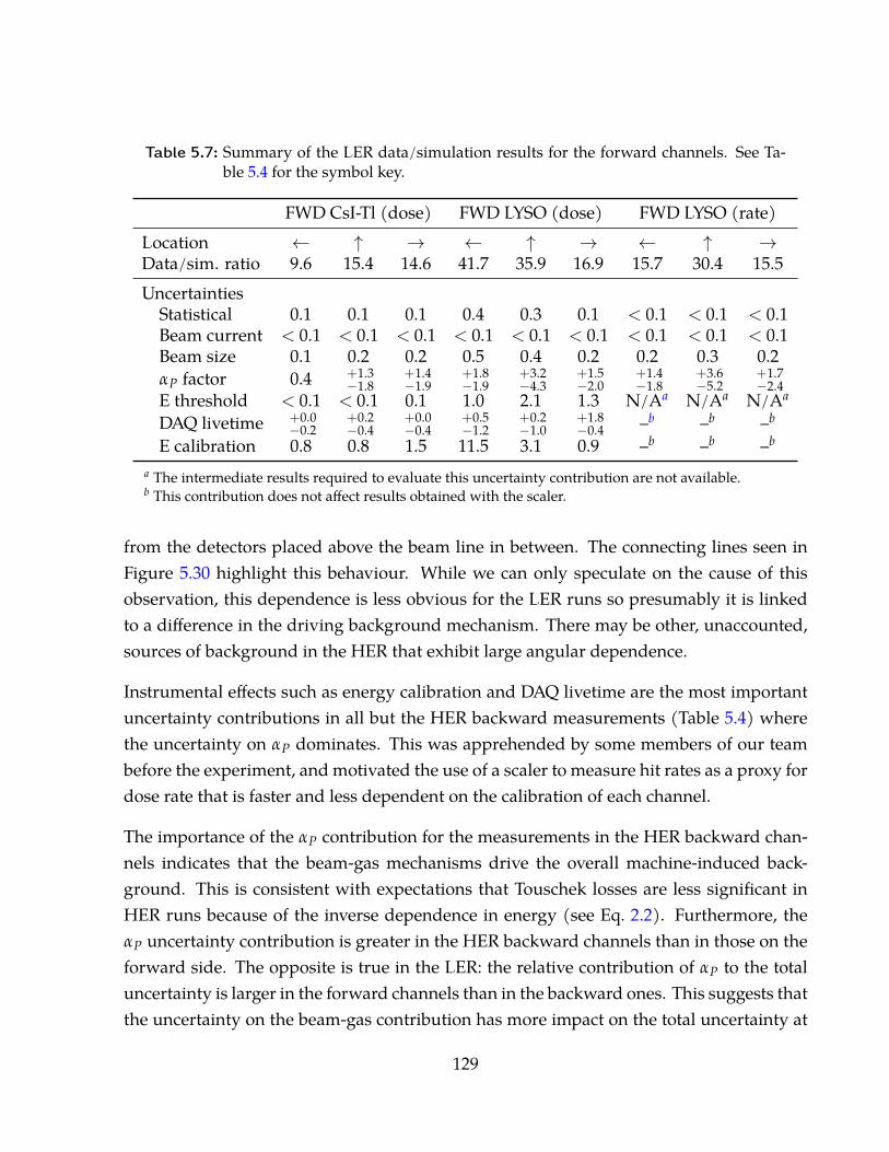
Table 5.7: Summary of the LER data/simulation results for the forward channels. See Ta-ble 5.4 for the symbol key.

FWD CsI-Tl (dose) FWD LYSO (dose) FWD LYSO (rate)Location ← ↑ → ← ↑ → ← ↑ →Data/sim. ratio 9.6 15.4 14.6 41.7 35.9 16.9 15.7 30.4 15.5Uncertainties

Statistical 0.1 0.1 0.1 0.4 0.3 0.1 < 0.1 < 0.1 < 0.1Beam current < 0.1 < 0.1 < 0.1 < 0.1 < 0.1 < 0.1 < 0.1 < 0.1 < 0.1Beam size 0.1 0.2 0.2 0.5 0.4 0.2 0.2 0.3 0.2αP factor 0.4 +1.3

−1.8+1.4−1.9

+1.8−1.9

+3.2−4.3

+1.5−2.0

+1.4−1.8

+3.6−5.2

+1.7−2.4

E threshold < 0.1 < 0.1 0.1 1.0 2.1 1.3 N/Aa N/Aa N/Aa

DAQ livetime +0.0−0.2

+0.2−0.4

+0.0−0.4

+0.5−1.2

+0.2−1.0

+1.8−0.4 –b –b –b

E calibration 0.8 0.8 1.5 11.5 3.1 0.9 –b –b –b

a The intermediate results required to evaluate this uncertainty contribution are not available.b This contribution does not affect results obtained with the scaler.

from the detectors placed above the beam line in between. The connecting lines seen inFigure 5.30 highlight this behaviour. While we can only speculate on the cause of thisobservation, this dependence is less obvious for the LER runs so presumably it is linkedto a difference in the driving background mechanism. There may be other, unaccounted,sources of background in the HER that exhibit large angular dependence.

Instrumental effects such as energy calibration and DAQ livetime are the most importantuncertainty contributions in all but the HER backward measurements (Table 5.4) wherethe uncertainty on αP dominates. This was apprehended by some members of our teambefore the experiment, and motivated the use of a scaler to measure hit rates as a proxy fordose rate that is faster and less dependent on the calibration of each channel.

The importance of the αP contribution for the measurements in the HER backward chan-nels indicates that the beam-gas mechanisms drive the overall machine-induced back-ground. This is consistent with expectations that Touschek losses are less significant inHER runs because of the inverse dependence in energy (see Eq. 2.2). Furthermore, theαP uncertainty contribution is greater in the HER backward channels than in those on theforward side. The opposite is true in the LER: the relative contribution of αP to the totaluncertainty is larger in the forward channels than in the backward ones. This suggests thatthe uncertainty on the beam-gas contribution has more impact on the total uncertainty at

129

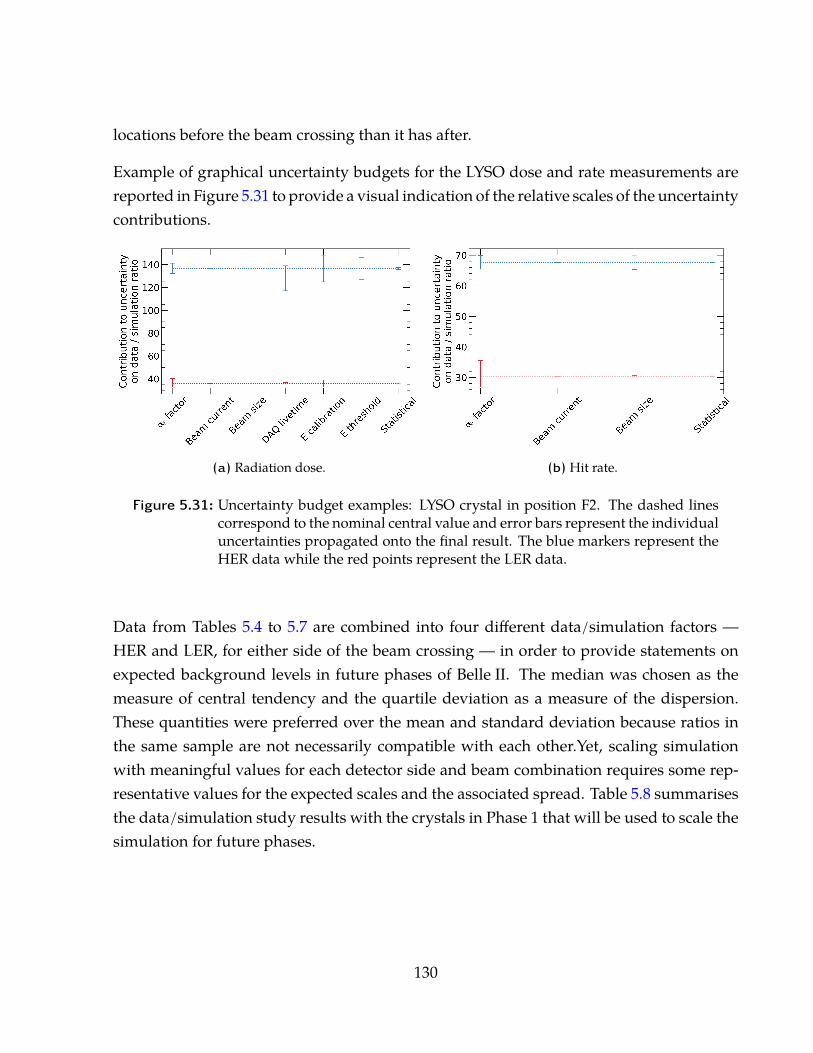
locations before the beam crossing than it has after.

Example of graphical uncertainty budgets for the LYSO dose and rate measurements arereported in Figure 5.31 to provide a visual indication of the relative scales of the uncertaintycontributions.

(a) Radiation dose. (b) Hit rate.

Figure 5.31: Uncertainty budget examples: LYSO crystal in position F2. The dashed linescorrespond to the nominal central value and error bars represent the individualuncertainties propagated onto the final result. The blue markers represent theHER data while the red points represent the LER data.

Data from Tables 5.4 to 5.7 are combined into four different data/simulation factors —HER and LER, for either side of the beam crossing — in order to provide statements onexpected background levels in future phases of Belle II. The median was chosen as themeasure of central tendency and the quartile deviation as a measure of the dispersion.These quantities were preferred over the mean and standard deviation because ratios inthe same sample are not necessarily compatible with each other.Yet, scaling simulationwith meaningful values for each detector side and beam combination requires some rep-resentative values for the expected scales and the associated spread. Table 5.8 summarisesthe data/simulation study results with the crystals in Phase 1 that will be used to scale thesimulation for future phases.

130

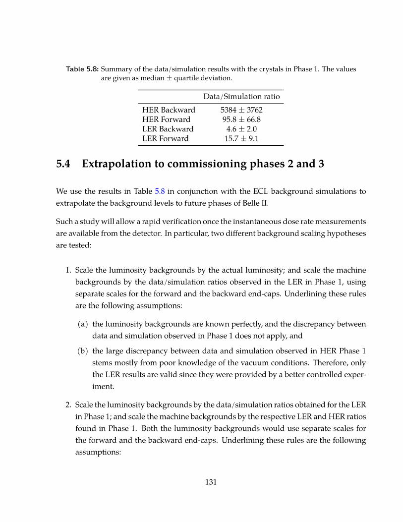
Table 5.8: Summary of the data/simulation results with the crystals in Phase 1. The valuesare given as median ± quartile deviation.

Data/Simulation ratioHER Backward 5384 ± 3762HER Forward 95.8 ± 66.8LER Backward 4.6 ± 2.0LER Forward 15.7 ± 9.1

5.4 Extrapolation to commissioning phases 2 and 3

We use the results in Table 5.8 in conjunction with the ECL background simulations toextrapolate the background levels to future phases of Belle II.

Such a study will allow a rapid verification once the instantaneous dose rate measurementsare available from the detector. In particular, two different background scaling hypothesesare tested:

1. Scale the luminosity backgrounds by the actual luminosity; and scale the machinebackgrounds by the data/simulation ratios observed in the LER in Phase 1, usingseparate scales for the forward and the backward end-caps. Underlining these rulesare the following assumptions:

(a) the luminosity backgrounds are known perfectly, and the discrepancy betweendata and simulation observed in Phase 1 does not apply, and

(b) the large discrepancy between data and simulation observed in HER Phase 1stems mostly from poor knowledge of the vacuum conditions. Therefore, onlythe LER results are valid since they were provided by a better controlled exper-iment.

2. Scale the luminosity backgrounds by the data/simulation ratios obtained for the LERin Phase 1; and scale the machine backgrounds by the respective LER and HER ratiosfound in Phase 1. Both the luminosity backgrounds would use separate scales forthe forward and the backward end-caps. Underlining these rules are the followingassumptions:

131

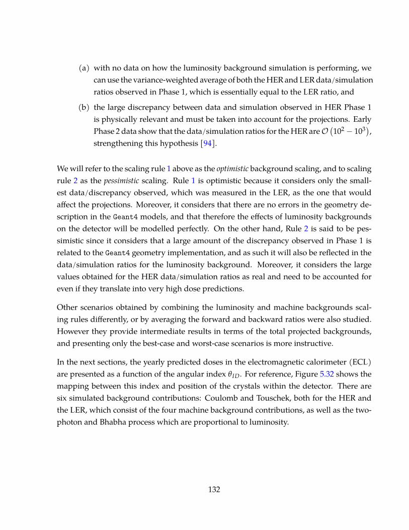
(a) with no data on how the luminosity background simulation is performing, wecan use the variance-weighted average of both the HER and LER data/simulationratios observed in Phase 1, which is essentially equal to the LER ratio, and

(b) the large discrepancy between data and simulation observed in HER Phase 1is physically relevant and must be taken into account for the projections. EarlyPhase 2 data show that the data/simulation ratios for the HER areO (102 − 103),strengthening this hypothesis [94].

We will refer to the scaling rule 1 above as the optimistic background scaling, and to scalingrule 2 as the pessimistic scaling. Rule 1 is optimistic because it considers only the small-est data/discrepancy observed, which was measured in the LER, as the one that wouldaffect the projections. Moreover, it considers that there are no errors in the geometry de-scription in the Geant4 models, and that therefore the effects of luminosity backgroundson the detector will be modelled perfectly. On the other hand, Rule 2 is said to be pes-simistic since it considers that a large amount of the discrepancy observed in Phase 1 isrelated to the Geant4 geometry implementation, and as such it will also be reflected in thedata/simulation ratios for the luminosity background. Moreover, it considers the largevalues obtained for the HER data/simulation ratios as real and need to be accounted foreven if they translate into very high dose predictions.

Other scenarios obtained by combining the luminosity and machine backgrounds scal-ing rules differently, or by averaging the forward and backward ratios were also studied.However they provide intermediate results in terms of the total projected backgrounds,and presenting only the best-case and worst-case scenarios is more instructive.

In the next sections, the yearly predicted doses in the electromagnetic calorimeter (ECL)are presented as a function of the angular index θID. For reference, Figure 5.32 shows themapping between this index and position of the crystals within the detector. There aresix simulated background contributions: Coulomb and Touschek, both for the HER andthe LER, which consist of the four machine background contributions, as well as the two-photon and Bhabha process which are proportional to luminosity.

132

012345

67

8910

11

12

1314151617181920212223242526272829303132333435363738394041424344454647484950515253545556575859

60

61

62

63

64

65

66

67

68

Figure 5.32: Mapping of the angular index θID in the ECL. The forward side of the detectoris on the right of the figure. Figure reproduced from [79].

5.4.1 Phase 2 of commissioning: L = 5.4× 1033 cm−2s−1L = 5.4× 1033 cm−2s−1L = 5.4× 1033 cm−2s−1

The highest luminosity achieved in Phase 2, 5.4× 1033 cm−2s−1, is approximately 10 timessmaller than the planned value. It is expected that the machine backgrounds would be thedominating contribution.

Optimistic scenario

Figure 5.33 shows the total radiation dose projection for Phase 2 assuming the optimisticdata/simulation scaling. The Touschek LER background is dominating in this picture,and all yearly equivalent doses are below the 10 Gy/yr tolerance value used in Belle 2. Theluminosity backgrounds, negligible in the forward end-cap, are only a small fraction of thetotal backward end-cap background.

Pessimistic scenario

Figure 5.34 shows the total radiation dose projections for Phase 2 assuming the pessimisticdata/simulation scaling. In this scenario, the luminosity backgrounds are 13.5 times larger,and the backwards HER backgrounds are scaled by a factor of approximately 5400. Thisgives a maximal dose of 96 Gy/yr delivered to the last row crystals on the backward side,although with considerable uncertainty. This dose is ten times larger than the acceptedtolerance for Belle II operations.

133

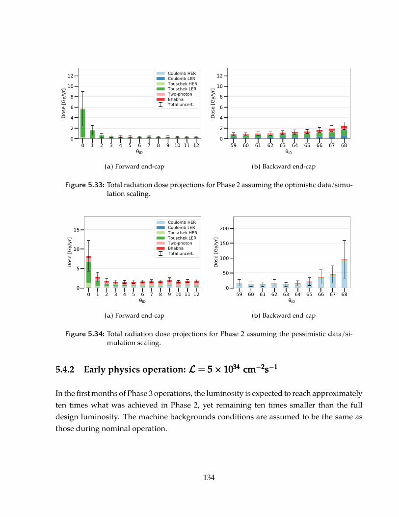
0 1 2 3 4 5 6 7 8 9 10 11 12ID

0

2

4

6

8

10

12

Dose

[Gy/

yr]

Coulomb HERCoulomb LERTouschek HERTouschek LERTwo-photonBhabhaTotal uncert.

(a) Forward end-cap

59 60 61 62 63 64 65 66 67 68ID

0

2

4

6

8

10

12

Dose

[Gy/

yr]

(b) Backward end-cap

Figure 5.33: Total radiation dose projections for Phase 2 assuming the optimistic data/simu-lation scaling.

0 1 2 3 4 5 6 7 8 9 10 11 12ID

0

5

10

15

Dose

[Gy/

yr]

Coulomb HERCoulomb LERTouschek HERTouschek LERTwo-photonBhabhaTotal uncert.

(a) Forward end-cap

59 60 61 62 63 64 65 66 67 68ID

0

50

100

150

200

Dose

[Gy/

yr]

(b) Backward end-cap

Figure 5.34: Total radiation dose projections for Phase 2 assuming the pessimistic data/si-mulation scaling.

5.4.2 Early physics operation: L = 5× 1034 cm−2s−1L = 5× 1034 cm−2s−1L = 5× 1034 cm−2s−1

In the first months of Phase 3 operations, the luminosity is expected to reach approximatelyten times what was achieved in Phase 2, yet remaining ten times smaller than the fulldesign luminosity. The machine backgrounds conditions are assumed to be the same asthose during nominal operation.

134

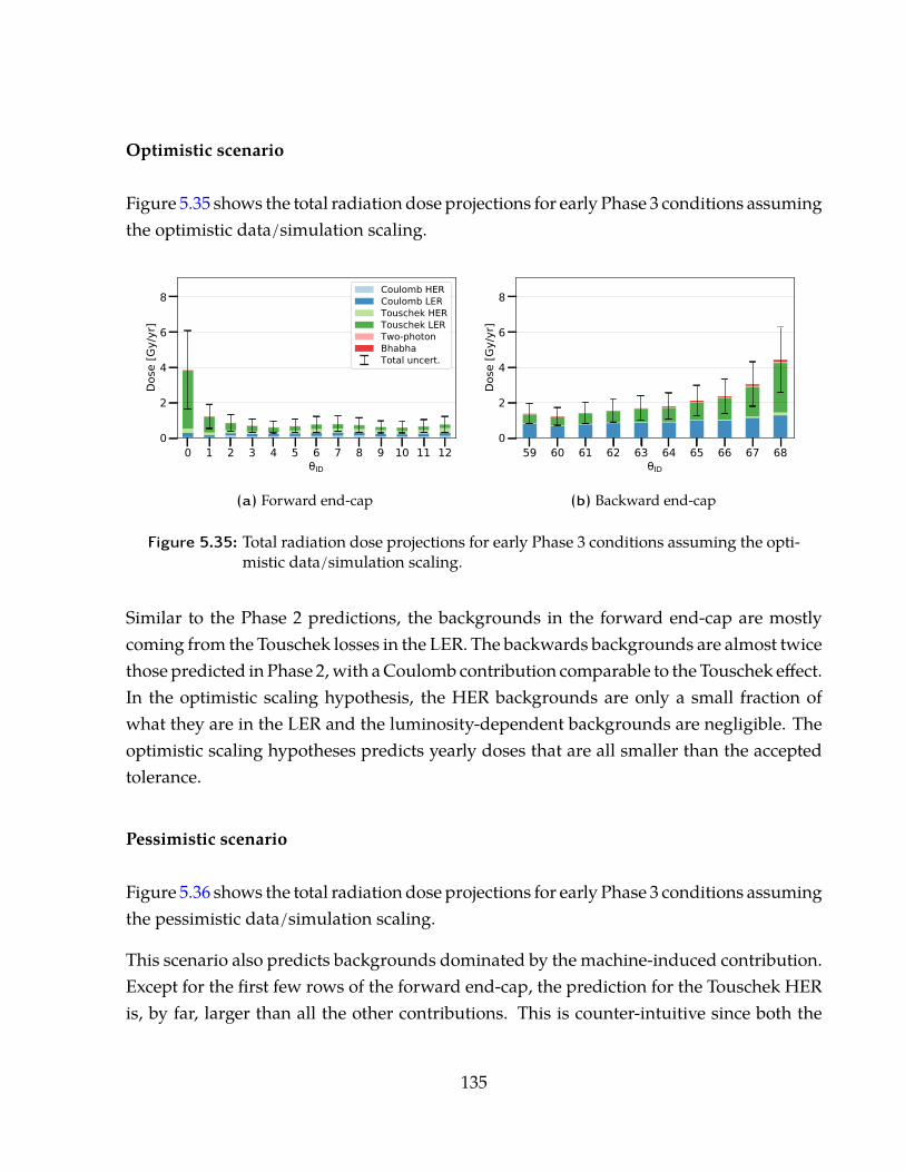
Optimistic scenario

Figure 5.35 shows the total radiation dose projections for early Phase 3 conditions assumingthe optimistic data/simulation scaling.

0 1 2 3 4 5 6 7 8 9 10 11 12ID

0

2

4

6

8

Dose

[Gy/

yr]

Coulomb HERCoulomb LERTouschek HERTouschek LERTwo-photonBhabhaTotal uncert.

(a) Forward end-cap

59 60 61 62 63 64 65 66 67 68ID

0

2

4

6

8

Dose

[Gy/

yr]

(b) Backward end-cap

Figure 5.35: Total radiation dose projections for early Phase 3 conditions assuming the opti-mistic data/simulation scaling.

Similar to the Phase 2 predictions, the backgrounds in the forward end-cap are mostlycoming from the Touschek losses in the LER. The backwards backgrounds are almost twicethose predicted in Phase 2, with a Coulomb contribution comparable to the Touschek effect.In the optimistic scaling hypothesis, the HER backgrounds are only a small fraction ofwhat they are in the LER and the luminosity-dependent backgrounds are negligible. Theoptimistic scaling hypotheses predicts yearly doses that are all smaller than the acceptedtolerance.

Pessimistic scenario

Figure 5.36 shows the total radiation dose projections for early Phase 3 conditions assumingthe pessimistic data/simulation scaling.

This scenario also predicts backgrounds dominated by the machine-induced contribution.Except for the first few rows of the forward end-cap, the prediction for the Touschek HERis, by far, larger than all the other contributions. This is counter-intuitive since both the

135

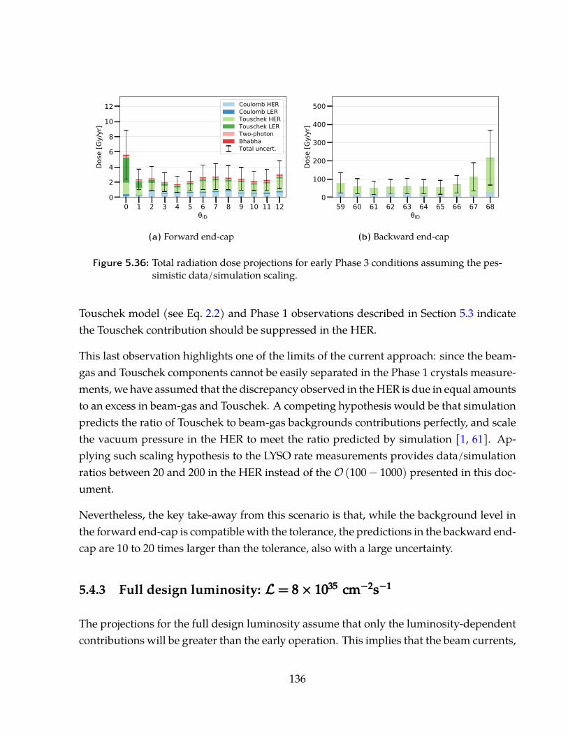
0 1 2 3 4 5 6 7 8 9 10 11 12ID

0

2

4

6

8

10

12Do

se [G

y/yr

]Coulomb HERCoulomb LERTouschek HERTouschek LERTwo-photonBhabhaTotal uncert.

(a) Forward end-cap

59 60 61 62 63 64 65 66 67 68ID

0

100

200

300

400

500

Dose

[Gy/

yr]

(b) Backward end-cap

Figure 5.36: Total radiation dose projections for early Phase 3 conditions assuming the pes-simistic data/simulation scaling.

Touschek model (see Eq. 2.2) and Phase 1 observations described in Section 5.3 indicatethe Touschek contribution should be suppressed in the HER.

This last observation highlights one of the limits of the current approach: since the beam-gas and Touschek components cannot be easily separated in the Phase 1 crystals measure-ments, we have assumed that the discrepancy observed in the HER is due in equal amountsto an excess in beam-gas and Touschek. A competing hypothesis would be that simulationpredicts the ratio of Touschek to beam-gas backgrounds contributions perfectly, and scalethe vacuum pressure in the HER to meet the ratio predicted by simulation [1, 61]. Ap-plying such scaling hypothesis to the LYSO rate measurements provides data/simulationratios between 20 and 200 in the HER instead of the O (100− 1000) presented in this doc-ument.

Nevertheless, the key take-away from this scenario is that, while the background level inthe forward end-cap is compatible with the tolerance, the predictions in the backward end-cap are 10 to 20 times larger than the tolerance, also with a large uncertainty.

5.4.3 Full design luminosity: L = 8× 1035 cm−2s−1L = 8× 1035 cm−2s−1L = 8× 1035 cm−2s−1

The projections for the full design luminosity assume that only the luminosity-dependentcontributions will be greater than the early operation. This implies that the beam currents,

136

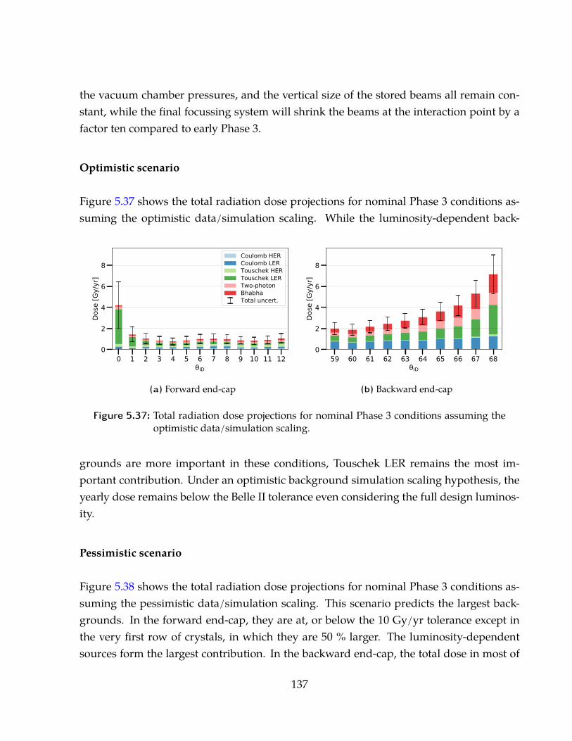
the vacuum chamber pressures, and the vertical size of the stored beams all remain con-stant, while the final focussing system will shrink the beams at the interaction point by afactor ten compared to early Phase 3.

Optimistic scenario

Figure 5.37 shows the total radiation dose projections for nominal Phase 3 conditions as-suming the optimistic data/simulation scaling. While the luminosity-dependent back-

0 1 2 3 4 5 6 7 8 9 10 11 12ID

0

2

4

6

8

Dose

[Gy/

yr]

Coulomb HERCoulomb LERTouschek HERTouschek LERTwo-photonBhabhaTotal uncert.

(a) Forward end-cap

59 60 61 62 63 64 65 66 67 68ID

0

2

4

6

8

Dose

[Gy/

yr]

(b) Backward end-cap

Figure 5.37: Total radiation dose projections for nominal Phase 3 conditions assuming theoptimistic data/simulation scaling.

grounds are more important in these conditions, Touschek LER remains the most im-portant contribution. Under an optimistic background simulation scaling hypothesis, theyearly dose remains below the Belle II tolerance even considering the full design luminos-ity.

Pessimistic scenario

Figure 5.38 shows the total radiation dose projections for nominal Phase 3 conditions as-suming the pessimistic data/simulation scaling. This scenario predicts the largest back-grounds. In the forward end-cap, they are at, or below the 10 Gy/yr tolerance except inthe very first row of crystals, in which they are 50 % larger. The luminosity-dependentsources form the largest contribution. In the backward end-cap, the total dose in most of

137

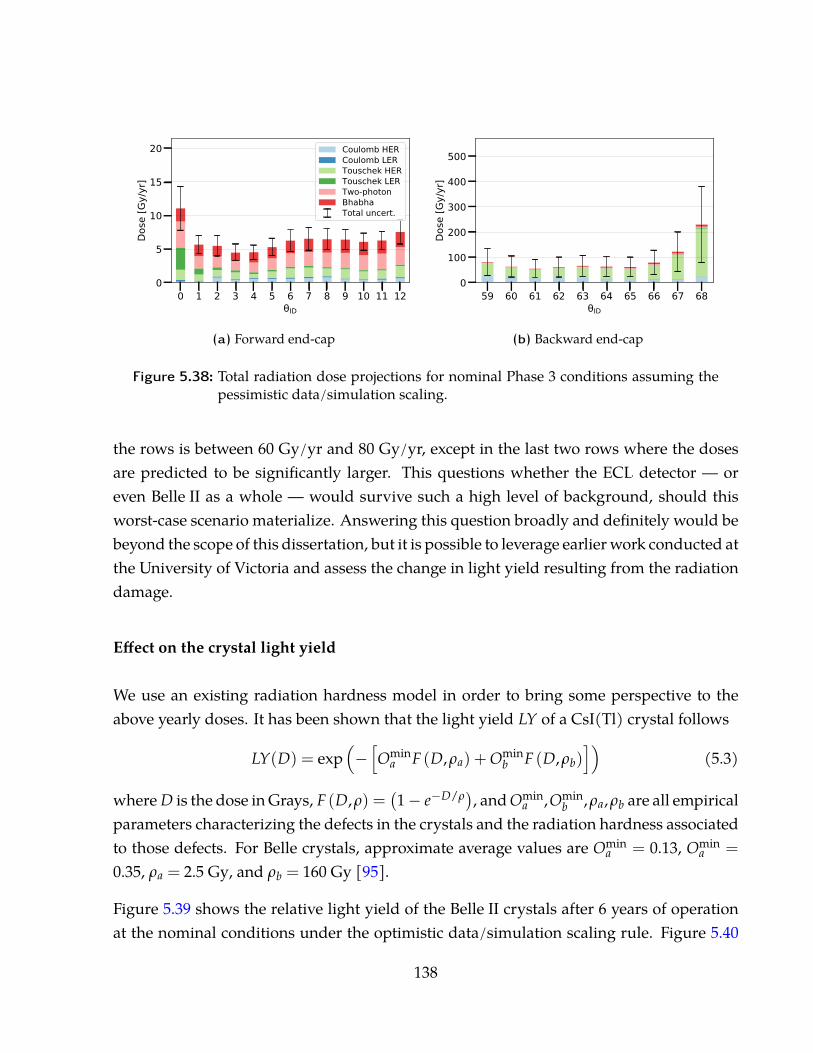
0 1 2 3 4 5 6 7 8 9 10 11 12ID

0

5

10

15

20Do

se [G

y/yr

]Coulomb HERCoulomb LERTouschek HERTouschek LERTwo-photonBhabhaTotal uncert.

(a) Forward end-cap

59 60 61 62 63 64 65 66 67 68ID

0

100

200

300

400

500

Dose

[Gy/

yr]

(b) Backward end-cap

Figure 5.38: Total radiation dose projections for nominal Phase 3 conditions assuming thepessimistic data/simulation scaling.

the rows is between 60 Gy/yr and 80 Gy/yr, except in the last two rows where the dosesare predicted to be significantly larger. This questions whether the ECL detector — oreven Belle II as a whole — would survive such a high level of background, should thisworst-case scenario materialize. Answering this question broadly and definitely would bebeyond the scope of this dissertation, but it is possible to leverage earlier work conducted atthe University of Victoria and assess the change in light yield resulting from the radiationdamage.

Effect on the crystal light yield

We use an existing radiation hardness model in order to bring some perspective to theabove yearly doses. It has been shown that the light yield LY of a CsI(Tl) crystal follows

LY(D) = exp(−[Omin

a F (D,ρa) + Ominb F (D,ρb)

])(5.3)

where D is the dose in Grays, F (D,ρ) =(1− e−D/ρ

), and Omina ,Omin

b ,ρa,ρb are all empiricalparameters characterizing the defects in the crystals and the radiation hardness associatedto those defects. For Belle crystals, approximate average values are Omin

a = 0.13, Omina =

0.35, ρa = 2.5 Gy, and ρb = 160 Gy [95].

Figure 5.39 shows the relative light yield of the Belle II crystals after 6 years of operationat the nominal conditions under the optimistic data/simulation scaling rule. Figure 5.40

138

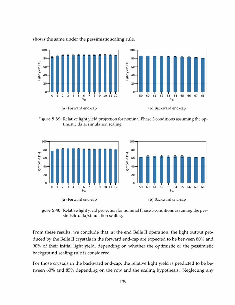
shows the same under the pessimistic scaling rule.

0 1 2 3 4 5 6 7 8 9 10 11 12ID

0

20

40

60

80

100

Light

yie

ld [%

]

(a) Forward end-cap

59 60 61 62 63 64 65 66 67 68ID

0

20

40

60

80

100

Light

yie

ld [%

]

(b) Backward end-cap

Figure 5.39: Relative light yield projection for nominal Phase 3 conditions assuming the op-timistic data/simulation scaling.

0 1 2 3 4 5 6 7 8 9 10 11 12ID

0

20

40

60

80

100

Light

yie

ld [%

]

(a) Forward end-cap

59 60 61 62 63 64 65 66 67 68ID

0

20

40

60

80

100

Light

yie

ld [%

]

(b) Backward end-cap

Figure 5.40: Relative light yield projection for nominal Phase 3 conditions assuming the pes-simistic data/simulation scaling.

From these results, we conclude that, at the end Belle II operation, the light output pro-duced by the Belle II crystals in the forward end-cap are expected to be between 80% and90% of their initial light yield, depending on whether the optimistic or the pessimisticbackground scaling rule is considered.

For those crystals in the backward end-cap, the relative light yield is predicted to be be-tween 60% and 85% depending on the row and the scaling hypothesis. Neglecting any

139

impact of radiation on the rest of the readout chain, this decrease in light yield would bedirectly proportional to an increase in the energy threshold to maintain minimal signal-to-noise ratio. A 40% decrease in light yield would also mean a 30% degradation of thephoto-statistic contribution on the energy resolution, which depends on the root of thenumber of emitted photons. At 1 MeV or below, the photo-statistic contribution to theenergy resolution is comparable in scale to the intrinsic scintillator resolution [96, 97].However for photon energies expected in Belle II, the scintillator resolution become thedominant component so the total resolution is less affected.

Finally, despite a 40% reduction of their light yield, such radiation-damaged CsI(Tl) crys-tals would still provide more than ten times the amount of light than new pure CsI crystals.Therefore the radiation damage to the crystals alone could be tolerated if the situation doesnot improve, even if the pessimistic scenarios predict doses beyond the specifications.

***

140

Chapter 6

Concluding remarks

6.1 Aims

The question addressed in this dissertation is “What are the quantitative characteristics of thebeam-induced background radiation associated with single beams in Phase 1 of SuperKEKB oper-ations under different beam configurations, and how precisely are these modelled in simulations ofthe accelerator?”. In order to answer this question, we reached our general goals of mea-suring the beam backgrounds in the region of the where Belle II ECL endcaps are located,and exploiting the results to update the background predictions for the future phases ofSuperKEKB commissioning.

Moreover, this document describes the work achieved to mitigate the background level inthe ECL, through the implementation of a electromagnetic and neutron shields betweenthe end-caps and the beam lines. It’s worth noting that, due to scheduling considerations,the design of the shields themselves could not leverage the knowledge gained from the firstBeast II results. Nonetheless, the design optimization studies provided the best perfor-mances meeting the available volume and mass constraints, and therefore the ECL shieldsthemselves wouldn’t be different if they had been designed using the Beast II results. Thegoal of “mitigating the impact of the predicted machine-induced background through the provisionof a radiation shield for the ECL” was met with the successful installation of the shields in thedetector within the overall construction schedule.

141

6.2 Findings

The findings are broken down into three main categories: those related to the shapes of en-ergy distributions, observations showing the evolution of beam-gas conditions in Phase 1,and results pertaining to the level of agreement between simulation and measurements.

6.2.1 Energy distributions

We measured the machine backgrounds spectra under different operating conditions us-ing data from the CsI(Tl) and LYSO crystals. After normalization, the general shapes ofthe LYSO spectra are consistent with the simulation in nominal conditions and outside ofinjection periods. Background sources that are not modelled, namely the electron-cloudeffect and the injection noise, manifested themselves as higher-energy structures in thespectra extending up to 80-100 MeV. Studies of beam-gas and Touschek runs showed that,with LYSO, the measurements match the predicted shapes.

The CsI(Tl) spectra do not exhibit as much fine-grained structure as those obtained fromLYSO, due to a lower energy resolution of the former. The analysis power of the spec-tra obtained with CsI(Tl) is also much lower due to pile-up effects: the distributions arebroadened by having multiple low-energy hits during the acquisition windows.

Therefore we found that LYSO, with its good light output and fast signal time structure,has a distinctive advantage over CsI(Tl) for measuring the structure of the relatively low-energy spectra of machine backgrounds, which, in nominal conditions are mostly below40 MeV.

6.2.2 Evolution of beam conditions in Phase 1

We found that the nature of the residual gas constituents in the vacuum chamber has anotable impact on the level of beam-gas backgrounds, and that the effective atomic numberis a good descriptor for this effect. The explanatory power of this metric appeared to belimited by the measurement uncertainty of the residual gas analyser, which was used un-calibrated in Phase 1. Moreover, the study was constrained to the LER since there was nosuch device in the HER.

142

Measurements of the vacuum scrubbing showed a reduction of dynamic pressure withrespect to the delivered beam dose (the time-integrated current). The reduction followeda power-law as expected, and a corresponding reduction of beam-gas background wasmeasured by all Beast II detectors. From a power-law model, we predict that the low-energy ring should be operated for more than 104 A·h after the end of Phase 1 to reach thedesired vacuum level at the design current.

Moreover, the Beast II group was able to observe an improvement in the background con-ditions after the implementation of countermeasures against the electron-cloud effect bythe SuperKEKB group.

Finally, a study of transient background phenomena, referred to as “beam-dust events”after their most probable cause, showed that the data does not indicate a reduction inthe rate of those events as commissioning progresses. Moreover, there was only a weakcorrelation between the Beast II detections and those seen with other monitors scatteredaround SuperKEKB, implying that the impacts of these events are highly localized. Onlythose transients occurring in the SuperKEKB sections close to Beast II were observed at astatistically significant rate.

6.2.3 Agreement between data and simulation

We found that the absolute value of measured dose rates — for CsI(Tl) and LYSO channels— and hit rates — for CsI(pure) and LYSO channels — is significantly greater than whatwas simulated. The average discrepancy was approximately a factor 10 in the LER. It wassignificantly larger in the forward (upstream) detectors: four times what was observed inthe backward channels.

A similar result was more difficult to assess for the HER, where the lower pressure, un-known residual gas, and lower relative contribution from Touschek meant a larger rela-tive uncertainty on the measurement. Nonetheless, our results were larger than predic-tions by a factor ranging from a few hundred to a few thousand, which was corrobo-rated by early results in Phase 2. However, the measured HER backgrounds were threeto six times smaller than the corresponding levels measured in LER runs. In the HER, thedata/simulation ratio was also significantly larger in the upstream channels, which are on

143

the backward side of the detector: the backward ratio was 40 times larger than the forwardratio.

6.3 Implications

This work has implications for the future phases of Belle II commissioning, as well as, moregenerally for future generations of e+e− collider experiments.

6.3.1 For Belle II

The main implication for Belle II is that, since the measured backgrounds are at least an or-der of magnitude larger than simulation, extra care must be taken when interpreting thatsimulation to predict the life expectancy of the detector. Machine-induced backgroundsare notoriously difficult to predict accurately, and a large safety margin should be consid-ered.

For the ECL end-caps specifically, our projections show that the light yield of the forwardend-cap crystals is expected to drop by 10% to 20% over the duration of the experiment,depending on whether we use optimistic or pessimistic projections for the backgrounddose rate. For the backward end-cap, the decrease in light yield could reach 40% in theworst-case scenario. The resulting reduction in energy resolution would be compoundedwith the radiation damage on the rest of the readout chain, so this should be consideredwhen evaluating the performance of the detector towards the end of the experiment.

6.3.2 For future e+e−e+e−e+e− colliders

For the broader e+e− community and future experiments such as the International LinearCollider (ILC) or Future Circular Collider (FCC), this work sets the scale of the differ-ent background-generating phenomena, and provides a benchmark to evaluate machinebackground models. It showed that available numerical tools were applicable to showhow the backgrounds change with the operating conditions of the accelerator, althoughthe uncertainty on the absolute scale of those predictions can be quite large. This implies

144

that measuring the background level as early as possible in the accelerator commissioningprocess is a well-motivated approach.

6.4 Recommendations

The perspective gained through the accomplishment of this work enables us to formu-late the following recommendations regarding beam backgrounds at SuperKEKB/Belle II.These recommendations fall into three main categories: measurements, models, and back-ground management.

6.4.1 Background measurement methodologies

Monitor the residual gas constituents more precisely. Using calibrated residual gas an-alyzers more precisely in both vacuum chambers of SuperKEKB would reduce the uncer-tainty on the effective atomic number. This work showed the importance of the natureof the residual gas to quantify the level of beam-gas background expected. Yet, the cur-rent readings offer mostly qualitative information about the constituents of that gas, andfor only one of the beams. Having more precision on the residual gas would enable amore definitive determination of the dependence on the atomic number. This informationshould then be fed into the next evolution of the accelerator simulation software (see theother recommendation below to that effect).

Provide more precise pressure calibrations. As of writing this Dissertation, there is verylimited knowledge of the vacuum chamber pressures when these are at the bottom of theirrange, around the 10−8 Pa. In general, the large uncertainty associated with the pressurecorrection factor also means that the pressure readings do not provide the quantitativeinformation necessary to make precise statements about the expected level of beam-gasbackgrounds. Having more rigorous pressure sensor calibrations would reduce one of themajor contributions to the total uncertainty of the results presented.

Use fast detectors for the electromagnetic background with good low-energy resolution.The spectra presented in Section 5.1.2 show the limits of using large CsI(Tl) crystals to

145

assess the energy distributions of beam-induce backgrounds. Since the background hitrates can be large and are mostly at energies below 40 MeV, faster and smaller crystalssuch as LYSO were observed to perform better in all observed conditions.

Monitor the calibration of the background detectors more frequently. A significant dif-ficulty in this work was to recover from the severe degradation of the detectors and to com-pensate their calibration for any sensitivity drift. In a future background measurementexperiment, there should be systematic means to monitor the “health” of the systems ona continuous basis. This feature should be designed early in the experiments since phys-ical access to the detectors is often limited. In line with the previous recommendation,the natural radioactivity occurring in LYSO crystals could be exploited to provide suchcontinuous monitoring.

Analyse the Phase 2 and Phase 3 parametric scans early. The data recorded in Phase 2and Phase 3 should be analysed promptly to test whether the data/simulation discrepancyobserved in the HER is due to Touschek losses, beam-gas scattering, or other un-modelledcontributions. One of the shortcoming of the current study is the inability disentangle thebackground contributions with quantitative certainty. Phases 2 and 3 operation, at beamparameters distinct from those in Phase 1, should produce a different proportion of eachbackground contributor. There should be early checks of the level of agreement betweenour models and the measurements to test the different background scaling hypothesesdiscussed in this Dissertation.

6.4.2 Background models

Improve the fluid mechanics model in accelerator simulations. The beam-gas back-ground has been shown by this work to be a significant contribution to the data/simulationdiscrepancy. This finding is also corroborated by other work studying the beam lifetimeas a proxy for the background level [1]. An incremental improvement of the backgroundsimulations should involve modelling how the average pressure is projected onto all lo-cal pressure measurements, also how this position-dependent pressure affects beam-gasbackground generation.

146

Incorporate a multi-constituent residual gas model in the accelerator simulations. Inline with the first recommendations of both Sections 6.4.1 and 6.4.2, the beam-gas interac-tion model should incorporate a mixture of different residual gas constituents. This workdemonstrated that the residual gas is indeed composed of a plurality of species, each hav-ing specific beam-gas interaction cross sections. The effective atomic number model usedin this Dissertation enabled the use of simulation tools that require a single value for theatomic number of the gas. However, there could be benefits to incorporate multiple gasesin the accelerator models and have a more complete description of how the different mix-tures affect the level of beam-gas background produced. For example, there are extra termsin Equation 2.6 that do not solely depend on the square of the atomic number.

Undertake a verification and validation study of the SAD software. The complexity ofthe simulation software involved, together with a heavy reliance of the detector designwork on the outputs of the simulations, justify a dedicated effort to understand these toolsbetter. There should be a thorough review of the each of the functionalities of the softwareand of each step in the analysis pipeline, and the implementation of unit testing for thecritical elements to ensure their usability. Verification and Validation (V&V) frameworksare common place in a production-grade software life-cycles (see [98], for example).

Validate the implementation of the accelerator and detector geometry. The detectors,vacuum chambers and surrounding environment are implemented in Geant4. The accu-racy of this implementation should be assessed by conducting a systematic cross-checkwith engineering drawings, when available. Because beam background is generated whenlost particles collide with the walls of the vacuum chamber and interact with the surround-ing material, any inconsistency in the material description will translate into differencesbetween the simulated and the measured results.

6.4.3 Background management

Re-asses the shielding strategy for the whole Belle II detector. Given the expected ex-cess in machine background compared to the levels used in the Belle II design phase, itwould be useful to reconsider the shielding strategy for the whole Belle II detector andsee possible areas where extra shielding would be added. Such passive elements could

147

be inserted, for example, during the detector replacements or upgrades that are alreadyplanned to recover from the expected radiation damage. As mentioned in Section 6.1, theECL shield is already an optimal design considering the mass and volume constraints, butthere should be a detector-wide effort to determine the best shield placements and poten-tial improvements given the expected background situation.

Consider planning for detector replacements or upgrades. The results presented in thisDissertation paint a pessimistic picture of the background situation in the operation phaseof Belle II, specifically on the backward side. Given the limitations of this study, it is ofcourse a possibility that the situation will not be as dire as the one presented. Yet, alreadypreparing recovery plans would mitigate the risk of machine downtime associated withhaving to redesign and build new detector systems within a few months notice.

Study the impact of radiation damage on the physics performance of the detector. Ac-cording to the results presented in this Dissertation, the damage to the detectors, specif-ically on the backward side, are expected to be significant. There should be a dedicatedeffort to determine how the damage to the different systems affect the overall physics mea-surements, in order to prioritize any maintenance or shielding work.

Exploit the ECL shields background monitor real time data. When available, comparethe readings of the background monitors installed within the ECL shields to provide anindependent check of the data/simulation discrepancy. The simulation should fully imple-ment these detectors and a model of the readout chain. A live display of the backgroundrates measured by these sensors together with their simulated output for the current beamconditions would provide valuable information about an unexpected background situa-tion. This would also provide advanced data about the degradation rate of the Belle IIsystems due to machine background, and about the rate at which they approach their de-sign usage limits.

148

6.5 Final remarks

Phase 1 of SuperKEKB commissioning was a necessary experiment for the group to gainexpertise about the main contributions to machine background, their modelling and theuseful ways to characterize them experimentally. The conditions were notably differentthan those expected for the Physics runs, yet the work enabled us to provide advancedwarning about the quantitative accuracy of the background models used to determine thelife expectancy and the performance of the Belle II detector.

Backgrounds can be affected by differing SuperKEKB operations, including collimator set-tings, and these studies indicate that there is a need to ensure that the backgrounds arereduced as much as possible, as these studies suggest that, without further mitigation,backgrounds may be at a level that shortens the lifetime of parts of the Belle II detector.

Going forward, monitoring the background levels closely, improving the predictive powerof our models, and elaborating plans in case pessimistic projections materialize will eachbe critical to ensure the integrity of the detector and adequate performance throughout itsoperation. The success of the Belle II programme depends on it.

***

149

Bibliography

[1] P. M. Lewis, et al., “First Measurements of Beam Backgrounds at SuperKEKB”,Nuclear Instruments and Methods in Physics Research Section A: Accelerators,Spectrometers, Detectors and Associated Equipment A914 (2019) 69–144,arXiv:1802.01366 [physics.ins-det].

[2] J. Brodzicka, et al., “Physics achievements from the Belle experiment”, Progress ofTheoretical and Experimental Physics 2012 no. 1, (2012) 110.

[3] J. P. Lees, V. Poireau, V. Tisserand, E. Grauges, and Others, “Time-IntegratedLuminosity Recorded by the BABAR Detector at the PEP-II e+e− Collider”, NuclearInstruments and Methods in Physics Research Section A: Accelerators, Spectrometers,Detectors and Associated Equipment A726 (2013) 203–213, arXiv:1301.2703[hep-ex].

[4] K. Abe, et al., “Observation of Large CP Violation in the Neutral B Meson System”,Physical Review Letters 87 no. 9, (2001) 091802, arXiv:0107061 [hep-ex].

[5] B. Aubert, et al., (The BABAR Collaboration), “Observation of CP violation in theB0 meson system”, Physical Review Letters 87 (Aug, 2001) 091801.

[6] The Royal Swedish Academy of Sciences, “Broken Symmetries - ScientificBackground on the Nobel Prize in Physics”, 2008. http://www.nobelprize.org/nobel_prizes/physics/laureates/2008/advanced.html.

[7] B. Aubert, et al., (The The BABAR Collaboration), “Measurement of the CPasymmetry amplitude sin2β with B0 mesons”, Physical Review Letters 89 (Oct,2002) 201802.

150

[8] K. Abe, et al., (The Belle Collaboration), “Improved measurement ofmixing-induced CP violation in the neutral B meson system”, Physical Review D66(Oct, 2002) 071102.

[9] J. Beringer, et al., (The Particle Data Group), “Review of particle physics”, PhysicalReview D86 (Jul, 2012) 010001.

[10] K. Park, et al., “Observation of a Narrow Charmoniumlike State in ExclusiveB±→ K±π+π− J/ψ Decays”, Physical Review C 91 no. 4, (2015) 045203.

[11] (The Belle II Collaboration), E. Kou and P. Urquijo, eds., The Belle II Physics Book.2018. arXiv:1808.10567 [hep-ex].

[12] The Belle II Collaboration and the SuperKEKB Accelerator Group, “Public generalslides”, 2016. https://confluence.desy.de/display/BI/Public+GeneralSlides.[Online; accessed 2018-10-20].

[13] (The Belle II Collaboration), E. Kou and P. Urquijo, “Introdution”, in The Belle IIPhysics Book [11]. arXiv:1808.10567 [hep-ex].

[14] J. Bennett, “Belle II physics prospects, status and schedule”, Journal of Physics:Conference Series 770 no. 1, (2016) 012044.

[15] J. M. Roney and D. MacFarlane, “BABAR celebrates its 25th anniversary”, CERNCourrier (March-April, 2019) , p. 19.

[16] A. D. Sakharov, “Violation ofCPin variance,casymmetry, and baryon asymmetry ofthe universe”, Soviet Physics Uspekhi 34 no. 5, (May, 1991) 392–393.

[17] M. Endo, S. Mishima, and M. Yamaguchi, “Recent measurements of cpasymmetries of b→ φk0 and b→ η′ks at b-factories suggest new cp violation inleft-handed squark mixing”, Physics Letters B 609 no. 1, (2005) 95 – 101.

[18] B. Aubert, et al., (The BABAR Collaboration), “Observation of cp violation inb→ η′K0 decays”, Phys. Rev. Lett. 98 (Jan, 2007) 031801.

[19] K.-F. Chen, et al., (The Belle Collaboration), “Observation of time-dependent cpviolation in B0→ η

′K0 decays and improved measurements of cp asymmetries in

B0→ ϕK0, K0SK0

SK0S and B0→ j/ψK0 decays”, Phys. Rev. Lett. 98 (Jan, 2007) 031802.

151

[20] R. Itoh, “Status of Belle II and physics prospects”, Nuclear and Particle PhysicsProceedings 285-286 (2017) 155 – 159. Sixth Workshop on Theory, Phenomenologyand Experiments in Flavour Physics Interplay of Flavour Physics with Electroweaksymmetry breaking.

[21] J. P. Lees, et al., (The BABAR Collaboration), “Evidence for an excess ofB→ D(∗)τ−ντ decays”, Physical Review Letters 109 (Sep, 2012) 101802.

[22] J. P. Lees, et al., (The BABAR Collaboration), “Evidence of B+→ τ+ν decays withhadronic b tags”, Physical Review D88 (Aug, 2013) 031102.

[23] G. Ciezarek, M. Franco Sevilla, B. Hamilton, R. Kowalewski, T. Kuhr, V. Luth, andY. Sato, “A Challenge to Lepton Universality in B Meson Decays”, Nature 546(2017) 227–233, arXiv:1703.01766 [hep-ex].

[24] S. Lavignac, I. Masina, and C. A. Savoy, “τ→ µγ and τ→ eγ as probes of neutrinomass models”, Physics Letters B 520 no. 3, (2001) 269 – 278.

[25] B. W. Lee and R. E. Shrock, “Natural suppression of symmetry violation in gaugetheories: Muon- and electron-lepton-number nonconservation”, Phys. Rev. D 16(Sep, 1977) 1444–1473.

[26] B. Aubert, et al., (The BABAR Collaboration), “Searches for lepton flavor violationin the decays τ±→ e±γ and τ±→ µ±γ”, Phys. Rev. Lett. 104 (Jan, 2010) 021802.

[27] K. Hayasaka, et al., (The Belle Collaboration), “New search for τ→ µγ and τ→ eγ

decays at Belle”, Physics Letters B 666 no. 1, (2008) 16 – 22.

[28] M. Khlopov, Fundamentals of Cosmic Particle Physics, ch. 2. Hidden sector of particlephysics, pp. 15–68. SpringerLink : Bucher. Cambridge International SciencePublishing Limited, 2012.

[29] R. Essig, P. Schuster, and N. Toro, “Probing Dark Forces and Light Hidden Sectorsat Low-Energy e+e- Colliders”, Physical Review D80 (2009) 015003,arXiv:0903.3941 [hep-ph].

[30] B. Batell, M. Pospelov, and A. Ritz, “Probing a Secluded U(1) at B-factories”,Physical Review D79 (2009) 115008, arXiv:0903.0363 [hep-ph].

152

[31] The Belle II Collaboration, “Super KEKB and Belle II”, 2017.https://www.belle2.org/project/super_kekb_and_belle_ii. [Online; accessed2018-07-23].

[32] K. Akai, K. Furukawa, and H. Koiso, “Superkekb collider”, Nuclear Instruments andMethods in Physics Research Section A: Accelerators, Spectrometers, Detectors andAssociated Equipment 907 (2018) 188 – 199. Advances in Instrumentation andExperimental Methods (Special Issue in Honour of Kai Siegbahn).

[33] The SuperKEKB Accelerator Group.

[34] T. Abe, et al., “Belle II Technical Design Report”, Tech. Rep. KEK-REPORT-2010-1,KEK — High Energy Accelerator Research Organization, Nov., 2010.arXiv:1011.0352 [physics.ins-det].

[35] S. D. Henderson and M. Sullivan, “Beam Induced Detector Backgrounds andIrradiation in e+e− colliders”, in Handbook of Accelerator Physics and Engineering,A. W. Chao, K. H. Mess, M. Tigner, and F. Zimmermann, eds., ch. 3.3.9,pp. 286–293. World Scientifc publishing, Singapore, 2nd ed., 2013.

[36] T. Natsui, Y. Ogawa, M. Yoshida, and X. Zhou, “High charge low emittance RF gunfor SuperKEKB”, in Proc. of International Particle Accelerator Conference (IPAC’12),New Orleans, Louisiana, USA, May 20-25, 2012, International Particle AcceleratorConference, pp. 1533 – 1535. JACoW, Geneva, Switzerland, May, 2012.

[37] T. Miura et al., “Upgrade Status of Injector LINAC for SuperKEKB”, in Proc. ofInternational Particle Accelerator Conference (IPAC’14), Dresden, Germany, June 15-20,2014, no. 5 in International Particle Accelerator Conference, pp. 59–61. JACoW,Geneva, Switzerland, July, 2014.

[38] T. Kamitani et al., “SuperKEKB Positron Source Construction Status”, in Proc. ofInternational Particle Accelerator Conference (IPAC’14), Dresden, Germany, June 15-20,2014, no. 5 in International Particle Accelerator Conference, pp. 579–581. JACoW,Geneva, Switzerland, July, 2014.

[39] K. Sasahara, et al., “Positron production from a tungsten single crystal at the KEK8-GeV electron linac”, in Proc. of ICFA2001 Beam Dynamics Workshop on Laser BeamInteractions, Stony Brook, U.S.A. 2001.

153

[40] C. Bernardini, G. F. Corazza, G. Di Giugno, G. Ghigo, J. Haissinski, P. Marin,R. Querzoli, and B. Touschek, “Lifetime and Beam Size in a Storage Ring”, PhysicalReview Letters 10 no. 9, (May, 1963) 407–409.

[41] A. Piwinski, “The Touschek effect in strong focusing storage rings”, tech. rep.,DESY-98-179, 1998. arXiv:9903034 [physics].

[42] H. Bruck, Accelerateurs circulaires de particules. Presses Universitaires de France,Paris, 1966.

[43] J. L. Duff, “Single and multiple Touschek effects”, in CERN Acccelerator School:Accelerator Physics, pp. 114–130. Berlin, Germany, 1988. CERN ReportLAL-RT-88-08.

[44] K. Hirata, “An introduction to SAD”, in Proceedings of the 2nd Advanced ICFA BeamDyanmics Workshop, J. Hagel and E. Keil, eds. Lugano, Switzerland, Apr, 1988.

[45] S. Agostinelli, et al., “Geant4—a simulation toolkit”, Nuclear Instruments andMethods in Physics Research Section A: Accelerators, Spectrometers, Detectors andAssociated Equipment 506 no. 3, (2003) 250–303.

[46] O. B. Malyshev, “Gas dynamics modelling for particle accelerators”, Vacuum 86no. 11, (2012) 1669–1681.

[47] F. C. Porter, “Luminosity lifetime at an asymmetric e+e− collider”, NuclearInstruments and Methods in Physics Research Section A: Accelerators, Spectrometers,Detectors and Associated Equipment 302 no. 2, (1991) 209–216.

[48] P. C. Marin, “Designing accelerator vacuum systems”, in CERN Accelerator School :Vacuum Technology, pp. 271–280. Snekersten, Denmark, May, 1999. CERN ReportOPEN-2000-286.

[49] M. A. Furman, “Electron-cloud effect”, in Handbook of Accelerator Physics andEngineering, A. W. Chao, K. H. Mess, M. Tigner, and F. Zimmermann, eds.,ch. 2.4.14, pp. 137–163. World Scientifc Publishing, Singapore, 2nd ed., 2013.

[50] Y. Suetsugu, K. Shibata, T. Ishibashi, K. Kanazawa, M. Shirai, S. Terui, andH. Hisamatsu, “First commissioning of the SuperKEKB vacuum system”, PhysicalReview Accel. Beams 19 (Dec, 2016) 121001.

154

[51] T. Baer, et al., “UFOs in the LHC”, Tech. Rep. CERN-ATS-2011-276, CERN, Sep,2011. https://cds.cern.ch/record/1379150.

[52] G. Papotti, M. Albert, B. Auchmann, E. Holzer, M. Kalliokoski, and A. Lechner,“Macroparticle-Induced Losses During 6.5 TeV LHC Operation”, in Proceedings ofInternational Particle Accelerator Conference (IPAC’16), Busan, Korea, May 8-13, 2016,no. 7 in International Particle Accelerator Conference, pp. 1481–1484. JACoW,Geneva, Switzerland, June, 2016. doi:10.18429/JACoW-IPAC2016-TUPMW023.

[53] Y. Tanimoto, T. Honda, and S. Sakanaka, “Experimental demonstration and visualobservation of dust trapping in an electron storage ring”, Physical Review SpecialTopics - Accelerators and Beams 12 (Nov, 2009) 110702.

[54] A. W. Chao, K. H. Mess, M. Tigner, and F. Zimmermann, eds., Handbook ofAccelerator Physics and Engineering. World Scientifc publishing, Singapore, 2nd ed.,2013.

[55] K. Shibata, “SuperKEKB Vacuum System”, in Joint INFN-CERN-EuCARD-AccNetWorkshop on Electron-Cloud Effects: ECLOUD’12, p. 5 p. La Biodola, Isola d’Elba,Italy, June, 2012.

[56] W. Kaabi, H. Jenhani, A. Variola, G. Keppel, and V. Palmieri, “Titanium NitrideCoating as a Multipactor Suppressor”, in 23rd Particle accelerator Conference, PAC’09,p. WE5PFP004. Vancouver, Canada„ May, 2009.

[57] T. Ishibashi, Y. Suetsugu, and S. Terui, “Collimators for SuperKEKB Main Ring”, inProc. of International Particle Accelerator Conference (IPAC’17), Copenhagen, Denmark,14–19 May, 2017, no. 8 in International Particle Accelerator Conference,pp. 2929–2932. JACoW, Geneva, Switzerland, May, 2017.

[58] K. Kanazawa, “Status of SuperKEKB construction”, Nuclear and Particle PhysicsProceedings 273-275 (2016) 204 – 209. 37th International Conference on HighEnergy Physics (ICHEP). Distributed under a Creative Commons Attribution 4.0International License (CC BY 4.0).

[59] T. Kohriki, “Belle-ll(Nano beam) IR=±41.5 mrad.(Top view A)”, 2014.

[60] I. Nakamura, Sept., 2003.

155

[61] S. R. de Jong, “8th Background Campaign: ECL”, in 17th Open Meeting of the Belle IICollaboration. KEK, Tsukuba, Japan, Feb, 2014.

[62] A. Beaulieu, “Electromagnetic Calorimeter – End-cap shields project definitionreport”, tech. rep., BELLE2-NOTE-TE-2015-032, 2015.

[63] A. Beaulieu, “Electromagnetic Calorimeter – End-cap shields conceptual designreport”, tech. rep., BELLE2-NOTE-TE-2015-023, 2015.

[64] A. Beaulieu, “Electromagnetic Calorimeter – End-cap shields technical designreport”, tech. rep., BELLE2-NOTE-TE-2016-002, 2016.

[65] The Belle II Collaboration, “Public structure”, 2017.https://confluence.desy.de/display/BI/Public+Structure. [Online; accessed2017-07-13].

[66] Dassault Systemes, “SolidWorks 2016 Professionnal”. Academic licence providedby CMC Microsystems, 2016.

[67] A. C. Fernandes, M. Felizardo, A. Kling, J. G. Marques, and T. Morlat, “Studies onthe efficiency of the neutron shielding for the SIMPLE dark matter search”, NuclearInstruments and Methods in Physics Research Section A: Accelerators, Spectrometers,Detectors and Associated Equipment 623 no. 3, (2010) 960–967.

[68] T. Ebisawa, et al., “Shield evaluation of cold neutron curved guide tubes for J-PARCneutron resonance spin echo spectrometers”, Nuclear Instruments and Methods inPhysics Research Section A: Accelerators, Spectrometers, Detectors and AssociatedEquipment 600 no. 1, (2009) 126–128.

[69] M. Igashira, H. Kitazawa, and N. Yamamuro, “A heavy shield for the gamma-raydetector used in fast neutron experiments”, Nuclear Instruments and Methods inPhysics Research Section A: Accelerators, Spectrometers, Detectors and AssociatedEquipment 245 no. 2–3, (1986) 432–437.

[70] I. Stekl, S. Pospısil, V. E. Kovalenko, V. Vorobel, C. Leroy, F. Piquemal, R. Eschbach,and C. Marquet, “Monte-Carlo simulations of neutron shielding for the ATLASforward region”, Nuclear Instruments and Methods in Physics Research Section A:Accelerators, Spectrometers, Detectors and Associated Equipment 452 no. 3, (2000)458–469.

156

[71] J. Aad and Others, “The ATLAS Experiment at the CERN Large Hadron Collider”,Journal of Instrumentation 3 no. 08, (2008) S08003.

[72] J. Sodomka, C. Leroy, J. Palla, S. Pospisvil, and I. Vstekl, “The Shielding of theATLAS Forward Region from the point of view of Materials Technology and someConstruction Aspects”, Tech. Rep. ATL-TECH-98-033, CERN-ATL-TECH-98-033,CERN, 1998.

[73] J. Han-Tao, T. Jing-Yu, and Y. Zheng, “Study on collimation and shielding of theback-streaming neutrons at the CSNS target”, Chinese Phys. C 37 no. 11, (2013)117002.

[74] S. Blondel, Optimisation du blindage contre les neutrons pour le demonstrateur deSuperNEMO et analyse de la double desintegration β du neodyme-150 vers les etatsexcites du samarium-150 avec le detecteur NEMO 3. PhD thesis, Universite Paris Sud,Orsay, 2013.

[75] G. Lindstrom and V. Angela, “Notes on the fluence normalisation based on theNIEL scaling hypothesis”, tech. rep., ROSE/TN/2000-02, 2000.https://rd48.web.cern.ch/rd48/technical-notes/rosetn00-02.ps.

[76] G. Lindstrom and V. Angela, “Displacement damage in silicon, on-linecompilation”, 2000. http://rd50.web.cern.ch/RD50/NIEL/default.html.

[77] ANSYS inc., “ANSYS Mechanical, Release 15”. Academic licence provided byCMC Microsystems, 2013.

[78] R. E. von Mises, “Mechanik der festen Korper im plastisch deformablen Zustand.”,Nachrichten von der Gesellschaft der Wissenschaften zu Gottingen,Mathematisch-Physikalische Klasse 1 (1913) 582–592.

[79] S. R. de Jong, Study of thermal neutron flux from SuperKEKB in the Belle IIcommissioning detector. PhD thesis, University of Victoria, 2017.

[80] J. H. Gross, Mass spectrometry: A textbook. Springer Berlin Heidelberg, Berlin,Heidelberg, 2 ed., 2011.

[81] Y. Suetsugu. Private communication, 2016.

157

[82] D. J. Mitchell, “Measurement and calibration techniques used in computer partialpressure analysis”, Journal of Vacuum Science & Technology A: Vacuum, Surfaces, andFilms 3 no. 3, (May, 1985) 527–532.

[83] M. Derrick, D. Gacek, N. Hill, B. Musgrave, R. Noland, E. Petereit, J. Repond,R. Stanek, and K. Sugano, “Design and construction of the ZEUS barrelcalorimeter”, Nuclear Instruments and Methods in Physics Research Section A:Accelerators, Spectrometers, Detectors and Associated Equipment 309 no. 1-2, (Nov,1991) 77–100.

[84] Hamamatsu Photonics K.K., “R580 Photomultiplier Tube”, TPMH1100E0, June,2014. https://www.hamamatsu.com/resources/pdf/etd/R580_TPMH1100E.pdf.[Online; accessed 2010-04-30].

[85] Hamamatsu Photonics K.K., “Photomultiplier Tubes and Assemblies forScintillation Counting & High Energy Physics”, TPMZ0003E0, April, 2017. https://www.hamamatsu.com/resources/pdf/etd/High_energy_PMT_TPMZ0003E.pdf.[Online; accessed 2010-04-30].

[86] M.-M. Be, et al., Table de Radionucleides, vol. 3 of Monographie BIPM-5. BureauInternational des Poids et Mesures, Pavillon de Breteuil, F-92310 Sevres, France,2006.

[87] H. Saeki, T. Momose, and H. Ishimaru, “Observations of dust trapping phenomenain the tristan accumulation ring and a study of dust removal in a beam chamber”,Review of Scientific Instruments 62 no. 4, (1991) 874–885,http://dx.doi.org/10.1063/1.1142024.

[88] F. Zimmermann, “Trapped dust in HERA and DORIS”, Tech. Rep.DESY-HERA-93-08, DESY, Hamburg, Jul, 1993.http://cds.cern.ch/record/252789.

[89] J. W. Flanagan, K. Ohmi, H. Fukuma, S. Hiramatsu, M. Tobiyama, andE. Perevedentsev, “Observation of Vertical Betatron Sideband due to ElectronClouds in the KEKB Low Energy Ring”, Physical Review Letters 94 (Feb, 2005)054801.

158

[90] O. Grobner, A. Mathewson, H. Stori, P. Strubin, and R. Souchet, “Studies of photoninduced gas desorption using synchrotron radiation”, Vacuum 33 no. 7, (1983)397–406.

[91] O. B. Malyshev, “Gas dynamics modelling for particle accelerators”, Vacuum 86no. 11, (2012) 1669 – 1681. Vacuum Gas Dynamics: Theory, experiments andpractical applications.

[92] A. Boyarintsev, et al., “Study of radiation hardness of pure CsI crystals for belle-IIcalorimeter”, Journal of Instrumentation 11 no. 03, (Mar, 2016) P03013–P03013.

[93] E. Jones, T. Oliphant, P. Peterson, et al., “SciPy: Open source scientific tools forPython”, 2001–. http://www.scipy.org/. [Online; accessed 2018-10-20].

[94] L. Santelj, “Phase 2 background simulation”. Internal communication presentedduring the 2018-10-10 BEAST/Backgrounds group meeting., 2018.

[95] S. Longo and J. Roney, “Radiation hardness of 30 cm long CsI(Tl) crystals”, Journalof Instrumentation 11 no. 08, (2016) P08017.

[96] P. Dorenbos, J. T. M. de Haas, and C. W. E. van Eijk, “Non-proportionality in thescintillation response and the energy resolution obtainable with scintillationcrystals”, IEEE Transactions on Nuclear Science 42 no. 6, (Dec, 1995) 2190–2202.

[97] M. Moszynski, M. Kapusta, D. Wolski, M. Szawlowski, and W. Klamra, “Energyresolution of scintillation detectors with large area avalanche photodiodes andphotomultipliers light readout”, in 1997 IEEE Nuclear Science Symposium ConferenceRecord, vol. 1, pp. 206–211 vol.1. Nov, 1997.

[98] “IEEE Standard for System, Software, and Hardware Verification and Validation”,IEEE Std 1012-2016 (Revision of IEEE Std 1012-2012/ Incorporates IEEE Std1012-2016/Cor1-2017) (Sep., 2017) 1–260.

[99] E. Oberg, F. D. Jones, H. H. Ryffel, and C. J. McCauley, Machinery’s Handbook.Industrial Press, Inc. Industrial Press, Incorporated, 2012.

[100] MatWeb LLC, “The MatWeb™ Materials Database”, 2017.http://www.matweb.com.

159

Appendices

160

Appendix A

Detailed calibration results

A-1

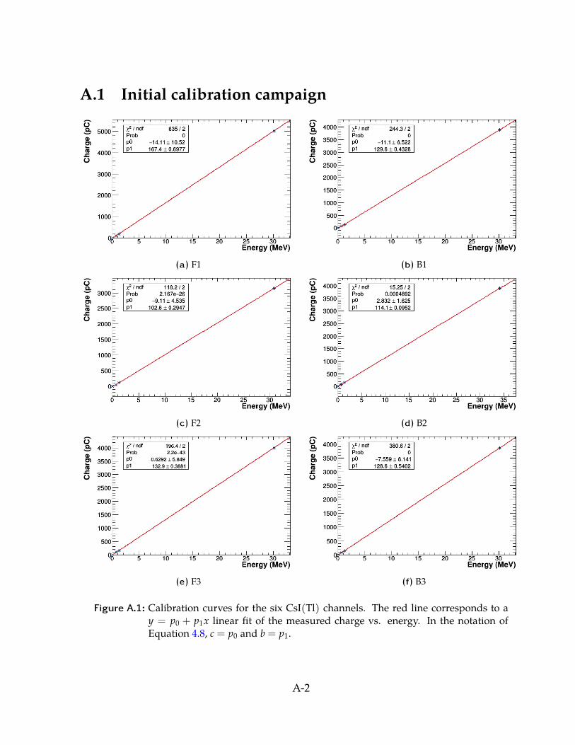
A.1 Initial calibration campaign

(a) F1 (b) B1

(c) F2 (d) B2

(e) F3 (f) B3

Figure A.1: Calibration curves for the six CsI(Tl) channels. The red line corresponds to ay = p0 + p1x linear fit of the measured charge vs. energy. In the notation ofEquation 4.8, c = p0 and b = p1.

A-2

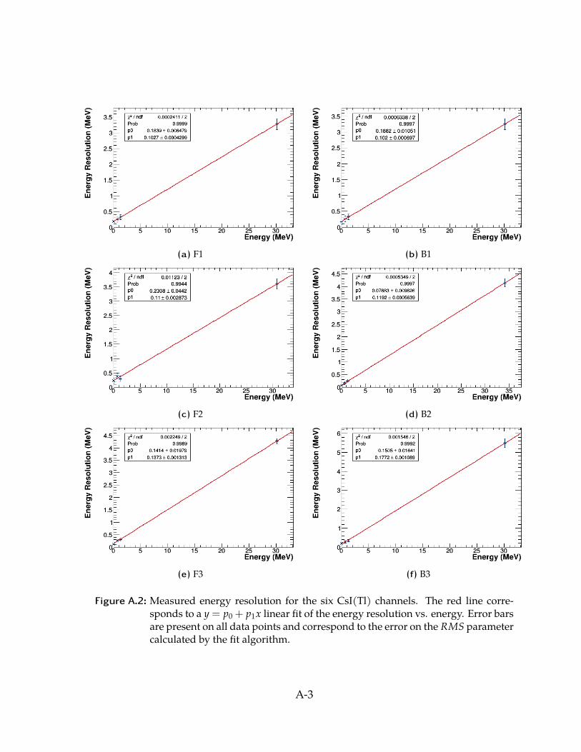
(a) F1 (b) B1

(c) F2 (d) B2

(e) F3 (f) B3

Figure A.2: Measured energy resolution for the six CsI(Tl) channels. The red line corre-sponds to a y = p0 + p1x linear fit of the energy resolution vs. energy. Error barsare present on all data points and correspond to the error on the RMS parametercalculated by the fit algorithm.

A-3

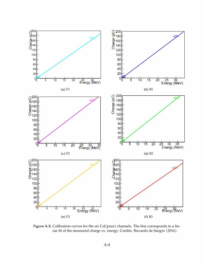
(a) F1 (b) B1

(c) F2 (d) B2

(e) F3 (f) B3

Figure A.3: Calibration curves for the six CsI(pure) channels. The line corresponds to a lin-ear fit of the measured charge vs. energy. Credits: Riccardo de Sangro (2016).

A-4

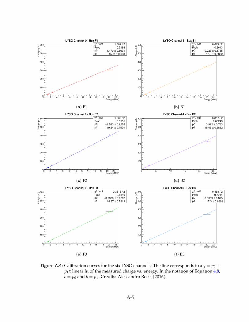
Energy (MeV)0 2 4 6 8 10 12 14 16 18 20 22

Charg

e (

pC

)

0

100

200

300

400

500

600

LYSO Channel 0 ­ Box F1 / ndf 2χ 1.309 / 2

Prob 0.5198p0 0.8034± 1.179 p1 0.633± 15.81

/ ndf 2χ 1.309 / 2

Prob 0.5198p0 0.8034± 1.179 p1 0.633± 15.81

LYSO Channel 0 ­ Box F1

(a) F1Energy (MeV)

0 2 4 6 8 10 12 14 16 18 20 22

Charg

e (

pC

)

0

100

200

300

400

500

600

LYSO Channel 3 ­ Box B1 / ndf 2χ 0.079 / 2

Prob 0.9613p0 0.8735± 0.223 p1 0.6882± 17.3

/ ndf 2χ 0.079 / 2

Prob 0.9613p0 0.8735± 0.223 p1 0.6882± 17.3

LYSO Channel 3 ­ Box B1

(b) B1

Energy (MeV)0 2 4 6 8 10 12 14 16 18 20 22

Charg

e (

pC

)

0

100

200

300

400

500

600

LYSO Channel 1 ­ Box F2 / ndf 2χ 1.037 / 2

Prob 0.5955p0 0.9555±1.523 − p1 0.7524± 19.24

/ ndf 2χ 1.037 / 2

Prob 0.5955p0 0.9555±1.523 − p1 0.7524± 19.24

LYSO Channel 1 ­ Box F2

(c) F2Energy (MeV)

0 5 10 15 20 25

Charg

e (

pC

)

0

100

200

300

400

500

600

LYSO Channel 4 ­ Box B2 / ndf 2χ 6.857 / 2

Prob 0.03243p0 0.763± 3.992 p1 0.5832± 15.05

/ ndf 2χ 6.857 / 2

Prob 0.03243p0 0.763± 3.992 p1 0.5832± 15.05

LYSO Channel 4 ­ Box B2

(d) B2

Energy (MeV)0 2 4 6 8 10 12 14 16 18 20 22

Charg

e (

pC

)

0

100

200

300

400

500

600

LYSO Channel 2 ­ Box F3 / ndf 2χ 0.3616 / 2

Prob 0.8346p0 0.9292±0.7939 − p1 0.7319± 18.37

/ ndf 2χ 0.3616 / 2

Prob 0.8346p0 0.9292±0.7939 − p1 0.7319± 18.37

LYSO Channel 2 ­ Box F3

(e) F3Energy (MeV)

0 2 4 6 8 10 12 14 16 18 20 22

Charg

e (

pC

)

0

100

200

300

400

500

600

LYSO Channel 5 ­ Box B3 / ndf 2χ 0.468 / 2

Prob 0.7914p0 0.875± 0.6359 p1 0.6891± 17.3

/ ndf 2χ 0.468 / 2

Prob 0.7914p0 0.875± 0.6359 p1 0.6891± 17.3

LYSO Channel 5 ­ Box B3

(f) B3

Figure A.4: Calibration curves for the six LYSO channels. The line corresponds to a y = p0 +p1x linear fit of the measured charge vs. energy. In the notation of Equation 4.8,c = p0 and b = p1. Credits: Alessandro Rossi (2016).

A-5

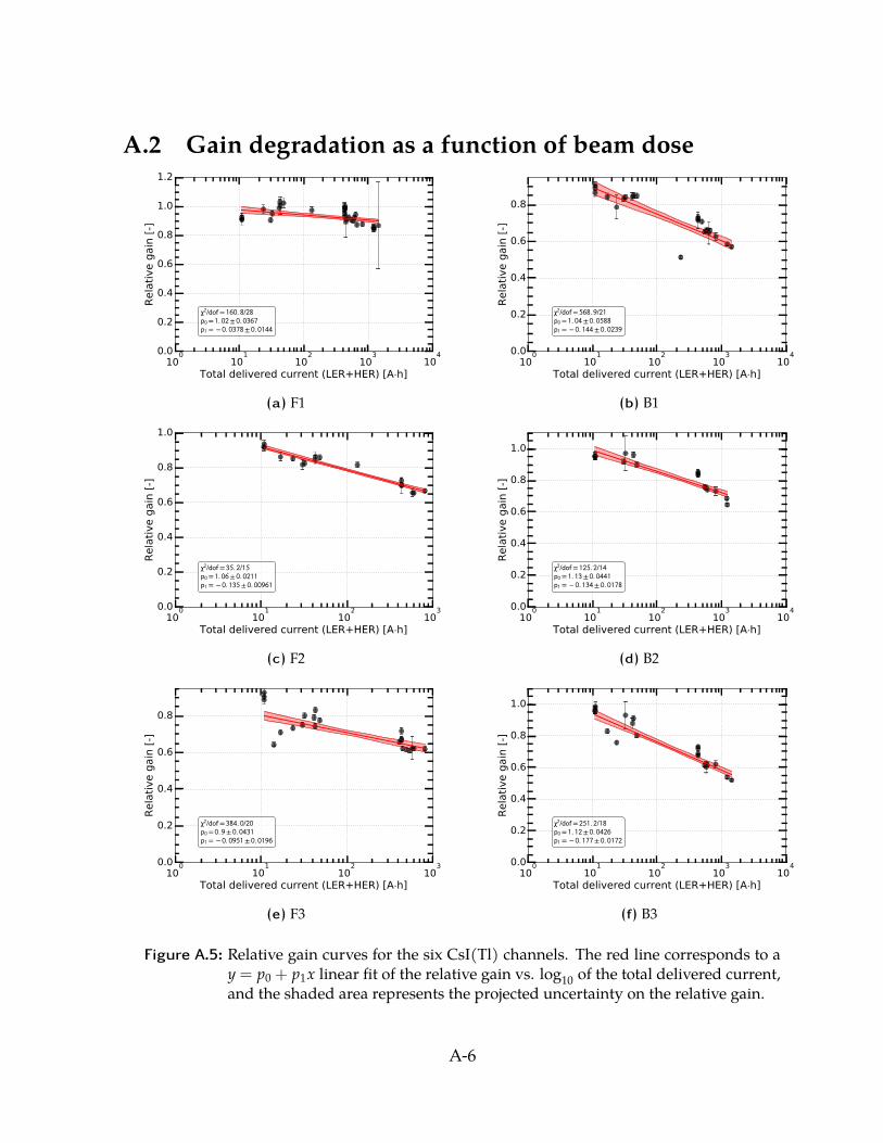
A.2 Gain degradation as a function of beam dose

100

101

102

103

104

Total delivered current (LER+HER) [A h]

0.0

0.2

0.4

0.6

0.8

1.0

1.2

Rela

tive g

ain

[-]

/ = . /= . ± .= . ± .

(a) F1

100

101

102

103

104

Total delivered current (LER+HER) [A h]

0.0

0.2

0.4

0.6

0.8

Rela

tive g

ain

[-]

/ = . /= . ± .= . ± .

(b) B1

100

101

102

103

Total delivered current (LER+HER) [A h]

0.0

0.2

0.4

0.6

0.8

1.0

Rela

tive g

ain

[-]

/ = . /= . ± .= . ± .

(c) F2

100

101

102

103

104

Total delivered current (LER+HER) [A h]

0.0

0.2

0.4

0.6

0.8

1.0

Rela

tive g

ain

[-]

/ = . /= . ± .= . ± .

(d) B2

100

101

102

103

Total delivered current (LER+HER) [A h]

0.0

0.2

0.4

0.6

0.8

Rela

tive g

ain

[-]

/ = . /= . ± .= . ± .

(e) F3

100

101

102

103

104

Total delivered current (LER+HER) [A h]

0.0

0.2

0.4

0.6

0.8

1.0

Rela

tive g

ain

[-]

/ = . /= . ± .= . ± .

(f) B3

Figure A.5: Relative gain curves for the six CsI(Tl) channels. The red line corresponds to ay = p0 + p1x linear fit of the relative gain vs. log10 of the total delivered current,and the shaded area represents the projected uncertainty on the relative gain.

A-6

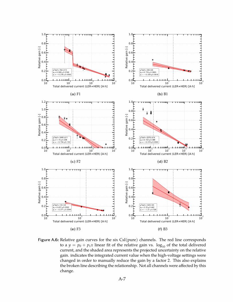
100

101

102

103

Total delivered current (LER+HER) [A h]

0.0

0.2

0.4

0.6

0.8

1.0

Rela

tive g

ain

[-]

/ = . /= . ± .= . ± .

(a) F1

100

101

102

Total delivered current (LER+HER) [A h]

0.0

0.2

0.4

0.6

0.8

1.0

Rela

tive g

ain

[-]

/ = . /= . ± .= . ± .

(b) B1

100

101

102

103

Total delivered current (LER+HER) [A h]

0.0

0.2

0.4

0.6

0.8

1.0

1.2

Rela

tive g

ain

[-]

/ = . /= . ± .= . ± .

(c) F2

100

101

102

103

104

Total delivered current (LER+HER) [A h]

0.0

0.2

0.4

0.6

0.8

1.0

Rela

tive g

ain

[-]

/ = . /= . ± .= . ± .

(d) B2

100

101

102

Total delivered current (LER+HER) [A h]

0.0

0.2

0.4

0.6

0.8

1.0

Rela

tive g

ain

[-]

/ = . /= . ± .= . ± .

(e) F3

100

101

102

Total delivered current (LER+HER) [A h]

0.0

0.2

0.4

0.6

0.8

1.0

Rela

tive g

ain

[-]

/ = . /= . ± .= . ± .

(f) B3

Figure A.6: Relative gain curves for the six CsI(pure) channels. The red line correspondsto a y = p0 + p1x linear fit of the relative gain vs. log10 of the total deliveredcurrent, and the shaded area represents the projected uncertainty on the relativegain. indicates the integrated current value when the high-voltage settings werechanged in order to manually reduce the gain by a factor 2. This also explainsthe broken line describing the relationship. Not all channels were affected by thischange.

A-7

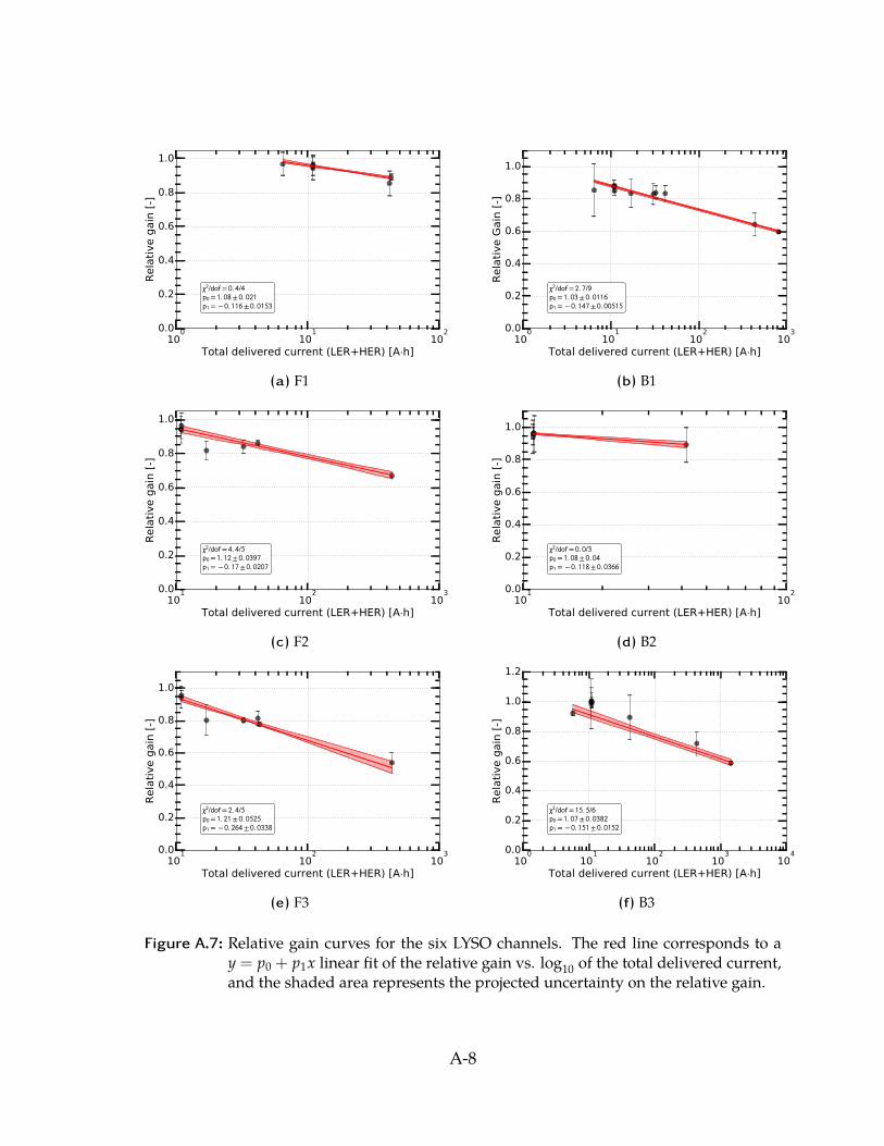
100

101

102

Total delivered current (LER+HER) [A h]

0.0

0.2

0.4

0.6

0.8

1.0R

ela

tive g

ain

[-]

/ = . /= . ± .= . ± .

(a) F1

100

101

102

103

Total delivered current (LER+HER) [A h]

0.0

0.2

0.4

0.6

0.8

1.0

Rela

tive G

ain

[-]

/ = . /= . ± .= . ± .

(b) B1

101

102

103

Total delivered current (LER+HER) [A h]

0.0

0.2

0.4

0.6

0.8

1.0

Rela

tive g

ain

[-]

/ = . /= . ± .= . ± .

(c) F2

101

102

Total delivered current (LER+HER) [A h]

0.0

0.2

0.4

0.6

0.8

1.0

Rela

tive g

ain

[-]

/ = . /= . ± .= . ± .

(d) B2

101

102

103

Total delivered current (LER+HER) [A h]

0.0

0.2

0.4

0.6

0.8

1.0

Rela

tive g

ain

[-]

/ = . /= . ± .= . ± .

(e) F3

100

101

102

103

104

Total delivered current (LER+HER) [A h]

0.0

0.2

0.4

0.6

0.8

1.0

1.2

Rela

tive g

ain

[-]

/ = . /= . ± .= . ± .

(f) B3

Figure A.7: Relative gain curves for the six LYSO channels. The red line corresponds to ay = p0 + p1x linear fit of the relative gain vs. log10 of the total delivered current,and the shaded area represents the projected uncertainty on the relative gain.

A-8

Appendix B

Mechanical Drawings

ContentsB.1 Belle-II Top View 41.5-R14 . . . . . . . . . . . . . . . . . . . . . . . . . . . B-2B.2 ECL Endcap Shields Envelopes ECL-SHLDS-000 . . . . . . . . . . . . . . B-3

B-1

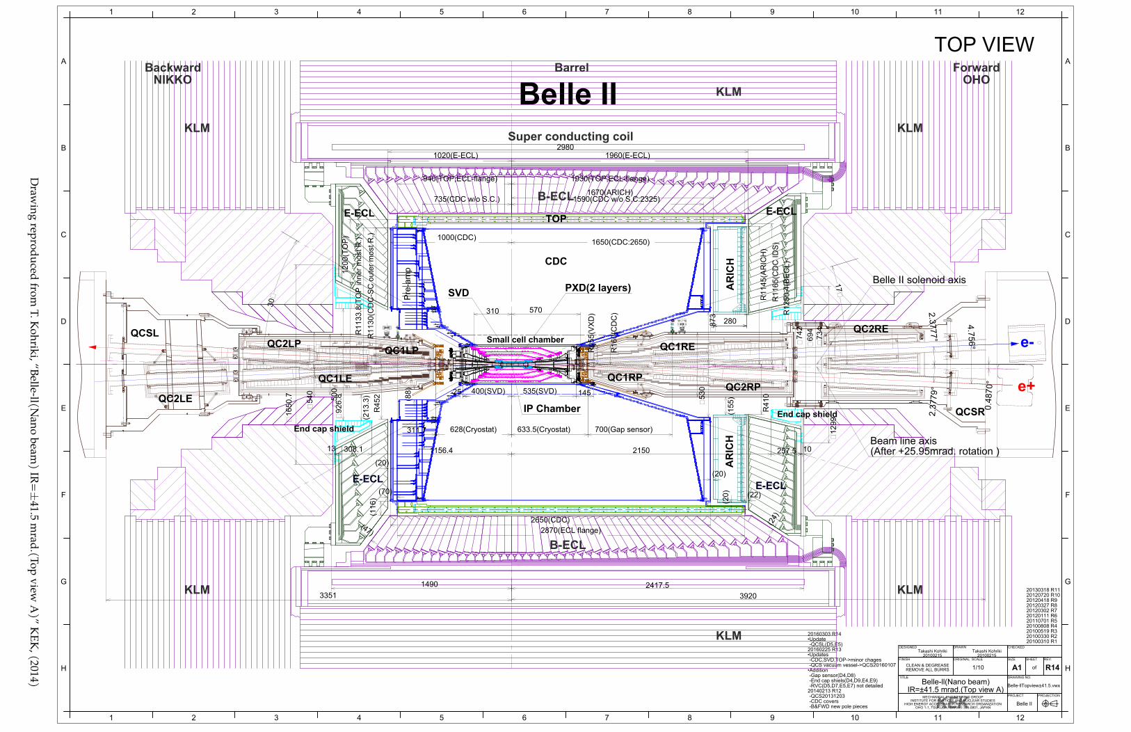
2.3777°

Belle-llTopview±41.5.vwx

1

1

2

2

3

3

4

4

5

5

6

6

7

7

8

8

9

9

10

10

11

11

12

12

A A

B B

C C

D D

E E

F F

G G

H H

Takashi Kohriki20100215

Takashi Kohriki20100215

R14A1

Belle II

1/10

Belle-ll(Nano beam)IR=±41.5 mrad.(Top view A)

KEK

DESIGNED DRAWN

of

ORIGINAL SCALEFINISH

DRAWING NO.

MECHANICAL ENGINEERING GROUPINSTITUTE FOR PARTICLE AND NUCLEAR STUDIES

HIGH ENERGY ACCELERATOR RESEARCH ORGANIZATIONOHO 1-1, TSUKUBA, IBARAKI 305-0801, JAPAN

TITLE

PROJECT

SIZE SHEET REV.

PROJECTION

CHECKED

CLEAN & DEGREASEREMOVE ALL BURRS

R16

0(C

DC

)

280570

R11

45(A

RIC

H)

TOP VIEW

CDC

Small cell chamber

633.5(Cryostat)628(Cryostat)

R11

65(C

DC

IDS

)

Super conducting coil

B-ECL

E-ECL

E-ECL

E-ECL

E-ECL

2650(CDC)

R12

50.4

(BE

CL)

KLM

KLM

KLM

KLMKLM

KLM

BarrelBackwardNIKKO

ForwardOHO

e+

e-

2.37

79°

4.756°

20130318 R1120120720 R1020120418 R920120327 R820120302 R720120111 R620110701 R520100808 R420100519 R320100330 R220100310 R1

R11

33.8

(TO

P in

ner m

ost R

.)R

1130

(CD

C-S

C o

uter

mos

t R.)

R45

2

R41

0

R15

5(V

XD

)

400(SVD) 535(SVD)

Pre

-am

p

PXD(2 layers)

0.48

70°

Beam line axis(After +25.95mrad. rotation )

Belle II solenoid axisSVD

IP Chamber

310

1670(ARICH)

1020(E-ECL)

1930(TOP,ECL-flange)940(TOP,ECL-flange)

735(CDC w/o S.C.) 1590(CDC w/o S.C:2325)

1960(E-ECL)2980

QCSR

QC2RE

QC2LE

QC2LP

QC1LE QC1RP

QC1RE

QC2RP

QC1LP

Belle II

2870(ECL flange)

1200

(TO

P)

AR

ICH

AR

ICH

20160303 R14•Update -QCSL(D5,E5)20160225 R13•Updates -CDC,SVD,TOP->minor chages -QCS vacuum vessel->QCS20160107•Addition -Gap sensor(D4,D8) -End cap shiels(D4,D9,E4,E9) -RVC(D5,D7,E5,E7) not detailed20140213 R12 -QCS20131203 -CDC covers -B&FWD new pole pieces

3351 3920

ｿ73

4

1490 2417.5

30ｼ

17ｼ

ｿ50

0

ｿ54

0

ｿ69

4ｿ

742

1000(CDC) 1650(CDC:2650)

ｿ92

6.8

QCSL

ｿ53

0ｿ

873

End cap shieldEnd cap shield

1156.4 2150 257.5308.113 10

ｿ16

50.7

ｿ12

99

(213

.3)

(155

)

(20)

(20)

(24)

(22)

(20)

(116

)

(47)

(70)

(88)

B-ECL

TOP

311.7 700(Gap sensor)

25 145

Drawingreproduced

fromT.Kohriki,“Belle-ll(Nanobeam

)IR=±

41.5mrad.(Top

viewA)”KEK,(2014)

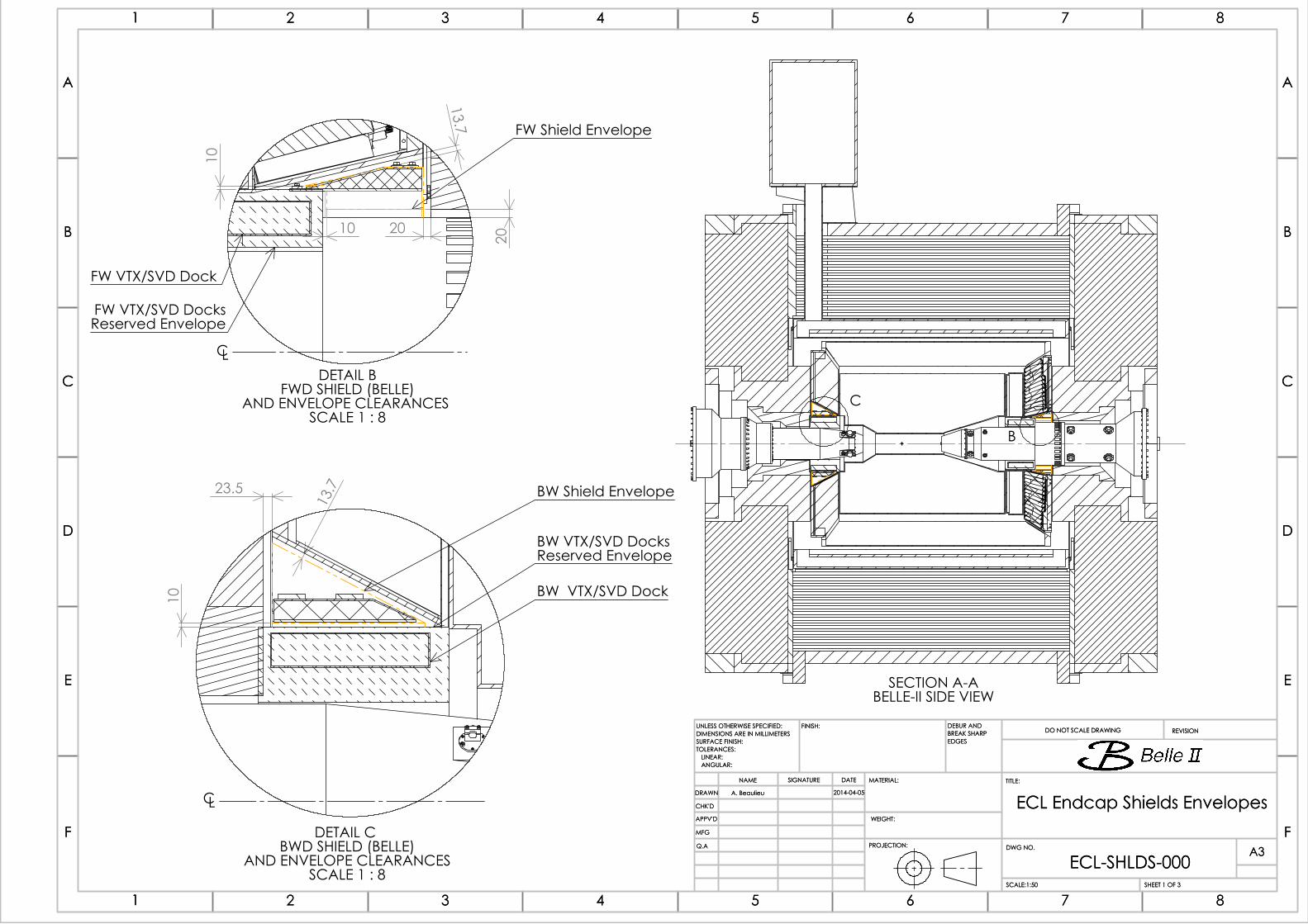
87654321

87654321

D

F

E

C

B

A

D

F

E

C

B

A

87654321

87654321

D

F

E

C

B

A

D

F

E

C

B

A

0

A

A

B

C

SECTION A-ABELLE-II SIDE VIEW

10 1

0

20

13.7

20

DETAIL BFWD SHIELD (BELLE)

AND ENVELOPE CLEARANCES SCALE 1 : 8

FW Shield Envelope

FW VTX/SVD DocksReserved Envelope

FW VTX/SVD Dock

13.

7

10

23.5

DETAIL C BWD SHIELD (BELLE)

AND ENVELOPE CLEARANCESSCALE 1 : 8

BW Shield Envelope

BW VTX/SVD DocksReserved Envelope

BW VTX/SVD Dock

CL

CL ECL Endcap Shields Envelopes

ECL-SHLDS-000

2014-04-05A. Beaulieu

WEIGHT:

A3

SHEET 1 OF 3SCALE:1:50

DWG NO.

TITLE:

REVISIONDO NOT SCALE DRAWING

MATERIAL:DATESIGNATURENAME

DEBUR AND BREAK SHARP EDGES

FINISH:UNLESS OTHERWISE SPECIFIED:DIMENSIONS ARE IN MILLIMETERSSURFACE FINISH:TOLERANCES: LINEAR: ANGULAR:

Q.A

MFG

APPV'D

CHK'D

DRAWN

PROJECTION:

ECL Endcap Shields Envelopes

ECL-SHLDS-000

2014-04-05A. Beaulieu

WEIGHT:

A3

SHEET 1 OF 3SCALE:1:50

DWG NO.

TITLE:

REVISIONDO NOT SCALE DRAWING

MATERIAL:DATESIGNATURENAME

DEBUR AND BREAK SHARP EDGES

FINISH:UNLESS OTHERWISE SPECIFIED:DIMENSIONS ARE IN MILLIMETERSSURFACE FINISH:TOLERANCES: LINEAR: ANGULAR:

Q.A

MFG

APPV'D

CHK'D

DRAWN

PROJECTION:

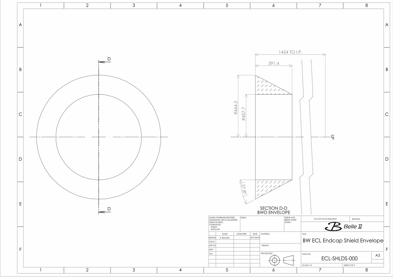
87654321

87654321

D

F

E

C

B

A

D

F

E

C

B

A

D

D

391.4

1454 TO I.P.

R45

7.7

R66

4.2

27.8°

SECTION D-DBWD ENVELOPE

CL

BW ECL Endcap Shield Envelope

ECL-SHLDS-000

2014-04-05A. Beaulieu

WEIGHT:

A3

SHEET 2 OF 3SCALE:1:10

DWG NO.

TITLE:

REVISIONDO NOT SCALE DRAWING

MATERIAL:DATESIGNATURENAME

DEBUR AND BREAK SHARP EDGES

FINISH:UNLESS OTHERWISE SPECIFIED:DIMENSIONS ARE IN MILLIMETERSSURFACE FINISH:TOLERANCES: LINEAR: ANGULAR:

Q.A

MFG

APPV'D

CHK'D

DRAWN

PROJECTION:

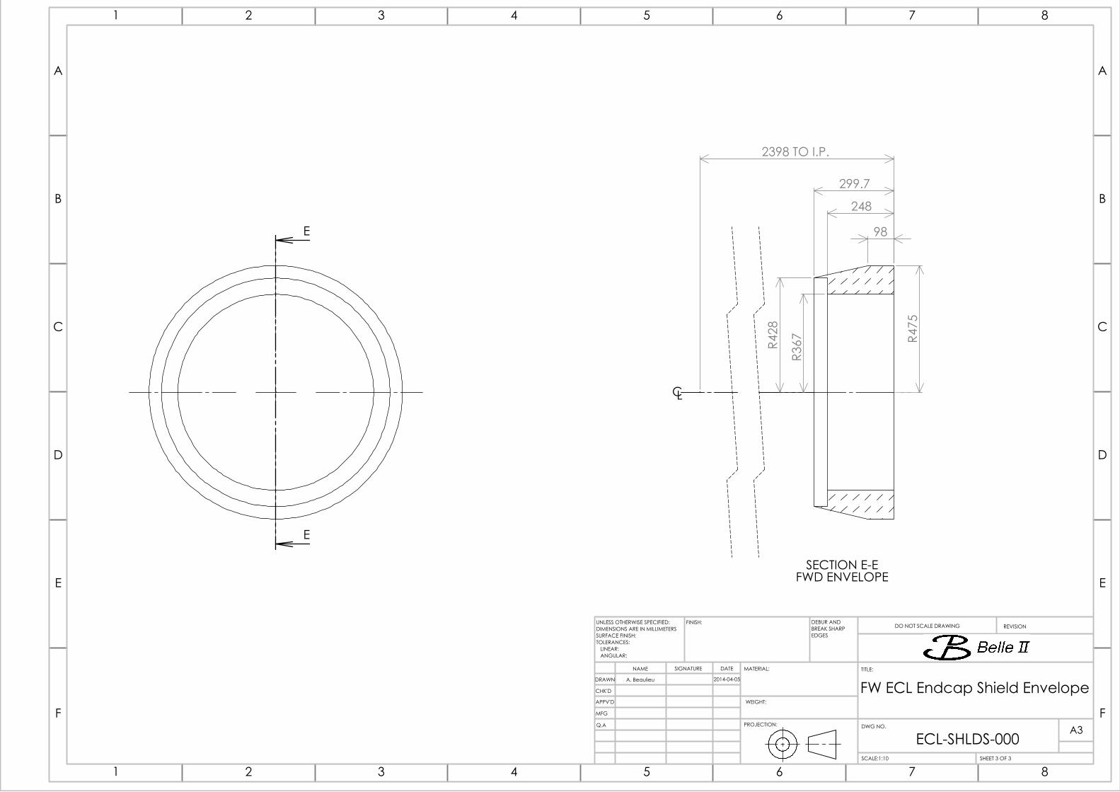
87654321

87654321

D

F

E

C

B

A

D

F

E

C

B

A

E

E

98

248

299.7

2398 TO I.P.

R36

7

R42

8

R47

5

SECTION E-EFWD ENVELOPE

CL

FW ECL Endcap Shield Envelope

ECL-SHLDS-000

2014-04-05A. Beaulieu

WEIGHT:

A3

SHEET 3 OF 3SCALE:1:10

DWG NO.

TITLE:

REVISIONDO NOT SCALE DRAWING

MATERIAL:DATESIGNATURENAME

DEBUR AND BREAK SHARP EDGES

FINISH:UNLESS OTHERWISE SPECIFIED:DIMENSIONS ARE IN MILLIMETERSSURFACE FINISH:TOLERANCES: LINEAR: ANGULAR:

Q.A

MFG

APPV'D

CHK'D

DRAWN

PROJECTION:

Appendix C

Results of the ECL shields conceptualdesign studies

The next sections contain the performance plots for the five set of concepts. They are allorganized as follows. First the result of a material scan is presented; these show the mate-rial density in units of inverse radiation length 1/x0. Second, the map of the yearly dosein the entire ECL is presented. Third, the total yearly dose averaged over the crystal θID

is presented. The last plot is the yearly neutron flux in the diodes, again as a function ofcrystal row index.

For the θID averages, the small gray dots correspond to the result averaged over a singlerow, while the large black dots with error bars represent an average over nominally 4 rows(sometimes less to exclude the innermost rows and avoid averaging together end-cap rowswith barrel rows). The error bars correspond to the statistical uncertainty associated withthe size of the simulation samples.

Again, row 0 refers to the innermost row of crystal of the forward end-cap, whereas row69 is the innermost row of the backward end-cap.

C-1

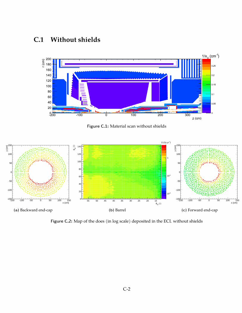
C.1 Without shields

Figure C.1: Material scan without shields

x (cm)-150 -100 -50 0 50 100 150

y (c

m)

-150

-100

-50

0

50

100

150

(a) Backward end-cap (-)

IDθ

(-)

IDφ

0

20

40

60

80

100

120

140

-210

-110

1

152025303540455055

)-1D (Gy yr

(b) Barrelx (cm)

-150 -100 -50 0 50 100 150

y (c

m)

-150

-100

-50

0

50

100

150

(c) Forward end-cap

Figure C.2: Map of the does (in log scale) deposited in the ECL without shields

C-2

IDθ

0 10 20 30 40 50 60

)-1

Cry

stal

rad

iatio

n do

se (

Gy

yr

0

0.5

1

1.5

2

2.5

3

IDθAverage /

IDθAverage / 4

Figure C.3: Radiation dose as a function for crystal row index without shields

IDθ

0 10 20 30 40 50 60

)-1

yr

-2N

eutr

on fl

ux in

the

diod

es (

hits

cm

0

10

20

30

40

50

IDθAverage /

IDθAverage / 4

Figure C.4: Neutron flux as a function for crystal row index without shields

C-3

C.2 Concepts 0

Figure C.5: Material scan of concepts 0

x (cm)-150 -100 -50 0 50 100 150

y (c

m)

-150

-100

-50

0

50

100

150

(a) Backward end-cap (-)

IDθ

(-)

IDφ

0

20

40

60

80

100

120

140

-210

-110

1

152025303540455055

)-1D (Gy yr

(b) Barrelx (cm)

-150 -100 -50 0 50 100 150

y (c

m)

-150

-100

-50

0

50

100

150

(c) Forward end-cap

Figure C.6: Map of the dose (in log scale) deposited in the ECL with concepts 0

C-4

IDθ

0 10 20 30 40 50 60

)-1

Cry

stal

rad

iatio

n do

se (

Gy

yr

0

0.5

1

1.5

2

2.5

3

IDθAverage /

IDθAverage / 4

Figure C.7: Radiation dose as a function for crystal row index for concepts 0

IDθ

0 10 20 30 40 50 60

)-1

yr

-2N

eutr

on fl

ux in

the

diod

es (

hits

cm

0

10

20

30

40

50

IDθAverage /

IDθAverage / 4

Figure C.8: Neutron flux as a function for crystal row index for concepts 0

C-5

C.3 Concepts A1

Figure C.9: Material scan of concepts A1

x (cm)-150 -100 -50 0 50 100 150

y (c

m)

-150

-100

-50

0

50

100

150

(a) Backward end-cap (-)

IDθ

(-)

IDφ

0

20

40

60

80

100

120

140

-210

-110

1

152025303540455055

)-1D (Gy yr

(b) Barrelx (cm)

-150 -100 -50 0 50 100 150

y (c

m)

-150

-100

-50

0

50

100

150

(c) Forward end-cap

Figure C.10: Map of the dose (in log scale) deposited in the ECL with concepts A1

C-6

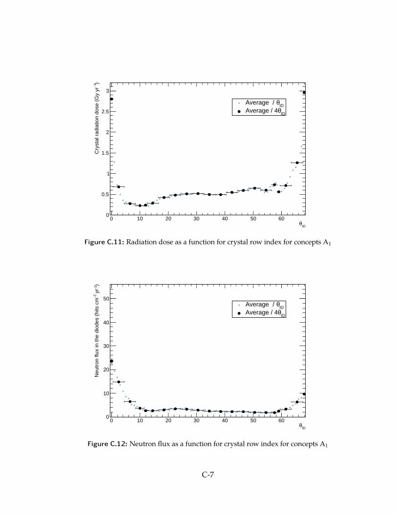
IDθ

0 10 20 30 40 50 60

)-1

Cry

stal

rad

iatio

n do

se (

Gy

yr

0

0.5

1

1.5

2

2.5

3

IDθAverage /

IDθAverage / 4

Figure C.11: Radiation dose as a function for crystal row index for concepts A1

IDθ

0 10 20 30 40 50 60

)-1

yr

-2N

eutr

on fl

ux in

the

diod

es (

hits

cm

0

10

20

30

40

50

IDθAverage /

IDθAverage / 4

Figure C.12: Neutron flux as a function for crystal row index for concepts A1

C-7

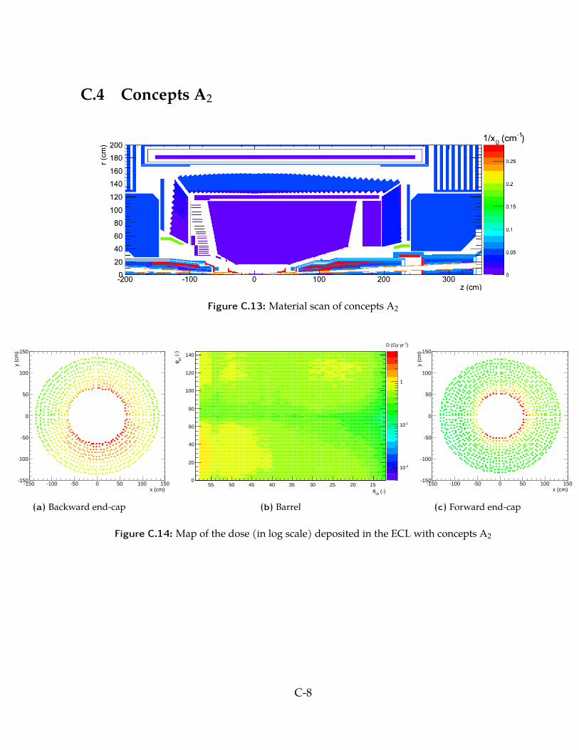
C.4 Concepts A2

Figure C.13: Material scan of concepts A2

x (cm)-150 -100 -50 0 50 100 150

y (c

m)

-150

-100

-50

0

50

100

150

(a) Backward end-cap (-)

IDθ

(-)

IDφ

0

20

40

60

80

100

120

140

-210

-110

1

152025303540455055

)-1D (Gy yr

(b) Barrelx (cm)

-150 -100 -50 0 50 100 150

y (c

m)

-150

-100

-50

0

50

100

150

(c) Forward end-cap

Figure C.14: Map of the dose (in log scale) deposited in the ECL with concepts A2

C-8

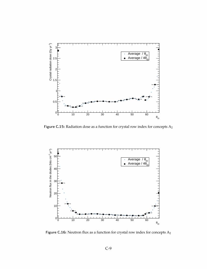
IDθ

0 10 20 30 40 50 60

)-1

Cry

stal

rad

iatio

n do

se (

Gy

yr

0

0.5

1

1.5

2

2.5

3

IDθAverage /

IDθAverage / 4

Figure C.15: Radiation dose as a function for crystal row index for concepts A2

IDθ

0 10 20 30 40 50 60

)-1

yr

-2N

eutr

on fl

ux in

the

diod

es (

hits

cm

0

10

20

30

40

50

IDθAverage /

IDθAverage / 4

Figure C.16: Neutron flux as a function for crystal row index for concepts A2

C-9

C.5 Concepts B1

Figure C.17: Material scan of concepts B1

x (cm)-150 -100 -50 0 50 100 150

y (c

m)

-150

-100

-50

0

50

100

150

(a) Backward end-cap (-)

IDθ

(-)

IDφ

0

20

40

60

80

100

120

140

-210

-110

1

152025303540455055

)-1D (Gy yr

(b) Barrelx (cm)

-150 -100 -50 0 50 100 150

y (c

m)

-150

-100

-50

0

50

100

150

(c) Forward end-cap

Figure C.18: Map of the dose (in log scale) deposited in the ECL with concepts B1

C-10

IDθ

0 10 20 30 40 50 60

)-1

Cry

stal

rad

iatio

n do

se (

Gy

yr

0

0.5

1

1.5

2

2.5

3

IDθAverage /

IDθAverage / 4

Figure C.19: Radiation dose as a function for crystal row index for concepts B1

IDθ

0 10 20 30 40 50 60

)-1

yr

-2N

eutr

on fl

ux in

the

diod

es (

hits

cm

0

10

20

30

40

50

IDθAverage /

IDθAverage / 4

Figure C.20: Neutron flux as a function for crystal row index for concepts B1

C-11

C.6 Concepts B2

Figure C.21: Material scan of concepts B2

x (cm)-150 -100 -50 0 50 100 150

y (c

m)

-150

-100

-50

0

50

100

150

(a) Backward end-cap (-)

IDθ

(-)

IDφ

0

20

40

60

80

100

120

140

-210

-110

1

152025303540455055

)-1D (Gy yr

(b) Barrelx (cm)

-150 -100 -50 0 50 100 150

y (c

m)

-150

-100

-50

0

50

100

150

(c) Forward end-cap

Figure C.22: Map of the dose (in log scale) deposited in the ECL with concepts B2

C-12

IDθ

0 10 20 30 40 50 60

)-1

Cry

stal

rad

iatio

n do

se (

Gy

yr

0

0.5

1

1.5

2

2.5

3

IDθAverage /

IDθAverage / 4

Figure C.23: Radiation dose as a function for crystal row index for concepts B2

IDθ

0 10 20 30 40 50 60

)-1

yr

-2N

eutr

on fl

ux in

the

diod

es (

hits

cm

0

10

20

30

40

50

IDθAverage /

IDθAverage / 4

Figure C.24: Neutron flux as a function for crystal row index for concepts B2

C-13

C.7 Concepts C1

Figure C.25: Material scan of concepts C1

x (cm)-150 -100 -50 0 50 100 150

y (c

m)

-150

-100

-50

0

50

100

150

(a) Backward end-cap (-)

IDθ

(-)

IDφ

0

20

40

60

80

100

120

140

-210

-110

1

152025303540455055

)-1D (Gy yr

(b) Barrelx (cm)

-150 -100 -50 0 50 100 150

y (c

m)

-150

-100

-50

0

50

100

150

(c) Forward end-cap

Figure C.26: Map of the dose (in log scale) deposited in the ECL with concepts C1

C-14

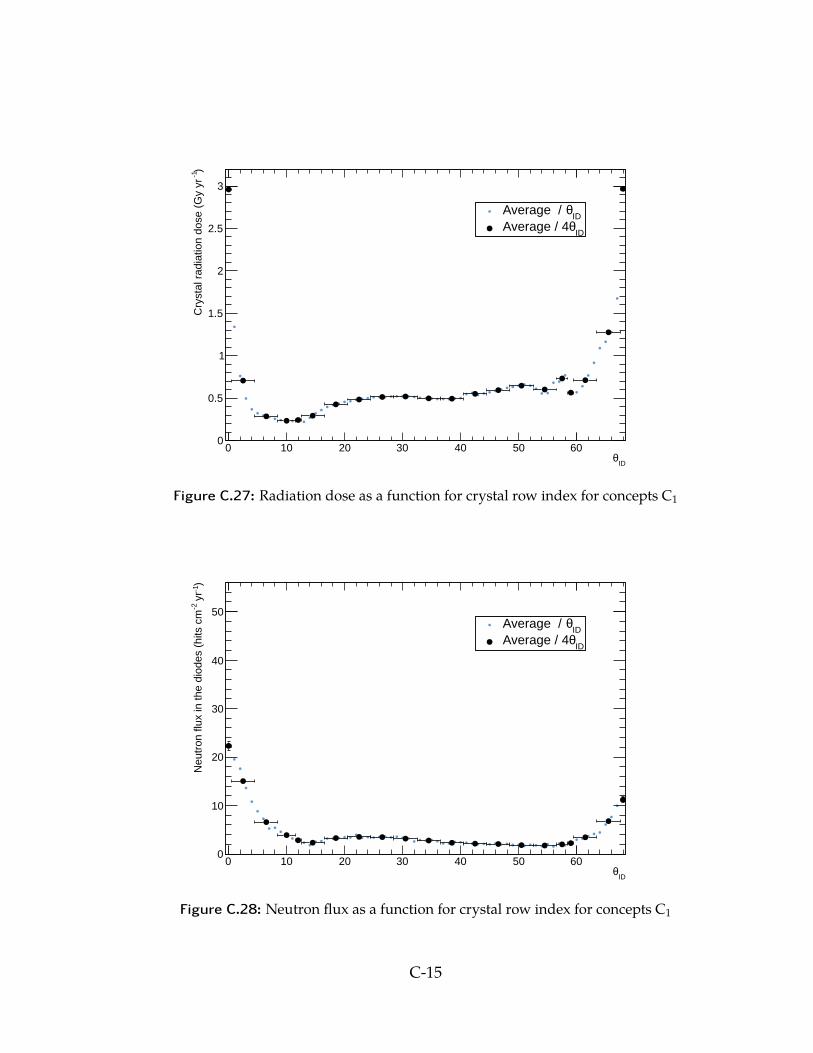
IDθ

0 10 20 30 40 50 60

)-1

Cry

stal

rad

iatio

n do

se (

Gy

yr

0

0.5

1

1.5

2

2.5

3

IDθAverage /

IDθAverage / 4

Figure C.27: Radiation dose as a function for crystal row index for concepts C1

IDθ

0 10 20 30 40 50 60

)-1

yr

-2N

eutr

on fl

ux in

the

diod

es (

hits

cm

0

10

20

30

40

50

IDθAverage /

IDθAverage / 4

Figure C.28: Neutron flux as a function for crystal row index for concepts C1

C-15

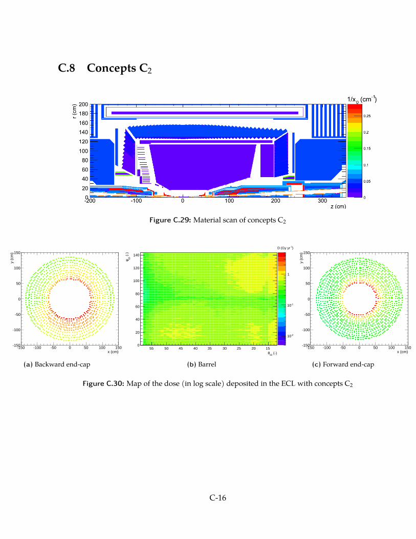
C.8 Concepts C2

Figure C.29: Material scan of concepts C2

x (cm)-150 -100 -50 0 50 100 150

y (c

m)

-150

-100

-50

0

50

100

150

(a) Backward end-cap (-)

IDθ

(-)

IDφ

0

20

40

60

80

100

120

140

-210

-110

1

152025303540455055

)-1D (Gy yr

(b) Barrelx (cm)

-150 -100 -50 0 50 100 150

y (c

m)

-150

-100

-50

0

50

100

150

(c) Forward end-cap

Figure C.30: Map of the dose (in log scale) deposited in the ECL with concepts C2

C-16

IDθ

0 10 20 30 40 50 60

)-1

Cry

stal

rad

iatio

n do

se (

Gy

yr

0

0.5

1

1.5

2

2.5

3

IDθAverage /

IDθAverage / 4

Figure C.31: Radiation dose as a function for crystal row index for concepts C2

IDθ

0 10 20 30 40 50 60

)-1

yr

-2N

eutr

on fl

ux in

the

diod

es (

hits

cm

0

10

20

30

40

50

IDθAverage /

IDθAverage / 4

Figure C.32: Neutron flux as a function for crystal row index for concepts C2

C-17

Appendix D

Detail of the ECL shields technical design

The next sections contain the detail of technical design studies and the design choices thatled to the final shield geometries. It complements the general information about the shielddesign reported in section 3, in the body of this Dissertation.

In section D.1, the modelled supports and load conditions are described with respect to ageneral frame of reference, and the general approach to the structural analyses is explainedin greater detail than in section 3.

Section D.2 presents the geometries, components, materials and manufacturing for eachof the sub-systems of the backward shield, together with the relevant calculations andjustifications. Section D.3 presents the same information for the forward shield. The resultsof the structural analyses are summarized in section D.4.

Finally, section D.5 describes the fabrication process and documents the design changesthat were required to help either fabrication or installation.

D.1 General design of the shields

D.1.1 System of reference

The system of reference used in all further discussions is defined in Figure D.1. The originis located at the intersection of the shells revolution axis and the plane where the shields

D-1

attachments join the ECL end-cap. The Z axis is along the shells revolution axis and pointsaway from the Belle II interaction point, the Y axis is directed vertically upwards, and theX axis completes a right-handed coordinate system.

Y

Z X

Y

Figure D.1: System of reference for the load cases

D.1.2 Applied loads and design safety factor

Definition of the loads

The loads applied to the ECL shields are derived from the ECL design report. We defined10 different load and support scenarios for each shield, listed in Table D.1. In this table,the ”Figure” line indicates which sub-figure of Figure D.2 represents the supports and thedirection of the force.

It is important to note that all loads on the shields were assumed to be static: the shieldshave no mobile parts, and the repetition rate of transportation and potential earthquakeloads is low enough that fatigue effects can be neglected.

D-2

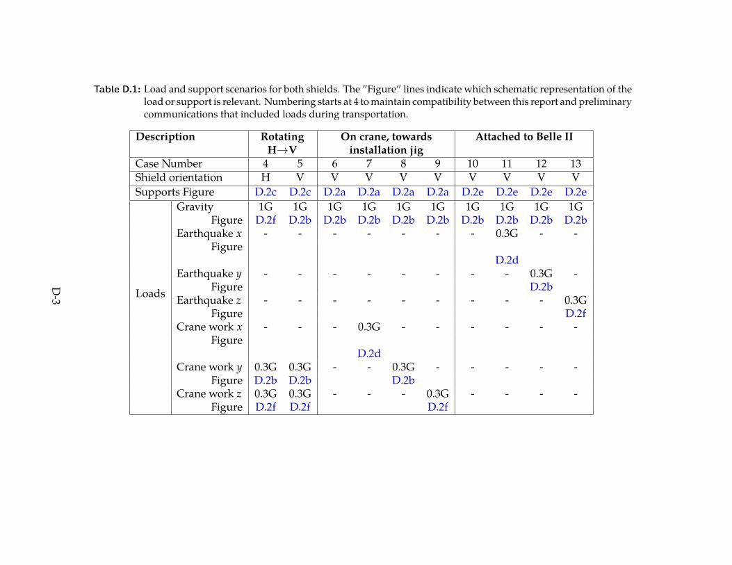
Table D.1: Load and support scenarios for both shields. The ”Figure” lines indicate which schematic representation of theload or support is relevant. Numbering starts at 4 to maintain compatibility between this report and preliminarycommunications that included loads during transportation.

Description RotatingH→V

On crane, towardsinstallation jig

Attached to Belle II

Case Number 4 5 6 7 8 9 10 11 12 13Shield orientation H V V V V V V V V VSupports Figure D.2c D.2c D.2a D.2a D.2a D.2a D.2e D.2e D.2e D.2e

Loads

Gravity 1G 1G 1G 1G 1G 1G 1G 1G 1G 1GFigure D.2f D.2b D.2b D.2b D.2b D.2b D.2b D.2b D.2b D.2b

Earthquake x - - - - - - - 0.3G - -Figure

D.2dEarthquake y - - - - - - - - 0.3G -

Figure D.2bEarthquake z - - - - - - - - - 0.3G

Figure D.2fCrane work x - - - 0.3G - - - - - -

FigureD.2d

Crane work y 0.3G 0.3G - - 0.3G - - - - -Figure D.2b D.2b D.2b

Crane work z 0.3G 0.3G - - - 0.3G - - - -Figure D.2f D.2f D.2f

D-3

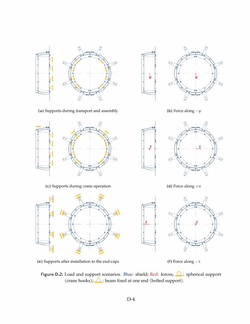
(a) Supports during transport and assembly

F F

(b) Force along −y

(c) Supports during crane operation

FF

(d) Force along +x

(e) Supports after installation to the end-caps

FF

(f) Force along −z

Figure D.2: Load and support scenarios. Blue: shield; Red: forces; : spherical support(crane hooks); : beam fixed at one end (bolted support).

D-4

Description of the supports

The shields are supported by bolted connections with either the jig adapters or the ECLend-caps, except for cases 4 and 5 where a special attachment can also used for liftingoperations. The bolted connections are modelled as rigid beam elements fixed at one endand connected to the shield at the other. Moreover, the mating surfaces are assumed tobe frictionless. This is a conservative assumption since, in this view, the bolts themselvesneed to support all the load. Because the surface of the ECL end-cap where the shields areattached is consists of irregular thin sheet metal, a good ”friction joint” cannot be assumedbetween these two.

For cases 4 and 5, there are also a crane attachment on each side of the Y − Z plane thatare modelled as spherical joints: allowing all rotations but no translation.

Mechanical properties of selected materials

The properties below were assumed for the mechanical resistance studies [77].

Lead

� Density: ρ = 11.3 g/cm3

� Young’s Modulus: E = 14 GPa

� Poisson’s Ratio: ν = 0.42

� Tensile Yield Strength: σy = 18 MPa

� Tensile Ultimate Strength: σu = 18 MPa

304 Stainless steel

� Density: ρ = 7.75g/cm3

� Young’s Modulus: E = 193 GPa

D-5

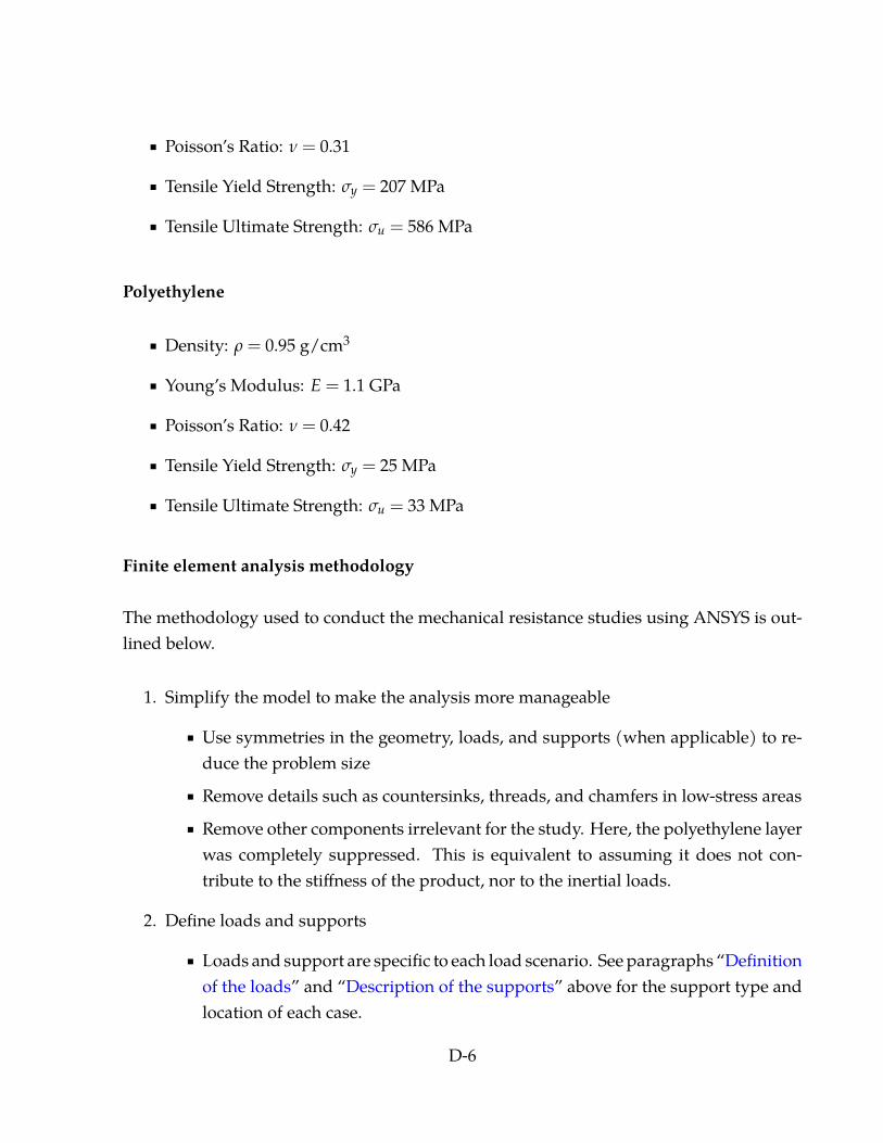
� Poisson’s Ratio: ν = 0.31

� Tensile Yield Strength: σy = 207 MPa

� Tensile Ultimate Strength: σu = 586 MPa

Polyethylene

� Density: ρ = 0.95 g/cm3

� Young’s Modulus: E = 1.1 GPa

� Poisson’s Ratio: ν = 0.42

� Tensile Yield Strength: σy = 25 MPa

� Tensile Ultimate Strength: σu = 33 MPa

Finite element analysis methodology

The methodology used to conduct the mechanical resistance studies using ANSYS is out-lined below.

1. Simplify the model to make the analysis more manageable

� Use symmetries in the geometry, loads, and supports (when applicable) to re-duce the problem size

� Remove details such as countersinks, threads, and chamfers in low-stress areas� Remove other components irrelevant for the study. Here, the polyethylene layer

was completely suppressed. This is equivalent to assuming it does not con-tribute to the stiffness of the product, nor to the inertial loads.

2. Define loads and supports

� Loads and support are specific to each load scenario. See paragraphs “Definitionof the loads” and “Description of the supports” above for the support type andlocation of each case.

D-6

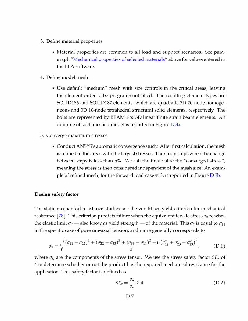
3. Define material properties

� Material properties are common to all load and support scenarios. See para-graph “Mechanical properties of selected materials” above for values entered inthe FEA software.

4. Define model mesh

� Use default “medium” mesh with size controls in the critical areas, leavingthe element order to be program-controlled. The resulting element types areSOLID186 and SOLID187 elements, which are quadratic 3D 20-node homoge-neous and 3D 10-node tetrahedral structural solid elements, respectively. Thebolts are represented by BEAM188: 3D linear finite strain beam elements. Anexample of such meshed model is reported in Figure D.3a.

5. Converge maximum stresses

� Conduct ANSYS’s automatic convergence study. After first calculation, the meshis refined in the areas with the largest stresses. The study stops when the changebetween steps is less than 5%. We call the final value the ”converged stress”,meaning the stress is then considered independent of the mesh size. An exam-ple of refined mesh, for the forward load case #13, is reported in Figure D.3b.

Design safety factor

The static mechanical resistance studies use the von Mises yield criterion for mechanicalresistance [78]. This criterion predicts failure when the equivalent tensile stress σv reachesthe elastic limit σy — also know as yield strength — of the material. This σv is equal to σ11

in the specific case of pure uni-axial tension, and more generally corresponds to

σv =

√(σ11 − σ22)

2 + (σ22 − σ33)2 + (σ33 − σ11)

2 + 6(σ2

12 + σ223 + σ2

13

)2

2, (D.1)

where σij are the components of the stress tensor. We use the stress safety factor SFσ of4 to determine whether or not the product has the required mechanical resistance for theapplication. This safety factor is defined as

SFσ =σy

σv≥ 4. (D.2)

D-7

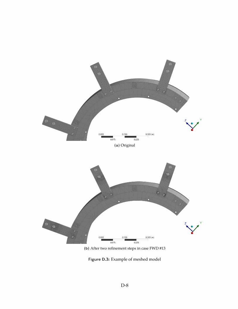
(a) Original

(b) After two refinement steps in case FWD #13

Figure D.3: Example of meshed model

D-8

The maximal displacements dmax were also checked to ensure the shields would not contactsurrounding structures during operation or installation. They are expected to be muchsmaller than the clearances around the product, which are at least 10 mm. The criterionfor acceptance was set to be smaller than the 1.5 mm default manufacturing tolerance:

dmax ≤ 1 mm. (D.3)

D.2 Design of the backward shield

D.2.1 Shell

The main purposes of the shell are to contain the electromagnetic radiation shield, and pro-vide attachment points to fix the two halves together as well as fixing the shield assemblyto the jigs and the ECL end-caps. The shield comprises two symmetrical shells.

Geometry

The geometry of one of the shells is represented in Figure D.4. The mounting points fortransport, described later in this section, are drawn transparent.

Components, materials and manufacturing

The shells are welded assemblies of nominally 4mm and 6mm thick AISI304 stainless steelsheets. Because they will be manufactured in Canada, we the use of the closest imperialequivalent dimension: gauge #9 (3.97 mm) and gauge #4 (5.95 mm) respectively [99].

The sheet metal components will be laser-cut to dimensions using provided CAD geome-try, and cold-rolled where needed. They will be welded with continuous beads to ensurethe assemblies are tight and allow casting the lead for the electromagnetic radiation shield.

The two shells are attached together by two identical pairs of plates above and below theshield, shown in Figure D.5. The rear connections are identical to those of the Belle design.

D-9

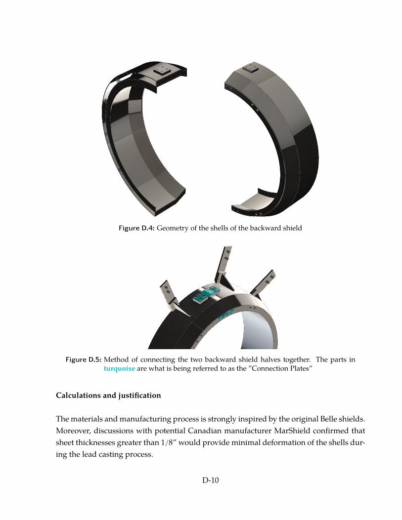
Figure D.4: Geometry of the shells of the backward shield

Figure D.5: Method of connecting the two backward shield halves together. The parts inturquoise are what is being referred to as the ”Connection Plates”

Calculations and justification

The materials and manufacturing process is strongly inspired by the original Belle shields.Moreover, discussions with potential Canadian manufacturer MarShield confirmed thatsheet thicknesses greater than 1/8” would provide minimal deformation of the shells dur-ing the lead casting process.

D-10

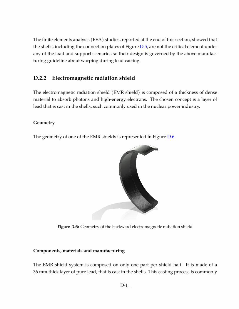
The finite elements analysis (FEA) studies, reported at the end of this section, showed thatthe shells, including the connection plates of Figure D.5, are not the critical element underany of the load and support scenarios so their design is governed by the above manufac-turing guideline about warping during lead casting.

D.2.2 Electromagnetic radiation shield

The electromagnetic radiation shield (EMR shield) is composed of a thickness of densematerial to absorb photons and high-energy electrons. The chosen concept is a layer oflead that is cast in the shells, such commonly used in the nuclear power industry.

Geometry

The geometry of one of the EMR shields is represented in Figure D.6.

Figure D.6: Geometry of the backward electromagnetic radiation shield

Components, materials and manufacturing

The EMR shield system is composed on only one part per shield half. It is made of a36 mm thick layer of pure lead, that is cast in the shells. This casting process is commonly

D-11

used in the nuclear industry. During the design phase, we found two potential Canadianmanufacturers having capability and experience in this kind of projects. The process caninvolve multiple re-heating of the parts to fill potential voids left in the initial casting, aswell as testing the final product with radiation sources to ensure no residual cavities arefound before delivery of the product. These companies are :

� MarShield Custom Radiation Shielding Products, 4140 Morris Dr, Burlington ON

� Ultraray Radiation Protection, 760 Pacific Rd #3, Oakville ON

Calculations and justification

Calculation of the required lead thickness is detailed in Section 3.2 of this document. Thesestudies showed that the selected concept, with a nominal 40 mm thick layer of lead wouldreduce the radiation dose by 13% in the innermost row of the backward ECL end-cap.

Most significantly, it was observed that the actual lead thickness could deviate within -0.5 cm to +1.0 cm without appreciable change in the shielding efficiency. This result waspreviously reported in Figure 3.6, where the radiation level safety factor — how manytimes the expected dose is smaller than the acceptable limit — is displayed as a functionof the variation of lead thickness for both shields.

The final thickness value of 36 mm is within that range, and was obtained as a compromiseto allow sufficient room for the shell and the neutron radiation shield within the availablevolume.

D.2.3 Neutron shield

Geometry

The neutron radiation shield system is composed of four sub-assemblies each covering 90◦and arranged as depicted in Figure D.7. The geometry of one of these sub-assemblies isrepresented in Figure D.8. They are held to the shield shell by means of an aluminiumcover.

D-12

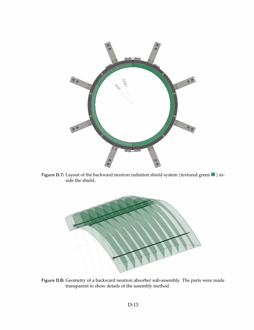
Figure D.7: Layout of the backward neutron radiation shield system (textured green ) in-side the shield.

Figure D.8: Geometry of a backward neutron absorber sub-assembly. The parts were madetransparent to show details of the assembly method.

D-13

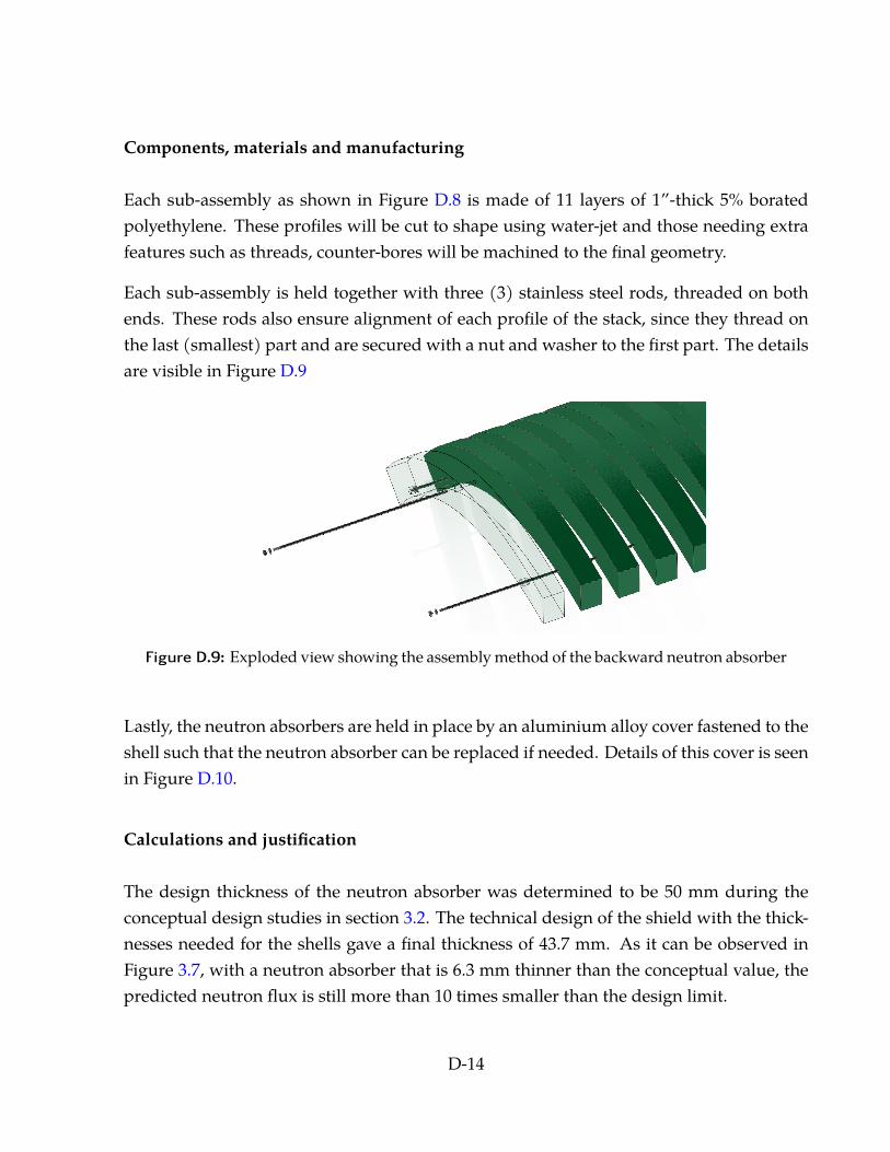
Components, materials and manufacturing

Each sub-assembly as shown in Figure D.8 is made of 11 layers of 1”-thick 5% boratedpolyethylene. These profiles will be cut to shape using water-jet and those needing extrafeatures such as threads, counter-bores will be machined to the final geometry.

Each sub-assembly is held together with three (3) stainless steel rods, threaded on bothends. These rods also ensure alignment of each profile of the stack, since they thread onthe last (smallest) part and are secured with a nut and washer to the first part. The detailsare visible in Figure D.9

Figure D.9: Exploded view showing the assembly method of the backward neutron absorber

Lastly, the neutron absorbers are held in place by an aluminium alloy cover fastened to theshell such that the neutron absorber can be replaced if needed. Details of this cover is seenin Figure D.10.

Calculations and justification

The design thickness of the neutron absorber was determined to be 50 mm during theconceptual design studies in section 3.2. The technical design of the shield with the thick-nesses needed for the shells gave a final thickness of 43.7 mm. As it can be observed inFigure 3.7, with a neutron absorber that is 6.3 mm thinner than the conceptual value, thepredicted neutron flux is still more than 10 times smaller than the design limit.

D-14

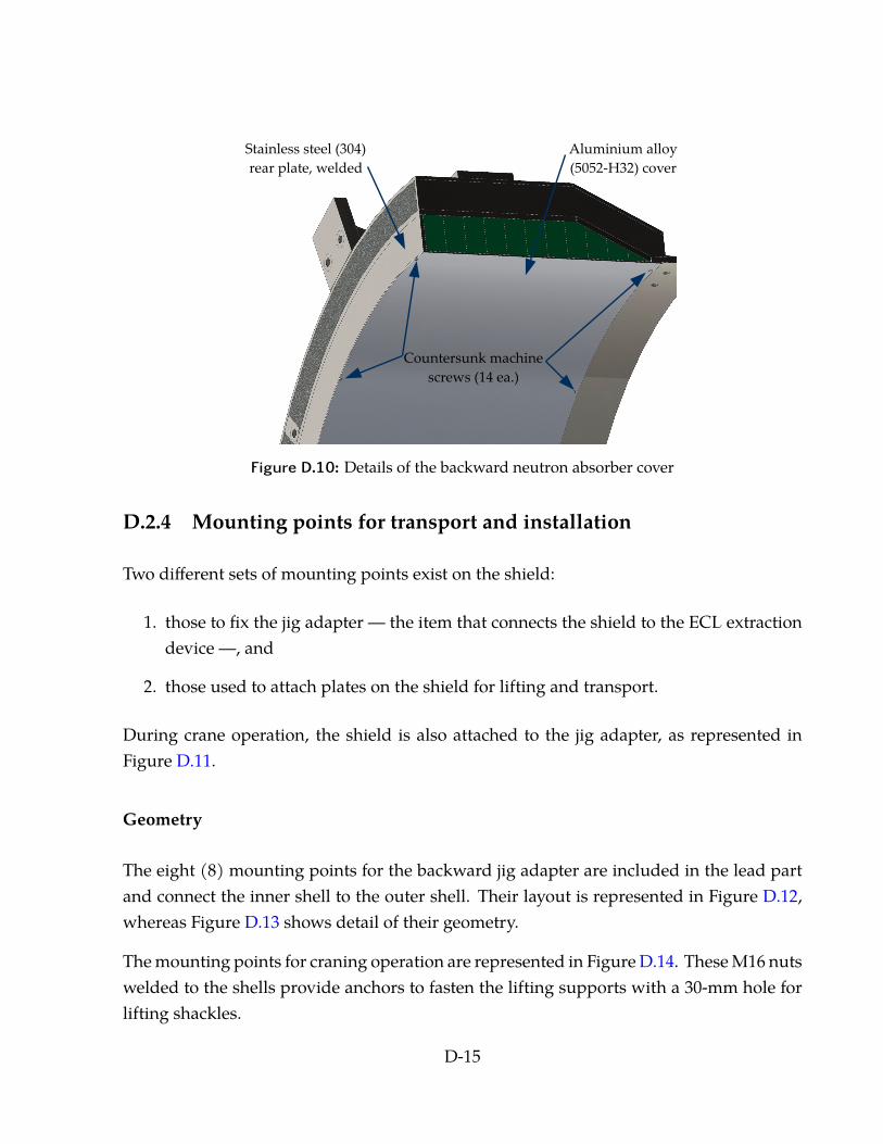
Aluminium alloy (5052-H32) cover

Stainless steel (304) rear plate, welded

Countersunk machine screws (14 ea.)

Figure D.10: Details of the backward neutron absorber cover

D.2.4 Mounting points for transport and installation

Two different sets of mounting points exist on the shield:

1. those to fix the jig adapter — the item that connects the shield to the ECL extractiondevice —, and

2. those used to attach plates on the shield for lifting and transport.

During crane operation, the shield is also attached to the jig adapter, as represented inFigure D.11.

Geometry

The eight (8) mounting points for the backward jig adapter are included in the lead partand connect the inner shell to the outer shell. Their layout is represented in Figure D.12,whereas Figure D.13 shows detail of their geometry.

The mounting points for craning operation are represented in Figure D.14. These M16 nutswelded to the shells provide anchors to fasten the lifting supports with a 30-mm hole forlifting shackles.

D-15

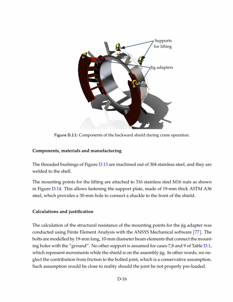
Jig adapters

Supports for lifting

Figure D.11: Components of the backward shield during crane operation.

Components, materials and manufacturing

The threaded bushings of Figure D.13 are machined out of 304 stainless steel, and they arewelded to the shell.

The mounting points for the lifting are attached to 316 stainless steel M16 nuts as shownin Figure D.14. This allows fastening the support plate, made of 19-mm thick ASTM A36steel, which provides a 30-mm hole to connect a shackle to the front of the shield.

Calculations and justification

The calculation of the structural resistance of the mounting points for the jig adapter wasconducted using Finite Element Analysis with the ANSYS Mechanical software [77]. Thebolts are modelled by 19-mm long, 10-mm diameter beam elements that connect the mount-ing holes with the ”ground”. No other support is assumed for cases 7,8 and 9 of Table D.1,which represent movements while the shield is on the assembly jig. In other words, we ne-glect the contribution from friction to the bolted joint, which is a conservative assumption.Such assumption would be close to reality should the joint be not properly pre-loaded.

D-16

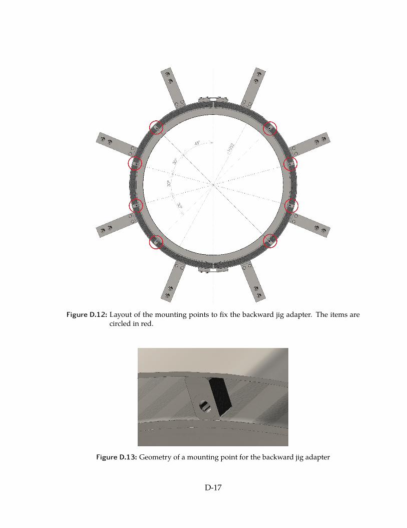
Figure D.12: Layout of the mounting points to fix the backward jig adapter. The items arecircled in red.

Figure D.13: Geometry of a mounting point for the backward jig adapter

D-17

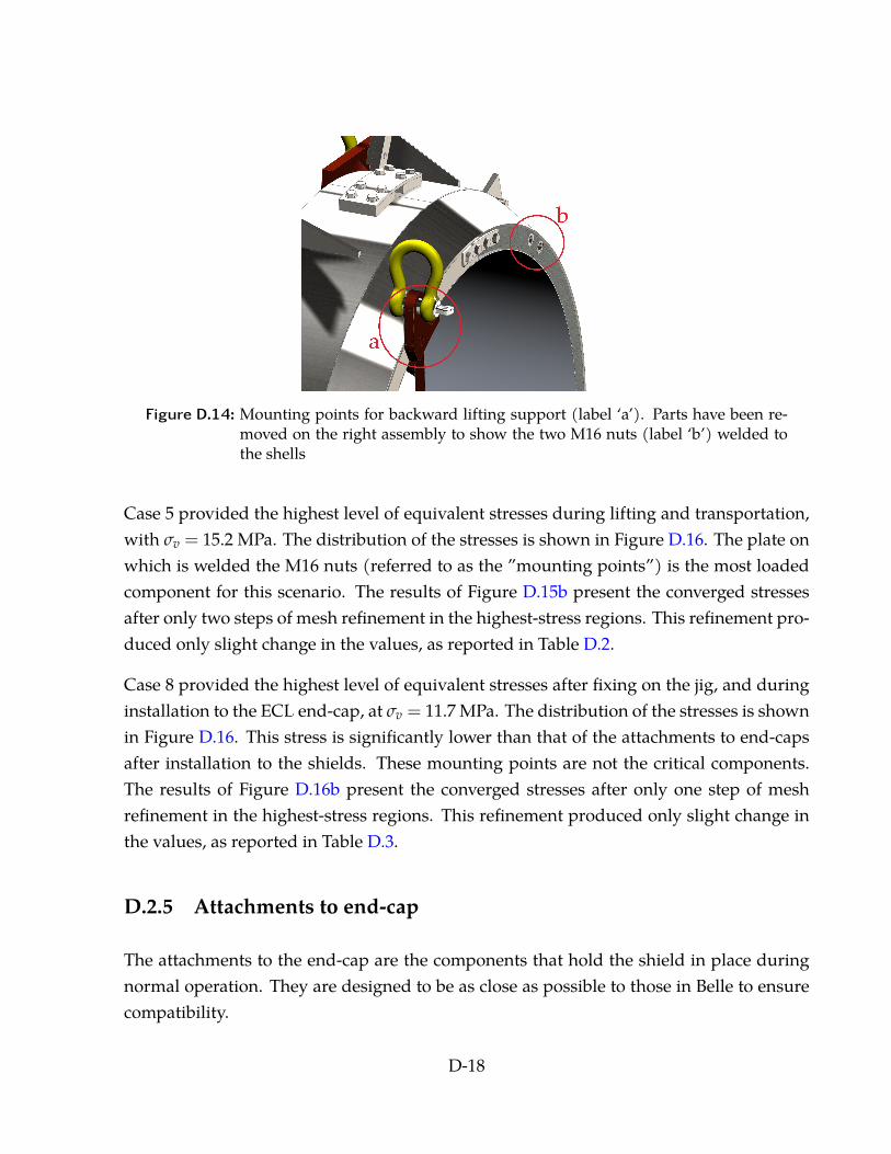
Figure D.14: Mounting points for backward lifting support (label ‘a’). Parts have been re-moved on the right assembly to show the two M16 nuts (label ‘b’) welded tothe shells

Case 5 provided the highest level of equivalent stresses during lifting and transportation,with σv = 15.2 MPa. The distribution of the stresses is shown in Figure D.16. The plate onwhich is welded the M16 nuts (referred to as the ”mounting points”) is the most loadedcomponent for this scenario. The results of Figure D.15b present the converged stressesafter only two steps of mesh refinement in the highest-stress regions. This refinement pro-duced only slight change in the values, as reported in Table D.2.

Case 8 provided the highest level of equivalent stresses after fixing on the jig, and duringinstallation to the ECL end-cap, at σv = 11.7 MPa. The distribution of the stresses is shownin Figure D.16. This stress is significantly lower than that of the attachments to end-capsafter installation to the shields. These mounting points are not the critical components.The results of Figure D.16b present the converged stresses after only one step of meshrefinement in the highest-stress regions. This refinement produced only slight change inthe values, as reported in Table D.3.

D.2.5 Attachments to end-cap

The attachments to the end-cap are the components that hold the shield in place duringnormal operation. They are designed to be as close as possible to those in Belle to ensurecompatibility.

D-18

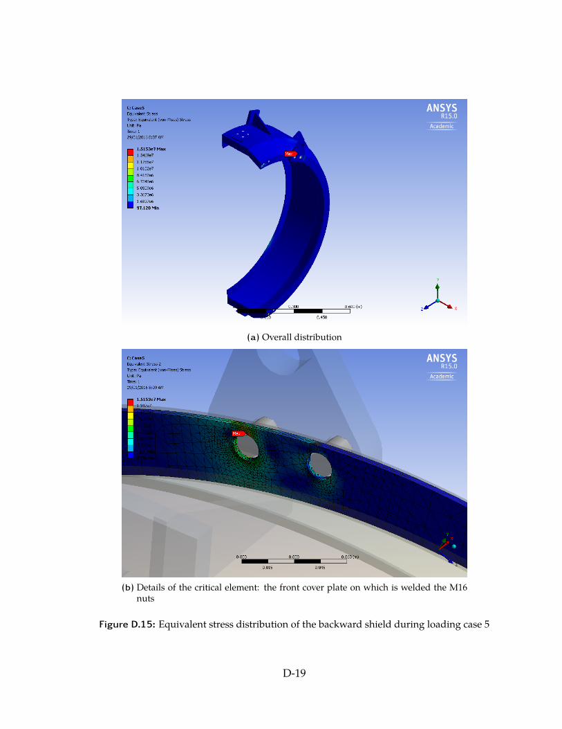
(a) Overall distribution

(b) Details of the critical element: the front cover plate on which is welded the M16nuts

Figure D.15: Equivalent stress distribution of the backward shield during loading case 5

D-19

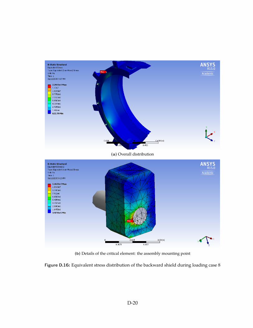
(a) Overall distribution

(b) Details of the critical element: the assembly mounting point

Figure D.16: Equivalent stress distribution of the backward shield during loading case 8

D-20

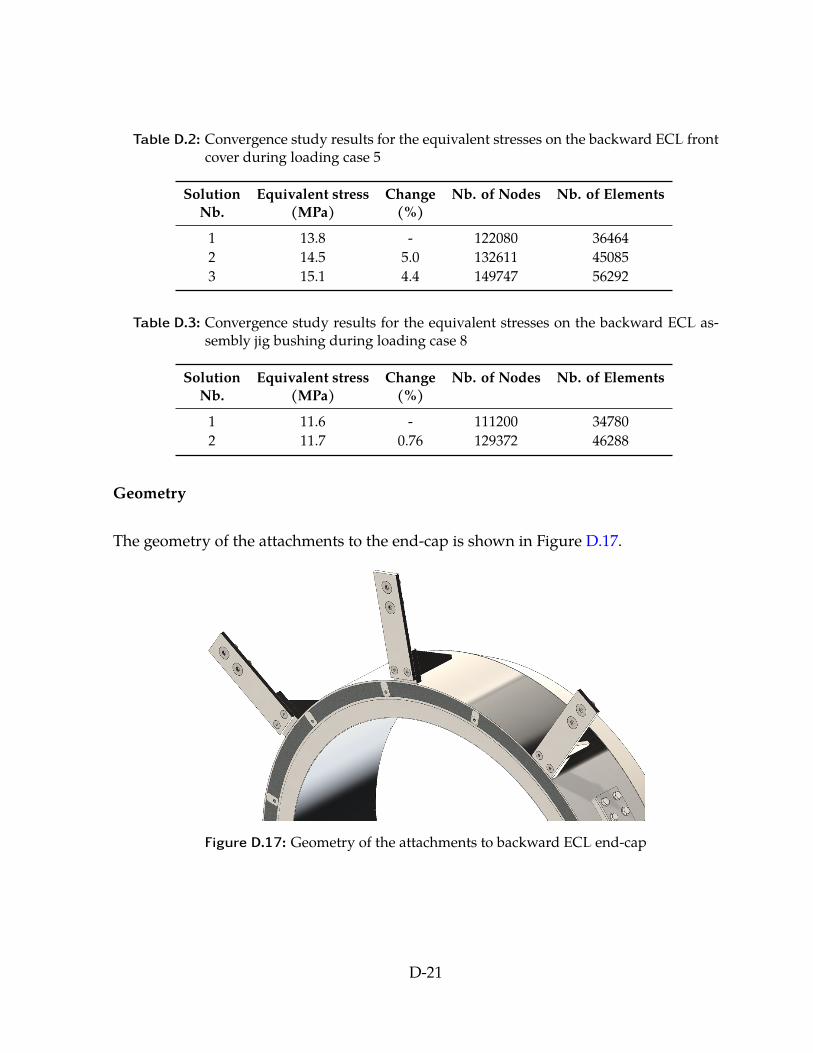
Table D.2: Convergence study results for the equivalent stresses on the backward ECL frontcover during loading case 5

Solution Equivalent stress Change Nb. of Nodes Nb. of ElementsNb. (MPa) (%)

1 13.8 - 122080 364642 14.5 5.0 132611 450853 15.1 4.4 149747 56292

Table D.3: Convergence study results for the equivalent stresses on the backward ECL as-sembly jig bushing during loading case 8

Solution Equivalent stress Change Nb. of Nodes Nb. of ElementsNb. (MPa) (%)

1 11.6 - 111200 347802 11.7 0.76 129372 46288

Geometry

The geometry of the attachments to the end-cap is shown in Figure D.17.

Figure D.17: Geometry of the attachments to backward ECL end-cap

D-21

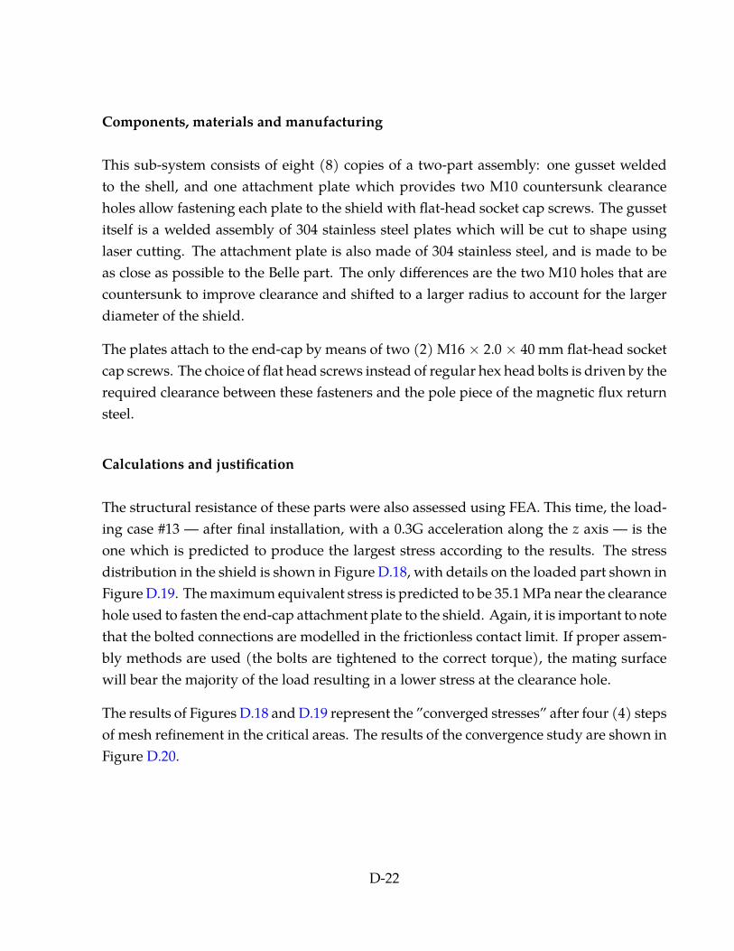
Components, materials and manufacturing

This sub-system consists of eight (8) copies of a two-part assembly: one gusset weldedto the shell, and one attachment plate which provides two M10 countersunk clearanceholes allow fastening each plate to the shield with flat-head socket cap screws. The gussetitself is a welded assembly of 304 stainless steel plates which will be cut to shape usinglaser cutting. The attachment plate is also made of 304 stainless steel, and is made to beas close as possible to the Belle part. The only differences are the two M10 holes that arecountersunk to improve clearance and shifted to a larger radius to account for the largerdiameter of the shield.

The plates attach to the end-cap by means of two (2) M16 × 2.0 × 40 mm flat-head socketcap screws. The choice of flat head screws instead of regular hex head bolts is driven by therequired clearance between these fasteners and the pole piece of the magnetic flux returnsteel.

Calculations and justification

The structural resistance of these parts were also assessed using FEA. This time, the load-ing case #13 — after final installation, with a 0.3G acceleration along the z axis — is theone which is predicted to produce the largest stress according to the results. The stressdistribution in the shield is shown in Figure D.18, with details on the loaded part shown inFigure D.19. The maximum equivalent stress is predicted to be 35.1 MPa near the clearancehole used to fasten the end-cap attachment plate to the shield. Again, it is important to notethat the bolted connections are modelled in the frictionless contact limit. If proper assem-bly methods are used (the bolts are tightened to the correct torque), the mating surfacewill bear the majority of the load resulting in a lower stress at the clearance hole.

The results of Figures D.18 and D.19 represent the ”converged stresses” after four (4) stepsof mesh refinement in the critical areas. The results of the convergence study are shown inFigure D.20.

D-22

Figure D.18: Equivalent stress distribution in the backward shield during loading case #13.

D.3 Design of the forward shield

The general design of the forward shield if similar to that of the backward one. As such,many descriptions encountered in Section D.2 are also valid for the forward shield and arereproduced here for completeness.

D.3.1 Shell

The main purposes of the shell are to contain the electromagnetic radiation shield, andprovide attachment points to fix the two halves together as well a fixing the shield assemblyto the jigs and the ECL end-caps. The shield comprises two symmetrical shells.

D-23

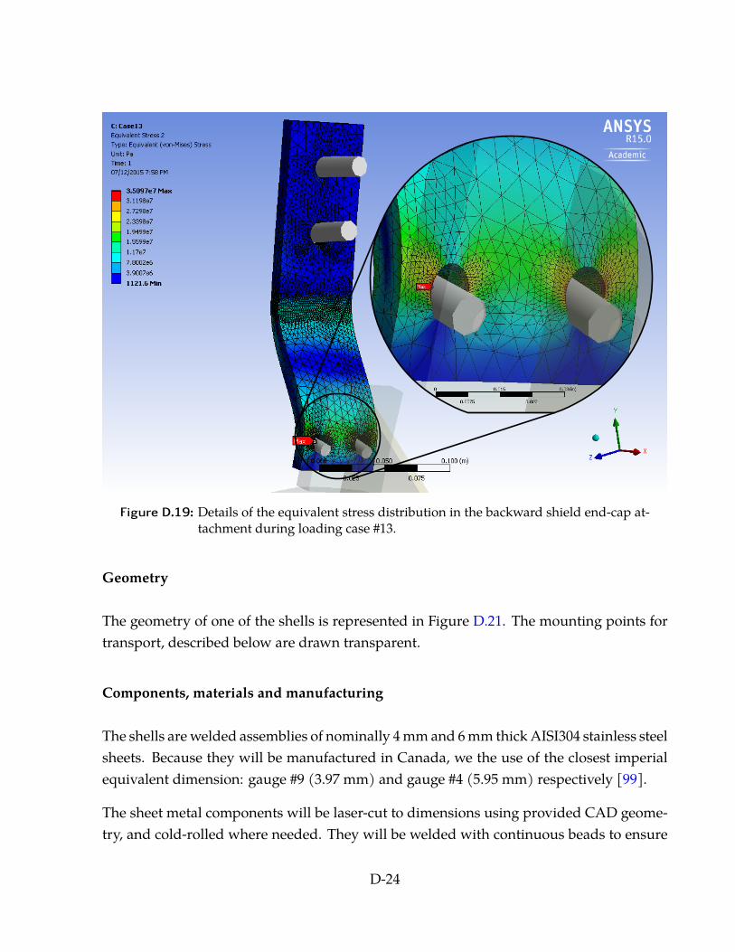
Figure D.19: Details of the equivalent stress distribution in the backward shield end-cap at-tachment during loading case #13.

Geometry

The geometry of one of the shells is represented in Figure D.21. The mounting points fortransport, described below are drawn transparent.

Components, materials and manufacturing

The shells are welded assemblies of nominally 4 mm and 6 mm thick AISI304 stainless steelsheets. Because they will be manufactured in Canada, we the use of the closest imperialequivalent dimension: gauge #9 (3.97 mm) and gauge #4 (5.95 mm) respectively [99].

The sheet metal components will be laser-cut to dimensions using provided CAD geome-try, and cold-rolled where needed. They will be welded with continuous beads to ensure

D-24

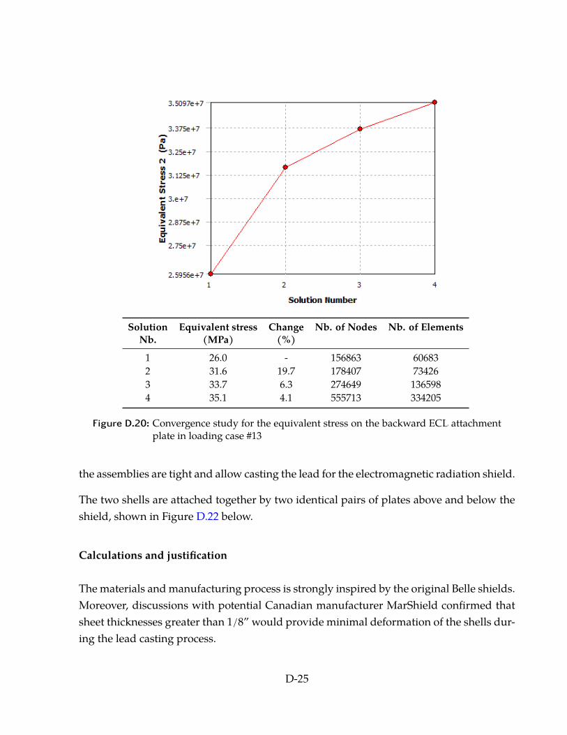
Solution Equivalent stress Change Nb. of Nodes Nb. of ElementsNb. (MPa) (%)

1 26.0 - 156863 606832 31.6 19.7 178407 734263 33.7 6.3 274649 1365984 35.1 4.1 555713 334205

Figure D.20: Convergence study for the equivalent stress on the backward ECL attachmentplate in loading case #13

the assemblies are tight and allow casting the lead for the electromagnetic radiation shield.

The two shells are attached together by two identical pairs of plates above and below theshield, shown in Figure D.22 below.

Calculations and justification

The materials and manufacturing process is strongly inspired by the original Belle shields.Moreover, discussions with potential Canadian manufacturer MarShield confirmed thatsheet thicknesses greater than 1/8” would provide minimal deformation of the shells dur-ing the lead casting process.

D-25

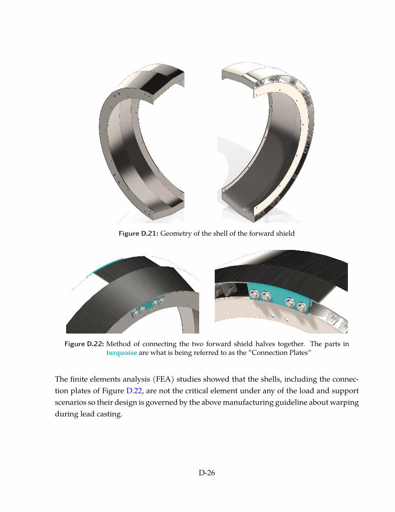
Figure D.21: Geometry of the shell of the forward shield

Figure D.22: Method of connecting the two forward shield halves together. The parts inturquoise are what is being referred to as the ”Connection Plates”

The finite elements analysis (FEA) studies showed that the shells, including the connec-tion plates of Figure D.22, are not the critical element under any of the load and supportscenarios so their design is governed by the above manufacturing guideline about warpingduring lead casting.

D-26

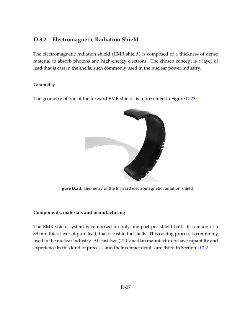
D.3.2 Electromagnetic Radiation Shield

The electromagnetic radiation shield (EMR shield) is composed of a thickness of densematerial to absorb photons and high-energy electrons. The chosen concept is a layer oflead that is cast in the shells, such commonly used in the nuclear power industry.

Geometry

The geometry of one of the forward EMR shields is represented in Figure D.23.

Figure D.23: Geometry of the forward electromagnetic radiation shield

Components, materials and manufacturing

The EMR shield system is composed on only one part per shield half. It is made of a39 mm thick layer of pure lead, that is cast in the shells. This casting process is commonlyused in the nuclear industry. At least two (2) Canadian manufacturers have capability andexperience in this kind of process, and their contact details are listed in Section D.2.2.

D-27

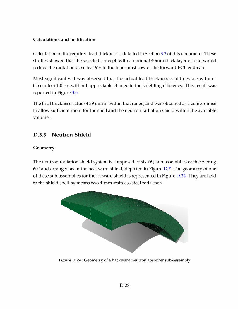
Calculations and justification

Calculation of the required lead thickness is detailed in Section 3.2 of this document. Thesestudies showed that the selected concept, with a nominal 40mm thick layer of lead wouldreduce the radiation dose by 19% in the innermost row of the forward ECL end-cap.

Most significantly, it was observed that the actual lead thickness could deviate within -0.5 cm to +1.0 cm without appreciable change in the shielding efficiency. This result wasreported in Figure 3.6.

The final thickness value of 39 mm is within that range, and was obtained as a compromiseto allow sufficient room for the shell and the neutron radiation shield within the availablevolume.

D.3.3 Neutron Shield

Geometry

The neutron radiation shield system is composed of six (6) sub-assemblies each covering60◦ and arranged as in the backward shield, depicted in Figure D.7. The geometry of oneof these sub-assemblies for the forward shield is represented in Figure D.24. They are heldto the shield shell by means two 4-mm stainless steel rods each.

Figure D.24: Geometry of a backward neutron absorber sub-assembly

D-28

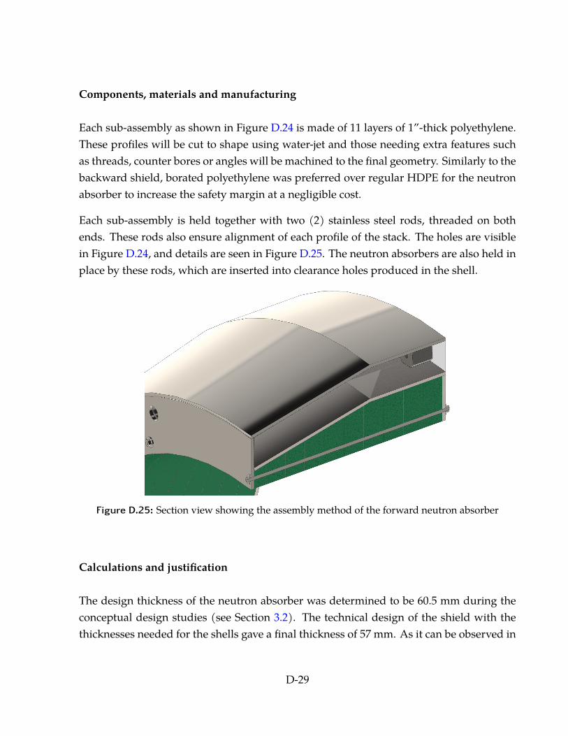
Components, materials and manufacturing

Each sub-assembly as shown in Figure D.24 is made of 11 layers of 1”-thick polyethylene.These profiles will be cut to shape using water-jet and those needing extra features suchas threads, counter bores or angles will be machined to the final geometry. Similarly to thebackward shield, borated polyethylene was preferred over regular HDPE for the neutronabsorber to increase the safety margin at a negligible cost.

Each sub-assembly is held together with two (2) stainless steel rods, threaded on bothends. These rods also ensure alignment of each profile of the stack. The holes are visiblein Figure D.24, and details are seen in Figure D.25. The neutron absorbers are also held inplace by these rods, which are inserted into clearance holes produced in the shell.

Figure D.25: Section view showing the assembly method of the forward neutron absorber

Calculations and justification

The design thickness of the neutron absorber was determined to be 60.5 mm during theconceptual design studies (see Section 3.2). The technical design of the shield with thethicknesses needed for the shells gave a final thickness of 57 mm. As it can be observed in

D-29

Figure 3.7, with a neutron absorber that is 3.5 mm thinner than the conceptual value, thepredicted neutron flux is still approximately than 5 times smaller than the design limit.

D.3.4 Mounting points for transport and installation

Similarly to the backward shield, two different sets of mounting points exist on the shield:

1. those to fix the jig adapter — the part that connects the shield to the assembly device—, and

2. those used to attach plates on the shield for lifting and transport.

During crane operation, the shield is also attached to the jig adapter, as represented inFigure D.26.

Jig adapters

Supports for lifting

Figure D.26: Components of the forward shield during crane operation. The supports forlifting are optional.

Geometry

The eight (8) mounting points for the forward jig adapter are included in the lead partand connect the inner shell to the outer shell. Their layout is represented in Figure D.27.

D-30

Figure D.28 shows the detail of their geometry. While very similar to those of the backwardshield in their design (see Figure D.13), their dimensions are different.

The mounting points for craning operations are represented in Figure D.29. They are in-stalled as provisions to enable the use of lifting shackles on the shield instead of wrappinga sling around it in order to make it vertical during the installation process (loading cases#4 and #5).

D-31

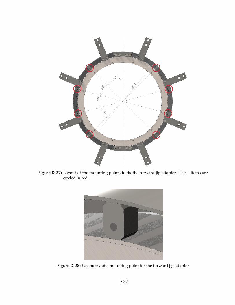
Figure D.27: Layout of the mounting points to fix the forward jig adapter. These items arecircled in red.

Figure D.28: Geometry of a mounting point for the forward jig adapter

D-32

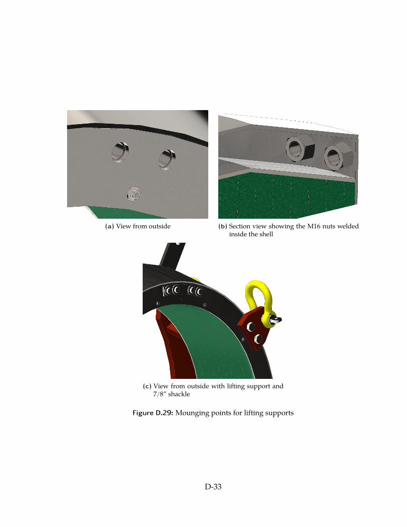
(a) View from outside (b) Section view showing the M16 nuts weldedinside the shell

(c) View from outside with lifting support and7/8” shackle

Figure D.29: Mounging points for lifting supports

D-33

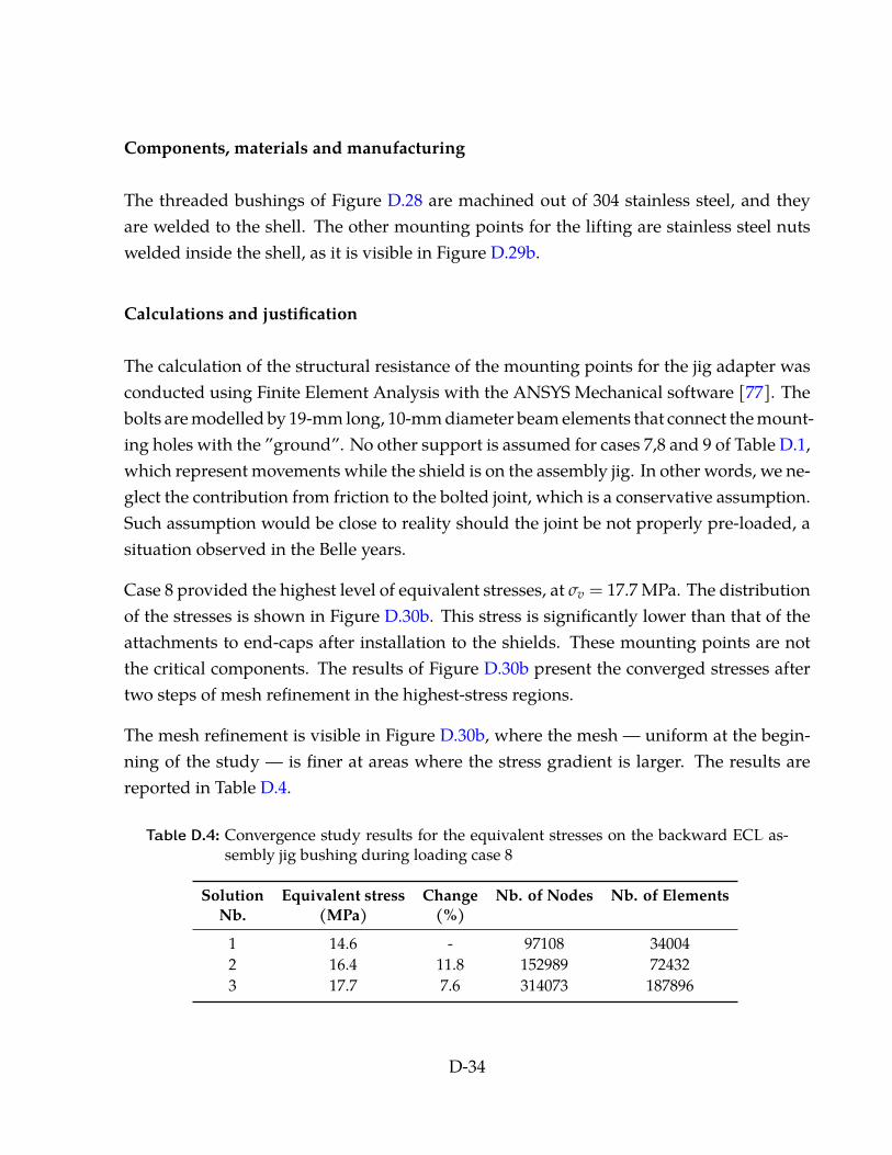
Components, materials and manufacturing

The threaded bushings of Figure D.28 are machined out of 304 stainless steel, and theyare welded to the shell. The other mounting points for the lifting are stainless steel nutswelded inside the shell, as it is visible in Figure D.29b.

Calculations and justification

The calculation of the structural resistance of the mounting points for the jig adapter wasconducted using Finite Element Analysis with the ANSYS Mechanical software [77]. Thebolts are modelled by 19-mm long, 10-mm diameter beam elements that connect the mount-ing holes with the ”ground”. No other support is assumed for cases 7,8 and 9 of Table D.1,which represent movements while the shield is on the assembly jig. In other words, we ne-glect the contribution from friction to the bolted joint, which is a conservative assumption.Such assumption would be close to reality should the joint be not properly pre-loaded, asituation observed in the Belle years.

Case 8 provided the highest level of equivalent stresses, at σv = 17.7 MPa. The distributionof the stresses is shown in Figure D.30b. This stress is significantly lower than that of theattachments to end-caps after installation to the shields. These mounting points are notthe critical components. The results of Figure D.30b present the converged stresses aftertwo steps of mesh refinement in the highest-stress regions.

The mesh refinement is visible in Figure D.30b, where the mesh — uniform at the begin-ning of the study — is finer at areas where the stress gradient is larger. The results arereported in Table D.4.

Table D.4: Convergence study results for the equivalent stresses on the backward ECL as-sembly jig bushing during loading case 8

Solution Equivalent stress Change Nb. of Nodes Nb. of ElementsNb. (MPa) (%)

1 14.6 - 97108 340042 16.4 11.8 152989 724323 17.7 7.6 314073 187896

D-34

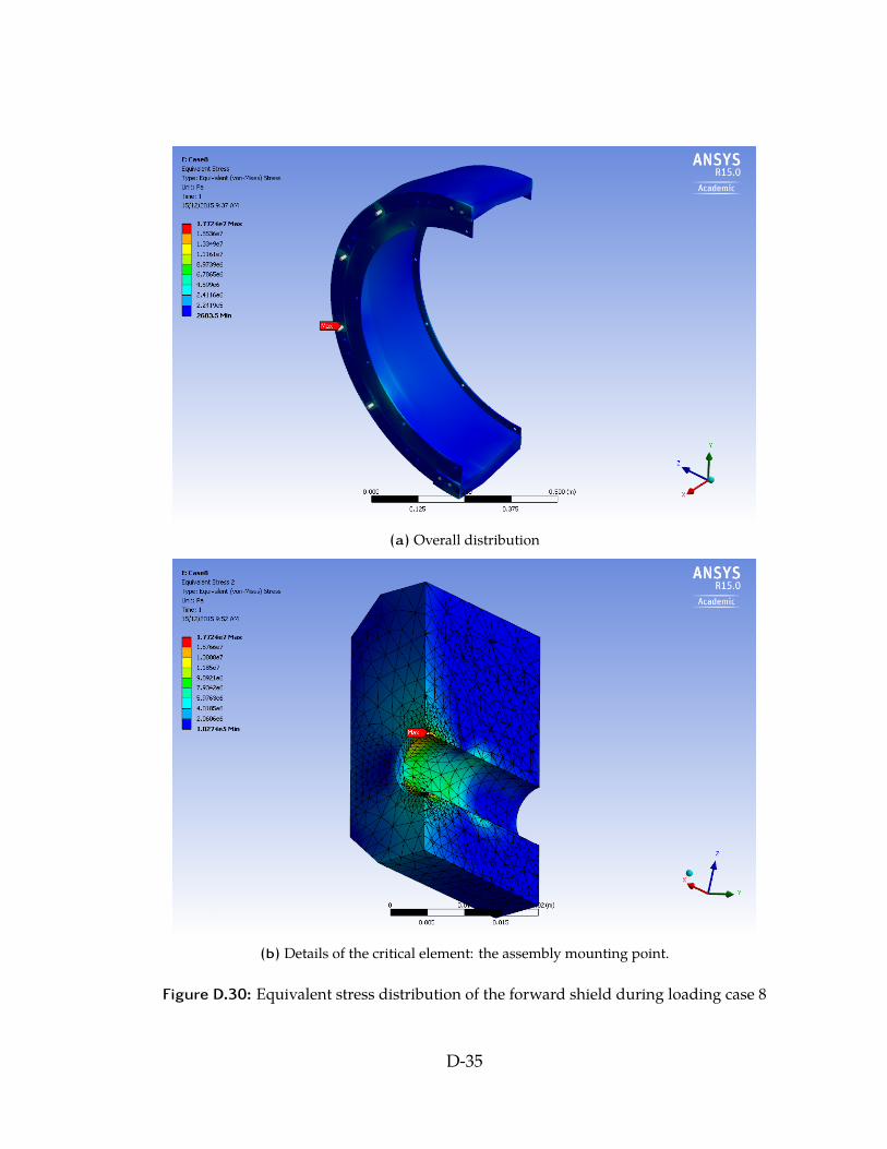
(a) Overall distribution

(b) Details of the critical element: the assembly mounting point.

Figure D.30: Equivalent stress distribution of the forward shield during loading case 8

D-35

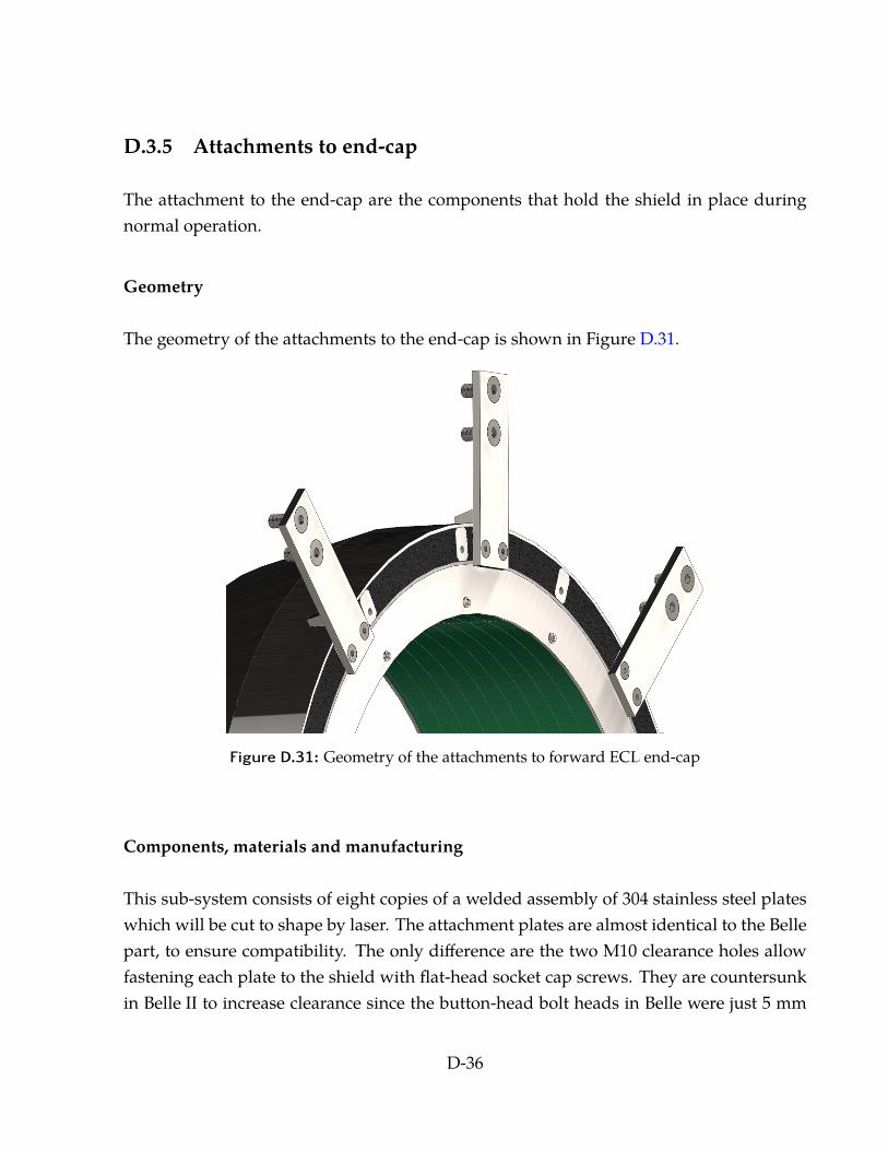
D.3.5 Attachments to end-cap

The attachment to the end-cap are the components that hold the shield in place duringnormal operation.

Geometry

The geometry of the attachments to the end-cap is shown in Figure D.31.

Figure D.31: Geometry of the attachments to forward ECL end-cap

Components, materials and manufacturing

This sub-system consists of eight copies of a welded assembly of 304 stainless steel plateswhich will be cut to shape by laser. The attachment plates are almost identical to the Bellepart, to ensure compatibility. The only difference are the two M10 clearance holes allowfastening each plate to the shield with flat-head socket cap screws. They are countersunkin Belle II to increase clearance since the button-head bolt heads in Belle were just 5 mm

D-36

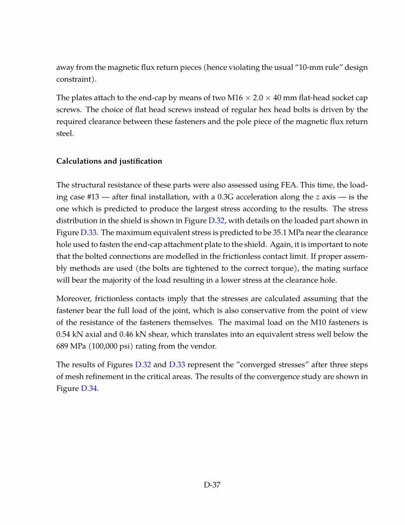
away from the magnetic flux return pieces (hence violating the usual “10-mm rule” designconstraint).

The plates attach to the end-cap by means of two M16 × 2.0 × 40 mm flat-head socket capscrews. The choice of flat head screws instead of regular hex head bolts is driven by therequired clearance between these fasteners and the pole piece of the magnetic flux returnsteel.

Calculations and justification

The structural resistance of these parts were also assessed using FEA. This time, the load-ing case #13 — after final installation, with a 0.3G acceleration along the z axis — is theone which is predicted to produce the largest stress according to the results. The stressdistribution in the shield is shown in Figure D.32, with details on the loaded part shown inFigure D.33. The maximum equivalent stress is predicted to be 35.1 MPa near the clearancehole used to fasten the end-cap attachment plate to the shield. Again, it is important to notethat the bolted connections are modelled in the frictionless contact limit. If proper assem-bly methods are used (the bolts are tightened to the correct torque), the mating surfacewill bear the majority of the load resulting in a lower stress at the clearance hole.

Moreover, frictionless contacts imply that the stresses are calculated assuming that thefastener bear the full load of the joint, which is also conservative from the point of viewof the resistance of the fasteners themselves. The maximal load on the M10 fasteners is0.54 kN axial and 0.46 kN shear, which translates into an equivalent stress well below the689 MPa (100,000 psi) rating from the vendor.

The results of Figures D.32 and D.33 represent the ”converged stresses” after three stepsof mesh refinement in the critical areas. The results of the convergence study are shown inFigure D.34.

D-37

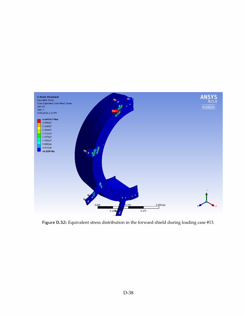
Figure D.32: Equivalent stress distribution in the forward shield during loading case #13.

D-38

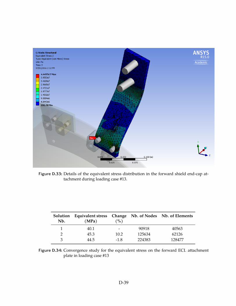
Figure D.33: Details of the equivalent stress distribution in the forward shield end-cap at-tachment during loading case #13.

Solution Equivalent stress Change Nb. of Nodes Nb. of ElementsNb. (MPa) (%)

1 40.1 - 90918 405632 45.3 10.2 125634 621263 44.5 -1.8 224383 128477

Figure D.34: Convergence study for the equivalent stress on the forward ECL attachmentplate in loading case #13

D-39

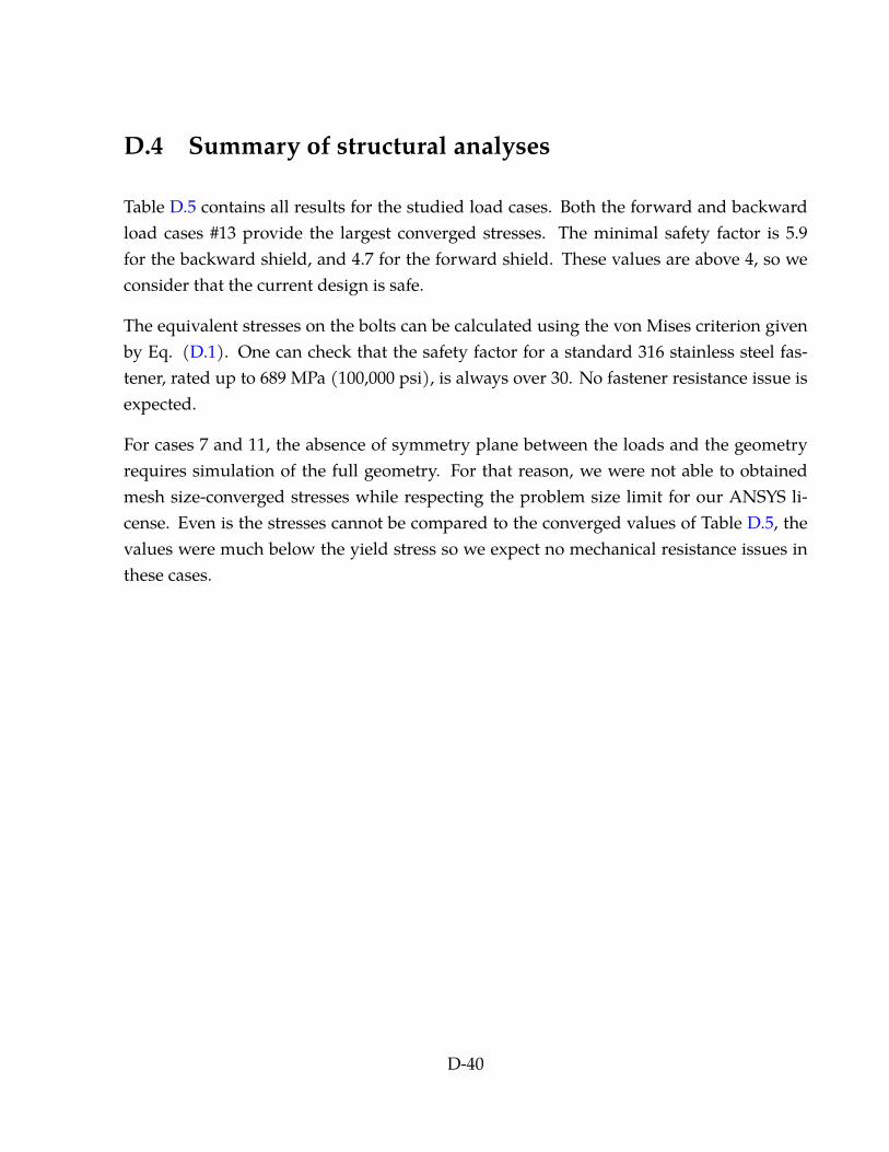
D.4 Summary of structural analyses

Table D.5 contains all results for the studied load cases. Both the forward and backwardload cases #13 provide the largest converged stresses. The minimal safety factor is 5.9for the backward shield, and 4.7 for the forward shield. These values are above 4, so weconsider that the current design is safe.

The equivalent stresses on the bolts can be calculated using the von Mises criterion givenby Eq. (D.1). One can check that the safety factor for a standard 316 stainless steel fas-tener, rated up to 689 MPa (100,000 psi), is always over 30. No fastener resistance issue isexpected.

For cases 7 and 11, the absence of symmetry plane between the loads and the geometryrequires simulation of the full geometry. For that reason, we were not able to obtainedmesh size-converged stresses while respecting the problem size limit for our ANSYS li-cense. Even is the stresses cannot be compared to the converged values of Table D.5, thevalues were much below the yield stress so we expect no mechanical resistance issues inthese cases.

D-40

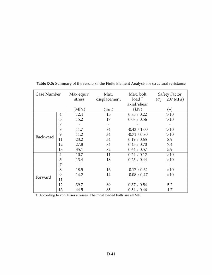
Table D.5: Summary of the results of the Finite Element Analysis for structural resistance

Case Number Max equiv.stress

Max.displacement

Max. boltload †

axial/shear

Safety Factor(σy = 207 MPa)

(MPa) (µm) (kN) (–)

Backward

4 12.4 15 0.85 / 0.22 >105 15.2 17 0.08 / 0.56 >107 - - - -8 11.7 84 -0.43 / 1.00 >109 11.2 34 -0.71 / 0.80 >1011 23.2 54 0.19 / 0.65 8.912 27.8 84 0.45 / 0.70 7.413 35.1 82 0.64 / 0.57 5.9

Forward

4 10.7 11 0.24 / 0.12 >105 13.4 18 0.25 / 0.44 >107 - - - -8 18.5 16 -0.17 / 0.62 >109 14.2 14 -0.08 / 0.47 >1011 - - - -12 39.7 69 0.37 / 0.54 5.213 44.5 85 0.54 / 0.46 4.7

†: According to von Mises stresses. The most loaded bolts are all M10.

D-41

D.5 Fabrication and commissioning

D.5.1 Vendor

A public bidding process was managed by the University of Victoria Purchasing Services.The winner of the process was not part of the early manufacturer network explorationduring the project definition phases. However we were convinced of their ability to deliverquality components because of their good documentation practices, extensive supplier net-work, and rich previous experiences with sheet metal stainless steel. Their proximity to theUniversity of Victoria also made possible frequent visits to follow the fabrication processmore closely. The project was awarded to

� Turbulent Diffusion Technology Inc., 2601 Murray St Port Moody, BC V3H 1X1, Canada

who managed and sub-contracted the work in agreement with our contract terms.

D.5.2 Modifications from design drawings

Apart from the expected heat-induces geometric deviation during welding, three itemswere manufactured differently than the original specification drawings. There are no im-pact on the shields performance or usability, but these chances should nonetheless be doc-umented.

Forward bushings

The forward bushings are installed in sets of three: two of them for the attachment plates tothe end-caps — visible in Figure D.31 — and the remaining one for the end-cap assemblyjig, seen in Figure D.26. These bushings are separated by a 12-mm gap.

During a visit to the manufacturer on January 27th, 2017, we were informed this gap wasnot sufficient for the welding nozzle, and the bushings were instead welded at the outsideedges only after producing a supplementary 5-mm fillet on that edge for better penetration.See Figure D.35 for a picture showing two of such completed welds.

D-42

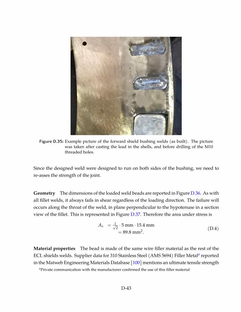
Figure D.35: Example picture of the forward shield bushing welds (as built). The picturewas taken after casting the lead in the shells, and before drilling of the M10threaded holes.

Since the designed weld were designed to run on both sides of the bushing, we need tore-asses the strength of the joint.

Geometry The dimensions of the loaded weld beads are reported in Figure D.36. As withall fillet welds, it always fails in shear regardless of the loading direction. The failure willoccurs along the throat of the weld, in plane perpendicular to the hypotenuse in a sectionview of the fillet. This is represented in Figure D.37. Therefore the area under stress is

As = 1√2· 5 mm · 15.4 mm= 89.8 mm2.

(D.4)

Material properties The bead is made of the same wire filler material as the rest of theECL shields welds. Supplier data for 310 Stainless Steel (AMS 5694) Filler Metala reportedin the Matweb Engineering Materials Database [100] mentions an ultimate tensile strength

aPrivate communication with the manufacturer confirmed the use of this filler material

D-43

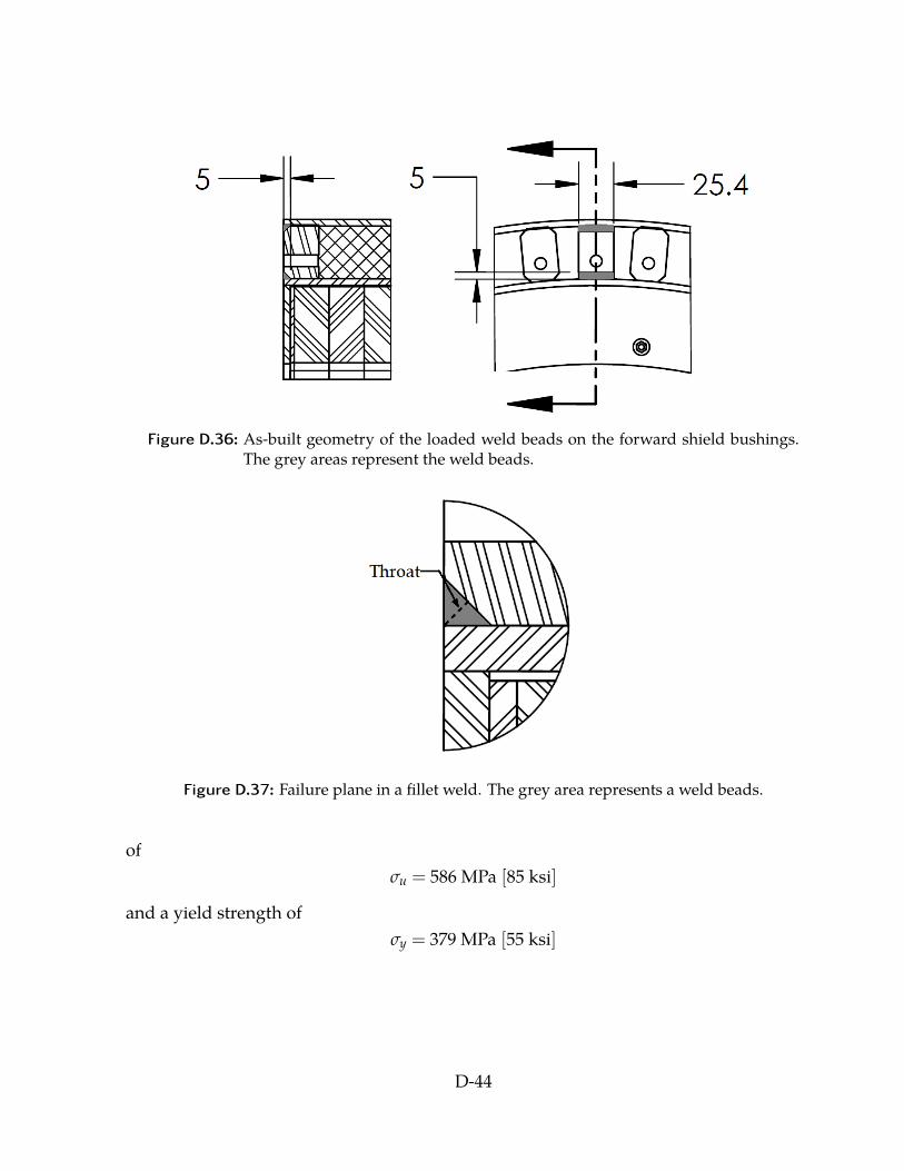
Figure D.36: As-built geometry of the loaded weld beads on the forward shield bushings.The grey areas represent the weld beads.

Figure D.37: Failure plane in a fillet weld. The grey area represents a weld beads.

ofσu = 586 MPa [85 ksi]

and a yield strength ofσy = 379 MPa [55 ksi]

D-44

where the value in brackets is the original specification in imperial units. By using the vonMises criterion [78], we approximate the shear strength of the material to

σs = 1√3σy

≈ 219 MPa. (D.5)

The surrounding material, 304 stainless steel, has a nominal σy = 207 MPa.

Loads To check the resistance of the structure without re-doing all numerical studies, weconsider conservative assumptions simplifying the problem. We calculate the safety factorof joints if the whole mass of a forward half-shield is held by only one of these bushings.Furthermore, we applied the load in a direction as to “pull” it out of the shells such thatonly the welds are providing mechanical resistance (as opposed to having contributionsfrom the surrounding structure). The half-shield assemblies have a mass m = 186 kg (es-timated from the SolidWorks model), so this corresponds of a load

P = mg= 1825 N (D.6)

taken by both weld beads. This conservative load can be compared to the maximum loadtaken by the bolt that attaches to these bushings. From loading case FWD # 13 resultsreported in Table D.5, the maximum calculated load is 540 N axially and 460 N in shear,or an “equivalent von Mises load” of 884 N on the bolt. This justifies our statement thatP = 1825 N is a conservative load on the bushing, yet in the right order of magnitude sothat the calculation is meaningful.

Stress calculation Still conservatively assuming this load is taken under pure shear boththe top and bottom welds, the area under stress is twice that of a single bead. The shearstress is therefore

σ =P

2As= 10.2 MPa

(D.7)

Result and implications The 10.2 MPa pure shear provides a safety factor of almost SFσ =

21.5 for the weld bead itself. This factor sufficient to ensure mechanical resistance of theweld. If one considers the same stresses in the surrounding material — 304 stainless steel,

D-45

which has a lower elastic limit — the safety factor is down to just under SFσ = 11.8. Thisis also well beyond our design guideline of SFσ ≥ 4.

In conclusion, the departure from the design weld beads during fabrication shouldn’t poseany significant risk to the mechanical soundness of the structure.

Backward attachment plates

The gussets to attach the backward shield to the end-cap (ref. Figure D.17) were welded atthe wrong angular position (23◦ instead of 22.5◦) because of an ambiguity in the drawingswe provided. This was noticed just before shipping, so instead of moving these weldedparts, we decided to manufacture wider attachment plates that would be attached to alaser-cut jig replicating the mounting holes on the end-cap. The actual plates were 12.6 mmwider than the original design.

The bolt clearance holes were then drilled to match the actual positions on the shield, whichwere off by approximately 5 mm. Wider plates shouldn’t have any impact other than in-creased structural resistance since there are no surrounding components that can interferewith them in the final application. However, extra care must be taken during installation:since they were produced to match as-built positions, each one is uniquely numbered (1through 8) and must be installed at the corresponding position. The as-built plates arerepresented in Figure D.38.

Backward neutron absorber cover

For the backward shield, the neutron absorber cover is an aluminium alloy sheet fastenedwith small countersunk screws to the shells (see Figure D.10). The design screw size wasM2× 0.6. However the tension required to hold the cover in place was greater than ex-pected due to geometric distortions from welding. Many of these screws broke duringassembly, so the manufacturer upgraded to M2.5× 0.45 screws and this solves the prob-lem. No impact other than strengthening the cover is expected from this change.

D-46

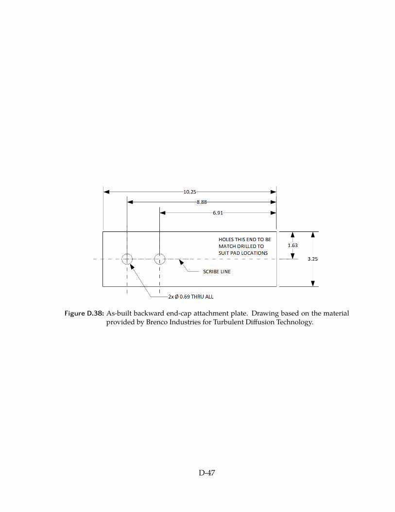
Figure D.38: As-built backward end-cap attachment plate. Drawing based on the materialprovided by Brenco Industries for Turbulent Diffusion Technology.

D-47

***

D-48