bankers, markets & investors nº 124 may-june 2013 managing sovereign credit risk exposure in a...

Bankers, Markets & Investors nº 124 may-june 2013 5

Managing Sovereign Credit Risk Exposure in a Global Equity Portfolio

■ Introduction

The recent sovereign risk crisis in developed countries has reminded equity investors around the globe that, even when not directly holding government bonds, they may be heavily affected by worsening of sovereign credit risk conditions. For example, it became clear that stocks of companies which benefi t from implicit guarantees pro-vided by the government, such as banks, may be affected by news on sovereign risk conditions. Likewise, stocks of companies that benefi t from public spending or from tax incentives may suffer in times when public fi nances worsen. The academic literature actually provides ample evidence that stock returns are indeed sensitive to sove-reign risk (see e.g. Belo et al (2011), Gandhi and Lustig (2011) Cutler (1988), Ang and Longstaff (2011), Longstaff et al (2011), Jeanneret (2010), Hume and Kim (2008)).

An investor might be interested to avoid such sovereign risk exposure of his equity portfolio for a variety of rea-sons. For example, a public pension fund has a motivation to avoid sovereign risk exposure in his equity portfolio as the contributions to the fund depend on government funding and benefi ciaries’ incomes are also sensitive to public fi nances. Moreover, an investor who is exposed to sovereign credit risk through government bonds may wish to avoid taking too much of the same risk exposure when investing in an equity portfolio.

In this paper, we reliably categorize stocks by their expo-sure to sovereign risk in order to create equity portfolios with low sovereign risk exposure. We use robust estima-tion techniques to measure stocks return sensitivities to changes in sovereign credit default swap spreads. Our main fi nding is that such a measurement of sovereign risk exposure of stocks is reliable out-of-sample. In bad times where negative news occurs on sovereign risk conditions, our low sovereign beta portfolios indeed outperform high sovereign beta portfolios. Our approach thus provides a way of identifying which stock portfolios will allow an investor who is already exposed to sovereign risk to avoid loading up on exposure to the same risk factor in his equity investments.

The remainder of the paper fi rst explains why and how we proxy for sovereign risk, then provides details on how we measure exposure to this factor and fi nally resents out-of-sample performance and characteristics of the portfolios with different levels of sovereign risk beta.

■ I. The sovereign credit risk factor

Sovereign credit risk spill over to equity markets, both at the aggregate level and at the fi rm level. The question of how the aggregate stock market is impacted by the sove-reign credit risk factor has been studied quite broadly. This paper adds to the existing literature on the cross-sectional differences in exposure across fi rms to this risk factor. In this section, we discuss what a reasonable proxy for the sovereign risk factor would be and present a detailed methodology for constructing the proxy for the sovereign risk factor. A descriptive statistics of the proxy and it’s relation with other standard equity risk factors follows.

I.1. RELATED LITERATURE: DOES SOVEREIGN CREDIT RISK SPILL OVER TO THE EQUITY MARKETS?How sovereign credit risks spill over to fi nancial mar-

kets at the aggregate level has been the focus of a number of recent papers. For instance, one of the main fi nding of Longstaff and Ang (2011) is the existence of a strong negative relationship between stock market index returns and sovereign credit risk in both the U.S. and the Euro-zone. Longstaff, Pan, Pedersen and Singleton (2011) fi nd a strong relation between the sovereign CDS spreads and the global risk premiums.

Expanding the scope of the analysis to the spillover effects to equity return volatility, Jeanneret (2010) shows that a higher risk of sovereign default in Europe negatively impacts equity market returns and it partially explains equity return volatility in the U.S. Changes in sovereign credit ratings also spill over to both equity returns and return volatility. Hooper, Hume and Kim (2008) analyse

FELIX GOLTZxxxfonctionxxxEDHEC Risk Institute, EDHEC Business SchoolERI Scientifi c Beta

ASHISH LODHxxxfonctionxxxERI Scientifi c Beta

FAHD RACHIDYxxxfonctionxxxERI Scientifi c Beta

Article_Rachidy.indd Sec1:5Article_Rachidy.indd Sec1:5 16/04/13 11:1016/04/13 11:10

Bankers, Markets & Investors nº 124 may-june 20136

MANAGING SOVEREIGN CREDIT RISK EXPOSURE IN A GLOBAL EQUITY PORTFOLIO

the spillover effects of sovereign rating changes on inter-national fi nancial markets and fi nd a signifi cant positive correlation between rating changes and stock return changes, and a signifi cant negative correlation between rating changes and stock return volatility.

Ferreira and Gama (2007) look at the spillover impacts of a credit rating or outlook change in one country onto the industries in other countries. They fi nd that these cross-markets and cross-countries spillover effects at the industry level are more pronounced in traded goods industries and small industries. In a paper looking at cross-sectional differences in an industry sector, Smirlock and Kaufold (1987) show that sovereign credit risk has a signifi cant impact across bank stock prices.

Part of the literature has been focusing on the analysis of the different transmission channels through which sovereign credit risk can spill over to equity markets. We highlight here empirical research papers with a focus on three main transmission channels: government spending, implicit guarantees and taxes.

Firstly, fi rm revenues can be directly dependent on public spending.1 Belo et al (2011) fi nd signifi cant relationship between fi rms’ exposure to public spending and their stock returns. Sovereign credit risk may therefore spill over to equity markets through the public spending chan-nel. Secondly, higher sovereign credit risk arising from a worsening of sovereign fi nances may change the benefi ts that companies derive from implicit state guarantees and hence potentially impact stock returns through this channel. Gandhi and Lustig (2011) analyze the asymmet-ric nature of U.S. government guarantee in the event of fi nancial disaster and fi nd that small bank stocks earn a risk premium over large banks stocks. Lastly sovereign credit risk spillover effects may be channeled through taxes. Cutler (1988) examines the stock market’s reaction to the U.S. Tax Reform Act of 1986. Overall and shows that the stock returns are impacted by the sovereign risk through the tax channel depending on their exposure to these tax changes.

I.2. RELATED LITERATURE: ARE RATINGS, BOND YIELD SPREADS OR CDS SPREADS INFORMATIONAL MEASURES OF SOVEREIGN CREDIT RISK?We will use in this paper sovereign credit risk spreads

(CDS) premia as a proxy for sovereign credit risk. An extensive literature exists on the different approaches used to measure sovereign credit risk, whether through Credit Rating Agency (CRA) ratings, sovereign bond yield spreads or Credit Default Swap (CDS) spreads. We discuss here the advantages and disadvantages of these different approaches and explain our preference for CDS spreads.

CRA ratings use accounting and fundamental data: critics have argued that ratings are backward-looking, static, confi ned to the quality of the debt and lag credit risk changes. Indeed Moody’s, S&P and Fitch defi ne their ratings as a long term opinion of credit risk through the economic cycle (Altman and Rijken 2004). In line with this fi nding, Hull and White (2004), Blanco et al. (2005)

showed that CDS prices lead changes in ratings respecti-vely on sovereign and corporate CDS markets. Moreover, a recent study by Flannery, Houston and Partnoy (2010) evaluates the possibility of using CDS spreads as substitutes for credit ratings. It reveals that CDS spreads incorporate new information signifi cantly more quickly than credit ratings. The authors conclude their paper by advancing the idea that CDS spreads are promising market-based tools for regulatory and private purposes, and they may serve as a viable substitute for credit ratings.

While using market-based measures (e.g. bond yields or CDS spreads) may seem an attractive alternative, recent literature on the information content of these instruments suggests different interpretations.

As Longstaff et al (2005) emphasized, credit-default swap are contracts by defi nition and not securities. The contractual nature of these instruments makes them less sensitive to liquidity. However, current fi ndings suggest that CDS spreads do not only account for cre-dit risk and that liquidity may play a non-negligible role. Berndt et al (2005) and Pan and Singleton (2008) show respectively that corporate and sovereign CDS spreads are too high to account only for default risk, they suggested a liquidity factor as possible component to represent the non-default part. To this end, Tang and Yan (2007) and Bongaerts, De Jong and Driessen (2011) studied the effect of liquidity on corporate CDSs and although liquidity is priced in CDS spread changes, its magnitude is weak.

A large amount of literature has tried to explain the components of corporate bond yields2. The consensus from these studies is that corporate bond yields are hea-vily infl uenced by other factors than credit risk, such as liquidity risk, tax and macroeconomic variables.

In fact, the results found in the corporate CDS and bond markets are not refl ective of the dynamics obser-ved on the sovereign side. As such, there are papers that study credit and liquidity effects on sovereign bond yields such as Codogno, Favero and Missale (2003), Geyer, Kossmeier and Pichler (2004), Beber, Brandt and Kavajecz (2009), Favero, Pagano and Thadden (2010), Schwarz (2010) and Monfort and Renne (2011). These studies do fi nd that liquidity is present in sovereign bond yields, while some authors argue that liquidity is important, others advance that it plays a trivial role. On the other hand, the literature studying the information quality of sovereign CDS is rather limited3. Pan and Singleton (2008) show that the term structures of CDS spreads contain signifi cant information about both the risk-neutral credit-event arrival rate and the loss-given-default. Similarly, Longstaff et al (2011) exploit the information in the term structure of sovereign CDS spreads in order to decompose the spreads into risk-premium and default-risk components. They conclude that the default-risk component explains a larger part of the spread. Moreover, Remonala et al (2008) estimate a dynamic market-based measure of sovereign risk and use it to decompose sovereign CDS spreads. They show that the jump-at-default risk premium is priced in the spreads.




Nevertheless, some papers argue that sovereign bond spreads have better information content than CDS spreads. For instance, Badaoui, Cathcart and El Jahel (2012) ana-lyse the information content of sovereign bond yields and CDS spreads and fi nd that sovereign bond spreads are less subject to liquidity frictions and therefore could represent a better proxy for sovereign default risk. In a similar study, Badaoui, Cathcart and El Jahel (2012) provide empirical evidence that liquidity risk participates directly to the variation over-time of the term structure of sovereign CDS spreads.

The question of whether CDS spreads have more infor-mational advantage on default risk than bond spreads (or vice versa) is however not the primary goal of our paper. While there is no clear consensus in the academic literature on which measure best represents sovereign default risk, the fact that CDSs refl ect current market expectations on the strength of the creditworthiness of sovereign economies is important for our empirical exercise as it will help us better understand the cross-sectional differences in individual stock exposure to sovereign risk under contemporary market conditions4. For this reason, we utilize CDSs as a sovereign default risk measure, although further research is warranted to investigate the effect of other credit measures (e.g. bond yield spreads) on stock returns. Moreover, our use of CDS spreads means that we do not need to select a risk-free reference which would be required for the determination of bond spreads5.

I.3. CONSTRUCTING A PROXY FOR SOVEREIGN CREDIT RISK BASED ON CDS SPREADSSince we are interested here in observing how stock

returns react to the “news”, we work with changes in CDS spreads rather than levels (following Ang et al. (2006), Campbell (1996), Petkova (2006)). Furthermore, CDS spread changes refl ect innovations in sovereign credit risk conditions and avoid econometric issues related to highly serially correlated variables.

We defi ne the sovereign “World CDS factor” as the negative of weekly percentage change in the arithmetic average of the fi ve-year sovereign CDS spreads of the countries in our data set for each point in time.6 We use this measure as a proxy for global sovereign credit risk. Longstaff et al (2011), who use CDS data to study the nature of sovereign risk, show that sovereign risk across countries is highly correlated and that most of sovereign risk can be explained by a set of global fac-tors. In other words, the country specifi c component in the sovereign credit risk is very small. Furthermore, Avramov et al (2012) show that in the presence of glo-bal sovereign risk factor, the country specifi c factors do not explain the global equity returns. This is our prime reason for choosing a single factor to represent global sovereign risk in our model. The objective is not to capture regional differences but to construct a proxy for a factor that best represents the global sovereign risk. Since we construct global equity portfolios with a desired exposure to the global sovereign risk factor, we

select a model that takes into account only single global factor. Our risk factor is therefore signed in order to be consistent with the following relationship: a negative value for the World CDS factor means bad news on the sovereign credit risk front, a positive value for the World CDS factor means good news. If the simple average CDS spread value increases (decreases), this means bad (good) news and our factor will have a low (high) value. An increase on CDS spreads (hence a negative World CDS factor) represents additional cost for investors who buy these contracts as a credit default protection. Therefore, to hedge against this extra cost, investors will search for low sovereign-beta portfolios (e.g. negative beta): in times of bad (negative) news, low beta stocks tend to have higher returns compared to the average stock thus providing a form of protection in bad times.

I.4. CDS DATA Our fi ve year CDS spread data spans from 22nd December

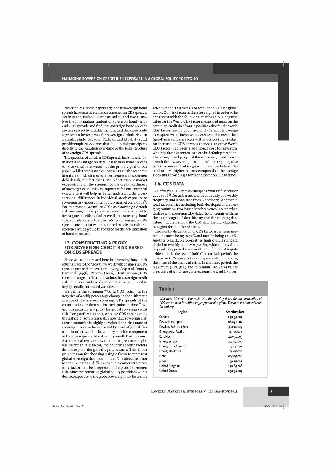
2000 to 16th December 2011, with both daily and weekly frequency, and is obtained from Bloomberg. We cover in total 44 countries including both developed and emer-ging countries. Two issues have been encountered when dealing with sovereign CDS data. Not all countries share the same length of data history and the missing data values.7 Table 1 shows the CDS data history, classifi ed by region for the sake of clarity.

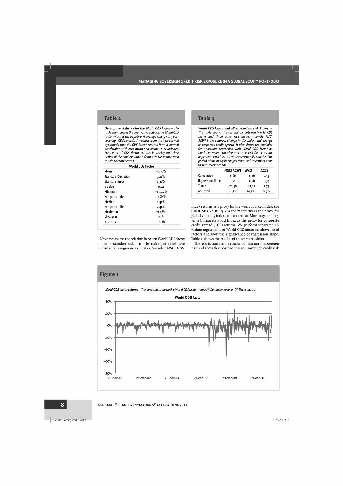
The weekly distribution of CDS factor is far from nor-mal; the mean being -0.72% and median being +0.40%. Another remarkable property is high overall standard deviation (weekly std dev = 7.24%), which stems from high volatility period since 2008. From fi gure 1, it is quite evident that in the second half of the analysis period, the change in CDS spreads became quite volatile marking the onset of the fi nancial crisis. In the same period, the maximum (+27.36%) and minimum (-60.42%) values are observed which are quite extreme for weekly values.

Table 1

CDS data history – The table lists the starting dates for the availability of CDS spread data for different geographical regions. The data is obtained from Bloomberg.

Region Starting date Canada 25/09/2009Dev.Asia ex Japan 08/03/2002Dev.Eur. Ex UK ex Euro 31/01/2003Emerg. Asia Pacifi c 16/11/2001Eurobloc 28/03/2003Emerg.Europe 20/10/2000Emerg.Latin America 19/10/2001Emerg.ME-Africa 13/10/2000Israel 01/10/2004Japan 17/01/2003United Kingdom 15/08/2008United States 25/09/2009




Next, we assess the relation between World CDS factor and other standard risk factors by looking at correlations and univariate regression statistics. We select MSCI ACWI

Index returns as a proxy for the world market index, the CBOE SPX Volatility VIX index returns as the proxy for global volatility index, and returns on Morningstar long-term Corporate Bond Index as the proxy for corporate credit spread (CCS) returns. We perform separate uni-variate regressions of World CDS factor on above listed factors and look the signifi cance of regression slope. Table 3 shows the results of these regressions.

The results confi rm the economic intuition on sovereign risk and show that positive news on sovereign credit risk

Table 2

Descriptive statistics for the World CDS factor – The table summarizes the descriptive statistics of World CDS factor which is the negative of average change in 5 year sovereign CDS spreads. P-value is from the t-test of null hypothesis that the CDS factor returns form a normal distribution with zero mean and unknown covariance. Frequency of CDS factor returns is weekly and time period of the analysis ranges from 22nd December 2000 to 16th December 2011.

World CDS FactorMean –0.72%Standard Deviation 7.24%Standard Error 0.30%p value 0.02Minimum –60.42%25th percentile –2.84%Median 0.40%75th percentile 2.49%Maximum 27.36%Skewness –2.61Kurtosis 19.88

Figure 1

World CDS factor returns – The fi gure plots the weekly World CDS factor from 22nd December 2000 to 16th December 2011.

40%

20%

0%

–20%

–40%

–60%

–80%

World CDS factor

29-dec-00 29-dec-02 29-dec-04 29-dec-06 29-dec-08 29-dec-10

Table 3

World CDS factor and other standard risk factors – The table shows the correlation between World CDS factor and three other risk factors; namely MSCI ACWI Index returns, change in VIX Index, and change in corporate credit spread. It also shows the statistics for univariate regression with World CDS factor as the independent variable and each risk factor as the dependent variables. All returns are weekly and the time period of the analysis ranges from 22nd December 2000 to 16th December 2011.

MSCI ACWI ΔVIX ΔCCSCorrelation 0,66 –0,46 0.13Regression Slope 1,74 –0,26 0.74T-stat 20,40 –12,32 2.75Adjusted R² 41,5% 20,2% 0.3%




are positively linked to the equity market (higher returns and lower volatility) and the corporate bond market (lower yield spreads). The correlation of CDS factor returns with equity market returns is fairly strong (66%) which is confi rmed by signifi cant slope in the univariate regression. On the other hand, the correlation between CDS factor and CCS factor – although positive - is quite weak (13%) and no strong inference can be derived from the regression analysis either. This also means that it’s necessary to control for market beta while estimating sovereign beta by regression.

■ II. Measuring individual stocks’ exposure to the World CDS factor

II.1. STOCK DATAWe select a universe of 2700 large and mid cap stocks

from the global stock universe for our analysis, comprising 47 countries with both developed and emerging econo-mies. Weekly and daily returns of stocks are obtained from Datastream for the period 22nd December 2000 to 16th December 2011. All returns are calculated in terms of total nominal returns (which include dividends) in US dollars.

II.2. MODEL DEFINITION: MEASURING STOCKS’ “SOVEREIGN” BETASThe aim is to estimate stock’s exposure to the global

sovereign credit risk. We do it by using a model that uses sovereign credit risk factor and stock specifi c market risk factor. We use the standard methodology where we regress stock returns onto the World CDS risk factor, while controlling for the broad market risk factor, to estimate stocks’ “sovereign” beta. The market risk factor is the returns of country index to which stock belongs. The country index is formed by market cap weighting all stocks that are present in our universe from the respective country. This sovereign beta will allow for selection and classifi cation of stocks based on their sovereign credit risk’s exposure. Equation 1 describes our regression model8:

ri,t = αi +βSRi ,CDSt +βMiCt + εi,t

ri,t is return on the i-th stock at time t, βSRi is the “sove-reign” beta i.e. exposure of the i-th stock to the World CDS risk factor, CDSt is the returns of World CDS factor at time t, βMi is the market beta of i-th stock, and ci,t is stock i’s country index return at time t. Market factor serves as a control variable to avoid country specifi c effects appea-ring in the measure of sovereign risk exposure. This will ensure that low exposures to sovereign default risk are not simply driven by low market betas.

The regression is performed quarterly9, with weekly and daily data and a rolling back-window of 2 years (104 weeks) and 1 year (250 days) respectively. At each reba-lancing date, the average of the weekly and daily betas is

then computed. This averaging procedure allows us to achieve a higher level of robustness and avoids conclu-sions that are susceptible to the frequency or to time period specifi c effects.

II.3. HOW TO IMPROVE SOVEREIGN BETAS’ STABILITY?Betas estimated by time series regression are highly uns-

table. Ang et al. (2012) have shown that an OLS regression of stock returns on a risk factor could lead to beta estimates with high levels of instability10. In other words, the error due to sample risk is quite high and it must be reduced by imposing a structure or a model. Imposing a model can reduce sample risk but it inevitably induces model risk. The aim is to fi nd an optimal trade-off between sample risk and model risk such that the resulting estimates are as robust as possible.

Bayesian estimation is one such technique, which combines sample based estimate and prior estimate in a certain proportion, to produce more reliable estimate of the variable. It is well known that ordinary least square regression gives us an estimate of beta which is the unbiased estimate of ‘true beta’ and for which the sampling error is minimum. On the other hand, the Bayesian method is used when some useful prior information on stock betas is present and the estimation error and not the sampling error needs to be minimized. In other words, the Baye-sian method aims to achive out-of-sample robustness of the estimated beta (Vasicek, 1973).11 The choice of prior, which represents the belief before sample data is taken into account, remains the most important question concerning this method. Typically, any measure of beta that has been found to perform well out of sample is a good choice for prior. We use average industry group sovereign beta as the prior since stocks belonging to the same industry are more likely to be exposed to similar systematic risks.12

We use Vasicek’s (1973) Bayesian estimation technique– which has been widely used in the context of estimating market betas - to obtain more robust sovereign betas’ estimates. Vasicek (1973) proposed a Bayesian adjust-ment to the sample estimate towards a prior, the degree of adjustment being proportional to the precision of the sample estimate and the prior distribution13. Vasicek beta is a weighted average of the historical beta estimate and its average industry beta, as represented by the following equation:

βi2 =σβi1

2

σβ12 +σβi1

2( )β1 +

σβ12

σβ12 +σβi1

2( )βi1

β1 is the cross sectional simple average beta across the

sample of stocks in an industry group, βi1 is the estima-

ted historical beta (OLS beta) for stock i, σβ2

2 is the

variance of the distribution of the historical estimates of betas over the sample of stocks in the industry group, and

σβi1

2 is the square of the standard error of the esti-




mate of the historical beta for the stock i. Thus sovereign betas of stocks with relatively low standard errors of beta (i.e. precisely estimated betas) will be mainly determined by the estimated stock beta, while betas of stocks with imprecise beta estimates will be “shrunk” to the cross sectional average14 in the industry group.

The performance of the Vasicek technique in forecas-ting future market betas has been shown by Klemkosky and Martin (1975) to be more accurate than unadjusted OLS betas. Empirical results for market betas suggest the actual beta tends to be closer to the average cross-sectional beta than the estimate obtained from historical beta. For brevity, we only report results using the Bayesian estimation of sovereign betas in the main part of this paper. In the appendix, we compare Vasicek’s Bayesian estimation to the OLS estimation of our sovereign betas and these results suggest that estimation error is much lower when using the Bayesian approach.

II.4. CONSTRUCTION OF DECILE PORTFOLIOSIn order to analyze the behavior of stocks with different

exposure to sovereign risk, we group stocks into portfolios based on our estimates of sovereign risk exposure. Analy-sis based on sorted portfolios is preferred to individual security level analysis as grouping stocks into portfolios reduces the noise contained in individual stock returns (Fama and MacBeth, 1973). We construct deciles portfo-lios and analyse their risk and return characteristics using the following methodology. Each quarter, we fi rst sort the stocks in our universe by market beta (i.e. by the estimate

for bMi in equation 1 above) and split them into ten deciles. Stocks within each decile are then sorted by their sovereign beta and are further divided into 10 sub-deciles. We make low sovereign beta stock selection by picking the stocks in every fi rst sub-decile (sorted on sovereign beta) of the ten original deciles (sorted on market beta). Similarly, we create remaining 9 baskets of stocks sorted on sovereign beta while controlling for market beta. Stocks in each decile portfolio are equally weighted and returns are computed out-of-sample. The “Low Sov Beta” and “High Sov Beta” portfolios are the fi rst and the tenth decile portfolios respectively. Cap weighted portfolios show qualitatively similar results (see Appendix).

■ III. Out-of-sample results

All portfolios are rebalanced quarterly and portfolio returns are buy-hold returns over the quarter. Each quarter/ rebalancing, we create decile portfolios based on parameters estimated using the information over past two years. We then look at the out-of-sample (realized) weekly returns of these portfolios over the following quarter. We avoid survivorship bias by including all stocks in the quarterly rebalanced universe, without considering whether these stocks will “survive” the next quarter. The stocks which have insuffi cient past return data are excluded from the decile portfolios, because their sovereign betas cannot be estimated. The stocks with incomplete history of return data over the following quarter are included in the decile portfolios.15 Not doing so will induce a look-ahead bias in the analysis.

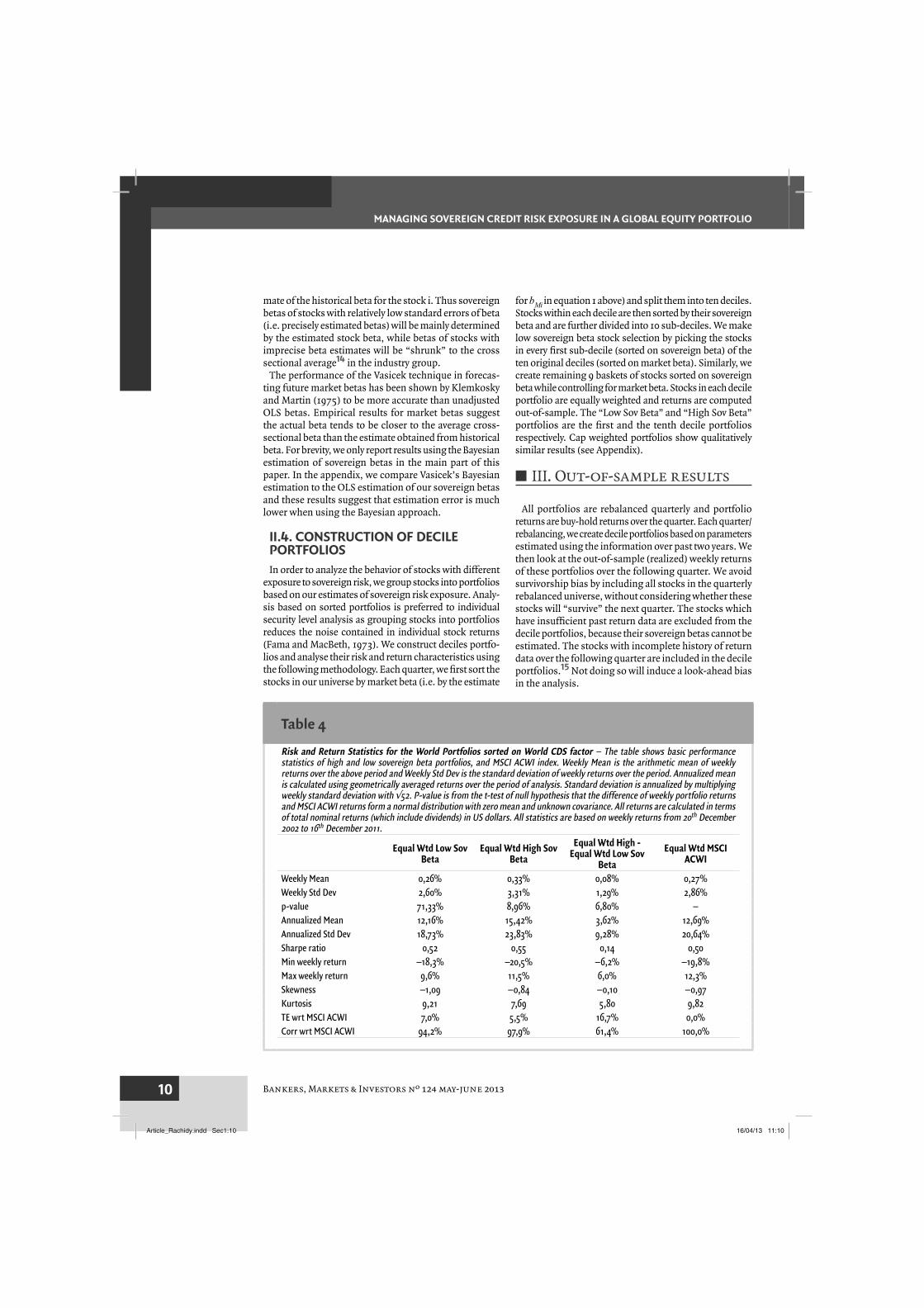
Table 4

Risk and Return Statistics for the World Portfolios sorted on World CDS factor – The table shows basic performance statistics of high and low sovereign beta portfolios, and MSCI ACWI index. Weekly Mean is the arithmetic mean of weekly returns over the above period and Weekly Std Dev is the standard deviation of weekly returns over the period. Annualized mean is calculated using geometrically averaged returns over the period of analysis. Standard deviation is annualized by multiplying weekly standard deviation with √52. P-value is from the t-test of null hypothesis that the difference of weekly portfolio returns and MSCI ACWI returns form a normal distribution with zero mean and unknown covariance. All returns are calculated in terms of total nominal returns (which include dividends) in US dollars. All statistics are based on weekly returns from 20th December 2002 to 16th December 2011.

Equal Wtd Low Sov Beta

Equal Wtd High Sov Beta

Equal Wtd High - Equal Wtd Low Sov

BetaEqual Wtd MSCI

ACWI

Weekly Mean 0,26% 0,33% 0,08% 0,27%Weekly Std Dev 2,60% 3,31% 1,29% 2,86%p-value 71,33% 8,96% 6,80% –Annualized Mean 12,16% 15,42% 3,62% 12,69%Annualized Std Dev 18,73% 23,83% 9,28% 20,64%Sharpe ratio 0,52 0,55 0,14 0,50Min weekly return –18,3% –20,5% –6,2% –19,8%Max weekly return 9,6% 11,5% 6,0% 12,3%Skewness –1,09 –0,84 –0,10 –0,97Kurtosis 9,21 7,69 5,80 9,82TE wrt MSCI ACWI 7,0% 5,5% 16,7% 0,0%Corr wrt MSCI ACWI 94,2% 97,9% 61,4% 100,0%




III.1. PORTFOLIOS’ RISK AND RETURN In this section we examine the risk and return properties

of the portfolios with different exposure to sovereign risk. We present the out-of-sample results for the risk and return statistics for the “High Sov Beta”, “Low Sov Beta”, and a long-short (high – low) portfolio with stocks’ sovereign betas calculated using the Bayesian estimation method and the World CDS factor. The time period of this ana-lysis is from 20th December 2002 to 16th December 2011. We focus on the comparison of portfolios’ mean return, standard deviation and Sharpe Ratio. We also compare their performance statistics with that of equal weighted MSCI ACWI Index (used as the benchmark) over the same time period. The p-values are obtained from a two sided t-test used to see if the portfolio returns are signi-fi cantly different from the equal weighted MSCI ACWI Index returns. Additionally, we report the tracking error and correlation of these portfolios with respect to equal weighted MSCI ACWI Index, and extreme weekly returns realized by them. Table 4 summarizes these results.

Table 4 shows that over the sample period, the mean weekly return of “High Sov Beta” portfolio is 0.33% which is more than that of “Low Sov Beta” portfolio (0.26%). However the returns of both high and low sovereign risk portfolios are not signifi cantly different from MSCI ACWI returns at 95% confi dence level. The “High Sov Beta” portfolio exhibits higher returns and higher vola-tility than “Low Sov Beta” portfolio. The “Low Sov Beta” portfolio however displays lower skewness and higher kurtosis than the “High Sov Beta” portfolio showing that the avoidance of exposure to a specifi c risk factor did not reduce extreme risks in the distribution of returns.

III.2. AVERAGE CONDITIONAL RETURN OF THE HIGH AND LOW SOVEREIGN PORTFOLIOSIn this section, we look at the returns of portfolios

conditional on the change in sovereign credit risk level. Indeed the intuition here is that if our measure of sove-reign risk exposure holds out of sample, the low sove-reign risk portfolio should have higher returns than the high sovereign risk portfolio in an environment where the level of sovereign credit risk is high and vice versa.

Table 5

World High/Low Sovereign Beta Portfolio returns during good/bad news weeks – The table shows the differences between the mean weekly returns of the High Sovereign Beta and Low Sovereign Beta portfolios and their statistical signifi cance over two periods characterized by good news and bad news weeks respectively. All returns are calculated in terms of total nominal returns (which include dividends) in US dollars. All statistics are based on weekly returns from 20th December 2002 to 16th December 2011.Good News Weeks High – Low Sov BetaWeekly Returns 0,96%p-value 0,00%Bad News Weeks High – Low Sov BetaWeekly Returns –0,94%p-value 0,00%

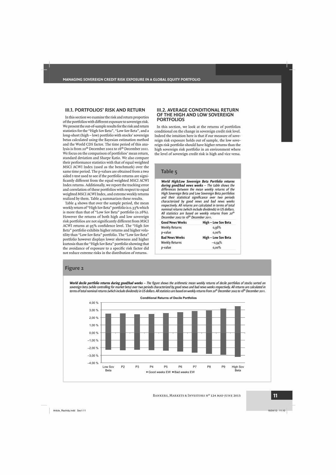
Figure 2

World decile portfolio returns during good/bad weeks – The fi gure shows the arithmetic mean weekly returns of decile portfolios of stocks sorted on sovereign beta (while controlling for market beta) over two periods characterized by good news and bad news weeks respectively. All returns are calculated in terms of total nominal returns (which include dividends) in US dollars. All statistics are based on weekly returns from 20th December 2002 to 16th December 2011.y

4,00 %

3,00 %

2,00 %

1,00 %

0,00 %

–1,00 %

–2,00 %

–3,00 %

–4,00 %Low Sov

BetaP2 P3 P4 P5 P6 P7 P8 P9 High Sov

BetaGood weeks EW Bad weeks EW

Conditional Returns of Decile Portfolios




We divide the realized weekly return observations over the entire period into fi ve quintiles sorted by the weekly change in the World CDS factor to classify weeks into weeks with “good” or “bad” news on sovereign credit risk. The fi rst and the last quintile are respectively the “weeks with good news” and “weeks with bad news”. A high sovereign credit risk regime is defi ned by the weeks with “bad news” on sovereign credit risk and vice versa. Table 5 shows the average return of the long-short (High Sov Beta - Low Sov Beta) portfolio during the two regimes and its statistical signifi cance.

Our out-of-sample results are consistent with the intuition. The Low sovereign risk portfolio has lower returns than High sovereign risk portfolio during the weeks with “good news” on sovereign credit risk, and has higher returns during weeks with “bad news”. The difference in mean weekly returns is more than 90 bps and is statistically signifi cant at the 99% confi dence interval for both “good news” and “bad news” regimes. The magnitude of the difference in returns is quite big for weekly return values.

We examine in more detail, the relation between sen-sitivity to sovereign credit risk and portfolios’ average return during the two regimes – good news and bad news weeks. Figure 2 plots the average conditional return of the deciles portfolios for different regimes. During the weeks with good news on sovereign credit risk, the empirical results show that High Sov Beta portfolios have higher weekly returns going forward, while Low Sov Beta portfolios have lower returns. During the weeks with bad news, portfolios with higher exposure to sovereign credit risk exhibit larger negative returns than portfolios with lower exposure. Overall, using the World CDS factor as a proxy for global sovereign credit risk allows us to cal-culate a reliable estimate of stocks’ individual exposure to sovereign credit risk. It also shows that low sovereign

beta stocks have better hedging properties with regard to sovereign credit risk going forward.

III.3. DO LOW AND HIGH SOVEREIGN RISK PORTFOLIOS SUFFER FROM BIASES?The properties of portfolios with high or low sovereign

risk exposure could be questioned if these portfolios exhibit strong biases compared to the market index. If deciles portfolios exhibit biases on other risk factors than sovereign credit risk, our previous results could indeed be the consequence of portfolios’ exposure to these other factors. We simply verify here ex-post that deciles portfolios constructed with our methodology have similar characteristics.

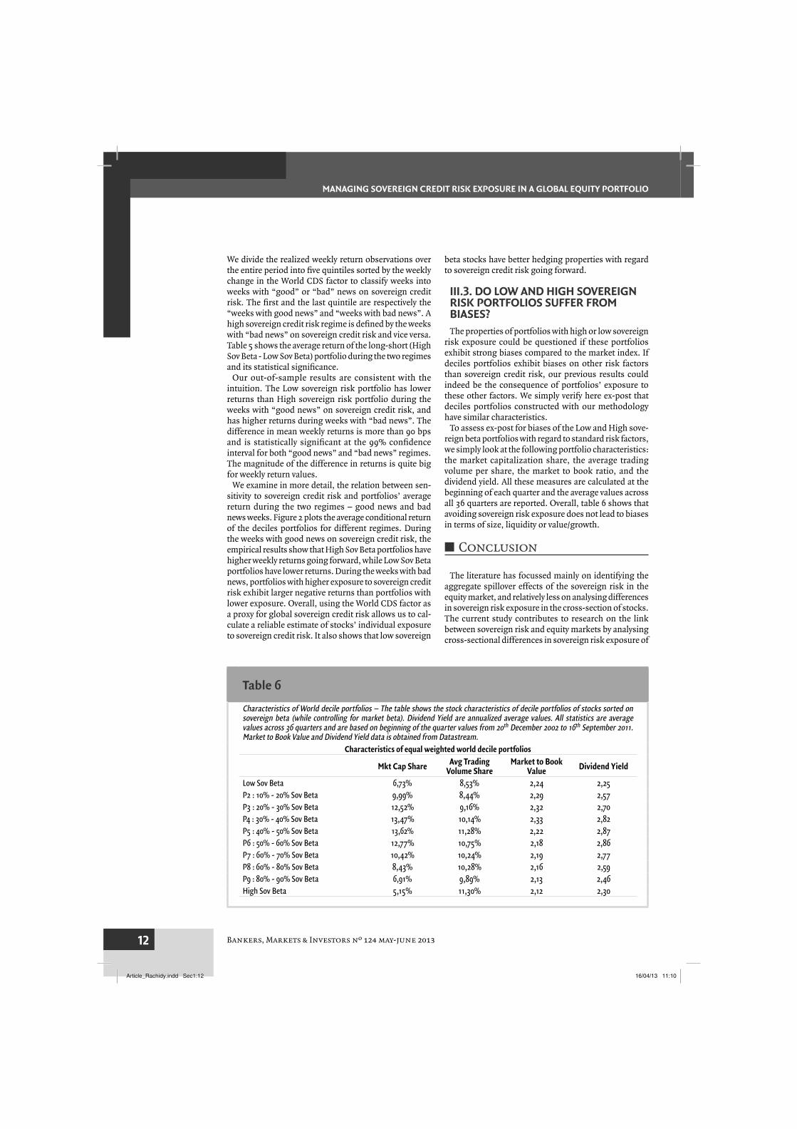
To assess ex-post for biases of the Low and High sove-reign beta portfolios with regard to standard risk factors, we simply look at the following portfolio characteristics: the market capitalization share, the average trading volume per share, the market to book ratio, and the dividend yield. All these measures are calculated at the beginning of each quarter and the average values across all 36 quarters are reported. Overall, table 6 shows that avoiding sovereign risk exposure does not lead to biases in terms of size, liquidity or value/growth.

■ Conclusion

The literature has focussed mainly on identifying the aggregate spillover effects of the sovereign risk in the equity market, and relatively less on analysing differences in sovereign risk exposure in the cross-section of stocks. The current study contributes to research on the link between sovereign risk and equity markets by analysing cross-sectional differences in sovereign risk exposure of

Table 6

Characteristics of World decile portfolios – The table shows the stock characteristics of decile portfolios of stocks sorted on sovereign beta (while controlling for market beta). Dividend Yield are annualized average values. All statistics are average values across 36 quarters and are based on beginning of the quarter values from 20th December 2002 to 16th September 2011. Market to Book Value and Dividend Yield data is obtained from Datastream.

Characteristics of equal weighted world decile portfolios

Mkt Cap Share Avg Trading Volume Share

Market to Book Value Dividend Yield

Low Sov Beta 6,73% 8,53% 2,24 2,25P2 : 10% - 20% Sov Beta 9,99% 8,44% 2,29 2,57P3 : 20% - 30% Sov Beta 12,52% 9,16% 2,32 2,70P4 : 30% - 40% Sov Beta 13,47% 10,14% 2,33 2,82P5 : 40% - 50% Sov Beta 13,62% 11,28% 2,22 2,87P6 : 50% - 60% Sov Beta 12,77% 10,75% 2,18 2,86P7 : 60% - 70% Sov Beta 10,42% 10,24% 2,19 2,77P8 : 60% - 80% Sov Beta 8,43% 10,28% 2,16 2,59P9 : 80% - 90% Sov Beta 6,91% 9,89% 2,13 2,46High Sov Beta 5,15% 11,30% 2,12 2,30




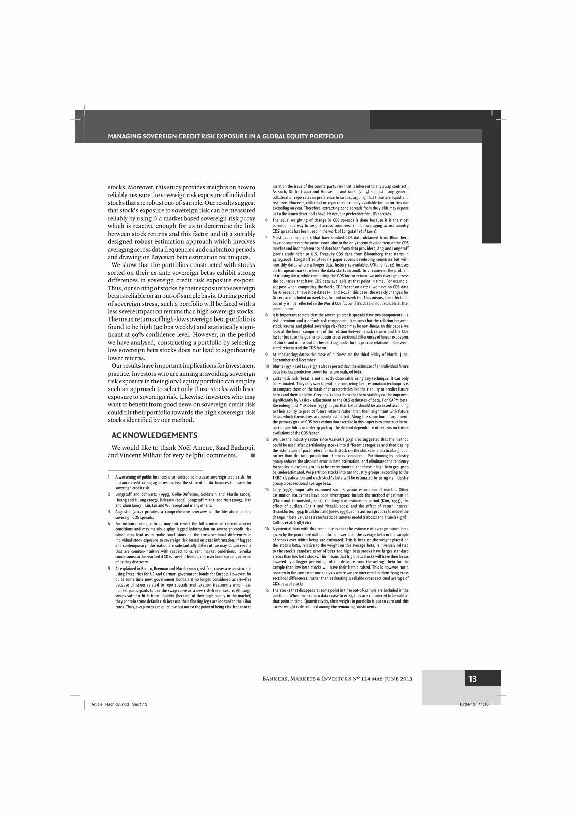
stocks. Moreover, this study provides insights on how to reliably measure the sovereign risk exposure of individual stocks that are robust out-of-sample. Our results suggest that stock’s exposure to sovereign risk can be measured reliably by using i) a market based sovereign risk proxy which is reactive enough for us to determine the link between stock returns and this factor and ii) a suitably designed robust estimation approach which involves averaging across data frequencies and calibration periods and drawing on Bayesian beta estimation techniques.

We show that the portfolios constructed with stocks sorted on their ex-ante sovereign betas exhibit strong differences in sovereign credit risk exposure ex-post. Thus, our sorting of stocks by their exposure to sovereign beta is reliable on an out-of-sample basis. During period of sovereign stress, such a portfolio will be faced with a less severe impact on returns than high sovereign stocks. The mean returns of high-low sovereign beta portfolio is found to be high (90 bps weekly) and statistically signi-fi cant at 99% confi dence level. However, in the period we have analysed, constructing a portfolio by selecting low sovereign beta stocks does not lead to signifi cantly lower returns.

Our results have important implications for investment practice. Investors who are aiming at avoiding sovereign risk exposure in their global equity portfolio can employ such an approach to select only those stocks with least exposure to sovereign risk. Likewise, investors who may want to benefi t from good news on sovereign credit risk could tilt their portfolio towards the high sovereign risk stocks identifi ed by our method.

ACKNOWLEDGEMENTSWe would like to thank Noël Amenc, Saad Badaoui,

and Vincent Milhau for very helpful comments. ■

1 A worsening of public fi nances is considered to increase sovereign credit risk: for instance credit rating agencies analyse the state of public fi nances to assess for sovereign credit risk.

2 Longstaff and Schwartz (1995), Colin-Dufresne, Goldstein and Martin (2001), Huang and Huang (2003), Driessen (2005), Longstaff Mithal and Neis (2005), Han and Zhou (2007), Lin, Lui and Wu (2009) and many others.

3 Augustin (2012) provides a comprehensive overview of the literature on the sovereign CDS spreads.

4 For instance, using ratings may not reveal the full content of current market conditions and may mainly display lagged information on sovereign credit risk which may lead us to make conclusions on the cross-sectional differences in individual stock exposure to sovereign risk based on past information. If lagged and contemporary information are substantially different, we may obtain results that are counter-intuitive with respect to current market conditions. Similar conclusions can be reached if CDSs have the leading role over bond spreads in terms of pricing discovery.

5 As explained in Blanco, Brennan and Marsh (2005), risk free curves are constructed using Treasuries for US and German government bonds for Europe. However, for quite some time now, government bonds are no longer considered as risk-free because of issues related to repo specials and taxation treatments which lead market participants to use the swap curve as a new risk-free measure. Although swaps suffer a little from liquidity (because of their high supply in the market) they contain some default risk because their fl oating legs are indexed to the Libor rates. Thus, swap rates are quite low but not to the point of being risk-free (not to

mention the issue of the counterparty risk that is inherent to any swap contract). As such, Duffi e (1999) and Houweling and Vorst (2005) suggest using general collateral or repo rates in preference to swaps, arguing that these are liquid and risk free. However, collateral or repo rates are only available for maturities not exceeding on year. Therefore, extracting bond spreads from the yields may expose us to the issues described above. Hence, our preference for CDS spreads.

6 The equal weighting of change in CDS spreads is done because it is the most parsimonious way to weight across countries. Similar averaging across country CDS spreads has been used in the work of Longstaff et al (2011).

7 Most academic papers that have studied CDS data obtained from Bloomberg have encountered the same issues, due to the only recent development of the CDS market and incompleteness of database from data providers. Ang and Longstaff (2011) study refer to U.S. Treasury CDS data from Bloomberg that starts in 14/05/2008. Longstaff et al (2011) paper covers developing countries but with monthly data, where a longer data history is available. O’Kane (2012) focuses on European market where the data starts in 2008. To circumvent the problem of missing data, while computing the CDS factor return, we only average across the countries that have CDS data available at that point in time. For example, suppose when computing the World CDS factor on date t, we have no CDS data for Greece, but have it on dates t+1 and t+2: in this case, the weekly changes for Greece are included on week t+2, but not on week t+1. This means, the effect of a country is not refl ected in the World CDS factor if it’s data in not available at that point in time.

8 It is important to note that the sovereign credit spreads have two components – a risk premium and a default risk component. It means that the relation between stock returns and global sovereign risk factor may be non-linear. In this paper, we look at the linear component of the relation between stock returns and the CDS factor because the goal is to obtain cross sectional differences of linear exposures of stocks and not to fi nd the best-fi tting model for the precise relationship between stock returns and the CDS factor.

9 At rebalancing dates: the close of business on the third Friday of March, June, September and December.

10 Blume (1971) and Levy (1971) also reported that the estimate of an individual fi rm’s beta has low predictive power for future realized beta.

11 Systematic risk (beta) is not directly observable using any technique, it can only be estimated. They only way to evaluate competing beta estimation techniques is to compare them on the basis of characteristics like their ability to predict future betas and their stability. Grey et al (2009) show that beta stability can be improved signifi cantly by Vasicek adjustment to the OLS estimates of beta. For CAPM beta, Rosenberg and McKibben (1973) argue that betas should be assessed according to their ability to predict future returns rather than their alignment with future betas which themselves are poorly estimated. Along the same line of argument, the primary goal of CDS beta estimation exercise in this paper is to construct beta-sorted portfolios in order tp pick up the desired dependence of returns on future evolutions of the CDS factor.

12 We use the industry sector since Vasicek (1973) also suggested that the method could be used after partitioning stocks into different categories and then basing the estimation of parameters for each stock on the stocks in a particular group, rather than the total population of stocks considered. Partitioning by industry group reduces the absolute error in beta estimation, and eliminates the tendency for stocks in low beta groups to be overestimated, and those in high beta groups to be underestimated. We partition stocks into ten Industry groups, according to the TRBC classifi cation and each stock’s beta will be estimated by using its Industry group cross sectional average beta.

13 Lally (1998) empirically examined such Bayesian estimation of market. Other estimation issues that have been investigated include the method of estimation (Chan and Lanonishok, 1992), the length of estimation period (Kim, 1993), the effect of outliers (Shalit and Yitzaki, 2001) and the effect of return interval (Frankfurter, 1994; Brailsford and Josev, 1997). Some authors propose to model the change in beta values as a stochastic parameter model (Fabozzi and Francis (1978), Collins et al. (1987) etc)

14 A potential bias with this technique is that the estimate of average future beta given by the procedure will tend to be lower than the average beta in the sample of stocks over which betas are estimated. This is because the weight placed on the stock’s beta, relative to the weight on the average beta, is inversely related to the stock’s standard error of beta and high beta stocks have larger standard errors than low beta stocks. This means that high beta stocks will have their betas lowered by a bigger percentage of the distance from the average beta for the sample than low beta stocks will have their beta’s raised. This is however not a concern in the context of our analysis where we are interested in identifying cross sectional differences, rather than estimating a reliable cross sectional average of CDS beta of stocks.

15 The stocks that disappear at some point in time out-of-sample are included in the portfolio. When their return data cease to exist, they are considered to be sold at that point in time. Quantitatively, their weight in portfolio is put to zero and this excess weight is distributed among the remaining constituents.




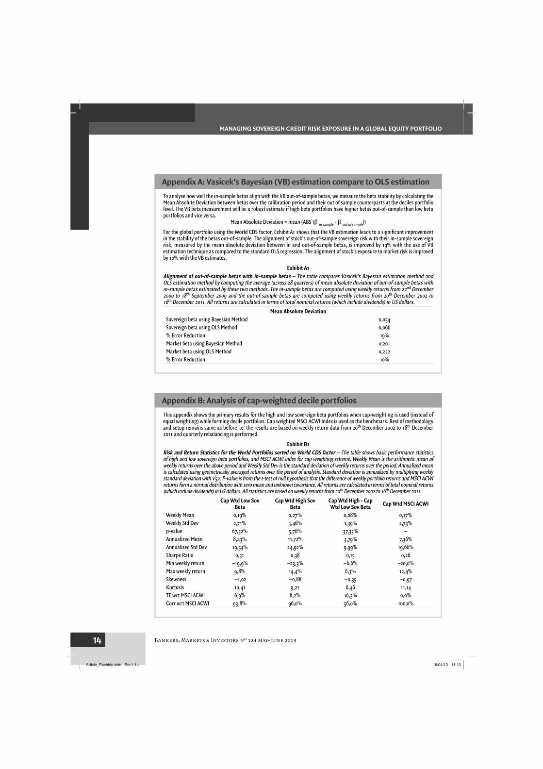
To analyse how well the in-sample betas align with the VB out-of-sample betas, we measure the beta stability by calculating the Mean Absolute Deviation between betas over the calibration period and their out of sample counterparts at the deciles portfolio level. The VB beta measurement will be a robust estimate if high beta portfolios have higher betas out-of-sample than low beta portfolios and vice versa.

Mean Absolute Deviation = mean (ABS (β in sample - β out of sample))

For the global portfolio using the World CDS factor, Exhibit A1 shows that the VB estimation leads to a signifi cant improvement in the stability of the betas out-of-sample. The alignment of stock’s out-of-sample sovereign risk with their in-sample sovereign risk, measured by the mean absolute deviation between in and out-of-sample betas, is improved by 19% with the use of VB estimation technique as compared to the standard OLS regression. The alignment of stock’s exposure to market risk is improved by 10% with the VB estimates.

Exhibit A1Alignment of out-of-sample betas with in-sample betas – The table compares Vasicek’s Bayesian estimation method and OLS estimation method by computing the average (across 28 quarters) of mean absolute deviation of out-of-sample betas with in-sample betas estimated by these two methods. The in-sample betas are computed using weekly returns from 22nd December 2000 to 18th September 2009 and the out-of-sample betas are computed using weekly returns from 20th December 2002 to 16th December 2011. All returns are calculated in terms of total nominal returns (which include dividends) in US dollars.

Mean Absolute DeviationSovereign beta using Bayesian Method 0,054Sovereign beta using OLS Method 0,066% Error Reduction 19%Market beta using Bayesian Method 0,201Market beta using OLS Method 0,222% Error Reduction 10%

Appendix A: Vasicek’s Bayesian (VB) estimation compare to OLS estimation

This appendix shows the primary results for the high and low sovereign beta portfolios when cap-weighting is used (instead of equal weighting) while forming decile portfolios. Cap weighted MSCI ACWI Index is used as the benchmark. Rest of methodology and setup remains same as before i.e. the results are based on weekly return data from 20th December 2002 to 16th December 2011 and quarterly rebalancing is performed.

Exhibit B1Risk and Return Statistics for the World Portfolios sorted on World CDS factor – The table shows basic performance statistics of high and low sovereign beta portfolios, and MSCI ACWI index for cap weighting scheme. Weekly Mean is the arithmetic mean of weekly returns over the above period and Weekly Std Dev is the standard deviation of weekly returns over the period. Annualized mean is calculated using geometrically averaged returns over the period of analysis. Standard deviation is annualized by multiplying weekly standard deviation with √52. P-value is from the t-test of null hypothesis that the difference of weekly portfolio returns and MSCI ACWI returns form a normal distribution with zero mean and unknown covariance. All returns are calculated in terms of total nominal returns (which include dividends) in US dollars. All statistics are based on weekly returns from 20th December 2002 to 16th December 2011.

Cap Wtd Low Sov Beta

Cap Wtd High Sov Beta

Cap Wtd High - Cap Wtd Low Sov Beta Cap Wtd MSCI ACWI

Weekly Mean 0,19% 0,27% 0,08% 0,17%Weekly Std Dev 2,71% 3,46% 1,39% 2,73%p-value 67,32% 5,76% 37,33% –Annualized Mean 8,43% 11,72% 3,79% 7,36%Annualized Std Dev 19,54% 24,92% 9,99% 19,66%Sharpe Ratio 0,31 0,38 0,15 0,26Min weekly return –19,9% –23,3% –6,6% –20,0%Max weekly return 9,8% 14,4% 6,3% 12,4%Skewness –1,02 –0,88 –0,35 –0,97Kurtosis 10,41 9,21 6,46 11,14TE wrt MSCI ACWI 6,9% 8,2% 16,3% 0,0%Corr wrt MSCI ACWI 93,8% 96,0% 56,0% 100,0%

Appendix B: Analysis of cap-weighted decile portfolios




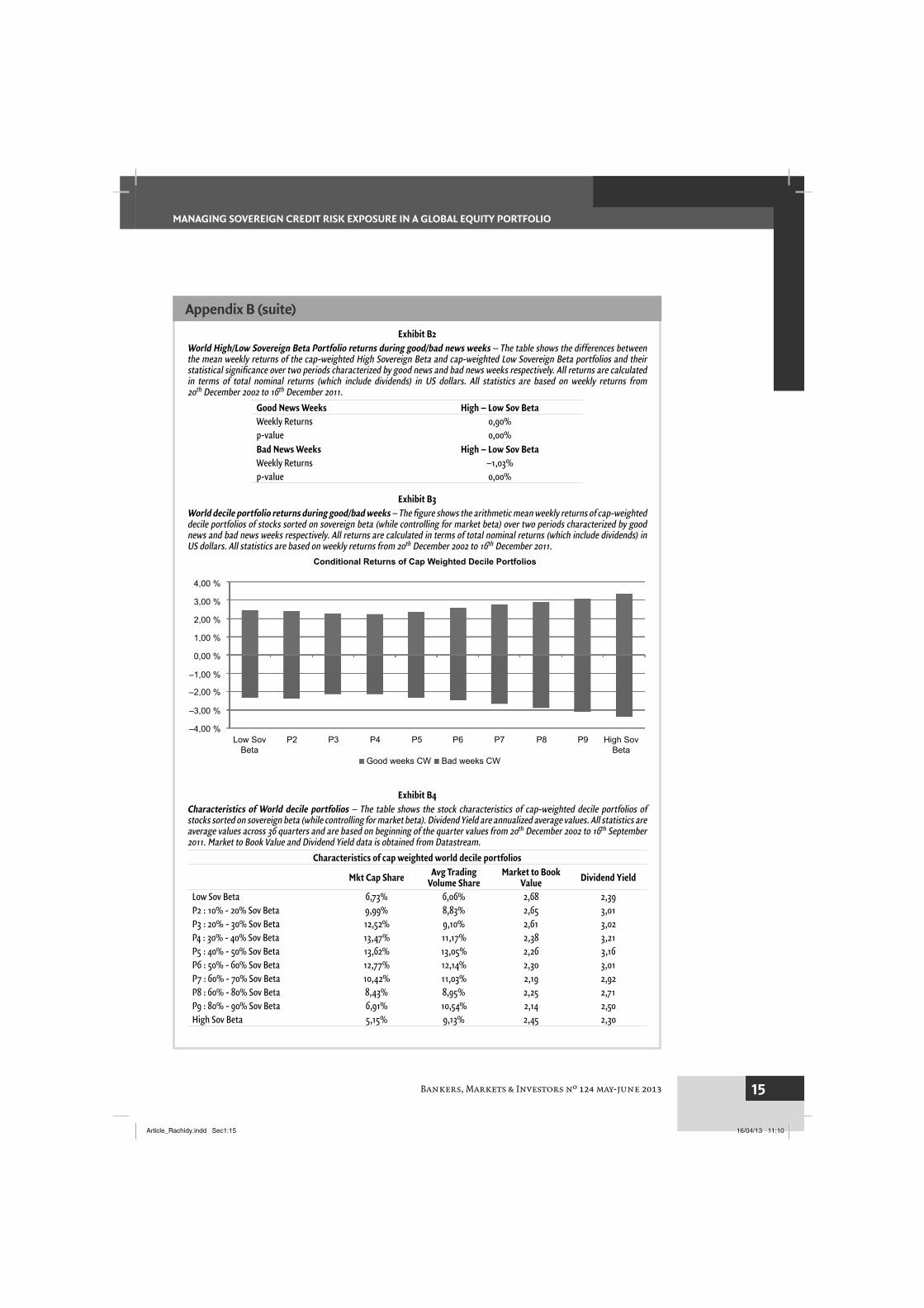
Exhibit B2World High/Low Sovereign Beta Portfolio returns during good/bad news weeks – The table shows the differences between the mean weekly returns of the cap-weighted High Sovereign Beta and cap-weighted Low Sovereign Beta portfolios and their statistical signifi cance over two periods characterized by good news and bad news weeks respectively. All returns are calculated in terms of total nominal returns (which include dividends) in US dollars. All statistics are based on weekly returns from 20th December 2002 to 16th December 2011.

Good News Weeks High – Low Sov BetaWeekly Returns 0,90%p-value 0,00%Bad News Weeks High – Low Sov BetaWeekly Returns –1,03%p-value 0,00%

Exhibit B3World decile portfolio returns during good/bad weeks – The fi gure shows the arithmetic mean weekly returns of cap-weighted decile portfolios of stocks sorted on sovereign beta (while controlling for market beta) over two periods characterized by good news and bad news weeks respectively. All returns are calculated in terms of total nominal returns (which include dividends) in US dollars. All statistics are based on weekly returns from 20th December 2002 to 16th December 2011.y

4,00 %

3,00 %

2,00 %

1,00 %

0,00 %

–1,00 %

–2,00 %

–3,00 %

–4,00 %Low Sov


Beta

Conditional Returns of Cap Weighted Decile Portfolios

Good weeks CW Bad weeks CW

Exhibit B4Characteristics of World decile portfolios – The table shows the stock characteristics of cap-weighted decile portfolios of stocks sorted on sovereign beta (while controlling for market beta). Dividend Yield are annualized average values. All statistics are average values across 36 quarters and are based on beginning of the quarter values from 20th December 2002 to 16th September 2011. Market to Book Value and Dividend Yield data is obtained from Datastream.

Characteristics of cap weighted world decile portfolios




Appendix B (suite)




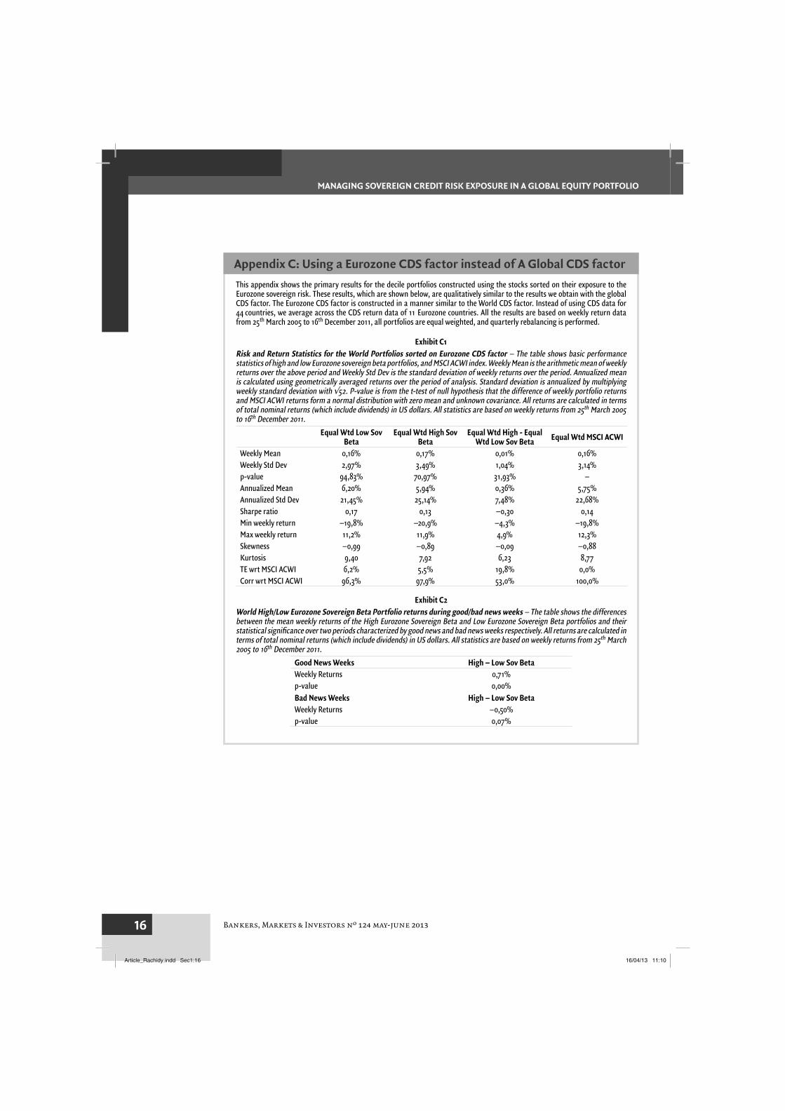
This appendix shows the primary results for the decile portfolios constructed using the stocks sorted on their exposure to the Eurozone sovereign risk. These results, which are shown below, are qualitatively similar to the results we obtain with the global CDS factor. The Eurozone CDS factor is constructed in a manner similar to the World CDS factor. Instead of using CDS data for 44 countries, we average across the CDS return data of 11 Eurozone countries. All the results are based on weekly return data from 25th March 2005 to 16th December 2011, all portfolios are equal weighted, and quarterly rebalancing is performed.

Exhibit C1Risk and Return Statistics for the World Portfolios sorted on Eurozone CDS factor – The table shows basic performance statistics of high and low Eurozone sovereign beta portfolios, and MSCI ACWI index. Weekly Mean is the arithmetic mean of weekly returns over the above period and Weekly Std Dev is the standard deviation of weekly returns over the period. Annualized mean is calculated using geometrically averaged returns over the period of analysis. Standard deviation is annualized by multiplying weekly standard deviation with √52. P-value is from the t-test of null hypothesis that the difference of weekly portfolio returns and MSCI ACWI returns form a normal distribution with zero mean and unknown covariance. All returns are calculated in terms of total nominal returns (which include dividends) in US dollars. All statistics are based on weekly returns from 25th March 2005 to 16th December 2011.

Equal Wtd Low Sov Beta

Equal Wtd High Sov Beta

Equal Wtd High - Equal Wtd Low Sov Beta Equal Wtd MSCI ACWI

Weekly Mean 0,16% 0,17% 0,01% 0,16%Weekly Std Dev 2,97% 3,49% 1,04% 3,14%p-value 94,83% 70,97% 31,93% –Annualized Mean 6,20% 5,94% 0,36% 5,75%Annualized Std Dev 21,45% 25,14% 7,48% 22,68%Sharpe ratio 0,17 0,13 –0,30 0,14Min weekly return –19,8% –20,9% –4,3% –19,8%Max weekly return 11,2% 11,9% 4,9% 12,3%Skewness –0,99 –0,89 –0,09 –0,88Kurtosis 9,40 7,92 6,23 8,77TE wrt MSCI ACWI 6,2% 5,5% 19,8% 0,0%Corr wrt MSCI ACWI 96,3% 97,9% 53,0% 100,0%

Exhibit C2World High/Low Eurozone Sovereign Beta Portfolio returns during good/bad news weeks – The table shows the differences between the mean weekly returns of the High Eurozone Sovereign Beta and Low Eurozone Sovereign Beta portfolios and their statistical signifi cance over two periods characterized by good news and bad news weeks respectively. All returns are calculated in terms of total nominal returns (which include dividends) in US dollars. All statistics are based on weekly returns from 25th March 2005 to 16th December 2011.

Good News Weeks High – Low Sov BetaWeekly Returns 0,71%p-value 0,00%Bad News Weeks High – Low Sov BetaWeekly Returns –0,50%p-value 0,07%

Appendix C: Using a Eurozone CDS factor instead of A Global CDS factor




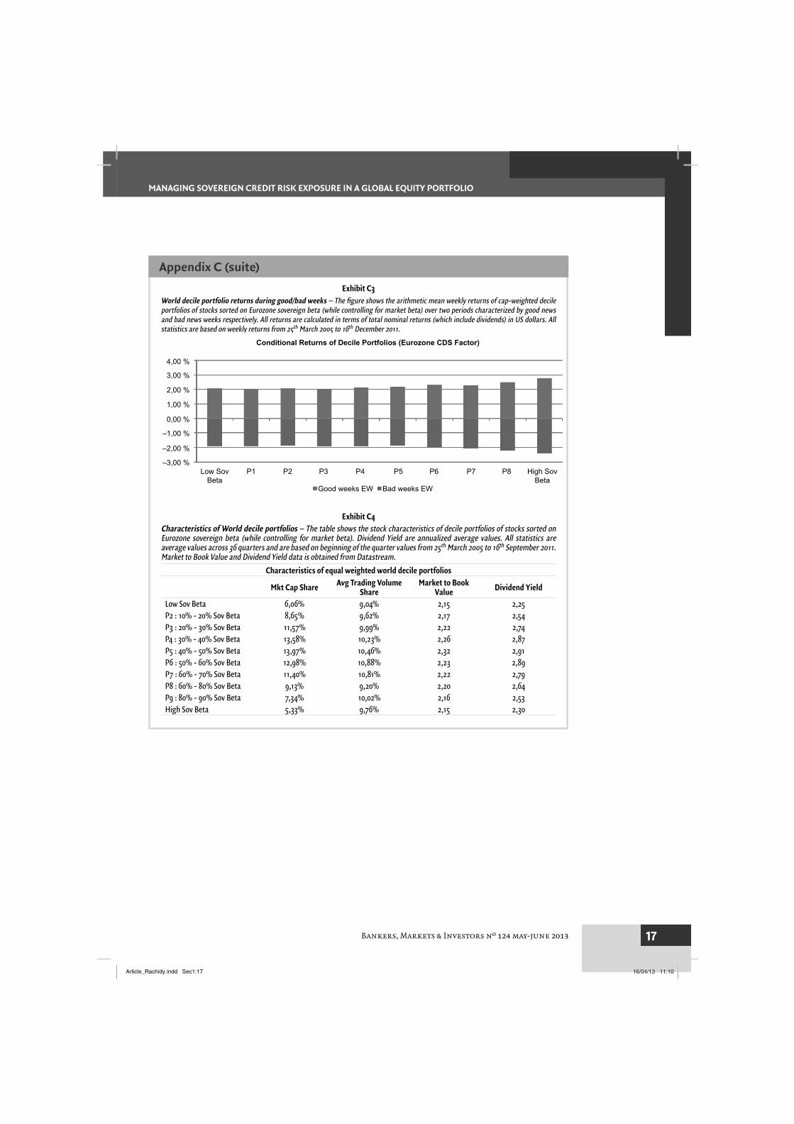
Exhibit C3World decile portfolio returns during good/bad weeks – The fi gure shows the arithmetic mean weekly returns of cap-weighted decile portfolios of stocks sorted on Eurozone sovereign beta (while controlling for market beta) over two periods characterized by good news and bad news weeks respectively. All returns are calculated in terms of total nominal returns (which include dividends) in US dollars. All statistics are based on weekly returns from 25th March 2005 to 16th December 2011. y 5 5

4,00 %

3,00 %

2,00 %

1,00 %

0,00 %

–1,00 %

–2,00 %

–3,00 %Low Sov


BetaGood weeks EW Bad weeks EW

Conditional Returns of Decile Portfolios (Eurozone CDS Factor)

Exhibit C4Characteristics of World decile portfolios – The table shows the stock characteristics of decile portfolios of stocks sorted on Eurozone sovereign beta (while controlling for market beta). Dividend Yield are annualized average values. All statistics are average values across 36 quarters and are based on beginning of the quarter values from 25th March 2005 to 16th September 2011. Market to Book Value and Dividend Yield data is obtained from Datastream.

Characteristics of equal weighted world decile portfolios




Appendix C (suite)




■ Alesina, A.(1987). Macroeconomic Policy in a Two-Party System as a Repeated Game, The Quarterly Journal of Economics 102, 651-78.

■ Alesina, A. (2009). Large Change in Fiscal Policy: Taxes vs Spending. Harvard Institute of Economic Research Discussion Paper No. 2180

■ Alessandri, P, and A G Haldane (2009). Banking on the State. Bank of England, mimeo, November.

■ Ang, A., and Geert Bekaert (2002). International Asset Allocation with Regime Shifts, Review of Financial Studies 15, 1137-1187.

■ Ang, A., Hodrick, Robert J., Xing, Yuhang and Zhang, Xiaoyan (2006). The Cross-Section of Volatility and Expected Returns. Journal of Finance, Vol. 61, No. 1, 259-299.

■ Ang, A., and F.A. Longstaff (2011). Systemic Sovereign Credit Risk: Lessons from the U.S. and Europe

■ Augustin, P. (2012). Sovereign Credit Risk Premia. Working Paper, Stockholm School of Economics

■ Arezki, R., B. Candelon, and N.R. Sy A. (2011). Sovereign Rating News and Financial Markets Spillovers: Evidence from the European Debt Crisis. IMF Working Paper

■ Aunon-Nerin, D., D. Cossin, T. Hricko, and Z. Huang (2002). Exploring for the Determinants of Credit Risk in Credit Default Swap Transaction Data: Is Fixed Income Markets’ Information Suffi cient to Evaluate Credit Risk?, Working Paper, HEC-University of Lausanne.

■ Avramov, D., T. Chordia, G. Jostova, and A. Philipov (2012). The World Price of Credit Risk. June 1st.

■ Badaoui, S., Lara Cathcart, and Lina El-Jahel, (2012). Do Sovereign Credit Default Swaps Represent a Clean Measure of Sovereign Default Risk? A Factor Model Approach. October

■ Badaoui, S., Lara Cathcart, and Lina El-Jahel, (2012). Implied Liquidity Risk in the Term Structure of Sovereign Credit Default Swap Spreads. October

■ A. Beber, M.W. Brandt, and K.A. Kavajecz (2008). Flight-to-Quality or Flight-to-Liquidity? Evidence from the Euro-Area Bond Market. Review of Financial Studies

■ Beim, D.O., and C.W. Calomiris (2000). Emerging Financial Markets. New York: McGraw Hill/Irwin).

■ Belo, F., V.D. Gala, and Jun Li, (2011). Government Spending, Political Cycles and the Cross Section of Stock Returns

■ A. Berndt, R. Douglas, D. Duffi e, M. Ferguson, and D. Schranz (2005). Measuring Default Risk Premia from Default Swap Rates and EDFs. Working Paper.

■ Blanco, R., S. Brennan, and I. Marsh (2005). An Empirical Analysis of the Dynamic Relation between Investment-Grade Bonds and Credit Default Swaps. Journal of Finance 60, 2255-2281.

■ Blume, M. (1971). On the Assessment of Risk. Journal of Finance 26, 1-10.

■ Blume, M. (1975). Betas and their Regression Tendencies. Journal of Finance 30, 785-795.

■ Borensztein, E., and U Panizza (2009). The Costs of Sovereign Default. IMF Staff Paper, Palgrave Macmillan Journals, vol. 56(4), November

■ Campbell, J.Y. (1996). Understanding Risk and Return. Journal of Political Economy, Vol. 104, No. 2, 298-345.

■ Collin-Dufresne, P., R. Goldstein, and S. Martin (2001). The Determinants of Credit Spread Changes. Journal of Finance 56, 2177-2207.

■ Cooper M.J., W.E. Jackson, and G.A. Patterson (2003). Evidence of Predictability in the Cross-Section of Bank Stock Returns. Journal of Banking & Finance, Volume 27, Issue 5, May, Pages 817-850

■ Das, S., M. Kalimpalli, and S. Nayak (2011). Did CDS Trading Improve the Market for Corporate Bonds, Working Paper.

■ Demirgüç-Kunt, A., and H Huizinga (2010). Are banks too Big to Fail or too Big to Save? International Evidence from Equity Prices and CDS Spreads. European Banking Center Discussion Paper, no 2010-59, January

■ Driessen J. (2005). Is Default Event Risk Priced in Corporate Bonds? Review of Financial Studies 18(1): 165_195,.

■ Duffi e D. (1999). Credit Swap Valuation, Financial Analyst Journal 55.

■ Duffi e, D., and K.J. Singleton (1999). Modeling the Term Structure of Defaultable Bonds. Review of Financial Studies 12(4):687-720.

■ Duffi e, D., and K.J. Singleton (2003). Credit Risk. Princeton University Press, Princeton, NJ.

■ Duffi e, D., L.H. Pedersen, and K.J. Singleton (2003). Modeling Sovereign Yield Spreads: A Case Study of Russian Debt. Journal of Finance 58, 119-159.

■ Elton, E., M. Gruber, D. Agrawal, and C. Mann (2001). Explaining the Rate Spread on Corporate Bonds. Journal of Finance 56, 247-277

■ Fama, E.F., and K.R. French (1992). The Cross-Section of Expected Stock Returns. Journal of Finance 47 (2): 427-465.

■ Fama, E.F., and J.D. MacBeth (1973). Risk, Return, and Equilibrium: Empirical Tests. Journal of Political Economy 81, 607{636.

■ Ferreira, M., and P.M. Gama (2007). Does Sovereign Debt Ratings News Spill over to International Stock Markets? Journal of Banking and Finance 31, 3162-3182

■ Flannery, M., J. Houston, and F. Partnoy (2010). Credit Default Swap Spreads as Viable Substitutes for Credit Ratings. University of Pennsylvania Law Review 158, 2085 2123.

■ Gande, A., and D.C. Parsley (2005). News Spillovers in the Sovereign Debt Market. Journal of Financial Economics, Vol. 75, 691-734

■ Geyer, A., S. Kossmeier, and S. Pichler (2004). Measuring Systematic Risk in Emu Government Yield Spreads (April 1st, 2003). Review of Finance, Vol. 8, No. 2, 171-197.

■ Goldstein M., G. Kaminsky, and C. Reinhart (2000). Assessing Financial Vulnerability an Early Warning System for Emerging Markets. Institute of International Economics

■ Gray, S., J. Hall, D. Klease, and A. McCrystal (2009). Bias, Stability, and Predictive Ability in the Measurement of Systematic Risk. Accounting Research Journal, Vol. 22 Iss: 3, 220-236.

References




■ Griffi n, J.M. (2002). Are the Fama and French Factors Global or Country Specifi c? Review of Financial Studies 15, 783-803.

■ Han S., and H. Zhou (2008). Effects of Liquidity on the Nondefault Component of Corporate Yield Spreads: Evidence from Intraday Transactions Data. Working Paper.

■ Houweling, P., and T. Vorst (2005). An Empirical Comparison of Default Swap Pricing Models. Journal of International Money and Finance

■ Huang, J., and M. Huang (2002). How much of the Corporate-Treasury Yield Spread is Due to Credit Risk? NYU Working Paper No. S-CDM-02-05.

■ Hilscher, J., and Y. Nosbusch (2010). Determinants of Sovereign Risk: Macroeconomic Fundamentals and the Pricing of Sovereign Debt. Review of Finance 4(2), 235-262

■ Hooper, V., J. Hume, P. Tim, and Kim, Suk-Joong (2008). Sovereign Rating Changes - Do They Provide New Information for Stock Markets? Economic Systems, Vol. 32/2, 142-166.

■ Huang, J., and M. Huang (2003). How much of the Corporate-Treasury Yield Spread is Due to Credit Risk, Working Paper, Stanford University

■ Hull, J., M. Predescu, and A. White (2004). The Relationship between Credit Default Swap Spreads, Bond Yields, and Credit Rating Announcements. Journal of Banking and Finance 28, 2789-2811.

■ Jeanneret, A. (2009). The Dynamics of Sovereign Credit Risk. Working Paper, University of Lausanne.

■ Jeanneret, A. (2010). Sovereign Default Risk and the U.S. Equity Market. Working Paper, HEC Montreal

■ Jegadeesha Narasimhan, and Joshua Livnat (2006). Revenue Surprises and Stock Returns. Journal of Accounting and Economics, Volume 41, Issues 1-2, April, 147-171

■ Lally, M. (1998). An Examination of Blume and Vasicek Betas. The Financail Review 33, 183-198.

■ Lee, K-H., H. Sapriza, and Y. Wu (2010). Sovereign debt ratings changes and stock liquidity around the world. SNU Institute for Research in Finance and Economics

■ Levy, R. A. (1971). On the Short-Term Stationarity of Beta Coeffi cients. Financial Analysts Journal 27, 55-62.

■ H. Lin, S. Liu, and C. Wu (2009). Liquidity Premia in the Credit Default Swap and Corporate Bond Markets. Working Paper.

■ Longstaff F.A., and Schwartz E.S. (1995). A Simple Approach to Valuing Risky Fixed and Floating Rate Debt. Journal of fi nance.

■ Longstaff F.A., S. Mithal, and E. Neis (2005). Corporate Yield Spreads: Default Risk or Liquidity? New Evidence from the Credit Default Swap Market. The Journal of Finance 5.

■ Longstaff, F.A., Jun Pan, Lasse H. Pedersen, and Kenneth J. Singleton (2011). How Sovereign is Sovereign Credit Risk? American Economic Journal: Macroeconomics, forthcoming.

■ Monfort, A., and J.-P. Renne (2011). Credit and Liquidity Risks in Euro-area Sovereign Yield Curves. Working Paper 2011-26, Centre de Recherche en Economie et Statistique, Banque de France.

■ O’Kane, D. (2012). The Link between Eurozone Sovereign Debt and CDS Prices. EDHEC-Risk Institute Working Paper

■ O’Kane, D., and R. McAdie (2001). Explaining the Basis: Cash versus Default Swaps, Lehman Brothers Fixed Income Research.

■ Petkova, R. (2006). Do the Fama-French Factors Proxy for Innovations in Predictive Variables? Journal of Finance, Vol. 61, No. 2, 581-612.

■ Pu, X. (2009). Liquidity Commonality across the Bond and CDS Markets. The Journal of Fixed Income 2009.19.1:26-39.

■ Pukthuanthong-Le, K., F.A. Elayan, and L. Rose (2007). Equity and Debt Market Responses to Sovereign Credit Ratings Announcement, Global Finance Journal.

■ Remolona, E., M. Scatigna, and E. Wu (2008). The Dynamic Pricing of Sovereign Risk in Emerging Markets: Fundamentals and Risk Aversion, The Journal of Fixed Income 17, 57-71.

■ Rosenberg, B., and W. McKibbin (1973). The Prediction of Systematic and Specifi c Risk in Common Stocks, Journal of Financial and Quantitative Analysis, 8(2), 317-333.

■ Singleton, K., and J. Pan (2008). Default and Recovery Implicit in the Term Structure of Sovereign CDS Spreads. Journal of Finance Vol. LXIII, 2345-2384.

■ Smirlock, M., and H. Kaufold (1987). Bank Foreign Lending, Mandatory Disclosure Rules, and the Reaction of Bank Stock Prices to the Mexican Debt Crisis, Journal of Business, v. 60, iss. 3, 347-64

■ Reinhart, C., K. Rogoff, and M. A. Savastano (2003). Debt Intolerance. Brooking Papers on Economic Activity 1, 1-70.

■ Schwarz, K. (2011). Mind the gap: Disentangling credit and liquidity in risk spreads. Working Paper.

■ Steiger, F. (2010). The Impact of Credit Risk and Implied Volatility on Stock Returns. May.

■ Sturzenegger, F., and J. Zettelmeyer (2006). Debt Defaults and Lessons from a Decade of Crises. Cambridge, Massachusetts: MIT Press.

■ Tang D.Y., and Yan H.: Liquidity and Credit Default Swap Spreads. Working Paper (2007). University of Hong Kong and University of South Carolina; Shanghai Jiao Tong University (SJTU)

■ Ten Raa, Thijs (2006). The Economics of Input-Output Analysis. Cambridge University Press.

■ Trapp, M. (2009). Trading the Bond-CDS Basis - The Role of Credit Risk and Liquidity. CFR Working Paper No. 09-16.

■ Vasicek, O. (1973). A Note on Using Cross-Sectional Information in Bayesian Estimation of Security Betas. Journal of Finance 28, 1233-1239.

References (suite)


bankers, markets & investors nº 124 may-june 2013 managing sovereign credit risk exposure in a...

Documents

References

Article_Rachidy.indd Sec1:18Article_Rachidy.indd Sec1:18 16/04/13 11:1016/04/13 11:10
Bankers, Markets & Investors nº 124 may-june 2013 19